10,000 Matching Annotations
  1. Oct 2025
    1. Author response:

      The following is the authors’ response to the original reviews.

      Public Reviews (consolidated):

      In the microglia research community, it is accepted that microglia change their shape both gradually and acutely along a continuum that is influenced by external factors both in their microenvironments and in circulation. Ideally, a given morphological state reflects a functional state that provides insight into a microglia's role in physiological and pathological conditions. The current manuscript introduces MorphoCellSorter, an open-source tool designed for automated morphometric analysis of microglia. This method adds to the many programs and platforms available to assess the characteristics of microglial morphology; however, MorphoCellSorter is unique in that it uses Andrew's plotting to rank populations of cells together (in control and experimental groups) and presents "big picture" views of how entire populations of microglia alter under different conditions. Notably, MorphoCellSorter is versatile, as it can be used across a wide array of imaging techniques and equipment. For example, the authors use MorphoCellSorter on images of fixed and live tissues representing different biological contexts such as embryonic stages, Alzheimer's disease models, stroke, and primary cell cultures.

      This manuscript outlines a strategy for efficiently ranking microglia beyond the classical homeostatic vs. active morphological states. The outcome offers only a minor improvement over the already available strategies that have the same challenge: how to interpret the ranking functionally.

      We would like to thank the reviewers for their careful reading and constructive comments and questions. While MorphoCellSorter currently does not rank cells functionally based on their morphology, its broad range of application, ease of use and capacity to handle large datasets provide a solid foundation. Combined with advances in single-cell transcriptomics, MorphoCellSorter could potentially enable the future prediction of cell functions based on morphology.

      Strengths and Weaknesses:

      (1) The authors offer an alternative perspective on microglia morphology, exploring the option to rank microglia instead of categorizing them with means of clusterings like k-means, which should better reflect the concept of a microglia morphology continuum. They demonstrate that these ranked representations of morphology can be illustrated using histograms across the entire population, allowing the identification of potential shifts between experimental groups. Although the idea of using Andrews curves is innovative, the distance between ranked morphologies is challenging to measure, raising the question of whether the authors oversimplify the problem.

      We have access to the distance between cells through the Andrew’s score of each cell. However, the challenge is that these distances are relative values and specific to each dataset. While we believe that these distances could provide valuable information, we have not yet determined the most effective way to represent and utilize this data in a meaningful manner.

      Also, the discussion about the pipeline's uniqueness does not go into the details of alternative models.The introduction remains weak in outlining the limitations of current methods (L90). Acknowledging this limitation will be necessary.

      Thank you for these insightful comments. The discussion about alternative methods was already present in the discussion L586-598 but to answer the request of the reviewers, we have revised the introduction and discussion sections to more clearly address the limitations of current methods, as well as discussed the uniqueness of the pipeline. Additionally, we have reorganized Figure 1 to more effectively highlight the main caveats associated with clustering, the primary method currently in use.

      (2) The manuscript suffers from several overstatements and simplifications, which need to be resolved. For example:

      a)  L40: The authors talk about "accurately ranked cells". Based on their results, the term "accuracy" is still unclear in this context.

      Thank you for this comment. Our use of the term "accurately" was intended to convey that the ranking was correct based on comparison with human experts, though we agree that it may have been overstated. We have removed "accurately" and propose to replace it with "properly" to better reflect the intended meaning.

      b) L50: Microglial processes are not necessarily evenly distributed in the healthy brain. Depending on their embedded environment, they can have longer process extensions (e.g., frontal cortex versus cerebellum).

      Thank you for raising this point to our attention. We removed evenly to be more inclusive on the various morphologies of microglia cells in this introductory sentence

      c)  L69: The term "metabolic challenge" is very broad, ranging from glycolysis/FAO switches to ATP-mediated morphological adaptations, and it needs further clarification about the author's intended meaning.

      Thank you for this comment, indeed we clarified to specify that we were talking about the metabolic challenge triggered by ischemia and added a reference as well.

      d) L75: Is morphology truly "easy" to obtain?

      Yes, it is in comparison to other parameters such as transcripts or metabolism, but we understand the point made by the reviewer and we found another way of writing it. As an alternative we propose: “morphology is an indicator accessible through…”

      e) L80: The sentence structure implies that clustering or artificial intelligence (AI) are parameters, which is incorrect. Furthermore, the authors should clarify the term "AI" in their intended context of morphological analysis.

      We apologize for this confusing writing, we reformulated the sentence as follows: “Artificial intelligence (AI) approaches such as machine learning have also been used to categorize morphologies (Leyh et al., 2021)”.

      f) L390f: An assumption is made that the contralateral hemisphere is a non-pathological condition. How confident are the authors about this statement? The brain is still exposed to a pathological condition, which does not stop at one brain hemisphere.

      We did not say that the contralateral is non-pathological but that the microglial cells have a non-pathological morphology which is slightly different. The contralateral side in ischemic experiments is classically used as a control (Rutkai et al 2022). Although It has been reported that differences in transcript levels can be found between sham operated animals and contralateral hemisphere in tMCAO mice (Filippenkov et al 2022) https://doi.org/10.3390/ijms23137308 showing that indeed the contralateral side is in a different state that sham controls, no report have been made on differences in term of morphology.

      We have removed “non-pathological” to avoid misinterpretations

      g)  Methodological questions:

      a) L299: An inversion operation was applied to specific parameters. The description needs to clarify the necessity of this since the PCA does not require it.

      Indeed, we are sorry for this lack of explanation. Some morphological indexes rank cells from the least to the most ramified, while others rank them in the opposite order. By inverting certain parameters, we can standardize the ranking direction across all parameters, simplifying data interpretation. This clarification has been added to the revised manuscript as follows:

      “Lacunarity, roundness factor, convex hull radii ratio, processes cell areas ratio and skeleton processes ratio were subjected to an inversion operation in order to homogenize the parameters before conducting the PCA: indeed, some parameters rank cells from the least to the most ramified, while others rank them in the opposite order. By inverting certain parameters, we can standardize the ranking direction across all parameters, thus simplifying data interpretation.”

      b) Different biological samples have been collected across different species (rat, mouse) and disease conditions (stroke, Alzheimer's disease). Sex is a relevant component in microglia morphology. At first glance, information on sex is missing for several of the samples. The authors should always refer to Table 1 in their manuscript to avoid this confusion. Furthermore, how many biological animals have been analyzed? It would be beneficial for the study to compare different sexes and see how accurate Andrew's ranking would be in ranking differences between males and females. If they have a rationale for choosing one sex, this should be explained.

      As reported in the literature, we acknowledge the presence of sex differences in microglial cell morphology. Due to ethical considerations and our commitment to reducing animal use, we did not conduct dedicated experiments specifically for developing MorphoCellSorter. Instead, we relied on existing brain sections provided by collaborators, which were already prepared and included tissue from only one sex—either female or male—except in the case of newborn pups, whose sex is not easily determined. Consequently, we were unable to evaluate whether MorphoCellSorter is sensitive enough to detect morphological differences in microglia attributable to sex. Although assessing this aspect is feasible, we are uncertain if it would yield additional insights relevant to MorphoCellSorter’s design and intended applications.

      To address this, we have included additional references in Table 1 of the revised manuscript and clearly indicated the sex of the animals from which each dataset was obtained.

      c) In the methodology, the slice thickness has been given in a range. Is there a particular reason for this variability?

      We could not spot any range in the text, we usually used 30µm thick sections in order to have entire or close to entire microglia cells.

      Although the thickness of the sections was identical for all the sections of a given dataset, only the plans containing the cells of interest were selected during the imaging for both of the ischemic stroke model. This explains why depending on how the cell is distributed in Z the range of the plans acquired vary.

      Also, the slice thickness is inadequate to cover the entire microglia morphology. How do the authors include this limitation of their strategy? Did the authors define a cut-off for incomplete microglia?

      We found that 30 µm sections provide an effective balance, capturing entire or nearly entire microglial cells (consistent with what we observe in vivo) while allowing sufficient antibody penetration to ensure strong signal quality, even at the section's center. In our segmentation process, we excluded microglia located near the section edges (i.e., cells with processes visible on the first or last plane of image acquisition, as well as those close to the field of view’s boundary). Although our analysis pipeline should also function with thicker sections (>30 µm), we confirmed that thinner sections (15 µm or less) are inadequate for detecting morphological differences, as tested initially on the AD model. Segmented, incomplete microglia lack the necessary structural information to accurately reflect morphological differences thus impairing the detection of existing morphological differences.

      c) The manuscript outlines that the authors have used different preprocessing pipelines, which is great for being transparent about this process. Yet, it would be relevant to provide a rationale for the different imaging processing and segmentation pipelines and platform usages (Supplementary Figure 7). For example, it is not clear why the Z maximum projection is performed at the end for the Alzheimer's Disease model, while it's done at the beginning of the others.

      The same holds through for cropping, filter values, etc. Would it be possible to analyze the images with the same pipelines and compare whether a specific pipeline should be preferable to others?

      The pre-processing steps depend on the quality of the images in each dataset. For example, in the AD dataset, images acquired with a wide-field microscope were considerably noisier compared to those obtained via confocal microscopy. In this case, reducing noise plane-by-plane was more effective than applying noise reduction on a Z-projection, as we would typically do for confocal images. Given that accurate segmentation is essential for reliable analysis in MorphoCellSorter, we chose to tailor the segmentation approach for each dataset individually. We recommend future users of MorphoCellSorter take a similar approach. This clarification has been added to the discussion.

      On a note, Matlab is not open-access,

      This is correct. We are currently translating this Matlab script in Python, this will be available soon on Github. https://github.com/Pascuallab/MorphCellSorter.

      This also includes combining the different animals to see which insights could be gained using the proposed pipelines.

      Because of what we have been explaining earlier, having a common segmentation process for very diverse types of acquisitions (magnification, resolution and type of images) is not optimal in terms of segmentation and accuracy in the analysis. Although we could feed MorphoCellSorter with all this data from a unique segmentation pipeline, the results might be very difficult to interprete.

      d) L227: Performing manual thresholding isn't ideal because it implies the preprocessing could be improved. Additionally, it is important to consider that morphology may vary depending on the thresholding parameters. Comparing different acquisitions that have been binarized using different criteria could introduce biases.

      As noted earlier, segmentation is not the main focus of this paper, and we leave it to users to select the segmentation method best suited to their datasets. Although we acknowledge that automated thresholding would be in theory ideal, we were confronted toimage acquisitions that were not uniform, even within the same sample. For instance, in ischemic brain samples, lipofuscin from cell death introduces background noise that can artificially impact threshold levels. We tested global and local algorithms to automatically binarize the cells but these approaches resulted often on imperfect and not optimized segmentation for every cell. In our experience, manually adjusting the threshold provides a more accurate, reliable, and comparable selection of cellular elements, even though it introduces some subjectivity. To ensure consistency in segmentation, we recommend that the same person performs the analysis across all conditions. This clarification has been added to the discussion.

      e) Parameter choices: L375: When using k-means clustering, it is good practice to determine the number of clusters (k) using silhouette or elbow scores. Simply selecting a value of k based on its previous usage in the literature is not rigorous, as the optimal number of clusters depends on the specific data structure. If they are seeking a more objective clustering approach, they could also consider employing other unsupervised techniques, (e.g. HDBSCAN) (L403f).

      We do agree with the referee’s comment but, the purpose of the k-mean we used was just to illustrate the fact that the clusters generated are artificial and do not correspond to the reality of the continuum of microglia morphology. In the course of the study we used the elbow score to determine the k means but this did not work well because no clear elbow was visible in some datasets (probably because of the continuum of microglia morphologies). Anyway, using whatever k value will not change the problem that those clusters are quite artificial and that the boundaries of those clusters are quite arbitrary whatever the way k is determined manually or mathematically.

      L373: A rationale for the choice of the 20 non-dimensional parameters as well as a detailed explanation of their computation such as the skeleton process ratio is missing. Also, how strongly correlated are those parameters, and how might this correlation bias the data outcomes?

      Thank you for raising this point. There is no specific rationale beyond our goal of being as exhaustive as possible, incorporating most of the parameters found in the literature, as well as some additional ones that we believed could provide a more thorough description of microglial morphology.

      Indeed, some of these parameters are correlated. Initially, we considered this might be problematic, but we quickly found that these correlations essentially act as factors that help assign more weight to certain parameters, reflecting their likely greater importance in a given dataset. Rather than being a limitation, the correlated parameters actually enhance the ranking. We tested removing some of these parameters in earlier versions of MorphoCellSorter, and found that doing so reduced the accuracy of the tool.

      Differences between circularity and roundness factors are not coming across and require further clarification.

      These are two distinct ways of characterizing morphological complexity, and we borrowed these parameters and kept the name from the existing literature, not necessarily in the context of microglia. In our case, these parameters are used to describe the overall shape of the cell. The advantage of using different metrics to calculate similar parameters is that, depending on the dataset, one method may be better suited to capture specific morphological features of a given dataset. MorphoCellSorter selects the parameter that best explains the greatest dispersion in the data, allowing for a more accurate characterization of the morphology. In Author response image 1 you will see how circularity and roundness describe differently cells

      Author response image 1.

      Correlation between Circularity and Roundness Factor in the Alzheimer disease dataset. A second order polynomial correlation exists between the two parameters in our dataset. Indeed (1) a single maximum is shared between both parameters. However, Circularity and Roundness Factor are not entirely redundant, as examplified by (2) the possible variety of Roundness Factors for a given Circularity as well as (3) the very different morphology minima of these two parameters.

      One is applied to the soma and the other to the cell, but why is neither circularity nor loudness factor applied to both?

      None of the parameters concern the cell body by itself. The cell body is always relative to another metric(s). Because these parameters and what they represent does not seem to be very clear we have added a graphic representation of the type of measurements and measure they provide in the revised version of the manuscript (Supplemental figure 8).

      f) PCA analysis:

      The authors spend a lot of text to describe the basic principles of PCA. PCA is mathematically well-described and does not require such depth in the description and would be sufficient with references.

      Thank you for this comment indeed the description of PCA may be too exhaustive, we will simplify the text.

      Furthermore, there are the following points that require attention:

      L321: PC1 is the most important part of the data could be an incorrect statement because the highest dispersion could be noise, which would not be the most relevant part of the data. Therefore, the term "important" has to be clarified.

      We are not sure in the case of segmented images the noise would represent most of the data, as by doing segmentation we also remove most of the noise, but maybe the reviewer is concerned about another type of noise? Nonetheless, we thank the reviewer for his comment and we propose the following change, that should solve this potential issue.

      PC<sub>1<.sub> is the direction in which data is most dispersed.”

      L323: As before, it's not given that the first two components hold all the information.

      Thank you for this comment we modified this statement as follows: “The two first components represent most of the information (about 70%), hence we can consider the plan PC<sub>1</sub>, PC<sub>2</sub> as the principal plan reducing the dataset to a two dimensional space”

      L327 and L331 contain mistakes in the nomenclature: Mix up of "wi" should be "wn" because "i" does not refer to anything. The same for "phi i = arctan(yn/wn)" should be "phi n".

      Thanks a lot for these comments. We have made the changes in the text as proposed by the reviewer.

      L348: Spearman's correlation measures monotonic correlation, not linear correlation. Either the authors used Pearson Correlation for linearity or Spearman correlation for monotonic. This needs to be clarified to avoid misunderstandings.

      Sorry for the misunderstanding, we did use Spearman correlation which is monotonic, we thus changed linear by monotonic in the text. Thanks a lot for the careful reading.

      g) If the authors find no morphological alteration, how can they ensure that the algorithm is sensitive enough to detect them? When morphologies are similar, it's harder to spot differences. In cases where morphological differences are more apparent, like stroke, classification is more straightforward.

      We are not entirely sure we fully understand the reviewer's comment. When data are similar or nearly identical, MorphoCellSorter performs comparably to human experts (see Table 1). However, the advantage of using MorphoCellSorter is that it ranks cells do.much faster while achieving accuracy similar to that of human experts AND gives them a value on an axis (andrews score), which a human expert certainly can't. For example, in the case of mouse embryos, MorphoCellSorter’s ranking was as accurate as that made by human experts. Based on this ranking, the distributions were similar, suggesting that the morphologies are generally consistent across samples.

      The algorithm itself does not detect anything—it simply ranks cells according to the provided parameters. Therefore, it is unlikely that sensitivity is an issue; the algorithm ranks the cells based on existing data. The most critical factor in the analysis is the segmentation step, which is not the focus of our paper. However, the more accurate the segmentation, the more distinct the parameters will be if actual differences exist. Thus, sensitivity concerns are more related to the quality of image acquisition or the segmentation process rather than the ranking itself. Once MorphoCellSorter receives the parameters, it ranks the cells accordingly. When cells are very similar, the ranking process becomes more complex, as reflected in the correlation values comparing expert rankings to those from MorphoCellSorter (Table 1).

      Moreover, MorphoCellSorter does not only provide a ranking: the morphological indexes automatically computed offer useful information to compare the cells’ morphology between groups.

      h) Minor aspects:

      % notation requires to include (weight/volume) annotation.

      This has been done in the revised version of the manuscript

      Citation/source of the different mouse lines should be included in the method sections (e.g. L117).

      The reference of the mouse line has been added (RRID:IMSR_JAX:005582) to the revised version of the manuscript.

      L125: The length of the single housing should be specified to ensure no variability in this context.

      The mice were kept 24h00 individually, this is now stated in the text

      L673: Typo to the reference to the figure.

      This has been corrected, thank you for your thoughtful reading.

      Recommendations for the authors:

      Reviewer #1 (Recommendations for the authors):

      Methods

      (1) Alzheimer's disease model: was a perfusion performed and then an hour later brains extracted? Please clarify.

      This is indeed what has been done.

      (2) For in vitro microglial studies: was a percoll gradient used for the separation of immune cells? What percentage percoll was used? Was there separation of myelin and associated debris with the percoll centrifugation? Please clarify the protocol as it is not completely clear how these cells were separated from the initial brain lysate suspension. What cell density was plated?

      The protocol has been completed, as followed: “Myelin and debris were then eliminated thanks to a Percoll® PLUS solution (E0414, Sigma-Aldrich) diluted with DPBS10X (14200075, Gibco) and enriched in MgCl<sub>2</sub> and CaCl<sub>2</sub> (for 50 mL of myelin separation buffer: 90 mL of Percoll PLUS, 10 mL of DPBS10X, 90 μL of 1 M CaCl<sub>2</sub> solution, and 50 μL of 1 M MgCl<sub>2</sub> solution).”. Thank you for your feedback.

      (3) How are the microglia "automatically cropped" in FIJI (for the Phox2b mutant)? Is there a function/macro in the program you used? This is very important for the workflow and needs to be clarified. The methods section of this manuscript is a guide for future users of this workflow and should be as descriptive as possible. It would be useful to give detailed information on the manual classification process, perhaps as a supplement. The authors do a nice job pointing out that these older methods are not effective in categorizing microglia that don't necessarily fit into a predefined phenotype.

      The protocol has been completed, as follows “. Briefly, the centroid of each detected object (i.e. microglia), except the ones on the borders, were detected, and a crop of 300x300 pixels around the objects were generated. Then, the pixels belonging to neighboring cells were manually removed on each generated crop.

      (4) Please address the concern that manual tuning and thresholding are required for this method's accuracy. Is this easily reproducible?

      Yes, it is easily reproducible for a given experimenter and is better suited than automatic thresholding. Although segmentation is not the primary focus of this paper, we leave it to users to choose the segmentation method that best fits their datasets.

      To address your question, we acknowledge that automated thresholding would theoretically be ideal. However, we encountered challenges due to non-uniform image acquisitions, even within the same sample. For instance, in ischemic brain samples, lipofuscin resulting from cell death introduced background noise that could artificially influence threshold levels. We tested both global and local algorithms for automatic binarization of cells, but these approaches often produced suboptimal segmentation results for individual cells.

      Based on our experience, manually adjusting the threshold provided more accurate, reliable, and consistent selection of cellular elements, even though it introduces a degree of subjectivity. To maintain consistency, we recommend that the same individual perform the analysis across all conditions.

      This clarification has been incorporated into the discussion as follows: “Although, automated thresholding would be ideal. In our case, image acquisitions were not entirely uniform, even within the same sample. For instance, in ischemic brain samples, lipofuscin from cell death introduces background noise that can artificially impact threshold levels. This effect is observed even when comparing contralateral and ipsilateral sides of the same brain. In our experience, manually adjusting the threshold provides a more accurate, reliable, and comparable selection of cellular elements, even though it introduces some subjectivity. To ensure consistency in segmentation, we recommend that the same person performs the analysis across all conditions. “

      (5) How are the authors performing the PCA---what program (e.g .R)? Again, please be explicit about how these mathematical operations were computed. (lines 302-345).

      The PCA was made in Matlab, the code can be found on Github (https://github.com/Pascuallab/MorphCellSorter), as stated in the discussion.

      Other:

      (1) Can the authors comment on the challenges of the in vitro microglial analyses? The correlation of the experts v. MorphoCellSorter is much less than the fixed tissue. This is not addressed in the manuscript.

      In vitro, microglial cells exhibit a narrower range of morphological diversity compared to ex vivo or in vivo conditions. A higher proportion of cells share similar morphologies or morphologies with comparable complexities, which makes establishing a precise ranking more challenging. Consequently, the rank of many cells could be adjusted without significantly affecting the overall quality of the ranking.

      This explains why the rankings tend to show slightly greater divergence between experts. Interestingly, the ranking generated by MorphoCellSorter, which is objective and not subject to human bias, lies roughly midway between the rankings of the two experts.

      (2) You point out that the MorphoCellSorter may not be suited for embryonic/prenatal microglial analysis.

      This must be a misunderstanding because it is not what we concluded; we found that the ranking was correct but that we could not spot any differences due to transgenic alteration.

      The lack of differences observed in the embryonic microglia (Figure 5) is not necessarily surprising, as embryonic microglia have diverse morphological characteristics--- immature microglia do not possess highly ramified processes until postnatal development [see Hirosawa et al. (2005) https://doi.org/10.1002/jnr.20480 -they use an Iba1-GFP transgenic mouse to visualize prenatal microglia]. Also, see Bennett et al. (2016) [https://doi.org/10.1073/pnas.1525528113] which shows mature microglia not appearing until 14 days postnatal.

      We agree with the reviewer on that point nonetheless MorphoCellSorter provides an information on the fact that the population is homogeneous and that the mutation has no effect on the morphology.

      (3) Although a semantic issue, Figure 1's categorization of microglia shows predefined groups of microglia do not necessarily usefully bin many cells. Is still possible to categorize the microglia without using hotly debated categorization methods? The literature review in the current manuscript correctly points out the spectrum phenomenon of microglial activation states, though some of the suggestions from Paolicelli et al. (2022) are not put into action. The use of "activated" only further perpetuates the oversimplified classification of microglia. Perhaps the authors could consider using the term "reactive", as it is recognized by the Microglial nomenclature paper cited above. Are "amoeboid microglia" not "activated microglia"? "Reactive" is a less loaded term and is a recommended descriptor. Amoeboid microglia are commonly understood to be indicative of a highly proinflammatory environment, though you could potentially use "hyper-reactive" to differentiate them from the slightly ramified "reactive" cells.

      We changed activated microglia to reactive microglia as requested by the reviewer in the text. Thanks a lot for your comment

      (4) The graphs in Figures 3 B-D are visually difficult to interpret. The better color contrast between the MorphoCellSorter/Expert and Expert1/Expert2 would be useful--- perhaps a color for Expert 1 and a different color for Expert 2. Is this the ranking from the same data in Figure 1 (lines 420-421)? It is unclear what the x-axis represents in 3B-D. E-G is much more intuitive.

      We believe the confusion stems more from Figure 1 than Figure 3, as both figures use similar representations for entirely different analyses (clustering vs. ranking). To address this, we have provided an updated version of Figure 1 to help clarify this distinction and avoid any potential misinterpretation.

      Regarding Figure 3B-D, we do not fully see the need for changing the colors. These panels are histograms that display the distribution of rank differences either between experts and MorphoCellSorter or between the two experts. Assigning specific colors to the experts or MorphoCellSorter would be challenging, as the histograms represent comparative distributions involving both an expert and MorphoCellSorter or the ranking differences between the two experts.

      The same reasoning applies to Figures 3E-G. In these scatter plots, each point is defined by an ordinate (ranking value for one expert) and an abscissa (ranking value for either the other expert or MorphoCellSorter). Therefore, it would not be straightforward or meaningful to assign distinct colors to these elements within this context.

      (5) Line 217: use the term "imaged" rather than "generated" ... or "images were generated of clusters of microglia located .... using MICROSOPE and Zen software." You aren't generating microglia, rather, you are generating images.

      Thanks a lot for raising this problem, we changed the sentence as followed: “For the AD model, crops of individual microglial cells located in the secondary visual cortex were extracted from images using the Zen software (v3.5, Zeiss) and exported to the Tif image format.

      (6) Elaborate on how an "inversion operation" was applied to Lacunarity, roundness factor, convex hull radii ratio, processes cell areas ratio, and skeleton processes. (Lines 299-300) Furthermore, a paragraph separation would be useful if the "inversion operation" is not what is described in the text immediately after this description.

      Indeed, we are sorry for this lack of explanation. Some morphological indexes rank cells from the least to the most ramified, while others rank them in the opposite order. By inverting certain parameters, we can standardize the ranking direction across all parameters, simplifying data interpretation. This clarification has been added to the revised manuscript as follows:

      “Lacunarity, roundness factor, convex hull radii ratio, processes cell areas ratio and skeleton processes ratio were subjected to an inversion operation in order to homogenize the parameters before conducting the PCA: indeed, some parameters rank cells from the least to the most ramified, while others rank them in the opposite order. By inverting certain parameters, we can standardize the ranking direction across all parameters, thus simplifying data interpretation.”

      (7) Line 560: "measureclarke" seems to be an error associated with the reference. Please correct.

      Thanks a lot, this has been corrected

      (8) Discussion: compare MorphoCellSorter to the MIC-MAC program used by Salamanca et al. (2019). They use a similar approach, albeit not Andrew's plot.

      We have added the Salamanca reference

      Reviewer #2 (Recommendations for the authors):

      While it's not expected that the authors address the significance of the morphology in relation to function here, they could help highlight the issue and produce data that would enhance the paper's significance. Therefore, I recommend a small-scale and straightforward study where the authors couple their analysis with a marker (e.g. Lysotracker or Mitotracker) to produce data that link their morphometric analysis to more functional readouts. Furthermore, I encourage the authors to elaborate on the practical applications of these morphometric tools and the implications of their measurements, as this would provide context for their work, which, as it stands, feels like just another tool.

      We would like to thank the reviewer for their thoughtful comment and suggestion. Indeed, MorphoCellSorter is simply another tool, but one that offers a more convenient and efficient approach, producing a variety of results tailored to specific research needs. We strongly believe that MorphoCellSorter should be used in conjunction with other tools, depending on the specific research question.

      In our view, MorphoCellSorter is particularly well-suited for researchers who need a quick and efficient way to determine whether their treatment, gene invalidation, or other experimental conditions affect microglial morphology. In this context, MorphoCellSorter is fast, user-friendly, and highly effective. However, for those who aim to uncover detailed differences in cell morphology, other tools requiring more time-intensive, full reconstructions of the cells would be more appropriate.

      Providing additional data on the relationship between cellular function and morphology could certainly pave the way for new questions and more robust evidence. For instance, combining single-cell transcriptomics with morphological analysis would be an excellent approach to exploring the relationship between function and morphology. However, this would involve significant time, expense, and effort, and it represents a different line of inquiry altogether.

      While it would be ideal to clearly demonstrate the link between morphology and function, we are concerned that pursuing such a goal would considerably delay the implementation and adoption of our tool, potentially raising additional questions beyond the scope of this study.!

      Minor comments:

      (1) Can MorphCellSorter be adapted for use with other cell types (e.g., astrocytes)?

      Yes it could, we have made some pretty conclusive analysis on astrocytes but some parameters have to be adapted before being released.

      (2) What modifications would be necessary? If it is not applicable, would a name that includes "Microglia" be more descriptive?

      Modification would be quite minor, it is mainly the parameters being considered that would change, this is the reason why we will keep the MorphoCellSorter name. Thank you for the suggestion!

      (3) A common challenge with such tools is the technical expertise required to use them. Could a user-friendly interface be developed to better fulfill its intended purpose and benefit the community?

      This is a good point thank you, and the answer is yes, we will translate our Matlab code to Python to open it to a wider audience and we will certainly work on a friendly user interface!

      (4) Given that this tool relies on imaging, can users trace a cell (or group of cells) back to the original image?

      Yes, it is possible if each crop is annotated with the spatial coordinates during the segmentation step. It is not yet implemented in the actual version of the software but mainly depend on the way segmentation is performed, which is not the topic of the paper.

      (5)  Line 36: The "biologically relevant" statement is central and needs to be expanded.

      This is not easy as it is the abstract with a word limit. What we mean by this sentence is that when classifying cells we force them by mathematical tools to enter in a group of cells based on metrics that have not necessarily a biological meaning. We suggest the following modification “However, this classification may lack biological relevance, as microglial morphologies represent a continuum rather than distinct, separate groups, and do not correspond to mathematically defined, clusters irrelevant of microglial cells function.”

      (6) Line 49-50: Provide reference and elaborate. For example, does this apply during early life?

      We have slightly changed the sentence and added a reference.

      (7) Line 69: Provide reference.

      The reference, Hubert et al 2021 has been added

      (8) Lines 78-88: A table summarizing other efforts in morphometric characterization of microglia would be helpful in distinguishing your work from others.

      This has already been done in some review articles; we thus added the references to address readers to these reviews. Here is the revised version of the sentence: “ To date, the literature contains a wide variety of criteria to quantitatively describe microglial morphology, ranging from descriptive measures such as cell body surface area, perimeter, and process length to indices calculating different parameters such as circularity, roundness, branching index, and clustering (Adaikkan et al., 2019; Heindl et al., 2018; Kongsui, Beynon, Johnson, & Walker, 2014; Morrison et al., 2017; Young & Morrison, 2018)”

      (9) Lines 130, 145: Please provide complete genotype information and the sources of the animals used.

      It has been done

      (10) Materials and Methods:

      (1) Standardize the presentation of products (e.g., using # consistently).

      It has been done

      (2) Provide versions of software used.

      We have modified accordingly

      (3) Lines 372-373: A table listing the 20 parameters with brief explanations (as partially done in Materials and Methods) would greatly improve readability.

      This is done in supp figure 8

      (4) Since nomenclature is a critical issue in the literature, you used specific definitions (lines 376-383). However, please indicate (with a reference) why you use the term "activated," as it implies that the others are non-activated. Alternatively, define "activated" cluster differently.

      We change activated microglia to reactive microglia as requested by the reviewer #1.

      (4) Figure 1: In my opinion placing this figure as the first main figure is problematic as it confuses the message of the paper. Since the authors are introducing a new approach for morphological characterization in Figure 2, I recommend the latter for the sake of readability and clarity should be the first main image, while Figure 1 can move the supplements.

      We do agree with the reviewer, we thus changed figure one as explained earlier to reviewer 1. Nonetheless because it is an important step of our reflection process we believe it can stay as a figure. We hope the change made in figure one clarifies the message of the paper.

      (5) Figure 1: Please indicate on the figure the marker for the analysis.

      Figure 2 has been changed

      (6) No funding agencies are communicated.

      This has been corrected

    1. Author response:

      The following is the authors’ response to the original reviews

      Reviewer #1:

      (1) Line numbers are missing.

      Added

      (2) VR classroom. Was this a completely custom design based on Unity, or was this developed on top of some pre-existing code? Many aspects of the VR classroom scenario are only introduced (e.g., how was the lip-speech synchronisation done exactly?). Additional detail is required. Also, is or will the experiment code be shared publicly with appropriate documentation? It would also be useful to share brief example video-clips.

      We have added details about the VR classroom programming to the methods section (p. 6-7), and we have now included a video-example as supplementary material.

      “Development and programming of the VR classroom were done primarily in-house, using assets (avatars and environment) were sourced from pre-existing databases. The classroom environment was adapted from assets provided by Tirgames on TurboSquid (https://www.turbosquid.com/Search/Artists/Tirgames) and modified to meet the experimental needs. The avatars and their basic animations were sourced from the Mixamo library, which at the time of development supported legacy avatars with facial blendshapes (this functionality is no longer available in current versions of Mixamo). A brief video example of the VR classroom is available at: https://osf.io/rf6t8.

      “To achieve realistic lip-speech synchronization, the teacher’s lip movements were controlled by the temporal envelope of the speech, adjusting both timing and mouth size dynamically. His body motions were animated using natural talking gestures.”

      While we do intent to make the dataset publicly available for other researchers, at this point we are not making the code for the VR classroom public. However, we are happy to share it on an individual-basis with other researchers who might find it useful for their own research in the future.

      (3) "normalized to the same loudness level using the software Audacity". Please specify the Audacity function and parameters.

      We have added these details (p.7)

      “All sound-events were normalized to the same loudness level using the Normalize function in the audio-editing software Audacity (theaudacityteam.org, ver 3.4), with the peak amplitude parameter set to -5 dB, and trimmed to a duration of 300 milliseconds.“

      (4) Did the authors check if the participants were already familiar with some of the content in the mini-lectures?

      This is a good point. Since the mini-lectures spanned many different topics, we did not pre-screen participants for familiarity with the topics, and it is possible that some of the participants had some pre-existing knowledge.

      In hindsight, it would have been good to have added some reflective questions regarding participants prior knowledge as well as other questions such as level of interest in the topic and/or how well they understood the content. These are elements that we hope to include in future versions of the VR classroom.

      (5) "Independent Component Analysis (ICA) was then used to further remove components associated with horizontal or vertical eye movements and heartbeats". Please specify how this selection was carried out.

      Selection of ICA components was done manually based on visual inspection of their time-course patterns and topographical distributions, to identify components characteristic of blinks, horizontal eye-movements and heartbeats). Examples of these distinct components are provided in Author response image 1 below. These is now specified in the methods section.

      Author response image 1.

      (6) "EEG data was further bandpass filtered between 0.8 and 20 Hz". If I understand correctly, the data was filtered a second time. If that's the case, please do not do that, as that will introduce additional and unnecessary filtering artifacts. Instead, the authors should replace the original filter with this one (so, filtering the data only once). Please see de Cheveigne and Nelkn, Neuron, 2019 for an explanation. Also, please provide an explanation of the rationale for further restricting the cut-off bands in the methods section. Finally, further details on the filters should be included (filter type and order, for example).

      Yes, the data was indeed filtered twice. The first filter is done as part of the preprocessing procedure, in order to remove extremely high- and low- frequency noise but retain most activity within the range of “neural” activity. This broad range is mostly important for the ICA procedure, so as to adequately separate between ocular and neural contribution to the recorded signal.

      However, since both the speech tracking responses and ERPs are typically less broadband and are comprised mostly of lower frequencies (e.g., those that make up the speech-envelope), a second narrower filter was applied to improve TRF model-fit and make ERPs more interpretable.

      In both cases we used a fourth order zero-phase Butterworth IIR filter with 1-seconds of padding, as implemented in the Fieldtrip toolbox. We have added these details to the manuscript.

      (7) "(~ 5 minutes of data in total), which is insufficient for deriving reliable TRFs". That is a bit pessimistic and vague. What does "reliable" mean? I would tend to agree when talking about individual subject TRFs, which 5 min per participant can be enough at the group level. Also, this depends on the specific speech material. If the features are univariate or multivariate. Etc. Please narrow down and clarify this statement.

      We determined that the data in the Quiet condition (~5 min) was insufficient for performing reliable TRF analysis, by assessing whether its predictive-power was significantly better than chance. As shown in Author response image 2 below, the predictive power achieved using this data was not higher than values obtained in permuted data (p = 0.43). Therefore, we did not feel that it was appropriate to include TRF analysis of the Quiet condition in this manuscript. We have now clarified this in the manuscript (p. 10)

      Author response image 2.

      (8) "Based on previous research in by our group (Kaufman & Zion Golumbic 2023), we chose to use a constant regularization ridge parameter (λ= 100) for all participants and conditions". This is an insufficient explanation. I understand that there is a previous paper involved. However, such an unconventional choice that goes against the original definition and typical use of these methods should be clearly reported in this manuscript.

      We apologize for not clarifying this point sufficiently, and have added an explanation of this methodological choice (p.11):

      “The mTRF toolbox uses a ridge-regression approach for L2 regularization of the model to ensure better generalization to new data. We tested a range of ridge parameter values (λ's) and used a leave-one-out cross-validation procedure to assess the model’s predictive power, whereby in each iteration, all but one trials are used to train the model, and it is then applied to the left-out trial. The predictive power of the model (for each λ) is estimated as the Pearson’s correlation between the predicted neural responses and the actual neural responses, separately for each electrode, averages across all iterations. We report results of the model with the λ the yielded the highest predictive power at the group-level (rather than selecting a different λ for each participant which can lead to incomparable TRF models across participants; see discussion in Kaufman & Zion Golumbic 2023).”

      Assuming that the explanation will be sufficiently convincing, which is not a trivial case to make, the next issue that I will bring up is that the lambda value depends on the magnitude of input and output vectors. While the input features are normalised, I don't see that described for the EEG signals. So I assume they are not normalized. In that case, the lambda would have at least to be adapted between subjects to account for their different magnitude.

      We apologize for omitting this detail – yes, the EEG signals were normalized prior to conducting the TRF analysis. We have updated the methods section to explicitly state this pre-processing step (p.10).

      Another clarification, is that value (i.e., 100) would not be comparable either across subjects or across studies. But maybe the authors have a simple explanation for that choice? (note that this point is very important as this could lead others to use TRF methods in an inappropriate way - but I understand that the authors might have specific reasons to do so here). Note that, if the issue is finding a reliable lambda per subject, a more reasonable choice would be to use a fixed lambda selected on a generic (i.e., group-level) model. However selecting an arbitrary lambda could be problematic (e.g., would the results replicate with another lambda; and similarly, what if a different EEG system was used, with different overall magnitude, hence the different impact of the regularisation).

      We fully agree that selecting an arbitrary lambda is problematic (esp across studies). As clarified above, the group-level lambda chosen here for the encoding more was data-driven, optimized based on group-level predictive power.

      (9) "L2 regularization of the model, to reduce its complexity". Could the authors explain what "reduce its complexity" refers to?

      Our intension here was to state that the L2 regularization constrains the model’s weights so that it can better generalize between to left-out data. However, for clarity we have now removed this statement.

      (10) The same lambda value was used for the decoding model. From personal experience, that is very unlikely to be the optimal selection. Decoding models typically require a different (usually larger) lambda than forward models, which can be due to different reasons (different SNR of "input" of the model and, crucially, very different dimensionality).

      We agree with the reviewer that treatment of regularization parameters might not be identical for encoding and decoding models. Our initial search of lambda parameters was limited to λ= 0.01 - 100, with λ= 100 showing the best reconstruction correlations. However, following the reviewer’s suggestion we have now broadened the range and found that, in fact reconstruction correlations are further improved and the best lambda is λ= 1000 (see Author response image 3 below, left panel). Importantly, the difference in decoding reconstruction correlations between the groups is maintained regardless of the choice of lambda (although the effect-size varies; see Author response image 3, right panel). We have now updated the text to reflect results of the model with λ= 1000.

      Author response image 3.

      (11) Skin conductance analysis. Additional details are required. For example, how was the linear interpolation done exactly? The raw data was downsampled, sure. But was an anti-aliasing filter applied? What filter exactly? What implementation for the CDA was run exactly?

      We have added the following details to the methods section (p. 14):

      “The Skin Conductance (SC) signal was analyzed using the Ledalab MATLAB toolbox (version 3.4.9; Benedek and Kaernbach, 2010; http://www.ledalab.de/) and custom-written scripts. The raw data was downsampled to 16Hz using FieldTrip's ft_resampledata function, which applies a built-in anti-aliasing low-pass filter to prevent aliasing artifacts. Data were inspected manually for any noticeable artifacts (large ‘jumps’), and if present were corrected using linear interpolation in Ledalab. A continuous decomposition analysis (CDA) was employed to separate the tonic and phasic SC responses for each participant. The CDA was conducted using the 'sdeco' mode (signal decomposition), which iteratively optimizes the separation of tonic and phasic components using the default regularization settings.”

      (12) "N1- and P2 peaks of the speech tracking response". Have the authors considered using the N1-P2 complex rather than the two peaks separately? Just a thought.

      This is an interesting suggestion, and we know that this has been used sometimes in more traditional ERP literature. In this case, since neither peak was modulated across groups, we did not think this would yield different results. However, it is a good point to keep in mind for future work.

      (13) Figure 4B. The ticks are missing. From what I can see (but it's hard without the ticks), the N1 seems later than in other speech-EEG tracking experiments (where is closer to ~80ms). Could the authors comment on that? Or maybe this looks similar to some of the authors' previous work?

      We apologize for this and have added ticks to the figure.

      In terms of time-course, a N1 peak at around 100ms is compatible with many of our previous studies, as well as those from other groups.

      (14) Figure 4C. Strange thin vertical grey bar to remove.

      Fixed.

      (15) Figure 4B: What about the topographies for the TRF weights? Could the authors show that for the main components?

      Yes. The topographies of the main TRF components are similar to those of the predictive power and are compatible with auditory responses. We have added them to Figure 4B.

      (16) Figure 4B: I just noticed that this is a grand average TRF. That is ok (but not ideal) only because the referencing is to the mastoids. The more appropriate way of doing this is to look at the GFP, instead, which estimates the presence of dipoles. And then look at topographies of the components. Averaging across channels makes the plotted TRF weaker and noisier. I suggest adding the GFP to the plot. Also, the colour scale in Figure 4A is deceiving, as blue is usually used for +/- in plots of the weights. While that is a heatmap, where using a single colour or even yellow to red would be less deceiving at first look. Only cosmetics, indeed. The result is interesting nonetheless!

      We apologize for this, and agree with the reviewer that it is better not to average across EEG channels. In the revised Figure, we now show the TRFs based on the average of electrodes FC1, FC2, and FCz, which exhibited the strongest activity for the two main components.

      Following the previous comment, we have also included the topographical representation of the TRF main components, to give readers a whole-head perspective of the TRF.

      We have also fixed the color-scales.

      We are glad that the reviewer finds this result interesting!

      (17) Figure 4C. This looks like a missed opportunity. That metric shows a significant difference overall. But is that underpinned but a generally lower envelope reconstruction correlation, or by a larger deviation in those correlations (so, that metric is as for the control in some moments, but it drops more frequently due to distractibility)?

      We understand the reviewer’s point here, and ideally would like to be able to address this in a more fine-grained analysis, for example on a trial-by-trial basis. However, the design of the current experiment was not optimized for this, in terms of (for example) number of trials, the distribution of sound-events and behavioral outcomes. We hope to be able to address this issue in our future research.

      (18) I am not a fan of the term "accuracy" for indicating envelope reconstruction correlations. Accuracy is a term typically associated with classification. Regression models are typically measured through errors, loss, and sometimes correlations. 'Accuracy' is inaccurate (no joke intended).

      We accept this comment and now used the term “reconstruction correlation”.

      (19) Discussion. "The most robust finding in". I suggest using more precise terminology. For example, "largest effect-size".

      We agree and have changed the terminology (p. 31).

      (20) "individuals who exhibited higher alpha-power [...]". I probably missed this. But could the authors clarify this result? From what I can see, alpha did not show an effect on the group. Is this referring to Table 2? Could the authors elaborate on that? How does that reconcile with the non-significant effect of the group? In that same sentence, do you mean "and were more likely"? If that's the case, and they were more likely to report attentional difficulties, how is it that there is no group-effect when studying alpha?

      Yes, this sentence refers to the linear regression models described in Figure 10 and in Table 2. As the reviewer correctly points out, this is one place where there is a discrepancy between the results of the between-group analysis (ADHD diagnosis yes/no) and the regression analysis, which treats ADHD symptoms as a continuum, across both groups. The same is true for the gaze-shift data, which also did not show a significance between-group effect but was identified in the regression analysis as contributing to explaining the variance in ADHD symptoms.

      We discuss this point on pages 30-31, noting that “although the two groups are clearly separable from each other, they are far from uniform in the severity of symptoms experienced”, which motivated the inclusion of both analyses in this paper.

      At the bottom of p. 31 we specifically address the similarities and differences between the between-group and regression-based results. In our opinion, this pattern emphasizes that while neither approach is ‘conclusive’, looking at the data through both lenses contributes to an overall better understanding of the contributing factors, as well as highlighting that “no single neurophysiological measure alone is sufficient for explaining differences between the individuals – whether through the lens of clinical diagnosis or through report of symptoms”.

      (21) "why in the latter case the neural speech-decoding accuracy did not contribute to explaining ASRS scores [...]". My previous point 1 on separating overall envelope decoding from its deviation could help there. The envelope decoding correlation might go up and down due to SNR, while you might be more interested in the dynamics over time (i.e., looking at the reconstructions over time).

      Again, we appreciate this comment, but believe that this additional analysis is outside the scope of what would be reliably-feasible with the current dataset. However, since the data will be made publicly available, perhaps other researchers will have better ideas as to how to do this.

      (22) Data and code sharing should be discussed. Also, specific links/names and version numbers should be included for the various libraries used.

      We are currently working on organizing the data to make it publicly available on the Open Science Project.

      We have updated links and version numbers for the various toolboxes/software used, throughout the manuscript.

      Reviewer #2:

      (1) While it is highly appreciated to study selective attention in a naturalistic context, the readers would expect to see whether there are any potential similarities or differences in the cognitive and neural mechanisms between contexts. Whether the classic findings about selective attention would be challenged, rebutted, or confirmed? Whether we should expect any novel findings in such a novel context? Moreover, there are some studies on selective attention in the naturalistic context though not in the classroom, it would be better to formulate specific hypotheses based on previous findings both in the strictly controlled and naturalistic contexts.

      Yes, we fully agree that comparing results across different contexts would be extremely beneficial and important.

      The current paper serves as an important proof-first-concept demonstrating the plausibility and scientific potential of using combined EEG-VR-eyetracking to study neurophysiological aspects of attention and distractibility, but is also the basis for formulating specific hypothesis that will be tested in follow-up studies.

      If fact, a follow up study is already ongoing in our lab, where we are looking into this point, by testing users in different VR scenarios (e.g., classroom, café, office etc.), and assessing whether similar neurophysiological patterns are observed across contexts and to what degree they are replicable within and across individuals. We hope to share these data with the community in the near future.

      (2) Previous studies suggest handedness and hemispheric dominance might impact the processing of information in each hemisphere. Whether these issues have been taken into consideration and appropriately addressed?

      This is an interesting point. In this study we did not specifically control for handedness/hemispheric dominance, since most of the neurophysiological measured used here are sensory/auditory in their nature, and therefore potentially invariant to handedness. Moreover, the EEG signal is typically not very sensitive to hemispheric dominance, at least for the measures used here. However, this might be something to consider more explicitly in future studies. Nonetheless, we have added handedness information to the Methods section (p. 5): “46 right-handed, 3 left-handed”

      (3) It would be interesting to know how students felt about the Virtual Classroom context, whether it is indeed close to the real classroom or to some extent different.

      Yes, we agree. Obviously, the VR classroom differs in many ways from a real classroom, in terms of the perceptual experience, social aspects and interactive possibilities. We did ask participants about their VR experience after the experiment, and most reported feeling highly immersed in the VR environment and engaged in the task, with a strong sense of presence in the virtual-classroom.

      We note that, in parallel to the VR studies in our lab, we are also conducting experiments in real classrooms, and we hope that the cross-study comparison will be able to shed more light on these similarities/differences.

      (4) One intriguing issue is whether neural tracking of the teacher's speech can index students' attention, as the tracking of speech may be relevant to various factors such as sound processing without semantic access.

      Another excellent point. While separating the ‘acoustic’ and ‘semantic’ contributions to the speech tracking response is non-trivial, we are currently working on methodological approaches to do this (again, in future studies) following, for example, the hierarchical TRF approach used by Brodbeck et al. and others.

      (5) There are many results associated with various metrics, and many results did not show a significant difference between the ADHD group and the control group. It is difficult to find the crucial information that supports the conclusion. I suggest the authors reorganize the results section and report the significant results first, and to which comparison(s) the readers should pay attention.

      We apologize if the organization of the results section was difficult to follow. This is indeed a challenge when collecting so many different neurophysiological metrics.

      To facilitate this, we have now added a paragraph at the beginning of the result section, clarifying its structure (p.16):

      The current dataset is extremely rich, consisting of many different behavioral, neural and physiological responses. In reporting these results, we have separated between metrics that are associated with paying attention to the teacher (behavioral performance, neural tracking of the teacher’s speech, and looking at the teacher), those capturing responses to the irrelevant sound-events (ERPs and event-related changes in SC and gaze); as well as more global neurophysiological measures that may be associated with the listeners’ overall ‘state’ of attention or arousal (alpha- and beta-power and tonic SC).

      Moreover, within each section we have ordered the analysis such that the ones with significant effects are first. We hope that this contributes to the clarity of the results section.

      (6) The difference between artificial and non-verbal humans should be introduced earlier in the introduction and let the readers know what should be expected and why.

      We have added this to the Introduction (p. 4)

      (7) It would be better to discuss the results against a theoretical background rather than majorly focusing on technical aspects.

      We appreciate this comment. In our opinion, the discussion does contain a substantial theoretical component, both regarding theories of attention and attention-deficits, and also regarding their potential neural correlates. However, we agree that there is always room for more in depth discussion.

      Reviewer #3:

      Major:

      (1) While the study introduced a well-designed experiment with comprehensive physiological measures and thorough analyses, the key insights derived from the experiment are unclear. For example, does the high ecological validity provide a more sensitive biomarker or a new physiological measure of attention deficit compared to previous studies? Or does the study shed light on new mechanisms of attention deficit, such as the simultaneous presence of inattention and distraction (as mentioned in the Conclusion)? The authors should clearly articulate their contributions.

      Thanks for this comment.

      We would not say that this paper is able to provide a ‘more sensitive biomarker’ or a ‘new physiological measure of attention’ – in order to make those type of grand statements we would need to have much more converging evidence from multiple studies and using both replication and generalization approaches.

      Rather, from our perspective, the key contribution of this work is in broadening the scope of research regarding the neurophysiological mechanisms involved in attention and distraction.

      Specifically, this work:

      (1) Offers a significant methodological advancement of the field – demonstrating the plausibility and scientific potential of using combined EEG-VR-eyetracking to study neurophysiological aspects of attention and distractibility in contexts that ‘mimic’ real-life situations (rather than highly controlled computerized tasks).

      (2) Provides a solid basis formulating specific mechanistic hypothesis regarding the neurophysiological metrics associated with attention and distraction, the interplay between them, and their potential relation to ADHD-symptoms. Rather than being an end-point, we see these results as a start-point for future studies that emphasize ecological validity and generalizability across contexts, that will hopefully lead to improved mechanisms understanding and potential biomarkers of real-life attentional capabilities (see also response to Rev #2 comment #1 above).

      (3) Highlights differences and similarities between the current results and those obtained in traditional ‘highly controlled’ studies of attention (e.g., in the way ERPs to sound-events differ between ADHD and controls; variability in gaze and alpha-power; and more broadly about whether ADHD symptoms do or don’t map onto specific neurophysiological metrics). Again, we do not claim to give a definitive ’answer’ to these issues, but rather to provide a new type of data that can expands the conversation and address the ecological validity gap in attention research.

      (2) Based on the multivariate analyses, ASRS scores correlate better with the physiological measures rather than the binary deficit category. It may be worthwhile to report the correlation between physiological measures and ASRS scores for the univariate analyses. Additionally, the correlation between physiological measures and behavioral accuracy might also be interesting.

      Thanks for this. The beta-values reported for the regression analysis reflect the correlations between the different physiological measures and the ASRS scores (p. 30). From a statistical perspective, it is better to report these values rather than the univariate correlation-coefficients, since these represent the ‘unique’ relationship with each factor, after controlling for all the others.

      The univariate correlations between the physiological measures themselves, as well as with behavioral accuracy, are reported in Figure 10

      (3) For the TRF and decoding analysis, the authors used a constant regularization parameter per a previous study. However, the optimal regularization parameter is data-dependent and may differ between encoding and decoding analyses. Furthermore, the authors did not conduct TRF analysis for the quiet condition due to the limited ~5 minutes of data. However, such a data duration is generally sufficient to derive a stable TRF with significant predictive power (Mesik and Wojtczak, 2023).

      The reviewer raises two important points, also raised by Rev #1 (see above).

      Regarding the choice of regularization parameters, we have now clarified that although we used a common lambda value for all participants, it was selected in a data-driven manner, so as to achieve an optimal predictive power at the group-level.

      See revised methods section:

      “The mTRF toolbox uses a ridge-regression approach for L2 regularization of the model to ensure better generalization to new data. We tested a range of ridge parameter values (λ's) and used a leave-one-out cross-validation procedure to assess the model’s predictive power, whereby in each iteration, all but one trials are used to train the model, and it is then applied to the left-out trial. The predictive power of the model (for each λ) is estimated as the Pearson’s correlation between the predicted neural responses and the actual neural responses, separately for each electrode, averages across all iterations. We report results of the model with the λ the yielded the highest predictive power at the group-level (rather than selecting a different λ for each participant which can lead to incomparable TRF models across participants; see discussion in Kaufman & Zion Golumbic 2023).”

      Regarding whether data was sufficient in the Quiet condition for performing TRF analysis – we are aware of the important work by Mesik & Wojtczak, and had initially used this estimate when designing our study. However, when assessing the predictive-power of the TRF model trained on data from the Quiet condition, we found that it was not significantly better than chance (see Author response image 2, ‘real’ predictive power vs. permuted data). Therefore, we ultimately did not feel that it was appropriate to include TRF analysis of the Quiet condition in this manuscript. We have now clarified this in the manuscript (p. 10)

      (4) As shown in Figure 4, for ADHD participants, decoding accuracy appears to be lower than the predictive power of TRF. This result is surprising because more data (i.e., data from all electrodes) is used in the decoding analysis.

      This is an interesting point – however, in our experience it is not necessarily the case that decoding accuracy (i.e., reconstruction correlation with the stimulus) is higher than encoding predictive-power. While both metrics use Pearson’s’ correlations, they quantify the similarity between two different types of signals (the EEG and the speech-envelope). Although the decoding procedure does use data from all electrodes, many of them don’t actually contain meaningful information regarding the stimulus, and thus could just as well hinder the overall performance of the decoding.

      (5) Beyond the current analyses, the authors may consider analyzing inter-subject correlation, especially for the gaze signal analysis. Given that the area of interest during the lesson changes dynamically, the teacher might not always be the focal point. Therefore, the correlation of gaze locations between subjects might be better than the percentage of gaze duration on the teacher.

      Thanks for this suggestion. We have tried to look into this, however working with eye-gaze in a 3-D space is extremely complex and we are not able to calculate reliable correlations between participants.

      (6) Some preprocessing steps relied on visual and subjective inspection. For instance, " Visual inspection was performed to identify and remove gross artifacts (excluding eye movements) " (P9); " The raw data was downsampled to 16Hz and inspected for any noticeable artifacts " (P13). Please consider using objective processes or provide standards for subjective inspections.

      We are aware of the possible differences between objective methods of artifact rejection vs. use of manual visual inspection, however we still prefer the manual (subjective) approach. As noted, in this case only very large artifacts were removed, exceeding ~ 4 SD of the amplitude variability, so as to preserve as many full-length trials as possible.

      (7) Numerous significance testing methods were employed in the manuscript. While I appreciate the detailed information provided, describing these methods in a separate section within the Methods would be more general and clearer. Additionally, the authors may consider using a linear mixed-effects model, which is more widely adopted in current neuroscience studies and can account for random subject effects.

      Indeed, there are many statistical tests in the paper, given the diverse types of neurophysiological data collected here. We actually thought that describing the statistics per method rather than in a separate “general” section would be easier to follow, but we understand that readers might diverge in their preferences.

      Regarding the use of mixed-effect models – this is indeed a great approach. However, it requires deriving reliable metrics on a per-trial basis, and while this might be plausible for some of our metrics, the EEG and GSR metrics are less reliable at this level. This is why we ultimately chose to aggregate across trials and use a regular regression model rather than mixed-effects.

      (8) Some participant information is missing, such as their academic majors. Given that only two lesson topics were used, the participants' majors may be a relevant factor.

      To clarify – the mini-lectures presented here actually covered a large variety of topics, broadly falling within the domains of history, science and social-science and technology. Regarding participants’ academic majors, these were relatively diverse, as can be seen in Author response table 1 and Author response image 4.

      Author response table 1.

      Author response image 4.

      (9) Did the multiple regression model include cross-validation? Please provide details regarding this.

      Yes, we used a leave-one-out cross validation procedure. We have now clarified this in the methods section which now reads:

      “The mTRF toolbox uses a ridge-regression approach for L2 regularization of the model to ensure better generalization to new data. We tested a range of ridge parameter values (λ's) and used a leave-one-out cross-validation procedure to assess the model’s predictive power, whereby in each iteration, all but one trials are used to train the model, and it is then applied to the left-out trial. The predictive power of the model (for each λ) is estimated as the Pearson’s correlation between the predicted neural responses and the actual neural responses, separately for each electrode, averages across all iterations. We report results of the model with the λ the yielded the highest predictive power at the group-level (rather than selecting a different λ for each participant which can lead to incomparable TRF models across participants; see discussion in Kaufman & Zion Golumbic 2023).”

      Minor:

      (10) Typographical errors: P5, "forty-nine 49 participants"; P21, "$ref"; P26, "Table X"; P4, please provide the full name for "SC" when first mentioned.

      Thanks! corrected

    1. Author response:

      The following is the authors’ response to the original reviews.

      Public Reviews:

      Reviewer #1 (Public Review):

      Hippocampal place cells display a sequence of firing activities when the animal travels through a spatial trajectory at a behavioral time scale of seconds to tens of seconds. Interestingly, parts of the firing sequence also occur at a much shorter time scale: ~120 ms within individual cycles of theta oscillation. These so-called theta sequences are originally thought to naturally result from the phenomenon of theta phase precession. However, there is evidence that theta sequences do not always occur even when theta phase precession is present, for example, during the early experience of a novel maze. The question is then how they emerge with experience (theta sequence development). This study presents evidence that a special group of place cells, those tuned to fast-gamma oscillations, may play a key role in theta sequence development.

      The authors analyzed place cells, LFPs, and theta sequences as rats traveled a circular maze in repeated laps. They found that a group of place cells were significantly tuned to a particular phase of fast-gamma (FG-cells), in contrast to others that did not show such tunning (NFG-cells). The authors then omitted FG-cells or the same number of NFG-cells, in their algorithm of theta sequence detection and found that the quality of theta sequences, quantified by a weighted correlation, was worse with the FG-cell omission, compared to that with the NFG-cell omission, during later laps, but not during early laps. What made the FG-cells special for theta sequences? The authors found that FG-cells, but not NFG-cells, displayed phase recession to slow-gamma (25 - 45 Hz) oscillations (within theta cycles) during early laps (both FG- and NFG-cells showed slow-gamma phase precession during later laps). Overall, the authors conclude that FG-cells contribute to theta sequence development through slow-gamma phase precession during early laps.

      How theta sequences are formed and developed during experience is an important question, because these sequences have been implicated in several cognitive functions of place cells, including memory-guided spatial navigation. The identification of FG-cells in this study is straightforward. Evidence is also presented for the role of these cells in theta sequence development. However, given several concerns elaborated below, whether the evidence is sufficiently strong for the conclusion needs further clarification, perhaps, in future studies.

      We thank the reviewer for these positive comments.

      (1) The results in Figure 3 and Figure 8 seems contradictory. In Figure 8, all theta sequences displayed a seemingly significant weighted correlation (above 0) even in early laps, which was mostly due to FG-cell sequences but not NFG-cell sequences (correlation for NFG-sequences appeared below 0). However, in Figure 3H, omitting FG-cells and omitting NFG-cells did not produce significant differences in the correlation. Conversely, FG-cell and NFG-cell sequences were similar in later laps in Figure 8 (NFG-cell sequences appeared even better than FG-cell sequences), yet omitting NFG-cells produced a better correlation than omitting FG-cells. This confusion may be related to how "FG-cell-dominant sequences" were defined, which is unclear in the manuscript. Nevertheless, the different results are not easy to understand.

      We thank the reviewer for pointing out this important problem.  The potential contradictory can be interpreted by different sequence dataset included in Fig3 and Fig8, described as follows.

      (1) In Fig 3, all sequences decoded without either FG or NFG cells were included, defined as exFG-sequences and exNFG sequences, so that we couldn’t observe sequence development at early phase and thus the weighted correlation was low.  (2) In Fig8, however, the sequences with either FG or NFG cells firing across at least 3 slow gamma cycles were included, defined as FG-cell sequences and NFG-cell sequences.  This criterion ensures to investigate the relationship between sequence development and slow gamma phase precession, so that these sequences were contributed by cells likely to show slow gamma phase precession.  These definitions have been updated to the “Theta sequences detection” section of the Methods (Line 606-619).

      At early phase, there’s still no difference of weighted correlation between FG-cell sequences and NFG-cell sequences (Author response image 1A, Student’s t test, t(65)=0.2, p=0.8, Cohen's D=0.1), but the FG-cell sequences contained high proportion of slow gamma phase precession (Fig8F).  At late phase, both FG-cell sequences and NFG-cell sequences exhibited slow gamma phase precession, so that their weighted correlation were high with no difference (Author response image 1B, Student’s t test, t(62)=-1.1, p=0.3, Cohen's D=0.3).  This result further indicates that the theta sequence development requires slow gamma phase precession, especially for FG cells during early phase.

      Author response image 1.

      (2) The different contributions between FG-cells and NFG-cells to theta sequences are supposed not to be caused by their different firing properties (Figure 5). However, Figure 5D and E showed a large effect size (Cohen's D = 07, 0.8), although not significant (P = 0.09, 0.06). But the seemingly non-significant P values could be simply due to smaller N's (~20). In other parts of the manuscript, the effect sizes were comparable or even smaller (e.g. D = 0.5 in Figure 7B), but interpreted as positive results: P values were significant with large N's (~480 in Fig. 7B). Drawing a conclusion purely based on a P value while N is large often renders the conclusion only statistical, with unclear physical meaning. Although this is common in neuroscience publications, it makes more sense to at least make multiple inferences using similar sample sizes in the same study.

      We thank the reviewer for this kind suggestion.  We made multiple inferences using similar sample sizes as much as possible.  In Fig7B, we did the statistical analysis with sessions as samples, and we found the significant conclusion was maintained.  These results have been updated to the revised manuscript (Lines 269-270).and the Fig7B has been replaced correspondingly.

      (3) In supplementary Figure 2 - S2, FG-cells displayed stronger theta phase precession than NFG-cells, which could be a major reason why FG-cells impacted theta sequences more than NFG cells. Although factors other than theta phase precession may contribute to or interfere with theta sequences, stronger theta phase precession itself (without the interference of other factors), by definition, can lead to stronger theta sequences.

      This is a very good point.  The finding that FG-cells displayed stronger theta phase precession than NFG-cells was consistent with the finding of Guardamagna et al., 2023 Cell Rep, that the theta phase precession pattern emerged with strong fast gamma.  Since slow gamma phase precession occurred within theta cycles, it is hard to consider the contribution of these factors to theta sequences development, without taking theta phase precession into account.  But one should be noted that the theta sequences could not be developed even if theta phase precession existed from the very beginning of the exploration (Feng et al., 2025 J Neurosci).  These findings suggest that theta phase precession, together with other factors, impact theta sequence development.  However, the weight of each factor and their interaction still need to be further investigated.  We have discussed this possibility in the Discussion section (Lines 361- 373).

      (4) The slow-gamma phase precession of FG-cells during early laps is supposed to mediate or contribute to the emergence of theta sequences during late laps (Figure 1). The logic of this model is unclear. The slow-gamma phase precession was present in both early and late laps for FG-cells, but only present in late laps for NFG-cells. It seems more straightforward to hypothesize that the difference in theta sequences between early and later laps is due to the difference in slow-gamma phase precession of NFG cells between early and late laps. Although this is not necessarily the case, the argument presented in the manuscript is not easy to follow.

      We thank the reviewer for pointing this out.  The slow gamma phase precession was first found in my previous publication (Zheng et al., 2016 Neuron), which indicates a temporally compressed manner for coding spatial information related to memory retrieval.  In this case, we would expect that slow gamma phase precession occurred in all cells during late laps, because spatial information was retrieved when rats have been familiar with the environment.  However, during early laps when novel information was just encoded, there would be balance between fast gamma and slow gamma modulation of cells for upcoming encoding-retrieval transition.  A possibility is that FG-cells support this balance by receiving modulation of both fast gamma and slow gamma, but with distinct phase-coding modes (fast gamma phase locking and slow gamma phase precession) in a temporally coordinated manner.  We have discussed this possibility in the Discussion section (Lines 415- 428).

      (5) There are several questions on the description of methods, which could be addressed to clarify or strengthen the conclusions.

      (i) Were the identified fast- and slow-gamma episodes mutually exclusive?

      Yes, the fast- and slow-gamma episodes are mutually exclusive. We have added descriptions in the “Detection of gamma episodes” section in the Methods part (Lines 538-550).

      (ii) Was the task novel when the data were acquired? How many days (from the 1st day of the task) were included in the analysis? When the development of the theta sequence was mentioned, did it mean the development in a novel environment, in a novel task, or purely in a sense of early laps (Lap 1, 2) on each day?

      We thank the reviewer for pointing this out.  The task was not novel to rats in this dataset, because only days with good enough recording quality for sequence decoding were included in this paper, which were about day2-day10 for each rat.  However, we still observed the process of sequence formation because of the rat’s exploration interest during early laps.  Thus, when the development of the theta sequence was mentioned, it meant a sense of early laps on each day.

      (iii) How were the animals' behavioral parameters equalized between early and later laps? For example, speed or head direction could potentially produce the differences in theta sequences.

      This is a very good point.  In terms of the effect of running speed on theta sequences, we quantified the running speeds during theta sequences across trials 1-5.  We found that the rats were running at stable running speed, which has been reported in Fig.3F.  In terms of the effect of head direction on theta sequences, we measured the angle difference between head direction and running direction.  We found that the angle difference for each lap was distributed around 0, with no significant difference across laps (Fig.S3, Watson-Williams multi-sample test, F(4,55)=0.2, p=0.9, partial η<sup>2</sup>= 0.01).  These results indicate that the differences in theta sequences across trials cannot be interpreted by the variability of behavioral parameters.  We have updated these results and corresponding methods in the revised manuscript (Lines 172-175, Lines 507-511, with a new Fig.S3).

      Reviewer #2 (Public Review):

      This manuscript addresses an important question that has not yet been solved in the field, what is the contribution of different gamma oscillatory inputs to the development of "theta sequences" in the hippocampal CA1 region? Theta sequences have received much attention due to their proposed roles in encoding short-term behavioral predictions, mediating synaptic plasticity, and guiding flexible decision-making. Gamma oscillations in CA1 offer a readout of different inputs to this region and have been proposed to synchronize neuronal assemblies and modulate spike timing and temporal coding. However, the interactions between these two important phenomena have not been sufficiently investigated. The authors conducted place cell and local field potential (LFP) recordings in the CA1 region of rats running on a circular track. They then analyzed the phase locking of place cell spikes to slow and fast gamma rhythms, the evolution of theta sequences during behavior, and the interaction between these two phenomena. They found that place cells with the strongest modulation by fast gamma oscillations were the most important contributors to the early development of theta sequences and that they also displayed a faster form of phase precession within slow gamma cycles nested with theta. The results reported are interesting and support the main conclusions of the authors. However, the manuscript needs significant improvement in several aspects regarding data analysis, description of both experimental and analytical methods, and alternative interpretations, as I detail below.

      • The experimental paradigm and recordings should be explained at the beginning of the Results section. Right now, there is no description whatsoever which makes it harder to understand the design of the study.

      We thank the reviewer for this kind suggestion.  The description of experimental paradigm and recordings has been added to the beginning of the results section (Lines 114-119).

      • An important issue that needs to be addressed is the very small fraction of CA1 cells phased-locked to slow gamma rhythms (3.7%). This fraction is much lower than in many previous studies, that typically report it in the range of 20-50%. However, this discrepancy is not discussed by the authors. This needs to be explained and additional analysis considered. One analysis that I would suggest, although there are also other valid approaches, is to, instead of just analyzing the phase locking in two discrete frequency bands, compute the phase locking will all LFP frequencies from 25-100 Hz. This will offer a more comprehensive and unbiased view of the gamma modulation of place cell firing. Alternative metrics to mean vector length that is less sensitive to firing rates, such as pairwise phase consistency index (Vinck et a., Neuroimage, 2010), could be implemented. This may reveal whether the low fraction of phase-locked cells could be due to a low number of spikes entering the analysis.

      We thank the reviewer for this constructive suggestion.  A previous work also on Long-Evans rats showed that the proportion of slow gamma phase-locked cells during novelty exploration was ~20%, however it dropped to ~10% during familiar exploration (Fig.4E, Kitanishi et al., 2015 Neuron).  This suggests that the proportion of slow gamma phase-locked cells may decreased with familiarity of the environment, which supports our data.  In addition, we also calculated the pairwise phase consistency index in terms of the effect of spike counts on MVL.  We could observe that the tendency of PPC (Author response image 2A) and MVL (Author response image 2B) along frequency bands were consistent across different subsets of cells, suggesting that the determination of cell subsets by MVL metric was not biased by the low number of spikes.  These results further shed light to the contribution of slow gamma phase precession of place cells to theta sequence development.

      Author response image 2.

      • From the methods, it is not clear to me whether the reference LFP channel was consistently selected to be a different one that where the spikes analyzed were taken. This is the better practice to reduce the contribution of spike leakage that could substantially inflate the coupling with faster gamma frequencies. These analyses need to be described in more detail.

      We thank the reviewer for pointing this out.  In the main manuscript, we used local LFPs as the cells were recorded from the same tetrode.  In addition, we selected an individual tetrode which located at stratum pyramidale and at the center of the drive bundle for each rat.  We detected a similar proportion of FG-cells by using LFPs on this tetrode, compared with that using local LFPs (Author response image 3A-B, Chi-squared test, χ<sup>2</sup>= 0.9, p=0.4, Cramer V=0.03).  We further found that the PPC measurement of FG- and NFG-cells were different at fast gamma band by using central LFPs (Author response image 3D), consistent with that by using local LFPs (Author response image 3C).  Therefore, these results suggest that the findings related to fast gamma was not due to the contribution of spike leakage in the local LFPs.  We have updated the description in the manuscript (Lines 553-557, 566-568).

      Author response image 3.

      • The initial framework of the authors of classifying cells into fast gamma and not fast gamma modulated implies a bimodality that may be artificial. The authors should discuss the nuances and limitations of this framework. For example, several previous work has shown that the same place cell can couple to different gamma oscillations (e.g., Lastoczni et al., Neuron, 2016; Fernandez-Ruiz et al., Neuron, 2017; Sharif et al., Neuron,2021).

      We thank the reviewer for this kind suggestion.  We have cited these references and discussed the possibility of bimodal phase-locking in the manuscript (Lines 430-433).

      • It would be useful to provide a more thorough characterization of the physiological properties of FG and NFG cells, as this distinction is the basis of the paper. Only very little characterization of some place cell properties is provided in Figure 5. Important characteristics that should be very feasible to compare include average firing rate, burstiness, estimated location within the layer (i.e., deep vs superficial sublayers) and along the transverse axis (i.e., proximal vs distal), theta oscillation frequency, phase precession metrics (given their fundamental relationship with theta sequences), etc.

      We thank the reviewer for this constructive suggestion.  In addition to the characterizations shown in Fig5, we also analyzed firing rate, anatomical location and theta modulation to compare the physiological properties of FG- and NFG-cells.

      In terms of the firing properties of both types of cells, we found that the mean firing rate of FG-cell was higher than NFG-cell (Fig. 5A, Student's t-test, t(22) = 2.1, p = 0.04, Cohen's D = 0.9), which was consistent with the previous study that the firing rate was higher during fast gamma than during slow gamma (Zheng et al., 2015 Hippocampus).  However, the spike counts of excluded FG- and NFG-cells for decoding were similar (Fig. 5B, Student's t-test, t(22) = 1.2, p = 0.3, Cohen's D = 0.5), suggesting that the differences found in theta sequences cannot be accounted for by different decoding quality related to spike counts.  In addition, we measured the burstiness based on the distribution of inter-spike-intervals, and we found that the bursting probability of spikes was not significantly different between FG and NFG cells (Author response image 4A, Student's t-test, t(22) = 0.6, p=0.5, Cohen's d=0.3).

      In terms of theta modulation of cells, we first compared the theta frequency related to the firing of FG and NFG cells.  We detected the instantaneous theta frequency at each spike timing of FG and NFG cells, and found that it was not significantly different between cell types (Author response image 4B, Student's t-test, t(22) = -0.5, p=0.6, Cohen's d=0.2).  In addition, we found the proportion of cells with significant theta phase precession was greater in FG-cells than in NFG-cells (Fig. S2E).  However, the slope and starting phase of theta phase precession was not significantly different between FG and NFG cells (Author response image 4C, Student's t-test, t(21) = 0.3, p=0.8, Cohen's d=0.1; Author response image 4D, Watson-Williams test, F(1,21)=0.5, p=0.5, partial η<sup>2</sup>=0.02).

      In terms of the anatomical location of FG and NFG cells, we identified tetrode traces in slices for each cell.  We found that both FG and NFG cells were recorded from the deep layer of dorsal CA1, with no difference of proportions between cell types (Author response image 4E, Chi-squared test, χ<sup>2</sup>=0.5, p=0.5, Cramer V=0.05).  The distribution of FG-cells he NFG-cells along the transverse axis was also similar between cell types (Author response image 4F, χ<sup>2</sup>=0.08, p=0.8, Cramer V=0.02).

      Author response image 4.

      • It is not clear to me how the analysis in Figure 6 was performed. In Figure 6B I would think that the grey line should connect with the bottom white dot in the third panel, which would be the interpretation of the results.

      We thank the reviewer for raising this good point.  The grey line was just for intuitional observation, not a quantitative analysis.  We have removed the grey lines from all heat maps in Fig.6.

      Reviewer #3 (Public Review):

      [Editors' note: This review contains many criticisms that apply to the whole sub-field of slow/fast gamma oscillations in the hippocampus, as opposed to this particular paper. In the editors' view, these comments are beyond the scope of any single paper. However, they represent a view that, if true, should contextualise the interpretation of this paper and all papers in the sub-field. In doing so, they highlight an ongoing debate within the broader field.]

      Summary:

      The authors aimed to elucidate the role of dynamic gamma modulation in the development of hippocampal theta sequences, utilizing the traditional framework of "two gammas," a slow and a fast rhythm. This framework is currently being challenged, necessitating further analyses to establish and secure the assumed premises before substantiating the claims made in the present article.

      The results are too preliminary and need to integrate contemporary literature. New analyses are required to address these concerns. However, by addressing these issues, it may be possible to produce an impactful manuscript.

      We thank the reviewer for raising these important questions in the hippocampal gamma field.  We have done a lot of new analyses according to the comments to strengthen our manuscript.

      I. Introduction

      Within the introduction, multiple broad assertions are conveyed that serve as the premise for the research. However, equally important citations that are not mentioned potentially contradict the ideas that serve as the foundation. Instances of these are described below:

      (1) Are there multiple gammas? The authors launched the study on the premise that two different gamma bands are communicated from CA3 and the entorhinal cortex. However, recent literature suggests otherwise, offering that the slow gamma component may be related to theta harmonics:

      From a review by Etter, Carmichael and Williams (2023)

      "Gamma-based coherence has been a prominent model for communication across the hippocampal-entorhinal circuit and has classically focused on slow and fast gamma oscillations originating in CA3 and medial entorhinal cortex, respectively. These two distinct gammas are then hypothesized to be integrated into hippocampal CA1 with theta oscillations on a cycle-to-cycle basis (Colgin et al., 2009; Schomburg et al., 2014). This would suggest that theta oscillations in CA1 could serve to partition temporal windows that enable the integration of inputs from these upstream regions using alternating gamma waves (Vinck et al., 2023). However, these models have largely been based on correlations between shifting CA3 and medial entorhinal cortex to CA1 coherence in theta and gamma bands. In vivo, excitatory inputs from the entorhinal cortex to the dentate gyrus are most coherent in the theta band, while gamma oscillations would be generated locally from presumed local inhibitory inputs (Pernía-Andrade and Jonas, 2014). This predominance of theta over gamma coherence has also been reported between hippocampal CA1 and the medial entorhinal cortex (Zhou et al., 2022). Another potential pitfall in the communication-through-coherence hypothesis is that theta oscillations harmonics could overlap with higher frequency bands (Czurkó et al., 1999; Terrazas et al., 2005), including slow gamma (Petersen and Buzsáki, 2020). The asymmetry of theta oscillations (Belluscio et al., 2012) can lead to harmonics that extend into the slow gamma range (Scheffer-Teixeira and Tort, 2016), which may lead to a misattribution as to the origin of slow-gamma coherence and the degree of spike modulation in the gamma range during movement (Zhou et al., 2019)."

      And from Benjamin Griffiths and Ole Jensen (2023)

      "That said, in both rodent and human studies, measurements of 'slow' gamma oscillations may be susceptible to distortion by theta harmonics [53], meaning open questions remain about what can be attributed to 'slow' gamma oscillations and what is attributable to theta."

      This second statement should be heavily considered as it is from one of the original authors who reported the existence of slow gamma.

      Yet another instance from Schomburg, Fernández-Ruiz, Mizuseki, Berényi, Anastassiou, Christof Koch, and Buzsáki (2014):

      "Note that modulation from 20-30 Hz may not be related to gamma activity but, instead, reflect timing relationships with non-sinusoidal features of theta waves (Belluscio et al., 2012) and/or the 3rd theta harmonic."

      One of this manuscript's authors is Fernández-Ruiz, a contemporary proponent of the multiple gamma theory. Thus, the modulation to slow gamma offered in the present manuscript may actually be related to theta harmonics.

      With the above emphasis from proponents of the slow/fast gamma theory on disambiguating harmonics from slow gamma, our first suggestion to the authors is that they A) address these statements (citing the work of these authors in their manuscript) and B) demonstrably quantify theta harmonics in relation to slow gamma prior to making assertions of phase relationships (methodological suggestions below). As the frequency of theta harmonics can extend as high as 56 Hz (PMID: 32297752), overlapping with the slow gamma range defined here (25-45 Hz), it will be important to establish an approach that decouples the two phenomena using an approach other than an arbitrary frequency boundary.

      We agree with the reviewer that the theta oscillations harmonics could overlap with higher frequency bands including slow gamma, as the above reviews discussed.  In order to rule out the possibility of theta harmonics effects in this study, we added new analyses in this letter (see below).

      (2) Can gammas be segregated into different lamina of the hippocampus? This idea appears to be foundational in the premise of the research but is also undergoing revision.

      As discussed by Etter et al. above, the initial theory of gamma routing was launched on coherence values. However, the values reported by Colgin et al. (2009) lean more towards incoherence (a value of 0) rather than coherence (1), suggesting a weak to negligible interaction. Nevertheless, this theory is coupled with the idea that the different gamma frequencies are exclusive to the specific lamina of the hippocampus.

      Recently, Deschamps et al. (2024) suggested a broader, more nuanced understanding of gamma oscillations than previously thought, emphasizing their wide range and variability across hippocampal layers. This perspective challenges the traditional dichotomy of gamma sub-bands (e.g., slow vs. medium gamma) and their associated cognitive functions based on a more rigid classification according to frequency and phase relative to the theta rhythm. Moreover, they observed all frequencies across all layers.

      Similarly, the current source density plots from Belluscio et al. (2012) suggest that SG and FG can be observed in both the radiatum and lacunosum-moleculare.

      Therefore, if the initial coherence values are weak to negligible and both slow and fast gamma are observed in all layers of the hippocampus, can the different gammas be exclusively related to either anatomical inputs or psychological functions (as done in the present manuscript)? Do these observations challenge the authors' premise of their research? At the least, please discuss.

      We thank the reviewer for raising this point, which I believe still remains controversial in this field.  We also thank the reviewer for providing detailed proofs of existence forms of gamma rhythms.  The reviewer was considering 2 aspects of gamma: 1) the reasonability of dividing slow and fast gamma by specific frequency bands; 2) the existence of gamma across all hippocampal layers, which challenged the functional significance of different types of gamma rhythms.  Although the results in Douchamps et al., 2024 challenged the idea of rigid gamma sub-bands, we still could see separate slow and fast gamma components exclusively occurred along time course, with central frequency of slow gamma lower than ~60Hz and central frequency of fast gamma higher than ~60Hz (Fig.1b of Douchamps et al., 2024).  This was also seen in the rat dataset of this reference (Fig. S3).  Since their behavioral test required both memory encoding and retrieval processes, it was hard to distinguish the role of different gamma components as they may dynamically coordinate during complex memory process.  Thus, although the behavioral performance can be decoded from broad range of gamma, we still cannot deny the existence of difference gamma rhythms and their functional significance during difference memory phases.

      (3) Do place cells, phase precession, and theta sequences require input from afferent regions? It is offered in the introduction that "Fast gamma (~65-100Hz), associated with the input from the medial entorhinal cortex, is thought to rapidly encode ongoing novel information in the context (Fernandez-Ruiz et al., 2021; Kemere, Carr, Karlsson, & Frank, 2013; Zheng et al., 2016)".

      CA1 place fields remain fairly intact following MEC inactivation include Ipshita Zutshi, Manuel Valero, Antonio Fernández-Ruiz , and György Buzsáki (2022)- "CA1 place cells and assemblies persist despite combined mEC and CA3 silencing" and from Hadas E Sloin, Lidor Spivak, Amir Levi, Roni Gattegno, Shirly Someck, Eran Stark (2024) - "These findings are incompatible with precession models based on inheritance, dual-input, spreading activation, inhibition-excitation summation, or somato-dendritic competition. Thus, a precession generator resides locally within CA1."

      These publications, at the least, challenge the inheritance model by which the afferent input controls CA1 place field spike timing. The research premise offered by the authors is couched in the logic of inheritance, when the effect that the authors are observing could be governed by local intrinsic activity (e.g., phase precession and gamma are locally generated, and the attribution to routed input is perhaps erroneous). Certainly, it is worth discussing these manuscripts in the context of the present manuscript.

      We thank the review for this discussion.  The main purpose of our current study is to investigate the mechanism of theta sequence development along with learning, which may or may not dependent on theta phase precession of single place cells as it remains controversial in this field.  Also, there is a limitation in this study that all gamma components were recorded from stratum pyramidale, thus we cannot make any conclusion on the originate of gamma in modulating sequence development.

      II. Results

      (1) Figure 2-

      a. There is a bit of a puzzle here that should be discussed. If slow and fast frequencies modulate 25% of neurons, how can these rhythms serve as mechanisms of communication/support psychological functions? For instance, if fast gamma is engaged in rapid encoding (line 72) and slow gamma is related to the integration processing of learned information (line 84), and these are functions of the hippocampus, then why do these rhythms modulate so few cells? Is this to say 75% of CA1 neurons do not listen to CA3 or MEC input?

      The proportion ~25% was the part of place cells phase-locked to either slow or fast gamma.  However, one of the main findings in this study was that most cells were modulated by slow gamma as they fired at precessed slow gamma phase within a theta cycle (Figs 6-8), which would promote information compression for theta sequence development.  Therefore, we didn’t mean that only a small proportion of cells were modulated by gamma rhythms and contributed to this process.

      b. Figure 2. It is hard to know if the mean vector lengths presented are large or small. Moreover, one can expect to find significance due to chance. For instance, it is challenging to find a frequency in which modulation strength is zero (please see Figure 4 of PMID: 30428340 or Figure 7 of PMID: 31324673).

      i. Please construct the histograms of Mean Vector Length as in the above papers, using 1 Hz filter steps from 1-120Hz and include it as part of Figure 2 (i.e., calculate the mean vector length for the filtered LFP in steps of 1-2 Hz, 2-3 Hz, 3-4 Hz,... etc). This should help the authors portray the amount of modulation these neurons have relative to the theta rhythm and other frequencies. If the theta mean vector length is higher, should it be considered the primary modulatory influence of these neurons (with slow and fast gammas as a minor influence)?

      We thank the review for this suggestion.  We measured the mean vector length at 5Hz step (equivalent to 1Hz step), and we found that the FG-cells were phase-locked to fast gamma rhythms even stronger than that to theta (Author response image 2B, mean MVL of theta=0.126±0.007, mean MVL of theta=0.175±0.006, paired t-test, t(112)=-5.9, p=0.01, Cohen's d=0.7).  In addition, in some previous studies with significant fast gamma phase locking, the MVL values were around 0.15 by using broad gamma band (Kitanishi et al., 2015 Neuron, Lasztóczi et al., 2016 Neuron, Tomar et al., 2021 Front Behav Neurosci, and Asiminas et al., 2022 Molecular Autism), which was consistent with the value in this study.  Therefore, we don’t believe that fast gamma was only a minor influence of these neurons.

      ii. It is possible to infer a neuron's degree of oscillatory modulation without using the LFP. For instance, one can create an ISI histogram as done in Figure 1 here (https://www.biorxiv.org/content/10.1101/2021.09.20.461152v3.full.pdf+html; "Distinct ground state and activated state modes of firing in forebrain neurons"). The reciprocal of the ISI values would be "instantaneous spike frequency". In favor of the Douchamps et al. (2024) results, the figure of the BioRXiV paper implies that there is a single gamma frequency modulate as there is only a single bump in the ISIs in the 10^-1.5 to 10^-2 range. Therefore, to vet the slow gamma results and the premise of two gammas offered in the introduction, it would be worth including this analysis as part of Figure 2.

      By using suggested method, we calculated the ISI distribution on log scale for FG-cells and NFG-cells during behavior (Author response image 5).  We could observe that the ISI distribution of FG-cells had a bump in the 10<sup>-1.5</sup>= to 10<sup>-2</sup>= range (black bar), in particular in the fast gamma range (10<sup>-2</sup>= to 10<sup>-1.8</sup>=).

      Author response image 5.

      c. There are some things generally concerning about Figure 2.

      i. First, the raw trace does not seem to have clear theta epochs (it is challenging to ascertain the start and end of a theta cycle). Certainly, it would be worth highlighting the relationship between theta and the gammas and picking a nice theta epoch.

      We thank the review for this suggestion.  We've updated this figure with a nice theta epoch in the revised manuscript.

      ii. Also, in panel A, there looks to be a declining amplitude relationship between the raw, fast, and slow gamma traces, assuming that the scale bars represent 100uV in all three traces. The raw trace is significantly larger than the fast gamma. However, this relationship does not seem to be the case in panel B (in which both the raw and unfiltered examples of slow and fast gamma appear to be equal; the right panels of B suggest that fast gamma is larger than slow, appearing to contradict the A= 1/f organization of the power spectral density). Please explain as to why this occurs. Including the power spectral density (see below) should resolve some of this.

      We thank the review for pointing this out.  The scales of y-axis of LFPs tracs in Fig.2B was not consistent, which mislead the comparison of amplitude between slow and fast gamma.  We have unified y axis scales across different gamma types in the revised manuscript.  Moreover, we also have replaced these examples with more typical ones (also see the response below).

      iii. Within the example of spiking to phase in the left side of Panel B (fast gamma example)- the neuron appears to fire near the trough twice, near the peak twice, and somewhere in between once. A similar relationship is observed for the slow gamma epoch. One would conclude from these plots that the interaction of the neuron with the two rhythms is the same. However, the mean vector lengths and histograms below these plots suggest a different story in which the neuron is modulated by FG but not SG. Please reconcile this.

      We thank the review for pointing this out.  We found that the fast gamma phase locking was robust across FG-cells with fast gamma peak as the preferred phase.  Therefore, we have replaced these examples with more typical ones, so that the examples were consistent with the group effect.

      iv. For calculating the MVL, it seems that the number of spikes that the neuron fires would play a significant role. Working towards our next point, there may be a bias of finding a relationship if there are too few spikes (spurious clustering due to sparse data) and/or higher coupling values for higher firing rate cells (cells with higher firing rates will clearly show a relationship), forming a sort of inverse Yerkes-Dodson curve. Also, without understanding the magnitude of the MVL relative to other frequencies, it may be that these values are indeed larger than zero, but not biologically significant.

      - Please provide a scatter plot of Neuron MVL versus the Neuron's Firing Rate for 1) theta (7-9 Hz), 2) slow gamma, and 3) fast gamma, along with their line of best fit.

      - Please run a shuffle control where the LFP trace is shifted by random values between 125-1000ms and recalculate the MVL for theta, slow, and fast gamma. Often, these shuffle controls are done between 100-1000 times (see cross-correlation analyses of Fujisawa, Buzsaki et al.).

      - To establish that firing rate does not play a role in uncovering modulation, it would be worth conducting a spike number control, reducing the number of spikes per cell so that they are all equal before calculating the phase plots/MVL.

      We thank the review for raising this point.  Beside of the MVL value, we also calculated the pairwise phase consistency (PPC) as suggested by Reviewer2, which is not sensitive to the spike counts.  We found that the phase locking strength to either rhythm (theta or gamma) was comparable between MVL and PPC measurements (Author response image 2).  Moreover, we quantified the relationship between MVL and mean firing rate, as suggested.  We found that the MVL value for theta, slow gamma and fast gamma was negatively correlated with mean firing rate (Author response image 6, Pearson correlation, theta: R<sup>2</sup>= 0.06, Pearson’s r=-0.3, p=1.3×10<sup>-8</sup>=; slow gamma: R<sup>2</sup>= 0.1, Pearson’s r=-0.4, p=2.4×10<sup>-17</sup>=; fast gamma: R<sup>2</sup>= 0.03, Pearson’s r=-0.2, p=4.3×10<sup>-5</sup>=).  These results help us rule out the concerns of the effect of spikes counts on the phase modulation measurement.

      Author response image 6.

      (2) Something that I anticipated to see addressed in the manuscript was the study from Grosmark and Buzsaki (2016): "Cell assembly sequences during learning are "replayed" during hippocampal ripples and contribute to the consolidation of episodic memories. However, neuronal sequences may also reflect preexisting dynamics. We report that sequences of place-cell firing in a novel environment are formed from a combination of the contributions of a rigid, predominantly fast-firing subset of pyramidal neurons with low spatial specificity and limited change across sleep-experience-sleep and a slow-firing plastic subset. Slow-firing cells, rather than fast-firing cells, gained high place specificity during exploration, elevated their association with ripples, and showed increased bursting and temporal coactivation during postexperience sleep. Thus, slow- and fast-firing neurons, although forming a continuous distribution, have different coding and plastic properties."

      My concern is that much of the reported results in the present manuscript appear to recapitulate the observations of Grosmark and Buzsaki, but without accounting for differences in firing rate. A parsimonious alternative explanation for what is observed in the present manuscript is that high firing rate neurons, more integrated into the local network and orchestrating local gamma activity (PING), exhibit more coupling to theta and gamma. In this alternative perspective, it's not something special about how the neurons are entrained to the routed fast gamma, but that the higher firing rate neurons are better able to engage and entrain their local interneurons and, thus modulate local gamma. However, this interpretation challenges the discussion around the importance of fast gamma routed from the MEC.

      a. Please integrate the Grosmark & Buzsaki paper into the discussion.

      b. Also, please provide data that refutes or supports the alternative hypothesis in which the high firing rate cells are just more gamma modulated as they orchestrate local gamma activity through monosynaptic connections with local interneurons (e.g., Marshall et al., 2002, Hippocampal pyramidal cell-interneuron spike transmission is frequency dependent and responsible for place modulation of interneuron discharge). Otherwise, the attribution to a MEC routed fast gamma routing seems tenuous.

      c. It is mentioned that fast-spiking interneurons were removed from the analysis. It would be worth including these cells, calculating the MVL in 1 Hz increments as well as the reciprocal of their ISIs (described above).

      We thank the review for this suggestion.  Because we found the mean firing rate of FG-cells was higher than that of NFG-cells, it would be possible that the FG-cells are mainly overlapped with fast-firing cells (rigid cells) in Grosmark et al., 2016 Science.  Actually, in this study, we aimed to investigate how fast and slow gamma rhythms modulated neurons dynamically during learning, rather than defining new cell types.  Thus, we don’t think this work was just a replication of the previous publication.  We have added this description in the Discussion part (Lines 439-441).  In addition, we don’t have enough number of interneurons to support the analysis between interneurons and place cells.  Therefore, we couldn’t make any statement about where was the fast gamma originated (CA1 locally or routed from MEC) in this study.

      (3) Methods - Spectral decomposition and Theta Harmonics.

      a. It is challenging to interpret the exact parameters that the authors used for their multi-taper analysis in the methods (lines 516-526). Tallon-Baudry et al., (1997; Oscillatory γ-Band (30-70 Hz) Activity Induced by a Visual Search Task in Humans) discuss a time-frequency trade-off where frequency resolution changes with different temporal windows of analysis. This trade-off between time and frequency resolution is well known as the uncertainty principle of signal analysis, transcending all decomposition methods. It is not only a function of wavelet or FFT, and multi-tapers do not directly address this. (The multitaper method, by using multiple specially designed tapers -like the Slepian sequences- smooths the spectrum. This smoothing doesn't eliminate leakage but distributes its impact across multiple estimates). Given the brevity of methods and the issues of theta harmonics as offered above, it is worth including some benchmark trace testing for the multi-taper as part of the supplemental figures.

      i. Please spectrally decompose an asymmetric 8 Hz sawtooth wave showing the trace and the related power spectral density using the multiple taper method discussed in the methods.

      ii. Please also do the same for an elliptical oscillation (perfectly symmetrical waves, but also capable of casting harmonics). Matlab code on how to generate this time series is provided below:

      A = 1; % Amplitude

      T = 1/8; % Period corresponding to 8 Hz frequency

      omega = 2*pi/T; % Angular frequency

      C = 1; % Wave speed

      m = 0.9; % Modulus for the elliptic function (0<m<1 for cnoidal waves)

      x = linspace(0, 2*pi, 1000); % temporal domain

      t = 0; % Time instant

      % Calculate B based on frequency and speed

      B = sqrt(omega/C);

      % Cnoidal wave equation using the Jacobi elliptic function

      u = A .* ellipj(B.*(x - C*t), m).^2;

      % Plotting the cnoidal wave

      figure;

      plot(x./max(x), u);

      title('8 Hz Cnoidal Wave');

      xlabel('time (x)');

      ylabel('Wave amplitude (u)');

      grid on;

      The Symbolic Math Toolbox needs to be installed and accessible in your MATLAB environment to use ellipj. Otherwise, I trust that, rather than plotting a periodic orbit around a circle (sin wave) the authors can trace the movement around an ellipse with significant eccentricity (the distance between the two foci should be twice the distance between the co-vertices).

      We thank the review for this suggestion.  In the main text of manuscript, we only applied Morlet's wavelet method to calculate the time varying power of rhythms.  Multitaper method was used for the estimation of power spectra across running speeds, which was shown in the manuscript.  Therefore, we removed the description of Multitaper method and updated the Morlet's wavelet power spectral analysis in the Methods (Lines 541-544).

      As suggested, we estimated the power spectral densities of 8 Hz sawtooth and elliptical oscillation by using these methods, and compared them with the results from FFT.  We found that both the Multitaper's and Morlet's wavelet methods could well capture the 8Hz oscillatory components (Author response image 7).  However, we could observe harmonic components from FFT spectrum.

      Author response image 7.

      iii. Line 522: "The power spectra across running speeds and absolute power spectrum (both results were not shown).". Given the potential complications of multi-taper discussed above, and as each convolution further removes one from the raw data, it would be the most transparent, simple, and straightforward to provide power spectra using the simple fft.m code in Matlab (We imagine that the authors will agree that the results should be robust against different spectral decomposition methods. Otherwise, it is concerning that the results depend on the algorithm implemented and should be discussed. If gamma transience is a concern, the authors should trigger to 2-second epochs in which slow/fast gamma exceeds 3-7 std. dev. above the mean, comparing those resulting power spectra to 2-second epochs with ripples - also a transient event). The time series should be at least 2 seconds in length (to avoid spectral leakage issues and the issues discussed in Talon-Baudry et al., 1997 above).

      Please show the unmolested power spectra (Y-axis units in mV2/Hz, X-axis units as Hz) as a function of running speed (increments of 5 cm/s) for each animal. I imagine three of these PSDs for 3 of the animals will appear in supplemental methods while one will serve as a nice manuscript figure. With this plot, please highlight the regions that the authors are describing as theta, slow, and fast gamma. Also, any issues should be addressed should there be notable differences in power across animals or tetrodes (issues with locations along proximal-distal CA1 in terms of MEC/LEC input and using a local reference electrode are discussed below).

      As suggested, we firstly estimated the power spectra as a function of running speeds in each running lap, and showed them separately for each rat, by using the multitaper spectral analysis (Author response image 8).  In addition, to achieve unmolested power spectra, the short-time Fourier transform (STFT) was used for this analysis at the same frequency resolution (Author response image 9).  We could see that the power spectra were consistent between these two methods.  Notably, there seems no significant theta harmonic component in the slow gamma band range.

      The multitaper spectral analysis was performed as follows.  The power spectra were measured across different running speeds as described previously (Ahmed et al., 2012 J Neurosci; Zheng et al., 2015 Hippocampus; Zheng et al., 2016 eNeuro).  Briefly, the absolute power spectrum was calculated for 0.5s moving window and 0.2s step size of the LFPs recordings each lap, using the multitaper spectral analysis in the Chronux toolbox (Mitra and Bokil, 2008, http://chronux.org/) and STFT spectral analysis in Matlab script stft.m.  In the multitaper method, the time-bandwidth product parameter (TW) was set at 3, and the number of tapers (K) was set at 5.  In the STFT method, the FFT length was set at 2048, which was equivalent with the parameters used in multitaper method.  Running speed was calculated (see “Estimation of running speed and head direction” section in the manuscript) and averaged within each 0.5s time window corresponding to the LFP segments.  Then, the absolute power at each frequency was smoothed with a Gaussian kernel centered on given speed bin.  The power spectral as a function of running speed and frequency were plotted in log scale.  Also, the colormap was in log scale, allowing for comparisons across different frequencies that would otherwise be difficult due to the 1/f decay of power in physiological signals.

      Author response image 8.

      Author response image 9.

      iv. Schomberg and colleagues (2014) suggested that the modulation of neurons in the slow gamma range could be related to theta harmonics (see above). Harmonics can often extend in a near infinite as they regress into the 1/f background (contributing to power, but without a peak above the power spectral density slope), making arbitrary frequency limits inappropriate. Therefore, in order to support the analyses and assertions regarding slow gamma, it seems necessary to calculate a "theta harmonic/slow gamma ratio". Aru et al. (2015; Untangling cross-frequency coupling in neuroscience) offer that: " The presence of harmonics in the signal should be tested by a bicoherence analysis and its contribution to CFC should be discussed." Please test both the synthetic signals above and the raw LFP, using temporal windows of greater than 4 seconds (again, the large window optimizes for frequency resolution in the time-frequency trade-off) to calculate the bicoherence. As harmonics are integers of theta coupled to itself and slow gamma is also coupled to theta, a nice illustration and contribution to the field would be a method that uses the bispectrum to isolate and create a "slow gamma/harmonic" ratio.

      We thank the reviewer for providing the method regarding on the theta harmonics.  We firstly measured the theta harmonics on the synthesized signal by using the biphasic coherence method, and we could clearly observe the nonlinear coupling between theta rhythm and its harmonics (Author response image 10).

      Author response image 10.

      In addition, we also measured the bicoherence on raw traces during slow gamma episodes.  We did not see nonlinear coupling between slow gamma and theta bands in this real data (mean bicoherence=0.1±0.0002) compared with that in the synthesized signal (mean bicoherence=0.7 for elliptical waves and 0.5 for sawtooth waves), suggesting that the slow gamma detected in this study was not pure theta harmonic (Author response image 11C, F, I, in red boxes).  Therefore, we believe that the contribution of theta harmonic in slow gamma is not significant.

      Author response image 11.

      (4) I appreciate the inclusion of the histology for the 4 animals. Knerim and colleagues describe a difference in MEC projection along the proximal-distal axis of the CA1 region (https://www.ncbi.nlm.nih.gov/pmc/articles/PMC3866456/)- "There are also differences in their direct projections along the transverse axis of CA1, as the LEC innervates the region of CA1 closer to the subiculum (distal CA1), whereas the MEC innervates the region of CA1 closer to CA2 and CA3 (proximal CA1)" From the histology, it looks like some of the electrodes are in the part of CA1 that would be dominated by LEC input while a few are closer to where the MEC would project.

      a. How do the authors control for these differences in projections? Wouldn't this change whether or not fast gamma is observed in CA1?

      b. I am only aware of one manuscript that describes slow gamma in the LEC which appeared in contrast to fast gamma from the MEC (https://www.science.org/doi/10.1126/science.abf3119). One would surmise that the authors in the present manuscript would have varying levels of fast gamma in their CA1 recordings depending on the location of the electrodes in the Proximal-distal axis, to the extent that some of the more medial tetrodes may need to be excluded (as they should not have fast gamma, rather they should be exclusively dominated by slow gamma). Alternatively, the authors may find that there is equal fast gamma power across the entire proximal-distal axis. However, this would pose a significant challenge to the LEC/slow gamma and MEC/fast gamma routing story of Fernandez-Ruiz et al. and require reconciliation/discussion.

      c. Is there a difference in neuron modulation to these frequencies based on electrode location in CA1?

      We thank the reviewer for this concern, which was also raised by Reviewer2.  We aligned the physical location of LFP channels in the proximal-distal axis based on histology.  In our dataset, only 2 rats were recorded from both distal and proximal hippocampus, so we calculated the gamma power from both sites in these rats.  We found that slow power was higher from proximal tetrodes than that from distal tetrodes (Author response image 12, repeated measure ANOVA, F(1,7)=10.2, p=0.02, partial η <sup>2</sup>=0.8).  However, fast gamma power were similar between different recording sites (F(1,7)=0.008, p=0.9, partial η <sup>2</sup>=0.001).  These results are partially consistent with the LEC/slow gamma and MEC/fast gamma routing story of Fernandez-Ruiz’s work.  The main reason would be that all LFPs were recorded from tetrodes in stratum pyramidale, deep layer in particular (Author response image 4E), so that it was hard to precisely identify their distance to distal/proximal apical dendrites.

      Author response image 12.

      In terms of the anatomical location of FG and NFG cells, we identified tetrode traces in slices for each cell.  We found that both FG and NFG cells were recorded from the deep layer of dorsal CA1, with no difference of proportions between cell types (Author response image 4E, Chi-squared test, χ<sup>2</sup>=0.5, p=0.5, Cramer V=0.05).  The distribution of FG-cells he NFG-cells along the transverse axis was also similar between cell types (Author response image 4F, χ<sup>2</sup>=0.08, p=0.8, Cramer V=0.02).

      (5) Given a comment in the discussion (see below), it will be worth exploring changes in theta, theta harmonic, slow gamma, and fast gamma power with running speed as no changes were observed with theta sequences or lap number versus. Notably, Czurko et al., report an increase in theta and harmonic power with running speed (1999) while Ahmed and Mehta (2012) report a similar effect for gamma.

      a. Please determine if the oscillations change in power and frequency of the rhythms discussed above change with running speed using the same parameters applied in the present manuscript. The specific concern is that how the authors calculate running speed is not sensitive enough to evaluate changes.

      We thank the reviewer for this suggestion.  The description of running speed quantification has been updated in the Method (see “Estimation of running speed and head direction” section, Lines 501-511).  Overall, the sample frequency of running speed was25Hz which would be sensitive enough to evaluate the behavioral changes.

      By measuring the rhythmic power changing as a function of running speed (Author response image 8 and Author response image 9), we could observe that theta power was increased as running speed getting higher.  Consistent with the results in (Ahmed and Mehta, 2012) and our previous study (Zheng et al., 2015), the fast gamma power was increasing and slow gamma power was decreasing when running speed was getting high.

      In addition, we also estimated the rhythmic frequency as a function of running speed in the slow and fast episodes respectively.  We found that fast gamma frequency was increased with running speed (Author response image 13, linear regression, R<sup>2</sup>=0.4, corr=0.6, p=9.9×10<sup>-15</sup>), whereas slow gamma frequency was decreased with running speed (R<sup>2</sup>=0.2, corr=-0.4, p=8.8×10<sup>-6</sup>).  Although significant correlation was found between gamma frequency and running speed, consistent with the previous studies, the frequency change (~70-75Hz for fast gamma and ~30-28Hz for slow gamma) was not big enough to affect the sequence findings in this study.  In additiontheta frequency was maintained in either slow episodes (R<sup>2</sup>=0.02, corr=-0.1, p=0.1) or fast episodes (R<sup>2</sup>=0.004, corr=0.06, p=0.5), consistent with results in Fig.1G of Kropff et al., 2021 Neuron.

      Author response image 13.

      b. It is astounding that animals ran as fast as they did in what appears to be the first lap (Figure 3F), especially as rats' natural proclivity is thigmotaxis and inquisitive exploration in novel environments. Can the authors expand on why they believe their rats ran so quickly on the first lap in a novel environment and how to replicate this? Also, please include the individual values for each animal on the same plot.

      We thank the reviewer for pointing this out.  The task was not brand new to rats in this dataset, because only days with good enough recording quality for sequence decoding were included in this paper, which were about day2-day10 for each rat.  However, we still observed the process of sequence formation because of the rat’s exploration interest during early laps.  Thus, in terms exploration behaviors, the rats ran at relative high speeds across laps (Author response image 14, each gray line represents the running speed within an individual session).

      Author response image 14.

      c. Can the authors explain how the statistics on line 169 (F(4,44)) work? Specifically, it is challenging to determine how the degrees of freedom were calculated in this case and throughout if there were only 4 animals (reported in methods) over 5 laps (depicted in Figure 3F. Given line 439, it looks like trials and laps are used synonymously). Four animals over 5 laps should have a DOF of 16.

      This statistic result was performed with each session/day as a sample (n=12 sessions/days).  The statistics were generated by repeated measures ANOVA on 5 trials in 12 sessions, with a DOF of 44.

      (6) Throughout the manuscript, I am concerned about an inflation of statistical power. For example on line 162, F(2,4844). The large degrees of freedom indicate that the sample size was theta sequences or a number of cells. Since multiple observations were obtained from the same animal, the statistical assumption of independence is violated. Therefore, the stats need to be conducted using a nested model as described in Aarts et al. (2014; https://pubmed.ncbi.nlm.nih.gov/24671065/). A statistical consult may be warranted.

      We thank the reviewer for this suggestion.  We have replaced this statistic result by using generalized linear mixed model with ratID being a covariate.  These results have been updated in the revised manuscript (Lines 164-167).

      (7) It is stated that one tetrode served as a quiet recording reference. The "quiet" part is an assumption when often, theta and gamma can be volume conducted to the cortex (e.g., Sirota et al., 2008; This is often why laboratories that study hippocampal rhythms use the cerebellum for the differential recording electrode and not an electrode in the corpus callosum). Generally, high frequencies propagate as well as low frequencies in the extracellular milieu (https://www.eneuro.org/content/4/1/ENEURO.0291-16.2016). For transparency, the authors should include a limitation paragraph in their discussion that describes how their local tetrode reference may be inadvertently diminishing and/or distorting the signal that they are trying to isolate. Otherwise, it would be worth hearing an explanation as to how the author's approach avoids this issue.

      In terms of the locations of references, we had 2 screws above the cerebellum in the skull connected to the recording drive ground, and 1 tetrode in a quiet area of the cortex serving as the recording reference.  We agree that the theta and gamma can be volume conducted to the cortex which may affect the power of these rhythms in the stratum pyramidale.  However, we didn’t mean to measure or compare the absolute theta or gamma power in this study, as we only cared about the phase modulation of gamma to place cells.  Therefore, we believe the location of recording reference would not make significant effect on our conclusion.

      Apologetically, this review is already getting long. Moreover, I have substantial concerns that should be resolved prior to delving into the remainder of the analyses. e.g., the analyses related to Figure 3-5 assert that FG cells are important for sequences. However, the relationship to gamma may be secondary to either their relationship to theta or, based on the Grosmark and Buzsaki paper, it may just be a phenomenon coupled to the fast-firing cells (fast-firing cells showing higher gamma modulation due to a local PING dynamic). Moreover, the observation of slow gamma is being challenged as theta harmonics, even by the major proponents of the slow/fast gamma theory. Therefore, the report of slow gamma precession would come as an unsurprising extension should they be revealed to be theta harmonics (however, no control for harmonics was implemented; suggestions were made above). Following these amendments, I would be grateful for the opportunity to provide further feedback.

      III. Discussion.

      a. Line 330- it was offered that fast gamma encodes information while slow gamma integrates in the introduction. However, in a task such as circular track running (from the methods, it appears that there is no new information to be acquired within a trial), one would guess that after the first few laps, slow gamma would be the dominant rhythm. Therefore, one must wonder why there are so few neurons modulated by slow gamma (~3.7%).

      The proportion of ~3.7% was the part of place cells phase-locked to slow gamma.  However, we aimed to find that the slow gamma phase precession of place cells promoted the theta sequence development.  We would not expect the cells phase-locked to slow gamma if phase precession occurred.

      b. Line 375: The authors contend that: "...slow gamma, related to information compression, was also required to modulate fast gamma phase-locked cells during sequence development. We replicated the results of slow gamma phase precession at the ensemble level (Zheng et al., 2016), and furthermore observed it at late development, but not early development, of theta sequences." In relation to the idea that slow gamma may be coupled to - if not a distorted representation of - theta harmonics, it has been observed that there are changes in theta relative to novelty.

      i. A. Jeewajee, C. Lever, S. Burton, J. O'Keefe, and N. Burgess (2008) report a decrease in theta frequency in novel circumstances that disappears with increasing familiarity.

      ii. One could surmise that this change in frequency is associated with alterations in theta harmonics (observed here as slow gamma), challenging the author's interpretation.

      iii. Therefore, the authors have a compelling opportunity to replicate the results of Jeewajee et al., characterizing changes of theta along with the development of slow gamma precession, as the environment becomes familiar. It will become important to demonstrate, using bicoherence as offered by Aru et al., how slow gamma can be disambiguated from theta harmonics. Specifically, we anticipate that the authors will be able to quantify A) theta harmonics (the number, and their respective frequencies and amplitudes), B) the frequency and amplitude of slow gamma, and C) how they can be quantitatively decoupled. Through this, their discussion of oscillatory changes with novelty-familiarity will garner a significant impact.

      We think we have demonstrated that the slow gamma observed in this study was not purely theta harmonics.  We didn’t focus on the frequency change of slow gamma or theta rhythms in this study.  Further investigation will be carried out on this topic in the future.

      c. Broadly, it is interesting that the authors emphasize the gamma frequency throughout the discussion. Given that the power spectral density of the Local Field Potential (LFP) exhibits a log-log relationship between amplitude and frequency, as described by Buzsáki (2005) in "Rhythms of the Brain," and considering that the LFP is primarily generated through synaptic transmembrane currents (Buzsáki et al., 2012), it seems parsimonious to consider that the bulk of synaptic activity occurs at lower frequencies (e.g., theta). Since synaptic transmission represents the most direct form of inter-regional communication, one might wonder why gamma (characterized by lower amplitude rhythms) is esteemed so highly compared to the higher amplitude theta rhythm. Why isn't the theta rhythm, instead, regarded as the primary mode of communication across brain regions? A discussion exploring this question would be beneficial.

      We thank the reviewer for this deep thinking.  When stating the conclusion on gamma rhythms, we didn’t mean to weaken the role of theta rhythm.  Conversely, the fast or slow gamma episodes were detected riding on theta rhythms, and we believe that the information compression should occur at a finer scale within a theta cycle scale.  More investigation will be carried out on this topic in the future.

      Recommendations for the authors:

      Reviewer #1 (Recommendations For The Authors):

      (1) It is helpful to clearly define "FG-cell sequences" before the relevant results are described in the Results section. More importantly, the seemingly conflicting results between Figure 3 and Figure 8 may need to be clarified.

      The “exFG-sequences and exNFG sequences”, “FG-cell sequences and NFG-cell sequences” have been defined clearly in the revised manuscript.  Moreover, the seemingly conflicting results between Figure 3 and Figure 8 have been interpreted properly.

      (2) It is helpful to clearly state the N and what defines a sample whenever a result is described.

      In each statistical results, the N and what defines a sample have been clarified in the revised manuscript.

      (3) Addressing the questions regarding the methods (#5) would clarify some of the results.

      The questions regarding the Methods part has addressed in the revised manuscript.

      (4) Line #244: "successful" should be "successive"?

      Fixed.

      Reviewer #2 (Recommendations For The Authors):

      - The writing of the manuscript can be substantially improved.

      The manuscript can be substantially revised and updated.

      - I noticed that the last author of the manuscript is not the lead or corresponding and has only provided a limited contribution to this work (according to the detailed author contributions). The second to last author seems to be the main senior intellectual contributor and supervisor, together with the third to last author. This speaks of potential bad academic practices where a senior person whose intellectual contribution to the study is relatively minor takes the last author position, against the standard conventions on authorship worldwide. I strongly suggest that this is corrected.

      We thank the reviewer for raising this problem.  The last author Dr. Ming was also a senior author and supervised this project with large contribution.  We have fixed his role as a co-corresponding author in the revised manuscript.

    1. Author Response

      The following is the authors’ response to the original reviews.

      Public Reviews:

      Reviewer #1 (Public Review):

      Qin et al. set out to investigate the role of mechanosensory feedback during swallowing and identify neural circuits that generate ingestion rhythms. They use Drosophila melanogaster swallowing as a model system, focusing their study on the neural mechanisms that control cibarium filling and emptying in vivo. They find that pump frequency is decreased in mutants of three mechanotransduction genes (nompC, piezo, and Tmc), and conclude that mechanosensation mainly contributes to the emptying phase of swallowing. Furthermore, they find that double mutants of nompC and Tmc have more pronounced cibarium pumping defects than either single mutants or Tmc/piezo double mutants. They discover that the expression patterns of nompC and Tmc overlap in two classes of neurons, md-C and md-L neurons. The dendrites of md-C neurons warp the cibarium and project their axons to the subesophageal zone of the brain. Silencing neurons that express both nompC and Tmc leads to severe ingestion defects, with decreased cibarium emptying. Optogenetic activation of the same population of neurons inhibited filling of the cibarium and accelerated cibarium emptying. In the brain, the axons of nompC∩Tmc cell types respond during ingestion of sugar but do not respond when the entire fly head is passively exposed to sucrose. Finally, the authors show that nompC∩Tmc cell types arborize close to the dendrites of motor neurons that are required for swallowing, and that swallowing motor neurons respond to the activation of the entire Tmc-GAL4 pattern.

      Strengths:

      • The authors rigorously quantify ingestion behavior to convincingly demonstrate the importance of mechanosensory genes in the control of swallowing rhythms and cibarium filling and emptying

      • The authors demonstrate that a small population of neurons that express both nompC and Tmc oppositely regulate cibarium emptying and filling when inhibited or activated, respectively

      • They provide evidence that the action of multiple mechanotransduction genes may converge in common cell types

      Thank you for your insightful and detailed assessment of our work. Your constructive feedback will help to improve our manuscript.

      Weaknesses:

      • A major weakness of the paper is that the authors use reagents that are expressed in both md-C and md-L but describe the results as though only md-C is manipulated-Severing the labellum will not prevent optogenetic activation of md-L from triggering neural responses downstream of md-L. Optogenetic activation is strong enough to trigger action potentials in the remaining axons. Therefore, Qin et al. do not present convincing evidence that the defects they see in pumping can be specifically attributed to md-C.

      Thank you for your comments. This is important point that we did not adequately address in the original preprint. We have obtained imaging and behavioral results that strongly suggest md-C, rather than md-L, are essential for swallowing behavior.

      36 hours after the ablation of the labellum, the signals of md-L were hardly observable when GFP expression was driven by the intersection between Tmc-GAL4 & nompC-QF (see F Figure 3—figure supplement 1A). This observation indicates that the axons of md-L likely degenerated after 36 hours, and were unlikely to influence swallowing. Moreover, the projecting pattern of Tmc-GAL4 & nompC-QF>>GFP exhibited no significant changes in the brain post labellum ablation.

      Furthermore, even after labellum ablation for 36 hours, flies exhibited responses to light stimulation (see Figure 3—figure supplement 1B-C, Video 5) when ReaChR was expressed in md-C. We thus reasoned that md-C but not md-L, plays a crucial role in the swallowing process.

      • GRASP is known to be non-specific and prone to false positives when neurons are in close proximity but not synaptically connected. A positive GRASP signal supports but does not confirm direct synaptic connectivity between md-C/md-L axons and MN11/MN12.

      In this study, we employed the nSyb-GRASP, wherein the GRASP is expressed at the presynaptic terminals by fusion with the synaptic marker nSyb. This method demonstrates an enhanced specificity compared to the original GRASP approach.

      Additionally, we utilized +/ UAS-nSyb-spGFP1-10, lexAop-CD4-spGFP11 ; + / MN-LexA fruit flies as a negative control to mitigate potential false signals originating from the tool itself (Author response image 1, scale bar = 50μm). Beside the genotype Tmc-Gal4, Tub(FRT. Gal80) / UAS-nSyb-spGFP1-10, lexAop-CD4-spGFP11 ; nompC-QF, QUAS-FLP / MN-LexA fruit flies discussed in this manuscript, we also incorporated genotype Tmc-Gal4, Tub(FRT. Gal80) / lexAop-nSyb-spGFP1-10, UAS-CD4-spGFP11 ; nompC-QF, QUAS-FLP / MN-LexA fruit flies as a reverse control (Author response image 2). Unexpectedly, similar positive signals were observed, indicating that, positive signals may emerge due to close proximity between neurons even with nSyb-GRASP.

      Author response image 1.

      It should be noted that the existence of synaptic projections from motor neurons (MN) to md-C cannot be definitively confirmed at this juncture. At present, we can only posit the potential for synaptic connections between md-C and motor neurons. A more conclusive conclusion may be attainable with the utilization of comprehensive whole-brain connectome data in future studies.

      Author response image 2.

      • As seen in Figure 2—figure supplement 1, the expression pattern of Tmc-GAL4 is broader than md-C alone. Therefore, the functional connectivity the authors observe between Tmc expressing neurons and MN11 and 12 cannot be traced to md-C alone

      It is true that the expression pattern of Tmc-GAL4 is broader than that of md-C alone. Our experiments, including those flies expressing TNT in Tmc+ neurons, demonstrated difficulties in emptying (Figure 2A, 2D). Notably, we encountered challenges in finding fly stocks bearing UAS>FRT-STOP-P2X2. Consequently, we opted to utilize Tmc-GAL4 to drive UAS-P2X2 instead. We believe that the results further support our hypothesis on the role of md-C in the observed behavioral change in emptying.

      Overall, this work convincingly shows that swallowing and swallowing rhythms are dependent on several mechanosensory genes. Qin et al. also characterize a candidate neuron, md-C, that is likely to provide mechanosensory feedback to pumping motor neurons, but the results they present here are not sufficient to assign this function to md-C alone. This work will have a positive impact on the field by demonstrating the importance of mechanosensory feedback to swallowing rhythms and providing a potential entry point for future investigation of the identity and mechanisms of swallowing central pattern generators.

      Reviewer #2 (Public Review):

      In this manuscript, the authors describe the role of cibarial mechanosensory neurons in fly ingestion. They demonstrate that pumping of the cibarium is subtly disrupted in mutants for piezo, TMC, and nomp-C. Evidence is presented that these three genes are co-expressed in a set of cibarial mechanosensory neurons named md-C. Silencing of md-C neurons results in disrupted cibarial emptying, while activation promotes faster pumping and/or difficulty filling. GRASP and chemogenetic activation of the md-C neurons is used to argue that they may be directly connected to motor neurons that control cibarial emptying.

      The manuscript makes several convincing and useful contributions. First, identifying the md-C neurons and demonstrating their essential role for cibarium emptying provides reagents for further studying this circuit and also demonstrates the important of mechanosensation in driving pumping rhythms in the pharynx. Second, the suggestion that these mechanosensory neurons are directly connected to motor neurons controlling pumping stands in contrast to other sensory circuits identified in fly feeding and is an interesting idea that can be more rigorously tested in the future.

      At the same time, there are several shortcomings that limit the scope of the paper and the confidence in some claims. These include:

      a) the MN-LexA lines used for GRASP experiments are not characterized in any other way to demonstrate specificity. These were generated for this study using Phack methods, and their expression should be shown to be specific for MN11 and MN12 in order to interpret the GRASP experiments.

      Thanks for the suggestion. We have checked the expression pattern of MN-LexA, which is similar to MN-GAL4 used in previous work (Manzo et al., PNAS., 2012, PMID:22474379) . Here is the expression pattern:

      Author response image 3.

      b) There is also insufficient detail for the P2X2 experiment to evaluate its results. Is this an in vivo or ex vivo prep? Is ATP added to the brain, or ingested? If it is ingested, how is ATP coming into contact with md-C neuron if it is not a chemosensory neuron and therefore not exposed to the contents of the cibarium?

      The P2X2 experimental preparation was done ex vivo. We immersed the fly in the imaging buffer, as described in the Methods section under Functional Imaging. Following dissection and identification of the subesophageal zone (SEZ) area under fluorescent microscopy, we introduced ATP slowly into the buffer, positioned at a distance from the brain

      c) In Figure 3C, the authors claim that ablating the labellum will remove the optogenetic stimulation of the md-L neuron (mechanosensory neuron of the labellum), but this manipulation would presumably leave an intact md-L axon that would still be capable of being optogenetically activated by Chrimson.

      Please refer to the corresponding answers for reviewer 1 and Figure 3—figure supplement 1.

      d) Average GCaMP traces are not shown for md-C during ingestion, and therefore it is impossible to gauge the dynamics of md-C neuron activation during swallowing. Seeing activation with a similar frequency to pumping would support the suggested role for these neurons, although GCaMP6s may be too slow for these purposes.

      Profiling the dynamics of md-C neuron activation during swallowing is crucial for unraveling the operational model of md-C and validating our proposed hypothesis. Unfortunately, our assay faces challenges in detecting probable 6Hz fluorescent changes with GCaMP6s.

      In general, we observed an increase of fluorescent signals during swallowing, but movement of alive flies during swallowing influenced the imaging recording, so we could not depict a decent tracing for calcium imaging for md-C neurons. To enhance the robustness of our findings, patching the md-C neurons would be a more convincing approach. As illustrated in Figure 2, the somata of md-C neurons are situated in the cibarium rather than the brain. patching of the md-C neuron somata in flies during ingestion is difficult.

      e) The negative result in Figure 4K that is meant to rule out taste stimulation of md-C is not useful without a positive control for pharyngeal taste neuron activation in this same preparation.

      We followed methods used in the previous work (Chen et al., Cell Rep., 2019, PMID:31644916), which we believe could confirm that md-C do not respond to sugars.

      In addition to the experimental limitations described above, the manuscript could be organized in a way that is easier to read (for example, not jumping back and forth in figure order).

      Thanks for your suggestion and the manuscript has been reorganized.

      Reviewer #3 (Public Review):

      Swallowing is an essential daily activity for survival, and pharyngo-laryngeal sensory function is critical for safe swallowing. In Drosophila, it has been reported that the mechanical property of food (e.g. Viscosity) can modulate swallowing. However, how mechanical expansion of the pharynx or fluid content sense and control swallowing was elusive. Qin et al. showed that a group of pharyngeal mechanosensory neurons, as well as mechanosensory channels (nompC, Tmc, and Piezo), respond to these mechanical forces for regulation of swallowing in Drosophila melanogaster.

      Strengths:

      There are many reports on the effect of chemical properties of foods on feeding in fruit flies, but only limited studies reported how physical properties of food affect feeding especially pharyngeal mechanosensory neurons. First, they found that mechanosensory mutants, including nompC, Tmc, and Piezo, showed impaired swallowing, mainly the emptying process. Next, they identified cibarium multidendritic mechanosensory neurons (md-C) are responsible for controlling swallowing by regulating motor neuron (MN) 12 and 11, which control filling and emptying, respectively.

      Weaknesses:

      While the involvement of md-C and mechanosensory channels in controlling swallowing is convincing, it is not yet clear which stimuli activate md-C. Can it be an expansion of cibarium or food viscosity, or both? In addition, if rhythmic and coordinated contraction of muscles 11 and 12 is essential for swallowing, how can simultaneous activation of MN 11 and 12 by md-C achieve this? Finally, previous reports showed that food viscosity mainly affects the filling rather than the emptying process, which seems different from their finding.

      We have confirmed that swallowing sucrose water solution activated md-C neurons, while sucrose water solution alone could not (Figure 4J-K). We hypothesized that the viscosity of the food might influence this expansion process.

      While we were unable to delineate the activation dynamics of md-C neurons, our proposal posits that these neurons could be activated in a single pump cycle, sequentially stimulating MN12 and MN11. Another possibility is that the activation of md-C neurons acts as a switch, altering the oscillation pattern of the swallowing central pattern generator (CPG) from a resting state to a working state.

      In the experiments with w1118 flies fed with MC (methylcellulose) water, we observed that viscosity predominantly affects the filling process rather than the emptying process, consistent with previous findings. This raises an intriguing question. Our investigation into the mutation of mechanosensitive ion channels revealed a significant impact on the emptying process. We believe this is due to the loss of mechanosensation affecting the vibration of swallowing circuits, thereby influencing both the emptying and filling processes. In contrast, viscosity appears to make it more challenging for the fly to fill the cibarium with food, primarily attributable to the inherent properties of the food itself.

      Reviewer #4 (Public Review):

      A combination of optogenetic behavioral experiments and functional imaging are employed to identify the role of mechanosensory neurons in food swallowing in adult Drosophila. While some of the findings are intriguing and the overall goal of mapping a sensory to motor circuit for this rhythmic movement are admirable, the data presented could be improved.

      The circuit proposed (and supported by GRASP contact data) shows these multi-dendritic neurons connecting to pharyngeal motor neurons. This is pretty direct - there is no evidence that they affect the hypothetical central pattern generator - just the execution of its rhythm. The optogenetic activation and inhibition experiments are constitutive, not patterned light, and they seem to disrupt the timing of pumping, not impose a new one. A slight slowing of the rhythm is not consistent with the proposed function.

      Motor neurons implicated in patterned motions can be considered effectors of Central Pattern Generators (CPGs)(Marder et al., Curr Biol., 2001, PMID: 11728329; Hurkey et al., Nature., 2023, PMID:37225999). Given our observation of the connection between md-C neurons and motor neurons, it is reasonable to speculate that md-C neurons influence CPGs. Compared to the patterned light (0.1s light on and 0.1s light off) used in our optogenetic experiments, we noted no significant changes in their responses to continuous light stimulation. We think that optogenetic methods may lead to overstimulation of md-C neurons, failing to accurately mimic the expansion of the cibarium during feeding.

      Dysfunction in mechanosensitive ion channels or mechanosensory neurons not only disrupts the timing of pumping but also results in decreased intake efficiency (Figure 1E). The water-swallowing rhythm is generally stable in flies, and swallowing is a vital process that may involve redundant ion channels to ensure its stability.

      The mechanosensory channel mutants nompC, piezo, and TMC have a range of defects. The role of these channels in swallowing may not be sufficiently specific to support the interpretation presented. Their other defects are not described here and their overall locomotor function is not measured. If the flies have trouble consuming sufficient food throughout their development, how healthy are they at the time of assay? The level of starvation or water deprivation can affect different properties of feeding - meal size and frequency. There is no description of how starvation state was standardized or measured in these experiments.

      Defects in mechanosensory channel mutants nompC, piezo, and TMC, have been extensively investigated (Hehlert et al., Trends Neurosci., 2021, PMID:332570000). Mutations in these channels exhibit multifaceted effects, as illustrated in our RNAi experiments (see Figure 2E). Deprivation of water and food was performed in empty fly vials. It's important to note that the duration of starvation determines the fly's willingness to feed but not the pump frequency (Manzo et al., PNAS., 2012, PMID:22474379).

      In most cases, female flies were deprived water and food in empty vials for 24 hours because after that most flies would be willing to drink water. The deprivation time is 12 hours for flies with nompC and Tmc mutated or flies with Kir2.1 expressed in md-C neurons, as some of these flies cannot survive 24h deprivation.

      The brain is likely to move considerably during swallow, so the GCaMP signal change may be a motion artifact. Sometimes this can be calculated by comparing GCaMP signal to that of a co-expressed fluorescent protein, but there is no mention that this is done here. Therefore, the GCaMP data cannot be interpreted.

      We did not co-express a fluorescent protein with GCaMP for md-C. The head of the fly was mounted onto a glass slide, and we did not observe significant signal changes before feeding.

      Recommendations for the authors:

      Reviewer #1 (Recommendations For The Authors):

      .>Abstract: I disagree that swallow is the first step of ingestion. The first paragraph also mentions the final checkpoint before food ingestion. Perhaps sufficient to say that swallow is a critical step of ingestion.

      Indeed, it is not rigorous enough to say “first step”. This has been replaced by “early step”.

      Introduction:

      Line 59: "Silence" should be "Silencing"

      This has been replaced.

      Results:

      Lines 91-92: I am not clear about what this means. 20% of nompC and 20% of wild-type flies exhibit incomplete filling? So nompC is not different from wild-type?

      Sorry for the mistake. Viscous foods led to incomplete emptying (not incomplete filling), as displayed in Video 4. The swallowing behavior differs between nompC mutants and wild-type flies, as illustrated in Figure 1C, Figure 1—figure supplement 1A-C and video 1&5.

      When fed with 1% MC water solution (Figure 1—figure supplement 1E-H). We found that when fed with 1% MC watere solution, Tmc or piezo mutants displayed incomplete emptying, which could constitute a long time proportion of swallowing behavior; while only 20% of nompC flies and 20% of wild-type flies sporadically exhibit incomplete emptying, which is significantly different. Though the percent of flies displaying incomplete pump is similar between nompC mutant and wild-type files, you can find it quite different in video 1 and 5.

      Line 94: Should read: “while for foods with certain viscosity, the pump of Tmc or piezo mutants might"

      What evidence is there for weakened muscle motion? The phenotypes of all three mutants is quite similar, so concluding that they have roles in initiation versus swallowing strength is not well supported -this would be better moved to the discussion since it is speculative.

      Muscles are responsible for pumping the bolus from the mouth to the crop. In the case of Tmc or piezo mutants, as evidenced by incomplete filling for viscous foods (see Video 4), we speculate that the loss of sensory stimuli leads to inadequate muscle contraction. The phenotypes observed in Tmc and piezo mutants are similar yet distinct from those of the wild-type or nompC mutant, as shown in Video 1 and 4. The phrase "due to weakened muscle motion" has been removed for clarity.

      Line 146: If md-L neurons are also labeled by this intersection, then you are not able to know whether the axons seen in the brain are from md-L or md-C neurons. Line 148: cutting the labellum is not sufficient to ablate md-L neurons. The projections will still enter the brain and can be activated with optogenetics, even after severing the processes that reside in the labellum.

      Please refer to the responses for reviewer #1 (Public Review):” A major weakness of the paper…” and Figure 4.

      Line 162: If the fly head alone is in saline, do you know that the sucrose enters the esophagus? The more relevant question here is whether the md-C neurons respond to mechanical force. If you could artificially inflate the cibarium with air and see the md-C neurons respond that would be a more convincing result. So far you only know that these are activated during ingestion, but have not shown that they are activated specifically by filling or emptying. In addition, you are not only imaging md-C (md-L is also labeled). This caveat should be mentioned.

      We followed the methods outlined in the previous work (Chen et al., Cell Rep., 2019, PMID:31644916), which suggested that md-C neurons do not respond to sugars. While we aimed to mechanically stimulate md-C neurons, detecting signal changes during different steps of swallowing is challenging. This aspect could be further investigated in subsequent research with the application of adequate patch recording or two-photon microscopy (TPM).

      Figure 3: It is not clear what the pie charts in Figure 3 A refer to. What are the three different rows, and what does blue versus red indicate?

      Figure 3A illustrates three distinct states driven by CsChrimson light stimulation of md-C neurons, with the proportions of flies exhibiting each state. During light activation, flies may display difficulty in filling, incomplete filling, or a normal range of pumping. The blue and red bars represent the proportions of flies showing the corresponding state, as indicated by the black line.

      Figure 4: Where are the example traces for J? The comparison in K should be average dF/F before ingestion compared with average dF/F during ingestion. Comparing the in vitro response to sucrose to the in vivo response during ingestion is not a useful comparison.

      Please refer to the answers for reviewer #2 question d).

      Reviewer #2 (Recommendations For The Authors):

      Suggested experiments that would address some of my concerns listed in the public review include:

      a) high resolution SEZ images of MN-LexA lines crossed to LexAop-GFP to demonstrate their specificity

      b) more detail on the P2X2 experiment. It is hard to make suggestions beyond that without first seeing the details.

      c) presenting average GCaMP traces for all calcium imaging results

      d) to rule out taste stimulation of md-C (Figure 4K) I would suggest performing more extensive calcium imaging experiments with different stimuli. For example, sugar, water, and increasing concentrations of a neutral osmolyte (e.g. PEG) to suppress the water response. I think that this is more feasible than trying to get an in vitro taste prep to be convincing.

      Please refer to the responses for public review of reviewer #2.

      Reviewer #3 (Recommendations For The Authors):

      Below I list my suggestions as well as criticisms.

      (1) It would be excellent if the authors could demonstrate whether varying levels of food viscosity affect md-C activation.

      That is a good point, and could be studied in future work.

      (2) It is not clear whether an intersectional approach using TMC-GAL4 and nompC-QF abolishes labelling of the labellar multidendritic neurons. If this is the case, please show labellar multidendritic neurons in TMC-GAL4 only flies and flies using the intersectional approach. Along with this question, I am concerned that labellum-removed flies could be used for feeding assay.

      Intersectional labelling using TMC-GAL4 and nompC-QF could not abolish labelling of the labellar multidendritic neurons (Author response image 4). Labellum-removed flies could be used for feeding assay (Figure 3—figure supplement 1B-C, video 5), but once LSO or cibarium of fly was damaged, swallowing behavior would be affected. Removing labellum should be very careful.

      Author response image 4.

      (3) Please provide the detailed methods for GRASP and include proper control.

      Please refer to the responses for public review of reviewer #1.

      (4) The authors hypothesized that md-C sequentially activates MN11 and 12. Is the time gap between applying ATP on md-C and activation of MN11 or MN12 different? Please refer to the responses for public review of reviewer #3. The time gap between applying ATP on md-C and activation of MN11 or MN12 didn’t show significant differences, and we think the reason is that the ex vivo conditions could not completely mimic in vivo process.

      I found the manuscript includes many errors, which need to be corrected.

      (1) The reference formatting needs to be rechecked, for example, lines 37, 42, and 43.

      (2) Line 44-46: There is some misunderstanding. The role of pharyngeal mechanosensory neurons is not known compared with chemosensory neurons.

      (3) Line 49: Please specify which type of quality of food. Chemical or physical?

      (4) Line 80 and Figure 1B-D Authors need to put filling and emptying time data in the main figure rather than in the supplementary figure. Otherwise, please cite the relevant figures in the text(S1A-C).

      (5) Line 84-85; Is "the mutant animals" indicating only nompC? Please specify it.

      (6) Figure 1a: It is hard to determine the difference between the series of images. And also label filling and emptying under the time.

      (7) S1E-H: It is unclear what "Time proportion of incomplete pump" means. Please define it.

      (8) Please reorganize the figures to follow the order of the text, for example, figures 2 and 4

      (9) Figure 4A. There is mislabelling in Figure 4A. It is supposed to be phalloidin not nc82.

      (10) Figure 4K: It does not match the figure legend and main text.

      (11) Figure 4D and G: Please indicate ATP application time point.

      Thanks for your correction and all the points mentioned were revised.

      Reviewer #4 (Recommendations For The Authors):

      The figures need improvement. 1A has tiny circles showing pharynx and any differences are unclear.

      The expression pattern of some of these drivers (Supplement) seems quite broad. The tmc nompC intersection image in Figure 1F is nice but the cibarium images are hard to interpret: does this one show muscle expression? What are "brain" motor neurons? Where are the labellar multi-dendritic neurons?

      Tmc nompC intersection image show no expression in muscles. Somata of motor neurons 12 or 11 situated at SEZ area of brain, while somata of md-C neurons are in the cibarium. Image of md-L neurons was posted in response for reviewer #3 (Recommendations For The Authors):

      Why do the assays alternate between swallowing food and swallowing water?

      Thank for your suggestion, figure 1A has been zoomed-in. The Tmc nompC intersection image in Figure 2F displayed the position of md-C neurons in a ventral perspective, and muscles were not labelled. We stained muscles in cibarium by phalloidin and the image is illustrated in Figure 4A, while we didn’t find overlap between md-C neurons and muscles. Image of md-L neurons were posted as Author response image 4.

      In the majority of our experiments, we employed water to test swallowing behavior, while we used methylcellulose water solution to test swallowing behavior of mechanoreceptor mutants, and sucrose solution for flies with md-C neurons expressing GCaMP since they hardly drank water when their head capsules were open.

      How starved or water-deprived were the flies?

      One day prior to the behavioral assays, flies were transferred to empty vials (without water or food) for 24 hours for water deprivation. Flies who could not survive 24h deprivation would be deprived for 12h.

      How exactly was the pumping frequency (shown in Fig 1B) measured? There is no description in the methods at all. If the pump frequency is scored by changes in blue food intensity (arbitrary units?), this seems very subjective and maybe image angle dependent. What was camera frame rate? Can it capture this pumping speed adequately? Given the wealth of more quantitative methods for measuring food intake (eg. CAFE, flyPAD), it seems that better data could be obtained.

      How was the total volume of the cibarium measured? What do the pie charts in Figure 3A represent?

      The pump frequency was computed as the number of pumps divided by the time scale, following the methodology outlined in Manzo et al., 2012. Swallowing curves were plotted using the inverse of the blue food intensity in the cibarium. In this representation, ascending lines signify filling, while descending lines indicate emptying (see Figure 2D, 3B). We maintain objectivity in our approach since, during the recording of swallowing behavior, the fly was fixed, and we exclusively used data for analysis when the Region of Interest (ROI) was in the cibarium. This ensures that the intensity values accurately reflect the filling and emptying processes. Furthermore, we conducted manual frame-by-frame checks of pump frequency, and the results align with those generated by the time series analyzer V3 of ImageJ.

      For the assessment of total volume of ingestion, we referred the methods of CAFE, utilizing a measurable glass capillary. We then calculated the ingestion rate (nL/s) by dividing the total volume of ingestion by the feeding time.

      The changes seem small, in spite of the claim of statistical significance.

      The observed stability in pump frequency within a given genotype underscores the significance of even seemingly small changes, which is statistically significant. We speculate that the stability in swallowing frequency suggests the existence of a redundant mechanism to ensure the robustness of the process. Disruption of one channel might potentially be partially compensated for by others, highlighting the vital nature of the swallowing mechanism.

      How is this change in pump frequency consistent with defects in one aspect of the cycle - either ingestion (activation) or expulsion (inhibition)?

      Please refer to Figure 2, 3. Both filling and emptying process were affects, while inhibition mainly influences emptying time (Figure 1—figure supplement 1).

      for the authors:

      Line 48: extensively

      Line 62 - undiscovered.

      Line 107, 463: multi

      Line 124: What is "dysphagia?" This is an unusual word and should be defined.

      Line 446: severe

      Line 466: in the cibarium or not?

      Thanks for your correction and all the places mentioned were revised.

    1. Author response:

      The following is the authors’ response to the original reviews

      Public Reviews:  

      Reviewer #1 (Public review):  

      Summary:  

      This work examines the binding of several phosphonate compounds to a membrane-bound pyrophosphatase using several different approaches, including crystallography, electron paramagnetic resonance spectroscopy, and functional measurements of ion pumping and pyrophosphatase activity. The work attempts to synthesize these different approaches into a model of inhibition by phosphonates in which the two subunits of the functional dimer interact differently with the phosphonate.  

      Strengths:  

      This study integrates a variety of approaches, including structural biology, spectroscopic measurements of protein dynamics, and functional measurements. Overall, data analysis was thoughtful, with careful analysis of the substrate binding sites (for example calculation of POLDOR omit maps).  

      Weaknesses:  

      Unfortunately, the protein did not crystallize with the more potent phosphonate inhibitors. Instead, structures were solved with two compounds with weak inhibitory constants >200 micromolar, which limits the molecular insight into compounds that could possibly be developed into small molecule inhibitors. Likewise, the authors choose to focus the spectroscopy experiments on these weaker binders, missing an opportunity to provide insight into the interaction between more potent binders and the protein. 

      We acknowledge the reviewer concern regarding the choice of weaker inhibitors. We attempted cocrystallization with all available inhibitors, including those with higher potency. However, despite numerous efforts, these potent inhibitors yielded low-resolution crystals, making them unsuitable for detailed structural analysis. Therefore, we chose to focus on the weaker binders, as we were able to obtain high-quality crystal structures for these compounds. This allowed us to perform DEER spectroscopy and monitor conformational TmPPase state ensembles in solution with the added advantage of accurately analysing the data against structural models derived from X-ray crystallography. Using these weaker inhibitors enabled a more precise interpretation of the DEER data, thus providing reliable insights into the conformational dynamics and inhibition mechanism. As suggested by the reviewer, in the revised version, we add new DEER experiments, conditions and analysis on two of the more potent inhibitors (alendronate and pamidronate) to provide additional insight into their interactions. Furthermore, we also implemented additional DEER data on the cytoplasmic side of TmPPase; at a new site we identified (with the advantage of being an endogenous cysteine residue) and spin labelled (C599R1), given the DEER data for the previous T211R1cytoplasmic site were difficult to interpret owing to the highly dynamic nature of this region. The new pair C599R1 yielded high-quality DEER traces and indicated more clearly than T211R1, distance distributions consistent with asymmetry across the sampled conditions.  Again, as suggested by the reviewer, alendronate and pamidronate DEER measurements were also recorded for this site (cytoplasmic side; C599R1) as well as the periplasmic side (525R1).

      In general, the manuscript falls short of providing any major new insight into membrane-bound pyrophosphatases, which are a very well-studied system. Subtle changes in the structures and ensemble distance distributions suggest that the molecular conformations might change a little bit under different conditions, but this isn't a very surprising outcome. It's not clear whether these changes are functionally important, or just part of the normal experimental/protein ensemble variation. 

      We respectfully disagree with the reviewer. The scale of motions particularly seen in solution (and now on a new reliable spin pair (C599R1) located on the cytoplasmic side) correspond to those seen in the full panoply of crystal structures of mPPases. Some proteins undergo very large conformational changes during catalysis – such as the rotary ATPase. This one does not, meaning that the precise motions we describe here are relevant and observed in solution for the first time. Conformational changes in the ensemble, whether large or small, represent essential protein motions which underlie key mPPase catalytic function. These dynamic transitions are extremely challenging to monitor, especially in so many conditions and our DEER spectroscopy data demonstrate the sensitivity and resolution necessary to monitor these subtle changes in equilibria, even if these are only a few Angstroms. For several of the conditions we investigated by DEER in solution, corresponding X-ray structures have been solved, with the derived distances agreeing well with the DEER distributions. This further validates the biological relevance of the structures, and reveals the complete conformational ensemble, intractable using other current approaches. Indeed, some conformational states were previously seen using serial time-resolved X-ray static structures and were consistent with asymmetry.

      The ZLD-bound crystal structure doesn't predict the DEER distances, and the conformation of Na+ binding site sidechains in the ZLD structure doesn't predict whether sodium currents occur. This might suggest that the ZLD structure captures a conformation that does not recapitulate what is happening in solution/ a membrane. 

      We agree with the reviewer that the ZLD-bound crystal structure does not predict the DEER distances. However, we believe this discrepancy arises from the steric bulkiness of ZLD inhibitor, which prevents the closure of the hydrolytic centre. Additionally, the absence of Na+ at the ion gate in the ZLD-bound structure suggests that Na+ transport does not occur, a conclusion further supported by our electrometric measurements. We agree with the reviewer; distances observed in the DEER experiments might represent a potential new conformation in solution, not captured by the static X-ray structure, thereby offering new insights into the dynamic nature of the protein under physiological conditions. This serves to emphasize the complementarity of the DEER approach to Xray crystallography and redoubles the importance of using both techniques. Finally, the static X-ray structures have not captured the asymmetric conformations that must exist to explain half-of-thesites reactivity, where DEER yields distance distributions, across all 16 cases tested here (two mutants with eight conditions each), that are consistent with asymmetry.

      Reviewer #2 (Public review):  

      Summary:  

      Crystallographic analysis revealed the asymmetric conformation of the dimer in the inhibitor-bound state. Based on this result, which is consistent with previous time-resolved analysis, authors verified the dynamics and distance between spin introduced label by DEER spectroscopy in solution and predicted possible patterns of asymmetric dimer.  

      Strengths:  

      Crystal structures with inhibitor bound provide detailed coordination in the binding pocket thus useful information for the mPPase field and maybe for drug development.  

      Weaknesses:  

      The distance information measured by DEER is advantageous for verifying the dynamics and structure of membrane protein in solution. However, regarding T211 data, which, as the authors themselves stated, lacks measurement precision, it is unclear for readers how confident one can judge the conclusion leading from these data for the cytoplasmic side. 

      We thank the reviewer for acknowledging the advantageous use of the DEER methodology for identifying dynamic states of membrane proteins in solution. In our original manuscript, we used two sites in our analysis: S525 (periplasm) and T211 (cytoplasm), in which S525R1 yielded highquality DEER data, while T211R1 yielded weak (or no) visual oscillations, leading to broad distributions for the several conditions tested. In the revised manuscript, we now added a third site at the cytoplasmic side (C599R1 located at TMH14), which yielded high-quality DEER data and comparable to S525R1. Both C599R1 and C525R1 spin pairs generated distance distributions for all 16 conditions (two mutants of eight conditions each) that were described well by the solution-state ensemble adopting a predominantly asymmetric conformation.  

      Furthermore, we have tailored our interpretation of the T211R1 DEER data, and refrain from using the data to draw conclusions about the TmPPase conformational ensemble in the presence of different inhibitors. However, we still opted to include the T211R1 data in the SI because they confirm an important structural feature of mPPase in solution conditions; the intrinsically dynamic behaviour of the loop5-6 where T211 is located. This observation in solution is also consistent with our previous (Kellosalo et al., Science, 2012; Li et al., Nat. Commun, 2016; Vidilaseris et al., Sci. Adv., 2019; Strauss et al., EMBO Rep., 2024) and current X-ray crystallography data. To reiterate, we excluded T211R1 from any analysis relating to mPPase asymmetry and our conclusions were entirely based on the S525R1 and new C599R1 DEER data, which allowed us to monitor both sides on the membrane.  

      The distance information for the luminal site, which the authors claim is more accurate, does not indicate either the possibility or the basis for why it is the ensemble of two components and not simply a structure with a shorter distance than the crystal structure.  

      We thank the reviewer for pointing out this possibility and alternative interpretation of our DEER data. We now provide further analysis to show that our DEER data from both membrane sides reporters are highly consistent with (although they cannot completely exclude) asymmetry and rephrase to be inclusive of other possibilities. Importantly, this additional possibility does not affect the current interpretation of the data in our manuscript. Furthermore, we have removed Fig. 6 from the manuscript, and we now include a direct comparison of the in silico predicted distribution coming from the asymmetric hybrid structure with the 8 conditions tested, for both mutants (i.e. S525R1 and C599R1).

      Reviewer #3 (Public review):  

      Summary:  

      Membrane-bound pyrophosphatases (mPPases) are homodimeric proteins that hydrolyze pyrophosphate and pump H+/Na+ across membranes. They are attractive drug targets against protist pathogens. Non-hydrolysable PPi analogue bisphosphonates such as risedronate (RSD) and pamidronate (PMD) serve as primary drugs currently used. Bisphosphonates have a P-C-P bond, with its central carbon can accommodate up to two substituents, allowing a large compound variability. Here the authors solved two TmPPase structures in complex with the bisphosphonates etidronate (ETD) and zoledronate (ZLD) and monitored their conformational ensemble using DEER spectroscopy in solution. These results reveal the inhibition mechanism of these compounds, which is crucial for developing future small molecule inhibitors.  

      Strengths:  

      The authors show that seven different bisphosphonates can inhibit TmPPase with IC50 values in the micromolar range. Branched aliphatic and aromatic modifications showed weaker inhibition.  

      High-resolution structures for TmPPase with ETD (3.2 Å) and ZLD (3.3 Å) are determined. These structures reveal the binding mode and shed light on the inhibition mechanism. The nature of modification on the bisphosphonate alters the conformation of the binding pocket.  

      The conformational heterogeneity is further investigated using DEER spectroscopy under several conditions.  

      Weaknesses:  

      The authors observed asymmetry in the TmPPase-ELD structure above the hydrolytic center. The structural asymmetry arises due to differences in the orientation of ETD within each monomer at the active site. As a result, loop5-6 of the two monomers is oriented differently, resulting in the observed asymmetry. The authors attempt to further establish this asymmetry using DEER spectroscopy experiments. However, the (over)interpretation of these data leads to more confusion than any further understanding. DEER data suggest that the asymmetry observed in the TmPPase-ELD structure in this region might be funneled from the broad conformational space under the crystallization conditions. 

      We respectfully disagree with the reviewer. The asymmetry was previously established using serial time crystallography (Strauss et al., EMBO Rep, 2024) and biochemical assays (e.g. Malinen et al., Prot. Sci., 2022; Artukka et al., Biochem J, 2018; Luoto et al., PNAS, 2013) and partially seen in one static structure (Vidilaseris et al., Sci Adv 2019). DEER data here also show that the previously proposed asymmetry is also present (and this presence of asymmetry is consistent across all DEER data) within the TmPPase conformational ensemble in solution conditions. Although we cannot rule out the possibility that the TmPPase monomers adopt a metastable intermediate state, in such a case we would expect the distance changes reported by DEER to be symmetric across both membrane sides. However, we observe a symmetry breaking between the cytoplasmic and periplasmic TmPPase sites. Indeed, DEER data yield distance distributions similar to that of the hybrid asymmetric structure under all: apo, +Ca, +Ca/ETD, +ETD, +ZLD, +IDP, +PAM, +ALE conditions.

      DEER data for position T211R1 at the enzyme entrance reveal a highly flexible conformation of loop56 (and do not provide any direct evidence for asymmetry, Figure EV8).

      Please see relevant response above. We acknowledge that T211 is indeed situated on a highly dynamic loop, which is important for gating and our DEER data confirm the high flexibility of this protein region. Given we have not observed dipolar oscillations, leading to broad distributions, we have stated in the original manuscript that we will not establish the presence of any asymmetry in solution on the basis of T211, rather relying on the S525R1 and the new C599R1 sites, for which we have acquired high-quality DEER data, as was also pointed out and has been commented on by all reviewers. We have provided data at the C599R1 position (same cytoplasmic side as 211 for which we have now limited our analysis to a minimum) which further provides evidence for asymmetry, including two new conditions.

      Similarly, data for position S521R1 near the exit channel do not directly support the proposed asymmetry for ETD.  

      The reviewer appears to suggest that we hold the S525R1 DEER data as direct proof of asymmetry; this is combative on the grounds that to directly prove asymmetry would require time-resolved DEER measurements, far beyond the scope of this work. Rather, we have applied DEER measurements to explore whether asymmetry (observed previously via time-resolved X-ray crystallography) is also present (or indeed a possibility) in solution. All our S525R1 and C599R1 DEER data (recorded for eight conditions) are consistent with asymmetry (see also detailed response above).

      Despite the high quality of the data, they reveal a very similar distance distribution. The reported changes in distances are very small (+/- 0.3 nm), which can be accommodated by a change of spin label rotamer distribution alone. Further, these spin labels are located on a flexible loop, thereby making it difficult to directly relate any distance changes to the global conformation

      We thank the reviewer for recognising the high quality of our DEER data for the S525R1 site which we now complement with a new pair on the cytoplasmic facing membrane side (C599R1) with DEER data of comparable quality as for S525R1, where visual oscillations in the raw traces for both spin pairs, as in our case, reportedly lead to highly accurate and reliable distributions, able to separate (in fortuitous cases) helical movements of only a few Angstroms (Peter et al., Nature Comms 13:4396, 2022; Klose et al., Biophys J 120:4842-4858, 2021). The ability of DEER/PELDOR offering near Angstrom resolution was also previously demonstrated by the acquisition and solution of highresolution multi-subunit spin-labelled membrane protein structures (Pliotas at al., PNAS, 2012; Pliotas et al., Nat Struct Mol Biol, 2015; Pliotas, Methods Enzymol, 2017) as well as its ability in detecting small (and of similar to mPPase magnitude) conformational changes in different integral membrane protein systems (Kapsalis et al., Nature Comms, 2019; Kubatova et al., PNAS, 2023; Schmidt et al., JACS, 2024; Lane et al., Structure, 2024; Hett et al., JACS, 2021; Zhao et al., Nature, 2024), occurring under different conditions and/or stimuli in solution and/or lipid environment. The changes here are not below the detection sensitivity of DEER (e.g. ~ 7 Angstroms between the two modal distance extremes (+Ca vs +IDP for S525R1), and with all other conditions showing intermediate changes.  

      We agree with the reviewer that these changes are relatively small, but they are expected for membrane ion pumps. Indeed, none of the mPPase structures show helical movements of greater than half a turn, and that only in helices 6 and 12. There appear to be larger-scale loop closing motions of the 5-6 loop that includes T211, due to the presence of E217 which binds to one of the Mg<sup>2+</sup> ions that coordinate the leaving group phosphate. This is, inter alia, the reason that this loop is so flexible: it cannot order before substrate is bound.  

      The reviewer suggests that the subtle distance shifts detected arise only from changes of label rotamer distribution. However, the concerted nature of the modal distance shifts with respect to multiple different conditions at a single labelling site strongly suggests that preferential rotamer orientations are not the cause. Indeed, for so many spin labels to undergo an arbitrary shift that the modal distance of the entire distribution changes – and in the absence of any conformational change – appears improbable. Here we have the resolution to detect such subtle differences by DEER, given there are unambiguous shifts in our time domain data (i.e. the position of the minimum of the first dipolar oscillation) (Fig 4) and these are reflected in the modal distances in the distributions. We also refrain from performing any quantitative analysis and use qualitative trends in modal distance shifts only; all which support our proposed model of a symmetry breaking across the membrane face. To further belabour this point, we do not quantify the DEER data (for instance through parametric fitting) to extract populations of different conformational states and we appreciate that to do so would be highly prone to error; however we do (and can, we feel without over-interpretation) assert that the modal distances shift.  

      The interpretations listed below are not supported by the data presented:  

      (1) 'In the presence of Ca2+, the distance distribution shifts towards shorter distances, suggesting that the two monomers come closer at the periplasmic side, and consistent with the predicted distances derived from the TmPPase:Ca structure.'

      Problem: This is a far-stretched interpretation of a tiny change, which is not reliable for the reasons described in the paragraph above. 

      While the authors overall agree with the reviewer assessment that ±0.3 nm is a small (not a minor) change, there are literature examples quantifying (or using for quantification) distribution peaks separated by similar Δr. (Kubatova et al., PNAS, 2023; Schmidt et al., JACS, 2024; Hett et al., JACS, 2021; Zhao et al., Nature, 2024). However, the time-domain data clearly indicate the position of the first minimum of the dipolar oscillation shifts to shorter dipolar evolution time. The sensitivity of the time-domain data to subtle changes in dipolar coupling frequency is significantly improved compared to the distance distributions.

      Importantly, we have fitted Gaussians to the experimental distance distributions of 525R1 output by the Comparative Deer Analyzer 2.0 and observed a change in the distribution width in presence of Ca2+, implying the rotameric freedom of the spin label is restricted. However, the CW-EPR for 525R1 indicate that the rotational correlation time of the spin label is highly consistent between conditions (the spectra are almost identical); this cannot be explained simply by rotameric preference of the spin label (as asserted by the reviewer 3), as there is no (further) immobilisation observed from the CW-EPR of apo-state (Figure EV9) to that in presence of Ca2+. Furthermore, in the absence of conformational changes, it is reasonable to assume (and demonstrable from the CW-EPR data) that the rotamer cloud should not significantly change between conditions. However, Gaussian fits of the two extreme cases yielding the longest (i.e., in presence of IDP) and shortest (in presence of ZLD) modal distances for the 525R1 DEER data indicated significant (i.e., above the noise floor after Tikhonov validation) probability density for the IDP condition at 50 Å (P(r) = 0.18). This occurs at four standard deviations above the mean of the Guassian fit to the +ZLD condition, which by random chance should occur with <0.007% probability.  

      As in previous response, the method can detect changes of such magnitude which are not small, but physiologically relevant and expected for integral membrane proteins, such as mPPases. Indeed, even in equal (or more) complex systems such as heptameric mechanosensitive channel proteins DEER provided sub-Angstrom accuracy, when a spin labelled high resolution XRC structure was solved (Pliotas et al., PNAS, 2012; Pliotas et al., Nat Struct Mol Biol, 2015). Despite this being an ideal case where DEER accuracy was experimentally validated another high-resolution structural method on modified membrane protein and is not very common it demonstrates the power of the method, especially when strong oscillations are present in the raw DEER data (as here for mPPase S525R1, and C599R1), even when multiple distances are present, Angstrom resolution is achievable in such challenging protein classes.

      (2) 'Based on the DEER data on the IDP-bound TmPPase, we observed significant deviations between the experimental and the in silico distances derived from the TmPPase:IDP X-ray structure for both cytoplasmic- (T211R1) and periplasmic-end (S525R1) sites (Figure 4D and Figure EV8D). This deviation could be explained by the dimer adopting an asymmetric conformation under the physiological conditions used for DEER, with one monomer in a closed state and the other in an open state.'  

      Problem: The authors are trying to establish asymmetry using the DEER data. Unfortunately, no significant difference is observed (between simulation and experiment) for position 525 as the authors claim (Figure 4D bottom panel). The observed difference for position 112 must be accounted for by the flexibility and the data provide no direct evidence for any asymmetry.  

      Reviewer 3 is incorrect in suggesting that we are trying to prove asymmetry through the DEER data. That is a well-known fact in the literature (e.g. Vidilaseris et al, Sci Adv 2019) where we show (1) that the exit channel inhibitor ATC (i.e. close to S525R1) binds better in solution to the TmPPase:PPi complex than the TmPPase:PPi<sub>2</sub> complex, and (2) that ATC binds in an asymmetric fashion to the TmPPase:IDP<sub>2</sub> complex with just one ATC dimer on one of the exit channels. We merely use the DEER data to support this well-established fact.  

      However, because we agree that the DEER data in presence of IDP does not provide direct proof for asymmetry; particularly for the cytoplasmic facing mutant T211R1, we have refrained from interpreting T211R1 data beyond being a highly dynamic loop region (as evidenced by the broad distributions). As pointed out by the reviewer, the differences in distance distributions between conditions observed for T211R1 likely arise from conformational heterogeneity in solution. Furthermore, we now report DEER data on another new site (C599R1), which is also on the cytoplasmic side and yields high quality DEER data comparable to the S525R1 data (commended for their quality by both the reviewers). The C599R1 measurements show that in all conditions tested, highly similar distributions are observed, inconsistent with the in silico predicted distance distributions from the symmetric X-ray structures, but consistent with an asymmetric hybrid structure (i.e. open-closed) in solution. Importantly, the difference between the fully open (6.8 nm modal distance) and fully closed (4.8 nm modal distance) states of the C599R1 dimer is larger than for the S525R1 dimer pair. Thus, delineating the asymmetric hybrid conformation from the symmetric conformations is more robust.

      (3) 'Our new structures, together with DEER distance measurements that monitor the conformational ensemble equilibrium of TmPPase in solution, provide further solid experimental evidence of asymmetry in gating and transitional changes upon substrate/inhibitor binding.'  

      Problem: See above. The DEER data do not support any asymmetry. 

      We feel that the reviewer comments here are somewhat unfounded. All the DEER data (for 525R1 periplasmic and C599R1 cytoplasmic sites are described, most parsimoniously, using an asymmetric hybrid structure. In particular, the new C599R1 distance distributions are poorly described by the symmetric X-ray crystal structures, with a conserved modal distance of approx. 5.8 nm throughout the tested conditions that aligns nicely with the in silico predictions from the asymmetric hybrid structure. Additionally, all S525R1 and C599R1 data well exceed the relevant criteria of the recent white paper (Schiemann et al., 2021, JACS) from the EPR community to be considered reliably interpretable (strong visual oscillations in the raw traces; signal-to-noise ratio .r.t modulation depth of > 20 in all cases; replicates have been performed and added into the maintext or supplementary; near quantitative labelling efficiency (evidenced by lack of free spin label signal in the CW-EPR spectra); analysed using the CDA (now Figure EV10) to avoid confirmation bias).

      While the DEER data do not prove asymmetry, we do not claim proof of asymmetry in the above sentence. We concede to rephrase the offending sentence above as: “Our new structures, together with DEER distance measurements that monitor the conformational ensemble of TmPPase in solution, do not exclude asymmetry in gating and transitional changes upon substrate/inhibitor binding and are consistent with our proposed model.” We feel that this reframed conjecture of asymmetry is well founded; indeed, comparing all the 16 experimentally derived DEER distance distributions for the 525R1 and 599R1 sites with in-silico modelling performed on the hybridised asymmetric structure (i.e., comprised of one monomer bound to Ca2+ and another bound to IDP) yields overlap coefficients (Islam and Roux, JPC B, 2015) of >0.85. This implies the envelope of the modelled distance distribution is quantitatively inside the envelope of the experimental distance distributions. Thus, the DEER data support asymmetry (previously observed by time-resolved XRC) in solution, and while we appreciate that ideally one would measure time-resolved DEER to directly correlate kinetics of conformational changes within the ensemble to the catalytic cycle of mPPase, (and this is something we aim to do in the future), it is far beyond the scope of this study.

      Indeed, half-of-the-sites reactivity has been demonstrated in at least the following papers

      (Vidilaseris et al, Sci Acv. ,2019, Strauss et al, EMBO Rep. 2024, Malinen et al Prot Sci, 2022, Artukka et al Biochem J, 2018; Luoto et al, PNAS, 2013). Half-of-the sites activity requires asymmetry in the mechanism, and therefore asymmetric motions in the active site (viz 211) and exit channel (viz 525). As mentioned above, we have demonstrated this for other inhibitors (Vidilaseris et al 2019) and as part of a time-resolved experiment (Strauss et al 2024). In fact, given the wealth of evidence showing that the symmetrical crystal structures sample a non- or less-productive conformation of the protein, it would be quixotic to propose the DEER experiments - in solution - do not generate asymmetric conformations. It certainly doesn’t obey Occam’s razor of choosing the simplest possible explanation that covers the data.

      (4) Based on these observations, and the DEER data for +IDP, which is consistent with an asymmetric conformation of TmPPase being present in solution, we propose five distinct models of TmPPase (Figure 7).  

      Problem: Again, the DEER data do not support any asymmetry and the authors may revisit the proposed models. 

      We have redressed the proposed models and limited them to four asymmetric models to clearly illustrate the apo/+Ca/+Ca:ETD-state (model 1) and highlight the distinct binding patterns of various inhibitors (ETD, ZLD and IDP; model 2-4), which result in a variety of closed/open-open states. In this version, we clarify that the proposed models are not solely based on the DEER data but all DEER data recorded for multiple conditions, inhibitors and for two opposite membrane side facing reporters are highly consistent, and are grounded in both current and previously solved structures, with the DEER data providing additional consistency with these models.

      (5) 'In model 2 (Figure 7), one active site is semi-closed, while the other remains open. This is supported by the distance distributions for S525R1 and T211R1 for +Ca/ETD informed by DEER, which agrees with the in silico distance predictions generated by the asymmetric TmPPase:ETD X-ray structure'  

      Problem: Neither convincing nor supported by the data 

      We respectfully disagree with the reviewer. However, owing to the conformational heterogeneity of T211R1, we now exclude T211R1 data from quantitative interpretation of changes to the conformational ensemble. Instead, we include new DEER data from site C599R1, which provides high-quality and convincing data that is consistent with asymmetry at the cytoplasmic face, and inconsistent with in silico distance distributions derived from symmetric X-ray crystal structures. Furthermore, the S525R1 distance distributions for the +ETD (corresponding to +Ca/ETD) and +ZLD conditions were directly compared with both the apo-state distance distribution (corresponding to a fully open, symmetric conformation) and the in silico predicted distributions of the asymmetric hybrid structure (corresponding to an open-closed conformation). Overlap coefficients were calculated (given in the main text) that indicated the +ETD (corresponding to +Ca/ETD) and +ZLD S525R1 distributions were more consistent with the apo-state distance distribution. This suggests that while on the cytosolic face of the membrane, an open-closed conformation is favoured, on the periplasmic face, a symmetric open-open conformation is favoured.

      Recommendations for the authors:  

      Reviewer #1 (Recommendations for the authors):   

      (1) The DEER experiments were performed with the two crystallized inhibitors, ETD and ZLD, along with previously characterized IDP. It would increase the impact of a tighter-binding phosphonate was examined since the inhibitory mechanism of these molecules is of greater interest. 

      We acknowledge the reviewer concern regarding the choice of weaker inhibitors. We chose to focus on the weaker binders, as we were able to obtain high-quality crystal structures for these compounds. This allowed us to perform DEER spectroscopy with the added advantage of accurately analysing the data against structural models derived from X-ray crystallography. In the revised version, we also include results from alendronate and pamidronate, two of the tighter inhibitors, which show similar and consistent results to the others.

      (2) I'm not able to find the concentrations of ETD and ZLD used for the DEER experiments. This information should be added to the Methods section on sample prep for EPR. 

      The information is already mentioned in the Method section on sample preparation for EPR spectroscopy (page 24), where we indicated that the protein aliquots were incubated with a final concentration of 2 mM inhibitors or 10 mM CaCl2 (30 min, RT). However, we recognise that this may not have been sufficiently clear. To clarify, we now explicitly state that the concentration of ETD and ZLD (amongst other inhibitors) used for the DEER experiments is 2 mM.  

      (3) There should be additional detail about the electrometry replicates. Does "triplicate" mean three measurements on the same sensor, three different sensors, and different protein preparations? At a minimum, data should be collected from three different sensors to ensure that the negative results (lack of current) for ETD and ZLD are not due to a failed sensor prep. In addition, Data from the other replicates should be shown in a supplementary figure, either the traces, or in a summary figure. Are the traces shown collected on the same sensor? They could be, in principle, since the inhibitor is washed away after each perfusion. 

      Yes, by 'triplicate', we mean three measurements taken on the same sensor. All traces shown were collected from a single sensor. Thank you for your advice; we now show here additional data from other sensors that display the same pattern. As for the possibility of a failed sensor preparation, this is unlikely since we always ensure the sensor quality with the substrate (PPi) as a positive control after each measurement.

      Author response image 1.

      (4) I'm confused by the NEM modification assay, and I don't think there is enough information in this manuscript for a reader to figure out what is happening. Why is the protein active if an inhibitor is present? I understand that there is a conformational change in the presence of the inhibitor that buries a cysteine, but the inhibitor itself should diminish function, correct? Is the inhibitor removed before testing the function? In addition, it would be clearer if the cysteines that are modified are indicated in the main text. I don't understand what is being shown in Figure Ev2. Shouldn't the accessible cysteines in the apo form be shown? Finally, the sentence "IDP has been reported to prevent the NEM modification..." does not make sense to me. Should the word "by" be removed from this sentence? 

      We apologize for the confusion. Yes, the inhibitors were removed before testing the protein function. In Figure EV2, the accessible cysteines are shown for both the apo and IDP-bound states. As seen, the accessible cysteines in the IDP-bound states are fewer than those in the apo state, meaning fewer cysteines are available for modification. Consequently, more activity is retained when IDP binds due to the reduction in accessible cysteines. We have addressed this in the manuscript (see the method section on the NEM modification assay).

      (5) Why does the model in Figure 7 show the small molecules bound to only one subunit, when they are crystallized in both subunits? 

      We propose that the small molecules bound to the two subunits in the crystal structure is likely a result of substrate inhibition, given the excess inhibitor used during crystallisation (e.g. Artukka, et al., Biochemical Journal, 2018; Vidilaseris, et al., Science Advances, 2022). Our PELDOR data indicate that in solution, the small molecules bound to TmPPase are in an intermediate state between both subunits being closed and both being open, most likely with at least one subunit in an open state. This is also consistent with previous kinetic studies (Anashkin, V. A., et al., International Journal of Molecular Sciences, 22, 2021), which showed that the binding constant of IDP to the second subunit is around 120 times higher than that of the first subunit.

      (6) The authors argue that the two ETDs bound in the two protomers adopt distinct conformations. Can this be further supported, for example, by swapping the position of the two ETDs between the two protomers and calculating a difference map (there should be corresponding negative/positive density if the modelling of the two different conformations is robust)? 

      As per the reviewer suggestion, we swapped the positions of the two ETDs between the protomers and calculated the difference electron density map. This analysis, presented in Figure EV3, reveals corresponding negative and positive electron density peaks, indicating that the ETDs indeed adopt distinct conformations in each protomer, supporting the accuracy of our modeling.

      (7) Are the changes in loop conformation possibly due to crystal packing differences for the two protomers? 

      We examined the crystal packing of the two protomers and found no interactions at the loop regions (red coloured in Author response image 2 below) that could be attributed to crystal packing differences. Therefore, we rule out this possibility.

      Author response image 2.

      (8) Typos:  

      Legend for Figure EV2 cystine - cysteine  

      Page 14, last sentence of the first paragraph: further - further  

      Figure 6 legend: there is no reference to panel B.  

      Thanks for pointing out the typos, now they are fixed.

      Reviewer #2 (Recommendations for the authors):  

      (1) T211 is located on the same loop where ligand/inhibitor-coordinating side chains (E217, D218) are located. It has not been tested whether spin labeling here would affect inhibitor binding. 

      We test all the mutant(s) activity before spin labelling, but not the activity of the spin-labelled mutants. MTSSL spin labels are typically not structurally perturbing. In particular, the T211R1 site that the reviewer is referring to is now not included in our interpretation of conformational changes occurring during mPPase’s functional cycle.

      (2) Why should the spin label be introduced to T211, which is recognized as a flexible region in the crystal structure? Authors should search for suitable residues except for T211 and other residues in this loop to evaluate the cytoplasmic distance. 

      We acknowledge the reviewer’s concern regarding the flexibility of the T211 region for spin labelling. Given the challenges associated with TmPPase, including reduced protein expression, loss of function, or inaccessibility upon spin labelling at certain sites, we have explored alternative residues. After extensive testing, we identified C599 as a suitable site for spin labelling resulting in high-quality DEER data. The results from spin labelling at C599 have been incorporated into the revised manuscript.

      (3) On the other hand, DEER data for S525 is solid, as the authors stated. This residue is located on the luminal side of the enzyme. However, the description of the luminal side structure and the comparison of symmetric/asymmetric dimer in this par are missing in the paper. 

      We thank the viewer for their positive assessment of the S525R1 DEER data. The data for 525 and now also for 599 spin pairs are indeed solid given the strong visual oscillation we observed particularly in such a challenging system.   

      We presented the periplasmic sites in the crystal structure dimer (Figure 4A), highlighting both the symmetrical region and the asymmetric model in Figure 4. In the revised version, we include additional details about this region and our rationale for labeling at position S525.

      (4) The conclusion models (Figure 7) are misleading. In the crystal structure, the 5-6Loop distance between each monomer should be close given the location of the dimer interface, and the actual distance between T211 in the structure (for example, in 5lzq) is about 10A. Nevertheless, the model depicts this distance longer than S525 (40.7A in 5LZQ), which would give a false impression. 

      We would like to apologize for the misleading model. We have now corrected the models to ensure they are consistent with their respective regions in the crystal structures.

      (5) P8 last paragraph  

      It is hard to imagine that in a crystal lattice, the straight inhibitor always binds to monomer A, and the neighboring monomer is always attached to a slightly tilted inhibitor, which causes asymmetry. For example, wouldn't it mean that it would first bind to one of them, which would then affect the neighboring monomer via 5-6 Loop, which would then affect its binding pose? So in this case, the inhibitor did not ARAISE asymmetry, and this is where it is misleading for readers. 

      We apologize for the confusion. What we intended to convey is that the first inhibitor binds to one protomer, which then affects the conformation of the neighbouring monomer, ultimately influencing its binding pose. This is required for half-of-the-sites reactivity, which is well-established in this system. This is reflected in our crystal structure, where we observed asymmetry in the loop 5-6 region and the ETD orientation between the two protomers. We have addressed this in the manuscript accordingly.

      (6) P11 L4 EV10 instead of EV8? 

      Thanks for pointing out. We have corrected it accordingly.

      (7) P11 L5 It is difficult to determine whether the peak is broad or sharp. Should be evaluated quantitatively by showing the half-value width of the peak. This may also be helpful to judge whether the peak is a mixture of two components or a single one. 

      We have taken this analysis out and rephrased the offending sentence. We have also added the FWHM values as the Reviewer suggested, and corresponding standard deviations for the distance distributions (under approximation as Gaussian distribution).   

      (8) Throughout the paper, the topology of the enzyme may be difficult to follow for readers who are not experts in this field. Please indicate the membrane plane's location or a figure's viewpoint in the caption. 

      We acknowledge the importance of making our figures accessible to all readers. In the revised manuscript, we have enhanced the clarity of our figures by explicitly indicating the membrane plane’s location and specifying the viewpoint in each figure caption. For example, we have added annotations such as “Top view of the superposition of chain A (cyan) and chain B (wheat), showing the relative movements (black arrow) of helices. The membrane plane is indicated by dashed lines.”

      (9) Figure 2B Check the color of the helix.  

      IDP and ETD are almost the same color, so it is difficult to see the superposition. It would be easier to understand the reading by, for example, using a lighter or transparent color set only for IDPs.  

      We acknowledge the reviewer concern regarding the colour similarity between the IDP and ETD in Figure 2B, which hinders clear differentiation. To enhance visual distinction, we have adjusted the colour scheme by changing the TmPPase:IDP structure colour to light blue. This modification improves the clarity of the superposition, making the structural differences more discernible.

      (10) Figure 2C Check the coordination state (dotted line), there appears to be coordination between E217Cg and Mg. Also, water that is located near N492 appears to be a bit distant from Mg, why does this act as a ligand? Stereo view or view from different angles, and distance information would help the reader understand the bonding state in more detail.  

      Yes, we confirm that Mg<sup>2+</sup> is coordinated by the oxygen atoms from both the side chain and main chain of residue E217. The water molecule near N492 is not directly coordinated with Mg<sup>2+</sup> but interacts with the O5 atom of one of the phosphate groups in ETD. To enhance clarity, we have updated Figure 2C (and other related figures) to include stereo views.  

      (11) Figure 5A: in the Bottom view (lower left), the symmetric dimer does not look symmetric. Better to view from a 2-fold axis exactly.  

      We have taken this figure out entirely and instead add a direct comparison to the in silico predicted distribution from the asymmetric hybrid structure to all 16 experimental DEER distributions. We have added the symmetric and asymmetric structures to Fig. 4A and view the symmetric structure along the 2-fold axis, as suggested.   

      (12) Figure 5B: Indicate which data is plotted in the caption.  

      As mentioned above, we have taken this figure out, as we felt quantifying two overlapping populations from a single Gaussian was over-interpretation of the data, and at the suggestion of reviewer 3, we have tailored our interpretation here.  

      (13) Figure EV8:  

      Because the authors discuss a lot about their conclusive model based on this data, Figure EV8 should be treated as a main figure, not a supplement. However, this reviewer has serious concerns about the measurement in this figure. Because DEER for T211 is too noisy, I don't see the point in discussing this in detail. For example, in the Ca/ETD data, there is a peak near 50A, but it would be difficult for TM5 to move away from this distance unless the protein unfolds. I do not find it meaningful to discuss using measurement results in which such an impossible distance is detected as a peak.  

      A: Show top view as in Figure 5  

      D: 2nd row dotted line. Regarding the in silico model that is used as a reference to compare the distance information, the distance of 40-50 A for T211 in the Ca-bound form is hard to imagine. PDB 4av6 model shows that T211 is disordered and not visible, but given the position of the TM5 helix, it does not appear to be that different from the IDR binding structure (5LZQ, 10A between two T211). The structures of in silico models are not shown in the figure, as it is only mentioned as modeled in Rossetafold. Please indicate their structures, especially focused on the relative orientation of T211 and S525 in the dimer, which would allow readers to determine the distances.  

      We acknowledge the reviewer’s concerns regarding Figure EV8 and the DEER data for T211R1. Upon re-evaluation, we recognize that the non-oscillating nature of the DEER data for T211R1 leads to broad distributions, indicating increased conformational dynamics, which is expected for a highly dynamic loop. Consequently, we have limited the discussion and interpretation of T211R1 in the revised manuscript and focused more on C599R1.

      Reviewer #3 (Recommendations for the authors):  

      A careful interpretation of the data in view of these limitations and without directly linking to asymmetry could solve the problem of the over-interpretation of the DEER data.  

      We respectfully disagree with the reviewer. Please see our detailed response above.  

      Additional comments:  

      (1) Did the authors use a Cys-less construct for spin labeling and DEER experiments?  

      We utilized a nearly Cys-less construct in which all native cysteines were mutated to serine, except for Cys183, which was retained due to its buried location and functional importance. We then introduced single cysteine mutations for spin labelling. For C599, Ser599 was reverted to cysteine.

      (2) The time data for position T211R1 is too short for most cases (Figure EV8D) for a reliable distance determination. No confidence interval is given for the '+Ca' sample distance distributions.  

      We recorded longer time traces for two of the conditions to better assign the background. We did not use the 211R1 data to reach any conclusions regarding asymmetry, which were based on the 525R1 and the 599R1 data. We now simply include T211R1 data to indicate the high mobility observed at loop5-6. We have added the confidence interval for the +Ca condition.  

      (3) It is recommended to mention the 2+1 artefact obvious at the end of the DEER data. 

      In the methods section, we have mentioned that the “2+1” artefact present at the end of the S525R1, and T211R1 DEER data likely arises from using a 65 MHz offset, rather than an 80 MHz offset (as for the C599R1 data), which avoids significant overlap of the pump and detection pulses. We also mention in the methods section that owing to the intense “2+1” artefact, the decision was made to truncate the artefact away, to minimise the impact on data treatment. As for motivation to use the lower offset of 65 MHz, we did so to maximise the achievable signal-to-noise ratio (SNR), as particularly for the T211R1 data, the detected echo was quite weak. This was further exacerbated by the poor transverse relaxation time observed at that site.  

      (4) Please check the number of significant digits for all the reported values. 

      We have addressed the number of significant digits as requested.

      (5) Please report the mean distances from DEER experiments with the standard deviation or FWHM.

      We have addressed this in the revised manuscript, we report modal distances rather than the mean distances and provide the FWHM and standard deviation.

    1. Author response:

      The following is the authors’ response to the original reviews

      Reviewer #1:

      Weaknesses:

      (1) Only Experiment 1 of Rademaker et al (2019) is reanalyzed. The previous study included another experiment (Expt 2) using different types of distractors which did result in distractor-related costs to neural and behavioral measures of working memory. The Rademaker et al (2019) study uses these two results to conclude that neural WM representations are protected from distraction when distraction does not impact behavior, but conditions that do impact behavior also impact neural WM representations. Considering this previous result is critical for relating the present manuscript's results to the previous findings, it seems necessary to address Experiment 2's data in the present work

      We thank the reviewer for the proposal to analyze Experiment 2 where subjects completed the same type of visual working memory task, but instead had either a flashing orientation distractor or a naturalistic (gazebo or face) distractor present during two-thirds of the trials. As the reviewer points out, unlike Experiment 1, these two conditions in Experiment 2 had a behavioral impact on recall accuracy, when compared to the blank delay. We have now run the temporal cross-decoding analysis, temporally-stable neural subspace analysis, and condition cross-decoding analysis in Experiment 2. The results from the stable subspace analysis are present in Figure 3, while the results from the temporal cross-decoding analysis and condition cross-decoding analysis are present in the Supplementary Data.

      First, we are unable to draw strong conclusions from the temporal cross-decoding analysis, as the decoding accuracies across time in Experiment 2 are much lower compared to Experiment 1. In some ROIs of the naturalistic distractor condition we see that some diagonal elements are not part of the above-chance decoding cluster, making it difficult to draw any conclusions regarding dynamic clusters. We do see some dynamic coding in the naturalistic condition in V3 where the off-diagonals do not show above-chance decoding. Since the temporal cross-decoding provides low accuracies, we do not examine the dynamics of neural subspaces across time.

      We do, however, run the stable subspace analysis on the flashing orientation distractor condition. Just like in Experiment 1, we examine temporally stable target and distractor subspaces. When projecting the distractor onto the working memory target subspace, we see a higher overlap between the two as compared to Experiment 1. A similar pattern is seen also when projecting the target onto the distractor subspace. We still see an above-chance principal angle between the target and distractor; however, this angle is qualitatively smaller compared to Experiment 1. This shows that the degree of separation between the two neural subspaces is impacted by behavioral performance during recall.

      (2) Primary evidence for 'dynamic coding', especially in the early visual cortex, appears to be related to the transition between encoding/maintenance and maintenance/recall, but the delay period representations seem overall stable, consistent with previous findings

      We agree with the reviewer that we primarily see dynamic coding between the encoding/maintenance and at the end of the maintenance periods, implying the WM representations are stable in most ROIs. The only place where we argue that we might see more dynamic coding during the delay itself is in V1 during the noise distractor trials in Experiment 1.

      (3) Dynamicism index used in Figure 1f quantifies the proportion of off-diagonal cells with significant differences in decoding performance from the diagonal cell. It's unclear why the proportion of time points is the best metric, rather than something like a change in decoding accuracy. This is addressed in the subsequent analysis considering coding subspaces, but the utility of the Figure 1f analysis remains weakly justified.

      We agree that other metrics can also provide a summary of dynamics; here, the dynamicism index just acts as a summary visualizing the dynamic elements. It offers an intuitive way to visualize peaks and troughs of the dynamic code across the extent of the trial.

      (4) There is no report of how much total variance is explained by the two PCs defining the subspaces of interest in each condition, and timepoint. It could be the case that the first two principal components in one condition (e.g., sensory distractor) explain less variance than the first two principal components of another condition.

      We thank the reviewer for this comment. We have now included the percent variance explained for the two PCs in both the temporally-stable target and distractor subspace and the dynamic subspace analysis. The percent-explained is comparable across analyses; the first PC ranges from 43-50% and the second ranges from 28-37%. The PCs within each analysis (dynamic no-distractor, orientation and noise distractor; temporally-stable target and distractor) are even closer in range (Figure 2c and 3d).

      (5) Converting a continuous decoding metric (angular error) to "% decoding accuracy" serves to obfuscate the units of the actual results. Decoding precision (e.g., sd of decoding error histogram) would be more interpretable and better related to both the previous study and behavioral measures of WM performance.

      We thank the reviewer for the comments. FCA is a linear function of the angular error that uses the following equation:

      We think that the FCA does not obfuscate the results, but instead provides an intuitive scale where 0% accuracy corresponds to a 180° error, 50% to a 90° error and so on. This also makes it easy to reverse-calculate the absolute error if need be. Our lab has previously used this method in other neuroimaging papers with continuous variables (Barbieri et al. 2023, Weber et al. 2024).

      We do, however, agree that “% decoding accuracy” does not provide an accurate reflection of the metric used. We have thus now changed “% decoding accuracy” to “Accuracy (% FCA)”.

      (6) This report does not make use of behavioral performance data in the Rademaker et al (2019) dataset.

      We have now analyzed Experiment 2 which, as previously mentioned by the reviewer and unlike Experiment 1, showed a decrease in recall accuracy during the two distractor conditions. We address the results from Experiment 2 in a previous response (please see Weaknesses 1).

      We do not, however, relate single subject behavioral performance to neural measurements, as we do not think there is enough power to do so with a small number of subjects in both Experiment 1 and 2. 

      (7) Given there were observed differences between individual retinotopic ROIs in the temporal cross-decoding analyses shown in Figure 1, the lack of data presented for the subspace analyses for the corresponding individual ROIs is a weakness

      We have now included an additional supplementary figure that shows individual plots of each ROI for the temporally stable subspace analysis for both Experiment 1 and Experiment 2 (Supplementary Figure 5). 

      Reviewer #1 (Recommendations For The Authors):

      (1) Is there any relationship between stable/dynamic coding properties and aspects of behavioral performance? This seems like a major missed opportunity to better understand the behavioral relevance or importance of the proposed dynamic and orthogonal coding schemes. For example, is it the case that participants who have more orthogonal coding subspaces between orientation distractor and remembered orientation show less of a behavioral consequence to distracting orientations? Less induced bias? I know these differences weren't significant at the group level in the original study, but maybe individual variability in the metrics of this study can explain differences in performance between participants in the reported dataset

      As mentioned in the previous response, we do not run individual correlations between dynamic or orthogonal coding metrics and behavioral performance, because of the small number of subjects in both experiments. We believe that for a brain-behavior correlation between average behavioral error of subjects and an average brain measure, we would need a larger sample size.  

      (2) The voxel selection procedure differs from the original study. The authors should add additional detail about the number of voxels included in their analyses, and how this number of voxels compares to that used in the original study.

      We have now added a figure summarizing the number of voxels selected across participants. We do select fewer voxels compared to Rademaker et al. 2019 (see their Supplementary Tables 9 and 10 and our Supplementary Figure 8). For example we have ~500 voxels on average in V1 in Experiment 1, while the original study had ~1000. As mentioned in the methods, we aimed to select voxels that reliably responded to both the perception localizer conditions and the working memory trials.

      (3) Lines 428-436 specify details about how data is rescaled prior to decoding. The procedure seems to estimate rescaling factors according to some aspect of the training data, and then apply this rescaling to the training and testing data. Is there a possibility of leakage here? That is - do aspects of the training data impact aspects of the testing data, and could a decoder pick up on such leakage to change decoding? It seems this is performed for each training/testing timepoint pair, and so the temporal unfolding of results may depend on this analysis choice.

      Thank you for the suggestion. To prevent data leakage, the mean and standard deviation are computed exclusively from the training set. These scaling parameters are then applied to the test set, ensuring that no information from the test set influences the training process. This transformation simply adjusts the test set to the same scale as the training data, without exposing the model to unseen test data during training.

      (4) Figure 1d, V1: it looks like the 'dynamics' are a bit non-symmetric - perhaps the authors could comment on this detail of the results? Why would we expect there would be a dynamic cluster on one side of the diagonal, but not the other? Given that this region, condition is the primary evidence for a dynamic code that's not related to the beginning/end of delay (see other comments), figuring this out is of particular importance.

      We thank the reviewer for this question. We think that this is just due to small numerical differences in the upper and lower triangles of the matrix, rather than a neuroscientifically interesting effect. However, this is only a speculative observation.

      (5) I think it's important to address the issue I raised in "weaknesses" about variance explained by the top N principal components in each condition. What are we supposed to learn from data projected into subspaces fit to different conditions if the subspaces themselves are differently useful?

      Thank you, this has now been addressed in a previous comment (please see Weakness 4). 

      Reviewer #2:

      Weaknesses:

      (1) An alternative interpretation of the temporal dynamic pattern is that working memory representations become less reliable over time. As shown by the authors in Figure 1c and Figure 4a, the on-diagonal decoding accuracy generally decreased over time. This implies that the signal-to-noise ratio was decreasing over time. Classifiers trained with data of relatively higher SNR and lower SNR may rely on different features, leading to poor generalization performance. This issue should be addressed in the paper.

      We thank the reviewer for raising this issue and we have now run three simulations that aim to address whether a changing SNR across time might create dynamic clusters. 

      In the first simulation we created a dataset of 200 voxels that have a sine or cosine response function to orientations between 1° to 180°, the same orientations as the remembered target. A circular shift is applied to each voxel to vary preferred (or maximal) responses of each simulated voxel. We then assess the decoding performance under different SNR conditions during training and testing. For each of the seven iterations we selected 108 responses (out of 180) to train on and 108 to test on. To increase variability the selected trials differed in each iteration. Random white noise was applied to the data and thus the SNR was independently scaled according to the specified levels for train and test data. We then use the same pSVR decoder as in the temporal cross decoding analysis to train and test. 

      The second and third simulations more directly address whether increased noise levels  would induce the decoder to rely on different features of the no-distractor and noise distractor data. We use empirical data from the primary visual cortex (V1; where dynamic coding was seen in the noise distractor trials) under the no-distractor and noise distractor conditions for the second and third simulations, respectively. Data from time points 5.6–8.8 seconds after stimulus onset are averaged across five TRs. As in the first simulation, SNR is systematically manipulated by adding white noise. Additionally, to see whether the initial decrease in SNR and subsequent increase would result in dynamic coding clusters, we initially increased and subsequently decreased the amplitude of added noise. The same pSVR decoder was used to train and test on the data with different levels of added noise.

      We see an absence of dynamic elements in the SNR cross-decoding matrices, as the decoding accuracy primarily depends on the training data rather than test data. This results in some off-diagonal values in the decoding matrix that are higher, rather than smaller, than corresponding on-diagonal elements.

      We have now added a Methods section explaining the simulations in more detail and Supplementary Figure 9 showing the SNR cross-decoding matrices. 

      (2) The paper tests against a strong version of stable coding, where neural spaces representing WM contents must remain identical over time. In this version, any changes in the neural space will be evidence of dynamic coding. As the paper acknowledges, there is already ample evidence arguing against this possibility. However, the evidence provided here (dynamic coding cluster, angle between coding spaces) is not as strong as what prior studies have shown for meaningful transformations in neural coding. For instance, the principal angle between coding spaces over time was smaller than 8 degrees, and around 7 degrees between sensory distractors and WM contents. This suggests that the coding space for WM was largely overlapping across time and with that for sensory distractors. Therefore, the major conclusion that working memory contents are dynamically coded is not well-supported by the presented results.

      We thank the reviewer for this comment. The principal angles we calculate are above-baseline, meaning that we subtract the within-subspace principal angles from the between-subspace principal angles and take the average. Thus a 7 degree difference does not imply that there are only 7 degrees separating e.g. the sensory distractor from the target; it just indicates that the separation is 7 degrees above chance. 

      (3) Relatedly, the main conclusions, such as "VWM code in several visual regions did not generalize well between different time points" and "VWM and feature-matching sensory distractors are encoded in separable coding spaces" are somewhat subjective given that cross-condition generalization analyses consistently showed above chance-level performance. These results could be interpreted as evidence of stable coding. The authors should use more objective descriptions, such as 'temporal generalization decoding showed reduced decoding accuracy in off-diagonals compared to on-diagonals.

      Thank you, we agree that our previous claims might have been too strong. We have now toned down our statements in the Abstract and use “did not fully generalize” and “VWM and feature-matching sensory distractors are encoded in coding spaces that do not fully overlap.”

      Reviewer #2 (Recommendations For The Authors):

      Weakness 1 can potentially be addressed with data simulations that fix the signal pattern, vary the noise pattern, and perform the same temporal generalization analysis to test whether changes in SNR can lead to seemingly dynamic coding formats.

      Thank you for the great suggestion. We have now run the suggested simulations. Please see above (response to Weakness 1).

      There are mismatches in the statistical symbols shown in Figure 4 and Supplementary Table 2. It seems that there was a swap between the symbols for the noise between-condition and noise within-condition.

      Thank you, this has now been fixed.

    1. Author response:

      The following is the authors’ response to the original reviews.

      Public Reviews: 

      Reviewer #1 (Public Review):

      This manuscript presents a pipeline incorporating a deep generative model and peptide property predictors for the de novo design of peptide sequences with dual antimicrobial/antiviral functions. The authors synthesized and experimentally validated three peptides designed by the pipeline, demonstrating antimicrobial and antiviral activities, with one leading peptide exhibiting antimicrobial efficacy in animal models. However, the manuscript as it stands, has several major limitations on the computational side.

      Thanks for your comments. 

      Major issues:

      (1) The choice of GAN as the generative model. There are multiple deep generative frameworks (e.g., language models, VAEs, and diffusion models), and GANs are known for their training difficulty and mode collapse. Could the authors elaborate on the specific rationale behind choosing GANs for this task?

      We thank the reviewer for his/her concern on GAN models. We agree that there are some limitations of GAN itself such as its training difficulty, but we cannot deny its potential in generating biological sequences, especially in AMP generation. GAN and VAE are the two most commonly used generative models in the field of AMP design (Curr Opin Struct Biol 2023, 83:102733). AMPGAN (J Chem Inf Model, 2021, 61, 2198-2207.), Multi-CGAN (J Chem Inf Model 2024, 64, 1, 316–326), PepGAN (ACS Omega, 2020, 5, 22847-22851) and others have verified its application ability on peptide design. Moreover, PandoraGAN (Sn Comput Sci 2023, 4, 607) is one of the few works on AVP generation which is also based on GAN architecture. GAN updates the generator weights on the backpropagation from the discriminator directly rather than manually defined complicated loss function, which alleviates the reliance on input data. Our current results demonstrated that the trained GAN generator could produce novel sequences that featured high antimicrobial activity, both validated in silico and in vitro

      (2) The pipeline is supposed to generate peptides showing dual properties. Why were antiviral peptides not used to train the GAN? Would adding antiviral peptides into the training lead to a higher chance of getting antiviral generations?

      A major mechanism of antimicrobial peptides is to disrupt cell membranes. Thus, some antimicrobial peptides are reported with broad-spectrum antibacterial and antiviral activities, since the virus shares a membrane structure with bacteria, especially the enveloped viruses. In APD3 database, 244 of 3940 AMPs are labeled with antiviral activities. In constrast, most reported antiviral peptides inhibit the viruses by binding to specific targets (proteins and nucleic acids) related to viral proliferation so that they may not have antibacterial effects. Therefore, we trained the GAN with the AMP dataset. We chose this AMP dataset mainly for AMPredictor (with detailed logMIC label against E.coli) and then used the same dataset to train a GAN for simplification. 

      In the revised manuscript, we also tested adding available antiviral peptides from AVPdb to train the GAN model. The number of AVPs is 1,788 after removing overlaps with used AMP dataset. The GAN architecture and hyperparameters remain the same. After generating a batch of sequences with this trained generator, we scored them by AMPredictor and filtered them with five AVP classifiers. As expected, the predicted MIC values shifted to higher performance with 17 sequences < 5 μM and 39 sequences < 10 uM, and previous numbers are 26 and 42 in the manuscript. Among 39 sequences < 10 μM, 13 passed all five AVP classifiers and 17 passed four (33.3% and 43.6%, respectively). Previous ratios are 40.5% and 35.7% (17 and 15 out of 42). Two generators perform roughly the same for generating AVPs (76.9% vs. 76.1%) as evaluated by our rules (4 or more positives), but the generator trained solely with AMPs provided more AVPs with higher possibility (5 positives).

      We also experimentally tested dozens of generated peptides from two versions of generators (v1 for training solely on AMPs, v2 for training with AVPs, Figure 2 in revised manuscript). The ‘antiviral’ feature of a peptide was checked when significant inhibition was observed in immunofluorescence assays against HSV-1 at the concentration of 10 µM. Six and seven antiviral peptides were found out of 12 tested peptides from generators v1 and v2, respectively. Therefore, the success rates for two versions of generators are about 60% (including three reported peptides in the original manuscript) and show no significant difference.

      (3) For the antimicrobial peptide predictor, where were the contact maps of peptides sourced from?

      The contact maps of AMPs were predicted from ESM, which were obtained at the same time when obtaining the ESM embeddings (Methods section, Page 24, Line 538: Pretrained language model esm1b_t33_650M_UR50S was used to provide the embeddings and the contact maps.)

      (4) Morgan fingerprint can be used to generate amino acid features. Would it be better to concatenate ESM features with amino acid-level fingerprints and use them as node features of GNN?

      We thank the reviewer for this suggestion. We test using ESM and fingerprint (FP) features on graph nodes and the result is shown in Author response table 1. AMPredictor (ESM on nodes, FP after GNN) still performed slightly better than concatenating FP on node features on four regression metrics. 

      Author response table 1.

      Results of AMPredictor with fingerprint on nodes 

      (5) Although the number of labeled antiviral peptides may be limited, the input features (ESM embeddings) should be predictive enough when coupled with shallow neural networks. Have the authors tried simple GNNs on antiviral prediction and compared the prediction performance to those of existing tools?

      We thank the reviewer for his/her suggestion on AVP predictions. We haven’t tried it. An important reason is that we focused on developing regressors instead of binary classifiers. Currently available AVP data with numerical labels did not support training a reliable regressor, for their limited amount as well as heterogenous virus target and experimental assay. Therefore, we decided to use reported AVP classifiers as an additional filter following AMPredictor. Since only using one classifier may lead to bias, we chose five AVP classifiers as ensemble votes. 

      (6) Instead of using global alignment to get match scores, the authors should use local alignment.

      We calculated the match scores by global alignment methods referred to AMPGAN v2 (J Chem Inf Model 2021, 61, 2198−2207), CLaSS (Nat Biomed Eng 2021 5, 613–623), and AMPTrans-lstm (Comput Struct Biotechnol J 2022, 21, 463-471), to check the similarity between the generated sequences and any sequences in the training set. In addition, we also used local alignment to check the novelty of peptides (regarding the next question). 

      (7) How novel are the validated peptides? The authors should run a sequence alignment to get the most similar known AMP for each validated peptide, and analyze whether they are similar.

      We have listed the most similar AMP segments to our generated peptides from the training set and DRAMP database (28,233 sequences after filtering out those containing irregular characters). BLAST parameters were set as CLaSS (Nat Biomed Eng 2021 5, 613–623) for short peptides. The lowest Evalue of P001 aligned with the training set is 1.2, and no hits were found for P001 with DRAMP. Two E-values of P002 are 1.4 and 0.46. P076 had no hits in the training set and got a high E-value of 7.0 with DRAMP. Detailed alignments are shown below. This result indicates that our three validated AMPs are novel. 

      Since we generated more sequences using two versions of generator for validation, we also checked the BLAST E-value of these validated peptides. The results are listed in Table S3. All sequences obtained E-values > 0.1 and some of them had no hits when aligned with the training set or the DRAMP database. 

      Author response image 1.

      Alignments of three validated peptides.

      (8) Only three peptides were synthesized and experimentally validated. This is too few and unacceptable in this field currently. The standard is to synthesize and characterize several dozens of peptides at the very least to have a robust study.

      We thank the reviewer for the suggestion and promoted our models to generate >10 times more peptides in the revised manuscript. We have synthesized and tested more peptides in vitro and added these results in the revised manuscript (Figure 2). From two versions of generators (trained with or without AVPs), we selected 24 peptides in total for antibacterial and antiviral validations. All 24 peptides showed antibacterial activity towards at least bacterial strain, and 13 peptides were screened out through the quick antiviral test. This result indicates the capability of our design method for bifunctional AMPs with a notable success rate (60%).

      Reviewer #2 (Public Review):

      Summary:

      This study marks a noteworthy advance in the targeted design of AMPs, leveraging a pioneering deeplearning framework to generate potent bifunctional peptides with specificity against both bacteria and viruses. The introduction of a GAN for generation and a GCN-based AMPredictor for MIC predictions is methodologically robust and a major stride in computational biology. Experimental validation in vitro and in animal models, notably with the highly potent P076 against a multidrug-resistant bacterium and P002's broad-spectrum viral inhibition, underpins the strength of their evidence. The findings are significant, showcasing not just promising therapeutic candidates, but also demonstrating a replicable means to rapidly develop new antimicrobials against the threat of drug-resistant pathogens.

      Strengths:

      The de novo AMP design framework combines a generative adversarial network (GAN) with an AMP predictor (AMPredictor), which is a novel approach in the field. The integration of deep generative models and graph-encoding activity regressors for discovering bifunctional AMPs is cutting-edge and addresses the need for new antimicrobial agents against drug-resistant pathogens. The in vitro and in vivo experimental validations of the AMPs provide strong evidence to support the computational predictions. The successful inhibition of a spectrum of pathogens in vitro and in animal models gives credibility to the claims. The discovery of effective peptides, such as P076, which demonstrates potent bactericidal activity against multidrug-resistant A. baumannii with low cytotoxicity, is noteworthy. This could have far-reaching implications for addressing antibiotic resistance. The demonstrated activity of the peptides against both bacterial and viral pathogens suggests that the discovered AMPs have a wide therapeutic potential and could be effective against a range of pathogens.

      We thank the reviewer for the comments.

      Reviewer #3 (Public Review):

      Summary:

      Dong et al. described a deep learning-based framework of antimicrobial (AMP) generator and regressor to design and rank de novo antimicrobial peptides (AMPs). For generated AMPs, they predicted their minimum inhibitory concentration (MIC) using a model that combines the Morgan fingerprint, contact map, and ESM language model. For their selected AMPs based on predicted MIC, they also use a combination of antiviral peptide (AVP) prediction models to select AMPs with potential antiviral activity. They experimentally validated 3 candidates for antimicrobial activity against S. aureus, A. baumannii, E. coli, and P. aeruginosa, and their toxicity on mouse blood and three human cell lines. The authors select their most promising AMP (P076) for in vivo experiments in A. baumannii-infected mice. They finally test the antiviral activity of their 3 AMPs against viruses.

      Strengths:

      -The development of de novo antimicrobial peptides (AMPs) with the novelty of being bifunctional (antimicrobial and antiviral activity).

      -Novel, combined approach to AMP activity prediction from their amino acid sequence.

      Weaknesses:

      (1) I missed justification on why training AMPs without information of their antiviral activity would generate AMPs that could also have antiviral activity with such high frequency (32 out of 104).

      Thanks for your inquiry. A major mechanism of antimicrobial peptides is to disrupt cell membranes. Thus, some antimicrobial peptides are reported with broad-spectrum antibacterial and antiviral activities, since the virus shares a membrane structure with bacteria, especially the enveloped viruses. In APD3 database, 244 of 3940 AMPs are labeled with antiviral activities. However, several reported antiviral peptides inhibit the viruses by binding to specific targets (proteins and nucleic acids) related to viral proliferation so that they may not have antibacterial effects. Therefore, we trained the GAN with the AMP dataset. We chose this AMP dataset mainly for AMPredictor (with detailed logMIC label against E.coli) and then used the same dataset to train a GAN for simplification. In addition, it’s not 32 antiviral candidates out of 104 but 32 out of 42 peptides with predicted MIC < 10 µM because we did the filtering process stepwise. 

      In revision, we also tested adding available antiviral peptides from AVPdb to train the GAN model (generator v2). The number of AVPs is 1,788 after removing overlaps with used AMP dataset. The GAN architecture and hyperparameters remain the same. We used generator v2 to obtain a batch of sequences and screened out bifunctional candidates following the same procedure. 30 out of 39 peptides with predicted MIC < 10 µM passed four or five AVP predictors. Therefore, two generators perform roughly the same for generating AVP candidates (76.9% vs. 76.1%). 

      (2) The justification for AMP predictor advantages over previous tools lacks rationale, comparison with previous tools (e.g., with the very successful AMP prediction approach described by Ma et al. 10.1038/s41587-022-01226-0), and proper referencing.

      Thanks for your suggestion. Ma et al. proposed ensemble binary classification models to mine AMPs from metagenomes successfully. However, we concentrated on the development of regression models. As a regressor, AMPredictor predicts the specific logMIC value of the input sequences instead of giving a yes/no answer. Since the training settings and evaluation metrics are different for the classification and regression tasks, we could not compare AMPredictor with Ma et al. directly. Instead, we compared the performance of AMPredictor with some regression baseline models (Figure S2a) and our model outperformed them. 

      (3) Experimental validation of three de novo AMPs is a very low number compared to recent similar studies.

      Thanks for pointing out this shortcoming. We have synthesized and tested more peptides in vitro and added these results in the revised manuscript (Figure 2). From two versions of generators (trained with or without AVPs), we selected 24 peptides in total for antibacterial and antiviral validations. All 24 peptides showed antibacterial activity towards at least bacterial strain, and 13 peptides were screened out through the quick antiviral test. This result indicates the capability of our design method for bifunctional AMPs with a notable success rate (60%).

      (4) I have concerns regarding the in vivo experiments including i) the short period of reported survival compared to recent studies (0.1038/s41587-022-01226-0, 10.1016/j.chom.2023.07.001, 0.1038/s41551-022-00991-2) and ii) although in Figure 2 f and g statistics have been provided, log scale y-axis would provide a better comparative representation of different conditions.

      Thank you for your suggestions. 

      i) In current study, we monitored the survival of mice with peritoneal bacterial infection for 48 h.

      Because abdominal bacterial infection can induce severe sepsis and cause mouse death within 40 h (Sci Adv 2019, 5(7), eaax1946), the 48 h is sufficient to evaluate the therapeutic efficacy of antimicrobial peptides (Nat Biotechnol 2019, 37(10), 1186-1197).

      ii) In Figure 2f and 2g (3f and 3g in the revised manuscript), the y-axis has already been in log-scale and tick labels are marked in scientific notation.

      (5) I had difficulty reading the story because of the use of acronyms without referring to their full name for the first time, and incomplete annotation in figures and captions.

      Thank you for pointing this. We have checked the manuscript carefully and modified the figure captions during revision. 

      Reviewer #2 (Recommendations For The Authors):

      (1) To validate the generalizability of the model, it would be prudent to include data on AMPs targeting a broader range of bacteria and viruses. This could help ensure that the peptides designed are not narrowly focused on E. coli but are effective against a more extensive set of pathogens. 

      Thanks for your suggestions. We just incorporated AMPs with E. coli activity labels since it is the most common strain among available AMP databases. As for a regressive model (AMPredictor), the fitting object should be defined concisely, which means limited targeting bacteria. Some other articles also focused on E. coli labels as well (Nat Commun 2023, 14, 7197; mSystems 2023, 8, e0034523). 

      We used the same processed dataset to train the GAN generator for simplification. Most reported AMPs have the potential to target various microbes. We have counted the antimicrobial labels of these peptides in our dataset, shown in Figure S1b. In addition to E. coli, some of the peptides target Grampositive S. aureus, fungus C. albicans, and other bacterial species as well. Our experimental validation also reveals the wide spectrum of designed peptides inhibiting Gram-negative, Gram-positive, drugresistant bacteria, and enveloped viruses. With the expansion of well-curated AMP databases, we expect to update the model with larger scale datasets in the near future. 

      (2) Conduct sensitivity analyses to understand how minor changes in the peptide sequences impact the model’s predictions. This will reduce the chances of overlooking potential AMP candidates due to the model’s inability to capture subtle changes.

      Thank you for this valuable suggestion. We kept similar known peptide sequences in the training sets regarding that a single mutation may have an impact on their antimicrobial performances. We took P001 as an example to perform the sensitivity analysis by site saturation mutagenesis in silico. Author response image 2 represents the change of antimicrobial activity scores as predicted by AMPredictor. Since the predicted MIC of P001 is 0.949 µM (experimentally measured value is 0.80 µM), most single mutations lead to higher scores (i.e., worse performance), especially Asp (D) and Glu (E) residues with negative charges. The largest change value of single amino acid replacement is 25.51 (W6D). Although this value may not reflect the actual changes, it is enough to be distinguished when screening and ranking candidate sequences.

      Author response image 2.

      Site saturated mutagenesis of P001. Color shows the change of predicted MIC against E. coli as predicted by AMPredictor (lower score is better).

      (3) Given the relatively short length of the peptides, typically ranging from 10 to 20 residues, the authors might consider employing a fully-connected graph in the peptide’s graphical representation. This approach could potentially simplify the model without sacrificing the descriptive power due to the limited size of the peptides.

      Thanks for your suggestions. We tested fully-connected graph edge encodings and the results on the test set were shown in Author response table 2 below. We found that AMPredictor with peptide contact map still performed better on Pearson correlation coefficient and CI, while using fully-connected graphs reached a slightly improved RMSE and MSE. Nonetheless, using fully-connected graph demands about 10time memory and more computational costs when processing more complicated message-passing. Therefore, the involvement of structural information is still a preferred choice.

      Author response table 2.

      Results of AMPredictor with different graph edge encodings

      (4) Upon reviewing Table S1, it is apparent that the application of ESM embeddings alone achieves commendable prediction accuracy. It would be intriguing to investigate whether the adoption of the more recent ESM models-specifically the second-generation ESM2 t36_3B, t48_15B, and t33_650Mcould enhance model performance beyond that observed using the esm1b_t33_650M_UR50S model described in the manuscript. 

      Thanks for your suggestions. Here, we included various ESM2 models’ outputs as our node features and presented the results in Author response table 3. Notably, the dimensions of esm2_t36_3B and esm2_t48_15B are 2560 and 5120, respectively, while both esm2_t33_650M and esm1b_t33_650M are 1280 dimensions. 

      Interestingly, we found that larger models don’t lead to improved performance. ESM-1b version still holds the best metrics in RMSE, MSE, and Pearson correlation coefficient. This indicates that the choice of pretrained model versions depended on specific downstream tasks. 

      Author response table 3.

      Results of AMPredictor with different ESM versions

      (5) It may be pertinent to reevaluate the use of the MM-PBSA approach within the scope of this study. Typically, MM-PBSA is utilized to estimate the free energy differences between the bound and unbound states of solvated molecules. The application of MM-PBSA is to calculate binding energies between proteins and membranes is unconventional and infrequently documented in the literature. Therefore, it is recommended that the authors consider omitting this portion of the manuscript, or provide a robust justification for its inclusion and application in this context.

      Thanks for your comments on MM/PBSA methods. There have been several literatures using this approach to calculate peptide-membrane binding free energy (Langmuir 2016, 32, 1782-1790; J Cell Biochem 2018, 119, 9205-9216; J Chem Inf Model 2019, 59, 3262-3276; Molecular Therapy Oncolytics 2019, 16, 7-19; Microbiology Spectrum 2023, 11, e0320622; J Chem Inf Model 2023, 63, 5823-5833) and we referred to their settings, such as the dielectric constant. All of these works built similar all-atom systems including cationic antimicrobial peptides and membrane bilayers, and utilized MM/PBSA method to describe the absorption process of the peptide from an unbound initial state. The order of magnitude of our calculation results is consistent with other reported works. Additionally, computational results may provide supporting evidence and we discussed that this quantitative energy calculation should be considered along with other observed metrics. 

      Reviewer #3 (Recommendations For The Authors):

      The weaknesses I mentioned in the Public Review may be addressed by improving the writing and presentation and corrections to the text and figures.

      Thanks for your suggestion. We have carefully checked and improved the presentation of text and figures in the revised manuscript.

    1. Author Response

      The following is the authors’ response to the original reviews.

      REVIEWER 1

      The claim that olivooid-type feeding was most likely a prerequisite transitional form to jet-propelled swimming needs much more support or needs to be tailored to olivooids. This suggests that such behavior is absent (or must be convergent) before olivooids, which is at odds with the increasing quantities of pelagic life (whose modes of swimming are admittedly unconstrained) documented from Cambrian and Neoproterozoic deposits. Even among just medusozoans, ancestral state reconstruction suggests that they would have been swimming during the Neoproterozoic (Kayal et al., 2018; BMC Evolutionary Biology) with no knowledge of the mechanics due to absent preservation.

      Thanks for your suggestions. Yes, we agree with you that the ancestral swimming medusae may appear before the early Cambrian, even at the Neoproterozoic deposits. However, discussions on the affinities of Ediacaran cnidarians are severely limited because of the lack of information concerning their soft anatomy. So, it is hard to detect the mechanics due to absent preservation. Olivooids found from the basal Cambrian Kuanchuanpu Formation can be reasonably considered as cnidarians based on their radial symmetry, external features, and especially the internal anatomies (Bengtson and Yue 1997; Dong et al. 2013; 2016; Han et al. 2013; 2016; Liu et al. 2014; Wang et al. 2017; 2020; 2022). The valid simulation experiment here was based on the soft tissue preserved in olivooids.

      While the lack of ambient flow made these simulations computationally easier, these organisms likely did not live in stagnant waters even within the benthic boundary layer. The absence of ambient unidirectional laminar current or oscillating current (such as would be found naturally) biases the results.

      Many thanks for your suggestion concerning the lack of ambient flow in the simulations. We revised the section “Perspectives for future work and improvements” (lines 381-392 in our revised version of manuscript). Conducting the simulations without ambient flow can reduce the computational cost and, of course, making the simulation easier, while adding ambient flow can lead to poorer convergency and more technical issues. Meanwhile, we strongly agreed that these (benthic) organisms did not live in stagnant waters, as discussed in Liu et al. 2022. However, reducing computational complexity is not the main reason that the ambient flow was not incorporated in the simulations. As we discussed in section “Perspectives for future work and improvements”, our work focuses on the theoretical effect caused by the dynamics (based on fossil observation and hypothesis) of polyp on ambient environment (i.e., how fast the organism inhales water from ambient environment) rather than effect caused by ambient flow on organism (e.g., drag forces), which was what previous palaeontological CFD simulations mainly focused based on fossil morphology and hydrodynamics. To this end, we mainly concern the flow velocity above or near peridermal aperture (and vorticity computed in this paper) generated only by polyp’s dynamics itself without the interference of ambient flow (as many CFD simulations for modern jellyfish, i.e., McHenry & Jed 2003; Gemmell et al. 2013; Sahin et al. 2009. All those simulations were conducted under hydrostatic conditions). Adding ambient flow to our simulations “biases” the flow velocity profiles we expect to obtain in this case.

      Nevertheless, we do agree that the ambient unidirectional laminar current or oscillating current plays an important role in feeding and respiration behavior of Quadrapyrgites. Further investigations need to be realized by designing a set of new insightful simulations and is beyond the scope of this work. We conducted CFD simulations incorporated with a randomly generated surface that imitated uneven seabed, where unidirectional laminar current and oscillating current (or vortex) were formed and exerted on Quadrapyrgites located in different places on the surface (Zhang et al. 2022). We assumed that combining the method we used in Zhang et al. 2022 and the velocity profiles collected in this work to conduct new simulations may be a promising way to further investigate the effect of the ambient current on organisms’ active feeding behavior.

      There is no explanation for how this work could be a breakthrough in simulation gregarious feeding as is stated in the manuscript.

      Thanks for your suggestion. We revised the section “Perspectives for future work and improvements” (lines 396-404 in our revised version of manuscript).

      Conducting simulations of gregarious active feeding behavior generally need to model multi (or clustered) organisms, which is beyond the present computational capability. However, exploiting the simulation result and thus building a simplified model can be possible to realize that, as we may apply an inlet or outlet boundary condition to the peridermal aperture of Quadrapyrgites with corresponding exhale or inhale flow velocity profiles collected in this work. By doing this we can obtain a simplified version of an active feeding Quadrapyrgites model without using computational expensive moving mesh feature. Such a model can be used solely or in cluster to investigate gregarious feeding behavior incorporated with ambient current. Those above are explicit explanations for how this work could be a “breakthrough” in simulation gregarious feeding. However, we modified the corresponding description in section “Perspectives for future work and improvements” to make it more appropriate.

      Throughout the manuscript there are portions that are difficult to digest due to grammar, which I suspect is due to being written in a second language. This is particularly problematic when the reader is attempting to understand if the authors are stating an idea is well documented versus throwing out hypotheses/interpretations.

      Thanks. Our manuscript was checked and corrected by a native speaker of English again.

      Line-by-line:

      L023: "Although fossil evidence suggests..."

      L026: "demonstrated" instead of "proven"

      We corrected them accordingly.

      L030: "The hydrostatic simulations show that the..." Maybe I'm confused by the wording, but shouldn't this be the case since it's a set part of the model?

      As is demonstrated in our manuscript, all the simulations were conducted under “hydrostatic” environment. We originally intend to use the description “hydrostatic” here to emphasize the simulation condition we set in our work. However, it can literally lead to misunderstanding that some of the simulations we conducted are “hydrostatic” while the others are not. To this end, deleting the word “hydrostatic” here (line 30) may be appropriate to eliminate confusion.

      L058: "lacking soft tissue" Haootia preservation suggests it is soft tissue (Liu et al., 2014), unless the preceding sentence is not including Haootia, in which case this section is confusingly worded

      Thank you. We deleted the sentence “However, their affinities are not without controversy as the lacking soft tissue.”

      L085: change "proxy"

      Yes, we changed to “Considering their polypoid shape and cubomedusa-type anatomy, the hatched olivooids appear to a type of periderm-bearing polyp-shaped medusa (Wang et al. 2020) (lines 86-88).”

      L092: "assist in feeding" has this been stated before? Citation needed, else this interpretation should primarily be in the discussion

      Yes, you are right. We cited the reference at the end of the mentioned sentence (lines 91-94).

      L095: Remove "It is suggested that"

      Thanks for your suggestions. We corrected it.

      L100: "Probably the..." here to the end belongs in the discussion and not introduction.

      Thanks for your suggestions. We corrected the sentences.

      L108: "an abapical"

      Thanks for your suggestions. We revised it in line 107.

      L112: "for some distance" be specific or remove

      Yes, we deleted “for some distance” in line 111.

      L133: I can't find a corresponding article to Zhang et al., 2022. Is this the correct reference?

      The article Zhang et al. 2022 (entitled “Effect of boundary layer on simulation of microbenthic fossils in coastal and shallow seas”.) was in press at the time when we first submitted this manuscript. We complemented the corresponding term in References with the doi (10.13745/j.esf.sf.2023.5.32), which may help readers to locate this article easier.

      L138: You can't be positive that your simulations "provide a good reproduction of the movement." You have attempted to reconstruct said movement, but the language here is overly firm - as is "pave a new way"

      Thanks for your suggestions. We corrected the corresponding description (lines 138-140) to make it more rigorous.

      L149: "No significant change" implies statistics were computed that are not presented here.

      The statistics were computed by using built-in function of Excel and presented in Table supplement 2 (deposited in figshare, https://doi.org/10.6084/m9.figshare.23282627.v2) rather than in manuscript. To be specific, the error computations are followed by the formula of relative error, which is defined by:

      where u_z denotes the velocity profile collected on each cut point z with the current mesh parameters, u_z^* denotes the velocity profile collected on each cut point z with the next finer mesh parameters, i denotes each time step (from 0.01 to 4.0). In this case, the total average error was computed by averaging the sum of each 〖error〗_i on corresponding time step. The results are red marked in Table supplement 2. We revised the corresponding description in lines 140-146

      L152: "line graphs" >> "profiles"

      Thanks for your suggestions. We corrected it in line 144.

      L159: remove "significant" unless statistics are being reported, in which case those need to be explained in detail.

      Thanks for your suggestions. We removed "significant" and corrected the corresponding sentences in lines 150-153 to make them more rigorous.

      L159: I would recommend including a supplemental somewhere that shows how tall the modeled Quadrapyrgites is and where the cut lines exist above it.

      Many thanks for your suggestions. Corresponding complementation was made in the last paragraph of section “Computational fluid dynamics” (line 455 and line 535). We agree that it is appropriate to elucidate the height of modeled Quadrapyrgites and the position of each cut point. Hence, we add a supplementary figure (entitled Figure supplement 1) to illustrate those above.

      L183: "The maximum vorticity magnitude was set..." I do not follow what this threshold is based on the current phrasing.

      The vorticity magnitude mentioned here is the visualisation range of the color scalebar, which can be set manually set in the software. The positive number represent the vortex rotated counterclockwise, while the negative number represent that rotated clockwise on the cut plane. In this case, the visualisation range is [-0.001,0.001] (i.e., the absolute value of 0.001 is the threshold), as the color scalebar in Figure 7. Decreasing the threshold, for example, setting the visualisation range to [-0.0001,0.0001], can capture smaller vorticity on the cut plane, as the figure below on the left. Otherwise, setting the range to [-0.01,0.01] will focus on bigger vorticity, as the figure below on the right. We found [-0.001,0.001] could be an appropriate parameter to visualize the vortex near periderm based on our trial. To be more rigorous and to avoid confusion, we modified the description in the corresponding place of the manuscript (lines 172-174).

      Author response image 1.

      L201: "3.9-4 s"

      Thanks, we corrected it in line 191.

      L269: "Sahin et al.,..." add to the next paragraph

      Yes, we rearranged the corresponding two paragraphs (lines 258-289).

      L344: "Higher expansion-contraction..." this needs references and/or more justification.

      Thanks. We deleted the sentence.

      L446: two layers of hexahedral elements is a very low number for meshing boundary layer flow

      Many thanks for your question. We agree that an appropriate hexahedral elements mesh for boundary layer is essential to recover boundary flow, especially in cases where turbulence model incorporated with wall function is adopted such as the standard k-epsilon model. In this case, the boundary flow is not the main point since the velocity profile was collected above periderm aperture rather than near no-slip wall region. What else, we do not need drag (related to sheer stress and pressure difference) computations in this case, which requires a more accurate flow velocity reconstruction near no-slip walls as what previous palaeontological CFD simulations have done. Thus, we think two layers of hexahedral elements are enough. What else, hexahedral elements added to periderm aperture domain, as illustrated in figure below, can let the velocity near wall vary smoothly and thus can benefit the convergency of simulations.

      Author response image 2.

      L449: similar to comments regarding lines 146-148, key information is missing here. Figure 3C appears to be COMSOL's default meshing routine. While it is true that the domain is discretized in a non-uniform manner, no information is provided as to what mesh parameters were "tuned" to determine "optimal settings" or what those settings are (or how they are optimal).

      Many thanks for your question. Specific mesh parameters were listed in Table supplement 3 and corresponding descriptions and modifications were made both in lines 475-479 and lines 542-549. In most CFD cases, the mesh parameters need to be tuned to ensure a balance between computational cost and accuracy. If the difference of the result obtained from present mesh and that obtained from the next finer mesh ranges from 5% -10%, the present mesh is expected to be “optimal”. To achieve this, we prescribed several sets of different mesh (mainly concerning maximum and minimum element size) to each subdomain (domain of the inner cavity, domain of the peridermal aperture and domain outside of fossil model) of the whole computational domain in the test model. Subsequently, we refined the mesh step by step as much as possible and adjust the element size of subdomains to find suitable mesh parameters, that is how the mesh parameters were "tuned". We agree that we should explicit what mesh parameters were tuned and what those settings are.

      Figure 7 should have the timesteps included and the scaling of the arrows should be explicit in the caption

      Many thanks for your suggestions. We intended to use the white arrows to represent the velocity orientation rather than true velocity scale in Figure 7 (Instead, the white arrows in Animation supplement 1 represent a normalized velocity profile). To avoid confusion, we revised Figure 7 with timesteps and arrows represent a normalized velocity profile, making it consistent with Animation supplement 1. Corresponding modification is also made in the caption of Figure 7.

      The COMSOL simulation files (raw data) are missing from the supplemental data. These should be posted to Dryad or here.

      We uploaded the files to Dryad (https://datadryad.org/stash/share/QGDSqLh8HOll7ofl6JWVrqM57Rp62ZPjvZU0AQQHwTY), and added the corresponding link to section “Data Availability Statement”.

      REVIEWER 2

      Lines 319-334: The omission in this paragraph of Paraconularia ediacara Leme, Van Iten and Simoes (2022) from the terminal Ediacaran of Brazil is a serious matter, as (1) the medusozoan affinities of this fossil are every bit as well established as those of anabaritids, Sphenothallus, Cambrorhytium and Byronia, and (2) P. ediacara was a large (centimetric) polyp, the presence of which in Precambrian times is thus a problem for the simple evolutionary scenario (very small polyps followed later in evolutionary history by large polyps) outlined in the paragraph. Thus, Paraconularia ediacara must be mentioned in this paper, both in connection with the early evolution of size in cnidarian polyps and in other places where the early evolution of cnidarians is discussed.

      Thanks for your important suggestions. We added some sentences in lines 323-326 as following: “Significantly, the large-bodied, skeletonized conulariids-like Paraconularia found from the terminal Ediacaran Tamengo Formation of Brazil confirmed their ancient predators like the extant medusozoans and suggested the origin of cnidarians even farther into the deep evolutionary scenario (Leme et al. 2022).”

      Line 23. Delete the word, been.

      Line 25. Replace conjecture with conjectural.

      Line 26. Delete the word, the before calyx-like.

      Line 32. Replace consisting with consistent.

      Thanks for your suggestions. We all corrected them.

    1. Author response:

      The following is the authors’ response to the original reviews.

      eLife assessment

      This is a valuable study in which the authors provide an expression profile of the human blood fluke, Schistosoma mansoni. A strength of this solid study is in its inclusion of in situ hybridisation to validate the predictions of the transcript analysis.

      We thank the reviewers and the editor for their effort and expertise in reviewing our manuscript. We have made changes based on the reviews and believe this has greatly strengthened our manuscript. We appreciate their insightful comments and suggestions.

      Public Reviews:

      Reviewer #1 (Public Review):

      In this work, the authors provide a valuable transcriptomic resource for the intermediate free-living transmission stage (miracidium larva) of the blood fluke. The single-cell transcriptome inventory is beautifully supplemented with in situ hybridization, providing spatial information and absolute cell numbers for many of the recovered transcriptomic states. The identification of sex-specific transcriptomic states within the populations of stem cells was particularly unexpected. The work comprises a rich resource to complement the biology of this complex system, however falls short in some technical aspects of the bioinformatic analyses of the generated sequence data.

      (1) Four sequencing libraries were generated and then merged for analysis, however, the authors fail to document any parameters that would indicate that the clustering does not suffer from any batch effects.

      We thank the reviewer for this comment which has given us the opportunity to elaborate on this interesting point. Consequently, we have added evidence to show that the data do not suffer from batch effects between samples (e.g. between sorted samples 1 and 4, and unsorted samples 2 and 3). We now show that there are contributions to all clusters from sorted and unsorted samples and highlight the benefits to using both conditions in a cell atlas with unknown cell types.

      Accordingly, we have now added the following paragraph to line 153:

      There were contributions from sorted and unsorted samples in almost all clusters (except ciliary plates). We found that some cell/tissue types had similar recovery from both methods (e.g. Stem A, Muscle 2, and Tegument), others were preferentially recovered by sorting (e.g Neuron 1, Neuron 4, and Stem E), and some were depleted by sorting (e.g. Parenchyma 1, Protonephridia, and Ciliary plates) (Supplementary Figure 1) , Supplementary Table 4). This variation in recovery, therefore, enabled us to maximise the discovery and inclusion of different cell types in the atlas.

      We have now added a Supplementary Figure 1 showing the contribution of sorted and unsorted cells to the Seurat clusters. We have also included a Supplementary Table 4 detailing the cell number contribution for both conditions and the percentages in order to easily compare differential recovery between cell types.

      These are added to the manuscript.

      (2) Additionally, the authors switch between analysis platforms without a clear motivation or explanation of what the fundamental differences between these platforms are. While in theory, any biologically robust observation should be recoverable from any permutation of analysis parameters, it has been recently documented that the two popular analysis platforms (Seurat - R and scanPy python) indeed do things slightly differently and can give different results (https://www.biorxiv.org/content/10.1101/2024.04.04.588111v1). For this reason, I don't think that one can claim that Seurat fails to find clusters resolved by SAM without running a similar pipeline on the cluster alone as was done with SAM/scanPy here. The manuscript itself needs to be checked carefully for misleading statements in this regard.

      We thank the reviewer for this comment and agree that it’s important to increase the clarity on this matter. We have added additional detail to explain that results of subclustering Neuron 1 using Seurat and SAM/ScanPy were broadly similar, but that we presented the results from the SAM/ScanPy analysis due to the strengths of SAM in detecting small differences in gene expression (Tarashanky et al., 2019 PMID: 31524596). We have included here the UMAP showing subclustering of Neuron 1 in Seurat for comparison.

      Author response image 1.

      UMAP showing subclustering of Neuron 1 cluster in Seurat (SCT normalisation, PC = 19, resolution = 0.3).

      We’ve added this additional text to the ‘Neuron abundance and diversity’ section on line 220:

      We explored whether Neuron 1 could be further subdivided into transcriptionally distinct cells by subclustering (Supplementary Figure 2; Supplementary Table 6) using the self-assembling manifold (SAM) algorithm (Tarashansky et al., 2019) with ScanPy (Wolf et al., 2018), given its reported strength in discerning subtle variation in gene expression (Tarashansky et al., 2019), although a similar topology was subsequently found using Seurat.

      (3) Similarly, the manuscript contains many statements regarding clusters being 'connected to', or forming a 'bridge' on the UMAP projection. One must be very careful about these types of statements, as the relative position of cells on a reduced-dimension cell map can be misleading (see Chari and Pachter 2023). To support these types of interpretations, the authors should provide evidence of gene expression transitions that support connectivity as well as stability estimates of such connections under different parameter conditions. Otherwise, these descriptors hold little value and should be dropped and the transcriptomic states simply defined as clusters with no reference to their positions on the UMAP.

      We thank the reviewer for this thoughtful comment. We agree and have rephrased those statements accordingly e.g. line numbers 218, 439, 543, and 557.

      (4) The underlying support for the clusters as transcriptomically unique identities is not well supported by the dot plots provided. The authors used very permissive parameters to generate marker lists, which hampers the identification of highly specific marker genes. This permissive approach can allow for extensive lists of upregulated genes for input into STRING/GO analyses, this is less useful for evaluating the robustness of the cluster states. Running the Seurat::FindAllMarkers with more stringent parameters would give a more selective set of genes to display and thereby increase the confidence in the reader as to the validity of profiles selected as being transcriptomically unique.

      The Reviewer is correct in noting that we used a permissive approach to enable a better understanding of the biology of each cluster, based on analysing enriched functions. However, we disagree about the suitability of the approach for finding markers. First, the permissive approach produced longer candidate lists, but those with the best AUC scores for each cluster are at the top of the list for each cluster. Second, some of the markers with lower expression also revealed interesting biology (e.g. Notum in the muscles). Furthermore, we used filtering on the marker genes lists to increase the minimum marker gene scores for analyses such as the GO analyses (details in the GO section of the methods). It’s important to stress that our approach also utilised validation by FISH for top marker genes, as well as biologically informative genes that were lower down the marker gene list.

      (5) Figure 5B shows a UMAP representation of cell positions with a statement that the clustering disappears. As a visual representation of this phenomenon, the UMAP is a very good tool, however, to make this statement you need to re-cluster your data after the removal of this gene set and demonstrate that the data no longer clusters into A/B and C/D.

      We’ve added Supplementary Figure 13 to show that after removing WSR and ZSR genes and reclustering, the data no longer clusters in A/B and C/D, even at a higher resolution where clusters appear oversplit.

      Also, as a reader, these data beg the question: which genes are removed here? Is there an over-representation of any specific 'types' of genes that could lead to any hypotheses of the function? Perhaps the STRING/GO analyses of this gene set could be informative.

      We have performed GO-enrichment analyses on W-specific genes, Z-specific genes and both together compared to the rest of the genome, but we did not find very informative results (see Supplementary Table 13 that we have now added, line 464). This may be due to the large difference in size. There are approx 900 Z-specific genes (males two copy, females one copy), while approx 30 W-specific genes many of which have homologs in the Z-specific region of the genome. Instead we suggest that tissue-specific regulation of gene dosage compensation is the more likely explanation as reported for other species (Valsecchi et al. 2018).

      (6) How do the proportions of cell types characterized via in situ here compare to the relative proportions of clusters obtained? It does not correspond to the percentages of the clusters captured (although this should be quantified in a similar manner in order to make this comparison direct: 10,686/20,478 = ~50% vs. 7%), how do you interpret this discrepancy? While this is mentioned in the discussion, there is no sufficient postulation as to why you have an overabundance of the stem cells compared to their presence in the tissue. While it is true that you could have a negative selection of some cell types, for example as stated the size of the penetration glands exceeds both that of the 10x capabilities (40uM), and the 30uM filters used in the protocol, this does not really address why over half of the captured cells represent 'stem cells'. A more realistic interpretation would be biological rather than merely technical. For example, while the composition of the muscle cells and the number of muscle transcriptomes captured are quite congruent at ~20%, the organism is composed of more than 50% of neurons, but only 15% of the transcriptomic states are assigned to neuronal. Could it be that a large fraction of the stem cells are actually neural progenitors? Are there other large inconsistencies between the cluster sizes and the fraction of expected cells? Could you look specifically at early transcription factors that are found in the neurons (or other cell types) within the various stem cell populations to help further refine the precursor/cell type relationships?

      Yes, it is really interesting that more than 50% of cells in the animal are neurons whereas more than 50% of cells in scRNAseq data are stem cells. This dataset provides a unique opportunity to compare tissue composition in the whole animal to the corresponding single cell RNAseq dataset.

      The table (in Supplementary Table 17) shows the percentage of cells from each tissue type in the miracidium (identified via in situ hybridisation of tissue-type marker genes) and in the scRNAseq to understand this phenomenon.

      This table shows that the single cell protocol used in this study negatively selected for nerves and tegument, and positively selected for stem and parenchyma. The composition of the muscle and protonephridia cells and the number of muscle and protonephridia transcriptomes captured are quite congruent.

      This technical finding is also biologically consistent. For instance, the tegument cells span the body wall muscles, with the cell bodies below and a syncytial layer above. It is not known how the tegument fragments during the dissociation process, and which parts of the cells get packaged by the 10X GEMs. Because of tegumental structure, the cells are likely prone to damage, and therefore we speculate that is why the tegument cells are under-represented in our 10X data. Unusually shaped fragments may not have been captured in 10X GEMs and of those that were, damaged or distressed tegument cells/fragments may have been excluded post-sequencing, by QC filters including cell calling, mitochondrial percentage and low transcript count (e.g. if there there was a tegumental fragment with 100 transcripts it would have not passed QC). Stem cells are spherical with a large nucleus:cytoplasm ratio, likely making them more robust during dissociation and more likely to be captured in 10X GEMs.

      We don’t think that a large fraction of the stem cells are actually neural progenitors because:

      (1) we used previously reported marker genes of different tissue types to identify the single cell RNAseq clusters, e.g. Ago2-1 for stem cells, which has been used in multiple life stages.

      (2) The stem cell transcriptomes express many previously reported stem cell marker genes.

      (3) We found that the stem cells from the single cell data generally had higher numbers of transcripts than the other cell types which is consistent with the Wang et al. 2013 observation that RNA marker POPO-1 could distinguish germinal (stem) cells from other cell types as they are RNA rich.

      (4) We also found higher numbers of ribosomal related transcripts in our stem cell transcriptomes, which is consistent with Pan’s observation that part of the distinct morphology of stem cells is densely packed ribosomes in the cytoplasm.

      In order to elaborate on this discussion we have generated new visualisations:

      (1) A UMAP of the stem cell marker ago2-1 (Supplementary figure 10), to further illustrate our evidence in classifying the stem cell clusters

      (2) A co-expression plot of the stem cell marker ago2-1 with neural marker complexin to confirm that there is little coexpression (the most coexpression being in Neuron 1 and Stem F). We identified that 15.56% of cells in the Stem F cluster show some expression of complexin (neural marker), suggesting that a small fraction of Stem F may be early/precursor neurons, but the gene expression indicates that the majority of cells in Stem F are more likely to be stem cells than any other tissue type. There is little to no complexin expression in the other stem clusters.

      (3) Expression plots of the 5 neurogenins (TFs involved in neuronal differentiation) we could identify using WormBase ParaSite in these data. Four of the five showed very little expression, and not in specific clusters. The fifth (Smp_072470) showed slightly more expression, though still sparse, mostly across the stem and neural clusters not enough to indicate that any of the stem clusters are neural progenitors.

      Author response image 2.

      Coexpression UMAP showing the expression of stem cell marker Ago2-1 and neural marker complexin.

      Author response image 3.

      UMAPs showing the expression five putative neurogenins of S.mansoni.

      Reviewer #2 (Public Review):

      Summary:

      In this manuscript the authors have generated a single-cell atlas of the miracidium, the first free-living stage of an important human parasite, Schistosoma mansoni. Miracidia develop from eggs produced in the mammalian (human) host and are released into freshwater, where they can infect the parasite's intermediate snail host to continue the life cycle. This study adds to the growing single-cell resources that have already been generated for other life-cycle stages and, thus, provides a useful resource for the field.

      Strengths:

      Beyond generating lists of genes that are differentially expressed in different cell types, the authors validated many of the cluster-defining genes using in situ hybridization chain reaction. In addition to providing the field with markers for many of the cell types in the parasite at this stage, the authors use these markers to count the total number of various cell types in the organism. Because the authors realized that their cell isolation protocols were biasing the cell types they were sequencing, they applied a second method to help them recover additional cell types.

      Schistosomes have ZW sex chromosomes and the authors make the interesting observation that the stem cells at this stage are already expressing sex (i.e. W)-specific genes.

      Weaknesses:

      The sample sizes upon which the in situ hybridization results and cell counts are based are either not stated (in most cases) or are very small (n=3). This lack of clarity about biological replicates and sample sizes makes it difficult for the reader to assess the robustness of the results and the extremely small sample sizes (when provided) are a missed opportunity to explore the variability of the system, or lack thereof.

      We have now added more details about the methods we used for validating cell type marker genes by in situ hybridisation. We have added to the methods that ‘We carried out at least three in situ hybridisation experiments for each marker gene we validated (each experiment was a biological replicate). From each experiment we imaged (by confocal microscopy) at least 10 miracidia (technical replicates) per marker gene experiment.’ on line 1036.

      In the figure legends we have added the number of miracidia that were screened, and documented the percentage of the screened larvae that showed the in situ gene expression pattern that is seen in the images in the figures, and that we described in the text.

      We manually segmented the nuclei of pan tissue marker genes, and we did this for one miracidium in the case of all tissues, except stem cells where we segmented stem cells in five larvae. Manual segmentation of gene expression in a confocal z-stack is very time consuming. We consider that the variability of different cell and tissue types (stereotypy) between miracidia is beyond the scope of this paper and can be investigated in future work.

      Although assigning transcripts to a given cell type is usually straightforward via in situ experiments, the authors fail to consider the potential difficulty of assigning the appropriate nuclei to cells with long cytoplasmic extensions, like neurons. In the absence of multiple markers and a better understanding of the nervous system, it seems likely that the authors have overestimated the number of neurons and misassigned other cell types based on their proximity to neural projections.

      This is a valid point, and we acknowledge the difficulties of assigning a nucleus to a cell using mRNA expression only and in the absence of a cell membrane marker. We tried to address this issue by labelling the cell membranes using an antibody against beta catenin after the HCR in situ protocol. This method has been used successfully on sections on slides (Schulte et al., 2024), but we failed to get usable results in our miracidia whole-mounts. The beta catenin localisation marked the membranes of the gland cells but didn’t do the same for the neurons or other cell types (see image below).

      Author response image 4.

      Image showing a maximum intensity projection of a subvolume of a confocal z-stack of a miracidia wholemount in situ hybridisation (by HCR) for paramyosin counterstained with a beta catenin antibody (1:600 concentration of Sigma C2206). The cell membrane of a lateral gland is clearly labelled, but those of the neurons of the brain and the paramyosin+ muscle cells are not.

      Our observation that 57% of the cells in a miracidium are nerves is high compared to the C.elegans hermaphrodite adult in which 302 out of 959 cells are neurons (Hobert et al., 2016), few studies have equivalent data with which to make comparisons. Despite this, and the limitation described above, we believe that we have not overestimated the number of neural cells. During the process of validating the marker genes and closely examining gene expression in hundreds of miracidia, we noted that the nuclei of different tissue types are distinct and recognisable (see figure below). The nuclei of stem, tegument and parenchymal cells are comparatively large and spherical with obvious nucleoli (i). The four nuclei of the apical gland cell are angular, pentagonal in shape and sit adjoining each other (inside red dashed circle, i-iii), those of the two lateral glands are bilaterally symmetrical and surrounded by flask shaped cytoplasm (arrows, iv). The nuclei of the body wall muscle cells are peripheral and flattened on the outer edge (iii). The notum+ muscle cell nuclei are anterior of the apical gland (manuscript Figure 2E). The only other two tissue types are the nerves and protonephridia, and their nuclei are smaller and more compact/condensed. In situ expression of the protonephridia marker suggests that 6 cells make up the protonephridial system (manuscript Figure 4 B&E). Therefore, by process of elimination, the remaining nuclei should belong to neurons. The complexin expression pattern supports this and we counted 209 nuclei that were surrounded by cpx transcript expression. To help the reader interpret this for themselves we have added confocal z-stacks of miracidia where tissue level markers have been multiplexed (supplementary videos 18-20). We counted all tissue type cells individually and the tissue type cell numbers added up to the overall cell count.

      Author response image 5.

      Image showing the diversity of nucleus morphology between tissue types in the miracidium.

      Biologically, it is not surprising that this larva is dominated by neural cells. It must navigate a complex aquatic environment and identify a suitable mollusc host in less than 12 hours. It is a non-feeding vehicle that must deliver the stem cells to a suitable environment where they can develop into the subsequent life cycle stage. Accordingly, the cell type composition reflects this challenge.

      The conclusion that germline genes are expressed in the miracidia stem cells seems greatly overstated in the absence of any follow-up validation. The expression scales for genes like eled and boule are more than 3 orders of magnitude smaller than those used for any of the robustly expressed genes presented throughout the paper. These scales are undefined, so it isn't entirely clear what they represent, but neither of these genes is detected at levels remotely high (or statistically significant) enough to survive filters for cluster-defining genes.

      Given that germ cells often develop early in embryogenesis and arrest the cell cycle until later in development, and that these transcripts reveal no unspliced forms, it seems plausible that the authors are detecting some maternally supplied transcripts that have yet to be completely degraded.

      We agree that the expression of genes such as eled and boule are low. We made this clear in the figure legends and text, and have now added scale information to the figure legends. We did not explore these genes as cluster-defining genes, partly due to their comparatively low levels of expression, but as genes already reported to be important in germ line specification. We found the expression of these genes to be consistent with our hypothesis that the Kappa stem cells may include germ line segregated cells, but our hypothesis does not rest on these lower-expressed genes.

      It is certainly possible that we have detected some maternally supplied transcripts in the miracidia stem cells. However experiments to distinguish between zygotic and maternal transcripts using metabolic labelling of zygotic transcripts (e.g. Fishman et al. 2023) would be hard in this species due to the hard egg capsule and its ectolethical embryogenesis. Therefore this is out of scope for this work, but this would be a very interesting topic to follow up on and develop tools for.

      We have added these sentences to the Discussion ln 746 ‘Intriguingly, the presence of spliced-only copies of the germline defining genes eled and boule could suggest that they are maternal transcripts that have been restricted to the primordial germ cells during embryogenesis, as is the case in Zebrafish embryos (Fishman et al., 2023). An alternative explanation is that unspliced transcripts exist for these lowly expressed genes but their abundance was below our threshold for detection.’

      Reviewer #1 (Recommendations For The Authors):

      Ln 138: specify the version of Seurat used, and reference the primary papers for this software. Also, from the dot plot shown here, these do not all appear to be supported by unique gene sets. How was the final clustering determined? This information is in the methods section, but a summary here could make it more robust for the readership.

      In addition to the details in the methods section, we have added the version and referenced the version-specific primary paper for Seurat when it is first mentioned. We have also summarised the methods used to select the final clustering when we first present the results to aid in clarity.

      We added to line 140 ‘Using Seurat (version 4.3.0) (Hao et al., 2021), 19 distinct clusters of cells were identified, along with putative marker genes best able to discriminate between the populations (Figure 1C & D and Supplementary Table 2 and 3). We used Seurat’s JackStraw and ElbowPlot, along with molecular cross-validation to select the number of principal components, and Seurat’s clustree to select a resolution where clusters were stable (Hao et al., 2021).’

      Ln 147: isn't seven stem cell clusters a lot? See comment in public review.

      We did not have preconceived expectations of the number of stem cell clusters, and were guided by the data and gene expression. In doing so we also discovered that four of those clusters were likely only two ‘biologically or functionally distinct’ clusters, but these split into four clusters based on the expression of genes on the sex-specific regions of the chromosomes, which was both unexpected and interesting.

      Figure 1D: gene model names are un-informative for the general reader. Can you provide any putative gene identities here to render this plot interpretable? For example in the main text you state that Smp-085540 is paramyosin; please use this annotation in all your visual material (as is used in Figure 2A).

      We have added gene names to the dotplots in all figures with the locus identifier (minus the ‘Smp’ prefix) in brackets after the gene name.

      Ln 191:196 Identification of the two muscle clusters as circular and longitudinal muscles is very well supported. However, it would be interesting to look specifically at the genes that are different here. Did the authors attempt to specifically pull out genes differentially expressed between these two groups, or only examine the output of FindAllMarkers at this point?

      We did indeed look specifically for genes differentially expressed between the muscle clusters, the results of which can be found in Supplementary Table 5 (Line 206). This analysis revealed “Wnt-11-1 (circular) and MyoD (longitudinal) were among the most differentially expressed genes”, which were important findings in our understanding of the muscle cells in the miracidium.

      Ln 207: "connected to stem F" - does this refer specifically to their relative positions on the UMAP in Figure 1C? One must be very careful about these types of statements, as the relative position of cells on a reduced-dimension cell map can be misleading (public review).

      We agree, and have rephrased accordingly.

      Ln 209:211: Here the authors switch from Seurat (R) as an analysis package, to SAM (python) for subset analysis of one large neural cluster. The results indicate that there may be small populations of transcriptomically distinct neural subtypes also within the neural1 cluster, but that the vast majority of these cells do not express unique transcriptomic profiles. Also in the supplementary material for this (SF1) there is a question of whether or not there is any clustering according to batch effects.

      In general, I find the neuronal section a little difficult to follow and it is unclear how many unique profiles are present and which are documented with in situ. I would recommend re-running the analysis on the entire neural subset (n1:5: complexin positive) and generating an inventory of putatively unique neural states with the associated in situ validation altogether in a main figure.

      In response to comments above we have both clarified our reasoning for using SAM analysis, and presented more details on possible batch effects. We have gone through the neural system results in order to make it clearer for the reader to follow.

      Ln 236: here the authors introduce a STRING analysis for the first time. Also, this method requires some introduction for the general audience in terms of its goals and general functionality and output.

      We used STRING analysis on some well defined clusters to provide additional clues about function. At the first mention of STRING (neuron 3 results) we have added the following statement to give more introduction to the reader: “STRING analysis of the top 100 markers of Neuron 3 predicted two protein interaction networks with functional enrichment: ….”

      Ln. 280:281. It is unclear why Steger et al is referenced here. In what way does a description of neural and glandular cell transcriptomic similarity in a Cnidarian inform your data on a member of the playhelmenthes? (which should also be referenced in the introduction: to which phylogenetic lineage does Schistosoma belong).

      We have now added that the Schistosoma belong to the Platyhelminths on the first line of the introduction.

      Ln 295 we have added ‘We expected to find a discrete cluster(s) for the penetration glands, and that it would show similarities to the neural clusters (as glandular cells arise from neuroglandular precursor cells in other animals, such as the sea anemone, Nematostella vectensis, Steger et al., 2022).’

      Ln 339: explain the motivation for generating a further plate-based scRNA of the ciliary plates.

      We wished to include the ciliary plates alongside the gland cells for plate based RNAseq as they are unique to the miracidium stage and wanted to make sure we had captured them in this study.

      Ln 345: Define the tegumental cells for the general reader.

      We have added further description on tegument cells in the introduction and tegument results section, e.g. on line 61, 366).

      Ln 365: "this cluster" is imprecise. Which cluster are we looking at here?' Also: were flame cells already described morphologically at this stage, or is this the first description of the protonephridial system for this stage of the life cycle?

      We have now clarified which cluster we are talking about in the text. The flame cells have been described using TEM before (Pan, 1980).

      Stem Cells: also here you refer to cells as 'bridge' which refers to the configuration of the UMAP. While this is likely a biological representation of a different differentiation state, the nomination of this based solely on the UMAP representation should be avoided.

      We have rephrased this.

      Figure 5B: What is neuron 6? This was Neuron 3 in Figure 1.

      Thank you for spotting these mistakes in the labelling, we have corrected them now.

      Ln 421:438 - Here you represent a UMAP representation of the cell positions, but state that the clustering disappears. See comment in Public Review.

      Modified accordingly, see response in public review.

      Ln 472 "Cells in stem E, F, and G in silico clusters might be stressed/damaged/dying cells or cells in transcriptionally transitional states." Is there any evidence supporting either of these conclusions?

      We found that 15.56% of the cells in Stem F expressed the neural marker complexin, leading us to consider the possibility that a fraction of these cells may be neural precursors. Stem F also had some cells with a mitochondrial % near the maximum threshold we set, suggesting they could be experiencing some stress. Since we could not identify clear markers for these clusters, their function and a more specific identity, beyond ‘stem’, is not yet known.

      That the two stem cell populations contribute to different parts of the next life cycle stage is interesting. The combined analysis suffers from the same issues as the previous analysis in terms of sample distribution; are the 'grey' sporocyst cells also contributing to the stem A/B (kappa) C/D (delta/phi) clusters? This is not possible to tell from the plot as the miracidia may simply be plotted on the top. A different representation of sample contribution to clusters is warranted.

      We have made an alternative visualisation here to demonstrate that the miracidia cells are not plotted on top of the sporocyst stem cells. Unfortunately this visual is hampered as there is not a straightforward way to split the panels. In the figure below, the left pane shows the miracidia cells, and the right pane shows the sporocyst cells. Below that, we have included the original figure for comparison. It can be clearly seen that there are three miracidia tegument cells in the sporocyst tegument cluster, and one sporocyst cell in the miracidia stem cells (Stem E), but the miracidia A/B and C/D stem cells are not plotted on top of any sporocyst cells.

      Author response image 6.

      Methods: Why is the multiplet rate estimate at >50% for the unsorted sample?

      We have added more detail on this: “The estimated doublet rate was calculated based on 10X loading guidelines and adjusted for our sample concentrations”.

      Reviewer #2 (Recommendations For The Authors):

      (1) The manuscript would benefit from a more careful consideration of what was already known based on previous literature, which would help the authors to better put their results in context. For example, previous work suggested that one of the sporocyst stem cell populations (phi) gives rise to tegument and other temporary larval structures; this appears not to be mentioned here. The model in Figure 7 suggests that two of the stem cell populations are gone at day 15 post-infection; the literature shows that those cells can still be detected at this stage (there are just far fewer of them).

      We have added the definition of Kappa, Delta and Phi as per Wang et al (2018) in the stem cell results p13 ln 428.

      We have amended Figure 7 to include further elements from the Wang et al (2018) paper that show that mother sporocyst stem cells classified as delta and phi are still detectable on day 15 post-infection in mother sporocysts.

      We intentionally didn’t put too much emphasis on fitting our data to the model of Wang et al (2018), because a) it’s a different life cycle stage and b) the single cell data the model was based on was from 35 stem cells and gathered using a different method, c) more recent data (Diaz, Attenborough et al. 2024) with 119 stem cells from sporocysts did not recover the same populations of stem cells. We therefore linked our data to previous literature where it was relevant but focused on being led by the data we gathered (>10,000 stem cells).

      (2) To add some detail to the public comment about the lack of clarity about sample sizes and biological replicates, and how this leads to questions about the robustness of the results, Figures 4 B and F show the expression pattern for the same parenchyma marker (Smp_318890) in two different samples. The patterns appear quite distinctive. In B, the cell bodies are so clearly labeled that the signal appears oversaturated. In F the cell bodies are barely apparent. Based on the single-cell clustering, it should be possible to distinguish between Parenchyma clusters 1 and 2 based on the levels of this transcript. Careful quantification of signal intensity from multiple samples across multiple experiments might enable the authors to detect such differences.

      The reason the expression patterns look different between panels 4Bii and 4F is that in 4Bii we have manually segmented the nuclei of the parenchymal cells in order to count them, whereas in the images in 4F there is no segmentation. We have made this more clear in this legend now, and also in the legends of Figures 2,3, and 5. If there was any signal intensity difference between parenchyma 1 and 2 cells based on expression of the marker gene, Smp_318890, it was not obvious. We carried out 6 experiments for parenchyma markers, multiplexing the pan-parenchyma marker, Smp_318890, with markers for parenchyma 2 but we were unable to distinguish between the two populations.

      (3) The authors find that the "somatic" stem cells in miracidia seem to combine attributes of the previously defined delta and phi stem cells from sporocysts. Because the 3 classes of sporocyst stem cells were defined by expression of nanos-2 and fgfrA, using those probes in in-situ experiments could have helped them resolve whether or not the miracidial cells represent precursors that can adopt either fate or if the heterogeneity is already present in miracidia.

      In silico expression of the marker genes for the 3 classes of sporocyst stem cells didn’t support those three classes in the miracidia stem cells (See supplementary table 10). We further subclustered the delta/phi cells to see if we could recover separate delta and phi populations but we were unable to do so. We therefore did not pursue in situ experiments of these genes. We instead prioritised cluster-defining genes in the miracidia stem cell populations rather than cluster defining genes in the sporocyst (defined by Wang et al., 2018), but we still explored these in silico. For example, instead of using klf to define Kappa (Wang et al 2018), we used UPPA to validate the Kappa population as it showed similar expression to klf but higher expression levels and was specific to that population. However, like Wang et al 2018, we did use p53, which is a cluster marker of delta and phi in sporocysts, as it showed clear and high expression in our miracidia delta/phi population. We were guided by our data and our knowledge of the literature. More in depth single cell RNAseq is needed from the mother and daughter sporocyst stages to understand the heterogeneity and fates of these stem populations.

      (4) Scale bars should be included throughout the figures and the scale should be defined either on the figure or in the legend. Similarly, all the scales used for velocity and expression analysis should be defined.

      We have added scale bars to all figures and legends.

      The statements “Gene expression has been log-normalised and scaled using Seurat(v. 4.3.0)”, “Gene expression has been normalised (CPM) and log-transformed using scvelo(v. 0.2.4)”, or “Library size was normalised and gene expression values were log-normalised using SAM (v1.0.1) and Scanpy (v1.8.2)” has been added to all figures as appropriate.

      (5) The table entitled In situ hybridization probes (Supplementary Table 15) contains no probe sequences, so any interested reader wishing to use these probes would have to design their own. To ensure the reproducibility of the results presented here, the authors should provide the probe sequences they used.

      In Supplementary Table 15 we have added the Molecular Instruments Lot number of all the probes used. Anyone wanting to repeat the experiment can order the same probes from the company.

      (6) It is unclear how useful the supplemental figures showing the STRING enrichment analyses will be for readers. Unannotated Smp gene identifiers provide no way to help readers digest the information in these hairballs. It would probably be best to replace the Smp names with useful annotations based on their orthologs; if not, these figures could probably be dropped entirely. (Also, the bottom panel of Supplementary Figure 7 has the word "Lorem" embedded on one of the connecting nodes.)

      “Lorem” has been removed.

      Many of the genes in these analyses do not have short descriptions, therefore we have used Smp gene identifiers in the STRING analysis supplementary figures. These ‘Smp_’ numbers can be used to search WormBase Parasite, where a description can be found and the history of the gene ID traced. This latter function facilitates searching for these genes in the literature and consistency between versions as gene models are updated.

      Minor edits

      (1) Figures 4A-D aren't cited in the text until after 4E-F are. It seems like moving the section on protonephridial cells (line 364) before the section on tegumental cells (line 345) better reflects the order of the figures.

      Thank you for flagging this, we have updated the in-text citations of Figure 4.

      (2) In-text references to Sarfati et al, 2021 should be to Nanes Sarfati, as listed in the references. Poteaux et al 2023 is cited in the text, but not in the reference list.

      Both of these have been fixed.

    1. Author response:

      The following is the authors’ response to the original reviews.

      Public Reviews:

      Reviewer #1 (Public Review):

      Summary:

      The study introduces and validates the Cyclic Homogeneous Oscillation (CHO) detection method to precisely determine the duration, location, and fundamental frequency of non-sinusoidal neural oscillations. Traditional spectral analysis methods face challenges in distinguishing the fundamental frequency of non-sinusoidal oscillations from their harmonics, leading to potential inaccuracies. The authors implement an underexplored approach, using the auto-correlation structure to identify the characteristic frequency of an oscillation. By combining this strategy with existing time-frequency tools to identify when oscillations occur, the authors strive to solve outstanding challenges involving spurious harmonic peaks detected in time-frequency representations. Empirical tests using electrocorticographic (ECoG) and electroencephalographic (EEG) signals further support the efficacy of CHO in detecting neural oscillations.

      Response:  We thank the reviewer for recognizing the strengths of our method in this encouraging review and for the opportunity to further improve and finalize our manuscript.

      Strengths:

      (1) The paper puts an important emphasis on the 'identity' question of oscillatory identification. The field primarily identifies oscillations through frequency, space (brain region), and time (length, and relative to task or rest). However, more tools that claim to further characterize oscillations by their defining/identifying traits are needed, in addition to data-driven studies about what the identifiable traits of neural oscillations are beyond frequency, location, and time. Such tools are useful for potentially distinguishing between circuit mechanistic generators underlying signals that may not otherwise be distinguished. This paper states this problem well and puts forth a new type of objective for neural signal processing methods.

      Response:  We sincerely appreciate this encouraging summary of the objective of our manuscript.

      (2) The paper uses synthetic data and multimodal recordings at multiple scales to validate the tool, suggesting CHO's robustness and applicability in various real-data scenarios. The figures illustratively demonstrate how CHO works on such synthetic and real examples, depicting in both time and frequency domains. The synthetic data are well-designed, and capable of producing transient oscillatory bursts with non-sinusoidal characteristics within 1/f noise. Using both non-invasive and invasive signals exposes CHO to conditions which may differ in extent and quality of the harmonic signal structure. An interesting followup question is whether the utility demonstrated here holds for MEG signals, as well as source-reconstructed signals from non-invasive recordings.

      Response:  We thank the reviewer for this excellent suggestion.  Indeed, our next paper will focus on applying our CHO method to signals that were source-reconstructed from non-invasive recordings (e.g., MEG and EEG) to extract their periodic activity.

      (3) This study is accompanied by open-source code and data for use by the community.

      Response:  We thank the reviewer for recognizing our effort to widely disseminate our method to the broader community.

      Weaknesses:

      (1) Due to the proliferation of neural signal processing techniques that have been designed to tackle issues such as harmonic activity, transient and event-like oscillations, and non-sinusoidal waveforms, it is naturally difficult for every introduction of a new tool to include exhaustive comparisons of all others. Here, some additional comparisons may be considered for the sake of context, a selection of which follows, biased by the previous exposure of this reviewer. One emerging approach that may be considered is known as state-space models with oscillatory and autoregressive components (Matsuda 2017, Beck 2022). State-space models such as autoregressive models have long been used to estimate the auto-correlation structure of a signal. State-space oscillators have recently been applied to transient oscillations such as sleep spindles (He 2023). Therefore, state-space oscillators extended with auto-regressive components may be able to perform the functions of the present tool through different means by circumventing the need to identify them in time-frequency. Another tool that should be mentioned is called PAPTO (Brady 2022). Although PAPTO does not address harmonics, it detects oscillatory events in the presence of 1/f background activity. Lastly, empirical mode decomposition (EMD) approaches have been studied in the context of neural harmonics and nonsinusoidal activity (Quinn 2021, Fabus 2022). EMD has an intrinsic relationship with extrema finding, in contrast with the present technique. In summary, the existence of methods such as PAPTO shows that researchers are converging on similar approaches to tackle similar problems. The existence of time-domain approaches such as state-space oscillators and EMD indicates that the field of timeseries analysis may yield even more approaches that are conceptually distinct and may theoretically circumvent the methodology of this tool.

      Response:  We thank the reviewer for this valuable insight.  In our manuscript, we acknowledge emerging approaches that employ state-space models or EMD for time-frequency analysis.  However, it's crucial to clarify that the primary focus in our study is on the detection and identification of the fundamental frequency, as well as the onset/offset of non-sinusoidal neural oscillations.  Thus, our emphasis lies specifically on these aspects.  We hope that future studies will use our methods as the basis to develop better methods for time-frequency analysis that will lead to a deeper understanding of harmonic structures.  

      Our Limitation section is addressing this issue.  Specifically, we recognize that a more sophisticated time-frequency analysis could contribute to improved sensitivity and that the core claim of our study is centered around the concept of increasing specificity in the detection of non-sinusoidal oscillations.  We hope that future studies will use this as a basis for improving time-frequency analysis in general.  Notably, our open-source code will greatly enable these future studies in this endeavor.  Specifically, in the first step of our algorithm, the timefrequency estimation can be replaced with any other preferred time-frequency analysis, such as state-space models, EMD, Wavelet transform, Gabor transform, and Matching Pursuit. 

      For our own follow-up study, we plan to conduct a thorough review and comparison of emerging approaches employing state-space models or EMD for time-frequency analysis.  In this study, we aim to identify which approach, including the six methods mentioned by the reviewer (Matsuda 2017, Beck 2022, He 2023, Brady 2022, Quinn 2021, and Fabus 2022), can maximize the estimation of the fundamental frequency of non-sinusoidal neural oscillations using CHO.  The insights provided by the reviewer are appreciated, and we will carefully consider these aspects in our follow-up study.  

      In the revision of this manuscript, we are setting the stage for these future studies.  Specifically, we added a discussion paragraph within the Limitation section about the state-space model, and EMD approaches:

      “However, because our CHO method is modular, the FFT-based time-frequency analysis can be replaced with more sophisticated time-frequency estimation methods to improve the sensitivity of neural oscillation detection.  Specifically, a state-space model (Matsuda 2017, Beck 2022, He 2023, Brady 2022) or empirical mode decomposition (EMD, Quinn 2021, Fabus 2022) may improve the estimation of the auto-correlation of the harmonic structure underlying nonsinusoidal oscillations.  Furthermore, a Gabor transform or matching pursuit-based approach may improve the onset/offset detection of short burst-like neural oscillations (Kus 2013 and Morales 2022).”

      (2) The criteria that the authors use for neural oscillations embody some operating assumptions underlying their characteristics, perhaps informed by immediate use cases intended by the authors (e.g., hippocampal bursts). The extent to which these assumptions hold in all circumstances should be investigated. For instance, the notion of consistent auto-correlation breaks down in scenarios where instantaneous frequency fluctuates significantly at the scale of a few cycles. Imagine an alpha-beta complex without harmonics (Jones 2009). If oscillations change phase position within a timeframe of a few cycles, it would be difficult for a single peak in the auto-correlation structure to elucidate the complex time-varying peak frequency in a dynamic fashion. Likewise, it is unclear whether bounding boxes with a pre-specified overlap can capture complexes that maneuver across peak frequencies.

      Response:  We thank the reviewer for this valuable insight into the methodological limitations in the detection of neural oscillations that exhibit significant fluctuations in their instantaneous frequency.  Indeed, our CHO method is also limited in the ability to detect oscillations with fluctuating instantaneous frequencies.  This is because CHO uses an auto-correlation-based approach to detect neural oscillations that exhibit two or more cycles.  If oscillations change phase position within a timeframe of a few cycles, CHO cannot detect the oscillation because the periodicity is not expressed within the auto-correlation.  This limitation can be partially overcome by relaxing the detection threshold (see Line 30 of Algorithm 1 in the revised manuscript) for the auto-correlation analysis.  However, relaxing the detection threshold, in consequence, increases the probability of detecting other aperiodic activity as well. To clarify how CHO determines the periodicity of oscillations, and to educate the reader about the tradeoff between detecting oscillations with fluctuating instantaneous frequencies and avoiding detecting other aperiod activity, we have added pseudo code and a new subsection in the Methods.

      Author response table 1.

      Algorithm 1

      A new subsection titled “Tradeoffs in adjusting the hyper-parameters that govern the detection in CHO”.

      “The ability of CHO to detect neural oscillations and determine their fundamental frequency is governed by four principal hyper-parameters.  Adjusting these parameters requires understanding their effect on the sensitivity and specificity in the detection of neural oscillations. 

      The first hyper-parameter is the number of time windows (N in Line 5 in Algorithm 1), that is used to estimate the 1/f noise.  In our performance assessment of CHO, we used four windows, resulting in estimation periods of 250 ms in duration for each 1/f spectrum.  A higher number of time windows results in smaller estimation periods and thus minimizes the likelihood of observing multiple neural oscillations within this time window, which otherwise could confound the 1/f estimation.  However, a higher number of time windows and, thus, smaller time estimation periods may lead to unstable 1/f estimates. 

      The second hyper-parameter defines the minimum number of cycles of a neural oscillation to be detected by CHO (see Line 23 in Algorithm 1).  In our study, we specified this parameter to be two cycles.  Increasing the number of cycles increases specificity, as it will reject spurious oscillations.  However, increasing the number also reduces sensitivity as it will reject short oscillations.

      The third hyper-parameter is the significance threshold that selects positive peaks within the auto-correlation of the signal.  The magnitude of the peaks in the auto-correlation indicates the periodicity of the oscillations (see Line 26 in Algorithm 1).  Referred to as "NumSTD," this parameter denotes the number of standard errors that a positive peak has to exceed to be selected to be a true oscillation.  For this study, we set the "NumSTD" value to 1.  Increasing the "NumSTD" value increases specificity in the detection as it reduces the detection of spurious peaks in the auto-correlation.  However, increasing the "NumSTD" value also decreases the sensitivity in the detection of neural oscillations with varying instantaneous oscillatory frequencies. 

      The fourth hyper-parameter is the percentage of overlap between two bounding boxes that trigger their merger (see Line 31 in Algorithm 1).  In our study, we set this parameter to 75% overlap.  Increasing this threshold yields more fragmentation in the detection of oscillations, while decreasing this threshold may reduce the accuracy in determining the onset and offset of neural oscillations.”

      (3) Related to the last item, this method appears to lack implementation of statistical inferential techniques for estimating and interpreting auto-correlation and spectral structure. In standard practice, auto-correlation functions and spectral measures can be subjected to statistical inference to establish confidence intervals, often helping to determine the significance of the estimates. Doing so would be useful for expressing the likelihood that an oscillation and its harmonic has the same autocorrelation structure and fundamental frequency, or more robustly identifying harmonic peaks in the presence of spectral noise. Here, the authors appear to use auto-correlation and time-frequency decomposition more as a deterministic tool rather than an inferential one. Overall, an inferential approach would help differentiate between true effects and those that might spuriously occur due to the nature of the data. Ultimately, a more statistically principled approach might estimate harmonic structure in the presence of noise in a unified manner transmitted throughout the methodological steps.

      Response:  We thank the reviewer for sharing this insight on further enhancing our method.  Indeed, CHO does not make use of statistical inferential statistics to estimate and interpret the auto-correlation and underlying spectral structure of the neural oscillation.  Implementing this approach within CHO would require calculating phase-phase coupling across all cross-frequency bands and bounding boxes.  However, as mentioned in the introduction section and Figure 1GL, phase-phase coupling analysis cannot fully ascertain whether the oscillations are phaselocked and thus are harmonics or, indeed, independent oscillations.  This ambiguity, combined with the exorbitant computational complexity of the entailed permutation test and the requirement to perform the analysis across all cross-frequency bands, channels, and trials, makes phase-phase coupling impracticable in determining the fundamental frequency of neural oscillations in real-time and, thus, the use in closed-loop neuromodulation applications.  Thus, within our study, we prioritized determining the fundamental frequency without considering the structure of harmonics.  

      An inferential approach can be implemented by adjusting the significance threshold that selects positive peaks within the auto-correlation of the signal.  Currently, this threshold is set to represent the approximate confidence bounds of the periodicity of the fundamental frequency.  To clarify this issue, we added additional pseudo code and a new subsection, titled “Tradeoffs in adjusting the hyper-parameters that govern the detection in CHO,” in the Methods section.

      In future studies, we will investigate the harmonic structure of neural oscillations based on a large data set.  This exploration will help us understand how non-sinusoidal properties may influence the harmonic structure.  Your input is highly appreciated, and we will diligently incorporate these considerations into our research.

      See Author response table 1.

      A new subsection titled “Tradeoffs in adjusting the hyper-parameters that govern the detection in CHO”.

      “The ability of CHO to detect neural oscillations and determine their fundamental frequency is governed by four principal hyper-parameters.  Adjusting these parameters requires understanding their effect on the sensitivity and specificity in the detection of neural oscillations. 

      The first hyper-parameter is the number of time windows (N in Line 5 in Algorithm 1), that is used to estimate the 1/f noise.  In our performance assessment of CHO, we used four windows, resulting in estimation periods of 250 ms in duration for each 1/f spectrum.  A higher number of time windows results in smaller estimation periods and thus minimizes the likelihood of observing multiple neural oscillations within this time window, which otherwise could confound the 1/f estimation.  However, a higher number of time windows and, thus, smaller time estimation periods may lead to unstable 1/f estimates. 

      The second hyper-parameter defines the minimum number of cycles of a neural oscillation to be detected by CHO (see Line 23 in Algorithm 1).  In our study, we specified this parameter to be two cycles.  Increasing the number of cycles increases specificity, as it will reject spurious oscillations.  However, increasing the number also reduces sensitivity as it will reject short oscillations.

      The third hyper-parameter is the significance threshold that selects positive peaks within the auto-correlation of the signal.  The magnitude of the peaks in the auto-correlation indicates the periodicity of the oscillations (see Line 26 in Algorithm 1).  Referred to as "NumSTD," this parameter denotes the number of standard errors that a positive peak has to exceed to be selected to be a true oscillation.  For this study, we set the "NumSTD" value to 1.  Increasing the "NumSTD" value increases specificity in the detection as it reduces the detection of spurious peaks in the auto-correlation.  However, increasing the "NumSTD" value also decreases the sensitivity in the detection of neural oscillations with varying instantaneous oscillatory frequencies. 

      The fourth hyper-parameter is the percentage of overlap between two bounding boxes that trigger their merger (see Line 31 in Algorithm 1).  In our study, we set this parameter to 75% overlap.  Increasing this threshold yields more fragmentation in the detection of oscillations, while decreasing this threshold may reduce the accuracy in determining the onset and offset of neural oscillations.”

      (4) As with any signal processing method, hyperparameters and their ability to be tuned by the user need to be clearly acknowledged, as they impact the robustness and reproducibility of the method. Here, some of the hyperparameters appear to be: a) number of cycles around which to construct bounding boxes and b) overlap percentage of bounding boxes for grouping. Any others should be highlighted by the authors and clearly explained during the course of tool dissemination to the community, ideally in tutorial format through the Github repository.

      Response:  We thank the reviewer for this helpful suggestion.  In response, we added a new subsection that describes the hyper-parameters of CHO as follows:

      A new subsection named “Tradeoffs in adjusting the hyper-parameters that govern the detection in CHO”.

      “The ability of CHO to detect neural oscillations and determine their fundamental frequency is governed by four principal hyper-parameters.  Adjusting these parameters requires understanding their effect on the sensitivity and specificity in the detection of neural oscillations. 

      The first hyper-parameter is the number of time windows (N in Line 5 in Algorithm 1), that is used to estimate the 1/f noise.  In our performance assessment of CHO, we used four windows, resulting in estimation periods of 250 ms in duration for each 1/f spectrum.  A higher number of time windows results in smaller estimation periods and thus minimizes the likelihood of observing multiple neural oscillations within this time window, which otherwise could confound the 1/f estimation.  However, a higher number of time windows and, thus, smaller time estimation periods may lead to unstable 1/f estimates. 

      The second hyper-parameter defines the minimum number of cycles of a neural oscillation to be detected by CHO (see Line 23 in Algorithm 1).  In our study, we specified this parameter to be two cycles.  Increasing the number of cycles increases specificity, as it will reject spurious oscillations.  However, increasing the number also reduces sensitivity as it will reject short oscillations.

      The third hyper-parameter is the significance threshold that selects positive peaks within the auto-correlation of the signal.  The magnitude of the peaks in the auto-correlation indicates the periodicity of the oscillations (see Line 26 in Algorithm 1).  Referred to as "NumSTD," this parameter denotes the number of standard errors that a positive peak has to exceed to be selected to be a true oscillation.  For this study, we set the "NumSTD" value to 1.  Increasing the "NumSTD" value increases specificity in the detection as it reduces the detection of spurious peaks in the auto-correlation.  However, increasing the "NumSTD" value also decreases the sensitivity in the detection of neural oscillations with varying instantaneous oscillatory frequencies. 

      The fourth hyper-parameter is the percentage of overlap between two bounding boxes that trigger their merger (see Line 31 in Algorithm 1).  In our study, we set this parameter to 75% overlap.  Increasing this threshold yields more fragmentation in the detection of oscillations, while decreasing this threshold may reduce the accuracy in determining the onset and offset of neural oscillations.”

      (5) Most of the validation demonstrations in this paper depict the detection capabilities of CHO. For example, the authors demonstrate how to use this tool to reduce false detection of oscillations made up of harmonic activity and show in simulated examples how CHO performs compared to other methods in detection specificity, sensitivity, and accuracy. However, the detection problem is not the same as the 'identity' problem that the paper originally introduced CHO to solve. That is, detecting a non-sinusoidal oscillation well does not help define or characterize its non-sinusoidal 'fingerprint'. An example problem to set up this question is: if there are multiple oscillations at the same base frequency in a dataset, how can their differing harmonic structure be used to distinguish them from each other? To address this at a minimum, Figure 4 (or a followup to it) should simulate signals at similar levels of detectability with different 'identities' (i.e. different levels and/or manifestations of harmonic structure), and evaluate CHO's potential ability to distinguish or cluster them from each other. Then, does a real-world dataset or neuroscientific problem exist in which a similar sort of exercise can be conducted and validated in some way? If the "what" question is to be sufficiently addressed by this tool, then this type of task should be within the scope of its capabilities, and validation within this scenario should be demonstrated in the paper. This is the most fundamental limitation at the paper's current state.

      Response: Thank you for your insightful suggestion; we truly appreciate it. We recognize that the 'identity' problem requires further studies to develop appropriate methods. Our current approach does not fully address this issue, as it may detect asymmetric non-sinusoidal oscillations with multiple harmonic peaks, without accounting for different shapes of nonsinusoidal oscillations.

      The main reason we could not fully address the “identity” problem results from the general absence of a defined ground truth, i.e., data for which we know the harmonic structure. To overcome this barrier, we would need datasets from well-characterized cognitive tasks or neural disorders.  For example, Cole et al. 2017 showed that the harmonic structure of beta oscillations can explain the degree of Parkinson’s disease, and Hu et al. 2023 showed that the number of harmonic peaks can localize the seizure onset zone. Future studies could use the data from these two studies to study whether CHO can distinguish different harmonic structures of pathological neural oscillations.

      In this paper, we showed the basic identity of neural oscillations, encompassing elements such as the fundamental frequency and onset/offset. Your valuable insights contribute significantly to our ongoing efforts, and we appreciate your thoughtful consideration of these aspects. In response, we added a new paragraph in the Limitation of the discussion section as below:

      “Another limitation of this study is that it does not assess the harmonic structure of neural oscillations. Thus, CHO cannot distinguish between oscillations that have the same fundamental frequency but differ in their non-sinusoidal properties.  This limitation stems from the objective of this study, which is to identify the fundamental frequency of non-sinusoidal neural oscillations.  Overcoming this limitation requires further studies to improve CHO to distinguish between different non-sinusoidal properties of pathological neural oscillations.  The data that is necessary for these further studies could be obtained from the wide range of studies that have linked the harmonic structures in the neural oscillations to various cognitive functions (van Dijk et al., 2010; Schalk, 2015; Mazaheri and Jensen, 2008) and neural disorders (Cole et al., 2017; Jackson et al., 2019; Hu et al., 2023). For example, Cole et al. 2017 showed that a harmonic structure of beta oscillations can explain the degree of Parkinson’s disease, and Hu et al. 2023 showed the number of harmonic peaks can localize the seizure onset zone. “

      References:

      Beck AM, He M, Gutierrez R, Purdon PL. An iterative search algorithm to identify oscillatory dynamics in neurophysiological time series. bioRxiv. 2022. p. 2022.10.30.514422.

      doi:10.1101/2022.10.30.514422

      Brady B, Bardouille T. Periodic/Aperiodic parameterization of transient oscillations (PAPTO)Implications for healthy ageing. Neuroimage. 2022;251: 118974.

      Fabus MS, Woolrich MW, Warnaby CW, Quinn AJ. Understanding Harmonic Structures Through Instantaneous Frequency. IEEE Open J Signal Process. 2022;3: 320-334.

      Jones SR, Pritchett DL, Sikora MA, Stufflebeam SM, Hämäläinen M, Moore CI. Quantitative analysis and biophysically realistic neural modeling of the MEG mu rhythm: rhythmogenesis and modulation of sensory-evoked responses. J Neurophysiol. 2009;102: 3554-3572.

      He M, Das P, Hotan G, Purdon PL. Switching state-space modeling of neural signal dynamics. PLoS Comput Biol. 2023;19: e1011395.

      Matsuda T, Komaki F. Time Series Decomposition into Oscillation Components and Phase Estimation. Neural Comput. 2017;29: 332-367.

      Quinn AJ, Lopes-Dos-Santos V, Huang N, Liang W-K, Juan C-H, Yeh J-R, et al. Within-cycle instantaneous frequency profiles report oscillatory waveform dynamics. J Neurophysiol. 2021;126: 1190-1208.

      Reviewer #2 (Public Review):

      Summary:

      A new toolbox is presented that builds on previous toolboxes to distinguish between real and spurious oscillatory activity, which can be induced by non-sinusoidal waveshapes. Whilst there are many toolboxes that help to distinguish between 1/f noise and oscillations, not many tools are available that help to distinguish true oscillatory activity from spurious oscillatory activity induced in harmonics of the fundamental frequency by non-sinusoidal waveshapes. The authors present a new algorithm which is based on autocorrelation to separate real from spurious oscillatory activity. The algorithm is extensively validated using synthetic (simulated) data, and various empirical datasets from EEG, intracranial EEG in various locations and domains (i.e. auditory cortex, hippocampus, etc.).

      Strengths:

      Distinguishing real from spurious oscillatory activity due to non-sinusoidal waveshapes is an issue that has plagued the field for quite a long time. The presented toolbox addresses this fundamental problem which will be of great use for the community. The paper is written in a very accessible and clear way so that readers less familiar with the intricacies of Fourier transform and signal processing will also be able to follow it. A particular strength is the broad validation of the toolbox, using synthetic, scalp EEG, EcoG, and stereotactic EEG in various locations and paradigms.

      Weaknesses:

      At many parts in the results section critical statistical comparisons are missing (e.g. FOOOF vs CHO). Another weakness concerns the methods part which only superficially describes the algorithm. Finally, a weakness is that the algorithm seems to be quite conservative in identifying oscillatory activity which may render it only useful for analysing very strong oscillatory signals (i.e.

      alpha), but less suitable for weaker oscillatory signals (i.e. gamma).

      Response: We thank Reviewer #2 for the assistance in improving this manuscript.  In the revised manuscript, we have added the missing statistical comparisons, detailed pseudo code, and a subsection that explains the hyper-parameters of CHO.  We also recognize the limitations of CHO in detecting gamma oscillations.  While our results demonstrate beta-band oscillations in ECoG and EEG signals (see Figures 5 and 6), we had no expectation to find gamma-band oscillations during a simple reaction time task.  This is because of the general absence of ECoG electrodes over the occipital cortex, where such gamma-band oscillations may be found. 

      Nevertheless, our CHO method should be able to detect gamma-band oscillations.  This is because if there are gamma-band oscillations, they will be reflected as a bump over the 1/f fit in the power spectrum, and CHO will detect them.  We apologize for not specifying the frequency range of the synthetic non-sinusoidal oscillations.  The gamma band was also included in our simulation. We added the frequency range (1-40 Hz) of the synthetic nonsinusoidal oscillations in the subsection, the caption of Figure 4, and the result section.

      Reviewer #1 (Recommendations For The Authors):

      (1) The example of a sinusoidal neural oscillation in Fig 1 seems to still exhibit a great deal of nonsinusoidal behavior. Although it is largely symmetrical, it has significant peak-trough symmetry as well as sharper peak structure than typical sinusoidal activity. Nevertheless, it has less harmonic structure than the example on the left. A more precisely-stated claim might be that non-sinusoidal behavior is not the distinguishing characteristic between the two, but rather the degree of harmonic structure.

      Response: We are grateful for this thoughtful observation. In response, we now recognize that the depicted example showcases pronounced peak-trough symmetry and sharpness, characteristics that might not be typically associated with sinusoidal behavior. We now better understand that the key differentiator between the examples lies not only in their nonsinusoidal behavior but also in their harmonic structure. To reflect this better understanding, we have refined our manuscript to more accurately articulate the differences in harmonic structure, in accordance with your suggestion. Specifically, we revised the caption of Fig 1 in the manuscript as follows:

      The caption of the Fig 1G-L.

      “We applied the same statistical test to a more sinusoidal neural oscillation (G). Since this neural oscillation more closely resembles a sinusoidal shape, it does not exhibit any prominent harmonic peaks in the alpha and beta bands within the power spectrum (H) and time-frequency domain (I).  Consequently, our test found that the phase of the theta-band and beta-band oscillations were not phase-locked (J-L).  Thus, this statistical test suggests the absence of a harmonic structure.”

      (2) The statement "This suggests that most of the beta oscillations

      detected by conventional methods are simply harmonics of the predominant asymmetric alpha oscillation." is potentially overstated. It is important to constrain this statement to the auditory cortex in which the authors conduct the validation, because true beta still exists elsewhere. The same goes for the beta-gamma claim later on. In general, use of "may be" is also more advisable than the definitive "are".

      Response: We thank the reviewer for this thoughtful feedback. To avoid the potential overstatement of our findings we revised our statement on beta oscillations in the manuscript as follows:

      Discussion:

      “This suggests that most of the beta oscillations detected by conventional methods within auditory cortex may be simply harmonics of the predominant asymmetric alpha oscillation.”

      Reviewer #2 (Recommendations For The Authors):

      All my concerns are medium to minor and I list them as they appear in the manuscript. I do not suggest new experiments or a change in the results, instead I focus on writing issues only.

      a) Line 50: A reference to the seminal paper by Klimesch et al (2007) on alpha oscillations and inhibition would seem appropriate here.

      Response: We added the reference to Klimesch et al. (2007).

      b) Figure 4: It is unclear which length for the simulated oscillations was used to generate the data in panels B-G.

      Response: We generated oscillations that were 2.5 cycles in length and 1-3 seconds in duration. We added this information to the manuscript as follows.

      Figure 4:

      “We evaluated CHO by verifying its specificity, sensitivity, and accuracy in detecting the fundamental frequency of non-sinusoidal oscillatory bursts (2.5 cycles, 1–3 seconds long) convolved with 1/f noise.”

      Results (page 5, lines 163-165):

      “To determine the specificity and sensitivity of CHO in detecting neural oscillations, we applied CHO to synthetic non-sinusoidal oscillatory bursts (2.5 cycles, 1–3 seconds long) convolved with 1/f noise, also known as pink noise, which has a power spectral density that is inversely proportional to the frequency of the signal.”

      Methods (page 20, lines 623-626):

      “While empirical physiological signals are most appropriate for validating our method, they generally lack the necessary ground truth to characterize neural oscillation with sinusoidal or non-sinusoidal properties. To overcome this limitation, we first validated CHO on synthetic nonsinusoidal oscillatory bursts (2.5 cycles, 1–3 seconds long) convolved with 1/f noise to test the performance of the proposed method.”

      c) Figure 5 - supplements: Would be good to re-organize the arrangement of the plots on these figures to facilitate the comparison between Foof and CHO (i.e. by presenting for each participant FOOOF and CHO together).

      Response: We combined Figure 5-supplementary figures 1 and 2 into Figure 5-supplementary figure 1, Figure 6-supplementary figures 1 and 2 into Figure 6-supplementary figure 1, and Figure 8-supplementary figures 1 and 2 into Figure 8-supplementary figure 1. 

      Author response image 1.

      Figure 5-supplementary figure 1:

      Author response image 2.

      Figure 6-supplementary figure 1:

      Author response image 3.

      Figure 8-supplementary figure 1:

      d) Statistics: Almost throughout the results section where the empirical results are described statistical comparisons are missing. For instance, in lines 212-213 the statement that CHO did not detect low gamma while FOOOF did is not backed up by the appropriate statistics. This issue is also evident in all of the following sections (i.e. EEG results, On-offsets of oscillations, SEEG results, Frequency and duration of oscillations). I feel this is probably the most important point that needs to be addressed.

      Response: We added statistical comparisons to Figure 5 (ECoG), 6 (EEG), and the results section as follows.

      Author response image 4.

      Validation of CHO in detecting oscillations in ECoG signals. A. We applied CHO and FOOOF to determine the fundamental frequency of oscillations from ECoG signals recorded during the pre-stimulus period of an auditory reaction time task. FOOOF detected oscillations primarily in the alpha- and beta-band over STG and pre-motor area.  In contrast, CHO also detected alpha-band oscillations primarily within STG, and more focal beta-band oscillations over the pre-motor area, but not STG. B. We investigated the occurrence of each oscillation within defined cerebral regions across eight ECoG subjects. The horizontal bars and horizontal lines represent the median and median absolute deviation (MAD) of oscillations occurring across the eight subjects. An asterisk (*) indicates statistically significant differences in oscillation detection between CHO and FOOOF (Wilcoxon rank-sum test, p<0.05 after Bonferroni correction).”

      Author response image 5.

      Validation of CHO in detecting oscillations in EEG signals. A. We applied CHO and FOOOF to determine the fundamental frequency of oscillations from EEG signals recorded during the pre-stimulus period of an auditory reaction time task.  FOOOF primarily detected alpha-band oscillations over frontal/visual areas and beta-band oscillations across all areas (with a focus on central areas). In contrast, CHO detected alpha-band oscillations primarily within visual areas and detected more focal beta-band oscillations over the pre-motor area, similar to the ECoG results shown in Figure 5. B. We investigated the occurrence of each oscillation within the EEG signals across seven subjects. An asterisk (*) indicates statistically significant differences in oscillation detection between CHO and FOOOF (Wilcoxon rank-sum test, p<0.05 after Bonferroni correction). CHO exhibited lower entropy values of alpha and beta occurrence than FOOOF across 64 channels. C. We compared the performance of FOOO and CHO in detecting oscillation across visual and pre-motor-related EEG channels. CHO detected more alpha and beta oscillations in visual cortex than in pre-motor cortex. FOOOF detected alpha and beta oscillations in visual cortex than in pre-motor cortex.

      We added additional explanations of our statistical results to the “Electrocorticographic (ECoG) results” and “Electroencephalographic (EEG) results” sections.

      “We compared neural oscillation detection rates between CHO and FOOOF across eight ECoG subjects.  We used FreeSurfer to determine the associated cerebral region for each ECoG location. Each subject performed approximately 400 trials of a simple auditory reaction-time task.  We analyzed the neural oscillations during the 1.5-second-long pre-stimulus period within each trial. CHO and FOOOF demonstrated statistically comparable results in the theta and alpha bands despite CHO exhibiting smaller median occurrence rates than FOOOF across eight subjects. Notably, within the beta band, excluding specific regions such as precentral, pars opercularis, and caudal middle frontal areas, CHO's beta oscillation detection rate was significantly lower than that of FOOOF (Wilcoxon rank-sum test, p < 0.05 after Bonferroni correction). This suggests comparable detection rates between CHO and FOOOF in premotor and Broca's areas, while the detection of beta oscillations by FOOOF in other regions, such as the temporal area, may represent harmonics of theta or alpha, as illustrated in Figure 5A and B. Furthermore, FOOOF exhibited a higher sensitivity in detecting delta, theta, and low gamma oscillations overall, although both CHO and FOOOF detected only a limited number of oscillations in these frequency bands.”

      “We assessed the difference in neural oscillation detection performance between CHO and FOOOF across seven EEG subjects.  We used EEG electrode locations according to the 10-10 electrode system and assigned each electrode to the appropriate underlying cortex (e.g., O1 and O2 for the visual cortex). Each subject performed 200 trials of a simple auditory reaction-time task.  We analyzed the neural oscillations during the 1.5-second-long pre-stimulus period. In the alpha band, CHO and FOOOF presented statistically comparable outcomes. However, CHO exhibited a greater alpha detection rate for the visual cortex than for the pre-motor cortex, as shown in Figures 6B and C. The entropy of CHO's alpha oscillation occurrences (3.82) was lower than that of FOOOF (4.15), with a maximal entropy across 64 electrodes of 4.16. Furthermore, in the beta band, CHO's entropy (4.05) was smaller than that of FOOOF (4.15). These findings suggest that CHO may offer a more region-specific oscillation detection than FOOOF.

      As illustrated in Figure 6C, CHO found fewer alpha oscillations in pre-motor cortex (FC2 and FC4) than in occipital cortex (O1 and O2), while FOOOF found more beta oscillations occurrences in pre-motor cortex (FC2 and FC4) than in occipital cortex. However, FOOOF found more alpha and beta oscillations in visual cortex than in pre-motor cortex.

      Consistent with ECoG results, FOOOF demonstrated heightened sensitivity in detecting delta, theta, and low gamma oscillations. 

      Nonetheless, both CHO and FOOOF identified only a limited number of oscillations in delta and theta frequency bands.

      Contrary to the ECoG results, FOOOF found more low gamma oscillations in EEG subjects than in ECoG subjects.”

      e) Line 248: The authors find an oscillatory signal in the hippocampus with a frequency at around 8 Hz, which they refer to as alpha. However, several researchers (including myself) may label this fast theta, according to the previous work showing the presence of fast and slow theta oscillations in the human hippocampus (https://pubmed.ncbi.nlm.nih.gov/21538660/, https://pubmed.ncbi.nlm.nih.gov/32424312/).

      Response: We replaced “alpha” with “fast theta” in the figure and text. We added a citation for Lega et al. 2012.

      f) Line 332: It could also be possible that the auditory alpha rhythms don’t show up in the EEG because a referencing method was used that was not ideal for picking it up. In general, re-referencing is an important preprocessing step that can make the EEG be more susceptible to deep or superficial sources and that should be taken into account when interpreting the data.

      Response: We re-referenced our signals using a common median reference (see Methods section). After close inspection of our results, we found that the EEG topography shown in Figure 6 did not show the auditory alpha oscillation because the alpha power of visual locations greatly exceeded that of those locations that reflect oscillations in the auditory cortex. Further, while our statistical analysis shows that CHO detected auditory alpha oscillations, this analysis also shows that CHO detected significantly more visual alpha oscillations.

      g) Line 463: It seems that the major limitation of the algorithm lies in its low sensitivity which is discussed by the authors. The authors seem to downplay this a bit by saying that the algorithm works just fine at SNRs that are comparable to alpha oscillations. However, alpha is the strongest single in human EEG which may make the algorithm less suitable for picking up less prominent oscillatory signals, i.e. gamma, theta, ripples, etc. Is CHO only seeing the ‘tip of the iceberg’?

      Response:  We performed the suggested analysis. For the theta band, this analysis generated convincing statistical results for ECoG signals (Figures 5, 6, and the results section). For theta oscillation detection, we found no statistical difference between CHO and FOOOF.  Since FOOOF has a high sensitivity even under SNRs (as shown in our simulation), our analysis suggests that CHO and FOOOF should perform equally well in the detection of theta oscillation, even when the theta oscillation amplitude is small.

      To validate the ability of CHO to detect oscillations in high-frequency bands (> 40Hz), such as gamma oscillations and ripples, our follow-up study is applying CHO in the detection of highfrequency oscillations (HFOs) in electrocorticographic signals recorded during seizures.  To this end, our follow-up study analyzed 26 seizures from six patients.  In this analysis, CHO showed similar sensitivity and specificity as the epileptogenicity index (EI), which is the most commonly used method to detect seizure onset times and zones. The results of this follow-up study were presented at the American Epilepsy Society Meeting in December of 2023, and we are currently preparing a manuscript for submission to a peer-reviewed journal. 

      In this study, we want to investigate the performance of CHO in detecting the most prominent neural oscillations (e.g., alpha and beta). Future studies will investigate the performance of  CHO in detecting more difficult to observe oscillations (delta in sleep stages, theta in the hippocampus during memory tasks, and high-frequency oscillation or ripples in seizure or interictal data. 

      h) Methods: The methods section, especially the one describing the CHO algorithm, is lacking a lot of detail that one usually would like to see in order to rebuild the algorithm themselves. I appreciate that the code is available freely, but that does not, in my opinion, relief the authors of their duty to describe in detail how the algorithm works. This should be fixed before publishing.

      Response: We now present pseudo code to describe the algorithms within the new subsection on the hyper-parameterization of CHO.

      See Author response table 1.

      A new subsection titled “Tradeoffs in adjusting the hyper-parameters that govern the detection in CHO.”

      “The ability of CHO to detect neural oscillations and determine their fundamental frequency is governed by four principal hyper-parameters.  Adjusting these parameters requires understanding their effect on the sensitivity and specificity in the detection of neural oscillations. 

      The first hyper-parameter is the number of time windows (N in Line 5 in Algorithm 1), that is used to estimate the 1/f noise.  In our performance assessment of CHO, we used four time windows, resulting in estimation periods of 250 ms in duration for each 1/f spectrum.  A higher number of time windows results in smaller estimation periods and thus minimizes the likelihood of observing multiple neural oscillations within this time window, which otherwise could confound the 1/f estimation.  However, a higher number of time windows and, thus, smaller time estimation periods may lead to unstable 1/f estimates. 

      The second hyper-parameter defines the minimum number of cycles of a neural oscillation to be detected by CHO (see Line 23 in Algorithm 1).  In our study, we specified this parameter to be two cycles.  Increasing the number of cycles increases specificity, as it will reject spurious oscillations.  However, increasing the number also sensitivity as it will reject short oscillations.

      The third hyper-parameter is the significance threshold that selects positive peaks within the auto-correlation of the signal.  The magnitude of the peaks in the auto-correlation indicates the periodicity of the oscillations (see Line 26 in Algorithm 1).  Referred to as "NumSTD," this parameter denotes the number of standard errors that a positive peak has to exceed to be selected to be a true oscillation.  For this study, we set the "NumSTD" value to 1 (the approximate 68% confidence bounds).  Increasing the "NumSTD" value increases specificity in the detection as it reduces the detection of spurious peaks in the auto-correlation.  However, increasing the "NumSTD" value also decreases the sensitivity in the detection of neural oscillations with varying instantaneous oscillatory frequencies. 

      The fourth hyper-parameter is the percentage of overlap between two bounding boxes that trigger their merger (see Line 31 in Algorithm 1).  In our study, we set this parameter to 75% overlap.  Increasing this threshold yields more fragmentation in the detection of oscillations, while decreasing this threshold may reduce the accuracy in determining the onset and offset of neural oscillations.”

    1. Author Response

      The following is the authors’ response to the original reviews.

      Recommendations

      Recommendation #1: Address potential confounds in the experimental design:

      (1a) Confounding factors between baseline to early learning. While the visual display of the curved line remains constant, there are at least three changes between these two phases: 1) the presence of reward feedback (the focus of the paper); 2) a perturbation introduced to draw a hidden, mirror-symmetric curved line; 3) instructions provided to use reward feedback to trace the line on the screen (intentionally deceitful). As such, it remains unclear which of these factors are driving the changes in both behavior and bold signals between the two phases. The absence of a veridical feedback phase in which participants received reward feedback associated with the shown trajectory seems like a major limitation.

      (1b) Confounding Factors Between Early and Late Learning. While the authors have focused on interpreting changes from early to late due to the explore-exploit trade-off, there are three additional factors possibly at play: 1) increasing fatigue, 2) withdrawal of attention, specifically related to individuals who have either successfully learned the perturbation within the first few trials or those who have simply given up, or 3) increasing awareness of the perturbation (not clear if subjective reports about perturbation awareness were measured.). I understand that fMRI research is resource-intensive; however, it is not clear how to rule out these alternatives with their existing data without additional control groups. [Another reviewer added the following: Why did the authors not acquire data during a control condition? How can we be confident that the neural dynamics observed are not due to the simple passage of time? Or if these effects are due to the task, what drives them? The reward component, the movement execution, increased automaticity?]

      We have opted to address both of these points above within a single reply, as together they suggest potential confounding factors across the three phases of the task. We would agree that, if the results of our pairwise comparisons (e.g., Early > Baseline or Late > Early) were considered in isolation from one another, then these critiques of the study would be problematic. However, when considering the pattern of effects across the three task phases, we believe most of these critiques can be dismissed. Below, we first describe our results in this context, and then discuss how they address the reviewers’ various critiques.

      Recall that from Baseline to Early learning, we observe an expansion of several cortical areas (e.g., core regions in the DMN) along the manifold (red areas in Fig. 4A, see manifold shifts in Fig. 4C) that subsequently exhibit contraction during Early to Late learning (blue areas in Fig. 4B, see manifold shifts in Fig. 4D). We show this overlap in brain areas in Author response image 1 below, panel A. Notably, several of these brain areas appear to contract back to their original, Baseline locations along the manifold during Late learning (compare Fig. 4C and D). This is evidenced by the fact that many of these same regions (e.g., DMN regions, in Author response image 1 panel A below) fail to show a significant difference between the Baseline and Late learning epochs (see Author response image 1 panel B below, which is taken from supplementary Fig 6). That is, the regions that show significant expansion and subsequent contraction (in Author response image 1 panel A below) tend not to overlap with the regions that significantly changed over the time course of the task (in Author response image 1 panel B below).

      Author response image 1.

      Note that this basic observation above is not only true of our regional manifold eccentricity data, but also in the underlying functional connectivity data associated with individual brain regions. To make this second point clearer, we have modified and annotated our Fig. 5 and included it below. Note the reversal in seed-based functional connectivity from Baseline to Early learning (leftmost brain plots) compared to Early to Late learning (rightmost brain plots). That is, it is generally the case that for each seed-region (A-C) the areas that increase in seed-connectivity with the seed region (in red; leftmost plot) are also the areas that decrease in seed-connectivity with the seed region (in blue; rightmost plot), and vice versa. [Also note that these connectivity reversals are conveyed through the eccentricity data — the horizontal red line in the rightmost plots denote the mean eccentricity of these brain regions during the Baseline phase, helping to highlight the fact that the eccentricity of the Late learning phase reverses back towards this Baseline level].

      Author response image 2.

      Critically, these reversals in brain connectivity noted above directly counter several of the critiques noted by the reviewers. For instance, this reversal pattern of effects argues against the idea that our results during Early Learning can be simply explained due to the (i) presence of reward feedback, (ii) presence of the perturbation or (iii) instructions to use reward feedback to trace the path on the screen. Indeed, all of these factors are also present during Late learning, and yet many of the patterns of brain activity during this time period revert back to the Baseline patterns of connectivity, where these factors are absent. Similarly, this reversal pattern strongly refutes the idea that the effects are simply due to the passage of time, increasing fatigue, or general awareness of the perturbation. Indeed, if any of these factors alone could explain the data, then we would have expected a gradual increase (or decrease) in eccentricity and connectivity from Baseline to Early to Late learning, which we do not observe. We believe these are all important points when interpreting the data, but which we failed to mention in our original manuscript when discussing our findings.

      We have now rectified this in the revised paper, where we now write in our Discussion:

      “Finally, it is important to note that the reversal pattern of effects noted above suggests that our findings during learning cannot be simply attributed to the introduction of reward feedback and/or the perturbation during Early learning, as both of these task-related features are also present during Late learning. In addition, these results cannot be simply explained due to the passage of time or increasing subject fatigue, as this would predict a consistent directional change in eccentricity across the Baseline, Early and Late learning epochs.”

      However, having said the above, we acknowledge that one potential factor that our findings cannot exclude is that they are (at least partially) attributable to changes in subjects’ state of attention throughout the task. Indeed, one can certainly argue that Baseline trials in our study don’t require a great deal of attention (after all, subjects are simply tracing a curved path presented on the screen). Likewise, for subjects that have learned the hidden shape, the Late learning trials are also likely to require limited attentional resources (indeed, many subjects at this point are simply producing the same shape trial after trial). Consequently, the large shift in brain connectivity that we observe from Baseline to Early Learning, and the subsequent reversion back to Baseline-levels of connectivity during Late learning, could actually reflect a heightened allocation of attention as subjects are attempting to learn the (hidden) rewarded shape. However, we do not believe that this would reflect a ‘confound’ of our study per se — indeed, any subject who has participated in a motor learning study would agree that the early learning phase of a task is far more cognitively demanding than Baseline trials and Late learning trials. As such, it is difficult to disentangle this ‘attention’ factor from the learning process itself (and in fact, it is likely central to it).

      Of course, one could have designed a ‘control’ task in which subjects must direct their attention to something other than the learning task itself (e.g., divided attention paradigm, e.g., Taylor & Thoroughman, 2007, 2008, and/or perform a secondary task concurrently (Codol et al., 2018; Holland et al., 2018), but we know that this type of manipulation impairs the learning process itself. Thus, in such a case, it wouldn’t be obvious to the experimenter what they are actually measuring in brain activity during such a task. And, to extend this argument even further, it is true that any sort of brain-based modulation can be argued to reflect some ‘attentional’ process, rather than modulations related to the specific task-based process under consideration (in our case, motor learning). In this regard, we are sympathetic to the views of Richard Andersen and colleagues who have eloquently stated that “The study of how attention interacts with other neural processing systems is a most important endeavor. However, we think that over-generalizing attention to encompass a large variety of different neural processes weakens the concept and undercuts the ability to develop a robust understanding of other cognitive functions.” (Andersen & Cui, 2007, Neuron). In short, it appears that different fields/researchers have alternate views on the usefulness of attention as an explanatory construct (see also articles from Hommel et al., 2019, “No one knows what attention is”, and Wu, 2023, “We know what attention is!”), and we personally don’t have a dog in this fight. We only highlight these issues to draw attention (no pun intended) that it is not trivial to separate these different neural processes during a motor learning study.

      Nevertheless, we do believe these are important points worth flagging for the reader in our paper, as they might have similar questions. To this end, we have now included in our Discussion section the following text:

      “It is also possible that some of these task-related shifts in connectivity relate to shifts in task-general processes, such as changes in the allocation of attentional resources (Bédard and Song, 2013; Rosenberg et al., 2016) or overall cognitive engagement (Aben et al., 2020), which themselves play critical roles in shaping learning (Codol et al., 2018; Holland et al., 2018; Song, 2019; Taylor and Thoroughman, 2008, 2007; for a review of these topics, see Tsay et al., 2023). Such processes are particularly important during the earlier phases of learning when sensorimotor contingencies need to be established. While these remain questions for future work, our data nevertheless suggest that this shift in connectivity may be enabled through the PMC.”

      Finally, we should note that, at the end of testing, we did not assess participants' awareness of the manipulation (i.e., that they were, in fact, being rewarded based on a mirror image path). In hindsight, this would have been a good idea and provided some value to the current project. Nevertheless, it seems clear that, based on several of the learning profiles observed (e.g., subjects who exhibited very rapid learning during the Early Learning phase, more on this below), that many individuals became aware of a shape approximating the rewarded path. Note that we have included new figures (see our responses below) that give a better example of what fast versus slower learning looks like. In addition, we now note in our Methods that we did not probe participants about their subjective awareness re: the perturbation:

      “Note that, at the end of testing, we did not assess participants’ awareness of the manipulation (i.e., that they were, in fact, being rewarded based on a mirror image path of the visible path).”

      Recommendation #2: Provide more behavioral quantification.

      (2a) The authors chose to only plot the average learning score in Figure 1D, without an indication of movement variability. I think this is quite important, to give the reader an impression of how variable the movements were at baseline, during early learning, and over the course of learning. There is evidence that baseline variability influences the 'detectability' of imposed rotations (in the case of adaptation learning), which could be relevant here. Shading the plots by movement variability would also be important to see if there was some refinement of the moment after participants performed at the ceiling (which seems to be the case ~ after trial 150). This is especially worrying given that in Fig 6A there is a clear indication that there is a large difference between subjects' solutions on the task. One subject exhibits almost a one-shot learning curve (reaching a score of 75 after one or two trials), whereas others don't seem to really learn until the near end. What does this between-subject variability mean for the authors' hypothesized neural processes?

      In line with these recommendations, we have now provided much better behavioral quantification of subject-level performance in both the main manuscript and supplementary material. For instance, in a new supplemental Figure 1 (shown below), we now include mean subject (+/- SE) reaction times (RTs), movement times (MTs) and movement path variability (our computing of these measures are now defined in our Methods section).

      As can be seen in the figure, all three of these variables tended to decrease over the course of the study, though we note there was a noticeable uptick in both RTs and MTs from the Baseline to Early learning phase, once subjects started receiving trial-by-trial reward feedback based on their movements. With respect to path variability, it is not obvious that there was a significant refinement of the paths created during late learning (panel D below), though there was certainly a general trend for path variability to decrease over learning.

      Author response image 3.

      Behavioral measures of learning across the task. (A-D) shows average participant reward scores (A), reaction times (B), movement times (C) and path variability (D) over the course of the task. In each plot, the black line denotes the mean across participants and the gray banding denotes +/- 1 SEM. The three equal-length task epochs for subsequent neural analyses are indicated by the gray shaded boxes.

      In addition to these above results, we have also created a new Figure 6 in the main manuscript, which now solely focuses on individual differences in subject learning (see below). Hopefully, this figure clarifies key features of the task and its reward structure, and also depicts (in movement trajectory space) what fast versus slow learning looks like in the task. Specifically, we believe that this figure now clearly delineates for the reader the mapping between movement trajectory and the reward score feedback presented to participants, which appeared to be a source of confusion based on the reviewers’ comments below. As can be clearly observed in this figure, trajectories that approximated the ‘visible path’ (black line) resulted in fairly mediocre scores (see score color legend at right), whereas trajectories that approximated the ‘reward path’ (dashed black line, see trials 191-200 of the fast learner) resulted in fairly high scores. This figure also more clearly delineates how fPCA loadings derived from our functional data analysis were used to derive subject-level learning scores (panel C).

      Author response image 4.

      Individual differences in subject learning performance. (A) Examples of a good learner (bordered in green) and poor learner (bordered in red). (B) Individual subject learning curves for the task. Solid black line denotes the mean across all subjects whereas light gray lines denote individual participants. The green and red traces denote the learning curves for the example good and poor learners denoted in A. (C) Derivation of subject learning scores. We performed functional principal component analysis (fPCA) on subjects’ learning curves in order to identify the dominant patterns of variability during learning. The top component, which encodes overall learning, explained the majority of the observed variance (~75%). The green and red bands denote the effect of positive and negative component scores, respectively, relative to mean performance. Thus, subjects who learned more quickly than average have a higher loading (in green) on this ‘Learning score’ component than subjects who learned more slowly (in red) than average. The plot at right denotes the loading for each participant (open circles) onto this Learning score component.

      The reviewers note that there are large individual differences in learning performance across the task. This was clearly our hope when designing the reward structure of this task, as it would allow us to further investigate the neural correlates of these individual differences (indeed, during pilot testing, we sought out a reward structure to the task that would allow for these intersubject differences). The subjects who learn early during the task end up having higher fPCA scores than the subjects who learn more gradually (or learn the task late). From our perspective, these differences are a feature, and not a bug, and they do not negate any of our original interpretations. That is, subjects who learn earlier on average tend to contract their DAN-A network during the early learning phase whereas subjects who learn more slowly on average (or learn late) instead tend to contract their DAN-A network during late learning (Fig. 7).

      (2b) In the methods, the authors stated that they scaled the score such that even a perfectly traced visible path would always result in an imperfect score of 40 patients. What happens if a subject scores perfectly on the first try (which seemed to have happened for the green highlighted subject in Fig 6A), but is then permanently confronted with a score of 40 or below? Wouldn't this result in an error-clamp-like (error-based motor adaptation) design for this subject and all other high performers, which would vastly differ from the task demands for the other subjects? How did the authors factor in the wide between-subject variability?

      We think the reviewers may have misinterpreted the reward structure of the task, and we apologize for not being clearer in our descriptions. The reward score that subjects received after each trial was based on how well they traced the mirror-image of the visible path. However, all the participant can see on the screen is the visible path. We hope that our inclusion of the new Figure 6 (shown above) makes the reward structure of the task, and its relationship to movement trajectories, much clearer. We should also note that, even for the highest performing subject (denoted in Fig. 6), it still required approximately 20 trials for them to reach asymptote performance.

      (2c) The study would benefit from a more detailed description of participants' behavioral performance during the task. Specifically, it is crucial to understand how participants' motor skills evolve over time. Information on changes in movement speed, accuracy, and other relevant behavioral metrics would enhance the understanding of the relationship between behavior and brain activity during the learning process. Additionally, please clarify whether the display on the screen was presented continuously throughout the entire trial or only during active movement periods. Differences in display duration could potentially impact the observed differences in brain activity during learning.

      We hope that with our inclusion of the new Supplementary Figure 1 (shown above) this addresses the reviewers’ recommendation. Generally, we find that RTs, MTs and path variability all decrease over the course of the task. We think this relates to the early learning phase being more attentionally demanding and requiring more conscious effort, than the later learning phases.

      Also, yes, the visible path was displayed on the screen continuously throughout the trial, and only disappeared at the 4.5 second mark of each trial (when the screen was blanked and the data was saved off for 1.5 seconds prior to commencement of the next trial; 6 seconds total per trial). Thus, there were no differences in display duration across trials and phases of the task. We have now clarified this in the Methods section, where we now write the following:

      “When the cursor reached the target distance, the target changed color from red to green to indicate that the trial was completed. Importantly, other than this color change in the distance marker, the visible curved path remained constant and participants never received any feedback about the position of their cursor.”

      (2d) It is unclear from plots 6A, 6B, and 1D how the scale of the behavioral data matches with the scaling of the scores. Are these the 'real' scores, meaning 100 on the y-axis would be equivalent to 40 in the task? Why then do all subjects reach an asymptote at 75? Or is 75 equivalent to 40 and the axis labels are wrong?

      As indicated above, we clearly did a poor job of describing the reward structure of our task in our original paper, and we now hope that our inclusion of Figure 6 makes things clear. A ‘40’ score on the y-axis would indicate that a subject has perfectly traced the visible path whereas a perfect ‘100’ score would indicate that a subject has perfectly traced the (hidden) mirror image path.

      The fact that several of the subjects reach asymptote around 75 is likely a byproduct of two factors. Firstly, the subjects performed their movements in the absence of any visual error feedback (they could not see the position of a cursor that represented their hand position), which had the effect of increasing motor variability in their actions from trial to trial. Secondly, there appears to be an underestimation among subjects regarding the curvature of the concealed, mirror-image path (i.e., that the rewarded path actually had an equal but opposite curvature to that of the visible path). This is particularly evident in the case of the top-performing subject (illustrated in Figure 6A) who, even during late learning, failed to produce a completely arched movement.

      (2e) Labeling of Contrasts: There is a consistent issue with the labeling of contrasts in the presented figures, causing confusion. While the text refers to the difference as "baseline to early learning," the label used in figures, such as Figure 4, reads "baseline > early." It is essential to clarify whether the presented contrast is indeed "baseline > early" or "early > baseline" to avoid any misinterpretation.

      We thank the reviewers for catching this error. Indeed, the intended label was Early > Baseline, and this has now been corrected throughout.

      Recommendation #3. Clarify which motor learning mechanism(s) are at play.

      (3a) Participants were performing at a relatively low level, achieving around 50-60 points by the end of learning. This outcome may not be that surprising, given that reward-based learning might have a substantial explicit component and may also heavily depend on reasoning processes, beyond reinforcement learning or contextual recall (Holland et al., 2018; Tsay et al., 2023). Even within our own data, where explicit processes are isolated, average performance is low and many individuals fail to learn (Brudner et al., 2016; Tsay et al., 2022). Given this, many participants in the current study may have simply given up. A potential indicator of giving up could be a subset of participants moving straight ahead in a rote manner (a heuristic to gain moderate points). Consequently, alterations in brain networks may not reflect exploration and exploitation strategies but instead indicate levels of engagement and disengagement. Could the authors plot the average trajectory and the average curvature changes throughout learning? Are individuals indeed defaulting to moving straight ahead in learning, corresponding to an average of 50-60 points? If so, the interpretation of brain activity may need to be tempered.

      We can do one better, and actually give you a sense of the learning trajectories for every subject over time. In the figure below, which we now include as Supplementary Figure 2 in our revision, we have plotted, for each subject, a subset of their movement trajectories across learning trials (every 10 trials). As can be seen in the diversity of these trajectories, the average trajectory and average curvature would do a fairly poor job of describing the pattern of learning-related changes across subjects. Moreover, it is not obvious from looking at these plots the extent to which poor learning subjects (i.e., subjects who never converge on the reward path) actually ‘give up’ in the task — rather, many of these subjects still show some modulation (albeit minor) of their movement trajectories in the later trials (see the purple and pink traces). As an aside, we are also not entirely convinced that straight ahead movements, which we don’t find many of in our dataset, can be taken as direct evidence that the subject has given up.

      Author response image 5

      Variability in learning across subjects. Plots show representative trajectory data from each subject (n=36) over the course of the 200 learning trials. Coloured traces show individual trials over time (each trace is separated by ten trials, e.g., trial 1, 10, 20, 30, etc.) to give a sense of the trajectory changes throughout the task (20 trials in total are shown for each subject).

      We should also note that we are not entirely opposed to the idea of describing aspects of our findings in terms of subject engagement versus disengagement over time, as such processes are related at some level to exploration (i.e., cognitive engagement in finding the best solution) and exploitation (i.e., cognitively disengaging and automating one’s behavior). As noted in our reply to Recommendation #1 above, we now give some consideration of these explanations in our Discussion section, where we now write:

      “It is also possible that these task-related shifts in connectivity relates to shifts in task-general processes, such as changes in the allocation of attentional resources (Bédard and Song, 2013; Rosenberg et al., 2016) or overall cognitive engagement (Aben et al., 2020), which themselves play critical roles in shaping learning (Codol et al., 2018; Holland et al., 2018; Song, 2019; Taylor and Thoroughman, 2008, 2007; for a review of these topics, see Tsay et al., 2023). Such processes are particularly important during the earlier phases of learning when sensorimotor contingencies need to be established. While these remain questions for future work, our data nevertheless suggest that this shift in connectivity may be enabled through the PMC.”

      (3b) The authors are mixing two commonly used paradigms, reward-based learning, and motor adaptation, but provide no discussion of the different learning processes at play here. Which processes were they attempting to probe? Making this explicit would help the reader understand which brain regions should be implicated based on previous literature. As it stands, the task is hard to interpret. Relatedly, there is a wealth of literature on explicit vs implicit learning mechanisms in adaptation tasks now. Given that the authors are specifically looking at brain structures in the cerebral cortex that are commonly associated with explicit and strategic learning rather than implicit adaptation, how do the authors relate their findings to this literature? Are the learning processes probed in the task more explicit, more implicit, or is there a change in strategy usage over time? Did the authors acquire data on strategies used by the participants to solve the task? How does the baseline variability come into play here?

      As noted in our paper, our task was directly inspired by the reward-based motor learning tasks developed by Dam et al., 2013 (Plos One) and Wu et al., 2014 (Nature Neuroscience). What drew us to these tasks is that they allowed us to study the neural bases of reward-based learning mechanisms in the absence of subjects also being able to exploit error-based mechanisms to achieve learning. Indeed, when first describing the task in the Results section of our paper we wrote the following:

      “Importantly, because subjects received no visual feedback about their actual finger trajectory and could not see their own hand, they could only use the score feedback — and thus only reward-based learning mechanisms — to modify their movements from one trial to the next (Dam et al., 2013; Wu et al., 2014).”

      If the reviewers are referring to ‘motor adaptation’ in the context in which that terminology is commonly used — i.e., the use of sensory prediction errors to support error-based learning — then we would argue that motor adaptation is not a feature of the current study. It is true that in our study subjects learn to ‘adapt’ their movements across trials, but this shaping of the movement trajectories must be supported through reinforcement learning mechanisms (and, of course, supplemented by the use of cognitive strategies as discussed in the nice review by Tsay et al., 2023). We apologize for not being clearer in our paper about this key distinction and we have now included new text in the introduction to our Results to directly address this:

      “Importantly, because subjects received no visual feedback about their actual finger trajectory and could not see their own hand, they could only use the score feedback — and thus only reward-based learning mechanisms — to modify their movements from one trial to the next (Dam et al., 2013; Wu et al., 2014). That is, subjects could not use error-based learning mechanisms to achieve learning in our study, as this form of learning requires sensory errors that convey both the change in direction and magnitude needed to correct the movement.”

      With this issue aside, we are well aware of the established framework for thinking about sensorimotor adaptation as being composed of a combination of explicit and implicit components (indeed, this has been a central feature of several of our other recent neuroimaging studies that have explored visuomotor rotation learning, e.g., Gale et al., 2022 PNAS, Areshenkoff et al., 2022 elife, Standage et al., 2023 Cerebral Cortex). However, there has been comparably little work done on these parallel components within the domain of reinforcement learning tasks (though see Codol et al., 2018; Holland et al., 2018, van Mastrigt et al., 2023; see also the Tsay et al., 2023 review), and as far as we can tell, nothing has been done to date in the reward-based motor learning area using fMRI. By design, we avoided using descriptors of ‘explicit’ or ‘implicit’ in our study because our experimental paradigm did not allow a separate measurement of those two components to learning during the task. Nevertheless, it seems clear to us from examining the subjects’ learning curves (see supplementary figure 2 above), that individuals who learn very quickly are using strategic processes (such as action exploration to identify the best path) to enhance their learning. As we noted in an above response, we did not query subjects after the fact about their strategy use, which admittedly was a missed opportunity on our part.

      Author response image 6.

      With respect to the comment on baseline variability and its relationship to performance, this is an interesting idea and one that was explored in the Wu et al., 2014 Nature Neuroscience paper. Prompted by the reviewers, we have now explored this idea in the current data set by testing for a relationship between movement path variability during baseline trials (all 70 baseline trials, see Supplementary Figure 1D above for reference) and subjects’ fPCA score on our learning task. However, when we performed this analysis, we did not observe a significant positive relationship between baseline variability and subject performance. Rather, we actually found a trend towards a negative relationship (though this was non-significant; r=-0.2916, p=0.0844). Admittedly, we are not sure what conclusions can be drawn from this analysis, and in any case, we believe it to be tangential to our main results. We provide the results (at right) for the reviewers if they are interested. This may be an interesting avenue for exploration in future work.

      Recommendation #4: Provide stronger justification for brain imaging methods.

      (4a) Observing how brain activity varies across these different networks is remarkable, especially how sensorimotor regions separate and then contract with other, more cognitive areas. However, does the signal-to-noise ratio in each area/network influence manifold eccentricity and limit the possible changes in eccentricity during learning? Specifically, if a region has a low signal-to-noise ratio, it might exhibit minimal changes during learning (a phenomenon perhaps relevant to null manifold changes in the striatum due to low signal-to-noise); conversely, regions with higher signal-to-noise (e.g., motor cortex in this sensorimotor task) might exhibit changes more easily detected. As such, it is unclear how to interpret manifold changes without considering an area/network's signal-to-noise ratio.

      We appreciate where these concerns are coming from. First, we should note that the timeseries data used in our analysis were z-transformed (mean zero, 1 std) to allow normalization of the signal both over time and across regions (and thus mitigate the possibility that the changes observed could simply reflect mean overall signal changes across different regions). Nevertheless, differences in signal intensity across brain regions — particularly between cortex and striatum — are well-known, though it is not obvious how these differences may manifest in terms of a task-based modulation of MR signals.

      To examine this issue in the current data set, we extracted, for each subject and time epoch (Baseline, Early and Late learning) the raw scanner data (in MR arbitrary units, a.u.) for the cortical and striatal regions and computed the (1) mean signal intensity, (2) standard deviation of the signal (Std) and (3) temporal signal to noise ratio (tSNR; calculated by mean/Std). Note that in the fMRI connectivity literature tSNR is often the preferred SNR measure as it normalizes the mean signal based on the signal’s variability over time, thus providing a general measure of overall ‘signal quality’. The results of this analysis, averaged across subjects and regions, is shown below.

      Author response image 7.

      Note that, as expected, the overall signal intensity (left plot) of cortex is higher than in the striatum, reflecting the closer proximity of cortex to the receiver coils in the MR head coil. In fact, the signal intensity in cortex is approximately 38% higher than that in the striatum (~625 - 450)/450). However, the signal variation in cortex is also greater than striatum (middle plot), but in this case approximately 100% greater (i.e., (~5 - 2.5)/2.5)). The result of this is that the tSNR (mean/std) for our data set and the ROI parcellations we used is actually greater in the striatum than in cortex (right plot). Thus, all else being equal, there seems to have been sufficient tSNR in the striatum for us to have detected motor-learning related effects. As such, we suspect the null effects for the striatum in our study actually stem from two sources.

      The first likely source is the relatively lower number of striatal regions (12) as compared to cortical regions (998) used in our analysis, coupled with our use of PCA on these data (which, by design, identifies the largest sources of variation in connectivity). In future studies, this unbalance could be rectified by using finer parcellations of the striatum (even down to the voxel level) while keeping the same parcellation of cortex (i.e., equate the number of ‘regions’ in each of striatum and cortex). The second likely source is our use of a striatal atlas (the Harvard-Oxford atlas) that divides brain regions based on their neuroanatomy rather than their function. In future work, we plan on addressing this latter concern by using finer, more functionally relevant parcellations of striatum (such as in Tian et al., 2020, Nature Neuroscience). Note that we sought to capture these interrelated possible explanations in our Discussion section, where we wrote the following:

      “While we identified several changes in the cortical manifold that are associated with reward-based motor learning, it is noteworthy that we did not observe any significant changes in manifold eccentricity within the striatum. While clearly the evidence indicates that this region plays a key role in reward-guided behavior (Averbeck and O’Doherty, 2022; O’Doherty et al., 2017), there are several possible reasons why our manifold approach did not identify this collection of brain areas. First, the relatively small size of the striatum may mean that our analysis approach was too coarse to identify changes in the connectivity of this region. Though we used a 3T scanner and employed a widely-used parcellation scheme that divided the striatum into its constituent anatomical regions (e.g., hippocampus, caudate, etc.), both of these approaches may have obscured important differences in connectivity that exist within each of these regions. For example, areas such the hippocampus and caudate are not homogenous areas but themselves exhibit gradients of connectivity (e.g., head versus tail) that can only be revealed at the voxel level (Tian et al., 2020; Vos de Wael et al., 2021). Second, while our dimension reduction approach, by design, aims to identify gradients of functional connectivity that account for the largest amounts of variance, the limited number of striatal regions (as compared to cortex) necessitates that their contribution to the total whole-brain variance is relatively small. Consistent with this perspective, we found that the low-dimensional manifold architecture in cortex did not strongly depend on whether or not striatal regions were included in the analysis (see Supplementary Fig. 6). As such, selective changes in the patterns of functional connectivity at the level of the striatum may be obscured using our cortex x striatum dimension reduction approach. Future work can help address some of these limitations by using both finer parcellations of striatal cortex (perhaps even down to the voxel level)(Tian et al., 2020) and by focusing specifically on changes in the interactions between the striatum and cortex during learning. The latter can be accomplished by selectively performing dimension reduction on the slice of the functional connectivity matrix that corresponds to functional coupling between striatum and cortex.”

      (4b) Could the authors clarify how activity in the dorsal attention network (DAN) changes throughout learning, and how these changes also relate to individual differences in learning performance? Specifically, on average, the DAN seems to expand early and contract late, relative to the baseline. This is interpreted to signify that the DAN exhibits lesser connectivity followed by greater connectivity with other brain regions. However, in terms of how these changes relate to behavior, participants who go against the average trend (DAN exhibits more contraction early in learning, and expansion from early to late) seem to exhibit better learning performance. This finding is quite puzzling. Does this mean that the average trend of expansion and contraction is not facilitative, but rather detrimental, to learning? [Another reviewer added: The authors do not state any explicit hypotheses, but only establish that DMN coordinates activity among several regions. What predictions can we derive from this? What are the authors looking for in the data? The work seems more descriptive than hypothesis-driven. This is fine but should be clarified in the introduction.]

      These are good questions, and we are glad the reviewers appreciated the subtlety here. The reviewers are indeed correct that the relationship of the DAN-A network to behavioral performance appears to go against the grain of the group-level results that we found for the entire DAN network (which we note is composed of both the DAN-A and DAN-B networks). That is, subjects who exhibited greater contraction from Baseline to Early learning and likewise, greater expansion from Early to Late learning, tended to perform better in the task (according to our fPCA scores). However, on this point it is worth noting that it was mainly the DAN-B network which exhibited group-level expansion from Baseline to Early Learning whereas the DAN-A network exhibited negligible expansion. This can be seen in Author response image 8 below, which shows the pattern of expansion and contraction (as in Fig. 4), but instead broken down into the 17-network parcellation. The red asterisk denotes the expansion from Baseline to Early learning for the DAN-B network, which is much greater than that observed for the DAN-A network (which is basically around the zero difference line).

      Author response image 8.

      Thus, it appears that the DAN-A and DAN-B networks are modulated to a different extent during the task, which likely contributes to the perceived discrepancy between the group-level effects (reported using the 7-network parcellation) and the individual differences effects (reported using the finer 17-network parcellation). Based on the reviewers’ comments, this seems like an important distinction to clarify in the manuscript, and we have now described this nuance in our Results section where we now write:

      “...Using this permutation testing approach, we found that it was only the change in eccentricity of the DAN-A network that correlated with Learning score (see Fig. 7C), such that the more the DAN-A network decreased in eccentricity from Baseline to Early learning (i.e., contracted along the manifold), the better subjects performed at the task (see Fig. 7C, scatterplot at right). Consistent with the notion that changes in the eccentricity of the DAN-A network are linked to learning performance, we also found the inverse pattern of effects during Late learning, whereby the more that this same network increased in eccentricity from Early to Late learning (i.e., expanded along the manifold), the better subjects performed at the task (Fig. 7D). We should note that this pattern of performance effects for the DAN-A — i.e., greater contraction during Early learning and greater expansion during Late learning being associated with better learning — appears at odds with the group-level effects described in Fig. 4A and B, where we generally find the opposite pattern for the entire DAN network (composed of the DAN-A and DAN-B subnetworks). However, this potential discrepancy can be explained when examining the changes in eccentricity using the 17-network parcellation (see Supplementary Figure 8). At this higher resolution level we find that these group-level effects for the entire DAN network are being largely driven by eccentricity changes in the DAN-B network (areas in anterior superior parietal cortex and premotor cortex), and not by mean changes in the DAN-A network. By contrast, our present results suggest that it is the contraction and expansion of areas of the DAN-A network (and not DAN-B network) that are selectively associated with differences in subject learning performance.”

      Finally, re: the reviewers’ comments that we do not state any explicit hypotheses etc., we acknowledge that, beyond our general hypothesis stated at the outset about the DMN being involved in reward-based motor learning, our study is quite descriptive and exploratory in nature. Such little work has been done in this research area (i.e., using manifold learning approaches to study motor learning with fMRI) that it would be disingenuous to have any stronger hypotheses than those stated in our Introduction. Thus, to make the exploratory nature of our study clear to the reader, we have added the following text (in red) to our Introduction:

      “Here we applied this manifold approach to explore how brain activity across widely distributed cortical and striatal systems is coordinated during reward-based motor learning. We were particularly interested in characterizing how connectivity between regions within the DMN and the rest of the brain changes as participants shift from learning the relationship between motor commands and reward feedback, during early learning, to subsequently using this information, during late learning. We were also interested in exploring whether learning-dependent changes in manifold structure relate to variation in subject motor performance.”

      We hope these changes now make it obvious the intention of our study.

      (4c) The paper examines a type of motor adaptation task with a reward-based learning component. This, to me, strongly implicates the cerebellum, given that it has a long-established crucial role in adaptation and has recently been implicated in reward-based learning (see work by Wagner & Galea). Why is there no mention of the cerebellum and why it was left out of this study? Especially given that the authors state in the abstract they examine cortical and subcortical structures. It's evident from the methods that the authors did not acquire data from the cerebellum or had too small a FOV to fully cover it (34 slices at 4 mm thickness 136 mm which is likely a bit short to fully cover the cerebellum in many participants). What was the rationale behind this methodological choice? It would be good to clarify this for the reader. Related to this, the authors need to rephrase their statements on 'whole-brain' connectivity matrices or analyses - it is not whole-brain when it excludes the cerebellum.

      As we noted above, we do not believe this task to be a motor adaptation task, in the sense that subjects are not able to use sensory prediction errors (and thus error-based learning mechanisms) to improve their performance. Rather, by denying subjects this sensory error feedback they are only able to use reinforcement learning processes, along with cognitive strategies (nicely covered in Tsay et al., 2023), to improve performance. Nevertheless, we recognize that the cerebellum has been increasingly implicated in facets of reward-based learning, particularly within the rodent domain (e.g., Wagner et al., 2017; Heffley et al., 2018; Kostadinov et al., 2019, etc.). In our study, we did indeed collect data from the cerebellum but did not include it in our original analyses, as we wanted (1) the current paper to build on prior work in the human and macaque reward-learning domain (which focuses solely on striatum and cortex, and which rarely discusses cerebellum, see Averbeck & O’Doherty, 2022 & Klein-Flugge et al., 2022 for recent reviews), and, (2) allow this to be a more targeted focus of future work (specifically we plan on focusing on striatal-cerebellar interactions during learning, which are hypothesized based on the neuroanatomical tract tracing work of Bostan and Strick, etc.). We hope the reviewers respect our decisions in this regard.

      Nevertheless, we acknowledge that based on our statements about ‘whole-brain’ connectivity and vagueness about what we mean by ‘subcortex,’ that this may be confusing for the reader. We have now removed and/or corrected such references throughout the paper (however, note that in some cases it is difficult to avoid reference to “whole-brain” — e.g., “whole-brain correlation map” or “whole-brain false discovery rate correction”, which is standard terminology in the field).

      In addition, we are now explicit in our Methods section that the cerebellum was not included in our analyses.

      “Each volume comprised 34 contiguous (no gap) oblique slices acquired at a ~30° caudal tilt with respect to the plane of the anterior and posterior commissure (AC-PC), providing whole-brain coverage of the cerebrum and cerebellum. Note that for the current study, we did not examine changes in cerebellar activity during learning.”

      (4d) The authors centered the matrices before further analyses to remove variance associated with the subject. Why not run a PCA on the connectivity matrices and remove the PC that is associated with subject variance? What is the advantage of first centering the connectivity matrices? Is this standard practice in the field?

      Centering in some form has become reasonably common in the functional connectivity literature, as there is considerable evidence that task-related (or cognitive) changes in whole-brain connectivity are dwarfed by static, subject-level differences (e.g., Gratton, et al, 2018, Neuron). If covariance matrices were ordinary scalar values, then isolating task-related changes could be accomplished simply by subtracting a baseline scan or mean score; but because the space of covariance matrices is non-Euclidean, the actual computations involved in this subtraction are more complex (see our Methods). However, fundamentally (and conceptually) our procedure is simply ordinary mean-centering, but adapted to this non-Euclidean space. Despite the added complexity, there is considerable evidence that such computations — adapted directly to the geometry of the space of covariance matrices — outperform simpler methods, which treat covariance matrices as arrays of real numbers (e.g. naive substraction, see Dodero et al. & Ng et al., references below). Moreover, our previous work has found that this procedure works quite well to isolate changes associated with different task conditions (Areshenkoff et al., 2021, Neuroimage; Areshenkoff et al., 2022, elife).

      Although PCA can be adapted to work well with covariance matrix valued data, it would at best be a less direct solution than simply subtracting subjects' mean connectivity. This is because the top components from applying PCA would be dominated by both subject-specific effects (not of interest here), and by the large-scale connectivity structure typically observed in component based analyses of whole-brain connectivity (i.e. the principal gradient), whereas changes associated with task-condition (the thing of interest here) would be buried among the less reliable components. By contrast, our procedure directly isolates these task changes.

      References cited above:

      Dodero, L., Minh, H. Q., San Biagio, M., Murino, V., & Sona, D. (2015, April). Kernel-based classification for brain connectivity graphs on the Riemannian manifold of positive definite matrices. In 2015 IEEE 12th international symposium on biomedical imaging (ISBI) (pp. 42-45). IEEE.

      Ng, B., Dressler, M., Varoquaux, G., Poline, J. B., Greicius, M., & Thirion, B. (2014). Transport on Riemannian manifold for functional connectivity-based classification. In Medical Image Computing and Computer-Assisted Intervention–MICCAI 2014: 17th International Conference, Boston, MA, USA, September 14-18, 2014, Proceedings, Part II 17 (pp. 405-412). Springer International Publishing.

      (4e) Seems like a missed opportunity that the authors just use a single, PCA-derived measure to quantify learning, where multiple measures could have been of interest, especially given that the introduction established some interesting learning-related concepts related to exploration and exploitation, which could be conceptualized as movement variability and movement accuracy. It is unclear why the authors designed a task that was this novel and interesting, drawing on several psychological concepts, but then chose to ignore these concepts in the analysis.

      We were disappointed to hear that the reviewers did not appreciate our functional PCA-derived measure to quantify subject learning. This is a novel data-driven analysis approach that we have previously used with success in recent work (e.g., Areshenkoff et al., 2022, elife) and, from our perspective, we thought it was quite elegant that we were able to describe the entire trajectory of learning across all participants along a single axis that explained the majority (~75%) of the variance in the patterns of behavioral learning data. Moreover, the creation of a single behavioral measure per participant (what we call a ‘Learning score’, see Fig. 6C) helped simplify our brain-behavior correlation analyses considerably, as it provided a single measure that accounts for the natural auto-correlation in subjects’ learning curves (i.e., that subjects who learn quickly also tend to be better overall learners by the end of the learning phase). It also avoids the difficulty (and sometimes arbitrariness) of having to select specific trial bins for behavioral analysis (e.g., choosing the first 5, 10, 20 or 25 trials as a measure of ‘early learning’, and so on). Of course, one of the major alternatives to our approach would have involved fitting an exponential to each subject’s learning curves and taking measures like learning rate etc., but in our experience we have found that these types of models don’t always fit well, or derive robust/reliable parameters at the individual subject level. To strengthen the motivation for our approach, we have now included the following text in our Results:

      “To quantify this variation in subject performance in a manner that accounted the auto-correlation in learning performance over time (i.e., subjects who learned more quickly tend to exhibit better performance by the end of learning), we opted for a pure data-driven approach and performed functional principal component analysis (fPCA; (Shang, 2014)) on subjects’ learning curves. This approach allowed us to isolate the dominant patterns of variability in subject’s learning curves over time (see Methods for further details; see also Areshenkoff et al., 2022).”

      In any case, the reviewers may be pleased to hear that in current work in the lab we are using more model-based approaches to attempt to derive sets of parameters (per participant) that relate to some of the variables of interest described by the reviewers, but that we relate to much more dynamical (shorter-term) changes in brain activity.

      (4f) Overall Changes in Activity: The manuscript should delve into the potential influence of overall changes in brain activity on the results. The choice of using Euclidean distance as a metric for quantifying changes in connectivity is sensitive to scaling in overall activity. Therefore, it is crucial to discuss whether activity in task-relevant areas increases from baseline to early learning and decreases from early to late learning, or if other patterns emerge. A comprehensive analysis of overall activity changes will provide a more complete understanding of the findings.

      These are good questions and we are happy to explore this in the data. However, as mentioned in our response to query 4a above, it is important to note that the timeseries data for each brain region was z-scored prior to analysis, with the aim of removing any mean changes in activity levels (note that this is a standard preprocessing step when performing functional connectivity analysis, given that mean signal changes are not the focus of interest in functional connectivity analyses).

      To further emphasize these points, we have taken our z-scored timeseries data and calculated the mean signal for each region within each task epoch (Baseline, Early and Late learning, see panel A in figure below). The point of showing this data (where each z-score map looks near identical across the top, middle and bottom plots) is to demonstrate just how miniscule the mean signal changes are in the z-scored timeseries data. This point can also be observed when plotting the mean z-score signal across regions for each epoch (see panel B in figure below). Here we find that Baseline and Early learning have a near identical mean activation level across regions (albeit with slightly different variability across subjects), whereas there is a slight increase during late learning — though it should be noted that our y-axis, which measures in the thousandths, really magnifies this effect.

      To more directly address the reviewers’ comments, using the z-score signal per region we have also performed the same statistical pairwise comparisons (Early > Baseline and Late>Early) as we performed in the main manuscript Fig. 4 (see panel C in Author response image 9 below). In this plot, areas in red denote an increase in activity from Baseline to Early learning (top plot) and from Early to Late learning (bottom plot), whereas areas in blue denote a decrease for those same comparisons. The important thing to emphasize here is that the spatial maps resulting from this analysis are generally quite different from the maps of eccentricity that we report in Fig. 4 in our paper. For instance, in the figure below, we see significant changes in the activity of visual cortex between epochs but this is not found in our eccentricity results (compare with Fig. 4). Likewise, in our eccentricity results (Fig. 4), we find significant changes in the manifold positioning of areas in medial prefrontal cortex (MPFC), but this is not observed in the activation levels of these regions (panel C below). Again, we are hesitant to make too much of these results, as the activation differences denoted as significant in the figure below are likely to be an effect on the order of thousandths of a z-score (e.g., 0.002 > 0.001), but this hopefully assuages reviewers’ concerns that our manifold results are solely attributable to changes in overall activity levels.

      We are hesitant to include the results below in our paper as we feel that they don’t add much to the interpretation (as the purpose of z-scoring was to remove large activation differences). However, if the reviewers strongly believe otherwise, we would consider including them in the supplement.

      Author response image 9.

      Examination of overall changes in activity across regions. (A) Mean z-score maps across subjects for the Baseline (top), Early Learning (middle) and Late learning (bottom) epochs. (B) Mean z-score across brain regions for each epoch. Error bars represent +/- 1 SEM. (C) Pairwise contrasts of the z-score signal between task epochs. Positive (red) and negative (blue) values show significant increases and decreases in z-score signal, respectively, following FDR correction for region-wise paired t-tests (at q<0.05).

    1. Author response:

      The following is the authors’ response to the current reviews.

      Reviewer #1 (Public Review):

      Summary:

      This manuscript explores the impact of serotonin on olfactory coding in the antennal lobe of locusts and odor-evoked behavior. The authors use serotonin injections paired with an odorevoked palp-opening response assay and bath application of serotonin with intracellular recordings of odor-evoked responses from projection neurons (PNs).

      Strengths:

      The authors make several interesting observations, including that serotonin enhances behavioral responses to appetitive odors in starved and fed animals, induces spontaneous bursting in PNs, directly impacts PN excitability, and uniformly enhances PN responses to odors.

      Weaknesses:

      The one remaining issue to be resolved is the theoretical discrepancy between the physiology and the behavior. The authors provide a computational model that could explain this discrepancy and provide the caveat that while the physiological data was collected from the antennal lobe, but there could be other olfactory processing stages involved. Indeed other processing stages could be the sites for the computational functions proposed by the model. There is an additional caveat which is that the physiological data were collected 5-10 minutes after serotonin application whereas the behavioral data were collected 3 hours after serotonin application. It is difficult to link physiological processes induced 5 minutes into serotonin application to behavioral consequences 3 hours subsequent to serotonin application. The discrepancy between physiology and behavior could easily reflect the timing of action of serotonin (i.e. differences between immediate and longer-term impact).

      For our behavioral experiments, we waited 3 hours after serotonin injection to allow serotonin to penetrate through the layers of air sacks and the sheath, and for the locusts to calm down and recover their baseline POR activity levels. For the physiology experiments, we noticed that the quality of the patch decreased over time after serotonin introduction. Hence, it was difficult to hold cells for that long. However, the point raised by the reviewer is well-taken. We have performed additional experiments to show that the changes in POR levels to different odorants are rapid and can be observed within 15 minutes of injecting serotonin (Author response image 2) and that the physiological changes in PNs (bursting spontaneous activity, maintenance of temporal firing patterns, and increase odor-evoked responses) persists when the cells are held for longer duration (i.e. 3 hours akin to our behavioral experiments). It is worth noting that 3-hour in-vivo intracellular recordings are not easily achievable and come with many experimental constraints. So far, we have managed to record from two PNs that were held for this long and add them to this rebuttal to support our conclusions. (Author response image 1).

      Author response image 1.

      Spontaneous and odor-evoked responses in individual PNs remain consistent for three hours after serotonin introduction into the recording chamber/bath. (A) Representative intracellular recording showing membrane potential fluctuations in a projection neuron (PN) in the antennal lobe. Spontaneous and odor-evoked responses to four odorants (pink color bars, 4 s duration) are shown before (control) and after serotonin application (5HT). Voltage traces 30 minutes (30min), 1 hour (1h), 2 hours (2h), and 3 hours (3h) after 5HT application are shown to illustrate the persisting effect of serotonin during spontaneous and odor-evoked activity periods. (B) Rasterized spiking activities in two recorded PNs are shown. Spontaneous and odor-evoked responses are shown in all 5 consecutive trials. Note that the odor-evoked response patterns are maintained, but the spontaneous activity patterns are altered after serotonin introduction.

      Author response image 2.

      Palp-opening response (POR) patterns to different odorants remain consistent following serotonin introduction. The probability of PORs is shown as a bar plot for four different odorants; hexanol (green), benzaldehyde (blue), linalool (red), and ammonium (purple). PORs before serotonin injection (solid bars) are compared against response levels after serotonin injection (striped bars). As can be noted, PORs to the four odorants remain consistent when tested 15 minutes and 3 hours after (5HT) serotonin injection.

      Overall, the study demonstrates the impact of serotonin on odor-evoked responses of PNs and odor-guided behavior in locusts. Serotonin appears to have non-linear effects including changing the firing patterns of PNs from monotonic to bursting and altering behavioral responses in an odor-specific manner, rather than uniformly across all stimuli presented.

      We thank the reviewer for again providing very useful feedback for improving our manuscript.

      Reviewer #2 (Public Review):

      Summary:

      The authors investigate the influence of serotonin on feeding behavior and electrophysiological responses in the antennal lobe of locusts. They find that serotonin injection changes behavior in an odor-specific way. In physiology experiments, they can show that projection neurons in the antennal lobe generally increase their baseline firing and odor responses upon serotonin injection. Using a modeling approach the authors propose a framework on how a general increase in antennal lobe output can lead to odor-specific changes in behavior.

      Strengths:

      This study shows that serotonin affects feeding behavior and odor processing in the antennal lobe of locusts, as serotonin injection increases activity levels of projection neurons. This study provides another piece of evidence that serotonin is a general neuromodulator within the early olfactory processing system across insects and even phyla.

      Weaknesses:

      I still have several concerns regarding the generalizability of the model and interpretation of results. The authors cannot provide evidence that serotonin modulation of projection neurons impacts behavior.

      This is true and likely to be true for any study linking neural responses to behavior. There are multiple circuits and pathways that would get impacted by a neuromodulator like serotonin. What we showed with our physiology is how spontaneous and odor-evoked responses in the very first neural network that receives olfactory sensory neuron input are altered by serotonin. Given the specificity of the changes in behavioral outcomes (i.e. odor-specific increase and decrease in an appetitive behavior) and non-specificity in the changes at the level of individual PNs (general increase in odor-evoked spiking activity), we presented a relatively simple computational model to address the apparent mismatch between neural and behavioral responses. (Author response image 4).

      The authors show that odor identity is maintained after 5-HT injection, however, the authors do not show if PN responses to different odors were differently affected after serotonin exposure.

      The PN responses to different odorants changed in a qualitatively similar fashion. (Author response image 3)

      Author response image 3.

      PN activity before and after 5HT application are compared for different cellodor combinations. As can be noted, the changes are qualitatively similar in all cases. After 5HT application, the baseline activity became more bursty, but the odor-evoked response patterns were robustly maintained for all odorants.

      Regarding the model, the authors show that the model works for odors with non-overlapping PN activation. However, only one appetitive, one neutral, and one aversive odor has been tested and modeled here. Can the fixed-weight model also hold for other appetitive and aversive odors that might share more overlap between active PNs? How could the model generate BZA attraction in 5-HT exposed animals (as seen in behavior data in Figure 1) if the same PNs just get activated more?

      Author response image 4.

      Testing the generality of the proposed computational model. To test the generality of the model proposed we used a published dataset [Chandak and Raman, 2023]: Neural dataset – 89 PN responses to a panel of twenty-two odorants; Behavioral dataset – probability of POR responses to the same twenty-two odorants. We built the model using just the three odorants overlapping between the two datasets: hexanol, benzaldehyde and linalool. The true probability of POR values of the twenty odorants and the POR probability predicted by the model are shown for all twenty-two odorants as a scatter plot. As can be noted, there is a high correlation (0.79) between the true and the predicted values.

      The authors should still not exclude the possibility that serotonin injections could affect behavior via modulation of other cell types than projection neurons. This should still be discussed, serotonin might rather shut down baseline activation of local inhibitory neurons - and thus lead to the interesting bursting phenotypes, which can also be seen in the baseline response, due to local PN-to-LN feedback.

      As we agreed, there could be other cells that are impacted by serotonin release. Our goal in this study was to characterize how spontaneous and odor-evoked responses in the very first neural network that receives olfactory sensory neuron input are altered by serotonin. Within this circuit, there are local inhibitory neurons (LNs), as correctly indicated by this reviewer. Surprisingly, our preliminary data indicates that LNs are not shut down but also have an enhanced odor-evoked neural response. (Author response image 5.) Further data would be needed to verify this observation and determine the mechanism that mediate the changes in PN excitability. Irrespective, since PN activity should incorporate the effects of changes in the local neuron responses and is the sole output from the antennal lobe that drives all downstream odor-evoked activity, we focused on them in this study.

      Author response image 5.

      Representative traces showing intracellular recording from a local neuron in the antennal lobe. Five consecutive trials are shown. Note that LNs in the locust antennal lobe are non-spiking. The LN activity before, during, and after the presentation of benzaldehyde and hexanol (colored bar; 4s) are shown. The Left and Right panels show LN activity before and after the application of 5HT. As can be noted, 5HT did not shut down odor-evoked activity in this local neuron.

      The authors did not fully tone down their claims regarding causality between serotonin and starved state behavioral responses. There is no proof that serotonin injection mimics starved behavioral responses.

      Specific minor issues:<br /> It is still unclear how naturalistic the chosen odor concentrations are. This is especially important as behavioral responses to different concentrations of odors are differently modulated after serotonin injection (Figure 2: Linalool and Ammonium). The new method part does not indicate the concentrations of odors used for electrophysiology.

      All odorants were diluted to 0.01-10% concentration by volume in either mineral oil or distilled water. This information is included in the Methods section. For most odorants used in the study, the lower concentrations only evoked a very weak neural response, and the higher concentrations evoked more robust responses. The POR responses for these odorants at various concentrations chosen are included in Figure 2. Note, that the responses to linalool and ammonium remained weak throughout the concentration changes, compared to hexanol and benzaldehyde.

      Did all tested PNs respond to all odorants?

      No, only a subset of them responses to each odorant. These responses have been well characterized in earlier publications [included refs].

      The authors do not show if PN responses to different odors were differently affected after serotonin exposure. They describe that ON responses were robust, but OFF responses were less consistent after 5-HT injection. Was this true across all odors tested? Example traces are shown, but the odor is not indicated in Figure 4A. Figure 4D shows that many odor-PN combinations did not change their peak spiking activity - was this true across odorants? In Figure 5 - are PNs ordered by odor-type exposure?

      Also, Figure 6A only shows example trajectories for odorants - how does the average look? Regarding the data used for the model - can the new dataset from the 82 odor-PN pairs reproduce the activation pattern of the previously collected dataset of 89 pairs?

      What is shown in Figure 6A is the trial-averaged response trajectory combining activities of all 82 odor-PN pairs. 82 odor-PN pair was collected intracellularly examining the responses to four odorants before and after 5HT application. The second dataset involving 89 PN responses to 22 odorants was collected extracellularly. They have qualitative similarities in each odorant activate a unique subset of those neurons.

      The authors toned down their claims that serotonin injection can mimic the starved state behavioral response. However, some sentences still indicate this finding and should also be toned down:

      last sentence of introduction - "In sum, our results provide a more systems-level view of how a specific neuromodulator (serotonin) alters neural circuits to produce flexible behavioral outcomes."

      We believe we showed this with our computational model, how uniform changes in the neural responses could lead to variable and odor-specific changes in behavioral PORs.

      discussion: "Finally, fed locusts injected with serotonin generated similar appetitive responses to food-related odorants as starved locusts indicating the role of serotonin in hunger statedependent modulation of odor-evoked responses." This claim is not supported.

      Figure 7 shows that the fed locusts had lower POR to hex and bza. The POR responses significantly increased after the 5HT application. However, we have rephrased this sentence to limit our claims to this result. "Finally, fed locusts injected with serotonin generated similar appetitive palp-opening responses to food-related odorants as observed in starved locusts”

      last results: "However, consistent with results from the hungry locusts, the introduction of serotonin increased the appetitive POR responses to HEX and BZA. Intriguingly, the appetitive responses of fed locusts treated with 5HT were comparable or slightly higher than the responses of hungry locusts to the same set of odorants."

      Again this sentence simply describes the result shown in Figure 7.

      In Figure 7 - BZA response seems unchanged in hungry and fed animals and only 5-HT injection enhances the response. There is only one example where 5-HT application and starvation induce the same change in behavior - N=1 is not enough to conclude that serotonin influences food-driven behaviors.

      The reviewer is ignoring the lack of changes to PORs to linalool and ammonium. Taken together, serotonin increased PORs to only two of the four odorants in starved locusts. The responses after 5HT modulation to these four odorants were similar in fed locusts treated with 5HT and starved locusts.

      Also, this seems to be wrongly interpreted in Figure 7: "It is worth noting that responses to LOOL and AMN, non-food related odorants with weaker PORs, remained unchanged in fed locusts treated with 5HT." The authors indicate a significant reduction in POR after 5-HT injection on LOOL response in Figure 7.

      Revised.<br /> It is worth noting that responses to LOOL and AMN, non-food related odorants with weaker PORs, and reduced in fed locusts treated with 5HT."

      Also, the newly added sentence at the end of the discussion does not make sense: "However, since 5HT increased behavioral responses in both fed and hungry locusts, the precise role of 5HT modulation and whether it underlies hunger-state dependent modulation of appetitive behavior still remains to be determined."<br /> The authors did not test 5-HT injection in starved animals

      The results shown in Figure 1 compare the POR responses of starved locusts before and after 5HT introduction.

      We again thank the reviewer for useful feedback to further improve our manuscript.


      The following is the authors’ response to the original reviews.

      Reviewer #1 (Public Review):

      Summary:

      This manuscript explores the impact of serotonin on olfactory coding in the antennal lobe of locusts and odor-evoked behavior. The authors use serotonin injections paired with an odor-evoked palp-opening response assay and bath application of serotonin with intracellular recordings of odor-evoked responses from projection neurons (PNs).

      Strengths:

      The authors make several interesting observations, including that serotonin enhances behavioral responses to appetitive odors in starved and fed animals, induces spontaneous bursting in PNs, and uniformly enhances PN responses to odors. Overall, I had no technical concerns. Weaknesses:

      While there are several interesting observations, the conclusions that serotonin enhanced sensitivity specifically and that serotonin had feeding-state-specific effects, were not supported by the evidence provided. Furthermore, there were other instances in which much more clarification was needed for me to follow the assumptions being made and inadequate statistical testing was reported.

      Major concerns.

      • To enhance olfactory sensitivity, the expected results would be that serotonin causes locusts to perceive each odor as being at a relatively higher concentration. The authors recapitulate a classic olfactory behavioral phenomenon where higher odor concentrations evoke weaker responses which is indicative of the odors becoming aversive. If serotonin enhanced the sensitivity to odors, then the dose-response curve should have shifted to the left, resulting in a more pronounced aversion to high odor concentrations. However, the authors show an increase in response magnitude across all odor concentrations. I don't think the authors can claim that serotonin enhances the behavioral sensitivity to odors because the locusts no longer show concentration-dependent aversion. Instead, I think the authors can claim that serotonin induces increased olfactory arousal.

      The reviewer makes a valid point. Bath application of serotonin increased POR behavioral responses across all odor concentrations, and concentration-dependent aversion was also not observed. Furthermore, the monotonic relationship between projection neuron responses and the intensity of current injection is altered when serotonin is exogenously introduced (see Author response image 1; see below for more explanation). Hence, our data suggests that serotonin alters the dose-response relationship between neural/behavioral responses and odor intensity. As recommended, we have followed what the reviewer has suggested and revised our claim to serotonin inducing increase in olfactory arousal. The new physiology data has been added as Supplementary Figure 3 to the revised manuscript.

      • The authors report that 5-HT causes PNs to change from tonic to bursting and conclude that this stems from a change in excitability. However, excitability tests (such as I/V plots) were not included, so it's difficult to disambiguate excitability changes from changes in synaptic input from other network components.

      To confirm that the PN excitability did indeed change after serotonin application, we performed a new set of current-clamp recordings. In these experiments, we monitored the spiking activities in individual PNs as we injected different levels of current injections (200 – 1000 pico Amperes). Note that locust LNs that provide recurrent inhibition arborize and integrate inputs from a large number of sensory neurons and projection neurons. Therefore, activating a single PN should not activate the local neurons and therefore the antennal lobe network.

      We found that the total spiking activity monotonically increased with the magnitude of the current injection in all four PNs recorded (Author response image 1). However, after serotonin injection, we found that the spiking activity remained relatively stable and did not systematically vary with the magnitude of the current injection. While the changes in odor-evoked responses may incorporate both excitability changes in individual PNs and recurrent feedback inhibition through GABAergic LNs, these results from our current injection experiments unambiguously indicate that there are changes in excitability at the level of individual PNs. We have added this result to the revised manuscript.

      Author response image 1.

      Current-injection induced spiking activity in individual PNs is altered after serotonin application. (A) Representative intracellular recordings showing membrane potential fluctuations as a function of time for one projection neuron (PNs) in the locust antennal lobe. A two-second window when a positive 200-1000pA current was applied is shown. Firing patterns before (left) and after (right) serotonin application are shown for comparison. Note, the spiking activity changes after the 5HT application. The black bar represents the 20mV scale. (B) Dose-response curves showing the average number of action potentials (across 5 trials) during the 2second current pulse before (green) and after (purple) serotonin for each recorded PN. Note that the current intensity was systematically increased from 200 pA to 1000 pA. The (C) The mean number of spikes across the four recorded cells during current injection is shown. The color progression represents the intensity of applied current ranging 200pA (leftmost bar) to 1000pA (rightmost bar). The dose-response trends before (green) and after (purple) 5HT application are shown for comparison. The error bars represent SEM across the four cells.

      • There is another explanation for the theoretical discrepancy between physiology and behavior, which is that odor coding is further processing in higher brain regions (ie. Other than the antennal lobe) not studied in the physiological component of this study. This should at least be discussed.

      This is a valid argument. For our model of neural mapping onto behavior to work, we only need the odorant that evokes or suppresses PORs to activate a distinct set of neurons. Having said that, our extracellular recording results (Fig. 6E) indicate that hexanol (high POR) and linalool (low POR) do activate highly non-overlapping sets of PNs in the antennal lobe. Hence, our results suggest that the segregation of neural activity based on behavioral relevance already begins in the antennal lobe. We have added this clarification to the discussion section.

      • The authors cannot claim that serotonin underlies a hunger state-dependent modulation, only that serotonin impacts responses to appetitive odors. Serotonin enhanced PORs for starved and fed locusts, so the conclusion would be that serotonin enhances responses regardless of the hunger state. If the authors had antagonized 5-HT receptors and shown that feeding no longer impacts POR, then they could make the claim that serotonin underlies this effect. As it stands, these appear to be two independent phenomena.

      This is also a valid point. We have clarified this in the revised manuscript.

      Reviewer #2 (Public Review):

      Summary:

      The authors investigate the influence of serotonin on feeding behavior and electrophysiological responses in the antennal lobe of locusts. They find that serotonin injection changes behavior in an odorspecific way. In physiology experiments, they can show that antennal lobe neurons generally increase their baseline firing and odor responses upon serotonin injection. Using a modeling approach the authors propose a framework on how a general increase in antennal lobe output can lead to odorspecific changes in behavior. The authors finally suggest that serotonin injection can mimic a change in a hunger state.

      Strengths:

      This study shows that serotonin affects feeding behavior and odor processing in the antennal lobe of locusts, as serotonin injection increases activity levels of antennal lobe neurons. This study provides another piece of evidence that serotonin is a general neuromodulator within the early olfactory processing system across insects and even phyla. Weaknesses:

      I have several concerns regarding missing control experiments, unclear data analysis, and interpretation of results.

      A detailed description of the behavioral experiments is lacking. Did the authors also provide a mineral oil control and did they analyze the baseline POR response? Is there an increase in baseline response after serotonin exposure already at the behavioral output level? It is generally unclear how naturalistic the chosen odor concentrations are. This is especially important as behavioral responses to different concentrations of odors are differently modulated after serotonin injection (Figure 2: Linalool and Ammonium).

      POR protocol: Sixth instar locusts (Schistocera americana) of either sex were starved for 24-48 hours before the experiment or taken straight from the colony and fed blades of grass for the satiated condition. Locusts were immobilized by placing them in the plastic tube and securing their body with black electric tape (see Author response image 2). Locusts were given 20 - 30 minutes to acclimatize after placement in the immobilization tube. As can be noted, the head of the locusts along with the antenna and maxillary palps protruded out of this immobilization tube so they can be freely moved by the locusts. Note that the maxillary palps are sensory organs close to the mouth parts that are used to grab food and help with the feeding process.

      It is worth noting that our earlier studies had shown that the presentation of ‘appetitive odorants’ triggers the locust to open their maxillary palps even when no food is presented (Saha et al., 2017; Nizampatnam et al., 2018; Nizampatnam et al., 2022; Chandak and Raman, 2023.) Furthermore, our earlies results indicate that the probability of palp opening varies across different odorants (Chandak and Raman, 2023). We chose four odorants that had a diverse range of palp-opening: supra-median (hexanol), median (benzaldehyde), and sub-median (linaool). Therefore, each locust in our experiments was presented with one concentration of four odorants (hexanol, benzaldehyde, linalool, and ammonium) in a pseudorandomized order. The odorants were chosen based on our physiology results such that they evoked different levels of spiking activities.

      The odor pulse was 4 s in duration and the inter-pulse interval was set to 60 s. The experiments were recorded using a web camera (Microsoft) placed right in front of the locusts. The camera was fully automated with the custom MATLAB script to start recording 2 seconds before the odor pulse and end recording at odor termination. An LED was used to track the stimulus onset/offset. The POR responses were manually scored offline. Responses to each odorant were scored a 0 or 1 depending on if the palps remained closed or opened. A positive POR was defined as a movement of the maxillary palps during the odor presentation time window as shown on the locust schematic (Main Paper Figure 1).

      Author response image 2.

      Pictures showing the behavior experiment setup and representative palp-opening responses in a locust.

      As the reviewer inquired, we performed a new series of POR experiments, where we explored POR responses to mineral oil and hexanol, before and after serotonin injection. For this study, we used 10 locusts that were starved 24-48 hours before the experiment. Note that hexanol was diluted at 1% (v/v) concentration in mineral oil. Our results reveal that locusts PORs to hexanol (~ 50% PORs) were significantly higher than those triggered by mineral oil (~10% PORs). Injection of serotonin increased the POR response rate to hexanol but did not alter the PORs evoked by mineral oil (Author response image 3).

      Author response image 3.

      Serotonin does not alter the palp-opening responses evoked by paraffin oil. The PORs before and after (5HT) serotonin injection are summarized and shown as a bar plot for hexanol and paraffin oil. Striped bars signify the data collected after 5HT injection. Significant differences are identified in the plot (one-tailed paired-sample t-test; (*p<0.05).

      Regarding recordings of potential PNs - the authors do not provide evidence that they did record from projection neurons and not other types of antennal lobe neurons. Thus, these claims should be phrased more carefully.

      In the locust antennal lobe, only the cholinergic projection neurons fire full-blown sodium spikes. The GABAergic local neurons only fire calcium ‘spikelets’ (Laurent, TINS, 1996; Stopfer et al., 2003; see Author response image 4 for an example). Hence, we are pretty confident that we are only recording from PNs. Furthermore, due to the physiological properties of the LNs, their signals being too small, they are also not detected in the extracellular recordings from the locust antennal lobe. Hence, we are confident with our claims and conclusion.

      Author response image 4.

      PN vs LN physiological differences: Left: A representative raw voltage traces recorded from a local neuron before, during, and after a 4-second odor pulse are shown. Note that the local neurons in the locust antennal lobe do not fire full-blown sodium spikes but only fire small calcium spikelets. On the right: A representative raw voltage trace recorded from a representative projection neuron is shown for comparison. Clear sodium spikes are clearly visible during spontaneous and odor-evoked periods. The gray bar represents 4 seconds of odor pulse. The vertical black bar represents the 40mV.

      The presented model suggests labeled lines in the antennal lobe output of locusts. Could the presented model also explain a shift in behavior from aversion to attraction - such as seen in locusts when they switch from a solitarious to a gregarious state? The authors might want to discuss other possible scenarios, such as that odor evaluation and decision-making take place in higher brain regions, or that other neuromodulators might affect behavioral output. Serotonin injections could affect behavior via modulation of other cell types than antennal lobe neurons. This should also be discussed - the same is true for potential PNs - serotonin might not directly affect this cell type, but might rather shut down local inhibitory neurons.

      There are multiple questions here. First, regarding solitary vs. gregarious states, we are currently repeating these experiments on solitary locusts. Our preliminary results (not included in the manuscript) indicate that the solitary animals have increased olfactory arousal and respond with a higher POR but are less selective and respond similarly to multiple odorants. We are examining the physiology to determine whether the model for mapping neural responses onto behavior could also explain observations in solitary animals.

      Second, this reviewer makes the point raised by Reviewer 1. We agree that odor evaluation and decisionmaking might take place in higher brain regions. All we could conclude based on our data is that a segregation of neural activity based on behavioral relevance might provide the simplest approach to map non-specific increase in stimulus-evoked neural responses onto odor-specific changes in behavioral outcome. Furthermore, our results indicate that hexanol and linalool, two odorants that had an increase and decrease in PORs after serotonin injection, had only minimal neural response overlap in the antennal lobe. These results suggest that the formatting of neural activity to support varying behavioral outcomes might already begin in the antennal lobe. We have added this to our discussion.

      Third, regarding serotonin impacting PNs, we performed a new set of current-clamp experiments to examine this issue (Author response image 1). Our results clearly show that projection neuron activity in response to current injections (that should not incorporate feedback inhibition through local neurons) was altered after serotonin injection. Therefore, the observed changes in the odor-evoked neural ensemble activity should incorporate modulation at both individual PN level and at the network level. We have added this to our discussion as well.

      Finally, the authors claim that serotonin injection can mimic the starved state behavioral response. However, this is only shown for one of the four odors that are tested for behavior (HEX), thus the data does not support this claim.

      We note that Hex is the only appetitive odorant in the panel. But, as reviewer 1 has also brought up a similar point, we have toned down our claims and will investigate this carefully in a future study.

      Recommendations for the authors:

      Reviewer #1 (Recommendations For The Authors):

      • Was the POR of the locusts towards linalool and ammonium higher than towards a blank odor cartridge? I ask because the locusts appear to be less likely to respond to these odors and so I am concerned that this assay is not relevant to the ecological context of these odors. In other words, perhaps serotonin did not enhance the responses to these odors in this assay, because this is not a context in which locusts would normally respond to these odors.

      The POR response to linalool and ammonium is lower and comparable to that of paraffin oil. Serotonin does not increase POR responses to paraffin oil but does increase response to hexanol (an appetitive odorant). We have clarified this using new data (Author response image 5).

      • It seems to me that Figure 5C is the crux for understanding the potential impact of 5-HT on odor coding, but it is somewhat confusing and underutilized. Is the implication that 5-HT decorrelates spontaneous activity such that when an odor stimulus arrives, the odor-evoked activity deviates to a greater degree? The authors make claims about this figure that require the reader to guess as to the aspect of the figure to which they are referring.

      The reviewer makes an astute observation. Yes, the spontaneous activity in the antennal lobe network before serotonin introduction is not correlated with the ensemble spontaneous activity after serotonin bath application. Remarkably, the odor-evoked responses were highly similar, both in the reduced PCA space and when assayed using high-dimensional ensemble neural activity vectors. Whether the changes in network spontaneous activity have a function in odor detection and recognition is not fully understood and cannot be convincingly answered using our data. But this is something that we had pondered.

      • The modeling component summarized in Figure 6 needs clarification and more detail. Perhaps example traces associated with positive weighting within neural ensemble 1 relative to neural ensemble 2? I struggled to understand conceptually how the model resolved the theoretical discrepancy between physiology and behavior.

      As recommended, here is a plot showing the responses of four PNs that had positive weights to hexanol and linalool. As can be expected, each PN in this group had higher responses to hexanol and no response to linalool. Further, the four PNs that received negative weights had response only to linalool.

      Author response image 5.

      Odor-evoked responses of four PNs that received positive weights in the model (top panel), and four PNs that were assigned negative weights in the model (bottom).

      • Was there a significant difference between the PORs of hungry vs. fed locusts? The authors state that they differ and provide statistics for the comparisons to locusts injected with 5-HT, but then don't provide any statistical analyses of hungry vs. fed animals.

      The POR responses to HEX (an appetitive odorant) were significantly different between the hungry and starved locusts.

      Author response image 6.

      A bar plot summarizing PORs to all four odors for satiated locust (highlighted with stripes), before (dark shade), and after 5HT injection (lighter shade). To allow comparison before 5HT injection for starved locust plotted as well (without stripes). The significance was determined using a one-tailed paired-sample ttest(*p<0.05).

      • Were any of the effects of 5-HT on odor-evoked PN responses significant? No statistics are provided.

      We examined the distribution of odor-evoked responses in PNs before and after 5HT introduction. We found that the overall distribution was not significantly different between the two (one-tailed pairedsample t-test; p = 0.93).

      Author response image 7.

      Comparison of the distribution of odor-evoked PN responses before (green) and after (purple) 5HT introduction. One-tailed paired sample t-test was used to compare the two distributions.

      • The authors interchangeably use "serotonin", "5HT" and "5-HT" throughout the manuscript, but this should be consistent.

      This has been fixed in the revised manuscript.

      • On page 2 the authors provide an ecological relevance for linalool as being an additive in pesticides, however, linalool is a common floral volatile chemical. Is the implication that locusts have learned to associate linalool with pesticides?

      Linalool is a terpenoid alcohol that has a floral odor but has also been used as a pesticide and insect repellent [Beier et al., 2014]. As shown in Author response image 2, it evoked the least POR responses amongst a diverse panel of 22 odorants that were tested. We have clarified how we chose odorants based on the prior dataset in the Methods section.

      • In Figure 1, there should be a legend in the figure itself indicating that the black box indicates the absence of POR and the white box indicates presence, rather than just having it in the legend text.

      Done.

      • In Figure 2, the raw data from each animal can be moved to the supplements. The way it is presented is overwhelming and the order of comparisons is difficult to follow.

      Done.

      • For the induction of bursting in PNs by the application of 5-HT, were there any other metrics observed such as period, duration of bursts, or peak burst frequency? The authors rely on ISI, but there are other bursting metrics that could also be included to understand the nature of this observation. In particular, whether the bursts are likely due to changes in intrinsic biophysical properties of the PNs or polysynaptic effects.

      We could use other metrics as the reviewer suggests. Our main point is that the spontaneous activity of individual PNs changed. We have added a new current-injection experiments to show that the PNs output to square pulses of current becomes different after serotonin application (Author response image 1)

      • Were 4-vinyl anisole, 1-nonanol, and octanoic acid selected as additional odors because they had particular ecological relevance, or was it for the diversity of chemical structure?

      These odorants were selected based on both, chemical structure and ecological relevance. The logic behind this was to have a very diverse odor panel that consisted of food odorant – Hexanol, aggregation pheromone – 4-vinyl anisole, sex pheromone – benzaldehyde, acid – octanoic acid, base – ammonium, and alcohol – 1-nonanol. Additionally, we selected these odors based on previous neural and behavioral data on these odorants (Chandak and Raman, 2023, Traner and Raman, 2023, Nizampatnam et al, 2022 & 2018; Saha et al., 2017 & 2013).

      Reviewer #2 (Recommendations For The Authors):

      The electrophysiology dataset combines all performed experiments across all tested different PN-odor pairs. How many odors have been tested in a single PN and how many PNs have been tested for a single odor? This information is not present in the current manuscript. Can the authors exclude that there are odor-specific modulations?

      In total, our dataset includes recordings from 19 PNs. Seven PNs were tested on a panel of seven odorants (4-vinyl anisole, 1-nonanol, octanoic acid, Hex, Bza, Lool, and Amn), and the remaining twelve were tested with the four main odorants used in the study (Hex, Bza, Lool, and Amn). This information has been added to the Methods section

      How did the authors choose the concentrations of serotonin injections and bath applications - is this a naturalistic amount?

      The serotonin concentration for ephys experiments was chosen based on trial-error experiments:

      0.01mM was the highest concentration that did not cause cell death. For the behavioral experiments, we increased the concentration (0.1 M) due to the presence of anatomical structures in the locust's head such as air sacks, sheath as well as hemolymph which causes some degree of dilution that we cannot control.

      Behavior experiments were performed 3 hours after injection - ephys experiments 5-10 minutes following bath application. Can the authors exclude that serotonin affects neural processing differently on these different timescales?

      We cannot exclude this possibility. We did ePhys experiments 5-10 minutes after bath application as it would be extremely hard to hold cells for that long.

      A longer delay was required for our behavioral experiments as the locusts tended to be a bit more agitated with larger spontaneous movements of palps as well as exhibited unprompted vomiting. A 3hour period allowed the locust to regain its baseline level movements after 5HT introduction. [This information has been added to the methods section of the revised manuscript]

      Concerning the analysis of electrophysiological data. The authors should correct for changes in the baseline before performing PCA analysis. And how much of the variance is explained by PC1 and PC2?

      We did not correct for baseline changes or subtract baseline as we wanted to show that the odor-evoked neural responses still robustly encoded information about the identity of the odorant.

      The authors should perform dye injections after recordings to visualize the cell type they recorded from. Serotonin might affect also other cell types in the antennal lobe.

      As mentioned above, in the locust antennal lobe only PNs fire full-blown sodium spikes, and LNs only fire calcium spikelets (Author response image 4). Since these signals are small, they will be buried under the noise floor when using extracellular recording electrodes for monitoring responses in the AL antennal lobe.

      Hence we are pretty certain what type of cells we are recording from.

      There were several typos in the manuscript, please check again.

      We have fixed many of the grammatical errors and typos in the revised version.

    1. Author response:

      The following is the authors’ response to the original reviews

      Public Reviews:

      Reviewer #1 (Public Review):

      Summary:

      Most studies in sensory neuroscience investigate how individual sensory stimuli are represented in the brain (e.g., the motion or color of a single object). This study starts tackling the more difficult question of how the brain represents multiple stimuli simultaneously and how these representations help to segregate objects from cluttered scenes with overlapping objects.

      Strengths

      The authors first document the ability of humans to segregate two motion patterns based on differences in speed. Then they show that a monkey's performance is largely similar; thus establishing the monkey as a good model to study the underlying neural representations.

      Careful quantification of the neural responses in the middle temporal area during the simultaneous presentation of fast and slow speeds leads to the surprising finding that, at low average speeds, many neurons respond as if the slowest speed is not present, while they show averaged responses at high speeds. This unexpected complexity of the integration of multiple stimuli is key to the model developed in this paper.

      One experiment in which attention is drawn away from the receptive field supports the claim that this is not due to the involuntary capture of attention by fast speeds.

      A classifier using the neuronal response and trained to distinguish single-speed from bi-speed stimuli shows a similar overall performance and dependence on the mean speed as the monkey. This supports the claim that these neurons may indeed underlie the animal's decision process.

      The authors expand the well-established divisive normalization model to capture the responses to bi-speed stimuli. The incremental modeling (eq 9 and 10) clarifies which aspects of the tuning curves are captured by the parameters.

      We thank the Reviewer for the thorough summary of the findings and supportive comments.

      Weaknesses

      While the comparison of the overall pattern of behavioral performance between monkeys and humans is important, some of the detailed comparisons are not well supported by the data. For instance, whether the monkey used the apparent coherence simply wasn't tested and a difference between 4 human subjects and a single monkey subject cannot be tested statistically in a meaningful manner. I recommend removing these observations from the manuscript and leaving it at "The difference between the monkey and human results may be due to species differences or individual variability" (and potentially add that there are differences in the task as well; the monkey received feedback on the correctness of their choice, while the humans did not.)

      Thanks for the suggestion. We agree and have modified the text accordingly. We now state on page 8, lines 189-191, "The difference between the monkey and human results may be due to species differences or individual variability. The differences in behavioral tasks may also play a role – the monkey received feedback on the correctness of the choice, whereas human subjects did not."

      A control experiment aims to show that the "fastest speed takes all" behavior is general by presenting two stimuli that move at fast/slow speeds in orthogonal directions. The claim that these responses also show the "fastest speed takes all" is not well supported by the data. In fact, for directions in which the slow speed leads to the largest response on its own, the population response to the bi-speed stimulus is the average of the response to the components (This is fine. One model can explain all direction tuning curve, which also explain averaging at the slower speed stronger directions). Only for the directions where the fast speed stimulus is the preferred direction is there a bias towards the faster speed (Figure 7A). The quantification of this effect in Figure 7B seems to suggest otherwise, but I suspect that this is driven by the larger amplitude of Rf in Figure 8, and the constraint that ws and wf are constant across directions. The interpretation of this experiment needs to be reconsidered.

      The Reviewer raised a good question. Our model with fixed weights for faster and slower components across stimulus directions provided a parsimonious explanation for the whole tuning curve, regardless of whether the faster component elicited a stronger response than the slower component. Because the model can be well constrained by the measured direction-tuning curves, we did not restrain 𝑤 and 𝑤 to sum to one, which is more general. The linear weighted summation (LWS) model fits the neuronal responses to the bi-speed stimuli very well, accounting for an average of 91.8% (std = 7.2%) of the response variance across neurons. As suggested by the Reviewer, we now use the normalization model to fit the data with fixed weights across all motion directions. The normalization model also provides a good fit, accounting for an average of 90.5% (std = 7.1%) of the response variance across neurons.

      Note that in the new Figure 8A, at the left side of the tuning curve (i.e., at negative vector average (VA) directions), where the slower component moving in a more preferred direction of the neurons than the faster component, the bi-speed response (red curve) is slightly lower than the average of the component response (gray curve), indicating a bias toward the weaker faster component. Therefore, the faster speed bias does not occur only when the faster component moves in the more preferred direction. This can also be seen in the direction-tuning curves of an example neuron that we added to the figure (new Fig. 8B). The peak responses to the slower and faster component were about the same, but the neuron still showed a faster-speed bias. At negative VA directions, the red curve is lower than the response average (gray curve) and is biased toward the weaker (faster) component.  

      The faster-speed bias also occurs when the peak response to the slower component is stronger than the faster component. As a demonstration, Author response image 1 1 shows an example MT neuron that has a slow preferred speed (PS = 1.9 deg/s) and was stimulated by two speeds of 1.2 and 4.8 deg/s. The peak response to the faster component (blue) was weaker than that to the slower component (green). However, this neuron showed a strong bias toward the faster component. A normalization model fit with fixed weights for the faster and slower components (black curve) described the neuronal response to both speeds (red) well. This neuron was not included in the neuron population shown in Figure 8 because it was not tested with stimulus speeds of 2.5 and 10 deg/s.

      Author response image 1.

      An example MT neuron was tested with stimulus speeds of 1.2 and 4.8 deg/s. The preferred speed of this neuron was 1.9 deg/s. Fixed weights of 0.59 for the faster component and 0.12 for the slower component described the responses to the bispeed stimuli well using a normalization model. The neuron showed a faster-speed bias although its peak response to the slower component was higher than that of the faster component.

      We modified the text to clarify these points:

      Page 19, lines 405 – 410, “The bi-speed response was biased toward the faster component regardless of whether the response to the faster component was stronger (in positive VA directions) or weaker (in negative VA directions) than that to slower component (Fig. 8A). The result from an example neuron further demonstrated that, even when the peak firing rates of the faster and slower component responses were similar, the response elicited by the bi-speed stimuli was still biased toward the faster component (Fig. 8B). ”

      Page 19, lines 421 – 427, “Because the model can be well constrained by the measured direction-tuning curves, it is not necessary to require 𝑤 and 𝑤 to sum to one, which is more general. An implicit assumption of the model is that, at a given pair of stimulus speeds, the response weights for the slower and faster components are fixed across motion directions. The model fitted MT responses very well, accounting for an average of 91.8% of the response variance (std = 7.2%, N = 21) (see Methods). The success of the model supports the assumption that the response weights are fixed across motion directions.”

      Reviewer #2 (Public Review):

      Summary:

      This is a paper about the segmentation of visual stimuli based on speed cues. The experimental stimuli are random dot fields in which each dot moves at one of two velocities. By varying the difference between the two speeds, as well as the mean of the two speeds, the authors estimate the capacity of observers (human and non-human primates) to segment overlapping motion stimuli. Consistent with previous work, perceptual segmentation ability depends on the mean of the two speeds. Recordings from area MT in monkeys show that the neuronal population to compound stimuli often shows a bias towards the faster-speed stimuli. This bias can be accounted for with a computational model that modulates single-neuron firing rates by the speed preferences of the population. The authors also test the capacity of a linear classifier to produce the psychophysical results from the MT data.

      Strengths:

      Overall, this is a thorough treatment of the question of visual segmentation with speed cues. Previous work has mostly focused on other kinds of cues (direction, disparity, color), so the neurophysiological results are novel. The connection between MT activity and perceptual segmentation is potentially interesting, particularly as it relates to existing hypotheses about population coding.

      We thank the Reviewer for the summary and comments.

      Weaknesses:

      Page 10: The relationship between (R-Rs) and (Rf-Rs) is described as "remarkably linear". I don't actually find this surprising, as the same term (Rs) appears on both the x- and y-axes. The R^2 values are a bit misleading for this reason.

      The Reviewer is correct that subtracting a common term Rs from R and Rf would introduce correlation between (R-Rs) and (Rf-Rs). To address this concern, we conducted an additional analysis. We showed that, at most speed pairs, the R^2 values between (R-Rs) and (Rf-Rs) based on the data are significantly higher than the R^2 values between (R’-Rs) and (RfRs), in which R’ was a random combination of Rs and Rf. Since the same Rs was commonly subtracted in calculating R^2 (data) and R^2 (simulation), the difference between R^2 (data) and R^2 (simulation) suggests that the response pattern of R contributes to the additional correlation.

      We now acknowledge this confounding factor and describe the new analysis results on page 14, lines 309 – 326. Please also see the response to Reviewer 3 about a similar concern.

      Figure 9: I'm confused about the linear classifier section of the paper. The idea makes sense - the goal is to relate the neuronal recordings to the psychophysical data. However the results generally provide a poor quantitative match to the psychophysical data. There is mention of a "different paper" (page 26) involving a separate decoding study, as well as a preprint by Huang et al. (2023) that has better decoding results. But the Huang et al. preprint appears to be identical to the current manuscript, in that neither has a Figure 12, 13, or 14. The text also says (page 26) that the current paper is not really a decoding study, but the linear classifier (Figure 9F) is a decoder, as noted on page 10. It sounds like something got mixed up in the production of two or more papers from the same dataset.

      We apologize for the confusion regarding the reference of Huang et al. (2023, bioRxiv). We referred to an earlier version of this bioRxiv manuscript (version 1), which included decoding analysis. In the bibliography, we provided two URLs for this pre-print. While the second link was correct, the first URL automatically links to the latest version (version 2), which did not have the abovementioned decoding analysis.

      The analysis in Figure 9 is to apply a classifier to discriminate two-speed from singlespeed stimuli, which is a decoding analysis as the Reviewer pointed out. We revised the result section about the classifier to make it clear what the classifier can and cannot explain (pages 2223, lines 516-534). We also included a sentence at the end of this section that leads to additional decoding analysis to extract motion speed(s) from MT population responses (page 23, lines 541543), “To directly evaluate whether the population neural responses elicited by the bi-speed stimulus carry information about two speeds, it is important to conduct a decoding analysis to extract speed(s) from MT population responses.”

      In any case, I think that some kind of decoding analysis would really strengthen the current paper by linking the physiology to the psychophysics, but given the limitations of the linear classifier, a more sophisticated approach might be necessary -- see for example Zemel, Dayan, and Pouget, 1998. The authors might also want to check out closely related work by Treue et al. (Nature Neuroscience 2000) and Watamaniuk and Duchon (1992).

      We thank the Reviewer for the suggestion and agree that it is useful to incorporate additional decoding analysis that can better link physiology results to psychophysics. The decoding analysis we conducted was motivated by the framework proposed by Zemel, Dayan, and Pouget (1998), and also similar to the idea briefly mentioned in the Discussion of Treue et al. (2000). We have added the decoding analysis to this paper on pages 25-32.  

      What do we learn from the normalization model? Its formulation is mostly a restatement of the results - that the faster and slower speeds differentially affect the combined response. This hypothesis is stated quantitatively in equation 8, which seems to provide a perfectly adequate account of the data. The normalization model in equation 10 is effectively the same hypothesis, with the mean population response interposed - it's not clear how much the actual tuning curve in Figure 10A even matters, since the main effect of the model is to flatten it out by averaging the functions in Figure 10B. Although the fit to the data is reasonable, the model uses 4 parameters to fit 5 data points and is likely underconstrained; the parameters other than alpha should at least be reported, as it would seem that sigma is actually the most important one. And I think it would help to examine how robust the statistical results are to different assumptions about the normalization pool.

      In the linear weighted summation model (LWS) model (Eq. 8), the weights Ws and Wf are free parameters. We think the value of the normalization model (Eq. 9) is that it provides an explanation of what determines the response weights. We agree with the Reviewer that using the normalization model (Eq. 9) with 4 parameters to fit 5 data points of the tuning curves to bispeed stimuli of individual neurons is under-constrained. We, therefore, removed the section using the normalization model to fit overlapping stimuli moving in the same direction at different speeds.

      A better way to constrain the normalization model is to use the full direction-tuning curves of MT neurons in response to two stimulus components moving in different directions at different speeds, as shown in Figure 8. We now use the normalization model (Eq. 9) to fit this data set (also suggested by Reviewer 1), in addition to the LWS model. We now report the median values of the model parameters of the normalization model, including the exponent n, sigma, alpha, and the constant c. We also compared the normalization model fit with the linear summation (LWS) model. We discuss the limitations of our data set and what needs to be done in future studies. The revisions are on page 20, lines 434-467 in the Results, and pages 34-35, lines 818-829 in Discussion.

      Reviewer #3 (Public Review):

      Summary:

      This study concerns how macaque visual cortical area MT represents stimuli composed of more than one speed of motion.

      Strengths:

      The study is valuable because little is known about how the visual pathway segments and preserves information about multiple stimuli. The study presents compelling evidence that (on average) MT neurons represent the average of the two speeds, with a bias that accentuates the faster of the two speeds. An additional strength of the study is the inclusion of perceptual reports from both humans and one monkey participant performing a task in which they judged whether the stimuli involved one vs two different speeds. Ultimately, this study raises intriguing questions about how exactly the response patterns in visual cortical area MT might preserve information about each speed, since such information could potentially be lost in an average response as described here, depending on assumptions about how MT activity is evaluated by other visual areas.

      Weaknesses:

      My main concern is that the authors are missing an opportunity to make clear that the divisive normalization, while commonly used to describe neural response patterns in visual areas (and which fits the data here), fails on the theoretical front as an explanation for how information about multiple stimuli can be preserved. Thus, there is a bit of a disconnect between the goal of the paper - how does MT represent multiple stimuli? - and the results: mostly averaging responses which, while consistent with divisive normalization, would seem to correspond to the perception of a single intermediate speed. This is in contrast to the psychophysical results which show that subjects can at least distinguish one from two speeds. The paper would be strengthened by grappling with this conundrum in a head-on manner.

      We thank the Reviewer for the constructive comments. We agree with the Reviewer that it is important to connect the encoding of multiple speeds with the perception. The Reviewer also raised an important question regarding whether multiple speeds can be extracted from population neural responses, given the encoding rules characterized in this study.

      It is a hard problem to extract multiple stimulus values from the population neural response. Inspired by the theoretical framework proposed by Zemel et al. (1998), we conducted a detailed decoding study to extract motion speed(s) from MT population responses. We used the decoded speed(s) to perform a discrimination task similar to our psychophysics task and compared the decoder's performance with perception. We found that, at X4 speed difference, we could decode two speeds based on MT response, and the decoder's performance was similar to that of perception. However, at X2 speed difference, except at the slowest speeds of 1.25 and 2.5 deg/s, the decoder cannot extract two speeds and cannot differentiate between a bi-speed stimulus and a single log-mean speed stimulus. We have added the decoding analysis to this paper on pages 25-32. We also discuss the implications and limitations of these results (pages 35-36, lines 852-884).

      Recommendations for the authors:

      Reviewer #1 (Recommendations For The Authors):

      Classifier:

      One question I have is how the classifier's performance scales with the number of neurons used in the analysis. Here that number is set to the number that was recorded, but it is a free parameter in this analysis. Why does the arbitrary choice of 100 neurons match the animals' performance?

      We apologize for the unclearness of this point. The decoding using the classifier was based on the neural responses of 100 recorded MT neurons in our data set. The number of 100 neurons was not a free parameter. We need to reconstruct the population neural response based on the responses of the recorded neurons and their preferred speeds (red and black dots in Figure 9A-E).  

      We spline-fitted the reconstructed population neural responses (red and black curves in Figure 9-E). One way to change the number of neurons used for the decoding is to resample N points along the spline-fitted population responses, using N as a free parameter. However, we think it is better to conduct decoding based on the responses from the recorded neurons rather than based on interpolated responses. We now clarify on page 22, lines 520-522, that we based on the responses of the 100 recorded neurons in our dataset to do the classification (decoding).

      Normalization Model:

      Although the model is phenomenological, a schematic circuit diagram could help the reader understand how this could work (I think this is worthwhile even though the data cannot distinguish among different implementations of divisive normalization).

      Thanks for this suggestion. We agree that a circuit diagram would help the readers understand how the model works. However, as the Reviewer pointed out, our data cannot distinguish between different implementations of the model. For example, divisive normalization can occur on the inputs to MT neurons or on MT neurons themselves. The circuit mechanism of weighting the component responses is not clear either. A schematic circuit diagram then mainly serves to recapitulate the normalization model in Equation 9. We, therefore, choose not to add a schematic circuit diagram at this time. We are interested in developing a circuit model to account for how visual neurons represent multiple stimuli in future studies.

      Another suggestion is that the time courses could be used to constrain the model; the fact that it takes a while after the onset of the slow-speed response for averaging to reveal itself suggests the presence of inertia/hysteresis in the circuit).

      We agree that the time course of MT responses could be used to constrain the model. This is also why we think it is important to document the time course in this paper. We now state in the Results, page 17, lines 354-357:

      “At slow speeds, the very early faster-speed bias suggests a likely role of feedforward inputs to MT on the faster-speed bias. The slightly delayed reduction (normalization) in the bispeed response relative to the stronger component response also helps constrain the circuit model for divisive normalization.”

      Two-Direction Experiment:

      Applying the normalization model to this dataset could help determine its generality.

      This is a good point. We now apply the normalization model (Eq. 9) to fit this data set with the full direction tuning curves in response to two stimuli moving in different directions at different speeds. Please also see the response to Reviewer 2 about the normalization model fit.

      The results of the normalization model fit are now described on page 20 and Figure 8A, B, D.

      Reviewer #2 (Recommendations For The Authors):

      In terms of impact, I would say that the presentation is geared largely toward people who go to VSS. To broaden the appeal, the authors might consider a more general formulation of the four hypotheses stated at the bottom of page 3. These are prominent ideas in systems neuroscience - population encoding, Bayesian inference, etc.

      We thank the Reviewer for the suggestion. We have revised the Introduction accordingly on pages 3-4, lines 43-69. Please also see the response to Reviewer 3 about the Introduction.

      Figure 5: It might be helpful to show the predictions for different hypotheses. If the response to the transparent stimulus is equal to that of the faster stimulus, you will have a line with slope 1. If it is equal to the response to the slow stimulus, all points will lie on the x-axis. In between you get lines with slopes less than 1.

      In Figures 5F1 and 5F2, we show dotted lines indicating faster-all (i.e., faster-componenttake-all), response averaging, and slower-all (i.e., slower-component-take-all) on the X-axis. We show those labels in between Figs. 5F1 and F2.

      Figure 6: The analysis is not motivated by any particular question, and the results are presented without any quantitation. This section could be better motivated or else removed.

      We now better motivate the section about the response time course on page 16, lines 336 – 339: “The temporal dynamics of the response bias toward the faster component may provide a useful constraint on the neural model that accounts for this phenomenon. We therefore examined the timecourse of MT response to the bi-speed stimuli. We asked whether the faster-speed bias occurred early in the neuronal response or developed gradually.”

      On page 17, lines 354-357, we also state that “At slow speeds, the very early faster-speed bias suggests a likely role of feedforward inputs to MT on the faster-speed bias. The slightly delayed reduction (normalization) in the bi-speed response relative to the stronger component response also helps constrain the circuit model for divisive normalization.”

      Equation (9): There appears to be an "S" missing in the denominator.

      We double-checked and did not see a missing "S" in Equation 9, on page 20.  

      Reviewer #3 (Recommendations For The Authors):

      This is an impressive study, with the chief strengths being the computational/theoretical motivation and analyses and the inclusion of psychophysics together with primate neurophysiology. The manuscript is well-written and the figures are clear and convincing (with a couple of suggestions detailed below).

      We thank the Reviewer for the comments.

      Specific suggestions:

      (1) Intro para 3

      "It is conceivable that the responses of MT neurons elicited by two motion speeds may follow one of the following rules: (1) averaging the responses elicited by the individual speed components; (2) bias toward the speed component that elicits a stronger response, i.e. "soft-max operation" (Riesenhuber and Poggio, 1999); (3) bias toward the slower speed component, which may better represent the more probable slower speeds in nature scenes (Weiss et al., 2002); (4) bias toward the faster speed component, which may benefit the segmentation of a faster-moving stimulus from a slower background."

      This would be a good place to point out which of these options is likely to preserve vs. lose information and how.

      It seems to me that only #2 is clearly information-preserving, assuming that there are neurons with a variety of different speed preferences such that different neurons will exhibit different "winners". #1 would predict subjects would perceive only an intermediate speed, whereas #3 would predict perceiving only/primarily the slower speed and #4 would predict only/primarily perceiving the faster speed.

      The difference between "only" and "primarily" would depend on whether the biases are complete or only partial. I acknowledge that the behavioral task in the study is not a "report all perceived speeds" task, but rather a 1 vs 2 speeds task, so the behavioral assay is not a direct assessment of the question I'm raising here, but I think it should still be possible to write about the perceptual implications of these different possibilities for encoding in an informative way.

      Thanks for the suggestions. We have revised this paragraph in the Introduction on pages 3 – 4, lines 43 – 69.

      (2) Analysis clarifications

      The section "Relationship between the responses to bi-speed stimuli and constituent stimulus components" could use some clarification/rearrangement/polish. I had to read it several times. Possibly, rearrangement, simplification/explanation of nomenclature, and building up from a simpler to a more complex case would help. If I understand correctly, the outcome of the analysis is to obtain a weight value for every combination of slow and fast speeds used. The R's in equation 5 are measured responses, observed on the single stimulus and combined stimulus trials. It was not clear to me if the R's reflect average responses or individual trial responses; this should be clarified. Ws = 1- wf so in essence only 1 weight is computed for each combination. Then, in the subsequent sections of the manuscript, the authors explore whether the weight computed for each stimulus combination is the same or does it vary across conditions. If I have this right, then walking through these steps will aid the reader.

      The Reviewer is correct. We now walk through these steps and better state the rationale for this approach. The R's in Equation 5 are trial-averaged responses, not trial-by-trial responses.

      We have clarified these points on page 13.

      To take a particular example, the sentence "Using this approach to estimate the response weights for individual neurons can be inaccurate because, at each speed pair, the weights are determined only by three data points" struck me as a rather backdoor way to get at the question. Is the estimate noisy? Or does the weighting vary systematically across speeds? I think the authors are arguing the latter; if so, it would be valuable to say so.

      We wanted to estimate the weighting for each speed pair and determine whether the weights change with the stimulus speeds. Indeed, we found that the weights change systematically across speed pairs. The issue was not because the estimate was noisy (see below in response to the second paragraph for point 3.  

      We have clarified this point in the text, on page 13, lines 273 – 280: “Our goal was to estimate the weights for each speed pair and determine whether the weights change with the stimulus speeds. In our main data set, the two speed components moved in the same direction. To determine the weights of 𝑤 and w<sub>f</sub> for each neuron at each speed pair, we have three data points R, R<sub>s</sub>, and R<sub>f</sub>, which are trial-averaged responses. Since it is not possible to solve for both variables, 𝑤 and w<sub>f</sub>, from a single equation (Eq. 5) with three data values, we introduced an additional constraint: 𝑤 + w<sub>f</sub> =1. While this constraint may not yield the exact weights that would be obtained with a fully determined system, it nevertheless allows us to characterize how the relative weights vary with stimulus speed.”

      (3) Figure 5

      Related to the previous point, Figures 5A-E are subject to a possible confound. When plotting x vs y values, it is critical that the x and y not depend trivially on the same value. Here, the plots are R-Rs and Rf-Rs. Rs, therefore, is contained in both the x and y values. Assume, for the sake of argument, that R and Rf are constants, whereas Rs is drawn from a distribution of random noise. When Rs, by chance, has an extreme negative value, R-Rs and Rf-Rs will be large positive values. The solution to this artificial confound is to split the trials that generate Rs into two halves and subtract one half from R and the other half from Rf. Then, the same noisy draw will not be contributing to both x and y. The above is what is needed if the authors feel strongly about including this analysis.

      The Reviewer is correct that subtracting a common term (Rs) would introduce a correlation between (R-Rs) and (Rf-Rs) (Reviewer 2 also raised this point). R's in Equations 5, 6, 7 (and Figure 5A-E) are trial-averaged responses. So, we cannot address the issue by dividing R’s into two halves. Our results showed that the regression slope (W<sub>f</sub>) changed from near 1 to about 0.5 as the stimulus speeds increased, and the correlation coefficient between (R – Rs) and (R<sub>f</sub> – Rs) was high at slow stimulus speeds. To determine whether these results can be explained by the confounding factor of subtracting a common term Rs, rather than by the pattern of R in representing two speeds, we did an additional analysis. We acknowledged the issue and described the new analysis on page 13, lines 303 – 326:

      “Our results showed that the bi-speed response showed a strong bias toward the faster component when the speeds were slow and changed progressively from a scheme of ‘fastercomponent-take-all’ to ‘response-averaging’ as the speeds of the two stimulus components increased (Fig. 5F1). We found similar results when the speed separation between the stimulus components was small (×2), although the bias toward the faster component at low stimulus speeds was not as strong as x4 speed separation (Fig. 5A2-F2 and Table 1).  

      In the regression between (𝑅 – 𝑅<sub>s</sub>) and (𝑅<sub>f</sub> – 𝑅<sub>s</sub>), 𝑅<sub>s</sub> was a common term and therefore could artificially introduce correlations. We wanted to determine whether our estimates of the regression slope (𝑤<sub>f</sub>) and the coefficient of determination (𝑅<sup>2</sup>) can be explained by this confounding factor. At each speed pair and for each neuron from the data sample of the 100 neurons shown in Figure 5, we simulated the response to the bi-speed stimuli (𝑅 <sub>e</sub>) as a randomly weighted sum of 𝑅<sub>f</sub> and 𝑅<sub>s</sub> of the same neuron.

      𝑅<sub>e</sub> = 𝑎𝑅<sub>f</sub> + (1 − 𝑎)𝑅<sub>s</sub>,

      in which 𝑎 was a randomly generated weight (between 0 and 1) for 𝑅<sub>f</sub>, and the weights for 𝑅<sub>f</sub> and 𝑅<sub>s</sub> summed to one. We then calculated the regression slope and the correlation coefficient between the simulated 𝑅<sub>e</sub> - 𝑅<sub>s</sub> and 𝑅<sub>f</sub> - 𝑅<sub>s</sub> across the 100 neurons. We repeated the process 1000 times and obtained the mean and 95% confidence interval (CI) of the regression slope and the 𝑅<sup>2</sup>. The mean slope based on the simulated responses was 0.5 across all speed pairs. The estimated slope (𝑤<sub>f</sub>) based on the data was significantly greater than the simulated slope at slow speeds of 1.25/5, 2.5/10 (Fig. 5F1), and 1.25/2.5, 2.5/5, and 5/10 degrees/s (Fig. 5F2) (bootstrap test, see p values in Table 1). The estimated 𝑅<sup>2</sup> based on the data was also significantly higher than the simulated 𝑅<sup>2</sup> for most of the speed pairs (Table 1). These results suggest that the faster-speed bias at the slow stimulus speeds and the consistent response weights across the neuron population at each speed pair are not analysis artifacts.”

      However, I don't see why the analysis is needed at all. Can't Figure 5F be computed on its own? Rather than computing weights from the slopes in 5A-E, just compute the weights from each combination of stimulus conditions for each neuron, subject to the constraint ws=1-wf. I think this would be simpler to follow, not subject to the noise confound described in the previous point, and likely would make writing about the analysis easier.

      We initially tried the suggested approach to determine the weights of the individual neurons. The weights from each speed combination for each neuron are calculated by:  𝑤<sub>s</sub> = , 𝑤<sub>f</sub> , and 𝑤<sub>s</sub> and 𝑤<sub>f</sub> sum to 1. 𝑅, 𝑅<sub>f</sub> and  𝑅<sub>s</sub> are the responses to the same motion direction. Using this approach to estimate response weights for individual neurons can be unreliable, particularly when 𝑅<sub>f</sub> and 𝑅<sub>s</sub> are similar. This situation often arises when the two speeds fall on opposite sides of the neuron's preferred speed, resulting in a small denominator (𝑅<sub>f</sub> - 𝑅<sub>s</sub>) and, consequently, an artificially inflated weight estimate. We therefore used an alternative approach. We estimated the response weights for the neuronal population at each speed pair (𝑅<sub>f</sub> - 𝑅<sub>s</sub>) using linear regression of (𝑅 - 𝑅<sub>s</sub>) against (𝑅<sub>f</sub> - 𝑅<sub>s</sub>). The slope is the weight for the faster component for the population. This approach overcame the difficulty of determining the response weights for single neurons.

      Nevertheless, if the data provide better constraints, it is possible to estimate the response weights for each speed pair for individual neurons. For example, we can calculate the weights for single neurons by using stimuli that move in different directions at two speeds. By characterizing the full direction tuning curves for R, R<sub>f</sub>, and Rs, we have sufficient data to constrain the response weights for single neurons, as we did for the speed pair of 2.5 and 10º/s in Figure 8. In future studies, we can use this approach to measure the response weights for single neurons at different speed pairs and average the weights across the neuron population.  

      We explain these considerations in the Results (pages 13–14, lines 265-326) and Discussion (pages 34-35, lines 818-829).

      (4) Figure 7

      Bidirectional analysis. It would be helpful to have a bit more explanation for why this analysis is not subject to the ws=1-wf constraint. In Figure 7B, a line could be added to show what ws + wf =1 would look like (i.e. a line with slope -1 going from (0,1) to (1,0); it looks like these weights are a little outside that line but there is still a negative trend suggesting competition.

      For the data set when visual stimuli move in the same direction at different speeds, we included a constraint that W<sub>s</sub> and W<sub>f</sub> sum to 1. This is because one cannot solve two independent variables (Ws and Wf) using one equation R = W<sub>s</sub> · R<sub>s</sub> + W<sub>f</sub> R<sub>f</sub>, with three data values (R, Rs, Rf).

      In the dataset using bi-directional stimuli (now Fig. 8), we can use the full direction tuning curves to constrain the linear weighted (LWS) summation model and the normalization model. So, we did not need to impose the additional constraint that Ws and Wf sum to one, which is more general. We now clarify this in the text, on page 19, lines 421-423.

      As suggested, we added a line showing Ws + Wf = 1 for the LWS model fit (Fig. 8C) and the normalization model fit (Fig. 8D) (also see page 21, lines 482-484). Although 𝑤 and 𝑤 are not constrained to sum to one in the model fits, the fitted weights are roughly aligned with the dashed lines of Ws + Wf = 1.

      (5) Attention task

      General wording suggestions - a caution against using "attention" as a causal/mechanistic explanation as opposed to a hypothesized cognitive state. For example, "We asked whether the faster-speed bias was due to bottom-attention being drawn toward the faster stimulus component". This could be worded more conservatively as whether the bias is "still present if attention is directed elsewhere" - i.e. a description of the experimental manipulation.

      We intended to test the hypothesis of whether the faster-speed bias can be explained by attention automatically drawn to the faster component and therefore enhance the contribution of the faster component to the bi-speed response. We now state it as a possible explanation to be tested. We changed the subtitle of this section to be more conservative: “Faster-speed bias still present when attention was directed away from the RFs”, on page 18, line 363.

      We also modified the text on page 18, lines 364-367: “One possible explanation for the faster-speed bias may be that bottom-up attention is drawn toward the faster stimulus component, enhancing the response to the faster component. To address this question, we asked whether the faster-speed bias was still present if attention was directed away from the RFs.”

      Relatedly, in the Discussion, the section on "Neural mechanisms", the sentence "The faster-speed bias was not due to an attentional modulation" should be rephrased as something like 'the bias survived or was still present despite an attentional modulation requiring the monkey to attend elsewhere'.

      Our motivation for doing the attention-away experiment was to determine whether a bottom-up attentional modulation can explain the faster-speed bias. We now describe the results as suggested by the Reviewer. But we’d also like to interpret the implications of the results. In Discussion, page 34, lines 789-790, we now state: “We found that the faster-speed bias was still present when attention was directed away from the RFs, suggesting that the faster-speed bias cannot be explained by an attentional modulation.”  

      (6) "A model that accounts for the neuronal responses to bi-speed stimuli". This section opens with: "We showed that the neuronal response in MT to a bi-speed stimulus can be described by a weighted sum of the neuron's responses to the individual speed components". "Weighted average" would be more appropriate here, given that ws = 1-wf.

      As mentioned above, the added constraint of Ws+Wf = 1 was only a practical solution for determining the weights for the data set using visual stimuli moving in the same direction. More generally, Ws and Wf do not need to sum to one. As such, we prefer the wording of weighted sum.

      (7) "As we have shown previously using visual stimuli moving transparently in different directions, a classifier's performance of discriminating a bi-directional stimulus from a singledirection stimulus is worse when the encoding rule is response-averaging than biased toward one of the stimulus components" - this is important! Can this be worked into the Introduction?

      Yes, we now also mention this point in the Introduction regarding response averaging on page 4, lines 54-57: “While decoding two stimuli from a unimodal response is theoretically possible (Zemel et al., 1998; Treue et al., 2000), response averaging may result in poorer segmentation compared to encoding schemes that emphasize individual components, as demonstrated in neural coding of overlapping motion directions (Xiao and Huang, 2015).” Also, please see the response to point 1 above.

      (8) Minor, but worth catching now - is the use of initials for human participants consistent with best practices approved at your institution?

      Thanks for checking. The letters are not the initials of the human subjects. They are coded characters. We have clarified it in the legend of Figure 1, on page 7, line 168.

    1. Author Response

      We would like to thank the Editors and Reviewers for their comprehensive review of the manuscript. We appreciate your feedback, and we will carefully consider all your comments in the revision of the manuscript. Below are our provisional responses to your comments.

      eLife assessment

      This manuscript reveals important insights into the role of ipsilateral descending pathways in locomotion, especially following unilateral spinal cord injury. The study provides solid evidence that this method improves the injured side's ability to support weight, and as such the findings may lead to new treatments for stroke, spinal cord injuries, or unilateral cerebral injuries. However, the methods and results need to be better detailed, and some of the statistical analysis enhanced.

      Thank you for your assessment. We will incorporate various textual enhancements in the final version of the manuscript to address the weaknesses you have pointed out. The specific improvements are outlined below.

      Public Reviews:

      Reviewer #1 (Public Review):

      Summary:

      This manuscript provides potentially important new information about ipsilateral cortical impact on locomotion. A number of issues need to be addressed.

      Strengths:

      The primary appeal and contribution of this manuscript are that it provides a range of different measures of ipsilateral cortical impact on locomotion in the setting of impaired contralateral control. While the pathways and mechanisms underlying these various measures are not fully defined and their functional impacts remain uncertain, they comprise a rich body of results that can inform and guide future efforts to understand cortical control of locomotion and to develop more effective rehabilitation protocols.

      Weaknesses:

      1. The authors state that they used a cortical stimulation location that produced the largest ankle flexion response (lines 102-104). Did other stimulation locations always produce similar, but smaller responses (aside from the two rats that showed ipsilateral neuromodulation)? Was there any site-specific difference in response to stimulation location?

      We derived motor maps in each rat, akin to the representation depicted in Fig 6. In each rat, alternative cortical sites did, indeed, produce distal or proximal contralateral leg flexion responses. Distal responses were more likely to be evoked in the rostral portion of the array, similarly to proximal responses early after injury. This distribution in responses across different cortical sites is reported in this study (Fig. 6) and is consistent with our prior work. The Results section will be revised to provide additional clarification and context for the data presented in Figure 6.

      1. Figure 2: There does not appear to be a strong relationship between the percentage of spared tissue and the ladder score. For example, the animal with the mild injury (based on its ladder score) in the lower left corner of Figure 2A has less than 50% spared tissue, which is less spared tissue than in any animal other than the two severe injuries with the most tissue loss. Is it possible that the ladder test does not capture the deficits produced by this spinal cord injury? Have the authors looked for a region of the spinal cord that correlates better with the deficits that the ladder test produces? The extent of damage to the region at the base of the dorsal column containing the corticospinal tract would be an appropriate target area to quantify and compare with functional measures.

      In Fig. S6 of our 2021 publication "Bonizzato and Martinez, Science Translational Medicine", we investigated the predictive value of tissue sparing in specific sub-regions of the spinal cord for ladder performance. Specifically, we examined the correlation between the accuracy of left leg ladder performance in the acute state and the preservation of the corticospinal tract (CST). Our results indicated that dorsal CST sparing serves as a mild predictor for ladder deficits, confirming the results obtain in this study.

      1. Lines 219-221: The authors state that "phase-coherent stimulation reinstated the function of this muscle, leading to increased burst duration (90{plus minus}18% of the deficit, p=0.004, t-test, Fig. 4B) and total activation (56{plus minus}13% of the deficit, p=0.014, t-test, Fig. 3B). This way of expressing the data is unclear. For example, the previous sentence states that after SCI, burst duration decreased by 72%. Does this mean that the burst duration after stimulation was 90% higher than the -72% level seen with SCI alone, i.e., 90% + -72% = +18%? Or does it mean that the stimulation recovered 90% of the portion of the burst duration that had been lost after SCI, i.e., -72% * (100%-90%)= -7%? The data in Figure 4 suggests the latter. It would be clearer to express both these SCI alone and SCI plus stimulation results in the text as a percent of the pre-SCI results, as done in Figure 4.

      Your assessment is correct; we intended to report that the stimulation recovered 90% of the portion of the burst duration that had been lost after SCI. This point will be addressed in the revision of the manuscript.

      1. Lines 227-229: The authors claim that the phase-dependent stimulation effects in SCI rats are immediate, but they don't say how long it takes for these effects to be expressed. Are these effects evident in the response to the first stimulus train, or does it take seconds or minutes for the effects to be expressed? After the initial expression of these effects, are there any gradual changes in the responses over time, e.g., habituation or potentiation?

      The effects are immediately expressed at the very first occurrence of stimulation. We never tested a rat completely naïve to stimuli, as each treadmill session involves prior cortical mapping to identify a suitable active site for involvement in locomotor experiments. Yet, as demonstrated in Supplementary Video 1 accompanying our 2021 publication on contralateral effects of cortical stimulation, "Bonizzato and Martinez, Science Translational Medicine," the impact of phase-dependent cortical stimulation on movement modulation is instantaneous and ceases promptly upon discontinuation of the stimulation. We did not quantify potential gradual changes in responsiveness over time, but we cannot exclude that for long stimulation sessions (e.g., 30 min or more), stimulus amplitude may need to be slightly increased over time to compensate habituation.

      1. Awake motor maps (lines 250-277): The analysis of the motor maps appears to be based on measurements of the percentage of channels in which a response can be detected. This analytic approach seems incomplete in that it only assesses the spatial aspect of the cortical drive to the musculature. One channel could have a just-above-threshold response, while another could have a large response; in either case, the two channels would be treated as the same positive result. An additional analysis that takes response intensity into account would add further insight into the data, and might even correlate with the measures of functional recovery. Also, a single stimulation intensity was used; the results may have been different at different stimulus intensities.

      We confirm that maps of cortical stimulation responsiveness may vary at different stimulus amplitudes. To establish an objective metric of excitability, we identified 100µA as a reliable stimulation amplitude across rats and used this value to build the ipsilateral motor representation results in Figure 6. This choice allows direct comparison with Figure 6 of our 2021 article, related to contralateral motor representation. The comparison reveals a lack of correlation with functional recovery metrics in the ipsilateral case, in contrast to the successful correlation achieved in the contralateral case.

      Regarding the incorporation of stimulation amplitudes into the analysis, as detailed in the Method section (lines 770-771), we systematically tested various stimulation amplitudes to determine the minimal threshold required for eliciting a muscle twitch, identified as the threshold value. This process was conducted for each electrode site. Upon reviewing these data, we considered the possibility of presenting an additional assessment of ipsilateral cortical motor representation based on stimulation thresholds. However, the representation depicted in the figure did not differ significantly from the data presented in Figure 6A. Furthermore, this representation introduced an additional weakness, as it was unclear how to represent the absence of a response in the threshold scale. We chose to arbitrarily designate it as zero on the inverse logarithmic scale, where, for reference, 100 µA is positioned at 0.2 and 50 µA at 0.5.

      In conclusion, we believe that the conclusions drawn from this analysis align substantially with those in the text. The addition of the threshold analysis, in our assessment, would not contribute significantly to improving the manuscript.

      Author response image 1.

      Threshold analysis

      Author response image 2.

      Original occurrence probability analysis, for comparison.

      1. Lines 858-860: The authors state that "All tests were one-sided because all hypotheses were strictly defined in the direction of motor improvement." By using the one-sided test, the authors are using a lower standard for assessing statistical significance that the overwhelming majority of studies in this field use. More importantly, ipsilateral stimulation of particular kinds or particular sites might conceivably impair function, and that is ignored if the analysis is confined to detecting improvement. Thus, a two-sided analysis or comparable method should be used. This appropriate change would not greatly modify the authors' current conclusions about improvements.

      Our original hypothesis, drawn from previous studies involving cortical stimulation in rats and cats, as well as other neurostimulation research for movement restoration, posited a favorable impact of neurostimulation on movement. Consistent with this hypothesis, we designed our experiments with a focus on enhancing movement, emphasizing a strict direction of improvement.

      It's important to note that a one-sided test is the appropriate match for a one-sided hypothesis, and it is not a lower standard in statistics. Each experiment we conducted was constructed around a strictly one-sided hypothesis: the inclusion of an extensor-inducing stimulus would enhance extension, and the inclusion of a flexion-inducing stimulus would enhance flexion. This rationale guided our choice of the appropriate statistical test.

      We acknowledge your concern regarding the potential for ipsilateral stimulation to have negative effects on locomotion, which might not be captured when designing experiments based on one-sided hypotheses. This concern is valid, and we will explicitly mention it in the statistics section. Nonetheless, even if such observations were made, they could serve as the basis for triggering an ad-hoc follow-up study.

      Reviewer #2 (Public Review):

      Summary:

      The authors' long-term goals are to understand the utility of precisely phased cortex stimulation regimes on recovery of function after spinal cord injury (SCI). In prior work, the authors explored the effects of contralesion cortex stimulation. Here, they explore ipsilesion cortex stimulation in which the corticospinal fibers that cross at the pyramidal decussation are spared. The authors explore the effects of such stimulation in intact rats and rats with a hemisection lesion at the thoracic level ipsilateral to the stimulated cortex. The appropriately phased microstimulation enhances contralateral flexion and ipsilateral extension, presumably through lumbar spinal cord crossed-extension interneuron systems. This microstimulation improves weight bearing in the ipsilesion hindlimb soon after injury, before any normal recovery of function would be seen. The contralateral homologous cortex can be lesioned in intact rats without impacting the microstimulation effect on flexion and extension during gait. In two rats ipsilateral flexion responses are noted, but these are not clearly demonstrated to be independent of the contralateral homologous cortex remaining intact.

      Strengths:

      This paper adds to prior data on cortical microstimulation by the laboratory in interesting ways. First, the strong effects of the spared crossed fibers from the ipsi-lesional cortex in parts of the ipsi-lesion leg's step cycle and weight support function are solidly demonstrated. This raises the interesting possibility that stimulating the contra-lesion cortex as reported previously may execute some of its effects through callosal coordination with the ipsi-lesion cortex tested here. This is not fully discussed by the authors but may represent a significant aspect of these data. The authors demonstrate solidly that ablation of the contra-lesional cortex does not impede the effects reported here. I believe this has not been shown for the contra-lesional cortex microstimulation effects reported earlier, but I may be wrong. Effects and neuroprosthetic control of these effects are explored well in the ipsi-lesion cortex tests here.

      In the revised version of the manuscript, we will incorporate various text improvements to address the points you have highlighted below. Additionally, we will integrate the suggested discussion topic on callosal coordination related to contralateral cortical stimulation.

      Weaknesses:

      Some data is based on very few rats. For example (N=2) for ipsilateral flexion effects of microstimulation. N=3 for homologous cortex ablation, and only ipsi extension is tested it seems. There is no explicit demonstration that the ipsilateral flexion effects in only 2 rats reported can survive the contra-lateral cortex ablation. We agree with this assessment. The ipsilateral flexion representation is here reported as a rare but consistent phenomenon, which we believe to have robustly described with Figure 7 experiments. We will underline in the text that the ablation experiment did not conclude on the unilateral-cortical nature of ipsilateral flexion effects.

      Some improvements in clarity and precision of descriptions are needed, as well as fuller definitions of terms and algorithms.

      Likely Impacts: This data adds in significant ways to prior work by the authors, and an understanding of how phased stimulation in cortical neuroprosthetics may aid in recovery of function after SCI, especially if a few ambiguities in writing and interpretation are fully resolved.

      The manuscript text will be revised in its final version, and we seek to eliminate any ambiguity in writing, data interpretation and algorithms.

      Reviewer #3 (Public Review):

      Summary:

      This article aims to investigate the impact of neuroprosthesis (intracortical microstimulation) implanted unilaterally on the lesion side in the context of locomotor recovery following unilateral thoracic spinal cord injury.

      Strength:

      The study reveals that stimulating the left motor cortex, on the same side as the lesion, not only activates the expected right (contralateral) muscle activity but also influences unexpected muscle activity on the left (ipsilateral) side. These muscle activities resulted in a substantial enhancement in lift during the swing phase of the contralateral limb and improved trunk-limb support for the ipsilateral limb. They used different experimental and stimulation conditions to show the ipsilateral limb control evoked by the stimulation. This outcome holds significance, shedding light on the engagement of the "contralateral projecting" corticospinal tract in activating not only the contralateral but also the ipsilateral spinal network.

      The experimental design and findings align with the investigation of the stimulation effect of contralateral projecting corticospinal tracts. They carefully examined the recovery of ipsilateral limb control with motor maps. They also tested the effective sites of cortical stimulation. The study successfully demonstrates the impact of electrical stimulation on the contralateral projecting neurons on ipsilateral limb control during locomotion, as well as identifying important stimulation spots for such an effect. These results contribute to our understanding of how these neurons influence bilateral spinal circuitry. The study's findings contribute valuable insights to the broader neuroscience and rehabilitation communities.

      Thank you for your assessment of this manuscript. The final version of the manuscript will incorporate your suggestions for improving term clarity and will also enhance the discussion on the mechanism of spinal network engagement, as outlined below.

      Weakness:

      The term "ipsilateral" lacks a clear definition in the title, abstract, introduction, and discussion, potentially causing confusion for the reader. In the next revision of the manuscript, we will provide a clear definition of the term "ipsilateral."

      The unexpected ipsilateral (left) muscle activity is most likely due to the left corticospinal neurons recruiting not only the right spinal network but also the left spinal network. This is probably due to the joint efforts of the neuroprosthesis and activation of spinal motor networks which work bilaterally at the spinal level. However, in my opinion, readers can easily link the ipsilateral cortical network to the ipsilateral-projecting corticospinal tract, which is less likely to play a role in ipsilateral limb control in this study since this tract is disrupted by the thoracic spinal injury.

      We agree with your assessment. The discussion section paragraph presenting putative mechanisms of cortico-spinal transmission in the effects presented in the results will be enhanced to reflect these suggestions.

    1. Author Response

      Reviewer #1 (Public Review):

      The authors introduce a computational model that simulates the dendrites of developing neurons in a 2D plane, subject to constraints inspired by known biological mechanisms such as diffusing trophic factors, trafficked resources, and an activity-dependent pruning rule. The resulting arbors are analyzed in terms of their structure, dynamics, and responses to certain manipulations. The authors conclude that 1) their model recapitulates a stereotyped timecourse of neuronal development: outgrowth, overshoot, and pruning 2) Neurons achieve near-optimal wiring lengths, and Such models can be useful to test proposed biological mechanisms- for example, to ask whether a given set of growth rules can explain a given observed phenomenon - as developmental neuroscientists are working to understand the factors that give rise to the intricate structures and functions of the many cell types of our nervous system.

      Overall, my reaction to this work is that this is just one instantiation of many models that the author could have built, given their stated goals. Would other models behave similarly? This question is not well explored, and as a result, claims about interpreting these models and using them to make experimental predictions should be taken warily. I give more detailed and specific comments below.

      We thank the reviewer for the summary of the work. We find the criticism “that this is one instantiation of many models [we] could have built” can apply to any model. To quote George Box, “all models are wrong, but some models are useful” was the moto that drove our modeling approach. In principle, there are infinitely many possible models. We chose one of the most minimalistic models which implements known biological mechanisms including activity-independent and -dependent phases of dendritic growth, and constrained parameters based on experimental data. We compare the proposed model to other alternatives in the Discussion section, especially to the models of Hermann Cuntz which propose very different strategies for growth.

      However, the reviewer is right that within the type of model we chose, we could have more extensively explored the sensitivity to parameters. In the revised manuscript we will investigate the sensitivity of model output to variations of specific parameters, as explained below.

      Point 1.1. Line 109. After reading the rest of the manuscript, I worry about the conclusion voiced here, which implies that the model will extrapolate well to manipulations of all the model components. How were the values of model parameters selected? The text implies that these were selected to be biologically plausible, but many seem far off. The density of potential synapses, for example, seems very low in the simulations compared to the density of axons/boutons in the cortex; what constitutes a potential synapse? The perfect correlations between synapses in the activity groups is flawed, even for synapses belonging to the same presynaptic cell. The density of postsynaptic cells is also orders of magnitude of, etc. Ideally, every claim made about the model's output should be supported by a parameter sensitivity study. The authors performed few explorations of parameter sensitivity and many of the choices made seem ad hoc.

      It is indeed important to clarify how the model parameters were selected. Here we provide a short justification for some of these parameters, which will be included in the revised manuscript.

      1) Potential synapse density: We modelled 1,500 potential synapses in a cortical sheet of size 185x185 microns squared. We used 1 pixel per μm to capture approximately 1 μm thick dendrites. Therefore, we started with initial density of 0.044 potential synapses per μm^2. From Author Response Image 1 we can see that at the end of our simulation time ~1,000 potential synapses remain. So in fact, the density of potential synapses is totally sufficient, since not many potential synapses end up connected. The rapid slowing down of growth in our model is not due to a depletion of potential synaptic partners as the number of potential synapses remains high. Nonetheless, we will explore this in the revised manuscript. (this figure will be included in the revised submission):

      2) Stabilized synapse density: Since ~1,000 of the potential synapses in the modeled cortical sheet remain available, ~500 become connected to the dendrites of the 9 somas in the modeled cortical sheet. This means that the density of stable connected synapses is approximately 0.015 synapses per μm^2. This is also the number that is shown in Figure 3b, which is about 60 synapses stabilized per cell. This density is much easier to compare to experimental data, and below we provide some numbers from literature we already cited in the manuscript as well as a recent preprint.

      In the developing cortex:

      • Leighton, Cheyne and Lohmann 2023 https://doi.org/10.1101/2023.03.02.530772 find up to 0.4 synapses per μm in pyramidal neurons in vivo in the developing mouse visual cortex at P8 to P13. This is almost identical to our value of 0.4 synapses per μm.

      • Ultanir et al., 2007 https://doi.org/10.1073/pnas.0704031104 find 0.7 to 1.7 spines per μm in pyramidal neurons in vivo in L2/3 of the developing mouse cortex, at P10 to P20.

      • Glynn et al., 2011 https://doi.org/10.1038/nn.2764 find 0.1 to 0.7 spines per μm^2 in pyramidal neurons in vivo and in vitro in L2/3 of the developing mouse cortex, at P8 to P60.

      In the developing hippocampus:

      Although these values vary somewhat across experiments, in most cases they are in agreement with our chosen values, especially when taking into account that we are modeling development (rather than adulthood).

      3) Soma/neuron density: Indeed, we did not exactly mention this number anywhere in the paper. But from the figures we can infer 9 somas growing dendrites on an area of ~34,000 μm^2. Thus, neuron density would be 300 neurons per mm^2. This number seems a bit low after a short search through the literature. For e.g. Keller et al., 2018 https://www.frontiersin.org/articles/10.3389/fnana.2018.00083/full reports about 90,000 neurons per mm^3, albeit in adulthood.

      We are also performing a sensitivity analysis where some of these parameters are varied and will include this in the revised manuscript. In particular:

      (1) We will vary the nature of the input correlations. In the current model, the synapses in each correlated group receive spike trains with a perfect correlation and there are no correlations across the groups. We will reduce the correlations within group and add non-zero correlations across the groups.

      (2) We will vary the density of the neuronal somas. We expect that higher densities of somas will either yield smaller dendritic areas because the different neurons compete more or result in a state where nearby neurons have to complement each other regarding their activity preferences.

      (3) We will introduce dynamics in the potential synapses to model the dynamics of axons. We plan to explore several scenarios. We could introduce a gradual increase in the density of potential synapses and implement a cap on the number of synapses that can be alive at the same time, and vary that cap. We could also introduce a lifetime of each synapse (following for example a lognormal distribution). A potential synapse can disappear if it does not form a stable synapse in its lifetime, in which case it could move to a different location.

      Point 1.2. Many potentially important phenomena seem to be excluded. I realize that no model can be complete, but the choice of which phenomena to include or exclude from this model could bias studies that make use of it and is worth serious discussion. The development of axons is concurrent with dendrite outgrowth, is highly dynamic, and perhaps better understood mechanistically. In this model, the inputs are essentially static. Growing dendrites acquire and lose growth cones that are associated with rapid extension, but these do not seem to be modeled. Postsynaptic firing does not appear to be modeled, which may be critical to activity-dependent plasticity. For example, changes in firing are a potential explanation for the global changes in dendritic pruning that occur following the outgrowth phase.

      As the reviewer concludes, no model can be complete. In agreement with this, here we would like to quote a paragraph from a very nice paper by Larry Abbott (“Theoretical Neuroscience Rising, Neuron 2008 https://www.sciencedirect.com/science/article/pii/S0896627308008921) which although published more than 10 years ago, still applies today:

      “Identifying the minimum set of features needed to account for a particular phenomenon and describing these accurately enough to do the job is a key component of model building. Anything more than this minimum set makes the model harder to understand and more difficult to evaluate. The term ‘‘realistic’’ model is a sociological rather than a scientific term. The truly realistic model is as impossible and useless a concept as Borges’ ‘‘map of the empire that was of the same scale as the empire and that coincided with it point for point’’ (Borges, 1975). […] The art of modeling lies in deciding what this subset should be and how it should be described.”

      We have clearly stated in the Introduction (e.g. lines 37-75) which phenomena we include in the model and why. The Discussion also compares our model to others (lines 315-373), pointing out that most models either focus on activity-independent or activity-dependent phases. We include both, combining literature on molecular gradients and growth factors, with activity-dependent connectivity refinements instructed by spontaneous activity. We could not think of a more tractable, more minimalist model that would include both activity-independent or activity-dependent aspects. Therefore, we feel that the current manuscript provides sufficient motivation but also a discussion of limitations of the current model.

      Regarding including the concurrent development of axons, we agree this is very interesting and currently not addressed in the model. As noted at the bottom of our reply to point 1.1, bullet (3) we are now revising the manuscript to include a simplified form of axonal dynamics by allowing changes in the lifetime and location of potential synapses, which come from axons of presynaptic partners.

      Regarding postsynaptic firing, this is indeed super relevant and an important point to consider. In one of our recent publications (Kirchner and Gjorgjieva, 2021 https://www.nature.com/articles/s41467-021-23557-3), we studied only an activity-dependent model for the organization of synaptic inputs on non-growing dendrites which have a fixed length. There, we considered the effect of postsynaptic firing and demonstrated that it plays an important role in establishing a global organization of synapses on the entire dendritic tree of the neuron, and not just local dendritic branches. For example, we showed that could that it could lead to the emergence of retinotopic maps which have been found experimentally (Iacaruso et al., 2017 https://www.nature.com/articles/nature23019). Since we use the same activity-dependent plasticity model in this paper, we expect that the somatic firing will have the same effect on establishing synaptic distributions on the entire dendritic tree. We will make a note of this in the Discussion in the revised paper.

      Point 1.3. Line 167. There are many ways to include activity -independent and -dependent components into a model and not every such model shows stability. A key feature seems to be that larger arbors result in reduced growth and/or increased retraction, but this could be achieved in many ways (whether activity dependent or not). It's not clear that this result is due to the combination of activity-dependent and independent components in the model, or conceptually why that should be the case.

      We never argued for model uniqueness. There are always going to be many different models (at different spatial and temporal scales, at different levels of abstraction). We can never study all of them and like any modeling study in systems neuroscience we have chosen one model approach and investigated this approach. We do compare the current model to others in the Discussion. If the reviewers have a specific implementation that we should compare our model to as an alternative, we could try, but not if this means doing a completely separate project.

      Point 1.4. Line 183. The explanation of overshoot in terms of the different timescales of synaptic additions versus activity-dependent retractions was not something I had previously encountered and is an interesting proposal. Have these timescales been measured experimentally? To what extent is this a result of fine-tuning of simulation parameters?

      We found that varying the amount of BDNF controls the timescale of the activity-dependent plasticity (see our Figure 5c). Hence, changing the balance between synaptic additions vs. retractions is already explored in Figure 5e and f. Here we show that the overshoot and retraction does not have to be fine-tuned but may be abolished if there is too much activity-dependent plasticity.

      Regarding the relative timescales of synaptic additions vs. retractions: since the first is mainly due to activity-independent factors, and the second due to activity-dependent plasticity, the questions is really about the timescales of the latter two. As we write in the Introduction (lines 60-62), manipulating activity-dependent synaptic transmission has been found to not affect morphology but rather the density and specificity of synaptic connections (Ultanir et al. 2007 https://doi.org/10.1073/pnas.0704031104), supporting the sequential model we have (although we do not impose the sequence, as both activity-independent and activity-dependent mechanisms are always “on”; but note that activity-dependent plasticity can only operate on synapses that have already formed).

      Point 1.5. Line 203. This result seems at odds with results that show only a very weak bias in the tuning distribution of inputs to strongly tuned cortical neurons (e.g. work by Arthur Konnerth's group). This discrepancy should be discussed.

      First, we note that the correlated activity experienced by our modeled synapses (and resulting synaptic organization) does not necessarily correspond to visual orientation, or any stimulus feature, for that matter.

      Nonetheless, this is a very interesting question and there is some variability in what the experimental data show. Many studies have shown that synapses on dendrites are organized into functional synaptic clusters: across brain regions, developmental ages and diverse species from rodent to primate (Kleindienst et al. 2011; Takahashi et al. 2012; Winnubst et al. 2015; Gökçe et al., 2016; Wilson et al. 2016; Iacaruso et al., 2017; Scholl et al., 2017; Niculescu et al. 2018; Kerlin et al. 2019; Ju et al. 2020). Interestingly, some in vivo studies have reported lack of fine-scale synaptic organization (Varga et al. 2011; X. Chen et al. 2011; T.-W. Chen et al. 2013; Jia et al. 2010; Jia et al. 2014), while others reported clustering for different stimulus features in different species. For example, dendritic branches in the ferret visual cortex exhibit local clustering of orientation selectivity but do not exhibit global organization of inputs according to spatial location and receptive field properties (Wilson et al. 2016; Scholl et al., 2017). In contrast, synaptic inputs in mouse visual cortex do not cluster locally by orientation, but only by receptive field overlap, and exhibit a global retinotopic organization along the proximal-distal axis (Iacaruso et al., 2017). We proposed a theoretical framework to reconcile these data: combining activity-dependent plasticity similar to the BDNF-proBDNF model that we used in the current work, and a receptive field model for the different species (Kirchner and Gjorgjieva, 2021 https://www.nature.com/articles/s41467-021-23557-3). We can mention this aspect in the revised manuscript.

      Point 1.6. Line 268. How does the large variability in the size of the simulated arbors relate to the relatively consistent size of arbors of cortical cells of a given cell type? This variability suggests to me that these simulations could be sensitive to small changes in parameters (e.g. to the density or layout of presynapses).

      As noted at the bottom of our reply to point 1.1, bullet (3) we are now revising the manuscript to include changes in the lifetime and location of potential synapses.

      Point 1.7. The modeling of dendrites as two-dimensional will likely limit the usefulness of this model. Many phenomena- such as diffusion, random walks, topological properties, etc - fundamentally differ between two and three dimensions.

      The reviewer is right about there being differences between two and three dimensions. But a simpler model does not mean a useless model even if not completely realistic. We have ongoing work that extends the current model to 3D but is beyond the scope of the current paper. In systems neuroscience, people have found very interesting results making such simplified geometric assumptions about networks, for instance the one-dimensional ring model has been used to uncover fundamental insights about computations even though highly simplified and abstracted.

      Point 1.8. The description of wiring lengths as 'approximately optimal' in this text is problematic. The plotted data show that the wiring lengths are several deviations away from optimal, and the random model is not a valid instantiation of the 2D non-overlapping constraints the authors imposed. A more appropriate null should be considered.

      We did not use the term “optimal” in line with previous literature. We wrongly referred to the minimal wiring length as the optimal wiring length, but neurons can optimize their wiring not only by minimizing their dendritic length (e.g. work of Hermann Cuntz). In the revised manuscript, we will replace the term “optimal wiring” with “minimal wiring”. Then we will compare the wiring length in the model with the theoretically minimal wiring length, the random wiring length and the actual data.

      Point 1.9. It's not clear to me what the authors are trying to convey by repeatedly labeling this model as 'mechanistic'. The mechanisms implemented in the model are inspired by biological phenomena, but the implementations have little resemblance to the underlying biophysical mechanisms. Overall my impression is that this is a phenomenological model intended to show under what conditions particular patterns are possible. Line 363, describing another model as computational but not mechanistic, was especially unclear to me in this context.

      What we mean by mechanistic is that we implement equations that model specific mechanisms i.e. we have a set of equations that implement the activity-independent attraction to potential synapses (with parameters such as the density of synapses, their spatial influence, etc) and the activity-dependent refinement of synapses (with parameters such as the ratio of BDNF and proBDNF to induce potentiation vs depression, the activity-dependent conversion of one factor to the other, etc). This is a bottom-up approach where we combine multiple elements together to get to neuronal growth and synaptic organization. This approach is in stark contrast to the so-called top-down or normative approaches where the method would involve defining an objective function (e.g. minimal dendritic length) which depends on a set of parameters and then applying a gradient descent or other mathematical optimization technique to get at the parameters that optimize the objective function. This latter approach we would not call mechanistic because it involves an abstract objective function (who could say what a neuron or a circuit should be trying to optimize) and a mathematical technique for how to optimize the function (we don’t know of neurons can compute gradients of abstract objective functions).

      Hence our model is mechanistic, but it does operate at a particular level of abstraction/simplification. We don’t model individual ion channels, or biophysics of synaptic plasticity (opening and closing of NMDA channels, accumulation of proteins at synapses, protein synthesis). We do, however, provide a biophysical implementation of the plasticity mechanism though the BDNF/proBDNF model which is more than most models of plasticity achieve, because they typically model a phenomenological STDP or Hebbian rule that just uses activity patterns to potential or depress synaptic weights, disregarding how it could be implemented.

      Reviewer #2 (Public Review):

      This work combines a model of two-dimensional dendritic growth with attraction and stabilisation by synaptic activity. The authors find that constraining growth models with competition for synaptic inputs produces artificial dendrites that match some key features of real neurons both over development and in terms of final structure. In particular, incorporating distance-dependent competition between synapses of the same dendrite naturally produces distinct phases of dendritic growth (overshoot, pruning, and stabilisation) that are observed biologically and leads to local synaptic organisation with functional relevance. The approach is elegant and well-explained, but makes some significant modelling assumptions that might impact the biological relevance of the results.

      Strengths:

      The main strength of the work is the general concept of combining morphological models of growth with synaptic plasticity and stabilisation. This is an interesting way to bridge two distinct areas of neuroscience in a manner that leads to findings that could be significant for both. The modelling of both dendritic growth and distance-dependent synaptic competition is carefully done, constrained by reasonable biological mechanisms, and well-described in the text. The paper also links its findings, for example in terms of phases of dendritic growth or final morphological structure, to known data well.

      Weaknesses:

      The major weaknesses of the paper are the simplifying modelling assumptions that are likely to have an impact on the results. These assumptions are not discussed in enough detail in the current version of the paper.

      1) Axonal dynamics.

      A major, and lightly acknowledged, assumption of this paper is that potential synapses, which must come from axons, are fixed in space. This is not realistic for many neural systems, as multiple undifferentiated neurites typically grow from the soma before an axon is specified (Polleux & Snider, 2010). Further, axons are also dynamic structures in early development and, at least in some systems, undergo activity-dependent morphological changes too (O'Leary, 1987; Hall 2000). This paper does not consider the implications of joint pre- and post-synaptic growth and stabilisation.

      We thank the reviewer for the summary of the strengths and weaknesses of the work. While we feel that including a full model of axonal dynamics is beyond the scope of the current manuscript, some aspects of axonal dynamics can be included. In a revised model, we will introduce a gradual increase in the density of potential synapses and implement a cap on the number of synapses that can be alive at the same time, and vary that cap. We plan to also introduce a lifetime of each synapse (following for example a lognormal distribution). A potential synapse can disappear if it does not form a stable synapse in its lifetime, in which case it could move to a different location. See also our reply to reviewer comment 1.1, bullet (3).

      2) Activity correlations

      On a related note, the synapses in the manuscript display correlated activity, but there is no relationship between the distance between synapses and their correlation. In reality, nearby synapses are far more likely to share the same axon and so display correlated activity. If the input activity is spatially correlated and synaptic plasticity displays distance-dependent competition in the dendrites, there is likely to be a non-trivial interaction between these two features with a major impact on the organisation of synaptic contacts onto each neuron.

      We are exploring the amount of correlation (between and within correlated groups) to include in the revised manuscript (see also our reply to reviewer comment 1.1, bullet (1)).

      However, previous experimental work, (Kleindienst et al., 2011 https://doi.org/10.1016/j.neuron.2011.10.015) has provided anatomical and functional analyses that it is unlikely that the functional synaptic clustering on dendritic branches is the result of individual axons making more than one synapse (see pg. 1019).

      3) BDNF dynamics

      The models are quite sensitive to the ratio of BDNF to proBDNF (eg Figure 5c). This ratio is also activity-dependent as synaptic activation converts proBDNF into BDNF. The models assume a fixed ratio that is not affected by synaptic activity. There should at least be more justification for this assumption, as there is likely to be a positive feedback relationship between levels of BDNF and synaptic activation.

      The reviewer is correct. We used the BDNF-proBDNF model for synaptic plasticity based on our previous work: Kirchner and Gjorgjieva, 2021 https://www.nature.com/articles/s41467-021-23557-3.

      There, we explored only the emergence of functionally clustered synapses on static dendrites which do not grow. In the Methods section (Parameters and data fitting) we justify the choice of the ratio of BDNF to proBDNF from published experimental work. We also performed sensitivity analysis (Supplementary Fig. 1) and perturbation simulations (Supplementary Fig. 3), which showed that the ratio is crucial in regulating the overall amount of potentiation and depression of synaptic efficacy, and therefore has a strong impact on the emergence and maintenance of synaptic organization. Since we already performed all this analysis, we do not expect there will be any differences in the current model which includes dendritic growth, as the activity-dependent mechanism has such a different timescale.

      A further weakness is in the discussion of how the final morphologies conform to principles of optimal wiring, which is quite imprecise. 'Optimal wiring' in the sense of dendrites and axons (Cajal, 1895; Chklovskii, 2004; Cuntz et al, 2007, Budd et al, 2010) is not usually synonymous with 'shortest wiring' as implied here. Instead, there is assumed to be a balance between minimising total dendritic length and minimising the tree distance (ie Figure 4c here) between synapses and the site of input integration, typically the soma. The level of this balance gives the deviation from the theoretical minimum length as direct paths to synapses typically require longer dendrites. In the model this is generated by the guidance of dendritic growth directly towards the synaptic targets. The interpretation of the deviation in this results section discussing optimal wiring, with hampered diffusion of signalling molecules, does not seem to be correct.

      We agree with this comment. We had wrongly used the term “optimal wiring” as neurons can optimize their wiring not only by minimizing their dendritic length but other factors as noted by the reviewer. In the revised manuscript will replace the term “optimal wiring” with “minimal wiring” and discuss these differences to previous work.

      Reviewer #3 (Public Review):

      The authors propose a mechanistic model of how the interplay between activity-independent growth and an activity-dependent synaptic strengthening/weaken model influences the dendrite shape, complexity and distribution of synapses. The authors focus on a model for stellate cells, which have multiple dendrites emerging from a soma. The activity independent component is provided by a random pool of presynaptic sites that represent potential synapses and that release a diffusible signal that promotes dendritic growth. Then a spontaneous activity pattern with some correlation structure is imposed at those presynaptic sites. The strength of these synapses follow a learning rule previously proposed by the lab: synapses strengthen when there is correlated firing across multiple sites, and synapses weaken if there is uncorrelated firing with the relative strength of these processes controlled by available levels of BDNF/proBDNF. Once a synapse is weakened below a threshold, the dendrite branch at that site retracts and loses its sensitivity to the growth signal

      The authors run the simulation and map out how dendrites and synapses evolve and stabilize. They show that dendritic trees growing rapidly and then stabilize by balancing growth and retraction (Figure 2). They also that there is an initial bout of synaptogenesis followed by loss of synapses, reflecting the longer amount of time it takes to weaken a synapse (Figure 3). They analyze how this evolution of dendrites and synapses depends on the correlated firing of synapses (i.e. defined as being in the same "activity group"). They show that in the stabilized phase, synapses that remain connected to a given dendritic branch are likely to be from same activity group (Figure 4). The authors systemically alter the learning rule by changing the available concentration of BDNF, which alters the relative amount of synaptic strengthening, which in turn affects stabilization, density of synapses and interestingly how selective for an activity group one dendrite is (Figure 5). In addition the authors look at how altering the activity-independent factors influences outgrowth (Figure 6). Finally, one of the interesting outcomes is that the resulting dendritic trees represent "optimal wiring" solutions in the sense that dendrites use the shortest distance given the distribution of synapses. They compare this distribute to one published data to see how the model compared to what has been observed experimentally.

      There are many strengths to this study. The consequence of adding the activity-dependent contribution to models of synapto- and dendritogenesis is novel. There is some exploration of parameters space with the motivation of keeping the parameters as well as the generated outcomes close to anatomical data of real dendrites. The paper is also scholarly in its comparison of this approach to previous generative models. This work represented an important advance to our understanding of how learning rules can contribute to dendrite morphogenesis

      We thank the reviewer for the positive evaluation of the work and the suggestions below.

    1. Author Response

      eLife assessment

      This potentially valuable study uses classic neuroanatomical techniques and synchrotron X-ray tomography to investigate the mapping of the trunk within the brainstem nuclei of the elephant brain. Given its unique specializations, understanding the somatosensory projections from the elephant trunk would be of general interest to evolutionary neurobiologists, comparative neuroscientists, and animal behavior scientists. However, the anatomical analysis is inadequate to support the authors' conclusion that they have identified the elephant trigeminal sensory nuclei rather than a different brain region, specifically the inferior olive.

      Comment: We are happy that our paper is considered to be potentially valuable. Also, the editors highlight the potential interest of our work for evolutionary neurobiologists, comparative neuroscientists, and animal behavior scientists. The editors are more negative when it comes to our evidence on the identification of the trigeminal nucleus vs the inferior olive. We have five comments on this assessment. (i) We think this assessment is heavily biased by the comments of referee 2. We will show that the referee’s comments are more about us than about our paper. Hence, the referee failed to do their job (refereeing our paper) and should not have succeeded in leveling our paper. (ii) We have no ad hoc knock-out experiments to distinguish the trigeminal nucleus vs the inferior olive. Such experiments (extracellular recording & electrolytic lesions, viral tracing would be done in a week in mice, but they cannot and should not be done in elephants. (iii) We have extraordinary evidence. Nobody has ever described a similarly astonishing match of body (trunk folds) and myeloarchitecture in the trigeminal system before. (iv) We will show that our assignment of the trigeminal nucleus vs the inferior olive is more plausible than the current hypothesis about the assignment of the trigeminal nucleus vs the inferior olive as defended by referee 2. We think this is why it is important to publish our paper. (v) We think eLife is the perfect place for our publication because the deviating views of referee 2 are published along.

      Change: We performed additional peripherin-antibody staining to differentiate the inferior olive and trigeminal nucleus. Peripherin is a cytoskeletal protein that is found in peripheral nerves and climbing fibers. Specifically, climbing fibers of various species (mouse, rabbit, pig, cow, and human; Errante et al., 1998) are stained intensely with peripherin-antibodies. What is tricky for our purposes is that there is also some peripherin-antibody reactivity in the trigeminal nuclei (Errante et al., 1998). Such peripherin-antibody reactivity is weaker, however, and lacks the distinct axonal bundle signature that stems from the strong climbing fiber peripherin-reactivity as seen in the inferior olive (Errante et al., 1998). As can be seen in Author response image 1, we observe peripherin-reactivity in axonal bundles (i.e. in putative climbing fibers), in what we think is the inferior olive. We also observe weak peripherin-reactivity, in what we think is the trigeminal nucleus, but not the distinct and strong labeling of axonal bundles. These observations are in line with our ideas but are difficult to reconcile with the views of the referee. Specifically, the lack of peripherin-reactive axon bundles suggests that there are no climbing fibres in what the referee thinks is the inferior olive.

      Errante, L., Tang, D., Gardon, M., Sekerkova, G., Mugnaini, E., & Shaw, G. (1998). The intermediate filament protein peripherin is a marker for cerebellar climbing fibres. Journal of neurocytology, 27, 69-84.

      Author response image 1.

      The putative inferior olive but not the putative trigeminal nucleus contains peripherin-positive axon bundles (presumptive climbing fibers). (A) Overview picture of a brainstem section stained with anti-peripherin-antibodies (white color). Anti-peripherin-antibodies stain climbing fibers in a wide variety of mammals. The section comes from the posterior brainstem of African elephant cow Bibi; in this posterior region, both putative inferior olive and trigeminal nucleus are visible. Note the bright staining of the dorsolateral nucleus, the putative inferior olive according to Reveyaz et al., and the trigeminal nucleus according to Maseko et al., 2013. (B) High magnification view of the dorsolateral nucleus (corresponding to the upper red rectangle in A). Anti-peripherin-positive axon bundles (putative climbing fibers) are seen in support of the inferior olive hypothesis of Reveyaz et al. (C) High magnification view of the ventromedial nucleus (corresponding to the lower red rectangle in A). The ventromedial nucleus is weakly positive for peripherin but contains no anti-peripherin-positive axon bundles (i.e. no putative climbing fibers) in support of the trigeminal nucleus hypothesis of Reveyaz et al. Note that myelin stripes – weakly visible as dark omissions – are clearly anti-peripherin-negative.

      Reviewer #1:

      Summary:

      This fundamental study provides compelling neuroanatomical evidence underscoring the sensory function of the trunk in African and Asian elephants. Whereas myelinated tracts are classically appreciated as mediating neuronal connections, the authors speculate that myelinated bundles provide functional separation of trunk folds and display elaboration related to the "finger" projections. The authors avail themselves of many classical neuroanatomical techniques (including cytochrome oxidase stains, Golgi stains, and myelin stains) along with modern synchrotron X-ray tomography. This work will be of interest to evolutionary neurobiologists, comparative neuroscientists, and the general public, with its fascinating exploration of the brainstem of an icon sensory specialist.

      Comment: We are incredibly grateful for this positive assessment.

      Changes: None.

      Strengths:

      • The authors made excellent use of the precious sample materials from 9 captive elephants.

      • The authors adopt a battery of neuroanatomical techniques to comprehensively characterize the structure of the trigeminal subnuclei and properly re-examine the "inferior olive".

      • Based on their exceptional histological preparation, the authors reveal broadly segregated patterns of metabolic activity, similar to the classical "barrel" organization related to rodent whiskers.

      Comment: The referee provides a concise summary of our findings.

      Changes: None.

      Weaknesses:

      • As the authors acknowledge, somewhat limited functional description can be provided using histological analysis (compared to more invasive techniques).

      • The correlation between myelinated stripes and trunk fold patterns is intriguing, and Figure 4 presents this idea beautifully. I wonder - is the number of stripes consistent with the number of trunk folds? Does this hold for both species?

      Comment: We agree with the referee’s assessment. We note that cytochrome-oxidase staining is an at least partially functional stain, as it reveals constitutive metabolic activity. A significant problem of the work in elephants is that our recording possibilities are limited, which in turn limits functional analysis. As indicated in Figure 4 for the African elephant Indra, there was an excellent match of trunk folds and myelin stripes. Asian elephants have more, and less conspicuous trunk folds than African elephants. As illustrated in Figure 6, Asian elephants have more, and less conspicuous myelin stripes. Thus, species differences in myelin stripes correlate with species differences in trunk folds.

      Changes: We clarify the relation of myelin stripe and trunk fold patterns in our discussion of Figure 6.  

      Reviewer #2 (Public Review):

      The authors describe what they assert to be a very unusual trigeminal nuclear complex in the brainstem of elephants, and based on this, follow with many speculations about how the trigeminal nuclear complex, as identified by them, might be organized in terms of the sensory capacity of the elephant trunk.

      Comment: We agree with the referee’s assessment that the putative trigeminal nucleus described in our paper is highly unusual in size, position, vascularization, and myeloarchitecture. This is why we wrote this paper. We think these unusual features reflect the unique facial specializations of elephants, i.e. their highly derived trunk. Because we have no access to recordings from the elephant brainstem, we cannot back up all our functional interpretations with electrophysiological evidence; it is therefore fair to call them speculative.

      Changes: None.

      The identification of the trigeminal nuclear complex/inferior olivary nuclear complex in the elephant brainstem is the central pillar of this manuscript from which everything else follows, and if this is incorrect, then the entire manuscript fails, and all the associated speculations become completely unsupported.

      Comment: We agree.

      Changes: None.

      The authors note that what they identify as the trigeminal nuclear complex has been identified as the inferior olivary nuclear complex by other authors, citing Shoshani et al. (2006; 10.1016/j.brainresbull.2006.03.016) and Maseko et al (2013; 10.1159/000352004), but fail to cite either Verhaart and Kramer (1958; PMID 13841799) or Verhaart (1962; 10.1515/9783112519882-001). These four studies are in agreement, but the current study differs.

      Comment & Change: We were not aware of the papers of Verhaart and included them in the revised ms.

      Let's assume for the moment that the four previous studies are all incorrect and the current study is correct. This would mean that the entire architecture and organization of the elephant brainstem is significantly rearranged in comparison to ALL other mammals, including humans, previously studied (e.g. Kappers et al. 1965, The Comparative Anatomy of the Nervous System of Vertebrates, Including Man, Volume 1 pp. 668-695) and the closely related manatee (10.1002/ar.20573). This rearrangement necessitates that the trigeminal nuclei would have had to "migrate" and shorten rostrocaudally, specifically and only, from the lateral aspect of the brainstem where these nuclei extend from the pons through to the cervical spinal cord (e.g. the Paxinos and Watson rat brain atlases), the to the spatially restricted ventromedial region of specifically and only the rostral medulla oblongata. According to the current paper, the inferior olivary complex of the elephant is very small and located lateral to their trigeminal nuclear complex, and the region from where the trigeminal nuclei are located by others appears to be just "lateral nuclei" with no suggestion of what might be there instead.

      Comment: We have three comments here:

      1) The referee correctly notes that we argue the elephant brainstem underwent fairly major rearrangements. In particular, we argue that the elephant inferior olive was displaced laterally, by a very large cell mass, which we argue is an unusually large trigeminal nucleus. To our knowledge, such a large compact cell mass is not seen in the ventral brain stem of any other mammal.

      2) The referee makes it sound as if it is our private idea that the elephant brainstem underwent major rearrangements and that the rest of the evidence points to a conventional ‘rodent-like’ architecture. This is far from the truth, however. Already from the outside appearance (see our Figure 1B and Figure 6A) it is clear that the elephant brainstem has huge ventral bumps not seen in any other mammal. An extraordinary architecture also holds at the organizational level of nuclei. Specifically, the facial nucleus – the most carefully investigated nucleus in the elephant brainstem – has an appearance distinct from that of the facial nuclei of all other mammals (Maseko et al., 2013; Kaufmann et al., 2022). If both the overall shape and the constituting nuclei of the brainstem are very different from other mammals, it is very unlikely if not impossible that the elephant brainstem follows in all regards a conventional ‘rodent-like’ architecture.

      3) The inferior olive is an impressive nucleus in the partitioning scheme we propose (Author response image 1). In fact – together with the putative trigeminal nucleus we describe – it’s the most distinctive nucleus in the elephant brainstem. We have not done volumetric measurements and cell counts here, but think this is an important direction for future work. What has informed our work is that the inferior olive nucleus we describe has the serrated organization seen in the inferior olive of all mammals. We will discuss these matters in depth below.

      Changes: None.

      Such an extraordinary rearrangement of brainstem nuclei would require a major transformation in the manner in which the mutations, patterning, and expression of genes and associated molecules during development occur. Such a major change is likely to lead to lethal phenotypes, making such a transformation extremely unlikely. Variations in mammalian brainstem anatomy are most commonly associated with quantitative changes rather than qualitative changes (10.1016/B978-0-12-804042-3.00045-2).

      Comment: We have two comments here:

      1) The referee claims that it is impossible that the elephant brainstem differs from a conventional brainstem architecture because this would lead to lethal phenotypes etc. Following our previous response, this argument does not hold. It is out of the question that the elephant brainstem looks very different from the brainstem of other mammals. Yet, it is also evident that elephants live. The debate we need to have is not if the elephant brainstem differs from other mammals, but how it differs from other mammals.

      2). In principle we agree with the referee’s thinking that the model of the elephant brainstem that is most likely correct is the one that requires the least amount of rearrangements to other mammals. We therefore prepared a comparison of the model the referee is proposing (Maseko et al., 2013; see Author response table 1 below) with our proposition. We scored these models on their similarity to other mammals. We find that the referee’s ideas (Maseko et al., 2013) require more rearrangements relative to other mammals than our suggestion.

      Changes: Inclusion of Author response table 1, which we discuss in depth below.

      The impetus for the identification of the unusual brainstem trigeminal nuclei in the current study rests upon a previous study from the same laboratory (10.1016/j.cub.2021.12.051) that estimated that the number of axons contained in the infraorbital branch of the trigeminal nerve that innervate the sensory surfaces of the trunk is approximately 400 000. Is this number unusual? In a much smaller mammal with a highly specialized trigeminal system, the platypus, the number of axons innervating the sensory surface of the platypus bill skin comes to 1 344 000 (10.1159/000113185). Yet, there is no complex rearrangement of the brainstem trigeminal nuclei in the brain of the developing or adult platypus (Ashwell, 2013, Neurobiology of Monotremes), despite the brainstem trigeminal nuclei being very large in the platypus (10.1159/000067195). Even in other large-brained mammals, such as large whales that do not have a trunk, the number of axons in the trigeminal nerve ranges between 400,000 and 500,000 (10.1007/978-3-319-47829-6_988-1). The lack of comparative support for the argument forwarded in the previous and current study from this laboratory, and that the comparative data indicates that the brainstem nuclei do not change in the manner suggested in the elephant, argues against the identification of the trigeminal nuclei as outlined in the current study. Moreover, the comparative studies undermine the prior claim of the authors, informing the current study, that "the elephant trigeminal ganglion ... point to a high degree of tactile specialization in elephants" (10.1016/j.cub.2021.12.051). While clearly, the elephant has tactile sensitivity in the trunk, it is questionable as to whether what has been observed in elephants is indeed "truly extraordinary".

      Comment: These comments made us think that the referee is not talking about the paper we submitted, but that the referee is talking about us and our work in general. Specifically, the referee refers to the platypus and other animals dismissing our earlier work, which argued for a high degree of tactile specialization in elephants. We think the referee’s intuitions are wrong and our earlier work is valid.

      Changes: We prepared a Author response image 2 (below) that puts the platypus brain, a monkey brain, and the elephant trigeminal ganglion (which contains a large part of the trunk innervating cells) in perspective.

      Author response image 2.

      The elephant trigeminal ganglion is comparatively large. Platypus brain, monkey brain, and elephant ganglion. The elephant has two trigeminal ganglia, which contain the first-order somatosensory neurons. They serve mainly for tactile processing and are large compared to a platypus brain (from the comparative brain collection) and are similar in size to a monkey brain. The idea that elephants might be highly specialized for trunk touch is also supported by the analysis of the sensory nerves of these animals (Purkart et al., 2022). Specifically, we find that the infraorbital nerve (which innervates the trunk) is much thicker than the optic nerve (which mediates vision) and the vestibulocochlear nerve (which mediates hearing). Thus, not everything is large about elephants; instead, the data argue that these animals are heavily specialized for trunk touch.

      But let's look more specifically at the justification outlined in the current study to support their identification of the unusually located trigeminal sensory nuclei of the brainstem.

      (1) Intense cytochrome oxidase reactivity.

      (2) Large size of the putative trunk module.

      (3) Elongation of the putative trunk module.

      (4) The arrangement of these putative modules corresponds to elephant head anatomy.

      (5) Myelin stripes within the putative trunk module that apparently match trunk folds.

      (6) Location apparently matches other mammals.

      (7) Repetitive modular organization apparently similar to other mammals.

      (8) The inferior olive described by other authors lacks the lamellated appearance of this structure in other mammals.

      Comment: We agree those are key issues.

      Changes: None.

      Let's examine these justifications more closely.

      (1) Cytochrome oxidase histochemistry is typically used as an indicative marker of neuronal energy metabolism. The authors indicate, based on the "truly extraordinary" somatosensory capacities of the elephant trunk, that any nuclei processing this tactile information should be highly metabolically active, and thus should react intensely when stained for cytochrome oxidase. We are told in the methods section that the protocols used are described by Purkart et al (2022) and Kaufmann et al (2022). In neither of these cited papers is there any description, nor mention, of the cytochrome oxidase histochemistry methodology, thus we have no idea of how this histochemical staining was done. To obtain the best results for cytochrome oxidase histochemistry, the tissue is either processed very rapidly after buffer perfusion to remove blood or in recently perfusion-fixed tissue (e.g., 10.1016/0165-0270(93)90122-8). Given: (1) the presumably long post-mortem interval between death and fixation - "it often takes days to dissect elephants"; (2) subsequent fixation of the brains in 4% paraformaldehyde for "several weeks"; (3) The intense cytochrome oxidase reactivity in the inferior olivary complex of the laboratory rat (Gonzalez-Lima, 1998, Cytochrome oxidase in neuronal metabolism and Alzheimer's diseases); and (4) The lack of any comparative images from other stained portions of the elephant brainstem; it is difficult to support the justification as forwarded by the authors. The histochemical staining observed is likely background reactivity from the use of diaminobenzidine in the staining protocol. Thus, this first justification is unsupported.

      Comment: The referee correctly notes the description of our cytochrome-oxidase reactivity staining was lacking. This is a serious mistake of ours for which we apologize very much. The referee then makes it sound as if we messed up our cytochrome-oxidase staining, which is not the case. All successful (n = 3; please see our technical comments in the recommendation section) cytochrome-oxidase stainings were done with elephants with short post-mortem times (≤ 2 days) to brain removal/cooling and only brief immersion fixation (≤ 1 day). Cytochrome-oxidase reactivity in elephant brains appears to be more sensitive to quenching by fixation than is the case for rodent brains. We think it is a good idea to include a cytochrome-oxidase staining overview picture because we understood from the referee’s comments that we need to compare our partitioning scheme of the brainstem with that of other authors. To this end, we add a cytochrome-oxidase staining overview picture (Author response image 3) along with an alternative interpretation from Maseko et al., 2013.

      Changes: 1) We added details on our cytochrome-oxidase reactivity staining protocol and the cytochrome-oxidase reactivity in the elephant brain in general recommendation.

      2) We provide a detailed discussion of the technicalities of cytochrome-oxidase staining below in the recommendation section, where the referee raised further criticisms.

      3) We include a cytochrome-oxidase staining overview picture (Author response image 2) along with an alternative interpretation from Maseko et al., 2013.

      Author response image 3.

      Cytochrome-oxidase staining overview along with the Maseko et al. (2013) scheme Left, coronal cytochrome-oxidase staining overview from African elephant cow Indra; the section is taken a few millimeters posterior to the facial nucleus. Brown is putatively neural cytochrome-reactivity, and white is the background. Black is myelin diffraction and (seen at higher resolution, when you zoom in) erythrocyte cytochrome-reactivity in blood vessels (see our Figure 1E-G); such blood vessel cytochrome-reactivity is seen, because we could not perfuse the animal. There appears to be a minimal outside-in-fixation artifact (i.e. a more whitish/non-brownish appearance of the section toward the borders of the brain). This artifact is not seen in sections from Indra that we processed earlier or in other elephant brains processed at shorter post-mortem/fixation delays (see our Figure 1C). Right, coronal partitioning scheme of Maseko et al. (2013) for the elephant brainstem at an approximately similar anterior-posterior level.

      The same structures can be recognized left and right. The section is taken at an anterior-posterior level, where we encounter the trigeminal nuclei in pretty much all mammals. Note that the neural cytochrome reactivity is very high, in what we refer to as the trigeminal-nuclei-trunk-module and what Maseko et al. refer to as inferior olive. Myelin stripes can be recognized here as white omissions.

      At the same time, the cytochrome-oxidase-reactivity is very low in what Maseko et al. refer to as trigeminal nuclei. The indistinct appearance and low cytochrome-oxidase-reactivity of the trigeminal nuclei in the scheme of Maseko et al. (2013) is unexpected because trigeminal nuclei stain intensely for cytochrome-oxidase-reactivity in most mammals and because the trigeminal nuclei represent the elephant’s most important body part, the trunk. Staining patterns of the trigeminal nuclei as identified by Maseko et al. (2013) are very different at more posterior levels; we will discuss this matter below.

      Justifications (2), (3), and (4) are sequelae from justification (1). In this sense, they do not count as justifications, but rather unsupported extensions.

      Comment: These are key points of our paper that the referee does not discuss.

      Changes: None.

      (4) and (5) These are interesting justifications, as the paper has clear internal contradictions, and (5) is a sequelae of (4). The reader is led to the concept that the myelin tracts divide the nuclei into sub-modules that match the folding of the skin on the elephant trunk. One would then readily presume that these myelin tracts are in the incoming sensory axons from the trigeminal nerve. However, the authors note that this is not the case: "Our observations on trunk module myelin stripes are at odds with this view of myelin. Specifically, myelin stripes show no tapering (which we would expect if axons divert off into the tissue). More than that, there is no correlation between myelin stripe thickness (which presumably correlates with axon numbers) and trigeminal module neuron numbers. Thus, there are numerous myelinated axons, where we observe few or no trigeminal neurons. These observations are incompatible with the idea that myelin stripes form an axonal 'supply' system or that their prime function is to connect neurons. What do myelin stripe axons do, if they do not connect neurons? We suggest that myelin stripes serve to separate rather than connect neurons." So, we are left with the observation that the myelin stripes do not pass afferent trigeminal sensory information from the "truly extraordinary" trunk skin somatic sensory system, and rather function as units that separate neurons - but to what end? It appears that the myelin stripes are more likely to be efferent axonal bundles leaving the nuclei (to form the olivocerebellar tract). This justification is unsupported.

      Comment: The referee cites some of our observations on myelin stripes, which we find unusual. We stand by the observations and comments. The referee does not discuss the most crucial finding we report on myelin stripes, namely that they correspond remarkably well to trunk folds.

      Changes: None.

      (6) The authors indicate that the location of these nuclei matches that of the trigeminal nuclei in other mammals. This is not supported in any way. In ALL other mammals in which the trigeminal nuclei of the brainstem have been reported they are found in the lateral aspect of the brainstem, bordered laterally by the spinal trigeminal tract. This is most readily seen and accessible in the Paxinos and Watson rat brain atlases. The authors indicate that the trigeminal nuclei are medial to the facial nerve nucleus, but in every other species, the trigeminal sensory nuclei are found lateral to the facial nerve nucleus. This is most salient when examining a close relative, the manatee (10.1002/ar.20573), where the location of the inferior olive and the trigeminal nuclei matches that described by Maseko et al (2013) for the African elephant. This justification is not supported.

      Comment: The referee notes that we incorrectly state that the position of the trigeminal nuclei matches that of other mammals. We think this criticism is justified.

      Changes: We prepared a comparison of the Maseko et al. (2013) scheme of the elephant brainstem with our scheme of the elephant brainstem (see Author response table 1). Here we acknowledge the referee’s argument and we also changed the manuscript accordingly.

      (7) The dual to quadruple repetition of rostrocaudal modules within the putative trigeminal nucleus as identified by the authors relies on the fact that in the neurotypical mammal, there are several trigeminal sensory nuclei arranged in a column running from the pons to the cervical spinal cord, these include (nomenclature from Paxinos and Watson in roughly rostral to caudal order) the Pr5VL, Pr5DM, Sp5O, Sp5I, and Sp5C. However, these nuclei are all located far from the midline and lateral to the facial nerve nucleus, unlike what the authors describe in the elephants. These rostrocaudal modules are expanded upon in Figure 2, and it is apparent from what is shown that the authors are attributing other brainstem nuclei to the putative trigeminal nuclei to confirm their conclusion. For example, what they identify as the inferior olive in Figure 2D is likely the lateral reticular nucleus as identified by Maseko et al (2013). This justification is not supported.

      Comment: The referee again compares our findings to the scheme of Maseko et al. (2013) and rejects our conclusions on those grounds. We think such a comparison of our scheme is needed, indeed.

      Changes: We prepared a comparison of the Maseko et al. (2013) scheme of the elephant brainstem with our scheme of the elephant brainstem (see Author response table 1).

      (8) In primates and related species, there is a distinct banded appearance of the inferior olive, but what has been termed the inferior olive in the elephant by other authors does not have this appearance, rather, and specifically, the largest nuclear mass in the region (termed the principal nucleus of the inferior olive by Maseko et al, 2013, but Pr5, the principal trigeminal nucleus in the current paper) overshadows the partial banded appearance of the remaining nuclei in the region (but also drawn by the authors of the current paper). Thus, what is at debate here is whether the principal nucleus of the inferior olive can take on a nuclear shape rather than evince a banded appearance. The authors of this paper use this variance as justification that this cluster of nuclei could not possibly be the inferior olive. Such a "semi-nuclear/banded" arrangement of the inferior olive is seen in, for example, giraffe (10.1016/j.jchemneu.2007.05.003), domestic dog, polar bear, and most specifically the manatee (a close relative of the elephant) (brainmuseum.org; 10.1002/ar.20573). This justification is not supported.

      Comment: We carefully looked at the brain sections referred to by the referee in the brainmuseum.org collection. We found contrary to the referee’s claims that dogs, polar bears, and manatees have a perfectly serrated (a cellular arrangement in curved bands) appearance of the inferior olive. Accordingly, we think the referee is not reporting the comparative evidence fairly and we wonder why this is the case.

      Changes: None.

      Thus, all the justifications forwarded by the authors are unsupported. Based on methodological concerns, prior comparative mammalian neuroanatomy, and prior studies in the elephant and closely related species, the authors fail to support their notion that what was previously termed the inferior olive in the elephant is actually the trigeminal sensory nuclei. Given this failure, the justifications provided above that are sequelae also fail. In this sense, the entire manuscript and all the sequelae are not supported.

      Comment: We disagree. To summarize:

      (1) Our description of the cytochrome oxidase staining lacked methodological detail, which we have now added; the cytochrome oxidase reactivity data are great and support our conclusions.

      (2)–(5)The referee does not really discuss our evidence on these points.

      (6) We were wrong and have now fixed this mistake.

      (7) The referee asks for a comparison to the Maseko et al. (2013) scheme (agreed, see Author response image 4 4 and Author response table 1).

      (8) The referee bends the comparative evidence against us.

      Changes: None.

      A comparison of the elephant brainstem partitioning schemes put forward by Maseko et al 2013 and by Reveyaz et al.

      To start with, we would like to express our admiration for the work of Maseko et al. (2013). These authors did pioneering work on obtaining high-quality histology samples from elephants. Moreover, they made a heroic neuroanatomical effort, in which they assigned 147 brain structures to putative anatomical entities. Most of their data appear to refer to staining in a single elephant and one coronal sectioning plane. The data quality and the illustration of results are excellent.

      We studied mainly two large nuclei in six (now 7) elephants in three (coronal, parasagittal, and horizontal) sectioning planes. The two nuclei in question are the two most distinct nuclei in the elephant brainstem, namely an anterior ventromedial nucleus (the trigeminal trunk module in our terminology; the inferior olive in the terminology of Maseko et al., 2013) and a more posterior lateral nucleus (the inferior olive in our terminology; the posterior part of the trigeminal nuclei in the terminology of Maseko et al., 2013).

      Author response image 4 gives an overview of the two partitioning schemes for inferior olive/trigeminal nuclei along with the rodent organization (see below).

      Author response image 4.

      Overview of the brainstem organization in rodents & elephants according to Maseko et. (2013) and Reveyaz et al. (this paper).

      The strength of the Maseko et al. (2013) scheme is the excellent match of the position of elephant nuclei to the position of nuclei in the rodent (Author response image 4). We think this positional match reflects the fact that Maseko et al. (2013) mapped a rodent partitioning scheme on the elephant brainstem. To us, this is a perfectly reasonable mapping approach. As the referee correctly points out, the positional similarity of both elephant inferior olive and trigeminal nuclei to the rodent strongly argues in favor of the Maseko et al. (2013), because brainstem nuclei are positionally very conservative.

      Other features of the Maseko et al. (2013) scheme are less favorable. The scheme marries two cyto-architectonically very distinct divisions (an anterior indistinct part) and a super-distinct serrated posterior part to be the trigeminal nuclei. We think merging entirely distinct subdivisions into one nucleus is a byproduct of mapping a rodent partitioning scheme on the elephant brainstem. Neither of the two subdivisions resemble the trigeminal nuclei of other mammals. The cytochrome oxidase staining patterns differ markedly across the anterior indistinct part (see our Author response image 4) and the posterior part of the trigeminal nuclei and do not match with the intense cytochrome oxidase reactivity of other mammalian trigeminal nuclei (Referee Figure 3). Our anti-peripherin staining indicates that there probably no climbing fibers, in what Maseko et al. think. is inferior olive; this is a potentially fatal problem for the hypothesis. The posterior part of Maseko et al. (2013) trigeminal nuclei has a distinct serrated appearance that is characteristic of the inferior olive in other mammals. Moreover, the inferior olive of Maseko et al. (2013) lacks the serrated appearance of the inferior olive seen in pretty much all mammals; this is a serious problem.

      The partitioning scheme of Reveyaz et al. comes with poor positional similarity but avoids the other problems of the Maseko et al. (2013) scheme. Our explanation for the positionally deviating location of trigeminal nuclei is that the elephant grew one of the if not the largest trigeminal systems of all mammals. As a result, the trigeminal nuclei grew through the floor of the brainstem. We understand this is a post hoc just-so explanation, but at least it is an explanation.

      The scheme of Reveyaz et al. was derived in an entirely different way from the Maseko model. Specifically, we were convinced that the elephant trigeminal nuclei ought to be very special because of the gigantic trigeminal ganglia (Purkart et al., 2022). Cytochrome-oxidase staining revealed a large distinct nucleus with an elongated shape. Initially, we were freaked out by the position of the nucleus and the fact that it was referred to as inferior olive by other authors. When we found an inferior-olive-like nucleus at a nearby (although at an admittedly unusual) location, we were less worried. We then optimized the visualization of myelin stripes (brightfield imaging etc.) and were able to collect an entire elephant trunk along with the brain (African elephant cow Indra). When we made the one-to-one match of Indra’s trunk folds and myelin stripes (Figure 4) we were certain that we had identified the trunk module of the trigeminal nuclei. We already noted at the outset of our rebuttal that we now consider such certainty a fallacy of overconfidence. In light of the comments of Referee 2, we feel that a further discussion of our ideas is warranted. A strength of the Reveyaz model is that nuclei look like single anatomical entities. The trigeminal nuclei look like trigeminal nuclei of other mammals, the trunk module has a striking resemblance to the trunk and the inferior olive looks like the inferior olive of other mammals.

      We evaluated the fit of the two models in the form of a table (Author response table 1; below). Unsurprisingly, Author response table 1 aligns with our views of elephant brainstem partitioning.

      Author response table 1.

      Qualitative evaluation of elephant brainstem partitioning schemes

      ++ = Very attractive; + = attractive; - = unattractive; -- = very unattractive We scored features that are clear and shared by all mammals – as far as we know them – as very attractive. We scored features that are clear and are not shared by all mammals – as far as we know them – as very unattractive. Attractive features are either less clear or less well-shared features. Unattractive features are either less clear or less clearly not shared features.

      Author response table 1 suggests two conclusions to us. (i) The Reveyaz et al. model has mainly favorable properties. The Maseko et al. (2013) model has mainly unfavorable properties. Hence, the Reveyaz et al. model is more likely to be true. (ii) The outcome is not black and white, i.e., both models have favorable and unfavorable properties. Accordingly, we overstated our case in our initial submission and toned down our claims in the revised manuscript.

      What the authors have not done is to trace the pathway of the large trigeminal nerve in the elephant brainstem, as was done by Maseko et al (2013), which clearly shows the internal pathways of this nerve, from the branch that leads to the fifth mesencephalic nucleus adjacent to the periventricular grey matter, through to the spinal trigeminal tract that extends from the pons to the spinal cord in a manner very similar to all other mammals. Nor have they shown how the supposed trigeminal information reaches the putative trigeminal nuclei in the ventromedial rostral medulla oblongata. These are but two examples of many specific lines of evidence that would be required to support their conclusions. Clearly, tract tracing methods, such as cholera toxin tracing of peripheral nerves cannot be done in elephants, thus the neuroanatomy must be done properly and with attention to detail to support the major changes indicated by the authors.

      Comment: The referee claims that Maseko et al. (2013) showed by ‘tract tracing’ that the structures they refer to trigeminal nuclei receive trigeminal input. This statement is at least slightly misleading. There is nothing of what amounts to proper ‘tract tracing’ in the Maseko et al. (2013) paper, i.e. tracing of tracts with post-mortem tracers. We tried proper post-mortem tracing but failed (no tracer transport) probably as a result of the limitations of our elephant material. What Maseko et al. (2013) actually did is look a bit for putative trigeminal fibers and where they might go. We also used this approach. In our hands, such ‘pseudo tract tracing’ works best in unstained material under bright field illumination, because myelin is very well visualized. In such material, we find: (i) massive fiber tracts descending dorsoventrally roughly from where both Maseko et al. 2013 and we think the trigeminal tract runs. (ii) These fiber tracts run dorsoventrally and approach, what we think is the trigeminal nuclei from lateral.

      Changes: Ad hoc tract tracing see above.

      So what are these "bumps" in the elephant brainstem?

      Four previous authors indicate that these bumps are the inferior olivary nuclear complex. Can this be supported?

      The inferior olivary nuclear complex acts "as a relay station between the spinal cord (n.b. trigeminal input does reach the spinal cord via the spinal trigeminal tract) and the cerebellum, integrating motor and sensory information to provide feedback and training to cerebellar neurons" (https://www.ncbi.nlm.nih.gov/books/NBK542242/). The inferior olivary nuclear complex is located dorsal and medial to the pyramidal tracts (which were not labeled in the current study by the authors but are clearly present in Fig. 1C and 2A) in the ventromedial aspect of the rostral medulla oblongata. This is precisely where previous authors have identified the inferior olivary nuclear complex and what the current authors assign to their putative trigeminal nuclei. The neurons of the inferior olivary nuclei project, via the olivocerebellar tract to the cerebellum to terminate in the climbing fibres of the cerebellar cortex.

      Comment: We agree with the referee that in the Maseko et al. (2013) scheme the inferior olive is exactly where we expect it from pretty much all other mammals. Hence, this is a strong argument in favor of the Maseko et al. (2013) scheme and a strong argument against the partitioning scheme suggested by us.

      Changes: Please see our discussion above.

      Elephants have the largest (relative and absolute) cerebellum of all mammals (10.1002/ar.22425), this cerebellum contains 257 x109 neurons (10.3389/fnana.2014.00046; three times more than the entire human brain, 10.3389/neuro.09.031.2009). Each of these neurons appears to be more structurally complex than the homologous neurons in other mammals (10.1159/000345565; 10.1007/s00429-010-0288-3). In the African elephant, the neurons of the inferior olivary nuclear complex are described by Maseko et al (2013) as being both calbindin and calretinin immunoreactive. Climbing fibres in the cerebellar cortex of the African elephant are clearly calretinin immunopositive and also are likely to contain calbindin (10.1159/000345565). Given this, would it be surprising that the inferior olivary nuclear complex of the elephant is enlarged enough to create a very distinct bump in exactly the same place where these nuclei are identified in other mammals?

      Comment: We agree with the referee that it is possible and even expected from other mammals that there is an enlargement of the inferior olive in elephants. Hence, a priori one might expect the ventral brain stem bumps to the inferior olive, this is perfectly reasonable and is what was done by previous authors. The referee also refers to calbindin and calretinin antibody reactivity. Such antibody reactivity is indeed in line with the referee’s ideas and we considered these findings in our Referee Table 1. The problem is, however, that neither calbindin nor calretinin antibody reactivity are highly specific and indeed both nuclei in discussion (trigeminal nuclei and inferior olive) show such reactivity. Unlike the peripherin-antibody staining advanced by us, calbindin nor calretinin antibody reactivity cannot distinguish the two hypotheses debated.

      Changes: Please see our discussion above.

      What about the myelin stripes? These are most likely to be the origin of the olivocerebellar tract and probably only have a coincidental relationship with the trunk. Thus, given what we know, the inferior olivary nuclear complex as described in other studies, and the putative trigeminal nuclear complex as described in the current study, is the elephant inferior olivary nuclear complex. It is not what the authors believe it to be, and they do not provide any evidence that discounts the previous studies. The authors are quite simply put, wrong. All the speculations that flow from this major neuroanatomical error are therefore science fiction rather than useful additions to the scientific literature.

      Comment: It is unlikely that the myelin stripes are the origin of the olivocerebellar tract as suggested by the referee. Specifically, the lack of peripherin-reactivity indicates that these fibers are not climbing fibers (Referee Figure 1). In general, we feel the referee does not want to discuss the myelin stripes and obviously thinks we made up the strange correspondence of myelin stripes and trunk folds.

      Changes: Please see our discussion above.

      What do the authors actually have?

      The authors have interesting data, based on their Golgi staining and analysis, of the inferior olivary nuclear complex in the elephant.

      Comment: The referee reiterates their views.

      Changes: None.

      Reviewer #3 (Public Review):

      Summary:

      The study claims to investigate trunk representations in elephant trigeminal nuclei located in the brainstem. The researchers identified large protrusions visible from the ventral surface of the brainstem, which they examined using a range of histological methods. However, this ventral location is usually where the inferior olivary complex is found, which challenges the author's assertions about the nucleus under analysis. They find that this brainstem nucleus of elephants contains repeating modules, with a focus on the anterior and largest unit which they define as the putative nucleus principalis trunk module of the trigeminal. The nucleus exhibits low neuron density, with glia outnumbering neurons significantly. The study also utilizes synchrotron X-ray phase contrast tomography to suggest that myelin-stripe-axons traverse this module. The analysis maps myelin-rich stripes in several specimens and concludes that based on their number and patterning they likely correspond with trunk folds; however, this conclusion is not well supported if the nucleus has been misidentified.

      Comment: The referee gives a concise summary of our findings. The referee acknowledges the depth of our analysis and also notes our cellular results. The referee – in line with the comments of Referee 2 – also points out that a misidentification of the nucleus under study is potentially fatal for our analysis. We thank the referee for this fair assessment.

      Changes: We feel that we need to alert the reader more broadly to the misidentification concern. We think the critical comments of Referee 2, which will be published along with our manuscript, will go a long way in doing so. We think the eLife publishing format is fantastic in this regard. We will also include pointers to these concerns in the revised manuscript.

      Strengths:

      The strength of this research lies in its comprehensive use of various anatomical methods, including Nissl staining, myelin staining, Golgi staining, cytochrome oxidase labeling, and synchrotron X-ray phase contrast tomography. The inclusion of quantitative data on cell numbers and sizes, dendritic orientation and morphology, and blood vessel density across the nucleus adds a quantitative dimension. Furthermore, the research is commendable for its high-quality and abundant images and figures, effectively illustrating the anatomy under investigation.

      Comment: Again, a very fair and balanced set of comments. We are thankful for these comments.

      Changes: None.

      Weaknesses:

      While the research provides potentially valuable insights if revised to focus on the structure that appears to be the inferior olivary nucleus, there are certain additional weaknesses that warrant further consideration. First, the suggestion that myelin stripes solely serve to separate sensory or motor modules rather than functioning as an "axonal supply system" lacks substantial support due to the absence of information about the neuronal origins and the termination targets of the axons. Postmortem fixed brain tissue limits the ability to trace full axon projections. While the study acknowledges these limitations, it is important to exercise caution in drawing conclusions about the precise role of myelin stripes without a more comprehensive understanding of their neural connections.

      Comment: The referee points out a significant weakness of our study, namely our limited understanding of the origin and targets of the axons constituting the myelin stripes. We are very much aware of this problem and this is also why we directed high-powered methodology like synchrotron X-ray tomograms to elucidate the structure of myelin stripes. Such analysis led to advances, i.e., we now think, what looks like stripes are bundles and we understand the constituting axons tend to transverse the module. Such advances are insufficient, however, to provide a clear picture of myelin stripe connectivity.

      Changes: We think solving the problems raised by the referee will require long-term methodological advances and hence we will not be able to solve these problems in the current revision. Our long-term plans for confronting these issues are the following: (i) Improving our understanding of long-range connectivity by post-mortem tracing and MR-based techniques such as Diffusion-Tensor-Imaging. (ii) Improving our understanding of mid and short-range connectivity by applying even larger synchrotron X-ray tomograms and possible serial EM.

      Second, the quantification presented in the study lacks comparison to other species or other relevant variables within the elephant specimens (i.e., whole brain or brainstem volume). The absence of comparative data for different species limits the ability to fully evaluate the significance of the findings. Comparative analyses could provide a broader context for understanding whether the observed features are unique to elephants or more common across species. This limitation in comparative data hinders a more comprehensive assessment of the implications of the research within the broader field of neuroanatomy. Furthermore, the quantitative comparisons between African and Asian elephant specimens should include some measure of overall brain size as a covariate in the analyses. Addressing these weaknesses would enable a richer interpretation of the study's findings.

      Comment: The referee suggests another series of topics, which include the analysis of brain parts volumes or overall brain size. We agree these are important issues, but we also think such questions are beyond the scope of our study.

      Changes: We hope to publish comparative data on elephant brain size and shape later this year.  

    1. Author response:

      Reviewer #1 (Evidence, reproducibility and clarity (Required)): 

      Summary: 

      Laura Morano and colleagues have performed a screen to identify compounds that interfere with the formation of TopBP1 condensates. TopBP1 plays a crucial role in the DNA damage response, and specifically the activation of ATR. They found that the GSK-3b inhibitor AZD2858 reduced the formation of TopBP1 condensates and activation of ATR and its downstream target CHK1 in colorectal cancer cell lines treated with the clinically relevant irinotecan active metabolite SN-38. This inhibition of TopBP1 condensates by AZD2858 was independent from its effect on GSK-3b enzymatic activity. Mechanistically, they show that AZD2858 thus can interfere with intra-S-phase checkpoint signaling, resulting in enhanced cytostatic and cytotoxic effects of SN-38 (or SN-38+Fluoracil aka FOLFIRI) in vitro in colorectal carcinoma cell lines. 

      Major comments: 

      Overall the work is rigorous and the main conclusions are convincing. However, they only show the effects of their combination treatments on colorectal cancer cell lines. I'm worried that blocking the formation of TopB1 condensates will also be detrimental in non-transformed cells. Furthermore it is somewhat disappointing that it remains unclear how AZD2858 blocks selfassembly of TopBP1 condensates, although I understand that unraveling this would be complex and somewhat out-of-reach for now. 

      We appreciate your feedback and fully recognize the importance of understanding how AZD2858 blocks the assembly of TopBP1 condensates. While we understand your disappointment, addressing this question remains a key focus for us. Keeping in mind that unravelling such a mechanism in vitro or in vivo is rather challenging, we have consulted an expert who has made efforts to predict the potential docking sites of AZD2858 on TopBP1, which may provide valuable insights for future experimental investigations. Using an AlphaFold model (no crystal or cryo-EM structure available) and looking for suitable pockets or cavities in which AZD2858 could bind, the analyses, though requiring cautious interpretation, suggested that AZD2858 may target the BRCT1 and BRCT8 domains (as shown below, two pockets n°1 and 7 with sufficient volume and surrounded by b-sheets structures like other GSK3 inhibitor) of TopBP1.

      However, these are preliminary results that require further exploration and experimental validation to confirm their significance and mechanistic implications.

      Author response image 1.

      Here are some specific points for improvement: 

      (1) The authors conclude that "These data supports [sic] the feasibility of targeting condensates formed in response to DNA damage to improve chemotherapy-based cancer treatments". To support this conclusion the authors need to show that proliferating non-transformed cells (e.g. primary cell cultures or organoids) can tolerate the combination of AZD2858 + SN-38 (or FOLFIRI) better than colorectal cancer cells. 

      We would like to thank the reviewer for this vital suggestion to prove that this combination is effective on tumor cells and not very toxic on healthy cells. We therefore used a healthy colon cell line (CCD841) and tested the efficacy of each treatment alone (FOLFIRI and AZD2858) as well as the combination FOLFIRI+AZD2858. We compared the results obtained in the CCD841 cell line with those obtained in the HCT116 colorectal cancer cell line. The results presented below show not only that each treatment alone is much less effective on CCD841 lines, but also that the combination is not synergistic.

      Author response image 2.

      Page 19 "This suggests that the combination... arrests the cell cycle before mitosis in a DNAPKsc-dependent manner." I find the remark that this arrest would be DNA-PKcs-dependent too speculative. I suppose that the authors base this claim on reference 55 but if they want to support this claim they need to prove this by adding DNA-PKcs inhibitors to their treated cells. 

      Thank you for your thoughtful comment. We agree with the reviewer that claiming the G2/M arrest is DNA-PKcs-dependent without direct experimental evidence is speculative. While we initially based this hypothesis on reference 55, we acknowledge that further experiments, such as the use of DNA-PKcs inhibitors, would be necessary to robustly support this claim.

      Given that this observation was intended as a potential explanation for the G2/M arrest observed at 6 and 12 hours of treatment with AZD2858 + SN-38 (compared to SN-38 alone), and considering that exploring this pathway is not the primary focus of our study, we have decided to remove this hypothesis from both the figure and the text to avoid any ambiguity.

      We appreciate the reviewer’s input and will consider investigating this pathway in future studies.

      (2) When discussing Figure S5B the authors claim that SN-38 + AZD2858 progressively increases the fractions of BrdU positive cells, but this is not supported by statistical analysis.

      The fractions are still very small, so I would like to see statistics on these data. Alternatively, the authors could take out this conclusion. 

      Thank you for your valuable comment. In response, we have conducted a statistical analysis (Mann-Whitney test) on the data, and the results have been added to Figure S5C for the 6-hour time point and Figure S5D for the 12-hour time point, based on three independent biological replicates. We hope this provides the necessary clarification.

      Minor comments: 

      - Page 5 Materials and methods - Cell culture. Last sentence "Add in what medium you cultured them" looks like an internal review remark and should probably be removed? 

      We apologize for this oversight. The medium has now been specified, and the sentence has been removed.

      - The numbers in all the synergy matrices (in white font) are extremely small and virtually unreadable, and visually distracting. I recommend taking these out altogether. 

      We believe that the reduction in figure quality may be due to the PDF compression, which affected the resolution of the figures. We are happy to provide high-resolution versions of the figures separately for clarity. If the issue persists even with the higher resolution, we will consider removing the numbers, as suggested.

      - The legends of the synergy matrices (for example Fig 1D, 4E, 5, 6) are often extremely small, making it difficult to understand them intuitively. Please enlarge them and label them more clearly, and use larger fonts. In the legend of Figure 5D,E a green matrix indicating % live cells is mentioned but I don't see it. Do they mean the grey matrix? 

      We have enlarged the figure legends and will provide high-resolution versions of the figures to ensure all details are clearly readable. Regarding Figure 5D,E: we acknowledge that the color may appear differently (more green or gray) depending on the display or printer settings. To avoid any confusion, we have corrected the legend to specify that the color in question is khaki, rather than green. Moreover, following suggestions of the reviewer #2, these figures have been respectively moved to Figure S6B and S6C.

      - Figure S2. Perhaps I misunderstand the PML body experiment but the authors seem to use PML body formation to support their idea that AZD2858 blocks TopBP1 condensate formation and not just any condensate formation. However, if this is the case they would need a proper positive control, i.e. an additional experimental condition in which they do see PLM bodies. 

      Arsenic is a well-known positive control for experiments involving PML bodies due to its ability to induce specific responses in PML proteins and modify PML nuclear bodies (NBs) structure and function (Jaffray et al., 2023, JCB ; Zhu et al., 1997, PNAS). Thus, we used Arsenic as a positive control and observed a significant increase in PML NBs vs the other conditions (Kruskal-Wallis test) as indicated below. We thus implemented the results in the corresponding figure S2B and text.

      Author response image 3.

      PML condensates were tested after 2 h of incubation. AZD2858 : 100nM ; SN-38 : 300nM ; Arsenic : 6µM. ****: p<0.0001 (Kruskal-Wallis test).

      - The quantification of the flow cytometry data needs to be clarified. I find it strange that in the figures (for example Figure 3A and 3C) representative examples are shown of apparently 3 replicates, and that the percentages shown in these examples are then the given in the text as the overall numbers; for example on page 18 "...BrdU incorporation increased from 16.11% (SN38 alone) to 41.83% (combination)...". This type of description is done in multiple places in the Results section and is confusing. It would be clearer if the authors show proper quantifications (mean +/- sem) of the percentages of (the relevant) gated populations. Besides, I don't think it make a lot of sense to mention in the text the percentages with 2 decimals behind the comma. This suggests a level of precision that does not seem justified in flow cytometry data. Finally, all flow cytometry plots look visually very busy and all the text is crammed in with really small fonts. Cleaning them up and enlarging the fonts of the remaining text/numbers would really improve the readability of the figures. 

      Thank you for your helpful comments. We understand your concern regarding the flow cytometry quantification. Indeed, the percentages presented in the figures are derived from representative replicates, and we acknowledge that this presentation could be confusing. To address this, we have included a table summarizing the data from all replicates to improve readability [Table S2 and S3 in the new version]. Second, we specified in the text that the data are representative biological replicates when needed. Third, we have performed statistical analyses on the three replicates when necessary, as shown in Supplementary Figure S5C-F in the new version. The text has been revised to reflect the correct statistical interpretation.

      Regarding the use of two decimal, we are unable to remove them due to limitations in the software (Kaluza) used for flow cytometry analysis. However, we agree that this level of precision may not be warranted, and we have revised the text where appropriate to reduce confusion.

      - In Figure 5G the authors show that FOLFIRI + AZD2858 are synergistic in two SN-38-resistant cell lines. They conclude that this combination may overcome drug resistance. But tried to figure out the used FOLFIRI concentrations used in these cell lines and they still seem far higher than the SN-38-sensitive HCT116 cell lines, so I would like to see a bit more nuance in their interpretation. I think overcoming drug resistance is an overstatement, and perhaps alleviating would be a better term 

      Thank you for highlighting this important point; we have adjusted the text accordingly.

      - The legend in Table S2 refers to Figure 5A-B; this should be Figure 4A-B. 

      Thank you, this has been corrected and Table S2 is now moved to Table S4 .

      Reviewer #1 (Significance (Required)): 

      The finding that AZD2858 block TOPbp1 condensate formation via a pleiotropic effect of this compound is interesting and convincing. To my best knowledge it's a novel finding which is interesting to the potential target audience mentioned below. Their findings that inhibition of TOPbp1 condensation and ATR signaling via AZD2858 may synergize with FOLFIRI therapy in colorectal cancer cells are still very preliminary, because the effects on non-cancerous cells are not tested. 

      Researchers involved in early cancer drug discovery and cell biologists studying DNA damage responses in cancer cells seem to me typical audience interested and influenced by this paper. 

      I'm a cell biologist studying cell cycle fate decisions, and adaptation of cancer cells & stem cells to (drug-induced) stress. My expertise aligns well with the work presented throughout this paper. 

      Reviewer #2 (Evidence, reproducibility and clarity (Required)): 

      The authors have extended their previous research to develop TOPBP1 as a potential drug target for colorectal cancer by inhibiting its condensation. Utilizing an optogenetic approach, they identified the small molecule AZD2858, which inhibits TOPBP1 condensation and works synergistically with first-line chemotherapy to suppress colorectal cancer cell growth. The authors investigated the mechanism and discovered that disrupting TOPBP1 assembly inhibits the ATR/Chk1 signaling pathway, leading to increased DNA damage and apoptosis, even in drug-resistant colorectal cancer cell lines. Addressing the following concerns would enhance clarity and further in vivo work may improve significance: 

      (1) How does the optogenetic method for inducing condensates compare to the DNA damage induction mechanism? 

      Optogenetics provides a versatile and precise approach for controlling the condensation of scaffold proteins in both space and time. This method enables us to study the role of biomolecular condensates with minute-scale resolution, separating their formation from potentially confounding upstream events, such as DNA damage, and providing valuable insights into their specific function. Importantly, based on our previous publications on TopBP1 or SLX4 optogenetic condensates, we have substantial evidence indicating that light-induced condensates closely mimic those formed in response to DNA damage:

      - Functional similarity: Optogenetic condensates recapitulate endogenous condensates formed upon exposure of the cells of DNA damaging agents, and include most known partner proteins involved in the DNA damage response. It was shown for light induced-TopBP1 and SLX4 condensates (1-3).

      - Dynamic reversibility: Optogenetic condensates and DNA damage induced condensates are both dynamic and reversible. They dissolve within 15 minutes of light deactivation or after removal of the damaging agent (1,3).

      - Chromatin association: Both optogenetic and DNA damage-induced condensates are bound to chromatin or localized at sites of DNA damage (3).

      - Regulation: Both types of condensates are regulated similarly, with their formation triggered by the same signaling pathways. ATR basal activity drives the nucleation of opto-TopBP1 condensates and endogenous TopBP1 structures upon light exposure (1). Likewise, sumoylation modifications regulate the formation of opto-SLX4 condensates and endogenous SLX4 condensates (3).

      - Structurally: Using super-resolution imaging by stimulation-emission-depletion (STED) microscopy, we observed that endogenous SLX4 nanocondensates formed globular clusters that were indistinguishable from recombinant light induced SLX4 condensates (1,3).  

      (1) Frattini C, Promonet A, Alghoul E, Vidal-Eychenie S, Lamarque M, Blanchard MP, et al. TopBP1 assembles nuclear condensates to switch on ATR signaling. Molecular Cell. 18 mars 2021;81(6):1231-1245.e8. 

      (2) Alghoul E, Basbous J, Constantinou A. An optogenetic proximity labeling approach to probe the composition of inducible biomolecular condensates in cultured cells. STAR Protocols. 2021;2(3):100677. 

      (3) Alghoul E, Basbous J, Constantinou A. Compartmentalization of the DNA damage response: Mechanisms and functions. DNA Repair. août 2023;128:103524.

      (2) Why wasn't the initial screen conducted on the HCT116-SN50 resistant cell line? 

      Thank you for raising this important question, which we also considered at the outset of the project. After careful consideration, we decided to use the HCT116 WT cells in order to obtain initial data from an unmodified cell line. It is worth mentioning that HCT116-SN50 cells exhibit slower proliferation compared to WT cells, and they also express an efflux pump capable of pumping out SN38. We were concerned that these factors might interfere with the optogenetic assay, which is why we chose to perform the screen using the WT HCT116 cells.

      (3) The labels in Fig. 1D are difficult to recognize. 

      This issue was also raised by Reviewer #1. We suspect that the PDF conversion may have reduced the resolution of the figures, so we will provide them separately in high resolution. In addition, we have increased the size of some labels to improve their clarity.

      The selected cell image in Fig. 2A for SN-38 seems over-representative; unselected cells appear similar to other groups. Why does AZD2858 itself induce TopBP1 condensates in the plot, yet this is not evident in the images? 

      Thank you for your comment; we have updated the figure with a more representative image. We indeed observe that AZD2858 alone induces a slight increase in TopBP1 condensates. However, this increase did not lead to the activation of the ATR/Chk1 signaling pathway, as shown by the Western blot data presented in Fig. 2B. In addition, AZD2858 specifically prevents the formation of TopBP1 condensates induced by SN38 treatment, and the level of TopBP1 condensates does not return to the basal levels observed in untreated cells, but rather to those observed with AZD2858 treatment. During the 2-hour AZD2858 treatment, the progression of replication forks was unaffected (Fig. 3A and 3B). However, when AZD2858 was added alone to the Xenopus egg extracts, there was increased recruitment of TopBP1 to the chromatin (Fig. 2E). This result suggests that AZD2858 alone can induce the assembly of TopBP1 on chromatin to initiate DNA replication (a well-established role of TopBP1), but the number and concentration of TopBP1 molecules did not reach levels sufficient to activate the ATR/Chk1 pathway.

      (4) In Fig. 3A, despite the drastic change in the FACS plot shape, the quantifications appear quite similar. 

      Thank you for this insightful observation. The gates for the S phase were intentionally set wider to avoid biasing the results and inadvertently excluding the population that incorporates BrdU weakly (but still incorporates it) in the SN-38 only condition. As a result, the percentage of cells within this gate remains similar, even though the overall shape of the FACS plot changes, reflecting a shift in the distribution of BrdU incorporation. This point has now been clarified in the legend of the Figure 3A.

      This effect can also be attributed to the relatively short treatment time (2 hours), which captures early changes in DNA synthesis. The effect becomes more pronounced at later time points, as shown in Figure 3C. For example, after 6 hours of treatment, the percentage of BrdU-positive cells increases from 15% with SN-38 alone to 41% with the AZD2858 combination, demonstrating a clearer impact on DNA synthesis. A graph summarizing the statistical analysis has been added to Figure S5C for the 6-hour time point and Figure S5D for the 12-hour time point, based on data from three independent biological replicates.

      (5) The results section is imbalanced; Figs. 5 and 6 could be combined into one figure. 

      We have combined Figures 5 and 6 into a single figure to optimize the presentation of results. To avoid overloading the new figure, some of the data have been moved to supplementary figures, ensuring the main figure remains clear and focused.

      (6) An in vivo study is anticipated to assess the drug's efficacy. 

      Although AZD2858 was developed a few years ago, there is a limited amount of in vivo data available, which led us to consider potential issues related to the drug's biodistribution or its pharmacokinetics (PK). Despite these concerns, we proceeded with preliminary in vivo studies, testing various diluents and injection routes for AZD2858. However, we observed that the compound was not effective in vivo. Given the strong synergistic effects observed in vitro, we concluded that AZD2858 was likely not being distributed properly in the mice. As a result, we have decided to conduct a more detailed investigation into the pharmacokinetics (PK), pharmacodynamics (PD), and absorption, distribution, metabolism, and excretion (ADME) of AZD2858 to better understand its in vivo behavior and efficacy. Therefore, the in vivo evaluation of AZD2858 will be addressed in a separate study specifically focused on this aspect.

      Reviewer #2 (Significance (Required)): 

      Addressing the stated concerns would enhance clarity and further in vivo work may improve significance. 

      Reviewer #3 (Evidence, reproducibility and clarity (Required)): 

      Summary 

      In 2021 (PMID: 33503405) and 2024 (PMID: 38578830) Constantinou and colleagues published two elegant papers in which they demonstrated that the Topbp1 checkpoint adaptor protein could assemble into mesoscale phase-separated condensates that were essential to amplify activation of the PIKK, ATR, and its downstream effector kinase, Chk1, during DNA damage signalling. A key tool that made these studies possible was the use of a chimeric Topbp1 protein bearing a cryptochrome domain, Cry2, which triggered condensation of the chimeric Topbp1 protein, and thus activation of ATR and Chk1, in response to irradiation with blue light without the myriad complications associated with actually exposing cells to DNA damage. 

      In this current report Morano and co-workers utilise the same optogenetic Topbp1 system to investigate a different question, namely whether Topbp1 phase-condensation can be inhibited pharmacologically to manipulate downstream ATR-Chk1 signalling. This is of interest, as the therapeutic potential of the ATR-Chk1 pathway is an area of active investigation, albeit generally using more conventional kinase inhibitor approaches. 

      The starting point is a high throughput screen of 4730 existing or candidate small molecule anticancer drugs for compounds capable of inhibiting the condensation of the Topbp1-Cry2mCherry reporter molecule in vivo. A surprisingly large number of putative hits (>300) were recorded, from which 131 of the most potent were selected for secondary screening using activation of Chk1 in response to DNA damage induced by SN-38, a topoisomerase inhibitor, as a surrogate marker for Topbp1 condensation. From this the 10 most potent compounds were tested for interactions with a clinically used combination of SN-38 and 5-FU (FOLFIRI) in terms of cytotoxicity in HCT116 cells. The compound that synergised most potently with FOLFIRI, the GSK3-beta inhibitor drug AZD2858, was selected for all subsequent experiments. 

      AZD2858 is shown to suppress the formation of Topbp1 (endogenous) condensates in cells exposed to SN-38, and to inhibit activation of Chk1 without interfering with activation of ATM or other endpoints of damage signalling such as formation of gamma-H2AX or activation of Chk2 (generally considered to be downstream of ATM). AZD2858 therefore seems to selectively inhibit the Topbp1-ATR-Chk1 pathway without interfering with parallel branches of the DNA damage signalling system, consistent with Topbp1 condensation being the primary target. Importantly, neither siRNA depletion of GSK3-beta, or other GSK3-beta inhibitors were able to recapitulate this effect, suggesting it was a specific non-canonical effect of AZD2858 and not a consequence of GSK3-beta inhibition per se. 

      To understand the basis for synergism between AZD2858 and SN-38 in terms of cell killing, the effect of AZD2858 on the replication checkpoint was assessed. This is a response, mediated via ATR-Chk1, that modulates replication origin firing and fork progression in S-phase cell under conditions of DNA damage or when replication is impeded. SN-38 treatment of HCT116 cells markedly suppresses DNA replication, however this was partially reversed by co-treatment with AZD2858, consistent with the failure to activate ATR-Chk1 conferring a defect in replication checkpoint function. 

      Figures 4 and 5 demonstrate that AZD2858 can markedly enhance the cytotoxic and cytostatic effects of SN-38 and FOLFIRI through a combination of increased apoptosis and growth arrest according to dosage and treatment conditions. Figure 6 extends this analysis to cells cultured as spheroids, sometimes considered to better represent tumor responses compared to single cell cultures. 

      Major comments 

      Most of the data presented is of good technical quality and supports the conclusions drawn. There are however a small number of instances where this is not true; ie where the data are of insufficient technical quality, or where the description or interpretation of the results is at variance with the data which is presented. Some examples: 

      (1) Fig.2E - the claim that "we observed an increase in RPA, Topb1 and Pol-epsilon levels when CPT and AZD2858 were added together" do not seem to be justified by the data provided. It is also unclear what the purpose/ significance of this experiment is. 

      Thank you for pointing out the contradiction in Figure 2E. Upon review, we identified an error in the labeling of conditions (CPT and AZD2858 were inadvertently swapped). The corrected figure now clearly shows that, at the 60-minute timepoint after starting replication, the combination of

      CPT and AZD2858 results in a greater accumulation of TopBP1, Pol ε, and RPA on chromatin compared to CPT alone. We have revised the sentence to: "Our data demonstrate that combining CPT and AZD2858 earlier enhances the accumulation of replication-related factors (RPA, TopBP1, and Pol ε) on chromatin compared to CPT treatment alone, particularly visible at the 60minute after starting replication."

      The significance of this experiment lies in its connection to the earlier observation that AZD2858 restores BrdU incorporation when combined with SN-38, as shown in flow cytometry data (Figure 3A). At a molecular level, this was further supported by DNA fiber assays, which revealed that replication tracks (CldU tracts) were longer in the combination treatment compared to SN-38 alone (Figure 3B).

      To strengthen and validate these findings, we chose to employ the Xenopus egg extract system for several reasons. This model provides a highly controlled environment where DNA replication occurs without confounding effects from transcription or translation. Moreover, replication is limited to a single round, offering a unique opportunity to specifically interrogate replication mechanisms. These attributes make the Xenopus model an ideal system to confirm that AZD2858 facilitates replication recovery in the presence of replication stress induced by agents like CPT. This will lead, in longer treatment, to accumulation of DNA damage and apoptosis (Figure 3D-E and Figure 4A-D)

      (2) Figs. 3 A and C certainly show that the SN-38-mediated suppression of DNA synthesis is modified and partially alleviated by co-treatment with AZD2858. The statement however that "prolonged co-incubation with AZD2858 for 6 and 12 hours effectively abolished the SN-38 induced S-phase checkpoint" is clearly misleading. If this were true, then the BrdU incorporation profiles of the respective samples would be similar or identical to control, which clearly they are not. Clearly AZD2858 is affecting the imposition of the S-phase checkpoint in some way, but not "abolishing" it. 

      We appreciate the reviewer’s detailed observations regarding Figures 3A and 3C and the phrasing in our manuscript. We agree that the term "abolished" is not precise in describing the effects of AZD2858 on the SN-38-induced S-phase checkpoint.

      To clarify: our data indicate that co-treatment with AZD2858 modifies and partially alleviates the SN-38-induced suppression of DNA synthesis, as demonstrated by increased BrdU incorporation relative to SN-38 treatment alone. However, as the reviewer correctly points out, the BrdU incorporation profiles of the co-treated samples do not fully return to control non treated cells levels. This suggests that while AZD2858 significantly mitigates the S-phase checkpoint, it does not completely abolish it.

      We have revised the statement in the manuscript to better reflect these findings, as follows: "Prolonged co-incubation with AZD2858 for 6 and 12 hours significantly alleviated the SN-38induced S-phase checkpoint, as evidenced by the partially increased BrdU incorporation. However, the population of co-treated cells is heterogeneous: some cells exhibit BrdU incorporation levels similar to those of untreated control cells, while others incorporate BrdU at levels comparable to cells treated with SN-38 alone. This indicates that AZD2858 does not fully restore DNA synthesis to control levels across the entire cell population."

      This revised phrasing aligns with the data presented and acknowledges the partial recovery of DNA synthesis observed. Thank you for bringing this to our attention and helping us improve the accuracy of our conclusions.

      (3) Fig. 3 E. The western blots of pDNA-PKcs (S2056) and total DNA-PKcs are really not interpretable. It is possible to sympathise that these reagents are probably extremely difficult to work with and obtain clear results, however uninterpretable results are not acceptable. 

      We agree that the data presented in the Fig3E are difficult to interpret. As noted by Reviewer 1, we recognize the challenge of obtaining clear and reliable results with these specific reagents. Based on this feedback, and to ensure the robustness of our conclusions, we have decided to exclude these specifics blots from the revised manuscript.

      We believe that this adjustment will enhance the clarity and reliability of the manuscript while focusing on the other, more interpretable data presented. Thank you for pointing this out, and we appreciate your understanding.

      (4) Fig. 3D. This is a puzzling image. Described as a PFGE assay, it presumably depicts an agarose gel, with intact genomic DNA at the top and a discrete band below representing fragmented genomic DNA. This is a little surprising, as fragmented genomic DNA does not usually appear as a specific band but as a heterogenous population or "smear". Nevertheless, even if one accepts this premise, it is unclear what is meant by "DSBs remained elevated after the combined treatment" when the intensity of this band is equivalent for both SN-38 and SN-38 + AZD2858 treatments. 

      We thank the reviewer for his insightful comments regarding the PFGE results in Figure 3D. We agree that the appearance of a discrete band, rather than a heterogeneous smear, is atypical for fragmented genomic DNA in this assay. However, by enhancing the signal intensity (as shown below), the expected smear becomes more appreciable.

      Author response image 4.

      Regarding the interpretation of the band intensities, we agree that the signals for SN-38 and SN38 + AZD2858 appear similar under these specific conditions. At the relatively high concentration of SN-38 used in this experiment (300 nM), it is indeed challenging to observe a more pronounced effect on DNA breaks. This is why we proposed the "DSBs remained elevated after the combined treatment" because the band intensity of SN-38 single agent treated cells or combined with AZD2858 is comparable. However, we note a slightly more intense γH2AX signal over time when AZD2858 is combined with SN-38 compared to SN-38 alone (Figure 3E). Furthermore, under lower, sub-optimal doses of SN-38 and over extended incubation treatment (48h), we observe a clearer increase in fragmented DNA bands, as demonstrated in Figure 4D.

      Minor comments 

      (1) Fig. 1. A surprisingly large number of compounds scored positive in the primary screen for inhibition of Topbp1 condensation (>300). Of the 131 of these selected for secondary screening using Chk1 activation (S345 phosphorylation) as a readout approximately 2/3 were negative, implying that a majority of the tested compounds inhibited Topbp1 condensation but not Chk1 activation. What could explain that?

      Thank you for this thoughtful comment. The discrepancy between the large number of compounds scoring positive for TopBP1 condensation inhibition and the smaller number inhibiting Chk1 activation (S345 phosphorylation) could be attributed to several factors:

      • Different cell lines and induction methods: The initial screen was conducted in HEK293 TrexFlpin cells overexpressing optoTopBP1, while the secondary screen used HCT116 cells. In addition, the methods used to induce the respective pathways were distinct: in the primary screen, we employed a blue light induction of opto-TopBP1 condensates, whereas in the secondary screen, we used an SN-38 treatment to induce DNA replication stress and activate the Chk1 pathway. These differences could account for the varying responses observed in the two screens.

      • The compounds that inhibited TopBP1 condensation might not fully block Chk1 activation. While they disrupt TopBP1 condensation, they may still allow for partial activation of Chk1 or Chk1 activation through alternative mechanisms. For instance, Chk1 activation could be mediated by other signaling pathways or molecules, such as ETAA1, a known Chk1 activator (1). Thus, TopBP1 condensation inhibition does not necessarily translate to complete inhibition of Chk1 activation, especially if ETAA1 is employed by cells as a rescue activator.

      • Some compounds may affect chromosome dynamics, potentially generating mechanical forces or torsional stress that could activate the ATR/Chk1 pathway independently of TopBP1

      (2).

      These factors suggest that while the compounds effectively disrupt TopBP1 condensation, they may not always fully inhibit the downstream Chk1 activation, pointing to the complexity of the DNA damage response pathways. 

      (1) Bass, T. E. et al. ETAA1 acts at stalled replication forks to maintain genome integrity. Nat Cell Biol 18, 1185–1195 (2016).

      (2) Kumar, A. et al. ATR Mediates a Checkpoint at the Nuclear Envelope in Response to Mechanical Stress. Cell 158, 633–646 (2014).

      (2) Fig. 2D. The protein-protein interaction assay shown demonstrates that AZD2858 ablates the light-induced auto-interaction between exogenous opto-Topbp1 molecules and ATR plus or minus SN-38, but clearly endogenous Topbp1 molecules do not participate. Why is this? 

      The biotin proximity labeling assay was conducted without exposing cells to light, using a TurboID module fused to TopBP1-mCherry-CRY2. Stable cell lines were then generated in HEK293 TrexFlpIn cells, where endogenous TopBP1 is still expressed. Upon adding doxycycline, the recombinant TurboID-TopBP1-mCherry-Cry2 (opto-TopBP1) is induced at levels comparable to endogenous TopBP1 (Fig 2D).

      Since the opto-TopBP1 construct exhibits behavior similar to that of endogenous TopBP1 (1), we used it to investigate whether TopBP1 self-assembly and its interaction with ATR are influenced by AZD2858 alone or in combination with SN38. Our results show that treatment with SN38 increases the proximity between opto-TopBP1 and the endogenous TopBP1 (not fused to TurboID). However, AZD2858, either alone or in combination with SN38, disrupts the selfassembly of recombinant TopBP1 with itself as well as its interaction with endogenous TopBP1.

      (1) Frattini C, Promonet A, Alghoul E, Vidal-Eychenie S, Lamarque M, Blanchard MP, et al. TopBP1 assembles nuclear condensates to switch on ATR signaling. Molecular Cell. 18 mars 2021;81(6):1231-1245.e8.

      Reviewer #3 (Significance (Required)): 

      Significance 

      Liquid phase separation of protein complexes is increasingly recognised as a fundamental mechanism in signal transduction and other cellular processes. One recent and important example was that of Topbp1, whose condensation in response to DNA damage is required for efficient activation of the ATR-Chk1 pathway. The current study asks a related but distinct question; can protein condensation be targeted by drugs to manipulate signalling pathways which in the main rely on protein kinase cascades? 

      Here, the authors identify an inhibitor of GSK3-beta as a novel inhibitor of DNA damage-induced Topbp1 condensation and thus of ATR-Chk1 signalling. 

      This work will be of interest to researchers in the fields of DNA damage signalling, biophysics of protein condensation, and cancer chemotherapy.

    1. Author response:

      Public Reviews:

      Reviewer #1 (Public review):

      In this paper by Brickwedde et al., the authors observe an increase in posterior alpha when anticipating auditory as opposed to visual targets. The authors also observe an enhancement in both visual and auditory steady-state sensory evoked potentials in anticipation of auditory targets, in correlation with enhanced occipital alpha. The authors conclude that alpha does not reflect inhibition of early sensory processing, but rather orchestrates signal transmission to later stages of the sensory processing stream. However, there are several major concerns that need to be addressed in order to draw this conclusion.

      First, I am not convinced that the frequency tagging method and the associated analyses are adequate for dissociating visual vs auditory steady-state sensory evoked potentials.

      Second, if the authors want to propose a general revision for the function of alpha, it would be important to show that alpha effects in the visual cortex for visual perception are analogous to alpha effects in the auditory cortex for auditory perception.

      Third, the authors propose an alternative function for alpha - that alpha orchestrates signal transmission to later stages of the sensory processing stream. However, the supporting evidence for this alternative function is lacking. I will elaborate on these major concerns below.

      (1) Potential bleed-over across frequencies in the spectral domain is a major concern for all of the results in this paper. The fact that alpha power, 36Hz and 40Hz frequency-tagged amplitude and 4Hz intermodulation frequency power is generally correlated with one another amplifies this concern. The authors are attaching specific meaning to each of these frequencies, but perhaps there is simply a broadband increase in neural activity when anticipating an auditory target compared to a visual target?

      We appreciate the reviewer’s insightful comment regarding the potential bleed-over across frequencies in the spectral domain. We fully acknowledge that the trade-off between temporal and frequency resolution is a challenge, particularly given the proximity of the frequencies we are examining.

      To address this concern, we performed additional analyses to investigate whether there is indeed a broadband increase in neural activity when anticipating an auditory target as compared to a visual target, as opposed to distinct frequency-specific effects. Our results show that the bleed-over between frequencies is minimal and does not significantly affect our findings. Specifically, we repeated the analyses using the same filter and processing steps for the 44 Hz frequency. At this frequency, we did not observe any significant differences between conditions.

      These findings suggest that the effects we report are indeed specific to the 40 Hz frequency band and not due to a general broadband increase in neural activity. We hope this addresses the reviewer’s concern and strengthens the validity of our frequency-specific results.

      Author response image 1.

      Illustration of bleeding over effects over a span of 4 Hz. A, 40 Hz frequency-tagging data over the significant cluster differing between when expecting an auditory versus a visual target (identical to Fig. 9 in the manuscript). B, 44 Hz signal over the same cluster chosen for A. The analysis was identical with the analysis performed in  A, apart from the frequency for the band-pass filter.

      We do, however, not specifically argue against the possibility of a broadband increase when anticipating an auditory compared to a visual target. But even a broadband-increase would directly contradict the alpha inhibition hypothesis, which poses that an increase in alpha completely disengages the whole cortex. We will clarify this point in the revised manuscript.

      (2) Moreover, 36Hz visual and 40Hz auditory signals are expected to be filtered in the neocortex. Applying standard filters and Hilbert transform to estimate sensory evoked potentials appears to rely on huge assumptions that are not fully substantiated in this paper. In Figure 4, 36Hz "visual" and 40Hz "auditory" signals seem largely indistinguishable from one another, suggesting that the analysis failed to fully demix these signals.

      We appreciate the reviewer’s insightful concern regarding the filtering and demixing of the 36 Hz visual and 40 Hz auditory signals, and we share the same reservations about the reliance on standard filters and the Hilbert transform method.

      To address this, we would like to draw attention to Author response image 1, which demonstrates that a 4 Hz difference is sufficient to effectively demix the signals using our chosen filtering and Hilbert transform approach. We believe that the reason the 36 Hz visual and 40 Hz auditory signals show similar topographies lies not in incomplete demixing but rather in the possibility that this condition difference reflects sensory integration, rather than signal contamination.

      This interpretation is further supported by our findings with the intermodulation frequency at 4 Hz, which also suggests cross-modal integration. Furthermore, source localization analysis revealed that the strongest condition differences were observed in the precuneus, an area frequently associated with sensory integration processes. We will expand on this in the discussion section to better clarify this point.

      (3) The asymmetric results in the visual and auditory modalities preclude a modality-general conclusion about the function of alpha. However, much of the language seems to generalize across sensory modalities (e.g., use of the term 'sensory' rather than 'visual').

      We thank the reviewer for pointing this out and agree that in some cases we have not made a good enough distinction between visual and sensory. We will make sure, that when using ‘sensory’, we either describe overall theories, which are not visual-exclusive or refer to the possibility of a broad sensory increase. However, when directly discussing our results and the interpretation thereof, we will now use ‘visual’ in the revised manuscript.

      (4) In this vein, some of the conclusions would be far more convincing if there was at least a trend towards symmetry in source-localized analyses of MEG signals. For example, how does alpha power in the primary auditory cortex (A1) compare when anticipating auditory vs visual target? What do the frequency-tagged visual and auditory responses look like when just looking at the primary visual cortex (V1) or A1?

      We thank the reviewer for this important suggestion and have added a virtual channel analysis. We were however, not interested in alpha power in primary auditory cortex, as we were specifically interested in the posterior alpha, which is usually increased when expecting an auditory compared to a visual target (and used to be interpreted as a blanket inhibition of the visual cortex). We will improve upon the clarity concerning this point in the manuscript.

      We have however, followed the reviewer’s suggestion of a virtual channel analysis, showing that the condition differences are not observable in primary visual cortex for the 36 Hz visual signal and in primary auditory cortex for the 40 Hz auditory signal. Our data clearly shows that there is an alpha condition difference in V1, while there no condition difference for 36 Hz in V1 and for 40 Hz in Heschl’s Gyrus (see Author response image 2).

      Author response image 2.

      Virtual channels for V1 and Helschl’s gyrus. A, alpha power for the virtual channel created in V1 (Calcerine_L and Calcerine_R from AAL atlas; Tzourio-Mazoyer et al., 2002, NeuroImage). A cluster permutation analysis over time (between -2 and 0) revealed a significant condition difference between ~ -2 and -1.7 s (p = 0.0449). B, 36 Hz frequency-tagging signal for the virtual channel created in V1 (equivalent to the procedure in A). The same cluster permutation as performed in A revealed no significant condition differences. C, 40 Hz frequency-tagging signal for the virtual channel created in Heschl’s gryrus (Heschl_L and Heschl_R from AAL atlas; Tzourio-Mazoyer et al., 2002, NeuroImage). The same cluster permutation as performed in A revealed no significant condition differences.

      (5) Blinking would have a huge impact on the subject's ability to ignore the visual distractor. The best thing to do would be to exclude from analysis all trials where the subjects blinked during the cue-to-target interval. The authors mention that in the MEG experiment, "To remove blinks, trials with very large eye-movements (> 10 degrees of visual angle) were removed from the data (See supplement Fig. 5)." This sentence needs to be clarified since eye-movements cannot be measured during blinking. In addition, it seems possible to remove putative blink trials from EEG experiments as well, since blinks can be detected in the EEG signals.

      We thank the reviewer for mentioning that we were making this point confusing. From the MEG-data, we removed eyeblinks using ICA. Alone for the supplementary Fig. 5 analysis, we used the eye-tracking data to confirm that participants were in fact fixating the centre of the screen. For this analysis, we removed trials with blinks (which can be seen in the eye-tracker as huge amplitude movements or as large eye-movements in degrees of visual angle; see Author response image 3 below to show a blink in the MEG data and the according eye-tracker data in degrees of visual angle). We will clarify this in the methods section.

      As for the concern closed eyes to ignore visual distractors, in both experiments we can observe highly significant distractor cost in accuracy for visual distractors, which we hope will convince the reviewer that our visual distractors were working as intended.

      Author response image 3.

      Illustration of eye-tracker data for a trial without and a trial with a blink. All data points recorded during this trial are plottet. A, ICA component 1, which reflects blinks and its according data trace in a trial. No blink is visible. B, eye-tracker data transformed into degrees of visual angle for the trial depicted in A. C, ICA component 1, which reflects blinks and its according data trace in a trial. A clear blink is visible. D, eye-tracker data transformed into degrees of visual angle for the trial depicted in C.

      (6) It would be interesting to examine the neutral cue trials in this task. For example, comparing auditory vs visual vs neutral cue conditions would be indicative of whether alpha was actively recruited or actively suppressed. In addition, comparing spectral activity during cue-to-target period on neutral-cue auditory correct vs incorrect trials should mimic the comparison of auditory-cue vs visual-cue trials. Likewise, neutral-cue visual correct vs incorrect trials should mimic the attention-related differences in visual-cue vs auditory-cue trials.

      We thank the reviewer for this suggestion. We have analysed the neutral cue trials in the EEG dataset (see suppl. Fig. 1) and will expand this figure to show all conditions. There were no significant differences to auditory or visual cues, but descriptively alpha power was higher for neutral cues compared to visual cues and lower for neutral cues compared to auditory cues. While this may suggest that for visual trials alpha is actively suppressed and for auditory trials actively recruited, we do not feel comfortable to make this claim, as the neutral condition may not reflect a completely neutral state. The neutral task can still be difficult, especially because of the uncertainty of the target modality.

      As for the analysis of incorrect versus correct trials, we love the idea, but unfortunately the accuracy rate was quite high so that the number of incorrect trials would not be sufficient to perform a reliable analysis.

      (7) In the abstract, the authors state that "This implies that alpha modulation does not solely regulate 'gain control' in early sensory areas but rather orchestrates signal transmission to later stages of the processing stream." However, I don't see any supporting evidence for the latter claim, that alpha orchestrates signal transmission to later stages of the processing stream. If the authors are claiming an alternative function to alpha, this claim should be strongly substantiated.

      We thank the reviewer for pointing out, that we have not sufficiently explained our case. The first point refers to gain control akin to the alpha inhibition hypothesis, which claims that increases in alpha disengage a whole cortical area. Since we have confirmed the alpha increase in our data to originate from primary visual cortex through source analysis, this should lead to decreased visual processing. The increase in 36 Hz visual processing therefore directly contradicts the alpha inhibition hypothesis. We propose an alternative explanation for the functionality of alpha activity in this task. Through pulsed inhibition, information packages of relevant visual information could be transmitted down the processing stream, thereby enhancing relevant visual signal transmission. We believe the fact that the enhanced visual 36 Hz signal we found correlated with visual alpha power on a trial-by-trial basis, and did not originate from primary visual cortex, but from areas known for sensory integration supports our claim.

      We will make this point clearer in our revised manuscript.

      Reviewer #2 (Public review):

      Brickwedde et al. investigate the role of alpha oscillations in allocating intermodal attention. A first EEG study is followed up with a MEG study that largely replicates the pattern of results (with small to be expected differences). They conclude that a brief increase in the amplitude of auditory and visual stimulus-driven continuous (steady-state) brain responses prior to the presentation of an auditory - but not visual - target speaks to the modulating role of alpha that leads them to revise a prevalent model of gating-by-inhibition.

      Overall, this is an interesting study on a timely question, conducted with methods and analysis that are state-of-the-art. I am particularly impressed by the author's decision to replicate the earlier EEG experiment in MEG following the reviewer's comments on the original submission. Evidently, great care was taken to accommodate the reviewer's suggestions.

      We thank the reviewer for the positive feedback and expression of interest in the topic of our manuscript.

      Nevertheless, I am struggling with the report for two main reasons: It is difficult to follow the rationale of the study, due to structural issues with the narrative and missing information or justifications for design and analysis decisions, and I am not convinced that the evidence is strong, or even relevant enough for revising the mentioned alpha inhibition theory. Both points are detailed further below.

      We thank the reviewer for raising this important point. We will revise our introduction and results in line with the reviewer’s suggestions, hoping that our rationale will then be easier to follow and that our evidence will be more convincing.

      Strength/relevance of evidence for model revision: The main argument rests on 1) a rather sustained alpha effect following the modality cue, 2) a rather transient effect on steady-state responses just before the expected presentation of a stimulus, and 3) a correlation between those two. Wouldn't the authors expect a sustained effect on sensory processing, as measured by steady-state amplitude irrespective of which of the scenarios described in Figure 1A (original vs revised alpha inhibition theory) applies? Also, doesn't this speak to the role of expectation effects due to consistent stimulus timing? An alternative explanation for the results may look like this: Modality-general increased steady-state responses prior to the expected audio stimulus onset are due to increased attention/vigilance. This effect may be exclusive (or more pronounced) in the attend-audio condition due to higher precision in temporal processing in the auditory sense or, vice versa, too smeared in time due to the inferior temporal resolution of visual processing for the attend-vision condition to be picked up consistently. As expectation effects will build up over the course of the experiment, i.e., while the participant is learning about the consistent stimulus timing, the correlation with alpha power may then be explained by a similar but potentially unrelated increase in alpha power over time.

      We thank the reviewer for raising these insightful questions and suggestions.

      It is true that our argument rests on a rather sustained alpha effect and a rather transient effect on steady-state responses and a correlation between the two. However, this connection would not be expected under the alpha inhibition hypothesis, which states that alpha activity would inhibit a whole cortical area (when irrelevant to the task), exerting “gain control”. This notion directly contradicts our results of the “irrelevant” visual information a) being transmitted at all and b) increasing.

      However, it has been shown on many occasions that alpha activity exerts pulsed inhibition, so we proposed an alternative theory of an involvement in signal transmission. In this case, the cyclic inhibition would serve as an ordering system, which only allows for high-priority information to pass, resulting in higher signa-to-noise. We do not make a claim about how fast or when these signals are transmitted in relation to alpha power. For instance, it could be that alpha power increases as a preparatory state even before signal is actually transmitted.  Zhigalov (2020 Hum. Brain M.) has shown that in V1, frequency-tagging responses were up-and down regulated with attention – independent of alpha activity.

      But we do believe that the fact that visual alpha power correlates on a trial-by-trial level with visual 36 Hz frequency-tagging increases and (a relationship which has not been found in V1, see Zhigalov 2020, Hum. Brain Mapp.) suggest a strong connection. Furthermore, the fact that the alpha modulation originates from early visual areas and occurs prior to any frequency-tagging changes, while the increase in frequency-tagging can be observed in areas which are later in the processing stream (such as the precuneus) is strongly indicative for an involvement of alpha power in the transmission of this signal. We cannot fully exclude alternative accounts and mechanisms which effect both alpha power and frequency-tagging responses. 

      We do believe that the alternative account described by the reviewer does not contradict our theory, as we do believe that the alpha power modulation may reflect an expectation effect (and the idea that it could be related to the resolution of auditory versus visual processing is very interesting!). It is also possible that this expectation is, as the reviewer suggests, related to attention/vigilance and might result in a modality-general signal increase. And indeed, we can observe an increase in the frequency-tagging response in sensory integration areas. Accordingly, we believe that the alternative explanation provided by the reviewer contradicts the alpha inhibition hypothesis, but not necessarily our alternative theory.

      We will revise the discussion, which we hope will make our case stronger and easier to follow. Additionally, we will mention the possibility for alternative explanations as well as the possibility, that alpha networks fulfil different roles in different locations/task environments.

      Structural issues with the narrative and missing information: Here, I am mostly concerned with how this makes the research difficult to access for the reader. I list the major points below:

      In the introduction the authors pit the original idea about alpha's role in gating against some recent contradictory results. If it's the aim of the study to provide evidence for either/or, predictions for the results from each perspective are missing. Also, it remains unclear how this relates to the distinction between original vs revised alpha inhibition theory (Fig. 1A). Relatedly if this revision is an outcome rather than a postulation for this study, it shouldn't be featured in the first figure.

      We agree with the reviewer that we have not sufficiently clarified our goal as well as how different functionalities of alpha oscillations would lead to different outcomes. We will revise the introduction and restructure the results and hope that it will be easier to follow.

      The analysis of the intermodulation frequency makes a surprise entrance at the end of the Results section without an introduction as to its relevance for the study. This is provided only in the discussion, but with reference to multisensory integration, whereas the main focus of the study is focussed attention on one sense. (Relatedly, the reference to "theta oscillations" in this sections seems unclear without a reference to the overlapping frequency range, and potentially more explanation.) Overall, if there's no immediate relevance to this analysis, I would suggest removing it.

      We thank the reviewer for pointing this out and will add information about this frequency to the introduction part. We believe that the intermodulation frequency analysis is important, as it potentially supports the notion that condition differences in the visual-frequency tagging response are related to downstream processing rather than overall visual information processing in V1. We would therefore prefer to leave this analysis in the manuscript.

      Reviewer #3 (Public review):

      Brickwedde et al. attempt to clarify the role of alpha in sensory gain modulation by exploring the relationship between attention-related changes in alpha and attention-related changes in sensory-evoked responses, which surprisingly few studies have examined given the prevalence of the alpha inhibition hypothesis. The authors use robust methods and provide novel evidence that alpha likely exhibits inhibitory control over later processing, as opposed to early sensory processing, by providing source-localization data in a cross-modal attention task.

      This paper seems very strong, particularly given that the follow-up MEG study both (a) clarifies the task design and separates the effect of distractor stimuli into other experimental blocks, and (b) provides source-localization data to more concretely address whether alpha inhibition is occurring at or after the level of sensory processing, and (c) replicates most of the EEG study's key findings.

      We are very grateful to the reviewer for their positive feedback and evaluation of our work.

      There are some points that would be helpful to address to bolster the paper. First, the introduction would benefit from a somewhat deeper review of the literature, not just reviewing when the effects of alpha seem to occur, but also addressing how the effect can change depending on task and stimulus design (see review by Morrow, Elias & Samaha (2023).

      We thank the reviewer for this suggestion and agree. We will add a paragraph to the introduction which refers to missing correlation studies and the impact of task design.

      Additionally, the discussion could benefit from more cautionary language around the revision of the alpha inhibition account. For example, it would be helpful to address some of the possible discrepancies between alpha and SSEP measures in terms of temporal specificity, SNR, etc. (see Peylo, Hilla, & Sauseng, 2021). The authors do a good job speculating as to why they found differing results from previous cross-modal attention studies, but I'm also curious whether the authors think that alpha inhibition/modulation of sensory signals would have been different had the distractors been within the same modality or whether the cues indicated target location, rather than just modality, as has been the case in so much prior work?

      We thank the reviewer for suggesting these interesting discussion points and will include a paragraph in our discussion which goes deeper into these topics.

      Overall, the analyses and discussion are quite comprehensive, and I believe this paper to be an excellent contribution to the alpha-inhibition literature.

    1. Author Response

      We thank the reviewers and editorial team for the positive reaction to our paper and for the constructive recommendations and comments on our work. Here we provide a brief provisional response to key points that were identified. We will give a detailed point-by-point response with highlighted changes in our manuscript when we upload the revised version of our paper.

      Reviewer 1:

      Statistical evaluation of the null

      In Experiment 2, we inferred the existence of a null effect of image category on suppression depth based on frequentist statistics. At the reviewer’s suggestion we performed a statistical evaluation of the evidence in favour of the null effect using a Bayesian repeated measures ANOVA implemented in JASP. That analysis provides strong evidence for the null (BF01= 20.38) and will be included in the final version of the paper.

      Likelihood of exceptional cases

      We acknowledge that our selection of categories is only a sampling of possible categories to which our novel tCFS method can be applied for deriving suppression depth. Other possibilities that come to mind include objects that emerge from specific configurations of simple 'tokens' such as dots (such as actions defined by biological motion (Watson et al., 2004)) or different shaped tokens configured to generate pareidolia faces (Zhou et al., 2021). We will expand on the possibility of these exceptional cases impacting bCFS and reCFS thresholds in the discussion of our revised manuscript.

      Reviewer 2:

      In response to the claim “the paper overreaches by claiming breakthrough thresholds are insufficient for drawing certain conclusions about subconscious processing.”

      We agree that breakthrough thresholds can provide useful information to draw conclusions about unconscious processing – as our procedure is predicated on breakthrough thresholds. Our key point is that breakthrough provides only half of the needed information and will amend our manuscript accordingly. In so doing, we will also shift our focus toward the influence of semantics and low-level factors, including discussion of the possibility that suppression depth and bCFS thresholds could be driven by statistically orthogonal factors.

      Reviewer 3:

      On the appropriateness of log-transformed contrast

      Our motivation to quantify suppression depth after log-transform to decibel scale was two-fold. First, we recognised that the traditional use of a linear contrast ramp in bCFS is at odds with the well-characterised profile of contrast discrimination thresholds which obey a power law (Legge, 1981) and the observations that neural contrast response functions show the same compressive non-linearity in many different cortical processing areas (e.g.: V1, V2, V3, V4, MT, MST, FST, TEO. See Ekstrom et al., 2009). Increasing contrast in linear steps could thus lead to a rapid saturation of the response function, which may account for the overshoot that has been reported in many canonical bCFS studies. For example, in Jiang et al. (2007), target contrast reached 100% after 1 second, yet average suppression times for faces and inverted faces were 1.36 and 1.76 seconds respectively. As contrast response functions in visual neurons saturate at high contrast, the upper levels of a linear contrast ramp have less and less effect on the target's strength. This approach to response asymptote may have exaggerated small differences between stimulus conditions and may have inflated some previously reported differences. In sum, the use of a log-transformed contrast ramp allows finer increments in contrast to be explored before saturation, a simple manipulation which we hope will be adopted by our field.

      Second, by quantifying suppression depth as a decibel change, we enable the comparison of suppression depth between experiments and laboratories, which inevitably differ in presentation environments. As a comparison, a reaction-time for bCFS of 1.36 s cannot easily be compared without access to near-identical stimulation and testing environments. In addition, once ramp contrast is log-transformed it effectively linearises the neural contrast response function. This means that different studies that use different contrast levels for masker or target can be directly compared because a given suppression depth (for example, 15 dB) is the same proportionate difference between bCFS and reCFS regardless of the contrasts used in the particular study.

      We also acknowledge that different stimulus categories may engage neural and visual processing associated with different contrast gain values (e.g., magno- vs parvo-mediated processing). But the breaks and returns to suppression of a given stimulus category would be dependent on the same contrast gain function appropriate for that stimulus which thus permits their direct comparison. Indeed, this is why our novel approach offers a promising technique for comparing suppression depth associated with various stimulus categories (a point mentioned above). Viewed in this way, differences in actual durations of break times (such as we report in our paper) may tell us more about differences in gain control within neural mechanisms responsible for processing of those categories.

      Consider that preferential processing could shift both bCFS and reCFS thresholds together

      This is related to the point raised in the previous comment. A stimulus that is preferentially processed (such as a face) could have lower bCFS and reCFS thresholds than other stimuli such that it emerges into awareness at a lower contrast but also remains visible at lower contrasts. We plan to address this interpretation of our data in our revised discussion and highlight that this type of preferential processing could well occur, and yet could still produce the same uniform suppression depth.

      Can the effect of contrast ramp be explained by slower RTs?

      A 500 ms reaction time estimate would not account for the magnitude of the changes observed in Experiment 3. Suppression depths in our slow, medium, and fast contrast ramps were 9.64 dB, 14.64 dB and 18.97 dB, respectively (produced by step sizes of .035, .07 and .105 dB per video frame at 60 fps). At each rate, assuming a 500 ms reaction time for both thresholds (1 second total) would capture a change of 2.1 dB, 4.2 dB, 6.3 dB. This difference cannot account for the size of the effects observed between our different ramp speeds.

      Non-zero switch rate probability affecting ramping

      We agree that for a given ramp speed there is a variable probability of a switch in perceptual state for both bCFS and reCFS portions of the trial. To put it in other words, for a given ramp speed and a given observer the distribution of durations at which transitions occur will exhibit variance. We see that variance in our data (just as it’s present in conventional binocular rivalry duration histograms), as a non-zero probability of switches at very short durations (for example). One might surmise that slower ramp speeds would afford more opportunity for stochastic transitions to occur and that the measured suppression depths for slow ramps are underestimates of the suppression depth produced by contrast adaptation. Yet by the same token, the same underestimation would occur during fast ramp speeds, indicating that that difference may be even larger than we reported. In our revision we will spell this out in more detail, and indicate that a non-zero probability of switches at any time may lead to an underestimation of all recorded suppression depths.

      In our data, we believe the contribution of these stochastic switches are minimal. Our current Supplementary Figure 1(d) indicates that there is a non-zero probability of responses early in each ramp (e.g. durations < 2 seconds), yet these are a small proportion of all percept durations. This small proportion is clear in the empirical cumulative density function of percept durations, which we include in Author response image 1, and will address in our detailed response. Notably, during slow-ramp conditions, average percept durations actually increased, implying a resistance to any effect of early stochastic switching. We plan to expand on our analysis of these reaction-time differences in our revised manuscript.

      Author response image 1.

      The specificity of the DHO fit

      In our revised manuscript we will increase the justification for this model, and plan to include a comparison of model fits over time (as opposed to response number in the current manuscript).

      References

      Ekstrom, L. B., Roelfsema, P. R., Arsenault, J. T., Kolster, H., & Vanduffel, W. (2009). Modulation of the contrast response function by electrical microstimulation of the macaque frontal eye field. The Journal of Neuroscience: The Official Journal of the Society for Neuroscience, 29(34), 10683–10694.

      Jiang, Y., Costello, P., & He, S. (2007). Processing of invisible stimuli: advantage of upright faces and recognizable words in overcoming interocular suppression. Psychological Science, 18(4), 349–355.

      Legge, G. E. (1981). A power law for contrast discrimination. Vision Research, 21(4), 457–467.

      Watson, T. L., Pearson, J., & Clifford, C. W. G. (2004). Perceptual grouping of biological motion promotes binocular rivalry. Current Biology: CB, 14(18), 1670–1674.

      Zhou, L.-F., Wang, K., He, L., & Meng, M. (2021). Twofold advantages of face processing with or without visual awareness. Journal of Experimental Psychology. Human Perception and Performance, 47(6), 784–794.

    1. Author response:

      Public Reviews:

      Reviewer #1 (Public review):

      Summary:

      This paper is an elegant, mostly observational work, detailing observations that polysome accumulation appears to drive nucleoid splitting and segregation. Overall I think this is an insightful work with solid observations.

      Thank you for your appreciation and positive comments. In our view, an appealing aspect of this proposed biophysical mechanism for nucleoid segregation is its self-organizing nature and its ability to intrinsically couple nucleoid segregation to biomass growth, regardless of nutrient conditions.

      Strengths:

      The strengths of this paper are the careful and rigorous observational work that leads to their hypothesis. They find the accumulation of polysomes correlates with nucleoid splitting, and that the nucleoid segregation occurring right after splitting correlates with polysome segregation. These correlations are also backed up by other observations:

      (1) Faster polysome accumulation and DNA segregation at faster growth rates.

      (2) Polysome distribution negatively correlating with DNA positioning near asymmetric nucleoids.

      (3) Polysomes form in regions inaccessible to similarly sized particles.

      These above points are observational, I have no comments on these observations leading to their hypothesis.

      Thank you!

      Weaknesses:

      It is hard to state weaknesses in any of the observational findings, and furthermore, their two tests of causality, while not being completely definitive, are likely the best one could do to examine this interesting phenomenon.

      It is indeed difficult to prove causality in a definitive manner when the proposed coupling mechanism between nucleoid segregation and gene expression is self-organizing, i.e., does not involve a dedicated regulatory molecule (e.g., a protein, RNA, metabolite) that we could have depleted through genetic engineering to establish causality. We are grateful to the reviewer for recognizing that our two causality tests are the best that can be done in this context.

      Points to consider / address:

      Notably, demonstrating causality here is very difficult (given the coupling between transcription, growth, and many other processes) but an important part of the paper. They do two experiments toward demonstrating causality that help bolster - but not prove - their hypothesis. These experiments have minor caveats, my first two points.

      (1) First, "Blocking transcription (with rifampicin) should instantly reduce the rate of polysome production to zero, causing an immediate arrest of nucleoid segregation". Here they show that adding rifampicin does indeed lead to polysome loss and an immediate halting of segregation - data that does fit their model. This is not definitive proof of causation, as rifampicin also (a) stops cell growth, and (b) stops the translation of secreted proteins. Neither of these two possibilities is ruled out fully.

      That’s correct; cell growth also stops when gene expression is inhibited, which is consistent with our model in which gene expression within the nucleoid promotes nucleoid segregation and biomass growth (i.e., cell growth), inherently coupling these two processes. This said, we understand the reviewer’s point: the rifampicin experiment doesn’t exclude the possibility that protein secretion and cell growth drive nucleoid segregation. We are assuming that the reviewer is envisioning an alternative model in which sister nucleoids would move apart because they would be attached to the membrane through coupled transcription-translation-protein secretion (transertion) and the membrane would expand between the separating nucleoids, similar to the model proposed by Jacob et al in 1963 (doi:10.1101/SQB.1963.028.01.048). There are several observations arguing against this cell elongation/transertion model.

      (1) For this alternative mechanism to work, membrane growth must be localized at the middle of the splitting nucleoids (i.e., midcell position for slow growth and ¼ and ¾ cell positions for fast growth) to create a directional motion. To our knowledge, there is no evidence of such localized membrane incorporation. Furthermore, even if membrane growth was localized at the right places, the fluidity of the cytoplasmic membrane (PMID: 6996724, 20159151, 24735432, 27705775) would be problematic. To circumvent the membrane fluidity issue, one could potentially evoke an additional connection to the rigid peptidoglycan, but then again, peptidoglycan growth would have to be localized at the middle of the splitting nucleoid. However, peptidoglycan growth is dispersed early in the cell division cycle when the nucleoid splitting happens in fast growing cells and only appears to be zonal after the onset of cell constriction (PMID: 35705811, 36097171, 2656655).

      (2) Even if we ignore the aforementioned caveats, Paul Wiggins’s group ruled out the cell elongation/transertion model by showing that the rate of cell elongation is slower than the rate of chromosome segregation (PMID: 23775792). In the revised manuscript, we wil clarify this point and provide confirmatory data showing that the cell elongation rate is indeed slower than the nucleoid segregation rate, indicating that it cannot be the main driver.

      (3) Furthermore, our correlation analysis comparing the rate of nucleoid segregation to the rate of either cell elongation or polysome accumulation argues that polysome accumulation plays a larger role than cell elongation in nucleoid segregation. These data were already shown in Figure 1H and Figure 1 – figure supplement 3 of the original manuscript but were not highlighted in this context. We will revise the text to clarify this point.

      (4) The asymmetries in nucleoid compaction that we described in our paper are predicted by our model. We do not see how they could be explained by cell growth or protein secretion.

      (5) We also show that polysome accumulation at ectopic sites (outside the nucleoid) results in correlated nucleoid dynamics, consistent with our proposed mechanism. These nucleoid dynamics cannot be explained by cell growth or protein secretion (transertion).

      (1a) As rifampicin also stops all translation, it also stops translational insertion of membrane proteins, which in many old models has been put forward as a possible driver of nucleoid segregation, and perhaps independent of growth. This should at last be mentioned in the discussion, or if there are past experiments that rule this out it would be great to note them.

      It is not clear to us how the attachment of the DNA to the cytoplasmic membrane could alone create a directional force to move the sister nucleoids. We agree that old models have proposed a role for cell elongation (providing the force) and transertion (providing the membrane tether).  Please see our response above for the evidence (from the literature and our work) against it. This was mentioned in the introduction and Results section, but we agree that this was not well explained. We will add experimental data and revise the text to clarify these points.

      (1b) They address at great length in the discussion the possibility that growth may play a role in nucleoid segregation. However, this is testable - by stopping surface growth with antibiotics. Cells should still accumulate polysomes for some time, it would be easy to see if nucleoids are still segregated, and to what extent, thereby possibly decoupling growth and polysome production. If successful, this or similar experiments would further validate their model.

      We reviewed the literature and could not find a drug that stops cell growth without stopping gene expression. Any drug that affects the membrane integrity or potential stops gene expression, which requires ATP.  However, our experiment in which we drive polysome accumulation at ectopic sites decouples polysome accumulation from cell growth. In this experiment, by redirecting most of chromosome gene expression to a single plasmid-encoded gene, we reduce the rate of cell growth but still create a large accumulation of polysomes at an ectopic location. This ectopic polysome accumulation is sufficient to affect nucleoid dynamics in a correlated fashion. In the revised manuscript, we will clarify this point and add model simulations to show that our experimental observations are predicted by our model.

      (2) In the second experiment, they express excess TagBFP2 to delocalize polysomes from midcell. Here they again see the anticorrelation of the nucleoid and the polysomes, and in some cells, it appears similar to normal (polysomes separating the nucleoid) whereas in others the nucleoid has not separated. The one concern about this data - and the differences between the "separated" and "non-separated" nuclei - is that the over-expression of TagBFP2 has a huge impact on growth, which may also have an indirect effect on DNA replication and termination in some of these cells. Could the authors demonstrate these cells contain 2 fully replicated DNA molecules that are able to segregate?

      We will perform the requested experiment.

      (3) What is not clearly stated and is needed in this paper is to explain how polysomes do (or could) "exert force" in this system to segregate the nucleoid: what a "compaction force" is by definition, and what mechanisms causes this to arise (what causes the "force") as the "compaction force" arises from new polysomes being added into the gaps between them caused by thermal motions.

      They state, "polysomes exert an effective force", and they note their model requires "steric effects (repulsion) between DNA and polysomes" for the polysomes to segregate, which makes sense. But this makes it unclear to the reader what is giving the force. As written, it is unclear if (a) these repulsions alone are making the force, or (b) is it the accumulation of new polysomes in the center by adding more "repulsive" material, the force causes the nucleoids to move. If polysomes are concentrated more between nucleoids, and the polysome concentration does not increase, the DNA will not be driven apart (as in the first case) However, in the second case (which seems to be their model), the addition of new material (new polysomes) into a sterically crowded space is not exerting force - it is filling in the gaps between the molecules in that region, space that needs to arise somehow (like via Brownian motion). In other words, if the polysome region is crowded with polysomes, space must be made between these polysomes for new polysomes to be inserted, and this space must be made by thermal (or ATP-driven) fluctuations of the molecules. Thus, if polysome accumulation drives the DNA segregation, it is not "exerting force", but rather the addition of new polysomes is iteratively rectifying gaps being made by Brownian motion.

      We apologize for the understandable confusion. In our picture, the polysomes and DNA (conceptually considered as small plectonemic segments) basically behave as dissolved particles. If these particles were noninteracting, they would simply mix. However, both polysomes and DNA segments are large enough to interact sterically. So as density increases, steric avoidance implies a reduced conformational entropy and thus a higher free energy per particle. We argue (based on Miangolarra et al. PNAS 2021 PMID: 34675077 and Xiang et al. Cell 2021 PMID: 34186018) that the demixing of polysomes and DNA segments occurs because DNA segments pack better with each other than they do with polysomes. This raises the free energy cost associated with DNA-polysome interactions compared to DNA-DNA interactions.  We model this effect by introducing a term in the free energy χ_np, which refer to as a repulsion between DNA and polysomes, though as explained above it arises from entropic effects. At realistic cellular densities of DNA and polysomes this repulsive interaction is strong enough to cause the DNA and polysomes to phase separate.

      This same density-dependent free energy that causes phase separation can also give rise to forces, just in the way that a higher pressure on one side of a wall can give rise to a net force on the wall. Indeed, the “compaction force” we refer to is fundamentally an osmotic pressure difference. At some stages during nucleoid segregation, the region of the cell between nucleoids has a higher polysome concentration, and therefore a higher osmotic pressure, than the regions near the poles. This results in a net poleward force on the sister nucleoids that drives their migration toward the poles. This migration continues until the osmotic pressure equilibrates. Therefore, both phase separation (due to the steric repulsion described above) and nonequilibrium polysome production and degradation (which creates the initial accumulation of polysomes around midcell) are essential ingredients for nucleoid segregation.

      This will be clarified in the revised text, with the support of additional simulation results.

      The authors use polysome accumulation and phase separation to describe what is driving nucleoid segregation. Both terms are accurate, but it might help the less physically inclined reader to have one term, or have what each of these means explicitly defined at the start. I say this most especially in terms of "phase separation", as the currently huge momentum toward liquid-liquid interactions in biology causes the phrase "phase separation" to often evoke a number of wider (and less defined) phenomena and ideas that may not apply here. Thus, a simple clear definition at the start might help some readers.

      Phase separation means that the DNA-polysome steric repulsion is strong enough to drive their demixing, which creates a compact nucleoid. As mentioned in a previous point, this effect is captured in the free energy by the χ_np term, which is an effective repulsion between DNA and polysomes, though as explained above it arises from entropic effects.

      In the revised manuscript, we will illustrate this with our theoretical model by initializing a cell with a diffuse nucleoid and low polysome concentration. For the sake of simplicity, we assume that the cell does not elongate. We observe that the DNA-polysome steric repulsion is sufficient to compact the nucleoid and place it at mid-cell.

      (4) Line 478. "Altogether, these results support the notion that ectopic polysome accumulation drives nucleoid dynamics". Is this right? Should it not read "results support the notion that ectopic polysome accumulation inhibits/redirects nucleoid dynamics"?

      We think that this is correct; the ectopic polysome accumulation drives nucleoid dynamics. In our theoretical model, we can introduce polysome production at fixed sources to mimic the experiments where ectopic polysome production is achieved by high plasmid expression (Fig. 6). The model is able to recapitulate the two main phenotypes observed in experiments. These new simulation results will be added to the revised manuscript.

      (5) It would be helpful to clarify what happens as the RplA-GFP signal decreases at midcell in Figure 1- is the signal then increasing in the less "dense" parts of the cell? That is, (a) are the polysomes at midcell redistributing throughout the cell? (b) is the total concentration of polysomes in the entire cell increasing over time?

      It is a redistribution—the RplA-GFP signal remains constant in concentration from cell birth to division (Figure 1 – Figure Supplement 1E). This will be clarified in the revised text.

      (6) Line 154. "Cell constriction contributed to the apparent depletion of ribosomal signal from the mid-cell region at the end of the cell division cycle (Figure 1B-C and Movie S1)" - It would be helpful if when cell constriction began and ended was indicated in Figures 1B and C.

      Good idea. We will add markers to indicate the start of cell constriction. We will also indicate that cell birth and division correspond to the first and last images/timepoint in Fig. 1B and C, respectively.

      (7) In Figure 7 they demonstrate that radial confinement is needed for longitudinal nucleoid segregation. It should be noted (and cited) that past experiments of Bacillus l-forms in microfluidic channels showed a clear requirement role for rod shape (and a given width) in the positing and the spacing of the nucleoids.

      Wu et al, Nature Communications, 2020 . "Geometric principles underlying the proliferation of a model cell system" https://dx.doi.org/10.1038/s41467-020-17988-7

      Good point. We will add this reference. Thank you.

      (8) "The correlated variability in polysome and nucleoid patterning across cells suggests that the size of the polysome-depleted spaces helps determine where the chromosomal DNA is most concentrated along the cell length. This patterning is likely reinforced through the displacement of the polysomes away from the DNA dense region"

      It should be noted this likely functions not just in one direction (polysomes dictating DNA location), but also in the reverse - as the footprint of compacted DNA should also exclude (and thus affect) the location of polysomes

      We agree that the effects could go both ways at this early stage of the story. We will revise the text accordingly.  

      (9) Line 159. Rifampicin is a transcription inhibitor that causes polysome depletion over time. This indicates that all ribosomal enrichments consist of polysomes and therefore will be referred to as polysome accumulations hereafter". Here and throughout this paper they use the term polysome, but cells also have monosomes (and 2 somes, etc). Rifampicin stops the assembly of all of these, and thus the loss of localization could occur from both. Thus, is it accurate to state that all transcription events occur in polysomes? Or are they grouping all of the n-somes into one group?

      In the discussion, we noted that our term “polysomes” also includes monosomes for simplicity, but we agree that the term should have been defined much earlier. This will be done in the revised manuscript.

      Thank you for the valuable comments and suggestions!

      Reviewer #2 (Public review):

      Summary:

      The authors perform a remarkably comprehensive, rigorous, and extensive investigation into the spatiotemporal dynamics between ribosomal accumulation, nucleoid segregation, and cell division. Using detailed experimental characterization and rigorous physical models, they offer a compelling argument that nucleoid segregation rates are determined at least in part by the accumulation of ribosomes in the center of the cell, exerting a steric force to drive nucleoid segregation prior to cell division. This evolutionarily ingenious mechanism means cells can rely on ribosomal biogenesis as the sole determinant for the growth rate and cell division rate, avoiding the need for two separate 'sensors,' which would require careful coupling.

      Terrific summary! Thank you for your positive assessment.

      Strengths:

      In terms of strengths; the paper is very well written, the data are of extremely high quality, and the work is of fundamental importance to the field of cell growth and division. This is an important and innovative discovery enabled through a combination of rigorous experimental work and innovative conceptual, statistical, and physical modeling.

      Thank you!

      Weaknesses:

      In terms of weaknesses, I have three specific thoughts.

      Firstly, my biggest question (and this may or may not be a bona fide weakness) is how unambiguously the authors can be sure their ribosomal labeling is reporting on polysomes, specifically. My reading of the work is that the loss of spatial density upon rifampicin treatment is used to infer that spatial density corresponds to polysomes, yet this feels like a relatively indirect way to get at this question, given rifampicin targets RNA polymerase and not translation. It would be good if a more direct way to confirm polysome dependence were possible.

      The heterogeneity of ribosome distribution inside E. coli cells has been attributed to polysomes by many labs (PMID: 25056965, 38678067, 22624875, 31150626, 34186018, 10675340).  The attribution is also consistent with single-molecule tracking experiments showing that slow-moving ribosomes (polysomes) are excluded by the nucleoid whereas fast-diffusing ribosomes (free ribosomal subunits) are distributed throughout the cytoplasm (PMID: 25056965, 22624875).

      Furthermore, inhibition of translation initiation with kasugamycin treatment, which decreases the pool of polysomes, results in a homogenization of ribosomes and expansion of the nucleoid (see Author response image 1). This further supports the rifampicin experiments. Given that the attribution of ribosome heterogeneity to polysomes is well accepted in the field, we would prefer to not include these kasugamycin data in the revised manuscript because long-term exposure to this drug leads to nucleoid re-compaction (PMID: 25250841 and PMID: 34186018). This secondary effect may possibly be due to a dysregulated increase in synthesis of naked rRNAs (PMID: 14460744, PMID: 2114400, and PMID: 2448483) or ribosome aggregation, which we are currently investigating.

      Author response image 1.

      Effects of kasugamycin treatment on the intracellular distribution of ribosomes and nucleoids. Representative single cell (CJW7323) growing in M9gluCAAT.  Kasugamycin (3 mg/mL) was added at time = 0 min. Show is the early response (0-30 min) to the drug characterized by the homogenization of the ribosomal RplA-GFP fluorescence and the expansion of the HupA-mCherry-labeled nucleoids. For each segmented cell, the RplA-GFP and HupA-mCherry signals were normalized by the average fluorescence.

      Second, the authors invoke a phase separation model to explain the data, yet it is unclear whether there is any particular evidence supporting such a model, whether they can exclude simpler models of entanglement/local diffusion (and/or perhaps this is what is meant by phase separation?) and it's not clear if claiming phase separation offers any additional insight/predictive power/utility. I am OK with this being proposed as a hypothesis/idea/working model, and I agree the model is consistent with the data, BUT I also feel other models are consistent with the data. I also very much do not think that this specific aspect of the paper has any bearing on the paper's impact and importance.

      We appreciate the reviewer’s comment, but the output of our reaction-diffusion model is a bona fide phase separation (spinodal decomposition). So, we feel that we need to use the term when reporting the modeling results. Inside the cell, the situation is more complicated. As the reviewer points out, there likely are entanglements (not considered in our model) and other important factors (please see our discussion on the model limitations). This said, we will revise our text to clarify our terms and proposed mechanism.

      Finally, the writing and the figures are of extremely high quality, but the sheer volume of data here is potentially overwhelming. I wonder if there is any way for the authors to consider stripping down the text/figures to streamline things a bit? I also think it would be useful to include visually consistent schematics of the question/hypothesis/idea each of the figures is addressing to help keep readers on the same page as to what is going on in each figure. Again, there was no figure or section I felt was particularly unclear, but the sheer volume of text/data made reading this quite the mental endurance sport! I am completely guilty of this myself, so I don't think I have any super strong suggestions for how to fix this, but just something to consider.

      We agree that there is a lot to digest. We will add schematics and a didactic simulation. We will also try to streamline the text.

      Reviewer #3 (Public review):

      Summary:

      Papagiannakis et al. present a detailed study exploring the relationship between DNA/polysome phase separation and nucleoid segregation in Escherichia coli. Using a combination of experiments and modelling, the authors aim to link physical principles with biological processes to better understand nucleoid organisation and segregation during cell growth.

      Strengths:

      The authors have conducted a large number of experiments under different growth conditions and physiological perturbations (using antibiotics) to analyse the biophysical factors underlying the spatial organisation of nucleoids within growing E. coli cells. A simple model of ribosome-nucleoid segregation has been developed to explain the observations.

      Weaknesses:

      While the study addresses an important topic, several aspects of the modelling, assumptions, and claims warrant further consideration.

      Thank you for your feedback. Please see below for a response to each concern. 

      Major Concerns:

      Oversimplification of Modelling Assumptions:

      The model simplifies nucleoid organisation by focusing on the axial (long-axis) dimension of the cell while neglecting the radial dimension (cell width). While this approach simplifies the model, it fails to explain key experimental observations, such as:

      (1) Inconsistencies with Experimental Evidence:

      The simplified model presented in this study predicts that translation-inhibiting drugs like chloramphenicol would maintain separated nucleoids due to increased polysome fractions. However, experimental evidence shows the opposite-separated nucleoids condense into a single lobe post-treatment (Bakshi et al 2014), indicating limitations in the model's assumptions/predictions. For the nucleoids to coalesce into a single lobe, polysomes must cross the nucleoid zones via the radial shells around the nucleoid lobes.

      We do not think that the results from chloramphenicol-treated cells are inconsistent with our model. Our proposed mechanism predicts that nucleoids will condense in the presence of chloramphenicol, consistent with experiments. It also predicts that nucleoids that were still relatively close at the time of chloramphenicol treatment could fuse if they eventually touched through diffusion (thermal fluctuation) to reduce their interaction with the polysomes and minimize their conformational energy. Fusion is, however, not expected for well-separated nucleoids since their diffusion is slow in the crowded cytoplasm. This is consistent with our experimental observations: In the presence of a growth-inhibitory concentration of chloramphenicol (70 μg/mL), nucleoids in relatively close proximity can fuse, but well-separated nucleoids condense and do not fuse. Since the growth rate inhibition is not immediate upon chloramphenicol treatment, many cells with well-separated condensed nucleoids divide during the first hour. As a result, the non-fusion phenotype is more obvious in non-dividing cells, achieved by pre-treating cells with the cell division inhibitor cephalexin (50μg/mL). In these polyploid elongated cells, well-separated nucleoids condensed but did not fuse, not even after an hour in the presence of chloramphenicol (as illustrated in Author response image 2).

      In Bakshi et al, 2014, nucleoid fusion was shown for a single cell in which the sister nucleoids were relatively close to each other at the time of chloramphenicol treatment. Population statistics were provided for the relative length and width of the nucleoids, but not for the fusion events. So, it is unclear whether the illustrated fusion was universal or not. Also, we note that Bakshi et al (2014) used a chloramphenicol concentration of 300 μg/mL, which is 20-fold higher than the minimal inhibitory concentration for growth, compared to 70 μg/mL in our experiments.

      Author response image 2.

      Effects of chloramphenicol treatment on the intracellular distribution of ribosomes and nucleoids in non-dividing cells. Exponentially growing cells (M9glyCAAT at 30°C) were pre-treated with cephalexin for one hour before being spotted on an 1% agarose pad for time-lapse imaging. The agarose pad contained M9glyCAAT, cephalexin, and chloramphenicol.  (A) Phase contrast, RplA-GFP fluorescence and HupA-mCherry fluorescence images of a representative single cell. Three timepoints are shown, including the first image after spotting on the agarose pad (at 0 min), 30 minutes and one hour of chloramphenicol treatment. (B) One-dimensional profiles of the ribosomal (RplA-GFP) and nucleoid (HupA-mCherry) fluorescence from the cells shown in panel A. These intensity profiles correspond to the average fluorescence along the medial axis of the cell considering a 6-pixel region (0.4 μm) centered on the central line of the cell. The fluorescence intensity is plotted along the relative cell length, scaled from 0 to 100% between the two poles, illustrating the relative nucleoid length (L<sub>DNA</sub>/L<sub>cell</sub>) that was plotted by Bakshi et al in 2014 (PMID: 25250841).

      (2) The peripheral localisation of nucleoids observed after A22 treatment in this study and others (e.g., Japaridze et al., 2020; Wu et al., 2019), which conflicts with the model's assumptions and predictions. The assumption of radial confinement would predict nucleoids to fill up the volume or ribosomes to go near the cell wall, not the nucleoid, as seen in the data.

      The reviewer makes a good point that DNA attachment to the membrane through transertion likely contributes to the nucleoid being peripherally localized in A22 cells. We will revise the text to add this point. However, we do not think that this contradicts the proposed nucleoid segregation mechanism based on phase separation and out-of-equilibrium dynamics described in our model. On the contrary, by attaching the nucleoid to the cytoplasmic membrane along the cell width, transertion might help reduce the diffusion and thus exchange of polysomes across nucleoids. We will revise the text to discuss transertion over radial confinement.

      (3) The radial compaction of the nucleoid upon rifampicin or chloramphenicol treatment, as reported by Bakshi et al. (2014) and Spahn et al. (2023), also contradicts the model's predictions. This is not expected if the nucleoid is already radially confined.

      We originally evoked radial confinement to explain the observation that polysome accumulations do not equilibrate between DNA-free regions. We agree that transertion is an alternative explanation. Thank you for bringing it to our attention. However, please note that this does not contradict the model. In our view, it actually supports the 1D model by providing a reasonable explanation for the slow exchange of polysomes across DNA-free regions. The attachment of the nucleoid to the membrane along the cell width may act as diffusion barrier. We will revise the text and the title of the manuscript accordingly.

      (4) Radial Distribution of Nucleoid and Ribosomal Shell:

      The study does not account for well-documented features such as the membrane attachment of chromosomes and the ribosomal shell surrounding the nucleoid, observed in super-resolution studies (Bakshi et al., 2012; Sanamrad et al., 2014). These features are critical for understanding nucleoid dynamics, particularly under conditions of transcription-translation coupling or drug-induced detachment. Work by Yongren et al. (2014) has also shown that the radial organisation of the nucleoid is highly sensitive to growth and the multifork nature of DNA replication in bacteria.

      We will discuss the membrane attachment. Please see the previous response.

      The omission of organisation in the radial dimension and the entropic effects it entails, such as ribosome localisation near the membrane and nucleoid centralisation in expanded cells, undermines the model's explanatory power and predictive ability. Some observations have been previously explained by the membrane attachment of nucleoids (a hypothesis proposed by Rabinovitch et al., 2003, and supported by experiments from Bakshi et al., 2014, and recent super-resolution measurements by Spahn et al.).

      We agree—we will add a discussion about membrane attachment in the radial dimension. See previous responses.

      Ignoring the radial dimension and membrane attachment of nucleoid (which might coordinate cell growth with nucleoid expansion and segregation) presents a simplistic but potentially misleading picture of the underlying factors.

      As mentioned above, we will discuss membrane attachment in the revised manuscript.

      This reviewer suggests that the authors consider an alternative mechanism, supported by strong experimental evidence, as a potential explanation for the observed phenomena:

      Nucleoids may transiently attach to the cell membrane, possibly through transertion, allowing for coordinated increases in nucleoid volume and length alongside cell growth and DNA replication. Polysomes likely occupy cellular spaces devoid of the nucleoid, contributing to nucleoid compaction due to mutual exclusion effects. After the nucleoids separate following ter separation, axial expansion of the cell membrane could lead to their spatial separation.

      This “membrane attachment/cell elongation” model is reminiscent to the hypothesis proposed by Jacob et al in 1963 (doi:10.1101/SQB.1963.028.01.048). There are several lines of evidence arguing against it as the major driver of nucleoid segregation:

      (Below is a slightly modified version of our response to a comment from Reviewer 1—see page 3)

      (1) For this alternative model to work, axial membrane expansion (i.e., cell elongation) would have to be localized at the middle of the splitting nucleoids (i.e., midcell position for slow growth and ¼ and ¾ cell positions for fast growth) to create a directional motion. To our knowledge, there is no evidence of such localized membrane incorporation.  Furthermore, even if membrane growth was localized at the right places, the fluidity of the cytoplasmic membrane (PMID: 6996724, 20159151, 24735432, 27705775) would be problematic. To go around this fluidity issue, one could potentially evoke a potential connection to the rigid peptidoglycan, but then again, peptidoglycan growth would have to be localized at the middle of the splitting nucleoid to “push” the sister nucleoid apart from each other. However, peptidoglycan growth is dispersed prior to cell constriction (PMID: 35705811, 36097171, 2656655).

      (2) Even if we ignore the aforementioned caveats, Paul Wiggins’s group ruled out the cell elongation/transertion model by showing that the rate of cell elongation is slower than the rate of chromosome segregation (PMID: 23775792). In the revised manuscript, we will provide additional data showing that the cell elongation rate is indeed slower than the nucleoid segregation rate.

      (3) Furthermore, our correlation analysis comparing the rate of nucleoid segregation to the rate of either cell elongation or polysome accumulation argues that polysome accumulation plays a larger role than cell elongation in nucleoid segregation. These data were already shown in the original manuscript (Figure 1I and Figure 1 – figure supplement 3) but were not highlighted in this context. We will revise the text to clarify this point.

      (4) The membrane attachment/cell elongation model does not explain the nucleoid asymmetries described in our paper (Figure 3), whereas they can be recapitulated by our model.

      (5) The cell elongation/transertion model cannot predict the aberrant nucleoid dynamics observed when chromosomal expression is largely redirected to plasmid expression. In the revised manuscript, we will add simulation results showing that these nucleoid dynamics are predicted by our model.

      In line of these arguments, we do not believe that a mechanism based on membrane attachment and cell elongation is the major driver of nucleoid segregations. However, we do believe that it may play a complementary role (see “Nucleoid segregation likely involves multiple factors” in the Discussion). We will revise this section to clarify our thoughts and mention the potential role of transertion.

      Incorporating this perspective into the discussion or future iterations of the model may provide a more comprehensive framework that aligns with the experimental observations in this study and previous work.

      As noted above, we will revise the text to mention about transertion.

      Simplification of Ribosome States:

      Combining monomeric and translating ribosomes into a single 'polysome' category may overlook spatial variations in these states, particularly during ribosome accumulation at the mid-cell. Without validating uniform mRNA distribution or conducting experimental controls such as FRAP or single-molecule measurements to estimate the proportions of ribosome states based on diffusion, this assumption remains speculative.

      Indeed, for simplicity, we adopt an average description of all polysomes with an average diffusion coefficient and interaction parameters, which is sufficient for capturing the fundamental mechanism underlying nucleoid segregation. To illustrate that considering multiple polysome species does not change the physical picture, we consider an extension of our model, which contains three polysome species, each with a different diffusion coefficient (D<SUB>P</SUB> = 0.018, 0.023, or 0.028 μm<sup>2</sup>/s), reflecting that polysomes with more ribosomes will have a lower diffusion coefficient. Simulation of this model reveals that the different polysome species have essentially the same concentration distribution, suggesting that the average description in our minimal model is sufficient for our purposes. We will present these new simulation results in the revised manuscript.

    1. Author Response

      Reviewer #1 (Public Review):

      Summary:

      Alonso-Calleja and colleagues explore the role of TGR5 in adult hematopoiesis at both steady state and post-transplantation. The authors utilize two different mouse models including a TGR5-GFP reporter mouse to analyze the expression of TGR5 in various hematopoietic cell subsets. Using germline Tgr5-/- mice it's reported that loss of Tgr5 has no significant impact on steady-state hematopoiesis, with a small decrease in trabecular bone fraction, associated with a reduction in proximal tibia adipose tissue, and an increase in marrow phenotypic adipocytic precursors. The authors further explored the role of stroma TGR5 expression in the hematopoietic recovery upon bone marrow transplantation of wild-type cells, although the studies supporting this claim are weak. Overall, while most of the hematopoietic phenotypes have negative results or small effects, the role of TGR5 in adipose tissue regulation is interesting to the field.

      We thank Reviewer 1 for having identified some strengths and weaknesses of our study. As summarized below, we will work to consolidate the weaknesses of our study.

      Strengths:

      • This is the first time the role of TGR5 has been examined in the bone marrow.

      • This paper supports further exploration of the role of bile acids in bone marrow transplantation and possible therapeutic strategies.

      Weaknesses:

      • The authors fail to describe whether niche stroma cells or adipocyte progenitor cells (APCs) express TGR5.

      We are currently working to address this question using our reporter model and expect to be able to provide the data in the next version of the reviewed preprint.

      • Although the authors note a significant reduction in bone marrow adipose tissue in Tgr5-/- mice, they do not address whether this is white or brown adipose tissue especially since BA-TGR5 signaling has been shown to play a role in beiging.

      The nature of BMAT and how it relates to brown, white or brown/beige adipose tissue has been a persistent question in the field. Our understanding is that BMAT is currently considered a distinct adipose depot that is neither white nor brown/beige. BMAT does not express UCP1 to an appreciable extent, with reports showing its expressing possibly detecting contamination by tissues surrounding bone (Craft et al., 2019). Beyond this consideration, as the regulated BMAT in TGR5-/- mice is almost absent, determination of the brown/beige vs white nature of the regulated BMAT remains technically challenging.

      In Figure 1, the authors explore different progenitor subsets but stop short of describing whether TGR5 is expressed in hematopoietic stem cells (HSCs).

      Figure 1 of the originally submitted manuscript described TGR5 expression in committed myeloid progenitors (CMP, GMP and MEP). Below we provide the requested data (expression in MPPs and HSCs in Author response image 1) and we have further expanded our data with the expression in megakaryocyte progenitors (MkProg - Lin-cKit+Sca1-CD41+CD150+) as shown in Author response image 2.

      Author response image 1.

      Frequencies of GFP+ cells in MPPs and HSCs in the BM of 8-12-week-old male TGR5:GFP mice and their controls (n=9 for Wild-type control mice, n=11 for TGR5:GFP mice). Results represent the mean ± s.e.m., n represents biologically independent replicates. Two-tailed Student’s t-test was used for statistical analysis. p-values (exact value) are indicated.

      Author response image 2.

      A, representative flow cytometry gating strategy used to identify megakaryocyte progenitors (MkProg) and GFP positivity in TGR5:GFP mice and their wild-type controls. B, frequencies of GFP+ cells in MkProg population in the BM of 8-12-week-old male TGR5:GFP mice and their controls (n=3 for Wild-type control mice, n=4 for TGR5:GFP mice). Results represent the mean ± s.e.m., n represents biologically independent replicates. Two-tailed Student’s t-test (B) was used for statistical analysis. p-values (exact value) are indicated.

      • Are there more CD45+ cells in the BM because hematopoietic cells are proliferating more due to a direct effect of the loss of Tgr5 or is it because there is just more space due to less trabecular bone?

      While we do not have direct evidence to address this question, we see approximately an average 20% increase in CD45+ cell counts in the baseline Tgr5-/- mice. The absolute volume of bone and BMAT lost in these animals does not account for 20% of the total volume of the medullary cavity, so we speculate that the increase in CD45+ counts is not due exclusively to an increase in available volume.

      • In Figure 4 no absolute cell counts are provided to support the increase in immunophenotypic APCs (CD45-Ter119-CD31-Sca1+CD24-) in the stroma of Tgr5-/- mice. Accordingly, the absolute number of total stromal cells and other stroma niche cells such as MSCs, ECs are missing.

      We initially chose not to report the total number of cells per leg, as the processing of the bones for stroma isolation is less homogenous than that of the HSPC populations (which we do by crushing whole bones with a mortar and pestle). Regardless of these considerations, the data for absolute counts of APCs (left panel), the stroma-enriched fraction (CD45-Ter119-CD31- - middle panel) and endothelial cells (CD45-Ter119-CD31+ - right panel) is provided in Author response image 3. Note that the number of cells plated for CFU-F and BMSC in vitro differentiation is constant between the genotypes, thus confirming the importance of ther elative abundance data shown in the submitted version of the manuscript. In conclusion, we have prioritized the data showing the relative overrepresentation of APC progenitors in the BM stroma as measured by flow cytometry in a per cell basis, which is in line with the functional in vitro data. Further studies could address the specific question through 3D wholemount studies once APC in situ markers are firmly characterized.

      Author response image 3.

      Left panel: absolute number of adipocyte progenitor cells (APCs) in the CD45-Ter119-CD31- BM stromal gate for bothTgr5+/+ and Tgr5−/− (n=5). Middle panel: absolute number of cells isolated from the stroma-enriched BM fraction (CD45-Ter119-CD31-) in the same mice. Right panel: absolute number of endothelial cells, defined as CD45-Ter119-CD31+, in the same BM isolates.

      • There are issues with the reciprocal transplantation design in Fig 4. Why did the authors choose such a low dose (250 000) of BM cells to transplant? If the effect is true and relevant, the early recovery would be observed independently of the setup and a more robust engraftment dataset would be observed without having lethality post-transplant. On the same note, it's surprising that the authors report ~70% lethality post-transplant from wild-type control mice (Fig 4E), according to the literature 200 000 BM cells should ensure the survival of the recipient post-TBI. Overall, the results even in such a stringent setup still show minimal differences and the study lacks further in-depth analyses to support the main claim.

      We thank the reviewer for this comment. On the one hand, we disagree on the relevance of the effect size, as Tgr5-/- mice recover from low levels of platelets significantly faster than the Tgr5+/+ controls. Underlining the relevance, in a clinical setting, G-CSF is administered to patients routinely even if the acceleration of recovery is of 1-2 days (Trivedi et al., 2009).

      From the point of view of the mortality, we agree that it is higher than expected. We have suffered from cases of swollen muzzles syndrome in our facilities that have greatly hampered our ability to perform myeloablation experiments (Garrett et al., 2019), as even sublethal doses have resulted in the appearance of severe side effects that are reasons for euthanasia under Swiss legislation. For example, a strong reduction in mobility requires immediate euthanasia. All experiments were performed blinded to genotype allocation, so we can reasonably exclude experimenter bias. Finally, it could be argued that mice with more marked symptomatology leading to euthanasia are more likely to have hematopoietic deficits, which in our case was mostly seen for Tgr5+/+animals. We have therefore chosen to report mortality together with the longitudinal assessment of peripheral blood counts.

      • Mechanistically, how does the loss of Tgr5 impact hematopoietic regeneration following sublethal irradiation?

      The question of a non-lethal hematopoietic stress is a very relevant one. Unfortunately, and as delineated in the previous point, we have been seriously conditioned by cases of swollen muzzles syndrome (Garrett et al., 2019) that have stopped us from proceeding with more irradiation studies. We will profit from the change of animal facility that will consolidate during the upcoming year Labora(tory of Regenerative Hematopoiesis) to address this point in follow-up studies.

      • Only male mice were used throughout this study. It would be beneficial to know whether female mice show similar results.

      We agree with this comment, and we expect to include the characterization of BM microenvironment (Figure 3 of the current manuscript) in females in the reviewed version of the manuscript when a suitable cohort becomes available.

      Reviewer #2 (Public Review):

      Summary: In this manuscript, the authors examined the role of the bile acid receptor TGR5 in the bone marrow under steady-state and stress hematopoiesis. They initially showed the expression of TGR5 in hematopoietic compartments and that loss of TGR5 doesn't impair steady-state hematopoiesis. They further demonstrated that TGR5 knockout significantly decreases BMAT, increases the APC population, and accelerates the recovery upon bone marrow transplantation.

      Strengths: The manuscript is well-structured and well-written.

      We thank Reviewer #2 for this comment.

      Weaknesses: The mechanism is not clear, and additional studies need to be performed to support the authors' conclusion.

      We agree with Reviewer #2 that more studies are needed to understand what the role of TGR5 in the hematopoietic system is. We have been hampered in our studies of stress hematopoiesis because of frequent cases of swollen muzzles syndrome (Garrett et al., 2019), which has made difficult to continue with experiments involving myelosuppression (see response to Reviewer #1 as well). Further studies are planned or ongoing, including determining the role of the microbiome on the observed TGR5 bone and hematopoiesis stress phenotypes, but will be the focus of a separate study.

      References

      Craft, C.S., Robles, H., Lorenz, M.R., Hilker, E.D., Magee, K.L., Andersen, T.L., Cawthorn, W.P., MacDougald, O.A., Harris, C.A., Scheller, E.L., 2019. Bone marrow adipose tissue does not express UCP1 during development or adrenergic-induced remodeling. Sci Rep 9, 17427. https://doi.org/10.1038/s41598-019-54036-x

      Garrett, J., Sampson, C.H., Plett, P.A., Crisler, R., Parker, J., Venezia, R., Chua, H.L., Hickman, D.L., Booth, C., MacVittie, T., Orschell, C.M., Dynlacht, J.R., 2019. Characterization and Etiology of Swollen Muzzles in Irradiated Mice. Radiat Res 191, 31–42. https://doi.org/10.1667/RR14724.1

      Trivedi, M., Martinez, S., Corringham, S., Medley, K., Ball, E.D., 2009. Optimal use of G-CSF administration after hematopoietic SCT. Bone Marrow Transplant 43, 895–908. https://doi.org/10.1038/bmt.2009.75

    1. Author response:

      Public Reviews:

      Reviewer #1 (Public review):

      Summary:

      The study by McKim et al seeks to provide a comprehensive description of the connectivity of neurosecretory cells (NSCs) using a high-resolution electron microscopy dataset of the fly brain and several single-cell RNA seq transcriptomic datasets from the brain and peripheral tissues of the fly. They use connectomic analyses to identify discrete functional subgroups of NSCs and describe both the broad architecture of the synaptic inputs to these subgroups as well as some of the specific inputs including from chemosensory pathways. They then demonstrate that NSCs have very few traditional presynapses consistent with their known function as providing paracrine release of neuropeptides. Acknowledging that EM datasets can't account for paracrine release, the authors use several scRNAseq datasets to explore signaling between NSCs and characterize widespread patterns of neuropeptide receptor expression across the brain and several body tissues. The thoroughness of this study allows it to largely achieve it's goal and provides a useful resource for anyone studying neurohormonal signaling.

      Strengths:

      The strengths of this study are the thorough nature of the approach and the integration of several large-scale datasets to address short-comings of individual datasets. The study also acknowledges the limitations that are inherent to studying hormonal signaling and provides interpretations within the the context of these limitations.

      Weaknesses:

      Overall, the framing of this paper needs to be shifted from statements of what was done to what was found. Each subsection, and the narrative within each, is framed on topics such as "synaptic output pathways from NSC" when there are clear and impactful findings such as "NSCs have sparse synaptic output". Framing the manuscript in this way allows the reader to identify broad takeaways that are applicable to other model system. Otherwise, the manuscript risks being encyclopedic in nature. An overall synthesis of the results would help provide the larger context within which this study falls.

      We agree with the reviewer and will replace all the subsection titles as suggested.

      The cartoon schematic in Figure 5A (which is adapted from a 2020 review) has an error. This schematic depicts uniglomerular projection neurons of the antennal lobe projecting directly to the lateral horn (without synapsing in the mushroom bodies) and multiglomerular projection neurons projecting to the mushroom bodies and then lateral horn. This should be reversed (uniglomerular PNs synapse in the calyx and then further project to the LH and multiglomerular PNs project along the mlACT directly to the LH) and is nicely depicted in a Strutz et al 2014 publication in eLife.

      We thank the reviewer for spotting this error. We will modify the schematic as suggested.

      Reviewer #2 (Public review):

      Summary:

      The authors aim to provide a comprehensive description of the neurosecretory network in the adult Drosophila brain. They sought to assign and verify the types of 80 neurosecretory cells (NSCs) found in the publicly available FlyWire female brain connectome. They then describe the organization of synaptic inputs and outputs across NSC types and outline circuits by which olfaction may regulate NSCs, and by which Corazon-producing NSCs may regulate flight behavior. Leveraging existing transcriptomic data, they also describe the hormone and receptor expressions in the NSCs and suggest putative paracrine signaling between NSCs. Taken together, these analyses provide a framework for future experiments, which may demonstrate whether and how NSCs, and the circuits to which they belong, may shape physiological function or animal behavior.

      Strengths:

      This study uses the FlyWire female brain connectome (Dorkenwald et al. 2023) to assign putative cell types to the 80 neurosecretory cells (NSCs) based on clustering of synaptic connectivity and morphological features. The authors then verify type assignments for selected populations by matching cluster sizes to anatomical localization and cell counts using immunohistochemistry of neuropeptide expression and markers with known co-expression.

      The authors compare their findings to previous work describing the synaptic connectivity of the neurosecretory network in larval Drosophila (Huckesfeld et al., 2021), finding that there are some differences between these developmental stages. Direct comparisons between adults and larvae are made possible through direct comparison in Table 1, as well as the authors' choice to adopt similar (or equivalent) analyses and data visualizations in the present paper's figures.

      The authors extract core themes in NSC synaptic connectivity that speak to their function: different NSC types are downstream of shared presynaptic outputs, suggesting the possibility of joint or coordinated activation, depending on upstream activity. NSCs receive some but not all modalities of sensory input. NSCs have more synaptic inputs than outputs, suggesting they predominantly influence neuronal and whole-body physiology through paracrine and endocrine signaling.

      The authors outline synaptic pathways by which olfactory inputs may influence NSC activity and by which Corazon-releasing NSCs may regulate flight. These analyses provide a basis for future experiments, which may demonstrate whether and how such circuits shape physiological function or animal behavior.

      The authors extract expression patterns of neuropeptides and receptors across NSC cell types from existing transcriptomic data (Davie et al., 2018) and present the hypothesis that NSCs could be interconnected via paracrine signaling. The authors also catalog hormone receptor expression across tissues, drawing from the Fly Cell Atlas (Li et al., 2022).

      Weaknesses:

      The clustering of NSCs by their presynaptic inputs and morphological features, along with corroboration with their anatomical locations, distinguished some, but not all cell types. The authors attempt to distinguish cell types using additional methodologies: immunohistochemistry (Figure 2), retrograde trans-synaptic labeling, and characterization of dense core vesicle characteristics in the FlyWire dataset (Figure 1, Supplement 1). However, these corroborating experiments often lacked experimental replicates, were not rigorously quantified, and/or were presented as singular images from individual animals or even individual cells of interest. The assignments of DH44 and DMS types remain particularly unconvincing.

      We thank the reviewer for this comment. We would like to clarify that the images presented in Figure 2 and Figure 1 Supplement 1 are representative images based on at least 5 independent samples. We will clarify this in the figure caption and methods. The electron micrographs showing dense core vesicle (DCV) characteristics (Figure 1 Supplement E-G) are also representative images based on examination of multiple neurons. However, we agree with the reviewer that a rigorous quantification would be useful to showcase the differences between DCVs from NSC subtypes. Therefore, we have now performed a quantitative analysis of the DCVs in putative m-NSC<sup>DH44</sup> (n=6), putative m-NSC<sup>DMS</sup> (n=6) and descending neurons (n=4) known to express DMS. For consistency, we examined the cross section of each cell where the diameter of nuclei was the largest. We quantified the mean gray value of at least 50 DCV per cell. Our analysis shows that mean gray values of putative m-NSC<sup>DMS</sup> and DMS descending neurons are not significantly different, whereas the mean gray values of m-NSC<sup>DH44</sup> are significantly larger. This analysis is in agreement with our initial conclusion.

      Author response image 1.

      The authors present connectivity diagrams for visualization of putative paracrine signaling between NSCs based on their peptide and receptor expression patterns. These transcriptomic data alone are inadequate for drawing these conclusions, and these connectivity diagrams are untested hypotheses rather than results. The authors do discuss this in the Discussion section.

      We fully agree with the reviewer and will further elaborate on the limitations of our approach in the revised manuscript. However, there is a very high-likelihood that a given NSC subtype can signal to another NSC subtype using a neuropeptide if its receptor is expressed in the target NSC. This is due to the fact that all NSC axons are part of the same nerve bundle (nervi corpora cardiaca) which exits the brain. The axons of different NSCs form release sites that are extremely close to each other. Neuropeptides from these release sites can easily diffuse via the hemolymph to peripheral tissues that (e.g. fat body and ovaries) that are much further away from the release sites on neighboring NSCs. We believe that neuropeptide receptors are expressed in NSCs near these release sites where they can receive inputs not just from the adjacent NSCs but also from other sources such as the gut enteroendocrine cells. Hence, neuropeptide diffusion is not a limiting factor preventing paracrine signaling between NSCs and receptor expression is a good indicator for putative paracrine signaling.

      Reviewer #3 (Public review):

      Summary:

      The manuscript presents an ambitious and comprehensive synaptic connectome of neurosecretory cells (NSC) in the Drosophila brain, which highlights the neural circuits underlying hormonal regulation of physiology and behaviour. The authors use EM-based connectomics, retrograde tracing, and previously characterised single-cell transcriptomic data. The goal was to map the inputs to and outputs from NSCs, revealing novel interactions between sensory, motor, and neurosecretory systems. The results are of great value for the field of neuroendocrinology, with implications for understanding how hormonal signals integrate with brain function to coordinate physiology.

      The manuscript is well-written and provides novel insights into the neurosecretory connectome in the adult Drosophila brain. Some, additional behavioural experiments will significantly strengthen the conclusions.

      Strengths:

      (1) Rigorous anatomical analysis

      (2) Novel insights on the wiring logic of the neurosecretory cells.

      Weaknesses:

      (1) Functional validation of findings would greatly improve the manuscript.

      We agree with this reviewer that assessing the functional output from NSCs would improve the manuscript. Given that we currently lack genetic tools to measure hormone levels and that behaviors and physiology are modulated by NSCs on slow timescales, it is difficult to assess the immediate functional impact of the sensory inputs to NSC using approaches such as optogenetics. However, since l-NSC<sup>CRZ</sup> are the only known cell type that provide output to descending neurons, we will functionally test this output pathway using different behavioral assays recommended by this reviewer.

    1. Author Response

      Public Reviews

      We thank both reviewers for taking the time and effort to think critically about our paper and point out areas where it can be improved. In this document, we do our best to clarify any misunderstandings with the hope that further consideration about the strengths and weaknesses of our approach will be possible. Our responses are in bold.

      Reviewer #1 (Public Review):

      Summary:

      In their manuscript, Schmidlin, Apodaca, et al try to answer fundamental questions about the evolution of new phenotypes and the trade-offs associated with this process. As a model, they use yeast resistance to two drugs, fluconazole and radicicol. They use barcoded libraries of isogenic yeasts to evolve thousands of strains in 12 different environments. They then measure the fitness of evolved strains in all environments and use these measurements to examine patterns in fitness trade-offs. They identify only six major clusters corresponding to different trade-off profiles, suggesting the vast genotypic landscape of evolved mutants translates to a highly constrained phenotypic space. They sequence over a hundred evolved strains and find that mutations in the same gene can result in different phenotypic profiles.

      Overall, the authors deploy innovative methods to scale up experimental evolution experiments, and in many aspects of their approach tried to minimize experimental variation.

      We thank the reviewer for this positive assessment of our work. We are happy that the reviewer noted what we feel is a unique strength of our approach: we scaled up experimental evolution by using DNA barcodes and by exploring 12 related selection pressures. Despite this scaling up, we still see phenotypic convergence among the 744 adaptive mutants we study.

      The environments we study represent 12 different concentrations or combinations of two drugs, radicicol and fluconazole. Our hope is that this large dataset (774 mutants x 12 environments) will be useful, both to scientists who are generally interested in the genetic and phenotypic underpinnings of adaptation, and to scientists specifically interested in the evolution of drug resistance.

      Weaknesses:

      (1) One of the objectives of the authors is to characterize the extent of phenotypic diversity in terms of resistance trade-offs between fluconazole and radicicol. To minimize noise in the measurement of relative fitness, the authors only included strains with at least 500 barcode counts across all time points in all 12 experimental conditions, resulting in a set of 774 lineages passing this threshold. This corresponds to a very small fraction of the starting set of ~21 000 lineages that were combined after experimental evolution for fitness measurements.

      This is a misunderstanding that we will work to clarify in the revision. Our starting set did not include 21,000 adaptive lineages. The total number of unique adaptive lineages in this starting set is much lower than 21,000 for two reasons.

      First, ~21,000 represents the number of single colonies we isolated in total from our evolution experiments. Many of these isolates possess the same barcode, meaning they are duplicates. Second, and more importantly, most evolved lineages do not acquire adaptive mutations, meaning that many of the 21,000 isolates are genetically identical to their ancestor. In our revised manuscript, we will explicitly state that these 21,000 isolated lineages do not all represent unique, adaptive lineages. In figure 2 and all associated text, we will change the word “lineages” to “isolates,” where relevant.

      More broadly speaking, several previous studies have demonstrated that diverse genetic mutations converge at the level of phenotype, and have suggested that this convergence makes adaptation more predictable (PMID33263280, PMID37437111, PMID22282810, PMID25806684). Our study captures mutants that are overlooked in previous studies, such as those that emerge across subtly different selection pressures (e.g., 4 𝜇g/ml vs. 8 𝜇g/ml flu) and those that are undetectable in evolutions lacking DNA barcodes. Thus, while our experimental design misses some mutants (see next comment), it captures many others. Note that 774 adaptive lineages is more than most previous studies. Thus, we feel that “our work – showing that 774 mutants fall into a much smaller number of groups” is important because it “contributes to growing literature suggesting that the phenotypic basis of adaptation is not as diverse as the genetic basis (lines 161 - 162).”

      As the authors briefly remark, this will bias their datasets for lineages with high fitness in all 12 environments, as all these strains must be fit enough to maintain a high abundance.

      The word “briefly” feels a bit unfair because we discuss this bias on 3 separate occasions (on lines 146 - 147, 260 - 264, and in more detail on 706 - 714). We even walk through an example of a class of mutants that our study misses. We say, “our study is underpowered to detect adaptive lineages that have low fitness in any of the 12 environments. This is bound to exclude large numbers of adaptive mutants. For example, previous work has shown some FLU resistant mutants have strong tradeoffs in RAD (Cowen and Lindquist 2005). Perhaps we are unable to detect these mutants because their barcodes are at too low a frequency in RAD environments, thus they are excluded from our collection of 774.”

      In our revised version, we will add more text to the first mention of these missing mutants (lines 146 - 147) so that the implications are more immediately made apparent.

      While we “miss” some classes of mutants, we “catch” other classes that may have been missed in previous studies of convergence. For example, we observe a unique class of FLU-resistant mutants that primarily emerged in evolution experiments that lack FLU (Figure 3). Thus, we think that the unique design of our study, surveying 12 environments, allows us to make a novel contribution to the study of phenotypic convergence.

      One of the main observations of the authors is phenotypic space is constrained to a few clusters of roughly similar relative fitness patterns, giving hope that such clusters could be enumerated and considered to design antimicrobial treatment strategies. However, by excluding all lineages that fit in only one or a few environments, they conceal much of the diversity that might exist in terms of trade-offs and set up an inclusion threshold that might present only a small fraction of phenotypic space with characteristics consistent with generalist resistance mechanisms or broadly increased fitness. This has important implications regarding the general conclusions of the authors regarding the evolution of trade-offs.

      We discussed these implications in some detail in the 16 lines mentioned above (146 - 147, 260 - 264, 706 - 714). To add to this discussion, we will also add the following sentence to the end of the paragraph on lines 697 - 714: “This could complicate (or even make impossible) endeavors to design antimicrobial treatment strategies that thwart resistance”.

      We will also add a new paragraph that discusses these implications earlier in our manuscript. This paragraph will highlight the strengths of our method (e.g., that we “catch” classes of mutants that are often overlooked) while being transparent about the weaknesses of our approach (e.g., that we “miss” mutants with strong tradeoffs).

      (2) Most large-scale pooled competition assays using barcodes are usually stopped after ~25 to avoid noise due to the emergence of secondary mutations.

      The rate at which new mutations enter a population is driven by various factors such as the mutation rate and population size, so choosing an arbitrary threshold like 25 generations is difficult.

      We conducted our fitness competition following previous work using the Levy/Blundell yeast barcode system, in which the number of generations reported varies from 32 to 40 (PMID33263280, PMID27594428, PMID37861305, see PMID27594428 for detailed calculation of the fraction of lineages biased by secondary mutations in this system).

      The authors measure fitness across ~40 generations, which is almost the same number of generations as in the evolution experiment. This raises the possibility of secondary mutations biasing abundance values, which would not have been detected by the whole genome sequencing as it was performed before the competition assay.

      We understand how the reviewer came to this misunderstanding and will adjust our revised manuscript accordingly. Previous work has demonstrated that, in this particular evolution platform, most of the mutations actually occur during the transformation that introduces the DNA barcodes (PMID25731169). In other words, these mutations do not accumulate during the 40 generations of evolution, they are already there. So the observation that we collect a genetically diverse pool of adaptive mutants after 40 generations of evolution is not evidence that 40 generations is enough time for secondary mutations to bias abundance values.

      (3) The approach used by the authors to identify and visualize clusters of phenotypes among lineages does not seem to consider the uncertainty in the measurement of their relative fitness. As can be seen from Figure S4, the inter-replicate difference in measured fitness can often be quite large. From these graphs, it is also possible to see that some of the fitness measurements do not correlate linearly (ex.: Med Flu, Hi Rad Low Flu), meaning that taking the average of both replicates might not be the best approach.

      This concern, and all subsequent concerns, seem to be driven by either (a) general concerns about the noisiness of fitness measurements obtained from large-scale barcode fitness assays or (b) general concerns about whether the clusters obtained from our dimensional reduction approach capture this noise as opposed to biologically meaningful differences.

      We will respond to each concern point-by-point, but want to start by generally stating that (a) our particular large-scale barcode fitness assay has several features that diminish noise, and (b) we devote 4 figures and 200 lines of text to demonstrating that these clusters capture biologically meaningful differences between mutants (and not noise).

      In terms of this specific concern, we performed an analysis of noise in the submitted manuscript: Our noisiest fitness measurements correspond to barcodes that are the least abundant and thus suffer the most from stochastic sampling noise. These are also the barcodes that introduce the nonlinearity the reviewer mentions. We removed these from our dataset by increasing our coverage threshold from 500 reads to 5,000 reads. The clusters did not collapse, which suggests that they were not capturing noise (Figure S7 panel B). But we agree with the reviewer that this analysis alone is not sufficient to conclude that the clusters distinguish groups of mutants with unique fitness tradeoffs.

      Because the clustering approach used does not seem to take this variability into account, it becomes difficult to evaluate the strength of the clustering, especially because the UMAP projection does not include any representation of uncertainty around the position of lineages.

      To evaluate the strength of the clustering, we performed numerous analyses including whole genome sequencing, growth experiments, reclustering, and tracing the evolutionary origins of each cluster (Figures 5 - 8). All of these analyses suggested that our clusters capture groups of mutants that have different fitness tradeoffs. We will adjust our revised manuscript to make clear that we do not rely on the results of a clustering algorithm alone to draw conclusions about phenotypic convergence.

      We are also grateful to the reviewer for helping us realize that, as written, our manuscript is not clear with regard to how we perform clustering. We are not using UMAP to decide which mutant belongs to which cluster. Recent work highlights the importance of using an independent clustering method (PMID37590228). Although this recent work addresses the challenge of clustering much higher dimensional data than we survey here, we did indeed use an independent clustering method (gaussian mixture model). In other words, we use UMAP for visualization but not clustering. We also confirm our clustering results using a second independent method (hierarchical clustering; Figure S8). And in our revised manuscript, will confirm with a third method (PCA, see below). We will adjust the main text and the methods section to make these choices clearer.

      This might paint a misleading picture where clusters appear well separate and well defined but are in fact much fuzzier, which would impact the conclusion that the phenotypic space is constricted.

      The salient question is whether the clusters are so “fuzzy” that they are not meaningful. That interpretation seems unreasonable. Our clusters group mutants with similar genotypes, evolutionary histories, and fitness tradeoffs (Figures 5 - 8). Clustering mutants with similar behaviors is important and useful. It improves phenotypic prediction by revealing which mutants are likely to have at least some phenotypic effects in common. And it also suggests that the phenotypic space is constrained, at least to some degree, which previous work suggests is helpful in predicting evolution (PMID33263280, PMID37437111, PMID22282810, PMID25806684).

      (4) The authors make the decision to use UMAP and a gaussian mixed model to cluster and represent the different fitness landscapes of their lineages of interest. Their approach has many caveats. First, compared to PCA, the axis does not provide any information about the actual dissimilarities between clusters. Using PCA would have allowed a better understanding of the amount of variance explained by components that separate clusters, as well as more interpretable components.

      The components derived from PCA are often not interpretable. It’s not obvious that each one, or even the first one, will represent some intuitive phenotype, like resistance to fluconazole.

      Moreover, we see many non-linearities in our data. For example, fitness in a double drug environment is not predicted by adding up fitness in the relevant single drug environments. Also, there are mutants that have high fitness when fluconazole is absent or abundant, but low fitness when mild concentrations are present. These types of nonlinearities can make the axes in PCA very difficult to interpret, plus these nonlinearities can be missed by PCA, thus we prefer other clustering methods.

      We will adjust our revised manuscript to explain these reasons why we chose UMAP and GMM over PCA.

      Also, we will include PCA in the supplement of our revised manuscript. Please find below PC1 vs PC2, with points colored according to the cluster assignment in figure 4 (i.e. using a gaussian mixture model). It appears the clusters are largely preserved.

      Author response image 1.

      Second, the advantages of dimensional reduction are not clear. In the competition experiment, 11/12 conditions (all but the no drug, no DMSO conditions) can be mapped to only three dimensions: concentration of fluconazole, concentration of radicicol, and relative fitness. Each lineage would have its own fitness landscape as defined by the plane formed by relative fitness values in this space, which can then be examined and compared between lineages.

      We worry that the idea stems from apriori notions of what the important dimensions should be. It also seems like this would miss important nonlinearities such as our observation that low fluconazole behaves more like a novel selection pressure than a dialed down version of high fluconazole.

      Also, we believe the reviewer meant “fitness profile” and not “fitness landscape”. A fitness landscape imagines a walk where every “step” is a mutation. Most lineages in barcoded evolution experiments possess only a single adaptive mutation. A single-step walk is not enough to build a landscape, though others are expanding barcoded evolution experiments beyond the first step (PMID34465770, PMID31723263), so maybe one day this will be possible.

      Third, the choice of 7 clusters as the cutoff for the multiple Gaussian model is not well explained. Based on Figure S6A, BIC starts leveling off at 6 clusters, not 7, and going to 8 clusters would provide the same reduction as going from 6 to 7. This choice also appears arbitrary in Figure S6B, where BIC levels off at 9 clusters when only highly abundant lineages are considered.

      We agree. We did not rely on the results of BIC alone to make final decisions about how many clusters to include. We thank the reviewer for pointing out this gap in our writing. We will adjust our revised manuscript to explain that we ultimately chose to describe 6 clusters that we were able to validate with follow-up experiments. In figures 5, 6, 7, and 8, we use external information to validate the clusters that we report in figure 4. And in lines 697 – 714, we explain that there are may be additional clusters beyond those we tease apart in this study.

      This directly contradicts the statement in the main text that clusters are robust to noise, as more a stringent inclusion threshold appears to increase and not decrease the optimal number of clusters. Additional criteria to BIC could have been used to help choose the optimal number of clusters or even if mixed Gaussian modeling is appropriate for this dataset.

      We are under the following impression: If our clustering method was overfitting, i.e. capturing noise, the optimal number of clusters should decrease when we eliminate noise. It increased. In other words, the observation that our clusters did not collapse (i.e. merge) when we removed noise suggests these clusters were not capturing noise.

      More generally, our validation experiments, described below, provide additional evidence that our clusters capture meaningful differences between mutants (and not noise).

      (5) Large-scale barcode sequencing assays can often be noisy and are generally validated using growth curves or competition assays.

      Some types of bar-seq methods, in particular those that look at fold change across two time points, are noisier than others that look at how frequency changes across multiple timepoints (PMID30391162). Here, we use the less noisy method. We also reduce noise by using a stricter coverage threshold than previous work (e.g., PMID33263280), and by excluding batch effects by performing all experiments simultaneously (PMID37237236).

      The main assay we use to measure fitness has been previously validated (PMID27594428). No subsequent study using this assay validates using the methods suggested by the reviewer (see PMID37861305, PMID33263280, PMID31611676, PMID29429618, PMID37192196, PMID34465770, PMID33493203).

      More to the point, bar-seq has been used, without the reviewer’s suggested validation, to demonstrate that the way some mutant’s fitness changes across environments is different from other mutants (PMID33263280, PMID37861305, PMID31611676, PMID33493203, PMID34596043). This is the same thing that we use bar-seq to demonstrate.

      For all of these reasons, we are hesitant to confirm bar-seq itself as a valid way to infer fitness. It seems this is already accepted as a standard in our field.

      Having these types of results would help support the accuracy of the main assay in the manuscript and thus better support the claims of the authors.

      We don’t agree that fitness measurements obtained from this bar-seq assay generally require validation. But we do agree that it is important to validate whether the mutants in each of our 6 clusters indeed are different from one another in meaningful ways, in particular, in that they have different fitness tradeoffs. We have four figures (5 - 8) and 200 lines of text dedicated to validating whether our clusters capture reproducible and biologically meaningful differences between mutants. Happily, one of these figures (Fig 7) includes growth curves, which are exactly the type of validation experiment asked for by the reviewer.

      Below, we walk through the different types of validation experiments that are present in our original manuscript, and additional validation experiments that we plan to include in the revised version. We are hopeful that these validation experiments are sufficient, or at the very least, that this list empowers reviewers to point out where more work is needed.

      (1) Mutants from different clusters have different growth curves: In our original manuscript, we measured growth curves corresponding to a fitness tradeoff that we thought was surprising. Mutants in clusters 4 and 5 both have fitness advantages in single drug conditions. While mutants from cluster 4 also are advantageous in the double drug conditions, mutants from cluster 5 are not! We validated these different behaviors by studying growth curves for a mutant from each cluster (Figures 7 and S10).

      (2) Mutants from different clusters have different evolutionary origins: In our original manuscript, we came up with a novel way to ask whether the clusters capture different types of adaptive mutants. We asked whether the mutants in each cluster originate from different evolution experiments. Indeed they often do (see pie charts in Figures 6, 7, 8). This method also provides evidence supporting each cluster’s differing fitness tradeoffs.

      For example, mutants in cluster 5 appear to have a tradeoff in a double drug condition (described above). They rarely originate from that evolution condition, unlike mutants in nearby cluster 4 (see Figure 7).

      (3) Mutants from each cluster often fall into different genes: In our original manuscript, we sequenced many of these mutants and show that mutants in the same gene are often found in the same cluster. For example, all 3 IRA1 mutants are in cluster 6 (Fig 8), both GPB2 mutants are in cluster 4 (Figs 7 & 8), and 35/36 PDR mutants are in either cluster 2 or 3 (Figs 5 & 6).

      (4) Mutants from each cluster have behaviors previously observed in the literature: In our original manuscript, we compared our sequencing results to the literature and found congruence. For example, PDR mutants are known to provide a fitness benefit in fluconazole and are found in clusters that have high fitness in fluconazole (lines 457 - 462). Previous work suggests that some mutations to PDR have different tradeoffs than others, which is what we see (lines 540 - 542). IRA1 mutants were previously observed to have high fitness in our “no drug” condition, and are found in the cluster that has the highest fitness in the “no drug” condition (lines 642 - 646). Previous work even confirms the unusual fitness tradeoff we observe where IRA1 and other cluster 6 mutants have low fitness only in low concentrations of fluconazole (lines 652 - 657).

      (5) Mutants largely remain in their clusters when we use alternate clustering methods: In our original manuscript, we performed various different reclustering and/or normalization approaches on our data (Fig 6, S5, S7, S8, S9). The clusters of mutants that we observe in figure 4 do not change substantially when we recluster the data. We will add PCA (see above) to these analyses in our revised manuscript.

      (6) We will include additional data showing that mutants in different clusters have different evolutionary origins: Cluster 1 is defined by high fitness in low fluconazole that declines with increasing fluconazole (see Fig 4E and Fig 5C). In our revised manuscript, we will show that cluster 1 lineages were overwhelmingly sampled from evolutions conducted in our lowest concentration of fluconazole (see figure panel A below). No other cluster’s evolutionary history shows this pattern (figures 6, 7, and 8).

      (7) We will include additional data showing that mutants in different clusters have different growth curves: Cluster 1 lineages are unique in that their fitness advantage is specific to low flu and trades off in higher concentrations of fluconazole. We obtained growth curves for three cluster 1 mutants (2 SUR1 mutants and 1 UPC2 mutant). We compared them to growth curves for three PDR mutants (from clusters 2 and 3). Cluster 1 mutants appear to have the highest growth rates and reach the higher carrying capacity in low fluconazole (see red and green lines in Author response image 2 panel B below). But the cluster 1 mutants are negatively affected by higher concentrations of fluconazole, much more so than the mutants from clusters 2 and 3 (see Author response image 2 panel C below). This is consistent with the different fitness tradeoffs we observe for each cluster (figures 4 and 5). We will include a more detailed version of this analysis and the figures below in our revised manuscript.

      Author response image 2.

      Validation experiments demonstrate that cluster 1 mutants have uniquely high fitness in only the lowest concentration of fluconazole. (A) The mutant lineages in cluster 1 were largely sampled from evolution experiments performed in low flu. This is not true of other clusters (see pie charts in main manuscript). (B) In low flu (4 𝜇g/ml), Cluster 1 lineages (red/UPC2 and green/SUR1) grow faster and achieve higher density than lineages from clusters 2 and 3 (blue/PDR). This is consistent with barseq measurements demonstrating that cluster 1 mutants have the highest fitness in low flu. (C) Cluster 1 lineages are sensitive to increasing flu concentrations (SUR1 and UPC2 mutants, middle and rightmost graphs). This is apparent in that the gray (8 𝜇g/ml flu) and light blue (32 𝜇g/ml flu) growth curves rise more slowly and reach lower density than the dark blue curves (4 𝜇g/ml flu). But this is not the case for the PDR mutants from clusters 2 and 3 (leftmost graph). These observations are consistent with the bar-seq fitness data presented in the main manuscript (Fig 4E).

      With all of these validation efforts combined, we are hopeful that the reviewer is now more convinced that our clusters capture groups of mutants with different fitness tradeoffs (as opposed to noise). We want to conclude by saying that we are grateful to the reviewer for making us think deeply about areas where we can include additional validation efforts as well as areas where we can make our manuscript clearer.

      Reviewer #2 (Public Review):

      Summary:

      Schmidlin & Apodaca et al. aim to distinguish mutants that resist drugs via different mechanisms by examining fitness tradeoffs across hundreds of fluconazole-resistant yeast strains. They barcoded a collection of fluconazole-resistant isolates and evolved them in different environments with a view to having relevance for evolutionary theory, medicine, and genotypephenotype mapping.

      Strengths:

      There are multiple strengths to this paper, the first of which is pointing out how much work has gone into it; the quality of the experiments (the thought process, the data, the figures) is excellent. Here, the authors seek to induce mutations in multiple environments, which is a really large-scale task. I particularly like the attention paid to isolates with are resistant to low concentrations of FLU. So often these are overlooked in favour of those conferring MIC values >64/128 etc. What was seen is different genotype and fitness profiles. I think there's a wealth of information here that will actually be of interest to more than just the fields mentioned (evolutionary medicine/theory).

      We are very grateful for this positive review. This was indeed a lot of work! We are happy that the reviewer noted what we feel is a unique strength of our manuscript: that we survey adaptive isolates across multiple environments, including low drug concentrations.

      Weaknesses:

      Not picking up low fitness lineages - which the authors discuss and provide a rationale as to why. I can completely see how this has occurred during this research, and whilst it is a shame I do not think this takes away from the findings of this paper. Maybe in the next one!

      We thank the reviewer for these words of encouragement and will work towards catching more low fitness lineages in our next project.

      In the abstract the authors focus on 'tradeoffs' yet in the discussion they say the purpose of the study is to see how many different mechanisms of FLU resistance may exist (lines 679-680), followed up by "We distinguish mutants that likely act via different mechanisms by identifying those with different fitness tradeoffs across 12 environments". Whilst I do see their point, and this is entirely feasible, I would like a bit more explanation around this (perhaps in the intro) to help lay-readers make this jump. The remainder of my comments on 'weaknesses' are relatively fixable, I think:

      We think that phrasing the “jump” as a question might help lay readers get from point A to point B. So, in the introduction of our revised manuscript, we will add a paragraph roughly similar to this one: “If two groups of drug-resistant mutants have different fitness tradeoffs, does it mean that they provide resistance through different underlying mechanisms? Alternatively, it could mean that both provide drug resistance via the same mechanism, but some mutations come with a cost that others don’t pay. However, another way to phrase this alternative is to say that both groups of mutants affect fitness through different suites of mechanisms that are only partially overlapping. And so, by identifying groups of mutants with different fitness tradeoffs, we argue that we will be uncovering sets of mutations that impact fitness through different underlying mechanisms. The ability to do so would be useful for genotype-phenotype mapping endeavors.”

      In the introduction I struggle to see how this body of research fits in with the current literature, as the literature cited is a hodge-podge of bacterial and fungal evolution studies, which are very different! So example, the authors state "previous work suggests that mutants with different fitness tradeoffs may affect fitness through different molecular mechanisms" (lines 129-131) and then cite three papers, only one of which is a fungal research output. However, the next sentence focuses solely on literature from fungal research. Citing bacterial work as a foundation is fine, but as you're using yeast for this I think tailoring the introduction more to what is and isn't known in fungi would be more appropriate. It would also be great to then circle back around and mention monotherapy vs combination drug therapy for fungal infections as a rationale for this study. The study seems to be focused on FLU-resistant mutants, which is the first-line drug of choice, but many (yeast) infections have acquired resistance to this and combination therapy is the norm.

      In our revised manuscript, we will carefully review all citations. The issue may stem from our attempt to reach two different groups of scientists. We ourselves are broadly interested in the structure of the genotype-phenotype-fitness map (PMID33263280, PMID32804946). Though the 3 papers the reviewer mentions on lines 132 - 133 all pertain to yeast, we cite them because they are studies about the complexity of this map. Their conclusions, in theory, should apply broadly, beyond yeast. Similarly, the reason we cite papers from yeast, as well as bacteria and cancer, is that we believe general conclusions about the genotype-phenotype-fitness map should apply broadly. For example, the sentence the reviewer highlights, “previous work suggests that mutants with different fitness tradeoffs may affect fitness through different molecular mechanisms” is a general observation about the way genotype maps to fitness. So we cited papers from across the tree of life to support this sentence.

      On the other hand, because we study drug resistant mutations, we also hope that our work is of use to scientists studying the evolution of resistance. We agree with the reviewer that in this regard, some of our findings may be especially pertinent to the evolution of resistance to antifungal drugs. We will consider this when reviewing the citations in our revised manuscript and add some text to clarify these points.

      Methods: Line 769 - which yeast? I haven't even seen mention of which species is being used in this study; different yeast employ different mechanisms of adaptation for resistance, so could greatly impact the results seen. This could help with some background context if the species is mentioned (although I assume S. cerevisiae).

      In the revised manuscript, we will make clear that we study S. cerevisiae.

      In which case, should aneuploidy be considered as a mechanism? This is mentioned briefly on line 556, but with all the sequencing data acquired this could be checked quickly?

      We like this idea and we are working on it, but it is not straightforward. The reviewer is correct in that we can use the sequencing data that we already have. But calling aneuploidy with certainty is tough because its signal can be masked by noise. In other words, some regions of the genome may be sequenced more than others by chance. Given this is not straightforward, at least not for us, this analysis will likely have to wait for a subsequent paper.

      I think the authors could be bolder and try and link this to other (pathogenic) yeasts. What are the implications of this work on say, Candida infections?

      Perhaps because our background lies in general study of the genotype-phenotype map, we did not want to make bold assertions about how our work might apply to pathogenic yeasts. But we see how this could be helpful and will add some discussion points about this. Specifically, we will discuss which of the genes and mutants we observe are also found in Candida. We will also investigate whether our observation that low fluconazole represents a seemingly unique challenge, not just a milder version of high fluconazole, has any corollary in the Candida literature.

    1. Author response:

      We thank the reviewers for their thorough reading and thoughtful feedback. Below, we provisionally address each of the concerns raised in the public reviews, and outline our planned revision that aims to further clarify and strengthen the manuscript.

      In our response, we clarify our conceptualization of elasticity as a dimension of controllability, formalizing it within an information-theoretic framework, and demonstrating that controllability and its elasticity are partially dissociable. Furthermore, we provide clarifications and additional modeling results showing that our experimental design and modeling approach are well-suited to dissociating elasticity inference from more general learning processes, and are not inherently biased to find overestimates of elasticity. Finally, we clarify the advantages and disadvantages of our canonical correlation analysis (CCA) approach for identifying latent relationships between multidimensional data sets, and provide additional analyses that strengthen the link between elasticity estimation biases and a specific psychopathology profile.

      Reviewer 1:

      This research takes a novel theoretical and methodological approach to understanding how people estimate the level of control they have over their environment, and how they adjust their actions accordingly. The task is innovative and both it and the findings are well-described (with excellent visuals). They also offer thorough validation for the particular model they develop. The research has the potential to theoretically inform the understanding of control across domains, which is a topic of great importance.

      We thank the reviewer for their favorable appraisal and valuable suggestions, which have helped clarify and strengthen the study’s conclusion. 

      An overarching concern is that this paper is framed as addressing resource investments across domains that include time, money, and effort, and the introductory examples focus heavily on effort-based resources (e.g., exercising, studying, practicing). The experiments, though, focus entirely on the equivalent of monetary resources - participants make discrete actions based on the number of points they want to use on a given turn. While the same ideas might generalize to decisions about other kinds of resources (e.g., if participants were having to invest the effort to reach a goal), this seems like the kind of speculation that would be better reserved for the Discussion section rather than using effort investment as a means of introducing a new concept (elasticity of control) that the paper will go on to test.

      We thank the reviewer for pointing out a lack of clarity regarding the kinds of resources tested in the present experiment. Investing additional resources in the form of extra tickets did not only require participants to pay more money. It also required them to invest additional time – since each additional ticket meant making another attempt to board the vehicle, extending the duration of the trial, and attentional effort – since every attempt required precisely timing a spacebar press as the vehicle crossed the screen. Given this involvement of money, time, and effort resources, we believe it would be imprecise to present the study as concerning monetary resources in particular. That said, we agree with the Reviewer that results might differ depending on the resource type that the experiment or the participant considers most. Thus, in our revision of the manuscript, we will make sure to clarify the kinds of resources the experiment involved, and highlight the open question of whether inferences concerning the elasticity of control generalize across different resource domains.

      Setting aside the framing of the core concepts, my understanding of the task is that it effectively captures people's estimates of the likelihood of achieving their goal (Pr(success)) conditional on a given investment of resources. The ground truth across the different environments varies such that this function is sometimes flat (low controllability), sometimes increases linearly (elastic controllability), and sometimes increases as a step function (inelastic controllability). If this is accurate, then it raises two questions.

      First, on the modeling front, I wonder if a suitable alternative to the current model would be to assume that the participants are simply considering different continuous functions like these and, within a Bayesian framework, evaluating the probabilistic evidence for each function based on each trial's outcome. This would give participants an estimate of the marginal increase in Pr(success) for each ticket, and they could then weigh the expected value of that ticket choice (Pr(success)*150 points) against the marginal increase in point cost for each ticket. This should yield similar predictions for optimal performance (e.g., opt-out for lower controllability environments, i.e., flatter functions), and the continuous nature of this form of function approximation also has the benefit of enabling tests of generalization to predict changes in behavior if there was, for instance, changes in available tickets for purchase (e.g., up to 4 or 5) or changes in ticket prices. Such a model would of course also maintain a critical role for priors based on one's experience within the task as well as over longer timescales, and could be meaningfully interpreted as such (e.g., priors related to the likelihood of success/failure and whether one's actions influence these). It could also potentially reduce the complexity of the model by replacing controllability-specific parameters with multiple candidate functions (presumably learned through past experience, and/or tuned by experience in this task environment), each of which is being updated simultaneously.

      Second, if the reframing above is apt (regardless of the best model for implementing it), it seems like the taxonomy being offered by the authors risks a form of "jangle fallacy," in particular by positing distinct constructs (controllability and elasticity) for processes that ultimately comprise aspects of the same process (estimation of the relationship between investment and outcome likelihood). Which of these two frames is used doesn't bear on the rigor of the approach or the strength of the findings, but it does bear on how readers will digest and draw inferences from this work. It is ultimately up to the authors which of these they choose to favor, but I think the paper would benefit from some discussion of a common-process alternative, at least to prevent too strong of inferences about separate processes/modes that may not exist. I personally think the approach and findings in this paper would also be easier to digest under a common-construct approach rather than forcing new terminology but, again, I defer to the authors on this.

      We thank the reviewer for suggesting this interesting alternative modeling approach. We agree that a Bayesian framework evaluating different continuous functions could offer advantages, particularly in its ability to generalize to other ticket quantities and prices. We will attempt to implement this as an alternative model and compare it with the current model.  

      We also acknowledge the importance of avoiding a potential "jangle fallacy". We entirely agree with the Reviewer that elasticity and controllability inferences are not distinct processes. Specifically, we view resource elasticity as a dimension of controllability, hence the name of our ‘elastic controllability’ model. In response to this and other Reviewers’ comments, we now offer a formal definition of elasticity as the reduction in uncertainty about controllability due to knowing the amount of resources the agent is able and willing to invest (see further details in response to Reviewer 3 below).  

      With respect to how this conceptualization is expressed in the modelling, we note that the representation in our model of maximum controllability and its elasticity via different variables is analogous to how a distribution may be represented by separate mean and variance parameters. Ultimately, even in the model suggested by the Reviewer, there would need to be a dedicated variable representing elasticity, such as the probability of sloped controllability functions. A single-process account thus allows that different aspects of this process would be differently biased (e.g., one can have an accurate estimate of the mean of a distribution but overestimate its variance). Therefore, our characterization of distinct elasticity and controllability biases (or to put it more accurately, ‘elasticity of controllability bias’ and ‘maximum controllability bias’) is consistent with a common construct account. 

      That said, given the Reviewer’s comments, we believe that some of the terminology we used may have been misleading. In our planned revision, we will modify the text to clarify that we view elasticity as a dimension of controllability that can only be estimated in conjunction with controllability. 

      Reviewer 2:

      This research investigates how people might value different factors that contribute to controllability in a creative and thorough way. The authors use computational modeling to try to dissociate "elasticity" from "overall controllability," and find some differential associations with psychopathology. This was a convincing justification for using modeling above and beyond behavioral output and yielded interesting results. Interestingly, the authors conclude that these findings suggest that biased elasticity could distort agency beliefs via maladaptive resource allocation. Overall, this paper reveals some important findings about how people consider components of controllability.

      We appreciate the Reviewer's positive assessment of our findings and computational approach to dissociating elasticity and overall controllability.

      The primary weakness of this research is that it is not entirely clear what is meant by "elastic" and "inelastic" and how these constructs differ from existing considerations of various factors/calculations that contribute to perceptions of and decisions about controllability. I think this weakness is primarily an issue of framing, where it's not clear whether elasticity is, in fact, theoretically dissociable from controllability. Instead, it seems that the elements that make up "elasticity" are simply some of the many calculations that contribute to controllability. In other words, an "elastic" environment is inherently more controllable than an "inelastic" one, since both environments might have the same level of predictability, but in an "elastic" environment, one can also partake in additional actions to have additional control overachieving the goal (i.e., expend effort, money, time).

      We thank the reviewer for highlighting the lack of clarity in our concept of elasticity. We first clarify that elasticity cannot be entirely dissociated from controllability because it is a dimension of controllability. If no controllability is afforded, then there cannot be elasticity or inelasticity. This is why in describing the experimental environments, we only label high-controllability, but not low-controllability, environments as ‘elastic’ or ‘inelastic’. For further details on this conceptualization of elasticity, and a planned revision of the text, see our response above to Reviewer 1. 

      Second, we now clarify that controllability can also be computed without knowing the amount of resources the agent is able and willing to invest, for instance by assuming infinite resources available or a particular distribution of resource availabilities. However, knowing the agent’s available resources often reduces uncertainty concerning controllability. This reduction in uncertainty is what we define as elasticity. Since any action requires some resources, this means that no controllable environment is entirely inelastic if we also consider agents that do not have enough resources to commit any action. However, even in this case environments can differ in the degree to which they are elastic. For further details on this formal definition, see our response to Reviewer 3 below. We will make these necessary clarifications in the revised manuscript. 

      Importantly, whether an environment is more or less elastic does not determine whether it is more or less controllable. In particular, environments can be more controllable yet less elastic. This is true even if we allow that investing different levels of resources (i.e., purchasing 0, 1, 2, or 3 tickets) constitute different actions, in conjunction with participants’ vehicle choices. Below, we show this using two existing definitions of controllability. 

      Definition 1, reward-based controllability<sup>1</sup>: If control is defined as the fraction of available reward that is controllably achievable, and we assume all participants are in principle willing and able to invest 3 tickets, controllability can be computed in the present task as:

      where P(S' \= goal ∣ 𝑆, 𝐴, 𝐶 ) is the probability of reaching the treasure from present state 𝑆 when taking action A and investing C resources in executing the action. In any of the task environments, the probability of reaching the goal is maximized by purchasing 3 tickets (𝐶 = 3) and choosing the vehicle that leads to the goal (𝐴 = correct vehicle). Conversely, the probability of reaching the goal is minimized by purchasing 3 tickets (𝐶 = 3) and choosing the vehicle that does not lead to the goal (𝐴 = wrong vehicle). This calculation is thus entirely independent of elasticity, since it only considers what would be achieved by maximal resource investment, whereas elasticity consists of the reduction in controllability that would arise if the maximal available 𝐶 is reduced. Consequently, any environment where the maximum available control is higher yet varies less with resource investment would be more controllable and less elastic. 

      Note that if we also account for ticket costs in calculating reward, this will only reduce the fraction of achievable reward and thus the calculated control in elastic environments.   

      Definition 2, information-theoretic controllability<sup>2</sup>: Here controllability is defined as the reduction in outcome entropy due to knowing which action is taken:

      I(S'; A, C | S) = H(S'|S) - H(S'|S, A, C)

      where H(S'|S) is the conditional entropy of the distribution of outcomes S' given the present state 𝑆, and H(S'|S, A, C) is the conditional entropy of the outcome given the present state, action, and resource investment. 

      To compare controllability, we consider two environments with the same maximum control:

      • Inelastic environment: If the correct vehicle is chosen, there is a 100% chance of reaching the goal state with 1, 2, or 3 tickets. Thus, out of 7 possible action-resource investment combinations, three deterministically lead to the goal state (≥1 tickets and correct vehicle choice), three never lead to it (≥1 tickets and wrong vehicle choice), and one (0 tickets) leads to it 20% of the time (since walking leads to the treasure on 20% of trials).

      • Elastic Environment: If the correct vehicle is chosen, the probability of boarding it is 0% with 1 ticket, 50% with 2 tickets, and 100% with 3 tickets. Thus, out of 7 possible actionresource investment combinations, one deterministically leads to the goal state (3 tickets and correct vehicle choice), one never leads to it (3 tickets and wrong vehicle choice), one leads to it 60% of the time (2 tickets and correct vehicle choice: 50% boarding + 50% × 20% when failing to board), one leads to it 10% of time (2 ticket and wrong vehicle choice), and three lead to it 20% of time (0-1 tickets).

      Here we assume a uniform prior over actions, which renders the information-theoretic definition of controllability equal to another definition termed ‘instrumental divergence’3,4. We note that changing the uniform prior assumption would change the results for the two environments, but that would not change the general conclusion that there can be environments that are more controllable yet less elastic. 

      Step 1: Calculating H(S'|S)

      For the inelastic environment:

      P(goal) = (3 × 100% + 3 × 0% + 1 × 20%)/7 = .46, P(non-goal) = .54  H(S'|S) = – [.46 × log<sub>2</sub>(.46) + .54 × log<sub>2</sub>(.54)] \= 1 bit

      For the elastic environment:

      P(goal) \= (1 × 100% + 1 × 0% + 1 × 60% + 1 × 10% + 3 × 20%)/7 \= .33, P(non-goal) \= .67  H(S'|S) = – [.33 × log<sub>2</sub>(.33) + .67 × log<sub>2</sub>(.67)] \= .91 bits

      Step 2: Calculating H(S'|S, A, C)

      Inelastic environment: Six action-resource investment combinations have deterministic outcomes entailing zero entropy, whereas investing 0 tickets has a probabilistic outcome (20%). The entropy for 0 tickets is: H(S'|C \= 0) \= -[.2 × log<sub>2</sub>(.2) + 0.8 × log<sub>2</sub> (.8)] = .72 bits. Since this actionresource investment combination is chosen with probability 1/7, the total conditional entropy is approximately .10 bits

      Elastic environment: 2 actions have deterministic outcomes (3 tickets with correct/wrong vehicle), whereas the other 5 actions have probabilistic outcomes:

      2 tickets and correct vehicle (60% success): 

      H(S'|A = correct, C = 2) = – [.6 × log<sub>2</sub>(.6) + .4 × log<sub>2</sub>(.4)] \= .97 bits 2 tickets and wrong vehicle (10% success): 

      H(S'|A = wrong, C = 2) = – [.1 × <sub>2</sub>(.1) + .9 × <sub>2</sub>(.9)] \= .47 bits 0-1 tickets (20% success):

      H(S'|C = 0-1) = – [.2 × <sub>2</sub>(.2) + .8 × <sub>2</sub> .8)] \= .72 bits

      Thus the total conditional entropy of the elastic environment is: H(S'|S, A, C) = (1/7) × .97 + (1/7) × .47 + (3/7) × .72 \= .52 bits

      Step 3: Calculating I(S' | A, S)  

      Inelastic environment: I(S'; A, C | S) = H(S'|S) – H(S'|S, A, C) = 1 – 0.1 = .9 bits 

      Elastic environment: I(S'; A, C | S) = H(S'|S) – H(S'|S, A, C) = .91 – .52 = .39 bits

      Thus, the inelastic environment offers higher information-theoretic controllability (.9 bits) compared to the elastic environment (.39 bits). 

      Of note, even if each combination of cost and goal reaching is defined as a distinct outcome, then information-theoretic controllability is higher for the inelastic (2.81 bits) than for the elastic (2.30 bits) environment. 

      In sum, for both definitions of controllability, we see that environments can be more elastic yet less controllable. We will amend the manuscript to clarify this distinction between controllability and its elasticity.

      Reviewer 3:

      A bias in how people infer the amount of control they have over their environment is widely believed to be a key component of several mental illnesses including depression, anxiety, and addiction. Accordingly, this bias has been a major focus in computational models of those disorders. However, all of these models treat control as a unidimensional property, roughly, how strongly outcomes depend on action. This paper proposes---correctly, I think---that the intuitive notion of "control" captures multiple dimensions in the relationship between action and outcome is multi-dimensional. In particular, the authors propose that the degree to which outcome depends on how much *effort* we exert, calling this dimension the "elasticity of control". They additionally propose that this dimension (rather than the more holistic notion of controllability) may be specifically impaired in certain types of psychopathology. This idea thus has the potential to change how we think about mental disorders in a substantial way, and could even help us better understand how healthy people navigate challenging decision-making problems.

      Unfortunately, my view is that neither the theoretical nor empirical aspects of the paper really deliver on that promise. In particular, most (perhaps all) of the interesting claims in the paper have weak empirical support.

      We appreciate the Reviewer's thoughtful engagement with our research and recognition of the potential significance of distinguishing between different dimensions of control in understanding psychopathology. We believe that all the Reviewer’s comments can be addressed with clarifications or additional analyses, as detailed below.  

      Starting with theory, the elasticity idea does not truly "extend" the standard control model in the way the authors suggest. The reason is that effort is simply one dimension of action. Thus, the proposed model ultimately grounds out in how strongly our outcomes depend on our actions (as in the standard model). Contrary to the authors' claims, the elasticity of control is still a fixed property of the environment. Consistent with this, the computational model proposed here is a learning model of this fixed environmental property. The idea is still valuable, however, because it identifies a key dimension of action (namely, effort) that is particularly relevant to the notion of perceived control. Expressing the elasticity idea in this way might support a more general theoretical formulation of the idea that could be applied in other contexts. See Huys & Dayan (2009), Zorowitz, Momennejad, & Daw (2018), and Gagne & Dayan (2022) for examples of generalizable formulations of perceived control.

      We thank the Reviewer for the suggestion that we formalize our concept of elasticity to resource investment, which we agree is a dimension of action. We first note that we have not argued against the claim that elasticity is a fixed property of the environment. We surmise the Reviewer might have misread our statement that “controllability is not a fixed property of the environment”. The latter statement is motivated by the observation that controllability is often higher for agents that can invest more resources (e.g., a richer person can buy more things). We will clarify this in our revision of the manuscript.

      To formalize elasticity, we build on Huys & Dayan’s definition of controllability(1) as the fraction of reward that is controllably achievable, 𝜒 (though using information-theoretic definitions(2,3) would work as well). To the extent that this fraction depends on the amount of resources the agent is able and willing to invest (max 𝐶), this formulation can be probabilistically computed without information about the particular agent involved, specifically, by assuming a certain distribution of agents with different amounts of available resources. This would result in a probability distribution over 𝜒. Elasticity can thus be defined as the amount of information obtained about controllability due to knowing the amount of resources available to the agent: I(𝜒; max 𝐶). We will add this formal definition to the manuscript.  

      Turning to experiment, the authors make two key claims: (1) people infer the elasticity of control, and (2) individual differences in how people make this inference are importantly related to psychopathology. Starting with claim 1, there are three sub-claims here; implicitly, the authors make all three. (1A) People's behavior is sensitive to differences in elasticity, (1B) people actually represent/track something like elasticity, and (1C) people do so naturally as they go about their daily lives. The results clearly support 1A. However, 1B and 1C are not supported. Starting with 1B, the experiment cannot support the claim that people represent or track elasticity because the effort is the only dimension over which participants can engage in any meaningful decision-making (the other dimension, selecting which destination to visit, simply amounts to selecting the location where you were just told the treasure lies). Thus, any adaptive behavior will necessarily come out in a sensitivity to how outcomes depend on effort. More concretely, any model that captures the fact that you are more likely to succeed in two attempts than one will produce the observed behavior. The null models do not make this basic assumption and thus do not provide a useful comparison.

      We appreciate the reviewer's critical analysis of our claims regarding elasticity inference, which as detailed below, has led to an important new analysis that strengthens the study’s conclusions. However, we respectfully disagree with two of the Reviewer’s arguments. First, resource investment was not the only meaningful decision dimension in our task, since participant also needed to choose the correct vehicle to get to the right destination. That this was not trivial is evidenced by our exclusion of over 8% of participants who made incorrect vehicle choices more than 10% of the time. Included participants also occasionally erred in this choice (mean error rate = 3%, range [0-10%]). 

      Second, the experimental task cannot be solved well by a model that simply tracks how outcomes depend on effort because 20% of the time participants reached the treasure despite failing to board their vehicle of choice. In such cases, reward outcomes and control were decoupled. Participants could identify when this was the case by observing the starting location, which was revealed together with the outcome (since depending on the starting location, the treasure location was automatically reached by walking). To determine whether participants distinguished between control-related and non-control-related reward, we have now fitted a variant of our model to the data that allows learning from each of these kinds of outcomes by means of a different free parameter. The results show that participants learned considerably more from control-related outcomes. They were thus not merely tracking outcomes, but specifically inferred when outcomes can be attributed to control. We will include this new analysis in the revised manuscript.

      Controllability inference by itself, however, still does not suffice to explain the observed behavior. This is shown by our ‘controllability’ model, which learns to invest more resources to improve control, yet still fails to capture key features of participants’ behavior, as detailed in the manuscript. This means that explaining participants’ behavior requires a model that not only infers controllability—beyond merely outcome probability—but also assumes a priori that increased effort could enhance control. Building these a priori assumption into the model amounts to embedding within it an understanding of elasticity – the idea that control over the environment may be increased by greater resource investment. 

      That being said, we acknowledge the value in considering alternative computational formulations of adaptation to elasticity. Thus, in our revision of the manuscript, we will add a discussion concerning possible alternative models.  

      For 1C, the claim that people infer elasticity outside of the experimental task cannot be supported because the authors explicitly tell people about the two notions of control as part of the training phase: "To reinforce participants' understanding of how elasticity and controllability were manifested in each planet, [participants] were informed of the planet type they had visited after every 15 trips." (line 384).

      We thank the reviewer for highlighting this point. We agree that our experimental design does not test whether people infer elasticity spontaneously. Our research question was whether people can distinguish between elastic and inelastic controllability. The results strongly support that they can, and this does have potential implications for behavior outside of the experimental task. Specifically, to the extent that people are aware that in some contexts additional resource investment improve control, whereas in other contexts it does not, then our results indicate that they would be able to distinguish between these two kinds of contexts through trial-and-error learning. That said, we agree that investigating whether and how people spontaneously infer elasticity is an interesting direction for future work. We will clarify the scope of the present conclusions in the revised manuscript.

      Finally, I turn to claim 2, that individual differences in how people infer elasticity are importantly related to psychopathology. There is much to say about the decision to treat psychopathology as a unidimensional construct. However, I will keep it concrete and simply note that CCA (by design) obscures the relationship between any two variables. Thus, as suggestive as Figure 6B is, we cannot conclude that there is a strong relationship between Sense of Agency and the elasticity bias---this result is consistent with any possible relationship (even a negative one). The fact that the direct relationship between these two variables is not shown or reported leads me to infer that they do not have a significant or strong relationship in the data.

      We agree that CCA is not designed to reveal the relationship between any two variables. However, the advantage of this analysis is that it pulls together information from multiple variables. Doing so does not treat psychopathology as unidimensional. Rather, it seeks a particular dimension that most strongly correlates with different aspects of task performance. This is especially useful for multidimensional psychopathology data because such data are often dominated by strong correlations between dimensions, whereas the research seeks to explain the distinctions between the dimensions. Similar considerations hold for the multidimensional task parameters, which although less correlated, may still jointly predict the relevant psychopathological profile better than each parameter does in isolation. Thus, the CCA enabled us to identify a general relationship between task performance and psychopathology that accounts for different symptom measures and aspects of controllability inference. 

      Using CCA can thus reveal relationships that do not readily show up in two-variable analyses. Indeed, the direct correlation between Sense of Agency (SOA) and elasticity bias was not significant – a result that, for completeness, we will now report in the supplementary materials along with all other direct correlations. We note, however, that the CCA analysis was preregistered and its results were replicated. Furthermore, an auxiliary analysis specifically confirmed the contributions of both elasticity bias (Figure 6D, bottom plot) and, although not reported in the original paper, of the Sense of Agency score (SOA; p\=.03 permutation test) to the observed canonical correlation. Participants scoring higher on the psychopathology profile also overinvested resources in inelastic environments but did not futilely invest in uncontrollable environments (Figure 6A), providing external validation to the conclusion that the CCA captured meaningful variance specific to elasticity inference. The results thus enable us to safely conclude that differences in elasticity inferences are significantly associated with a profile of controlrelated psychopathology to which SOA contributed significantly.  

      Finally, whereas interpretation of individual CCA loadings that were not specifically tested remains speculative, we note that the pattern of loadings largely replicated across the initial and replication studies (see Figure 6B), and aligns with prior findings. For instance, the positive loadings of SOA and OCD match prior suggestions that a lower sense of control leads to greater compensatory effort(7), whereas the negative loading for depression scores matches prior work showing reduced resource investment in depression(5-6).

      We will revise the text to better clarify the advantageous and disadvantageous of our analytical approach, and the conclusions that can and cannot be drawn from it.

      There is also a feature of the task that limits our ability to draw strong conclusions about individual differences in elasticity inference. As the authors clearly acknowledge, the task was designed "to be especially sensitive to overestimation of elasticity" (line 287). A straightforward consequence of this is that the resulting *empirical* estimate of estimation bias (i.e., the gamma_elasticity parameter) is itself biased. This immediately undermines any claim that references the directionality of the elasticity bias (e.g. in the abstract). Concretely, an undirected deficit such as slower learning of elasticity would appear as a directed overestimation bias. When we further consider that elasticity inference is the only meaningful learning/decisionmaking problem in the task (argued above), the situation becomes much worse. Many general deficits in learning or decision-making would be captured by the elasticity bias parameter. Thus, a conservative interpretation of the results is simply that psychopathology is associated with impaired learning and decision-making.

      We apologize for our imprecise statement that the task was ‘especially sensitive to overestimation of elasticity’, which justifiably led to Reviewer’s concern that slower elasticity learning can be mistaken for elasticity bias. To make sure this was not the case, we made use of the fact that our computational model explicitly separates bias direction (λ) from the rate of learning through two distinct parameters, which initialize the prior concentration and mean of the model’s initial beliefs concerning elasticity (see Methods pg. 22). The higher the concentration of the initial beliefs (𝜖), the slower the learning. Parameter recovery tests confirmed that our task enables acceptable recovery of both the bias λ<sub>elasticity</sub> (r=.81) and the concentration 𝝐<sub>elasticity</sub> (r=.59) parameters. And importantly, the level of confusion between the parameters was low (confusion of 0.15 for 𝝐<sub>elasticity</sub>→ λ<sub>elasticity</sub> and 0.04 for λ<sub>elasticity</sub>→ 𝝐<sub>elasticity</sub>). This result confirms that our task enables dissociating elasticity biases from the rate of elasticity learning. 

      Moreover, to validate that the minimal level of confusion existing between bias and the rate of learning did not drive our psychopathology results, we re-ran the CCA while separating concentration from bias parameters. The results (Author response image 1) demonstrate that differences in learning rate (𝜖) had virtually no contribution to our CCA results, whereas the contribution of the pure bias (𝜆) was preserved. 

      We will incorporate these clarifications and additional analysis in our revised manuscript.

      Author response image 1.

      Showing that a model parameter correlates with the data it was fit to does not provide any new information, and cannot support claims like "a prior assumption that control is likely available was reflected in a futile investment of resources in uncontrollable environments." To make that claim, one must collect independent measures of the assumption and the investment.

      We apologize if this and related statements seemed to be describing independent findings. They were merely meant to describe the relationship between model parameters and modelindependent measures of task performance. It is inaccurate, though, to say that they provide no new information, since results could have been otherwise. For instance, instead of a higher controllability bias primarily associating with futile investment of resources in uncontrollable environments, it could have been primarily associated with more proper investment of resources in high-controllability environments. Additionally, we believe these analyses are of value to readers who seek to understand the role of different parameters in the model. In our planned revision, we will clarify that the relevant analyses are merely descriptive. 

      Did participants always make two attempts when purchasing tickets? This seems to violate the intuitive model, in which you would sometimes succeed on the first jump. If so, why was this choice made? Relatedly, it is not clear to me after a close reading how the outcome of each trial was actually determined.

      We thank the reviewer for highlighting the need to clarify these aspects of the task in the revised manuscript. 

      When participants purchased two extra tickets, they attempted both jumps, and were never informed about whether either of them succeeded. Instead, after choosing a vehicle and attempting both jumps, participants were notified where they arrived at. This outcome was determined based on the cumulative probability of either of the two jumps succeeding. Success meant that participants arrived at where their chosen vehicle goes, whereas failure meant they walked to the nearest location (as determined by where they started from). 

      Though it is unintuitive to attempt a second jump before seeing whether the first succeed, this design choice ensured two key objectives. First, that participants would consistently need to invest not only more money but also more effort and time in planets with high elastic controllability. Second, that the task could potentially generalize to the many real-world situations where the amount of invested effort has to be determined prior to seeing any outcome, for instance, preparing for an exam or a job interview. 

      It should be noted that the model is heuristically defined and does not reflect Bayesian updating. In particular, it overestimates control by not using losses with less than 3 tickets (intuitively, the inference here depends on your beliefs about elasticity). I wonder if the forced three-ticket trials in the task might be historically related to this modeling choice.

      We apologize for not making this clear, but in fact losing with less than 3 tickets does reduce the model’s estimate of available control. It does so by increasing the elasticity estimates

      (a<sub>elastic≥1</sub>, a<sub>elastic2</sub> parameters), signifying that more tickets are needed to obtain the maximum available level of control, thereby reducing the average controllability estimate across ticket investment options. 

      It would be interesting to further develop the model such that losing with less than 3 tickets would also impact inferences concerning the maximum available control, depending on present beliefs concerning elasticity, but the forced three-ticket purchases already expose participants to the maximum available control, and thus, the present data may not be best suited to test such a model. These trials were implemented to minimize individual differences concerning inferences of maximum available control, thereby focusing differences on elasticity inferences. We will discuss the Reviewer’s suggestion for a potentially more accurate model in the revised manuscript. 

      References

      (1) Huys, Q. J. M., & Dayan, P. (2009). A Bayesian formulation of behavioral control. Cognition, 113(3), 314– 328.

      (2) Ligneul, R. (2021). Prediction or causation? Towards a redefinition of task controllability. Trends in Cognitive Sciences, 25(6), 431–433.

      (3) Mistry, P., & Liljeholm, M. (2016). Instrumental divergence and the value of control. Scientific Reports, 6, 36295.

      (4) Lin, J. (1991). Divergence measures based on the Shannon entropy. IEEE Transactions on Information Theory, 37(1), 145–151

      (5) Cohen RM, Weingartner H, Smallberg SA, Pickar D, Murphy DL. Effort and cognition in depression. Arch Gen Psychiatry. 1982 May;39(5):593-7. doi: 10.1001/archpsyc.1982.04290050061012. PMID: 7092490.

      (6) Bi R, Dong W, Zheng Z, Li S, Zhang D. Altered motivation of effortful decision-making for self and others in subthreshold depression. Depress Anxiety. 2022 Aug;39(8-9):633-645. doi: 10.1002/da.23267. Epub 2022 Jun 3. PMID: 35657301; PMCID: PMC9543190.

      (7) Tapal, A., Oren, E., Dar, R., & Eitam, B. (2017). The Sense of Agency Scale: A measure of consciously perceived control over one's mind, body, and the immediate environment. Frontiers in Psychology, 8, 1552

    1. Author response:

      Reviewer 1:

      There are no significant weaknesses to signal in the manuscript. However, in order to fully conclude that there is no obvious advantage for the linguistic dimension in neonates, it would have been most useful to test a third condition in which the two dimensions were pitted against each other, that is, in which they provide conflicting information as to the boundaries of the words comprised in the artificial language. This last condition would have allowed us to determine whether statistical learning weighs linguistic and non-linguistic features equally, or whether phonetic content is preferentially processed.

      We appreciate the reviewers' suggestion that a stream with conflicting information would provide valuable insights. In the present study, we started with a simpler case involving two orthogonal features (i.e., phonemes and voices), with one feature being informative and the other uninformative, and we found similar learning capacities for both. Future work should explore whether infants—and humans more broadly—can simultaneously track regularities in multiple speech features. However, creating a stream with two conflicting statistical structures is challenging. To use neural entrainment, the two features must lead to segmentation at different chunk sizes so that their effects lead to changes in power/PLV at different frequencies—for instance, using duplets for the voice dimension and triplets for the linguistic dimension  (or vice versa). Consequently, the two dimensions would not be directly comparable within the same participant in terms of the number of distinguishable syllables/voices, memory demand, or SNR given the 1/F decrease in amplitude of background EEG activity. This would involve comparisons between two distinct groups counter-balancing chunk size and linguistic non-linguistic dimension. Considering the test phase, words for one dimension would have been part-words for the other dimension. As we are measuring differences and not preferences, interpreting the results would also have been difficult. Additionally, it may be difficult to find a sufficient number of clearly discriminable voices for such a design (triplets imply 12 voices). Therefore, an entirely different experimental paradigm would need to be developed.

      If such a design were tested, one possibility is that the regularities for the two dimensions are calculated in parallel, in line with the idea that the calculation of statistical regularities is a ubiquitous implicit mechanism (see Benjamin et al., 2024, for a proposed neural mechanism). Yet, similar to our present study, possibly only phonetic features would be used as word candidates. Another possibility is that only one informative feature would be explicitly processed at a time due to the serial nature of perceptual awareness, which may prioritise one feature over the other.

      Note: The reviewer’s summary contains a typo: syllabic rate (4 Hz) –not 2 Hz, and word rate (2 Hz) –not 4 Hz.

      Reviewer 2:

      N400: I am skeptical regarding the interpretation of the phoneme-specific ERP effect as a precursor of the N400 and would suggest toning it down. While the authors are correct in that infant ERP components are typically slower and more posterior compared to adult components, and the observed pattern is hence consistent with an adult N400, at the same time, it could also be a lot of other things. On a functional level, I can't follow the author's argument as to why a violation in phoneme regularity should elicit an N400, since there is no evidence for any semantic processing involved. In sum, I think there is just not enough evidence from the present paradigm to confidently call it an N400.

      The reviewer is correct that we cannot definitively determine the type of processing reflected by the ERP component that appears when neonates hear a triplet after exposure to a stream with phonetic regularities. We interpreted this component as a precursor to the N400, based on prior findings in speech segmentation tasks without semantic content, where a ~400 ms component emerged when adult participants recognised pseudowords (Sander et al., 2002) or during structured streams of syllables (Cunillera et al., 2006, 2009). Additionally, the component we observed had a similar topography and timing to those labelled as N400 in infant studies, where semantic processing was involved (Parise et al., 2010; Friedrich & Friederici, 2011).

      Given our experimental design, the difference we observed must be related to the type of regularity during familiarisation (either phonemes or voices). Thus, we interpreted this component as reflecting lexical search— a process which could be triggered by a linguistic structure but which would not be relevant to a non-linguistic regularity such as voices. However, we are open to alternative interpretations. In any case, this difference between the two streams reveals that computing regularities based on phonemes versus voices does not lead to the same processes. We will revise and tone down the corresponding part of the discussion to clarify that it is just a possible interpretation of the results.  

      Female and male voices: Why did the authors choose to include male and female voices? While using both female and male stimuli of course leads to a higher generalizability, it also introduces a second dimension for one feature that is not present for this other (i.e., phoneme for Experiment 1 and voice identity plus gender for Experiment 2). Hence, couldn't it also be that the infants extracted the regularity with which one gender voice followed the other? For instance, in List B, in the words, one gender is always followed by the other (M-F or F-M), while in 2/3 of the part-words, the gender is repeated (F-F and M-M). Wouldn't you expect the same pattern of results if infants learned regularities based on gender rather than identity?

      We used three female and three male voices to maximise acoustic variability. The streams were synthesised using MBROLA, which provides a limited set of artificial voices. Indeed, there were not enough French voices of acceptable quality, so we also used two Italian voices (the phonemes used existed in both Italian and French).

      Voices differ in timbre, and female voices tend to be higher pitched. However, it is sometimes difficult to categorise low-pitched female voices and high-pitched male voices. Given that gender may be an important factor in infants' speech perception (newborns, for instance, prefer female voices at birth), we conducted tests to assess whether this dimension could have influenced our results.  

      We first quantified the transitional probabilities matrices during the structured stream of Experiment 2, considering that there are only two types of voices: Female and Male.  

      For List A, all transition probabilities are equal to 0.5 (P(M|F), P(F|M), P(M|M), P(F|F)), resulting in flat TPs throughout the stream (see Author response image 1, top). Therefore, we would not expect neural entrainment at the word rate (2 Hz), nor would we anticipate ERP differences between the presented duplets in the test phase.

      For List B, P(M|F)=P(F|M)=0.66 while P(M|M)=P(F|F)=0.33. However, this does not produce a regular pattern of TP drops throughout the stream (see Author response image 1, bottom). As a result, strong neural entrainment at 2 Hz was unlikely, although some degree of entrainment might have occasionally occurred due to some drops occurring at a 2 Hz frequency. Regarding the test phase, all three Words and only one Part-word presented alternating patterns (TP=0.6). Therefore, the difference in the ERPs between Words and Partwords in List B might be attributed to gender alternation.  

      However, it seems unlikely that gender alternation alone explains the entire pattern of results, as the effect is inconsistent and appears in only one of the lists. To rule out this possibility, we analysed the effects in each list separately.

      Author response image 1.

      Transition probabilities (TPs) across the structured stream in Experiment 2, considering voices processed by gender (Female or Male). Top: List A. Bottom: List B.

      We computed the mean activation within the time windows and electrodes of interest and compared the effects of word type and list using a two-way ANOVA. For the difference between Words and Part-words over the positive cluster, we observed a main effect of word type (F(1,31) = 5.902, p = 0.021), with no effects of list or interactions (p > 0.1). Over the negative cluster, we again observed a main effect of word type (F(1,31) = 10.916, p = 0.0016), with no effects of list or interactions (p > 0.1). See Author response image 2.  

      Author response image 2.

      Difference in ERP voltage (Words – Part-words) for the two lists (A and B); W=Words; P=Part-Words, 

      We conducted a similar analysis for neural entrainment during the structured stream on voices. A comparison of entrainment at 2 Hz between participants who completed List A and List B showed no significant differences (t(30) = -0.27, p = 0.79). A test against zero for each list indicated significant entrainment in both cases (List A: t(17) = 4.44, p = 0.00036; List B: t(13) = 3.16, p = 0.0075). See Author response image 3.

      Author response image 3.

      Neural entrainment at 2Hz during the structured stream of Experiment 2 for Lists A and B.

      Words entrainment over occipital electrodes: Do you have any idea why the duplet entrainment effect occurs over the electrodes it does, in particular over the occipital electrodes (which seems a bit unintuitive given that this is a purely auditory experiment with sleeping neonates).

      Neural entrainment might be considered as a succession of evoked response induced by the stream. After applying an average reference in high-density EEG recordings, the auditory ERP in neonates typically consists of a central positivity and a posterior negativity with a source located at the electrical zero in a single-dipole model (i.e. approximately in the superior temporal region (Dehaene-Lambertz & Dehaene, 1994). In adults, because of the average reference (i.e. the sum of voltages is equal to zero at each time point) and because the electrodes cannot capture the negative pole of the auditory response, the negativity is distributed around the head. In infants, however, the brain is higher within the skull, allowing for a more accurate recording of the negative pole of the auditory ERP (see Author response image 4 for the location of electrodes in an infant head model).  

      Besides the posterior electrodes, we can see some entrainment on more anterior electrodes that probably corresponds to the positive pole of the auditory ERP.

      Author response image 4.

      International 10–20 sensors' location on the skull of an infant template, with the underlying 3-D reconstruction of the grey-white matter interface and projection of each electrode to the cortex. Computed across 16 infants (from Kabdebon et al, Neuroimage, 2014). The O1, O2, T5, and T6 electrodes project lower than in adults.

      Reviewer 3:

      (1) While it's true that voice is not essential for language (i.e., sign languages are implemented over gestures; the use of voices to produce non-linguistic sounds, like laughter), it is a feature of spoken languages. Thus I'm not sure if we can really consider this study as a comparison between linguistic and non-linguistic dimensions. In turn, I'm not sure that these results show that statistical learning at birth operates on non-linguistic features, being voices a linguistic dimension at least in spoken languages. I'd like to hear the authors' opinions on this.

      On one hand, it has been shown that statistical learning (SL) operates across multiple modalities and domains in human adults and animals. On the other hand, SL is considered essential for infants to begin parsing speech. Therefore, we aimed to investigate whether SL capacities at birth are more effective on linguistic dimensions of speech, potentially as a way to promote language learning.

      We agree with the reviewer that voices play an important role in communication (e.g., for identifying who is speaking); however, they do not contribute to language structure or meaning, and listeners are expected to normalize across voices to accurately perceive phonemes and words. Thus, voices are speech features but not linguistic features. Additionally, in natural speech, there are no abrupt voice changes within a word as in our experiment; instead, voice changes typically occur on a longer timescale and involve only a limited number of voices, such as in a dialogue. Therefore, computing regularities based on voice changes would not be useful in real-life language learning. We considered that contrasting syllables and voices was an elegant way to test SL beyond its linguistic dimension, as the experimental paradigm is identical in both experiments.  

      Along the same line, in the Discussion section, the present results are interpreted within a theoretical framework showing statistical learning in auditory non-linguistic (string of tones, music) and visual domains as well as visual and other animal species. I'm not sure if that theoretical framework is the right fit for the present results.

      (2) I'm not sure whether the fact that we see parallel and independent tracking of statistics in the two dimensions of speech at birth indicates that newborns would be able to do so in all the other dimensions of the speech. If so, what other dimensions are the authors referring to?

      The reviewer is correct that demonstrating the universality of SL requires testing additional modalities and acoustic dimensions. However, we postulate that SL is grounded in a basic mechanism of long-term associative learning, as proposed in Benjamin et al. (2024), which relies on a slow decay in the representation of a given event. This simple mechanism, capable of operating on any representational output, accounts for many types of sequence learning reported in the literature (Benjamin et al., in preparation). We will revise the discussion section to clarify this theoretical framework.

      (3) Lines 341-345: Statistical learning is an evolutionary ancient learning mechanism but I do not think that the present results are showing it. This is a study on human neonates and adults, there are no other animal species involved therefore I do not see a connection with the evolutionary history of statistical learning. It would be much more interesting to make claims on the ontogeny (rather than philogeny) of statistical learning, and what regularities newborns are able to detect right after birth. I believe that this is one of the strengths of this work.

      We did not intend to make claims about the phylogeny of SL. Since SL appears to be a learning mechanism shared across species, we use it as a framework to suggest that SL may arise from general operational principles applicable to diverse neural networks. Thus, while it is highly useful for language acquisition, it is not specific to it. We will revise this section to tone down our claims.  

      (4) The description of the stimuli in Lines 110-113 is a bit confusing. In Experiment 1, e.g., "pe" and "tu" are both uttered by the same voice, correct? ("random voice each time" is confusing). Whereas in Experiment 2, e.g., "pe" and "tu" are uttered by different voices, for example, "pe" by yellow voice and "tu" by red voice. If this is correct, then I recommend the authors to rephrase this section to make it more clear.

      To clarify, in Experiment 1, the voices were randomly assigned to each syllable, with the constraint that no voice was repeated consecutively. This means that syllables within the same word were spoken by different voices, and each syllable was heard with various voices throughout the stream. As a result, neonates had to retrieve the words based solely on syllabic patterns, without relying on consistent voice associations or specific voice relationships.

      In Experiment 2, the design was orthogonal: while the syllables were presented in a random order, the voices followed a structured pattern. Similar to Experiment 1, each syllable (e.g., “pe” and “tu”) was spoken by different voices. The key difference is that in Experiment 2, the structured regularities were applied to the voices rather than the syllables. In other words, the “green” voice was always followed by the “red” voice for example but uttered different syllables.

      We will revise the methods section to clarify these important points.

      (5) Line 114: the sentence "they should compute a 36 x 36 TPs matrix relating each acoustic signal, with TPs alternating between 1/6 within words and 1/12 between words" is confusing as it seems like there are different acoustic signals. Can the authors clarify this point?

      Thank you for highlighting this point. To clarify, our suggestion is that neonates might not track regularities between phonemes and voices as separate features. Instead, they may treat each syllable-voice combination as a distinct item—for example, "pe" spoken by the "yellow" voice is one item, while "pe" spoken by the "red" voice is another. Under this scenario, there would be a total of 36 unique items (6 syllables × 6 voices), and infants would need to track regularities between these 36 combinations.

      We will rephrase this sentence in the manuscript to make it clearer.

    1. Author response:

      Public Reviews:

      Reviewer #1 (Public review):

      We thank the reviewer for his valuable input and careful assessment, which have significantly improved the clarity and rigor of our manuscript.

      Summary:

      Mazer & Yovel 2025 dissect the inverse problem of how echolocators in groups manage to navigate their surroundings despite intense jamming using computational simulations.

      The authors show that despite the 'noisy' sensory environments that echolocating groups present, agents can still access some amount of echo-related information and use it to navigate their local environment. It is known that echolocating bats have strong small and large-scale spatial memory that plays an important role for individuals. The results from this paper also point to the potential importance of an even lower-level, short-term role of memory in the form of echo 'integration' across multiple calls, despite the unpredictability of echo detection in groups. The paper generates a useful basis to think about the mechanisms in echolocating groups for experimental investigations too.

      Strengths:

      (1) The paper builds on biologically well-motivated and parametrised 2D acoustics and sensory simulation setup to investigate the various key parameters of interest

      (2) The 'null-model' of echolocators not being able to tell apart objects & conspecifics while echolocating still shows agents successfully emerge from groups - even though the probability of emergence drops severely in comparison to cognitively more 'capable' agents. This is nonetheless an important result showing the direction-of-arrival of a sound itself is the 'minimum' set of ingredients needed for echolocators navigating their environment.

      (3) The results generate an important basis in unraveling how agents may navigate in sensorially noisy environments with a lot of irrelevant and very few relevant cues.

      (4) The 2D simulation framework is simple and computationally tractable enough to perform multiple runs to investigate many variables - while also remaining true to the aim of the investigation.

      Weaknesses:

      There are a few places in the paper that can be misunderstood or don't provide complete details. Here is a selection:

      (1) Line 61: '... studies have focused on movement algorithms while overlooking the sensory challenges involved' : This statement does not match the recent state of the literature. While the previous models may have had the assumption that all neighbours can be detected, there are models that specifically study the role of limited interaction arising from a potential inability to track all neighbours due to occlusion, and the effect of responding to only one/few neighbours at a time e.g. Bode et al. 2011 R. Soc. Interface, Rosenthal et al. 2015 PNAS, Jhawar et al. 2020 Nature Physics.

      We appreciate the reviewer's comment and the relevant references. We have revised the manuscript accordingly to clarify the distinction between studies that incorporate limited interactions and those that explicitly analyze sensory constraints and interference. We have refined our statement to acknowledge these contributions while maintaining our focus on sensory challenges beyond limited neighbor detection, such as signal degradation, occlusion effects, and multimodal sensory integration (see lines 61-64):

      While collective movement has been extensively studied in various species, including insect swarming, fish schooling, and bird murmuration (Pitcher, Partridge and Wardle, 1976; Partridge, 1982; Strandburg-Peshkin et al., 2013; Pearce et al., 2014; Rosenthal, Twomey, Hartnett, Wu, Couzin, et al., 2015; Bastien and Romanczuk, 2020; Davidson et al., 2021; Aidan, Bleichman and Ayali, 2024), as well as in swarm robotics agents performing tasks such as coordinated navigation and maze-solving (Faria Dias et al., 2021; Youssefi and Rouhani, 2021; Cheraghi, Shahzad and Graffi, 2022), most studies have focused on movement algorithms , often assuming full detection of neighbors (Parrish and Edelstein-Keshet, 1999; Couzin et al., 2002, 2005; Sumpter et al., 2008; Nagy et al., 2010; Bialek et al., 2012; Gautrais et al., 2012; Attanasi et al., 2014). Some models have incorporated limited interaction rules where individuals respond to one or a few neighbors due to sensory constraints (Bode, Franks and Wood, 2011; Jhawar et al., 2020). However, fewer studies explicitly examine how sensory interference, occlusion, and noise shape decision-making in collective systems (Rosenthal et al., 2015).

      (2) The word 'interference' is used loosely places (Line 89: '...took all interference signals...', Line 319: 'spatial interference') - this is confusing as it is not clear whether the authors refer to interference in the physics/acoustics sense, or broadly speaking as a synonym for reflections and/or jamming.

      To improve clarity, we have revised the manuscript to distinguish between different types of interference:

      · Acoustic interference (jamming): Overlapping calls that completely obscure echo detection, preventing bats from perceiving necessary environmental cues.

      · Acoustic interference (masking): Partial reduction in signal clarity due to competing calls.

      · Spatial interference: Physical obstruction by conspecifics affecting movement and navigation.

      We have updated the manuscript to use these terms consistently and explicitly define them in relevant sections (see lines 87-94 and 329-330). This distinction ensures that the reader can differentiate between interference as an acoustic phenomenon and its broader implications in navigation.

      (3) The paper discusses original results without reference to how they were obtained or what was done. The lack of detail here must be considered while interpreting the Discussion e.g. Line 302 ('our model suggests...increasing the call-rate..' - no clear mention of how/where call-rate was varied) & Line 323 '..no benefit beyond a certain level..' - also no clear mention of how/where call-level was manipulated in the simulations.

      All tested parameters, including call rate dynamics and call intensity variations, are detailed in the Methods section and Tables 1 and 2. Specifically:

      · Call Rate Variation: The Inter-Pulse Interval (IPI) was modeled based on documented echolocation behavior, decreasing from 100 msec during the search phase to 35 msec (~28 calls per second) at the end of the approach phase, and to 5 msec (200 calls per second) during the final buzz (see Table 2). This natural variation in call rate was not manually manipulated in the model but emerged from the simulated bat behavior.

      · Call Intensity Variation: The tested call intensity levels (100, 110, 120, 130 dB SPL) are presented in Table 1 under the “Call Level” parameter. The effect of increasing call intensity was analyzed in relation to exit probability, jamming probability, and collision rate. This is now explicitly referenced in the Discussion.

      We have revised the manuscript to explicitly reference these aspects in the Results and Discussion sections.

      Reviewer #2 (Public review):

      We are grateful for the reviewer’s insightful feedback, which has helped us clarify key aspects of our research and strengthen our conclusions.

      This manuscript describes a detailed model of bats flying together through a fixed geometry. The model considers elements that are faithful to both bat biosonar production and reception and the acoustics governing how sound moves in the air and interacts with obstacles. The model also incorporates behavioral patterns observed in bats, like one-dimensional feature following and temporal integration of cognitive maps. From a simulation study of the model and comparison of the results with the literature, the authors gain insight into how often bats may experience destructive interference of their acoustic signals and those of their peers, and how much such interference may actually negatively affect the groups' ability to navigate effectively. The authors use generalized linear models to test the significance of the effects they observe.

      In terms of its strengths, the work relies on a thoughtful and detailed model that faithfully incorporates salient features, such as acoustic elements like the filter for a biological receiver and temporal aggregation as a kind of memory in the system. At the same time, the authors' abstract features are complicating without being expected to give additional insights, as can be seen in the choice of a two-dimensional rather than three-dimensional system. I thought that the level of abstraction in the model was perfect, enough to demonstrate their results without needless details. The results are compelling and interesting, and the authors do a great job discussing them in the context of the biological literature.

      The most notable weakness I found in this work was that some aspects of the model were not entirely clear to me.

      For example, the directionality of the bat's sonar call in relation to its velocity. Are these the same?

      For simplicity, in our model, the head is aligned with the body, therefore the direction of the echolocation beam is the same as the direction of the flight.

      Moreover, call directionality (directivity) is not directly influenced by velocity. Instead, directionality is estimated using the piston model, as described in the Methods section. The directionality is based on the emission frequency and is thus primarily linked to the behavioral phases of the bat, with frequency shifts occurring as the bat transitions from search to approach to buzz phases. During the approach phase, the bat emits calls with higher frequencies, resulting in increased directionality. This is supported by the literature (Jakobsen and Surlykke, 2010; Jakobsen, Brinkløv and Surlykke, 2013). This phase is also associated with a natural reduction in flight speed, which is a well-documented behavioral adaptation in echolocating bats (Jakobsen et al., 2024).

      To clarify this in the manuscript, we have updated the text to explicitly state that directionality follows phase-dependent frequency changes rather than being a direct function of velocity, see lines 460-465.

      If so, what is the difference between phi_target and phi_tx in the model equations?

      represents the angle between the bat and the reflected object (target).

      the angle [rad], between the masking bat and target (from the transmitter’s perspective)

      refers to the angle between the transmitting conspecific and the receiving focal bat, from the transmitter’s point of view.

      represents the angle between the receiving bat and the transmitting bat, from the receiver’s point of view.

      These definitions have been explicitly stated in the revised manuscript to prevent any ambiguity (lines 467-468). Additionally, a Supplementary figure demonstrating the geometrical relations has been added to the manuscript.

      Author response image 1.

      What is a bat's response to colliding with a conspecific (rather than a wall)?

      In nature, minor collisions between bats are common and typically do not result in significant disruptions to flight (Boerma et al., 2019; Roy et al., 2019; Goldstein et al., 2024).Given this, our model does not explicitly simulate the physical impact of a collision event. Instead, during the collision event the bat keeps decreasing its velocity and changing its flight direction until the distance between bats is above the threshold (0.4 m). We assume that the primary cost of such interactions arises from the effort required to avoid collisions, rather than from the collision itself. This assumption aligns with observations of bat behavior in dense flight environments, where individuals prioritize collision avoidance rather than modeling post-collision dynamics.

      From the statistical side, it was not clear if replicate simulations were performed. If they were, which I believe is the right way due to stochasticity in the model, how many replicates were used, and are the standard errors referred to throughout the paper between individuals in the same simulation or between independent simulations, or both?

      The number of repetitions for each scenario is detailed in Table 1, but we included it in a more prominent location in the text for clarity. Specifically, we now state (Lines 274-275):

      "The number of repetitions for each scenario was as follows: 1 bat: 240; 2 bats: 120; 5 bats: 48; 10 bats: 24; 20 bats: 12; 40 bats: 12; 100 bats: 6."

      Regarding the reported standard errors, they are calculated across all individuals within each scenario, without distinguishing between different simulation trials.

      We clarified in the revised text (Lines 534-535 in Statistical Analysis)

      Overall, I found these weaknesses to be superficial and easily remedied by the authors. The authors presented well-reasoned arguments that were supported by their results, and which were used to demonstrate how call interference impacts the collective's roost exit as measured by several variables. As the authors highlight, I think this work is valuable to individuals interested in bat biology and behavior, as well as to applications in engineered multi-agent systems like robotic swarms.

      Reviewer #3 (Public review):

      We sincerely appreciate the reviewer’s thoughtful comments and the time invested in evaluating our work, which have greatly contributed to refining our study.

      We would like to note that in general, our model often simplifies some of the bats’ abilities, under the assumption that if the simulated bats manage to perform this difficult task with simpler mechanisms, real better adapted bats will probably perform even better. This thought strategy will be repeated in several of the answers below.

      Summary:

      The authors describe a model to mimic bat echolocation behavior and flight under high-density conditions and conclude that the problem of acoustic jamming is less severe than previously thought, conflating the success of their simulations (as described in the manuscript) with hard evidence for what real bats are actually doing. The authors base their model on two species of bats that fly at "high densities" (defined by the authors as colony sizes from tens to tens of thousands of individuals and densities of up to 33.3 bats/m2), Pipistrellus kuhli and Rhinopoma microphyllum. This work fits into the broader discussion of bat sensorimotor strategies during collective flight, and simulations are important to try to understand bat behavior, especially given a lack of empirical data. However, I have major concerns about the assumptions of the parameters used for the simulation, which significantly impact both the results of the simulation and the conclusions that can be made from the data. These details are elaborated upon below, along with key recommendations the authors should consider to guide the refinement of the model.

      Strengths:

      This paper carries out a simulation of bat behavior in dense swarms as a way to explain how jamming does not pose a problem in dense groups. Simulations are important when we lack empirical data. The simulation aims to model two different species with different echolocation signals, which is very important when trying to model echolocation behavior. The analyses are fairly systematic in testing all ranges of parameters used and discussing the differential results.

      Weaknesses:

      The justification for how the different foraging phase call types were chosen for different object detection distances in the simulation is unclear. Do these distances match those recorded from empirical studies, and if so, are they identical for both species used in the simulation?

      The distances at which bats transition between echolocation phases are identical for both species in our model (see Table 2). These distances are based on well-documented empirical studies of bat hunting and obstacle avoidance behavior (Griffin, Webster and Michael, 1958; Simmons and Kick, 1983; Schnitzler et al., 1987; Kalko, 1995; Hiryu et al., 2008; Vanderelst and Peremans, 2018). These references provide extensive evidence that insectivorous bats systematically adjust their echolocation calls in response to object proximity, following the characteristic phases of search, approach, and buzz.

      To improve clarity, we have updated the text to explicitly state that the phase transition distances are empirically grounded and apply equally to both modeled species (lines 430-447).

      What reasoning do the authors have for a bat using the same call characteristics to detect a cave wall as they would for detecting a small insect?

      In echolocating bats, call parameters are primarily shaped by the target distance and echo strength. Accordingly, there is little difference in call structure between prey capture and obstacles-related maneuvers, aside from intensity adjustments based on target strength (Hagino et al., 2007; Hiryu et al., 2008; Surlykke, Ghose and Moss, 2009; Kothari et al., 2014). In our study, due to the dense cave environment, the bats are found to operate in the approach phase nearly all the time, which is consistent with natural cave emergence, where they are navigating through a cluttered environment rather than engaging in open-space search. For one of the species (Rhinopoma M.), we also have empirical recordings of individuals flying under similar conditions (Goldstein et al., 2024). Our model was designed to remain as simple as possible while relying on conservative assumptions that may underestimate bat performance. If, in reality, bats fine-tune their echolocation calls even earlier or more precisely during navigation than assumed, our model would still conservatively reflect their actual capabilities.

      We actually used logarithmically frequency modulated (FM) chirps, generated using the MATLAB built-in function chirp(t, f0, t1, f1, 'logarithmic'). This method aligns with the nonlinear FM characteristics of Pipistrellus kuhlii (PK) and Rhinopoma microphyllum (RM) and provides a realistic approximation of their echolocation signals. We acknowledge that this was not sufficiently emphasized in the original text, and we have now explicitly highlighted this in the revised version to ensure clarity (sell Lines 447-449 in Methods).

      The two species modeled have different calls. In particular, the bandwidth varies by a factor of 10, meaning the species' sonars will have different spatial resolutions. Range resolution is about 10x better for PK compared to RM, but the authors appear to use the same thresholds for "correct detection" for both, which doesn't seem appropriate.

      The detection process in our model is based on Saillant’s method using a filter bank, as detailed in the paper (Saillant et al., 1993; Neretti et al., 2003; Sanderson et al., 2003). This approach inherently incorporates the advantages of a wider bandwidth, meaning that the differences in range resolution between the species are already accounted for within the signal-processing framework. Thus, there is no need to explicitly adjust the model parameters for bandwidth variations, as these effects emerge from the applied method.

      Also, the authors did not mention incorporating/correcting for/exploiting Doppler, which leads me to assume they did not model it.

      The reviewer is correct. To maintain model simplicity, we did not incorporate the Doppler effect or its impact on echolocation. The exclusion of Doppler effects was based on the assumption that while Doppler shifts can influence frequency perception, their impact on jamming and overall navigation performance is minor within the modelled context.

      The maximal Doppler shifts expected for the bats in this scenario are of ~ 1kHz. These shifts would be applied variably across signals due to the semi-random relative velocities between bats, leading to a mixed effect on frequency changes. This variability would likely result in an overall reduction in jamming rather than exacerbating it, aligning with our previous statement that our model may overestimate the severity of acoustic interference. Such Doppler shifts would result in errors of 2-4 cm in localization (i.e., 200-400 micro-seconds) (Boonman, Parsons and Jones, 2003). 

      We have now explicitly highlighted this in the revised version (see Lines 468-470).

      The success of the simulation may very well be due to variation in the calls of the bats, which ironically enough demonstrates the importance of a jamming avoidance response in dense flight. This explains why the performance of the simulation falls when bats are not able to distinguish their own echoes from other signals. For example, in Figure C2, there are calls that are labeled as conspecific calls and have markedly shorter durations and wider bandwidths than others. These three phases for call types used by the authors may be responsible for some (or most) of the performance of the model since the correlation between different call types is unlikely to exceed the detection threshold. But it turns out this variation in and of itself is what a jamming avoidance response may consist of. So, in essence, the authors are incorporating a jamming avoidance response into their simulation.

      We fully agree that the natural variations in call design between the phases contribute significantly to interference reduction (see our discussion in a previous paper in Mazar & Yovel, 2020). However, we emphasize that this cannot be classified as a Jamming Avoidance Response (JAR). In our model, bats respond only to the physical presence of objects and not to the acoustic environment or interference itself. There is no active or adaptive adjustment of call design to minimize jamming beyond the natural phase-dependent variations in call structure. Therefore, while variation in call types does inherently reduce interference, this effect emerges passively from the modeled behavior rather than as an intentional strategy to avoid jamming.

      The authors claim that integration over multiple pings (though I was not able to determine the specifics of this integration algorithm) reduces the masking problem. Indeed, it should: if you have two chances at detection, you've effectively increased your SNR by 3dB.

      The reviewer is correct. Indeed, integration over multiple calls improves signal-to-noise ratio (SNR), effectively increasing it by approximately 3 dB per doubling of observations. The specifics of the integration algorithm are detailed in the Methods section, where we describe how sensory information is aggregated across multiple time steps to enhance detection reliability.

      They also claim - although it is almost an afterthought - that integration dramatically reduces the degradation caused by false echoes. This also makes sense: from one ping to the next, the bat's own echo delays will correlate extremely well with the bat's flight path. Echo delays due to conspecifics will jump around kind of randomly. However, the main concern is regarding the time interval and number of pings of the integration, especially in the context of the bat's flight speed. The authors say that a 1s integration interval (5-10 pings) dramatically reduces jamming probability and echo confusion. This number of pings isn't very high, and it occurs over a time interval during which the bat has moved 5-10m. This distance is large compared to the 0.4m distance-to-obstacle that triggers an evasive maneuver from the bat, so integration should produce a latency in navigation that significantly hinders the ability to avoid obstacles. Can the authors provide statistics that describe this latency, and discussion about why it doesn't seem to be a problem?

      As described in the Methods section, the bat’s collision avoidance response does not solely rely on the integration process. Instead, the model incorporates real-time echoes from the last calls, which are used independently of the integration process for immediate obstacle avoidance maneuvers. This ensures that bats can react to nearby obstacles without being hindered by the integration latency. The slower integration on the other hand is used for clustering, outlier removal and estimation wall directions to support the pathfinding process, as illustrated in Supplementary Figure 1.

      Additionally, our model assumes that bats store the physical positions of echoes in an allocentric coordinate system (x-y). The integration occurs after transforming these detections from a local relative reference frame to a global spatial representation. This allows for stable environmental mapping while maintaining responsiveness to immediate changes in the bat’s surroundings.

      See lines 518-523 in the revied version.

      The authors are using a 2D simulation, but this very much simplifies the challenge of a 3D navigation task, and there is an explanation as to why this is appropriate. Bat densities and bat behavior are discussed per unit area when realistically it should be per unit volume. In fact, the authors reference studies to justify the densities used in the simulation, but these studies were done in a 3D world. If the authors have justification for why it is realistic to model a 3D world in a 2D simulation, I encourage them to provide references justifying this approach.

      We acknowledge that this is a simplification; however, from an echolocation perspective, a 2D framework represents a worst-case scenario in terms of bat densities and maneuverability:

      · Higher Effective Density: A 2D model forces all bats into a single plane rather than distributing them through a 3D volume, increasing the likelihood of overlap in calls and echoes and making jamming more severe. As described in the text: the average distance to the nearest bat in our simulation is 0.27m (with 100 bats), whereas reported distances in very dense colonies are 0.5m, as observed in Myotis grisescens and Tadarida brasiliensis (Fujioka et al., 2021; Sabol and Hudson, 1995; Betke et al., 2008; Gillam et al, 2010)

      · Reduced Maneuverability: In 3D space, bats can use vertical movement to avoid obstacles and conspecifics. A 2D constraint eliminates this degree of freedom, increasing collision risk and limiting escape options.

      Thus, our 2D model provides a conservative difficult test case, ensuring that our findings are valid under conditions where jamming and collision risks are maximized. Additionally, the 2D framework is computationally efficient, allowing us to perform multiple simulation runs to explore a broad parameter space and systematically test the impact of different variables.

      To address the reviewer’s concern, we have clarified this justification in the revised text and will provide supporting references where applicable: (see Methods lines 407-412)

      The focus on "masking" (which appears to be just in-band noise), especially relative to the problem of misassigned echoes, is concerning. If the bat calls are all the same waveform (downsweep linear FM of some duration, I assume - it's not clear from the text), false echoes would be a major problem. Masking, as the authors define it, just reduces SNR. This reduction is something like sqrt(N), where N is the number of conspecifics whose echoes are audible to the bat, so this allows the detection threshold to be set lower, increasing the probability that a bat's echo will exceed a detection threshold. False echoes present a very different problem. They do not reduce SNR per se, but rather they cause spurious threshold excursions (N of them!) that the bat cannot help but interpret as obstacle detection. I would argue that in dense groups the mis-assignment problem is much more important than the SNR problem.

      There is substantial literature supporting the assumption that bats can recognize their own echoes and distinguish them from conspecific signals (Schnitzler and Bioscience, 2001‏; Kazial, Burnett and Masters, 2001; Burnett and Masters, 2002; Kazial, Kenny and Burnett, 2008; Chili, Xian and Moss, 2009; Yovel et al., 2009; Beetz and Hechavarría, 2022). However, we acknowledge that false echoes may present a major challenge in dense groups. To address this, we explicitly tested the impact of the self-echo identification assumption in our study see Results Figure 4: The impact of confusion on performance, and lines 345-355 in the Discussion.

      Furthermore, we examined a full confusion scenario, where all reflected echoes from conspecifics were misinterpreted as obstacle reflections (i.e., 100% confusion). Our results show that this significantly degrades navigation performance, supporting the argument that echo misassignment is a critical issue. However, we also explored a simple mitigation strategy based on temporal integration with outlier rejection, which provided some improvement in performance. This suggests that real bats may possess additional mechanisms to enhance self-echo identification and reduce false detections. See lines XX in the manuscript for further discussion.

      The criteria set for flight behavior (lines 393-406) are not justified with any empirical evidence of the flight behavior of wild bats in collective flight. How did the authors determine the avoidance distances? Also, what is the justification for the time limit of 15 seconds to emerge from the opening? Instead of an exit probability, why not instead use a time criterion, similar to "How long does it take X% of bats to exit?"

      While we acknowledge that wild bats may employ more complex behaviors for collision avoidance, we chose to implement a simplified decision-making rule in our model to maintain computational tractability.

      The avoidance distances (1.5 m from walls and 0.4 m from other bats) were selected as internal parameters to ensure coherent flight trajectories while maintaining a reasonable collision rate. These distances provide a balance between maneuverability and stability, preventing erratic flight patterns while still enabling effective obstacle avoidance. In the revised paper, we have added supplementary figures illustrating the effect of model parameters on performance, specifically focusing on the avoidance distance.

      The 15-second exit limit was determined as described in the text (Lines 403-404): “A 15-second window was chosen because it is approximately twice the average exit time for 40 bats and allows for a second corrective maneuver if needed.” In other words, it allowed each bat to circle the ‘cave’ twice to exit even in the most crowded environment. This threshold was set to keep simulation time reasonable while allowing sufficient time for most bats to exit successfully.

      We acknowledge that the alternative approach suggested by the reviewer—measuring the time taken for a certain percentage of bats to exit—is also valid. However, in our model, some outlier bats fail to exit and continue flying for many minutes, Such simulations would lead to excessive simulation times making it difficult to generate repetitions and not teaching us much – they usually resulted from the bat slightly missing the opening (see video S1. Our chosen approach ensures practical runtime constraints while still capturing relevant performance metrics.

      What is the empirical justification for the 1-10 calls used for integration?

      The "average exit time for 40 bats" is also confusing and not well explained. Was this determined empirically? From the simulation? If the latter, what are the conditions? Does it include masking, no masking, or which species?

      Previous studies have demonstrated that bats integrate acoustic information received sequentially over several echolocation calls (2-15), effectively constructing an auditory scene in complex environments (Ulanovsky and Moss, 2008; Chili, Xian and Moss, 2009; Moss and Surlykke, 2010; Yovel and Ulanovsky, 2017; Salles, Diebold and Moss, 2020). Additionally, bats are known to produce echolocation sound groups when spatiotemporal localization demands are high (Kothari et al., 2014). Studies have documented call sequences ranging from 2 to 15 grouped calls (Moss et al., 2010), and it has been hypothesized that grouping facilitates echo segregation.

      We did not use a single integration window - we tested integration sizes between 1 and 10 calls and presented the results in Figure 3A. This range was chosen based on prior empirical findings and to explore how different levels of temporal aggregation impact navigation performance. Indeed, the results showed that the performance levels between 5-10 calls integration window (Figure 3A)

      Regarding the average exit time for 40 bats, this value was determined from our simulations, where it represents the mean time for successful exits under standard conditions with masking.

      We have revised the text to clarify these details see, lines 466.

      References:

      Aidan, Y., Bleichman, I. and Ayali, A. (2024) ‘Pausing to swarm: locust intermittent motion is instrumental for swarming-related visual processing’, Biology letters, 20(2), p. 20230468. Available at: https://doi.org/10.1098/rsbl.2023.0468.

      Attanasi, A. et al. (2014) ‘Collective Behaviour without Collective Order in Wild Swarms of Midges’. Edited by T. Vicsek, 10(7). Available at: https://doi.org/10.1371/journal.pcbi.1003697.

      Bastien, R. and Romanczuk, P. (2020) ‘A model of collective behavior based purely on vision’, Science Advances, 6(6). Available at: https://doi.org/10.1126/sciadv.aay0792.

      Beetz, M.J. and Hechavarría, J.C. (2022) ‘Neural Processing of Naturalistic Echolocation Signals in Bats’, Frontiers in Neural Circuits, 16, p. 899370. Available at: https://doi.org/10.3389/FNCIR.2022.899370/BIBTEX.

      Betke, M. et al. (2008) ‘Thermal Imaging Reveals Significantly Smaller Brazilian Free-Tailed Bat Colonies Than Previously Estimated’, Journal of Mammalogy, 89(1), pp. 18–24. Available at: https://doi.org/10.1644/07-MAMM-A-011.1.

      Bialek, W. et al. (2012) ‘Statistical mechanics for natural flocks of birds’, Proceedings of the National Academy of Sciences, 109(13), pp. 4786–4791. Available at: https://doi.org/10.1073/PNAS.1118633109.

      Bode, N.W.F., Franks, D.W. and Wood, A.J. (2011) ‘Limited interactions in flocks: Relating model simulations to empirical data’, Journal of the Royal Society Interface, 8(55), pp. 301–304. Available at: https://doi.org/10.1098/RSIF.2010.0397.

      Boerma, D.B. et al. (2019) ‘Wings as inertial appendages: How bats recover from aerial stumbles’, Journal of Experimental Biology, 222(20). Available at: https://doi.org/10.1242/JEB.204255/VIDEO-3.

      Boonman, A.M., Parsons, S. and Jones, G. (2003) ‘The influence of flight speed on the ranging performance of bats using frequency modulated echolocation pulses’, The Journal of the Acoustical Society of America, 113(1), p. 617. Available at: https://doi.org/10.1121/1.1528175.

      Burnett, S.C. and Masters, W.M. (2002) ‘Identifying Bats Using Computerized Analysis and Artificial Neural Networks’, North American Symposium on Bat Research, 9.

      Cheraghi, A.R., Shahzad, S. and Graffi, K. (2022) ‘Past, Present, and Future of Swarm Robotics’, in Lecture Notes in Networks and Systems. Available at: https://doi.org/10.1007/978-3-030-82199-9_13.

      Chili, C., Xian, W. and Moss, C.F. (2009) ‘Adaptive echolocation behavior in bats for the analysis of auditory scenes’, Journal of Experimental Biology, 212(9), pp. 1392–1404. Available at: https://doi.org/10.1242/jeb.027045.

      Couzin, I.D. et al. (2002) ‘Collective Memory and Spatial Sorting in Animal Groups’, Journal of Theoretical Biology, 218(1), pp. 1–11. Available at: https://doi.org/10.1006/jtbi.2002.3065.

      Couzin, I.D. et al. (2005) ‘Effective leadership and decision-making in animal groups on the move’, Nature, 433(7025), pp. 513–516. Available at: https://doi.org/10.1038/nature03236.

      Davidson, J.D. et al. (2021) ‘Collective detection based on visual information in animal groups’, Journal of the Royal Society, 18(180), p. 2021.02.18.431380. Available at: https://doi.org/10.1098/rsif.2021.0142.

      Faria Dias, P.G. et al. (2021) ‘Swarm robotics: A perspective on the latest reviewed concepts and applications’, Sensors. Available at: https://doi.org/10.3390/s21062062.

      Fujioka, E. et al. (2021) ‘Three-Dimensional Trajectory Construction and Observation of Group Behavior of Wild Bats During Cave Emergence’, Journal of Robotics and Mechatronics, 33(3), pp. 556–563. Available at: https://doi.org/10.20965/jrm.2021.p0556.

      Gautrais, J. et al. (2012) ‘Deciphering Interactions in Moving Animal Groups’, PLOS Computational Biology, 8(9), p. e1002678. Available at: https://doi.org/10.1371/JOURNAL.PCBI.1002678.

      Gillam, E.H. et al. (2010) ‘Echolocation behavior of Brazilian free-tailed bats during dense emergence flights’, Journal of Mammalogy, 91(4), pp. 967–975. Available at: https://doi.org/10.1644/09-MAMM-A-302.1.

      Goldstein, A. et al. (2024) ‘Collective Sensing – On-Board Recordings Reveal How Bats Maneuver Under Severe 4 Acoustic Interference’, Under Review, pp. 1–25.

      Griffin, D.R., Webster, F.A. and Michael, C.R. (1958) ‘THE ECHOLOCATION OF FLYING INSECTS BY BATS ANIMAL BEHAVIOUR , Viii , 3-4’.

      Hagino, T. et al. (2007) ‘Adaptive SONAR sounds by echolocating bats’, International Symposium on Underwater Technology, UT 2007 - International Workshop on Scientific Use of Submarine Cables and Related Technologies 2007, pp. 647–651. Available at: https://doi.org/10.1109/UT.2007.370829.

      Hiryu, S. et al. (2008) ‘Adaptive echolocation sounds of insectivorous bats, Pipistrellus abramus, during foraging flights in the field’, The Journal of the Acoustical Society of America, 124(2), pp. EL51–EL56. Available at: https://doi.org/10.1121/1.2947629.

      Jakobsen, L. et al. (2024) ‘Velocity as an overlooked driver in the echolocation behavior of aerial hawking vespertilionid bats’. Available at: https://doi.org/10.1016/j.cub.2024.12.042.

      Jakobsen, L., Brinkløv, S. and Surlykke, A. (2013) ‘Intensity and directionality of bat echolocation signals’, Frontiers in Physiology, 4 APR(April), pp. 1–9. Available at: https://doi.org/10.3389/fphys.2013.00089.

      Jakobsen, L. and Surlykke, A. (2010) ‘Vespertilionid bats control the width of their biosonar sound beam dynamically during prey pursuit’, 107(31). Available at: https://doi.org/10.1073/pnas.1006630107.

      Jhawar, J. et al. (2020) ‘Noise-induced schooling of fish’, Nature Physics 2020 16:4, 16(4), pp. 488–493. Available at: https://doi.org/10.1038/s41567-020-0787-y.

      Kalko, E.K. V. (1995) ‘Insect pursuit, prey capture and echolocation in pipistrelle bats (Microchirptera)’, Animal Behaviour, 50(4), pp. 861–880.

      Kazial, K.A., Burnett, S.C. and Masters, W.M. (2001) ‘ Individual and Group Variation in Echolocation Calls of Big Brown Bats, Eptesicus Fuscus (Chiroptera: Vespertilionidae) ’, Journal of Mammalogy, 82(2), pp. 339–351. Available at: https://doi.org/10.1644/1545-1542(2001)082<0339:iagvie>2.0.co;2.

      Kazial, K.A., Kenny, T.L. and Burnett, S.C. (2008) ‘Little brown bats (Myotis lucifugus) recognize individual identity of conspecifics using sonar calls’, Ethology, 114(5), pp. 469–478. Available at: https://doi.org/10.1111/j.1439-0310.2008.01483.x.

      Kothari, N.B. et al. (2014) ‘Timing matters: Sonar call groups facilitate target localization in bats’, Frontiers in Physiology, 5 MAY. Available at: https://doi.org/10.3389/fphys.2014.00168.

      Moss, C.F. and Surlykke, A. (2010) ‘Probing the natural scene by echolocation in bats’, Frontiers in Behavioral Neuroscience. Available at: https://doi.org/10.3389/fnbeh.2010.00033.

      Nagy, M. et al. (2010) ‘Hierarchical group dynamics in pigeon flocks’, Nature 2010 464:7290, 464(7290), pp. 890–893. Available at: https://doi.org/10.1038/nature08891.

      Neretti, N. et al. (2003) ‘Time-frequency model for echo-delay resolution in wideband biosonar’, The Journal of the Acoustical Society of America, 113(4), pp. 2137–2145. Available at: https://doi.org/10.1121/1.1554693.

      Parrish, J.K. and Edelstein-Keshet, L. (1999) ‘Complexity, Pattern, and Evolutionary Trade-Offs in Animal Aggregation’, Science, 284(5411), pp. 99–101. Available at: https://doi.org/10.1126/SCIENCE.284.5411.99.

      Partridge, B.L. (1982) ‘The Structure and Function of Fish Schools’, 246(6), pp. 114–123. Available at: https://doi.org/10.2307/24966618.

      Pearce, D.J.G. et al. (2014) ‘Role of projection in the control of bird flocks’, Proceedings of the National Academy of Sciences of the United States of America, 111(29), pp. 10422–10426. Available at: https://doi.org/10.1073/pnas.1402202111.

      Pitcher, T.J., Partridge, B.L. and Wardle, C.S. (1976) ‘A blind fish can school’, Science, 194(4268), pp. 963–965. Available at: https://doi.org/10.1126/science.982056.

      Rosenthal, S.B., Twomey, C.R., Hartnett, A.T., Wu, H.S., Couzin, I.D., et al. (2015) ‘Revealing the hidden networks of interaction in mobile animal groups allows prediction of complex behavioral contagion’, Proceedings of the National Academy of Sciences of the United States of America, 112(15), pp. 4690–4695. Available at: https://doi.org/10.1073/pnas.1420068112.

      Rosenthal, S.B., Twomey, C.R., Hartnett, A.T., Wu, H.S. and Couzin, I.D. (2015) ‘Revealing the hidden networks of interaction in mobile animal groups allows prediction of complex behavioral contagion’, Proceedings of the National Academy of Sciences of the United States of America, 112(15), pp. 4690–4695. Available at: https://doi.org/10.1073/PNAS.1420068112/-/DCSUPPLEMENTAL/PNAS.1420068112.SAPP.PDF.

      Roy, S. et al. (2019) ‘Extracting interactions between flying bat pairs using model-free methods’, Entropy, 21(1). Available at: https://doi.org/10.3390/e21010042.

      Sabol, B.M. and Hudson, M.K. (1995) ‘Technique using thermal infrared-imaging for estimating populations of gray bats’, Journal of Mammalogy, 76(4). Available at: https://doi.org/10.2307/1382618.

      Saillant, P.A. et al. (1993) ‘A computational model of echo processing and acoustic imaging in frequency- modulated echolocating bats: The spectrogram correlation and transformation receiver’, The Journal of the Acoustical Society of America, 94(5). Available at: https://doi.org/10.1121/1.407353.

      Salles, A., Diebold, C.A. and Moss, C.F. (2020) ‘Echolocating bats accumulate information from acoustic snapshots to predict auditory object motion’, Proceedings of the National Academy of Sciences of the United States of America, 117(46), pp. 29229–29238. Available at: https://doi.org/10.1073/PNAS.2011719117/SUPPL_FILE/PNAS.2011719117.SAPP.PDF.

      Sanderson, M.I. et al. (2003) ‘Evaluation of an auditory model for echo delay accuracy in wideband biosonar’, The Journal of the Acoustical Society of America, 114(3), pp. 1648–1659. Available at: https://doi.org/10.1121/1.1598195.

      Schnitzler, H., Bioscience, E.K.- and 2001‏, undefined (no date) ‘Echolocation by insect-eating bats: we define four distinct functional groups of bats and find differences in signal structure that correlate with the typical echolocation ‏’, academic.oup.com‏HU Schnitzler, EKV Kalko‏Bioscience, 2001‏•academic.oup.com‏ [Preprint]. Available at: https://academic.oup.com/bioscience/article-abstract/51/7/557/268230 (Accessed: 17 March 2025).

      Schnitzler, H.-U. et al. (1987) ‘The echolocation and hunting behavior of the bat,Pipistrellus kuhli’, Journal of Comparative Physiology A, 161(2), pp. 267–274. Available at: https://doi.org/10.1007/BF00615246.

      Simmons, J.A. and Kick, S.A. (1983) ‘Interception of Flying Insects by Bats’, Neuroethology and Behavioral Physiology, pp. 267–279. Available at: https://doi.org/10.1007/978-3-642-69271-0_20.

      Strandburg-Peshkin, A. et al. (2013) ‘Visual sensory networks and effective information transfer in animal groups’, Current Biology. Cell Press. Available at: https://doi.org/10.1016/j.cub.2013.07.059.

      Sumpter, D.J.T. et al. (2008) ‘Consensus Decision Making by Fish’, Current Biology, 18(22), pp. 1773–1777. Available at: https://doi.org/10.1016/J.CUB.2008.09.064.

      Surlykke, A., Ghose, K. and Moss, C.F. (2009) ‘Acoustic scanning of natural scenes by echolocation in the big brown bat, Eptesicus fuscus’, Journal of Experimental Biology, 212(7), pp. 1011–1020. Available at: https://doi.org/10.1242/JEB.024620.

      Theriault, D.H. et al. (no date) ‘Reconstruction and analysis of 3D trajectories of Brazilian free-tailed bats in flight‏’, cs-web.bu.edu‏ [Preprint]. Available at: https://cs-web.bu.edu/faculty/betke/papers/2010-027-3d-bat-trajectories.pdf (Accessed: 4 May 2023).

      Ulanovsky, N. and Moss, C.F. (2008) ‘What the bat’s voice tells the bat’s brain’, Proceedings of the National Academy of Sciences of the United States of America, 105(25), pp. 8491–8498. Available at: https://doi.org/10.1073/pnas.0703550105.

      Vanderelst, D. and Peremans, H. (2018) ‘Modeling bat prey capture in echolocating bats : The feasibility of reactive pursuit’, Journal of theoretical biology, 456, pp. 305–314.

      Youssefi, K.A.R. and Rouhani, M. (2021) ‘Swarm intelligence based robotic search in unknown maze-like environments’, Expert Systems with Applications, 178. Available at: https://doi.org/10.1016/j.eswa.2021.114907.

      Yovel, Y. et al. (2009) ‘The voice of bats: How greater mouse-eared bats recognize individuals based on their echolocation calls’, PLoS Computational Biology, 5(6). Available at: https://doi.org/10.1371/journal.pcbi.1000400.

      Yovel, Y. and Ulanovsky, N. (2017) ‘Bat Navigation’, The Curated Reference Collection in Neuroscience and Biobehavioral Psychology, pp. 333–345. Available at: https://doi.org/10.1016/B978-0-12-809324-5.21031-6.

    1. Author response:

      eLife Assessment 

      This valuable study investigates how the neural representation of individual finger movements changes during the early period of sequence learning. By combining a new method for extracting features from human magnetoencephalography data and decoding analyses, the authors provide incomplete evidence of an early, swift change in the brain regions correlated with sequence learning, including a set of previously unreported frontal cortical regions. The addition of more control analyses to rule out that head movement artefacts influence the findings, and to further explain the proposal of offline contextualization during short rest periods as the basis for improvement performance would strengthen the manuscript. 

      We appreciate the Editorial assessment on our paper’s strengths and novelty.  We have implemented additional control analyses to show that neither task-related eye movements nor increasing overlap of finger movements during learning account for our findings, which are that contextualized neural representations in a network of bilateral frontoparietal brain regions actively contribute to skill learning.  Importantly, we carried out additional analyses showing that contextualization develops predominantly during rest intervals.

      Public Reviews:

      We thank the Reviewers for their comments and suggestions, prompting new analyses and additions that strengthened our report.

      Reviewer #1 (Public review): 

      Summary: 

      This study addresses the issue of rapid skill learning and whether individual sequence elements (here: finger presses) are differentially represented in human MEG data. The authors use a decoding approach to classify individual finger elements and accomplish an accuracy of around 94%. A relevant finding is that the neural representations of individual finger elements dynamically change over the course of learning. This would be highly relevant for any attempts to develop better brain machine interfaces - one now can decode individual elements within a sequence with high precision, but these representations are not static but develop over the course of learning. 

      Strengths: The work follows a large body of work from the same group on the behavioural and neural foundations of sequence learning. The behavioural task is well established and neatly designed to allow for tracking learning and how individual sequence elements contribute. The inclusion of short offline rest periods between learning epochs has been influential because it has revealed that a lot, if not most of the gains in behaviour (ie speed of finger movements) occur in these so-called micro-offline rest periods. The authors use a range of new decoding techniques, and exhaustively interrogate their data in different ways, using different decoding approaches. Regardless of the approach, impressively high decoding accuracies are observed, but when using a hybrid approach that combines the MEG data in different ways, the authors observe decoding accuracies of individual sequence elements from the MEG data of up to 94%. 

      We have previously showed that neural replay of MEG activity representing the practiced skill correlated with micro-offline gains during rest intervals of early learning, 1 consistent with the recent report that hippocampal ripples during these offline periods predict human motor sequence learning2.  However, decoding accuracy in our earlier work1 needed improvement.  Here, we reported a strategy to improve decoding accuracy that could benefit future studies of neural replay or BCI using MEG.

      Weaknesses: 

      There are a few concerns which the authors may well be able to resolve. These are not weaknesses as such, but factors that would be helpful to address as these concern potential contributions to the results that one would like to rule out. Regarding the decoding results shown in Figure 2 etc, a concern is that within individual frequency bands, the highest accuracy seems to be within frequencies that match the rate of keypresses. This is a general concern when relating movement to brain activity, so is not specific to decoding as done here. As far as reported, there was no specific restraint to the arm or shoulder, and even then it is conceivable that small head movements would correlate highly with the vigor of individual finger movements. This concern is supported by the highest contribution in decoding accuracy being in middle frontal regions - midline structures that would be specifically sensitive to movement artefacts and don't seem to come to mind as key structures for very simple sequential keypress tasks such as this - and the overall pattern is remarkably symmetrical (despite being a unimanual finger task) and spatially broad. This issue may well be matching the time course of learning, as the vigor and speed of finger presses will also influence the degree to which the arm/shoulder and head move. This is not to say that useful information is contained within either of the frequencies or broadband data. But it raises the question of whether a lot is dominated by movement "artefacts" and one may get a more specific answer if removing any such contributions. 

      Reviewer #1 expresses concern that the combination of the low-frequency narrow-band decoder results, and the bilateral middle frontal regions displaying the highest average intra-parcel decoding performance across subjects is suggestive that the decoding results could be driven by head movement or other artefacts.

      Head movement artefacts are highly unlikely to contribute meaningfully to our results for the following reasons. First, in addition to ICA denoising, all “recordings were visually inspected and marked to denoise segments containing other large amplitude artifacts due to movements” (see Methods). Second, the response pad was positioned in a manner that minimized wrist, arm or more proximal body movements during the task. Third, while head position was not monitored online for this study, the head was restrained using an inflatable air bladder, and head position was assessed at the beginning and at the end of each recording. Head movement did not exceed 5mm between the beginning and end of each scan for all participants included in the study. Fourth, we agree that despite the steps taken above, it is possible that minor head movements could still contribute to some remaining variance in the MEG data in our study. The Reviewer states a concern that “it is conceivable that small head movements would correlate highly with the vigor of individual finger movements”. However, in order for any such correlations to meaningfully impact decoding performance, such head movements would need to: (A) be consistent and pervasive throughout the recording (which might not be the case if the head movements were related to movement vigor and vigor changed over time); and (B) systematically vary between different finger movements, and also between the same finger movement performed at different sequence locations (see 5-class decoding performance in Figure 4B). The possibility of any head movement artefacts meeting all these conditions is extremely unlikely.

      Given the task design, a much more likely confound in our estimation would be the contribution of eye movement artefacts to the decoder performance (an issue appropriately raised by Reviewer #3 in the comments below). Remember from Figure 1A in the manuscript that an asterisk marks the current position in the sequence and is updated at each keypress. Since participants make very few performance errors, the position of the asterisk on the display is highly correlated with the keypress being made in the sequence. Thus, it is possible that if participants are attending to the visual feedback provided on the display, they may move their eyes in a way that is systematically related to the task.  Since we did record eye movements simultaneously with the MEG recordings (EyeLink 1000 Plus; Fs = 600 Hz), we were able to perform a control analysis to address this question. For each keypress event during trials in which no errors occurred (which is the same time-point that the asterisk position is updated), we extracted three features related to eye movements: 1) the gaze position at the time of asterisk position update (or keyDown event), 2) the gaze position 150ms later, and 3) the peak velocity of the eye movement between the two positions. We then constructed a classifier from these features with the aim of predicting the location of the asterisk (ordinal positions 1-5) on the display. As shown in the confusion matrix below (Author response image 1), the classifier failed to perform above chance levels (Overall cross-validated accuracy = 0.21817):

      Author response image 1.

      Confusion matrix showing that three eye movement features fail to predict asterisk position on the task display above chance levels (Fold 1 test accuracy = 0.21718; Fold 2 test accuracy = 0.22023; Fold 3 test accuracy = 0.21859; Fold 4 test accuracy = 0.22113; Fold 5 test accuracy = 0.21373; Overall cross-validated accuracy = 0.2181). Since the ordinal position of the asterisk on the display is highly correlated with the ordinal position of individual keypresses in the sequence, this analysis provides strong evidence that keypress decoding performance from MEG features is not explained by systematic relationships between finger movement behavior and eye movements (i.e. – behavioral artefacts).

      In fact, inspection of the eye position data revealed that a majority of participants on most trials displayed random walk gaze patterns around a center fixation point, indicating that participants did not attend to the asterisk position on the display. This is consistent with intrinsic generation of the action sequence, and congruent with the fact that the display does not provide explicit feedback related to performance. A similar real-world example would be manually inputting a long password into a secure online application. In this case, one intrinsically generates the sequence from memory and receives similar feedback about the password sequence position (also provided as asterisks), which is typically ignored by the user. The minimal participant engagement with the visual task display observed in this study highlights another important point – that the behavior in explicit sequence learning motor tasks is highly generative in nature rather than reactive to stimulus cues as in the serial reaction time task (SRTT).  This is a crucial difference that must be carefully considered when designing investigations and comparing findings across studies.

      We observed that initial keypress decoding accuracy was predominantly driven by contralateral primary sensorimotor cortex in the initial practice trials before transitioning to bilateral frontoparietal regions by trials 11 or 12 as performance gains plateaued.  The contribution of contralateral primary sensorimotor areas to early skill learning has been extensively reported in humans and non-human animals. 1,3-5  Similarly, the increased involvement of bilateral frontal and parietal regions to decoding during early skill learning in the non-dominant hand is well known.  Enhanced bilateral activation in both frontal and parietal cortex during skill learning has been extensively reported6-11, and appears to be even more prominent during early fine motor skill learning in the non-dominant hand12,13.  The frontal regions identified in these studies are known to play crucial roles in executive control14, motor planning15, and working memory6,8,16-18 processes, while the same parietal regions are known to integrate multimodal sensory feedback and support visuomotor transformations6,8,16-18, in addition to working memory19. Thus, it is not surprising that these regions increasingly contribute to decoding as subjects internalize the sequential task.  We now include a statement reflecting these considerations in the revised Discussion.

      A somewhat related point is this: when combining voxel and parcel space, a concern is whether a degree of circularity may have contributed to the improved accuracy of the combined data, because it seems to use the same MEG signals twice - the voxels most contributing are also those contributing most to a parcel being identified as relevant, as parcels reflect the average of voxels within a boundary. In this context, I struggled to understand the explanation given, ie that the improved accuracy of the hybrid model may be due to "lower spatially resolved whole-brain and higher spatially resolved regional activity patterns".

      We strongly disagree with the Reviewer’s assertion that the construction of the hybrid-space decoder is circular. To clarify, the base feature set for the hybrid-space decoder constructed for all participants includes whole-brain spatial patterns of MEG source activity averaged within parcels. As stated in the manuscript, these 148 inter-parcel features reflect “lower spatially resolved whole-brain activity patterns” or global brain dynamics. We then independently test how well spatial patterns of MEG source activity for all voxels distributed within individual parcels can decode keypress actions. Again, the testing of these intra-parcel spatial patterns, intended to capture “higher spatially resolved regional brain activity patterns”, is completely independent from one another and independent from the weighting of individual inter-parcel features. These intra-parcel features could, for example, provide additional information about muscle activation patterns or the task environment. These approximately 1150 intra-parcel voxels (on average, within the total number varying between subjects) are then combined with the 148 inter-parcel features to construct the final hybrid-space decoder. In fact, this varied spatial filter approach shares some similarities to the construction of convolutional neural networks (CNNs) used to perform object recognition in image classification applications. One could also view this hybrid-space decoding approach as a spatial analogue to common time-frequency based analyses such as theta-gamma phase amplitude coupling (PAC), which combine information from two or more narrow-band spectral features derived from the same time-series data.

      We directly tested this hypothesis – that spatially overlapping intra- and inter-parcel features portray different information – by constructing an alternative hybrid-space decoder (HybridAlt) that excluded average inter-parcel features which spatially overlapped with intra-parcel voxel features, and comparing the performance to the decoder used in the manuscript (HybridOrig). The prediction was that if the overlapping parcel contained similar information to the more spatially resolved voxel patterns, then removing the parcel features (n=8) from the decoding analysis should not impact performance. In fact, despite making up less than 1% of the overall input feature space, removing those parcels resulted in a significant drop in overall performance greater than 2% (78.15% ± SD 7.03% for HybridOrig vs. 75.49% ± SD 7.17% for HybridAlt; Wilcoxon signed rank test, z = 3.7410, p = 1.8326e-04) (Author response image 2).

      Author response image 2.

      Comparison of decoding performances with two different hybrid approaches. HybridAlt: Intra-parcel voxel-space features of top ranked parcels and inter-parcel features of remaining parcels. HybridOrig:  Voxel-space features of top ranked parcels and whole-brain parcel-space features (i.e. – the version used in the manuscript). Dots represent decoding accuracy for individual subjects. Dashed lines indicate the trend in performance change across participants. Note, that HybridOrig (the approach used in our manuscript) significantly outperforms the HybridAlt approach, indicating that the excluded parcel features provide unique information compared to the spatially overlapping intra-parcel voxel patterns.

      Firstly, there will be a relatively high degree of spatial contiguity among voxels because of the nature of the signal measured, i.e. nearby individual voxels are unlikely to be independent. Secondly, the voxel data gives a somewhat misleading sense of precision; the inversion can be set up to give an estimate for each voxel, but there will not just be dependence among adjacent voxels, but also substantial variation in the sensitivity and confidence with which activity can be projected to different parts of the brain. Midline and deeper structures come to mind, where the inversion will be more problematic than for regions along the dorsal convexity of the brain, and a concern is that in those midline structures, the highest decoding accuracy is seen. 

      We definitely agree with the Reviewer that some inter-parcel features representing neighboring (or spatially contiguous) voxels are likely to be correlated. This has been well documented in the MEG literature20,21 and is a particularly important confound to address in functional or effective connectivity analyses (not performed in the present study). In the present analysis, any correlation between adjacent voxels presents a multi-collinearity problem, which effectively reduces the dimensionality of the input feature space. However, as long as there are multiple groups of correlated voxels within each parcel (i.e. - the effective dimensionality is still greater than 1), the intra-parcel spatial patterns could still meaningfully contribute to the decoder performance. Two specific results support this assertion.

      First, we obtained higher decoding accuracy with voxel-space features [74.51% (± SD 7.34%)] compared to parcel space features [68.77% (± SD 7.6%)] (Figure 3B), indicating individual voxels carry more information in decoding the keypresses than the averaged voxel-space features or parcel-space features.  Second, Individual voxels within a parcel showed varying feature importance scores in decoding keypresses (Author response image 3). This finding supports the Reviewer’s assertion that neighboring voxels express similar information, but also shows that the correlated voxels form mini subclusters that are much smaller spatially than the parcel they reside in.

      Author response image 3.

      Feature importance score of individual voxels in decoding keypresses: MRMR was used to rank the individual voxel space features in decoding keypresses and the min-max normalized MRMR score was mapped to a structural brain surface. Note that individual voxels within a parcel showed different contribution to decoding.


      Some of these concerns could be addressed by recording head movement (with enough precision) to regress out these contributions. The authors state that head movement was monitored with 3 fiducials, and their time courses ought to provide a way to deal with this issue. The ICA procedure may not have sufficiently dealt with removing movement-related problems, but one could eg relate individual components that were identified to the keypresses as another means for checking. An alternative could be to focus on frequency ranges above the movement frequencies. The accuracy for those still seems impressive and may provide a slightly more biologically plausible assessment. 

      We have already addressed the issue of movement related artefacts in the first response above. With respect to a focus on frequency ranges above movement frequencies, the Reviewer states the “accuracy for those still seems impressive and may provide a slightly more biologically plausible assessment”. First, it is important to note that cortical delta-band oscillations measured with local field potentials (LFPs) in macaques is known to contain important information related to end-effector kinematics22,23 muscle activation patterns24 and temporal sequencing25 during skilled reaching and grasping actions. Thus, there is a substantial body of evidence that low-frequency neural oscillatory activity in this range contains important information about the skill learning behavior investigated in the present study. Second, our own data shows (which the Reviewer also points out) that significant information related to the skill learning behavior is also present in higher frequency bands (see Figure 2A and Figure 3—figure supplement 1). As we pointed out in our earlier response to questions about the hybrid space decoder architecture (see above), it is likely that different, yet complimentary, information is encoded across different temporal frequencies (just as it is encoded across different spatial frequencies). Again, this interpretation is supported by our data as the highest performing classifiers in all cases (when holding all parameters constant) were always constructed from broadband input MEG data (Figure 2A and Figure 3—figure supplement 1).  

      One question concerns the interpretation of the results shown in Figure 4. They imply that during the course of learning, entirely different brain networks underpin the behaviour. Not only that, but they also include regions that would seem rather unexpected to be key nodes for learning and expressing relatively simple finger sequences, such as here. What then is the biological plausibility of these results? The authors seem to circumnavigate this issue by moving into a distance metric that captures the (neural network) changes over the course of learning, but the discussion seems detached from which regions are actually involved; or they offer a rather broad discussion of the anatomical regions identified here, eg in the context of LFOs, where they merely refer to "frontoparietal regions". 

      The Reviewer notes the shift in brain networks driving keypress decoding performance between trials 1, 11 and 36 as shown in Figure 4A. The Reviewer questions whether these substantial shifts in brain network states underpinning the skill are biologically plausible, as well as the likelihood that bilateral superior and middle frontal and parietal cortex are important nodes within these networks.

      First, previous fMRI work in humans performing a similar sequence learning task showed that flexibility in brain network composition (i.e. – changes in brain region members displaying coordinated activity) is up-regulated in novel learning environments and explains differences in learning rates across individuals26.  This work supports our interpretation of the present study data, that brain networks engaged in sequential motor skills rapidly reconfigure during early learning.

      Second, frontoparietal network activity is known to support motor memory encoding during early learning27,28. For example, reactivation events in the posterior parietal29 and medial prefrontal30,31 cortex (MPFC) have been temporally linked to hippocampal replay, and are posited to support memory consolidation across several memory domains32, including motor sequence learning1,33,34.  Further, synchronized interactions between MPFC and hippocampus are more prominent during early learning as opposed to later stages27,35,36, perhaps reflecting “redistribution of hippocampal memories to MPFC” 27.  MPFC contributes to very early memory formation by learning association between contexts, locations, events and adaptive responses during rapid learning37. Consistently, coupling between hippocampus and MPFC has been shown during, and importantly immediately following (rest) initial memory encoding38,39.  Importantly, MPFC activity during initial memory encoding predicts subsequent recall40. Thus, the spatial map required to encode a motor sequence memory may be “built under the supervision of the prefrontal cortex” 28, also engaged in the development of an abstract representation of the sequence41.  In more abstract terms, the prefrontal, premotor and parietal cortices support novice performance “by deploying attentional and control processes” 42-44 required during early learning42-44. The dorsolateral prefrontal cortex DLPFC specifically is thought to engage in goal selection and sequence monitoring during early skill practice45, all consistent with the schema model of declarative memory in which prefrontal cortices play an important role in encoding46,47.  Thus, several prefrontal and frontoparietal regions contributing to long term learning 48 are also engaged in early stages of encoding. Altogether, there is strong biological support for the involvement of bilateral prefrontal and frontoparietal regions to decoding during early skill learning.  We now address this issue in the revised manuscript.

      If I understand correctly, the offline neural representation analysis is in essence the comparison of the last keypress vs the first keypress of the next sequence. In that sense, the activity during offline rest periods is actually not considered. This makes the nomenclature somewhat confusing. While it matches the behavioural analysis, having only key presses one can't do it in any other way, but here the authors actually do have recordings of brain activity during offline rest. So at the very least calling it offline neural representation is misleading to this reviewer because what is compared is activity during the last and during the next keypress, not activity during offline periods. But it also seems a missed opportunity - the authors argue that most of the relevant learning occurs during offline rest periods, yet there is no attempt to actually test whether activity during this period can be useful for the questions at hand here. 

      We agree with the Reviewer that our previous “offline neural representation” nomenclature could be misinterpreted. In the revised manuscript we refer to this difference as the “offline neural representational change”. Please, note that our previous work did link offline neural activity (i.e. – 16-22 Hz beta power and neural replay density during inter-practice rest periods) to observed micro-offline gains49.

      Reviewer #2 (Public review): 

      Summary 

      Dash et al. asked whether and how the neural representation of individual finger movements is "contextualized" within a trained sequence during the very early period of sequential skill learning by using decoding of MEG signal. Specifically, they assessed whether/how the same finger presses (pressing index finger) embedded in the different ordinal positions of a practiced sequence (4-1-3-2-4; here, the numbers 1 through 4 correspond to the little through the index fingers of the non-dominant left hand) change their representation (MEG feature). They did this by computing either the decoding accuracy of the index finger at the ordinal positions 1 vs. 5 (index_OP1 vs index_OP5) or pattern distance between index_OP1 vs. index_OP5 at each training trial and found that both the decoding accuracy and the pattern distance progressively increase over the course of learning trials. More interestingly, they also computed the pattern distance for index_OP5 for the last execution of a practice trial vs. index_OP1 for the first execution in the next practice trial (i.e., across the rest period). This "off-line" distance was significantly larger than the "on-line" distance, which was computed within practice trials and predicted micro-offline skill gain. Based on these results, the authors conclude that the differentiation of representation for the identical movement embedded in different positions of a sequential skill ("contextualization") primarily occurs during early skill learning, especially during rest, consistent with the recent theory of the "micro-offline learning" proposed by the authors' group. I think this is an important and timely topic for the field of motor learning and beyond. <br /> Strengths 

      The specific strengths of the current work are as follows. First, the use of temporally rich neural information (MEG signal) has a large advantage over previous studies testing sequential representations using fMRI. This allowed the authors to examine the earliest period (= the first few minutes of training) of skill learning with finer temporal resolution. Second, through the optimization of MEG feature extraction, the current study achieved extremely high decoding accuracy (approx. 94%) compared to previous works. As claimed by the authors, this is one of the strengths of the paper (but see my comments). Third, although some potential refinement might be needed, comparing "online" and "offline" pattern distance is a neat idea. 

      Weaknesses 

      Along with the strengths I raised above, the paper has some weaknesses. First, the pursuit of high decoding accuracy, especially the choice of time points and window length (i.e., 200 msec window starting from 0 msec from key press onset), casts a shadow on the interpretation of the main result. Currently, it is unclear whether the decoding results simply reflect behavioral change or true underlying neural change. As shown in the behavioral data, the key press speed reached 3~4 presses per second already at around the end of the early learning period (11th trial), which means inter-press intervals become as short as 250-330 msec. Thus, in almost more than 60% of training period data, the time window for MEG feature extraction (200 msec) spans around 60% of the inter-press intervals. Considering that the preparation/cueing of subsequent presses starts ahead of the actual press (e.g., Kornysheva et al., 2019) and/or potential online planning (e.g., Ariani and Diedrichsen, 2019), the decoder likely has captured these future press information as well as the signal related to the current key press, independent of the formation of genuine sequential representation (e.g., "contextualization" of individual press). This may also explain the gradual increase in decoding accuracy or pattern distance between index_OP1 vs. index_OP5 (Figure 4C and 5A), which co-occurred with performance improvement, as shorter inter-press intervals are more favorable for the dissociating the two index finger presses followed by different finger presses. The compromised decoding accuracies for the control sequences can be explained in similar logic. Therefore, more careful consideration and elaborated discussion seem necessary when trying to both achieve high-performance decoding and assess early skill learning, as it can impact all the subsequent analyses.

      The Reviewer raises the possibility that (given the windowing parameters used in the present study) an increase in “contextualization” with learning could simply reflect faster typing speeds as opposed to an actual change in the underlying neural representation. The issue can essentially be framed as a mixing problem. As correct sequences are generated at higher and higher speeds over training, MEG activity patterns related to the planning, execution, evaluation and memory of individual keypresses overlap more in time. Thus, increased overlap between the “4” and “1” keypresses (at the start of the sequence) and “2” and “4” keypresses (at the end of the sequence) could artefactually increase contextualization distances even if the underlying neural representations for the individual keypresses remain unchanged (assuming this mixing of representations is used by the classifier to differentially tag each index finger press). If this were the case, it follows that such mixing effects reflecting the ordinal sequence structure would also be observable in the distribution of decoder misclassifications. For example, “4” keypresses would be more likely to be misclassified as “1” or “2” keypresses (or vice versa) than as “3” keypresses. The confusion matrices presented in Figures 3C and 4B and Figure 3—figure supplement 3A in the previously submitted manuscript do not show this trend in the distribution of misclassifications across the four fingers.

      Moreover, if the representation distance is largely driven by this mixing effect, it’s also possible that the increased overlap between consecutive index finger keypresses during the 4-4 transition marking the end of one sequence and the beginning of the next one could actually mask contextualization-related changes to the underlying neural representations and make them harder to detect. In this case, a decoder tasked with separating individual index finger keypresses into two distinct classes based upon sequence position might show decreased performance with learning as adjacent keypresses overlapped in time with each other to an increasing extent. However, Figure 4C in our previously submitted manuscript does not support this possibility, as the 2-class hybrid classifier displays improved classification performance over early practice trials despite greater temporal overlap.

      We also conducted a new multivariate regression analysis to directly assess whether the neural representation distance score could be predicted by the 4-1, 2-4 and 4-4 keypress transition times observed for each complete correct sequence (both predictor and response variables were z-score normalized within-subject). The results of this analysis affirmed that the possible alternative explanation put forward by the Reviewer is not supported by our data (Adjusted R2 = 0.00431; F = 5.62). We now include this new negative control analysis result in the revised manuscript.

      Overall, we do strongly agree with the Reviewer that the naturalistic, self-paced, generative task employed in the present study results in overlapping brain processes related to planning, execution, evaluation and memory of the action sequence. We also agree that there are several tradeoffs to consider in the construction of the classifiers depending on the study aim. Given our aim of optimizing keypress decoder accuracy in the present study, the set of trade-offs resulted in representations reflecting more the latter three processes, and less so the planning component. Whether separate decoders can be constructed to tease apart the representations or networks supporting these overlapping processes is an important future direction of research in this area. For example, work presently underway in our lab constrains the selection of windowing parameters in a manner that allows individual classifiers to be temporally linked to specific planning, execution, evaluation or memory-related processes to discern which brain networks are involved and how they adaptively reorganize with learning. Results from the present study (Figure 4—figure supplement 2) showing hybrid-space decoder prediction accuracies exceeding 74% for temporal windows spanning as little as 25ms and located up to 100ms prior to the keyDown event strongly support the feasibility of such an approach.

      Related to the above point, testing only one particular sequence (4-1-3-2-4), aside from the control ones, limits the generalizability of the finding. This also may have contributed to the extremely high decoding accuracy reported in the current study. 

      The Reviewer raises a question about the generalizability of the decoder accuracy reported in our study. Fortunately, a comparison between decoder performances on Day 1 and Day 2 datasets does provide some insight into this issue. As the Reviewer points out, the classifiers in this study were trained and tested on keypresses performed while practicing a specific sequence (4-1-3-2-4). The study was designed this way as to avoid the impact of interference effects on learning dynamics. The cross-validated performance of classifiers on MEG data collected within the same session was 90.47% overall accuracy (4-class; Figure 3C). We then tested classifier performance on data collected during a separate MEG session conducted approximately 24 hours later (Day 2; see Figure 3—supplement 3). We observed a reduction in overall accuracy rate to 87.11% when tested on MEG data recorded while participants performed the same learned sequence, and 79.44% when they performed several previously unpracticed sequences. Both changes in accuracy are important with regards to the generalizability of our findings. First, 87.11% performance accuracy for the trained sequence data on Day 2 (a reduction of only 3.36%) indicates that the hybrid-space decoder performance is robust over multiple MEG sessions, and thus, robust to variations in SNR across the MEG sensor array caused by small differences in head position between scans.  This indicates a substantial advantage over sensor-space decoding approaches. Furthermore, when tested on data from unpracticed sequences, overall performance dropped an additional 7.67%. This difference reflects the performance bias of the classifier for the trained sequence, possibly caused by high-order sequence structure being incorporated into the feature weights. In the future, it will be important to understand in more detail how random or repeated keypress sequence training data impacts overall decoder performance and generalization. We strongly agree with the Reviewer that the issue of generalizability is extremely important and have added a new paragraph to the Discussion in the revised manuscript highlighting the strengths and weaknesses of our study with respect to this issue.

      In terms of clinical BCI, one of the potential relevance of the study, as claimed by the authors, it is not clear that the specific time window chosen in the current study (up to 200 msec since key press onset) is really useful. In most cases, clinical BCI would target neural signals with no overt movement execution due to patients' inability to move (e.g., Hochberg et al., 2012). Given the time window, the surprisingly high performance of the current decoder may result from sensory feedback and/or planning of subsequent movement, which may not always be available in the clinical BCI context. Of course, the decoding accuracy is still much higher than chance even when using signal before the key press (as shown in Figure 4 Supplement 2), but it is not immediately clear to me that the authors relate their high decoding accuracy based on post-movement signal to clinical BCI settings.

      The Reviewer questions the relevance of the specific window parameters used in the present study for clinical BCI applications, particularly for paretic patients who are unable to produce finger movements or for whom afferent sensory feedback is no longer intact. We strongly agree with the Reviewer that any intended clinical application must carefully consider these specific input feature constraints dictated by the clinical cohort, and in turn impose appropriate and complimentary constraints on classifier parameters that may differ from the ones used in the present study.  We now highlight this issue in the Discussion of the revised manuscript and relate our present findings to published clinical BCI work within this context.

      One of the important and fascinating claims of the current study is that the "contextualization" of individual finger movements in a trained sequence specifically occurs during short rest periods in very early skill learning, echoing the recent theory of micro-offline learning proposed by the authors' group. Here, I think two points need to be clarified. First, the concept of "contextualization" is kept somewhat blurry throughout the text. It is only at the later part of the Discussion (around line #330 on page 13) that some potential mechanism for the "contextualization" is provided as "what-and-where" binding. Still, it is unclear what "contextualization" actually is in the current data, as the MEG signal analyzed is extracted from 0-200 msec after the keypress. If one thinks something is contextualizing an action, that contextualization should come earlier than the action itself. 

      The Reviewer requests that we: 1) more clearly define our use of the term “contextualization” and 2) provide the rationale for assessing it over a 200ms window aligned to the keyDown event. This choice of window parameters means that the MEG activity used in our analysis was coincident with, rather than preceding, the actual keypresses.  We define contextualization as the differentiation of representation for the identical movement embedded in different positions of a sequential skill. That is, representations of individual action elements progressively incorporate information about their relationship to the overall sequence structure as the skill is learned. We agree with the Reviewer that this can be appropriately interpreted as “what-and-where” binding. We now incorporate this definition in the Introduction of the revised manuscript as requested.

      The window parameters for optimizing accurate decoding individual finger movements were determined using a grid search of the parameter space (a sliding window of variable width between 25-350 ms with 25 ms increments variably aligned from 0 to +100ms with 10ms increments relative to the keyDown event). This approach generated 140 different temporal windows for each keypress for each participant, with the final parameter selection determined through comparison of the resulting performance between each decoder.  Importantly, the decision to optimize for decoding accuracy placed an emphasis on keypress representations characterized by the most consistent and robust features shared across subjects, which in turn maximize statistical power in detecting common learning-related changes. In this case, the optimal window encompassed a 200ms epoch aligned to the keyDown event (t0 = 0 ms).  We then asked if the representations (i.e. – spatial patterns of combined parcel- and voxel-space activity) of the same digit at two different sequence positions changed with practice within this optimal decoding window.  Of course, our findings do not rule out the possibility that contextualization can also be found before or even after this time window, as we did not directly address this issue in the present study.  Ongoing work in our lab, as pointed out above, is investigating contextualization within different time windows tailored specifically for assessing sequence skill action planning, execution, evaluation and memory processes.

      The second point is that the result provided by the authors is not yet convincing enough to support the claim that "contextualization" occurs during rest. In the original analysis, the authors presented the statistical significance regarding the correlation between the "offline" pattern differentiation and micro-offline skill gain (Figure 5. Supplement 1), as well as the larger "offline" distance than "online" distance (Figure 5B). However, this analysis looks like regressing two variables (monotonically) increasing as a function of the trial. Although some information in this analysis, such as what the independent/dependent variables were or how individual subjects were treated, was missing in the Methods, getting a statistically significant slope seems unsurprising in such a situation. Also, curiously, the same quantitative evidence was not provided for its "online" counterpart, and the authors only briefly mentioned in the text that there was no significant correlation between them. It may be true looking at the data in Figure 5A as the online representation distance looks less monotonically changing, but the classification accuracy presented in Figure 4C, which should reflect similar representational distance, shows a more monotonic increase up to the 11th trial. Further, the ways the "online" and "offline" representation distance was estimated seem to make them not directly comparable. While the "online" distance was computed using all the correct press data within each 10 sec of execution, the "offline" distance is basically computed by only two presses (i.e., the last index_OP5 vs. the first index_OP1 separated by 10 sec of rest). Theoretically, the distance between the neural activity patterns for temporally closer events tends to be closer than that between the patterns for temporally far-apart events. It would be fairer to use the distance between the first index_OP1 vs. the last index_OP5 within an execution period for "online" distance, as well. 

      The Reviewer suggests that the current data is not convincing enough to show that contextualization occurs during rest and raises two important concerns: 1) the relationship between online contextualization and micro-online gains is not shown, and 2) the online distance was calculated differently from its offline counterpart (i.e. - instead of calculating the distance between last IndexOP5 and first IndexOP1 from a single trial, the distance was calculated for each sequence within a trial and then averaged).

      We addressed the first concern by performing individual subject correlations between 1) contextualization changes during rest intervals and micro-offline gains; 2) contextualization changes during practice trials and micro-online gains, and 3) contextualization changes during practice trials and micro-offline gains (Author response image 4). We then statistically compared the resulting correlation coefficient distributions and found that within-subject correlations for contextualization changes during rest intervals and micro-offline gains were significantly higher than online contextualization and micro-online gains (t = 3.2827, p = 0.0015) and online contextualization and micro-offline gains (t = 3.7021, p = 5.3013e-04). These results are consistent with our interpretation that micro-offline gains are supported by contextualization changes during the inter-practice rest period.

      Author response image 4.

      Distribution of individual subject correlation coefficients between contextualization changes occurring during practice or rest with  micro-online and micro-offline performance gains. Note that, the correlation distributions were significantly higher for the relationship between contextualization changes during rest and micro-offline gains than for contextualization changes during practice and either micro-online or offline gain.

      With respect to the second concern highlighted above, we agree with the Reviewer that one limitation of the analysis comparing online versus offline changes in contextualization as presented in the reviewed manuscript, is that it does not eliminate the possibility that any differences could simply be explained by the passage of time (which is smaller for the online analysis compared to the offline analysis). The Reviewer suggests an approach that addresses this issue, which we have now carried out.   When quantifying online changes in contextualization from the first IndexOP1 the last IndexOP5 keypress in the same trial we observed no learning-related trend (Author response image 5, right panel). Importantly, offline distances were significantly larger than online distances regardless of the measurement approach and neither predicted online learning (Author response image 6).

      Author response image 5.

      Trial by trial trend of offline (left panel) and online (middle and right panels) changes in contextualization. Offline changes in contextualization were assessed by calculating the distance between neural representations for the last IndexOP5 keypress in the previous trial and the first IndexOP1 keypress in the present trial. Two different approaches were used to characterize online contextualization changes. The analysis included in the reviewed manuscript (middle panel) calculated the distance between IndexOP1 and IndexOP5 for each correct sequence, which was then averaged across the trial. This approach is limited by the lack of control for the passage of time when making online versus offline comparisons. Thus, the second approach controlled for the passage of time by calculating distance between the representations associated with the first IndexOP1 keypress and the last IndexOP5 keypress within the same trial. Note that while the first approach showed an increase online contextualization trend with practice, the second approach did not.

      Author response image 6.

      Relationship between online contextualization and online learning is shown for both within-sequence (left; note that this is the online contextualization measure used in the reviewd manuscript) and across-sequence (right) distance calculation. There was no significant relationship between online learning and online contextualization regardless of the measurement approach.

      A related concern regarding the control analysis, where individual values for max speed and the degree of online contextualization were compared (Figure 5 Supplement 3), is whether the individual difference is meaningful. If I understood correctly, the optimization of the decoding process (temporal window, feature inclusion/reduction, decoder, etc.) was performed for individual participants, and the same feature extraction was also employed for the analysis of representation distance (i.e., contextualization). If this is the case, the distances are individually differently calculated and they may need to be normalized relative to some stable reference (e.g., 1 vs. 4 or average distance within the control sequence presses) before comparison across the individuals. 

      The Reviewer makes a good point here. We have now implemented the suggested normalization procedure in the analysis provided in the revised manuscript.

      Reviewer #3 (Public review): 

      Summary: 

      One goal of this paper is to introduce a new approach for highly accurate decoding of finger movements from human magnetoencephalography data via dimension reduction of a "multi-scale, hybrid" feature space. Following this decoding approach, the authors aim to show that early skill learning involves "contextualization" of the neural coding of individual movements, relative to their position in a sequence of consecutive movements. Furthermore, they aim to show that this "contextualization" develops primarily during short rest periods interspersed with skill training and correlates with a performance metric which the authors interpret as an indicator of offline learning. <br /> Strengths: 

      A clear strength of the paper is the innovative decoding approach, which achieves impressive decoding accuracies via dimension reduction of a "multi-scale, hybrid space". This hybrid-space approach follows the neurobiologically plausible idea of the concurrent distribution of neural coding across local circuits as well as large-scale networks. A further strength of the study is the large number of tested dimension reduction techniques and classifiers (though the manuscript reveals little about the comparison of the latter). 

      We appreciate the Reviewer’s comments regarding the paper’s strengths.

      A simple control analysis based on shuffled class labels could lend further support to this complex decoding approach. As a control analysis that completely rules out any source of overfitting, the authors could test the decoder after shuffling class labels. Following such shuffling, decoding accuracies should drop to chance level for all decoding approaches, including the optimized decoder. This would also provide an estimate of actual chance-level performance (which is informative over and beyond the theoretical chance level). Furthermore, currently, the manuscript does not explain the huge drop in decoding accuracies for the voxel-space decoding (Figure 3B). Finally, the authors' approach to cortical parcellation raises questions regarding the information carried by varying dipole orientations within a parcel (which currently seems to be ignored?) and the implementation of the mean-flipping method (given that there are two dimensions - space and time - what do the authors refer to when they talk about the sign of the "average source", line 477?). 

      The Reviewer recommends that we: 1) conduct an additional control analysis on classifier performance using shuffled class labels, 2) provide a more detailed explanation regarding the drop in decoding accuracies for the voxel-space decoding following LDA dimensionality reduction (see Fig 3B), and 3) provide additional details on how problems related to dipole solution orientations were addressed in the present study.  

      In relation to the first point, we have now implemented a random shuffling approach as a control for the classification analyses. The results of this analysis indicated that the chance level accuracy was 22.12% (± SD 9.1%) for individual keypress decoding (4-class classification), and 18.41% (± SD 7.4%) for individual sequence item decoding (5-class classification), irrespective of the input feature set or the type of decoder used. Thus, the decoding accuracy observed with the final model was substantially higher than these chance levels.  

      Second, please note that the dimensionality of the voxel-space feature set is very high (i.e. – 15684). LDA attempts to map the input features onto a much smaller dimensional space (number of classes-1; e.g. –  3 dimensions, for 4-class keypress decoding). Given the very high dimension of the voxel-space input features in this case, the resulting mapping exhibits reduced accuracy. Despite this general consideration, please refer to Figure 3—figure supplement 3, where we observe improvement in voxel-space decoder performance when utilizing alternative dimensionality reduction techniques.

      The decoders constructed in the present study assess the average spatial patterns across time (as defined by the windowing procedure) in the input feature space.  We now provide additional details in the Methods of the revised manuscript pertaining to the parcellation procedure and how the sign ambiguity problem was addressed in our analysis.

      Weaknesses: 

      A clear weakness of the paper lies in the authors' conclusions regarding "contextualization". Several potential confounds, described below, question the neurobiological implications proposed by the authors and provide a simpler explanation of the results. Furthermore, the paper follows the assumption that short breaks result in offline skill learning, while recent evidence, described below, casts doubt on this assumption. 

      We thank the Reviewer for giving us the opportunity to address these issues in detail (see below).

      The authors interpret the ordinal position information captured by their decoding approach as a reflection of neural coding dedicated to the local context of a movement (Figure 4). One way to dissociate ordinal position information from information about the moving effectors is to train a classifier on one sequence and test the classifier on other sequences that require the same movements, but in different positions50. In the present study, however, participants trained to repeat a single sequence (4-1-3-2-4). As a result, ordinal position information is potentially confounded by the fixed finger transitions around each of the two critical positions (first and fifth press). Across consecutive correct sequences, the first keypress in a given sequence was always preceded by a movement of the index finger (=last movement of the preceding sequence), and followed by a little finger movement. The last keypress, on the other hand, was always preceded by a ring finger movement, and followed by an index finger movement (=first movement of the next sequence). Figure 4 - Supplement 2 shows that finger identity can be decoded with high accuracy (>70%) across a large time window around the time of the key press, up to at least +/-100 ms (and likely beyond, given that decoding accuracy is still high at the boundaries of the window depicted in that figure). This time window approaches the keypress transition times in this study. Given that distinct finger transitions characterized the first and fifth keypress, the classifier could thus rely on persistent (or "lingering") information from the preceding finger movement, and/or "preparatory" information about the subsequent finger movement, in order to dissociate the first and fifth keypress. Currently, the manuscript provides no evidence that the context information captured by the decoding approach is more than a by-product of temporally extended, and therefore overlapping, but independent neural representations of consecutive keypresses that are executed in close temporal proximity - rather than a neural representation dedicated to context. 

      Such temporal overlap of consecutive, independent finger representations may also account for the dynamics of "ordinal coding"/"contextualization", i.e., the increase in 2-class decoding accuracy, across Day 1 (Figure 4C). As learning progresses, both tapping speed and the consistency of keypress transition times increase (Figure 1), i.e., consecutive keypresses are closer in time, and more consistently so. As a result, information related to a given keypress is increasingly overlapping in time with information related to the preceding and subsequent keypresses. The authors seem to argue that their regression analysis in Figure 5 - Figure Supplement 3 speaks against any influence of tapping speed on "ordinal coding" (even though that argument is not made explicitly in the manuscript). However, Figure 5 - Figure Supplement 3 shows inter-individual differences in a between-subject analysis (across trials, as in panel A, or separately for each trial, as in panel B), and, therefore, says little about the within-subject dynamics of "ordinal coding" across the experiment. A regression of trial-by-trial "ordinal coding" on trial-by-trial tapping speed (either within-subject or at a group-level, after averaging across subjects) could address this issue. Given the highly similar dynamics of "ordinal coding" on the one hand (Figure 4C), and tapping speed on the other hand (Figure 1B), I would expect a strong relationship between the two in the suggested within-subject (or group-level) regression. Furthermore, learning should increase the number of (consecutively) correct sequences, and, thus, the consistency of finger transitions. Therefore, the increase in 2-class decoding accuracy may simply reflect an increasing overlap in time of increasingly consistent information from consecutive keypresses, which allows the classifier to dissociate the first and fifth keypress more reliably as learning progresses, simply based on the characteristic finger transitions associated with each. In other words, given that the physical context of a given keypress changes as learning progresses - keypresses move closer together in time and are more consistently correct - it seems problematic to conclude that the mental representation of that context changes. To draw that conclusion, the physical context should remain stable (or any changes to the physical context should be controlled for). 

      The issues raised by Reviewer #3 here are similar to two issues raised by Reviewer #2 above and agree they must both be carefully considered in any evaluation of our findings.

      As both Reviewers pointed out, the classifiers in this study were trained and tested on keypresses performed while practicing a specific sequence (4-1-3-2-4). The study was designed this way as to avoid the impact of interference effects on learning dynamics. The cross-validated performance of classifiers on MEG data collected within the same session was 90.47% overall accuracy (4-class; Figure 3C). We then tested classifier performance on data collected during a separate MEG session conducted approximately 24 hours later (Day 2; see Figure 3—supplement 3). We observed a reduction in overall accuracy rate to 87.11% when tested on MEG data recorded while participants performed the same learned sequence, and 79.44% when they performed several previously unpracticed sequences. This classification performance difference of 7.67% when tested on the Day 2 data could reflect the performance bias of the classifier for the trained sequence, possibly caused by mixed information from temporally close keypresses being incorporated into the feature weights.

      Along these same lines, both Reviewers also raise the possibility that an increase in “ordinal coding/contextualization” with learning could simply reflect an increase in this mixing effect caused by faster typing speeds as opposed to an actual change in the underlying neural representation. The basic idea is that as correct sequences are generated at higher and higher speeds over training, MEG activity patterns related to the planning, execution, evaluation and memory of individual keypresses overlap more in time. Thus, increased overlap between the “4” and “1” keypresses (at the start of the sequence) and “2” and “4” keypresses (at the end of the sequence) could artefactually increase contextualization distances even if the underlying neural representations for the individual keypresses remain unchanged (assuming this mixing of representations is used by the classifier to differentially tag each index finger press). If this were the case, it follows that such mixing effects reflecting the ordinal sequence structure would also be observable in the distribution of decoder misclassifications. For example, “4” keypresses would be more likely to be misclassified as “1” or “2” keypresses (or vice versa) than as “3” keypresses. The confusion matrices presented in Figures 3C and 4B and Figure 3—figure supplement 3A in the previously submitted manuscript do not show this trend in the distribution of misclassifications across the four fingers.

      Following this logic, it’s also possible that if the ordinal coding is largely driven by this mixing effect, the increased overlap between consecutive index finger keypresses during the 4-4 transition marking the end of one sequence and the beginning of the next one could actually mask contextualization-related changes to the underlying neural representations and make them harder to detect. In this case, a decoder tasked with separating individual index finger keypresses into two distinct classes based upon sequence position might show decreased performance with learning as adjacent keypresses overlapped in time with each other to an increasing extent. However, Figure 4C in our previously submitted manuscript does not support this possibility, as the 2-class hybrid classifier displays improved classification performance over early practice trials despite greater temporal overlap.

      As noted in the above replay to Reviewer #2, we also conducted a new multivariate regression analysis to directly assess whether the neural representation distance score could be predicted by the 4-1, 2-4 and 4-4 keypress transition times observed for each complete correct sequence (both predictor and response variables were z-score normalized within-subject). The results of this analysis affirmed that the possible alternative explanation put forward by the Reviewer is not supported by our data (Adjusted R2 = 0.00431; F = 5.62). We now include this new negative control analysis result in the revised manuscript.

      Finally, the Reviewer hints that one way to address this issue would be to compare MEG responses before and after learning for sequences typed at a fixed speed. However, given that the speed-accuracy trade-off should improve with learning, a comparison between unlearned and learned skill states would dictate that the skill be evaluated at a very low fixed speed. Essentially, such a design presents the problem that the post-training test is evaluating the representation in the unlearned behavioral state that is not representative of the acquired skill. Thus, this approach would not address our experimental question: “do neural representations of the same action performed at different locations within a skill sequence contextually differentiate or remain stable as learning evolves”.

      A similar difference in physical context may explain why neural representation distances ("differentiation") differ between rest and practice (Figure 5). The authors define "offline differentiation" by comparing the hybrid space features of the last index finger movement of a trial (ordinal position 5) and the first index finger movement of the next trial (ordinal position 1). However, the latter is not only the first movement in the sequence but also the very first movement in that trial (at least in trials that started with a correct sequence), i.e., not preceded by any recent movement. In contrast, the last index finger of the last correct sequence in the preceding trial includes the characteristic finger transition from the fourth to the fifth movement. Thus, there is more overlapping information arising from the consistent, neighbouring keypresses for the last index finger movement, compared to the first index finger movement of the next trial. A strong difference (larger neural representation distance) between these two movements is, therefore, not surprising, given the task design, and this difference is also expected to increase with learning, given the increase in tapping speed, and the consequent stronger overlap in representations for consecutive keypresses. Furthermore, initiating a new sequence involves pre-planning, while ongoing practice relies on online planning (Ariani et al., eNeuro 2021), i.e., two mental operations that are dissociable at the level of neural representation (Ariani et al., bioRxiv 2023). 

      The Reviewer argues that the comparison of last finger movement of a trial and the first in the next trial are performed in different circumstances and contexts. This is an important point and one we tend to agree with. For this task, the first sequence in a practice trial (which is pre-planned offline) is performed in a somewhat different context from the sequence iterations that follow, which involve temporally overlapping planning, execution and evaluation processes.  The Reviewer is particularly concerned about a difference in the temporal mixing effect issue raised above between the first and last keypresses performed in a trial. However, in contrast to the Reviewers stated argument above, findings from Korneysheva et. al (2019) showed that neural representations of individual actions are competitively queued during the pre-planning period in a manner that reflects the ordinal structure of the learned sequence.  Thus, mixing effects are likely still present for the first keypress in a trial. Also note that we now present new control analyses in multiple responses above confirming that hypothetical mixing effects between adjacent keypresses do not explain our reported contextualization finding. A statement addressing these possibilities raised by the Reviewer has been added to the Discussion in the revised manuscript.

      In relation to pre-planning, ongoing MEG work in our lab is investigating contextualization within different time windows tailored specifically for assessing how sequence skill action planning evolves with learning.

      Given these differences in the physical context and associated mental processes, it is not surprising that "offline differentiation", as defined here, is more pronounced than "online differentiation". For the latter, the authors compared movements that were better matched regarding the presence of consistent preceding and subsequent keypresses (online differentiation was defined as the mean difference between all first vs. last index finger movements during practice).  It is unclear why the authors did not follow a similar definition for "online differentiation" as for "micro-online gains" (and, indeed, a definition that is more consistent with their definition of "offline differentiation"), i.e., the difference between the first index finger movement of the first correct sequence during practice, and the last index finger of the last correct sequence. While these two movements are, again, not matched for the presence of neighbouring keypresses (see the argument above), this mismatch would at least be the same across "offline differentiation" and "online differentiation", so they would be more comparable. 

      This is the same point made earlier by Reviewer #2, and we agree with this assessment. As stated in the response to Reviewer #2 above, we have now carried out quantification of online contextualization using this approach and included it in the revised manuscript. We thank the Reviewer for this suggestion.

      A further complication in interpreting the results regarding "contextualization" stems from the visual feedback that participants received during the task. Each keypress generated an asterisk shown above the string on the screen, irrespective of whether the keypress was correct or incorrect. As a result, incorrect (e.g., additional, or missing) keypresses could shift the phase of the visual feedback string (of asterisks) relative to the ordinal position of the current movement in the sequence (e.g., the fifth movement in the sequence could coincide with the presentation of any asterisk in the string, from the first to the fifth). Given that more incorrect keypresses are expected at the start of the experiment, compared to later stages, the consistency in visual feedback position, relative to the ordinal position of the movement in the sequence, increased across the experiment. A better differentiation between the first and the fifth movement with learning could, therefore, simply reflect better decoding of the more consistent visual feedback, based either on the feedback-induced brain response, or feedback-induced eye movements (the study did not include eye tracking). It is not clear why the authors introduced this complicated visual feedback in their task, besides consistency with their previous studies.

      We strongly agree with the Reviewer that eye movements related to task engagement are important to rule out as a potential driver of the decoding accuracy or contextualization effect. We address this issue above in response to a question raised by Reviewer #1 about the impact of movement related artefacts in general on our findings.

      First, the assumption the Reviewer makes here about the distribution of errors in this task is incorrect. On average across subjects, 2.32% ± 1.48% (mean ± SD) of all keypresses performed were errors, which were evenly distributed across the four possible keypress responses. While errors increased progressively over practice trials, they did so in proportion to the increase in correct keypresses, so that the overall ratio of correct-to-incorrect keypresses remained stable over the training session. Thus, the Reviewer’s assumptions that there is a higher relative frequency of errors in early trials, and a resulting systematic trend phase shift differences between the visual display updates (i.e. – a change in asterisk position above the displayed sequence) and the keypress performed is not substantiated by the data. To the contrary, the asterisk position on the display and the keypress being executed remained highly correlated over the entire training session. We now include a statement about the frequency and distribution of errors in the revised manuscript.

      Given this high correlation, we firmly agree with the Reviewer that the issue of eye movement-related artefacts is still an important one to address. Fortunately, we did collect eye movement data during the MEG recordings so were able to investigate this. As detailed in the response to Reviewer #1 above, we found that gaze positions and eye-movement velocity time-locked to visual display updates (i.e. – a change in asterisk position above the displayed sequence) did not reflect the asterisk location above chance levels (Overall cross-validated accuracy = 0.21817; see Author response image 1). Furthermore, an inspection of the eye position data revealed that a majority of participants on most trials displayed random walk gaze patterns around a center fixation point, indicating that participants did not attend to the asterisk position on the display. This is consistent with intrinsic generation of the action sequence, and congruent with the fact that the display does not provide explicit feedback related to performance. As pointed out above, a similar real-world example would be manually inputting a long password into a secure online application. In this case, one intrinsically generates the sequence from memory and receives similar feedback about the password sequence position (also provided as asterisks), which is typically ignored by the user. Notably, the minimal participant engagement with the visual task display observed in this study highlights an important difference between behavior observed during explicit sequence learning motor tasks (which is highly generative in nature) with reactive responses to stimulus cues in a serial reaction time task (SRTT).  This is a crucial difference that must be carefully considered when comparing findings across studies. All elements pertaining to this new control analysis are now included in the revised manuscript.

      The authors report a significant correlation between "offline differentiation" and cumulative micro-offline gains. However, it would be more informative to correlate trial-by-trial changes in each of the two variables. This would address the question of whether there is a trial-by-trial relation between the degree of "contextualization" and the amount of micro-offline gains - are performance changes (micro-offline gains) less pronounced across rest periods for which the change in "contextualization" is relatively low? Furthermore, is the relationship between micro-offline gains and "offline differentiation" significantly stronger than the relationship between micro-offline gains and "online differentiation"? 

      In response to a similar issue raised above by Reviewer #2, we now include new analyses comparing correlation magnitudes between (1) “online differention” vs micro-online gains, (2) “online differention” vs micro-offline gains and (3) “offline differentiation” and micro-offline gains (see Author response images 4, 5 and 6 above). These new analyses and results have been added to the revised manuscript. Once again, we thank both Reviewers for this suggestion.

      The authors follow the assumption that micro-offline gains reflect offline learning.

      This statement is incorrect. The original Bonstrup et al (2019) 49 paper clearly states that micro-offline gains must be carefully interpreted based upon the behavioral context within which they are observed, and lays out the conditions under which one can have confidence that micro-offline gains reflect offline learning.  In fact, the excellent meta-analysis of Pan & Rickard (2015) 51, which re-interprets the benefits of sleep in overnight skill consolidation from a “reactive inhibition” perspective, was a crucial resource in the experimental design of our initial study49, as well as in all our subsequent work. Pan & Rickard stated:

      “Empirically, reactive inhibition refers to performance worsening that can accumulate during a period of continuous training (Hull, 1943). It tends to dissipate, at least in part, when brief breaks are inserted between blocks of training. If there are multiple performance-break cycles over a training session, as in the motor sequence literature, performance can exhibit a scalloped effect, worsening during each uninterrupted performance block but improving across blocks52,53. Rickard, Cai, Rieth, Jones, and Ard (2008) and Brawn, Fenn, Nusbaum, and Margoliash (2010) 52,53 demonstrated highly robust scalloped reactive inhibition effects using the commonly employed 30 s–30 s performance break cycle, as shown for Rickard et al.’s (2008) massed practice sleep group in Figure 2. The scalloped effect is evident for that group after the first few 30 s blocks of each session. The absence of the scalloped effect during the first few blocks of training in the massed group suggests that rapid learning during that period masks any reactive inhibition effect.”

      Crucially, Pan & Rickard51 made several concrete recommendations for reducing the impact of the reactive inhibition confound on offline learning studies. One of these recommendations was to reduce practice times to 10s (most prior sequence learning studies up until that point had employed 30s long practice trials). They stated:

      “The traditional design involving 30 s-30 s performance break cycles should be abandoned given the evidence that it results in a reactive inhibition confound, and alternative designs with reduced performance duration per block used instead 51. One promising possibility is to switch to 10 s performance durations for each performance-break cycle Instead 51. That design appears sufficient to eliminate at least the majority of the reactive inhibition effect 52,53.”

      We mindfully incorporated recommendations from Pan and Rickard51  into our own study designs including 1) utilizing 10s practice trials and 2) constraining our analysis of micro-offline gains to early learning trials (where performance monotonically increases and 95% of overall performance gains occur), which are prior to the emergence of the “scalloped” performance dynamics that are strongly linked to reactive inhibition effects. 

      However, there is no direct evidence in the literature that micro-offline gains really result from offline learning, i.e., an improvement in skill level.

      We strongly disagree with the Reviewer’s assertion that “there is no direct evidence in the literature that micro-offline gains really result from offline learning, i.e., an improvement in skill level.”  The initial Bönstrup et al. (2019) 49 report was followed up by a large online crowd-sourcing study (Bönstrup et al., 2020) 54. This second (and much larger) study provided several additional important findings supporting our interpretation of micro-offline gains in cases where the important behavioral conditions clarified above were met (see Author response image 7 below for further details on these conditions).

      Author response image 7.

      Micro-offline gains observed in learning and non-learning contexts are attributed to different underlying causes. (A) Micro-offline and online changes relative to overall trial-by-trial learning. This figure is based on data from Bönstrup et al. (2019) 49. During early learning, micro-offline gains (red bars) closely track trial-by-trial performance gains (green line with open circle markers), with minimal contribution from micro-online gains (blue bars). The stated conclusion in Bönstrup et al. (2019) is that micro-offline gains only during this Early Learning stage reflect rapid memory consolidation (see also 54). After early learning, about practice trial 11, skill plateaus. This plateau skill period is characterized by a striking emergence of coupled (and relatively stable) micro-online drops and micro-offline increases. Bönstrup et al. (2019) as well as others in the literature 55-57, argue that micro-offline gains during the plateau period likely reflect recovery from inhibitory performance factors such as reactive inhibition or fatigue, and thus must be excluded from analyses relating micro-offline gains to skill learning.  The Non-repeating groups in Experiments 3 and 4 from Das et al. (2024) suffer from a lack of consideration of these known confounds.

      Evidence documented in that paper54 showed that micro-offline gains during early skill learning were: 1) replicable and generalized to subjects learning the task in their daily living environment (n=389); 2) equivalent when significantly shortening practice period duration, thus confirming that they are not a result of recovery from performance fatigue (n=118);  3) reduced (along with learning rates) by retroactive interference applied immediately after each practice period relative to interference applied after passage of time (n=373), indicating stabilization of the motor memory at a microscale of several seconds consistent with rapid consolidation; and 4) not modified by random termination of the practice periods, ruling out a contribution of predictive motor slowing (N = 71) 54.  Altogether, our findings were strongly consistent with the interpretation that micro-offline gains reflect memory consolidation supporting early skill learning. This is precisely the portion of the learning curve Pan and Rickard51 refer to when they state “…rapid learning during that period masks any reactive inhibition effect”.

      This interpretation is further supported by brain imaging evidence linking known memory-related networks and consolidation mechanisms to micro-offline gains. First, we reported that the density of fast hippocampo-neocortical skill memory replay events increases approximately three-fold during early learning inter-practice rest periods with the density explaining differences in the magnitude of micro-offline gains across subjects1. Second, Jacobacci et al. (2020) independently reproduced our original behavioral findings and reported BOLD fMRI changes in the hippocampus and precuneus (regions also identified in our MEG study1) linked to micro-offline gains during early skill learning. 33 These functional changes were coupled with rapid alterations in brain microstructure in the order of minutes, suggesting that the same network that operates during rest periods of early learning undergoes structural plasticity over several minutes following practice58. Third, even more recently, Chen et al. (2024) provided direct evidence from intracranial EEG in humans linking sharp-wave ripple events (which are known markers for neural replay59) in the hippocampus (80-120 Hz in humans) with micro-offline gains during early skill learning. The authors report that the strong increase in ripple rates tracked learning behavior, both across blocks and across participants. The authors conclude that hippocampal ripples during resting offline periods contribute to motor sequence learning. 2

      Thus, there is actually now substantial evidence in the literature directly supporting the assertion “that micro-offline gains really result from offline learning”.  On the contrary, according to Gupta & Rickard (2024) “…the mechanism underlying RI [reactive inhibition] is not well established” after over 80 years of investigation60, possibly due to the fact that “reactive inhibition” is a categorical description of behavioral effects that likely result from several heterogenous processes with very different underlying mechanisms.

      On the contrary, recent evidence questions this interpretation (Gupta & Rickard, npj Sci Learn 2022; Gupta & Rickard, Sci Rep 2024; Das et al., bioRxiv 2024). Instead, there is evidence that micro-offline gains are transient performance benefits that emerge when participants train with breaks, compared to participants who train without breaks, however, these benefits vanish within seconds after training if both groups of participants perform under comparable conditions (Das et al., bioRxiv 2024). 

      It is important to point out that the recent work of Gupta & Rickard (2022,2024) 55 does not present any data that directly opposes our finding that early skill learning49 is expressed as micro-offline gains during rest breaks. These studies are essentially an extension of the Rickard et al (2008) paper that employed a massed (30s practice followed by 30s breaks) vs spaced (10s practice followed by 10s breaks) to assess if recovery from reactive inhibition effects could account for performance gains measured after several minutes or hours. Gupta & Rickard (2022) added two additional groups (30s practice/10s break and 10s practice/10s break as used in the work from our group). The primary aim of the study was to assess whether it was more likely that changes in performance when retested 5 minutes after skill training (consisting of 12 practice trials for the massed groups and 36 practice trials for the spaced groups) had ended reflected memory consolidation effects or recovery from reactive inhibition effects. The Gupta & Rickard (2024) follow-up paper employed a similar design with the primary difference being that participants performed a fixed number of sequences on each trial as opposed to trials lasting a fixed duration. This was done to facilitate the fitting of a quantitative statistical model to the data.  To reiterate, neither study included any analysis of micro-online or micro-offline gains and did not include any comparison focused on skill gains during early learning. Instead, Gupta & Rickard (2022), reported evidence for reactive inhibition effects for all groups over much longer training periods. Again, we reported the same finding for trials following the early learning period in our original Bönstrup et al. (2019) paper49 (Author response image 7). Also, please note that we reported in this paper that cumulative micro-offline gains over early learning did not correlate with overnight offline consolidation measured 24 hours later49 (see the Results section and further elaboration in the Discussion). Thus, while the composition of our data is supportive of a short-term memory consolidation process operating over several seconds during early learning, it likely differs from those involved over longer training times and offline periods, as assessed by Gupta & Rickard (2022).

      In the recent preprint from Das et al (2024) 61,  the authors make the strong claim that “micro-offline gains during early learning do not reflect offline learning” which is not supported by their own data.   The authors hypothesize that if “micro-offline gains represent offline learning, participants should reach higher skill levels when training with breaks, compared to training without breaks”.  The study utilizes a spaced vs. massed practice group between-subjects design inspired by the reactive inhibition work from Rickard and others to test this hypothesis. Crucially, the design incorporates only a small fraction of the training used in other investigations to evaluate early skill learning1,33,49,54,57,58,62.  A direct comparison between the practice schedule designs for the spaced and massed groups in Das et al., and the training schedule all participants experienced in the original Bönstrup et al. (2019) paper highlights this issue as well as several others (Author response image 8):

      Author response image 8.

      (A) Comparison of Das et al. Spaced & Massed group training session designs, and the training session design from the original Bönstrup et al. (2019) 49 paper. Similar to the approach taken by Das et al., all practice is visualized as 10-second practice trials with a variable number (either 0, 1 or 30) of 10-second-long inter-practice rest intervals to allow for direct comparisons between designs. The two key takeaways from this comparison are that (1) the intervention differences (i.e. – practice schedules) between the Massed and Spaced groups from the Das et al. report are extremely small (less than 12% of the overall session schedule) and (2) the overall amount of practice is much less than compared to the design from the original Bönstrup report 49  (which has been utilized in several subsequent studies). (B) Group-level learning curve data from Bönstrup et al. (2019) 49 is used to estimate the performance range accounted for by the equivalent periods covering Test 1, Training 1 and Test 2 from Das et al (2024). Note that the intervention in the Das et al. study is limited to a period covering less than 50% of the overall learning range.

      First, participants in the original Bönstrup et al. study 49 experienced 157.14% more practice time and 46.97% less inter-practice rest time than the Spaced group in the Das et al. study (Author response image 8).  Thus, the overall amount of practice and rest differ substantially between studies, with much more limited training occurring for participants in Das et al.  

      Second, and perhaps most importantly, the actual intervention (i.e. – the difference in practice schedule between the Spaced and Massed groups) employed by Das et al. covers a very small fraction of the overall training session. Identical practice schedule segments for both the Spaced & Massed groups are indicated by the red shaded area in Author response image 8. Please note that these identical segments cover 94.84% of the Massed group training schedule and 88.01% of the Spaced group training schedule (since it has 60 seconds of additional rest). This means that the actual interventions cover less than 5% (for Massed) and 12% (for Spaced) of the total training session, which minimizes any chance of observing a difference between groups.

      Also note that the very beginning of the practice schedule (during which Figure R9 shows substantial learning is known to occur) is labeled in the Das et al. study as Test 1.  Test 1 encompasses the first 20 seconds of practice (alternatively viewed as the first two 10-second-long practice trials with no inter-practice rest). This is immediately followed by the Training 1 intervention, which is composed of only three 10-second-long practice trials (with 10-second inter-practice rest for the Spaced group and no inter-practice rest for the Massed group). Author response image 8 also shows that since there is no inter-practice rest after the third Training practice trial for the Spaced group, this third trial (for both Training 1 and 2) is actually a part of an identical practice schedule segment shared by both groups (Massed and Spaced), reducing the magnitude of the intervention even further.

      Moreover, we know from the original Bönstrup et al. (2019) paper49 that 46.57% of all overall group-level performance gains occurred between trials 2 and 5 for that study. Thus, Das et al. are limiting their designed intervention to a period covering less than half of the early learning range discussed in the literature, which again, minimizes any chance of observing an effect.

      This issue is amplified even further at Training 2 since skill learning prior to the long 5-minute break is retained, further constraining the performance range over these three trials. A related issue pertains to the trials labeled as Test 1 (trials 1-2) and Test 2 (trials 6-7) by Das et al. Again, we know from the original Bönstrup et al. paper 49 that 18.06% and 14.43% (32.49% total) of all overall group-level performance gains occurred during trials corresponding to Das et al Test 1 and Test 2, respectively. In other words, Das et al averaged skill performance over 20 seconds of practice at two time-points where dramatic skill improvements occur. Pan & Rickard (1995) previously showed that such averaging is known to inject artefacts into analyses of performance gains.

      Furthermore, the structure of the Test in Das et. al study appears to have an interference effect on the Spaced group performance after the training intervention.  This makes sense if you consider that the Spaced group is required to now perform the task in a Massed practice environment (i.e., two 10-second-long practice trials merged into one long trial), further blurring the true intervention effects. This effect is observable in Figure 1C,E of their pre-print. Specifically, while the Massed group continues to show an increase in performance during test relative to the last 10 seconds of practice during training, the Spaced group displays a marked decrease. This decrease is in stark contrast to the monotonic increases observed for both groups at all other time-points.

      Interestingly, when statistical comparisons between the groups are made at the time-points when the intervention is present (as opposed to after it has been removed) then the stated hypothesis, “If micro-offline gains represent offline learning, participants should reach higher skill levels when training with breaks, compared to training without breaks”, is confirmed.

      The data presented by Gupta and Rickard (2022, 2024) and Das et al. (2024) is in many ways more confirmatory of the constraints employed by our group and others with respect to experimental design, analysis and interpretation of study findings, rather than contradictory. Still, it does highlight a limitation of the current micro-online/offline framework, which was originally only intended to be applied to early skill learning over spaced practice schedules when reactive inhibition effects are minimized49. Extrapolation of this current framework to post-plateau performance periods, longer timespans, or non-learning situations (e.g. – the Non-repeating groups from Experiments 3 & 4 in Das et al. (2024)), when reactive inhibition plays a more substantive role, is not warranted. Ultimately, it will be important to develop new paradigms allowing one to independently estimate the different coincident or antagonistic features (e.g. - memory consolidation, planning, working memory and reactive inhibition) contributing to micro-online and micro-offline gains during and after early skill learning within a unifying framework.

      References

      (1) Buch, E. R., Claudino, L., Quentin, R., Bonstrup, M. & Cohen, L. G. Consolidation of human skill linked to waking hippocampo-neocortical replay. Cell Rep 35, 109193 (2021). https://doi.org:10.1016/j.celrep.2021.109193

      (2) Chen, P.-C., Stritzelberger, J., Walther, K., Hamer, H. & Staresina, B. P. Hippocampal ripples during offline periods predict human motor sequence learning. bioRxiv, 2024.2010.2006.614680 (2024). https://doi.org:10.1101/2024.10.06.614680

      (3) Classen, J., Liepert, J., Wise, S. P., Hallett, M. & Cohen, L. G. Rapid plasticity of human cortical movement representation induced by practice. J Neurophysiol 79, 1117-1123 (1998).

      (4) Karni, A. et al. Functional MRI evidence for adult motor cortex plasticity during motor skill learning. Nature 377, 155-158 (1995). https://doi.org:10.1038/377155a0

      (5) Kleim, J. A., Barbay, S. & Nudo, R. J. Functional reorganization of the rat motor cortex following motor skill learning. J Neurophysiol 80, 3321-3325 (1998).

      (6) Shadmehr, R. & Holcomb, H. H. Neural correlates of motor memory consolidation. Science 277, 821-824 (1997).

      (7) Doyon, J. et al. Experience-dependent changes in cerebellar contributions to motor sequence learning. Proc Natl Acad Sci U S A 99, 1017-1022 (2002).

      (8) Toni, I., Ramnani, N., Josephs, O., Ashburner, J. & Passingham, R. E. Learning arbitrary visuomotor associations: temporal dynamic of brain activity. Neuroimage 14, 1048-1057 (2001).

      (9) Grafton, S. T. et al. Functional anatomy of human procedural learning determined with regional cerebral blood flow and PET. J Neurosci 12, 2542-2548 (1992).

      (10) Kennerley, S. W., Sakai, K. & Rushworth, M. F. Organization of action sequences and the role of the pre-SMA. J Neurophysiol 91, 978-993 (2004). https://doi.org:10.1152/jn.00651.2003 00651.2003 [pii]

      (11) Hardwick, R. M., Rottschy, C., Miall, R. C. & Eickhoff, S. B. A quantitative meta-analysis and review of motor learning in the human brain. Neuroimage 67, 283-297 (2013). https://doi.org:10.1016/j.neuroimage.2012.11.020

      (12) Sawamura, D. et al. Acquisition of chopstick-operation skills with the non-dominant hand and concomitant changes in brain activity. Sci Rep 9, 20397 (2019). https://doi.org:10.1038/s41598-019-56956-0

      (13) Lee, S. H., Jin, S. H. & An, J. The difference in cortical activation pattern for complex motor skills: A functional near- infrared spectroscopy study. Sci Rep 9, 14066 (2019). https://doi.org:10.1038/s41598-019-50644-9

      (14) Battaglia-Mayer, A. & Caminiti, R. Corticocortical Systems Underlying High-Order Motor Control. J Neurosci 39, 4404-4421 (2019). https://doi.org:10.1523/JNEUROSCI.2094-18.2019

      (15) Toni, I., Thoenissen, D. & Zilles, K. Movement preparation and motor intention. Neuroimage 14, S110-117 (2001). https://doi.org:10.1006/nimg.2001.0841

      (16) Wolpert, D. M., Goodbody, S. J. & Husain, M. Maintaining internal representations: the role of the human superior parietal lobe. Nat Neurosci 1, 529-533 (1998). https://doi.org:10.1038/2245

      (17) Andersen, R. A. & Buneo, C. A. Intentional maps in posterior parietal cortex. Annu Rev Neurosci 25, 189-220 (2002). https://doi.org:10.1146/annurev.neuro.25.112701.142922 112701.142922 [pii]

      (18) Buneo, C. A. & Andersen, R. A. The posterior parietal cortex: sensorimotor interface for the planning and online control of visually guided movements. Neuropsychologia 44, 2594-2606 (2006). https://doi.org:S0028-3932(05)00333-7 [pii] 10.1016/j.neuropsychologia.2005.10.011

      (19) Grover, S., Wen, W., Viswanathan, V., Gill, C. T. & Reinhart, R. M. G. Long-lasting, dissociable improvements in working memory and long-term memory in older adults with repetitive neuromodulation. Nat Neurosci 25, 1237-1246 (2022). https://doi.org:10.1038/s41593-022-01132-3

      (20) Colclough, G. L. et al. How reliable are MEG resting-state connectivity metrics? Neuroimage 138, 284-293 (2016). https://doi.org:10.1016/j.neuroimage.2016.05.070

      (21) Colclough, G. L., Brookes, M. J., Smith, S. M. & Woolrich, M. W. A symmetric multivariate leakage correction for MEG connectomes. NeuroImage 117, 439-448 (2015). https://doi.org:10.1016/j.neuroimage.2015.03.071

      (22) Mollazadeh, M. et al. Spatiotemporal variation of multiple neurophysiological signals in the primary motor cortex during dexterous reach-to-grasp movements. J Neurosci 31, 15531-15543 (2011). https://doi.org:10.1523/JNEUROSCI.2999-11.2011

      (23) Bansal, A. K., Vargas-Irwin, C. E., Truccolo, W. & Donoghue, J. P. Relationships among low-frequency local field potentials, spiking activity, and three-dimensional reach and grasp kinematics in primary motor and ventral premotor cortices. J Neurophysiol 105, 1603-1619 (2011). https://doi.org:10.1152/jn.00532.2010

      (24) Flint, R. D., Ethier, C., Oby, E. R., Miller, L. E. & Slutzky, M. W. Local field potentials allow accurate decoding of muscle activity. J Neurophysiol 108, 18-24 (2012). https://doi.org:10.1152/jn.00832.2011

      (25) Churchland, M. M. et al. Neural population dynamics during reaching. Nature 487, 51-56 (2012). https://doi.org:10.1038/nature11129

      (26) Bassett, D. S. et al. Dynamic reconfiguration of human brain networks during learning. Proc Natl Acad Sci U S A 108, 7641-7646 (2011). https://doi.org:10.1073/pnas.1018985108

      (27) Albouy, G., King, B. R., Maquet, P. & Doyon, J. Hippocampus and striatum: dynamics and interaction during acquisition and sleep-related motor sequence memory consolidation. Hippocampus 23, 985-1004 (2013). https://doi.org:10.1002/hipo.22183

      (28) Albouy, G. et al. Neural correlates of performance variability during motor sequence acquisition. Neuroimage 60, 324-331 (2012). https://doi.org:10.1016/j.neuroimage.2011.12.049

      (29) Qin, Y. L., McNaughton, B. L., Skaggs, W. E. & Barnes, C. A. Memory reprocessing in corticocortical and hippocampocortical neuronal ensembles. Philos Trans R Soc Lond B Biol Sci 352, 1525-1533 (1997). https://doi.org:10.1098/rstb.1997.0139

      (30) Euston, D. R., Tatsuno, M. & McNaughton, B. L. Fast-forward playback of recent memory sequences in prefrontal cortex during sleep. Science 318, 1147-1150 (2007). https://doi.org:10.1126/science.1148979

      (31) Molle, M. & Born, J. Hippocampus whispering in deep sleep to prefrontal cortex--for good memories? Neuron 61, 496-498 (2009). https://doi.org:S0896-6273(09)00122-6 [pii] 10.1016/j.neuron.2009.02.002

      (32) Frankland, P. W. & Bontempi, B. The organization of recent and remote memories. Nat Rev Neurosci 6, 119-130 (2005). https://doi.org:10.1038/nrn1607

      (33) Jacobacci, F. et al. Rapid hippocampal plasticity supports motor sequence learning. Proc Natl Acad Sci U S A 117, 23898-23903 (2020). https://doi.org:10.1073/pnas.2009576117

      (34) Albouy, G. et al. Maintaining vs. enhancing motor sequence memories: respective roles of striatal and hippocampal systems. Neuroimage 108, 423-434 (2015). https://doi.org:10.1016/j.neuroimage.2014.12.049

      (35) Gais, S. et al. Sleep transforms the cerebral trace of declarative memories. Proc Natl Acad Sci U S A 104, 18778-18783 (2007). https://doi.org:0705454104 [pii] 10.1073/pnas.0705454104

      (36) Sterpenich, V. et al. Sleep promotes the neural reorganization of remote emotional memory. J Neurosci 29, 5143-5152 (2009). https://doi.org:10.1523/JNEUROSCI.0561-09.2009

      (37) Euston, D. R., Gruber, A. J. & McNaughton, B. L. The role of medial prefrontal cortex in memory and decision making. Neuron 76, 1057-1070 (2012). https://doi.org:10.1016/j.neuron.2012.12.002

      (38) van Kesteren, M. T., Fernandez, G., Norris, D. G. & Hermans, E. J. Persistent schema-dependent hippocampal-neocortical connectivity during memory encoding and postencoding rest in humans. Proc Natl Acad Sci U S A 107, 7550-7555 (2010). https://doi.org:10.1073/pnas.0914892107

      (39) van Kesteren, M. T., Ruiter, D. J., Fernandez, G. & Henson, R. N. How schema and novelty augment memory formation. Trends Neurosci 35, 211-219 (2012). https://doi.org:10.1016/j.tins.2012.02.001

      (40) Wagner, A. D. et al. Building memories: remembering and forgetting of verbal experiences as predicted by brain activity. Science (New York, N.Y.) 281, 1188-1191 (1998).

      (41) Ashe, J., Lungu, O. V., Basford, A. T. & Lu, X. Cortical control of motor sequences. Curr Opin Neurobiol 16, 213-221 (2006).

      (42) Hikosaka, O., Nakamura, K., Sakai, K. & Nakahara, H. Central mechanisms of motor skill learning. Curr Opin Neurobiol 12, 217-222 (2002).

      (43) Penhune, V. B. & Steele, C. J. Parallel contributions of cerebellar, striatal and M1 mechanisms to motor sequence learning. Behav. Brain Res. 226, 579-591 (2012). https://doi.org:10.1016/j.bbr.2011.09.044

      (44) Doyon, J. et al. Contributions of the basal ganglia and functionally related brain structures to motor learning. Behavioural brain research 199, 61-75 (2009). https://doi.org:10.1016/j.bbr.2008.11.012

      (45) Schendan, H. E., Searl, M. M., Melrose, R. J. & Stern, C. E. An FMRI study of the role of the medial temporal lobe in implicit and explicit sequence learning. Neuron 37, 1013-1025 (2003). https://doi.org:10.1016/s0896-6273(03)00123-5

      (46) Morris, R. G. M. Elements of a neurobiological theory of hippocampal function: the role of synaptic plasticity, synaptic tagging and schemas. The European journal of neuroscience 23, 2829-2846 (2006). https://doi.org:10.1111/j.1460-9568.2006.04888.x

      (47) Tse, D. et al. Schemas and memory consolidation. Science 316, 76-82 (2007). https://doi.org:10.1126/science.1135935

      (48) Berlot, E., Popp, N. J. & Diedrichsen, J. A critical re-evaluation of fMRI signatures of motor sequence learning. Elife 9 (2020). https://doi.org:10.7554/eLife.55241

      (49) Bonstrup, M. et al. A Rapid Form of Offline Consolidation in Skill Learning. Curr Biol 29, 1346-1351 e1344 (2019). https://doi.org:10.1016/j.cub.2019.02.049

      (50) Kornysheva, K. et al. Neural Competitive Queuing of Ordinal Structure Underlies Skilled Sequential Action. Neuron 101, 1166-1180 e1163 (2019). https://doi.org:10.1016/j.neuron.2019.01.018

      (51) Pan, S. C. & Rickard, T. C. Sleep and motor learning: Is there room for consolidation? Psychol Bull 141, 812-834 (2015). https://doi.org:10.1037/bul0000009

      (52) Rickard, T. C., Cai, D. J., Rieth, C. A., Jones, J. & Ard, M. C. Sleep does not enhance motor sequence learning. J Exp Psychol Learn Mem Cogn 34, 834-842 (2008). https://doi.org:10.1037/0278-7393.34.4.834

      53) Brawn, T. P., Fenn, K. M., Nusbaum, H. C. & Margoliash, D. Consolidating the effects of waking and sleep on motor-sequence learning. J Neurosci 30, 13977-13982 (2010). https://doi.org:10.1523/JNEUROSCI.3295-10.2010

      (54) Bonstrup, M., Iturrate, I., Hebart, M. N., Censor, N. & Cohen, L. G. Mechanisms of offline motor learning at a microscale of seconds in large-scale crowdsourced data. NPJ Sci Learn 5, 7 (2020). https://doi.org:10.1038/s41539-020-0066-9

      (55) Gupta, M. W. & Rickard, T. C. Dissipation of reactive inhibition is sufficient to explain post-rest improvements in motor sequence learning. NPJ Sci Learn 7, 25 (2022). https://doi.org:10.1038/s41539-022-00140-z

      (56) Jacobacci, F. et al. Rapid hippocampal plasticity supports motor sequence learning. Proceedings of the National Academy of Sciences 117, 23898-23903 (2020).

      (57) Brooks, E., Wallis, S., Hendrikse, J. & Coxon, J. Micro-consolidation occurs when learning an implicit motor sequence, but is not influenced by HIIT exercise. NPJ Sci Learn 9, 23 (2024). https://doi.org:10.1038/s41539-024-00238-6

      (58) Deleglise, A. et al. Human motor sequence learning drives transient changes in network topology and hippocampal connectivity early during memory consolidation. Cereb Cortex 33, 6120-6131 (2023). https://doi.org:10.1093/cercor/bhac489

      (59) Buzsaki, G. Hippocampal sharp wave-ripple: A cognitive biomarker for episodic memory and planning. Hippocampus 25, 1073-1188 (2015). https://doi.org:10.1002/hipo.22488

      (60) Gupta, M. W. & Rickard, T. C. Comparison of online, offline, and hybrid hypotheses of motor sequence learning using a quantitative model that incorporate reactive inhibition. Sci Rep 14, 4661 (2024). https://doi.org:10.1038/s41598-024-52726-9

      (61) Das, A., Karagiorgis, A., Diedrichsen, J., Stenner, M.-P. & Azanon, E. “Micro-offline gains” convey no benefit for motor skill learning. bioRxiv, 2024.2007.2011.602795 (2024). https://doi.org:10.1101/2024.07.11.602795

      (62) Mylonas, D. et al. Maintenance of Procedural Motor Memory across Brief Rest Periods Requires the Hippocampus. J Neurosci 44 (2024). https://doi.org:10.1523/JNEUROSCI.1839-23.2024

    1. UI and UX 101 for Web Developers and Designers

      I agree that colors are a big factor for websites, just like they are for other things. For example, the color yellow is used for most road signs and school buses because it's one of the first colors that catches our attention. Warmer colors seem to have more energy, while cooler colors tend to relax. Lighter colors feel "lighter", while darker colors feel heavier. The way you color your website does just as much to set the theme as your content does.

    2. UI and UX 101 for Web Developers and DesignersTap to unmute2xUI and UX 101 for Web Developers and DesignersStefan Mischook 5,964 views 1 year agoSearchCopy linkInfoShoppingIf playback doesn't begin shortly, try restarting your device.Pull up for precise seeking2:00•You're signed outVideos you watch may be added to the TV's watch history and influence TV recommendations. To avoid this, cancel and sign in to YouTube on your computer.CancelConfirmgroup besides the live coaching sessionsand uh the interactiveUp nextLiveUpcomingCancelPlay NowStefan MischookSubscribeSubscribedContact: stefan@studioweb.com Entrepreneur | Educator | Tech Mentor I’ve been an entrepreneur since 18, launching my first business in the pet industry before shifting into tech. By 1994, I was building commercial websites, and in 2002, I released my first programming and entrepreneurship courses. In 2011 I launched StudioWeb.com, a gamified teaching and classroom management platform now used in schools across North America. My book, Web Design Start Here (published in 2015), continues to receive great reviews and is available on Amazon. YouTube: What started as a YouTube hobby has grown into a thriving platform where I share insights on coding, entrepreneurship, and tech. I’ve been fortunate to collaborate with top brands, including PayPal, Docker, JetBrains, Wix, BenQ, and more. If you’re looking for a trusted voice in tech and business, let’s connect. StefThe State of the Developer Ecosystem in 202529:00HideShareInclude playlistAn error occurred while retrieving sharing information. Please try again later.Stable VolumeAmbient modeAnnotationsSubtitles/CC (1)English (auto-generated)Sleep timerOffPlayback speed2QualityAuto (1440p HD)14:1014:17 / 15:42•Watch full videoLive••27:14My Unconventional Coding Story | Self-TaughtTravis Media812K views • 2 years agoLivePlaylist ()Mix (50+)14:21The Only 5 Web Design Skills That Actually Matter (2025)Self-Made Web Designer143K views • 3 months agoLivePlaylist ()Mix (50+)15:59I Just Started My Own Car CompanyAndy Didorosi188K views • 12 days agoLivePlaylist ()Mix (50+)15:24how to progress faster than anyone else (in tech)Phillip Choi64K views • 8 days agoLivePlaylist ()Mix (50+)12:237. Foundational Models for Generative Computational Design by Prof. Ferdous Alam (MIT)Jitesh Panchal4 views • 33 minutes agoLivePlaylist ()Mix (50+)22:41Reacting to 21 Design Portfolios in 22 MinutesFlux Academy925K views • 2 years agoLivePlaylist ()Mix (50+)1:19:28Oz Pearlman (Mentalist): This Small Mistake Makes People Dislike You! They Do This, They’re Lying!The Diary Of A CEO168K views • 10 hours agoLivePlaylist ()Mix (50+)23:31The Most Regretted College DegreesSpeeed551K views • 5 days agoLivePlaylist ()Mix (50+)15:344 levels of UI/UX design (and BIG mistakes to avoid)Tim Gabe311K views • 6 months agoLivePlaylist ()Mix (50+)26:35How to Start Freelancing in 2024Stefan Mischook54K views • 1 year agoLivePlaylist ()Mix (50+)15:09Why 2025 is the single most pivotal year in our lifetime | Peter LeydenBig Think and Freethink682K views • 3 days agoLivePlaylist ()Mix (50+)43:53Freelance Web Developer RoadmapTraversy Media146K views • 7 months agoLivePlaylist ()Mix (50+) Toggle info cards/end screens visibility UI and UX 101 for Web Developers and Designers
      1. Alignment
      2. Negative Space
      3. Fonts
      4. Colors
      5. UX vs UI: Usability

      It's all about the eye and the visual aspect of the website building. You may be a great coder and developer and can create many crazy and fascinating functions, but if your website is too cluttered with buttons, its not going to be usable.

    1. Thank you for submitting this paper. I think the paper requires substantial, major revisions to be published. Throughout the paper I noted many instances where references or examples would help make the intent clear. I also think the message of the paper would benefit from several figures to demonstrate workflows or ideas. The figures presented are essentially tables, and I think the message could be made clearer for the reader if they were presented as flow charts or at least with clear numbering to hook the ideas to the reader - e.g., Figures 1 & 2 would benefit from having numbers on the key ideas.

      The paper is lacking many instances of citation, and at times reads as though it is an essay delivering an opinion. I'm not sure if this is the type of article that the journal would like, but two examples of sentences missing citations are:

      1. "Over the last two decades, an unexpectedly large number of peer-reviewed findings across many scientific disciplines have been found to be irreproducible upon closer inspection." (Introduction, page 2)

      2. "A large number of examples cited in this context involves faulty software or inappropriate use of software" (Introduction, page 3)

      Two examples of sentences missing examples are:

      1. Experimental software evolves at a much faster pace than mature software, and documentation is rarely up to date or complete (in Mature vs. experimental software, page 7). Could the author provide more examples of what "experimental software" is? There is also consistent use of universal terms like "...is rarely up to date or complete", which would be better phrased as "is often not up to date or complete"

      2. There are various techniques for ensuring or verifying that a piece of software conforms to a formal specification.

      Overall the paper introduces many new concepts, and I think it would greatly benefit from being made shorter and more concise, with adding some key figures for the reader to refer back to to understand these new ideas. The paper is well written, and it is clear the author is a great writer, and has put a lot of thought into the ideas. However it is my opinion that because these ideas are so big and require so much unpacking, they are also harder to understand. The reader would benefit from having more guidance to come back to understand these ideas.

      I hope this review is helpful to the author.

      Review comments

      Introduction

      Highlight [page 2]: Ever since the beginnings of organized science in the 17th century, researchers are expected to put all facts supporting their conclusions on the table, and allow their peers to inspect them for accuracy, pertinence, completeness, and bias. Since the 1950s, critical inspection has become an integral part of the publication process in the form of peer review, which is still widely regarded as a key criterion for trustworthy results.

      • and Note [page 2]: Both of these statements feel like they should have some peer review, or reference on them, I believe. What was the beginnings of organised science in the 1600s? Why since the 1950s? Why not sooner? What happened then?

      Highlight [page 2]: Over the last two decades, an unexpectedly large number of peer-reviewed findings across many scientific disciplines have been found to be irreproducible upon closer inspection.

      Highlight [page 2]: In the quantitative sciences, almost all of today’s research critically relies on computational techniques, even when they are not the primary tool for investigation - and Note [page 2]: Again, it does feel like it would be great to acknowledge research in this space.

      Highlight [page 2]: But then, scientists mostly abandoned doubting.

      • and Note [page 2]: This feels like an essay, where show me the evidence for where you can say something like this?

      Highlight [page 2]: Automation bias

      • and Note [page 2]: What is automation bias?

      Highlight [page 3]: A large number of examples cited in this context involves faulty software or inappropriate use of software

      • and Note [page 3]: Can you provide some examples of the examples cited that you are referring to here?

      Highlight [page 3]: A particularly frequent issue is the inappropriate use of statistical inference techniques.

      • and Note [page 3]: Please provide citations to these frequent issues.

      Highlight [page 3]: The Open Science movement has made a first step towards dealing with automated reasoning in insisting on the necessity to publish scientific software, and ideally making the full development process transparent by the adoption of Open Source practices - and Note [page 3]: Could you provide an example of one of these Open Science movements?

      Highlight [page 3]: Almost no scientific software is subjected to independent review today.

      • and Note [page 3]: How can you justify this claim?

      Highlight [page 3]: In fact, we do not even have established processes for performing such reviews

      Highlight [page 3]: as I will show

      • and Note [page 3]: How will you show this?

      Highlight [page 3]: is as much a source of mistakes as defects in the software itself

      • and Note [page 3]: Again, this feels like a statement of fact without evidence or citation.

      Highlight [page 3]: This means that reviewing the use of scientific software requires particular attention to potential mismatches between the software’s behavior and its users’ expectations, in particular concerning edge cases and tacit assumptions made by the software developers. They are necessarily expressed somewhere in the software’s source code, but users are often not aware of them.

      • and Note [page 3]: The same can be said of assumptions for equations and mathematics - the problem here is dealing with abstraction of complexity and the potential unintended consequences.

      Highlight [page 4]: the preservation of epistemic diversity

      • and Note [page 4]: Please define epistemic diversity
      Reviewability of automated reasoning systems

      Highlight [page 5]: The five dimensions of scientific software that influence its reviewability.

      • and Note [page 5]: It might be clearer to number these in the figure, and also I might suggest changing the “convivial” - it’s a pretty unusual word?
      Wide-spectrum vs. situated software

      Highlight [page 6]: In between these extremes, we have in particular domain libraries and tools, which play a very important role in computational science, i.e. in studies where computational techniques are the principal means of investigation

      • and Note [page 6]: I’m not very clear on this example - can you provide an example of a “domain library” or “domain tool” ?

      Highlight [page 6]: Situated software is smaller and simpler, which makes it easier to understand and thus to review.

      • and Note [page 6]: I’m not sure I agree it is always smaller and simpler - the custom code for a new method could be incredibly complicated.

      Highlight [page 6]: Domain tools and libraries

      • and Note [page 6]: Can you give an example of this?
      Mature vs. experimental software

      Highlight [page 7]: Experimental software evolves at a much faster pace than mature software, and documentation is rarely up to date or complete

      • and Note [page 7]: Could the author provide more examples of what “experimental software” is? There is also consistent use of universal terms like “…is rarely up to date or complete”, which would be better phrased as “is often not up to date or complete”

      Highlight [page 7]: An extreme case of experimental software is machine learning models that are constantly updated with new training data.

      • and Note [page 7]: Such as…

      Highlight [page 7]: interlocutor

      • and Note [page 7]: suggest “middle man” or “mediator”, ‘interlocutor’ isn’t a very common word

      Highlight [page 7]: A grey zone

      • and Note [page 7]: I think it would be helpful to discuss black and white zones before this.

      Highlight [page 7]: The libraries of the scientific Python ecosystem

      • and Note [page 7]: Do you mean SciPy? https://scipy.org/. Can you provide an example of the frequent changes that break backward compatibility?

      Highlight [page 7]: too late that some of their critical dependencies are not as mature as they seemed to be

      • and Note [page 7]: Again, can you provide some evidence for this?

      Highlight [page 7]: The main difference in practice is the widespread use of experimental software by unsuspecting scientists who believe it to be mature, whereas users of instrument prototypes are usually well aware of the experimental status of their equipment.

      • and Note [page 7]: Again this feels like an assertion without evidence. Is this an essay, or a research paper?
      Convivial vs. proprietary software

      Highlight [page 8]: Convivial software [Kell 2020], named in reference to Ivan Illich’s book “Tools for conviviality” [Illich 1973], is software that aims at augmenting its users’ agency over their computation

      • and Note [page 8]: It would be really helpful if the author would define the word, “convivial” here. It would also be very useful if they went on to give an example of what they meant by: “…software that aims at augmenting its users’ agency over their computation.” How does it augment the users agency?

      Highlight [page 8]: Shaw recently proposed the less pejorative term vernacular developers [Shaw 2022]

      • and Note [page 8]: Could you provide an example of what makes “vernacular developers” different, or just what they mean by this term?

      Highlight [page 8]: which Illich has described in detail

      • and Note [page 8]: Should this have a citation to Illich then in this sentence?

      Highlight [page 8]: what has happened with computing technology for the general public

      • and Note [page 8]: Can you give an example of this. Do you mean the rise of Apple and Windows? MS Word? Facebook? A couple of examples would be really useful to make this point clear.

      Highlight [page 8]: tech corporations

      • and Note [page 8]: Suggest “tech corporations” be “technology corporations”.

      Highlight [page 8]: Some research communities have fallen into this trap as well, by adopting proprietary tools such as MATLAB as a foundation for their computational tools and models.

      • and Note [page 8]: Can you provide an example of the alternative here, what would be the way to avoid this trap - use software such as Octave, or?

      Highlight [page 8]: Historically, the Free Software movement was born in a universe of convivial technology.

      • and Note [page 8]: If it is historic, can you please provide a reference to this?

      Highlight [page 8]: most of the software they produced and used was placed in the public domain

      • and Note [page 8]: Can you provide an example of this? I’m also curious how the software was placed in the public domain if there was no way to distribute it via the internet.

      Highlight [page 8]: as they saw legal constraints as the main obstacle to preserving conviviality

      • and Note [page 8]: Again, these are conjectures that are lacking a reference or example, can you provide some examples of references of this?

      Highlight [page 9]: Software complexity has led to a creeping loss of user agency, to the point that even building and installing Open Source software from its source code is often no longer accessible to non-experts, making them dependent not only on the development communities, but also on packaging experts. An experience report on building the popular machine learning library PyTorch from source code nicely illustrates this point [Courtès 2021].

      • and Note [page 9]: Can you summarise what makes it difficult to install Open Source Software? Again, this statement feels like it is making a strong generalisation without clear evidence to support this. The article by Courtès (https://hpc.guix.info/blog/2021/09/whats-in-a-package/), actually notes that it’s straightforward to install PyTorch via pip, but using an alternative package manager causes difficulty. The point you are making here seems to be that building and installing most open source software is almost prohibitive, but I think you’ve given strong evidence for this claim, and I don’t understand how this builds into your overall argument.

      Highlight [page 9]: It survives mainly in communities whose technology has its roots in the 1980s, such as programming systems inheriting from Smalltalk (e.g. Squeak, Pharo, and Cuis), or the programmable text editor GNU Emacs.

      • and Note [page 9]: Can you give an example of how it survives in these communities?

      Highlight [page 9]: FLOSS has been rapidly gaining in popularity, and receives strong support from the Open Science movement

      • and Note [page 9]: Can you provide some evidence to back this statement up?

      Highlight [page 9]: the traditional values of scientific research.

      • and Note [page 9]: Can you state what you mean by “traditional values of scientific research”

      Highlight [page 9]: always been convivial

      • and Note [page 9]: Can you provide a further explanation of what makes them convivial?
      Transparent vs. opaque software

      Highlight [page 9]: Transparent software

      • and Note [page 9]: It might be useful to explain a distinction between transparent and open software - or to perhaps open with a statement for why we are talking about transparent and opaque software.

      Highlight [page 9]: Large language models are an extreme example.

      • and Note [page 9]: Based on your definition of transparent software - every action produces a visible result. If I type something into an LLM and get an immediate and visible result, how is this different? It is possible you are stating that the behaviour is able to be easily interpreted, or perhaps the behaviour is easy to understand?

      Highlight [page 10]: Even highly interactive software, for example in data analysis, performs nonobvious computations, yielding output that an experienced user can perhaps judge for plausibility, but not for correctness.

      • and Note [page 10]: Could you give a small example of this?

      Highlight [page 10]: It is much easier to develop trust in transparent than in opaque software.

      • and Note [page 10]: Can you state why it is easier to develop this trust?

      Highlight [page 10]: but also less important

      • and Note [page 10]: Can you state why it is less important?

      Highlight [page 10]: even a very weak trustworthiness indicator such as popularity becomes sufficient

      • and Note [page 10]: becomes sufficient for what? Reviewing? Why does it become sufficient?

      Highlight [page 10]: This is currently a much discussed issue with machine learning models,

      • and Note [page 10]: Given it is currently much discussed, could you link to at least 2 research articles discussing this point?

      Highlight [page 10]: treated extensively in the philosophy of science.

      • and Note [page 10]: Given that is has been treated extensively, can you please provide some key references after this statement? You do go on to cite one paper, but it would be helpful to mention at least a few key articles.
      Size of the minimal execution environment

      Highlight [page 11]: The importance of this execution environment is not sufficiently appreciated by most researchers today, who tend to consider it a technical detail

      • and Note [page 11]: This statement is a bit of a sweeping generalisation - why is it not sufficiently appreciated? What evidence do you have of this?

      Highlight [page 11]: Software environments have only recently been recognized as highly relevant for automated reasoning in science and beyond

      • and Note [page 11]: Where have they been only recently recognised?

      Highlight [page 11]: However, they have not yet found their way into mainstream computational science.

      • and Note [page 11]: Could you provide an example of what it might look like if they were in mainstream computational science? For example, https://github.com/ropensci/rix implements using reproducible environments for R with NIX. What makes this not mainstream? Are you talking about mainstream in the sense of MS Excel? SPSS/SAS/STATA?
      Analogies in experimental and theoretical science

      Highlight [page 12]: Non-industrial components are occasionally made for special needs, but this is discouraged by their high manufacturing cost

      • and Note [page 12]: Can you provide an example of this?

      Highlight [page 12]: cables

      • and Note [page 12]: What do you mean by a cable? As in a computer cable? An electricity cable?

      Highlight [page 13]: which an experienced microscopist will recognize. Software with a small defect, on the other hand, can introduce unpredictable errors in both kind and magnitude, which neither a domain expert nor a professional programmer or computer scientist can diagnose easily.

      • and Note [page 13]: I don’t think this is a fair comparison. Surely there must be instances of experiences microscopists not identifying defects? Similarly, why can’t there be examples of domain expert or professional programmer/computer scientist identifying errors. Don’t unit tests help protect us against some of our errors? Granted, they aren’t bullet proof, and perhaps act more like guard rails.

      Highlight [page 13]: where “traditional” means not relying on any form of automated reasoning.

      • and Note [page 13]: Can you give an example of what a “traditional” scientific model or theory
      Improving the reviewability of automated reasoning systems

      Highlight [page 14]: Figure 2: Four measures that can be taken to make scientific software more trustworthy.

      • and Note [page 14]: Could the author perhaps instead call these “four measures” or perhaps give them a better name, and number them?
      Review the reviewable

      Highlight [page 14]: mature wide-spectrum software

      • and Note [page 14]: Can you give an example of what “mature wide-spectrum software” is?

      Highlight [page 15]: The main difficulty in achieving such audits is that none of today’s scientific institutions consider them part of their mission.

      Science vs. the software industry

      Highlight [page 15]: Many computers, operating systems, and compilers were designed specifically for the needs of scientists.

      • and Note [page 15]: Could you give an example of this? E.g., FORTRAN? COBAL?

      Highlight [page 15]: Today, scientists use mostly commodity hardware

      • and Note [page 15]: Can you explain what you mean by “commodity hardware”, and give an example.

      Highlight [page 15]: even considered advantageous if it also creates a barrier to reverse- engineering of the software by competitors

      • and Note [page 15]: Can you give an example of this?

      Highlight [page 15]: few customers (e.g. banks, or medical equipment manufacturers) are willing to pay for

      • and Note [page 15]: What about software like SPSS/STATA/SAS - surely many many industries, and also researchers will pay for software like this that is considered mature?
      Emphasize situated and convivial software

      Highlight [page 16]: a convivial collection of more situated modules, possibly supported by a shared wide-spectrum layer.

      • and Note [page 16]: Could you give an example of what this might look like practically? Are you saying things like SciPy would be restructured into many separate modules, or?

      Highlight [page 16]: In terms of FLOSS jargon, users make a partial fork of the project. Version control systems ensure provenance tracking and support the discovery of other forks. Keeping up to date with relevant forks of one’s software, and with the motivations for them, is part of everyday research work at the same level as keeping up to date with publications in one’s wider community. In fact, another way to describe this approach is full integration of scientific software development into established research practices, rather than keeping it a distinct activity governed by different rules.

      • and Note [page 16]: Could the author provide a diagram or schematic to more clearly show how such a system would work with forks etc?

      Highlight [page 17]: a universe is very

      • and Note [page 17]: Perhaps this could be “would be very different” - since this doesn’t yet exist, right?

      Highlight [page 17]: Improvement thus happens by small-step evolution rather than by large-scale design. While this may look strange to anyone used to today’s software development practices, it is very similar to how scientific models and theories have evolved in the pre-digital era.

      • and Note [page 17]: I think some kind of schematic or workflow to compare existing practices to this new practice would be really useful to articulate these points. I also think this new method of development you are proposing should have a concrete name.

      Highlight [page 17]: Existing code refactoring tools can probably be adapted to support application-specific forks, for example via code specialization. But tools for working with the forks, i.e. discovering, exploring, and comparing code from multiple forks, are so far lacking. The ideal toolbox should support both forking and merging, where merging refers to creating consensual code versions from multiple forks. Such maintenance by consensus would probably be much slower than maintenance performed by a coordinated team.

      • and Note [page 17]: Perhaps an example of screenshot of a diff could be used to demonstrate that we can make these changes between two branches/commits, but comparing multiple is challenging?
      Make scientific software explainable

      Highlight [page 18]: An interesting line of research in software engineering is exploring possibilities to make complete software systems explainable [Nierstrasz and Girba 2022]. Although motivated by situated business applications, the basic ideas should be transferable to scientific computing

      • and Note [page 18]: Is this similar to concepts such as “X-AI” or “X-ML” - that is, “Explainable” Artificial Intelligence or Machine Learning?

      Highlight [page 18]: Unlike traditional notebooks, Glamorous Toolkit [feenk.com 2023],

      • and Note [page 18]: It appears that you have introduced “Glamorous Toolkit” as an example of these three principles? It feels like it should be introduced earlier in this paragraph?

      Highlight [page 18]: In Glamorous Toolkit, whenever you look at some code, you can access corresponding examples (and also other references to the code) with a few mouse clicks

      • and Note [page 18]: I think it would be very beneficial to show screenshots of what the author means - while I can follow the link to Glamorous Toolkit, bitrot is a thing, and that might go away, so it would good to see exactly what the author means when they discuss these examples.
      Use Digital Scientific Notations

      Highlight [page 18]: There are various techniques for ensuring or verifying that a piece of software conforms to a formal specification

      • and Note [page 18]: Can you give an example of these techniques?

      Highlight [page 18]: The use of these tools is, for now, reserved to software that is critical for safety or security,

      • and Note [page 18]: Again, could you give an example of this point? Which tools, and which software is critical for safety or security?

      Highlight [page 19]: formal specifications

      • and Note [page 19]: It would be really helpful if you could demonstrate an example of a formal specification so we can understand how they could be considered constraints.

      Highlight [page 19]: All of them are much more elaborate than the specification of the result they produce. They are also rather opaque.

      • and Note [page 19]: It isn’t clear to me how these are opaque - if the algorithm is defined, it can be understood, how is it opaque?

      Highlight [page 19]: Moreover, specifications are usually more modular than algorithms, which also helps human readers to better understand what the software does [Hinsen 2023]

      • and Note [page 19]: A tight example of this would be really useful to make this point clear. Perhaps with a figure of a specification alongside an algorithm.

      Highlight [page 19]: In software engineering, specifications are written to formalize the expected behavior of the software before it is written. The software is considered correct if it conforms to the specification.

      • and Note [page 19]: Is an example of this test drive development?

      Highlight [page 19]: A formal specification has to evolve in the same way, and is best seen as the formalization of the scientific knowledge. Change can flow from specification to software, but also in the opposite direction.

      • and Note [page 19]: Again, I think a good figure here would be very helpful in articulating this clearly.

      Highlight [page 19]: My own experimental Digital Scientific Notation, Leibniz [Hinsen 2024], is intended to resemble traditional mathematical notation as used e.g. in physics. Its statements are embeddable into a narrative, such as a journal article, and it intentionally lacks typical programming language features such as scopes that do not exist in natural language, nor in mathematical notation.

      • and Note [page 19]: Could we see an example of what this might look like?
      Conclusion

      Highlight [page 20]: Situated software is easy to recognize.

      • and Note [page 20]: Could you provide some examples?

      Highlight [page 20]: Examples from the reproducibility crisis support this view

      • and Note [page 20]: Can you provide some example papers that you mention here?

      Highlight [page 21]: The ideal structure for a reliable scientific software stack would thus consist of a foundation of mature software, on top of which a transparent layer of situated software, such as a script, a notebook, or a workflow, orchestrates the computations that together answer a specific scientific question. Both layers of such a stack are reviewable, as I have explained in section 3.1, but adequate reviewing processes remain to be enacted.

      • and Note [page 21]: Again, I think it would be very insightful for the reader to have a clear figure to rest these ideas upon.

      Highlight [page 21]: has been neglected by research institutions all around the world

      • and Note [page 21]: I do not think this is true - could you instead say “neglected my most/many” perhaps?
    2. Dear editors and reviewers, Thank you for your careful reading of my manuscript and the detailed and insightful feedback. It has contributed significantly to the improvements in the revised version. Please find my detailed responses below.

      1 Reviewer 1

      Thank you for this helpful review, and in particular for pointing out the need for more references, illustrations, and examples in various places of my manuscript. In the case of the section on experimental software, the search for examples made clear to me that the label was in fact badly chosen. I have relabeled the dimension as “stable vs. evolving software”, and rewritten the section almost entirely. Another major change motivated by your feedback is the addition of a figure showing the structure of a typical scientific software stack (Fig. 2), and of three case studies (section 2.7) in which I evaluate scientific software packages according to my five dimensions of reviewability. The discussion of conviviality (section 2.4), a concept that is indeed not widely known yet, has been much expanded. I have followed the advice to add references in many places. I have been more hesitant to follow the requests for additional examples and illustrations, because of the inevitable conflict with the equally understandable request to make the paper more compact. In many cases, I have preferred to refer to examples discussed in the literature. A few comments deserve a more detailed reply:

      Introduction

      Highlight [page 3]: In fact, we do not even have established processes for performing such reviews

      and Note [page 3]: I disagree, there is the Journal of Open Source Software: https://joss.theoj.org/, rOpenSci has a guide for development of peer review of statistical software: https://github.com/ropensci/statistical software-review-book, and also maintain a very clear process of software review: https://ropensci.org/software-review/

      As I say in the section “Review the reviewable”, these reviews are not independent critical examination of the software as I define it. Reviewers are not asked to evaluate the software’s correctness or appropriateness for any specific purpose. They are expected to comment only on formal characteristics of the software publication process (e.g. “is there a license?”), and on a few software engineering quality indicators (“is there a test suite?”).

      Highlight [page 3]: This means that reviewing the use of scientific software requires particular attention to potential mismatches between the software’s behavior and its users’ expectations, in particular concerning edge cases and tacit assumptions made by the software developers. They are necessarily expressed somewhere in the software’s source code, but users are often not aware of them.

      and Note [page 3]: The same can be said of assumptions for equations and mathematics- the problem here is dealing with abstraction of complexity and the potential unintended consequences.

      Indeed. That’s why we need someone other than the authors to go through mathematical reasoning and verify it. Which we do.

      Reviewability of automated reasoning systems

      Wide-spectrum vs. situated software

      Highlight [page 6]: Situated software is smaller and simpler, which makes it easier to understand and thus to review.

      and Note [page 6]: I’m not sure I agree it is always smaller and simpler- the custom code for a new method could be incredibly complicated.

      The comparison is between situated software and more generic software performing the same operation. For example, a script reading one specific CSV file compared to a subroutine reading arbitrary CSV files. I have yet to see a case in which abstraction from a concrete to a generic function makes code smaller or simpler.

      Convivial vs. proprietary software

      Highlight [page 8]: most of the software they produced and used was placed in the public domain

      and Note [page 8]: Can you provide an example of this? I’m also curious how the software was placed in the public domain if there was no way to distribute it via the internet.

      Software distribution in science was well organized long before the Internet, it was just slower and more expensive. Both decks of punched cards and magnetic tapes were routinely sent by mail. The earliest organized software distribution for science I am aware of was the DECUS Software Library in the early 1960s.

      Size of the minimal execution environment

      Note [page 11]: Could you provide an example of what it might look like if they were in mainstream computational science? For example, https://github.com/ropensci/rix implements using reproducible environments for R with NIX. What makes this not mainstream? Are you talking about mainstream in the sense of MS Excel? SPSS/SAS/STATA?

      I have looked for quantitative studies on software use in science that would allow to give a precise meaning to “mainstream”, but I have not been able to find any. Based on my personal experience, mostly with teaching MOOCs on computational science in which students are asked about the software they use, the most widely used platform is Microsoft Windows. Linux is already a minority platform (though overrepresented in computer science), and Nix users are again a small minority among Linux users.

      Analogies in experimental and theoretical science

      Highlight [page 13]: which an experienced microscopist will recognize. Soft ware with a small defect, on the other hand, can introduce unpredictable errors in both kind and magnitude, which neither a domain expert nor a professional programmer or computer scientist can diag- nose easily.

      and Note [page 13]: I don’t think this is a fair comparison. Surely there must be instances of experiences microscopists not identifying defects? Similarly, why can’t there be examples of domain expert or professional program mer/computer scientist identifying errors. Don’t unit tests help protect us against some of our errors? Granted, they aren’t bullet proof, and perhaps act more like guard rails.

      There are probably cases of microscopists not noticing defects, but my point is that if you ask them to look for defects, they know what to do (and I have made this clearer in my text). For contrast, take GROMACS (one of my case studies in the revised manuscript) and ask either an expert programmer or an experienced computational biophysicist if it correctly implements, say, the AMBER force field. They wouldn’t know what to do to answer that question, both because it is ill-defined (there is no precise definition of the AMBER force field) and because the number of possible mistakes and symptoms of mistakes is enormous. I have seen a protein simulation program fail for proteins whose number of atoms was in a narrow interval, defined by the size that a compiler attributed to a specific data structure. I was able to catch and track down this failure only because a result was obviously wrong for my use case. I have never heard of similar issues with microscopes.

      Improving the reviewability of automated reasoning systems

      Review the reviewable

      Highlight [page 15]: The main difficulty in achieving such audits is that none of today’s scientific institutions consider them part of their mission.

      and Note [page 15]: I disagree. Monash provides an example here where they view software as a first class research output: https://robjhyndman.com/files/EBS_research_software.pdf

      This example is about superficial reviews in the context of career evaluation. Other institutions have similar processes. As far as I know, none of them ask reviewers to look at the actual code and comment on its correctness or its suitability for some specific purpose.

      Science vs. the software industry

      Highlight [page 15]: few customers (e.g. banks, or medical equipment manufacturers) are willing to pay for

      and Note [page 15]: What about software like SPSS/STATA/SAS- surely many many industries, and also researchers will pay for software like this that is considered mature?

      I could indeed extend the list of examples to include various industries. Compared to the huge number of individuals using PCs and smartphones, that’s still few customers.

      Emphasize situated and convivial software

      Note [page 16]: Could the author provide a diagram or schematic to more clearly show how such a system would work with forks etc?

      I have decided the contrary: I have significantly shortened this section, removing all speculation about how the ideas could be turned into concrete technology. The reason is that I have been working on this topic since I wrote the reviewed version of this manuscript, and I have a lot more to say about it than would be reasonable to include in this work. This will become a separate article.

      Make scientific software explainable

      Note [page 18]: I think it would be very beneficial to show screenshots of what the author means- while I can follow the link to Glamorous Toolkit, bitrot is a thing, and that might go away, so it would good to see exactly what the author means when they discuss these examples.

      Unfortunately, static screenshots can only convey a limited impression of Glamorous Toolkit, but I agree that they have are a more stable support than the software itself. Rather than adding my own screenshots, I refer to a recent paper by the authors of Glamorous Toolkit that includes many screenshots for illustration.

      Use Digital Scientific Notations

      Highlight [page 19]: formal specifications and Note [page 19]: It would be really helpful if you could demonstrate an example of a formal specification so we can understand how they could be considered constraints.

      Highlight [page 19]: Moreover, specifications are usually more modular than algorithms, which also helps human readers to better understand what the software does [Hinsen 2023]

      and Note [page 19]: A tight example of this would be really useful to make this point clear. Perhaps with a figure of a specification alongside an algorithm.

      I do give an example: sorting a list. To write down an actual formalized version, I’d have to introduce a formal specification language and explain it, which I think goes well beyond the scope of this article. Illustrating modularity requires an even larger example. This is, however, an interesting challenge which I’d be happy to take up in a future article.

      Highlight [page 19]: In software engineering, specifications are written to formalize the expected behavior of the software before it is written. The software is considered correct if it conforms to the specification.

      and Note [page 19]: Is an example of this test drive development?

      Not exactly, though the underlying idea is similar: provide a condition that a result must satisfy as evidence for being correct. With testing, the condition is spelt out for one specific input. In a formal specification, the condition is written down for all possible inputs.

      2 Reviewer 2

      First of all, I would like to thank the reviewer for this thoughtful review. It addresses many points that require clarifications in the my article, which I hope to have done adequately in the revised version.

      One such point is the role and form of reviewing processes for software. I have made it clearer that I take “review” to mean “critical independent inspection”. It could be performed by the user of a piece of software, but the standard case should be a review performed by experts at the request of some institution that then publishes the reviewer’s findings. There is no notion of gatekeeping attached to such reviews. Users are free to ignore them. Given that today, we publish and use scientific software without any review at all, the risk of shifting to the opposite extreme of having reviewers become gatekeepers seems unlikely to me.

      Your comment on users being software developers addresses another important point that I had failed to make clear: conviviality is all about diminishing the distinction between developers and users. Users gain agency over their computations at the price of taking on more of a developer role. This is now stated explicitly in the revised article. Your hypothesis that I want scientific software to be convivial is only partially true. I want convivially structured software to be an option for scientists, with adequate infrastructure and tooling support, but I do not consider it to be the best approach for all scientific software.

      The paragraph on the relevance and importance of reviewing in your comment is a valid point of view but, unsurprisingly, not mine. In the grand scheme of science, no specific quality assurance measure is strictly necessary. There is always another layer above that will catch mistakes that weren’t detected in the layer below. It is thus unlikely that unreliable software will cause all of science to crumble. But from many perspectives, including overall efficiency, personal satisfaction of practitioners, and insight derived from the process, it is preferable to catch mistakes as closely as possible to their source. Pre-digital theoreticians have always double-checked their manual calculations before submitting their papers, rather than sending off unchecked results and count on confrontation with experiment for finding mistakes. I believe that we should follow this same approach with software. The cost of mistakes can be quite high. Consider the story of the five retracted protein structures that I cite in my article (Miller, 2006, 10.1126/science.314.5807.1856). The five publications that were retracted involved years of work by researchers, reviewers, and editors. In between their publication and their retraction, other protein crystallographers saw their work rejected because it was in contradiction with the high-profile articles that later turned out to be wrong. The whole story has probably involved a few ruined careers in addition to its monetary cost. In contrast, independent critical examination of the software and the research processes in which it was used would likely have spotted the problem rather quickly (Matthews, 2007).

      You point out that reviewability is also a criterion in choosing software to build on, and I agree. Building on other people’s software requires trusting it. Incorporating it into one’s own work (the core principle of convivial software) requires understanding it. This is in fact what motivated my reflections on this topic. I am not much interested in neatly separating epistemic and practical issues. I am a practitioner, my interest in epistemology comes from a desire for improving practices.

      Review holism is something I have not thought about before. I consider it both impossible to apply in practice and of little practical value. What I am suggesting, and I hope to have made this clearer in my revision, is that reviewing must take into account the dependency graph. Reviewing software X requires a prior review of its dependencies (possibly already done by someone else), and a consideration of how each dependency influences the software under consideration. However, I do not consider Donoho’s “frictionless reproducibility” a sufficient basis for trust. It has the same problem as the widespread practice of tacitly assuming a piece of software to be correct because it is widely used. This reasoning is valid only if mistakes have a high chance of being noticed, and that’s in my experience not true for many kinds of research software. “It works”, when pronounced by a computational scientist, really means “There is no evidence that it doesn’t work”.

      This is also why I point out the chaotic nature of computation. It is not about Humphreys’ “strange errors”, for which I have no solution to offer. It is about the fact that looking for mistakes requires some prior idea of what the symptoms of a mistake might be. Experienced researchers do have such prior ideas for scientific instruments, and also e.g. for numerical algorithms. They come from an understanding of the instruments and their use, including in particular a knowledge of how they can go wrong. But once your substrate is a Turing-complete language, no such understanding is possible any more. Every programmer has made the experience of chasing down some bug that at first sight seems impossible. My long-term hope is that scientific computing will move towards domain-specific languages that are explicitly not Turing-complete, and offer useful guarantees in exchange. Unfortunately, I am not aware of any research in this space.

      I fully agree with you that internalist justifications are preferable to reliabilistic ones. But being fundamentally a pragmatist, I don’t care much about that distinction. Indisputable justification doesn’t really exist anywhere in science. I am fine with trust that has a solid basis, even if there remains a chance of failure. I’d already be happy if every researcher could answer the question “why do you trust your computational results?” in a way that shows signs of critical reflection.

      What I care about ultimately is improving practices in computational science. Over the last 30 years, I have seen numerous mistakes being discovered by chance, often leading to abandoned research projects. Some of these mistakes were due to software bugs, but the most common cause was an incorrect mental model of what the software does. I believe that the best technique we have found so far to spot mistakes in science is critical independent inspection. That’s why I am hoping to see it applied more widely to computation.

      2.1 References

      Miller, G. (2006) A Scientist’s Nightmare: Software Problem Leads to Five Retractions. Science 314, 1856. https://doi.org/10.1126/science.314.5807.1856

      Matthews, B.W. (2007) Five retracted structure reports: Inverted or incorrect? Protein Science 16, 1013. https://doi.org/10.1110/ps.072888607

      3 Editor

      Bayesian methods often use MCMC, which is often slow and creates long chains of estimates; however, the chains will show if the likelihood does not have a clear maximum, which is usually from a badly specified model...

      That is an interesting observation I haven’t seen mentioned bedore. I agree that Bayesian inference is particularly amenable to inspection. One more reason to normalize inspection and inspectability in computational science.

      Some reflection on the growing use of AI to write software may be worthwhile.

      The use of AI in writing and reviewing software is a topic I have considered for this review, since the technology has evolved enormously since I wrote the current version of the manuscript. However, in view of reviewer 1’s constant admonition to back up statements with citations, I refrained from delving into this topic. We all know it’s happening, but it’s too early to observe a clear impact on research software. I have therefore limited myself to a short comment in the Conclusion section.

      I wondered if highly-used software should get more scrutiny.

      This is an interesting suggestion. If and when we get serious about reviewing code, resource allocation will become an important topic. For getting started, it’s probably more productive to review newly published code than heavily used code, because there is a better chance that authors actually act on the feedback and improve their code before it has many users. That in turn will help improve the reviewing process, which is what matters most right now, in my opinion.

      “supercomputers are rare”, should this be “relatively rare” or am I speaking from a privileged university where I’ve always had access to supercomputers.

      If you have easy access to supercomputer, you should indeed consider yourself privileged. But did you ever use supercomputer time for reviewing someone else’s work? I have relatively easy access to supercomputers as well, but I do have to make a re quest and promise to do innovative research with the allocated resources.

      I did think about “testthat” at multiple points whilst reading the paper (https://testthat.r-lib.org/)

      I hadn’t seen “testthat” before, not being much of a user of R. It looks interesting, and reminds me of similar test support features in Smalltalk which I found very helpful. Improving testing culture is definitely a valuable contribution to improving computational practices.

      Can badges on github about downloads and maturity help (page 7)?

      Badges can help, on GitHub or elsewhere, e.g. in scientific software catalogs. I see them as a coarse-grained output of reviewing. The right balance to find is between the visibility of a badge and the precision of a carefully written review report. One risk with badges is the temptation to automate the evaluation that leads to it. This is fine for quantitative measures such as test coverage, but what we mostly lack today is human expert judgement on software.

    1. Author response:

      The following is the authors’ response to the original reviews.

      Reviewer #1 (Public review):

      Summary:

      The paper presents a model for sequence generation in the zebra finch HVC, which adheres to cellular properties measured experimentally. However, the model is fine-tuned and exhibits limited robustness to noise inherent in the inhibitory interneurons within the HVC, as well as to fluctuations in connectivity between neurons. Although the proposed microcircuits are introduced as units for sub-syllabic segments (SSS), the backbone of the network remains a feedforward chain of HVC_RA neurons, similar to previous models.

      Strengths:

      The model incorporates all three of the major types of HVC neurons. The ion channels used and their kinetics are based on experimental measurements. The connection patterns of the neurons are also constrained by the experiments.

      Weaknesses:

      The model is described as consisting of micro-circuits corresponding to SSS. This presentation gives the impression that the model's structure is distinct from previous models, which connected HVC_RA neurons in feedforward chain networks (Jin et al 2007, Li & Greenside, 2006; Long et al 2010; Egger et al 2020). However, the authors implement single HVC_RA neurons into chain networks within each micro-circuit and then connect the end of the chain to the start of the chain in the subsequent micro-circuit. Thus, the HVC_RA neuron in their model forms a single-neuron chain. This structure is essentially a simplified version of earlier models.

      In the model of the paper, the chain network drives the HVC_I and HVC_X neurons. The role of the micro-circuits is more significant in organizing the connections: specifically, from HVC_RA neurons to HVC_I neurons, and from HVC_I neurons to both HVC_X and HVC_RA neurons.

      We thank Reviewer 1 for their thoughtful comments.

      While the reviewer is correct about the fact that the propagation of sequential activity in this model is primarily carried by HVC<sub>RA</sub> neurons in a feed-forward manner, we need to emphasize that this is true only if there is no intrinsic or synaptic perturbation to the HVC network. For example, we showed in Figures 10 and 12 how altering the intrinsic properties of HVC<sub>X</sub> neurons or for interneurons disrupts sequence propagation. In other words, while HVC<sub>RA</sub> neurons are the key forces to carry the chain forward, the interplay between excitation and inhibition in our network as well as the intrinsic parameters for all classes of HVC neurons are equally important forces in carrying the chain of activity forward. Thus, the stability of activity propagation necessary for song production depend on a finely balanced network of HVC neurons, with all classes contributing to the overall dynamics. Moreover, all existing models that describe premotor sequence generation in the HVC either assume a distributed model (Elmaleh et al., 2021) that dictates that local HVC circuitry is not sufficient to advance the sequence but rather depends upon moment to-moment feedback through Uva (Hamaguchi et al., 2016), or assume models that rely on intrinsic connections within HVC to propagate sequential activity. In the latter case, some models assume that HVC is composed of multiple discrete subnetworks that encode individual song elements (Glaze & Troyer, 2013; Long & Fee, 2008; Wang et al., 2008), but lacks the local connectivity to link the subnetworks, while other models assume that HVC may have sufficient information in its intrinsic connections to form a single continuous network sequence (Long et al. 2010). The HVC model we present extends the concept of a feedforward network by incorporating additional neuronal classes that influence the propagation of activity (interneurons and HVC<sub>X</sub> neurons). We have shown that any disturbance of the intrinsic or synaptic conductances of these latter neurons will disrupt activity in the circuit even when HVC<sub>RA</sub> neurons properties are maintained. 

      In regard to the similarities between our model and earlier models, several aspects of our model distinguish it from prior work. In short, while several models of how sequence is generated within HVC have been proposed (Cannon et al., 2015; Drew & Abbott, 2003; Egger et al., 2020; Elmaleh et al., 2021; Galvis et al., 2018; Gibb et al., 2009a, 2009b; Hamaguchi et al., 2016; Jin, 2009; Long & Fee, 2008; Markowitz et al., 2015), all the models proposed either rely on intrinsic HVC circuitry to propagate sequential activity, rely on extrinsic feedback to advance the sequence or rely on both. These models do not capture the complex details of spike morphology, do not include the right ionic currents, do not incorporate all classes of HVC neurons, or do not generate realistic firing patterns as seen in vivo. Our model is the first biophysically realistic model that incorporates all classes of HVC neurons and their intrinsic properties. We tuned the intrinsic and the synaptic properties bases on the traces collected by Daou et al. (2013) and Mooney and Prather (2005) as shown in Figure 3. The three classes of model neurons incorporated to our network as well as the synaptic currents that connect them are based on Hodgkin- Huxley formalisms that contain ion channels and synaptic currents which had been pharmacologically identified. This is an advancement over prior models that primarily focused on the role of synaptic interactions or external inputs. The model is based on feedforward chain of microcircuits that encode for the different sub-syllabic segments and that interact with each other through structured feedback inhibition, defining an ordered sequence of cell firing. Moreover, while several models highlight the critical role of inhibitory interneurons in shaping the timing and propagation of bursts of activity in HVC<sub>RA</sub> neurons, our work offers an intricate and comprehensive model that help understand this critical role played by inhibition in shaping song dynamics and ensuring sequence propagation.

      How useful is this concept of micro-circuits? HVC neurons fire continuously even during the silent gaps. There are no SSS during these silent gaps.

      Regarding the concern about the usefulness of the 'microcircuit' concept in our study, we appreciate the comment and we are glad to clarify its relevance in our network. While we acknowledge that HVC<sub>RA</sub> neurons interconnect microcircuits, our model's dynamics are still best described within the framework of microcircuitry particularly due to the firing behavior of HVC<sub>X</sub> neurons and interneurons. Here, we are referring to microcircuits in a more functional sense, rather than rigid, isolated spatial divisions (Cannon et al. 2015), and we now make this clear on page 21. A microcircuit in our model reflects the local rules that govern the interaction between all HVC neuron classes within the broader network, and that are essential for proper activity propagation. For example, HVC<sub>INT</sub> neurons belonging to any microcircuit burst densely and at times other than the moments when the corresponding encoded SSS is being “sung”. What makes a particular interneuron belong to this microcircuit or the other is merely the fact that it cannot inhibit HVC<sub>RA</sub> neurons that are housed in the microcircuit it belongs to. In particular, if HVC<sub>INT</sub> inhibits HVC<sub>RA</sub> in the same microcircuit, some of the HVC<sub>RA</sub> bursts in the microcircuit might be silenced by the dense and strong HVC<sub>INT</sub> inhibition breaking the chain of activity again. Similarly, HVC<sub>X</sub> neurons were selected to be housed within microcircuits due to the following reason: if an HVC<sub>X</sub> neuron belonging to microcircuit i sends excitatory input to an HVC<sub>INT</sub> neuron in microcircuit j, and that interneuron happens to select an HVC<sub>RA</sub> neuron from microcircuit i, then the propagation of sequential activity will halt, and we’ll be in a scenario similar to what was described earlier for HVC<sub>INT</sub> neurons inhibiting HVC<sub>RA</sub> neurons in the same microcircuit.

      We agree that there are no sub-syllabic segments described during the silent gaps and we thank the reviewer to pointing this out. Although silent gaps are integral to the overall process of song production, we have not elaborated on them in this model due to the lack of a clear, biophysically grounded representation for the gaps themselves at the level of HVC. Our primary focus has been on modeling the active, syllable-producing phases of the song, where the HVC network’s sequential dynamics are critical for song. However, one can think the encoding of silent gaps via similar mechanisms that encode SSSs, where each gap is encoded by similar microcircuits comprised of the three classes of HVC neurons (let’s call them GAP rather than SSS) that are active only during the silent gaps. In this case, the propagation of sequential activity is carried throughout the GAPs from the last SSS of the previous syllable to the first SSS of the subsequent syllable. This is no described more clearly on page 22 of the manuscript.

      A significant issue of the current model is that the HVC_RA to HVC_RA connections require fine-tuning, with the network functioning only within a narrow range of g_AMPA (Figure 2B). Similarly, the connections from HVC_I neurons to HVC_RA neurons also require fine-tuning. This sensitivity arises because the somatic properties of HVC_RA neurons are insufficient to produce the stereotypical bursts of spikes observed in recordings from singing birds, as demonstrated in previous studies (Jin et al 2007; Long et al 2010). In these previous works, to address this limitation, a dendritic spike mechanism was introduced to generate an intrinsic bursting capability, which is absent in the somatic compartment of HVC_RA neurons. This dendritic mechanism significantly enhances the robustness of the chain network, eliminating the need to fine-tune any synaptic conductances, including those from HVC_I neurons (Long et al 2010). Why is it important that the model should NOT be sensitive to the connection strengths?

      We thank the reviewer for the comment. While mathematical models designed for highly complex nonlinear biological processes tangentially touch the biological realism, the current network as is right now is the first biologically realistic-enough network model designed for HVC that explains sequence propagation. We do not include dendritic processes in our network although that increases the realistic dynamics for various reasons. 1) The ion channels we integrated into the somatic compartment are known pharmacologically (Daou et al. 2013), but we don’t know about the dendritic compartment’s intrinsic properties of HVC neurons and the cocktail of ion channels that are expressed there. 2) We are able to generate realistic bursting in HVC<sub>RA</sub> neurons despite the single compartment, and the main emphasis in this network is on the interactions between excitation and inhibition, the effects of ion channels in modulating sequence propagation, etc … 3) The network model already incorporates thousands of ODEs that govern the dynamics of each of the HVC neurons, so we did not want to add more complexity to the network especially that we don’t know the biophysical properties of the dendritic compartments.

      Therefore, our present focus is on somatic dynamics and the interaction between HVC<sub>RA</sub> and HVC<sub>INT</sub> neurons, but we acknowledge the importance of these processes in enhancing network resiliency. Although we agree that adding dendritic processes improves robustness, we still think that somatic processes alone can offer insightful information on the sequential dynamics of the HVC network. While the network should be robust across a wide range of parameters, it is also essential that certain parameters are designed to filter out weaker signals, ensuring that only reliable, precise patterns of activity propagate. Hence, we specifically chose to make the HVC<sub>RA</sub>-to-HVC<sub>RA</sub> excitatory connections more sensitive (narrow range of values) such that only strong, precise and meaningful stimuli can propagate through the network representing the high stereotypy and precision seen in song production.

      First, the firing of HVC_I neurons is highly noisy and unreliable. HVC_I neurons fire spontaneous, random spikes under baseline conditions. During singing, their spike timing is imprecise and can vary significantly from trial to trial, with spikes appearing or disappearing across different trials. As a result, their inputs to HVC_RA neurons are inherently noisy. If the model relies on precisely tuned inputs from HVC_I neurons, the natural fluctuations in HVC_I firing would render the model non-functional. The authors should incorporate noisy HVC_I neurons into their model to evaluate whether this noise would render the model non-functional.

      We acknowledge that under baseline and singing settings, interneurons fire in an extremely noisy and inaccurate manner, although they exhibit time locked episodes in their activity (Hahnloser et al 2002, Kozhinikov and Fee 2007). In order to mimic the biological variability of these neurons, our model does, in fact, include a stochastic current to reflect the intrinsic noise and random variations in interneuron firing shown in vivo (and we highlight this in the Methods). However, to make sure the network is resilient to this randomness in interneuron firing, introduced a stochastic input current of the form I<sub>noise</sub> (t)= σ.ξ(t) where ξ(t) is a Gaussian white noise with zero mean and unit variance, and σ is the noise amplitude. This stochastic drive was introduced to every model neuron and it mimics the fluctuations in synaptic input arising from random presynaptic activity and background noise. For values of σ within 1-5% of the mean synaptic conductance, the stochastic current has no effect on network propagation. For larger values of σ, the desired network activity was disrupted or halted. We now talk about this on page 22 of the manuscript.  

      Second, Kosche et al. (2015) demonstrated that reducing inhibition by suppressing HVC_I neuron activity makes HVC_RA firing less sparse but does not compromise the temporal precision of the bursts. In this experiment, the local application of gabazine should have severely disrupted HVC_I activity. However, it did not affect the timing precision of HVC_RA neuron firing, emphasizing the robustness of the HVC timing circuit. This robustness is inconsistent with the predictions of the current model, which depends on finely tuned inputs and should, therefore, be vulnerable to such disruptions.

      We thank the reviewer for the comment. The differences between the Kosche et al. (2015) findings and the predictions of our model arise from differences in the aspect of HVC function we are modeling. Our model is more sensitive to inhibition, which is a designed mechanism for achieving precise song patterning. This is a modeling simplification we adopted to capture specific characteristics of HVC function. Hence, Kosche et al. (2015) findings do not invalidate the approach of our model, but highlights that HVC likely operates with several, redundant mechanisms that overall ensure temporal precision. 

      Third, the reliance on fine-tuning of HVC_RA connections becomes problematic if the model is scaled up to include groups of HVC_RA neurons forming a chain network, rather than the single HVC_RA neurons used in the current work. With groups of HVC_RA neurons, the summation of presynaptic inputs to each HVC_RA neuron would need to be precisely maintained for the model to function. However, experimental evidence shows that the HVC circuit remains functional despite perturbations, such as a few degrees of cooling, micro-lesions, or turnover of HVC_RA neurons. Such robustness cannot be accounted for by a model that depends on finely tuned connections, as seen in the current implementation.

      Our model of individual HVC<sub>RA</sub> neurons and as stated previously is reductive model that focuses on understanding the mechanisms that govern sequential neural activity. We agree that scaling the model to include many of HVC<sub>RA</sub> neurons poses challenges, specifically concerning the summation of presynaptic inputs. However, our model can still be adapted to a larger network without requiring the level of fine-tuning currently needed. In fact, the current fine-tuning of synaptic connections in the model is a reflection of fundamental network mechanisms rather than a limitation when scaling to a larger network. Besides, one important feature of this neural network is redundancy. Even if some neurons or synaptic connections are impaired, other neurons or pathways can compensate for these changes, allowing the activity propagation to remain intact.

      The authors examined how altering the channel properties of neurons affects the activity in their model. While this approach is valid, many of the observed effects may stem from the delicate balancing required in their model for proper function. In the current model, HVC_X neurons burst as a result of rebound activity driven by the I_H current. Rebound bursts mediated by the I_H current typically require a highly hyperpolarized membrane potential. However, this mechanism would fail if the reversal potential of inhibition is higher than the required level of hyperpolarization. Furthermore, Mooney (2000) demonstrated that depolarizing the membrane potential of HVC_X neurons did not prevent bursts of these neurons during forward playback of the bird's own song, suggesting that these bursts (at least under anesthesia, which may be a different state altogether) are not necessarily caused by rebound activity. This discrepancy should be addressed or considered in the model.

      In our HVC network model, one goal with HVC<sub>X</sub> neurons is to generate bursts in their underlying neuron population. Since HVC<sub>X</sub> neurons in our model receive only inhibitory inputs from interneurons, we rely on inhibition followed by rebound bursts orchestrated by the I<sub>H</sub> and the I<sub>CaT</sub> currents to achieve this goal. The interplay between the T-type Ca<sup>++</sup> current and the H current in our model is fundamental to generate their corresponding bursts, as they are sufficient for producing the desired behavior in the network. Due to this interplay, we do not need significant inhibition to generate rebound bursts, because the T-type Ca<sub>++</sub> current’s conductance can be stronger leading to robust rebound bursting even when the degree of inhibition is not very strong. This is now highlighted on page 42 in the revised version.

      Some figures contain direct copies of figures from published papers. It is perhaps a better practice to replace them with schematics if possible.

      We wanted on purpose to keep the results shown in Mooney and Prather (2005) to be shown as is, in order to compare them with our model simulations highlighting the degree of resemblance. We believe that creating schematics of the Mooney and Prather (2005) results will not have the same impact, similarly creating a schematic for Hahnloser et al (2002) results won’t help much. However, if the reviewer still believes that we should do that, we’re happy to do it.

      Reviewer #2 (Public review):

      Summary:

      In this paper, the authors use numerical simulations to try to understand better a major experimental discovery in songbird neuroscience from 2002 by Richard Hahnloser and collaborators. The 2002 paper found that a certain class of projection neurons in the premotor nucleus HVC of adult male zebra finch songbirds, the neurons that project to another premotor nucleus RA, fired sparsely (once per song motif) and precisely (to about 1 ms accuracy) during singing.

      The experimental discovery is important to understand since it initially suggested that the sparsely firing RA-projecting neurons acted as a simple clock that was localized to HVC and that controlled all details of the temporal hierarchy of singing: notes, syllables, gaps, and motifs. Later experiments suggested that the initial interpretation might be incomplete: that the temporal structure of adult male zebra finch songs instead emerged in a more complicated and distributed way, still not well understood, from the interaction of HVC with multiple other nuclei, including auditory and brainstem areas. So at least two major questions remain unanswered more than two decades after the 2002 experiment: What is the neurobiological mechanism that produces the sparse precise bursting: is it a local circuit in HVC or is it some combination of external input to HVC and local circuitry? And how is the sparse precise bursting in HVC related to a songbird's vocalizations? The authors only investigate part of the first question, whether the mechanism for sparse precise bursts is local to HVC. They do so indirectly, by using conductance-based Hodgkin-Huxley-like equations to simulate the spiking dynamics of a simplified network that includes three known major classes of HVC neurons and such that all neurons within a class are assumed to be identical. A strength of the calculations is that the authors include known biophysically deduced details of the different conductances of the three major classes of HVC neurons, and they take into account what is known, based on sparse paired recordings in slices, about how the three classes connect to one another. One weakness of the paper is that the authors make arbitrary and not well-motivated assumptions about the network geometry, and they do not use the flexibility of their simulations to study how their results depend on their network assumptions. A second weakness is that they ignore many known experimental details such as projections into HVC from other nuclei, dendritic computations (the somas and dendrites are treated by the authors as point-like isopotential objects), the role of neuromodulators, and known heterogeneity of the interneurons. These weaknesses make it difficult for readers to know the relevance of the simulations for experiments and for advancing theoretical understanding.

      Strengths:

      The authors use conductance-based Hodgkin-Huxley-like equations to simulate spiking activity in a network of neurons intended to model more accurately songbird nucleus HVC of adult male zebra finches. Spiking models are much closer to experiments than models based on firing rates or on 2-state neurons.

      The authors include information deduced from modeling experimental current-clamp data such as the types and properties of conductances. They also take into account how neurons in one class connect to neurons in other classes via excitatory or inhibitory synapses, based on sparse paired recordings in slices by other researchers. The authors obtain some new results of modest interest such as how changes in the maximum conductances of four key channels (e.g., A-type K+ currents or Ca-dependent K+ currents) influence the structure and propagation of bursts, while simultaneously being able to mimic accurately current-clamp voltage measurements.

      Weaknesses:

      One weakness of this paper is the lack of a clearly stated, interesting, and relevant scientific question to try to answer. In the introduction, the authors do not discuss adequately which questions recent experimental and theoretical work have failed to explain adequately, concerning HVC neural dynamics and its role in producing vocalizations. The authors do not discuss adequately why they chose the approach of their paper and how their results address some of these questions.

      For example, the authors need to explain in more detail how their calculations relate to the works of Daou et al, J. Neurophys. 2013 (which already fitted spiking models to neuronal data and identified certain conductances), to Jin et al J. Comput. Neurosci. 2007 (which already discussed how to get bursts using some experimental details), and to the rather similar paper by E. Armstrong and H. Abarbanel, J. Neurophys 2016, which already postulated and studied sequences of microcircuits in HVC. This last paper is not even cited by the authors.

      We thank the reviewer for this valuable comment, and we agree that we did not clarify enough throughout the paper the utility of our model or how it advanced our understanding of the HVC dynamics and circuitry. To that end, we revised several places of the manuscript and made sure to cite and highlight the relevance and relatedness of the mentioned papers.

      In short, and as mentioned to Reviewer 1, while several models of how sequence is generated within HVC have been proposed (Cannon et al., 2015; Drew & Abbott, 2003; Egger et al., 2020; Elmaleh et al., 2021; Galvis et al., 2018; Gibb et al., 2009a, 2009b; Hamaguchi et al., 2016; Jin, 2009; Long & Fee, 2008; Markowitz et al., 2015; Jin et al., 2007), all the models proposed either rely on intrinsic HVC circuitry to propagate sequential activity, rely on extrinsic feedback to advance the sequence or rely on both. These models do not capture the complex details of spike morphology, do not include the right ionic currents, do not incorporate all classes of HVC neurons, or do not generate realistic firing patterns as seen in vivo. Our model is the first biophysically realistic model that incorporates all classes of HVC neurons and their intrinsic properties. 

      No existing hypothesis had been challenged with our model, rather; our model is a distillation of the various models that’s been proposed for the HVC network. We go over this in detail in the Discussion. We believe that the network model we developed provide a step forward in describing the biophysics of HVC circuitry, and may throw a new light on certain dynamics in the mammalian brain, particularly the motor cortex and the hippocampus regions where precisely-timed sequential activity is crucial. We suggest that temporally-precise sequential activity may be a manifestation of neural networks comprised of chain of microcircuits, each containing pools of excitatory and inhibitory neurons, with local interplay among neurons of the same microcircuit and global interplays across the various microcircuits, and with structured inhibition as well as intrinsic properties synchronizing the neuronal pools and stabilizing timing within a firing sequence.

      The authors' main achievement is to show that simulations of a certain simplified and idealized network of spiking neurons, which includes some experimental details but ignores many others, match some experimental results like current-clamp-derived voltage time series for the three classes of HVC neurons (although this was already reported in earlier work by Daou and collaborators in 2013), and simultaneously the robust propagation of bursts with properties similar to those observed in experiments. The authors also present results about how certain neuronal details and burst propagation change when certain key maximum conductances are varied. However, these are weak conclusions for two reasons. First, the authors did not do enough calculations to allow the reader to understand how many parameters were needed to obtain these fits and whether simpler circuits, say with fewer parameters and simpler network topology, could do just as well. Second, many previous researchers have demonstrated robust burst propagation in a variety of feed-forward models. So what is new and important about the authors' results compared to the previous computational papers?

      A major novelty of our work is the incorporation of experimental data with detailed network models. While earlier works have established robust burst propagation, our model uses realistic ion channel kinetics and feedback inhibition not only to reproduce experimental neural activity patterns but also to suggest prospective mechanisms for song sequence production in the most biophysical way possible. This aspect that distinguishes our work from other feed-forward models. We go over this in detail in the Discussion. However, the reviewer is right regarding the details of the calculations conducted for the fits, we will make sure to highlight this in the Methods and throughout the manuscript with more details.

      We believe that the network model we developed provide a step forward in describing the biophysics of HVC circuitry, and may throw a new light on certain dynamics in the mammalian brain, particularly the motor cortex and the hippocampus regions where precisely-timed sequential activity is crucial. We suggest that temporally-precise sequential activity may be a manifestation of neural networks comprised of chain of microcircuits, each containing pools of excitatory and inhibitory neurons, with local interplay among neurons of the same microcircuit and global interplays across the various microcircuits, and with structured inhibition as well as intrinsic properties synchronizing the neuronal pools and stabilizing timing within a firing sequence.

      Also missing is a discussion, or at least an acknowledgment, of the fact that not all of the fine experimental details of undershoots, latencies, spike structure, spike accommodation, etc may be relevant for understanding vocalization. While it is nice to know that some models can match these experimental details and produce realistic bursts, that does not mean that all of these details are relevant for the function of producing precise vocalizations. Scientific insights in biology often require exploring which of the many observed details can be ignored and especially identifying the few that are essential for answering some questions. As one example, if HVC-X neurons are completely removed from the authors' model, does one still get robust and reasonable burst propagation of HVC-RA neurons? While part of the nucleus HVC acts as a premotor circuit that drives the nucleus RA, part of HVC is also related to learning. It is not clear that HVC-X neurons, which carry out some unknown calculation and transmit information to area X in a learning pathway, are relevant for burst production and propagation of HVCRA neurons, and so relevant for vocalization. Simulations provide a convenient and direct way to explore questions of this kind.

      One key question to answer is whether the bursting of HVC-RA projection neurons is based on a mechanism local to HVC or is some combination of external driving (say from auditory nuclei) and local circuitry. The authors do not contribute to answering this question because they ignore external driving and assume that the mechanism is some kind of intrinsic feed-forward circuit, which they put in by hand in a rather arbitrary and poorly justified way, by assuming the existence of small microcircuits consisting of a few HVC-RA, HVC-X, and HVC-I neurons that somehow correspond to "sub-syllabic segments". To my knowledge, experiments do not suggest the existence of such microcircuits nor does theory suggest the need for such microcircuits. 

      Recent results showed a tight correlation between the intrinsic properties of neurons and features of song (Daou and Margoliash 2020, Medina and Margoliash 2024), where adult birds that exhibit similar songs tend to have similar intrinsic properties. While this is relevant, we acknowledge that not all details may be necessary for every aspect of vocalization, and future models could simplify concentrate on core dynamics and exclude certain features while still providing insights into the primary mechanisms.

      The question of whether HVC<sub>X</sub> neurons are relevant for burst propagation given that our model includes these neurons as part of the network for completeness, the reviewer is correct, the propagation of sequential activity in this model is primarily carried by HVC<sub>RA</sub> neurons in a feed-forward manner, but only if there is no perturbation to the HVC network. For example, we have shown how altering the intrinsic properties of HVC<sub>X</sub> neurons or for interneurons disrupts sequence propagation. In other words, while HVC neurons are the key forces to carry the chain forward, the interplay between excitation and inhibition in our network as well as the intrinsic parameters for all classes of HVC neurons are equally important forces in carrying the chain of activity forward. Thus, the stability of activity propagation necessary for song production depend on a finely balanced network of HVC neurons, with all classes contributing to the overall dynamics.

      We agree with the reviewer however that a potential drawback of our model is that its sole focus is on local excitatory connectivity within the HVC (Kornfeld et al., 2017; Long et al., 2010), while HVC neurons receive afferent excitatory connections (Akutagawa & Konishi, 2010; Nottebohm et al., 1982) that plays significant roles in their local dynamics. For example, the excitatory inputs that HVC neurons receive from Uvaeformis may be crucial in initiating (Andalman et al., 2011; Danish et al., 2017; Galvis et al., 2018) or sustaining (Hamaguchi et al., 2016) the sequential activity. While we acknowledge this limitation, our main contribution in this work is the biophysical insights onto how the patterning activity in HVC is largely shaped by the intrinsic properties of the individual neurons as well as the synaptic properties where excitation and inhibition play a major role in enabling neurons to generate their characteristic bursts during singing. This is true and holds irrespective of whether an external drive is injected onto the microcircuits or not. We elaborated on this further in the revised version in the Discussion.

      Another weakness of this paper is an unsatisfactory discussion of how the model was obtained, validated, and simulated. The authors should state as clearly as possible, in one location such as an appendix, what is the total number of independent parameters for the entire network and how parameter values were deduced from data or assigned by hand. With enough parameters and variables, many details can be fit arbitrarily accurately so researchers have to be careful to avoid overfitting. If parameter values were obtained by fitting to data, the authors should state clearly what the fitting algorithm was (some iterative nonlinear method, whose results can depend on the initial choice of parameters), what the error function used for fitting (sum of least squares?) was, and what data were used for the fitting.

      The authors should also state clearly the dynamical state of the network, the vector of quantities that evolve over time. (What is the dimension of that vector, which is also the number of ordinary differential equations that have to be integrated?) The authors do not mention what initial state was used to start the numerical integrations, whether transient dynamics were observed and what were their properties, or how the results depended on the choice of the initial state. The authors do not discuss how they determined that their model was programmed correctly (it is difficult to avoid typing errors when writing several pages or more of a code in any language) or how they determined the accuracy of the numerical integration method beyond fitting to experimental data, say by varying the time step size over some range or by comparing two different integration algorithms.

      We thank the reviewer again. The fitting process in our model occurred only at the first stage where the synaptic parameters were fit to the Mooney and Prather as well as the Kosche results. There was no data shared and we merely looked at the figures in those papers and checked the amplitude of the elicited currents, the magnitudes of DC-evoked excitations etc … and we replicated that in our model. While this is suboptimal, it was better for us to start with it rather than simply using equations for synaptic currents from the literature for other types of neurons (that are not even HVC’s or in the songbird) and integrate them into our network model. The number of ODEs that govern the dynamics of every model neuron is listed on page 10 of the manuscript as well as in the Appendix.  Moreover, we highlighted the details of this fitting process in the revised version.

      Also disappointing is that the authors do not make any predictions to test, except rather weak ones such as that varying a maximum conductance sufficiently (which might be possible by using dynamic clamps) might cause burst propagation to stop or change its properties. Based on their results, the authors do not make suggestions for further experiments or calculations, but they should.

      We agree that making experimental testable predictions is crucial for the advancement of the model. Our predictions include testing whether eradication of a class of neurons such as HVC<sub>X</sub> neurons disrupts activity propagation which can be done through targeted neuron elimination. This also can be done through preventing rebound bursting in HVC<sub>X</sub> by pharmacologically blocking the I<sub>H</sub> channels. Others include down regulation of certain ion channels (pharmacologically done through ion blockers) and testing which current is fundamental for song production (and there a plenty of test based our results, like the SK current, the T-type Ca<sup>2+</sup> current, the A-type K<sup>+</sup> current, etc…). We incorporated these into the Discussion of the revised manuscript to better demonstrate the model's applicability and to guide future research directions.

      Main issues:

      (1) Parameters are overly fine-tuned and often do not match known biology to generate chains. This fine-tuning does not reveal fundamental insights.

      (1a) Specific conductances (e.g. AMPA) are finely tweaked to generate bursts, in part due to a lack of a dendritic mechanism for burst generation. A dendritic mechanism likely reflects the true biology of HVC neurons.

      We acknowledge that the model does not include active dendritic processes and we do not regard this as a limitation. In fact, our present approach, although simplified, is intended to focus on somatic mechanisms to identify minimal conditions required for stable sequential propagation. We know HVC<sub>RA</sub> neurons possess thin, spiny dendrites which can contribute to burst initiation and shaping. Future models that include such nonlinear dendritic mechanisms would likely reduce the need for fine tuning of specific conductances at the soma and consequently better match the known biology of HVC<sub>RA</sub> neurons. 

      In text: “While our simplified, somatically driven architecture enables better exploration of mechanisms for sequence propagation, future extensions of the model will incorporate dendritic compartments to more accurately reflect the intrinsic bursting mechanisms observed in HVC<sub>RA</sub> neurons.”

      (1b) In this paper, microcircuits are simulated and then concatenated to make the HVC chain, resulting in no representations during silent gaps. This is out of touch with the known HVC function. There is no anatomical nor functional evidence for microcircuits of the kind discussed in this paper or in the earlier and rather similar paper by Eve Armstrong and Henry Abarbanel (J. Neurophy 2016). One can write a large number of papers in which one makes arbitrary unconstrained guesses of network structure in HVC and, unless they reveal some novel principle or surprising detail, they are all going to be weak.

      Although the model is composed of sequentially activated microcircuits, the gaps between each microcircuit’s output do not represent complete silence in the network. During these periods, other neurons such as those in other microcircuits may still exhibit bursting activity. Thus, what may appear as a 'silent gap' from the perspective of a given output microcircuit is, in fact, part of the ongoing background dynamics of the larger HVC neuron network. We fully acknowledge the reviewer's point that there is no direct anatomical or physiological evidence supporting the presence of microcircuits with this structure in HVC. Our intention was not to propose the existence of such a physical model but to use it as a computational simplification to make precise sequential bursting activity feasible given the biologically realistic neuronal dynamics used. Hence, our use of 'microcircuits' refers to a modeling construct rather than a structural hypothesis. Even if the network topology is hypothetical, we still believe that the temporal structuring suggested allows us to generate specific predictions for future work about burst timing and neuronal connections.

      (1c) HVC interneuron discharge in the author's model is overly precise; addressing the observation that these neurons can exhibit noisy discharge. Real HVC interneurons are noisy. This issue is critical: All reviewers strongly recommend that the authors should, at the minimum in a revision, focus on incorporating HVC-I noise in their model.

      We agree that capturing the variability in interneuron bursting is critical for biological realism. In our model, HVC interneurons receive stochastic background current that introduces variability in their firing patterns as observed in vivo. This variability is seen in our simulations and produces more biologically realistic dynamics while maintaining sequence propagation. We clarify this implementation in the Methods section. 

      (1d) Address the finding that Kosche et al show that even with reduced inhibition, HVCra neuronal timing is preserved; it is the burst pattern that is affected.

      The differences between the Kosche et al. (2015) findings and the predictions of our model arise from differences in the aspect of HVC function we are modeling. Our model is more sensitive to inhibition, which is a designed mechanism for achieving precise song patterning. This is a modeling simplification we adopted to capture specific characteristics of HVC function. 

      We acknowledged this point in the discussion: “While findings of Kosche et al. (2015) emphasize the robustness of the HVC timing circuit to inhibition, our model is more sensitive to inhibition, highlighting that HVC likely operates with several, redundant mechanisms that overall ensure temporal precision.”

      (1e) The real HVC is robust to microlesions, cooling, and HVCra neuron turnover. The model in this paper relies on precise HVCra connectivity and is not robust.

      Although our model is grounded in the biologically observed behavior of HVC neurons in vivo, we don’t claim that it fully captures the resilience seen in the HVC network. Instead, we see this as a simplified framework that helps us explore the basic principles of sequential activity. In the future, adding features like recurrent excitation, synaptic plasticity, or homeostatic mechanisms could make the model more robust.

      (1f) There is unclear motivation for Ih-driven HVCx bursting, given past findings from the Mooney group.

      Daou et al (2013) noticed that the observed in HVC<sub>X</sub> and HVC<sub>INT</sub> neurons in response to hyperpolarizing current pulses (Dutar et al. 1998; Kubota and Saito 1991; Kubota and Taniguchi 1998) was completely abolished after the application of the drug ZD 7288 in all of the neurons tested indicating that the sag in these HVC neurons is due to the hyperpolarization-activated inward current (I<sub>h</sub>). in addition, the sag and the rebound seen in these two neuron groups were larger as for larger hyperpolarization current pulses.

      (1g) The initial conditions of the network and its activity under those conditions, as well as the possible reliance on external inputs, are not defined.

      In our model, network activity is initiated through a brief, stochastic excitatory input to a small HVC<sub>RA</sub> neuron of one microcircuit. This drive represents a simplified version of external input from upstream brain regions known to project to HVC, such as nuclei in the high vocal center's auditory pathways such as Nif and Uva. Modeling the activity of these upstream regions and their influence on HVC dynamics is an ongoing research work to be published in the future.

      (1h) It has been known from the time of Hodgkin and Huxley how to include temperature dependences for neuronal dynamics so another suggestion is for the authors to add such dependences for the three classes of neurons and see if their simulation causes burst frequencies to speed up or slow down as T is varied.

      We added this as limitation to the discussion section: “Our model was run at a fixed physiological temperature, but it's well known going all the way back to Hodgkin and Huxley that both ion channel activity and synaptic dynamics can change with temperature. In future work, adding temperature scaling (like Q10 factors) could help us explore how burst timing and sequence speed change with temperature changes, and how neural activity in HVC would/would not preserve its precision under different physiological conditions.”

      (2) The scope of the paper and its objectives must be clearly defined. Defining the scope and providing caveats for what is not considered will help the reader contextualize this study with other work.

      (2a) The paper does not consider the role of external inputs to HVC, which are very likely important for the capacity of the HVC chain to tile the entire song, including silent gaps.

      The role of afferent input to HVC particularly from nuclei such as Uva and Nif is critical in shaping the timing and initiation of HVC sequences throughout the song, including silent intervals. In fact, external inputs are likely involved in more than just triggering sequences, they may also influence the continuity of activity across motifs. However, in this study, we chose to focus on the intrinsic dynamics of HVC as a step toward understanding the internal mechanisms required for generating temporally precise sequences and for this reason, we used a simplified external input only to initiate activity in the chain.

      (2b) The paper does not consider important dendritic mechanisms that almost certainly facilitate the all-or-none bursting behavior of HVC projection neurons. the authors need to mention and discuss that current-clamped neuronal response - in which an electrode is inserted into the soma and then a constant current-step is applied - bypasses dendritic structure and dendritic processing and so is an incomplete way to characterize a neuron's properties. In particular, claiming to fit current-clamp data accurately and then claiming that one now has a biophysically accurate network model, as the authors do, is greatly misleading.

      While we addressed this is 1a, we do not suggest that our model is a fully accurate biophysical representation of HVC network. Instead, we see it as a simplified framework that helps reveal how much of HVC’s sequential activity can be explained by somatic properties and synaptic interactions alone. However, additional biological mechanisms, like dendritic processing, are likely to play an important role and should be explored in future work.

      (2c) The introduction does not provide a clear motivation for the paper - what hypotheses are being tested? What is at stake in the model outcomes? It is not inherently informative to take a known biological representation and fine-tune a limited model to replicate that representation.

      We explicitly added the hypotheses to the revised introduction.

      (2d) There have been several published modeling efforts applied to the HVC chain (Seung, Fee, Long, Greenside, Jin, Margoliash, Abarbanel). These and others need to be introduced adequately, and it needs to be crystal clear what, if anything, the present study is adding to the canon.

      While several influential models have explored how HVC might generate sequences ranging from synfire chains to recurrent dynamics or externally driven sequences (e.g., Seung, Fee, Long, Greenside, Jin, Abarbanel, and others), these models could not capture the detailed dynamics observed in vivo. Our aim was to bridge a gap in the modeling literature by exploring how far biophysically grounded intrinsic properties and experimentally supported synaptic connections that are local to the HVC can alone produce temporally precise sequences. We have proven that these mechanisms are sufficient to generate these sequences, although some missing components (such as dendritic mechanisms or external inputs) might be needed to fully capture the complexity and robustness of HVC function.

      (2e) The authors mention learning prominently in the abstract, summary, and introduction but this paper has nothing to do with learning. Most or all mentions of learning should be deleted since they are misleading.

      We appreciate the reviewer’s observation however our intent by referencing learning was not to suggest that our model directly simulates learning processes, but rather to place HVC function within the broader context of song learning and production, where temporal sequencing plays a fundamental role. Yet, repeated references to learning may be misleading given that our current model does not incorporate plasticity, synaptic modification, or developmental changes. Hence, we have carefully revised the manuscript to rephrase mentions of learning unless directly relevant to context. 

      (3) Using the model for hypothesis generation and prediction of experimental results.

      (3a) The utility of a model is to provide conceptual insight into how or why the real HVC functions as it does, or to predict outcomes in yet-to-be conducted experiments to help motivate future studies. This paper does not adequately achieve these goals.

      We revised the Discussion of the manuscript to better emphasize potential contributions and point out many experiments that could validate or challenge the model’s predictions. These include dynamic clamp or ion channel blockers targeting A-type K<sup>+</sup> in HVC<sub>RA</sub> neurons to assess their impact on burst precision, optogenetic disruption of inhibitory interneurons to observe changes in burst timing and sequence propagation, pharmacological modulation of I<sub>h</sub> or I<sub>CaT</sub> in HVC<sub>X</sub> and interneurons etc. 

      (3b) Additionally, it can be interesting to conduct an experiment on an existing model; for example, what happens to the HVCra chain in your model if you delete the HVCx neurons? What happens if you block NMDA receptors? Such an approach in a modeling paper can help motivate hypotheses and endow the paper with a sense of purpose.

      We agree that running targeted experiments to test our computational model such as removing an HVC neuron population or blocking a synaptic receptor can be a powerful way to generate new ideas and guide future experiments. While we didn’t include these specific tests in the current study, the model is well suited for this kind of exploration. For instance, removing interneurons could help us better understand their role in shaping the timing of HVC<sub>RA</sub> bursts. These are great directions for future experiments, and we now highlight this in the discussion as a way the model could be used to guide experiments.

      (4) Changes to the paper's organization may improve clarity.

      (4a) Nearly all equations should be moved to an Appendix so that the main part of the paper can focus on the science: assumptions made, details of simulations, conclusions obtained, and their significance. The authors present many equations without discussion which weakens the paper.

      Equations moved to appendix.

      (4b) There are many grammatical errors, e.g., verbs do not match the subject in terms of being single or plural. The authors need to run their manuscript through a grammar checker.

      Done.

      (4c) Many of the figures are poorly designed and should be substantially modified. E.g. in Figure 1B, too many colors are used, making it hard to grasp what is being plotted and the colors are not needed. Figures 1C and 1D are entire figures taken from other papers, and there is no way a reader will be able to see or appreciate all the details when this figure is published on a single page. Figure 2 uses colors for dots that are almost identical, and the colors could be avoided by using different symbols. Figure 5 fills an entire page but most of the figure conveys no information, there is no need to show the same details for all 120 neurons, just show the top 1/3 of this figure; the same for Figure 7, a lot of unnecessary information is being included. Figure 10, the bottom time series of spikes should be replaced with a time series of rates, cannot extract useful information.

      Adjusted as requested. 

      (4d) Table 1 is long and largely uninteresting, and should be moved to an appendix.

      Table 1 moved to appendix.

      (4e) Many sentences are not carefully written, which greatly weakens the paper. As one typical example, the first sentence in the Discussion section "In this study, we have designed a neural network model that describes [sic] zebra finch song production in the HVC." This is inaccurate, the model does not describe song production, it just explores some properties of one nucleus involved with song production. Just one or few sentences like this is ok but there are so many sentences of this kind that the reader loses faith in the authors.

      Thank you for raising this point, we revised the manuscript to improve the precision of the writing. We replaced the first sentence of the discussion with this: "In this study, we developed a biophysically realistic neural network model to explore how intrinsic neuronal properties and local connectivity within the songbird nucleus HVC may support the generation of temporally precise activity sequences associated with zebra finch song."

    1. One of Synthesizer's most complex tasks is tracking overlapping memory writes:

      This is second important part. In which cases this aliasing resolution is required? "Overlapping" is just one example but not all.

      Example one: Suppose that MSTORE is going to store a DataPt "X" (32 bytes) in the memory at offset 0x03. After some time has passed, MLOAD is loading a 32-byte memory value at offset 0x00 to the stack. Say this "Y". Suppose there have been no "overlapping" during the meantime. Do you think the returned stack value "Y" is still the same as "X" even if there was no overlapping?

      Example 2: In general, Calldata can be much longer than 32 bytes. So whenever EVM is going to load specific function input argument "Y" onto the stack, it chunks the Calldata.

      It's quite tricky for a Synthesizer to shadow this, since DataPts cannot deal with words greater than 32 bytes! The current version of the Synthesizer avoids solving this problem: it simply takes the resulted chunk made by the EVM as an Oracle. The next version, currently in development, will fundamentally solve this: it will create another virtual MemoryPt dedicated to CallData and store DataPts for the function selector and function arguments there—this process is the reverse of resolving aliasing.

      Please see this code for dealing with "CALLDATALOAD".

    1. So, scientists have to think about the social consequences of being wrong. That means science isn’t just about data—it’s also about ethics, responsibility, and trust.

      There are a lot of experiments and studies that require other people. The idea of morals and ethnics is something that should be discussed and solidified before doing anything at all.

    2. Science has a sexism problem. Women’s research is often cited less than men’s, even when it’s just as good

      I feel like this idea is brought up in a lot of conversations but people don't actually know how big of a problem this is. We miss out on important perspectives that couldn't have been found otherwise.

    1. The Department of Early Education and Care supports the tremendous work thatis done each day in child care centers, school age programs and family child carehomes. It’s your hard work and efforts that make child care programs and familychild care homes safe, caring environments where children can grow, discover,play and learn.

      I have never read this article with my teaching group but can already tell this will help us with a plethora of useful information to help us in this teaching journey. At the pre-K age, self-control is really non-existent, especially if the basis for those skills aren't being enforced at home. It's a challenge at this age because they are VERY cute, and I'm just the teacher, so I can image the challenge of establishing boundaries and teaching self-control at home is a large one.

    2. Children may act out in disruptive ways for avariety of reasons, many of which are, in fact,developmentally appropriate.

      This is definitely something I have referenced in my career, that almost all disruptive or behavioral issues are always developmentally appropriate for children. I do wonder if there is a specific line on when it may pass into inappropriate and how to handle that in the best way. My co-workers and I never take anything personally and always use our experience and knowledge to understand that children are just children and are being developmentally appropriate for their age, probably 99 percent of the time. It's surprising to me that there is any situation that a child's behavior may be considered developmentally inappropriate as I can't say I have had to experience that first hand.

  2. social-media-ethics-automation.github.io social-media-ethics-automation.github.io
    1. And Adobe encrypted their passwords improperly and then hackers leaked their password database of 153 million users

      I could just read the article but I'll do that later. but basically, I've always been confused on when hackers release the passwords of a bunch or users of a website or similar. Not so much how they do it (I still don't know how) but more so how they share that information. Like, do they just share the passwords without it's respected user? In that case it wouldn't be absolutely terrible since you still wouldn't know which password is for what account, but a smart hacker to maybe use a bot to try each of the 153 million passwords on one account (would still take ages, but at least you have a finite number of passwords to try). Or, do hackers put up all the password along with the users in a massive spreadsheet? That would make sense, you can just look up an account to hack and hack it easily. But do they share this on public platforms like Reddit? Do they share it directly with each other? Do they post it on some sort of evil dark web place? I'll find out I guess.

    1. Author response:

      The following is the authors’ response to the original reviews.

      Reviewer #1 (Public review):

      Summary:

      The manuscript "Lifestyles shape genome size and gene content in fungal pathogens" by Fijarczyk et al. presents a comprehensive analysis of a large dataset of fungal genomes to investigate what genomic features correlate with pathogenicity and insect associations. The authors focus on a single class of fungi, due to the diversity of lifestyles and availability of genomes. They analyze a set of 12 genomic features for correlations with either pathogenicity or insect association and find that, contrary to previous assertions, repeat content does not associate with pathogenicity. They discover that the number of proteincoding genes, including the total size of non-repetitive DNA does correlate with pathogenicity. However, unique features are associated with insect associations. This work represents an important contribution to the attempts to understand what features of genomic architecture impact the evolution of pathogenicity in fungi.

      Strengths:

      The statistical methods appear to be properly employed and analyses thoroughly conducted. The manuscript is well written and the information, while dense, is generally presented in a clear manner.

      Weaknesses:

      My main concerns all involve the genomic data, how they were annotated, and the biases this could impart to the downstream analyses. The three main features I'm concerned with are sequencing technology, gene annotation, and repeat annotation.

      We thank the reviewer for all the comments. We are aware that the genome assemblies are of heterogeneous quality since they come from many sources. The goal of this study was to make the best use of the existing assemblies, with the assumption that noise introduced by the heterogeneity of sequencing methods should be overcome by the robustness of evolutionary trends and the breadth and number of analyzed assemblies. Therefore, at worst, we would expect a decrease in the power to detect existing trends. It is important to note that the only way to confidently remove all potential biases would be to sequence and analyze all species in the same way; this would require a complete study and is beyond the scope of the work presented here. Nevertheless some biases could affect the results in a negative way, eg. is if they affect fungal lifestyles differently. We therefore made an attempt to explore the impact of sequencing technology, gene and repeat annotation approach among genomes of different fungal lifestyles. Details are described in Supplementary Results and below. Overall, even though the assembly size and annotations conducted with Augustus can sometimes vary compared to annotations from other resources, such as JGI Mycocosm, we do not observe a bias associated with fungal lifestyles. Comparison of annotations conducted with Augustus and JGI Mycocosm dataset revealed variation in gene-related features that reflect biological differences rather than issues with annotation.  

      The collection of genomes is diverse and includes assemblies generated from multiple sequencing technologies including both short- and long-read technologies. Not only has the impact of the sequencing method not been evaluated, but the technology is not even listed in Table S1. From the number of scaffolds it is clear that the quality of the assemblies varies dramatically. This is going to impact many of the values important for this study, including genome size, repeat content, and gene number.

      We have now added sequencing technology in Table S1 as it was reported in NCBI. We evaluated the impact of long-read (Nanopore, PacBio, Sanger) vs short-read assemblies in Supplementary Results. In short, the proportion of different lifestyles (pathogenic vs. nonpathogenic, IA vs non-IA) were the same for short- and long-read assemblies. Indeed, longread assemblies were longer, had a higher fraction of repeats and less genes on average, but the differences between pathogenic vs. non-pathogenic (or IA vs non-IA) species were in the same direction for two sequencing technologies and in line with our results. There were some discrepancies, eg. mean intron length was longer for pathogens with long-read assemblies, but slightly shorter on average for short-read assemblies (and to lesser extent GC and pseudo tRNA count), which could explain weaker or mixed results in our study for these features.

      Additionally, since some filtering was employed for small contigs, this could also bias the results.

      The reason behind setting the lower contig length threshold was the fact that assemblies submitted to NCBI have varying lower-length thresholds. This is because assemblers do not output contigs above a certain length, and this threshold can be manipulated by the user. Setting a common min contig length was meant to remove this variation, knowing that any length cut-off will have a larger effect on short-read based assemblies than long-read-based assemblies. Notably, genome assemblies of corresponding species in JGI Mycocosm have a minimum contig length of 865 bp, not much lower than in our dataset. Importantly, in a response to a comment of previous reviewer, repeat content was recalculated on raw assembly lengths instead of on filtered assembly length. 

      I have considerable worries that the gene annotation methods could impart biases that significantly affect the main conclusions. Only 5 reference training sets were used for the Sordariomycetes and these are unequally distributed across the phylogeny. Augusts obviously performed less than ideally, as the authors reported that it under-annotated the genomes by 10%. I suspect it will have performed worse with increasing phylogenetic distance from the reference genomes. None of the species used for training were insectassociated, except for those generated by the authors for this study. As this feature was used to split the data it could impact the results. Some major results rely explicitly on having good gene annotations, like exon length, adding to these concerns. Looking manually at Table S1 at Ophiostoma, it does seem to be a general trend that the genomes annotated with Magnaporthe grisea have shorter exons than those annotated with H294. I also wonder if many of the trends evident in Figure 5 are also the result of these biases. Clades H1 and G each contain a species used in the training and have an increase in genes for example.

      We have applied 6 different reference training sets (instead of one) precisely to address the problem of increasing phylogenetic distance of annotated species. To further investigate the impact of chosen species for training, we plotted five gene features (number of genes, number of introns, intron length, exon length, fraction of genes with introns) as a function of   branch length distance from the species (or genus) used as a training set for annotation. We don’t see systematic biases across different training sets. However,  trends are very clear for clades annotated with fusarium. This set of species includes Hypocreales and Microascales, which is indeed unfortunate since Microascales is an IA group and at the same time the most distant from the fusarium genus in this set. To clarify if this trend is related to annotation bias or a biological trend, we compared gene annotations with those of Mycocosm, between Hypocreales Fusarium species, Hypocreales non-Fusarium species, and Microascales, and we observe exactly the same trends in all gene features. 

      Similarly, among species that were annotated with magnaporthe_grisea, Ophiostomatales (another IA group) are among the most distant from the training set species. Here, however, another order, Diaporthales, is similarly distant, yet the two orders display different feature ranges. In terms of exon length, top 2 species in this training set include Ophiostoma, and they reach similar exon length as the Ophiostoma species annotated using H294 as a training set. In summary, it is possible that the choice of annotation species has some effect on feature values; however, in this dataset, these biases are likely mitigated by biological differences among lifestyles and clades. 

      Unfortunately, the genomes available from NCBI will vary greatly in the quality of their repeat masking. While some will have been masked using custom libraries generated with software like Repeatmodeler, others will probably have been masked with public databases like repbase. As public databases are again biased towards certain species (Fusarium is well represented in repbase for example), this could have significant impacts on estimating repeat content. Additionally, even custom libraries can be problematic as some software (like RepeatModeler) will include multicopy host genes leading to bona fide genes being masked if proper filtering is not employed. A more consistent repeat masking pipeline would add to the robustness of the conclusions.

      We have searched for the same species in JGI Mycocosm and were able to retrieve 58 genome assemblies with matching species, with 19 of them belonging to the same strain as in our dataset. Overall we found no differences in genome assembly length. Interestingly, repeat content was slightly higher for NCBI genome assemblies compared to JGI Mycocosm assemblies, perhaps due to masking of host multicopy genes, as the reviewer mentioned. By comparing pathogenic and non-pathogenic species for the same 19 strains, we observe that JGI Mycocosm annotates fewer repeats in pathogenic species than Augustus annotations (but trends are similar when taking into account 58 matching species). Given a small number of samples, it is hard to draw any strong conclusions; however, the differences that we see are in favor of our general results showing no (or negative) correlation of repeat content with pathogenicity. 

      To a lesser degree, I wonder what impact the use of representative genomes for a species has on the analyses. Some species vary greatly in genome size, repeat content, and architecture among strains. I understand that it is difficult to address in this type of analysis, but it could be discussed.

      In our case the use of protein sequences could underestimate divergence between closely related strains from the same species. We also excluded strains of the same species to avoid overrepresentation of closely related strains with similar lifestyle traits. We agree that some changes in the genome architecture can occur very rapidly, even at the species level, though analyzing emergence of eg. pathogenicity at the population level would require a slightly different approach which accounts for population-level processes. 

      Reviewer #2 (Public review):

      Summary:

      In this paper, the authors report on the genomic correlates of the transition to the pathogenic lifestyle in Sordariomycetes. The pathogenic lifestyle was found to be better explained by the number of genes, and in particular effectors and tRNAs, but this was modulated by the type of interacting host (insect or not insect) and the ability to be vectored by insects.

      Strengths:

      The main strength of this study lies in the size of the dataset, and the potentially high number of lifestyle transitions in Sordariomycetes.

      Weaknesses:

      The main strength of the study is not the clarity of the conclusions.

      (1) This is due firstly to the presentation of the hypotheses. The introduction is poorly structured and contradictory in some places. It is also incomplete since, for example, fungusinsect associations are not mentioned in the introduction even though they are explicitly considered in the analyses.

      We thank the reviewer for pointing this out. We strived to address all comments and suggestions of the reviewer to clarify the message and remove the contradictions. We also added information about why we included insect-association trait in our analysis. 

      (2) The lack of clarity also stems from certain biases that are challenging to control in microbial comparative genomics. Indeed, defining lifestyles is complicated because many fungi exhibit different lifestyles throughout their life cycles (for instance, symbiotic phases interspersed with saprotrophic phases). In numerous fungi, the lifestyle referenced in the literature is merely the sampling substrate (such as wood or dung), which doesn't mean that this substrate is a crucial aspect of the life cycle. This issue is discussed by the authors, but they do not eliminate the underlying uncertainties.

      We agree with the reviewer that lack of certainty in the lifestyle or range of possible lifestyles of studied species is a weakness in this analysis. We are limited by the information available in the literature. We hope that our study will increase interest in collecting such data in the future.

      Reviewer #3 (Public review):

      Summary:

      This important study combines comparative genomics with other validation methods to identify the factors that mediate genome size evolution in Sordariomycetes fungi and their relationship with lifestyle. The study provides insights into genome architecture traits in this Ascomycete group, finding that, rather than transposons, the size of their genomes is often influenced by gene gain and loss. With an excellent dataset and robust statistical support, this work contributes valuable insights into genome size evolution in Sordariomycetes, a topic of interest to both the biological and bioinformatics communities.

      Strengths:

      This study is complete and well-structured.

      Bioinformatics analysis is always backed by good sampling and statistical methods. Also, the graphic part is intuitive and complementary to the text.

      Weaknesses:

      The work is great in general, I just had issues with the Figure 1B interpretation.

      I struggled a bit to find the correspondence between this sentence: "Most genomic features were correlated with genome size and with each other, with the strongest positive correlation observed between the size of the assembly excluding repeats and the number of genes (Figure 1B)." and the Figure 1B. Perhaps highlighting the key p values in the figure could help.

      We thank the reviewer for pointing out this sentence. Perhaps the misunderstanding comes from the fact that in this sentence one variable is missing. The correct version should be “Most genomic features were correlated with genome size and with each other, with the strongest positive correlation observed between the genome size, the genome size excluding repeats and the number of genes (Figure 1B)”. Also, the variable names now correspond better to those shown on the figure.

      Reviewer #1 (Recommendations for the authors):

      The authors have clearly done a lot of good work, and I think this study is worthwhile. I understand that my concerns about the underlying data could necessitate rerunning the entire analysis with better gene models, but there may be another option. JGI has a fairly standard pipeline for gene and repeat annotation. Their gene predictions are based on RNA data from the sequenced strain and should be quite good in general. One could either compare the annotations from this manuscript to those in mycocosm for genomes that are identical and see if there are systematic biases, or rerun some analyses on a subset of genomes from mycocosm. Indeed, it's possible that the large dataset used here compensates for the above concerns, but without some attempt to evaluate these issues, it's difficult to have confidence in the results.

      We very appreciate the positive reception of our manuscript. Following the reviewer’s comments we have investigated gene annotations in comparison with those of JGI Mycocosm, even though only 58 species were matching and only 19 of them were from the same strain. This dataset is not representative of the Sordariomycetes diversity (most species come from one clade), therefore will not reflect the results we obtained in this study. To note, the reason for not choosing JGI Mycocosm in the first place, was the poor representation of the insect-associated species, which we found key in this study. In general, we found that assembly lengths were nearly identical, number of genes was higher, and the repeat content was lower for the JGI Mycocosm dataset. When comparing different lifestyles (in particular pathogens vs. non-pathogens), we found the same differences for our and JGI Mycocosm annotations, with one exception being the repeat content. In the small subset (19 same-strain assemblies), our dataset showed the same level of repeats between the two lifestyles, whereas JGI Mycocosm showed lower repeat content for pathogens (but notably for all 58 species, the trend was same for our and JGI Mycocosm annotations). None of these observations are in conflict with our results where we find no or negative association of repeat content with pathogens. 

      The figures are very information-dense. While I accept that this is somewhat of a necessity for presenting this type of study, if the authors could summarize the important information in easier-to-interpret plots, that could help improve readability.

      We put a lot of effort into showing these complicated results in as approachable manner as possible. Given that other reviewers find them intuitive we decided to keep most of them as they are. To add more clarification, we added one supplementary figure showing distributions of genomic traits across lifestyles. Moreover, in Figure 5, a phylogenetic tree was added with position of selected clades, as well as a scatterplot showing distributions of mean values for genome size and number of genes for those clades. If the reviewer has any specific suggestions on what to improve and in which figure, we’re happy to consider it. 

      Reviewer #2 (Recommendations for the authors):

      I have no major comments on the analyses, which have already been extensively revised. My major criticism is the presentation of the background, which is very insufficient to understand the importance or relevance of the results presented fully.

      Lines are not numbered, unfortunately, which will not help the reading of my review.

      (1) The introduction could better present the background and hypotheses:

      (a) After reading the introduction, I still didn't have a clear understanding of the specific 'genome features' the study focuses on. The introduction fails to clearly outline the current knowledge about the genetic basis of the pathogenic lifestyle: What is known, what remains unknown, what constitutes a correlation, and what has been demonstrated? This lack of clarity makes reading difficult.

      We thank the reviewer for pointing this out. We have now included in the introduction a list of genomic traits we focus on. We also tried to be more precise about demonstrated pathogenic traits and other correlated traits in the introduction. 

      (b) Page 3. « Various features of the genome have been implicated in the evolution of the pathogenic lifestyle. » The cited studies did not genuinely link genome features to lifestyle, so the authors can't use « implicated in » - correlation does not imply causation.

      This sentence also somehow contradicts the one at the end of the paragraph: « we still have limited knowledge of which genomic features are specific to pathogenic lifestyle

      We thank the reviewer for this comment. We added a phrase “correlated with or implicated in” and changed the last sentence of the paragraph into “Yet we still have limited knowledge of how important and frequent different genomic processes are in the evolution of pathogenicity across phylogenetically distinct groups of fungi and whether we can use genomic signatures left by some of these processes as predictors of pathogenic state.”.

      (c) Page 3: « Fungal pathogen genomes, and in particular fungal plant pathogen genomes have been often linked to large sizes with expansions of TEs, and a unique presence of a compartmentalized genome with fast and slow evolving regions or chromosomes » Do the authors really need to say « often »? Do they really know how often?

      We removed “often”.

      (d) Such accessory genomic compartments were shown to facilitate the fast evolution of effectors (Dong, Raffaele, and Kamoun 2015) ». The cited paper doesn't « show » that genomic compartments facilitate the fast evolution of effectors. It's just an observation that there might be a correlation. It's an opinion piece, not a research manuscript.

      We changed the sentence to “Such accessory genomic compartments could facilitate the fast evolution of effectors”.

      (e) even though such architecture can facilitate pathogen evolution, it is currently recognized more as a side effect of a species evolutionary history rather than a pathogenicity related trait ». This sentence somehow contradicts the following one: « Such accessory genomic compartments were shown to facilitate the fast evolution of effectors".

      Here we wanted to point out that even though accessory genome compartments and TE expansions can facilitate pathogen evolution the origin of such architecture is not linked to pathogenicity. We reformulated the sentence to “Even though such architecture can facilitate pathogen evolution, it is currently recognized that its origin is more likely a side effect of a species evolutionary history rather than being caused by pathogenicity”.

      (f) As the number of genes is strongly correlated with fungal genome size (Stajich 2017), such expansions could be a major contributor to fungal genome size. » This sentence suggests that pathogens might have bigger genomes because they have more effectors. This is contradictory to the sentence right after « At the end of the spectrum are the endoparasites Microsporidia, which have among the smallest known fungal genomes ».

      The authors state that pathogens have bigger genomes and then they take an example of a pathogen that has a minimal genome. I know it's probably because they lost genes following the transition to endoparasitism and not related to their capacity to cause disease. I just want to point out that their writing could be more precise. I invite authors to think of young scholars who are new to the field of fungal evolutionary genomics.

      We thank the reviewer for prompting us to clarify the text. We rewrote this short extract as follows “Notably, not all pathogenic species experience genome or gene expansions, or show compartmentalized genome architecture. While gene family expansions are important for some pathogens, the contrary can be observed in others, such as Microsporidia. Due to transition to obligatory intracellular lifestyle these fungi show signatures of strong genome contractions and reduced gene repertoire (Katinka et al. 2001) without compromising their ability to induce disease in the host. This raises questions about universal genomic mechanisms of transition to pathogenic state.”

      (g) I find it strange that the authors do not cite - and do not present the major results of two other studies that use the same type of approach and ask the same type of question in Sordariomycetes, although not focusing on pathogenicity:

      Hensen et al.: https://pubmed.ncbi.nlm.nih.gov/37820761/

      Shen et al.: https://pubmed.ncbi.nlm.nih.gov/33148650/

      We thank the reviewer for pointing out this omission. We now added more information in the introduction to highlight the importance of the phylogenetic context in studying genome evolution as demonstrated by these studies. The following part was added to introduction:  “Other phylogenomic studies investigating a wide range of Ascomycete species, while not explicitly focusing on the neutral evolution hypothesis, have found strong phylogenetic signals in genome evolution, reflected in distinct genome characteristics (e.g., genome size, gene number, intron number, repeat content) across lineages or families (Shen et al. 2020; Hensen et al. 2023). Variation in genome size has been shown to correlate with the activity of the repeat-induced point mutation (RIP) mechanism (Hensen et al. 2023; Badet and Croll 2025), by which repeated DNA is targeted and mutated. RIP can potentially lead to a slower rate of emergence of new genes via duplication (Galagan et al. 2003), and hinder TE proliferation limiting genome size expansion (Badet and Croll 2025). Variation in genome dynamics across lineages has also been suggested to result from environmental context and lifestyle strategies (Shen et al. 2020), with Saccharomycotina yeast fungi showing reductive genome evolution and Pezizomycotina filamentous fungi exhibiting frequent gene family expansions. Given the strong impact of phylogenetic membership,  demographic history (Ne) and host-specific adaptations of pathogens on their genomes, we reasoned that further examination of genomic sequences in groups of species with various lifestyles can generate predictions regarding the architecture of pathogenic genomes.”

      (h) Genome defense mechanisms against repeated elements, such as RIP, are not mentioned while they could have a major impact on genome size (Hensen et al cited above; Badet and Croll https://www.biorxiv.org/content/10.1101/2025.01.10.632494v1.full).

      This citation is added in the text above.

      (i) Should the reader assume that the genome features to be examined are those mentioned in the first paragraph or those in the penultimate one?

      In the last paragraph of the introduction we included the complete list of investigated genomic traits.

      (j) The insect-associated lifestyle is mentioned only in the research questions on page 4, but not earlier in the introduction. Why should we care about insect-associated fungi?

      We apologize for this omission. We added a sentence explaining how neutral evolution hypotheses can explain patterns of genome evolution in endoparasites and species with specialized vectors (traits present in insect-associated species) and added a sentence in the last paragraph that this is the reason why we have selected this trait for analysis.  

      (2) Why use concatenation to infer phylogeny?

      (a) Kapli et al. https://pubmed.ncbi.nlm.nih.gov/32424311/ « Analyses of both simulated and empirical data suggest that full likelihood methods are superior to the approximate coalescent methods and to concatenation »

      (b) It also seems that a homogeneous model was used, and not a partitioned model, while the latter are more powerful. Why?

      We thank the reviewer for the comment. When we were reconstructing the phylogenetic tree  we were not aware of the publication and we followed common practices from literature for phylogenetic tree reconstruction even though currently they are not regarded as most optimal. In fact, in the first round of submission, we have included both concatenation as well as a multispecies coalescent method based on 1000 busco sequences and a concatenation method with different partitions for 250 busco sequences. All three methods produced similar topologies. Since the results were concordant, we chose to omit these analyses from the manuscript to streamline the presentation and focus on the most important results.

      (3) Other comments:

      Is there a table listing lifestyles?

      Yes, lifestyles (pathogenicity and insect-association) are listed in Supplementary Table S1. 

      (4) Summary:

      (a) seemingly similar pathogens »: meaning unclear; on what basis are they similar? why « seemingly »?

      We removed “seemingly” from the sentence.

      (b) Page 4: what's the difference between genome feature and genome trait?

      There is no difference. We apologize for the confusion. We changed “feature” to “trait” whenever it refers to the specific 13 genomic traits analyzed in this study.

      (c) Page 22: Braker, not Breaker

      corrected

      What do the authors mean when they write that genes were predicted with Augustus and Braker? Do they mean that the two sets of gene models were combined? Gene counts are based on Augustus (P24): why not Braker?

      We only meant here that gene annotation was performed using Braker pipeline, which uses a particular version of Augustus. We corrected the sentence.

      (d) Figure 2B and 2C:

      'Undetermined sign' or 'Positive/Negative' would be better than « YES » or it's just impossible to understand the figure without reading the legend.

      We changed “YES” to “UNDETERMINED SIGN” as suggested by the reviewer.

  3. social-media-ethics-automation.github.io social-media-ethics-automation.github.io
    1. People in the antiwork subreddit [h26] found the website where Kellogg’s posted their job listing to replace the workers. So those Redditors suggested they spam the site with fake applications, poisoning the job application data, so Kellogg’s wouldn’t be able to figure out which applications were legitimate or not (we could consider this a form of trolling). Then Kellogg’s wouldn’t be able to replace the striking workers, and they would have to agree to better working conditions.

      I think that it's fascinating that the term used is poison. Almost implying that it will affect or poison others, like the internet is connected and that we can work together just like in real life.

  4. inst-fs-iad-prod.inscloudgate.net inst-fs-iad-prod.inscloudgate.net
    1. epen staff understanding. It’s crucial for educators to keep in mind the many factors, some of them invisible, that play a role in students’ class-room actions. Many nonminority or middle-class teachers cannot under-stand why children from poor backgrounds act the way they do at school. Teachers don’t need to come from their students’ cultures to be able to teach them, but empathy and cultural knowledge are essential. Therefore, an introduction to how students are affected by poverty is highly useful.Consider summarizing information from this chapter or other sources and sharing it with staff. Hold discuss

      I find this passage meaningful because it reminds teachers that students’ behavior often reflects hidden struggles rather than lack of effort. I agree that empathy and cultural understanding are key for educators to truly connect with and support students from low-income backgrounds. My question is how schools can ensure that this kind of professional learning becomes a lasting part of teacher training instead of just a one-time workshop.

    1. “Bad faith” here means pretending to hold views or feelings, while not actually holding them (this may be intentional, or it may be through self-deception).

      As much as I enjoy the concept of trolling and feel that it's one of the most unique parts of the internet, bad faith arguing has gotten so out of control and soiled so much discourse that takes place online. The idea that now people will engage in discussions or arguments while positing opinions and ideas they don't really stand for completely derails the concept of debate in the first place, and so while I enjoy a bit of trolling here and there, bad faith I believe is just unhealthy.

    1. Private message. November 2023. Page Version ID: 1185376021. URL: https://en.wikipedia.org/w/index.php?title=Private_message&oldid=1185376021 (visited on 2023-12-05).

      This article outlines how direct messaging systems have evolved across social media platforms, but what stood out to me is few of these systems are truly private. Even when messages are labeled as direct or personal, they are still stored on centralized servers that companies can access for moderation, data analysis, or even advertising purposes. This connects directly to 9.1's discussion of privacy illusions. How private online communication is often just a matter of perception. It makes me question whether privacy online is ever absolute, or if it's always conditional on the platform's policies and profit motives.

  5. social-media-ethics-automation.github.io social-media-ethics-automation.github.io
    1. For example, a social media application might offer us a way of “Private Messaging” [i1] (also called Direct Messaging) with another user. But in most cases those “private” messages are stored in the computers at those companies, and the company might have computer programs that automatically search through the messages, and people with the right permissions might be able to view them directly.

      I find this section very relatable because it captures how fragile our sense of privacy really online. The example of private messaging makes me think about how I often assume my DMs are confidential, even though they are stored and possibly analyzes by the platform itself. What feels private to users is often just conveniently invisible. I think this blurring between private and public spaces is what makes digital privacy so psychologically complex. It's not only about hiding information but about controlling context and audience. The idea that company can read what I write to a friend reminds me that privacy online is less of a right and more of a temporary permission.

    1. Social Media platforms use the data they collect on users and infer about users to increase their power and increase their profits. One of the main goals of social media sites is to increase the time users are spending on their social media sites. The more time users spend, the more money the site can get from ads, and also the more power and influence those social media sites have over those users. So social media sites use the data they collect to try and figure out what keeps people using their site, and what can they do to convince those users they need to open it again later. Social media sites then make their money by selling targeted advertising, meaning selling ads to specific groups of people with specific interests. So, for example, if you are selling spider stuffed animal toys, most people might not be interested, but if you could find the people who want those toys and only show your ads to them, your advertising campaign might be successful, and those users might be happy to find out about your stuffed animal toys. But targeting advertising can be used in less ethical ways, such as targeting gambling ads at children, or at users who are addicted to gambling, or the 2016 Trump campaign ‘target[ing] 3.5m black Americans to deter them from voting’ [h18].

      Honestly, it’s kind of wild how social media uses our data to keep us hooked. I get how targeted ads can be helpful sometimes, like showing you stuff you might actually want, but it also feels manipulative. The part that stood out to me most is how they use data to figure out what keeps people on the app longer—it’s like they’re studying us just to make sure we don’t stop scrolling. I’ve definitely noticed that when I like one type of video, suddenly my feed is full of that topic, and it’s super easy to waste time without realizing it. It makes me wonder how much control we really have over what we see online.

  6. social-media-ethics-automation.github.io social-media-ethics-automation.github.io
    1. Web tracking. October 2023. Page Version ID: 1181294364. URL: https://en.wikipedia.org/w/index.php?title=Web_tracking&oldid=1181294364 (visited on 2023-12-05).

      This article explains how websites collect user data through cookies, browser fingerprinting, and other invisible scripts to monitor behavior across the internet. What struck me most is how this type of tracking creates an enormous secondary market for personal data. It connects directly to Ch8's discussion of data mining, because the same "mined" information used for analytics can also be used for manipulation, such as targeted advertising or misinformation campaigns. Reading this makes me realize that web tracking isn't just a technical issue, it's a question of digital consent and autonomy. When algorithms know more about us than we do about them, the balance of power becomes deeply uneven.

    2. Catherine Stinson. The Dark Past of Algorithms That Associate Appearance and Criminality. American Scientist, January 2021. URL: https://www.americanscientist.org/article/the-dark-past-of-algorithms-that-associate-appearance-and-criminality (visited on 2023-12-05).

      I found Catherine Stinson’s “The Dark Past of Algorithms That Associate Appearance and Criminality” especially compelling — it highlights how seemingly neutral data-mining efforts (for example facial recognition or risk scoring) embed deep historical biases and reinforce harmful associations. It makes me reflect: when we apply mining methods in social-media contexts, it’s not just about data quality but also which associations we’re willing to carry forward.

    3. This article was mainly about even though we did not intend to show some personal information online, people can still get it from other methods, such as our friends' connections. Researchers studied how social networks map out who is connected to whom. It also proves that privacy isn't just about what we share, it’s also about what our friends share or connect with. Because our friends build the network around us, their actions can indirectly show more personal information about ourselves.

    1. And now it's just mud and rocks

      Seaman mentions that there are places in the Antarctic where she's never seen the ground before, as there had always been snow cover. However, now the snow is gone and it's just mud and rocks.

    Annotators

    URL

    1. Even small wording differences can substantially affect the answers people provide.

      It’s interesting how something as small as changing one word or phrase can completely shift how people interpret a question. This made me think about how often survey results in the news might be influenced by the way questions are asked, not just by people’s actual opinions. I think this shows that writing survey questions is more of a science than I realized, it takes a lot of testing and awareness to get it right. Overall, this part of the reading made me appreciate how much work goes into making surveys fair, balanced, and truly representative of what people think.

    2. Research has shown that, compared with the better educated and better informed, less educated and less informed respondents have a greater tendency to agree with such statements. This is sometimes called an “acquiescence bias”

      Agreed. Another thought I had is that people frequently find it more difficult to challenge a statement than to agree with it, so sometimes it's also important to factor in that people can be less inclined to challenge a faulty/inaccurate assumption just because they might have a hard time articulating their disagreement or because they've had less experience exercising critical thinking where they're encouraged to challenge an assumption/the status quo.

    1. This framework goes beyond just meetingregulatory limits; it is about fostering a nighttime acoustic environment that contributes to the serenity of thecommunity.

      I like this part. The author says we should not just follow the minimum rules. We should try to create a city that feels peaceful for everyone. It's not just about avoiding fines; it's about making the community a better place to live.

    2. The survey results showed that 41% of respondents suffered from anxiety while 35% ofrespondents suffered from disturbed sleep due to noise

      This is a direct link between bar noise and health problems. It's not just about being annoyed. The noise causes real mental health issues like anxiety and sleep problems for many people. This is very strong evidence for my research.

    Annotators

    1. lol I remember when someone asked if they should report someone that cheated and everyone ganged up on them 😭 Ig it’s really an ethical predicament, you’ll face the consequences eventually whether you’re ratted out or you eventually realize you’re just plain dumb and didn’t learn anything

      this is a test

    1. “I know. But if I do it, then it will be nice again if I say things are like white elephants, and you’ll like it?” “I’ll love it. I love it now but I just can’t think about it. You know how I get when I worry.” “If I do it you won’t ever worry?” “I won’t worry about that because it’s perfectly simple.” “Then I’ll do it. Because I don’t care about me.” “What do you mean?” “I don’t care about me.” “Well, I care about you.” “Oh, yes. But I don’t care about me. And I’ll do it and then everything will be fine.” “I don’t want you to do it if you feel that way.”

      The woman agrees to the operation to please the man, showing she cares more about him than herself, while the man pretends to care but still wants her to do it.

    2. “I’ll go with you and I’ll stay with you all the time. They just let the air in and then it’s all perfectly natural.” “Then what will we do afterward?” “We’ll be fine afterward. Just like we were before.” “What makes you think so?” “That’s the only thing that bothers us. It’s the only thing that’s made us unhappy.”

      The man tells the woman it will be easy and solve their problems, trying to make her feel better.

    1. Paul was constantly writing letters to far-flung christian communities throughout the Mediterranean world.

      Those letters weren’t just personal notes, but powerful tools shaping belief. It’s amazing that we still read and study those epistles thousands of years later!

    1. Author response:

      The following is the authors’ response to the original reviews

      Public Reviews:

      Reviewer #1 (Public Review):

      Summary:

      What are the overarching principles by which prokaryotic genomes evolve? This fundamental question motivates the investigations in this excellent piece of work. While it is still very common in this field to simply assume that prokaryotic genome evolution can be described by a standard model from mathematical population genetics, and fit the genomic data to such a model, a smaller group of researchers rightly insists that we should not have such preconceived ideas and instead try to carefully look at what the genomic data tell us about how prokaryotic genomes evolve. This is the approach taken by the authors of this work. Lacking a tight theoretical framework, the challenge of such approaches is to devise analysis methods that are robust to all our uncertainties about what the underlying evolutionary dynamics might be.

      The authors here focus on a collection of ~300 single-cell genomes from a relatively well-isolated habitat with relatively simple species composition, i.e. cyanobacteria living in hotsprings in Yellowstone National Park, and convincingly demonstrate that the relative simplicity of this habitat increases our ability to interpret what the genomic data tells us about the evolutionary dynamics.

      Using a very thorough and multi-faceted analysis of these data, the authors convincingly show that there are three main species of Synechococcus cyanobacteria living in this habitat, and that apart from very frequent recombination within each species (which is in line with insights from other recent studies) there is also a remarkably frequent occurrence of hybridization events between the different species, and with as of yet unidentified other genomes. Moreover, these hybridization events drive much of the diversity within each species. The authors also show convincing evidence that these hybridization events are not neutral but are driven by selected by natural selection.

      Strengths:

      The great strength of this paper is that, by not making any preconceived assumptions about what the evolutionary dynamics is expected to look like, but instead devising careful analysis methods to tease apart what the data tells us about what has happened in the evolution in these genomes, highly novel and unexpected results are obtained, i.e. the major role of hybridization across the 3 main species living in this habitat.

      The analysis is very thorough and reading the detailed supplementary material it is clear that these authors took a lot of care in devising these methods and avoiding the pitfalls that unfortunately affect many other studies in this research area.

      The picture of the evolutionary dynamics of these three Synechococcus species that emerge from this analysis is highly novel and surprising. I think this study is a major stepping stone toward the development of more realistic quantitative theories of genome evolution in prokaryotes.

      The analysis methods that the authors employ are also partially novel and will no doubt be very valuable for analysis of many other datasets.

      We thank the reviewer for their appreciation of our work.

      Weaknesses:

      I feel the main weakness of this paper is that the presentation is structured such that it is extremely difficult to read. I feel readers have essentially no chance to understand the main text without first fully reading the 50-page supplement with methods and 31 supplementary materials. I think this will unfortunately strongly narrow the audience for this paper and below in the recommendations for the authors I make some suggestions as to how this might be improved.<br /> A very interesting observation is that a lot of hybridization events (i.e. about half) originate from species other than the alpha, beta, and gamma Synechococcus species from which the genomes that are analyzed here derive. For this to occur, these other species must presumably also be living in the same habitat and must be relatively abundant. But if they are, why are they not being captured by the sampling? I did not see a clear explanation for this very common occurrence of hybridization events from outside of these Synechococcus species. The authors raise the possibility that these other species used to live in these hot springs but are now extinct. I'm not sure how plausible this is and wonder if there would be some way to find support for this in the data (e.g that one does not observe recent events of import from one of these unknown other species). This was one major finding that I believe went without a clear interpretation.

      We agree with the reviewer that the extent of hybridization with other species is surprising. While we do feel that our metagenome data provide convincing evidence that “X” species are not present in MS or OS, we cannot currently rule out the presence of X in other springs. In the revision we explicitly mention the alternative hypothesis (Lines 239-242).

      The core entities in the paper are groups of orthologous genes that show clear evidence of hybridization. It is thus very frustating that exactly the methods for identifying and classifying these hybridization events were really difficult to understand (sections I and V of the supplement). Even after several readings, I was unsure of exactly how orthogroups were classified, i.e. what the difference between M and X clusters is, what a `simple hybrid' corresponds to (as opposed to complex hybrids?), what precisely the definitions of singlet and non-singlet hybrids are, etcetera. It also seems that some numbers reported in the main text do not match what is shown in the supplement. For example, the main text talks about "around 80 genes with more than three clusters (SM, Sec. V; fig. S17).", but there is no group with around 80 genes shown in Fig S17! And similarly, it says "We found several dozen (100 in α and 84 in β) simple hybrid loci" and I also cannot match those numbers to what is shown in the supplement. I am convinced that what the authors did probably made sense. But as a reader, it is frustrating that when one tries to understand the results in detail, it is very difficult to understand what exactly is going on. I mention this example in detail because the hybrid classification is the core of this paper, but I had similar problems in other sections.

      We thank the reviewer for pointing out these issues with our original presentation. In the revision, we have redone most of the analysis to simplify the methods and check the consistency of the results. We did not find any qualitative differences in our results after reanalysis, but some of the numbers for different hybridization patterns have changed. The most notable difference is an increase in the number of alpha-gamma simple hybrids and a corresponding decrease in mixed-species clusters (now labeled mosaic hybrids). These transfers are difficult to assign because we only have access to a single gamma genome. We have added a short explanation of this point in Lines 219-222.

      To improve the presentation, we significantly expanded the “Results” section to better explain our analysis and the different steps we take. We included two additional figures (Figs. 3 and 4) that illustrate the different types of hybrids and the heterogeneity in the diversity of alpha which is discussed in the main text and is important for interpreting our results. We also included two additional figures (Figs. 2 and 6) that were previously in the Appendix but were mentioned in the main text. We believe these changes should address most of the issues raised by the reviewer and hopefully make the manuscript easier to read.

      Although I generally was quite convinced by the methods and it was clear that the authors were doing a very thorough job, there were some instances where I did not understand the analysis. For example, the way orthogroups were built is very much along the lines used by many in the field (i.e. orthoMCL on the graph of pairwise matchings, building phylogenies of connected components of the graph, splitting the phylogenies along long branches). But then to subdivide orthogroups into clusters of different species, the authors did not use the phylogenetic tree already built but instead used an ad hoc pairwise hierarchical average linkage clustering algorithm.

      The reviewer is correct that there is an unexplained discrepancy between the clustering methods we used at different steps in our pipeline. We followed previous work by using phylogenetic distances for the initial clustering of orthogroups. On these scales we expect hybridization to play a minor role and phylogenetic distances to correlate reasonably well with evolutionary divergence. However, because of the extensive hybridization we observed, the use of phylogenetic models for species clustering is more difficult to justify. We therefore chose to simply use pairwise nucleotide distances, which make fewer assumptions about the underlying evolutionary processes and should be more robust. We have briefly explained our reasoning and the details of our clustering method in the revision (Lines 182-190).

      Reviewer #2 (Public Review):

      Summary:

      Birzu et al. describe two sympatric hotspring cyanobacterial species ("alpha" and "beta") and infer recombination across the genome, including inter-species recombination events (hybridization) based on single-cell genome sequencing. The evidence for hybridization is strong and the authors took care to control for artefacts such as contamination during sequencing library preparation. Despite hybridization, the species remain genetically distinct from each other. The authors also present evidence for selective sweeps of genes across both species - a phenomenon which is widely observed for antibiotic resistance genes in pathogens, but rarely documented in environmental bacteria.

      Strengths:

      This manuscript describes some of the most thorough and convincing evidence to date of recombination happening within and between cohabitating bacteria in nature. Their single-cell sequencing approach allows them to sample the genetic diversity from two dominant species. Although single-cell genome sequences are incomplete, they contain much more information about genetic linkage than typical short-read shotgun metagenomes, enabling a reliable analysis of recombination. The authors also go to great lengths to quality-filter the single-cell sequencing data and to exclude contamination and read mismapping as major drivers of the signal of recombination.

      We thank the reviewer for their appreciation of our work.

      Weaknesses:

      Despite the very thorough and extensive analyses, many of the methods are bespoke and rely on reasonable but often arbitrary cutoffs (e.g. for defining gene sequence clusters etc.). Much of this is warranted, given the unique challenges of working with single-cell genome sequences, which are often quite fragmented and incomplete (30-70% of the genome covered). I think the challenges of working with this single-cell data should be addressed up-front in the main text, which would help justify the choices made for the analysis.

      We have significantly expanded the “Results” section to better justify and explain the choices we made during our analysis. We hope these changes address the reviewer’s concerns and make the manuscript more accessible to readers.

      The conclusions could also be strengthened by an analysis restricted to only a subset of the highest quality (>70% complete) genomes. Even if this results in a much smaller sample size, it could enable more standard phylogenetic methods to be applied, which could give meaningful support to the conclusions even if applied to just ~10 genomes or so from each species. By building phylogenetic trees, recombination events could be supported using bootstraps, which would add confidence to the gene sequence clustering-based analyses which rely on arbitrary cutoffs without explicit measures of support.

      It seems to us that the reviewer’s suggestion presupposes that the recombination events we find can be described as discrete events on an asexual phylogeny, similar to how rare mutations are treated in standard phylogenetic inference. Popular tools, such as ClonalFrame and its offshoots, have attempted to identify individual recombination events starting from these assumptions. But the main conclusion of both our linkage and SNP block analysis is that the ClonalFrame assumptions do not hold for our data. Under a clonal frame, the SNP blocks we observe should be perfectly linked, similar to mutations on an asexual tree. But our results in Fig. 7D show the opposite. Part of the issue may have been that in our original presentation, we only briefly discuss the results of our linkage analysis and refer readers to the Appendix for more details. To fix this issue we have added an extra figure (Fig. 2), showing rapid linkage decrease in both species and that at long distances the linkage values are essentially identical to the unlinked case, similar to sexual populations. We hope that this change will help clarify this point.

      The manuscript closes without a cartoon (Figure 4) which outlines the broad evolutionary scenario supported by the data and analysis. I agree with the overall picture, but I do think that some of the temporal ordering of events, especially the timing of recombination events could be better supported by data. In particular, is there evidence that inter-species recombination events are increasing or decreasing over time? Are they currently at steady-state? This would help clarify whether a newly arrived species into the caldera experiences an initial burst of accepting DNA from already-present species (perhaps involving locally adaptive alleles), or whether recombination events are relatively constant over time.

      The reviewer raises some very interesting questions about the dynamics of recombination in the population, which we hope to pursue in future work. We have added this as an open question in the Discussion (Lines 365-382).

      These questions could be answered by counting recombination events that occur deeper or more recently in a phylogenetic tree.

      The reviewer here seems to presuppose that recombination is rare enough that a phylogenetic tree can reliably be inferred, which is contrary to our linkage analysis (see the response to an earlier comment). Perhaps the reviewer missed this point in our original manuscript since it was discussed primarily in the Appendix. See also our response to a previous comment by the reviewer.

      The cartoon also shows a 'purple' species that is initially present, then donates some DNA to the 'blue' species before going extinct. In this model, 'purple' DNA should also be donated to the more recently arrived 'orange' species, in proportion to its frequency in the 'blue' genome. This is a relatively subtle detail, but it could be tested in the real data, and this may actually help discern the order of the inferred recombination events.

      We have included an extra figure in the main text (Fig. 6) that addresses the question of timing of events. A quantitative test of our cartoon model along the lines the reviewer suggested would certainly be worthwhile and we hope to do that in future work.  

      The abstract also makes a bold claim that is not well-supported by the data: "This widespread mixing is contrary to the prevailing view that ecological barriers can maintain cohesive bacterial species..." In fact, the two species are cohesive in the sense that they are identifiable based on clustering of genome-wide genetic diversity (as shown in Fig 1A). I agree that the mixing is 'widespread' in the sense that it occurs across the genome (as shown in Figure 2A) but it is clearly not sufficient to erode species boundaries. So I believe the data is consistent with a Biological Species Concept (sensu Bobay & Ochman, Genome Biology & Evolution 2017) that remains 'fuzzy' - such that there are still inter-species recombination events, just not sufficient to erode the cohesion of genomic clusters. Therefore, I think the data supports the emerging picture of most bacteria abiding by some version of a BSC, and is not particularly 'contrary' to the prevailing view.

      We have revised the phrase mentioned by the reviewer to “prevent genetic mixture between bacterial species,” which more accurately represents our conclusions. 

      The final Results paragraph begins by posing a question about epistatic interactions, but fails to provide a definitive answer to the extent of epistasis in these genomes. Quantifying epistatic effects in bacterial genomes is certainly of interest, but might be beyond the scope of this paper. This could be a Discussion point rather than an underdeveloped section of the Results.

      We agree with the reviewer that an exhaustive analysis of epistasis in the population is beyond the scope of the manuscript. Our original intention was to answer whether SNP blocks we discovered showed evidence of strong linkage, as might be expected if only a small number of strains are present in the population. In light of the previous comments by the reviewer regarding the consistency with the clonal frame hypothesis, we believe this is especially relevant for our results. Moreover, the results we found‑especially for the beta population‑were quite conclusive: SNP block linkages in beta are indistinguishable from an unlinked model. To avoid misdirecting the reader about the significance of our results, we have revised the relevant paragraph (Lines 316-319).

      Recommendations For The Authors:

      Reviewer #1 (Recommendations For The Authors):

      Although I am entirely convinced of the validity of the results, methodology, and interpretations presented in this work, I must say I found the paper very hard to read. And I think I am really quite familiar with these kinds of approaches. I fear that for people other than experts on these kinds of comparative genomic analyses, this paper will be almost impossible to read. With the aim of expanding the audience for this compelling work, I think the authors might want to consider ways to improve the presentation.

      At the end of a long project, the obtained results typically form a web of mutual interconnections and dependencies and one of the key challenges in presenting the results in a paper is having to untangle this web of connected results and analysis into a linear ordered narrative so that, at any point in the narrative, understanding the next point only depends on previous points in the narrative. I frankly feel that this paper fails at this.

      The paper reads to me as if one author put together the supplement by essentially writing a report of all the analyses that were done together with supplementary figures summarizing all those analyses, and that another author then wrote the main text by using the materials in the supplement almost in the way a cook uses ingredients for a dish. Almost every other sentence in the main text refers to results in the (31!) supplementary figures and can only be understood by reading the appropriate corresponding sections in the supplementary materials. I found it essentially impossible to read the main text without having first read the entire 50-page supplement.

      I think the paper could be hugely improved by trying to restructure the presentation so as to make it more linear. The main text can be expanded to include a summary of the crucial methods and analysis results from the supplement needed to understand the narrative in the main text. For example, as it currently stands it is really challenging to understand what is shown in figures 2 and 3 of the main text without having to first read a very substantial part of the supplement. Figure 3, even after having read the relevant sections in the supplement, took me quite a while to understand and almost felt like a puzzle to decypher. Rethinking which parts of the supplement are really necessary would also help. Finally, it would also help if the terminology was kept as simple, transparent, and consistent as possible.

      I understand that my suggestion to thoroughly reorganize the presentation may feel like a big hassle, but I am afraid that in its current form, these important results are essentially rendered inaccessible to all but a small group of experts in this area. This paper deserves a wider readership.

      We thank the reviewer for these valuable suggestions. In the revision, we have significantly expanded and restructured the “Results” section to make the presentation more linear, as the reviewer suggested (see our reply to the public comment by the reviewer for details). We hope these changes will make the manuscript easier to read.

      Reviewer #2 (Recommendations For The Authors):

      I found this paper challenging to follow since the main text was so condensed and the supplementary material so extensive. Given that eLife does not impose strong limits on the length of the main text, I suggest moving some key sections from the supplement into the main text to make it easier for the reader to follow rather than flipping back and forth. Adding to the confusion, supplementary figures were referenced out of order in the main text (e.g. S23 is referenced before S1). Please check the numbering and ensure figures are mentioned in the main text in the correct order.

      We thank the reviewer for their feedback on the presentation of the results. In response to similar comments from Reviewer #1, we have significantly expanded and restructured the “Results” section to make it easier to read (see also our responses to Reviewer #1).

      Page 2: The term 'coevolution' is typically reserved for two species that mutually impose selective pressures on one another (e.g. predator-prey interactions; see Janzen, Evolution 1980). In the context of these two cyanobacterial species, it's not clear that this is the case so I would simply refer to them 'cohabitating' or being sympatric in the same environment.

      It is true that the term "coevolution” has become associated with predator-prey interactions, as the reviewer said. However, we feel that in our case “coevolution” fairly accurately describes the continual hybridization over long time scales we observe. We have therefore chosen to keep the term.

      Page 3: The authors mention that the gamma SAG is ~70% complete, which turns out to be quite high. It would be useful to mention early in the Results the mean/median completeness across SAGs, and how this leads to some challenges in analysing the data. Some of the material from the Supplement could be moved into the Results here.

      We have added a short note on the completeness in the Results (Lines 153-154). We have also added an extra figure in Appendix 1 with the completeness of all the SAGs for interested readers.

      I was left puzzled by the sentence: "Alternatively, high rates of recombination could generate different genotypes within each genome cluster that are adapted to different temperatures, with the relative frequencies of each cluster being only a correlated and not a causal driver of temperature adaptation." This is suggesting that individual genes or alleles, rather than entire genomes, could be adapted to temperature. But figure 1B seems to imply that the entire genome is adapted to different temperatures. Anyway, this does not seem to be a key point and could probably be removed (or clarified if the authors deem this an important point, which I failed to understand).

      We have revised this section to clarify the alternative hypothesis mentioned by the reviewer (Lines 100-103).

      Page 4. 'Several dozen' hybrid genes were found, but please also specify how many genes were tested. In general, it would be good to briefly outline the sample size (SAGs or genes) considered for each analysis.

      We have added the total numbers of genes we analyzed at each step of our analysis.

      'Mosaic hybrid loci' are mentioned alongside the issue of poor alignment. Presumably, the mosaic hybrid loci are first filtered to remove the poor alignments? This should be specified, and please mention how many loci are retained before/after this filter.

      We thank the reviewer for highlighting this important point. In the revision, we have implemented a more aggressive filtering of genes with poor alignments. We have added an extra paragraph to Appendix 1 (step 5 in the pipeline analysis) briefly explaining the issue.

      Page 5. "By contrast, the diversity of mosaic loci was typical of other loci within beta, suggesting most of the beta genome has undergone hybridization." Please point to the data (figure) to support this statement.

      We have restructured our discussion of the different hybrid loci so this comment is no longer relevant. In case the reviewer is interested, the synonymous diversity within beta was 0.047, while in mosaic hybrids it was 0.064.

      Page 6. "The largest diversity trough contained 28 genes." Since this trough is discussed in detail and seems to be of interest, it would be nice to illustrate it, perhaps as an inset in Figure 2 or as a separate figure. If I understood correctly, this trough includes genes (in a nitrogen-fixation pathway) that are present in all genomes, but are exchanged by homologous recombination. So I don't think it's correct to say that the "ancestors acquired the ability to fix nitrogen." Rather, the different alleles of these same genes were present in the ancestor. So perhaps there was a selective sweep involving alleles in this region that provided adaptation to local nitrogen sources or concentrations, but not a gain of new genes. Perhaps I misunderstood, in which case clarification would be appreciated.

      The reviewer raises an interesting possibility. We agree that it is in principle possible that the ancestor contained the nitrogen fixation genes and the selective sweep simply replaced the ancestral alleles. In this particular case, there is additional evidence that the entire pathway was acquired around roughly the same time from gene order. The gene order between alpha and beta is almost entirely different, with only a few segments containing more than 2-3 genes in the same order, as shown by Bhaya et al. 2007 and confirmed by additional unpublished analysis of the SAGs. One of the few exceptions is the nitrogen fixation pathway, which has essentially the same gene order over more than 20 kbp. Thus, if the ancestor of both alpha and beta contained the nitrogen-fixation pathway, we would expect these genes to be scatter across the genome. We have revised the sentences in question to clarify this point (Lines 260-271).

      Page 6. Last paragraph on epistasis references Fig 3C, but I believe it should be Fig 3D.

      Fixed.

      Page 7. Figure 3 legend. "Note that alpha-2 is identical to gamma here." I believe it should be beta, not gamma.

      The reviewer is correct. We have fixed this error.

      Page 8. What is the evidence for "at least six independent colonizers"? I could not find the data supporting this claim.

      The statement mentioned by the reviewer was based on the maximum number of species clusters we identified in different core genes. However, during the revision, we found that only a handful of genes contained five or more clusters. We did find several tens of genes with four clusters. In addition, Rosen et al. (2018) also found additional 16S clusters at low frequency in the same springs. Based on these results we conservatively estimate that at least four independent strains colonized the caldera, but the number could be much greater. We have revised the text in question accordingly (Lines 336-339) and added Fig. 2 in Appendix 1 to support the conclusion.

      Page 9. Line 200: "acting to homogenize the population." It should be specified that the population is only homogenized at these introgressed loci, not genome-wide. Otherwise, the genome-wide species clusters seen in Fig 1 would not be maintained.

      It is true that the selective sweeps that lead to diversity throughs only homogenize the introgressed loci. But other hybrid segments could also rise to high frequency in the population during the sweep through hitchhiking. The fact that we observe SNP blocks generated through secondary recombination events of introgressed segments throughout the genome supports this view. While we do not fully understand the dynamics of this process currently, we do feel that the current evidence supports the statement that mixing is occurring throughout the genome and not just at a few loci so we have kept the original statement.

      The final sentence (lines 221-222) is vague and uninformative. On the one hand, "investigating whether hybridization plays a major role" is what the current manuscript has already done - depending on what is meant by 'major' (how much of the genome? Or whether there are ecological implications?). It is also not clear what is meant by a predictive theory and 'possible evolutionary scenarios. This should be elaborated upon, otherwise, it is not clear what the authors mean. Otherwise, this sentence could be cut.

      We thank the reviewer for their feedback. One possible source of confusion could be that in this sentence we were referring to detecting hybridization in other communities. We have changed “these communities” to “other communities” to make this clearer.

      Supplement.

      Broadly speaking, I appreciate the thorough and careful analysis of the single cell data. On the other hand, it is hard to evaluate whether these custom analyses are doing what is intended in many cases. Would it be possible to consider an analysis using more established methods, e.g. taking a subset of genomes with 'good' completeness and using Panaroo to find the core and accessory genome, then ClonalFrameML or Gubbins to infer a phylogeny and recombination events? Such analyses could probably be applied to a subset of the sample with relatively complete genomes. I don't want to suggest an overly time-consuming analysis, but the authors could consider what would be feasible.

      We have added a comparison between our analysis and that from two other methods, including ClonalFrameML mentioned by the author. One important point that we feel might have been lost in the first version is that our linkage results imply that recombination is not rare such that it can be mapped onto an asexual tree as assumed by ClonalFrameML. Note that this is not simply due to technical limitations due to incomplete coverage and is instead a consequence of the evolutionary dynamics of the population. Consistent with this, we found several inconsistencies in how recombination events were assigned by ClonalFrameML. We have summarized these conclusions in Appendix 7 of the revised manuscript.

      Page 8. Line 190. What is meant by 'minimal compositional bias'?

      We mean that the sample is not biased towards strains that grow in the lab. We have revised the sentence to clarify.

      Page 25. Figure S14 is not referenced in the text.

      We have added part of this figure to the main text since it illustrates one of our main results, namely that sites at long genomic distances are essentially unlinked.

      Page 26. The 'unlinked controls' (line 530) are very useful, but it would be even more informative to see if these controls also show the same decline in linkage with distance in the genome as observed in the real data. In particular, it would be good to know if the observed rapid decline in linkage with distance in the low-diversity regions is also observed in controls. Currently, it is unclear if this observation might be due to higher uncertainty in inferring linkage in low-diversity regions, which by definition have less polymorphism to include in the linkage calculation.

      We thank the reviewer for the suggestion. After further consideration, we have decided to remove the subsection on linkage decrease in the low-diversity regions. We feel such detailed quantitative analysis would be better suited for a more technical paper, which we hope to do at a later time.

      Page 26. There are some sections with missing identifiers (Sec ??).

      Fixed.

      Page 27. The information about the typical breadth of SAG coverage (~30%) would be better to include earlier in the Supplement, and also mentioned in the main text so the reader can more easily understand the nature of the dataset.

      We have added an extra figure with the SAG coverages to Appendix 1.

      Page 29. Any sensitivity analysis around the S = 0.9 value? Even if arbitrary, could the authors provide justification why they think this value is reasonable?

      We have significantly revised this section in response to earlier comments by one of the reviewers. We hope that this would clarify the details of our methods to interested readers. To answer the reviewer’s specific question, we chose this heuristic after examining the fraction of cells of each species in different species clusters. For the clusters assigned to alpha and beta, we found a sharp peak near one and that a cutoff of 0.9 captured most clusters while still being high enough to inconsistent with a mixed cluster.

      Page 30. I could not see where Fig. S17 was mentioned in the text. Also, how are 'simple hybrid genes' defined?

      We have removed this figure in the revision. The definition of the different types of hybrid genes have been added to the main text in response to a comment from the other reviewer.

      Page 36. It is hard to see that divergence is 'high' relative to what reference. Would it be possible to include the expected value (from ref. 12) in the plot, or at least explicitly mentioned in the text?

      We have added the mean synonymous and non-synonymous divergences between alpha and beta to the figures for reference.

      Page 38. Line 770 "would be comparable to that of beta." This is not necessarily the case since beta could have a different time to its most recent common ancestor. It could have a different time to the last bottleneck or selective sweep, etc.

      We thank the reviewer for pointing out this misleading statement. Our point here was that in the first scenario the TMRCA of alpha and beta would be similar since the diversity in the high-diversity alpha genes is similar to beta. We have clarified this statement in the revision.

      Page 39. Line 793. The use of the term 'genomic backbone' implies the presence of a clonal frame, which is not what the data seems to support. Perhaps another term such as 'genetic diversity' would more appropriately capture the intended meaning here.

      We agree with the reviewer that the low-diversity regions may not be asexual. We used “genomic backbone” to distinguish from the “clonal frame,” which is usually used to mean that the backbone is asexual. We have added a note in the revision to clarify this point.

      Page 39. Lines 802-805. I found this explanation hard to follow. Could the logic be clarified?

      We simply meant that although the beta distribution is unimodal, it is not consistent with a simple Poisson distribution, unlike in alpha. We have added an extra sentence to clarify this.

    1. Author response:

      The following is the authors’ response to the previous reviews

      Public Reviews:

      Reviewer #2 (Public review):

      In this valuable manuscript, Lin et al attempt to examine the role of long non coding RNAs (lncRNAs) in human evolution, through a set of population genetics and functional genomics analyses that leverage existing datasets and tools. Although the methods are incomplete and at times inadequate, the results nonetheless point towards a possible contribution of long non coding RNAs to shaping humans, and suggest clear directions for future, more rigorous study.

      Comments on revisions:

      I thank the authors for their revision and changes in response to previous rounds of comments. As it had been nearly two years since I last saw the manuscript, I reread the full text to familiarise myself again with the findings presented. While I appreciate the changes made and think they have strengthened the manuscript, I still find parts of it a bit too speculative or hyperbolic. In particular, I think claims of evolutionary acceleration and adaptation require more careful integration with existing human/chimpanzee genetics and functional genomics literature.

      We thank the reviewer heartfully for the great patience and valuable comments, which have helped us further improve the manuscript. Before responding to comments point by point, we provide a summary here.

      (1) On parameters and cutoffs.

      Parameters and cutoffs influence data analysis. The large number of Supplementary Notes, Supplementary Figures, and Supplementary Tables indicates that we paid great attention to the influence of parameters and robustness of analyses. Specifically, here we explain the DBS sequence distance cutoff of 0.034, which determines the top 20% genes that most differentiate humans from chimpanzees and influences the gene set enrichment analysis (Figure 2). As described in the revised manuscript, we estimated this cutoff based on Song et al., verified its rationality based on Prufer et al. (Song et al. 2021; Prufer et al. 2017), and measured its influence by examining slightly different cutoff values (e.g., 0.035).

      (2) Analyses of HS TFs and HS TF DBSs.

      It is desirable to compare the contribution of HS lncRNAs and HS TFs to human evolution. Identifying HS TFs faces the challenges that different institutions (e.g., NCBI and Ensembl) annotate orthologous genes using different criteria, and that multiple human TF lists have been published by different research groups. Recently, Kirilenko et al. identified orthologous genes in hundreds of placental mammals and birds and organized different types of genes into datasets of parewise comparison (e.g., hg38-panTro6) using humans and mice as references (Kirilenko et al. Integrating gene annotation with orthology inference at scale. Science 2023). Based on (a) the many2zero and one2zero gene lists in the “hg38-panTro6” dataset, (b) three human TF lists reported by two studies (Bahram et al. 2015; Lambert et al. 2018) and used in the SCENIC package, we identified HS TFs. The number of HS TFs and HS lncRNAs (5 vs 66) alone lends strong evidence suggesting that HS lncRNAs have contributed more significantly to human evolution than HS TFs (note that 5 is the union of three intersections between <many2zero + one2zero> and the three <human TF list>).

      TF DBS (i.e., TFBS) prediction has also been challenging because they are very short (mostly about 10 bp) and TF-DNA binding involves many cofactors (Bianchi et al. Zincore, an atypical coregulator, binds zinc finger transcription factors to control gene expression. Science 2025). We used two TF DBS prediction programs to predict HS TF DBSs, including the well-established FIMO program (whose results have been incorporated into the JASPAR database) (Rauluseviciute et al. JASPAR 2024: 20th anniversary of the open-access database of transcription factor binding profiles Open Access. NAR 2023) and the recently reported CellOracle program (Kamimoto et al. Dissecting cell identity via network inference and in silico gene perturbation. Nature 2023). Then, we performed downstream analyses and obtained two major results. One is that on average (per base), fewer selection signals are detected in HS TF DBSs (anyway, caution is needed because TF DBSs are very short); the other is that HS TFs and HS lncRNAs contribute to human evolution in quite different ways (Supplementary Figs. 25 and 26).

      (3) On genes with more transcripts may appear as spurious targets of HS lncRNAs.

      Now, the results of HS TF DBSs allow us to address the question of whether genes with more transcripts may appear as spurious targets of HS lncRNAs. We note that (a) we predicted HS lncRNA DBSs and HS TF DBSs in the same promoter regions before the same 179128 Ensembl-annotated transcripts (release 79), (b) we used the same GTEx transcript expression matrices in the analyses of HS TF DBSs and HS lncRNA DBSs (the GTEx database includes gene expression matrices and transcript expression matrices, the latter includes multiple transcripts of a gene). Thus, the analyses of HS TF DBSs provide an effective control for examining the question of whether genes with more transcripts may appear as spurious targets of HS lncRNAs, and consequently, cause the high percentages of HS lncRNA-target transcript pairs that show correlated expression in the brain (Figure 3). We find that the percentages of HS TF-target transcript pairs that show correlated expression are also high in the brain, but the whole profile in GTEx tissues is significantly different from that of HS lncRNA DBSs (Figure 3A; Supplementary Figure 25). On the other hand, on the distribution of significantly changed DBSs in GTEx tissues, the difference between HS lncRNA DBSs and HS TF DBSs is more apparent (Figure 3B; Supplementary Figure 26). Together, these suggest that the brain-enriched distribution of co-expressed HS lncRNA-target transcript pairs must arise from HS lncRNA-mediated transcriptional regulation rather than from the transcript number difference.

      (4) Additional notes on HS TFs and HS TF DBSs.

      First, the “many2zero” and “one2zero” gene lists in the “hg38-panTro6” dataset of Kirilenko et al. provide the most update, but not most complete, data on human-specific genes because “hg38-panTro6” is a pairwise comparison. On the other hand, the Ensembl database also annotates orthologous genes, but lacks such pairwise comparisons as “hg38-panTro6”. Therefore, not all HS genes based on “hg38-panTro6” agree with orthologous genes in the Ensembl database. Second, if HS genes are identified based on both Ensembl and Kirilenko et al., HS TFs will be fewer.

      (5) On speculative or hyperbolic claims.

      First, the title “Human-specific lncRNAs contributed critically to human evolution by distinctly regulating gene expression” is now further supported by HS TF DBSs analyses. Second, we have carefully revised the entire manuscript, trying to make it more readable, accurate, logically reasonable, and biologically acceptable. Third, specifically, in the revision, we avoid speculative or hyperbolic claims in results, interpretations, and discussions as possible as we can. This includes the tone-down of statements and claims, for example, using “reshape” to replace “rewire” and using “suggest” to replace “indicate”. Since the revisions are pervasive, we do not mark all of them, except those that are directly relevant to the reviewer’s comments.

      (1) Line 155: "About 5% of genes have significant sequence differences in humans and chimpanzees," This statement needs a citation, and a definition of what is meant by 'significant', especially as multiple lines below instead mention how it's not clear how many differences matter, or which of them, etc.

      Different studies give different estimates, from 1.24% (Ebersberger et al. Genomewide Comparison of DNA Sequences between Humans and Chimpanzees. Am J Hum Genet. 2002) to 5% (Britten RJ. Divergence between samples of chimpanzee and human DNA sequences is 5%, counting indels. PNAS 2002). The 5% for significant gene sequence differences arises when considering a broader range of genetic variations, particularly insertions and deletions of genetic material (indels). To provide more accurate information, we have replaced this simple statement with a more comprehensive one and cited the above two papers.

      (2) line 187: "Notably, 97.81% of the 105141 strong DBSs have counterparts in chimpanzees, suggesting that these DBSs are similar to HARs in evolution and have undergone human-specific evolution." I do not see any support for the inference here. Identifying HARs and acceleration relies on a far more thorough methodology than what's being presented here. Even generously, pairwise comparison between two taxa only cannot polarise the direction of differences; inferring human-specific change requires outgroups beyond chimpanzee.

      Here, we actually made an analogy but not an inference; therefore, we used such words as “suggesting” and “similar” instead of using more confirmatory words. We have revised the latter half sentence, saying “raising the possibility that these sequences have evolved considerably during human evolution”.

      (3) line 210: "Based on a recent study that identified 5,984 genes differentially expressed between human-only and chimpanzee-only iPSC lines (Song et al., 2021), we estimated that the top 20% (4248) genes in chimpanzees may well characterize the human-chimpanzee differences". I do not agree with the rationale for this claim, and do not agree that it supports the cutoff of 0.034 used below. I also find that my previous concerns with the very disparate numbers of results across the three archaics have not been suitably addressed.

      (1) Indeed, “we estimated that the top 20% (4248) genes in chimpanzees may well characterize the human-chimpanzee differences” is an improper claim; we made this mistake due to the flawed use of English.

      (2) What we need is a gene number, which (a) indicates genes that effectively differentiate humans from chimpanzees, (b) can be used to set a DBS sequence distance cutoff. Since this study is the first to systematically examine DBSs in humans and chimpanzees, we must estimate this gene number based on studies that identify differentially expressed genes in humans and chimpanzees. We choose Song et al. 2021 (Song et al. Genetic studies of human–chimpanzee divergence using stem cell fusions. PNAS 2021), which identified 5984 differentially expressed genes, including 4377 genes whose differential expression is due to trans-acting differences between humans and chimpanzeees. To the best of our knowledge, this is the only published data on trans-acting differences between humans and chimpanzeees, and most HS lncRNAs and their DBSs/targets have trans-acting relationships (see Supplementary Table 2). Based on these numbers, we chose a DBS sequence distance cutoff of 0.034, which corresponds to 4248 genes (the top 20%), slightly fewer than 4377.

      (3) If we chose DBS sequence distance cutoff=0.033 or 0.035, slightly more or fewer genes would be determined, raising the question of whether they would significantly influence the downstream gene set enrichment analysis (Figure 2). We found that 91 genes have a DBS sequence distance of 0.034. Thus, if cutoff=0.035, 4248-91=4157 genes were determined, and the influence on gene set enrichment analysis was very limited.

      (4) On the disparate numbers of results across the three archaics. Figure 1A is based on Figure 2 in Prufer et al. 2017. At first glance, our Figure 1A indicates that Altai Neanderthal is older than Denisovan (upon kya), making our result “identified 1256, 2514, and 134 genes in Altai Neanderthals, Denisovans, and Vindija Neanderthals” unreasonable. However, Prufer et al. (2017) reported that “It has been suggested that Denisovans received gene flow from a hominin lineage that diverged prior to the common ancestor of modern humans, Neandertals, and Denisovans……In agreement with these studies, we find that the Denisovan genome carries fewer derived alleles that are fixed in Africans, and thus tend to be older, than the Altai Neandertal genome”. This note by Prufer et al. provides an explanation for our result, which is that more genes with large DBS sequence distances were identified in Denisovans than in Altai Neanderthals. Of course, the 1256, 2514, and 134 depend on the cutoff of 0.034. If cutoff=0.035, these numbers change slightly, but their relationships remain (i.e., more genes in Denisovans). We examined multiple cutoff values and found that more genes in Denisovans have large DBS sequence distances than in Altai Neanderthals.

      (4) I also think that there is still too much of a tendency to assume that adaptive evolutionary change is the only driving force behind the observed results in the results. As I've stated before, I do not doubt that lncRNAs contribute in some way to evolutionary divergence between these species, as do other gene regulatory mechanisms; the manuscript leans down on it being the sole, or primary force, however, and that requires much stronger supporting evidence. Examples include, but are not limited to:

      (1) Indeed, the observed results are also caused by other genomic elements and mechanisms (but it is hardly feasible to identify and differentiate them in a single study), and we do not assume that adaptive evolutionary change is the only driving force. Careful revisions have been made to avoid leaving readers the impression that we have this tendency or hold the simple assumption.

      (2) Comparing HS lncRNAs to HS TFs is critical, and we have done this.

      (5) line 230: "These results reveal when and how HS lncRNA-mediated epigenetic regulation influences human evolution." This statement is too speculative.

      We have toned down the statement, just saying “These results provide valuable insights into when and how HS lncRNA-mediated epigenetic regulation impacts human evolution”.

      Line 268: "yet the overall results agree well with features of human evolution." What does this mean? This section is too short and unclear.

      (1) First, the sentence “Selection signals in YRI may be underestimated due to fewer samples and smaller sample sizes (than CEU and CHB), yet the overall results agree well with features of human evolution” has been deleted, because CEU, CHB, and YRI samples are comparable (100, 99, and 97, respectively).

      (2) Now the sentence has been changed to “These results agree well with findings reported in previous studies, including that fewer selection signals are detected in YRI (Sabeti et al., 2007; Voight et al., 2006)”.

      (3) On “This section is too short and unclear” - To make the manuscript more readable, we adopt short sections instead of long ones. This section expresses that (a) our finding that more selection signals were detected in CEU and CHB than in YRI agrees with well-established findings (Voight et al. A Map of Recent Positive Selection in the Human Genome. PLoS Biology 2006; Sabeti et al. Genome-wide detection and characterization of positive selection in human populations. Nature 2007), (b) in considerable DBSs, selection signals were detected by multiple tests.

      Line 325: "and form 198876 HS lncRNA-DBS pairs with target transcripts in all tissues." This has not been shown in this paper - sequence based analyses simply identify the “potential” to form pairs.

      This section describes transcriptomic analysis using the GTEx data. Indeed, target transcripts of HS lncRNAs are results of sequence-based analysis, and a predicted target is not necessarily regulated by the HS lncRNA in a tissue. Here, “pair” means a pair of HS lncRNA-target transcript whose expression shows significant Pearson correlation in a GTEx tissue (by the way, we do not mean correlation equals regulation; actually, we identified HS lncRNA-mediated transcriptional regulation upon both DBS-targeting relationship and correlation relationship).

      Line 423: "Our analyses of these lncRNAs, DBSs, and target genes, including their evolution and interaction, indicate that HS lncRNAs have greatly promoted human evolution by distinctly rewiring gene expression." I do not agree that this conclusion is supported by the findings presented - this would require significant additional evidence in the form of orthogonal datasets.

      (1) As mentioned above, we have used “reshape” to replace “rewire” and used “suggest” to replace “indicate”. In addition, we have substantially revised the Discussion, in which this sentence is replaced by “our results suggest that HS lncRNAs have greatly reshaped (or even rewired) gene expression in humans”.

      (2) Multiple citations have been added, including Voight et al. 2006 (Voight et al. A Map of Recent Positive Selection in the Human Genome. PLoS Biology 2006) and Sabeti et al. 2007 (Sabeti et al. Genome-wide detection and characterization of positive selection in human populations. Nature 2007).

      (3) We have analyzed HS TF DBSs, and the obtained results also support the critical contribution of HS lncRNAs.

      I also return briefly to some of my comments before, in particular on the confounding effects of gene length and transcript/isoform number. In their rebuttal the authors argued that there was no need to control for this, but this does in fact matter. A gene with 10 transcripts that differ in the 5' end has 10 times as many chances of having a DBS than a gene with only 1 transcript, or a gene with 10 transcripts but a single annotated TSS. When the analyses are then performed at the gene level, without taking into account the number of transcripts, this could introduce a bias towards genes with more annotated isoforms. Similarly, line 246 focuses on genes with "SNP numbers in CEU, CHB, YRI are 5 times larger than the average." Is this controlled for length of the DBS? All else being equal a longer DBS will have more SNPs than a shorter one. It is therefore not surprising that the same genes that were highlighted above as having 'strong' DBS, where strength is impacted by length, show up here too.

      (1) In gene set enrichment analysis (Figure 2, which is a gene-level analysis), when determining genes differentiating humans from chimpanzees based on DBS sequence distance, if a gene has multiple transcripts/DBSs, we choose the DBS with the largest distance. That is, the input to g:Profiler is a non-redundant gene list.

      (2) In GTEx data analysis (Figure 3, which is a transcriptome-level analysis), the analyses of HS TF DBSs using the GTEx data provide evidence suggesting that different DBS/transcript numbers of genes are unlikely to cause confounding effects. As explained above, we predicted HS TF DBSs in the same promoter regions of 179128 Ensembl-annotated transcripts (release 79), but Supplementary Figures 25 and 26 are distinctly different from Figure 3AB.

      (3) In evolutionary analysis, a gene with 10 DBSs has a higher chance of having selection signals than a gene with 1 DBS. This is biologically plausible, because many conserved genes have novel transcripts whose expression is species-, tissue-, or developmental period-specific, and DBSs before these novel transcripts may differ from DBSs before conserved transcripts.

      (4) “line 246 focuses on genes with "SNP numbers in CEU, CHB, YRI are 5 times larger than the average." Is this controlled for the length of the DBS?” - This is a defect. We have now computed SNP numbers per base and used the new table to replace the old Supplementary Table 8. After examining the new table, we find that the major results of SNP analysis remain.

      (5) On “Is this controlled for length of the DBS? All else being equal a longer DBS will have more SNPs than a shorter one” - We do not think there are reasons to control for the length of DBSs; also, what “All else being equal” means matters. First, DBS sequences have specific features; thus, the feature of a long DBS is stronger than the feature of a short one, making a long DBS less likely to be generated by chance in the genome and less likely to be predicted wrongly than a short one. This means that longer DBSs are less likely to be false ones (note our explanation that the chance of a DBS of 147 bp, the mean length of DBSs, to be wrongly predicted is extremely low, p<8.2e-19 to 1.5e-48). Second, the difference in length suggests a difference in binding affinity, which in turn influences the regulation of the specific transcripts and influences the analysis of GTEx data. Third, it cannot be excluded that some SNPs may be selection signals (detecting selection signal is challenging, and many selection signals cannot be detected by statistical tests, see Grossman et al. A composite of multiple signals distinguishes causal variants in regions of positive selection. Science 2010).

      (6) On “It is therefore not surprising that the same genes that were highlighted above as having 'strong' DBS, where strength is impacted by length” - Indeed, strength is influenced by length, see the above response.

      Recommendations for the authors:

      Reviewer #2 (Recommendations for the authors):

      Finally, figure 1 panels D and F are not legible - the font is tiny! There's also a typo in panel A, where "Homo Sapien" should be "Homo sapiens".

      (1) “Homo sapien” is changed to “Homo sapiens”.

      (2) Even if we double the font size, they are still too small. Inserting a very large panel D into Figure 1 will make Figure 1 ugly, and converting Figure 1D into an independent figure is unnecessary. Actually, panels 1D and F are illustrative figures; the full Fig.1D is Supplementary Figure 6, and the full Fig.1F is Figure 3. We have revised Fig.1’s legend to explain these.

    1. Note: This response was posted by the corresponding author to Review Commons. The content has not been altered except for formatting.

      Learn more at Review Commons


      Reply to the reviewers

      Reviewer #1

      Major comments:

      (comment #1)- It is interesting that TRF2 loss not only fails to increase γH2AX/53BP1 levels but may even slightly reduce them (e.g., Fig. S2c and the IF images). While the main hypothesis is that TRF2 loss does not trigger telomere dysfunction in NSCs, this observation raises the possibility that TRF2 itself contributes to DDR signaling (ATM-P, γH2AX, 53BP1) in these cells and that in its absence, cells are not able to form those foci. To exclude the possibility that telomere-specific DDR is being missed due to an overall dampened DDR response in the absence of TRF2, it would be informative to induce exogenous DSBs in TRF2-depleted cells and test DDR competence (e.g., IF for γH2AX/53BP1). In other words, are those NSC lacking TRF2 even able to form H2AX/53BP1 foci when damaged? In addition, it would be interesting to perform telomere fusion analysis in TRF2 silenced cells (and TRF1 silenced cells as a positive control).

      We acknowledge a slight reduction; however, this difference is not statistically significant (Fig S2c,e). We will quantify the levels of DDR markers upon TRF2 loss and exogenous DSBs and include it in the subsequent revision.

      (comment #2)-A TRF2 ChIP-seq should be performed in NSC as this list of genes (named TAN genes in the text) was determined using a ChIP performed in another cell line (HT1080). For the ChIP-qPCR in the various conditions, primers for negative control regions should be included to show the specific binding of TRF2 to the promoter of the genes associated with neuronal differentiation. For example, an intergenic region and/or promoters of genes that are not associated with neuronal differentiation (or don't contain a potential G4). The same comment goes true for the gene expression analysis: a few genes that are not bound by TRF2 should be included as negative controls to exclude a potential global effect of TRF2 loss on gene expression (ideally a RNA-seq would be performed instead). We have performed NSC-specific TRF2 ChIP-seq for an upcoming manuscript, which confirms TRF2 occupancy at multiple promoters of differentiation-associated genes. These data are provided solely for confidential evaluation by the designated reviewers.

      Regarding the ChIP-qPCR control experiments: We thank reviewer for pointing this out, indeed we included controls in our PCR assays as positive (telomeric) and TRF2-nonbinding loci (GAPDH, RPS18, and ACTB, based on HT1080 TRF2 ChIP-seq data) as negative controls. These results were not included earlier for clarity given that we were presenting several ChIP-PCR figures - in response to the comment we have included this now in the revised version (Fig. S3d,e). Gene expression analyses show selective upregulation of the TAN genes upon TRF2 loss (data normalised to GAPDH); whereas negative control genes lacking TRF2 binding (RPS18, ACTB) remain unchanged, ruling out non-specific effects. (Fig S3f,g,j,k).

      -(comment #3) A co-IP should be performed between the TRF2 PTM mutant K176R or WT TRF2 and REST and PRC2 components to directly show a defect of interaction between them when TRF2 is mutated (a co-IP with DNase/RNase treatment to exclude nucleic-acid bridging). The TRF2 PTM mutant T188N also seems to lead to an increased differentiation (Fig. S5a). Could the author repeat the measure of gene expression and co-IP with REST upon the overexpression of this mutant too?

      We confirm that DNase/RNase is routinely included in our pull-down experiments to exclude nucleic-acid bridging, with detailed methodology now elaborated in the Methods section. Not including this in the manuscript Methods was an oversight from our side. Our data demonstrate that only REST directly interacts with TRF2, while TRF2 engages PRC2 indirectly via REST, as also previously shown by us and others (page 6; ref. [62]; Sharma et al., ref. [15]).

      We thank the reviewer for noting the apparent differentiation in Fig. S5a. However, this observation represents rare spontaneous differentiation event and is not statistically significant (as shown in Fig S5b). Consistently, gene expression analysis of the TRF2-T188N mutant shows no significant change in TRF2-associated neuronal differentiation (TAN) genes. Therefore, Co-IP for TRF2-T188N with REST was not done.

      (comment #4) - The authors show that the G4 ligands SMH14.6 and Bis-indole carboxamide upregulate TAN genes and promote neuronal differentiation, but the underlying mechanism remains unclear. Bis-indole carboxamide is generally considered a G4 stabilizer, while SMH14.6 is less characterized and should be better introduced. The authors should clarify how G4 stabilization would interfere with TRF2 binding, it seems that it would likely be by blocking access. A more detailed discussion, and ideally TRF2 ChIP after ligand treatment and/or G4 helicase treatment, would strengthen the model.

      We clarify that Bis-indole carboxamide acts as a G4 stabilizer, while SMH14.6 is also a noted G4-binding ligand that stabilizes G4s (ref. [15]). The exclusion of TRF2 from G4 motifs in gene promoters by G4-binding ligands has also been documented previously (ref. [18]). In line with these findings, ChIP experiments performed following ligand treatment revealed a decreased occupancy of TRF2 at TAN gene promoters, supporting the proposed mechanism (added Fig. 6h).

      Minor comments:

      • Supp Figures related to the scRNA-seq are difficult to read (blurry).

      Corrected

      • Fig S1h: The red box mentioned in the legend is not visible

      Corrected

      • In the text, the Figures 1 f-g are misannotated as Fig 1m and l

      Corrected

      • The symbol γ of γH2AX is missing in the text

      Corrected

      • Fig.3d, please indicate in the legend that it is done in SH-SY5Y.

      Added SH-SY5Y in the legend of Fig. 3d.

      • Fig. S3b: Please consider replotting this panel with an increased y-axis scale. As currently presented, the TRF2 ChIP-seq peaks at several promoters appear truncated by the scaling.

      Corrected

      Reviewer #2 (Evidence, reproducibility and clarity (Required)):

      1. For most of the data graphs in the manuscript, there is no indication of the number of independent biological replicates carried out (which should ideally be plotted as individual dots overlaying the column graphs), or what the error bars represent, or what statistical test was used. All the figure legends and methods have now been updated with the corresponding biological replicates per experiment, with error bars as SD/SEM and the corresponding statistical test along with p values.

      Figure S1.1a: needs a marker to show that the tissue is dentate gyrus.

      We acknowledge the reviewers' concern that high-magnification images alone make it difficult to verify whether the fields are taken from the correct anatomical location. The dentate gyrus (DG) of the hippocampus is a well-defined structure. In the revised figure (Fig S1.1a), we now include a low-magnification image showing the entire hippocampus, including the CA fields, along with two high-magnification fields specifically from the DG region. Consistent with our claim, the co-immunostaining demonstrates that Sox2-positive neural stem cells in the DG are also positive for TRF2.

      Figure 1c (and all other flow cytometry panels throughout the manuscript): it is not clear if the expression of any of these proteins, except maybe MAP2, are significantly different in the presence or absence of TRF2. These differences need to be presented more quantitatively, with the results compiled from multiple biological replicates and analysed statistically. I am not sure that flow cytometry is the best way to determine differences in protein expression levels for non-surface proteins, because many of the reported differences are not at all convincing.

      To detect intracellular/nuclear proteins by flow cytometry, cells were permeabilized using pre-chilled 0.2% Triton X-100 for 10 minutes, as described in the Methods section.

      We have revised the figures (Fig 1c,e) and now included statistical analysis from three independent biological replicates for these experiments.(Fig S1.4h-j, S2e, S6d)

      Fig 1d: has TRF2 been effectively silenced in this experiment? There appears to be just as many TRF2+ nuclei in the "TRF2 silenced" panel vs the control, including in the cells with neurite outgrowths.

      Quantification of nuclear levels of TRF2 showing decrease in nuclear TRF2 has been included in supplementary Fig S1g.

      Fig 2a-c: these experiments need a positive control, showing increased expression of these proteins in mNSC and SH-SY5Y cells in response to a DNA damaging agent. Again, flow cytometry may not be the best method for this; immunofluorescence combined with telomere FISH would be more convincing.

      We confirm that doxorubicin induces 53BP1 foci (IF-FISH Sup Fig. S2b) and TRF1 silencing elevates γH2AX (Sup Fig. S2c) validating DDR sensitivity. Unlike TRF2 loss (Fig. 2a-c), no TIFs appear with IF and telomere probes (Fig. 2d, Sup Fig. 2a), and without TIFs, there is no telomeric fusion. Flow cytometry was performed with Triton X- 100 to target nuclear protein. These findings adequately address the concern; therefore, further IF-FISH experiments were not included in the present study.

      To conclude that telomere damage is not occurring, an independent marker of such damage, such as telomere fusions, should also be measured.

      In response to uncapped telomeres, ATM kinase activates the DNA damage response (DDR), recruiting γH2AX and 53BP1 to telomeres, which precedes the end-to-end fusions (Takai et al., 2003; Maciejowski & de Lange, 2015; Takai et al., 2003; d'Adda di Fagagna et al., 2003; Cesare & Reddel, 2010; Hayashi et al., 2012; Sarek et al., 2015). We observe no DDR activation or foci (Fig. 2; Sup. Fig. 2). This absence of a DDR response and TIFs indicates no telomere uncapping, negating the need for direct telomere fusion analysis.

      Figure S2b is lacking a no-doxorubicin control.

      Untreated control has been included Fig. S2b.

      Figures 3a and 3b need a positive control (e.g. TRF2 binding to telomeric DNA) and a negative control (e.g. a promoter that did not show any TRF2 binding in the HT1080 ChiP-seq experiment in Fig S3).

      We have included positive (telomere) and negative (GAPDH) controls (based on HT1080 TRF2 ChIP-seq data) for the TRF2 ChIP assay in Supplementary Fig. S3d,e. Additionally, positive and negative controls for all ChIP experiments conducted in this study are presented in Supplementary Figs. S3d, S3e, S3h, S3i, S4c-h, and S5c-e

      The data in Figure 3 would be more compelling if all experiments were also performed in fibroblasts to confirm the cell-type specificity of the effect.

      Our HT1080 fibrosarcoma ChIP-seq data (ref. [18]; Sup. Fig. 3a,b) show TRF2 binding to TAN gene promoters in a fibroblast-derived model, with enrichment in neurogenesis-related genes (refs. [19,20]). In fibroblasts TRF2 depletion, as expected, induce telomere dysfunction and DDR (Fig. 2d; Sup. Fig. 2a), and eventually cell-cycle arrest and cell death as also reported earlier (van Steensel et al., 1998; Smogorzewska & de Lange, 2002). Therefore, the suggested experiments which would require sustained TRF2-depletion are not possible to perform in fibroblasts. TRF2 occupancy on the promoter of the genes in question in cells other than NSC was noted in HT1080 cells (ref. [18]; Sup. Fig. 3a,b).

      No references are provided for the TRF2 posttranslational modifications on R17, K176, K190 and T188. What is the evidence for these modifications, and is it known if they participate in the telomeric role of TRF2?

      These lines with references have been included in the manuscript (highlighted in blue).

      R17 methylation enhances telomere stability (66). K176/K190 acetylation stabilizes telomeres and is deacetylated by SIRT6 (67). T188 phosphorylation facilitates telomere repair after DSBs(68). These PTMs primarily support telomeric roles.

      The experiments in Fig 5 should also be performed with WT TRF2, to confirm that effects are not due to the overexpression of TRF2.

      WT TRF2 shows no differentiation phenotype and change in TAN gene expression (Fig. 1f,g; 3h, Sup Fig. 5a). Confirming effects are not due to TRF2 overexpression.

      Fig 5c has not been described in the text, and there are multiple technical problems with the TRF2 WT experiment: i) There appears to be significant background binding of REST to the IgG beads, though this blot has such high background it is hard to tell (the REST blot in Fig S4b is also of poor quality), ii) TRF2 is migrating at two different positions in the Input and IP lanes, and the TRF2 band in the K176R blot is at a different position to either, and iii) the relative loading of the Input and IP lanes is not indicated, so it's not clear why K176R appears to be so enriched in the IP.

      We acknowledge the oversight in not citing Fig 5c in the manuscript. This has been corrected, and, highlighted in blue in the revised manuscript.

      i) Multiple optimization attempts were made for the Co-IP experiments, and the presented figure reflects the best achievable result despite REST blot smearing, a pattern also reported previously (Ref. 65). The TRF2-REST interaction is well established, and a similar background was also observed in the cited study

      ii)Variable migration patterns of TRF2 were also noted in the cited study (Ref. 65), consistent with our observations. Our primary emphasis, however, is on the TRF2 K176R mutant, which clearly disrupts its interaction with REST.

      iii)The input loading corresponds to 10% of the total lysate. As the experiments were conducted independently, variations in transfection and pull-down efficiencies may account for observed differences.

      To rule out indirect effects of the G4 ligands on the results in Fig 6g, the binding of BG4 and TRF2 at the promoters of these genes should be measured by ChIP.

      To confirm that G4 ligand effects on TAN gene promoters are direct, TRF2 occupancy was assessed using ChIP. Significantly decreased occupancy of TRF2 was noted at TAN gene promoters, (added Fig. 6h). This implies that ligand-induced changes in TRF2 binding are directly linked to promoter-level G4 stabilization.

      Minor comments:

      1. The size of all the size markers in western blots should be added to the figures. Size has been included in all the western blots

      2. There are several figure panels that are incorrectly referenced in the text, e.g. Fig S1.1 (e-f) should be Fig S1.1 (e-h); Fig. 1m should be Fig. 1f; Figs 5e and 5f have been swapped.

      Corrected.

      1. Fig S1.4 is not referred to in the text. It is not clear what the purpose of Fig S1.4a is.

      The following line has been included in the manuscript highlighted in blue.

      Neurospheres were characterized using PAX6, a NSC marker (Fig S1.4a).

      Are the experiments in Figs 3e, 4a, 4c and 4e using 4-OHT treatment, or siRNA? If the latter, I don't think a control for the effectiveness of the knockdown in this cell type has been included anywhere in the manuscript.

      It is using siRNA, a western blot showing the effectiveness of knockdown is presented in supplementary figure S4c (now S4a).

      The lanes of the western blots in Fig S4c are not labelled.

      Corrected.

      1. Given that the experiments in Fig 5 were carried out on a background of endogenous WT TRF2 expression, presumably the K176R mutant is having a dominant negative effect. To understand the mechanism of this effect (e.g, is it simply due to replacement of endogenous WT TRF2 at its genomic binding sites by a large excess of exogenous K176R, or is dimerisation with WT TRF2 needed?) it would be helpful to know the relative expression levels of endogenous and K176R TRF2.

      To address the query, qRT-PCR with 3′ UTR-specific primers showed no change in endogenous TRF2 mRNA upon K176R expression in SH-SY5Y cells, while primers detecting total TRF2 revealed ~10-fold higher expression of K176R compared to control (Figure below). This indicates the absence of suppression of endogenous TRF2 mRNA. Given that the mutant's DNA binding is intact (Fig. 5f), the dominant-negative effect of K176R likely arises from overexpression of the exogenous mutant.

      For the sentence "...and critical for transcription factor binding including epigenetic functions that are G4 dependent" (bottom of page 3 of the PDF), the authors cite only their own prior papers, but there are examples from others that could be cited.

      We have incorporated citations from other research groups, now included as references 23-26.

    2. Note: This preprint has been reviewed by subject experts for Review Commons. Content has not been altered except for formatting.

      Learn more at Review Commons


      Referee #2

      Evidence, reproducibility and clarity

      This manuscript examines the effects of depletion of the telomeric protein TRF2 in mouse neural stem cells, using mice carrying a floxed allele of TRF2 and inducible Cre recombinase under the control of the stem cell-specific Nestin promoter. The results are also backed up in a human neuroblastoma cell line that has progenitor-like properties. There is no apparent induction of telomere damage in either of these cell types, but there is an increase in expression of neurogenesis genes. This is accompanied by an increase in binding of TRF2 to the relevant promoters, and evidence is provided that this binding involves G-quadruplexes in the promoters.

      On the whole, these core findings of this study are interesting, and reasonably robust. However, the study as a whole is marred by a large number of technical issues and missing controls which should be addressed prior to publication:

      1. For most of the data graphs in the manuscript, there is no indication of the number of independent biological replicates carried out (which should ideally be plotted as individual dots overlaying the column graphs), or what the error bars represent, or what statistical test was used.
      2. Figure S1.1a: needs a marker to show that the tissue is dentate gyrus.
      3. Figure 1c (and all other flow cytometry panels throughout the manuscript): it is not clear if the expression of any of these proteins, except maybe MAP2, are significantly different in the presence or absence of TRF2. These differences need to be presented more quantitatively, with the results compiled from multiple biological replicates and analysed statistically. I am not sure that flow cytometry is the best way to determine differences in protein expression levels for non-surface proteins, because many of the reported differences are not at all convincing.
      4. Fig 1d: has TRF2 been effectively silenced in this experiment? There appears to be just as many TRF2+ nuclei in the "TRF2 silenced" panel vs the control, including in the cells with neurite outgrowths.
      5. Fig 2a-c: these experiments need a positive control, showing increased expression of these proteins in mNSC and SH-SY5Y cells in response to a DNA damaging agent. Again, flow cytometry may not be the best method for this; immunofluorescence combined with telomere FISH would be more convincing.
      6. To conclude that telomere damage is not occurring, an independent marker of such damage, such as telomere fusions, should also be measured.
      7. Figure S2b is lacking a no-doxorubicin control.
      8. Figures 3a and 3b need a positive control (e.g. TRF2 binding to telomeric DNA) and a negative control (e.g. a promoter that did not show any TRF2 binding in the HT1080 ChiP-seq experiment in Fig S3).
      9. The data in Figure 3 would be more compelling if all experiments were also performed in fibroblasts to confirm the cell-type specificity of the effect.
      10. No references are provided for the TRF2 postranslational modifications on R17, K176, K190 and T188. What is the evidence for these modifications, and is it known if they participate in the telomeric role of TRF2?
      11. The experiments in Fig 5 should also be performed with WT TRF2, to confirm that effects are not due to the overexpression of TRF2.
      12. Fig 5c has not been described in the text, and there are multiple technical problems with the TRF2 WT experiment: i) There appears to be significant background binding of REST to the IgG beads, though this blot has such high background it is hard to tell (the REST blot in Fig S4b is also of poor quality), ii) TRF2 is migrating at two different positions in the Input and IP lanes, and the TRF2 band in the K176R blot is at a different position to either, and iii) the relative loading of the Input and IP lanes is not indicated, so it's not clear why K176R appears to be so enriched in the IP.
      13. To rule out indirect effects of the G4 ligands on the results in Fig 6g, the binding of BG4 and TRF2 at the promoters of these genes should be measured by ChIP.

      Minor comments:

      1. The size of all the size markers in western blots should be added to the figures.
      2. There are several figure panels that are incorrectly referenced in the text, e.g. Fig S1.1 (e-f) should be Fig S1.1 (e-h); Fig. 1m should be Fig. 1f; Figs 5e and 5f have been swapped.
      3. Fig S1.4 is not referred to in the text. It is not clear what the purpose of Fig S1.4a is.
      4. Are the experiments in Figs 3e, 4a, 4c and 4e using 4-OHT treatment, or siRNA? If the latter, I don't think a control for the effectiveness of the knockdown in this cell type has been included anywhere in the manuscript.
      5. The lanes of the western blots in Fig S4c are not labelled.
      6. Given that the experiments in Fig 5 were carried out on a background of endogenous WT TRF2 expression, presumably the K176R mutant is having a dominant negative effect. To understand the mechanism of this effect (e.g is it simply due to replacement of endogenous WT TRF2 at its genomic binding sites by a large excess of exogenous K176R, or is dimerisation with WT TRF2 needed?) it would be helpful to know the relative expression levels of endogenous and K176R TRF2.
      7. For the sentence "...and critical for transcription factor binding including epigenetic functions that are G4 dependent" (bottom of page 3 of the PDF), the authors cite only their own prior papers, but there are examples from others that could be cited.

      Significance

      The protein TRF2 was first identified as one of the core proteins that bind to the double-stranded region of telomeric DNA, and its many-faceted role in telomere protection has been well studied over the last 3 decades. More recent data from several labs indicate that TRF2 has additional roles outside the telomere, including in regulating gene expression, but these roles are so far much less characterised. Also, it has recently been shown that mouse ES cells, unexpectedly, do not require TRF2 for telomere protection (references 3 and 4 in this paper).

      The findings of the current findings expand the type of stem cells in which TRF2 is likely to be playing more of a role elsewhere in the genome, and not at telomeres, and hence is likely to be of high interest to both researchers of telomere biology, and those interested in the regulation of stem cell biology and neurogenesis.

      The strengths of the study are its novelty, its use of an inducible system to knock out TRF2 in the mouse neural stem cells of interest, and a thorough analysis of changes in gene expression and promoter occupancy across a range of genes of relevance to neurogenesis. The major weakness of the study, as descibed above, is the large number of technical problems, missing controls and missing indications of biological reproducibility.

    1. Reviewer #2 (Public Review):

      Summary:

      The article from Zheng et al. proposes an interesting hypothesis that the Med16 subunit of Mediator detaches from the complex, associates with transcription factor UBP1, and this complex activates or represses specific sets of genes in human cells. Despite my excitement upon reading the abstract, I was concerned by the lack of rigor in the experimental design. The only statement in the abstract that has some experimental support is the finding that Med16 dissociates from the Mediator and forms a subcomplex, but the data shown remain incomplete.

      Strengths:

      The authors have preliminary evidence that a stable Med16 complex may exist and that it may regulate specific sets of genes.

      Weaknesses:

      The experiments are poorly designed and can only infer possible roles for Med16 or UBP1 at this point. Furthermore, the data are often of poor quality and lack replication and quantitation. In other cases, key data such as MS results aren't even shown. Instead, we are given a curated list of only about 6 proteins (Figure S1), a subset of which the authors chose to pursue with follow-up experiments. This is not the expected level of scientific process.

      (1) The data supporting the Med16 dissociation and co-association with UBP1 are incomplete and not convincing at this stage. According to the Methods and text, the gel filtration column was run with "un-dialyzed HeLa cell nuclear extract" and eluted in 300mM KCl buffer. The extracts were generated with the Dignam/Roeder method according to the text. Undialyzed, that means the extract would be between 0.4 - 0.5M NaCl. Under these high salt conditions (not physiological), it's possible and even plausible that Mediator subunits could separate over time. This caveat is not mentioned or controlled for by the authors. Because a putative Med16 subcomplex is a foundational point of the article, this is concerning.

      The data are incomplete because a potential Med16 complex is not defined biochemically. The current state suggests a smaller Med16-containing complex that may also contain UBP1 and other factors, but its composition is not determined. This is important because if you're going to conclude a new and biologically relevant Med16 complex, which is a point of the article, then readers will expect you to do that.

      Equally concerning are the IP-western results shown in Figure 1. In my opinion, these experiments do nothing to support the claims of the authors. The authors use hexanediols at 5% or 10% in an effort to disrupt the Mediator complex. Assuming this was weight/volume, that means ~400 to 800mM hexanediol solution, which is fairly high and can be expected to disrupt protein complexes, but the effects haven't been carefully assessed as far as I'm aware. The 2,5 HD (Figure 1B) experiments appear to simply contain greater protein loading, and this may contribute to the apparent differential results. In fact, in looking at the data, it seems that all MED subunits probed show the same trend as Med16. They are all reduced in the 1,6HD experiment relative to the 2,5 HD experiment. But it's hard to know, because replicates weren't completed and quantitation was not done. There aren't even loading controls. Other concerns about the IP-Western experiments are outlined in point 2.

      (2) At no point do the authors apply rigorous methods to test their hypothesis. Instead, methods are applied that have been largely discredited over time and can only serve as preliminary data for pilot studies, and cannot be used to draw definitive conclusions about protein function.

      a) IP-westerns are fraught with caveats, especially the way they were performed here, in which the beads were washed at relatively low salt and then eluted by boiling the beads in loading buffer. This will "elute" bound proteins, but also proteins that non-specifically interact with or precipitate on the beads. And because Westerns are so sensitive, it is easy to generate positive results. It's just not a rigorous experiment.

      b) Many conclusions relied on transient transfection experiments, which are problematic because they require long timeframes, during which secondary/indirect effects from expression/overexpression will result. This is especially true if the proteins being artificially expressed/overexpressed are major transcription regulators, which is the case here. It is simply impossible to separate direct from indirect effects with these types of experiments. Another concern is that there was no effort to assess whether the induced protein levels were near physiological levels. Protein overexpression, especially if the protein is a known regulator of pol2 transcription (e.g., UBP1 or Med16), will create many unintended consequences.

      c) Many conclusions were made based upon shRNA knockdown experiments, which are problematic because they require long timeframes (see above point), which makes it nearly impossible to identify effects that are direct vs. indirect/secondary/tertiary effects. Also, shRNA experiments will have off-target effects, which have been widely reported for well over a decade. An advantage of shRNA knockdowns is that they prevent genetic adaptation (a caveat with KO cell lines). A minimal test would be to show phenotypic rescue of the knockdown by expressing a knockdown-resistant Med16 (for example), but these types of experiments were not done.

      d) Many experiments used reporter assays, which involved artificial, non-native promoters. Reporters are good for pilot studies, but they aren't a rigorous test of direct regulatory roles for Med16 or other proteins. Reporters don't even measure transcription directly. In fact, no experiment in this study directly measures transcription. An RNA-seq experiment was done with overexpressed or Med16 knockdown cells, but these required long timeframes and RNA-seq measures steady-state mRNA, which doesn't test the potential direct effects of these proteins on nascent transcription.

      e) The MS experiments show promise, but the data were not shown, so it's hard to judge. The reader cannot compare/contrast the experiments, and we have no indication of the statistical confidence of the proteins identified. How many biological replicate MS experiments were performed?

      (3) The data are over-interpreted, and alternative (and more plausible) hypotheses are ignored. Many examples of this, some of which are alluded to in the points above. For example, Med16 loss or overexpression will cause compensatory responses in cells. An expected result is that Mediator composition will be disrupted, since Med16 directly interacts with several other subunits. Also in yeast, the Robert, Gross, and Morse labs showed that loss of Med16/Sin4 causes loss of other tail module subunits, and this would be expected to cause major changes in the transcriptome. The authors also mention that yeast Med16/Sin4 "alters chromatin accessibility globally" and this would be expected to cause major changes in the transcriptome, leading to unintended consequences that will make data analysis and identification of direct Med16 effects impossible. The unintended consequences will be magnified with prolonged disruption of MED16 levels in cells (e.g., longer than 4h). These unintended consequences are hard to predict or define, and are likely to be widespread given the pivotal role of Mediator in gene expression. One unintended consequence appears to be loss of pol2 upon Med16 over-expression, as suggested by the western blot in Figure 8B. I point this out as just one example of the caveats/pitfalls associated with long-term knockdowns or over-expression.

    1. A UX competitive analysis should be done prior to starting work on a new project. Since competitors can emerge at any time or may increase (or improve) their offerings, the competitive research should be iterative and continue as long as you are working on that project.

      I agree with this idea that competitive analysis should be ongoing instead of a one-time thing. It makes sense that the design landscape keeps changing, so research that stops after the first draft would fail to take into account new trends or competitors. I’ve definitely seen projects fall behind because they assumed the competition stayed the same. This section fortified my belief that UX work isn’t just creative, rather it’s about staying alert and constantly adapting. Staying ahead, even.

    1. Of course, we should analyze critically any statements coming from someone whose primary purpose it is to maximize profits for their company.

      I agree with this because most of the time people post about stuff. Not because they care, but because they want likes, views, or money. Companies especially are always looking for profit, and they’ll say almost anything to get people to buy their stuff. It’s easy to believe what we see online, but that’s not always smart. A lot of it is fake or just trying to get our attention. People should learn to think for themselves and not just trust everything that they see.

    2. Google and several related properties including YouTube and Calico (a biotech company)

      I always knew Google was huge, but I didn’t really get how deep it goes until I looked more into it. They got YouTube, some biotech thing called Calico, and even Eric Schmidt working with places like Khan Academy and The Economist. It’s kinda wild how they’re involved in everything from tech to education to science. At this point, Google’s not just a search engine, it’s like its own universe. They control so much of what we see online, especially with videos. I read somewhere that around 65% of websites that have videos are connected to Google somehow. That’s insane. It honestly makes me think about how much power they have and how much we depend on them without realizing it. Like every time I’m online, using YouTube or looking something up, I’m in their world without even thinking about it.

    1. I researched the legal definition of “administrative sealing,”and it includes putting large stone blocks in front of theestablishment to keep the owner from opening it. Th

      This is a powerful example of how enforcement can become extreme. Major Rosado didn't just issue fines; he physically blocked businesses with concrete blocks. This shows that the "instability" of noise control isn't just about rules being confusing; it's also about how different leaders can interpret and enforce those rules in very different ways

    2. hile this extensive assemblageof actors, spread across documents and offices, is deployedto stabilize the fine and solve her problem, Ms. Freire mightcome to the conclusion that the PSIU is either corrupt or in-efficient—perhaps both!

      This story about Ms. Freire's complaint shows just how slow and frustrating the government process is. Even though the system is technically working, it's so slow that the person who made the complaint feels like the government is failing her. This highlights the massive gap between rules on paper and real-world results.

    Annotators

    1. hile this extensive assemblageof actors, spread across documents and offices, is deployedto stabilize the fine and solve her problem, Ms. Freire mightcome to the conclusion that the PSIU is either corrupt or in-efficient—perhaps both!

      This story about Ms. Freire's complaint shows just how slow and frustrating the government process is. Even though the system is technically working, it's so slow that the person who made the complaint feels like the government is failing her. This highlights the massive gap between rules on paper and real-world results.

    Annotators

    1. Note: This response was posted by the corresponding author to Review Commons. The content has not been altered except for formatting.

      Learn more at Review Commons


      Reply to the reviewers

      We thank the reviewers for their thoughtful and constructive feedback, which helped us strengthen the study on both the computational and biological side. In response, we added substantial new analyses and results in a total of 26 new supplementary figures and a new supplementary note. Importantly, we demonstrated that our approach generalizes beyond tissue outcomes by predicting final-timepoint morphology clusters from early frames with good accuracy as new Figure 4C. Furthermore, we completely restructured and expanded the human expert panel: six experts now provided >30,000 annotations across evenly spaced time intervals, allowing us to benchmark human predictions against CNNs and classical models under comparable conditions. We verified that morphometric trajectories are robust: PCA-based reductions and nearest-neighbor checks confirmed that patterns seen in t-SNE/UMAP are genuine, not projection artifacts. To test whether z-stacks are required, we re-did all analyses with sum- and maximum-intensity projections across five slices; results were unchanged, showing that single-slice imaging is sufficient. From a bioinformatics perspective, we performed negative-label baselines, downsampling analyses to quantify dataset needs, and statistical tests confirming CNNs significantly outperform classical models. Biologically, we clarified that each well contains one organoid, further introduced the Latent Determination Horizon concept tied to expert visibility thresholds, and discussed limits in cross-experiment transfer alongside strategies for domain adaptation and adaptive interventions. Finally, we clarified methods, corrected terminology and a scaler leak, and made all code and raw data publicly available.

      Together, these revisions in our opinion provide an even clearer, more reproducible, and stronger case for the utility of predictive modeling in retinal organoid development.


      Reviewer #1 (Evidence, reproducibility and clarity (Required)):

      This study presents predictive modeling for developmental outcome in retinal organoids based on high-content imaging. Specifically, it compares the predictive performance of an ensemble of deep learning models with classical machine learning based on morphometric image features and predictions from human experts for four different task: prediction of RPE presence and lense presence (at the end of development) as well as the respective sizes. It finds that the DL model outperforms the other approaches and is predictive from early timepoints on, strongly indicating a time-frame for important decision steps in the developmental trajectory.

      Response: We thank the reviewer for the constructive and thoughtful feedback. In response to the review as found below, we have made substantial revisions and additions to the manuscript. Specifically, we clarified key aspects of the experimental setup, changed terminology regarding training/validation/test sets, and restructured our human expert baseline analysis by collecting and integrating a substantially larger dataset of expert annotations according to suggestion. We introduced the Latent Determination Horizon concept with clearer rationale and grounding. Most importantly, we significantly expanded our interpretability analyses across three CNN architectures and eight attribution methods, providing comprehensive quantitative evaluations and supplementary figures that extend beyond the initial DenseNet121 examples (new Supplementary Figures S29-S37). We also ensured full reproducibility by making both code and raw data publicly available with documentation. While certain advanced interpretability methods (e.g., Discover) could not be integrated despite considerable effort, we believe the revised manuscript presents a robust, well-documented, and carefully qualified analysis of CNN predictions in retinal organoid development.

      Major comments: I find the paper over-all well written and easy to understand. The findings are relevant (see significance statement for details) and well supported. However, I have some remarks on the description and details of the experimental set-up, the data availability and reproducibility / re-usability of the data.

      1. Some details about the experimental set-up are unclear to me. In particular, it seems like there is a single organoid per well, as the manuscript does not mention any need for instance segmentation or tracking to distinguish organoids in the images and associate them over time. Is that correct? If yes, it should be explicitly stated so. Are there any specific steps in the organoid preparation necessary to avoid multiple organoids per well? Having multiple organoids per well would require the aforementioned image analysis steps (instance segmentation and tracking) and potentially add significant complexity to the analysis procedure, so this information is important to estimate the effort for setting up a similar approach in other organoid cultures (for example cancer organoids, where multiple organoids per well are common / may not be preventable in certain experimental settings).

      Response: We thank the reviewer for this question. We agree that these preprocessing steps would add more complexity to our presented preprocessing steps and would definitely be required in some organoid systems. In our experimental setup, there is only one organoid per well which forms spontaneously after cell seeding from (almost) all seeded cells. There are no additional steps necessary in order to ensure this behaviour in our setup. We amended the Methods section to now explicitly state this accordingly (paragraph ‘Organoid timelapse imaging’).

      The terminology used with respect to the test and validation set is contrary to the field, and reporting the results on the test set (should be called validation set), should be avoided since it is used to select models. In more detail: the terms "test set" and "validation set" (introduced in 213-221) are used with the opposite meaning to their typical use in the deep learning literature. Typically, the validation set refers to a separate split that is used to monitor convergence / avoid overfitting during training, and the test set refers to an external set that is used to evaluate the performance of trained models. The study uses these terms in an opposite manner, which becomes apparent from line 624: "best performing model ... judged by the loss of the test set.". Please exchange this terminology, it is confusing to a machine learning domain expert. Furthermore, the performance on the test set (should be called validation set) is typically not reported in graphs, as this data was used for model selection, and thus does not provide an unbiased estimate of model performance. I would remove the respective curves from Figures 3 and 4.

      Response: We are thankful for the reviewers comments on this matter. Indeed, we were using an opposite terminology compared to what is commonly used within the field. We have adjusted the Results, Discussion and Methods sections as well as the figures accordingly. Further, we added a corresponding disclaimer for the code base in the github repository. However, we prefer to not remove the respective curves from the figures. We think that this information is crucial to interpret the variability in accuracy between organoids from the same experiments and organoids acquired from a different, independent experiment. The results suggest that the accuracy for organoids within the same experiments is still higher, indicating to users the potential accuracy drop resulting from independent experiments. As we think that this is crucial information for the interpretability of our results, we would like to still include it side-by-side with the test data in the figures.

      The experimental set-up for the human expert baseline is quite different to the evaluation of the machine learning models. The former is based on the annotation of 4,000 images by seven expert, the latter based on a cross-validation experiments on a larger dataset. First of all, the details on the human expert labeling procedure is very sparse, I could only find a very short description in the paragraph 136-144, but did not find any further details in the methods section. Please add a methods section paragraph that explains in more detail how the images were chosen, how they were assigned to annotators, and if there was any redundancy in annotation, and if yes how this was resolved / evaluated. Second, the fact that the set-up for human experts and ML models is quite different means that these values are not quite comparable in a statistical sense. Ideally, human estimators would follow the same set-up as in ML (as in, evaluate the same test sets). However, this would likely prohibitive in the required effort, so I think it's enough to state this fact clearly, for example by adding a comment on this to the captions of Figure 3 and 4.

      Response: We thank the reviewer for this constructive suggestion. We agree that the curves for human evaluations in the original draft were calculated differently compared to the curves for the classification algorithms, mostly stemming from feasibility of data set annotation at the time. In order to still address this suggestion, we went on to repeat and substantially expand the number of images annotated and thus revised the full human expert annotation. Each one of 6 human experts was asked to predict/interpret 6 images of each organoid within the full dataset. In order to select the images, we divided the time course (0-72h) into 6 evenly spaced intervals of 12 hours. For each interval, one image per organoid and human expert was randomly selected and assigned. This resulted in a total of 31,626 classified images (up from 4000 in the original version of the manuscript), from which the assigned images were overlapping between experts for each source interval but not for the individual images. We then changed the calculation of the curves to be the same as for the classification analysis: F1 data were calculated for each experiment over 6 timeframes and all experts, and plotted within the respective figure. We have amended the Methods section accordingly and replaced the respective curves within Figures 3 and 4 and Supplementary Figures S1, S8 and S19.

      It is unclear to me where the theoretical time window for the Latent Determination Horizon in Figure 5 (also mentioned in line 350) comes from? Please explain this in more detail and provide a citation for it.

      Response: We thank the reviewer for this important point. The Latent Determination Horizon (LDH) is a conceptual framework we introduced in this study to describe the theoretical period during which the eventual presence of a tissue outcome of interest (TOI) is being determined but not yet detectable. It is derived from two main observations in our dataset: (i) the inherent intra- and inter-experimental heterogeneity of organoid outcomes despite standardized protocols, and (ii) the progressive increase in predictive performance of our deep learning models over time, which suggests that informative morphological features only emerge gradually. We have now clarified this rationale in the manuscript (Discussion section) further and explicitly stated that the LDH is a concept we introduce here, rather than a previously described or cited term.

      The timewindow is defined by the TOI visibility, which is defined empirically as indicated by the results of our human expert panel (compare also Supplementary Figure S1).

      The intepretability analysis (Figure 4, 634-639) based on relevance backpropagation was performed based on DenseNet121 only. Why did you choose this model and not the ResNet / MobileNet? I think it is quite crucial to see if there are any differences between these model, as this would show how much weight can be put on the evidence from this analysis and I would suggest to add an additional experiment and supplementary figure on this.

      Response: We thank the reviewer for this important comment regarding the interpretability analysis and the choice of model. In the original submission, we restricted the attribution analyses shown in originial Figure 4C to DenseNet121, which served as our main reference model throughout the study. This choice was made primarily for clarity and to avoid redundancy in the main figures, as all three convolutional neural network (CNN) architectures (DenseNet121, ResNet50, MobileNetV3_Large) achieved comparable classification performance on our tasks.

      In response to the reviewer’s concern, we have now extended the interpretability analyses to include all three CNN architectures and a total of eight attribution methods (new Supplementary Note 1). Specifically, we generated saliency maps for DenseNet121, ResNet50, and MobileNetV3_Large across multiple time points and evaluated them using a systematic set of metrics: pairwise method agreement within each model (new Supplementary Figure S29), cross-model consistency per method (new Supplementary Figure S34), entropy and diffusion of saliencies over time (new Supplementary Figure S35), regional voting overlap across methods (new Supplementary Figure S36), and spatial drift of saliency centers of mass (new Supplementary Figure S37).

      These pooled analyses consistently showed that attribution methods differ markedly in the regions they prioritize, but that their relative behaviors were mostly stable across the three CNN architectures. For example, Grad-CAM and Guided Grad-CAM exhibited strong internal agreement and progressively focused relevance into smaller regions, while gradient-based methods such as DeepLiftSHAP and Integrated Gradients maintained broader and more diffuse relevance patterns but were the most consistent across models. Perturbation-based methods like Feature Ablation and Kernel SHAP often showed decreasing entropy and higher spatial drift, again similarly across architectures.

      To further address the reviewer’s point, we visualized the organoid depicted in original Figure 4C across all three CNNs and all eight attribution methods (new Supplementary Figures S30-S33). These comparisons confirm and extend analysis of the qualitative patterns described in original Figure 4C and show that they are not specific to DenseNet121, but are representative of the general behavior across architectures.

      In sum, we observed notable differences in how relevance was assigned and how consistently these assignments aligned. Highlighted organoid patterns were not consistent enough across attribution methods for us to be comfortable to base unequivocal biological interpretation on them. Nevertheless we believe that the analyses in response to the reviewer’s suggestions (new Supplementary Note 1 and new Supplementary Figures S29-S37) add valuable context to what can be expected from machine learning models in an organoid research setting.

      As we did not base further unequivocal biological claims on the relevance backpropagation, we decided to move the analyses to the Supporting Information and now show a new model predicting organoid morphology by morphometrics clustering at the final imaging timepoint in new Figure 4C in line with suggestions by Reviewer #3.

      The code referenced in the code availability statement is not yet present. Please make it available and ensure a good documentation for reproducibility. Similarly, it is unclear to me what is meant by "The data that supports the findings will be made available on HeiDoc". Does this only refer to the intermediate results used for statistical analysis? I would also recommend to make the image data of this study available. This could for example be done through a dedicated data deposition service such as BioImageArchive or BioStudies, or with less effort via zenodo. This would ensure both reproducibility as well as potential re-use of the data. I think the latter point is quite interesting in this context; as the authors state themselves it is unclear if prediction of the TOIs isn't even possible at an earlier point that could be achieved through model advances, which could be studied by making this data available.

      Response: We thank the reviewer for this comment. We have now made the repository and raw data public on the suggested platform (Zenodo) and apologize for this oversight. The links are contained within the github repository which is stated in the manuscript under “Data availability”.

      Minor comments:

      Line 315: Please add a citation for relevance backpropagation here.

      Response: We have included citations for all relevance backpropagation methods used in the paper.

      Line 591: There seems to be typo: "[...] classification of binary classification [...]"

      Response: Corrected as suggested.

      Line 608: "[...] where the images of individual organoids served as groups [...]" It is unclear to me what this means.

      Response: We wanted to express that organoid images belonging to one organoid were assigned in full to a training/validation set. We have now stated this more clearly in the Methods section.

      Reviewer #1 (Significance (Required)):

      General assessment: This study demonstrates that (retinal) organoid development can be predicted from early timepoints with deep learning, where these cannot be discerned by human experts or simpler machine learning models. This fact is very interesting in itself due to its implication for organoid development, and could provide a valuable tool for molecular analysis of different organoid populations, as outlined by the authors. The contribution could be strengthened by providing a more thorough investigation of what features in the image are predictive at early timepoints, using a more sophisticated approach than relevance backprop, e.g. Discover (https://www.nature.com/articles/s41467-024-51136-9). This could provide further biological insight into the underlying developmental processes and enhance the understanding of retinal organoid development.

      Response: We thank the reviewer for this assessment and suggestion. We agree that identifying image features predictive at early timepoints would add important biological context. We therefore attempted to apply Discover to our dataset. However, we were unable to get the system to run successfully. After considerable effort, we concluded that this approach could not be integrated into our current analysis. Instead, we report our substantially expanded results obtained with relevance backpropagation, which provided the most interpretable and reproducible insights for our study as described above (New Supplementary Note 1, new Supplementary Figures S29-S37).

      Advance: similar studies that predict developmental outcome based on image data, for example cell proliferation or developmental outcome exist. However, to the best of my knowledge, this study is the first to apply such a methodology to organoids and convincingly shows is efficacy and argues is potential practical benefits. It thus constitutes a solid technical advance, that could be especially impactful if it could be translated to other organoid systems in the future.

      Response: We thank the reviewer for this positive assessment of our work and for highlighting its novelty and potential impact. We are encouraged that the reviewer recognizes the value of applying predictive modeling to organoids and the opportunities this creates for translation to other organoid systems.

      Audience: This research is of interest to a technical audience. It will be of immediate interest to researchers working on retinal organoids, who could adapt and use the proposed system to support experiments by better distinguishing organoids during development. To enable this application, code and data availability should be ensured (see above comments on reproducibility). It is also of interest to researchers in other organoid systems, who may be able to adapt the methodology to different developmental outcome predictions. Finally, it may also be of interest to image analysis / deep learning researchers as a dataset to improve architectures for predictive time series modeling.

      My research background: I am an expert in computer vision and deep learning for biomedical imaging, especially in microscopy. I have some experience developing image analysis for (cancer) organoids. I don't have any experience on the wet lab side of this work.

      Response: We thank the reviewer for this encouraging feedback and for recognizing the broad relevance of our work across retinal organoid research, other organoid systems, and the image analysis community. We are pleased that the potential utility of our dataset and methodology is appreciated by experts in computer vision and biomedical imaging. We have now made the repository and raw data public and apologize for this oversight. The links are provided in the manuscript under “Data availability”.

      Constantin Pape


      Reviewer #2 (Evidence, reproducibility and clarity (Required)):

      Summary: Afting et al. present a computational pipeline for analyzing timelapse brightfield images of retinal organoids derived from Medaka fish. Their pipeline processes images along two paths: 1) morphometrics (based on computer vision features from skimage) and 2) deep learning. They discovered, through extensive manual annotation of ground truth, that their deep learning method could predict retinal pigmented epithelium and lens tissue emergence in time points earlier than either morphometrics or expert predictions. Our review is formatted based on the review commons recommendation.

      Response: We thank the reviewer for the detailed and constructive feedback, which has greatly improved the clarity and rigor of our manuscript. In response, we have corrected a potential data leakage issue, re-ran the affected analyses, and confirmed that results remain unchanged. We clarified the use of data augmentation in CNN training, tempered some claims throughout the text, and provided stronger justification for our discretization approach together with new supplementary analyses (New Supplementary Figures S26, S27). We substantially expanded our interpretability analyses across three CNN architectures and eight attribution methods, quantified their consistency and differences (new Supplementary Figures S29, S34-S37, new Supplementary Note 1), and added comprehensive visualizations (New S30-S33). We also addressed technical artifact controls, provided downsampling analyses to support our statement on sample size sufficiency (new Supplementary Figure S28), and included negative-control baselines with shuffled labels in Figures 3 and 4. Furthermore, we improved the clarity of terminology, figures, and methodological descriptions, and we have now made both code and raw data publicly available with documentation. Together, we believe these changes further strengthen the robustness, reproducibility, and interpretability of our study while carefully qualifying the claims.

      Major comments:

      Are the key conclusions convincing?

      Yes, the key conclusion that deep learning outperforms morphometric approaches is convincing. However, several methodological details require clarification. For instance, were the data splitting procedures conducted in the same manner for both approaches? Additionally, the authors note in the methods: "The validation data were scaled to the same range as the training data using the fitted scalers obtained from the training data." This represents a classic case of data leakage, which could artificially inflate performance metrics in traditional machine learning models. It is unclear whether the deep learning model was subject to the same issue. Furthermore, the convolutional neural network was trained with random augmentations, effectively increasing the diversity of the training data. Would the performance advantage still hold if the sample size had not been artificially expanded through augmentation?

      Response: We thank the reviewer for raising these important methodological points. As Reviewer #1 correctly noted, our use of the terms validation and test may have contributed to confusion. To clarify: in the original analysis the scalers were fitted on the training and validation data and then applied to the test data. This indeed constitutes a form of data leakage. We have corrected the respective code, re-ran all analyses that were potentially affected, and did not observe any meaningful change in the reported results. The Methods section has been amended to clarify this important detail.

      For the neural networks, each image was normalized independently (per image), without using dataset-level statistics, thereby avoiding any risk of data leakage.

      Regarding data augmentation, the convolutional neural network was indeed trained with augmentations. Early experiments without augmentation led to severe overfitting, confirming that the performance advantage would not hold without artificially increasing the effective sample size. We have added a clarifying statement in the Methods section to make this explicit.

      Should the authors qualify some of their claims as preliminary or speculative, or remove them altogether? Their claims are currently preliminary, pending increased clarity and additional computational experiments described below.

      Response: We believe our additionally performed computational experiments qualify all the claims we make in the revised version of the manuscript.

      Would additional experiments be essential to support the claims of the paper? Request additional experiments only where necessary for the paper as it is, and do not ask authors to open new lines of experimentation.

      • The authors discretize continuous variables into four bins for classification. However, a regression framework may be more appropriate for preserving the full resolution of the data. At a minimum, the authors should provide a stronger justification for this binning strategy and include an analysis of bin performance. For example, do samples near bin boundaries perform comparably to those near the bin centers? This would help determine whether the discretization introduces artifacts or obscures signals.

      Response: We thank the reviewer for this thoughtful suggestion. We agree that regression frameworks can, in principle, preserve the full resolution of continuous outcome variables. However, in our setting we deliberately chose a discretization approach. First, the discretized outcome categories correspond to ranges of tissue sizes that are biologically meaningful and allow direct comparison to expert annotations. In practice, human experts also tend to judge tissue presence and size in categorical rather than strictly continuous terms, which was mirrored by our human expert annotation strategy. As we aimed to compare deep learning with classical machine learning models and with expert annotations across the same prediction tasks, a categorical outcome formulation provided the most consistent and fair framework. Secondly, the underlying outcome variables did not follow a normal distribution, but instead exhibited a skewed and heterogeneous spread. Regression models trained on such distributions often show biases toward the most frequent value ranges, which may obscure less common but biologically important outcomes. Discretization mitigated this issue by balancing the prediction task across defined size categories.

      In line with the reviewer’s request, we have now analyzed the performance in relation to the distance of each sample from the bin center. These results are provided as new Supplementary Figures S26 and S27. Interestingly, for the classical machine learning classifiers, F1 scores tended to be somewhat higher for samples close to bin edges. For the convolutional neural networks, however, F1 scores were more evenly distributed across distances from bin centers. While the reason for this difference remains unclear, the analysis demonstrates that the discretization did not obscure predictive signals in either framework. We have amended the results section accordingly.

      • The relevance backpropagation interpretation analysis is not convincing. The authors argue that the model's use of pixels across the entire image (rather than just the RPE region) indicates that the deep learning approach captures holistic information. However, only three example images are shown out of hundreds, with no explanation for their selection, limiting the generalizability of the interpretation. Additionally, it is unclear how this interpretability approach would work at all in earlier time points, particularly before the model begins making confident predictions around the 8-hour mark. It is also not specified whether the input used for GradSHAP matches the input used during CNN training. The authors should consider expanding this analysis by quantifying pixel importance inside versus outside annotated regions over time. Lastly, Figure 4C is missing a scale bar, which would aid in interpretability.

      Response: We thank the reviewer for raising these important concerns. In the initial version we showed examples of relevance backpropagation that suggested CNNs rely on visible RPE or lens tissue for their predictions (original Figure 4C). Following the reviewer’s comment, we expanded the analysis extensively across all models and attribution methods (compare new Supplementary Note 1), and quantified agreement, consistency, entropy, regional overlap, and drift (new Supplementary Figures S29 and S34-S37), as well as providing comprehensive visualizations across models and methods (new Supplementary Figures S30-S33).

      This extended analysis showed that attribution methods behave very differently from each other, but consistently so across the three CNN architectures. Each method displayed characteristic patterns, for example in entropy or center-of-mass drift, but the overlap between methods was generally low. While integrated gradients and DeepLiftSHAP tended to concentrate on tissue regions, other methods produced broader or shifting relevance patterns, and overall we could not establish robust or interpretable signals from a biological point of view that would support stronger conclusions.

      We have therefore revised the text to focus on descriptive results only, without making claims about early structural information or tissue-specific cues being used by the networks. We also added missing scale bars and clarified methodological details. Together, the revised section now reflects the extensive work performed while remaining cautious about what can and cannot be inferred from saliency methods in this setting.

      • The authors claim that they removed technical artifacts to the best of their ability, but it is unclear if the authors performed any adjustment beyond manual quality checks for contamination. Did the authors observe any illumination artifacts (either within a single image or over time)? Any other artifacts or procedures to adjust?

      Response: We thank the reviewer for this comment. We have not performed any adjustment beyond manual quality control post organoid seeding. The aforementioned removal of technical artifacts included, among others, seeding at the same time of day, seeding and cell processing by the same investigator according to a standardized protocol, usage of reproducible chemicals (same LOT, frozen only once, etc.) and temperature control during image acquisition. We adhered strictly to internal, previously published workflows that were aimed to reduce any variability due to technical variations during cell harvesting, organoid preparation and imaging. We have clarified this important point in the Methods section.

      • In line 434-436 the authors state "In this work, we used 1,000 organoids in total, to achieve the reported prediction accuracies. Yet, we suspect that as little as ~500 organoids are sufficient to reliably recapitulate our findings." It is unclear what evidence the authors use to support this claim? The authors could perform a downsampling analysis to determine tradeoff between performance and sample size.

      Response: We thank the reviewer for this important comment. To clarify, our statement regarding the sufficiency of ~500 organoids was based on a downsampling-style analysis we had already performed. In this analysis, we systematically reduced the number of experiments used for training and assessed predictive performance for both CNN- and classifier-based approaches (former Supplementary Figure S11, new Supplementary Figure S28). For CNNs, performance curves plateaued at approximately six experiments (corresponding to ~500 organoids), suggesting that increasing the sample size further only marginally improved prediction accuracy. In contrast, we did not observe a clear plateau for the machine learning classifiers, indicating that these models can achieve comparable performance with fewer training experiments. We have revised the manuscript text to clarify that this conclusion is derived from these analyses, and continue to include Supplementary Figure S11 as new Supplementary Figure S28 for transparency (compare Supplementary Note 1).

      Are the suggested experiments realistic in terms of time and resources? It would help if you could add an estimated cost and time investment for substantial experiments. Yes, we believe all experiments are realistic in terms of time and resources. We estimate all experiments could be completed in 3-6 months.

      Response: We confirm that the suggested experiments are realistic in terms of time and resources and have been able to complete them within 6 months.

      Are the data and the methods presented in such a way that they can be reproduced? No, the code is not currently available. We were not able to review the source code.

      Response: We have now made the repository public. We apologize for this initial oversight. The links are provided in the revised version of the manuscript under “Data availability”.

      Are the experiments adequately replicated and statistical analysis adequate?

      • The experiments are adequately replicated.

      • The statistical analysis (deep learning) is lacking a negative control baseline, which would be helpful to observe if performance is inflated.

      Response: We thank the reviewer for this comment. We have calculated the respective curves with neural networks and machine learning classifiers that were trained on data with shuffled labels and have included these results as a separate curve in the respective Figures 3 and 4. We have also amended the Methods section accordingly.

      Minor comments:

      Specific experimental issues that are easily addressable.

      Are prior studies referenced appropriately?

      Yes.

      Are the text and figures clear and accurate?

      The authors must improve clarity on terminology. For example, they should define a comprehensive dataset, significant, and provide clarity on their morphometrics feature space. They should elaborate on what they mean by "confounding factor of heterogeneity".

      Response: We thank the reviewer for highlighting the need to clarify terminology. We have revised the manuscript accordingly. Specifically, we now explicitly define comprehensive dataset as longitudinal brightfield imaging of ~1,000 organoids from 11 independent experiments, imaged every 30 minutes over several days, covering a wide range of developmental outcomes at high temporal resolution. Furthermore, we replaced the term significantly with wording that avoids implying statistical significance, where appropriate. We have clarified the morphometrics feature space in the Methods section in a more detailed fashion, describing the custom parameters that we used to enhance the regionprops_table function of skimage.

      Do you have suggestions that would help the authors improve the presentation of their data and conclusions? - Figure 2C describes a distance between what? The y axis is likely too simple. Same confusion over Figure 2D. Was distance computed based on tsne coordinates?

      Response: We thank the reviewer for pointing out this potential source of confusion. The distances shown in original Figures 2C and 2D were not calculated in tSNE space. Instead, morphometrics features were first Z-scaled, and then dimensionality reduction by PCA was applied, with the first 20 principal components retaining ~93% of the variance. Euclidean distances were subsequently computed in this 20-dimensional PC space. For inter-organoid distances (Figure 2C), we calculated mean pairwise Euclidean distances between all organoids at each imaging time point, capturing the global divergence of organoid morphologies over time in an experiment-specific manner. For intra-organoid distances (Figure 2D), we calculated Euclidean distances between consecutive time points (n vs. n+1) for each individual organoid, thereby quantifying the extent of morphological change within organoids over time. We have revised the Figure legend and Methods section to make these definitions clearer.

      • The authors perform a Herculean analysis comparing dozens of different machine learning classifiers. They select two, but they should provide justification for this decision.

      Response: We thank the reviewer for this comment. In our initial machine learning analyses, we systematically benchmarked a broad set of classifiers on the morphometrics feature space, using cross-validation and hyperparameter tuning where appropriate. The classifiers that we ultimately focused on were those that consistently achieved the best performance in these comparisons. This process is described in the Methods and summarized in the Supplementary Figures S4 and S15 (for sum- and maximum-intensity z-projections new Supplementary Figures S5/6 and S16/17), which show the results of the benchmarking. We have clarified the text to state that the selected classifiers were chosen on the basis of their superior performance in these evaluations.

      • It would be good to get a sense for how these retinal organoids grow - are they moving all over the place? They are in Matrigel so maybe not, but are they rotating?

      Can the author's approach predict an entire non-emergence experiment? The authors tried to standardize protocol, but ultimately if It's deriving this much heterogeneity, then how well it will actually generalize to a different lab is a limitation.

      Response: We thank the reviewer for these thoughtful questions. The retinal organoids in our study were embedded in low concentrations of Matrigel and remained relatively stable in position throughout imaging. We did not observe substantial displacement or lateral movement of organoids, and no systematic rotation could be detected in our dataset. Small morphological rearrangements within organoids were observed, but the gross positioning of organoids within the wells remained consistent across time-lapse recordings.

      Regarding generalization across laboratories, we agree with the reviewer that this is an important limitation. While we minimized technical variability by adhering to a highly standardized, published protocol (see Methods), considerable heterogeneity remained at both intra- and inter-experimental levels. This variability likely reflects inherent properties of the system, similar the reportings in the literature across organoid systems, rather than technical artifacts, and poses a potential challenge for applying our models to independently generated datasets. We therefore highlight the need for future work to test the robustness of our models across laboratories, which will be essential to determine the true generalizability of our approach. We have amended the Discussion accordingly.

      • The authors should dampen claims throughout. For example, in the abstract they state, "by combining expert annotations with advanced image analysis". The image analysis pipelines use common approaches.

      Response: We thank the reviewer for this comment. We agree that the individual image analysis steps we used, such as morphometric feature extraction, are based on well-established algorithms. By referring to “advanced image analysis,” we intended to highlight not the novelty of each single algorithm, but rather the way in which we systematically combined a large number of quantitative parameters and leveraged them through machine learning models to generate predictive insights into organoid development.

      • The authors state: "the presence of RPE and lenses were disagreed upon by the two independently annotating experts in a considerable fraction of organoids (3.9 % for RPE, 2.9% for lenses).", but it is unclear why there were two independently annotating experts. The supplements say images were split between nine experts for annotation.

      Response: We thank the reviewer for pointing out this ambiguity. To clarify, the ground truth definition at the final time point was established by two experts who annotated all organoids. These two annotators were part of the larger group of six experts who contributed to the earlier human expert annotation tasks. Thus, while six experts provided annotations for subsets of images during the expert prediction experiments, the final annotation for every single organoid at its last time frame was consistently performed by the same two experts to ensure a uniform ground truth. We have amended this in the revised manuscript to make this distinction clear.

      • Details on the image analysis pipeline would be helpful to clarify. For example, why did they choose to measure these 165 morphology features? Which descriptors were used to quantify blur? Did the authors apply blur metrics per FOV or per segmented organoid?

      Response: We thank the reviewer for this comment. To clarify, we extracted 165 morphometric features per segmented organoid, combining standard scikit-image region properties with custom implementations (e.g., blur quantified as the variance of the Laplace filter response within the organoid mask). All metrics, including blur, were calculated per segmented organoid rather than per full field of view. This broad feature space was deliberately chosen to capture size, shape, and intensity distributions in a comprehensive and unbiased manner. We now provide a more detailed description of the preprocessing steps, the full feature list, and the exact code implementations are provided in the Methods section (“Large-scale time-lapse Image analysis”) of the revised version of the manuscript as well as in the source code github repository.

      • The description of the number of images is confusing and distracts from the number of organoids. The number of organoids and number of timepoints used would provide a better description of the data with more value. For example, does this image count include all five z slices?

      Response: We thank the reviewer for this comment. The reported image count includes slice 3 only, which we based our models on. The five z-slices that we used to create the MAX- and SUM-intensity z-projections would increase this number 5-fold. While we agree that the number of organoids and time points are highly informative metrics and have provided these details in the manuscript, we also believe that reporting the image count is valuable, as it directly reflects the size of the dataset processed by our analysis pipelines. For this reason, we prefer to keep the current description.

      • The authors should consider applying a maximum projection across the five z slices (rather than the middle z) as this is a common procedure in image analysis. Why not analyze three-dimensional morphometrics or deep learning features? Might this improve performance further?

      Response: We thank the reviewer for this valuable suggestion. To address this point, we repeated all analyses using both sum- and maximum-intensity z-projections and have included the results as new Supplementary Figures S8-S10, S13/S14 for TOI emergence and new Supplementary Figures S19-S21, S24/S25 for TOI sizes (classifier benchmarking and hyperparameter tuning in new Supplementary Figures S5/S6 and S16/S17). These additional analyses did not reveal a noticeable improvement in performance, suggesting that projections incorporating all slices are not strictly necessary in our setting. An analysis that included all five z-slices separately for classification would indeed be of interest, but was not feasible within the scope of this study, as it would substantially increase the computational demands beyond the available resources and timeframe.

      • There is a lot of manual annotation performed in this work, the authors could speculate how this could be streamlined for future studies. How does the approach presented enable streamlining?

      Response: We thank the reviewer for raising this important point. The current study relied on expert visual review, which is time-intensive, but our findings suggest several ways to streamline future work. For instance, model-assisted prelabeling could be used to automatically accept high-confidence cases while routing only uncertain cases to experts. Active sampling strategies, focusing expert review on boundary cases or rare classes, as well as programmatic checks from morphometrics (e.g., blur or contrast to flag low-quality frames), could further reduce effort. Consensus annotation could be reserved only for cases where the model and expert disagree or confidence is low. Finally, new experiments could be bootstrapped with a small seed set of annotated organoids for fine-tuning before switching to such a model-assisted workflow. These possibilities are enabled by our approach, where organoids are imaged individually, morphometrics provide automated quality indicators, and the CNN achieves reliable performance at early developmental stages, making model-in-the-loop annotation a feasible and efficient strategy for future studies. We have added a clarifying paragraph to the Discussion accordingly.

      Reviewer #2 (Significance (Required)):

      Describe the nature and significance of the advance (e.g. conceptual, technical, clinical) for the field. The paper's advance is technical (providing new methods for organoid quality control) and conceptual (providing proof of concept that earlier time points contain information to predict specific future outcomes in retinal organoids)

      Place the work in the context of the existing literature (provide references, where appropriate).

      • The authors do a good job of placing their work in context in the introduction.
      • The work presents a simple image analysis pipeline (using only the middle z slice) to process timelapse organoid images. So not a 4D pipeline (time and space), just 3D (time). It is likely that more and more of these approaches will be developed over time, and this article is one of the early attempts.

      • The work uses standard convolutional neural networks.

      Response: We thank the reviewer for this assessment. We agree that our work represents one of the early attempts in this direction, applying a straightforward pipeline with standard convolutional neural networks, and we appreciate the reviewer’s acknowledgment of how the study has been placed in context within the Introduction.

      State what audience might be interested in and influenced by the reported findings. - Data scientists performing image-based profiling for time lapse imaging of organoids.

      • Retinal organoid biologists

      • Other organoid biologists who may have long growth times with indeterminate outcomes.

      Response: We thank the reviewer for outlining the relevant audiences. We agree that the reported findings will be of interest to data scientists working on image-based profiling, retinal organoid biologists, and more broadly to organoid researchers facing long culture times with uncertain developmental outcomes.

      Define your field of expertise with a few keywords to help the authors contextualize your point of view. Indicate if there are any parts of the paper that you do not have sufficient expertise to evaluate. - Image-based profiling/morphometrics

      • Organoid image analysis

      • Computational biology

      • Cell biology

      • Data science/machine learning

      • Software

      This is a signed review:

      Gregory P. Way, PhD

      Erik Serrano

      Jenna Tomkinson

      Michael J. Lippincott

      Cameron Mattson

      Department of Biomedical Informatics, University of Colorado


      Reviewer #3 (Evidence, reproducibility and clarity (Required)):

      Summary:

      This manuscript by Afting et. al. addresses the challenge of heterogeneity in retinal organoid development by using deep learning to predict eventual tissue outcomes from early-stage images. The central hypothesis is that deep learning can forecast which tissues an organoid will form (specifically retinal pigmented epithelium, RPE, and lens) well before those tissues become visibly apparent. To test this, the authors assembled a large-scale time-lapse imaging dataset of ~1,000 retinal organoids (~100,000 images) with expert annotations of tissue outcomes. They characterized the variability in organoid morphology and tissue formation over time, focusing on two tissues: RPE (which requires induction) and lens (which appears spontaneously). The core finding is that a deep learning model can accurately predict the emergence and size of RPE and lens in individual organoids at very early developmental stages. Notably, a convolutional neural network (CNN) ensemble achieved high predictive performance (F1-scores ~0.85-0.9) hours before the tissues were visible, significantly outperforming human experts and classical image-analysis-based classifiers. This approach effectively bypasses the issue of stochastic developmental heterogeneity and defines an early "determination window" for fate decisions. Overall, the study demonstrates a proof-of-concept that artificial intelligence can forecast organoid differentiation outcomes non-invasively, which could revolutionize how organoid experiments are analyzed and interpreted.

      Recommendation:

      While this manuscript addresses an important and timely scientific question using innovative deep learning methodologies, it currently cannot be recommended for acceptance in its present form. The authors must thoroughly address several critical limitations highlighted in this report. In particular, significant issues remain regarding the generalizability of the predictive models across different experimental conditions, the interpretability of deep learning predictions, and the use of Euclidean distance metrics in high-dimensional morphometric spaces-potentially leading to distorted interpretations of organoid heterogeneity. These revisions are essential for validating the general applicability of their approach and enhancing biological interpretability. After thoroughly addressing these concerns, the manuscript may become suitable for future consideration.

      Response: We thank the reviewer for the thoughtful and constructive comments. In response, we expanded our analyses in several key ways. We clarified limitations regarding external datasets. Interpretability analyses were greatly extended across three CNN architectures and eight attribution methods (new Supplementary Figures S29-S37, new Supplementary Note 1), showing consistent but method-specific behaviors; as no reproducible biologically interpretable signals emerged, we now present these results descriptively and clearly state their limitations. We further demonstrated the flexibility of our framework by predicting morphometric clusters in addition to tissue outcomes (new Figure 4C), confirmed robustness of the morphometrics space using PCA and nearest-neighbor analyses (new Supplementary Figure S3), and added statistical tests confirming CNNs significantly outperform classical classifiers (Supplementary File 1). Finally, we made all code and raw data publicly available, clarified species context, and added forward-looking discussion on adaptive interventions. We believe these revisions now further improve the rigor and clarity of our work.

      Major Issues (with Suggestions):

      1. Generalization to Other Batches or Protocols: The drop in performance on independent validation experiments suggests the model may partially overfit to specific experimental conditions. A major concern is how well this approach would work on organoids from a different batch or produced by a slightly different differentiation protocol. Suggestion: The authors should clarify the extent of variability between their "independent experiment" and training data (e.g., were these done months apart, with different cell lines or minor protocol tweaks?). To strengthen confidence in the model's robustness, I recommend testing the trained model on one or more truly external datasets, if available (for instance, organoids generated in a separate lab or under a modified protocol). Even a modest analysis showing the model can be adapted (via transfer learning or re-training) to another dataset would be valuable. If new data cannot be added, the authors should explicitly discuss this limitation and perhaps propose strategies (like domain adaptation techniques or more robust training with diverse conditions) to handle batch effects in future applications.

      Response: We thank the reviewer for this important comment. We fully agree with the reviewer that this would be an amazing addition to the manuscript. Unfortunately we are not able to obtain the requested external data set. Although retinal organoid systems exist and are widely used across different species lines, to the best of our knowledge our laboratory is the only one currently raising retinal organoids from primary embryonic pluripotent stem cells of Oryzias latipes and there is currently only one known (and published) differentiation protocol which allows the successful generation of these organoids. We note that our datasets were collected over the course of nine months, which already introduces variability across time and thus partially addresses concerns regarding batch effects. While we did not have access to truly external datasets (e.g., from other laboratories), we have clarified this limitation as suggested in the revised version of the manuscript and outlined strategies such as domain adaptation and training on more diverse conditions as promising future directions to improve robustness.

      Biological Interpretation of Early Predictive Features: The study currently concludes that the CNN picks up on complex, non-intuitive features that neither human experts nor conventional analysis could identify. However, from a biological perspective, it would be highly insightful to know what these features are (e.g., subtle texture, cell distribution patterns, etc.). Suggestion: I encourage the authors to delve deeper into interpretability. They might try complementary explainability techniques (for example, occlusion tests where parts of the image are masked to see if predictions change, or activation visualization to see what patterns neurons detect) beyond GradientSHAP. Additionally, analyzing false predictions might provide clues: if the model is confident but wrong for certain organoids, what visual traits did those have? If possible, correlating the model's prediction confidence with measured morphometrics or known markers (if any early marker data exist) could hint at what the network sees. Even if definitive features remain unidentified, providing the reader with any hypothesis (for instance, "the network may be sensing a subtle rim of pigmentation or differences in tissue opacity") would add value. This would connect the AI predictions back to biology more strongly.

      Response: We thank the reviewer for this thoughtful suggestion. We agree that linking CNN predictions to specific biological features would be highly valuable. In response, we expanded our interpretability analyses beyond GradientSHAP to a broad set of attribution methods and quantified their behavior across models and timepoints (new Supplementary Figures S29-S37, new Supplementary Note 1). While some methods (e.g., Integrated Gradients, DeepLiftSHAP) occasionally highlighted visible tissue regions, others produced diffuse or shifting relevance, and overall overlap was low. Therefore, our results did not yield reproducible, interpretable biological signals.

      Given these results, we have refrained from speculating about specific early image features and now present the interpretability analyses descriptively. We agree that future studies integrating imaging with molecular markers will be required to directly link early predictive cues to defined biological processes.

      Expansion to Other Outcomes or Multi-Outcome Prediction: The focus on RPE and lens is well-justified, but these are two outcomes within retinal organoids. A major question is whether the approach could be extended to predict other cell types or structures (e.g., presence of certain retinal neurons, or malformations) or even multiple outcomes at once. Suggestion: The authors should discuss the generality of their approach. Could the same pipeline be trained to predict, say, photoreceptor layer formation or other features if annotated? Are there limitations (like needing binary outcomes vs. multi-class)? Even if outside the scope of this study, a brief discussion would reassure readers that the method is not intrinsically limited to these two tissues. If data were available, it would be interesting to see a multi-label classification (predict both RPE and lens presence simultaneously) or an extension to other organoid systems in future. Including such commentary would highlight the broad applicability of this platform.

      Response: We thank the reviewer for this helpful and important suggestion. While our study focused on RPE and lens as the most readily accessible tissues of interest in retinal organoids, our new analyses demonstrate that the pipeline is not limited to these outcomes. In addition to tissue-specific predictions, we trained both a convolutional neural network (on image data) and a decision tree classifier (on morphometrics features) to predict more abstract morphological clusters defined at the final timepoint using the morphometrics features, showing that both approaches could successfully capture non-tissue features from early frames (new Figure 4C). This illustrates that the framework can be extended beyond binary tissue outcomes to multi-class problems, and predict relevant outcomes like the overall organoid morphology. Given appropriate annotations, the framework could in principle be trained to detect additional structures such as photoreceptor layers or malformations. Furthermore, the CNN architecture we employed and the morphometrics feature space are compatible with multi-label classification, meaning simultaneous prediction of several outcomes would also be feasible. We have clarified this point in the discussion to highlight the methodological flexibility and potential generality of our approach and are excited to share this very interesting, additional model with the readership.

      Curse of high dimensionality: Using Euclidean distance in a 165-dimensional morphometric space likely suffers from the curse of dimensionality, which diminishes the meaning of distances as dimensionality increases. In such high-dimensional settings, the range of pairwise distances tends to collapse, undermining the ability to discern meaningful intra- vs. inter-organoid differences. Suggestion: To address this, I would encourage the authors to apply principal component analysis (PCA) in place of (or prior to) tSNE. PCA would reduce the data to a few dominant axes of variation that capture most of the morphometric variance, directly revealing which features drive differences between organoids. These principal components are linear combinations of the original 165 parameters, so one can examine their loadings to identify which morphometric traits carry the most information - yielding interpretable axes of biological variation (e.g., organoid size, shape complexity, etc.). In addition, I would like to mention an important cautionary remark regarding tSNE embeddings. tSNE does not preserve global geometry of the data. Distances and cluster separations in a tSNE map are therefore not faithful to the original high-dimensional distances and should be interpreted with caution. See Chari T, Pachter L (2023), The specious art of single-cell genomics, PLoS Comput Biol 19(8): e1011288, for an enlightening discussion in the context of single cell genomics. The authors have shown that extreme dimensionality reduction to 2D can introduce significant distortions in the data's structure, meaning the apparent proximity or separation of points in a tSNE plot may be an artifact of the algorithm rather than a true reflection of morphometric similarity. Implementing PCA would mitigate high-dimensional distance issues by focusing on the most informative dimensions, while also providing clear, quantitative axes that summarize organoid heterogeneity. This change would strengthen the analysis by making the results more robust (avoiding distance artifacts) and biologically interpretable, as each principal component can be traced back to specific morphometric features of interest.

      Response: We thank the reviewer for this mention. Indeed, high dimensionality and dimensionality reductions can lead to false interpretations. We approached this issue as follows: First, we calculated the same TSNE projections and distances using the first 20 PCs and supplied these data as the new Figure 2 and new Supplementary Figure 2. While the scale of the data shifted slightly, there were no differences in the data distribution that would contradict our prior conclusions.

      In order to confirm the findings and further emphasize the validity of our dimensionality reduction, we calculated the intersection of 30 nearest neighbors in raw data space (or pca space) compared and 30 nearest neighbors in reduced space (TSNE or UMAP, as we wanted to emphasize that this was not an effect specific for TSNE projections and would also be valid in a dimensionality reduction which is more known to preserve global structure rather than local structure). As shown in the new Supplementary Figure S3 (A-D), the high jaccard index confirmed that our projections accurately reflect the data’s structure obtained from raw distance measurements. Moreover, the jaccard index generally increased over time, which is best explained by a stronger morphological similarity of organoids at timepoint 0 and reflected by the dense point cloud in the TSNE projections at that timepoint. The described effects were independent of the usage of data derived from 20 PCs versus data derived from all 165 dimensions.

      We next wanted to confirm the conclusion that data points obtained from organoids at later timepoints were more closely related to each other than data points from different organoids. We therefore identified the 30 nearest neighbor data points, showing that at later timepoints these 30 nearest neighbor data points were almost all attributable to the same organoid (new Supplementary Figure S3 E/F). This was only not the case for experiments that lacked in between timepoints (E007 and E002), therefore misaligning the organoids in the reduced space and convoluting the nearest neighbor analysis.

      We have included the respective new Figures and new Supplementary Figures and linked them in the main manuscript.

      Statistical Reporting and Significance: The manuscript focuses on F1-score as the metric to report accuracy over time, which is appropriate. However, it's not explicitly stated whether any statistical significance tests were performed on the differences between methods (e.g., CNN vs human, CNN vs classical ML). Suggestion: The authors could report statistical significance of the performance differences, perhaps using a permutation test or McNemar's test on predictions. For example, is the improvement of the CNN ensemble over the Random Forest/QDA classifier statistically significant across experiments? Given the n of organoids, this should be assessable. Demonstrating significance would add rigor to the analysis.

      Response: We thank the reviewer for this helpful suggestion. Following the recommendation, we quantified per-experiment differences in predictive performance by calculating the area under the F1-score curves (AUC) for each classifier and experiment. We then compared methods using paired Wilcoxon signed-rank tests across experiments, with Holm-Bonferroni correction for multiple comparisons. This analysis confirmed that the CNN consistently and significantly outperformed the baseline models and classical machine learning classifiers in validation and test organoids, while CNNs were notably but not significantly better performing in test organoids for RPE area and lens sizes compared to the machine learning classifiers. In summary, the findings add the requested statistical rigor to our findings. The results of these tests are now provided in the Supplementary Material as Supplementary File 1.

      Minor Issues (with Suggestions):

      1. Data Availability: Given the resource-intensive nature of the work, the value to the community will be highest if the data is made publicly available. I understand that this is of course at the behest of the authors and they do mention that they will make the data available upon publication of the manuscript. For the time being, the authors can consider sharing at least a representative subset of the data or the trained model weights. This will allow others to build on their work and test the method in other contexts, amplifying the impact of the study.

      Response: We have now made the repository and raw data public and apologize for this oversight. The link for the github repository is now provided in the manuscript under “Data availability”, while the links for the datasets are contained within the github repository.

      Discussion - Future Directions: The Discussion does a good job of highlighting applications (like guiding molecular analysis). One minor addition could be speculation on using this approach to actively intervene: for example, could one imagine altering culture conditions mid-course for organoids predicted not to form RPE, to see if their fate can be changed? The authors touch on reducing variability by focusing on the window of determination; extending that thought to an experimental test (though not done here) would inspire readers. This is entirely optional, but a sentence or two envisioning how predictive models enable dynamic experimental designs (not just passive prediction) would be a forward-looking note to end on.

      Response: We thank the reviewer for this constructive suggestion. We have expanded the discussion to briefly address how predictive modeling could go beyond passive observation. Specifically, we now discuss that predictive models may enable dynamic interventions, such as altering culture conditions mid-course for organoids predicted not to form RPE, to test whether their developmental trajectory can be redirected. While outside the scope of the present work, this forward-looking perspective emphasizes how predictive modeling could inspire adaptive experimental strategies in future studies.

      I believe with the above clarifications and enhancements - especially regarding generalizability and interpretability - the paper will be suitable for broad readership. The work represents an exciting intersection of developmental biology and AI, and I commend the authors for this contribution.

      Response: We thank the reviewer for the positive assessment and their encouraging remarks regarding the contribution of our work to these fields.

      Novelty and Impact:

      This work fills an important gap in organoid biology and imaging. Previous studies have used deep learning to link imaging with molecular profiles or spatial patterns in organoids, but there remained a "notable gap" in predicting whether and to what extent specific tissues will form in organoids. The authors' approach is novel in applying deep learning to prospectively predict organoid tissue outcomes (RPE and lens) on a per-organoid basis, something not previously demonstrated in retinal organoids. Conceptually, this is a significant advance: it shows that fate decisions in a complex 3D culture model can be predicted well in advance, suggesting the existence of subtle early morphogenetic cues that only a sophisticated model can discern. The findings will be of broad interest to researchers in organoid technology, developmental biology, and biomedical AI.

      Response: We thank the reviewer for this thoughtful and encouraging assessment. We agree that our study addresses an important gap by prospectively predicting tissue outcomes at the single-organoid level, and we appreciate the recognition that this represents a conceptual advance with relevance not only for retinal organoids but also for broader applications in organoid biology, developmental biology, and biomedical AI.

      Methodological Rigor and Technical Quality:

      The study is methodologically solid and carefully executed. The authors gathered a uniquely large dataset under consistent conditions, which lends statistical power to their analyses. They employ rigorous controls: an expert panel provided human predictions as a baseline, and a classical machine learning pipeline using quantitative image-derived features was implemented for comparison. The deep learning approach is well-chosen and technically sound. They use an ensemble of CNN architectures (DenseNet121, ResNet50, and MobileNetV3) pre-trained on large image databases, fine-tuning them on organoid images. The use of image segmentation (DeepLabV3) to isolate the organoid from background is appropriate to ensure the models focus on the relevant morphology. Model training procedures (data augmentation, cross-entropy loss with class balancing, learning rate scheduling, and cross-validation) are thorough and follow best practices. The evaluation metrics (primarily F1-score) are suitable for the imbalanced outcomes and emphasize prediction accuracy in a biologically relevant way. Importantly, the authors separate training, test, and validation sets in a meaningful manner: images of each organoid are grouped to avoid information leakage, and an independent experiment serves as a validation to test generalization. The observation that performance is slightly lower on independent validation experiments underscores both the realism of their evaluation and the inherent heterogeneity between experimental batches. In addition, the study integrates interpretability (using GradientSHAP-based relevance backpropagation) to probe what image features the network uses. Although the relevance maps did not reveal obvious human-interpretable features, the attempt reflects a commendable thoroughness in analysis. Overall, the experimental design, data analysis, and reporting are of high quality, supporting the credibility of the conclusions.

      Response: We thank the reviewer for their very positive and detailed assessment. We appreciate the recognition of our efforts to ensure methodological rigor and reproducibility, and we agree that interpretability remains an important but challenging area for future work.

      Reviewer #3 (Significance (Required)):

      Scientific Significance and Conceptual Advances:

      Biologically, the ability to predict organoid outcomes early is quite significant. It means researchers can potentially identify when and which organoids will form a given tissue, allowing them to harvest samples at the right moment for molecular assays or to exclude organoids that will not form the desired structure. The manuscript's results indicate that RPE and lens fate decisions in retinal organoids are made much earlier than visible differentiation, with predictive signals detectable as early as ~11 hours for RPE and ~4-5 hours for lens. This suggests a surprising synchronization or early commitment in organoid development that was not previously appreciated. The authors' introduction of deep learning-derived determination windows refines the concept of a developmental "point of no return" for cell fate in organoids. Focusing on these windows could help in pinpointing the molecular triggers of these fate decisions. Another conceptual advance is demonstrating that non-invasive imaging data can serve a predictive role akin to (or better than) destructive molecular assays. The study highlights that classical morphology metrics and even expert eyes capture mainly recognition of emerging tissues, whereas the CNN detects subtler, non-intuitive features predictive of future development. This underlines the power of deep learning to uncover complex phenotypic patterns that elude human analysis, a concept that could be extended to other organoid systems and developmental biology contexts. In sum, the work not only provides a tool for prediction but also contributes conceptual insights into the timing of cell fate determination in organoids.

      Response: We thank the reviewer for this thoughtful and positive assessment. We agree that the determination windows provide a valuable framework to study early fate decisions in organoids, and we have emphasized this point in the discussion to highlight the biological significance of our findings.

      Strengths:

      The combination of high-resolution time-lapse imaging with advanced deep learning is innovative. The authors effectively leverage AI to solve a biological uncertainty problem, moving beyond qualitative observations to quantitative predictions. The study uses a remarkably large dataset (1,000 organoids, >100k images), which is a strength as it captures variability and provides robust training data. This scale lends confidence that the model isn't overfit to a small sample. By comparing deep learning with classical machine learning and human predictions, the authors provide context for the model's performance. The CNN ensemble consistently outperforms both the classical algorithms and human experts, highlighting the value added by the new method. The deep learning model achieves high accuracy (F1 > 0.85) at impressively early time points. The fact that it can predict lens formation just ~4.5 hours into development with confidence is striking. Performance remained strong and exceeded human capability at all assessed times. Key experimental and analytical steps (segmentation, cross-validation between experiments, model calibration, use of appropriate metrics) are executed carefully. The manuscript is transparent about training procedures and even provides source code references, enhancing reproducibility. The manuscript is generally well-written with a logical flow from the problem (organoid heterogeneity) to the solution (predictive modeling) and clear figures referenced.

      Response: We thank the reviewer for this very positive and encouraging assessment of our study, particularly regarding the scale of our dataset, the methodological rigor, and the reproducibility of our approach.

      Weaknesses and Limitations:

      Generalizability Across Batches/Conditions: One limitation is the variability in model performance on organoids from independent experiments. The CNN did slightly worse on a validation set from a separate experiment, indicating that differences in the experimental batch (e.g., slight protocol or environmental variations) can affect accuracy. This raises the question of how well the model would generalize to organoids generated under different protocols or by other labs. While the authors do employ an experiment-wise cross-validation, true external validation (on a totally independent dataset or a different organoid system) would further strengthen the claim of general applicability.

      Response: We thank the reviewer for this important point. We agree that generalizability across batches and experimental conditions is a key consideration. We have carefully revised the discussion to explicitly address this limitation and to highlight the variability observed between independent experiments.

      Interpretability of the Predictions: Despite using relevance backpropagation, the authors were unable to pinpoint clear human-interpretable image features that drive the predictions. In other words, the deep learning model remains somewhat of a "black box" in terms of what subtle cues it uses at early time points. This limits the biological insight that can be directly extracted regarding early morphological indicators of RPE or lens fate. It would be ideal if the study could highlight specific morphological differences (even if minor) correlated with fate outcomes, but currently those remain elusive.

      Response: We thank the reviewer for raising this important point. Indeed, while our models achieved robust predictive performance, the underlying morphological cues remained difficult to interpret using relevance backpropagation. We believe this limitation reflects both the subtlety of the early predictive signals and the complexity of the features captured by deep learning models, which may not correspond to human-intuitive descriptors. We have clarified this limitation in the Discussion and Supplementary Note 1 and emphasize that further methodological advances in interpretability, or integration with complementary molecular readouts, will be essential to uncover the precise morphological correlates of fate determination.

      Scope of Outcomes: The study focuses on two particular tissues (RPE and lens) as the outcomes of interest. These were well-chosen as examples (one induced, one spontaneous), but they do not encompass the full range of retinal organoid fates (e.g., neural retina layers). It's not a flaw per se, but it means the platform as presented is specialized. The method might need adaptation to predict more complex or multiple tissue outcomes simultaneously.

      Response: We agree with the reviewer that our study focuses on two specific tissues, RPE and lens, which served as proof-of-concept outcomes representing both induced and spontaneous differentiation events. While this scope is necessarily limited, we believe it demonstrates the general feasibility of our approach. We have clarified in the Discussion that the same framework could, in principle, be extended to additional retinal fates such as neural retina layers, or even to multi-label prediction tasks, provided appropriate annotations are available. We now provide additional experiments showing that even abstract morphological classes are well predictable. This will be an important next step to broaden the applicability of our platform.

      Requirement of Large Data and Annotations: Practically, the approach required a very large imaging dataset and extensive manual annotation; each organoid's RPE and lens outcome, plus manual masking for training the segmentation model. This is a substantial effort that may be challenging to reproduce widely. The authors suggest that perhaps ~500 organoids might suffice to achieve similar results, but the data requirement is still high. Smaller labs or studies with fewer organoids might not immediately reap the full benefits of this approach without access to such imaging throughput.

      Response: We thank the reviewer for highlighting this important point. We agree that the generation of a large imaging dataset and the associated annotations represent a substantial investment of time and resources. At the same time, we consider this effort highly relevant, as it reflects the intrinsic heterogeneity of organoid systems rather than technical artifacts, and therefore ensures robust model training. We have clarified this limitation in the discussion. While our full dataset included ~1,000 organoids, our downsampling analysis suggests that as few as ~500 organoids may already be sufficient to reproduce the key findings, which we believe makes the approach feasible for many organoid systems (compare new Supplementary Note 1). Moreover, as we outline in the Discussion, future refinements such as combining image- and tabular-based features or incorporating fluorescence data could further enhance predictive power and reduce annotation effort.

      Medaka Fish vs. Other Systems: The retinal organoids in this study appear to be from medaka fish, whereas much organoid research uses human iPSC-derived organoids. It's not fully clear in the manuscript as to how the findings translate to mammalian or human organoids. If there are species-specific differences, the applicability to human retinal organoids (which are important for disease modeling) might need discussion. This is a minor point if the biology is conserved, but worth noting as a potential limitation.

      Response: We thank the reviewer for pointing out this important consideration. We have now explicitly clarified in the Discussion that our proof-of-concept study was performed in medaka organoids, which offer high reproducibility and rapid development. While species-specific differences may exist, the predictive framework is not inherently restricted to medaka and should, in principle, be transferable to mammalian or human iPSC/ESC-derived organoids, provided sufficiently annotated datasets are available. We have amended the Discussion accordingly.

      Predicting Tissue Size is Harder: The model's accuracy in predicting how much tissue (relative area) an organoid will form, while good, is notably lower than for simply predicting presence/absence. Final F1 scores for size classes (~0.7) indicate moderate success. This implies that quantitatively predicting organoid phenotypic severity or extent is more challenging, perhaps due to more continuous variation in size. The authors do acknowledge the lower accuracy for size and treat it carefully.

      Response: We thank the reviewer for this observation and agree with their interpretation. We have already acknowledged in the manuscript that predicting tissue size is more challenging than predicting tissue presence/absence, and we believe we have treated these results with appropriate caution in the revised version of the manuscript.

      Latency vs. Determination: While the authors narrow down the time window of fate determination, it remains somewhat unclear whether the times at which the model reaches high confidence truly correspond to the biological "decision point" or are just the earliest detection of its consequences. The manuscript discusses this caveat, but it's an inherent limitation that the predictive time point might lag the actual internal commitment event. Further work might be needed to link these predictions to molecular events of commitment.

      Response: We agree with the reviewer. As noted in the Discussion, the time points identified by our models likely reflect the earliest detectable morphological consequences of fate determination, rather than the exact molecular commitment events themselves. Establishing a direct link between predictive signals and underlying molecular mechanisms will require future experimental work.

    2. Note: This preprint has been reviewed by subject experts for Review Commons. Content has not been altered except for formatting.

      Learn more at Review Commons


      Referee #3

      Evidence, reproducibility and clarity

      Summary:

      This manuscript by Afting et. al. addresses the challenge of heterogeneity in retinal organoid development by using deep learning to predict eventual tissue outcomes from early-stage images. The central hypothesis is that deep learning can forecast which tissues an organoid will form (specifically retinal pigmented epithelium, RPE, and lens) well before those tissues become visibly apparent. To test this, the authors assembled a large-scale time-lapse imaging dataset of ~1,000 retinal organoids (~100,000 images) with expert annotations of tissue outcomes. They characterized the variability in organoid morphology and tissue formation over time, focusing on two tissues: RPE (which requires induction) and lens (which appears spontaneously). The core finding is that a deep learning model can accurately predict the emergence and size of RPE and lens in individual organoids at very early developmental stages. Notably, a convolutional neural network (CNN) ensemble achieved high predictive performance (F1-scores ~0.85-0.9) hours before the tissues were visible, significantly outperforming human experts and classical image-analysis-based classifiers. This approach effectively bypasses the issue of stochastic developmental heterogeneity and defines an early "determination window" for fate decisions. Overall, the study demonstrates a proof-of-concept that artificial intelligence can forecast organoid differentiation outcomes non-invasively, which could revolutionize how organoid experiments are analyzed and interpreted.

      Recommendation:

      While this manuscript addresses an important and timely scientific question using innovative deep learning methodologies, it currently cannot be recommended for acceptance in its present form. The authors must thoroughly address several critical limitations highlighted in this report. In particular, significant issues remain regarding the generalizability of the predictive models across different experimental conditions, the interpretability of deep learning predictions, and the use of Euclidean distance metrics in high-dimensional morphometric spaces-potentially leading to distorted interpretations of organoid heterogeneity. These revisions are essential for validating the general applicability of their approach and enhancing biological interpretability. After thoroughly addressing these concerns, the manuscript may become suitable for future consideration.

      Major Issues (with Suggestions):

      1. Generalization to Other Batches or Protocols: The drop in performance on independent validation experiments suggests the model may partially overfit to specific experimental conditions. A major concern is how well this approach would work on organoids from a different batch or produced by a slightly different differentiation protocol. Suggestion: The authors should clarify the extent of variability between their "independent experiment" and training data (e.g., were these done months apart, with different cell lines or minor protocol tweaks?). To strengthen confidence in the model's robustness, I recommend testing the trained model on one or more truly external datasets, if available (for instance, organoids generated in a separate lab or under a modified protocol). Even a modest analysis showing the model can be adapted (via transfer learning or re-training) to another dataset would be valuable. If new data cannot be added, the authors should explicitly discuss this limitation and perhaps propose strategies (like domain adaptation techniques or more robust training with diverse conditions) to handle batch effects in future applications.
      2. Biological Interpretation of Early Predictive Features: The study currently concludes that the CNN picks up on complex, non-intuitive features that neither human experts nor conventional analysis could identify. However, from a biological perspective, it would be highly insightful to know what these features are (e.g., subtle texture, cell distribution patterns, etc.). Suggestion: I encourage the authors to delve deeper into interpretability. They might try complementary explainability techniques (for example, occlusion tests where parts of the image are masked to see if predictions change, or activation visualization to see what patterns neurons detect) beyond GradientSHAP. Additionally, analyzing false predictions might provide clues: if the model is confident but wrong for certain organoids, what visual traits did those have? If possible, correlating the model's prediction confidence with measured morphometrics or known markers (if any early marker data exist) could hint at what the network sees. Even if definitive features remain unidentified, providing the reader with any hypothesis (for instance, "the network may be sensing a subtle rim of pigmentation or differences in tissue opacity") would add value. This would connect the AI predictions back to biology more strongly.
      3. Expansion to Other Outcomes or Multi-Outcome Prediction: The focus on RPE and lens is well-justified, but these are two outcomes within retinal organoids. A major question is whether the approach could be extended to predict other cell types or structures (e.g., presence of certain retinal neurons, or malformations) or even multiple outcomes at once. Suggestion: The authors should discuss the generality of their approach. Could the same pipeline be trained to predict, say, photoreceptor layer formation or other features if annotated? Are there limitations (like needing binary outcomes vs. multi-class)? Even if outside the scope of this study, a brief discussion would reassure readers that the method is not intrinsically limited to these two tissues. If data were available, it would be interesting to see a multi-label classification (predict both RPE and lens presence simultaneously) or an extension to other organoid systems in future. Including such commentary would highlight the broad applicability of this platform.
      4. Curse of high dimensionality: Using Euclidean distance in a 165-dimensional morphometric space likely suffers from the curse of dimensionality, which diminishes the meaning of distances as dimensionality increases. In such high-dimensional settings, the range of pairwise distances tends to collapse, undermining the ability to discern meaningful intra- vs. inter-organoid differences. Suggestion: To address this, I would encourage the authors to apply principal component analysis (PCA) in place of (or prior to) tSNE. PCA would reduce the data to a few dominant axes of variation that capture most of the morphometric variance, directly revealing which features drive differences between organoids. These principal components are linear combinations of the original 165 parameters, so one can examine their loadings to identify which morphometric traits carry the most information - yielding interpretable axes of biological variation (e.g., organoid size, shape complexity, etc.). In addition, I would like to mention an important cautionary remark regarding tSNE embeddings. tSNE does not preserve global geometry of the data. Distances and cluster separations in a tSNE map are therefore not faithful to the original high-dimensional distances and should be interpreted with caution. See Chari T, Pachter L (2023), The specious art of single-cell genomics, PLoS Comput Biol 19(8): e1011288, for an enlightening discussion in the context of single cell genomics. The authors have shown that extreme dimensionality reduction to 2D can introduce significant distortions in the data's structure, meaning the apparent proximity or separation of points in a tSNE plot may be an artifact of the algorithm rather than a true reflection of morphometric similarity. Implementing PCA would mitigate high-dimensional distance issues by focusing on the most informative dimensions, while also providing clear, quantitative axes that summarize organoid heterogeneity. This change would strengthen the analysis by making the results more robust (avoiding distance artifacts) and biologically interpretable, as each principal component can be traced back to specific morphometric features of interest.
      5. Statistical Reporting and Significance: The manuscript focuses on F1-score as the metric to report accuracy over time, which is appropriate. However, it's not explicitly stated whether any statistical significance tests were performed on the differences between methods (e.g., CNN vs human, CNN vs classical ML). Suggestion: The authors could report statistical significance of the performance differences, perhaps using a permutation test or McNemar's test on predictions. For example, is the improvement of the CNN ensemble over the Random Forest/QDA classifier statistically significant across experiments? Given the n of organoids, this should be assessable. Demonstrating significance would add rigor to the analysis.

      Minor Issues (with Suggestions):

      1. Data Availability: Given the resource-intensive nature of the work, the value to the community will be highest if the data is made publicly available. I understand that this is of course at the behest of the authors and they do mention that they will make the data available upon publication of the manuscript . For the time being, the authors can consider sharing at least a representative subset of the data or the trained model weights. This will allow others to build on their work and test the method in other contexts, amplifying the impact of the study.
      2. Discussion - Future Directions: The Discussion does a good job of highlighting applications (like guiding molecular analysis). One minor addition could be speculation on using this approach to actively intervene: for example, could one imagine altering culture conditions mid-course for organoids predicted not to form RPE, to see if their fate can be changed? The authors touch on reducing variability by focusing on the window of determination; extending that thought to an experimental test (though not done here) would inspire readers. This is entirely optional, but a sentence or two envisioning how predictive models enable dynamic experimental designs (not just passive prediction) would be a forward-looking note to end on.

      I believe with the above clarifications and enhancements - especially regarding generalizability and interpretability - the paper will be suitable for broad readership. The work represents an exciting intersection of developmental biology and AI, and I commend the authors for this contribution.

      Novelty and Impact:

      This work fills an important gap in organoid biology and imaging. Previous studies have used deep learning to link imaging with molecular profiles or spatial patterns in organoids, but there remained a "notable gap" in predicting whether and to what extent specific tissues will form in organoids. The authors' approach is novel in applying deep learning to prospectively predict organoid tissue outcomes (RPE and lens) on a per-organoid basis, something not previously demonstrated in retinal organoids. Conceptually, this is a significant advance: it shows that fate decisions in a complex 3D culture model can be predicted well in advance, suggesting the existence of subtle early morphogenetic cues that only a sophisticated model can discern. The findings will be of broad interest to researchers in organoid technology, developmental biology, and biomedical AI.

      Methodological Rigor and Technical Quality:

      The study is methodologically solid and carefully executed. The authors gathered a uniquely large dataset under consistent conditions, which lends statistical power to their analyses. They employ rigorous controls: an expert panel provided human predictions as a baseline, and a classical machine learning pipeline using quantitative image-derived features was implemented for comparison. The deep learning approach is well-chosen and technically sound. They use an ensemble of CNN architectures (DenseNet121, ResNet50, and MobileNetV3) pre-trained on large image databases, fine-tuning them on organoid images. The use of image segmentation (DeepLabV3) to isolate the organoid from background is appropriate to ensure the models focus on the relevant morphology. Model training procedures (data augmentation, cross-entropy loss with class balancing, learning rate scheduling, and cross-validation) are thorough and follow best practices. The evaluation metrics (primarily F1-score) are suitable for the imbalanced outcomes and emphasize prediction accuracy in a biologically relevant way. Importantly, the authors separate training, test, and validation sets in a meaningful manner: images of each organoid are grouped to avoid information leakage, and an independent experiment serves as a validation to test generalization. The observation that performance is slightly lower on independent validation experiments underscores both the realism of their evaluation and the inherent heterogeneity between experimental batches. In addition, the study integrates interpretability (using GradientSHAP-based relevance backpropagation) to probe what image features the network uses. Although the relevance maps did not reveal obvious human-interpretable features, the attempt reflects a commendable thoroughness in analysis. Overall, the experimental design, data analysis, and reporting are of high quality, supporting the credibility of the conclusions.

      Significance

      Scientific Significance and Conceptual Advances:

      Biologically, the ability to predict organoid outcomes early is quite significant. It means researchers can potentially identify when and which organoids will form a given tissue, allowing them to harvest samples at the right moment for molecular assays or to exclude organoids that will not form the desired structure. The manuscript's results indicate that RPE and lens fate decisions in retinal organoids are made much earlier than visible differentiation, with predictive signals detectable as early as ~11 hours for RPE and ~4-5 hours for lens. This suggests a surprising synchronization or early commitment in organoid development that was not previously appreciated. The authors' introduction of deep learning-derived determination windows refines the concept of a developmental "point of no return" for cell fate in organoids. Focusing on these windows could help in pinpointing the molecular triggers of these fate decisions. Another conceptual advance is demonstrating that non-invasive imaging data can serve a predictive role akin to (or better than) destructive molecular assays. The study highlights that classical morphology metrics and even expert eyes capture mainly recognition of emerging tissues, whereas the CNN detects subtler, non-intuitive features predictive of future development. This underlines the power of deep learning to uncover complex phenotypic patterns that elude human analysis, a concept that could be extended to other organoid systems and developmental biology contexts. In sum, the work not only provides a tool for prediction but also contributes conceptual insights into the timing of cell fate determination in organoids.

      Strengths:

      The combination of high-resolution time-lapse imaging with advanced deep learning is innovative. The authors effectively leverage AI to solve a biological uncertainty problem, moving beyond qualitative observations to quantitative predictions. The study uses a remarkably large dataset (1,000 organoids, >100k images), which is a strength as it captures variability and provides robust training data. This scale lends confidence that the model isn't overfit to a small sample. By comparing deep learning with classical machine learning and human predictions, the authors provide context for the model's performance. The CNN ensemble consistently outperforms both the classical algorithms and human experts, highlighting the value added by the new method. The deep learning model achieves high accuracy (F1 > 0.85) at impressively early time points. The fact that it can predict lens formation just ~4.5 hours into development with confidence is striking. Performance remained strong and exceeded human capability at all assessed times. Key experimental and analytical steps (segmentation, cross-validation between experiments, model calibration, use of appropriate metrics) are executed carefully. The manuscript is transparent about training procedures and even provides source code references, enhancing reproducibility. The manuscript is generally well-written with a logical flow from the problem (organoid heterogeneity) to the solution (predictive modeling) and clear figures referenced.

      Weaknesses and Limitations:

      Generalizability Across Batches/Conditions: One limitation is the variability in model performance on organoids from independent experiments. The CNN did slightly worse on a validation set from a separate experiment, indicating that differences in the experimental batch (e.g., slight protocol or environmental variations) can affect accuracy. This raises the question of how well the model would generalize to organoids generated under different protocols or by other labs. While the authors do employ an experiment-wise cross-validation, true external validation (on a totally independent dataset or a different organoid system) would further strengthen the claim of general applicability.

      Interpretability of the Predictions: Despite using relevance backpropagation, the authors were unable to pinpoint clear human-interpretable image features that drive the predictions. In other words, the deep learning model remains somewhat of a "black box" in terms of what subtle cues it uses at early time points. This limits the biological insight that can be directly extracted regarding early morphological indicators of RPE or lens fate. It would be ideal if the study could highlight specific morphological differences (even if minor) correlated with fate outcomes, but currently those remain elusive.

      Scope of Outcomes: The study focuses on two particular tissues (RPE and lens) as the outcomes of interest. These were well-chosen as examples (one induced, one spontaneous), but they do not encompass the full range of retinal organoid fates (e.g., neural retina layers). It's not a flaw per se, but it means the platform as presented is specialized. The method might need adaptation to predict more complex or multiple tissue outcomes simultaneously.

      Requirement of Large Data and Annotations: Practically, the approach required a very large imaging dataset and extensive manual annotation; each organoid's RPE and lens outcome, plus manual masking for training the segmentation model. This is a substantial effort that may be challenging to reproduce widely. The authors suggest that perhaps ~500 organoids might suffice to achieve similar results, but the data requirement is still high. Smaller labs or studies with fewer organoids might not immediately reap the full benefits of this approach without access to such imaging throughput.

      Medaka Fish vs. Other Systems: The retinal organoids in this study appear to be from medaka fish, whereas much organoid research uses human iPSC-derived organoids. It's not fully clear in the manuscript as to how the findings translate to mammalian or human organoids. If there are species-specific differences, the applicability to human retinal organoids (which are important for disease modeling) might need discussion. This is a minor point if the biology is conserved, but worth noting as a potential limitation.

      Predicting Tissue Size is Harder: The model's accuracy in predicting how much tissue (relative area) an organoid will form, while good, is notably lower than for simply predicting presence/absence. Final F1 scores for size classes (~0.7) indicate moderate success. This implies that quantitatively predicting organoid phenotypic severity or extent is more challenging, perhaps due to more continuous variation in size. The authors do acknowledge the lower accuracy for size and treat it carefully.

      Latency vs. Determination: While the authors narrow down the time window of fate determination, it remains somewhat unclear whether the times at which the model reaches high confidence truly correspond to the biological "decision point" or are just the earliest detection of its consequences. The manuscript discusses this caveat, but it's an inherent limitation that the predictive time point might lag the actual internal commitment event. Further work might be needed to link these predictions to molecular events of commitment.

    3. Note: This preprint has been reviewed by subject experts for Review Commons. Content has not been altered except for formatting.

      Learn more at Review Commons


      Referee #2

      Evidence, reproducibility and clarity

      Summary: Afting et al. present a computational pipeline for analyzing timelapse brightfield images of retinal organoids derived from Medaka fish. Their pipeline processes images along two paths: 1) morphometrics (based on computer vision features from skimage) and 2) deep learning. They discovered, through extensive manual annotation of ground truth, that their deep learning method could predict retinal pigmented epithelium and lens tissue emergence in time points earlier than either morphometrics or expert predictions. Our review is formatted based on the review commons recommendation.

      Major comments:

      Are the key conclusions convincing?

      Yes, the key conclusion that deep learning outperforms morphometric approaches is convincing. However, several methodological details require clarification. For instance, were the data splitting procedures conducted in the same manner for both approaches? Additionally, the authors note in the methods: "The validation data were scaled to the same range as the training data using the fitted scalers obtained from the training data." This represents a classic case of data leakage, which could artificially inflate performance metrics in traditional machine learning models. It is unclear whether the deep learning model was subject to the same issue. Furthermore, the convolutional neural network was trained with random augmentations, effectively increasing the diversity of the training data. Would the performance advantage still hold if the sample size had not been artificially expanded through augmentation?

      Should the authors qualify some of their claims as preliminary or speculative, or remove them altogether? Their claims are currently preliminary, pending increased clarity and additional computational experiments described below.

      Would additional experiments be essential to support the claims of the paper? Request additional experiments only where necessary for the paper as it is, and do not ask authors to open new lines of experimentation.

      • The authors discretize continuous variables into four bins for classification. However, a regression framework may be more appropriate for preserving the full resolution of the data. At a minimum, the authors should provide a stronger justification for this binning strategy and include an analysis of bin performance. For example, do samples near bin boundaries perform comparably to those near the bin centers? This would help determine whether the discretization introduces artifacts or obscures signals.
      • The relevance backpropagation interpretation analysis is not convincing. The authors argue that the model's use of pixels across the entire image (rather than just the RPE region) indicates that the deep learning approach captures holistic information. However, only three example images are shown out of hundreds, with no explanation for their selection, limiting the generalizability of the interpretation. Additionally, it is unclear how this interpretability approach would work at all in earlier time points, particularly before the model begins making confident predictions around the 8-hour mark. It is also not specified whether the input used for GradSHAP matches the input used during CNN training. The authors should consider expanding this analysis by quantifying pixel importance inside versus outside annotated regions over time. Lastly, Figure 4C is missing a scale bar, which would aid in interpretability.
      • The authors claim that they removed technical artifacts to the best of their ability, but it is unclear if the authors performed any adjustment beyond manual quality checks for contamination. Did the authors observe any illumination artifacts (either within a single image or over time)? Any other artifacts or procedures to adjust?
      • In line 434-436 the authors state "In this work, we used 1,000 organoids in total, to achieve the reported prediction accuracies. Yet, we suspect that as little as ~500 organoids are sufficient to reliably recapitulate our findings." It is unclear what evidence the authors use to support this claim? The authors could perform a downsampling analysis to determine tradeoff between performance and sample size.

      Are the suggested experiments realistic in terms of time and resources? It would help if you could add an estimated cost and time investment for substantial experiments.

      Yes, we believe all experiments are realistic in terms of time and resources. We estimate all experiments could be completed in 3-6 months.

      Are the data and the methods presented in such a way that they can be reproduced?

      No, the code is not currently available. We were not able to review the source code.

      Are the experiments adequately replicated and statistical analysis adequate?

      • The experiments are adequately replicated.
      • The statistical analysis (deep learning) is lacking a negative control baseline, which would be helpful to observe if performance is inflated.

      Minor comments:

      Specific experimental issues that are easily addressable.

      Are prior studies referenced appropriately?

      Yes.

      Are the text and figures clear and accurate?

      The authors must improve clarity on terminology. For example, they should define a comprehensive dataset, significant, and provide clarity on their morphometrics feature space. They should elaborate on what they mean by "confounding factor of heterogeneity".

      Do you have suggestions that would help the authors improve the presentation of their data and conclusions?

      • Figure 2C describes a distance between what? The y axis is likely too simple. Same confusion over Figure 2D. Was distance computed based on tsne coordinates?
      • The authors perform a Herculean analysis comparing dozens of different machine learning classifiers. They select two, but they should provide justification for this decision.
      • It would be good to get a sense for how these retinal organoids grow - are they moving all over the place? They are in Matrigel so maybe not, but are they rotating? Can the author's approach predict an entire non-emergence experiment? The authors tried to standardize protocol, but ultimately if It's deriving this much heterogeneity, then how well it will actually generalize to a different lab is a limitation.
      • The authors should dampen claims throughout. For example, in the abstract they state, "by combining expert annotations with advanced image analysis". The image analysis pipelines use common approaches.
      • The authors state: "the presence of RPE and lenses were disagreed upon by the two independently annotating experts in a considerable fraction of organoids (3.9 % for RPE, 2.9% for lenses).", but it is unclear why there were two independently annotating experts. The supplements say images were split between nine experts for annotation.
      • Details on the image analysis pipeline would be helpful to clarify. For example, why did they choose to measure these 165 morphology features? Which descriptors were used to quantify blur? Did the authors apply blur metrics per FOV or per segmented organoid?
      • The description of the number of images is confusing and distracts from the number of organoids. The number of organoids and number of timepoints used would provide a better description of the data with more value. For example, does this image count include all five z slices?
      • The authors should consider applying a maximum projection across the five z slices (rather than the middle z) as this is a common procedure in image analysis. Why not analyze three-dimensional morphometrics or deep learning features? Might this improve performance further?
      • There is a lot of manual annotation performed in this work, the authors could speculate how this could be streamlined for future studies. How does the approach presented enable streamlining?

      Significance

      Describe the nature and significance of the advance (e.g. conceptual, technical, clinical) for the field.

      The paper's advance is technical (providing new methods for organoid quality control) and conceptual (providing proof of concept that earlier time points contain information to predict specific future outcomes in retinal organoids)

      Place the work in the context of the existing literature (provide references, where appropriate).

      • The authors do a good job of placing their work in context in the introduction.
      • The work presents a simple image analysis pipeline (using only the middle z slice) to process timelapse organoid images. So not a 4D pipeline (time and space), just 3D (time). It is likely that more and more of these approaches will be developed over time, and this article is one of the early attempts.
      • The work uses standard convolutional neural networks.

      State what audience might be interested in and influenced by the reported findings.

      • Data scientists performing image-based profiling for time lapse imaging of organoids.
      • Retinal organoid biologists
      • Other organoid biologists who may have long growth times with indeterminate outcomes.

      Define your field of expertise with a few keywords to help the authors contextualize your point of view. Indicate if there are any parts of the paper that you do not have sufficient expertise to evaluate.

      • Image-based profiling/morphometrics
      • Organoid image analysis
      • Computational biology
      • Cell biology
      • Data science/machine learning
      • Software

      This is a signed review: Gregory P. Way, PhD Erik Serrano Jenna Tomkinson Michael J. Lippincott Cameron Mattson Department of Biomedical Informatics, University of Colorado

    1. Additionally, groups keep trying to re-invent old debunked pseudo-scientific (and racist) methods of judging people based on facial features (size of nose, chin, forehead, etc.), but now using artificial intelligence [h10]. Social media data can also be used to infer information about larger social trends like the spread of misinformation [h11]. One particularly striking example of an attempt to infer information from seemingly unconnected data was someone noticing that the number of people sick with COVID-19 correlated with how many people were leaving bad reviews of Yankee Candles saying “they don’t have any scent” (note: COVID-19 can cause a loss of the ability to smell):

      It’s really shocking to realize how much personal information can be inferred from simple online behavior. The idea that AI or data mining can guess someone’s sexual orientation or addiction tendency just from their friend list or social activity feels invasive and unethical. I personally think it crosses a line between public and private life.

      At the same time, I understand why companies want to use data to “predict” users—it’s part of how social media algorithms work. But when this data is used to judge people’s race or personality through pseudo-scientific facial recognition, it becomes a form of digital discrimination. It makes me wonder if we are gradually losing control of our identities online.

    1. At the violet hour, when the eyes and back

      “Violet! You’re turning violet, Violet!” Wonka shouts as the girl swells into blue, her face and hands and body shading into purple—it’s almost a violent process. I am certain Eliot was not thinking of Charlie and the Chocolate Factory as he wrote of this violet, just as he was not Tiresias, gifted with foresight. In Ovid, Tiresias is blinded after striking two snakes, only to regain vision through prophecy. To perceive the present, Tiresias must see the future in the past. In this story, past, present, and future exist as articulated, distinct definitions that blend into a single dissonant moment of perception, one where time collapses into color. In Eliot, as in Ovid, sight is never linear; to see is to blur. Tiresias’s vision moves backward and forward, a violet haze where beginnings and endings share the same hue. The present becomes residue, what has already happened and what is still to come– a constant turning, violet to violent, prophecy to memory. That blur extends beyond time into the human. The women of The Waste Land are not distinct but refracted images of one another. They fold into Tiresias’s field of vision until they become the same woman, seen again and again under different light. Each one repeats the same gestures: speaking into silence, waiting for a knock, cleaning up the fragments of her life. The plural dissolves into the singular, but not individuality; rather, a collective exhaustion. The private and public collapse too. The boudoir bleeds into the barroom, the domestic into the civic, until all speech feels communal—shared, overheard, half-remembered. The commons replaces the person; intimacy becomes collective. Tiresias watches as individuality gives way to type, as woman becomes women becomes one.

    2. good night.

      “RON: Once I make my move, the queen will take me. Then you’re free to check the king. HARRY: No. Ron, no! HERMIONE: He’s going to sacrifice himself. RON: Do you want to stop Snape from getting that stone or not? Harry, it’s you that has to go on. I know it. Not me. Not Hermione. You. Knight to H3.” The scene feels like the final game, the sacrifice, the victory THE GAME. Pound’s The Game of Chess works that way too. The definite article locks the world in structure: “Red knights, brown bishops, bright queens.” Everything burns with precision, every piece belongs to the pattern. “The” implies consequence. Each move means something, each color holds.<br /> But Eliot’s A Game of Chess loosens that grip. A, not the. Suddenly the game isn’t singular or grand but one of many, maybe endless. The definite becomes indefinite, the sacrifice hollow. “‘My nerves are bad tonight. Yes, bad. Stay with me.’” The moves don’t land, “‘What shall I do now? What shall I do?’” There’s no check, no king, just exhaustion masquerading as strategy. The board gleams under purpose; a board flickers under repetition. Pound’s definite article closes the frame; Eliot’s indefinite article opens it until it collapses. THE Game demands sacrifice. A Game doesn’t even notice one’s been made. You don’t know A game is over, until THE game starts, and it's time to say goodnight.

    3. Here is no water but only rock

      Eliot constantly mentions tarot cards and myths with themes of fertility and sterility. There is also a big contrast between water and fire. In a poem filled with so many symbols and elements indicating destruction and//or a form of darkness, water has served as a palette cleanser and a symbol of life, spirit, and purification. And so, it is interesting how here, there is "no water but only rock." Eliot later writes on lines 338-339, "If there were only water amongst the rock / Dead mountain mouth of carious teeth that cannot spit." This image perfectly encapsulates the sterility in this section and the true "waste land." It's also interesting how the title of this section is literally "What the Thunder Said," and yet, there is only "dry sterile thunder without rain" (line 342). In Themis, Harrison explains that thunder was not just a sound, but a manifestation of divine power, or mana, a force that brought a life-giving rain. In contrast, the thunder in this section is empty and a form of revelation without its substance. It promises meaning but delivers none. In this way, it mirrors a modern world where ancient symbols have lost their power. Finally, from Hermit Thrush, Eliot states that the hermit thrush was "the sweetest singer of all American birds." Its song is not one of mere prettiness, but of "tranquil clearness of tone and exalted serenity." By introducing it here, Eliot holds up an ideal of pure, natural, spiritual music, a stark contrast to the "dry grass singing" and the "cicada." The thrush's song is inseparable from the "sound of water over a rock." The "Drip drop drip drop drop drop drop" is both the sound of water and the rhythm of the bird's song. This fusion creates a single, transcendent symbol for grace, creativity, and spiritual renewal.

    4. A current under sea

      In the "Death by Water" section, the power comes from what it turned out not to be as much as what it became. The ten lines were carved out of a much longer, more narrative draft about a grim fishing voyage. By cutting all the backstory and noise, Eliot and Pound basically transformed a tedious story into a haunting epitaph, almost as if they realized the idea of death was more powerful than the messy process of dying. What's really interesting is how this condensed version seems to be in conversation with other, grander stories of death at sea. There's Dante's Ulysses, who's damned for his ambitious, endless quest for knowledge. And then there's the myth of Hylas, who's almost magically absorbed into the water by lovesick nymphs. But Phlebas isn't a hero or a lover; he's a Phoenician merchant. His world was "profit and loss." His death isn't a tragic punishment or a mythical transformation. it just happens. The water here isn't really saving or damning him; it's just this neutral, indifferent force that processes his body, erasing his identity. The ending suddenly shifts and speaks directly to "you who turn the wheel." It feels like a warning, but I'm not entirely sure what it's warning against. Maybe it's that in our own focus on modern, practical concerns, like turning the wheel of our own lives, looking for the next opportunity, we're all just as vulnerable to being completely undone as Phlebas was. It's not about a grand failure, but a quiet, universal one. The poem seems to be suggesting that this kind of anonymous, materialistic death is the modern condition, and we're all sort of drifting toward it.

    5. Weialala leia 290 Wallala leialala

      Line 266 says, "The river sweats / Oil and tar." This line is contradictory in obvious ways; for one, a healthy river should not contain industrial waste like "oil and tar." The polluted river is another example of how nature is disrupted by modern life and industrialization. Also, a river shouldn't "sweat;" it's supposed to flow. The following line, as well as line 273, describes how "the barges drift" and "wash" rather than sail with purpose. There are hints of rhythm in this section, but they are inconsistent and sluggish, mimicking "the turning tide." Further down, lines 277-78 state "Weialala leia / Wallala leialala," which, in the context of Wagner, refers to the Rhinemaidens' song, a sorrowful song of lost gold and a pure, natural world despoiled by greed. By placing it here, Eliot transplants this lament to the polluted Thames. The modern world has its own stolen gold (industrial wealth), which has similarly cursed it, leading to spiritual decay. The song becomes a ghostly echo of a lost purity, now meaningless in its new context, just a sound the river makes. The scene of the poem then shifts to a ghostly memory: "Elizabeth and Leicester / Beating oars / The stern was formed / A gilded shell / Red and gold." This seems like a moment of romance and pageantry. However, Froude reveals the reality beneath the "gilded shell." Froude's history details the political intrigue, the suspected murder of Leicester's wife, and Elizabeth's calculated use of marriage as a political tool. Their relationship was not pure passion but a "fatal affection" entangled with power, suspicion, and death. The "brisk swell" in line 284 that they create is not just water, but the ripple of historical consequence and personal sin. The same Rhinemaidens' lament follows them, subtly linking their political greed to Alberich's curse on the ring.

    6. To Carthage then I came

      Eliot's choice to directly quote Augustine's confession, "To Carthage then I came," brings forth the full context of that arrival, where Carthage is described as a place "where there sang all around me in my ears a cauldron of unholy loves." This directly relates to what Eliot has been showing throughout the poem, the degraded, mechanical relationships between men and women in the Wasteland. Just as Carthage corrupted Augustine to the point where his "soul was sickly and full of sores," the disesed relationships in The Wasteland also cause spiritual corruption, Eliot then follows with the repetition "Burning burning burning burning," directly referencing the Buddha's Fire Sermon, "With the fire of passion, say I, with the fire of hatred, with the fire of infatuation; with birth, old age, death, sorrow, lamentation, misery, grief, and despair are they on fire." Eliot's use of the fire insists that the people in the Wasteland haven't distanced themselves from their senses, and as a result they suffer. Eliot then uses another of Augustine's confessions, "O Lord Thou pluckest me out." Here Augustine admits that even though he recognizes how "those beautiful patterns which through men's souls are conveyed into their cunning hands, come from that Beauty, which is above our souls, which my soul day and night sigheth after," he still finds himself entangled in outward beauties, and needs God's mercy to repeatedly pull him free. By placing these two voices together, Buddha and Augustine, Eliot is suggesting that the people in The Wasteland are in need of saving. Regardless of the solution, whether it's distancing from their burning senses or God coming to pluck them. They must be saved from their unholy behavior.

    1. To have a good relationship, just as to have a long-lasting car, we should engage in routine maintenance.

      I liked the comparison between maintaining relationships and car maintenance, it’s a good reminder that relationships need consistent care

    1. Note: This response was posted by the corresponding author to Review Commons. The content has not been altered except for formatting.

      Learn more at Review Commons


      Reply to the reviewers

      We would like to thank all the reviewers for their valuable comments and criticisms. We have thoroughly revised the manuscript and the resource to address all the points raised by the reviewers. Below, we provide a point-by-point response for the sake of clarity.

      Reviewer #1

      __Evidence, reproducibility and clarity __

      Summary: This manuscript, "MAVISp: A Modular Structure-Based Framework for Protein Variant Effects," presents a significant new resource for the scientific community, particularly in the interpretation and characterization of genomic variants. The authors have developed a comprehensive and modular computational framework that integrates various structural and biophysical analyses, alongside existing pathogenicity predictors, to provide crucial mechanistic insights into how variants affect protein structure and function. Importantly, MAVISp is open-source and designed to be extensible, facilitating reuse and adaptation by the broader community.

      Major comments: - While the manuscript is formally well-structured (with clear Introduction, Results, Conclusions, and Methods sections), I found it challenging to follow in some parts. In particular, the Introduction is relatively short and lacks a deeper discussion of the state-of-the-art in protein variant effect prediction. Several methods are cited but not sufficiently described, as if prior knowledge were assumed. OPTIONAL: Extend the Introduction to better contextualize existing approaches (e.g., AlphaMissense, EVE, ESM-based predictors) and clarify what MAVISp adds compared to each.

      We have expanded the introduction on the state-of-the-art of protein variant effects predictors, explaining how MAVISp departs from them.

      - The workflow is summarized in Figure 1(b), which is visually informative. However, the narrative description of the pipeline is somewhat fragmented. It would be helpful to describe in more detail the available modules in MAVISp, and which of them are used in the examples provided. Since different use cases highlight different aspects of the pipeline, it would be useful to emphasize what is done step-by-step in each.

      We have added a concise, narrative description of the data flow for MAVISp, as well as improved the description of modules in the main text. We will integrate the results section with a more comprehensive description of the available modules, and then clarify in the case studies which modules were applied to achieve specific results.

      OPTIONAL: Consider adding a table or a supplementary figure mapping each use case to the corresponding pipeline steps and modules used.

      We have added a supplementary table (Table S2) to guide the reader on the modules and workflows applied for each case study

      We also added Table S1 to map the toolkit used by MAVISp to collect the data that are imported and aggregated in the webserver for further guidance.

      - The text contains numerous acronyms, some of which are not defined upon first use or are only mentioned in passing. This affects readability. OPTIONAL: Define acronyms upon first appearance, and consider moving less critical technical details (e.g., database names or data formats) to the Methods or Supplementary Information. This would greatly enhance readability.

      We revised the usage of acronyms following the reviewer’s directions of defying them at first appearance.

      • The code and trained models are publicly available, which is excellent. The modular design and use of widely adopted frameworks (PyTorch and PyTorch Geometric) are also strong points. However, the Methods section could benefit from additional detail regarding feature extraction and preprocessing steps, especially the structural features derived from AlphaFold2 models. OPTIONAL: Include a schematic or a table summarizing all feature types, their dimensionality, and how they are computed.

      We thank the reviewer for noticing and praising the availability of the tools of MAVISp. Our MAVISp framework utilizes methods and scores that incorporate machine learning features (such as EVE or RaSP), but does not employ machine learning itself. Specifically, we do not use PyTorch and do not utilize features in a machine learning sense. We do extract some information from the AlphaFold2 models that we use (such as the pLDDT score and their secondary structure content, as calculated by DSSP), and those are available in the MAVISp aggregated csv files for each protein entry and detailed in the Documentation section of the MAVISp website.

      • The section on transcription factors is relatively underdeveloped compared to other use cases and lacks sufficient depth or demonstration of its practical utility. OPTIONAL: Consider either expanding this section with additional validation or removing/postponing it to a future manuscript, as it currently seems preliminary.

      We have removed this section and included a mention in the conclusions as part of the future directions.

      Minor comments: - Most relevant recent works are cited, including EVE, ESM-1v, and AlphaFold-based predictors. However, recent methods like AlphaMissense (Cheng et al., 2023) could be discussed more thoroughly in the comparison.

      We have revised the introduction to accommodate the proper space for this comparison.

      • Figures are generally clear, though some (e.g., performance barplots) are quite dense. Consider enlarging font sizes and annotating key results directly on the plots.

      We have revised Figure 2 and presented only one case study to simplify its readability. We have also changed Figure 3, whereas retained the other previous figures since they seemed less problematic.

      • Minor typographic errors are present. A careful proofreading is highly recommended. Below are some of the issues I identified: Page 3, line 46: "MAVISp perform" -> "MAVISp performs" Page 3, line 56: "automatically as embedded" -> "automatically embedded" Page 3, line 57: "along with to enhance" -> unclear; please revise Page 4, line 96: "web app interfaces with the database and present" -> "presents" Page 6, line 210: "to investigate wheatear" -> "whether" Page 6, lines 215-216: "We have in queue for processing with MAVISp proteins from datasets relevant to the benchmark of the PTM module." -> unclear sentence; please clarify Page 15, line 446: "Both the approaches" -> "Both approaches" Page 20, line 704: "advantage of multi-core system" -> "multi-core systems"

      We have done a proofreading of the entire article, including the points above

      Significance

      General assessment: the strongest aspects of the study are the modularity, open-source implementation, and the integration of structural information through graph neural networks. MAVISp appears to be one of the few publicly available frameworks that can easily incorporate AlphaFold2-based features in a flexible way, lowering the barrier for developing custom predictors. Its reproducibility and transparency make it a valuable resource. However, while the technical foundation is solid and the effort substantial, the scientific narrative and presentation could be significantly improved. The manuscript is dense and hard to follow in places, with a heavy use of acronyms and insufficient explanation of key design choices. Improving the descriptive clarity, especially in the early sections, would greatly enhance the impact of this work.

      Advance

      to the best of my knowledge, this is one of the first modular platforms for protein variant effect prediction that integrates structural data from AlphaFold2 with bioinformatic annotations and even clinical data in an extensible fashion. While similar efforts exist (e.g., ESMfold, AlphaMissense), MAVISp distinguishes itself through openness and design for reusability. The novelty is primarily technical and practical rather than conceptual.

      Audience

      this study will be of strong interest to researchers in computational biology, structural bioinformatics, and genomics, particularly those developing variant effect predictors or analyzing the impact of mutations in clinical or functional genomics contexts. The audience is primarily specialized, but the open-source nature of the tool may diffuse its use among more applied or translational users, including those working in precision medicine or protein engineering.

      Reviewer expertise: my expertise is in computational structural biology, molecular modeling, and (rather weak) machine learning applications in bioinformatics. I am familiar with graph-based representations of proteins, AlphaFold2, and variant effects based on Molecular Dynamics simulations. I do not have any direct expertise in clinical variant annotation pipelines.

      Reviewer #2

      __Evidence, reproducibility and clarity __

      Summary: The authors present a pipeline and platform, MAVISp, for aggregating, displaying and analysis of variant effects with a focus on reclassification of variants of uncertain clinical significance and uncovering the molecular mechanisms underlying the mutations.

      Major comments: - On testing the platform, I was unable to look-up a specific variant in ADCK1 (rs200211943, R115Q). I found that despite stating that the mapped refseq ID was NP_001136017 in the HGVSp column, it was actually mapped to the canonical UniProt sequence (Q86TW2-1). NP_001136017 actually maps to Q86TW2-3, which is missing residues 74-148 compared to the -1 isoform. The Uniprot canonical sequence has no exact RefSeq mapping, so the HGVSp column is incorrect in this instance. This mapping issue may also affect other proteins and result in incorrect HGVSp identifiers for variants.

      We would like to thank the reviewer for pointing out these inconsistencies. We have revised all the entries and corrected them. If needed, the history of the cases that have been corrected can be found in the closed issues of the GitHub repository that we use for communication between biocurators and data managers (https://github.com/ELELAB/mavisp_data_collection). We have also revised the protocol we follow in this regard and the MAVISp toolkit to include better support for isoform matching in our pipelines for future entries, as well as for the revision/monitoring of existing ones, as detailed in the Method Section. In particular, we introduced a tool, uniprot2refseq, which aids the biocurator in identifying the correct match in terms of sequence length and sequence identity between RefSeq and UniProt. More details are included in the Method Section of the paper. The two relevant scripts for this step are available at: https://github.com/ELELAB/mavisp_accessory_tools/

      - The paper lacks a section on how to properly interpret the results of the MAVISp platform (the case-studies are helpful, but don't lay down any global rules for interpreting the results). For example: How should a variant with conflicts between the variant impact predictors be interpreted? Are specific indicators considered more 'reliable' than others?

      We have added a section in Results to clarify how to interpret results from MAVISp in the most common use cases.

      • In the Methods section, GEMME is stated as being rank-normalised with 0.5 as a threshold for damaging variants. On checking the data downloaded from the site, GEMME was not rank-normalised but rather min-max normalised. Furthermore, Supplementary text S4 conflicts with the methods section over how GEMME scores are classified, S4 states that a raw-value threshold of -3 is used.

      We thank the reviewer for spotting this inconsistency. This part in the main text was left over from a previous and preliminary version of the pre-print, we have revised the main text. Supplementary Text S4 includes the correct reference for the value in light of the benchmarking therewithin.

      • Note. This is a major comment as one of the claims is that the associated web-tool is user-friendly. While functional, the web app is very awkward to use for analysis on any more than a few variants at once. The fixed window size of the protein table necessitates excessive scrolling to reach your protein-of-interest. This will also get worse as more proteins are added. Suggestion: add a search/filter bar. The same applies to the dataset window.

      We have changed the structure of the webserver in such a way that now the whole website opens as its own separate window, instead of being confined within the size permitted by the website at DTU. This solves the fixed window size issue. Hopefully, this will improve the user experience.

      We have refactored the web app by adding filtering functionality, both for the main protein table (that can now be filtered by UniProt AC, gene name or RefSeq ID) and the mutations table. Doing this required a general overhaul of the table infrastructure (we changed the underlying engine that renders the tables).

      • You are unable to copy anything out of the tables.
      • Hyperlinks in the tables only seem to work if you open them in a new tab or window.

      The table overhauls fixed both of these issues

      • All entries in the reference column point to the MAVISp preprint even when data from other sources is displayed (e.g. MAVE studies).

      We clarified the meaning of the reference column in the Documentation on the MAVISp website, as we realized it had confused the reviewer. The reference column is meant to cite the papers where the computationally-generated MAVISp data are used, not external sources. Since we also have the experimental data module in the most recent release, we have also refactored the MAVISp website by adding a “Datasets and metadata” page, which details metadata for key modules. These include references to data from external sources that we include in MAVISp on a case-by-case basis (for example the results of a MAVE experiment). Additionally, we have verified that the papers using MAVISp data are updated in https://elelab.gitbook.io/mavisp/overview/publications-that-used-mavisp-data and in the csv file of the interested proteins.

      Here below the current references that have been included in terms of publications using MAVISp data:

      SMPD1

      ASM variants in the spotlight: A structure-based atlas for unraveling pathogenic mechanisms in lysosomal acid sphingomyelinase

      Biochim Biophys Acta Mol Basis Dis

      38782304

      https://doi.org/10.1016/j.bbadis.2024.167260

      TRAP1

      Point mutations of the mitochondrial chaperone TRAP1 affect its functions and pro-neoplastic activity

      Cell Death & Disease

      40074754

      https://doi.org/10.1038/s41419-025-07467-6

      BRCA2

      Saturation genome editing-based clinical classification of BRCA2 variants

      Nature

      39779848

      0.1038/s41586-024-08349-1

      TP53, GRIN2A, CBFB, CALR, EGFR

      TRAP1 S-nitrosylation as a model of population-shift mechanism to study the effects of nitric oxide on redox-sensitive oncoproteins

      Cell Death & Disease

      37085483

      10.1038/s41419-023-05780-6

      KIF5A, CFAP410, PILRA, CYP2R1

      Computational analysis of five neurodegenerative diseases reveals shared and specific genetic loci

      Computational and Structural Biotechnology Journal

      38022694

      https://doi.org/10.1016/j.csbj.2023.10.031

      KRAS

      Combining evolution and protein language models for an interpretable cancer driver mutation prediction with D2Deep

      Brief Bioinform

      39708841

      https://doi.org/10.1093/bib/bbae664

      OPTN

      Decoding phospho-regulation and flanking regions in autophagy-associated short linear motifs

      Communications Biology

      40835742

      10.1038/s42003-025-08399-9

      DLG4,GRB2,SMPD1

      Deciphering long-range effects of mutations: an integrated approach using elastic network models and protein structure networks

      JMB

      40738203

      doi: 10.1016/j.jmb.2025.169359

      Entering multiple mutants in the "mutations to be displayed" window is time-consuming for more than a handful of mutants. Suggestion: Add a box where multiple mutants can be pasted in at once from an external document.

      During the table overhaul, we have revised the user interface to add a text box that allows free copy-pasting of mutation lists. While we understand having a single input box would have been ideal, the former selection interface (which is also still available) doesn’t allow copy-paste. This is a known limitation in Streamlit.

      Minor comments

      • Grammar. I appreciate that this manuscript may have been compiled by a non-native English speaker, but I would be remiss not to point out that there are numerous grammar errors throughout, usually sentence order issues or non-pluralisation. The meaning of the authors is mostly clear, but I recommend very thoroughly proof-reading the final version.

      We have done proofreading on the final version of the manuscript

      • There are numerous proteins that I know have high-quality MAVE datasets that are absent in the database e.g. BRCA1, HRAS and PPARG.

      Yes, we are aware of this. It is far from trivial to properly import the datasets from multiplex assays. They often need to be treated on a case-by-case basis. We are in the process of carefully compiling locally all the MAVE data before releasing it within the public version of the database, so this is why they are missing. We are giving priorities to the ones that can be correlated with our predictions on changes in structural stability and then we will also cover the rest of the datasets handling them in batches. Having said this, we have checked the dataset for BRCA1, HRAS, and PPARG. We have imported the ones for PPARG and BRCA1 from ProtGym, referring to the studies published in 10.1038/ng.3700 and 10.1038/s41586-018-0461-z, respectively. Whereas for HRAS, checking in details both the available data and literature, while we did identify a suitable dataset (10.7554/eLife.27810), we struggled to understand what a sensible cut-off for discriminating between pathogenic and non-pathogenic variants would be, and so ended up not including it in the MAVISp dataset for now. We will contact the authors to clarify which thresholds to apply before importing the data.

      • Checking one of the existing MAVE datasets (KRAS), I found that the variants were annotated as damaging, neutral or given a positive score (these appear to stand-in for gain-of-function variants). For better correspondence with the other columns, those with positive scores could be labelled as 'ambiguous' or 'uncertain'.

      In the KRAS case study presented in MAVISP, we utilized the protein abundance dataset reported in (http://dx.doi.org/10.1038/s41586-023-06954-0) and made available in the ProteinGym repository (specifically referenced at https://github.com/OATML-Markslab/ProteinGym/blob/main/reference_files/DMS_substitutions.csv#L153). We adopted the precalculated thresholds as provided by the ProteinGym authors. In this regard, we are not really sure the reviewer is referring to this dataset or another one on KRAS.

      • Numerous thresholds are defined for stabilizing / destabilizing / neutral variants in both the STABILITY and the LOCAL_INTERACTION modules. How were these thresholds determined? I note that (PMC9795540) uses a ΔΔG threshold of 1/-1 for defining stabilizing and destabilizing variants, which is relatively standard (though they also say that 2-3 would likely be better for pinpointing pathogenic variants).

      We improved the description of our classification strategies for both modules in the Documentation page of our website. Also, we explained more clearly the possible sources of ‘uncertain’ annotations for the two modules in both the web app (Documentation page) and main text. Briefly, in the STABILITY module, we consider FoldX and either Rosetta or RaSP to achieve a final classification. We first classify one and the other independently, according to the following strategy:

      If DDG ≥ 3, the mutation is Destabilizing If DDG ≤ −3, the mutation is Stabilizing If −2 We then compare the classifications obtained by the two methods: if they agree, then that is the final classification, if they disagree, then the final classification is Uncertain. The thresholds were selected based on a previous study, in which variants with changes in stability below 3 kcal/mol were not featuring a markedly different abundance at cellular level [10.1371/journal.pgen.1006739, 10.7554/eLife.49138]

      Regarding the LOCAL_INTERACTION module, it works similarly as for the Stability module, in that Rosetta and FoldX are considered independently, and an implicit classification is performed for each, according to the rules (values in kcal/mol)

      If DDG > 1, the mutation is Destabilizing. If DDG Each mutation is therefore classified for both methods. If the methods agree (i.e., if they classify the mutation in the same way), their consensus is the final classification for the mutation; if they do not agree, the final classification will be Uncertain.

      If a mutation does not have an associated free energy value, the relative solvent accessible area is used to classify it: if SAS > 20%, the mutation is classified as Uncertain, otherwise it is not classified.

      Thresholds here were selected according to best practices followed by the tool authors and more in general in the literature, as the reviewer also noticed.

      • "Overall, with the examples in this section, we illustrate different applications of the MAVISp results, spanning from benchmarking purposes, using the experimental data to link predicted functional effects with structural mechanisms or using experimental data to validate the predictions from the MAVISp modules."

      The last of these points is not an application of MAVISp, but rather a way in which external data can help validate MAVISp results. Furthermore, none of the examples given demonstrate an application in benchmarking (what is being benchmarked?).

      We have revised the statements to avoid this confusion in the reader.

      • Transcription factors section. This section describes an intended future expansion to MAVISp, not a current feature, and presents no results. As such, it should be moved to the conclusions/future directions section.

      We have removed this section and included a mention in the conclusions as part of the future directions.

      • Figures. The dot-plots generated by the web app, and in Figures 4, 5 and 6 have 2 legends. After looking at a few, it is clear that the lower legend refers to the colour of the variant on the X-axis - most likely referencing the ClinVar effect category. This is not, however, made clear either on the figures or in the app.

      The reviewer’s interpretation on the second legend is correct - it does refer to the ClinVar classification. Nonetheless, we understand the positioning of the legend makes understanding what the legend refers to not obvious. We also revised the captions of the figures in the main text. On the web app, we have changed the location of the figure legend for the ClinVar effect category and added a label to make it clear what the classification refers to.

      • "We identified ten variants reported in ClinVar as VUS (E102K, H86D, T29I, V91I, P2R, L44P, L44F, D56G, R11L, and E25Q, Fig.5a)" E25Q is benign in ClinVar and has had that status since first submitted.

      We have corrected this in the text and the statements related to it.

      Significance

      Platforms that aggregate predictors of variant effect are not a new concept, for example dbNSFP is a database of SNV predictions from variant effect predictors and conservation predictors over the whole human proteome. Predictors such as CADD and PolyPhen-2 will often provide a summary of other predictions (their features) when using their platforms. MAVISp's unique angle on the problem is in the inclusion of diverse predictors from each of its different moules, giving a much wider perspective on variants and potentially allowing the user to identify the mechanistic cause of pathogenicity. The visualisation aspect of the web app is also a useful addition, although the user interface is somewhat awkward. Potentially the most valuable aspect of this study is the associated gitbook resource containing reports from biocurators for proteins that link relevant literature and analyse ClinVar variants. Unfortunately, these are only currently available for a small minority of the total proteins in the database with such reports. For improvement, I think that the paper should focus more on the precise utility of the web app / gitbook reports and how to interpret the results rather than going into detail about the underlying pipeline.

      We appreciate the interest in the gitbook resource that we also see as very valuable and one of the strengths of our work. We have now implemented a new strategy based on a Python script introduced in the mavisp toolkit to generate a template Markdown file of the report that can be further customized and imported into GitBook directly (​​https://github.com/ELELAB/mavisp_accessory_tools/). This should allow us to streamline the production of more reports. We are currently assigning proteins in batches for reporting to biocurator through the mavisp_data_collection GitHub to expand their coverage. Also, we revised the text and added a section on the interpretation of results from MAVISp. with a focus on the utility of the web-app and reports.

      In terms of audience, the fast look-up and visualisation aspects of the web-platform are likely to be of interest to clinicians in the interpretation of variants of unknown clinical significance. The ability to download the fully processed dataset on a per-protein database would be of more interest to researchers focusing on specific proteins or those taking a broader view over multiple proteins (although a facility to download the whole database would be more useful for this final group).

      While our website only displays the dataset per protein, the whole dataset, including all the MAVISp entries, is available at our OSF repository (https://osf.io/ufpzm/), which is cited in the paper and linked on the MAVISp website. We have further modified the MAVISp database to add a link to the repository in the modes page, so that it is more visible.

      My expertise. - I am a protein bioinformatician with a background in variant effect prediction and large-scale data analysis.

      Reviewer #3 (Evidence, reproducibility and clarity (Required)):

      Evidence, reproducibility and clarity:

      Summary:

      The authors present MAVISp, a tool for viewing protein variants heavily based on protein structure information. The authors have done a very impressive amount of curation on various protein targets, and should be commended for their efforts. The tool includes a diverse array of experimental, clinical, and computational data sources that provides value to potential users interested in a given target.

      Major comments:

      Unfortunately I was not able to get the website to work correctly. When selecting a protein target in simple mode, I was greeted with a completely blank page in the app window. In ensemble mode, there was no transition away from the list of targets at all. I'm using Firefox 140.0.2 (64-bit) on Ubuntu 22.04. I would like to explore the data myself and provide feedback on the user experience and utility.

      We have tried reproducing the issue mentioned by the reviewer, using the exact same Ubuntu and Firefox versions, but unfortunately failed to produce it. The website worked fine for us under such an environment. The issue experienced by the reviewer may have been due to either a temporary issue with the web server or a problem with the specific browser environment they were working in, which we are unable to reproduce. It would be useful to know the date that this happened to verify if it was a downtime on the DTU IT services side that made the webserver inaccessible.

      I have some serious concerns about the sustainability of the project and think that additional clarifications in the text could help. Currently is there a way to easily update a dataset to add, remove, or update a component (for example, if a new predictor is published, an error is found in a predictor dataset, or a predictor is updated)? If it requires a new round of manual curation for each protein to do this, I am worried that this will not scale and will leave the project with many out of date entries. The diversity of software tools (e.g., three different pipeline frameworks) also seems quite challenging to maintain.

      We appreciate the reviewer’s concerns about long-term sustainability. It is a fair point that we consider within our steering group, who oversee and plans the activities and meet monthly. Adding entries to MAVISp is moving more and more towards automation as we grow. We aim to minimize the manual work where applicable. Still, an expert-based intervention is really needed in some of the steps, and we do not want to renounce it. We intend to keep working on MAVISp to make the process of adding and updating entries as automated as possible, and to streamline the process when manual intervention is necessary. From the point of view of the biocurators, they have three core workflows to use for the default modules, which also automatically cover the source of annotations. We are currently working to streamline the procedures behind LOCAL_INTERACTION, which is the most challenging one. On the data manager and maintainers' side, we have workflows and protocols that help us in terms of automation, quality control, etc, and we keep working to improve them. Among these, we have workflows to use for the old entries updates. As an example, the update of erroneously attributed RefSeq data (pointed out by reviewer 2) took us only one week overall (from assigning revisions and importing to the database) because we have a reduced version of Snakemake for automation that can act on only the affected modules. Also, another point is that we have streamlined the generation of the templates for the gitbook reports (see also answer to reviewer 2).

      The update of old entries is planned and made regularly. We also deposit the old datasets on OSF for transparency, in case someone needs to navigate and explore the changes. We have activities planned between May and August every year to update the old entries in relation to changes of protocols in the modules, updates in the core databases that we interact with (COSMIC, Clinvar etc). In case of major changes, the activities for updates continue in the Fall. Other revisions can happen outside these time windows if an entry is needed or a specific research project and needs updates too.

      Furthermore, the community of people contributing to MAVISp as biocurators or developers is growing and we have scientists contributing from other groups in relation to their research interest. We envision that for this resource to scale up, our team cannot be the only one producing data and depositing it to the database. To facilitate this we launched a pilot for a training event online (see Event page on the website) and we will repeat it once per year. We also organize regular meetings with all the active curators and developers to plan the activities in a sustainable manner and address the challenges we encounter.

      As stated in the manuscript, currently with the team of people involved, automatization and resources that we have gathered around this initiative we can provide updates to the public database every third month and we have been regularly satisfied with them. Additionally, we are capable of processing from 20 to 40 proteins every month depending also on the needs of revision or expansion of analyses on existing proteins. We also depend on these data for our own research projects and we are fully committed to it.

      Additionally, we are planning future activities in these directions to improve scale up and sustainability:

      • Streamlining manual steps so that they are as convenient as fast as possible for our curators, e.g. by providing custom pages on the MAVISp website
      • Streamline and automatize the generation of useful output, for instance the reports, by using a combination of simple automation and large language models
      • Implement ways to share our software and scripts with third parties, for instance by providing ready made (or close to) containers or virtual machines
      • For a future version 2 if the database grows in a direction that is not compatible with Streamlit, the web data science framework we are currently using, we will rewrite the website using a framework that would allow better flexibility and performance, for instance using Django and a proper database backend. On the same theme, according to the GitHub repository, the program relies on Python 3.9, which reaches end of life in October 2025. It has been tested against Ubuntu 18.04, which left standard support in May 2023. The authors should update the software to more modern versions of Python to promote the long-term health and maintainability of the project.

      We thank the reviewer for this comment - we are aware of the upcoming EOL of Python 3.9. We tested MAVISp, both software package and web server, using Python 3.10 (which is the minimum supported version going forward) and Python 3.13 (which is the latest stable release at the time of writing) and updated the instructions in the README file on the MAVISp GitHub repository accordingly.

      We plan on keeping track of Python and library versions during our testing and updating them when necessary. In the future, we also plan to deploy Continuous Integration with automated testing for our repository, making this process easier and more standardized.

      I appreciate that the authors have made their code and data available. These artifacts should also be versioned and archived in a service like Zenodo, so that researchers who rely on or want to refer to specific versions can do so in their own future publications.

      Since 2024, we have been reporting all previous versions of the dataset on OSF, the repository linked to the MAVISp website, at https://osf.io/ufpzm/files/osfstorage (folder: previous_releases). We prefer to keep everything under OSF, as we also use it to deposit, for example, the MD trajectory data.

      Additionally, in this GitHub page that we use as a space to interact between biocurators, developers, and data managers within the MAVISp community, we also report all the changes in the NEWS space: https://github.com/ELELAB/mavisp_data_collection

      Finally, the individual tools are all available in our GitHub repository, where version control is in place (see Table S1, where we now mapped all the resources used in the framework)

      In the introduction of the paper, the authors conflate the clinical challenges of variant classification with evidence generation and it's quite muddled together. They should strongly consider splitting the first paragraph into two paragraphs - one about challenges in variant classification/clinical genetics/precision oncology and another about variant effect prediction and experimental methods. The authors should also note that they are many predictors other than AlphaMissense, and may want to cite the ClinGen recommendations (PMID: 36413997) in the intro instead.

      We revised the introduction in light of these suggestions. We have split the paragraph as recommended and added a longer second paragraph about VEPs and using structural data in the context of VEPs. We have also added the citation that the reviewer kindly recommended.

      Also in the introduction on lines 21-22 the authors assert that "a mechanistic understanding of variant effects is essential knowledge" for a variety of clinical outcomes. While this is nice, it is clearly not the case as we can classify variants according to the ACMG/AMP guidelines without any notion of specific mechanism (for example, by combining population frequency data, in silico predictor data, and functional assay data). The authors should revise the statement so that it's clear that mechanistic understanding is a worthy aspiration rather than a prerequisite.

      We revised the statement in light of this comment from the reviewer

      In the structural analysis section (page 5, lines 154-155 and elsewhere), the authors define cutoffs with convenient round numbers. Is there a citation for these values or were these arbitrarily chosen by the authors? I would have liked to see some justification that these assignments are reasonable. Also there seems to be an error in the text where values between -2 and -3 kcal/mol are not assigned to a bin (I assume they should also be uncertain). There are other similar seemingly-arbitrary cutoffs later in the section that should also be explained.

      We have revised the text making the two intervals explicit, for better clarity.

      On page 9, lines 294-298 the authors talk about using the PTEN data from ProteinGym, rather than the actual cutoffs from the paper. They get to the latter later on, but I'm not sure why this isn't first? The ProteinGym cutoffs are somewhat arbitrarily based on the median rather than expert evaluation of the dataset, and I'm not sure why it's even worth mentioning them when proper classifications are available. Regarding PTEN, it would be quite interesting to see a comparison of the VAMP-seq PTEN data and the Mighell phosphatase assay, which is cited on page 9 line 288 but is not actually a VAMP-seq dataset. I think this section could be interesting but it requires some additional attention.

      We have included the data from Mighell’s phosphatase assay as provided by MAVEdb in the MAVISp database, within the experimental_data module for PTEN, and we have revised the case study, including them and explaining better the decision of supporting both the ProteinGym and MAVEdb classification in MAVISp (when available). See revised Figure3, Table 1 and corresponding text.

      The authors mention "pathogenicity predictors" and otherwise use pathogenicity incorrectly throughout the manuscript. Pathogenicity is a classification for a variant after it has been curated according to a framework like the ACMG/AMP guidelines (Richards 2015 and amendments). A single tool cannot predict or assign pathogenicity - the AlphaMissense paper was wrong to use this nomenclature and these authors should not compound this mistake. These predictors should be referred to as "variant effect predictors" or similar, and they are able to produce evidence towards pathogenicity or benignity but not make pathogenicity calls themselves. For example, in Figure 4e, the terms "pathogenic" and "benign" should only be used here if these are the classifications the authors have derived from ClinVar or a similar source of clinically classified variants.

      The reviewer is correct, we have revised the terminology we used in the manuscript and refers to VEPs (Variant Effect Predictors)

      Minor comments:

      The target selection table on the website needs some kind of text filtering option. It's very tedious to have to find a protein by scrolling through the table rather than typing in the symbol. This will only get worse as more datasets are added.

      We have revised the website, adding a filtering option. In detail, we have refactored the web app by adding filtering functionality, both for the main protein table (that can now be filtered by UniProt AC, gene name, or RefSeq ID) and the mutations table. Doing this required a general overhaul of the table infrastructure (we changed the underlying engine that renders the tables).

      The data sources listed on the data usage section of the website are not concordant with what is in the paper. For example, MaveDB is not listed.

      We have revised and updated the data sources on the website, adding a metadata section with relevant information, including MaveDB references where applicable.

      Figure 2 is somewhat confusing, as it partially interleaves results from two different proteins. This would be nicer as two separate figures, one on each protein, or just of a single protein.

      As suggested by the reviewer, we have now revised the figure and corresponding legends and text, focusing only on one of the two proteins.

      Figure 3 panel b is distractingly large and I wonder if the authors could do a little bit more with this visualization.

      We have revised Figure 3 to solve these issues and integrating new data from the comparison with the phosphatase assay

      Capitalization is inconsistent throughout the manuscript. For example, page 9 line 288 refers to VampSEQ instead of VAMP-seq (although this is correct elsewhere). MaveDB is referred to as MAVEdb or MAVEDB in various places. AlphaMissense is referred to as Alphamissense in the Figure 5 legend. The authors should make a careful pass through the manuscript to address this kind of issues.

      We have carefully proofread the paper for these inconsistencies

      MaveDB has a more recent paper (PMID: 39838450) that should be cited instead of/in addition to Esposito et al.

      We have added the reference that the reviewer recommended

      On page 11, lines 338-339 the authors mention some interesting proteins including BLC2, which has base editor data available (PMID: 35288574). Are there plans to incorporate this type of functional assay data into MAVISp?

      The assay mentioned in the paper refers to an experimental setup designed to investigate mutations that may confer resistance to the drug venetoclax. We started the first steps to implement a MAVISp module aimed at evaluating the impact of mutations on drug binding using alchemical free energy perturbations (ensemble mode) but we are far from having it complete. We expect to import these data when the module will be finalized since they can be used to benchmark it and BCL2 is one of the proteins that we are using to develop and test the new module.

      Reviewer #3 (Significance (Required)):

      Significance:

      General assessment:

      This is a nice resource and the authors have clearly put a lot of effort in. They should be celebrated for their achievments in curating the diverse datasets, and the GitBooks are a nice approach. However, I wasn't able to get the website to work and I have raised several issues with the paper itself that I think should be addressed.

      Advance:

      New ways to explore and integrate complex data like protein structures and variant effects are always interesting and welcome. I appreciate the effort towards manual curation of datasets. This work is very similar in theme to existing tools like Genomics 2 Proteins portal (PMID: 38260256) and ProtVar (PMID: 38769064). Unfortunately as I wasn't able to use the site I can't comment further on MAVISp's position in the landscape.

      We have expanded the conclusions section to add a comparison and cite previously published work, and linked to a review we published last year that frames MAVISp in the context of computational frameworks for the prediction of variant effects. In brief, the Genomics 2 Proteins portal (G2P) includes data from several sources, including some overlapping with MAVISp such as Phosphosite or MAVEdb, as well as features calculated on the protein structure. ProtVar also aggregates mutations from different sources and includes both variant effect predictors and predictions of changes in stability upon mutation, as well as predictions of complex structures. These approaches are only partially overlapping with MAVISp. G2P is primarily focused on structural and other annotations of the effect of a mutation; it doesn’t include features about changes of stability, binding, or long-range effects, and doesn’t attempt to classify the impact of a mutation according to its measurements. It also doesn’t include information on protein dynamics. Similarly, ProtVar does include information on binding free energies, long effects, or dynamical information.

      Audience:

      MAVISp could appeal to a diverse group of researchers who are interested in the biology or biochemistry of proteins that are included, or are interested in protein variants in general either from a computational/machine learning perspective or from a genetics/genomics perspective.

      My expertise:

      I am an expert in high-throughput functional genomics experiments and am an experienced computational biologist with software engineering experience.

    2. Note: This preprint has been reviewed by subject experts for Review Commons. Content has not been altered except for formatting.

      Learn more at Review Commons


      Referee #3

      Evidence, reproducibility and clarity

      Summary:

      The authors present MAVISp, a tool for viewing protein variants heavily based on protein structure information. The authors have done a very impressive amount of curation on various protein targets, and should be commended for their efforts. The tool includes a diverse array of experimental, clinical, and computational data sources that provides value to potential users interested in a given target.

      Major comments:

      Unfortunately I was not able to get the website to work properly. When selecting a protein target in simple mode, I was greeted with a completely blank page in the app window, and in ensemble mode, there was no transition away from the list of targets at all. I'm using Firefox 140.0.2 (64-bit) on Ubuntu 22.04. I would have liked to be able to explore the data myself and provide feedback on the user experience and utility.

      I have some serious concerns about the sustainability of the project and think that additional clarifications in the text could help. Currently is there a way to easily update a dataset to add, remove, or update a component (for example, if a new predictor is published, an error is found in a predictor dataset, or a predictor is updated)? If it requires a new round of manual curation for each protein to do this, I am worried that this will not scale and will leave the project with many out of date entries. The diversity of software tools (e.g., three different pipeline frameworks) also seems quite challenging to maintain.

      On the same theme, according to the GitHub repository, the program relies on Python 3.9, which reaches end of life in October 2025. It has been tested against Ubuntu 18.04, which left standard support in May 2023. The authors should update the software to more modern versions of Python to promote the long-term health and maintainability of the project.

      I appreciate that the authors have made their code and data available. These artifacts should also be versioned and archived in a service like Zenodo, so that researchers who rely on or want to refer to specific versions can do so in their own future publications.

      In the introduction of the paper, the authors conflate the clinical challenges of variant classification with evidence generation and it's quite muddled together. The y should strongly consider splitting the first paragraph into two paragraphs - one about challenges in variant classification/clinical genetics/precision oncology and another about variant effect prediction and experimental methods. The authors should also note that they are many predictors other than AlphaMissense, and may want to cite the ClinGen recommendations (PMID: 36413997) in the intro instead.

      Also in the introduction on lines 21-22 the authors assert that "a mechanistic understanding of variant effects is essential knowledge" for a variety of clinical outcomes. While this is nice, it is clearly not the case as we are able to classify variants according to the ACMG/AMP guidelines without any notion of specific mechanism (for example, by combining population frequency data, in silico predictor data, and functional assay data). The authors should revise the statement so that it's clear that mechanistic understanding is a worthy aspiration rather than a prerequisite.

      In the structural analysis section (page 5, lines 154-155 and elsewhere), the authors define cutoffs with convenient round numbers. Is there a citation for these values or were these arbitrarily chosen by the authors? I would have liked to see some justification that these assignments are reasonable. Also there seems to be an error in the text where values between -2 and -3 kcal/mol are not assigned to a bin (I assume they should also be uncertain). There are other similar seemingly-arbitrary cutoffs later in the section that should also be explained.

      On page 9, lines 294-298 the authors talk about using the PTEN data from ProteinGym, rather than the actual cutoffs from the paper. They get to the latter later on, but I'm not sure why this isn't first? The ProteinGym cutoffs are somewhat arbitrarily based on the median rather than expert evaluation of the dataset and I'm not sure why it's even worth mentioning them when proper classifications are available. Regarding PTEN, it would be quite interesting to see a comparison of the VAMP-seq PTEN data and the Mighell phosphatase assay, which is cited on page 9 line 288 but is not actually a VAMP-seq dataset. I think this section could be interesting but it requires some additional attention.

      The authors mention "pathogenicity predictors" and otherwise use pathogenicity incorrectly throughout the manuscript. Pathogenicity is a classification for a variant after it has been curated according to a framework like the ACMG/AMP guidelines (Richards 2015 and amendments). A single tool cannot predict or assign pathogenicity - the AlphaMissense paper was wrong to use this nomenclature and these authors should not compound this mistake. These predictors should be referred to as "variant effect predictors" or similar, and they are able to produce evidence towards pathogenicity or benignity but not make pathogenicity calls themselves. For example, in Figure 4e, the terms "pathogenic" and "benign" should only be used here if these are the classifications the authors have derived from ClinVar or a similar source of clinically classified variants.

      Minor comments:

      The target selection table on the website needs some kind of text filtering option. It's very tedious to have to find a protein by scrolling through the table rather than typing in the symbol. This will only get worse as more datasets are added.

      The data sources listed on the data usage section of the website are not concordant with what is in the paper. For example, MaveDB is not listed.

      I found Figure 2 to be a bit confusing in that it partially interleaves results from two different proteins. I think this would be nicer as two separate figures, one on each protein, or just of a single protein.

      Figure 3 panel b is distractingly large and I wonder if the authors could do a little bit more with this visualization.

      Capitalization is inconsistent throughout the manuscript. For example, page 9 line 288 refers to VampSEQ instead of VAMP-seq (although this is correct elsewhere). MaveDB is referred to as MAVEdb or MAVEDB in various places. AlphaMissense is referred to as Alphamissense in the Figure 5 legend. The authors should make a careful pass through the manuscript to address this kind of issues.

      MaveDB has a more recent paper (PMID: 39838450) that should be cited instead of/in addition to Esposito et al.

      On page 11, lines 338-339 the authors mention some interesting proteins including BLC2, which has base editor data available (PMID: 35288574). Are there plans to incorporate this type of functional assay data into MAVISp?

      Significance

      General assessment:

      This is a nice resource and the authors have clearly put a lot of effort in. They should be celebrated for their achievments in curating the diverse datasets, and the GitBooks are a nice approach. However, I wasn't able to get the website to work and I have raised several issues with the paper itself that I think should be addressed.

      Advance:

      New ways to explore and integrate complex data like protein structures and variant effects are always interesting and welcome. I appreciate the effort towards manual curation of datasets. This work is very similar in theme to existing tools like Genomics 2 Proteins portal (PMID: 38260256) and ProtVar (PMID: 38769064). Unfortunately as I wasn't able to use the site I can't comment further on MAVISp's position in the landscape.

      Audience:

      MAVISp could appeal to a diverse group of researchers who are interested in the biology or biochemistry of proteins that are included, or are interested in protein variants in general either from a computational/machine learning perspective or from a genetics/genomics perspective.

      My expertise:

      I am an expert in high-throughput functional genomics experiments and am an experienced computational biologist with software engineering experience.

    1. Benjamin explains that the sociotechnical imaginary is not just about revealing “how the technical andsocial components of design are intertwined, but also imagines how they might be configureddifferently.”

      Design is also practice, it's a step in-between theory and application. It's about understanding logistics from the inside without causing real havoc or backfire. It's about learning to predict, to see the holes and gaps that may arise before they do. Design, at the end, is about bridging the theory-application divide. It helps solidfy theories while seeing their limitations in a safe space, dispelling the myth of sudden talent (from an illusion of explanatory depth), and warning against creeping normality by remaining revisionist (iterating) through the practice.

    Annotators

  7. inst-fs-iad-prod.inscloudgate.net inst-fs-iad-prod.inscloudgate.net
    1. diet diversity increasedIC levels

      It’s fascinating that diversity, not just quantity drives immune strength. This almost parallels human nutrition. And suggests that health might rely more on variety than abundance. I wonder if monoculture farming could indirectly weaken pollinator immunity by limiting their like “immune menu" I guess

    1. Note: This response was posted by the corresponding author to Review Commons. The content has not been altered except for formatting.

      Learn more at Review Commons


      Reply to the reviewers

      __Reviewer #1 (Evidence, reproducibility and clarity (Required)): __

      This study explores chromatin organization around trans-splicing acceptor sites (TASs) in the trypanosomatid parasites Trypanosoma cruzi, T. brucei and Leishmania major. By systematically re-analyzing MNase-seq and MNase-ChIP-seq datasets, the authors conclude that TASs are protected by an MNase-sensitive complex that is, at least in part, histone-based, and that single-copy and multi-copy genes display differential chromatin accessibility. Altogether, the data suggest a common chromatin landscape at TASs and imply that chromatin may modulate transcript maturation, adding a new regulatory layer to an unusual gene-expression system.

      I value integrative studies of this kind and appreciate the careful, consistent data analysis the authors implemented to extract novel insights. That said, several aspects require clarification or revision before the conclusions can be robustly supported. My main concerns are listed below, organized by topic/result section.

      TAS prediction * Why were TAS predictions derived only from insect-stage RNA-seq data? Restricting TAS calls to one life stage risks biasing predictions toward transcripts that are highly expressed in that stage and may reduce annotation accuracy for lowly expressed or stage-specific genes. Please justify this choice and, if possible, evaluate TAS robustness using additional transcriptomes or explicitly state the limitation.

      TAS predictions derived only from insect-stage RNA-seq data because in a previous study it was shown that there are no significant differences between stages in the 5’UTR procesing in T. cruzi life stages (https://doi.org/10.3389/fgene.2020.00166) We are not testing an additional transcriptome here, because the robustness of the software was already probed in the original article were UTRme was described (Radio S, 2018 doi:10.3389/fgene.2018.00671).

      Results - "There is a distinctive average nucleosome arrangement at the TASs in TriTryps": * You state that "In the case of L. major the samples are less digested." However, Supplementary Fig. S1 suggests that replicate 1 of L. major is less digested than the T. brucei samples, while replicate 2 of L. major looks similarly digested. Please clarify which replicates you reference and correct the statement if needed.

      The reviewer has a good point. We made our statement based on the value of the maximum peak of the sequenced DNA molecules, which in general is a good indicative of the extension of the digestion achieved by the sample (Cole H, NAR, 2011).

      As the reviewer correctly points, we should have also considered the length of the DNA molecules in each percentile. However, in this case both, T. brucei’s and L major’s samples were gel purified before sequencing and it is hard to know exactly what fragments were left behind in each case. Therefore, it is better not to over conclude on that regard.

      We have now comment on this in the main manuscript, and we have clarified in the figure legends which data set we used in each case.

      * It appears you plot one replicate in Fig. 1b and the other in Suppl. Fig. S2. Please indicate explicitly which replicate is in each plot. For T. brucei, the NDR upstream of the TAS is clearer in Suppl. Fig. S2 while the TAS protection is less prominent; based on your digestion argument, this should correspond to the more-digested replicate. Please confirm.

      The replicates used for the construction of each figure are explicitly indicated in Table S1. Although we have detailed in the table the original publication, the project and accession number for each data set, the reviewer is correct that in this case it was still not completely clear to which length distribution heatmap was each sample associated with. To avoid this confusion, we have now added the accession number for each data set to the figure legends and also clarified in Table S1. Regarding the reviewer’s comment on the correspondence between the observed TAS protection and the extent of samples digestion, he/she is correct that for a more digested sample we would expect a clearer NDR. In this case, the difference in the extent of digestion between these two samples is minor, as observed the length of the main peak in the length distribution histogram for sequenced DNA molecules is the same. These two samples GSM5363006, represented in Fig1 b, and GSM5363007, represented in S2, belong to the same original paper (Maree et al 2017), and both were gel purified before sequencing. Therefore, any difference between them could not only be the result of a minor difference in the digestion level achieved in each experiment but could be also biased by the fragments included or not during gel purification. Therefore, I would not over conclude about TAS protection from this comparison. We have now included a brief comment on this, in the figure discussion

      * The protected region around the TAS appears centered on the TAS in T. brucei but upstream in L. major. This is an interesting difference. If it is technical (different digestion or TAS prediction offset), explain why; if likely biological, discuss possible mechanisms and implications.

      We appreciate the reviewer suggestion. We cannot assure if it is due to technical or biological reasons, but there is evidence that L. major ‘s genome has a different dinucleotide content and it might have an impact on nucleosome assembly. We have now added a comment about this observation in the final discussion of the manuscript.

      Results - "An MNase sensitive complex occupies the TASs in T. brucei": * The definition of "MNase activity" and the ordering of samples into Low/Intermediate/High digestion are unclear. Did you infer digestion levels from fragment distributions rather than from controlled experimental timepoints? In Suppl. Fig. S3a it is not obvious how "Low digestion" was defined; that sample's fragment distribution appears intermediate. Please provide objective metrics (e.g., median fragment length, fraction 120-180 bp) used to classify digestion levels.

      As the reviewer suggests, the ideal experiment would be to perform a time course of MNase reaction with all the samples in parallel, or to work with a fixed time point adding increasing amounts of MNase. However, even when making controlled experimental timepoints, you need to check the length distribution histogram of sequenced DNA molecules to be sure which level of digestion you have achieved.

      In this particular case, we used public available data sets to make this analysis. We made an arbitrary definition of low, intermediate and high level of digestion, not as an absolute level of digestion, but as a comparative output among the tested samples. We based our definition on the comparison of __the main peak in length distribution heatmaps because this parameter is the best metric to estimate the level of digestion of a given sample. It represents the percentage of the total DNA sequenced that contains the predominant length in the sample tested. __Hence, we considered:

      low digestion: when the main peak is longer than the expected protection for a nucleosome (longer than 150 bp). We expect this sample to contain additional longer bands that correspond to less digested material.

      intermediate digestion, when the main peak is the expected for the nucleosome core-protection (˜146-150bp).

      high digestion, when the main peak is shorter than that (shorter than 146 bp). This case, is normally accompanied by a bigger dispersion in fragment sizes.

      To do this analysis, we chose samples that render different MNase protection of the TAS when plotting all the sequenced DNA molecules relative to this point and we used this protection as a predictor of the extent of sample digestion (Figure 2). To corroborate our hypothesis, that the degree of TAS protection was indeed related to the extent of the MNase digestion of a given sample, we looked at the length distribution histogram of the sequenced DNA molecules in each case. It is the best measurement of the extent of the digestion achieved, especially, when sequencing the whole sample without any gel purification and representing all the reads in the analysis as we did. The only caveat is with the sample called “intermediate digestion 1” that belongs to the original work of Mareé 2017, since only this data set was gel purified.

      Whether the sample used in Figure 1 (from Mareé 2017) is also from the same lab and is an MNase-seq. Strictly speaking, there is no methodological difference between MNase-seq and the input of a native MNase-ChIP-seq, since the input does not undergo the IP.

      * Several fragment distributions show a sharp cutoff at ~100-125 bp. Was this due to gel purification or bioinformatic filtering? State this clearly in Methods. If gel purification occurred, that can explain why some datasets preserve the MNase-sensitive region.

      The sharp cutoff is neither due to gel purification or bioinformatic filtering, it is just due to the length of the paired-end read used in each case. In earlier works the most common was to sequence only 50bp, with the improvement of technologies it went up to 75,100 or 125 bp. We have now clarified in Table S1 the length of the paired-reads used in each case when possible.

      * Please reconcile cases where samples labeled as more-digested contain a larger proportion of >200 bp fragments than supposedly less-digested samples; this ordering affects the inference that digestion level determines the loss/preservation of TAS protection. Based on the distributions I see, "Intermediate digestion 1" appears most consistent with an expected MNase curve - please confirm and correct the manuscript accordingly.

      As explained above, it's a common observation in MNase digestion of chromatin that more extensive digestion can still result in a broad range of fragment sizes, including some longer fragments. This seemingly counter-intuitive result is primarily due to the non-uniform accessibility of chromatin and the sequence preference of the MNase enzyme, which has a preference for AT reach sequences.

      The rationale of this is as follows: when you digest chromatin with MNase and the objective is to map nucleosomes genome-wide, the ideal situation would be to get the whole material contained in the mononucleosome band. Given that MNase is less efficient to digest protected DNA but, if the reaction proceeds further, it always ends up destroying part of it, the result is always far from perfect. The better situation we can get, is to obtain samples were ˜80% of the material is contained in the mononucloesome band. __And here comes the main point: __even in the best scenario, you always get some additional longer bands, such as those for di or tri nucleosomes. If you keep digesting, you will get less than 80 % in the nucleosome band and, those remaining DNA fragments that use to contain di and tri nucleosomes start getting digested as well, originating a bigger dispersion in fragments sizes. How do we explain persistence of Long Fragments? The longest fragments (di-, tri-nucleosomes) that persist in a highly digested sample are the ones that were originally most highly protected by proteins or higher-order structure, or by containing a poor AT sequence content, making their linker DNA extremely resistant to initial cleavage. Once the majority of the genome is fragmented, these few resistant longer fragments become a more visible component of the remaining population, contributing to a broader size dispersion. Hence, you end up observing a bigger dispersion in length distributions in the final material. Bottom line, it is not a good practice to work with under or over digested samples. Our main point, is to emphasize that especially when comparing samples, it important to compare those with comparable levels of digestion. Otherwise, a different sampling of the genome will be represented in the remaining sequenced DNA.

      Results - "The MNase sensitive complexes protecting the TASs in T. brucei and T. cruzi are at least partly composed of histones": * The evidence that histones are part of the MNase-sensitive complex relies on H3 MNase-ChIP signal in subnucleosomal fragment bins. This seems to conflict with the observation (Fig. 1) that fragments protecting TASs are often nucleosome-sized. Please reconcile these points: are H3 signals confined to subnucleosomal fragments flanking the TAS while the TAS itself is depleted of H3? Provide plots that compare MNase-seq and H3 ChIP signals stratified by consistent fragment-size bins to clarify this.

      What we learned from other eukaryotic organisms that were deeply studied, such as yeast, is that NDRs are normally generated at regulatory points in the genome. In this sense, yeast tRNA genes have a complex with a bootprint smaller than a nucleosome formed by TFIIIC-TFIIB (Nagarajavel, doi: 10.1093/nar/gkt611). On the other hand, many promotor regions have an MNase-sensitive complex with a nucleosome-size footprint, but it does not contain histones (Chereji, et al 2017, doi:10.1016/j.molcel.2016.12.009). The reviewer is right that from Figure 1 and S2 we could observe that the footprint of whatever occupies the TAS region, especially in T. brucei, is nucleosome-size. However, it only shows the size, but it doesn’t prove the nature of its components. Nevertheless, those are only MNase-seq data sets. Since it does not include a precipitation with specific antibodies, we cannot confirm the protecting complex is made up by histones. In parallel, a complementary study by Wedel 2017, from Siegel’s lab, shows that using a properly digested sample and further immunoprecipitating with a-H3 antibody, the TAS is not protected by nucleosomes at least not when analyzing nucleosome size-DNA molecules. Besides, Briggs et. al 2018 (doi: 10.1093/nar/gky928) showed that at least at intergenic regions H3 occupancy goes down while R-loops accumulation increases. We have now added a supplemental figure associated to Figure 3 (new Suplemental 5) replotting R-loops and MNase-ChIP-seq for H3 relative to our predicted TAS showing this anti-correlation and how it partly correlates with MNase protection as well. As a control we show that Rpb9 trends resembles H3 as Siegel’s lab have shown in Wedel 2018.

      * Please indicate which datasets are used for each panel in Suppl. Fig. S4 (e.g., Wedel et al., Maree et al.), and avoid calling data from different labs "replicates" unless they are true replicates.

      In most of our analysis we used real replicated experiments. Such is the case MNase-seq data used in Figure 1, with the corresponding replicate experiments used in Figure S2; T. cruzi MNase-ChIP-seq data used in Figure 3b and 4a with the respective replicate used in Figures S4 and S5 (now S6 in the revised manuscript). The only case in which we used experiments coming from two different laboratories, is in the case of MNase-ChIP-seq for H3 from T. brucei. Unfortunately, there are only two public data sets coming each of them from different laboratories. The samples used in Fig 3 (from Siegel’s lab) whether the IP from H3 represented in S4 and S5 (S6 n the updated version) comes from another lab (Patterton’s). To be more rigorous, we now call them data 1 and 2 when comparing these particular case.

      The reviewer is right that in this particular case one is native chromatin (Pattertons’) while the other one is crosslinked (Siegel’s). We have now clarified it in the main text that unfortunately we do not count on a replicate but even under both condition the result remains the same, and this is compatible with my own experience, were crosslinking does not affect the global nucleosome patterns (compared nucleosome organization from crosslinked chromatin MNAse-seq inputs Chereji, Mol Cell, 2017 doi: 10.1016/j.molcel.2016.12.009 and native MNase-seq from Ocampo, NAR, 2016 doi: 10.1093/nar/gkw068).

      * Several datasets show a sharp lower bound on fragment size in the subnucleosomal range (e.g., ~80-100 bp). Is this a filtering artifact or a gel-size selection? Clarify in Methods and, if this is an artifact, consider replotting after removing the cutoff.

      We have only filtered adapter dimmer or overrepresented sequences when needed. In Figures 2 and S3 we represented all the sequenced reads. In other figures when we sort fragments sizes in silico, such as nucleosome range, dinucleosome or subnucleosome size, we make a note in the figure legends. What the reviewer points is related to the length of the sequence DNA fragment in each experiment. As we explained above, the older data-sets were performed with 50 bp paired-end reads, the newer ones are 75, 100 or 125bp. This is information is now clarified in Table S1.

      __Results - "The TASs of single and multi-copy genes are differentially protected by nucleosomes": __

      __ __* Please include T. brucei RNA-seq data in Suppl. Fig. S5b as you did for T. cruzi.

      We have shown chromatin organization for T. brucei in S5b to show that there is a similar trend. Unfortunately, we did not get a robust list of multi-copy genes for T. brucei as we did get for T. cruzi, therefore we do not want to over conclude showing the RNA-seq for these subsets of genes. The limitation is related to the fact that UTRme restrict the search and is extremely strict when calling sites at repetitive regions.

      * Discuss how low or absent expression of multigene families affects TAS annotation (which relies on RNA-seq) and whether annotation inaccuracies could bias the observed chromatin differences.

      The mapping of occurrence and annotations that belong to repetitive regions has great complexity. UTRme is specially designed to avoid overcalling those sites. In other words, there is a chance that we could be underestimating the number of predicted TASs at multi-copy genes. Regarding the impact on chromatin analysis, we cannot rule out that it might have an impact, but the observation favors our conclusion, since even when some TASs at multi-copy genes can remain elusive, we observe more nucleosome density at those places.

      * The statement that multi-copy genes show an "oscillation" between AT and GC dinucleotides is not clearly supported: the multi-copy average appears noisier and is based on fewer loci. Please tone down this claim or provide statistical support that the pattern is periodic rather than noisy.

      We have fixed this now in the preliminary revised version

      * How were multi-copy genes defined in T. brucei? Include the classification method in Methods.

      This classification was done the same way it was explained for T. cruzi

      Genomes and annotations: * If transcriptomic data for the Y strain was used for T. cruzi, please explain why a Y strain genome was not used (e.g., Wang et al. 2021 GCA_015033655.1), or justify the choice. For T. brucei, consider the more recent Lister 427 assembly (Tb427_2018) from TriTrypDB. Use strain-matched genomes and transcriptomes when possible, or discuss limitations.

      The most appropriate way to analyze high throughput data, is to aline it to the same genome were the experiments were conducted. This was clearly illustrated in a previous publication from our group were we explained how should be analyzed data from the hybrid CL Brener strain. A common practice in the past was to use only Esmeraldo-like genome for simplicity, but this resulted in output artifacts. Therefore, we aligned it to CL Brener genome, and then focused the main analysis on the Esmeraldo haplotype (Beati Plos ONE, 2023). Ideally, we should have counted on transcriptomic data for the same strain (CL Brener or Esmeraldo). Since this was not the case at that moment, we used data from Y strain that belongs to the same DTU with Esmeraldo.

      In the case of T. brucei, when we started our analysis and the software code for UTRme was written, the previous version of the genome was available. Upon 2018 version came up, we checked chromatin parameters and observed that it did not change the main observations. Therefore, we continue working with our previous setups.

      Reproducibility and broader integration: * Please share the full analysis pipeline (ideally on GitHub/Zenodo) so the results are reproducible from raw reads to plots.

      We are preparing a full pipeline in GitHub. We will make it available before manuscript full revision

      * As an optional but helpful expansion, consider including additional datasets (other life stages, BSF MNase-seq, ATAC-seq, DRIP-seq) where available to strengthen comparative claims.

      We are now including a new suplemental figure including DRIP-seq and Rp9 ChIP-seq (revised S5). Additionally, we added a new panel c to figure 4, representing FAIRE-seq data for T. cruzi fore single and multi-copy genes

      We are working on ATAC-seq analysis and BSF MNase-seq

      Optional analyses that would strengthen the study: * Stratify single-copy genes by expression (high / medium / low) and examine average nucleosome occupancy at TASs for each group; a correlation between expression and NDR depth would strengthen the functional link to maturation.

      We have now included a panel in suplemental figure 5 (now revised S6), showing the concordance for chromatin organization of stratified genes by RNA-seq levels relative to TAS.

      __Minor / editorial comments: __ * In the Introduction, the sentence "transcription is initiated from dispersed promoters and in general they coincide with divergent strand switch regions" should be qualified: such initiation sites also include single transcription start regions.

      We have clarified this in the preliminary revised version

      * Define the dotted line in length distribution plots (if it is not the median, please clarify) and consider placing it at 147 bp across plots to ease comparison.

      The dotted line is just to indicate where the maximum peak is located. It is now clarified in figure legends.

      * In Suppl. Fig. 4b "Replicate2" the x-axis ticks are misaligned with labels - please fix.

      We have now fixed the figure. Thanks for noticing this mistake.

      * Typo in the Introduction: "remodellingremodeling" → "remodeling

      Thanks for noticing this mistake, it is fixed in the current version of the manuscript

      **Referee cross-commenting** Comment 1: I think Reviewer #2 and Reviewer #3 missed that they authors of this manuscript do cite and consider the results from Wedel at al. 2017. They even re-analysed their data (e.g. Figure 3a). I second Reviewer #2 comment indicating that the inclusion of a schematic figure to help readers visualize and better understand the findings would be an important addition.

      Comment 2: I agree with Reviewer #3 that the use of different MNase digestion procedures in the different datasets have to be considered. On the other hand, I don't think there is a problem with figure 1 showing an MNase-protected TAS for T. brucei as it is based on MNase-seq data and reproduces the reported results (Maree et al. 2017). What the Siegel lab did in Wedel et al. 2017 was MNase-ChIPseq of H3 showing nucleosome depletion at TAS, but both results are not necessary contradictory: There could still be something else (which does not contain H3) sitting on the TAS protecting it from MNase digestion.

      Reviewer #1 (Significance (Required)):

      This study provides a systematic comparative analysis of chromatin landscapes at trans-splicing acceptor sites (TASs) in trypanosomatids, an area that has been relatively underexplored. By re-analyzing and harmonizing existing MNase-seq and MNase-ChIP-seq datasets, the authors highlight conserved and divergent features of nucleosome occupancy around TASs and propose that chromatin contributes to the fidelity of transcript maturation. The significance lies in three aspects: 1. Conceptual advance: It broadens our understanding of gene regulation in organisms where transcription initiation is unusual and largely constitutive, suggesting that chromatin can still modulate post-transcriptional processes such as trans-splicing. 2. Integrative perspective: Bringing together data from T. cruzi, T. brucei and L. major provides a comparative framework that may inspire further mechanistic studies across kinetoplastids. 3. Hypothesis generation: The findings open testable avenues about the role of chromatin in coordinating transcript maturation, the contribution of DNA sequence composition, and potential interactions with R-loops or RNA-binding proteins. Researchers in parasitology, chromatin biology, and RNA processing will find it a useful resource and a stimulus for targeted experimental follow-up.

      My expertise is in gene regulation in eukaryotic parasites, with a focus on bioinformatic analysis of high-throughput sequencing data

      __Reviewer #2 (Evidence, reproducibility and clarity (Required)): __

      Siri et al. perform a comparative analysis using publicly available MNase-seq data from three trypanosomatids (T. brucei, T. cruzi, and Leishmania), showing that a similar chromatin profile is observed at TAS (trans-splicing acceptor site) regions. The original studies had already demonstrated that the nucleosome profile at TAS differs from the rest of the genome; however, this work fills an important gap in the literature by providing the most reliable cross-species comparison of nucleosome profiles among the tritryps. To achieve this, the authors applied the same computational analysis pipeline and carefully evaluated MNase digestion levels, which are known to influence nucleosome profiling outcomes.

      In my view, the main conclusion is that the profiles are indeed similar-even when comparing T. brucei and T. cruzi. This was not clear in previous studies (and even appeared contradictory, reporting nucleosome depletion versus enrichment) largely due to differences in chromatin digestion across these organisms. The manuscript could be improved with some clarifications and adjustments:

      1. The authors state from the beginning that available MNase data indicate altered nucleosome occupancy around the TAS. However, they could also emphasize that the conclusions across the different trypanosomatids are inconsistent and even contradictory: NDR in T. cruzi versus protection-in different locations-in T. brucei and Leishmania.

      We start our manuscript by referring to the first MNase-seq data sets publicly available for each TriTryp and we point that one of the main observations, in each of them, is the occurrence of a change in nucleosome density or occupancy at intergenic regions. In T. cruzi, in a previous publication from our group, we stablished that this intergenic drop in nucleosome density occurs near the trans-splicing acceptor site. In this work, we extend our study to the other members of TriTryps: T. brucei and L. major.

      In T. brucei the papers from Patterton’s lab and Siegel’s lab came out almost simultaneously in 2017. Hence, they do not comment on each other’s work. The first one claims the presence of a well-positioned nucleosome at the TAS by using MNase-seq, while the second one, shows an NDR at the TAS by using MNase-ChIP-seq. However, we do not think they are contradictory, or they have inconsistency. We brought them together along the manuscript because we think these works can provide complementary information.

      On one hand, we infer data from Pattertons lab is slightly less digested than the sample from Siegel’s lab. Therefore, we discuss that this moderate digestion must be the reason why they managed to detect an MNase protecting complex sitting at the TAS (Figure 1). On the other hand, Sigel’s lab includes an additional step by performing MNase-ChIP-seq, showing that when analyzing nucleosome size fragments, histones are not detected at the TAS. Here, we go further in this analysis on figure 3, showing that only when looking at subnucleosome-size fragments, we are able to detect histone H3. And this is also true for T. cruzi.

      By integrating every analysis in this work and the previous ones, we propose that TASs are protected by an MNase-sensitive complex (probed in Figure 2). This complex most likely is only partly formed by histones, since only when analyzing sub-nucleosomes size DNA molecules we can detect histone H3 (Figure 3). To be absolutely sure that the complex is not entirely made up by histones, future studies should perform an MNse-ChIP-seq with less digested samples. However, it was previously shown that R-loops are enriched at those intergenic NDRs (Briggs, 2018 doi: 10.1093/nar/gky928) and that R-loops have plenty of interacting proteins (Girasol, 2023 10.1093/nar/gkad836). Therefore, most likely, this MNase-sensitive complexed have a hybrid nature made up by H3 and some other regulatory molecules, possibly involved in trans-splicing. We have now added a new figure S5 showing R-loop co-localization with the NDR.

      Regarding the comparison between different organisms, after explaining the sensitivity to MNase of the TAS protecting complex, we discuss that when comparing equally digested samples T. cruzi and T. brucei display a similar chromatin landscape with a mild NDR at the TAS (See T. cruzi represented in Figure 1 compared to T. brucei represented in Intermediate digestion 2 in Figure 2, intermediate digestion in the revised manuscript). Unfortunately, we cannot make a good comparison with L. major, since we do not count on a similar level of digestion.

      Another point that requires clarification concerns what the authors mean in the introduction and discussion when they write that trypanosomes have "...poorly organized chromatin with nucleosomes that are not strikingly positioned or phased." On the other hand, they also cite evidence of organization: "...well-positioned nucleosome at the spliced-out region.. in Leishmania (ref 34)"; "...a well-positioned nucleosome at the TASs for internal genes (ref37)"; "...a nucleosome depletion was observed upstream of every gene (ref 35)." Aren't these examples of organized chromatin with at least a few phased nucleosomes? In addition, in ref 37, figure 4 shows at least two (possibly three to four) nucleosomes that appear phased. In my opinion, the authors should first define more precisely what they mean by "poorly organized chromatin" and clarify that this interpretation does not contradict the findings highlighted in the cited literature.

      For a better understanding of nucleosome positioning and phasing I recommend the review: Clark 2010 doi:10.1080/073911010010524945, Figure 4. Briefly, in a cell population there are different alternative positions that a given nucleosome can adopt. However, some are more favorable. When talking about favorable positions, we refer to the coordinates in the genome that are most likely covered by a nucleosome and are predominant in the cell population. Additionally, nucleosomes could be phased or not. This refers not only the position in the genome, but to the distance relative to a given point. In yeast, or in highly transcribed genes of more complex eukaryotes, nucleosomes are regularly spaced and phased relative to the transcription start site (TSS) or to the +1 nucleosome (Ocampo, NAR, 2016, doi:10.1093/nar/gkw068). In trypanosomes, nucleosomes have some regular distribution when making a browser inspection but, given that they are not properly phased with respect to any point, it is almost impossible to make a spacing estimation from paired-end data. This is also consistent with a chromatin that is transcribed in an almost constitutive manner.

      As the reviewer mention, we do site evidence of organization. We think the original observations are correct, but we do not fully agree with some of the original statements. In this manuscript our aim is to take the best we learned from their original works and to make a constructive contribution adding to the original discussions. In this regard, in trypanosomes there are some conserved patterns in the chromatin landscape, but their nucleosomes are far from being well-positioned or phased. For a better understanding, compare the variations observed in the y axis when representing av. nucleosome occupancy in yeast with those observed in trypanosomes and you will see that the troughs and peaks are much more prominent in yeast than the ones observed in any TryTryp member.

      Following the reviewer’s suggestion we have now clarified this in the main text

      The paper would also benefit from the inclusion of a schematic figure to help readers visualize and better understand the findings. What is the biological impact of having nucleosomes, di-nucleosomes, or sub-nucleosomes at TAS? This is not obvious to readers outside the chromatin field. For example, the following statement is not intuitive: "We observed that, when analyzing nucleosome-size (120-180 bp) DNA molecules or longer fragments (180-300 bp), the TASs of either T. cruzi or T. brucei are mostly nucleosome-depleted. However, when representing fragments smaller than a nucleosome-size (50-120 bp) some histone protection is unmasked (Fig. 3 and Fig. S4). This observation suggests that the MNase sensitive complex sitting at the TASs is at least partly composed of histones." Please clarify.

      We appreciate the reviewer’s suggestion to make a schematic figure. We are working on this and will be added to the manuscript upon final revision.

      Regarding the biological impact of having mono, di or subnucleosome fragments, it is important to unveil the fragment size of the protected DNA to infer the nature of the protecting complex. In the case of tRNA genes in yeast, at pol III promoters they found footprints smaller than a nucleosome size that ended up being TFIIB-TFIIC (Nagarajavel, doi: 10.1093/nar/gkt611). Therefore, detecting something smaller than a nucleosome might suggest the binding of trans-acting factors different than histones or involving histones in a mixed complex. These mixed complexes are also observed, and that is the case of the centromeric nucleosome which has a very peculiar composition (Ocampo and Clark, Cells Reports, 2015). On the other hand, if instead we detect bigger fragments, it could be indicative of the presence of bigger protecting molecules or that those regions are part of higher order chromatin organization still inaccessible for MNase linker digestions.

      Here we show on 2Dplots, that complex or components protecting the TAS have nucleosome size, but we cannot assure they are entirely made up by histones, since, only when looking at subnucleosome-size fragments, we are able to detect histone H3. We have now added part of this explanation to the discussion.

      By integrating every analysis in this work and the previous ones, we propose that the TAS is protected by an MNase-sensitive complex (Figure 2). This complex most likely is only partly formed by histones, since only when analyzing sub-nucleosomes size DNA molecules we can detect histone H3 (Figure 3). As explained above, to be absolutely sure that the complex is not entirely made up by histones, future studies should perform an MNse-ChIP-seq with less digested samples. However, it was previously shown that R-loops are enriched at those intergenic NDRs (Briggs 2018) and that R-loops have plenty of interacting proteins (Girasol, 2023). Therefore, most likely, this MNase-sensitive complexed have a hybrid nature made up by H3 and some other regulatory molecules. We have now added a new S5 figure showing R-loop co-localization.

      Some references are missing or incorrect:

      we will make a thorough revision

      "In trypanosomes, there are no canonical promoter regions." - please check Cordon-Obras et al. (Navarro's group). Thank you for the appropiate suggestion.

      We have now added this reference

      Please, cite the study by Wedel et al. (Siegel's group), which also performed MNase-seq analysis in T. brucei.

      We understand that reviewer number 2# missed that we cited this reference and that we did used the raw data from the manuscript of Wedel et. al 2017 form Siegel’s group. We used the MNase-ChIP-seq data set of histone H3 in our analysis for Figures 3, S4b and S5b (S6c in the revised version), also detailed in table S1. To be even more explicit we have now included the accession number of each data set in the figure legend.

      Figure-specific comments: Fig. S3: Why does the number of larger fragments increase with greater MNase digestion? Shouldn't the opposite be expected?

      This a good observation. As we also explained to reviewer#1:

      It's a common observation in MNase digestion of chromatin that more extensive digestion can still result in a broad range of fragment sizes, including some longer fragments. This seemingly counter-intuitive result is primarily due to the non-uniform accessibility of chromatin and the sequence preference of the MNase enzyme.

      The rationale of this is as follows: when you digest chromatin with MNase and the objective is to map nucleosomes genome-wide, the ideal situation would to get the whole material contained in the mononucleosome band. Given that MNase is less efficient to digest protected DNA but, if the reaction proceeds further, it always ends up destroying part of it, the result is always far from perfect. The better situation we can get, is to obtain samples were ˜80% of the material is contained in the mononucloesome band. __And here comes the main point: __even in the best scenario, you always have some additional longer bands, such as those for di or tri nucleosomes. If you keep digesting, you will get less than 80 % in the nucleosome band and, those remaining DNA fragments that use to contain di and tri nucleosomes start getting digested as well originating a bigger dispersion in fragments sizes. How do we explain persistence of Long Fragments? The longest fragments (di-, tri-nucleosomes) that persist in a highly digested sample are the ones that were originally most highly protected by proteins or higher-order structure, making their linker DNA extremely resistant to initial cleavage. Once the majority of the genome is fragmented, these few resistant longer fragments become a more visible component of the remaining population, contributing to a broader size dispersion. Hence, there you end up having a bigger dispersion in length distributions in the final material. Bottom line, it is not a good practice to work with under or overdigested samples. Our main point is to emphasize that especially when comparing samples, it important to compare those with comparable levels of digestion. Otherwise, a different sampling of the genome will be represented in the remaining sequenced DNA Fig. S5B: Why not use MNase conditions under which T. cruzi and T. brucei display comparable profiles at TAS? This would facilitate interpretation.

      The reviewer made a reasonable observation. The reason why we used MNase-ChIP_seq instead of just MNase to test occupancy at TAS at the subsets of genes, is because we intended to be more certain if we were talking about the presence of histones or something else. By using IP for histone H3 we can see that at multi-copy genes this protein is present when looking at nucleosome-size fragments. Additionally, as shown in figure S4b, length distribution histograms are also similar for the compared IPs.

      Minor points:

      There are several typos throughout the manuscript.

      Thanks for the observation. We will check carefully.

      Methods: "Dinucelotide frecuency calculation."

      We will add a code in GitHub

      Reviewer #2 (Significance (Required)):

      In my view, the main conclusion is that the profiles are indeed similar-even when comparing T. brucei and T. cruzi. This was not clear in previous studies (and even appeared contradictory, reporting nucleosome depletion versus enrichment) largely due to differences in chromatin digestion across these organisms. Audience: basic science and specialized readers.

      Expertise: epigenetics and gene expression in trypanosomatids.

      __Reviewer #3 (Evidence, reproducibility and clarity (Required)): __

      The authors analysed publicly accessible MNase-seq data in TriTryps parasites, focusing on the chromatin structure around trans-splicing acceptor sites (TASs), which are vital for processing gene transcripts. They describe a mild nucleosome depletion at the TAS of T. cruzi and L. major, whereas a histone-containing complex protects the TASs of T. brucei. In the subsequent analysis of T. brucei, they suggest that a Mnase-sensitive complex is localised at the TASs. For single-copy versus multi-copy genes, the authors show different di-nucleotide patterns and chromatin structures. Accordingly, they propose this difference could be a novel mechanism to ensure the accuracy of trans-splicing in these parasites.

      Before providing an in- depth review of the manuscript, I note that some missing information would have helped in assessing the study more thoroughly; however, in the light of the available information, I provide the following comments for consideration.

      The numbering of the figures, including the figure legends, is missing in the PDF file. This is essential for assessing the provided information.

      We apologized for not including the figure numbers in the main text, although they are located in the right place when called in the text. The omission was unwillingly made when figure legends were moved to the bottom of the main text. This is now fixed in the updated version of the manuscript.

      The publicly available Mnase- seq data are manyfold, with multiple datasets available for T. cruzi, for example. It is unclear from the manuscript which dataset was used for which figure. This must be clarified.

      This was detailed in Table S1. We have now replaced the table by an improved version, and we have also included the accession number of each data set used in the figure legends.

      Why do the authors start in figure 1 with the description of an MNase- protected TAS for T.brucei, given that it has been clearly shown by the Siegel lab that there is a nucleosome depletion similar to other parasites?

      We did not want to ignore the paper from Patterton’s lab because it was the first one to map nucleosomes genome-wide in T. brucei and the main finding of that paper claimed the existence of a well-positioned nucleosome at intergenic regions, what we though constitutes a point worth to be discussed. While Patterton’s work use MNase-seq from gel-purified samples and provides replicated experiments sequenced in really good depth; Siegel’s lab uses MNase-ChIP-seq of histone H3 but performs only one experiment and its input was not sequenced. So, each work has its own caveats and provides different information that together contributes to make a more comprehensive study. We think that bringing up both data sets to the discussion, as we have done in Figures 1 and 3, helps us and the community working in the field to enrich the discussion.

      If the authors re- analyse the data, they should compare their pipeline to those used in the other studies, highlighting differences and potential improvements.

      We are working on this point. We will provide a more detail description in the final revision.

      Since many figures resemble those in already published studies, there seems little reason to repeat and compare without a detailed comparison of the pipelines and their differences.

      Following the reviewer advice, we are now working on highlighting the main differences that justify analyzing the data the way we did and will be added in the finally revised method section.

      At a first glance, some of the figures might look similar when looking at the original manuscripts comparing with ours. However, with a careful and detailed reading of our manuscripts you can notice that we have added several analyses that allow to unveil information that was not disclosed before.

      First, we perform a systematic comparison analyzing every data set the same way from beginning to end, being the main difference with previous studies the thorough and precise prediction of TAS for the three organisms. Second, we represent the average chromatin organization relative to those predicted TASs for TriTryps and discuss their global patterns. Third, by representing the average chromatin into heatmaps, we show for the very first time, that those average nucleosome landscape are not just an average, they keep a similar organization in most of the genome. These was not done in any of the previous manuscripts except for our own (Beati, PLOS One 2023). Additionally, we introduce the discussion of how the extension of MNase reaction can affect the output of these experiments and we show 2D-plots and length distribution heatmaps to discuss this point (a point completely ignored in all the chromatin literature for trypanosomes). Furthermore, we made a far-reaching analysis by considering the contributions of each publish work even when addressed by different techniques. Finally, we discuss our findings in the context of a topic of current interest in the field, such as TriTryp’s genome compartmentalization.

      Several previous Mnase- seq analysis studies addressing chromatin accessibility emphasized the importance of using varying degrees of chromatin digestion, from low to high digestion (30496478, 38959309, 27151365).

      The reviewer is correct, and this point is exactly what we intended to illustrate in figure number 2. We appreciate he/she suggests these references that we are now citing in the final discussion. Just to clarify, using varying degrees of chromatin digestion is useful to make conclusions about a given organism but when comparing samples, strains, histone marks, etc. It is extremely important to do it upon selection of similar digested samples.

      No information on the extent of DNA hydrolysis is provided in the original Mnase- seq studies. This key information can not be inferred from the length distribution of the sequenced reads.

      The reviewer is correct that “No information on the extent of DNA hydrolysis is provided in the original Mnase-seq studies” and this is another reason why our analysis is so important to be published and discussed by the scientific community working in trypanosomes. We disagree with the reviewer in the second statement, since the level of digestion of a sequenced sample is actually tested by representing the length distribution of the total DNA sequenced. It is true that before sequencing you can, and should, check the level of digestion of the purified samples in an agarose gel and/or in a bioanalyzer. It could be also tested after library preparation, but before sequencing, expecting to observe the samples sizes incremented in size by the addition of the library adapters. But, the final test of success when working with MNase digested samples is to analyze length of DNA molecules by representing the histograms with length distribution of the sequenced DNA molecules. Remarkably, on occasions different samples might look very similar when run in a gel, but they render different length distribution histograms and this is because the nucleosome core could be intact but they might have suffered a differential trimming of the linker DNA associated to it or even be chewed inside (see Cole Hope 2011, section 5.2, doi: 10.1016/B978-0-12-391938-0.00006-9, for a detailed explanation).

      As the input material are selected, in part gel- purified mono- nucleosomal DNA bands. Furthermore the datasets are not directly comparable, as some use native MNase, while others employ MNase after crosslinking; some involve short digestion times at 37 {degree sign} C, while others involve longer digestion at lower temperatures. Combining these datasets to support the idea of an MNase- sensitive complex at the TAS of T. brucei therefore may not be appropriate, and additional experiments using consistent methodologies would strengthen the study's conclusions.

      In my opinion, describing an MNase- sensitive complex based solely on these data is not feasible. It requires specifically designed experiments using a consistent method and well- defined MNase digestion kinetics.

      As the reviewer suggests, the ideal experiment would be to perform a time course of MNase reaction with all the samples in parallel, or to work with a fix time point adding increasing amounts of MNase. However, the information obtained from the detail analysis of the length distribution histogram of sequenced DNA molecules the best test of the real outcome. In fact, those samples with different digestion levels were probably not generated on purpose.

      The only data sets that were gel purified are those from Mareé 2017 (Patterton’s lab), used in Figures 1, S1 and S2 and those from L. major shown in Fig 1. It was a common practice during those years, then we learned that is not necessary to gel purify, since we can sort fragment sizes later in silico when needed.

      As we explained to reviewer #1, to avoid this conflict, we decided to remove this data from figures 2 and S3. In summary, the 3 remaining samples comes from the same lab, and belong to the same publication (Mareé 2022). These sample are the inputs of native MNase ChIp-seq, obtain the same way, totally comparable among each other.

      Reviewer #3 (Significance (Required)):

      Due to the lack of controlled MNase digestion, use of heterogeneous datasets, and absence of benchmarking against previous studies, the conclusions regarding MNase-sensitive complexes and their functional significance remain speculative. With standardized MNase digestion and clearly annotated datasets, this study could provide a valuable contribution to understanding chromatin regulation in TriTryps parasites.

      As we have explained in the previous point our conclusions are valid since we do not compare in any figure samples coming from different treatments. The only exception to this comment could be in figure 3 when talking about MNase-ChIP-seq. We have now added a clear and explicit comment in the section and the discussion that despite having subtle differences in experimental procedures we arrive to the same results. This is the case for T. cruzi IP, run from crosslinked chromatin, compared to T. brucei’s IP, run from native chromatin.

      Along the years it was observed in the chromatin field that nucleosomes are so tightly bound to DNA that crosslinking is not necessary. However, it is still a common practice specially when performing IPs. In our own hands, we did not observe any difference at the global level neither in T. cruzi or in my previous work with yeast.

      ...

    1. Does it feel like the typebars are catching in the guide, or something binding deeper in the machine? If it's the guide (this is going to sound crazy), grasp the top of the typebar and sort of wiggle it side to side in the segment. Not overly forceful as you don't want to bend the segment slots, but just enough to allow the spring steel to realign. Test, and adjust if needed. It sounds kind of unhinged, but this is the fix for most American made machines that have bars getting stuck in the guide. I've done this with Royals, Coronas, and Underwoods in front of clients before and they look at me like I'm an idiot wizard. Ha If the top of the bar is seriously bent this won't work and you'll need a repair person to use some side alignment pliers, but if the bar is just tweaked it usually works very well with a bit of practice. My unsubstantiated belief of why this occurs is US companies using the same grade(if not the same company) of steel in their bars that tend to be a little softer than their European competitors. *You DON'T want to try this with an Olympia or other German made machines. 😅 If it's coming from deeper in the machine, check the linkages to make sure they're not tweaked and binding against each other. Hope this helps!

      advice via Nashville Typewriter, a repair person. <br /> https://reddit.com/r/typewriters/comments/1o4qxvn/chasing_problems_stuck_keys/

  8. inst-fs-iad-prod.inscloudgate.net inst-fs-iad-prod.inscloudgate.net
    1. Oh you sound White, you think you're White," they said. And the idea of sounding White was just so absurd to me .... So ninth grade was sort of traumatic in that I started listening to rap music, which I really just don't like. [I said] I'm gonna be Black, and it was just that stupid. But it's more than just how one acts, you know. [The other Black women there] were not into me for the longest time.

      I feel like i can connect to this in a deeper level because although i have alot of education under my belt and tons of experience in various areas my speech has never been the most eloquent and thus ive been oftentimes seen as less intelligent than i truly am and can do nothing but act as though the belittling doesn't impact me

    2. ts 0 swa the peer group, the kids in the cafeteria, that holds the answers to these questio

      At a time when young people are actively forming their identities, the approval or disapproval of peers can shape how they express themselves not just socially, but culturally and racially. This pressure isn’t only about fitting in; it’s about aligning with a shared sense of belonging and resisting narratives imposed by the dominant culture.

    3. Most children of color, Cross and Cross point out, "are socialized to develop an identity that integrates competencies for transacting race, ethnicity and culture in everyday life.

      Personal Annotation: I relate to this idea because growing up, I also had to learn how to navigate between different cultural expectations. Whether it was at school, with friends, or at home, I often had to adjust how I expressed myself depending on who I was around. This passage reminds me that developing this kind of cultural flexibility is not just about fitting in—it’s a key part of understanding who I am and where I come from.

    1. Author response:

      The following is the authors’ response to the original reviews.

      Reviewer #1 (Public review): 

      Summary: 

      In this manuscript, the authors describe a good-quality ancient maize genome from 15th-century Bolivia and try to link the genome characteristics to Inca influence. Overall, the manuscript is below the standard in the field. In particular, the geographic origin of the sample and its archaeological context is not well evidenced. While dating of the sample and the authentication of ancient DNA have been evidenced robustly, the downstream genetic analyses do not support the conclusion that genomic changes can be attributed to Inca influence. Furthermore, sections of the manuscript are written incoherently and with logical mistakes. In its current form, this paper is not robust and possibly of very narrow interest. 

      Strengths: 

      Technical data related to the maize sample are robust. Radiocarbon dating strongly evidenced the sample age, estimated to be around 1474 AD. Authentication of ancient DNA has been done robustly. Spontaneous C-to-T substitutions, which are present in all ancient DNA, are visible in the reported sample with the expected pattern. Despite a low fraction of C-to-T at the 1st base, this number could be consistent with the cool and dry climate in which the sample was preserved. The distribution of DNA fragment sizes is consistent with expectations for a sample of this age. 

      Weaknesses: 

      Thank you for all your thoughtful comments. See below for comments on each.

      (1) Archaeological context for the maize sample is weakly supported by speculation about the origin and has unreasonable claims weighing on it. Perhaps those findings would be more convincing if the authors were to present evidence that supports their conclusions: i) a map of all known tombs near La Paz, ii) evidence supporting the stone tomb origins of this assemblage, and iii) evidence supporting non-Inca provenance of the tomb. 

      We believe we are clear about what information we have about context.  First, the intake records from the MSU Museum from 1890 are not as detailed as we would like, but we cannot enhance them. The mummified girl and her accoutrements, including the maize, came from a stone tower or chullpa south of La Paz, in what is now Bolivia. We do not know which stone chullpa, so a map would be of limited use.  The mortuary group is identified as Inca, but as we note the accoutrements do not appear of high status, so it is possible that she is not an elite.  Mud tombs are normally attributed to the local population, and stone towers to Inca or elites. We have clarified at multiple places in the text that the maize is from the period of Inca incursion in this part of Bolivia and have modified text to reflect greater uncertainty of Inca or local origin, but that selection for environmentally favorable characteristics had taken place.  Regardless, there are three 15th c CE or AD AMS ages on the maize, a cucurbita rind, and a camelid fiber.  The maize is almost certainly mid to late 15th century CE.

      (2) Dismissal of the admixture in the reported samples is not evidenced correctly. Population f3 statistic with an outgroup is indeed one of the most robust metrics for sample relatedness; however, it should not be used as a test of admixture. For an admixture test, the population f3 statistic should be used in the form: i) target population, ii) one possible parental population, iii) another possible parental population. This is typically done iteratively with all combinations of possible parental populations. Even in such a form, the population f3 statistic is not very sensitive to admixture in cases of strong genetic drift, and instead population f4 statistic (with an outgroup) is a recommended test for admixture. 

      We have removed “Our admixture f3-statistics test results suggest aBM is not admixed” in our revised manuscript. Since our goal here is to identify which group(s) has(have) the highest relatedness with aBM, so population f3 statistic with an outgroup is the most robust metric to do the test and to support our conclusion here.

      (3) The geographic placement of the sample based on genetic data is not robust. To make use of the method correctly, it would be necessary to validate that genetic samples in this region follow the assumption of the 'isolation-by-distance' with dense sampling, which has not been done. Additionally, the authors posit that "This suggests that aBM might not only be genetically related to the archaeological maize from ancient Peru, but also in the possible geographic location." The method used to infer the location is based on pure genetic estimation. The above conclusion is not supported by this method, and it directly contradicts the authors' suggestion that the sample comes from Bolivia.  

      We understood that it is necessary to validate the assumption of the 'isolation-by-distance' with dense sampling. But we did not do it because: 1) the ancient maize age ranges from ~5000BP to ~100BP and they were found in very different countries at different times. 2) isolation-by-distance is a population genetic concept and it's often used to test whether populations that are geographically farther apart are also more genetically different. Considering we only have 17 ancient samples in total our sample size is not sufficient for a big population test.

      For "It directly contradicts the authors' suggestion that the sample comes from Bolivia.”, as we described in our manuscript that “Given the provenience of the aBM and its age, it is possible the samples were local or alternatively were introduced into western highland Bolivia from the Inca core area – modern Peru.” The sample recording file did show the aBM sample was found in Bolivia, but we do not know where aBM originally came from before it was found in Bolivia. To answer this question, we used locator.py to predict the potential geographic location that aBM may have originally come from, and our results showed that the predicted location is inside of modern Peru and is also very close to archaeological Peruvian maize.  

      Therefore, our conclusion that "This suggests that aBM might not only be genetically related to the archaeological maize from ancient Peru, but also in the possible geographic location” does not contradict that the sample was found Bolivia.

      (4) The conclusion that Ancient Andean maize is genetically similar to European varieties and hence shares a similar evolutionary history is not well supported. The PCA plot in Figure 4 merely represents sample similarity based on two components (jointly responsible for about 20% of the variation explained), and European samples could be very distant based on other components. Indeed, the direct test using the outgroup f3 statistic does not support that European varieties are particularly closely related to ancient Andean maize. Perhaps these are more closely related to Brazil? We do not know, as this has not been measured. 

      Our conclusion is “We also found that a few types of maize from Europe have a much closer distance to the archaeological maize cluster compared to other modern maize, which indicates maize from Europe might expectedly share certain traits or evolutionary characteristics with ancient maize. It is also consistent with the historical fact that maize spread to Europe after Christopher Columbus's late 15th century voyages to the Americas. But as shown, maize also has diversity inside the European maize cluster. It is possible that European farmers and merchants may have favored different phenotypic traits, and the subsequent spread of specific varieties followed the new global geopolitical maps of the Colonial era”.

      We understood your concerns that two components only explain about 20% of the variation. But as you can see from the Figure 2b in Grzybowski, M.W. et al., 2023 publication, it described that “the first principal component (PC1) of variation for genetic marker data roughly corresponded to the division between domesticated maize and maize wild relatives is only 1.3%”. It shows this is quite common in maize, especially when the datasets include landraces, hybrids, and wild relatives. For our maize dataset, we have archaeological maize data ranging from ~5,000BP to ~100BP, and we also have modern maize, which makes the genetic structure of our data more complicated. Therefore, we think our two components are currently the best explanation currently possible. We also included PCA plot based on component 1 and 3 in Fig4_PCA13.pdf. It does not show that the European samples are very distant.

      For “Perhaps these are more closely related to Brazil?”, thank you for this very good question, but we apologize that we cannot answer this question from our current study because our study focuses on identifying the location where aBM originally came from, establishing and explaining patterns of genetic variability of maize, with a specific focus on maize strains that are related to our current aBM. Thus, we will not explore the story between maize from Brazil and European maize in our current study.

      (5) The conclusion that long branches in the phylogenetic tree are due to selection under local adaptation has no evidence. Long branches could be the result of missing data, nucleotide misincorporations, genetic drift, or simply due to the inability of phylogenetic trees to model complex population-level relationships such as admixture or incomplete lineage sorting. Additionally, captions to Figure S3, do not explain colour-coding.  

      We have removed “aBM tends to have long branches compare to tropicalis maize, which can be explained by adaption for specific local environment by time.” in our revised manuscript.

      We have added the color-coding information under Fig. S3 in our revised manuscript.

      (6) The conclusion that selection detected in aBM sample is due to Inca influence has no support. Firstly, selection signature can be due to environmental or other factors. To disentangle those, the authors would need to generate the data for a large number of samples from similar cultural contexts and from a wide-ranging environmental context, followed by a formal statistical test. Secondly, allele frequency increase can be attributed to selection or demographic processes, and alone is not sufficient evidence for selection. The presented XP-EHH method seems more suitable. Overall, methods used in this paper raise some concerns: i) how accurate are allele-frequency tests of selection when only single individual is used as a proxy for a whole population, ii) the significance threshold has been arbitrary fixed to an absolute number based on other studies, but the standard is to use, for example, top fifth percentile. Finally, linking selection to particular GO terms is not strong evidence, as correlation does not imply causation, and links are unclear anyway. 

      In sum, this manuscript presents new data that seems to be of high quality, but the analyses are frequently inappropriate and/or over-interpreted. 

      Regarding your suggestion that “from similar cultural contexts and from a wide-ranging environmental context, followed by a formal statistical test”, we apologize that this cannot be done in our current study because we could not find other archaeological maize samples/datasets that are from similar cultural contexts.

      For “Secondly, allele frequency increase can be attributed to selection or demographic processes, and alone is not sufficient evidence for selection.” Yes, we agree, and that’s why we said it “inferred” the conclusion instead of “indicated”. Furthermore, we revised the whole manuscript following all reviewers’ comments and reorganized and reduced the part on selection on aBM.

      For “The presented XP-EHH method seems more suitable”, we do not think XP-EHH is the best method that could be used here because we only have one aBM sample, but XP-EHH is more suitable for a population analysis.

      For “Finally, linking selection to particular GO terms is not strong evidence, as correlation does not imply causation, and links are unclear anyway.”, as we described in our manuscript, our results “inferred” instead of “indicated” the conclusion.

      Reviewer #2 (Public review): 

      Summary: 

      The manuscript presents valuable new datasets from two ancient maize seeds that contribute to our growing understanding of the maize evolution and biodiversity landscape in pre-colonial South America. Some of the analyses are robust, but the selection elements are not supported. 

      Strengths: 

      The data collection is robust, and the data appear to be of sufficiently high quality to carry out some interesting analytical procedures. The central finding that aBM maize is closely related to maize from the core Inca region is well supported, although the directionality of dispersal is not supported. 

      Weaknesses: 

      Thank you for your comments and suggestions. See below for responses and explanations.

      The selection results are not justified, see examples in the detailed comments below. 

      (1) The manuscript mentions cultural and natural selection (line 76), but then only gives a couple of examples of selecting for culinary/use traits. There are many examples of selection to tolerate diverse environments that could be relevant for this discussion, if desired. 

      We have added related examples with references supported in our revised manuscript.  

      (2) I would be extremely cautious about interpreting the observations of a Spanish colonizer (lines 95-99) without very significant caveats. Indigenous agriculture and food ways would have been far more nuanced than what could be captured in this context, and the genocidal activities of the Europeans would have impacted food production activities to a degree, and any contemporaneous accounts need to be understood through that lens.  

      We agree with the first part of this comment and have softened our use of this particular textual material such that it is far less central to interpretation.While of interest, we cannot evaluate the impact of colonial European activities or observational bias for purposes of this analysis.

      (3) The f3 stats presented in Figure 2 are not set up to test any specific admixture scenarios, so it is unsupported to conclude that the aBM maize is not admixed on this basis (lines 201-202). The original f3 publication (Patterson et al, 2012) describes some scenarios where f3 characteristics associate with admixture, but in general, there are many caveats to this approach, and it's not the ideal tool for admixture testing, compared with e.g., f4 and D (abba-baba) statistics.  

      You make an important point that f3 stats is not the ideal tool for admixture testing. Since our study goal here is to identify which group(s) has(have) the highest relatedness with aBM, the population f3 statistic with an outgroup is the most robust metrics with which to do the test and to support our conclusion here. We have removed the “Our admixture f3-statistics test results suggest aBM is not admixed” in our revised manuscript.

      (4) I'm a little bit skeptical that the Locator method adds value here, given the small training sample size and the wide geographic spread and genetic diversity of the ancient samples that include Central America. The paper describing that method (Battey et al 2020 eLife) uses much larger datasets, and while the authors do not specifically advise on sample sizes, they caution about small sample size issues. We have already seen that the ancient Peruvian maize has the most shared drift with aBM maize on the basis of the f3 stats, and the Locator analysis seems to just be reiterating that. I would advise against putting any additional weight on the Locator results as far as geographic origins, and personally I would skip this analysis in this case.  

      As we described in our manuscript, we have 17 archaeological samples in total. Please find more detailed information from the “geographical location prediction” section.

      We cannot add more ancient samples because they are all that we could find from all previous publications. We may still want to keep this analysis because f3 stats indicates the genome similarity, but the purpose of locator.py analysis is indicating the predicted location of origin of a genetic sample by comparing it to a set of samples of known geographic origin. 

      (5) The overlap in PCA should not be used to confirm that aBM is authentically ancient, because with proper data handling, PCA placement should be agnostic to modern/ancient status (see lines 224-226). It is somewhat unexpected that the ancient Tehuacan maize (with a major teosinte genomic component) falls near the ancient South American maize, but this could be an artifact of sampling throughout the PCA and the lack of teosinte samples that might attract that individual.  

      We have removed “which supports the authenticity of aBM as archaeological maize” in our revised manuscript. The PCA was only applied for all maize samples, so we did not include any teosinte samples in the analysis.

      (6) What has been established (lines 250-251) is genetic similarity to the Inca core area, not necessarily the directionality. Might aBM have been part of a cultural region supplying maize to the Inca core region, for example? Without a specific test of dispersal directionality, which I don't think is possible with the data at hand, this is somewhat speculative. 

      We added this and re-wrote this part in our revised manuscript.

      (7) Singleton SNPs are not a typical criterion for identifying selection; this method needs some citations supporting the exact approach and validation against neutral expectations (line 278). Without Datasets S2 and S3, which are not included with this submission, it is difficult to assess this result further. However, it is very unexpected that ~18,000 out of ~49,000 SNPs would be unique to the aBM lineage. This most likely reflects some data artifact (unaccounted damage, paralogs not treated for high coverage, which are extremely prevalent in maize, etc). I'm confused about unique SNPs in this context. How can they be unique to the aBM lineage if the SNPs used overlap the Grzybowski set? The GO results do not include any details of the exact method used or a statistical assessment of the results. It is not clear if the GO terms noted are statistically enriched.  

      We have added references 53 and 54 in our revised manuscript, and we also uploaded the Datasets S2 and S3.

      For “I'm confused about unique SNPs in this context. How can they be unique to the aBM lineage if the SNPs used overlap the Grzybowski set?”, as we described in our materials and method part that “To achieve potential unique selection on aBM, we calculated the allele frequency for each SNPs between aBM and other archaeological maize, resulting in allele frequency data for 49,896 SNPs. Of these,18,668 SNPs were unique to aBM.”  Thus, the unique SNPs for aBM came from the comparison between aBM with other archaeological maize, and we did not use any modern maize data from the Grzybowski set.

      For “The GO results do not include any details of the exact method used or a statistical assessment of the results. It is not clear if the GO terms noted are statistically enriched.” We did not do GO Term enrichment, so there are no statistical assessments for the results. What we have done was we retained the GO Terms information for each gene by checking their biological process from MaizeGDB, after that, we summarized the results in Dataset S4.

      (8) The use of XP-EHH with pseudo haplotype variant calls is not viable (line 293). It is not clear what exact implementation of XP-EHH was used, but this method generally relies on phased or sometimes unphased diploid genotype calls to observe shared haplotypes, and some minimum population size to derive statistical power. No implementation of XP-EHH to my knowledge is appropriate for application to this kind of dataset. 

      We used the same XP-EHH as this publication “Sabeti, P.C. et al. Genome-wide detection and characterization of positive selection in human populations. Nature 449, 913-918 (2007).” Specifically in our analysis, the SNP information of modern maize was compared with ancient maize. The code is available in https://doi.org/10.5061/dryad.w6m905qtd.

      XP-EHH is a statistical method used in population genetics to detect recent positive selection in one population compared to another, and it often applied in modern large maize populations in previous research. In our study, we wanted to detect recent positive selection in modern maize compared to ancient maize, thus, we applied XP-EHH here. Although the population size of ancient maize is not big, it is the best method that we can apply for our dataset here to detect recent selection on modern maize.

      Reviewer #3 (Public review): 

      Summary: 

      The authors seek to place archaeological maize samples (2 kernels) from Bolivia into genetic and geographical context and to assess signatures of selection. The kernels were dated to the end of the Incan empire, just prior to European colonization. Genetic data and analyses were used to characterize the distance from other ancient and modern maize samples and to predict the origin of the sample, which was discovered in a tomb near La Paz, Bolivia. Given the conquest of this region by the Incan empire, it is possible that the sample could be genetically similar to populations of maize in Peru, the center of the Incan empire. Signatures of selection in the sample could help reveal various environmental variables and cultural preferences that shaped maize genetic diversity in this region at that time. 

      Strengths: 

      The authors have generated substantial genetic data from these archaeological samples and have assembled a data set of published archaeological and modern maize samples that should help to place these samples in context. The samples are dated to an interesting time in the history of South America during a period of expansion of the Incan empire and just prior to European colonization. Much could be learned from even this small set of samples. 

      Weaknesses: 

      Many thanks for your comments and suggestions.  We have addressed these below and provided further explanation.

      (1) Sample preparation and sequencing: 

      Details of the quality of the samples, including the percentage of endogenous DNA are missing from the methods. The low percentage of mapped reads suggests endogenous DNA was low, and this would be useful to characterize more fully. Morphological assessment of the samples and comparison to morphological data from other maize varieties is also missing. It appears that the two kernels were ground separately and that DNA was isolated separately, but data were ultimately pooled across these genetically distinct individuals for analysis. Pooling would violate assumptions of downstream analysis, which included genetic comparison to single archaeological and modern individuals. 

      We did not do the morphological assessment of the samples and comparison to morphological data from other maize varieties because we only have 2 aBM kernels, and we do not have other archaeological samples that could be used to do comparison.

      For “It appears that the two kernels were ground separately and that DNA was isolated separately, but data were ultimately pooled across these genetically distinct individuals for analysis”, as you can see from our Materials and Methods section that “Whole kernels were crushed in a mortar and pestle”, these two kernels were ground together before sequenced. 

      While morphological assessment of the sample would be interesting, most morphological data reported for maize are from microremains (starch, phytoliths, pollen) and this is beyond the scope of our study. Most studies of macrobotanical remains do not appear to focus solely on individual kernels, but instead on (or in combination with) cob and ear shape, which were not available in the assemblage.

      (2) Genetic comparison to other samples: 

      The authors did not meaningfully address the varying ages of the other archaeological samples and modern maize when comparing the genetic distance of their samples. The archaeological samples were as old as >5000 BP to as young as 70 BP and therefore have experienced varying extents of genetic drift from ancestral allele frequencies. For this reason, age should explicitly be included in their analysis of genetic relatedness. 

      We have changed related part in our revised manuscript.

      (3) Assessment of selection in their ancient Bolivian sample: 

      This analysis relied on the identification of alleles that were unique to the ancient sample and inferred selection based on a large number of unique SNPs in two genes related to internode length. This could be a technical artifact due to poor alignment of sequence data, evidence supporting pseudogenization, or within an expected range of genetic differentiation based on population structure and the age of the samples. More rigor is needed to indicate that these genetic patterns are consistent with selection. This analysis may also be affected by the pooling of the Bolivian archaeological samples.  

      We do not think it is because of poor alignment of sequence data since we used BWA v0.7.17 with disabled seed (-l 1024) and 0 mismatch alignment. Therefore, there are no SNPs that could come from poor alignment. Please see our detailed methods description here “For the archaeological maize samples, adapters were removed and paired reads were merged using AdapterRemoval60 with parameters --minquality 20 --minlength 30. All 5՛ thymine and 3՛ adenine residues within 5nt of the two ends were hard-masked, where deamination was most concentrated. Reads were then mapped to soft-masked B73 v5 reference genome using BWA v0.7.17 with disabled seed (-l 1024 -o 0 -E 3) and a quality control threshold (-q 20) based on the recommended parameter61 to improve ancient DNA mapping”.

      For “More rigor is needed to indicate that these genetic patterns are consistent with selection”, Could you please be more specific about which method or approach we should use here? For example, methods from specific publications that could be referenced? Or which specific tool could be used?

      “This analysis may also be affected by the pooling of the Bolivian archaeological samples.” As we could not prove these two seeds came from two different individual plants, we do not think this analysis was affected by the pooling of the Bolivian archaeological samples.

      (4) Evidence of selection in modern vs. ancient maize: In this analysis, samples were pooled into modern and ancient samples and compared using the XP-EHH statistic. One gene related to ovule development was identified as being targeted by selection, likely during modern improvement. Once again, ancient samples span many millennia and both South, Central, and North America. These, and the modern samples included, do not represent meaningfully cohesive populations, likely explaining the extremely small number of loci differentiating the groups. This analysis is also complicated by the pooling of the Bolivian archaeological samples. 

      Yes, it is possible that ovule development might be a modern improvement. We re-wrote this part in our revised manuscript.

      Reviewer #1 (Recommendations for the authors): 

      My suggestion is to address the comments that outline why the methods used or results obtained are not sufficient to support your conclusions. Overall, I suggest limiting the narrative of Inca influence and framing it as speculation in the discussion section. Presenting conclusions of Inca influence in the title and abstract is not appropriate, given the very questionable evidence. 

      We agree and have changed the title to “Fifteenth century CE Bolivian maize reveals genetic affinities with ancient Peruvian maize”.

      Reviewer #2 (Recommendations for the authors): 

      (1) Line 74: Mexicana is another subspecies of teosinte; the distinction is between ssp. mexicana and ssp. parviglumis (Balsas teosinte), not mexicana and teosinte. 

      We have corrected this in our revised manuscript.

      (2) Line 100-102: This is a bit confusing, it cannot have been a symbol of empire "since its first introduction", since its introduction long predates the formation of imperial politics in the region. Reference 17 only treats the late precolonial Inca context, while ref 22 (which cites maize cultivation at 2450 BC, not 3000 BC) makes no reference to ritual/feasting contexts; it simply documents early phytolith evidence for maize cultivation. As such, this statement is not supported by the references offered.

      lines 100-102. This point is well taken and was poor prose on our part.  We have modified this discussion to reflect both the confusing statement and we have corrected our mistake in age for reference 22. associated prose has been modified accordingly.

      We have corrected them as “Indeed, in the Andes, previous research showed that under the Inca empire, maize was fulfilled multiple contextual roles. In some cases, it operated as a sacred crop” and “…since its first introduction to the region around 2500 BC”.

      (3) Line 161: IntCal is likely not the appropriate calibration curve for this region; dates should probably be calibrated using SHCal.  

      We greatly appreciate this important (and correct) observation. We have completely recalibrated the maize AMS result based on the southern hemisphere calibration curve, discussed the new calibrations, and have also invoked two other AMS dates also subjected to the southern hemisphere calibration on associated material for comparison.We are confident in a 15th century AD/CE age for the maize, most likely mid- to late 15th century.  

      (4) Lines 167-169: The increase of G and A residues shown in Supplementary Figure S1a is just before the 5' end of the read within the reference genome context, and is related to fragmentation bias - a different process from postmortem deamination. Deamination leads to 5' C->T and 3' G->A, resulting in increased T at 5' ends and increased A at 3' ends, and the diagnostic damage curve. The reduction of C/T just before reads begin is not a result of deamination. 

      We have removed the “Both features are indicative of postmortem deamination patterns” in our revised manuscript.

      (5) Lines 187-196 This section presents a lot of important external information establishing hypotheses, and needs some references.  

      We have added the related references here.

      (6) Line 421: This makes it sound like damage masking was done BEFORE read mapping. However, this conflicts with the previous paragraph about map Damage, and Supplementary Figure 1 still shows a slight but perceptible damage curve, which is impossible if all terminal Ts and As are hard-masked. This should be reconciled.  

      The Supplementary Figure 1 shows the raw ancient maize DNA sample before damage masking. Specifically, Step1: We used map Damage to check/estimate if the damage exists, and we made the Supplementary Figure 1. Step 2: Then we used our own code hard-masked the damage bases and did read mapping.

      The purpose of Supplementary Figure 1 is to show the authenticity of aBM as archaeological maize. Therefore, it should show a slight but perceptible damage curve.

      (7) Line 460: PCA method is not given (just the LD pruning and the plotting).  

      The merged dataset of SNPs for archaeological and modern maize was used for PCA analysis by using “plink –pca”.

      (8) "tropicalis" maize is not common usage, it is not clear to me what this refers to. 

      We have changed all “tropicalis maize” as “tropical maize” in our revised manuscript.

      (9) The Figure 4 color palette is not accessible for colorblind/color-deficient vision.  

      We have changed the color of Figure 4. Please find the new colors in our upload Figure 4.

      (10) Datasets S2 and S3 are not included with this submission. 

      Thank you for letting us know and your suggestion. We have included Datasets S2 and S3 here.

    1. Reviewer #1 (Public review):

      Summary:

      In this study, the authors identified and described the transcriptional trajectories leading to CMs during early mouse development, and characterized the epigenetic landscapes that underlie early mesodermal lineage specification.

      The authors identified two transcriptomic trajectories from a mesodermal population to cardiomyocytes, the MJH and PSH trajectories. These trajectories are relevant to the current model for the First Heart Field (FHF) and the Second Heart Field (SHF) differentiation. Then, the authors characterized both gene expression and enhancer activity of the MJH and PSH trajectories, using a multiomics analysis. They highlighted the role of Gata4, Hand1, Foxf1, and Tead4 in the specification of the MJH trajectory. Finally, they performed a focused analysis of the role of Hand1 and Foxf1 in the MJH trajectory, showing their mutual regulation and their requirement for cardiac lineage specification.

      Strengths:

      The authors performed an extensive transcriptional and epigenetic analysis of early cardiac lineage specification and differentiation which will be of interest to investigators in the field of cardiac development and congenital heart disease. The authors considered the impact of the loss of Hand1 and Foxf1 in-vitro and Hand1 in-vivo.

      Weaknesses:

      The authors used previously published scRNA-seq data to generate two described transcriptomic trajectories.

      (1) Details of the re-analysis step should be added, including a careful characterization of the different clusters and maker genes, more details on the WOT analysis, and details on the time stamp distribution along the different pseudotimes. These details would be important to allow readers to gain confidence that the two major trajectories identified are realistic interpretations of the input data.

      The authors have also renamed the cardiac trajectories/lineages, departing from the convention applied in hundreds of papers, making the interpretation of their results challenging.

      (2) The concept of "reverse reasoning" applied to the Waddington-OT package for directional mass transfer is not adequately explained. While the authors correctly acknowledged Waddington-OT's ability to model cell transitions from ancestors to descendants (using optimal transport theory), the justification for using a "reverse reasoning" approach is missing. Clarifying the rationale behind this strategy would be beneficial.

      (3) As the authors used the EEM cell cluster as a starting point to build the MJH trajectory, it's unclear whether this trajectory truly represents the cardiac differentiation trajectory of the FHF progenitors:<br /> - This strategy infers that the FHF progenitors are mixed in the same cluster as the extra-embryonic mesoderm, but no specific characterization of potential different cell populations included in this cluster was performed to confirm this.

      - The authors identified the EEM cluster as a Juxta-cardiac field, without showing the expression of the principal marker Mab21l2 per cluster and/or on UMAPs.

      - As the FHF progenitors arise earlier than the Juxta-cardiac field cells, it must be possible to identify an early FHF progenitor population (Nkx2-5+; Mab21l2-) using the time stamp. It would be more accurate to use this FHF cluster as a starting point than the EEM cluster to infer the FHF cardiac differentiation trajectory.

      These concerns call into question the overall veracity of the trajectory analysis, and in fact, the discrepancies with prior published heart field trajectories are noted but the authors fail to validate their new interpretation. Because their trajectories are followed for the remainder of the paper, many of the interpretations and claims in the paper may be misleading. For example, these trajectories are used subsequently for annotation of the multiomic data, but any errors in the initial trajectories could result in errors in multiomic annotation, etc, etc.

      (4) As mentioned in the discussion, the authors identified the MJH and PSH trajectories as non-overlapping. But, the authors did not discuss major previously published data showing that both FHF and SHF arise from a common transcriptomic progenitor state in the primitive streak (DOI: 10.1126/science.aao4174; DOI: 10.1007/s11886-022-01681-w). The authors should consider and discuss the specifics of why they obtained two completely separate trajectories from the beginning, how these observations conflict with prior published work, and what efforts they have made at validation.

      (5) Figures 1D and E are confusing, as it's unclear why the authors selected only cells at E7.0. Also, panels 1D 'Trajectory' and 'Pseudotime' suggest that the CM trajectory moves from the PSH cells to the MJH. This result is confusing, and the authors should explain this observation.

      (6) Regarding the PSH trajectory, it's unclear how the authors can obtain a full cardiac differentiation trajectory from the SHF progenitors as the SHF-derived cardiomyocytes are just starting to invade the heart tube at E8.5 (DOI: 10.7554/eLife.30668).

      The above notes some of the discrepancies between the author's trajectory analysis and the historical cardiac development literature. Overall, the discrepancies between the author's trajectory analysis and the historical cardiac development literature are glossed over and not adequately validated.

      (7) The authors mention analyzing "activated/inhibited genes" from Peng et al. 2019 but didn't specify when Peng's data was collected. Is it temporally relevant to the current study? How can "later stage" pathway enrichment be interpreted in the context of early-stage gene expression?

      (8) Motif enrichment: cluster-specific DAEs were analyzed for motifs, but the authors list specific TFs rather than TF families, which is all that motif enrichment can provide. The authors should either list TF families or state clearly that the specific TFs they list were not validated beyond motifs.

      (9) The core regulatory network is purely predictive. The authors again should refrain from language implying that the TFs in the CRN have any validated role.

      Regarding the in vivo analysis of Hand1 CKO embryos, Figures 6 and 7:

      (10) How can the authors explain the presence of a heart tube in the E9.5 Hand1 CKO embryos (Figure 6B) if, following the authors' model, the FHF/Juxta-cardiac field trajectory is disrupted by Hand1 CKO? A more detailed analysis of the cardiac phenotype of Hand1 CKO embryos would help to assess this question.

      (11) The cell proportion differences observed between Ctrl and Hand1 CKO in Figure 6D need to be replicated and an appropriate statistical analysis must be performed to definitely conclude the impact of Hand1 CKO on cell proportions.

      (12) The in-vitro cell differentiations are unlikely to recapitulate the complexity of the heart fields in-vivo, but they are analyzed and interpreted as if they do.

      (13) The schematic summary of Figure 7F is confusing and should be adjusted based on the following considerations:<br /> (a) the 'Wild-type' side presents 3 main trajectories (SHF, Early HT and JCF), but uses a 2-color code and the authors described only two trajectories everywhere else in the article (aka MJH and PSH). It's unclear how the SHF trajectory (blue line) can contribute to the Early HT, when the Early HT is supposed to be FHF-associated only (DOI: 10.7554/eLife.30668). As mentioned previously in Major comment 3., this model suggests a distinction between FHF and JCF trajectories, which is not investigated in the article.<br /> (b) the color code suggests that the MJH (FHF-related) trajectory will give rise to the right ventricle and outflow tract (green line), which is contrary to current knowledge.

      Minor comments:

      (1) How genes were selected to generate Figure 1F? Is this a list of top differentially expressed genes over each pseudotime and/or between pseudotimes?

      (2) Regarding Figure 1G, it's unclear how inhibited signaling can have an increased expression of underlying genes over pseudotimes. Can the authors give more details about this analysis and results?

      (3) How do the authors explain the visible Hand1 expression in Hand1 CKO in Figure S7C 'EEM markers'? Is this an expected expression in terms of RNA which is not converted into proteins?

      (4) The authors do not address the potential presence of doublets (merged cells) within their newly generated dataset. While they mention using "SCTransform" for normalization and artifact removal, it's unclear if doublet removal was explicitly performed.

      Comments on revised version:

      Summary:

      The authors have not addressed the major philosophical problems with the initial submission. They interpret their data without care to conform to years of prior publications in the field. This causes the authors to draw fanciful conclusions that are highly likely to be inaccurate (at best).

      Q1R1: The authors gave more details about the characterization of cell types and the two identified trajectories.

      a) It remains unclear how the authors generated this list. Are they manually selected genes based on relevant literature or an unbiased marker gene identification analysis? Either references should be added, or the bioinformatics explanation should be included in the method section.<br /> b) Revised text satisfies the comment.<br /> c) Revised text satisfies the comment.

      Other comments:

      Figure 1F: left annotation needs to be corrected (two "JCF specific").

      Q2R1: Revised text satisfies the comment.

      Q3R1 (1): Revised text satisfies the comment.

      Q3R1 (2): a) The explanation of how the authors built the JCF trajectory makes sense and the renaming from "MJH" to "JCF" is correct and better represents the identification that was made using time points from E7.5 to E8.5. However, the explanation given does not answer our original question. Our original comment asked about the FHF differentiation trajectory. The authors built the "MJH" trajectory as the combined "FHF/JCF" trajectory, however, it is not directly established whether the FHF and JCF progenitor differentiation trajectories are the same. The authors did not directly try to identify the FHF and JCF trajectories separately using appropriate real time windows but only assumed that they were the same. Every link between JCF and FHF trajectories assuming that they are shared without prior identification of the FHF progenitor differentiation trajectory should be removed from the manuscript (e.g. page 4: "namely the JCF trajectory (the Hand1-expressing early extraembryonic mesoderm - JCF and FHF - CM)").

      b) Adding the Mab21l2 ICA plot satisfies the comment.

      c) The explanation given by the authors regarding the FHF trajectory analysis is missing important details. The authors started the reverse trajectory analysis from E7.75 cardiomyocytes as being the FHF.

      - The authors should be mindful with the distinction between FHF progenitors and FHF-derived cardiomyocytes.<br /> - It is unclear whether cells called after the starting point (E7.75 CMs) in the reverse FHF trajectory, were collected prior E7.75. Can the authors add more details, and a real time point distribution along the FHF pseudotime to their analysis? Also, what cells belong to the FHF trajectory after the E7.75 CMs in the reverse direction? These cells should be shown as in Figure 1A and 1B for the JCF and SHF trajectories.<br /> - As the FHF arises first and differentiates into the cardiac crescent prior to or at the same time the JCF and SHF emerge, it is impossible for late progenitors (JCF and SHF) to contribute to the early FHF progenitor pool. Therefore, the observation that "both JCF and SHF lineages contribute to the early FHF progenitor population" can not be correct. It is also not what Dominguez et al showed. This misinterpretation goes against the current literature (e.g. DOI: 10.1038/ncb3024) and will leads to confusion.

      Q4R1: Revised text and figure satisfy the comment.

      Q5R1: The answer satisfies the comment.

      Q6R1: a) The authors did not address the question and did not change their language in the manuscript. As SHF-derived cardiomyocytes are missing (because they are generated after E8.5), the part of the SHF trajectory going from SHF progenitors to the E8.5 heart tube must be inaccurate.

      b) The authors correctly mentioned, both JCF and SHF will contribute to the four-chamber heart. However, as the dataset used by the authors spans only to E8.5 (which is days before the completion of the four-chamber heart), and all SHF and the vast majority of JCF contributions don't reach the heart until after E8.5, any claims about trajectories from JCF/SHF progenitor pools to cardiomyocytes should be removed because they do not correspond to prior published and accepted work.

      Q7R1: Especially because gene expression levels change over time, the authors might have considered genes as specific and restricted to a pathway based on their expression at a given time (e.g. later time), but at another time (e.g. earlier time), the same genes could have another expression pattern and not be pathway-specific anymore.

      Q8R1: Revised text satisfies the comment.

      Q9R1: Revised text satisfies the comment.

      Q10R1: Thank you for analyzing deeper the cardiac phenotype of the Hand1 cKO embryos.

      Regarding the presence of a heart tube, while, following the authors' model the FHF/JCF trajectory is disrupted:

      - Renaming the "MSH" to "JCF" is more accurate to the data shown by the authors as mainly the EEM is altered after Hand1 cKO.<br /> - The presence of the heart tube suggests that even if the JCF is altered, the FHF can still produce a cardiac crescent and a heart tube (as observed in Hand1-null embryos DOI: 10.1038/ng0398-266). The schematic Figure 7F suggests that only the SHF contribution will allow the formation of the heart tube. This unorthodox idea would need to be assessed by an alternate approach. More likely is that the model simply ignores the FHF contribution (the most important up to E8.5). The schematic is therefore incomplete and inaccurate and should be removed or edited to correspond to the prior literature.

      Q11R1: It is unclear what "replicates" mean in the authors' answer, as if they have been pooled without replicate-specific barcodes they are no longer replicates and should be considered as a single sample. This should be explicitly written in the method section.<br /> Thank you for your IF staining/quantification. If DAPI was used, it should be written in the figure caption.

      Q12R1: Revised text satisfies the comment.

      Q13R1: The answer given by the authors did not satisfy the comment because of the following:

      - The authors investigated two differentiation trajectories (JCF and SHF) in the article but Figure 7F presents three trajectories (JCF, SHF, and Early HT). The "Early HT" is neither mentioned, nor discussed in the manuscript.<br /> - Figure 7F suggests that the "Early HT" trajectory corresponds to a combination of the SHF and JCF trajectories but does not mention the early FHF trajectory. This is going against the current literature. This relates to the comments of Q10R1.<br /> - As the authors rightly point out, the SHF will be contributing to the heart tube, but through a cell invasion of the already differentiated heart tube (10.1016/j.devcel.2023.01.010). Our prior comments did not question the implication of the SHF to the looping and ballooning process but mentioned that the heart tube arises before the invasion from SHF and is FHF-derived. Figure 7F in the context of Hand1-null suggest that the heart tube will form from the SHF lineage, which is confusing as the SHF is known to contribute by invasion of the (already-formed) FHF-derived heart tube. The FHF lineage is missing from the authors' model.<br /> - In the revised manuscript, the FHF trajectory analysis is still unclear and suggests that the JCF and SHF progenitors contribute to the FHF progenitor which is going against current literature. This relates to the comments of Q3R1 (2).

      Overall, the schematic Figure 7F is very confusing as it does not follow already published data without being fully validated and therefore is inaccurate and misleading.

      Minor comments:

      The answers satisfy the minor comments.

    2. Author response:

      The following is the authors’ response to the original reviews

      Reviewer #1 (Public Review):

      Summary:

      In this study, the authors identified and described the transcriptional trajectories leading to CMs during early mouse development, and characterized the epigenetic landscapes that underlie early mesodermal lineage specification.

      The authors identified two transcriptomic trajectories from a mesodermal population to cardiomyocytes, the MJH and PSH trajectories. These trajectories are relevant to the current model for the First Heart Field (FHF) and the Second Heart Field (SHF) differentiation. Then, the authors characterized both gene expression and enhancer activity of the MJH and PSH trajectories, using a multiomics analysis. They highlighted the role of Gata4, Hand1, Foxf1, and Tead4 in the specification of the MJH trajectory. Finally, they performed a focused analysis of the role of Hand1 and Foxf1 in the MJH trajectory, showing their mutual regulation and their requirement for cardiac lineage specification.

      Strengths:

      The authors performed an extensive transcriptional and epigenetic analysis of early cardiac lineage specification and differentiation which will be of interest to investigators in the field of cardiac development and congenital heart disease. The authors considered the impact of the loss of Hand1 and Foxf1 in-vitro and Hand1 in-vivo.

      Weaknesses:

      The authors used previously published scRNA-seq data to generate two described transcriptomic trajectories.

      We agree that a two-route cardiac development model has been described, which is consistent with our analyses. However, the developmental origins and key events by early lineage specification is unclear. Our study provided new insights from the following aspects:

      a) Computational analyses inferred the earliest cardiac fate segregation by E6.75-7.0.

      b) Provided the new-generated E7.0 multi-omics data which revealed the transcriptomic and chromatin accessibility landscape.

      c) Utilized multi-omics and ChIP-seq data to construct a core regulatory network underlying the JCF lineage specification.

      d) Applied in vitro and in vivo analyses, which elucidated the synergistic and different roles of key transcription factors, HAND1 and FOXF1.

      Q1R1: Details of the re-analysis step should be added, including a careful characterization of the different clusters and maker genes, more details on the WOT analysis, and details on the time stamp distribution along the different pseudotimes. These details would be important to allow readers to gain confidence that the two major trajectories identified are realistic interpretations of the input data.

      R1R1: Thank you for the valuable suggestion. In the last version, we characterized the two major trajectories by identifying their common or specific gene sets, and by profiling the expression dynamics along pseudotime (Figure 1F). But we realized a careful description was not provided. In the revised manuscript, we have made the following improvements:

      a) Provided marker gene analyses based on cell types as well as developmental lineages to support the E7.0 progenitor clusters (Figure S1F).

      b) For Figure 1F: revised the text and introduced characteristic genes for the two trajectories.

      c) For WOT analysis: provided more details in the first paragraph of the ‘Results’ section.

      R2R1: The authors have also renamed the cardiac trajectories/lineages, departing from the convention applied in hundreds of papers, making the interpretation of their results challenging.

      R2R1: Agreed. We have changed the MJH as JCF lineage and PSH as SHF lineage.

      Q3R1: The concept of "reverse reasoning" applied to the Waddington-OT package for directional mass transfer is not adequately explained. While the authors correctly acknowledged Waddington-OT's ability to model cell transitions from ancestors to descendants (using optimal transport theory), the justification for using a "reverse reasoning" approach is missing. Clarifying the rationale behind this strategy would be beneficial.

      R3R1: Thank you for pointing out the unclear explanation. As mentioned in R1R1, we have clarified the rationale in the revised manuscript. 

      We would like to provide some additional details: WOT is designed for time-series scRNA-seq data where the time/stage each single cell is given. At any adjacent time points t<sub>i</sub> and t<sub>i+1</sub>, WOT estimates the transition probability of all cells at t<sub>i</sub> to all cells at t<sub>i+1</sub>. One can select a cell set of interest at any time point t<sub>i</sub> to infer their ancestors at t<sub>i-1</sub> or their descendants at t<sub>i+1</sub> by sums of the transition probabilities. As introduced in the original paper, WOT allows for both ‘forward’ and ‘reverse’ inference (DOI: 10.1016/j.cell.2019.01.006).

      Q3R1: As the authors used the EEM cell cluster as a starting point to build the MJH trajectory, it's unclear whether this trajectory truly represents the cardiac differentiation trajectory of the FHF progenitors:

      - This strategy infers that the FHF progenitors are mixed in the same cluster as the extra-embryonic mesoderm, but no specific characterization of potential different cell populations included in this cluster was performed to confirm this.

      To build the MJH trajectory, we performed a two-step analysis:

      (1) Firstly, we used E8.5 CM cells as a starting point to perform WOT computational reverse lineage tracing and identify CM progenitors at each time point.

      (2) Secondly, we selected EEM cells from the E7.5 CM progenitor pool, as a starting point to perform WOT analysis. Cells along this trajectory consist of the JCF lineage (Figure 1B).

      The reason why we chose to use this subset of E7.5 EEM cells was due to its purity. It is distinct from the SHF lineage as suggested by their separation in the UMAP. It is also different from FHF cells as no FHF/CM markers were detected by E7.5. 

      It is admitted that it is infeasible to achieve 100% purity in this single cell omics analysis, but we believe the current strategy of defining the JCF lineage is reasonable. The distinct gene expression dynamics (Figure 1F) and spatial mapping results (Figure 1C), between JCF and SHF lineages, also supported our conclusion.

      - The authors identified the EEM cluster as a Juxta-cardiac field, without showing the expression of the principal marker Mab21l2 per cluster and/or on UMAPs.

      Thank you for your suggestion. We have added Mab21l2 expression plots in the ICA layout (new Figure S1D), showing its transient expression dynamics, consistent with Tyser et al (DOI: 10.1126/science.abb2986).

      - As the FHF progenitors arise earlier than the Juxta-cardiac field cells, it must be possible to identify an early FHF progenitor population (Nkx2-5+; Mab21l2-) using the time stamp. It would be more accurate to use this FHF cluster as a starting point than the EEM cluster to infer the FHF cardiac differentiation trajectory.

      We appreciate your insights. We used the early FHF progenitor population (E7.75 Nkx2-5+; Mab21l2- CM cells) as the starting point and identified its progenitor cells by E7.0 (Figure S2A). Results suggest both JCF and SHF lineages contribute to the early FHF progenitor population, consistent with live imaging-based single cell tracing by Dominguez et al (DOI: 10.1016/j.cell.2023.01.001).

      These concerns call into question the overall veracity of the trajectory analysis, and in fact, the discrepancies with prior published heart field trajectories are noted but the authors fail to validate their new interpretation. Because their trajectories are followed for the remainder of the paper, many of the interpretations and claims in the paper may be misleading. For example, these trajectories are used subsequently for annotation of the multiomic data, but any errors in the initial trajectories could result in errors in multiomic annotation, etc, etc.

      Thank you for your valuable comments. In the revised manuscript, we have added details about the trajectory analysis including the procedure of WOT lineage inference, marker gene expression and early FHF lineage tracing. We also renamed the two trajectories to avoid confusion with prior published heart field trajectories. Generally, our trajectories are consistent with the published evidence about two major lineages contributing to the linear heart tube:

      a) Clonal analysis: two trajectories exist which demonstrate differential contribution to the E8.5 cardiac tube (Meilhac et al, DOI: 10.1016/s1534-5807(04)00133-9).

      b) Live imaging: JCF cells contribute to the forming heart (Tyser et al, DOI: 10.1126/science.abb2986; Dominguez et al, DOI: 10.1016/j.cell.2023.01.001).

      c) Genetic labelling based lineage tracing: early Hand1+ mesodermal cells differentiate and contribute to the cardiac crescent (Zhang et al, DOI: 10.1161/CIRCRESAHA.121.318943).

      Molecular events by the initial segregation of the two lineages were not characterized before, which are the main focus of our paper. Our analyses suggest that the JCF lineage segregates earlier from the nascent/mixed mesoderm status, also consistent with the clonal analysis (Meilhac et al, DOI: 10.1016/s1534-5807(04)00133-9).

      Q4R1: As mentioned in the discussion, the authors identified the MJH and PSH trajectories as nonoverlapping. But, the authors did not discuss major previously published data showing that both FHF and SHF arise from a common transcriptomic progenitor state in the primitive streak (DOI: 10.1126/science.aao4174; DOI: 10.1007/s11886-022-01681-w). The authors should consider and discuss the specifics of why they obtained two completely separate trajectories from the beginning, how these observations conflict with prior published work, and what efforts they have made at validation.

      R4R1: Thank you for the important question. For trajectory analysis, we assigned cells to the trajectory with higher fate probability, resulting in ‘non-overlapping’ cell sets. However, the statement of ‘two non-overlapping trajectories’ is inaccurate. We performed analysis of fate divergence between two trajectories (which was not shown in the first version), which suggests, before E7.0, mesodermal cells have similar probabilities to choose either trajectory (Figure S1E). We agree with you and previously published data that the JCF and SHF arise from a common progenitor pool. Correction has been made in the revised manuscript.

      Q5R1: Figures 1D and E are confusing, as it's unclear why the authors selected only cells at E7.0. Also, panels 1D 'Trajectory' and 'Pseudotime' suggest that the CM trajectory moves from the PSH cells to the MJH. This result is confusing, and the authors should explain this observation.

      R5R1: Thank you for pointing out the confusion. As mentioned in R4R1, trajectory analysis indicates JCFSHF fate segregation by E7.0 and we used Figures 1D and E to characterize the cellular status. By E7.0, JCF progenitors are at EEM or MM status, while SHF progenitors are still at the earlier differentiation stage (NM). This result is consistent with previous clonal analysis (Meilhac et al, DOI: 10.1016/s1534-5807(04)00133-9) which demonstrates an apparent earlier segregation of the first lineage. Our interpretation of the pseudotime analysis is that it represents different levels of differentiation, instead of developmental direction.

      Q6R1: Regarding the PSH trajectory, it's unclear how the authors can obtain a full cardiac differentiation trajectory from the SHF progenitors as the SHF-derived cardiomyocytes are just starting to invade the heart tube at E8.5 (DOI: 10.7554/eLife.30668).

      R6R1.1: We agree with your opinion. Our trajectory analysis covers E8.5 SHF-derived CM cells and progenitors. Cells that differentiate as CM cells after E8.5 were missed.

      The above notes some of the discrepancies between the author's trajectory analysis and the historical cardiac development literature. Overall, the discrepancies between the author's trajectory analysis and the historical cardiac development literature are glossed over and not adequately validated.

      R6R1.2: Historical cardiac development related literature provided evidence, using multiple techniques, which support the existence of two cardiac lineages with common progenitors at the beginning and overlapping contribution of the four-chamber heart. Our trajectory analysis is in agreement with this model and provides more detailed molecular insights about lineage segregation by E7.0. Thank you for pointing out our mistakes describing the observations. We have corrected the text and provided additional data (Figure S1D-F and S2), aiming to resolved the confusions.

      Q7R1: The authors mention analyzing "activated/inhibited genes" from Peng et al. 2019 but didn't specify when Peng's data was collected. Is it temporally relevant to the current study? How can "later stage" pathway enrichment be interpreted in the context of early-stage gene expression?

      R7R1: The gene sets of "activated/inhibited genes" were collected from several published perturbation datasets (Gene Expression Omnibus accession numbers GSE48092, GSE41260, GSE17879, GSE69669, GSE15268 and GSE31544) using mouse ES cells or embryos. For a specific pathway, the gene set is fixed but the gene expression levels, which change over time, reflect the pathway enrichment. This explains the differential pathway enrichment between early and late stages.

      Q8R1: Motif enrichment: cluster-specific DAEs were analyzed for motifs, but the authors list specific TFs rather than TF families, which is all that motif enrichment can provide. The authors should either list TF families or state clearly that the specific TFs they list were not validated beyond motifs.

      R8R1: Thank you for your comment. For the DAE motif analysis, we firstly inferred the motif and TF families, then tested which specific TFs are expressed in the corresponding cell cluster. We have added this information in the legend of Figure 2D.

      Q9R1: The core regulatory network is purely predictive. The authors again should refrain from language implying that the TFs in the CRN have any validated role.

      R9R1: Thank you for your kind suggestion. We have revised the manuscript to avoid any misleading implications, as follows:

      “Through single-cell multi-omics analysis, a predicted core regulatory network (CRN) in JCF is identified, consisting of transcription factors (TFs) GATA4, TEAD4, HAND1 and FOXF1.”

      Q10R1: Regarding the in vivo analysis of Hand1 CKO embryos, Figures 6 and 7:

      How can the authors explain the presence of a heart tube in the E9.5 Hand1 CKO embryos (Figure 6B) if, following the authors' model, the FHF/Juxta-cardiac field trajectory is disrupted by Hand1 CKO? A more detailed analysis of the cardiac phenotype of Hand1 CKO embryos would help to assess this question.

      R10R1: Thank you for your valuable suggestion. In the revised manuscript, we have added detailed analysis of the cardiac phenotype of Hand1 CKO embryo (Figure S8C). Data suggest that by E8.5 when heart looping initiate in control group (14/17), the hearts of Hand1 CKO embryos (3/3) still demonstrate a linear tube morphology. By E9.5 when atrium and ventricle become distinct in WT embryos, heart looping of Hand1 CKO embryos is abnormal. The cardiac defects of our MESP1CRE driven Hand1 conditional KO are consistent with those of Hand1-null mutant mice (Doi: 10.1038/ng0398-266; D oi: 10.1038/ng0398-271).

      Author response image 1.

      The bright field images of E8.5-E9.5 Ctrl and Hand1 CKO mouse embryos. The arrows indicating the embryonic heart (h) and head folds (hf). Scale bars (E8.5): 200 μm; scale bars (E9.5): 500 μm.

      Q11R1: The cell proportion differences observed between Ctrl and Hand1 CKO in Figure 6D need to be replicated and an appropriate statistical analysis must be performed to definitely conclude the impact of Hand1 CKO on cell proportions.

      R11R1: We appreciate your valuable suggestion. As Figure 6D is based on scRNA-seq experiment, where replicates were merged as one single sequencing library, statistical analysis is infeasible. To address potential concerns about cell proportions, we added IF staining experiments of EEM marker gene, Vim, in serial embryo sections (Figure S8D). Statistical analysis indicates a significant decrease of VIM+ EEM cell proportion of Hand1 CKO embryos.

      Q12R1: The in-vitro cell differentiations are unlikely to recapitulate the complexity of the heart fields invivo, but they are analyzed and interpreted as if they do.

      R12R1: We agree with your opinion. In the revised manuscript, we tuned down the interpretation of the invitro cell differentiation data. 

      Previous version:

      I.  “The analysis indicated that HAND1 and FOXF1 could dually regulate MJH specification through directly activating the MJH specific genes and inhibiting the PSH specific genes.”

      II. “Together, our data indicated that mutual regulation between HAND1 and FOXF1 could play a key role in MJH cardiac progenitor specification.”

      III. “Thus, our data further supported the specific and synergistic roles of HAND1 and FOXF1 in MJH cardiac progenitor specification.”

      Revised version:

      I.  “The analysis indicated that HAND1 and FOXF1 were able to directly activate the JCF specific genes.”

      II. “Together, our in vitro experimental data indicated that mutual regulation between HAND1 and FOXF1 could play a key role in activation of JCF specific genes.”

      III. “These results suggest that HAND1 and FOXF1 may cooperatively regulate early cardiac lineage specification by promoting JCF-associated gene expression and suppressing alternative mesodermal programs.”

      Q13R1: The schematic summary of Figure 7F is confusing and should be adjusted based on the following considerations:

      (a) the 'Wild-type' side presents 3 main trajectories (SHF, Early HT and JCF), but uses a 2-color code and the authors described only two trajectories everywhere else in the article (aka MJH and PSH). It's unclear how the SHF trajectory (blue line) can contribute to the Early HT, when the Early HT is supposed to be FHF-associated only (DOI: 10.7554/eLife.30668). As mentioned previously in Major comment 3., this model suggests a distinction between FHF and JCF trajectories, which is not investigated in the article.

      R13R1(a): Thank you for your great insights. The paper you mentioned used Nkx2.5_cre/+; Rosa26tdtomato+/- and _Nkx2.5_eGFP embryos to reconstruct the cardiac morphologies between E7.5 and E8.2. Their 3D models clearly demonstrate the transition from yolk sac to FHF and then SHF (Figure 2A’ and A’’). The location of yolk sac is defined as JCF in later literature (DOI: 10.1126/science.abb2986). However, as _Nkx2.5 mainly marks cells after the entry of the heart tube, it is unable to reflect the lineage contribution by JCF or SHF. As in R3R1, more and more evidence support the contribution of both lineages to the Early HT, which is discussed in a recent review paper (DOI: 0.1016/j.devcel.2023.01.010).

      (b) the color code suggests that the MJH (FHF-related) trajectory will give rise to the right ventricle and outflow tract (green line), which is contrary to current knowledge.

      R13R1(b): Thank you for pointing out the confusion. The coloring of outflow tract is not an indication of JCF lineage contribution. We have changed the color of JCF/SHF trajectory in the revised model.

      Minor comments:

      Q14R1: How genes were selected to generate Figure 1F? Is this a list of top differentially expressed genes over each pseudotime and/or between pseudotimes?

      R14R1: For each trajectory, we ranked genes by the correlation between expression levels and pseudotime.

      Top 1000 genes for each group were selected.

      Q15R1: Regarding Figure 1G, it's unclear how inhibited signaling can have an increased expression of underlying genes over pseudotimes. Can the authors give more details about this analysis and results?

      R15R1: The increased expression of ‘inhibited genes’ could be explained as an indication of decreasing signaling levels or compensation effect by other signaling pathways. We appreciate your kind suggestion. Details about this analysis have been added in the Method section.

      Q16R1: How do the authors explain the visible Hand1 expression in Hand1 CKO in Figure S7C 'EEM markers'? Is this an expected expression in terms of RNA which is not converted into proteins?

      R16R1: Our opinion is that the visible Hand1 expression caused by the imperfect knock-out efficiency by Mesp1-Cre driven system.

      Q17R1: The authors do not address the potential presence of doublets (merged cells) within their newly generated dataset. While they mention using "SCTransform" for normalization and artifact removal, it's unclear if doublet removal was explicitly performed.

      R17R1: We appreciate your kind reminder. Doublet removal was performed using R package ‘DoubletFinder’ (DOI: 10.1016/j.cels.2019.03.003). We have added this information in the revised manuscript.

      Reviewer #2 (Public review):

      Summary of goals:

      The aims of the study were to identify new lineage trajectories for the cardiac lineages of the heart, and to use computational and cell and animal studies to identify and validate new gene regulatory mechanisms involved in these trajectories.

      Strengths:

      The study addresses the long-standing yet still not fully answered questions of what drives the earliest specification mechanisms of the heart lineages. The introduction demonstrates a good understanding of the relevant lineage trajectories that have been previously established, and the significance of the work is well described. The study takes advantage of several recently published data sets and attempts to use these in combination to uncover any new mechanisms underlying early mesoderm/cardiac specification mechanisms. A strength of the study is the use of an in vitro model system (mESCs) to assess the functional relevance of the key players identified in the computational analysis, including innovative technology such as CRISPR-guided enhancer modulations. Lastly, the study generates mesoderm-specific Hand1 LOF embryos and assesses the differentiation trajectories in these animals, which represents a strong complementary approach to the in vitro and computational analysis earlier in the paper. The manuscript is clearly written and the methods section is detailed and comprehensive.

      Comments and Weaknesses:

      Overall: The computational analysis presented here integrates a large number of published data sets with one new data point (E7.0 single cell ATAC and RNA sequencing). This represents an elegant approach to identifying new information using available data. However, the data presentation at times becomes rather confusing, and relatively strong statements and conclusions are made based on trajectory analysis or other inferred mechanisms while jumping from one data set to another. The cell and in vivo work on Hand1 and Foxf1 is an important part of the study. Some additional experiments in both of these model systems could strongly support the novel aspects that were identified by the computational studies leading into the work.

      We appreciate your positive comments and insightful suggestions. In the revised manuscript, we have incorporated additional analyses and experimental validations to address the concerns raised. Specifically, we added RNA velocity analysis to independently support the identification of the MJH and PSH trajectories, performed immunofluorescence staining of mesodermal and cardiac markers in Hand1 and Foxf1 knockout models, and included Vim staining-based quantification in Hand1 CKO embryos to assess developmental outcomes in vivo. Furthermore, we revised potentially overinterpreted conclusions, clarified methodological details of WOT analysis. These revisions have strengthened both the rigor and clarity of the manuscript.

      Q1R2: Definition of MJH and PSH trajectory:

      The study uses previously published data sets to identify two main new differentiation trajectories: the MJH and the PSH trajectory (Figure 1). A large majority of subsequent conclusions are based on in-depth analysis of these two trajectories. For this reason, the method used to identify these trajectories (WTO, which seems a highly biased analysis with many manually chosen set points) should be supported by other commonly used methods such as for example RNA velocity analysis. This would inspire some additional confidence that the MJH and PSH trajectories were chosen as unbiased and rigorous as possible and that any follow-up analysis is biologically relevant.

      R1R2: We appreciate your valuable comments. It is totally agreed that other commonly used methods help strengthen our conclusion about the two main trajectories. To this end, we performed RNA velocity analysis for the cardiac specification. Results support the contribution to CM along the MJH and PSH routes.

      Author response image 2.

      UMAP layout is colored by cell types. Developmental directions, shown as arrows, are inferred by RNA-velocity analysis.

      Actually, several recent studies indicated a convergence cardiac developing model where progenitors reach a myocardial state along two trajectories (DOI: 10.1016/j.devcel.2023.01.010). However, when and how specification between the two routes were unclear. Our data and analysis revealed a clear fate separation by E7.0 from transcriptomic and epigenetic perspectives, where unbiased RNA velocity analysis was performed (Figure 2C).

      We would like to clarify how we performed WOT (DOI: 10.1016/j.cell.2019.01.006) analysis: the only manually chosen cell set was the starting set, which was all cardiomyocyte cells by E8.5, of computational reverse lineage tracing. The ancestor cells were predicted in an unbiased manner among all mesodermal cells.

      Q2R2.1: Identification of MJH and PSH trajectory progenitors:

      The study defines various mesoderm populations from the published data set (Figure 1A-E), including nascent mesoderm, mixed mesoderm, and extraembryonic mesoderm. It further assigns these mesoderm populations to the newly identified MJH/PSH trajectories. Based on the trajectory definition in Figure 1A it appears that both trajectories include all 3 mesoderm populations, albeit at different proportions and it seems thus challenging to assign these as unique progenitor populations for a distinct trajectory, as is done in the epigenetic study by comparing clusters 8 (MJH) and 2 (PSH)(Figure 2). 

      R2R2.1: According to our model, the most significant difference between the two trajectories is their enrichment of EEM and PM cell types (Figure 1B), which represent the middle stages of cardiac development. Both trajectories begin as Mesp1+ Nascent mesoderm cells (Figure 1F), which is supported by Mesp1 lineage tracing (DOI: 10.1161/CIRCRESAHA.121.318943), and ends as cardiomyocytes. Our epigenetic analysis focused on the E7.0 stage when the two trajectories could be clearly separated and when JCF and SHF lineages were at mixed mesoderm and nascent mesoderm states, respectively. However, SHF lineage was predicted to bypass mixed mesoderm state later on.

      Q2R2.2: Along similar lines, the epigenetic analysis of clusters 2 and 8 did not reveal any distinct differences in H3K4m1, H3K27ac, or H3K4me3 at any of the time points analyzed (Figure 2F). While conceptually very interesting, the data presented do not seem to identify any distinct temporal patterns or differences in clones 2 and 8 (Figure 2H), and thus don't support the conclusion as stated: "the combined transcriptome and chromatin accessibility analysis further supported the early lineage segregation of MJH and the epigenetic priming at gastrulation stage for early cardiac genes".

      R2R2.2: In the epigenetic analysis, we delineated the temporal dynamics of E7.0 cluster-specific DAEs by selecting earlier (E6.5) and later (E7.5) time points. DAEs of C8 and C2 represent regulatory elements for the JCF and SHF lineages, respectively. We also included C1 DAEs as a reference to demonstrate the relative activity of C8 and C2. The overall temporal pattern suggests activation of C8 & C2, as their H3K4me1 and H3K27ac levels surpass C1 over time. Between C8 and C2, the following distinctions could be observed:

      a) H3K4me1 levels of C8 are higher by E6.5 and E7.0, with low H3K27ac levels, indicating early priming of C8 DAEs.

      b) By E7.5, H3K4me1 levels of C8 are caught up by C2 in E7.5 anterior mesoderm (E7.5_AM, Figure 2F column 3), where cardiac mesoderm is located.

      c) H3K4me1 and H3K27ac levels of C8 are similar as C1 in the posterior mesoderm (E7.5_P, Figure 2F column 4) and much higher than C2.

      d) From the perspective of chromatin accessibility, hundreds of characteristic DAEs were identified for C2 and C8 (Figure 2D), exemplified by the primed and active enhancers which were predicted to interact with cluster-specific genes (Figure 2H).

      Together with the transcriptomic analyses (Figure 2C), these data are consistent with our conclusion about early lineage segregation and epigenetic priming.

      Q3R2: Function of Hand1 and Foxf1 during early cardiac differentiation:

      The study incorporated some functional studies by generating Hand1 and Foxf1 KO mESCs and differentiated them into mesoderm cells for RNA sequencing. These lines would present relevant tools to assess the role of Hand1 and Foxf1 in mesoderm formation, and a number of experiments would further support the conclusions, which are made for the most part on transcriptional analysis. For example, the study would benefit from quantification of mesoderm cells and subsequent cardiomyocytes during differentiation (via IF, or more quantitatively, via flow cytometry analysis). These data would help interpret any of the findings in the bulk RNAseq data, and help to assess the function of Hand1 and Foxf1 in generating the cardiac lineages. Conclusions such as "the analysis indicated that HAND1 and FOXF1 could dually regulate MJH specification through directly activating the MJH specific genes and inhibiting PSH specific genes" seem rather strong given the data currently provided.

      R3R2: Thank you for your kind suggestions. We added IF staining of mesodermal (Zic3), JCF (Hand1) and cardiac markers (Tnnt2), followed by cell quantification. Results indicate that Hand1 and Foxf1 knockout leads to reduced commitment to the JCF lineage, evidenced by the loss of Hand1 expression, accumulation of undifferentiated Zic3+ mesoderm, and impaired cardiomyocyte formation (Tnnt2+), consistent with the up-regulation of JCF lineage specific genes and the downregulation of SHF lineage specific genes.

      We also revised the conclusion as “These results suggest that HAND1 and FOXF1 may cooperatively regulate early cardiac lineage specification by promoting JCF-associated gene expression and suppressing alternative mesodermal programs.”.

      (4) Analysis of Hand1 cKO embryos:

      Adding a mouse model to support the computational analysis is a strong way to conclude the study. Given the availability of these early embryos, some of the findings could be strengthened by performing a similar analysis to Figure 7B&C and by including some of the specific EEM markers found to be differentially regulated to complement the structural analysis of the embryos.

      R4R2: hank you for your positive comments and help. In the revised manuscript, we performed IF staining of EEM marker Vim in a similar fashion as Figure 7B&C (Figure S8D). In comparison with control embryos, the Hand1 CKO embryos demonstrated significant less number of Vim+ cells, further strengthening the conclusion that Hand1 CKO blocked the developmental progression toward JCF direction.

      Q5R2: Current findings in the context of previous findings:

      The introduction carefully introduces the concept of lineage specification and different progenitor pools. Given the enormous amount of knowledge already available on Hand1 and Foxf1, and their role in specific lineages of the early heart, some of this information should be added, ideally to the discussion where it can be put into context of what the present findings add to the existing understanding of these transcription factors and their role in early cardiac specification.

      R5R2: We appreciate your positive comments and kind reminder. We have added discussion about how our study could be put into the body of findings on Hand1 and Foxf1. Although these two genes have been validated to be functionally important for heart development, it is unclear when and how they affect this process. Using in-vivo and in-vitro models and single cell multi-omics analyses, we provided evidence to fill the gaps from multiple aspects, including cell state temporal dynamics, regulatory network, and epigenetic regulation underlying the very early cardiac lineage specification.

      Reviewer #3 (Public review):

      Q1R3: In Figure 1A, could the authors justify using E8.5 CMs as the endpoint for the second lineage and better clarify the chamber identities of the E8.5 CMs analysed? Why are the atrial genes in Figure 1C of the PSH trajectory not present in Table S1.1, which lists pseudotime-dependent genes for the MJH/PSH trajectories from Figure 1F?

      R1R3: Thank you for your comments. We used E8.5 CMs as the endpoint of the second (SHF) lineage because this stage represents a critical point where SHF-derived cardiomyocytes have begun distinct differentiation, allowing us to capture terminal lineage states reliably. The chamber identities of E8.5 CMs were determined based on known marker genes (DOI: 10.1186/s13059-025-03633-3). The atrial genes shown in Figure 1C reflect cluster-specific markers that may not meet the strict pseudotime-dependency criteria used to generate Table S1.1, which lists genes dynamically changing along the MJH/PSH trajectories.

      Q2R3: Could the authors increase the resolution of their trajectory and genomic analyses to distinguish between the FHF (Tbx5+ HCN4+) and the JCF (Mab21l2+/ Hand1+) within the MJH lineage? Also, clarify if the early extraembryonic mesoderm contributes to the FHF.

      R2R3: Thank you for your great suggestions. To distinguish between the FHF and JCF trajectories, we used early FHF progenitor population (E7.75 Nkx2-5+; Mab21l2- CM cells) as the starting point and performed WOT lineage inference (Figure S2A). Results suggest that both JCF and SHF progenitors contribute to the FHF, consistent with live imaging-based single cell tracing by Dominguez et al (DOI: 10.1016/j.cell.2023.01.001) and lineage tracing results by Zhang et al (DOI: 10.1161/CIRCRESAHA.121.318943). We also analyzed the expression levels of FHF marker genes (Tbx5, Hcn4) and observed their activation along both trajectories (Figure S2B).

      Q3R3: The authors strongly assume that the juxta-cardiac field (JCF), defined by Mab21l2 expression at E7.5 in the extraembryonic mesoderm, contributes to CMs. Could the authors explain the evidence for this? Could the authors identify Mab21l2 expression in the left ventricle (LV) myocardium and septum transversum at E8.5 (see Saito et al., 2013, Biol Open, 2(8): 779-788)? If such a JCF contribution to CMs exists, the extent to which it influences heart development should be clarified or discussed.

      R3R3: Thank you for the important question. For the JCF contribution to the heart tube, several lines of evidence have been published in recent years using micro-dissection of mouse embryonic heart (DOI: 10.1126/science.abb2986), live imaging (DOI: 10.1016/j.cell.2023.01.001) and lineage tracing approaches (DOI: 10.1161/CIRCRESAHA.121.318943). According to Tyser et al (DOI: 10.1126/science.abb2986), Mab21l2 expression is detected in septum transversum at E8.5 and the Mab21l2+ lineage contribute to LV, basically consistent with the literature you mentioned (Saito et al., 2013, Biol Open, 2(8): 779-788). Our lineage inference analyses further support the model and suggest earlier specification by JCF. However, the focus of our work is the transcriptional and epigenetic regulation of underlying the JCF developmental trajectory.

      Q4R3: Could the authors distinguish the Hand1+ pericardium from JCF progenitors in their single-cell data and explain why they excluded other cell types, such as the endocardium/endothelium and pericardium, or even the endoderm, as endpoints of their trajectory analysis? At the NM and MM mesoderm stages, how did the authors distinguish the earliest cardiac cells from the surrounding developing mesoderm?

      R4R3: We appreciate your insightful question. In our other study (DOI: 10.1186/s13059-025-03633-3), we tried to further divide the CM cells as subclusters and it seems that their difference is mainly driven by the segmentation of the heart tube (e.g. LV, RV, OFT etc.). By the E8.5 stage, we are unable to identify the Hand1+ pericardium cluster. 

      Also, it seems infeasible to distinguish endocardium from other endothelium cells only using singlecell data. High resolution spatial transcriptome data is required. Alternatively, we analyzed the E7.0 mesodermal lineages and determined C5/6 as hematoendothelial progenitors. Marker gene analysis indicate that their lineage segregation has started by this stage (Figure S4C and Author response image 3).

      Author response image 3.

      UMAP layout, using scRNA-seq (Reference data) and snRNA-seq (Multiome data), is colored by cell types (left). Expression of hematoendothelial progenitor marker genes is shown (right).

      We did observe the difference between the earliest cardiac cells from the surrounding developing mesoderm. As in Figure 1D, cells belonging to the JCF lineage (Hand1 high/Lefty2 low) were clustered at the EEM/MM end, in contrast to the NM cells.

      Q5R3: Could the authors contrast their trajectory analysis with those of Lescroart et al. (2018), Zhang et al., Tyser et al., and Krup et al.?

      R5R3: Thank you for the valuable suggestion. We compared our model with the suggested ones and summarized as follows:

      (1) Lescroart et al: The JCF and SHF progenitor cells match their DCT2 (Bmp4+) and DCT3 (Foxc2+) clusters, respectively.

      (2) Zhang et al: The JCF lineage matches their EEM-DC (developing CM)-CM trajectory. The SHF lineage is consistent with their NM-LPM (lateral plate mesoderm)-DC (developing CM)-CM trajectory. Notably, their EEM-DC-CM also expressed FHF marker (Tbx5) at later stages.

      (3) Tyser et al: we performed data integration analysis and found the correspondence between JCF progenitors (EEM cells from the cardiac trajectory) and their Me5, as well as SHF progenitors (PM cells from the cardiac trajectory) with Me7. In their model, both Me5 and Me7 contribute to Me4 (representing the FHF), consistent with our results (see Tyser et al., 2021 and Pijuan-Sala et al., 2019).

      (4) Krup et al also performed URD lineage inference, providing a model with CM (12) and Cardiac mesoderm (29) as cardiac end points. Their model did not seem to suggest distinct trajectories between JCF and SHF lineages, as both JCF (Hand1) and SHF (Isl1) markers co-expressed in CM.

      Q6R3: Previous studies suggest that Mesp2 expression starts at E8 in the presomitic mesoderm (Saga et al., 1997). Could the authors provide in situ hybridization or HCR staining to confirm the early E7 Mesp2 expression suggested by the pseudo-time analysis of the second lineage.

      R6R3: We validated the expression of E7 Mesp2 using Geo-seq spatial transcriptome data (Author response image 4, upper). Results suggest the high spatial enrichment of Mesp2 expression in primitive streak (T+) and/or nascent mesoderm (Mesp1+) cells, which correspond to the progenitors of the second lineage.

      In situ hybridization data (PMID: 17360776) also supports the early expression of Mesp2 by E7 (Author response image 4, lower).

      Author response image 4.

      (Upper) E7 Geo-seq data for selected genes: T, Mesp1, and Mesp2. (Lower) Mesp2 expression during early development; image acquired from Morimoto et al. (PMID: 17360776).

      Q7R3: Could the authors also confirm the complementary Hand1 and Lefty2 expression patterns at E7 using HCR or in situ hybridization? Hand1 expression in the first lineage is plausible, considering lineage tracing results from Zhang et al.

      R7R3: Thank you for your great suggestion. We observed spatially complementary expression patterns of Hand1 and Lefty2 in the Geo-seq spatial transcriptomic data. In the mesoderm layer, Hand1 is highly expressed in the proximal end. While Lefty2+ cells exhibit preference toward the distal direction.

      Author response image 5.

      E7 Geo-seq data for selected genes: Hand1 and Lefty2.

      Q8R3: Could the authors explain why Hand1 and Lefty2+ cells are more likely to be multipotent progenitors, as mentioned in the text?

      R8R3: Thank you for your question. Here, we observed E7.0 Mesp1+ and Lefty2+ nascent mesodermal cells assigned to both the JCF and SHF lineages (Figure 1D), indicating their multipotency. On the other hand, we also found low expressions of JCF markers, Hand1 and Msx2, by the early stage of the SHF trajectory (Figure 1F). Thus, we concluded that both Hand1+ and Lefty2+ E7.0 mesodermal cells are likely to be multipotent.

      Q9R3: Could the authors comment on the low Mesp1 expression in the mesodermal cells (MM) of the MJH trajectory at E7 (Figure 1D)? Is Mesp1 transiently expressed early in MJH progenitors and then turned off by E7? Have all FHF/JCF/SHF cells expressed Mesp1?

      R9R3: Thank you for the insightful questions. Zhang et al. (PMID: 34162224) performed scRNA-seq analysis of Mesp1 lineage-traced cells, which indicate the contribution of Mesp1+ cells to FHF, JCF, and SHF. This is also supported by Dominguez et al. utilizing live imaging approaches (PMID: 36736300). Our temporal dynamics analysis suggests that along the JCF trajectory, Mesp1 is turned off as JCF characteristic genes were up regulated (Figure 1F and S1D).

      Q10R3: Could the authors clarify if their analysis at E7 comprises a mixture of embryonic stages or a precisely defined embryonic stage for both the trajectory and epigenetic analyses? How do the authors know that cells of the second lineage are readily present in the E7 mesoderm they analysed (clusters 0, 1, and 2 for the multiomic analysis)?

      R10R3: Thank you for your questions. Although embryos were collected at E7.0, the developmental stages could be variable. As exemplified by Karl Theiler’s book, “The House Mouse: Atlas of Embryonic Development”, mesoderm was visible for some E7.0 egg cylinders but not in others. To test whether cells of the second lineage are present in the E7.0 mesoderm, we analyzed the WOT lineage tracing results and the cell type composition by E7.0 (Author response image 6, left panel). Most cells belong to the nascent mesoderm (NM) or mixed mesoderm (MM), while almost no cells were assigned to the primitive streak (PS). To avoid the possibility that the E7.0 embryos represented later stages, we also analyzed the E6.75 cells of the second lineage (Author response image 6, middle panel). Results suggest that NM cells were still the dominant contributors to the second lineage, although ~22.6% cells were assigned to the PS. The abovementioned analyses were performed using the scRNA-seq data. The embryos of the E7.0 single-cell multi-omics represent similar developmental stages as the scRNAseq data, as suggested by the well-aligned UMAPs (Figure S1D, right panel). Thus, we conclude that for the multi-omics data, the cells of the second lineage are also readily present in the mesoderm.

      Author response image 6.

      (Left and middle) Lineage inference and cell type composition at E7.0 and E6.75. (Right) UMAPs of E7.0 multi-omics and scRNA-seq data.

      Q11R3: Could the authors further comment on the active Notch signaling observed in the first and second lineages, considering that Notch's role in the early steps of endocardial lineage commitment, but not of CMs, during gastrulation has been previously described by Lescroart et al. (2018)?

      R11R3: We appreciate your kind suggestion. As reported by Lescroart et al. (2018), using Notch1CreERT2/Rosa-tdTomato mice and tamoxifen administration at E6.5, early expression of Notch1 mostly marked endocardial cells (ECs, 76.9-83.9%), with minor contribution to the cardiomyocytes (6.0-16.6%) and to the epicardial cells (EPs, 6.0-6.5%). The lineage specificity of Notch1 is consistent with our E7.0 multi-omics data, where its expression was mainly observed in the NM and hematoendothelial progenitors (Author response image 7). Interestingly, expression of other NOTCH receptor genes (Notch2 and Notch3) and ligand genes (Dll1 and Dll3) in the CM lineages. Notch3 demonstrate higher expression in the first lineage, while Dll1 and Dll3 were highly expressed in the second lineage. The study by Lescroart et al. (2018) emphasized the role of Notch1 as an EC lineage marker, while our analyses aimed at the activity of the NOTCH pathway.

      Author response image 7.

      Expression of representative NOTCH genes at E7.0 (multi-omics data).

      Q12R3: In cluster 8, Figure 2D, it seems that levels of accessibility in cluster 8 are relatively high for genes associated with endothelium/endocardium development in addition to MJH genes. Could the authors comment and/or provide further analysis?

      R12R3: Thanks for you for raising this interesting point. To confirm the association of these genes with endothelium (EC) and/or MJH, we analyzed their expression levels by E7.0 (progenitor stage) and E8.0 (differentiated stage) (Author response image 8). Among target genes of MJH-specific DAEs (cluster 3/7/8 in Figure 2D), Pmp22, Mest, Npr1, Pkp2, and Pdgfb were expressed in the hematoendothelial progenitors. The Nrp1 gene and PDGF pathway play critical roles in endothelial development by modulating cell migration (PMID: 15920019 and 28167492), which is also important for MJH cells. In addition, we observed common ATAC-seq peaks in both hematoendothelial and MJH clusters (Author response image 9), indicating shared regulatory elements. Interestingly, Pdgfb is not expressed by CM in vivo, it is actively expressed in the CM of the in vitro system (Author response image 9). These results indicate regulatory and functional closeness between hematoendothelial and MJH cell groups, at early stages of lineage establishment.

      Author response image 8.

      Regulatory connection between MJH and endothelial cells (ECs).

      Author response image 9.

      Representative genome browser snapshots of scATAC-seq (aggregated gene expression and chromatin accessibility for each cluster) and RNA-seq at the Pdgfb locus.

      Q13R3: Can the authors clarify why they state that cluster 8 DAEs are primed before the full activation of their target genes, considering that Bmp4 and Hand1 peak activities seem to coincide with their gene expression in Figure 2G?

      R13R3: Thanks for your great question. The overall analyses indicate low to medium levels of H3K4me1 and H3K27ac by E6.5-7.0 at cluster 8 DAEs, which were fully activated by E7.5 (Figure 2F). Further inspections suggest different epigenetic status of individual DAEs (Figure 3H), which could be active (K4me1+/K27ac+), primed (K4me1+/K27ac-), or inactive (K4me1-/K27ac-). Thus, we concluded that many DAEs could be primed before full activation. The coincidence of enhancer peak activities and gene expression was observed by aggregating single cell clusters at a single stage E7.0, which does not rule out the possibility that these enhancers are epigenetically primed at earlier stages.

      Q14R3: Did the authors extend the multiomic analysis to Nanog+ epiblast cells at E7 and investigate if cardiac/mesodermal priming exists before mesodermal induction (defined by T/Mesp1 onset of expression)?

      R14R3: We appreciate your kind suggestion. We observed low levels of T/Mesp1 expression in the E7.0 Nanog+ epiblast cells (Author response image 10). Interestingly, the T+/Mesp1+ cells were not clustered toward any specific differentiation directions in the UMAP. We also analyzed DAE activities in each single cell by averaging over the C1/C2/C8 DAE sets. The C2 and C8 DAEs were clearly less active than the C1 DAEs. But C2/C8-DAE active cells were observed among the E7.0 Nanog+ epiblast cells. These data indicate the early priming exists in epiblast cells before the commitment to cardiac/mesodermal differentiation.

      Author response image 10.

      Gene expression and DAE activity levels of E7.0 Nanog+ epiblast cells shown in UMAP layout.

      Q15R3: In the absence of duplicates, it is impossible to statistically compare the proportions of mesodermal cell populations in Hand1 wild-type and knockout (KO) embryos or to assess for abnormal accumulation of PS, NM, and MM cells. Could the authors analyse the proportions of cells by careful imaging of Hand1 wild-type and KO embryos instead?

      R15R3: Thank you for your important question. To assess the proportions of mesodermal cell populations in E7.25 wild-type and Hand1-CKO embryos, we analyzed the serial coronal sections of the extraembryonic portions and performed staining of the Vim gene, which marks the extra-embryonic mesodermal (EEM) cells (Figure S8D). We then counted the numbers of mesodermal/Vim+ EEM cells and calculated the relative proportion of Vim+ EEM cells in each section. The proportion of Vim+ EEM cells was statistically lower in the Hand1-CKO embryo, consistent with our model that Hand1 deletion led to blocked MJH specification.

      Q16R3: Could the authors provide high-resolution images for Figure 7 B-C-D as they are currently hard to interpret?

      R16R3: Thank you for your suggestion. We have replaced Figure 7B-C-D with high-resolution images.

      Recommendations for the authors:  

      Reviewing Editor Comments:

      Discussions among reviewers emphasize the importance of better addressing and validating the trajectory analysis by using more common and alternative bioinformatics and spatial approaches. Further discussion on whether there is a common transcriptional progenitor between the two trajectories is also required to enhance the significance of the study. For functional analysis, further validations are needed as the current data only partially support the claims. Please see public reviews for details.

      Reviewer #2 (Recommendations For The Authors):

      Beyond the suggestions made in the public review, below are some minor aspects for consideration:

      The manuscript is well written overall but may benefit from a thorough read-through and editing of some minor grammatical errors.

      We have carefully read through the manuscript and corrected minor grammatical errors to improve clarity and readability.

      Figure 2C: RNA velocity information gets largely lost due to the color choice of EEM and MM (black) on which the direction of arrows can't be appreciated.

      We have updated the color scheme in Figure 2C.

      Figure 6D: sample information is partially cut off in the graph.

      Sample information is completely shown now.

      The last paragraph of the discussion has some formatting issues with the references.

      We have corrected the formatting issues with the references.

      The methods and results section does not comment on if, or how many embryos were pooled for the sequencing analysis performed for this study.

      We have added the numbers of embryos for sequencing analyses in the methods section.

      Reviewer #3 (Recommendations For The Authors):

      Minor:

      In the discussion, authors could reconsider the sentence: "The process of cardiac lineage segregation is a complex one that may involve TF regulatory networks and signaling pathways," as it is not informative.

      We have re-written the sentence as: “Thus, additional regulation must exist and instructs the process of JCF-SHF lineage segregation.”

  9. inst-fs-iad-prod.inscloudgate.net inst-fs-iad-prod.inscloudgate.net
    1. he Monterey Park hills with only mediocre grades, who on several occa-sions had paid Alan to write his papers for him because he was “too lazy” to do them himself. Howard’s professed belief that he too could have got-ten into Berkeley or UCLA if he was “Mexican” perpetuated stereotypes of Mexican Americans as inherently academically defi cient, indicating that he believed Alan could only have gained admitt ance under special cir-cumstances.58 Th e second incident involved Alan’s best friend, who was Chinese American: “When we graduated from eighth grade, he wrote in my yearbook that I was . . . the only smart Mexican he knew, or the smart-est Mexican he knew. And I kind of felt like, that sucks, you know, why would he say that? And then I thought about it, and I was like, well, I was one of the few in the class

      This part really hits hard. It shows how deeply stereotypes get ingrained, even among students themselves. Howard’s comments and the yearbook note show how normalized these ideas were that academic success was expected of Asians but seen as unusual for Mexican Americans. It’s crazy how these assumptions aren’t just held by peers, but also reinforced by teachers and counselors, making it almost impossible for students to break out of those roles. It really highlights how early and subtly racial hierarchies get embedded in schools.

    2. One’s race is not irrelevant but integral. A conception of racialized privilege, like theorizations of white racial privilege, must also take into consideration deep historical contexts, structural forces, and durable material benefi ts, all of which taken together can ultimately lead to substantial increases in life opportunities as well as insulation from “group- diff erentiated vulnerabilities to premature death.”44 While a conception of Asian American privilege can never be the same as white privilege, which is based on historical and material legacies of white supremacy that are still enacted and perpetuated on an everyda

      This really makes you think. It shows that privilege isn’t just about individual advantages, it’s built into systems and history. Asian American privilege isn’t the same as white privilege, but it still comes with benefits that protect some people from certain hardships and give them more opportunities. Understanding these differences is important because it helps us see how structural forces affect different groups in unique ways, instead of treating all privilege the same.

    3. High in the mid- 1980s, believed that curricular tracking infl uenced social cliques to the degree that “they usually never mixed. Th ey were like traveling on two diff erent planes within the same geographic location.” He recalled being almost the only Asian American in the “industrial arts” (shop) class: “all the kids in that class were from Alhambra” (as opposed to the wealthier Monterey Park hills) and “mostly Mexican guys.” Th e class w

      It shows how much tracking can shape not just academics but social life too. Being separated into different classes creates these invisible walls between groups, and it also reinforces harmful stereotypes, like linking certain students with criminality just because of the class they are in. It’s crazy how something as simple as class placement can affect how students see themselves and each other, and even influence their opportunities later on.

    1. Note: This response was posted by the corresponding author to Review Commons. The content has not been altered except for formatting.

      Learn more at Review Commons


      Reply to the reviewers

      Note: This preprint has been reviewed by subject experts for Review Commons. Content has not been altered except for formatting.


      Reply to the Reviewers

      We thank the reviewers for their positive assessments overall and for many helpful suggestions for clarification to make the manuscript more accessible to a broader audience. We made minor text changes and added more labels to the figures to address these comments.

      • *

      __Referee #1

      __

      Summary: In this study, the authors show a genetic interaction of the lipid receptors Lpr-1, Lpr-3 and Scav-2 in C. elegans. They show that Lpr-1 loss-of-function specifically affects aECM localization of Lpr-3 and attribute the lethality of Lpr-1 mutants to this phenotype. The authors performed a mutagenesis screen and identified a third lipid receptor, Scav-2, as a modulating factor: loss of scav-2 partially rescues the Lpr-1 phenotype. The authors created a variety of tools for this study, notably Crispr-Cas9-mediated knock-ins for endogenous tagging of the receptors.

      Major comments:

      1. while the authors provide a nice diagram showing the potential roles and interplay of lpr-1, lpr-3 and scav-2, it remains unclear what their respective cargo is. The nature of interaction between the proteins remains unclear from the data.

      Response

      • We agree that identifying the relevant cargo(s) will be key to understanding the detailed mechanisms involved and that the lack of such information is a limitation of our study. However, the impact of our study is to show that these lipid transporters functionally interact to affect aECM organization, a role that could be relevant to many systems, including humans.

      As an optional (since time-consuming) experiment I would suggest trying more tissue-specific lipidomics.

      Response

      • This would be an interesting future experiment but is outside our current technical capabilities.

      The lipidomics data should be presented in the figures, even if there were no significant changes. Importantly, show the lipid abundance at least of total lipids, better of individual classes, normalized to the material input (e.g. number of embryos, protein).

      Response

      • The reviewer is right to point out that lipid variations could occur at different levels, and that we should exercise caution. However, the unsupervised lipidomics analysis would have detected not only individual lipid variations, but also variations in the total or subgroup lipid content. Indeed, the eggs were weighed prior to extraction and each sample was extracted with the same precise volume of solvent before analysis. Furthermore, the LC-MS/MS injection sequence included blanks and quality control (QC) samples. The blanks were the extraction solvent, which allowed us to control for features unrelated to the biological samples. The QC sample was a mixture of all the samples included in the injection sequence, reflecting the central values of the model. If a subclass of samples, such as the lpr-1 mutant, had been characterized by a decrease in one lipid, a subgroup of lipids, or all lipids, it would have clustered separately. Instead, our PCA showed that the variation between samples of the same genotype (wild type, lpr-1 mutant, or lpr-1; scav-2) was similar to the variation between samples from two different genotypes. This means that we did not detect modifications to lipid quantity specifically or in total. A figure illustrating the lipid contents would show no difference between groups.

      Figure 1g: I do not understand what the lpr3:gfp signal is: the punctae in the overview image? and where are they in the zoom image showing anulli and alae? Also, how where the anulli and alae structures labeled? please provide more information

      Response

      • All of the fluorescent signal shown in this figure panel corresponds to the indicated LPR fusion - no other labelling method was used. SfGFP::LPR-3 labels the matrix structures (alae and annuli) as well as some puncta – the ratio of matrix to puncta changes over developmental stages. We edited the figure legend to make this more clear.

      One point that is not sufficiently adressed is that the authors deduce from the inability of the scav-2 gfp knock in to suppress lpr1 lethality that scav2 function is not impaired. This is quite indirect. Can the authors provide more convincing evidence that scav-2 ki has normal function?

      Response

      • Suppression of lpr-1 (or other aECM mutant) lethality is the only known phenotype caused by loss of scav-2 Therefore, this is the only phenotype for which we can do a rescue experiment to test functionality of the knock-in. The data presented do indicate that the knock-in fusion retains significant function.

      In general, the data is clearly presented and the statistical analyses look sound.

      Response

      • Thank you

      __Minor comments: __

      Please provide page and line numbers!

      Response:

      • done

      Avoid contractions like "don't" in both text and figure legends

      Response:

      • changed one instance of “don’t” to “do not”

      Page 12: I do not understand the meaning of the sentence "This transgene also caused more modest lethality in a wild-type background"

      Response:

      • Wording changed to “This transgene caused very little lethality in a wild-type background (Fig. 6C), indicating it is not generally toxic.”

      Figure 7: what is meant with "Dodt"?

      Response:

      • Dodt gradient contrast imaging is a method for transmitted light imaging similar to DIC and is used on some confocal microscopes. It is now explained in the Methods section. We removed the Dodt label from Figure 7 since it seems to be confusing and it is not really important whether the brightfield image is DIC or Dodt.

        Reviewer #1 (Significance (Required)):

        The study is experimentally sound and uses numerous novel tools, such as endogenously tagged lipid receptors. It is an interesting study for researchers in basic research studying lipid receptors and ECM biology. It provides insights on the genetic interaction of lipid receptors. My expertise is in lipid biochemistry, inter-organ lipid trafficking and imaging. I am not very familiar with C. elegans genetics.

      __Referee #2 __ 1. The manuscript is very well written; the documentation is fine, but some more details are needed for better following the subject for readers not familiar with nematode anatomy.

      For instance, while alae are somehow explained, annuli are not - structures that look abnormal in lpr1 and lpr1-scav2 mutants (Fig. 5B).

      Response

      • Apologies for this oversight. We added annuli labels to Figure 1 and Figure 5 panels and added descriptions of annuli to the Figure 1 legend and the Results text.

      Moreover, the authors show in Fig. 1 the punctae etc in the epidermis, whereas in Fig. 2 the show Lpr3 accumulation or not in the duct and the pore (lpr1). How do they localize in the cells of these structures at high magnification? It is also important to see the Lpr3 localisation in lpr1 mutants shown in Fig. 2A with the quality of the images shown in Fig. 1F. This applies also to Figs. 4 and 5.

      Responses:

      • The embryonic duct and pore cells are very small and we have not reliably seen puncta within them. In Figs 2 and 5, we supplemented the duct and pore images with those from the epidermis, which is a much larger tissue, allowing us to resolve puncta and matrix structures with better resolution.
      • The laser settings in Figs 2,4,5 (as opposed to Fig. 1) were chosen to avoid saturation of the matrix signal so that we could do accurate quantifications as shown. The images are unmodified with respect to brightness and therefore appear relatively dim – but we think they convey the observations very accurately.

      I would like to see punctae in lpr1-scav2 doubles.

      Response:

      • Puncta in this genotype are shown for the epidermis in Figure 5. It has not been possible to see puncta specifically within the embryonic duct and pore.

      Regarding the central mechanism, one possibility is - what the authors describe - that Lpr1 is needed for Lpr3 accumulation in ducts and tubes. Alternatively, Lpr1 is needed for duct and tube expansion, in lack of which Lpr3 is unable to reach its destination that is the lumina. Scav2, in this scenario, might be antagonist of tube and duct expansion, and thereby rescue the Lpr1 mutant phenotype independently. Admittedly, the non-accumulation of Lpr3 in scav2 mutants argues against a lpr1-independent function of scav2.

      Responses:

      • LPR-1 is indeed needed to maintain duct and pore tube integrity as the tubes grow, but in mutants the tubes appear to collapse at a later stage than we imaged here (Stone et al 2009). The ~normal accumulation of LET-4 and LET-653 further argues that the duct and pore tubes are still intact at the 1.5-to-2-fold stages. Therefore, we conclude that the defect in LPR-3 accumulation precedes duct and pore collapse.
      • The changes we document in the epidermis also show that the lpr-1 mutant affects LPR-3 accumulation in another (non-tube) tissue.

      In any case, to underline the aspect of Lpr1-Scav2 dosage relationship, the authors may also have a look at Lpr3 distribution in lpr1 heterozygous, and lpr1-scav2 double heterozygous worms. In this spirit, it would be interesting to see the semi-dominant effects of scav2 on Lpr3 localisation in lpr1 mutants by microscopy.

      Response:

      • Because of the hermaphroditism of C. elegans, it would be technically challenging to confidently identify heterozygous (vs. homozygous) embryos for confocal imaging. We do not think that the results would be informative enough to warrant the effort, given that we’ve already shown that scav-2 heterozygosity can partly suppress lpr-1 The expectation is that LPR-3 levels would be partially restored in the scav-2 het, but it might take a very large sample size to confidently assess that partial effect.

      One word to the overexpression studies: it is surprising that the amounts of Scav2 delivered by the expression through the grl-2 promoter in the lpr1, scav2 background are almost matching those by the opposite effect of scav2 mutations on lpr1 dysfunction.

      Response:

      • The reviewer refers to the transgenic rescue experiment with the grl-2pro::SCAV-2 transgene. Because the scav-2 mutant phenotype being tested is suppression of lpr-1 lethality, the expected result from scav-2 rescue is to restore the lpr-1 lethal phenotype to the strain. This is exactly the result we see. We have revised the text to more clearly explain the logic.

      One issue concerns the localization of scav2-gfp "rarely" in vesicles: what are these vesicles?

      Response

      • Only a handful of vesicles were seen across all the images we collected, and we have not yet identified them. They could be associated with either SCAV-2 delivery or removal from the plasma membrane, as now stated in the text. SCAV-2 trafficking would be an interesting area for further study but is beyond the scope of this paper.

      One comment to the Let653 transgenes/knock-ins: the localization of transgenic Let653-gfp may be normal in lpr1 mutants because there are wild-type copies in the background.

      Response

      • There are wild type copies of LET-653 in the background, but no wild type copies of LPR-1. Even if the untagged LET-653 would be recruiting the tagged LET-653 as the reviewer suggests, we can still conclude that lpr-1 loss does not prevent the untagged LET-653 (and thus also the tagged LET-653) from accumulating in the duct lumen matrix.

      One thought to the model: if Scav2 has a function in a lpr1 background, this means that yet another transporter X delivers the substrate for Scav2, isn't it?

      Response

      • Yes, we completely agree with this interpretation and have revised the discussion and Figure 8 legend to more explicitly make this point.

      A word to the term haploinsifficient that is used in this study: scav2 mutants would be haploinsifficient if the heterozygous worms died in an otherwise wild-type background.

      Response

      • We disagree with this comment. The term “haploinsufficient” simply means that heterozygosity for a deletion or other loss of function allele can cause a mutant phenotype – the term is not restricted to lethal phenotypes.

        Reviewer #2 (Significance (Required)):

        Alexandra C.Belfi and colleagues wrote the manuscript entitled "Opposing roles for lipocalins and a CD36 family scavenger receptor in apical extracellular matrix-dependent protection of narrow tube integrity" in which they report on their findings on the genetic and cell-biological interaction between the lipid transporters Lpr1 and scav2 in the nematode C. elegans. In principle, these two proteins are involved in shaping the apical extracellular matrix (aECM) of ducts by regulating the amounts of Lpr3 in the extracellular space. While seems to act cell autonomously, Lpr1 has a non-cell autonomous effect on Lpr3.


      __Referee #3 __ Summary: Using a powerful combination of genetic and quantitative imaging approaches, Belfi et al., describe novel findings on the roles of several lipocalins-secreted lipid carrier proteins-in the production and organization of the apical extracellular matrix (aECM) required for small diameter tube formation in C. elegans. The work comprises a substantial extension of previous studies carried out by the Sundaram lab, which has pioneered studies into the roles of aECM and accessory proteins in creating the duct-pore excretion tube and which also plays a role in patterning of the epidermal cuticle. One core finding is that the lipocalin LPR-1 does not stably associate with the aECM but is instead required for the incorporation of another lipocalin, LPR-3. A second major finding is that reduction of function in SCAV-2, a SCARB family membrane lipid transporter, suppresses lpr-1 mutant lethality along with associated duct-pore defects and mislocalization of LPR-3. Likewise loss of scav-2 partially suppresses defects in two other aECM proteins and restores defects in LPR-3 localization in one of them (let-653). Additional genetic and protein localization studies lead to the model that LPR-1 and SCAV-2 may antagonistically regulate one or more lipid or lipoprotein factors necessary for LPR-3 localization and duct-pore formation. A role for LPR-1 and LPR-3 at lysosomes is clearly implicated based on co-localization studies, although a specific role for lysosomes (or related organelles) is not defined. Finally, MS data suggests that neither LPR-1 or SCAV-2 grossly affect lipid composition in embryos, consistent with dietary interventions failing to affect mutant phenotypes. Ultimately, a plausible schematic model is presented to explain for much of the data.

      __*Major comments:

      *__

      1. The studies are very thorough, convincing, and generally well described. Conclusions are logical and well grounded. Additional experiments are not required to support the authors major conclusions, and the data and methods are described in a sufficient detail to allow replication. As such my comments are minor and should be addressable at the author's discretion in writing.

      Response

      • Thank you for these positive comments

        __Minor comments: __2) In the abstract, "tissue-specific suppression" made me think that there was going to be a tissue-specific knockdown experiment, which was not the case. Rather scav-2 suppression is specific to the duct-pore, which corresponds to where scav-2 is expressed. Consider rewording this.

      Response

      • Wording was changed to “duct/pore-specific suppression”

        3) Page 5. Suggest wording change to, "Whereas LPR-3 incorporates stably into the precuticle, suggesting a structural role in matrix organization, LPR-1..."

      Response

      • Done

        4) LIMP-2 versus LIMP2. Both are used. Uniprot lists LIMP2, but some papers use LIMP-2. Choose one and be consistent.

      Response

      • Everything changed to LIMP2.

        5) Some of the data for S6 Fig wasn't referred to directly in the text. Namely results regarding pcyt-1 and pld-1. I'd suggest incorporating this into the results section possibly using, "As a control for our lipid supplementation experiments..."

      Response

      • These experiments are now described on page 11.

        6) Page 12 bottom. I understand the use of "oppose", but another way to put it is that SCAV-2 and LPR-1 (antagonistically or collectively) modulate aECM composition. Other terms that might confuse some readers is the use of upstream and downstream, although I OK with its use in the context of this work.

      Response

      • The genetics indicate that lpr-1 and scav-2 have opposite effects on tube shaping and LPR-3 localization, so they do function antagonistically rather than collectively/cooperatively; we decided to keep this terminology.

        7) Page 16. I understand the logic that SCAV-2 is unlikely to directly modulate LPR-3 given its presumed molecular function. But is it possible that LPR-3 levels are already maxed out in the aECM so that loss of SCAV-2 doesn't lead to any increase? Conversely, one could argue that even if acting indirectly, SCAV-2 could have led to increased LPR-3 levels, unless they were already maxed.

      Response

      • This is a good point and the possibility is now mentioned in the Results page 9. We also changed our wording in the Abstract and Discussion to acknowledge the possibility that LPR-3 could be the SCAV-2 cargo, though we still don’t favor this model.

        8) Figure legend 1. I did not see an asterisk in figure 1B.

      Response

      • thanks for catching this error, text removed

        9) Figure 1C. Might want to define the "degree" term in the legend for people outside the field.

      Response

      • We added an explanation to the figure legend.

        10) Fig 1 G. I was just wondering if cuticle autofluorescence was an issue for taking these images.

      Response

      • Cuticle auto fluorescence is generally quite dim in L4s with our settings, and it was not an issue at this mid/late L4 stage, which corresponds to when both LPR fusions are at their brightest. Note that both large panels are MAX projections and yet you can’t see any cuticle auto-fluorescence in the LPR-1 panel.

        11) Fig 2 and others. Please define error bars.

      Response

      • These correspond to the standard deviation; this information is now added to the Methods.

        12) Fig 5. From the images, it looks like lpr-1; scav-2 doubles might have a worse (pre)cuticle defect in LPR-3 localization than lpr-1 singles. If so that would be interesting and would suggest that their relationship with respect to the modulation of LPR-3 is context dependent. Admittedly, the lack of obvious scav-2 expression in the epidermis would not be consistent with an effect (positive or negative).

      Response

      • The lpr-1 scav-2 strain is certainly not improved over lpr-1 but we have not noted any consistent worsening of the phenotype either.

        13) Consider defining Dodt in the first figure legend where it appears.

      Response

      • Dodt gradient contrast imaging is a method of transmitted light imaging similar to DIC and is used on some confocal microscopes. It is now explained in the Methods section. We removed the term from Figure 7 since it seems to be confusing.

        14) For Mander's, is there a reason to report just one of the two findings (M1 or M2) versus both?

      Response

      • We now include the 2nd Manders value in the figure legend and note that value is much lower (0.25) because much of the red signal is lysosomes (where green would be quenched by acidity).

        15) Consider referring to specific panels (A, B...) within references to the supplemental files.

      Response

      • done

        16) Fig S6E. Neither "increasing nor increasing" to "increasing nor decreasing".

      Response

      • fixed

        **Referees cross-commenting**

        I thought that Reviewers 1 and 2 brought up some good points. My sense is that Belfi and colleagues can address most of these in writing, but are of course welcome to add new data as they see fit. I get that it's not a "perfect" paper where everything is explained fully or comes together, but I don't see that as a flaw that needs to be fixed. I think that the manuscript represents a good deal of work (as it is) and provides a sufficient advance while also suggesting an interesting link to disease. It will be up to individual journals to decide if the findings meets their criteria.

        Reviewer #3 (Significance (Required)):

        Significance: The work carried out in this paper, and more generally by the Sundaram lab, always has a ground-breaking element because very few labs in the field have studied in detail the developmental roles and regulation of the aECM, in large part because it can be challenging to dissect. The core findings in this study are rather novel and unexpected, namely the opposing roles of the paralogous LPR-1 and LPR-3 lipocalins and their functional interactions with SCAV-2. The study does stop short of finding specific molecules (lipid or lipoprotein) that would mediate the effects they report, and it wasn't yet clear how the lysosomal co-loc plays a role, but this is not a criticism of the work presented or the forward progress. I was particularly intrigued by the idea, presented in the discussion, that disruption of vascular aECM could potentially account for some of the (complex) observations regarding the role of lipocalins and SCARB proteins in human disease. This would represent a new avenue for researchers to consider and underscores the power of using non-biased approaches in model systems.

        As for all my reviews, this is signed by David Fay.

      • *

    2. Note: This preprint has been reviewed by subject experts for Review Commons. Content has not been altered except for formatting.

      Learn more at Review Commons


      Referee #3

      Evidence, reproducibility and clarity

      Summary:

      Using a powerful combination of genetic and quantitative imaging approaches, Belfi et al., describe novel findings on the roles of several lipocalins-secreted lipid carrier proteins-in the production and organization of the apical extracellular matrix (aECM) required for small diameter tube formation in C. elegans. The work comprises a substantial extension of previous studies carried out by the Sundaram lab, which has pioneered studies into the roles of aECM and accessory proteins in creating the duct-pore excretion tube and which also plays a role in patterning of the epidermal cuticle. One core finding is that the lipocalin LPR-1 does not stably associate with the aECM but is instead required for the incorporation of another lipocalin, LPR-3. A second major finding is that reduction of function in SCAV-2, a SCARB family membrane lipid transporter, suppresses lpr-1 mutant lethality along with associated duct-pore defects and mislocalization of LPR-3. Likewise loss of scav-2 partially suppresses defects in two other aECM proteins and restores defects in LPR-3 localization in one of them (let-653). Additional genetic and protein localization studies lead to the model that LPR-1 and SCAV-2 may antagonistically regulate one or more lipid or lipoprotein factors necessary for LPR-3 localization and duct-pore formation. A role for LPR-1 and LPR-3 at lysosomes is clearly implicated based on co-localization studies, although a specific role for lysosomes (or related organelles) is not defined. Finally, MS data suggests that neither LPR-1 or SCAV-2 grossly affect lipid composition in embryos, consistent with dietary interventions failing to affect mutant phenotypes. Ultimately, a plausible schematic model is presented to explain for much of the data.

      Major comments:

      The studies are very thorough, convincing, and generally well described. Conclusions are logical and well grounded. Additional experiments are not required to support the authors major conclusions, and the data and methods are described in a sufficient detail to allow replication. As such my comments are minor and should be addressable at the author's discretion in writing.

      Minor comments:

      1) In the abstract, "tissue-specific suppression" made me think that there was going to be a tissue-specific knockdown experiment, which was not the case. Rather scav-2 suppression is specific to the duct-pore, which corresponds to where scav-2 is expressed. Consider rewording this.

      2) Page 5. Suggest wording change to, "Whereas LPR-3 incorporates stably into the precuticle, suggesting a structural role in matrix organization, LPR-1..."

      3) LIMP-2 versus LIMP2. Both are used. Uniprot lists LIMP2, but some papers use LIMP-2. Choose one and be consistent.

      4) Some of the data for S6 Fig wasn't referred to directly in the text. Namely results regarding pcyt-1 and pld-1. I'd suggest incorporating this into the results section possibly using, "As a control for our lipid supplementation experiments..."

      5) Page 12 bottom. I understand the use of "oppose", but another way to put it is that SCAV-2 and LPR-1 (antagonistically or collectively) modulate aECM composition. Other terms that might confuse some readers is the use of upstream and downstream, although I OK with its use in the context of this work.

      6) Page 16. I understand the logic that SCAV-2 is unlikely to directly modulate LPR-3 given its presumed molecular function. But is it possible that LPR-3 levels are already maxed out in the aECM so that loss of SCAV-2 doesn't lead to any increase? Conversely, one could argue that even if acting indirectly, SCAV-2 could have led to increased LPR-3 levels, unless they were already maxed.

      7) Figure legend 1. I did not see an asterisk in figure 1B.

      8) Figure 1C. Might want to define the "degree" term in the legend for people outside the field.

      9) Fig 1 G. I was just wondering if cuticle autofluorescence was an issue for taking these images.

      10) Fig 2 and others. Please define error bars.

      11) Fig 5. From the images, it looks like lpr-1; scav-2 doubles might have a worse (pre)cuticle defect in LPR-3 localization than lpr-1 singles. If so that would be interesting and would suggest that their relationship with respect to the modulation of LPR-3 is context dependent. Admittedly, the lack of obvious scav-2 expression in the epidermis would not be consistent with an effect (positive or negative).

      12) Consider defining Dodt in the first figure legend where it appears.

      13) For Mander's, is there a reason to report just one of the two findings (M1 or M2) versus both?

      14) Consider referring to specific panels (A, B...) within references to the supplemental files.

      15) Fig S6E. Neither "increasing nor increasing" to "increasing nor decreasing".

      As for all my reviews, this is signed by David Fay.

      Referees cross-commenting

      I thought that Reviewers 1 and 2 brought up some good points. My sense is that Belfi and colleagues can address most of these in writing, but are of course welcome to add new data as they see fit. I get that it's not a "perfect" paper where everything is explained fully or comes together, but I don't see that as a flaw that needs to be fixed. I think that the manuscript represents a good deal of work (as it is) and provides a sufficient advance while also suggesting an interesting link to disease. It will be up to individual journals to decide if the findings meets their criteria.

      Significance

      Significance:

      The work carried out in this paper, and more generally by the Sundaram lab, always has a ground-breaking element because very few labs in the field have studied in detail the developmental roles and regulation of the aECM, in large part because it can be challenging to dissect. The core findings in this study are rather novel and unexpected, namely the opposing roles of the paralogous LPR-1 and LPR-3 lipocalins and their functional interactions with SCAV-2. The study does stop short of finding specific molecules (lipid or lipoprotein) that would mediate the effects they report, and it wasn't yet clear how the lysosomal co-loc plays a role, but this is not a criticism of the work presented or the forward progress. I was particularly intrigued by the idea, presented in the discussion, that disruption of vascular aECM could potentially account for some of the (complex) observations regarding the role of lipocalins and SCARB proteins in human disease. This would represent a new avenue for researchers to consider and underscores the power of using non-biased approaches in model systems.

    1. Getting a good grade in college often relies on finding and using the best and most authoritative information on a topic. To do this, you have to think critically, work through the resources you find, and construct your own ideas. In this course we focus on developing research skills, which include finding information appropriate to your needs, evaluating that information, and using it ethically. These skills take time, effort, and reflection to acquire.

      This passage emphasizes the importance of developing strong research and critical thinking skills in college. It explains that academic success depends on finding credible and authoritative information, evaluating it carefully, and using it responsibly. I think this highlights how research isn’t just about gathering facts it’s about understanding sources deeply and forming your own well-supported ideas through reflection and effort. I can say I’m starting to become more comfortable with constructing my own ideas.

    1. For example, Netflix is a subscription service that keeps its content (streaming movies and television shows) behind a paywall. The majority of scholarly resources are also locked behind paywalls, although they may look slightly different. This means that people across the world are shut out from accessing many scholarly materials. The Open Access movement is a solution to making information like this accessible.

      This is new information to me. I didn’t realize that most scholarly resources are locked behind paywalls similar to Netflix. It’s interesting to learn that this limits access to research for many people around the world. The mention of the Open Access movement really stands out because it shows how important it is to make educational information freely available to everyone, not just those who can afford it.

    1. Some reasons people engage in trolling behavior include: Amusement: Trolls often find the posts amusing, whether due to the disruption or emotional reaction. If the motivation is amusement at causing others’ pain, that is called doing it for the lulz [g6]. Gatekeeping: Some trolling is done in a community to separate out an ingroup from outgroup (sometimes called newbies or normies). The ingroup knows that a post is just trolling, but the outgroup is not aware and will engage earnestly. This is sometimes known as trolling the newbies. Feeling Smart: Going with the gatekeeping role above, trolling can make a troll or observer feel smarter than others, since they are able to see that it is trolling while others don’t realize it. Feeling Powerful: Trolling sometimes gives trolls a feeling of empowerment when they successfully cause disruption or cause pain.** Advance and argument / make a point: Trolling is sometimes done in order to advance an argument or make a point. For example, proving that supposedly reliable news sources are gullible by getting them to repeat an absurd gross story [g5]. Punish or stop: Some trolling is in service of some view of justice, where a person, group or organization is viewed as doing something “bad” or “deserving” of punishment, and trolling is a way of fighting back

      I think it's interesting how so much of internet culture is centered around "trolling" which is an inherently negative practice with the sole purpose of provoking people and drawing out reactions. Since so much of the internet is anonymous, I think that it teaches people that they do not have consequences for their actions and can therefore act in any way they want, which explains why trolling is so popular.

    2. Trolling sometimes gives trolls a feeling of empowerment when they successfully cause disruption or cause pain.

      I think this sentence really resonates with people. Many times, internet trolls don't just aim to be "funny", but rather they seek a sense of existence or superiority by manipulating others' emotions. Seeing others get angry at them makes them feel they have the upper hand. However, this "sense of power" is actually quite empty. It's merely a temporary emotional satisfaction, and behind it lies a sense of loneliness. Instead of causing pain, it's better to use that urge to express oneself to do something that can truly trigger communication or reflection.

  10. opentextbooks.library.arizona.edu opentextbooks.library.arizona.edu
    1. How are we influenced by social media? How is social media influenced by us? And why have this book title represent humans as social media?

      Social media has a ton of power over how we think and see stuff, but we also kinda control it too by what we post, like, and share. It’s like this never-ending cycle where we influence it and it influences us right back. I get why a book would call humans “social media” because honestly, we kinda are. We create it, we keep it going. For me, it really hits different since I run my own sports media page with over 3,000 followers. I see how fast people’s opinions can change just from one post or video. It makes me wanna be more careful about what I put out there, making sure it’s real and not just something for clicks. A lot of older folks don’t really know how to tell what’s true online, and that can make them believe stuff that’s totally off. It’s kinda crazy how powerful it all is.

    2. Social media metrics and feeds today offer limitless data and indications of what society is expressing today, but the science on new media shows this data is systematically skewed.

      Social media metrics can be pretty unfair, especially when people share their opinions and they’re not ignored, just pushed aside or hidden. Sometimes it feels pointless to even speak up when it’s obvious that someone’s controlling what we see. The internet gives us endless information, but it doesn’t always show the full picture of what’s really happening in the world.

    1. 7.3.5. Flooding Police app with K-pop videos

      Damn I did not know the kpop stans had our back like that. It's so messed up that they were encouraging vigilante justice like this during those protests. Very red scare "tell the government if you think your neighbor is a communist" type of reality where the govenmnet has their own group of loyalists amoungst the masses that are just a massive organized snitching operation. I believe that this has spawned a new type of influencer. Weather on the left or the right someone will go to the opposing side's protest or event either undercover or purposefully disruptively in order to get clips to post on their accounts. But this is a very good example of trolling for good, I would have rather the trolls uploaded something meaningful to the cause on mass but I guess thats part of the appeal of it is that its silly and unserious.

    1. The work ‘Evolution of Peer Review in Scientific Communication’ provides a concise and readable summary of the historical role of peer review in modern science. The paper categorises the peer review practices into three models: (1) traditional pre-publication peer review; (2) registered reports; (3) post-publication peer review. The author compares the three models and draws the conclusion that the “third model offers the best way to implement the main function of scientific communication”.

      I would contest this conclusion. In my eyes the three models serve different aims - with more or less drawbacks. For example, although Model 3 is less chance to insert bias to the readers, it also weakens the filtering function of the review system. Let’s just think about the dangers of machine-generated articles, paper-mills, p-hacked research reports and so on. Although the editors do some pre-screening for the submissions, in a world with only Model 3 peer review the literature could easily get loaded with even more ‘garbage’ than in a model where additional peers help the screening.

      Compared to registered reports other aspects can come to focus that Model 3 cannot cover. It’s the efficiency of researchers’ work. In the care of registered reports, Stage 1 review can still help researchers to modify or improve their research design or data collection method. Empirical work can be costly and time-consuming and post-publication review can only say that “you should have done it differently then it would make sense”.

      Finally, the author puts openness as a strength of Model 3. In my eyes, openness is a separate question. All models can work very openly and transparently in the right circumstances. This dimension is not an inherent part of the models.

      In conclusion, I would not make verdict over the models, instead emphasise the different functions they can play in scientific communication.

      A minor comment: I found that a number of statements lack references in the Introduction. I would have found them useful for statements such as “There is a point of view that peer review is included in the implicit contract of the researcher.”

    2. Response to the Editors and the Reviewers

      I am sincerely grateful to the editors and peer reviewers at MetaROR for their detailed feedback and valuable comments and suggestions. I have addressed each point below.

      Handling editor

      1. “However, the article’s progression and arguments, along with what it seeks to contribute to the literature need refinement and clarification. The argument for PRC is under-developed due to a lack of clarity about what the article means by scientific communication. Clarity here might make the endorsement of PRC seem like less of a foregone conclusion.”

      The structure of the paper (and discussion) has changed significantly to address the feedback.

      2. “I strongly endorse the main theme of most of the reviews, which is that the progression and underlying justifications for this article’s arguments needs a great deal of work. In my view, this article’s main contribution seems to be the evaluation of the three peer review models against the functions of scientific communication. I say ‘seems to be’ because the article is not very clear on that and I hope you will consider clarifying what your manuscript seeks to add to the existing work in this field. In any case, if that assessment of the three models is your main contribution, that part is somewhat underdeveloped. Moreover, I never got the sense that there is clear agreement in the literature about what the tenets of scientific communication are. Note that scientific communication is a field in its own right.”

      I have implemented a more rigorous approach to argumentation in response. “Scientific communication” was replaced by “scholarly communication.”

      3. “I also agree that paper is too strongly worded at times, with limitations and assumptions in the analysis minimised or not stated. For example, all of the typologies and categories drawn could easily be reorganised and there is a high degree of subjectivity in this entire exercise. Subjective choices should be highlighted and made salient for the reader. Note that greater clarity, rigour, and humility may also help with any alleged or actual bias.”

      I have incorporated the conceptual framework and description of the research methodology. However, the Discussion section reflects my personal perspective in some points, which I have explicitly highlighted to ensure clarity.

      4. “I agree with Reviewer 3 that the ‘we’ perspective is distracting.”

      This has been fixed.

      5. “The paragraph starting with ‘Nevertheless’ on page 2 is very long.”

      The text was restructured.

      6. “There are many points where language could be shortened for readability, for example:

      Page 3: ‘decision on publication’ could be ‘publication decision’.

      Page 5: ‘efficiency of its utilization’ could be ‘its efficiency’.

      Page 7: ‘It should be noted…’ could be ‘Note that…’.”

      I have proofread the text.

      7. “Page 7: ‘It should be noted that..’ – this needs a reference.”

      This statement has been moved to the Discussion section, paraphrased, and reference added

      “It should be also noted that peer review innovations pull in opposing directions, with some aiming to increase efficiency and reduce costs, while others aim to promote rigor and increase costs (Kaltenbrunner et al., 2022).”

      8. “I’m not sure that registered reports reflect a hypothetico-deductive approach (page 6). For instance, systematic reviews (even non-quantitative ones) are often published as registered reports and Cochrane has required this even before the move towards registered reports in quantitative psychology.”

      I have added this clarification.

      9. “I agree that modular publishing sits uneasily as its own chapter.”

      Modular publishing has been combined with registered reports into the deconstructed publication group of models, now Section 5.1.

      10. “Page 14: ‘The "Publish-Review-Curate" model is universal that we expect to be the future of scientific publishing. The transition will not happen today or tomorrow, but in the next 5-10 years, the number of projects such as eLife, F1000Research, Peer Community in, or MetaROR will rapidly increase’. This seems overly strong (an example of my larger critique and that of the reviewers).”

      This part of the text has been rewritten.

      Reviewer 1

      11. “For example, although Model 3 is less chance to insert bias to the readers, it also weakens the filtering function of the review system. Let’s just think about the dangers of machine-generated articles, paper-mills, p-hacked research reports and so on. Although the editors do some pre-screening for the submissions, in a world with only Model 3 peer review the literature could easily get loaded with even more ‘garbage’ than in a model where additional peers help the screening.”

      I think that generated text is better detected by software tools. At the same time, I tried and described the pros and cons of different models in a more balanced way in the concluding section.

      12. “Compared to registered reports other aspects can come to focus that Model 3 cannot cover. It’s the efficiency of researchers’ work. In the care of registered reports, Stage 1 review can still help researchers to modify or improve their research design or data collection method. Empirical work can be costly and time-consuming and post-publication review can only say that ‘you should have done it differently then it would make sense’.”

      Thank you very much for this valuable contribution, I have added this statement at P. 11.

      13. “Finally, the author puts openness as a strength of Model 3. In my eyes, openness is a separate question. All models can work very openly and transparently in the right circumstances. This dimension is not an inherent part of the models.”

      I think that the model, providing peer reviews to all the submissions, ensures maximum transparency. However, I have made effort to make the wording more balanced and distinguish my personal perspective from the literature.

      14. “In conclusion, I would not make verdict over the models, instead emphasize the different functions they can play in scientific communication.”

      This idea has been reflected now in the concluding section.

      15. “A minor comment: I found that a number of statements lack references in the Introduction. I would have found them useful for statements such as ‘There is a point of view that peer review is included in the implicit contract of the researcher.’”

      Thank you for your feedback. I have implemented a more rigorous approach to argumentation in response.

      Reviewer 2

      16. “The primary weakness of this article is that it presents itself as an 'analysis' from which they 'conclude' certain results such as their typology, when this appears clearly to be an opinion piece. In my view, this results in a false claim of objectivity which detracts from what would

      otherwise be an interesting and informative, albeit subjective, discussion, and thus fails to discuss the limitations of this approach.”

      I have incorporated the conceptual framework and description of the research methodology. However, the Discussion section reflects my personal perspective in some points, which I have explicitly highlighted to ensure clarity.

      17. “A secondary weakness is that the discussion is not well structured and there are some imprecisions of expression that have the potential to confuse, at least at first.”

      The structure of the paper (and discussion) has changed significantly.

      18. “The evidence and reasoning for claims made is patchy or absent. One instance of the former is the discussion of bias in peer review. There are a multitude of studies of such bias and indeed quite a few meta-analyses of these studies. A systematic search could have been done here but there is no attempt to discuss the totality of this literature. Instead, only a few specific studies are cited. Why are these ones chosen? We have no idea. To this extent I am not convinced that the references used here are the most appropriate.”

      I have reviewed the existing references and incorporated additional sources. However, the study does not claim to conduct a systematic literature review; rather, it adopts an interpretative approach to literature analysis.

      19. “Instances of the latter are the claim that ‘The most well-known initiatives at the moment are ResearchEquals and Octopus’ for which no evidence is provided, the claim that ‘we believe that journal-independent peer review is a special case of Model 3’ for which no further argument is provided, and the claim that ‘the function of being the "supreme judge" in deciding what is "good" and "bad" science is taken on by peer review’ for which neither is provided.

      Thank you for your feedback. I have implemented a more rigorous approach to argumentation in response.

      20. “A particular example of this weakness, which is perhaps of marginal importance to the overall paper but of strong interest to this reviewer is the rather odd engagement with history within the paper. It is titled "Evolution of Peer Review" but is really focussed on the contemporary state-of-play. Section 2 starts with a short history of peer review in scientific publishing, but that seems intended only to establish what is described as the 'traditional' model of peer review. Given that that short history had just shown how peer review had been continually changing in character over centuries - and indeed Kochetkov goes on to describe further changes - it is a little difficult to work out what 'traditional' might mean here; what was 'traditional' in 2010 was not the same as what was 'traditional' in 1970. It is not clear how seriously this history is being taken. Kochetkov has earlier written that "as early as the beginning of the 21st century, it was argued that the system of peer review is 'broken'" but of course criticisms - including fundamental criticisms - of peer review are much older than this. Overall, this use of history seems designed to privilege the experience of a particular moment in time, that coincides with the start of the metascience reform movement.”

      While the paper addresses some aspects of peer review history, it does not provide a comprehensive examination of this topic. A clarifying statement to this effect has been included in the methodology section.

      “… this section incorporates elements of historical analysis, it does not fully qualify as such because primary sources were not directly utilized. Instead, it functions as an interpretative literature review, and one that is intentionally concise, as a comprehensive history of peer review falls outside the scope of this research”.

      21. “Section 2 also demonstrates some of the second weakness described, a rather loose structure. Having moved from a discussion of the history of peer review to detail the first model, 'traditional' peer review, it then also goes on to describe the problems of this model. This part of the paper is one of the best - and best - evidenced. Given the importance of it to the main thrust of the discussion it should probably have been given more space as a Section all on its own.”

      This section (now Section 4) has been extended, see also previous comment.

      22. “Another example is Section 4 on Modular Publishing, in which Kochetkov notes "Strictly speaking, modular publishing is primarily an innovative approach for the publishing workflow in general rather than specifically for peer review." Kochetkov says "This is why we have placed this innovation in a separate category" but if it is not an innovation in peer review, the bigger question is 'Why was it included in this article at all?'.”

      Modular publishing has been combined with registered reports into the deconstructed publication group of models, now Section 5.1.

      23. “One example of the imprecisions of language is as follows. The author also shifts between the terms 'scientific communication' and 'science communication' but, at least in many contexts familiar to this reviewer, these are not the same things, the former denoting science-internal dissemination of results through publication (which the author considers), conferences and the like (which the author specifically excludes) while the latter denotes the science-external public dissemination of scientific findings to non-technical audiences, which is entirely out of scope for this article.”

      Thank you for your remark. As a non- native speaker, I initially did not grasp the distinction between the terms. However, I believe the phrase ‘scholarly communication’ is the most universally applicable term. This adjustment has now been incorporated into the text.

      24. “A final note is that Section 3, while an interesting discussion, seems largely derivative from a typology of Waltman, with the addition of a consideration of whether a reform is 'radical' or 'incremental', based on how 'disruptive' the reform is. Given that this is inherently a subjective decision, I wonder if it might not have been more informative to consider 'disruptiveness' on a scale and plot it accordingly. This would allow for some range to be imagined for each reform as well; surely reforms might be more or less disruptive depending on how they are implemented. Given that each reform is considered against each model, it is somewhat surprising that this is not presented in a tabular or graphical form.”

      Ultimately, I excluded this metric due to its current reliance on purely subjective judgment. Measuring 'disruptiveness', e.g., through surveys or interviews remains a task for future research.

      25. “Reconceptualize this as an opinion piece. Where systematic evidence can be drawn upon to make points, use that, but don't be afraid to just present a discussion from what is clearly a well-informed author.”

      I cannot definitively classify this work as an opinion piece. In fact, this manuscript synthesizes elements of a literature review, research article, and opinion essay. My idea was to integrate the strengths of all three genres.

      26. “Reconsider the focus on history and 'evolution' if the point is about the current state of play and evaluation of reforms (much as I would always want to see more studies on the history and evolution of peer review).”

      I have revised the title to better reflect the study’s scope and explicitly emphasize its focus on contemporary developments in the field.

      “Peer Review at the Crossroads”

      27. “Consider ways in which the typology might be expanded, even if at subordinate level.”

      I have updated the typology and introduced the third tier, where it is applicable (see Fig.2).

      Reviewer 3

      28. “In my view, the biggest issue with the current peer review system is the low quality of reviews, but the manuscript only mentions this fleetingly. The current system facilitates publication bias, confirmation bias, and is generally very inconsistent. I think this is partly due to reviewers’ lack of accountability in such a closed peer review system, but I would be curious to hear the author’s ideas about this, more elaborately than they provide them as part of issue 2.

      I have elaborated on this issue in the footnote.

      29. “I’m missing a section in the introduction on what the goals of peer review are or should be. You mention issues with peer review, and these are mostly fair, but their importance is only made salient if you link them to the goals of peer review. The author does mention some functions of peer review later in the paper, but I think it would be good to expand that discussion and move it to a place earlier in the manuscript.”

      The functions of peer review are summarized in the first paragraph of Introduction.

      30. “Table 1 is intuitive but some background on how the author arrived at these categorizations would be welcome. When is something incremental and when is something radical? Why are some innovations included but not others (e.g., collaborative peer review, see https://content.prereview.org/how-collaborative-peer-review-can-transform-scientific-research/)?”

      Collaborative peer review, namely, Prereview was mentioned in the context of Model 3 (Publish-Review-Curate). However, I have extended this part of the paper.

      31“‘Training of reviewers through seminars and online courses is part of the strategies of many publishers. At the same time, we have not been able to find statistical data or research to assess the effectiveness of such training.’ (p. 5)  There is some literature on this, although not recent. See work by Sara Schroter for example, Schroter et al., 2004; Schroter et al., 2008)”

      Thank you very much, I have added these studies and a few more recent ones.

      32. “‘It should be noted that most initiatives aimed at improving the quality of peer review simultaneously increase the costs.’ (p. 7) This claim needs some support. Please explicate why this typically is the case and how it should impact our evaluations of these initiatives.”

      I have moved this part to the Discussion section.

      33. “I would rephrase “Idea of the study” in Figure 2 since the other models start with a tangible output (the manuscript). This is the same for registered reports where they submit a tangible report including hypotheses, study design, and analysis plan. In the same vein, I think study design in the rest of the figure might also not be the best phrasing. Maybe the author could use the terminology used by COS (Stage 1 manuscript, and Stage 2 manuscript, see Details & Workflow tab of https://www.cos.io/initiatives/registered-reports). Relatedly, “Author submits the first version of the manuscript” in the first box after the ‘Manuscript (report)’ node maybe a confusing phrase because I think many researchers see the first version of the manuscript as the stage 1 report sent out for stage 1 review.”

      Thank you very much. Stage 1 and Stage 2 manuscripts look like suitable labelling solution.

      34. “One pathway that is not included in Figure 2 is that authors can decide to not conduct the study when improvements are required. Relatedly, in the publish-review-curate model, is revising the manuscripts based on the reviews not optional as well? Especially in the case of

      3a, authors can hardly be forced to make changes even though the reviews are posted on the platform.”

      All the four models imply a certain level of generalization; thus, I tried to avoid redundant details. However, I have added this choice to the PRC model (now, Model 4).

      35. “I think the author should discuss the importance of ‘open identities’ more. This factor is now not explicitly included in any of the models, while it has been found to be one of the main characteristics of peer review systems (Ross-Hellauer, 2017).”

      This part has been extended.

      36. “More generally, I was wondering why the author chose these three models and not others. What were the inclusion criteria for inclusion in the manuscript? Some information on the underlying process would be welcome, especially when claims like ‘However, we believe that journal-independent peer review is a special case of Model 3 (‘Publish-Review-Curate’).’ are made without substantiation.”

      The study included four generalized models of peer review that involved some level of abstraction.

      37. “Maybe it helps to outline the goals of the paper a bit more clearly in the introduction. This helps the reader to know what to expect.”

      The Introduction has been revised including the goal and objectives.

      38. “The Modular Publishing section is not inherently related to peer review models, as you mention in the first sentence of that paragraph. As such, I think it would be best to omit this section entirely to maintain the flow of the paper. Alternatively, you could shortly discuss it in the discussion section but a separate paragraph seems too much from my point of view.”

      Modular publishing has been combined with registered reports into the fragmented publishing group of models, now in Section 5.

      39. “Labeling model 3 as post-publication review might be confusing to some readers. I believe many researchers see post-publication review as researchers making comments on preprints, or submitting commentaries to journals. Those activities are substantially different from the publish-review-curate model so I think it is important to distinguish between these types.”

      The label was changed into Publish- Review-Curate model.

      40. “I do not think the conclusions drawn below Table 3 logically follow from the earlier text. For example, why are “all functions of scientific communication implemented most quickly and transparently in Model 3”? It could be that the entire process takes longer in Model 3 (e.g. because reviewers need more time), so that Model 1 and Model 2 lead to outputs quicker. The same holds for the following claim: ‘The additional costs arising from the independent assessment of information based on open reviews are more than compensated by the emerging opportunities for scientific pluralism.’ What is the empirical evidence for this? While I personally do think that Model 3 improves on Model 1, emphatic statements like this require empirical evidence. Maybe the author could provide some suggestions on how we can attain this evidence. Model 2 does have some empirical evidence underpinning its validity (see Scheel, Schijen, Lakens, 2021; Soderberg et al., 2021; Sarafoglou et al. 2022) but more meta-research inquiries into the effectiveness and cost-benefits ratio of registered reports would still be welcome in general.”

      The Discussion section has been substantially revised to address this point. While I acknowledge the current scarcity of empirical studies on innovative peer review models, I have incorporated a critical discussion of this methodological gap. I am grateful for the suggested literature on RRs, which I have now integrated into the relevant subsection.

      41. “What is the underlaying source for the claim that openness requires three conditions?”

      I have made effort to clarify within the text that this reflects my personal stance.

      42. “‘If we do not change our approach, science will either stagnate or transition into other forms of communication.’ (p. 2) I don’t think this claim is supported sufficiently strongly. While I agree there are important problems in peer review, I think would need to be a more in-depth and evidence-based analysis before claims like this can be made.”

      The sentence has been rephrased.

      43. “On some occasions, the author uses ‘we’ while the study is single authored.”

      This has been fixed.

      44. “Figure 1: The top-left arrow from revision to (re-)submission is hidden”

      I have updated Figure 1.

      45. “‘The low level of peer review also contributes to the crisis of reproducibility in scientific research (Stoddart, 2016).’ (p. 4) I assume the author means the low quality of peer review.”

      This has been fixed.

      46. “‘Although this crisis is due to a multitude of factors, the peer review system bears a significant responsibility for it.’ (p. 4) This is also a big claim that is not substantiated”

      I have paraphrased this sentence as “While multiple factors drive this crisis, deficiencies in the peer review process remain a significant contributor.” and added a footnote.

      47. “‘Software for automatic evaluation of scientific papers based on artificial intelligence (AI) has emerged relatively recently” (p. 5) The author could add RegCheck (https://regcheck.app/) here, even though it is still in development. This tool is especially salient in light of the finding that preregistration-paper checks are rarely done as part of reviews (see Syed, 2023)”

      Thank you very much, I have added this information.

      48. “There is a typo in last box of Figure 1 (‘decicion’ instead of ‘decision’). I also found typos in the second box of Figure 2, where ‘screns’ should be ‘screens’, and the author decision box where ‘desicion’ should be ‘decision’”

      This has been fixed.

      49. “Maybe it would be good to mention results blinded review in the first paragraph of 3.2. This is a form of peer review where the study is already carried out but reviewers are blinded to the results. See work by Locascio (2017), Grand et al. (2018), and Woznyj et al. (2018).”

      Thanks, I have added this (now section 5.2)

      50. “Is ‘Not considered for peer review’ in figure 3b not the same as rejected? I feel that it is rejected in the sense that neither the manuscript not the reviews will be posted on the platform.”

      Changed into “Rejected”

      51. “‘In addition to the projects mentioned, there are other platforms, for example, PREreview12, which departs even more radically from the traditional review format due to the decentralized structure of work.’ (p. 11) For completeness, I think it would be helpful to add some more information here, for example why exactly decentralization is a radical departure from the traditional model.”

      I have extended this passage.

      52. “‘However, anonymity is very conditional - there are still many “keys” left in the manuscript, by which one can determine, if not the identity of the author, then his country, research group, or affiliated organization.’ (p.11) I would opt for the neutral ‘their’ here instead of ‘his’, especially given that this is a paragraph about equity and inclusion.”

      This has been fixed.

      53. “‘Thus, “closeness” is not a good way to address biases.’ (p. 11) This might be a straw man argument because I don’t believe researchers have argued that it is a good method to combat biases. If they did, it would be good to cite them here. Alternatively, the sentence could be

      omitted entirely.

      I have omitted the sentence.

      54. “I would start the Modular Publishing section with the definition as that allows readers to interpret the other statements better.”

      Modular publishing has been combined with registered reports into the deconstructed publication group of models, now in Section 5, general definition added.

      55. “It would be helpful if the Models were labeled (instead of using Model 1, Model 2, and Model 3) so that readers don’t have to think back what each model involved.”

      All the models represent a kind of generalization, which is why non-detailed labels are used. The text labels may vary depending on the context.

      56. “Table 2: ‘Decision making’ for the editor’s role is quite broad, I recommend to specify and include what kind of decisions need to be made.”

      Changed into “Making accept/reject decisions”

      57. “Table 2: ‘Aim of review’ – I believe the aim of peer review differs also within these models (see the ‘schools of thought’ the author mentions earlier), so maybe a statement on what the review entails would be a better way to phrase this.”

      Changed into “What does peer review entail?”

      58. “Table 2: One could argue that the object of the review’ in Registered Reports is also the manuscript as a whole, just in different stages. As such, I would phrase this differently.

      Current wording fits your remark: “Manuscript in terms of study design and execution”

      Reviewer 4

      59. “Page 3: It’s hard to get a feel for the timeline given the dates that are described. We have peer review becoming standard after WWII (after 1945), definitively established by the second half of the century, an example of obligatory peer review starting in 1976, and in crisis by the end of the 20th century. I would consider adding examples that better support this timeline – did it become more common in specific journals before 1976? Was the crisis by the end of the 20th century something that happened over time or something that was already intrinsic to the institution? It doesn’t seem like enough time to get established and then enter crisis, but more details/examples could help make the timeline clear. Consider discussing the benefits of the traditional model of peer review.”

      This section has been extended.

      60. “Table 1 – Most of these are self-explanatory to me as a reader, but not all. I don’t know what a registered report refers to, and it stands to reason that not all of these innovations are familiar to all readers. You do go through each of these sections, but that’s not clear when I initially look at the table. Consider having a more informative caption. Additionally, the left column is “Course of changes” here but “Directions” in text. I’d pick one and go with it for consistency.”

      Table 1 has been replaced by Figure 2. I have also extended text descriptions, added definitions.

      61. “With some of these methods, there’s the ability to also submit to a regular journal. Going to a regular journal presumably would instigate a whole new round of review, which may or may not contradict the previous round of post-publication review and would increase the length of time to publication by going through both types. If someone has a goal to publish in a journal, what benefit would they get by going through the post-publication review first, given this extra time?”

      Some of these platforms, e.g., F1000, Lifecycle Journal, replace conventional journal publishing. Modular publishing allows for step-by-step feedback from peers. An important advantage of RRs over other peer review models lies in their capacity to enhance research efficiency. By conducting peer review at Stage 1, researchers gain the opportunity to refine their study design or data collection protocols before empirical work begins. Other models of review can offer critiques such as "the study should have been conducted differently" without actionable opportunity for improvement. The key motivation for having my paper reviewed in MetaROR is the quality of peer review – I have never received so many comments, frankly! Moreover, platforms such as MetaROR usually have partnering journals.

      62. “There’s a section talking about institutional change (page 14). It mentions that openness requires three conditions – people taking responsibility for scientific communication, authors and reviewers, and infrastructure. I would consider adding some discussion of readers and evaluators. Readers have to be willing to accept these papers as reliable, trustworthy, and respectable to read and use the information in them. Evaluators such as tenure committees and potential employers would need to consider papers submitted through these approaches as evidence of scientific scholarship for the effort to be worthwhile for scientists.”

      I have omitted these conditions and employed the Moore’s Technology Adoption Life Cycle. Thank you very much for your comment!

      63. Based on this overview, which seems somewhat skewed towards the merits of these methods (conflict of interest, limited perspective on downsides to new methods/upsides to old methods), I am not quite ready to accept this effort as equivalent of a regular journal and pre-publication peer review process. I look forward to learning more about the approach and seeing this review method in action and as it develops.

      The Discussion section has been substantially revised to address this point. While I acknowledge the current scarcity of empirical studies on innovative peer review models, I have incorporated a critical discussion of this methodological gap.

    1. Author response:

      The following is the authors’ response to the original reviews

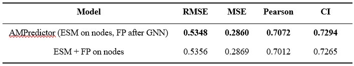
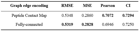
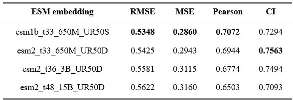
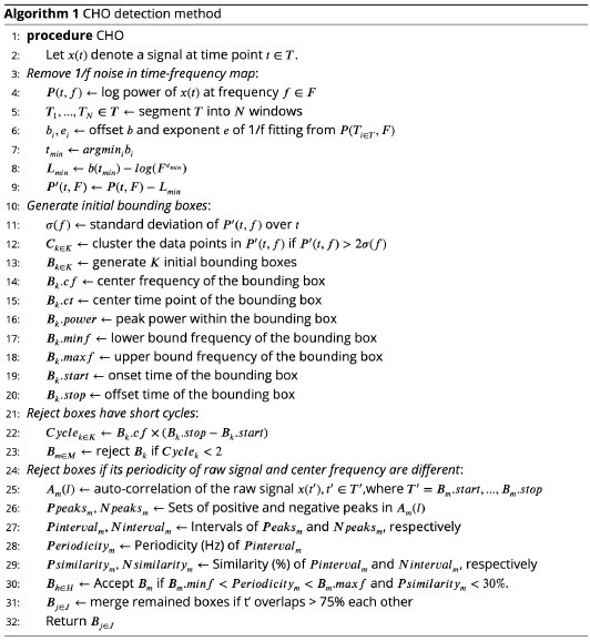
      We thank all the reviewers for their constructive comments. We have carefully considered your feedback and revised the manuscript accordingly. The major concern raised was the applicability of SegPore to the RNA004 dataset. To address this, we compared SegPore with f5c and Uncalled4 on RNA004, and found that SegPore demonstrated improved performance, as shown in Table 2 of the revised manuscript.

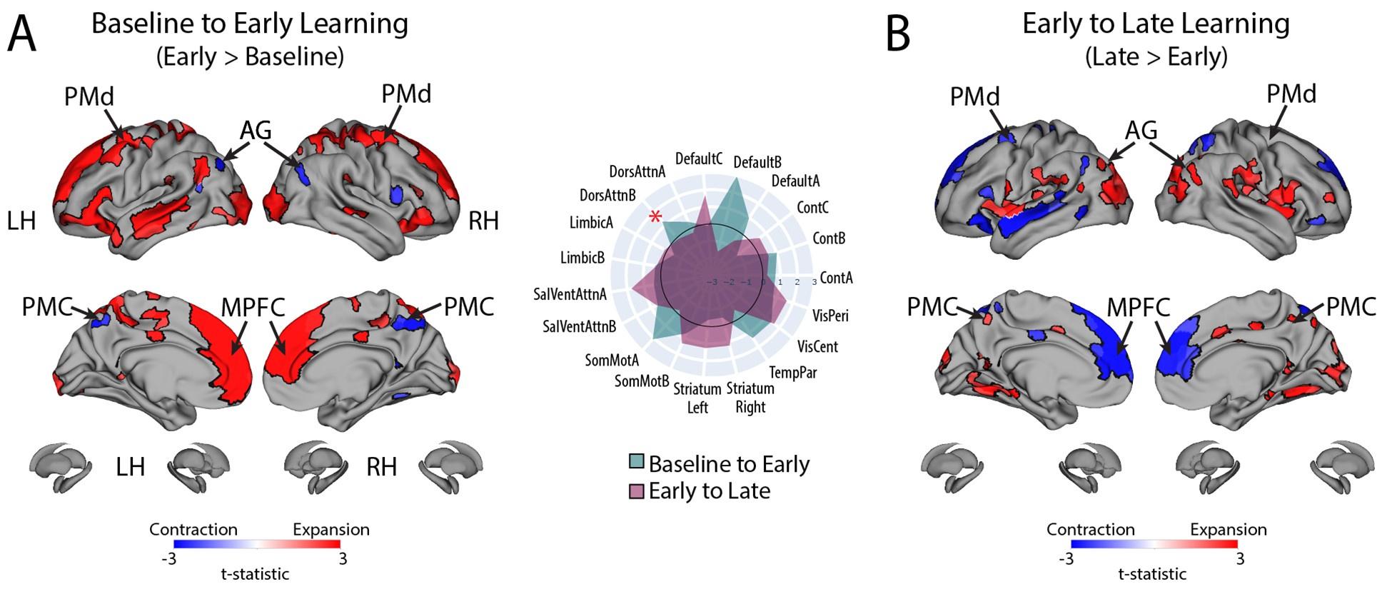
      Following the reviewers’ recommendations, we updated Figures 3 and 4. Additionally, we added one table and three supplementary figures to the revised manuscript:

      · Table 2: Segmentation benchmark on RNA004 data

      · Supplementary Figure S4: RNA translocation hypothesis illustrated on RNA004 data

      · Supplementary Figure S5: Illustration of Nanopolish raw signal segmentation with eventalign results

      · Supplementary Figure S6: Running time of SegPore on datasets of varying sizes

      Below, we provide a point-by-point response to your comments.

      Reviewer #1 (Public review):

      Summary:

      In this manuscript, the authors describe a new computational method (SegPore), which segments the raw signal from nanopore-direct RNA-Seq data to improve the identification of RNA modifications. In addition to signal segmentation, SegPore includes a Gaussian Mixture Model approach to differentiate modified and unmodified bases. SegPore uses Nanopolish to define a first segmentation, which is then refined into base and transition blocks. SegPore also includes a modification prediction model that is included in the output. The authors evaluate the segmentation in comparison to Nanopolish and Tombo, and they evaluate the impact on m6A RNA modification detection using data with known m6A sites. In comparison to existing methods, SegPore appears to improve the ability to detect m6A, suggesting that this approach could be used to improve the analysis of direct RNA-Seq data.

      Strengths:

      SegPore addresses an important problem (signal data segmentation). By refining the signal into transition and base blocks, noise appears to be reduced, leading to improved m6A identification at the site level as well as for single-read predictions. The authors provide a fully documented implementation, including a GPU version that reduces run time. The authors provide a detailed methods description, and the approach to refine segments appears to be new.

      Weaknesses:

      In addition to Nanopolish and Tombo, f5c and Uncalled4 can also be used for segmentation, however, the comparison to these methods is not shown.

      The method was only applied to data from the RNA002 direct RNA-Sequencing version, which is not available anymore, currently, it remains unclear if the methods still work on RNA004.

      Thank you for your comments.

      To clarify the background, there are two kits for Nanopore direct RNA sequencing: RNA002 (the older version) and RNA004 (the newer version). Oxford Nanopore Technologies (ONT) introduced the RNA004 kit in early 2024 and has since discontinued RNA002. Consequently, most public datasets are based on RNA002, with relatively few available for RNA004 (as of 30 June 2025).

      Nanopolish and Tombo were developed for raw signal segmentation and alignment using RNA002 data, whereas f5c and Uncalled4are the only two software supporting RNA004 data.  Since the development of SegPore began in January 2022, we initially focused on RNA002 due to its data availability. Accordingly, our original comparisons were made against Nanopolish and Tombo using RNA002 data.

      We have now updated SegPore to support RNA004 and compared its performance against f5c and Uncalled4 on three public RNA004 datasets.

      As shown in Table 2 of the revised manuscript, SegPore outperforms both f5c and Uncalled4 in raw signal segmentation. Moreover, the jiggling translocation hypothesis underlying SegPore is further supported, as shown in Supplementary Figure S4.

      The overall improvement in accuracy appears to be relatively small.

      Thank you for the comment.

      We understand that the improvements shown in Tables 1 and 2 may appear modest at first glance due to the small differences in the reported standard deviation (std) values. However, even small absolute changes in std can correspond to substantial relative reductions in noise, especially when the total variance is low.

      To better quantify the improvement, we assume that approximately 20% of the std for Nanopolish, Tombo, f5c, and Uncalled4 arises from noise. Using this assumption, we calculate the relative noise reduction rate of SegPore as follows:

      Noise reduction rate = (baseline std − SegPore std) / (0.2 × baseline std) ​​

      Based on this formula, the average noise reduction rates across all datasets are:

      - SegPore vs Nanopolish: 49.52%

      - SegPore vs Tombo: 167.80%

      - SegPore vs f5c: 9.44%

      - SegPore vs Uncalled4: 136.70%

      These results demonstrate that SegPore can reduce the noise level by at least 9% given a noise level of 20%, which we consider a meaningful improvement for downstream tasks, such as base modification detection and signal interpretation. The high noise reduction rates observed in Tombo and Uncalled4 (over 100%) suggest that their actual noise proportion may be higher than our 20% assumption.

      We acknowledge that this 20% noise level assumption is an approximation. Our intention is to illustrate that SegPore provides measurable improvements in relative terms, even when absolute differences appear small.

      The run time and resources that are required to run SegPore are not shown, however, it appears that the GPU version is essential, which could limit the application of this method in practice.

      Thank you for your comment.

      Detailed instructions for running SegPore are provided in github (https://github.com/guangzhaocs/SegPore). Regarding computational resources, SegPore currently requires one CPU core and one Nvidia GPU to perform the segmentation task efficiently.

      We present SegPore’s runtime for typical datasets in Supplementary Figure S6 in the revised manuscript.  For a typical 1 GB fast5 file, the segmentation takes approximately 9.4 hours using a single NVIDIA DGX‑1 V100 GPU and one CPU core.

      Currently, GPU acceleration is essential to achieve practical runtimes with SegPore. We acknowledge that this requirement may limit accessibility in some environments. To address this, we are actively working on a full C++ implementation of SegPore that will support CPU-only execution. While development is ongoing, we aim to release this version in a future update.

      Reviewer #2 (Public review):

      Summary:

      The work seeks to improve the detection of RNA m6A modifications using Nanopore sequencing through improvements in raw data analysis. These improvements are said to be in the segmentation of the raw data, although the work appears to position the alignment of raw data to the reference sequence and some further processing as part of the segmentation, and result statistics are mostly shown on the 'data-assigned-to-kmer' level.

      As such, the title, abstract, and introduction stating the improvement of just the 'segmentation' does not seem to match the work the manuscript actually presents, as the wording seems a bit too limited for the work involved.

      The work itself shows minor improvements in m6Anet when replacing Nanopolish eventalign with this new approach, but clear improvements in the distributions of data assigned per kmer. However, these assignments were improved well enough to enable m6A calling from them directly, both at site-level and at read-level.

      Strengths:

      A large part of the improvements shown appear to stem from the addition of extra, non-base/kmer specific, states in the segmentation/assignment of the raw data, removing a significant portion of what can be considered technical noise for further analysis. Previous methods enforced the assignment of all raw data, forcing a technically optimal alignment that may lead to suboptimal results in downstream processing as data points could be assigned to neighbouring kmers instead, while random noise that is assigned to the correct kmer may also lead to errors in modification detection.

      For an optimal alignment between the raw signal and the reference sequence, this approach may yield improvements for downstream processing using other tools.<br /> Additionally, the GMM used for calling the m6A modifications provides a useful, simple, and understandable logic to explain the reason a modification was called, as opposed to the black models that are nowadays often employed for these types of tasks.

      Weaknesses:

      The work seems limited in applicability largely due to the focus on the R9's 5mer models. The R9 flow cells are phased out and not available to buy anymore. Instead, the R10 flow cells with larger kmer models are the new standard, and the applicability of this tool on such data is not shown. We may expect similar behaviour from the raw sequencing data where the noise and transition states are still helpful, but the increased kmer size introduces a large amount of extra computing required to process data and without knowledge of how SegPore scales, it is difficult to tell how useful it will really be. The discussion suggests possible accuracy improvements moving to 7mers or 9mers, but no reason why this was not attempted.

      Thank you for pointing out this important limitation. Please refer to our response to Point 1 of Reviewer 1 for SegPore’s performance on RNA004 data. Notably, the jiggling behavior is also observed in RNA004 data, and SegPore achieves better performance than both f5c and Uncalled4.

      The increased k-mer size in RNA004 affects only the training phase of SegPore (refer to Supplementary Note 1, Figure 5 for details on the training and testing phases). Once the baseline means and standard deviations for each k-mer are established, applying SegPore to RNA004 data proceeds similarly to RNA002. This is because each k-mer in the reference sequence has, at most, two states (modified and unmodified). While the larger k-mer size increases the size of the parameter table, it does not increase the computational complexity during segmentation. Although estimating the initial k-mer parameter table requires significant time and effort on our part, it does not affect the runtime for end users applying SegPore to RNA004 data.

      Extending SegPore from 5-mers to 7-mers or 9-mers for RNA002 data would require substantial effort to retrain the model and generate sufficient training data. Additionally, such an extension would make SegPore’s output incompatible with widely used upstream and downstream tools such as Nanopolish and m6Anet, complicating integration and comparison. For these reasons, we leave this extension for future work.

      The manuscript suggests the eventalign results are improved compared to Nanopolish. While this is believably shown to be true (Table 1), the effect on the use case presented, downstream differentiation between modified and unmodified status on a base/kmer, is likely limited as during actual modification calling the noisy distributions are usually 'good enough', and not skewed significantly in one direction to really affect the results too terribly.

      Thank you for your comment. While current state-of-the-art (SOTA) methods perform well on benchmark datasets, there remains significant room for improvement. Most SOTA evaluations are based on limited datasets, primarily covering DRACH motifs in human and mouse transcriptomes. However, m6A modifications can also occur in non-DRACH motifs, where current models may underperform. Additionally, other RNA modifications—such as pseudouridine, inosine, and m5C—are less studied, and their detection may benefit from improved signal modeling.

      We would also like to emphasize that raw signal segmentation and RNA modification detection are distinct tasks. SegPore focuses on the former, providing a cleaner, more interpretable signal that can serve as a foundation for downstream tasks. Improved segmentation may facilitate the development of more accurate RNA modification detection algorithms by the community.

      Scientific progress often builds incrementally through targeted improvements to foundational components. We believe that enhancing signal segmentation, as SegPore does, contributes meaningfully to the broader field—the full impact will become clearer as the tool is adopted into more complex workflows.

      Furthermore, looking at alternative approaches where this kind of segmentation could be applied, Nanopolish uses the main segmentation+alignment for a first alignment and follows up with a form of targeted local realignment/HMM test for modification calling (and for training too), decreasing the need for the near-perfect segmentation+alignment this work attempts to provide. Any tool applying a similar strategy probably largely negates the problems this manuscript aims to improve upon.

      We thank the reviewer for this insightful comment.

      To clarify, Nanopolish provides three independent commands: polya, eventalign, and call-methylation.

      - The polya command identifies the adapter, poly(A) tail, and transcript region in the raw signal.

      - The eventalign command aligns the raw signal to a reference sequence, assigning a signal segment to individual k-mers in the reference.

      - The call-methylation command detects methylated bases from DNA sequencing data.

      The eventalign command corresponds to “the main segmentation+alignment for a first alignment,” while call-methylation corresponds to “a form of targeted local realignment/HMM test for modification calling,” as mentioned in the reviewer’s comment. SegPore’s segmentation is similar in purpose to Nanopolish’s eventalign, while its RNA modification estimation component is similar in concept to Nanopolish’s call-methylation.

      We agree the general idea may appear similar, but the implementations are entirely different. Importantly, Nanopolish’s call-methylation is designed for DNA sequencing data, and its models are not trained to recognize RNA modifications. This means they address distinct research questions and cannot be directly compared on the same RNA modification estimation task. However, it is valid to compare them on the segmentation task, where SegPore exhibits better performance (Table 1).

      We infer the reviewer may suggest that because m6Anet is a deep neural network capable of learning from noisy input, the benefit of more accurate segmentation (such as that provided by SegPore) might be limited. This concern may arise from the limited improvement of SegPore+m6Anet over Nanopolish+m6Anet in bulk analysis (Figure 3). Several factors may contribute to this observation:

      (i) For reads aligned to the same gene in the in vivo data, alignment may be inaccurate due to pseudogenes or transcript isoforms.

      (ii) The in vivo benchmark data are inherently more complex than in vitro datasets and may contain additional modifications (e.g., m5C, m7G), which can confound m6A calling by altering the signal baselines of k-mers.

      (iii) m6Anet is trained on events produced by Nanopolish and may not be optimal for SegPore-derived events.

      (iv) The benchmark dataset lacks a modification-free (IVT) control sample, making it difficult to establish a true baseline for each k-mer.

      In the IVT data (Figure 4), SegPore shows a clear improvement in single-molecule m6A identification, with a 3~4% gain in both ROC-AUC and PR-AUC. This demonstrates SegPore’s practical benefit for applications requiring higher sensitivity at the molecule level.

      As noted earlier, SegPore’s contribution lies in denoising and improving the accuracy of raw signal segmentation, which is a foundational step in many downstream analyses. While it may not yet lead to a dramatic improvement in all applications, it already provides valuable insights into the sequencing process (e.g., cleaner signal profiles in Figure 4) and enables measurable gains in modification detection at the single-read level. We believe SegPore lays the groundwork for developing more accurate and generalizable RNA modification detection tools beyond m6A.

      We have also added the following sentence in the discussion to highlight SegPore’s limited performance in bulk analysis:

      “The limited improvement of SegPore combined with m6Anet over Nanopolish+m6Anet in bulk in vivo analysis (Figure 3) may be explained by several factors: potential alignment inaccuracies due to pseudogenes or transcript isoforms, the complexity of in vivo datasets containing additional RNA modifications (e.g., m5C, m7G) affecting signal baselines, and the fact that m6Anet is specifically trained on events produced by Nanopolish rather than SegPore. Additionally, the lack of a modification-free control (in vitro transcribed) sample in the benchmark dataset makes it difficult to establish true baselines for each k-mer. Despite these limitations, SegPore demonstrates clear improvement in single-molecule m6A identification in IVT data (Figure 4), suggesting it is particularly well suited for in vitro transcription data analysis.”

      Finally, in the segmentation/alignment comparison to Nanopolish, the latter was not fitted(/trained) on the same data but appears to use the pre-trained model it comes with. For the sake of comparing segmentation/alignment quality directly, fitting Nanopolish on the same data used for SegPore could remove the influences of using different training datasets and focus on differences stemming from the algorithm itself.

      In the segmentation benchmark (Table 1), SegPore uses the fixed 5-mer parameter table provided by ONT. The hyperparameters of the HHMM are also fixed and not estimated from the raw signal data being segmented. Only in the m6A modification task,  SegPore does perform re-estimation of the baselines for the modified and unmodified states of k-mers. Therefore, the comparison with Nanopolish is fair, as both tools rely on pre-defined models during segmentation.

      Appraisal:

      The authors have shown their method's ability to identify noise in the raw signal and remove their values from the segmentation and alignment, reducing its influences for further analyses. Figures directly comparing the values per kmer do show a visibly improved assignment of raw data per kmer. As a replacement for Nanopolish eventalign it seems to have a rather limited, but improved effect, on m6Anet results. At the single read level modification modification calling this work does appear to improve upon CHEUI.

      Impact:

      With the current developments for Nanopore-based modification largely focusing on Artificial Intelligence, Neural Networks, and the like, improvements made in interpretable approaches provide an important alternative that enables a deeper understanding of the data rather than providing a tool that plainly answers the question of whether a base is modified or not, without further explanation. The work presented is best viewed in the context of a workflow where one aims to get an optimal alignment between raw signal data and the reference base sequence for further processing. For example, as presented, as a possible replacement for Nanopolish eventalign. Here it might enable data exploration and downstream modification calling without the need for local realignments or other approaches that re-consider the distribution of raw data around the target motif, such as a 'local' Hidden Markov Model or Neural Networks. These possibilities are useful for a deeper understanding of the data and further tool development for modification detection works beyond m6A calling.

      Reviewer #3 (Public review):

      Summary:

      Nucleotide modifications are important regulators of biological function, however, until recently, their study has been limited by the availability of appropriate analytical methods. Oxford Nanopore direct RNA sequencing preserves nucleotide modifications, permitting their study, however, many different nucleotide modifications lack an available base-caller to accurately identify them. Furthermore, existing tools are computationally intensive, and their results can be difficult to interpret.

      Cheng et al. present SegPore, a method designed to improve the segmentation of direct RNA sequencing data and boost the accuracy of modified base detection.

      Strengths:

      This method is well-described and has been benchmarked against a range of publicly available base callers that have been designed to detect modified nucleotides.

      Weaknesses:

      However, the manuscript has a significant drawback in its current version. The most recent nanopore RNA base callers can distinguish between different ribonucleotide modifications, however, SegPore has not been benchmarked against these models.

      I recommend that re-submission of the manuscript that includes benchmarking against the rna004_130bps_hac@v5.1.0 and rna004_130bps_sup@v5.1.0 dorado models, which are reported to detect m5C, m6A_DRACH, inosine_m6A and PseU.<br /> A clear demonstration that SegPore also outperforms the newer RNA base caller models will confirm the utility of this method.

      Thank you for highlighting this important limitation. While Dorado, the new ONT basecaller, is publicly available and supports modification-aware basecalling, suitable public datasets for benchmarking m5C, inosine, m6A, and PseU detection on RNA004 are currently lacking. Dorado’s modification-aware models are trained on ONT’s internal data, which is not publicly released. Therefore, it is not currently feasible to evaluate or directly compare SegPore’s performance against Dorado for m5C, inosine, m6A, and PseU detection.

      We would also like to emphasize that SegPore’s main contribution lies in raw signal segmentation, which is an upstream task in the RNA modification detection pipeline. To assess its performance in this context, we benchmarked SegPore against f5c and Uncalled4 on public RNA004 datasets for segmentation quality. Please refer to our response to Point 1 of Reviewer 1 for details.

      Our results show that the characteristic “jiggling” behavior is also observed in RNA004 data (Supplementary Figure S4), and SegPore achieves better segmentation performance than both f5c and Uncalled4 (Table 2).

      Recommendations for the authors:

      Reviewing Editor:

      Please note that we also received the following comments on the submission, which we encourage you to take into account:

      took a look at the work and for what I saw it only mentions/uses RNA002 chemistry, which is deprecated, effectively making this software unusable by anyone any more, as RNA002 is not commercially available. While the results seem promising, the authors need to show that it would work for RNA004. Notably, there is an alternative software for resquiggling for RNA004 (not Tombo or Nanopolish, but the GPU-accelerated version of Nanopolish (f5C), which does support RNA004. Therefore, they need to show that SegPore works for RNA004, because otherwise it is pointless to see that this method works better than others if it does not support current sequencing chemistries and only works for deprecated chemistries, and people will keep using f5C because its the only one that currently works for RNA004. Alternatively, if there would be biological insights won from the method, one could justify not implementing it in RNA004, but in this case, RNA002 is deprecated since March 2024, and the paper is purely methodological.

      Thank you for the comment. We agree that support for current sequencing chemistries is essential for practical utility. While SegPore was initially developed and benchmarked on RNA002 due to the availability of public data, we have now extended SegPore to support RNA004 chemistry.

      To address this concern, we performed a benchmark comparison using public RNA004 datasets against tools specifically designed for RNA004, including f5c and Uncalled4. Please refer to our response to Point 1 of Reviewer 1 for details. The results show that SegPore consistently outperforms f5c and Uncalled4 in segmentation accuracy on RNA004 data.

      Reviewer #2 (Recommendations for the authors):

      Various statements are made throughout the text that require further explanation, which might actually be defined in more detail elsewhere sometimes but are simply hard to find in the current form.

      (1) Page 2, “In this technique, five nucleotides (5mers) reside in the nanopore at a time, and each 5mer generates a characteristic current signal based on its unique sequence and chemical properties (16).”

      5mer? Still on R9 or just ignoring longer range influences, relevant? It is indeed a R9.4 model from ONT.

      Thank you for the observation. We apologize for the confusion and have clarified the relevant paragraph to indicate that the method is developed for RNA002 data by default. Specifically, we have added the following sentence:

      “Two versions of the direct RNA sequencing (DRS) kits are available: RNA002 and RNA004. Unless otherwise specified, this study focuses on RNA002 data.”

      (2) Page 3, “Employ models like Hidden Markov Models (HMM) to segment the signal, but they are prone to noise and inaccuracies.”

      That's the alignment/calling part, not the segmentation?

      Thank you for the comment. We apologize for the confusion. To clarify the distinction between segmentation and alignment, we added a new paragraph before the one in question to explain the general workflow of Nanopore DRS data analysis and to clearly define the task of segmentation. The added text reads:

      “The general workflow of Nanopore direct RNA sequencing (DRS) data analysis is as follows. First, the raw electrical signal from a read is basecalled using tools such as Guppy or Dorado, which produce the nucleotide sequence of the RNA molecule. However, these basecalled sequences do not include the precise start and end positions of each ribonucleotide (or k-mer) in the signal. Because basecalling errors are common, the sequences are typically mapped to a reference genome or transcriptome using minimap2 to recover the correct reference sequence. Next, tools such as Nanopolish and Tombo align the raw signal to the reference sequence to determine which portion of the signal corresponds to each k-mer. We define this process as the segmentation task, referred to as "eventalign" in Nanopolish. Based on this alignment, Nanopolish extracts various features—such as the start and end positions, mean, and standard deviation of the signal segment corresponding to a k-mer. This signal segment or its derived features is referred to as an "event" in Nanopolish.”

      We also revised the following paragraph describing SegPore to more clearly contrast its approach:

      “In SegPore, we first segment the raw signal into small fragments using a Hierarchical Hidden Markov Model (HHMM), where each fragment corresponds to a sub-state of a k-mer. Unlike Nanopolish and Tombo, which directly align the raw signal to the reference sequence, SegPore aligns the mean values of these small fragments to the reference. After alignment, we concatenate all fragments that map to the same k-mer into a larger segment, analogous to the "eventalign" output in Nanopolish. For RNA modification estimation, we use only the mean signal value of each reconstructed event.”

      We hope this revision clarifies the difference between segmentation and alignment in the context of our method and resolves the reviewer’s concern.

      (3) Page 4, Figure 1, “These segments are then aligned with the 5mer list of the reference sequence fragment using a full/partial alignment algorithm, based on a 5mer parameter table. For example, 𝐴𝑗 denotes the base "A" at the j-th position on the reference.”

      I think I do understand the meaning, but I do not understand the relevance of the Aj bit in the last sentence. What is it used for?

      When aligning the segments (output from Step 2) to the reference sequence in Step 3, it is possible for multiple segments to align to the same k-mer. This can occur particularly when the reference contains consecutive identical bases, such as multiple adenines (A). For example, as shown in Fig. 1A, Step 3, the first two segments (μ₁ and μ₂) are aligned to the first 'A' in the reference sequence, while the third segment is aligned to the second 'A'. In this case, the reference sequence AACTGGTTTC...GTC, which contains exactly two consecutive 'A's at the start. This notation helps to disambiguate segment alignment in regions with repeated bases.

      Additionally, this figure and its subscript include mapping with Guppy and Minimap2 but do not mention Nanopolish at all, while that seems an equally important step in the preprocessing (pg5). As such it is difficult to understand the role Nanopolish exactly plays. It's also not mentioned explicitly in the SegPore Workflow on pg15, perhaps it's part of step 1 there?

      We thank the reviewer for pointing this out. We apologize for the confusion. As mentioned in the public response to point 3 of Reviewer 2, SegPore uses Nanopolish to identify the poly(A) tail and transcript regions from the raw signal. SegPore then performs segmentation and alignment on the transcript portion only. This step is indeed part of Step 1 in the preprocessing workflow, as described in Supplementary Note 1, Section 3.

      To clarify this in the main text, we have updated the preprocessing paragraph on page 6 to explicitly describe the role of Nanopolish:

      “We begin by performing basecalling on the input fast5 file using Guppy, which converts the raw signal data into ribonucleotide sequences. Next, we align the basecalled sequences to the reference genome using Minimap2, generating a mapping between the reads and the reference sequences. Nanopolish provides two independent commands: "polya" and "eventalign".
The "polya" command identifies the adapter, poly(A) tail, and transcript region in the raw signal, which we refer to as the poly(A) detection results. The raw signal segment corresponding to the poly(A) tail is used to standardize the raw signal for each read. The "eventalign" command aligns the raw signal to a reference sequence, assigning a signal segment to individual k-mers in the reference. It also computes summary statistics (e.g., mean, standard deviation) from the signal segment for each k-mer. Each k-mer together with its corresponding signal features is termed an event. These event features are then passed into downstream tools such as m6Anet and CHEUI for RNA modification detection. For full transcriptome analysis (Figure 3), we extract the aligned raw signal segment and reference sequence segment from Nanopolish's events for each read by using the first and last events as start and end points. For in vitro transcription (IVT) data with a known reference sequence (Figure 4), we extract the raw signal segment corresponding to the transcript region for each input read based on Nanopolish’s poly(A) detection results.”

      Additionally, we revised the legend of Figure 1A to explicitly include Nanopolish in step 1 as follows:

      “The raw current signal fragments are paired with the corresponding reference RNA sequence fragments using Nanopolish.”

      (4) Page 5, “The output of Step 3 is the "eventalign," which is analogous to the output generated by the Nanopolish "eventalign" command.”

      Naming the function of Nanopolish, the output file, and later on (pg9) the alignment of the newly introduced methods the exact same "eventalign" is very confusing.

      Thank you for the helpful comment. We acknowledge the potential confusion caused by using the term “eventalign” in multiple contexts. To improve clarity, we now consistently use the term “events” to refer to the output of both Nanopolish and SegPore, rather than using "eventalign" as a noun. We also added the following sentence to Step 3 (page 6) to clearly define what an “event” refers to in our manuscript:

      “An "event" refers to a segment of the raw signal that is aligned to a specific k-mer on a read, along with its associated features such as start and end positions, mean current, standard deviation, and other relevant statistics.”

      We have revised the text throughout the manuscript accordingly to reduce ambiguity and ensure consistent terminology.

      (5) Page 5, “Once aligned, we use Nanopolish's eventalign to obtain paired raw current signal segments and the corresponding fragments of the reference sequence, providing a precise association between the raw signals and the nucleotide sequence.”

      I thought the new method's HHMM was supposed to output an 'eventalign' formatted file. As this is not clearly mentioned elsewhere, is this a mistake in writing? Is this workflow dependent on Nanopolish 'eventalign' function and output or not?

      We apologize for the confusion. To clarify, SegPore is not dependent on Nanopolish’s eventalign function for generating the final segmentation results. As described in our response to your comment point 2 and elaborated in the revised text on page 4, SegPore uses its own HHMM-based segmentation model to divide the raw signal into small fragments, each corresponding to a sub-state of a k-mer. These fragments are then aligned to the reference sequence based on their mean current values.

      As explained in the revised manuscript:

      “In SegPore, we first segment the raw signal into small fragments using a Hierarchical Hidden Markov Model (HHMM), where each fragment corresponds to a sub-state of a k-mer. Unlike Nanopolish and Tombo, which directly align the raw signal to the reference sequence, SegPore aligns the mean values of these small fragments to the reference. After alignment, we concatenate all fragments that map to the same k-mer into a larger segment, analogous to the "eventalign" output in Nanopolish. For RNA modification estimation, we use only the mean signal value of each reconstructed event.”

      To avoid ambiguity, we have also revised the sentence on page 5 to more clearly distinguish the roles of Nanopolish and SegPore in the workflow. The updated sentence now reads:

      “Nanopolish provides two independent commands: "polya" and "eventalign".
The "polya" command identifies the adapter, poly(A) tail, and transcript region in the raw signal, which we refer to as the poly(A) detection results. The raw signal segment corresponding to the poly(A) tail is used to standardize the raw signal for each read. The "eventalign" command aligns the raw signal to a reference sequence, assigning a signal segment to individual k-mers in the reference. It also computes summary statistics (e.g., mean, standard deviation) from the signal segment for each k-mer. Each k-mer together with its corresponding signal features is termed an event. These event features are then passed into downstream tools such as m6Anet and CHEUI for RNA modification detection. For full transcriptome analysis (Figure 3), we extract the aligned raw signal segment and reference sequence segment from Nanopolish's events for each read by using the first and last events as start and end points. For in vitro transcription (IVT) data with a known reference sequence (Figure 4), we extract the raw signal segment corresponding to the transcript region for each input read based on Nanopolish’s poly(A) detection results.”

      (6) Page 5, “Since the polyA tail provides a stable reference, we normalize the raw current signals across reads, ensuring that the mean and standard deviation of the polyA tail are consistent across all reads.”

      Perhaps I misread this statement: I interpret it as using the PolyA tail to do the normalization, rather than using the rest of the signal to do the normalization, and that results in consistent PolyA tails across all reads.

      If it's the latter, this should be clarified, and a little detail on how the normalization is done should be added, but if my first interpretation is correct:

      I'm not sure if its standard deviation is consistent across reads. The (true) value spread in this section of a read should be fairly limited compared to the rest of the signal in the read, so the noise would influence the scale quite quickly, and such noise might be introduced to pores wearing down and other technical influences. Is this really better than using the non-PolyA tail part of the reads signal, using Median Absolute Deviation to scale for a first alignment round, then re-fitting the signal scaling using Theil Sen on the resulting alignments (assigned read signal vs reference expected signal), as Tombo/Nanopolish (can) do?

      Additionally, this kind of normalization should have been part of the Nanopolish eventalign already, can this not be re-used? If it's done differently it may result in different distributions than the ONT kmer table obtained for the next step.

      Thank you for this detailed and thoughtful comment. We apologize for the confusion. The poly(A) tail–based normalization is indeed explained in Supplementary Note 1, Section 3, but we agree that the motivation needed to be clarified in the main text.

      We have now added the following sentence in the revised manuscript (before the original statement on page 5 to provide clearer context:

      “Due to inherent variability between nanopores in the sequencing device, the baseline levels and standard deviations of k-mer signals can differ across reads, even for the same transcript. To standardize the signal for downstream analyses, we extract the raw current signal segments corresponding to the poly(A) tail of each read. Since the poly(A) tail provides a stable reference, we normalize the raw current signals across reads, ensuring that the mean and standard deviation of the poly(A) tail are consistent across all reads. This step is crucial for reducing…..”

      We chose to use the poly(A) tail for normalization because it is sequence-invariant—i.e., all poly(A) tails consist of identical k-mers, unlike transcript sequences which vary in composition. In contrast, using the transcript region for normalization can introduce biases: for instance, reads with more diverse k-mers (having inherently broader signal distributions) would be forced to match the variance of reads with more uniform k-mers, potentially distorting the baseline across k-mers.

      In our newly added RNA004 benchmark experiment, we used the default normalization provided by f5c, which does not include poly(A) tail normalization. Despite this, SegPore was still able to mask out noise and outperform both f5c and Uncalled4, demonstrating that our segmentation method is robust to different normalization strategies.

      (7) Page 7, “The initialization of the 5mer parameter table is a critical step in SegPore's workflow. By leveraging ONT's established kmer models, we ensure that the initial estimates for unmodified 5mers are grounded in empirical data.”

      It looks like the method uses Nanopolish for a first alignment, then improves the segmentation matching the reference sequence/expected 5mer values. I thought the Nanopolish model/tables are based on the same data, or similarly obtained. If they are different, then why the switch of kmer model? Now the original alignment may have been based on other values, and thus the alignment may seem off with the expected kmer values of this table.

      Thank you for this insightful question. To clarify, SegPore uses Nanopolish only to identify the poly(A) tail and transcript regions from the raw signal. In the bulk in vivo data analysis, we use Nanopolish’s first event as the start and the last event as the end to extract the aligned raw signal chunk and its corresponding reference sequence. Since SegPore relies on Nanopolish solely to delineate the transcript region for each read, it independently aligns the raw signals to the reference sequence without refining or adjusting Nanopolish’s segmentation results.

      While SegPore's 5-mer parameter table is initially seeded using ONT’s published unmodified k-mer models, we acknowledge that empirical signal values may deviate from these reference models due to run-specific technical variation and the presence of RNA modifications. For this reason, SegPore includes a parameter re-estimation step to refine the mean and standard deviation values of each k-mer based on the current dataset.

      The re-estimation process consists of two layers. In the outer layer, we select a set of 5mers that exhibit both modified and unmodified states based on the GMM results (Section 6 of Supplementary Note 1), while the remaining 5mers are assumed to have only unmodified states. In the inner layer, we align the raw signals to the reference sequences using the 5mer parameter table estimated in the outer layer (Section 5 of Supplementary Note 1). Based on the alignment results, we update the 5mer parameter table in the outer layer. This two-layer process is generally repeated for 3~5 iterations until the 5mer parameter table converges.This re-estimation ensures that:

      (1) The adjusted 5mer signal baselines remain close to the ONT reference (for consistency);

      (2) The alignment score between the observed signal and the reference sequence is optimized (as detailed in Equation 11, Section 5 of Supplementary Note 1);

      (3) Only 5mers that show a clear difference between the modified and unmodified components in the GMM are considered subject to modification.

      By doing so, SegPore achieves more accurate signal alignment independent of Nanopolish’s models, and the alignment is directly tuned to the data under analysis.

      (8) Page 9, “The output of the alignment algorithm is an eventalign, which pairs the base blocks with the 5mers from the reference sequence for each read (Fig. 1C).”

      “Modification prediction

      After obtaining the eventalign results, we estimate the modification state of each motif using the 5mer parameter table.”

      This wording seems to have been introduced on page 5 but (also there) reads a bit confusingly as the name of the output format, file, and function are now named the exact same "eventalign". I assume the obtained eventalign results now refer to the output of your HHMM, and not the original Nanopolish eventalign results, based on context only, but I'd rather have a clear naming that enables more differentiation.

      We apologize for the confusion. We have revised the sentence as follows for clarity:

      “A detailed description of both alignment algorithms is provided in Supplementary Note 1. The output of the alignment algorithm is an alignment that pairs the base blocks with the 5mers from the reference sequence for each read (Fig. 1C). Base blocks aligned to the same 5-mer are concatenated into a single raw signal segment (referred to as an “event”), from which various features—such as start and end positions, mean current, and standard deviation—are extracted. Detailed derivation of the mean and standard deviation is provided in Section 5.3 in Supplementary Note 1. In the remainder of this paper, we refer to these resulting events as the output of eventalign analysis or the segmentation task. ”

      (9) Page 9, “Since a single 5mer can be aligned with multiple base blocks, we merge all aligned base blocks by calculating a weighted mean. This weighted mean represents the single base block mean aligned with the given 5mer, allowing us to estimate the modification state for each site of a read.”

      I assume the weights depend on the length of the segment but I don't think it is explicitly stated while it should be.

      Thank you for the helpful observation. To improve clarity, we have moved this explanation to the last paragraph of the previous section (see response to point 8), where we describe the segmentation process in more detail.

      Additionally, a complete explanation of how the weighted mean is computed is provided in Section 5.3 of Supplementary Note 1. It is derived from signal points that are assigned to a given 5mer.

      (10) Page 10, “Afterward, we manually adjust the 5mer parameter table using heuristics to ensure that the modified 5mer distribution is significantly distinct from the unmodified distribution.”

      Using what heuristics? If this is explained in the supplementary notes then please refer to the exact section.

      Thank you for pointing this out. The heuristics used to manually adjust the 5mer parameter table are indeed explained in detail in Section 7 of Supplementary Note 1.

      To clarify this in the manuscript, we have revised the sentence as follows:

      “Afterward, we manually adjust the 5mer parameter table using heuristics to ensure that the modified 5mer distribution is significantly distinct from the unmodified distribution (see details in Section 7 of Supplementary Note 1).”

      (11) Page 10, “Once the table is fixed, it is used for RNA modification estimation in the test data without further updates.”

      By what tool/algorithm? Perhaps it is your own implementation, but with the next section going into segmentation benchmarking and using Nanopolish before this seems undefined.

      Thank you for pointing this out. We use our own implementation. See Algorithm 3 in Section 6 of Supplementary Note 1.

      We have revised the sentence for clarity:

      “Once a stabilized 5mer parameter table is estimated from the training data, it is used for RNA modification estimation in the test data without further updates. A more detailed description of the GMM re-estimation process is provided in Section 6 of Supplementary Note 1.”

      (12) Page 11, “A 5mer was considered significantly modified if its read coverage exceeded 1,500 and the distance between the means of the two Gaussian components in the GMM was greater than 5.”

      Considering the scaling done before also not being very detailed in what range to expect, this cutoff doesn't provide any useful information. Is this a pA value?

      Thank you for the observation. Yes, the value refers to the current difference measured in picoamperes (pA). To clarify this, we have revised the sentence in the manuscript to include the unit explicitly:

      “A 5mer was considered significantly modified if its read coverage exceeded 1,500 and the distance between the means of the two Gaussian components in the GMM was greater than 5 picoamperes (pA).”

      (13) Page 13, “The raw current signals, as shown in Figure 1B.”

      Wrong figure? Figure 2B seems logical.

      Thank you for catching this. You are correct—the reference should be to Figure 2B, not Figure 1B. We have corrected this in the revised manuscript.

      (14) Page 14, Figure 2A, these figures supposedly support the jiggle hypothesis but the examples seem to match only half the explanation. Any of these jiggles seem to be followed shortly by another in the opposite direction, and the amplitude seems to match better within each such pair than the next or previous segments. Perhaps there is a better explanation still, and this behaviour can be modelled as such instead.

      Thank you for your comment. We acknowledge that the observed signal patterns may appear ambiguous and could potentially suggest alternative explanations. However, as shown in Figure 2A, the red dots tend to align closely with the baseline of the previous state, while the blue dots align more closely with the baseline of the next state. We interpret this as evidence for the "jiggling" hypothesis, where k-mer temporarily oscillates between adjacent states during translocation.

      That said, we agree that more sophisticated models could be explored to better capture this behavior, and we welcome suggestions or references to alternative models. We will consider this direction in future work.

      (15) Page 15, “This occurs because subtle transitions within a base block may be mistaken for transitions between blocks, leading to inflated transition counts.”

      Is it really a "subtle transition" if it happens within a base block? It seems this is not a transition and thus shouldn't be named as such.

      Thank you for pointing this out. We agree that the term “subtle transition” may be misleading in this context. We revised the sentence to clarify the potential underlying cause of the inflated transition counts:

      “This may be due to a base block actually corresponding to a sub-state of a single 5mer, rather than each base block corresponding to a full 5mer, leading to inflated transition counts. To address this issue, SegPore’s alignment algorithm was refined to merge multiple base blocks (which may represent sub-states of the same 5mer) into a single 5mer, thereby facilitating further analysis.”

      (16) Page 15, “The SegPore "eventalign" output is similar to Nanopolish's "eventalign" command.”

      To the output of that command, I presume, not to the command itself.

      Thank you for pointing out the ambiguity. We have revised the sentence for clarity:

      “The final outputs of SegPore are the events and modification state predictions. SegPore’s events are similar to the outputs of Nanopolish’s "eventalign" command, in that they pair raw current signal segments with the corresponding RNA reference 5-mers. Each 5-mer is associated with various features — such as start and end positions, mean current, and standard deviation — derived from the paired signal segment.”

      (17) Page 15, “For selected 5mers, SegPore also provides the modification rate for each site and the modification state of that site on individual reads.”

      What selection? Just all kmers with a possible modified base or a more specific subset?

      We revised the sentence to clarify the selection criteria:

      “For selected 5mers that exhibit both a clearly unmodified and a clearly modified signal component, SegPore reports the modification rate at each site, as well as the modification state of that site on individual reads.”

      (18) Page 16, “A key component of SegPore is the 5mer parameter table, which specifies the mean and standard deviation for each 5mer in both modified and unmodified states (Figure 2A).”

      Wrong figure?

      Thank you for pointing this out. You are correct—it should be Figure 1A, not Figure 2A. We intended to visually illustrate the structure of the 5mer parameter table in Figure 1A, and we have corrected this reference in the revised manuscript.

      (19) Page 16, Table 1, I can't quite tell but I assume this is based on all kmers in the table, not just a m6A modified subset. A short added statement to make this clearer would help.

      Yes, you are right—it is averaged over all 5mers. We have revised the sentence for clarity as follows:

      " As shown in Table 1, SegPore consistently achieved the best performance averaged on all 5mers across all datasets..…."

      (20) Page 16, “Since the peaks (representing modified and unmodified states) are separable for only a subset of 5mers, SegPore can provide modification parameters for these specific 5mers. For other 5mers, modification state predictions are unavailable.”

      Can this be improved using some heuristics rather than the 'distance of 5' cutoff as described before? How small or big is this subset, compared to how many there should be to cover all cases?

      We agree that more sophisticated strategies could potentially improve performance. In this study, we adopted a relatively conservative approach to minimize false positives by using a heuristic cutoff of 5 picoamperes. This value was selected empirically and we did not explore alternative cutoffs. Future work could investigate more refined or data-driven thresholding strategies.

      (21) Page 16, “Tombo used the "resquiggle" method to segment the raw signals, and we standardized the segments using the polyA tail to ensure a fair comparison.”

      I don't know what or how something is "standardized" here.

      Standardized’ refers to the poly(A) tail–based signal normalization described in our response to point 6. We applied this normalization to Tombo’s output to ensure a fair comparison across methods. Without this standardization, Tombo’s performance was notably worse. We revised the sentence as follows:

      “Tombo used the "resquiggle" method to segment the raw signals, and we standardized the segments using the poly(A) tail to ensure a fair comparison (See preprocessing section in Materials and Methods).”

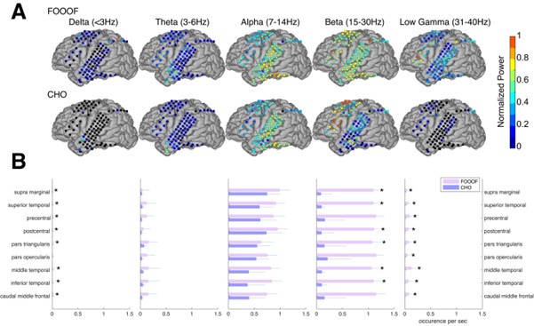
      (22) Page 16, “To benchmark segmentation performance, we used two key metrics: (1) the log-likelihood of the segment mean, which measures how closely the segment matches ONT's 5mer parameter table (used as ground truth), and (2) the standard deviation (std) of the segment, where a lower std indicates reduced noise and better segmentation quality. If the raw signal segment aligns correctly with the corresponding 5mer, its mean should closely match ONT's reference, yielding a high log-likelihood. A lower std of the segment reflects less noise and better performance overall.”

      Here the segmentation part becomes a bit odd:

      A: Low std can be/is achieved by dropping any noisy bits, making segments really small (partly what happens here with the transition segments). This may be 'true' here, in the sense that the transition is not really part of the segment, but the comparison table is a bit meaningless as the other tools forcibly assign all data to kmers, instead of ignoring parts as transition states. In other words, it is a benchmark that is easy to cheat by assigning more data to noise/transition states.

      B: The values shown are influenced by the alignment made between the read and expected reference signal. Especially Tombo tends to forcibly assign data to whatever looks the most similar nearby rather than providing the correct alignment. So the "benchmark of the segmentation performance" is more of an "overall benchmark of the raw signal alignment". Which is still a good, useful thing, but the text seems to suggest something else.

      Thank you for raising these important concerns regarding the segmentation benchmarking.

      Regarding point A, the base blocks aligned to the same 5mer are concatenated into a single segment, including the short transition blocks between them. These transition blocks are typically very short (4~10 signal points, average 6 points), while a typical 5mer segment contains around 20~60 signal points. To assess whether SegPore’s performance is inflated by excluding transition segments, we conducted an additional comparison: we removed 6 boundary signal points (3 from the start and 3 from the end) from each 5mer segment in Nanopolish and Tombo’s results to reduce potential noise. The new comparison table is shown in the following:

      SegPore consistently demonstrates superior performance. Its key contribution lies in its ability to recognize structured noise in the raw signal and to derive more accurate mean and standard deviation values that more faithfully represent the true state of the k-mer in the pore. The improved mean estimates are evidenced by the clearly separated peaks of modified and unmodified 5mers in Figures 3A and 4B, while the improved standard deviation is reflected in the segmentation benchmark experiments.

      Regarding point B, we apologize for the confusion. We have added a new paragraph to the introduction to clarify that the segmentation task indeed includes the alignment step.

      “The general workflow of Nanopore direct RNA sequencing (DRS) data analysis is as follows. First, the raw electrical signal from a read is basecalled using tools such as Guppy or Dorado, which produce the nucleotide sequence of the RNA molecule. However, these basecalled sequences do not include the precise start and end positions of each ribonucleotide (or k-mer) in the signal. Because basecalling errors are common, the sequences are typically mapped to a reference genome or transcriptome using minimap2 to recover the correct reference sequence. Next, tools such as Nanopolish and Tombo align the raw signal to the reference sequence to determine which portion of the signal corresponds to each k-mer. We define this process as the segmentation task, referred to as "eventalign" in Nanopolish. Based on this alignment, Nanopolish extracts various features—such as the start and end positions, mean, and standard deviation of the signal segment corresponding to a k-mer. This signal segment or its derived features is referred to as an "event" in Nanopolish. The resulting events serve as input for downstream RNA modification detection tools such as m6Anet and CHEUI.”

      (23) Page 17 “Given the comparable methods and input data requirements, we benchmarked SegPore against several baseline tools, including Tombo, MINES (26), Nanom6A (27), m6Anet, Epinano (28), and CHEUI (29).”

      It seems m6Anet is actually Nanopolish+m6Anet in Figure 3C, this needs a minor clarification here.

      m6Anet uses Nanopolish’s estimated events as input by default.

      (24) Page 18, Figure 3, A and B are figures without any indication of what is on the axis and from the text I believe the position next to each other on the x-axis rather than overlapping is meaningless, while their spread is relevant, as we're looking at the distribution of raw values for this 5mer. The figure as is is rather confusing.

      Thanks for pointing out the confusion. We have added concrete values to the axes in Figures 3A and 3B and revised the figure legend as follows in the manuscript:

      “(A) Histogram of the estimated mean from current signals mapped to an example m6A-modified genomic location (chr10:128548315, GGACT) across all reads in the training data, comparing Nanopolish (left) and SegPore (right). The x-axis represents current in picoamperes (pA).

      (B) Histogram of the estimated mean from current signals mapped to the GGACT motif at all annotated m6A-modified genomic locations in the training data, again comparing Nanopolish (left) and SegPore (right). The x-axis represents current in picoamperes (pA).”

      (25) Page 18 “SegPore's results show a more pronounced bimodal distribution in the raw signal segment mean, indicating clearer separation of modified and unmodified signals.”

      Without knowing the correct values around the target kmer (like Figure 4B), just the more defined bimodal distribution could also indicate the (wrongful) assignment of neighbouring kmer values to this kmer instead, hence this statement lacks some needed support, this is just one interpretation of the possible reasons.

      Thank you for the comment. We have added concrete values to Figures 3A and 3B to support this point. Both peaks fall within a reasonable range: the unmodified peak (125 pA) is approximately 1.17 pA away from its reference value of 123.83 pA, and the modified peak (118 pA) is around 7 pA away from the unmodified peak. This shift is consistent with expected signal changes due to RNA modifications (usually less than 10 pA), and the magnitude of the difference suggests that the observed bimodality is more likely caused by true modification events rather than misalignment.

      (26) Page 18 “Furthermore, when pooling all reads mapped to m6A-modified locations at the GGACT motif, SegPore showed prominent peaks (Fig. 3B), suggesting reduced noise and improved modification detection.”

      I don't think the prominent peaks directly suggest improved detection, this statement is a tad overreaching.

      We revised the sentense to the following:

      “SegPore exhibited more distinct peaks (Fig. 3B), indicating reduced noise and potentially enabling more reliable modification detection”.

      (27) Page18 “(2) direct m6A predictions from SegPore's Gaussian Mixture Model (GMM), which is limited to the six selected 5mers.”

      The 'six selected' refers to what exactly? Also, 'why' this is limited to them is also unclear as it is, and it probably would become clearer if it is clearly defined what this refers to.

      It is explained the page 16 in the SegPore’s workflow in the original manuscript as follows:

      “A key component of SegPore is the 5mer parameter table, which specifies the mean and standard deviation for each 5mer in both modified and unmodified states (Fig. 2A1A). Since the peaks (representing modified and unmodified states) are separable for only a subset of 5mers, SegPore can provide modification parameters for these specific 5mers. For other 5mers, modification state predictions are unavailable.”

      e select a small set of 5mers that show clear peaks (modified and unmodified 5mers) in GMM in the m6A site-level data analysis. These 5mers are provided in Supplementary Fig. S2C, as explained in the section “m6A site level benchmark” in the Material and Methods (page 12 in the original manuscript).

      “…transcript locations into genomic coordinates. It is important to note that the 5mer parameter table was not re-estimated for the test data. Instead, modification states for each read were directly estimated using the fixed 5mer parameter table. Due to the differences between human (Supplementary Fig. S2A) and mouse (Supplementary Fig. S2B), only six 5mers were found to have m6A annotations in the test data’s ground truth (Supplementary Fig. S2C). For a genomic location to be identified as a true m6A modification site, it had to correspond to one of these six common 5mers and have a read coverage of greater than 20. SegPore derived the ROC and PR curves for benchmarking based on the modification rate at each genomic location….”

      We have updated the sentence as follows to increase clarity:

      “which is limited to the six selected 5mers that exhibit clearly separable modified and unmodified components in the GMM (see Materials and Methods for details).”

      (28) Page 19, Figure 4C, the blue 'Unmapped' needs further explanation. If this means the segmentation+alignment resulted in simply not assigning any segment to a kmer, this would indicate issues in the resulting mapping between raw data and kmers as the data that probably belonged to this kmer is likely mapped to a neighbouring kmer, possibly introducing a bimodal distribution there.

      This is due to deletion event in the full alignment algorithm. See Page 8 of SupplementaryNote1:

      During the traceback step of the dynamic programming matrix, not every 5mer in the reference sequence is assigned a corresponding raw signal fragment—particularly when the signal’s mean deviates substantially from the expected mean of that 5mer. In such cases, the algorithm considers the segment to be generated by an unknown 5mer, and the corresponding reference 5mer is marked as unmapped.

      (29) Page 19, “For six selected m6A motifs, SegPore achieved an ROC AUC of 82.7% and a PR AUC of 38.7%, earning the third-best performance compared with deep leaning methods m6Anet and CHEUI (Fig. 3D).”

      How was this selection of motifs made, are these related to the six 5mers in the middle of Supplementary Figure S2? Are these the same six as on page 18? This is not clear to me.

      It is the same, see the response to point 27.

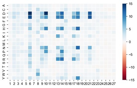
      (30) Page 21 “Biclustering reveals that modifications at the 6th, 7th, and 8th genomic locations are specific to certain clusters of reads (clusters 4, 5, and 6), while the first five genomic locations show similar modification patterns across all reads.”

      This reads rather confusingly. Both the '6th, 7th, and 8th genomic locations' and 'clusters 4,5,6' should be referred to in clearer terms. Either mark them in the figure as such or name them in the text by something that directly matches the text in the figure.

      We have added labels to the clusters and genomic locations Figure 4C, and revised the sentence as follows:

      “Biclustering reveals that modifications at g6 are specific to cluster C4, g7 to cluster C5, and g8 to cluster C6, while the first five genomic locations (g1 to g5) show similar modification patterns across all reads.”

      (31) Page 21, “We developed a segmentation algorithm that leverages the jiggling property in the physical process of DRS, resulting in cleaner current signals for m6A identification at both the site and single-molecule levels.”

      Leverages, or just 'takes into account'?

      We designed our HHMM specifically based on the jiggling hypothesis, so we believe that using the term “leverage” is appropriate.

      (32) Page 21, “Our results show that m6Anet achieves superior performance, driven by SegPore's enhanced segmentation.”

      Superior in what way? It barely improves over Nanopolish in Figure 3C and is outperformed by other methods in Figure 3D. The segmentation may have improved but this statement says something is 'superior' driven by that 'enhanced segmentation', so that cannot refer to the segmentation itself.

      We revise it as follows in the revised manuscript:

      ”Our results demonstrate that SegPore’s segmentation enables clear differentiation between m6A-modified and unmodified adenosines.”

      (33) Page 21, “In SegPore, we assume a drastic change between two consecutive 5mers, which may hold for 5mers with large difference in their current baselines but may not hold for those with small difference.”

      The implications of this assumption don't seem highlighted enough in the work itself and may be cause for falsely discovering bi-modal distributions. What happens if such a 5mer isn't properly split, is there no recovery algorithm later on to resolve these cases?

      We agree that there is a risk of misalignment, which can result in a falsely observed bimodal distribution. This is a known and largely unavoidable issue across all methods, including deep neural network–based methods. For example, many of these models rely on a CTC (Connectionist Temporal Classification) layer, which implicitly performs alignment and may also suffer from similar issues.

      Misalignment is more likely when the current baselines of neighboring k-mers are close. In such cases, the model may struggle to confidently distinguish between adjacent k-mers, increasing the chance that signals from neighboring k-mers are incorrectly assigned. Accurate baseline estimation for each k-mer is therefore critical—when baselines are accurate, the correct alignment typically corresponds to the maximum likelihood.

      We have added the following sentence to the discussion to acknowledge this limitation:

      “As with other RNA modification estimation methods, SegPore can be affected by misalignment errors, particularly when the baseline signals of adjacent k-mers are similar. These cases may lead to spurious bimodal signal distributions and require careful interpretation.”

      (34) Page 21, “Currently, SegPore models only the modification state of the central nucleotide within the 5mer. However, modifications at other positions may also affect the signal, as shown in Figure 4B. Therefore, introducing multiple states to the 5mer could help to improve the performance of the model.”

      The meaning of this statement is unclear to me. Is SegPore unable to combine the information of overlapping kmers around a possibly modified base (central nucleotide), or is this referring to having multiple possible modifications in a single kmer (multiple states)?

      We mean there can be modifications at multiple positions of a single 5mer, e.g. C m5C m6A m7G T. We have revised the sentence to:

      “Therefore, introducing multiple states for a 5mer to accout for modifications at mutliple positions within the same 5mer could help to improve the performance of the model.”

      (35) Page 22, “This causes a problem when apply DNN-based methods to new dataset without short read sequencing-based ground truth. Human could not confidently judge if a predicted m6A modification is a real m6A modification.”

      Grammatical errors in both these sentences. For the 'Human could not' part, is this referring to a single person's attempt or more extensively tested?

      Thanks for the comment. We have revised the sentence as follows:

      “This poses a challenge when applying DNN-based methods to new datasets without short-read sequencing-based ground truth. In such cases, it is difficult for researchers to confidently determine whether a predicted m6A modification is genuine (see Supplmentary Figure S5).”

      (36) Page 22, “…which is easier for human to interpret if a predicted m6A site is real.”

      "a" human, but also this probably meant to say 'whether' instead of 'if', or 'makes it easier'.

      Thanks for the advice. We have revise the sentence as follows:

      “One can generally observe a clear difference in the intensity levels between 5mers with an m6A and those with a normal adenosine, which makes it easier for a researcher to interpret whether a predicted m6A site is genuine.”

      (37) Page 22, “…and noise reduction through its GMM-based approach…”

      Is the GMM providing noise reduction or segmentation?

      Yes, we agree that it is not relevant. We have removed the sentence in the revised manuscript as follows:

      “Although SegPore provides clear interpretability and noise reduction through its GMM-based approach, there is potential to explore DNN-based models that can directly leverage SegPore's segmentation results.”

      (38) Page 23, “SegPore effectively reduces noise in the raw signal, leading to improved m6A identification at both site and single-molecule levels…”

      Without further explanation in what sense this is meant, 'reduces noise' seems to overreach the abilities, and looks more like 'masking out'.

      Following the reviewer’s suggestion, we change it to ‘mask out'’ in the revised manuscript.

      “SegPore effectively masks out noise in the raw signal, leading to improved m6A identification at both site and single-molecule levels.”

      Reviewer #3 (Recommendations for the authors):

      I recommend the publication of this manuscript, provided that the following comments (and the comments above) are addressed.

      In general, the authors state that SegPore represents an improvement on existing software. These statements are largely unquantified, which erodes their credibility. I have specified several of these in the Minor comments section.

      Page 5, Preprocessing: The authors comment that the poly(A) tail provides a stable reference that is crucial for the normalisation of all reads. How would this step handle reads that have variable poly(A) tail lengths? Or have interrupted poly(A) tails (e.g. in the case of mRNA vaccines that employ a linker sequence)?

      We apologize for the confusion. The poly(A) tail–based normalization is explained in Supplementary Note 1, Section 3.

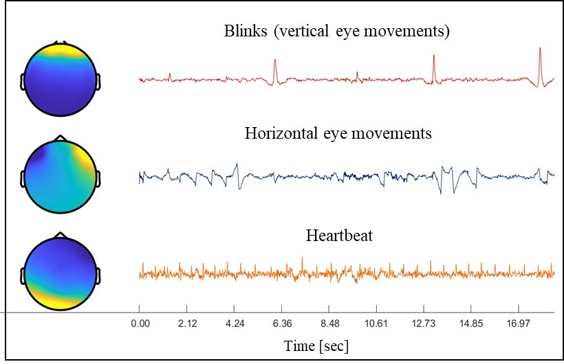
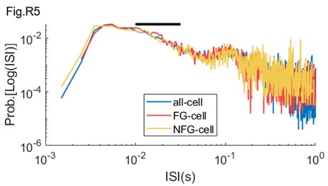
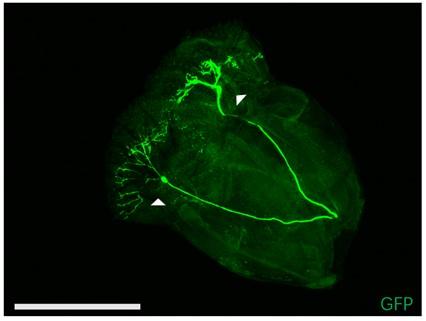
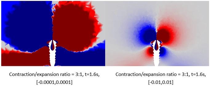
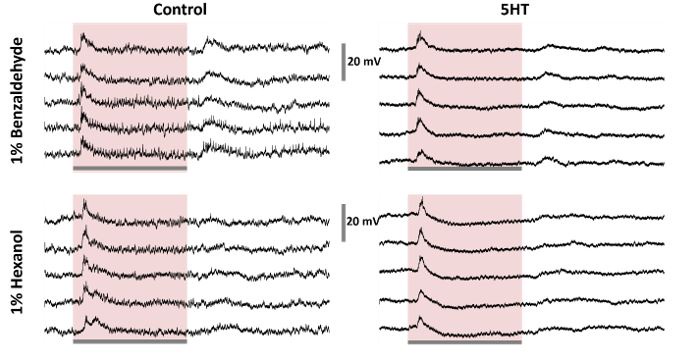
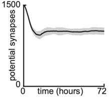
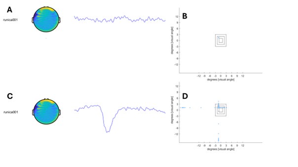
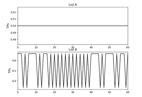
      As shown in Author response image 1 below, the poly(A) tail produces a characteristic signal pattern—a relatively flat, squiggly horizontal line. Due to variability between nanopores, raw current signals often exhibit baseline shifts and scaling of standard deviations. This means that the signal may be shifted up or down along the y-axis and stretched or compressed in scale.

      Author response image 1.

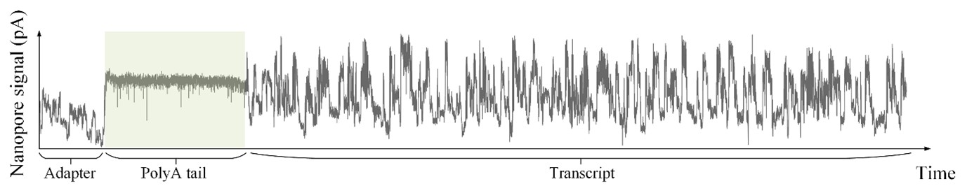
      The normalization remains robust with variable poly(A) tail lengths, as long as the poly(A) region is sufficiently long. The linker sequence will be assigned to the adapter part rather than the poly(A) part.

      To improve clarity in the revised manuscript, we have added the following explanation:

      “Due to inherent variability between nanopores in the sequencing device, the baseline levels and standard deviations of k-mer signals can differ across reads, even for the same transcript. To standardize the signal for downstream analyses, we extract the raw current signal segments corresponding to the poly(A) tail of each read. Since the poly(A) tail provides a stable reference, we normalize the raw current signals across reads, ensuring that the mean and standard deviation of the poly(A) tail are consistent across all reads. This step is crucial for reducing…..”

      We chose to use the poly(A) tail for normalization because it is sequence-invariant—i.e., all poly(A) tails consist of identical k-mers, unlike transcript sequences which vary in composition. In contrast, using the transcript region for normalization can introduce biases: for instance, reads with more diverse k-mers (having inherently broader signal distributions) would be forced to match the variance of reads with more uniform k-mers, potentially distorting the baseline across k-mers.

      Page 7, 5mer parameter table: r9.4_180mv_70bps_5mer_RNA is an older kmer model (>2 years). How does your method perform with the newer RNA kmer models that do permit the detection of multiple ribonucleotide modifications? Addressing this comment is crucial because it is feasible that SegPore will underperform in comparison to the newer RNA base caller models (requiring the use of RNA004 datasets).

      Thank you for highlighting this important point. For RNA004, we have updated SegPore to ensure compatibility with the latest kit. In our revised manuscript, we demonstrate that the translocation-based segmentation hypothesis remains valid for RNA004, as supported by new analyses presented in the supplementary Figure S4.

      Additionally, we performed a new benchmark with f5c and Uncalled4 in RNA004 data in the revised manuscript (Table 2), where SegPore exhibit a better performance than f5c and Uncalled4.

      We agree that benchmarking against the latest Dorado models—specifically rna004_130bps_hac@v5.1.0 and rna004_130bps_sup@v5.1.0, which include built-in modification detection capabilities—would provide valuable context for evaluating the utility of SegPore. However, generating a comprehensive k-mer parameter table for RNA004 requires a large, well-characterized dataset. At present, such data are limited in the public domain. Additionally, Dorado is developed by ONT and its internal training data have not been released, making direct comparisons difficult.

      Our current focus is on improving raw signal segmentation quality, which are upstream tasks critical to many downstream analyses, including RNA modification detection. Future work may include benchmarking SegPore against models like Dorado once appropriate data become available.

      The Methods and Results sections contain redundant information - please streamline the information in these sections and reduce the redundancy. For example, the benchmarking section may be better situated in the Results section.

      Following your advice, we have removed redundant texts about the Segmentation benchmark from Materials and Methods in the revised manuscript.

      Minor comments

      (1) Introduction

      Page 3: "By incorporating these dynamics into its segmentation algorithm...". Please provide an example of how motor protein dynamics can impact RNA translocation. In particular, please elaborate on why motor protein dynamics would impact the translocation of modified ribonucleotides differently to canonical ribonucleotides. This is provided in the results, but please also include details in the Introduction.

      Following your advice, we added one sentence to explain how the motor protein affect the translocation of the DNA/RNA molecule in the revised manuscript.

      “This observation is also supported by previous reports, in which the helicase (the motor protein) translocates the DNA strand through the nanopore in a back-and-forth manner. Depending on ATP or ADP binding, the motor protein may translocate the DNA/RNA forward or backward by 0.5-1 nucleotides.”

      As far as we understand, this translocation mechanism is not specific to modified or unmodified nucleotides. For further details, we refer the reviewer to the original studies cited.

      Page 3: "This lack of interpretability can be problematic when applying these methods to new datasets, as researchers may struggle to trust the predictions without a clear understanding of how the results were generated." Please provide details and citations as to why researchers would struggle to trust the predictions of m6Anet. Is it due to a lack of understanding of how the method works, or an empirically demonstrated lack of reliability?

      Thank you for pointing this out. The lack of interpretability in deep learning models such as m6Anet stems primarily from their “black-box” nature—they provide binary predictions (modified or unmodified) without offering clear reasoning or evidence for each call.

      When we examined the corresponding raw signals, we found it difficult to visually distinguish whether a signal segment originated from a modified or unmodified ribonucleotide. The difference is often too subtle to be judged reliably by a human observer. This is illustrated in the newly added Supplementary Figure S5, which shows Nanopolish-aligned raw signals for the central 5mer GGACT in Figure 4B, displayed both uncolored and colored by modification state (according to the ground truth).

      Although deep neural networks can learn subtle, high-dimensional patterns in the signal that may not be readily interpretable, this opacity makes it difficult for researchers to trust the predictions—especially in new datasets where no ground truth is available. The issue is not necessarily an empirically demonstrated lack of reliability, but rather a lack of transparency and interpretability.

      We have updated the manuscript accordingly and included Supplementary Figure S5 to illustrate the difficulty in interpreting signal differences between modified and unmodified states.

      Page 3: "Instead of relying on complex, opaque features...". Please provide evidence that the research community finds the figures generated by m6Anet to be difficult to interpret, or delete the sections relating to its perceived lack of usability.

      See the figure provided in the response to the previous point. We added a reference to this figure in the revised manuscript.

      “Instead of relying on complex, opaque features (see Supplementary Figure S5), SegPore leverages baseline current levels to distinguish between…..”

      (2) Materials and Methods

      Page 5, Preprocessing: "We begin by performing basecalling on the input fast5 file using Guppy, which converts the raw signal data into base sequences.". Please change "base" to ribonucleotide.

      Revised as requested.

      Page 5 and throughout, please refer to poly(A) tail, rather than polyA tail throughout.

      Revised as requested.

      Page 5, Signal segmentation via hierarchical Hidden Markov model: "...providing more precise estimates of the mean and variance for each base block, which are crucial for downstream analyses such as RNA modification prediction." Please specify which method your HHMM method improves upon.

      Thank you for the suggestion. Since this section does not include a direct comparison, we revised the sentence to avoid unsupported claims. The updated sentence now reads:

      "...providing more precise estimates of the mean and variance for each base block, which are crucial for downstream analyses such as RNA modification prediction."

      Page 10, GMM for 5mer parameter table re-estimation: "Typically, the process is repeated three to five times until the 5mer parameter table stabilizes." How is the stabilisation of the 5mer parameter table quantified? What is a reasonable cut-off that would demonstrate adequate stabilisation of the 5mer parameter table?

      Thank you for the comment. We assess the stabilization of the 5mer parameter table by monitoring the change in baseline values across iterations. If the absolute change in baseline values for all 5mers is less than 1e-5 between two consecutive iterations, we consider the estimation to have stabilized.

      Page 11, M6A site level benchmark: why were these datasets selected? Specifically, why compare human and mouse ribonuclotide modification profiles? Please provide a justification and a brief description of the experiments that these data were derived from, and why they are appropriate for benchmarking SegPore.

      Thank you for the comment. These data are taken from a previous benchmark studie about m6A estimation from RNA002 data in the literature (https://doi.org/10.1038/s41467-023-37596-5). We think the data are appropreciate here.

      Thank you for the comment. The datasets used were taken from a previous benchmark study on m6A estimation using RNA002 data (https://doi.org/10.1038/s41467-023-37596-5). These datasets include human and mouse transcriptomes and have been widely used to evaluate the performance of RNA modification detection tools. We selected them because (i) they are based on RNA002 chemistry, which matches the primary focus of our study, and (ii) they provide a well-characterized and consistent benchmark for assessing m6A detection performance. Therefore, we believe they are appropriate for validating SegPore.

      (3) Results

      Page 13, RNA translocation hypothesis: "The raw current signals, as shown in Fig. 1B...". Please check/correct figure reference - Figure 1B does not show raw current signals.

      Thank you for pointing this out. The correct reference should be Figure 2B. We have updated the figure citation accordingly in the revised manuscript.

      Page 19, m6A identification at the site level: "For six selected m6A motifs, SegPore achieved an ROC AUC of 82.7% and a PR AUC of 38.7%, earning the third best performance compared with deep leaning methods m6Anet and CHEUI (Fig. 3D)." SegPore performs third best of all deep learning methods. Do the authors recommend its use in conjunction with m6Anet for m6A detection? Please clarify in the text.

      This sentence aims to convey that SegPore alone can already achieve good performance. If interpretability is the primary goal, we recommend using SegPore on its own. However, if the objective is to identify more potential m6A sites, we suggest using the combined approach of SegPore and m6Anet. That said, we have chosen not to make explicit recommendations in the main text to avoid oversimplifying the decision or potentially misleading readers.

      Page 19, m6A identification at the single molecule level: "one transcribed with m6A and the other with normal adenosine". I assume that this should be adenine? Please replace adenosine with adenine throughout.

      Thank you for pointing this out. We have revised the sentence to use "adenine" where appropriate. In other instances, we retain "adenosine" when referring specifically to adenine bound to a ribose sugar, which we believe is suitable in those contexts.

      Page 19, m6A identification at the single molecule level: "We used 60% of the data for training and 40% for testing". How many reads were used for training and how many for testing? Please comment on why these are appropriate sizes for training and testing datasets.

      In total, there are 1.9 million reads, with 1.14 million used for training and 0.76 million  for testing (60% and 40%, respectively). We chose this split to ensure that the training set is sufficiently large to reliably estimate model parameters, while the test set remains substantial enough to robustly evaluate model performance. Although the ratio was selected somewhat arbitrarily, it balances the need for effective training with rigorous validation.

      (4) Discussion

      Page 21: "We believe that the de-noised current signals will be beneficial for other downstream tasks." Which tasks? Please list an example.

      We have revised the text for clarity as follows:

      “We believe that the de-noised current signals will be beneficial for other downstream tasks, such as the estimation of m5C, pseudouridine, and other RNA modifications.”

      Page 22: "One can generally observe a clear difference in the intensity levels between 5mers with a m6A and normal adenosine, which is easier for human to interpret if a predicted m6A site is real." This statement is vague and requires qualification. Please reference a study that demonstrates the human ability to interpret two similar graphs, and demonstrate how it relates to the differences observed in your data.

      We apologize for the confusion. We have revised the sentence as follows:

      “One can generally observe a clear difference in the intensity levels between 5mers with an m6A and those with a normal adenosine, which makes it easier for a researcher to interpret whether a predicted m6A site is genuine.”

      We believe that Figures 3A, 3B, and 4B effectively illustrate this concept.

      Page 23: How long does SegPore take for its analyses compared to other similar tools? How long would it take to analyse a typical dataset?

      We have added run-time statistics for datasets of varying sizes in the revised manuscript (see Supplementary Figure S6). This figure illustrates SegPore’s performance across different data volumes to help estimate typical processing times.

      (5) Figures

      Figure 4C. Please number the hierachical clusters and genomic locations in this figure. They are referenced in the text.

      Following your suggestion, we have labeled the hierarchical clusters and genomic locations in Figure 4C in the revised manuscript.

      In addition, we revised the corresponding sentence in the main text as follows: “Biclustering reveals that modifications at g6 are specific to cluster C4, g7 to cluster C5, and g8 to cluster C6, while the first five genomic locations (g1 to g5) show similar modification patterns across all reads.”

  11. social-media-ethics-automation.github.io social-media-ethics-automation.github.io
    1. Whitney Phillips. Internet Troll Sub-Culture's Savage Spoofing of Mainstream Media [Excerpt]. Scientific American, May 2015. URL: https://www.scientificamerican.com/article/internet-troll-sub-culture-s-savage-spoofing-of-mainstream-media-excerpt/ (visited on 2023-12-05).

      Phillips argues that trolling isn’t some fringe glitch—it feeds on the same attention economy that mainstream media uses, which is why hoaxes and outrage travel so well. A helpful detail from her piece is how “it’s just a joke” functions as a shield: ambiguity lets trolls toggle between sincerity and irony to avoid accountability while still harvesting attention. That framework reframes cases like the “Forever Alone Flashmob” as not only individual cruelty but also a media-system problem: amplification (retweets, headlines, livestreams) is the fuel. My takeaway is that platform and newsroom practices—e.g., not linking to troll content, slowing virality for unverifiable claims, and de-incentivizing engagement spikes—are as important as user education for reducing harm.

    1. Author response:

      The following is the authors’ response to the original reviews.

      Reviewer #1 (Public Review):

      Summary:

      The study explored the biomechanics of kangaroo hopping across both speed and animal size to try and explain the unique and remarkable energetics of kangaroo locomotion.

      Strengths:

      The study brings kangaroo locomotion biomechanics into the 21st century. It is a remarkably difficult project to accomplish. There is excellent attention to detail, supported by clear writing and figures.

      Weaknesses:

      The authors oversell their findings, but the mystery still persists. 

      The manuscript lacks a big-picture summary with pointers to how one might resolve the big question.

      General Comments

      This is a very impressive tour de force by an all-star collaborative team of researchers. The study represents a tremendous leap forward (pun intended) in terms of our understanding of kangaroo locomotion. Some might wonder why such an unusual species is of much interest. But, in my opinion, the classic study by Dawson and Taylor in 1973 of kangaroos launched the modern era of running biomechanics/energetics and applies to varying degrees to all animals that use bouncing gaits (running, trotting, galloping and of course hopping). The puzzling metabolic energetics findings of Dawson & Taylor (little if any increase in metabolic power despite increasing forward speed) remain a giant unsolved problem in comparative locomotor biomechanics and energetics. It is our "dark matter problem".

      Thank you for the kind words.

      This study is certainly a hop towards solving the problem. But, the title of the paper overpromises and the authors present little attempt to provide an overview of the remaining big issues. 

      We have modified the title to reflect this comment.  “Postural adaptations may contribute to the unique locomotor energetics seen in hopping kangaroos”

      The study clearly shows that the ankle and to a lesser extent the mtp joint are where the action is. They clearly show in great detail by how much and by what means the ankle joint tendons experience increased stress at faster forward speeds.

      Since these were zoo animals, direct measures were not feasible, but the conclusion that the tendons are storing and returning more elastic energy per hop at faster speeds is solid. The conclusion that net muscle work per hop changes little from slow to fast forward speeds is also solid. 

      Doing less muscle work can only be good if one is trying to minimize metabolic energy consumption. However, to achieve greater tendon stresses, there must be greater muscle forces. Unless one is willing to reject the premise of the cost of generating force hypothesis, that is an important issue to confront. Further, the present data support the Kram & Dawson finding of decreased contact times at faster forward speeds. Kram & Taylor and subsequent applications of (and challenges to) their approach supports the idea that shorter contact times (tc) require recruiting more expensive muscle fibers and hence greater metabolic costs. Therefore, I think that it is incumbent on the present authors to clarify that this study has still not tied up the metabolic energetics across speed problems and placed a bow atop the package. 

      Fortunately, I am confident that the impressive collective brain power that comprises this author list can craft a paragraph or two that summarizes these ideas and points out how the group is now uniquely and enviably poised to explore the problem more using a dynamic SIMM model that incorporates muscle energetics (perhaps ala' Umberger et al.). Or perhaps they have other ideas about how they can really solve the problem.

      You have raised important points, thank you for this feedback. We have added a limitations and considerations section to the discussion which highlights that there are still unanswered questions. Line 311-328

      Considerations and limitations

      “First, we believe it is more likely that the changes in moment arms and EMA can be attributed to speed rather than body mass, given the marked changes in joint angles and ankle height observed at faster hopping speeds. However, our sample included a relatively narrow range of body masses (13.7 to 26.6 kg) compared to the potential range (up to 80 kg), limiting our ability to entirely isolate the effects of speed from those of mass. Future work should examine a broader range of body sizes. Second, kangaroos studied here only hopped at relatively slow speeds, which bounds our estimates of EMA and tendon stress to a less critical region. As such, we were unable to assess tendon stress at fast speeds, where increased forces would reduce tendon safety factors closer to failure. A different experimental or modelling approach may be needed, as kangaroos in enclosures seem unwilling to hop faster over force plates. Finally, we did not determine whether the EMA of proximal hindlimb joints (which are more difficult to track via surface motion capture markers) remained constant with speed. Although the hip and knee contribute substantially less work than the ankle joint (Fig. 4), the majority of kangaroo skeletal muscle is located around these proximal joints. A change in EMA at the hip or knee could influence a larger muscle mass than at the ankle, potentially counteracting or enhancing energy savings in the ankle extensor muscle-tendon units. Further research is needed to understand how posture and muscles throughout the whole body contribute to kangaroo energetics.”

      Additionally, we added a line “Peak GRF also naturally increased with speed together with shorter ground contact durations (Fig. 2b, Suppl. Fig 1b)” (line 238) to highlight that we are not proposing that changes in EMA alone explain the full increase in tendon stress. Both GRF and EMA contribute substantially (almost equally) to stress, and we now give more equal discussion to both. For instance, we now also evaluate how much each contributes: “If peak GRF were constant but EMA changed from the average value of a slow hop to a fast hop, then stress would increase 18%, whereas if EMA remained constant and GRF varied by the same principles, then stress would only increase by 12%. Thus, changing posture and decreasing ground contact duration both appear to influence tendon stress for kangaroos, at least for the range of speeds we examined” (Line 245-249)

      We have added a paragraph in the discussion acknowledging that the cost of generating force problem is not resolved by our work, concluding that “This mechanism may help explain why hopping macropods do not follow the energetic trends observed in other species (Dawson and Taylor 1973, Baudinette et al. 1992, Kram and Dawson 1998), but it does not fully resolve the cost of generating force conundrum” Line 274-276.

      I have a few issues with the other half of this study (i.e. animal size effects). I would enjoy reading a new paragraph by these authors in the Discussion that considers the evolutionary origins and implications of such small safety factors. Surely, it would need to be speculative, but that's OK.

      We appreciate this comment from the reviewer, however could not extend the study to discuss animal size effects because, as we now note in the results: “The range of body masses may not be sufficient to detect an effect of mass on ankle moment in addition to the effect of speed.” Line 193

      Reviewer #2 (Public Review):

      Summary

      This is a fascinating topic that has intrigued scientists for decades. I applaud the authors for trying to tackle this enigma. In this manuscript, the authors primarily measured hopping biomechanics data from kangaroos and performed inverse dynamics. 

      While these biomechanical analyses were thorough and impressively incorporated collected anatomical data and an Opensim model, I'm afraid that they did not satisfactorily address how kangaroos can hop faster and not consume more metabolic energy, unique from other animals.  Noticeably, the authors did not collect metabolic data nor did they model metabolic rates using their modelling framework. Instead, they performed a somewhat traditional inverse dynamics analysis from multiple animals hopping at a self-selected speed.

      In the current study, we aimed to provide a joint-level explanation for the increases of tendon stress that are likely linked to metabolic energy consumption.

      We have now included a limitations section in the manuscript (See response to Rev 1). We plan to expand upon muscle level energetics in the future with a more detailed musculoskeletal model.

      Within these analyses, the authors largely focused on ankle EMA, discussing its potential importance (because it affects tendon stress, which affects tendon strain energy, which affects muscle mechanics) on the metabolic cost of hopping. However, EMA was roughly estimated (CoP was fixed to the foot, not measured) and did not detectibly associate with hopping speed (see results Yet, the authors interpret their EMA findings as though it systematically related with speed to explain their theory on how metabolic cost is unique in kangaroos vs. other animals

      As noted in our methods, EMA was not calculated from a fixed centre of pressure (CoP). We did fix the medial-lateral position, owing to the fact that both feet contacted the force plate together, but the anteroposterior movement of the CoP was recorded by the force plate and thus allowed to move. We report the movement (or lack of movement) in our results. The anterior-posterior axis is the most relevant to lengthening or shortening the distance of the ‘out-lever’ R, and thereby EMA. It is necessary to assume fixed medial-lateral position because a single force trace and CoP is recorded when two feet land on the force plate. The mediallateral forces on each foot cancel out so there is no overall medial-lateral movement if the forces are symmetrical (e.g. if the kangaroo is hopping in a straight path and one foot is not in front of the other). We only used symmetrical trials so that the anterior-posterior movement of the CoP would be reliable. We have now added additional details into the text to clarify this

      Indeed, the relationship between R and speed (and therefore EMA and speed) was not significant. However, the significant change in ankle height with speed, combined with no systematic change in COP at midstance, demonstrates that R would be greater at faster speeds. If we consider the nonsignificant relationship between R and speed to indicate that there is no change in R, then these two results conflict. We could not find a flaw in our methods, so instead concluded that the nonsignificant relationship between R and speed may be due to a small change in R being undetectable in our data. Taking both results into account, we believe it is more likely that there is a non-detectable change in R, rather than no change in R with speed, but we presented both results for transparency. We have added an additional section into the results to make this clearer (Line 177-185) “If we consider the nonsignificant relationship between R (and EMA) and speed to indicate that there is no change in R, then it conflicts with the ankle height and CoP result. Taking both into account, we think it is more likely that there is a small, but important, change in R, rather than no change in R with speed. It may be undetectable because we expect small effect sizes compared to the measurement range and measurement error (Suppl. Fig. 3h), or be obscured by a similar change in R with body mass. R is highly dependent on the length of the metatarsal segment, which is longer in larger kangaroos (1 kg BM corresponded to ~1% longer segment, P<0.001, R<sup>2</sup>=0.449). If R does indeed increase with speed, both R and r will tend to decrease EMA at faster speeds.”

      These speed vs. biomechanics relationships were limited by comparisons across different animals hopping at different speeds and could have been strengthened using repeated measures design

      There is significant variation in speed within individuals, not just between individuals. The preferred speed of kangaroos is 2-4.5 m/s, but most individuals showed a wide speed range within this. Eight of our 16 kangaroos had a maximum speed that was 1-2m/s faster than their slowest trial. Repeated measures of these eight individuals comprises 78 out of the 100 trials.   It would be ideal to collect data across the full range of speeds for all individuals, but it is not feasible in this type of experimental setting. Interference with animals such as chasing is dangerous to kangaroos as they are prone to adverse reactions to stress. We have now added additional information about the chosen hopping speeds into the results and methods sections to clarify this “The kangaroos elected to hop between 1.99 and 4.48 m s<sup>-1</sup>, with a range of speeds and number of trials for each individual (Suppl. Fig. 9).”  (Line 381-382)

      There are also multiple inconsistencies between the authors' theory on how mechanics affect energetics and the cited literature, which leaves me somewhat confused and wanting more clarification and information on how mechanics and energetics relate

      We thank the reviewer for this comment. Upon rereading we now understand the reviewers position, and have made substantial revisions to the introduction and discussion (See comments below) 

      My apologies for the less-than-favorable review, I think that this is a neat biomechanics study - but am unsure if it adds much to the literature on the topic of kangaroo hopping energetics in its current form.

      Again we thank the reviewer for their time and appreciate their efforts to strengthen our manuscript.

      Reviewer #3 (Public Review):

      Summary:

      The goal of this study is to understand how, unlike other mammals, kangaroos are able to increase hopping speed without a concomitant increase in metabolic cost. They use a biomechanical analysis of kangaroo hopping data across a range of speeds to investigate how posture, effective mechanical advantage, and tendon stress vary with speed and mass. The main finding is that a change in posture leads to increasing effective mechanical advantage with speed, which ultimately increases tendon elastic energy storage and returns via greater tendon strain. Thus kangaroos may be able to conserve energy with increasing speed by flexing more, which increases tendon strain.

      Strengths:

      The approach and effort invested into collecting this valuable dataset of kangaroo locomotion is impressive. The dataset alone is a valuable contribution.

      Thank you!

      Weaknesses:

      Despite these strengths, I have concerns regarding the strength of the results and the overall clarity of the paper and methods used (which likely influences how convincingly the main results come across).

      (1) The paper seems to hinge on the finding that EMA decreases with increasing speed and that this contributes significantly to greater tendon strain estimated with increasing speed. It is very difficult to be convinced by this result for a number of reasons:

      It appears that kangaroos hopped at their preferred speed. Thus the variability observed is across individuals not within. Is this large enough of a range (either within or across subjects) to make conclusions about the effect of speed, without results being susceptible to differences between subjects? 

      Apologies, this was not clear in the manuscript. Kangaroos hopping at their preferred speed means we did not chase or startle them into high speeds to comply with ethics and enclosure limitations. Thus we did not record a wide range of speeds within the bounds of what kangaroos are capable of in the wild (up to 12 m/s), but for the range we did measure (~2-4.5 m/s), there is a large amount of variation in hopping speed within each individual kangaroo. Out of 16 individuals, eight individuals had a difference of 1-2m/s between their slowest and fastest trials, and these kangaroos accounted for 78 out of 100 trials. Of the remainder, six individuals had three for fewer trials each, and two individuals had highly repeatable speeds (3 out of 4, and 6 out of 7 trials were within 0.5 m/s). We have now removed the terminology “preferred speed” e.g line 115. We have added additional information about the chosen hopping speeds into the results and methods, including an appendix figure “The kangaroos elected to hop between 1.99 and 4.48 m s<sup>-1</sup>, with a range of speeds and number of trials for each individual (Suppl. Fig. 9).” (Line 381-382)

      In the literature cited, what was the range of speeds measured, and was it within or between subjects?

      For other literature, to our knowledge the highest speed measured is ~9.5m/s (see supplementary Fig1b) and there were multiple measures for several individuals (see methods Kram & Dawson 1998). 

      Assuming that there is a compelling relationship between EMA and velocity, how reasonable is it to extrapolate to the conclusion that this increases tendon strain and ultimately saves metabolic cost?  They correlate EMA with tendon strain, but this would still not suggest a causal relationship (incidentally the p-value for the correlation is not reported). 

      The functions that underpin these results (e.g. moment = GRF*R) come from physical mechanics and geometry, rather than statistical correlations. Additionally, a p-value is not appropriate in the relationship between EMA and stress (rather than strain) because the relationship does not appear to be linear. We have made it clearer in the discussion that we are not proposing that entire change in stress is caused by changes in EMA, but that the increase in GRF that naturally occurs with speed will also explain some of the increase in stress, along with other potential mechanisms. The discussion has been extensively revised to reflect this. 

      Tendon strain could be increasing with ground reaction force, independent of EMA. Even if there is a correlation between strain and EMA, is it not a mathematical necessity in their model that all else being equal, tendon stress will increase as ema decreases? I may be missing something, but nonetheless, it would be helpful for the authors to clarify the strength of the evidence supporting their conclusions.

      Yes, GRF also contributes to the increase in tendon stress in the mechanism we propose (Suppl. Fig. 8), see the formulas in Fig 6, and we have made this clearer in the revised discussion (see above comment).  You are correct that mathematically stress is inversely proportional to EMA, which can be observed in Fig. 7a, and we did find that EMA decreases. 

      The statistical approach is not well-described. It is not clear what the form of the statistical model used was and whether the analysis treated each trial individually or grouped trials by the kangaroo. There is also no mention of how many trials per kangaroo, or the range of speeds (or masses) tested. 

      The methods include the statistical model with the variables that we used, as well as the kangaroo masses (13.7 to 26.6 kg, mean: 20.9 ± 3.4 kg). We did not have sufficient within individual sample size to use a linear mixed effect model including subject as a random factor, thus all trials were treated individually. We have included this information in the results section. 

      We have now moved the range of speeds from the supplementary material to the results and figure captions. We have added information on the number of trials per kangaroo to the methods, and added Suppl. Fig. 9 showing the distribution of speeds per kangaroo.

      We did not group the data e.g. by using an average speed per individual for all their trials, or by comparing fast to slow groups for statistical analysis (the latter was only for display purposes in our figures, which we have now made clearer in the methods statistics section). 

      Related to this, there is no mention of how different speeds were obtained. It seems that kangaroos hopped at a self-selected pace, thus it appears that not much variation was observed. I appreciate the difficulty of conducting these experiments in a controlled manner, but this doesn’t exempt the authors from providing the details of their approach.

      Apologies, this was not clear in the manuscript. Kangaroos hopping at their preferred speed means we did not chase or startle them into high speeds to comply with ethics and enclosure limitations. Thus we did not record a wide range of speeds within the bounds of what kangaroos are capable of in the wild (up to 12 m/s). We have now removed the terminology “preferred speed” e.g. line 115. We have added additional information about the chosen hopping speeds into the results and methods, including an appendix figure (see above comment). (Line 381-382)

      Some figures (Figure 2 for example) present means for one of three speeds, yet the speeds are not reported (except in the legend) nor how these bins were determined, nor how many trials or kangaroos fit in each bin. A similar comment applies to the mass categories. It would be more convincing if the authors plotted the main metrics vs. speed to illustrate the significant trends they are reporting.

      Thank you for this comment. The bins are used only for display purposes and not within the statistical analysis. We have clarified this in the revised manuscript: “The data was grouped into body mass (small 17.6±2.96 kg, medium 21.5±0.74 kg, large 24.0±1.46 kg) and speed (slow 2.52±0.25 m s<sup>-1</sup>, medium 3.11±0.16 m s<sup>-1</sup>, fast 3.79±0.27 m s<sup>-1</sup>) subsets for display purposes only”. (Line 495-497)

      (2) The significance of the effects of mass is not clear. The introduction and abstract suggest that the paper is focused on the effect of speed, yet the effects of mass are reported throughout as well, without a clear understanding of the significance. This weakness is further exaggerated by the fact that the details of the subject masses are not reported.

      Indeed, the primary aim of our study was to explore the influence of speed, given the uncoupling of energy from hopping speed in kangaroos. We included mass to ensure that the effects of speed were not driven by body mass (i.e.: that larger kangaroos hopped faster). Subject masses were reported in the first paragraph of the methods, albeit some were estimated as outlined in the same paragraph.

      (3) The paper needs to be significantly re-written to better incorporate the methods into the results section. Since the results come before the methods, some of the methods must necessarily be described such that the study can be understood at some level without turning to the dedicated methods section. As written, it is very difficult to understand the basis of the approach, analysis, and metrics without turning to the methods.

      The methods after the discussion is a requirement of the journal. We have incorporated some methods in the results where necessary but not too repetitive or disruptive, e.g. Fig. 1 caption, and specifying we are only analysing EMA for the ankle joint

      Reviewing Editor (Recommendations For The Authors):

      Below is a list of specific recommendations that the authors could address to improve the eLife assessment:

      (1) Based on the data presented and the fact that metabolic energy was not measured, the authors should temper their conclusions and statements throughout the manuscript regarding the link between speed and metabolic energy savings. We recommend adding text to the discussion summarizing the strengths and limitations of the evidence provided and suggesting future steps to more conclusively answer this mystery.

      There is a significant body of work linking metabolic energy savings to measured increases in tendon stress in macropods. However, the purpose of this paper was to address the unanswered questions about why tendon stress increases. We found that stress did not only increase due to GRF increasing with speed as expected, but also due to novel postural changes which decreased EMA. In the revised manuscript, we have tempered our conclusions to make it clearer that it is not just EMA affecting stress, and added limitations throughout the manuscript (see response to Rev 1). 

      (2) To provide stronger evidence of a link between speed, mechanics, and metabolic savings the authors can consider estimating metabolic energy expenditure from their OpenSIM model. This is one suggestion, but the authors likely have other, possibly better ideas. Such a model should also be able to explain why the metabolic rate increases with speed during uphill hopping.

      Extending the model to provide direct metabolic cost estimates will be the goal of a future paper, however the models does not have detailed muscle characteristics to do this in the formulation presented here. It would be a very large undertaking which is beyond the scope of the current manuscript. As per the comment above, the results of this paper are not reliant on metabolic performance. 

      (3) The authors attempt to relate the newly quantified hopping biomechanics to previously published metabolic data. However, all reviewers agree that the logic in many instances is not clear or contradictory. Could one potential explanation be that at slow speeds, forces and tendon strain are small, and thus muscle fascicle work is high? Then, with faster speeds, even though the cost of generating isometric force increases, this is offset by the reduction in the metabolic cost of muscular work. The paper could provide stronger support for their hypotheses with a much clearer explanation of how the kinematics relate to the mechanics and ultimately energy savings.

      In response to the reviewers comments, we have substantially modified the discussion to provide clearer rationale.

      (4) The methods and the effort expended to collect these data are impressive, but there are a number of underlying assumptions made that undermine the conclusions. This is due partly to the methods used, but also the paper's incomplete description of their methods. We provide a few examples below:

      It would be helpful if the authors could speak to the effect of the limited speeds tested and between-animal comparisons on the ability to draw strong conclusions from the present dataset. ·

      Throughout the discussion, the authors highlight the relationship between EMA and speed. However, this is misleading since there was no significant effect of speed on EMA. Speed only affected the muscle moment arm, r. At minimum, this should be clarified and the effect on EMA not be overstated. Additionally, the resulting implications on their ability to confidently say something about the effect of speed on muscle stress should be discussed. 

      We have now provided additional details, (see responses above) to these concerns. For instance, we added a supplementary figure showing the speed distribution per individual. The primary reviewer concern (that each kangaroo travelled at a single speed) was due to a miscommunication around the terminology “preferred” which has now been corrected. 

      We now elaborate in the results why we are not very concerned that EMA is insignificant. The statistical insignificance of EMA is ultimately due to the insignificance of the direct measurement of R, however, we now better explain in the results why we believe that this statistical insignificance is due to error/noise of the measurement which is relatively large compared to the effect size. Indirect indications of how R may increase with speed (via ankle height from the ground) are statistically significant. Lines 177-185. 

      We consider this worth reporting because, for instance, an 18% change in EMA will be undetectable by measurement, but corresponds to an 18% change in tendon stress which is measurable and physiologically significant (safety factor would decrease from 2 to 1.67).  We presented both significant and insignificant results for transparency. 

      We have also discussed this within a revised limitations section of the manuscript (Line 311328). 

      Reviewer #1 (Recommendations For The Authors):

      Title: I would cut the first half of the title. At least hedge it a bit. "Clues" instead of "Unlocking the secrets".

      We have revised the title to: “Postural adaptations may contribute to the unique locomotor energetics seen in hopping kangaroos”

      In my comments, ... typically indicates a stylistic change suggested to the text.

      Overall, the paper covers speed and size. Unfortunately, the authors were not 100% consistent in the order of presenting size then speed, or speed then size. Just choose one and stick with it.

      We have attempted to keep the order of presenting size and speed consistent, however there are several cases where this would reduce the readability of the manuscript and so in some cases this may vary. 

      One must admit that there is a lot of vertical scatter in almost all of the plots. I understand that these animals were not in a lab on a treadmill at a controlled speed and the animals wear fur coats so marker placements vary/move etc. But the spread is quite striking, e.g. Figure 5a the span at one speed is almost 10x. Can the authors address this somewhere? Limitations section?

      The variation seen likely results from attempting to display data in a 2D format, when it is in fact the result of multiple variables, including speed, mass, stride frequency and subject specific lengths. Slight variations in these would be expected to produce some noise around the mean, and I think it’s important to consider this while showing the more dominant effects. 

      In many locations in the manuscript, the term "work" is used, but rarely if ever specified that this is the work "per hop". The big question revolves around the rate of metabolic energy consumption (i.e. energy per time or average metabolic power), one must not forget that hop frequency changes somewhat across speed, so work per hop is not the final calculation.

      Thank you for this comment. We have now explicitly stated work per hop in figure captions and in the results (line 208). The change in stride frequency at this range of speeds is very small, particularly compared to the variance in stride frequency (Suppl. Fig. 1d), which is consistent with other researchers who found that stride frequency was constant or near constant in macropods at analogous speeds (e.g. Dawson and Taylor 1973, Baudinette et al. 1987). 

      Line 61 ....is likely related.

      Added “likely” (line 59)

      Line 86 I think the Allen reference is incomplete. Wasn't it in J Exp Biology?

      Thank you. Changed. 

      Line 122 ... at faster speeds and in larger individuals.

      Changed: “We hypothesised that (i) the hindlimb would be more crouched at faster speeds, primarily due to the distal hindlimb joints (ankle and metatarsophalangeal), independent of changes with body mass” (Line 121-122).

      Line 124 I found this confusing. Try to re-word so that you explain you mean more work done by the tendons and less by the ankle musculature.

      Amended: “changes in moment arms resulting from the change in posture would contribute to the increase in tendon stress with speed, and may thereby contribute to energetic savings by increasing the amount of positive and negative work done by the ankle without requiring additional muscle work” (Line 123)

      Line 129 hopefully "braking" not "breaking"!

      Thank you. Fixed. (Line 130)

      Line 129 specify fore-aft horizontal force.

      Added "fore-aft" to "negative fore-aft horizontal component" (Line 130-131)

      Line 130 add something like "of course" or "naturally" since if there is zero fore-aft force, the GRF vector of course must be vertical. 

      Added "naturally" (Line 132)

      Line 138 clarify that this section is all stance phase. I don't recall reading any swing phase data.

      Changed to: "Kangaroo hindlimb stance phase kinematics varied…" (Line 141)

      Line 143 and elsewhere. I found the use of dorsiflexion and plantarflexion confusing. In Figure 3, I see the ankle never flexing more than 90 degrees. So, the ankle joint is always in something of a flexed position, though of course it flexes and extends during contact. I urge the authors to simplify to flextion/extension and drop the plantar/dorsi.

      We have edited this section to describe both movements as greater extension (plantarflexion). (Line 147). We have further clarified this in the figure caption for figure 3.  

      Line 147 ...changes were…

      Fixed, line 150

      Line 155 I'm a bit confused here. Are the authors calculating some sort of overall EMA or are they saying all of the individual joint EMAs all decreased?

      Thank you, we clarified that it is at the ankle. Line 158

      Line 158 since kangaroos hop and are thus positioned high and low throughout the stance phase, try to avoid using "high" and "low" for describing variables, e.g. GRF or other variables. Just use "greater/greatest" etc.

      Thanks for this suggestion. We have changed "higher" into "greater" where appropriate throughout the manuscript e.g. line 161

      Lines 162 and 168 same comment here about "r" and "R". Do you mean ankle or all joints?

      Clarified that it is the gastrocnemius and plantaris r, and the R to the ankle. (Lines 164-165)

      Line 173 really, ankle height?

      Added: ankle height is "vertical distance from the ground". Line 177

      Line 177 is this just the ankle r?

      Added "of the ankle" line 158 and “Achilles” line 187 

      Line 183 same idea, which tendon/tendons are you talking about here?

      Added "Achilles" to be more clear (Line 187)

      Line 195 substitute "converted" for "transferred".

      Done (Line 210)

      Line 223 why so vague? i.e. why use "may"? Believe in your data. ...stress was also modulated by changes....

      Changed "may" to "is"

      Line 229 smaller ankle EMA (especially since you earlier talked about ankle "height").

      Changed “lower” to “smaller” Line 254

      Line 2236 ...and return elastic energy…

      Added "elastic" line 262

      Line 244 IMPORTANT: Need to explain this better! I think you are saying that the net work at the ankle is staying the same across speed, BUT it is the tendons that are storing and returning that work, it's not that the muscles are doing a lot of negative/positive work.

      Changed: “The consistent net work observed among all speeds suggests the ankle extensor muscle-tendon units are performing similar amounts of ankle work independent of speed, which would predominantly be done by the tendon.” Line 270-272)

      Line 258-261 I think here is where you are over-selling the data/story. Although you do say "a" mechanism (and not "the" mechanism, you still need to deal with the cost of generating more force and generating that force faster.

      We removed this sentence and replaced it with a discussion of the cost of generating force hypothesis, and alternative scenarios for the how force and metabolics could be uncoupled. 

      Line 278 "the" tendon? Which tendon?

      Added "Achilles"

      Line 289. I don't think one can project into the past.

      Changed “projected” to "estimated"

      Line 303 no problem, but I've never seen a paper in biology where the authors admit they don't know what species they were studying!

      Can’t be helped unfortunately. It is an old dataset and there aren’t photos of every kangaroo. Fortunately, from the grey and red kangaroos we can distinguish between, we know there are no discernible species effects on the data. 

      Lines 304-306 I'm not clear here. Did you use vertical impulse (and aerial time) to calculate body weight? Or did you somehow use the braking/propulsive impulse to calculate mass? I would have just put some apples on the force plate and waited for them to stop for a snack.

      Stationary weights were recorded for some kangaroos which did stand on the force plate long enough, but unfortunately not all of them were willing to do so. In those cases, yes, we used impulse from steady-speed trials to estimate mass. We cross-checked by estimated mass from segment lengths (as size and mass are correlated). This is outlined in the first paragraph of the methods.

      Lines 367 & 401 When you use the word "scaled" do you mean you assumed geometric similarity?

      No, rather than geometric scaling, we allowed scaling to individual dimensions by using the markers at midstance for measurements. We have amended the paragraph to clarify that the shape of the kangaroo changes and that mass distribution was preserved during the shape change (line 441-446) 

      Lines 381-82 specify "joint work"

      Added "joint work"  (Line 457)

      Figure 1 is gorgeous. Why not add the CF equation to the left panel of the caption?

      We decided to keep the information in the figure caption. “Total leg length was calculated as the sum of the segment lengths (solid black lines) in the hindlimb and compared to the pelvisto-toe distance (dashed line) to calculate the crouch factor”

      Figure 2 specify Horizontal fore-aft.

      Done

      Figure 3g I'd prefer the same Min. Max Flexion vertical axis labels as you use for hip & knee.

      While we appreciate the reviewer trying to increase the clarity of this figure, we have left it as plantar/dorsi flexion since these are recognised biomechanical terms. To avoid confusion, we have further defined these in the figure caption “For (f-g), increased plantarflexion represents a decrease in joint flexion, while increased dorsiflexion represents increased flexion of the joint.”

      Figure 4. I like it and I think that you scaled all panels the same, i.e. 400 W is represented by the same vertical distance in all panels. But if that's true, please state so in the Caption. It's remarkable how little work occurs at the hip and knee despite the relatively huge muscles there.

      Is it true that the y axes are all at the same scale. We have added this to the caption. 

      Figure 5 Caption should specify "work per hop".

      Added

      Figure 7 is another beauty.

      Thank you!

      Supplementary Figure 3 is this all ANKLE? Please specify.

      Clarified that it is the gastrocnemius and plantaris r, and the R to the ankle.

      Reviewer #2 (Recommendations For The Authors):

      To 'unlock the secrets of kangaroo locomotor energetics' I expected the authors to measure the secretive outcome variable, metabolic rate using laboratory measures. Rather, the authors relied on reviewing historic metabolic data and collecting biomechanics data across different animals, which limits the conclusions of this manuscript.

      We have revised to the title to make it clearer that we are investigating a subset of the energetics problem, specifically posture. “Postural adaptations may contribute to the unique locomotor energetics seen in hopping kangaroos.” We have also substantially modified the discussion to temper the conclusions from the paper. 

      After reading the hypothesis, why do the authors hypothesize about joint flexion and not EMA? Because the following hypothesis discusses the implications of moment arms on tendon stress, EMA predictions are more relevant (and much more discussed throughout the manuscript).

      Ankle and MTP angles are the primary drivers of changes in r, R & thus, EMA. We used a two part hypothesis to capture this. We have rephased the hypotheses: “We hypothesised that (i) the hindlimb would be more crouched at faster speeds, primarily due to the distal hindlimb joints (ankle and metatarsophalangeal), independent of changes with body mass, and (ii) changes in moment arms resulting from the change in posture would contribute to the increase in tendon stress with speed, and may thereby contribute to energetic savings by increasing the amount of positive and negative work done by the ankle without requiring additional muscle work.”

      If there were no detectable effects of speed on EMA, are kangaroos mechanically like other animals (Biewener Science 89 & JAP 04) who don't vary EMA across speeds? Despite no detectible effects, the authors state [lines 228-229] "we found larger and faster kangaroos were more crouched, leading to lower ankle EMA". Can the authors explain this inconsistency? Lines 236 "Kangaroos appear to use changes in posture and EMA". I interpret the paper as EMA does not change across speed.

      Apologies, we did not sufficiently explain this originally. We now explain in the results our reasoning behind our belief that EMA and R may change with speed. “If we consider the nonsignificant relationship between R (and EMA) and speed to indicate that there is no change in R, then it conflicts with the ankle height and CoP result. Taking both into account, we think it is more likely that there is a small, but important, change in R, rather than no change in R with speed. It may be undetectable because we expect small effect sizes compared to the measurement range and measurement error (Suppl. Fig. 3h), or be obscured by a similar change in R with body mass. R is highly dependent on the length of the metatarsal segment, which is longer in larger kangaroos (1 kg BM corresponded to ~1% longer segment, P<0.001, R<sup>2</sup>=0.449). If R does indeed increase with speed, both R and r will tend to decrease EMA at faster speeds.” (Line 177-185)

      Lines 335-339: "We assumed the force was applied along phalanx IV and that there was no medial or lateral movement of the centre of pressure (CoP)". I'm confused, did the authors not measure CoP location with respect to the kangaroo limb? If not, this simple estimation undermines primary results (EMA analyses).

      We have changed "The anterior or posterior movement of the CoP was recorded by the force plate" to read: "The fore-aft movement of the CoP was recorded by the force plate within the motion capture coordinate system" (Line 406-407) and added more justification for fixing the CoP movement in the other axis: “It was necessary to assume the CoP was fixed in the mediallateral axis because when two feet land on the force plate, the lateral forces on each foot are not recorded, and indeed cancel if the forces are symmetrical (i.e. if the kangaroo is hopping in a straight path and one foot is not in front of the other). We only used symmetrical trials to ensure reliable measures of the anterior-posterior movement of the CoP.” (Line 408-413)

      The introduction makes many assertions about the generalities of locomotion and the relationship between mechanics and energetics. I'm afraid that the authors are selectively choosing references without thoroughly evaluating alternative theories. For example, Taylor, Kram, & others have multiple papers suggesting that decreasing EMA and increasing muscle force (and active muscle volume) increase metabolic costs during terrestrial locomotion. Rather, the authors suggest that decreasing EMA and increasingly high muscle force at faster speeds don't affect energetics unless muscle work increases substantially (paragraph 2)? If I am following correctly, does this theory conflict with active muscle volume ideas that are peppered throughout this manuscript?

      Yes, as you point out, the same mechanism does lead to different results in kangaroos vs humans, for instance, but this is not a contradiction. In all species, decreasing EMA will result in an increase in muscle force due to less efficient leverage (i.e. lower EMA) of the muscles, and the muscle-tendon unit will be required to produce more force to balance the joint moment. As a consequence, human muscles activate a greater volume in order for the muscle-tendon unit to increase muscle work and produce enough force. We are proposing that in kangaroos, the increase in work is done by the achilles tendon rather than the muscles. Previous research suggests that macropod ankle muscles contract isometrically or that the fibres do not shorten more at faster speeds i.e. muscle work does not increase with speed. Instead, the additional force seems to come from the tendon storing and subsequently returning more strain energy (indicated by higher stress). We found that the increase in tendon stress comes from higher ground force at faster speeds, and from it adopting a more crouched posture which increases the tendons’ stresses compared to an upright posture for a given speed (think of this as increasing the tendon’s stress capacity). We have substantially revised the discussion to highlight this.

      Similarly, does increased gross or net tendon mechanical energy storage & return improve hopping energetics? Would more tendon stress and strain energy storage with a given hysteresis value also dissipate more mechanical energy, requiring leg muscles to produce more net work? Does net or gross muscle work drive metabolic energy consumption?

      Based on the cost of generating force hypothesis, we think that gross muscle work would be linked to driving metabolic energy consumption. Our idea here is that the total body work is a product of the work done by the tendon and the muscle combined. If the tendon has the potential to do more work, then the total work can increase without muscle work needing to increase.

      The results interpret speed effects on biomechanics, but each kangaroo was only collected at 1 speed. Are inter-animal comparisons enough to satisfy this investigation?

      We have added a figure (Suppl Fig 9) to demonstrate the distribution of speed and number of trials per kangaroo. We have also removed "preferred" from the manuscript as this seems to cause confusion. Most kangaroos travelled at a range of “casual” speeds.

      Abstract: Can the authors more fully connect the concept of tendon stress and low metabolic rates during hopping across speeds? Surely, tendon mechanics don't directly drive the metabolic cost of hopping, but they affect muscle mechanics to affect energetics.

      Amended to: " This phenomenon may be related to greater elastic energy savings due to increasing tendon stress; however, the mechanisms which enable the rise in stress, without additional muscle work remain poorly understood." (Lines 25-27).

      The topic sentence in lines 61-63 may be misleading. The ensuing paragraph does not substantiate the topic sentence stating that ankle MTUs decouple speeds and energetics.

      We added "likely" to soften the statement. (Line 59)

      Lines 84-86: In humans, does more limb flexion and worse EMA necessitate greater active muscle volume? What about muscle contractile dynamics - See recent papers by Sawicki & colleagues that include Hill-type muscle mechanics in active muscle volume estimates.

      Added: “Smaller EMA requires greater muscle force to produce a given force on the ground, thereby demanding a greater volume of active muscle, and presumably greater metabolic rates than larger EMA for the same physiology”. (Line 80-82)

      Lines 106: can you give the context of what normal tendon safety factors are?

      Good idea. Added: "far lower than the typical safety factor of four to eight for mammalian tendons (Ker et al. 1988)." Line 106-107

      I thought EMA was relatively stable across speeds as per Biewener [Science & JAP '04]. However the authors gave an example of an elephant to suggest that it is typically inversely related to speed. Can the authors please explain the disconnect and the most appropriate explanation in this paragraph?

      Knee EMA in particular changed with speed in Biewener 2004. What is “typical” probably depends on the group of animals studied; e.g., cursorial quadrupedal mammals generally seem to maintain constant EMA, but other groups do not.

      These cases are presented to show a range of consequences for changing EMA (usually with mass, but sometimes with speed). We have made several adjustments to the paragraph to make this clearer. Lines 85-93.

      The results depend on the modeled internal moment arm (r). How confident are the authors in their little r prediction? Considering complications of joint mechanics in vivo including muscle bulging. Holzer et al. '20 Sci Rep demonstrated that different models of the human Achilles tendon moment arm predict vastly different relationships between the moment arm and joint angle.

      Our values for r and EMA closely align with previous papers which measured/calculate these values in kangaroos, such as Kram 1998, and thus we are confident in our interpretation.  

      This is a misleading results sentence: Small decreases in EMA correspond to a nontrivial increase in tendon stress, for instance, reducing EMA from 0.242 (mean minimum EMA of the slow group) to 0.206 (mean minimum EMA of the fast group) was associated with an ~18% increase in tendon stress. The authors could alternatively say that a ~15% decrease in EMA was associated with an ~18% increase in tendon stress, which seems pretty comparable.

      Thank you for pointing this out, it is important that it is made clearer. Although the change in relative magnitude is approximately the same (as it should be), this does not detract from the importance. The "small decrease in EMA" is referring to the absolute values, particularly in respect to the measurement error/noise. The difference is small enough to have been undetectable with other methods used in previous studies. We have amended the sentence to clarify this.

      It now reads: “Subtle decreases in EMA which may have been undetected in previous studies correspond to discernible increases in tendon stress. For instance, reducing EMA from 0.242 (mean minimum EMA of the slow group) to 0.206 (mean minimum EMA of the fast group) was associated with an increase in tendon stress from ~50 MPa to ~60 MPa, decreasing safety factor from 2 to 1.67 (where 1 indicates failure), which is both measurable and physiologically significant.” (Line 195-200)

      Lines 243-245: "The consistent net work observed among all speeds suggests the ankle extensors are performing similar amounts of ankle work independent of speed." If this is true, and presumably there is greater limb work performed on the center of mass at faster speeds (Donelan, Kram, Kuo), do more proximal leg joints increase work and energy consumption at faster speeds?

      The skin over the proximal leg joints (knee and hip) moves too much to get reliable measures of EMA from the ratio of moment arms. This will be pursued in future work when all muscles are incorporated in the model so knee and hip EMA can be determined from muscle force.

      We have added limitations and considerations paragraph to the manuscript: “Finally, we did not determine whether the EMA of proximal hindlimb joints (which are more difficult to track via surface motion capture markers) remained constant with speed. Although the hip and knee contribute substantially less work than the ankle joint (Fig. 4), the majority of kangaroo skeletal muscle is located around these proximal joints. A change in EMA at the hip or knee could influence a larger muscle mass than at the ankle, potentially counteracting or enhancing energy savings in the ankle extensor muscle-tendon units. Further research is needed to understand how posture and muscles throughout the whole body contribute to kangaroo energetics.” (Line 321-328)

      Lines 245-246: "Previous studies using sonomicrometry have shown that the muscles of tammar wallabies do not shorten considerably during hops, but rather act near-isometrically as a strut" Which muscles? All muscles? Extensors at a single joint?

      Added "gastrocnemius and plantaris" Line 164-165

      Lines 249-254: "The cost of generating force hypothesis suggests that faster movement speeds require greater rates of muscle force development, and in turn greater cross-bridge cycling rates, driving up metabolic costs (Taylor et al. 1980, Kram and Taylor 1990). The ability for the ankle extensor muscle fibres to remain isometric and produce similar amounts of work at all speeds may help explain why hopping macropods do not follow the energetic trends observed in quadrupedal species." These sentences confuse me. Kram & Taylor's cost of force-generating hypothesis assumes that producing the same average force over shorter contact times increases metabolic rate. How does 'similar muscle work' across all speeds explain the ability of macropods to use unique energetic trends in the cost of force-generating hypothesis context?

      Thank you for highlighting this confusion. We have substantially revised the discussion clarify where the mechanisms presented deviate from the cost of generating force hypothesis. Lines 270-309

      Reviewer #3 (Recommendations For The Authors):

      In addition to the points described in the public review, I have additional, related, specific comments:

      (1) Results: Please refer to the hypotheses in the results, and relate the the findings back to the hypotheses.

      We now relate the findings back to the hypotheses 

      Line 142 “In partial support of hypothesis (i), greater masses and faster speeds were associated with more crouched hindlimb postures (Fig. 3a,c).”.

      Lines 205-206: “The increase in tendon stress with speed, facilitated in part by the change in moment arms by the shift in posture, may explain changes in ankle work (c.f. Hypothesis (ii)).” 

      (2) Results: please provide the main statistical results either in-line or in a table in the main text.

      We (the co-authors) have discussed this at length, and have agreed that the manuscript is far more readable in the format whereby most statistics lie within the supplementary tables, otherwise a reader is met with a wall of statistics. We only include values in the main text when the magnitude is relevant to the arguments presented in the results and discussion.

      (3) Line 140: Describe how 'crouched' was defined.

      We have now added a brief definition of ‘Crouch factor’ after the figure caption. (Line 143) (Fig. 3a,c; where crouch factor is the ratio of total limb length to pelvis to toe distance).

      (4) Line 162: This seems to be a main finding and should be a figure in the main text not supplemental. Additionally, Supplementary Figures 3a and b do not show this finding convincingly There should be a figure plotting r vs speed and r vs mass.

      The combination of r and R are represented in the EMA plot in the main text. The r and R plots are relegated to the supplementary because the main text is already very crowded.  Thank you for the suggestion for the figure plotting r and R versus speed, this is now included as Suppl. Fig. 3h

      (5) Line 166: Supplementary Figure 3g does not show the range of dorsiflexion angles as a function of speed. It shows r vs dorsiflexion angle. Please correct.

      Thanks for noticing this, it was supposed to reference Fig 3g rather than Suppl Fig 3g in the sentence regarding speed. We have fixed this, Line 170. 

      We had added a reference to Suppl Fig 3 on Line 169 as this shows where the peak in r with ankle angle occurs (114.4 degrees).

      (6) Line 184: Where are the statistical results for this statement?

      The relationship between stress and EMA does not appear to be linear, thus we only present R<sup>^</sup>2 for the power relationship rather than a p-value. 

      (7) Line 192: The authors should explain how joint work and power relate/support the overall hypotheses. This section also refers to Figures 4 and 5 even though Figures 6 and 7 have already been described. Please reorganize.

      We have added a sentence at the end of the work and power section to mention hypothesis (ii) and lead into the discussion where it is elaborated upon. 

      “The increase in positive and negative ankle work may be due to the increase in tendon stress rather than additional muscle work.” Line 219-220 We have rearranged the figure order.

      (8) The statistics are not reported in the main text, but in the supplementary tables. If a result is reported in the main text, please report either in-line or with a table in the main text.

      We leave most statistics in the supplementary tables to preserve the readability of the manuscript. We only include values in the main text when the magnitude is relevant to the arguments raised in the results and discussion.

    1. Author response:

      The following is the authors’ response to the original reviews.

      Reviewer #1 (Public review):

      Summary:

      This paper presents results from four independent experiments, each of which tests for rhythmicity in auditory perception. The authors report rhythmic fluctuations in discrimination performance at frequencies between 2 and 6 Hz. The exact frequency depends on the ear and experimental paradigm, although some frequencies seem to be more common than others.

      Strengths:

      The first sentence in the abstract describes the state of the art perfectly: "Numerous studies advocate for a rhythmic mode of perception; however, the evidence in the context of auditory perception remains inconsistent". This is precisely why the data from the present study is so valuable. This is probably the study with the highest sample size (total of > 100 in 4 experiments) in the field. The analysis is very thorough and transparent, due to the comparison of several statistical approaches and simulations of their sensitivity. Each of the experiments differs from the others in a clearly defined experimental parameter, and the authors test how this impacts auditory rhythmicity, measured in pitch discrimination performance (accuracy, sensitivity, bias) of a target presented at various delays after noise onset.

      Weaknesses:

      (1) The authors find that the frequency of auditory perception changes between experiments. I think they could exploit differences between experiments better to interpret and understand the obtained results. These differences are very well described in the Introduction, but don't seem to be used for the interpretation of results. For instance, what does it mean if perceptual frequency changes from between- to within-trial pitch discrimination? Why did the authors choose this experimental manipulation? Based on differences between experiments, is there any systematic pattern in the results that allows conclusions about the roles of different frequencies? I think the Discussion would benefit from an extension to cover this aspect.

      We believe that interpreting these differences remains difficult and a precise, detailed (and possibly mechanistic) interpretation is beyond the goal of the present study. The main goal of this study was to explore the consistency and variability of effects across variations of the experimental design and samples of participants. Interpreting specific effects, e.g. at particular frequencies, would make sense mostly if differences between experiments have been confirmed in a separate reproduction. Still, we do provide specific arguments for why differences in the outcome between different experiments, e.g. with and without explicit trial initialization by the participants, could be expected. See lines 91ff in the introduction and 786ff in the discussion.

      (2) The Results give the impression of clear-cut differences in relevant frequencies between experiments (e.g., 2 Hz in Experiment 1, 6 Hz in Exp 2, etc), but they might not be so different. For instance, a 6 Hz effect is also visible in Experiment 1, but it just does not reach conventional significance. The average across the three experiments is therefore very useful, and also seems to suggest that differences between experiments are not very pronounced (otherwise the average would not produce clear peaks in the spectrum). I suggest making this point clearer in the text.

      We have revised the conclusions to note that the present data do not support clear cut differences between experiments. For this reason we also refrain from detailed interpretations of specific effects, as suggested by this reviewer in point 1 above.

      (3) I struggle to understand the hypothesis that rhythmic sampling differs between ears. In most everyday scenarios, the same sounds arrive at both ears, and the time difference between the two is too small to play a role for the frequencies tested. If both ears operate at different frequencies, the effects of the rhythm on overall perception would then often cancel out. But if this is the case, why would the two ears have different rhythms to begin with? This could be described in more detail.

      This hypothesis was not invented by us, but in essence put forward in previous work. The study by Ho et al. CurrBiol 2017 has reported rhythmic effects at different frequencies in the left and right ears, and we here tried to reproduce these effects. One could speculate about an ear-difference based on studies reporting a right-ear advantage in specific listening tasks, and the idea that different time scales of rhythmic brain activity may be specifically prevail in the left and right cortical hemispheres; hence it does not seem improbable that there could be rhythmic effects in both ears at different frequencies. We note this in the introduction, l. 65ff.

      Reviewer #2 (Public review):

      Summary:

      The current study aims to shed light on why previous work on perceptual rhythmicity has led to inconsistent results. They propose that the differences may stem from conceptual and methodological issues. In a series of experiments, the current study reports perceptual rhythmicity in different frequency bands that differ between different ear stimulations and behavioral measures.

      The study suggests challenges regarding the idea of universal perceptual rhythmicity in hearing.

      Strengths:

      The study aims to address differences observed in previous studies about perceptual rhythmicity. This is important and timely because the existing literature provides quite inconsistent findings. Several experiments were conducted to assess perceptual rhythmicity in hearing from different angles. The authors use sophisticated approaches to address the research questions.

      Weaknesses:

      (1) Conceptional concerns:

      The authors place their research in the context of a rhythmic mode of perception. They also discuss continuous vs rhythmic mode processing. Their study further follows a design that seems to be based on paradigms that assume a recent phase in neural oscillations that subsequently influence perception (e.g., Fiebelkorn et al.; Landau & Fries). In my view, these are different facets in the neural oscillation research space that require a bit more nuanced separation. Continuous mode processing is associated with vigilance tasks (work by Schroeder and Lakatos; reduction of low frequency oscillations and sustained gamma activity), whereas the authors of this study seem to link it to hearing tasks specifically (e.g., line 694). Rhythmic mode processing is associated with rhythmic stimulation by which neural oscillations entrain and influence perception (also, Schroeder and Lakatos; greater low-frequency fluctuations and more rhythmic gamma activity). The current study mirrors the continuous rather than the rhythmic mode (i.e., there was no rhythmic stimulation), but even the former seems not fully fitting, because trials are 1.8 s short and do not really reflect a vigilance task. Finally, previous paradigms on phase-resetting reflect more closely the design of the current study (i.e., different times of a target stimulus relative to the reset of an oscillation). This is the work by Fiebelkorn et al., Landau & Fries, and others, which do not seem to be cited here, which I find surprising. Moreover, the authors would want to discuss the role of the background noise in resetting the phase of an oscillation, and the role of the fixation cross also possibly resetting the phase of an oscillation. Regardless, the conceptional mixture of all these facets makes interpretations really challenging. The phase-reset nature of the paradigm is not (or not well) explained, and the discussion mixes the different concepts and approaches. I recommend that the authors frame their work more clearly in the context of these different concepts (affecting large portions of the manuscript).

      Indeed, the paradigms used here and in many similar previous studies incorporate an aspect of phase-resetting, as the presentation of a background noisy may effectively reset ongoing auditory cortical processes. Studies trying to probe for rhythmicity in auditory perception in the absence any background noise have not shown any effect (Zoefel and Heil, 2013), perhaps because the necessary rhythmic processes along auditory pathways are only engaged when some sound is present. We now discuss these points, and also acknowledge the mentioned studies in the visual system; l. 57.

      (2) Methodological concerns:

      The authors use a relatively unorthodox approach to statistical testing. I understand that they try to capture and characterize the sensitivity of the different analysis approaches to rhythmic behavioral effects. However, it is a bit unclear what meaningful effects are in the study. For example, the bootstrapping approach that identifies the percentage of significant variations of sample selections is rather descriptive (Figures 5-7). The authors seem to suggest that 50% of the samples are meaningful (given the dashed line in the figure), even though this is rarely reached in any of the analyses. Perhaps >80% of samples should show a significant effect to be meaningful (at least to my subjective mind). To me, the low percentage rather suggests that there is not too much meaningful rhythmicity present. 

      We note that there is no clear consensus on what fraction of experiments should be expected or how this way of quantifying effects should be precisely valued (l. 441ff). However, we now also clearly acknowledge in the discussion that the effective prevalence is not very high (l. 663).

      I suggest that the authors also present more traditional, perhaps multi-level, analyses: Calculation of spectra, binning, or single-trial analysis for each participant and condition, and the respective calculation of the surrogate data analysis, and then comparison of the surrogate data to the original data on the second (participant) level using t-tests. I also thought the statistical approach undertaken here could have been a bit more clearly/didactically described as well.

      We here realize that our description of the methods was possibly not fully clear. We do follow the strategy as suggested by this reviewer, but rather than comparing actual and surrogate data based on a parametric t-test, we compare these based on a non-parametric percentile-based approach. This has the advantage of not making specific (and possibly not-warranted) assumptions about the distribution of the data. We have revised the methods to clarify this, l. 332ff. 

      The authors used an adaptive procedure during the experimental blocks such that the stimulus intensity was adjusted throughout. In practice, this can be a disadvantage relative to keeping the intensity constant throughout, because, on average, correct trials will be associated with a higher intensity than incorrect trials, potentially making observations of perceptual rhythmicity more challenging. The authors would want to discuss this potential issue. Intensity adjustments could perhaps contribute to the observed rhythmicity effects. Perhaps the rhythmicity of the stimulus intensity could be analyzed as well. In any case, the adaptive procedure may add variance to the data.

      We have added an analysis of task difficulty to the results (new section “Effects of adaptive task difficulty“) to address this. Overall we do not find systematic changes in task difficulty across participants for most of the experiments, but for sure one cannot rule out that this aspect of the design also affects the outcomes.  Importantly, we relied on an adaptive task difficulty to actually (or hopefully) reduce variance in the data, by keeping the task-difficulty around a certain level. Give the large number of trials collected, not using such an adaptive produce may result in performance levels around chance or near ceiling, which would make impossible to detect rhythmic variations in behavior. 

      Additional methodological concerns relate to Figure 8. Figures 8A and C seem to indicate that a baseline correction for a very short time window was calculated (I could not find anything about this in the methods section). The data seem very variable and artificially constrained in the baseline time window. It was unclear what the reader might take from Figure 8.

      This figure was intended mostly for illustration of the eye tracking data, but we agree that there is no specific key insight to be taken from this. We removed this. 

      Motivation and discussion of eye-movement/pupillometry and motor activity: The dual task paradigm of Experiment 4 and the reasons for assessing eye metrics in the current study could have been better motivated. The experiment somehow does not fit in very well. There is recent evidence that eye movements decrease during effortful tasks (e.g., Contadini-Wright et al. 2023 J Neurosci; Herrmann & Ryan 2024 J Cog Neurosci), which appears to contradict the results presented in the current study. Moreover, by appealing to active sensing frameworks, the authors suggest that active movements can facilitate listening outcomes (line 677; they should provide a reference for this claim), but it is unclear how this would relate to eye movements. Certainly, a person may move their head closer to a sound source in the presence of competing sound to increase the signal-to-noise ratio, but this is not really the active movements that are measured here. A more detailed discussion may be important. The authors further frame the difference between Experiments 1 and 2 as being related to participants' motor activity. However, there are other factors that could explain differences between experiments. Self-paced trials give participants the opportunity to rest more (inter-trial durations were likely longer in Experiment 2), perhaps affecting attentional engagement. I think a more nuanced discussion may be warranted.

      We expanded the motivation of why self-pacing trials may effectively alter how rhythmic processes affect perception, and now also allude to attention and expectation related effects (l. 786ff). Regarding eye movements we now discuss the results in the light of the previously mentioned studies, but again refrain from a very detailed and mechanistic interpretation (l. 782).

      Discussion:

      The main data in Figure 3 showed little rhythmicity. The authors seem to glance over this fact by simply stating that the same phase is not necessary for their statistical analysis. Previous work, however, showed rhythmicity in the across-participant average (e.g., Fiebelkorn's and similar work). Moreover, one would expect that some of the effects in the low-frequency band (e.g., 2-4 Hz) are somewhat similar across participants. Conduction delays in the auditory system are much smaller than the 0.25-0.5 s associated with 2-4 Hz. The authors would want to discuss why different participants would express so vastly different phases that the across-participant average does not show any rhythmicity, and what this would mean neurophysiologically.

      We now discussion the assumptions and implications of similar or distinct phases of rhythmic processes within and between participants (l. 695ff). In particular we note that different origins of the underlying neurophysiological processes eventually may suggest that such assumptions are or a not warranted.  

      An additional point that may require more nuanced discussion is related to the rhythmicity of response bias versus sensitivity. The authors could discuss what the rhythmicity of these different measures in different frequency bands means, with respect to underlying neural oscillations.

      We expanded discussion to interpret what rhythmic changes in each of the behavioral metric could imply (l. 706ff).

      Figures:

      Much of the text in the figures seems really small. Perhaps the authors would want to ensure it is readable even for those with low vision abilities. Moreover, Figure 1A is not as intuitive as it could be and may perhaps be made clearer. I also suggest the authors discuss a bit more the potential monoaural vs binaural issues, because the perceptual rhythmicity is much slower than any conduction delays in the auditory system that could lead to interference.

      We tried to improve the font sizes where possible, and discuss the potential monaural origins as suggested by other reviewers. 

      Reviewer #3 (Public review):

      Summary:

      The finding of rhythmic activity in the brain has, for a long time, engendered the theory of rhythmic modes of perception, that humans might oscillate between improved and worse perception depending on states of our internal systems. However, experiments looking for such modes have resulted in conflicting findings, particularly in those where the stimulus itself is not rhythmic. This paper seeks to take a comprehensive look at the effect and various experimental parameters which might generate these competing findings: in particular, the presentation of the stimulus to one ear or the other, the relevance of motor involvement, attentional demands, and memory: each of which are revealed to effect the consistency of this rhythmicity.

      The need the paper attempts to resolve is a critical one for the field. However, as presented, I remain unconvinced that the data would not be better interpreted as showing no consistent rhythmic mode effect. It lacks a conceptual framework to understand why effects might be consistent in each ear but at different frequencies and only for some tasks with slight variants, some affecting sensitivity and some affecting bias.

      Strengths:

      The paper is strong in its experimental protocol and its comprehensive analysis, which seeks to compare effects across several analysis types and slight experiment changes to investigate which parameters could affect the presence or absence of an effect of rhythmicity. The prescribed nature of its hypotheses and its manner of setting out to test them is very clear, which allows for a straightforward assessment of its results

      Weaknesses:

      There is a weakness throughout the paper in terms of establishing a conceptual framework both for the source of "rhythmic modes" and for the interpretation of the results. Before understanding the data on this matter, it would be useful to discuss why one would posit such a theory to begin with. From a perceptual side, rhythmic modes of processing in the absence of rhythmic stimuli would not appear to provide any benefit to processing. From a biological or homeostatic argument, it's unclear why we would expect such fluctuations to occur in such a narrow-band way when neither the stimulus nor the neurobiological circuits require it.

      We believe that the framework for why there may be rhythmic activity along auditory pathways that shapes behavioral outcomes has been laid out in many previous studies, prominently here (Schroeder et al., 2008; Schroeder and Lakatos, 2009; Obleser and Kayser, 2019). Many of the relevant studies are cited in the introduction, which is already rather long given the many points covered in this study. 

      Secondly, for the analysis to detect a "rhythmic mode", it must assume that the phase of fluctuations across an experiment (i.e., whether fluctuations are in an up-state or down-state at onset) is constant at stimulus onset, whereas most oscillations do not have such a total phase-reset as a result of input. Therefore, some theoretical positing of what kind of mechanism could generate this fluctuation is critical toward understanding whether the analysis is well-suited to the studied mechanism.

      In line with this and previous comments (by reviewer 2) we have expanded the discussion to consider the issue of phase alignment (l. 695ff). 

      Thirdly, an interpretation of why we should expect left and right ears to have distinct frequency ranges of fluctuations is required. There are a large number of statistical tests in this paper, and it's not clear how multiple comparisons are controlled for, apart from experiment 4 (which specifies B&H false discovery rate). As such, one critical method to identify whether the results are not the result of noise or sample-specific biases is the plausibility of the finding. On its face, maintaining distinct frequencies of perception in each ear does not fit an obvious conceptual framework.

      Again this point was also noted by another reviewer and we expanded the introduction and discussion in this regard (l. 65ff).

      Reviewer #1 (Recommendations for the authors):

      (1) An update of the AR-surrogate method has recently been published (https://doi.org/10.1101/2024.08.22.609278). I appreciate that this is a lot of work, and it is of coursee up to the authors, but given the higher sensitivity of this method, it might be worth applying it to the four datasets described here.

      Reading this article we note that our implementation of the AR-surrogate method was essentially as suggested here, and not as implemented by Brookshire. In fact we had not realized that Brookshire had apparently computed the spectrum based on the group-average data. As explained in the Methods section, as now clarified even better, we compute for each participant the actual spectrum of this participant’s data, and a set of surrogate spectra. We then perform a group-average of both to compute the p-value of the actual group-average based on the percentile of the distribution of surrogate averages. This send step differs from Harris & Beale, which used a one-sided t-test. The latter is most likely not appropriate in a strict statistical sense, but possibly more powerful for detecting true results compared to the percentile-based approach that we used (see l. 332ff).

      (2) When results for the four experiments are reported, a reminder for the reader of how these experiments differ from each other would be useful.

      We have added this in the Results section.

      "considerable prevalence of differences around 4Hz, with dual‐task requirements leading to stronger rhythmicity in perceptual sensitivity". There is a striking similarity to recently published data (https://doi.org/10.1101/2024.08.10.607439 ) demonstrating a 4-Hz rhythm in auditory divided attention (rather than between modalities as in the present case). This could be a useful addition to the paragraph.

      We have added a reference to this preprint, and additional previous work pointing in the same direction mentioned in there.  

      (3) There are two typos in the Introduction: "related by different from the question", and below, there is one "presented" too much.

      These have been fixed.

      Reviewer #3 (Recommendations for the authors):

      My major suggestion is that these results must be replicated in a new sample. I understand this is not simple to do and not always possible, but at this point, no effect is replicated from one experiment to the next, despite very small changes in protocol (especially experiment 1 vs 2). It's therefore very difficult to justify explaining the different effects as real as opposed to random effects of this particular sample. While the bootstrapping effects show the level of consistency of the effect within the sample studied, it can not be a substitute for a true replication of the results in a new sample.

      We agree that only an independent replication can demonstrate the robustness of the results. We do consider experiment 1 a replication test of Ho et al. CurrBiol 2017, which results in different results than reported there. But more importantly, we consider the analysis of ‘reproducibility’ by simulating participant samples a key novelty of the present work, and want to emphasize this over the within-study replication of the same experiment.  In fact, in light of the present interpretation of the data, even a within-study replication would most likely not offer a clear-cut answer. 

      As I said in the public review, the interpretation of the results, and of why perceptual cycles in arhythmic stimuli could be a plausible theory to begin with, is lacking. A conceptual framework would vastly improve the impact and understanding of the results.

      We tried to strengthen the conceptual framework in the introduction. We believe that this is in large provided by previous work, and the aim of the present study was to explore the robustness of effects and not to suggest and discover novel effects. 

      Minor comments:

      (1) The authors adapt the difficulty as a function of performance, which seems to me a strange choice for an experiment that is analyzing the differences in performance across the experiment. Could you add a sentence to discuss the motivation for this choice?

      We now mention the rationale in the Methods section and in a new section of the Results. There we also provide additional analyses on this parameter.

      (2) The choice to plot the p-values as opposed to the values of the actual analysis feels ill-advised to me. It invites comparison across analyses that isn't necessarily fair. It would be more informative to plot the respective analysis outputs (spectral power, regression, or delta R2) and highlight the windows of significance and their overlap across analyses. In my opinion, this would be more fair and accurate depiction of the analyses as they are meant to be used.

      We do disagree. As explained in the Methods (l. 374ff): “(Showing p-values) … allows presenting the results on a scale that can be directly compared between analysis approaches, metrics, frequencies and analyses focusing on individual ears or the combined data. Each approach has a different statistical sensitivity, and the underlying effect sizes (e.g. spectral power) vary with frequency for both the actual data and null distribution. As a result, the effect size reaching statistical significance varies with frequency, metrics and analyses.” 

      The fact that the level of power (or R2 or whatever metric we consider) required to reach significance differs between analyses (one ear, both ears), metrics (d-prime, bias, RT) and between analyses approaches makes showing the results difficult, as we would need a separate panel for each of those. This would multiply the number of panels required e.g. for Figure 4 by 3, making it a figure with 81 axes. Also neither the original quantities of each analysis (e.g. spectral power) nor the p-values that we show constitute a proper measure of effect size in a statistical sense. In that sense, neither of these is truly ideal for comparing between analyses, metrics etc. 

      We do agree thought that many readers may want to see the original quantification and thresholds for statistical significance. We now show these in an exemplary manner for the Binned analysis of Experiment 1, which provides a positive result and also is an attempt to replicate the findings by  Ho et al 2017. This is shown in new Figure 5. 

      (3) Typo in line 555 (+ should be plus minus).

      (4) Typo in line 572: "Comparison of 572 blocks with minus dual task those without"

      (5) Typo in line 616: remove "one".

      (6) Line 666 refers to effects in alpha band activity, but it's unclear what the relationship is to the authors' findings, which peak around 6 Hz, lower than alpha (~10 Hz).

      (7) Line 688 typo, remove "amount of".

      These points have been addressed.  

      (8) Oculomotor effect that drives greater rhythmicity at 3-4 Hz. Did the authors analyze the eye movements to see if saccades were also occurring at this rate? It would be useful to know if the 3-4 Hz effect is driven by "internal circuitry" in the auditory system or by the typical rate of eye movement.

      A preliminary analysis of eye movement data was in previous Figure 8, which was removed on the recommendation of another review.  This showed that the average saccade rate is about 0.01 saccade /per trial per time bin, amounting to on average less than one detected saccade per trial. Hence rhythmicity in saccades is unlikely to explain rhythmicity in behavioral data at the scale of 34Hz. We now note this in the Results.

      Obleser J, Kayser C (2019) Neural Entrainment and Attentional Selection in the Listening Brain. Trends Cogn Sci 23:913-926.

      Schroeder CE, Lakatos P (2009) Low-frequency neuronal oscillations as instruments of sensory selection. Trends Neurosci 32:9-18.

      Schroeder CE, Lakatos P, Kajikawa Y, Partan S, Puce A (2008) Neuronal oscillations and visual amplification of speech. Trends Cogn Sci 12:106-113.

      Zoefel B, Heil P (2013) Detection of Near-Threshold Sounds is Independent of EEG Phase in Common Frequency Bands. Front Psychol 4:262.

    1. Reviewer #1 (Public review):

      This is an interesting study on the nature of representations across the visual field. The question of how peripheral vision differs from foveal vision is a fascinating and important one. The majority of our visual field is extra-foveal yet our sensory and perceptual capabilities decline in pronounced and well-documented ways away from the fovea. Part of the decline is thought to be due to spatial averaging ('pooling') of features. Here, the authors contrast two models of such feature pooling with human judgments of image content. They use much larger visual stimuli than in most previous studies, and some sophisticated image synthesis methods to tease apart the prediction of the distinct models.

      More importantly, in so doing, the researchers thoroughly explore the general approach of probing visual representations through metamers-stimuli that are physically distinct but perceptually indistinguishable. The work is embedded within a rigorous and general mathematical framework for expressing equivalence classes of images and how visual representations influence these. They describe how image-computable models can be used to make predictions about metamers, which can then be compared to make inferences about the underlying sensory representations. The main merit of the work lies in providing a formal framework for reasoning about metamers and their implications, for comparing models of sensory processing in terms of the metamers that they predict, and for mapping such models onto physiology. Importantly, they also consider the limits of what can be inferred about sensory processing from metamers derived from different models.

      Overall, the work is of a very high standard and represents a significant advance over our current understanding of perceptual representations of image structure at different locations across the visual field. The authors do a good job of capturing the limits of their approach I particularly appreciated the detailed and thoughtful Discussion section and the suggestion to extend the metamer-based approach described in the MS with observer models. The work will have an impact on researchers studying many different aspects of visual function including texture perception, crowding, natural image statistics and the physiology of low- and mid-level vision.

      The main weaknesses of the original submission relate to the writing. A clearer motivation could have been provided for the specific models that they consider, and the text could have been written in a more didactic and easy to follow manner. The authors could also have been more explicit about the assumptions that they make.

      Comments following re-submission:

      Overall, I think the authors have done a satisfactory job of addressing most of the points I raised.

      There's one final issue which I think still needs better discussion.

      I think reviewer 2 articulated better than I have the point I was concerned about: the relationship between JNDs and metamers as depicted in the schematics and indeed in the whole conceptualization.

      I think the issue here is that there seems to be a conflating of two concepts- 'subthreshold' and 'metamer'-and I'm not convinced it is entirely unproblematic. It's true that two stimuli that cannot be discriminated from one another due to the physical differences being too small to detect reliably by the visual system are a form of metamer in the strict definition 'physically different, but perceptually the same'.<br /> However, I don't think this is the scientifically substantial notion of metamer that enabled insights into trichromacy. That form of metamerism is due to the principle of univariance in feature encoding, and involves conditions in which physically very different stimuli are mapped to one and the same point in sensory encoding space whether or not there is any noise in the system. When I say 'physically very different' I mean different by a large enough amount that they would be far above threshold, potentially orders of magnitude larger than a JND if the system's noise properties were identical but the system used a different sensory basis set to measure them. This seems to be a very different kind of 'physically different, but perceptually the same'.

      I do think the notion of metamerism can obviously be very usefully extended beyond photoreceptors and photon absorptions. In the interesting case of texture metamers, what I think is meant is that stimuli would be discriminable if scrutinised in the fovea, but because they have the same statistics they are treated as equivalent. I think the discussion of this could still be clearly articulated in the manuscript. It would benefit from a more thorough discussion of the difference between metamerism and subthreshold, especially in the context of the Voronoi diagrams at the beginning.

      It needs to be made clear to the reader why it is that two stimuli that are physically similar (e.g., just spanning one of the edges in the diagram) can be discriminable, while at the same time, two stimuli that are very different (e.g., at opposite ends of a cell) can't.

      Do the cells include BOTH those sets of stimuli that cannot be discriminated just because of internal noise AND those that can't be discriminated because they are projected to literally the same point in the sensory encoding space? What are the strengths and limits of models that involve the strict binarization of sensory representations, and how can they be integrated with models dealing with continuous differences? These seem like important background concepts that ought to be included in either the introduction of discussion sections. In this context it might also be helpful to refer to the notion of 'visual equivalence' as described by:

      Ramanarayanan, G., Ferwerda, J., Walter, B., & Bala, K. (2007). Visual equivalence: towards a new standard for image fidelity. ACM Transactions on Graphics (TOG), 26(3), 76-es.

      Other than that, I congratulate the authors on a very interesting study, and look forward to reading the final version.

    2. Author response:

      The following is the authors’ response to the original reviews.

      Reviewer #1 (Public Review):

      This is an interesting study of the nature of representations across the visual field. The question of how peripheral vision differs from foveal vision is a fascinating and important one. The majority of our visual field is extra-foveal yet our sensory and perceptual capabilities decline in pronounced and well-documented ways away from the fovea. Part of the decline is thought to be due to spatial averaging (’pooling’) of features. Here, the authors contrast two models of such feature pooling with human judgments of image content. They use much larger visual stimuli than in most previous studies, and some sophisticated image synthesis methods to tease apart the prediction of the distinct models.

      More importantly, in so doing, the researchers thoroughly explore the general approach of probing visual representations through metamers-stimuli that are physically distinct but perceptually indistinguishable. The work is embedded within a rigorous and general mathematical framework for expressing equivalence classes of images and how visual representations influence these. They describe how image-computable models can be used to make predictions about metamers, which can then be compared to make inferences about the underlying sensory representations. The main merit of the work lies in providing a formal framework for reasoning about metamers and their implications, for comparing models of sensory processing in terms of the metamers that they predict, and for mapping such models onto physiology. Importantly, they also consider the limits of what can be inferred about sensory processing from metamers derived from different models.

      Overall, the work is of a very high standard and represents a significant advance over our current understanding of perceptual representations of image structure at different locations across the visual field. The authors do a good job of capturing the limits of their approach and I particularly appreciated the detailed and thoughtful Discussion section and the suggestion to extend the metamer-based approach described in the MS with observer models. The work will have an impact on researchers studying many different aspects of visual function including texture perception, crowding, natural image statistics, and the physiology of low- and mid-level vision.

      The main weaknesses of the original submission relate to the writing. A clearer motivation could have been provided for the specific models that they consider, and the text could have been written in a more didactic and easy-to-follow manner. The authors could also have been more explicit about the assumptions that they make.

      Thank you for the summary. We appreciate the positives noted above. We address the weaknesses point by point below.

      Reviewer #2 (Public Review):

      Summary

      This paper expands on the literature on spatial metamers, evaluating different aspects of spatial metamers including the effect of different models and initialization conditions, as well as the relationship between metamers of the human visual system and metamers for a model. The authors conduct psychophysics experiments testing variations of metamer synthesis parameters including type of target image, scaling factor, and initialization parameters, and also compare two different metamer models (luminance vs energy). An additional contribution is doing this for a field of view larger than has been explored previously

      General Comments

      Overall, this paper addresses some important outstanding questions regarding comparing original to synthesized images in metamer experiments and begins to explore the effect of noise vs image seed on the resulting syntheses. While the paper tests some model classes that could be better motivated, and the results are not particularly groundbreaking, the contributions are convincing and undoubtedly important to the field. The paper includes an interesting Voronoi-like schematic of how to think about perceptual metamers, which I found helpful, but for which I do have some questions and suggestions. I also have some major concerns regarding incomplete psychophysical methodology including lack of eye-tracking, results inferred from a single subject, and a huge number of trials. I have only minor typographical criticisms and suggestions to improve clarity. The authors also use very good data reproducibility practices.

      Thank you for the summary. We appreciate the positives noted above. We address the weaknesses point by point below.

      Specific Comments

      Experimental Setup

      Firstly, the experiments do not appear to utilize an eye tracker to monitor fixation. Without eye tracking or another manipulation to ensure fixation, we cannot ensure the subjects were fixating the center of the image, and viewing the metamer as intended. While the short stimulus time (200ms) can help minimize eye movements, this does not guarantee that subjects began the trial with correct fixation, especially in such a long experiment. While Covid-19 did at one point limit in-person eye-tracked experiments, the paper reports no such restrictions that would have made the addition of eye-tracking impossible. While such a large-scale experiment may be difficult to repeat with the addition of eye tracking, the paper would be greatly improved with, at a minimum, an explanation as to why eye tracking was not included.

      Addressed on pg. 25, starting on line 658.

      Secondly, many of the comparisons later in the paper (Figures 9,10) are made from a single subject. N=1 is not typically accepted as sufficient to draw conclusions in such a psychophysics experiment. Again, if there were restrictions limiting this it should be discussed. Also (P11) Is subject sub-00 is this an author? Other expert? A naive subject? The subject’s expertise in viewing metamers will likely affect their performance.

      Addressed on pg. 14, starting on line 308.

      Finally, the number of trials per subject is quite large. 13,000 over 9 sessions is much larger than most human experiments in this area. The reason for this should be justified.

      In general, we needed a large number of trials to fit full psychometric functions for stimuli derived for both models, with both types of comparison, both initializations, and over many target images. We could have eliminated some of these, but feel that having a consistent dataset across all these conditions is a strength of the paper.

      In addition to the sentence on pg. 14, line 318, a full enumeration of trials is now described on pg. 23, starting on line 580.

      Model

      For the main experiment, the authors compare the results of two models: a ’luminance model’ that spatially pools mean luminance values, and an ’energy model’ that spatially pools energy calculated from a multi-scale pyramid decomposition. They show that these models create metamers that result in different thresholds for human performance, and therefore different critical scaling parameters, with the basic luminance pooling model producing a scaling factor 1/4 that of the energy model. While this is certain to be true, due to the luminance model being so much simpler, the motivation for the simple luminance-based model as a comparison is unclear.

      The use of simple models is now addressed on pg. 3, starting on line 98, as well as the sentence starting on pg. 4 line 148: the luminance model is intended as the simplest possible pooling model.

      The authors claim that this luminance model captures the response of retinal ganglion cells, often modeled as a center-surround operation (Rodieck, 1964). I am unclear in what aspect(s) the authors claim these center-surround neurons mimic a simple mean luminance, especially in the context of evidence supporting a much more complex role of RGCs in vision (Atick & Redlich, 1992). Why do the authors not compare the energy model to a model that captures center-surround responses instead? Do the authors mean to claim that the luminance model captures only the pooling aspects of an RGC model? This is particularly confusing as Figures 6 and 9 show the luminance and energy models for original vs synth aligning with the scaling of Midget and Parasol RGCs, respectively. These claims should be more clearly stated, and citations included to motivate this. Similarly, with the energy model, the physiological evidence is very loosely connected to the model discussed.

      We have removed the bars showing potential scaling values measured by electrophysiology in the primate visual system and attempted to clarify our language around the relationship between these models and physiology. Our metamer models are only loosely connected to the physiology, and we’ve decided in revision not to imply any direct connection between the model parameters and physiological measurements. The models should instead be understood as loosely inspired by physiology, but not as a tool to localize the representation (as was done in the Freeman paper).

      The physiological scaling values are still used as the mean of the priors on the critical scaling value for model fitting, as described on pg. 27, starting on line 698.

      Prior Work:

      While the explorations in this paper clearly have value, it does not present any particularly groundbreaking results, and those reported are consistent with previous literature.The explorations around critical eccentricity measurement have been done for texture models (Figure 11) in multiple papers (Freeman 2011, Wallis, 2019, Balas 2009). In particular, Freeman 20111 demonstrated that simpler models, representing measurements presumed to occur earlier in visual processing need smaller pooling regions to achieve metamerism. This work’s measurements for the simpler models tested here are consistent with those results, though the model details are different. In addition, Brown, 2023 (which is miscited) also used an extended field of view (though not as large as in this work). Both Brown 2023, and Wallis 2019 performed an exploration of the effect of the target image. Also, much of the more recent previous work uses color images, while the author’s exploration is only done for greyscale.

      We were pleased to find consistency of our results with previous studies, given the (many) differences in stimuli and experimental conditions (especially viewing angle), while also extending to new results with the luminance model, and the effects of initialization. Note that only one of the previous studies (Freeman and Simoncelli, 2011) used a pooled spectral energy model. Moreover, of the previous studies, only one (Brown et al., 2023) used color images (we have corrected that citation - thanks for catching the error).

      Discussion of Prior Work:

      The prior work on testing metamerism between original vs. synthesized and synthesized vs. synthesized images is presented in a misleading way. Wallis et al.’s prior work on this should not be a minor remark in the post-experiment discussion. Rather, it was surely a motivation for the experiment. The text should make this clear; a discussion of Wallis et al. should appear at the start of that section. The authors similarly cite much of the most relevant literature in this area as a minor remark at the end of the introduction (P3L72).

      The large differences we observed between comparison types (original vs synthesized, compared to synthesized vs synthesized) surprised us. Understanding such difference was not a primary motivation for the work, but it is certainly an important component of our results. In the introduction, we thought it best to lay out the basic logic of the metamer paradigm for foveated vision before mentioning the complications that are introduced in both the Wallis and Brown papers (paragraph beginning p. 3, line 109). Our results confirm and bolster the results of both of those earlier works, which are now discussed more fully in the Introduction (lines 109 and following).

      White Noise: The authors make an analogy to the inability of humans to distinguish samples of white noise. It is unclear however that human difficulty distinguishing samples of white noise is a perceptual issue- It could instead perhaps be due to cognitive/memory limitations. If one concentrates on an individual patch one can usually tell apart two samples. Support for these difficulties emerging from perceptual limitations, or a discussion of the possibility of these limitations being more cognitive should be discussed, or a different analogy employed.

      We now note the possibility of cognitive limits on pg. 8, starting on line 243, as well as pg. 22, line 571. The ability of observers to distinguish samples of white noise is highly dependent on display conditions. A small patch of noise (i.e., large pixels, not too many) can be distinguished, but a larger patch cannot, especially when presented in the periphery. This is more generally true for textures (as shown in Ziemba and Simoncelli (2021)). Samples of white noise at the resolution used in our study are indistinguishable.

      Relatedly, in Figure 14, the authors do not explain why the white noise seeds would be more likely to produce syntheses that end up in different human equivalence classes.

      In figure 14, we claim that white noise seeds are more likely to end up in the same human equivalence classes than natural image seeds. The explanation as to why we think this may be the case is now addressed on pg. 19, starting on line 423.

      It would be nice to see the effect of pink noise seeds, which mirror the power spectrum of natural images, but do not contain the same structure as natural images - this may address the artifacts noted in Figure 9b.

      The lack of pink noise seeds is now addressed on pg. 19, starting on line 429.

      Finally, the authors note high-frequency artifacts in Figure 4 & P5L135, that remain after syntheses from the luminance model. They hypothesize that this is due to a lack of constraints on frequencies above that defined by the pooling region size. Could these be addressed with a white noise image seed that is pre-blurred with a low pass filter removing the frequencies above the spatial frequency constrained at the given eccentricity?

      The explanation for this is similar to the lack of pink noise seeds in the previous point: the goal of metamer synthesis is model testing, and so for a given model, we want to find model metamers that result in the smallest possible critical scaling value. Taking white noise seed images and blurring them will almost certainly remove the high frequencies visible in luminance metamers in figure 4 and thus result in a larger critical scaling value, as the reviewer points out. However, the logic of the experiments requires finding the smallest critical scaling value, and so these model metamers would be uninformative. In an early stage of the project, we did indeed synthesize model metamers using pink noise seeds, and observed that the high frequency artifacts were less prominent.

      Schematic of metamerism: Figures 1,2,12, and 13 show a visual schematic of the state space of images, and their relationship to both model and human metamers. This is depicted as a Voronoi diagram, with individual images near the center of each shape, and other images that fall at different locations within the same cell producing the same human visual system response. I felt this conceptualization was helpful. However, implicitly it seems to make a distinction between metamerism and JND (just noticeable difference). I felt this would be better made explicit. In the case of JND, neighboring points, despite having different visual system responses, might not be distinguishable to a human observer.

      Thanks for noting this – in general, metamers are subthreshold, and for the purpose of the diagram, we had to discretize the space showing metameric regions (Voronoi regions) around a set of stimuli. We’ve rewritten the captions to explain this better. We address the binary subthreshold nature of the metamer paradigm in the discussion section (pg. 19, line 438).

      In these diagrams and throughout the paper, the phrase ’visual stimulus’ rather than ’image’ would improve clarity, because the location of the stimulus in relation to the fovea matters whereas the image can be interpreted as the pixels displayed on the computer.

      We agree and have tried to make this change, describing this choice on pg. 3 line 73.

      Other

      The authors show good reproducibility practices with links to relevant code, datasets, and figures.

      Reviewer #1 (Recommendations For The Authors):

      In its current form, I found the introduction to be too cursory. I felt that the article would benefit from a clearer motivation for the two models that are considered as the reader is left unclear why these particular models are of special scientific significance. The luminance model is intended to capture some aspects of retinal ganglion cells response characteristics and the spectral energy model is intended to capture some aspects of the primary visual cortex. However, one can easily imagine models that include the pooling of other kinds of features, and it would be helpful to get an idea of why these are not considered. Which aspects of processing in the retina and V1 are being considered and which are being left out, and why? Why not consider representations that capture even higher-order statistical structure than those covered by the spectral energy model (or even semantics)? I think a bit of rewriting with this in mind could improve the introduction.

      Along similar lines, I would have appreciated having the logic of the study explained more explicitly and didactically: which overarching research question is being asked, how it is operationalised in the models and experiments, and what are the predictions of the different models. Figures 2 and 3 are certainly helpful, but I felt further explanations would have made it easier for the reader to follow. Throughout, the writing could be improved by a careful re-reading with a view to making it easier to understand. For example, where results are presented, a sentence or two expanding on the implications would be helpful.

      I think the authors could also be more explicit about the assumptions they make. While these are obviously (tacitly) included in the description of the models themselves, it would be helpful to state them more openly. To give one example, when introducing the notion of critical scaling, on p.6 the authors state as if it is a self-evident fact that "metamers can be achieved with windows whose size is matched to that of the underlying visual neurons". This presumably is true only under particular conditions, or when specific assumptions about readout from populations of neurons are invoked. It would be good to identify and state such assumptions more directly (this is partly covered in the Discussion section ’The linking proposition underlying the metamer paradigm’, but this should be anticipated or moved earlier in the text).

      We agree that our introduction was too cursory and have reworked it. We have also backed off of the direct comparison to physiology and clarified that we chose these two as the simplest possible pooling models. We have also added sentences at the end of each result section attempting to summarize the implication (before discussing them fully in the discussion). Hopefully the logic and assumptions are now clearer.

      There are also some findings that warrant a more extensive discussion. For example, what is the broader implication of the finding that original vs. synthesised and synthesised vs. synthesised comparisons exhibit very different scaling values? Does this tell us something about internal visual representations, or is it simply capturing something about the stimuli?

      We believe this difference is a result of the stimuli that are used in the experiment and thus the synthesis procedure itself, which interacts with the model’s pooled image feature. We have attempted to update the relevant figures and discussions to clarify this, in the sections starting on pg 17 line 396 and pg. 19 line 417.

      At some points in the paper, a third model (’texture model’) creeps into the discussion, without much explanation. I assume that this refers to models that consider joint (rather than marginal) statistics of wavelet responses, as in the famous Portilla & Simoncelli texture model. However, it would be helpful to the reader if the authors could explain this.

      Addressed on pg. 3, starting on line 94.

      Minor corrections.

      Caption of Figure 3: ’top’ and ’bottom’ should be ’left’ and ’right’

      Line 177: ’smallest tested scaling values tested’. Remove one instance of ’tested’

      Line 212: ’the images-specific psychometric functions’ -> ’image-specific’

      Line 215: ’cloud-like pink noise’. It’s not literally pink noise, so I would drop this.

      Line 236: ’Importantly, these results cannot be predicted from the model, which gives no specific insight as to why some pairs are more discriminable than others’. The authors should specify what we do learn from the model if it fails to provide insight into why some image pairs are more discriminable than others.

      Figure 9: it might be helpful to include small insets with the ’highway’ and ’tiles’ source images to aid the reader in understanding how the images in 9B were generated.

      Table 1 placement should be after it is first referred to on line 258.

      In the Discussion section "Why does critical scaling depend on the comparison being performed", it would be helpful to consider the case where the two model metamers *are* distinguishable from each other even though each is indistinguishable from the target image. I would assume that this is possible (e.g., if the target image is at the midpoint between the two model images in image space and each of the stimuli is just below 1 JND away from the target). Or is this not possible for some reason?

      Regarding line 236: this specific line has been removed, and the discussion about this issue has all been consolidated in the final section of the discussion, starting on pg. 19 line 438.

      Regarding the final comment: this is addressed in the paragraph starting on pg. 16 line 386. To expand upon that: the situation laid out by the reviewer is not possible in our conceptualization, in which metamerism is transitive and image discriminability is binary. In order to investigate situations like the one laid out by the reviewer, one needs models whose representations have metric properties, i.e., which allow you to measure and reason about perceptual distance, which we refer to in the paragraph starting on pg. 20 line 460. We also note that this situation has not been observed in this or any other pooling model metamer study that we are aware of. All other minor changes have been addressed.

      Reviewer #2 (Recommendations For The Authors):

      Original image T should be marked in the Voronoi diagrams.

      Brown et al is miscited as 2021 should be ACM Transactions on Applied Perception 2023.

      Figure 3 caption: models are left and right, not top and bottom.

      Thanks, all of the above have been addressed.

      References

      BrownReral Encoding, in the Human Visual System. ACM Transactions on Applied Perception. 2023 Jan; 20(1):1–22.http://dx.doi.org/10.1145/356460, Dutell V, Walter B, Rosenholtz R, Shirley P, McGuire M, Luebke D. Efficient Dataflow Modeling of Periph-5, doi: 10.1145/3564605.

      Freeman Jdoi: 10.1038/nn.2889, Simoncelli EP. Metamers of the ventral stream. Nature Neuroscience. 2011 aug; 14(9):1195–1201..

      Ziemba CMnications. 2021 jul; 12(1)., Simoncelli EP. Opposing Effects of Selectivity and Invariance in Peripheral Vision. Nature Commu-https://doi.org/10.1038/s41467-021-24880-5, doi: 10.1038/s41467-021-24880-5.

    1. Reviewer #3 (Public review):

      Summary:

      This study looked at slow changes in neuronal activity (on the order of minutes to hours) in the superior colliculus (SC) and prefrontal cortex (PFC) of two monkeys. They found that SC activity shows slow drift in neuronal activity like in the cortex. They then computed a motor index in SC neurons. By definition, this index is low if the neuron has stronger visual responses than motor response, and it is low if the neuron has weaker visual responses and stronger motor responses. The authors found that the slow drift in neuronal activity was more prevalent in the low motor index SC neurons and less prevalent in the high motor index neurons. In addition, the authors measured pupil diameter and found it to correlate with slow drifts in neuronal activity, but only in the neurons with lower motor index of the SC. They concluded that arousal signals affecting slow drifts in neuronal modulations are brain-wide. They also concluded that these signals are not present in the deepest SC layers, and they interpreted this to mean that this minimizes the impact of arousal on unwanted eye movements.

      Strengths:

      The paper is clear and well-written.

      Showing slow drifts in the SC activity is important to demonstrate that cortical slow drifts could be brain-wide.

      Weaknesses:

      The authors find that the SC cells with the low motor index are modulated by pupil diameter. However, this could be completely independent of an "arousal signal". These cells have substantial visual sensitivity. If the pupil diameter changes, then their activity should be influenced since the monkey is watching a luminous display. So, in this regard, the fact that they do not see "an arousal signal" in the most motor neurons (through the pupil diameter analyses) is not evidence that the arousal signal is filtered out from the motor neurons. It could simply be that these neurons simply do not get affected by the pupil diameter because they do not have visual sensitivity. So, even with the pupil data, it is still a bit tricky for me to interpret that arousal signals are excluded from the "output layers" of the SC.

      Of course, the general conclusion is that the motor neurons will not have the arousal signal. It's just the interpretation that is different in the sense that the lack of the arousal signal is due to a lack of visual sensitivity in the motor neurons.

      I think that it is important to consider the alternative caveat of different amounts of light entering the system. Changes in light level caused by pupil diameter variations can be quite large. Please also note that I do not mean the luminance transient associated with the target onset. I mean the luminance of the gray display. it is a source of light. if the pupil diameter changes, then the amount of light entering to the visually sensitive neurons also changes.

      Comments on revised manuscript:

      The authors have addressed my first primary comment. For the light comment, I'm still not sure they addressed it. At the very least, they should explicitly state the possibility that the amount of light entering from the gray background can matter greatly, and it is not resolved by simply changing the analysis interval to the baseline pre-stimulus epoch. I provide more clear details below:

      In line 194 of the redlined version of the article (in the Introduction), the citation to Baumann et al., PNAS, 2023 is missing near the citation of Jagadisan and Gandhi, 2022. Besides replicating Jagadisan and Gandhi, 2022, this other study actually showed that the subspaces for the visual and motor epochs are orthogonal to each other

      Line 683 (and around) of the redlined version of the article (in the Results): I'm very confused here. When I mentioned visual modulation by changed pupil diameter, I did not mean the transient changes associated with the brief onset of the cue in the memory-guided saccade task. I meant the gray background of the display itself. This is a strong source of light. If the pupil diameter changes across trials, then the amount of light entering the eye also changes from the gray background. Thus, visually-responsive neurons will have different amount of light driving them. This will also happen in the baseline interval containing only a fixation spot. The arguments made by the authors here do not address this point at all. So, please modify the text to explicitly state the possibility that the global luminance of the display (as filtered by the pupil diameter) alters the amount of light driving the visually-responsive neurons and could contribute to the higher effects seen in the more visual neurons.

      The figures (everywhere, including the responses to reviewers) are very low resolution and all equations in methods are missing.

      I'm very confused by Fig. 2 - supplement 2. Panel B shows a firing rate burst aligned to *microsaccade* onset. Does that mean you were in the foveal SC? i.e. how can neurons have a motor burst to the target of the memory-guided saccade and also for microsaccades? And which microsaccade directions caused such a burst? And what does it mean to compute the motor index and spike count for microsaccades in panel C? if you were in the proper SC location for the saccade target, then shouldn't you *not* get any microsaccade-related burst at all? This is very confusing to me and needs to be clarified

    1. Critiques are two-way. It is not just one person providing critical feedback, but rather the designer articulating the rationale for their decisions (why they made the choices that they did) and the critic responding to those judgements. The critic might also provide their own counter-judgements to understand the designer’s rationale further.

      I have to agree with professor Ko that good critique is a conversation over a single opinion. I've been in situations such as group project in my other INFO classes where people can simply say that that looks good or "I think you should fix that small..." without having proper reasoning. ALso the article mention the hamburger rule as it's not just about being nice, but about giving feedback that will help people or project grow. This reminded me that giving critical feedback is important and that also helping the other grow, Personally, I am very much open to critical feedback as long as the reasoning is good!

    2. One way to avoid this harm, while still sharing harsh feedback, is to follow a simple rule: if you’re going to say something sharply negative, say something genuinely positive first, and perhaps something genuinely positive after as well. Some people call this the “hamburger” rule, other people call it a “shit sandwich.” Whatever you want to call it, finding something positive to say about something you don’t like forces you to consider the possibility that there is something actually good about the idea, even though all you might notice is what isn’t working.

      I think this section nails something that goes way beyond design. It’s just good communication in general. I agree that giving balanced feedback forces you to slow down and actually see what’s working instead of jumping straight to criticism. The “shit sandwich” rule might sound funny, but it’s surprisingly useful, especially in group projects where people can get defensive fast. It made me realize that how feedback is delivered can decide whether an idea improves or dies.

    3. There are several things to notice about the exchange above. It’s respectful, with each person listening and accepting what the other person is saying. It’s collaborative, with each person contributing knowledge to the conversation. It’s grounded in design rationale and design judgement, focusing on why choices are made and why different choices were made, and how that might effect the success of the solution.

      Reading the sample critique above really helped me understand what a "good" critique looks like, which is something I feel like is rarely focused on in other courses I have taken. I like the idea of critique as a conversation more than just a required Canvas comment. It's much easier to misunderstand ideas if you are not able to ask the designers any questions– I feel I have misunderstood other people's ideas and that my own ideas have been misunderstood when there is no communication. This has also shown me how I can improve my own critiques if I really engage with the idea I am critiquing and ask the designer questions about their idea.

    1. Ask anyone who has dealt with persistent harassment online, especially women: [trolls stopping because they are ignored] is not usually what happens. Instead, the harasser keeps pushing and pushing to get the reaction they want with even more tenacity and intensity. It’s the same pattern on display in the litany of abusers and stalkers, both online and off, who escalate to more dangerous and threatening beha

      I agree with the idea that just “not feeding the trolls” doesn’t always work. Sometimes ignoring them gives them more space to keep spreading hate, especially when the target is already being attacked or harassed. I think the article makes a good point that it’s unfair to put all the responsibility on the person being targeted.

  12. inst-fs-iad-prod.inscloudgate.net inst-fs-iad-prod.inscloudgate.net
    1. The sharp division that exists between immigrant and U.S.-born youth is a striking feature, particularly when one considers that many of the U.S.-born students have parents and grandparents who are from Mexico. However, such divisions have been observed among Mexican adults as well (Rodriguez & Nunez, 1986). This discussion should not be taken to mean that immigrants should not be accorded their much-needed, and often deficient, language support systems. I simply want to express that the broader Mexican community's collective interest to achieve academically gels co

      It’s kind of crazy how even within the same community, these divisions get reinforced by schools. Immigrant students might get support for language, which is important, but at the same time, U.S.born students can end up at a disadvantage just because of how the system sorts and treats them. It shows that schools aren’t just neutral spaces, they actively shape who gets opportunities and who falls behind, and that can end up weakening the collective success of the whole community.

    1. The reason we wanted to do it, more than anything, was, what’s the first step in handling addiction? It’s admitting you’ve got a problem,” he said. “And this was intended to get people to ask themselves that question: ‘Do I have a problem here?’”

      I don't think it's necessarily a problem or that people are addicted to cars, but rather they have just been so accustomed to it they never questioned it.

    1. Perhaps even after narrowing your research topic you still find an overwhelming amount of resources.

      I think especially with the Internet and that being the primary space where people are researching, it could be especially hard and overwhelming finding resources. I think key trait of a researcher is flexibility and being able to understand the scope and resources you have your disposal when doing research. Even in the context of more professional work you are often given a certain budget a certain timeline that will restrict your project in a certain way. I think it's just essential that from the beginning you have a clear understanding of what your budget is quote unquote into sure to ask and refine with peers.

    1. at the time of the Declaration of Independence, and when the Constitution of the United States was framed and adopted. But the public history of every European nation displays it in a manner too plain to be mistaken.

      Taney uses the historical context of the 1770s to argue that Black people were never part of the political community. It's another way he locks the meaning of the constitution in the past. I disagree because laws should reflect growth not just the history.

  13. social-media-ethics-automation.github.io social-media-ethics-automation.github.io
    1. When someone presents themselves as open and as sharing their vulnerabilities with us, it makes the connection feel authentic. We feel like they have entangled their wellbeing with ours by sharing their vulnerabilities with us. Think about how this works with celebrity personalities. Jennifer Lawrence became a favorite of many when she tripped at the Oscars [f2], and turned the moment into her persona as someone with a cool-girl, unpolished, unfiltered way about her. She came across as relatable and as sharing her vulnerabilities with us, which let many people feel that they had a closer, more authentic connection with her. Over time, that persona has come to be read differently, with some suggesting that this open-styled persona is in itself also a performance. Does this mean that her performance of vulnerability was inauthentic?

      This chapter about authenticity really make me reflect on the current "performative" male trend. As you may know, the stereotype for these performative males goes along the lines of things like drinking matcha, wearing tote bags, listening to indie music like Clario... etc. In hindsight, you can chop this up as just ones interests, regardless of their gender. But the reason it's such a big trend is because people can sense when a guy is doing it purely for validation. More specifically- female validation, since these interests are more stereotypically women's interests. So like the text reads, "humans do not like to be duped", and when people can tell something is inauthentic, they're not going to take it seriously.

    2. Many users were upset that what they had been watching wasn’t authentic. That is, users believed the channel was presenting itself as true events about a real girl, and it wasn’t that at all. Though, even after users discovered it was fictional, the channel continued to grow in popularity.

      This made me think about how people’s reactions to “fake” content depend on their expectations. Some fans felt betrayed, but others didn’t really care once they knew it was scripted. I feel like this shows that people don’t always need something to be 100% real to enjoy it, they just want to know what kind of relationship they’re in. It reminds me of how influencers act online now. Even if their posts are planned, as long as we know it’s part of their brand and not pretending to be completely natural, it still feels authentic in its own way.

    1. How do you notice yourself changing how you express yourself in different situations, particularly on social media? Do you feel like those changes or expressions are authentic to who you are, do they compromise your authenticity in some way?

      On social media, for example, Instagram, I only post regarding my running. I share a very small portion of my life with the internet; therefore, some people only view me as an athlete. Meeting me in person or discovering other aspects of my life might initally seem inauthentic, as I am only seen as a runner. When they realize I am more than that, they can think I was inauthentic/hiding a part of myself. However, I feel like it does not compromise my authenticity. I am just portraying one aspect of my life, and it’s up to the consumer whether they choose to see my full personality or not.

  14. social-media-ethics-automation.github.io social-media-ethics-automation.github.io
    1. Alex Norcia. Brand Twitter Is Absurd, and It Will Only Get Worse. Vice, February 2019. URL: https://www.vice.com/en/article/pangw8/brand-twitter-is-absurd-and-it-will-only-get-worse (visited on 2023-11-24).

      Brand twitter is a quite ridiculous part of marketing where a lot of accounts that are meant to advertise a certain company/product try to interact with others on the platform. There are many examples of this on the internet where certain brands would either poke fun of one another or post a strangely specific/realistic scenario that the brand itself could not experience. It was popularized around 2018 since it is a way to make the brand seem more human but it has made some people upset. Some believe that it is a cheap cash grab and seems like brands are trying too hard to be relatable while others think it’s just a fun way thing to come across online.

    1. How do you notice yourself changing how you express yourself in different situations, particularly on social media? Do you feel like those changes or expressions are authentic to who you are, do they compromise your authenticity in some way?

      I feel like the way that you change yourself based on the people that you are with. Personally, I am very different between my family, friends, peers, teachers, etc. I don’t believe that I am pretending to be someone else in most of the scenarios, it’s just that I am different in those environments. In a way, they might compromise my authenticity but overall, it is just the way I perceive myself in those situations since I still have underlying traits that make me who I am.

  15. drive.google.com drive.google.com
    1. And here’s the problem: Dashboard Culture has reigned supreme without any meaningful critique — not because we embraced it, but because so many abandoned the field to go Camo. Fifteen-second debate “owns” are the closest we get to public intelligent deliberation nowadays — but it’s just “critique” designed for and by the dashboard. No depth or sustenance. Just empty calorie spectacle.

      that is not why

    1. style of artistic expression that heeds and uses thesubconscious or unconscious human mind, including dreams and dreamlikeimagery,

      The specific writing that poetry is, is very healing. It helps express emotions in a way that only our individual brains can think of. Every one can write down I'm sad but it's the way everyone would describe their sadness in a unique way. When someone might say it feels like pouring rain another person might say it's like getting hit by a bus. The same thing can be true about happiness too. No one would describe their happiness the same way. Someone might say It feels like the sun is shinning just for me, when another person might say it feels like I picked up a lucky penny. It's a healing way to let our subconscious come out and speak

    1. By the time any young person happened upon Self-Reliance, they were probably 99% of the way to being an intellectually mature, highly capable person, and just wanted a bit of self confidence to follow through on good ideas that were coming into their heads—as a result of being that well educated and trained.When the same advice falls on the ears of people who are not as well informed and not as good at thinking systematically, though, it’s rubbish.

      hm. I believe this as itself but distrust the meta

    1. This comes down to a distinction between the flow and stock of carbon. The planet does not care about the annual rate of emissions (the flow), what matters is the accumulated stock of carbon in the atmosphere—that’s what governs the degree of warming. The thousands of news articles during the pandemic wondering if a drop in emissions predicted a drop in temperatures exemplified the flow misconception. “Climate is a stock-not-a-flow problem” should be something that people are taught in schools. And it’s not just laypeople. A classic paper by John Sterman tested engineers and scientists at MIT and found that they too were clueless about stocks in their mental models of climate change: “​​Adults’ mental models of climate change violate conservation of matter.”

      Difference netween stock and flow of carbon in the atmosphere it is the stock of carbon what's the problem,. Is not a flow problem, is a stock problem. And this model is something that needs to be changed in the mental models of climate change.

    1. Reading strategies play a crucial role in enhancing reading comprehension. They encompass varioustechniques and approaches that readers employ to understand, interpret, and retain the information presented in atext. These strategies may include previewing, skimming, scanning, making predictions, asking questions, makingconnections, summarizing, visualizing, and monitoring comprehension.Mokhtari and Reichard (2020) identifyseveral reading strategies that are often categorized into three main types: global, problem-solving, and supportstrategies.

      This means that reading strategies are essential tools for better understanding what we read. By using techniques like skimming, summarizing, or asking questions, readers can remember and explain ideas more clearly. It reminds me that good reading isn’t just natural — it’s something we can improve through practice and strategy. write of rocel gomez pingol

    2. Reading, according to recent literature, is a multifaceted process that involves understanding, interpreting,and engaging with texts to achieve specific goals, expand knowledge, and participate in society. The PISA 2018framework defines reading literacy as the ability to understand, use, evaluate, reflect on, and engage with texts tofulfil one’s objectives, develop potential, and interact within society.

      This means reading is more than just recognizing words — it’s about understanding, thinking critically, and applying what we learn in real life. It shows that reading helps us reach goals, gain knowledge, and connect with others in society. Reading is not only a school skill but also an important lifelong ability for communication and growth.

    1. Arnong educators there has to be an acknowledgment that any effort to transform institutions so that they reflect a multi-cultural standpoint must take inta consideration the t'cars teachers have when asked to shift their paradigms. There must be training si tes where teac

      This fear of shifting paradigms isn’t just about losing control; it’s about the lack of support for teachers to learn new methods. Multicultural education can’t work if educators are left to navigate the change alone, they need structured training, not just pressure to be more inclusive.

    2. Arnong educators there has to be an acknowledgment that any effort to transform institutions so that they reflect a multi-cultural standpoint must take inta consideration the t'cars teachers have when asked to shift their paradigms.

      This statement is powerful because it shows that educational change isn’t just about students—it’s also about teachers confronting their own fears. I agree with hooks that shifting paradigms can feel threatening, since teachers risk losing authority or comfort. It makes me think about how much emotional work is required for true multicultural teaching, not just intellectual work.

  16. inst-fs-iad-prod.inscloudgate.net inst-fs-iad-prod.inscloudgate.net
    1. This form of early tracking, or dividing children into labeled groups based on the teacher's designation of their skill level, seems innocent. What we know, however, based on mounds of research-most notably among them Rist's (1970/2000) study of same-raced children of various social classes-is that teacher and peer expectations for academic achievement (and their subsequent treatment of students) are based largely on low and negative perceptions of the poor, regardless of their actual ability.

      This early tracking isn’t just about skill level but about bias.The labels stick early, becoming a self-fulfilling prophecy, if you’re called a worm, teachers expect less, peers mock you, and eventually you believe you’re not smart enough. It’s a cruel way schools structure inequality before kids even understand what "class" means.

  17. inst-fs-iad-prod.inscloudgate.net inst-fs-iad-prod.inscloudgate.net
    1. Yet this progress has met limits. Hispanics and inner city residents still drop out much more frequently than others, the gap between black and white achievement rose during the 1990s after declining in the previous decade, the achievement gap between students from lower-and higher-class families has barely budged, and poor students in poor urban schools have dramatically lower rates of literacy and arithmetic or scientific competence. Most importantly, life chances depend increasingly on attaining higher education, but class back-ground is as important as ever in determining who attends and finishes a four-year college.

      Learning about these persistent gaps was a wake-up call for me, as I’d previously heard mostly positive stories about U.S. education reform.This makes me think that progress in education isn’t just about passing policies. It’s about making sure those policies reach the most vulnerable groups.

    1. Smart (or people-smart) This means having common sense about people, i.e. being aware of and perceptive about other people, asking good questions, listening well and knowing how to respond effectively. In our full 11-page summary, we (i) break down the nuances, common behavioral traits and signs of lack for each of the 3 virtues above, (ii) explain what happens if 1 or more of these virtues are missing, and (iii) elaborate on if/how such gaps can be addressed/nurtured.

      Okay, so the "smart" virtue being about people skills and not actual intelligence kind of blew my mind. I've definitely been on teams before where the smartest person in the group was actually the worst team member because they had no idea how to read social situations. When we did that conflict exercise, or well when my team. I'm realizing I probably need to work on this more myself because I tend to just say what I think without always considering how it's landing with everyone else. Does anyone else struggle with knowing when to speak up versus when to just let something go?

    2. Humble Humility means focusing on the greater good, instead of focusing on yourself or having an inflated ego. Humble people are willing to own up to their failures or flaws, apologize for their mistakes, accept others’ apologies and can sincerely appreciate others’ strengths/skills. It’s the most important trait of being a great team player.

      The way Lencioni breaks down humility here is kind of different from what I expected. I always thought being humble just meant not bragging, but he's talking about something deeper - like actually putting the team first even when you could take credit. This reminds me of when our group was working on the Recipe Lookup app and we had that whole debate about how our backend/database should be. I was worried about having to implement our own database from scratch but I was a stronger supporter of setting up our own database to have total control over what our database does. However, the team was able to find an API that will give us exactly what we need for the application, without all the hassle. What I'm still trying to figure out though is how you balance humility with actually contributing your ideas. Like, if you're too humble, doesn't that mean you might hold back good suggestions?

    1. I then realized after looking into the docker container while the project is running, autogpt is in fact writing files to this directory /app/autogpt/workspace/auto_gpt_workspace . Though it's only accessible via the running docker container via Terminal. Though due to the nature of docker containers, as soon as you exit the running AutoGPT, you will lose any documents it creates. So it could be that running this project via docker has a particular issue moving the files back out whenever it completes a write to a file. I'm totally new to AutoGPT, I just set it up yesterday & I will try to investigate why this issue is happening.
    1. Thursday 7th of June 1804 Set out early passed the head of the Isd from the Isd. N. 61° W. to the mouth of a Creek Called big monitu on St. Sd. 41/2 ms. psd. a Sand bar in the river, Som Buffalow Sign Sent out George Drewyer & Newmon to hunt Capt Lewis and 6 men went to a Lick up this Creek on the right Side over 2 mes. & 2 other not far above the water runs out of the bank & not verry Strong. 3 to 500 G for a bushell.

      Observation: They left early, went past Big Monitu Creek, saw buffalo tracks, and Lewis checked out a salt spring with some men.

      Interpretation: This shows they were looking at animals and natural things like salt while they traveled.

      Connection: It links to how the trip was about learning what the land had, not just moving through it.

      I learned that Lewis and his team studied everything around them, like animals and natural resources such as salt. This adds to my connection because it shows the expedition was about discovery and learning what the new land could offer. It’s important because their findings helped the U.S. understand the land’s value, resources, and how people could live there. It shows how exploration helped the country grow and use its new land wisely.

      Context: In 1804, the U.S. had just bought this land in the Louisiana Purchase. People didn’t know what was there, so the expedition was sent to study the land, animals, and resources.

    2. Capt. Lewis took meridean altd. of Suns U. L. with the octant above Split Rock C. &made the altitude 37° 6′ 00 error of octt. as useal 2° 0′ 0″ + The Countrey for Several miles below is good, on the top of the high land back is also tolerable land Some buffalow Sign to day I am Still verry unwell with a Sore throat & head ake

      Observation: Lewis measured the sun, noticed traces of buffalo, said the land was pretty good, and wrote that he was sick with a sore throat and headache.

      Interpretation: This shows they were still studying the land and sky, even when they felt sick.

      Connection: It ties to how the trip was about learning and exploring, not just traveling.

      I learned that Lewis kept studying the land and animals even when he was sick. This adds to my connection because it shows how hard he worked to help the U.S. learn about new places. It’s important because his notes and measurements taught people what the land was like and what could be found there.

      Context: In 1804, the U.S. had just bought this land. The trip was meant to find out what was there like animals, land, and resources that people back east didn’t know about yet.

    1. Reviewer #3 (Public review):

      Summary:

      This paper investigates the Matthew effect, where early success in funding peer review can translate into potentially unwarranted later success. It also investigated the previously found "setback" effect for those who narrowly miss out on funding.

      Strengths:

      The study used data from six funding agencies, which increases the generalisability, and was able to link bibliographic data for around 95% of applicants. The authors nicely illustrate how the previously found "setback" effect for near-miss applicants could be a collider bias due to those who chose to apply sometime later. This is a good explanation for the counter-intuitive effect and is nicely shown in Figure 5.

      Weaknesses:

      Most of the methods were clearly presented, but I have a few questions and comments, as outlined below.

      In Figure 4(a) why are the "post" means much lower than the "pre"? This contradicts the expected research trajectory of researchers. Or is this simply due to less follow-up time? But doesn't the field citation ratio control for follow-up time?

      The choice of the log-normal distribution for latent quality was not entirely clear to me. This would create some skew, rather than a symmetric distribution, which may be reasonable but log-normal distributions can have a very long tail which might not mimic reality, as I would not expect a small number of researchers to be extremely above the crowd. However, then the skew was potentially dampened by using percentile scores. Some further reasoning and plots of the priors would help.

      Can the authors confirm the results of Figure S9 which show no visible effect of altering the standard deviation for the review parameter or the mean citations? Is this just because the prior for quality is dominated by the data? Could it be that the width of the distribution for quality does not matter, as it's the relative difference/ranking that counts? So the beta in equation 6 changes to adjust to the different quality scale?

      The contrary result for the FWF is not explained (Table S3). Does this funder have different rules around re-applicants or many other competing funders?

      The outlined qualitative research sounds worthwhile. Another potential mechanism (based on anecdote) is that some researchers react irrationally to rejection or acceptance, tending to think that the whole agency likes or hates their work based on one experience. Many researchers do not appreciate that it was a somewhat random selection of reviewers who viewed their work, and it will unlikely be the same reviewers next time.

      "A key implication is the importance of encouraging promising, but initially unsuccessful applicants to reapply." Yes, A policy implication is to give people multiple chances to be lucky, perhaps by giving fewer grants to more people, which could be achieved by shortening the funding period (e.g., 4 year fellowships instead of 5 years). Although this will have some costs as applicants would need to spend more time on applications and suffer increased stress of shorter-term contracts. The bridge grants is potentially an ideal half-way house between many short-term and few long-term awards. Giving more grants to fewer people is supported by this analysis showing a diminishing returns in research outputs with more funding, DOI: 10.1371/journal.pone.0065263.

      Making more room for re-applicants also made me wonder if there should be an upper cap on funding, potentially for people who have been incredibly successful. Of course, funders generally want to award successful researchers, but people who've won over some limit, for example $50 million, could likely be expected to win funding from other sources such as philanthropy and business. Graded caps could occur by career stage.

    1. Author response:

      The following is the authors’ response to the previous reviews.

      Reviewer #1 (Public review):

      Summary:

      This work investigated how the sense of control influences perceptions of stress. In a novel "Wheel Stopping" task, the authors used task variations in difficulty and controllability to measure and manipulate perceived control in two large cohorts of online participants. The authors first show that their behavioral task has good internal consistency and external validity, showing that perceived control during the task was linked to relevant measures of anxiety, depression, and locus of control. Most importantly, manipulating controllability in the task led to reduced subjective stress, showing a direct impact of control on stress perception. However, this work has minor limitations due to the design of the stressor manipulations/measurements and the necessary logistics associated with online versus in-person stress studies.

      Nevertheless, this research adds to our understanding of when and how control can influence the effects of stress and is particularly relevant to mental health interventions.

      We thank the reviewer for their clear and accurate summary of the findings. 

      Strengths:

      The primary strength of this research is the development of a unique and clever task design that can reliably and validly elicit variations in beliefs about control. Impressively, higher subjective control in the task was associated with decreased psychopathology measures such an anxiety and depression in a non-clinical sample of participants. In addition, the authors found that lower control and higher difficulty in the task led to higher perceived stress, suggesting that the task can reliably manipulate perceptions of stress. Prior tasks have not included both controllability and difficulty in this manner and have not directly tested the direct influence of these factors on incidental stress, making this work both novel and important for the field.

      We thank the reviewer for their positive comments.

      Weaknesses:

      One minor weakness of this research is the validity of the online stress measurements and manipulations. In this study, the authors measure subjective stress via self-report both during the task and also after either a Trier Social Stress Test (high-stress condition) or a memory test (low-stress condition). One concern is that these stress manipulations were really "threats" of stress, where participants never had to complete the stress tasks (i.e., recording a speech for judgment). While this is not unusual for an in-lab study and can reliably elicit substantial stress/anxiety, in an online study, there is a possibility for communication between participants (via online forums dedicated to such communication), which could weaken the stress effects. That said, the authors did find sensible increases and decreases of perceived stress between relevant time points, but future work could improve upon this design by including more complete stress manipulations and measuring implicit physiological signs of stress.

      We thank the reviewer for urging us to expand on this point. The reviewer is right that stress was merely anticipatory and is in that sense different to the canonical TSST. However, there are ample demonstrations that such anticipatory stress inductions are effective at reliably eliciting physiological and psychological stress responses (e.g. Nasso et al., 2019; Schlatter et al., 2021; Steinbeis et al., 2015). Further, there is evidence that online versions of the TSST are also effective (DuPont et al., 2022; Meier et al., 2022), including evidence that the speech preparation phase conducted online was related to increases in heart rate and blood pressure (DuPont et al., 2022). Importantly, and as the reviewer notes in relation to our study specifically, the anticipatory TSST had a significant impact on subjective stress in the expected direction demonstrating that it was effective at eliciting subjective stress. We have elaborated further on this in our manuscript (pages 8 and 9) as follows: 

      “Prior research has found TSST anticipation to elicit both psychological and physiological stress responses [37-39], suggesting that the task anticipation would be a valid stress induction despite participants not performing the speech task. Moreover, prior research has validated the use of remote TSST in online settings [40, 41], including evidence that the speech preparation phase (online) was related to increased heart rate and blood pressure compared to controls [40].”

      Reviewer #2 (Public review):

      Summary:

      The authors have developed a behavioral paradigm to experimentally manipulate the sense of control experienced by the participants by changing the level of difficulty of a wheel-stopping task. In the first study, this manipulation is tested by administering the task in a factorial design with two levels of controllability and two levels of stressor intensity to a large number of participants online while simultaneously recording subjective ratings on perceived control, anxiety, and stress. In the second study, the authors used the wheel-stopping task to induce a high sense of controllability and test whether this manipulation buffers the response to a subsequent stress induction when compared to a neutral task, like looking at pleasant videos.

      We thank the reviewer for their accurate summary.

      Strengths:

      (1) The authors validate a method to manipulate stress.

      (2) The authors use an experimental manipulation to induce an enhanced sense of controllability to test its impact on the response to stress induction.

      (3) The studies involved big sample sizes.

      We thank the reviewer for noting these positive aspects of our study. 

      Weaknesses:

      (1) The study was not preregistered.

      This is correct.

      (2) The control manipulation is conflated with task difficulty, and, therefore the reward rate. Although the authors acknowledge this limitation at the end of the discussion, it is a very important limitation, and its implications are not properly discussed. The discussion states that this is a common limitation with previous studies of control but omits that many studies have controlled for it using yoking.

      We agree that these are very important issues to consider in the interpretation of our findings. It is important to note, that while our task design does not separate these constructs, we are able to do so in our statistical analyses. For example, our measure of perceived difficulty was included in analyses assessing the fluctuations in stress and control in which subjective control still had a unique effect on the experience of stress over and above perceived difficulty, suggesting that subjective control explains variance in stress beyond what is accounted for by perceived difficulty. Similarly, we have also included additional analyses in which we include the win rate (i.e. percentage of trials won) as a covariate when assessing the relationship between subjective control, perceived difficulty and subjective stress, in which subjective control and perceived difficulty still uniquely predict subjective stress when controlling for win rate. This suggests that there is unique variance in subjective control, separate from perceived task difficulty and win rate that is relevant to stress. We have included these analyses (page 16 of manuscript) as follows:

      “To further isolate the relationship between subjective control and stress separate from perceived task difficulty or objective task performance, we also included the overall win rate (percentage of trials won during the WS task) in the models. In Study 1, lower feelings of control were related to higher levels of subjective stress (β= -0.12, p<.001) even when controlling for both  win rate (β= -0.06, p=.220) and perceived task difficulty (β= 0.37, p<.001, Table S10). This also replicated in Study 2, where lower subjective control was associated with higher feelings of stress (β= -0.32, p<.001) when controlling for perceived task difficulty (β= 0.31, p<.001) and win rate (β= -0.11, p=.428, Table S11). This suggests that there is unique variance in subjective feelings of control, separate from task performance, relevant to subjective stress.”

      As well as expanding on this in the Discussion (pages 27 and 28) as follows:

      “While our task design does not separate control from obtained reward, we are able to do so in the statistical analyses. Like with perceived difficulty, we statistically accounted for reward rate and showed that the relationship between subjective control and stress was not accounted for by reward rate, for example. Similarly, participants received feedback after every trial, and thus feedback valence may contribute to stress perception. However, given that overall win rate (which captures the feedback received during the task) did not predict stress over and above perceived difficulty or subjective control, it suggests that feedback is unlikely to relate to stress over and above difficulty. Future work will need to disentangle this further to rule out such potential confounds.”

      Further, in terms of the wider literature on these issues, we have added more to this point in our discussion, especially in relation to previous literature that also varies control by reward rate (e.g. Dorfman & Gershman, 2019, who use a reward rate of 80% in high control conditions and 50% in low control conditions). This can be found in the manuscript on page 27 as follows: 

      “Previous research typically accounts for different outcomes (e.g. punishment) by yoking controllable and uncontrollable conditions [3] though other work has manipulated the controllability of rewards by changing the reward rate [for example 30] where a decoy stimulus is rewarded 50% of the time in the low control condition but 80% in the high control condition).”

      (3) The methods are not always clear enough, and it is difficult to know whether all the manipulations are done within-subjects or some key manipulations are done between subjects.

      We have added more information in the methods section (page 8) clarifying withinsubject manipulations (WS task parameters) and between-subject manipulations (stressor intensity task, WS task version in Study 1, and WS task/video task in Study 2). Additionally, as recommended by Reviewer 1, we have provided more information in the methods section and Table S3 regarding the details of on-screen written feedback provided to participants after each trial of the WS Task.

      (4) The analysis of internal consistency is based on splitting the data into odd/even sliders. This choice of data parcellation may cause missed drifts in task performance due to learning, practice effects, or tiredness, thus potentially inflating internal consistency.

      We agree that this can indeed be an issue, though drift is likely to be present in any task including even in mood in resting-state (Jangraw et al., 2023). To respond to this specific point, we parcellated the timepoints into a 1<sup>st</sup>/2<sup>nd</sup> half split and report the ICC in the supplementary information. While values are lower, indeed likely due to systematic drifts in task performance as participants learn to perform the task (especially for Study 2 since the order of parameters were designed to get easier throughout the experiment), the ICC values are still high. Control sliders: Study 1 = 0.82, Study 2: = 0.68; Difficulty sliders: Study 1: = 0.84, Study 2 = 0.57; Stress sliders: Study 1 = 0.45, Study 2 = 0.71. As seen, the lowest ICC is for stress sliders in Study 1. This may be because the first 3 sliders (included in the 1<sup>st</sup> half split) were all related to the stress task (initial, post-stress, task, post-debrief) and the final 4 sliders (in the 2<sup>nd</sup> half split) were the three sliders during the WS task and shortly afterwards. 

      (5) Study 2 manipulates the effect of domain (win versus loss WS task), but the interaction of this factor with stressor intensity is not included in the analysis.

      We agree that this would be a valuable analysis to include. We have run additional analyses (section Sensitivity and Exploratory Analyses, pages 24 and 25), testing the interaction of Domain (win or loss) with stressor intensity (and time) when predicting the stress buffering and stress relief effects. This revealed no significant main effects of domain or interactions including domain, suggesting that domain did not impact the stress induction or relief differently depending on whether it was followed by the high or low stressor intensity condition. While the control by time interaction (our main effect of interest) still held for stress induction in this more complex model, the control by time interaction did not hold for the stress relief. However, this more complex model did not provide a better fit for the data, motivating us to continue to draw conclusions from the original model specification with domain as a covariate (rather than an interaction).

      We outline these analyses on page 24 of the manuscript, as follows:

      “Third, we included the interaction of domain with stressor intensity and with time, to test whether the win or loss domain in the WS task significantly impacted stress induction or stress relief differently depending on stressor intensity. There were no significant effects or interactions of domain (Table S14) for stress induction or stress relief, and the main effect of interest (the interaction between time and control) still held for the stress induction (β= 10.20, SE=4.99 p=.041, Table S14), though was no longer significant for the stress relief  (β= 6.72, SE=4.28, p=.117, Table S14). This more complex model did not significantly improve model fit (χ<sup>²</sup>(3)= 1.46, p=.691) compared to our original specification (with domain as a covariate rather than an interaction) and had slightly worse fit (higher AIC and BIC) than the original model (AIC = 5477.2 versus 5472.7, BIC = 5538.5 versus 5520.8).”

      This study will be of interest to psychologists and cognitive scientists interested in understanding how controllability and its subjective perception impact how people respond to stress exposure. Demonstrating that an increased sense of control buffers/protects against subsequent stress is important and may trigger further studies to characterize this phenomenon better. However, beyond the highlighted weaknesses, the current study only studied the effect of stress induction consecutive to the performance of the WS task on the same day and its generalizability is not warranted.

      We thank the reviewer for this assessment and agree that we cannot assume these findings would generalise to more prolonged effects on stress responses.

      Reviewer #3 (Public review):

      Summary:

      This is an interesting investigation of the benefits of perceiving control and its impact on the subjective experience of stress. To assess a subjective sense of control, the authors introduce a novel wheel-stopping (WS) task where control is manipulated via size and speed to induce low and high control conditions. The authors demonstrate that the subjective sense of control is associated with experienced subjective stress and individual differences related to mental health measures. In a second experiment, they further show that an increased sense of control buffers subjective stress induced by a trier social stress manipulation, more so than a more typical stress buffering mechanism of watching neutral/calming videos.

      We agree with this accurate summary of our study. 

      Strengths:

      There are several strengths to the manuscript that can be highlighted. For instance, the paper introduces a new paradigm and a clever manipulation to test an important and significant question. Additionally, it is a well-powered investigation that allows for confidence in replicability and the ability to show both high internal consistency and high external validity with an interesting set of individual difference analyses. Finally, the results are quite interesting and support prior literature while also providing a significant contribution to the field with respect to understanding the benefits of perceiving control.

      We thank the reviewer for this positive assessment. 

      Weaknesses:

      There are also some questions that, if addressed, could help our readership.

      (1) A key manipulation was the high-intensity stressor (Anticipatory TSST signal), which was measured via subjective ratings recorded on a sliding scale at different intervals during testing. Typically, the TSST conducted in the lab is associated with increases in cortisol assessments and physiological responses (e.g., skin conductance and heart rate). The current study is limited to subjective measures of stress, given the online nature of the study. Since TSST online may also yield psychologically different results than in the lab (i.e., presumably in a comfortable environment, not facing a panel of judges), it would be helpful for the authors to briefly discuss how the subjective results compare with other examples from the literature (either online or in the lab). The question is whether the experienced stress was sufficiently stressful given that it was online and measured via subjective reports. The control condition (low intensity via reading recipes) is helpful, but the low-intensity stress does not seem to differ from baseline readings at the beginning of the experiment.

      We agree that it would be helpful to expand on this further. Similar to the comment made by Reviewer 1, we wish to point out that there are ample demonstrations that such anticipatory stress inductions are effective at reliably eliciting physiological and psychological stress responses (e.g. Nasso et al., 2019; Schlatter et al., 2021; Steinbeis et al., 2015). Further, there is evidence that online versions of the TSST are also effective (DuPont et al., 2022; Meier et al., 2022), including evidence that the speech preparation phase conducted online was related to increases in heart rate and blood pressure (DuPont et al., 2022). We have elaborated further on this in our manuscript on pages 8 and 9 as follows:

      “Prior research has found TSST anticipation to elicit both psychological and physiological stress responses [37-39], suggesting that the task anticipation would be a valid stress induction despite participants not performing the speech task. Moreover, prior research has validated the use of remote TSST in online settings [40, 41], including evidence that the speech preparation phase (online) was related to increased heart rate and blood pressure compared to controls [40].”

      (2) The neutral videos represent an important condition to contrast with WS, but it raises two questions. First, the conditions are quite different in terms of experience, and it is interesting to consider what another more active (but not controlled per se) condition would be in comparison to the WS performance. That is, there is no instrumental action during the neutral video viewing (even passive ratings about the video), and the active demands could be an important component of the ability to mitigate stress. Second, the subjective ratings of the stress of the neutral video appear equivalent to the win condition. Would it have been useful to have a high arousal video (akin to the loss condition) to test the idea that experience of control will buffer against stress? That way, the subjective stress experience of stress would start at equivalent points after WS3.

      We agree with the reviewer that this is an important issue to clarify. In our deliberations when designing this study, we considered that that any task with actionoutcome contingencies would have a degree of controllability. To better distinguish experiences of control (WS task) to an experience of no/neutral control (i.e., neither high nor low controllability), we decided to use a task in which no actions were required during the task itself. Importantly, however, there was an active demand and concentration was still required in order to perform the attention checks regarding the content of the videos and ratings of the videos. 

      Thank you for the suggestion of having a high arousal video condition. This would indeed be interesting to test how experiencing ‘neutral’ control and high(er) stress levels preceding the stressor task influences stress buffering and stress relief, and we have included this suggestion for future research in the discussion section (page 28) as below:

      “Another avenue for future research would be to test how control buffers against stress when compared to a neutral control scenario of higher stress levels, akin to the loss domain in the WS Task, given that participants found the video condition generally relaxing. However, given that we found no differences dependent on domain for the stress induction in the WS Task conditions, it is possible that different versions of a neutral control condition would not impact the stress induction.”

      (3) For the stress relief analysis, the authors included time points 2 and 3 (after the stressor and debrief) but not a baseline reading before stress. Given the potential baseline differences across conditions, can this decision be justified in the manuscript?

      We thank the reviewer for raising this. Regarding the stress relief analyses (timepoints 2 and 3) and not including timepoint 1 (after the WS/video task) stress in the model, we have added to the manuscript that there was no significant difference in stress ratings between the high control and neutral control (collapsed across stress and domain) at timepoint 1 (hence why we do not think it’s necessary to include in the stress relief model). Nevertheless, we have now included a sensitivity analysis to test the Timepoint*Control interaction of stress relief when including timepoint 1 stress as a covariate. The timepoint by control interaction still holds, suggesting that the initial stress level prior to the stress induction does not impact our results of interest. The details of this analysis are included in the Sensitivity and Exploratory Analyses section on page 24:

      “Although there were no significant differences between control groups in subjective stress immediately after the WS/video task (t(175.6)=1.17, p=.244), we included participants’ stress level after the WS/video task as a covariate in the stress relief analyses (Table S12). The results revealed a main effect of initial stress (β= 0.643, SE=0.040, p<.001, Table S12) on the stress relief after the stressor debrief. Compared to excluding initial stress as in the original analyses (Table 4), there was now no longer a main effect of domain (β= 0.236, SE=2.60, p=.093, Table S12), but the inference of all other effects remained the same. Importantly, there was still a significant time by control interaction (β= 9.65, SE=3.74, p=.010, Table S12) showing that the decrease in stress after the debrief was greater in the highly controllable WS condition than the neutral control video condition, even when accounting for the initial stress level.”

      (4) Is the increased control experience during the losses condition more valuable in mitigating experienced stress than the win condition?

      We agree that this would be helpful to clarify. To test whether the loss domain was more valuable at mitigating experiences of stress than the win condition, we ran additional analyses with just the high control condition (WS task) to test for a Domain*Time interaction. This revealed no significant Domain*Time interaction, suggesting that the stress buffering or stress relief effect was not dependent on domain in the high control conditions. These analyses are outlined in the Sensitivity and Exploratory Analyses section on page 25:

      “Finally, to test whether the loss domain was more valuable at mitigating experiences of stress than the win condition, we ran additional analyses with just the high control condition (WS task) for the stress induction and stress relief to test for an interaction of domain and time. For the stress induction, there was no significant two-way interaction of domain and time (β= -1.45, SE=4.80, p=.763), nor a significant three-way interaction of domain by time by stressor intensity (β= -3.96, SE=6.74, p=.557, Table S15), suggesting that there were no differences in the stress induction dependent on domain. Similarly for the stress relief, there was no significant two-way interaction of domain and time (β= -5.92, SE=4.42, p=.182), nor a significant three-way interaction of domain by time by stressor intensity interaction (β= 8.86, SE=6.21, p=.154, Table S15), suggesting that there were no differences in the stress relief dependent on the WS Task domain.

      (5) The subjective measure of control ("how in control do you feel right now") tends to follow a successful or failed attempt at the WS task. How much is the experience of control mediated by the degree of experienced success/schedule of reinforcement? Is it an assessment of control or, an evaluation of how well they are doing and/or resolution of uncertainty? An interesting paper by Cockburn et al. 2014 highlights the potential for positive prediction errors to enhance the desire for control.

      We thank the reviewer for this comment. Similar to comments regarding reward rate, our task does not allow us to fully separate control from success/reinforcement because of the manipulation of difficulty. However, we did undertake sensitivity analyses and the inclusion of overall win rate accounted for limited variance when predicting stress over and above subjective control and difficulty (page 16). 

      “To further isolate the relationship between subjective control and stress separate from perceived task difficulty or objective task performance, we also included the overall win rate (percentage of trials won during the WS task) in the models. In Study 1, lower feelings of control were related to higher levels of subjective stress (β= -0.12, p<.001) even when controlling for both  win rate (β= -0.06, p=.220) and perceived task difficulty (β= 0.37, p<.001, Table S10). This also replicated in Study 2, where lower subjective control was associated with higher feelings of stress (β= -0.32, p<.001) when controlling for perceived task difficulty (β= 0.31, p<.001) and win rate (β= -0.11, p=.428, Table S11). This suggests that there is unique variance in subjective feelings of control, separate from task performance, relevant to subjective stress.” 

      (6) While the authors do a very good job in their inclusion and synthesis of the relevant literature, they could also amplify some discussion in specific areas. For example, operationalizing task controllability via task difficulty is an interesting approach. It would be useful to discuss their approach (along with any others in the literature that have used it) and compare it to other typically used paradigms measuring control via presence or absence of choice, as mentioned by the authors briefly in the introduction.

      We are delighted to expand on this particular point and have done so in the Discussion on page 27:

      “Previous research typically accounts for different outcomes (e.g. punishment) by yoking controllable and uncontrollable conditions [3] though other work has manipulated the controllability of rewards by changing the reward rate [for example 30] where a decoy stimulus is rewarded 50% of the time in the low control condition but 80% in the high control condition). While our task design does not separate control from obtained reward, we are able to do so in the statistical analyses.” 

      (7) The paper is well-written. However, it would be useful to expand on Figure 1 to include a) separate figures for study 1 (currently not included) and 2, and b) a timeline that includes the measurements of subjective stress (incorporated in Figure 1). It would also be helpful to include Figure S4 in the manuscript.

      We have expanded Figure 1 to include both Studies 1 and 2 and a timeline of when subjective stress was assessed throughout the experiment as well as adding Figure S4 to the main manuscript (now top panel within Figure 4). 

      Reviewer #1 (Recommendations for the authors):

      (1) Study 2 shows a greater decrease in subjective stress after the high-control task manipulation than after the pleasant video. One possible confound is whether the amount of time to complete the WS task and the video differ. It could be helpful to look at the average completion time for the WS task and compare that to the length of the videos. Alternatively, in future studies, control for this by dynamically adjusting the video play length to each participant based on how long they took to complete the WS task.

      This is an interesting suggestion. As a result, we have included the time taken as a covariate in the stress induction and stress relief analyses to ensure that any differences in time between the WS task and video task were not accounting for any of the stress induction or relief analyses. Controlling for the total time taken did not impact the stress induction or relief results. This is included in the Sensitivity and Exploratory Analyses section on page 24:

      “Our second sensitivity analyses was conducted because the experiment took longer to complete for the video condition (mean = 54.3 minutes, SD = 12.4 minutes) than the WS task condition (mean = 39.7 minutes, SD = 12.8 minutes, t(186.19)=-9.32, p<.001). We therefore included the total time (in ms) as a covariate in the stress induction and stress relief analyses for Study 2. This showed that accounting for total time did not change the results of interest (Table S13), further highlighting that the time by control interactions were robust.”

      (2) Because participants received feedback about their success/failure in the WS task, a confounding factor could be that they received positive feedback on highly controllable trials and negative feedback on low control trials (and/or highly difficult trials). This would suggest that it is not controllability per se that contributes to stress perception but rather feedback valence. The authors show that this is a likely factor in their results in Study 2, which shows significant effects of the loss domain on perceived control and stress. Was a similar analysis done in Study 1? Do participants receive feedback in Study 1? It would be helpful to include this information somewhere in the manuscript. I would be curious to know whether *any* feedback at all influences controllability/stress perceptions.

      We thank the reviewer for this interesting suggestion. It is an interesting question as to whether feedback valence is related to stress in Study 1, and we have added this point to the Discussion on pages 27 and 28. To speak to this point, when we include the overall win rate (which captures the subsequent feedback received) when predicting subjective stress, win rate is not a significant predictor of stress over and above perceived difficulty and subjective control, suggesting that overall feedback valence may not be related to stress in Study 1. We take this as evidence that feedback may not be as important in terms of accounting for the relationship between stress and control. However, we unfortunately do not have any data in which there was no feedback provided to speak to this conclusively. This would be an interesting future study. The excerpt below is added to pages 27 and 28 of the discussion section:

      “Like with perceived difficulty, we statistically accounted for reward rate and showed that the relationship between subjective control and stress was not accounted for by reward rate, for example. Similarly, participants received feedback after every trial, and thus feedback valence may contribute to stress perception. However, given that overall win rate (which captures the feedback received during the task) did not predict stress over and above perceived difficulty or subjective control, it suggests that feedback is unlikely to relate to stress over and above difficulty. Future work will need to disentangle this further to rule out such potential confounds.”

      To respond specifically to the reviewer’s question about the feedback given to participants, written feedback was provided on screen to participants on a trial-bytrial basis also in Study 1 (i.e. for both studies), and we have provided more clarity about this in the manuscript on page 8 as well as providing additional details in Table S3:

      “After each trial, participants were shown written feedback on screen as to whether the segment had successfully stopped on the red zone (or not), and the associated reward (or lack of). See Table S3 for details.”

      (3) I'm not sure how to interpret the fact that in Figure S1, the BICs are all essentially the same. Does this mean that you don't really need all of these varying aspects of the task to achieve the same effects? Could the task be made simpler?

      The similarity of BIC values suggests that a simpler WS task would have produced a worse account of the data approximately in keeping with the extent to which it is a simpler model. Here, the BIC scores for the models are similar, suggesting that adding these parameters adds explanatory power in keeping with what would have been expected from adding a parameter, but not more. We do note that the BIC is a relatively strict and conservative comparison. The fact that the most complex model overall narrowly improves parsimony; combined with the interpretable parameter values and the prior expectations given the task setup led us to focus on this most complex model.  

      (4) A minor point, but the authors refer to their sample as "neurotypical." Were they assessed for prior/current psychopathology/medications? If not, I might use a different term here (perhaps "non-clinical sample"), since some prior work has shown that online samples actually have higher instances of psychopathology compared to community samples.

      We have changed the phrasing of ‘neurotypical’ to a ‘non-clinical sample’ as recommended.

      Reviewer #2 (Recommendations for the authors):

      Figure 4S is very informative and could be presented in the main text.

      We have expanded Figure 1 to include both Studies 1 and 2 and a timeline of when subjective stress was assessed throughout the experiment as well as adding Figure S4 to the main manuscript (top panel of Figure 4). 

      References:

      Dorfman, H. M., & Gershman, S. J. (2019). Controllability governs the balance between Pavlovian and instrumental action selection. Nature Communications, 10(1), 5826. https://doi.org/10.1038/s41467-019-13737-7

      DuPont, C. M., Pressman, S. D., Reed, R. G., Manuck, S. B., Marsland, A. L., & Gianaros, P. J. (2022). An online Trier social stress paradigm to evoke affective and cardiovascular responses. Psychophysiology, 59(10), e14067. https://doi.org/10.1111/psyp.14067

      Jangraw, D. C., Keren, H., Sun, H., Bedder, R. L., Rutledge, R. B., Pereira, F., Thomas, A. G., Pine, D. S., Zheng, C., Nielson, D. M., & Stringaris, A. (2023). A highly replicable decline in mood during rest and simple tasks. Nature Human Behaviour, 7(4), 596–610. https://doi.org/10.1038/s41562-023-015197

      Meier, M., Haub, K., Schramm, M.-L., Hamma, M., Bentele, U. U., Dimitroff, S. J., Gärtner, R., Denk, B. F., Benz, A. B. E., Unternaehrer, E., & Pruessner, J. C. (2022). Validation of an online version of the trier social stress test in adult men and women. Psychoneuroendocrinology, 142, 105818. https://doi.org/10.1016/j.psyneuen.2022.105818

      Nasso, S., Vanderhasselt, M.-A., Demeyer, I., & De Raedt, R. (2019). Autonomic regulation in response to stress: The influence of anticipatory emotion regulation strategies and trait rumination. Emotion, 19(3), 443–454. https://doi.org/10.1037/emo0000448

      Schlatter, S., Schmidt, L., Lilot, M., Guillot, A., & Debarnot, U. (2021). Implementing biofeedback as a proactive coping strategy: Psychological and physiological effects on anticipatory stress. Behaviour Research and Therapy, 140, 103834. https://doi.org/10.1016/j.brat.2021.103834

      Steinbeis, N., Engert, V., Linz, R., & Singer, T. (2015). The effects of stress and affiliation on social decision-making: Investigating the tend-and-befriend pattern. Psychoneuroendocrinology, 62, 138–148. https://doi.org/10.1016/j.psyneuen.2015.08.003

  18. inst-fs-iad-prod.inscloudgate.net inst-fs-iad-prod.inscloudgate.net
    1. What is decidedly not similar about these two schools, however, are their student populations, as measured by poverty rates, ethnic backgrounds, English proficiency, and even physical fitness.

      This quote highlights how schools in the same area can have completely different student demographics. Factors like poverty, ethnicity, and language ability create unequal learning environments. It shows that educational inequality isn’t just about funding—it’s also about the diverse challenges students face based on their backgrounds.

  19. inst-fs-iad-prod.inscloudgate.net inst-fs-iad-prod.inscloudgate.net
    1. Without an adult to encourage her to cake algebra, the gateway to college preparatory math and science courses, or to advise her on where she might seek academic support, Chantelle made a decision that is likely to affect her preparation for college and therefore will have bearing in the long term on her opportunities after high school.

      This sentence really shows how much a single decision can shape a student’s future. I feel bad for Chantelle because it’s not her fault—she just didn’t have the same guidance as others. It makes me realize how important mentorship and support are, especially for students who don’t have that help at home.

    2. I have a [private] tutor now, and she's planning to be a math teacher at Berkeley High, and rhe [geome-try] books she's like an exjpert at going through because her school created them.

      This line exposes how access to private tutoring and insider knowledge reinforces educational inequality. Jennifer’s success isn’t just due to effort, but rather it’s supported by resources that connect her to the very system evaluating her. Her tutor’s familiarity with the school’s materials gives Jennifer an advantage that many students, like Chantelle, simply can’t access. This shows how inequality is subtly structured within schools, where privilege often operates through networks, familiarity, and access to guidance rather than overt discrimination.

    3. This chapter explores the ways in which school structure serves to repro<luce inequality. It begLns with Beth C. Rubin, Jean Yonemura Wing, and Pedro A. Noguera examining tracking "Berkeley High style," probing the means through which racial and class-based inequalities are perpetuated through course placement.

      I think it point out that inequality in schools isn’t just about individual effort, it’s built into the structure itself. “Tracking,” or sorting students into different academic levels, often reflects race and class more than actual ability. For example, wealthier or white students might be placed in honors classes while students of color are steered toward lower tracks, limiting their access to advanced opportunities.

    4. Social scientists have identified significant resources, or forms of capital, th::tr play a role in influencing student academic out-comes. Research has shown that economic capital, that is, the w~alch and income of parents, is one of the primary factors influ-ep.cing student achieveme11t (Coleman and others, 1966; Roth-stein, 2004; Farkas, 2004 ). Student achievement is also influenced _l,y more subtle resources sud; as social capital-the benefits derived from c<;mnections to networks and individuals with power and influence (Coleman, 1988; Stanton-Salazar, 1997, 2001; Noguera, 2003 )-and cultural capital (Bourdieu and Wacquant, 1992)-the t~sces, styles, habits, language, behaviors, appearance, and customs c.hat serve as indicators of status anJ privilege.

      I think that success in school isn’t just about talent, it’s shaped by the resources students have. For example, a wealthy student might afford SAT prep or private tutoring, while another gains help through family connections. Even knowing how to speak or behave in ways teachers value gives some students an advantage.

    1. “I Do, We Do, You Do”

      I like this way of instruction honestly. It's a way I think that can hit the way that each student can learn. It's also not just straight up throwing these kids into the deep end with the lessons and the units.

    1. And now: it is easy to forget what I came for among so many who have always lived here

      I think when she says it's easy to forget what she came for, it;s because there's so much to take in down there ; not just the wounds and broken things, but also strange , hauntingly beautiful details that make you want to stay and wander.Tat's why there seem to be people who have 'always lived here' - they've settles among the ruins, maybe trapped by it or maybe finding a kind of comfort in it.

    1. Graffiti and other notes left on walls were used for sharing updates, spreading rumors, and tracking accounts

      Cool that graffiti has kind of changed in a way where people will tag pretty much whatever just with their name when it used to be more informative. That informative part of street art I think it has been taken by flyers or posters that will have updates or messages. But more and more these days I am seeing explicitly politic graffiti around witch seems a bit closer to it's original use.

    1. Secondly, in labour it is the particular characteristic of my individual-ity that is affirmed, because it is my individual life that is affirmed.Labour here, therefore, would be true, active prope
      1. “In labour it is the particular characteristic of my individuality that is affirmed”

      Normally, under capitalism, your work doesn’t reflect who you really are — it’s just a task to earn money.

      But in true human labour, your work expresses your unique skills, talents, and personality — your individuality.

      So, when you work freely and creatively, you are affirming yourself as a unique person.

      1. “Because it is my individual life that is affirmed”

      Labour becomes meaningful because it reflects your life and your choices.

      Your work is no longer just a job you must do to survive; it expresses who you are.

      Think of it like painting a picture, writing a story, or making something with your own ideas — your work is a piece of yourself.

    2. The object is therefore something negative, something that cancelsitself out, a nullity. This nullity of the object has not only a negativebut a positive meaning for consciousness, for this nullity of the objectis precisely the self-confirmation of what is non-objective, theabstraction, consciousness itself. The nullity of the object has thepositive meaning for consciousness itself that it knows this nullity, theobjective being, to be its self-alienation, knows it to be the result ofits self-alienation alone [. .. ] The manner of being of consciousness,and of anything that is for consciousness, is knowing. Knowing isits only act. Something comes to be for consciousness insofar asconsciousness knows this something. Knowing is its only objective rela-tionship. - It now knows the nothingness of the object, i.e. the non-existence of the distinction between the object and itself, the non-being of the object for it, because it knows the object to be its ownself alienation, knows itself, knowing as object, because the object ismerely the semblance of an object, a self-imposed illusion whose beingis nothing other than knowing itself which has confronted itself withitself, and hence with a nullity, with something having no objectivityoutside of knowing; or knowing knows that in relating itself to anobject, it is only outside itself, alienates itself, that it itself appears toitself as object, or that what appears to it as object is only itself.On the other hand, says Hegel, another moment is also presenthere, namely that consciousness has in equal measure supersededthis alienation and objectivity and taken it back into itself, and so isat home in its other-being as such

      The object is “nothing” outside consciousness.

      Hegel says that objects, as we experience them, are really just reflections of our own consciousness.

      They have no independent reality apart from how we know them. In that sense, they are “null” or “nothing” on their own.

      This “nothingness” is actually meaningful.

      Even though objects are “null,” this nullity helps consciousness understand itself.

      By recognizing that the object is just a reflection of itself, consciousness confirms its own nature. So the object’s nullity has a positive role: it’s a mirror for self-awareness.

      Consciousness only exists in knowing.

      For Hegel, consciousness is defined by knowing.

      Something exists “for consciousness” only if consciousness knows it. That’s why the object’s reality is tied to our awareness of it.

      Objects are really “self-alienation.”

      When we encounter an object, it seems separate from us. But Hegel says this separateness is illusory.

      The object is just consciousness seeing itself as “other,” so in relating to the object, consciousness is interacting with itself in disguise.

      Consciousness overcomes this alienation.

      Finally, consciousness realizes that the object is only a reflection of itself.

      It can “take back” this alienation—seeing that what appeared to be external is actually part of itself.

      In this way, consciousness becomes “at home” with the object and with itself.

    3. s negation of nega-tion,

      What’s the “negation”?

      In Marx’s dialectical way of thinking (influenced by Hegel), a negation means the denial or destruction of something.

      Under capitalism, human life is “negated.”

      People are alienated from their work, from each other, and from themselves.

      Human potential and creativity are suppressed — so capitalism is a negation of true human life.

      1. What’s the “negation of negation”?

      If capitalism is the first negation (it destroys real human freedom), then communism is the negation of that negation — it overcomes alienation and restores humanity.

      So communism is not just tearing down capitalism — it’s affirming real human life again, by freeing people from alienation

    1. Reviewer #2 (Public Review):

      The authors use ThT dye as a Nernstian potential dye in E. coli. Quantitative measurements of membrane potential using any cationic indicator dye are based on the equilibration of the dye across the membrane according to Boltzmann's law.

      Ideally, the dye should have high membrane permeability to ensure rapid equilibration. Others have demonstrated that E.coli cells in the presence of ThT do not load unless there is blue light present, that the loading profile does not look like it is expected for a cationic Nernstian dye. They also show that the loading profile of the dye is different for E.coli cells deleted for the TolC pump. I, therefore, objected to interpreting the signal from the ThT as a Vm signal when used in E.coli. Nothing the authors have said has suggested that I should be changing this assessment.

      Specifically, the authors responded to my concerns as follows:

      (1) 'We are aware of this study, but believe it to be scientifically flawed. We do not cite the article because we do not think it is a particularly useful contribution to the literature.' This seems to go against ethical practices when it comes to scientific literature citations. If the authors identified work that handles the same topic they do, which they believe is scientifically flawed, the discussion to reflect that should be included.

      (2)'The Pilizota group invokes some elaborate artefacts to explain the lack of agreement with a simple Nernstian battery model. The model is incorrect not the fluorophore.'<br /> It seems the authors object to the basic principle behind the usage of Nernstian dyes. If the authors wish to use ThT according to some other model, and not as a Nernstian indicator, they need to explain and develop that model. Instead, they state 'ThT is a Nernstian voltage indicator' in their manuscript and expect the dye to behave like a passive voltage indicator throughout it.

      (3)'We think the proton effect is a million times weaker than that due to potassium i.e. 0.2 M K+<br /> versus 10-7 M H+. We can comfortably neglect the influx of H+ in our experiments.'<br /> I agree with this statement by the authors. At near-neutral extracellular pH, E.coli keeps near-neutral intracellular pH, and the contribution from the chemical concentration gradient to the electrochemical potential of protons is negligible. The main contribution is from the membrane potential. However, this has nothing to do with the criticism to which this is the response of the authors. The criticism is that ThT has been observed not to permeate the cell without blue light. The blue light has been observed to influence the electrochemical potential of protons (and given that at near-neutral intracellular and extracellular pH this is mostly the membrane potential, as authors note themselves, we are talking about Vm effectively). Thus, two things are happening when one is loading the ThT, not just expected equilibration but also lowering of membrane potential. The electrochemical potential of protons is coupled via the membrane potential to all the other electrochemical potentials of ions, including the mentioned K+.

      (4) 'The vast majority of cells continue to be viable. We do not think membrane damage is dominating.' In response to the question on how the authors demonstrated TMRM loading and in which conditions (and while reminding them that TMRM loading profile in E.coli has been demonstrated in Potassium Phosphate buffer). The request was to demonstrate TMRM loading profile in their condition as well as to show that it does not depend on light. Cells could still be viable, as membrane permeabilisation with light is gradual, but the loading of ThT dye is no longer based on simple electrochemical potential (of the dye) equilibration.

      (5) On the comment on the action of CCCP with references included, authors include a comment that consists of phrases like 'our understanding of the literature' with no citations of such literature. Difficult to comment further without references.

      (6) 'Shielding would provide the reverse effect, since hyperpolarization begins in the dense centres of the biofilms. For the initial 2 hours the cells receive negligible blue light. Neither of the referee's comments thus seem tenable.'<br /> The authors have misunderstood my comment. I am not advocating shielding (I agree that this is not it) but stating that this is not the only other explanation for what they see (apart from electrical signaling). The other I proposed is that the membrane has changed in composition and/or the effective light power the cells can tolerate. The authors comment only on the light power (not convincingly though, giving the number for that power would be more appropriate), not on the possible changes in the membrane permeability.

      (7) 'The work that TolC provides a possible passive pathway for ThT to leave cells seems slightly niche. It just demonstrates another mechanism for the cells to equilibrate the concentrations of ThT in a Nernstian manner i.e. driven by the membrane voltage.' I am not sure what the authors mean by another mechanism. The mechanism of action of a Nernstian dye is passive equilibration according to the electrochemical potential (i.e. until the electrochemical potential of the dye is 0).

      (8) 'In the 70 years since Hodgkin and Huxley first presented their model, a huge number of similar models have been proposed to describe cellular electrophysiology. We are not being hyperbolic when we state that the HH models for excitable cells are like the Schrödinger<br /> equation for molecules. We carefully adapted our HH model to reflect the currently understood electrophysiology of E. coli.'

      I gave a very concrete comment on the fact that in the HH model conductivity and leakage are as they are because this was explicitly measured. The authors state that they have carefully adopted their model based on what is currently understood for E.coli electrophysiology. It is not clear how. HH uses gKn^4 based on Figure2 here https://www.ncbi.nlm.nih.gov/pmc/articles/PMC1392413/pdf/jphysiol01442-0106.pdf, i.e. measured rise and fall of potassium conductance on msec time scales. I looked at the citation the authors have given and found a resistance of an entire biofilm of a given strain at 3 applied voltages. So why n^4 based on that? Why does unknown current have gqz^4 form? Sodium conductance in HH is described by m^3hgNa (again based on detailed conductance measurements), so why unknown current in E.coli by gQz^4? Why leakage is in the form that it is, based on what measurement?

      Throughout their responses, the authors seem to think that collapsing the electrochemical gradient of protons is all about protons, and this is not the case. At near neutral inside and outside pH, the electrochemical potential of protons is simply membrane voltage. And membrane voltage acts on all ions in the cell.

      Authors have started their response to concrete comments on the usage of ThT dye with comments on papers from my group that are not all directly relevant to this publication. I understand that their intention is to discredit a reviewer but given that my role here is to review this manuscript, I will only address their comments to the publications/part of publications that are relevant to this manuscript and mention what is not relevant.

      Publications in the order these were commented on.

      (1) In a comment on the paper that describes the usage of ThT dye as a Nernstian dye authors seem to talk about a model of an entire active cell.<br /> 'Huge oscillations occur in the membrane potentials of E. coli that cannot be described by the SNB model.' The two have nothing to do with each other. Nernstian dye equilibrates according to its electrochemical potential. Once that happens it can measure the potential (under the assumption that not too much dye has entered and thus lowered too much the membrane potential under measurement). The time scale of that is important, and the dye can only measure processes that are slower than that equilibration. If one wants to use a dye that acts under a different model, first that needs to be developed, and then coupled to any other active cell model.

      (2) The part of this paper that is relevant is simply the usage of TMRM dye. It is used as Nernstian dye, so all the above said applies. The rest is a study of flagellar motor.

      (3) The authors seem to not understand that the electrochemical potential of protons is coupled to the electrochemical potentials of all other ions, via the membrane potential. In the manuscript authors talk about, PMF~Vm, as DeltapH~0. Other than that this publication is not relevant to their current manuscript.

      (4) The manuscript in fact states precisely that PMF cannot be generated by protons only and some other ions need to be moved out for the purpose. In near neutral environment it stated that these need to be cations (K+ e.g.). The model used in this manuscript is a pump-leak model. Neither is relevant for the usage of ThT dye.

      Further comments include, along the lines of:

      'The editors stress the main issue raised was a single referee questioning the use of ThT as an indicator of membrane potential. We are well aware of the articles by the Pilizota group and we believe them to be scientifically flawed. The authors assume there are no voltage-gated ion channels in E. coli and then attempt to explain motility data based on a simple Nernstian battery model (they assume E. coli are unexcitable<br /> matter). This in turn leads them to conclude the membrane dye ThT is faulty, when in fact it is a problem with their simple battery model.'

      The only assumption made when using a cationic Nernstian dye is that it equilibrates passively across the membrane according to its electrochemical potential. As it does that, it does lower the membrane potential, which is why as little as possible is added so that this is negligible. The equilibration should be as fast as possible, but at the very least it should be known, as no change in membrane potential can be measured that is faster than that.

      This behaviour should be orthogonal to what the cell is doing, it is a probe after all. If the cell is excitable, a Nernstian dye can be used, as long as it's still passively equilibrating and doing so faster than any changes in membrane potential due to excitations of the cells. There are absolutely no assumptions made on the active system that is about to be measured by this expected behaviour of a Nernstian dye. And there shouldn't be, it is a probe. If one wants to use a dye that is not purely Nernstian that behaviour needs to be described and a model proposed. As far as I can find, authors do no such thing.

      There is a comment on the use of a flagellar motor as a readout of PMF, stating that the motor can be stopped by YcgR citing the work from 2023. Indeed, there is a range of references such as https://doi.org/10.1016/j.molcel.2010.03.001 that demonstrate this (from around 2000-2010 as far as I am aware). The timescale of such slowdown is hours (see here Figure 5 https://www.cell.com/cell/pdf/S0092-8674(10)00019-X.pdf). Needless to say, the flagellar motor when used as a probe, needs to stay that in the conditions used. Thus one should always be on the lookout at any other such proteins that could slow it down and we are not aware of yet or make the speed no longer proportional to the PMF. In the papers my group uses the motor the changes are fast, often reversible, and in the observation window of 30min. They are also the same with DeltaYcgR strain, which we have not included as it seemed given the time scales it's obvious, but certainly can in the future (as well as stay vigilant on any conditions that would render the motor a no longer suitable probe for PMF).

  20. social-media-ethics-automation.github.io social-media-ethics-automation.github.io
    1. What is user friction? Why you're losing users and how to stop. August 2023. URL: https://www.fullstory.com/user-friction/ (visited on 2023-11-24).

      I actually found this article really interesting, since it spoke to things I feel myself and many other users have experienced online before. Many of us have rage clicked at old websites that refuse to load, even though there's no logical indication that brute force will somehow force the program to work. And cognitive or emotional friction is a very real issue, as sometimes when the website or UI is frustrating enough it's easier to just abandon it altogether.

    2. Social networking service. November 2023. Page Version ID: 1186603996. URL: https://en.wikipedia.org/w/index.php?title=Social_networking_service&oldid=1186603996#History (visited on 2023-11-24).

      The Wikipedia article on Social networking services traces how early online communities evolved from simple bulletin boards to complex social ecosystems. What stood out to me was how the article highlights the shift from chronological, user-driven spaces to algorithmic, engagement-driven platforms. This connects directly to the discussion in Section 5.6 about "friction" and "affordances"--as platforms became more automated, they started shaping our behavior through invisible design choices. Reading this made me realize that social media's design evolution isn't just technical progress; it's a history of how digital architectures have gradually gained power over attention and emotion.

    1. Family violence harms everyone, but not equally; women are three times more likely than men to be victims. In the case of deadly violence, government statistics show us that 33 percent of female victims of homicide—but just 3 percent of male victims—are killed by spouses, partners, or ex-partners. Nationwide, the most recent annual death toll from family violence was 1,351 women. Overall, women are more likely to be injured by a family member than to be mugged or raped by a stranger or hurt in an automobile accident

      It’s honestly really sad to see that women are often victims of homicide or violence, especially when it’s by their own family members. The fact alone is heartbreaking and shows how serious and personal this problem is. It makes me wonder if the government or police are doing anything to address and prevent this kind of violence.

    1. We engage in a rhetorical discourse with technology every day. Therefore, as designers, it is all the more necessary for us to understand the architectonic nature of rhetoric and it’s connections with design, specifically UX Design, as we are responsible for initiating, coordinating, and developing this very discourse with our users.

      This statement insightfully highlights how UX design isn’t just about functionality or aesthetics it’s a form of communication. As designers, we constantly speak to users through interfaces, layouts, and interactions. Understanding rhetoric helps us recognize that every design choice conveys meaning and influences behavior, making the designer’s role not just technical but deeply persuasive and communicative.

    2. I’ve realized it’s much more than just making websites or apps look good. UX design focuses on how people actually experience and interact with technology. It’s about understanding users what they need, what frustrates them, and what makes their experience easier or more enjoyable. A UX designer combines creativity with problem-solving to create designs that are both practical and appealing. In short, UX design is about shaping digital experiences that feel natural and help people achieve their goals without confusion or frustration.

    1. Author response:

      The following is the authors’ response to the original reviews

      Public Reviews:

      Reviewer #1 (Public review):

      Summary:

      This manuscript presents a study on expectation manipulation to induce placebo and nocebo effects in healthy participants. The study follows standard placebo experiment conventions with the use of TENS stimulation as the placebo manipulation. The authors were able to achieve their aims. A key finding is that placebo and nocebo effects were predicted by recent experience, which is a novel contribution to the literature. The findings provide insights into the differences between placebo and nocebo effects and the potential moderators of these effects.

      Specifically, the study aimed to:

      (1) assess the magnitude of placebo and nocebo effects immediately after induction through verbal instructions and conditioning

      (2) examine the persistence of these effects one week later, and

      (3) identify predictors of sustained placebo and nocebo responses over time.

      Strengths:

      An innovation was to use sham TENS stimulation as the expectation manipulation. This expectation manipulation was reinforced not only by the change in pain stimulus intensity, but also by delivery of non-painful electrical stimulation, labelled as TENS stimulation.

      Questionnaire-based treatment expectation ratings were collected before conditioning and after conditioning, and after the test session, which provided an explicit measure of participants' expectations about the manipulation.

      The finding that placebo and nocebo effects are influenced by recent experience provides a novel insight into a potential moderator of individual placebo effects.

      We thank the reviewer for their thorough evaluation of our manuscript and for highlighting the novelty and originality of our study.

      Weaknesses:

      There are a limited number of trials per test condition (10), which means that the trajectory of responses to the manipulation may not be adequately explored.

      We appreciate the reviewer’s comment regarding the number of trials in the test phase. The trial number was chosen to ensure comparability with previous studies addressing similar research questions with similar designs (e.g. Colloca et al., 2010). Our primary objective was to directly compare placebo and nocebo effects within a within-subject design and to examine their persistence one week after the first test session. While we did not specifically aim to investigate the trajectory of responses within a single testing session, we fully agree that a comprehensive analysis of the trajectories of expectation effects on pain would be a valuable extension of our work. We have now acknowledged this limitation and future direction in the revised manuscript.

      The paragraph reads as follows: “It is important to note that our study was designed in alignment with previous studies addressing similar questions (e.g., Colloca et al., 2010). Our primary aim was to directly compare placebo and nocebo effects in a within-subject design and assess their persistence of these effects one week following the first test session. One limitation of our approach is the relatively short duration of each session, which may have limited our ability to examine the trajectory of responses within a single session. Future studies could address this limitation by increasing the number of trials for a more comprehensive analysis.”

      On day 8, one stimulus per stimulation intensity (i.e., VAS 40, 60, and 80) was applied before the start of the test session to re-familiarise participants with the thermal stimulation. There is a potential risk of revealing the manipulation to participants during the re-familiarization process, as they were not previously briefed to expect the painful stimulus intensity to vary without the application of sham TENS stimulation.

      We thank the reviewer for the opportunity to clarify this point. Participants were informed at the beginning of the experiment that we would use different stimulation intensities to re-familiarize them with the stimuli before the second test session. We are therefore confident that participants perceived this step as part of a recalibration rather than associating it with the experimental manipulation. We have added this information to the revised version of the manuscript.

      The paragraph now reads as follows: “On day 8, one stimulus per stimulation intensity (i.e., VAS 40, 60 and 80) was applied before the start of the test session to re-familiarise participants with the thermal stimulation. Note that participants were informed that these pre-test stimuli were part of the recalibration and refamiliarization procedure conducted prior to the second test session.”

      The differences between the nocebo and control conditions in pain ratings during conditioning could be explained by the differing physiological effects of the different stimulus intensities, so it is difficult to make any claims about expectation effects here.

      We appreciate the reviewer’s comment and agree that, despite the careful calibration of the three pain stimuli, we cannot entirely rule out the possibility that temporal dynamics during the conditioning session were influenced by differential physiological effects of the varying stimulus intensities (e.g., intensity-dependent habituation or sensitization). We have addressed this in the revision of the manuscript, but we would like to emphasize that the stronger nocebo effects during the test phase are statistically controlled for any differences in the conditioning session.

      The paragraph now reads: “This asymmetry is noteworthy in and of itself because it occurred despite the equidistant stimulus calibration relative to the control condition prior to conditioning. It may be the result of different physiological effects of the stimuli over time or amplified learning in the nocebo condition, consistent with its heightened biological relevance, but it could also be a stronger effect of the verbal instructions in this condition.”

      A randomisation error meant that 25 participants received an unbalanced number of 448 trials per condition (i.e., 10 x VAS 40, 14 x VAS 60, 12 x VAS 80).

      We agree that this is indeed unfortunate. However, we would like to point out that all analyses reported in the manuscript have been controlled for the VAS ratings in the conditioning session, i.e., potential effects of the conditioned placebo and nocebo stimuli. Moreover, we have now conducted additional analyses, presented here in our response to the reviewers, to demonstrate that this imbalance did not systematically bias the results. Importantly, the key findings observed during the test phase remain robust despite this issue.

      Specifically, when excluding these 25 participants from the analyses, the reported stronger nocebo compared to placebo effects in the test session on day 1 remain unchanged. Likewise, the comparison of placebo and nocebo effects between days 1 and 8 shows the same pattern when excluding the participants in question. The only exception is the interaction between effect (placebo vs nocebo) x session (day 1 vs day 8), which changed from a borderline significant result (p = .049) to insignificant (p = .24). However, post hoc tests continued to show the same pattern as originally reported: a significant reduction in the nocebo effect from day 1 to day 8 and no significant change in the placebo effect.

      Reviewer #2 (Public review):

      Summary:

      Kunkel et al aim to answer a fundamental question: Do placebo and nocebo effects differ in magnitude or longevity? To address this question, they used a powerful within-participants design, with a very large sample size (n=104), in which they compared placebo and nocebo effects - within the same individuals - across verbal expectations, conditioning, testing phase, and a 1-week follow-up. With elegant analyses, they establish that different mechanisms underlie the learning of placebo vs nocebo effects, with the latter being acquired faster and extinguished slower. This is an important finding for both the basic understanding of learning mechanisms in humans and for potential clinical applications to improve human health.

      Strengths:

      Beyond the above - the paper is well-written and very clear. It lays out nicely the need for the current investigation and what implications it holds. The design is elegant, and the analyses are rich, thoughtful, and interesting. The sample size is large which is highly appreciated, considering the longitudinal, in-lab study design. The question is super important and well-investigated, and the entire manuscript is very thoughtful with analyses closely examining the underlying mechanisms of placebo versus nocebo effects.

      We thank the reviewer for their positive evaluation of our manuscript and for acknowledging the methodological rigor and the significant implications for clinical applications and the broader research field.

      Weaknesses:

      There were two highly addressable weaknesses in my opinion:

      (1) I could not find the preregistration - this is crucial to verify what analyses the authors have committed to prior to writing the manuscript. Please provide a link leading directly to the preregistration - searching for the specified number in the suggested website yielded no results.

      We thank the reviewer for pointing this out. We included a link to the preregistration in the revised manuscript. This study was pre-registered with the German Clinical Trial Register (registration number: DRKS00029228; https://drks.de/search/de/trial/DRKS00029228).

      (2) There is a recurring issue which is easy to address: because the Methods are located after the Results, many of the constructs used, analyses conducted, and even the main placebo and nocebo inductions are unclear, making it hard to appreciate the results in full. I recommend finding a way to detail at the beginning of the results section how placebo and nocebo effects have been induced. While my background means I am familiar with these methods, other readers will lack that knowledge. Even a short paragraph or a figure (like Figure 4) could help clarify the results substantially. For example, a significant portion of the results is devoted to the conditioning part of the experiment, while it is unknown which part was involved (e.g., were temperatures lowered/increased in all trials or only in the beginning).

      We thank the reviewer for their helpful comment and agree that the Results section requires additional information that would typically be provided by the Methods section if it directly followed the Introduction. In response, we have moved the former Figure 4 from the Methods section to the beginning of the Results section as a new Figure 1, to improve clarity. Further, we have revised the Methods section to explicitly state that all trials during the conditioning phase were manipulated in the same way.

      Recommendations for the Authors:

      Reviewer #1 (Recommendations for the authors):

      (1) Given that the authors are claiming (correctly) that there is only limited work comparing placebo/nocebo effects, there are some papers missing from their citations:

      Nocebo responses are stronger than placebo responses after subliminal pain conditioning - - Jensen, K., Kirsch, I., Odmalm, S., Kaptchuk, T. J. & Ingvar, M. Classical conditioning of analgesic and hyperalgesic pain responses without conscious awareness. Proc. Natl. Acad. Sci. USA 112, 7863-7 (2015)

      We thank the reviewer and have now included this relevant publication into the introduction of the revised manuscript.

      Hird, E.J., Charalambous, C., El-Deredy, W. et al. Boundary effects of expectation in human pain perception. Sci Rep 9, 9443 (2019). https://doi.org/10.1038/s41598-019-45811-x

      We thank the reviewer for suggesting this relevant publication. We have now included it into the discussion of the revised manuscript by adding the following paragraph:

      “Recent work using a predictive coding framework further suggests that nocebo effects may be less susceptible to prediction error than placebo effects (Hird et al., 2019), which could contribute to their greater persistence and strength in our study.”

      (2) The trial-by-trial pain ratings could have been usefully modelled with a computational model, such as a Bayesian model (this is especially pertinent given the reference to Bayesian processing in the discussion). A multilevel model could also be used to increase the power of the analysis. This is a tentative suggestion, as I appreciate it would require a significant investment of time and work - alternatively, the authors could acknowledge it in the Discussion as a useful future avenue for investigation, if this is preferred.

      We thank the reviewer for this thoughtful suggestion. While we agree that computational modelling approaches could provide valuable insights into individual learning, our study was not designed with this in mind and the relatively small number of trials per condition and the absence of trial-by-trial expectancy ratings limit the applicability of such models. We have therefore chosen not to pursue such analysis but highlight it in the discussion as a promising direction for future research.

      “Notably, the most recent experience was the most predictive in all three analyses; for instance, the placebo effect on day 8 was predicted by the placebo effect on day 1, not by the initial conditioning. This finding supports the Bayesian inference framework, where recent experiences are weighted more heavily in the process of model updating because they are more likely to reflect the current state of the environment, providing the most relevant and immediate information needed to guide future actions and predictions24. Interestingly, while a change in pain predicted subsequent nocebo effects, it seemed less influential than for placebo effects. This aligns with findings that longer conditioning enhanced placebo effects, while it did not affect nocebo responses10 and the conclusion that nocebo instruction may be sufficient to trigger nocebo responses. Using Bayesian modeling, future studies could identify individual differences in the development of placebo and nocebo effects by integrating prior experiences and sensory inputs, providing a probabilistic framework for understanding the underlying mechanisms.”

      (3) The paper is missing any justification of sample size, i.e. power analysis - please include this.

      We apologize for the missing information on our a priori power analysis. As there is a lack of prior studies investigating within-subjects comparisons of placebo and nocebo effects that could inform precise effect size estimates for our research question, we based our calculation on the ability detect small effects. Specifically, the study was powered to detect effect sizes in the range of d = 0.2 - 0.25 with α = .05 and power = .9, yielding a required sample size of N = 83-129. We have now added this information to the methods section of the revised manuscript.

      (4) "On day 8, one stimulus per stimulation intensity (i.e., VAS 40, 60 and 80) was applied before the start of the test session to re-familiarise participants with the thermal stimulation."

      What were the instructions about this? Was it before the electrode was applied? This runs the risk of unblinding participants, as they only expect to feel changes in stimulus intensity due to the TENS stimulation.

      We thank the reviewer for pointing out the potential risk of unblinding participants due to the re-familiarization process prior to the second test session. We would like to clarify that we followed specific procedures to prevent participants from associating this process with the experimental manipulation. The re-familiarisation with the thermal stimuli was conducted after the electrode had been applied and re-tested to ensure that both stimulus modalities were re-introduced in a consistent and neutral context. Participants were explicitly informed that both procedures were standard checks prior to the actual test session (“We will check both once again before we begin the actual measurement.”). For the thermal stimuli, we informed participants that they would experience three different intensities to allow the skin to acclimate (e.g., “...we will test the heat stimuli in 3 trials with different temperatures, allowing your skin to acclimate to the stimuli. …”), without implying any connection to the experimental conditions.

      Importantly, this re-familiarization procedure mirrored what participants had already experienced during the initial calibration session on day 1. We therefore assume that participants interpreted as a routine technical step rather than part of the experimental manipulation. We have now clarified this procedure in the methods section of the revised manuscript.

      (5) "For a comparison of pain intensity ratings between time-points, an ANOVA with the within-subject factors Condition (placebo, nocebo, control) and Session (day 1, day 8) was carried out. For the comparison of placebo and nocebo effects between the two test days, an ANOVA with the with-subject factors Effect (placebo effect, nocebo effect) and Session (day 1, day 8) was used."

      It seems that one ANOVA is looking at raw pain scores and one is looking at difference scores, but this is a bit confusing - please rephrase/clarify this, and explain why it is useful to include both.

      We thank the reviewer for highlighting this point. Our primary analyses focus on placebo and nocebo effects, which we define as the difference in pain intensity ratings between the control and the placebo condition (placebo effect) and the nocebo and the control condition (nocebo effect), respectively.

      To examine whether condition effects were present at each time-point, we first conducted two separate repeated measures ANOVAs - one for day 1 and one for day 8 - with the within-subject factor CONDITION (placebo, nocebo, control).

      To compare the magnitude and persistence of placebo and nocebo effects over time, we then calculated the above-mentioned difference scores and submitted these to a second ANOVA with within-subject factors EFFECT (placebo vs. nocebo effect) and SESSION (day 1 vs. day 8). We have now clarified this approach on page 19 of the revised manuscript. To avoid confusion, the Condition x Session ANOVA has been removed from the manuscript.

      (6) Please can the authors provide a figure illustrating trial-by-trial ratings during test trials as well as during conditioning trials?

      In response to the reviewer’s point, we now provide the trial-by-trial ratings of the test phases on days 1 and 8 as an additional figure in the Supplement (Figure S1) and would like to clarify that trial-by-trial pain intensity ratings of the conditioning phase are displayed in Figure 2C of the manuscript,

      (7) "Separate multiple linear regression analyses were performed to examine the influence of expectations (GEEE ratings) and experienced effects (VAS ratings) on subsequent placebo and nocebo effects. For day 1, the placebo effect was entered as the dependent variable and the following variables as potential predictors: (i) expected improvement with placebo before conditioning, (ii) placebo effect during conditioning and (iii) the expected improvement with placebo before the test session at day 1"

      The term "placebo effect during conditioning" is a bit confusing - I believe this is just the effect of varying stimulus intensities - please could the authors be more explicit on the terminology they use to describe this? NB changes in pain rating during the conditioning trials do not count as a placebo/nocebo effect, as most of the change in rating will reflect differences in stimulation intensity.

      We agree with the reviewer that the cited paragraph refers to the actual application of lower or higher pain stimuli during the conditioning session, rather than genuinely induced placebo or nocebo effect. We thank the reviewer for this helpful observation and have revised the terminology, accordingly, now referring to these as “pain relief during conditioning” and “pain worsening during conditioning”.

      (8) Supplementary materials: "The three temperature levels were perceived as significantly different (VAS ratings; placebo condition: M= 32.90, SD= 16.17; nocebo condition: M= 56.62, SD= 17.09; control condition: M= 80.84, SD= 12.18"

      This suggests that the VAS rating for the control condition was higher than for the nocebo condition. Please could the authors clarify/correct this?

      We thank the reviewer for spotting this error. The values for the control and the nocebo condition had accidentally been swapped. This has now been corrected in the manuscript: control condition: M= 56.62, SD= 17.09; nocebo condition: M= 80.84, SD= 12.18.

      (9) "To predict placebo responses a week later (VAScontrol - VASplacebo at day 8), the same independent variables were entered as for day 1 but with the following additional variables (i) the placebo effect at day 1 and (ii) the expected improvement with placebo before the test session at day 8."

      Here it would be much clearer to say 'pain ratings during test trials at day 1".

      We agree with the reviewer and have revised the manuscript as suggested.

      (10) For completeness, please present the pain intensity ratings during conditioning as well as calibration/test trials in the figure.

      Please see our answer to comment (6).

      (11) In Figure 1a, it looks like some participants had rated the control condition as zero by day 8. If so, it's inappropriate to include these participants in the analysis if they are not responding to the stimulus. Were these the participants who were excluded due to pain insensitivity?

      On day 8, the lowest pain intensity ratings observed were VAS 3 in the placebo condition and VAS 2 in the control condition, both from the same participant. All other participants reported minimum values of VAS 11 or higher (all on a scale from 0-100). Thus, no participant provided a pain rating of VAS 0, and all ratings indicated some level of pain perception in response to the stimulus. We did not define an exclusion criterion based on day 8 pain ratings in our preregistration, and we did not observe any technical issues with the stimulation procedure. To avoid post-hoc exclusions and maintain consistency with our preregistered analysis plan, we therefore decided to include all participants in the analysis.

      (12) "Comparison of day 1 and day 8. A direct comparison of placebo and nocebo effects on day 1 and day 8 pain intensity ratings showed a main effect of Effect with a stronger nocebo effect (F(1,97)= 53.93, 131 p< .001, η2= .36) but no main effect of Day (F(1,97)= 2.94, p= .089, η2 = .029). The significant Effect x Session interaction indicated that the placebo effect and the nocebo effect developed differently over time (F(1,97)= 3.98, p= .049, η2 = .039)"

      This is confusing as it talks about a main effect of "day" and then interaction with "session" - are they two different models? The authors need to clarify.

      We thank the reviewer for pointing this out. In our analysis, “Session” is the correct term for the experimental factor, which has two factor levels, “day 1” and “day 8”. This has now been corrected in the revised manuscript.

      Reviewer #2 (Recommendations for the authors):

      (1) More information on how "size of the effect" in Figures 1b and 2b was calculated is needed; this can be in the legend. If these are differences between control and each condition, then they were reversed for one condition (nocebo?), which is ok - but this should be clearly explained.

      We agree with the reviewer and have now revised the figure legends to improve clarity. The legends now read:

      1b: “Figure 1. Pain intensity ratings and placebo and nocebo effects during calibration and test sessions. (A) Mean pain intensity ratings in the placebo, nocebo and control condition during calibration, and during the test sessions at day 1 and day 8. (B) Placebo effect (control condition - placebo condition, i.e., positive value of difference) and nocebo effect (nocebo condition - control condition, i.e., positive value of difference) on day 1 and day 8. Error bars indicate the standard error of the mean, circles indicate mean ratings of individual participants. *: p < .001, : p < .01, n.s.: non-significant.”

      2b: “Figure 2. Mean and trial-by-trial pain intensity ratings, placebo and nocebo effects during conditioning. (A) Mean pain intensity ratings of the placebo, nocebo and control condition during conditioning. (B) Placebo effect (control condition - placebo condition, i.e., positive value of difference) and nocebo effect (nocebo condition - control condition, i.e., positive value of difference) during conditioning. (C) Trial-by-trial pain intensity ratings (with confidence intervals) during conditioning. Error bars indicate the standard error of the mean, circles indicate mean ratings of individual participants. ***: p < .001.”

      (2) In the methods, I was missing a clear understanding of how many trials there were in the conditioning phase, and then how many in the other testing phases. Also, how long did the experiment last in total?

      We apologize that the exact number of trials in the testing phases was not clear in the original manuscript. We now indicate on page 18 of the revised manuscript that we used 10 trials per condition in the test sessions. We have also added information on the duration of each test day (i.e., three hours on day 1 and one hour on day 8) on page 15.

      (3) In expectancy ratings, line 186 - are improvement and worsening expectations different from expected pain relief? It is implied that these are two different constructs - it would be helpful to clarify that.

      We agree that this is indeed confusing and would like to clarify that both refer to the same construct. We used the Generic rating scale for previous treatment experiences, treatment expectations, and treatment effects (GEEE questionnaire, Rief et al. 2021) that discriminates between expected symptom improvement, expected symptom worsening, and expected side effects due to a treatment. We now use the terms “expected pain relief” and “expected pain worsening” throughout the whole manuscript.

      (4) In the last section of the Results, somatosensory amplification comes out of nowhere - and could be better introduced (see point 2 above).

      We agree with the reviewer that introducing the concept of somatosensory amplification and its potential link to placebo/nocebo effects only in the Methods is unhelpful, given that this section appears at the end of the manuscript. We therefore now introduce the relevant publication (Doering et al., 2015) before reporting our findings on this concept.

      (5) In line 169, if the authors want to specify what portion of the variance was explained by expectancy, they could conduct a hierarchical regression, where they first look at R2 without the expectancy entered, and only then enter it to obtain the R2 change.

      We fully agree that hierarchical regression can be a useful approach for isolating the contribution of variables. However, in our case, expectancy was assessed at different time points (e.g., before conditioning and before the test session on day 1), and there was no principled rationale for determining the order in which these different expectancy-related variables should be entered into a hierarchical model.

      That said, in response to the reviewer’s suggestion, we have now conducted hierarchical regression analyses in which all expectancy-related variables were entered together as a single block (see below). These analyses largely confirmed the findings reported so far and are provided here in the response to the reviewers below. Given the exploratory nature of this grouping and the lack of an a priori hierarchy, we feel that the standard multiple regression models remain the most appropriate for addressing our research question because it allows us to evaluate the total contribution of expectancy-related predictors while also examining the individual contribution of each variable within the block. We would therefore prefer to retain these as the primary analyses in the manuscript.

      Results of the hierarchical regression analyses:

      Day 1 - Placebo response: In step 1, we entered the difference in pain intensity ratings between the control and the placebo condition during conditioning as a predictor. In step 2, we added the two variables reflecting expectations (i.e., expected improvement with placebo (i) before conditioning and (ii) before the test session on day 1). This allowed us to assess whether expectation-related variables explained additional variance beyond the effect of conditioning.

      The overall regression model at step 1 was significant, F(1, 102) = 13.42, p < .001, explaining 11.6% of the variance in the dependent variable (R<sup>2</sup> = .116). Adding the expectancy-related predictors in step 2 did not lead to a significant increase in explained variance, ΔR<sup>2</sup> = .007, F(2, 100) = 0.384, p = .682. Thus, the conditioning response significantly predicted placebo-related pain reduction on day 1, but additional information on expectations did not account for further variance.

      Day 1 - Nocebo response: The equivalent analysis was run for the nocebo response on day 1. In step 1, the pain intensity difference between the nocebo and the control condition was entered as a predictor before adding the two expectancy ratings (i.e., expected worsening with nocebo (i) before conditioning and (ii) before the test session on day 1).

      In step 1, the regression model was not statistically significant, F(1, 102) = 2.63, p = .108, and explained only 2.5% of the variance in nocebo response (R<sup>2</sup> = .025). Adding the expectation-related predictors in Step 2 slightly increased the explained variance by ΔR<sup>2</sup> = .027, but this change was also non-significant, F(2, 100) = 1.41, p = .250. The overall variance explained by the full model remained low (R<sup>2</sup> = .052). These results suggest that neither conditioning nor expectation-related variables reliably predicted nocebo-related pain increases on day 1.

      Day 8 - Placebo response: For the prediction of the placebo effect on day 8, the following variables reflecting perceived effects were entered as predictors in step 1: the difference in pain intensity ratings between the control and the placebo condition (i) during conditioning and (ii) on day 1. In step 2, the variables reflecting expectations were added: the expected improvement with placebo (i) before conditioning, (ii) before the test session on day 1 and (iii) before the test session on day 8.

      In step 1, the model was statistically significant, F(3, 95) = 14.86, p < .001, explaining 23.8% of the variance in the placebo response (R<sup>2</sup> = .238, Adjusted R<sup>2</sup> = .222). In step 2, the addition of the expectation-related predictors resulted in a non-significant improvement in model fit, ΔR<sup>2</sup> = .051, F(3, 92) = 2.21, p = .092. The overall variance explained by the full model increased modestly to 29.0%.

      Day 8 - Nocebo response: For the equivalent analyses of nocebo responses on day 8, the following variables were included in step 1: the difference in pain intensity ratings between the nocebo and the control condition (i) during conditioning and (ii) on day 1. In step 2, we entered the variables reflecting nocebo expectations including expected worsening with nocebo (i) before conditioning, (ii) before the test session on day 1 and (iii) before the test session on day 8. In step 1, the model significantly predicted the day 8 nocebo response, F(3, 95) = 6.04, p = .003, accounting for 11.3% of the variance (R<sup>2</sup> = .113, Adjusted R<sup>2</sup> = .094). However, the addition of expectation-related predictors in Step 2 resulted in only a negligible and non-significant improvement, ΔR<sup>2</sup> = .006, F(3, 92) = 0.215, p = .886. The full model explained just 11.9% of the variance (R<sup>2</sup> = .119).

      Typos:

      (6) Abstract - 104 heathy xxx (word missing).

      (7) Line 61 - reduce or decrease - I think you meant increase.

      Thank you, we have now corrected both sentences.

      References

      Colloca L, Petrovic P, Wager TD, Ingvar M, Benedetti F. How the number of learning trials affects placebo and nocebo responses. Pain. 2010

      Doering BK, Nestoriuc Y, Barsky AJ, Glaesmer H, Brähler E, Rief W. Is somatosensory amplification a risk factor for an increased report of side effects? Reference data from the German general population. J Psychosom Res. 2015

    1. By contrast, real definitions aim not just to tell us about the waywords are used, but also to find some attributes that are in some wayessential to the object being defined. A chemist trying to find out thestructure and properties of matter is trying to form a real definition ofthe thing studied. However, identifying the essential attributes can bedifficult, and the whole idea of trying to find essential attributes canbe considered problematic.

      But, and maybe it's philosophical or even a metaphysical thought, can things be essentially true without having a social influence? Like even math is based on theories, we say 1+1=2 because it fits, but it's a theory. So real definitions are also based on verbal agreements. (It's more a questioning about the definition of these definitions, I get the difference and how it applies to game study.)

    1. Author response:

      The following is the authors’ response to the previous reviews

      Reviewer #1 (Public review):

      Summary:

      In the manuscript the authors describe a new pipeline to measure changes in vasculature diameter upon optogenetic stimulation of neurons. The work is useful to better understand the hemodynamic response on a network /graph level.

      Strengths:

      The manuscript provides a pipeline that allows to detect changes in the vessel diameter as well as simultaneously allows to locate the neurons driven by stimulation.

      The resulting data could provide interesting insights into the graph level mechanisms of regulating activity dependent blood flow.

      Weaknesses:

      (1) The manuscript contains (new) wrong statements and (still) wrong mathematical formulas.

      The symbols in these formulas have been updated to disambiguate them, and the accompanying statements have been adjusted for clarity.

      (2) The manuscript does not compare results to existing pipelines for vasculature segmentation (opensource or commercial). Comparing performance of the pipeline to a random forest classifier (illastik) on images that are not preprocessed (i.e. corrected for background etc.) seems not a particularly useful comparison.

      We’ve now included comparisons to Imaris (a commercial) for segmentation and VesselVio (open-source) for graph extraction software.

      For the ilastik comparison, the images were preprocessed prior to ilastik segmentation, specifically by doing intensity normalization.

      Example segmentations utilizing Imaris have now been included. Imaris leaves gaps and discontinuities in the segmentation masks, as shown in Supplementary Figure 10. The Imaris segmentation masks also tend to be more circular in cross-section despite irregularities on the surface of the vessels observable in the raw data and identified in manual segmentation. This approach also requires days to months to generate per image stack.

      A comparison to VesselVio has now also been generated, and results are visualized in Supplementary Figure 11. VesselVio generates individual graphs for each time point, resulting in potential discrepancies in the structure of the graphs from different time points. Furthermore, Vesselvio uses distance transformation to estimate the vascular radius, which renders the vessel radius estimates highly susceptible to variation in the user selected methodology used to obtain segmentation results; while our approach uses intensity gradient-based boundary detection from centerlines in the image instead mitigating this bias. We have added the following paragraph to the Discussion section on the comparisons with the two methods:

      “Comparison with commercial and open-source vascular analysis pipelines

      To compare our results with those achievable on these data with other pipelines for segmentation and graph network extraction, we compared segmentation results qualitatively with Imaris version 9.2.1 (Bitplane) and vascular graph extraction with VesselVio [1]. For the Imaris comparison, three small volumes were annotated by hand to label vessels. Example slices of the segmentation results are shown in Supplementary Figure 10. Imaris tended to either over- or under-segment vessels, disregard fine details of the vascular boundaries, and produce jagged edges in the vascular segmentation masks. In addition to these issues with segmentation mask quality, manual segmentation of a single volume took days for a rater to annotate. To compare to VesselVio, binary segmentation masks (one before and one after photostimulation) generated with our deep learning models were loaded into VesselVio for graph extraction, as VesselVio does not have its own method for generating segmentation masks. This also facilitates a direct comparison of the benefits of our graph extraction pipeline to VesselVio. Visualizations of the two graphs are shown in Supplementary Figure 11. Vesselvio produced many hairs at both time points, and the total number of segments varied considerably between the two sequential stacks: while the baseline scan resulted in 546 vessel segments, the second scan had 642 vessel segments. These discrepancies are difficult to resolve in post-processing and preclude a direct comparison of individual vessel segments across time. As the segmentation masks we used in graph extraction derive from the union of multiple time points, we could better trace the vasculature and identify more connections in our extracted graph. Furthermore, VesselVio relies on the distance transform of the user supplied segmentation mask to estimate vascular radii; consequently, these estimates are highly susceptible to variations in the input segmentation masks.We repeatedly saw slight variations between boundary placements of all of the models we utilized (ilastik, UNet, and UNETR) and those produced by raters. Our pipeline mitigates this segmentation method bias by using intensity gradient-based boundary detection from centerlines in the image (as opposed to using the distance transform of the segmentation mask, as in VesselVio).”

      (3) The manuscript does not clearly visualize performance of the segmentation pipeline (e.g. via 2d sections, highlighting also errors etc.). Thus, it is unclear how good the pipeline is, under what conditions it fails or what kind of errors to expect.

      On reviewer’s comment, 2D slices have been added in the Supplementary Figure 4.

      (4) The pipeline is not fully open-source due to use of matlab. Also, the pipeline code was not made available during review contrary to the authors claims (the provided link did not lead to a repository). Thus, the utility of the pipeline was difficult to judge.

      All code has been uploaded to Github and is available at the following location: https://github.com/AICONSlab/novas3d

      The Matlab code for skeletonization is better at preserving centerline integrity during the pruning of hairs from centerlines than the currently available open-source methods.

      - Generalizability: The authors addressed the point of generalizability by applying the pipeline to other data sets. This demonstrates that their pipeline can be applied to other data sets and makes it more useful.  However, from the visualizations it's unclear to see the performance of the pipeline, where the pipelines fails etc. The 3d visualizations are not particularly helpful in this respect . In addition, the dice measure seems quite low, indicating roughly 20-40% of voxels do not overlap between inferred and ground truth. I did not notice this high discrepancy earlier. A thorough discussion of the errors appearing in the segmentation pipeline would be necessary in my view to better assess the quality of the pipeline.

      2D slices from the additional datasets have been added in the Supplementary Figure 13 to aid in visualizing the models’ ability to generalize to other datasets.

      The dice range we report on (0.7-0.8) is good when compared to those (0.56-86) of 3D segmentations of large datasets in microscopy [2], [3], [4], [5], [6]. Furthermore, we had two additional raters segment three images from the original training set. We found that the raters had a mean inter class correlation  of 0.73 [7]. Our model outperformed this Dice score on unseen data: Dice scores from our generalizability tests on C57 mice and Fischer rats on par or higher than this baseline.

      Reviewer #2 (Public review):

      The authors have addressed most of my concerns sufficiently. There are still a few serious concerns I have. Primarily, the temporal resolution of the technique still makes me dubious about nearly all of the biological results. It is good that the authors have added some vessel diameter time courses generated by their model. But I still maintain that data sampling every 42 seconds - or even 21 seconds - is problematic. First, the evidence for long vascular responses is lacking. The authors cite several papers:

      Alarcon-Martinez et al. 2020 show and explicitly state that their responses (stimulus-evoked) returned to baseline within 30 seconds. The responses to ischemia are long lasting but this is irrelevant to the current study using activated local neurons to drive vessel signals.

      Mester et al. 2019 show responses that all seem to return to baseline by around 50 seconds post-stimulus.

      In Mester et al. 2019, diffuse stimulations with blue light showed a return to baseline around 50 seconds post-stimulus (cf. Figure 1E,2C,2D). However, focal stimulations where the stimulation light is raster scanned over a small region focused in the field of view show longer-lasting responses (cf. Figure 4) that have not returned to baseline by 70 seconds post-stimulus [8]. Alarcon-Martinez et al. do report that their responses return baseline within 30 seconds; however, their physiological stimulation may lead to different neuronal and vessel response kinetics than those elicited by the optogenetic stimulations as in current work.

      O'Herron et al. 2022 and Hartmann et al. 2021 use opsins expressed in vessel walls (not neurons as in the current study) and directly constrict vessels with light. So this is unrelated to neuronal activity-induced vascular signals in the current study.

      We agree that optogenetic activation of vessel-associated cells is distinct from optogenetic activation of neurons, but we do expect the effects of such perturbations on the vasculature to have some commonalities.

      There are other papers including Vazquez et al 2014 (PMID: 23761666) and Uhlirova et al 2016 (PMID: 27244241) and many others showing optogenetically-evoked neural activity drives vascular responses that return back to baseline within 30 seconds. The stimulation time and the cell types labeled may be different across these studies which can make a difference. But vascular responses lasting 300 seconds or more after a stimulus of a few seconds are just not common in the literature and so are very suspect - likely at least in part due to the limitations of the algorithm.

      The photostimulation in Vazquez et al. 2014 used diffuse photostimulation with a fiberoptic probe similar to Mester et al. 2019 as opposed to raster scanning focal stimulation we used in this study and in the study by Mester et al. 2019  where we observed the focal photostimulation to elicited longer than a minute vascular responses. Uhlirova et al. 2016 used photostimulation powers between 0.7 and 2.8 mW, likely lower than our 4.3 mW/mm<sup>2</sup> photostimulation. Further, even with focal photostimulation, we do see light intensity dependence of the duration of the vascular responses. Indeed, in Supplementary Figure 2, 1.1 mW/mm<sup>2</sup> photostimulation leads to briefer dilations/constrictions than does 4.3 mW/mm<sup>2</sup>; the 1.1 mW/mm<sup>2</sup> responses are in line, duration wise, with those in Uhlirova et al. 2016.

      Critically, as per Supplementary Figure 2, the analysis of the experimental recordings acquired at 3-second temporal resolution did likewise show responses in many vessels lasting for tens of seconds and even hundreds of seconds in some vessels.

      Another major issue is that the time courses provided show that the same vessel constricts at certain points and dilates later. So where in the time course the data is sampled will have a major effect on the direction and amplitude of the vascular response. In fact, I could not find how the "response" window is calculated. Is it from the first volume collected after the stimulation - or an average of some number of volumes? But clearly down-sampling the provided data to 42 or even 21 second sampling will lead to problems. If the major benefit to the field is the full volume over large regions that the model can capture and describe, there needs to be a better way to capture the vessel diameter in a meaningful way.

      In the main experiment (i.e. excluding the additional experiments presented in the Supplementary Figure 2 that were collected over a limited FOV at 3s per stack), we have collected one stack every 42 seconds. The first slice of the volume starts following the photostimulation, and the last slice finishes at 42 seconds. Each slice takes ~0.44 seconds to acquire. The data analysis pipeline (as demonstrated by the Supplementary Figure 2) is not in any way limited to data acquired at this temporal resolution and - provided reasonable signal-to-noise ratio (cf. Figure 5) - is applicable, as is, to data acquired at much higher sampling rates.

      It still seems possible that if responses are bi-phasic, then depth dependencies of constrictors vs dilators may just be due to where in the response the data are being captured - maybe the constriction phase is captured in deeper planes of the volume and the dilation phase more superficially. This may also explain why nearly a third of vessels are not consistent across trials - if the direction the volume was acquired is different across trials, different phases of the response might be captured.

      Alternatively, like neuronal responses to physiological stimuli, the vascular responses elicited by increases in neuronal activity may themselves be variable in both space and time.

      I still have concerns about other aspects of the responses but these are less strong. Particularly, these bi-phasic responses are not something typically seen and I still maintain that constrictions are not common. The authors are right that some papers do show constriction. Leaving out the direct optogenetic constriction of vessels (O'Herron 2022 & Hartmann 2021), the Alarcon-Martinez et al. 2020 paper and others such as Gonzales et al 2020 (PMID: 33051294) show different capillary branches dilating and constricting. However, these are typically found either with spontaneous fluctuations or due to highly localized application of vasoactive compounds. I am not familiar with data showing activation of a large region of tissue - as in the current study - coupled with vessel constrictions in the same region. But as the authors point out, typically only a few vessels at a time are monitored so it is possible - even if this reviewer thinks it unlikely - that this effect is real and just hasn't been seen.

      Uhlirova et al. 2016 (PMID: 27244241) observed biphasic responses in the same vessel with optogenetic stimulation in anesthetized and unanesthetized animals (cf Fig 1b and Fig 2, and section “OG stimulation of INs reproduces the biphasic arteriolar response”). Devor et al. (2007) and Lindvere et al. (2013) also reported on constrictions and dilations being elicited by sensory stimuli.

      I also have concerns about the spatial resolution of the data. It looks like the data in Figure 7 and Supplementary Figure 7 have a resolution of about 1 micron/pixel. It isn't stated so I may be wrong. But detecting changes of less than 1 micron, especially given the noise of an in vivo prep (brain movement and so on), might just be noise in the model. This could also explain constrictions as just spurious outputs in the model's diameter estimation. The high variability in adjacent vessel segments seen in Figure 6C could also be explained the same way, since these also seem biologically and even physically unlikely.

      Thank you for your comment. To address this important issue, we performed an additional validation experiment where we placed a special order of fluorescent beads with a known diameter of 7.32 ± 0.27um, imaged them following our imaging protocol, and subsequently used our pipeline to estimate their diameter. Our analysis converged on the manufacturer-specified diameters, estimating the diameter to be 7.34 ± 0.32. The manuscript has been updated to detail this experiment, as below:

      Methods section insert

      “Second, our boundary detection algorithm was used to estimate the diameters of fluorescent beads of a known radius imaged under similar acquisition parameters. Polystyrene microspheres labelled with Flash Red (Bangs Laboratories, inc, CAT# FSFR007) with a nominal diameter of 7.32um and a specified range of 7.32 ± 0.27um as determined by the manufacturer using a Coulter counter were imaged on the same multiphoton fluorescence microscope set-up used in the experiment (identical light path, resonant scanner, objective, detector, excitation wavelength and nominal lateral and axial resolutions, with 5x averaging). The images of the beads had a higher SNR than our images of the vasculature, so Gaussian noise was added to the images to degrade the SNR to the same level of that of the blood vessels. The images of the beads were segmented with a threshold, centroids calculated for individual spheres, and planes with a random normal vector extracted from each bead and used to estimate the diameter of the beads. The same smoothing and PSF deconvolution steps were applied in this task. We then reported the mean and standard deviation of the distribution of the diameter estimates. A variety of planes were used to estimate the diameters.”

      Results Section Insert

      “Our boundary detection algorithm successfully estimated the radius of precisely specified fluorescent beads. The bead images had a signal-to-noise ratio of 6.79 ± 0.16 (about 35% higher than our in vivo images): to match their SNR to that of in vivo vessel data, following deconvolution, we added Gaussian noise with a standard deviation of 85 SU to the images, bringing the SNR down to 5.05 ± 0.15. The data processing pipeline was kept unaltered except for the bead segmentation, performed via image thresholding instead of our deep learning model (trained on vessel data). The bead boundary was computed following the same algorithm used on vessel data: i.e., by the average of the minimum intensity gradients computed along 36 radial spokes emanating from the centreline vertex in the orthogonal plane. To demonstrate an averaging-induced decrease in the uncertainty of the bead radius estimates on a scale that is finer than the nominal resolution of the imaging configuration, we tested four averaging levels in 289 beads. Three of these averaging levels were lower than that used on the vessels, and one matched that used on the vessels (36 spokes per orthogonal plane and a minimum of 10 orthogonal planes per vessel). As the amount of averaging increased, the uncertainty on the diameter of the beads decreased, and our estimate of the bead's diameter converged upon the manufacturer's Coulter counter-based specifications (7.32 ± 0.27um), as tabulated below in Table 1.”

      Bibliography

      (1) J. R. Bumgarner and R. J. Nelson, “Open-source analysis and visualization of segmented vasculature datasets with VesselVio,” Cell Rep. Methods, vol. 2, no. 4, Apr. 2022, doi: 10.1016/j.crmeth.2022.100189.

      (2) G. Tetteh et al., “DeepVesselNet: Vessel Segmentation, Centerline Prediction, and Bifurcation Detection in 3-D Angiographic Volumes,” Front. Neurosci., vol. 14, Dec. 2020, doi: 10.3389/fnins.2020.592352.

      (3) N. Holroyd, Z. Li, C. Walsh, E. Brown, R. Shipley, and S. Walker-Samuel, “tUbe net: a generalisable deep learning tool for 3D vessel segmentation,” Jul. 24, 2023, bioRxiv. doi: 10.1101/2023.07.24.550334.

      (4) W. Tahir et al., “Anatomical Modeling of Brain Vasculature in Two-Photon Microscopy by Generalizable Deep Learning,” BME Front., vol. 2020, p. 8620932, Dec. 2020, doi: 10.34133/2020/8620932.

      (5) R. Damseh, P. Delafontaine-Martel, P. Pouliot, F. Cheriet, and F. Lesage, “Laplacian Flow Dynamics on Geometric Graphs for Anatomical Modeling of Cerebrovascular Networks,” ArXiv191210003 Cs Eess Q-Bio, Dec. 2019, Accessed: Dec. 09, 2020. (Online). Available: http://arxiv.org/abs/1912.10003

      (6) T. Jerman, F. Pernuš, B. Likar, and Ž. Špiclin, “Enhancement of Vascular Structures in 3D and 2D Angiographic Images,” IEEE Trans. Med. Imaging, vol. 35, no. 9, pp. 2107–2118, Sep. 2016, doi: 10.1109/TMI.2016.2550102.

      (7) T. B. Smith and N. Smith, “Agreement and reliability statistics for shapes,” PLOS ONE, vol. 13, no. 8, p. e0202087, Aug. 2018, doi: 10.1371/journal.pone.0202087.

      (8) J. R. Mester et al., “In vivo neurovascular response to focused photoactivation of Channelrhodopsin-2,” NeuroImage, vol. 192, pp. 135–144, May 2019, doi: 10.1016/j.neuroimage.2019.01.036.

    1. His point? Half of being creative is believing you can, because the ability is already in you.

      I really like this point as it reminded me of my own hobbies and creativity. As a photographer when I first started taking photos, I would often compared myself with those who have much more experience even though I was very much a beginner or even felt like I wasn't creative enough. Although looking up to others is good to get more inspiration and learn, I think that I was doing it to the point where it was hurting me more then i was learning. Over time, I realized that creativity and finding my own 'presets' just took a lot of time and practive. The more I experience with different styles of photography and editing styles, I started developing my own visions and editing styles. This reading reflected and how creativity isn't talent but it's also about ability to see different things and express it which i can take forward with this class.

    2. How do you figure out what’s wrong with those bad ideas? Externalize often. The more you express those ideas—in words, in sketches, in prototypes, in demos—the more visible those flaws will be to you and other people. There’s a reason that Leonardo da Vinci kept a notebook in which he sketched and wrote every idea he had: it allowed him to see those ideas, share those ideas, critique those ideas, and improve those ideas. Had he kept them all in his head, his limited capacity to see and reason about those ideas would have greatly limited his productivity.

      I really like this section and think the idea of externalizing your ideas is super useful. I've noticed that when I sketch something out or explain it to someone else, I can spot the flaws way more easily than if I just keep it in my head. The Leonardo da Vinci example makes a lot of sense too as it shows even really smart people need a way to organize their thoughts. It's making me realize I should probably write down or sketch my ideas more often instead of trying to remember everything.

    3. These are not big, challenging questions to ask, they’re just big, challenge questions to answer.

      I often find that the questions that are worth solving are the most complex to answer, but the problems that I'm most capable of solving are often very niche and specific usage scenarios (e.g. filtering emails into 3 separate buckets). So I think a big part of being creative is also knowing where to set your scopes & boundaries. Often times it's more effective to solve part of the problem than trying to tackle the whole (e.g. Tesla solved the entire EV infrastructure from production to charging & maintenance, but not all EV companies need to do that in order to be considered an effective solution).

    4. Externalize often. The more you express those ideas—in words, in sketches, in prototypes, in demos—the more visible those flaws will be to you and other people. There’s a reason that Leonardo da Vinci kept a notebook in which he sketched and wrote every idea he had: it allowed him to see those ideas, share those ideas, critique those ideas, and improve those ideas. Had he kept them all in his head, his limited capacity to see and reason about those ideas would have greatly limited his productivity.

      I really like how this section connects creativity to the act of expressing ideas instead of just thinking about them. I agree that externalizing thoughts makes it way easier to catch flaws. Whenever I try to hold everything in my head, I lose track of details or overestimate the quality of my idea. It’s also kind of motivating to think that even someone like da Vinci needed to write everything down to make sense of it.

    5. First, I just argued, people are inherently creative, at least within the bounds of their experience, so you can just ask them for ideas. For example, if I asked you, as a student, to imagine improvements or alternatives to lectures, with some time to reflect, you could probably tell me all kinds of alternatives that might be worth exploring.

      I like this part because it reminds me that everyone is creative in their own way even if they don’t call themselves “designers.” I agree that students probably have the best ideas for improving lectures since we experience the problems firsthand. It’s validating to think that good design can start from simple reflections instead of some big expert process.

  21. www.newyorker.com www.newyorker.com
    1. don’t sing benna in Sunday school; you mustn’t speak to wharf-rat boys, not even to give directions; don’t eat fruits on the street—flies will follow you; but I don’t sing benna on Sundays at all and never in Sunday school; this is how to sew on a button; this is how to make a buttonhole for the button you have just sewed on;

      Point of view - a mix of second person yet the girl’s first person memory. The dominant voice is addressing her daughter with “you” statements. The “you” statements are also filtered through the daughter’s perspective as she remembers her mother’s teachings. The mother’s voice is primary, but it’s the girl’s internal experience of these instructions that frames whose point of view it is.

    1. This real world sounds like an awfully depressing place to live. It's aplace where new ideas, unfamiliar approaches, and foreign concepts alwayslose. The only things that win are what people already know and do, even ifthose things are flawed and inefficient.

      History has shown again and again that the “real world” isn’t all that real — it’s mostly just collective fear dressed up as wisdom.

    1. Reviewer #3 (Public review):

      Summary:

      The authors performed wide-field and 2-photon imaging in vivo in awake head-fixed mice, to compare receptive fields and tonotopic organization in thalamocortical recipient (TR) neurons vs corticothalamic (CT) neurons of mouse auditory cortex. TR neurons were found in all cortical layers while CT neurons were restricted to layer 6. The TR neurons at nominal depths of 200-400 microns have a remarkable degree of tonotopy (as good if not better than tonotopic maps reported by multiunit recordings). In contrast, CT neurons were very heterogenous in terms of their best frequency (BF), even when focusing on the low vs high frequency regions of primary auditory cortex. CT neurons also had wider tuning.

      Strengths:

      This is a thorough examination using modern methods, helping to resolve a question in the field with projection-specific mapping.

      Weaknesses:

      There are some limitations due to the methods, and it's unclear what the importance of these responses are outside of behavioral context or measured at single timepoints given the plasticity, context-dependence, and receptive field 'drift' that can occur in cortex.

      (1) Probably the biggest conceptual difficulty I have with the paper is comparing these results to past studies mapping auditory cortex topography, mainly due to differences in methods. Conventionally, tonotopic organization is observed for characteristic frequency maps (not best frequency maps), as tuning precision degrades and best frequency can shift as sound intensity increases. The authors used six attenuation levels (30-80 dB SPL) and report that the background noise of the 2-photon scope is <30 dB SPL, which seems very quiet. The authors should at least describe the sound-proofing they used to get the noise level that low, and some sense of noise across the 2-40 kHz frequency range would be nice as a supplementary figure. It also remains unclear just what the 2-photon dF/F response represents in terms of spikes. Classic mapping using single-unit or multi-unit electrodes might be sensitive to single spikes (as might be emitted at characteristic frequency), but this might not be as obvious for Ca2+ imaging. This isn't a concern for the internal comparison here between TR and CT cells as conditions are similar, but is a concern for relating the tonotopy or lack thereof reported here to other studies.

      (2) It seems a bit peculiar that while 2721 CT neurons (N=10 mice) were imaged, less than half as many TR cells were imaged (n=1041 cells from N=5 mice). I would have expected there to be many more TR neurons even mouse for mouse (normalizing by number of neurons per mouse), but perhaps the authors were just interested in a comparison data set and not being as thorough or complete with the TR imaging?

      (3) The authors definitions of neuronal response type in the methods needs more quantitative detail. The authors state: ""Irregular" neurons exhibited spontaneous activity with highly variable responses to sound stimulation. "Tuned" neurons were responsive neurons that demonstrated significant selectivity for certain stimuli. "Silent" neurons were defined as those that remained completely inactive during our recording period (> 30 min). For tuned neurons, the best frequency (BF) was defined as the sound frequency associated with the highest response averaged across all sound levels." The authors need to define what their thresholds are for 'highly variable', 'significant', and 'completely inactive'. Is best frequency the most significant response, the global max (even if another stimulus evokes a very close amplitude response), etc.

      Comments on revisions:

      I think the authors misunderstood my point about sound level and characteristic frequency vs best frequency tonotopic maps. Yes, many studies of cortical responses present stimuli at higher intensities than the characteristic frequencies, but as tuning curves widen with sound level, the macroscopic tonotopic organization of primary auditory cortex breaks down at higher intensities. This is why most of the classic studies of tonotopy e.g., from the Merzenich lab) generated maps of characteristic frequency. As I mentioned before, this isn't so much of an issue for the authors' comparisons of TR vs CT organization in their own study, but in general, this makes it difficult to compare aspects of spatially-organized tonotopy from imaging studies with the older electrophysiological 'truer' tonotopic maps. That said, this means that CT cells also might be tonotopically organized if the authors had been able to look at lower intensity tuning properties.

    1. "Even if I was publishing it to no one, it's just the threat of anaudience,"

      The idea that when we know other people are going to see our thoughts, we make sure to fully evaluate and understand what we are saying so that it is the best it can be.

    2. "Even if I was publishing it to no one, it's just the threat of anaudience,

      The idea that an audience sharpens thought brings up ideas of Thompson’s example with children solving puzzles

    1. In most cases, after the initial data representation is created, the computer runs a compression algorithm, which takes the image, sound, or video, and finds a way of storing it in much less computer memory, often losing some of the quality when doing so.

      My friends and I often love taking photos, and I've noticed that when we try sending photos to each other on apps such as Instagram..etc., the image quality does become fuzzy. Sending images through iMessage/email on the other hand, often doesn't distort the photo too much, or can even keep the same quality. Now relating back to our reading, this I found is because for such a big app like Instagram, compressing the photo makes it much faster to upload and download images. IMessage however keeps the quality because it is sent between apple servers (mainly relating to iPhones), and email just attaches the full file, which often takes longer to download but will retain much of it's resolution.

    1. 1st item has index 0 2nd item has index 1 3rd item has index 2 etc.

      I used to think it was weird that Python starts counting from 0 instead of 1. Like, why not just start with 1 like normal people? But after reading that it’s because of how programming languages were developed, it actually makes a bit more sense now. I also didn’t realize strings are kind of like lists too—that’s pretty cool. The example with the authors and the word “ethics” really helped me see how indexing works in real code.

    1. One classic example is the tendency to overlook the interests of children and/or people abroad when we post about travels, especially when fundraising for ‘charity tourism’. One could go abroad, and take a picture of a cute kid running through a field, or a selfie with kids one had traveled to help out. It was easy, in such situations, to decide the likely utility of posting the photo on social media based on the interest it would generate for us, without thinking about

      Before reading this, I had never thought of this situation (the woman posting with kids from a different country) in this way before. However, it's so true. The woman should not be posting a child without their consent. Additionally, posting about the trip and taking advantage of the kids in that way almost devalues the original purpose of the trip. It makes me question the woman's motives. Did she really go abroad to raise money and help out? Or did she just want to take photos so the world would know she was a good person who goes abroad and volunteers. It's important to remember that social media is only one side of the picture. We see only what the person is showing us, not their intention behind it.

    1. To address these issues, universities must carefully consider the benefits and drawbacks of AI integration and implement strict policies to ensure fair and ethical evaluation of medical students.

      Just as AI can transform the medical education scene with increased efficiency and individualized help, AI comes with its own set of problems. It’s not perfect and just like any piece of technology, it can fail. This paragraph highlights the importance of having review processes and guidelines to ensure that the AI is being more helpful than not.

    1. What would it take for you to move to the mountains? MountainBlog Annina UZH Tuesday, 28 January 2025 8426 Hits 0 Comments Written by Tamar Kutubidze, Nini Lagvilava, Sonja Lussi & Charlene ZehnderA collaboration between students from Tbilisi State University and the University of Zurich Imagine a serene village nestled in the Swiss Alps, with breathtaking views and quiet streets that seem straight out of a storybook. Now, imagine this village isn't just a fairytale, it is a place willing to pay you to call it home. Welcome to Albinen, a small village in the Valais mountains of Switzerland. Perched 1'300 meters above sea level, Albinen has only 240 residents (SWI swissinfo, 2017). In 2017, facing a bleak future, Albinen took a bold step. The plan? Offer monetary incentives to attract new residents. To qualify, applicants needed to be under 45, commit to staying at least 10 years, and invest 200'000 Swiss Francs in property development (Siebrecht, 2017).Fast forward to seven years later: has the plan worked? Albinen's goal was modest, to attract five families in five years, with the hope of ten families in ten years. By 2022, the initiative looked promising on paper. Albinen approved 17 applications, supported 31 adults and 16 children, and spent CHF 710'000. However, the head of the municipality remains unconvinced (Lynch 2023). Despite the program's success in applications, Albinen's population dropped from 273 to 262 between 2017-2023 (Metry 2024). Infrastructure challenges remain a significant issue, and integration has been slow. A local of Albinen reported that newly arrived residents are rarely seen in the village (Lynch 2023), sparking concerns that they might view Albinen as a second-home destination rather than a permanent community. This leads us to ask: are these newcomers committed to revitalizing Albinen, or are they simply seeking a picturesque retreat? Svaneti, Georgia. (Image source: https://www.caucasus-trekking.com/regions/svaneti) Albinen, Switzerland. (Image source: https://www.borghisvizzera.ch/de/scheda/albinen) Depopulation of mountainous regions isn't unique to Albinen. It's also a challenge in Georgia's Caucasus Mountains, where issues like limited infrastructure, rural economies, and poor connectivity drive people to seek better opportunities in the lowlands (Telbisz, et al., 2020). The Georgian government addresses this by offering financial aid, agricultural subsidies, and housing support in remote areas. In regions like Svaneti and Tusheti, eco-tourism initiatives are combined with efforts to encourage permanent settlement. Mountain regions in both countries, Georgia, and Switzerland, therefore, face similar issues with depopulation. Almost a quarter of the population lives in the Alps, yet many mountain villages are seeing dwindling numbers (Alpenkonvention, 2015). While the approaches differ, both countries share the same goal: revitalization. Albinen's initiative drew international media attention and still receives up to 100 applications daily from Germany, Austria, Croatia, Sri Lanka, Mexico, and Brazil (Hess 2017). The problem: the press omitted key details, giving people from around the world false hope for a better life in Switzerland. Most applications fail to meet the requirements, creating unnecessary work for the municipality (Lynch 2023). While Albinen achieved its target of attracting families, its deeper goal of transforming into a thriving, cohesive community remains elusive.Research suggests that successful revitalization initiatives require more than financial incentives. They need robust infrastructure, opportunities for community engagement, and long-term planning (Telbisz et al., 2020). In Georgia, the stakes are high. Mountain villages are more than homes; they are living monuments to ancient traditions, music, and architecture. Revitalizing these areas could preserve a unique cultural heritage while supporting ecological sustainability. However, achieving this requires a balanced approach that ensures both integration and sustainable development. With the right strategies, Georgia's mountain villages could thrive again as vibrant, self-sustaining communities.So, what would it take for you to move to the mountains? Would breathtaking views and monetary incentives be enough, or does it take something deeper, like a sense of belonging? The examples of Albinen, Svaneti and Tusheti offer no easy solutions but invite us to reflect on what truly makes a place feel like home.

      მოცემული ბლოგი განხილავს და მაქსიმალური სიზუსტით აღწერს მაღალმთიან რეგიონებში არსებულ ყველაზე რთულ და აქტუალურ პრობლემას-ტერიტორიის მოსახლებისგან დაცლას. ბლოგის ავტორები გვაცნობენ შვეიცარიის ალპურ ზონაში არსებულ პატარა სოფელ ალბინენს. მოსახლეოობის სიმწირის პრობლემის აღმოსაფხვრელად სახელმწიფო იძულებული გახდა შეემუშავებინა ახალი ფინანსური დახმარების პროექტი, რომელსაც მათი აზრით უნდა გაეზარდა მოსახლეობის დაინტერესება და მოტივაცია ეცხოვრათ და კვლავ შეეტანათ ახალი სიცოცხლე მაღალმთიან რეგიონში. ინიციატივის შედეგებმა (სოფლის მოსახლეობა შემცირდა 273დან 262მდე) ცხადყო, რომ მხოლოდ ფინანსური წახალისება არაა საკმარისი ისეთ პირობებში საცხოვრებლად სადაც მწირია ინფრასტრუქტურული, სოციალური, კულტურული განვითარებისა და უზრუნველყოფის შანსები. ბლოგი პარალელეს ავლებს საქართველოს მაღალმთიან რეგიონებთან-სვანეთთან და თუშეთთან, სადაც ანალოგიური პრობლემები დიდი ხანია არსებობს. სოფლები იცლება ეკონომიკური განვითარების არარსებობის გამო. საქართველოც ანალოგიურად ცდილობს რეგიონის გაძლიერებას ფინანსური დახმარებებით, ეკოტურიზმის განვითარებით, თუმცა პროცესი შეუქცევადია, საქართველოს მთიანი რეგიონები ნელ-ნელა იცლება მოსახლეობისგან. ბლოგზე დაყრდნობით შეგვიძლია დავასკვნათ რომ მსგავსი პრობლემების აღმოფხვრა შეუძლებელია მხოლოდ ფინანსური სტიმულებით. აუცილებელია ინფრასტრუქტურის განვითარება, სოციალური ცხოვრების გაუმჯობესება, თუნდაც იმისთვის, რომ ახალი მოსახლეობა მარტივად ინტეგრირდეს გარემოსთან, ისეთი პროცესების უზრუნველყოფა, რაც გაზრდის კულტურულად და სოციალურად აქტიური ცხოვრების არსებობის შესაძლებლობას.

    1. he meeting restarted without the audience, as the audience was escorted out of the room under a policepresence

      When governance collapses into shouting, it’s a sign that the process has lost legitimacy. I recall that, in our school’s committee, before reaching a consensus on the mask policy, we first agreed on the rules of discussion: respect, turn-taking, and focusing on shared goals (protecting students). Once stakeholders feel respected, they are more likely to listen. It’s never just about the decision; it’s about how it is made.

    2. The wearing or the refraining fromwearing of masks was an indicator of how the Trustees were going to vote on the Motion.

      It's striking how a simple public health tool turned into a symbol of identity. During the COVID-19 pandemic, I observed the same polarization within my kids' Catholic French school committee in Lebanon. Masks weren't just medical; they represented belief, trust, and even belonging. In moments like this, stakeholder management becomes emotional negotiation. It is crucial to understand that each position is rooted in fairness, religious beliefs, and personal values. I learned that leadership in polarized spaces isn't about convincing; it's about creating space for dialogue without judgment.

    1. Show cod

      @Valentin These forest plots are really hard to read, it's so dense without spacing. Let's work together on some ways of making it more informative.

      I'm also puzzled as to why so many papers are shown only one type of rating and not the other. I know that some of our evaluators did not give ratings like this, and in some cases, we didn't even encourage it. But why is it missing for some of the llms? Did it just not have time to finish processing it?

      Maybe it's a display issue? It seems that the papers that were rated highest in terms of these tiers by the human raters did not get rated by the LLMs. Or maybe it just didn't show up in the graph?

    1. Television chefs are excellent examples of speakers who frequently inform through demonstration. While many of them make the process of speaking while cooking look effortless, it took much practice over many years to make viewers think it is effortless.

      The section about informing through demonstration made me think of YouTube tutorials. The book mentions that TV chefs multitask by cooking and explaining, which is very similar to how online creators show and narrate at the same time. It’s a reminder that good demonstrations require careful planning, not just knowledge of the steps. If I were to do a demo speech, I’d probably practice a lot so I don’t lose my audience.

    2. Aside from finding credible and objective sources, informative speakers also need to take time to find engaging information. This is where sharp research skills are needed to cut through all the typical information that comes up in the research process to find novel information.

      The section about “novel information” stood out because it says audiences get more engaged when they hear something unexpected. This makes sense because I usually pay attention more in class when a teacher shares surprising trivia instead of repeating things I already know. It’s a reminder that even a simple topic can be made interesting with the right research. For my own speeches, I should aim to find unique angles instead of just the obvious facts.

    1. Just like if you were exploring a new city alone, feeling anxious, it’s important to remember there are other people around you who can guide you

      I think it is important to go through a learning journey with a friend, because then you can practice with each other, travel with each other, and it will jut motivate you. If you are alone through your journey though, going and meeting people who are already fluent or going down the same path as you can be important, because if you don't, you will defiantly want to give up when it gets hard. So with aquatints, you will stay motivated and get practice and help that you need.

    1. Author response:

      The following is the authors’ response to the original reviews.

      Public Review

      GENERAL QUESTIONS:

      (1) For many enveloped viruses, the attachment factors - paradoxically - are also surface glycoproteins, often complexed with a distinct fusion protein. The authors note here that the glycoportiens do not inhibit the initial binding, but only limit the stability of the adhesive interface needed for subsequent membrane fusion and viral uptake. How these antagonistic tendencies might play out should be discussed.

      When the surface density of receptor molecules for a virus with glycans increases, the density of free glycans not bound to the virus increases along with the amount of virus adsorbed. However, if the total amount of glycans is considered to be a function of the receptor density, the reaction may become more complicated. This complication may also be affected by the prolonged infection. If the receptor density on the cell surface is high, the infection inhibitory effect of glycans may not be obtained in a system in which a high concentration of virus is supplied from the outside world for a long time. This is because once viruses have entered the cell, they accumulate inside the cell, and viral infection is affected by the total accumulated amount, which is the integration of the number of viruses that have entered over time. This distinction indicates that the virus entry reaction and the total amount of infection in the cell must be considered separately. This is an important point, but it was not clearly mentioned in the original manuscript.

      Our experiments were conducted under conditions that clearly allowed us to detect the virusinhibiting function of glycans without being affected by the above points. In order to clarify these points, we will revise this article as follows, referring to an experiment that is somewhat related to this discussion (the Adenovirus infection experiment into HEK293T cells shown in Figure S1F)..

      (Page-3, Introduction)

      While there are known examples of glycans that function as viral receptors (Thompson et al., 2019), these results demonstrate that a variety of glycoproteins negatively regulate viral infection in a wide range of systems. All of these results suggest that bulky membrane glycoproteins nonspecifically inhibit viral infection.

      (Page 20, Discussion)

      When the virus receptor is a glycoprotein or glycan itself, the inhibition of virus infection by glycans becomes more complex because the total amount of glycans is also a function of the receptor density. It is also important to note that the total amount of infection into a cell is the time integral of virus entry. Even if the probability of virus entry is significantly reduced by glycans, the cumulative number of virus entries may increase if high concentrations of virus continue to be supplied from outside the cell for a long period of time. In the case of Adenovirus, which continues to amplify in HEK293T cells after infection, we showed that MUC1 on the cell surface has an inhibitory effect on long-term cumulative infection (Supplementary Figure 1F). However, such an accumulation effect may be caseby-case depending on the virus cell system, and may be more pronounced when the cell surface density of virus receptor molecules is high. As a result, if the virus receptor molecule is a glycan or glycoprotein and infection continues for a long period of time, the infection inhibition effect may not be observed despite an apparent increase in the total amount of glycans in the cell. In any case, our results clarified the factor of virus entry inhibition dependent on the total amount of glycans because appropriate conditions were set.

      (2) Unlike polymers tethered to solid surface undergoing mushroom-to-brush transition in densitydependent manner, the glycoproteins at the cell surface are of course mobile (presumably in a density-dependent manner). They can thus redistribute in spatial patterns, which serve to minimize the free energy. I suggest the authors explicitly address how these considerations influence the in vitro reconstitution assays seeking to assess the glycosylation-dependent protein packing.

      We performed additional experiments using lipid bilayers that had lost fluidity, and found that there is no significant difference in protein binding between fluid and nonfluid bilayers. The redistribution of molecules due to molecular fluidity may play some roles but not in our experimental systems. It suggests that glycoproteins can generate intermolecular repulsion even in fluid conditions such as cell membranes, just as they do on the solid phase. This experiment was also very useful because it allowed us to compare our results in the fluid bilayer with solid-state measurements of saturation molecular density and the brush transition. This comparison gave us confidence that in the reconstituted membrane system, even at saturation density, the membrane proteins are not as stretched as they are in the condensed brush state. We have therefore added a new paragraph and a new figure (Supplementary Fig. 5B) to discuss this issue, as follows:

      The molecular structural state of these proteins needs to be further discussed to estimate the contribution of f<sub>el</sub>, which represents resistance to molecular elongation. Our results suggest that these densely packed nonglycosylated molecules are no longer in a free mushroom state. However, their saturation density was several times lower than previously reported brush transition densities, such as 65000 µm<sup>-2</sup> for 17 kDa polyacrylamide (R<sub>F</sub> ~ 15 nm) on a solid surface (Wu et al., 2002). To compare our data on fluid bilayers with previously reported data on solid surfaces, we performed additional experiments with lipid bilayers that lost fluidity. No significant changes in protein binding between fluid and nonfluid bilayers were observed for both b-MUC1 and g-MUC1 molecules (Supplementary Figure 5B). This result suggests that membrane fluidity does not affect the average intermolecular distance or other relevant parameters that control molecular binding in the reconstituted system. Based on these, we speculate that the saturated protein density observed in our experiments is lower than or at most comparable to the actual brush transition density. Thus, although these crowded proteins may be restricted from free random motion, they are not significantly extended as in the condensed brush state, in which the contribution of resistance to molecular extension f<sub>el</sub> is expected to be small relative to the overall free energy of the system.

      (3) The discussion of the role of excluded volume in steric repulsion between glycoprotein needs clarification. As presented, it's unclear what the role of "excluded volume" effects is in driving steric repulsion? Do the authors imply depletion forces? Or the volume unavailable due to stochastic configurations of gaussian chains? How does the formalism apply to branched membrane glycoproteins is not immediately obvious.

      Regarding the excluded volume due to steric repulsion between glycoproteins, we considered the volume that cannot be used by glycans as Gaussian chains branching from the main chain. We would like to expand on this point by adding several papers that make similar arguments. I'm glad you brought this up because we hadn't considered depletion forces - the excluded volume between glycoproteins should generate a depletion force, but in this case we believe this force will not have a significant effect on viruses that are larger than the glycoproteins. We also attempted to clarify the discussion in this section by focusing on intermolecular repulsion, and restructured paragraphs, which are also related to General Question 2 and Specific Question 2. The relevant part has been revised as follows. (page 15~page16):

      To compare the packing of proteins with different molecular weights and R<sub>F</sub>, These were smaller than the coverage of molecules at hexagonal close packing that is ~90.7%. In contrast, the coverage of b-CD43 and b-MUC1 at saturated binding was estimated to be greater than 100% under this normalization standard, indicating that the mean projected sizes of these molecules in surface direction were smaller than those expected from their R<sub>F</sub> Thus, it is clear that glycosylation reduces the saturation density of membrane proteins, regardless of molecular size.

      Highly glycosylated proteins resisted densification, indicating that some intermolecular repulsion is occurring. In the framework of polymer brush theory, the intermolecular repulsion of densely packed highly glycosylated proteins is due to an increase in either f<sub>el</sub>, f<sub>int</sub> (d<R<sub>F</sub>), or both (Hansen et al., 2003; Wu et al., 2002). The term of intermolecular interaction, f<sub>int</sub>, is regulated by intermolecular steric repulsion, which occurs when neighboring molecules cannot approach the excluded volume created by the stochastic configuration of the polymer chain (Attili et al., 2012; Faivre et al., 2018; Kreussling and Ullman, 1954; Kuo et al., 2018; Paturej et al., 2016). The magnitude of this steric repulsion depends largely on R<sub>F</sub> in dilute solutions, but the molecular structure may also affect it when molecules are densified on a surface. In other words, the glycans protruding between molecules can cause steric inhibition between neighboring proteins (Figure 5D). Such intermolecular repulsion due to branched side chains occurs only when the molecules are in close proximity and sterically interact on a twodimensional surface, but not in dilute solution, and does not occur in unbranched polymers such as underglycosylated proteins (Figure 5D). Based on the above, we propose the following model for membrane proteins: Only when the membrane proteins are glycosylated does strong steric repulsion occur between neighboring molecules during the densification process, suppressing densification.

      The molecular structural state of these proteins needs to be further discussed to estimate the contribution of f<sub>el</sub>, which represents resistance to molecular elongation. Our results suggest that these densely packed nonglycosylated molecules are no longer in a free mushroom state. However, their saturation density was several times lower than previously reported brush transition densities, such as 65000 µm<sup>-2</sup> for 17 kDa polyacrylamide (R<sub>F</sub> ~ 15 nm) on a solid surface (Wu et al., 2002). To compare our data on fluid bilayers with previously reported data on solid surfaces, we performed additional experiments with lipid bilayers that lost fluidity. No significant changes in protein binding between fluid and nonfluid bilayers were observed for both b-MUC1 and g-MUC1 molecules (Supplementary Figure 5B). This result suggests that membrane fluidity does not affect the average intermolecular distance or other relevant parameters that control molecular binding in the reconstituted system. Based on these, we speculate that the saturated protein density observed in our experiments is lower than or at most comparable to the actual brush transition density. Thus, although these crowded proteins may be restricted from free random motion, they are not significantly extended as in the condensed brush state, in which the contribution of resistance to molecular extension f<sub>el</sub>, is expected to be small relative to the overall free energy of the system.

      Note that this does not mean that glycoproteins cannot form condensed brush structures: in fact, highly glycosylated molecules (e.g., MUC1) can form brush structures in cells when such proteins are expressed at very high densities. (Shurer et al., 2019). In these cells, ………. Such membrane deformation results in the increase of total surface area to reduce the density of glycoproteins, indicating that there is strong intermolecular repulsion between glycoproteins. In any case, the free energy of the system is determined by the balance between protein binding and insertion into the membrane, protein deformation, and repulsive forces between proteins, which determine the density of proteins depending on the configuration of the system. Thus, although strong intermolecular repulsions were prominently observed in our simplified system, this may not be the case in other systems. ……

      (4) The authors showed that glycoprotein expression inversely correlated with viral infection and link viral entry inhibition to steric hindrance caused by the glycoprotein. Alternative explanations would be that the glycoprotein expression (a) reroutes endocytosed viral particles or (b) lowers cellular endocytic rates and via either mechanism reduce viral infection. The authors should provide evidence that these alternatives are not occurring in their system. They could for example experimentally test whether non-specific endocytosis is still operational at similar levels, measured with fluid-phase markers such as 10kDa dextrans.

      The results of the experiment suggested by the reviewer are shown in the new Supplementary Figure 3B. (This results in generation of a new Supplementary Figure 3, and previous Supplementary Figures 4-5 are now renumbered as Supplementary Figures 5-6). Endocytosis of 10KDa dextran was attenuated by the expression of several large-sized molecules, but was not affected by the expression of many other glycoproteins that have the ability to inhibit infection. These results were clearly different from the results in which virus infection was inhibited more by the amount of glycan than by molecular weight. Therefore, it was found that many glycoproteins inhibit virus infection through processes other than endocytosis. Based on the above, we have added the following to the manuscript: (p9 New paragraph:)

      We also investigated the effect of membrane glycoproteins on membrane trafficking, another process involved in viral infection. Expression of MUC1 with higher number of tandem repeats reduced the dextran transport in the fluid phase, while expression of multiple membrane glycoproteins that have infection inhibitory effects, including truncated MUC1 molecules, showed no effect on fluid phase endocytosis, indicating a molecular weight-dependent effect (Supplementary Figure 3B). The molecular weight-dependent inhibition of endocytosis may be due to factors such as steric inhibition of the approach of dextran molecules or a reduction in the transportable volume within the endosome. In any case, it is clear that many low molecular weight glycoproteins inhibit infection by disturbing processes other than endocytosis. Based on the above, we focus on the effect of glycoproteins on the formation of the interface between the virus and the cell membrane.

      (5) The authors approach their system with the goal of generalizing the cell membrane (the cumulative effect of all cell membrane molecules on viral entry), but what about the inverse? How does the nature of the molecule seeking entry affect the interface? For example, a lipid nanoparticle vs a virus with a short virus-cell distance vs a virus with a large virus-cell distance?

      Thank you for your interesting comment. If the molecular size of the ligand is large, it should affect virus adsorption and molecular exclusion from the interface. In lipid nanoparticle applications, controlling this parameter may contribute to efficiency. In addition, a related discussion is the influence of virus shell molecules that are not bound to the receptor. I will revise the text based on the above.

      Discussion (as a new paragraph after the paragraph added in Q1):

      In this study, we attempted to generalize the surface structure on the cell side, but the surface structure on the virus side may also have an effect. The efficiency of virus adsorption and the efficiency of cell membrane protein exclusion from the interface will change depending on the molecular length of the receptor-ligand, although receptor priming also has an effect. In addition, free ligands of the viral envelope or other coexisting glycoproteins may also have an effect as they are also required for exclusion from the virus-cell interface. In fact, there are reports that expression of CD43 and PSGL-1 on the virus surface reduces virus infection efficiency (Murakami et al., 2020). Such interface structure may be one of the factors that determine the infection efficiency that differs depending on the virus strain. More generally, modification of the surface structure may be effective for designing materials such as lipid nanoparticles that construct the interface with cell.

      SPECIFIC QUESTIONS:

      (1) The proposed mechanism indicates that glycosylation status does not produce an effect in the "trapping" of virus, but in later stages of the formation of the virus/membrane interface due to the high energetic costs of displacing highly glycosylated molecules at the vicinity of the virus/membrane interface. It is suggested to present a correlation between the levels of glycans in the Calu-3 cell monolayers and the number of viral particles bound to cell surface at different pulse times. Results may be quantified following the same method as shown in Figure 2 for the correlation between glycosylation levels and viral infection (in this case the resulting output could be number of viral particles bound as a function of glycan content).

      The results of this experiment are now shown as Supplementary Figure 2F and 2G. We compared the amount of virus bound after incubation for 10 minutes or for 3 hours as in the infection experiment, but no negative correlation was found between the total amount of glycans on the surface of the Calu3 monolayer and the amount of virus bound. Interestingly, there was a sight positive correlation was detected, which may be due to concentrated virus receptor expressions in glycan-enriched cells. This result shows that glycoproteins do not strongly inhibit virus binding. We will amend the text as follows (see also Q6).

      (Page 10)

      Glycans could be one of the biochemical substances ……We found that a large number of SARS-CoV2-PP can still bind to cells even when cells expressed sufficient amounts of the glycoprotein that could account for the majority of glycans within these cells and inhibit viral infection (Figure 3A). Similarly, on the two-dimensional culture surface of Calu-3 cells, no negative correlation was observed between the number of viruses bound and the total amount of glycans on the cell surface (Supplementary Figure 2F-G). The slight positive correlation between bound virus and glycans may be due to higher expression levels of viral receptors in glycan-rich cells. ….

      (2) The use of the purified glycosylated and non-glycosylated ectodomains of MUC1 and CD-43 to establish a relationship between glycosylation and protein density into lipid bilayers on silica beads is an elegant approach. An assessment of the impact of glycosylation in the structural conformation of both proteins, for instance determining the Flory radius of the glycosylated and non-glycosylated ectodomains by the FRET-FLIM approach used in Figure 4 would serve to further support the hypothesis of the article.

      Unfortunately, the proposed experiment did not provide a strong enough FRET signal for analysis. This was due in part to the difficulty in constructing a bead-coated bilayer incorporating PlasMem Bright Red, which established a good FRET pair in cell experiments. We also tried other fluorescent molecules, but were unable to obtain a strong and stable FRET signal. Another reason may be that the curvature of the beads is larger than that of the cells, making it difficult to obtain a sufficient cumulative FRET effect from multiple membrane dyes. We plan to improve the experimental system in the future.

      On the other hand, we also found that in this system, the signal changes were very subtle, making it difficult to detect molecular conformational changes using FRET. After reconsidering general questions (2) and (3), we speculated that the molecular density in the experiment, even at saturation binding, was below or at most equivalent to the brush transition point. In other words, proteins on the bead-coated bilayer may not be significantly extended in the vertical direction. Therefore, the conformational changes of these proteins may not be large enough to be detected by the FRET assay. We updated Figure 3C and Figure 5D (model description) to better reflect the above discussion and introduced the following discussion in the manuscript.

      (page11)

      We introduced the framework of conventional polymer brush theory to study the structure of viruscell interfaces containing proteins……. Numerous experimental measurements of the formation of polymer brushes have also been reported (Overney et al., 1996; Wu et al., 2002; Zhao and Brittain, 2000). In these measurements, the transition to a brush typically occurs at a density higher than that required to pack a surface with hemispherical polymers of diameter R<sub>F</sub>. This is the point at which the energy loss due to repulsive forces between adjacent molecules (f<sub>int</sub>) exceeds the energy required to stretch the polymer perpendicularly into a brush (f<sub>el</sub>).

      (page16)

      The molecular structural state of these proteins needs to be further discussed to estimate the contribution of f<sub>el</sub>, which represents resistance to molecular elongation. Our results suggest that these densely packed nonglycosylated molecules are no longer in a free mushroom state. However, their saturation density was several times lower than previously reported brush transition densities, such as 65000 µm<sup>-2</sup> for 17 kDa polyacrylamide (R<sub>F</sub> ~ 15 nm) on a solid surface (Wu et al., 2002). To compare our data on fluid bilayers with previously reported data on solid surfaces, we performed additional experiments with lipid bilayers that lost fluidity. No significant changes in protein binding between fluid and nonfluid bilayers were observed for both b-MUC1 and g-MUC1 molecules (Supplementary Figure 5B). This result suggests that membrane fluidity does not affect the average intermolecular distance or other relevant parameters that control molecular binding in the reconstituted system. Based on these, we speculate that the saturated protein density observed in our experiments is lower than or at most comparable to the actual brush transition density. Thus, although these crowded proteins may be restricted from free random motion, they are not significantly extended as in the condensed brush state, in which the contribution of resistance to molecular extension f<sub>el</sub> is expected to be small relative to the overall free energy of the system.

      Note that this does not mean that glycoproteins cannot form condensed brush structures: in fact, highly glycosylated molecules (e.g., MUC1) can form brush structures in cells when such proteins are expressed at very high densities. (Shurer et al., 2019). In these cells, ………. Such membrane deformation results in the increase of total surface area to reduce the density of glycoproteins, indicating that there is strong intermolecular repulsion between glycoproteins. In any case, the free energy of the system is determined by the balance between protein binding and insertion into the membrane, protein deformation, and repulsive forces between proteins, which determine the density of proteins depending on the configuration of the system. Thus, although strong intermolecular repulsions were prominently observed in our simplified system, this may not be the case in other systems. ……

      (3) The MUC1 glycoprotein is reported to have a dramatic effect in reducing viral infection shown in Fig 1F. On the contrary, in a different experiment shown in Fig2D and Fig2H MUC1 has almost no effect in reducing viral infection. It is not clear how these two findings can be compatible.

      The immunostaining results show that the density of MUC1 molecules is very low in the experimental system in Figure 2 (Figure 2C), which is supported by the SC-RNASeq data (as shown in Supplementary Figure 2A, MUC1 is not listed as a top molecule). In other words, the MUC1 expression level in this experiment is too low to affect virus infection inhibition. On the other hand, the Pearson correlation function represents the strength of the linear relationship between two variables, so it is not the most appropriate indicator for seeing the correlation with the MUC1 expression level, which has little change (Figure 2D, 2F). In fact, even TOS analysis, which can see the correlation by focusing on the cells with the highest expression level, cannot detect the correlation (Figure 2H).Therefore, the MUC1 data in Figure 2DFH will be annotated and corrected in the figure legend.

      Figure2 Legend:

      MUC1 has a small mean expression level and variance, and is more affected by measurement noise than other molecules when calculating the Pearson correlation function (Figure 2C-2F). In addition, the number of cells in which expression can be detected is small, so no significant correlation was detected by TOS analysis (Figure 2H).

      (4) Why is there a shift in the use of the glycan marker? How does this affect the conclusions? For the infection correlation relating protein expression with glycan content the PNA-lectin was used together with flow cytometry. For imaging the infection and correlating with glycan content the SSA-lectin is used.

      For each cell line, we selected the lectin that could be measured over the widest dynamic range. This lectin is thought to recognize the predominant glycan species in the cell line (Fig. S1C, Fig. 2D). In our model, we believe that viral infection inhibition is not specific to the type of sugar, but is highly dependent on the total amount of glycans. If this hypothesis is correct, the reason we used different lectins in each experiment is simply to select the lectin that recognizes the most predominant glycan species that is most convenient for predicting the total amount of glycans in cells. This hypothesis is consistent with our observations, where the total amount of glycans estimated by different lectins could explain the infection inhibition in a similar way in the experiments in Figures 1 and 2, and the TOS analysis in Figure 2 showed that minor glycans also have an infection inhibitory effect. On the other hand, it is of course possible to predict the total amount of glycans more accurately by obtaining as much information on glycans as possible (related to Q5). Based on the above discussion, the manuscript will be revised as follows.

      Page5

      Using HEK293T cell lines exogenously expressing genes of these proteins tagged with fluorescent markers, their glycosylation was measured by binding of a lectin from Arachis hypogaea (PNA), and the number of these proteins in the cells was measured simultaneously. PNA was used for the measurement because it has a wider dynamic range than other lectins (Supplementary Figure 1C). This suggests that GalNAc recognized by PNA is predominantly present on glycans of HEK293T cells, especially on the termini of glycans that are amenable to lectin binding, compared to other saccharides.. …

      page9  

      Our findings suggest that membrane glycoproteins nonspecifically inhibit viral infection, and we hypothesize that their inhibitory function is also nonspecific depending on the type of glycan. Our hypothesis is consistent with the observations in the TOS analysis. Although minor saccharide species in the system (such as GlcNAc and GalNAc recognized by DSA, WGA, or PNA) showed anticolocalization with infection, their scores were much lower than those of major saccharide species. This suggests that all major and minor saccharide species have an infection inhibitory effect, but cells enriched with minor type glycans are only partially present in the system, and the contribution of these cells to virus inhibition is also partial. It is also consistent with the observation that the amount of GalNAc recognized by PNA determines the virus infection inhibition in HEK 293T cells (Figure 1). Therefore, we believe that our assay using a single type of predominantly expressed lectin is still useful for estimating the total glycan content. Nevertheless, the virus infection rate may show a better correlation with a more accurately estimated total glycan in each cell. For example, the use of multiple lectins with appropriate calibration to integrate multiple signals to simultaneously detect a wider range of saccharide species would allow for more accurate estimation. It should be noted that the amount of bound lectin does not necessarily measure the overall glycan composition but likely reflects the sugar population at the free end of the glycan chain to which the lectin binds most.

      (5) The authors in several instances comment on the relevance and importance of the total glycan content. Nevertheless, these conclusions are often drawn when using only one glycan-binding lectin. In fact, the anti-correlation with viral infection is distinct for the various lectins (Fig 2D and Fig 2H). Would it make more sense to use a combination of lectins to get a full glycan spectrum?

      As stated in the answer to Q4, we believe that we were able to detect the infection-suppressing effect of the total glycan amount by using the measurement value of the major component glycan as an approximation. However, as you pointed out, if we could accurately measure the minor glycan components and add up their values, we believe that we could measure the total glycan amount more accurately. In order to measure multiple glycans simultaneously and with high accuracy, some kind of biochemical calibration may be necessary to compare the measurements of lectin-glycan pairs with different binding constants. We believe that these are very useful techniques, and would like to consider them as a future challenge. The corrections listed in Q4 are shown below.

      (Page 9)

      Nevertheless, the virus infection rate may show a better correlation with a more accurately estimated total glycan in each cell. For example, the use of multiple lectins with appropriate calibration to integrate multiple signals to simultaneously detect a wider range of glycans would allow for more accurate estimation. …….

      (6) Fig 3A shows virus binding to HEK cells upon MUC1 expression. Please provide the surface expression of the MUC1 so that the data can be compared to Fig 1F. Nevertheless, it is not clear why the authors used MUC expression as a parameter to assess virus binding. Alternatively, more conclusive data supporting the hypothesis would be the absence of a correlation between total glycan content and virus binding capacity.

      The relationship between the expression level of MUC1 in each cell and the amount of virus binding is shown in Supplementary Figure 3A. There is no correlation between the two. In HEK293T cells, many glycans are modified with MUC1, so MUC1 was used as the indicator for analysis (Supplementary Figure 1C). As you pointed out, it is better to use the amount of glycan as an indicator, so we analyzed the relationship between the amount of bound virus and the amount of glycan on the surface on the Calu-3 monolayer (Supplementary Figure 2F, 2G, introduced in the answer to Specific (Q1)). In any case, no correlation was found between virus binding and surface glycans. I will correct the manuscript as follows.

      (page 9)

      Glycans could be one of the biochemical substances that link the intracellular molecular composition and macroscopic steric forces at the cell surface. To clarify this connection, we further investigated the mechanism by which membrane glycoproteins inhibit viral infection. First, we measured viral binding to cells to determine which step of infection is inhibited. We found that a large number of SARS-CoV2-PP can still bind to cells even when cells expressed sufficient amounts of the glycoprotein that could account for the majority of glycans within these cells and inhibit viral infection (Figure 3A). Similarly, on the two-dimensional culture surface of Calu-3 cells, no correlation was observed between the number of viruses bound and the total amount of glycans on the cell surface (Supplementary Figure 2F-G). These results indicate that glycoproteins do not inhibit virus binding to cells, but rather inhibit the steps required for subsequent virus internalization.

      (7) While the use of the Flory model could provide a simplification for a (disordered) flexible structure such as MUC1, where the number of amino acids equals N in the Flory model, this generalisation will not hold for all the proteins. Because folding will dramatically change the effective polypeptide chain-length and reduce available positioning of the amino acids, something the authors clearly measured (Fig 4G), this generalisation is not correct. In fact, the generalisation does not seem to be required because the authors provide an estimation for the effective Flory radius using their FRET approach

      Current theories generalizing the Flory model to proteins are incomplete, and it is certainly not possible to accurately estimate the size of individual molecules undergoing different folding. However, we found such a generalized model to be useful in understanding the overall properties of membrane proteins. In our experiments, we were indeed able to obtain the R<sub>F</sub>s of some individual molecules by FRET measurements. However, this modeling made it possible to estimate the distribution range of the RFs, including for larger proteins that cannot be measured by FRET. For example, from our results, we can estimate that the upper limit of the RFs of the longest membrane proteins is about 10.5 nm, assuming that the proteins follow the Flory model in all respects except for the shortening of the effective length due to folding. These analyses are useful for physical modeling of nonspecific phenomena, as in our case.

      In order to discuss the balance between such theoretical validity and the convenience of practical handling, we revise the manuscript as follows.

      (page 13) 

      This shift in ν indicates that glycosylation increases the size of the protein at equilibrium, but the change in R<sub>F</sub> is slight, e.g., a 1.3-fold increase for one of the longest ectodomains with N = 4000 when these values of ν are applied. This calculation also gives a rough estimate of the upper limit of the R<sub>F</sub> of the extracellular domains of all membrane proteins in the human genome (approximately 10.5 nm). Physically, this change in ν by glycosylation may be caused by the increased intramolecular exclusion induced sterically between glycan chains. This estimated ν are much smaller than that of 0.6 for polymers in good solvents, possibly due to protein folding or anchoring effects on the membrane. In fact, the ν of an intrinsically disordered protein in solution has been reported to be close to 0.6 (Riback et al., 2019; Tesei et al., 2024). Overall, these analyses using the Flory model provide information on the size distribution of membrane proteins and the influence of glycans, although the model cannot predict the exact size of each protein due to its specific folding.

      MINOR COMMENTS/EDITS:

      (1) In Figures 2A and 2C, as well as Supplemental Figure 2C, the fluorescent images indicate that GFP expression differs among the various groups. Ideally, these should be at the same GFP expression level, as the glycan and antibody staining occurred post-viral infection. For instance, ACE2 is a well-known positive control and should enhance SARS-CoV-2 infection. Yet, based on the findings presented in Supplemental Figure 2C, ACE2 appears to correlate with the lowest infection rate. The relationship between the infection rate and key glycoproteins needs clearer quantification.

      We measured the virus inhibition effect specific to each molecule using a cell line expressing low levels of viral receptors and glycoproteins (Fig. 1). On the other hand, the system in Fig. 2 contains diverse viral receptors and glycoproteins and has not been genetically manipulated. (We apologize that there was a typo in our description of experiment, which will be corrected, as shown below). The variation in infection rate between samples was caused by multiple factors but was not related to the molecule for which the correlation was measured. The receptor-based normalization used in the experiment in Fig. 1 cannot be applied in this system in Fig.2 due to the complexity of the gene expression profile. Therefore, instead of such parameter-based normalization, we applied Pearson correlation and TOS analysis. In the calculation of Pearson correlation, intensities are normalized. TOS analysis allows the analysis of colocalization between the groups with the highest fluorescence intensity. Therefore, in both cases of variation in overall infection rate and variation in the distribution of infected populations, samples with large variations can be reasonably compared by Pearson correlation and TOS analysis, respectively. We extend the discussion on statistics and revise the manuscript as follows.

      (page 8-9)

      To test this hypothesis, we infected a monolayer of epithelial cells endogenously expressing highly heterogeneous populations of glycoproteins with SARS-CoV-2-PP, and measured viral infection from cell to cell visually by microscope imaging. …

      Pearson correlation is effective for comparing samples with varying scales of data because it normalizes the data values by the mean and variance. However, as observed in our experiments, this may not be the case when the distribution of data within a sample varies between samples. In addition, as has already been reported, the distribution of infected cells often deviates significantly from the normal distribution of data that is the premise of Pearson correlation (Russell et al., 2018) (Figure 2B). To further analyze data in such nonlinear situations, we applied the threshold overlap score (TOS) analysis (Figure 2G-H, Supplementary Figure 2E). This is one statistical method for analyzing nonlinear correlations, and is specialized for colocalization analysis in dual color images (Sheng et al., 2016). TOS analysis involves segmentation of the data based on signal intensity, as in other nonlinear statistics (Reshef et al., 2011). The computed TOS matrix indicates whether the number of objects classified in each region is higher or lower than expected for uniformly distributed data, which reflects co-localization or anti-localization in dual-color imaging data. For example, calculated TOS matrices show strong anti-localization for infection and glycosylation when both signals are high (Figure 2GH). This confirms that high infection is very unlikely to occur in cells that express high levels of glycans. The TOS analysis also yielded better anti-localization scores for some of the individual membrane proteins, especially those that are heterogeneously distributed across cells (Figure 2H). This suggests that TOS analysis can highlight the inhibitory function of molecules that are sparsely expressed among cells, reaffirming that high expression of a single type of glycoprotein can create an infection-protective surface in a single cell and that such infection inhibition is not protein-specific. In contrast, for more uniformly distributed proteins such as the viral receptor ACE2, TOS analysis and Pearson correlation showed similar trends, although the two are mathematically different (Figure 2D, 2H). Because glycoprotein expression levels and virus-derived GFP levels were treated symmetrically in these statistical calculations, the same logic can be applied when considering the heterogeneity of infection levels among cells. Therefore, it is expected that TOS analysis can reasonably compare samples with different virus infection level distributions by focusing on cells with high infection levels in all samples.

      (2) For clarity, the authors should consider separating introductory and interpretive remarks from the presentation of results. These seem to get mixed up. The introduction section could be expanded to include more details about glycoproteins, their relevance to viral infection, and explanations of N- and O-glycosylation.

      Following the suggestion, (1) we added an explanation of the relationship between glycoproteins and viral infection, and N-glycosylation and O-glycosylation to the Introduction section, and (2) moved the introductory parts in the Results section to the Introduction section, as follows.

      (1; page3)

      While there are known examples of glycans that function as viral receptors (Thompson et al., 2019), these results demonstrate that a variety of glycoproteins negatively regulate viral infection in a wide range of systems. These glycoprotein groups have no common amino acid sequences or domains. The glycans modified by these proteins include both the N-type, which binds to asparagine, and the O-type, which binds to serine and threonine. Furthermore, there have been no reports of infection-suppressing effects according to the specific monosaccharide type in the glycan. All of these results suggest that bulky membrane glycoproteins nonspecifically inhibit viral infection.

      (2 : Page 4-5)

      To confirm that glycans are a general chemical factor of steric repulsion, an extensive list of glycoproteins on the cell membrane surface would be useful. The wider the range of proteins to be measured, the better. Therefore, we collect information on glycoproteins on the genome and compile them into a list that is easy to use for various purposes. Then, by analyzing sample molecules selected from this list, it may be possible to infer the effect of the entire glycoprotein population on the steric inhibition of virus infection, despite the complexity and diversity of the Glycome (Dworkin et al., 2022; Huang et al., 2021; Moremen et al., 2012; Rademacher et al., 1988). Elucidation of the mechanism of how glycans regulate steric repulsion will also be useful to quantitatively discuss the relationship between steric repulsion and intracellular molecular composition. For this purpose, we apply the theories of polymer physics and interface chemistry.

      Results

      List of membrane glycoproteins in human genome and their inhibitory effect on virus infection

      To test the hypothesis that glycans contribute to steric repulsion at the cell surface, we first generate a list of glycoproteins in the human genome and then measure the glycan content and inhibitory effect on viral infection of test proteins selected from the list (Figure 1A). To compile the list of glycoproteins, we ….

      (3) In the sentence, "glycoproteins expressed lower than CD44 or other membrane proteins including ERBB2 did not exhibit any such correlation, although ERBB2 expressed ~4 folds higher amount than CD44 and shared ~7% among all membrane proteins," it is unclear which protein has a higher expression level: CD44 or ERBB2? Furthermore, the use of the word "although" needs clarification.

      Corrected as follows:

      (page 8)

      ……showed a weak inverse correlation with viral infection; even such a weak correlation was not observed with other proteins, including ERBB2, which is approximately four-fold more highly expressed than CD44

      (4) In Supplementary Figure 5, please provide an explanation of the data in the figure legend, particularly what the green and red signals represent.

      Corrected as follows:

      STORM images of all analyzed cells, expressing designated proteins. The detected spots of SNAPsurface Alexa 647 bound to each membrane protein are shown in red, and the spots of CF568conjugated anti-mouse IgG secondary antibody that recognizes Spike on SARS-CoV2-PP are shown in green. For cells, a pair of two-color composite images and a CF658-only image are shown. Numbers on axes are coordinates in nanometer.

      (5) It would be good to see a comprehensive demonstration of the exact method for estimation of membrane protein density (in the SI), since this is an integral part of many of the analyses in this paper. The method is detailed in the Methods section in text and is generally acceptable, but this methodology can vary quite widely and would be more convincing with calibration data provided.

      We added flow cytometry and fluorometer data for calibration (Supplementary Figure 1L,M) and introduced a sentence explaining the procedure for obtaining the values used for calibration as follows:

      (page 54)

      …….Liposome standards containing fluorescent molecules (0.01– 0.75 mol% perylene (Sigma), 0.1– 1.25 mol% Bodipy FL (Thermo), and 0.005– 0.1% DiD) as well as DOPC (Avanti polar lipids) were measured in flow cytometry (Supplmentary Figure 1L). Meanwhile, by fluorimeter, fluorescence signals of these liposomes and known concentrations of recombinant mTagBFP2, AcGFP and TagRFP-657 proteins and SNAP-Surface 488 and Alexa 647 dyes (New England Biolabs) were measured in the same excitation and emission ranges as in flow cytometry assays (Supplementary Figure 1M). Ratios between the integral of fluorescent intensities in this range between two dyes of interest are used for converting the signals measured in flow cytometry. Additional information needed for calibration is the size difference between liposomes and cells. The average diameter of liposomes is measured to be 130 nm, and the diameter of HEK 293T cells is estimated to be 13 µm (Furlan et al., 2014; Kaizuka et al., 2021b; Ushiyama et al., 2015). From these data, the signal from cells acquired by flow cytometry can be calibrated to molecular surface density. For example, the Alexa 647 signal acquired by flow cytometry can be converted to the signal of the same concentration of DID dye using fluorometer data, but the density of the dye is unknown at this point. This converted DID signal can then be calibrated to the density on liposomes rather than cells using liposome flow cytometry data. Finally, adjusted for the size difference between liposomes and cells, the surface molecular density on cells is determined. By going through one cycle of these procedures, we could obtain calibration unit, such as 1 flow cytometry signal for a cell in the designated illumination and detection setting = 0.0272 mTagBFP2 µm<sup>-2</sup> on cell surface.

      (Figure legend, Supporting Figure 1: )

      … L. Flow cytometry measurements for liposomes containing serially diluted dye-conjugated lipids and fluorescent membrane incorporating molecules (Bodipy-FL, peryelene, and DID) with indicated mol%. Linear fitting shown was used for calibration.  M. Fluorescence emission spectrum for equimolar molecules (50µM for green and far-red channels, and 100µM for blue channel), excited at 405 nm, 488 nm, and 638 nm, respectively. Membrane dyes were measured as incorporated in liposomes. Purified recombinant mTagBFP2 was used.

      (6) Fig 2A: The figure legend should describe the microscopy method for a quick and easy reference.

      Corrected as follows:

      (Figure legend, Figure 2)

      A. Maximum projection of Z-stack images at 1 µm intervals taken with a confocal microscope. SARSCoV2-pp-infected, air-liquid interface (ALI)-cultured Calu-3 cell monolayers were chemically fixed and imaged by binding of Alexa Fluor 647-labeled Neu5AC-specific lectin from Sambucus sieboldiana (SSA) and GFP expression from the infecting virus.

      (7) Fig 2B: what is the color bar supposed to represent? Is it the pixel density per a particular value? Units and additional description are required. In addition, these are "arbitrary units" of fluorescence, but you should tell us if they've been normalized and, if so, how. They must have been normalized, since the values are between 0 and 1, but then why does the scale bar for SSA only go to 0.5?

      The color bar shows the number of pixels for each dot, resulting in the scale for density scatter plot. The scale on the X-axis was incorrect. All these issues have been fixed in this revision, in the figure and in the legend as follows.

      (Figure legend, Figure 2)

      B. Density scatter plot of normalized fluorescence intensities in all pixels in Figure 2A in both GFP and SSA channels. Color indicates the pixel density.  

      (8) Fig 3D has a typo: this should most likely be "grafted polymer."

      (9) Fig 3E has a suspected typo: in the text, the author uses the word "exclusion" instead of "extrusion." The former makes more sense in this context.

      (10) Fig 5A has a typo: "Suppoorted" instead of Supported Lipid Bilayer.

      (11) Fig 7E-F has a suspected typo: Again, this should most likely be the word "exclusion" instead of "extrusion."

      Thank you so much for pointing out these mistakes, I have corrected them all as suggested.

      (12) Which other molecules are referred to, on page 6 (middle), that do not have an inhibitory effect? Please specify.

      We specified the molecules that have inhibitory effects, and revised as follows: 

      These proteins include those previously reported (MUC1, CD43) as well as those not yet reported (CD44, SDC1, CD164, F174B, CD24, PODXL) (Delaveris et al., 2020; Murakami et al., 2020). In contrast, other molecules (VCAM-1, EPHB1, TMEM123, etc.) showed little inhibitory effect on infection within the density range we used.

      (13) Fig 2 B: the color LUT is not labelled nor explained.

      Corrected as described in (7)

      (14) Please provide the scale bars for figures Fig 2A, C, E and Suppl Fig 2C, D.

      Corrected. 

      (15) Please provide the name for the example of a 200 aa protein that is meant to inhibit viral infection but is not bigger than ACE2. Also providing the densities in Fig 3A would help to correlate the data to Fig 1F.

      Corrected as follows: 

      (page 10)

      We found that a large number of SARS-CoV2-PP can still bind to cells even when cells expressed sufficient amounts of the glycoprotein (mean density ~50 µm<sup>-2</sup>) that could account for the majority of glycans within these cells and inhibit viral infection (Figure 3A). …..

      In our measurements, a protein with extracellular domain of ~200 amino acids (e.g. CD164 (138aa)) at a density of ~100 μm-2 showed significant inhibition in viral infection. This molecule is shorter than the receptor ACE2 (722 aa),

      (16) In the experiments conducted in HeK cells expressing the different glycoproteins studies it is mentioned that results of infection were normalised by the amount ACE2 expression. Is the expression of receptor homogenous in the experiments conducted in Figure 2? Clarify in the methods if the expression of receptor has been quantified and somehow used to correct the intensity values of GFP used to determine infection.

      As also explained for Q1, the system in Fig. 2 contains diverse viral receptors and glycoproteins, and the receptor-based normalization used in the experiment in Fig. 1 cannot be applied. Instead, we applied Pearson correlation and TOS analysis. In the calculation of Pearson correlation, intensities are normalized. TOS analysis allows the analysis of colocalization between the groups with the highest fluorescence intensity. Therefore, in both cases of variation in overall infection rate and variation in the distribution of infected populations, samples with large variations can be reasonably compared by Pearson correlation and TOS analysis, respectively. We extend the discussion on statistics and revise the manuscript as follows.

      (page 8-9)

      Pearson correlation is effective for comparing samples with varying scales of data because it normalizes the data values by the mean and variance. However, as observed in our experiments, this may not be the case when the distribution of data within a sample varies between samples. In addition, as has already been reported, the distribution of infected cells often deviates significantly from the normal distribution of data that is the premise of Pearson correlation (Russell et al., 2018) (Figure 2B). To further analyze data in such nonlinear situations, we applied the threshold overlap score (TOS) analysis (Figure 2G-H, Supplementary Figure 2E). This is one statistical method for analyzing nonlinear correlations, and is specialized for colocalization analysis in dual color images (Sheng et al., 2016). TOS analysis involves segmentation of the data based on signal intensity, as in other nonlinear statistics (Reshef et al., 2011). The computed TOS matrix indicates whether the number of objects classified in each region is higher or lower than expected for uniformly distributed data, which reflects co-localization or anti-localization in dual-color imaging data. For example, calculated TOS matrices show strong anti-localization for infection and glycosylation when both signals are high (Figure 2GH). This confirms that high infection is very unlikely to occur in cells that express high levels of glycans. The TOS analysis also yielded better anti-localization scores for some of the individual membrane proteins, especially those that are heterogeneously distributed across cells (Figure 2H). This suggests that TOS analysis can highlight the inhibitory function of molecules that are sparsely expressed among cells, reaffirming that high expression of a single type of glycoprotein can create an infection-protective surface in a single cell and that such infection inhibition is not protein-specific. In contrast, for more uniformly distributed proteins such as the viral receptor ACE2, TOS analysis and Pearson correlation showed similar trends, although the two are mathematically different (Figure 2D, 2H). Because glycoprotein expression levels and virus-derived GFP levels were treated symmetrically in these statistical calculations, the same logic can be applied when considering the heterogeneity of infection levels among cells. Therefore, it is expected that TOS analysis can reasonably compare samples with different virus infection level distributions by focusing on cells with high infection levels in all samples.

      (17) Can you provide additional details about the method of thresholding to eliminate "background" localisations in STORM?

      Method section was corrected as follows: 

      (page 59)

      …Viral protein spots not close to cell membranes were eliminated by thresholding with nearby spot density for cell protein. Specifically, the entire image was pixelated with a 0.5µm square box and all viral protein signals within the box that had no membrane protein signals were removed. Also, viral protein spots only sparsely located were eliminated by thresholding with nearby spot density for viral protein. This thresholding process removed any detected viral protein spot that did not have more than 100 other viral protein spots within 1µm.

      (18) The article says "It was shown that the number of bound lectins correlated with the amount of glycans, not with number of proteins (Figure 1E)". Figure 1E correlates experimental PNA/mol with predicted glycosylation sites, not with the number of expressed proteins. Correct sentence with the right Figure reference.

      As you pointed out, the meaning of this sentence was not clear. We have amended it as follows to clarify our intention:

      (page 8)

      Since a wide range of glycoproteins inhibit viral infection, it is possible that all types of glycoproteins have an additive effect for this function. ……. In this cell line, this inverse correlation was most pronounced when quantifying N-acetylneuraminic acid (Neu5AC, recognized by lectins SSA and MAL) compared to the various types of glycans, while some other glycans also showed weak correlations (Supplementary Figure 2C). These results showed that the amount of virus infection in cell anticorrelated with the amount of total glycans on the cell surface. As amount of glycans is determined by the total population of glycocalyx, infection inhibitory effect can be additive by glycoprotein populations as we hypothesized.

      If the inhibitory effect is nonspecific and additive, the contribution of each protein is likely to be less significant. To confirm this, we also measured the correlation between the density of each glycoprotein and viral infection. CD44, which was shown to…….. Our results demonstrate that total glycan content is a superior indicator than individual glycoprotein expression for assessing infection inhibition effect generated by cell membrane glycocalyx. These results are consistent with our hypothesis regarding the additive nature of the nonspecific inhibitory effects of each glycoprotein.

  22. drive.google.com drive.google.com
    1. her lastthought maybe this: that he never even knew what she lookedlike, and she on an express to the grave.

      It’s troubling that the narrator thought, I believe the woman didn’t care about whether the blind man knew what she looked like. She just knew her husband sincerely loved her.

    1. Author response:

      The following is the authors’ response to the original reviews.

      Reviewer #1(Public Review):

      Major comments:

      (1) Interpretation of key results and relationship between different parts of the manuscript. The manuscript begins with an information-transmission ansatz which is described as ”independent of the computational goal” (e.g. p. 17). While information theory indeed is not concerned with what quantity is being encoded (e.g. whether it is sensory periphery or hippocampus), the goal of the studied system is to *transmit* the largest amount of bits about the input in the presence of noise. In my view, this does not make the proposed framework ”independent of the computational goal”. Furthermore, the derived theory is then applied to a DDC model which proposes a very specific solution to inference problems. The relationship between information transmission and inference is deep and nuanced. Because the writing is very dense, it is quite hard to understand how the information transmission framework developed in the first part applies to the inference problem. How does the neural coding diagram in Figure 3 map onto the inference diagram in Figure 10? How does the problem of information transmission under constraints from the first part of the manuscript become an inference problem with DDCs? I am certain that authors have good answers to these questions - but they should be explained much better.

      We are very thankful to the reviewer for highlighting the potential confusion surrounding these issues, in particular the relationship between the two halves of the paper – which was previously exacerbated by the length of the paper. We have now added further explanations at different points within the manuscript to better disentangle these issues and clarify our key assumptions. We have also significantly cut the length of the paper by moving more technical discussions to the Methods or Appendices. We will summarise these changes here and also clarify the rationale for our approach and point out potential disagreements with the reviewer.

      Key to our approach is that we indeed do not assume the entire goal of the studied neural system (whether part of the sensory system or not) is to transmit the largest amount of information about the stimulus input (in the presence of noise). In fact, general computations, including the inference of latent causes of inputs, often require filtering out or ignoring some information in the sensory input. It is thus not plausible that tuning curves in general (i.e. in an arbitrary part of the nervous system) are optimised solely with regards to the criterion of information transmission. Accordingly we do not assume they are entirely optimised for that purpose. However, we do make a key assumption or hypothesis (which like any hypothesis might turn out to be partly or entirely wrong): that (1) a minimal feature of the tuning curve (its scale or gain) is entirely free to be optimised for the aim of information transmission (or more precisely the goal of combating the detrimental effect of neural noise on coding fidelity), (2) other aspects of the population tuning curve structure (i.e. the shape of individual tuning curves and their arrangement across the population) are determined by (other) computational goals beyond efficient coding. (Conceptually, this is akin to the modularization between indispensible error correction and general computations in a digital computer, and the need for the former to be performed in a manner that is agnostic as to the computations performed.) We have added two paragraphs in the manuscript which present the above rationale and our key hypothesis or assumption. The first of these was added to the (second paragraph of the) Introduction section, and the second is a new paragraph following Eq. 1 (which is about the gain-shape decomposition of the tuning curves, and the optimisation of the former based on efficient coding) of Results.

      Our paper can be divided into two parts. In the first part, we develop a general, computationally agnostic (in the above sense, just as in the digital computer example), efficient coding theory. In the second part, we apply that theory to a specific form of computation, namely the DDC framework for Bayesian inference. The latter theory now determines the tuning curve shapes. When combined with the results of the first part (which dictate the tuning curve scale or gain according to efficient coding theory), this “homeostatic DDC” model makes full predictions for the tuning curves (i.e., both scale and shape) and how they should adapt to stimulus statistics.

      So to summarise, it is not the case that the problem of information transmission (or rather mitigating the effect noise on coding fidelity under metabolic constraints), dealt with in the first part, has become a problem of Bayesian inference. But rather, the dictates of efficient coding for optimal gains for coding fidelity (under constraints) have been applied to and combined with a computational theory of inference.

      We have added new expository text before and after Eq. 17 in Sec. 2.7 (at the beginning of the second part of the paper on homeostatic DDCs) to again make the connection with the first part and the rationale for its combination with the original DDC framework more clear.

      With the changes outlined above, we believe and hope the connection between the two parts (which we agree with the reviewer, was indeed rather obscure previously) has been adequately clarified.

      (2) Clarity of writing for an interdisciplinary audience. I do not believe that in its current form, the manuscript is accessible to a broader, interdisciplinary audience such as eLife readers. The writing is very dense and technical, which I believe unnecessarily obscures the key results of this study.

      We thank the reviewer for this comment. We have taken several steps to improve the accessibility of this work for an interdisciplinary audience. Firstly, several sections containing dense, mathematical writing have now been moved into appendices or the Methods section, out from the main text; in their place we have made efforts to convey the core of the results, and to providing intuitions, without going into unnecessary technical detail. Secondly, we have added additional figures to help illustrate key concepts or assumptions (see Fig. 1B clarifying the conceptual approach to efficient coding and homeostatic adaptation, and Fig. 8A describing the clustered population). Lastly, we have made sure to refer back to the names of symbols more often, so as to make the analysis easier to follow for a reader with an experimental background.

      (3) Positioning within the context of the field and relationship to prior work. While the proposed theory is interesting and timely, the manuscript omits multiple closely related results which in my view should be discussed in relationship to the current work. In particular, a number of recent studies propose normative criteria for gain modulation in populations: • Duong, L., Simoncelli, E., Chklovskii, D. and Lipshutz, D., 2024. Adaptive whitening with fast gain modulation and slow synaptic plasticity. Advances in Neural Information Processing Systems

      Tring, E., Dipoppa, M. and Ringach, D.L., 2023. A power law describes the magnitude of adaptation in neural populations of primary visual cortex. Nature Communications, 14(1), p.8366.

      Ml ynarski, W. and Tkaˇcik, G., 2022. Efficient coding theory of dynamic attentional modulation. PLoS Biology

      Haimerl, C., Ruff, D.A., Cohen, M.R., Savin, C. and Simoncelli, E.P., 2023. Targeted V1 co-modulation supports task-adaptive sensory decisions. Nature Communications • The Ganguli and Simoncelli framework has been extended to a multivariate case and analyzed for a generalized class of error measures:

      Yerxa, T.E., Kee, E., DeWeese, M.R. and Cooper, E.A., 2020. Efficient sensory coding of multidimensional stimuli. PLoS Computational Biology

      Wang, Z., Stocker, A.A. and Lee, D.D., 2016. Efficient neural codes that minimize LP reconstruction error. Neural Computation, 28(12),

      We thank the reviewer again for bringing these works to our attention. For each, we explain whether we chose to include them in our Discussion section, and why.

      (1) Duong et al. (2024): We decided not to discuss this manuscript, as our assessment is that it is very relevant to our work. That study starts with the assumption that the goal of the sensory system under study is to whiten the signal covariance matrix, which is not the assumption we start with. A mechanistic ingredient (but not the only one) in their approach is gain modulation. However, in their case it is the gains of computationally auxiliary inhibitory neurons that is modulated and not (as in our case) the gain the (excitatory) coding neurons (i.e. those which encode information about the stimulus and whose response covariance is whitened). These key distinction make the connection with our work quite loose and we did not discuss this work.

      (2) Tring et al. (2023): We have added a discussion of the results of this paper and its relationship to the results of our work and that of Benucci et al. This appears in the 7th paragraph of the Discussion. This study is indeed highly relevant to our paper, as it essentially replicates the Benucci et al. experiment, this time in awake mice (rather than anesthetised cats). However, in contrast to the resul‘ts of Benucci et al., Tring et al. do not find firing rate homeostasis in mouse V1. A second, remarkable finding of Tring et al. is that adaptation mainly changes the scale of the population response vector, and only minimally affects its direction. While Tring et al. do not portray it as such, this behaviour amounts to pure stimulus-specific adaptation without the neuron-specific factor found in the Benucci et al. results (see Eq. 24 of our manuscript). As we discuss in our manuscript, when our homeostatic DDC model is based on an ideal-observer generative model, it also displays pure stimulus-specific adaptation with no neuronal factor. Our final model for Benucci’s data did contain a neural factor, because we used a non-ideal observer DDC (in particular, we assumed a smoother prior distribution over orientations compared to the distribution used in the experiment - which has a very sharp peak – as it is more natural given the inductive biases we expect in the brain). The resultant neural factor suppresses the tuning curves tuned to the adaptor stimulus. Interestingly, when gain adaptation is incomplete, and happens to a weaker degree compared to what is necessary for firing rate homeostasis, an additional neural factor emerges that is greater than one for neurons tuned to the adaptor stimulus. These two multiplicative neural factors can approximately cancel each other; such a theory would thus predict both deviation from homeostasis and approximately pure stimulus-specific adaptation. We plan to explore this possibility in future work.

      (3) Ml ynarski and Tkaˇcik (2022): We are now citing and discussing this work in the Discussion (penultimate paragraph), in the context of a possible future direction, namely extending our framework to cover the dynamics of adaptation (via a dynamic efficient gain modulation and dynamic inference). We have noted there that Mlynarski have used such a framework (which while similar has key technical differences with our approach) based on a task-dependent efficient coding objective to model top-down attentional modulation. By contrast, we have studied bottom-up and task-independent adaptation, and it would be interesting to extend our framework and develop a model to make predictions for the temporal dynamics of such adaptation.

      (4) Haimerl et al. (2023): We have elected not to include this work within our discussion either, as we do not believe it is sufficiently relevant to our work to warrant inclusion. Although this paper also considers gain modulation of neural activity, the setting and the aims of the theoretical work and the empirical phenomena it is applied to are very different from our case in various ways. Most importantly, this paper is not offering a normative account of gain modulation; rather, gain modulation is used as a mechanism for enabling fast adaptive readouts of task relevant information.

      (5) Yerxa et al. (2020): We have now included a discussion of this paper in our Discussion section. Note that, even though this study generalises the Ganguli and Simoncelli framework to higher diemsnions, just like that paper it still places strict requirements (which are arguably even more stringent in higher dimensions) on the form of the tuning curves in the population, viz. that there exists a differentiable transform of the stimulus space which renders these unimodal curves completely homogeneous (i.e., of the same shape, and placed regularly and with uniform density).

      (6) Wang et al. (2016): We have included this paper in our discussion as well. As above, this paper does not consider general tuning curves, and places the same constraint on their shape and arrangement as in Ganguli and Simoncelli paper.

      More detailed comments and feedback:

      (1) I believe that this work offers the possibility to address an important question about novelty responses in the cortex (e.g. Homann et al, 2021 PNAS). Are they encoding novelty per-se, or are they inefficient responses of a not-yet-adapted population? Perhaps it’s worth speculating about.

      We are not sure why the relatively large responses to “novel” or odd-ball stimuli should be considered inefficient or unadapted: in the context in which those stimuli are infrequent odd-balls (and thus novel or surprising when occurring), efficient coding theory would indeed typically predict a large response compared to the (relatively suppressed) responses to frequently occurring stimuli. Of course, if the statistics change and the odd-ball stimulus now becomes frequent, adaptation should occur and would be expected to suppress responses to this stimulus. As to the question of whether (large) responses to infrequent stimuli can or should be characterised as novelty responses: this is partly an interpretational or semantic issue – unless it is grounded in knowledge of how downstream populations use this type of coding in V1, which could then provide a basis for solidly linking them to detection of novelty per se. In short, our theory, could be applied to Homann et al.’s data, but we consider that beyond the scope of the current paper.

      (2) Clustering in populations - typically in efficient coding studies, tuning curve distributions are a consequence of input statistics, constraints, and optimality criteria. Here the authors introduce randomly perturbed curves for each cluster - how to interpret that in light of the efficient coding theory? This links to a more general aspect of this work - it does not specify how to find optimal tuning curves, just how to modulate them (already addressed in the discussion).

      We begin by addressing the reviewer’s more general concern regarding the fact that our theory does not address the problem of finding optimal tuning curves, only that of modulating them optimally. As we expound within the updated version of the paper (see the newly expanded 3rd paragraph in Sec. 2.1 and the expanded 2nd paragraph in Introduction), it is not plausible that the sole function of sensory systems, and neural circuits more generally, is the transmission of information. There are many other computational tasks which must be performed by the system, such as the inference of the latent causes of sensory inputs. For many such tasks, it is not even desirable to have complete transmission of information about the external stimulus, since a substantial portion of that information is not important for the task at hand, and must be discarded. For example, such discarding of information is the basis of invariant representations that occur, e.g., in higher visual areas. So we recognise that tuning curve shapes are in general dictated and shaped by computational goals beyond transmission of information or error correction. As such, we have remained agnostic as to the computational goals of neural systems and therefore the shape of the tuning curve. We have made the assumption and adopted the postulate that those computational goals determine the shape of the tuning curves, leaving the gains to be adjuted freely for the purpose of mitigating the effect noise on coding fidelity (this is similar to how error correction is done in computers independendently of the computations performed). by assuming that those computational goals are captured adequately by the shape of tuning curves, this leaves us free to optimise the gains of those curves for purely information theoretic objectives. Finally, we note that the case where the tuning curve shapes are additionally optimised for information transmission is a special case of our more general approach. For further discussion, see the updated version of our introduction.

      We now turn to our choice to model clusters using random perturbations. This is, of course, a toy model for clustering tuning curves within a population. With this toy model we are attempting to capture the important aspects of tuning curve clusters within the population while not over-complicating the simulations. Within any neural population, there will be tuning curves that are similar; however, such curves will inevitably be heterogeneous, as opposed to completely identical. Thus, when we cluster together similar curves there will be an “average” cluster tuning curve (found by, e.g., normalising all individual curves and taking the average), which all other tuning curves within the cluster are deviations from. The random perturbations we apply are our attempt to capture these deviations. However, note that the perturbations are not fully random, but instead have an “effective dimensionality” which we vary over. By giving the perturbations an effective dimensionality, we aim to capture the fact that deviations from the average cluster tuning curve may not be fully random, and may display some structure.

      (3) Figure 8 - where do Hz come from as physical units? As I understand there are no physical units in simulations.

      We have clarified this within the figure caption. The within-cluster optimisation problem requires maximising a quadratic program subject to a constraint on the total mean spike count of the cluster. The objective for the quadratic program is however mathematically homogeneous. So we can scale the variables and parameters in a consistent to be in units of Hz – i.e., turn them into mean firing rates, instead of mean spike counts, with an assumption on the length of the coding time interval. We fix this cluster firing rate to be k × 5 Hz, so that the average single-neuron firing rate is 5 Hz (based on empirical estimates – see our Sec. 2.5). This agrees with our choice of µ in our simulations (i.e., µ = 10) if we assume a coding interval of 0.1 seconds.

      (4) Inference with DDCs in changing environments. To perform efficient inference in a dynamically changing environment (as considered here), an ideal observer needs some form of posterior-prior updating. Where does that enter here?

      A shortcoming of our theory, in its current form, is that it applies only to the system in “steady-state”, without specifying the dynamics of how adaptation temporlly evolves (we assume the enrivonment has periods of relative stability that are of relatively long duration compared to the dynamical timescales of adaptation, and consider the properties of the well-adapted steady state population). Thus our efficient coding theory (which predicts homeostatic adaptation under the outlined conditions) is silent on the time-course over which homeostasis occurs. Likewise, the DDC theory (in its original formulation in Vertes & Sahani) is silent on dynamic updating of posteriors and considers only static inference with a fixed internal model. We have now discuss a new future directoin in the Discussion (where we cite the work of Mlynarski and Tkacik) to point out that our theory can in principle be extended (based on dynamic inference and efficient coding) to account for the dynamics of attention, but this is beyond the scope of the current work.

      (5) Page 6 - ”We did this in such a way that, for all , the correlation matrices, (), were derived from covariance matrices with a 1/n power-law eigenspectrum (i.e., the ranked eigenvalues of the covariance matrix fall off inversely with their rank), in line with the findings of Stringer et al. (2019) in the primary visual cortex.” This is a very specific assumption, taken from a study of a specific brain region - how does it relate to the generality of the approach?

      Our efficient coding framework has been formulated without relying on any specific assumptions about the form of the (signal or noise) correlation matrices in cortex. The homeostatic solution to this efficient coding problem, however, emerges under certain conditions. But, as we demonstrate in our discussion of the analytic solutions to our efficient coding objective and the conditions necessary for the validity of the homeostatic solution, we expect homeostasis to arise whenever the signal geometry is sufficiently high-dimensional (among other conditions). By this we mean that the fall-off of the eigenvalues of the signal correlation matrix must be sufficiently slow. Thus, a fall-off in the eigenvalue spectrum slower than 1/n would favor homeostasis even more than our results. If the fall off was faster, then whether or not (and to what degree) firing rate homeostasis becomes suboptimal depends on factors such as the fastness of the fall-off and also the size of the population. Thus (1) rate homeostasis does not require the specific 1/n spectrum, but that spectrum is consistent with the conditions for optimality of rate homeostasis, (2) in our simulations we had to make a specific choice, and relying on empirical observations in V1 was of course a well-justified choice (moreover, as far as we are aware, there have been no other studies that have characterised the spectrum of the signal covariance matrix in response to natural stimuli, based on large population recordings).

      Reviewer #2 (Public Review):

      Strengths:

      The problem of efficient coding is a long-standing and important one. This manuscript contributes to that field by proposing a theory of efficient coding through gain adjustments, independent of the computational goals of the system. The main result is a normative explanation for firing rate homeostasis at the level of neural clusters (groups of neurons that perform a similar computation) with firing rate heterogeneity within each cluster. Both phenomena are widely observed, and reconciling them under one theory is important.

      The mathematical derivations are thorough as far as I can tell. Although the model of neural activity is artificial, the authors make sure to include many aspects of cortical physiology, while also keeping the models quite general.

      Section 2.5 derives the conditions in which homeostasis would be near-optimal in the cortex, which appear to be consistent with many empirical observations in V1. This indicates that homeostasis in V1 might be indeed close to the optimal solution to code efficiently in the face of noise.

      The application to the data of Benucci et al 2013 is the first to offer a normative explanation of stimulus-specific and neuron-specific adaptation in V1.

      We thank the reviewer for these assessments.

      Weaknesses:

      The novelty and significance of the work are not presented clearly. The relation to other theoretical work, particularly Ganguli and Simoncelli and other efficient coding theories, is explained in the Discussion but perhaps would be better placed in the Introduction, to motivate some of the many choices of the mathematical models used here.

      We thank the reviewer for this comment; we have updated our introduction to make clearer the relationship between this work and previous works within efficient coding theory. Please see the expanded 2nd paragraph of Introduction which gives a short account of previous efficient coding theories and now situates our work and differentiates it more clearly from past work.

      The manuscript is very hard to read as is, it almost feels like this could be two different papers. The first half seems like a standalone document, detailing the general theory with interesting results on homeostasis and optimal coding. The second half, from Section 2.7 on, presents a series of specific applications that appear somewhat disconnected, are not very clearly motivated nor pursued in-depth, and require ad-hoc assumptions.

      We thank the reviewer for this suggestion. The reviewer is right to note that our paper contains both the exposition of a general efficient coding theory framework in addition to applications of that framework. Following your advice we have implemented the following changes. (1) significantly shortened or entirely moved some of the less central results in the second half of Results, to the Methods or appendices (this includes the entire former section 2.7 and significant shortening of the section on implementation of Bayes ratio coding by divisive normalisation). (2) We have added a new figure (Fig 1B) and two long pieces of text to the (2nd paragraph of) Introduction, after Eq. (1), and in Sec. 2.7 (introducing homeostatic DDCs) to more clearly explain and clarify the assumptions underlying our efficient coding theory, and its connection with the second half of the Results (i.e. application to DDC theory of Bayesian inference), and better motivate why we consider the homeostatic DDC.

      For instance, it is unclear if the main significant finding is the role of homeostasis in the general theory or the demonstration that homeostatic DDC with Bayes Ratio coding captures V1 adaptation phenomena. It would be helpful to clarify if this is being proposed as a new/better computational model of V1 compared to other existing models.

      We see the central contribution of our work as not just that homeostasis arises as a result of an efficient coding objective, but also that this homeostasis is sufficient to explain V1 adaptation phenomena - in particular, stimulus specific adaptation (SSA) - when paired with an existing theory of neural representation, the DDC (itself applied to orientation coding in V1). Homeostatic adaptation alone does not explain SSA; nor do DDCs. However, when the two are combined they provide an explanation for SSA. This finding is significant, as it unifies two forms of adaptation (SSA and homeostatic adaptation) whose relationship was not previously appreciated. Our field does not currently have a standard model of V1, and we do not claim to have provided one either; rather, different models have captured different phenomena in V1, and we have done so for homeostatic SSA in V1.

      Early on in the manuscript (Section 2.1), the theory is presented as general in terms of the stimulus dimensionality and brain area, but then it is only demonstrated for orientation coding in V1.

      The efficient coding theory developed in Section 2 is indeed general throughout, we make no assumptions regarding the shape of the tuning curves or the dimensionality of the stimulus. Further, our demonstrations of the efficient coding theory through numerical simulations - make assumptions only about the form of the signal and noise covariance matrices. When we later turn our attention away from the general case, our choice to focus on orientation coding in V1 was motivated by empirical results demonstrating a co-occurrence of neural homeostasis and stimulus specific adaptation in V1.

      The manuscript relies on a specific response noise model, with arbitrary tuning curves. Using a population model with arbitrary tuning curves and noise covariance matrix, as the basis for a study of coding optimality, is problematic because not all combinations of tuning curves and covariances are achievable by neural circuits (e.g. https://pubmed.ncbi.nlm.nih.gov/27145916/ )

      First, to clarify, our theory allows for complete generality of neural tuning curve shapes, and assumes a broad family of noise models (which, while not completely arbitrary, includes cases of biological relevance and/or models commonly used in the theoretical literature). Within this class of noise covariance models, we have shown numerical results for different values for different parameters of the noise covariance model, but more importantly, have analytically outlined the general properties and requirements on noise strength and structure (and its relationship to tuning curves and signal structure) under which homeostatic adaptation would be optimal. Regarding the point that not all combinations of tuning curves and noise covariances occur in biology or are achievable by neural circuits: (1) If we are guessing correctly the specific point of the reviewer’s reference to the review paper by Kohn et al. 2016, we have in fact prominently discussed the case of information limiting noise which corresponds to a specific relationship between signal structure (as determined by tuning curves) and noise structure (as specified by the noise covariance matrix). Our family of noise models include that biologically relevant case and we have indeed paid it particular attention in our simulations and discussions (see discussion of Fig. 7 in Sec. 2.3, and that of aligned noise in Sec. 2.5). (2) As for the more general or abstract point that not all combinations of noise covariance and tuning curve structures are achievable by neural circuits, we can make the following comments. First, in lieu of a full theoretical or empirical understanding of the achievable combinations (which does not exist), we have outlined conditions for homeostatic adaptations under a broad class of noise models and arbitrary tuning curves. If some combinations within this class are not realised in biology, that does not invalidate the theoretical results, as the latter have been derived under more general conditions, which nevertheless include combinations that do occur in biology and are achievable by neural circuits (which, as pointed out, include the important case of aligned noise and signal structure – as reviewed in Kohn et al.– to which we have paid particular attention).

      The paper Benucci et al 2013 shows that homeostasis holds for some stimulus distributions, but not others i.e. when the ’adapter’ is present too often. This manuscript, like the Benucci paper, discards those datasets. But from a theoretical standpoint, it seems important to consider why that would be the case, and if it can be predicted by the theory proposed here.

      The theory we provide predicts that, under certain (specified) conditions, we ought to see deviation from exact homeostatic results; indeed, we provide a first order approximation to the optimal gains in this case which quantifies such deviations when they are small. However, unfortunately the form of this deviation depends on a precise choice of stimulus statistics (e.g. the signal correlation matrix, the noise correlation matrix averaged over all stimulus space, and other stimulus statistics), in contrasts to the universality of the homeostatic solution, when it is a valid approximation. In our model of Benucci et al.’s experiment, we restrict to a simple one-dimensional stimulus space (corresponding to orientated gratings), without specifying neural responses to all stimuli; as such, we are not immediately able to make predictions about whether the homeostatic failure can be predicted using the specific form of deviation from homeostasis. However, we acknowledge that this is a weakness of our analysis, and that a more complete investigation would address this question. For reasons of space, we elected not to pursue this further. We have added a paragraph to our Discussion (8th paragraph) explaining this.

      Reviewer#1 (Recommendations for the authors):

      (1) To make the article more accessible I would suggest the following:

      (a) Include a few more illustrations or diagrams that demonstrate key concepts: adaptationof an entire population, clustering within a population, different sources of noise, inference with homeostatic DDCs, etc.

      We thank the reviewer for this suggestion - we have added an additional figure in (Figure 8, Panel A) to explain the concept of clustering within a population. We also added a new panel to Figure 1 (Figure 1B) which we hope will clarify the conceptual postulate underlying our efficient coding framework and its link to the second half of the paper.

      (b) Within the text refer to names of quantities much more often, rather than relying onlyon mathematical symbols (e.g. w,r,Ω, etc).

      We thank the reviewer for the suggestion; we have updated the text accordingly and believe this has improved the clarity of the exposition.

      (2) It is hard to distill which components of the considered theory are crucial to reproducing the experimental observations in Figure 12. Is it the homeostatic modulation, efficient coding, DDCs, or any combination of those or all of them necessary to reproduce the experiment? I believe this could be explained much better, also with an audience of experimentalists in mind.

      We have updated the text to provide additional clarity on this matter (see the pointers to these changes and additions in the revised manuscript, given above in response to your first comment). In particular, reproducing the experimental results requires combining DDCs with homeostatic modulation – with the latter a consequence of our efficient coding theory, and not an independent ingredient or assumption.

      (3) It would be good to comment on how sensitive the results are to the assumptions made, parameter values, etc. For example: do conclusions depend on statistics of neural responses in simulated environments? Do they generalize for different values of the constraint µ? This could be addressed in the discussion / supplementary material.

      This issue is already discussed extensively within the text - see Sec. 2.4, Analytical insight on the optimality of homeostasis, and Sec. 2.5, Conditions for the validity of the homeostatic solution to hold in cortex. In these sections, we outline that - provided a certain parameter combination is small - we expect the homeostatic result to hold. Accordingly, we anticipate that our numerical results will generalise to any settings in which that parameter combination remains small.

      (4) How many neurons/units were used for simulations?

      We apologies for omitting this detail; we used 10,000 units for our simulations. We have edited both the main text and the methods section to reflect this.

      (5) Typos etc: a) Figure 5 caption - the order of panels B and C is switched. b) Figure 6A - I suggest adding a colorbar.

      Thank you. We have relabelled the panels B and C in the appropriate figures so that the ordering in the figure caption is correct. We feel that a colourbar in figure 6A would be unnecessary, since we are only trying to convey the concept of uniform correlations, rather than any particular value for the correlations; as such we have elected not to add a colourbar. We have, however, added a more explicit explanation of this cartoon matrix in the figure caption, by referring to the colors of diagonal vs off-diagonal elements.

      Reviewer#2 (Recommendations for the authors):

      The text on page 10, with the perturbation analysis, could be moved to a supplement, leaving here only the intuition.

      We thank the reviewer for this suggestion; we have moved much of the argument into the appendix so as to not distract the reader with unnecessary technical details.

      Text before eq. 12 “...in cluster a maximize the objective...” should be ‘minimize’?

      The cluster objective as written is indeed maximised, as stated in the text. Note that, in the revised manuscript, this argument has been moved to an appendix to reduce the density of mathematics in the main text.

      Top of page 25 “S<sub>0</sub> and S<sub>0</sub>” should be “S<sub>0</sub> and S<sub>1</sub>”?

      Thank you, we have corrected the manuscript accordingly.

    1. Reviewer #2 (Public review):

      Summary:

      This study investigates the role of the enzyme Alcohol Dehydrogenase 5 (ADH5) in brown adipose tissue (BAT) during aging. BAT is crucial for thermogenesis and energy balance, but its function and mass diminish with age, contributing to metabolic dysfunction and age-related diseases. ADH5, also known as S-nitrosoglutathione reductase, regulates nitric oxide (NO) signaling by damaging S-nitrosylation modifications from proteins. The authors show that aging in mice leads to increased protein S-nitrosylation but reduced ADH5 expression in BAT, resulting in impaired metabolic and cognitive functions. Deletion of ADH5 in BAT accelerates tissue senescence and systemic metabolic decline.

      Mechanisticaremoving lly, aging suppresses ADH5 via downregulation of heat shock factor 1 (HSF1), a master regulator of protein homeostasis. Importantly, pharmacologically boosting HSF1 improves BAT function and mitigates both metabolic and cognitive declines in aged mice. The findings highlight a critical HSF1-ADH5 pathway in BAT that protects against aging-related dysfunction, suggesting that targeting this pathway may offer new therapeutic strategies for improving metabolic health and cognition during aging.

      Strengths:

      This research provides insight into the interplay between redox biology, proteostasis, and metabolic decline in aging. By identifying a specific enzyme that controls SNO status in BAT and further developing a therapy to target ADH5 in BAT to prevent age-related decline, the authors have identified a putative mechanism to combat age-related decline in BAT function.

      Weaknesses:

      (1) Sex needs to be considered as a biological variable, at a minimum in the reporting of the phenotypes observed in this manuscript, but also potentially by further experimentation. The only mention of sex I could find is that the authors reported the general protein SNO status in BAT is increased with age in male C57Bl/6J mice. Is this also true in female mice? For all of the ADH5 knockout mouse data, are these also male mice? Do female ADH5 knockout mice have a consistent phenotype, or are the sex differences?

      (2) It would be helpful to know the extent of ADH5 loss in the adipose tissue of knockout mice, either by mRNA or by immunoblotting for ADH5. It could also be helpful to know if ADH5 is deleted from the inguinal adipose tissue of these mice, especially since they seem to accumulate fat mass as they age (Figure 2B).

      (3) For Figure 4D, the ChiP, it would be better to show the IgG control pulldowns. Also, there's an unexpected thing where all the values for the Adh5 flox mice are exactly the same - how is this possible? Finally, it's not clear how these BAT samples were treated with HSF1A - was this done in vivo or ex vivo?

      (4) I didn't understand what was on the y-axis in Figure 5A, nor how it was measured. I assume it's HSF1A, and maybe it's the part in the methods with the Metabolomic Analysis, but this wasn't clear. It would also help if release from the NC-Vehicle formulation could be included as a negative control.

      (5) What happens to BAT protein S-nitrosylation in HSF1A-treated mice?

      (6) Figure 1B: What is the age of the positive (ADH5BKO) and negative (Adh5 fl) mice?

      (7) Figure 1F: Can you clarify what I'm looking at in the P16ink4a panels? The red staining? Is the blue staining DAPI? This is also a problem in Figures 3C, 3D and 5G, and 5I. Figure 4B looks great - maybe this could be used as an example?

      (8) Figure 3B looks a bit odd since 7 of the 12 total mice seem to have an IL-beat level of exactly 5. I was a bit unclear about why arbitrary units were used for IL-1β levels since it says an ELISA was used to quantify IL-1β; however, in the methods the authors describe a Bio-Rad Laboratories Bio-plex Pro Mouse Cytokine 23-Plex approach, which I don't think is an ELISA. Can the approach to measuring IL-1β be clarified, and could the authors explain why they can't show units of mass for IL-1β levels?

      (9) Figure 2C and 2D: I don't really understand why the Heat or VO2 need to be expressed as fold changes. Can't these just be expressed with absolute units? It's also confusing why the heat fold change is 1.0 in the light and the dark for the floxed animal. I bet this is because the knockout is normalized to the floxed animal for light and then normalized again for the dark period, but since both are on the same graph, readers could be confused into thinking there is no difference in the heat production or VO2 between light and dark, which would be surprising. This could all just be solved if absolute units were used.

    2. Author response:

      Reviewer #1 (Public review):

      The topic is appealing given the rise in the aging population and the unclear role of BAT function in this process. Overall, the study uses several techniques, is easy to follow, and addresses several physiological and molecular manifestations of aging.  However, the study lacks an appropriate statistical analysis, which severely affects the conclusions of the work. Therefore, interpretation of the findings is limited and must be done with caution. 

      We greatly appreciate the reviewer’s encouragement. Our team is fully committed to maintaining clarity and rigor in the design, execution, and reporting of this study. We are grateful to the reviewers for bringing these issues to our attention. We also acknowledge and are working on that several statistical analyses could be reperformed to better emphasize our focus on the genetic effect of ADH5 deletion in mice of the same age.

      Reviewer #2 (Public review):

      Strengths: 

      This research provides insight into the interplay between redox biology, proteostasis, and metabolic decline in aging. By identifying a specific enzyme that controls SNO status in BAT and further developing a therapy to target ADH5 in BAT to prevent age-related decline, the authors have identified a putative mechanism to combat age-related decline in BAT function. 

      We greatly appreciate the reviewer’s encouragement. 

      Weaknesses: 

      (1) Sex needs to be considered as a biological variable, at a minimum in the reporting of the phenotypes observed in this manuscript, but also potentially by further experimentation. 

      We thank the reviewer for the insightful remark, and we agree with the reviewer that sex needs to be considered as a biological variable. We will assess ADH5 expression in aged female mice.

      (2)  It would be helpful to know the extent of ADH5 loss in the adipose tissue of knockout mice, either by mRNA or by immunoblotting for ADH5. It could also be helpful to know if ADH5 is deleted from the inguinal adipose tissue of these mice, especially since they seem to accumulate fat mass as they age (Figure 2B). 

      We thank the reviewer for the comment/suggestion. Indeed, we have measured the ADH5 expression in both brown adipose tissue (BAT) and inguinal adipose tissue (iWAT). We regret that we did not include our results in the first submission and will provide these results in the revised manuscript.

      (3)  For Figure 4D, the ChiP, it would be better to show the IgG control pulldowns. Finally, it's not clear how these BAT samples were treated with HSF1A - was this done in vivo or ex vivo? 

      We thank the reviewer for their thoughtful comment and will provide detailed information in the revised manuscript.

      (4) I didn't understand what was on the y-axis in Figure 5A, nor how it was measured.

      We apologize for not making these critical points clearer in the first submission. In the revised manuscript we will include, in detail, the logistics of the experiments in the materials and methods section, figure annotation and figure legends.  

      (5) What happens to BAT protein S-nitrosylation in HSF1A-treated mice? 

      We thank the reviewer for the insightful remark, and we will measure general protein Snitrosylation status in the BAT of HSF1A-treated mice. 

      (6) Figure 1B: What is the age of the positive (ADH5BKO) and negative (Adh5 fl) mice? 

      We regret that we did not describe our results clearly in the first submission and will provide detailed information in the revised manuscript.

      (7) Figure 1F: Can you clarify what I'm looking at in the P16ink4a panels? The red staining? Is the blue staining DAPI? This is also a problem in Figures 3C, 3D and 5G, and 5I. Figure 4B looks great - maybe this could be used as an example?  

      We regret that we did not present results clearly in the first submission and will provide detailed information in the revised manuscript.

      (8) Figure 3B looks a bit odd. Can the approach to measuring IL-1β be clarified, and could the authors explain why they can't show units of mass for IL-1β levels? 

      We will provide detailed information in the revised manuscript.

      (9) Figure 2C and 2D: I don't really understand why the Heat or VO2 need to be expressed as fold changes. Can't these just be expressed with absolute units? 

      We thank the reviewer for the insightful comment. We will present these results as suggested in the revised manuscript.

    1. “They’re older now,” he reflects. “Really, they just ran out of energy. I think they have agreed that I’m a lost cause.”

      This is the first of the segments that really stick out to me, both in the tragic acceptance of something that no one should really endure, but also in a personal sense in that the "ran out of energy" tidbit reminds me of some advice my grandmother gave me. Generally, I think she was wrong, but there in some cases it's true that "people don't change with age, just lose their energy." Still, I'm glad he both found a way to reconcile with them and that he manages to not let their continued lack of care affect him.

      The next part that stood out to me is surprisingly close by this one, which is in the next paragraph when he spoke of his first experience with a broken modifier. Funnily enough, I think Brown's use of the same technique is the first time I've noticed it before. It's interesting to get a look into what sparked the inspiration for using certain methods in a professional's writing, especially for what seems to me a very unorthodox tool in his arsenal.

      Lastly, I'll touch up on the Duplex, because of the three poems, not only was this one the most striking to me in its rhythm and content, but because I hadn't yet realized he created an entirely new format. The duplex feels so familiar yet so new at the same time, it feels like exactly what I'd be looking for in a poem yet only came about for the first time by Brown's hand in recent times. I honestly had no clue people were even successfully creating new poem formats nowadays, as I always envisioned story formats to have already been set in stone long ago. As Brown said, it really does sound elegant no matter what, and combined with how each subject within Duplex leads into one another so well, it easily makes it my favorite of the three poems from the Tradition we've read today,

    1. Your ability to read (and to write and think critically) was painstakingly developed throughout your life. Given the state of the world, now is definitely not the right time to give up on reading and other human abilities. Just because AI can be your go-between and do something for you doesn’t mean it should—there are already too many filters between us and reality. (Here’s why reality is a good thing.)

      I truly connect with this point as it’s a strong reminder that abilities such as reading, writing, and critical thinking are not merely educational tasks but fundamental human skills we've honed over many years. Lin (2025) correctly points out that delegating tasks to AI may further detach us from reality, particularly at a time when misinformation and mediated experiences already distort our perception of the world. It also prompts me to consider how crucial direct involvement is for genuine learning. AI can analyze and condense information, but it cannot substitute for the profound understanding, subtlety, and personal significance gained from engaging with texts independently. Maintaining and exercising those skills seems more crucial now than at any other time.

    2. So, just because we have access to those tools is no guarantee that we will actually use them, even when it’s crucial to our understanding.

      This insight strongly aligns with educational practice. Access by itself does not lead to learning; motivation, discipline, and critical thinking are crucial. It serves as a reminder that despite having tools like AI, students require organized opportunities and direction to utilize them in a meaningful way rather than just superficially.

    3. Yes, jobs are essential, especially in a society with a very thin social-safety net, and it’s naïve and hopelessly romantic to think that jobs shouldn’t be a concern for university students. It’s very possible that your job after college will involve using AI to some extent, and therefore it’s important for students to learn how to best do that. But just as it’s important for everyone to know how to do basic math despite the wide availability of calculators, that also means you still need to know how to think for yourself and learn new knowledge even if AI is widely available.

      This is true, If AI can completely fulfill a job, why hire you? The author gave a great example: we all have computers in our phones, but some people can do some complex calculations, why can't I? This shows that we shouldn't just use AI simply, but learn how to use it correctly to help you accomplish tasks that others cannot complete.

    4. Even among college students who have more education than the average American, many won’t look up the definition of words they don’t know, even though it’s so easy. Again, that little extra step can be a major hurdle, and too many people can’t be bothered and are happy to remain ignorant, whether we’re talking about calculators, dictionaries, or other tools. So, just because we have access to those tools is no guarantee that we will actually use them, even when it’s crucial to our understanding.

      Technology can help us live and learn better, which depends on how we use it. If we use technology correctly, it can improve our ability. But if we ignore it or use it only to quickly fulfill a task, then it will not truly help us grow

    5. Back to the university: what are you supposed to be learning here? At minimum, you’ll probably pick up bits of knowledge here and there, but an effective education isn’t just about memorizing facts. It’s much more than about learning that but also learning how, especially given Cal Poly’s motto of “Learn by Doing.” But if you rely on using AI for your coursework, you might not even be learning that some particular thing is true. With AI and search engines, you can still access that knowledge you’re supposed to be learning, but being able to access x isn’t the same as internalizing x; the latter is much more useful, as we’ll discuss more below in part 3, “Future risks.”

      I think this is an important distinction. Just being able to access information with AI isn’t the same as actually learning and internalizing it. Memorizing facts may not be the point of education, but being able to apply and use knowledge is. If we skip the process of working through ideas ourselves then we risk missing the deeper how of learning

    6. For instance, it’s hard to imagine anyone would want to hire this new UCLA graduate who bragged at graduation about his ChatGPT use to get through school (if he indeed did that), everything else being equal. You might be able to AI-cheat your way through college, but is that really a skill that employers are looking for?

      I see Lin’s point, but it also seems likely that employers will want graduates who can integrate AI into their work. The real issue may not be whether students use AI, but how they’re taught to balance it with their own thinking and judgment. Just like calculators became part of math education, maybe AI should become part of building new literacies in today’s classrooms.

    7. Hopefully, you’re still in school because you understand that it’s still important to learn something in this education you are paying for, even if your endgame is to just receive a degree you can flash to employers and get on with your life. Imagine that it’s required to join a gym and complete a bunch of fitness courses in order to land a certain job, such as being a firefighter or some other physically demanding work. Would it be ok to just send in a robot in your place to do all that heavy lifting and other workouts? Even if you could get away with it, why would you want to, especially if you expect to do well in that job?

      While I understand Lin's attempt to reason with the archetype of the lazy postsecondary student, whose mantra is "Cs get degrees," I think that there a lot of institutional issues that are not being touched on.

      A lot of university students pay everything that they have to take courses that are beyond out of touch with their interests and career path. While, Lin stated that university is not vocational school, this section brings it back to the idea of becoming successful in a certain field. I find this confusing and inconsistent.

      I believe that one of the issues that pushes students towards AI use is the fact that programs rarely reflect people's goals. They are often a combination of learning vocational knowledge, niche interests that do not appeal to everyone and whatever electives fit into one's schedule.

    8. Last but certainly not least here, LLMs require a tremendous amount of energy throughout the entire lifecycle, from building data centers to training AI to processing user queries. Looking at just one company, Google’s carbon emissions have gone up by more than 50% in recent years because of its AI energy needs; by 2026, this will be about the energy demand for Japan, which is the #5 country in terms of annual energy consumption. Given that we’re facing both an energy crisis and a climate crisis, widespread use of AI will make both worse, so much so that lawsuits are being filed or contemplated related to this environmental impac

      I hadn't previously considered the environmental side of AI, but it’s alarming that the energy demands of LLMs are so massive. Training AI and running data centers at this scale clearly has a real impact on both energy consumption and carbon emissions. Comparing Google’s AI energy use to the consumption of an entire country really puts things into perspective.

    1. The dominant purpose of prior restraint is prevention of an act ofspeech.6 In this way prior restraints differ from subsequent sanctions.

      This quote helps me to understand the importance of prior restraint. It isn't just punishing someone after they speak it's stopping them from speaking at all.That makes it way more powerful and dangerous than consequences that come after the fact because it takes away the freedom to even try to share your ideas.

    1. Now, as an adult, you have learned to use rhetoric to be persuasive and to recognize when others are trying to persuade you. Imagine the following situation. A basic question arises among roommates: Where should we go for dinner? Your roommates want to go to Emiliano’s Pizza Pavilion again, and their reasoning seems sound.

      I like how this example is showing rhetoric in an everyday example. It’s showing that persuasion isn’t really just for essays but is being used for things like deciding where to eat.