10,000 Matching Annotations
  1. Nov 2025
  2. social-media-ethics-automation.github.io social-media-ethics-automation.github.io
    1. Doxing. December 2023. Page Version ID: 1189390304. URL: https://en.wikipedia.org/w/index.php?title=Doxing&oldid=1189390304 (visited on 2023-12-10). [q2] Roni Jacobson. I’ve Had a Cyberstalker Since I Was 12. Wired, 2016. URL: https://www.wired.com/2016/02/ive-had-a-cyberstalker-since-i-was-12/ (visited on 2023-12-10). [q3] Constance Grady. Chrissy Teigen’s fall from grace. Vox, June 2021. URL: https://www.vox.com/culture/22451970/chrissy-teigen-courtney-stodden-controversy-explained (visited on 2023-12-10). [q4] Dogpiling (Internet). November 2023. Page Version ID: 1187471785. URL: https://en.wikipedia.org/w/index.php?title=Dogpiling_(Internet)&oldid=1187471785 (visited on 2023-12-10). [q5] Emiliano De Cristofaro. 4chan raids: how one dark corner of the internet is spreading its shadows. The Conversation, November 2016. URL: http://theconversation.com/4chan-raids-how-one-dark-corner-of-the-internet-is-spreading-its-shadows-68394 (visited on 2023-12-10). [q6] Lone wolf attack. December 2023. Page Version ID: 1187839644. URL: https://en.wikipedia.org/w/index.php?title=Lone_wolf_attack&oldid=1187839644#Stochastic_terrorism (visited on 2023-12-10). [q7] Stochastic terrorism. October 2023. Page Version ID: 76245726. URL: https://en.wiktionary.org/w/index.php?title=stochastic_terrorism&oldid=76245726 (visited on 2023-12-10). [q8] Ellen Ioanes. An atmosphere of violence: Stochastic terror in American politics. Vox, November 2022. URL: https://www.vox.com/2022/11/5/23441858/violence-stochastic-terror-american-politics-trump-pelosi (visited on 2023-12-10). [q9] Ellie Hall. Twitter Data Has Revealed A Coordinated Campaign Of Hate Against Meghan Markle. BuzzFeed News, October 2021. URL: https://www.buzzfeednews.com/article/ellievhall/bot-sentinel-meghan-markle-prince-harry-twitter (visited on 2023-12-10). [q10] FBI–King suicide letter. November 2023. Page Version ID: 1184939326. URL: https://en.wikipedia.org/w/index.php?title=FBI%E2%80%93King_suicide_letter&oldid=1184939326 (visited on 2023-12-10). [q11] Hanna Ziady. One reason Meghan suffered racist UK coverage: The media is not diverse. CNN, March 2021. URL: https://www.cnn.com/2021/03/08/media/uk-media-meghan-race-diversity/index.html (visited on 2023-12-10). [q12] Amnesty Decoders. Troll Patrol Findings. URL: https://decoders.amnesty.org/projects/troll-patrol/findings (visited on 2023-12-10). [q13] Intersectionality. December 2023. Page Version ID: 1189426651. URL: https://en.wikipedia.org/w/index.php?title=Intersectionality&oldid=1189426651 (visited on 2023-12-10). [q14] Kimberlé Crenshaw. December 2023. Page Version ID: 1188130250. URL: https://en.wikipedia.org/w/index.php?title=Kimberl%C3%A9_Crenshaw&oldid=1188130250 (visited on 2023-12-10). [q15] Bell hooks. December 2023. Page Version ID: 1189289299. URL: https://en.wikipedia.org/w/index.php?title=Bell_hooks&oldid=1189289299 (visited on 2023-12-10). [q16] Alice E. Marwick. Morally Motivated Networked Harassment as Normative Reinforcement. Social Media + Society, 7(2):20563051211021378, April 2021. URL: https://doi.org/10.1177/20563051211021378 (visited on 2023-12-10), doi:10.1177/20563051211021378. [q17] Ku Klux Klan. December 2023. Page Version ID: 1189166211. URL: https://en.wikipedia.org/w/index.php?title=Ku_Klux_Klan&oldid=1189166211 (visited on 2023-12-10). [q18] Willennar Genealogy Center. Eckhart public library's online photo archive. URL: https://willennar.catalogaccess.com/ (visited on 2023-12-10). [q19] Camila Domonoske. On The Internet, Everyone Knows 'You're Racist': Twitter Account IDs Marchers. NPR, August 2017. URL: https://www.npr.org/sections/thetwo-way/2017/08/14/543418271/on-the-internet-everyone-knows-you-re-a-racist-twitter-account-ids-marchers (visited on 2023-12-10). [q20] Yes, You're Racist [@YesYoureRacist]. UPDATE: Cole White, the first person I exposed, no longer has a job 💁‍♂️ #GoodNightColeWhite #ExposeTheAltRight #Charlottesville. August 2017. URL: https://twitter.com/YesYoureRacist/status/896713553666871296 (visited on 2023-12-10). [q21] German Lopez. The debate over punching white nationalist Richard Spencer in the face, explained. Vox, January 2017. URL: https://www.vox.com/identities/2017/1/26/14369388/richard-spencer-punched-alt-right-trump (visited on 2023-12-10). [q22] Christina Capecchi and Katie Rogers. Killer of Cecil the Lion Finds Out That He Is a Target Now, of Internet Vigilantism. The New York Times, July 2015. URL: https://www.nytimes.com/2015/07/30/us/cecil-the-lion-walter-palmer.html (visited on 2023-12-10). [q23] Jane Dalton. Dentist who slaughtered Cecil the lion ‘hunts and kills protected wild ram’ just four years on. The Independent, July 2020. URL: https://www.independent.co.uk/news/world/asia/walter-palmer-cecil-lion-hunt-ram-sheep-mongolia-a9613856.html (visited on 2023-12-10). [q24] Punch up. August 2023. Page Version ID: 75836594. URL: https://en.wiktionary.org/w/index.php?title=punch_up&oldid=75836594 (visited on 2023-12-10). [q25] Index on Censorship. Interview with a troll. Index on Censorship, September 2011. URL: https://www.indexoncensorship.org/2011/09/interview-with-a-troll/ (visited on 2023-12-10). [q26] Gamergate (harassment campaign). December 2023. Page Version ID: 1189066559. URL: https://en.wikipedia.org/w/index.php?title=Gamergate_(harassment_campaign)&oldid=1189066559 (visited on 2023-12-10). [q27] Innuendo Studios. Why Are You So Angry? Part 1: A Short History of Anita Sarkeesian. URL: https://www.youtube.com/watch?v=6y8XgGhXkTQ&list=PLJA_jUddXvY62dhVThbeegLPpvQlR4CjF&index=2 (visited on 2023-12-10). [q28] Devin Coldewey. Study finds Reddit's controversial ban of its most toxic subreddits actually worked. TechCrunch, September 2017. URL: https://techcrunch.com/2017/09/11/study-finds-reddits-controversial-ban-of-its-most-toxic-subreddits-actually-worked/ (visited on 2023-12-10). [q29] Casey Newton. Why social networks like Clubhouse need better blocking tools. The Verge, February 2021. URL: https://www.theverge.com/2021/2/10/22275568/blocking-clubhouse-block-party-social-networks (visited on 2023-12-10). [q30] Joshua Adams. Quote Tweets Have Turned Us All Into Jerks. OneZero, November 2020. URL: https://onezero.medium.com/quote-tweets-have-turned-us-all-into-jerks-d5776c807942 (visited on 2023-11-18). [q31] Heather Schwedel. “Dunking” Is Delicious Sport. Slate, December 2017. URL: https://slate.com/technology/2017/12/dunking-is-delicious-and-also-probably-making-twitter-terrible.html (visited on 2023-12-05). [q32] Katherine Alejandra Cross. It's Not Your Fault You're a Jerk on Twitter. Wired, February 2022. URL: https://www.wired.com/story/social-media-harassment-platforms/ (visited on 2023-11-18). [q33] Kurt Wagner. Inside Twitter’s ambitious plan to clean up its platform. Vox, March 2019. URL: https://www.vox.com/2019/3/8/18245536/exclusive-twitter-healthy-conversations-dunking-research-product-incentives (visited on 2023-11-18). [q34] Nick Statt. Twitter tests a warning message that tells users to rethink offensive replies. The Verge, May 2020. URL: https://www.theverge.com/2020/5/5/21248201/twitter-reply-warning-harmful-language-revise-tweet-moderation (visited on 2023-11-18). [q35] James Vincent. Twitter updates offensive tweet warnings, accepts that you like to swear at your friends. The Verge, May 2021. URL: https://www.theverge.com/2021/5/5/22420586/twitter-offensive-tweet-warning-prompt-updated-success-rate (visited on 2023-11-18). [q36] Eugen Rochko (@Gargron@mastodon.social). I've made a deliberate choice against a quoting feature because it inevitably adds toxicity to people's behaviours. you are ... March 2018. URL: {https://mastodon.social/@Gargron/99662106175542726} (visited on 2023-11-18). [q37] Hilda Bastian. Quote Tweeting: Over 30 Studies Dispel Some Myths. Absolutely Maybe, January 2023. URL: https://absolutelymaybe.plos.org/2023/01/12/quote-tweeting-over-30-studies-dispel-some-myths/ (visited on 2023-11-18). [q38] Jon Pincus. Mastodon: a partial history (DRAFT). The Nexus Of Privacy, November 2022. URL: https://privacy.thenexus.today/mastodon-a-partial-history/ (visited on 2023-12-01). [q39] Dr. Johnathan Flowers (@shengokai@zirk.us). The quote tweet function in conjunction with the hashtag are what allow users to align with communities, and communities with conversations…. November 2022. URL: https://zirk.us/@shengokai/109347027270208314 (visited on 2023-11-18). [q40] Okereke, Mekka (@mekkaokereke@mastodon.cloud). @Gabadabs@is.nota.live i know that we can have more pleasant interactions on mastodon than on twitter. i already feel it. what i'm unsure... November 2022. URL: https://mastodon.cloud/@mekkaokereke/109334079258663352 (visited on 2023-11-18). [q41] Mekka Okereke. Content warning: Graphic example of reply visibility abuse. September 2023. URL: https://hachyderm.io/@mekkaokereke/111010421955145872 (visited on 2023-12-06). [q42] Mekka Okereke. @zachnfine @JamesWidman @Sablebadger @staidwinnow @Jorsh From your screenshot above, and the scenario I listed below, imagine if:1) the…. September 2023. URL: https://hachyderm.io/@mekkaokereke/111012743709881062 (visited on 2023-12-06). [q43] this barbie is a cackling hag [@lesliezye]. Hung out in this space for a few hours yesterday. it got weird. since twitter is still up i am now going to do discourse about it https://t.co/dq61qpNaat. November 2022. URL: https://twitter.com/lesliezye/status/1593631667037638660 (visited on 2023-11-18). [q44] jrm4 (@jrm4@mastodon.social). Here's the thing: twitter's ability to rapidly spread objectionable and distressing content is (was?) the *best* thing about it, not the... January 2023. URL: https://mastodon.social/@jrm4/109702486481162255 (visited on 2023-11-18). [q45] This You? June 2020. URL: https://knowyourmeme.com/memes/this-you (visited on 2023-11-18). [q46] FBI [@FBI]. On this 40th anniversary of #MLKDay as a federal holiday, the #FBI honors one of the most prominent leaders of the Civil Rights movement and reaffirms its commitment to Dr. King’s legacy of fairness and equal justice for all. https://t.co/yXqVRyicTU. January 2023. URL: https://twitter.com/FBI/status/1614986534318493696 (visited on 2023-11-18). [q47] Marc Lamont Hill [@marclamonthill]. This you? https://t.co/v7qXFbkq2s. January 2023. URL: https://twitter.com/marclamonthill/status/1615156250735435782 (visited on 2023-11-18). [q48] Eugen Rochko (@Gargron@mastodon.social). I don't feel as strongly about quote posts as i did in 2018. personally, i am not a fan, but there is clearly a lot of demand for it. we're considering it. January 2023. URL: https://mastodon.social/@Gargron/109623891328707089 (visited on 2023-11-18). [q49] Mastodon (@Mastodon@mastodon.social). You asked for it, and it’s coming. quote posts, search, and groups are on their way. in the meantime, check out the new onboarding experience launching today. https://blog.joinmastodon.org/2023/05/a-new-onboarding-experience-on-mastodon/. May 2023. URL: https://mastodon.social/@Mastodon/110294411952997299 (visited on 2023-11-18). [q50] Eugen Rochko. A new onboarding experience on Mastodon. May 2023. URL: https://blog.joinmastodon.org/2023/05/a-new-onboarding-experience-on-mastodon/ (visited on 2023-11-21). [q51] Justin Hendrix. The Whiteness of Mastodon. November 2022. URL: https://techpolicy.press/the-whiteness-of-mastodon/ (visited on 2023-11-18). [q52] Jon Pincus. Black Twitter, quoting, and white views of toxicity on Mastodon. The Nexus Of Privacy, December 2022. URL: https://privacy.thenexus.today/black-twitter-quoting-and-white-toxicity-on-mastodon/ (visited on 2023-11-18). [q53] Ally Perry. Woman Cooks for Neighbors, Somehow Offends People on the Internet. November 2022. URL: https://cheezburger.com/18473221/woman-cooks-for-neighbors-somehow-offends-people-on-the-internet (visited on 2023-11-21). [q54] Emily Heil. A woman made chili for neighbors, and outrage ensued. Was she wrong? Washington Post, November 2022. URL: https://www.washingtonpost.com/food/2022/11/18/chili-neighbors-twitter-etiquette/ (visited on 2023-11-21). { requestKernel: true, binderOptions: { repo: "binder-examples/jupyter-stacks-datascience", ref: "master", }, codeMirrorConfig: { theme: "abcdef", mode: "python" }, kernelOptions: { name: "python3", path: "./ch17_harassment" }, predefinedOutput: true } kernelName = 'python3'

      After looking at the Wired article by Roni Jacobson, one thing that really stuck with me was how long-term and personal online harassment can get. The chapter talks about dogpiling and harassment in a kind of “big picture” way, but her story makes it feel way more real. She explains how a random person online basically followed her for years, posting rumors about her and trying to mess with her life even as she grew up.

      What hit me the most was that she didn’t even do anything to “cause” it — she was literally a kid when it started. It shows how the internet gives people this power to fixate on someone and keep attacking them from behind a screen, and there’s not always an easy way to stop it.

      It made me realize that harassment isn’t just about one bad moment online — sometimes it becomes a whole pattern that affects someone’s safety, their mental health, and how they see the internet in general. The chapter talks about vulnerability and marginalized groups, but this article adds another layer: sometimes it’s not even about identity, sometimes people get targeted for no reason at all. And that randomness honestly makes the internet feel a little more dangerous than I thought.

    1. Author response:

      The following is the authors’ response to the original reviews.

      Public Reviews:

      Reviewer #1 (Public review)::

      Summary:

      The work used open peer reviews and followed them through a succession of reviews and author revisions. It assessed whether a reviewer had requested the author include additional citations and references to the reviewers' work. It then assessed whether the author had followed these suggestions and what the probability of acceptance was based on the authors decision.

      Strengths and weaknesses:

      The work's strengths are the in-depth and thorough statistical analysis it contains and the very large dataset it uses. The methods are robust and reported in detail. However, this is also a weakness of the work. Such thorough analysis makes it very hard to read! It's a very interesting paper with some excellent and thought provoking references but it needs to be careful not to overstate the results and improve the readability so it can be disseminated widely. It should also discuss more alternative explanations for the findings and, where possible, dismiss them.

      I have toned down the language including a more neutral title. To help focus on the main results, I have moved four paragraphs from the methods to the supplement. These are the sample size, the two sensitivity analyses on including co-reviewers and confounding by reviewers’ characteristics, and the analysis examining potential bias for the reviewers with no OpenAlex record.

      Reviewer #2 (Public review):

      Summary:

      This article examines reviewer coercion in the form of requesting citations to the reviewer's own work as a possible trade for acceptance and shows that, under certain conditions, this happens.

      Strengths:

      The methods are well done and the results support the conclusions that some reviewers "request" self-citations and may be making acceptance decisions based on whether an author fulfills that request.

      Weaknesses:

      The author needs to be more clear on the fact that, in some instances, requests for selfcitations by reviewers is important and valuable.

      This is a key point. I have included a new text analysis to examine this issue and have addressed this in the updated discussion.

      Reviewer #3 (Public review):

      Summary:

      In this article, Barnett examines a pressing question regarding citing behavior of authors during the peer review process. In particular, the author studies the interaction between reviewers and authors, focusing on the odds of acceptance, and how this may be affected by whether or not the authors cited the reviewers' prior work, whether the reviewer requested such citations be added, and whether the authors complied/how that affected the reviewer decision-making.

      Strengths:

      The author uses a clever analytical design, examining four journals that use the same open peer review system, in which the identities of the authors and reviewers are both available and linkable to structured data. Categorical information about the approval is also available as structured data. This design allows a large scale investigation of this question.

      Weaknesses:

      My concerns pertain to the interpretability of the data as presented and the overly terse writing style.

      Regarding interpretability, it is often unclear what subset of the data are being used both in the prose and figures. For example, the descriptive statistics show many more Version 1 articles than Version 2+. How are the data subset among the different possible methods?

      I have now included the number of articles and reviews in the legends of each plot. There are more version 1 articles because some are “approved” at this stage and hence a second version is never submitted (I’ve now specifically mentioned this in the discussion).

      Likewise, the methods indicate that a matching procedure was used comparing two reviewers for the same manuscript in order to control for potential confounds. However, the number of reviews is less than double the number of Version 1 articles, making it unclear which data were used in the final analysis. The methods also state that data were stratified by version. This raises a question about which articles/reviews were included in each of the analyses. I suggest spending more space describing how the data are subset and stratified. This should include any conditional subsetting as in the analysis on the 441 reviews where the reviewer was not cited in Version 1 but requested a citation for Version 2. Each of the figures and tables, as well as statistics provided in the text should provide this information, which would make this paper much more accessible to the reader.

      [Note from editor: Please see "Editorial feedback" for more on this]

      The numbers are now given in every figure legend, and show the larger sample size for the first versions.

      The analysis of the 441 reviews was an unplanned analysis that is separate to the planned models. The sample size is much smaller than the main models due to the multiple conditions applied to the reviewers: i) reviewed both versions, ii) not cited in first version, iii) requested a self-citation in their first review.

      Finally, I would caution against imputing motivations to the reviewers, despite the important findings provided here. This is because the data as presented suggest a more nuanced interpretation is warranted. First, the author observes similar patterns of accept/reject decisions whether the suggested citation is a citation to the reviewer or not (Figs 3 and 4). Second, much of the observed reviewer behavior disappears or has much lower effect sizes depending on whether "Accept with Reservations" is considered an Accept or a Reject. This is acknowledged in the results text, but largely left out of the discussion. The conditional analysis on the 441 reviews mentioned above does support a more cautious version of the conclusion drawn here, especially when considered alongside the specific comments left by reviewers that were mentioned in the results and information in Table S.3. However, I recommend toning the language down to match the strength of the data.

      I have used more cautious language throughout, including a new title. The new text analysis presented in the updated version also supports a more cautious approach.

      Reviewer #4 (Public review):

      Summary:

      This work investigates whether a citation to a referee made by a paper is associated with a more positive evaluation by that referee for that paper. It provides evidence supporting this hypothesis. The work also investigates the role of self citations by referees where the referee would ask authors to cite the referee's paper.

      Strengths:

      This is an important problem: referees for scientific papers must provide their impartial opinions rooted in core scientific principles. Any undue influence due to the role of citations breaks this requirement. This work studies the possible presence and extent of this.

      Barring a few issues discussed below, the methods are solid and well done. The work uses a matched pair design which controls for article-level confounding and further investigates robustness to other potential confounds.

      It is surprising that even in these investigated journals where referee names are public, there is prevalence of such citation-related behaviors.

      Weaknesses:

      Some overall claims are questionable:

      "Reviewers who were cited were more likely to approve the article, but only after version 1" It also appears that referees who were cited were less likely to approve the article in version 1. This null or slightly negative effect undermines the broad claim of citations swaying referees. The paper highlights only the positive results while not including the absence (and even reversal) of the effect in version 1 in its narrative.

      The reversed effect for version 1 is interesting, but the adjusted 99.4% confidence interval includes 1 and hence it’s hard to be confident that this is genuinely in the reverse direction. However, it is certainly far from the strongly positive association for versions 2+.

      "To the best of our knowledge, this is the first analysis to use a matched design when examining reviewer citations" Does not appear to be a valid claim based on the literature reference [18]

      This previous paper used a matched design but then did not used a matched analysis. Hence, I’ve changed the text in my paper to “first analysis to use a matched design and analysis”. This may seem a minor claim of novelty, but not using a matched analysis for matched data could discard much of the benefits of the matching.

      It will be useful to have a control group in the analysis associated to Figure 5 where the control group comprises matched reviews that did not ask for a self citation. This will help demarcate words associated with approval under self citation (as compared to when there is no self citation). The current narrative appears to suggest an association of the use of these words with self citations but without any control.

      Thanks for this useful suggestion. I have added a control group of reviewers who requested citations to articles other than their own. The words requested were very similar to the previous analysis, hence I’ve needed to reinterpret the results from the text analysis as “please” and “need” are not exclusively used by those requesting selfcitations. I also fixed a minor error in the text analysis concerning the exclusion of abstracts of shorter than 100 characters.

      More discussion on the recommendations will help:

      For the suggestion that "the reviewers initially see a version of the article with all references blinded and no reference list" the paper says "this involves more administrative work and demands more from peer reviewers". I am afraid this can also degrade the quality of peer review, given that the research cannot be contextualized properly by referees. Referees may not revert back to all their thoughts and evaluations when references are released afterwards.

      This is an interesting point, but I don’t think it’s certain that this would happen. For example, revisiting the review may provide a fresh perspective and new ideas; this sometimes happens for me when I review the second version of an article. Ideally an experiment is needed to test this approach, as it is difficult to predict how authors and reviewers will react.

      Recommendations for the Authors:

      Editorial feedback:

      I wonder if the article would benefit from a shorter title, such as the one suggested below. However, please feel free to not change the title if you prefer.

      [i] Are peer reviewers influenced by their work being cited (or not)?

      I like the slightly simpler: “Are peer reviewers influenced by their work being cited?”

      [ii] To better reflect the findings in the article, please revise the abstract along the following lines:

      Peer reviewers for journals sometimes write that one or more of their own articles should have been cited in the article under review. In some cases such comments are justified, but in other cases they are not. Here, using a sample of more than 37000 peer reviews for four journals that use open peer review and make all article versions available, we use a matched study design to explore this and other phenomena related to citations in the peer review process. We find that reviewers who were cited in the article under review were less likely to approve the original version of an article compared with reviewers who were not cited (odds ratio = 0.84; adjusted 99.4% CI: 0.69-1.03), but were more likely to approve a revised article in which they were cited (odds ratio = 1.61; adjusted 99.4% CI: 1.16-2.23). Moreover, for all versions of an article, reviewers who asked for their own articles to be cited were much less likely to approve the article compared with reviewers who did not do this (odds ratio = 0.15; adjusted 99.4% CI: 0.08-0.30). However, reviewers who had asked for their own articles to be cited were much more likely to approve a revised article that cited their own articles compared to a revised article that did not (odds ratio = 3.5; 95% CI: 2.0-6.1).

      I have re-written the abstract along the lines suggested. I have not included the finding that cited reviewers were less likely to approve the article due to the adjusted 99.4% interval including 1.

      [iii] The use of the phrase "self-citation" to describe an author citing an article by one of the reviewers is potentially confusing, and I suggest you avoid this phrase if possible.

      I have removed “self-citation” everywhere and instead used “citations to their own articles”.

      [iv] I think the captions for figures 2, 3 and 4 from benefit from rewording to more clearly describe what is being shown in the figure. Please consider revising the caption for figure 2 as follows, and revising the captions for figures 3 and 4 along similar lines. Please also consider replotting some of the panels so that the values on the horizontal axes of the top panel align with the values on the bottom panel.

      I have aligned the odds and probability axes as suggested which better highlights the important differences. I have updated the figure captions as outlined.

      Figure 2: Odds ratios and probabilities for reviewers giving a more or less favourable recommendation depending on whether they were cited in the article.

      Top left: Odds ratios for reviewers giving a more favourable (Approved) or less favourable (Reservations or Not approved) recommendation depending on whether they were cited in the article. Reviewers who were cited in version 1 of the article (green) were less likely to make a favourable recommendation (odds ratio = 0.84; adjusted 99.4% CI: 0.691.03), but they were more likely to make a favourable recommendation (odds ratio = 1.61; adjusted 99.4% CI: 1.16-2.23) if they were cited in a subsequent version (blue). Top right: Same data as top left displayed in terms of probabilities. From the top, the lines show the probability of a reviewer approving: a version 1 article in which they are not cited (please give mean value and CI); a version 1 article in which they are cited (mean value and CI); a version 2 (or higher) article in which they are not cited (mean value and CI); and a version 2 (or higher) article in which they are cited (mean value and CI).

      Bottom left: Same data as top left except that more favourable is now defined as Approved or Reservations, and less favourable is defined as Not approved. Again, reviewers who were cited in version 1 were less likely to make a favourable recommendation (odds ratio = 0.84; adjusted 99.4% CI: 0.57-1.23),and reviewers who were cited in subsequent versions were more likely to make a favourable recommendation (odds ratio = 1.12; adjusted 99.4% CI: 0.59-2.13).

      Bottom right: Same data as bottom left displayed in terms of probabilities. From the top, the lines show the probability of a reviewer approving: a version 1 article in which they are not cited (please give mean value and CI); a version 1 article in which they are cited (mean value and CI); a version 2 (or higher) article in which they are not cited (mean value and CI); and a version 2 (or higher) article in which they are cited (mean value and CI).

      This figure is based on an analysis of [Please state how many articles, reviewers, reviews etc are included in this analysis].

      In all the panels a dot represents a mean, and a horizontal line represents an adjusted 99.4% confidence interval.

      Reviewer #1 (Recommendations for the Authors):

      A big recommendation to the author would be to consider putting a lot of the statistical analysis in an appendix and describing the methods and results in more accessible terms in the main text. This would help more readers see the baby through the bath water

      I have moved four paragraphs from the methods to the supplement. These are the sample size, the two sensitivity analyses on including co-reviewers and confounding by reviewers’ characteristics, and the analysis examining potential bias for the reviewers with no OpenAlex record.

      One possibility, that may have been accounted for, but it is hard to say given the density of the analysis, is the possibility that an author who follows the recommendations to cite the reviewer has also followed all the other reviewer requests. This could account for the much higher likelihood of acceptance. Conversely an author who has rejected the request to cite the reviewer may be more likely to have rejected many of the other suggestions leading to a rejection. I couldn't discern whether the analysis had accounted for this possibility. If it has it need to be said more prominently, if it hasn't this possibility at least needs to be discussed. It would be good to see other alternative explanations for the results discussed (and if possible dismissed) in the discussion section too.

      This is an interesting idea. It’s also possible that authors more often accept and include any citation requests as it gives them more license to push back on other more involved changes that they would prefer not to make, e.g., running a new analysis. To examine this would require an analysis of the authors’ responses to the reviewers, and I have now added this as a limitation.

      I hope this paper will have an impact on scientific publishing but I fear that it won't. This is no reflection on the paper but a more a reflection on the science publishing system.

      I do not have any additional references (written by myself or others!) I would like the author to include

      Thanks. I appreciate that extra thought is needed when peer reviewing papers on peer review. I do not know the reviewers’ names! I have added one additional reference suggested by the reviewers which had relevant results on previous surveys of coercive citations for the section on “Related research”.

      Reviewer #2 (Recommendations for the Authors):

      (1) Would it be possible for the author to control for academic discipline? Some disciplines cite at different rates and have different citation sub-cultures; for example, Wilhite and Fong (2012) show that editorial coercive citation differs among the social science and business disciplines. Is it possible that reviewers from different disciplines just take a totally different view of requesting self-citations?

      Wilhite, A.W., & Fong, E.A. 2012. Coercive citation in academic publishing. Science, 335: 542-543.

      This is an interesting idea, but the number of disciplines would need to be relatively broad to keep a sufficient sample size. The Catch-22 is then whether broad disciplines are different enough to show cultural differences. Overall, this is an idea for future work.

      (2) I would like the author to be much more clear about their results in the discussion section. In line 214, they state that "Reviewers who requested a self-citation were much less likely to approve the article for all versions." Maybe in the discussion some language along the lines of "Although reviewers who requested self-citation were actually much less likely to approve an article, my more detailed analyses show that this was not the case when reviewers requested a self-citation without reason or with the inclusion of coercive language such as 'need' or 'please'." Again, word it as you like, but I think it should be made clear that requests for self-citation alone is not a problem. In fact, I would argue that what the author says in lines 250 to 255 in the discussion reflects that reviewers who request self-citations (maybe for good reasons) are more likely to be the real experts in the area and why those who did not request a self-cite did not notice the omission. It is my understanding that editors are trying to get warm bodies to review and thus reviewers are not all equally qualified. Could it be that requesting self-citations for a good reason is a proxy for someone who actually knows the literature better? I'm not saying this is s fact, but it is a possibility. I get this is said in the abstract, but worth fleshing out in the discussion.

      I have updated the discussion after a new text analysis and have addressed this important question of whether self-citations are different from citations to other articles. The idea that some self-citers are more aware of the relevant literature is interesting, although this is very hard to test because they could also just be more aware of their own work. The question of whether self-citations are justified is a key question and one that I’ve tried to address in an updated discussion.

      Reviewer #3 (Recommendations for the Authors):

      Data and code availablility are in good shape. At a high level, I recommend:

      Toning down the interpretation of reviewers' motivation, especially since some of this is mitigated by findings presented in the paper.

      I have reworded the discussion and included a warning on the observational study design.

      Devote more time detailing exactly what data are being presented in each figure/table and results section as described in more detail in the main review (n, selection criteria, conditional subsetting, etc.).

      I agree and have provided more details in each figure legend.

      Reviewer #4 (Recommendations for the Authors):

      A few aspects of the paper are not clear:

      I did not follow Figure 4. Are the "self citation" labels supposed to be "citation to other research"?

      Thanks for picking up this error which has now been fixed.

      I did not understand how to parse the left column of Figure 2

      As per the editor’s suggestion, the figure legend has been updated.

      Table 3: Please use different markers for the different curves so that it is clearly demarcated even in grayscale print

      I presume you meant Figure 3 not Table 3. I’ve varied the symbols in all three odds ratio plots.

      Supplementary S3: Typo "Approvep" Fixed, thanks.

      OTHER CHANGES: As well as the four reviews, my paper was reviewed by an AI-reviewer which provided some useful suggestions. I have mentioned this review in the acknowledgements. I have reversed the order of figure 5 to show the probability of “Approved” as this is simpler to interpret.

    1. brozelam • 1y ago My phone number has been on the national so not call list since 2007. That means any call from anyone with whom I do not have direct, prior relationship where I specifically and expressly gave permission to contact me has run a foul of both federal TCPA and my state's law, combined.  After some trial and error, I have Cube ACR app running on my Android phone to record every phone call. I take the call, act interested enough to get their information, keep notes and logs. Usually I would give them a made up email to my own domain(s) so I can see who else they sell my information to as well.  I also have a dummy bank account with debit card and like $1 in it if they ask for it. Once I get them to email me, or am able to verify who the caller is, including by putting up with  their entire sales pitch, I tell them to put me on the do not call list and I hang up. It's in their best interest not to call back but I already have cause for suing them. Most of them are stupid and will recycle you back and call again over and over. Especially if you tick them off they'll revenge dial you. I've had actual law firms pushing covid relief funds angry call me after I keep them on the phone with bulllshit interest and then sys no thanks. Paid Cube ACR allows you to make notes so I note who it was. So I just kept notes with the name of the end caller since they usually call through call centers in India, typically. The first defendant called 8 times after I told them to stop and put me on their do not call list. Their call center agent heard the call recorder warning when I accidentally mashed a number and called back to threaten me. That was an hour after I told them I'm not interested and to stop. Altogether they had call me 4 times in 4 hours. If they call back it usually means they do not have a do not call list even though the FCC requires it. That alone is something like $44,000 fine by the government and I use as leverage to settle and extract info on who is selling and reselling my information.  I would give them fake names with a specific spelling, month later someone else calls and uses that exact name. In my state I get $5000 for 3rd and subsequent calls for each violation of statues so - calling after do not call request, obfuscating their real identity/number, failure to maintain dnc, list and procedures etc each one is a separate fine I am entitled to by state statute and able to collect. Including attorneys fees. My case was solid enough for lawyers to take on so I went that route. Lawyers usually won't go for single call violations but you can drag a caller to small claims court however, in your own state, even for 1 call if they refuse to settle and you have your evidence lined up and it's solid - the call recording, emails from them, etc. A typical call will be worth around $5000 depending on your state laws too. All fines for the violations are about $1500 each for violation federal law so it adds up.  I'm typing this from my phone but if there's something you have a question about feel free to ask
    1. This chapter shows that synthesis isn't just summarizing it's about connecting ideas from different texts and finding common themes. it explains how writers blend sources in a meaningful way to create their own point or argument.

    1. . Assembling the Original DNA: You start with a double-stranded DNA molecule. One strand has the sequence 5'-GCAT-3', and it's paired with its complementary strand, which is 3'-CGTA-5'. Remember, A always pairs with T, and G always pairs with C.

      Separating the Strands (Helicase): This is like the job of the enzyme DNA helicase. It unwinds and separates the double-stranded DNA into two single strands.

      Building Daughter Strands : Each of the original strands now serves as a template for building a new, complementary strand. This is what DNA polymerase does. It adds nucleotides to the 3' end of the new strand, following the base-pairing rules. So, for the template 5'-GCAT-3', the new strand will be 3'-CGTA-5'. And for the template 3'-CGTA-5', the new strand will be 5'-GCAT-3'. Disassembling the Model: This just refers to taking apart the physical model you built to represent the DNA. It's not a step that happens in actual DNA replication in a cell.

      Final Answer: DNA replication steps: assembling original DNA, separating strands (helicase), building daughter strands (DNA polymerase), and disassembling the model.

    1. Author Response:

      Reviewer #1 (Public Review):

      The work by Wang et al. examined how task-irrelevant, high-order rhythmic context could rescue the attentional blink effect via reorganizing items into different temporal chunks, as well as the neural correlates. In a series of behavioral experiments with several controls, they demonstrated that the detection performance of T2 was higher when occurring in different chunks from T1, compared to when T1 and T2 were in the same chunk. In EEG recordings, they further revealed that the chunk-related entrainment was significantly correlated with the behavioral effect, and the alpha-band power for T2 and its coupling to the low-frequency oscillation were also related to behavioral effect. They propose that the rhythmic context implements a second-order temporal structure to the first-order regularities posited in dynamic attention theory.

      Overall, I find the results interesting and convincing, particularly the behavioral part. The manuscript is clearly written and the methods are sound. My major concerns are about the neural part, i.e., whether the work provides new scientific insights to our understanding of dynamic attention and its neural underpinnings.

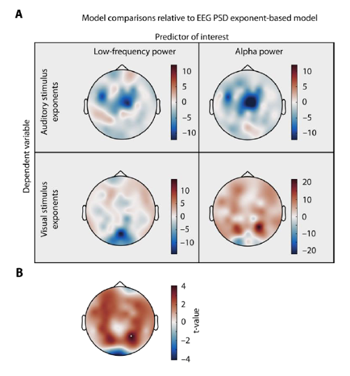
      1) A general concern is whether the observed behavioral related neural index, e.g., alpha-band power, cross-frequency coupling, could be simply explained in terms of ERP response for T2. For example, when the ERP response for T2 is larger for between-chunk condition compared to within-chunk condition, the alpha-power for T2 would be also larger for between-chunk condition. Likewise, this might also explain the cross-frequency coupling results. The authors should do more control analyses to address the possibility, e.g., plotting the ERP response for the two conditions and regressing them out from the oscillatory index.

      Many thanks for the comment. In short, the enhancement in alpha power and cross-frequency coupling results in the between-cycle condition compared with those in the within-cycle condition cannot be accounted for by the ERP responses for T2.

      In general, the rhythmic stimulation in the AB paradigm prevents EEG signals from returning to the baseline. Therefore, we cannot observe typical ERP components purely related to individual items, except for the P1 and N1 components related to the stream onset, which reveals no difference between the two conditions and are trailed by steady-state responses (SSRs) resonating at the stimulus rate (Fig. R1).

      Fig. R1. ERPs aligned to stream onset. EEG signals were filtered between 1–30 Hz, baseline-corrected (-200 to 0 ms before stream onset) and averaged across the electrodes in left parieto-occipital area where 10-Hz alpha power showed attentional modulation effect.

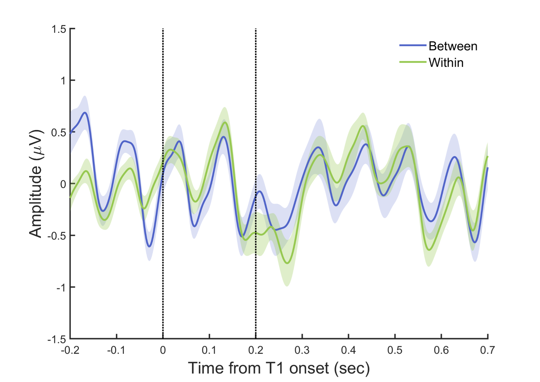
      To further inspect the potential differences in the target-related ERP signals between the within- and between-cycle conditions, we plotted the target-aligned waveforms for these experimental conditions. As shown in Fig. R2, a drop of ERP amplitude occurred for both conditions around T2 onset, and the difference between these two conditions was not significant (paired t-test estimated on mean amplitude every 20 ms from 0 to 700 ms relative to T1 onset, p > .05, FDR-corrected).

      Fig. R2. ERPs aligned to T1 onset. EEG signals were filtered between 1–30 Hz, and baseline-corrected using signals -100 to 0 ms before T1 onset. The two dash lines indicate the onset of T1 and T2, respectively.

      Since there is a trend of enhanced ERP response for the between-cycle relative to the within-cycle condition during the period of 0 to 100 ms after T2 onset (paired t-test on mean amplitude, p =.065, uncorrected), we then directly examined whether such post-T2 responses contribute to the behavioral attentional modulation effect and behavior-related neural indices. Crucially, we did not find any significant correlation of such T2-related ERP enhancement with the behavioral modulation index (BMI), or with the reported effects of alpha power and cross-frequency coupling (PAC). Furthermore, after controlling for the T2-related ERP responses, there still remains a significant correlation between the delta-alpha PAC and the BMI (rpartial = .596, p = .019), which is not surprising given that the PAC is calculated based on an 800-ms time window covering more pre-T2 than post-T2 periods (see the response to point #4 for details) rather than around the T2 onset. Taken together, these results clearly suggest that the T2-related ERP responses cannot explain the attentional modulation effect and the observed behavior-related neural indices.

      2) The alpha-band increase for T2 is indeed contradictory to the well known inhibitory function of alpha-band in attention. How could a target that is better discriminated elicit stronger inhibitory response? Related to the above point, the observed enhancement in alpha-band power and its coupling to low-frequency oscillation might derive from an enhanced ERP response for T2 target.

      Many thanks for the comment. We have briefly discussed this point in the revised manuscript (page 18, line 477).

      A widely accepted function of alpha activity in attention is that alpha oscillations suppress irrelevant visual information during spatial selection (Kelly et al., 2006; Thut et al., 2006; Worden et al., 2000). However, it becomes a controversial issue when there exists rhythmic sensory stimulation at alpha-band, just like the situation in the current study where both the visual stream and the contextual auditory rhythm were emitted at 10 Hz. In such a case, alpha-band neural responses at the stimulation frequency can be interpreted as either passively evoked steady-state responses (SSR) or actively synchronized intrinsic brain rhythms. From the former perspective (i.e., the SSR view), an increase in the amplitude or power at the stimulus frequency may indicate an enhanced attentional allocation to the stimulus stream that may result in better target detection (Janson et al., 2014; Keil et al., 2006; Müller & Hübner, 2002). Conversely, the latter view of the inhibitory function of intrinsic alpha oscillations would produce the opposite prediction. In a previous AB study, Janson and colleagues (2014) investigated this issue by separating the stimulus-evoked activity at 12 Hz (using the same power analysis method as ours) from the endogenous alpha oscillations ranging from 10.35 to 11.25 Hz (as indexed by individual alpha frequency, IAF). Interestingly, they found a dissociation between these two alpha-band neural responses, showing that the RSVP frequency power was higher in non-AB trials (T2 detected) than in AB trials (T2 undetected) while the IAF power exhibited the opposite pattern. According to these findings, the currently observed increase in alpha power for the between-cycle condition may reflect more of the stimulus-driven processes related to attentional enhancement. However, we don’t negate the effect of intrinsic alpha oscillations in our study, as the current design is not sufficient to distinguish between these two processes. We have discussed this point in the revised manuscript (page 18, line 477). Also, we have to admit that “alpha power” may not be the most precise term to describe our findings of the stimulus-related results. Thus, we have specified it as “neural responses to first-order rhythms at 10 Hz” and “10-Hz alpha power” in the revised manuscript (see page 12 in the Results section and page 18 in the Discussion section).

      As for the contribution of T2-related ERP response to the observed effect of 10 Hz power and cross-frequency coupling, please refer to our response to point #1.

      References:

      Janson, J., De Vos, M., Thorne, J. D., & Kranczioch, C. (2014). Endogenous and Rapid Serial Visual Presentation-induced Alpha Band Oscillations in the Attentional Blink. Journal of Cognitive Neuroscience, 26(7), 1454–1468. https://doi.org/10.1162/jocn_a_00551

      Keil, A., Ihssen, N., & Heim, S. (2006). Early cortical facilitation for emotionally arousing targets during the attentional blink. BMC Biology, 4(1), 23. https://doi.org/10.1186/1741-7007-4-23

      Kelly, S. P., Lalor, E. C., Reilly, R. B., & Foxe, J. J. (2006). Increases in Alpha Oscillatory Power Reflect an Active Retinotopic Mechanism for Distracter Suppression During Sustained Visuospatial Attention. Journal of Neurophysiology, 95(6), 3844–3851. https://doi.org/10.1152/jn.01234.2005

      Müller, M. M., & Hübner, R. (2002). Can the Spotlight of Attention Be Shaped Like a Doughnut? Evidence From Steady-State Visual Evoked Potentials. Psychological Science, 13(2), 119–124. https://doi.org/10.1111/1467-9280.00422

      Thut, G., Nietzel, A., Brandt, S., & Pascual-Leone, A. (2006). Alpha-band electroencephalographic activity over occipital cortex indexes visuospatial attention bias and predicts visual target detection. The Journal of Neuroscience : The Official Journal of the Society for Neuroscience, 26(37), 9494–9502. https://doi.org/10.1523/JNEUROSCI.0875-06.2006

      Worden, M. S., Foxe, J. J., Wang, N., & Simpson, G. V. (2000). Anticipatory Biasing of Visuospatial Attention Indexed by Retinotopically Specific α-Bank Electroencephalography Increases over Occipital Cortex. Journal of Neuroscience, 20(6), RC63–RC63. https://doi.org/10.1523/JNEUROSCI.20-06-j0002.2000

      3) To support that it is the context-induced entrainment that leads to the modulation in AB effect, the authors could examine pre-T2 response, e.g., alpha-power, and cross-frequency coupling, as well as its relationship to behavioral performance. I think the pre-stimulus response might be more convincing to support the authors' claim.

      Many thanks for the insightful suggestion. We have conducted additional analyses.

      Following this suggestion, we have examined the 10-Hz alpha power within the time window of -100–0 ms before T2 onset and found stronger activity for the between-cycle condition than for the within-cycle condition. This pre-T2 response is similar to the post-T2 response except that it is more restricted to the left parieto-occipital cluster (CP3, CP5, P3, P5, PO3, PO5, POZ, O1, OZ, t(15) = 2.774, p = .007), which partially overlaps with the cluster that exhibits a delta-alpha coupling effect significantly correlated with the BMI. We have incorporated these findings into the main text (page 12, line 315) and the Fig. 5A of the revised manuscript.

      As for the coupling results reported in our manuscript, the coupling index (PAC) was calculated based on the activity during the second and third cycles (i.e., 400 to 1200 ms from stream onset) of the contextual rhythm, most of which covers the pre-T2 period as T2 always appeared in the third cycle for both conditions. Together, these results on pre-T2 10-Hz alpha power and cross-frequency coupling, as well as its relationship to behavioral performance, jointly suggest that the observed modulation effect is caused by the context-induced entrainment rather than being a by-product of post-T2 processing.

      4) About the entrainment to rhythmic context and its relation to behavioral modulation index. Previous studies (e.g., Ding et al) have demonstrated the hierarchical temporal structure in speech signals, e.g., emergence of word-level entrainment introduced by language experience. Therefore, it is well expected that imposing a second-order structure on a visual stream would elicit the corresponding steady-state response. I understand that the new part and main focus here are the AB effects. The authors should add more texts explaining how their findings contribute new understandings to the neural mechanism for the intriguing phenomena.

      Many thanks for the suggestion. We have provided more discussion in the revised manuscript (page 17, line 447).

      We have provided more discussion on this important issue in the revised manuscript (page 17, line 447). In brief, our study demonstrates how cortical tracking of feature-based hierarchical structure reframes the deployment of attentional resources over visual streams. This effect, distinct from the hierarchical entrainment to speech signals (Ding et al., 2016; Gross et al., 2013), does not rely on previously acquired knowledge about the structured information and can be established automatically even when the higher-order structure comes from a task-irrelevant and cross-modal contextual rhythm. On the other hand, our finding sheds fresh light on the adaptive value of the structure-based entrainment effect by expanding its role from rhythmic information (e.g., speech) perception to temporal attention deployment. To our knowledge, few studies have tackled this issue in visual or speech processing.

      References:

      Ding, N., Melloni, L., Zhang, H., Tian, X., & Poeppel, D. (2016). Cortical tracking of hierarchical linguistic structures in connected speech. Nature Neuroscience, 19(1), 158–164. https://doi.org/10.1038/nn.4186

      Gross, J., Hoogenboom, N., Thut, G., Schyns, P., Panzeri, S., Belin, P., & Garrod, S. (2013). Speech Rhythms and Multiplexed Oscillatory Sensory Coding in the Human Brain. PLoS Biol, 11(12). https://doi.org/10.1371/journal.pbio.1001752

      Reviewer #2 (Public Review):

      In cognitive neuroscience, a large number of studies proposed that neural entrainment, i.e., synchronization of neural activity and low-frequency external rhythms, is a key mechanism for temporal attention. In psychology and especially in vision, attentional blink is the most established paradigm to study temporal attention. Nevertheless, as far as I know, few studies try to link neural entrainment in the cognitive neuroscience literature with attentional blink in the psychology literature. The current study, however, bridges this gap.

      The study provides new evidence for the dynamic attending theory using the attentional blink paradigm. Furthermore, it is shown that neural entrainment to the sensory rhythm, measured by EEG, is related to the attentional blink effect. The authors also show that event/chunk boundaries are not enough to modulate the attentional blink effect, and suggest that strict rhythmicity is required to modulate attention in time.

      In general, I enjoyed reading the manuscript and only have a few relatively minor concerns.

      1) Details about EEG analysis.

      . First, each epoch is from -600 ms before the stimulus onset to 1600 ms after the stimulus onset. Therefore, the epoch is 2200 s in duration. However, zero-padding is needed to make the epoch duration 2000 s (for 0.5-Hz resolution). This is confusing. Furthermore, for a more conservative analysis, I recommend to also analyze the response between 400 ms and 1600 ms, to avoid the onset response, and show the results in a supplementary figure. The short duration reduces the frequency resolution but still allows seeing a 2.5-Hz response.

      Thanks for the comments. Each epoch was indeed segmented from -600 to 1600 ms relative to the stimulus onset, but in the spectrum analysis, we only used EEG signals from stream onset (i.e., time point 0) to 1600 ms (see the Materials and Methods section) to investigate the oscillatory characteristics of the neural responses purely elicited by rhythmic stimuli. The 1.6-s signals were zero-padded into a 2-s duration to achieve a frequency resolution of 0.5 Hz.

      According to the reviewer’s suggestion, we analyzed the EEG signals from 400 ms to 1600 ms relative to stream onset to avoid potential influence of the onset response, and showed the results in Figure 4. Basically, we can still observe spectral peaks at the stimulus frequencies of 2.5, 5 (the harmonic of 2.5 Hz), and 10 Hz for both power and ITPC spectrum. However, the peak magnitudes were much weaker than those of 1.6-s signals especially for 2.5 Hz, and the 2.5-Hz power did not survive the multiple comparisons correction across frequencies (FDR threshold of p < .05), which might be due to the relatively low signal-to-noise ratio for the analysis based on the 1.2-s epochs (only three cycles to estimate the activity at 2.5 Hz). Importantly, we did identify a significant cluster for 2.5 Hz ITPC in the left parieto-occipital region showing a positive correlation with the individuals’ BMI (Fig. R3; CP5, TP7, P5, P7, PO5, PO7, O1; r = .538, p = .016), which is consistent with the findings based on the longer epochs.

      Fig. R3. Neural entrainment to contextual rhythms during the period of 400–1600 ms from stream onset. (A) The spectrum for inter-trial phase coherence (ITPC) of EEG signals from 400 to 1600 ms after the stimulus onset. Shaded areas indicate standard errors of the mean. (B) The 2.5-Hz ITPC was significantly correlated with the behavioral modulation index (BMI) in a parieto-occipital cluster, as indicated by orange stars in the scalp topographic map.

      Second, "The preprocessed EEG signals were first corrected by subtracting the average activity of the entire stream for each epoch, and then averaged across trials for each condition, each participant, and each electrode." I have several concerns about this procedure.

      (A) What is the entire stream? It's the average over time?

      Yes, as for the power spectrum analysis, EEG signals were first demeaned by subtracting the average signals of the entire stream over time from onset to offset (i.e., from 0 to 1600 ms) before further analysis. We performed this procedure following previous studies on the entrainment to visual rhythms (Spaak et al., 2014). We have clarified this point in the “Power analysis” part of the Materials and Methods section (page 25, line 677).

      References:

      Spaak, E., Lange, F. P. de, & Jensen, O. (2014). Local Entrainment of Alpha Oscillations by Visual Stimuli Causes Cyclic Modulation of Perception. The Journal of Neuroscience, 34(10), 3536–3544. https://doi.org/10.1523/JNEUROSCI.4385-13.2014

      (B) I suggest to do the Fourier transform first and average the spectrum over participants and electrodes. Averaging the EEG waveforms require the assumption that all electrodes/participants have the same response phase, which is not necessarily true.

      Thanks for the suggestion. In an AB paradigm, the evoked neural responses are sufficiently time-locked to the periodic stimulation, so it is reasonable to quantify power estimate with spectral decomposition performed on trial-averaged EEG signals (i.e., evoked power). Moreover, our results of inter-trial phase coherence (ITPC), which estimated the phase-locking value across trials based on single-trial decomposed phase values, also provided supporting evidence that the EEG waveforms were temporally locked across trials to the 2.5-Hz temporal structure in the context session.

      Nevertheless, we also took the reviewer’s suggestion seriously and analyzed the power spectrum on the average of single-trial spectral transforms, i.e., the induced power, which puts emphasis on the intrinsic non-phase-locked activities. In line with the results of evoked power and ITPC, the induced power spectrum in context session also peaked at 2.5 Hz and was significantly stronger than that in baseline session at 2.5 Hz (t(15) = 4.186, p < .001, FDR-corrected with a p value threshold < .001). Importantly, Person correlation analysis also revealed a positive cluster in the left parieto-occipital region, indicating the induced power at 2.5 Hz also had strong relevance with the attentional modulation effect (P7, PO7, PO5, PO3; r = .606, p = .006). We have added these additional findings to the revised manuscript (page 11, line 288; see also Figure 4—figure supplement 1).

      2) The sequences are short, only containing 16 items and 4 cycles. Furthermore, the targets are presented in the 2nd or 3rd cycle. I suspect that a stronger effect may be observed if the sequence are longer, since attention may not well entrain to the external stimulus until a few cycles. In the first trial of the experiment, they participant may not have a chance to realize that the task-irrelevant auditory/visual stimulus has a cyclic nature and it is not likely that their attention will entrain to such cycles. As the experiment precedes, they learns that the stimulus is cyclic and may allocate their attention rhythmically. Therefore, I feel that the participants do not just rely on the rhythmic information within a trial but also rely on the stimulus history. Please discuss why short sequences are used and whether it is possible to see buildup of the effect over trials or over cycles within a trial.

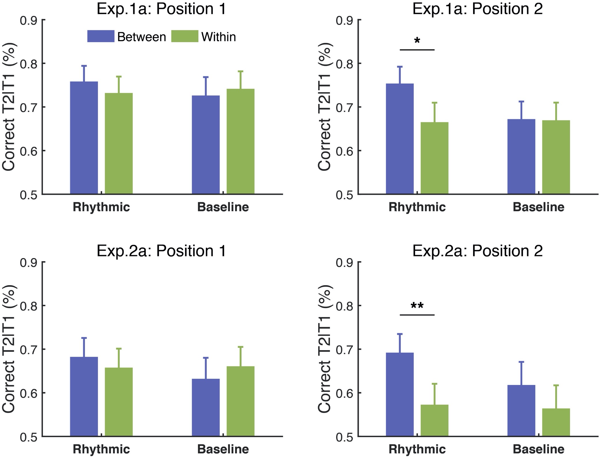
      Thanks for the comments. Typically, to induce a classic pattern of AB effect, the RSVP stream should contain 3–7 distractors before the first target (T1), with varying lengths of distractors (0–7) between two targets and at least 2 items after the second target (T2). In our study, we created the RSVP streams following these rules, which allowed us to observe the typical AB effect that T2 performance was deteriorated at Lag 2 relative to that at Lag 8. Nevertheless, we agree with the reviewer that longer streams would be better for building up the attentional entrainment effect, as we did observe the attentional modulation effect ramped up as the stream proceeded over cycles, consistent with the reviewer’s speculation. In Experiments 1a (using auditory context) and 2a (using color-defined visual context), we adopted two sets of target positions—an early one where T2 appeared at the 6th or 8th position (in the 2nd cycle) of the visual stream, and a late one where T2 appeared at the 10th or 12th position (in the 3rd cycle) of the visual stream. In the manuscript, we reported T2 performance with all the target positions combined, as no significant interaction was found between the target positions and the experimental conditions (ps. > .1). However, additional analysis demonstrated a trend toward an increase of the attentional modulation effect over cycles, from the early to the late positions. As shown in Fig. R4, the modulation effect went stronger and reached significance for the late positions (for Experiment 1a, t(15) = 2.83, p = .013, Cohen’s d = 0.707; for Experiment 2a, t(15) = 3.656, p = .002, Cohen’s d = 0.914) but showed a weaker trend for the early positions (for Experiment 1a, t(15) = 1.049, p = .311, Cohen’s d = 0.262; for Experiment 2a, t(15) = .606, p = .553, Cohen’s d = 0.152).

      Fig. R4. Attentional modulation effect built up over cycles in Experiments 1a & 2a. Error bars represent 1 SEM; * p<0.05, ** p<0.01.

      However, we did not observe an obvious buildup effect across trials in our study. The modulation effect of contextual rhythms seems to be a quick process that the effect is evident in the first quarter of trials in Experiment 1a (for, t(15) = 2.703, p = .016, Cohen’s d = 0.676) and in the second quarter of trials in Experiment 2a (for, t(15) = 2.478, p = .026, Cohen’s d = 0.620.

      3) The term "cycle" is used without definition in Results. Please define and mention that it's an abstract term and does not require the stimulus to have "cycles".

      Thanks for the suggestion. By its definition, the term “cycle” refers to “an interval of time during which a sequence of a recurring succession of events or phenomena is completed” or “a course or series of events or operations that recur regularly and usually lead back to the starting point” (Merriam-Webster dictionary). In the current study, we stuck to the recurrent and regular nature of “cycle” in general while defined the specific meaning of “cycle” by feature-based periodic changes of the contextual stimuli in each experiment (page 5, line 101; also refer to Procedures in the Materials and Methods section for details). For example, in Experiment 1a, the background tone sequence changed its pitch value from high to low or vice versa isochronously at a rate of 2.5 Hz, thus forming a rhythmic context with structure-based cycles of 400 ms. Note that we did not use the more general term “chunk”, because arbitrary chunks without the regularity of cycles are insufficient to trigger the attentional modulation effect in the current study. Indeed, the effect was eliminated when we replaced the rhythmic cycles with irregular chunks (Experiments 1d & 1e).

      4) Entrainment of attention is not necessarily related to neural entrainment to sensory stimulus, and there is considerable debate about whether neural entrainment to sensory stimulus should be called entrainment. Too much emphasis on terminology is of course counterproductive but a short discussion on these issues is probably necessary.

      Thanks for the comments. As commonly accepted, entrainment is defined as the alignment of intrinsic neuronal activity to the temporal structure of external rhythmic inputs (Lakatos et al., 2019; Obleser & Kayser, 2019). Here, we are interested in the functional roles of cortical entrainment to the higher-order temporal structure imposed on first-order sensory stimulation, and used the term entrainment to describe the phase-locking neural responses to such hierarchical structure following literature on auditory and visual perception (Brookshire et al., 2017; Doelling & Poeppel, 2015). In our study, the consistent results of power and ITPC have provided strong evidence that neural entrainment at the structure level (2.5 Hz) is significantly correlated with the observed attentional modulation effect. However, this does not mean that the entrainment of attention is necessarily associated with neural entrainment to sensory stimulus in a broader context, as attention may also be guided by predictions based on non-isochronous temporal regularity without requiring stimulus-based oscillatory entrainment (Breska & Deouell, 2017; Morillon et al._2016).

      On the other hand, there has been a debate about whether the neural alignment to rhythmic stimulation reflects active entrainment of endogenous oscillatory processes (i.e., induced activity) or a series of passively evoked steady-state responses (Keitel et al., 2019; Notbohm et al., 2016; Zoefel et al., 2018). The latter process is also referred to as “entrainment in a broad sense” by Obleser & Kayser (2019). Given that a presented rhythm always evokes event-related potentials, a better question might be whether the observed alignment reflects the entrainment of endogenous oscillations in addition to evoked steady-state responses. Here we attempted to tackle this issue by measuring the induced power, which emphasizes the intrinsic non-phase-locked activity, in addition to the phase-locked evoked power. Specifically, we quantified these two kinds of activities with the average of single-trial EEG power spectra and the power spectra of trial-averaged EEG signals, respectively, according to Keitel et al. (2019). In addition to the observation of evoked responses to the contextual structure, we also demonstrated an attention-related neural tracking of the higher-order temporal structure based on the induced power at 2.5 Hz (see Figure 4—figure supplement 1), suggesting that the observed attentional modulation effect is at least partially derived from the entrainment of intrinsic oscillatory brain activity. We have briefly discussed this point in the revised manuscript (page 17, line 460).

      References:

      Breska, A., & Deouell, L. Y. (2017). Neural mechanisms of rhythm-based temporal prediction: Delta phase-locking reflects temporal predictability but not rhythmic entrainment. PLOS Biology, 15(2), e2001665. https://doi.org/10.1371/journal.pbio.2001665

      Brookshire, G., Lu, J., Nusbaum, H. C., Goldin-Meadow, S., & Casasanto, D. (2017). Visual cortex entrains to sign language. Proceedings of the National Academy of Sciences, 114(24), 6352–6357. https://doi.org/10.1073/pnas.1620350114

      Doelling, K. B., & Poeppel, D. (2015). Cortical entrainment to music and its modulation by expertise. Proceedings of the National Academy of Sciences, 112(45), E6233–E6242. https://doi.org/10.1073/pnas.1508431112

      Henry, M. J., Herrmann, B., & Obleser, J. (2014). Entrained neural oscillations in multiple frequency bands comodulate behavior. Proceedings of the National Academy of Sciences, 111(41), 14935–14940. https://doi.org/10.1073/pnas.1408741111

      Keitel, C., Keitel, A., Benwell, C. S. Y., Daube, C., Thut, G., & Gross, J. (2019). Stimulus-Driven Brain Rhythms within the Alpha Band: The Attentional-Modulation Conundrum. The Journal of Neuroscience, 39(16), 3119–3129. https://doi.org/10.1523/JNEUROSCI.1633-18.2019

      Lakatos, P., Gross, J., & Thut, G. (2019). A New Unifying Account of the Roles of Neuronal Entrainment. Current Biology, 29(18), R890–R905. https://doi.org/10.1016/j.cub.2019.07.075

      Morillon, B., Schroeder, C. E., Wyart, V., & Arnal, L. H. (2016). Temporal Prediction in lieu of Periodic Stimulation. Journal of Neuroscience, 36(8), 2342–2347. https://doi.org/10.1523/JNEUROSCI.0836-15.2016

      Notbohm, A., Kurths, J., & Herrmann, C. S. (2016). Modification of Brain Oscillations via Rhythmic Light Stimulation Provides Evidence for Entrainment but Not for Superposition of Event-Related Responses. Frontiers in Human Neuroscience, 10. https://doi.org/10.3389/fnhum.2016.00010

      Obleser, J., & Kayser, C. (2019). Neural Entrainment and Attentional Selection in the Listening Brain. Trends in Cognitive Sciences, 23(11), 913–926. https://doi.org/10.1016/j.tics.2019.08.004

      Zoefel, B., ten Oever, S., & Sack, A. T. (2018). The Involvement of Endogenous Neural Oscillations in the Processing of Rhythmic Input: More Than a Regular Repetition of Evoked Neural Responses. Frontiers in Neuroscience, 12. https://doi.org/10.3389/fnins.2018.00095

      Reviewer #3 (Public Review):

      The current experiment tests whether the attentional blink is affected by higher-order regularity based on rhythmic organization of contextual features (pitch, color, or motion). The results show that this is indeed the case: the AB effect is smaller when two targets appeared in two adjacent cycles (between-cycle condition) than within the same cycle defined by the background sounds. Experiment 2 shows that this also holds for temporal regularities in the visual domain and Experiment 3 for motion. Additional EEG analysis indicated that the findings obtained can be explained by cortical entrainment to the higher-order contextual structure. Critically feature-based structure of contextual rhythms at 2.5 Hz was correlated with the strength of the attentional modulation effect.

      This is an intriguing and exciting finding. It is a clever and innovative approach to reduce the attention blink by presenting a rhythmic higher-order regularity. It is convincing that this pulling out of the AB is driven by cortical entrainment. Overall, the paper is clear, well written and provides adequate control conditions. There is a lot to like about this paper. Yet, there are particular concerns that need to be addressed. Below I outline these concerns:

      1) The most pressing concern is the behavioral data. We have to ensure that we are dealing here with a attentional blink. The way the data is presented is not the typical way this is done. Typically in AB designs one see the T2 performance when T1 is ignored relative to when T1 has to be detected. This data is not provided. I am not sure whether this data is collected but if so the reader should see this.

      Many thanks for the suggestion. We appreciate the reviewer for his/her thoughtful comments. To demonstrate the AB effect, we did include two T2 lag conditions in our study (Experiments 1a, 1b, 2a, and 2b)—a short-SOA condition where T2 was located at the second lag of T1 (i.e., SOA = 200 ms), and a long-SOA condition where T2 appeared at the 8th lag of T1 (i.e., SOA = 800 ms). In a typical AB effect, T2 performance at short lags is remarkably impaired compared with that at long lags. In our study, we consistently replicated this effect across the experiments, as reported in the Results section of Experiment 1 (page 5, line 106). Overall, the T2 detection accuracy conditioned on correct T1 response was significantly impaired in the short-SOA condition relative to that in the long-SOA condition (mean accuracy > 0.9 for all experiments), during both the context session and the baseline session. More crucially, when looking into the magnitude of the AB effect as measured by (ACClong-SOA - ACCshort-SOA)/ACClong-SOA, we still obtained a significant attentional modulation effect (for Experiment 1a, t(15) = -2.729, p = .016, Cohen’s d = 0.682; for Experiment 2a, t(15) = -4.143, p <.001, Cohen’s d = 1.036) similar to that reflected by the short-SOA condition alone, further confirming that cortical entrainment effectively influences the AB effect.

      Although we included both the long- and short-SOA conditions in the current study, we focused on T2 performance in the short-SOA condition rather than along the whole AB curve for the following reasons. Firstly, for the long-SOA conditions, the T2 performance is at ceiling level, making it an inappropriate baseline to probe the attentional modulation effect. We focused on Lag 2 because previous research has identified a robust AB effect around the second lag (Raymond et al., 1992), which provides a reasonable and sensitive baseline to probe the potential modulation effect of the contextual auditory and visual rhythms. Note that instead of using multiple lags, we varied the length of the rhythmic cycles (i.e., a cycle of 300 ms, 400 ms, and 500 ms corresponding to a rhythm frequency of 3.3 Hz, 2.5 Hz, and 2 Hz, respectively, all within the delta band), and showed that the attentional modulation effect could be generalized to these different delta-band rhythmic contexts, regardless of the absolute positions of the targets within the rhythmic cycles.

      As to the T1 performance, the overall accuracy was very high, ranging from 0.907 to 0.972, in all of our experiments. The corresponding results have been added to the Results section of the revised manuscript (page 5, line 103). Notably, we did not find T1-T2 trade-offs in most of our experiments, except in Experiment 2a where T1 performance showed a moderate decrease in the between-cycle condition relative to that in the within-cycle condition (mean ± SE: 0.888 ± 0.026 vs. 0.933 ± 0.016, respectively; t(15) = -2.217, p = .043). However, by examining the relationship between the modulation effects (i.e., the difference between the two experimental conditions) on T1 and T2, we did not find any significant correlation (p = .403), suggesting that the better performance for T2 was not simply due to the worse performance in detecting T1.

      Finally, previous studies have shown that ignoring T1 would lead to ceiling-level T2 performance (Raymond et al., 1992). Therefore, we did not include such manipulation in the current study, as in that case, it would be almost impossible for us to detect any contextual modulation effect.

      References:

      Raymond, J. E., Shapiro, K. L., & Arnell, K. M. (1992). Temporary suppression of visual processing in an RSVP task: An attentional blink? Journal of Experimental Psychology: Human Perception and Performance, 18(3), 849–860. https://doi.org/10.1037/0096-1523.18.3.849

      2) Also, there is only one lag tested. The ensure that we are dealing here with a true AB I would like to see that more than one lag is tested. In the ideal situation a full AB curve should be presented that includes several lags. This should be done for at least for one of the experiments. It would be informative as we can see how cortical entrainment affects the whole AB curve.

      Many thanks for the suggestion. Please refer to our response to the point #1 for “Reviewer #3 (Public Review)”. In short, we did include two T2 lag conditions in our study (Experiments 1a, 1b, 2a and 2b), and the results replicated the typical AB effect. We have clarified this point in the revised manuscript (page 5, line 106).

      3) Also, there is no data regarding T1 performance. It is important to show that this the better performance for T2 is not due to worse performance in detecting T1. So also please provide this data.

      Many thanks for the suggestion. Please refer to our response to the point #1 or “Reviewer #3 (Public Review)”. We have reported the T1 performance in the revised manuscript (page 5, line 103), and the results didn’t show obvious T1-T2 trade-offs.

      4) The authors identify the oscillatory characteristics of EEG signals in response to stimulus rhythms, by examined the FFT spectral peaks by subtracting the mean power of two nearest neighboring frequencies from the power at the stimulus frequency. I am not familiar with this procedure and would like to see some justification for using this technique.

      According to previous studies (Nozaradan, 2011; Lenc e al., 2018), the procedure to subtract the average amplitude of neighboring frequency bins can remove unrelated background noise, like muscle activity or eye movement. If there were no EEG oscillatory responses characteristic of stimulus rhythms, the amplitude at a given frequency bin should be similar to the average of its neighbors, and thus no significant peaks could be observed in the subtracted spectrum.

      References:

      Lenc, T., Keller, P. E., Varlet, M., & Nozaradan, S. (2018). Neural tracking of the musical beat is enhanced by low-frequency sounds. Proceedings of the National Academy of Sciences, 115(32), 8221–8226. https://doi.org/10.1073/pnas.1801421115

      Nozaradan, S., Peretz, I., Missal, M., & Mouraux, A. (2011). Tagging the Neuronal Entrainment to Beat and Meter. The Journal of Neuroscience, 31(28), 10234–10240. https://doi.org/10.1523/JNEUROSCI.0411-11.2011

    1. Author Response:

      Evaluation Summary:

      Since DBS of the habenula is a new treatment, these are the first data of its kind and potentially of high interest to the field. Although the study mostly confirms findings from animal studies rather than bringing up completely new aspects of emotion processing, it certainly closes a knowledge gap. This paper is of interest to neuroscientists studying emotions and clinicians treating psychiatric disorders. Specifically the paper shows that the habenula is involved in processing of negative emotions and that it is synchronized to the prefrontal cortex in the theta band. These are important insights into the electrophysiology of emotion processing in the human brain.

      The authors are very grateful for the reviewers’ positive comments on our study. We also thank all the reviewers for the comments which has helped to improve the manuscript.

      Reviewer #1 (Public Review):

      The study by Huang et al. report on direct recordings (using DBS electrodes) from the human habenula in conjunction with MEG recordings in 9 patients. Participants were shown emotional pictures. The key finding was a transient increase in theta/alpha activity with negative compared to positive stimuli. Furthermore, there was a later increase in oscillatory coupling in the same band. These are important data, as there are few reports of direct recordings from the habenula together with the MEG in humans performing cognitive tasks. The findings do provide novel insight into the network dynamics associated with the processing of emotional stimuli and particular the role of the habenula.

      Recommendations:

      How can we be sure that the recordings from the habenula are not contaminated by volume conduction; i.e. signals from neighbouring regions? I do understand that bipolar signals were considered for the DBS electrode leads. However, high-frequency power (gamma band and up) is often associated with spiking/MUA and considered less prone to volume conduction. I propose to also investigate that high-frequency gamma band activity recorded from the bipolar DBS electrodes and relate to the emotional faces. This will provide more certainty that the measured activity indeed stems from the habenula.

      We thank the reviewer for the comment. As the reviewer pointed out, bipolar macroelectrode can detect locally generated potentials, as demonstrated in the case of recordings from subthalamic nucleus and especially when the macroelectrodes are inside the subthalamic nucleus (Marmor et al., 2017). However, considering the size of the habenula and the size of the DBS electrode contacts, we have to acknowledge that we cannot completely exclude the possibility that the recordings are contaminated by volume conduction of activities from neighbouring areas, as shown in Bertone-Cueto et al. 2019. We have now added extra information about the size of the habenula and acknowledged the potential contamination of activities from neighbouring areas through volume conduction in the ‘Limitation’:

      "Another caveat we would like to acknowledge that the human habenula is a small region. Existing data from structural MRI scans reported combined habenula (the sum of the left and right hemispheres) volumes of ~ 30–36 mm3 (Savitz et al., 2011a; Savitz et al., 2011b) which means each habenula has the size of 2~3 mm in each dimension, which may be even smaller than the standard functional MRI voxel size (Lawson et al., 2013). The size of the habenula is also small relative to the standard DBS electrodes (as shown in Fig. 2A). The electrodes used in this study (Medtronic 3389) have electrode diameter of 1.27 mm with each contact length of 1.5 mm, and contact spacing of 0.5 mm. We have tried different ways to confirm the location of the electrode and to select the contacts that is within or closest to the habenula: 1.) the MRI was co-registered with a CT image (General Electric, Waukesha, WI, USA) with the Leksell stereotactic frame to obtain the coordinate values of the tip of the electrode; 2.) Post-operative CT was co-registered to pre-operative T1 MRI using a two-stage linear registration using Lead-DBS software. We used bipolar signals constructed from neighbouring macroelectrode recordings, which have been shown to detect locally generated potentials from subthalamic nucleus and especially when the macroelectrodes are inside the subthalamic nucleus (Marmor et al., 2017). Considering that not all contacts for bipolar LFP construction are in the habenula in this study, as shown in Fig. 2, we cannot exclude the possibility that the activities we measured are contaminated by activities from neighbouring areas through volume conduction. In particular, the human habenula is surrounded by thalamus and adjacent to the posterior end of the medial dorsal thalamus, so we may have captured activities from the medial dorsal thalamus. However, we also showed that those bipolar LFPs from contacts in the habenula tend to have a peak in the theta/alpha band in the power spectra density (PSD); whereas recordings from contacts outside the habenula tend to have extra peak in beta frequency band in the PSD. This supports the habenula origin of the emotional valence related changes in the theta/alpha activities reported here."

      We have also looked at gamma band oscillations or high frequency activities in the recordings. However, we didn’t observe any peak in high frequency band in the average power spectral density, or any consistent difference in the high frequency activities induced by the emotional stimuli (Fig. S1). We suspect that high frequency activities related to MUA/spiking are very local and have very small amplitude, so they are not picked up by the bipolar LFPs measured from contacts with both the contact area for each contact and the between-contact space quite large comparative to the size of the habenula.

      A

      B

      Figure S1. (A) Power spectral density of habenula LFPs across all time period when emotional stimuli were presented. The bold blue line and shadowed region indicates the mean ± SEM across all recorded hemispheres and the thin grey lines show measurements from individual hemispheres. (B) Time-frequency representations of the power response relative to pre-stimulus baseline for different conditions showing habenula gamma and high frequency activity are not modulated by emotional

      References:

      Savitz JB, Bonne O, Nugent AC, Vythilingam M, Bogers W, Charney DS, et al. Habenula volume in post-traumatic stress disorder measured with high-resolution MRI. Biology of Mood & Anxiety Disorders 2011a; 1(1): 7.

      Savitz JB, Nugent AC, Bogers W, Roiser JP, Bain EE, Neumeister A, et al. Habenula volume in bipolar disorder and major depressive disorder: a high-resolution magnetic resonance imaging study. Biological Psychiatry 2011b; 69(4): 336-43.

      Lawson RP, Drevets WC, Roiser JP. Defining the habenula in human neuroimaging studies. NeuroImage 2013; 64: 722-7.

      Marmor O, Valsky D, Joshua M, Bick AS, Arkadir D, Tamir I, et al. Local vs. volume conductance activity of field potentials in the human subthalamic nucleus. Journal of Neurophysiology 2017; 117(6): 2140-51.

      Bertone-Cueto NI, Makarova J, Mosqueira A, García-Violini D, Sánchez-Peña R, Herreras O, et al. Volume-Conducted Origin of the Field Potential at the Lateral Habenula. Frontiers in Systems Neuroscience 2019; 13:78.

      Figure 3: the alpha/theta band activity is very transient and not band-limited. Why refer to this as oscillatory? Can you exclude that the TFRs of power reflect the spectral power of ERPs rather than modulations of oscillations? I propose to also calculate the ERPs and perform the TFR of power on those. This might result in a re-interpretation of the early effects in theta/alpha band.

      We agree with the reviewer that the activity increase in the first time window with short latency after the stimuli onset is very transient and not band-limited. This raise the question that whether this is oscillatory or a transient evoked activity. We have now looked at this initial transient activity in different ways: 1.) We quantified the ERP in LFPs locked to the stimuli onset for each emotional valence condition and for each habenula. We investigated whether there was difference in the amplitude or latency of the ERP for different stimuli emotional valence conditions. As showing in the following figure, there is ERP with stimuli onset with a positive peak at 402 ± 27 ms (neutral stimuli), 407 ± 35 ms (positive stimuli), 399 ± 30 ms (negative stimuli). The flowing figure (Fig. 3–figure supplement 1) will be submitted as figure supplement related to Fig. 3. However, there was no significant difference in ERP latency or amplitude caused by different emotional valence stimuli. 2.) We have quantified the pure non-phase-locked (induced only) power spectra by calculating the time-frequency power spectrogram after subtracting the ERP (the time-domain trial average) from time-domain neural signal on each trial (Kalcher and Pfurtscheller, 1995; Cohen and Donner, 2013). This shows very similar results as we reported in the main manuscript, as shown in Fig. 3–figure supplement 2. These further analyses show that even though there were event related potential changes time locked around the stimuli onset, and this ERP did NOT contribute to the initial broad-band activity increase at the early time window shown in plot A-C in Figure 3. The figures of the new analyses and following have now been added in the main text:

      "In addition, we tested whether stimuli-related habenula LFP modulations primarily reflect a modulation of oscillations, which is not phase-locked to stimulus onset, or, alternatively, if they are attributed to evoked event-related potential (ERP). We quantified the ERP for each emotional valence condition for each habenula. There was no significant difference in ERP latency or amplitude caused by different emotional valence stimuli (Fig. 3–figure supplement 1). In addition, when only considering the non phase-locked activity by removing the ERP from the time series before frequency-time decomposition, the emotional valence effect (presented in Fig. 3–figure supplement 2) is very similar to those shown in Fig.3. These additional analyses demonstrated that the emotional valence effect in the LFP signal is more likely to be driven by non-phase-locked (induced only) activity."

      A

      B

      Fig. 3–figure supplement 1. Event-related potential (ERP) in habenula LFP signals in different emotional valence (neutral, positive and negative) conditions. (A) Averaged ERP waveforms across patients for different conditions. (B) Peak latency and amplitude (Mean ± SEM) of the ERP components for different conditions.

      Fig. 3–figure supplement 2. Non-phase-locked activity in different emotional valence (neutral, positive and negative) conditions (N = 18). (A) Time-frequency representation of the power changes relative to pre-stimulus baseline for three conditions. Significant clusters (p < 0.05, non-parametric permutation test) are encircled with a solid black line. (B) Time-frequency representation of the power response difference between negative and positive valence stimuli, showing significant increased activity the theta/alpha band (5-10 Hz) at short latency (100-500 ms) and another increased theta activity (4-7 Hz) at long latencies (2700-3300 ms) with negative stimuli (p < 0.05, non-parametric permutation test). (C) Normalized power of the activities at theta/alpha (5-10 Hz) and theta (4-7 Hz) band over time. Significant difference between the negative and positive valence stimuli is marked by a shadowed bar (p < 0.05, corrected for multiple comparison).

      References:

      Kalcher J, Pfurtscheller G. Discrimination between phase-locked and non-phase-locked event-related EEG activity. Electroencephalography and Clinical Neurophysiology 1995; 94(5): 381-4.

      Cohen MX, Donner TH. Midfrontal conflict-related theta-band power reflects neural oscillations that predict behavior. Journal of Neurophysiology 2013; 110(12): 2752-63.

      Figure 4D: can you exclude that the frontal activity is not due to saccade artifacts? Only eye blink artifacts were reduced by the ICA approach. Trials with saccades should be identified in the MEG traces and rejected prior to further analysis.

      We understand and appreciate the reviewer’s concern on the source of the activity modulations shown in Fig. 4D. We tried to minimise the eye movement or saccade in the recording by presenting all figures at the centre of the screen, scaling all presented figures to similar size, and presenting a white cross at the centre of the screen preparing the participants for the onset of the stimuli. Despite this, participants my still make eye movements and saccade in the recording. We used ICA to exclude the low frequency large amplitude artefacts which can be related to either eye blink or other large eye movements. However, this may not be able to exclude artefacts related to miniature saccades. As shown in Fig. 4D, on the sensor level, the sensors with significant difference between the negative vs. positive emotional valence condition clustered around frontal cortex, close to the eye area. However, we think this is not dominated by saccades because of the following two reasons:

      1.) The power spectrum of the saccadic spike artifact in MEG is characterized by a broadband peak in the gamma band from roughly 30 to 120 Hz (Yuval-Greenberg et al., 2008; Keren et al., 2010). In this study the activity modulation we observed in the frontal sensors are limited to the theta/alpha frequency band, so it is different from the power spectra of the saccadic spike artefact.

      2.) The source of the saccadic spike artefacts in MEG measurement tend to be localized to the region of the extraocular muscles of both eyes (Carl et al., 2012).We used beamforming source localisation to identify the source of the activity modulation reported in Fig. 4D. This beamforming analysis identified the source to be in the Broadmann area 9 and 10 (shown in Fig. 5). This excludes the possibility that the activity modulation in the sensor level reported in Fig. 4D is due to saccades. In addition, Broadman area 9 and 10, have previously been associated with emotional stimulus processing (Bermpohl et al., 2006), Broadman area 9 in the left hemisphere has also been used as the target for repetitive transcranial magnetic stimulation (rTMS) as a treatment for drug-resistant depression (Cash et al., 2020). The source localisation results, together with previous literature on the function of the identified source area suggest that the activity modulation we observed in the frontal cortex is very likely to be related to emotional stimuli processing.

      References:

      Yuval-Greenberg S, Tomer O, Keren AS, Nelken I, Deouell LY. Transient induced gamma-band response in EEG as a manifestation of miniature saccades. Neuron 2008; 58(3): 429-41.

      Keren AS, Yuval-Greenberg S, Deouell LY. Saccadic spike potentials in gamma-band EEG: characterization, detection and suppression. NeuroImage 2010; 49(3): 2248-63.

      Carl C, Acik A, Konig P, Engel AK, Hipp JF. The saccadic spike artifact in MEG. NeuroImage 2012; 59(2): 1657-67.

      Bermpohl F, Pascual-Leone A, Amedi A, Merabet LB, Fregni F, Gaab N, et al. Attentional modulation of emotional stimulus processing: an fMRI study using emotional expectancy. Human Brain Mapping 2006; 27(8): 662-77.

      Cash RFH, Weigand A, Zalesky A, Siddiqi SH, Downar J, Fitzgerald PB, et al. Using Brain Imaging to Improve Spatial Targeting of Transcranial Magnetic Stimulation for Depression. Biological Psychiatry 2020.

      The coherence modulations in Fig 5 occur quite late in time compared to the power modulations in Fig 3 and 4. When discussing the results (in e.g. the abstract) it reads as if these findings are reflecting the same process. How can the two effect reflect the same process if the timing is so different?

      As the reviewer pointed out correctly, the time window where we observed the coherence modulations happened quite late in time compared to the initial power modulations in the frontal cortex and the habenula (Fig. 4). And there was another increase in the theta band activities in the habenula area even later, at around 3 second after stimuli onset when the emotional figure has already disappeared. Emotional response is composed of a number of factors, two of which are the initial reactivity to an emotional stimulus and the subsequent recovery once the stimulus terminates or ceases to be relevant (Schuyler et al., 2014). We think these neural effects we observed in the three different time windows may reflect different underlying processes. We have discussed this in the ‘Discussion’:

      "These activity changes at different time windows may reflect the different neuropsychological processes underlying emotion perception including identification and appraisal of emotional material, production of affective states, and autonomic response regulation and recovery (Phillips et al., 2003a). The later effects of increased theta activities in the habenula when the stimuli disappeared were also supported by other literature showing that, there can be prolonged effects of negative stimuli in the neural structure involved in emotional processing (Haas et al., 2008; Puccetti et al., 2021). In particular, greater sustained patterns of brain activity in the medial prefrontal cortex when responding to blocks of negative facial expressions was associated with higher scores of neuroticism across participants (Haas et al., 2008). Slower amygdala recovery from negative images also predicts greater trait neuroticism, lower levels of likability of a set of social stimuli (neutral faces), and declined day-to-day psychological wellbeing (Schuyler et al., 2014; Puccetti et al., 2021)."

      References:

      Schuyler BS, Kral TR, Jacquart J, Burghy CA, Weng HY, Perlman DM, et al. Temporal dynamics of emotional responding: amygdala recovery predicts emotional traits. Social Cognitive and Affective Neuroscience 2014; 9(2): 176-81.

      Phillips ML, Drevets WC, Rauch SL, Lane R. Neurobiology of emotion perception I: The neural basis of normal emotion perception. Biological Psychiatry 2003a; 54(5): 504-14.

      Haas BW, Constable RT, Canli T. Stop the sadness: Neuroticism is associated with sustained medial prefrontal cortex response to emotional facial expressions. NeuroImage 2008; 42(1): 385-92.

      Puccetti NA, Schaefer SM, van Reekum CM, Ong AD, Almeida DM, Ryff CD, et al. Linking Amygdala Persistence to Real-World Emotional Experience and Psychological Well-Being. Journal of Neuroscience 2021: JN-RM-1637-20.

      Be explicit on the degrees of freedom in the statistical tests given that one subject was excluded from some of the tests.

      We thank the reviewers for the comment. The number of samples used for each statistics analysis are stated in the title of the figures. We have now also added the degree of freedom in the main text when parametric statistical tests such as t-test or ANOVAs have been used. When permutation tests (which do not have any degrees of freedom associated with it) are used, we have now added the number of samples for the permutation test.

      Reviewer #2 (Public Review):

      In this study, Huang and colleagues recorded local field potentials from the lateral habenula in patients with psychiatric disorders who recently underwent surgery for deep brain stimulation (DBS). The authors combined these invasive measurements with non-invasive whole-head MEG recordings to study functional connectivity between the habenula and cortical areas. Since the lateral habenula is believed to be involved in the processing of emotions, and negative emotions in particular, the authors investigated whether brain activity in this region is related to emotional valence. They presented pictures inducing negative and positive emotions to the patients and found that theta and alpha activity in the habenula and frontal cortex increases when patients experience negative emotions. Functional connectivity between the habenula and the cortex was likewise increased in this band. The authors conclude that theta/alpha oscillations in the habenula-cortex network are involved in the processing of negative emotions in humans.

      Because DBS of the habenula is a new treatment tested in this cohort in the framework of a clinical trial, these are the first data of its kind. Accordingly, they are of high interest to the field. Although the study mostly confirms findings from animal studies rather than bringing up completely new aspects of emotion processing, it certainly closes a knowledge gap.

      In terms of community impact, I see the strengths of this paper in basic science rather than the clinical field. The authors demonstrate the involvement of theta oscillations in the habenula-prefrontal cortex network in emotion processing in the human brain. The potential of theta oscillations to serve as a marker in closed-loop DBS, as put forward by the authors, appears less relevant to me at this stage, given that the clinical effects and side-effects of habenula DBS are not known yet.

      We thank the reviewers for the favourable comments about the implication of our study in basic science and about the value of our study in closing a knowledge gap. We agree that further studies would be required to make conclusions about the clinical effects and side-effects of habenula DBS.

      Detailed comments:

      The group-average MEG power spectrum (Fig. 4B) suggests that negative emotions lead to a sustained theta power increase and a similar effect, though possibly masked by a visual ERP, can be seen in the habenula (Fig. 3C). Yet the statistics identify brief elevations of habenula theta power at around 3s (which is very late), a brief elevation of prefrontal power a time 0 or even before (Fig. 4C) and a brief elevation of Habenula-MEG theta coherence around 1 s. It seems possible that this lack of consistency arises from a low signal-to-noise ratio. The data contain only 27 trails per condition on average and are contaminated by artifacts caused by the extension wires.

      With regard to the nature of the activity modulation with short latency after stimuli onset: whether this is an ERP or oscillation? We have now investigated this. In summary, by analysing the ERP and removing the influence of the ERP from the total power spectra, we didn’t observe stimulus emotional valence related modulation in the ERP, and the modulation related to emotional valence in the pure induced (non-phase-locked) power spectra was similar to what we have observed in the total power shown in Fig. 3. Therefore, we argue that the theta/alpha increase with negative emotional stimuli we observed in both habenula and prefrontal cortex 0-500 ms after stimuli onset are not dominated by visual or other ERP.

      With regard to the signal-to-noise ratio from only 27 trials per condition on average per participant: We have tried to clean the data by removing the trials with obvious artefacts characterised by increased measurements in the time domain over 5 times the standard deviation and increased activities across all frequency bands in the frequency domain. After removing the trials with artefacts, we have 27 trials per condition per subject on average. We agree that 27 trials per condition on average is not a high number, and increasing the number of trials would further increase the signal-to-noise ratio. However, our studies with EEG recordings and LFP recordings from externalised patients have shown that 30 trials was enough to identify reduction in the amplitude of post-movement beta oscillations at the beginning of visuomotor adaption in the motor cortex and STN (Tan et al., 2014a; Tan et al., 2014b). These results of motor error related modulation in the post-movement beta have been repeated by other studies from other groups. In Tan et al. 2014b, with simultaneous EEG and STN LFP measurements and a similar number of trials (around 30), we also quantified the time-course of STN-motor cortex coherence during voluntary movements. This pattern has also been repeated in a separate study from another group with around 50 trials per participant (Talakoub et al., 2016). In addition, similar behavioural paradigm (passive figure viewing paradigm) has been used in two previous studies with LFP recordings from STN from different patient groups (Brucke et al., 2007; Huebl et al., 2014). In both studies, a similar number of trials per condition around 27 was used. The authors have identified meaningful activity modulation in the STN by emotional stimuli. Therefore, we think the number of trials per condition was sufficient to identify emotional valence induced difference in the LFPs in the paradigm.

      We agree that the measurement of coherence can be more susceptible to noise and suffer from the reduced signal-to-noise ratio in MEG recording. In Hirschmann et al. 2013, 5 minutes of resting recording and 5 minutes of movement recording from 10 PD patients were used to quantify movement related changes in STN-cortical coherence and how this was modulated by levodopa (Hirschmann et al., 2013). Litvak et al. (2012) have identified movement-related changes in the coherence between STN LFP and motor cortex with recording with simultaneous STN LFP and MEG recordings from 17 PD patients and 20 trials in average per participant per condition (Litvak et al., 2012). With similar methods, van Wijk et al. (2017) used recordings from 9 patients and around on average in 29 trials per hand per condition, and they identified reduced cortico-pallidal coherence in the low-beta decreases during movement (van Wijk et al., 2017). So the trial number per condition participant we used in this study are comparable to previous studies.

      The DBS extension wires do reduce signal-to-noise ratio in the MEG recording. therefore the spatiotemporal Signal Space Separation (tSSS) method (Taulu and Simola, 2006) implemented in the MaxFilter software (Elekta Oy, Helsinki, Finland) has been applied in this study to suppress strong magnetic artifacts caused by extension wires. This method has been proved to work well in de-noising the magnetic artifacts and movement artifacts in MEG data in our previous studies (Cao et al., 2019; Cao et al., 2020). In addition, the beamforming method proposed by several studies (Litvak et al., 2010; Hirschmann et al., 2011; Litvak et al., 2011) has been used in this study. In Litvak et al., 2010, the artifacts caused by DBS extension wires was detailed described and the beamforming was demonstrated to effectively suppress artifacts and thereby enable both localization of cortical sources coherent with the deep brain nucleus. We have now added more details and these references about the data cleaning and the beamforming method in the main text. With the beamforming method, we did observe the standard movement-related modulation in the beta frequency band in the motor cortex with 9 trials of figure pressing movements, shown in the following figure for one patient as an example (Figure 5–figure supplement 1). This suggests that the beamforming method did work well to suppress the artefacts and help to localise the source with a low number of trials. The figure on movement-related modulation in the motor cortex in the MEG signals have now been added as a supplementary figure to demonstrate the effect of the beamforming.

      Figure 5–figure supplement 1. (A) Time-frequency maps of MEG activity for right hand button press at sensor level from one participant (Case 8). (B) DICS beamforming source reconstruction of the areas with movement-related oscillation changes in the range of 12-30 Hz. The peak power was located in the left M1 area, MNI coordinate [-37, -12, 43].

      References:

      Tan H, Jenkinson N, Brown P. Dynamic neural correlates of motor error monitoring and adaptation during trial-to-trial learning. Journal of Neuroscience 2014a; 34(16): 5678-88.

      Tan H, Zavala B, Pogosyan A, Ashkan K, Zrinzo L, Foltynie T, et al. Human subthalamic nucleus in movement error detection and its evaluation during visuomotor adaptation. Journal of Neuroscience 2014b; 34(50): 16744-54.

      Talakoub O, Neagu B, Udupa K, Tsang E, Chen R, Popovic MR, et al. Time-course of coherence in the human basal ganglia during voluntary movements. Scientific Reports 2016; 6: 34930.

      Brucke C, Kupsch A, Schneider GH, Hariz MI, Nuttin B, Kopp U, et al. The subthalamic region is activated during valence-related emotional processing in patients with Parkinson's disease. European Journal of Neuroscience 2007; 26(3): 767-74.

      Huebl J, Spitzer B, Brucke C, Schonecker T, Kupsch A, Alesch F, et al. Oscillatory subthalamic nucleus activity is modulated by dopamine during emotional processing in Parkinson's disease. Cortex 2014; 60: 69-81.

      Hirschmann J, Ozkurt TE, Butz M, Homburger M, Elben S, Hartmann CJ, et al. Differential modulation of STN-cortical and cortico-muscular coherence by movement and levodopa in Parkinson's disease. NeuroImage 2013; 68: 203-13.

      Litvak V, Eusebio A, Jha A, Oostenveld R, Barnes G, Foltynie T, et al. Movement-related changes in local and long-range synchronization in Parkinson's disease revealed by simultaneous magnetoencephalography and intracranial recordings. Journal of Neuroscience 2012; 32(31): 10541-53.

      van Wijk BCM, Neumann WJ, Schneider GH, Sander TH, Litvak V, Kuhn AA. Low-beta cortico-pallidal coherence decreases during movement and correlates with overall reaction time. NeuroImage 2017; 159: 1-8.

      Taulu S, Simola J. Spatiotemporal signal space separation method for rejecting nearby interference in MEG measurements. Physics in Medicine and Biology 2006; 51(7): 1759-68.

      Cao C, Huang P, Wang T, Zhan S, Liu W, Pan Y, et al. Cortico-subthalamic Coherence in a Patient With Dystonia Induced by Chorea-Acanthocytosis: A Case Report. Frontiers in Human Neuroscience 2019; 13: 163.

      Cao C, Li D, Zhan S, Zhang C, Sun B, Litvak V. L-dopa treatment increases oscillatory power in the motor cortex of Parkinson's disease patients. NeuroImage Clinical 2020; 26: 102255.

      Litvak V, Eusebio A, Jha A, Oostenveld R, Barnes GR, Penny WD, et al. Optimized beamforming for simultaneous MEG and intracranial local field potential recordings in deep brain stimulation patients. NeuroImage 2010; 50(4): 1578-88.

      Litvak V, Jha A, Eusebio A, Oostenveld R, Foltynie T, Limousin P, et al. Resting oscillatory cortico-subthalamic connectivity in patients with Parkinson's disease. Brain 2011; 134(Pt 2): 359-74.

      Hirschmann J, Ozkurt TE, Butz M, Homburger M, Elben S, Hartmann CJ, et al. Distinct oscillatory STN-cortical loops revealed by simultaneous MEG and local field potential recordings in patients with Parkinson's disease. NeuroImage 2011; 55(3): 1159-68.

      I doubt that the correlation between habenula power and habenula-MEG coherence (Fig. 6C) is informative of emotion processing. First, power and coherence in close-by time windows are likely to to be correlated irrespective of the task/stimuli. Second, if meaningful, one would expect the strongest correlation for the negative condition, as this is the only condition with an increase of theta coherence and a subsequent increase of theta power in the habenula. This, however, does not appear to be the case.

      The authors included the factors valence and arousal in their linear model and found that only valence correlated with electrophysiological effects. I suspect that arousal and valence scores are highly correlated. When fed with informative yet highly correlated variables, the significance of individual input variables becomes difficult to assess in many statistical models. Hence, I am not convinced that valence matters but arousal not.

      For the correlation shown in Fig. 6C, we used a linear mixed-effect modelling (‘fitlme’ in Matlab) with different recorded subjects as random effects to investigate the correlations between the habenula power and habenula-MEG coherence at an earlier window, while considering all trials together. Therefore the reported value in the main text and in the figure (k = 0.2434 ± 0.1031, p = 0.0226, R2 = 0.104) show the within subjects correlation that are consistent across all measured subjects. The correlation is likely to be mediated by emotional valence condition, as negative emotional stimuli tend to be associated with both high habenula-MEG coherence and high theta power in the later time window tend to happen in the trials with.

      The arousal scores are significantly different for the three valence conditions as shown in Fig. 1B. However, the arousal scores and the valence scores are not monotonically correlated, as shown in the following figure (Fig. S2). The emotional neutral figures have the lowest arousal value, but have the valence value sitting between the negative figures and the positive figures. We have now added the following sentence in the main text:

      "This nonlinear and non-monotonic relationship between arousal scores and the emotional valence scores allowed us to differentiate the effect of the valence from arousal."

      Table 2 in the main text show the results of the linear mixed-effect modelling with the neural signal as the dependent variable and the valence and arousal scores as independent variables. Because of the non-linear and non-monotonic relationship between the valence and arousal scores, we think the significance of individual input variables is valid in this statistical model. We have now added a new figure (shown below, Fig. 7) with scatter plots showing the relationship between the electrophysiological signal and the arousal and emotional valence scores separately using Spearman’s partial correlation analysis. In each scatter plot, each dot indicates the average measurement from one participant in one emotional valence condition. As shown in the following figure, the electrophysiological measurements linearly correlated with the valence score, but not with the arousal scores. However, the statistics reported in this figure considered all the dots together. The linear mixed effect modelling taking into account the interdependency of the measurements from the same participant. So the results reported in the main text using linear mixed effect modelling are statistically more valid, but supplementary figure here below illustrate the relationship.

      Figure S2. Averaged valence and arousal ratings (mean ± SD) for figures of the three emotional condition. (B) Scatter plots showing the relationship between arousal and valence scores for each emotional condition for each participant.

      Figure 7. Scatter plots showing how early theta/alpha band power increase in the frontal cortex (A), theta/alpha band frontal cortex-habenula coherence (B) and theta band power increase in habenula stimuli (C) changed with emotional valence (left column) and arousal (right column). Each dot shows the average of one participant in each categorical valence condition, which are also the source data of the multilevel modelling results presented in Table 2. The R and p value in the figure are the results of partial correlation considering all data points together.

      Page 8: "The time-varying coherence was calculated for each trial". This is confusing because coherence quantifies the stability of a phase difference over time, i.e. it is a temporal average, not defined for individual trials. It has also been used to describe the phase difference stability over trials rather than time, and I assume this is the method applied here. Typically, the greatest coherence values coincide with event-related power increases, which is why I am surprised to see maximum coherence at 1s rather than immediately post-stimulus.

      We thank the reviewer for pointing out this incorrect description. As the reviewer pointed out correctly, the method we used describe the phase difference stability over trials rather than time. We have now clarified how coherence was calculated and added more details in the methods:

      "The time-varying cross trial coherence between each MEG sensor and the habenula LFP was first calculated for each emotional valence condition. For this, time-frequency auto- and cross-spectral densities in the theta/alpha frequency band (5-10 Hz) between the habenula LFP and each MEG channel at sensor level were calculated using the wavelet transform-based approach from -2000 to 4000 ms for each trial with 1 Hz steps using the Morlet wavelet and cycle number of 6. Cross-trial coherence spectra for each LFP-MEG channel combination was calculated for each emotional valence condition for each habenula using the function ‘ft_connectivityanalysis’ in Fieldtrip (version 20170628). Stimulus-related changes in coherence were assessed by expressing the time-resolved coherence spectra as a percentage change compared to the average value in the -2000 to -200 ms (pre-stimulus) time window for each frequency."

      In the Morlet wavelet analysis we used here, the cycle number (C) determines the temporal resolution and frequency resolution for each frequency (F). The spectral bandwidth at a given frequency F is equal to 2F/C while the wavelet duration is equal to C/F/pi. We used a cycle number of 6. For theta band activities around 5 Hz, we will have the spectral bandwidth of 25/6 = 1.7 Hz and the wavelet duration of 6/5/pi = 0.38s = 380ms.

      As the reviewer noticed, we observed increased activities across a wide frequency band in both habenula and the prefrontal cortex within 500 ms after stimuli onset. But the increase of cross-trial coherence starts at around 300 ms. The increase of coherence in a time window without increase of power in either of the two structures indicates a phase difference stability across trials in the oscillatory activities from the two regions, and this phase difference stability across trials was not secondary to power increase.

      Reviewer #3 (Public Review):

      This paper describes the oscillatory activity of the habenula using local field potentials, both within the region and, through the use of MEG, in connection to the prefrontal cortex. The characteristics of this activity were found to vary with the emotional valence but not with arousal. Sheding light on this is relevant, because the habenula is a promising target for deep brain stimulation.

      In general, because I am not much on top of the literature on the habenula, I find difficult to judge about the novelty and the impact of this study. What I can say is that I do find the paper is well-written and very clear; and the methods, although quite basic (which is not bad), are sound and rigourous.

      We thank the reviewer for the positive comments about the potential implication of our study and on the methods we used.

      On the less positive side, even though I am aware that in this type of studies it is difficult to have high N, the very low N in this case makes me worry about the robustness and replicability of the results. I'm sure I have missed it and it's specified somewhere, but why is N different for the different figures? Is it because only 8 people had MEG? The number of trials seems also a somewhat low. Therefore, I feel the authors perhaps need to make an effort to make up for the short number of subjects in order to add confidence to the results. I would strongly recommend to bootstrap the statistical analysis and extract non-parametric confidence intervals instead of showing parametric standard errors whenever is appropriate. When doing that, it must be taken into account that each two of the habenula belong to the same person; i.e. one bootstraps the subjects not the habenula.

      We do understand and appreciate the concern of the reviewer on the low sample numbers due to the strict recruitment criteria for this very early stage clinical trial: 9 patients for bilateral habenula LFPs, and 8 patients with good quality MEGs. Some information to justify the number of trials per condition for each participant has been provided in the reply to the Detailed Comments 1 from Reviewer 2. The sample number used in each analysis was included in the figures and in the main text.

      We have used non-parametric cluster-based permutation approach (Maris and Oostenveld, 2007) for all the main results as shown in Fig. 3-5. Once the clusters (time window and frequency band) with significant differences for different emotional valence conditions have been identified, parametric statistical test was applied to the average values of the clusters to show the direction of the difference. These parametric statistics are secondary to the main non-parametric permutation test.

      In addition, the DICS beamforming method was applied to localize cortical sources exhibiting stimuli-related power changes and cortical sources coherent with deep brain LFPs for each subject for positive and negative emotional valence conditions respectively. After source analysis, source statistics over subjects was performed. Non-parametric permutation testing with or without cluster-based correction for multiple comparisons was applied to statistically quantify the differences in cortical power source or coherence source between negative and positive emotional stimuli.

      References:

      Maris E, Oostenveld R. Nonparametric statistical testing of EEG- and MEG-data. Journal of Neuroscience Methods 2007; 164(1): 177-90.

      Related to this point, the results in Figure 6 seem quite noisy, because interactions (i.e. coherence) are harder to estimate and N is low. For example, I have to make an effort of optimism to believe that Fig 6A is not just noise, and the result in Fig 6C is also a bit weak and perhaps driven by the blue point at the bottom. My read is that the authors didn't do permutation testing here, and just a parametric linear-mixed effect testing. I believe the authors should embed this into permutation testing to make sure that the extremes are not driving the current p-value.

      We have now quantified the coherence between frontal cortex-habenula and occipital cortex-habenula separately (please see more details in the reply to Reviewer 2 (Recommendations for the authors 6). The new analysis showed that the increase in the theta/alpha band coherence around 1 s after the negative stimuli was only observed between prefrontal cortex-habenula and not between occipital cortex-habenula. This supports the argument that Fig. 6A is not just noise.

    1. Author Response

      Reviewer #1:

      Köster and colleagues present a brief report in which they study in 9 month-old babies the electrophysiological responses to expected and unexpected events. The major finding is that in addition to a known ERP response, an NC present between 400-600 ms, they observe a differential effect in theta oscillations. The latter is a novel result and it is linked to the known properties of theta oscillations in learning. This is a nice study, with novel results and well presented. My major reservation however concerns the push the authors make for the novelty of the results and their interpretation as reflecting brain dynamics and rhythms. The reason for that is, that any ERP, passed through the lens of a wavelet/FFT etc, will yield a response at a particular frequency. This is especially the case for families of ERP responses related to unexpected event e.g., MMR, and NC, etc. For which there is plenty of literature linking them to responses to surprising event, and in particular in babies; and which given their timing will be reflected in delta/theta oscillations. The reason why I am pressing on this issue, is because there is an old, but still ongoing debate attempting to dissociate intrinsic brain dynamics from simple event related responses. This is by no means trivial and I certainly do not expect the authors to resolve it, yet I would expect the authors to be careful in their interpretation, to warn the reader that the result could just reflect the known ERP, to avoid introducing confusion in the field.

      We would like to thank the author for highlighting the novelty of the results. Critically, there is one fundamental difference in investigating the ERP response and the trial-wise oscillatory power, which we have done in the present analysis: when looking at the evoked oscillatory response (i.e., the TF characteristics of the ERP), the signal is averaged over trials first and then subjected to a wavelet transform. However, when looking at the ongoing (or total) oscillatory response, the wavelet transform is applied at the level of the single trial, before the TF response of the single trials is averaged across the trials of one condition trials (for a classical illustration, see Tallon-Baudry & Bertrand, 1999; TICS, Box 2). We have now made this distinction more salient throughout the manuscript.

      In the present study, the results did not suggest a relation between the ERP and the ongoing theta activity, because the topography, temporal evolution, and polarity of the ERP and the theta response were very dissimilar: Looking at Figure 2 (A and B) and Figure 3 (B and C), the Nc peaks at central electrodes, but the theta response is more distributed, and the expected versus unexpected difference was specific for the .4 to .6 s time window, but the theta difference lasted the whole trial. Furthermore, the NC was higher for expected versus unexpected, which should (due to the low frequency) rather lead to a higher theta power for unexpected, in contrast to expected events for the time frequency analysis for the Nc. To verify this intuition, we now ran a wavelet analysis on the evoked response (i.e., the ERP) and, for a direct comparison, also plotted the ongoing oscillatory response for the central electrodes (see Additional Figure 1). These additional analyses nicely illustrate that the trial-wise theta response provides a fundamentally different approach to analyze oscillatory brain dynamics.

      Because this is likely of interest to many readers, we also report the results of the wavelet analysis of the ERP versus the analysis of the ongoing theta activity at central electrodes and the corresponding statistics in the result section, and have also included the Additional Figure in the supplementary materials, as Figure S2.

      Additional Figure 1. Comparison of the topography and time course for the 4 – 5 Hz activity for the evoked (A, B) and the ongoing (C, D) oscillatory response at central electrodes (400 – 600 ms; Cz, C3, C4; baseline: -100 – 0 ms). (A) Topography for the difference between unexpected and expected events in the evoked oscillatory response. (B) The corresponding time course at central electrodes, which did not reveal a significant difference between 400 – 600 ms, t(35) = 1.57, p = .126. (C) Topography for the same contrast in the ongoing oscillatory response and (D) the corresponding time course at central electrodes, which did likewise not reveal a significant difference between 400 – 600 ms, t(35) = -1.26, p = .218. The condition effects (unexpected - expected) were not correlated between the evoked and the ongoing response, r = .23, p = .169.

      A second aspect that I would like the authors to comment on is the power of the experimental design to measure surprise. From the methods, I gathered that the same stimulus materials and with the same frequency were presented as expected and unexpected endings. If that is the case, what is the measure of surprise? For once the same materials are shown causing habituation and reducing novelty and second the experiment introduces a long-term expectation of a 50:50 proportion of expected/unexpected events. I might be missing something here, which is likely as the methods are quite sparse in the description of what was actually done.

      We have used 4 different stimuli types (variants) in each of the 4 different domains, with either an expected or unexpected outcome. This resulted in 32 distinct stimulus sequences, which we presented twice, resulting in (up to) 64 trials. We have now described this approach and design in more detail and have also included all stimuli as supplementary material (Figure S1). In particular, we have used multiple types in each domain to reduce potential habituation or expectation effects. Still, we agree that one difficulty may be that, over time, infants got used to the fact that expected and unexpected outcomes were to be similarly “expected” (i.e., 50:50). However, if this was the case it would have resulted in a reduction (or disappearance) of the condition effect, and would thus also reduce the condition difference that we found, rather than providing an alternative explanation. We now included this consideration in the method section (p. 7).

      Two more comments concerning the analysis choices:

      1) The statistics for the ERP and the TF could be reported using a cluster size correction. These are well established statistical methods in the field which would enable to identify the time window/topography that maximally distinguished between the expected and the unexpected condition both for ERP and TF. Along the same lines, the authors could report the spatial correlation of the ERP/TF effects.

      For the ERP analysis we used the standard electrodes typically analyzed for the Nc in order to replicate effects found in former research (Langeloh et al., 2020; see also, Kayhan et al., 2019; Reynolds and Richards, 2005; Webb et al., 2005). For the TF analyses we used the most conservative criterion, namely all scalp recorded electrodes and the whole time window from 0 to 2000 ms, such that we did not make any choice regarding time window or the electrodes (i.e., which could be corrected for against other choices). We have now made those choices clearer in the method section, and why we think that, under these condition a multiple comparison correction is not needed/applicable (p. 10). Regarding the spatial correlation of the ERP and TF effects, we explained in response to the first comment the very different nature of the TF decomposition of the ERP and ongoing oscillatory activity and also that these were found to be interdependent (i.e., uncorrelated). We hope that with the additional analysis included in response to this comment that this difference is much clearer now.

      2) While I can see the reason why the authors chose to keep the baseline the same between the ERP and the TF analysis, for time frequency analysis it would be advisable to use a baseline amounting to a comparable time to the frequency of interest; and to use a period that does not encroach in the period of interest i.e., with a wavelet = 7 and a baseline -100:0 the authors are well into the period of interested.

      The difficulty in choosing the baseline in the present study was two-fold. First, we were interested in the ERP and the change in neural oscillations upon the onset of an outcome picture within a continuous presentation of pictures, forming a sequence. Second, we wanted to use a similar baseline for both analyses, to make them comparable. Because the second picture (the picture before the outcome picture) also elicited both an ERP and an oscillatory response at ~ 4 Hz (see Additional Figure 2), we choose a baseline just before the onset of the outcome stimulus, from -100 to 0 ms. Also we agree that the possibility to take a longer and earlier baseline, in particular for the TF results would have been favorable, but still consider that the -100 to 0 ms is still the best choice for the present analysis. Notably, because we found an increase in theta oscillations and the critical difference relies on a higher theta rhythm in one compared to the other condition, the effects of the increase in theta, if they effected the baseline, this effect would counteract rather than increase the current effect. We now explain this choice in more detail (p.10).

      Additional Figure 1. Display of the grand mean signals prior to the -100 to 0 baseline and outcome stimulus. (A) The time-frequency response across all scalp-recorded electrodes, as well as (B) the ERP at the central electrodes (Cz, C3, C4) across both conditions show a similar response to the 2. picture like the outcome picture. Thus a baseline just prior to the stimulus of interest was chosen, consistent for both analyses.

      Reviewer #2:

      The manuscript reports increases in theta power and lower NC amplitude in response to unexpected (vs. expected) events in 9-month-olds. The authors state that the observed increase in theta power is significant because it is in line with an existing theory that the theta rhythm is involved in learning in mammals. The topic is timely, the results are novel, the sample size is solid, the methods are sound as far as I can tell, and the use of event types spanning multiple domains (e.g. action, number, solidity) is a strength. The manuscript is short, well-written, and easy to follow.

      1) The current version of the manuscript states that the reported findings demonstrate that the theta rhythm is involved in processing of prediction error and supports the processing of unexpected events in 9-month-old infants. However, what is strictly shown is that watching at least some types of unexpected events enhance theta rhythm in 9-month-old infants, i.e. an increase in the theta rhythm is associated with processing unexpected events in infants, which suggests that an increase in the theta rhythm is a possible neural correlate of prediction error in this age range. While the present novel findings are certainly suggestive, more data and/or analyses would be needed to corroborate/confirm the role of the observed infant theta rhythm in processing prediction error, or document whether and how this increase in the theta rhythm supports the processing of unexpected events in infants. (As an example, since eye-tracking data were collected, are trial-by-trial variations in theta power increases to unexpected outcomes related to how long individual infants looked to the unexpected outcome pictures?) If it is not possible to further confirm/corroborate the role of the theta rhythm with this dataset, then the discussion, abstract, and title should be revised to more closely reflect what the current data shows (as the wording of the conclusion currently does), and clarify how future research may test the hypothesis that the infant theta rhythm directly supports the processing of prediction error in response to unexpected events.

      We would like to thank the reviewer for acknowledging the merit of the present research.

      On the one hand, we have revised our manuscript and are now somewhat more careful with our conclusion, in particular with regard to the refinement of basic expectations. On the other hand, we consider the concept of “violation to expectation” (VOE), which is one of the most widely used concepts in infancy research, very closely linked to the concept of a prediction error processing, namely a predictive model is violated. In particular, we have made this conceptual link in a recent theoretical paper (Köster et al., 2020), and based on former theoretical considerations about the link between these two concepts (e.g., see Schubotz 2015; Prediction and Expectation). In particular, in the present study we used a set of four different domains of violation of expectation paradigms, which are among the best established domains of infants core knowledge (e.g., action, solidity, cohesion, number; cf. Spelke & Kinzler, 2007). It was our specific goal not to replicate, for another time, that infants possess expectations (i.e., make predictions) in these domains, but to “flip the coin around” and investigate infants’ prediction error more generally, independent of the specific domain. We have now made the conceptual link between VOE and prediction error processing more explicit in the introduction of the manuscript and also emphasize that we choose a variety of domains to obtain a more general neural marker for infant processing of prediction errors.

      Having said this, indeed, we planned to assess and compare both infants gaze behavior and EEG response. Unfortunately, this was not very successful and the concurrent recording only worked for a limited number of infants and trials. This led us to the decision to make the eye-tracking study a companion study and to collect more eye-tracking data in an independent sample of infants after the EEG assessment was completed, such that a match between the two measures was not feasible. We now make this choice more explicit in the method section (p. 7). In addition, contrary to our basic assumption we did not find an effect in the looking time measure. Namely, there was no difference between expected and unexpected outcomes. We assume that this is due to the specificities of the current design that was rather optimized for EEG assessments: We used a high number of repetitions (64), with highly variable domains (4), and restricted the time window for potential looking time effects to 5 seconds, which is highly uncommon in the field and therefore not directly comparable with former studies.

      Finally, besides the ample evidence from former studies using VOE paradigms, if it were not the unexpected vs. expected (i.e., unpredicted vs. predicted) condition contrast which explains the differences we found in the ERP and the theta response, there would need to be an alternative explanation for the differential responses in the EEG, which produce the hypothesized effects. (Please also note that there are many studies relying their VOE assumption on ERPs alone, here we have two independent measures suggesting that infants discriminated between those conditions.)

      2) The current version of the manuscript states "The ERP effect was somewhat consistent across conditions, but the effect was mainly driven by the differences between expected and unexpected events in the action and the number domain (Figure S1). The results were more consistent across domains for the condition difference in the 4 - 5 Hz activity, with a peak in the unexpected-expected difference falling in the 4 - 5 Hz range across all electrodes (Figure S2)". However, the similarity/dissimilarity of NC and theta activity responses across domains was not quantified or tested. Looking at Figures S1 and S2, it is not that obvious to me that theta responses were more consistent across domains than NC responses. I understand that there were too few trials to formally test for any effect of domain (action, number, solidity, cohesion) on NC and theta responses, either alone or in interaction with outcome (expected, unexpected). It may still be possible to test for correlations of the topography and time-course of the individual average unexpected-expected difference in NC and theta responses across domains at the group level, or to test for an effect of outcome (expected, unexpected) in individual domains for subgroups of infants who contributed enough trials. Alternatively, claims of consistency across domains may be altered throughout, in which case the inability to test whether the theta and/or NC signatures of unexpected event processing found are consistent across domains (vs. driven by some domains) should be acknowledged as a limitation of the present study.

      We agree that this statement rather reflected our intuition and would not surpass statistical analysis given the low number of trials. So we are happy to refrain from this claim and simply refer to the supplementary material for the interested reader and also mention this as a perspective for future research in the discussion (p. 12; p. 15).

      As outlined in our previous response, it was also not our goal to draw conclusions about each single domain, but rather to present a diversity of stimulus types from different core knowledge domains to gain a more generalized neural marker for infants’ processing of unexpected, i.e., unpredicted events.

      Reviewer #3:

      General assessment:

      In this manuscript, the authors bring up a contemporary and relevant topic in the field, i.e. theta rhythm as a potential biomarker for prediction error in infancy. Currently, the literature is rich on discussions about how, and why, theta oscillations in infancy implement the different cognitive processes to which they have been linked. Investigating the research questions presented in this manuscript could therefore contribute to fill these gaps and improve our understanding of infants' neural oscillations and learning mechanisms. While we appreciate the motivation behind the study and the potential in the authors' research aim, we find that the experimental design, analyses and conclusions based on the results that can be drawn thereafter, lack sufficient novelty and are partly problematic in their description and implementation. Below, we list our major concerns in more detail, and make suggestions for improvements of the current analyses and manuscript.

      Summary of major concerns:

      1) Novelty:

      (a) It is unclear how the study differs from Berger et al., 2006 apart from additional conditions. Please describe this study in more detail and how your study extends beyond it.

      We would like to thank the reviewers for emphasizing the timeliness and relevance of the study.

      The critical difference between the present study and the study by Berger et al. 2006 was that the authors applied, as far as we understand this from Figure 4 and the method section of their study, the wavelet analysis to the ERP signal. In contrast, in the present study, we applied the wavelet analysis at the level of single trials. We now explain the difference between the two signals in more detail in the revised manuscript and also included an additional comparison between the evoked (i.e., ERP) and the ongoing (i.e., total) oscillatory response (for more details, please see the first response to the first comment of reviewer 1).

      (b) Seemingly innovative aspects (as listed below), which could make the study stand out among previous literature, but are ultimately not examined. Consequently, it is also not clear why they are included.

      -Relation between Nc component and theta.

      -Consistency of the effect across different core knowledge domains.

      -Consistency of the effect across the social and non-social domains.

      -Link between infants looking at time behavior and theta.

      We are thankful for these suggestions, which are closely related to the points raised by reviewer 1 and 2. With regard to the relation between the Nc and the theta response, we have now included a direct comparison of these signals (see Additional Figure 1, i.e., novel Figure S2; for details, please see the first response to the first comment of reviewer 1). Regarding the consistency of effects across domains, we have explained in response to point 1 by reviewer 2 that this was not the specific purpose of the present study, but we aimed at using a diversity of VOE stimuli to obtain a more general neural signature for infants’ prediction error processing, and explain this in more detail in the revised manuscript. Having said this, we agree that the question of consistency of effects between conditions is highly interesting, but we would not consider the data robust enough to confidently test these differences given the limited number of trials available per stimulus category. We now discuss this as a direction for future research (p. 15). Finally, we also agree with regard to the link between looking times and the theta rhythm. As also outlined in response to point 1 by reviewer 2 (paragraph 2), we initially had this plan, but did not succeed in obtaining a satisfactory number of trials in the dual recording of EEG and eye-tracking, which made us change these plans. This is now explained in detail in the method section (p. 7).

      (c) The reason to expect (or not) a difference at this age, compared to what is known from adult neural processing, is not adequately explained.

      -Potentially because of neural generators in mid/pre-frontal cortex? See Lines 144-146.

      The overall aim of the present study was to identify the neural signature for prediction error processing in the infant brain, which has, to the best of our knowledge, not been done this explicitly and with a focus on the ongoing theta activity and across a variety of violations in infants’ core knowledge domains. Because we did not expect a specific topography of this effect, in particular across multiple domains, we included all electrodes in the analyses. We have now clarified this in the method section (p. 10).

      (d) The study is not sufficiently embedded in previous developmental literature on the functionality of theta. That is, consider theta's role in error processing, but also the increase of theta over time of an experiment and it's link to cognitive development. See, for example: Braithwaite et al., 2020; Conejero et al., 2018; Adam et al., 2020.

      We are thankful that the reviewer indicated these works and have now included them in the introduction and discussion. Closest to the present study is the study by Conejero et al., 2018. However, this study is also based on theta analyses of the ERP, not of the ongoing oscillatory response and it includes considerably older infants (i.e., 16-month-olds instead of 9-month-olds as in the present study).

      2) Methodology:

      (a) Design: It is unclear what exactly a testing session entails.

      -Was the outcome picture always presented for 5secs? The methods section suggests that, but the introduction of the design and Figure 1 do not. This might be misleading. Please change in Figure 1 to 5sec if applicable.

      Yes, the final images were shown for 5s in order to simultaneously assess infants’ looking times. However, we included trials in the EEG analysis if infants looked for 2s, so this is the more relevant info for the analysis. We now clarified this in the method section (p. 7) and have also added this info in the figure caption.

      -Were infants' eye-movements tracked simultaneously to the EEG recording? If so, please present findings on their looking time and (if possible) pupil size. Also examine the relation to theta power. This would enhance the novelty and tie these findings to the larger looking time literature that the authors refer to in their introduction.

      Yes, in response to the second reviewer (comment 1) we explained in more detail why the joint analysis of the EEG and looking time data was not possible: We planned to assess both, infants gaze behavior and EEG response. Unfortunately, this was not very successful and the dual recording only worked for a few infants and trials. This led us to collect more eye-tracking data after the EEG assessment was completed, such that a match between the two measures was not feasible. We now clarified this in the method section (p. 7).

      (b) Analysis:

      -In terms of extracting theta power information: The baseline of 100ms is extremely short for a comparison in the frequency domain, since it does not even contain half a cycle of the frequency of interest, i.e. 4Hz. We appreciate the thought to keep the baseline the same as in the ERP analysis (which currently is hardly focused on in the manuscript), but it appears problematic for the theta analysis. Also, if we understand the spectral analysis correctly, the window the authors are using to estimate their spectral estimates is largely overlapping between baseline and experimental window. The question arises whether a baseline is even needed here, or if a direct contrast between conditions might be better suited.

      Please see our explanation about the choice of the baseline in our response to reviewer 1, comment 2. Because our stimulus sequences were highly variable, likely leading to highly variable overall theta activity, and our specific interest was in the change in theta activity upon the onset of the unexpected versus unpredicted outcome, we still consider it useful to take a baseline here. Also because this makes the study more closely comparable to the existing literature. We now clarified this in the method section (p. 9)

      -In terms of statistical testing

      -It appears that the authors choose the frequency band that will be entered in the statistical analysis from visual inspection of the differences between conditions. They write: "we found the strongest difference between 4 - 5 Hz (see lower panel of Figure 3). Therefore, and because this is the first study of this kind, we analyzed this frequency range." ll. 277-279). This approach seems extremely problematic since it poses a high risk for 'double-dipping'. This is crucial and needs to be addressed. For instance, the authors could run non-parametric permutation tests on the time-frequency domain using FDR correction or cluster-based permutation tests on the topography.

      -Lack of examining time- / topographic specificity.

      Please also note the sentence before this citation, which states our initial hypothesis: “While our initial proposal was to look at the difference in the 4 Hz theta rhythm between conditions (Köster et al., 2019), we found the strongest difference between 4 – 5 Hz (see lower panel of Figure 3).” Note that the hypothesis of 4 Hz can be clearly derived from our 2019 study. We would maintain that the center frequency we took for the analysis 4.5Hz (i.e., 4 – 5Hz) is very close to this original hypothesis and, considering that we applied a novel design and analyses in very young infants, could indeed hardly have fallen more closely to this initial proposal. The frequency choice is also underlined, as the reviewer remarks, by the consistency of this peak across domains, peaking at 4Hz (cohesion), 4.5Hz (action), and 5Hz (solidity, number). Importantly, please note that we have chosen the electrodes and time window very conservatively, namely by including the whole time period and all electrodes, which we now explain in more detail on p. 10. Please also see our response to reviewer 1, comment “1)”.

      3) Interpretation of results:

      (a) The authors interpret the descriptive findings of Figure S1 as illustration of the consistency of the results across the four knowledge domains. While we would partly agree with this interpretation based on column A of that figure (even though also there the peak shifts between domains), columns B and C do not picture a consistent pattern of data. That is, the topography appears very different between domains and so does the temporal course of the 4-5Hz power, with only showing higher power in the action and number domain, not in the other two. Since none of these data were compared statistically, any interpretation remains descriptive. Yet, we would like to invite the authors to critically reconsider their interpretation. You also might want to consider adding domain (action, number etc.) as a covariate to your statistical model.

      We agree with the reviewers (reviewer 2 and reviewer 3) that our initial interpretation of the data regarding the consistency of effects across domains may have been too strong. Thus, in the revised version of the manuscript, we do not state that the TF analysis revealed more consistent results. Given that the analysis was based on a different subsample and highly variable in trial numbers, we did not enter them as a covariate in the statistical model.

    1. Author Response

      Reviewer #1:

      Hutchings et al. report an updated cryo-electron tomography study of the yeast COP-II coat assembled around model membranes. The improved overall resolution and additional compositional states enabled the authors to identify new domains and interfaces--including what the authors hypothesize is a previously overlooked structural role for the SEC31 C-Terminal Domain (CTD). By perturbing a subset of these new features with mutants, the authors uncover some functional consequences pertaining to the flexibility or stability of COP-II assemblies.

      Overall, the structural and functional work appears reliable, but certain questions and comments should be addressed prior to publication. However, this reviewer failed to appreciate the conceptual advance that warrants publication in a general biology journal like eLIFE. Rather, this study provides a valuable refinement of our understanding of COP-II that I believe is better suited to a more specialized, structure-focused journal.

      We agree that in our original submission our description of the experimental setup, indeed similar to previous work, did not fully capture the novel findings of this paper. Rather than being simply a higher resolution structure of the COPII coat, in fact we have discovered new interactions in the COPII assembly network, and we have probed their functional roles, significantly changing our understanding of the mechanisms of COPII-mediated membrane curvature. In the revised submission we have included additional genetic data that further illuminate this mechanism, and have rewritten the text to better communicate the novel aspects of our work.

      Our combination of structural, functional and genetic analyses goes beyond refining our textbook understanding of the COPII coat as a simple ‘adaptor and cage’, but rather it provides a completely new picture of how dynamic regulation of assembly and disassembly of a complex network leads to membrane remodelling.

      These new insights have important implications for how coat assembly provides structural force to bend a membrane but is still able to adapt to distinct morphologies. These questions are at the forefront of protein secretion, where there is debate about how different types of carriers might be generated that can accommodate cargoes of different size.

      Major Comments: 1) The authors belabor what this reviewer thinks is an unimportant comparison between the yeast reconstruction of the outer coat vertex with prior work on the human outer coat vertex. Considering the modest resolution of both the yeast and human reconstructions, the transformative changes in cryo-EM camera technology since the publication of the human complex, and the differences in sample preparation (inclusion of the membrane, cylindrical versus spherical assemblies, presence of inner coat components), I did not find this comparison informative. The speculations about a changing interface over evolutionary time are unwarranted and would require a detailed comparison of co-evolutionary changes at this interface. The simpler explanation is that this is a flexible vertex, observed at low resolution in both studies, plus the samples are very different.

      We do agree that our proposal that the vertex interface changes over evolutionary time is speculative and we have removed this discussion. We agree that a co-evolutionary analysis will be enlightening here, but is beyond the scope of the current work.

      We respectfully disagree with the reviewer’s interpretation that the difference between the two vertices is due to low resolution. The interfaces are clearly different, and the resolutions of the reconstructions are sufficient to state this. The reviewer’s suggestion that the difference in vertex orientation might be simply attributable to differences in sample, such as inclusion of the membrane, cylindrical versus spherical morphology, or presence of inner coat components were ruled out in our original submission: we resolved yeast vertices on spherical vesicles (in addition to those on tubes) and on membrane-less cages. These analyses clearly showed that neither the presence of a membrane, nor the change in geometry (tubular vs. spherical) affect vertex interactions. These experiments are presented in Supplementary Fig 4 (Supplementary Fig. 3 in the original version). Similarly, we discount that differences might be due to the presence or absence of inner coat components, since membrane-less cages were previously solved in both conditions and are no different in terms of their vertex structure (Stagg et al. Nature 2006 and Cell 2008).

      We believe it is important to report on the differences between the two vertex structures. Nevertheless, we have shifted our emphasis on the functional aspects of vertex formation and moved the comparison between the two vertices to the supplement.

      2) As one of the major take home messages of the paper, the presentation and discussion of the modeling and assignment of the SEC31-CTD could be clarified. First, it isn't clear from the figures or the movies if the connectivity makes sense. Where is the C-terminal end of the alpha-solenoid compared to this new domain? Can the authors plausibly account for the connectivity in terms of primary sequence? Please also include a side-by-side comparison of the SRA1 structure and the CTD homology model, along with some explanation of the quality of the model as measured by Modeller. Finally, even if the new density is the CTD, it isn't clear from the structure how this sub-stoichiometric and apparently flexible interaction enhances stability. Hence, when the authors wrote "when the [CTD] truncated form was the sole copy of Sec31 in yeast, cells were not viable, indicating that the novel interaction we detect is essential for COPII coat function." Maybe, but could this statement be a leap to far? Is it the putative interaction essential, or is the CTD itself essential for reasons that remain to be fully determined?

      The CTD is separated from the C-terminus of the alpha solenoid domain by an extended domain (~350 amino acids) that is predicted to be disordered, and contains the PPP motifs and catalytic fragment that contact the inner coat. This is depicted in cartoon form in Figures 3A and 7, and discussed at length in the text. This arrangement explains why no connectivity is seen, or expected. We could highlight the C-terminus of the alpha-solenoid domain to emphasize where the disordered region should emerge from the rod, but connectivity of the disordered domain to the CTD could arise from multiple positions, including from an adjacent rod.

      The reviewer’s point about the essentiality of the CTD being independent of its interaction with the Sec31 rod, is an important one. The basis for our model that the CTD enhances stability or rigidity of the coat is the yeast phenotype of Sec31-deltaCTD, which resembles that of a sec13 null. Both mutants are lethal, but rescued by deletion of emp24, which leads to more easily deformable membranes (Čopič et al. Science 2012). We agree that even if this model is true, the interaction of the CTD with Sec31 that our new structure reveals is not proven to drive rigidity or essentiality. We have tempered this hypothesis and added alternative possibilities to the discussion.

      We have included the SRA1 structure in Supplementary Fig 5, as requested, and the model z-score in the Methods. The Z-score, as calculated by the proSA-web server is -6.07 (see figure below, black dot), and falls in line with experimentally determined structures including that of the template (PDB 2mgx, z-score = -5.38).

      img

      3) Are extra rods discussed in Fig. 4 are a curiosity of unclear functional significance? This reviewer is concerned that these extra rods could be an in vitro stoichiometry problem, rather than a functional property of COP-II.

      This is an important point, that, as we state in the paper, cannot be answered at the moment: the resolution is too low to identify the residues involved in the interaction. Therefore we are hampered in our ability to assess the physiological importance of this interaction. We still believe the ‘extra’ rods are an important observation, as they clearly show that another mode of outer coat interaction, different from what was reported before, is possible.

      The concern that interactions visualised in vitro might not be physiologically relevant is broadly applicable to structural biology approaches. However, our experimental approach uses samples that result from active membrane remodelling under near-physiological conditions, and we therefore expect these to be less prone to artefacts than most in vitro reconstitution approaches, where proteins are used at high concentrations and in high salt buffer conditions.

      4) The clashsccore for the PDB is quite high--and I am dubious about the reliability of refining sidechain positions with maps at this resolution. In addition to the Ramchandran stats, I would like to see the Ramachandran plot as well as, for any residue-level claims, the density surrounding the modeled side chain (e.g. S742).

      The clashscore is 13.2, which, according to molprobity, is in the 57th percentile for all structures and in the 97th for structures of similar resolutions. We would argue therefore that the clashscore is rather low. In fact, the model was refined from crystal structures previously obtained by other groups, which had worse clashscore (17), despite being at higher resolution. Our refinement has therefore improved the clashscore. During refinement we have chosen restraint levels appropriate to the resolution of our map (Afonine et al., Acta Cryst D 2018)

      The Ramachandran plot is copied here and could be included in a supplemental figure if required. We make only one residue-level claim (S742), the density for which is indeed not visible at our resolution. We claim that S742 is close to the Sec23-23 interface, and do not propose any specific interactions. Nevertheless we have removed reference to S742 from the manuscript. We included this specific information because of the potential importance of this residue as a site of phosphorylation, thereby putting this interface in broader context for the general eLife reader.

      img

      Minor Comments:

      1) The authors wrote "To assess the relative positioning of the two coat layers, we analysed the localisation of inner coat subunits with respect to each outer coat vertex: for each aligned vertex particle, we superimposed the positions of all inner coat particles at close range, obtaining the average distribution of neighbouring inner coat subunits. From this 'neighbour plot' we did not detect any pattern, indicating random relative positions. This is consistent with a flexible linkage between the two layers that allows adaptation of the two lattices to different curvatures (Supplementary Fig 1E)." I do not understand this claim, since the pattern both looks far from random and the interactions depend on molecular interactions that are not random. Please clarify.

      We apologize for the confusion: the pattern of each of the two coats are not random. Our sentence refers to the positions of inner and outer coats relative to each other. The two lattices have different parameters and the two layers are linked by flexible linkers (the 350 amino acids referred to above). We have now clarified the sentence.

      2) Related to major point #1, the author wrote "We manually picked vertices and performed carefully controlled alignments." I do now know what it means to carefully control alignments, and fear this suggests human model bias.

      We used different starting references for the alignments, with the precise aim to avoid model bias. For both vesicle and cage vertex datasets, we have aligned the subtomograms against either the vertex obtained from tubules, or the vertex from previously published membrane-less cages. In all cases, we retrieved a structure that resembles the one on tubules, suggesting that the vertex arrangement we observe isn’t simply the result of reference bias. This procedure is depicted in Supplementary Fig 4 (Supplementary Fig. 3 in the original manuscript), but we have now clarified it also in the methods section.

      3) Why do some experiments use EDTA? I may be confused, but I was surprised to see the budding reaction employed 1mM GMPPNP, and 2.5mM EDTA (but no Magnesium?). Also, for the budding reaction, please replace or expand upon the "the 10% GUV (v/v)" with a mass or molar lipid-to-protein ratio.

      We regret the confusion. As stated in the methods, all our budding reactions are performed in the presence of EDTA and Magnesium, which is present in the buffer (at 1.2 mM). The reason is to facilitate nucleotide exchange, as reported and validated in Bacia et al., Scientific Reports 2011.

      Lipids in GUV preparations are difficult to quantify. We report the stock concentrations used, but in each preparation the amount of dry lipid that forms GUVs might be different, as is the concentration of GUVs after hydration. However since we analyse reactions where COPII proteins have bound and remodelled individual GUVs, we do not believe the protein/lipid ratio influences our structures.

      4) Please cite the AnchorMap procedure.

      We cite the SerialEM software, and are not aware of other citations specifically for the anchor map procedure.

      5) Please edit for typos (focussing, functionl, others)

      Done

      Reviewer #2:

      The manuscript describes new cryo-EM, biochemistry, and genetic data on the structure and function of the COPII coat. Several new discoveries are reported including the discovery of an extra density near the dimerization region of Sec13/31, and "extra rods" of Sec13/31 that also bind near the dimerization region. Additionally, they showed new interactions between the Sec31 C-terminal unstructured region and Sec23 that appear to bridge multiple Sec23 molecules. Finally, they increased the resolution of the Sec23/24 region of their structure compared to their previous studies and were able to resolve a previously unresolved L-loop in Sec23 that makes contact with Sar1. Most of their structural observations were nicely backed up with biochemical and genetic experiments which give confidence in their structural observations. Overall the paper is well-written and the conclusions justified.

      However, this is the third iteration of structure determination of the COPII coat on membrane with essentially the same preparation and methods. Each time, there has been an incremental increase in resolution and new discoveries, but the impact of the present study is deemed to be modest. The science is good, but it may be more appropriate for a more specialized journal. Areas of specific concern are described below.

      As described above, we respectfully disagree with this interpretation of the advance made by the current work. This work improves on previous work in many aspects. The resolution of the outer coat increases from over 40A to 10-12A, allowing visualisation of features that were not previously resolved, including a novel vertex arrangement, the Sec31 CTD, and the outer coat ‘extra rods’. An improved map of the inner coat also allows us to resolve the Sec23 ‘L-loop’. We would argue that these are not just extra details, but correspond to a suite of novel interactions that expand our understanding of the complex COPII assembly network. Moreover, we include biochemical and genetic experiments that not only back up our structural observations but bring new insights into COPII function. As pointed out in response to reviewer 1, we believe our work contributes a significant conceptual advance, and have modified the manuscript to convey this more effectively.

      1) The abstract is vague and should be re-written with a better description of the work.

      We have modified the abstract to specifically outline what we have done and the major new discoveries of this paper.

      2) Line 166 - "Surprisingly, this mutant was capable of tubulating GUVs". This experiment gets to one of the fundamental unknown questions in COPII vesiculation. It is not clear what components are driving the membrane remodeling and at what stages during vesicle formation. Isn't it possible that the tubulation activity the authors observe in vitro is not being driven at all by Sec13/31 but rather Sec23/24-Sar1? Their Sec31ΔCTD data supports this idea because it lacks a clear ordered outer coat despite making tubules. An interesting experiment would be to see if tubules form in the absence of all of Sec13/31 except the disordered domain of Sec31 that the authors suggest crosslinks adjacent Sec23/24s.

      This is an astute observation, and we agree with the reviewer that the source of membrane deformation is not fully understood. We favour the model that budding is driven significantly by the Sec23-24 array. To further support this, we have performed a new experiment, where we expressed Sec31ΔN in yeast cells lacking Emp24, which have more deformable membranes and are tolerant to the otherwise lethal deletion of Sec13. While Sec31ΔN in a wild type background did not support cell viability, this was rescued in a Δemp24 yeast strain, strongly supporting the hypothesis that a major contributor to membrane remodelling is the inner coat, with the outer coat becoming necessary to overcome membrane bending resistance that ensues from the presence of cargo. We now include these results in Figure 1.

      However, we must also take into account the results presented in Fig. 6, where we show that weakening the Sec23-24 interface still leads to budding, but only if Sec13-31 is fully functional, and that in this case budding leads to connected pseudo-spherical vesicles rather than tubes. When Sec13-31 assembly is also impaired, tubes appear unstructured. We believe this strongly supports our conclusions that both inner and outer coat interactions are fundamental for membrane remodelling, and it is the interplay between the two that determines membrane morphology (i.e. tubes vs. spheres).

      To dissect the roles of inner and outer coats even further, we have done the experiment that the reviewer suggests: we expressed Sec31768-1114, but the protein was not well-behaved and co-purified with chaperones. We believe the disordered domain aggregates when not scaffolded by the structured elements of the rod. Nonetheless, we used this fragment in a budding reaction, and could not see any budding. We did not include this experiment as it was inconclusive: the lack of functionality of the purified Sec31 fragment could be attributed to the inability of the disordered region to bind its inner coat partner in the absence of the scaffolding Sec13-31 rod. As an alternative approach, we have used a version of Sec31 that lacks the CTD, and harbours a His tag at the N-terminus (known from previous studies to partially disrupt vertex assembly). We think this construct is more likely to be near native, since both modifications on their own lead to functional protein. We could detect no tubulation with this construct by negative stain, while both control constructs (Sec31ΔCTD and Nhis-Sec31) gave tubulation. This suggests that the cross-linking function of Sec31 is not sufficient to tubulate GUV membranes, but some degree of functional outer coat organisation (either mediated by N- or C-terminal interactions) is needed. It is also possible that the lack of outer coat organisation might lead to less efficient recruitment to the inner coat and cross-linking activity. We have added this new observation to the manuscript.

      3) Line 191 - "Inspecting cryo-tomograms of these tubules revealed no lozenge pattern for the outer 192 coat" - this phrasing is vague. The reviewer thinks that what they mean is that there is a lack of order for the Sec13/31 layer. Please clarify.

      The reviewer is correct, we have changed the sentence.

      4) Line 198 - "unambiguously confirming this density corresponds to 199 the CTD." This only confirms that it is the CTD if that were the only change and the Sec13/31 lattice still formed. Another possibility is that it is density from other Sec13/31 that only appears when the lattice is formed such as the "extra rods". One possibility is that the density is from the extra rods. The reviewer agrees that their interpretation is indeed the most likely, but it is not unambiguous. The authors should consider cross-linking mass spectrometry.

      We have removed the word ‘unambiguously’, and changed to ‘confirming that this density most likely corresponds to the CTD’. Nonetheless, we believe that our interpretation is correct: the extra rods bind to a different position, and themselves also show the CTD appendage. In this experiment, the lack of the CTD was the only biochemical change.

      5) In the Sec31ΔCTD section, the authors should comment on why ΔCTD is so deleterious to oligomer organization in yeast when cages form so abundantly in preparations of human Sec13/31 ΔC (Paraan et al 2018).

      We have added a comment to address this. “Interestingly, human Sec31 proteins lacking the CTD assemble in cages, indicating that either the vertex is more stable for human proteins and sufficient for assembly, or that the CTD is important in the context of membrane budding but not for cage formation in high salt conditions.”

      6) The data is good for the existence of the "extra rods", but significance and importance of them is not clear. How can these extra densities be distinguished from packing artifacts due to imperfections in the helical symmetry.

      Please also see our response to point 3 from reviewer 1. Regarding the specific concern that artefacts might be a consequence of imperfection in the helical symmetry, we would argue such imperfections are indeed expected in physiological conditions, and to a much higher extent. For this reason interactions seen in the context of helical imperfections are likely to be relevant. In fact, in normal GTP hydrolysis conditions, we expect long tubes would not be able to form, and the outer coat to be present on a wide range of continuously changing membrane curvatures. We think that the ability of the coat to form many interactions when the symmetry is imperfect might be exactly what confers the coat its flexibility and adaptability.

      7) Figure 5 is very hard to interpret and should be redone. Panels B and C are particularly hard to interpret.

      We have made a new figure where we think clarity is improved.

      8) The features present in Sec23/24 structure do not reflect the reported resolution of 4.7 Å. It seems that the resolution is overestimated.

      We report an average resolution of 4.6 Å. In most of our map we can clearly distinguish beta strands, follow the twist of alpha helices and see bulky side chains. These features typically become visible at 4.5-5A resolution. We agree that some areas are worse than 4.6 Å, as typically expected for such a flexible assembly, but we believe that the average resolution value reported is accurate. We obtained the same resolution estimate using different software including relion, phenix and dynamo, so that is really the best value we can provide. To further convince ourselves that we have the resolution we claim, we sampled EM maps from the EMDB with the same stated resolution (we just took the 7 most recent ones which had an associated atomic model), and visualised their features at arbitrary positions. For both beta strands and alpha helices, we do not feel our map looks any worse than the others we have examined. We include a figure here.

      img

      9) Lines 315/316 - "We have combined cryo-tomography with biochemical and genetic assays to obtain a complete picture of the assembled COPII coat at unprecedented resolution (Fig. 7)"

      10) Figure 7. is a schematic model/picture the authors should reference a different figure or rephrase the sentence.

      We now refer to Fig 7 in a more appropriate place.

      Reviewer #3:

      The manuscript by Hutchings et al. describes several previously uncharacterised molecular interactions in the coats of COP-II vesicles by using a reconstituted coats of yeast COPI-II. They have improved the resolution of the inner coat to 4.7A by tomography and subtomogram averaging, revealing detailed interactions, including those made by the so-called L-loop not observed before. Analysis of the outer layer also led to new interesting discoveries. The sec 31 CTD was assigned in the map by comparing the WT and deletion mutant STA-generated density maps. It seems to stabilise the COP-II coats and further evidence from yeast deletion mutants and microsome budding reconstitution experiments suggests that this stabilisation is required in vitro. Furthermore, COP-II rods that cover the membrane tubules in right-handed manner revealed sometimes an extra rod, which is not part of the canonical lattice, bound to them. The binding mode of these extra rods (which I refer to here a Y-shape) is different from the canonical two-fold symmetric vertex (X-shape). When the same binding mode is utilized on both sides of the extra rod (Y-Y) the rod seems to simply insert in the canonical lattice. However, when the Y-binding mode is utilized on one side of the rod and the X-binding mode on the other side, this leads to bridging different lattices together. This potentially contributes to increased flexibility in the outer coat, which maybe be required to adopt different membrane curvatures and shapes with different cargos. These observations build a picture where stabilising elements in both COP-II layers contribute to functional cargo transport. The paper makes significant novel findings that are described well. Technically the paper is excellent and the figures nicely support the text. I have only minor suggestions that I think would improve the text and figure.

      We thank the reviewer for helpful suggestions which we agree improve the manuscript.

      Minor Comments:

      L 108: "We collected .... tomograms". While the meaning is clear to a specialist, this may sound somewhat odd to a generic reader. Perhaps you could say "We acquired cryo-EM data of COP-II induced tubules as tilt series that were subsequently used to reconstruct 3D tomograms of the tubules."

      We have changed this as suggested

      L 114: "we developed an unbiased, localisation-based approach". What is the part that was developed here? It seems that the inner layer particle coordinates where simply shifted to get starting points in the outer layer. Developing an approach sounds more substantial than this. Also, it's unclear what is unbiased about this approach. The whole point is that it's biased to certain regions (which is a good thing as it incorporates prior knowledge on the location of the structures).

      We have modified the sentence to “To target the sparser outer coat lattice for STA, we used the refined coordinates of the inner coat to locate the outer coat tetrameric vertices”, and explain the approach in detail in the methods.

      L 124: "The outer coat vertex was refined to a resolution of approximately ~12 A, revealing unprecedented detail of the molecular interactions between Sec31 molecules (Supplementary Fig 2A)". The map alone does not reveal molecular interactions; the main understanding comes from fitting of X-ray structures to the low-resolution map. Also "unprecedented detail" itself is somewhat problematic as the map of Noble et al (2013) of the Sec31 vertex is also at nominal resolution of 12 A. Furthermore, Supplementary Fig 2A does not reveal this "unprecedented detail", it shows the resolution estimation by FSC. To clarify, these points you could say: "Fitting of the Sec31 atomic model to our reconstruction vertex at 12-A resolution (Supplementary Fig 2A) revealed the molecular interactions between different copies of Sec31 in the membrane-assembled coat.

      We have changed the sentence as suggested.

      L 150: Can the authors exclude the possibility that the difference is due to differences in data processing? E.g. how the maps amplitudes have been adjusted?

      Yes, we can exclude this scenario by measuring distances between vertices in the right and left handed direction. These measurements are only compatible with our vertex arrangement, and cannot be explained by the big deviation from 4-fold symmetry seen in the membrane-less cage vertices.

      L 172: "that wrap tubules either in a left- or right-handed manner". Don't they do always both on each tubule? Now this sentence could be interpreted to mean that some tubules have a left-handed coat and some a right-handed coat.

      We have changed this sentence to clarify. “Outer coat vertices are connected by Sec13-31 rods that wrap tubules both in a left- and right-handed manner.”

      L276: "The difference map" hasn't been introduced earlier but is referred to here as if it has been.

      We now introduce the difference map.

      L299: Can "Secondary structure predictions" denote a protein region "highly prone to protein binding"?

      Yes, this is done through DISOPRED3, a feature include in the PSIPRED server we used for our predictions. The reference is: Jones D.T., Cozzetto D. DISOPRED3: precise disordered region predictions with annotated protein-binding activity Bioinformatics. 2015; 31:857–863. We have now added this reference to the manuscript.

      L316: It's true that the detail in the map of the inner coat is unprecedented and the model presented in Figure 7 is partially based on that. But here "unprecedented resolution" sounds strange as this sentence refers to a schematic model and not a map.

      We have changed this by moving the reference to Fig 7 to a more appropriate place

      L325: "have 'compacted' during evolution" -> remove. It's enough to say it's more compact in humans and less compact in yeast as there could have been different adaptations in different organisms at this interface.

      We have changed as requested. See also our response to reviewer 1, point 1.

      L327: What's exactly meant by "sequence diversity or variability at this density".

      We have now clarified: “Since multiple charge clusters in yeast Sec31 may contribute to this interaction interface (Stancheva et al., 2020), the low resolution could be explained by the fact that the density is an average of different sequences.”

      L606-607: The description of this custom data processing approach is difficult to follow. Why is in-plane flip needed and how is it used here?

      Initially particles are picked ignoring tube directionality (as this cannot be assessed easily from the tomograms due to the pseudo-twofold symmetry of the Sec23/24/Sar1 trimer). So the in plane rotation of inner coat subunit could be near 0 or 180°. For each tube, both angles are sampled (in-plane flip). Most tubes result in the majority of particles being assigned one of the two orientations (which is then assumed as the tube directionality). Particles that do not conform are removed, and rare tubes where directionality cannot be determined are also removed. We have re-written the description to clarify these points: “Initial alignments were conducted on a tube-by-tube basis using the Dynamo in-plane flip setting to search in-plane rotation angles 180° apart. This allowed to assign directionality to each tube, and particles that were not conforming to it were discarded by using the Dynamo dtgrep_direction command in custom MATLAB scripts”

      L627: "Z" here refers to the coordinate system of aligned particles not that of the original tomogram. Perhaps just say "shifted 8 pixels further away from the membrane".

      Changed as requested.

      L642-643: How can the "left-handed" and "right-handed" rods be separated here? These terms refer to the long-range organisation of the rods in the lattice it's not clear how they were separated in the early alignments.

      They are separated by picking only one subset using the dynamo sub-boxing feature. This extracts boxes from the tomogram which are in set positions and orientation relative to the average of previously aligned subtomograms. From the average vertex structure, we sub-box rods at 4 different positions that correspond to the centre of the rods, and the 2-fold symmetric pairs are combined into the same dataset. We have clarified this in the text: “The refined positions of vertices were used to extract two distinct datasets of left and right-handed rods respectively using the dynamo sub-boxing feature.”

      Figure 2B. It's difficult to see the difference between dark and light pink colours.

      We have changed colours to enhance the difference.

      Figure 3C. These panels report the relative frequency of neighbouring vertices at each position; "intensity" does not seem to be the right measure for this. You could say that the colour bar indicates the "relative frequency of neighbouring vertices at each position" and add detail how the values were scaled between 0 and 1. The same applies to SFigure 1E.

      Changed as requested.

      Figure 4. The COP-II rods themselves are relatively straight, and they are not left-handed or right-handed. Here, more accurate would be "architecture of COPII rods organised in a left-handed manner". (In the text the authors may of course define and then use this shorter expression if they so wish.) Panel 4B top panel could have the title "left-handed" and the lower panel should have the title "right-handed" (for consistency and clarity).

      We have now defined left- and right-handed rods in the text, and have changed the figure and panel titles as requested.

    1. Author response:

      The following is the authors’ response to the previous reviews.

      Reviewer #1 (Public review):

      Summary:

      This work shows that a specific adenosine deaminase protein in Dictyostelium generates the ammonia that is required for tip formation during Dictyostelium development. Cells with an insertion in the ADGF gene aggregate but do not form tips. A remarkable result, shown in several different ways, is that the ADGF mutant can be rescued by exposing the mutant to ammonia gas. The authors also describe other phenotypes of the ADGF mutant such as increased mound size, altered cAMP signalling, and abnormal cell type differentiation. It appears that the ADGF mutant has defects in the expression of a large number of genes, resulting in not only the tip defect but also the mound size, cAMP signalling, and differentiation phenotypes.

      Strengths:

      The data and statistics are excellent.

      (1) Weaknesses: The key weakness is understanding why the cells bother to use a diffusible gas like ammonia as a signal to form a tip and continue development.

      Ammonia can come from a variety of sources both within and outside the cells and this can be from dead cells also. Ammonia by increasing cAMP levels, trigger collective cell movement thereby establishing a tip in Dictyostelium. A gaseous signal can act over long distances in a short time and for instance ammonia promotes synchronous development in a colony of yeast cells (Palkova et al., 1997; Palkova and Forstova, 2000). The slug tip is known to release ammonia probably favouring synchronized development of the entire colony of Dictyostelium. However, after the tips are established ammonia exerts negative chemotaxis probably helping the slugs to move away from each other ensuring equal spacing of the fruiting bodies (Feit and Sollitto, 1987).

      It is well known that ammonia serves as a signalling molecule influencing both multicellular organization and differentiation in Dictyostelium (Francis, 1964; Bonner et al., 1989; Bradbury and Gross, 1989). Ammonia by raising the pH of the intracellular acidic vesicles of prestalk cells (Poole and Ohkuma, 1981; Gross et al, 1983), and the cytoplasm, is known to increase the speed of chemotaxing amoebae (Siegert and Weijer, 1989; Van Duijn and Inouye, 1991), inducing collective cell movement (Bonner et al., 1988, 1989), favoring tipped mound development.

      Ammonia produced in millimolar concentrations during tip formation (Schindler and Sussman, 1977) could ward off other predators in soil. For instance, ammonia released by Streptomyces symbionts of leaf-cutting ants is known to inhibit fungal pathogens (Dhodary and Spiteller, 2021). Additionally, ammonia may be recycled back into amino acids, as observed during breast cancer proliferation (Spinelli et al., 2017). Such a process may also occur in starving Dictyostelium cells, supporting survival and differentiation. These findings suggest that ammonia acts as both a local and long-range regulatory signal, integrating environmental and cellular cues to coordinate multicellular development.

      (2) The rescue of the mutant by adding ammonia gas to the entire culture indicates that ammonia conveys no positional information within the mound.

      Ammonia reinforces or maintains the positional information by elevating cAMP levels, favoring prespore differentiation (Bradbury and Gross, 1989; Riley and Barclay, 1990; Hopper et al., 1993). Ammonia is known to influence rapid patterning of Dictyostelium cells confined in a restricted environment (Sawai et al., 2002). In adgf mutants that have low ammonia levels, both neutral red staining (a marker for prestalk and ALCs) (Figure. S3) and the prestalk marker ecmA/ ecmB expression (Figure. 7D) are higher than the WT and the mound arrest phenotype can be reversed by exposing the adgf mutant mounds to ammonia.

      Prestalk cells are enriched in acidic vesicles, and ammonia, by raising the pH of these vesicles and the cytoplasm (Davies et al 1993; Van Duijn and Inouye 1991), plays an active role in collective cell movement during tip formation (Bonner et al., 1989).

      (3) By the time the cells have formed a mound, the cells have been starving for several hours, and desperately need to form a fruiting body to disperse some of themselves as spores, and thus need to form a tip no matter what.

      Exposure of adgf mounds to ammonia, led to tip development within 4 h (Figure. 5). In contrast, adgf controls remained at the mound stage for at least 30 h. This demonstrates that starvation alone is not the trigger for tip development and ammonia promotes the transition from mound to tipped mound formation.

      Many mound arrest mutants are blocked in development and do not proceed to form fruiting bodies (Carrin et al., 1994). Further, not all the mound arrest mutants tested in this study were rescued by ADA enzyme (Figure. S4A), and they continue to stay as mounds.

      (4) One can envision that the local ammonia concentration is possibly informing the mound that some minimal number of cells are present (assuming that the ammonia concentration is proportional to the number of cells), but probably even a minuscule fruiting body would be preferable to the cells compared to a mound. This latter idea could be easily explored by examining the fate of the ADGF cells in the mound - do they all form spores? Do some form spores?

      Or perhaps the ADGF is secreted by only one cell type, and the resulting ammonia tells the mound that for some reason that cell type is not present in the mound, allowing some of the cells to transdifferentiate into the needed cell type. Thus, elucidating if all or some cells produce ADGF would greatly strengthen this puzzling story.

      A fraction of adgf mounds form bulkier spore heads by the end of 36 h as shown in Figure. 2H. This late recovery may be due to the expression of other ADA isoforms. Mixing WT and adgf mutant cell lines results in a chimeric slug with mutants occupying the prestalk region (Figure. 8) and suggests that WT ADGF favours prespore differentiation. However, it is not clear if ADGF is secreted by a particular cell type, as adenosine can be produced by both cell types, and the activity of three other intracellular ADAs may vary between the cell types. To address whether adgf expression is cell type-specific, prestalk and prespore cells will be separated by fluorescence activated cell sorter (FACS), and thereafter, adgf expression will be examined in each population.

      Reviewer #2 (Public review):

      Summary:

      The paper describes new insights into the role of adenosine deaminase-related growth factor (ADGF), an enzyme that catalyses the breakdown of adenosine into ammonia and inosine, in tip formation during Dictyostelium development. The ADGF null mutant has a pre-tip mound arrest phenotype, which can be rescued by the external addition of ammonia. Analysis suggests that the phenotype involves changes in cAMP signalling possibly involving a histidine kinase dhkD, but details remain to be resolved.

      Strengths:

      The generation of an ADGF mutant showed a strong mound arrest phenotype and successful rescue by external ammonia. Characterization of significant changes in cAMP signalling components, suggesting low cAMP signalling in the mutant and identification of the histidine kinase dhkD as a possible component of the transduction pathway. Identification of a change in cell type differentiation towards prestalk fate

      (1) Weaknesses: Lack of details on the developmental time course of ADGF activity and cell type type-specific differences in ADGF expression.

      adgf expression was examined at 0, 8, 12, and 16 h (Figure. 1), and the total ADA activity was assayed at 12 and 16 h (Figure. 3). Previously, the 12 h data was not included, and it’s been added now (Figure. 3A). The adgf expression was found to be highest at 16 h and hence, the ADA assay was carried out at that time point. Since the ADA assay will also report the activity of other three isoforms, it will not exclusively reflect ADGF activity.

      Mixing WT and adgf mutant cell lines results in a chimeric slug with mutants occupying the prestalk region (Figure. 8) suggesting that WT adgf favours prespore differentiation. To address whether adgf expression is cell type-specific, prestalk and prespore cells will be separated by fluorescence activated cell sorter (FACS), and thereafter, adgf expression will be examined in each population.

      (2) The absence of measurements to show that ammonia addition to the null mutant can rescue the proposed defects in cAMP signalling.

      The adgf mutant in comparison to WT has diminished acaA expression (Fig. 6B) and reduced cAMP levels (Fig. 6A) both at 12 and 16 h of development. The cAMP levels were measured at 8 h and 12 h in the mutant.

      We would like to add that ammonia is known to increase cAMP levels (Riley and Barclay, 1990; Feit et al., 2001) in Dictyostelium. Exposure to ammonia increases acaA expression in WT (Figure. 7B) and is likely to increase acaA expression/ cAMP levels in the mutant also (Riley and Barclay, 1990; Feit et al., 2001) thereby rescuing the defects in cAMP signalling. Based on the comments, cAMP levels will also be measured in the mutant after the rescue with ammonia.

      (3) No direct measurements in the dhkD mutant to show that it acts upstream of adgf in the control of changes in cAMP signalling and tip formation.

      cAMP levels will be quantified in the dhkD mutant after treatment with ammonia. The histidine kinases dhkD and dhkC are reported to modulate phosphodiesterase RegA activity, thereby maintaining cAMP levels (Singleton et al., 1998; Singleton and Xiong, 2013). By activating RegA, dhkD ensures proper cAMP distribution within the mound, which is essential for the patterning of prestalk and prespore cells, as well as for tip formation (Singleton and Xiong, 2013). Therefore, ammonia exposure to dhkD mutants is likely to regulate cAMP signalling and thereby tip formation.

      Reviewer #1 (Recommendations for the authors):

      (1) Lines: 47,48 - "The gradient of these morphogens along the slug axis determines the cell fate, either as prestalk (pst) or as prespore (psp) cells." - many workers have shown that this is not true - intrinsic factors such as cell cycle phase drive cell fate.

      Thank you for pointing this out. We have removed the line and rephrased as “Based on cell cycle phases, there exists a dichotomy of cell types, that biases cell fate as prestalk or prespore (Weeks and Weijer, 1994; Jang and Gomer, 2011).

      (2) Line 48 - PKA - please explain acronyms at first use.

      Corrected

      (3) Line 56 - The relationship between adenosine deaminase and ADGF is a bit unclear, please clarify this more.

      Adenosine deaminase (ADA) is intracellular, whereas adenosine deaminase related growth factor (ADGF) is an extracellular ADA and has a growth factor activity (Li and Aksoy, 2000; Iijima et al., 2008).

      (4) Figure 1 - where are these primers, and the bsr cassette, located with respect to the coding region start and stop sites?

      The primer sequences are mentioned in the supplementary table S2. The figure legend is updated to provide a detailed description.

      (5) Line 104 - 37.47% may be too many significant figures.

      Corrected

      (6) Line 123 - 1.003 Å may be too many significant figures.

      Corrected

      (7) Line 128 - Since the data are in the figure, you don't need to give the numbers, also too many significant figures.

      Corrected

      (8) Figure 3G - did the DCF also increase mound size? It sort of looks like it did.

      Yes, the addition of DCF increases the mound size (now Figure. 2G).

      (9) Figure 3I - the spore mass shown here for ADGF - looks like there are 3 stalks protruding from it; this can happen if a plate is handled roughly and the spore masses bang into each other and then merge

      Thank you for pointing this out. The figure 3I (now Figure. 2I) is replaced.

      (10) Lines 160-162 - since the data are in the figure, you don't need to give the numbers, also too many significant figures.

      Corrected.

      (11) Line 165 - ' ... that are involved in adenosine formation' needs a reference.

      Reference is included.

      (12) Line 205 - 'Addition of ADA to the CM of the mutant in one compartment.' - might clarify that the mutant is the ADGF mutant

      Yes, revised to 'Addition of ADA to the CM of the adgf mutant in one compartment.'

      (13) Lines 222-223 need a reference for caffeine acting as an adenosine antagonist.

      Reference is included.

      (14) Figure 8B - left - use a 0-4 or so scale so the bars are more visible.

      Thank you for the suggestion. The scale of the y-axis is adjusted to 0-4 in Figure. 7B to enhance the visibility of the bars.

      Reviewer #2 (Recommendations for the authors):

      The paper describes new insights into the role of ADGF, an enzyme that catalyses the breakdown of adenosine in ammonia and inosine, in tip formation in Dictyostelium development.

      A knockout of the gene results in a tipless mound stage arrest and the mounds formed are somewhat larger in size. Synergy experiments show that the effect of the mutation is non-cell autonomous and further experiments show that the mound arrest phenotype can be rescued by the provision of ammonia vapour. These observations are well documented. Furthermore, the paper contains a wide variety of experiments attempting to place the observed effects in known signalling pathways. It is suggested that ADGF may function downstream of DhkD, a histidine kinase previously implicated in ammonia signalling. Ammonia has long been described to affect different aspects, including differentiation of slug and culmination stages of Dictyostelium development, possibly through modulating cAMP signalling, but the exact mechanisms of action have not yet been resolved. The experiments reported here to resolve the mechanistic basis of the mutant phenotype need focusing and further work.

      (1) The paper needs streamlining and editing to concentrate on the main findings and implications.

      The manuscript will be revised extensively.

      Below is a list of some more specific comments and suggestions.

      (2) Introduction: Focus on what is relevant to understanding tip formation and the role of nucleotide metabolism and ammonia (see https://doi.org/10.1016/j.gde.2016.05.014).leading). This could lead to the rationale for investigating ADGF.

      The manuscript will be revised extensively

      (3) Lines 36-38 are not relevant. Lines 55-63 need shortening and to focus on ADGF, cellular localization, and substrate specificity.

      The manuscript will be revised accordingly. Lines 36-38 will be removed, and the lines 55-63 will be shortened.

      In humans, two isoforms of ADA are known including ADA1 and ADA2, and the Dictyostelium homolog of ADA2 is adenosine deaminase-related growth factor (ADGF). Unlike ADA that is intracellular, ADGF is extracellular and also has a growth factor activity (Li and Aksoy, 2000; Iijima et al., 2008). Loss-of-function mutations in ada2 are linked to lymphopenia, severe combined immunodeficiency (SCID) (Gaspar, 2010), and vascular inflammation due to accumulation of toxic metabolites like dATP (Notarangelo, 2016; Zhou et al., 2014).

      (4) Results: This section would benefit from better streamlining by a separation of results that provide more mechanistic insight from more peripheral observations.

      The manuscript will be revised and the peripheral observations (Figure. 2) will be shifted to the supplementary information.

      (5) Line 84 needs to start with a description of the goal, to produce a knockout.

      Details on the knockout will be elaborated in the revised manuscript. Line number 84 (now 75). Dictyostelium cell lines carrying mutations in the gene adgf were obtained from the genome wide Dictyostelium insertion (GWDI) bank and were subjected to further analysis to know the role of adgf during Dictyostelium development.

      (6) Knockout data (Figure 1) can be simplified and combined with a description of the expression profile and phenotype Figure 3 F, G, and Figure 5. Higher magnification and better resolution photographs of the mutants would be desirable.

      Thank you, as suggested the data will be simplified (section E will be removed) and combined with a description of the expression profile and, the phenotype images of Figure 3 F, G, and Figure 5 ( now Figure. 2 F, G, and Figure. 4) will be replaced with better images/ resolution.

      (7) It would also be relevant to know which cells actually express ADGF during development, using in-situ hybridisation or promoter-reporter constructs.

      To address whether adgf expression is cell type-specific, prestalk and prespore cells will be separated by fluorescence activated cell sorter (FACS), and thereafter, adgf expression will be examined in each population.

      (8) Figure 2 - Information is less directly relevant to the topic of the paper and can be omitted (or possibly in Supplementary Materials).

      Figure. 2 will be moved to supplementary materials.

      (9) Figures 4A, B - It is shown that as could be expected ada activity is somewhat reduced and adenosine levels are slightly elevated. However, the fact that ada levels are low at 16hrs could just imply that differentiation of the ADGF- cells is blocked/delayed at an earlier time point. To interpret these data, it would be necessary to see an ada activity and adenosine time course comparison of wt and mutant, or to see that expression is regulated in a celltype specific manner that could explain this (see above). It would be good to combine this with the observation that ammonia levels are lower in the ADGF- mutant than wildtype and that the mutant phenotype, mound arrest can be rescued by an external supply of ammonia (Figure 6).

      In Dictyostelium four isoforms of ADA including ADGF are present, and thus the time course of total ADA activity will also report the function of other isoforms. Further, a number of pathways, generate adenosine (Dunwiddie et al., 1997; Boison and Yegutkin, 2019). ADGF expression was examined at 0, 8, 12 and 16 h (Fig 1) and the ADA activity was assayed at 12 h, the time point where the expression gradually increases and reaches a peak at 16 h. Earlier, we have not shown the 12 h activity data which will be included in the revised version. ADGF expression was found to be highly elevated at 16 h and adenosine/ammonia levels were measured at the two points indicated in the mutant.

      (10) Panel 4C could be combined with other measurements trying to arrive at more insight in the mechanisms by which ammonia controls tip formation.

      Panel 4C (now 3C) illustrates the genes involved in the conversion of cAMP to adenosine. Since Figure. 3 focuses on adenosine levels and ADA activity in both WT and adgf mutants, we have retained Panel 3C in Figure. 3, for its relevance to the experiment.

      (11) There is a large variety of experiments attempting to link the mutant phenotype and its rescue by ammonia to cAMP signalling, however, the data do not yet provide a clear answer.

      It is well known that ammonia increases cAMP levels (Riley and Barclay, 1990; Feit et al., 2001) and adenylate cyclase activity (Cotter et al., 1999) in D. discoideum, and exposure to ammonia increases acaA expression (Fig 7B) suggesting that ammonia regulates cAMP signaling. To address the concerns, cAMP levels will be quantified in the mutant after ammonia treatment.

      (12) The mutant is shown to have lower cAMP levels at the mound stage which ties in with low levels of acaA expression (Figures 7A and B), also various phosphodiesterases, the extracellular phosphodiesterase pdsa and the intracellular phosphodiesterase regA show increased expression. Suggesting a functional role for cAMP signalling is that the addition of di cGMP, a known activator of acaA, can also rescue the mound phenotype (Figure 7E). There appears to be a partial rescue of the mound arrest phenotype level by the addition of 8Br-cAMP (fig 7C), suggesting that intracellular cAMP levels rather than extracellular cAMP signalling can rescue some of the defects in the ADGF- mutant. Better images and a time course would be helpful.

      The relevant images will be replaced and a developmental time course after 8-Br-cAMP treatment will be included in the revised manuscript (Figure. 6D).

      (13) There is also the somewhat surprising observation that low levels of caffeine, an inhibitor of acaA activation also rescues the phenotype (Figure 7F).

      With respect to caffeine action on cAMP levels, the reports are contradictory. Caffeine has been reported to increase adenylate cyclase expression thereby increasing cAMP levels (Hagmann, 1986) whereas Alvarez-Curto et al., (2007) found that caffeine reduced intracellular cAMP levels in Dictyostelium. Caffeine, although is a known inhibitor of ACA, is also known to inhibit PDEs (Nehlig et al., 1992; Rosenfeld et al., 2014). Therefore, if caffeine differentially affects ADA and PDE activity, it may potentially counterbalance the effects and rescue the phenotype.

      (14) The data attempting to asses cAMP wave propagation in mounds (Fig 7H) are of low quality and inconclusive in the absence of further analysis. It remains unresolved how this links to the rescue of the ADGF- phenotype by ammonia. There are no experiments that measure any of the effects in the mutant stimulated with ammonia or di-cGMP.

      The relevant images will be replaced (now Figure. 6H). Ammonia by increasing acaA expression (Figure. 7B), and cAMP levels (Figure. 7C) may restore spiral wave propagation, thereby rescuing the mutant.

      (15) A possible way forward could also come from the observation that ammonia can rescue the wobbling mound arrest phenotype from the histidine kinase mutant dhkD null mutant, which has regA as its direct target, linking ammonia and cAMP signalling. This is in line with other work that had suggested that another histidine kinase, dhkC transduces an ammonia signal sensor to regA activation. A dhkC null mutant was reported to have a rapid development phenotype and skip slug migration (Dev. Biol. (1998) 203, 345). There is no direct evidence to show that dhkD acts upstream of ADGF and changes in cAMP signalling, for instance, measurements of changes in ADA activity in the mutant.

      cAMP levels will be quantified in the dhkD mutant after ammonia treatment and accordingly, the results will be revised.

      (16) The paper makes several further observations on the mutant. After 16 hrs of development the adgf- mutant shows increased expression of the prestalk cell markers ecmA and ecmB and reduced expression of the prespore marker pspA. In synergy experiments with a majority of wildtype, these cells will sort to the tip of the forming slug, showing that the differentiation defect is cell autonomous (Fig 9). This is interesting but needs further work to obtain more mechanistic insight into why a mutant with a strong tip/stalk differentiation tendency fails to make a tip. Here again, knowing which cells express ADGF would be helpful.

      The adgf mutant shows increased prestalk marker expression in the mound but do not form a tip. It is well known that several mound arrest mutants form differentiated cells but are blocked in development with no tips (Carrin et al., 1994). This is addressed in the discussions (539). To address whether adgf expression is cell type-specific, prestalk and prespore cells will be separated by fluorescence activated cell sorter (FACS), and thereafter, adgf expression will be examined in each population.

      (17) The observed large mound phenotype could as suggested possibly be explained by the low ctn, smlA, and high cadA and csA expression observed in the mutant (Figure 3). The expression of some of these genes (csA) is known to require extracellular cAMP signalling. The reported low level of acaA expression and high level of pdsA expression could suggest low levels of cAMP signalling, but there are no actual measurements of the dynamics of cAMP signalling in this mutant to confirm this.

      The acaA expression was examined at 8 and 12 h (Figure. 6B) and cAMP levels were measured at 12 and 16 h in the adgf mutants (Figure. 6A). Both acaA expression and cAMP levels were reduced, suggesting that cells expressing adgf regulate acaA expression and cAMP levels. This regulation, in turn, is likely to influence cAMP signaling, collective cell movement within mounds, ultimately driving tip development. Exposure to ammonia led to increased acaA expression (Figure. 7B) in in WT. Based on the comments above, cAMP levels will be measured in the mutant before and after rescue with ammonia.

      (18) Furthermore, it would be useful to quantify whether ammonia addition to the mutant reverses mound size and restores any of the gene expression defects observed.

      Ammonia treatment soon after plating or six hours after plating, had no effect on the mound size (Figure. 5G).

      (19) There are many experimental data in the supplementary data that appear less relevant and could be omitted Figure S1, S3, S4, S7, S8, S9, S10.

      Figure S8, S9, S10 are omitted. We would like to retain the other figures

      Figure S1 (now Figure. S2): It is widely believed that ammonia comes from protein (White and Sussman, 1961; Hames and Ashworth, 1974; Schindler and Sussman, 1977) and RNA (Walsh and Wright, 1978) catabolism. Figure. S2 shows no significant difference in protein and RNA levels between WT and adgf mutant strains, suggesting that adenosine deaminaserelated growth factor (ADGF) activity serves as a major source of ammonia and plays a crucial role in tip organizer development in Dictyostelium. Thus, it is important to retain this figure.

      Figure S3 (now Figure. S4): The figure shows the treatment of various mound arrest mutants and multiple tip mutants with ADA enzyme and DCF, respectively, to investigate the pathway through which adgf functions. Additionally, it includes the rescue of the histidine kinase mutant dhkD with ammonia, indicating that dhkD acts upstream of adgf via ammonia signalling. Therefore, it is important to retain this figure.

      Figure S4 (now Figure. S5): This figure represents the developmental phenotype of other deaminase mutants. Unlike adgf mutants, mutations in other deaminases do not result in complete mound arrest, despite some of these genes exhibiting strong expression during development. This underscores the critical role of adenosine deamination in tip formation. Therefore, let this figure be retained.

      Figure S7 (now Figure. S8): Figure S8 presents the transcriptomic profile of ADGF during gastrulation and pre-gastrulation stages across different organisms, indicating that ADA/ADGF is consistently expressed during gastrulation in several vertebrates (Pijuan-Sala et al., 2019; Tyser et al., 2021). Notably, the process of gastrulation in higher organisms shares remarkable similarities with collective cell movement within the Dictyostelium mound (Weijer, 2009), suggesting a previously overlooked role of ammonia in organizer development. This implies that ADA may play a fundamental role in regulating morphogenesis across species, including Dictyostelium and vertebrates. Therefore, we would like to retain this figure.

      (20). Given the current state of knowledge, speculation about the possible role of ADGF in organiser function in amniotes seems far-fetched. It is worth noting that the streak is not equivalent to the organiser. The discussion would benefit from limiting itself to the key results and implications.

      The discussion is revised accordingly by removing the speculative role of ADGF in organizer function in amniotes. The lines “It is likely that ADA plays a conserved, fundamental role in regulating morphogenesis in Dictyostelium and other organisms including vertebrates” have been removed.

    1. Stories fulfill many purposes. As I discussed in the last issue, they can help us relate facts in a memorable way. They can drive emotional engagement and, as they do, help us make decisions. Stories can be simulators for life, allowing us to preview—and practice for—events that we have not had a chance to experience first-hand.

      I really connected with this quote because it explains why storytelling is so effective. I agree that stories help facts stick better, and thinking about it, most of the meaningful lessons I’ve learned in my own life came through someone’s story, not just raw information. The idea that stories act like “simulators for life” also stood out to me, because it’s true that hearing someone else’s experience can prepare us for situations we haven’t faced yet. This made me realize how much storytelling shapes the way we understand people, which makes it a powerful tool in design and communication.

    2. The missing element The missing element is simple: tension. The tension can be subtle, as it would be if the next line of the story was: …and behind the garden was a freshly dug grave. Or the tension might be more obvious, as it would be if the next line of the story was: …and amidst the tomato plants lay a bloody hatchet, half buried in the mud. Now, two things are clear. First, I’ll never make my living as a Hollywood screenwriter. And second, tension is needed to compel a reader’s interest. With the introduction of tension, the story really starts. Up until then, we just had a collection of facts. There was no compelling narrative. Note that I could have arranged those facts in any order, without making a significant difference to your interest.

      I like this section because it captures how essential tension is to storytelling. It’s what turns plain information into something people actually care about. I agree that without some sense of conflict or uncertainty, even well-written pieces feel flat. It reminded me that design and communication work the same way, you need a spark of tension or curiosity to hold people’s attention.

    1. This small percentage of people doing most of the work in some areas is not a new phenomenon. In many aspects of our lives, some tasks have been done by a small group of people with specialization or resources. Their work is then shared with others. This goes back many thousands of years with activities such as collecting obsidian [p36] and making jewelry, to more modern activities like writing books, building cars, reporting on news, and making movies.

      Reading this chapter about crowdsourcing and “power users vs lurkers” actually make me a little uncomfortable, because I suddenly realize I am part of the problem. On platforms like Reddit, StackOverflow, or even course discussion boards, I usually just read other people’s posts and almost never answer or edit anything. I still get so much benefit from the 1% of people who do most of the work, but they don’t really get equal reward for that labor, except maybe some reputation points or social status. It feels a bit unfair that so much “invisible work” is done by a tiny group, and platforms basically depend on their free time and motivation. At the same time, I understand why lurkers exist: sometimes we are shy, or afraid to be wrong in public, or just tired. I wonder if platforms should design more gentle “on-ramps” for contribution, so it’s less scary to move from lurker to low-key contributor instead of this huge jump.

    1. he term “cancel culture”

      Cancel culture had become a big part of life especially in adolescence in my opinion. I first got a phone during covid so I had never been exposed to social media before that. During covid social media was kind of all we had as teenagers and so I spent a ton of time creating posts and consuming posts. I saw a lot of creators get canceled and shamed for things that they had done. Some had really done bad things and did not deserve to be famous on the platform, some were pretty minor and go blown out of proportion for the sake of entertainment on social media. This always led me to be afraid of being canceled even though I wasn't even famous, but I still would feel like my every step on social media could be criticized. I don't think that overall cancel culture is a bad thing, but it sure has led to a cancel culture in real life as well. In high school if a rumor spread about someone then that was who they were. They were cancelled. Then years later it would turn out that they didn't actually do the bad thing. It's just created a culture that no one wants to look bad or support anything bad, which is a good thing I guess because people want to be good. But it is also not facilitating very much investigation into these accusations and leading to people being cut off from society more easily and often.

  3. open.library.ubc.ca open.library.ubc.ca
    1. e- conomic dependence is a whole network of emotional and psychological relationships

      This explains that dependency is not just financial, it’s also emotional, making abuse more complicated.

    1. Author Response:

      Reviewer #1 (Public Review):

      This paper provides experimental and modeling analysis of the inter-brain coupling of socially interacting bats, and reports that coordinated brain activity evolves at a slower time scale than the activity describing the differences. Specifically, the paper finds that there is an attracting submanifold corresponding to the mean (or "common mode") of neural activity, and that the dynamics in the orthogonal eigenmode, corresponding to the difference in brain activity, decays rapidly. These rapid decays in the difference mode are referred to as "catch up" activity.

      There are two main findings:

      1) Neural activity (especially higher frequency LFP activity in the 30-150Hz range) is modulated by social context. Specifically, the ratio of the averaged, moment-to-moment MEAN:DIFF ratio is much higher when the bats are in a single chamber, clearly indicating that the animals are coordinating their neural activity. This change also seems to hold -- although not as striking -- in lower-frequency LFP and spiking activity.

      2) The time scales of the mean vs. difference dynamics are segregated: the "difference dynamics" evolve at a faster time scale than "similarity dynamics", seems to be well supported.

      The basic finding is presented in Figure 1. The rest of the paper is focused on a modeling study to garner further insight into the dynamics.

      Weaknesses:

      This is an entirely phenomenological paper, and while it claims to garner "mechanistic insight", it is unclear what that means.

      We regret not clarifying sufficiently what we meant by “mechanistic insight.” The insight is the following: functional across-brain coupling acts as positive feedback to the mean component of neural activity, which amplifies it and slows it down; at the same time, it acts as negative feedback to the difference component, which suppresses it and speeds it up. Thus, findings (1) and (2) in the reviewer’s summary above can be explained by the same model mechanism. As the reviewer pointed out below, the details of the model are complex, which could have made the simple mechanism above opaque. Thus, we analyzed two simplified versions of the model to make the mechanistic insight clear. This is detailed below in our response to the reviewer’s comment on model complexity.

      The basic idea of the model is simple and somewhat interesting, but the details are extremely complex. There are many examples of this, but the method used to "regress out" the behavior was very hard to interpret.

      The method for regressing out behavior was described in Materials and Methods section 3.10, and we regret having neglected to reference it in the main text. We now reference it at the first instance in the main text where this is relevant.

      On the face of it, the model is extremely simple: a two-state linear dynamical system. However, this simplistic description buries extreme complexity. The model is extremely complex as involves a large number of parameters (e.g., time switching 'b' values, the values of which are completely unclear), the switching over time of these parameters based on hand-scored animal behavioral state, and the complex mix of markovian and linear dynamical systems theoretic results.

      As the reviewer pointed out, the core of the model is very simple: a linear dynamical system that models neural activity coupling. The model mechanism of positive and negative feedback, which is responsible for reproducing the two experimental results summarized by the reviewer above, is contained in this core (see Materials and Methods section 3.7 for details). On top of this, the model has a layer of complexity, involving a Markov chain model of behavior and a large number of behavioral parameters. This layer of complexity is independent from the feedback mechanism of the core of the model. Thus, while it makes the model more biologically realistic, it is not required to reproduce the two main experimental results. To explicitly show this, and to better understand the dependence of model behavior on its parameters, we analyzed two reduced versions of the model. The first reduced model replaces the behavioral inputs with white noise. The original model is , where a is neural activity, , is the coupling matrix, b is behavioral modulation, and τ is a time constant. b is where the complexity lies, as it is simulated using a Markov chain and involves many parameters. To strip away this layer of complexity, we replaced b with noise having a simple structure, namely, the mean and difference components of b having identical, flat power spectra. Importantly, this noise input does not induce correlation between bats, and it amounts to inputs of the same magnitude and same timescales to the mean and difference components of a. The resulting reduced model has only two parameters, the functional self-coupling C_S and functional across-brain coupling C_I (for simplicity, τ can be absorbed into the other parameters). We are interested in the two results the reviewer summarized above: (1) the mean component of neural activity having a larger variance than the difference component; (2) the mean component having a slow timescale than the difference component. In the manuscript, these are respectively quantified using the variance ratio and the power spectral centroid ratio of the mean and difference components. The reduced model allowed us to derive analytical expressions for these two quantities (see Materials and Methods section 3.8 for details). We found that they have very simple dependence on the functional coupling parameters: the variance ratio (mean variance divided by difference variance) is approximately , and the centroid ratio (mean centroid divided by difference centroid) is approximately .

      This parameter dependence is visualized below (note that the color maps are in log scale, and the white spaces are regions where the model is unstable).

      In the experimental data, the mean component had larger variance and lower power spectral centroid than the difference component. This corresponds to the parameter regime of (enclosed by dashed lines). Thus, a positive C_I acts as positive feedback to the mean component and negative feedback to the difference component, modulating their variance and timescales in opposite directions. This is consistent with the analysis of the original model in Materials and Methods section 3.7. In the revised manuscript, we’ve now added analysis of this reduced model to the Results section, and the above figure has been added as Figure 3I-J.

      The reviewer has stated a concern regarding the large number of parameters that set the input level according to behavioral state (b_resting, b_(social grooming), b_fighting, etc.). These parameters are important for ensuring that the model outputs realistic levels of behaviorally modulated neural activity (discussed below in our reply regarding model fit), but they are not important for the main results on variance and timescales. To demonstrate this, we studied a second reduced model. This model is identical to our original model except that, for each simulation, each of the behavior parameters (b_fighting, etc.) was independently drawn from the uniform distribution from 0 to 1. Despite the completely random behavioral parameters, this reduced model reproduces the variance and timescales results just like the original model, as shown in the figure below (compare with Figure 3E-F).

      To summarize, the reduced models allowed us to identify the simple parameter dependence of the modeling results, and showed that the simple linear dynamical system at the core of the original model is sufficient to reproduce the two main experimental observations.

      Indeed, a fundamental weakness of the model is that the Markov chain is taken as an "input" to the 2-state linear systems model, as if somehow the neural state does not affect the state transitions.

      Yes, this is a limitation of our model. We’ve added a discussion of this limitation, as well as future directions for overcoming it, in the Discussion section. The reason we did not model neural control of behavioral transitions is that it is under-constrained by existing data. While the brain obviously controls behaviors, not every part of the brain controls every behavior. Of the 11 behaviors observed in this study, we do not know which of them is controlled by the bat frontal cortex, and we do not know how they might be controlled (i.e., what specific spatiotemporal activity patterns affects behaviors in what ways). Without this knowledge, it’s unclear how to implement neural control of behavior in the model. This knowledge requires perturbation studies (lesion, inactivation, or activity manipulation) to establish casual relationships from neural activity to specific behaviors in the bat, which will be an important future direction.

      On the other hand, as the reviewer stated, our model included behavioral modulation of neural activity. It is well known that in mammals, arousal and movement modulate neural activity globally across cortex (McGinley et al., 2015, Neuron). Thus, given that different behaviors in general involve different levels of arousal and movement, our model included behavior-dependent modulation of frontal cortical neural activity. Finally, for the reviewer’s convenience, we also quote below the paragraph addressing this issue in the revised Discussion. “Another limitation of our model is the “open-loop” nature of the relationship between behavior and neural activity. Specifically, we modeled neural activity as being modulated by behavior, but behavior was modeled using a Markov chain that is independent from the neural activity. In reality, neural activity and behavior form a closed-loop, with different social behaviors being controlled by the neural activity of specific neural populations in specific brain regions. Thus, an important future direction is to close the loop by incorporating neural control of social behaviors into models of the inter-brain relationship in bats. This will require future experimental studies to identify which frontal cortical regions and populations in bats are necessary or sufficient to control social behaviors, as well as the detailed causal relationship from neural activity to social behavior. Furthermore, as social interactions can occur at multiple timescales, it will be interesting to investigate how these are controlled by neural activity at different timescales, and how those timescales are shaped by functional across-brain coupling. In summary, such a closed-loop model will shed light on how inter-brain activity patterns and dynamic social interactions co-evolve and feedback onto each other.”

      Further, the Markov assumption is not rigorously tested.

      We have now tested the Markov assumption, using the following methods. We compared three models of bat behaviors: (1) the independent model, where the behavioral state at a given time point is independent from the state at other time points; (2) the 1st-order dependency model, where the behavioral state at a given time point depends on the state at the previous time point only; (3) the 2nd-order dependency model, where the behavioral state at a given time point depends on the states at the two previous time points. The Markov assumption corresponds to model (2), which is used as a part of the main model of the paper. Note that models with longer time-dependencies (≥3) were not tested because the number of parameters grows exponentially with model order and our dataset is not large enough to fit them.

      To compare the three models, we split the behavioral data into a training set and a test set, fitted each model on the training set (Laplace smoothing was used to avoid assigning zero probability to unobserved events), and calculated the log-likelihood of the test set under each model. The figure below shows the cross-validated likelihoods for the behavioral data of one-chamber (A) and two-chambers (B) sessions, which were fitted separately; circles and error bars are means and standard deviations across 100 random splits of the data into training and test sets.

      As the figure above shows, the 1st-order model had the highest likelihood on average. This does not necessarily prove that bat behavior obeys the Markov assumption (if we had a lot more data, we might be able to fit better 2nd-order and higher-order models). But this does mean that, given the amount of data we have, the best model that we can fit is the 1st-order Markov chain. Thus, this result supports our usage of the Markov chain in the main model of the paper. In the revised manuscript, the above figure is included as Figure 3—figure supplement 2A-B, and the analysis is described in Materials and Methods section 3.5.

      No model selecting or other model validation appears to be done.

      To evaluate model fit, we simulated our model using experimentally observed behaviors (rather than simulating behaviors using a Markov chain), and compared the simulated neural activity with the experimentally observed activity (see Materials and Methods section 3.6 for detailed procedures). The comparison for an example experimental session is shown below, where we’ve plotted the experimentally observed neural activity and behaviors for bat 1 (A) and bat 2 (B), along with the simulated neural activity. The correlation coefficient between data and model are indicated above each plot. These are representative examples, as the average correlation over all sessions and bats is 0.72 (standard deviation is 0.10). This figure was added to the revised manuscript as Figure 3—figure supplement 1.

      In evaluating model fit, we realized that the model in the original manuscript produced outputs with a DC offset different from that of the data. Thus, in the revised manuscript (including the figure above), we added one more behavioral parameter (b_constant) that adjusts the DC offset, which is a parameter that reflects the effect of a baseline arousal level on neural activity (Materials and Methods section 3.4). Note that, since the only effect of this parameter is to adjust the DC offset of neural activity, it does not change any of the results in the paper.

      In short, the model, while very interesting, is so complex that it is literally impossible to evaluate. The authors report literally no shortcomings of their model. They do not report parameter estimation methods. They do not report fitting errors or other model validation metrics. The only evaluation is whether it can produce certain outputs that are similar to biological data. While the latter is certainly important, all models are wrong, and it essential to have a model simple enough to understand, both in terms of how it works and how it fails.

      The comments on the complexity of the model and on fitting errors have been addressed above. Regarding parameter estimation methods, they were described in Materials and Methods section 3.14, and we regret having neglected to directly reference it in the original manuscript. We now reference the section in the legend of Figure 3A which is the first place to introduce the parameters. Briefly, the behavioral parameters (b_resting, b_fighting, etc.) were simply chosen to be the average neural activity during the respective behaviors from the data; the other parameters were chosen by hand to roughly match the levels of activity from the data, keeping within the parameter regime of identified from the analyses. As we showed above, these parameters provide a reasonable fit to the data.

      The reason we chose the parameters heuristically in this way, rather than by minimizing some error objective, is the following. Our goal was to build a model that could qualitatively reproduce the experimental findings in a robust manner, that is, without fine-tuning of parameters. Thus, we analyzed the model to understand how model behaviors depend on the parameters, and to identify the parameter regime that reproduces the qualitative trends seen in the data (Figure 3I-J; Materials and Methods sections 3.7 and 3.8). Guided by these analyses, we chose parameters heuristically without algorithmic fine-tuning.

      Finally, following suggestions from reviewer 1 and reviewer 3, we have added discussions of shortcomings of the models (the last two paragraphs of the Discussion). With these discussions of model limitations, along with the presentation of simple insights into model mechanism from the reduced models above, we believe we have now presented a model that is “simple enough to understand, both in terms of how it works and how it fails.”

      In general, while the basic finding is fairly interesting, and the experiments and their findings are highly relevant to the field, the modeling and its explication fall short.

      It is not that it is wrong or bad; however, it is not clear that such a complex model increases our understanding beyond the experimental findings in Figure 1, and if it does, there has to be a major caveat that the model itself is not carefully vetted.

      Based on the reviewer’s comments on the model’s complexity, we have analyzed reduced versions of the model to understand its simple underlying mechanisms, as described above. This goes beyond the experimental findings in Figure 1, as it provides a computational mechanism that could give rise to those experimental findings. Moreover, based on the reviewer’s comments, we have more carefully vetted the model, by evaluating model fit and testing different behavioral models that assume or doesn’t assume the Markov property. Finally, we now discuss caveats of the model in the Discussion section, including the open-loop nature of the model as pointed out by the reviewer.

    1. Author response:

      Reviewer #1 (Public Review):

      In this paper, Tompary & Davachi present work looking at how memories become integrated over time in the brain, and relating those mechanisms to responses on a priming task as a behavioral measure of memory linkage. They find that remotely but not recently formed memories are behaviorally linked and that this is associated with a change in the neural representation in mPFC. They also find that the same behavioral outcomes are associated with the increased coupling of the posterior hippocampus with category-sensitive parts of the neocortex (LOC) during a post-learning rest period-again only for remotely learned information. There was also correspondence in rest connectivity (posterior hippocampus-LOC) and representational change (mPFC) such that for remote memories specifically, the initial post-learning connectivity enhancement during rest related to longer-term mPFC representational change.

      This work has many strengths. The topic of this paper is very interesting, and the data provide a really nice package in terms of providing a mechanistic account of how memories become integrated over a delay. The paper is also exceptionally well-written and a pleasure to read. There are two studies, including one large behavioral study, and the findings replicate in the smaller fMRI sample. I do however have two fairly substantive concerns about the analytic approach, where more data will be required before we can know whether the interpretations are an appropriate reflection of the findings. These and other concerns are described below.

      Thank you for the positive comments! We are proud of this work, and we feel that the paper is greatly strengthened by the revisions we made in response to your feedback. Please see below for specific changes that we’ve made.

      1) One major concern relates to the lack of a pre-encoding baseline scan prior to recent learning.

      a) First, I think it would be helpful if the authors could clarify why there was no pre-learning rest scan dedicated to the recent condition. Was this simply a feasibility consideration, or were there theoretical reasons why this would be less "clean"? Including this information in the paper would be helpful for context. Apologies if I missed this detail in the paper.

      This is a great point and something that we struggled with when developing this experiment. We considered several factors when deciding whether to include a pre-learning baseline on day two. First, the day 2 scan session was longer than that of day 1 because it included the recognition priming and explicit memory tasks, and the addition of a baseline scan would have made the length of the session longer than a typical scan session – about 2 hours in the scanner in total – and we were concerned that participant engagement would be difficult to sustain across a longer session. Second, we anticipated that the pre-learning scan would not have been a ‘clean’ measure of baseline processing, but rather would include signal related to post-learning processing of the day 1 sequences, as multi-variate reactivation of learned stimuli have been observed in rest scans collected 24-hours after learning (Schlichting & Preston, 2014). We have added these considerations to the Discussion (page 39, lines 1047-1070).

      b) Second, I was hoping the authors could speak to what they think is reflected in the post-encoding "recent" scan. Is it possible that these data could also reflect the processing of the remote memories? I think, though am not positive, that the authors may be alluding to this in the penultimate paragraph of the discussion (p. 33) when noting the LOC-mPFC connectivity findings. Could there be the reinstatement of the old memories due to being back in the same experimental context and so forth? I wonder the extent to which the authors think the data from this scan can be reflected as strictly reflecting recent memories, particularly given it is relative to the pre-encoding baseline from before the remote memories, as well (and therefore in theory could reflect both the remote + recent). (I should also acknowledge that, if it is the case that the authors think there might be some remote memory processing during the recent learning session in general, a pre-learning rest scan might not have been "clean" either, in that it could have reflected some processing of the remote memories-i.e., perhaps a clean pre-learning scan for the recent learning session related to point 1a is simply not possible.)

      We propose that theoretically, the post-learning recent scan could indeed reflect mixture of remote and recent sequences. This is one of the drawbacks of splitting encoding into two sessions rather than combining encoding into one session and splitting retrieval into an immediate and delayed session; any rest scans that are collected on Day 2 may have signal that relates to processing of the Day 1 remote sequences, which is why we decided against the pre-learning baseline for Day 2, as you had noted.

      You are correct that we alluded to in our original submission when discussing the LOC-mPFC coupling result, and we have taken steps to discuss this more explicitly. In Brief, we find greater LOC-mPFC connectivity only after recent learning relative to the pre-learning baseline, and cortical-cortical connectivity could be indicative of processing memories that already have undergone some consolidation (Takashima et al., 2009; Smith et al., 2010). From another vantage point, the mPFC representation of Day 1 learning may have led to increased connectivity with LOC on Day 2 due to Day 1 learning beginning to resemble consolidated prior knowledge (van Kesteren et al., 2010). While this effect is consistent with prior literature and theory, it's unclear why we would find evidence of processing of the remote memories and not the recent memories. Furthermore, the change in LOC-mPFC connectivity in this scan did not correlate with memory behaviors from either learning session, which could be because signal from this scan reflects a mix of processing of the two different learning sessions. With these ideas in mind, we have fleshed out the discussion of the post-encoding ‘recent’ scan in the Discussion (page 38-39, lines 1039-1044).

      c) Third, I am thinking about how both of the above issues might relate to the authors' findings, and would love to see more added to the paper to address this point. Specifically, I assume there are fluctuations in baseline connectivity profile across days within a person, such that the pre-learning connectivity on day 1 might be different from on day 2. Given that, and the lack of a pre-learning connectivity measure on day 2, it would logically follow that the measure of connectivity change from pre- to post-learning is going to be cleaner for the remote memories. In other words, could the lack of connectivity change observed for the recent scan simply be due to the lack of a within-day baseline? Given that otherwise, the post-learning rest should be the same in that it is an immediate reflection of how connectivity changes as a function of learning (depending on whether the authors think that the "recent" scan is actually reflecting "recent + remote"), it seems odd that they both don't show the same corresponding increase in connectivity-which makes me think it may be a baseline difference. I am not sure if this is what the authors are implying when they talk about how day 1 is most similar to prior investigation on p. 20, but if so it might be helpful to state that directly.

      We agree that it is puzzling that we don’t see that hippocampal-LOC connectivity does not also increase after recent learning, equivalently to what we see after remote learning. However, the fact that there is an increase from baseline rest to post-recent rest in mPFC – LOC connectivity suggests that it’s not an issue with baseline, but rather that the post-recent learning scan is reflecting processing of the remote memories (although as a caveat, there is no relationship with priming).

      On what is now page 23, we were referring to the notion that the Day 1 procedure (baseline rest, learning, post-learning rest) is the most straightforward replication of past work that finds a relationship between hippocampal-cortical coupling and later memory. In contrast, the Day 2 learning and rest scan are less ‘clean’ of a replication in that they are taking place in the shadow of Day 1 learning. We have clarified this in the Results (page 23, lines 597-598).

      d) Fourth and very related to my point 1c, I wonder if the lack of correlations for the recent scan with behavior is interpretable, or if it might just be that this is a noisy measure due to imperfect baseline correction. Do the authors have any data or logic they might be able to provide that could speak to these points? One thing that comes to mind is seeing whether the raw post-learning connectivity values (separately for both recent and remote) show the same pattern as the different scores. However, the authors may come up with other clever ways to address this point. If not, it might be worth acknowledging this interpretive challenge in the Discussion.

      We thought of three different approaches that could help us to understand whether the lack of correlations in between coupling and behavior in the recent scan was due to noise. First, we correlated recognition priming with raw hippocampal-LOC coupling separately for pre- and post-learning scans, as in Author response image 1:

      Author response image 1.

      Note that the post-learning chart depicts the relationship between post-remote coupling and remote priming and between post-recent coupling and recent priming (middle). Essentially, post-recent learning coupling did not relate to priming of recently learned sequences (middle; green) while there remains a trend for a relationship between post-remote coupling and priming for remotely learned sequences (middle; blue). However, the significant relationship between coupling and priming that we reported in the paper (right, blue) is driven both by the initial negative relationship that is observed in the pre-learning scan and the positive relationship in the post-remote learning scan. This highlights the importance of using a change score, as there may be spurious initial relationships between connectivity profiles and to-be-learned information that would then mask any learning- and consolidation-related changes.

      We also reasoned that if comparisons between the post-recent learning scan and the baseline scan are noisier than between the post-remote learning and baseline scan, there may be differences in the variance of the change scores across participants, such that changes in coupling from baseline to post-recent rest may be more variable than coupling from baseline to post-remote rest. We conducted F-tests to compare the variance of the change in these two hippocampal-LO correlations and found no reliable difference (ratio of difference: F(22, 22) = 0.811, p = .63).

      Finally, we explored whether hippocampal-LOC coupling is more stable across participants if compared across two rest scans within the same imaging session (baseline and post-remote) versus across two scans across two separate sessions (baseline and post-recent). Interestingly, coupling was not reliably correlated across scans in either case (baseline/post-remote: r = 0.03, p = 0.89 Baseline/post-recent: r = 0.07, p = .74).

      Finally, we evaluated whether hippocampal-LOC coupling was correlated across different rest scans (see Author response image 2). We reasoned that if such coupling was more correlated across baseline and post-remote scans relative to baseline and post-recent scans, that would indicate a within-session stability of participants’ connectivity profiles. At the same time, less correlation of coupling across baseline and post-recent scans would be an indication of a noisier change measure as the measure would additionally include a change in individuals’ connectivity profile over time. We found that there was no difference in the correlation of hipp-LO coupling is across sessions, and the correlation was not reliably significant for either session (baseline/post-remote: r = 0.03, p = 0.89; baseline/post-recent: r = 0.07, p = .74; difference: Steiger’s t = 0.12, p = 0.9).

      Author response image 2.

      We have included the raw correlations with priming (page 25, lines 654-661, Supplemental Figure 6) as well as text describing the comparison of variances (page 25, lines 642-653). We did not add the comparison of hippocampal-LOC coupling across scans to the current manuscript, as an evaluation of stability of such coupling in the context of learning and reactivation seems out of scope of the current focus of the experiment, but we find this result to be worthy of follow-up in future work.

      In summary, further analysis of our data did not reveal any indication that a comparison of rest connectivity across scan sessions inserted noise into the change score between baseline and post-recent learning scans. However, these analyses cannot fully rule that possibility out, and the current analyses do not provide concrete evidence that the post-recent learning scan comprises signals that are a mixture of processing of recent and remote sequences. We discuss these drawbacks in the Discussion (page 39, lines 1047-1070).

      2) My second major concern is how the authors have operationalized integration and differentiation. The pattern similarity analysis uses an overall correspondence between the neural similarity and a predicted model as the main metric. In the predicted model, C items that are indirectly associated are more similar to one another than they are C items that are entirely unrelated. The authors are then looking at a change in correspondence (correlation) between the neural data and that prediction model from pre- to post-learning. However, a change in the degree of correspondence with the predicted matrix could be driven by either the unrelated items becoming less similar or the related ones becoming more similar (or both!). Since the interpretation in the paper focuses on change to indirectly related C items, it would be important to report those values directly. For instance, as evidence of differentiation, it would be important to show that there is a greater decrease in similarity for indirectly associated C items than it is for unrelated C items (or even a smaller increase) from pre to post, or that C items that are indirectly related are less similar than are unrelated C items post but not pre-learning. Performing this analysis would confirm that the pattern of results matches the authors' interpretation. This would also impact the interpretation of the subsequent analyses that involve the neural integration measures (e.g., correlation analyses like those on p. 16, which may or may not be driven by increased similarity among overlapping C pairs). I should add that given the specificity to the remote learning in mPFC versus recent in LOC and anterior hippocampus, it is clearly the case that something interesting is going on. However, I think we need more data to understand fully what that "something" is.

      We recognize the importance of understanding whether model fits (and changes to them) are driven by similarity of overlapping pairs or non-overlapping pairs. We have modified all figures that visualize model fits to the neural integration model to separately show fits for pre- and post-learning (Figure 3 for mPFC, Supp. Figure 5 for LOC, Supp. Figure 9 for AB similarity in anterior hippocampus & LOC). We have additionally added supplemental figures to show the complete breakdown of similarity each region in a 2 (pre/post) x 2 (overlapping/non-overlapping sequence) x 2 (recent/remote) chart. We decided against including only these latter charts rather than the model fits since the model fits strike a good balance between information and readability. We have also modified text in various sections to focus on these new results.

      In brief, the decrease in model fit for mPFC for the remote sequences was driven primarily by a decrease in similarity for the overlapping C items and not the non-overlapping ones (Supplementary Figure 3, page 18, lines 468-472).

      Interestingly, in LOC, all C items grew more similar after learning, regardless of their overlap or learning session, but the increase in model fit for C items in the recent condition was driven by a larger increase in similarity for overlapping pairs relative to non-overlapping ones (Supp. Figure 5, page 21, lines 533-536).

      We also visualized AB similarity in the anterior hippocampus and LOC in a similar fashion (Supplementary Figure 9).

      We have also edited the Methods sections with updated details of these analyses (page 52, lines 1392-1397). We think that including these results considerably strengthen our claims and we are pleased to have them included.

      3) The priming task occurred before the post-learning exposure phase and could have impacted the representations. More consideration of this in the paper would be useful. Most critically, since the priming task involves seeing the related C items back-to-back, it would be important to consider whether this experience could have conceivably impacted the neural integration indices. I believe it never would have been the case that unrelated C items were presented sequentially during the priming task, i.e., that related C items always appeared together in this task. I think again the specificity of the remote condition is key and perhaps the authors can leverage this to support their interpretation. Can the authors consider this possibility in the Discussion?

      It's true that only C items from the same sequence were presented back-to-back during the priming task, and that this presentation may interfere with observations from the post-learning exposure scan that followed it. We agree that it is worth considering this caveat and have added language in the Discussion (page 40, lines 1071-1086). When designing the study, we reasoned that it was more important for the behavioral priming task to come before the exposure scans, as all items were shown only once in that task, whereas they were shown 4-5 times in a random order in the post-learning exposure phase. Because of this difference in presentation times, and because behavioral priming findings tend to be very sensitive, we concluded that it was more important to protect the priming task from the exposure scan instead of the reverse.

      We reasoned, however, that the additional presentation of the C items in the recognition priming task would not substantially override the sequence learning, as C items were each presented 16 times in their sequence (ABC1 and ABC2 16 times each). Furthermore, as this reviewer suggests, the order of C items during recognition was the same for recent and remote conditions, so the fact that we find a selective change in neural representation for the remote condition and don’t also see that change for the recent condition is additional assurance that the recognition priming order did not substantially impact the representations.

      4) For the priming task, based on the Figure 2A caption it seems as though every sequence contributes to both the control and primed conditions, but (I believe) this means that the control transition always happens first (and they are always back-to-back). Is this a concern? If RTs are changing over time (getting faster), it would be helpful to know whether the priming effects hold after controlling for trial numbers. I do not think this is a big issue because if it were, you would not expect to see the specificity of the remotely learned information. However, it would be helpful to know given the order of these conditions has to be fixed in their design.

      This is a correct understanding of the trial orders in the recognition priming task. We chose to involve the baseline items in the control condition to boost power – this way, priming of each sequence could be tested, while only presenting each item once in this task, as repetition in the recognition phase would have further facilitated response times and potentially masked any priming effects. We agree that accounting for trial order would be useful here, so we ran a mixed-effects linear model to examine responses times both as a function of trial number and of priming condition (primed/control). While there is indeed a large effect of trial number such that participants got faster over time, the priming effect originally observed in the remote condition still holds at the same time. We now report this analysis in the Results section (page 14, lines 337-349 for Expt 1 and pages 14-15, lines 360-362 for Expt 2).

      5) The authors should be cautious about the general conclusion that memories with overlapping temporal regularities become neurally integrated - given their findings in MPFC are more consistent with overall differentiation (though as noted above, I think we need more data on this to know for sure what is going on).

      We realize this conclusion was overly simplistic and, in several places, have revised the general conclusions to be more specific about the nuanced similarity findings.

      6) It would be worth stating a few more details and perhaps providing additional logic or justification in the main text about the pre- and post-exposure phases were set up and why. How many times each object was presented pre and post, and how the sequencing was determined (were any constraints put in place e.g., such that C1 and C2 did not appear close in time?). What was the cover task (I think this is important to the interpretation & so belongs in the main paper)? Were there considerations involving the fact that this is a different sequence of the same objects the participants would later be learning - e.g., interference, etc.?

      These details can be found in the Methods section (pages 50-51, lines 1337-1353) and we’ve added a new summary of that section in the Results (page 17, lines 424- 425 and 432-435). In brief, a visual hash tag appeared on a small subset of images and participants pressed a button when this occurred, and C1 and C2 objects were presented in separate scans (as were A and B objects) to minimize inflated neural similarity due to temporal proximity.

      Reviewer #2 (Public Review):

      The manuscript by Tompary & Davachi presents results from two experiments, one behavior only and one fMRI plus behavior. They examine the important question of how to separate object memories (C1 and C2) that are never experienced together in time and become linked by shared predictive cues in a sequence (A followed by B followed by one of the C items). The authors developed an implicit priming task that provides a novel behavioral metric for such integration. They find significant C1-C2 priming for sequences that were learned 24h prior to the test, but not for recently learned sequences, suggesting that associative links between the two originally separate memories emerge over an extended period of consolidation. The fMRI study relates this behavioral integration effect to two neural metrics: pattern similarity changes in the medial prefrontal cortex (mPFC) as a measure of neural integration, and changes in hippocampal-LOC connectivity as a measure of post-learning consolidation. While fMRI patterns in mPFC overall show differentiation rather than integration (i.e., C1-C2 representational distances become larger), the authors find a robust correlation such that increasing pattern similarity in mPFC relates to stronger integration in the priming test, and this relationship is again specific to remote memories. Moreover, connectivity between the posterior hippocampus and LOC during post-learning rest is positively related to the behavioral integration effect as well as the mPFC neural similarity index, again specifically for remote memories. Overall, this is a coherent set of findings with interesting theoretical implications for consolidation theories, which will be of broad interest to the memory, learning, and predictive coding communities.

      Strengths:

      1) The implicit associative priming task designed for this study provides a promising new tool for assessing the formation of mnemonic links that influence behavior without explicit retrieval demands. The authors find an interesting dissociation between this implicit measure of memory integration and more commonly used explicit inference measures: a priming effect on the implicit task only evolved after a 24h consolidation period, while the ability to explicitly link the two critical object memories is present immediately after learning. While speculative at this point, these two measures thus appear to tap into neocortical and hippocampal learning processes, respectively, and this potential dissociation will be of interest to future studies investigating time-dependent integration processes in memory.

      2) The experimental task is well designed for isolating pre- vs post-learning changes in neural similarity and connectivity, including important controls of baseline neural similarity and connectivity.

      3) The main claim of a consolidation-dependent effect is supported by a coherent set of findings that relate behavioral integration to neural changes. The specificity of the effects on remote memories makes the results particularly interesting and compelling.

      4) The authors are transparent about unexpected results, for example, the finding that overall similarity in mPFC is consistent with a differentiation rather than an integration model.

      Thank you for the positive comments!

      Weaknesses:

      1) The sequence learning and recognition priming tasks are cleverly designed to isolate the effects of interest while controlling for potential order effects. However, due to the complex nature of the task, it is difficult for the reader to infer all the transition probabilities between item types and how they may influence the behavioral priming results. For example, baseline items (BL) are interspersed between repeated sequences during learning, and thus presumably can only occur before an A item or after a C item. This seems to create non-random predictive relationships such that C is often followed by BL, and BL by A items. If this relationship is reversed during the recognition priming task, where the sequence is always BL-C1-C2, this violation of expectations might slow down reaction times and deflate the baseline measure. It would be helpful if the manuscript explicitly reported transition probabilities for each relevant item type in the priming task relative to the sequence learning task and discussed how a match vs mismatch may influence the observed priming effects.

      We have added a table of transition probabilities across the learning, recognition priming, and exposure scans (now Table 1, page 48). We have also included some additional description of the change in transition probabilities across different tasks in the Methods section. Specifically, if participants are indeed learning item types and rules about their order, then both the control and the primed conditions would violate that order. Since C1 and C2 items never appeared together, viewing C1 would give rise to an expectation of seeing a BL item, which would also be violated. This suggests that our priming effects are driven by sequence-specific relationships rather than learning of the probabilities of different item types. We’ve added this consideration to the Methods section (page 45, lines 1212-1221).

      Another critical point to consider (and that the transition probabilities do not reflect) is that during learning, while C is followed either by A or BL, they are followed by different A or BL items. In contrast, a given A is always followed by the same B object, which is always followed by one of two C objects. While the order of item types is semi-predictable, the order of objects (specific items) themselves are not. This can be seen in the response times during learning, such that response times for A and BL items are always slower than for B and C items. We have explained this nuance in the figure text for Table 1.

      2) The choice of what regions of interest to include in the different sets of analyses could be better motivated. For example, even though briefly discussed in the intro, it remains unclear why the posterior but not the anterior hippocampus is of interest for the connectivity analyses, and why the main target is LOC, not mPFC, given past results including from this group (Tompary & Davachi, 2017). Moreover, for readers not familiar with this literature, it would help if references were provided to suggest that a predictable > unpredictable contrast is well suited for functionally defining mPFC, as done in the present study.

      We have clarified our reasoning for each of these choices throughout the manuscript and believe that our logic is now much more transparent. For an expanded reasoning of why we were motivated to look at posterior and not anterior hippocampus, see pages 6-7, lines 135-159, and our response to R2. In brief, past research focusing on post-encoding connectivity with the hippocampus suggests that posterior aspect is more likely to couple with category-selective cortex after learning neutral, non-rewarded objects much like the stimuli used in the present study.

      We also clarify our reasoning for LOC over mPFC. While theoretically, mPFC is thought to be a candidate region for coupling with the hippocampus during consolidation, the bulk of empirical work to date has revealed post-encoding connectivity between the hippocampus and category-selective cortex in the ventral and occipital lobes (page 6, lines 123-134).

      As for the use of the predictable > unpredictable contrast for functionally defining cortical regions, we reasoned that cortical regions that were sensitive to the temporal regularities generated by the sequences may be further involved in their offline consolidation and long-term storage (Danker & Anderson, 2010; Davachi & Danker, 2013; McClelland et al., 1995). We have added this justification to the Methods section (page 18, lines 454-460).

      3) Relatedly, multiple comparison corrections should be applied in the fMRI integration and connectivity analyses whenever the same contrast is performed on multiple regions in an exploratory manner.

      We now correct for multiple comparisons using Bonferroni correction, and this correction depends on the number of regions in which each analysis is conducted. Please see page 55, lines 1483-1490, in the Methods section for details of each analysis.

      Reviewer #3 (Public Review):

      The authors of this manuscript sought to illuminate a link between a behavioral measure of integration and neural markers of cortical integration associated with systems consolidation (post-encoding connectivity, change in representational neural overlap). To that aim, participants incidentally encoded sequences of objects in the fMRI scanner. Unbeknownst to participants, the first two objects of the presented ABC triplet sequences overlapped for a given pair of sequences. This allowed the authors to probe the integration of unique C objects that were never directly presented in the same sequence, but which shared the same preceding A and B objects. They encoded one set of objects on Day 1 (remote condition), another set of objects 24 hours later (recent condition) and tested implicit and explicit memory for the learned sequences on Day 2. They additionally collected baseline and post-encoding resting-state scans. As their measure of behavioral integration, the authors examined reaction time during an Old/New judgement task for C objects depending on if they were preceded by a C object from an overlapping sequence (primed condition) versus a baseline object. They found faster reaction times for the primed objects compared to the control condition for remote but not recently learned objects, suggesting that the C objects from overlapping sequences became integrated over time. They then examined pattern similarity in a priori ROIs as a measure of neural integration and found that participants showing evidence of integration of C objects from overlapping sequences in the medial prefrontal cortex for remotely learned objects also showed a stronger implicit priming effect between those C objects over time. When they examined the change in connectivity between their ROIs after encoding, they also found that connectivity between the posterior hippocampus and lateral occipital cortex correlated with larger priming effects for remotely learned objects, and that lateral occipital connectivity with the medial prefrontal cortex was related to neural integration of remote objects from overlapping sequences.

      The authors aim to provide evidence of a relationship between behavioral and neural measures of integration with consolidation is interesting, important, and difficult to achieve given the longitudinal nature of studies required to answer this question. Strengths of this study include a creative behavioral task, and solid modelling approaches for fMRI data with careful control for several known confounds such as bold activation on pattern analysis results, motion, and physiological noise. The authors replicate their behavioral observations across two separate experiments, one of which included a large sample size, and found similar results that speak to the reliability of the observed behavioral phenomenon. In addition, they document several correlations between neural measures and task performance, lending functional significance to their neural findings.

      Thank you for this positive assessment of our study!

      However, this study is not without notable weaknesses that limit the strength of the manuscript. The authors report a behavioral priming effect suggestive of integration of remote but not recent memories, leading to the interpretation that the priming effect emerges with consolidation. However, they did not observe a reliable interaction between the priming condition and learning session (recent/remote) on reaction times, meaning that the priming effect for remote memories was not reliably greater than that observed for recent. In addition, the emergence of a priming effect for remote memories does not appear to be due to faster reaction times for primed targets over time (the condition of interest), but rather, slower reaction times for control items in the remote condition compared to recent. These issues limit the strength of the claim that the priming effect observed is due to C items of interest being integrated in a consolidation-dependent manner.

      We acknowledge that the lack of a day by condition interaction in the behavioral priming effect should discussed and now discuss this data in a more nuanced manner. While it’s true that the priming effect emerges due to a slowing of the control items over time, this slowing is consistent with classic time-dependent effects demonstrating slower response times for more delayed memories. The fact that the response times in the primed condition does not show this slowing can be interpreted as a protection against this slowing that would otherwise occur. Please see page 29, lines 758-766, for this added discussion.

      Similarly, the interactions between neural variables of interest and learning session needed to strongly show a significant consolidation-related effect in the brain were sometimes tenuous. There was no reliable difference in neural representational pattern analysis fit to a model of neural integration between the short and long delays in the medial prefrontal cortex or lateral occipital cortex, nor was the posterior hippocampus-lateral occipital cortex post-encoding connectivity correlation with subsequent priming significantly different for recent and remote memories. While the relationship between integration model fit in the medial prefrontal cortex and subsequent priming (which was significantly different from that occurring for recent memories) was one of the stronger findings of the paper in favor of a consolidation-related effect on behavior, is it possible that lack of a behavioral priming effect for recent memories due to possible issues with the control condition could mask a correlation between neural and behavioral integration in the recent memory condition?

      While we acknowledge that lack of a statistically reliable interaction between neural measures and behavioral priming in many cases, we are heartened by the reliable difference in the relationship between mPFC similarity and priming over time, which was our main planned prediction. In addition to adding caveats in the discussion about the neural measures and behavioral findings in the recent condition (see our response to R1.1 and R1.4 for more details), we have added language throughout the manuscript noting the need to interpret these data with caution.

      These limitations are especially notable when one considers that priming does not classically require a period of prolonged consolidation to occur, and prominent models of systems consolidation rather pertain to explicit memory. While the authors have provided evidence that neural integration in the medial prefrontal cortex, as well as post-encoding coupling between the lateral occipital cortex and posterior hippocampus, are related to faster reaction times for primed objects of overlapping sequences compared to their control condition, more work is needed to verify that the observed findings indeed reflect consolidation dependent integration as proposed.

      We agree that more work is needed to provide converging evidence for these novel findings. However, we wish to counter the notion that systems consolidation models are relevant only for explicit memories. Although models of systems consolidation often mention transformations from episodic to semantic memory, the critical mechanisms that define the models involve changes in the neural ensembles of a memory that is initially laid down in the hippocampus and is taught to cortex over time. This transformation of neural traces is not specific to explicit/declarative forms of memory. For example, implicit statistical learning initially depends on intact hippocampal function (Schapiro et al., 2014) and improves over consolidation (Durrant et al., 2011, 2013; Kóbor et al., 2017).

      Second, while there are many classical findings of priming during or immediately after learning, there are several instances of priming used to measure consolidation-related changes to newly learned information. For instance, priming has been used as a measure of lexical integration, demonstrating that new word learning benefits from a night of sleep (Wang et al., 2017; Gaskell et al., 2019) or a 1-week delay (Tamminen & Gaskell, 2013). The issue is not whether priming can occur immediately, it is whether priming increases with a delay.

      Finally, it is helpful to think about models of memory systems that divide memory representations not by their explicit/implicit nature, but along other important dimensions such as their neural bases, their flexibility vs rigidity, and their capacity for rapid vs slow learning (Henke, 2010). Considering this evidence, we suggest that systems consolidation models are most useful when considering how transformations in the underlying neural memory representation affects its behavioral expression, rather than focusing on the extent that the memory representation is explicit or implicit.

      With all this said, we have added text to the discussion reminding the reader that there was no statistically significant difference in priming as a function of the delay (page 29, lines 764 - 766). However, we are encouraged by the fact that the relationship between priming and mPFC neural similarity was significantly stronger for remotely learned objects relative to recently learned ones, as this is directly in line with systems consolidation theories.

      References

      Abolghasem, Z., Teng, T. H.-T., Nexha, E., Zhu, C., Jean, C. S., Castrillon, M., Che, E., Di Nallo, E. V., & Schlichting, M. L. (2023). Learning strategy differentially impacts memory connections in children and adults. Developmental Science, 26(4), e13371. https://doi.org/10.1111/desc.13371

      Dobbins, I. G., Schnyer, D. M., Verfaellie, M., & Schacter, D. L. (2004). Cortical activity reductions during repetition priming can result from rapid response learning. Nature, 428(6980), 316–319. https://doi.org/10.1038/nature02400

      Durrant, S. J., Cairney, S. A., & Lewis, P. A. (2013). Overnight consolidation aids the transfer of statistical knowledge from the medial temporal lobe to the striatum. Cerebral Cortex, 23(10), 2467–2478. https://doi.org/10.1093/cercor/bhs244

      Durrant, S. J., Taylor, C., Cairney, S., & Lewis, P. A. (2011). Sleep-dependent consolidation of statistical learning. Neuropsychologia, 49(5), 1322–1331. https://doi.org/10.1016/j.neuropsychologia.2011.02.015

      Gaskell, M. G., Cairney, S. A., & Rodd, J. M. (2019). Contextual priming of word meanings is stabilized over sleep. Cognition, 182, 109–126. https://doi.org/10.1016/j.cognition.2018.09.007

      Henke, K. (2010). A model for memory systems based on processing modes rather than consciousness. Nature Reviews Neuroscience, 11(7), 523–532. https://doi.org/10.1038/nrn2850

      Kóbor, A., Janacsek, K., Takács, Á., & Nemeth, D. (2017). Statistical learning leads to persistent memory: Evidence for one-year consolidation. Scientific Reports, 7(1), 760. https://doi.org/10.1038/s41598-017-00807-3

      Kuhl, B. A., & Chun, M. M. (2014). Successful remembering elicits event-specific activity patterns in lateral parietal cortex. The Journal of Neuroscience, 34(23), 8051–8060. https://doi.org/10.1523/JNEUROSCI.4328-13.2014

      Richter, F. R., Chanales, A. J. H., & Kuhl, B. A. (2016). Predicting the integration of overlapping memories by decoding mnemonic processing states during learning. NeuroImage, 124, Part A, 323–335. https://doi.org/10.1016/j.neuroimage.2015.08.051

      Schapiro, A. C., Gregory, E., Landau, B., McCloskey, M., & Turk-Browne, N. B. (2014). The necessity of the medial-temporal lobe for statistical learning. Journal of Cognitive Neuroscience, 1–12. https://doi.org/10.1162/jocn_a_00578

      Schlichting, M. L., & Preston, A. R. (2014). Memory reactivation during rest supports upcoming learning of related content. Proceedings of the National Academy of Sciences, 111(44), 15845–15850. https://doi.org/10.1073/pnas.1404396111

      Smith, J. F., Alexander, G. E., Chen, K., Husain, F. T., Kim, J., Pajor, N., & Horwitz, B. (2010). Imaging systems level consolidation of novel associate memories: A longitudinal neuroimaging study. NeuroImage, 50(2), 826–836. https://doi.org/10.1016/j.neuroimage.2009.11.053

      Takashima, A., Nieuwenhuis, I. L. C., Jensen, O., Talamini, L. M., Rijpkema, M., & Fernández, G. (2009). Shift from hippocampal to neocortical centered retrieval network with consolidation. The Journal of Neuroscience, 29(32), 10087–10093. https://doi.org/10.1523/JNEUROSCI.0799-09.2009

      Tamminen, J., & Gaskell, M. G. (2013). Novel word integration in the mental lexicon: Evidence from unmasked and masked semantic priming. The Quarterly Journal of Experimental Psychology, 66(5), 1001–1025. https://doi.org/10.1080/17470218.2012.724694

      van Kesteren, M. T. R. van, Fernández, G., Norris, D. G., & Hermans, E. J. (2010). Persistent schema-dependent hippocampal-neocortical connectivity during memory encoding and postencoding rest in humans. Proceedings of the National Academy of Sciences, 107(16), 7550–7555. https://doi.org/10.1073/pnas.0914892107

      Wang, H.-C., Savage, G., Gaskell, M. G., Paulin, T., Robidoux, S., & Castles, A. (2017). Bedding down new words: Sleep promotes the emergence of lexical competition in visual word recognition. Psychonomic Bulletin & Review, 24(4), 1186–1193. https://doi.org/10.3758/s13423-016-1182-7

    1. Author Response:

      Reviewer #1 (Public Review):

      [...] While the study is addressing an interesting topic, I also felt this manuscript was limited in novel findings to take away. Certainly the study clearly shows that substitution saturation is achieved at synonymous CpG sites. However, subsequent main analyses do not really show anything new: the depletion of segregating sites in functional versus neutral categories (Fig 2) has been extensively shown in the literature and polymorphism saturation is not a necessary condition for observing this pattern.

      We agree with the reviewer that many of the points raised were appreciated previously and did not mean to convey another impression. Our aim was instead to highlight some unique opportunities provided by being at or very near saturation for mCpG transitions. In that regard, we note that although depletion of variation in functional categories is to be expected at any sample size, the selection strength that this depletion reflects is very different in samples that are far from saturated, where invariant sites span the entire spectrum from neutral to lethal. Consider the depletion per functional category relative to synonymous sites in the adjoining plot in a sample of 100k: ~40% of mCpG LOF sites do not have T mutations. From our Fig. 4 and b, it can be seen that these sites are associated with a much broader range of hs values than sites invariant at 780k, so that information about selection at an individual site is quite limited (indeed, in our p-value formulation, these sites would be assigned p≤0.35, see Fig. 1). Thus, only now can we really start to tease apart weakly deleterious mutations from strongly deleterious or even embryonic lethal mutations. This allows us to identify individual sites that are most likely to underlie pathogenic mutations and functional categories that harbor deleterious variation at the extreme end of the spectrum of possible selection coefficients. More generally, saturation is useful because it allows one to learn about selection with many fewer untested assumptions than previously feasible.

      Similarly, the diminishing returns on sampling new variable sites has been shown in previous studies, for example the first "large" human datasets ca. 2012 (e.g. Fig 2 in Nelson et al. 2012, Science) have similar depictions as Figure 3B although with smaller sample sizes and different approaches (projection vs simulation in this study).

      We agree completely: diminishing returns is expected on first principles from coalescent theory, which is why we cited a classic theory paper when making that point in the previous version of the manuscript. Nonetheless, the degree of saturation is an empirical question, since it depends on the unknown underlying demography of the recent past. In that regard, we note that Nelson et al. predict that at sample sizes of 400K chromosomes in Europeans, approximately 20% of all synonymous sites will be segregating at least one of three possible alleles, when the observed number is 29%. Regardless, not citing Nelson et al. 2012 was a clear oversight on our part, for which we apologize; we now cite it in that context and in mentioning the multiple merger coalescent.

      There are some simulations presented in Fig 4, but this is more of a hypothetical representation of the site-specific DFE under simulation conditions roughly approximating human demography than formal inference on single sites. Again, these all describe the state of the field quite well, but I was disappointed by the lack of a novel finding derived from exploiting the mutation saturation properties at methylated CpG sites.

      As noted above, in our view, the novelty of our results lies in their leveraging saturation in order to identify sites under extremely strong selection and make inferences about selection without the need to rely on strong, untested assumptions.

      However, we note that Fig 4 is not simply a hypothetical representation, in that it shows the inferred DFE for single mCpG sites for a fixed mutation rate and given a plausible demographic model, given data summarized in terms of three ranges of allele frequency (i.e., = 0, between 1 and 10 copies, or above 10 copies). One could estimate a DFE across all sites from those summaries of the data (i.e., from the proportion of mCpG sites in each of the three frequency categories), by weighting the three densities in Fig 4 by those proportions. That is, in fact, what is done in a recent preprint by Dukler et al. (2021, BioRxiv): they infer the DFE from two summaries of the allele frequency spectrum (in bins of sites), the proportion of invariant sites and the proportion of alleles at 1-70 copies, in a sample of 70K chromosomes.

      To illustrate how something similar could be done with Fig. 4 based on individual sites, we obtain an estimate of the DFE for LOF mutations (shown in Panel B and D for two different prior distributions on hs) by weighting the posterior densities in Panel A by the fraction of LOF mutations that are segregating (73% at 780K; 9% at 15K) and invariant (27% and 91% respectively); in panel C, we show the same for a different choice of prior. For the smaller sample size considered, the posterior distribution recapitulates the prior, because there is little information about selection in whether a site is observed to be segregating or invariant, and particularly about strong selection. In the sample of 780K, there is much more information about selection in a site being invariant and therefore, there is a shift towards stronger selection coefficients for LOF mutations regardless of the prior.

      Our goal was to highlight these points rather than infer a DFE using these two summaries, which throw out much of the information in the data (i.e., the allele frequency differences among segregating sites). In that regard, we note that the DFE inference would be improved by using the allele frequency at each of 1.1 million individual mCpG sites in the exome. We outline this next step in the Discussion but believe it is beyond the scope of our paper, as it is a project in itself – in particular it would require careful attention to robustness with regard to both the demographic model (and its impact on multiple hits), biased gene conversion and variability in mutation rates among mCpG sites. We now make these points explicitly in the Outlook.

      Similarly, I felt the authors posed a very important point about limitations of DFE inference methods in the Introduction but ended up not really providing any new insights into this problem. The authors argue (rightly so) that currently available DFE estimates are limited by both the sparsity of polymorphisms and limited flexibility in parametric forms of the DFE. However, the nonsynonymous human DFE estimates in the literature appear to be surprisingly robust to sample size: older estimates (Eyre-Walker et al. 2006 Genetics, Boyko et al. 2008 PLOS Genetics) seem to at least be somewhat consistent with newer estimates (assuming the same mutation rate) from samples that are orders of magnitude larger (Kim et al. 2017 Genetics).

      We are not quite sure what the reviewer has in mind by “somewhat consistent,” as Boyko et al. estimate that 35% of non-synonymous mutations have s>10^-2 while Kim et al. find that proportion to be “0.38–0.84 fold lower” than the Boyko et al. estimate (see, e.g., Fig. 4 in Kim et al., 2017). Moreover, the preprint by Dukler et al. mentioned above, which infers the DFE based on ~70K chromosomes, finds estimates inconsistent with those of Kim et al. (see SOM Table 2 and SOM Figure S5 in Dukler et al., 2021).

      More generally, given that even 70K chromosomes carry little information about much of the distribution of selection coefficients (see our Fig. 4), we expect that studies based on relatively sample sizes will basically recover something close to their prior; therefore, they should agree when they use the same or similar parametric forms for the distribution of selection coefficients and disagree otherwise. The dependence on that choice is nicely illustrated in Kim et al., who consider different choices and then perform inference on the same data set and with the same fixed mutation rate for exomes; depending on their choice anywhere between 5%-28% of non-synonymous changes are inferred to be under strong selection with s>=10^-2 (see their Table S4).

      Whether a DFE inferred under polymorphism saturation conditions with different methods is different, and how it is different, is an issue of broad and immediate relevance to all those conducting population genomic simulations involving purifying selection. The analyses presented as Fig 4A and 4B kind of show this, but they are more a demonstration of what information one might have at 1M+ sample sizes rather than an analysis of whether genome-wide nonsynonymous DFE estimates are accurate. In other words, this manuscript makes it clear that a problem exists, that it is a fundamental and important problem in population genetics, and that with modern datasets we are now poised to start addressing this problem with some types of sites, but all of this is already very well-appreciated except for perhaps the last point.

      At least a crude analysis to directly compare the nonsynonymous genome-wide DFE from smaller samples to the 780K sample would be helpful, but it should be noted that these kinds of analyses could be well beyond the scope of the current manuscript. For example, if methylated nonsynonymous CpG sites are under a different level of constraint than other nonsynonymous sites (Fig. S14) then comparing results to a genome-wide nonsynonymous DFE might not make sense and any new analysis would have to try and infer a DFE independently from synonymous/nonsynonymous methylated CpG sites.

      We are not sure what would be learned from this comparison, given that Figure 4 shows that, at least with an uninformative prior, there is little information about the true DFE in samples, even of tens of thousands of individuals. Thus, if some of the genome-wide nonsynonymous DFE estimates based on small sample sizes turn out to be accurate, it will be because the guess about the parametric shape of the DFE was an inspired one. In our view, that is certainly possible but not likely, given that the shape of the DFE is precisely what the field has been aiming to learn and, we would argue, what we are now finally in a position to do for CpG mutations in humans.

      Reviewer #2 (Public Review):

      This manuscript presents a simple and elegant argument that neutrally evolving CpG sites are now mutationally saturated, with each having a 99% probability of containing variation in modern datasets containing hundreds of thousands of exomes. The authors make a compelling argument that for CpG sites where mutations would create genic stop codons or impair DNA binding, about 20% of such mutations are strongly deleterious (likely impairing fitness by 5% or more). Although it is not especially novel to make such statements about the selective constraint acting on large classes of sites, the more novel aspect of this work is the strong site-by-site prediction it makes that most individual sites without variation in UK Biobank are likely to be under strong selection.

      The authors rightly point out that since 99% of neutrally evolving CpG sites contain variation in the data they are looking at, a CpG site without variation is likely evolving under constraint with a p value significance of 0.01. However, a weakness of their argument is that they do not discuss the associated multiple testing problem-in other words, how likely is it that a given non synonymous CpG site is devoid of variation but actually not under strong selection? Since one of the most novel and useful deliverables of this paper is single-base-pair-resolution predictions about which sites are under selection, such a multiple testing correction would provide important "error bars" for evaluating how likely it is that an individual CpG site is actually constrained, not just the proportion of constrained sites within a particular functional category.

      We thank the reviewer for pointing this out. One way to think about this problem might be in terms of false discovery rates, in which case the FDR would be 16% across all non-synonymous mCpG sites that are invariant in current samples, and ~4% for the subset of those sites where mutations lead to loss-of-function of genes.

      Another way to address this issue, which we had included but not emphasized previously, is by examining how one’s beliefs about selection should be updated after observing a site to be invariant (i.e., using Bayes odds). At current sample sizes and assuming our uninformative prior, for a non-synonymous mCpG site that does not have a C>T mutation, the Bayes odds are 15:1 in favor of hs>0.5x10^-3; thus the chance that such a site is not under strong selection is 1/16, given our prior and demographic model. These two approaches (FDR and Bayes odds) are based on somewhat distinct assumptions.

      We have now added and/or emphasized these two points in the main text.

      The paper provides a comparison of their functional predictions to CADD scores, an older machine-learning-based attempt at identifying site by site constraint at single base pair resolution. While this section is useful and informative, I would have liked to see a discussion of the degree to which the comparison might be circular due to CADD's reliance on information about which sites are and are not variable. I had trouble assessing this for myself given that CADD appears to have used genetic variation data available a few years ago, but obviously did not use the biobank scale datasets that were not available when that work was published.

      We apologize for the lack of clarity in the presentation. We meant to emphasize that de novo mutation rates vary across CADD deciles when considering all CpG sites (Fig. 2-figure supplement 5c), which confounds CADD precisely because it is based in part on which sites are variable. We have edited the manuscript to clarify this.

      Reading this paper left me excited about the possibility of examining individual invariant CpG sites and deducing how many of them are already associated with known disease phenotypes. I believe the paper does not mention how many of these invariant sites appear in Clinvar or in databases of patients with known developmental disorders, and I wondered how close to saturation disease gene databases might be given that individuals with developmental disorders are much more likely to have their exomes sequenced compared to healthy individuals. One could imagine some such analyses being relatively low hanging fruit that could strengthen the current paper, but the authors also make several reference to a companion paper in preparation that deals more directly with the problem of assessing clinical variant significance. This is a reasonable strategy, but it does give the discussion section of the paper somewhat of a "to be continued" feel.

      We apologize for the confusion that arose from our references to a second manuscript in prep. The companion paper is not a continuation of the current manuscript: it contains an analysis of fitness and pathogenic effects of loss-of-function variation in human exomes.

      Following the reviewer’s suggestion to address the clinical significance of our results, we have now examined the relationship of mCpG sites invariant in current samples with Clinvar variants. We find that of the approximately 59,000 non-synonymous mCpG sites that are invariant, only ~3.6% overlap with C>T variants associated with at least one disease and classified as likely pathogenic in Clinvar (~5.8% if we include those classified as uncertain or with conflicting evidence as pathogenic). Approximately 2% of invariant mCpGs have C>T mutations in what is, to our knowledge, the largest collection of de novo variants ascertained in ~35,000 individuals with developmental disorders (DDD, Kaplanis et al. 2020). At the level of genes, of the 10k genes that have at least one invariant non-synonymous mCpG, only 8% (11% including uncertain variants) have any non-synonymous hits in Clinvar, and ~8% in DDD. We think it highly unlikely that the large number of remaining invariant sites are not seen with mutations in these databases because such mutations are lethal; rather it seems to us to be the case that these disease databases are far from saturation as they contain variants from a relatively small number of individuals, are subject to various ascertainment biases both at the variant level and at the individual level, and only contain data for a small subset of existing severe diseases.

      With a view to assessing clinical relevance however, we can ask a related question, namely how informative being invariant in a sample of 780k is about pathogenicity in Clinvar. Although the relationship between selection and pathogenicity is far from straightforward, being an invariant non-synonymous mCpG in current samples not only substantially increases (15-10fold) the odds of hs > 0.5x10⁻³ (see Fig. 4b), it also increases the odds of being classified as pathogenic vs. benign in Clinvar 8-51 fold. In the DDD sample, we don’t know which variants are pathogenic; however, if we consider non-synonymous mutations that occur in consensus DDD genes as pathogenic (a standard diagnostic criterion), being invariant increases the odds of being classified as pathogenic 6-fold. We caution that both Clinvar classifications and the identification of consensus genes in DDD relies in part on whether a site is segregating in datasets like ExAC, so this exercise is somewhat circular. Nonetheless it illustrates that there is some information about clinical importance in mCpG sites that are invariant in current samples, and that the degree of enrichment (6 to 51-fold) is very roughly on par with the Bayes odds that we estimate of strong selection conditional on a site being invariant. We have added these findings to the main text and added the plot as Supplementary Figure 13.

      Reviewer #3 (Public Review):

      [...] The authors emphasize several times how important an accurate demographic model is. While we may be close to a solid demographic model for humans, this is certainly not the case for many other organisms. Yet we are not far off from sufficient sample sizes in a number of species to begin to reach saturation. I found myself wondering how different the results/inference would be under a different model of human demographic history. Though likely the results would be supplemental, it would be nice in the main text to be able to say something about whether results are qualitatively different under a somewhat different published model.

      We had previously examined the effect of a few demographic scenarios with large increases in population size towards the present on the average length of the genealogy of a sample (and hence the expected number of mutations at a site) in Figure 3-figure supplement 1b, but without quantifying the effect on our selection inference. Following this suggestion, we now consider a widely used model of human demography inferred from a relatively small sample, and therefore not powered to detect the huge increase in population size towards the present (Tennessen et al. 2012). Using this model, we find a poor fit to the proportion of segregating CpG sites (the observed fraction is 99% in 780k exomes, when the model predicts 49%). Also, as expected, inferences about selection depend on the accuracy of the demographic model (as can be seen by comparing panel B to Fig 4B in the main text).

      On a similar note, while a fixed hs simplifies much of the analysis, I wondered how results would differ for 1) completely recessive mutations and 2) under a distribution of dominance coefficients, especially one in which the most deleterious alleles were more recessive. Again, though I think it would strengthen the manuscript by no means do I feel this is a necessary addition, though some discussion of variation in dominance would be an easy and helpful add.

      There's some discussion of population structure, but I also found myself wondering about GxE. That is, another reason a variant might be segregating is that it's conditionally neutral in some populations and only deleterious in a subset. I think no analysis to be done here, but perhaps some discussion?

      We agree that our analysis ignores the possibilities of complete recessivity in fitness (h=0) as well as more complicated selection scenarios, such as spatially-varying selection (of the type that might be induced by GxE). We note however that so long as there are any fitness effects in heterozygotes, the allele dynamics will be primarily governed by hs; one might also imagine that under some conditions, the mean selection effect across environments would predict allele dynamics reasonably well even in the presence of GxE. Also worth exploring in our view is the standard assumption that hs remains fixed even as Ne changes dramatically. We now mention these points in the Outlook.

      Maybe I missed it, but I don't think the acronym DNM is explained anywhere. While it was fairly self-explanatory, I did have a moment of wondering whether it was methylation or mutation and can't hurt to be explicit.

      We apologize for the oversight and have updated the text accordingly.

    1. Author Response:

      Reviewer #1 (Public Review):

      The manuscript provides very high quality single-cell physiology combined with population physiology to reveal distinctives roles for two anatomically dfferent LN populations in the cockroach antennal lobe. The conclusion that non-spiking LNs with graded responses show glomerular-restricted responses to odorants and spiking LNs show similar responses across glomeruli generally supported with strong and clean data, although the possibility of selective interglomerular inhibition has not been ruled out. On balance, the single-cell biophysics and physiology provides foundational information useful for well-grounded mechanistic understanding of how information is processed in insect antennal lobes, and how each LN class contributes to odor perception and behavior.

      Thank you for this positive feedback.

      Reviewer #2 (Public Review):

      The manuscript "Task-specific roles of local interneurons for inter- and intraglomerular signaling in the insect antennal lobe" evaluates the spatial distribution of calcium signals evoked by odors in two major classes of olfactory local neurons (LNs) in the cockroach P. Americana, which are defined by their physiological and morphological properties. Spiking type I LNs have a patchy innervation pattern of a subset of glomeruli, whereas non-spiking type II LNs innervate almost all glomeruli (Type II). The authors' overall conclusion is that odors evoke calcium signals globally and relatively uniformly across glomeruli in type I spiking LNs, and LN neurites in each glomerulus are broadly tuned to odor. In contrast, the authors conclude that they observe odor-specific patterns of calcium signals in type II nonspiking LNs, and LN neurites in different glomeruli display distinct local odor tuning. Blockade of action potentials in type I LNs eliminates global calcium signaling and decorrelates glomerular tuning curves, converting their response profile to be more similar to that of type II LNs. From these conclusions, the authors infer a primary role of type I LNs in interglomerular signaling and type III LNs in intraglomerular signaling.

      The question investigated by this study - to understand the computational significance of different types of LNs in olfactory circuits - is an important and significant problem. The design of the study is straightforward, but methodological and conceptual gaps raise some concerns about the authors' interpretation of their results. These can be broadly grouped into three main areas.

      1) The comparison of the spatial (glomerular) pattern of odor-evoked calcium signals in type I versus type II LNs may not necessarily be a true apples-to-apples comparison. Odor-evoked calcium signals are an order of magnitude larger in type I versus type II cells, which will lead to a higher apparent correlation in type I cells. In type IIb cells, and type I cells with sodium channel blockade, odor-evoked calcium signals are much smaller, and the method of quantification of odor tuning (normalized area under the curve) is noisy. Compare, for instance, ROI 4 & 15 (Figure 4) or ROI 16 & 23 (Figure 5) which are pairs of ROIs that their quantification concludes have dramatically different odor tuning, but which visual inspection shows to be less convincing. The fact that glomerular tuning looks more correlated in type IIa cells, which have larger, more reliable responses compared to type IIb cells, also supports this concern.

      We agree with the reviewer that "the comparison of the spatial (glomerular) pattern of odor-evoked calcium signals is not necessarily a true apples-to-apples comparison". Type I and type II LNs are different neuron types. Given their different physiology and morphology, this is not even close to a "true apples-to-apples comparison" - and a key point of the manuscript is to show just that.

      As we have emphasized in response to Essential Revision 1, the differences in Ca2+ signals are not an experimental shortcoming but a physiologically relevant finding per se. These data, especially when combined with the electrophysiological data, contribute to a better understanding of these neurons’ physiological and computational properties.

      It is physiologically determined that the Ca2+ signals during odorant stimulation in the type II LNs are smaller than in type I LNs. And yes, the signals are small because small postsynpathetic Ca2+ currents predominantly cause the signals. Regardless of the imaging method, this naturally reduces the signal-to-noise ratio, making it more challenging to detect signals. To address this issue, we used a well-defined and reproducible method for analyzing these signals. In this context, we do not agree with the very general criticism of the method. The reviewer questions whether the signals are odorant-induced or just noise (see also minor point 12). If we had recorded only noise, we would expect all tuning curves (for each odorant and glomerulus) to be the same. In this context, we disagree with the reviewer's statement that the tuning curves do not represent the Ca2+ signals in Figure 4 (ROI 4 and 15) and Figure 5 (ROI 16 and 23). This debate reflects precisely the kind of 'visual inspection bias' that our clearly defined analysis aims to avoid. On close inspection, the differences in Ca2+ signals can indeed be seen. Figure II (of this letter) shows the signals from the glomeruli in question at higher magnification. The sections of the recordings that were used for the tuning curves are marked in red.

      Figure II: Ca2+ signals of selected glomeruli that were questioned by the reviewer.

      2) An additional methodological issue that compounds the first concern is that calcium signals are imaged with wide-field imaging, and signals from each ROI likely reflect out of plane signals. Out of plane artifacts will be larger for larger calcium signals, which may also make it impossible to resolve any glomerular-specific signals in the type I LNs.

      Thank you for allowing us to clarify this point. The reviewer comment implies that the different amplitudes of the Ca2+ signals indicate some technical-methodological deficiency (poorly chosen odor concentration). But in fact, this is a key finding of this study that is physiologically relevant and crucial for understanding the function of the neurons studied. These very differences in the Ca2+ signals are evidence of the different roles these neurons play in AL. The different signal amplitudes directly show the distinct physiology and Ca2+ sources that dominate the Ca2+ signals in type I and type II LNs. Accordingly, it is impractical to equalize the magnitude of Ca2+ signals under physiological conditions by adjusting the concentration of odor stimuli.

      In the following, we address these issues in more detail: 1) Imaging Method 2) Odorant stimulation 3) Cell type-specific Ca2+ signals

      1) Imaging Method:

      Of course, we agree with the reviewer comment that out-of-focus and out-of-glomerulus fluorescence can potentially affect measurements, especially in widefield optical imaging in thick tissue. This issue was carefully addressed in initial experiments. In type I LNs, which innervate a subset of glomeruli, we detected fluorescence signals, which matched the spike pattern of the electrophysiological recordings 1:1, only in the innervated glomeruli. In the not innervated ROIs (glomeruli), we detected no or comparatively very little fluorescence, even in glomeruli directly adjacent to innervated glomeruli.

      To illustrate this, FIGURE I (of this response letter) shows measurements from an AL in which an uniglomerular projection neuron was investigated in an a set of experiments that were not directly related to the current study. In this experiment, a train of action potential was induced by depolarizing current. The traces show the action potential induced fluorescent signals from the innervated glomerulus (glomerulus #1) and the directly adjacent glomeruli.

      These results do not entirely exclude that the large Ca2+ signals from the innervated LN glomeruli may include out-of-focus and out-of-glomerulus fluorescence, but they do show that the bulk of the signal is generated from the recorded neuron in the respective glomeruli.

      Figure I: Simultaneous electrophysiological and optophysiological recordings of a uniglomerular projection using the ratiometric Ca2+ indicator fura-2. The projection neuron has its arborization in glomerulus 1. The train of action potentials was induced with a depolarizing current pulse (grey bar).

      2) Odorant Stimulation: It is important to note that the odorant concentration cannot be varied freely. For these experiments, the odorant concentrations have to be within a 'physiologically meaningful' range, which means: On the one hand, they have to be high enough to induce a clear response in the projection neurons (the antennal lobe output). On the other hand, however, the concentration was not allowed to be so high that the ORNs were stimulated nonspecifically. These criteria were met with the used concentrations since they induced clear and odorant-specific activity in projection neurons.

      3) Cell type-specific Ca2+ signals:

      The differences in Ca2+ signals are described and discussed in some detail throughout the text (e.g., page 6, lines 119-136; page 9, lines 193-198; page 10-11, lines 226-235; page 14-15, line 309-333). Briefly: In spiking type I LNs, the observed large Ca2+ signals are mediated mainly by voltage-depended Ca2+ channels activated by the Na+-driven action potential's strong depolarization. These large Ca2+ signals mask smaller signals that originate, for example, from excitatory synaptic input (i.e., evoked by ligand-activated Ca2+ conductances). Preventing the firing of action potentials can unmask the ligand-activated signals, as shown in Figure 4 (see also minor comments 8. and 10.). In nonspiking type II LNs, the action potential-generated Ca2+ signals are absent; accordingly, the Ca2+ signals are much smaller. In our model, the comparatively small Ca2+ signals in type II LNs are mediated mainly by (synaptic) ligand-gated Ca2+ conductances, possibly with contributions from voltage-gated Ca2+ channels activated by the comparatively small depolarization (compared with type I LNs).

      Accordingly, our main conclusion, that spiking LNs play a primary role in interglomerular signaling, while nonspiking LNs play an essential role in intraglomeular signaling, can be DIRECTLY inferred from the differences in odorant induced Ca2+ signals alone.

      a) Type I LN: The large, simultaneous, and uniform Ca2+ signals in the innervated glomeruli of an individual type I LN clearly show that they are triggered in each glomerulus by the propagated action potentials, which conclusively shows lateral interglomerular signal propagation.

      b) Type II LNs: In the type II LNs, we observed relatively small Ca2+ signals in single glomeruli or a small fraction of glomeruli of a given neuron. Importantly, the time course and amplitude of the Ca2+ signals varied between different glomeruli and different odors. Considering that type II LNs in principle, can generate large voltage-activated Ca2+ currents (larger that type I LNS; page 4, lines 82-86, Husch et al. 2009a,b; Fusca and Kloppenburg 2021), these data suggest that in type II LNs electrical or Ca2+ signals spread only within the same glomerulus; and laterally only to glomeruli that are electrotonically close to the odorant stimulated glomerulus.

      Taken together, this means that our conclusions regarding inter- and intraglomerular signaling can be derived from the simultaneously recorded amplitudes and the dynamics of the membrane potential and Ca2+ signals alone. This also means that although the correlation analyses support this conclusion nicely, the actual conclusion does not ultimately depend on the correlation analysis. We had (tried to) expressed this with the wording, “Quantitatively, this is reflected in the glomerulus-specific odorant responses and the diverse correlation coefficiiants across…” (page 10, lines 216-217) and “ …This is also reflected in the highly correlated tuning curves in type I LNs and low correlations between tuning curves in type II LNs”(page 13, lines 293-295).

      3) Apart from the above methodological concerns, the authors' interpretation of these data as supporting inter- versus intra-glomerular signaling are not well supported. The odors used in the study are general odors that presumably excite feedforward input to many glomeruli. Since the glomerular source of excitation is not determined, it's not possible to assign the signals in type II LNs as arising locally - selective interglomerular signal propagation is entirely possible. Likewise, the study design does not allow the authors to rule out the possibility that significant intraglomerular inhibition may be mediated by type I LNs.

      The reviewer addresses an important point. However, from the comment, we get the impression that he/she has not taken into account the entire data set and the DISCUSSION. In fact, this topic has already been discussed in some detail in the original version (page 12, lines 268-271; page 15-16; lines 358-374). This section even has a respective heading: "Inter- and intraglomerular signaling via nonspiking type II LNs" (page 15, line 338). We apologize if our explanations regarding this point were unclear, but we also feel that the reviewer is arguing against statements that we did not make in this way.

      a) In 11 out of 18 type II LNs we found 'relatively uncorrelated' (r=0.43±0.16, N=11) glomerular tuning curves. These experiments argue strongly for a 'local excitation' with restricted signal propagation and do not provide support for interglomerular signal propagation. Thus, these results support our interpretation of intraglomerular signaling in this set of neurons.

      b) In 7 out of 18 experiments, we observed 'higher correlated' glomerular tuning curves (r=0.78±0.07, N=7). We agree with the reviewer that this could be caused by various mechanisms, including simultaneous input to several glomeruli or by interglomerular signaling. Both possibilities were mentioned and discussed in the original version of the manuscript (page 12, lines 268-271; page 15-16; lines 358-374). In the Discussion, we considered the latter possibility in particular (but not exclusively) for the type IIa1 neurons that generate spikelets. Their comparatively stronger active membrane properties may be particularly suitable for selective signal transduction between glomeruli.

      c) We have not ruled out that local signaling exists in type I LNs – in addition to interglomerular signaling. The highly localized Ca2+ signals in type I LNs, which we observed when Na+ -driven action potential generation was prevented, may support this interpretation. However, we would like to reiterate that the simultaneous electrophysiological and optophysiological recordings, which show highly correlated glomerular Ca2+ dynamics that match 1:1 with the simultaneously recorded action potential pattern, clearly suggest interglomerular signaling. We also want to emphasize that this interpretation is in agreement with previous models derived from electrophysiological studies(Assisi et al., 2011; Fujiwara et al., 2014; Hong and Wilson, 2015; Nagel and Wilson, 2016; Olsen and Wilson, 2008; Sachse and Galizia, 2002; Wilson, 2013).

      In light of the reviewer's comment(s), we have modified the text to clarify these points (page 14, lines 317-319).

      Reviewer #3 (Public Review):

      To elucidate the role of the two types of LNs, the authors combined whole-cell patch clamp recordings with calcium imaging via single cell dye injection. This method enables to monitor calcium dynamics of the different axons and branches of single LNs in identified glomeruli of the antennal lobe, while the membrane potential can be recorded at the same time. The authors recorded in total from 23 spiking (type I LN) and 18 non-spiking (type II LN) neurons to a set of 9 odors and analyzed the firing pattern as well as calcium signals during odor stimulation for individual glomeruli. The recordings reveal on one side that odor-evoked calcium responses of type I LNs are odor-specific, but homogeneous across glomeruli and therefore highly correlated regarding the tuning curves. In contrast, odor-evoked responses of type II LNs show less correlated tuning patterns and rather specific odor-evoked calcium signals for each glomerulus. Moreover the authors demonstrate that both LN types exhibit distinct glomerular branching patterns, with type I innervating many, but not all glomeruli, while type II LNs branch in all glomeruli.

      From these results and further experiments using pharmacological manipulation, the authors conclude that type I LNs rather play a role regarding interglomerular inhibition in form of lateral inhibition between different glomeruli, while type II LNs are involved in intraglomerular signaling by developing microcircuits in individual glomeruli.

      In my opinion the methodological approach is quite challenging and all subsequent analyses have been carried out thoroughly. The obtained data are highly relevant, but provide rather an indirect proof regarding the distinct roles of the two LN types investigated. Nevertheless, the conclusions are convincing and the study generally represents a valuable and important contribution to our understanding of the neuronal mechanisms underlying odor processing in the insect antennal lobe. I think the authors should emphasize their take-home messages and resulting conclusions even stronger. They do a good job in explaining their results in their discussion, but need to improve and highlight the outcome and meaning of their individual experiments in their results section.

      Thank you for this positive feedback.

      References:

      Assisi, C., Stopfer, M., Bazhenov, M., 2011. Using the structure of inhibitory networks to unravel mechanisms of spatiotemporal patterning. Neuron 69, 373–386. https://doi.org/10.1016/j.neuron.2010.12.019

      Das, S., Trona, F., Khallaf, M.A., Schuh, E., Knaden, M., Hansson, B.S., Sachse, S., 2017. Electrical synapses mediate synergism between pheromone and food odors in Drosophila melanogaster . Proc Natl Acad Sci U S A 114, E9962–E9971. https://doi.org/10.1073/pnas.1712706114

      Fujiwara, T., Kazawa, T., Haupt, S.S., Kanzaki, R., 2014. Postsynaptic odorant concentration dependent inhibition controls temporal properties of spike responses of projection neurons in the moth antennal lobe. PLOS ONE 9, e89132. https://doi.org/10.1371/journal.pone.0089132

      Fusca, D., Husch, A., Baumann, A., Kloppenburg, P., 2013. Choline acetyltransferase-like immunoreactivity in a physiologically distinct subtype of olfactory nonspiking local interneurons in the cockroach (Periplaneta americana). J Comp Neurol 521, 3556–3569. https://doi.org/10.1002/cne.23371

      Fuscà, D., and Kloppenburg, P. (2021). Odor processing in the cockroach antennal lobe-the network components. Cell Tissue Res.

      Hong, E.J., Wilson, R.I., 2015. Simultaneous encoding of odors by channels with diverse sensitivity to inhibition. Neuron 85, 573–589. https://doi.org/10.1016/j.neuron.2014.12.040

      Husch, A., Paehler, M., Fusca, D., Paeger, L., Kloppenburg, P., 2009a. Calcium current diversity in physiologically different local interneuron types of the antennal lobe. J Neurosci 29, 716–726. https://doi.org/10.1523/JNEUROSCI.3677-08.2009

      Husch, A., Paehler, M., Fusca, D., Paeger, L., Kloppenburg, P., 2009b. Distinct electrophysiological properties in subtypes of nonspiking olfactory local interneurons correlate with their cell type-specific Ca2+ current profiles. J Neurophysiol 102, 2834–2845. https://doi.org/10.1152/jn.00627.2009

      Nagel, K.I., Wilson, R.I., 2016. Mechanisms Underlying Population Response Dynamics in Inhibitory Interneurons of the Drosophila Antennal Lobe. J Neurosci 36, 4325–4338. https://doi.org/10.1523/JNEUROSCI.3887-15.2016

      Neupert, S., Fusca, D., Kloppenburg, P., Predel, R., 2018. Analysis of single neurons by perforated patch clamp recordings and MALDI-TOF mass spectrometry. ACS Chem Neurosci 9, 2089–2096.

      Olsen, S.R., Bhandawat, V., Wilson, R.I., 2007. Excitatory interactions between olfactory processing channels in the Drosophila antennal lobe. Neuron 54, 89–103. https://doi.org/10.1016/j.neuron.2007.03.010

      Olsen, S.R., Wilson, R.I., 2008. Lateral presynaptic inhibition mediates gain control in an olfactory circuit. Nature 452, 956–960. https://doi.org/10.1038/nature06864

      Sachse, S., Galizia, C., 2002. Role of inhibition for temporal and spatial odor representation in olfactory output neurons: a calcium imaging study. J Neurophysiol. 87, 1106–17.

      Shang, Y., Claridge-Chang, A., Sjulson, L., Pypaert, M., Miesenbock, G., 2007. Excitatory Local Circuits and Their Implications for Olfactory Processing in the Fly Antennal Lobe. Cell 128, 601–612.

      Wilson, R.I., 2013. Early olfactory processing in Drosophila: mechanisms and principles. Annu Rev Neurosci 36, 217–241. https://doi.org/10.1146/annurev-neuro-062111-150533

      Yaksi, E., Wilson, R.I., 2010. Electrical coupling between olfactory glomeruli. Neuron 67, 1034–1047. https://doi.org/10.1016/j.neuron.2010.08.041

    1. Author Response

      Reviewer #1 (Public Review):

      In computational modeling studies of behavioral data using reinforcement learning models, it has been implicitly assumed that parameter estimates generalize across tasks (generalizability) and that each parameter reflects a single cognitive function (interpretability). In this study, the authors examined the validity of these assumptions through a detailed analysis of experimental data across multiple tasks and age groups. The results showed that some parameters generalize across tasks, while others do not, and that interpretability is not sufficient for some parameters, suggesting that the interpretation of parameters needs to take into account the context of the task. Some researchers may have doubted the validity of these assumptions, but to my knowledge, no study has explicitly examined their validity. Therefore, I believe this research will make an important contribution to researchers who use computational modeling. In order to clarify the significance of this research, I would like the authors to consider the following points.

      1) Effects of model misspecification

      In general, model parameter estimates are influenced by model misspecification. Specifically, if components of the true process are not included in the model, the estimates of other parameters may be biased. The authors mentioned a little about model misspecification in the Discussion section, but they do not mention the possibility that the results of this study itself may be affected by it. I think this point should be discussed carefully.

      The authors stated that they used state-of-the-art RL models, but this does not necessarily mean that the models are correctly specified. For example, it is known that if there is history dependence in the choice itself and it is not modeled properly, the learning rates depending on valence of outcomes (alpha+, alpha-) are subject to biases (Katahira, 2018, J Math Pscyhol). In the authors' study, the effect of one previous choice was included in the model as choice persistence, p. However, it has been pointed out that not including the effect of a choice made more than two trials ago in the model can also cause bias (Katahira, 2018). The authors showed taht the learning rate for positive RPE, alpha+ was inconsistent across tasks. But since choice persistence was included only in Task B, it is possible that the bias of alpha+ was different between tasks due to individual differences in choice persistence, and thus did not generalize.

      However, I do not believe that it is necessary to perform a new analysis using the model described above. As for extending the model, I don't think it is possible to include all combinations of possible components. As is often said, every model is wrong, and only to varying degrees. What I would like to encourage the authors to do is to discuss such issues and then consider their position on the use of the present model. Even if the estimation results of this model are affected by misspecification, it is a fact that such a model is used in practice, and I think it is worthwhile to discuss the nature of the parameter estimates.

      We thank the reviewer for this thoughtful question, and have added the following paragraph to the discussion section that is aims to address it:

      “Another concern relates to potential model misspecification and its effects on model parameter estimates: If components of the true data-generating process are not included in a model (i.e., a model is misspecified), estimates of existing model parameters may be biased. For example, if choices have an outcome-independent history dependence that is not modeled properly, learning rate parameters have shown to be biased [63]. Indeed, we found that learning rate parameters were inconsistent across the tasks in our study, and two of our models (A and C) did not model history dependence in choice, while the third (model B) only included the effect of one previous choice (persistence parameter), but no multi-trial dependencies. It is hence possible that the differences in learning rate parameters between tasks were caused by differences in the bias induced by misspecification of history dependence, rather than a lack of generalization. Though pressing, however, this issue is difficult to resolve in practicality, because it is impossible to include all combinations of possible parameters in all computational models, i.e., to exhaustively search the space of possible models ("Every model is wrong, but to varying degrees"). Furthermore, even though our models were likely affected by some degree of misspecification, the research community is currently using models of this kind. Our study therefore sheds light on generalizability and interpretability in a realistic setting, which likely includes models with varying degrees of misspecification. Lastly, our models were fitted using robust computational tools and achieved good behavioral recovery (Fig. D.7), which also reduces the likelihood of model misspecification.“

      2) Issue of reliability of parameter estimates

      I think it is important to consider not only the bias in the parameter estimates, but also the issue of reliability, i.e., how stable the estimates will be when the same task is repeated with the same individual. For the task used in this study, has test-retest reliability been examined in previous studies? I think that parameters with low reliability will inevitably have low generalizability to other tasks. In this study, the use of three tasks seems to have addressed this issue without explicitly considering the reliability, but I would like the author to discuss this issue explicitly.

      We thank the reviewer for this useful comment, and have added the following paragraph to the discussion section to address it:

      “Furthermore, parameter generalizability is naturally bounded by parameter reliability, i.e., the stability of parameter estimates when participants perform the same task twice (test-retest reliability) or when estimating parameters from different subsets of the same dataset (split-half reliability). The reliability of RL models has recently become the focus of several parallel investigations [...], some employing very similar tasks to ours [...]. The investigations collectively suggest that excellent reliability can often be achieved with the right methods, most notably by using hierarchical model fitting. Reliability might still differ between tasks or models, potentially being lower for learning rates than other RL parameters [...], and differing between tasks (e.g., compare [...] to [...]). In this study, we used hierarchical fitting for tasks A and B and assessed a range of qualitative and quantitative measures of model fit for each task [...], boosting our confidence in high reliability of our parameter estimates, and the conclusion that the lack of between-task parameter correlations was not due to a lack of parameter reliability, but a lack of generalizability. This conclusion is further supported by the fact that larger between-task parameter correlations (r>0.5) than those observed in humans were attainable---using the same methods---in a simulated dataset with perfect generalization.“

      3) About PCA

      In this paper, principal component analysis (PCA) is used to extract common components from the parameter estimates and behavioral features across tasks. When performing PCA, were each parameter estimate and behavioral feature standardized so that the variance would be 1? There was no mention about this. It seems that otherwise the principal components would be loaded toward the features with larger variance. In addition, Moutoussis et al. (Neuron, 2021, 109 (12), 2025-2040) conducted a similar analysis of behavioral parameters of various decision-making tasks, but they used factor analysis instead of PCA. Although the authors briefly mentioned factor analysis, it would be better if they also mentioned the reason why they used PCA instead of factor analysis, which can consider unique variances.

      To answer the reviewer's first question: We indeed standardized all features before performing the PCA. Apologies for missing to include this information - we have now added a corresponding sentence to the methods sections.

      We also thank the reviewer for the mentioned reference, which is very relevant to our findings and can help explain the roles of different PCs. Like in our study, Moutoussis et al. found a first PC that captured variability in task performance, and subsequent PCs that captured task contrasts. We added the following paragraph to our manuscript:

      “PC1 therefore captured a range of "good", task-engaged behaviors, likely related to the construct of "decision acuity" [...]. Like our PC1, decision acuity was the first component of a factor analysis (variant of PCA) conducted on 32 decision-making measures on 830 young people, and separated good and bad performance indices. Decision acuity reflects generic decision-making ability, and predicted mental health factors, was reflected in resting-state functional connectivity, but was distinct from IQ [...].”

      To answer the reviewer's question about PCA versus FA, both approaches are relatively similar conceptually, and oftentimes share the majority of the analysis pipeline in practice. The main difference is that PCA breaks up the existing variance in a dataset in a new way (based on PCs rather than the original data features), whereas FA aims to identify an underlying model of latent factors that explain the observable features. This means that PCs are linear combinations of the original data features, whereas Factors are latent factors that give rise to the observable features of the dataset with some noise, i.e., including an additional error term.

      However, in practice, both methods share the majority of computation in the way they are implemented in most standard statistical packages: FA is usually performed by conducting a PCA and then rotating the resulting solution, most commonly using the Varimax rotation, which maximizes the variance between features loadings on each factor in order to make the result more interpretable, and thereby foregoing the optimal solution that has been achieved by the PCA (which lack the error term). Maximum variance in feature loadings means that as many features as possible will have loadings close to 0 and 1 on each factor, reducing the number of features that need to be taken into account when interpreting this factor. Most relevant in our situation is that PCA is usually a special case of FA, with the only difference that the solution is not rotated for maximum interpretability. (Note that this rotation can be minor if feature loadings already show large variance in the PCA solution.)

      To determine how much our results would change in practice if we used FA instead of PCA, we repeated the analysis using FA. Both are shown side-by-side below, and the results are quite similar:

      We therefore conclude that our specific results are robust to the choice of method used, and that there is reason to believe that our PC1 is related to Moutoussis et al.’s F1 despite the differences in method.

      Reviewer #2 (Public Review):

      I am enthusiastic about the comprehensive approach, the thorough analysis, and the intriguing findings. This work makes a timely contribution to the field and warrants a wider discussion in the community about how computational methods are deployed and interpreted. The paper is also a great and rare example of how much can be learned from going beyond a meta-analytic approach to systematically collect data that assess commonly held assumptions in the field, in this case in a large data-driven study across multiple tasks. My only criticism is that at times, the paper misses opportunities to be more constructive in pinning down exactly why authors observe inconsistencies in parameter fits and interpretation. And the somewhat pessimistic outlook relies on some results that are, in my view at least, somewhat expected based on what we know about human RL. Below I summarize the major ways in which the paper's conclusions could be strengthened.

      One key point the authors make concerns the generalizability of absolute vs. relative parameter values. It seems that at least in the parameter space defined by +LRs and exploration/noise (which are known to be mathematically coupled), subjects clustered similarly for tasks A and C. In other words, as the authors state, "both learning rate and inverse temperature generalized in terms of the relationships they captured between participants". This struck me as a more positive and important result than it was made out to be in the paper, for several reasons:

      • As authors point out in the discussion, a large literature on variable LRs has shown that people adapt their learning rates trial-by-trial to the reward function of the environment; given this, and given that all models tested in this work have fixed learning rates, while the three tasks vary on the reward function, the comparison of absolute values seems a bit like a red-herring.

      We thank the reviewers for this recommendation and have reworked the paper substantially to address the issue. We have modified the highlights, abstract, introduction, discussion, conclusion, and relevant parts of the results section to provide equal weight to the successes and failures of generalization.

      Highlights:

      ● “RL decision noise/exploration parameters generalize in terms of between-participant variation, showing similar age trajectories across tasks.”

      ● “These findings are in accordance with previous claims about the developmental trajectory of decision noise/exploration parameters.”

      Abstract:

      ● “We found that some parameters (exploration / decision noise) showed significant generalization: they followed similar developmental trajectories, and were reciprocally predictive between tasks.“

      The introduction now introduces different potential outcomes of our study with more equal weight:

      “Computational modeling enables researchers to condense rich behavioral datasets into simple, falsifiable models (e.g., RL) and fitted model parameters (e.g., learning rate, decision temperature) [...]. These models and parameters are often interpreted as a reflection of ("window into") cognitive and/or neural processes, with the ability to dissect these processes into specific, unique components, and to measure participants' inherent characteristics along these components.

      For example, RL models have been praised for their ability to separate the decision making process into value updating and choice selection stages, allowing for the separate investigation of each dimension. Crucially, many current research practices are firmly based on these (often implicit) assumptions, which give rise to the expectation that parameters have a task- and model-independent interpretation and will seamlessly generalize between studies. However, there is growing---though indirect---evidence that these assumptions might not (or not always) be valid.

      The following section lays out existing evidence in favor and in opposition of model generalizability and interpretability. Building on our previous opinion piece, which---based on a review of published studies---argued that there is less evidence for model generalizability and interpretability than expected based on current research practices [...], this study seeks to directly address the matter empirically.”

      We now also provide more even evidence for both potential outcomes:

      “Many current research practices are implicitly based on the interpretability and generalizability of computational model parameters (despite the fact that many researchers explicitly distance themselves from these assumptions). For our purposes, we define a model variable (e.g., fitted parameter, reward-prediction error) as generalizable if it is consistent across uses, such that a person would be characterized with the same values independent of the specific model or task used to estimate the variable. Generalizability is a consequence of the assumption that parameters are intrinsic to participants rather than task dependent (e.g., a high learning rate is a personal characteristic that might reflect an individual's unique brain structure). One example of our implicit assumptions about generalizability is the fact that we often directly compare model parameters between studies---e.g., comparing our findings related to learning-rate parameters to a previous study's findings related to learning-rate parameters. Note that such a comparison is only valid if parameters capture the same underlying constructs across studies, tasks, and model variations, i.e., if parameters generalize. The literature has implicitly equated parameters in this way in review articles [...], meta-analyses [...], and also most empirical papers, by relating parameter-specific findings across studies. We also implicitly evoke parameter generalizability when we study task-independent empirical parameter priors [...], or task-independent parameter relationships (e.g., interplay between different kinds of learning rates [...]), because we presuppose that parameter settings are inherent to participants, rather than task specific.

      We define a model variable as interpretable if it isolates specific and unique cognitive elements, and/or is implemented in separable and unique neural substrates. Interpretability follows from the assumption that the decomposition of behavior into model parameters "carves cognition at its joints", and provides fundamental, meaningful, and factual components (e.g., separating value updating from decision making). We implicitly invoke interpretability when we tie model variables to neural substrates in a task-general way (e.g., reward prediction errors to dopamine function [...]), or when we use parameters as markers of psychiatric conditions (e.g., working-memory parameter and schizophrenia [...]). Interpretability is also required when we relate abstract parameters to aspects of real-world decision making [...], and generally, when we assume that model variables are particularly "theoretically meaningful" [...].

      However, in midst the growing recognition of computational modeling, the focus has also shifted toward inconsistencies and apparent contradictions in the emerging literature, which are becoming apparent in cognitive [...], developmental [...], clinical [...], and neuroscience studies [...], and have recently become the focus of targeted investigations [...]. For example, some developmental studies have shown that learning rates increased with age [...], whereas others have shown that they decrease [...]. Yet others have reported U-shaped trajectories with either peaks [...] or troughs [...] during adolescence, or stability within this age range [...] (for a comprehensive review, see [...]; for specific examples, see [...]). This is just one striking example of inconsistencies in the cognitive modeling literature, and many more exist [...]. These inconsistencies could signify that computational modeling is fundamentally flawed or inappropriate to answer our research questions. Alternatively, inconsistencies could signify that the method is valid, but our current implementations are inappropriate [...]. However, we hypothesize that inconsistencies can also arise for a third reason: Even if both method and implementation are appropriate, inconsistencies like the ones above are expected---and not a sign of failure---if implicit assumptions of generalizability and interpretability are not always valid. For example, model parameters might be more context-dependent and less person-specific that we often appreciate [...]“

      In the results section, we now highlight findings more that are compatible with generalization: “For α+, adding task as a predictor did not improve model fit, suggesting that α+ showed similar age trajectories across tasks (Table 2). Indeed, α+ showed a linear increase that tapered off with age in all tasks (linear increase: task A: β = 0.33, p < 0.001; task B: β = 0.052, p < 0.001; task C: β = 0.28, p < 0.001; quadratic modulation: task A: β = −0.007, p < 0.001; task B: β = −0.001, p < 0.001; task C: β = −0.006, p < 0.001). For noise/exploration and Forgetting parameters, adding task as a predictor also did not improve model fit (Table 2), suggesting similar age trajectories across tasks.”

      “For both α+ and noise/exploration parameters, task A predicted tasks B and C, and tasks B and C predicted task A, but tasks B and C did not predict each other (Table 4; Fig. 2D), reminiscent of the correlation results that suggested successful generalization (section 2.1.2).”

      “Noise/exploration and α+ showed similar age trajectories (Fig. 2C) in tasks that were sufficiently similar (Fig. 2D).” And with respect to our simulation analysis (for details, see next section):

      “These results show that our method reliably detected parameter generalization in a dataset that exhibited generalization. ”

      We also now provide more nuance in our discussion of the findings:

      “Both generalizability [...] and interpretability (i.e., the inherent "meaningfulness" of parameters) [...] have been explicitly stated as advantages of computational modeling, and many implicit research practices (e.g., comparing parameter-specific findings between studies) showcase our conviction in them [...]. However, RL model generalizability and interpretability has so far eluded investigation, and growing inconsistencies in the literature potentially cast doubt on these assumptions. It is hence unclear whether, to what degree, and under which circumstances we should assume generalizability and interpretability. Our developmental, within-participant study revealed a nuanced picture: Generalizability and interpretability differed from each other, between parameters, and between tasks.”

      “Exploration/noise parameters showed considerable generalizability in the form of correlated variance and age trajectories. Furthermore, the decline in exploration/noise we observed between ages 8-17 was consistent with previous studies [13, 66, 67], revealing consistency across tasks, models, and research groups that supports the generalizability of exploration / noise parameters. However, for 2/3 pairs of tasks, the degree of generalization was significantly below the level of generalization expected for perfect generalization. Interpretability of exploration / noise parameters was mixed: Despite evidence for specificity in some cases (overlap in parameter variance between tasks), it was missing in others (lack of overlap), and crucially, parameters lacked distinctiveness (substantial overlap in variance with other parameters).”

      “Taken together, our study confirms the patterns of generalizable exploration/noise parameters and task-specific learning rate parameters that are emerging from the literature [13].”

      • Regarding the relative inferred values, it's unclear how high we really expect correlations between the same parameter across tasks to be. E.g., if we take Task A and make a second, hypothetical, Task B by varying one feature at a time (say, stochasticity in reward function), how correlated are the fitted LRs going to be? Given the different sources of noise in the generative model of each task and in participant behavior, it is hard to know whether a correlation coefficient of 0.2 is "good enough" generalizability.

      We thank the reviewer for this excellent suggestion, which we think helped answer a central question that our previous analyses had failed to address, and also provided answers to several other concerns raised by both reviewers in other section. We have conducted these additional analyses as suggested, simulating artificial behavioral data for each task, fitting these data using the models used in humans, repeating the analyses performed on humans on the new fitted parameters, and using bootstrapping to statistically compare humans to the hence obtained ceiling of generalization. We have added the following section to our paper, which describes the results in detail:

      “Our analyses so far suggest that some parameters did not generalize between tasks, given differences in age trajectories (section 2.1.3) and a lack of mutual prediction (section 2.1.4). However, the lack of correspondence could also arise due to other factors, including behavioral noise, noise in parameter fitting, and parameter trade-offs within tasks. To rule these out, we next established the ceiling of generalizability attainable using our method.

      We established the ceiling in the following way: We first created a dataset with perfect generalizability, simulating behavior from agents that use the same parameters across all tasks (suppl. Appendix E). We then fitted this dataset in the same way as the human dataset (e.g., using the same models), and performed the same analyses on the fitted parameters, including an assessment of age trajectories (suppl. Table E.8) and prediction between tasks (suppl. Tables E.9, E.10, and E.11). These results provide the practical ceiling of generalizability. We then compared the human results to this ceiling to ensure that the apparent lack of generalization was valid (significant difference between humans and ceiling), and not in accordance with generalization (lack of difference between humans and ceiling).

      Whereas humans had shown divergent trajectories for parameter alpha- (Fig. 2B; Table 1), the simulated agents did not show task differences for alpha- or any other parameter (suppl. Fig E.8B; suppl. Table E.8, even when controlling for age (suppl. Tables E.9 and E.10), as expected from a dataset of generalizing agents. Furthermore, the same parameters were predictive between tasks in all cases (suppl. Table E.11). These results show that our method reliably detected parameter generalization in a dataset that exhibited generalization.

      Lastly, we established whether the degree of generalization in humans was significantly different from agents. To this aim, we calculated the Spearman correlations between each pair of tasks for each parameter, for both humans (section 2.1.2; suppl. Fig. H.9) and agents, and compared both using bootstrapped confidence intervals (suppl. Appendix E). Human parameter correlations were significantly below the ceiling for all parameters except alpha+ (A vs B) and epsilon / 1/beta (A vs C; suppl. Fig. E.8C). This suggests that humans were within the range of maximally detectable generalization in two cases, but showed less-than-perfect generalization between other task combinations and for parameters Forgetting and alpha-.”

      • The +LR/inverse temp relationship seems to generalize best between tasks A/C, but not B/C, a common theme in the paper. This does not seem surprising given that in A and C there is a key additional task feature over the bandit task in B -- which is the need to retain state-action associations. Whether captured via F (forgetting) or K (WM capacity), the cognitive processes involved in this learning might interact with LR/exploration in a different way than in a task where this may not be necessary.

      We thank the reviewer for this comment, which raises an important issue. We are adding the specific pairwise correlations and scatter plots for the pairs of parameters the reviewer asked about below (“bf_alpha” = LR task A; “bf_forget” = F task A; “rl_forget” = F task C; “rl_log_alpha” = LR task C; “rl_K” = WM capacity task C):

      Within tasks:

      Between tasks:

      To answer the question in more detail, we have expanded our section about limitations stemming from parameter tradeoffs in the following way:

      “One limitation of our results is that regression analyses might be contaminated by parameter cross-correlations (sections 2.1.2, 2.1.3, 2.1.4), which would reflect modeling limitations (non-orthogonal parameters), and not necessarily shared cognitive processes. For example, parameters alpha and beta are mathematically related in the regular RL modeling framework, and we observed significant within-task correlations between these parameters for two of our three tasks (suppl. Fig. H.10, H.11). This indicates that caution is required when interpreting correlation results. However, correlations were also present between tasks (suppl. Fig. H.9, H.11), suggesting that within-model trade-offs were not the only explanation for shared variance, and that shared cognitive processes likely also played a role.

      Another issue might arise if such parameter cross-correlations differ between models, due to the differences in model parameterizations across tasks. For example, memory-related parameters (e.g., F, K in models A and C) might interact with learning- and choice-related parameters (e.g., alpha+, alpha-, noise/exploration), but such an interaction is missing in models that do not contain memory-related parameters (e.g., task B). If this indeed the case, i.e., parameters trade off with each other in different ways across tasks, then a lack of correlation between tasks might not reflect a lack of generalization, but just the differences in model parameterizations. Suppl. Fig. \ref{figure:S2AlphaBetaCorrelations} indeed shows significant, medium-sized, positive and negative correlations between several pairs of Forgetting, memory-related, learning-related, and exploration parameters (though with relatively small effect sizes; Spearman correlation: 0.17 < |r| < 0.22).

      The existence of these correlations (and differences in correlations between tasks) suggest that memory parameters likely traded off with each other, as well as with other parameters, which potentially affected generalizability across tasks. However, some of the observed correlations might be due to shared causes, such as a common reliance on age, and the regression analyses in the main paper control for these additional sources of variance, and might provide a cleaner picture of how much variance is actually shared between parameters.

      Furthermore, correlations between parameters within models are frequent in the existing literature, and do not prevent researchers from interpreting parameters---in this sense, the existence of similar correlations in our study allows us to address the question of generalizability and interpretability in similar circumstances as in the existing literature.”

      • More generally, isn't relative generalizability the best we would expect given systematic variation in task context? I agree with the authors' point that the language used in the literature sometimes implies an assumption of absolute generalizability (e.g. same LR across any task). But parameter fits, interactions, and group differences are usually interpreted in light of a single task+model paradigm, precisely b/c tasks vary widely across critical features that will dictate whether different algorithms are optimal or not and whether cognitive functions such as WM or attention may compensate for ways in which humans are not optimal. Maybe a more constructive approach would be to decompose tasks along theoretically meaningful features of the underlying Markov Decision Process (which gives a generative model), and be precise about (1) which features we expect will engage additional cognitive mechanisms, and (2) how these mechanisms are reflected in model parameters.

      We thank the reviewer for this comment, and will address both points in turn:

      (1) We agree with the reviewer's sentiment about relative generalizability: If we all interpreted our models exclusively with respect to our specific task design, and never expected our results to generalize to other tasks or models, there would not be a problem. However, the current literature shows a different pattern: Literature reviews, meta-analyses, and discussion sections of empirical papers regularly compare specific findings between studies. We compare specific parameter values (e.g., empirical parameter priors), parameter trajectories over age, relationships between different parameters (e.g., balance between LR+ and LR-), associations between parameters and clinical symptoms, and between model variables and neural measures on a regular basis. The goal of this paper was really to see if and to what degree this practice is warranted. And the reviewer rightfully alerted us to the fact that our data imply that these assumptions might be valid in some cases, just not in others.

      (2) With regard to providing task descriptions that relate to the MDP framework, we have included the following sentence in the discussion section:

      “Our results show that discrepancies are expected even with a consistent methodological pipeline, and using up-to-date modeling techniques, because they are an expected consequence of variations in experimental tasks and computational models (together called "context"). Future research needs to investigate these context factors in more detail. For example, which task characteristics determine which parameters will generalize and which will not, and to what extent? Does context impact whether parameters capture overlapping versus distinct variance? A large-scale study could answer these questions by systematically covering the space of possible tasks, and reporting the relationships between parameter generalizability and distance between tasks. To determine the distance between tasks, the MDP framework might be especially useful because it decomposes tasks along theoretically meaningful features of the underlying Markov Decision Process.“

      Another point that merits more attention is that the paper pretty clearly commits to each model as being the best possible model for its respective task. This is a necessary premise, as otherwise, it wouldn't be possible to say with certainty that individual parameters are well estimated. I would find the paper more convincing if the authors include additional information and analysis showing that this is actually the case.

      We agree with the sentiment that all models should fit their respective task equally well. However, there is no good quantitative measure of model fit that is comparable across tasks and models - for example, because of the difference in difficulty between the tasks, the number of choices explained would not be a valid measure to compare how well the models are doing across tasks. To address this issue, we have added the new supplemental section (Appendix C) mentioned above that includes information about the set of models compared, and explains why we have reason to believe that all models fit (equally) well. We also created the new supplemental Figure D.7 shown above, which directly compares human and simulated model behavior in each task, and shows a close correspondence for all tasks. Because the quality of all our models was a major concern for us in this research, we also refer the reviewer and other readers to the three original publications that describe all our modeling efforts in much more detail, and hopefully convince the reviewer that our model fitting was performed according to high standards.

      I am particularly interested to see whether some of the discrepancies in parameter fits can be explained by the fact that the model for Task A did not account for explicit WM processes, even though (1) Task A is similar to Task C (Task A can be seen as a single condition of Task C with 4 states and 2 possible visible actions, and stochastic rather than deterministic feedback) and (2) prior work has suggested a role for explicit memory of single episodes even in stateless bandit tasks such as Task B.

      We appreciate this very thoughtful question, which raises several important issues. (1) As the reviewer said, the models for task A and task C are relatively different even though the underlying tasks are relatively similar (minus the differences the reviewer already mentioned, in terms of visibility of actions, number of actions, and feedback stochasticity). (2) We also agree that the model for task C did not include episodic memory processes even though episodic memory likely played a role in this task, and agree that neither the forgetting parameters in tasks A and C, nor the noise/exploration parameters in tasks A, B, and C are likely specific enough to capture all the memory / exploration processes participants exhibited in these tasks.

      However, this problem is difficult to solve: We cannot fit an episodic-memory model to task B because the task lacks an episodic-memory manipulation (such as, e.g., in Bornstein et al., 2017), and we cannot fit a WM model to task A because it lacks the critical set-size manipulation enabling identification of the WM component (modifying set size allows the model to identify individual participants’ WM capacities, so the issue cannot be avoided in tasks with only one set size). Similarly, we cannot model more specific forgetting or exploration processes in our tasks because they were not designed to dissociate these processes. If we tried fitting more complex models that include these processes to these tasks, they would most likely lose in model comparison because the increased complexity would not lead to additional explained behavioral variance, given that the tasks do not elicit the relevant behavioral patterns. Because the models therefore do not specify all the cognitive processes that participants likely employ, the situation described by the reviewer arises, namely that different parameters sometimes capture the same cognitive processes across tasks and models, while the same parameters sometimes capture different processes.

      And while the reviewer focussed largely on memory-related processes, the issue of course extends much further: Besides WM, episodic memory, and more specific aspects of forgetting and exploration, our models also did not take into account a range of other processes that participants likely engaged in when performing the tasks, including attention (selectivity, lapses), reasoning / inference, mental models (creation and use), prediction / planning, hypothesis testing, etc., etc. In full agreement with the reviewer’s sentiment, we recently argued that this situation is ubiquitous to computational modeling, and should be considered very carefully by all modelers because it can have a large impact on model interpretation (Eckstein et al., 2021).

      If we assume that many more cognitive processes are likely engaged in each task than are modeled, and consider that every computational model includes just a small number of free parameters, parameters then necessarily reflect a multitude of cognitive processes. The situation is additionally exacerbated by the fact that more complex models become increasingly difficult to fit from a methodological perspective, and that current laboratory tasks are designed in a highly controlled and consequently relatively simplistic way that does not lend itself to simultaneously test a variety of cognitive processes.

      The best way to deal with this situation, we think, is to recognize that in different contexts (e.g., different tasks, different computational models, different subject populations), the same parameters can capture different behaviors, and different parameters can capture the same behaviors, for the reasons the reviewer lays out. Recognizing this helps to avoid misinterpreting modeling results, for example by focusing our interpretation of model parameters to our specific task and model, rather than aiming to generalize across multiple tasks. We think that recognizing this fact also helps us understand the factors that determine whether parameters will capture the same or different processes across contexts and whether they will generalize. This is why we estimated here whether different parameters generalize to different degrees, which other factors affect generalizability, etc. Knowing the practical consequences of using the kinds of models we currently use will therefore hopefully provide a first step in resolving the issues the reviewer laid out.

      It is interesting that one of the parameters that generalizes least is LR-. The authors make a compelling case that this is related to a "lose-stay" behavior that benefits participants in Task B but not in Task C, which makes sense given the probabilistic vs deterministic reward function. I wondered if we can rule out the alternative explanation that in Task C, LR- could reflect a different interpretation of instructions vis. a vis. what rewards indicate - do authors have an instruction check measure in either task that can be correlated with this "lose-stay" behavior and with LR-? And what does the "lose-stay" distribution look like, for Task C at least? I basically wonder if some of these inconsistencies can be explained by participants having diverging interpretations of the deterministic nature of the reward feedback in Task C. The order of tasks might matter here as well -- was task order the same across participants? It could be that due to the within-subject design, some participants may have persisted in global strategies that are optimal in Task B, but sub-optimal in Task C.

      The PCA analysis adds an interesting angle and a novel, useful lens through which we can understand divergence in what parameters capture across different tasks. One observation is that loadings for PC2 and PC3 are strikingly consistent for Task C, so it looks more like these PCs encode a pairwise contrast (PC2 is C with B and PC2 is C with A), primarily reflecting variability in performance - e.g. participants who did poorly on Task C but well on Task B (PC2) or Task A (PC3). Is it possible to disentangle this interpretation from the one in the paper? It also is striking that in addition to performance, the PCs recover the difference in terms of LR- on Task B, which again supports the possibility that LR- divergence might be due to how participants handle probabilistic vs. deterministic feedback.

      We appreciate this positive evaluation of our PCA and are glad that it could provide a useful lens for understanding parameters. We also agree to the reviewer's observation that PC2 and PC3 reflect task contrasts (PC2: task B vs task C; PC3: task A vs task C), and phrase it in the following way in the paper:

      “PC2 contrasted task B to task C (loadings were positive / negative / near-zero for corresponding features of tasks B / C / A; Fig. 3B). PC3 contrasted task A to both B and C (loadings were positive / negative for corresponding features on task A / tasks B and C; Fig. 3C).”

      Hence, the only difference between our interpretation and the reviewer’s seems to be whether PC3 contrasts task C to task B as well as task A, or just to task A. Our interpretation is supported by the fact that loadings for tasks A and C are quite similar on PC3; however, both interpretations seem appropriate.

      We also appreciate the reviewer's positive evaluation of the fact that the PCA reproduces the differences in LR-, and its relationship to probabilistic/deterministic feedback. The following section reiterates this idea:

      “alpha- loaded positively in task C, but negatively in task B, suggesting that performance increased when participants integrated negative feedback faster in task C, but performance decreased when they did the same in task B. As mentioned before, contradictory patterns of alpha- were likely related to task demands: The fact that negative feedback was diagnostic in task C likely favored fast integration of negative feedback, while the fact that negative feedback was not diagnostic in task B likely favored slower integration (Fig. 1E). This interpretation is supported by behavioral findings: "Lose-stay" behavior (repeating choices that produce negative feedback) showed the same contrasting pattern as alpha- on PC1. It loaded positively in task B, showing Lose-stay behavior benefited performance, but it loaded negatively on task C, showing that it hurt performance (Fig. 3A). This supports the claim that lower alpha- was beneficial in task B, while higher alpha- was beneficial in task C, in accordance with participant behavior and developmental differences.“

    1. Author Response:

      Reviewer #1:

      In this paper, Alhussein and Smith set out to determine whether motor planning under uncertainty (when the exact goal is unknown before the start of the movement) results in motor averaging (average between the two possible motor plans) or in performance optimization (one movement that maximizes the probability of successfully reaching to one of the two targets). Extending previous work by Haith et al. with two new, cleanly designed experiments, they show that performance optimization provides a better explanation of motor behaviour under uncertainty than the motor averaging hypothesis.

      We thank the reviewer for the kind words.

      1) The main caveat of experiment 1 is that it rules out one particular extreme version of the movement averaging idea- namely that the motor programs are averaged at the level of muscle commands or dynamics. It is still consistent with the idea that the participant first average the kinematic motor plans - and then retrieve the associated force field for this motor plan. This idea is ruled out in Experiment 2, but nonetheless I think this is worth adding to the discussion.

      This is a good point, and we have now included it in the paper as suggested – both in motivating the need for Expt 2 in the Results section and when interpreting the results of Expt 1 in the Discussion section.

      2) The logic of the correction for variability between the one-target and two-target trials in Formula 2 is not clear to me. It is likely that some of the variability in the two-target trials arises from the uncertainty in the decision - i.e. based on recent history one target may internally be assigned a higher probability than the other. This is variability the optimal controller should know about and therefore discard in the planning of the safety margin. How big was this correction factor? What is the impact when the correction is dropped ?

      Short Answer:

      (1) If decision uncertainty contributed to motor variability on 2-target trials as suggested, 2-target trials should display greater motor variability than 1-target trials. However, 1-target and 2-target trials display levels of motor variability that are essentially equal – with a difference of less than 1% overall, as illustrated in Fig R2, indicating that decision uncertainty, if present, has no clear effect on motor variability in our data.

      (2) The sigma2/sigma1 correction factor is, therefore, very close to 1, with an average value of 1.00 or 1.04 depending on how it’s computed. Thus, dropping it has little impact on the main result as shown in Fig R1.

      Longer, more detailed, answer:

      We agree that it could be reasonable to think that if it were true that motor variability on 2-target trials were consistently higher than that on 1-target trials, then the additional variability seen on 2-target trials might result from uncertainty in the decision which should not affect safety margins if the optimal controller knew about this variability. However, detailed analysis of our data suggests that this is not the case. We present several analyses below that flush this out.

      We apologize in advance that the response we provide to this seemingly straightforward comment is so lengthy (4+ pages!), especially since capitulating to the reviewer’s assertion that “correction” for the motor variability differences between 1 & 2-target trails should be removed from our analysis, would make essentially no difference in the main result, as shown Fig R1 above. Note that the error bars on the data show 95% confidence intervals. However, taking the difference in motor variability (or more specifically, it’s ratio) between 1-target and 2-target trials into account, is crucial for understanding inter-individual differences in motor responses in uncertain conditions. As this reviewer (and reviewer 2) points out below, we did a poor job of presenting the inter-individual differences analysis in the original version of this paper, but we have improved both the approach and the presentation in the current revision, and we think that this analysis is important, despite being secondary to the main result about the group-averaged findings.

      Therefore, we present analyses here showing that it is unlikely that decision uncertainty accounts for the individual-participant variability differences we observe between 1-target and 2-target trials in our experiments (Fig R2). Instead, we show that the variability differences we observe in different conditions for individual participants are due to (largely idiosyncratic) spatial differences in movement direction (Fig R3), which when taken into account, afford a clearly improved ability to predict the size of the safety margins around the obstacles, both in 1-target trials where there is no ‘decision’ to be made (Figs R4-R6) and in 2-target trials (Figs R5-R6).

      Variability is, on average, nearly identical on 1-target & 2-target trials, indicating no measurable decision-related increase in variability on 2-target trials

      At odds with the idea that decision uncertainty is responsible for a meaningful fraction of the 2-target trial variability that we measure, we find that motor variability on 2-target trials is essentially unchanged from that on one-target trials overall as shown in Fig R2 (error bars show 95% confidence intervals). This is the case for both the data from Expt 2a (6.59±0.42° vs 6.70±0.96°, p > 0.8), and for the critical data from Expt 2b that was designed to dissociate the MA hypothesis from the PO hypothesis (4.23 ±0.17° vs 4.23±0.27°, p > 0.8 for the data from Expt 2b), as well as when the data from Expts 2a-b are pooled (4.78±0.24° vs 4.81±0.35°, p > 0.8). Note that the nominal difference in motor variability between 1-target and 2-target trials was just 1.7% in the Expt 2a data, 0.1% in the Expt 2b data, and 0.6% in the pooled data. This suggests little to no overall contribution of decision uncertainty to the motor variability levels we measured in Expt 2.

      Correspondingly, the sigma2/sigma1 ‘correction factor’ (which serves to scale the safety margin observed on 1-target trials up or down based on increased or decreased motor variability on 2-target trials) is close to 1. Specifically, this factor is 1.01±0.13 (mean±SEM) for Expt 2a and 1.04±0.09 for Expt 2b, if measured as mean(sigma2i/sigma1i), where sigma1i and sigma2i are the SDs of the initial movement directions on 1-target and 2-target trials. This factor is 1.02 for Expt 2a and 1.00 for Expt 2b, if instead measured as mean(sigma2i)/mean(sigma1i), and thus in either case, dropping it has little effect on the main population-averaged results for Expt 2 presented in Fig 4b in the main paper. Fig R1 shows versions of the PO model predictions in Fig 4b computed with or without dropping the sigma2/sigma1 ‘correction factor’ that reviewer asks about. These with vs without versions are quite similar for the results from both Expt 2a and Expt 2b. In particular, the comparison between our experimental data and the population-average-based model predictions for the MA vs the PO hypotheses, show highly significant differences between the abilities of the MA and PO models to explain the experimental data in Expt 2b (Fig R1, right panel), whether or not the sigma2/sigma1 correction is included for the comparison between MA and PO predictions (p<10-13 whether or not the sigma2/sigma1 term included, p=4.31×10⁻¹⁴ with it vs p=4.29×10⁻¹⁴ without it). Analogously, for Expt 2a (where we did not expect to show meaningful differences between the MA and PO model predictions), we also find highly consistent results when the sigma2/sigma1 term is included vs not (Fig R1, left panel) (p=0.37 for the comparison between PO and MA predictions with the sigma2/sigma1 term included vs 0.38 without it).

      Analysis of left-side vs right-side 1-target trial data indicates the existence of participant-specific spatial patterns of variability.

      With the participant-averaged data showing almost identical levels of motor variability on 1-target and 2-target trials, it is not surprising that about half of participants showed nominally greater variability on 1-target trials and about half showed nominally greater variability on 2-target trials. What was somewhat surprising, however, was that 16 of the 26 individual participants in Expt 2b displayed significantly higher variability in one condition or the other at α=0.05 (and 12/26 at α=0.01). Why might this be the case? We found an analogous result when breaking down the 1-target trial data into +30° (right-target) and -30° (left-target) trials that could offer an explanation. Note that the 2-target trial data come from intermediate movements toward the middle of the workspace, whereas the 1-target trial data come from right-side or left-side movements that are directed even more laterally than the +30° or -30° targets themselves (the average movement directions to these obstacle-obstructed lateral targets were +52.8° and -49.0°, respectively, in the Expt 2b data, see Fig 4a in the main paper for an illustration). Given the large separation between 1 & 2-target trials (~50°) and between left and right 1-target trails (~100°), differences in motor variability would not be surprising. The analyses illustrated in Figs R3-R6 show that these spatial differences indeed have large intra-individual effects on movement variability (Fig R3) and, critically, large a subsequent effect on the ability to predict the safety margin observed in one movement direction from motor variability observed at another (Figs R4-R6).

      Fig R3 shows evidence for intra-individual direction-dependent differences in motor variability, obtained by looking at the similarity between within-participant spatially-matched (e.g. left vs left or right vs right, Fig R3a) compared to spatially-mismatched (left vs right, Fig R3b) motor variability across individuals. To perform this analysis fairly, we separated the 60 left-side obstacle1-target trial movements for each participant into those from odd-numbered vs even-numbered trials (30 each) to be compared. And we did the same thing for the 60 right-side obstacle 1-target trial movements. Fig R3a shows that there is a large (r=+0.70) and highly significant (p<10-6) across-participant correlation between the variability measured in the spatially-matched case, i.e. for the even vs odd trials from same-side movements, indicating that the measurement noise for measuring movement variability using n=30 movements (movement variability was measured by standard deviation) did not overwhelm inter-individual differences in movement variability.

      The strength of this correlation would increase/decrease if we had more/less data from each individual because that would decrease/increase the noise in measuring each individual’s variability. Therefore, to be fair, we maintained the same number of data points for each variability measurement (n=30) for the spatially-mismatched cases shown in Fig R3b and R3c. The strong positive relationship between odd-trial and even-trial variability across individuals that we observed in the spatially-matched case is completely obscured when the target direction is not controlled for (i.e. not maintained) within participants, even though left-target and right-target movements are randomly interspersed. In particular, Fig R3b shows that there remains only a small (r=+0.09) and non-significant (p>0.5) across-participant correlation between the variability measured for the even vs odd trials from opposite-side movements that have movement directions separated by ~100°. This indicates that idiosyncratic intra-individual spatial differences in motor variability are large and can even outweigh inter-individual differences in motor variability seen in Fig R3a. Fig R3c shows that an analogous effect holds between the laterally-directed 1-target trials and the more center-directed 2-target trials that have movement directions separated by ~50°. In this case, the correlation that remains when the target direction is not is maintained within participants, is also near zero (r=-0.13) and non-significant (p>0.3). It is possible that some other difference between 1-target & 2-target trials might also be at play here, but there is unlikely to be a meaningful effect from decision variability given the essentially equal group-average variability levels (Fig R2).

      Analysis of left-side vs right-side 1-target trial data indicates that participant-specific spatial patterns of variability correspond to participant-specific spatial differences in safety margins.

      Critically, dissection of the 1-target trial data also shows that the direction-dependent differences in motor variability discussed above for right-side vs left-side movements predict direction-dependent differences in the safety margins. In particular, comparison of panels a & b in Fig R4 shows that motor variability, if measured on the same side (e.g. the right-side motor variability for the right-side safety margin), strongly predicts interindividual differences in safety margin (r=0.60, p<0.00001, see Fig R4b). However, motor variability, if measured on the other side (e.g. the right-side motor variability for the left-side safety margin), fails to predict interindividual differences in safety margin (r=0.15, p=0.29, see Fig R4a). These data show that taking the direction-specific motor variability into account, allows considerably more accurate individual predictions of the safety margins used for these movements. In line with that idea, we also find that interindividual differences in the % difference between the motor variability measured on the left-side vs the right-side predicts inter-individual differences in the % difference between the safety margin measured on the left-side vs the right-side as shown in Fig R4c (r=0.52, p=0.006).

      Analyses of both 1-target trial and 2-target trial data indicate that participant-specific spatial patterns of variability correspond to participant-specific spatial differences in safety margins.

      Not surprisingly, the spatial/directional specificity of the ability to predict safety margins from measurements of motor variability observed in the 1-target trial data in Fig R4, is present in the 2-target data as well. Comparison of panels a-d in Fig R5 shows that motor variability from 1-target and 2-target trial data in Expt 2b strongly predict interindividual differences in 1-target and 2-target trial safety margins (r=0.72, p=3x10⁻⁵ for the 2-target trial data (see Fig R5d), r=0.59, p=1x10⁻³ for the 1-target trial data (see Fig R5a)).

      This is the case even though the 1-target and 2-target trial data display essentially equal population-averaged levels of motor variability. However, in Expt 2b, motor variability, if measured on 1-target trials fails to predict inter-individual differences in the safety margin on 2-target trials (r=0.18, p=0.39, see Fig R5c), and motor variability, if measured on 2 target trials fails to predict inter-individual differences in the safety margin on 1-target trials (r=-0.12, p=0.55, see Fig R5b). As an aside, note that Fig 5a is similar to 4b in content, in that 1-target trial safety margins are plotted against motor variability levels in both cases. But in 5a, the left and right- target data are averaged whereas in 4b the left and right-target data are both plotted resulting in 2N data points. Also note that the correlations are similar, r=+0.59 vs r=+0.60, indicating that in both cases the amount of motor variability predicts the size of the safety margin.

      A final analysis indicating that the spatial specificity of motor variability rather than the presence of decision variability accounts for the ability to predict safety margins is shown in Fig R6. This analysis makes use of the contrast between Expt 2b (where there is a wide spatial separation (51° on average) between 1-target trials and 2-target trials because participants steer laterally around the Expt 2b 1-target trial obstacles, i.e. away from the center), and Expt 2a (where there is only a narrow spatial separation (10.4° on average) between the movement directions of 1-target trials and 2-target trials because participants steer medially around the Expt 2a 1-target trial obstacles, i.e. toward the center). If the spatial specificity of motor variability drove the ability to predict safety margins (and thus movement direction) on 2-target trials, then such predictions should be noticeably improved in Expt 2a compared to Expt 2b, because the spatial match between 1-target trials and 2-target trials is five-fold better in Expt 2a than in Expt2b. Fig R6 shows that this is indeed the case. Specifically, comparison of the 3rd and 4th clusters of bars (i.e. the data on the right side of the plot), shows that the ability to predict 2-target trial safety margins from 1-target trial variability and conversely the ability to predict 1-target trial safety margins from 2-target trial variability are both substantially improved in Expt 2a compared to Expt 2b (compare the grey bars in the 4th vs the 3rd clusters of bars).

      Moreover, comparison of the 1st and 2nd clusters of bars (i.e. the data on the left side of the plot), shows that the ability to predict left 1-target trial safety margins from right 1-target trial variability and conversely the ability to predict right 1-target trial safety margins from left 1-target trial variability are also both substantially improved in Expt 2a compared to Expt 2b (compare the grey bars in the 1st vs the 2nd clusters of bars). This corresponds to a spatial separation between the movement directions on left vs right 1-target trials of 20.7° on average in Expt 2a in contrast to a much greater 102° in Expt 2b.

      The analyses illustrated in Figs R4-R6 make it clear that accurate prediction of interindividual differences in safety margins critically depend on spatially-specific information about motor variability, and we have, therefore, included this information for the analyses in the main paper, as it is especially important for the analysis of inter-individual differences in motor planning presented in Fig 5 of the manuscript.

      3) Equation 3 then becomes even more involved and I believe it constitutes somewhat of a distractions from the main story - namely that individual variations in the safety margin in the 1-target obstacle-obstructed movements should lead to opposite correlations under the PO and MA hypotheses with the safety margin observed in the uncertain 2-target movements (see Fig 5e). Given that the logic of the variance-correction factor (pt 2) remains shaky to me, these analyses seem to be quite removed from the main question and of minor interest to the main paper.

      The reviewer makes a good point. We agree that the original presentation made Equation 3 seem overly complex and possibly like a distraction as well. Based on the comment above and a number of comments and suggestions from Reviewer 2, we have now overhauled this content – streamlining it and making it clearer, in both motivation and presentation. Please see section 2.2 in the point-by-point response to reviewer 2 for details.

      Reviewer #2:

      The authors should be commended on the sharing of their data, the extensive experimental work, the experimental design that allows them to get opposite predictions for both hypotheses, and the detailed of analyses of their results. Yet, the interpretation of the results should be more cautious as some aspects of the experimental design offer some limitations. A thorough sensitivity analysis is missing from experiment 2 as the safety margin seems to be critical to distinguish between both hypotheses. Finally, the readability of the paper could also be improved by limiting the use of abbreviations and motivate some of the analyses further.

      We thank the reviewer for the kind words and for their help with this manuscript.

      1) The text is difficult to read. This is partially due to the fact that the authors used many abbreviations (MA, PO, IMD). I would get rid of those as much as possible. Sometimes, having informative labels could also help FFcentral and FFlateral would be better than FFA and FFB.

      We have reduced the number of abbreviations used in the paper from 11 to 4 (Expt, FF, MA, PO), and we thank the reviewer for the nice suggestion about changing FFA and FFB to FFLATERAL and FFCENTER. We agree that the suggested terms are more informative and have incorporated them.

      2) The most difficult section to follow is the one at the end of the result sections where Fig.5 is discussed. This section consists of a series of complicated analyses that are weakly motivated and explained. This section (starting on line 506) appears important to me but is extremely difficult to follow. I believe that it is important as it shows that, at the individual level, PO is also superior to MA to predict the behavior but it is poorly written and even the corresponding panels are difficult to understand as points are superimposed on each other (5b and e). In this section, the authors mention correcting for Mu1b and correcting for Sig2i/Sig1Ai but I don't know what such correction means. Furthermore, the authors used some further analyses (Eq. 3 and 4) without providing any graphical support to follow their arguments. The link between these two equations is also unclear. Why did the authors used these equations on the pooled datasets from 2a and 2b ? Is this really valid ? It is also unclear why Mu1Ai can be written as the product of R1Ai and Sig1Ai. Where does this come from ?

      We agree with the reviewer that this analysis is important, and the previous explanation was not nearly as clear as it could have been. To address this, we have now overhauled the specifics of the context in Figure 5 and the corresponding text – streamlining the text and making it clearer, in both motivation and presentation (see lines 473-545 in the revised manuscript). In addition to the improved text, we have clarified and improved the equations presented for analysis of the ability of the performance optimization (PO) model to explain inter-individual differences in motor planning in uncertain conditions (i.e. on 2-target trials) and have provided more direct graphical support for them. Eq 4 from the original manuscript has been removed, and instead we have expanded our analyses on what was previously Eq 3 (now Eq 5 in the revised manuscript). We have more clearly introduced this equation as a hybrid between using group-averaged predictions and participant-individualized predictions, where the degree of individualization for all parameters is specified with the individuation index 𝑘. For example, a value of 1 for 𝑘 would indicate complete weighting of the individuated model predictors. The equation that follows in the revised manuscript, Eq 6, is a straightforward extension of Eq 5 where each model parameter was instead multiplied by a different individuation index. With this, we now present the partial-R2 statistic associated with each model predictor (see revised Figs 5a and 5e) to elucidate the effect of each. We have, additionally, now plotted the relationships between the each of the 3 model predictors and the inter-individual differences that remain when the other two predictors are controlled (see revised Figs 5b-d and Fig 5f-h). These analyses are all shown separately for each experiment, as per the reviewer’s suggestion, in the revised version of Fig 5.

      Overall, this section is now motivated and discussed in a more straightforward manner, and now provides better graphical support for the analyses reported in the manuscript. We feel that the revised analysis and presentation (1) more clearly shows the extent to which inter-individual differences in motor planning can be explained by the PO model, and (2) does a better job of breaking down how the individual factors in the model contribute to this. We sincerely thank the reviewer for helping us to make the paper easier to follow and better illustrated here.

      3) In experiment 1, does the presence of a central target not cue the participants to plan a first movement towards the center while such a central target was never present in other motor averaging experiment.

      Unfortunately, the reviewer is mistaken here, as central target locations were present in several other experiments that advocated for motor averaging which we cite in the paper. The central target was not present on any 2-target trials in our experiments, in line with previous work. It was only present on 1-target center-target trials.

      In the adaptation domain, people complain that asking where people are aiming would induce a larger explicit component. Similarly, one could wonder whether training the participants to a middle target would not induce a bias towards that target under uncertainty.

      Any “bias” of motor output towards the center target would predict an intermediate motor output which would favor neither model because our experiment designs result in predictions for motor output on different sides of center for 2-target trials in both Expt 1 and Expt 2b. Thus we think any such effect, if it were to occur, would simply reduce the amplitude of the result. However, we found an approximately full-sized effect, suggesting that this is not a key issue.

      4) The predictions linked to experiment 2 are highly dependent on the amount of safety margin that is considered. While the authors mention these limitations in their paper, I think that it is not presented with enough details. For instance, I would like to see a figure similar to Fig.4B when the safety margin is varied.

      We apologize for any confusion here. The reviewer seems to be under the impression that we can specifically manipulate safety margins around the obstacle in making model predictions for experiment 2. This is, however, not the case for either of the two safety margins in the performance-optimization (PO) modelling. Let us clarify. First, the safety margin on 1-target trials, which serves as input to the PO model, is experimentally measured on obstacle-present 1-target trials, and thus cannot be manipulated. Second, the predicted safety margin on 2-target trials is the output of the PO model and thus cannot be manipulated. There is only one parameter in the main PO model (the one for making the PO prediction for the group-average data presented in Fig 4b, see Eq 4), and that is the motor cost weighting coefficient (𝛽). 𝛽 is implicitly present in Eq 2 as well, fixed at 1/2 in this baseline version of the PO model. It is of course true that changing the motor cost weighting will affect the model output (the predicted 2-trial safety margin), but we do not think that the reviewer is referring to that here, since he or she asks about that directly in section 2.4.4 and in section 2.4.6 below, where we provide the additional analysis requested.

      For exp1, it would be good to demonstrate that, even when varying the weight of the two one-target profiles for motor averaging, one never gets a prediction that is close to what is observed.

      Here the reviewer is referring an apparent inconsistency between our analysis of Expts 1 and 2, because in Expt 2 (but not in Expt 1) we examine the effect of varying the relative weight of the two 1-target trials for motor averaging. However, we only withheld this analysis in Expt 1 because it would have little effect. Unlike Expt 2, the measured motor output on left and right 1-target trials in Expt 1 is remarkably similar (see the left panel in Fig R7a below (which is based on Fig 2b from the manuscript)). This is because left and right 1-target trials in Expt 1 were adapted to the same FF perturbation ( FFLATERAL in both cases), whereas left and right 1-target trials in Expt 2 received very different perturbation levels, because one of these targets was obstacle-obstructed and the other was not. Therefore, varying the relative weightings in Expt 1 would have little effect on the MA prediction as shown in Fig R7b at right. We now realize that is point was not explained to readers, and we have now modified the text in the results section where the analysis of Expt 1 is discussed in order to include a summary of the explanation offered above. We thank the reviewer for surfacing this.

      It is unclear in the text that the performance optimization prediction simply consists of the force-profile for the center target. The authors should motivate this choice.

      We’re a bit unclear about this comment. This specific point is addressed in the first paragraph under the Results section, the second paragraph under the subsection titled “Adaptation to novel physical dynamics can elucidate the mechanisms for motor planning under uncertainty”, the Figure 2 captions, and in the second paragraph under the subsection titled “Adaptation to a multi-FF environment reveals that motor planning during uncertainty occurs via performance-optimization rather than motor averaging”. Direct quotes from the original manuscript are below:

      Line 143: “However, PO predicts that these intermediate movements should be planned so that they travel towards the midpoint of the potential targets in order to maximize the probability of final target acquisition. This would, in contrast to MA, predict that intermediate movements incorporate the learned adaptive response to FFB, appropriate for center-directed movements, allowing us to decisively dissociate PO from MA.”

      Line 200: “In contrast, PO would predict that participants produce the force pattern (FFB) appropriate for optimizing the planned intermediate movement since this movement maximizes the probability of successful target acquisition5,34 (Fig 1d, right).”

      Line 274: “The 2-target trial MA prediction corresponds to the average of the force profiles (adaptive responses) associated with the left and right 1-target EC trials plotted in Fig 2b, whereas the 2-target trial PO prediction corresponds to the force profile associated with the center target plotted in Fig 2b, as this is appropriate for optimizing a planned intermediate movement.”

      For the second experiment 2, the authors do not present a systematic sensitivity analysis. Fig. 5a and d is a good first step but they should also fit the data on exp2b and see how this could explain the behavior in exp 2a. Second, the authors should present the results of the sensitivity analysis like they did for the main predictions in Fig.4b.

      We thank the reviewer for these suggestions. We have now included a more-complete analysis in Fig R8 below, and presented it in the format of Fig 4b as suggested. Please note that we have included the analysis requested above in a revised version of Fig 4b in the manuscript, and ta related analysis requested in section 2.4.6 in the supplementary materials.

      Specifically, the partial version of the analysis that had been presented (where the cost weighting for PO as well as the target weighting for MA were fit on Expt 2a and cross-validated using the Expt 2b data, but not conversely fit on Expt 2b and tested on Expt 2a) was expanded to include cross-validation of the Expt 2b fit using the Expt 2a data. As expected, the results from the converse analysis (Expt2b à Expt2a) mirror the results from the original analysis (Expt 2a à Expt 2b) for the cost weighting in the PO model, where the self-fit mean squared prediction errors modestly by 11% for the Expt 2a data, and by 29% for the Expt 2b data. In contrast, for the target weighting in the MA model, the cross-validated predictions did not explain the data well, increasing the self-fit mean squared prediction errors by 115% for the Expt 2a data, and by 750% for the Expt 2b data. Please see lines 411-470 in the main paper for a full analysis.

      While I understand where the computation of the safety margin in eq.2 comes from, reducing the safety margin would make the predictions linked to the performance optimization look more and more towards the motor averaging predictions. How bad becomes the fit of the data then ?

      We think that this is essentially the same question as that asked in above in section 2.4.1. Please see our response in that section above. If that response doesn’t adequately answer this question, please let us know!

      How does the predictions look like if the motor costs are unbalanced (66 vs. 33%, 50 vs. 50% (current prediction), 33 vs. 66% ). What if, in Eq.2 the slope of the relationship was twice larger, twice smaller, etc.

      Fig R8 above shows how PO prediction would change using the 2:1 (66:33) and 1:2 (33:66) weightings suggested by the reviewer here, in comparison to the 1:1 weighting present in the original manuscript, the Expt 2a best fit weighting present in the original manuscript, and the Expt 2b best fit weighting that the reviewer suggested we include in section 2.4.2. Please note that this figure is now included as a supplementary figure to accompany the revised manuscript.

      The safety margin is the crucial element here. If it gets smaller and smaller, the PO prediction would look more and more like the MA predictions. This needs to be discussed in details. I also have the impression that the safety margin measured in exp 2a (single target trials) could be used for the PO predictions as they are both on the right side of the obstacle.

      We again apologize for the confusion. We are already using safety margin measurements to make PO predictions. Specifically, within Expt 2a, we use safety margin measurements from 1-target trials (in conjunction with variability measurements on 1 & 2 target trials) to estimate safety margins on 2-target trials. And analogously within Expt 2b, we use safety margin measurements from 1-target trials (in conjunction with variability measurements on 1 & 2 target trials) to estimate safety margins on 2-target trials. Fig 4b in the main paper shows the results of this prediction (and it now also includes the cross-validated predictions of the refined models as requested in Section 2.4.4 above. Relatedly Fig R1 in this letter shows that, at the group-average level, these predictions for 2-target trial behavior in both Expt 2a and Expt 2b are essentially identical whether they are based solely on the safety margins observed on 1-target trials or on these safety margins corrected for the relative motor variabilities on 1-target and 2-target trials.

      5) On several occasions (e.g. line 131), the authors mention that their result prove that humans form a single motor plan. They don't have any evidence for this specific aspect as they can only see the plan that is expressed. They can prove that the latter is linked to performance optimization and not to the motor averaging one. But the absence of motor averaging does not preclude the existence of other motor plans…. Line 325 is the right interpretation.

      Thanks for catching this. We agree and have now revised the text accordingly (see for example, lines 53, 134, and 693-695 in the revised manuscript).

      6) Line 228: the authors mention that there is no difference in adaptation between training and test periods but this does not seem to be true for the central target. How does that affect the interpretation of the 2-target trials data ? Would that explain the remaining small discrepancy between the refined PO prediction and the data (Fig.2f) ?

      There must be some confusion here. The adaptation levels in the training period and the test period data from the central target are indeed quite similar, with only a <10% nominal difference in adaptation between them that is not close to statistically significant (p=0.14). We also found similar adaptation levels between the training and test epochs for the lateral targets (p=0.65 for the left target and p=0.20 for the right target). We further note that the PO predictions are based on test period data. And so, even if there were a clear decrease in adaptation between training and test periods, it would not affect the fidelity of the predictions or present a problem, except in the extreme hypothetical case where the reduction was so great that the test period adaptation was not clearly different from zero (as that would infringe on the ability of the paradigm to make clearly opposite predications for the MA and PO model) – but that is certainly not the case in our data.

      Reviewer #3:

      In this study, Alhussein and Smith provide two strong tests of competing hypotheses about motor planning under uncertainty: Averaging of multiple alternative plans (MA) versus optimization of motor performance (PO). In this first study, they used a force field adaptation paradigm to test this question, asking if observed intermediate movements between competing reach goals reflected the average of adapted plans to each goal, or a deliberate plan toward the middle direction. In the second experiment, they tested an obstacle avoidance task, asking if obstacle avoidance behaviors were averaged with respect to movements to non-obstructed targets, or modulated to afford optimal intermediate movements based on a commuted "safety margin." In both experiments the authors observed data consistent with the PO hypothesis, and contradictory of the MA hypothesis. The authors thus conclude that MA is not a feasible hypothesis concerning motor planning under uncertainty; rather, people appear to generate a single plan that is optimized for the task at hand.

      I am of two minds about this (very nice) study. On the one hand, I think it is probably the most elegant examination of the MA idea to date, and presents perhaps the strongest behavioral evidence (within a single study) against it. The methods are sound, the analysis is rigorous, and it is clearly written/presented. Moreover, it seems to stress-test the PO idea more than previous work. On the other hand, it is hard for me to see a high degree of novelty here, given recent studies on the same topic (e.g. Haith et al., 2015; Wong & Haith, 2017; Dekleva et al., 2018). That is, I think these would be more novel findings if the motor-averaging concept had not been very recently "wounded" multiple times.

      We thank the reviewer for the kind words and for their help with this manuscript.

      The authors dutifully cite these papers, and offer the following reasons that one of those particular studies fell short (I acknowledge that there may be other reasons that are not as explicitly stated): On line 628, it is argued that Wong & Haith (2017) allowed for across-condition (i.e., timing/spacing constraints) strategic adjustments, such as guessing the cued target location at the start of the trial. It is then stated that, "While this would indeed improve performance and could therefore be considered a type of performance-optimization, such strategic decision making does not provide information about the implicit neural processing involved in programming the motor output for the intermediate movements that are normally planned under uncertain conditions." I'm not quite sure the current paper does this either? For example, in Exp 1, if people deliberately strategize to simply plan towards the middle on 2-target trials and feedback-correct after the cue is revealed (there is no clear evidence against them doing this), what do the results necessarily say about "implicit neural processing?" If I deliberately plan to the intermediate direction, is it surprising that my responses would inherit the implicit FF adaption responses from the associated intermediate learning trials, especially in light of evidence for movement- and/or plan-based representations in motor adaptation (Castro et al., 2011; Hirashima & Nozacki, 2012; Day et al., 2016; Sheahan et a., 2016)?

      The reviewer has a completely fair point here, and we agree that the experiments in the current study are amenable to explicit strategization. Thus, without further work, we cannot claim that the current results are exclusively driven by implicit neural processing.

      As the reviewer alludes to below, the possibility that the current results are driven by explicit processes in addition to or instead of implicit ones does not directly impact any of the analyses we present – or the general finding that performance-optimization, not motor averaging, underlies motor planning during uncertainty. Nonetheless, we have added a section in the discussion section to acknowledge this limitation. Furthermore, we highlight previous work demonstrating that restriction of movement preparation time suppresses explicit strategization (as the reviewer hints at below), and we suggest leveraging this finding in future work to investigate how motor output during goal uncertainty might be influenced under such constraints. This portion of the discussion section is quoted below:

      “An important consideration for the present results is that sensorimotor control engages both implicit and explicit adaptive processes to generate motor output47. Because motor output reflects combined contributions of these processes, determining their individual contributions can be difficult. In particular, the experiments in the present study used environmental perturbations to induce adaptive changes in motor output, but these changes may have been partially driven by explicit strategies, and thus the extent to which the motor output measured on 2-target trials reflects implicit vs explicit feedforward motor planning requires further investigation. One method for examining implicit motor planning during goal uncertainty might take inspiration from recent work showing that in visuomotor rotation tasks, restricting the amount of time available to prepare a movement appears to limit explicit strategization from contributing to the motor response48–51. Future work could dissociate the effects of MA and PO on intermediate movements in uncertain conditions at movement preparation times short enough to isolate implicit motor planning.”

      In that same vein, the Gallivan et al 2017 study is cited as evidence that intermediate movements are by nature implicit. First, it seems that this consideration would be necessarily task/design-dependent. Second, that original assumption rests on the idea that a 30˚ gradual visuomotor rotation would never reach explicit awareness or alter deliberate planning, an assumption which I'm not convinced is solid.

      We generally agree with the reviewer here. We might add that in addition to introducing the perturbation gradually, Gallivan and colleagues enforced a short movement preparation time (325ms). However, we agree that the extent to which explicit strategies contribute to motor output should clearly vary from one motor task to another, and on this basis alone, the Gallivan et al 2017 study should not be cited as evidence that intermediate movements must universally reflect implicit motor planning. We have explained this limitation in the discussion section (see quote below) and have revised the manuscript accordingly.

      “We note that Gallivan et al. 2017 attempted to control for the effects of explicit strategies by (1) applying the perturbation gradually, so that it might escape conscious awareness, and (2) enforcing a 325ms preparation time. Intermediate movements persisted under these conditions, suggesting that intermediate movements during goal uncertainty may indeed be driven by implicit processes. However, it is difficult to be certain whether explicit strategy use was, in fact, effectively suppressed, as the study did not assess whether participants were indeed unaware of the perturbation, and the preparation times used were considerably larger than the 222ms threshold shown to effectively eliminate explicit contributions to motor output."

      The Haith et al., 2015 study does not receive the same attention as the 2017 study, though I imagine the critique would be similar. However, that study uses unpredictable target jumps and short preparation times which, in theory, should limit explicit planning while also getting at uncertainty. I think the authors could describe further reasons that that paper does not convince them about a PO mechanism.

      We had omitted a detailed discussion of the Haith et al 2015 study as we think that the key findings, while interesting, have little to do with motor planning under uncertainty. But we now realize that we owe readers an explanation of our thoughts about it, which we have now included in the Discussion. This paragraph is quoted below, and we believe it provides a compelling reason why the Haith et al. 2015 study could be more convincing about PO for motor planning during uncertainty.

      “Haith and colleagues (2015) examined motor planning under uncertainty using a timed-response reaching task where the target suddenly shifted on a fraction (30%) of trials 150-550ms] before movement initiation. The authors observed intermediate movements when the target shift was modest (±45°), but direct movements towards either the original or shifted target position when the shift was large (±135°). The authors argued that because intermediate movements were not observed under conditions in which they would impair task performance, that motor planning under uncertainty generally reflects performance-optimization. This interpretation is somewhat problematic, however. In this task, like in the current study, the goal location was uncertain when initially presented; however, the final target was presented far enough before movement onset that this uncertainty was no longer present during the movement itself, as evidenced by the direct-to-target motion observed when the target location was shifted by ±135°. Therefore the intermediate movements observed when the target location shifted by ±45° are unlikely to reflect motor planning under uncertain conditions. Instead, these intermediate movements likely arose from a motor decision to supplement the plan elicited by the initial target presentation with a corrective augmentation when the plan for this augmentation was certain. The results thus provide beautiful evidence for the ability of the motor system to flexibly modulate the correction of existing motor plans, ranging from complete inhibition to conservative augmentation, when new information becomes available, but provide little information about the mechanisms for motor planning under uncertain conditions.”

      If the participants in Exp 2 were asked both "did you switch which side of the obstacle you went around" and "why did you do that [if yes to question 1]", what do the authors suppose they would say? It's possible that they would typically be aware of their decision to alter their plan (i.e., swoop around the other way) to optimize success. This is of course an empirical question. If true, it wouldn't hurt the authors' analysis in any way. However, I think it might de-tooth the complaint that e.g. the Wong & Haith study is too "explicit."

      The participants in Expts 1, 2a, and 2b were all distinct, so there was no side-switching between experiments per se. However, the reviewer’s point is well taken. Although we didn’t survey participants, it’s hard to imagine that any were unaware of which side they traveled around the obstacle in Expt 2. Certainly, there was some level of awareness in our experiments, and while we would like to believe that the main findings arose from low-level, implicit motor planning, we frankly do not know the extent to which our findings may have depended on explicit planning. We have now clarified this key point and discussed it’s implications in the discussion section of the revised paper. That said, we do still think that the direct-to-target movements in the Wong and Haith study were likely the result of a strategic approach to salvaging some reward in their task. Please see the new section in the discussion titled: “Implicit and explicit contributions to motor planning under uncertainty” which for convenience is copied below:

      Implicit and explicit contributions to motor planning under uncertainty An important consideration for the present results is that sensorimotor control engages both implicit and explicit adaptive processes to generate motor output. Because motor output reflects combined contributions of these processes, determining their individual contributions can be difficult. In particular, the experiments in the present study used environmental perturbations to induce adaptive changes in motor output, but these changes may have been partially driven by explicit strategies, and thus the extent to which the motor output measured on 2-target trials reflects implicit vs explicit feedforward motor planning requires further investigation. One method for examining implicit motor planning during goal uncertainty might take inspiration from recent work showing that in visuomotor rotation tasks, restricting the amount of time available to prepare a movement appears to limit explicit strategization from contributing to the motor response. Future work could dissociate the effects of MA and PO on intermediate movements in uncertain conditions at movement preparation times short enough to isolate implicit motor planning.

      We note that Gallivan et al. 2017 attempted to control for the effects of explicit strategies by (1) applying the perturbation gradually, so that it might escape conscious awareness, and (2) enforcing a 325ms preparation time. Intermediate movements persisted under these conditions, suggesting that intermediate movements during goal uncertainty may indeed be driven by implicit processes. However, it is difficult to be certain whether explicit strategy use was, in fact, effectively suppressed, as the study did not assess whether participants were indeed unaware of the perturbation, and the preparation times used were considerably larger than the 222ms threshold shown to effectively eliminate explicit contributions to motor output.

    1. Author Response

      Reviewer #1 (Public Review):

      This manuscript seeks to identify the mechanism underlying priority effects in a plantmicrobe-pollinator model system and to explore its evolutionary and functional consequences. The manuscript first documents alternative community states in the wild: flowers tend to be strongly dominated by either bacteria or yeast but not both. Then lab experiments are used to show that bacteria lower the nectar pH, which inhibits yeast - thereby identifying a mechanism for the observed priority effect. The authors then perform an experimental evolution unfortunately experiment which shows that yeast can evolve tolerance to a lower pH. Finally, the authors show that low-pH nectar reduces pollinator consumption, suggesting a functional impact on the plant-pollinator system. Together, these multiple lines of evidence build a strong case that pH has far-reaching effects on the microbial community and beyond.

      The paper is notable for the diverse approaches taken, including field observations, lab microbial competition and evolution experiments, genome resequencing of evolved strains, and field experiments with artificial flowers and nectar. This breadth can sometimes seem a bit overwhelming. The model system has been well developed by this group and is simple enough to dissect but also relevant and realistic. Whether the mechanism and interactions observed in this system can be extrapolated to other systems remains to be seen. The experimental design is generally sound. In terms of methods, the abundance of bacteria and yeast is measured using colony counts, and given that most microbes are uncultivable, it is important to show that these colony counts reflect true cell abundance in the nectar.

      We have revised the text to address the relationship between cell counts and colony counts with nectar microbes. Specifically, we point out that our previous work (Peay et al. 2012) established a close correlation between CFUs and cell densities (r2 = 0.76) for six species of nectar yeasts isolated from D. aurantiacus nectar at Jasper Ridge, including M. reukaufii.

      As for A. nectaris, we used a flow cytometric sorting technique to examine the relationship between cell density and CFU (figure supplement 1). This result should be viewed as preliminary given the low level of replication, but this relationship also appears to be linear, as shown below, indicating that colony counts likely reflect true cell abundance of this species in nectar.

      It remains uncertain how closely CFU reflects total cell abundance of the entire bacterial and fungal community in nectar. However, a close association is possible and may be even likely given the data above, showing a close correlation between CFU and total cell count for several yeast species and A. nectaris, which are indicated by our data to be dominant species in nectar.

      We have added the above points in the manuscript (lines 263-264, 938-932).

      The genome resequencing to identify pH-driven mutations is, in my mind, the least connected and developed part of the manuscript, and could be removed to sharpen and shorten the manuscript.

      We appreciate this perspective. However, given the disagreement between this perspective and reviewer 2’s, which asks for a more expanded section, we have decided to add a few additional lines (lines 628-637), briefly expanding on the genomic differences between strains evolved in bacteria-conditioned nectar and those evolved in low-pH nectar.

      Overall, I think the authors achieve their aims of identifying a mechanism (pH) for the priority effect of early-colonizing bacteria on later-arriving yeast. The evolution and pollinator experiments show that pH has the potential for broader effects too. It is surprising that the authors do not discuss the inverse priority effect of early-arriving yeast on later-arriving bacteria, beyond a supplemental figure. Understandably this part of the story may warrant a separate manuscript.

      We would like to point out that, in our original manuscript, we did discuss the inverse priority effects, referring to relevant findings that we previously reported (Tucker and Fukami 2014, Dhami et al. 2016 and 2018, Vannette and Fukami 2018). Specifically, we wrote that: “when yeast arrive first to nectar, they deplete nutrients such as amino acids and limit subsequent bacterial growth, thereby avoiding pH-driven suppression that would happen if bacteria were initially more abundant (Tucker and Fukami 2014; Vannette and Fukami 2018)” (lines 385-388). However, we now realize that this brief mention of the inverse priority effects was not sufficiently linked to our motivation for focusing mainly on the priority effects of bacteria on yeast in the present paper. Accordingly, we added the following sentences: “Since our previous papers sought to elucidate priority effects of early-arriving yeast, here we focus primarily on the other side of the priority effects, where initial dominance of bacteria inhibits yeast growth.” (lines 398-401).

      I anticipate this paper will have a significant impact because it is a nice model for how one might identify and validate a mechanism for community-level interactions. I suspect it will be cited as a rare example of the mechanistic basis of priority effects, even across many systems (not just pollinator-microbe systems). It illustrates nicely a more general ecological phenomenon and is presented in a way that is accessible to a broader audience.

      Thank you for this positive assessment.

      Reviewer #2 (Public Review):

      The manuscript "pH as an eco-evolutionary driver of priority effects" by Chappell et al illustrates how a single driver-microbial-induced pH change can affect multiple levels of species interactions including microbial community structure, microbial evolutionary change, and hummingbird nectar consumption (potentially influencing both microbial dispersal and plant reproduction). It is an elegant study with different interacting parts: from laboratory to field experiments addressing mechanism, condition, evolution, and functional consequences. It will likely be of interest to a wide audience and has implications for microbial, plant, and animal ecology and evolution.

      This is a well-written manuscript, with generally clear and informative figures. It represents a large body and variety of work that is novel and relevant (all major strengths).

      We appreciate this positive assessment.

      Overall, the authors' claims and conclusions are justified by the data. There are a few things that could be addressed in more detail in the manuscript. The most important weakness in terms of lack of information/discussion is that it looks like there are just as many or more genomic differences between the bacterial-conditioned evolved strains and the low-pH evolved strains than there are between these and the normal nectar media evolved strains. I don't think this negates the main conclusion that pH is the primary driver of priority effects in this system, but it does open the question of what you are missing when you focus only on pH. I would like to see a discussion of the differences between bacteria-conditioned vs. low-pH evolved strains.

      We agree with the reviewer and have included an expanded discussion in the revised manuscript [lines 628-637]. Specifically, to show overall genomic variation between treatments, we calculated genome-wide Fst comparing the various nectar conditions. We found that Fst was 0.0013, 0.0014, and 0.0015 for the low-pH vs. normal, low pH vs. bacteria-conditioned, and bacteria-conditioned vs. normal comparisons, respectively. The similarity between all treatments suggests that the differences between bacteria-conditioned and low pH are comparable to each treatment compared to normal. This result highlights that, although our phenotypic data suggest alterations to pH as the most important factor for this priority effect, it still may be one of many affecting the coevolutionary dynamics of wild yeast in the microbial communities they are part of. In the full community context in which these microbes grow in the field, multi-species interactions, environmental microclimates, etc. likely also play a role in rapid adaptation of these microbes which was not investigated in the current study.

      Based on this overall picture, we have included additional discussion focusing on the effect of pH on evolution of stronger resistance to priority effects. We compared genomic differences between bacteria-conditioned and low-pH evolved strains, drawing the reader’s attention to specific differences in source data 14-15. Loci that varied between the low pH and bacteria-conditioned treatments occurred in genes associated with protein folding, amino acid biosynthesis, and metabolism.

      Reviewer #3 (Public Review):

      This work seeks to identify a common factor governing priority effects, including mechanism, condition, evolution, and functional consequences. It is suggested that environmental pH is the main factor that explains various aspects of priority effects across levels of biological organization. Building upon this well-studied nectar microbiome system, it is suggested that pH-mediated priority effects give rise to bacterial and yeast dominance as alternative community states. Furthermore, pH determines both the strengths and limits of priority effects through rapid evolution, with functional consequences for the host plant's reproduction. These data contribute to ongoing discussions of deterministic and stochastic drivers of community assembly processes.

      Strengths:

      Provides multiple lines of field and laboratory evidence to show that pH is the main factor shaping priority effects in the nectar microbiome. Field surveys characterize the distribution of microbial communities with flowers frequently dominated by either bacteria or yeast, suggesting that inhibitory priority effects explain these patterns. Microcosm experiments showed that A. nectaris (bacteria) showed negative inhibitory priority effects against M. reukaffi (yeast). Furthermore, high densities of bacteria were correlated with lower pH potentially due to bacteria-induced reduction in nectar pH. Experimental evolution showed that yeast evolved in low-pH and bacteria-conditioned treatments were less affected by priority effects as compared to ancestral yeast populations. This potentially explains the variation of bacteria-dominated flowers observed in the field, as yeast rapidly evolves resistance to bacterial priority effects. Genome sequencing further reveals that phenotypic changes in low-pH and bacteriaconditioned nectar treatments corresponded to genomic variation. Lastly, a field experiment showed that low nectar pH reduced flower visitation by hummingbirds. pH not only affected microbial priority effects but also has functional consequences for host plants.

      We appreciate this positive assessment.

      Weaknesses:

      The conclusions of this paper are generally well-supported by the data, but some aspects of the experiments and analysis need to be clarified and expanded.

      The authors imply that in their field surveys flowers were frequently dominated by bacteria or yeast, but rarely together. The authors argue that the distributional patterns of bacteria and yeast are therefore indicative of alternative states. In each of the 12 sites, 96 flowers were sampled for nectar microbes. However, it's unclear to what degree the spatial proximity of flowers within each of the sampled sites biased the observed distribution patterns. Furthermore, seasonal patterns may also influence microbial distribution patterns, especially in the case of co-dominated flowers. Temperature and moisture might influence the dominance patterns of bacteria and yeast.

      We agree that these factors could potentially explain the presented results. Accordingly, we conducted spatial and seasonal analyses of the data, which we detail below and include in two new paragraphs in the manuscript [lines 290-309].

      First, to determine whether spatial proximity influenced yeast and bacterial CFUs, we regressed the geographic distance between all possible pairs of plants to the difference in bacterial or fungal abundance between the paired plants. If plant location affected microbial abundance, one should see a positive relationship between distance and the difference in microbial abundance between a given pair of plants: a pair of plants that were more distantly located from each other should be, on average, more different in microbial abundance. Contrary to this expectation, we found no significant relationship between distance and the difference in bacterial colonization (A, p=0.07, R2=0.0003) and a small negative association between distance and the difference in fungal colonization (B, p<0.05, R2=0.004). Thus, there was no obvious overall spatial pattern in whether flowers were dominated by yeast or bacteria.

      Next, to determine whether climatic factors or seasonality affected the colonization of bacteria and yeast per plant, we used a linear mixed model predicting the average bacteria and yeast density per plant from average annual temperature, temperature seasonality, and annual precipitation at each site, the date the site was sampled, and the site location and plant as nested random effects. We found that none of these variables were significantly associated with the density of bacteria and yeast in each plant.

      To look at seasonality, we also re-ordered Fig 2C, which shows the abundance of bacteria- and yeast-dominated flowers at each site, so that the sites are now listed in order of sampling dates. In this re-ordered figure, there is no obvious trend in the number of flowers dominated by yeast throughout the period sampled (6.23 to 7/9), giving additional indication that seasonality was unlikely to affect the results.

      Additionally, sampling date does not seem to strongly predict bacterial or fungal density within each flower when plotted.

      These additional analyses, now included (figure supplements 2-4) and described (lines 290-309) in the manuscript, indicate that the observed microbial distribution patterns are unlikely to have been strongly influenced by spatial proximity, temperature, moisture, or seasonality, reinforcing the possibility that the distribution patterns instead indicate bacterial and yeast dominance as alternative stable states.

      The authors exposed yeast to nectar treatments varying in pH levels. Using experimental evolution approaches, the authors determined that yeast grown in low pH nectar treatments were more resistant to priority effects by bacteria. The metric used to determine the bacteria's priority effect strength on yeast does not seem to take into account factors that limit growth, such as the environmental carrying capacity. In addition, yeast evolves in normal (pH =6) and low pH (3) nectar treatments, but it's unclear how resistance differs across a range of pH levels (ranging from low to high pH) and affects the cost of yeast resistance to bacteria priority effects. The cost of resistance may influence yeast life-history traits.

      The strength of bacterial priority effects on yeast was calculated using the metric we previously published in Vannette and Fukami (2014): PE = log(BY/(-Y)) - log(YB/(Y-)), where BY and YB represent the final yeast density when early arrival (day 0 of the experiment) was by bacteria or yeast, followed by late arrival by yeast or bacteria (day 2), respectively, and -Y and Y- represent the final density of yeast in monoculture when they were introduced late or early, respectively. This metric does not incorporate carrying capacity. However, it does compare how each microbial species grows alone, relative to growth before or after a competitor. In this way, our metric compares environmental differences between treatments while also taking into account growth differences between strains.

      Here we also present additional growth data to address the reviewer’s point about carrying capacity. Our experiments that compared ancestral and evolved yeast were conducted over the course of two days of growth. In preliminary monoculture growth experiments of each evolved strain, we found that yeast populations did reach carrying capacity over the course of the two-day experiment and population size declined or stayed constant after three and four days of growth.

      However, we found no significant difference in monoculture growth between the ancestral stains and any of the evolved strains, as shown in Figure supplement 12B. This lack of significant difference in monoculture suggests that differences in intrinsic growth rate do not fully explain the priority effects results we present. Instead, differences in growth were specific to yeast’s response to early arrival by bacteria.

      We also appreciate the reviewer’s comment about how yeast evolves resistance across a range of pH levels, as well as the effect of pH on yeast life-history traits. In fact, reviewer #2 pointed out an interesting trade-off in life history traits between growth and resistance to priority effects that we now include in the discussion (lines 535-551) as well as a figure in the manuscript (Figure 8).

    1. Author Response

      Reviewer #2 (Public Review):

      This paper by Angueyra, et al., adds to the field’s current understanding of photoreceptor specification and factors regulating opsin expression in vertebrates. Current models of specification of vertebrate photoreceptors are largely based on studies of mammals. However, a great number of animals including teleosts express a wider array of photoreceptor subtypes. Zebrafish for example have 4 distinct cone subtypes and rods. The approach is sound and the data are quite convincing. The only minor weaknesses are that the statistical analyses need to be revisited and the discussion should be a bit more focused.

      To identify differentially expressed transcription factors, the authors performed bulk RNA-seq of pooled, hand-sorted photoreceptors. The selection criterion was tightly controlled to limit unhealthy cells and cellular debris from other photoreceptors subtypes. The pooling of cells provided a considerable depth of sequencing, orders of magnitude better than scSeq. The authors identified known transcription factors and several that appear to be novel or their role has not been determined. The data are made available on the PIs website as is a program to access and compare the gene expression data.

      The authors then used CRISPR/Cas9 gene targeting of two known and several novel factors identified in their analysis for effects on cell fate decisions and opsin expression. Phenotyping performed on the injected larvae is possible, and the target genes were applied and sequenced to demonstrate the efficiency of the gene targeting. Targeting of 2 genes with know functions in photoreceptor specification in zebrafish, Tbx2b and Foxq2 resulted in the anticipated changes in cell fate, albeit, the strength of the alterations in cell fate in the F0 larvae appears to be less than the published phenotypes for the inherited alleles. Interestingly, the authors also identified the expression of an RH2 opsin in the SWS2 another cone type. The changes are subtle but important.

      The authors then targeted tbx2a, the function of which was not known. The result is quite interesting as it matches the increase of rods and decrease of UV cones observed in tbx2b mutants. However, the injected animals also showed RH2 opsin expression but are now in the LWS cone subtype. These data suggest that Tbx2 transcription factors repress misexpression of opsins in the wrong cell type.

      The authors also show that targeting additional differentially expressed factors does not affect photoreceptor fate or survival in the time frame investigated. These are important data to present. For these or any of the other targeted genes above, did the authors test for changes in photoreceptor number or survival?

      We have attempted to address this point, but the answer is not clear cut. We used activated caspase-3 inmmunolabeling as a marker of apoptosis (Lusk and Kwan 2022). At 5 dpf, the age we chose to make quantifications, we don’t see an increase in activated caspase-3 positive cells when we compare control and tbx2a F0 mutants (Reviewer Figure 1A-B). Labeled cells are very rare and located near the ciliary marginal zone irrespective of genotype. This suggests that there is no detectable active death at this late stage of development in tbx2 F0 mutants. Earlier in development, at 3 dpf, when photoreceptor subtypes first appear, there is also a normal wave of apoptosis in the retina (Blume et al. 2020; Biehlmaier, Neuhauss, and Kohler 2001), resulting in many cells positive for activated caspase-3; our preliminary quantifications don’t show a marked increase in the number of labeled cells in tbx2a F0 mutants, but we consider that it’s likely that subtle effects might be obscured by the physiological wave of apoptosis (Reviewer Figure 1C-D).

      Reviewer Figure 1 - Assessment of apoptosis in tbx2a F0 mutants. (A-B) Confocal images of 5 dpf larval eyes of control (A and A’) and tbx2a F0 mutants (B and B’) counterstained with DAPI (grey) and immunolabeled against activated Caspase 3 (yellow) show sparse and dim labeling, restricted to cells located in the ciliary marginal zone, without clear differences between groups. (C-D) Confocal images of 3 dpf larval eyes of control (C and C’) and tbx2a F0 mutants (D and D’) immunolabeled against activated Caspase 3 show many positive cells, located in all retinal layers, as expected from physiological apoptosis at this stage of development and without clear differences between groups.

      Furthermore, the additional single-cell RNA-seq datasets we have reanalyzed suggest that tbx2a and tbx2b are expressed by other retinal neurons and progenitors and not just photoreceptors (Reviewer Figure 2), further confounding attempts at the quantification of apoptosis specifically in photoreceptor progenitors.

      Reviewer Figure 2 – Expression of tbx2 paralogues across retinal cell types. The transcription factors tbx2a and tbx2b are expressed by many retinal cells. Plots show average counts across clusters in RNA-seq data obtained by Hoang et al. (2020).

      At this stage, we consider that fully resolving this issue is important and will require considerably more work, which we will pursue in the future using full germline mutants and live-imaging experiments.

      Reviewer #3 (Public Review):

      Angueyra et al. tried to establish the method to identify key factors regulating fate decisions in the retinal visual photoreceptor cells by combining transcriptomic and fast genome editing approaches. First, they isolated and pooled five subtypes of photoreceptor cells from the transgenic lines in each of which a specific subtype of photoreceptor cells are labeled by fluorescence protein, and then subjected them to RNA-seq analyses. Second, by comparing the transcriptome data, they extracted the list of the transcription factor genes enriched in the pooled samples. Third, they applied CRISPR-based F0 knockout to functionally identify transcription factor genes involved in cell fate decisions of photoreceptor subtypes. To benchmark this approach, they initially targeted foxq2 and nr2e3 genes, which have been previously shown to regulate S-opsin expression and S-cone cell fate (foxq2) and to regulate rhodopsin expression and rod fate (nr2e3). They then targeted other transcription factor genes in the candidate list and found that tbx2a and tbx2b are independently required for UV-cone specification. They also found that tbx2a expressed in the L-cone subtype and tbx2b expressed in L-cones inhibit M-opsin gene expression in the respective cone subtypes. From these data, the authors concluded that the transcription factors Tbx2a and Tbx2b play a central role in controlling the identity of all photoreceptor subtypes within the retina.

      Overall, the contents of this manuscript are well organized and technically sound. The authors presented convincing data, and carefully analyzed and interpreted them. It includes an evaluation of the presented data on cell-type specific transcriptome by comparing it with previously published ones. I think the current transcriptomic data will be a valuable platform to identify the genes regulating cell-type specific functions, especially in combination with the fast CRISPR-based in vivo screening methods provided here. I hope that the following points would be helpful for the authors to improve the manuscript appropriately.

      1) The manuscript uses the word “FØ” quite often without any proper definition. I wonder how “Ø” should be pronounced - zero or phi? This word is not common and has not been used in previous publications. I feel the phrase “F0 knockout,” which was used in the paper cited by the authors (Kroll et al 2021), is more straightforward. If it is to be used in the manuscript, please define “FØ” and “CRISPR-FØ screening” appropriately, especially in the abstract.

      We have made changes to replace “FØ” to “F0.” In our other citation (Hoshijima et al., 2019), “F0 embryo” was used throughout the paper. Following our references and Dr Kojima’s suggestion, we adopted “F0 mutant larva” as the most straightforward and less confusing term. We have also made changes in the abstract to define our approach more clearly and made appropriate changes throughout the manuscript.

      2) Figure 1-supplement 1 shows that opn1mw4 has quite high (normalized) FPKM in one of the S-cone samples in contrast to the least (or no) expression in the M-cone samples, in which opn1mw4 is expected to be detected. The authors should address a possible origin of this inconsistent result for opn1mw4 expression as well as a technical limitation of using the Tg(opn1mw2:egfp) line for detection of opn1mw4 expression in the GFP-positive cells.

      In Figure 1 - Supplement 1, we had attempted to provide a summarized figure of all phototransduction genes, but the big differences in expression levels — in particular, the high expression of opsins genes — forced us to use gene-by-gene normalization for display. Without normalization, the expression of opn1mw4 is very low across all samples, and its detection in that sole S-cone sample can likely be attributed to some degree of inherent noise in our methods. We have revised Figure 1 - Supplement 1: we find that we can avoid gene-by-gene normalization and still provide a good summary of the expression of phototransduction genes if the heatmap is broken down by gene families, which have more similar expression levels. In addition, we have added caveats to the use of the Tg(opn1mw2:egfp) line as our sole M-cone marker in the results section describing our RNA-seq approach, including our inability to provide data on Opn1mw4-expressing M cones.

      3) The manuscript lacks a description of the sampling time point. It is well known that many genes are expressed with daily (or circadian) fluctuation (cf. Doherty & Kay, 2010 Annu. Rev. Genet.). For example, the cone-specific gene list in Fig.2C includes a circadian clock gene, per3, whose expression was reported to fluctuate in a circadian manner in many tissues of zebrafish including the retina (Kaneko et al. 2006 PNAS). It appears to be cone-specific at this time point of sample collection as shown in Fig.2, but might be expressed in a different pattern at other time points (eg, rod expression). The authors should add, at least, a clear description of the sampling time points so as to make their data more informative.

      We have included this information in the materials and methods. We collected all our samples during the most active peak of the zebrafish circadian rhythm between 11am and 2pm (3h to 6h after light onset) to avoid the influence of circadian fluctuations in our analysis.

    1. Author Response

      Reviewer #1 (Public Review):

      In this work George et al. describe RatInABox, a software system for generating surrogate locomotion trajectories and neural data to simulate the effects of a rodent moving about an arena. This work is aimed at researchers that study rodent navigation and its neural machinery.

      Strengths:

      • The software contains several helpful features. It has the ability to import existing movement traces and interpolate data with lower sampling rates. It allows varying the degree to which rodents stay near the walls of the arena. It appears to be able to simulate place cells, grid cells, and some other features.

      • The architecture seems fine and the code is in a language that will be accessible to many labs.

      • There is convincing validation of velocity statistics. There are examples shown of position data, which seem to generally match between data and simulation.

      Weaknesses:

      • There is little analysis of position statistics. I am not sure this is needed, but the software might end up more powerful and the paper higher impact if some position analysis was done. Based on the traces shown, it seems possible that some additional parameters might be needed to simulate position/occupancy traces whose statistics match the data.

      Thank you for this suggestion. We have added a new panel to figure 2 showing a histogram of the time the agent spends at positions of increasing distance from the nearest wall. As you can see, RatInABox is a good fit to the real locomotion data: positions very near the wall are under-explored (in the real data this is probably because whiskers and physical body size block positions very close to the wall) and positions just away from but close to the wall are slightly over explored (an effect known as thigmotaxis, already discussed in the manuscript).

      As you correctly suspected, fitting this warranted a new parameter which controls the strength of the wall repulsion, we call this “wall_repel_strength”. The motion model hasn’t mathematically changed, all we did was take a parameter which was originally a fixed constant 1, unavailable to the user, and made it a variable which can be changed (see methods section 6.1.3 for maths). The curves fit best when wall_repel_strength ~= 2. Methods and parameters table have been updated accordingly. See Fig. 2e.

      • The overall impact of this work is somewhat limited. It is not completely clear how many labs might use this, or have a need for it. The introduction could have provided more specificity about examples of past work that would have been better done with this tool.

      At the point of publication we, like yourself, also didn’t know to what extent there would be a market for this toolkit however we were pleased to find that there was. In its initial 11 months RatInABox has accumulated a growing, global user base, over 120 stars on Github and north of 17,000 downloads through PyPI. We have accumulated a list of testimonials[5] from users of the package vouching for its utility and ease of use, four of which are abridged below. These testimonials come from a diverse group of 9 researchers spanning 6 countries across 4 continents and varying career stages from pre-doctoral researchers with little computational exposure to tenured PIs. Finally, not only does the community use RatInABox they are also building it: at the time of writing RatInABx has received logged 20 GitHub “Issues” and 28 “pull requests” from external users (i.e. those who aren’t authors on this manuscript) ranging from small discussions and bug-fixes to significant new features, demos and wrappers.

      Abridged testimonials:

      ● “As a medical graduate from Pakistan with little computational background…I found RatInABox to be a great learning and teaching tool, particularly for those who are underprivileged and new to computational neuroscience.” - Muhammad Kaleem, King Edward Medical University, Pakistan

      ● “RatInABox has been critical to the progress of my postdoctoral work. I believe it has the strong potential to become a cornerstone tool for realistic behavioural and neuronal modelling” - Dr. Colleen Gillon, Imperial College London, UK

      ● “As a student studying mathematics at the University of Ghana, I would recommend RatInABox to anyone looking to learn or teach concepts in computational neuroscience.” - Kojo Nketia, University of Ghana, Ghana

      ● “RatInABox has established a new foundation and common space for advances in cognitive mapping research.” - Dr. Quinn Lee, McGill, Canada

      The introduction continues to include the following sentence highlighting examples of past work which relied of generating artificial movement and/or neural dat and which, by implication could have been done better (or at least accelerated and standardised) using our toolbox.

      “Indeed, many past[13, 14, 15] and recent[16, 17, 18, 19, 6, 20, 21] models have relied on artificially generated movement trajectories and neural data.”

      • Presentation: Some discussion of case studies in Introduction might address the above point on impact. It would be useful to have more discussion of how general the software is, and why the current feature set was chosen. For example, how well does RatInABox deal with environments of arbitrary shape? T-mazes? It might help illustrate the tool's generality to move some of the examples in supplementary figure to main text - or just summarize them in a main text figure/panel.

      Thank you for this question. Since the initial submission of this manuscript RatInABox has been upgraded and environments have become substantially more “general”. Environments can now be of arbitrary shape (including T-mazes), boundaries can be curved, they can contain holes and can also contain objects (0-dimensional points which act as visual cues). A few examples are showcased in the updated figure 1 panel e.

      To further illustrate the tools generality beyond the structure of the environment we continue to summarise the reinforcement learning example (Fig. 3e) and neural decoding example in section 3.1. In addition to this we have added three new panels into figure 3 highlighting new features which, we hope you will agree, make RatInABox significantly more powerful and general and satisfy your suggestion of clarifying utility and generality in the manuscript directly.

      On the topic of generality, we wrote the manuscript in such a way as to demonstrate how the rich variety of ways RatInABox can be used without providing an exhaustive list of potential applications. For example, RatInABox can be used to study neural decoding and it can be used to study reinforcement learning but not because it was purpose built with these use-cases in mind. Rather because it contains a set of core tools designed to support spatial navigation and neural representations in general. For this reason we would rather keep the demonstrative examples as supplements and implement your suggestion of further raising attention to the large array of tutorials and demos provided on the GitHub repository by modifying the final paragraph of section 3.1 to read:

      “Additional tutorials, not described here but available online, demonstrate how RatInABox can be used to model splitter cells, conjunctive grid cells, biologically plausible path integration, successor features, deep actor-critic RL, whisker cells and more. Despite including these examples we stress that they are not exhaustive. RatInABox provides the framework and primitive classes/functions from which highly advanced simulations such as these can be built.”

      Reviewer #3 (Public Review):

      George et al. present a convincing new Python toolbox that allows researchers to generate synthetic behavior and neural data specifically focusing on hippocampal functional cell types (place cells, grid cells, boundary vector cells, head direction cells). This is highly useful for theory-driven research where synthetic benchmarks should be used. Beyond just navigation, it can be highly useful for novel tool development that requires jointly modeling behavior and neural data. The code is well organized and written and it was easy for us to test.

      We have a few constructive points that they might want to consider.

      • Right now the code only supports X,Y movements, but Z is also critical and opens new questions in 3D coding of space (such as grid cells in bats, etc). Many animals effectively navigate in 2D, as a whole, but they certainly make a large number of 3D head movements, and modeling this will become increasingly important and the authors should consider how to support this.

      Agents now have a dedicated head direction variable (before head direction was just assumed to be the normalised velocity vector). By default this just smoothes and normalises the velocity but, in theory, could be accessed and used to model more complex head direction dynamics. This is described in the updated methods section.

      In general, we try to tread a careful line. For example we embrace certain aspects of physical and biological realism (e.g. modelling environments as continuous, or fitting motion to real behaviour) and avoid others (such as the biophysics/biochemisty of individual neurons, or the mechanical complexities of joint/muscle modelling). It is hard to decide where to draw but we have a few guiding principles:

      1. RatInABox is most well suited for normative modelling and neuroAI-style probing questions at the level of behaviour and representations. We consciously avoid unnecessary complexities that do not directly contribute to these domains.

      2. Compute: To best accelerate research we think the package should remain fast and lightweight. Certain features are ignored if computational cost outweighs their benefit.

      3. Users: If, and as, users require complexities e.g. 3D head movements, we will consider adding them to the code base.

      For now we believe proper 3D motion is out of scope for RatInABox. Calculating motion near walls is already surprisingly complex and to do this in 3D would be challenging. Furthermore all cell classes would need to be rewritten too. This would be a large undertaking probably requiring rewriting the package from scratch, or making a new package RatInABox3D (BatInABox?) altogether, something which we don’t intend to undertake right now. One option, if users really needed 3D trajectory data they could quite straightforwardly simulate a 2D Environment (X,Y) and a 1D Environment (Z) independently. With this method (X,Y) and (Z) motion would be entirely independent which is of unrealistic but, depending on the use case, may well be sufficient.

      Alternatively, as you said that many agents effectively navigate in 2D but show complex 3D head and other body movements, RatInABox could interface with and feed data downstream to other softwares (for example Mujoco[11]) which specialise in joint/muscle modelling. This would be a very legitimate use-case for RatInABox.

      We’ve flagged all of these assumptions and limitations in a new body of text added to the discussion:

      “Our package is not the first to model neural data[37, 38, 39] or spatial behaviour[40, 41], yet it distinguishes itself by integrating these two aspects within a unified, lightweight framework. The modelling approach employed by RatInABox involves certain assumptions:

      1. It does not engage in the detailed exploration of biophysical[37, 39] or biochemical[38] aspects of neural modelling, nor does it delve into the mechanical intricacies of joint and muscle modelling[40, 41]. While these elements are crucial in specific scenarios, they demand substantial computational resources and become less pertinent in studies focused on higher-level questions about behaviour and neural representations.

      2. A focus of our package is modelling experimental paradigms commonly used to study spatially modulated neural activity and behaviour in rodents. Consequently, environments are currently restricted to being two-dimensional and planar, precluding the exploration of three-dimensional settings. However, in principle, these limitations can be relaxed in the future.

      3. RatInABox avoids the oversimplifications commonly found in discrete modelling, predominant in reinforcement learning[22, 23], which we believe impede its relevance to neuroscience.

      4. Currently, inputs from different sensory modalities, such as vision or olfaction, are not explicitly considered. Instead, sensory input is represented implicitly through efficient allocentric or egocentric representations. If necessary, one could use the RatInABox API in conjunction with a third-party computer graphics engine to circumvent this limitation.

      5. Finally, focus has been given to generating synthetic data from steady-state systems. Hence, by default, agents and neurons do not explicitly include learning, plasticity or adaptation. Nevertheless we have shown that a minimal set of features such as parameterised function-approximator neurons and policy control enable a variety of experience-driven changes in behaviour the cell responses[42, 43] to be modelled within the framework.

      • What about other environments that are not "Boxes" as in the name - can the environment only be a Box, what about a circular environment? Or Bat flight? This also has implications for the velocity of the agent, etc. What are the parameters for the motion model to simulate a bat, which likely has a higher velocity than a rat?

      Thank you for this question. Since the initial submission of this manuscript RatInABox has been upgraded and environments have become substantially more “general”. Environments can now be of arbitrary shape (including circular), boundaries can be curved, they can contain holes and can also contain objects (0-dimensional points which act as visual cues). A few examples are showcased in the updated figure 1 panel e.

      Whilst we don’t know the exact parameters for bat flight users could fairly straightforwardly figure these out themselves and set them using the motion parameters as shown in the table below. We would guess that bats have a higher average speed (speed_mean) and a longer decoherence time due to increased inertia (speed_coherence_time), so the following code might roughly simulate a bat flying around in a 10 x 10 m environment. Author response image 1 shows all Agent parameters which can be set to vary the random motion model.

      Author response image 1.

      • Semi-related, the name suggests limitations: why Rat? Why not Agent? (But its a personal choice)

      We came up with the name “RatInABox” when we developed this software to study hippocampal representations of an artificial rat moving around a closed 2D world (a box). We also fitted the random motion model to open-field exploration data from rats. You’re right that it is not limited to rodents but for better or for worse it’s probably too late for a rebrand!

      • A future extension (or now) could be the ability to interface with common trajectory estimation tools; for example, taking in the (X, Y, (Z), time) outputs of animal pose estimation tools (like DeepLabCut or such) would also allow experimentalists to generate neural synthetic data from other sources of real-behavior.

      This is actually already possible via our “Agent.import_trajectory()” method. Users can pass an array of time stamps and an array of positions into the Agent class which will be loaded and smoothly interpolated along as shown here in Fig. 3a or demonstrated in these two new papers[9,10] who used RatInABox by loading in behavioural trajectories.

      • What if a place cell is not encoding place but is influenced by reward or encodes a more abstract concept? Should a PlaceCell class inherit from an AbstractPlaceCell class, which could be used for encoding more conceptual spaces? How could their tool support this?

      In fact PlaceCells already inherit from a more abstract class (Neurons) which contains basic infrastructure for initialisation, saving data, and plotting data etc. We prefer the solution that users can write their own cell classes which inherit from Neurons (or PlaceCells if they wish). Then, users need only write a new get_state() method which can be as simple or as complicated as they like. Here are two examples we’ve already made which can be found on the GitHub:

      Author response image 2.

      Phase precession: PhasePrecessingPlaceCells(PlaceCells)[12] inherit from PlaceCells and modulate their firing rate by multiplying it by a phase dependent factor causing them to “phase precess”.

      Splitter cells: Perhaps users wish to model PlaceCells that are modulated by recent history of the Agent, for example which arm of a figure-8 maze it just came down. This is observed in hippocampal “splitter cell”. In this demo[1] SplitterCells(PlaceCells) inherit from PlaceCells and modulate their firing rate according to which arm was last travelled along.

      • This a bit odd in the Discussion: "If there is a small contribution you would like to make, please open a pull request. If there is a larger contribution you are considering, please contact the corresponding author3" This should be left to the repo contribution guide, which ideally shows people how to contribute and your expectations (code formatting guide, how to use git, etc). Also this can be very off-putting to new contributors: what is small? What is big? we suggest use more inclusive language.

      We’ve removed this line and left it to the GitHub repository to describe how contributions can be made.

      • Could you expand on the run time for BoundaryVectorCells, namely, for how long of an exploration period? We found it was on the order of 1 min to simulate 30 min of exploration (which is of course fast, but mentioning relative times would be useful).

      Absolutely. How long it takes to simulate BoundaryVectorCells will depend on the discretisation timestep and how many neurons you simulate. Assuming you used the default values (dt = 0.1, n = 10) then the motion model should dominate compute time. This is evident from our analysis in Figure 3f which shows that the update time for n = 100 BVCs is on par with the update time for the random motion model, therefore for only n = 10 BVCs, the motion model should dominate compute time.

      So how long should this take? Fig. 3f shows the motion model takes ~10-3 s per update. One hour of simulation equals this will be 3600/dt = 36,000 updates, which would therefore take about 72,000*10-3 s = 36 seconds. So your estimate of 1 minute seems to be in the right ballpark and consistent with the data we show in the paper.

      Interestingly this corroborates the results in a new inset panel where we calculated the total time for cell and motion model updates for a PlaceCell population of increasing size (from n = 10 to 1,000,000 cells). It shows that the motion model dominates compute time up to approximately n = 1000 PlaceCells (for BoundaryVectorCells it’s probably closer to n = 100) beyond which cell updates dominate and the time scales linearly.

      These are useful and non-trivial insights as they tell us that the RatInABox neuron models are quite efficient relative to the RatInABox random motion model (something we hope to optimise further down the line). We’ve added the following sentence to the results:

      “Our testing (Fig. 3f, inset) reveals that the combined time for updating the motion model and a population of PlaceCells scales sublinearly O(1) for small populations n > 1000 where updating the random motion model dominates compute time, and linearly for large populations n > 1000. PlaceCells, BoundaryVectorCells and the Agent motion model update times will be additionally affected by the number of walls/barriers in the Environment. 1D simulations are significantly quicker than 2D simulations due to the reduced computational load of the 1D geometry.”

      And this sentence to section 2:

      “RatInABox is fundamentally continuous in space and time. Position and velocity are never discretised but are instead stored as continuous values and used to determine cell activity online, as exploration occurs. This differs from other models which are either discrete (e.g. “gridworld” or Markov decision processes) or approximate continuous rate maps using a cached list of rates precalculated on a discretised grid of locations. Modelling time and space continuously more accurately reflects real-world physics, making simulations smooth and amenable to fast or dynamic neural processes which are not well accommodated by discretised motion simulators. Despite this, RatInABox is still fast; to simulate 100 PlaceCell for 10 minutes of random 2D motion (dt = 0.1 s) it takes about 2 seconds on a consumer grade CPU laptop (or 7 seconds for BoundaryVectorCells).”

      Whilst this would be very interesting it would likely represent quite a significant edit, requiring rewriting of almost all the geometry-handling code. We’re happy to consider changes like these according to (i) how simple they will be to implement, (ii) how disruptive they will be to the existing API, (iii) how many users would benefit from the change. If many users of the package request this we will consider ways to support it.

      • In general, the set of default parameters might want to be included in the main text (vs in the supplement).

      We also considered this but decided to leave them in the methods for now. The exact value of these parameters are subject to change in future versions of the software. Also, we’d prefer for the main text to provide a low-detail high-level description of the software and the methods to provide a place for keen readers to dive into the mathematical and coding specifics.

      • It still says you can only simulate 4 velocity or head directions, which might be limiting.

      Thanks for catching this. This constraint has been relaxed. Users can now simulate an arbitrary number of head direction cells with arbitrary tuning directions and tuning widths. The methods have been adjusted to reflect this (see section 6.3.4).

      • The code license should be mentioned in the Methods.

      We have added the following section to the methods:

      6.6 License RatInABox is currently distributed under an MIT License, meaning users are permitted to use, copy, modify, merge publish, distribute, sublicense and sell copies of the software.

    1. Author response:

      Reviewer #1 (Public Review):

      This paper proposes a novel framework for explaining patterns of generalization of force field learning to novel limb configurations. The paper considers three potential coordinate systems: cartesian, joint-based, and object-based. The authors propose a model in which the forces predicted under these different coordinate frames are combined according to the expected variability of produced forces. The authors show, across a range of changes in arm configurations, that the generalization of a specific force field is quite well accounted for by the model.

      The paper is well-written and the experimental data are very clear. The patterns of generalization exhibited by participants - the key aspect of the behavior that the model seeks to explain - are clear and consistent across participants. The paper clearly illustrates the importance of considering multiple coordinate frames for generalization, building on previous work by Berniker and colleagues (JNeurophys, 2014). The specific model proposed in this paper is parsimonious, but there remain a number of questions about its conceptual premises and the extent to which its predictions improve upon alternative models.

      A major concern is with the model's premise. It is loosely inspired by cue integration theory but is really proposed in a fairly ad hoc manner, and not really concretely founded on firm underlying principles. It's by no means clear that the logic from cue integration can be extrapolated to the case of combining different possible patterns of generalization. I think there may in fact be a fundamental problem in treating this control problem as a cue-integration problem. In classic cue integration theory, the various cues are assumed to be independent observations of a single underlying variable. In this generalization setting, however, the different generalization patterns are NOT independent; if one is true, then the others must inevitably not be. For this reason, I don't believe that the proposed model can really be thought of as a normative or rational model (hence why I describe it as 'ad hoc'). That's not to say it may not ultimately be correct, but I think the conceptual justification for the model needs to be laid out much more clearly, rather than simply by alluding to cue-integration theory and using terms like 'reliability' throughout.

      We thank the reviewer for bringing up this point. We see and treat this problem of finding the combination weights not as a cue integration problem but as an inverse optimal control problem. In this case, there can be several solutions to the same problem, i.e., what forces are expected in untrained areas, which can co-exist and give the motor system the option to switch or combine them. This is similar to other inverse optimal control problems, e.g. combining feedforward optimal control models to explain simple reaching. However, compared to these problems, which fit the weights between different models, we proposed an explanation for the underlying principle that sets these weights for the dynamics representation problem. We found that basing the combination on each motor plan's reliability can best explain the results. In this case, we refer to ‘reliability’ as execution reliability and not sensory reliability, which is common in cue integration theory. We have added further details explaining this in the manuscript.

      “We hypothesize that this inconsistency in results can be explained using a framework inspired by an inverse optimal control framework. In this framework the motor system can switch or combine between different solutions. That is, the motor system assigns different weights to each solution and calculates a weighted sum of these solutions. Usually, to support such a framework, previous studies found the weights by fitting the weighed sum solution to behavioral data (Berret, Chiovetto et al. 2011). While we treat the problem in the same manner, we propose the Reliable Dynamics Representation (Re-Dyn) mechanism that determines the weights instead of fitting them. According to our framework, the weights are calculated by considering the reliability of each representation during dynamic generalization. That is, the motor system prefers certain representations if the execution of forces based on this representation is more robust to distortion arising from neural noise. In this process, the motor system estimates the difference between the desired generalized forces and generated generalized forces while taking into consideration noise added to the state variables that equivalently define the forces.”

      A more rational model might be based on Bayesian decision theory. Under such a model, the motor system would select motor commands that minimize some expected loss, averaging over the various possible underlying 'true' coordinate systems in which to generalize. It's not entirely clear without developing the theory a bit exactly how the proposed noise-based theory might deviate from such a Bayesian model. But the paper should more clearly explain the principles/assumptions of the proposed noise-based model and should emphasize how the model parallels (or deviates from) Bayesian-decision-theory-type models.

      As we understand the reviewer's suggestion, the idea is to estimate the weight of each coordinate system based on minimizing a loss function that considers the cost of each weight multiplied by a posterior probability that represents the uncertainty in this weight value. While this is an interesting idea, we believe that in the current problem, there are no ‘true’ weight values. That is, the motor system can use any combination of weights which will be true due to the ambiguous nature of the environment. Since the force field was presented in one area of the entire workspace, there is no observation that will allow us to update prior beliefs regarding the force nature of the environment. In such a case, the prior beliefs might play a role in the loss function, but in our opinion, there is no clear rationale for choosing unequal priors except guessing or fitting prior probabilities, which will resemble any other previous models that used fitting rather than predictions.

      Another significant weakness is that it's not clear how closely the weighting of the different coordinate frames needs to match the model predictions in order to recover the observed generalization patterns. Given that the weighting for a given movement direction is over- parametrized (i.e. there are 3 variable weights (allowing for decay) predicting a single observed force level, it seems that a broad range of models could generate a reasonable prediction. It would be helpful to compare the predictions using the weighting suggested by the model with the predictions using alternative weightings, e.g. a uniform weighting, or the weighting for a different posture. In fact, Fig. 7 shows that uniform weighting accounts for the data just as well as the noise-based model in which the weighting varies substantially across directions. A more comprehensive analysis comparing the proposed noise-based weightings to alternative weightings would be helpful to more convincingly argue for the specificity of the noise-based predictions being necessary. The analysis in the appendix was not that clearly described, but seemed to compare various potential fitted mixtures of coordinate frames, but did not compare these to the noise-based model predictions.

      We agree with the reviewer that fitted global weights, that is, an optimal weighted average of the three coordinate systems should outperform most of the models that are based on prediction instead of fitting the data. As we showed in Figure 7 of the submitted version of the manuscript, we used the optimal fitted model to show that our noise-based model is indeed not optimal but can predict the behavioral results and not fall too short of a fitted model. When trying to fit a model across all the reported experiments, we indeed found a set of values that gives equal weights for the joints and object coordinate systems (0.27 for both), and a lower value for the Cartesian coordinate system (0.12). Considering these values, we indeed see how the reviewer can suggest a model that is based on equal weights across all coordinate systems. While this model will not perform as well as the fitted model, it can still generate satisfactory results.

      To better understand if a model based on global weights can explain the combination between coordinate systems, we perform an additional experiment. In this experiment, a model that is based on global fitted weights can only predict one out of two possible generalization patterns while models that are based on individual direction-predicted weights can predict a variety of generalization patterns. We show that global weights, although fitted to the data, cannot explain participants' behavior. We report these new results in Appendix 2.

      “To better understand if a model based on global weights can explain the combination between coordinate systems, we perform an additional experiment. We used the idea of experiment 3 in which participants generalize learned dynamics using a tool. That is, the arm posture does not change between the training and test areas. In such a case, the Cartesian and joint coordinate systems do not predict a shift in generalized force pattern while the object coordinate system predicts a shift that depends on the orientation of the tool. In this additional experiment, we set a test workspace in which the orientation of the tool is 90° (Appendix 2- figure 1A). In this case, for the test workspace, the force compensation pattern of the object based coordinate system is in anti-phase with the Cartesian/joint generalization pattern. Any globally fitted weights (including equal weights) can produce either a non-shifted or 90° shifted force compensation pattern (Appendix 2- figure 1B). Participants in this experiment (n=7) showed similar MPE reduction as in all previous experiments when adapting to the trigonometric scaled force field (Appendix 2- figure 1C). When examining the generalized force compensation patterns, we observed a shift of the pattern in the test workspace of 14.6° (Appendix 2- figure 1D). This cannot be explained by the individual coordinate system force compensation patterns or any combination of them (which will always predict either a 0° or 90° shift, Appendix 2- figure 1E). However, calculating the prediction of the Re-Dyn model we found a predicted force compensation pattern with a shift of 6.4° (Appendix 2- figure 1F). The intermediate shift in the force compensation pattern suggests that any global based weights cannot explain the results.”

      With regard to the suggestion that weighting is changed according to arm posture, two of our results lower the possibility that posture governs the weights:

      (1) In experiment 3, we tested generalization while keeping the same arm posture between the training and test workspaces, and we observed different force compensation profiles across the movement directions. If arm posture in the test workspaces affected the weights, we would expect identical weights for both test workspaces. However, any set of weights that can explain the results observed for workspace 1 will fail to explain the results observed in workspace 2. To better understand this point we calculated the global weights for each test workspace for this experiment and we observed an increase in the weight for the object coordinates system (0.41 vs. 0.5) and a reduction in the weights for the Cartesian and joint coordinates systems (0.29 vs. 0.24). This suggests that the arm posture cannot explain the generalization pattern in this case.

      (2) In experiments 2 and 3, we used the same arm posture in the training workspace and either changed the arm posture (experiment 2) or did not change the arm posture (experiment 3) in the test workspaces. While the arm posture for the training workspace was the same, the force generalization patterns were different between the two experiments, suggesting that the arm posture during the training phase (adaptation) does not set the generalization weights.

      Overall, this shows that it is not specifically the arm posture in either the test or the training workspaces that set the weights. Of course, all coordinate models, including our noise model, will consider posture in the determination of the weights.

      Reviewer #2 (Public Review):

      Leib & Franklin assessed how the adaptation of intersegmental dynamics of the arm generalizes to changes in different factors: areas of extrinsic space, limb configurations, and 'object-based' coordinates. Participants reached in many different directions around 360{degree sign}, adapting to velocity-dependent curl fields that varied depending on the reach angle. This learning was measured via the pattern of forces expressed in upon the channel wall of "error clamps" that were randomly sampled from each of these different directions. The authors employed a clever method to predict how this pattern of forces should change if the set of targets was moved around the workspace. Some sets of locations resulted in a large change in joint angles or object-based coordinates, but Cartesian coordinates were always the same. Across three separate experiments, the observed shifts in the generalized force pattern never corresponded to a change that was made relative to any one reference frame. Instead, the authors found that the observed pattern of forces could be explained by a weighted combination of the change in Cartesian, joint, and object-based coordinates across test and training contexts.

      In general, I believe the authors make a good argument for this specific mixed weighting of different contexts. I have a few questions that I hope are easily addressed.

      Movements show different biases relative to the reach direction. Although very similar across people, this function of biases shifts when the arm is moved around the workspace (Ghilardi, Gordon, and Ghez, 1995). The origin of these biases is thought to arise from several factors that would change across the different test and training workspaces employed here (Vindras & Viviani, 2005). My concern is that the baseline biases in these different contexts are different and that rather the observed change in the force pattern across contexts isn't a function of generalization, but a change in underlying biases. Baseline force channel measurements were taken in the different workspace locations and conditions, so these could be used to show whether such biases are meaningfully affecting the results.

      We agree with the reviewer and we followed their suggested analysis. In the following figure (Author response image 1) we plotted the baseline force compensation profiles in each workspace for each of the four experiments. As can be seen in this figure, the baseline force compensation is very close to zero and differs significantly from the force compensation profiles after adaptation to the scaled force field.

      Author response image 1.

      Baseline force compensation levels for experiments 1-4. For each experiment, we plotted the force compensation for the training, test 1, and test 2 workspaces.

      Experiment 3, Test 1 has data that seems the worst fit with the overall story. I thought this might be an issue, but this is also the test set for a potentially awkwardly long arm. My understanding of the object-based coordinate system is that it's primarily a function of the wrist angle, or perceived angle, so I am a little confused why the length of this stick is also different across the conditions instead of just a different angle. Could the length be why this data looks a little odd?

      Usually, force generalization is tested by physically moving the hand in unexplored areas. In experiment 3 we tested generalization using a tool which, as far as we know, was not tested in the past in a similar way to the present experiment. Indeed, the results look odd compared to the results of the other experiments, which were based on the ‘classic’ generalization idea. While we have some ideas regarding possible reasons for the observed behavior, it is out of the scope of the current work and still needs further examination.

      Based on the reviewer’s comment, we improved the explanation in the introduction regarding the idea behind the object based coordinate system

      “we could represent the forces as belonging to the hand or a hand-held object using the orientation vector connecting the shoulder and the object or hand in space (Berniker, Franklin et al. 2014).” The reviewer is right in their observation that the predictions of the object-based reference frame will look the same if we change the length of the tool. The object-based generalized forces, specifically the shift in the force pattern, depend only on the object's orientation but not its length (equation 4).

      The manuscript is written and organized in a way that focuses heavily on the noise element of the model. Other than it being reasonable to add noise to a model, it's not clear to me that the noise is adding anything specific. It seems like the model makes predictions based on how many specific components have been rotated in the different test conditions. I fear I'm just being dense, but it would be helpful to clarify whether the noise itself (and inverse variance estimation) are critical to why the model weights each reference frame how it does or whether this is just a method for scaling the weight by how much the joints or whatever have changed. It seems clear that this noise model is better than weighting by energy and smoothness.

      We have now included further details of the noise model and added to Figure 1 to highlight how noise can affect the predicted weights. In short, we agree with the reviewer there are multiple ways to add noise to the generalized force patterns. We choose a simple option in which we simulate possible distortions to the state variables that set the direction of movement. Once we calculated the variance of the force profile due to this distortion, one possible way is to combine them using an inverse variance estimator. Note that it has been shown that an inverse variance estimator is an ideal way to combine signals (e.g., Shahar, D.J. (2017) https://doi.org/10.4236/ojs.2017.72017). However, as we suggest, we do not claim or try to provide evidence for this specific way of calculating the weights. Instead, we suggest that giving greater weight to the less variable force representation can predict both the current experimental results as well as past results.

      Are there any force profiles for individual directions that are predicted to change shape substantially across some of these assorted changes in training and test locations (rather than merely being scaled)? If so, this might provide another test of the hypotheses.

      In experiments 1-3, in which there is a large shift of the force compensation curve, we found directions in which the generalized force was flipped in direction. That is, clockwise force profiles in the training workspace could change into counter-clockwise profiles in the test workspace. For example, in experiment 2, for movement at 157.5° we can see that the force profile was clockwise for the training workspace (with a force compensation value of 0.43) and movement at the same direction was counterclockwise for test workspace 1 (force compensation equal to -0.48). Importantly, we found that the noise based model could predict this change.

      Author response image 2.

      Results of experiment 2. Force compensation profiles for the training workspace (grey solid line) and test workspace 1 (dark blue solid line). Examining the force nature for the 157.5° direction, we found a change in the applied force by the participants (change from clockwise to counterclockwise forces). This was supported by a change in force compensation value (0.43 vs. -0.48). The noise based model can predict this change as shown by the predicted force compensation profile (green dashed line).

      I don't believe the decay factor that was used to scale the test functions was specified in the text, although I may have just missed this. It would be a good idea to state what this factor is where relevant in the text.

      We added an equation describing the decay factor (new equation 7 in the Methods section) according to this suggestion and Reviewer 1 comment on the same issue.

      Reviewer #3 (Public Review):

      The author proposed the minimum variance principle in the memory representation in addition to two alternative theories of the minimum energy and the maximum smoothness. The strength of this paper is the matching between the prediction data computed from the explicit equation and the behavioral data taken in different conditions. The idea of the weighting of multiple coordinate systems is novel and is also able to reconcile a debate in previous literature.

      The weakness is that although each model is based on an optimization principle, but the derivation process is not written in the method section. The authors did not write about how they can derive these weighting factors from these computational principles. Thus, it is not clear whether these weighting factors are relevant to these theories or just hacking methods. Suppose the author argues that this is the result of the minimum variance principle. In that case, the authors should show a process of how to derive these weighting factors as a result of the optimization process to minimize these cost functions.

      The reviewer brings up a very important point regarding the model. As shown below, it is not trivial to derive these weights using an analytical optimization process. We demonstrate one issue with this optimization process.

      The force representation can be written as (similar to equation 6):

      We formulated the problem as minimizing the variance of the force according to the weights w:

      In this case, the variance of the force is the variance-covariance matrix which can be minimized by minimizing the matrix trace:

      We will start by calculating the variance of the force representation in joints coordinate system:

      Here, the force variance is a result of a complex function which include the joints angle as a random variable. Expending the last expression, although very complex, is still possible. In the resulted expression, some of the resulted terms include calculating the variance of nested trigonometric functions of the random joint angle variance, for example:

      In the vast majority of these cases, analytical solutions do not exist. Similar issues can also raise for calculating the variance of complex multiplication of trigonometric functions such as in the case of multiplication of Jacobians (and inverse Jacobians)

      To overcome this problem, we turned to numerical solutions which simulate the variance due to the different state variables.

      In addition, I am concerned that the proposed model can cancel the property of the coordinate system by the predicted variance, and it can work for any coordinate system, even one that is not used in the human brain. When the applied force is given in Cartesian coordinates, the directionality in the generalization ability of the memory of the force field is characterized by the kinematic relationship (Jacobian) between the Cartesian coordinate and the coordinate of interest (Cartesian, joint, and object) as shown in Equation 3. At the same time, when a displacement (epsilon) is considered in a space and a corresponding displacement is linked with kinematic equations (e.g., joint displacement and hand displacement in 2 joint arms in this paper), the generated variances in different coordinate systems are linked with the kinematic equation each other (Jacobian). Thus, how a small noise in a certain coordinate system generates the hand force noise (sigma_x, sigma_j, sigma_o) is also characterized by the kinematics (Jacobian). Thus, when the predicted forcefield (F_c, F_j, F_o) was divided by the variance (F_c/sigma_c^2, F_j/sigma_j^2, F_o/sigma_o^2, ), the directionality of the generalization force which is characterized by the Jacobian is canceled by the directionality of the sigmas which is characterized by the Jacobian. Thus, as it has been read out from Fig*D and E top, the weight in E-top of each coordinate system is always the inverse of the shift of force from the test force by which the directionality of the generalization is always canceled.

      Once this directionality is canceled, no matter how to compute the weighted sum, it can replicate the memorized force. Thus, this model always works to replicate the test force no matter which coordinate system is assumed. Thus, I am suspicious of the falsifiability of this computational model. This model is always true no matter which coordinate system is assumed. Even though they use, for instance, the robot coordinate system, which is directly linked to the participant's hand with the kinematic equation (Jacobian), they can replicate this result. But in this case, the model would be nonsense. The falsifiability of this model was not explicitly written.

      As explained above, calculating the variability of the generalized forces given the random nature of the state variable is a complex function that is not summarized using a Jacobian. Importantly the model is unable to reproduce or replicate the test force arbitrarily. In fact, we have already shown this (see Appendix 1- figure 1), where when we only attempt to explain the data with either a single coordinate system (or a combination of two coordinate systems) we are completely unable to replicate the test data despite using this model. For example, in experiment 4, when we don’t use the joint based coordinate system, the model predicts zero shift of the force compensation pattern while the behavioral data show a shift due to the contribution of the joint coordinate system. Any arbitrary model (similar to the random model we tested, please see the response to Reviewer 1) would be completely unable to recreate the test data. Our model instead makes very specific predictions about the weighting between the three coordinate systems and therefore completely specified force predictions for every possible test posture. We added this point to the Discussion

      “The results we present here support the idea that the motor system can use multiple representations during adaptation to novel dynamics. Specifically, we suggested that we combine three types of coordinate systems, where each is independent of the other (see Appendix 1- figure 1 for comparison with other combinations). Other combinations that include a single or two coordinate system can explain some of the results but not all of them, suggesting that force representation relies on all three with specific weights that change between generalization scenarios.”

    1. Author Response

      Reviewer #1 (Public Review):

      This paper shows that a principled, interpretable model of auditory stimulus classification can not only capture behavioural data on which the model was trained but somewhat accurately predict behaviour for manipulated stimuli. This is a real achievement and gives an opportunity to use the model to probe potential underlying mechanisms. There are two main weaknesses. Firstly, the task is very simple: distinguishing between just two classes of stimuli. Both model and animals may be using shortcuts to solve the task, for example (this is suggested somewhat by Figure 8 which shows the guinea pig and model can both handle time-reversed stimuli).

      The task structure is indeed simple. In the context of categorization tasks that are typically used in animal experiments, however, we would argue that we are the higher end of stimulus complexity. Auditory categories used in most animal experiments typically employ a category boundary along a single stimulus parameter (for example, tone frequency or modulation frequency of AM noise). Only a few recent studies (for example, Yin et al., 2020; Town et al., 2018) have explored animal behavior with “non-compact” stimulus categories. Thus, we consider our task a significant step towards more naturalistic tasks.

      We were also faced with the practical factor of the trainability of guinea pigs (GPs). Prior to this study, guinea pigs have been trained using classical conditioning and aversive reinforcement on detecting tone frequency (e.g., Heffner et al., 1971; Edeline et al., 1993). More recently, competitive training paradigms have been developed for appetitive conditioning, using a single “footstep” sound as a target stimulus and manipulated sounds as non-target stimuli (Ojima and Horikawa, 2016). But as GPs had never been trained on more complex tasks before our study, we started with a conservative one vs. one categorization task. We mention this in the Discussion section of the revised manuscript (page 27, line 665).

      To determine whether these results hold for more complex tasks as well, after receiving the reviews of the original manuscript, we trained two GPs (that were originally trained and tested on the wheeks vs. whines task) further on a wheeks vs. many (whines, purrs, chuts) task. As earlier, we tested these GPs with new exemplars and verified that they generalized. In the figure below, the average performance of the two GPs on the regular (training) stimuli and novel (generalization) stimuli are shown in gray bars, and individual animal performances are shown as colored discs. The GPs achieved high performance for the novel stimuli, demonstrating generalization. We also implemented a 4-way WTA stage for a wheek vs. many model and verified that the model generalized to new stimuli as well.

      For frequency-shifted calls, these two GPs performed better for wheeks vs. many compared to the average for wheeks vs. whines shown in the main manuscript. The 4-way WTA model closely tracked GP behavioral trends.

      The psychometric curves for wheeks vs. many categorization in noise (different SNRs) did not differ substantially from the wheeks vs. whines task.

      We focused our one vs. many training on the two conditions that showed the greatest modulation in the one vs. one tasks. However, these preliminary results suggest that the one vs. one results presented in the manuscript are likely to extend to more complex classification tasks as well. We chose not to include these new data in the revised manuscript because we performed these experiments on only 2 animals, which were previously trained on a wheeks vs. whines task. In future studies, we plan to directly train animals on one vs. many tasks.

      Secondly, the predictions of the model do not appear to be quite as strong as the abstract and text suggest.

      We now replace subjective descriptors with actual effect size numbers to avoid overstatingresults. We also include additional modeling (classification based on the long-term spectrum) and discuss alternative possibilities to provide readers with points of comparison. Thus, readers can form their own opinions of the strengths of the observed effects.

      The model uses "maximally informative features" found by randomly initialising 1500 possible features and selecting the 20 most informative (in an information-theoretic sense). This is a really interesting approach to take compared to directly optimising some function to maximise performance at a task, or training a deep neural network. It is suggestive of a plausible biological approach and may serve to avoid overfitting the data. In a machine learning sense, it may be acting as a sort of regulariser to avoid overfitting and improve generalisation. The 'features' used are basically spectro-temporal patterns that are matched by sliding a crosscorrelator over the signal and thresholding, which is straightforward and interpretable.

      This intuition is indeed accurate – the greedy search algorithm (described in the original visionpaper by Ullman et al., 2002) sequentially adds features that add the most hits and the least false alarms compared to existing members of the MIF set to the final MIF set. The latter criterion (least false alarms) essentially guards against over-fitting for hits alone. A second factor is the intermediate size and complexity of MIFs. When MIFs are too large, there is certainly overfitting to the training exemplars, and the model does not generalize well (Liu et al., 2019).

      It is surprising and impressive that the model is able to classify the manipulated stimuli at all. However, I would slightly take issue with the statement that they match behaviour "to a remarkable degree". R^2 values between model and behaviour are 0.444, 0.674, 0.028, 0.011, 0.723, 0.468. For example, in figure 5 the lower R^2 value comes out because the model is not able to use as short segments as the guinea pigs (which the authors comment on in the results and discussion). In figure 6A (speeding up and slowing down the stimuli), the model does worse than the guinea pigs for faster stimuli and better for slower stimuli, which doesn't qualitatively match (not commented on by the authors). The authors state that the poor match is "likely because of random fluctuations in behavior (e..g motivation) across conditions that are unrelated to stimulus parameters" but it's not clear why that would be the case for this experiment and not for others, and there is no evidence shown for it.

      Thank you for this feedback. There are two levels at which we addressed these comments inthe revised manuscript.

      First, regarding the language – we have now replaced subjective descriptors with the statement that the model captures ~50% of the overall variance in behavioral data. The ~50% number is the average overall R2 between the model and data (0.6 and 0.37 for the chuts vs. purrs and wheeks vs. whine tasks respectively). We leave it to readers to interpret this number.

      Second, our original manuscript lacked clarity on exactly what aspects of the categorization behavior we were attempting to model. As recent studies have suggested, categorization behavior can be decomposed into two steps – the acquisition of the knowledge of auditory categories, and the expression of this knowledge in an operant task (Kuchibhotla et al., 2019; Moore and Kuchibhotla, 2022). Our model solely addresses how knowledge regarding categories is acquired (through the detection of maximally informative features). Other than setting a 10% error in our winner-take-all stage, we did not attempt to systematically model any other cognitive-behavioral effects such as the effect of motivation and arousal. Thus, in the revised manuscript, we have included a paragraph at the top of the Results section that defines our intent more clearly (page 5, line 117). We conclude the initial description of the behavior by stating that these factors are not intended to be captured by the model (page 6, line 171). We also edited a paragraph in the Discussion section for clarity on this point (page 26, line 629).

      In figure 11, the authors compare the results of training their model with all classes, versus training only with the classes used in the task, and show that with the latter performance is worse and matches the experiment less well. This is a very interesting point, but it could just be the case that there is insufficient training data.

      This could indeed be the case, and we acknowledge this as a potential explanation in therevised manuscript (page 22, line 537; page 27, line 653). Our original thinking was that if GPs were also learning discriminative features only using our training exemplars, they would face a similar training data constraint as well. But despite this constraint, the model’s performance is above d’=1 for natural calls – both training and novel calls; it is only the similarity with behavior on the manipulated stimuli that is lower than the one vs. many model. This phenomenon warrants further investigation.

      Reviewer #2 (Public Review):

      Kar et al aim to further elucidate the main features representing call type categorization in guinea pigs. This paper presents a behavioral paradigm in which 8 guinea pigs (GPs) were trained in a call categorization task between pairs of call types (chuts vs purrs; wheek vs whines). The GPs successfully learned the task and are able to generalize to new exemplars. GPs were tested across pitch-shifted stimuli and stimuli with various temporal manipulations. Complementing this data is multivariate classifier data from a model trained to perform the same task. The classifier model is trained on auditory nerve outputs (not behavioral data) and reaches an accuracy metric comparable to that of the GPs. The authors argue that the model performance is similar to that of the GPs in the manipulated stimuli, therefore, suggesting that the 'mid-level features' that the model uses may be similar to those exploited by the GPs. The behavioral data is impressive: to my knowledge, there is scant previous behavioral data from GPs performing an auditory task beyond audiograms measured using aversive conditioning by Heffner et al., in. 1970. [One exception that is notably omitted from the manuscript is Ojima and Horikawa 2016 (Frontiers)]. Given the popularity of GPs as a model of auditory neurophysiology these data open new avenues for investigation. This paper would be useful for neuroscientists using classifier models to simulate behavioral choice data in similar Go/No-Go experiments, especially in guinea pigs. The significance of the findings rests on the similarity (or not) of the model and GP performance as a validation of the 'intermediary features' approach for categorization. At the moment the study is underpowered for the statistical analysis the authors attempt to employ which frequently relies on non-significant p values for its conclusions; using a more sophisticated approach (a mixed effects model utilizing single trial responses) would provide a more rigorous test of the manipulations on behavior and allow a more complete assessment of the authors' conclusions.

      We thank the reviewer for their feedback and the suggestion for a more robust statistical approach. We have now replaced the repeated measures ANOVA based statistics for the behavior and model where more than 2 test conditions were presented (SNR, segment length, tempo shift, and frequency shift) with generalized linear models with a logit link function (logistic activation function). In these models, we predict the trial-by-trial behavioral or model outcome from predictors including stimulus type (Go or Nogo), parameter value (e.g., SNR value), parameter sign (e.g., positive or negative freq. shift), and animal ID as a random effect. To evaluate whether parameter value and sign had a significant contribution to the model, we compare this ‘full’ model against a null model that only has stimulus type as a predictor and animal ID as a random effect. These analyses are described in detail in the Materials and Methods section of the revised manuscript (page 36, line 930).

      These analyses reveal significant effects of segment length changes, and weak effects of tempo changes on behavior (as expected by the reviewer). Both the behavior and model showed similar statistical significance (except tempo shift for wheeks vs. whines) for whether performance was significantly affected by a given parameter.

      The behavioral data presented here are descriptive. The central conceptual conclusions of the manuscript are derived from the comparison between the model and behavioral data. For these comparisons, the p-value of statistical tests is not used. We realized that a description of how we compared model and behavioral data was not clear in the original manuscript. To compare behavioral data with the model, we fit a line to the d’ values obtained from the model plotted against the d’ values obtained from behavior, and computed the R2 value. We used the mean absolute error (MAE) to quantify the absolute deviation between model and behavior d’ values. Thus, high R2 values would signify a close correspondence between the model and behavior regardless of statistical significance of individual data points. We now clarify this in page 12, line 289. We derive R2 values for individual stimulus manipulations, as well as an overall R2 by pooling across all manipulations (presented in Fig. 11). This is now clarified in page 21, line 494.

      Reviewer #3 (Public Review):

      The authors designed a behavioral experiment based on a Go/ No-Go paradigm, to train guinea pigs on call categorization. They used two different pairs of call categories: chuts vs. purrs and wheeks vs. whines. During the training of the animals, it turned out that they change their behavioral strategies. Initially, they do not associate the auditory stimuli with rewards, and hence they overweight the No-Go behavior (low hit and false alarm rate). Subsequently, they learned the association between auditory stimuli and reward, leading to overweighting the Go behavior (high hit and false alarm rates). Finally, they learn to discriminate between the two call categories and show the corresponding behaviors, i.e. suppress the Go behavior for No-go stimuli (improved discrimination performance due to stable hit rates but lower false alarm rates).

      In order to derive a mechanistic explanation of the observed behaviors, the authors implemented a computational feature-based model, with which they mirrored all animal experiments, and subsequently compared the resulting performances.

      Strengths:

      In order to construct their model, the authors identified several different sets of so-called MIFs (most informative features) for each call category, that were best suited to accomplish the categorization task. Overall, model performance was in general agreement with behavioral performance for both the chuts vs. purrs and wheeks vs. whines tasks, in a wide range of different scenarios.

      Different instances of their model, i.e. models using different of those sets of MIFs, performed equally well. In addition, the authors could show that guinea pigs and models can generalize to categorize new call exemplars very rapidly.

      The authors also tested the categorization performance of guinea pigs and models in a more realistic scenario, i.e. communication in noisy environments. They find that both, guinea pigs and the model exhibit similar categorization-in-noise thresholds.

      Additionally, the authors also investigated the effect of temporal stretching/compression of calls on categorization performance. Remarkably, this had virtually no negative effect on both, models and animals. And both performed equally well, even for time reversal. Finally, the authors tested the effect of pitch change on categorization performance, and found very similar effects in guinea pigs and models: discrimination performance crucially depends on pitch change, i.e. systematically decreases with the percentage of change.

      Weaknesses:

      While their computational model can explain certain aspects of call categorization after training, it cannot explain the time course of different behavioral strategies shown by the guinea pigs during learning/training.

      Thank you for bringing this up – in hindsight the original manuscript lacked clarity on exactlywhat aspects of the behavior we were trying to model. As recent studies have suggested, categorization behavior can be decomposed into two steps – the acquisition of the knowledge of auditory categories, and the expression of this knowledge in an operant task (Kuchibhotla et al., 2019; Moore and Kuchibhotla, 2022) . Our model solely addresses how knowledge regarding categories is acquired (through the detection of maximally informative features). Other than setting a 10% error in our winner-take-all stage, we did not attempt to systematically model any other cognitive-behavioral effects such as the effect of motivation and arousal, or behavioral strategies. Thus, in the revised manuscript, we have included a paragraph at the top of the Results section that defines our intent more clearly (page 5, line 117). We conclude the initial description of the behavior by stating that these factors are not intended to be captured by the model (page 6, line 171). We also edited a paragraph in the Discussion section for clarity on this point (page 26, line 629).

      Furthermore, the model cannot account for the fact that short-duration segments of calls (50ms) already carry sufficient information for call categorization in the guinea pig experiment. Model performance, however, only plateaued after a 200 ms duration, which might be due to the fact that the MIFs were on average about 110 ms long.

      The segment-length data indeed demonstrates a deviation between the data and the model.As we had acknowledged in the original manuscript, this observation suggests further constraints (perhaps on feature length and/or bandwidth) that need to be imposed on the model to better match GP behavior. We originally did not perform this analysis because we wanted to demonstrate that a model with minimal assumptions and parameter tuning could capture aspects of GP behavior.

      We have now repeated the modeling by constraining the features to a duration of 75 ms (thelowest duration for which GPs show above-threshold performance). We found that the constrained MIF model better matched GP behavior on the segment-length task (R2 of 0.62 and 0.58 for the chuts vs. purrs and wheeks vs. whines tasks; with the model crossing d’=1 for 75 ms segments for most tested cases). The constrained MIF model maintained similarity to behavior for the other manipulations as well, and yielded higher overall R2 values (0.66 for chuts vs. purrs, 0.51 for wheeks vs. whines), thereby explaining an additional 10% of variance in GP behavior.

      In the revised manuscript, we included these results (page 28, line 699), and present results from the new analyses as Figure 11 – Figure Supplement 2.

      In the temporal stretching/compressing experiment, it remains unclear, if the corresponding MIF kernels used by the models were just stretched/compressed in a temporal direction to compensate for the changed auditory input. If so, the modelling results are trivial. Furthermore, in this case, the model provides no mechanistic explanation of the underlying neural processes. Similarly, in the pitch change experiment, if MIF kernels have been stretched/compressed in the pitch direction, the same drawback applies.

      We did not alter the MIFs in any way for the tests – the MIFs were purely derived by trainingthe animal on natural calls. In learning to generalize over the variability in natural calls, the model also achieved the ability to generalize over some manipulated stimuli. The fact that the model tracks GP behavior is a key observation supporting our argument that GPs also learn MIF-like features to accomplish call categorization.

      We had mentioned at a few places that the model was only trained on natural calls. To addclarity, we have now included sentences in the time-compression and frequency-shifting results affirming that we did not manipulate the MIFs to match test stimuli. We also include a couple of sentences in the Discussion section’s first paragraph stating the above argument (page 26, line 615).

    1. Author Response:

      Reviewer #1:

      The paper uses a microfluidic-based method of cell volume measurement to examine single cell volume dynamics during cell spreading and osmotic shocks. The paper successfully shows that the cell volume is largely maintained during cell spreading, but small volume changes depend on the rate of cell deformation during spreading, and cell ionic homeostasis. Specifically, the major conclusion that there is a mechano-osmotic coupling between cell shape and cell osmotic regulation, I think, is correct. Moreover, the observation that fast deforming cell has a larger volume change is informative.

      The authors examined a large number of conditions and variables. It's a paper rich in data and general insights. The detailed mathematical model, and specific conclusions regarding the roles of ion channels and cytoskeleton, I believe, could be improved with further considerations.

      We thank the referee for the nice comment on our work and for the detailed suggestions for improving it.

      Major points of consideration are below.

      1) It would be very helpful if there is a discussion or validation of the FXm method accuracy. During spreading, the cell volume change is at most 10%. Is the method sufficiently accurate to consider 5-10% change? Some discussion about this would be useful for the reader.

      This is an important point and we are sorry if it was not made clear in our initial manuscript. We have now made it more clear in the text (p. 4 and Figure S1E and S1F).

      The important point is that the absolute accuracy of the volume measure is indeed in the 5 to 10% range, but the relative precision (repeated measures on the same cell) is much higher, rather in the 1% range, as detailed below based on experimental measures.

      1) Accuracy of absolute volume measurements. The accuracy of the absolute measure of the volume depends on several parameters which can vary from one experiment to the other: the exact height of the chamber, and the biological variability form one batch of cell to another (we found that the distribution of volumes in a population of cultured cells depends strongly on the details of the culture – seeding density, substrate, etc... - which we normalized as much as possible to reduce this variability, as described in previous articles, e.g. see2). To estimate this variability overall, the simplest is to compare the average volume of the cell population in different experiments, carried out in different chambers and on different days.

      Graph showing the initial average volume of cells +/- STD for 7 spreading experiments and 27 osmotic shock experiments, expressed as a % deviation from the average volume over all the experiments.

      The average deviation is of 10.9 +/- 8%

      2) Precision of relative volume measurements. When the same cell is imaged several times in a time-lapse experiment, as it is spreading on a substrate, or as it is swelling or shrinking during an osmotic shock, most of the variability occurring from one experiment to another does not apply. To experimentally assess the precision of the measure, we performed high time resolution (one image every 30 ms) volume measurements of 44 spread cells during 9 s. During this period of time, the volume of the cell should not change significantly, thus giving the precision of the measure.

      Graph showing the coefficient of variation of the volume (STD/mean) for each individual cell (n=44) across the almost 300 frames of the movie. This shows that on average the precision of volume measurements for the same cell is 0.97±0.21%. In addition, if more precision was needed, averaging several consecutive measures can further reduce the noise, a method which is very commonly used but that we did not have to apply to our dataset.

      We have included these results in the revised manuscript, since they might help the reader to estimate what can be obtained from this method of volume measurement. We also point the reviewer to previous research articles using this method and showing both population averages and time-lapse data2–8 . Another validation of our volume measurement method comes from the relative volume changes in response to osmotic shock (Ponder’s relation) measured with FXm, which gave results very similar to the numbers of previously published studies. We actually performed these experiments to validate our method, since the results are not novel.

      2) The role of cell active contraction (myosin dynamics) is completely neglected. The membrane tether tension results, LatA and Y-compound results all indicate that there is a large influence of myosin contraction during cell spreading. I think most would not be surprised by this. But the model has no contribution from cortical/cytoskeletal active stress. The authors are correct that the osmotic pressure is much larger than hydraulic pressure, which is related to active contraction. But near steady state volume, the osmotic pressure difference must be equal to hydraulic pressure difference, as demanded by thermodynamics. Therefore, near equilibrium they must be close to each other in magnitude. During cell spreading, water dynamics is near equilibrium (given the magnitude of volume change), and therefore is it conceptually correct to neglect myosin active contraction? BTW, 1 solute model does not imply equal osmolarity between cytoplasm and external media. 1 solute model with active contraction was considered before, e.g., ref. 17 and Tao, et al, Biophys. J. 2015, and the steady state solution gives hydraulic pressure difference equal to osmotic pressure difference.

      This is an excellent point raised by the referee. We have two types of answers for this. First an answer from an experimental point of view, which shows that acto-myosin contractility does not seem to play a direct role in the control of the cell volume, at least in the cells we used here. Based on these results we then propose a theoretical reason why this is the case. It contrasts with the view proposed in the articles mentioned by the referee for a reason which is not coming from the physical principles, with which we fully agree, but from the actual numbers, available in the literature, of the amount of the various types of osmolytes inside the cell. We give these points in more details below and we hope they will convince the referee. We also now mention them explicitly in the main text of the article (p. 6-7, Figure S3F) and in the Supplementary file with the model.

      A. Experimental results

      To test the effect of acto-myosin contraction on cell volume, we performed two experiments:

      1) We measured the volume of same cell before and after treatment with the Rho kinase ROCK inhibitor Y-27632, which decreases cortical contractility. The experiment was performed on cells plated on poly-L-Lysin (PLL), like osmotic shock experiments, a substrate on which cells adhere, allowing the change of solution, but do not spread and remain rounded. This allowed us to evaluate the effect of the drug. Cells were plated on PLL-coated glass. The change of medium itself (with control medium) induced a change of volume of less than 2%, similar to control osmotic shock experiments (maybe due to shear stress). When the cells were treated with Y-27, the change of volume was similar to the change with the control medium (now commented in the text p. 6-7, Figure S3F). To make the analysis more complete, we distinguished the cells that remained round throughout the experiment from the cells which slightly spread, since spreading could have an effect on volume. Indeed we observed that treatment with Y-27 induced more cells to spread (Figure S3F), probably because the cortex was less tensed, allowing the adhesive forces on PLL to induce more spreading9. Nevertheless, the spreading remained rather slow and the volume change of cells treated or not with Y-27 was not significantly different. This shows that, in the absence of fast spreading induced by Y-27, the reduction of contractility per se does not have any effect on the cell volume.

      Graphs showing proportion of cells that spread during the experiments (left); average relative volume of round (middle) and spread (right) control (N=3, n=77) and Y-27 treated cells (N=4, N=297).

      2) To evaluate the impact of a reduction of contractility in the total absence of adhesion, we measured the average volume of control cells versus cells which have been pretreated with Y-27, plated on a non-adhesive substrate (PLL-PEG treatment). This experiment showed that the volume of the cells evolved similarly in time for both conditions, proving that contractility per se has no effect on the cell volume or cell growth, in the absence of spreading.

      Graphs showing average relative volume of control (N=5, n=354) and Y-27 (N=3, n=292) treated cells plated on PLL-PEG (left); distributions of initial volume for control (middle) and Y-27 treated cells (right) represented on the left graph.

      Taken together these results show that inhibition of contractility per se does not significantly affect cell volume. It thus confirms our interpretation of our results on cell spreading that reduction of contractility has an effect on cell volume, specifically in the context of cell spreading, primarily because it affects the spreading speed.

      B. Theoretical interpretation

      In accordance with our experiments, in our model, the effect of contractility is implicitly included in the model because it modulates the spreading dynamics, which is an input to the model, i.e. through the parameters tau_a and A_0.

      We do not include the effect of contractility directly in the water transport equation because our quantitative estimates support that the contribution of the hydrostatic pressure to the volume (or the volume change) is negligible in comparison to the osmotic pressure, and this even for small variation near the steady-state volume. The main important point is that the concentration of ions inside the cell is actually much lower than outside of the cell10,11. The difference is about 100 mM and corresponds mostly to nonionic small trapped osmolytes, such as metabolites12. The osmotic pressure corresponding to this is about 10^5 Pa. Taking the cortical tension to be of order of 1 mN/m and cell size to be about ten microns we get a hydrostatic pressure difference of about 100 Pa due to cortical tension. A significant change in cell volume, of the order observed during cell spreading (let’s consider a ten percent decrease) will increase the osmotic pressure of the trapped nonionic osmolytes by 10^4 Pa (their number in the cell remaining identical). For this osmotic pressure to be balanced by an increase in the hydrostatic pressure, the cortical tension would need to increase by a factor of 100, which we consider to be unrealistic. Therefore, we find it reasonable to ignore the contribution of the hydrostatic pressure difference in the water flux equation. It is also consistent with the novel experiments presented above which show that inhibition of cortical contractility changes the cells volume below what can be detected by our measures (thus likely at maximum in the 1% range). This is now explained in the main text and Supplementary file.

      Regarding our minimal model required to define cell volume, the reason why we believe one solute model is not sufficient is fundamentally the same as above: the concentration of trapped osmolytes is comparable to the total osmolarity, which means that their contribution to the total osmotic pressure cannot be discarded. Secondly, within the simplest one solute model, the pump and leak dynamics fixes in inner osmolytes concentration but does not involve the actual cell size. The most natural term that depends on the size is the Laplace pressure (inversely proportional to the cell size in a spherical cell model). But as discussed above, this term may only permit osmotic pressure differences of the order of 100 Pa, corresponding to an osmolytes concentration difference of the order of 0.1 mM. That is only a tiny fraction of the external medium osmolarity, which is about 300 mM. Such a model could thus only work for extremely fine tuning of the pump and leak rates to values with less than about 1% variation. Furthermore, such a model could not explain finite volume changes upon osmotic shocks without involving huge (100-fold) cell surface tension variations, as discussed above. For these reasons, we believe that the one-solute model is not appropriate to describe our experiments, and we feel that a trapped population of nonionic osmolytes is needed to balance the osmolarity difference created by the solute pump and leak.

      In the revised version of the manuscript, we have now added a section in Supplementary file and in the main text, explaining in more detail this approximation.

      3) The authors considered the role of Na, K, and Cl in the model, and used pharmacological inhibitors of NHE exchanger. I think this part of the experiments and model are somewhat weak. I am not sure the conclusions drawn are robust. First there are many ion channels/pumps in regulating Na, K and Cl. The most important of which is NaK exchanger. NHE also involves H, and this is not in the model. The ion flux expressions in the model are also problematic. The authors correctly includes voltage and concentration dependences, but used a constant active term S_i in SM eq. 3 for active pumping. I am not sure this is correct. Ion pump fluxes have been studied and proposed expressions based on experimental data exist. A study of Na, K, Cl dynamics, and membrane voltage on cell volume dynamics was published in Yellen et al, Biophys. J. 2018. In that paper, they used different expressions based on previously proposed flux expressions. It might be correct that in small concentration differences, their expressions can be linearized or approximated to achieve similar expressions as here. But this point should be considered more carefully.

      We thank the reviewer for this comment. Indeed, we have not well justified our use of the NHE inhibitor EIPA. Our aim was not to directly affect the major ion pumps involved in volume regulation (which would indeed rather be the Na+/K+ exchanger), because that would likely strongly impact the initial volume of the cell and not only the volume response to spreading, making the interpretation more difficult. We based our choice on previous publication, e.g.13, showing that EIPA inhibited the main fast volume changes previously reported for cultured cells: it was shown to inhibit volume loss in spreading cells, as well as mitotic cell swelling14,15. Using EIPA, we also found that, while the initial volume was only slightly affected, the volume loss was completely abolished even in fast spreading cells (Y-27 and EIPA combined treatment, Figure S5H). This clearly proves that the volume loss behavior can be abolished, without changing the speed of spreading, which was our main aim with this experiment.

      The most direct effect of inhibiting NHE exchangers is to change the cell pH16,17, which, given the low number of H protons in the cell (negligible contribution to cells osmotic pressure), cannot affect the cell volume directly. A well-studied mechanism through which proton transport can have indirect effect on cell volume is through the effect of pH on ion transporters or due to the coupling between NHE and HCO3/Cl exchanger. The latter case is well studied in the literature18. In brief, the flux of proton out of the cell through the NHE due to Na gradient leads to an outflux of HC03 and an influx of Cl. The change in Cl concentration will have an effect on the osmolarity and cell volume.

      We thus performed hyperosmotic shocks with this drug and we found that, as expected, it had no effect on the immediate volume change (the Ponder’s relation), but affected the rate of volume recovery (combined with cell growth). Overall, the cells treated with EIPA showed a faster volume increase, which is what is expected if active pumping rate is reduced. This is in contrast with the above mentioned mechanism of volume regulation which will to lead to a reduced volume recovery of EIPA treated cells. This leads us to conclude that there is potentially another effect of NHE perturbation. Changing the pH will have a large impact on the functioning of many other processes, in particular, it can have an effect on ion transport16. Overall, the cells treated with EIPA showed a faster volume increase, which is what is expected if active pumping rate is reduced.

      On the model side, the referee correctly points out that there are many ion transporters that are known to play a role in volume regulation which are not included in Eq. 3. In the revised manuscript we now start with a more general ion transport equation. We show that the main equation (Eq.1 - or Supplementary file Eq.13) relating volume change to tension is not affected by this generalization. This is because we consider only the linear relation between the small changes in volume and tension. We note that the generic description of the PML (Supplementary file Eqs.1-6) can be seen as general and does not require the pump and channel rates to be constant; both \Lambda_i and S_i can be a function of potential and ion concentration along with membrane tension. It is only later in the analysis that we do make the assumption that these parameters only depend on tension. This point is now made clear in the Supplementary file.

      There is a huge body of work both theoretical and experimental in which the effect of different ion transporters on cell volume is analyzed. The aim of this work is not to provide an analysis of cell volume and the effect of various co-transporters but is rather limited to understanding the coupling between cell spreading, surface tension and cell volume.

      To analytically estimate the sign of the mechano-osmotic coupling parameter alpha we use a minimal model. For this we indeed take the pumps and channels to be constant. As it is again a perturbative expansion around the steady state concentration, electric potential, and volume, the expression of alpha can be easily computed for a model with more general ion transporters. This generalization will come at the cost of additional parameters in the alpha expression. We decided to keep the simpler transport model, the goal of this estimate is merely to show that the sign of alpha is not a given and depends on relative values of parameters. Even for the simple model we present, the sign of alpha could be changed by varying parameters within reasonable ranges.

      Given these points, and the clarification of the reasons to use EIPA in our experiments, a full mechanistic explanation of the effect of this drug is beyond the scope of this work. Because of this we are not analyzing the effect of EIPA on the model parameter alpha in detail. We now clarified our interpretation of these results in the main text of the article.

      Reviewer #2:

      The work by Venkova et al. addresses the role of plasma membrane tension in cell volume regulation. The authors study how different processes that exert mechanical stress on cells affect cell volume regulation, including cell spreading, cell confinement and osmotic shock experiments. They use live cell imaging, FXm (cell volume) and AFM measurements and perform a comparative approach using different cell lines. As a key result the authors find that volume regulation is associated with cell spreading rate rather than absolute spreading area. Pharmacological assays further identified Arp2/3 and NHE1 as molecular regulators of volume loss during cell spreading. The authors present a modified mechano-osmotic pump and leak model (PLM) based on the assumption of a mechanosensitive regulation of ion flux that controls cell volume.

      This work presents interesting data and theoretical modelling that contribute new insight into the mechanisms of cell volume regulation.

      We thank the referee for the nice comments on our work. We really appreciate the effort (s)he made to help us improve our article, including the careful inspection of the figures. We think our work is much improved thanks to his/her input.

      Reviewer #3:

      The study by Venkova and co-workers studies the coupling between cell volume and the osmotic balance of the cell. Of course, a lot of work as already been done on this subject, but the main specific contribution of this work is to study the fast dynamics of volume changes after several types of perturbations (osmotic shocks, cell spreading, and cell compression). The combination of volume dynamics at very high time resolution, and the robust fits obtained from an adapted Pump and Leak Model (PLM) makes the article a step-forward in our understanding of how cell volume is regulated during cell deformations. The authors clearly show that:

      -The rate at which cell deforms directly impacts the volume change

      -Below a certain deformation rate (either by cell spreading or external compression), the cells adapt fast enough not to change their volume. The plot dV/dt vs dA/dt shows a clear proportionality relation.

      -The theoretical description of volume change dynamics with the extended PLM makes the overall conclusions very solid.

      Overall the paper is very well written, contains an impressive amount of quantitative data, comparing several cell types and physiological and artificial conditions.

      We thank the referee for the positive comment on our work.

      My main concern about this study is related to the role of membrane tension. In the PLM model, the coupling of cell osmosis to cell deformation is made through the membrane-tension dependent activity of ion channels. While the role of ion channels is extensively tested, it brings some surprising results. Moreover, the tension is measured only at fixed time points, and the comparison to theoretical predictions is not always as convincing as expected: when comparing fig 6I and 6J, I see that predictions shows that EIPA (+ or - Y27), CK-666 (+ or - Y27) and Y27 alone should have lower tension than in the control conditions, and this is clearly not the case in fig 6J. But I would not like to emphasize too much on those discrepancies, as the drugs in the real case must have broad effects that may not be directly comparable to the theory.

      We apologize for the mislabeling of the Figure 6I (now Figure 5I). This plot shows the theoretical estimate for the difference in tension (in the units of homeostatic tension) between the case when the cell loses its volume upon spreading (as observed in experiments) compared to the hypothetical situation when the cell does not lose volume upon spreading (alpha = 0). The positive value of the tension difference predicts that the cell tension would have been higher if the cell were not losing volume upon spreading, which is the case for the treatments with EIPA and CK-666 (+ Y27) and corresponds to what we found experimentally.

      It thus matches our experimental observations for drug treatments which reduce or abolish the volume loss during spreading and correspond to higher tether force only at short time.

      We have corrected the figure and figure legend and explained it better in the text.

      But I wonder if the authors would have a better time showing that the dynamics of tension are as predicted by theory in the first place, as comparing theoretical predictions with experiments using drugs with pleiotropic effects may be hazardous.

      Actually, a recent publication (https://doi.org/10.1101/2021.01.22.427801) shows that tension follows volume changes during osmotic shocks, and overall find the same dynamics of volume changes than in this manuscript. I am thus wondering if the authors could use the same technique than describe in this paper (FLIM of flipper probe) in order to study the dynamics of tension in their system, or at least refer to this paper in order to support their claim that tension is the coupling factor between volume and deformation.

      As was suggested by the referee, we tried to use the FLIPPER probe. We first tried to reproduce osmotic shock experiments adding to the HeLa cells 4% of PEG400 (+~200 mOsm) or 50% of H20 (-~170 mOsm) and measuring the average probe lifetime before and after the shock. We found significantly lower probe lifetime for hyperosmotic condition compared with control, and non-significant, but slightly higher lifetime for hypoosmotic shock. The magnitude of lifetime changes was comparable with the study cited by the reviewer, but the quality of our measures did not allow us to have a better resolution. Next we measured average lifetime for control and CK-666+Y-27 treated cells 30 min and 3 h after plating, because we have highest tether force values for CK-666+Y-27 at 30 min. We did not see a change in lifetime in control cells between 30 min and 3 h (which also did not see with the tether pulling). Cells treated with CK-666+Y-27 showed a slightly lower lifetime values than control cells, but both 30 min and 3 h after plating, which means that it did not correspond to the transient effect of fast spreading but probably rather to the effect of the drugs on the measure.

      Graph showing FLIPPER lifetime before and after osmotic shock for HeLa cells plated on PLL- coated substrate. Left: control (N=3, n=119) and hyperosmotic shock (N=3, n=115); Right: control (N=3, n=101) and hypoosmotic shock (N=3, n=80). p-value are obtained by t-test.

      Graph showing FLIPPER lifetime for control just after the plating on PLL-coated glass (the same data for control shown at the previous graph), 30 min (control: N=3, n=88; Y-27+CK-666: N=3, n=130) and 3 h (control: N=3, n=78; Y-27+CK-666: N=3, n=142) after plating on fibronectin-coated glass. p-value are obtained by t-test.

      Because the cell to cell variability might mask the trend of single cell changes in lifetime during spreading, we also tried to follow the lifetime of individual cells every 5 min along the spreading. Most illuminated cells did not spread, while cells in non-illuminated fields of view spread well, suggesting that even with an image every 5 minutes and the lowest possible illumination, the imaging was too toxic to follow cell spreading in time. We could obtain measures for a few cells, which did not show any particular trend, but their spreading was not normal. So we cannot really conclude much from these experiments.

      Graph showing FLIPPER lifetime changes for 3 individual cells plated on fibronectin-coated glass (shown in blue, magenta and green) and average lifetime of cells from non-illuminated field (cyan, n=7)

      Our conclusions are the following:

      1) We are able to visualize some change in the lifetime of the probe for osmotic shock experiments, similar to the published results, but with a rather large cell to cell variability.

      2) The spreading experiments comparing 30 minutes and 3 hours, in control or drug treated cells did not reproduce the results we observed with tether pulling, with a global effect of the drugs on the measures at both 30 min and 3 hours.

      3) Following single cells in time led to too much toxicity and prevented normal spreading.

      We think that this technology, which is still in its early developments, especially in terms of the microscope setting that has to be used (and we do not have it in our Institute, so we had to go on a platform in another institute with limited time to experiment), cannot be implemented in the frame of the revision of this article to provide reliable results. We thus consider that these experiments are for further development of the work and are out of the scope of this study. It would be very interesting to study in details the comparison between the oldest and more established method of tether pulling and the novel method of the FLIPPER probe, during cell spreading and in other contexts. To our knowledge this has never been done so far, so it is not in the frame of this study that we can do it. It is not clear from the literature that the two methods would measure the same thing in all conditions even if they might match in some.

    1. Author Response

      Reviewer #2 (Public Review):

      In this manuscript, the authors performed single-cell RNA sequencing (scRNA-seq) analysis on bone marrow CD34+ cells from young and old healthy donors to understand the age-dependent cellular and molecular alterations during human hematopoiesis. Using a logistic regression classifier trained on young healthy donors, they identified cell-type composition changes in old donors, including an expansion of hematopoietic stem cells (HSCs) and a reduction of committed lymphoid and myeloid lineages. They also identified cell-type-specific molecular alterations between young and old donors and age-associated changes in differentiation trajectories and gene regulatory networks (GRNs). Furthermore, by comparing the single-cell atlas of normal hematopoiesis with that of myelodysplastic syndrome (MDS), they characterized cellular and molecular perturbations affecting normal hematopoiesis in MDS.

      The present manuscript provides a valuable single-cell transcriptomic resource to understand normal hematopoiesis in humans and the age-dependent cellular and molecular alterations. However, their main claims are not well supported by the data presented. All results were based on computational predictions, not experimentally validated.

      Major points:

      1) The authors constructed a regularized logistic regression trained on young donors with manually annotated cell types and predicted cell type labels of cells from old and MDS samples. As the manual annotation of cell types was implicitly assumed as ground truth in this manuscript, I'm wondering whether the predicted cell types in old and MDS samples are consistent with the manual annotation. They should apply the same strategy used in young samples for manual annotation to old and MDS samples, and evaluate how accurate their classifier is.

      We performed manual annotation for each MDS sample independently, and for the 3 healthy elderly donors integrated dataset. To do so, we performed unsupervised clustering with Seurat and annotated the clusters using the same set of canonical marker genes that we used for the young data. We then analyzed the correspondences between the annotated clusters and the predictions by GLMnet. Results are shown on Figure 1a. We observe that the biggest disagreements between methods occur between adjacent identities, such as HSC and LMPP, GMP and GMP with more prominent granulocytes profile, or MEP, early and late erythroid. When we explore these disagreements along the erythroid branch, we see that they particularly occur close to the border between subpopulations (Figure 1b). This is consistent with the continuous nature of the differentiation and the difficulty to establish boundaries between cell compartments. However, we observe that miss-labeling between different hematopoietic lineages is rare.

      In addition, unsupervised clustering was not always able to directly separate the data in the expected subpopulations. We can see different clusters containing the same cell types (e.g. LMPP1, LMPP2), as well as individual clusters containing cells with different identities (e.g. pDC and monocyte progenitors). This is usually due to sources of variability different to cell identity present in the data Additional, supervised finetuning by local sub clustering and merging would be needed to correct for this. On the contrary, we believe that our GLMnet-based method focusses on gene expression related to identity, resulting in a classification that is better suited for our purpose.

      Figure 1 Comparison between GLMnet predictions and manually annotated clusters A) Heatmaps showing percentages of cells in manually annotated clusters (columns) that have been assigned to each of the cell identities predicted by our GLMnet classification method (rows). The analysis was performed independently for the elderly integrated dataset and for every MDS sample. B) UMAP plots showing disagreements in classification between adjacent cell compartments in the erythroid branch. Cells from one erythroid cluster per patient are colored by the identity assigned by the GLMnet classifier. Cells in gray are not in the highlighted cluster, nor labeled as MEP, erythroid early or erythroid late by our classifier.

      2) The cell-type composition changes in Figures 1 and 4 were descriptively presented without providing the statistical significance of the changes. In addition, the age-dependent cell-type composition changes should be validated by flow cytometry.

      We thank the reviewer for the comment. Significance of the changes is included in Supplementary File 3. In addition, we included the percentage of several cell types we validated by flow cytometry, namely HSCs, GMPs and MEPs, in young and elderly healthy individuals in the manuscript, as Figure 1-figure supplement 3. Similarly to what we detected in our bioinformatic analyses, flow cytometry data demonstrated a significant increase in the percentage of HSCs, as well as an increasing trend in MEPs and a slight decrease in the percentage of GMPs in elderly individuals, corroborating our previous results.

      3) In Figure 2, the authors used two different pseudo-time inference methods, STREAM, and Palantir. It is not clear why they used two different methods for trajectory inference. Do they provide the same differentiation trajectories? How robust are the results of trajectory inference algorithms? It seems to be inconsistent that the pseudotime inferred by STREAM was not used for downstream analysis and the new pseudotime was recalculated by using Palantir.

      We thank the reviewer for the comment. The reason behind using two different methods to perform similar analyses, is that each of them provides specific outputs that can be used to perform a more robust and comprehensive analysis. STREAM allows to unravel the differentiation trajectories in a single cell dataset with an unsupervised approach. Also the visualization provided by STREAM (Figure 2C and 2D) allows for a simple interpretation of the results to the reader. On the other hand, Palantir provides a more robust analysis to dissect how gene expression dynamics interact and change with differentiation trajectories. For this reason, we decided to use this second method to investigate how specific genes were altered in the monocytic compartment.

      As a resource article, the showcase of different methods can be valuable as it provides examples on how each tool can be used to obtain specific results, which can help any reader to decide which might be the best tool for their specific case.

      Just to confirm that pseudotime results are similar, we perform a correlation analysis with the pseudotime values obtained from each method. We observed a correlation coefficient of 0.78 (p.val < 2.2e-16) confirming the similarity among both tools.

      Figure 2. Correlation analysis of pseudotime values obtained with STREAM and PALANTIR.

      4) In Figure 2D, some HSCs seem to be committed to the erythroid lineage. The authors should carefully examine whether these HSCs are genuinely HSCS, not early erythroid progenitors.

      We thank the reviewer for the comment. We have performed a deep analysis regarding the classification of HSCs (See Figure 3). Our analyses reveal that none of the cells classified as HSCs express early erythroid progenitor markers. We have also used STREAM to show the expression of these markers along the obtained trajectory and observed that erythroid markers show expression in the erythroid trajectory but not in the HSC compartment (Figure 4).

      Figure 3 Expression of marker genes in the HSC compartment. Dot plot depicting the normalized scaled expression of canonical marker genes by HSC of the 5 young and 3 elderly healthy donors. Marker genes are colored by the cell population they characterize. Dot color represents expression levels, and dot size represents the percentage of cells that express a gene.

      Figure 4. Expression of erythroid markers in STREAM trajectories. Expression of GATA1 and HBB (erythroid markers) in the predicted differentiation trajectories.

      5) It is not clear how the authors draw a conclusion from Figure 3D that the number of common targets between transcription factors is reduced. Some quantifications should be provided.

      We thank the reviewer for the comment. We have updated the manuscript to better reflect our findings and emphasize that the predicted regulatory networks of HSCs in elderly donors is displayed as an independent network, compared to the young donors. (Page 6, line 36).

      “Overall, we observed that the predicted regulatory network of elderly HSCs (Figure 3d) appeared as an independent network compared to the young GRN. This finding could result in the loss of co-regulatory mechanisms in the elderly donors.”

      6) The constructed GRNs and related descriptions were based solely on the SCENIC analysis. By providing the results of an orthogonal prediction method for GRNs, the authors should evaluate how robust and consistent their predictions are.

      We thank the reviewer for the comment regarding the method to build gene regulatory networks. As a resource article, our manuscript describes a complete workflow to perform different aspects of single cell analyses. These steps go from automated classification, trajectory inference and GRN prediction. All the selected algorithms have already been benchmarked and compared against other tools that perform similar analysis. SCENIC has already been benchmarked against other algorithms (11) and by others (12).

      We do agree with the reviewer that these new predictions could provide strength to our findings, however we believe that these orthogonal predictions would better fit if our article was intended for the Research Article category instead of Tools and Resources.

      7) The observed age-dependent cellular and molecular alterations in human hematopoiesis are interesting, but I'm wondering whether the observed alterations are driven by inflammatory microenvironment or intrinsic properties of a subpopulation of HSCs affected by clonal hematopoiesis (CH). To address this, the authors can perform genotyping of transcriptomes (GoT) on old healthy donors with CH. By comparing the transcriptomes of cells with and without CH mutations, we can evaluate the effects of CH on age-associated molecular alterations.

      We thank the reviewer for the comment. Unfortunately, in order to perform GoT (genotyping of transcriptomes) on the healthy donors, requires modifying the standard 10x Genomics workflow to amplify the targeted locus and transcript of interest. This would require collecting new samples, optimizing the method and performing new analysis from scratch (from sequencing up to analysis). We believe this is not in the scope of the manuscript. On the other hand, we don’t have enough material to create new single cell libraries, this fact would require the addition of new donors and as a result, a complete new analysis to perform the integration.

      Reviewer #3 (Public Review):

      The authors have performed a transcriptional analysis of young/aged hematopoietic stem/progenitor cells which were obtained from normal individuals and those with MDS.

      The authors generated an important and valuable dataset that will be of considerable benefit to the field. However, the data appear to be over-interpreted at times (for example, GSEA analysis does not have "functionality", as the authors claim). On the other hand, a comparison between normal-aged HSC and HSC from MDS patients appears to be under-explored in trying to understand how this disease (which is more common in the elderly) disrupts HSC function.

      A more extensive cross-referencing of other normal HSPC/MDS HSCP datasets from aged humans would have been helpful to highlight the usefulness of the analytical tools that the authors have generated.

      Major points

      1) The authors detail methodology for identification of cell types from single-cell data - GLMnet. This portion of the text needs to be clarified as it is not immediately clear what it is or how it's being used. It also needs to be explained by what metric the classifier "performed better among progenitor cell types" and why this apparent advantage was sufficient to use it for the subsequent analysis. This is critical since interpretation of the data that follows depends on the validation of GLMnet as a reliable tool.

      We thank the review for the comment. We have updated the corresponding section to better describe how GLMnet is used and that the reasoning on why we decided to use GLMnet as our cell type annotation method instead of other available tools such as Seurat, is based on the results of the benchmark described in Figure 1-figure supplement 1. We also described the main differences between our method and Seurat (See Answer to Review 1, Question # 4).

      2) The finding of an increased number of erythroid progenitors and decreased number of myeloid cells in aged HPSC is surprising since aging is known to be associated with anemia and myeloid bias. Given that the initial validation of GLMnet is insufficiently described, this result raises concerns about the method. Along the same lines, the authors report that their tool detects a reduced frequency of monocyte progenitors. How does this finding correlate with the published data on aging humans? Is monocytopenia a feature of normal aging?

      We thank the reviewer for this comment, as changes in the output of HSCs as a consequence of aging are of high interest. According to the literature, there is clear evidence of the loss of lymphoid progeny with age (13,14), which goes in agreement with our results. However, in the case of the myeloid compartment, the effects of aging are not as clear. Studies in mice have indeed observed that the loss of lymphoid cells is accompanied by increased myeloid output, starting at the level of GMPs (Rossi et al. 2005; Florian et al. 2012; Min et al. 2006). But studies on human individuals have not found changes in numbers of these myeloid progenitors (Kuranda et al. 2011; Pang et al. 2011). In addition, in the mentioned studies, myeloid production was measured exclusively by its white blood cells fraction. More recent studies have focused on the other myeloid compartments: megakaryocyte and erythroid cells. Results point towards the increase of platelet-biased HSC with age (Sanjuan-Pla et al. 2013; Grover et al. 2016) and a possible expansion of megakaryocytic and erythroid progenitor populations (Yamamoto et al. 2018; Poscablo et al. 2021; Rundberg Nilsson et al. 2016), which may represent a compensatory mechanism for the ineffective differentiation towards this lineage in elderly individuals. This goes in line with the accumulation of MEPs we see in our data. Finally, and in accordance with the reduced frequency of monocyte progenitors observed, it has been shown that with increasing age, there is a gradual decline in the monocyte count (15).

      Regarding the concerns about our classification method raised by the reviewer, we have performed additional validations that we describe in answers to reviewer 1 comment #4 and reviewer 2 comment #1. To further confirm that the changes in cellular proportions we found are real, we applied two additional classification methods: Seurat transfer and Celltypist (16) to the elderly donors dataset. We obtained a similar expansion in MEPs, together with reduction of monocytic progenitors with the three methods (Figure 5).

      Figure 5 Classification of HSPCs from elderly donors. Barplot showing proportions of every cell subpopulation per elderly donor, resulting from three classification methods: GLMnet-based classifier, Seurat transfer and Celltypist. For the three methods, cells with prediction scores < 0,5 were labeled as “not assigned”.

      3) The use of terminology requires more clarity in order to better understand what kind of comparison has been performed, i.e. whether global transcriptional profiles are being compared, or those of specific subset populations. Also, the young/aged comparisons are often unclear, i.e. it's not evident whether the authors are referring to genes upregulated in aged HSC and downregulated in young HSC or vice versa. A more consistent data description would make the paper much easier to read.

      We thank the reviewer for this comment. We have updated the manuscript to provide more clarity in the description of the different comparisons made in our analyses. Most changes are located in the Transcriptional profiling of human young and elderly hematopoietic progenitor systems sub-section within the Results.

      4) The link between aging and MDS is not explored but could be an informative use of the data that the authors have generated. For example, anemia is a feature of both aging and MDS whereas neutropenia and thrombocytopenia only occur in MDS. Are there any specific pathways governing myeloid/platelet development that are only affected in MDS?

      Thank you for raising this comment. We believe that discriminating events that take place during healthy aging from those associated to MDS will be helpful to understand this particular disease, as it is so closely related to age. This is why, when analyzing MDS, we have considered young and elderly donors as two separate sets of healthy controls, the eldery donors being the most suitable one for comparisons with MDS samples.

      With regards to the comment on myeloid and platelet development, the GSEA analysis gives potentially useful information. MYC targets and oxidative phosphorylation are significantly enriched in the MEP compartment from MDS patients when compared to elderly donors, indicating that these progenitors may recover a more active profile with the disease. Hypoxia related genes, on the other hand, are more active in HSCs and MEPs from healthy elderly donors than in MDS. Hypoxia is known to be implicated in megakaryocyte and erythroid differentiation (17)

      5) MDS is a very heterogeneous disorder and while the authors did specify that they were using samples from MDS with multilineage dysplasia, more clinical details (blood counts, cytogenetics, mutational status) are needed to be able to interpret the data.

      We thank the reviewer for the comment. All the clinical details for each MDS patient are included in Supplementary File 5.

    1. Author Response

      Reviewer #1 (Public Review):

      1) Although I found the introduction well written, I think it lacks some information or needs to develop more on some ideas (e.g., differences between the cerebellum and cerebral cortex, and folding patterns of both structures). For example, after stating that "Many aspects of the organization of the cerebellum and cerebrum are, however, very different" (1st paragraph), I think the authors need to develop more on what these differences are. Perhaps just rearranging some of the text/paragraphs will help make it better for a broad audience (e.g., authors could move the next paragraph up, i.e., "While the cx is unique to mammals (...)").

      We have added additional context to the introduction and developed the differences between cerebral and cerebellar cortex, also re-arranging the text as suggested.

      2) Given that the authors compare the folding patterns between the cerebrum and cerebellum, another point that could be mentioned in the introduction is the fact that the cerebellum is convoluted in every mammalian species (and non-mammalian spp as well) while the cerebrum tends to be convoluted in species with larger brains. Why is that so? Do we know about it (check Van Essen et al., 2018)? I think this is an important point to raise in the introduction and to bring it back into the discussion with the results.

      We now mention in the introduction the fact that the cerebellum is folded in mammals, birds and some fishes, and provide references to the relevant literature. We have also expanded our discussion about the reasons for cortical folding in the discussion, which now contains a subsection addressing the subject (this includes references to the work of Van Essen).

      3) In the results, first paragraph, what do the authors mean by the volume of the medial cerebellum? This needs clarification.

      We have modified the relevant section in the results, and made the definition of the medial cerebellum more clear indicating that we refer to the vermal region of the cerebellum.

      4) In the results: When the authors mention 'frequency of cerebellar folding', do they mean the degree of folding in the cerebellum? At least in non-mammalian species, many studies have tried to compare the 'degree or frequency of folding' in the cerebellum by different proxies/measurements (see Iwaniuk et al., 2006; Yopak et al., 2007; Lisney et al., 2007; Yopak et al., 2016; Cunha et al., 2022). Perhaps change the phrase in the second paragraph of the result to: "There are no comparative analyses of the frequency of cerebellar folding in mammals, to our knowledge".

      We have modified the subsection in the methods referring to the measurement of folial width and folial perimeter to make the difference more clear. The folding indices that have been used previously (which we cite) are based on Zilles’s gyrification index. This index provides only a global idea of degree of folding, but it’s unable to distinguish a cortex with profuse shallow folds from one with a few deep ones. An example of this is now illustrated in Fig. 3d, where we also show how that problem is solved by the use of our two measurements (folial width and perimeter). The problem is also discussed in the section about the measurement of folding in the discussion section:

      “Previous studies of cerebellar folding have relied either on a qualitative visual score (Yopak et al. 2007, Lisney et al. 2008) or a “gyrification index” based on the method introduced by Zilles et al. (1988, 1989) for the study of cerebral folding (Iwaniuk et al. 2006, Cunha et al. 2020, 2021). Zilles’s gyrification index is the ratio between the length of the outer contour of the cortex and the length of an idealised envelope meant to reflect the length of the cortex if it were not folded. For instance, a completely lissencephalic cortex would have a gyrification index close to 1, while a human cerebral cortex typically has a gyrification index of ~2.5 (Zilles et al. 1988). This method has certain limitations, as highlighted by various researchers (Germanaud et al. 2012, 2014, Rabiei et al. 2018, Schaer et al. 2008, Toro et al. 2008, Heuer et al. 2019). One important drawback is that the gyrification index produces the same value for contours with wide variations in folding frequency and amplitude, as illustrated in Fig. 3d. In reality, folding frequency (inverse of folding wavelength) and folding amplitude represent two distinct dimensions of folding that cannot be adequately captured by a single number confusing both dimensions. To address this issue we introduced 2 measurements of folding: folial width and folial perimeter. These measurements can be directly linked to folding frequency and amplitude, and are comparable to the folding depth and folding wavelength we introduced previously for cerebral 3D meshes (Heuer et al. 2019). By using these measurements, we can differentiate folding patterns that could be confused when using a single value such as the gyrification index (Fig. 3d). Additionally, these two dimensions of folding are important, because they can be related to the predictions made by biomechanical models of cortical folding, as we will discuss now.”

      5) Sultan and Braitenberg (1993) measured cerebella that were sagittally sectioned (instead of coronal), right? Do you think this difference in the plane of the section could be one of the reasons explaining different results on folial width between studies? Why does the foliation index calculated by Sultan and Braitenberg (1993) not provide information about folding frequency?

      The measurement of foliation should be similar as far as enough folds are sectioned perpendicular to their main axis. This will be the case for folds in the medial cerebellum (vermis) sectioned sagittally, and for folds in the lateral cerebellum sectioned coronally. The foliation index of Sultan and Braitenberg does not provide a similar account of folding frequency as we do because they only measure groups of folia (what some called lamellae), whereas we measure individual folia. It is not easy to understand exactly how Sultan and Braitenberg proceeded from their paper. We contacted Prof. Fahad Sultan (we acknowledge his help in our manuscript). Author response image 1 provides a more clear description of their procedure:

      Author response image 1.

      As Author response image 1 shows, each of the structures that they call a fold is composed of several folia, and so their measurements are not comparable with ours which measure individual folia (a). The flattened representation (b) is made by stacking the lengths of the fold axes (dashed lines), separating them by the total length of each fold (the solid lines), which each may contain several folia.

      6) Another point that needs to be clarified is the log transformation of the data. Did the authors use log-transformed data for all types of analyses done in the study? Write this information in the material and methods.

      Yes, we used the log10 transformation for all our measurements. This is now mentioned in the methods section, and again in the section concerning allometry. We are including a link to all our code to facilitate exact replication of our entire method, including this transformation.

      7) The discussion needs to be expanded. The focus of the paper is on the folding pattern of the cerebellum (among different mammalian species) and its relationship with the anatomy of the cerebrum. Therefore, the discussion on this topic needs to be better developed, in my opinion (especially given the interesting results of this paper). For example, with the findings of this study, what can we say about how the folding of the cerebellum is determined across mammals? The authors found that the folial width, folial perimeter, and thickness of the molecular layer increase at a relatively slow rate across the species studied. Does this mean that these parameters have little influence on the cerebellar folding pattern? What mostly defines the folding patterns of the cerebellum given the results? Is it the interaction between section length and area? Can the authors explain why size does not seem to be a "limiting factor" for the folding of the cerebellum (for example, even relatively small cerebella are folded)? Is that because the 'white matter' core of the cerebellum is relatively small (thus more stress on it)?

      We have expanded the discussion as suggested, with subsections detailing the measuring of folding, the modelling of folding for the cerebrum and the cerebellum, and the role that cerebellar folding may play in its function. We refer to the literature on cortical folding modelling, and we discuss our results in terms of the factors that this research has highlighted as critical for folding. From the discussion subsection on models of cortical folding:

      “The folding of the cerebral cortex has been the focus of intense research, both from the perspective of neurobiology (Borrell 2018, Fernández and Borrell 2023) and physics (Toro and Burnod 2005, Tallinen et al. 2014, Kroenke and Bayly 2018). Current biomechanical models suggest that cortical folding should result from a buckling instability triggered by the growth of the cortical grey matter on top of the white matter core. In such systems, the growing layer should first expand without folding, increasing the stress in the core. But this configuration is unstable, and if growth continues stress is released through cortical folding. The wavelength of folding depends on cortical thickness, and folding models such as the one by Tallinen et al. (2014) predict a neocortical folding wavelength which corresponds well with the one observed in real cortices. Tallinen et al. (2014) provided a prediction for the relationship between folding wavelength λ and the mean thickness (𝑡) of the cortical layer: λ = 2π𝑡(µ/(3µ𝑠))1/3. (...)”

      From this biomechanical framework, our answers to the questions of the Reviewer would be:

      • How is the folding of the cerebellum determined across mammals? By the expansion of a layer of reduced thickness on top of an elastic layer (the white matter)

      • Folial width, folial perimeter, and thickness of the molecular layer increase at a relatively slow rate across the species studied. Does this mean that these parameters have little influence on the cerebellar folding pattern? On the contrary, that indicates that the shape of individual folia is stable, providing the smallest level of granularity of a folding pattern. In the extreme case where all folia had exactly the same size, a small cerebellum would have enough space to accommodate only a few folia, whereas a large cerebellum would accommodate many more.

      • What mostly defines the folding patterns of the cerebellum given the results? Is it the interaction between section length and area? It’s the mostly 2D expansion of the cerebellar cortical layer and its thickness.

      • Can the authors explain why size does not seem to be a "limiting factor" for the folding of the cerebellum? Because even a cerebellum of very small volume would fold if its cortex were thin enough and expanded sufficiently. That’s why the cerebellum folds even while being smaller than the cerebrum: because its cortex is much thinner.

      8) One caveat or point to be raised is the fact that the authors use the median of the variables measured for the whole cerebellum (e.g., median width and median perimeter across all folia). Although the cerebellum is highly uniform in its gross internal morphology and circuitry's organization across most vertebrates, there is evidence showing that the cerebellum may be organized in different functional modules. In that way, different regions or folia of the cerebellum would have different olivo-cortico-nuclear circuitries, forming, each one, a single cerebellar zone. Although it is not completely clear how these modules/zones are organized within the cerebellum, I think the authors could acknowledge this at the end of their discussion, and raise potential ideas for future studies (e.g., analyse folding of the cerebellum within the brain structure - vermis vs lateral cerebellum, for example). I think this would be a good way to emphasize the importance of the results of this study and what are the main questions remaining to be answered. For example, the expansion of the lateral cerebellum in mammals is suggested to be linked with the evolution of vocal learning in different clades (see Smaers et al., 2018). An interesting question would be to understand how foliation within the lateral cerebellum varies across mammalian clades and whether this has something to do with the cellular composition or any other aspect of the microanatomy as well as the evolution of different cognitive skills in mammals.

      We now address this point in a subsection of the discussion which details the implications of our methodological decisions and the limitations of our approach. It is true that the cerebellum is regionally variable. Our measurements of folial width, folial perimeter and molecular layer thickness are local, and we should be able to use them in the future to study regional variation. However, this comes with a number of difficulties. First, it would require sampling all the cerebellum (and the cerebrum) and not just one section. But even if that were possible that would increase the number of phenotypes, beyond the current scope of this study. Our central question about brain folding in the cerebellum compared to the cerebrum is addressed by providing data for a substantial number of mammalian species. As indicated by Reviewer #3, adding more variables makes phylogenetic comparative analyses very difficult because the models to fit become too large.

      Reviewer #2 (Public Review):

      1) The methods section does not address all the numerical methods used to make sense of the different brain metrics.

      We now provide more detailed descriptions of our measurements of foliation, phylogenetic models, analysis of partial correlations, phylogenetic principal components, and allometry. We have added illustrations (to Figs. 3 and 5), examples and references to the relevant literature.

      2) In the results section, it sometimes makes it difficult for the reader to understand the reason for a sub-analysis and the interpretation of the numerical findings.

      The revised version of our manuscript includes motivations for the different types of analyses, and we have also added a paragraph providing a guide to the structure of our results.

      3) The originality of the article is not sufficiently brought forward:

      a) the novel method to detect the depth of the molecular layer is not contextualized in order to understand the shortcomings of previously-established methods. This prevents the reader from understanding its added value and hinders its potential re-use in further studies.

      The revised version of the manuscript provides additional context which highlights the novelty of our approach, in particular concerning the measurement of folding and the use of phylogenetic comparative models. The limitations of the previous approaches are stated more clearly, and illustrated in Figs. 3 and 5.

      b) The numerous results reported are not sufficiently addressed in the discussion for the reader to get a full grasp of their implications, hindering the clarity of the overall conclusion of the article.

      Following the Reviewer’s advice, we have thoroughly restructured our results and discussion section.

      Reviewer #3 (Public Review):

      1) The first problem relates to their use of the Ornstein-Uhlenbeck (OU) model: they try fitting three evolutionary models, and conclude that the Ornstein-Uhlenbeck model provides the best fit. However, it has been known for a while that OU models are prone to bias and that the apparent superiority of OU models over Brownian Motion is often an artefact, a problem that increases with smaller sample sizes. (Cooper et al (2016) Biological Journal of the Linnean Society, 2016, 118, 64-77).

      Cooper et al.’s (2016) article “A Cautionary Note on the Use of Ornstein Uhlenbeck Models in Macroevolutionary Studies” suggests that comparing evolutionary models using the model’s likelihood leads often to incorrectly selecting OU over BM even for data generated from a BM process. However, Grabowski et al (2023) in their article ‘A Cautionary Note on “A Cautionary Note on the Use of Ornstein Uhlenbeck Models in Macroevolutionary Studies”’ suggest that Cooper et al.’s (2016) claim may be misleading. The work of Clavel et al. (2019) and Clavel and Morlon (2017) shows that the penalised framework implemented in mvMORPH can successfully recover the parameters of a multivariate OU process. To address more directly the concern of the Reviewer, we used simulations to evaluate the chances that we would decide for an OU model when the correct model was BM – a similar procedure to the one used by Cooper et al.’s (2016). However, instead of using the likelihood of the fitted models directly as Cooper et al. (2016) – which does not control for the number of parameters in the model – we used the Akaike Information Criterion, corrected for small sample sizes: AICc. The standard Akaike Information Criterion takes the number of parameters of the model into account, but this is not sufficient when the sample size is small. AICc provides a score which takes both aspects into account: model complexity and sample size. This information has been added to the manuscript:

      “We selected the best fitting model using the Akaike Information Criterion (AIC), corrected for 𝐴𝐼𝐶 = − 2 𝑙𝑜𝑔(𝑙𝑖𝑘𝑒𝑙𝑖ℎ𝑜𝑜𝑑) + 2 𝑝. This approximation is insufficient when the𝑝 sample size small sample sizes (AICc). AIC takes into account the number of parameters in the model: is small, in which case an additional correction is required, leading to the corrected AIC: 𝐴𝐼𝐶𝑐 = 𝐴𝐼𝐶 + (2𝑝2 + 2𝑝)/(𝑛 − 𝑝 − 1), where 𝑛 is the sample size.”

      In 1000 simulations of 9 correlated multivariate traits for 56 species (i.e., 56*9 data points) using our phylogenetic tree, only 0.7% of the times we would decide for OU when the real model was BM.

      2) Second, for the partial correlations (e.g. fig 7) and Principal Components (fig 8) there is a concern about over-fitting: there are 9 variables and only 56 data points (violating the minimal rule of thumb that there should be >10 observations per parameter). Added to this, the inclusion of variables lacks a clear theoretical rationale. The high correlations between most variables will be in part because they are to some extent measuring the same things, e.g. the five different measures of cerebellar anatomy which include two measures of folial size. This makes it difficult to separate their effects. I get that the authors are trying to tease apart different aspects of size, but in practice, I think these results (e.g. the presence of negative coefficients in Fig 7) are really hard or impossible to interpret. The partial correlation network looks like a "correlational salad" rather than a theoretically motivated hypothesis test. It isn't clear to me that the PC analyses solve this problem, but it partly depends on the aims of these analyses, which are not made very clear.

      PCA is simply a rigid rotation of the data, distances among multivariate data points are all conserved. Neither our PCA nor our partial correlation analysis involve model fitting, the concept of overfitting does not apply. PCA and partial correlations are also not used here for hypothesis testing, but as exploratory methods which provide a transformation of the data aiming at capturing the main trends of multivariate change. The aim of our analysis of correlation structure is precisely to avoid the “correlational salad” that the Reviewer mentions. The Reviewer is correct: all our variables are correlated to a varying degree (note that there are 56 data points per variable = 56*9 data points, not just 56 data points). Partial correlations and PCA aim at providing a principled way in which correlated measurements can be explored. In the revised version of the manuscript we include a more detailed description of partial correlations and PCA (phylogenetic). Whenever variables measure the same thing, they will be combined into the same principal component (these are the combinations shown in Fig. 8 b and d). Additionally, two variables may be correlated because of their correlation with a third variable (or more). Partial correlations address this possibility by looking at the correlations between the residuals of each pair of variables after all other variables have been covaried out. We provide a simple example which should make this clear, providing in particular an intuition for the meaning of negative correlations:

      “All our phenotypes were strongly correlated. We used partial correlations to better understand pairwise relationships. The partial correlation between 2 vectors of measurements a and b is the correlation between their residuals after the influence of all other measurements has been covaried out. Even if the correlation between a and b is strong and positive, their partial correlation could be 0 or even negative. Consider, for example, 3 vectors of measurements a, b, c, which result from the combination of uncorrelated random vectors x, y, z. Suppose that a = 0.5 x + 0.2 y + 0.1 z, b = 0.5 x - 0.2 y + 0.1 z, and c = x. The measurements a and b will be positively correlated because of the effect of x and z. However, if we compute the residuals of a and b after covarying the effect of c (i.e., x), their partial correlation will be negative because of the opposite effect of y on a and b. The statistical significance of each partial correlation being different than 0 was estimated using the edge exclusion test introduced by Whittaker (1990).”

      The rationale for our analyses has been made more clear in the revised version of the manuscript, aided by the more detailed description of our methods. In particular, we describe better the reason for our 2 measurements of folial shape – width and perimeter – which measure independent dimensions of folding (this is illustrated in Fig. 3d).

      3) The claim of concerted evolution between cortical and cerebellar values (P 11-12) seems to be based on analyses that exclude body size and brain size. It, therefore, seems possible - or even likely - that all these analyses reveal overall size effects that similarly influence the cortex and cerebellum. When the authors state that they performed a second PC analysis with body and brain size removed "to better understand the patterns of neuroanatomical evolution" it isn't clear to me that is what this achieves. A test would be a model something like [cerebellar measure ~ cortical measure + rest of the brain measure], and this would deal with the problem of 'correlation salad' noted below.

      The answer to this question is in the partial correlation diagram in Fig. 7c. This analysis does not exclude body weight nor brain weight. It shows that the strong correlation between cerebellar area and length is supported by a strong positive partial correlation, as is the link between cerebral area and length. There is a significant positive partial correlation between cerebellar section area and cerebral section length. That is, even after covarying everything else, there is still a correlation between cerebellar section area and cerebral section length (this partial correlation is equivalent to the suggestion of the Reviewer). Additionally, there is a positive partial correlation between body weight and cerebellar section area, but not significant partial correlation between body weight and cerebral section area or length. Our approach aims at obtaining a general view of all the relationships in the data. Testing an individual model would certainly decrease the number of correlations, however, it would provide only a partial view of the problem.

      4) It is not quite clear from fig 6a that the result does indeed support isometry between the data sets (predicted 2/3 slope), and no coefficient confidence intervals are provided.

      We have now added the numerical values of the CIs to all our plots in addition to the graphical representations (grey regions) in the previous version of the manuscript. The isometry slope (0.67) is either within the CIs (both for the linear and orthogonal regressions) or at the margin, indicating that if the relationships are not isometric, they are very close to it.

      Referencing/discussion/attribution of previous findings

      5) With respect to the discussion of the relationship between cerebellar architecture and function, and given the emphasis here on correlated evolution with cortex, Ramnani's excellent review paper goes into the issues in considerable detail, which may also help the authors develop their own discussion: Ramnani (2006) The primate cortico-cerebellar system: anatomy and function. Nature Reviews Neuroscience 7, 511-522 (2006)

      We have added references to the work of Ramnani.

      6) The result that humans are outliers with a more folded cerebellum than expected is interesting and adds to recent findings highlighting evolutionary changes in the hominin human cerebellum, cerebellar genes, and epigenetics. Whilst Sereno et al (2020) are cited, it would be good to explain that they found that the human cerebellum has 80% of the surface area of the cortex.

      We have added this information to the introduction:

      “In humans, the cerebellum has ~80% of the surface area of the cerebral cortex (Sereno et al. 2020), and contains ~80% of all brain neurons, although it represents only ~10% of the brain mass (Azevedo et al. 2009)”

      7) It would surely also be relevant to highlight some of the molecular work here, such as Harrison & Montgomery (2017). Genetics of Cerebellar and Neocortical Expansion in Anthropoid Primates: A Comparative Approach. Brain Behav Evol. 2017;89(4):274-285. doi: 10.1159/000477432. Epub 2017 (especially since this paper looks at both cerebellar and cortical genes); also Guevara et al (2021) Comparative analysis reveals distinctive epigenetic features of the human cerebellum. PLoS Genet 17(5): e1009506. https://doi.org/10.1371/journal. pgen.1009506. Also relevant here is the complex folding anatomy of the dentate nucleus, which is the largest structure linking cerebellum to cortex: see Sultan et al (2010) The human dentate nucleus: a complex shape untangled. Neuroscience. 2010 Jun 2;167(4):965-8. doi: 10.1016/j.neuroscience.2010.03.007.

      The information is certainly important, and could have provided a wider perspective on cerebellar evolution, but we would prefer to keep a focus on cerebellar anatomy and address genetics only indirectly through phylogeny.

      8) The authors state that results confirm previous findings of a strong relationship between cerebellum and cortex (P 3 and p 16): the earliest reference given is Herculano-Houzel (2010), but this pattern was discovered ten years earlier (Barton & Harvey 2000 Nature 405, 1055-1058. https://doi.org/10.1038/35016580; Fig 1 in Barton 2002 Nature 415, 134-135 (2002). https://doi.org/10.1038/415134a) and elaborated by Whiting & Barton (2003) whose study explored in more detail the relationship between anatomical connections and correlated evolution within the cortico-cerebellar system (this paper is cited later, but only with reference to suggestions about the importance of functions of the cerebellum in the context of conservative structure, which is not its main point). In fact, Herculano-Houzel's analysis, whilst being the first to examine the question in terms of numbers of neurons, was inconclusive on that issue as it did not control for overall size or rest of the brain (A subsequent analysis using her data did, and confirmed the partially correlated evolution - Barton 2012, Philos Trans R Soc Lond B Biol Sci. 367:2097-107. doi: 10.1098/rstb.2012.0112.)

      We apologise for this oversight, these references are now included.

    1. Author Response

      Reviewer #1 (Public Review):

      The central claim that the R400Q mutation causes cardiomyopathy in humans require(s) additional support.

      We regret that the reviewer interpreted our conclusions as described. Because of the extreme rarity of the MFN2 R400Q mutation our clinical data are unavoidably limited and therefore insufficient to support a conclusion that it causes cardiomyopathy “in humans”. Importantly, this is a claim that we did not make and do not believe to be the case. Our data establish that the MFN2 R400Q mutation is sufficient to cause lethal cardiomyopathy in some mice (Q/Q400a; Figure 4) and predisposes to doxorubicin-induced cardiomyopathy in the survivors (Q/Q400n; new data, Figure 7). Based on the clinical association we propose that R400Q may act as a genetic risk modifier in human cardiomyopathy.

      To avoid further confusion we modified the manuscript title to “A human mitofusin 2 mutation can cause mitophagic cardiomyopathy” and provide a more detailed discussion of the implications and limitations of our study on page 11).

      First, the claim of an association between the R400Q variant (identified in three individuals) and cardiomyopathy has some limitations based on the data presented. The initial association is suggested by comparing the frequency of the mutation in three small cohorts to that in a large database gnomAD, which aggregates whole exome and whole genome data from many other studies including those from specific disease populations. Having a matched control population is critical in these association studies.

      We have added genotyping data from the matched non-affected control population (n=861) of the Cincinnati Heart study to our analyses (page 4). The conclusions did not change.

      For instance, according to gnomAD the MFN2 Q400P variant, while not observed in those of European ancestry, has a 10-fold higher frequency in the African/African American and South Asian populations (0.0004004 and 0.0003266, respectively). If the authors data in table one is compared to the gnomAD African/African American population the p-value drops to 0.029262, which would not likely survive correction for multiple comparison (e.g., Bonferroni).

      Thank you for raising the important issue of racial differences in mutant allele prevalence and its association with cardiomyopathy. Sample size for this type of sub-group analysis is limited, but we are able to provide African-derived population allele frequency comparisons for both the gnomAD population and our own non-affected control group.

      As now described on page 4, and just as with the gnomAD population we did not observe MFN2 R400Q in any Caucasian individuals, either cardiomyopathy or control. Its (heterozygous only) prevalence in African American cardiomyopathy is 3/674. Thus, the R400Q minor allele frequency of 3/1,345 in AA cardiomyopathy compares to 10/24,962 in African gnomAD, reflecting a statistically significant increase in this specific population group (p=0.003308; Chi2 statistic 8.6293). Moreover, all African American non-affected controls in the case-control cohort were wild-type for MFN2 (0/452 minor alleles).

      (The source and characteristics of the subjects used by the authors in Table 1 is not clear from the methods.)

      The details of our study cohorts were inadvertently omitted during manuscript preparation. As now reported on pages 3 and 4, the Cincinnati Heart Study is a case-control study consisting of 1,745 cardiomyopathy (1,117 Caucasian and 628 African American) subjects and 861 non-affected controls (625 Caucasian and 236 African American) (Liggett et al Nat Med 2008; Matkovich et al JCI 2010; Cappola et al PNAS 2011). The Houston hypertrophic cardiomyopathy cohort [which has been screened by linkage analysis, candidate gene sequencing or clinical genetic testing) included 286 subjects (240 Caucasians and 46 African Americans) (Osio A et al Circ Res 2007; Li L et al Circ Res 2017).

      Relatedly, evaluation in a knock-in mouse model is offered as a way of bolstering the claim for an association with cardiomyopathy. Some caution should be offered here. Certain mutations have caused a cardiomyopathy in mice when knocked in have not been observed in humans with the same mutation. A recent example is the p.S59L variant in the mitochondrial protein CHCHD10, which causes cardiomyopathy in mice but not in humans (PMID: 30874923). While phenocopy is suggestive there are differences in humans and mice, which makes the correlation imperfect.

      We understand that a mouse is not a man, and as noted above we view the in vitro data in multiple cell systems and the in vivo data in knock-in mice as supportive for, not proof of, the concept that MFN2 R400Q can be a genetic cardiomyopathy risk modifier. As indicated in the following responses, we have further strengthened the case by including results from 2 additional, previously undescribed human MFN2 mutation knock-in mice.

      Additionally, the argument that the Mfn2 R400Q variant causes a dominant cardiomyopathy in humans would be better supported by observing of a cardiomyopathy in the heterozygous Mfn2 R400Q mice and not just in the homozygous Mfn2 R400Q mice.

      We are intrigued that in the previous comment the reviewer warns that murine phenocopies are not 100% predictive of human disease, and in the next sentence he/she requests that we show that the gene dose-phenotype response is the same in mice and humans. And, we again wish to note that we never argued that MFN2 R400Q “causes a dominant cardiomyopathy in humans.” Nevertheless, we understand the underlying concerns and in the revised manuscript we present data from new doxorubicin challenge experiments comparing cardiomyopathy development and myocardial mitophagy in WT, heterozygous, and surviving (Q/Q400n) homozygous Mfn2 R400Q KI mice (new Figure 7, panels E-G). Homozygous, but not heterozygous, R400Q mice exhibited an amplified cardiomyopathic response (greater LV dilatation, reduced LV ejection performance, exaggerated LV hypertrophy) and an impaired myocardial mitophagic response to doxorubicin. These in vivo data recapitulate new in vitro results in H9c2 rat cardiomyoblasts expressing MFN2 R400Q, which exhibited enhanced cytotoxicity (cell death and TUNEL labelling) to doxorubicin associated with reduced reactive mitophagy (Parkin aggregation and mitolysosome formation) (new Figure 7, panels A-D). Thus, under the limited conditions we have explored to date we do not observe cardiomyopathy development in heterozygous Mfn2 R400Q KI mice. However, we have expanded the association between R400Q, mitophagy and cardiomyopathy thereby providing the desired additional support for our argument that it can be a cardiomyopathy risk modifier.

      Relatedly, it is not clear what the studies in the KI mouse prove over what was already known. Mfn2 function is known to be essential during the neonatal period and the authors have previously shown that the Mfn2 R400Q disrupts the ability of Mfn2 to mediate mitochondrial fusion, which is its core function. The results in the KI mouse seem consistent with those two observations, but it's not clear how they allow further conclusions to be drawn.

      We strenuously disagree with the underlying proposition of this comment, which is that “mitochondrial fusion (is the) core function” of mitofusins. We also believe that our previous work, alluded to but not specified, is mischaracterized.

      Our seminal study defining an essential role for Mfn2 for perinatal cardiac development (Gong et al Science 2015) reported that an engineered MFN2 mutation that was fully functional for mitochondrial fusion, but incapable of binding Parkin (MFN2 AA), caused perinatal cardiomyopathy when expressed as a transgene. By contrast, another engineered MFN2 mutant transgene that potently suppressed mitochondrial fusion, but constitutively bound Parkin (MFN2 EE) had no adverse effects on the heart.

      Our initial description of MFN2 R400Q and observation that it exhibited impaired fusogenicity (Eschenbacher et al PLoS One 2012) reported results of in vitro studies and transgene overexpression in Drosophila. Importantly, a role for MFN2 in mitophagy was unknown at that time and so was not explored.

      A major point both of this manuscript and our work over the last decade on mitofusin proteins has been that their biological importance extends far beyond mitochondrial fusion. As introduced/discussed throughout our manuscript, MFN2 plays important roles in mitophagy and mitochondrial motility. Because this central point seems to have been overlooked, we have gone to great lengths in the revised manuscript to unambiguously show that impaired mitochondrial fusion is not the critical functional aspect that determines disease phenotypes caused by Mfn2 mutations. To accomplish this we’ve re-structured the experiments so that R400Q is compared at every level to two other natural MFN2 mutations linked to a human disease, the peripheral neuropathy CMT2A. These comparators are MFN2 T105M in the GTPase domain and MFN2 M376A/V in the same HR1 domain as MFN2 R400Q. Each of these human MFN2 mutations is fusion-impaired, but the current studies reveal that that their spectrum of dysfunction differs in other ways as summarized in Author response table 1:

      Author response table 1.

      We understand that it sounds counterintuitive for a mutation in a “mitofusin” protein to evoke cardiac disease independent of its appellative function, mitochondrial fusion. But the KI mouse data clearly relate the occurrence of cardiomyopathy in R400Q mice to the unique mitophagy defect provoked in vitro and in vivo by this mutation. We hope the reviewer will agree that the KI models provide fresh scientific insight.

      Additionally, the authors conclude that the effect of R400Q on the transcriptome and metabolome in a subset of animals cannot be explained by its effect on OXPHOS (based on the findings in Figure 4H). However, an alternative explanation is that the R400Q is a loss of function variant but does not act in a dominant negative fashion. According to this view, mice homozygous for R400Q (and have no wildtype copies of Mfn2) lack Mfn2 function and consequently have an OXPHOS defect giving rise to the observed transcriptomic and metabolomic changes. But in the rat heart cell line with endogenous rat Mfn2, exogenous of the MFN2 R400Q has no effect as it is loss of function and is not dominant negative.

      Our results in the original submission, which are retained in Figures 1D and 1E and Figure 1 Figure Supplement 1 of the revision, exclude the possibility that R400Q is a functional null mutant for, but not a dominant suppressor of, mitochondrial fusion. We have added additional data for M376A in the revision, but the original results are retained in the main figure panels and a new supplemental figure:

      Figure 1D reports results of mitochondrial elongation studies (the morphological surrogate for mitochondrial fusion) performed in Mfn1/Mfn2 double knock-out (DKO) MEFs. The baseline mitochondrial aspect ratio in DKO cells infected with control (b-gal containing) virus is ~2 (white bar), and increases to ~6 (i.e. ~normal) by forced expression of WT MFN2 (black bar). By contrast, aspect ratio in DKO MEFs expressing MFN2 mutants T105M (green bar), M376A and R400Q (red bars in main figure), R94Q and K109A (green bars in the supplemental figure) is only 3-4. For these results the reviewer’s and our interpretation agree: all of the MFN2 mutants studied are non-functional as mitochondrial fusion proteins.

      Importantly, Figure 1E (left panel) reports the results of parallel mitochondrial elongation studies performed in WT MEFs, i.e. in the presence of normal endogenous Mfn1 and Mfn2. Here, baseline mitochondrial aspect ratio is already normal (~6, white bar), and increases modestly to ~8 when WT MFN2 is expressed (black bar). By comparison, aspect ratio is reduced below baseline by expression of four of the five MFN2 mutants, including MFN2 R400Q (main figure and accompanying supplemental figure; green and red bars). Only MFN2 M376A failed to suppress mitochondrial fusion promoted by endogenous Mfns 1 and 2. Thus, MFN2 R400Q dominantly suppresses mitochondrial fusion. We have stressed this point in the text on page 5, first complete paragraph.

      Additionally, as the authors have shown MFN2 R400Q loses its ability to promote mitochondrial fusion, and this is the central function of MFN2, it is not clear why this can't be the explanation for the mouse phenotype rather than the mitophagy mechanism the authors propose.

      Please see our response #7 above beginning “We strenuously disagree...”

      Finally, it is asserted that the MFN2 R400Q variant disrupts Parkin activation, by interfering with MFN2 acting a receptor for Parkin. The support for this in cell culture however is limited. Additionally, there is no assessment of mitophagy in the hearts of the KI mouse model.

      The reviewer may have overlooked the studies reported in original Figure 5, in which Parkin localization to cultured cardiomyoblast mitochondria is linked both to mitochondrial autophagy (LC3-mitochondria overlay) and to formation of mito-lysosomes (MitoQC staining). These results have been retained and expanded to include MFN2 M376A in Figure 6 B-E and Figure 6 Figure Supplement 1 of the revised manuscript. Additionally, selective impairment of Parkin recruitment to mitochondria was shown in mitofusin null MEFs in current Figure 3C and Figure 3 Figure Supplement 1, panels B and C.

      The in vitro and in vivo doxorubicin studies performed for the revision further strengthen the mechanistic link between cardiomyocyte toxicity, reduced parkin recruitment and impaired mitophagy in MFN2 R400Q expressing cardiac cells: MFN2 R400Q-amplified doxorubicin-induced H9c2 cell death is associated with reduced Parkin aggregation and mitolysosome formation in vitro, and the exaggerated doxorubicin-induced cardiomyopathic response in MFN2 Q/Q400 mice was associated with reduced cardiomyocyte mitophagy in vivo, measured with adenoviral Mito-QC (new Figure 7).

      Reviewer #2 (Public Review):

      In this manuscript, Franco et al show that the mitofusin 2 mutation MFN2 Q400 impaires mitochondrial fusion with normal GTPase activity. MFN2 Q400 fails to recruit Parkin and further disrupts Parkin-mediated mitophagy in cultured cardiac cells. They also generated MFN2 Q400 knock-in mice to show the development of lethal perinatal cardiomyopathy, which had an impairment in multiple metabolic pathways.

      The major strength of this manuscript is the in vitro study that provides a thorough understanding in the characteristics of the MFN2 Q400 mutant in function of MFN2, and the effect on mitochondrial function. However, the in vivo MFN2 Q/Q400 knock-in mice are more troubling given the split phenotype of MFN2 Q/Q400a vs MFN2 Q/Q400n subtypes. Their main findings towards impaired metabolism in mutant hearts fail to distinguish between the two subtypes.

      Thanks for the comments. We do not fully understand the statement that “impaired metabolism in mutant hearts fails to distinguish between the two (in vivo) subtypes.” The data in current Figure 5 and its accompanying figure supplements show that impaired metabolism measured both as metabolomic and transcriptomic changes in the subtypes (orange Q400n vs red Q400a in Figure 5 panels A and D) are reflected in the histopathological analyses. Moreover, newly presented data on ROS-modifying pathways (Figure 5C) suggest that a central difference between Mfn2 Q/Q400 hearts that can compensate for the underlying impairment in mitophagic quality control (Q400n) vs those that cannot (Q400a) is the capacity to manage downstream ROS effects of metabolic derangements and mitochondrial uncoupling. Additional support for this idea is provided in the newly performed doxorubicin challenge experiments (Figure 7), demonstrating that mitochondrial ROS levels are in fact increased at baseline in adult Q400n mice.

      While the data support the conclusion that MFN2 Q400 causes cardiomyopathy, several experiments are needed to further understand mechanism.

      We thank the reviewer for agreeing with our conclusion that MFN2 Q400 can cause cardiomyopathy, which was the major issue raised by R1. As detailed below we have performed a great deal of additional experimentation, including on two completely novel MFN2 mutant knock-in mouse models, to validate the underlying mechanism.

      This manuscript will likely impact the field of MFN2 mutation-related diseases and show how MFN2 mutation leads to perinatal cardiomyopathy in support of previous literature.

      Thank you again. We think our findings have relevance beyond the field of MFN2 mutant-related disease as they provide the first evidence (to our knowledge) that a naturally occurring primary defect in mitophagy can manifest as myocardial disease.

    1. Author Response

      Reviewer #1 (Public Review):

      This work introduces a novel framework for evaluating the performance of statistical methods that identify replay events. This is challenging because hippocampal replay is a latent cognitive process, where the ground truth is inaccessible, so methods cannot be evaluated against a known answer. The framework consists of two elements:

      1) A replay sequence p-value, evaluated against shuffled permutations of the data, such as radon line fitting, rank-order correlation, or weighted correlation. This element determines how trajectory-like the spiking representation is. The p-value threshold for all accepted replay events is adjusted based on an empirical shuffled distribution to control for the false discovery rate.

      2) A trajectory discriminability score, also evaluated against shuffled permutations of the data. In this case, there are two different possible spatial environments that can be replayed, so the method compares the log odds of track 1 vs. track 2.

      The authors then use this framework (accepted number of replay events and trajectory discriminability) to study the performance of replay identification methods. They conclude that sharp wave ripple power is not a necessary criterion for identifying replay event candidates during awake run behavior if you have high multiunit activity, a higher number of permutations is better for identifying replay events, linear Bayesian decoding methods outperform rank-order correlation, and there is no evidence for pre-play.

      The authors tackle a difficult and important problem for those studying hippocampal replay (and indeed all latent cognitive processes in the brain) with spiking data: how do we understand how well our methods are doing when the ground truth is inaccessible? Additionally, systematically studying how the variety of methods for identifying replay perform, is important for understanding the sometimes contradictory conclusions from replay papers. It helps consolidate the field around particular methods, leading to better reproducibility in the future. The authors' framework is also simple to implement and understand and the code has been provided, making it accessible to other neuroscientists. Testing for track discriminability, as well as the sequentiality of the replay event, is a sensible additional data point to eliminate "spurious" replay events.

      However, there are some concerns with the framework as well. The novelty of the framework is questionable as it consists of a log odds measure previously used in two prior papers (Carey et al. 2019 and the authors' own Tirole & Huelin Gorriz, et al., 2022) and a multiple comparisons correction, albeit a unique empirical multiple comparisons correction based on shuffled data.

      With respect to the log odds measure itself, as presented, it is reliant on having only two options to test between, limiting its general applicability. Even in the data used for the paper, there are sometimes three tracks, which could influence the conclusions of the paper about the validity of replay methods. This also highlights a weakness of the method in that it assumes that the true model (spatial track environment) is present in the set of options being tested. Furthermore, the log odds measure itself is sensitive to the defined ripple or multiunit start and end times, because it marginalizes over both position and time, so any inclusion of place cells that fire for the animal's stationary position could influence the discriminability of the track. Multiple track representations during a candidate replay event would also limit track discriminability. Finally, the authors call this measure "trajectory discriminability", which seems a misnomer as the time and position information are integrated out, so there is no notion of trajectory.

      The authors also fail to make the connection with the control of the false discovery rate via false positives on empirical shuffles with existing multiple comparison corrections that control for false discovery rates (such as the Benjamini and Hochberg procedure or Storey's q-value). Additionally, the particular type of shuffle used will influence the empirically determined p-value, making the procedure dependent on the defined null distribution. Shuffling the data is also considerably more computationally intensive than the existing multiple comparison corrections.

      Overall, the authors make interesting conclusions with respect to hippocampal replay methods, but the utility of the method is limited in scope because of its reliance on having exactly two comparisons and having to specify the null distribution to control for the false discovery rate. This work will be of interest to electrophysiologists studying hippocampal replay in spiking data.

      We would like to thank the reviewer for the feedback.

      Firstly, we would like to clarify that it is not our intention to present this tool as a novel replay detection approach. It is indeed merely a novel tool for evaluating different replay detection methods. Also, while we previously used log odds metrics to quantify contextual discriminability within replay events (Tirole et al., 2021), this framework is novel in how it is used (to compare replay detection methods), and the use of empirically determined FPR-matched alpha levels. We have now modified the manuscript to make this point more explicit.

      Our use of the term trajectory-discriminability is now changed to track-discriminability in the revised manuscript, given we are summing over time and space, as correctly pointed out by the reviewer.

      While this approach requires two tracks in its current implementation, we have also been able to apply this approach to three tracks, with a minor variation in the method, however this is beyond the scope of our current manuscript. Prior experience on other tracks not analysed in the log odds calculation should not pose any issue, given that the animal likely replays many experiences of the day (e.g. the homecage). These “other” replay events likely contribute to candidate replay events that fail to have a statistically significant replay score on either track.

      With regard to using a cell-id randomized dataset to empirically estimate false-positive rates, we have provided a detailed explanation behind our choice of using an alpha level correction in our response to the essential revisions above. This approach is not used to examine the effect of multiple comparisons, but rather to measure the replay detection error due to non-independence and a non-uniform p value distribution. Therefore we do not believe that existing multiple comparison corrections such as Benjamini and Hochberg procedure are applicable here (Author response image 1-3). Given the potential issues raised with a session-based cell-id randomization, we demonstrate above that the null distribution is sufficiently independent from the four shuffle-types used for replay detection (the same was not true for a place field randomized dataset) (Author response image 4).

      Author response image 1.

      Distribution of Spearman’s rank order correlation score and p value for false events with random sequence where each neuron fires one (left), two (middle) or three (right) spikes.

      Author response image 2.

      Distribution of Spearman’s rank order correlation score and p value for mixture of 20% true events and 80% false events where each neuron fires one (left), two (middle) or three (right) spikes.

      Author response image 3.

      Number of true events (blue) and false events (yellow) detected based on alpha level 0.05 (upper left), empirical false positive rate 5% (upper right) and false discovery rate 5% (lower left, based on BH method)

      Author response image 4.

      Proportion of false events detected when using dataset with within and cross experiment cell-id randomization and place field randomization. The detection was based on single shuffle including time bin permutation shuffle, spike train circular shift shuffle, place field circular shift shuffle, and place bin circular shift shuffle.

      Reviewer #2 (Public Review):

      This study proposes to evaluate and compare different replay methods in the absence of "ground truth" using data from hippocampal recordings of rodents that were exposed to two different tracks on the same day. The study proposes to leverage the potential of Bayesian methods to decode replay and reactivation in the same events. They find that events that pass a higher threshold for replay typically yield a higher measure of reactivation. On the other hand, events from the shuffled data that pass thresholds for replay typically don't show any reactivation. While well-intentioned, I think the result is highly problematic and poorly conceived.

      The work presents a lot of confusion about the nature of null hypothesis testing and the meaning of p-values. The prescription arrived at, to correct p-values by putting animals on two separate tracks and calculating a "sequence-less" measure of reactivation are impractical from an experimental point of view, and unsupportable from a statistical point of view. Much of the observations are presented as solutions for the field, but are in fact highly dependent on distinct features of the dataset at hand. The most interesting observation is that despite the existence of apparent sequences in the PRE-RUN data, no reactivation is detectable in those events, suggesting that in fact they represent spurious events. I would recommend the authors focus on this important observation and abandon the rest of the work, as it has the potential to further befuddle and promote poor statistical practices in the field.

      The major issue is that the manuscript conveys much confusion about the nature of hypothesis testing and the meaning of p-values. It's worth stating here the definition of a p-value: the conditional probability of rejecting the null hypothesis given that the null hypothesis is true. Unfortunately, in places, this study appears to confound the meaning of the p-value with the probability of rejecting the null hypothesis given that the null hypothesis is NOT true-i.e. in their recordings from awake replay on different mazes. Most of their analysis is based on the observation that events that have higher reactivation scores, as reflected in the mean log odds differences, have lower p-values resulting from their replay analyses. Shuffled data, in contrast, does not show any reactivation but can still show spurious replays depending on the shuffle procedure used to create the surrogate dataset. The authors suggest using this to test different practices in replay detection. However, another important point that seems lost in this study is that the surrogate dataset that is contrasted with the actual data depends very specifically on the null hypothesis that is being tested. That is to say, each different shuffle procedure is in fact testing a different null hypothesis. Unfortunately, most studies, including this one, are not very explicit about which null hypothesis is being tested with a given resampling method, but the p-value obtained is only meaningful insofar as the null that is being tested and related assumptions are clearly understood. From a statistical point of view, it makes no sense to adjust the p-value obtained by one shuffle procedure according to the p-value obtained by a different shuffle procedure, which is what this study inappropriately proposes. Other prescriptions offered by the study are highly dataset and method dependent and discuss minutiae of event detection, such as whether or not to require power in the ripple frequency band.

      We would like to thank the reviewer for their feedback. The purpose of this paper is to present a novel tool for evaluating replay sequence detection using an independent measure that does not depend on the sequence score. As the reviewer stated, in this study, we are detecting replay events based on a set alpha threshold (0.05), based on the conditional probability of rejecting the null hypothesis given that the null hypothesis is true. For all replay events detected during PRE, RUN or POST, they are classified as track 1 or track 2 replay events by comparing each event’s sequence score relative to the shuffled distribution. Then, the log odds measure was only applied to track 1 and track 2 replay events selected using sequence-based detection. Its important to clarify that we never use log odds to select events to examine their sequenceness p value. Therefore, we disagree with the reviewer’s claim that for awake replay events detected on different tracks, we are quantifying the probability of rejecting the null hypothesis given that the null hypothesis is not true.

      However, we fully understand the reviewer’s concerns with a cell-id randomization, and the potential caveats associated with using this approach for quantifying the false positive rate. First of all, we would like to clarify that the purpose of alpha level adjustment was to facilitate comparison across methods by finding the alpha level with matching false-positive rates determined empirically. Without doing this, it is impossible to compare two methods that differ in strictness (e.g. is using two different shuffles needed compared to using a single shuffle procedure). This means we are interested in comparing the performance of different methods at the equivalent alpha level where each method detects 5% spurious events per track rather than an arbitrary alpha level of 0.05 (which is difficult to interpret if statistical tests are run on non-independent samples). Once the false positive rate is matched, it is possible to compare two methods to see which one yields more events and/or has better track discriminability.

      We agree with the reviewer that the choice of data randomization is crucial. When a null distribution of a randomized dataset is very similar to the null distribution used for detection, this should lead to a 5% false positive rate (as a consequence of circular reasoning). In our response to the essential revisions, we have discussed about the effect of data randomization on replay detection. We observed that while place field circularly shifted dataset and cell-id randomized dataset led to similar false-positive rates when shuffles that disrupt temporal information were used for detection, a place field circularly shifted dataset but not a cell-id randomized dataset was sensitive to shuffle methods that disrupted place information (Author response image 4). We would also like to highlight one of our findings from the manuscript that the discrepancy between different methods can be substantially reduced when alpha level was adjusted to match false-positive rates (Figure 6B). This result directly supports the utility of a cell-id randomized dataset in finding the alpha level with equivalent false positive rates across methods. Hence, while imperfect, we argue cell-id randomization remains an acceptable method as it is sufficiently different from the four shuffles we used for replay detection compared to place field randomized dataset (Author response image 4).

      While the use of two linear tracks was crucial for our current framework to calculate log odds for evaluating replay detection, we acknowledge that it limits the applicability of this framework. At the same time, the conclusions of the manuscript with regard to ripples, replay methods, and preplay should remain valid on a single track. A second track just provides a useful control for how place cells can realistically remap within another environment. However, with modification, it may be applied to a maze with different arms or subregions, although this is beyond the scope of our current study.

      Last of not least, we partly agree with the reviewer that the result can be dataset-specific such that the result may vary depending on animal’s behavioural state and experimental design. However, our results highlight the fact that there is a very wide distribution of both the track discriminability and the proportion of significant events detected across methods that are currently used in the field. And while we see several methods that appear comparable in their effectiveness in replay detection, there are also other methods that are deeply flawed (that have been previously been used in peer-reviewed publications) if the alpha level is not sufficiently strict. Regardless of the method used, most methods can be corrected with an appropriate alpha level (e.g. using all spikes for a rank order correlation). Therefore, while the exact result may be dataset-specific, we feel that this is most likely due to the number of cells and properties of the track more than the use of two tracks. Reporting of the empirically determined false-positive rate and use of alpha level with matching false-positive rate (such as 0.05) for detection does not require a second track, and the adoption of this approach by other labs would help to improve the interpretability and generalizability of their replay data.

      Reviewer #3 (Public Review):

      This study tackles a major problem with replay detection, which is that different methods can produce vastly different results. It provides compelling evidence that the source of this inconsistency is that biological data often violates assumptions of independent samples. This results in false positive rates that can vary greatly with the precise statistical assumptions of the chosen replay measure, the detection parameters, and the dataset itself. To address this issue, the authors propose to empirically estimate the false positive rate and control for it by adjusting the significance threshold. Remarkably, this reconciles the differences in replay detection methods, as the results of all the replay methods tested converge quite well (see Figure 6B). This suggests that by controlling for the false positive rate, one can get an accurate estimate of replay with any of the standard methods.

      When comparing different replay detection methods, the authors use a sequence-independent log-odds difference score as a validation tool and an indirect measure of replay quality. This takes advantage of the two-track design of the experimental data, and its use here relies on the assumption that a true replay event would be associated with good (discriminable) reactivation of the environment that is being replayed. The other way replay "quality" is estimated is by the number of replay events detected once the false positive rate is taken into account. In this scheme, "better" replay is in the top right corner of Figure 6B: many detected events associated with congruent reactivation.

      There are two possible ways the results from this study can be integrated into future replay research. The first, simpler, way is to take note of the empirically estimated false positive rates reported here and simply avoid the methods that result in high false positive rates (weighted correlation with a place bin shuffle or all-spike Spearman correlation with a spike-id shuffle). The second, perhaps more desirable, way is to integrate the practice of estimating the false positive rate when scoring replay and to take it into account. This is very powerful as it can be applied to any replay method with any choice of parameters and get an accurate estimate of replay.

      How does one estimate the false positive rate in their dataset? The authors propose to use a cell-ID shuffle, which preserves all the firing statistics of replay events (bursts of spikes by the same cell, multi-unit fluctuations, etc.) but randomly swaps the cells' place fields, and to repeat the replay detection on this surrogate randomized dataset. Of course, there is no perfect shuffle, and it is possible that a surrogate dataset based on this particular shuffle may result in one underestimating the true false positive rate if different cell types are present (e.g. place field statistics may differ between CA1 and CA3 cells, or deep vs. superficial CA1 cells, or place cells vs. non-place cells if inclusion criteria are not strict). Moreover, it is crucial that this validation shuffle be independent of any shuffling procedure used to determine replay itself (which may not always be the case, particularly for the pre-decoding place field circular shuffle used by some of the methods here) lest the true false-positive rate be underestimated. Once the false positive rate is estimated, there are different ways one may choose to control for it: adjusting the significance threshold as the current study proposes, or directly comparing the number of events detected in the original vs surrogate data. Either way, with these caveats in mind, controlling for the false positive rate to the best of our ability is a powerful approach that the field should integrate.

      Which replay detection method performed the best? If one does not control for varying false positive rates, there are two methods that resulted in strikingly high (>15%) false positive rates: these were weighted correlation with a place bin shuffle and Spearman correlation (using all spikes) with a spike-id shuffle. However, after controlling for the false positive rate (Figure 6B) all methods largely agree, including those with initially high false positive rates. There is no clear "winner" method, because there is a lot of overlap in the confidence intervals, and there also are some additional reasons for not overly interpreting small differences in the observed results between methods. The confidence intervals are likely to underestimate the true variance in the data because the resampling procedure does not involve hierarchical statistics and thus fails to account for statistical dependencies on the session and animal level. Moreover, it is possible that methods that involve shuffles similar to the cross-validation shuffle ("wcorr 2 shuffles", "wcorr 3 shuffles" both use a pre-decoding place field circular shuffle, which is very similar to the pre-decoding place field swap used in the cross-validation procedure to estimate the false positive rate) may underestimate the false positive rate and therefore inflate adjusted p-value and the proportion of significant events. We should therefore not interpret small differences in the measured values between methods, and the only clear winner and the best way to score replay is using any method after taking the empirically estimated false positive rate into account.

      The authors recommend excluding low-ripple power events in sleep, because no replay was observed in events with low (0-3 z-units) ripple power specifically in sleep, but that no ripple restriction is necessary for awake events. There are problems with this conclusion. First, ripple power is not the only way to detect sharp-wave ripples (the sharp wave is very informative in detecting awake events). Second, when talking about sequence quality in awake non-ripple data, it is imperative for one to exclude theta sequences. The authors' speed threshold of 5 cm/s is not sufficient to guarantee that no theta cycles contaminate the awake replay events. Third, a direct comparison of the results with and without exclusion is lacking (selecting for the lower ripple power events is not the same as not having a threshold), so it is unclear how crucial it is to exclude the minority of the sleep events outside of ripples. The decision of whether or not to select for ripples should depend on the particular study and experimental conditions that can affect this measure (electrode placement, brain state prevalence, noise levels, etc.).

      Finally, the authors address a controversial topic of de-novo preplay. With replay detection corrected for the false positive rate, none of the detection methods produce evidence of preplay sequences nor sequenceless reactivation in the tested dataset. This presents compelling evidence in favour of the view that the sequence of place fields formed on a novel track cannot be predicted by the sequential structure found in pre-task sleep.

      We would like to thank the reviewer for the positive and constructive feedback.

      We agree with the reviewer that the conclusion about the effect of ripple power is dataset-specific and is not intended to be a one-size-fit-all recommendation for wider application. But it does raise a concern that individual studies should address. The criteria used for selecting candidate events will impact the overall fraction of detected events, and makes the comparison between studies using different methods more difficult. We have updated the manuscript to emphasize this point.

      “These results emphasize that a ripple power threshold is not necessary for RUN replay events in our dataset but may still be beneficial, as long as it does not excessively eliminate too many good replay events with low ripple power. In other words, depending on the experimental design, it is possible that a stricter p-value with no ripple threshold can be used to detect more replay events than using a less strict p-value combined with a strict ripple power threshold. However, for POST replay events, a threshold at least in the range of a z-score of 3-5 is recommended based on our dataset, to reduce inclusion of false-positives within the pool of detected replay events.”

      “We make six key observations: 1) A ripple power threshold may be more important for replay events during POST compared to RUN. For our dataset, the POST replay events with ripple power below a z-score of 3-5 were indistinguishable from spurious events. While the exact ripple z-score threshold to implement may differ depending on the experimental condition (e.g. electrode placement, behavioural paradigm, noise level and etc) and experimental aim, our findings highlight the benefit of using ripple power threshold for detecting replay during POST. 2) ”

    1. Author Response:

      Reviewer #1 (Public Review):

      Overview

      This is a well-conducted study and speaks to an interesting finding in an important topic, whether ethological validity causes co-variation in gamma above and beyond the already present ethological differences present in systemic stimulus sensitivity.

      I like the fact that while this finding (seeing red = ethnologically valid = more gamma) seems to favor views the PI has argued for, the paper comes to a much simpler and more mechanistic conclusion. In short, it's good science.

      I think they missed a key logical point of analysis, in failing to dive into ERF <----> gamma relationships. In contrast to the modeled assumption that they have succeeded in color matching to create matched LGN output, the ERF and its distinct features are metrics of afferent drive in their own data. And, their data seem to suggest these two variables are not tightly correlated, so at very least it is a topic that needs treatment and clarity as discussed below.

      Further ERF analyses are detailed below.

      Minor concerns

      In generally, very well motived and described, a few terms need more precision (speedily and staircased are too inaccurate given their precise psychophysical goals)

      We have revised the results to clarify:

      "For colored disks, the change was a small decrement in color contrast, for gratings a small decrement in luminance contrast. In both cases, the decrement was continuously QUEST-staircased (Watson and Pelli, 1983) per participant and color/grating to 85% correct detection performance. Subjects then reported the side of the contrast decrement relative to the fixation spot as fast as possible (max. 1 s), using a button press."

      The resulting reaction times are reported slightly later in the results section.

      I got confused some about the across-group gamma analysis:

      "The induced change spectra were fit per participant and stimulus with the sum of a linear slope and up to two Gaussians." What is the linear slope?

      The slope is used as the null model – we only regarded gamma peaks as significant if they explained spectrum variance beyond any linear offsets in the change spectra. We have clarified in the Results:

      "To test for the existence of gamma peaks, we fit the per-participant, per-stimulus change spectra with three models: a) the sum of two gaussians and a linear slope, b) the sum of one Gaussian and a linear slope and c) only a linear slope (without any peaks) and chose the best-fitting model using adjusted R2-values."

      To me, a few other analyses approaches would have been intuitive. First, before averaging peak-aligned data, might consider transforming into log, and might consider making average data with measures that don't confound peak height and frequency spread (e.g., using the FWHM/peak power as your shape for each, then averaging).

      The reviewer comments on averaging peak-aligned data. This had been done specifically in Fig. 3C. Correspondingly, we understood the reviewer’s suggestion as a modification of that analysis that we now undertook, with the following steps: 1) Log-transform the power-change values; we did this by transforming into dB; 2) Derive FWHM and peak power values per participant, and then average those; we did this by a) fitting Gaussians to the per-participant, per-stimulus power change spectra, b) quantifiying FWHM as the Gaussian’s Standard Deviation, and the peak power as the Gaussian’s amplitude; 3) average those parameters over subjects, and display the resulting Gaussians. The resulting Gaussians are now shown in the new panel A in Figure 3-figure supplement 1.

      (A) Per-participant, the induced gamma power change peak in dB was fitted with a Gaussian added to an offset (for full description, see Methods). Plotted is the resulting Gaussian, with peak power and variance averaged over participants.

      Results seem to be broadly consistent with Fig. 3C.

      Moderate

      I. I would like to see a more precise treatment of ERF and gamma power. The initial slope of the ERF should, by typical convention, correlate strongly with input strength, and the peak should similarly be a predictor of such drive, albeit a weaker one. Figure 4C looks good, but I'm totally confused about what this is showing. If drive = gamma in color space, then these ERF features and gamma power should (by Occham's sledgehammer…) be correlated. I invoke the sledgehammer not the razor because I could easily be wrong, but if you could unpack this relationship convincingly, this would be a far stronger foundation for the 'equalized for drive, gamma doesn't change across colors' argument…(see also IIB below)…

      …and, in my own squinting, there is a difference (~25%) in the evoked dipole amplitudes for the vertically aligned opponent pairs of red- and green (along the L-M axis Fig 2C) on which much hinges in this paper, but no difference in gamma power for these pairs. How is that possible? This logic doesn't support the main prediction that drive matched differences = matched gamma…Again, I'm happy to be wrong, but I would to see this analyzed and explained intuitively.

      As suggested by the reviewer, we have delved deeper into ERF analyses. Firstly, we overhauled our ERF analysis to extract per-color ERF shape measures (such as timing and slope), added them as panels A and B in Figure 2-figure supplement 1:

      Figure 2-figure supplement 1. ERF and reaction time results: (A) Average pre-peak slope of the N70 ERF component (extracted from 2-12 ms before per-color, per-participant peak time) for all colors. (B) Average peak time of the N70 ERF component for all colors. […]. For panels A-C, error bars represent 95% CIs over participants, bar orientation represents stimulus orientation in DKL space. The length of the scale bar corresponds to the distance from the edge of the hexagon to the outer ring.

      We have revised the results to report those analyses:

      "The initial ERF slope is sometimes used to estimate feedforward drive. We extracted the per-participant, per-color N70 initial slope and found significant differences over hues (F(4.89, 141.68) = 7.53, pGG < 410 6). Specifically, it was shallower for blue hues compared to all other hues except for green and green-blue (all pHolm < 710-4), while it was not significantly different between all other stimulus hue pairs (all pHolm > 0.07, Figure 2-figure supplement 1A), demonstrating that stimulus drive (as estimated by ERF slope) was approximately equalized over all hues but blue.

      The peak time of the N70 component was significantly later for blue stimuli (Mean = 88.6 ms, CI95% = [84.9 ms, 92.1 ms]) compared to all (all pHolm < 0.02) but yellow, green and green-yellow stimuli, for yellow (Mean = 84.4 ms, CI95% = [81.6 ms, 87.6 ms]) compared to red and red-blue stimuli (all pHolm < 0.03), and fastest for red stimuli (Mean = 77.9 ms, CI95% = [74.5 ms, 81.1 ms]) showing a general pattern of slower N70 peaks for stimuli on the S-(L+M) axis, especially for blue (Figure 2-figure supplement 1B)."

      We also checked if our main findings (equivalence of drive-controlled red and green stimuli, weaker responses for S+ stimuli) are robust when controlled for differences in ERF parameters and added in the Results:

      "To attempt to control for potential remaining differences in input drive that the DKL normalization missed, we regressed out per-participant, per-color, the N70 slope and amplitude from the induced gamma power. Results remained equivalent along the L-M axis: The induced gamma power change residuals were not statistically different between red and green stimuli (Red: 8.22, CI95% = [-0.42, 16.85], Green: 12.09, CI95% = [5.44, 18.75], t(29) = 1.35, pHolm = 1.0, BF01 = 3.00).

      As we found differences in initial ERF slope especially for blue stimuli, we checked if this was sufficient to explain weaker induced gamma power for blue stimuli. While blue stimuli still showed weaker gamma-power change residuals than yellow stimuli (Blue: -11.23, CI95% = [-16.89, -5.57], Yellow: -6.35, CI95% = [-11.20, -1.50]), this difference did not reach significance when regressing out changes in N70 slope and amplitude (t(29) = 1.65, pHolm = 0.88). This suggests that lower levels of input drive generated by equicontrast blue versus yellow stimuli might explain the weaker gamma oscillations induced by them."

      We added accordingly in the Discussion:

      "The fact that controlling for N70 amplitude and slope strongly diminished the recorded differences in induced gamma power between S+ and S- stimuli supports the idea that the recorded differences in induced gamma power over the S-(L+M) axis might be due to pure S+ stimuli generating weaker input drive to V1 compared to DKL-equicontrast S- stimuli, even when cone contrasts are equalized.."

      Additionally, we made the correlation between ERF amplitude and induced gamma power clearer to read by correlating them directly. Accordingly, the relevant paragraph in the results now reads:

      "In addition, there were significant correlations between the N70 ERF component and induced gamma power: The extracted N70 amplitude was correlated across colors with the induced gamma power change within participants with on average r = -0.38 (CI95% = [-0.49, -0.28], pWilcoxon < 4*10-6). This correlation was specific to the gamma band and the N70 component: Across colors, there were significant correlation clusters between V1 dipole moment 68-79 ms post-stimulus onset and induced power between 28 54 Hz and 72 Hz (Figure 4C, rmax = 0.30, pTmax < 0.05, corrected for multiple comparisons across time and frequency)."

      II. As indicated above, the paper rests on accurate modeling of human LGN recruitment, based in fact on human cone recruitment. However, the exact details of how such matching was obtained were rapidly discussed-this technical detail is much more than just a detail in a study on color matching: I am not against the logic nor do I know of a flaw, but it's the hinge of the paper and is dealt with glancingly.

      A. Some discussion of model limitations

      B. Why it's valid to assume LGN matching has been achieved using data from the periphery: To buy knowledge, nobody has ever recorded single units in human LGN with these color stimuli…in contrast, the ERF is 'in their hands' and could be directly related (or not) to gamma and to the color matching predictions of their model.

      We have revised the respective paragraph of the introduction to read:

      "Earlier work has established in the non-human primate that LGN responses to color stimuli can be well explained by measuring retinal cone absorption spectra and constructing the following cone-contrast axes: L+M (capturing luminance), L-M (capturing redness vs. greenness), and S-(L+M) (capturing S-cone activation, which correspond to violet vs. yellow hues). These axes span a color space referred to as DKL space (Derrington, Krauskopf, and Lennie, 1984). This insight can be translated to humans (for recent examples, see Olkkonen et al., 2008; Witzel and Gegenfurtner, 2018), if one assumes that human LGN responses have a similar dependence on human cone responses. Recordings of human LGN single units to colored stimuli are not available (to our knowledge). Yet, sensitivity spectra of human retinal cones have been determined by a number of approaches, including ex-vivo retinal unit recordings (Schnapf et al., 1987), and psychophysical color matching (Stockman and Sharpe, 2000). These human cone sensitivity spectra, together with the mentioned assumption, allow to determine a DKL space for human observers. To show color stimuli in coordinates that model LGN activation (and thereby V1 input), monitor light emission spectra for colored stimuli can be measured to define the strength of S-, M-, and L-cone excitation they induce. Then, stimuli and stimulus background can be picked from an equiluminance plane in DKL space. "

      Reviewer #2 (Public Review):

      The major strengths of this study are the use of MEG measurements to obtain spatially resolved estimates of gamma rhythms from a large(ish) sample of human participants, during presentation of stimuli that are generally well matched for cone contrast. Responses were obtained using a 10deg diameter uniform field presented in and around the centre of gaze. The authors find that stimuli with equivalent cone contrast in L-M axis generated equivalent gamma - ie. that 'red' (+L-M) stimuli do not generate stronger responses than 'green (-L+M). The MEG measurements are carefully made and participants performed a decrement-detection task away from the centre of gaze (but within the stimulus), allowing measurements of perceptual performance and in addition controlling attention.

      There are a number of additional observations that make clear that the color and contrast of stimuli are important in understanding gamma. Psychophysical performance was worst for stimuli modulated along the +S-(L+M) direction, and these directions also evoked weakest evoked potentials and induced gamma. There also appear to be additional physiological asymmetries along non-cardinal color directions (e.g. Fig 2C, Fig 3E). The asymmetries between non-cardinal stimuli may parallel those seen in other physiological and perceptual studies and could be drawn out (e.g. Danilova and Mollon, Journal of Vision 2010; Goddard et al., Journal of Vision 2010; Lafer-Sousa et al., JOSA 2012).

      We thank the review for the pointers to relevant literature and have added in the Discussion:

      "Concerning off-axis colors (red-blue, green-blue, green-yellow and red-yellow), we found stronger gamma power and ERF N70 responses to stimuli along the green-yellow/red-blue axis (which has been called lime-magenta in previous studies) compared to stimuli along the red-yellow/green-blue axis (orange-cyan). In human studies varying color contrast along these axes, lime-magenta has also been found to induce stronger fMRI responses (Goddard et al., 2010; but see Lafer-Sousa et al., 2012), and psychophysical work has proposed a cortical color channel along this axis (Danilova and Mollon, 2010; but see Witzel and Gegenfurtner, 2013)."

      Similarly, the asymmetry between +S and -S modulation is striking and need better explanation within the model (that thalamic input strength predicts gamma strength) given that +S inputs to cortex appear to be, if anything, stronger than -S inputs (e.g. DeValois et al. PNAS 2000).

      We followed the reviewer’s suggestion and modified the Discussion to read:

      "Contrary to the unified pathway for L-M activation, stimuli high and low on the S-(L+M) axis (S+ and S ) each target different cell populations in the LGN, and different cortical layers within V1 (Chatterjee and Callaway, 2003; De Valois et al., 2000), whereby the S+ pathway shows higher LGN neuron and V1 afferent input numbers (Chatterjee and Callaway, 2003). Other metrics of V1 activation, such as ERPs/ERFs, reveal that these more numerous S+ inputs result in a weaker evoked potential that also shows a longer latency (our data; Nunez et al., 2021). The origin of this dissociation might lie in different input timing or less cortical amplification, but remains unclear so far. Interestingly, our results suggest that cortical gamma is more closely related to the processes reflected in the ERP/ERF: Stimuli inducing stronger ERF induced stronger gamma; and controlling for ERF-based measures of input drives abolished differences between S+ and S- stimuli in our data."

      Given that this asymmetry presents a potential exception to the direct association between LGN drive and V1 gamma power, we have toned down claims of a direct input drive to gamma power relationship in the Title and text and have refocused instead on L-M contrast.

      My only real concern is that the authors use a precomputed DKL color space for all observers. The problem with this approach is that the isoluminant plane of DKL color space is predicated on a particular balance of L- and M-cones to Vlambda, and individuals can show substantial variability of the angle of the isoluminant plane in DKL space (e.g. He, Cruz and Eskew, Journal of Vision 2020). There is a non-negligible chance that all the responses to colored stimuli may therefore be predicted by projection of the stimuli onto each individual's idiosyncratic Vlambda (that is, the residual luminance contrast in the stimulus). While this would be exhaustive to assess in the MEG measurements, it may be possible to assess perceptually as in the He paper above or by similar methods. Regardless, the authors should consider the implications - this is important because, for example, it may suggest that important of signals from magnocellular pathway, which are thought to be important for Vlambda.

      We followed the suggestion of the reviewer, performed additional analyses and report the new results in the following Results text:

      "When perceptual (instead of neuronal) definitions of equiluminance are used, there is substantial between-subject variability in the ratio of relative L- and M-cone contributions to perceived luminance, with a mean ratio of L/M luminance contributions of 1.5-2.3 (He et al., 2020). Our perceptual results are consistent with that: We had determined the color-contrast change-detection threshold per color; We used the inverse of this threshold as a metric of color change-detection performance; The ratio of this performance metric between red and green (L divided by M) had an average value of 1.48, with substantial variability over subjects (CI95% = [1.33, 1.66]).

      If such variability also affected the neuronal ERF and gamma power measures reported here, L/M-ratios in color-contrast change-detection thresholds should be correlated across subjects with L/M-ratios in ERF amplitude and induced gamma power. This was not the case: Change-detection threshold red/green ratios were neither correlated with ERF N70 amplitude red/green ratios (ρ = 0.09, p = 0.65), nor with induced gamma power red/green ratios (ρ = -0.17, p = 0.38)."

      Reviewer #3 (Public Review):

      This is an interesting article studying human color perception using MEG. The specific aim was to study differences in color perception related to different S-, M-, and L-cone excitation levels and especially whether red color is perceived differentially to other colors. To my knowledge, this is the first study of its kind and as such very interesting. The methods are excellent and manuscript is well written as expected this manuscript coming from this lab. However, illustrations of the results is not optimal and could be enhanced.

      Major

      The results presented in the manuscript are very interesting, but not presented comprehensively to evaluate the validity of the results. The main results of the manuscript are that the gamma-band responses to stimuli with absolute L-M contrast i.e. green and red stimuli do not differ, but they differ for stimuli on the S-(L+M) (blue vs red-green) axis and gamma-band responses for blue stimuli are smaller. These data are presented in figure 3, but in it's current form, these results are not well conveyed by the figure. The main results are illustrated in figures 3BC, which show the average waveforms for grating and for different color stimuli. While there are confidence limits for the gamma-band responses for the grating stimuli, there are no confidence limits for the responses to different color stimuli. Therefore, the main results of the similarities / differences between the responses to different colors can't be evaluated based on the figure and hence confidence limits should be added to these data.

      Figure 3E reports the gamma-power change values after alignment to the individual peak gamma frequencies, i.e. the values used for statistics, and does report confidence intervals. Yet, we see the point of the reviewer that confidence intervals are also helpful in the non-aligned/complete spectra. We found that inclusion of confidence intervals into Figure 3B,C, with the many overlapping spectra, renders those panels un-readable. Therefore, we included the new panel Figure 3-figure supplement 2A, showing each color’s spectrum separately:

      (A) Per-color average induced power change spectra. Banding shows 95% confidence intervals over participants. Note that the y-axis varies between colors.

      It is also not clear from the figure legend, from which time-window data is averaged for the waveforms.

      We have added in the legend:

      "All panels show power change 0.3 s to 1.3 s after stimulus onset, relative to baseline."

      The time-resolved profile of gamma-power changes are illustrated in Fig. 3D. This figure would a perfect place to illustrate the main results. However, of all color stimuli, these TFRs are shown only for the green stimuli, not for the red-green differences nor for blue stimuli for which responses were smaller. Why these TFRs are not showed for all color stimuli and for their differences?

      Figure 3-figure supplement 3. Per-color time-frequency responses: Average stimulus-induced power change in V1 as a function of time and frequency, plotted for each frequency.

      We agree with the reviewer that TFR plots can be very informative. We followed their request and included TFRs for each color as Figure 3-Figure supplement 3.

      Regarding the suggestion to also include TFRs for the differences between colors, we note that this would amount to 28 TFRs, one each for all color combinations. Furthermore, while gamma peaks were often clear, their peak frequencies varied substantially across subjects and colors. Therefore, we based our statistical analysis on the power at the peak frequencies, corresponding to peak-aligned spectra (Fig. 3c). A comparison of Figure 3C with Figure 3B shows that the shape of non-aligned average spectra is strongly affected by inter-subject peak-frequency variability and thereby hard to interpret. Therefore, we refrained from showing TFR for differences between colors, which would also lack the required peak alignment.

    1. Author Response:

      Reviewer #2 (Public Review):

      Summary:

      Frey et al develop an automated decoding method, based on convolutional neural networks, for wideband neural activity recordings. This allows the entire neural signal (across all frequency bands) to be used as decoding inputs, as opposed to spike sorting or using specific LFP frequency bands. They show improved decoding accuracy relative to standard Bayesian decoder, and then demonstrate how their method can find the frequency bands that are important for decoding a given variable. This can help researchers to determine what aspects of the neural signal relate to given variables.

      Impact:

      I think this is a tool that has the potential to be widely useful for neuroscientists as part of their data analysis pipelines. The authors have publicly available code on github and Colab notebooks that make it easy to get started using their method.

      Relation to other methods:

      This paper takes the following 3 methods used in machine learning and signal processing, and combines them in a very useful way. 1) Frequency-based representations based on spectrograms or wavelet decompositions (e.g. Golshan et al, Journal of Neuroscience Methods, 2020; Vilamala et al, 2017 IEEE international workshop on on machine learning for signal processing). This is used for preprocessing the neural data; 2) Convolutional neural networks (many examples in Livezey and Glaser, Briefings in Bioinformatics, 2020). This is used to predict the decoding output; 3) Permutation feature importance, aka a shuffle analysis (https://scikit-learn.org/stable/modules/permutation_importance.htmlhttps://compstat-lmu.github.io/iml_methods_limitations/pfi.html). This is used to determine which input features are important. I think the authors could slightly improve their discussion/referencing of the connection to the related literature.

      Overall, I think this paper is a very useful contribution, but I do have a few concerns, as described below.

      We thank the reviewer for the encouraging feedback and the helpful summary of the approaches we used. We are happy to read that they consider the framework to be a very useful contribution to the field of neuroscience. The reviewer raises several important questions regarding the influence measure/feature importance, the data format of the SVM and how the model can be used on EEG/ECoG datasets. Moreover, they suggest clarifying the general overview of the approach and to connect it more to the related literature. These are very helpful and thoughtful comments and we are grateful to be given the opportunity to address them.

      Concerns:

      1) The interpretability of the method is not validated in simulations. To trust that this method uncovers the true frequency bands that matter for decoding a variable, I feel it's important to show the method discovers the truth when it is actually known (unlike in neural data). As a simple suggestion, you could take an actual wavelet decomposition, and create a simple linear mapping from a couple of the frequency bands to an imaginary variable; then, see whether your method determines these frequencies are the important ones. Even if the model does not recover the ground truth frequency bands perfectly (e.g. if it says correlated frequency bands matter, which is often a limitation of permutation feature importance), this would be very valuable for readers to be aware of.

      2) It's unclear how much data is needed to accurately recover the frequency bands that matter for decoding, which may be an important consideration for someone wanting to use your method. This could be tested in simulations as described above, and by subsampling from your CA1 recordings to see how the relative influence plots change.

      We thank the reviewer for this really interesting suggestion to validate our model using simulations. Accordingly, we have now trained our model on simulated behaviours, which we created via linear mapping to frequency bands. As shown in Figure 3 - Supplement 2B, the frequency bands modulated by the simulated behaviour can be clearly distinguished from the unmodulated frequency bands. To make the synthetic data more plausible we chose different multipliers (betas) for each frequency component which explains the difference between the peak at 58Hz (beta = 2) and the peak at 3750Hz (beta = 1).

      To generate a more detailed understanding of how the detected influence of a variable changes based on the amount of data available, we conducted an additional analysis. Using the real data, we subsampled the training data from 1 to 35 minutes and fully retrained the model using cross-validation. We then used the original feature importance implementation to calculate influence scores across each cross-validation split. To quantify the similarity between the original influence measure and the downsampled influence we calculated the Pearson correlation between the downsampled influence and the one obtained when using the full training set. As can be seen in Figure 3 - Supplement 2A our model achieves an accurate representation of the true influence with as little as 5 minutes of training data (mean Pearson's r = 0.89 ± 0.06)

      Page 8-9: To further assess the robustness of the influence measure we conducted two additional analyses. First, we tested how results depended on the amount of training data - (1 - 35 minutes, see Methods). We found that our model achieves an accurate representation of the true influence with as little as 5 minutes of training data (mean Pearson's r = 0.89 ± 0.06, Figure 3 - Supplement 2A). Secondly, we assessed influence accuracy on a simulated behaviour in which we varied the ground truth frequency information (see Methods). The model trained on the simulated behaviour is able to accurately represent the ground truth information (modulated frequencies 58 Hz & 3750 Hz, Figure 3 - Supplement 2B)

      Page 20: To evaluate if the influence measure accurately captures the true information content, we used simulated behaviours in which ground truth information was known. We used the preprocessed wavelet transformed data from one animal and created a simulated behaviour ysb using uniform random noise. Two frequency bands were then modulated by the simulated behaviour using fnew = fold * β * ysb. We used β=2 for 58Hz and β=1 for 3750Hz. We then retrained the model using five-fold cross validation and evaluated the influence measure as previously described. We report the proportion of frequency bands that fall into the correct frequencies (i.e. the frequencies we chose to be modulated, 58 Hz & 3750 Hz).

      New supplementary Figure:

      Figure 3 - Supplement 2: Decoding influence for downsampled models and simulations. (A) To measure the robustness of the influence measure we downsampled the training data and retrained the model using cross-validation. We plot the Pearson correlation between the original influence distribution using the full training set and the influence distribution obtained from the downsampled data. Each dot shows one cross-validation split. Inset shows influence plots for two runs, one for 35 minutes of training data, the other in which model training consisted of only 5 minutes of training data. (B) We quantified our influence measure using simulated behaviours. We used the wavelet preprocessed data from one CA1 recording and simulated two behavioural variables which were modulated by two frequencies (58Hz & 3750Hz) using different multipliers (betas 2 & 1). We then trained the model using cross-validation and calculated the influence scores via feature shuffling.

      3)

      a) It is not clear why your method leads to an increase in decoding accuracy (Fig. 1)? Is this simply because of the preprocessing you are using (using the Wavelet coefficients as inputs), or because of your convolutional neural network. Having a control where you provide the wavelet coefficients as inputs into a feedforward neural network would be useful, and a more meaningful comparison than the SVM. Side note - please provide more information on the SVM you are using for comparison (what is the kernel function, are you using regularization?).

      We thank the reviewer for this suggestion and are sorry for the lack of documentation regarding the support vector machine model. The support vector machine was indeed trained on the wavelet transformed data and not on the spike sorted data as we wanted a comparison model which also uses the raw data. The high error of the support vector machine on wavelet transformed data might stem from two problems: (1) The input by design loses all spatial relevant information as the 3-D representation (frequencies x channels x time) needs to be flattened into a 1-D vector in order to train an SVM on it and (2) the SVM therefore needs to deal with a huge number of features. For example, even though the wavelets are downsampled to 30Hz, one sample still consists of (64 timesteps * 128 channels * 26 frequencies) 212992 features, which leads the SVM to be very slow to train and to an overfit on the training set.

      This exact problem would also be present in a feedforward neural network that uses the wavelet coefficients as input. Any hidden layer connected to the input, using a reasonable amount of hidden units will result in a multi-million parameter model (e.g. 512 units will result in 109051904 parameters for just the first layer). These models are notoriously hard to train and won’t fit many consumer-grade GPUs, which is why for most spatial signals including images or higher-dimensional signals, convolutional layers are the preferred and often only option to train these models.

      We have now included more detailed information about the SVM (including kernel function and regularization parameters) in the methods section of the manuscript.

      Page 19:To generate a further baseline measure of performance when decoding using wavelet transformed coefficients, we trained support vector machines to decode position from wavelet transformed CA1 recordings. We used either a linear kernel or a non-linear radial-basis-function (RBF) kernel to train the model, using a regularization factor of C=100. For the non-linear RBF kernel we set gamma to the default 1 / (num_features * var(X)) as implemented in the sklearn framework. The SVM model was trained on the same wavelet coefficients as the convolutional neural network

      b) Relatedly, because the reason for the increase in decoding accuracy is not clear, I don't think you can make the claim that "The high accuracy and efficiency of the model suggest that our model utilizes additional information contained in the LFP as well as from sub-threshold spikes and those that were not successfully clustered." (line 122). Based on the shown evidence, it seems to me that all of the benefits vs. the Bayesian decoder could just be due to the nonlinearities of the convolutional neural network.

      Thanks for raising this interesting point regarding the linear vs. non-linear information contained in the neural data. Indeed, when training the model with a linear activation function for the convolutions and fully connected layers, model performance drops significantly. To quantify this we ran the model with three different configurations regarding its activation functions. We (1) used nonlinear activation functions only in the convolutional layers (2) or the fully connected layers or (3) only used linear activation functions throughout the whole model. As expected the model with only linear activation functions performed the worst (linear activation functions 61.61cm ± 33.85cm, non-linear convolutional layers 22.99cm ± 18.67cm, non-linear fully connected layers 47.03cm ± 29.61cm, all layers non-linear 18.89cm ± 4.66cm). For comparison the Bayesian decoder achieves a decoding accuracy of 23.25cm ± 2.79cm on this data.

      Thus it appears that the reviewer is correct - the advantage of the CNN model comes in part from the non-linearity of the convolutional layers. The corollary of this is that there are likely non-linear elements in the neural data that the CNN but not Bayes decoder can access. However, the CNN does also receive wider-band inputs and thus has the potential to utilize information beyond just detected spikes.

      In response to the reviewers point and to the new analysis regarding the LFP models raised by reviewer 1, we have now reworded this sentence in the manuscript.

      Page 4: The high accuracy and efficiency of the model for these harder samples suggest that the CNN utilizes additional information from sub-threshold spikes and those that were not successfully clustered, as well as nonlinear information which is not available to the Bayesian decoder.

    1. Author Response:

      Reviewer #1:

      Salehinejad et al. run a battery of tests to investigate the effects of sleep deprivation on cortical excitability using TMS, LTP/LTD-like plasticity using tDCS, EEG-derived measures and behavioral task-performance. The study confirms evidence for sleep deprivation resulting in an increase in cortical excitability, diminishing LTP-like plasticity changes, increase in EEG theta band-power and worse task-performance. Additionally, a protocol usual resulting in LTD-like plasticity results in LTP-like changes in the sleep deprivation condition.

      We appreciate the reviewer's time for carefully reading our work and providing important suggestions/recommendations. In what follows, we addressed the comments one by one, revised the main text accordingly, and pasted the changes here as well.

      1) My main comment is regarding the motivation for executing this specific study setup, which did not become clear to me. It's a robust experimental design, with general approach quite similar to the (in the current manuscript heavily cited) Kuhn et al. 2016 study (which investigates cortical excitability, EEG markers, and changes in LTP mechanisms), with additional inclusion of LTD-plasticity measures. The authors list comprehensiveness as motivation, but the power of a comprehensive study like this would lie in being able to make comparisons across measures to identify new interrelations or interesting subgroups of participants differentially affected by sleep deprivations. These comparisons are presented in l. 322 and otherwise at the end of the supplementary material and the study does not seem to be designed with these as the main motivation in mind. Can the authors could comment on this & clarify their motivation? Maybe the authors can highlight in what way their study constitutes a methodological improvement and incorporates new aspects regarding hypothesis development as compared to e.g. Kuhn et al. 2016; currently, the authors highlight mainly the addition of LTD-plasticity protocols. Similarly, no motivation/context/hypotheses are given for saliva testing. There are a lot of different results, but e.g. the cortical excitability results are not discussed in depth, e.g. there is no effect on IO curve, but on other measures of excitability, the conclusion of that paragraph is only "our results demonstrate that corticocortical and corticospinal excitability are upscaled after sleep deprivation." There are some conflicting results regarding cortical excitability measures in the literature, possibly this could be discussed, so the reader can evaluate in what way the current study constitutes an improvement, for instance methodologically, over previous studies.

      Thank you for your comment/suggestion. The main motivation behind this study was to examine different physiological/behavioral/cognitive measures under sleep conditions and to provide a reasonably complete overview. This approach was not covered in detail by previous work, which is often limited to one or two pieces of behavioral and/or physiological evidence. Our study was not sufficiently powered to identify new interrelations between measures, because this was a secondary aim, although we found some relevant associations in exploratory analyses (i.e., association of motor learning with plasticity, and cortical excitability with memory and attention). Future studies, however, which are sufficiently powered for these comparisons, are needed to explore interrelations between physiological, and cognitive parameters more clearly and we stated this as a limitation (Page 22).

      That said, we agree that specific rationales of the study were not sufficiently clarified in the previous version. We rephrased and clarified respective motivations and rationales here:

      1) By comprehensive, we mean that we obtained measures from basic physiological parameters to behavior and higher-order cognition, which is not sufficiently covered so far. This includes also the exploration of expected associations between behavioral motor learning and plasticity measures, as well as excitability parameters and cognitive functions.

      2) In the Kuhn et al. (2016) study, cortical excitability was obtained by TMS intensity (single- pulse protocol) to elicit a predefined amplitude of the motor-evoked potential, which is a relatively unspecific parameter of corticospinal excitability. In the present study, cortical excitability was monitored by different TMS protocols, which cover not only corticospinal excitability, but also intracortical inhibition, facilitation, I-wave facilitation, and short-latency afferent inhibition, which allow more specific conclusions with respect to the involvement of cortical systems, neurotransmitters, and -modulators.

      3) Furthermore, Kuhn et al (2016) only investigated LTP-like, but not LTD-like plasticity. LTD- like plasticity was also not investigated in previous works to the best of our knowledge. LTD- like plasticity has however relevance for cognitive processing, and furthermore, knowledge about alterations of this kind of plasticity is important for mechanistic understanding of sleep- dependent plasticity alterations: The conversion of LTD-like to LTP-like plasticity under sleep deprivation is crucial for the interpretation of the study results as likely caused by cortical hyperactivity.

      4) Finally, an important motivation was to compare how brain physiology and cognition are differently affected by sleep deprivation, as compared to chronotype-dependent brain physiology, and cognitive performance, especially with respect to brain physiology, and performance at non-preferred times of the day. Our findings regarding the latter were recently published (Salehinejad et al., 2021) and comparisons of the present study with the published one have a novel, and important implications. Specifically, the results of both studies imply that the mechanistic background of sleep deprivation-, and non-optimal time of day performance- dependent reduced performance differs relevantly.

      We clarified these motivations in the introduction and discussion. Please see the revised text below:

      "The number of available studies about the impact of sleep deprivation on human brain physiology relevant for cognitive processes is limited, and knowledge is incomplete. With respect to cortical excitability, Kuhn et al. (2016) showed increased excitability under sleep deprivation via a global measure of corticospinal excitability, the TMS intensity needed to induce motor-evoked potentials of a specific amplitude. Specific information about the cortical systems, including neurotransmitters, and - modulators involved in these effects (e.g. glutamatergic, GABAergic, cholinergic), is however missing. The level of cortical excitability affects neuroplasticity, a relevant physiological derivate of learning, and memory formation. Kuhn and co-workers (2016) describe accordingly a sleep deprivation-dependent alteration of LTP-like plasticity in humans. The effects of sleep deprivation on LTD-like plasticity, which is required for a complete picture, have however not been explored so far. In the present study, we aimed to complete the current knowledge and explored also cognitive performance on those tasks which critically depend on cortical excitability (working memory, and attention), and neuroplasticity (motor learning) to gain mechanistic knowledge about sleep deprivation-dependent performance decline. Finally, we aimed to explore if the impact of sleep deprivation on brain physiology and cognitive performance differs from the effects of non-optimal time of day performance in different chronotypes, which we recently explored in a parallel study with an identical experimental design (Salehinejad et al., 2021). The use of measures of different modalities in this study allows us to comprehensively investigate the impact of sleep deprivation on brain and cognitive functions which is largely missing in the human literature."

      We added more details about the rationale for saliva sampling:

      "We also assessed resting-EEG theta/alpha, as an indirect measure of homeostatic sleep pressure, and examined cortisol and melatonin concentration to see how these are affected under sleep conditions, given the reported mixed effects in previous studies."

      We also rephrased the cortical excitability results. Please see the revised text below:

      "Taken together, our results demonstrate that glutamate-related intracortical excitability is upscaled after sleep deprivation. Moreover, cortical inhibition was decreased or turned into facilitation, which is indicative of enhanced cortical excitability as a result of GABAergic reduction. Corticospinal excitability did only show a trendwise upscaling, indicative for a major contribution of cortical, but not downstream excitability to this sleep deprivation-related enhancement."

      "The increase of cortical excitability parameters and the resultant synaptic saturation following sleep deprivation can explain the respective cognitive performance decline. It is, however, worth noting that our study was not powered to identify these correlations with sufficient reliability, and future studies that are powered for this aim are needed.

      Our findings have several implications. First, they show that sleep and circadian preference (i.e., chronotype) have functionally different impacts on human brain physiology and cognition. The same parameters of brain physiology and cognition were recently investigated at circadian optimal vs non-optimal time of day in two groups of early and late chronotypes (Salehinejad et al., 2021). While we found decreased cortical facilitation and lower neuroplasticity induction (same for both LTP and LTD) at the circadian nonpreferred time in that study (Salehinejad et al., 2021), in the present study we observed upscaled cortical excitability and a functionally different pattern of neuroplasticity alteration (i.e., diminished LTP-like plasticity induction and conversion of LTD- to LTP-like plasticity)."

      2) EEG-measures. In general, I find the presented evidence regarding a link between synaptic strength and human theta-power is weak. In humans, rhythmic theta activity can be found mostly in the form of midfrontal theta. Here, the largest changes seem to be in posterior electrodes (judging according to in Fig 4 bottom row), which will not capture rhythmic midfrontal theta in humans. Can the authors explain the scaling of the Fig. 4 top vs. bottom row, there seems to be a mismatch? No legend is given for the bottom row. The activity captured here is probably related to changes in nonrhythmic 1/f-type activity (which displays large changes relating to arousal: e.g. https://elifesciences.org/articles/55092. It would be of benefit to see a power spectrum for the EEG-measures to see the specific type of power changes across all frequencies & to verify that these are actually oscillatory peaks in individual subjects. As far as I understood, the referenced study Vyazovskiy et al., 2008 contains no information regarding theta as a marker for synaptic potentiation. The evidence that synaptic strength is captured by the specifically used measures needs to be strengthened or statements like "measured synaptic strength via the resting-EEG theta/alpha pattern" need to be more carefully stated.

      Thank you for this comment. We removed the Pz electrode from the figure and instead added F3 and F4 along with Fz and Cz to capture more mid-frontal regions. Please see the revised Figure 4. The top rows now include only midfrontal and midcentral areas (Fz, Cz, F3, F4), and show numerical comparisons of midfrontal theta which is significantly different across conditions (and larger after sleep deprivation). The purpose of the bottom figures, which are removed now, was just to provide an overall visual comparison of theta distribution across sleep conditions. However, we agree that the bottom-row figures are misleading because these just capture average theta band power without specifying midfrontal regions. We removed this part of the figure to prevent confusion. Please see below.

      Regarding the power spectrum, we also added new figures (4 g) showing how different frequency bands of the power spectrum are affected by sleep deprivation. Please see the revised Figure 4 below.

      Updated results, page 12-13:

      "In line with this, we investigated how sleep deprivation affects resting-state brain oscillations at the theta band (4-7 Hz), the beta band (15-30 Hz) as another marker of cortical excitability, vigilance and arousal (Eoh et al., 2005; Fischer et al., 2008) and the alpha band (8-14 Hz) which is important for cognition (e.g. memory, attention) (Klimesch, 2012). To this end, we analyzed EEG spectral power at mid-frontocentral electrodes (Fz, Cz, F3, F4) using a 4×2 mixed ANOVA. For theta activity, significant main effects of location (F1.71=18.68, p<0.001; ηp2=0.40) and sleep condition (F1=17.82, p<0.001; ηp2=0.39), but no interaction was observed, indicating that theta oscillations at frontocentral regions were similarly affected by sleep deprivation. Post hoc tests (paired, p<0.05) revealed that theta oscillations, grand averaged at mid-central electrodes, were significantly increased after sleep deprivation (p<0.001) (Fig. 4a,b). For the alpha band, the main effects of location (F1.49=12.92, p<0.001; ηp2=0.31) and sleep condition (F1=5.03, p=0.033; ηp2=0.15) and their interaction (F2.31=4.60, p=0.010; ηp2=0.14) were significant. Alpha oscillations, grand averaged at mid-frontocentral electrodes, were significantly decreased after sleep deprivation (p=0.033) (Fig. 4c,d). Finally, the analysis of beta spectral power showed significant main effects of location (F1.34=6.73, p=0.008; ηp2=0.19) and sleep condition (F1=6.98, p=0.013; ηp2=0.20) but no significant interaction. Beta oscillations, grand averaged at mid-frontocentral electrodes, were significantly increased after sleep deprivation (p=0.013) (Fig. 4e,f)."

      Fig. 4. Resting-state theta, alpha, and beta oscillations at electrodes Fz, Cz, F3 and F4. a,b Theta band activity was significantly higher after the sleep deprivation vs sufficient sleep condition (tFz=4.61, p<0.001; tCz=2.22, p=0.034; tF3=2.93, p=0.007; tF4=4.78, p<0.001). c,d, Alpha band activity was significantly lower at electrodes Fz and Cz (tFz=2.39, p=0.023; tCz=2.65, p=0.013) after the sleep deprivation vs the sufficient sleep condition. e,f, Beta band activity was significantly higher at electrodes Fz, Cz and F4 after sleep deprivation compared with the sufficient sleep condition (tFz=3.06, p=0.005; tCz=2.38, p= 0.024; tF4=2.25, p=0.032). g, Power spectrum including theta (4-7 Hz), alpha (8-14 Hz), and beta (15-30 Hz) bands at the electrodes Fz, Cz, F3 and F4 respectively. Data of one participant were excluded due to excessive noise. All pairwise comparisons for each electrode were calculated via post hoc Student’s t-tests (paired, p<0.05). n=29. Error bars represent s.e.m. ns = nonsignificant; Asterisks indicate significant differences. Boxes indicate the interquartile range that contains 50% of values (range from the 25th to the 75th percentile) and whiskers show the 1 to 99 percentiles.

      Regarding the reference, unfortunately, we were referring to a different work of the Vyazovskiy team. We meant Vyazovskiy et al. (2005). We removed this reference and the part that needed to be toned down from the introduction and added new relevant references while tuning down the statement about synaptic strength. Please see below:

      Revised text, Results, page 12:

      "So far, we found that sleep deprivation upscales cortical excitability, prevents induction of LTP-like plasticity, presumably due to saturated synaptic potentiation, and converts LTD- into LTP-like plasticity. Previous studies in animals (Vyazovskiy and Tobler, 2005; Leemburg et al., 2010) and humans (Finelli et al., 2000) have shown that EEG theta activity is a marker for homeostatic sleep pressure and increased cortical excitability (Kuhn et al., 2016)."

      3) In general, the authors generally do a good job pointing out multiple comparison corrected tests. In some cases, e.g. for their correlational analyses across measures, significant results are reported, but without a clearer discussion on what other tests were computed and how correction was applied, the evidence strength of these are hard to evaluate. Please check for all presented correlations.

      Thank you for your comment. For correlational analyses, no correction for multiple comparisons was computed, because these were secondary exploratory analyses. We state this now clearly in the manuscript. For the other analyses, the description of multiple comparisons is included below:

      Methods, pages 35-37:

      "For the TMS protocols with a double-pulse condition (i.e., SICI-ICF, I-wave facilitation, SAI), the resulting mean values were normalized to the respective single-pulse condition. First, mean values were calculated individually and then inter-individual means were calculated for each condition. For the I-O curves, absolute MEP values were used. To test for statistical significance, repeated-measures ANOVAs were performed with ISIs, TMS intensity (in I-O curve only), and condition (sufficient sleep vs sleep deprivation) as within-subject factors and MEP amplitude as the dependent variable. In case of significant results of the ANOVA, post hoc comparisons were performed using Bonferroni-corrected t-tests to compare mean MEP amplitudes of each condition against the baseline MEP and to contrast sufficient sleep vs sleep deprivation conditions. To determine if individual baseline measures differed within and between sessions, SI1mV and Baseline MEP were entered as dependent variables in a mixed-model ANOVA with session (4 levels) and condition (sufficient sleep vs sleep deprivation) as within-subject factors, and group (anodal vs cathodal) as between-subject factor. The mean MEP amplitude for each measurement time-point was normalized to the session’s baseline (individual quotient of the mean from the baseline mean) resulting in values representing either increased (> 1.0) or decreased (< 1.0) excitability. Individual averages of the normalized MEP from each time-point were then calculated and entered as dependent variables in a mixed-model ANOVA with repeated measures with stimulation condition (active, sham), time-point (8 levels), and sleep condition (normal vs deprivation) as within-subject factors and group (anodal vs cathodal) as between-subject factor. In case of significant ANOVA results, post hoc comparisons of MEP amplitudes at each time point were performed using Bonferroni-corrected t-tests to examine if active stimulation resulted in a significant difference relative to sham (comparison 1), baseline (comparison 2), the respective stimulation condition at sufficient sleepvs sleep deprivation (comparison 3), and the between-group comparisons at respective timepoints (comparison 4).

      The mean RT, RT variability and accuracy of blocks were entered as dependent variables in repeated-measures ANOVAs with block (5, vs 6, 6 vs 7) and condition (sufficient sleep vs sleep deprivation) as within-subject factors. Because the RT differences between blocks 5 vs 6 and 6 vs 7 were those of major interest, post hoc comparisons were performed on RT differences between these blocks using paired-sample t-tests (two-tailed, p<0.05) without correction for multiple comparisons. For 3-back, Stroop and AX-CPT tasks, mean and standard deviation of RT and accuracy were calculated and entered as dependent variables in repeated-measures ANOVAs with sleep condition (sufficient sleep vs sleep deprivation) as the within-subject factor. For significant ANOVA results, post hoc comparisons of dependent variables were performed using paired-sample t-tests (two-tailed, p<0.05) without correction for multiple comparisons.

      For the resting-state data, brain oscillations at mid-central electrodes (Fz, Cz, F3, F4) were analyzed with a 4×2 ANOVA with location (Fz, Cz, F3, F4) and sleep condition (sufficient sleep vs sleep deprivation) as the within-subject factors. For all tasks, individual ERP means were grand-averaged and entered as dependent variables in repeated-measures ANOVAs with sleep condition (sufficient sleep vs sleep deprivation) as the within-subject factor. Post hoc comparisons of grand-averaged amplitudes was performed using paired-sample t-tests (two-tailed, p<0.05) without correction for multiple comparisons.

      To assess the relationship between induced neuroplasticity and motor sequence learning, and the relationship between cortical excitability and cognitive task performance, we calculated Pearson correlations. For the first correlation, we used individual grand-averaged MEP amplitudes obtained from anodal and cathodal tDCS pooled for the time-points between 0, and 20 min after interventions, and individual motor learning performance (i.e. BL6-5 and BL6-7 RT difference) across sleep conditions. For the second correlation, we used individual grand-averaged MEP amplitudes obtained from each TMS protocol and individual accuracy/RT obtained from each task across sleep conditions. No correction for multiple comparisons was done for correlational analyses as these were secondary exploratory analyses."

      There are also inconsistencies like: " The average levels of cortisol and melatonin were lower after sleep deprivation vs sufficient sleep (cortisol: 3.51{plus minus}2.20 vs 4.85{plus minus}3.23, p=0.05; melatonin 10.50{plus minus}10.66 vs 16.07{plus minus}14.94, p=0.16)"

      The p-values are not significant here?

      Thank you for your comment. The p-value was only marginally significant for the cortisol level changes. We clarified this in the revision. Please see below:

      Revised text, page 19:

      "The average levels of cortisol and melatonin were numerically lower after sleep deprivation vs sufficient sleep (cortisol: 3.51±2.20 vs 4.85±3.23, p=0.056; melatonin 10.50±10.66 vs 16.07±14.94, p=0.16), but these differences were only marginally significant for the cortisol level and showed only a trendwise reduction for melatonin."

      Reviewer #2:

      This study represents the currently most comprehensive characterization of indices of synaptic plasticity and cognition in humans in the context of sleep deprivation. It provides further support for an interplay between the time course of synaptic strength/cortical excitability (homeostatic plasticity) and the inducibility of associative synaptic LTP- LTD-like plasticity. The study is of great interest, the translation of findings is of potential clinical relevance, the methods appear to be solid and the results are mostly convincing. I believe that the writing of the manuscript should be improved (e.g. quality of referencing), clearer framework and hypothesis, reduction of redundancies, and more precise discussion. However, all of these points can be addressed since the overall concept, design, conduct and findings are convincing and of great interest to the field of sleep research, but also more broader to the neurosciences, to clinicians and the public.

      We appreciate the reviewer's time for carefully reading our work and providing important suggestions/recommendations.

    1. Author Response:

      Reviewer #1 (Public Review):

      "Modality-specific tracking of attention and sensory statistics in the human electrophysiological spectral exponent," Waschke et al. This paper follows upon a recent paper by a subset of the same authors that laid out the signal processing-bases for decomposing the EEG signal into periodic (i.e., "oscillatory") and aperiodic components (Donoghue et al., 2020). Here, the focus is on establishing physiological and functional interpretations of one of these aperiodic components: the exponent term of the 1/f(to the x power) fit to the power spectrum (a.k.a., its 'slope'). This is very important work that will have strong and lasting impact on how people design and interpret the results from EEG experiments, and is also likely to trigger many reanalyses of previously published data sets. However, the manuscript could do a better job of explain WHY this is so. In this reviewer's opinion, more linkage with elements of Donoghue et al. (2020). would help considerably.

      First, a brief summary of what this manuscript does, and why it is important. The first section reanalyzes data sets in human subjects undergoing ketamine or propofol anaesthesia, known to influence the E:I balance in the neural circuits that give rise to the EEG. This is an important step in establishing the physiological validity of the fundamental proposition that flattening of the 1/f component reflects an increase in the E:I balance whereas steepening reflects a decrease. This is because these effects of these two anaesthetic agents has been well established in several invasive studies. The second section demonstrates the functional properties of 1/f slope, in that tracks shifts of attention between visual and auditory stimuli in an electrode-specific manner (i.e., posterior for visual, central for auditory), and it also captures aperiodic stucture in these stimuli. It's not too strong to say that, after this paper, EEG-related research will never be the same again. The reason for this, however, isn't stated as clearly as it could be.

      Thank you for your positive appraisal of our work! We appreciate that you see significant benefit to this work, and also understand that you see significant room from improvements in the way results are presented, framed and discussed and want to express our thanks for these helpful comments. Below, we elaborate on them and the changes they prompted in greater detail.

      With regard to exposition, the manuscript could be improved in terms of building on Donoghue et al. (2020). To simplify, a main take-away from Donoghue et al. (2020) is that many past interpretations of EEG signals have mistakenly attributed to task- (or state-) related changes to changes in one or more oscillatory components of the signal. Perhaps most egregiously, what can appear as a change in power in the alpha band can often be shown to be better explained as no change in alpha but instead a change in either the slope or the offset of the 1/f component of the power spectrum. (E.g., the bump at 10 Hz will increase or decrease if the slope of the 1/f component changes, even though the 'true' oscillator centered at 10 Hz hasn't changed.) In this paper, the authors demonstrate that many conditions, physiological state and cognitive challenge, influence 1/f slope in ways that are systematic and that occur independent of changes that may or may not be occuring simultaneously in oscillatory alpha. Broadly, the authors should consider two modifications: first, point out for each key experimental finding how attributing everything to changes in oscillatory alpha (or sometimes other frequencies) would lead to flawed inference; second, don't stop at demonstrating that the slope effects hold when alpha dynamics are partialed out, but also report the converse -- in what ways is oscillatory alpha sensitive to aspects of physiology and/or behavior that 1/f slope is not? Even if there aren't any such cases (which seems unlikely) it would be informative for this to be tested and reported.

      We agree that a stronger focus on the differentiation between oscillatory and 1/f aspects of EEG activity can help to improve the didactic strength of our manuscript. Wherever possible, we have tried to make clear that the separation of different oscillatory activity and aperiodic signals is essential to not confuse one for the other. This is not only the case for the analysis of anaesthesia data were changes in alpha and beta power have to be separated from changes in spectral exponent but also applies to the proposed attention contrast where common effects of alpha power have to be taken into account and differentiated from spectral exponents. Similarly, an alignment of stimulus spectra with EEG activity could appear as a twofold power change (e.g., increase over low, decrease over high frequencies) if no separation of oscillatory and aperiodic signal parts is performed.

      We agree that explicitly contrasting spectral exponents with estimates of low-frequency or alpha power is essential. The original version of the manuscript already included such a comparison for the effect of attention on EEG spectral exponents and alpha power, respectively. To expand this approach, we inverted models and used stimulus spectral exponents (auditory or visual) as dependent variables while using either EEG spectral exponents, low-frequency power or alpha power as predictors (among the same covariates as in the winning models of the original approach). In a next step, we used likelihood ratio tests to compare model fit separately at each electrode, resulting in a topography of model comparisons.

      (a) Attention contrasts

      As expected, based on decades of EEG research, and as can be seen in figure 3C, average EEG alpha power changed as a function of attentional focus, in a topographically specific manner. Importantly, the observed increase of alpha power from auditory to visual attention took place over and above the reported changes in EEG spectral exponents (as we had reported in the control analyses section). In other words, both EEG spectral exponents and EEG alpha power capture attention-related changes in brain dynamics, but are at least partially sensitive to distinct sources or mechanisms. In the updated version of the manuscript, we emphasize that changes in spectral exponents often can be mistaken for changes in alpha power (as in Donoghue et al., 2020), calling for a dedicated spectral parameterization approach. Attention-related changes in spectral exponents and alpha power might depict results of distinct modes of thalamic activity that transitions from tonic to bursty firing and shapes cortical activity to selectively process attended sensory input. In the updated version of the manuscript, we discuss the potential role of thalamic activity in greater detail. The updated parts of the discussion section are pasted below for convenience.

      “Despite these differences in the sensitivity of EEG signals, our results provide clear evidence for a modality-specific flattening of EEG spectra through the selective allocation of attentional resources. This attention allocation likely surfaces as subtle changes in E:I balance (Borgers et al., 2005; Harris and Thiele, 2011). Importantly, these results cannot be explained by observed attention-dependent differences in neural alpha power (8–12 Hz, Fig 3) which have been suggested to capture cortical inhibition or idling states (Cooper et al., 2003; Pfurtscheller et al., 1996). Also note that the employed spectral parameterization approach enabled to us to separate 1/f like signals from oscillatory activity and hence offered distinct estimates of spectral exponent and alpha power that would otherwise have been conflated (Donoghue et al., 2020).

      How could attentional goals come to shape spectral exponents and alpha oscillations? Both attention-related changes in EEG activity might trace back to distinct functions of thalamo-cortical circuits. On the one hand, bursts of thalamic activity that project towards sensory cortical areas might sculpt cortical excitability in an attention-dependent manner by inhibiting irrelevant distracting information (Klimesch et al., 2007; Saalmann and Kastner, 2011). On the other hand, tonic thalamic activity likely drives cortical desynchronization via glutamatergic projections and, with attentional focus, results in boosted representations of stimulus information within brain signals (Cohen and Maunsell, 2011; Harris and Thiele, 2011; Sherman, 2001).

      Our findings of separate attentional modulations of both, EEG spectral exponents and alpha power, point towards the involvement of both thalamic modes in the realization of attentional states. Recently, momentary trade-offs between both modes of thalamic activity have been suggested to give way to attention-related modulations of alpha power and E:I balance, as captured by EEG spectral exponents (Kosciessa et al., 2021). Here, task difficulty remained constant throughout the experiment an fluctuations between both modes might not follow momentary demand (Kosciessa et al., 2021; Pettine et al., 2021) but varying sensory-cognitive resources.

      Additionally, modulations of both alpha power and EEG spectral exponents appeared uncorrelated across individuals - further evidence that they reflect separate neural sources. Future studies that combine a systemic manipulation of E:I (e.g., through GABAergic agonists) with the investigation of attentional load in humans are needed to specify with greater detail how thalamic activity modes drive alpha oscillations and EEG spectral exponents. Specifying potential demand- and resource-dependent trade-offs between different modes of attention-related modulations of cortical activity and sensory processing will offer crucial insights into the neural basis of adaptive behaviour.”

      (b) Stimulus spectral exponent tracking

      We inverted all models and instead of modelling EEG spectral exponents, we used auditory or visual stimulus exponents as dependent variables. Predictors were identical to the previously reported models (see supplementary table for all details) but additionally included either single trial estimates of alpha power, low-frequency power, or EEG spectral exponents. Note that alpha power estimates were extracted using the same spectral parameterization approach that was used to estimate spectral exponents. Trials without an oscillation in the alpha range were excluded from all models to render likelihood comparisons interpretable (11.2%  3.4 %). Since oscillations were only seldomly detected in the low-frequency range (1–5 Hz), we instead used single trial power averaged across this range. For each electrode, 4 likelihood ratio tests were performed, one for each stimulus modality and one for each predictor (low-frequency or alpha power). Strikingly, low-frequency power resulted in worse model fits (non-positive likelihood ratio test statistics) compared to EEG spectral exponents across all electrodes and both stimulus modalities. The same was true for EEG alpha power when modelling auditory stimulus exponents. However, when modelling visual stimulus exponents, EEG alpha power displayed significantly improved model fit at one parietal electrode. In line with this observation, we observed a positive relationship between single trial alpha power and visual stimulus exponents at this parietal site (see below).

      Figure R5 Model comparison topographies. (a) Single trial auditory (upper row) or visual stimulus exponents (lower row) were modelled based on electrode wise low frequency power (left column) or alpha power (right) column, among other covariates. Models were compare d to a model of same size that only differed in the main predictor that consisted of single trial EEG spectral exponents. Topographies display the likelihood ratio test statistic, illustrating no improvements in model fit compared to EEG spectral exponent based models in all but one model family, illustrating the unique predictive power of aperiodic EEG activity in this context. Alpha power at one parietal electrode explained significantly more variance in visual stimulus exponents. (b) T values representi ng the main effect of alpha power on visual stimulus exponents. Highlighted electrode represents p< .05 after FDR correction.

      (c) Behavioural relevance of spectral exponent tracking

      Given the results from (b), we refrained from re-running PLS analysis focussing on the behavioural relevance of the links between low-frequency and alpha power with stimulus exponents. In our view, the absence of a significant link between single trial stimulus input and a measure of neural activity in this case precludes any further analysis on the between-subject level.

      Reviewer #2 (Public Review):

      The paper investigates two separate studies looking at the spectral exponent of the EEG 1/f-like spectrum: one a study of the effect of anesthesia type (propofol vs. ketamine), using publicly available data, and the other a traditional study of auditory and visual processing relying on selective attention to one modality vs. the other. The authors make a strong case that the value of the spectral exponent depends on the relevant condition, in both studies, but the case for the spectral exponent's dependence on the Excitation:Inhibition balance is much weaker.

      The paper presents the two separate studies as tightly linked, but by the end of the paper it appears they may be quite separate.

      The anesthesia study is brief and compelling. With respect to the effect of anesthesia type on spectral exponent, the results are very strong, and, given the results of Gao et al. (2017) and the stated properties of propofol vs. ketamine, the connection to E:I balance follows naturally.

      The auditory and spectral 1/f tracking study suffers from some weaknesses.

      Most importantly, the design is elegant and the results presented are very compelling. 1) Modality-specific attention selectively reduces the EEG spectral exponent (for relevant electrodes reflecting cortical processing of that modality); 2) Changing the value of the spectral exponent in the stimulus results in a similar change in the value of the spectral exponent of the response, but only for the selectively attended modality (and only for relevant electrodes); and 3) the amount of modality-specific spectral-exponent tracking predicts behavior. The interactions and main effects found all support the importance of the spectral exponent as a physiologically and behaviorally important index.

      The main problem is a weakness in analysis regarding whether the mechanistic origin of the above effects may be due to temporal tracking of the stimulus waveform (visual contrast/acoustic envelope) by the response waveform. [In the speech literature this would be referred to as "speech tracking", or, sometimes, as speech entrainment (in the weak sense of "entrainment").] As pointed out by the authors, this is not a steady state response because the instantaneous fluctuation rate of the stimulus is constantly changing, and so cannot be analyzed as such (it is also distinct from the evoked responses analyzed). But it is a good match for other analysis methods, for instance Ed Lalor's VESPA and AESPA methods, and their reverse-correlation descendants. Specifically, Lalor et al., 2009 analyzed EEG responses to a non-sinusoidal envelope modulation of a broadband noise carrier and found strong evidence for robust temporal locking. The success of such linear methods there (AESPA for auditory; VESPA for visual) implies that a change in the stimulus spectrum exponent would produce a similar change in the response spectrum exponent, having nothing to do with E:I balance.

      The evoked response analysis clearly aims to go in this direction, but since it does not reflect ongoing response properties, it cannot alone speak to this.

      Because this plausible mechanism for the spectral-exponent-tracking has not been explored, it is much harder to associate the observed spectral-exponent-tracking as originating from E:I balance. The study does not then hold together well with the anesthesia study, and weakens the links to E:I balance rather than strengthening it.

      Thank you for this in-depth assessment of our work and your general positive appraisal of it. Importantly, your major point of concern seems to at least partially trace back to a regrettable misunderstanding caused by the way we presented our results in the original version of the manuscript. While the first study aimed at establishing the validity of the EEG spectral exponent as a non-invasive marker of E:I, the second study had two objectives. First, to test attention-related changes in EEG spectral exponents that we assume to depict topographically specific changes in E:I. Second, to test the link between aperiodic stimulus features and aperiodic EEG activity by comparing stimulus spectral exponents and EEG spectral exponents. We understand that the reviewer is doubtful of the link between stimulus-related EEG spectral exponent changes and E:I – and so are we.

      In the updated version of the manuscript, we have tried to make it very clear that despite the displayed and inferred links between EEG spectral exponents and E:I balance, the positive relationship between stimulus spectral exponents and EEG spectral exponents does not necessarily reflect changes in E:I. Nevertheless, we feel that study 1 and 2 integrate well as they offer a comprehensive view on 1/f-like EEG activity and its sensitivity to (1) specific anaesthesia effects, (2) attentional focus, and (3) aperiodic stimulus features in a behaviourally-relevant way. While (1) and (2) can be mapped on to one underlying mechanism, cortical E:I balance, (3) rather represents bottom-up sensory cortical effects similar to those described in SSEP or speech tracking literature. The interaction of attentional focus and stimulus tracking illustrates the connection between top-down (or anaesthesia-driven) changes in E:I as captured by the EEG spectral exponent, and bottom-up sensory-related changes in EEG activity.

      Reviewer #3 (Public Review):

      The balance between excitation and inhibition in the cortex is an interesting topic, and it has already been a focus of study for a while. The current manuscript focuses on the 1/f slope of the EEG spectra as the neural substrate of the change in the balance between excitation and inhibition. While the approach they use to analyze their data is interesting, unfortunately, for the reasons I'll outline below the study's conclusions are not supported by the data, and the findings do not add any new insight conceptually or mechanistically to our understanding of attention, excitation or inhibition. While the study aims to "test the conjecture that 1/f-like EEG activity captures changes in the E:I balance of underlying neural populations.", ultimately the central conclusions of the work is just conjecture in that they are inference formed without sufficient evidence.

      Anaesthesia study: EEG spectral exponents as a non-invasive approximation of E:I balance The authors observe the 1/f slope was different over pre-selected central electrodes sites between 4 participants undergoing ketamine and propofol anaesthesia. The rather small sample size is a cause for concern, as are the authors' rationale for looking at the central electrodes -they claim these electrodes receive contributions from many cortical and subcortical sources, but that can be said of any other electrodes at the scalp. But I believe the most critical weakness here is the authors' claim that during anaesthesia is that propofol is "known" to result in a "net" increase of inhibition, while ketamine an increase in net excitation. We still know very little about what neurophysiologically is happening under anaesthesia and the concept of "net" inhibition and excitation is rather a gross simplification of what happens to the central nervous system under these two agents. Just as an example, propofol has been found to have some excitatory influence on brain function, with dosage of the anaesthetic also playing role: https://www.ncbi.nlm.nih.gov/pmc/articles/PMC2717965/. On the other hand, ketamine has been observed to inhibit interneurons and cortical stimulus-locked responses, but cause excitation in the auditory cortex : https://physoc.onlinelibrary.wiley.com/doi/10.1113/JP279705.

      Suffice to say the interaction between anaesthetic agents and the brain is rather complex. Decades of research has shown that the EEG spectra changes during anaesthesia. To rather arbitrarily say one agent has a net inhibitory impact while another excitatory impact, then link those to qualitative changes in the EEG spectra of 4 participants, and further link that back to E:I ratio is committing the scientific fallacy of Begging the Claim.

      We thank the reviewer for their insightful comments. Of course, we do not wish to challenge the complex nature of anaesthetic effects by any means and apologize if the original version of our manuscript had left that impression. Below, we outline that despite the complex impact of anaesthesia on central nervous activity, there exists plenty of evidence justifying our assumption of differentially altered E:I balance through propofol and ketamine, at least in cortical areas.

      First of all, we agree with the reviewer that a change in E:I balance certainly is not the only change that takes place in the central nervous system during anaesthesia. As has been shown before, propofol and ketamine affect the overall level of neural activity (Taub et al., 2013) and spiking (Quirk et al., 2209; Kajiwara et al., 2020), propofol is associated with frontal alpha oscillations and widespread changes in beta power (Purdon et al., 2012). In the updated version of the manuscript, we have added notions to these common patterns and discuss the oscillatory changes we observe in the current dataset.

      Importantly, while there might not be a single identifiable mechanism behind the host of different anaesthesia-induced changes in brain activity, there is relative clarity on the fact that higher doses of propofol drive a change in excitatory and inhibitory activity towards inhibition whereas ketamine drives disinhibition and hence shifts E:I towards excitation. In fact, the study by Deane et al. (2020) reports increased excitation and disinhibition in auditory cortex during ketamine anaesthesia, accompanied by stronger (not weaker, as stated by the reviewer) evoked responses. These findings speak to the validity of the simplification of a net increase of excitation under ketamine anaesthesia. Furthermore, the modelling results by McCarthy et al. (2008) target a dose- and cell-ensemble specific effect of propofol anaesthesia: paradoxical excitation. The observation that low doses of propofol can induce a temporary increase of excitatory activity is in stark contrast to the general GABA-A-potentiating and hence inhibiting nature of propofol (Concas et al., 1991). Importantly, however, higher doses of propofol as used in the analysed dataset are widely accepted to lead to relatively increased inhibition, even after initial paradoxical excitation (Concas et al., 1991; Zhang et al., 2009; Brown et al., 2011; Ching et al., 2010). Taken together, previous invasive physiology justifies the simplification of propofol as leading to net increased inhibition and ketamine leading to net excitation. Finally, our focus on the spectral exponent does not stem from a disregard of oscillatory changes in EEG activity but rather strictly follows from previous work that demonstrated the spectral exponent as a marker of E:I balance (Gao et al., 2017; Colombo et al., 2020; Lendner et al., 2021; Chini et al., 2021). Hence, the central goal of the presented analyses and results lies in the transfer of these previous results to non-invasive EEG recordings and the parameterization approach used by us. We hope that this becomes clearer in the updated version of the manuscript and have pasted relevant parts below.

      “Both anaesthetics exert widespread effects on the overall level of neural activity (Taub et al., 2013) as well as on oscillatory activity in the range of alpha and beta (8–12 Hz; ~15–30 Hz). Importantly, however, propofol is known to commonly result in a net increase of inhibition (Concas et al., 1991; Franks, 2008) whereas ketamine results in a relative increase of excitation (Deane et al., 2020; Miller et al., 2016). In accordance with invasive work and single cell modelling (Chini et al., 2021; Gao et al., 2017), propofol anaesthesia should thus lead to an increase in the spectral exponent (steepening of the spectrum) and ketamine anaesthesia to a decrease (flattening). Based on previous results, the effect of anaesthesia on EEG spectral exponents is expected to be highly consistent and display little topographical variation (Lendner et al., 2020). For simplicity, we focused on a set of 5 central electrodes that receive contributions from many cortical and subcortical sources (see Fig 1) but report topographically-resolved effects in the supplements (see Fig 1 supplement 1). Here, propofol anaesthesia led to an overall increase in EEG power which was especially pronounced in the alpha-beta range. Ketamine anaesthesia decreased the frequency of alpha oscillations and supressed power in the beta range. Importantly, however, EEG spectral exponents that were estimated while accounting for changes in oscillatory activity increased under propofol and decreased under ketamine anaesthesia in all participants (both ppermuted < .0009, Fig 1). These results replicate previous invasive findings and support the validity of EEG spectral exponents as markers of overall E:I balance in humans.”

      “[…] While the EEG spectral exponent as a remote, summary measure of brain electric activity can obviously not quantify local E:I in a given neural population, the non-invasive approximation demonstrated here enables inferences on global neural processes previously only accessible in animals and using invasive methods. Future studies should use a larger sample to directly compare dose-response relationships between GABA-A agonists or antagonists (e.g., Flumanezil) and the EEG spectral exponent as well as common oscillatory changes.”

      Regarding the reviewer’s comment on our choice of electrodes we first wish to highlight that several previous studies have revealed that anaesthesia effects commonly appear throughout the cortex of humans (Zhang et al., 2009; Lendner et al., 2020). Nevertheless, we understand that a priori choices of electrodes always are arbitrary to some degree. Hence, we performed pairwise comparisons of EEG spectral exponents between awake rest and anaesthesia (ketamine vs. propofol) at all 60 electrodes, resulting in the topographies of t-values shown below. As can be discerned from these topographies, ketamine anaesthesia entailed a reduction of spectral exponents across most areas of the scalp, peaking at frontal and central sites. Propofol led to increased EEG spectral components across all electrodes without a clear spatial pattern. The absence of an effect at the left mastoid likely traces back to artefactual recordings at that electrode site. In the updated version of the manuscript, we report topographies of comparisons in the supplements (figure 1 supplement 2).

      Figure R8 Topographically resolved t statistics comparing EEG spectral exponents between awake rest and different anaesthetics. Propofol leads to a wide spread increase in spectral exponents that is present across the entire scalp (left). Ketamine leads to a reduction in spectral exponents that is widely distributed but appears to peak at frontal and central electrodes (right).

      We acknowledge the small sample size of study 1 and have also added a more explicit notion to that in the updated version of our manuscript. Nevertheless, due to their consistency and the used permutation-based statistics which are appropriate for small sample sizes, the results of study can be interpreted. Furthermore, we realized that we had not included two additional participants of the publicly available dataset in our previous analysis. Both sets of recordings (ketamine / propofol) were included in the revised analyses of the data, further strengthening the reported results. Hence, despite the small sample size (now N = 5 per group), we believe that the used methods and the consistency of effects allows for a careful but clear interpretation, especially since they are in close agreement with previous invasive and modelling results as well as recent causal manipulation studies (Gao et al., 2017; Chini et al., 2021).

      Cross-modal study: EEG spectral exponents track modality-specific, attention-induced changes in E:I Here the authors observe a difference in 1/f slope depending on if the participants (n=24) were paying attention to the auditory or visual stream. My central issue here is again with the authors' assumptions: cross-modal attention reflects attention-induced E/I. While attention to a single sensory modality can result in decreased activity in cortical regions that process information from an unattended sensory modality, there is no basis here to say that the task-irrelevant region is actually inhibited. The authors here do observe differences in 1/f slope as a function of attentional location, and these differences do account for some of the variances in behavior in the task.

      But unfortunately other than a purely descriptive exercise, there is not any sort of mechanistic insight is revealed here with regards to attentional allocation, excitation, and inhibition.

      We wish to take this opportunity to briefly elaborate on our hypotheses behind the reported attention contrasts and their interpretation. Spectral exponents of invasively recorded neural field potentials have previously been shown to reflect pronounced changes in E:I balance, including recent causal optogenetic work explicitly testing this link (Gao et al., 2017; Chini, Pfeffer & Haganu-Opatz 2021). In a first step, we analysed data from different anaesthetics to establish the potency of non-invasive EEG recordings to track similar changes (see above). Building on these findings, we tested whether smaller, attention-related and topographically-specific changes in E:I balance can equally be observed by means of EEG spectral exponent changes. Importantly, topographically concise changes in E:I with attention have been reported previously in non-human animals (e.g., Kanashiro et al., 2017; Ni et al., 2018). We found an attention-related topographical pattern of EEG spectral exponents in support of such an idea: spectral exponents at occipital channels decreased during visual attention, pointing towards a relative increase of excitatory activity in visual cortical areas. The same effect was reduced at central electrodes and for auditory attention. These findings demonstrate the potency EEG spectral exponents to detect topographically-specific attention-related changes in brain activity that likely trace back to changes in E:I balance. Of note, we do not imply a role of E:I in the inhibition of unattended sensory input and activity in associated cortical areas but rather point to a potentially separate role of neural alpha power in this context. While it is generally difficult to draw strictly mechanistic insights based on correlational designs, our results at least strongly suggest a mechanistic role of modality-specific attention for EEG dynamics and E:I balance. Furthermore, by demonstrating separate effects of aperiodic activity and alpha power dynamics, we pave the way for a new line of studies (see comments by R1) on the neural dynamics of selective attention and their behavioural relevance in humans.

    1. Author Response

      Reviewer #3 (Public Review):

      Main results:

      1) TCR convergence is different from publicity: The authors look at CDR3 sequence features of convergent TCRs in the large Emerson CMV cohort. Amino usage does not perfectly correlate with codon degeneracy, for example, arginine (which has 6 codons) is less common in convergent TCRs, whereas leucine and serine are elevated. It's argued that there's more to convergence than just recombination biases, which makes sense. (I wonder if the trends for charged amino acids could be explained by the enrichment of convergent TCRs in CD8 T cells, which tend to have more acidic CDR3 loops). There's also a claim that the overlap between convergent and public TCRs is lower in tumors with a high mutational burden (TMB), but this part is sketchy: the definition of public TCRs is murky and hard to interpret, and the correlation between TMB and convergence-publicity overlap is modest (two cohorts with low TMB have higher overlap, and the other three have lower, but there is no association over those three, if anything the trend is in the other direction). It's also not clear why the overlap between COVID19 cohort convergent TCRs and public TCRs defined by the pre-2019 Emerson cohort should be high. A confounder here is the potential association between convergence and clonal expansion since expanded clonotypes can spawn apparently convergent TCRs due to sequencing errors. The paper "TCR Convergence in Individuals Treated With Immune Checkpoint Inhibition for Cancer" (Ref#5 here) gives evidence that sequencing errors may be inflating convergence in this specific dataset.

      We really appreciate the reviewer’s feedback. We respond to each of the reviewer’s points below:

      (1) Amino acid preference of convergent TCRs might be caused by CD8+ T cell enrichment. To test this hypothesis, we performed the same analysis using only CD8+ T cells (using the Cader 2019 lymphoma cohort). The results are shown below. We do not observe significant changes after excluding CD4+ T cells, indicating that this enrichment might be caused by factors other than CD4/CD8 differences.

      (2) Definition of public TCRs. We have changed the definition of public TCRs. Instead of mixing the Emerson cohort into each group and using the mixed cohort to define the public TCRs, we just used the 666 samples of the Emerson cohort to define the same set of public TCRs and applied them to each cohort. Both the dataset and the approach used in this manuscript is consistent with a previous study on the same topic (Madi et al., 2014, elife).

      (3) Convergence-publicity overlap: We agree with the reviewer that some high TMB tumors did not show further decrease of convergence-publicity overlap. One potential explanation is that the correlation between the two is not linear. By adding additional cohorts in this revision (healthy and recovered COVID-19 patients), we confirmed the previously observed overall trend between TMB and the overlap, which supported our conclusions (see figure below). On the other hand, we believe that the high overlap of convergent TCRs among healthy cohorts might result from exposure to common antigens. In the cancer patients, while still exposed, private antigens derived from tumor cells are expected to compete for resources, thus reducing the proportion of these public TCRs in the blood repertoire. The above discussion has been added to the revised manuscript:

      “Healthy individuals are expected to be exposed to common pathogens, which might induce public T cell responses. On the other hand, cancer patients have more neoantigens due to the accumulative mutation, which drives their antigen-specific T cells to recognize these 'private' antigens. This reduces the proportion of public TCRs in antigen-specific TCRs. Furthermore, a higher tumor mutation burden (TMB) would indicate a higher abundance of neoantigens, resulting in a lower ratio of public TCRs.”

      2) Convergent TCRs are more likely to be antigen-specific: This is nicely shown on two datasets: the large dextramer dataset from 10x genomics, and the COVID19 datasets from Adaptive biotech. But given previous work on TCR convergence, for example, the Pogorelyy ALICE paper, and many others, this is also not super-surprising.

      We thank the reviewer for bringing up this related work. In the Pogorelyy ALICE paper, the authors defined TCR neighbors based on one nucleotide difference of a given CDR3, which included both synonymous and non-synonymous changes. In other words, ALICE combines both convergence and mismatched (with hamming distance 1) sequences as neighbors. Although highly relevant, our approach is different by focusing only on the convergence, as mismatch has been extensively investigated by previous studies. We have now added this paper as Ref 27, and discussed the difference between ALICE and our method in the revised manuscript.

      3) Convergent T cells exhibit a CD8+ cytotoxic gene signature: This is based on a nice analysis of mouse and human single-cell datasets. One striking finding is that convergent TCRs are WAY more common in CD8+ T cells than in CD4+ T cells. It would be interesting to know how much of this could be explained by greater clonal expansion of CD8+ T cells, together with sequencing errors. A subtle point here is that some of the P values are probably inflated by the presence of expanded clonotypes: a group of cells belonging to the same expanded clonotype will tend to have similar gene expression (and therefore similar cluster membership), and will necessarily all be either convergent or not convergent collectively since they share the same TCR. So it's probably not quite right to treat them as independent for the purposes of assessing associations between gene expression clusters and convergence (or any other TCR-defined feature). You can see evidence for clonal expansion in Figure 3C, where TRAV genes are among the most enriched, suggesting that Cluster 04 may contain expanded clones.

      (1) We agree with the reviewer that a possible explanation of the CD8/CD4 difference is the larger cell expansion of CD8+ T cells. We tested this hypothesis by counting the number of T cell clones instead of cell number to remove the effect that would have been caused by CD8 T cell expansion. We first investigated the bulk TCR repertoire sequencing samples as Figure 3 - figure supplement 2C-2D (see figure below). We observed higher convergence levels for the CD8+ T cell clones compared to CD4+ T cells. The additional description of this topic was added at the last paragraph of the result section of “Convergent T cells exhibit a CD8+ cytotoxic gene signature” as follows:

      “The results may be explained by larger cell expansions of CD8+ T cells than CD4+ T cells. Therefore, we calculated the number of convergent clones within CD8+ T cells and CD4+ T cells from the above datasets to exclude the effects of cell expansion. As a result, in the scRNA-seq mouse data, while only 1.54% of the CD4+ clones were convergent, 3.76% of the CD8+ clones showed convergence. Likewise, 0.17% of convergent CD4+ T cell clones and 1.03% of convergent CD8+ T cell clones were found in human scRNA-seq data. In the bulk TCR-seq lymphoma data, similar results were also observed, where the gap between the convergent levels of CD4+ and CD8+ T cells narrowed but remained significant (Figure 3—figure supplement 2C-2D). In conclusion, these results suggest that CD8+ T cells show higher levels of convergence than CD4+ T cells, which substantiated our hypothesis that convergent T cells are more likely antigen-experienced. This observation has been tested using multiple datasets with diverse sequencing platforms and sequencing depth to minimize the impact of batch or other technical artifacts.”

      (2) We next investigated the effect of cell expansion in the single cell analysis. We agree with the reviewer that some highly-expanded convergent clones could inflate the p-value. Therefore, we revised the calculation of TCR convergence by using the T cell clone instead of individual cells. We observed that the clusters of interest mentioned in the paper (for both mouse and human data) remain at the top convergent level among all clusters (see table below), with p values estimated using Binomial exact test. These results supported our hypothesis that TCR convergence is enriched for T cell clusters that are more likely antigen-experienced.

      4) TCR convergence is associated with the clinical outcome of ICB treatment: The associations for the first analysis are described as significant in the text, and they are, but just barely (0.045 and 0.047, but you have to check the figure to see that).

      As suggested by the reviewer, we have added the p-value to the test so that it is easier to see. In this revision, we adopted another definition of convergent level, changing from the ratio of convergent TCR to the actual number of convergent T cell clones within each sample. The p-values were more significant using this new indicator (0.02 and 0.00038). To avoid the effect of other variables that might be correlative with convergent levels, especially the sequencing depth, the multivariate Cox model was used for both datasets tested in the paper, correcting for TCR clonality, TCR diversity and sequencing depth (and different treatment methods for melanomas data). As a result, convergence remains significantly prognostic after adjusting for the additional variables.

      5) Introduction/Discussion: Overall, the authors could do a better job citing previous work on convergence, for example, papers from Venturi on convergent recombination and the work from Mora and Walczak (ALICE, another recombination modeling). They also present the use of convergence as an ICB biomarker as a novel finding, but Ref 5 introduces this concept and validates it in another cohort. Ref 5 also has a careful analysis of the link between sequencing errors and convergence, which could have been more carefully considered here.

      We thank the reviewer for this excellent suggestion. We have added the citation of Venturi on convergent recombination as Ref 43 and we cited it at the last paragraph of the result selection:

      “Convergent recombination was claimed to be the mechanistic basis for public TCR response in many previous studies(Quigley et al., 2010; Venturi et al., 2006).”

      We also included work from Mora and Walczak in the fourth paragraph of the introduction and the third paragraph of the discussion as Ref 27 to introduce this TCR similarity-based clustering method as well as its application in predicting ICB response:

      “This idea has led several TCR similarity-based clustering algorithms, such as ALICE (Pogorelyy et al., 2019), TCRdist (Dash et al., 2017), GLIPH2 (Huang et al., 2020), iSMART (Zhang et al., 2020), and GIANA (Zhang et al., 2021), to be developed for studying antigen-driven T cell expansion during viral infection or tumorigenesis.”

      “In addition, the potential prognostic value of TCR convergence and TCR similarity-based clustering was testified in other studies(Looney et al., 2019; Pogorelyy et al., 2019).”

      Ref 5 was recited while discussing the effect of sequencing error on TCR convergence in the fourth paragraph of discussion:

      “Improper handling of sequencing errors may result in the overestimation of TCR convergence (Looney et al., 2019).”

    1. Author Response

      Reviewer #2 (Public Review):

      The manuscript by Carrasquilla and colleagues applied Mendelian Randomization (MR) techniques to study causal relationship of physical activity and obesity. Their results support the causal effects of physical activity on obesity, and bi-directional causal effects of sedentary time and obesity. One strength of this work is the use of CAUSE, a recently developed MR method that is robust to common violations of MR assumptions. The conclusion reached could potentially have a large impact on an important public health problem.

      Major comments:

      (1) While the effect of physical activity on obesity is in line with earlier studies, the finding that BMI has a causal effect on sedendary time is somewhat unexpected. In particular, the authors found this effect only with CAUSE, but the evidence from other MR methods do not reach statistical significance cutoff. The strength of CAUSE is more about the control of false positive, instead of high power. In general, the power of CAUSE is lower than the simple IVW method. This is also the case in this setting, of high power of exposure (BMI) but lower power of outcome (sedentary time) - see Fig. 2B of the CAUSE paper.

      It does not necessarily mean that the results are wrong. It's possible for example, by better modeling pleiotropic effects, CAUSE better captures the causal effects and have higher power. Nevertheless, it would be helpful to better understand why CAUSE gives high statistical significance while others not. Two suggestions here:

      (a) It is useful to visualize the MR analysis with scatter plot of the effect sizes of variants on the exposure (BMI) and outcome (sedentary time). In the plot, the variants can be colored by their contribution to the CAUSE statistics, see Fig. 4 of the CAUSE paper. This plot would help show, for example, whether there are outlier variants; or whether the results are largely driven by just a small number of variants.

      We agree and have now added a scatter plot of the expected log pointwise posterior density (ELPD) contributions of each variant to BMI and sedentary time, and the contributions of the variants to selecting either the causal model or the shared model (Figure 2-figure supplement 1 panel A). We identified one clear outlier variant (red circle) that we thus decided to remove before re-running the CAUSE analysis (panel B). We found that the causal effect of BMI on sedentary time remained of similar magnitude before and after the removal of this outlier variant (beta=0.13, P=6x10⁻⁴ and beta=0.13, P=3x10⁻⁵, respectively) (Supplementary File 1 and 2).

      We have added a paragraph in the Results section to describe these new findings:

      Lines 204-210: “We checked for outlier variants by producing a scatter plot of expected log pointwise posterior density (ELPD) contributions of the variants to BMI and sedentary time (Supplementary File 1), identifying one clear outlier variant (rs6567160 in MC4R gene) (Figure 2, Appendix 1—figure 2). However, the causal effect of BMI on sedentary time remained consistent even after removing this outlier variant from the CAUSE analysis (Supplementary File 1 and 2).”

      (b) CAUSE is susceptible to false positives when the value of q, a measure of the proportion of shared variants, is high. The authors stated that q is about 0.2, which is pretty small. However, it is unclear if this is q under the causal model or the sharing model. If q is small under the sharing model, the result would be quite convincing. This needs to be clarified.

      We thank the reviewer for a very relevant question. We have now clarified in the manuscript that all of the reported q values (~0.2) were under the causal model (lines 202-203). We applied the strict parameters for the priors in CAUSE in all of our analyses, which leads to high shared model q values (q=0.7-0.9). To examine whether our bidirectional causal findings for BMI and sedentary time may represent false positive results, we performed a further analysis to identify and exclude outlier variants, as described in our response to Question 7. I.e. we produced a scatter plot of expected log pointwise posterior density (ELPD) contributions of each variant to BMI and sedentary time, and the contributions of the variants to selecting either the causal model or the shared model (Supplementary Figure 2 panel A, shown above). We identified one clear outlier variant (red circle) that we thus removed (panel B), but the magnitude of the causal estimates was not affected by the exclusion of the variant (Supplementary File 1 and 2).

      (2) Given the concern above, it may be helpful to strengthen the results using additional strategy. Note that the biggest worry with BMI-sedentary time relation is that the two traits are both affected by an unobserved heritable factor. This hidden factor likely affects some behavior component, so most likely act through the brain. On the other hand, BMI may involve multiple tissue types, e.g. adipose. So the idea is: suppose we can partition BMI variants into different tissues, those acted via brain or via adipose, say; then we can test MR using only BMI variants in a certain tissue. If there is a causal effect of BMI on sedentary time, we expect to see similar results from MR with different tissues. If the two are affected by the hidden factor, then the MR analysis using BMI variants acted in adipose would not show significant results.

      While I think this strategy is feasible conceptually, I realize that it may be difficult to implement. BMI heritability were found to be primarily enriched in brain regulatory elements [PMID:29632380], so even if there are other tissue components, their contribution may be small. One paper does report that BMI is enriched in CD19 cells [PMID: 28892062], though. A second challenge is to figure out the tissue of origin of GWAS variants. This probably require fine-mapping analysis to pinpoint causal variants, and overlap with tissue-specific enhancer maps, not a small task. So I'd strongly encourage the authors to pursue some analysis along this line, but it would be understandable if the results of this analysis are negative.

      We thank the reviewer for a very interesting point to address. We cannot exclude the possibility of an unobserved heritable factor acting through the brain, and tissue-specific MR analyses would be one possible way to investigate this possibility. However, we agree with the reviewer that partitioning BMI variants into different tissues is not currently feasible as the causal tissues and cell types of the GWAS variants are not known. Nevertheless, we have now implemented a new analysis where we tried to stratify genetic variants into “brain-enriched” and “adipose tissue-enriched” groups, using a simple method based on the genetic variants’ effect sizes on BMI and body fat percentage.

      Our rationale for stratifying variants by comparing their effect sizes on BMI and body fat percentage is the following:

      BMI is calculated based on body weight and height (kg/m2) and it thus does not distinguish between body fat mass and body lean mass. Body fat percentage is calculated by dividing body fat mass by body weight (fat mass / weight * 100%) and it thus distinguishes body fat mass from body lean mass. Thus, higher BMI may reflect both increased fat mass and increased lean mass, whereas higher body fat percentage reflects that fat mass has increased more than lean mass.

      In case a genetic variant influences BMI through the CNS control of energy balance, its effect on body fat mass and body lean mass would be expected to follow the usual correlation between the traits in the population, where higher fat mass is strongly correlated with higher lean mass. In such a scenario, the variant would show a larger standardized effect size on BMI than on body fat percentage. In case a genetic variant more specifically affects adipose tissue, the variant would be expected to have a more specific effect on fat mass and less effect on lean mass. In such scenario, the variant would show a larger standardized effect size on body fat percentage than on BMI.

      We therefore stratified BMI variants into brain-specific and adipose tissue-specific variants by comparing their standardized effect sizes on BMI body body fat percentage. Of the 12,790 variants included in the BMI-sedentary time CAUSE analysis, 12,266 had stronger effects on BMI than on body fat percentage and were thus classified as “brain-specific”. The remaining 524 variants had stronger effects on body fat percentage than on BMI (“adipose tissue-specific”). To assess whether the stratification of the variants led to biologically meaningful groups, we performed DEPICT tissue-enrichment analyses. The analyses showed that the genes expressed near the “brain-specific” variants were enriched in the CNS (figure below, panel A), whereas the genes expressed near the “adipose tissue-specific” variants did not reach significant enrichment at any tissue, but the showed strongest evidence of being linked to adipocytes and adipose tissue (figure below, panel B).

      Figure legend: DEPICT cell, tissue and system enrichment bar plots for BMI-sedentary time analysis.

      Having established that the two groups of genetic variants likely represent tissue-specific groups, we re-estimated the causal relationship between BMI and sedentary time using CAUSE, separately for the two groups of variants. We found that the 12,266 “brain-specific” genetic variants showed a significant causal effect on sedentary time (P=0.003), but the effect was attenuated compared to the CAUSE analysis where all 12,790 variants (i.e. also including the 524 “adipose tissue-specific” variants) were included in the analysis (P=6.3.x10-4). The statistical power was much more limited for the “adipose tissue-specific” variants, and we did not find a statistically significant causal relationship between BMI and sedentary time using the 524 “adipose tissue-specific” variants only (P=0.19). However, the direction of the effect suggested the possibility of a causal effect in case a stronger genetic instrument was available. Taken together, our analyses suggest that both brain-enriched and adipose tissue-enriched genetic variants are likely to show a causal relationship between BMI and sedentary time, which would suggest that the causal relationship between BMI and sedentary time is unlikely to be driven by an unobserved heritable factor.

      Minor comments

      The term "causally associated" are confusing, e.g. in l32. If it's causal, then use the term "causal".

      We have now changed the term “causally associated” to “causal” throughout the manuscript.

      Reviewer #3 (Public Review):

      Given previous reports of an observational relationship between physical inactivity and obesity, Carrasquilla and colleagues aimed to investigate the causal relationship between these traits and establish the direction of effect using Mendelian Randomization. In doing so, the authors report strong evidence of a bidirectional causal relationship between sedentary time and BMI, where genetic liability for longer sedentary time increases BMI, and genetic liability for higher BMI causally increases sedentary time. The authors also give evidence of higher moderate and vigorous physical activity causally reducing BMI. However they do note that in the reverse direction there was evidence of horizontal pleiotropy where higher BMI causally influences lower levels of physical activity through alternative pathways.

      The authors have used a number of methods to investigate and address potential limiting factors of the study. A major strength of the study is the use of the CAUSE method. This allowed the authors to investigate all exposures of interest, in spite of a low number of suitable genetic instruments (associated SNPs with P-value < 5E-08) being available, which may not have been possible with the use of the more conventional MR methods alone. The authors were also able to overcome sample overlap with this method, and hence obtain strong causal estimates for the study. The authors have compared causal estimates obtained from other MR methods including IVW, MR Egger, the weighted median and weighted mode methods. In doing so, they were able to demonstrate consistent directions of effects for most causal estimates when comparing with those obtained from the CAUSE method. This helps to increase confidence in the results obtained and supports the conclusions made. This study is limited in the fact that the findings are not generalizable across different age-groups or populations - although the authors do state that similar results have been found in childhood studies. As the authors also make reference to, due to the nature of the BMI genetic instruments used, the findings of this study can only inform on the lifetime impact of higher BMI, and not the effect of a short-term intervention.

      The findings of this study will be of interest to those in the field of public health, and support current guidelines for the management of obesity.

      We thank the Reviewer for the valuable feedback and insights. We agree that the lack of generalizability of the findings across age groups and populations is an important limitation. We have now mentioned this in lines 341-342 of the manuscript:

      “The present study is also limited in the fact that the findings are not generalizable across different age-groups or populations.”

    1. Author Response:

      Reviewer #1:

      Zappia et al investigate the function of E2F transcriptional activity in the development of Drosophila, with the aim of understanding which targets the E2F/Dp transcription factors control to facilitate development. They follow up two of their previous papers (PMID 29233476, 26823289) that showed that the critical functions of Dp for viability during development reside in the muscle and the fat body. They use Dp mutants, and tissue-targetted RNAi against Dp to deplete both activating and repressive E2F functions, focussing primarily on functions in larval muscle and fat body. They characterize changes in gene expression by proteomic profiling, bypassing the typical RNAseq experiments, and characterize Dp loss phenotypes in muscle, fat body, and the whole body. Their analysis revealed a consistent, striking effect on carbohydrate metabolism gene products. Using metabolite profiling, they found that these effects extended to carbohydrate metabolism itself. Considering that most of the literature on E2F/Dp targets is focused on the cell cycle, this paper conveys a new discovery of considerable interest. The analysis is very good, and the data provided supports the authors' conclusions quite definitively. One interesting phenotype they show is low levels of glycolytic intermediates and circulating trehalose, which is traced to loss of Dp in the fat body. Strikingly, this phenotype and the resulting lethality during the pupal stage (metamorphosis) could be rescued by increasing dietary sugar. Overall the paper is quite interesting. It's main limitation in my opinion is a lack of mechanistic insight at the gene regulation level. This is due to the authors' choice to profile protein, rather than mRNA effects, and their omission of any DNA binding (chromatin profiling) experiments that could define direct E2F1/ or E2F2/Dp targets.

      We appreciate the reviewer’s comment. Based on previously published chromatin profiling data for E2F/Dp and Rbf in thoracic muscles (Zappia et al 2019, Cell Reports 26, 702–719) we discovered that both Dp and Rbf are enriched upstream the transcription start site of both cell cycle genes and metabolic genes (Figure 5 in Zappia et al 2019, Cell Reports 26, 702–719). Thus, our data is consistent with the idea that the E2F/Rbf is binding to the canonical target genes in addition to a new set of target genes encoding proteins involved in carbohydrate metabolism. We think that E2F takes on a new role, and rather than being re-targeted away from cell cycle genes. We agree that the mechanistic insight would be relevant to further explore.

      Reviewer #2:

      The study sets out to answer what are the tissue specific mechanisms in fat and muscle regulated by the transcription factor E2F are central to organismal function. The study also tries to address which of these roles of E2F are cell intrinsic and which of these mechanisms are systemic. The authors look into the mechanisms of E2F/Dp through knockdown experiments in both the fat body* (see weakness) and muscle of drosophila. They identify that muscle E2F contributes to fat body development but fat body KD of E2F does not affect muscle function. To then dissect the cause of adult lethality in flies, the authors proteomic and metabolomic profiling of fat and muscle to gain insights. While in the muscle, the cause seems to be an as of yet undetermined systemic change , the authors do conclude that adult lethality in fat body specific Dp knockdown is the result of decrease trehalose in the hemolymph and defects in lipid production in these flies. The authors then test this model by presenting fat body specific Dp knockdown flies with high sugar diet and showing adult survival is rescued. This study concurs with and adds to the emerging idea from human studies that E2F/Dp is critical for more than just its role in the cell-cycle and functions as a metabolic regulator in a tissue-specific manner. This study will be of interest to scientists studying inter-organ communication between muscle and fat.

      The conclusions of this paper are partially supported by data. The weaknesses can be mitigated by specific experiments and will likely bolster conclusions.

      1) This study relies heavily on the tissue specificity of the Gal4 drivers to study fat-muscle communication by E2F. The authors have convincingly confirmed that the cg-Gal4 driver is never turned on in the muscle and vice versa for Dmef2-Gal4. However, the cg-Gal4 driver itself is capable of turning on expression in the fat body cells and is also highly expressed in hemocytes (macrophage-like cells in flies). In fact, cg-Gal4 is used in numerous studies e.g.:https://www.ncbi.nlm.nih.gov/pmc/articles/PMC4125153/ to study the hemocytes and fat in combination. Hence, it is difficult to assess what contribution hemocytes provide to the conclusions for fat-muscle communication. To mitigate this, the authors could test whether Lpp-Gal4>Dp-RNAi (Lpp-Gal4 drives expression exclusively in fat body in all stages) or use ppl-Gal4 (which is expressed in the fat, gut, and brain) but is a weaker driver than cg. It would be good if they could replicate their findings in a subset of experiments performed in Figure 1-4.

      This is indeed an important point. We apologize for previously not including this information. Reference is now on page 7.

      Another fat body driver, specifically expressed in fat body and not in hemocytes, as cg-GAL4, was tested in previous work (Guarner et al Dev Cell 2017). The driver FB-GAL4 (FBti0013267), and more specifically the stock yw; P{w[+mW.hs]=GawB}FB P{w[+m*] UAS-GFP 1010T2}#2; P{w[+mC]=tubP-GAL80[ts]}2, was used to induce the loss of Dp in fat body in a time-controlled manner using tubGAL80ts. The phenotype induced in larval fat body of FB>DpRNAi,gal80TS recapitulates findings related to DNA damage response characterized in both Dp -/- and CG>Dp- RNAi (see Figure 5A-B, Guarner et al Dev Cell 2017). The activation of DNA damage response upon the loss of Dp was thoroughly studied in Guarner et al Dev Cell 2017. The appearance of binucleates in cg>DpRNAi is presumably the result of the abnormal transcription of multiple G2/M regulators in cells that have been able to repair DNA damage and to resume S-phase (see discussion in Guarner et al Dev Cell 2017). More details regarding the fully characterized DNA damage response phenotype were added on page 6 & 7 of manuscript.

      Additionally, r4-GAL4 was also used to drive Dp-RNAi specifically to fat body. But since this driver is weaker than cg-GAL4, the occurrence of binucleated cells in r4>DpRNAi fat body was mild (see Figure R1 below).

      As suggested by the reviewer, Lpp-GAL4 was used to knock down the expression of Dp specifically in fat body. All animals Lpp>DpRNAi died at pupa stage. New viability data were included in Figure 1-figure supplement 1. Also, larval fat body were dissected and stained with phalloidin and DAPI to visualize overall tissue structure. Binucleated cells were present in Lpp>DpRNAi fat body but not in the control Lpp>mCherry-RNAi (Figure 2-figure supplement 1B). These results were added to manuscript on page 7.

      Furthermore, Dp expression was knockdowned using a hemocyte-specific driver, hml-GAL4. No defects were detected in animal viability (data not shown).

      Thus, overall, we conclude that hemocytes do not seem to contribute to the formation of binucleated-cells in cg>Dp-RNAi fat body.

      Finally, since no major phenotype was found in muscles when E2F was inactivated in fat body (please see point 3 for more details), we consider that the inactivation E2F in both fat body and hemocytes did not alter the overall muscle morphology. Thus, exploring the contribution of cg>Dp-RNAi hemocytes in muscles would not be very informative.

      2) The authors perform a proteomics analysis on both fat body and muscle of control or the respective tissue specific knockdown of Dp. However, the authors denote technical limitations to procuring enough third instar larval muscle to perform proteomics and instead use thoracic muscles of the pharate pupa. While the technical limitations are understandable, this does raise a concern of comparing fat body and muscle proteomics at two distinct stages of fly development and likely contributes to differences seen in the proteomics data. This may impact the conclusions of this paper. It would be important to note this caveat of not being able to compare across these different developmental stage datasets.

      We appreciate the suggestion of the reviewer. This caveat was noted and included in the manuscript. Please see page 11.

      3) The authors show that the E2F signaling in the muscle controls whether binucleate fat body nuclei appear. In other words, is the endocycling process in fat body affected if muscle E2F function is impaired. However, they conclude that imparing E2F function in fat does not affect muscle. While muscle organization seems fine, it does appear that nuclear levels of Dp are higher in muscles during fat specific knock-down of Dp (Figure 1A, column 2 row 3, for cg>Dp-RNAi). Also there is an increase in muscle area when fat body E2F function is impaired. This change is also reflected in the quantification of DLM area in Figure 1B. But the authors don't say much about elevated Dp levels in muscle or increased DLM area of Fat specific Dp KD. Would the authors not expect Dp staining in muscle to be normal and similar to mCherry-RNAi control in Cg>dpRNAi? The authors could consider discussing and contextualizing this as opposed to making a broad statement regarding muscle function all being normal. Perhaps muscle function may be different, perhaps better when E2F function in fat is impaired.

      The overall muscle structure was examined in animals staged at third instar larva (Figure 1A-B). No defects were detected in muscle size between cg>Dp-RNAi animals and controls. In addition, the expression of Dp was not altered in cg>Dp-RNAi muscles compared to control muscles. The best developmental stage to compare the muscle structure between Mef2>Dp-RNAi and cg>Dp-RNAi animals is actually third instar larva, prior to their lethality at pupa stage (Figure 1- figure supplement 1).

      Based on the reviewer’s comment, we set up a new experiment to further analyze the phenotype at pharate stage. However, when we repeated this experiment, we did not recover cg>Dp-RNAi pharate, even though 2/3 of Mef2>Dp-RNAi animals survived up to late pupal stage. We think that this is likely due to the change in fly food provider. Since most cg>DpRNAi animals die at early pupal stage (>75% animals, Figure 1-figure supplement 1), pharate is not a good representative developmental stage to examine phenotypes. Therefore, panels were removed.

      Text was revised accordingly (page 6).

      4) In lines 376-380, the authors make the argument that muscle-specific knockdown can impair the ability of the fat body to regulate storage, but evidence for this is not robust. While the authors refer to a decrease in lipid droplet size in figure S4E this is not a statistically significant decrease. In order to make this case, the authors would want to consider performing a triglyceride (TAG) assay, which is routinely performed in flies.

      Our conclusions were revised and adjusted to match our data. The paragraph was reworded to highlight the outcome of the triglyceride assay, which was previously done. We realized the reference to Figure 6H that shows the triglyceride (TAG) assay was missing on page 17. Please see page 17 and page 21 of discussion.

    1. Author Response:

      Reviewer #1:

      Chen et al. trained male and female animals on an explore/exploit (2-armed bandit) task. Despite similar levels of accuracy in these animals, authors report higher levels of exploration in males than in females. The patterns of exploration were analyzed in fine-grained detail: males are less likely to stop exploring once exploring is initiated, whereas female mice stop exploring once they learn. Authors find that both learning rate (alpha) and noise parameter (beta) increase in exploration trials in a hidden Markov model (HMM). When reinforcement learning (RL) models were fitted to animal data, they report females had a higher learning rate and over days of testing, suggesting higher meta-learning in females. They also report that of the RL models they fit, the model incorporating a choice kernel updating rule was found to fit both male and female learning. The results do suggest one should pay greater attention to the influence of sex in learning and exploration. Another important takeaway from this study is that similar levels of accuracy do not imply similar strategies. Essential revisions include a request to show more primary behavioral data, to provide a rationale for the different RL models and their parameters, to clarify the difference between learning and 'steady state,' and to qualify how these experiments uniquely identify latent cognitive variables not previously explored with similar methods.

      We appreciate the reviewer’s thorough reading of the paper and hope that the changes we detail below will address these concerns.

      Reviewer #2:

      The authors investigated sex differences in explore-exploit tradeoff using a drifting binary bandit task in rodents. The authors tried to claim that males and females use different means to achieve similar levels of accuracy in making explore-exploit decisions. In particular, they argue that females explore less but learn more quickly during exploration. The topic is very interesting, but I am not yet convinced on the conclusions.

      Here are my major points:

      1) This paper showed that males explore more than females, and through computational modeling, they showed that females have a higher learning rate compared to males. The fact that males explore more and have lower learning rates compare to females, can be an interesting finding as the paper tried to claim, but it can also be that female rats simply learn the task better than male rats in the task used.

      We have revised the manuscript to better demonstrate that male mice did not acquire fewer rewards than females, and included all analyses and plots requested in this review. Ultimately, there was no evidence that they learned the task any less well than the females did. We appreciated this comment because it has strengthened the evidence we were able to present that males and females take different paths to the same outcome. Completing these analyses has also allowed us to clarify the relationship between RL learning rates and performance in this classic dynamic decision-making task.

      (a) First, from Figure 1B, it looks like p(reward, chance) are similar between sex, but visually the female rats' performances, p(reward, obtained), look slight better than males. It would be nice if the authors could show a bar plot comparison like in Figure 1C and 1E. A non-significant test here only fails to show sex differences in performance, but it cannot be concluded that there are no sex differences in performance here. Further evidence needs to be reported here to help readers see whether there are qualitative differences in performances at all.

      The requested bar plot has been added in as Figure 1C and illustrates our central point: male mice did not acquire fewer rewards than females, so there is no evidence that they learned the task any less well than the females did. The t-test result we originally reported suggests that we can discard the hypothesis that males and females have different mean levels of percent reward obtained, but we take the reviewer’s point that the male and female distributions may differ in other, more subtle ways. Therefore, we conducted a better statistical test here. The Kolmogorov-Smirnov (KS) test takes into account not only the means of the distributions but also the shapes of the distributions. The null hypothesis is that both groups were sampled from populations with identical distributions. It tests for any violation of that null hypothesis -- different medians, different variances, or different distributions. The KS test suggested that males and females are not just not significantly different in their reward acquisition performance (Kolmogorov-Smirnov D = 0.1875, p = 0.94), but that males and females have the same distribution of performance.

      New text from the manuscript (page 5, line 119-128):

      “There was no significant sex difference in the probability of rewards acquired above chance (Figure 1C, main effect of sex, F(1, 30) = 0.05, p = 0.83). While the mean of percent reward obtained did not differ across sexes, we consider the possibility that the distribution of reward acquisition in males and females might be different. We conducted the Kolmogorov-Smirnov (KS) test, which takes into account not only the means of the distributions but also the shapes of the distributions. The KS test suggested that males and females are not just not significantly different in their reward acquisition performance (Kolmogorov-Smirnov D = 0.1875, p = 0.94), but that males and females have the same distributions for reward acquisition. This result demonstrates equivalently strong understanding and performance of the task in both males and females.”

      (b) The exploration and exploitation states are defined by fitting a hidden Markov model. In the exploration phase, the agent chooses left and right randomly. From Figure 1E and 1F, it looks like for male rats, they choose completely randomly 70% of the times (around 50% for females). The exploration state here is confounded with the state of pure guessing (poor performance).

      This comment seems to confuse our descriptive HMM with a generative model. The HMM does not imply that choices are being made randomly. Instead, exploratory choices are modeled as a uniform distribution over choices. This was done only because this is the maximum entropy distribution for a categorical variable -- the distribution that makes the fewest assumptions about the true underlying distribution and thus does not bias the model towards or away from any particular pattern of choices during exploration. For example, (Ebitz et al., 2019) have shown that the HMM can recover periods of exploration that are highly structured and information- maximizing, despite being modeled in exactly this way.

      Because the model does not imply or require that exploratory choices are random, we could, in the future, ask whether these choices reflect random exploration or instead more directed forms of exploration. However, for various reasons, this task is not the ideal testbed for isolating random and directed exploration, though this is a direction we hope to go in the future. To clarify our model and address these issues for future research, we have added the following text (page 31, line 745-756):

      “The emissions model for the explore state was uniform across the options. The emissions model for the explore state was uniform across the options:

      This is simply the maximum entropy distribution for a categorical variable - the distribution that makes the fewest number of assumptions about the true distribution and thus does not bias the model towards or away from any particular type of high-entropy choice period. This doesn’t require, imply, impose, or exclude that decision-making happening under exploration is random. Ebitz et al. 2019 have shown that exploration was highly structured and information-maximizing, despite being modeled as a uniform distribution over choices (Ebitz et al., 2020, 2019). Because exploitation involves repeated sampling of each option, exploit states only permitted choice emissions that matched one option.”

      (c) Figure 2 basically says that you can choose randomly for two reasons, to be more "noisy" in your decisions (have a higher temperature term), or to ignore the values more (by having a learning rate of 0, you are just guessing). It would be nice to show a simulation of p(reward, obtained) by learning rate x inverse temperature (like in Figure 2C). From Figure 2B, it looks like higher learning rates means better value learning in this task. It seems to me that it's more likely the male rats simply learn the task more poorly and behave more randomly which show up as more exploration in the HMM model.

      This is an important comment and addressing it gave us a chance to show the complicated, nonlinear relationship between learning rate term and performance in this task. Per the reviewer’s request, we now include a plot showing how learning rate (ɑ) and inverse temperature (β)affect reward acquisition (Figure 3F). However, this figure demonstrates that higher learning rate does not mean better performance in this task. Performing well in this task requires both the ability to learn new information and the ability to hang onto the information that has already been learned. That can only happen when learning rates are moderate, not maximal. When the learning rate is maximal, behavior is reduced to a win-stay lose-shift policy, where only the outcome of the previous trial is taken into account for choice. This actually results in a lower percent of the reward obtained. We have addressed the difference between the learning rate parameter in the reinforcement learning (RL) model and actual learning performance in the comment above. We believe that this new figure illustrates an essential point that different strategies could result in the same learning performance.

      This result shows that the male strategy was a valid one that doesn’t perform worse than the female strategy. Not only did they have identical performance (Figure 1C), but their optimized RL parameters put them both within the same predicted performance gradient in this new plot (Figure 3F). That’s exactly why we believe that it is important to understand differences in how individuals approach the same task, even as they may achieve the same overall levels of performance.

      New text from the manuscript (page 14, line 368-385):

      “While females had significantly higher learning rate (α) than males, they did not obtain more rewards than males. This is because the learning rate parameter in an RL model does not equate to the learning performance, which is better measured by the number of rewards obtained. The learning rate parameter reflects the rate of value updating from past outcomes. Performing well in this task requires both the ability to learn new information and the ability to hang onto the previously learned information. That occurs when the learning rate is moderate but not maximal. When the learning rate is maximal (α = 1), only the outcome of the immediate past trial is taken into account for the current choice. This essentially reduces the strategy to a win-stay lose-shift strategy, where choice is fully dependent on the previous outcome. A higher learning rate in a RL model does not translate to better reward acquisition performance. To illustrate that different combinations of learning rate and decision noise can result in the same reward acquisition performance. We conducted computer simulations of 10,000 RL agents defined by different combinations of learning rate (α) and inverse temperature (β) and plotted their reward acquisition performance for the restless bandit task (Figure 3F). This figure demonstrates that 1) different learning rate and inverse temperature combinations can result in similar performance, 2) the optimal reward acquisition is achieved when learning rate is moderate. This result suggested that not only did males and females had identical performance, their optimized RL parameters put them both within the same predicted performance gradient in this plot.”

      (d) From figure 3E, it looks like female rats learn better across days but male rats do not, but I am not sure. If you plot p(reward, obtained) vs times(days), do you see an improvement in female rats as opposed to males? Figure 4 also showed that females show more win-stay-lose-shift behavior and use past information more, both are indicators of better learning in this task.

      Taken the above together, I am not convinced about the strategic sex differences in exploration, it looks more like that the female rats simply learn better in this task.

      Unfortunately, there was no change in performance across days in either males or females. Per request by the reviewer, we now included a new plot illustrating p (reward,obtained) over days in Supplemental Figure 1. Ultimately, this resonated with the points we clarified above and demonstrated in this figure: males and females had identical performance in this task.

      To the other points raised here, about sex differences in win-stay lose-shift and mutual information: these are the strategic differences at the heart of the paper, but again did not alter overall performance for the reasons detailed above. Figure 4 did show that females were doing more win-stay. However, after further examining win-stay behavior by explore-exploit states, we found that females were only doing more win stay during exploratory trials (Figure 5E). There was no difference in win-stay during the exploitative trials. Figure 5F also demonstrated that females did more win-stay lose- shift in the exploration state, indicating that females only learned better during exploration. Although males learned slower during exploration, they compensated that by exploring for longer. Both male and female strategies are equally effective and may be differentially advantageous in different tasks.

      Finally, to address the meta-learning: in developing our response to this comment and looking for any other signs of adaptation across days (sex differenced or not), we did revisit this results and decided to rewrite some passages to be more circumscribed about our interpretations. Figure 3E showed increased learning rate parameters across days in females. We were initially excited about this idea of meta-learning, however we find no other evidence of adaptation over time in multiple behavioral measures, including reward acquisition, response time, and retrieval time (Supplemental Figure 1). Changes in learning rate parameters over sessions from the RL model were marginally significant and we feel that it’s worth mentioning for completeness, but it was only a small contributor to the overall sex differences in the behavioral profile. As a result we have toned down the conclusion we drew from this result accordingly.

      New text from the manuscript (page 4, line 93-113):

      “It is worth noting that unlike other versions of bandit tasks such as the reversal learning task, in the restless bandit task, animals were encouraged to continuously learn about the most rewarding choice(s). There is no asymptotic performance during the task because the reward probability of each choice constantly changes. The performance is best measured by the amount of obtained reward. Prior to data collection, both male and female mice had learned to perform this task in the touchscreen operant chamber. To examine whether mice had learned the task, we first calculated the average probability of reward acquisition across sessions in males and females (Supplemental Figure 1A). There was no significant changes in the reward acquisition performance across sessions in both sexes, demonstrating that both males and females have learned to perform the task and had reached an asymptotic level of performance across sessions (two-way repeated measure ANOVA, main effect of session, p = 0.71). Then we examine two other primary behavioral metrics across sessions that are associated with learning: response time and reward retrieval time (Supplemental Figure 1B, C). Response time was calculated as the time elapsed between the display onset and the time when the nose poke response was completed. Reward retrieval time was measured as the time elapsed between nose-poke response and magazine entry for reward collection. There was no significant change in response time (two-way repeated measure ANOVA, main effect of session, p = 0.39) and reward retrieval time (main effect of session, p = 0.71) across sessions in both sexes, which again demonstrated that both sexes have learned how to perform the task. Since both sexes have learned to perform the task prior to data collection, variabilities in task performance are results of how animals learned and adapted their choices in response to the changing reward contingencies.”

      page 14, line 386-390:

      “One interesting finding is that, when compared learning rate across sessions within sex, females, but not males, showed increased learning rate over experience with task (Figure 3G, repeated measures ANOVA, female: main effect of time, F (2.26,33.97) = 5.27, p = 0.008; male: main effect of time, F(2.5,37.52) = 0.23, p = 0.84). This points to potential sex differences in meta-learning that could contribute to the differential strategies across sexes.”

      2) I do like how the authors define exploration states vs exploitation states via HMM using choices alone. It would be interesting to see how the sex differences in reaction time are modulated by exploration vs exploitation state. As the authors showed, RT in exploration state is longer. Hence, it would make a conceptual difference whether the sex difference in reaction times is due to different proportions of time spent on exploration vs exploitation across sex.

      That is a very interesting idea. We tested for this possibility by calculating a two-way ANOVA (with interaction) between explore-exploit state and sex in predicting RT. There was a significant main effect of state (RT is longer in explore state than exploit state, main effect of state: F (1,30) = 13.07, p = 0.0011), but males were slower during females during both exploitation and exploration (main effect of sex, F(1,30) = 14.15, p = 0.0007) and there was no significant interaction (F (1,30) = 0.279, P = 0.60). Unfortunately, this means that we cannot interpret the response time difference between males and females as a consequence of the greater male tendency to explore. Response time is a fairly noisy primary behavior metric, especially in the males, and a lot of other factors might be at play here, some of which we plan to follow up on in the future. We report this result as follows (page 10, line 248-254):

      “Since males had more exploratory trials, which took longer, we tested the possibility that the sex difference in response time was due to prolonged exploration in male by calculating a two- way ANOVA between explore-exploit state and sex in predicting response time. There was a significant main effect of state (main effect of state: F (1,30) = 13.07, p = 0.0011), but males were slower during females during both exploitation and exploration (main effect of sex, F(1,30) = 14.15, p = 0.0007) and there was no significant interaction (F (1,30) = 0.279, P = 0.60).”

      Reviewer #3:

      In the manuscript 'Sex differences in learning from exploration', Chen and colleagues investigated sex differences in decision making behavior during a two-armed spatial restless bandit task. Sex differences and exploration dysregulation has been observed in various neuropsychiatric disorders. Yet, it has been unclear whether sex differences in exploration and exploitation contributes to sex-linked vulnerabilities in neuropsychiatric disorders.

      Chen and colleagues applied comprehensive modeling (model free Hidden Markov model (HMM), and various reinforcement learning (RL) models) and behavioral analysis (analysis of choice behavior using the latent variables extracted from HMM), to answer this question. They found that male mice explored more than female mice and were more likely to spend an extended period of their time exploring before committing to a favored choice. In contrast, female mice were more likely to show elevated learning during the exploratory period, making exploration more efficient and allowing them to start exploiting a favored choice earlier.

      Overall, I find the question studied in this work interesting, and compelling. Also, the results were convincing and the analysis through. However, assumptions in the proposed HMM is not fully justified and additional analyses are needed to strengthen authors' claims. To be more specific, the effect of obtained reward on state transitions, and biased exploitations should be further explored.

      Thank you for your feedback. We have included two more complex versions of the Hidden Markov models (HMMs) that account for the effect of obtained reward on state transitions and biased exploitations. Although the additional parameters slightly improve the model fit, model comparison tests suggested that such improvement was not significant. We decided to use the original HMM from the original manuscript because it’s the simplest and best fit model that provides the best parameter estimation with the amount of data we have. We do appreciate the comments and believe that the inclusion of two new HMMs and justification of the original HMM has strengthened our claims.

    1. Author Response

      Reviewer #2 (Public Review):

      I believe the authors succeeded in finding neural evidence of reactivation during REM sleep. This is their main claim, and I applaud them for that. I also applaud their efforts to explore their data beyond this claim, and I think they included appropriate controls in their experimental design. However, I found other aspects of the paper to be unclear or lacking in support. I include major and medium-level comments:

      Major comments, grouped by theme with specifics below:

      Theta.

      Overall assessment: the theta effects are either over-emphasized or unclear. Please either remove the high/low theta effects or provide a better justification for why they are insightful.

      Lines ~ 115-121: Please include the statistics for low-theta power trials. Also, without a significant difference between high- and low-theta power trials, it is unclear why this analysis is being featured. Does theta actually matter for classification accuracy?

      Lines 123-128: What ARE the important bands for classification? I understand the point about it overlapping in time with the classification window without being discriminative between the conditions, but it still is not clear why theta is being featured given the non-significant differences between high/low theta and the lack of its involvement in classification. REM sleep is high in theta, but other than that, I do not understand the focus given this lack of empirical support for its relevance.

      Line 232-233: "8). In our data, trials with higher theta power show greater evidence of memory reactivation." Please do not use this language without a difference between high and low theta trials. You can say there was significance using high theta power and not with low theta power, but without the contrast, you cannot say this.

      Thank you, we have taken this point onboard. We thought the differences observed between classification in high and low theta power trials were interesting, but we can see why the reviewer feels there is a need for a stronger hypothesis here before reporting them. We have therefore removed this approach from the manuscript, and no longer split trials into high and low theta power.

      Physiology / Figure 2.

      Overall assessment: It would be helpful to include more physiological data.

      It would be nice, either in Figure 2 or in the supplement, to see the raw EEG traces in these conditions. These would be especially instructive because, with NREM TMR, the ERPs seem to take a stereotypical pattern that begins with a clear influence of slow oscillations (e.g., in Cairney et al., 2018), and it would be helpful to show the contrast here in REM.

      We thank the reviewer for these comments. We have now performed ERP and time-frequency analyses following a similar approach to that of (Cairney et al., 2018). We have added a section in the results for these analyses as follows:

      “Elicited response pattern after TMR cues

      We looked at the TMR-elicited response in both time-frequency and ERP analyses using a method similar to the one used in (Cairney et al., 2018), see methods. As shown in Figure 2a, the EEG response showed a rapid increase in theta band followed by an increase in beta band starting about one second after TMR onset. REM sleep is dominated by theta activity, which is thought to support the consolidation process (Diekelmann & Born, 2010), and increased theta power has previously been shown to occur after successful cueing during sleep (Schreiner & Rasch, 2015). We therefore analysed the TMR-elicited theta in more detail. Focussing on the first second post-TMR-onset, we found that theta was significantly higher here than in the baseline period, prior to the cue [-300 -100] ms, for both adaptation (Wilcoxon signed rank test, n = 14, p < 0.001) and experimental nights (Wilcoxon signed rank test, n = 14, p < 0.001). The absence of any difference in theta power between experimental and adaptation conditions (Wilcoxon signed rank test, n = 14, p = 0.68), suggests that this response is related to processing of the sound cue itself, not to memory reactivation. Turning to the ERP analysis, we found a small increase in ERP amplitude immediately after TMR onset, followed by a decrease in amplitude 500ms after the cue. Comparison of ERPs from experimental and adaptation nights showed no significant difference, (n= 14, p > 0.1). Similar to the time-frequency result, this suggests that the ERPs observed here relate to the processing of the sound cues rather than any associated memory.“

      And we have updated Figure 2.

      Also, please expand the classification window beyond 1 s for wake and 1.4 s for sleep. It seems the wake axis stops at 1 s and it would be instructive to know how long that lasts beyond 1 s. The sleep signal should also go longer. I suggest plotting it for at least 5 seconds, considering prior investigations (Cairney et al., 2018; Schreiner et al., 2018; Wang et al., 2019) found evidence of reactivation lasting beyond 1.4 s.

      Regarding the classification window, this is an interesting point. TMR cues in sleep were spaced 1.5 s apart and that is why we included only this window in our classification. Extending our window beyond 1.5 s would mean that we considered the time when the next TMR cue was presented. Similarly, in wake the duration of trials was 1.1 s thus at 1.1 s the next tone was presented.

      Following the reviewer’s comment, we have extended our window as requested even though this means encroaching on the next trial. We do this because it could be possible that there is a transitional period between trials. Thus, when we extended the timing in wake and looked at reactivation in the range 0.5 s to 1.6 s we found that the effect continued to ~1.2 s vs adaptation and chance, e.g. it continued 100 ms after the trial. Results are shown in the figures below.

      Temporal compression/dilation.

      Overall assessment: This could be cut from the paper. If the authors disagree, I am curious how they think it adds novel insight.

      Line 179 section: In my opinion, this does not show evidence for compression or dilation. If anything, it argues that reactivation unfolds on a similar scale, as the numbers are clustered around 1. I suggest the authors scrap this analysis, as I do not believe it supports any main point of their paper. If they do decide to keep it, they should expand the window of dilation beyond 1.4 in Figure 3B (why cut off the graph at a data point that is still significant?). And they should later emphasize that the main conclusion, if any, is that the scales are similar.

      Line 207 section on the temporal structure of reactivation, 1st paragraph: Once again, in my opinion, this whole concept is not worth mentioning here, as there is not really any relevant data in the paper that speaks to this concept.

      We thank the reviewer for these frank comments. On consideration, we have now removed the compression/dilation analysis.

      Behavioral effects.

      Overall assessment: Please provide additional analyses and discussion.

      Lines 171-178: Nice correlation! Was there any correlation between reactivation evidence and pre-sleep performance? If so, could the authors show those data, and also test whether this relationship holds while covarying our pre-sleep performance? The logic is that intact reactivation may rely on intact pre-sleep performance; conversely, there could be an inverse relationship if sleep reactivation is greater for initially weaker traces, as some have argued (e.g., Schapiro et al., 2018). This analysis will either strengthen their conclusion or change it -- either outcome is good.

      Thanks for these interesting points. We have now performed a new analysis to check if there was a correlation between classification performance and pre-sleep performance, but we found no significant correlation (n = 14, r = -0.39, p = 0.17). We have included this in the results section as follows:

      “Finally, we wanted to know whether the extent to which participants learned the sequence during training might predict the extent to which we could identify reactivation during subsequent sleep. We therefore checked for a correlation between classification performance and pre-sleep performance to determine whether the degree of pre-sleep learning predicted the extent of reactivation, this showed no significant correlation (n = 14, r = -0.39, p = 0.17). “

      Note that we calculated the behavioural improvement while subtracting pre-sleep performance and then normalising by it for both the cued and un-cued sequences as follows:

      [(random blocks after sleep - the best 4 blocks after sleep) – (random blocks pre-sleep – the best 4 blocks pre-sleep)] / (random blocks pre-sleep – the best 4 blocks pre-sleep).

      Unlike Schönauer et al. (2017), they found a strong correspondence between REM reactivation and memory improvement across sleep; however, there was no benefit of TMR cues overall. These two results in tandem are puzzling. Could the authors discuss this more? What does it mean to have the correlation without the overall effect? Or else, is there anything else that may drive the individual differences they allude to in the Discussion?

      We have now added a discussion of this point as follows:

      “We are at a very early phase in understanding what TMR does in REM sleep, however we do know that the connection between hippocampus and neocortex is inhibited by the high levels of Acetylcholine that are present in REM (Hasselmo, 1999). This means that the reactivation which we observe in the cortex is unlikely to be linked to corresponding hippocampal reactivation, so any consolidation which occurs as a result of this is also unlikely to be linked to the hippocampus. The SRTT is a sequencing task which relies heavily on the hippocampus, and our primary behavioural measure (Sequence Specific Skill) specifically examines the sequencing element of the task. Our own neuroimaging work has shown that TMR in non-REM sleep leads to extensive plasticity in the medial temporal lobe (Cousins et al., 2016). However, if TMR in REM sleep has no impact on the hippocampus then it is quite possible that it elicits cortical reactivation and leads to cortical plasticity but provides no measurable benefit to Sequence Specific Skill. Alternatively, because we only measured behavioural improvement right after sleep it is possible that we may have missed behavioural improvements that would have emerged several days later, as we know can occur in this task (Rakowska et al., 2021).”

      Medium-level comments

      Lines 63-65: "We used two sequences and replayed only one of them in sleep. For control, we also included an adaptation night in which participants slept in the lab, and the same tones that would later be played during the experimental night were played."

      I believe the authors could make a stronger point here: their design allowed them to show that they are not simply decoding SOUNDS but actual memories. The null finding on the adaptation night is definitely helpful in ruling this possibility out.

      We agree and would like to thank the reviewer for this point. We have now included this in the text as follows: “This provided an important control, as a null finding from this adaptation night would ensure that we are decoding actual memories, not just sounds. “

      Lines 129-141: Does reactivation evidence go down (like in their prior study, Belal et al., 2018)? All they report is theta activity rather than classification evidence. Also, I am unclear why the Wilcoxon comparison was performed rather than a simple correlation in theta activity across TMR cues (though again, it makes more sense to me to investigate reactivation evidence across TMR cues instead).

      Thanks a lot for the interesting point. In our prior study (Belal et. al. 2018), the classification model was trained on wake data and then tested on sleep data, which enabled us to examine its performance at different timepoints in sleep. However in the current study the classifier was trained on sleep and tested on wake, so we can only test for differential replay at different times during the night by dividing the training data. We fear that dividing sleep trials into smaller blocks in this way will lead to weakly trained classifiers with inaccurate weight estimation due to the few training trials, and that these will not be generalisable to testing data. Nevertheless, following your comment, we tried this, by dividing our sleep trials into two blocks, e.g. the first half of stimulation during the night and the second half of stimulation during the night. When we ran the analysis on these blocks separately, no clusters were found for either the first or second halves of stimulation compared to adaptation, probably due to the reasons cited above. Hence the differences in design between the two studies mean that the current study does not lend itself to this analysis.

      Line 201: It seems unclear whether they should call this "wake-like activity" when the classifier involved training on sleep first and then showing it could decode wake rather than vice versa. I agree with the author's logic that wake signals that are specific to wake will be unhelpful during sleep, but I am not sure "wake-like" fits here. I'm not going to belabor this point, but I do encourage the authors to think deeply about whether this is truly the term that fits.

      We agree that a better terminology is needed, and have now changed this: “In this paper we demonstrated that memory reactivation after TMR cues in human REM sleep can be decoded using EEG classifiers. Such reactivation appears to be most prominent about one second after the sound cue onset. ”

      Reviewer #3 (Public Review):

      The authors investigated whether reactivation of wake EEG patterns associated with left- and right-hand motor responses occurs in response to sound cues presented during REM sleep.

      The question of whether reactivation occurs during REM is of substantial practical and theoretical importance. While some rodent studies have found reactivation during REM, it has generally been more difficult to observe reactivation during REM than during NREM sleep in humans (with a few notable exceptions, e.g., Schonauer et al., 2017), and the nature and function of memory reactivation in REM sleep is much less well understood than the nature and function of reactivation in NREM sleep. Finding a procedure that yields clear reactivation in REM in response to sound cues would give researchers a new tool to explore these crucial questions.

      The main strength of the paper is that the core reactivation finding appears to be sound. This is an important contribution to the literature, for the reasons noted above.

      The main weakness of the paper is that the ancillary claims (about the nature of reactivation) may not be supported by the data.

      The claim that reactivation was mediated by high theta activity requires a significant difference in reactivation between trials with high theta power and trials with low theta, but this is not what the authors found (rather, they have a "difference of significances", where results were significant for high theta but not low theta). So, at present, the claim that theta activity is relevant is not adequately supported by the data.

      The authors claim that sleep replay was sometimes temporally compressed and sometimes dilated compared to wakeful experience, but I am not sure that the data show compression and dilation. Part of the issue is that the methods are not clear. For the compression/dilation analysis, what are the features that are going into the analysis? Are the feature vectors patterns of power coefficients across electrodes (or within single electrodes?) at a single time point? or raw data from multiple electrodes at a single time point? If the feature vectors are patterns of activity at a single time point, then I don't think it's possible to conclude anything about compression/dilation in time (in this case, the observed results could simply reflect autocorrelation in the time-point-specific feature vectors - if you have a pattern that is relatively stationary in time, then compressing or dilating it in the time dimension won't change it much). If the feature vectors are spatiotemporal patterns (i.e., the patterns being fed into the classifier reflect samples from multiple frequencies/electrodes / AND time points) then it might in principle be possible to look at compression, but here I just could not figure out what is going on.

      Thank you. We have removed the analysis of temporal compression and dilation from the manuscript. However, we wanted to answer anyway. In this analysis, raw data were smoothed and used as time domain features. The data was then organized as trials x channels x timepoints then we segmented each trial in time based on the compression factor we are using. For instance, if we test if sleep is 2x faster than wake we look at the trial lengths in wake which was 1.1 sec. and we take half of this value which is 0.55 sec. we then take a different window in time from sleep data such that each sleep trial will have multiple smaller segments each of 0.55 sec., we then add those segments as new trials and label them with the respective trial label. Afterwards, we resize those segments temporally to match the length of wake trials. We now reshape our data from trials x channels x timepoints to trials x channels_timepoints so we aggregate channels and timepoints into one dimension. We then feed this to PCA to reduce the dimensionality of channels_timepoints into principal components. We then feed the resultant features to a LDA classifier for classification. This whole process is repeated for every scaling factor and it is done within participant in the same fashion the main classification was done and the error bars were the standard errors. We compared the results from the experimental night to those of the adaptation night.

      For the analyses relating to classification performance and behavior, the authors presently show that there is a significant correlation for the cued sequence but not for the other sequence. This is a "difference of significances" but not a significant difference. To justify the claim that the correlation is sequence-specific, the authors would have to run an analysis that directly compares the two sequences.

      Thanks a lot. We have now followed this suggestion by examining the sequence specific improvement after removing the effect of the un-cued sequence from the cued sequence. This was done by subtracting the improvement of the un-cued sequence from the improvement for the cued sequence, and then normalising the result by the improvement of the un-cued sequence. The resulting values, which we term ‘cued sequence improvement’ showed a significant correlation with classification performance (n = 14, r = 0.56, p = 0.04). We have therefore amended this section of the manuscript as follows: We have updated the text as follows: “We therefore set out to determine whether there was a relationship between the extent to which we could classify reactivation and overnight improvement on the cued sequence. This revealed a positive correlation (n = 14, r = 0.56, p = 0.04), Figure 3b.”

    1. Author Response

      Reviewer #1 (Public Review):

      In this manuscript, the authors present a new technique for analysing low complexity regions (LCRs) in proteins- extended stretches of amino acids made up from a small number of distinct residue types. They validate their new approach against a single protein, compare this technique to existing methods, and go on to apply this to the proteomes of several model systems. In this work, they aim to show links between specific LCRs and biological function and subcellular location, and then study conservation in LCRs amongst higher species.

      The new method presented is straightforward and clearly described, generating comparable results with existing techniques. The technique can be easily applied to new problems and the authors have made code available.

      This paper is less successful in drawing links between their results and the importance biologically. The introduction does not clearly position this work in the context of previous literature, using relatively specialised technical terms without defining them, and leaving the reader unclear about how the results have advanced the field. In terms of their results, the authors further propose interesting links between LCRs and function. However, their analyses for these most exciting results rely heavily on UMAP visualisation and the use of tests with apparently small effect sizes. This is a weakness throughout the paper and reduces the support for strong conclusions.

      We appreciate the reviewer’s comments on our manuscript. To address comments about the clarity of the introduction and the position of our findings with respect to the rest of the field, we have made several changes to the text. We have reworked the introduction to provide a clearer view of the current state of the LCR field, and our goals for this manuscript. We also have made several changes to the beginnings and ends of several sections in the Results to explicitly state how each section and its findings help advance the goal we describe in the introduction, and the field more generally. We hope that these changes help make the flow of the paper more clear to the reader, and provide a clear connection between our work and the field.

      We address comments about the use of UMAPs and statistical tests in our responses to the specific comments below.

      Additionally, whilst the experimental work is interesting and concerns LCRs, it does not clearly fit into the rest of the body of work focused as it is on a single protein and the importance of its LCRs. It arguably serves as a validation of the method, but if that is the author's intention it needs to be made more clearly as it appears orthogonal to the overall drive of the paper.

      In response to this comment, we have made more explicit the rationale for choosing this protein at the beginning of this section, and clarify the role that these experiments play in the overall flow of the paper.

      Our intention with the experiments in Figure 2 was to highlight the utility of our approach in understanding how LCR type and copy number influence protein function. Understanding how LCR type and copy number can influence protein function is clearly outlined as a goal of the paper in the Introduction.

      In the text corresponding to Figure 2, we hypothesize how different LCR relationships may inform the function of the proteins that have them, and how each group in Figure 2A/B can be used to test these hypotheses. The global view provided by our method allows proteins to be selected on the basis of their LCR type and copy number for further study.

      To demonstrate the utility of this view, we select a key nucleolar protein with multiple copies of the same LCR type (RPA43, a subunit of RNA Pol I), and learn important features driving its higher-order assembly in vivo and in vitro. We learned that in vivo, a least two copies of RPA43’s K-rich LCRs are required for nucleolar integration, and that these K-rich LCRs are also necessary for in vitro phase separation.

      Despite this protein being a single example, we were able to gain important insights about how K-rich LCR copy number affects protein function, and that both in vitro higher order assembly and in vivo nucleolar integration can be explained by LCR copy number. We believe this opens the door to ask further questions about LCR type and copy number for other proteins using this line of reasoning.

      Overall I think the ideas presented in the work are interesting, the method is sound, but the data does not clearly support the drawing of strong conclusions. The weakness in the conclusions and the poor description of the wider background lead me to question the impact of this work on the broader field.

      For all the points where Reviewer #1 comments on the data and its conclusions, we provide explanations and additional analyses in our responses below showing that the data do indeed support our conclusions. In regards to our description of the wider background, we have reworked our introduction to more clearly link our work to the broader field, such that a more general audience can appreciate the impact of our work.

      Technical weaknesses

      In the testing of the dotplot based method, the manuscript presents a FDR rate based on a comparison between real proteome data and a null proteome. This is a sensible approach, but their choice of a uniform random distribution would be expected to mislead. This is because if the distribution is non-uniform, stretches of the most frequent amino will occur more frequently than in the uniform distribution.

      Thank you for pointing this out. The choice of null proteome was a topic of much discussion between the authors as this work was being performed. While we maintain that the uniform background is the most appropriate, the question from this reviewer and the other reviewers made us realize that a thorough explanation was warranted. For a complete explanation for our choice of this uniform null model, please see the newly added appendix section, Appendix 1.

      The authors would also like to point out that the original SEG algorithm (Wootton and Federhen, 1993) also made the intentional choice of using a uniform background model.

      More generally I think the results presented suggest that the results dotplot generates are comparable to existing methods, not better and the text would be more accurate if this conclusion was clearer, in the absence of an additional set of data that could be used as a "ground truth".

      We did not intend to make any strong claims about the relative performance of our approach vs. existing methods with regard to the sequence entropy of the called LCRs beyond them being comparable, as this was not the main focus of our paper. To clarify the text such that it reflects this, we have removed ‘or better’ from the text in this section.

      The authors draw links between protein localisation/function and LCR content. This is done through the use of UMAP visualisation and wilcoxon rank sum tests on the amino acid frequency in different localisations. This is convincing in the case of ECM data, but the arguments are substantially less clear for other localisations/functions. The UMAP graphics show generally that the specific functions are sparsely spread. Moreover when considering the sample size (in the context of the whole proteome) the p-value threshold obscures what appear to be relatively small effect sizes.

      We would first like to note that some of the amino acid frequency biases have been documented and experimentally validated by other groups, as we write and reference in the manuscript. Nonetheless, we have considered the reviewer's concerns, and upon rereading the section corresponding to Figure 3, we realize that our wording may have caused confusion in the interpretation there. In addition to clarifying this in the manuscript, we believe the following clarification may help in the interpretations drawn from that section.

      Each point in this analysis (and on the UMAP) is an LCR from a protein, and as such multiple LCRs from the same protein will appear as multiple points. This is particularly relevant for considering the interpretation of the functional/higher order assembly annotations because it is not expected that for a given protein, all of the LCRs will be directly relevant to the function/annotation. Just because proteins of an assembly are enriched for a given type of LCR does not mean that they only have that kind of LCR. In addition to the enriched LCR, they may or may not have other LCRs that play other roles.

      For example, a protein in the Nuclear Speckle may contain both an R/S-rich LCR and a Q-rich LCR. When looking at the Speckle, all of the LCRs of a protein are assigned this annotation, and so such a protein would contribute a point in the R/S region as well as elsewhere on the map. Because such "non-enriched" LCRs do not occur as frequently, and may not be relevant to Speckle function, they are sparsely spread.

      We have now changed the wording in that section of the main text to reflect that the expectation is not all LCRs mapping to a certain region, but enrichment of certain LCR compositions.

      Reviewer #3 (Public Review):

      The authors present a systematic assessment of low complexity sequences (LCRs) apply the dotplot matrix method for sequence comparison to identify low-complexity regions based on per-residue similarity. By taking the resulting self-comparison matrices and leveraging tools from image processing, the authors define LCRs based on similarity or non-similarity to one another. Taking the composition of these LCRs, the authors then compare how distinct regions of LCR sequence space compare across different proteomes.

      The paper is well-written and easy to follow, and the results are consistent with prior work. The figures and data are presented in an extremely accessible way and the conclusions seem logical and sound.

      My big picture concern stems from one that is perhaps challenging to evaluate, but it is not really clear to me exactly what we learn here. The authors do a fine job of cataloging LCRs, offer a number of anecdotal inferences and observations are made - perhaps this is sufficient in terms of novelty and interest, but if anyone takes a proteome and identifies sequences based on some set of features that sit in the tails of the feature distribution, they can similarly construct intriguing but somewhat speculative hypotheses regarding the possible origins or meaning of those features.

      The authors use the lysine-repeats as specific examples where they test a hypothesis, which is good, but the importance of lysine repeats in driving nucleolar localization is well established at this point - i.e. to me at least the bioinformatics analysis that precedes those results is unnecessary to have made the resulting prediction. Similarly, the authors find compositional biases in LCR proteins that are found in certain organelles, but those biases are also already established. These are not strictly criticisms, in that it's good that established patterns are found with this method, but I suppose my concern is that this is a lot of work that perhaps does not really push the needle particularly far.

      As an important caveat to this somewhat muted reception, I recognize that having worked on problems in this area for 10+ years I may also be displaying my own biases, and perhaps things that are "already established" warrant repeating with a new approach and a new light. As such, this particular criticism may well be one that can and should be ignored.

      We thank the reviewer for taking the time to read and give feedback for our manuscript. We respectfully disagree that our work does not push the needle particularly far.

      In the section titled ‘LCR copy number impacts protein function’, our goal is not to highlight the importance of lysines in nucleolar localization, but to provide a specific example of how studying LCR copy number, made possible by our approach, can provide specific biological insights. We first show that K-rich LCRs can mediate in vitro assembly. Moreover, we show that the copy number of K-rich LCRs is important for both higher order assembly in vitro and nucleolar localization in cells, which suggests that by mediating interactions, K-rich LCRs may contribute to the assembly of the nucleolus, and that this is related to nucleolar localization. The ability of our approach to relate previously unrelated roles of K-rich LCRs not only demonstrates the value of a unified view of LCRs but also opens the door to study LCR relationships in any context.

      Furthermore, our goal in identifying established biases in LCR composition for certain assemblies was to validate that the sequence space captures higher order assemblies which are known. In addition to known biases, we use our approach to uncover the roles of LCR biases that have not been explored (e.g. E-rich LCRs in nucleoli, see Figure 4 in revised manuscript), and discover new regions of LCR sequence space which have signatures of higher order assemblies (e.g. Teleost-specific T/H-rich LCRs). Collectively, our results show that a unified view of LCRs relates the disparate functions of LCRs.

      In response to these comments, we have added additional explanations at the end of several sections to clarify the impact of our findings in the scope of the broader field. Furthermore, as we note in our main response, we have added experimental data with new findings to address this concern.

      That overall concern notwithstanding, I had several other questions that sprung to mind.

      Dotplot matrix approach

      The authors do a fantastic job of explaining this, but I'm left wondering, if one used an algorithm like (say) SEG, defined LCRs, and then compared between LCRs based on composition, would we expect the results to be so different? i.e. the authors make a big deal about the dotplot matrix approach enabling comparison of LCR type, but, it's not clear to me that this is just because it combines a two-step operation into a one-step operation. It would be useful I think to perform a similar analysis as is done later on using SEG and ask if the same UMAP structure appears (and discuss if yes/no).

      Thank you for your thoughtful question about the differences between SEG and the dotplot matrix approach. We have tried our best to convey the advantages of the dotplot approach over SEG in the paper, but we did not focus on this for the following reasons:

      1) SEG and dotplot matrices are long-established approaches to assessing LCRs. We did not see it in the scope of our paper to compare between these when our main claim is that the approach as a whole (looking at LCR sequence, relationships, features, and functions) is what gives a broader understanding of LCRs across proteomes. The key benefits of dotplots, such as direct visual interpretation, distinguishing LCR types and copy number within a protein, are conveyed in Figure 1A-C and Figure 1 - figure supplements 1 and 4. In fact, these benefits of dotplots were acknowledged in the early SEG papers, where they recommended using dotplots to gain a prior understanding of protein sequences of interest, when it was not yet computationally feasible to analyze dotplots on the same scale as SEG (Wootton and Federhen, Methods in Enzymology, vol. 266, 1996, Pages 554-571). Thus, our focus is on the ability to utilize image processing tools to "convert" the intuition of dotplots into precise read-out of LCRs and their relationships on a multi-proteome scale. All that being said, we have considered differences between these methods as you can see from our technical considerations in part 2 below.

      2) SEG takes an approach to find LCRs irrespective of the type of LCR, primarily because SEG was originally used to mask LCR-containing regions in proteins to facilitate studies of globular domains. Because of this, the recommended usage of SEG commonly fuses nearby LCRs and designates the entire region as "low complexity". For the original purpose of SEG, this is understandable because it takes a very conservative approach to ensure that the non-low complexity regions (i.e. putative folded domains) are well-annotated. However, for the purpose of distinguishing LCR composition, this is not ideal because it is not stringent in separating LCRs that are close together, but different in composition. Fusion can be seen in the comparison of specific LCR calls of the collagen CO1A1 (Figure 1 - figure supplement 3E), where even the intermediate stringency SEG settings fuse LCR calls that the dotplot approach keeps separate. Finally, we did also try downstream UMAP analysis with LCRs called from SEG, and found that although certain aspects of the dotplot-based LCR UMAP are reflected in the SEG-based LCR UMAP, there is overall worse resolution with default settings, which is likely due to fused LCRs of different compositions. Attempting to improve resolution using more stringent settings comes at the cost of the number of LCRs assessed. We have attached this analysis to our rebuttal for the reviewer, but maintain that this comparison is not really the focus of our manuscript. We do not make strong claims about the dotplot matrices being better at calling LCRs than SEG, or any other method.

      UMAPs generated from LCRs called by SEG

      LCRs from repeat expansions

      I did not see any discussion on the role that repeat expansions can play in defining LCRs. This seems like an important area that should be considered, especially if we expect certain LCRs to appear more frequently due to a combination of slippy codons and minimal impact due to the biochemical properties of the resulting LCR. The authors pursue a (very reasonable) model in which LCRs are functional and important, but it seems the alternative (that LCRs are simply an unavoidable product of large proteomes and emerge through genetic events that are insufficiently deleterious to be selected against). Some discussion on this would be helpful. it also makes me wonder if the authors' null proteome model is the "right" model, although I would also say developing an accurate and reasonable null model that accounts for repeat expansions is beyond what I would consider the scope of this paper.

      While the role of repeat expansions in generating LCRs has been studied and discussed extensively in the LCR field, we decided to focus on the question of which LCRs exist in the proteome, and what may be the function downstream of that. The rationale for this is that while one might not expect a functional LCR to arise from repeat expansion, this argument is less of a concern in the presence of evidence that these LCRs are functional. For example, for many of these LCRs (e.g. a K-rich LCR, R/S-rich LCR, etc as in Figure 3), we know that it is sufficient for the integration of that sequence into the higher order assembly. Moreover, in more recent cases, variation of the length of an LCR was shown to have functional consequences (Basu et al., Cell, 2020), suggesting that LCR emergence through repeat expansions does not imply lack of function. Therefore, while we think the origin of a LCR is an interesting question, whether or not that LCR was gained through repeat expansions does not fall into the scope of this paper.

      In regards to repeat expansions as it pertains to our choice of null model, we reasoned that because the origin of an LCR is not necessarily coupled to its function, it would be more useful to retain LCR sequences even if they may be more likely to occur given a background proteome composition. This way, instead of being tossed based on an assumption, LCRs can be evaluated on their function through other approaches which do not assume that likelihood of occurrence inversely relates to function.

      While we maintain that the uniform background is the most appropriate, the question from this reviewer and the other reviewers made us realize that a thorough explanation was warranted for this choice of null proteome. For a complete explanation for our choice of this uniform null model, please see the newly added appendix section, Appendix 1.

      The authors would also like to point out that the original SEG algorithm (Wootton and Federhen, 1993) also made the intentional choice of using a uniform background model.

      Minor points

      Early on the authors discuss the roles of LCRs in higher-order assemblies. They then make reference to the lysine tracts as having a valence of 2 or 3. It is possibly useful to mention that valence reflects the number of simultaneous partners that a protein can interact with - while it is certainly possible that a single lysine tracts interacts with a single partner simultaneously (meaning the tract contributes a valence of 1) I don't think the authors can know that, so it may be wise to avoid specifying the specific valence.

      Thank you for pointing this out. We agree with the reviewer's interpretation and have removed our initial interpretation from the text and simply state that a copy number of at least two is required for RPA43’s integration into the nucleolus.

      The authors make reference to Q/H LCRs. Recent work from Gutiérrez et al. eLife (2022) has argued that histidine-richness in some glutamine-rich LCRs is above the number expected based on codon bias, and may reflect a mode of pH sensing. This may be worth discussing.

      We appreciate the reviewer pointing out this publication. While this manuscript wasn’t published when we wrote our paper, upon reading it we agree it has some very relevant findings. We have added a reference to this manuscript in our discussion when discussing Q/H-rich LCRs.

      Eric Ross has a number of very nice papers on this topic, but sadly I don't think any of them are cited here. On the question of LCR composition and condensate recruitment, I would recommend Boncella et al. PNAS (2020). On the question of proteome-wide LCR analysis, see Cascarina et al PLoS CompBio (2018) and Cascarina et al PLoS CompBio 2020.

      We appreciate the reviewer for noting this related body of work. We have updated the citations to include work from Eric Ross where relevant.

    1. Author response:

      The following is the authors’ response to the original reviews

      Public Reviews:

      Reviewer #1 (Public review):

      Summary:

      The study by Teplenin and coworkers assesses the combined effects of localized depolarization and excitatory electrical stimulation in myocardial monolayers. They study the electrophysiological behaviour of cultured neonatal rat ventricular cardiomyocytes expressing the light-gated cation channel Cheriff, allowing them to induce local depolarization of varying area and amplitude, the latter titrated by the applied light intensity. In addition, they used computational modeling to screen for critical parameters determining state transitions and to dissect the underlying mechanisms. Two stable states, thus bistability, could be induced upon local depolarization and electrical stimulation, one state characterized by a constant membrane voltage and a second, spontaneously firing, thus oscillatory state. The resulting 'state' of the monolayer was dependent on the duration and frequency of electrical stimuli, as well as the size of the illuminated area and the applied light intensity, determining the degree of depolarization as well as the steepness of the local voltage gradient. In addition to the induction of oscillatory behaviour, they also tested frequency-dependent termination of induced oscillations.

      Strengths:

      The data from optogenetic experiments and computational modelling provide quantitative insights into the parameter space determining the induction of spontaneous excitation in the monolayer. The most important findings can also be reproduced using a strongly reduced computational model, suggesting that the observed phenomena might be more generally applicable.

      Weaknesses:

      While the study is thoroughly performed and provides interesting mechanistic insights into scenarios of ventricular arrhythmogenesis in the presence of localized depolarized tissue areas, the translational perspective of the study remains relatively vague. In addition, the chosen theoretical approach and the way the data are presented might make it difficult for the wider community of cardiac researchers to understand the significance of the study.

      Reviewer #2 (Public review):

      In the presented manuscript, Teplenin and colleagues use both electrical pacing and optogenetic stimulation to create a reproducible, controllable source of ectopy in cardiomyocyte monolayers. To accomplish this, they use a careful calibration of electrical pacing characteristics (i.e., frequency, number of pulses) and illumination characteristics (i.e., light intensity, surface area) to show that there exists a "sweet spot" where oscillatory excitations can emerge proximal to the optogenetically depolarized region following electrical pacing cessation, akin to pacemaker cells. Furthermore, the authors demonstrate that a high-frequency electrical wave-train can be used to terminate these oscillatory excitations. The authors observed this oscillatory phenomenon both in vitro (using neonatal rat ventricular cardiomyocyte monolayers) and in silico (using a computational action potential model of the same cell type). These are surprising findings and provide a novel approach for studying triggered activity in cardiac tissue.

      The study is extremely thorough and one of the more memorable and grounded applications of cardiac optogenetics in the past decade. One of the benefits of the authors' "two-prong" approach of experimental preps and computational models is that they could probe the number of potential variable combinations much deeper than through in vitro experiments alone. The strong similarities between the real-life and computational findings suggest that these oscillatory excitations are consistent, reproducible, and controllable.

      Triggered activity, which can lead to ventricular arrhythmias and cardiac sudden death, has been largely attributed to sub-cellular phenomena, such as early or delayed afterdepolarizations, and thus to date has largely been studied in isolated single cardiomyocytes. However, these findings have been difficult to translate to tissue and organ-scale experiments, as well-coupled cardiac tissue has notably different electrical properties. This underscores the significance of the study's methodological advances: the use of a constant depolarizing current in a subset of (illuminated) cells to reliably result in triggered activity could facilitate the more consistent evaluation of triggered activity at various scales. An experimental prep that is both repeatable and controllable (i.e., both initiated and terminated through the same means).

      The authors also substantially explored phase space and single-cell analyses to document how this "hidden" bi-stable phenomenon can be uncovered during emergent collective tissue behavior. Calibration and testing of different aspects (e.g., light intensity, illuminated surface area, electrical pulse frequency, electrical pulse count) and other deeper analyses, as illustrated in Appendix 2, Figures 3-8, are significant and commendable.

      Given that the study is computational, it is surprising that the authors did not replicate their findings using well-validated adult ventricular cardiomyocyte action potential models, such as ten Tusscher 2006 or O'Hara 2011. This may have felt out of scope, given the nice alignment of rat cardiomyocyte data between in vitro and in silico experiments. However, it would have been helpful peace-of-mind validation, given the significant ionic current differences between neonatal rat and adult ventricular tissue. It is not fully clear whether the pulse trains could have resulted in the same bi-stable oscillatory behavior, given the longer APD of humans relative to rats. The observed phenomenon certainly would be frequency-dependent and would have required tedious calibration for a new cell type, albeit partially mitigated by the relative ease of in silico experiments.

      For all its strengths, there are likely significant mechanistic differences between this optogenetically tied oscillatory behavior and triggered activity observed in other studies. This is because the constant light-elicited depolarizing current is disrupting the typical resting cardiomyocyte state, thereby altering the balance between depolarizing ionic currents (such as Na+ and Ca2+) and repolarizing ionic currents (such as K+ and Ca2+). The oscillatory excitations appear to later emerge at the border of the illuminated region and non-stimulated surrounding tissue, which is likely an area of high source-sink mismatch. The authors appear to acknowledge differences in this oscillatory behavior and previous sub-cellular triggered activity research in their discussion of ectopic pacemaker activity, which is canonically expected more so from genetic or pathological conditions. Regardless, it is exciting to see new ground being broken in this difficult-to-characterize experimental space, even if the method illustrated here may not necessarily be broadly applicable.

      We thank the reviewers for their thoughtful and constructive feedback, as well as for recognizing the conceptual and technical strengths of our work. We are especially pleased that our integrated use of optogenetics, electrical pacing, and computational modelling was seen as a rigorous and innovative approach to investigating spontaneous excitability in cardiac tissue.

      At the core of our study was the decision to focus exclusively on neonatal rat ventricular cardiomyocytes. This ensured a tightly controlled and consistent environment across experimental and computational settings, allowing for direct comparison and deeper mechanistic insight. While extending our findings to adult or human cardiomyocytes would enhance translational relevance, such efforts are complicated by the distinct ionic properties and action potential dynamics of these cells, as also noted by Reviewer #2. For this foundational study, we chose to prioritize depth and clarity over breadth.

      Our computational domain was designed to faithfully reflect the experimental system. The strong agreement between both domains is encouraging and supports the robustness of our framework. Although some degree of theoretical abstraction was necessary (thereby sometimes making it a bit harder to read), it reflects the intrinsic complexity of the collective behaviours we aimed to capture such as emergent bi-stability. To make these ideas more accessible, we included simplified illustrations, a reduced model, and extensive supplementary material.

      A key insight from our work is the emergence of oscillatory behaviour through interaction of illuminated and non-illuminated regions. Rather than replicating classical sub-cellular triggered activity, this behaviour arises from systems-level dynamics shaped by the imposed depolarizing current and surrounding electrotonic environment. By tuning illumination and local pacing parameters, we could reproducibly induce and suppress these oscillations, thereby providing a controllable platform to study ectopy as a manifestation of spatial heterogeneity and collective dynamics.

      Altogether, our aim was to build a clear and versatile model system for investigating how spatial structure and pacing influence the conditions under which bistability becomes apparent in cardiac tissue. We believe this platform lays strong groundwork for future extensions into more physiologically and clinically relevant contexts.

      In revising the manuscript, we carefully addressed all points raised by the reviewers. We have also responded to each of their specific comments in detail, which are provided below.

      Recommendations for the Authors:

      Reviewer #1 (Recommendations for the authors):

      Please find my specific comments and suggestions below:

      (1) Line 64: When first introduced, the concept of 'emergent bi-stability' may not be clear to the reader.

      We concur that the full breadth of the concept of emergent bi-stability may not be immediately clear upon first mention. Nonetheless, its components have been introduced separately: “emergent” was linked to multicellular behaviour in line 63, while “bi-stability” was described in detail in lines 39–56. We therefore believe that readers could form an intuitive understanding of the combined term, which will be further clarified as the manuscript develops. To further ease comprehension of the reader, we have added the following clarification to line 64:

      “Within this dynamic system of cardiomyocytes, we investigated emergent bi-stability (a concept that will be explained more thoroughly later on) in cell monolayers under the influence of spatial depolarization patterns.”

      (2) Lines 67-80: While the introduction until line 66 is extremely well written, the introduction of both cardiac arrhythmia and cardiac optogenetics could be improved. It is especially surprising that miniSOG is first mentioned as a tool for optogenetic depolarisation of cardiomyocytes, as the authors would probably agree that Channelrhodopsins are by far the most commonly applied tools for optogenetic depolarisation (please also refer to the literature by others in this respect). In addition, miniSOG has side effects other than depolarisation, and thus cannot be the tool of choice when not directly studying the effects of oxidative stress or damage.

      The reviewer is absolutely correct in noting that channelrhodopsins are the most commonly applied tools for optogenetic depolarisation. We introduced miniSOG primarily for historical context: the effects of specific depolarization patterns on collective pacemaker activity were first observed with this tool (Teplenin et al., 2018). In that paper, we also reported ultralong action potentials, occurring as a side effect of cumulative miniSOG-induced ROS damage. In the following paragraph (starting at line 81), we emphasize that membrane potential can be controlled much better using channelrhodopsins, which is why we employed them in the present study.

      (3) Line 78: I appreciate the concept of 'high curvature', but please always state which parameter(s) you are referring to (membrane voltage in space/time, etc?).

      We corrected our statement to include the specification of space curvature of the depolarised region:

      “In such a system, it was previously observed that spatiotemporal illumination can give rise to collective behaviour and ectopic waves (Teplenin et al. (2018)) originating from illuminated/depolarised regions (with high spatial curvature).”

      (4) Line 79: 'bi-stable state' - not yet properly introduced in this context.

      The bi-stability mentioned here refers back to single cell bistability introduced in Teplenin et al. (2018), which we cited again for clarity.

      “These waves resulted from the interplay between the diffusion current and the single cell bi-stable state (Teplenin et al. (2018)) that was induced in the illuminated region.”

      (5) Line 84-85: 'these ion channels allow the cells to respond' - please describe the channel used; and please correct: the channels respond to light, not the cells. Re-ordering this paragraph may help, because first you introduce channels for depolarization, then you go back to both de- and hyperpolarization. On the same note, which channels can be used for hyperpolarization of cardiomyocytes? I am not aware of any, even WiChR shows depolarizing effects in cardiomyocytes during prolonged activation (Vierock et al. 2022). Please delete: 'through a direct pathway' (Channelrhodopsins a directly light-gated channels, there are no pathways involved).

      We realised that the confusion arose from our use of incorrect terminology: we mistakenly wrote hyperpolarisation instead of repolarisation. In addition to channelrhodopsins such as WiChR, other tools can also induce a repolarising effect, including light-activatable chloride pumps (e.g., JAWS). However, to improve clarity, we recognize that repolarisation is not relevant to our manuscript and therefore decided to remove its mention (see below). Regarding the reported depolarising effects of WiChR in Vierock et al. (2022), we speculate that these may arise either from the specific phenotype of the cardiomyocytes used in the study, i.e. human induced pluripotent stem cell-derived atrial myocytes (aCMs), or from the particular ionic conditions applied during patch-clamp recordings (e.g., a bath solution containing 1 mM KCl). Notably, even after prolonged WiChR activation, the aCMs maintained a strongly negative maximum diastolic potential of approximately –55 mV.

      “Although effects of illuminating miniSOG with light might lead to formation of depolarised areas, it is difficult to control the process precisely since it depolarises cardiomyocytes indirectly. Therefore, in this manuscript, we used light-sensitive ion channels to obtain more refined control over cardiomyocyte depolarisation. These ion channels allow the cells to respond to specific wavelengths of light, facilitating direct depolarisation (Ördög et al. (2021, 2023)). By inducing cardiomyocyte depolarisation only in the illuminated areas, optogenetics enables precise spatiotemporal control of cardiac excitability, an attribute we exploit in this manuscript (Appendix 2 Figure 1).”

      (6) Figure 1: What would be the y-axis of the 'energy-like curves' in B? What exactly did you plot here?

      The graphs in Figure 1B are schematic representations intended to clarify the phenomenon for the reader. They do not depict actual data from any simulation or experiment. We clarified this misunderstanding by specifying that Figure 1B is a schematic representation of the effects at play in this paper.

      “(B) Schematic representation showing how light intensity influences collective behaviour of excitable systems, transitioning between a stationary state (STA) at low illumination intensities and an oscillatory state (OSC) at high illumination intensities. Bi-stability occurs at intermediate light intensities, where transitions between states are dependent on periodic wave train properties. TR. OSC, transient oscillations.”

      To expand slightly beyond the paper: our schematic representation was inspired by a common visualization in dynamical systems used to illustrate bi-stability (for an example, see Fig. 3 in Schleimer, J. H., Hesse, J., Contreras, S. A., & Schreiber, S. (2021). Firing statistics in the bistable regime of neurons with homoclinic spike generation. Physical Review E, 103(1), 012407.). In this framework, the y-axis can indeed be interpreted as an energy landscape, which is related to a probability measure through the Boltzmann distribution: . Here, p denotes the probability of occupying a particular state (STA or OSC). This probability can be estimated from the area (BCL × number of pulses) falling within each state, as shown in Fig. 4C. Since an attractor corresponds to a high-probability state, it naturally appears as a potential well in the landscape.

      (7) Lines 92-93: 'this transition resulted for the interaction of an illuminated region with depolarized CM and an external wave train' - please consider rephrasing (it is not the region interacting with depolarized CM; and the external wave train could be explained more clearly).

      We rephrased our unclear sentence as follows:

      “This transition resulted from the interaction of depolarized cardiomyocytes in an illuminated region with an external wave train not originating from within the illuminated region.”

      (8) Figure 2 and elsewhere: When mentioning 'frequency', please state frequency values and not cycle lengths. Please also reconsider your distinction between high and low frequencies; 200 ms (5 Hz) is actually the normal heart rate for neonatal rats (300 bpm).

      In the revised version, we have clarified frequency values explicitly and included them alongside period values wherever frequency is mentioned, to avoid any ambiguity. We also emphasize that our use of "high" and "low" frequency is strictly a relative distinction within the context of our data, and not meant to imply a biological interpretation.

      (9) Lines 129-131: Why not record optical maps? Voltage dynamics in the transition zone between depolarised and non-depolarised regions might be especially interesting to look at?

      We would like to clarify that optical maps were recorded for every experiment, and all experimental traces of cardiac monolayer activity were derived from these maps. We agree with the reviewer that the voltage dynamics in the transition zone are particularly interesting. However, we selected the data representations that, in our view, best highlight the main mechanisms. When we analysed full voltage profiles, they didn’t add extra insights to this main mechanism. As the other reviewer noted, the manuscript already presents a wide range of regimes, so we decided not to introduce further complexity.

      (10) Lines 156-157: Why was the model not adapted to match the biophysical properties (e.g., kinetics, ion selectivity, light sensitivity) of Cheriff?

      The model was not adapted to the biophysical properties of Cheriff, because this would entail a whole new study involving extensive patch-clamping experiments, fitting, and calibration to model the correct properties of the ion channel. Beyond considerations of time efficiency, incorporating more specific modelling parameters would not change the essence of our findings. While numeric parameter ranges might shift, the core results would remain unchanged. This is a result of our experimental design where we applied constant illumination of long duration (6s or longer), thus making a difference in kinetical properties of an optogenetic tool irrelevant. In addition, we were able to observe qualitatively similar phenomena using many other depolarising optogenetic tools (e.g. ChR2, ReaChR, CatCh and more) in our in-vitro experiments. We ended up with Cheriff as our optotool-of-choice for the practical reasons of good light-sensitivity and a non-overlapping spectrum with our fluorescent dyes.

      Therefore, computationally using a more general depolarising ion channel hints at the more general applicability of the observed phenomena, supporting our claim of a universal mechanism  (demonstrated experimentally with CheRiff and computationally with ChR2).

      (11) Line 158: 1.7124 mW/mm^2 - While I understand that this is the specific intensity used as input in the model, I am convinced that the model is not as accurate to predict behaviour at this specific intensity (4 digits after the comma), especially given that the model has not been adapted to Cheriff (probably more light sensitive than ChR2). Can this be rephrased?

      We did not aim for quantitative correspondence between the computational model and the biological experiments, but rather for qualitative agreement and mechanistic insight (see line 157). Qualitative comparisons are computationally obtained in a whole range of different intensities, as demonstrated in the 3D diagram of Fig. 4C. We wanted to demonstrate that at one fixed light intensity (chosen to be 1.7124 mW/mm^2 for the most clear effect), it was possible for all three states (STA, OSC. TR. OSC.) to coexist depending on the number of pulses and their period. Therefore the specific intensity used in the computational model is correct, and for reproducibility, we have left it unchanged while clarifying that it refers specifically to the in silico model:

      “Simulating at a fixed constant illumination of 1.7124 𝑚𝑊∕𝑚𝑚<sup>2</sup> and a fixed number of 4 pulses, frequency dependency of collective bi-stability was reproduced in Figure 4A.”

      (12) Lines 160, 165, and elsewhere: 'Once again, Once more' - please delete or rephrase.

      We agree that we could have written these binding words better and reformulated them to:

      “Similar to the experimental observations, only intermediate electrical pacing frequencies (500-𝑚𝑠 period) caused transitions from collective stationary behaviour to collective oscillatory behaviour and ectopic pacemaker activity had periods (710 𝑚𝑠) that were different from the stimulation train period (500 𝑚𝑠). Figure 4B shows the accumulation of pulses necessary to invoke a transition from the collective stationary state to the collective oscillatory state at a fixed stimulation period (600 𝑚𝑠). Also in the in silico simulations, ectopic pacemaker activity had periods (750 𝑚𝑠) that were different from the stimulation train period (600 𝑚𝑠). Also for the transient oscillatory state, the simulations show frequency selectivity (Appendix 2 Figure 4B).”

      (13) Line 171: 'illumination strength': please refer to 'light intensity'.

      We have revised our formulation to now refer specifically to “light intensity”:

      “We previously identified three important parameters influencing such transitions: light intensity, number of pulses, and frequency of pulses.”

      (14) Lines 187-188: 'the illuminated region settles into this period of sending out pulses' - please rephrase, the meaning is not clear.

      We reformulated our sentence to make its content more clear to the reader:

      “For the conditions that resulted in stable oscillations, the green vertical lines in the middle and right slices represent the natural pacemaker frequency in the oscillatory state. After the transition from the stationary towards the oscillatory state, oscillatory pulses emerging from the illuminated region gradually dampen and stabilize at this period, corresponding to the natural pacemaker frequency.”

      (15) Figure 7: A)- please state in the legend which parameter is plotted on the y-axis (it is included in the main text, but should be provided here as well); C) The numbers provided in brackets are confusing. Why is (4) a high pulse number and (3) a low pulse number? Why not just state the number of pulses and add alpha, beta, gamma, and delta for the panels in brackets? I suggest providing the parameters (e.g., 800 ms cycle length, 2 pulses, etc) for all combinations, but not rate them with low, high, etc. (see also comment above).

      We appreciate the reviewer’s comments and have revised the caption for figure 7, which now reads as follows:

      “Figure 7. Phase plane projections of pulse-dependent collective state transitions. (A) Phase space trajectories (displayed in the Voltage – x<sub>r</sub> plane) of the NRVM computational model show a limit cycle (OSC) that is not lying around a stable fixed point (STA). (B) Parameter space slice showing the relationship between stimulation period and number of pulses for a fixed illumination intensity (1.72 𝑚𝑊 ∕𝑚𝑚2) and size of the illuminated area (67 pixels edge length). Letters correspond to the graphs shown in C. (C) Phase space trajectories for different combinations of stimulus train period and number of pulses (α: 800 ms cycle length + 2 pulses, β: 800 ms cycle length + 4 pulses, γ: 250 ms cycle length + 3 pulses, δ: 250 ms cycle length + 8 pulses). α and δ do not result in a transition from the resting state to ectopic pacemaker activity, as under these circumstances the system moves towards the stationary stable fixed point from outside and inside the stable limit cycle, respectively. However, for β and γ, the stable limit cycle is approached from outside and inside, respectively, and ectopic pacemaker activity is induced.”

      (16) Line 258: 'other dimensions by the electrotonic current' - not clear, please rephrase and explain.

      We realized that our explanation was somewhat convoluted and have therefore changed the text as follows:

      “Rather than producing oscillations, the system returns to the stationary state along dimensions other than those shown in Figure 7C (Voltage and x<sub>r</sub>), as evidenced by the phase space trajectory crossing itself. This return is mediated by the electrotonic current.”

      (17) Line 263: ‘increased too much’ – please rephrase using scientific terminology.

      We rephrased our sentence to:

      “However, this is not a Hopf bifurcation, because in that case the system would not return to the stationary state when the number of pulses exceeds a critical threshold.”

      (18) Line 275: 'stronger diffusion/electrotonic influence from the non-illuminated region' - not sure diffusion is the correct term here. Please explain by taking into account the membrane potential. Please make sure to use proper terminology. The same applies to lines 281-282.

      We appreciate this comment, which prompted us to revisit on our text. We realised that some sections could be worded more clearly, and we also identified an error in the legend of Supplementary Figure 7. The corresponding corrections are provided below:

      “However, repolarisation reserve does have an influence, prolonging the transition when it is reduced (Appendix 2 Figure 7). This effect can be observed either by moving further from the boundary of the illuminated region, where the electrotonic influence from the non-illuminated region is weaker, or by introducing ionic changes, such as a reduction in I<sub>Ks</sub> and/or I<sub>to</sub>. For example, because the electrotonic influence is weaker in the center of the illuminated region, the voltage there is not pulled down toward the resting membrane potential as quickly as in cells at the border of the illuminated zone.”

      “To add a multicellular component to our single cell model we introduced a current that replicates the effect of cell coupling and its associated electrotonic influence.”

      “Figure 7. The effect of ionic changes on the termination of pacemaker activity. The mechanism that moves the oscillating illuminated tissue back to the stationary state after high frequency pacing is dependent on the ionic properties of the tissue, i.e. lower repolarisation reserves (20% 𝐼<sub>𝐾𝑠</sub> + 50% 𝐼<sub>𝑡𝑜</sub>) are associated with longer transition times.”

      (19) Line 289: -58 mV (to be corrected), -20 mV, and +50 mV - please justify the selection of parameters chosen. This also applies elsewhere- the selection of parameters seems quite arbitrary, please make sure the selection process is more transparent to the reader.

      Our choice of parameters was guided by the dynamical properties of the illuminated cells as well as by illustrative purposes. The value of –58 mV corresponds to the stimulation threshold of the model. The values of 50 mV and –20 mV match those used for single-cell stimulation (Figure 8C2, right panel), producing excitable and bistable dynamics, respectively. We refer to this point in line 288 with the phrase “building on this result.” To maintain conciseness, we did not elaborate on the underlying reasoning within the manuscript and instead reported only the results.

      We also corrected the previously missed minus sign: -58 mV.

      (20) Figure 8 and corresponding text: I don't understand what stimulation with a voltage means. Is this an externally applied electric field? Or did you inject a current necessary to change the membrane voltage by this value? Please explain.

      Stimulation with a specific voltage is a standard computational technique and can be likened to performing a voltage-clamp experiment on each individual cell. In this approach, the voltage of every cell in the tissue is briefly forced to a defined value.

      (21) Figure 8C- panel 2: Traces at -20 mV and + 50 mV are identical. Is this correct? Please explain.

      Yes, that is correct. The cell responds similarly to a voltage stimulus of -20 mV or one of 50 mV, because both values are well above the excitation threshold of a cardiomyocyte.

      (22) Line 344 and elsewhere: 'diffusion current' - This is probably not the correct terminology for gap-junction mediated currents. Please rephrase.

      A diffusion current is a mathematical formulation for a gap junction mediated current here, so , depending on the background of the reader, one of the terms might be used focusing on different aspects of the results. In a mathematical modelling context one often refers to a diffusion current because cardiomyocytes monolayers and tissues can be modelled using a reaction-diffusion equation. From the context of fine-grain biological and biophysical details, one uses the term gap-junction mediated current. Our choice is motivated by the main target audience we have in mind, namely interdisciplinary researchers with a core background in the mathematics/physics/computer science fields.

      However, to not exclude our secondary target audience of biological and medical readers we now clarified the terminology, drawing the parallel between the different fields of study at line 79:

      “These waves resulted from the interplay between the diffusion current (also known in biology/biophysics as the gap junction mediated current) and the bi-stable state that was induced in the illuminated region.”

      (23) Lines 357-58: 'Such ectopic sources are typically initiated by high frequency pacing' - While this might be true during clinical testing, how would you explain this when not externally imposed? What could be biological high-frequency triggers?

      Biological high-frequency triggers could include sudden increases in heart rates, such as those induced by physical activity or emotional stress. Another possibility is the occurrence of paroxysmal atrial or ventricular fibrillation, which could then give rise to an ectopic source.

      (24) Lines 419-420: 'large ionic cell currents and small repolarising coupling currents'. Are coupling currents actually small in comparison to cellular currents? Can you provide relative numbers (~ratio)?

      Coupling currents are indeed small compared to cellular currents. This can be inferred from the I-V curve shown in Figure 8C1, which dips below 0 and creates bi-stability only because of the small coupling current. If the coupling current were larger, the system would revert to a monostable regime. To make this more concrete, we have now provided the exact value of the coupling current used in Figure 8C1.

      “Otherwise, if the hills and dips of the N-shaped steady-state IV curve were large (Figure 8C-1), they would have similar magnitudes as the large currents of fast ion channels, preventing the subtle interaction between these strong ionic cell currents and the small repolarising coupling currents (-0.103649 ≈ 0.1 pA).”

      (25) Line 426: Please explain how ‘voltage shocks’ were modelled.

      We would like to refer the reviewer to our response to comment (20) regarding how we model voltage shocks. In the context of line 426, a typical voltage shock corresponds to a tissue-wide stimulus of 50 mV. Independent of our computational model, line 426 also cites other publications showing that, in clinical settings, high-voltage shocks are unable to terminate ectopic sustained activity, consistent with our findings.

      (26) Lines 429 ff: 0.2pA/pF would correspond to 20 pA for a small cardiomyocyte of 100 pF, this current should be measurable using patch-clamp recordings.

      In trying to be succinct, we may have caused some confusion. The difference between the dips (-0.07 pA/pF) and hills (_≈_0.11 pA/pF) is approximately 0.18 pA/pF. For a small cardiomyocyte, this corresponds to deviations from zero of roughly ±10 pA. Considering that typical RMS noise levels in whole-cell patch-clamp recordings range from 2-10 pA , it is understandable that detecting these peaks and dips in an I-V curve (average current after holding a voltage for an extended period)  is difficult. Achieving statistical significance would therefore require patching a large number of cells.

      Given the already extensive scope of our manuscript in terms of techniques and concepts, we decided not to pursue these additional patch-clamp experiments.

      Reviewer #2 (Recommendations for the authors):

      Given the deluge of conditions to consider, there are several areas of improvement possible in communicating the authors' findings. I have the following suggestions to improve the manuscript.

      (1) Please change "pulse train" straight pink bar OR add stimulation marks (such as "*", or individual pulse icons) to provide better visual clarity that the applied stimuli are "short ON, long OFF" electrical pulses. I had significant initial difficulty understanding what the pulse bars represented in Figures 2, 3, 4A-B, etc. This may be partially because stimuli here could be either light (either continuous or pulsed) or electrical (likely pulsed only). To me, a solid & unbroken line intuitively denotes a continuous stimulation. I understand now that the pink bar represents the entire pulse-train duration, but I think readers would be better served with an improvement to this indicator in some fashion. For instance, the "phases" were much clearer in Figures 7C and 8D because of how colour was used on the Vm(t) traces. (How you implement this is up to you, though!)

      We have addressed the reviewer’s concern and updated the figures by marking each external pulse with a small vertical line (see below).

      (2) Please label the electrical stimulation location (akin to the labelled stimulation marker in circle 2 state in Figure 1A) in at least Figures 2 and 4A, and at most throughout the manuscript. It is unclear which "edge" or "pixel" the pulse-train is originating from, although I've assumed it's the left edge of the 2D tissue (both in vitro and silico). This would help readers compare the relative timing of dark blue vs. orange optical signal tracings and to understand how the activation wavefront transverses the tissue.

      We indicated the pacing electrode in the optical voltage recordings with a grey asterisk. For the in silico simulations, the electrode was assumed to be far away, and the excitation was modelled as a parallel wave originating from the top boundary, indicated with a grey zone.

      (3) Given the prevalence of computational experiments in this study, I suggest considering making a straightforward video demonstrating basic examples of STA, OSC, and TR.OSC states. I believe that a video visualizing these states would be visually clarifying to and greatly appreciated by readers. Appendix 2 Figure 3 would be the no-motion visualization of the examples I'm thinking of (i.e., a corresponding stitched video could be generated for this). However, this video-generation comment is a suggestion and not a request.

      We have included a video showing all relevant states, which is now part of the Supplementary Material.

      (4) Please fix several typos that I found in the manuscript:

      (4A) Line 279: a comma is needed after i.e. when used in: "peculiar, i.e. a standard". However, this is possibly stylistic (discard suggestion if you are consistent in the manuscript).

      (4B) Line 382: extra period before "(Figure 3C)".

      (4C) Line 501: two periods at end of sentence "scientific purposes.." .

      We would like to thank the reviewer for pointing out these typos. We have corrected them and conducted an additional check throughout the manuscript for minor errors.

    1. Author Response:

      Reviewer #1 (Public Review):

      [...] The major limitation of the manuscript lies in the framing and interpretation of the results, and therefore the evaluation of novelty. Authors claim for an important and unique role of beliefs-of-other-pain in altruistic behavior and empathy for pain. The problem is that these experiments mainly show that behaviors sometimes associated with empathy-for-pain can be cognitively modulated by changing prior beliefs. To support the notion that effects are indeed relating to pain processing generally or empathy for pain specifically, a similar manipulation, done for instance on beliefs about the happiness of others, before recording behavioural estimation of other people's happiness, should have been performed. If such a belief-about-something-else-than-pain would have led to similar results, in terms of behavioural outcome and in terms of TPJ and MFG recapitulating the pattern of behavioral responses, we would know that the results reflect changes of beliefs more generally. Only if the results are specific to a pain-empathy task, would there be evidence to associate the results to pain specifically. But even then, it would remain unclear whether the effects truly relate to empathy for pain, or whether they may reflect other routes of processing pain.

      We thank Reviewer #1's for these comments/suggestions regarding the specificity of belief effects on brain activity involved in empathy for pain. Our paper reported 6 behavioral/EEG/fMRI experiments that tested effects of beliefs of others’ pain on empathy and monetary donation (an empathy-related altruistic behavior). We showed not only behavioral but also neuroimaging results that consistently support the hypothesis of the functional role of beliefs of others' pain in modulations of empathy (based on both subjective and objective measures as clarified in the revision) and altruistic behavior. We agree with Reviewer 1# that it is important to address whether the belief effect is specific to neural underpinnings of empathy for pain or is general for neural responses to various facial expressions such as happy, as suggested by Reviewer #1. To address this issue, we conducted an additional EEG experiment (which can be done in a limited time in the current situation), as suggested by Reviewer #1. This new EEG experiment tested (1) whether beliefs of authenticity of others’ happiness influence brain responses to perceived happy expressions; (2) whether beliefs of happiness modulate neural responses to happy expressions in the P2 time window as that characterized effects of beliefs of pain on ERPs.

      Our behavioral results in this experiment (as Supplementary Experiment 1 reported in the revision) showed that the participants reported less feelings of happiness when viewing actors who simulate others' smiling compared to when viewing awardees who smile due to winning awards (see the figure below). Our ERP results in Supplementary Experiment 1 further showed that lack of beliefs of authenticity of others’ happiness (e.g., actors simulate others' happy expressions vs. awardees smile and show happy expressions due to winning an award) reduced the amplitudes of a long-latency positive component (i.e., P570) over the frontal region in response to happy expressions. These findings suggest that (1) there are possibly general belief effects on subjective feelings and brain activities in response to facial expressions; (2) beliefs of others' pain or happiness affect neural responses to facial expressions in different time windows after face onset; (3) modulations of the P2 amplitude by beliefs of pain may not be generalized to belief effects on neural responses to any emotional states of others. We reported the results of this new ERP experiment in the revision as Supplementary Experiment 1 and also discussed the issue of specificity of modulations of empathic neural responses by beliefs of others' pain in the revised Discussion (page 49-50).

      Figure Supplementary Experiment Figure 1. EEG results of Supplementary Experiment 1. (a) Mean rating scores of happy intensity related to happy and neutral expressions of faces with awardee or actor/actress identities. (b) ERPs to faces with awardee or actor/actress identities at the frontal electrodes. The voltage topography shows the scalp distribution of the P570 amplitude with the maximum over the central/parietal region. (c) Mean differential P570 amplitudes to happy versus neutral expressions of faces with awardee or actor/actress identities. The voltage topographies illustrate the scalp distribution of the P570 difference waves to happy (vs. neutral) expressions of faces with awardee or actor/actress identities, respectively. Shown are group means (large dots), standard deviation (bars), measures of each individual participant (small dots), and distribution (violin shape) in (a) and (c).

      In the revised Introduction we cited additional literatures to explain the concept of empathy, behavioral and neuroimaging measures of empathy, and how, similar to previous research, we studied empathy for others' pain using subjective (self reports) and objective (brain responses) estimation of empathy (page 6-7). In particular, we mentioned that subjective estimation of empathy for pain depends on collection of self-reports of others' pain and ones' own painful feelings when viewing others' suffering. Objective estimation of empathy for pain relies on recording of brain activities (using fMRI, EEG, etc.) that differentially respond to painful or non-painful stimuli applied to others. fMRI studies revealed greater activations in the ACC, AI, and sensorimotor cortices in response to painful or non-painful stimuli applied to others. EEG studies showed that event-related potentials (ERPs) in response to perceived painful stimulations applied to others' body parts elicited neural responses that differentiated between painful and neutral stimuli over the frontal region as early as 140 ms after stimulus onset (Fan and Han, 2008; see Coll, 2018 for review). Moreover, the mean ERP amplitudes at 140–180 ms predicted subjective reports of others' pain and ones' own unpleasantness. Particularly related to the current study, previous research showed that pain compared to neutral expressions increased the amplitude of the frontal P2 component at 128–188 ms after stimulus onset (Sheng and Han, 2012; Sheng et al., 2013; 2016; Han et al., 2016; Li and Han, 2019) and the P2 amplitudes in response to others' pain expressions positively predicted subjective feelings of own unpleasantness induced by others' pain and self-report of one's own empathy traits (e.g., Sheng and Han, 2012). These brain imaging findings indicate that brain responses to others' pain can (1) differentiate others' painful or non-painful emotional states to support understanding of others' pain and (2) predict subjective feelings of others' pain and one's own unpleasantness induced by others' pain to support sharing of others' painful feelings. These findings provide effective subjective and objective measures of empathy that were used in the current study to investigate neural mechanisms underlying modulation of empathy and altruism by beliefs of others’ pain.

      In addition, we took Reviewer #1’s suggestion for VPS analyses which examined specifically how neural activities in the empathy-related regions identified in the previous research (Krishnan et al., 2016, eLife) were modulated by beliefs of others’ pain. The results (page 40) provide further evidence for our hypothesis. We also reported new results of RSA analyses(page 39) that activities in the brain regions supporting affective sharing (e.g., insula), sensorimotor resonance (e.g., post-central gyrus), and emotion regulation (e.g., lateral frontal cortex) provide intermediate mechanisms underlying modulations of subjective feelings of others' pain intensity due to lack of BOP. We believe that, putting all these results together, our paper provides consistent evidence that empathy and altruistic behavior are modulated by BOP.

      Reviewer #2 (Public Review):

      [...] 1. In laying out their hypotheses, the authors write, "The current work tested the hypothesis that BOP provides a fundamental cognitive basis of empathy and altruistic behavior by modulating brain activity in response to others' pain. Specifically, we tested predictions that weakening BOP inhibits altruistic behavior by decreasing empathy and its underlying brain activity whereas enhancing BOP may produce opposite effects on empathy and altruistic behavior." While I'm a little dubious regarding the enhancement effects (see below), a supporting assumption here seems to be that at baseline, we expect that painful expressions reflect real pain experience. To that end, it might be helpful to ground some of the introduction in what we know about the perception of painful expressions (e.g., how rapidly/automatically is pain detected, do we preferentially attend to pain vs. other emotions, etc.).

      Thanks for this suggestion! We included additional details about previous findings related to processes of painful expressions in the revised Introduction (page 7-8). Specifically, we introduced fMRI and ERP studies of pain expressions that revealed structures and temporal procedure of neural responses to others' pain (vs. neutral) expressions. Moreover, neural responses to others' pain (vs. neutral) expressions were associated with self-report of others' feelings, indicating functional roles of pain-expression induced brain activities in empathy for pain.

      1. For me, the key takeaway from this manuscript was that our assessment of and response to painful expressions is contextually-sensitive - specifically, to information reflecting whether or not targets are actually in pain. As the authors state it, "Our behavioral and neuroimaging results revealed critical functional roles of BOP in modulations of the perception-emotion-behavior reactivity by showing how BOP predicted and affected empathy/empathic brain activity and monetary donations. Our findings provide evidence that BOP constitutes a fundamental cognitive basis for empathy and altruistic behavior in humans." In other words, pain might be an incredibly socially salient signal, but it's still easily overridden from the top down provided relevant contextual information - you won't empathize with something that isn't there. While I think this hypothesis is well-supported by the data, it's also backed by a pretty healthy literature on contextual influences on pain judgments (including in clinical contexts) that I think the authors might want to consider referencing (here are just a few that come to mind: Craig et al., 2010; Twigg et al., 2015; Nicolardi et al., 2020; Martel et al., 2008; Riva et al., 2015; Hampton et al., 2018; Prkachin & Rocha, 2010; Cui et al., 2016).

      Thanks for this great suggestion! Accordingly, we included an additional paragraph in the revised Discussion regarding how social contexts influence empathy and cited the studies mentioned here (page 46-47).

      1. I had a few questions regarding the stimuli the authors used across these experiments. First, just to confirm, these targets were posing (e.g., not experiencing) pain, correct? Second, the authors refer to counterbalancing assignment of these stimuli to condition within the various experiments. Was target gender balanced across groups in this counterbalancing scheme? (e.g., in Experiment 1, if 8 targets were revealed to be actors/actresses in Round 2, were 4 female and 4 male?) Third, were these stimuli selected at random from a larger set, or based on specific criteria (e.g., normed ratings of intensity, believability, specificity of expression, etc.?) If so, it would be helpful to provide these details for each experiment.

      We'd be happy to clarify these questions. First, photos of faces with pain or neutral expressions were adopted from the previous work (Sheng and Han, 2012). Photos were taken from models who were posing but not experience pain. These photos were taken and selected based on explicit criteria of painful expressions (i.e., brow lowering, orbit tightening, and raising of the upper lip; Prkachin, 1992). In addition, the models' facial expressions were validated in independent samples of participants (see Sheng and Han, 2012). Second, target gender was also balanced across groups in this counterbalancing scheme. We also analyzed empathy rating score and monetary donations related to male and female target faces and did not find any significant gender effect (see our response to Point 5 below). Third, because the face stimuli were adopted from the previous work and the models' facial expressions were validated in independent samples of participants regarding specificity of expression, pain intensity, etc (Sheng and Han, 2012), we did not repeat these validation in our participants. Most importantly, we counterbalanced the stimuli in different conditions so that the stimuli in different conditions (e.g., patient vs. actor/actress conditions) were the same across the participants in each experiment. The design like this excluded any potential confound arising from the stimuli themselves.

      1. The nature of the charitable donation (particularly in Experiment 1) could be clarified. I couldn't tell if the same charity was being referenced in Rounds 1 and 2, and if there were multiple charities in Round 2 (one for the patients and one for the actors).

      Thanks for this comment! Yes, indeed, in both Rounds 1 and 2, the participants were informed that the amount of one of their decisions would be selected randomly and donated to one of the patients through the same charity organization (we clarified these in the revised Method section, page 55-56). We made clear in the revision that after we finished all the experiments of this study, the total amount of the participants' donations were subject to a charity organization to help patients who suffer from the same disease after the study.

      1. I'm also having a hard time understanding the authors' prediction that targets revealed to truly be patients in the 2nd round will be associated with enhanced BOP/altruism/etc. (as they state it: "By contrast, reconfirming patient identities enhanced the coupling between perceived pain expressions of faces and the painful emotional states of face owners and thus increased BOP.") They aren't in any additional pain than they were before, and at the outset of the task, there was no reason to believe that they weren't suffering from this painful condition - therefore I don't see why a second mention of their pain status should increase empathy/giving/etc. It seems likely that this is a contrast effect driven by the actor/actress targets. See the Recommendations for the Authors for specific suggestions regarding potential control experiments. (I'll note that the enhancement effect in Experiment 2 seems more sensible - here, the participant learns that treatment was ineffective, which may be painful in and of itself.)

      Thanks for comments on this important point! Indeed, our results showed that reassuring patient identities in Experiment 1 or by noting the failure of medical treatment related to target faces in Experiment 2 increased rating scores of others' pain and own unpleasantness and prompted more monetary donations to target faces. The increased empathy rating scores and monetary donations might be due to that repeatedly confirming patient identity or knowing the failure of medical treatment increased the belief of authenticity of targets' pain and thus enhanced empathy. However, repeatedly confirming patient identity or knowing the failure of medical treatment might activate other emotional responses to target faces such as pity or helplessness, which might also influence altruistic decisions. We agree with Reviewer #2 that, although our subjective estimation of empathy in Exp. 1 and 2 suggested enhanced empathy in the 2nd_round test, there are alternative interpretations of the results and these should be clarified in future work. We clarified these points in the revised Discussion (page 41-42).

      1. I noted that in the Methods for Experiment 3, the authors stated "We recruited only male participants to exclude potential effects of gender difference in empathic neural responses." This approach continues through the rest of the studies. This raises a few questions. Are there gender differences in the first two studies (which recruited both male and female participants)? Moreover, are the authors not concerned about target gender effects? (Since, as far as I can tell, all studies use both male and female targets, which would mean that in Experiments 3 and on, half the targets are same-gender as the participants and the other half are other-gender.) Other work suggests that there are indeed effects of target gender on the recognition of painful expressions (Riva et al., 2011).

      Thanks for raising this interesting question! Therefore, we reanalyzed data in Exp. 1 by including participants' gender or face gender as an independent variable. The three-way ANOVAs of pain intensity scores and amounts of monetary donations with Face Gender (female vs. male targets) × Test Phase (1st vs. 2nd_round) × Belief Change (patient-identity change vs. patient-identity repetition) did not show any significant three-way interaction (F(1,59) = 0.432 and 0.436, p = 0.514 and 0.512, ηp2 = 0.007 and 0.007, 90% CI = (0, 0.079) and (0, 0.079), indicating that face gender do not influence the results (see the figure below). Similarly, the three-way ANOVAs with Participant Gender (female vs. male participants) × Test Phase × Belief Change did not show any significant three-way interaction (F(1,58) = 0.121 and 1.586, p = 0.729 and 0.213, ηp2 = 0.002 and 0.027, 90% CI = (0, 0.055) and (0, 0.124), indicating no reliable difference in empathy and donation between men and women. It seems that the measures of empathy and altruistic behavior in our study were not sensitive to gender of empathy targets and participants' sexes.

      image Figure legend: (a) Scores of pain intensity and amount of monetary donations are reported separately for male and female target faces. (b) Scores of pain intensity and amount of monetary donations are reported separately for male and female participants.

      1. I was a little unclear on the motivation for Experiment 4. The authors state "If BOP rather than other processes was necessary for the modulation of empathic neural responses in Experiment 3, the same manipulation procedure to assign different face identities that do not change BOP should change the P2 amplitudes in response to pain expressions." What "other processes" are they referring to? As far as I could tell, the upshot of this study was just to demonstrate that differences in empathy for pain were not a mere consequence of assignment to social groups (e.g., the groups must have some relevance for pain experience). While the data are clear and as predicted, I'm not sure this was an alternate hypothesis that I would have suggested or that needs disconfirming.

      Thanks for this comment! We feel sorry for not being able to make clear the research question in Exp. 4. In the revised Results section (page 27-28) we clarified that the learning and EEG recording procedures in Experiment 3 consisted of multiple processes, including learning, memory, identity recognition, assignment to social groups, etc. The results of Experiment 3 left an open question of whether these processes, even without BOP changes induced through these processes, would be sufficient to result in modulation of the P2 amplitude in response to pain (vs. neutral) expressions of faces with different identities. In Experiment 4 we addressed this issue using the same learning and identity recognition procedures as those in Experiment 3 except that the participants in Experiment 4 had to learn and recognize identities of faces of two baseball teams and that there is no prior difference in BOP associated with faces of beliefs of the two baseball teams. If the processes involved in the learn and reorganization procedures rather than the difference in BOP were sufficient for modulation of the P2 amplitude in response to pain (vs. neutral) expressions of faces, we would expect similar P2 modulations in Experiments 4 and 3. Otherwise, the difference in BOP produced during the learning procedure was necessary for the modulation of empathic neural responses, we would not expect modulations of the P2 amplitude in response to pain (vs. neutral) expressions in Experiment 4. We believe that the goal and rationale of Exp. 4 are clear now.

  4. social-media-ethics-automation.github.io social-media-ethics-automation.github.io
    1. Daniel Oberhaus. Nearly All of Wikipedia Is Written By Just 1 Percent of Its Editors. Vice, November 2017. URL: https://www.vice.com/en/article/7x47bb/wikipedia-editors-elite-diversity-foundation (visited on 2023-12-08).

      This article tells us that about 75% of Wikipedia is written by around 1% of its editors. This is a very typical example of crowdsourcing, however, the truth that most of people called "editors" actually did nothing. I used Wikipedia, and I knew there is so much knowledge on it. When I saw the data that only about 1300 editors wrote 75% of Wikipedia, I was shocked because all the editors volunteered to do these and they actually did a lot. And I think it's very important in every fields to have such leaders.

    2. [p1] Patreon. URL: https://www.patreon.com/ (visited on 2023-12-08). [p2] Kickstarter. URL: https://www.kickstarter.com/ (visited on 2023-12-08). [p3] GoFundMe: #1 Fundraising Platform for Crowdfunding. URL: https://www.gofundme.com/ (visited on 2023-12-08). [p4] Crowdsourcing. December 2023. Page Version ID: 1188348631. URL: https://en.wikipedia.org/w/index.php?title=Crowdsourcing&oldid=1188348631#Historical_examples (visited on 2023-12-08). [p5] WIRED. How to Not Embarrass Yourself in Front of the Robot at Work. September 2015. URL: https://www.youtube.com/watch?v=ho1RDiZ5Xew (visited on 2023-12-08). [p6] Jim Hollan and Scott Stornetta. Beyond being there. In Proceedings of the SIGCHI Conference on Human Factors in Computing Systems, CHI '92, 119–125. New York, NY, USA, June 1992. Association for Computing Machinery. URL: https://dl.acm.org/doi/10.1145/142750.142769 (visited on 2023-12-08), doi:10.1145/142750.142769. [p7] Jim Hollan and Scott Stornetta. Beyond being there. In Proceedings of the SIGCHI conference on Human factors in computing systems - CHI '92, 119–125. Monterey, California, United States, 1992. ACM Press. URL: http://portal.acm.org/citation.cfm?doid=142750.142769 (visited on 2023-12-08), doi:10.1145/142750.142769. [p8] CSCW 2023: The 26th ACM Conference On Computer-Supported Cooperative Work And Social Computing. URL: https://cscw.acm.org/2023/ (visited on 2023-12-08). [p9] CSCW '22 Awards. 2022. URL: https://programs.sigchi.org/cscw/2022/awards/best-papers (visited on 2023-12-08). [p10] CSCW '21 Awards. 2021. URL: https://programs.sigchi.org/cscw/2021/awards/best-papers (visited on 2023-12-08). [p11] CSCW '20 Awards. 2020. URL: https://programs.sigchi.org/cscw/2020/awards/best-papers (visited on 2023-12-08). [p12] Wikipedia. URL: https://www.wikipedia.org/ (visited on 2023-12-08). [p13] United States congressional staff edits to Wikipedia. December 2023. Page Version ID: 1188215095. URL: https://en.wikipedia.org/w/index.php?title=United_States_congressional_staff_edits_to_Wikipedia&oldid=1188215095 (visited on 2023-12-08). [p14] Quora. URL: https://www.quora.com/ (visited on 2023-12-08). [p15] Stack Overflow - Where Developers Learn, Share, & Build Careers. URL: https://stackoverflow.com/ (visited on 2023-12-08). [p16] Amazon Mechanical Turk. URL: https://www.mturk.com/ (visited on 2023-12-08). [p17] Upwork - The World’s Work Marketplace. 2023. URL: https://www.upwork.com/ (visited on 2023-12-08). [p18] Makeability Lab. Project Sidewalk. 2012. URL: https://sidewalk-chicago.cs.washington.edu/ (visited on 2023-12-08). [p19] Foldit. September 2023. Page Version ID: 1175905648. URL: https://en.wikipedia.org/w/index.php?title=Foldit&oldid=1175905648 (visited on 2023-12-08). [p20] Greg Little. TurKit: Tools for Iterative Tasks on Mechanical Turk. In Proceedings of the 2009 IEEE Symposium on Visual Languages and Human-Centric Computing (VL/HCC), VLHCC '09, 252–253. USA, September 2009. IEEE Computer Society. URL: https://doi.org/10.1109/VLHCC.2009.5295247 (visited on 2023-12-08), doi:10.1109/VLHCC.2009.5295247. [p21] Merriam-Webster. Definition of ad hoc. December 2023. URL: https://www.merriam-webster.com/dictionary/ad+hoc (visited on 2023-12-08). [p22] Jon M. Chu. Crazy Rich Asians. August 2018. [p23] Jeremy Gray. Missing hiker rescued after Twitter user tracks him down using his last-sent photo. DPReview, April 2021. URL: https://www.dpreview.com/news/0703531833/missing-hiker-rescued-after-twitter-user-tracks-him-down-using-a-photo (visited on 2023-12-08). [p24] Mike Gavin. Canucks' staffer uses social media to find fan who saved his life. NBC Sports Philadelphia, January 2022. URL: https://www.nbcsportsphiladelphia.com/nhl/philadelphia-flyers/canucks-staffer-uses-social-media-to-find-fan-who-saved-his-life/196044/ (visited on 2023-12-08). [p25] Adriana Diaz. Twitter tracks down mystery couple in viral proposal photos. New York Post, June 2021. URL: https://nypost.com/2021/06/24/twitter-tracks-down-mystery-couple-in-viral-proposal-photos/ (visited on 2023-12-08). [p26] Alexander Abad-Santos. Reddit's 'Find Boston Bombers' Founder Says 'It Was a Disaster' but 'Incredible'. The Atlantic, April 2013. URL: https://www.theatlantic.com/national/archive/2013/04/reddit-find-boston-bombers-founder-interview/315987/ (visited on 2023-12-08). [p27] BBC. Reddit apologises for online Boston 'witch hunt'. BBC News, April 2013. URL: https://www.bbc.com/news/technology-22263020 (visited on 2023-12-08). [p28] Heather Brown, Emily Guskin, and Amy Mitchell. The Role of Social Media in the Arab Uprisings. Pew Research Center's Journalism Project, November 2012. URL: https://www.pewresearch.org/journalism/2012/11/28/role-social-media-arab-uprisings/ (visited on 2023-12-08). [p29] MeToo movement. December 2023. Page Version ID: 1188872853. URL: https://en.wikipedia.org/w/index.php?title=MeToo_movement&oldid=1188872853 (visited on 2023-12-08). [p30] Catherine M. Vera-Burgos and Donyale R. Griffin Padgett. Using Twitter for crisis communications in a natural disaster: Hurricane Harvey. Heliyon, 6(9):e04804, September 2020. URL: https://www.sciencedirect.com/science/article/pii/S2405844020316479 (visited on 2023-12-08), doi:10.1016/j.heliyon.2020.e04804. [p31] Kate Starbird, Ahmer Arif, and Tom Wilson. Disinformation as Collaborative Work: Surfacing the Participatory Nature of Strategic Information Operations. Proc. ACM Hum.-Comput. Interact., 3(CSCW):127:1–127:26, November 2019. URL: https://dl.acm.org/doi/10.1145/3359229 (visited on 2023-12-08), doi:10.1145/3359229. [p32] Kate Starbird, Ahmer Arif, and Tom Wilson. Disinformation as Collaborative Work: Surfacing the Participatory Nature of Strategic Information Operations. Proc. ACM Hum.-Comput. Interact., 3(CSCW):1–26, November 2019. URL: https://dl.acm.org/doi/pdf/10.1145/3359229 (visited on 2023-12-09), doi:10.1145/3359229. [p33] Daniel Oberhaus. Nearly All of Wikipedia Is Written By Just 1 Percent of Its Editors. Vice, November 2017. URL: https://www.vice.com/en/article/7x47bb/wikipedia-editors-elite-diversity-foundation (visited on 2023-12-08). [p34] Stack Overflow. December 2023. Page Version ID: 1188966848. URL: https://en.wikipedia.org/w/index.php?title=Stack_Overflow&oldid=1188966848 (visited on 2023-12-08). [p35] Adam Wojcik, Stefan and Hughes. Sizing Up Twitter Users. Pew Research Center: Internet, Science & Tech, April 2019. URL: https://www.pewresearch.org/internet/2019/04/24/sizing-up-twitter-users/ (visited on 2023-12-08). [p36] Obsidian. December 2023. Page Version ID: 1188764876. URL: https://en.wikipedia.org/w/index.php?title=Obsidian&oldid=1188764876#Prehistoric_and_historical_use (visited on 2023-12-08). [p37] Melanie Walsh and Quinn Dombrowski. Chapter 6: network Analysis. August 2021. URL: https://melaniewalsh.github.io/Intro-Cultural-Analytics/06-Network-Analysis/00-Network-Analysis.html (visited on 2023-12-08). [p38] Melanie Walsh and Quinn Dombrowski. Intro to Cultural & Analytics: Version 1.1.0. August 2021. URL: https://zenodo.org/record/4411250 (visited on 2023-12-08), doi:10.5281/ZENODO.4411250.

      I found this source fascinating because it changes how I think about disinformation. Starbird and her co-authors argue that misinformation online isn’t always the work of one bad actor—it’s often collaborative, created and spread by everyday users who unintentionally participate in shaping false narratives. This makes me think about how easily people can get caught up in sharing misleading content without realizing they’re part of a larger system. It connects to the chapter’s idea of ad hoc crowdsourcing—just like people online come together to solve problems, they can also come together to spread rumors or false information. It’s a reminder that online collaboration can be powerful, but it also requires awareness and responsibility.

    1. If a revamp of the AtlanticCanada Portal is in the cards, two excellent models for what it could become areprovided by the Network in Canadian History and Environment (NiCHE) andActive History websites; tellingly, both of these websites use various social mediato promote the dissemination of history and, as a result, both reveal the potential ofhow the Internet and social media can positively impact our discipline.1

      This is a really cool observation about how Canadian historians are using the internet. It shows that they've made successful websites like NiCHE and Active History. These are great examples because they prove that you can use simple tools like social media to share history with the public. It tells us that the history of the internet in Canada isn't just a technical story it's a story about making history a more public and accessible thing.

    1. My supreme conviction was that if they were only organized in every branch of the service and all acted together in concert they could redress their wrongs and regulate the conditions of their employment. The stockholders of the corporation acted as one, why not the men? It was such a plain proposition—simply to follow the example set before their eyes by their masters—surely they could not fail to see it, act as one, and solve the problem.

      His thinking kind of sounds wrong in a way because everyone thinks differently. That's why it's so hard to communicate with people because sometimes they just assume things, and one person could think one way on a situation while the other does or says the complete opposite.

    1. Each of us constructs our own personal mythology from bits and frag-ments of information extracted from the media flow and transformed

      We all take pieces of media from TV, the internet, and other sources to make sense of our own lives. It's like everyone builds their own understanding from the information around them. This shows that media isn't something that we just passively watch. It actually shapes how we understand the world and communicate with others.

    1. If a student has been identified as being intellectually gifted and also has a 504 Plan or IEP, the designation of twice exceptional may be utilized. Researchers have found that 2% to 5% of students who are intellectually gifted also have a disability

      It’s interesting to realize how many gifted students also have disabilities—2% to 5% is different than I would have guessed. It makes me wonder how many twice exceptional students go unnoticed because their strengths and challenges mask each other. It also raises the question of whether our systems are really designed to see the full picture of a learner, rather than just one side of it.

    1. Author response:

      The following is the authors’ response to the original reviews.

      Reviewer #1 (Public review): 

      Summary: 

      In this work, van Paassen et al. have studied how CD8 T cell functionality and levels predict HIV DNA decline. The article touches on interesting facets of HIV DNA decay, but ultimately comes across as somewhat hastily done and not convincing due to the major issues. 

      (1) The use of only 2 time points to make many claims about longitudinal dynamics is not convincing. For instance, the fact that raw data do not show decay in intact, but do for defective/total, suggests that the present data is underpowered. The authors speculate that rising intact levels could be due to patients who have reservoirs with many proviruses with survival advantages, but this is not the parsimonious explanation vs the data simply being noisy without sufficient longitudinal follow-up. n=12 is fine, or even reasonably good for HIV reservoir studies, but to mitigate these issues would likely require more time points measured per person. 

      (1b) Relatedly, the timing of the first time point (6 months) could be causing a number of issues because this is in the ballpark for when the HIV DNA decay decelerates, as shown by many papers. This unfortunate study design means some of these participants may already have stabilized HIV DNA levels, so earlier measurements would help to observe early kinetics, but also later measurements would be critical to be confident about stability. 

      The main goal of the present study was to understand the relationship of the HIV-specific CD8 T-cell responses early on ART with the reservoir changes across the subsequent 2.5-year period on suppressive therapy. We have revised the manuscript in order to clarify this.  We chose these time points because the 24 week time point is past the initial steep decline of HIV DNA, which takes place in the first weeks after ART initiation. It is known that HIV DNA continues to decay for years after (Besson, Lalama et al. 2014, Gandhi, McMahon et al. 2017). 

      (2) Statistical analysis is frequently not sufficient for the claims being made, such that overinterpretation of the data is problematic in many places. 

      (2a) First, though plausible that cd8s influence reservoir decay, much more rigorous statistical analysis would be needed to assert this directionality; this is an association, which could just as well be inverted (reservoir disappearance drives CD8 T cell disappearance). 

      To correlate different reservoir measures between themselves and with CD8+ T-cell responses at 24 and 156 weeks, we now performed non-parametric (Spearman) correlation analyses, as they do not require any assumptions about the normal distribution of the independent and dependent variables. Benjamini-Hochberg corrections for multiple comparisons (false discovery rate, 0.25) were included in the analyses and did not change the results. 

      Following this comment we would like to note that the association between the T-cell response at 24 weeks and the subsequent decrease in the reservoir cannot be bi-directional (that can only be the case when both variables are measured at the same time point). Therefore, to model the predictive value of T-cell responses measured at 24 weeks for the decrease in the reservoir between 24 and 156 weeks, we fitted generalized linear models (GLM), in which we included age and ART regimen, in addition to three different measures of HIV-specific CD8+ T-cell responses, as explanatory variables, and changes in total, intact, and total defective HIV DNA between 24 and 156 weeks ART as dependent variables.

      (2b) Words like "strong" for correlations must be justified by correlation coefficients, and these heat maps indicate many comparisons were made, such that p-values must be corrected appropriately. 

      We have now used Spearman correlation analysis, provided correlation coefficients to justify the wording, and adjusted the p-values for multiple comparisons (Fig. 1, Fig 3., Table 2). Benjamini-Hochberg corrections for multiple comparisons (false discovery rate, 0.25) were included in the analyses and did not change the results.  

      (3) There is not enough introduction and references to put this work in the context of a large/mature field. The impacts of CD8s in HIV acute infection and HIV reservoirs are both deep fields with a lot of complexity. 

      Following this comment we have revised and expanded the introduction to put our work more in the context of the field (CD8s in acute HIV and HIV reservoirs). 

      Reviewer #2 (Public review): 

      Summary: 

      This study investigated the impact of early HIV specific CD8 T cell responses on the viral reservoir size after 24 weeks and 3 years of follow-up in individuals who started ART during acute infection. Viral reservoir quantification showed that total and defective HIV DNA, but not intact, declined significantly between 24 weeks and 3 years post-ART. The authors also showed that functional HIV-specific CD8⁺ T-cell responses persisted over three years and that early CD8⁺ T-cell proliferative capacity was linked to reservoir decline, supporting early immune intervention in the design of curative strategies. 

      Strengths: 

      The paper is well written, easy to read, and the findings are clearly presented. The study is novel as it demonstrates the effect of HIV specific CD8 T cell responses on different states of the HIV reservoir, that is HIV-DNA (intact and defective), the transcriptionally active and inducible reservoir. Although small, the study cohort was relevant and well-characterized as it included individuals who initiated ART during acute infection, 12 of whom were followed longitudinally for 3 years, providing unique insights into the beneficial effects of early treatment on both immune responses and the viral reservoir. The study uses advanced methodology. I enjoyed reading the paper. 

      Weaknesses: 

      All participants were male (acknowledged by the authors), potentially reducing the generalizability of the findings to broader populations. A control group receiving ART during chronic infection would have been an interesting comparison. 

      We thank the reviewer for their appreciation of our study. Although we had indeed acknowledged the fact that all participants were male, we have clarified why this is a limitation of the study (Discussion, lines 296-298). The reviewer raises the point that it would be useful to compare our data to a control group. Unfortunately, these samples are not yet available, but our study protocol allows for a control group (chronic infection) to ensure we can include a control group in the future.

      Reviewer #1 (Recommendations for the authors): 

      Minor: 

      On the introduction: 

      (1) One large topic that is mostly missing completely is the emerging evidence of selection on HIV proviruses during ART from the groups of Xu Yu and Matthias Lichterfeld, and Ya Chi Ho, among others. 

      Previously, it was only touched upon in the Discussion. Now we have also included this in the Introduction (lines 77-80).

      (2) References 4 and 5 don't quite match with the statement here about reservoir seeding; we don't completely understand this process, and certainly, the tissue seeding aspect is not known. 

      Line 61-62: references were changed and this paragraph was rewritten to clarify.

      (3) Shelton et al. showed a strong relationship with HIV DNA size and timing of ART initiation across many studies. I believe Ananwaronich also has several key papers on this topic. 

      References by Ananwaronich are included (lines 91-94).

      (4) "the viral levels decline within weeks of AHI", this is imprecise, there is a peak and a decline, and an equilibrium. 

      We agree and have rewritten the paragraph accordingly.

      (5) The impact of CD8 cells on viral evolution during primary infection is complex and likely not relevant for this paper. 

      We have left viral evolution out of the introduction in order to keep a focus on the current subject.

      (6) The term "reservoir" is somewhat polarizing, so it might be worth mentioning somewhere exactly what you think the reservoir is, I think, as written, your definition is any HIV DNA in a person on ART? 

      Indeed, we refer to the reservoir when we talk about the several aspects of the reservoir that we have quantified with our assays (total HIV DNA, unspliced RNA, intact and defective proviral DNA, and replication-competent virus). In most instances we try to specify which measurement we are referring to. We have added additional reservoir explanation to clarify our definition to the introduction (lines 55-58).

      (7) I think US might be used before it is defined. 

      We thank the reviewer for this notification, we have now also defined it in the Results section (line 131).

      (8) In Figure 1 it's also not clear how statistics were done to deal with undetectable values, which can be tricky but important. 

      We have now clarified this in the legend to Figure 2 (former Figure 1). Paired Wilcoxon tests were performed to test the significance of the differences between the time points. Pairs where both values were undetectable were always excluded from the analysis. Pairs where one value was undetectable and its detection limit was higher than the value of the detectable partner, were also excluded from the analysis. Pairs where one value was undetectable and its detection limit was lower than the value of the detectable partner, were retained in the analysis.

      In the discussion: 

      (1) "This confirms that the existence of a replication-competent viral reservoir is linked to the presence of intact HIV DNA." I think this statement is indicative of many of the overinterpretations without statistical justification. There are 4 of 12 individuals with QVOA+ detectable proviruses, which means there are 8 without. What are their intact HIV DNA levels? 

      We thank the reviewer for the question that is raised here. We have now compared the intact DNA levels (measured by IPDA) between participants with positive vs. negative QVOA output, and observed a significant difference. We rephrased the wording as follows: “We compared the intact HIV DNA levels at the 24-week timepoint between the six participants, from whom we were able to isolate replicating virus, and the fourteen participants, from whom we could not. Participants with positive QVOA had significantly higher intact HIV DNA levels than those with negative QVOA (p=0.029, Mann-Whitney test; Suppl. Fig. 3). Five of six participants with positive QVOA had intact DNA levels above 100 copies/106 PBMC, while thirteen of fourteen participants with negative QVOA had intact HIV DNA below 100 copies/106 PBMC (p=0.0022, Fisher’s exact test). These findings indicate that recovery of replication-competent virus by QVOA is more likely in individuals with higher levels of intact HIV DNA in IPDA, reaffirming a link between the two measurements.”

      (2) "To determine whether early HIV-specific CD8+ T-cell responses at 24 weeks were predictive for the change in reservoir size". This is a fundamental miss on correlation vs causation... it could be the inverse. 

      We thank the reviewer for the remark. We have calculated the change in reservoir size (the difference between the reservoir size at 24 weeks and 156 weeks ART) and analyzed if the HIVspecific CD8+ T-cell response at 24 weeks ART are predictive for this change. We do not think it can be inverse, as we have a chronological relationship (CD8+ responses at week 24 predict the subsequent change in the reservoir).

      (3) "This may suggest that active viral replication drives the CD8+ T-cell response." I think to be precise, you mean viral transcription drives CD8s, we don't know about the full replication cycle from these data. 

      We agree with the reviewer and have changed “replication” to “transcription” (line 280).

      (4) "Remarkably, we observed that the defective HIV DNA levels declined significantly between 24 weeks and 3 years on ART. This is in contrast to previous observations in chronic HIV infection (30)". I don't find this remarkable or in contrast: many studies have analyzed and/or modeled defective HIV DNA decay, most of which have shown some negative slope to defective HIV DNA, especially within the first year of ART. See White et al., Blankson et al., Golob et al., Besson et al., etc In addition, do you mean in long-term suppressed? 

      The point we would like to make is that,  compared to other studies, we found a significant, prominent decrease in defective DNA (and not intact DNA) over the course of 3 years, which is in contrast to other studies (where usually the decrease in intact is significant and the decrease in defective less prominent). We have rephrased the wording (lines 227-230) as follows:

      “We observed that the defective HIV DNA levels decreased significantly between 24 and 156 weeks of ART. This is different from studies in CHI, where no significant decrease during the first 7 years of ART (Peluso, Bacchetti et al. 2020, Gandhi, Cyktor et al. 2021), or only a significant decrease during the first 8 weeks on ART, but not in the 8 years thereafter, was observed (Nühn, Bosman et al. 2025).”

      Reviewer #2 (Recommendations for the authors): 

      (1) Page 4, paragraph 2 - will be informative to report the statistics here. 

      (2) Page 4, paragraph 4 - "General phenotyping of CD4+ (Suppl. Fig. 3A) and CD8+ (Supplementary Figure 3B) T-cells showed no difference in frequencies of naïve, memory or effector CD8+ T-cells between 24 and 156 weeks." - What did the CD4+ phenotyping show? 

      We thank the reviewer for the remark. Indeed, there were also no differences in frequencies of naïve, memory or effector CD4+ T-cells between 24 and 156 weeks. We have added this to the paragraph (now Suppl. Fig 4), lines 166-168.

      (3) Page 5, paragraph 3 - "Similarly, a broad HIV-specific CD8+ T-cell proliferative response to at least three different viral proteins was observed in the majority of individuals at both time points" - should specify n=? for the majority of individuals. 

      At time point 24 weeks, 6/11 individuals had a response to env, 10/11 to gag, 5/11 to nef, and 4/11 to pol. At 156 weeks, 8/11 to env, 10/11 to gag, 8/11 to nef and 9/11 to pol. We have added this to the text (lines 188-191).

      (4) Seven of 22 participants had non-subtype B infection. Can the authors explain the use of the IPDA designed by Bruner et. al. for subtype B HIV, and how this may have affected the quantification in these participants? 

      Intact HIV DNA was detectable in all 22 participants. We cannot completely exclude influence of primer/probe-template mismatches on the quantification results, however such mismatches could also have occurred in subtype B participants, and droplet digital PCR that IPDA is based on is generally much less sensitive to these mismatches than qPCR.

      (5) Page 7, paragraph 2 - the authors report a difference in findings from a previous study ("a decline in CD8 T cell responses over 2 years" - reference 21), but only provide an explanation for this on page 9. The authors should consider moving the explanation to this paragraph for easier understanding. 

      We agree with the reviewer that this causes confusion. Therefore, we have revised and changed the order in the Discussion.

      (6) Page 7, paragraph 2 - Following from above, the previous study (21) reported this contradicting finding "a decline in CD8 T cell responses over 2 years" in a CHI (chronic HIV) treated cohort. The current study was in an acute HIV treated cohort. The authors should explain whether this may also have resulted in the different findings, in addition to the use of different readouts in each study.

      We thank the reviewer for this attentiveness. Indeed, the study by Takata et al. investigates the reservoir and HIV-specific CD8+ T-cell responses in both the RV254/ SEARCH010 study who initiated ART during AHI and the RV304/ SEARCH013 who initiated ART during CHI. We had not realized that the findings of the decline in CD8 T cell responses were solely found in the RV304/ SEARCH013 (CHI cohort). It appears functional HIV specific immune responses were only measured in AHI at 96 weeks, so we have clarified this in the Discussion. 

      Besson, G. J., C. M. Lalama, R. J. Bosch, R. T. Gandhi, M. A. Bedison, E. Aga, S. A. Riddler, D. K. McMahon, F. Hong and J. W. Mellors (2014). "HIV-1 DNA decay dynamics in blood during more than a decade of suppressive antiretroviral therapy." Clin Infect Dis 59(9): 1312-1321.

      Gandhi, R. T., J. C. Cyktor, R. J. Bosch, H. Mar, G. M. Laird, A. Martin, A. C. Collier, S. A. Riddler, B. J. Macatangay, C. R. Rinaldo, J. J. Eron, J. D. Siliciano, D. K. McMahon and J. W. Mellors (2021). "Selective Decay of Intact HIV-1 Proviral DNA on Antiretroviral Therapy." J Infect Dis 223(2): 225-233.

      Gandhi, R. T., D. K. McMahon, R. J. Bosch, C. M. Lalama, J. C. Cyktor, B. J. Macatangay, C. R. Rinaldo, S. A. Riddler, E. Hogg, C. Godfrey, A. C. Collier, J. J. Eron and J. W. Mellors (2017). "Levels of HIV-1 persistence on antiretroviral therapy are not associated with markers of inflammation or activation." PLoS Pathog 13(4): e1006285.

      Nühn, M. M., K. Bosman, T. Huisman, W. H. A. Staring, L. Gharu, D. De Jong, T. M. De Kort, N. Buchholtz, K. Tesselaar, A. Pandit, J. Arends, S. A. Otto, E. Lucio De Esesarte, A. I. M. Hoepelman, R. J. De Boer, J. Symons, J. A. M. Borghans, A. M. J. Wensing and M. Nijhuis (2025). "Selective decline of intact HIV reservoirs during the first decade of ART followed by stabilization in memory T cell subsets." Aids 39(7): 798-811.

      Peluso, M. J., P. Bacchetti, K. D. Ritter, S. Beg, J. Lai, J. N. Martin, P. W. Hunt, T. J. Henrich, J. D. Siliciano, R. F. Siliciano, G. M. Laird and S. G. Deeks (2020). "Differential decay of intact and defective proviral DNA in HIV-1-infected individuals on suppressive antiretroviral therapy." JCI Insight 5(4).

    1. PovertyLiving in poverty is associated with conditions that make academic success difficult. For example,low-income children suffer from vision impairment at twice the normal rate. They endure thiscondition as a result of the poor prenatal development that occurs when low-income pregnantmothers do not get adequate care and nutrition (Morgan, 2019). Unfortunately, Black, Hispanic,and Native American students live in poverty at much higher rates than White families (Morgan,2018a; Sauter, 2018).Researchers have hypothesized that living in poverty contributes to the disproportionate rate ofstudents of color in special education since these students are more likely to be exposed to riskfactors that increase academic underachievement and behavioral problems. In addition to visionimpairment, low-income students suffer more from the effects of exposure to lead, high bloodpressure, and low birth weight (Morgan & Farkas, 2018).

      This section connects poverty to educational challenges that often lead to misplacement in special education. It’s striking how health and environmental factors outside of school still shape academic outcomes. It reinforces how addressing inequality means improving living conditions, not just classroom interventions.

    2. African American students ages 6 through 21 were over two times more likely to receive servicesfor emotional disturbance and intellectual disabilities

      This statistic is alarming because it shows a clear pattern of racial disproportionality. It suggests that Black students are being interpreted through a deficit lens, often due to cultural misunderstandings or implicit bias. The quote supports the argument that special education placement is not just about need—it’s about how teachers and systems perceive certain groups. This reinforces the need for culturally responsive training.

    3. ducators need to be aware of these and othercultural characteristics to reduce misinterpretations that lead to referrals to special education.Another strategy involves improving the inadequate schools many low-income students attend.Schools in low-income districts generally receive less funding than wealthier schools and operate

      Black children are not troublemakers and the problems that teachers have with them are often misunderstandings. It’s kinda wild how something like valuing harmony or being more cooperative can get labeled as a weakness, just because the teacher doesn’t get the cultural background. This honestly makes it clear that cultural training isn’t optional, it’s necessary if we don’t want kids getting pushed into special ed for the wrong reasons.

    1. Gender bias is also a problem not only for women. Young men whounderstand cultural messages about masculinity as encouraging their dem-onstration of superiority show their power through aggressive taunting.Whether because of pressure to conform to this problematic notion of malepower or out of concern that they will be thought to be weak or gay if theydon't harass, young men are the group most likely to harass LGBTQ youthand young cisgender women as well. Even though we live in a time whengender norms continue to stretch, especially for women, schools are stillinstitutions where gender sorting occurs, whether it is in the classroom or incommunity settings that debate policy and curricula. Sex education contin-ues to be a relatively conservative part of schools, leading with abstinencc-until-marriage messages that not only exclude most LGBTQ students,but also leave girls at disproportionate risk for unwanted pregnancy (notbecause-obviously-only girls can get pregnant, but because so few youngmen are held responsible for the children that result).

      This section highlights how rigid gender norms harm everyone not just women. It’s powerful how Mayo connects toxic masculinity to both harassment and the silencing of LGBTQ+ children. Schools play a big role in reinforcing these ideas especially through outdated sex ed that excludes queer students and fails to hold boys accountable.

    2. Heterosexism and heteronormativity, the beliefs and social practicesthat maintain the dominance of heterosexuality over other forms of sexu-ality, rely on a stable conception of binary genders.

      This passage shows how heteronormativity isn't just about who you like; it's a rulebook that ties gender expression to sexuality and uses both to sort who counts as "normal". In schools that rulebook shows up in dress codes, sports, bathrooms, and everyday talk.

    1. t’s difficult enough to be diagnosed with ADHD or social anxiety in middle-school. Youcould be the most heterosexual person out there with some minor health complications andpeople will still harass you; what more if they found out you were gay? Nowadays LGBTQ+students face the challenge of “coming-out” in a heteronormative world.

      From my own experience, a lot of things only start to feel “different” after other people point them out. When you’re just interacting with someone who has bipolar disorder or autism, you might notice that they act in a way that’s not typical, but you usually just adjust how you get along with them and it’s fine. There isn’t anything “wrong.” But once other classmates start saying that this person has a certain disorder or that their orientation is “weird,” you slowly get influenced. Something that was originally just unfamiliar becomes something you start to judge, and without even noticing it, you also begin to look at that person through a tinted lens.

    2. “I thought for a very long time that I was introverted. I realized that I just wanted to bemy true and genuine self - and that’s difficult if people act like it’s weird”

      I agree with Christina, that this quote definitely captures the experience of students not only who are LGBTQ but also who are introverted. It is so important to understand that this injustice happens everywhere not only in certain case but in others to. They can apply, relate, and be the same just different contexts. I was deeply moved with how we see similarities between student's form all communities. This is so powerful and needs to be explored more.

    1. For the ribbon vibrator portion, they had to choose at least one key to check, and likely choose one of the repair person's favorite default alignment keys.

      It's used in alignment because the capital H is both wide and tall and the lower case h goes above the midline which neither m nor n do. On serifed faces (especially), the HHHhhhHHH combination creates a pretty nice visual baseline to ensure the the type has the proper "motion" and is "on feet". These Hs at both ends of the platen and in the center help to check print evenness when doing the ring and cylinder adjustment. They're also useful when adjusting the level of the line indicator though other letters like m, n, z, and k aren't bad either. Letters like v and i are thinner or almost non-existent on the baseline in comparison.

      They also frequently use the / character which extends both above and below most other characters to ensure proper alignment with respect to both a bichrome ribbon and the strike against the platen. You want a nice even imprint from top to bottom. % is also good for this as well.

      Some of the repair manuals at https://site.xavier.edu/polt/typewriters/tw-manuals.html as well as some of Ted Munk's manuals available through the typewriter database describe many of these adjustments and suggest specific letters for easier visual inspections.

      I'd be curious to hear other repair people's favorite letters and characters.

      Incidentally, for installing ribbon, many but not all manuals will suggest putting the bichrome setting to red and then simultaneously pressing the G and H keys so that their typebars gently jam together just in front of the typing point. This raises the ribbon vibrator to its highest point and makes it easier to thread the ribbon into it.

      reply to https://old.reddit.com/r/typewriters/comments/1ovt8ry/but_why_the_h_key/

    1. Schools, like the rest of the social world, are structured by heterosexism-the assumption that everyone is and should be heterosexual

      This line clearly shows how deeply embedded heterosexism is in education. It’s not just about individual attitudes—schools themselves are built around assumptions that erase LGBTQ identities. I think this explains why so many students feel invisible in the curriculum and unsupported by staff. When the system assumes heterosexuality, LGBTQ youth must constantly navigate an environment not designed for them.

    1. There is nothing the busy man is less busied with than living: there is nothing that is harder to learn

      I like this acknowledgement of the ultimate art being life itself rather than some specific discipline done within it. The acknowledgement of how difficult that is, and how you don't actually learn it till it's just about over, is correct.

    1. How might school structures and pedagogical approaches change so that she is not so uncomfortably positioned?

      I really like how the author is essentially calling out how labels in schools can turn into whole identities, even when they don’t describe the kid fully at all. The way she talks about Lydia being positioned as “one of those children” shows how people act like disability is the only thing that matters. It kind of makes me think about how schools pretend to be supportive but sometimes they just push students into categories because it’s easier for them.

    1. Research is a three-VWDJHSURFHVV  VHHNLQJLQIRUPDWLRQWKDWLVQHZWRWKHUHVHDUFKHU LQWHUSUHWLQJHYDOXDWLQJDQGRUJDQL]LQJWKDWLQIRUPDWLRQDQG  UHSRUWLQJ WKDW LQIRUPDWLRQ WR RWKHUV WR DŲHFW VRPH DFWLRQ

      I like how Witte defines research as an active process that leads to action. It’s not just about gathering facts-its about making sense of them and using them for a purpose.

  5. inst-fs-iad-prod.inscloudgate.net inst-fs-iad-prod.inscloudgate.net
    1. Composition is about knowledge-making, not just writing about knowledge.

      To me this just opened up a new way of looking at things like writing isn’t just something that you write down on paper. It’s something you need to think about and create your own knowledge about when you do research, etc..

    1. movies have been carried forward through the years by teamwork. From themoment the raw film stock is purchased through its exposure, processing, editing, and projection, filmmakersdepend on a variety of artists, technologies, technicians,and craftspeople.

      It's so interesting how, even though directors usually get the spotlight, movies are never just one person's work. Every stage of a film requires a large crew and a team of specialists, each with their own expertise. There are so many crews, from photographers, production designers, composers, casting directors, to camera operators, cinematographers, VFX artists, and more. What we see on the screen is really the combination of all of these people's efforts and not just the director's vision. The final film only comes together through collaboration across so many different skills. Credits now make sure everyone who contributes is acknowledged, but they can go on for thousands of names that most of us don't even notice or stay to watch, which is kind of insane when you think about it.

  6. drive.google.com drive.google.com
    1. We should never forget that everything Adolf Hitler did in Germany was “legal” and everything theHungarian freedom fighters did in Hungary was “illegal

      This is a very bold comparison. It helps us see that just because something is legal, it doesn't make it good. It's kind of scary that something that horrible can actually be allowed by the law.

    2. Sometimes a law is just on its face and unjust in its application

      I like what he's saying here. I think what he's pointing out is that some laws might look good on the outside, but in reality, they have deeper reasons for making the law and it's not always good.

    1. The best technical leaders are incredibly political. They just don’t call it that. They call it “stakeholder management” or “building alignment” or “organizational awareness.” But it’s politics, and they’re good at it.
    1. Some philosophers, like Charles W. Mills, have pointed out that social contracts tend to be shaped by those in power, and agreed to by those in power, but they only work when a less powerful group is taken advantage of to support the power base of the contract deciders. This is a rough way of describing the idea behind Mills’s famous book, The Racial Contract. Mills said that the “we” of American society was actually a subgroup, a “we” within the broader community, and that the “we” of American society which agrees to the implicit social contract is a racialized “we”. That is, the contract is devised by and for, and agreed to by, white people, and it is rational–that is, it makes sense and it works–only because it assumes the subjugation and the exploitation of people of color. Mills argued that a truly just society would need to include ALL subgroups in devising and agreeing to the imagined social contract, instead of some subgroups using their rights and freedoms as a way to impose extra moderation on the rights and freedoms of other groups

      The chapter made me rethink “moderation” as more than just deleting bad posts—it’s also an ethical posture. I like the Rawls bit: behind the veil of ignorance, I wouldn’t know if I’m the small creator getting dog-piled or the mega-account driving engagement, so I’d probably choose rules that slow down pile-ons and brigading (rate limits, friction before replying, default-on muting for first-time posters). I do push back a little on the simple “offense ⇒ users leave” story; some communities (like 4chan/8chan) do thrive on edgy content, at least for a while, which shows “quality” is socially constructed and kinda market-shaped. The xkcd about free speech vs. hosting is spot on—folks (me too sometimes) confuse “the government can’t arrest me” with “the platform must amplify me,” which is just… not how it works. Also, advertiser power skews the “golden mean” toward brand safety; that’s not neutral. If we took Mills’s point seriously, moderation boards would need real power-sharing with racialized groups, not just advisory panels with no teeth. One practical question I still have: if platforms rely less on ads (more on subs), do the moderation incentives actually shift, or do we just create paywalled civility while the public squares get noisier? Tbh, I suspect mixed models can work, but the incentives ain’t ever perfectly aligned.

  7. social-media-ethics-automation.github.io social-media-ethics-automation.github.io
    1. Devin Coldewey. Study finds Reddit's controversial ban of its most toxic subreddits actually worked. TechCrunch, September 2017. URL: https://techcrunch.com/2017/09/11/study-finds-reddits-controversial-ban-of-its-most-toxic-subreddits-actually-worked/ (visited on 2023-12-08).

      [n6] (TechCrunch on Reddit’s bans) is encouraging—“80–90%” reductions sounds huge—but I worry about measurement drift. Hate speech can hop to coded language or move off-platform, so the metric maybe undercounts the harm. The piece also mentions migration to other subs (and elsewhere). That’s success for Reddit proper, sure, but did the overall ecosystem get better, or just re-sorted? I’d love to see follow-ups that combine text metrics with network maps (who talks to who after the ban) and a time-lag check, because norms don’t change overnight. Still, the result does challenge the fatalistic take that “bans never work.” They do something, and sometimes a lot. My takeaway: targeted removals + strong local mods + clear replacement spaces (healthy ones) probably beats vague “free speech” absolutism that, in practice, protects the loudest. Small nit: the headline sells the win; the body hints at nuance. That’s fine for news, but for policy I want the raw numbers, methods, and definitions—otherwise it’s easy to cherry-pick what feels good, which we all do a bit, me included.

    1. (H1a) Participants will show a competition effect, with more looks directed toward cohort competitors than unrelated distractors.

      I was trying to tie the hypotheses to the analyses (as i comment again below); this is more for me to understand it, maybe nothing needs to be changed here.

      H1a is tested by the parametric part of the model, with a significant intercept indicating log-odds different from 0 (so, a difference from 50%) over the whole critical window, and thus a cohort-versus-unrelated advantage. One possible complication is that in half of the trials there are two unrelated images, I'll think about that. Another possible complication is whether this will be estimated across cameras (as an omnibus "main effect") or within each camera.

      H1b is the effect of camera. IF we set up the model in this cohort-versus-unrelated way, then the effect of camera will express the difference between the cohort-versus-unrelated advantage between the two cameras. But that is currently H1c, it's just that it won't be an "interaction". But then maybe H1b is lost? Maybe it can still be tested, but with some other model, e.g., maybe a model on proportion of looks on any image out of the total of looks (including those outside of the areas of interest). But Im not sure this is what you were getting at.

    2. stability

      Perhaps this sentence could move higher up so that it's clear from the start the two aspects that are manipulated. Alternatively, hardware selection and stability could appear already above as something like: "We plan to manipulate two factors, hardware selection and participant stability, across two experiments" or some such. The only reason im suggesting this is that I was mentally connecting the "two factors" to the "environmental and technical sources" sentence that appears just before, which is not quite the same distinction?

    1. The point of this story is to provide a small but concrete example from my own daily lived experience of how larger systems—including norms, values, and assumptions—are encoded in and reproduced through the design of sociotechnical systems.d-undefined, .lh-undefined { background-color: rgba(0, 0, 0, 0.2) !important; }1Jonathan Calzada, or in political theorist Langdon Winner’s famous words, how “artifacts have politics.d-undefined, .lh-undefined { background-color: rgba(0, 0, 0, 0.2) !important; }4Muhammad Khurram, Yingying Han, katie wills evans, Jonathan Calzada.”.d-undefined, .lh-undefined { background-color: rgba(0, 0, 0, 0.2) !important; }1Elham Abdo9

      I found the idea that “artifacts have politics” to be both fascinating and eye-opening. I agree with Winner’s argument that technologies are not neutral, but instead reflect and reinforce the social and political values of the people who design them. For example, when I use social media platforms, I notice how the design choices—like infinite scroll or algorithmic recommendations—encourage specific behaviors such as constant engagement, which benefits companies economically but can harm users’ attention and well-being. This reading made me more aware of how even small features in technology embody broader assumptions about profit, productivity, and human behavior. I think it’s useful because it pushes us to see design as a form of power, not just function.

    2. As I expected, bright fluorescent yellow pixels on the flat-panel display highlight my groin area (see figure 0.1). You see, when I entered the scanner, the TSA operator on the other side was prompted by the UI to select Male or Female; the button for Male is blue, the button for Female is pink..d-undefined, .lh-undefined { background-color: rgba(0, 0, 0, 0.2) !important; }1Jonathan Calzada Since my gender presentation is nonbinary femme, usually the operator selects Female.

      I totally agree. This part really stood out to me too. I’ve read this story before, but it still makes me think about how something as simple as a “male or female” button can show the limits built into technology. It’s crazy how designs like that assume everyone fits into just two options, when that’s not the case at all. It really opened my eyes to how bias can exist in everyday things like airport scanners.

    1. Business magazine editor Chris Anderson explains, “We’re leaving the watercooler era, when most of us listened, watched and read from the same relatively small pool of mostly hit content. And we’re entering the microculture era, when we are all into different things.”

      This caught my attention because it shows how different media consumption is today compared to the past. I like the idea of the "watercooler era": everyone used to watch the same shows, read the same news, and share the same cultural reference points, so that you could talk about it with almost anyone. Now, it's completely different. We all follow different shows, influencers, apps, or YouTube channels based on our own interests. It makes sense that people can find communities that feel personal, but it also means that we don't have as many shared cultural moments anymore. I think this really explains why social media feels so fragmented, people are literally living in different microcultures" online, just like Chris Anderson says. It's fascinating to think about how this shift changes the way that we connect over media. It relates to some of the ideas discussed in the previous reading on Television Through Time.

    1. Code meshing what we all do whenever we communicate—writin, speakin, whateva.Code meshing blend dialects, international languages, local idioms, chat-roomlingo, and the rhetorical styles of various ethnic and cultural groups in both formaland informal speech acts

      this helps define what code meshing is and what it can be used for, but also explains that it's not just some small academic concept and that many people all over the world do it.

    1. By the second half of the book, the authors look at translanguaging in education as ameans of learning and teaching. The authors emphasize that translanguaging refers tonew ways of looking at language practices, beyond code switching, that position mixedlanguage practices as normative rather than simply a synthesis of languages or a hybrid.The translanguaging turn features trans-spaces, where meaning-making, creativity, andcriticality, all occur in a fluid motion. So, as bilinguals learn in a translanguaging envi-ronment, they are better able to show what they know. In a study to which the authorsrefer, kindergarteners used translanguaging for six metafunctions

      In the second half of the book, translanguaging is shown as a way to learn and teach. It’s not just switching between languages; it makes mixed language use normal and helps students be creative and think critically. For example, young children used translanguaging to work together and create new meanings.

    2. Ofelia Garcıa and Li Wei argue for a dynamic style of bilingualism rooted in what theyrefer to as ‘translanguaging’. The authors begin the book with the Welsh origins of theterm and progress through its treatment by various scholars. They point out that becausepeople translanguage all the time, it is a resource that should be utilized in the classroom.Indeed, teachers use translanguaging as a scaffolding technique to help students accesscontent. What the authors are more interested in working toward is beyond translanguag-ing as scaffold or technique. It is the acceptance of translanguaging as a legitimate prac-tice, at once transformative and transgressive as it seeks to challenge dominant narrativesand communicative structures

      The book “Translanguaging: language, bilingualism and education” by Ofelia García and Li Wei introduces the idea of translanguaging. The authors believe it’s more than just a teaching trick it should be seen as a powerful classroom tool that can change how we think about language and challenge old rules about which languages matter most.

    Annotators

    1. Her point is this: Metaphors are so often visual in nature, that we tend to equate understanding something with the ability to visualise it. Which explain why Einstein–always a visual thinkers–hated quantum mechanics. Because while the standard model helps making perfect mathematical sense of particle physics, it’s simply not possible to visualise what it proves to be true. But here’s the thing: metaphors don’t have to be visual in nature, and in fact going beyond the visual often allows us to naturally accommodate ambiguity. Trompe l’oeil images are just as maddening and hard to let go of as trying to visualise a quark that exists simultaneously in multiple places, but anyone can attest to feelings of ‘being torn‘ or ‘in two minds‘. Time is another metaphor that is notoriously hard to visualise, which hasn’t stopped anyone from experiencing it. Again it’s also a phenomenon that most of us feel behave in a highly irrational manner; slowing to a creep in one moment only to jump into action the next. The point that Julia Ravanis makes, the perspective she helps me see, is that quantum mechanics doesn’st have to ‘not make sense’. That the act of sense-making includes a chosen perspective, and that being mindful that there are more than one possible, even within science, means that the boundaries between it and the humanities are crumbling.

      [[Julia Ravanis]] in [[Skönheten i Kaos by Julia Ravanis]] is here said to argue that a way of moving past 'quantum mechanics does not make sense' is by letting go of default (visual) metaphors and using other metaphors that can embrace ambiguity. This sounds somewhat like [[Is het nieuwe uit te leggen in taal van het oude 20031104104340]] or even [[Avoid greedy reductionism 20041114065928]] accusation levelled here at Einstein.

    1. I confess that I judged her rather harshly because of the way she communicated — her use of language. That might not have been fair or accurate. For all I know, she might have been 42 years old. Or she might have just graduated summa cum laude from Stanford. But I couldn’t help being put off. (I didn’t do business with that bank.) Experiences like that are why it’s folly for colleges and universities not to require students to master SAE as a minimum requirement for earning a degree. Allowing students to substitute “their own language” — or worse, teaching them that our common language is somehow evil — merely sets them up for failure.

      There is always a time and place for certain attitude, way of speaking, etc. The way the lady reponded to him was unprofessional, she should have caught that before she sent it.

    1. There was a moment, in time, and in this place, when my brother, or my mother, or my father, or my sister, had to convey to me, for example, the danger in which I was standing from the white man standing just behind me, and to convey this with a speed, and in a language, that the white man could not possibly understand

      What this shows: Communicative function of Black English for safety/solidarity; opacity to dominant listeners.

      How I’ll connect it later: purpose-driven language (Baldwin) / Young’s claim that “It’s ATTITUDES,” not dialect deficits.

    1. Note: This response was posted by the corresponding author to Review Commons. The content has not been altered except for formatting.

      Learn more at Review Commons


      Reply to the reviewers

      Response to Reviewer’s Comments

      We thank all three reviewers for their thoughtful and detailed comments, which will help us to improve the quality and clarity of our manuscript.


      __Reviewer #1 (Evidence, reproducibility and clarity (Required)): __ Summary: In this work, Tripathi et al address the open question of how the Fat/Ds pathway affects organ shape, using the Drosophila wing as a model. The Fat/Ds pathway is a conserved but complex pathway, interacting with Hippo signalling to affect growth and providing planar cell polarity that can influence cellular dynamics during morphogenesis. Here, authors use genetic perturbations combined with quantification of larval, pupal, and adult wing shape and laser ablation to conclude that the Ft/Ds pathway affects wing shape only during larval stages in a way that is at least partially independent of its interaction with Hippo and rather due to an effect on tissue tension and myosin II distribution. Overall the work is clearly written and well presented. I only have a couple major comments on the limitations of the work.

      Major comments: 1. Authors conclude from data in Figures 1 and 2 that the Fat/Ds pathway only affects wing shape during larval stages. When looking at the pupal wing shape analysis in Figure 2L, however, it looks there is a difference in wt over time (6h-18h, consistent with literature), but that difference in time goes away in RNAi-ds, indicating that actually there is a role for Ds in changing shape during pupal stages, although the phenotype is clearly less dramatic than that of larval stages. No statistical test was done over time (within the genotype), however, so it's hard to say. I recommend the authors test over time - whether 6h and 18h are different in wild type and in ds mutant. I think this is especially important because there is proximal overgrowth in the Fat/Ds mutants, much of which is contained in the folds during larval stages. That first fold, however, becomes the proximal part of the pupal wing after eversion and contracts during pupal stages to elongate the blade (Aiguoy 2010, Etournay 2015). Also, according to Trinidad Curr Biol 2025, there is a role for Fat/Ds pathway in pupal stages. All of that to say that it seems likely that there would be a phenotype in pupal stages. It's true it doesn't show up in the adult wing in the experiments in Fig 1, but looking at the pupal wing itself is more direct - perhaps the very proximal effect is less prominent later, as there is potential for further development after 18hr before adulthood and the most proximal parts are likely anyway excluded in the analysis.

      Response: Our main purpose in examining pupal wing shape was to emphasize that wings lacking ds are visibly abnormal even at early pupal stages. The reviewer makes the point that the change in shape from 6h to 18h APF is greater in control wings than in RNAi-ds wings. We have added quantitation of this to the revised manuscript as suggested. This difference could be interpreted as indicating that Ds-Fat signaling actively contributes to wing shape during pupal morphogenesis. However, given the genetic evidence that Ds-Fat signaling influences wing shape only during larval growth, we favor the interpretation that it reflects consequences of Ds-Fat action during larval stages – eg, overgrowth of the wing, particularly the proximal wing and hinge as occurs in ds and fat mutants, could result in relatively less elongation during the pupal hinge contraction phase. This wouldn’t change our key conclusions, but it is something that we discuss in a revised manuscript.

      I think there needs to be a mention and some discussion of the fact that the wing is not really flat. While it starts out very flat at 72h, by 96h and beyond, there is considerable curvature in the pouch that may affect measurements of different axis and cell shape. It is not actually specified in the methods, so I assume the measurements were taken using a 2D projection. Not clear whether the curvature of the pouch was taken into account, either for cell shape measurements presented in Fig 4 or for the wing pouch dimensional analysis shown in Fig 3, 6, and supplements. Do perturbations in Ft/Ds affect this curvature? Are they more or less curved in one or both axes? Such a change could affect the results and conclusions. The extent to which the fat/ds mutants fold properly is another important consideration that is not mentioned. For example, maybe the folds are deeper and contain more material in the ds/fat mutants, and that's why the pouch is a different shape? At the very least, this point about the 3D nature of the wing disc must be raised in discussion of the limitations of the study. For the cell shape analysis, you can do a correction based on the local curvature (calculated from the height map from the projection). For the measurement of A/P, D/V axes of the wing pouch, best would be to measure the geodesic distance in 3D, but this is not reasonable to suggest at this point. One can still try to estimate the pouch height/curvature, however, both in wild type and in fat/ds mutants.

      Response: The wing pouch measurements were done on 2D projections of wing discs that were already slightly flattened by coverslips, so there is not much curvature outside of the folds. We will revise the methods to make sure this is clear. While we recognize that the absolute values measured can be affected by this, our conclusions are based on the qualitative differences in proportions between genotypes and time points, and we wouldn’t expect these to differ significantly even if 3D distances were measured. Obtaining accurate 3D measures is technically more challenging - it requires having spacers matching the thickness of the wing disc, which varies at different time points and genotypes, and then measuring distances across curved surfaces. What we propose to address this is to do a limited set of 3D measures on wild-type and dsmutant wing discs at early and late stages and which we expect will confirm our expectation that the conclusions of our analysis are unaffected, while at the same time providing an indication of how much curvature affects the values obtained. We will also make sure the issue of wing disc curvature and folds is discussed in the text.

      Minor comments: 1. The analysis of the laser ablation is not really standard - usually one looks at recoil velocity or a more complicated analysis of the equilibrium shape using a model (e.g Shivakumar and Lenne 2016, Piscitello-Gomez 2023, Dye et al 2021). One may be able to extract more information from these experiments - nevertheless, I doubt the conclusions would change, given that that there seems to be a pretty clear difference between wt and ds (OPTIONAL).

      Response: We will add measurements of recoil velocities to complement our current analysis of circular cuts.

      Figure 7G: I think you also need a statistical test between RNAi-ds and UAS-rokCA+RNAi-ds.

      Response: We include this statistical test in the revised manuscript (it shows that they are significantly different).

      In the discussion, there is a statement: "However, as mutation or knock down of core PCP components, including pk or sple, does not affect wing shape... 59." Reference 59 is quite old and as far as I can tell shows neither images nor quantifications of the wing shape phenotype (not sure it uses "knockdown" either - unless you mean hypomorph?). A more recent publication Piscitello-Gomez et al Elife 2023 shows a very subtle but significant wing shape phenotype in core PCP mutants. It doesn't change your logic, but I would change the statement to be more accurate by saying "mutation of core PCP components has only subtle changes in adult wing shape"

      Response: Thank-you for pointing this out, we have revised the manuscript accordingly.

      **Referee cross-commenting**

      Reviewer2: Reviewer 2 makes the statement: "The distance along the AP boundary from the pouch border to DV midline is topologically comparable to the PD length of the adult wing. The distance along the DV boundary from A border to P border is topologically comparable to the AP length of the adult wing."

      I disagree - the DV boundary wraps around the entire margin of the adult wing (as correctly drawn with the pink line in Fig 2A). It is not the same as the wide axis of the adult wing (perpendicular to the AP boundary). It is not trivial to map the proximal-distal axis of the larval wing to the proximal-distal axis of the adult, due to the changes in shape that occur during eversion. Thus, I find it much easier to look at the exact measurement that the authors make, and it is much more standard in the field, rather than what the reviewer suggests. Alternatively, one could I guess measure in the adult the ratio of the DV margin length (almost the circumference of the blade?) to the AP boundary length. That may be a more direct comparison. Actually the authors leave out the term "boundary" - what they call AP is actually the AP boundary, not the AP axis, and likewise for the DV - what they measure is DV boundary, but I only noticed that in the second read-through now. Just another note, these measurements of the pouch really only correspond to the very distal part of the wing blade, as so much of the proximal blade comes from the folds in the wing disc. Therefore, a measurement of only distal wing shape would be more comparable.

      Response: We thank Reviewer 1 for their comments here. In terms of the region measured, we measure to the inner Wg ring in the disc, the location of this ring in the adult is actually more proximal than described above (eg see Fig 1B of Liu, X., Grammont, M. & Irvine, K. D. Roles for scalloped and vestigial in regulating cell affinity and interactions between the wing blade and the wing hinge. Developmental Biology 228, 287–303 (2000)), and this defines roughly the region we have measured in adult wings (with the caveat noted above that the measurements in the disc can be affected by curvature and the hinge/pouch fold, which we will address).

      Reviewer 2 states that authors cannot definitively conclude anything about mechanical tension from their reported cutting data because the authors have not looked at initial recoil velocity. I strongly disagree. __The wing disc tissue is elastic on much longer timescales than what's considered after laser ablation (even hours), and the shape of the tissue after it equilibrates from a circular cut (1-2min) can indeed be used to infer tissue stresses (see Dye et al Elife 2021, Piscitello-Gomez et al eLife 2023, Tahaei et al arXiv 2024).__ In the wing disc, the direction of stresses inferred from initial recoil velocity are correlated with the direction of stresses inferred from analysing the equilibrium shape after a circular cut. Rearrangements, a primary mechanism of fluidization in epithelia, does not occur within 1'. Analysing the equilibrium shape after circular ablation may be more accurate for assessing tissue stresses than initial recoil velocity - in Piscitello-Gomez et al 2023, the authors found that a prickle mutation (PCP pathway) affected initial recoil velocity but not tissue stresses in the pupal wing. Such equilibrium circular cuts have also been used to analyze stresses in the avian embryo, where it correlates with directions of stress gathered from force inference methods (Kong et al Scientific Reports 2019). The Tribolium example noted by the reviewer is on the timescale of tens to hundreds of minutes - much longer than the timescale of laser ablation retraction. It is true the analysis of the ablation presented in this paper is not at the same level as those other cited papers and could be improved. But I don't think the analysis would be improved by additional experiments doing timelapse of initial retraction velocity.

      Response: Thank-you, we agree with Reviewer 1 here.

      Reviewer 2 states "If cell anistropy is caused by polarized myosin activity, that activity is typically polarized along the short edges not long edges" Not true in this case. Myosin II accumulates along long boundaries (Legoff and Lecuit 2013). "Therefore, interpreting what causes the cell anistropy and how DS regulates it is difficult," Agreed - but this is well beyond the scope of this manuscript. The authors clearly show that there is a change of cell shape, at least in these two regions. Better would be to quantify it throughout the pouch and across multiple discs. Similar point for myosin quantifications - yes, polarity would be interesting and possible to look at in these data, and it would be better to do so on multiple discs, but the lack of overall myosin on the junctions shown here is not nothing. Interpreting what Ft/Ds does to influence tension and myosin and eventually tissue shape is a big question that's not answered here. I think the authors do not claim to fully understand this though, and maybe further toning down the language of the conclusions could help.

      Response: We agree with Reviewer 1 here and will also add quantitation of myosin across multiple discs and will include higher magnification myosin images and polarity tests.

      Reviewer 3: I agree with many of the points raised by Reviewer 3, in particular that relevant for Fig 1. The additional experiments looking at myosin II localization and laser ablation in the other perturbations (Hippo and Rok mutants/RNAi) would certainly strengthen the conclusions.

      Response: Reviewer 3 comment on Fig 1 requests Ab stains to assess recovery of expression after downshift, which we will do.

      We will add examination of myosin localization in hpo RNAi wing discs, and in the ds/rok combinations. We note that the effects of Rok manipulations on myosin and on recoil velocity have been described previously (eg Rauskolb et al 2014).

      Reviewer #1 (Significance (Required)): I think the work provides a clear conceptual advance, arguing that the Ft/Ds pathway can influence mechanical stress independently of its interaction with Hippo and growth. Such a finding, if conserved, could be quite important for those studying morphogenesis and Fat function in this and other organisms. For this point, the genetic approach is a clear strength. Previous work in the Drosophila wing has already shown an adult wing phenotype for Ft/Ds mutations that was attributed to its role in the larval growth phase, as marked clones show aberrant growth in mutants. The novelty of this work is the dissection of the temporal progression of this phenotype and how it relates to Hippo and myosin II activation. It remains unclear exactly how Ft/Ds may affect tissue tension, except that it involves a downregulation of myosin II - the mechanism of that is not addressed here and would involve considerable more work. I think the temporal analysis of the wing pouch shape was quite revealing, providing novel information about how the phenotype evolves in time, in particular that there is already a phenotype quite early in development. As mentioned above, however, the lack of consideration of the wing disc as a 3D object is a potential limitation. While the audience is likely mostly developmental biologists working in basic research, it may also interest those studying the pathway in other contexts, including in vertebrates given its conservation and role in other processes.

      __Reviewer #2 (Evidence, reproducibility and clarity (Required)): __ The manuscript begins with very nice data from a ts sensitive period experiment. Instead of a ts mutation, the authors induced RNAi in a temperature dependent manner. The results are striking and strong. Knockdown of FT or DS during larval stages to late L3 changed shape while knockdown of FT or DS during later pupal stages did not. This indicates they are required during larval, not pupal stages of wing development for this shape effect. They did shift-up or shift-down at "early pupa stage" but precisely what stage that means was not described anywhere in the manuscript. White prepupal? Time? Likewise a shift-down was done at "late L3" but that meaning is also vague. Moreover, I was surprised to see they did not do a shift-up at the late L3 stage, to give completeness to the experiment. Why?

      Response: We have added more precise descriptions of the timing, and we will also add the requested late L3 shift-up experiment.

      Looking at the "shape" of the larval wing pouch they see a difference in the mutants. The pouch can be approximated as an ellipse, but with differing topology to the adult wing. Here, they muddled the analysis. The adult wing surface is analogous to one hemisphere of the larval wing pouch, ie., either dorsal or ventral compartment. The distance along the AP boundary from the pouch border to DV midline is topologically comparable to the PD length of the adult wing. The distance along the DV boundary from A border to P border is topologically comparable to the AP length of the adult wing. They confusingly call this latter metric the "DV length" and the former metric the "AP length" , and in fact they do not measure the PD length but PD+DP length. Confusing. Please change to make this consistent with earlier analysis of the adult and invert the reported ratio and divide by two.

      Then you would find the larval PD/AP ratio is smaller in the FT and DS mutants than wildtype, which resembles the smaller PD/AP ratio seen in the mutant adult wings. Totally consistent and also provides further evidence with the ts experiments that FT and DS exert shape effects in the larval phase of life.

      Response: As noted by Reviewer 1 in cross-referencing, some of the statements made by Reviewer 2 here are incorrect, eg “The distance along the DV boundary from A border to P border is topologically comparable to the AP length of the adult wing.” They are correct where they note that the A-P length we measure in the discs is actually equivalent to 2x the adult wing length, since we are measuring along both the dorsal and ventral wing, but this makes no difference to the analysis as the point is to compare shape between time points and genotypes, not to make inferences based on the absolute numbers obtained. The numerical manipulations suggested are entirely feasible but we think they are unnecessary.

      The remainder of the manuscript has experimental results that are more problematic, and really the authors do not figure out how the shape effect in larval stages is altered. I outline below the main problems.

      1. They compare the FT DS shape phenotypes to those of mutants or knockdowns in Hippo pathway genes (Hippo is known to be downstream of FT and DS). They find these Hippo perturbations do have shape effects trending in same direction as FT and DS effects. Knockdown reduces the PD/AP ratio while overexpressing WARTS increases the PD/AP ratio. The effect magnitudes are not as strong, but then again, they are using hypomorphic alleles and RNAi, which often induces partial or hypomorphic phenotypes. The effect strength is comparable when wing pouches are young but then dissipates over time, while FT and DS effects do not dissipate over time. The complexity of the data do not negate the idea that Hippo signaling is also playing some role and could be downstream of FT and DS in all of this. But the authors really downplay the data to the point of stating "These results imply that Ds-Fat influences wing pouch shape during wing disc growth separately from its effects on Hippo signaling." I think a more expansive perspective is needed given the caveats of the experiments.

      Response: Our results emphasize that the effects of Ds-Fat on wing shape cannot be explained solely by effects on Hippo signaling, eg as we stated on page 7 “These observations suggest that Hippo signaling contributes to, but does not fully explain, the influence of ds or fat on adult wing shape.” We also note that impairment of Hippo signaling has similar effects in younger discs, but very different effects in older discs, which clearly indicates that they are having very different effects during disc growth; we will revise the text to make sure our conclusions are clear.

                    The reviewer wonders whether some of the differences could be due to the nature of the alleles or gene knockdown. First, the *ex*, *ds*, and *fat* alleles that we use are null alleles (eg see FlyBase), so it is not correct to say that we use only hypomorphic alleles and RNAi. We do use a hypomorphic allele for wts, and RNAi for hpo, for the simple reason that null alleles in these genes are lethal, so adult wings could not be examined. A further issue that is not commented on by the reviewer, but is more relevant here, is that there are multiple inputs into Hippo signaling, so of course even a null allele for ex, ds or fat is not a complete shutdown of Hippo signaling. Nonetheless, one can estimate the relative impairment of Hippo signaling by measuring the increased size of the wings, and from this perspective the knockdown conditions that we use are associated with roughly comparable levels of Hippo pathway impairment, so we stand by our results. We do however, recognize that these issues could be discussed more clearly in the text, and will do so in a revised manuscript.
      

      Puzzlingly, this lack of taking seriously a set of complex results does not transfer to another set of experiments in which they inhibit or activate ROK, the rho kinase. When ROK is perturbed, they also see weak effects on shape when compared to FT or DS perturbation. This weakness is seen in adults, larvae, clones and in epistasis experiments. The epistasis experiment in particular convincingly shows that constitutuve ROK activation is not epistatic to loss of DS; in fact if anything the DS phenotype suppresses the ROK phenotype. These results also show that one cannot simply explain what FT and DS are doing with some single pathway or effector molecule like ROK. It is more complex than that.

      What I really think was needed were experiments combining FT and DS knockdown with other mutants or knockdowns in the Hippo and Rho pathways, and even combining Hippo and Rho pathway mutants with FT or DS intact, to see if there are genetic interactions (additive, synergistic, epistatic) that could untangle the phenotypic complexity.

      Response: We’re puzzled by these comments. First, we never claimed that what Fat or Ds do could be explained simply by manipulation of Rok (eg, see Discussion). Moreover, examination of wings and wing discs where ds is combined with Rho manipulations is in Fig 7, and Hippo and Rho pathway manipulation combinations are in Fig S5. We don’t think that combining ds or fat mutations with other Hippo pathway mutations would be informative, as it is well established that Ds-Fat are upstream regulators of Hippo signaling.

      Laser cutting experiments were done to see if there is anisotropy in tissue tension within the wing pouch. This was to test a favored idea that FT and DS activity generates anisotropy in tissue tension, thereby controlling overall anisotropic shape of the pouch. However there is a fundamental flaw to their laser cutting analysis. Laser cutting is a technique used to measure mechanical tension, with initial recoil velocity directly proportional to the tissue's tension. By cutting a small line and observing how quickly the edges of the cut snap apart, people can quantify the initial recoil velocity and infer the stored mechanical stress in the tissue at the time of ablation. Live imaging with high-speed microscopy is required to capture the immediate response of the tissue to the cut since initial recoil velocity occurs in the first few seconds. A kymograph is created by plotting the movement of the tissue edges over this time scale, perpendicular to the cut. The initial recoil velocity is the slope of the kymograph at time zero, representing how fast the severed edges move apart. A higher recoil velocity indicates higher mechanical tension in the tissue. However, the authors did not measure this initial recoil velocity but instead measured the distance between the severed edges at one time point: 60 seconds after cutting. This is much later than the time point at which the recoil usually begins to dissipate or decay. This decay phase typically lasts a minute or two, during which time the edges continue to separate but at a progressively slower rate. This time-dependent decay of the recoil reveals whether the tissue behaves more like a viscous fluid or an elastic solid. Therefore, the distance metric at 60 seconds is a measurement of both tension and the material properties of the cells. One cannot know then whether a difference in the distance is due to a difference in tension or fluidity of the cells. If the authors made measurements of edge separation at several time points in the first 10 seconds after ablation, they can deconvolute the two. Otherwise their analysis is inconclusive. Anisotropy in recoil could be caused by greater tissue fluidity along one axis. Observing a gradient of cell fluidity in a tissue along one axis of a tissue has been observed in the amnioserosa of Tribolium for example. (Related and important point - was the anisotropy of recoil oriented along the PD or AP axis or not oriented to either axis, this key point was never stated)..

      The authors cannot definitiviely conclude anything about mechanical tension from their reported cutting data.

      Response: As noted by Reviewer 1 in cross-commenting, there is no fluidity on a time scale of 1 minute in the wing disc, and circular ablations are an established methods to investigate tissue stress. We choose the circular ablation method in part because it interrogates stress over a larger area, whereas cutting individual junctions is subject to more variability, particularly as the orientation of the junction (eg radial vs tangential) impacts the tension detected in the wing disc. Nonetheless, we will add recoil measurements to the revised manuscript to complement our circular ablations, which we expect will provide independent confirmation of our results and address the Reviewer’s concern here.

      They measured the eccentricity of wing pouch cells near the pouch border, and found they were highly anisotropic compared to DS mutant cells at comparable locations. Cells were elongated but again what if either axis (PD or AP) they were elongated along was never stated. If cell anistropy is caused by polarized myosin activity, that activity is typically polarized along the short edges not long edges. Thus, recoil velocity after laaser cutting would be stonger along the axis aligned with short cell edges. It looks like the cutting anisotropy they see is greater along the axis aligned with long cell edges. Of course, if the cell anisotropy is caused by a pulling force exerted by the pouch boundary, then it would stretch the cells. This would in fact fit their cutting data. But then again, the observed cell anisotropy could also be caused by variation in the fluid-solid properties of the wing cells as discussed earlier. Compression of the cells then would deform them anisotropically and produce the anisotropic shapes that were observed, Therefore, interpreting what causes the cell anistropy and how DS regulates it is difficult,

      Response: As noted by Reviewer 1 in cross-commenting, it is well established that tension and myosin are higher along long edges in the proximal wing. However, we acknowledge that we could do a better job of making the location and orientation of the regions shown in these experiments clear and, we will address this in a revised manuscript.

      The imaging and analysis of the myosin RLC by GFP tagging is also flawed. SQH-GFP is a tried and true proxy for myosin activity in Drosophila. Although the authors image the wing pouch of wildtype and DS mutants. they did so under low magnification to image the entire pouch. This gives a "low-res" perspective of overall myosin but what they needed to do was image at high magnification in that proximal region of the pouch and see if Sqh-GFP is polarized in wildtype cells along certain cell edges aligned with an axis. And if such a polarity is observed, is it present or absent in the DS mutant. From the data shown in Figure 5, I cannot see any significant difference between wildtype and knocked down samples at this low resolution. Any difference, if there is any, is not really interpretable.

      Response: We agree that examination of myosin localization at high resolution to see if it is polarized is a worthwhile experiment. We did in fact do this, and myosin (Sqh:GFP) appeared unpolarized in ds mutants. However, the levels of myosin were so low that we didn’t feel confident in our assessment, so we didn’t include it. We now recognize that this was a mistake, and we will include high resolution myosin images and assessments of (lack of) polarity in a revised manuscript to address this comment.

      In conclusion, the manuscript has multiple problems that make it imposiible for the authors to make the claims they make in the current manuscript. And even if they calibrated their interpretations to fit the data, there is not much of a simple clear picture as to how FT and DS regulate pouch eccentricity in the larval wing.

      Response: We think that the legitimate issues raised are addressable, as described above, while some of the criticisms are incorrect (as noted by Reviewer 1).

      Reviewer #2 (Significance (Required)): This manuscript describes experiments studying the role that the protocadherins FAT and DACHSOUS play in determining the two dimensional "shape" of the fruit fly wing. By "shape", the manuscript really means how much the wing's outline, when approximated as an ellipse, deviates from a circle. The elliptical approximations of FT and DS mutant wings more closely resemble a circle compared to the more eccentric wildtype wings. This suggests the molecules contribute to anisotropic growth in some way. A great deal of attention has been paid on how FT and DS regulate overall organ growth and planar cell polarity, and the Irvine lab has made extensive contributions to these questions over the years. Somewhat understudied is how FT and DS regulate wing shape, and this manuscript focuses on that. It follows up on an interesting result that the Irvine lab published in 2019, in which mud mutants randomized spindle pole orientation in wing cells but did not change the eccentricity of wings, ruling out biased cell division orientation as a mechanism for the anisotropic growth.

      __Reviewer #3 (Evidence, reproducibility and clarity (Required)): __ Summary The authors investigate the mechanisms underlying epithelial morphogenesis using the Drosophila wing as a model system. Specifically, they analyze the contribution of the conserved Fat/Ds pathway to wing shape regulation. The main claim of the manuscript is that Ds/Fat controls wing shape by regulating tissue mechanical stress through MyoII levels, independently of Hippo signaling and tissue growth.

      Major Comments To support their main conclusions, the authors should address the following major points and consider additional experiments where indicated. Most of the suggested experiments are feasible within a reasonable timeframe, while a few are more technically demanding but would substantially strengthen the manuscript's central claims.

      Figure 1: The authors use temperature-sensitive inactivation of Fat or Ds to determine the developmental window during which these proteins regulate wing shape. To support this claim, it is essential to demonstrate that upon downshift during early pupal stages, Ds or Fat protein levels are restored to normal. For consistency, please include statistical analyses in Figure 1P and ensure that all y-axis values in shape quantifications start at 1.

      Response: We will do the requested antibody stains for Fat (Ds antibody is unfortunately no longer available, but the point made by the reviewer can be addressed by Fat as the approach and results are the same for both genes). We have also added the requested statistical analysis to Fig 1P, and adjusted the scales as requested.

      Figure 2: The authors propose that wing shape is regulated by Fat/Ds during larval development. However, Figure 2L suggests that wing elongation occurs in control conditions between 6 and 12 h APF, while this elongation is not observed upon Ds RNAi. The authors should therefore perform downshift experiments while monitoring wing shape during the pupal stage to substantiate their main claim. In addition, equivalent data for Fat loss of function should be included to support the assertion that Fat and Ds act similarly.

      Response: As noted in our response to point 1 of Reviewer 1, we agree that there does seem to be relatively more elongation in control wings than in ds RNAi wings, but we think this likely reflects effects of ds on growth during larval stages, and we will revise the manuscript to comment on this.

      We will also add the suggested examination of fat RNAi pupal wings.

      The suggested examination of pupal wing shape in downshift experiments is unfortunately not feasible. Our temperature shift experiments expressing ds or fat RNAi are done using the UAS-Gal4-Gal80tssystem. We also use the UAS-Gal4 system to mark the pupal wing. If we do a downshift experiment, then expression of the fluorescent marker will be shut down in parallel with the shut down of ds or fat RNAi, so the pupal wings would no longer be visible.

      Figure 3: The authors state that "These observations indicate that Ds-Fat signaling influences wing shape during the initial formation of the wing pouch, in addition to its effects during wing growth." This conclusion is not fully supported, as the authors only examine wing shape at 72 h AEL. At this stage, fat or ds mutant wings already display altered morphology. The authors could only make this claim if earlier time points were fully analyzed. In fact, the current data rather suggest that Ds function is required before 72 h AEL, as a rescue of wing shape is observed between 72 and 120 h AEL.

      Response: First, I think we are largely in agreement with the Reviewer, as the basis for our saying that DS-Fat are likely required during initial formation of the wing pouch is that our data show they must be required before 72 h AEL. Second, 72 h is the earliest that we can look using Wg expression as a marker, as at earlier stages it is in a ventral wedge rather than a ring around the future wing pouch + DV line (eg see Fig 8 of Tripathi, B. K. & Irvine, K. D. The wing imaginal disc. Genetics (2022) doi:10.1093/genetics/iyac020.). We can revise the text to make sure this is clear.

      Figure 4: The authors state that "The influence of Ds-Fat on wing shape is not explained by Hippo signaling." However, this conclusion is not supported by their data, which show that partial loss of ex or hippo causes clear defects in wing shape. In addition, the initial wing shape is affected in wts and ex mutants, and hypomorphic alleles were used for these experiments. Therefore, the main conclusion requires revision. It would be useful to include a complete dataset for hippo RNAi, ex, and wts conditions in Figure S1. The purpose and interpretation of the InR^CA experiments are also unclear. While InR^CA expression can increase tissue growth, Hippo signaling has functions beyond growth control. Whether Hippo regulates tissue shape through InR^CA-dependent mechanisms remains to be clarified.

      Response: As noted in our response to point 1 of Reviewer 2 - our results emphasize that the effects of Ds-Fat on wing shape cannot be explained solely by effects on Hippo signaling, eg as we stated on page 7 “These observations suggest that Hippo signaling contributes to, but does not fully explain, the influence of ds or fat on adult wing shape.” We also note that impairment of Hippo signaling has similar effects in younger discs, but very different effects in older discs, which clearly indicates that they are having very different effects during disc growth. We will make some revisions to the text to make sure that our conclusions are clear throughout.

      While we used a hypomorphic allele for wts, because null alleles are lethal, the ex allele that we used is described in Flybase as an amorph, not a hypomorph, and as noted in our response to Reviewer 2, we will add some discussion about relative strength of effects on Hippo signaling.

      In Fig S1, we currently show adult wings for ex[e1] and RNAi-Hpo, and wing discs for wts[P2]/wts[x1], and for ex[e1]. The wts combination does not survive to adult so we can’t include this. We will however, add hpo RNAi wing discs as requested.

                    The purpose of including InR^CA experiments is to try to separate effects of Hippo signaling from effects of growth, because InR signaling manipulation provides a distinct mechanism for increasing growth. We will revise the text to try to make sure this is clearer.
      

      Figure 5: This figure presents images of MyoII distribution, but no quantification across multiple samples is provided. Moreover, the relationship between changes in tissue stress and MyoII levels remains unclear. Performing laser ablation and MyoII quantification on the same samples would provide stronger support for the proposed conclusions.

      Response: We will revise the quantitation so that it presents analysis of averages across multiple discs, rather than representative examples of single discs.

      Both the myosin imaging, and the laser ablation were done on the same genotypes (wildtype and ds) at the same ages (108 h AEL) so we think it is valid to directly compare them. Moreover, the imaging conditions for laser ablation and myo quantification are different, so it’s not feasible to do them at the same time (For ablations we do a single Z plane and a single channel (has to include Ecad, or an equivalent junctional marker) on live discs, so that fast imaging can be done. For Myo imaging we do multiple Z stacks and multiple channels (eg Ecad and Myo), which is not compatible with the fast imaging needed for analysis of laser ablations).

      Figure 6: It is unclear when Rok RNAi and Rok^CA misexpression were induced. To substantiate their claims, the authors should measure both MyoII levels and mechanical tension under the different experimental conditions in which wing shape was modified through Rok modulation (i.e. the condition shown in Fig. 7G). For comparison, fat and ds data should be added to Fig 6H. Overall, the effects of Rok modulation appear milder than those of Fat manipulation. Given that Dachs has been shown to regulate tension downstream of Fat/Ds, it would be informative to determine whether tissue tension is altered in dachs mutant wings and to assess the relative contribution of Dachs- versus MyoII-mediated tension to wing shape control. It would also be interesting to test whether Rok activation can rescue dachs loss-of-function phenotypes.

      Response: In these Rok experiments there was no separate temporal control of Rok RNAi or Rok^CA expression, they were expressed under nub-Gal4 control throughout development.

      We will add examination of myosin in combinations of ds RNAi and rok manipulation as in Fig 7G to a revised manuscript.

      Data for fat and ds comparable to that shown in Fig 6H is already presented in Fig 3D, and we don’t think its necessary to reproduce this again in Fig 6H.

      We agree that the effects of Rok manipulations are milder than those of Fat manipulations; as we try to discuss, this could be because the pattern or polarity of myosin is also important, not just the absolute level, and we will add assessment of myosin polarity.

      The suggestion to also look at dachs mutants is reasonable, and we will add this. In addition, we plan to add an "activated" Dachs (a Zyxin-Dachs fusion protein previously described in Pan et al 2013) that we anticipate will provide further evidence that the effects of Ds-Fat are mediated through Dachs. We will also add the suggested experiment combining Rok activation with dachs loss-of-function.

      Figure 7: The authors use genetic interactions to support their claim that Fat controls wing shape independently of Hippo signaling. However, these interactions do not formally exclude a role for Hippo. Moreover, previous work has shown that tissue tension regulates Hippo pathway activity, implying that any manipulation of tension could indirectly affect Hippo and growth. To provide more direct evidence, the authors should further analyze MyoII localization and tissue tension under the various experimental conditions tested (as also suggested above).

      Response: As discussed above, our data clearly show that Fat has effects independently of Hippo signaling that are crucial for its effects on wing shape, but we did not mean to imply that the regulation of Hippo signaling by Fat makes no contribution to wing shape control, and we will revise the text to make this clearer. We will also add additional analysis of Myosin localization , as described above.

      Reviewer #3 (Significance (Required)): How organ growth and shape are controlled remains a fundamental question in developmental biology, with major implications for our understanding of disease mechanisms. The Drosophila wing has long served as a powerful and informative model to study tissue growth and morphogenesis. Work in this system has been instrumental in delineating the conserved molecular and mechanical processes that coordinate epithelial dynamics during development. The molecular regulators investigated by the authors are highly conserved, suggesting that the findings reported here are likely to be of broad biological relevance.

      Previous studies have proposed that anisotropic tissue growth regulates wing shape during larval development and that such anisotropy induces mechanical responses that promote MyoII localization (Legoff et al., 2013, PMID: 24046320; Mao et al., 2013, PMID: 24022370). The Ds/Fat system has also been shown to regulate tissue tension through the Dachs myosin, a known modulator of the Hippo/YAP signaling pathway. As correctly emphasized by the authors, the respective contributions of anisotropic growth and mechanical tension to wing shape control remain only partially understood. The current study aims to clarify this issue by analyzing the role of Fat/Ds in controlling MyoII localization and, consequently, wing shape. This represents a potentially valuable contribution. However, the proposed mechanistic link between Fat/Ds and MyoII localization remains insufficiently explored. Moreover, the role of MyoII is not fully discussed in the broader context of Dachs function and its known interactions with MyoII (Mao et al., 2011, PMID: 21245166; Bosveld et al., 2012, PMID: 22499807; Trinidad et al., 2024, PMID: 39708794). Most importantly, the experimental evidence supporting the authors' conclusions would benefit from further strengthening. It should also be noted that disentangling the relative contributions of anisotropic growth and MyoII polarization to tissue shape and size remains challenging, as MyoII levels are known to increase in response to anisotropic growth (Legoff et al., 2013; Mao et al., 2013), and mechanical tension itself can modulate Hippo/YAP signaling (Rauskolb et al., 2014, PMID: 24995985).

    2. Note: This preprint has been reviewed by subject experts for Review Commons. Content has not been altered except for formatting.

      Learn more at Review Commons


      Referee #1

      Evidence, reproducibility and clarity

      Summary:

      In this work, Tripathi et al address the open question of how the Fat/Ds pathway affects organ shape, using the Drosophila wing as a model. The Fat/Ds pathway is a conserved but complex pathway, interacting with Hippo signalling to affect growth and providing planar cell polarity that can influence cellular dynamics during morphogenesis. Here, authors use genetic perturbations combined with quantification of larval, pupal, and adult wing shape and laser ablation to conclude that the Ft/Ds pathway affects wing shape only during larval stages in a way that is at least partially independent of its interaction with Hippo and rather due to an effect on tissue tension and myosin II distribution. Overall the work is clearly written and well presented. I only have a couple major comments on the limitations of the work.

      Major comments:

      1. Authors conclude from data in Figures 1 and 2 that the Fat/Ds pathway only affects wing shape during larval stages. When looking at the pupal wing shape analysis in Figure 2L, however, it looks there is a difference in wt over time (6h-18h, consistent with literature), but that difference in time goes away in RNAi-ds, indicating that actually there is a role for Ds in changing shape during pupal stages, although the phenotype is clearly less dramatic than that of larval stages. No statistical test was done over time (within the genotype), however, so it's hard to say. I recommend the authors test over time - whether 6h and 18h are different in wild type and in ds mutant. I think this is especially important because there is proximal overgrowth in the Fat/Ds mutants, much of which is contained in the folds during larval stages. That first fold, however, becomes the proximal part of the pupal wing after eversion and contracts during pupal stages to elongate the blade (Aiguoy 2010, Etournay 2015). Also, according to Trinidad Curr Biol 2025, there is a role for Fat/Ds pathway in pupal stages. All of that to say that it seems likely that there would be a phenotype in pupal stages. It's true it doesn't show up in the adult wing in the experiments in Fig 1, but looking at the pupal wing itself is more direct - perhaps the very proximal effect is less prominent later, as there is potential for further development after 18hr before adulthood and the most proximal parts are likely anyway excluded in the analysis.
      2. I think there needs to be a mention and some discussion of the fact that the wing is not really flat. While it starts out very flat at 72h, by 96h and beyond, there is considerable curvature in the pouch that may affect measurements of different axis and cell shape. It is not actually specified in the methods, so I assume the measurements were taken using a 2D projection. Not clear whether the curvature of the pouch was taken into account, either for cell shape measurements presented in Fig 4 or for the wing pouch dimensional analysis shown in Fig 3, 6, and supplements. Do perturbations in Ft/Ds affect this curvature? Are they more or less curved in one or both axes? Such a change could affect the results and conclusions. The extent to which the fat/ds mutants fold properly is another important consideration that is not mentioned. For example, maybe the folds are deeper and contain more material in the ds/fat mutants, and that's why the pouch is a different shape? At the very least, this point about the 3D nature of the wing disc must be raised in discussion of the limitations of the study. For the cell shape analysis, you can do a correction based on the local curvature (calculated from the height map from the projection). For the measurement of A/P, D/V axes of the wing pouch, best would be to measure the geodesic distance in 3D, but this is not reasonable to suggest at this point. One can still try to estimate the pouch height/curvature, however, both in wild type and in fat/ds mutants.

      Minor comments:

      1. The analysis of the laser ablation is not really standard - usually one looks at recoil velocity or a more complicated analysis of the equilibrium shape using a model (e.g Shivakumar and Lenne 2016, Piscitello-Gomez 2023, Dye et al 2021). One may be able to extract more information from these experiments - nevertheless, I doubt the conclusions would change, given that that there seems to be a pretty clear difference between wt and ds (OPTIONAL).
      2. Figure 7G: I think you also need a statistical test between RNAi-ds and UAS-rokCA+RNAi-ds.
      3. In the discussion, there is a statement: "However, as mutation or knock down of core PCP components, including pk or sple, does not affect wing shape... 59." Reference 59 is quite old and as far as I can tell shows neither images nor quantifications of the wing shape phenotype (not sure it uses "knockdown" either - unless you mean hypomorph?). A more recent publication Piscitello-Gomez et al Elife 2023 shows a very subtle but significant wing shape phenotype in core PCP mutants. It doesn't change your logic, but I would change the statement to be more accurate by saying "mutation of core PCP components has only subtle changes in adult wing shape"

      Referee cross-commenting

      Reviewer2:

      Reviewer 2 makes the statement: "The distance along the AP boundary from the pouch border to DV midline is topologically comparable to the PD length of the adult wing. The distance along the DV boundary from A border to P border is topologically comparable to the AP length of the adult wing."

      I disagree - the DV boundary wraps around the entire margin of the adult wing (as correctly drawn with the pink line in Fig 2A). It is not the same as the wide axis of the adult wing (perpendicular to the AP boundary). It is not trivial to map the proximal-distal axis of the larval wing to the proximal-distal axis of the adult, due to the changes in shape that occur during eversion. Thus, I find it much easier to look at the exact measurement that the authors make, and it is much more standard in the field, rather than what the reviewer suggests. Alternatively, one could I guess measure in the adult the ratio of the DV margin length (almost the circumference of the blade?) to the AP boundary length. That may be a more direct comparison. Actually the authors leave out the term "boundary" - what they call AP is actually the AP boundary, not the AP axis, and likewise for the DV - what they measure is DV boundary, but I only noticed that in the second read-through now. Just another note, these measurements of the pouch really only correspond to the very distal part of the wing blade, as so much of the proximal blade comes from the folds in the wing disc. Therefore, a measurement of only distal wing shape would be more comparable.

      Reviewer 2 states that authors cannot definitively conclude anything about mechanical tension from their reported cutting data because the authors have not looked at initial recoil velocity. I strongly disagree. The wing disc tissue is elastic on much longer timescales than what's considered after laser ablation (even hours), and the shape of the tissue after it equilibrates from a circular cut (1-2min) can indeed be used to infer tissue stresses (see Dye et al Elife 2021, Piscitello-Gomez et al eLife 2023, Tahaei et al arXiv 2024). In the wing disc, the direction of stresses inferred from initial recoil velocity are correlated with the direction of stresses inferred from analysing the equilibrium shape after a circular cut. Rearrangements, a primary mechanism of fluidization in epithelia, does not occur within 1'. Analysing the equilibrium shape after circular ablation may be more accurate for assessing tissue stresses than initial recoil velocity - in Piscitello-Gomez et al 2023, the authors found that a prickle mutation (PCP pathway) affected initial recoil velocity but not tissue stresses in the pupal wing. Such equilibrium circular cuts have also been used to analyze stresses in the avian embryo, where it correlates with directions of stress gathered from force inference methods (Kong et al Scientific Reports 2019). The Tribolium example noted by the reviewer is on the timescale of tens to hundreds of minutes - much longer than the timescale of laser ablation retraction. It is true the analysis of the ablation presented in this paper is not at the same level as those other cited papers and could be improved. But I don't think the analysis would be improved by additional experiments doing timelapse of initial retraction velocity.

      Reviewer 2 states "If cell anistropy is caused by polarized myosin activity, that activity is typically polarized along the short edges not long edges" Not true in this case. Myosin II accumulates along long boundaries (Legoff and Lecuit 2013). "Therefore, interpreting what causes the cell anistropy and how DS regulates it is difficult," Agreed - but this is well beyond the scope of this manuscript. The authors clearly show that there is a change of cell shape, at least in these two regions. Better would be to quantify it throughout the pouch and across multiple discs. Similar point for myosin quantifications - yes, polarity would be interesting and possible to look at in these data, and it would be better to do so on multiple discs, but the lack of overall myosin on the junctions shown here is not nothing. Interpreting what Ft/Ds does to influence tension and myosin and eventually tissue shape is a big question that's not answered here. I think the authors do not claim to fully understand this though, and maybe further toning down the language of the conclusions could help.

      Reviewer 3:

      I agree with many of the points raised by Reviewer 3, in particular that relevant for Fig 1. The additional experiments looking at myosin II localization and laser ablation in the other perturbations (Hippo and Rok mutants/RNAi) would certainly strengthen the conclusions.

      Significance

      I think the work provides a clear conceptual advance, arguing that the Ft/Ds pathway can influence mechanical stress independently of its interaction with Hippo and growth. Such a finding, if conserved, could be quite important for those studying morphogenesis and Fat function in this and other organisms. For this point, the genetic approach is a clear strength. Previous work in the Drosophila wing has already shown an adult wing phenotype for Ft/Ds mutations that was attributed to its role in the larval growth phase, as marked clones show aberrant growth in mutants. The novelty of this work is the dissection of the temporal progression of this phenotype and how it relates to Hippo and myosin II activation. It remains unclear exactly how Ft/Ds may affect tissue tension, except that it involves a downregulation of myosin II - the mechanism of that is not addressed here and would involve considerable more work. I think the temporal analysis of the wing pouch shape was quite revealing, providing novel information about how the phenotype evolves in time, in particular that there is already a phenotype quite early in development. As mentioned above, however, the lack of consideration of the wing disc as a 3D object is a potential limitation. While the audience is likely mostly developmental biologists working in basic research, it may also interest those studying the pathway in other contexts, including in vertebrates given its conservation and role in other processes.

    1. When your left pinkie is the weakest finger and the 1 key is the longest reach, who cares on a mechanical typewriter? Even my later Smith-Coronas with a dedicated 1, I still use a lower case "l". It's probably more of a distraction for those who hunt and peck and expect the 1 to be up there with the rest of the numbers.

      I'm irked that the lower case "l" on my computer doesn't give me the number 1. I'm even more irked on my Royal FP with Clarion Double Gothic that I have to remember to do a capital "I" to get the 1 and end up with either a lower case "l" or sometimes even an upper case "L".

      I also have a macro for searching my computer drafts for asterisks so that I can change them to the appropriate apostrophes because my laptop keyboard is just wrong. I've got half a dozen different language keyboards installed on my computer, I just wish one of them was 1950's Royal Standard!

      reply to u/Obvious-Bug-5214 at https://old.reddit.com/r/typewriters/comments/1or7eb6/no_1_keydoes_anybidy_miss_it/

    1. Author response:

      The following is the authors’ response to the previous reviews

      Public Reviews:

      Reviewer #1 (Public review):

      Summary:

      In this manuscript, the authors describe a new computational method (SegPore), which segments the raw signal from nanopore direct RNA-Seq data to improve the identification of RNA modifications. In addition to signal segmentation, SegPore includes a Gaussian Mixture Model approach to differentiate modified and unmodified bases. SegPore uses Nanopolish to define a first segmentation, which is then refined into base and transition blocks. SegPore also includes a modification prediction model that is included in the output. The authors evaluate the segmentation in comparison to Nanopolish and Tombo (RNA002) as well as f5c and Uncalled 4 (RNA004), and they evaluate the impact on m6A RNA modification detection using data with known m6A sites. In comparison to existing methods, SegPore appears to improve the ability to detect m6A, suggesting that this approach could be used to improve the analysis of direct RNA-Seq data.

      Strengths:

      SegPore address an important problem (signal data segmentation). By refining the signal into transition and base blocks, noise appears to be reduced, leading to improved m6A identification at the site level as well as for single read predictions. The authors provide a fully documented implementation, including a GPU version that reduces run time. The authors provide a detailed methods description, and the approach to refine segments appears to be new.

      Weaknesses:

      The authors show that SegPore reduces noise compared to other methods, however the improvement in accuracy appears to be relatively small for the task of identifying m6A. To run SegPore, the GPU version is essential, which could limit the application of this method in practice.

      As discussed in Paragraph 4 of the Discussion, we acknowledge that the improvement of SegPore combined with m6Anet over Nanopolish+m6Anet in bulk in vivo analysis is modest. This outcome is likely influenced by several factors, including alignment inaccuracies caused by pseudogenes or transcript isoforms, the presence of additional RNA modifications that can affect signal baselines, and the fact that m6Anet is specifically trained on Nanopolish-derived events. Additionally, the absence of a modification-free (in vitro transcribed) control sample in the benchmark dataset makes it challenging to establish true k-mer baselines.

      Importantly, these challenges do not exist for in vitro data, where the signal is cleaner and better defined. As a result, SegPore achieves a clear and substantial improvement at the single-molecule level, demonstrating the strength of its segmentation approach and its potential to significantly enhance downstream analyses. These results indicate that SegPore is particularly well suited for benchmarking and mechanistic studies of RNA modifications under controlled experimental conditions, and they provide a strong foundation for future developments.

      We also recognize that the current requirement for GPU acceleration may limit accessibility in some computational environments. To address this, we plan to further optimize SegPore in future versions to support efficient CPU-only execution, thereby broadening its applicability and impact.

      Reviewer #2 (Public review):

      Summary:

      The work seeks to improve detection of RNA m6A modifications using Nanopore sequencing through improvements in raw data analysis. These improvements are said to be in the segmentation of the raw data, although the work appears to position the alignment of raw data to the reference sequence and some further processing as part of the segmentation, and result statistics are mostly shown on the 'data-assigned-to-kmer' level.

      As such, the title, abstract and introduction stating the improvement of just the 'segmentation' does not seem to match the work the manuscript actually presents, as the wording seems a bit too limited for the work involved.

      The work itself shows minor improvements in m6Anet when replacing Nanopolish' eventalign with this new approach, but clear improvements in the distributions of data assigned per kmer. However, these assignments were improved well enough to enable m6A calling from them directly, both at site-level and at read-level.

      A large part of the improvements shown appear to stem from the addition of extra, non-base/kmer specific, states in the segmentation/assignment of the raw data, removing a significant portion of what can be considered technical noise for further analysis. Previous methods enforced assignment of (almost) all raw data, forcing a technically optimal alignment that may lead to suboptimal results in downstream processing as datapoints could be assigned to neighbouring kmers instead, while random noise that is assigned to the correct kmer may also lead to errors in modification detection.

      For an optimal alignment between the raw signal and the reference sequence, this approach may yield improvements for downstream processing using other tools.

      Additionally, the GMM used for calling the m6A modifications provides a useful, simple and understandable logic to explain the reason a modification was called, as opposed to the black models that are nowadays often employed for these types of tasks.

      Weaknesses:

      The manuscript suggests the eventalign results are improved compared to Nanopolish. While this is believably shown to be true (Table 1), the effect on the use case presented, downstream differentiation between modified and unmodified status on a base/kmer, is likely limited for during downstream modification calling the noisy distributions are often 'good enough'. E.g. Nanopolish uses the main segmentation+alignment for a first alignment and follows up with a form of targeted local realignment/HMM test for modification calling (and for training too), decreasing the need for the near-perfect segmentation+alignment this work attempts to provide. Any tool applying a similar strategy probably largely negates the problems this manuscript aims to improve upon. Should a use-case come up where this downstream optimisation is not an option, SegPore might provide the necessary improvements in raw data alignment.

      Thank you for this thoughtful comment. We agree that many current state-of-the-art (SOTA) methods perform well on benchmark datasets, but we believe there is still substantial room for improvement. Most existing benchmarks are based on limited datasets, primarily focusing on DRACH motifs in human and mouse transcriptomes. However, m6A modifications can also occur in non-DRACH motifs, where current models tend to underperform. Furthermore, other RNA modifications, such as pseudouridine, inosine, and m5C, remain less studied, and their detection is likely to benefit from more accurate and informative signal modeling.

      It is also important to emphasize that raw signal segmentation and RNA modification detection are fundamentally distinct tasks. SegPore focuses on improving the segmentation step by producing a cleaner and more interpretable signal, which provides a stronger foundation for downstream analyses. Even if RNA modification detection algorithms such as m6Anet can partially compensate for noisy segmentation in specific cases, starting from a more accurate signal alignment can still lead to improved accuracy, robustness, and interpretability—particularly in challenging scenarios such as non-canonical motifs or less characterized modifications.

      Scientific progress in this field is often incremental, and foundational improvements can have a significant long-term impact. By enhancing raw signal segmentation, SegPore contributes an essential building block that we expect will enable the development of more accurate and generalizable RNA modification detection algorithms as the community integrates it into more advanced workflows.

      Appraisal:

      The authors have shown their methods ability to identify noise in the raw signal and remove their values from the segmentation and alignment, reducing its influences for further analyses. Figures directly comparing the values per kmer do show a visibly improved assignment of raw data per kmer. As a replacement for Nanopolish' eventalign it seems to have a rather limited, but improved effect, on m6Anet results. At the single read level modification modification calling this work does appear to improve upon CHEUI.

      Impact:

      With the current developments for Nanopore based modification calling largely focusing on Artificial Intelligence, Neural Networks and the likes, improvements made in interpretable approaches provide an important alternative that enables deeper understanding of the data rather than providing a tool that plainly answers the question of wether a base is modified or not, without further explanation. The work presented is best viewed in context of a workflow where one aims to get an optimal alignment between raw signal data and the reference base sequence for further processing. For example, as presented, as a possible replacement for Nanopolish' eventalign. Here it might enable data exploration and downstream modification calling without the need for local realignments or other approaches that re-consider the distribution of raw data around the target motif, such as a 'local' Hidden Markov Model or Neural Networks. These possibilities are useful for a deeper understanding of the data and further tool development for modification detection works beyond m6A calling.

      Reviewer #3 (Public review):

      Summary:

      Nucleotide modifications are important regulators of biological function, however, until recently, their study has been limited by the availability of appropriate analytical methods. Oxford Nanopore direct RNA sequencing preserves nucleotide modifications, permitting their study, however many different nucleotide modifications lack an available base-caller to accurately identify them. Furthermore, existing tools are computationally intensive, and their results can be difficult to interpret.

      Cheng et al. present SegPore, a method designed to improve the segmentation of direct RNA sequencing data and boost the accuracy of modified base detection.

      Strengths:

      This method is well described and has been benchmarked against a range of publicly available base callers that have been designed to detect modified nucleotides.

      Weaknesses:

      However, the manuscript has a significant drawback in its current version. The most recent nanopore RNA base callers can distinguish between different ribonucleotide modifications, however, SegPore has not been benchmarked against these models.

      The manuscript would be strengthened by benchmarking against the rna004_130bps_hac@v5.1.0 and rna004_130bps_sup@v5.1.0 dorado models, which are reported to detect m5C, m6A_DRACH, inosine_m6A and PseU.

      A clear demonstration that SegPore also outperforms the newer RNA base caller models will confirm the utility of this method.

      Thank you for highlighting this important limitation. While Dorado, the new ONT basecaller, is publicly available and supports modification-aware basecalling, suitable public datasets for benchmarking m5C, inosine, m6A, and PseU detection on RNA004 are currently lacking. Dorado’s modification-aware models are trained on ONT’s internal data, which is not publicly released. Therefore, it is currently not feasible to directly evaluate or compare SegPore’s performance against Dorado for these RNA modifications.

      We would also like to emphasize that SegPore’s primary contribution lies in raw signal segmentation, which is an upstream and foundational step in the RNA modification detection pipeline. As more publicly available datasets for RNA004 modification detection become accessible, we plan to extend our work to benchmark and integrate SegPore with modification detection tasks on RNA004 data in future studies.

      Recommendations for the authors:

      Reviewer #2 (Recommendations for the authors):

      Comments based on Author Response

      “However, it is valid to compare them on the segmentation task, where SegPore exhibits better performance (Table 1).”

      This dodges the point of the actual use case of this approach, as Nanopolish indeed does not support calling modifications for this kind of data, but the general approach it uses might, if adapted for this data, nullify the gains made in the examples presented.

      We respectfully disagree with the comment that the advantages demonstrated by SegPore could be “nullified”. Although SegPore’s performance is indeed more modest in in vivo datasets, it shows substantially better performance than CHEUI in in vitro data, clearly demonstrating that improved segmentation directly contributes to more accurate RNA modification estimation.

      It is worth noting that CHEUI relies on Nanopolish’s segmentation results for m6A detection. Despite this, SegPore outperforms CHEUI, further supporting the conclusion that segmentation quality has a meaningful impact on downstream modification calling.

      In conclusion, based on our current experimental results, SegPore is particularly well suited for RNA modification analysis from in vitro transcribed data, where its improved segmentation provides a clear advantage over existing methods.

      Further comments

      (2) “(2) Page 3  employ models like Hidden Markov Models (HMM) to segment the signal, but they are prone to noise and inaccuracies”

      “That's the alignment/calling part, not the segmentation?”

      “Current methods, such as Nanopolish, employ models like Hidden Markov Models (HMM) to segment the signal”

      I get the impression the word 'segment' has a different meaning in this work than what I'm used to based on my knowledge around Nanopolish and Tombo, see the deeper code examples further down below.

      Additionally, in Nanopolish there is a clear segmentation step (or event detection) without any HMM, then a sort of dynamic timewarping step that aligns the segments and re-combines some segments into a single segment where necessary afterwards. I believe the HMM in Nanopolish is not used at all unless modification calling, but if you can point out otherwise I'm open for proof.

      Now I believe it is the meaning of 'segmenting the signal' that confuses me, and now the clarification makes it a bit odd as well:

      “Nanopolish and Tombo align the raw signal to the reference sequence to determine which portion of the signal corresponds to each k-mer. We define this process as the segmentation task, referred to as "eventalign" in Nanopolish.”

      So now it's clearly stated the raw signal is being 'aligned' and then the process is suddenly defined as the 'segmentation task', and again referred to as "eventalign". Why is it not referred to as the 'alignment task' instead?

      I understand the segmentation and alignment parts are closely connected but to me, it seems this work picks the wrong word for the problem being solved.

      “Unlike Nanopolish and Tombo, which directly align the raw signal to the reference sequence,…”

      Looking at their code, I believe both Nanopolish and Tombo actually do segment the data first (or "event detection"), then they align the segments/events they found, and finally multiple events aligned to the same section are merged. See for yourself:

      Nanopolish:

      https://github.com/jts/nanopolish/blob/master/src/nanopolish_squiggle_read.cpp<br /> Line 233:

      cpp

      trim_and_segment_raw(fast5_data.rt, trim_start, trim_end, varseg_chunk, varseg_thresh);

      event_table et = detect_events(fast5_data.rt, *ed_params);

      Line 270:

      cpp

      // align events to the basecalled read

      std::vector event_alignment = adaptive_banded_simple_event_align(*this, *this->base_model[strand_idx], read_sequence);

      Where event detection is further defined at line 268 here:

      https://github.com/jts/nanopolish/blob/master/src/thirdparty/scrappie/event_detection.c

      Tombo:

      https://github.com/nanoporetech/tombo/blob/master/tombo/resquiggle.py

      line 1162 and onwards shows a ‘segment_signal’ call and the results are used in a ‘find_adaptive_base_assignment’ call, where ‘segment_signal’ starting at line 1057 tries to find where the signal jumps from a series of similar values to another (start of a base change in the pore), stored in ‘valid_cpts’, and the ‘find_adaptive_base_assignment’ tries to align the resulting segment values to the expected series of values:

      python

      valid_cpts, norm_signal, new_scale_values = segment_signal(

      map_res, num_events, rsqgl_params, outlier_thresh, const_scale)

      event_means = ts.compute_base_means(norm_signal, valid_cpts)

      dp_res = find_adaptive_base_assignment(

      valid_cpts, event_means, rsqgl_params, std_ref, map_res.genome_seq,

      start_clip_bases=map_res.start_clip_bases,

      seq_samp_type=seq_samp_type, reg_id=map_res.align_info.ID)

      These implementations are also why I find the choice of words for what is segmentation and what is alignment a bit confusing in this work, as both Tombo and Nanopolish do a similar, clear segmentation step (or an "event detection" step), followed by the alignment of the segments they determined. The terminology in this work appears to deviate from these.

      We thank the reviewer for the detailed comments!

      First of all, we sincerely apologize for our earlier misunderstanding regarding how Nanopolish and Tombo operate. Based on a closer examination of their source codes, we now recognize that both tools indeed include a segmentation step based on change-point detection methods, after which the resulting segments are aligned to the reference sequence. We have revised the relevant text in the manuscript accordingly:

      - “Current methods, such as Nanopolish, employ change-point detection methods to segment the signal and use dynamic programming methods and HMM to align the derived segments to the reference sequence,”

      - “We define this process as the segmentation and alignment task (abbreviated as the segmentation task), which is referred to as “eventalign” in Nanopolish.”

      - “In SegPore, we segment the raw signal into small fragments using a Hierarchical Hidden Markov Model (HHMM) and align the mean values of these fragments to the reference, where each fragment corresponds to a sub-state of a k-mer. By contrast, Nanopolish and Tombo use change-point–based methods to segment the signal and employ dynamic programming approaches together with profile HMMs to align the resulting segments to the reference sequence.”

      Regarding terminology, we originally borrowed the term “segmentation” from speech processing, where it refers to dividing continuous audio signals into meaningful units. In the context of nanopore signal analysis, segmentation and alignment are often tightly coupled steps. Because of this and because our initial focus was on methodological development rather than terminology, we used the term “segmentation task” to describe the combined process of signal segmentation and alignment.

      However, we now recognize that this terminology may cause confusion. Changing every instance of “segmentation” to “segmentation and alignment” or “alignment” would require substantial rewriting of the manuscript. Therefore, in this revision, we have clearly defined “segmentation task” as referring to the combined process of segmentation and alignment. We apologize for any earlier confusion and will adopt the term “alignment” in future work for greater clarity.

      (3) I think I do understand the meaning, but I do not understand the relevance of the Aj bit in the last sentence. What is it used for?

      Based on the response and another close look at Fig1, it turns out the j refers to extremely small numbers 1 and 2 in step 3. You may want in improve readability for these.

      Thank you for the suggestion. We have added subscripts to all nucleotides in the reference sequence in Figure 1A and revised the legend to clarify the notation and improve readability. Specifically, we now include the following explanation:

      “For example, A<sub>j</sub> denotes the base ‘A’ at the j-th position on the reference sequence. In this example, A<sub>1</sub> and A<sub>2</sub> refer to the first and second occurrences of ‘A’ in the reference sequence, respectively. Accordingly, μ<sub>1</sub> and μ<sub>2</sub> are aligned to A<sub>1</sub>, while μ<sub>3</sub> is aligned to A<sub>2</sub>”.

      (6) “We chose to use the poly(A) tail for normalization because it is sequence-invariant- i.e., all poly(A) tails consist of identical k-mers, unlike transcript sequences which vary in composition. In contrast, using the transcript region for normalization can introduce biases: for instance, reads with more diverse k-mers (having inherently broader signal distributions) would be forced to match the variance of reads with more uniform k-mers, potentially distorting the baseline across k-mers.”

      While the next part states there was a benchmark showing SegPore still works without this normalization, I think this answer does not touch upon the underlying issue I'm trying to point out here.

      - The biases mentioned here due to a more diverse (or different) subsets of k-mers in a read indeed affects the variance of the signal overall.

      - As I pointed out in my earlier remark here, this can be resolved using an approach of 'general normalization', 'mapping to expected signal', 'theil-sen fitting of scale and offset', 're-mapping to expected signal', as Tombo and Nanopolish have implemented.<br /> - Alternatively, one could use the reference sequence (using the read mapping information) and base the expected signal mean and standard deviation on that instead.

      - The polyA tail stability as an indicator for the variation in the rest of the signal seems a questionable assumption to me. A 'noisy' pore could introduce a large standard deviation using the polyA tail without increasing the deviations on the signal induced by the variety of k-mers, rather it would be representative for the deviations measured within a single k-mer segment. I thought this possible discrepancy is to be expected from a worn out pore, hence I'd imagine reads sequenced later in a run to provide worse results using this method.

      In the current version it is not the statement that is unclear, it is the underlying assumption of how this works that I question.

      We thank the reviewer for raising this important point and for the insightful discussion. Our choice of using the poly(A) tail for normalization is based on the working hypothesis that the poly(A) signal reflects overall pore-level variability and provides a stable reference for signal scaling. We find this to be a practical and effective approach in most experimental settings.

      We agree that more sophisticated strategies, such as “general normalization” or iterative fitting to the expected signal (as implemented in Tombo and Nanopolish), could in principle generate a "better" normalization. However, these approaches are significantly more challenging to implement in practice. This is because signal normalization and alignment are mutually dependent processes: baseline estimates for k-mers influence alignment accuracy, while alignment accuracy, in turn, affects baseline calculation. This interdependence becomes even more complex in the presence of RNA modifications, which alter signal distributions and further confound model fitting.

      It is worth noting that this limitation is already evident in our results. As shown in Figure 4B (first and second k-mers), Nanopolish produces more dispersed baselines than SegPore, even for these unmodified k-mers, suggesting inherent limitations in its normalization strategy. Ideally, baselines for the same k-mer should remain highly consistent across different reads.

      In contrast, poly(A)-based normalization offers a simpler and more robust solution that avoids this circular dependency. Because poly(A) sequences are compositionally homogeneous, they enable reliable estimation of scaling parameters without assumptions about k-mer composition or modification state. Regarding the reviewer’s concern about pore instability, we mitigate this issue by including only high-quality, confidently mapped reads in our analysis, which reduces the likelihood of incorporating signals from degraded or “noisy” pores.

      We fully agree that exploring more advanced normalization strategies is an important direction for future work, and we plan to investigate such approaches as the field progresses.

      (8) “In the remainder of this paper, we refer to these resulting events as the output of eventalign analysis or the segmentation task.”

      Picking only one descriptor rather than two alternatives would be easier to follow (and I'd prefer the first).

      Thank you for the suggestion. We have revised the sentence to:

      “In the remainder of this paper, we refer to these resulting events as the output of eventalign analysis, which also represents the final output of the segmentation and alignment task.”

      (9) “Additionally, a complete explanation of how the weighted mean is computed is provided in Section 5.3 of Supplementary Note 1. It is derived from signal points that are assigned to a given 5mer.”

      I believe there's no more mention of a weighted mean, and I don't get any hits when searching for 'weight'. Is that intentional?

      We apologize for the misplacement of the formulas. We have updated Section 5.3 of Supplementary Note 1 to clarify the definition of the weighted mean. Because multiple current signal segments may be aligned to a single k-mer, we computed the weighted mean for each k-mer across these segments, where the weight corresponds to the number of data points assigned to “curr” state in each event.

      (17) Response: We revised the sentence to clarify the selection criteria: "For selected 5mers “that exhibit both a clearly unmodified and a clearly” “modified signal component”, “SegPore reports the modification rate at each site,” “as well as the modification state of that site on individual reads.””

      So is this the same set described on page 13 ln 343 or not?

      “Due to the differences between human (Supplementary Fig. S2A) and mouse (Supplementary Fig. S2B), only six 5mers were found to have m6A annotations in the test data's ground truth (Supplementary Fig. S2C). For a genomic location to be identified as a true m6A modification site, it had to correspond to one of these six common 5mers and have a read coverage of greater than 20.”

      I struggle to interpret the 'For selected 5mers' part, as I'm not sure if this is a selection I'm supposed to already know at this point in the text or if it's a set just introduced here. If the latter, removing the word 'selected' would clear it up for me.

      We apologize for the confusion. What we mean is that when pooling signals aligned to the same k-mer across different genomic locations and reads, only a subset of k-mers exhibit a bimodal distribution — one peak corresponding to the unmodified state and another to the modified state. Other k-mers show a unimodal distribution, making it impossible to reliably estimate modification levels. We refer to the subset of k-mers that display a bimodal distribution as the “selected” k-mers.

      The “selected k-mers” described on page 13, line 343, must additionally have ground truth labels available in both the training and test datasets. There are 10 k-mers with ground truth annotations in the training data and 11 in the test data, and only 6 of these k-mers are shared between the two datasets, therefore only those 6 overlapping k-mers are retained for evaluation. These 6 k-mers satisfy both criteria: (1) exhibiting a bimodal distribution and (2) having ground truth annotations in both training and test sets.

      To improve clarity, we have removed the term “selected” from the sentence.

      (21) "Tombo used the "resquiggle" method to segment the raw signals, and we standardized the segments using the “poly(A)” tail to ensure a fair comparison “(See” “preprocessing section in Materials and Methods)."”

      In the Materials and Methods:

      “The raw signal segment corresponding to the poly(A) tail is used to standardize the raw signal for each read.”

      I cannot find more detailed information here on what the standardization does, do you mean to refer to Supplementary Note 1, Section 3 perhaps?

      Thank you for pointing this out. Yes, the standardization procedure is described in detail in Supplementary Note 1, Section 3. Tombo itself does not segment and align the raw signal on the absolute pA scale, which can result in very large variance in the derived events if the raw signal is used directly. To ensure a fair comparison, we therefore applied the same preprocessing steps to Tombo’s raw signals as we did for SegPore, using only the event boundary information from Tombo while standardizing the signal in the same way.

      We have revised the sentence for clarity as follows:

      “Tombo used the "resquiggle" method to segment the raw signals, but the resulting signals are not reported on the absolute pA scale. To ensure a fair comparison with SegPore, we standardized the segments using the poly(A) tail in the same way as SegPore (See preprocessing section in Materials and Methods).”

      (22A) The table shown does help showing the benchmark is unlikely to be 'cheated'. However I am suprised to see the Avg std for Nanopolish and Tombo going up instead of down, as I'd expect the transition values to increase the std, and hence, removing them should decrease these values. So why does this table show the opposite?

      I believe this table is not in the main text or the supplement, would it not be a good idea to cover this point somewhere in the work?

      Thank you for this insightful comment. In response, we carefully re-examined our analysis and identified a bug in the code related to boundary removal for Nanopolish. We have now corrected this issue and included the updated results in Supplementary Table S1 of the revised manuscript. As shown in the updated table, the average standard deviations decrease after removing the boundary regions for both Nanopolish and Tombo.

      We have now included this table in Supplementary Table S1 in the revised manuscript and added the following clarification:

      “It is worth noting that the data points corresponding to the transition state between two consecutive 5-mers are not included in the calculation of the standard deviation in SegPore’s results in Table 1. However, their exclusion does not affect the overall conclusion, as there are on average only ~6 points per 5-mer in the transition state (see Supplementary Table S1 for more details).”

      (22B) As mentioned in 2), I'm happy there's a clear definition of what is meant but I found the chosen word a bit odd.

      We apologize for the earlier unclear terminology. We now refer to it as the segmentation and alignment task, abbreviated as the segmentation task.

      (23) Reading back I can gather that from the text earlier, but the summation of what is being tested is this:

      “including Tombo, MINES (31), Nanom6A (32), m6Anet, Epinano (33), and CHEUI (20). “

      next, the identifier "Nanopolish+m6Anet" is, aside from the figure itself, only mentioned in the discussion. Adding a line that explains that "Nanopolish+m6Anet" is the default method of running m6Anet and "SegPore+m6Anet" replaces the Nanopolish part for m6Anet with Segpore, rather than jumping straight to "SegPore+m6Anet", would clarify where this identifier came from.

      Thank you for the helpful suggestion. We have added the identifier to the revised manuscript as follows:

      “Given their comparable methodologies and input data requirements, we benchmarked SegPore against several baseline tools, including Tombo, MINES (31), Nanom6A (32), m6Anet, Epinano (33), and CHEUI (20). By default, MINES and Nanom6A use eventalign results generated by Tombo, while m6Anet, Epinano, and CHEUI rely on eventalign results produced by Nanopolish. In Fig. 3C, ‘Nanopolish+m6Anet’ refers to the default m6Anet pipeline, whereas ‘SegPore+m6Anet’ denotes a configuration in which Nanopolish’s eventalign results are replaced with those from SegPore.”

      (24) For completeness I'd expect tickmarks and values on the y-axis as well.

      Thank you for the suggestion. We have updated Figures 3A and 3B in the revised manuscript to include tick marks and values on the y-axis as requested.

      (25) Considering this statement and looking back at figure 3a and 3b, wouldn't this be easier to observe if the histograms/KDE's were plotted with overlap in a single figure?

      We appreciate the suggestion. However, we believe that overlaying Figures 3A and 3B into a single panel would make the visualization cluttered and more difficult to interpret.

      (29) Please change the sentence in the text to make that clear. As it is written now (while it's the same number of motifs, so one might guess it) it does not seem to refer to that particular set of motifs and could be a new selection of 6 motifs.

      We appreciate the suggestion and have revised the sentence for clarity as follows:

      “We evaluated m6A predictions using two approaches: (1) SegPore’s segmentation results were fed into m6Anet, referred to as SegPore+m6Anet, which works for all DRACH motifs and (2) direct m6A predictions from SegPore’s Gaussian Mixture Model (GMM), which is limited to the six selected 5-mers shown in Supplementary Fig. S2C that exhibit clearly separable modified and unmodified components in the GMM (see Materials and Methods for details). ”

      (31) I think we have a different interpretation of the word 'leverage', or perhaps what it applies to. I'd say it leverages the jiggling if there's new information drawn from the jiggling behaviour. It's taking it into account if it filters for it. The HHMM as far as I understand tries to identify the jiggles, and ignore their values for the segmentation etc. So while one might see this as an approach that "leverages the hypothesis", I don't see how this HHMM "leverages the jiggling property" itself.

      Thank you for the helpful suggestion. We have replaced the word “leverages” with “models” in the revised manuscript.

      New points

      pg6ln166: “…we extract the aligned raw signal segment and reference sequence segment from Nanopolish's events [...] we extract the raw signal segment corresponding to the transcript region for each input read based on Nanopolish's poly(A) detection results.”

      It is not clear as to why this different approach is applied for these two cases in this part of the text.

      Thank you for pointing this out. The two approaches refer to different preprocessing strategies for in vivo and in vitro data.

      For in vivo data, a large proportion of reads do not span the full-length transcript and often map only to a portion of the reference sequence. Moreover, because a single gene can generate multiple transcript isoforms, a read may align equally well to several possible transcripts. Therefore, we extract only the raw signal segment that corresponds to the mapped portion of the transcript for each read.

      In contrast, for in vitro data, the transcript sequence is known precisely. As a result, we can directly extract all raw signals following the poly(A) tail and align them to the complete reference sequence.

      pg10ln259: An important distinction from classical global alignment algorithms is that one or multiple base blocks may align with a single 5mer.”

      If there was usually a 1:1 mapping the alignment algorithm would be more or less a direct match, so I think the multiple blocks aligning to a 5mer thing is actually quite common.

      Thank you for the comment. The “classical global alignment algorithm” here refers to the Needleman–Wunsch algorithm used for sequence alignment. Our intention was to highlight the conceptual difference between traditional sequence alignment and nanopore signal alignment. In classical sequence alignment, each base typically aligns to a single position in the reference. In contrast, in nanopore signal alignment, one or multiple signal segments — corresponding to varying dwell times of the motor protein — can align to a single 5-mer.

      We have revised the sentence as follows:

      “An important distinction from classical global alignment algorithms (Needleman–Wunsch algorithm)……”

      pg13ln356: "dwell time" is not defined or used before, I guess it's effectively the number of raw samples per segment but this should be clarified.

      Thank you for pointing this out. We have now added a clear definition of dwell time in the text as follows:

      "such as the normalized mean μ_i, standard deviation σ_i, dwell time l_i (number of data points in the event)."

      pg13ln358: “Feature vectors from 80% of the genomic locations were used for training, while the remaining 20% were set aside for validation.”

      I assume these are selected randomly but this is not explicitly stated here and should be.

      Yes, they are randomly selected. We have revised the sentence as follows:

      “Feature vectors from a randomly selected 80% of the genomic locations were used for training, while the remaining 20% were set aside for validation.”

      pg18ln488: The manuscript now evaluates RNA004 and compares against f5c and Uncalled4. It mentions the differences between RNA004 and RNA002, namely kmer size and current levels, but does not explain where the starting reference model values for the RNA004 model come from: In pg18ln492 they state "RNA004 provides reference values for 9mers", then later they seem to use a 5mer parameter table (pg19ln508), are they re-using the same table from RNA002 or did they create a 5mer table from the 9mer reference table?

      We apologize for the confusion. The reference model table for RNA004 9-mers is obtained from f5c (the array named ‘rna004_130bps_u_to_t_rna_9mer_template_model_builtin_data’in  https://raw.githubusercontent.com/hasindu2008/f5c/refs/heads/master/src/model.h).

      Author response image 1.

      We have revised the subsection header “5-mer parameter table” in the Method to “5-mer & 9-mer parameter table” to highlight this and added a paragraph about how to obtain the 9-mer parameter table:

      “In the RNA004 data analysis (Table 2), we obtained the 9-mer parameter table from the source code of f5c (version 1.5). Specifically, we used the array named ‘rna004_130bps_u_to_t_rna_9mer_template_model_builtin_data’ from the following file: https://raw.githubusercontent.com/hasindu2008/f5c/refs/heads/master/src/model.h (accessed on 17 October 2025).”

      Also, in page 18 line 195, we added the following sentence:

      “The 9-mer parameter table in pA scale for RNA004 data provided by f5c (see Materials and Methods) was used in the analysis.”

      pg19ln520: “Additionally, due to the differences of the k-mer motifs between human and mouse (Supplementary Fig. S2), six shared 5mers were selected to demonstrate SegPore's performance in modification prediction directly.”

      "the differences" - in occurrence rates, as I gather from the supplementary figure, but it would be good to explicitly state it in this sentence itself too.

      Thank you for the helpful suggestion. We agree that the original sentence was vague. The main reason for selecting only six 5-mers is the difference in the availability of ground truth labels for specific k-mer motifs between human and mouse datasets. We have revised the sentence accordingly:

      “Additionally, due to the differences in the availability of ground truth labels for specific k-mer motifs between human and mouse (Supplementary Fig. S2), six shared 5-mers were selected to directly demonstrate SegPore’s performance in modification prediction.”

      pg24ln654: “SegPore codes current intensity levels”

      "codes" is meant to be "stores" I guess? Perhaps "encodes"?

      Thank you for the suggestion. We have now replaced it with “encodes” in the revised manuscript.

      Lastly, looking at the feedback from the other reviewers comment:

      The 'HMM' mentioned in line 184 looks fine to me, the HHMM is 2 HMM's in a hierarchical setup and the text now refers to one of these HMM layers. If this is to be changed it would need to state the layer (e.g. "the outer HHMM layer") throughout the text instead.

      We agree with this assessment and believe that the term “inner HMM” is accurate in this context, as it correctly refers to one of the two HMM layers within the HHMM structure. Therefore, we have decided to retain the current terminology.

      Reviewer #3 (Recommendations for the authors):

      I recommend the publication of this manuscript, provided that the following comments are addressed.

      Page 5, Preprocessing: You comment that the poly(A) tail provides a stable reference that is crucial for the normalisation of all reads. How would this step handle reads that have interrupted poly(A) tails (e.g. in the case of mRNA vaccines that employ a linker sequence)? Or cell types that express TENT4A/B, which can include transcripts with non-A residues in the poly(A) tail: https://www.science.org/doi/full/10.1126/science.aam5794.

      It depends on Nanopolish’s ability to reliably detect the poly(A) tail. In general, the poly(A) region produces a long stretch of signals fluctuating around a current level of ~108.9 pA (RNA002) with relatively stable variation, which allows it to be identified and used for normalization.

      For in vivo data, if the poly(A) tail is interrupted (e.g., due to non-A residues or linker sequences), two scenarios are possible:

      (1) The poly(A) tail may not be reliably detected, in which case the corresponding read will be excluded from our analysis.

      (2) Alternatively, Nanopolish may still recognize the initial uninterrupted portion of the poly(A) signal, which is typically sufficient in length and stability to be used for signal normalization.

      For in vitro data, the poly(A) tails are uninterrupted, so this issue does not arise.

      All analyses presented in this study are based exclusively on reads with reliably detected poly(A) tails.

      Page 7, 5mer parameter table: r9.4_180mv_70bps_5mer_RNA is an older kmer model (>2 years). How does your method perform with the newer RNA kmer models that do permit the detection of multiple ribonucleotide modifications? Addressing this comment would be beneficial, however I understand that it would require the generation of new data, as limited RNA004 datasets are available in the public domain.

      “r9.4_180mv_70bps_5mer_RNA” is the most widely used k-mer model for RNA002 data. Regarding the newer k-mer models, we believe the reviewer is referring to the “modification basecalling” models available in Dorado, which are specifically designed for RNA004 data. At present, SegPore can perform RNA modification estimation only on RNA002 data, as this is the platform for which suitable training data and ground truth annotations are available. Evaluating SegPore’s performance with the newer RNA004 modification models would require new datasets containing known modification sites generated with RNA004 chemistry. Since such data are currently unavailable, we have not yet been able to assess SegPore under these conditions. This represents an important future direction for extending and validating our method.

      The Methods and Results sections contain redundant information -please streamline the information in these sections and reduce the redundancy.

      We thank the reviewer for this suggestion and acknowledge that there is some overlap between the Methods and Results sections. However, we feel that removing these parts could compromise the clarity and readability of the manuscript, especially given that Reviewer 2 emphasized the need for clearer explanations. We therefore decided to retain certain methodological descriptions in the Results section to ensure that key steps are understandable without requiring the reader to constantly cross-reference the Methods.

      Minor comments

      Please be consistent when referring to k-mers and 5-mers (sometimes denoted as 5mers - please change to 5-mers throughout).

      We have revised the manuscript to ensure consistency and now use “5-mers” throughout the text.

      Introduction

      Lines 80 - 112: Please condense this section to roughly half the length (1-2 paragraphs). In general, the results described in the introduction should be very brief, as they are described in full in the results section.

      Thank you for the suggestion. We have condensed the original three paragraphs into a single, more concise paragraph as follows:

      "SegPore is a novel tool for direct RNA sequencing (DRS) signal segmentation and alignment, designed to overcome key limitations of existing approaches. By explicitly modeling motor protein dynamics during RNA translocation with a Hierarchical Hidden Markov Model (HHMM), SegPore segments the raw signal into small, biologically meaningful fragments, each corresponding to a k-mer sub-state, which substantially reduces noise and improves segmentation accuracy. After segmentation, these fragments are aligned to the reference sequence and concatenated into larger events, analogous to Nanopolish’s “eventalign” output, which serve as the foundation for downstream analyses. Moreover, the “eventalign” results produced by SegPore enhance interpretability in RNA modification estimation. While deep learning–based tools such as m6Anet classify RNA modifications using complex, non-transparent features (see Supplementary Fig. S5), SegPore employs a simple Gaussian Mixture Model (GMM) to distinguish modified from unmodified nucleotides based on baseline current levels. This transparent modeling approach improves confidence in the predictions and makes SegPore particularly well-suited for biological applications where interpretability is essential."

      Line 104: Please change "normal adenosine" to "adenosine".

      We have revised the manuscript as requested and replaced all instances of “normal adenosine” with “adenosine” throughout the text.

      Materials and Methods

      Line 176: Please reword "...we standardize the raw current signals across reads, ensuring that the mean and standard deviation of the poly(A) tail are consistent across all reads." To "...we standardize the raw current signals for each read, ensuring that the mean and standard deviation are consistent across the poly(A) tail region."

      We have changed sentence as requested.

      “Since the poly(A) tail provides a stable reference, we standardize the raw current signals for each read, ensuring that the mean and standard deviation are consistent across the poly(A) tail region.”

      Line 182: Please describe the RNA translocation hypothesis, as this is the first mention of it in the text. Also, why is the Hierachical Hidden Markov model perfect for addressing the RNA translocation hypothesis? Explain more about how the HHMM works and why it is a suitable choice.

      We have revised the sentence as requested:

      “The RNA translocation hypothesis (see details in the first section of Results) naturally leads to the use of a hierarchical Hidden Markov Model (HHMM) to segment the raw current signal.”

      The motivation of the HHMM is explained in detail in the the first section “RNA translocation hypothesis” of Results. As illustrated in Figure 2, the sequencing data suggest that RNA molecules may translocate back and forth (often referred to as jiggling) while passing through the nanopore. This behavior results in complex current fluctuations that are challenging to model with a simple HMM. The HHMM provides a natural framework to address this because it can model signal dynamics at two levels. The outer HMM distinguishes between two major states — base states (where the signal corresponds to a stable sub-state of a k-mer) and transition states (representing transitions from one base state to the next). Within each base state, an inner HMM models finer signal variation using three states — “curr”, “prev”, and “next” — corresponding to the current k-mer sub-states and its neighboring k-mer sub-states. This hierarchical structure captures both the stable signal patterns and the stochastic translocation behavior, enabling more accurate and biologically meaningful segmentation of the raw current signal.

      Line 184: do you mean HHMM? Please be consistent throughout the text.

      As explained in the previous response, the HHMM consists of two layers: an outer HMM and an inner HMM. The term “HMM” in line 184 is meant to be read together with “inner” at the end of line 183, forming the phrase “inner HMM.” It seems the reviewer may have overlooked this when reading the text.

      Line 203: please delete: "It is obviously seen that".

      We have removed the phrase “It is obviously seen that” from the sentence as requested. The revised sentence now reads:

      “The first part of Eq. 2 represents the emission probabilities, and the second part represents the transition probabilities.”

      Line 314, GMM for 5mer parameter table re-estimation: "Typically, the process is repeated three to five times until the5mer parameter table stabilizes." How is the stabilisation of the 5mer parameter table quantified? What is a reasonable cut-off that would demonstrate adequate stabilisation of the 5mer parameter table? Please add details of this to the text.

      We have revised the sentence to clarify the stabilization criterion as follows:

      “Typically, the process is repeated three to five times until the 5-mer parameter table stabilizes (when the average change of mean values of all 5-mers is less than 5e-3).”

      Results

      Line 377: Please edit to read "Traditional base calling algorithms such as Guppy and Albacore assume that the RNA molecule is translocated unidirectionally through the pore by the motor protein."

      We have revised the sentence as:

      “In traditional basecalling algorithms such as Guppy and Albacore, we implicitly assume that the RNA molecule is translocated through the pore by the motor protein in a monotonic fashion, i.e., the RNA is pulled through the pore unidirectionally.”

      Line 555, m6A identification at the site level: "For six selected m6A motifs, SegPore achieved an ROC AUC of 82.7% and a PR AUC of 38.7%, earning the third best performance compared with deep leaning methods m6Anet and CHEUI (Fig. 3D)." So SegPore performs third best of all deep learning methods. Do you recommend its use in conjunction with m6Anet for m6A detection? Please clarify in the text. This will help to guide users to possible best practice uses of your software.

      Thank you for the suggestion. We have added a clarification in the revised manuscript to guide users.

      “For practical applications, we recommend taking the intersection of m6A sites predicted by SegPore and m6Anet to obtain high-confidence modification sites, while still benefiting from the interpretability provided by SegPore’s predictions.”

      Figures.

      Figure 1A please refer to poly(A) tail, rather than polyA tail.

      We have updated it to poly(A) tail in the revised manuscript.

    1. Author response:

      The following is the authors’ response to the previous reviews

      Reviewer #1 (Public Review): 

      Summary: 

      This paper by Schommartz and colleagues investigates the neural basis of memory reinstatement as a function of both how recently the memory was formed (recent, remote) and its development (children, young adults). The core question is whether memory consolidation processes as well as the specificity of memory reinstatement differ with development. A number of brain regions showed a greater activation difference for recent vs. remote memories at the long versus shorter delay specifically in adults (cerebellum, PHG, LOC). A different set showed decreases in the same comparison, but only in children (precuneus, RSC). The authors also used neural pattern similarity analysis to characterize reinstatement, though still in this revised paper I have substantive concerns about how the analyses were performed. While scene-specific reinstatement decreased for remote memories in both children and adults, claims about its presence cannot be made given the analyses. Gist-level reinstatement was observed in children but not adults, but I also have concerns about this analysis. Broadly, the behavioral and univariate findings are consistent with the idea memory consolidation differs between children and adults in important ways, and takes a step towards characterizing how.

      Strengths: 

      The topic and goals of this paper are very interesting. As the authors note, there is little work on memory consolidation over development, and as such this will be an important data point in helping us begin to understand these important differences. The sample size is great, particularly given this is an onerous, multi-day experiment; the authors are to be commended for that. The task design is also generally well controlled, for example as the authors include new recently learned pairs during each session.  

      Weaknesses: 

      As noted above and in my review of the original submission, the pattern similarity analysis for both item and category-level reinstatement were performed in a way that is not interpretable given concerns about temporal autocorrelation within scanning run.Unfortunately these issues remain of concern in this revision because they were not rectified. Most of my review focuses on this analytic issue, though I also outline additional concerns. 

      (1) The pattern similarity analyses are largely uninterpretable due to how they were performed. 

      (a) First, the scene-specific reinstatement index: The authors have correlated a neural pattern during a fixation cross (delay period) with a neural pattern associated with viewing a scene as their measure of reinstatement. The main issue with this is that these events always occurred back-to-back in time. As such, the two patterns will be similar due simply to the temporal autocorrelation in the BOLD signal. Because of the issues with temporal autocorrelation within scanning run, it is always recommended to perform such correlations only across different runs. In this case, the authors always correlated patterns extracted from the same run, and which moreover have temporal lags that are perfectly confounded with their comparison of interest (i.e., from Fig 4A, the "scene-specific" comparisons will always be back-to-back, having a very short temporal lag; "set-based" comparisons will be dispersed across the run, and therefore have a much higher lag). The authors' within-run correlation approach also yields correlation values that are extremely high - much higher than would be expected if this analysis was done appropriately. The way to fix this would be to restrict the analysis to only cross-run comparisons, which is not possible given the design. 

      To remedy this, in the revision the authors have said they will refrain from making conclusions about the presence of scene-specific reinstatement (i.e., reinstatement above baseline). While this itself is an improvement from the original manuscript, I still have several concerns. First, this was not done thoroughly and at times conclusions/interpretations still seem to imply or assume the presence of scene reinstatement (e.g., line 979-985, "our research supports the presence of scene-specific reinstatement in 5-to-7-year-old children"; line 1138). 

      We thank the reviewers for pointing out that there are inconsistencies in our writing. We agree that we cannot make any claims about the baseline level of scene-specific reinstatement. To reiterate, our focus is on the changes in reinstatement over time (30 minutes, 24 hours, and two weeks after learning), which showed a robust decrease. Importantly, scenespecific reinstatement indices for recent items — tested on different days — did not significantly differ, as indicated by non-significant main effects of Session (all p > .323) and Session x ROI interactions (all p > .817) in either age group. This supports our claim that temporal autocorrelation is stable and consistent across conditions and that the observed decline in scene-specific reinstatement reflects a time-dependent change in remote retrieval. We have revised the highlighted passages, accordingly, emphasizing the delay-related decrease in scene-specific reinstatement rather than its absolute magnitude. 

      Second, the authors' logic for the neural-behavioural correlations in the PLSC analysis involved restricting to regions that showed significant reinstatement for the gist analysis, which cannot be done for the analogous scene-specific reinstatement analysis. This makes it challenging to directly compare these two analyses since one was restricted to a small subset of regions and only children (gist), while scene reinstatement included both groups and all ROIs. 

      We thank the reviewer for pointing this out and want to clarify that it was not our intention to directly compare these analyses. For the neural-behavioral correlations, we included only those regions identified based on gist-like representations baseline, whereas for scene-specific reinstatement, we included all regions due to the absence of such a baseline. The primary aim of the PLSC analysis was to identify a set of regions that, after a stringent permutation and bootstrapping procedure, form a latent variable that explains a significant proportion of variance in behavioral performance across all participants. 

      Third, it is also unclear whether children and adults' values should be directly comparable given pattern similarity can be influenced by many factors like motion, among other things. 

      We thank the reviewer for raising this important point. In our multivariate analysis, we included confounding regressors specifically addressing motion-related artefacts. Following recent best practices for mitigating motion-related confounding factors in both adult and pediatric fMRI data (Ciric et al., 2017; Esteban et al., 2020; Jones et al., 2021; Satterthwaite et al., 2013), we implemented the most effective motion correction strategies. 

      Importantly, our group × session interaction analysis focuses on relative changes in reinstatement over time rather than comparing absolute levels of pattern similarity between children and adults. This approach controls for potential baseline differences and instead examines whether the magnitude of delay-related changes differs across groups. We believe this warrants the comparison and ensures that our conclusions are not driven by group-level differences in baseline similarity or motion artifacts.

      My fourth concern with this analysis relates to the lack of regional specificity of the effects. All ROIs tested showed a virtually identical pattern: "Scene-specific reinstatement" decreased across delays, and was greater in children than adults. I believe control analyses are needed to ensure artifacts are not driving these effects. This would greatly strengthen the authors' ability to draw conclusions from the "clean" comparison of day 1 vs. day 14. (A) The authors should present results from a control ROI that should absolutely not show memory reinstatement effects (e.g., white matter?). Results from the control ROI should look very different - should not differ between children and adults, and should not show decreases over time. 

      (C) If the same analysis was performed comparing the object cue and immediately following fixation (rather than the fixation and the immediately following scene), the results should look very different. I would argue that this should not be an index of reinstatement at all since it involves something presented visually rather than something reinstated (i.e., the scene picture is not included in this comparison). If this control analysis were to show the same effects as the primary analysis, this would be further evidence that this analysis is uninterpretable and hopelessly confounded. 

      We appreciate the reviewer’s suggestion to strengthen the interpretation of our findings by including appropriate control analyses to rule out non-memory-related artifacts. In response, we conducted several control analyses, detailed below, which collectively support the specificity of the observed reinstatement effects. The report of the results is included in the manuscript (line 593-619).

      We checked that item reinstatement for incorrectly remembered trial did not show any session-related decline for any ROI. This indicates that the reinstatement for correctly remembered items is memory-related (see Fig. S5 for details). 

      We conducted additional analyses on three subregions of the corpus callosum (the body, genu, and splenium). The results of the linear mixed-effects models revealed no significant group effect (all p > .426), indicating no differences between children and adults. In contrast, all three ROIs showed a significant main effect of Session (all p < .001). However, post hoc analyses indicated that this effect was driven by differences between the recent and the Day 14 remote condition. The main contrasts of interest – recent vs. Day 1 remote and Day 1 remote vs. Day 14 remote – were not significant (all p > .080; see Table S10.4), suggesting that, unlike in other ROIs, there was no delay-related decrease in scene-specific reinstatement in these white matter regions.

      Then we repeated our analysis using the same procedure but replaced the “scene” time window with the “object” time window. The rationale for this control is that comparing the object cue to the immediately following fixation period should not reflect scene reinstatement, as the object and the reinstated scene rely on distinct neural representations. Accordingly, we did not expect a delay-related decrease in the reinstatement index. Consistent with this expectation, the analysis using the object – fixation similarity index – though also influenced by temporal autocorrelation – did not reveal any significant effect of session or delay in any ROI (all p > .059; see Table S9, S9.1).

      Together, these control analyses provide converging evidence that our findings are not driven by global or non-specific signal changes. We believe that these control analyses strengthen our interpretation about delay-related decrease in scene-specific reinstatement index. 

      (B) Do the recent items from day 1 vs. day 14 differ? If so, this could suggest something is different about the later scans (and if not, it would be reassuring). 

      The recent items tested on day 1 and day14 do not differ (all p. > .323). This effect remains stable across all ROIs.

      (b) For the category-based neural reinstatement: (1) This suffers from the same issue of correlations being performed within run. Again, to correct this the authors would need to restrict comparisons to only across runs (i.e., patterns from run 1 correlated with patterns for run 2 and so on). The authors in their response letter have indicated that because the patterns being correlated are not derived from events in close temporal proximity, they should not suffer from the issue of temporal autocorrelation. This is simply not true. For example, see the paper by Prince et al. (eLife 2022; on GLMsingle). This is not the main point of Prince et al.'s paper, but it includes a nice figure that shows that, using standard modelling approaches, the correlation between (same-run) patterns can be artificially elevated for lags as long as ~120 seconds (and can even be artificially reduced after that; Figure 5 from that paper) between events. This would affect many of the comparisons in the present paper. The cleanest way to proceed is to simply drop the within-run comparisons, which I believe the authors can do and yet they have not. Relatedly, in the response letter the authors say they are focusing mainly on the change over time for reinstatement at both levels including the gist-type reinstatement; however, this is not how it is discussed in the paper. They in fact are mainly relying on differences from zero, as children show some "above baseline" reinstatement while adults do not, but I believe there were no significant differences over time (i.e., the findings the authors said they would lean on primarily, as they are arguably the most comparable).  

      We thank the reviewer for this important comment regarding the potential inflation of similarity values due to within-run comparisons.

      To address the reviewer’s concern, we conducted an additional cross-run analysis for all correctly retrieved trials. The approach restricted comparisons to non-overlapping runs (run1run2, run2-run3, run1-run3). This analysis revealed robust gist-like reinstatement in children for remote Day 14 memories in the mPFC (p = .035) and vlPFC (p = .0007), in adults’ vlPFC remote Day 1 memories (p = .029), as well as in children and adults remote Day 1 memories in LOC (p < .02). A significant Session effect in both regions (mPFC: p = .026; vlPFC: p = .002) indicated increased reinstatement for long delay (Day 14) compared to short-delay and recent session (all p < .05). Given that the cross-run results largely replicate and reinforce the effects found previously with within-run, we believe that combining both sources of information is methodologically justified and statistically beneficial. Specifically, both approaches independently identified significant gist-like reinstatement in children’s mPFC and vlPFC (although within-run vlPFC effect (short delay: p = .038; long delay p = .047) did not survive multiple comparisons), particularly for remote memories. Including both withinrun and between-run comparisons increases the number of unique, non-repeated trial pairs, improving statistical power without introducing redundancy. While we acknowledge that same-run comparisons may be influenced by residual autocorrelation (as shown by Prince et al. 2022, eLife), we believe that our design mitigates this risk through consistency between within-run and cross-run results, long inter-trial intervals, and trial-wise estimation of activation. We have adjusted the manuscript, accordingly, reporting the combined analysis. We also report cross-run and within-run analysis separately in supplementary materials (Tables S12.1, S12.2, showing that they converge with the cross-run results and thus strengthen rather than dilute the findings. 

      As suggested, we now explicitly highlight the change over time as the central finding. We observe a clear increase in gist-like reinstatement from recent to remote memories in children, particularly in mPFC and vlPFC. These effects based on combined within- and cross-run comparisons, are now clearly stated in the main results and interpreted in the discussion accordingly. 

      (2) This analysis uses a different approach of comparing fixations to one another, rather than fixations to scenes. In their response letter and the revised paper, the authors do provide a bit of reasoning as to why this is the most sensible. However, it is still not clear to me whether this is really "reinstatement" which (in my mind) entails the re-evoking of a neural pattern initially engaged during perception. Rather, could this be a shared neural state that is category specific? 

      We thank the reviewer for raising this important conceptual point about whether our findings reflect reinstatement in the classical sense — namely, the reactivation of perceptual neural patterns — or a shared, category-specific state.

      While traditional definitions of reinstatement emphasize item-specific reactivation (e.g., Ritchey et al., 2013; Xiao et al., 2017) it is increasingly recognized that memory retrieval can also involve the reactivation of abstracted, generalized, or gist-like representations, especially as memories consolidate. Our analysis follows this view, aimed to capture how memory representations evolve over time, particularly in development.

      Several studies support this broader notion of gist-like reinstatement. For instance, Chen et al. (2017) showed that while event-specific patterns were reinstated across the default mode network and medial temporal lobe, inter-subject recall similarity exceeded encodingretrieval similarity, suggesting transformation and abstraction beyond perceptual reinstatement. Zhuang et al. (2021) further showed that loss of neural distinctiveness in the

      MTL over time predicted false memories, linking neural similarity to representational instability. This aligns with our finding that greater gist-like reinstatement is associated with lower memory accuracy.

      Ye et al. (2020) discuss how memory representations are reshaped post-encoding — becoming more differentiated, integrated, or weakened depending on task goals and neural resources. While their work focuses on adults, our previous findings (Schommartz et al., 2023) suggest that children’s neural systems (the same sample) are structurally immature, making them more likely to rely on gist-based consolidation (see Fandakova et al., 2019). Adults, by contrast, may retain more item-specific traces.

      Relatedly, St-Laurent & Buchsbaum (2019) show that with repeated encoding, neural memory representations become increasingly distinct from perception, suggesting that reinstatement need not mimic perception. We agree that reinstatement does not always reflect reactivation of low-level sensory patterns, particularly over long delays or in developing brains.

      Finally, while we did not correlate retrieval patterns directly with perceptual encoding patterns, we assessed neural similarity among retrieved items within vs. between categories, based on non-repeated, independently sampled trials. This approach is intended to capture the structure and delay-related transformation of mnemonic representations, especially in terms of how they become more schematic or gist-like over time. Our findings align conceptually with the results of Kuhl et al. (2012), who used MVPA to show that older and newer visual memories can be simultaneously reactivated during retrieval, with greater reactivation of older memories interfering with retrieval accuracy for newer memories. Their work highlights how overlapping category-level representations in ventral temporal cortex can reflect competition among similar memories, even in the absence of item-specific cues. In our developmental context, we interpret the increased neural similarity among category members in children as possibly reflecting such representational overlap or competition, where generalized traces dominate over item-specific ones. This pattern may reflect a shift toward efficient but less precise retrieval, consistent with developmental constraints on memory specificity and consolidation.

      In this context, we view our findings as evidence of memory trace reorganization — from differentiated, item-level representations toward more schematic, gist-like neural patterns (Sekeres et al., 2018), particularly in children. Our cross-run analyses further confirm that this is not an artifact of same-run correlations or low-level confounds. We have clarified this distinction and interpretation throughout the revised manuscript (see lines 144-158; 1163-1170).

      In any case, I think additional information should be added to the text to clarify that this definition differs from others in the literature. The authors might also consider using some term other than reinstatement. Again (as I noted in my prior review), the finding of no category-level reinstatement in adults is surprising and confusing given prior work and likely has to do with the operationalization of "reinstatement" here. I was not quite sure about the explanation provided in the response letter, as category-level reinstatement is quite widespread in the brain for adults and is robust to differences in analytic procedures etc. 

      We agree that our operationalization of "reinstatement" differs from more conventional uses of the term, which typically involve direct comparisons between encoding and retrieval phases, often with item-level specificity. As our analysis is based on similarity among retrieval-phase trials (fixation-based activation patterns) and focuses on within- versus between-category neural similarity, we agree that the term reinstatement may suggest a stronger encoding–retrieval mapping than we are claiming.

      To avoid confusion and overstatement, we have revised the terminology throughout the manuscript: we now refer to our measure as “gist-like representations” rather than “gist-like reinstatement.” This change better reflects the nature of our analysis — namely, that we are capturing shared neural patterns among category-consistent memories that may reflect reorganized or abstracted traces, especially after delay and in development.

      As the reviewer rightly points out, category-level reinstatement is well documented in adults (e.g., Kuhl & Chun, 2014; Tompary et al., 2020; Tompary & Davachi, 2017). The absence of such effects in our adult group may indeed reflect differences in study design, particularly our use of non-repeated, cross-trial comparisons based on fixation events. It may also reflect different consolidation strategies, with adults preserving more differentiated or item-specific representations, while children form more schematic or generalizable representations — a pattern consistent with our interpretation and supported by prior work (Fandakova et al., 2019; Sekeres et al., 2018) 

      We have updated the relevant sections of the manuscript (Results, Discussion (particularly lines 1163- 1184), and Figure captions) to clarify this terminology shift and explicitly contrast our approach with more standard definitions of reinstatement. We hope this revision provides the needed conceptual clarity while preserving the integrity of our developmental findings.

      (3) Also from a theoretical standpoint-I'm still a bit confused as to why gist-based reinstatement would involve reinstatement of the scene gist, rather than the object's location (on the screen) gist. Were the locations on the screen similar across scene backgrounds from the same category? It seems like a different way to define memory retrieval here would be to compare the neural patterns when cued to retrieve the same vs. similar (at the "gist" level) vs. different locations across object-scene pairs. This is somewhat related to a point from my review of the initial version of this manuscript, about how scene reinstatement is not necessary. The authors state that participants were instructed to reinstate the scene, but that does not mean they were actually doing it. The point that what is being measured via the reinstatement analyses is actually not necessary to perform the task should be discussed in more detail in the paper. 

      We appreciate the reviewer’s thoughtful theoretical question regarding whether our measure of “gist-like representations” might reflect reinstatement of spatial (object-location) gist, rather than scene-level gist. We would like to clarify several key points about our task design and interpretation:

      (1) Object locations were deliberately varied and context dependent.

      In our stimulus set, each object was embedded in a rich scene context, and the locations were distributed across six distinct possible areas within each scene, with three possible object placements per location. These placements were manually selected to ensure realistic and context-sensitive positioning of objects within the scenes. Importantly, locations were not fixed across scenes within a given category. For example, objects placed in “forest” scenes could appear in different screen locations across different scene exemplars (e.g., one in the bottom-left side, another floating above). Therefore, the task did not introduce a consistent spatial schema across exemplars from the same scene category that could give rise to a “location gist.”

      (2) Scene categories provided consistent high-level contextual information.

      By contrast, the scene categories (e.g., farming, forest, indoor, etc.) provided semantically coherent and visually rich contextual backgrounds that participants could draw upon during retrieval. This was emphasized in the instruction phase, where participants were explicitly encouraged to recall the whole scene based on the stories they created during learning (not just the object or its position). While we acknowledge that we cannot directly verify the reinstated content, this instruction aligns with prior studies showing that scene and context reinstatement can occur even without direct task relevance (e.g., Kuhl & Chun, 2014; Ritchey et al., 2013).

      (3) Our results are unlikely to reflect location-based reinstatement.

      If participants had relied on a “location gist” strategy, we would have expected greater neural similarity across scenes with similar spatial layouts, regardless of category. However, our design avoids this confound by deliberately varying locations across exemplars within categories. Additionally, our categorical neural similarity measure contrasted within-category vs. between-category comparisons — making it sensitive to shared contextual or semantic structure, not simply shared screen positions.

      Considering this, we believe that the neural similarity observed in the mPFC and vlPFC in children at long delay reflects the emergence of scene-level, gist-like representations, rather than low-level spatial regularities. Nevertheless, we now clarify this point in the manuscript and explicitly discuss the limitation that reinstatement of scene context was encouraged but not required for successful task performance.

      Future studies could dissociate spatial and contextual components of reinstatement more directly by using controlled spatial overlap or explicit location recall conditions. However, given the current task structure, location-based generalization is unlikely to account for the category-level similarity patterns we observe.

      (2) Inspired by another reviewer's comment, it is unclear to me the extent to which age group differences can be attributed to differences in age/development versus memory strength. I liked the other reviewer's suggestions about how to identify and control for differences in memory strength, which I don't think the authors actually did in the revision. They instead showed evidence that memory strength does seem to be lower in children, which indicates this is an interpretive confound. For example, I liked the reviewer's suggestion of performing analyses on subsets of participants who were actually matched in initial learning/memory performance would have been very informative. As it is, the authors didn't really control for memory strength adequately in my opinion, and as such their conclusions about children vs. adults could have been reframed as people with weak vs. strong memories. This is obviously a big drawback given what the authors want to conclude. Relatedly, I'm not sure the DDM was incorporated as the reviewer was suggesting; at minimum I think the authors need to do more work in the paper to explain what this means and why it is relevant. (I understand putting it in the supplement rather

      than the main paper, but I still wanted to know more about what it added from an interpretive perspective.) 

      We appreciate the reviewer’s thoughtful concerns regarding potential confounding effects of memory strength on the observed age group differences. This is indeed a critical issue when interpreting developmental findings.

      While we agree that memory strength differs between children and adults — and our own DDM-based analysis confirms this, mirroring differences observed in accuracy — we would like to emphasize that these differences are not incidental but rather reflect developmental changes in the underlying memory system. Given the known maturation of both structural and functional memory-related brain regions, particularly the hippocampus and prefrontal cortex, we believe it would be theoretically inappropriate to control for memory strength entirely, as doing so would remove variance that is central to the age-related neural effects we aim to understand.

      To address the reviewer's concern empirically, we conducted an additional control analysis in which we subsampled children to include only those who reached learning criterion after two cycles (N = 28 out of 49 children, see Table S1.1, S1.2, Figure S1, Table S9.1), thereby selecting a high-performing subgroup. Importantly, this subsample replicated behavioral and neural results to the full group. This further suggests that the observed age group differences are not merely driven by differences in memory strength.

      As abovementioned, the results of the DDM support our behavioral findings, showing that children have lower drift rates for evidence accumulation, consistent with weaker or less accessible memory representations. While these results are reported in the Supplementary Materials (section S2.1, Figure S2, Table S2), we agree that their interpretive relevance should be more clearly explained in the main text. We have therefore updated the Discussion section to explicitly state how the DDM results provide converging evidence for our interpretation that developmental differences in memory quality — not merely strategy or task performance — underlie the observed neural differences (see lines 904-926).

      In sum, we view memory strength not as a confound to be removed, but as a meaningful and theoretically relevant factor in understanding the emergence of gist-like representations in children. We have clarified this interpretive stance in the revised manuscript and now discuss the role of memory strength more explicitly in the Discussion.

      (3) Some of the univariate results reporting is a bit strange, as they are relying upon differences between retrieval of 1- vs. 14-day memories in terms of the recent vs. remote difference, and yet don't report whether the regions are differently active for recent and remote retrieval. For example in Figure 3A, neither anterior nor posterior hippocampus seem to be differentially active for recent vs. remote memories for either age group (i.e., all data is around 0). Precuneus also interestingly seems to show numerically recent>remote (values mostly negative), whereas most other regions show the opposite. This difference from zero (in either direction) or lack thereof seems important to the message. In response to this comment on the original manuscript, the authors seem to have confirmed that hippocampal activity was greater during retrieval than implicit baseline. But this was not really my question - I was asking whether hippocampus is (and other ROIs in this same figure are) differently engaged for recent vs. remote memories.

      We thank the reviewer for bringing up this important point. Our previous analysis showed that both anterior and posterior regions of the hippocampus, anterior parahippocampal gyrus and precuneus exhibited significant activation from zero in children and adults for correctly remembered items (see Fig. S2, Table S7 in Supplementary Materials). Based on your suggestion, our additional analysis showed: 

      (i) The linear mixed-effects model for correctly remembered items showed no significant interaction effects (group x session x memory age (recent, remote)) for the anterior hippocampus (all p > .146; see Table S7.1).

      (ii) For the posterior hippocampus, we observed a significant main effect of group (F(1,85),   = 5.62, p = .038), showing significantly lower activation in children compared to adults (b = .03, t = -2.34, p = .021). No other main or interaction effects were significant (all p > .08; see Table S7.1).

      (iii) For the anterior PHG, that also showed no significant remote > recent difference, the model showed that there was indeed no difference between remote and recent items across age groups and delays (all p > .194; Table S7.1). 

      Moreover, when comparing recent and remote hippocampal activation directly, there were no significant differences in either group (all FDR-adjusted p > .116; Table S7.2), supporting the conclusion that hippocampal involvement was stable across delays for successfully retrieved items. 

      In contrast, analysis of unsuccessfully remembered items showed that hippocampal activation was not significantly different from zero in either group (all FDR-adjusted p > .052; Fig. S2.1, Table S7.1), indicating that hippocampal engagement was specific to successful memory retrieval.

      To formally test whether hippocampal activation differs between remembered and forgotten items, we ran a linear mixed-effects model with Group, Memory Success (remembered vs. forgotten), and ROI (anterior vs. posterior hippocampus) as fixed effects. This model revealed a robust main effect of memory success (F(1,1198) = 128.27, p < .001), showing that hippocampal activity was significantly higher for remembered compared to forgotten items (b = .06, t(1207) = 11.29, p < .001; Table S7.3). 

      As the reviewer noted, precuneus activation was numerically higher for recent vs. remote items, and this was confirmed in our analysis. While both recent and remote retrieval elicited significantly above-zero activation in the precuneus (Table S7.2), activation for recent items was significantly higher than for remote items, consistent across both age groups.

      Taken together, these analyses support the conclusion that hippocampal involvement in successful retrieval is sustained across delays, while other ROIs such as the precuneus may show greater engagement for more recent memories. We have now updated the manuscript text ( lines 370-390) and supplementary materials to reflect these findings more clearly, as well as to clarify the distinction between activation relative to baseline and memory-agerelated modulation.

      (4) Related to point 3, the claims about hippocampus with respect to multiple trace theory feel very unsupported by the data. I believe the authors want to conclude that children's memory retrieval shows reliance on hippocampus irrespective of delay, presumably because this is a detailed memory task. However the authors have not really shown this; all they have shown is that hippocampal involvement (whatever it is) does not vary by delay. But we do not have compelling evidence that the hippocampus is involved in this task at all. That hippocampus is more active during retrieval than implicit baseline is a very low bar and does not necessarily indicate a role in memory retrieval. If the authors want to make this claim, more data are needed (e.g., showing that hippocampal activity during retrieval is higher when the upcoming memory retrieval is successful vs. unsuccessful). In the absence of this, I think all the claims about multiple trace theory supporting retrieval similarly across delays and that this is operational in children are inappropriate and should be removed. 

      We thank the reviewer for pointing this out. We agree that additional analysis of hippocampal activity during successful and unsuccessful memory retrieval is warranted. This will provide stronger support for our claim that strong, detailed memories during retrieval rely on the hippocampus in both children and adults. Our previously presented results on the remote > recent univariate signal difference in the hippocampus (p. 14-18; lines 433-376, Fig. 3A) show that this difference does not vary between children and adults, or between Day 1 and Day 14. Our further analysis showed that both anterior and posterior regions of the hippocampus exhibited significant activation from zero in children and adults for correctly remembered items (see Fig. S2, Table S7 in Supplementary Materials). Based on your suggestion, our recent additional analysis showed:

      (i) For forgotten items, we did not observe any activation significantly higher than zero in either the anterior or posterior hippocampus for recent and remote memory on Day 1 and Day 14 in either age group (all p > .052 FDR corrected; see Table S7.1, Fig. S2.1).

      (ii) After establishing no difference between recent and remote activation across and between sessions (Day 1, Day 14), we conducted another linear mixed-effects model with group x memory success (remembered, forgotten) x region (anterior hippocampus, posterior hippocampus), with subject as a random effect. The model showed no significant effects for the memory success x region interaction (F = 1.12(1,1198), p = .289) and no significant group x memory success x region interaction (F = .017(1,1198), p = .895). However, we observed a significant main effect of memory success (F = 128.27(1,1198), p < .001), indicating significantly higher hippocampal activation for remembered compared to forgotten items (b = .06, t = 11.29, p <.001; see Table S7.3).

      (iii) Considering the comparatively low number of incorrect trials for recent items in the adult group, we reran this analysis only for remote items. Similarly, the model showed no significant effects for the memory success x region interaction (F = .72(1,555), p = .398) and no significant group x memory success x region interaction (F = .14(1,555), p = .705). However, we observed a significant main effect of memory success (F = 68.03(1,555), p < .001), indicating significantly higher hippocampal activation for remote remembered compared to forgotten items (b = .07, t = 8.20, p <.001; see Table S7.3).

      Taken together, our results indicate that significant hippocampal activation was observed only for correctly remembered items in both children and adults, regardless of memory age and session. For forgotten items, we did not observe any significant hippocampal activation in either group or delay. Moreover, hippocampal activation was significantly higher for remembered compared to forgotten memories. This evidence supports our conclusions regarding the Multiple Trace and Trace Transformation Theories, suggesting that the hippocampus supports retrieval similarly across delays, and provides novel evidence that this process is operational in both children and adults. This aligns also with Contextual Bindings Theory, as well as empirical evidence by Sekeres, Winokur, & Moscovitch (2018), among others. We have added this information to the manuscript.

      (5) There are still not enough methodological details in the main paper to make sense of the results. Some of these problems were addressed in the revision but others remain. For example, a couple of things that were unclear: that initially learned locations were split, where half were tested again at day 1 and the other half at day 14; what specific criterion was used to determine to pick the 'well-learned' associations that were used for comparisons at different delay periods (object-scene pairs that participants remembered accurately in the last repetition of learning? Or across all of learning?). 

      We thank the reviewer for pointing this out. The initially learned object-scene associations on Day 0 were split in two halves based on  their categories before the testing. Specifically, half of the pairs from the first set and half of the pairs from the second set of 30 object-scene associations were used to create the set 30 remote pair for Day 1 testing. A similar procedure was repeated for the remaining pairs to create a set of remote object-scene associations for Day 14 retrieval. We tried to equally distribute the categories of pairs between the testing sets. We added this information to the methods section of the manuscript (see p. 47, lines 12371243). In addition, the sets of association for delay test on Day 1 and Day 14 were not based on their learning accuracy. Of note, the analysis of variance revealed that there was no difference in learning accuracy between the two sets created for delay tests in either age group (children: p = .23; adults  p = .06). These results indicate that the sets were comprised of items learned with comparable accuracy in both age groups. 

      (6) In still find the revised Introduction a bit unclear. I appreciated the added descriptions of different theories of consolidation, though the order of presented points is still a bit hard to follow. Some of the predictions I also find a bit confusing as laid out in the introduction. (1) As noted in the paper multiple trace theory predicts that hippocampal involvement will remain high provided memories retained are sufficiently high detail. The authors however also predict that children will rely more on gist (than detailed) memories than adults, which would seem to imply (combined with the MTT idea) that they should show reduced hippocampal involvement over time (while in adults, it should remain high). However, the authors' actual prediction is that hippocampus will show stable involvement over time in both kids and adults. I'm having a hard time reconciling these points. (2) With respect to the extraction of gist in children, I was confused by the link to Fuzzy Trace Theory given the children in the present study are a bit young to be showing the kind of gist extraction shown in the Brainerd & Reyna data. Would 5-7 year olds not be more likely to show reliance on verbatim traces under that framework? Also from a phrasing perspective, I was confused about whether gist-like information was something different from just gist in this sentence: "children may be more inclined to extract gist information at the expense of detailed or gist-like information." (p. 8) - is this a typo? 

      We thank the reviewer for this thoughtful observation. 

      Our hypothesis of stable hippocampal engagement over time was primarily based on Contextual Binding Theory (Yonelinas et al., 2019), and the MTT, supported by the evidence provided by Sekeres et al., 2018, which posits that the hippocampus continues to support retrieval when contextual information is preserved, even for older, consolidated memories. Given that our object-location associations were repeatedly encoded and tied to specific scene contexts, we believe that retrieval success for both recent and remote memories likely involved contextual reinstatement, leading to sustained hippocampal activity. Also in accordance with the MTT and related TTT, different memory representations may coexist, including detailed and gist-like memories. Therefore, we suggest that children may not rely on highly detailed item-specific memory, but rather on sufficiently contextualized schematic traces, which still engage the hippocampus. This distinction is now made clearer in the Introduction (see lines 223-236).

      We appreciate the reviewer’s point regarding Fuzzy Trace Theory (Brainerd & Reyna, 2002). Indeed, in classic FTT, young children are thought to rely more on verbatim traces due to immature gist extraction mechanisms (primarily from verbal material). However, we use the term “gist-like representations” to refer to schematic or category-level retrieval that emerges through structured, repeated learning (as in our task). This form of abstraction may not require full semantic gist extraction in the FTT sense but may instead reflect consolidation-driven convergence onto shared category-level representations — especially when strategic resources are limited. We now clarify this distinction and revise the ambiguous sentence with typo (“at the expense of detailed or gist-like information”) to better reflect our intended meaning (see p.8).

      (7) For the PLSC, if I understand this correctly, the profiles were defined for showing associations with behaviour across age groups. (1) As such, is it not "double dipping" to then show that there is an association between brain profile and behaviour-must this not be true by definition? If I am mistaken, it might be helpful to clarify this in the paper. (2) In addition, I believe for the univariate and scene-specific reinstatement analyses these profiles were defined across both age groups. I assume this doesn't allow for separate definition of profiles across the two group (i.e., a kind of "interaction"). If this is the case, it makes sense that there would not be big age differences... the profiles were defined for showing an association across all subjects. If the authors wanted to identify distinct profiles in children and adults they may need to run another analysis. 

      We thank the reviewer for this thoughtful comment. 

      (1) We agree that showing the correlation between the latent variable and behavior may be redundant, as the relationship is already embedded in the PLSC solution and quantified by the explained variance. Our intention was merely to visualize the strength of this relationship. In hindsight, we agree that this could be misinterpreted, and we have removed the additional correlation figure from the manuscript.

      We also see the reviewer’s point that, given the shared latent profile across groups, it is expected that the strength of the brain-behavior relationship does not differ between age groups. Instead, to investigate group differences more appropriately, we examined whether children and adults differed in their expression of the shared latent variable (i.e., brain scores). This analysis revealed that children showed significantly lower brain scores than adults both in short delay, t(83) = -4.227, p = .0001, and long delay, t(74) = -5.653, p < .001, suggesting that while the brain-behavior profile is shared, its expression varies by group. We have added this clarification to the Results section (p. 19-20) of the revised manuscript. 

      (2) Regarding the second point, we agree with the reviewer that defining the PLS profiles across both age groups inherently limits the ability to detect group-specific association, as the resulting latent variables represent shared pattern across the full sample. To address this, we conducted additional PLS analyses separately within each age group to examine whether distinct neural upregulation profiles (remote > recent) emerge for short and long delay conditions.

      These within-group analyses, however, were based on smaller subsamples, which reduced statistical power, especially when using bootstrapping to assess the stability of the profiles. For the short delay, although some regions reached significance, the overall latent variables did not reach conventional thresholds for stability (all p > .069), indicating that the profiles were not robust. This suggests that within-group PLS analyses may be underpowered to detect subtle effects, particularly when modelling neural upregulation (remote > recent), which may be inherently small.

      Nonetheless, when we exploratively applied PLSC separately within each group using recent and remote activity levels against the implicit baseline (rather than the contrast remote > recent) and its relation to memory performance, we observed significant and stable latent variables in both children and adults. This implies that such contrasts (vs. baseline) may be more sensitive and better suited to detect meaningful brain–behavior relationships within age groups. We have added this clarification to the Results sections of the manuscript to highlight the limitations of within-group contrasts for neural upregulation. 

      Author response image 1.
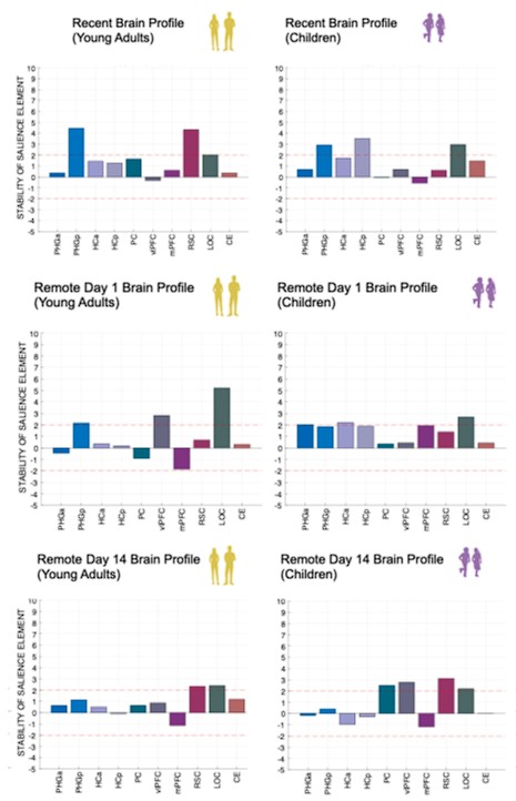
      (3) Also, as for differences between short delay brain profile and long delay brain profile for the scene-specific reinstatement - there are 2 regions that become significant at long delay that were not significant at a short delay (PC, and CE). However, given there are ceiling effects in behaviour at the short but not long delay, it's unclear if this is a meaningful difference or just a difference in sensitivity. Is there a way to test whether the profiles are statistically different from one another?

      We thank the reviewer for this comment. To better illustrate differential profiles also for high memory accuracy after immediate delay (30 minutes delay), we added the immediate (30 minutes delay) condition as a third reference point, given the availability of scene-specific reinstatement data at this time point. Interestingly, the immediate reinstatement profile revealed a different set of significant regions, with distinct expression patterns compared to both the short and long delay conditions. This supports the view that scene-specific reinstatement is not static but dynamically reorganized over time.

      Regarding the ceiling effect at short delay, we acknowledge this as a potential limitation. However, we note that our primary analyses were conducted across both age groups combined, and not solely within high-performing individuals. As such, the grouping may mitigate concerns that ceiling-level performance in a subset of participants unduly influenced the overall reinstatement profile. Moreover, we observed variation in neural reinstatement despite ceiling-level behavior, suggesting that the neural signal retains sensitivity to consolidation-related processes even when behavioral accuracy is near-perfect.

      While we agree that formal statistical comparisons of reinstatement profiles across delays (e.g., using representational profile similarity or interaction tests) could be an informative direction, we feel that this goes beyond the scope of the current manuscript. 

      (4) As I mentioned above, it also was not ideal in my opinion that all regions were included for the scene-specific reinstatement due to the authors' inability to have an appropriate baseline and therefore define above-chance reinstatement. It makes these findings really challenging to compare with the gist reinstatement ones. 

      We appreciate the reviewer’s comment and agree that the lack of a clearly defined baseline for scene-specific reinstatement limits our ability to determine whether these values reflect above-chance reinstatement. However, we would like to clarify that we do not directly compare the magnitude of scene-specific reinstatement to that of gist-like reinstatement in our analyses or interpretations. These two analyses serve complementary purposes: the scenespecific analysis captures trial-unique similarity (within-item reinstatement), while the gistlike analysis captures category-level representational structure (across items). Because they differ not only in baseline assumptions but also in analytical scope and theoretical interpretation, our goal was not to compare them directly, but rather to explore distinct but co-existing representational formats that may evolve differently across development and delay.

      (8) I would encourage the authors to be specific about whether they are measuring/talking about memory representations versus reinstatement, unless they think these are the same thing (in which case some explanation as to why would be helpful). For example, especially under the Fuzzy Trace framework, couldn't someone maintain both verbatim and gist traces of a memory yet rely more on one when making a memory decision? 

      We thank the reviewer for pointing out the importance of conceptual clarity when referring to memory representations versus reinstatement. We agree that these are distinct but related concepts: in our framework, memory representations refer to the neural content stored as a result of encoding and consolidation, whereas reinstatement refers to the reactivation of those representations during retrieval. Thus, reinstatement serves as a proxy for the underlying memory representation — it is how we measure or infer the nature (e.g., specificity, abstraction) of the stored content.

      Under Fuzzy Trace Theory, it is indeed possible for both verbatim and gist representations to coexist. Our interpretation is not that children lack verbatim traces, but rather that they are more likely to rely on schematic or gist-like representations during retrieval, especially after a delay. Our use of neural pattern similarity (reinstatement) reflects which type of representation is being accessed, not necessarily which traces exist in parallel.

      To avoid ambiguity, we have revised the manuscript to more explicitly distinguish between reinstatement (neural reactivation) and the representational format (verbatim vs. gist-like), especially in the framing of our hypotheses and interpretation of age group differences.

      (9) With respect to the learning criteria - it is misleading to say that "children needed between two to four learning-retrieval cycles to reach the criterion of 83% correct responses" (p. 9). Four was the maximum, and looking at the Figure 1C data it appears as though there were at least a few children who did not meet the 83% minimum. I believe they were included in the analysis anyway? Please clarify. Was there any minimum imposed for inclusion?

      We thank the reviewer for pointing this out. As stated in Methods Section (p. 50, lines 13261338) “These cycles ranged from a minimum of two to a maximum of four.<…> The cycles ended when participants provided correct responses to 83% of the trials or after the fourth cycle was reached.” We have corrected the corresponding wording in the Results section (line 286-289) to reflect this more accurately. Indeed, five children did not reach the 83% criterion but achieved final performance between 70 and 80% after the fourth learning cycle. These participants were included in this analysis for two main reasons:

      (1) The 83% threshold was established during piloting as a guideline for how many learningretrieval cycles to allow, not a strict learning criterion. It served to standardize task continuation, rather than to exclude participants post hoc.

      (2) The performance of these five children was still well above chance level (33%), indicating meaningful learning. Excluding them would have biased the sample toward higherperforming children and reduced the ecological validity of our findings. Including them ensures a more representative view of children’s performance under extended learning conditions.

      (10) For the gist-like reinstatement PLSC analysis, results are really similar a short and long delays and yet some of the text seems to implying specificity to the long delay. One is a trend and one is significant (p. 31), but surely these two associations would not be statistically different from one another?  

      We agree with the reviewer that the associations at short and long delays appeared similar. While a formal comparison (e.g., using a Z-test for dependent correlations) would typically be warranted, in the reanalyzed dataset only the long delay profile remains statistically significant, which limits the interpretability of such a comparison. 

      (11) As a general comment, I had a hard time tying all of the (many) results together. For example adults show more mature neocortical consolidation-related engagement, which the authors say is going to create more durable detailed memories, but under multiple trace theory we would generally think of neocortical representations as providing more schematic information. If the authors could try to make more connections across the different neural analyses, as well as tie the neural findings in more closely with the behaviour & back to the theoretical frameworks, that would be really helpful.  

      We thank the reviewer for this valuable suggestion. We have revised the discussion section to more clearly link the behavioral and neural findings and to interpret them in light of existing consolidation theories for better clarity. 

      Reviewer #2 (Public Review): 

      Schommartz et al. present a manuscript characterizing neural signatures of reinstatement during cued retrieval of middle-aged children compared to adults. The authors utilize a paradigm where participants learn the spatial location of semantically related item-scene memoranda which they retrieve after short or long delays. The paradigm is especially strong as the authors include novel memoranda at each delayed time point to make comparisons across new and old learning. In brief, the authors find that children show more forgetting than adults, and adults show greater engagement of cortical networks after longer delays as well as stronger item-specific reinstatement. Interestingly, children show more category-based reinstatement, however, evidence supports that this marker may be maladaptive for retrieving episodic details. The question is extremely timely both given the boom in neurocognitive research on the neural development of memory, and the dearth of research on consolidation in this age group. Also, the results provide novel insights into why consolidation processes may be disrupted in children. 

      We thank the reviewer for the positive evaluation.

      Comments on the revised version: 

      I carefully reviewed not only the responses to my own reviews as well as those raised by the other reviewers. While they addressed some of the concerns raised in the process, I think many substantive concerns remain. 

      Regarding Reviewer 1: 

      The authors point that the retrieval procedure is the same over time and similarly influenced by temporal autocorrelations, which makes their analysis okay. However, there is a fundamental problem as to whether they are actually measuring reinstatement or they are only measuring differences in temporal autocorrelation (or some non-linear combination of both). The authors further argue that the stimuli are being processed more memory wise rather than perception wise, however, I think there is no evidence for that and that perception-memory processes should be considered on a continuum rather than as discrete processes. Thus, I agree with reviewer 1 that these analyses should be removed. 

      We thank the reviewer for raising this important question. We would like to clarify a few key points regarding temporal autocorrelation and reinstatement.

      During the fixation window, participants were instructed to reinstate the scene and location associated with the cued object from memory. This task was familiar to them, as they had been trained in retrieving locations within scenes. Our analysis aims to compare the neural representations during this retrieval phase with those when participants view the scene, in order to assess how these representations change in similarity over time, as memories become less precise.

      We acknowledge that temporal proximity can lead to temporal autocorrelation. However, evidence suggests that temporal autocorrelation is consistent and stable across conditions (Gautama & Van Hulle, 2004; Woolrich et al., 2004). Shinn & Lagalwar (2021)further demonstrated that temporal autocorrelation is highly reliable at both the subject and regional levels. Given that we analyze regions of interest (ROIs) separately, potential spatial variability in temporal autocorrelation is not a major concern.

      No difference between item-specific reinstatement for recent items on day 1 and day 14 (which were merged) for further delay-related comparison also suggests that the reinstatement measure was stable for recent items even sampled at two different testing days. 

      Importantly, we interpret the relative change in the reinstatement index rather than its absolute value.

      In addition, when we conducted the same analysis for incorrectly retrieved memories, we did not observe any delay-related decline in reinstatement (see p. 25, lines 623-627). This suggests that the delay-related changes in reinstatement are specific to correctly retrieved memories. 

      Finally, our control analysis examining reinstatement between object and fixation time points (as suggested by Reviewer 1) revealed no delay-related effects in any ROI (see p.24, lines 605-612), further highlighting the specificity of the observed delay-related change in item reinstatement.

      We emphasize that temporal autocorrelation should be similar across all retrieval delays due to the identical task design and structure. Therefore, any observed decrease in reinstatement with increasing delay likely reflects a genuine change in the reinstatement index, rather than differences in temporal autocorrelation. Since our analysis includes only correctly retrieved items, and there is no perceptual input during the fixation window, this process is inherently memory-based, relying on mnemonic retrieval rather than sensory processing.

      We respectfully disagree with the reviewer's assertion that retrieval during the fixation period cannot be considered more memory-driven than perception-driven. At this time point, participants had no access to actual images of the scene, making it necessary for them to rely on mnemonic retrieval. The object cue likely triggered pattern completion for the learned object-scene association, forming a unique memory if remembered correctly(Horner & Burgess, 2013). This process is inherently mnemonic, as it is based on reconstructing the original neural representation of the scene (Kuhl et al., 2012; Staresina et al., 2013).

      While perception and memory processes can indeed be viewed as a continuum, some cognitive processes are predominantly memory-based, involving reconstruction rather than reproduction of previous experiences (Bartlett, 1932; Ranganath & Ritchey, 2012). In our task, although the retrieved material is based on previously encoded visual information, the process of recalling this information during the fixation period is fundamentally mnemonic, as it does not involve visual input. Our findings indicate that the similarity between memorybased representations and those observed during actual perception decreases over time, suggesting a relative change in the quality of the representations. However, this does not imply that detailed representations disappear; they may still be robust enough to support correct memory recall. Previous studies examining encoding-retrieval similarity have shown similar findings(Pacheco Estefan et al., 2019; Ritchey et al., 2013).

      We do not claim that perception and memory processes are entirely discrete, nor do we suggest that only perception is involved when participants see the scene. Viewing the scene indeed involves recognition processes, updating retrieved representations from the fixation period, and potentially completing missing or unclear information. This integrative process demonstrates the interrelation of perception and memory, especially in complex tasks like the one we employed.

      In conclusion, our task design and analysis support the interpretation that the fixation period is primarily characterized by mnemonic retrieval, facilitated by cue-triggered pattern completion, rather than perceptual processing. We believe this approach aligns with the current understanding of memory retrieval processes as supported by the existing literature.

      The authors seem to have a design that would allow for across run comparisons, however, they did not include these additional analyses. 

      Thank you for pointing this out. We ran as additional cross-run comparison. This results and further proceeding are reported in the comment for reviewer 1. 

      To address the reviewer’s concern, we conducted an additional cross-run analysis for all correctly retrieved trials. The approach restricted comparisons to non-overlapping runs (run1run2, run2-run3, run1-run3). This analysis revealed robust gist-like reinstatement in children for remote Day 14 memories in the mPFC (p = .035) and vlPFC (p = .0007), in adults’ vlPFC remote Day 1 memories (p = .029), as well as in children and adults remote Day 1 memories in LOC (p < .02). A significant Session effect in both regions (mPFC: p = .026; vlPFC: p = .002) indicated increased reinstatement for long delay (Day 14) compared to short-delay and recent session (all p < .05). Given that the cross-run results largely replicate and reinforce the effects found previously with within-run, we believe that combining both sources of information is methodologically justified and statistically beneficial. Specifically, both approaches independently identified significant gist-like reinstatement in children’s mPFC and vlPFC (although within-run vlPFC effect (short delay: p = .038; long delay p = .047) did not survive multiple comparisons), particularly for remote memories. Including both withinrun and between-run comparisons increases the number of unique, non-repeated trial pairs, improving statistical power without introducing redundancy. While we acknowledge that same-run comparisons may be influenced by residual autocorrelation(Prince et al., 2022), we believe that our design mitigates this risk through consistency between within-run and crossrun results, long inter-trial intervals, and trial-wise estimation of activation. We have adjusted the manuscript, accordingly, reporting the combined analysis. We also report cross-run and within-run analysis separately in supplementary materials (Tables S12.1, S12.2, showing that they converge with the cross-run results and thus strengthen rather than dilute the findings. 

      As suggested, we now explicitly highlight the change over time as the central finding. We observe a clear increase in gist-like reinstatement from recent to remote memories in children, particularly in mPFC and vlPFC. These effects based on combined within- and cross-run comparisons, are now clearly stated in the main results and interpreted in the discussion accordingly. 

      (1) The authors did not satisfy my concerns about different amounts of re-exposures to stimuli as a function of age, which introduces a serious confound in the interpretation of the neural data. 

      (2) Regarding Reviewer 1's point about different number of trials being entered into analysis, I think a more formal test of sub-sampling the adult trials is warranted. 

      (1) We thank the reviewer for pointing this out. Overall, children needed 2 to 4 learning cycles to improve their performance and reach the learning criteria, compared to 2 learning cycles in adults. To address the different amounts of re-exposure to stimuli between the age groups, we subsampled the child group to only those children who reached the learning criteria after 2 learning cycles. For this purpose, we excluded 21 children from the analysis who needed 3 or 4 learning cycles. This resulted in 39 young adults and 28 children being included in the subsequent analysis. 

      (i) We reran the behavioral analysis with the subsampled dataset (see Supplementary Materials,  Table S1.1, Fig. S1, Table S1.2). This analysis replicated the previous findings of less robust memory consolidation in children across all time delays. 

      (ii) We reran the univariate analysis (see in Supplementary Materials, Table S9.1). This analysis also replicated fully the previous findings. This indicates that the inclusion of child participants with greater material exposure during learning in the analysis of neural retrieval patterns did not affect the group differences in univariate neural results. 

      These subsampled results demonstrated that the amount of re-exposure to stimuli during encoding does not affect consolidation-related changes in memory retrieval at the behavioral and neural levels in children and adults across all time delays. We have added this information to the manuscript (line 343-348, 420-425). 

      (2) We appreciate Reviewer 1's suggestion to perform a formal test by sub-sampling the adult trials to match the number of trials in the child group. However, we believe that this approach may not be optimal for the following reasons:

      (i) Loss of Statistical Power: Sub-sampling the adult trials would result in a reduced sample size, potentially leading to a significant loss of statistical power and the ability to detect meaningful effects, particularly in a context where the adult group is intended to serve as a robust control or comparison group.

      (ii) Introducing sub-sampling could introduce variability that complicates the interpretation of results, particularly if the trial sub-sampling process does not fully capture the variability inherent in the original adult data.

      (iii) Robustness of Existing Findings: We have already addressed potential concerns about unequal trial numbers by conducting analyses that control for the number of learning cycles, as detailed in our supplementary materials. These analyses have shown that the observed effects are consistent, suggesting that the differences in trial numbers do not critically influence our findings.

      Given these considerations, we hope the reviewer understands our rationale and agrees that the current analysis is robust and appropriate for addressing the research questions.

      I also still fundamentally disagree with the use of global signals when comparing children to adults, and think this could very much skew the results. 

      We thank the reviewer for raising this important issue. To address this concern comprehensively, we have taken the following steps:

      (1) Overview of the literature support for global signal regression (GSR). A growing body of methodological and empirical research supports the inclusion of global signal repression as part of best practice denoising pipelines, particularly when analyzing pediatric fMRI data. Studies such as (Ciric et al., 2017; Parkes et al., 2018; J. D. Power et al., 2012, 2014; Power et al., 2012), and (Thompson et al., 2016) show that  GSR improves motion-related artifact removal. Critically, pediatric-specific studies (Disselhoff et al., 2025; Graff et al., 2022) conclude that pipelines including GSR are most effective for signal recovery and artifact removal in younger children. Graff et al. (2021) demonstrated that among various pipelines, GSR yielded the best noise reduction in 4–8-year-olds. Additionally, (Li et al., 2019; Qing et al., 2015) emphasized that GSR reduces artifactual variance without distorting the spatial structure of neural signals. (Ofoghi et al., 2021)demonstrated that global signal regression helps mitigate non-neuronal noise sources, including respiration, cardiac activity, motion, vasodilation, and scanner-related artifacts. Based on this and other recent findings, we consider GSR particularly beneficial for denoising paediatric  fMRI data in our study.

      (2) Empirical comparison of pipelines with and without GSR. We re-run the entire first-level univariate analysis using the pipeline that excluded the global signal regression. The resulting activation maps (see Supplementary Figure S3.2, S4.2, S5.2, S9.2) differed notably from the original pipeline. Specifically, group differences in cortical regions such as mPFC, cerebellum, and posterior PHG no longer reached significance, and the overall pattern of results appeared noisier. 

      (3) Evaluation of the pipeline differences. To further evaluate the impact of GSR, we conducted the following analyses:

      (a) Global signal is stable across groups and sessions. A linear mixed-effects model showed no significant main effects or interactions involving group or session on the global signal (F-values < 2.62, p > .11), suggesting that the global signal was not group- or session-dependent in our sample. 

      (b) Noise Reduction Assessment via Contrast Variability. We compared the variability (standard deviation and IQR) of contrast estimates across pipelines. Both SD (b = .070, p < .001) and IQR (b = .087, p < .001) were significantly reduced in the GSR pipeline, especially in children (p < .001) compared to adults (p = .048). This suggests that GSR reduces inter-subject variability in children, likely reflecting improved signal quality.

      (c) Residual Variability After Regressing Global Signal. We regressed out global signal post hoc from both pipelines and compared the residual variance. Residual standard deviation was significantly lower for the GSR pipeline (F = 199, p < .001), with no interaction with session or group, further indicating that GSR stabilizes the signal and attenuates non-neuronal variability.

      Conclusion

      In summary, while we understand the reviewer’s concern, we believe the empirical and theoretical support for GSR, especially in pediatric samples, justifies its use in our study. Nonetheless, to ensure full transparency, we provide full results from both pipelines in the Supplementary Materials and have clarified our reasoning in the revised manuscript.

      Reviewer #1 (Recommendations For The Authors): 

      (1) Some figures are still missing descriptions of what everything on the graph means; please clarify in captions. 

      We thank the reviewer for pointing this out. We undertook the necessary adjustments in the graph annotations. 

      (2) The authors conclude they showed evidence of neural reorganization of memory representations in children (p. 41). But the gist is not greater in children than adults, and also does not differ over time-so, I was confused about what this claim was based on? 

      We thank the reviewer for raising this question. Our results on gist-like reinstatements suggest that gist-like reinstatement was significantly higher in children compared to adults in the mPFC in addition to the child gist-like reinstatement indices being significantly higher than zero (see p.27-28). These results support our claim on neural reorganization of memory represenations in children. We hope this clarifies the issue. 

      References

      Bartlett, F. C. (1932). Remembering: A study in experimental and social psychology. Cambridge University Press.

      Brainerd, C. J., & Reyna, V. F. (2002). Fuzzy-Trace Theory: Dual Processes in Memory, Reasoning, and Cognitive Neuroscience (pp. 41–100). https://doi.org/10.1016/S00652407(02)80062-3

      Chen, J., Leong, Y. C., Honey, C. J., Yong, C. H., Norman, K. A., & Hasson, U. (2017). Shared memories reveal shared structure in neural activity across individuals. Nature Neuroscience, 20(1), 115–125. https://doi.org/10.1038/nn.4450

      Ciric, R., Wolf, D. H., Power, J. D., Roalf, D. R., Baum, G. L., Ruparel, K., Shinohara, R. T., Elliott, M. A., Eickhoff, S. B., Davatzikos, C., Gur, R. C., Gur, R. E., Bassett, D. S., & Satterthwaite, T. D. (2017). Benchmarking of participant-level confound regression strategies for the control of motion artifact in studies of functional connectivity. NeuroImage, 154, 174–187. https://doi.org/10.1016/j.neuroimage.2017.03.020

      Disselhoff, V., Jakab, A., Latal, B., Schnider, B., Wehrle, F. M., Hagmann, C. F., Held, U., O’Gorman, R. T., Fauchère, J.-C., & Hüppi, P. (2025). Inhibition abilities and functional brain connectivity in school-aged term-born and preterm-born children. Pediatric Research, 97(1), 315–324. https://doi.org/10.1038/s41390-024-03241-0

      Esteban, O., Ciric, R., Finc, K., Blair, R. W., Markiewicz, C. J., Moodie, C. A., Kent, J. D., Goncalves, M., DuPre, E., Gomez, D. E. P., Ye, Z., Salo, T., Valabregue, R., Amlien, I. K., Liem, F., Jacoby, N., Stojić, H., Cieslak, M., Urchs, S., … Gorgolewski, K. J. (2020). Analysis of task-based functional MRI data preprocessed with fMRIPrep. Nature Protocols, 15(7), 2186–2202. https://doi.org/10.1038/s41596-020-0327-3

      Fandakova, Y., Leckey, S., Driver, C. C., Bunge, S. A., & Ghetti, S. (2019). Neural specificity of scene representations is related to memory performance in childhood. NeuroImage, 199, 105–113. https://doi.org/10.1016/j.neuroimage.2019.05.050

      Gautama, T., & Van Hulle, M. M. (2004). Optimal spatial regularisation of autocorrelation estimates in fMRI analysis. NeuroImage, 23(3), 1203–1216.  https://doi.org/10.1016/j.neuroimage.2004.07.048

      Graff, K., Tansey, R., Ip, A., Rohr, C., Dimond, D., Dewey, D., & Bray, S. (2022). Benchmarking common preprocessing strategies in early childhood functional connectivity and intersubject correlation fMRI. Developmental Cognitive Neuroscience, 54, 101087. https://doi.org/10.1016/j.dcn.2022.101087

      Horner, A. J., & Burgess, N. (2013). The associative structure of memory for multi-element events. Journal of Experimental Psychology: General, 142(4), 1370–1383. https://doi.org/10.1037/a0033626

      Jones, J. S., the CALM Team, & Astle, D. E. (2021). A transdiagnostic data-driven study of children’s behaviour and the functional connectome. Developmental Cognitive Neuroscience, 52, 101027. https://doi.org/10.1016/j.dcn.2021.101027

      Kuhl, B. A., Bainbridge, W. A., & Chun, M. M. (2012). Neural Reactivation Reveals Mechanisms for Updating Memory. Journal of Neuroscience, 32(10), 3453–3461. https://doi.org/10.1523/JNEUROSCI.5846-11.2012

      Kuhl, B. A., & Chun, M. M. (2014). Successful Remembering Elicits Event-Specific Activity Patterns in Lateral Parietal Cortex. Journal of Neuroscience, 34(23), 8051–8060. https://doi.org/10.1523/JNEUROSCI.4328-13.2014

      Li, J., Kong, R., Liégeois, R., Orban, C., Tan, Y., Sun, N., Holmes, A. J., Sabuncu, M. R., Ge, T., & Yeo, B. T. T. (2019). Global signal regression strengthens association between resting-state functional connectivity and behavior. NeuroImage, 196, 126–141. https://doi.org/10.1016/j.neuroimage.2019.04.016

      Ofoghi, B., Chenaghlou, M., Mooney, M., Dwyer, D. B., & Bruce, L. (2021). Team technical performance characteristics and their association with match outcome in elite netball. International Journal of Performance Analysis in Sport, 21(5), 700–712. https://doi.org/10.1080/24748668.2021.1938424

      Pacheco Estefan, D., Sánchez-Fibla, M., Duff, A., Principe, A., Rocamora, R., Zhang, H., Axmacher, N., & Verschure, P. F. M. J. (2019). Coordinated representational reinstatement in the human hippocampus and lateral temporal cortex during episodic memory retrieval. Nature Communications, 10(1), 2255. https://doi.org/10.1038/s41467019-09569-0

      Parkes, L., Fulcher, B., Yücel, M., & Fornito, A. (2018). An evaluation of the efficacy, reliability, and sensitivity of motion correction strategies for resting-state functional MRI. NeuroImage, 171, 415–436. https://doi.org/10.1016/j.neuroimage.2017.12.073

      Power, J. D., Barnes, K. A., Snyder, A. Z., Schlaggar, B. L., & Petersen, S. E. (2012). Spurious but systematic correlations in functional connectivity MRI networks arise from subject motion. NeuroImage, 59(3), 2142–2154. https://doi.org/10.1016/j.neuroimage.2011.10.018

      Power, J. D., Mitra, A., Laumann, T. O., Snyder, A. Z., Schlaggar, B. L., & Petersen, S. E. (2014). Methods to detect, characterize, and remove motion artifact in resting state fMRI. NeuroImage, 84, 320–341. https://doi.org/10.1016/j.neuroimage.2013.08.048

      Power, S. D., Kushki, A., & Chau, T. (2012). Intersession Consistency of Single-Trial Classification of the Prefrontal Response to Mental Arithmetic and the No-Control State by NIRS. PLoS ONE, 7(7), e37791. https://doi.org/10.1371/journal.pone.0037791

      Prince, J. S., Charest, I., Kurzawski, J. W., Pyles, J. A., Tarr, M. J., & Kay, K. N. (2022). Improving the accuracy of single-trial fMRI response estimates using GLMsingle. ELife, 11. https://doi.org/10.7554/eLife.77599

      Qing, Z., Dong, Z., Li, S., Zang, Y., & Liu, D. (2015). Global signal regression has complex effects on regional homogeneity of resting state fMRI signal. Magnetic Resonance Imaging, 33(10), 1306–1313. https://doi.org/10.1016/j.mri.2015.07.011

      Ranganath, C., & Ritchey, M. (2012). Two cortical systems for memory-guided behaviour. Nature Reviews Neuroscience, 13(10), 713–726. https://doi.org/10.1038/nrn3338

      Ritchey, M., Wing, E. A., LaBar, K. S., & Cabeza, R. (2013). Neural Similarity Between Encoding and Retrieval is Related to Memory Via Hippocampal Interactions. Cerebral Cortex, 23(12), 2818–2828. https://doi.org/10.1093/cercor/bhs258

      Satterthwaite, T. D., Elliott, M. A., Gerraty, R. T., Ruparel, K., Loughead, J., Calkins, M. E., Eickhoff, S. B., Hakonarson, H., Gur, R. C., Gur, R. E., & Wolf, D. H. (2013). An improved framework for confound regression and filtering for control of motion artifact in the preprocessing of resting-state functional connectivity data. NeuroImage, 64, 240–256. https://doi.org/10.1016/j.neuroimage.2012.08.052

      Schommartz, I., Lembcke, P. F., Pupillo, F., Schuetz, H., de Chamorro, N. W., Bauer, M., Kaindl, A. M., Buss, C., & Shing, Y. L. (2023). Distinct multivariate structural brain profiles are related to variations in short- and long-delay memory consolidation across children and young adults. Developmental Cognitive Neuroscience, 59. https://doi.org/10.1016/J.DCN.2022.101192

      Sekeres, M. J., Winocur, G., & Moscovitch, M. (2018). The hippocampus and related neocortical structures in memory transformation. Neuroscience Letters, 680, 39–53. https://doi.org/10.1016/j.neulet.2018.05.006

      Shinn, L. J., & Lagalwar, S. (2021). Treating Neurodegenerative Disease with Antioxidants: Efficacy of the Bioactive Phenol Resveratrol and Mitochondrial-Targeted MitoQ and SkQ. Antioxidants, 10(4), 573. https://doi.org/10.3390/antiox10040573

      Staresina, B. P., Alink, A., Kriegeskorte, N., & Henson, R. N. (2013). Awake reactivation predicts memory in humans. Proceedings of the National Academy of Sciences, 110(52), 21159–21164. https://doi.org/10.1073/pnas.1311989110

      St-Laurent, M., & Buchsbaum, B. R. (2019). How Multiple Retrievals Affect Neural Reactivation in Young and Older Adults. The Journals of Gerontology: Series B, 74(7), 1086–1100. https://doi.org/10.1093/geronb/gbz075

      Thompson, G. J., Riedl, V., Grimmer, T., Drzezga, A., Herman, P., & Hyder, F. (2016). The Whole-Brain “Global” Signal from Resting State fMRI as a Potential Biomarker of Quantitative State Changes in Glucose Metabolism. Brain Connectivity, 6(6), 435–447. https://doi.org/10.1089/brain.2015.0394

      Tompary, A., & Davachi, L. (2017). Consolidation Promotes the Emergence of Representational Overlap in the Hippocampus and Medial Prefrontal Cortex. Neuron, 96(1), 228-241.e5. https://doi.org/10.1016/j.neuron.2017.09.005

      Tompary, A., Zhou, W., & Davachi, L. (2020). Schematic memories develop quickly, but are not expressed unless necessary. PsyArXiv.

      Woolrich, M. W., Behrens, T. E. J., Beckmann, C. F., Jenkinson, M., & Smith, S. M. (2004). Multilevel linear modelling for FMRI group analysis using Bayesian inference. NeuroImage, 21(4), 1732–1747. https://doi.org/10.1016/j.neuroimage.2003.12.023

      Xiao, X., Dong, Q., Gao, J., Men, W., Poldrack, R. A., & Xue, G. (2017). Transformed Neural Pattern Reinstatement during Episodic Memory Retrieval. The Journal of Neuroscience, 37(11), 2986–2998. https://doi.org/10.1523/JNEUROSCI.2324-16.2017

      Ye, Z., Shi, L., Li, A., Chen, C., & Xue, G. (2020). Retrieval practice facilitates memory updating by enhancing and differentiating medial prefrontal cortex representations. ELife, 9, 1–51. https://doi.org/10.7554/ELIFE.57023

      Yonelinas, A. P., Ranganath, C., Ekstrom, A. D., & Wiltgen, B. J. (2019). A contextual binding theory of episodic memory: systems consolidation reconsidered. Nature Reviews. Neuroscience, 20(6), 364–375. https://doi.org/10.1038/S41583-019-01504

      Zhuang, L., Wang, J., Xiong, B., Bian, C., Hao, L., Bayley, P. J., & Qin, S. (2021). Rapid neural reorganization during retrieval practice predicts subsequent long-term retention and false memory. Nature Human Behaviour, 6(1), 134–145.

      https://doi.org/10.1038/s41562-021-01188-4
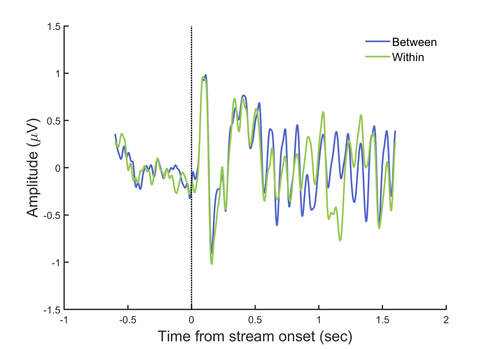
    1. Author response:

      The following is the authors’ response to the original reviews.

      Reviewer #1 (Public review):

      Summary:

      The Major Histocompatibility Complex (MHC) region is a collection of numerous genes involved in both innate and adaptive immunity. MHC genes are famed for their role in rapid evolution and extensive polymorphism in a variety of vertebrates. This paper presents a summary of gene-level gain and loss of orthologs and paralogs within MHC across the diversity of primates, using publicly available data.

      Strengths:

      This paper provides a strong case that MHC genes are rapidly gained (by paralog duplication) and lost over millions of years of macroevolution. The authors are able to identify MHC loci by homology across species, and from this infer gene duplications and losses using phylogenetic analyses. There is a remarkable amount of genic turnover, summarized in Figure 6 and Figure 7, either of which might be a future textbook figure of immune gene family evolution. The authors draw on state-of-the-art phylogenetic methods, and their inferences are robust insofar as the data might be complete enough to draw such conclusions.

      Weaknesses:

      One concern about the present work is that it relies on public databases to draw inferences about gene loss, which is potentially risky if the publicly available sequence data are incomplete. To say, for example, that a particular MHC gene copy is absent in a taxon (e.g., Class I locus F absent in Guenons according to Figure 1), we need to trust that its absence from the available databases is an accurate reflection of its absence in the genome of the actual organisms. This may be a safe assumption, but it rests on the completeness of genome assembly (and gene annotations?) or people uploading relevant data. This reviewer would have been far more comfortable had the authors engaged in some active spot-checking, doing the lab work to try to confirm absences at least for some loci and some species. Without this, a reader is left to wonder whether gene loss is simply reflecting imperfect databases, which then undercuts confidence in estimates of rates of gene loss.

      Indeed, just because a locus has not been confirmed in a species does not necessarily mean that it is absent. As we explain in the Figure 1 caption, only a few species have had their genomes extensively studied (gray background), and only for these species does the absence of a point in this figure mean that a locus is absent. The white background rows represent species that are not extensively studied, and we point out that the absence of a point does not mean that a locus is absent from the species, rather undiscovered. We have also added a parenthetical to the text to explain this (line 156): “Only species with rows highlighted in gray have had their MHC regions extensively studied (and thus only for these rows is the absence of a gene symbol meaningful).”

      While we agree that spot-checking may be a helpful next step, one of the goals of this manuscript is to collect and synthesize the enormous volume of MHC evolution research in the primates, which will serve as a jumping-off point for other researchers to perform important wet lab work.

      Some context is useful for comparing rates of gene turnover in MHC, to other loci. Changing gene copy numbers, duplications, and loss of duplicates, are common it seems across many loci and many organisms; is MHC exceptional in this regard, or merely behaving like any moderately large gene family? I would very much have liked to see comparable analyses done for other gene families (immune, like TLRs, or non-immune), and quantitative comparisons of evolutionary rates between MHC versus other genes. Does MHC gene composition evolve any faster than a random gene family? At present readers may be tempted to infer this, but evidence is not provided.

      Our companion paper (Fortier and Pritchard, 2025) demonstrates that the MHC is a unique locus in many regards, such as its evidence for deep balancing selection and its excess of disease associations. Thus, we expect that it is evolving faster than any random gene family. It would be interesting to repeat this analysis for other gene families, but that is outside of the scope of this project. Additionally, allele databases for other gene families are not nearly as developed, but as more alleles become available for other polymorphic families, a comparable analysis could become possible.

      We have added a paragraph to the discussion (lines 530-546) to clarify that we do not know for certain whether the MHC gene family is evolving rapidly compared to other gene families.

      While on the topic of making comparisons, the authors make a few statements about relative rates. For instance, lines 447-8 compare gene topology of classical versus non-classical genes; and line 450 states that classical genes experience more turnover. But there are no quantitative values given to these rates to provide numerical comparisons, nor confidence intervals provided (these are needed, given that they are estimates), nor formal statistical comparisons to confirm our confidence that rates differ between types of genes.

      More broadly, the paper uses sophisticated phylogenetic methods, but without taking advantage of macroevolutionary comparative methods that allow model-based estimation of macroevolutionary rates. I found the lack of quantitative measurements of rates of gene gain/loss to be a weakness of the present version of the paper, and something that should be readily remedied. When claiming that MHC Class I genes "turn over rapidly" (line 476) - what does rapidly mean? How rapidly? How does that compare to rates of genetic turnover at other families? Quantitative statements should be supported by quantitative estimates (and their confidence intervals).

      These statements refer to qualitative observations, so we cannot provide numerical values. We simply conclude that certain gene groups evolve faster or slower based on the species and genes present in each clade. It is difficult to provide estimates because of the incomplete sampling of genes that survived to the present day. In addition, the presence or absence of various orthologs in different species still needs to be confirmed, at which point it might be useful to be more quantitative. We have also added a paragraph to the discussion to address this concern and advocate for similar analyses of other gene families in the future when more data is available (lines 530-546).

      The authors refer to 'shared function of the MHC across species' (e.g. line 22); while this is likely true, they are not here presenting any functional data to confirm this, nor can they rule out neofunctionalization or subfunctionalization of gene duplicates. There is evidence in other vertebrates (e.g., cod) of MHC evolving appreciably altered functions, so one may not safely assume the function of a locus is static over long macroevolutionary periods, although that would be a plausible assumption at first glance.

      Indeed, we cannot assume that the function of a locus is static across time, especially for the MHC region. In our research, we read hundreds of papers that each focused on a small number of species or genes and gathered some information about them, sometimes based on functional experiments and sometimes on measures such as dN/dS. These provide some indication of a gene’s broad classification in a species or clade, even if the evidence is preliminary. Where possible, we used this preliminary evidence to give genes descriptors “classical,” “non-classical,” “dual characteristics,” “pseudogene,” “fixed”, or “unfixed.” Sometimes multiple individuals and haplotypes were analyzed, so we could even assign a minimum number of gene copies present in a species. We have aggregated all of these references into Supplementary Table 1 (for Class I/Figure 1) and Supplementary Table 2 (for Class II/Figure 2) along with specific details about which data points in these figures that each reference supports. We realize that many of these classifications are based on a small number of individuals or indirect measures, so they may change in the future as more functional data is generated.

      Reviewer #2 (Public review):

      Summary:

      The authors aim to provide a comprehensive understanding of the evolutionary history of the Major Histocompatibility Complex (MHC) gene family across primate species. Specifically, they sought to:

      (1) Analyze the evolutionary patterns of MHC genes and pseudogenes across the entire primate order, spanning 60 million years of evolution.

      (2) Build gene and allele trees to compare the evolutionary rates of MHC Class I and Class II genes, with a focus on identifying which genes have evolved rapidly and which have remained stable.

      (3) Investigate the role of often-overlooked pseudogenes in reconstructing evolutionary events, especially within the Class I region.

      (4) Highlight how different primate species use varied MHC genes, haplotypes, and genetic variation to mount successful immune responses, despite the shared function of the MHC across species.

      (5) Fill gaps in the current understanding of MHC evolution by taking a broader, multi-species perspective using (a) phylogenomic analytical computing methods such as Beast2, Geneconv, BLAST, and the much larger computing capacities that have been developed and made available to researchers over the past few decades, (b) literature review for gene content and arrangement, and genomic rearrangements via haplotype comparisons.

      (6) The authors overall conclusions based on their analyses and results are that 'different species employ different genes, haplotypes, and patterns of variation to achieve a successful immune response'.

      Strengths:

      Essentially, much of the information presented in this paper is already well-known in the MHC field of genomic and genetic research, with few new conclusions and with insufficient respect to past studies. Nevertheless, while MHC evolution is a well-studied area, this paper potentially adds some originality through its comprehensive, cross-species evolutionary analysis of primates, focus on pseudogenes and the modern, large-scale methods employed. Its originality lies in its broad evolutionary scope of the primate order among mammals with solid methodological and phylogenetic analyses.

      The main strengths of this study are the use of large publicly available databases for primate MHC sequences, the intensive computing involved, the phylogenetic tool Beast2 to create multigene Bayesian phylogenetic trees using sequences from all genes and species, separated into Class I and Class II groups to provide a backbone of broad relationships to investigate subtrees, and the presentation of various subtrees as species and gene trees in an attempt to elucidate the unique gene duplications within the different species. The study provides some additional insights with summaries of MHC reference genomes and haplotypes in the context of a literature review to identify the gene content and haplotypes known to be present in different primate species. The phylogenetic overlays or ideograms (Figures 6 and 7) in part show the complexity of the evolution and organisation of the primate MHC genes via the orthologous and paralogous gene and species pathways progressively from the poorly-studied NWM, across a few moderately studied ape species, to the better-studied human MHC genes and haplotypes.

      Weaknesses:

      The title 'The Primate Major Histocompatibility Complex: An Illustrative Example of GeneFamily Evolution' suggests that the paper will explore how the Major Histocompatibility Complex (MHC) in primates serves as a model for understanding gene family evolution. The term 'Illustrative Example' in the title would be appropriate if the paper aimed to use the primate Major Histocompatibility Complex (MHC) as a clear and representative case to demonstrate broader principles of gene family evolution. That is, the MHC gene family is not just one instance of gene family evolution but serves as a well-studied, insightful example that can highlight key mechanisms and concepts applicable to other gene families. However, this is not the case, this paper only covers specific details of primate MHC evolution without drawing broader lessons to any other gene families. So, the term 'Illustrative Example' is too broad or generalizing. In this case, a term like 'Case Study' or simply 'Example' would be more suitable. Perhaps, 'An Example of Gene Family Diversity' would be more precise. Also, an explanation or 'reminder' is suggested that this study is not about the origins of the MHC genes from the earliest jawed vertebrates per se (~600 mya), but it is an extension within a subspecies set that has emerged relatively late (~60 mya) in the evolutionary divergent pathways of the MHC genes, systems, and various vertebrate species.

      Thank you for your input on the title; we have changed it to “A case study of gene family evolution” instead.

      Thank you also for pointing out the potential confusion about the time span of our study. We have added “Having originated in the jawed vertebrates,” to a sentence in the introduction (lines 38-39). We have also added the sentence “Here, we focus on the primates, spanning approximately 60 million years within the over 500-million-year evolution of the family \citep{Flajnik2010}.“ to be more explicit about the context for our work (lines 59-61).

      Phylogenomics. Particular weaknesses in this study are the limitations and problems associated with providing phylogenetic gene and species trees to try and solve the complex issue of the molecular mechanisms involved with imperfect gene duplications, losses, and rearrangements in a complex genomic region such as the MHC that is involved in various effects on the response and regulation of the immune system. A particular deficiency is drawing conclusions based on a single exon of the genes. Different exons present different trees. Which are the more reliable? Why were introns not included in the analyses? The authors attempt to overcome these limitations by including genomic haplotype analysis, duplication models, and the supporting or contradictory information available in previous publications. They succeed in part with this multidiscipline approach, but much is missed because of biased literature selection. The authors should include a paragraph about the benefits and limitations of the software that they have chosen for their analysis, and perhaps suggest some alternative tools that they might have tried comparatively. How were problems with Bayesian phylogeny such as computational intensity, choosing probabilities, choosing particular exons for analysis, assumptions of evolutionary models, rates of evolution, systemic bias, and absence of structural and functional information addressed and controlled for in this study?

      We agree that different exons have different trees, which is exactly why we repeated our analysis for each exon in order to compare and contrast them. In particular, the exons encoding the binding site of the resulting protein (exons 2 and 3 for Class I and exon 2 for Class II) show evidence for trans-species polymorphism and gene conversion. These phenomena lead to trees that do not follow the species tree and are fascinating in and of themselves, which we explore in detail in our companion paper (Fortier and Pritchard, 2025). Meanwhile, the non-peptide-binding extracellular-domain-encoding exon (exon 4 for Class I and exon 3 for Class II) is comparably sized to the binding-site-encoding exons and provides an interesting functional contrast. As this exon is likely less affected by trans-species polymorphism, gene conversion, and convergent evolution, we present results from it most often in the main text, though we occasionally touch on differences between the exons. See lines 191-196, 223-226, and 407-414 for some examples of how we discuss the exons in the text. Additionally, all trees from all of these exons can be found in the supplement. 

      We agree that introns would valuable to study in this context. Even though the non--binding-site-encoding exons are probably *less* affected by trans-species polymorphism, gene conversion, and convergent evolution, they are still functional. The introns, however, experience much more relaxed selection, if any, and comparing their trees to those for the exons would be valuable and illuminating. We did not generate intron trees for two reasons. Most importantly, there is a dearth of data available for the introns; in the databases we used, there was often intron data available only for human, chimpanzee, and sometimes macaque, and only for a small subset of the genes. This limitation is at odds with the comprehensive, many-gene-many-species approach which we feel is the main novelty of this work. Secondly, the introns that *are* available are difficult to align. Even aligning the exons across such a highly-diverged set of genes and pseudogenes was difficult and required manual effort. The introns proved even more difficult to try to align across genes. In the future, when more intron data is available and sufficient effort is put into aligning them, it will be possible and desirable to do a comparable analysis. We also added a sentence to the “Data” section to briefly explain why we did not include introns (lines 134-135).

      We explain our Bayesian phylogenetics approach in detail in the Methods (lines 650-725), including our assumptions and our solutions to challenges specific to this application. For further explanation of the method itself, we suggest reading the original BEAST and BEAST2 papers (Drummond & Rambaut (2007), Drummond et al. (2012), Bouckaert et al. (2014), and Bouckaert et al. (2019)). Known structural and functional information helped us validate the alignments we used in this study, but the fact that such information is not fully known for every gene and species should not affect the method itself.

      Gene families as haplotypes. In the Introduction, the MHC is referred to as a 'gene family', and in paragraph 2, it is described as being united by the 'MHC fold', despite exhibiting 'very diverse functions'. However, the MHC region is more accurately described as a multigene region containing diverse, haplotype-specific Conserved Polymorphic Sequences, many of which are likely to be regulatory rather than protein-coding. These regulatory elements are essential for controlling the expression of multiple MHC-related products, such as TNF and complement proteins, a relationship demonstrated over 30 years ago. Non-MHC fold loci such as TNF, complement, POU5F1, lncRNA, TRIM genes, LTA, LTB, NFkBIL1, etc, are present across all MHC haplotypes and play significant roles in regulation. Evolutionary selection must act on genotypes, considering both paternal and maternal haplotypes, rather than on individual genes alone. While it is valuable to compile databases for public use, their utility is diminished if they perpetuate outdated theories like the 'birth-and-death model'. The inclusion of prior information or assumptions used in a statistical or computational model, typically in Bayesian analysis, is commendable, but they should be based on genotypic data rather than older models. A more robust approach would consider the imperfect duplication of segments, the history of their conservation, and the functional differences in inheritance patterns. Additionally, the MHC should be examined as a genomic region, with ancestral haplotypes and sequence changes or rearrangements serving as key indicators of human evolution after the 'Out of Africa' migration, and with disease susceptibility providing a measurable outcome. There are more than 7000 different HLA-B and -C alleles at each locus, which suggests that there are many thousands of human HLA haplotypes to study. In this regard, the studies by Dawkins et al (1999 Immunol Rev 167,275), Shiina et al. (2006 Genetics 173,1555) on human MHC gene diversity and disease hitchhiking (haplotypes), and Sznarkowska et al. (2020 Cancers 12,1155) on the complex regulatory networks governing MHC expression, both in terms of immune transcription factor binding sites and regulatory non-coding RNAs, should be examined in greater detail, particularly in the context of MHC gene allelic diversity and locus organization in humans and other primates.

      Thank you for these comments. To clarify that the MHC “region” is different from (and contains) the MHC “gene family” as we describe it, we changed a sentence in the abstract (lines 8-10) from “One large gene family that has experienced rapid evolution is the Major Histocompatibility Complex (MHC), whose proteins serve critical roles in innate and adaptive immunity.” to “One large gene family that has experienced rapid evolution lies within the Major Histocompatibility Complex (MHC), whose proteins serve critical roles in innate and adaptive immunity.” We know that the region is complex and contains many other genes and regulatory sequences; Figure 1 of our companion paper (Fortier and Pritchard, 2025) depicts these in order to show the reader that the MHC genes we focus on are just one part of the entire region.

      We love the suggestion to look at the many thousands of alleles present at each of the classical loci. This is the focus of our complimentary paper (Fortier and Pritchard, 2025) which explores variation at the allele level. In the current paper, we look mainly at the differences between genes and the use of different genes in different species.

      Diversifying and/or concerted evolution. Both this and past studies highlight diversifying selection or balancing selection model is the dominant force in MHC evolution. This is primarily because the extreme polymorphism observed in MHC genes is advantageous for populations in terms of pathogen defence. Diversification increases the range of peptides that can be presented to T cells, enhancing the immune response. The peptide-binding regions of MHC genes are highly variable, and this variability is maintained through selection for immune function, especially in the face of rapidly evolving pathogens. In contrast, concerted evolution, which typically involves the homogenization of gene duplicates through processes like gene conversion or unequal crossing-over, seems to play a minimal role in MHC evolution. Although gene duplication events have occurred in the MHC region leading to the expansion of gene families, the resulting paralogs often undergo divergent evolution rather than being kept similar or homozygous by concerted evolution. Therefore, unlike gene families such as ribosomal RNA genes or histone genes, where concerted evolution leads to highly similar copies, MHC genes display much higher levels of allelic and functional diversification. Each MHC gene copy tends to evolve independently after duplication, acquiring unique polymorphisms that enhance the repertoire of antigen presentation, rather than undergoing homogenization through gene conversion. Also, in some populations with high polymorphism or genetic drift, allele frequencies may become similar over time without the influence of gene conversion. This similarity can be mistaken for gene conversion when it is simply due to neutral evolution or drift, particularly in small populations or bottlenecked species. Moreover, gene conversion might contribute to greater diversity by creating hybrids or mosaics between different MHC genes. In this regard, can the authors indicate what percentage of the gene numbers in their study have been homogenised by gene conversion compared to those that have been diversified by gene conversion?

      We appreciate the summary, and we feel we have appropriately discussed both gene conversion and diversifying selection in the context of the MHC genes. Because we cannot know for sure when and where gene conversion has occurred, we cannot quantify percentages of genes that have been homogenized or diversified.  

      Duplication models. The phylogenetic overlays or ideograms (Figures 6 and 7) show considerable imperfect multigene duplications, losses, and rearrangements, but the paper's Discussion provides no in-depth consideration of the various multigenic models or mechanisms that can be used to explain the occurrence of such events. How do their duplication models compare to those proposed by others? For example, their text simply says on line 292, 'the proposed series of events is not always consistent with phylogenetic data'. How, why, when? Duplication models for the generation and extension of the human MHC class I genes as duplicons (extended gene or segmental genomic structures) by parsimonious imperfect tandem duplications with deletions and rearrangements in the alpha, beta, and kappa blocks were already formulated in the late 1990s and extended to the rhesus macaque in 2004 based on genomic haplotypic sequences. These studies were based on genomic sequences (genes, pseudogenes, retroelements), dot plot matrix comparisons, and phylogenetic analyses of gene and retroelement sequences using computer programs. It already was noted or proposed in these earlier 1999 studies that (1) the ancestor of HLA-P(90)/-T(16)/W(80) represented an old lineage separate from the other HLA class I genes in the alpha block, (2) HLA-U(21) is a duplicated fragment of HLA-A, (3) HLA-F and HLA-V(75) are among the earliest (progenitor) genes or outgroups within the alpha block, (4) distinct Alu and L1 retroelement sequences adjoining HLA-L(30), and HLA-N genomic segments (duplicons) in the kappa block are closely related to those in the HLA-B and HLA-C in the beta block; suggesting an inverted duplication and transposition of the HLA genes and retroelements between the beta and kappa regions. None of these prior human studies were referenced by Fortier and Pritchard in their paper. How does their human MHC class I gene duplication model (Fig. 6) such as gene duplication numbers and turnovers differ from those previously proposed and described by Kulski et al (1997 JME 45,599), (1999 JME 49,84), (2000 JME 50,510), Dawkins et al (1999 Immunol Rev 167,275), and Gaudieri et al (1999 GR 9,541)? Is this a case of reinventing the wheel?

      Figures 6 and 7 are intended to synthesize and reconcile past findings and our own trees, so they do not strictly adhere to the findings of any particular study and cannot fully match all studies. In the supplement, Figure 6 - figure supplement 1 and Figure 7 - figure supplement 1 duly credit all of the past work that went into making these trees. Most previous papers focus on just one aspect of these trees, such as haplotypes within a species, a specific gene or allelic lineage relationship, or the branching pattern of particular gene groups. We believe it was necessary to bring all of these pieces of evidence together. Even among papers with the same focus (to understand the block duplications that generated the current physical layout of the MHC), results differ. For example, Geraghty (1992), Hughes (1995), Kulski (2004)/Kulski (2005),  and Shiina (1999) all disagree on the exact branching order of the genes MHC-W, -P, and -T, and of MHC-G, -J, and -K. While the Kulski studies you pointed out were very thorough for their era, they still only relied on data from three species and one haplotype per species. Our work is not intended to replace or discredit these past works, simply build upon them with a larger set of species and sequences. We hope the hypotheses we propose in Figures 6 and 7 can help unify existing research and provide a more easily accessible jumping-off-point for future work.

      Results. The results are presented as new findings, whereas most if not all of the results' significance and importance already have been discussed in various other publications. Therefore, the authors might do better to combine the results and discussion into a single section with appropriate citations to previously published findings presented among their results for comparison. Do the trees and subsets differ from previous publications, albeit that they might have fewer comparative examples and samples than the present preprint? Alternatively, the results and discussion could be combined and presented as a review of the field, which would make more sense and be more honest than the current format of essentially rehashing old data.

      In starting this project, we found that a large barrier to entry to this field of study is the immense amount of published literature over 30+ years. It is both time-consuming and confusing to read up on the many nuances of the MHC genes, their changing names, and their evolution, making it difficult to start new, innovative projects. We acknowledge that while our results are not entirely novel, the main advantage of our work is that it provides a thorough, comprehensive starting point for others to learn about the MHC quickly and dive into new research. We feel that we have appropriately cited past literature in both the main text, appendices, and supplement, so that readers may dive into a particular area with ease.

      Minor corrections:

      (1) Abstract, line 19: 'modern methods'. Too general. What modern methods?

      To keep the abstract brief, the methods are introduced in the main text when each becomes relevant as well as in the methods section.

      (2) Abstract, line 25: 'look into [primate] MHC evolution.' The analysis is on the primate MHC genes, not on the entire vertebrate MHC evolution with a gene collection from sharks to humans. The non-primate MHC genes are often differently organised and structurally evolved in comparison to primate MHC.

      Thank you! We have added the word “primate” to the abstract (line 25).

      (3) Introduction, line 113. 'In a companion paper (Fortier and Pritchard, 2024)' This paper appears to be unpublished. If it's unpublished, it should not be referenced.

      This paper is undergoing the eLife editorial process at the same time; it will have a proper citation in the final version.

      (4) Figures 1 and 2. Use the term 'gene symbols' (circle, square, triangle, inverted triangle, diamond) or 'gene markers' instead of 'points'. 'Asterisks "within symbols" indicate new information.

      Thank you, the word “symbol” is much clearer! We have changed “points” to “symbols” in the captions for Figure 1, Figure 1 - figure supplement 1, Figure 2, and Figure 2 - figure supplement 1. We also changed this in the text (lines 157-158 and 170).

      (5) Figures. A variety of colours have been applied for visualisation. However, some coloured texts are so light in colour that they are difficult to read against a white background. Could darker colours or black be used for all or most texts?

      With such a large number of genes and species to handle in this work, it was nearly impossible to choose a set of colors that were distinct enough from each other. We decided to prioritize consistency (across this paper, its supplement, and our companion paper) as well as at-a-glance grouping of similar sequences. Unfortunately, this means we had to sacrifice readability on a white background, but readers may turn to the supplement if they need to access specific sequence names.

      (6) Results, line 135. '(Fortier and Pritchard, 2024)' This paper appears to be unpublished. If it's unpublished, it should not be referenced.

      Repeat of (3). This paper is undergoing the eLife editorial process at the same time; it will have a proper citation in the final version.

      (7) Results, lines 152 to 153, 164, 165, etc. 'Points with an asterisk'. Use the term 'gene symbols' (circle, square, triangle, inverted triangle, diamond) or 'gene markers' instead of 'points'. A point is a small dot such as those used in data points for plotting graphs .... The figures are so small that the asterisks in the circles, squares, triangles, etc, look like points (dots) and the points/asterisks terminology that is used is very confusing visually.

      Repeat of (4). Thank you, the word “symbol” is much clearer! We have changed “points” to “symbols” in the captions for Figure 1, Figure 1 - figure supplement 1, Figure 2, and Figure 2 - figure supplement 1. We also changed this in the text (lines 157-158 and 170).

      (8) Line 178 (BEA, 2024) is not listed alphabetically in the References.

      Thank you for catching this! This reference maps to the first bibliography entry, “SUMMARIZING POSTERIOR TREES.” We are unsure how to cite a webpage that has no explicit author within the eLife Overleaf template, so we will consult with the editor.

      (9) Lines 188-190. 'NWM MHC-G does not group with ape/OWM MHC-G, instead falling outside of the clade containing ape/OWM MHC-A, -G, -J and -K.' This is not surprising given that MHC-A, -G, -J, and -K are paralogs of each other and that some of them, especially in NWM have diverged over time from the paralogs and/or orthologs and might be closer to one paralog than another and not be an actual ortholog of OWM, apes or humans.

      We included this sentence to clarify the relationships between genes and to help describe what is happening in Figure 6. Figure 6 - figure supplement 1 includes all of the references that go into such a statement and Appendix 3 details our reasoning for this and other statements.

      (10) Line 249. Gene conversion: This is recombination between two different genes where a portion of the genes are exchanged with one another so that different portions of the gene can group within one or other of the two gene clades. Alternatively, the gene has been annotated incorrectly if the gene does not group within either of the two alternative clades. Another possibility is that one or two nucleotide mutations have occurred without a recombination resulting in a mistaken interpretation or conclusion of a recombination event. What measures are taken to avoid false-positive conclusions? How many MHC gene conversion (recombination) events have occurred according to the authors' estimates? What measures are taken to avoid false-positive conclusions?

      All of these possibilities are certainly valid. We used the program GENECONV to infer gene conversion events, but there is considerable uncertainty owing to the ages of the genes and the inevitable point mutations that have occurred post-event. Gene conversion was not the focus of our paper, so we did our best to acknowledge it (and the resulting differences between trees from different exons) without spending too much time diving into it. A list of inferred gene conversion events can be found in Figure 3 - source data 1 and Figure 4 - source data 1.

      (11) Lines 284-286. 'The Class I MHC region is further divided into three polymorphic blocks-alpha, beta, and kappa blocks-that each contains MHC genes but are separated by well-conserved non-MHC genes.' The MHC class I region was first designated into conserved polymorphic duplication blocks, alpha and beta by Dawkins et al (1999 Immunol Rev 167,275), and kappa by Kulski et al (2002 Immunol Rev 190,95), and should be acknowledged (cited) accordingly.

      Thank you for catching this! We have added these citations (lines 302-303)!

      (12) Lines 285-286. 'The majority of the Class I genes are located in the alpha-block, which in humans includes 12 MHC genes and pseudogenes.' This is not strictly correct for many other species, because the majority of class I genes might be in the beta block of new and old-world monkeys, and the authors haven't provided respective counts of duplication numbers to show otherwise. The alpha block in some non-primate mammalian species such as pigs, rats, and mice has no MHC class I genes or only a few. Most MHC class I genes in non-primate mammalian species are found in other regions. For example, see Ando et al (2005 Immunogenetics 57,864) for the pig alpha, beta, and kappa regions in the MHC class I region. There are no pig MHC genes in the alpha block.

      Yes, which is exactly why we use the phrase “in humans” in that particular sentence. The arrangement of the MHC in several other primate reference genomes is shown in Figure 1 - figure supplement 2.

      (13) Line 297 to 299. 'The alpha-block also contains a large number of repetitive elements and gene fragments belonging to other gene families, and their specific repeating pattern in humans led to the conclusion that the region was formed by successive block duplications (Shiina et al., 1999).' There are different models for successive block duplications in the alpha block and some are more parsimonious based on imperfect multigenic segmental duplications (Kulski et al 1999, 2000) than others (Shiina et al., 1999). In this regard, Kulski et al (1999, 2000) also used duplicated repetitive elements neighbouring MHC genes to support their phylogenetic analyses and multigenic segmental duplication models. For comparison, can the authors indicate how many duplications and deletions they have in their models for each species?

      We have added citations to this sentence to show that there are different published models to describe the successive block duplications (line 307). Our models in Figure 6 and Figure 7 are meant to aggregate past work and integrate our own, and thus they were not built strictly by parsimony. References can be found in Figure 6 - figure supplement 1 and Figure 7 - figure supplement 1.

      (14) Lines 315-315. 'Ours is the first work to show that MHC-U is actually an MHC-A-related gene fragment.' This sentence should be deleted. Other researchers had already inferred that MHC-U is actually an MHC-A-related gene fragment more than 25 years ago (Kulski et al 1999, 2000) when the MHC-U was originally named MHC-21.

      While these works certainly describe MHC-U/MHC-21 as a fragment in the 𝛼-block, any relation to MHC-A was by association only and very few species/haplotypes were examined. So although the idea is not wholly novel, we provide convincing evidence that not only is MHC-U related to MHC-A by sequence, but also that it is a very recent partial duplicate of MHC-A. We show this with Bayesian phylogenetic trees as well as an analysis of haplotypes across many more species than were included in those papers.  

      (15) Lines 361-362. 'Notably, our work has revealed that MHC-V is an old fragment.' This is not a new finding or hypothesis. Previous phylogenetic analysis and gene duplication modelling had already inferred HLA-V (formerly HLA-75) to be an old fragment (Kulski et al 1999, 2000).

      By “old,” we mean older than previous hypotheses suggest. Previous work has proposed that MHC-V and -P were duplicated together, with MHC-V deriving from an MHC-A/H/V ancestral gene and MHC-P deriving from an MHC-W/T/P ancestral gene (Kulski (2005), Shiina (1999)). However, our analysis (Figure 5A) shows that MHC-V sequences form a monophyletic clade outside of the MHC-W/P/T group of genes as well as outside of the MHC-A/B/C/E/F/G/J/K/L group of genes, which is not consistent with MHC-A and -V being closely related. Thus, we conclude that MHC-V split off earlier than the differentiation of these other gene groups and is thus older than previously thought. We explain this in the text as well (lines 317-327) and in Appendix 3.  

      (16) Line 431-433. 'the Class II genes have been largely stable across the mammals, although we do see some lineage-specific expansions and contractions (Figure 2 and Figure 2-gure Supplement 2).' Please provide one or two references to support this statement. Is 'gure' a typo?

      We corrected this typo, thank you! This conclusion is simply drawn from the data presented in Figure 2 and Figure 2 - figure supplement 2. The data itself comes from a variety of sources, which are already included in the supplement as Figure 2 - source data 1.

      (17) Line 437. 'We discovered far more "specific" events in Class I, while "broad-scale" events were predominant in Class II.' Please define the difference between 'specific' and 'broad-scale'.

      These terms are defined in the previous sentence (lines 466-469).

      450-451. 'This shows that classical genes experience more turnover and are more often affected by long-term balancing selection or convergent evolution.' Is balancing selection a form of divergent evolution that is different from convergent evolution? Please explain in more detail how and why balancing selection or convergent evolution affects classical and nonclassical genes differently.

      Balancing selection acts to keep alleles at moderate frequencies, preventing any from fixing in the population. In contrast, convergent evolution describes sequences or traits becoming similar over time even though they are not similar by descent. While we cannot know exactly what selective forces have occurred in the past, we observe different patterns in the trees for each type of gene. In Figures 1 and 2, viewers can see at first glance that the nonclassical genes (which are named throughout the text and thoroughly described in Appendix 3) appear to be longer-lived than the classical genes. In addition, lines 204-222 and 475-488 describe topological differences in the BEAST2 trees of these two types of genes. However, we acknowledge that it could be helpful to have additional, complimentary information about the classical vs. non-classical genes. Thus, we have added a sentence and reference to our companion paper (Fortier and Pritchard, 2025), which focuses on long-term balancing selection and draws further contrast between classical and non-classical genes. In lines 481-484, we added  “We further explore the differences between classical and non-classical genes in our companion paper, finding ancient trans-species polymorphism at the classical genes but not at the non-classical genes \citep{Fortier2025b}.”

      References

      Some references in the supplementary materials such as Alvarez (1997), Daza-Vamenta (2004), Rojo (2005), Aarnink (2014), Kulski (2022), and others are missing from the Reference list. Please check that all the references in the text and the supplementary materials are listed correctly and alphabetically.

      We will make sure that these all show up properly in the proof.

      Reviewer #3 (Public review):

      Summary:

      The article provides the most comprehensive overview of primate MHC class I and class II genes to date, combining published data with an exploration of the available genome assemblies in a coherent phylogenetic framework and formulating new hypotheses about the evolution of the primate MHC genomic region.

      Strengths:

      I think this is a solid piece of work that will be the reference for years to come, at least until population-scale haplotype-resolved whole-genome resequencing of any mammalian species becomes standard. The work is timely because there is an obvious need to move beyond short amplicon-based polymorphism surveys and classical comparative genomic studies. The paper is data-rich and the approach taken by the authors, i.e. an integrative phylogeny of all MHC genes within a given class across species and the inclusion of often ignored pseudogenes, makes a lot of sense. The focus on primates is a good idea because of the wealth of genomic and, in some cases, functional data, and the relatively densely populated phylogenetic tree facilitates the reconstruction of rapid evolutionary events, providing insights into the mechanisms of MHC evolution. Appendices 1-2 may seem unusual at first glance, but I found them helpful in distilling the information that the authors consider essential, thus reducing the need for the reader to wade through a vast amount of literature. Appendix 3 is an extremely valuable companion in navigating the maze of primate MHC genes and associated terminology.

      Weaknesses:

      I have not identified major weaknesses and my comments are mostly requests for clarification and justification of some methodological choices.

      Thank you so much for your kind and supportive review!

      Reviewer #1 (Recommendations for the authors):

      (1) Line 151: How is 'extensively studied' defined?

      Extensively studied is not a strict definition, but a few organisms clearly stand apart from the rest in terms of how thoroughly their MHC regions have been studied. For example, the macaque is a model organism, and individuals from many different species and populations have had their MHC regions fully sequenced. This is in contrast to the gibbon, for example, in which there is some experimental evidence for the presence of certain genes, but no MHC region has been fully sequenced from these animals.

      (2) Can you clarify how 'classical' and 'non-classical' MHC genes are being determined in your analysis?

      Classical genes are those whose protein products perform antigen presentation to T cells and are directly involved in adaptive immunity, while non-classical genes are those whose protein products do not do this. For example, these non-classical genes might code for proteins that interact with receptors on Natural Killer cells and influence innate immunity. The roles of these proteins are not necessarily conserved between closely related species, and experimental evidence is needed to evaluate this. However, in the absence of such evidence, wherever possible we have provided our best guess as to the roles of the orthologous genes in other species, presented in Figure 1 - source data 1 and Figure 2 - source data 1. This is based on whatever evidence is available at the moment, sometimes experimental but typically based on dN/dS ratios and other indirect measures.

      (3) I find the overall tone of the paper to be very descriptive, and at times meandering and repetitive, with a lot of similar kinds of statements being repeated about gene gain/loss. This is perhaps inevitable because a single question is being asked of each of many subsets of MHC gene types, and even exons within gene types, so there is a lot of repetition in content with a slightly different focus each time. This does not help the reader stay focused or keep track. I found myself wishing for a clearly defined question or hypothesis, or some rate parameter in need of estimation. I would encourage the authors to tighten up their phrasing, or consider streamlining the results with some better signposting to organize ideas within the results.

      We totally understand your critique, as we talk about a wide range of specific genes and gene groups in this paper. To improve readability, we have added many more signposting phrases and sentences:

      “Aside from MHC-DRB, …” (line 173)

      “Now that we had a better picture of the landscape of MHC genes present in different primates, we wanted to understand the genes’ relationships. Treating Class I, Class IIA, and Class IIB separately, ...” (line 179-180)

      “We focus first on the Class I genes.” (line 191)

      “... for visualization purposes…” (line195)

      “We find that sequences do not always assort by locus, as would be expected for a typical gene.” (lines 196-197)

      “... rather than being directly orthologous to the ape/OWM MHC-G genes.” (lines 201-202)

      “Appendix 3 explains each of these genes in detail, including previous work and findings from this study.“ (lines 202-203)

      “... (but not with NWM) …” (line 208)

      “While genes such as MHC-F have trees which closely match the overall species tree, other genes show markedly different patterns, …” (lines 212-213)

      “Thus, while some MHC-G duplications appear to have occurred prior to speciation events within the NWM, others are species-specific.” (lines 218-219)

      “... indicating rapid evolution of many of the Class I genes” (lines 220-221)

      “Now turning to the Class II genes, …“ (line 223)

      “(see Appendix 2 for details on allele nomenclature) “ (line 238)

      “(e.g. MHC-DRB1 or -DRB2)” (line 254)

      “...  meaning their names reflect previously-observed functional similarity more than evolutionary relatedness.” (lines 257-258)

      “(see Appendix 3 for more detail)” (line 311)

      “(a 5'-end fragment)” (line 324)

      “Therefore, we support past work that has deemed MHC-V an old fragment.” (lines 326-327)

      “We next focus on MHC-U, a previously-uncharacterized fragment pseudogene containing only exon 3.” (line 328-329)

      “However, it is present on both chimpanzee haplotypes and nearly all human haplotypes, and we know that these haplotypes diverged earlier---in the ancestor of human and gorilla. Therefore, ...” (lines 331-333)

      “Ours is the first work to show that MHC-U is actually an MHC-A-related gene fragment and that it likely originated in the human-gorilla ancestor.” (lines 334-336)  

      “These pieces of evidence suggest that MHC-K and -KL duplicated in the ancestor of the apes.” (lines 341-342)

      “Another large group of related pseudogenes in the Class I $\alpha$-block includes MHC-W, -P, and -T (see Appendix 3 for more detail).” (lines 349-350)

      “...to form the current physical arrangement” (lines 354)

      “Thus, we next focus on the behavior of this subgroup in the trees.” (line 358)

      “(see Appendix 3 for further explanation).” (line 369)

      “Thus, for the first time we show that there must have been three distinct MHC-W-like genes in the ape/OWM ancestor.” (lines 369-371)

      “... and thus not included in the previous analysis. ” (lines 376-377)

      “MHC-Y has also been identified in gorillas (Gogo-Y) (Hans et al., 2017), so we anticipate that Gogo-OLI will soon be confirmed. This evidence suggests that the MHC-Y and -OLI-containing haplotype is at least as old as the human-gorilla split. Our study is the first to place MHC-OLI in the overall story of MHC haplotype evolution“ (lines 381-384)

      “Appendix 3 explains the pieces of evidence leading to all of these conclusions (and more!) in more detail.” (lines 395-396)

      “However, looking at this exon alone does not give us a complete picture.” (lines 410-411)

      “...instead of with other ape/OWM sequences, …” (lines 413-414)

      “Figure 7 shows plausible steps that might have generated the current haplotypes and patterns of variation that we see in present-day primates. However, some species are poorly represented in the data, so the relationships between their genes and haplotypes are somewhat unclear.” (lines 427-429)

      “(and more-diverged)” (line 473)

      “(of both classes)” (line 476)

      “..., although the classes differ in their rate of evolution.”  (line 487-488)

      “Including these pseudogenes in our trees helped us construct a new model of $\alpha$-block haplotype evolution. “ (lines 517-518)

      (4) Line 480-82: "Notably...." why is this notable? Don't merely state that something is notable, explain what makes it especially worth drawing the reader's attention to: in what way is it particularly significant or surprising?

      We have changed the text from “Notably” to “In particular” (line 390) so that readers are expecting us to list some specific findings. Similarly, we changed “Notably” to “Specifically” (line 515).

      (5) The end of the discussion is weak: "provide context" is too vague and not a strong statement of something that we learned that we didn't know before, or its importance. This is followed by "This work will provide a jumping-off point for further exploration..." such as? What questions does this paper raise that merit further work?

      We have made this paragraph more specific and added some possible future research directions. It now reads “By treating the MHC genes as a gene family and including more data than ever before, this work enhances our understanding of the evolutionary history of this remarkable region. Our extensive set of trees incorporating classical genes, non-classical genes, pseudogenes, gene fragments, and alleles of medical interest across a wide range of species will provide context for future evolutionary, genomic, disease, and immunologic studies. For example, this work provides a jumping-off-point for further exploration of the evolutionary processes affecting different subsets of the gene family and the nuances of immune system function in different species. This study also provides a necessary framework for understanding the evolution of particular allelic lineages within specific MHC genes, which we explore further in our companion paper \citep{Fortier2025b}. Both studies shed light on MHC gene family evolutionary dynamics and bring us closer to understanding the evolutionary tradeoffs involved in MHC disease associations.” (lines 576-586)

      Reviewer #3 (Recommendations for the authors):

      (1) Figure 1 et seq. Classifying genes as having 'classical', 'non-classical' and 'dual' properties is notoriously difficult in non-model organisms due to the lack of relevant information. As you have characterised a number of genes for the first time in this paper and could not rely entirely on published classifications, please indicate the criteria you used for classification.

      The roles of these proteins are not necessarily conserved between closely related species, and experimental evidence is needed to evaluate this. However, in the absence of such evidence, wherever possible we have provided our best guess as to the roles of the orthologous genes in other species, presented in Figure 1 - source data 1 and Figure 2 - source data 1. This is based on whatever evidence is available at the moment, sometimes experimental but typically based on dN/dS ratios and other indirect measures.

      (2) Line 61 It's important to mention that classical MHC molecules present antigenic peptides to T cells with variable alphabeta T cell receptors, as non-classical MHC molecules may interact with other T cell subsets/types.

      Thank you for pointing this out; we have updated the text to make this clearer (lines 63-65). We changed “‘Classical’ MHC molecules perform antigen presentation to T cells---a key part of adaptive immunity---while ‘non-classical’ molecules have niche immune roles.” to “‘Classical’ MHC molecules perform antigen presentation to T cells with variable alphabeta TCRs---a key part of adaptive immunity---while ‘non-classical’ molecules have niche immune roles.”

      (3) Perhaps it's worth mentioning in the introduction that you are deliberately excluding highly divergent non-classical MHC molecules such as CD1.

      Thank you, it’s worth clarifying exactly what molecules we are discussing. We have added a sentence to the introduction (lines 38-43): “Having originated in the jawed vertebrates, this group of genes is now involved in diverse functions including lipid metabolism, iron uptake regulation, and immune system function (proteins such as zinc-𝛼2-glycoprotein (ZAG), human hemochromatosis protein (HFE), MHC class I chain–related proteins (MICA, MICB), and the CD1 family) \citep{Hansen2007,Kupfermann1999,Kaufman2022,Adams2013}. However, here we focus on…”

      (4) Line 94-105 This material presents results, it could be moved to the results section as it now somewhat disrupts the flow.

      We feel it is important to include a “teaser” of the results in the introduction, which can be slightly more detailed than that in the abstract.

      (5) Line 118-131 This opening section of the results sets the stage for the whole presentation and contains important information that I feel needs to be expanded to include an overview and justification of your methodological choices. As the M&M section is at the end of the MS (and contains limited justification), some information on two aspects is needed here for the benefit of the reader. First, as far as I understand, all phylogenetic inferences were based entirely on DNA sequences of individual (in some cases concatenated) exons. It would be useful for the reader to explain why you've chosen to rely on DNA rather than protein sequences, even though some of the genes you include in the phylogenetic analysis are highly divergent. Second, a reader might wonder how the "maximum clade credibility tree" from the Bayesian analysis compares to commonly seen trees with bootstrap support or posterior probability values assigned to particular clades. Personally, I think that the authors' approach to identifying and presenting representative trees is reasonable (although one might wonder why "Maximum clade credibility tree" and not "Maximum credibility tree" https://www.beast2.org/summarizing-posterior-trees/), since they are working with a large number of short, sometimes divergent and sometimes rather similar sequences - in such cases, a requirement for strict clade support could result in trees composed largely of polytomies. However, I feel it's necessary to be explicit about this and to acknowledge that the relationships represented by fully resolved bifurcating representative trees and interpreted in the study may not actually be highly supported in the sense that many readers might expect. In other words, the reader should be aware from the outset of what the phylogenies that are so central to the paper represent.

      We chose to rely on DNA rather than protein sequences because convergent evolution is likely to happen in regions that code for extremely important functions such as adaptive and innate immunity. Convergent evolution acts upon proteins while trans-species polymorphism retains ancient nucleotide variation, so studying the DNA sequence can help tease apart convergent evolution from trans-species polymorphism.

      As for the “maximum clade credibility tree”, this is a matter of confusing nomenclature. In the online reference guide (https://www.beast2.org/summarizing-posterior-trees/), the tree with the maximum product of the posterior clade probabilities is called the “maximum credibility tree” while the tree that has the maximum sum of posterior clade probabilities is called the “Maximum credibility tree”. The “Maximum credibility tree” (referring to the sum) appears to have only been named in this way in the first version of TreeAnnotator. However, the version of TreeAnnotator that I used lists the options “maximum clade credibility tree” and “maximum sum of clade probabilities”. So the context suggests that the “maximum clade credibility tree” option is actually maximizing the product. This “maximum clade credibility tree” is the setting I used for this project (in TreeAnnotator version 2.6.3).

      We agree that readers may not fully grasp what the collapsed trees represent upon first read. We have added a sentence to the beginning of the results (line 188-190) to make this more explicit.

      (6) Line 224, you're referring to the DPB1*09 lineage, not the DRB1*09 lineage.

      Indeed! We have changed these typos.

      (7) Line 409, why "Differences between MHC subfamilies" and not "Differences between MHC classes"?

      We chose the word “subfamilies” because we discuss the difference between classical and non-classical genes in addition to differences between Class I and Class II genes.

      (8) Line 529-544 This might work better as a table.

      We agree! This information is now presented as Table 1.

      (9) Line 547 MHC-DRB9 appears out of the blue here - please say why you are singling it out.

      Great point! We added a paragraph (lines 614-623) to explain why this was necessary.

      (10) Line 550-551 Even though you've screened the hits manually, it would be helpful to outline your criteria for this search.

      Thank you! We’ve added a couple of sentences to explain how we did this (lines 607-610).

      (11) Line 556-580 please provide nucleotide alignments as supplementary data so that the reader can get an idea of the actual divergence of the sequences that have been aligned together.

      Thank you! We’ve added nucleotide alignments as supplementary files.

      (12) Line 651-652 Why "Maximum clade credibility tree" and not "Maximum credibility tree"? 

      Repeat of (5). This is a matter of confusing nomenclature. In the online reference guide (https://www.beast2.org/summarizing-posterior-trees/), the tree with the maximum product of the posterior clade probabilities is called the “maximum credibility tree” while the tree that has the maximum sum of posterior clade probabilities is called the “Maximum credibility tree”. The “Maximum credibility tree” (referring to the sum) appears to have only been named in this way in the first version of TreeAnnotator. However, the version of TreeAnnotator that I used lists the options “maximum clade credibility tree” and “maximum sum of clade probabilities”. So the context suggests that the “maximum clade credibility tree” option is actually maximizing the product. This “maximum clade credibility tree” is the setting I used for this project (in TreeAnnotator version 2.6.3).

      (13) In the appendices, links to references do not work as expected.

      We will make sure these work properly when we receive the proofs.

    1. Reviewer #3 (Public review):

      Summary:

      In this paper, the authors demonstrate the inevitability of the emergence of spatial information in sufficiently complex systems, even those that are only trained on object recognition (i.e. not a "spatial" system). As such, they present an important null hypothesis that should be taken into consideration for experimental design and data analysis of spatial tuning and its relevance for behavior.

      Strengths:

      The paper's strengths include the use of a large multi-layer network trained in a detailed visual environment. This illustrates an important message for the field: that spatial tuning can be a result of sensory processing. While this is a historically recognized and often-studied fact in experimental neuroscience, it is made more concrete with the use of a complex sensory network. Indeed, the manuscript is a cautionary tale for experimentalists and computational researchers alike against blindly applying and interpreting metrics without adequate controls. The addition of the deep network, i.e. the argument that sufficient processing increases the likelihood of such a confound, is a novel and important contribution.

      Weaknesses:

      However, the work has a number of significant weaknesses. Most notably: the spatial tuning that emerges is precisely that we would expect from visually-tuned neurons, and they do not engage with literature that controls for these confounds or compare the quality or degree of spatial tuning with neural data; the ability to linearly decode position from a large number of units is not a strong test of spatial cognition; and the authors make strong but unjustified claims as to the implications of their results in opposition to, as opposed to contributing to, work being done in the field.

      The first weakness is that the degree and quality of spatial tuning that emerges in the network is not analyzed to the standards of evidence that have been used in well-controlled studies of spatial tuning in the brain. Specifically, the authors identify place cells, head direction cells, and border cells in their network, and their conjunctive combinations. However, these forms of tuning are the most easily confounded by visual responses, and it's unclear if their results will extend to observed forms of spatial tuning that are not.

      For example, consider the head direction cells in Figure 3C. In addition to increased activity in some directions, these cells also have a high degree of spatial nonuniformity, suggesting they are responding to specific visual features of the environment. In contrast, the majority of HD cells in the brain are only very weakly spatially selective, if at all, once an animal's spatial occupancy is accounted for (Taube et al 1990, JNeurosci). While the preferred orientation of these cells are anchored to prominent visual cues, when they rotate with changing visual cues the entire head direction system rotates together (cells' relative orientation relationships are maintained, including those that encode directions facing AWAY from the moved cue), and thus these responses cannot be simply independent sensory-tuned cells responding to the sensory change) (Taube et al 1990 JNeurosci, Zugaro et al 2003 JNeurosci, Ajbi et al 2023).

      As another example, the joint selectivity of detected border cells with head direction in Figure 3D suggests that they are "view of a wall from a specific angle" cells. In contrast, experimental work on border cells in the brain has demonstrated that these are robust to changes in the sensory input from the wall (e.g. van Wijngaarden et al 2020), or that many of them are are not directionally selective (Solstad et al 2008).

      The most convincing evidence of "spurious" spatial tuning would be the emergence of HD-independent place cells in the network, however, these cells are a very small minority (in contrast to hippocampal data, Thompson and Best 1984 JNeurosci, Rich et al 2014 Science), the examples provided in Figure 3 are significantly more weakly tuned than those observed in the brain.

      Indeed, the vast majority of tuned cells in the network are conjunctively selective for HD (Figure 3A). While this conjunctive tuning has been reported, many units in the hippocampus/entorhinal system are not strongly hd selective (Muller et al 1994 JNeurosci, Sangoli et al 2006 Science, Carpenter et al 2023 bioRxiv). Further, many studies have been done to test and understand the nature of sensory influence (e.g. Acharya et al 2016 Cell), and they tend to have a complex relationship with a variety of sensory cues, which cannot readily be explained by straightforward sensory processing (rev: Poucet et al 2000 Rev Neurosci, Plitt and Giocomo 2021 Nat Neuro). E.g. while some place cells are sometimes reported to be directionally selective, this directional selectivity is dependent on behavioral context (Markus et al 1995, JNeurosci), and emerges over time with familiarity to the environment (Navratiloua et al 2012 Front. Neural Circuits). Thus, the question is not whether spatially tuned cells are influenced by sensory information, but whether feed-forward sensory processing alone is sufficient to account for their observed turning properties and responses to sensory manipulations.

      These issues indicate a more significant underlying issue of scientific methodology relating to the interpretation of their result and its impact on neuroscientific research. Specifically, in order to make strong claims about experimental data, it is not enough to show that a control (i.e. a null hypothesis) exists, one needs to demonstrate that experimental observations are quantitatively no better than that control.

      Where the authors state that "In summary, complex networks that are not spatial systems, coupled with environmental input, appear sufficient to decode spatial information." what they have really shown is that it is possible to decode some degree of spatial information. This is a null hypothesis (that observations of spatial tuning do not reflect a "spatial system"), and the comparison must be made to experimental data to test if the so-called "spatial" networks in the brain have more cells with more reliable spatial info than a complex-visual control.

      Further, the authors state that "Consistent with our view, we found no clear relationship between cell type distribution and spatial information in each layer. This raises the possibility that "spatial cells" do not play a pivotal role in spatial tasks as is broadly assumed." Indeed, this would raise such a possibility, if 1) the observations of their network were indeed quantitatively similar to the brain, and 2) the presence of these cells in the brain were the only evidence for their role in spatial tasks. However, 1) the authors have not shown this result in neural data, they've only noticed it in a network and mentioned the POSSIBILITY of a similar thing in the brain, and 2) the "assumption" of the role of spatially tuned cells in spatial tasks is not just from the observation of a few spatially tuned cells. But from many other experiments including causal manipulations (e.g. Robinson et al 2020 Cell, DeLauilleon et al 2015 Nat Neuro), which the authors conveniently ignore. Thus, I do not find their argument, as strongly stated as it is, to be well-supported.

      An additional weakness is that linear decoding of position is not a measure of spatial cognition. The ability to decode position from a large number of weakly tuned cells is not surprising. However, based on this ability to decode, the authors claim that "'spatial' cells do not play a privileged role in spatial cognition". To justify this claim, the authors would need to use the network to perform e.g. spatial navigation tasks, then investigate the networks' ability to perform these tasks when tuned cells were lesioned.

      Finally, I find a major weakness of the paper to be the framing of the results in opposition to, as opposed to contributing to, the study of spatially tuned cells. For example, the authors state that "If a perception system devoid of a spatial component demonstrates classically spatially-tuned unit representations, such as place, head-direction, and border cells, can "spatial cells" truly be regarded as 'spatial'?" Setting aside the issue of whether the perception system in question does indeed demonstrate spatially-tuned unit representations comparable to those in the brain, I ask "Why not?" This seems to be a semantic game of reading more into a name than is necessarily there. The names (place cells, grid cells, border cells, etc) describe an observation (that cells are observed to fire in certain areas of an animal's environment). They need not be a mechanistic claim (that space "causes" these cells to fire) or even, necessarily, a normative one (these cells are "for" spatial computation). This is evidenced by the fact that even within e.g. the place cell community, there is debate as to these cells' mechanisms and function (eg memory, navigation, etc), or if they can even be said to only serve a single one function. However, they are still referred to as place cells, not as a statement of their function but as a history-dependent label that refers to their observed correlates with experimental variables. Thus, the observation that spatially tuned cells are "inevitable derivatives of any complex system" is itself an interesting finding which contributes to, rather than contradicts, the study of these cells. It seems that the authors have a specific definition in mind when they say that a cell is "truly" "spatial" or that a biological or artificial neural network is a "spatial system", but this definition is not stated, and it is not clear that the terminology used in the field presupposes their definition.

      In sum, the authors have demonstrated the existence of a control/null hypothesis for observations of spatially-tuned cells. However, 1) It is not enough to show that a control (null hypothesis) exists, one needs to test if experimental observations are no better than control, in order to make strong claims about experimental data, 2) the authors do not acknowledge the work that has been done in many cases specifically to control for this null hypothesis in experimental work or to test the sensory influences on these cells, and 3) the authors do not rigorously test the degree or source of spatial tuning of their units.

      Comments on revisions:

      While I'm happy to admit that standards of spatial tuning are not unified or consistent across the field, I do not believe the authors have addressed my primary concern: they have pointed out a null model, and then have constructed a strong opinion around that null model without actually testing if it's sufficient to account for neural data. I've slightly modified my review to that effect.

      I do think it would be good for the authors to state in the manuscript what they mean when they say that a cell is "truly" "spatial" or that a biological or artificial neural network is a "spatial system". This is implied throughout, but I was unable to find what would distinguish a "truly" spatial system from a "superfluous" one.

    1. The idea that the permanent record of the internet could hinge on the ethics of one stranger behind a server rack is deeply unsettling.

      It doesn't. No one should be relying on archive.is to fill this role today. It's like never putting a passcode on your phone and just treating it accordingly—as an insecure/untrustworthy device—or proactively working to revoke a leaked API key as soon as you discover that it has been leaked and just assuming that a malicious actor has already come across it and is planning to put it to use even if they haven't already done anything.

    1. Author response:

      The following is the authors’ response to the original reviews

      Public Reviews:

      Reviewer #1 (Public Review):

      Wang et al. studied an old, still unresolved problem: Why are reaching movements often biased? Using data from a set of new experiments and from earlier studies, they identified how the bias in reach direction varies with movement direction, and how this depends on factors such as the hand used, the presence of visual feedback, the size and location of the workspace, the visibility of the start position and implicit sensorimotor adaptation. They then examined whether a visual bias, a proprioceptive bias, a bias in the transformation from visual to proprioceptive coordinates and/or biomechanical factors could explain the observed patterns of biases. The authors conclude that biases are best explained by a combination of transformation and visual biases.

      A strength of this study is that it used a wide range of experimental conditions with also a high resolution of movement directions and large numbers of participants, which produced a much more complete picture of the factors determining movement biases than previous studies did. The study used an original, powerful, and elegant method to distinguish between the various possible origins of motor bias, based on the number of peaks in the motor bias plotted as a function of movement direction. The biomechanical explanation of motor biases could not be tested in this way, but this explanation was excluded in a different way using data on implicit sensorimotor adaptation. This was also an elegant method as it allowed the authors to test biomechanical explanations without the need to commit to a certain biomechanical cost function.

      We thank the reviewer for their enthusiastic comments.

      (1) The main weakness of the study is that it rests on the assumption that the number of peaks in the bias function is indicative of the origin of the bias. Specifically, it is assumed that a proprioceptive bias leads to a single peak, a transformation bias to two peaks, and a visual bias to four peaks, but these assumptions are not well substantiated. Especially the assumption that a transformation bias leads to two peaks is questionable. It is motivated by the fact that biases found when participants matched the position of their unseen hand with a visual target are consistent with this pattern. However, it is unclear why that task would measure only the effect of transformation biases, and not also the effects of visual and proprioceptive biases in the sensed target and hand locations. Moreover, it is not explained why a transformation bias would lead to this specific bias pattern in the first place.

      We would like to clarify two things.

      Frist, the measurements of the transformation bias are not entirely independent of proprioceptive and visual biases. Specifically, we define transformation bias as the misalignment between the internal representation of a visual target and the corresponding hand position. By this definition, the transformation error entails both visual and proprioceptive biases (see Author response image 1). Transformation biases have been empirically quantified in numerous studies using matching tasks, where participants either aligned their unseen hand to a visual target (Wang et al., 2021) or aligned a visual target to their unseen hand (Wilson et al., 2010). Indeed, those tasks are always considered as measuring proprioceptive biases assuming visual bias is small given the minimal visual uncertainty.

      Author response image 1.

      Second, the critical difference between models is in how these biases influence motor planning rather than how those biases are measured. In the Proprioceptive bias model, a movement is planned in visual space. The system perceives the starting hand position in proprioceptive space and transforms this into visual space (Vindras & Viviani, 1998; Vindras et al., 2005). As such, bias only affects the perceived starting position; there is no influence on the perceived target location (no visual bias).

      In contrast, the Transformation bias model proposes that while both the starting and target positions are perceived in visual space, movement is planned in proprioceptive space. Consequently, both positions must be transformed from visual space to proprioceptive coordinates before movement planning (i.e., where is my sensed hand and where do I want it to be). Under this framework, biases can emerge from both the start and target positions. This is how the transformation model leads to different predictions compared to the perceptual models, even if the bias is based on the same measurements.

      We now highlight the differences between the Transformation bias model and the Proprioceptive bias model explicitly in the Results section (Lines 192-200):

      “Note that the Proprioceptive Bias model and the Transformation Bias model tap into the same visuo-proprioceptive error map. The key difference between the two models arises in how this error influences motor planning. For the Proprioceptive Bias model, planning is assumed to occur in visual space. As such, the perceived position of the hand (based on proprioception) is transformed into the visual space. This will introduce a bias in the representation of the start position. In contrast, the Transformation Bias model assumes that the visually-based representations of the start and target positions need to be transformed into proprioceptive space for motor planning. As such, both positions are biased in the transformation process. In addition to differing in terms of their representation of the target, the error introduced at the start position is in opposite directions due to the direction of the transformation (see fig 1g-h).”

      In terms of the motor bias function across the workspace, the peaks are quantitatively derived from the model simulations. The number of peaks depends on how we formalize each model. Importantly, this is a stable feature of each model, regardless of how the model is parameterized. Thus, the number of peaks provides a useful criterion to evaluate different models.

      Figure 1 g-h illustrates the intuition of how the models generate distinct peak patterns. We edited the figure caption and reference this figure when we introduce the bias function for each model.

      (2) Also, the assumption that a visual bias leads to four peaks is not well substantiated as one of the papers on which the assumption was based (Yousif et al., 2023) found a similar pattern in a purely proprioceptive task.

      What we referred to in the original submission as “visual bias” is not an eye-centric bias, nor is it restricted to the visual system. Rather, it may reflect a domain-general distortion in the representation of position within polar space. We called it a visual bias as it was associated with the perceived location of the visual target in the current task. To avoid confusion, we have opted to move to a more general term and now refer to this as “target bias.”

      We clarify the nature of this bias when introducing the model in the Results section (Lines 164-169):

      “Since the task permits free viewing without enforced fixation, we assume that participants shift their gaze to the visual target; as such, an eye-centric bias is unlikely. Nonetheless, prior studies have shown a general spatial distortion that biases perceived target locations toward the diagonal axes(Huttenlocher et al., 2004; Kosovicheva & Whitney, 2017). Interestingly, this bias appears to be domain-general, emerging not only for visual targets but also for proprioceptive ones(Yousif et al., 2023). We incorporated this diagonal-axis spatial distortion into a Target Bias model. This model predicts a four-peaked motor bias pattern (Fig 1f).”

      We also added a paragraph in the Discussion to further elaborate on this model (Lines 502-511):

      “What might be the source of the visual bias in the perceived location of the target? In the perception literature, a prominent theory has focused on the role of visual working memory account based on the observation that in delayed response tasks, participants exhibit a bias towards the diagonals when recalling the location of visual stimuli(Huttenlocher et al., 2004; Sheehan & Serences, 2023). Underscoring that the effect is not motoric, this bias is manifest regardless of whether the response is made by an eye movement, pointing movement, or keypress(Kosovicheva & Whitney, 2017). However, this bias is unlikely to be dependent on a visual input as similar diagonal bias is observed when the target is specified proprioceptively via the passive displacement of an unseen hand(Yousif et al., 2023). Moreover, as shown in the present study, a diagonal bias is observed even when the target is continuously visible. Thus, we hypothesize that the bias to perceive the target towards the diagonals reflects a more general distortion in spatial representation rather than being a product of visual working memory.”

      (3) Another weakness is that the study looked at biases in movement direction only, not at biases in movement extent. The models also predict biases in movement extent, so it is a missed opportunity to take these into account to distinguish between the models.

      We thank the reviewer for this suggestion. We have now conducted a new experiment to assess angular and extent biases simultaneously (Figure 4a; Exp. 4; N = 30). Using our KINARM system, participants were instructed to make center-out movements that would terminate (rather than shoot past) at the visual target. No visual feedback was provided throughout the experiment.

      The Transformation Bias model predicts a two-peaked error function in both the angular and extent dimensions (Figure 4c). Strikingly, when we fit the data from the new experiment to both dimensions simultaneously, this model captures the results qualitatively and quantitatively (Figure 4e). In terms of model comparison, it outperformed alternative models (Figure 4g) particularly when augmented with a visual bias component. Together, these results provide strong evidence that a mismatch between visual and proprioceptive space is a key source of motor bias.

      This experiment is now reported within the revised manuscript (Lines 280-301).

      Overall, the authors have done a good job mapping out reaching biases in a wide range of conditions, revealing new patterns in one of the most basic tasks, but unambiguously determining the origin of these biases remains difficult, and the evidence for the proposed origins is incomplete. Nevertheless, the study will likely have a substantial impact on the field, as the approach taken is easily applicable to other experimental conditions. As such, the study can spark future research on the origin of reaching biases.

      We thank the reviewer for these summary comments. We believe that the new experiments and analyses do a better job of identifying the origins of motor biases.

      Reviewer #2 (Public Review):

      Summary:

      This work examines an important question in the planning and control of reaching movements - where do biases in our reaching movements arise and what might this tell us about the planning process? They compare several different computational models to explain the results from a range of experiments including those within the literature. Overall, they highlight that motor biases are primarily caused by errors in the transformation between eye and hand reference frames. One strength of the paper is the large number of participants studied across many experiments. However, one weakness is that most of the experiments follow a very similar planar reaching design - with slicing movements through targets rather than stopping within a target. Moreover, there are concerns with the models and the model fitting. This work provides valuable insight into the biases that govern reaching movements, but the current support is incomplete.

      Strengths:

      The work uses a large number of participants both with studies in the laboratory which can be controlled well and a huge number of participants via online studies. In addition, they use a large number of reaching directions allowing careful comparison across models. Together these allow a clear comparison between models which is much stronger than would usually be performed.

      We thank the reviewer for their encouraging comments.

      Weaknesses:

      Although the topic of the paper is very interesting and potentially important, there are several key issues that currently limit the support for the conclusions. In particular I highlight:

      (1) Almost all studies within the paper use the same basic design: slicing movements through a target with the hand moving on a flat planar surface. First, this means that the authors cannot compare the second component of a bias - the error in the direction of a reach which is often much larger than the error in reaching direction.

      Reviewer 1 made a similar point, noting that we had missed an opportunity to provide a more thorough assessment of reaching biases. As described above, we conducted a new experiment in which participants made pointing movements, instructed to terminate the movements at the target. These data allow us to analyze errors in both angular and extent dimensions. The transformation bias model successfully predicts angular and extent biases, outperformed the other models at both group and individual levels. We have now included this result as Exp 4 in the manuscript. Please see response to Reviewer 1 Comment 3 for details.

      Second, there are several studies that have examined biases in three-dimensional reaching movements showing important differences to two-dimensional reaching movements (e.g. Soechting and Flanders 1989). It is unclear how well the authors' computational models could explain the biases that are present in these much more common-reaching movements.

      This is an interesting issue to consider. We expect the mechanisms identified in our 2D work will generalize to 3D.

      Soechting and Flanders (1989) quantified 3D biases by measuring errors across multiple 2D planes at varying heights (see Author response image 2 for an example from their paper). When projecting their 3-D bias data to a horizontal 2D space, the direction of the bias across the 2D plane looks relatively consistent across different heights even though the absolute value of the bias varies (Author response image 2). For example, the matched hand position is generally to the leftwards and downward of the target. Therefore, the models we have developed and tested in a specific 2D plane are likely to generalize to other 2D plane of different heights.

      Author response image 2.

      However, we think the biases reported by Soechting and Flanders likely reflect transformation biases rather than motor biases. First, the movements in their study were performed very slowly (3–5 seconds), more similar to our proprioceptive matching tasks and much slower than natural reaching movements (<500ms). Given the slow speed, we suspect that motor planning in Soechting and Flanders was likely done in a stepwise, incremental manner (closed loop to some degree). Second, the bias pattern reported in Soechting and Flanders —when projected into 2D space— closely mirrors the leftward transformation errors observed in previous visuo-proprioceptive matching task (e.g., Wang et al., 2021).

      In terms of the current manuscript, we think that our new experiment (Exp 4, where we measure angular and radial error) provides strong evidence that the transformation bias model generalizes to more naturalistic pointing movements. As such, we expect these principles will generalize were we to examine movements in three dimensions, an extension we plan to test in future work.

      (2) The model fitting section is under-explained and under-detailed currently. This makes it difficult to accurately assess the current model fitting and its strength to support the conclusions. If my understanding of the methods is correct, then I have several concerns. For example, the manuscript states that the transformation bias model is based on studies mapping out the errors that might arise across the whole workspace in 2D. In contrast, the visual bias model appears to be based on a study that presented targets within a circle (but not tested across the whole workspace). If the visual bias had been measured across the workspace (similar to the transformation bias model), would the model and therefore the conclusions be different?

      We have substantially expanded the Methods section to clarify the modeling procedures (detailed below in section “Recommendations for the Authors”). We also provide annotated code to enable others to easily simulate the models.

      Here we address three points relevant to the reviewer’s concern about whether the models were tested on equal footing, and in particular, concern that the transformation bias model was more informed by prior literature than the visual bias model.

      First, our center-out reaching task used target locations that have been employed in both visual and proprioceptive bias studies, offering reasonable comprehensive coverage of the workspace. For example, for a target to the left of the body’s midline, visual biases tend to be directed diagonally (Kosovicheva & Whitney, 2017), while transformation biases are typically leftward and downward (Wang et al, 2021). In this sense, the models were similarly constrained by prior findings.

      Second, while the qualitative shape of each model was guided by prior empirical findings, no previous data were directly used to quantitatively constrain the models. As such, we believe the models were evaluated on equal footing. No model had more information or, best we can tell, an inherent advantage over the others.

      Third, reassuringly, the fitted transformation bias closely matches empirically observed bias maps reported in prior studies (Fig 2h). The strong correspondence provides convergent validity and supports the putative causality between transformation biases to motor biases.

      (3) There should be other visual bias models theoretically possible that might fit the experimental data better than this one possible model. Such possibilities also exist for the other models.

      Our initial hypothesis, grounded in prior literature, was that motor biases arise from a combination of proprioceptive and visual biases. This led us to thoroughly explore a range of visual models. We now describe these alternatives below, noting that in the paper, we chose to focus on models that seemed the most viable candidates. (Please also see our response to Reviewer 3, Point 2, on another possible source of visual bias, the oblique effect.)

      Quite a few models have described visual biases in perceiving motion direction or object orientation (e.g., Wei & Stocker, 2015; Patten, Mannion & Clifford, 2017). Orientation perception would be biased towards the Cartesian axis, generating a four-peak function. However, these models failed to account for the motor biases observed in our experiments. This is not surprising given that these models were not designed to capture biases related to a static location.

      We also considered a class of eye-centric models where biases for peripheral locations are measured under fixation. A prominent finding here is that the bias is along the radial axis in which participants overshoot targets when they fixate on the start position during the movement (Beurze et al., 2006; Van Pelt & Medendorp, 2008). Again, this is not consistent with the observed motor biases. For example, participants undershoot rightward targets when we measured the distance bias in Exp 4. Importantly, since most our tasks involved free viewing in natural settings with no fixation requirements, we considered it unlikely that biases arising from peripheral viewing play a major role.

      We note, though, that in our new experiment (Exp 4), participants observed the visual stimuli from a fixed angle in the KinArm setup (see Figure 4a). This setup has been shown to induce depth-related visual biases (Figure 4b, e.g., Volcic et al., 2013; Hibbard & Bradshaw, 2003). For this reason, we implemented a model incorporating this depth bias as part of our analyses of these data. While this model performed significantly worse than the transformation bias model alone, a mixed model that combined the depth bias and transformation bias provided the best overall fit. We now include this result in the main text (Lines 286-294).

      We also note that the “visual bias” we referred to in the original submission is not restricted to the visual system. A similar bias pattern has been observed when the target is presented visually or proprioceptively (Kosovicheva & Whitney, 2017; Yousif, Forrence, & McDougle, 2023). As such, it may reflect a domaingeneral distortion in the representation of position within polar space. Accordingly, in the revision, we now refer to this in a more general way, using the term “target bias.” We justify this nomenclature when introducing the model in the Results section (Lines 164-169). Please also see Reviewer 1 comment 2.

      We recognize that future work may uncover a better visual model or provide a more fine-grained account of visual biases (or biases from other sources). With our open-source simulation code, such biases can be readily incorporated—either to test them against existing models or to combine them with our current framework to assess their contribution to motor biases. Given our explorations, we expect our core finding will hold: Namely, that a combination of transformation and target biases offers the most parsimonious account, with the bias associated with the transformation process explaining the majority of the observed motor bias in visually guided movements.

      Given the comments from the reviewer, we expanded the discussion session to address the issue of alternative models of visual bias (lines 522-529):

      “Other forms of visual bias may influence movement. Depth perception biases could contribute to biases in movement extent(Beurze et al., 2006; Van Pelt & Medendorp, 2008). Visual biases towards the principal axes have been reported when participants are asked to report the direction of moving targets or the orientation of an object(Patten et al., 2017; Wei & Stocker, 2015). However, the predicted patterns of reach biases do not match the observed biases in the current experiments. We also considered a class of eye-centric models in which participants overestimate the radial distance to a target while maintaining central fixation(Beurze et al., 2006; Van Pelt & Medendorp, 2008). At odds with this hypothesis, participants undershot rightward targets when we measured the radial bias in Exp 4. The absence of these other distortions of visual space may be accounted for by the fact that we allowed free viewing during the task.”

      (4) Although the authors do mention that the evidence against biomechanical contributions to the bias is fairly weak in the current manuscript, this needs to be further supported. Importantly both proprioceptive models of the bias are purely kinematic and appear to ignore the dynamics completely. One imagines that there is a perceived vector error in Cartesian space whereas the other imagines an error in joint coordinates. These simply result in identical movements which are offset either with a vector or an angle. However, we know that the motor plan is converted into muscle activation patterns which are sent to the muscles, that is, the motor plan is converted into an approximation of joint torques. Joint torques sent to the muscles from a different starting location would not produce an offset in the trajectory as detailed in Figure S1, instead, the movements would curve in complex patterns away from the original plan due to the non-linearity of the musculoskeletal system. In theory, this could also bias some of the other predictions as well. The authors should consider how the biomechanical plant would influence the measured biases.

      We thank the reviewer for encouraging us on this topic and to formalize a biomechanical model. In response, we have implemented a state-of-the-art biomechanical framework, MotorNet

      (https://elifesciences.org/articles/88591), which simulates a six-muscle, two-skeleton planar arm model using recurrent neural networks (RNNs) to generate control policies (See Figure 6a). This model captures key predictions about movement curvature arising from biomechanical constraints. We view it as a strong candidate for illustrating how motor bias patterns could be shaped by the mechanical properties of the upper limb.

      Interestingly, the biomechanical model did not qualitatively or quantitatively reproduce the pattern of motor biases observed in our data. Specifically, we trained 50 independent agents (RNNs) to perform random point-to-point reaching movements across the workspace used in our task. We used a loss function that minimized the distance between the fingertip and the target over the entire trajectory. When tested on a center-out reaching task, the model produced a four-peaked motor bias pattern (Figure 6b), in contrast to the two-peaked function observed empirically. These results suggest that upper limb biomechanical constraints are unlikely to be a primary driver of motor biases in reaching. This holds true even though the reported bias is read out at 60% of the reaching distance, where biomechanical influences on the curvature of movement are maximal. We have added this analysis to the results (lines 367-373).

      It may seem counterintuitive that biomechanics plays a limited role in motor planning. This could be due to several factors. First, First, task demands (such as the need to grasp objects) may lead the biomechanical system to be inherently organized to minimize endpoint errors (Hu et al., 2012; Trumbower et al., 2009). Second, through development and experience, the nervous system may have adapted to these biomechanical influences—detecting and compensating for them over time (Chiel et al., 2009).

      That said, biomechanical constraints may make a larger contribution in other contexts; for example, when movements involve more extreme angles or span larger distances, or in individuals with certain musculoskeletal impairments (e.g., osteoarthritis) where physical limitations are more likely to come into play. We address this issue in the revised discussion.

      “Nonetheless, the current study does not rule out the possibility that biomechanical factors may influence motor biases in other contexts. Biomechanical constraints may have had limited influence in our experiments due to the relatively modest movement amplitudes used and minimal interaction torques involved. Moreover, while we have focused on biases that manifest at the movement endpoint, biomechanical constraints might introduce biases that are manifest in the movement trajectories.(Alexander, 1997; Nishii & Taniai, 2009) Future studies are needed to examine the influence of context on reaching biases.”

      Reviewer #3 (Public review):

      The authors make use of a large dataset of reaches from several studies run in their lab to try to identify the source of direction-dependent radial reaching errors. While this has been investigated by numerous labs in the past, this is the first study where the sample is large enough to reliably characterize isometries associated with these radial reaches to identify possible sources of errors.

      (1) The sample size is impressive, but the authors should Include confidence intervals and ideally, the distribution of responses across individuals along with average performance across targets. It is unclear whether the observed “averaged function” is consistently found across individuals, or if it is mainly driven by a subset of participants exhibiting large deviations for diagonal movements. Providing individual-level data or response distributions would be valuable for assessing the ubiquity of the observed bias patterns and ruling out the possibility that different subgroups are driving the peaks and troughs. It is possible that the Transformation or some other model (see below) could explain the bias function for a substantial portion of participants, while other participants may have different patterns of biases that can be attributable to alternative sources of error.

      We thank the reviewer for encouraging a closer examination of the individual-level data. We did include standard error when we reported the motor bias function. Given that the error distribution is relatively Gaussian, we opted to not show confidence intervals since they would not provide additional information.

      To examine individual differences, we now report a best-fit model frequency analysis. For Exp 1, we fit each model at the individual level and counted the number of participants that are best predicted by each model. Among the four single source models (Figure 3a), the vast majority of participants are best explained by the transformation bias model (48/56). When incorporating mixture models, the combined transformation + target bias model emerged as the best fit for almost all participants across experiments (50/56). The same pattern holds for Exp 3b, the frequency analysis is more distributed, likely due to the added noise that comes with online studies.

      We report this new analysis in the Results. (see Fig 3. Fig S2). Note that we opted to show some representative individual fits, selecting individuals whose data were best predicted by different models (Fig S2). Given that the number of peaks characterizes each model (independent of the specific parameter values), the two-peaked function exhibited for most participants indicates that the Transformation bias model holds at the individual level and not just at the group level.

      (2) The different datasets across different experimental settings/target sets consistently show that people show fewer deviations when making cardinal-directed movements compared to movements made along the diagonal when the start position is visible. This reminds me of a phenomenon referred to as the oblique effect: people show greater accuracy for vertical and horizontal stimuli compared to diagonal ones. While the oblique effect has been shown in visual and haptic perceptual tasks (both in the horizontal and vertical planes), there is some evidence that it applies to movement direction. These systematic reach deviations in the current study thus may reflect this epiphenomenon that applies across modalities. That is, estimating the direction of a visual target from a visual start position may be less accurate, and may be more biased toward the horizontal axis, than for targets that are strictly above, below, left, or right of the visual start position. Other movement biases may stem from poorer estimation of diagonal directions and thus reflect more of a perceptual error than a motor one. This would explain why the bias function appears in both the in-lab and on-line studies although the visual targets are very different locations (different planes, different distances) since the oblique effects arise independent of plane, distance, or size of the stimuli. When the start position is not visible like in the Vindras study, it is possible that this oblique effect is less pronounced; masked by other sources of error that dominate when looking at 2D reach endpoint made from two separate start positions, rather than only directional errors from a single start position. Or perhaps the participants in the Vindras study are too variable and too few (only 10) to detect this rather small direction-dependent bias.

      The potential link between the oblique effect and the observed motor bias is an intriguing idea, one that we had not considered. However, after giving this some thought, we see several arguments against the idea that the oblique effect accounts for the pattern of motor biases.

      First, by the oblique effect, perceptual variability is greater along the diagonal axes compared to the cardinal axes. These differences in perceptual variability have been used to explain biases in visual perception through a Bayesian model under the assumption that the visual system has an expectation that stimuli are more likely to be oriented along the cardinal axes (Wei & Stocker, 2015). Importantly, the model predicts low biases at targets with peak perceptual variability. As such, even though those studies observed that participants showed large variability for stimuli at diagonal orientations, the bias for these stimuli was close to zero. Given we observed a large bias for targets at locations along the diagonal axes, we do not think this visual effect can explain the motor bias function.

      Second, the reviewer suggested that the observed motor bias might be largely explained by visual biases (or what we now refer to as target biases). If this hypothesis is correct, we would anticipate observing a similar bias pattern in tasks that use a similar layout for visual stimuli but do not involve movement. However, this prediction is not supported. For example, Kosovicheva & Whitney (2017) used a position reproduction/judgment task with keypress responses (no reaching). The stimuli were presented in a similar workspace as in our task. Their results showed four-peaked bias function while our results showed a two-peaked function.

      In summary, we don’t think oblique biases make a significant contribution to our results.

      A bias in estimating visual direction or visual movement vector Is a more realistic and relevant source of error than the proposed visual bias model. The Visual Bias model is based on data from a study by Huttenlocher et al where participants “point” to indicate the remembered location of a small target presented on a large circle. The resulting patterns of errors could therefore be due to localizing a remembered visual target, or due to relative or allocentric cues from the clear contour of the display within which the target was presented, or even movements used to indicate the target. This may explain the observed 4-peak bias function or zig-zag pattern of “averaged” errors, although this pattern may not even exist at the individual level, especially given the small sample size. The visual bias source argument does not seem well-supported, as the data used to derive this pattern likely reflects a combination of other sources of errors or factors that may not be applicable to the current study, where the target is continuously visible and relatively large. Also, any visual bias should be explained by a coordinates centre on the eye and should vary as a function of the location of visual targets relative to the eyes. Where the visual targets are located relative to the eyes (or at least the head) is not reported.

      Thank you for this question. A few key points to note:

      The visual bias model has also been discussed in studies using a similar setup to our study. Kosovicheva & Whitney (2017) observed a four-peaked function in experiments in which participants report a remembered target position on a circle by either making saccades or using key presses to adjust the position of a dot. However, we agree that this bias may be attenuated in our experiment given that the target is continuously visible. Indeed, the model fitting results suggest the peak of this bias is smaller in our task (~3°) compared to previous work (~10°, Kosovicheva & Whitney, 2017; Yousif, Forrence, & McDougle, 2023).

      We also agree with the reviewer that this “visual bias” is not an eye-centric bias, nor is it restricted to the visual system. A similar bias pattern is observed even if the target is presented proprioceptively (Yousif, Forrence, & McDougle, 2023). As such, this bias may reflect a domain-general distortion in the representation of position within polar space. Accordingly, in the revision, we now refer to this in a more general way, using the term “target bias”, rather than visual bias. We justify this nomenclature when introducing the model in the Results section (Lines 164-169). Please also see Reviewer 1 comment 2 for details.

      Motivated by Reviewer 2, we also examined multiple alternative visual bias models (please refer to our response to Reviewer 2, Point 3.

      The Proprioceptive Bias Model is supposed to reflect errors in the perceived start position. However, in the current study, there is only a single, visible start position, which is not the best design for trying to study the contribution. In fact, my paradigms also use a single, visual start position to minimize the contribution of proprioceptive biases, or at least remove one source of systematic biases. The Vindras study aimed to quantify the effect of start position by using two sets of radial targets from two different, unseen start positions on either side of the body midline. When fitting the 2D reach errors at both the group and individual levels (which showed substantial variability across individuals), the start position predicted most of the 2D errors at the individual level – and substantially more than the target direction. While the authors re-plotted the data to only illustrate angular deviations, they only showed averaged data without confidence intervals across participants. Given the huge variability across their 10 individuals and between the two target sets, it would be more appropriate to plot the performance separately for two target sets and show confidential intervals (or individual data). Likewise, even the VT model predictions should differ across the two targets set since the visual-proprioceptive matching errors from the Wang et al study that the model is based on, are larger for targets on the left side of the body.

      To be clear, in the Transformation bias model, the vector bias at the start position is also an important source of error. The critical difference between the proprioceptive and transformation models is how bias influences motor planning. In the Proprioceptive bias model, movement is planned in visual space. The system perceives the starting hand position in proprioceptive space and transforms this into visual space (Vindras & Viviani, 1998; Vindras et al., 2005). As such, the bias is only relevant in terms of the perceived start position; it does not influence the perceived target location. In contrast, the transformation bias model proposes that while both the starting and target positions are perceived in visual space, movements are planned in proprioceptive space. Consequently, when the start and target positions are visible, both positions must be transformed from visual space to proprioceptive coordinates before movement planning. Thus, bias will influence both the start and target positions. We also note that to set the transformation bias for the start/target position, we referred to studies in which bias is usually referred to as proprioception error measurement. As such, changing the start position has a similar impact on the Transformation and the Proprioceptive Bias models in principle, and would not provide a stronger test to separate them.

      We now highlight the differences between the models in the Results section, making clear that the bias at the start position influences both the Proprioceptive bias and Transformation bias models (Lines 192200).

      “Note that the Proprioceptive Bias model and the Transformation Bias model tap into the same visuo-proprioceptive error map. The key difference between the two models arises in how this error influences motor planning. For the Proprioceptive Bias model, planning is assumed to occur in visual space. As such, the perceived position of the hand (based on proprioception) is transformed into visual space. This will introduce a bias in the representation of the start position. In contrast, the Transformation Bias model assumes that the visually-based representations of the start and target positions need to be transformed into proprioceptive space for motor planning. As such, both positions are biased in the transformation process. In addition to differing in terms of their representation of the target, the error introduced at the start position is in opposite directions due to the direction of the transformation (see fig 1g-h).”

      In terms of fitting individual data, we have conducted a new experiment, reported as Exp 4 in the revised manuscript (details in our response to Reviewer 1, comment 3). The experiment has a larger sample size (n=30) and importantly, examined error for both movement angle and movement distance. We chose to examine the individual differences in 2-D biases using this sample rather than Vindras’ data as our experiment has greater spatial resolution and more participants. At both the group and individual level, the Transformation bias model is the best single source model, and the Transformation + Target Bias model is the best combined model. These results strongly support the idea that the transformation bias is the main source of the motor bias.

      As for the different initial positions in Vindras et al (2005), the two target sets have very similar patterns of motor biases. As such, we opted to average them to decrease noise. Notably, the transformation model also predicts that altering the start location should have limited impact on motor bias patterns: What matters for the model is the relative difference between the transformation biases at the start and target positions rather than the absolute bias.

      Author response image 3.

      I am also having trouble fully understanding the V-T model and its associated equations, and whether visual-proprioception matching data is a suitable proxy for estimating the visuomotor transformation. I would be interested to first see the individual distributions of errors and a response to my concerns about the Proprioceptive Bias and Visual Bias models.

      We apologize for the lack of clarity on this model. To generate the T+V (Now Transformation + Target bias, or TR+TG) model, we assume the system misperceives the target position (Target bias, see Fig S5a) and then transforms the start and misperceived target positions into proprioceptive space (Fig S5b). The system then generates a motor plan in proprioceptive space; this plan will result in the observed motor bias (Fig. S5c). We now include this figure as Fig S5 and hope that it makes the model features salient.

      Regarding whether the visuo-proprioceptive matching task is a valid proxy for transformation bias, we refer the reviewer to the comments made by Public Reviewer 1, comment 1. We define the transformation bias as the discrepancy between corresponding positions in visual and proprioceptive space. This can be measured using matching tasks in which participants either aligned their unseen hand to a visual target (Wang et al., 2021) or aligned a visual target to their unseen hand (Wilson et al., 2010).

      Nonetheless, when fitting the model to the motor bias data, we did not directly impose the visual-proprioceptive matching data. Instead, we used the shape of the transformation biases as a constraint, while allowing the exact magnitude and direction to be free parameters (e.g., a leftward and downward bias scaled by distance from the right shoulder). Reassuringly, the fitted transformation biases closely matched the magnitudes reported in prior studies (Fig. 2h, 1e), providing strong quantitative support for the hypothesized causal link between transformation and motor biases.

      Recommendations for the authors:

      Overall, the reviewers agreed this is an interesting study with an original and strong approach. Nonetheless, there were three main weaknesses identified. First, is the focus on bias in reach direction and not reach extent. Second, the models were fit to average data and not individual data. Lastly, and most importantly, the model development and assumptions are not well substantiated. Addressing these points would help improve the eLife assessment.

      Reviewer #1 (Recommendations for the authors):

      It is mentioned that the main difference between Experiments 1 and 3 is that in Experiment 3, the workspace was smaller and closer to the shoulder. Was the location of the laptop relative to the participant in Experiment 3 known by the authors? If so, variations in this location across participants can be used to test whether the Transformation bias was indeed larger for participants who had the laptop further from the shoulder.

      Another difference between Experiments 1 and 3 is that in Experiment 1, the display was oriented horizontally, whereas it was vertical in Experiment 3. To what extent can that have led to the different results in these experiments?

      This is an interesting point that we had not considered. Unfortunately, for the online work we do not record the participants’ posture.

      Regarding the influence of display orientation (horizontal vs. vertical), Author response image 4 presents three relevant data points: (1) Vandevoorde and Orban de Xivry (2019), who measured motor biases in-person across nine target positions using a tablet and vertical screen; (2) Our Experiment 1b, conducted online with a vertical setup; (3) Our in-person Experiment 3b, using a horizontal monitor. For consistency, we focus on the baseline conditions with feedback, the only condition reported in Vandevoorde. Motor biases from the two in-person studies were similar despite differing monitor orientations: Both exhibited two-peaked functions with comparable peak locations. We note that the bias attenuation in Vandevoorde may be due to their inclusion of reward-based error signals in addition to cursor feedback. In contrast, compared to the in-person studies, the online study showed reduced bias magnitude with what appears to be a four peaked function. While more data are needed, these results suggest that the difference in the workspace (more restricted in our online study) may be more relevant than monitor orientation.

      Author response image 4.

      For the joint-based proprioceptive model, the equations used are for an arm moving in a horizontal plane at shoulder height, but the figures suggest the upper arm was more vertical than horizontal. How does that affect the predictions for this model?

      Please also see our response to your public comment 1. When the upper limb (or the lower limb) is not horizontal, it will influence the projection of the upper limb to the 2-D space. Effectively in the joint-based proprioceptive model, this influences the ratio between L1 and L2 (see  Author response image 5b below). However, adding a parameter to vary L1/L2 ratio would not change the set of the motor bias function that can be produced by the model. Importantly, it will still generate a one-peak function. We simulated 50 motor bias function across the possible parameter space. As shown by  Author response image 5c-d, the peak and the magnitude of the motor bias functions are very similar with and without the L1/L2 term. We characterize the bias function with the peak position and the peak-to-valley distance. Based on those two factors, the distribution of the motor bias function is very similar ( Author response image 5e-f). Moreover, the L1/L2 ratio parameter is not recoverable by model fitting ( Author response image 5c), suggesting that it is redundant with other parameters. As such we only include the basic version of the joint-based proprioceptive model in our model comparisons.

      Author response image 5.

      It was unclear how the models were fit and how the BIC was computed. It is mentioned that the models were fit to average data across participants, but the BIC values were based on all trials for all participants, which does not seem consistent. And the models are deterministic, so how can a log-likelihood be determined? Since there were inter-individual differences, fitting to average data is not desirable. Take for instance the hypothetical case that some participants have a single peak at 90 deg, and others have a single peak at 270 deg. Averaging their data will then lead to a pattern with two peaks, which would be consistent with an entirely different model.

      We thank the reviewer for raising these issues.

      Given the reviewers’ comments, we now report fits at both the group and individual level (see response to reviewer 3 public comment 1). The group-level fitting is for illustration purposes. Model comparison is now based on the individual-level analyses which show that the results are best explained by the transformation model when comparing single source models and best explained by the T+V (now TG+TR) model when consider all models. These new results strongly support the transformation model.

      Log-likelihoods were computed assuming normally distributed motor noise around the motor biases predicted by each model.

      We updated the Methods section as follows (lines 841-853):

      “We used the fminsearchbnd function in MATLAB to minimize the sum of loglikelihood (LL) across all trials for each participant. LL were computed assuming normally distributed noise around each participant’s motor biases:

      [11] LL = normpdf(x, b, c)

      where x is the empirical reaching angle, b is the predicted motor bias by the model, c is motor noise, calculated as the standard deviation of (x − b). For model comparison, we calculated the BIC as follow:

      [12] BIC = -2LL+k∗ln(n)

      where k is the number of parameters of the models. Smaller BIC values correspond to better fits. We report the sum of ΔBIC by subtracting the BIC value of the TR+TG model from all other models.

      For illustrative purposes, we fit each model at the group level, pooling data across all participants to predict the group-averaged bias function.”

      What was the delay of the visual feedback in Experiment 1?

      The visual delay in our setup was ~30 ms, with the procedure used to estimate this described in detail in Wang et al (2024, Curr. Bio.). We note that in calculating motor biases, we primarily relied on the data from the no-feedback block.

      Minor corrections

      In several places it is mentioned that movements were performed with proximal and distal effectors, but it's unclear where that refers to because all movements were performed with a hand (distal effector).

      By 'proximal and distal effectors,' we were referring to the fact that in the online setup, “reaching movements” are primarily made by finger and/or wrist movements across a trackpad, whereas in the inperson setup, the participants had to use their whole arm to reach about the workspace. To avoid confusion, we now refer to these simply as 'finger' versus 'hand' movements.

      In many figures, Bias is misspelled as Bais.

      Fixed.

      In Figure 3, what is meant by deltaBIC (*1000) etc? Literally, it would mean that the bars show 1,000 times the deltaBIC value, suggesting tiny deltaBIC values, but that's probably not what's meant.

      ×1000' in the original figure indicates the unit scaling, with ΔBIC values ranging from approximately 1000 to 4000. However, given that we now fit the models at the individual level, we have replaced this figure with a new one (Figure 3e) showing the distribution of individual BIC values.

      Reviewer #2 (Recommendations for the authors):

      I have concerns that the authors only examine slicing movements through the target and not movements that stop in the target. Biases create two major errors - errors in direction and errors in magnitude and here the authors have only looked at one of these. Previous work has shown that both can be used to understand the planning processes underlying movement. I assume that all models should also make predictions about the magnitude biases which would also help support or rule out specific models.

      Please see our response to Reviewer 1 public review 3.

      As discussed above, three-dimensional reaching movements also have biases and are not studied in the current manuscript. In such studies, biomechanical factors may play a much larger role.

      Please see our response to your public review.

      It may be that I am unclear on what exactly is done, as the methods and model fitting barely explain the details, but on my reading on the methods I have several major concerns.

      First, it feels that the visual bias model is not as well mapped across space if it only results from one study which is then extrapolated across the workspace. In contrast, the transformation model is actually measured throughout the space to develop the model. I have some concerns about whether this is a fair comparison. There are potentially many other visual bias models that might fit the current experimental results better than the chosen visual bias model.

      Please refers to our response to your public review.

      It is completely unclear to me why a joint-based proprioceptive model would predict curved planned movements and not straight movements (Figure S1). Changes in the shoulder and elbow joint angles could still be controlled to produce a straight movement. On the other hand, as mentioned above, the actual movement is likely much more complex if the physical starting position is offset from the perceived hand.

      Natural movements are often curved, reflecting a drive to minimize energy expenditure or biomechanical constraints (e.g., joint and muscle configuration). This is especially the case when the task emphasizes endpoint precision (Codol et al., 2024) like ours. Trajectory curvature was also observed in a recent simulation study in which a neural network was trained to control a biomechanical model (2-limb, 6muscles) with the cost function specified to minimize trajectory error (reach to a target with as straight a movement as possible). Even under these constraints, the movements showed some curvature. To examined whether the endpoint reaching bias somehow reflects the curvature (or bias during reaching), we included the prediction of this new biomechanical model in the paper to show it does not explain the motor bias we observed.

      To be clear, while we implemented several models (Joint-based proprioceptive model and the new biomechanical model) to examine whether motor biases can be explained by movement curvature, our goal in this paper was to identify the source of the endpoint bias. Our modeling results reveal a previously underappreciated source of motor bias—a transformation error that arises between visual and proprioceptive space—plays a dominant role in shaping motor bias patterns across a wide range of experiments, including naturalistic reaching contexts where vision and hand are aligned at the start position. While the movement curvature might be influenced by selectively manipulating factors that introduce a mismatch between the visual starting position and the actual hand position (such as Sober and Sabes, 2003), we think it will be an avenue for future work to investigate this question.

      The model fitting section is barely described. It is unclear how the data is fit or almost any other aspects of the process. How do the authors ensure that they have found the minimum? How many times was the process repeated for each model fit? How were starting parameters randomized? The main output of the model fitting is BIC comparisons across all subjects. However, there are many other ways to compare the models which should be considered in parallel. For example, how well do the models fit individual subjects using BIC comparisons? Or how often are specific models chosen for individual participants? While across all subjects one model may fit best, it might be that individual subjects show much more variability in which model fits their data. Many details are missing from the methods section. Further support beyond the mean BIC should be provided.

      We fit each model 150 times and for each iteration, the initial value of each parameter was randomly selected from a uniform distribution. The range for each parameter was hand tuned for each model, with an eye on making sure the values covered a reasonable range. Please see our response to your first minor comment below for the range of all parameters and how we decide the iteration number for each model.

      Given the reviewers’ comments in the individual difference, we now fit the models at individual level and report a frequency analysis, describing the best fitting model for each participant. In brief, the data for a vast majority of the participants was best explained by the transformation model when comparing single source models and by the T+V (TR+TG) model when consider all models. Please see response to reviewer 3 public comment 1 for the updated result.

      We updated the method session, and it reads as follows (lines 841-853):

      _“_We used the fminsearchbnd function in MATLAB to minimize the sum of loglikelihood (LL) across all trials for each participant. LL were computed assuming normally distributed noise around each participant’s motor biases:

      [11]       𝐿𝐿 = 𝑛𝑜𝑟𝑚𝑝𝑑𝑓(𝑥, 𝑏, 𝑐)

      where x is the empirical reaching angle, b is the predicted motor bias by the model, c is motor noise, calculated as the standard deviation of x-b.

      For model comparison, we calculated the BIC as follows:

      [12] BIC = -2LL+k∗ln(n)

      where k is the number of parameters of the models. Smaller BIC values correspond to better fits. We report the sum of ΔBIC by subtracting the BIC value of the TR+TG model from all other models.

      Line 305-307. The authors state that biomechanical issues would not predict qualitative changes in the motor bias function in response to visual manipulation of the start position. However, I question this statement. If the start position is offset visually then any integration of the proprioceptive and visual information to determine the start position would contain a difference from the real hand position. A calculation of the required joint torques from such a position sent through the mechanics of the limb would produce biases. These would occur purely because of the combination of the visual bias and the inherent biomechanical dynamics of the limb.

      We thank the reviewer for this comment. We have removed the statement regarding inferences about the biomechanical model based on visual manipulations of the start position. Additionally, we have incorporated a recently proposed biomechanical model into our model comparisons to expand our exploration of sources of bias. Please refer to our response to your public review for details.

      Measurements are made while the participants hold a stylus in their hand. How can the authors be certain that the biases are due to the movement and not due to small changes in the hand posture holding the stylus during movements in the workspace. It would be better if the stylus was fixed in the hand without being held.

      Below, we have included an image of the device used in Exp 1 for reference. The digital pen was fixed in a vertical orientation. At the start of the experiment, the experimenter ensured that the participant had the proper grip alignment and held the pen at the red-marked region. With these constraints, we see minimal change in posture during the task.

      Author response image 6.

      Minor Comments

      Best fit model parameters are not presented. Estimates of the accuracy of these measures would also be useful.

      In the original submission, we included a Table S1 that presented the best-fit parameters for the TR+TG (Previously T+V) model. Table S1 now shows the parameters for the other models (Exp 1b and 3b, only). We note the parameter values from these non-optimal models are hard to interpret given that core predictions are inconsistent with the data (e.g., number of peaks).

      We assume that by "accuracy of these measures," the reviewers are referring to the reliability of the model fits. To assess this, we conducted a parameter recovery analysis in which we simulated a range of model parameters for each model and then attempted to recover them through fitting. Each model was simulated 50 times, with the parameters randomly sampled from distributions used to define the initial fitting parameters. Here, we only present the results for the combined models (TR+TG, PropV+V, and PropJ+V), as the nested models would be even easier to fit.

      As shown in Fig. S4, all parameters were recovered with high accuracy, indicating strong reliability in parameter estimation. Additionally, we examined the log-likelihood as a function of fitting iterations (Fig. S4d). Based on this curve, we determined that 150 iterations were sufficient given that the log-likelihood values were asymptotic at this point. Moreover, in most cases, the model fitting can recover the simulated model, with minimal confusion across the three models (Fig. S4e).

      What are the (*1000) and (*100) in the Change in BIC y-labels? I assume they indicate that the values should be multiplied by these numbers. If these indicate that the BIC is in the hundreds or thousands it would be better the label the axes clearly, as the interpretation is very different (e.g. a BIC difference of 3 is not significant).

      ×1000' in the original figure indicates the unit scaling, with ΔBIC values ranging from approximately 1000 to 4000. However, given that we now fit the models at the individual level, we have replaced this figure with a new one showing the distribution of individual BIC values.

      Lines 249, 312, and 315, and maybe elsewhere - the degree symbol does not display properly.

      Corrected.

      Line 326. The authors mention that participants are unaware of their change in hand angle in response to clamped feedback. However, there may be a difference between sensing for perception and sensing for action. If the participants are unaware in terms of reporting but aware in terms of acting would this cause problems with the interpretation?

      This is an interesting distinction, one that has been widely discussed in the literature. However, it is not clear how to address this in the present context. We have looked at awareness in different ways in prior work with clamped feedback. In general, even when the hand direction might have deviated by >20d, participants report their perceived hand position after the movement as near the target (Tsay et al, 2020). We also have used post-experiment questionnaires to probe whether they thought their movement direction had changed over the course of the experiment (volitionally or otherwise). Again, participants generally insist they moved straight to the target throughout the experiment. So it seems that they unaware of any change in action or perception.

      Reaction time data provide additional support that participants are unaware of any change in behavior. The RT function remains flat after the introduction of the clamp, unlike the increases typically observed when participants engage in explicit strategy use (Tsay et al, 2024).

      Figure 1h: The caption suggests this is from the Wang 2021 paper. However, in the text 180-182 it suggests this might be the map from the current results. Can the authors clarify?

      Fig 1e is the data from Wang et al, 2021. We formalized an abstract map based on the spatial constrains observed in Fig 1e, and simulated the error at the start and target position based on this abstraction (Fig 1h). We have revised the text to now read (Lines 182-190):

      “Motor biases may thus arise from a transformation error between these coordinate systems. Studies in which participants match a visual stimulus to their unseen hand or vice-versa provide one way to estimate this error(Jones et al., 2009; Rincon-Gonzalez et al., 2011; van Beers et al., 1998; Wang et al., 12/2020). Two key features stand out in these data: First, the direction of the visuo-proprioceptive mismatch is similar across the workspace: For right-handers using their dominant limb, the hand is positioned leftward and downward from each target. Second, the magnitude increases with distance from the body (Fig 1d). Using these two empirical constraints, we simulated a visual-proprioceptive error map (Fig. 1h) by applying a leftward and downward error vector whose magnitude scaled with the distance from each location to a reference point.”

      Reviewer #3 (Recommendations for the authors):

      The central idea behind the research seems quite promising, and I applaud the efforts put forth. However, I'm not fully convinced that the current model formulations are plausible explanations. While the dataset is impressively large, it does not appear to be optimally designed to address the complex questions the authors aim to tackle. Moreover, the datasets used to formulate the 3 different model predictions are SMALL and exhibit substantial variability across individuals, and based on average (and thus "smoothed") data.

      We hope to have addressed these concerns with the two major changes to revised manuscript: 1) The new experiment in which we examine biases in both angle and extent and 2) the inclusion in the analyses of fits based on individual data sets.

    1. Cerquiglini shows that it’s the Norman accent that explains the differences between French and English in pairs like  guerre > war, jardin > garden, coussin > cushion, marché > market, bouteilleur  > butler.  English, he says, is not so much badly-pronounced French, but French pronounced with a Norman accent.

      I had no idea!

    1. Melodrama is a recurrent rhetorical form in environmental controversies

      The author argues that melodrama isn't just oversimplified good vs evil rhetoric but it's a set of coordinated appeals that can actually reveal hidden injustices in environmental issues. We should judge whether its appropriate and timely instead of seeing it as automatically harmful.

    1. Author response:

      The following is the authors’ response to the original reviews.

      Reviewer #1 (Public Review):

      (1) Discrepancies with previous findings need clarification, especially regarding the absence of similar behavioral effects in F1. Lack of discussion on the decision to modify paradigms instead of using the same model. Presentation of behavioral data in supplementary materials, with a recommendation to include behavioral quantification in main figures. Absence of quantification for freezing behavior, a crucial measure in fear conditioning.

      We agree, thank you. One of the major revisions we have made to this version of the manuscript is the addition of much more thorough analysis of our F1 behavior. While not captured by the (relatively gross) measure of the approach-avoid index, further analysis has highlighted interesting differences between the F1s of unpaired and paired offspring, and in an odor-specific manner. As these analyses have given rise to many new results and conclusions, we have attempted to adjust the manuscript to reflect the major change that we do, in fact, find effects in F1, if subtle. 

      Classical odor-shock pairing was used in both Dias & Ressler’s and our study to directly expand upon the findings of increase in cell number. This enabled our discovery of biasing of newborn OSNs. For our behavioral readouts, we chose to focus on the ethological behavior of avoidance. From our extensive behavioral analysis (Figures 5 & 6), we successfully identified several behavioral differences in the F1 offspring that had not previously been described.

      Reviewer #2 (Public Review):

      (1) The main weakness is the disconnect between the morphological changes reported and the lack of change in aversion to the odorant in F1 progeny. The authors also do not address the mechanisms underlying the inheritance of the phenotype, which may lie outside of the scope of the present study.

      Thank you for your comments. Our revised manuscript includes both new experiments and new analyses that probe the relationship between a change in cell number and a change in avoidance behavior, and we have revised the manuscript text to address this point directly. In short, we find both in the F0 generation (at extended time points) and in the F1, that an increase in cell number does not always correlate with avoidance behavior. However, we do find nuanced behavioral differences between the offspring of unpaired and paired fathers. Whether the increase in cell number in offspring is necessary to observe the behavioral changes is outside the scope of the current study, but certainly a question we are interested in answering in future work. 

      Reviewer #3 (Public Review):

      (1) In the abstract / summary, the authors raise expectations that are not supported by the data. For example, it is claimed that "increases in F0 were due to biased stem cell receptor choice." While an active field of study that has seen remarkable progress in the past decade, olfactory receptor gene choice and its relevant timing in particular is still unresolved. Here, Liff et al., do not pinpoint at what stage during differentiation the "biased choice" is made. 

      EdU is only taken into stem cells in the S phase, and differences in EdU-labeled M71 or MOR23 OSNs across fear conditioning groups indicates a biasing in subtype identity. We do not make claims regarding the exact stage of OSN maturation at which biasing may occur; rather, we demonstrate that the stem cells that were dividing during EdU administration are more likely to mature into an M71 OSN if a mouse receives paired acetophenone conditioning compared to unpaired or no conditioning (and similarly with MOR23 and lyral). This phenomenon must involve receptor choice, as that is the mechanism by which OSN subtypes form. 

      (2) Similarly, the concluding statement that the study provides "insight into the heritability of acquired phenotypes" is somewhat misleading. The experiments do not address the mechanisms underlying heritability. 

      We do not claim to provide direct insight into the mechanisms underlying heritability. Our experiments do provide insight into the heritability of acquired phenotypes, as we corroborate previous studies that this olfactory fear conditioning paradigm induces heritable changes in the nose and in behavior. We also demonstrate odor-specific behavioral differences in the offspring conditioned fathers, suggesting that the mechanisms underlying the specific behavioral phenotypes may be unique to the conditioning odorant, and not one universal mechanism. These results provide basic knowledge that will accelerate our ability to uncover the mechanisms driving heritable changes. 

      (3) The statement that "the percentage of newborn M71 cells is 4-5 times that of MOR23 may simply reflect differences in the birth rates of the two cell populations" should, if true, result in similar differences in the occurrence of mature OSNs with either receptor identity. According to Fig. 1H & J, however, this is not the case. 

      We have removed that statement from the manuscript, as subtype-specific differences in proliferation rates are not the focus of this study and we do not wish to make claims about it based on our EdU experiments. We do not compare our iDISCO cell density counts to EdU co-labeling counts nor ratio counts, as differences between M71 and MOR23 quantification in cleared tissue versus EdU uptake may simply reflect the inherent differences between methodologies. Our claims are solely within M71 cohorts and MOR23 cohorts. 

      (4) An important result is that Liff et al., in contrast to results from other studies, "do not observe the inheritance of odor-evoked aversion to the conditioned odor in the F1 generation." This discrepancy needs to be discussed. 

      This is discussed in the manuscript, and we report behavioral differences revealed by additional analyses. 

      (5) The authors speculate that "the increase in neurons responsive to the conditioned odor could enhance the sensitivity to, or the discrimination of, the paired odor in F0 and F1. This would enable the F1 population to learn that odor predicts shock with fewer training cycles or less odorant when trained with the conditioned odor." This is a fascinating idea that, in fact, could have been readily tested by Liff and coworkers. If this hypothesis were found true, this would substantially enhance the impact of the study for the field.

      We agree that additional F1 behavioral paradigms are a major next step to understand the functional behavioral differences that may emerge from an increase in specific OSN subtype. Due to the nontrivial amount of time and effort it requires to generate F1 offspring (on the order of many months), and because we do not test individual offspring in multiple behavioral assays (such that they are naïve to their father’s conditioning odor), these experiments are outside the scope of this current study. 

      Reviewer #1 (Recommendations For The Authors):

      (1) Considering that the authors are expanding upon the previous findings of Dias and Ressler (2014), it is crucial to clarify the discrepancies in the results between both works in the discussion. While I acknowledge the use of a different experimental design by the authors, if the premise assumes there is a universal mechanism for transgenerational acquired modification it prompts the question: Why don't we observe similar behavioral effects in F1 in the present model? This issue needs extensive discussion in the manuscript to advance the field's understanding of this topic. Additionally, I am also curious about the author's decision to modify the paradigms instead of using exactly the same model to further extend their findings on stem cells, for example. Could you please provide comments on this choice and elaborate on this aspect in the discussion? 

      We agree, thank you. One of the major revisions we have made to this version of the manuscript is the addition of much more thorough analysis of our F1 behavior. While not captured by the (relatively gross) measure of the approach-avoid index, further analysis has highlighted interesting differences between the F1s of unpaired and paired offspring, and in an odor-specific manner. As these analyses have given rise to many new results and conclusions, we have attempted to adjust the manuscript to reflect the major change that we do, in fact, find effects in F1, if subtle. 

      Classical odor-shock pairing was used in both Dias & Ressler’s and our study to directly expand upon the findings of increase in cell number. This enabled our discovery of biasing of newborn OSNs. For our behavioral readouts, we chose to focus on the ethological behavior of avoidance. From our extensive behavioral analysis (Figures 5 & 6), we successfully identified several behavioral differences in the F1 offspring that had not previously been described. We have revised the discussion section to elaborate on these decisions.

      We incorporated the behavioral data into the main figures and included a freezing metric to Figure 5 (F, J, & N). We did do an analysis of time spent freezing in the control vs. conditioned chamber, but since the F0 paired mice spend so little time in the conditioned odor chamber, they also spend most of their time freezing in the control odor chamber. Thus, we felt it was better to show the overall time spent freezing during the trial.

      (2) It is unclear why the authors chose to present all behavioral data to supplementary materials. I strongly recommend not only incorporating the behavioral data into the main figures but also expanding the behavioral quantification. It appears that the author dismissed the potential effects on F1 without a thorough exploration of animals' behaviors. The task contains valuable information that could be further investigated, potentially altering the findings or even the conclusions of the study. Notably, the absence of quantification for freezing behavior is incomprehensive. Freezing is a crucial measure in fear conditioning, and it's surprising that the authors did not mention it throughout the manuscript. I encourage the author to include freezing data in the analysis and other behavioral quantification as follows: a) freezing during odor presentation and ITI for conditioning days. b) freezing during odor preference test in all compartments. c) it is not very clear the design of the Odor preference behavioral testing. Is the odor presented in a discrete manner or the order is constantly presented in the compartment? Could the authors quantify the latency to avoid after the visit in the compartment? d) in the video it is very clear the animals are doing a lot of risk assessment, this could be also analyzed and included as a fear measure.  

      Thanks for the suggestion. We incorporated the behavioral data into the main figures and included a freezing metric to Figure 5 (F, J, & N). We did do an analysis of time spent freezing in the control vs. conditioned chamber, but since the F0 paired mice spend so little time in the conditioned odor chamber, they also spend most of their time freezing in the control odor chamber. Thus, we felt it was better to show the overall time spent freezing during the trial. In the methods section we describe that the odor is continuously bubbled into the chamber throughout the trial, but we have clarified this in the main text as well. As for further behavioral metrics like latencies and risk assessment, initial analyses have not shown anything in the F1 data that we wished to report here. Future work from the lab will investigate this further.

      (3) In the Dias and Ressler paper, a crucial difference exists between the models that could elucidate the absence of transgenerational effects on F1. In their study, the presence of the unconditioned stimulus (US) is consistent across all generations in the startle task. I am curious whether, in the present study, the authors considered pairing the F1 with a US-paired task in a protocol that does not induce fear conditioning (e.g., lower shock intensity or fewer pairings). Could this potentially lead to an increased response in the parental-paired offspring? Did the author consider this approach? I understand how extensive this experiment can be, therefore I'm not directly requesting, although it would be a fantastic achievement if the results are positive. Please consider discussing this fundamental difference in the manuscript. 

      To clarify, the F1 generation is presented with the unconditioned stimulus, just never conditioned with it. In these experiments, we were primarily interested in the F1’s naïve reaction to their father’s conditioning odorant, and whether the presentation of that odor in the absence of a stressor would lead to any fear-like behavioral responses.

      We have considered the experiments you have suggested and have ongoing projects in the lab further investigating F1 effects and whether their father’s experiences affect their ability to learn in conditioning tasks. Because of the amount of time and effort it requires to generate F1 offspring, and because we do not wish to test individual offspring in multiple assays, we do not present any of these experiments in the current manuscript. Ongoing work is looking into whether 1-day (vs. 3-day) conditioning is sufficient in the offspring of paired mice, and we appreciate the suggestion of subthreshold shock intensity. We will also clarify in the discussion that future work will try to answer these questions. 

      (4) If the videos were combined it would be better to appreciate the behavioral differences of paired vs unpaired. 

      Thank you for the suggestion, fixed. Video S1 is now a combination of unpaired and paired example videos. 

      (5) Figure 3E, is there an outlier in the paired group that is driving the difference? Please run an outlier test on the data if this has not been done. If already done, please express the stats. 

      We ran an outlier test using the ROUT method (Q=1%) and did not find any outliers to be removed. We also ran the same test on all other data and removed one mouse from the Acetophenone F1 Paired group in Figure 5 (also described in the Methods section). 

      (6) I understand that using the term "olfactory" twice in the title may seem redundant. However, the authors specifically demonstrate the effects of olfactory fear conditioning. I suggest including "odor-induced" before "fear conditioning" in the title for greater specificity and accuracy. This modification would better reflect the study's focus on olfactory fear conditioning, especially given the authors did not explore fear conditioning broadly (e.g., contextual, and auditory aspects were not examined). 

      Thank you for your feedback. We found “olfactory” twice as cumbersome. We have changed the title to “Fear conditioning biases olfactory sensory neuron expression across generations”, to more accurately highlight the importance of the olfactory sensory neuron expression, intergenerationally. 

      (7) The last page of the manuscript has a list of videos (8 videos), but only two were presented.

      We have made sure to include all 7 videos (videos 1 and 2 were combined) in this version.  

      Reviewer #2 (Recommendations For The Authors):

      (1) The analyses mentioned on lines 210-220 should be presented. 

      Thank you for the suggestion. We have removed this part of the manuscript as we do not have a large enough n to draw conclusions about cell longevity in this paper. Future studies in the lab will incorporate this analysis.

      Reviewer #3 (Recommendations For The Authors):

      (1) The manuscript contains several supplementary figures and movies that are not referred to in the main text. 

      All supplementary figures and movies are now referred to in the manuscript text.

      (2) In the abstract, the authors state that they "investigated changes in the morphology of the olfactory epithelium." I think that is (technically) not what they did. In fact, the authors do not show any morphometry of the epithelium (e.g., thickness, layers, etc.), but count the density of OSNs that share a specific receptor identity. Along the same lines, the authors state in the abstract that recent work has shown that conditioning is "resulting in increases in olfactory receptor frequencies." However, recent studies did not show increased "receptor frequencies", but changes in cell count. Whether (or not) receptor expression per OSN is also changed remains unknown (would be interesting though). 

      Yes, agreed. We changed “morphology” to “cellular composition.” We also changed any references to “receptor frequencies” to “olfactory sensory neuron frequencies.”

      (3) Reference 20 needs to be updated. 

      Thank you, updated.

      (4) l.52: the distribution of OSNs into (four) zones is a somewhat outdated concept as zonal boundaries are rather blurry. Generally, of course, dorsoventral differences are real. 

      Yes, we agree and changed the verbiage to “region” as opposed to “zone.” We mainly bring this up because it later becomes relevant that both M71 and MOR23 are expressed in the same (antero-dorsal) region and thus can be quantified with the same methodology.

      (5) Fig. 3B & C: the EdU background staining is quite peculiar. Any reason why the epithelium is mostly (with the sustentacular nuclei being a noticeable exception) devoid of background? 

      We use the ThermoFisher Click-iT Plus EdU kit (Invitrogen, C10638) and it has consistently produced very good signal to noise ratio.

      Responses to Editor’s note

      We thank the editor for their constructive suggestions. 

      (1) Should you choose to revise your manuscript, please include full statistical reporting including exact p-values wherever possible alongside the summary statistics (test statistic and df) and 95% confidence intervals. These should be reported for all key questions and not only when the p-value is less than 0.05. 

      Thank you for the suggestion. We created two supplementary tables with statistical reporting: Table S1 for the main figure statistics, and Table S2 for the supplementary figure statistics.

    1. The Sadkers observed hundreds of classes and watched as girls typi-cally raised their hands, arms bent at the elbow in a cautious, tentative,almost passive gesture. At other times they pause or stop to think beforeraising their arms straight and high. Educator Diana Meehan calls thisphenomenon the "girl pa use": If a teacher asks a question, a girl pa usesto think, Do I know this?Meanwhile, a boy blurts out an answer, and theclass moves on. 2 In contrast, when boys raise their hands, they fling themwildly in the air, up and down, up and down, again and again. Sometimesthese hand signals are accompanied by strange noises, "Ooh! Ooh! Me!Me! Ooooh!" Occasionally they even stand beside or on top of their seatsand wave one or both arms to get attention. "Ooh! Me! Mrs. Smith, callon me." In the social studies class about presidents, we saw boys as agroup grabbing attention while girls as a group were left out of the action.

      This passage really highlights how subtle gender norms shape participation in classrooms. The “girl pause” shows that girls are socialized to second-guess themselves before speaking, while boys are encouraged to be bold and assertive. What’s interesting is that even though these behaviors might seem small—like how they raise their hands or speak up—they reinforce who gets the teacher’s attention and whose voices are heard. It’s a quiet reminder that confidence and visibility in learning aren’t just about personality, but also about how society rewards certain behaviors over others.

    1. One of the ways social media can be beneficial to mental health is in finding community (at least if it is a healthy one, and not toxic like in the last section). For example, if you are bullied at school (and by classmates on some social media platform), you might find a different online community online that supports you. Or take the example of Professor Casey Fiesler finding a community that shared her interests (see also her article [m26]):

      My dad firmly believes that information spread on social media is not beneficial whatsoever. And while there is such an overflow of misinformation, bad faith arguments, and just pure hate present on the internet, most of those come out of the common goal of sharing information. There's so many things I've learned through social media I wouldn't have learned elsewhere, because it's more accessible and more simple than learning in a completely structured way. So I think that the information on social media is both the best and worst thing about the internet.

  8. social-media-ethics-automation.github.io social-media-ethics-automation.github.io
    1. Brian Resnick. The 2018 Nobel Prize reminds us that women scientists too often go unrecognized. Vox, October 2018. URL: https://www.vox.com/science-and-health/2018/10/2/17929366/nobel-prize-physics-donna-strickland (visited on 2023-12-08).

      This article made me think about how invisible work often gets ignored, whether it's in science or online moderation. The women scientist in the story didn't get credit for their research, just like many moderators don't get recognition for keeping platform safe. It reminded me that behind every clean social media feed, there are real people doing difficult and emotional work that most users never see.

    1. Doomscrolling is: “Tendency to continue to surf or scroll through bad news, even though that news is saddening, disheartening, or depressing. Many people are finding themselves reading continuously bad news about COVID-19 without the ability to stop or step back.”

      I find this definition of doomscrolling interesting because that is not how I would define or use the term doomscrolling. I always thought doomscrolling was just scrolling on short-form media content for long periods of time without a break, which I believe is the most common way that people my age use the term. I think it's cool to see how the term originated during the COVID-19 pandemic and how it has evolved since then.

    1. While taking a break from parts or all of social media can be good for someone’s mental health

      I think this statement presents a relatively moderate and realistic perspective: It does not deny the value of social media, but rather acknowledges that in certain situations, taking a break can indeed help people relax and reduce the stress caused by negative content. Compared to the one-size-fits-all view that "social media is inherently harmful", this statement shows a more balanced attitude, which is more in line with people's real-life experiences. It's like turning off your phone occasionally doesn't mean you oppose the digital age; it's just giving yourself a chance to breathe.

    2. Researchers at Facebook decided to try to measure how their recommendation algorithm was influencing people’s mental health. So they changed their recommendation algorithm to show some people more negative posts and some people more positive posts. They found that people who were given more negative posts tended to post more negatively themselves. Now, this experiment was done without informing users that they were part of an experiment, and when people found out that they might be part of a secret mood manipulation experiment, they were upset [m5].

      Honestly, this part kinda scares me a bit. It shows the feed isn’t just reflecting our mood, it’s quietly shaping it. If a platform can nudge me to post more negative stuff just by tilting the mix, that’s a lot of soft power, like weather control for emotions. I get that A/B tests are normal in tech, but here the “test” bleeds into mental health and consent. Users didn’t sign up to be mood-tuned guinea pigs, right? Also, the result hints emotional contagion is real at scale—which means mitigation should be a design goal, not an accident. Why not flip the script: make “well-being impact” a KPI next to engagement? And give me a simple “why am I seeing this vibe?” control, so I can dial down negativity without turning into a toxic-positivity bubble. I’m not gonna lie, the ethics bar here feels too low, and we should raise it, like, alot.

    3. 13.1.1. Digital Detox?

      I find the concept of "digital detox" interesting, but also overly idealistic. The article argues that simply viewing social media as harmful oversimplifies the complexities of reality, I agree with that. As a person who uses social media daily, I find complete abstinence is unrealistic. Instead, I believe it's important to recognize how platforms manipulate our attention and emotions. The issue isn't just about the tools themselves, but also how we use them. This perspective is more practical than simply labeling technology as "bad."

  9. social-media-ethics-automation.github.io social-media-ethics-automation.github.io
    1. Anya Kamenetz. Facebook's own data is not as conclusive as you think about teens and mental health. NPR, October 2021. URL: https://www.npr.org/2021/10/06/1043138622/facebook-instagram-teens-mental-health (visited on 2023-12-08).

      This article points out that Facebook's research about Instagram and teen mental health wasn't as clear as people thought. I like that it reminds us how complicated this issue really is. It's easy to blame social media for everything, but the truth is more mixed. For some teens it might make things worse, but for others it can be a place to find support. It made me think we should focus more on how people use these apps instead of just saying they're good or bad.

    2. Digital detox. November 2023. Page Version ID: 1187412856. URL:

      This wikipedia entry explains that a digital detox is a detox from devices such as smartphones, computers, iPads. I think that this would be really good for people, or even just a social media detox. The entry also explained that it is for a certain period of time. So it could just be one day, see how many times you reach for it. I've tried this and it feels terrible but it's why I try a social media detox.

    1. The sign of optical rotation, although different for the two enantiomers of a chiral molecule,at the same temperature, cannot be used to establish the absolute configuration of an enantiomer; this is because the sign of optical rotation for a particular enantiomer may change when the temperature changes.
      1. Absolute Configuration (R/S) = The Name This is the molecule's fixed, structural identity. Using a set of rules, scientists can look at the 3D arrangement of its atoms and give it a permanent name, like "(R)-Ibuprofen" or "(S)-Ibuprofen."

      This name never changes, regardless of temperature, pressure, or what you dissolve it in.

      It's like your name is "Alex"—you are "Alex" whether you are happy, sad, hot, or cold.

      1. Optical Rotation (+/-) = The Mood This is a measurable behavior, not a fixed identity. It's what the molecule does to light when you shine it through a solution in a lab.

      If it bends light clockwise, we call it (+), or "happy."

      If it bends light counter-clockwise, we call it (-), or "sad."

      🐻 The Core Problem Your "name" (R/S) and your "mood" (+/-) are not permanently linked.

      Just like a person, a molecule's "mood" (its behavior) can change with the conditions.

      At room temperature (a normal day), the (R) molecule might be "happy" (a + rotation).

      But if you crank up the heat (change the temperature), that same (R) molecule might get "cranky" and become "sad" (a - rotation).

      Its name is still (R), but its measured behavior changed.

      The Takeaway: You can't just measure the "mood" (+) of a molecule and say, "Ah, that must be the (R) molecule." Its behavior (+ or -) can change with the temperature, but its true identity (R or S) cannot

    1. Author response:

      The following is the authors’ response to the original reviews.

      Reviewer #1 (Public Review):

      Summary:

      In this study, Gu et al. employed novel viral strategies, combined with in vivo two-photon imaging, to map the tone response properties of two groups of cortical neurons in A1. The thalamocortical recipient (TR neurons) and the corticothalamic (CT neurons). They observed a clear tonotopic gradient among TR neurons but not in CT neurons. Moreover, CT neurons exhibited high heterogeneity of their frequency tuning and broader bandwidth, suggesting increased synaptic integration in these neurons. By parsing out different projecting-specific neurons within A1, this study provides insight into how neurons with different connectivity can exhibit different frequency response-related topographic organization.

      Strengths:

      This study reveals the importance of studying neurons with projection specificity rather than layer specificity since neurons within the same layer have very diverse molecular, morphological, physiological, and connectional features. By utilizing a newly developed rabies virus CSN-N2c GCaMP-expressing vector, the authors can label and image specifically the neurons (CT neurons) in A1 that project to the MGB. To compare, they used an anterograde trans-synaptic tracing strategy to label and image neurons in A1 that receive input from MGB (TR neurons).

      Weaknesses:

      Perhaps as cited in the introduction, it is well known that tonotopic gradient is well preserved across all layers within A1, but I feel if the authors want to highlight the specificity of their virus tracing strategy and the populations that they imaged in L2/3 (TR neurons) and L6 (CT neurons), they should perform control groups where they image general excitatory neurons in the two depths and compare to TR and CT neurons, respectively. This will show that it's not their imaging/analysis or behavioral paradigms that are different from other labs. 

      We thank the reviewer for these constructive suggestions. As recommended, we have performed control experiments that imaged the general excitatory neurons in superficial layers (shown below), and the results showed a clear tonotopic gradient, which was consistent with previous findings (Bandyopadhyay et al., 2010; Romero et al., 2020; Rothschild et al., 2010; Tischbirek et al., 2019), thereby validating the reliability of our imaging/analysis approach. The results are presented in a new supplemental figure (Figure 2- figure supplementary 3).

      Related publications:

      (1) Gu M, Li X, Liang S, Zhu J, Sun P, He Y, Yu H, Li R, Zhou Z, Lyu J, Li SC, Budinger E, Zhou Y, Jia H, Zhang J, Chen X. 2023. Rabies virus-based labeling of layer 6 corticothalamic neurons for two-photon imaging in vivo. iScience 26: 106625. DIO: https://doi.org/10.1016/j.isci.2023.106625, PMID: 37250327

      (2) Bandyopadhyay S, Shamma SA, Kanold PO. 2010. Dichotomy of functional organization in the mouse auditory cortex. Nat Neurosci 13: 361-8. DIO: https://doi.org/10.1038/nn.2490, PMID: 20118924

      (3) Romero S, Hight AE, Clayton KK, Resnik J, Williamson RS, Hancock KE, Polley DB. 2020. Cellular and Widefield Imaging of Sound Frequency Organization in Primary and Higher Order Fields of the Mouse Auditory Cortex. Cerebral Cortex 30: 1603-1622. DIO: https://doi.org/10.1093/cercor/bhz190, PMID: 31667491

      (4) Rothschild G, Nelken I, Mizrahi A. 2010. Functional organization and population dynamics in the mouse primary auditory cortex. Nat Neurosci 13: 353-60. DIO: https://doi.org/10.1038/nn.2484, PMID: 20118927

      (5) Tischbirek CH, Noda T, Tohmi M, Birkner A, Nelken I, Konnerth A. 2019. In Vivo Functional Mapping of a Cortical Column at Single-Neuron Resolution. Cell Rep 27: 1319-1326 e5. DIO: https://doi.org/10.1016/j.celrep.2019.04.007, PMID: 31042460

      Figures 1D and G, the y-axis is Distance from pia (%). I'm not exactly sure what this means. How does % translate to real cortical thickness?

      We thank the reviewer for this question. The distance of labeled cells from pia was normalized to the entire distance from pia to L6/WM border for each mouse, according to the previous study (Chang and Kawai, 2018). For all mice tested, the entire distance from pia to L6/WM border was 826.5 ± 23.4 mm (in the range of 752.9 to 886.1).

      Related publications:

      Chang M, Kawai HD. 2018. A characterization of laminar architecture in mouse primary auditory cortex. Brain Structure and Function 223: 4187-4209. DIO: https://doi.org/10.1007/s00429-018-1744-8, PMID: 30187193

      For Figure 2G and H, is each circle a neuron or an animal? Why are they staggered on top of each other on the x-axis? If the x-axis is the distance from caudal to rostral, each neuron should have a different distance? Also, it seems like it's because Figure 2H has more circles, which is why it has more variation, thus not significant (for example, at 600 or 900um, 2G seems to have fewer circles than 2H). 

      We sincerely appreciate the reviewer’s careful attention to the details of our figures. Each circle in the Figure 2G and H represents an individual imaging focal plane from different animals, and the median BF of some focal planes may be similar, leading to partial overlap. In the regions where overlap occurs, the brightness of the circle will be additive.

      Since fewer CT neurons, compared to TR neurons, responded to pure tones within each focal plane, as shown in Figure 2- figure supplementary 2, a larger number of focal planes were imaged to ensure a consistent and robust analysis of the pure tone response characteristics. The higher variance and lack of correlation in CT neurons is a key biological finding, not an artifact of sample size. The data clearly show a wide spread of median BFs at any given location for CT neurons, a feature absent in the TR population.

      Similarly, in Figures 2J and L, why are the circles staggered on the y-axis now? And is each circle now a neuron or a trial? It seems they have many more circles than Figure 2G and 2H. Also, I don't think doing a correlation is the proper stats for this type of plot (this point applies to Figures 3H and 3J).

      We regret any confusion have caused. In fact, Figure 2 illustrates the tonotopic gradient of CT and TR neurons at different scales. Specifically, Figures 2E-H present the imaging from the focal plane perspective (23 focal planes in Figures 2G, 40 focal planes in Figures 2H), whereas Figures 2I-L provide a more detailed view at the single-cell level (481 neurons in Figures 2J, 491 neurons in Figures 2L). So, Figures 2J and L do indeed have more circles than Figures 2G and H. The analysis at these varying scales consistently reveals the presence of a tonotopic gradient in TR neurons, whereas such a gradient is absent in CT neurons.

      We used Pearson correlation as a standard and direct method to quantify the linear relationship between a neuron's anatomical position and its frequency preference, which is widely used in the field to provide a quantitative measure (R-value) and a significance level (p-value) for the strength of a tonotopic gradient. The same statistical logic applies to testing for spatial gradients in local heterogeneity in Figure 3. We are confident that this is an appropriate and informative statistical approach for these data.

      What does the inter-quartile range of BF (IQRBF, in octaves) imply? What's the interpretation of this analysis? I am confused as to why TR neurons show high IQR in HF areas compared to LF areas, which means homogeneity among TR neurons (lines 213 - 216). On the same note, how is this different from the BF variability?  Isn't higher IQR equal to higher variability?

      We thank the reviewer for raising this important point. IQRBF, is a measure of local tuning heterogeneity. It quantifies the diversity of BFs among neighboring neurons. A small IQRBF means neighbors are similarly tuned (an orderly, homogeneous map), while a large IQRBF means neighbors have very different BFs (a disordered, heterogeneous map). (Winkowski and Kanold, 2013; Zeng et al., 2019).

      From the BF position reconstruction of all TR neurons (Figures 2I), most TR neurons respond to high-frequency sounds in the high-frequency (HF) region, but some neurons respond to low frequencies such as 2 kHz, which contributes to high IQR in HF areas. This does not contradict our main conclusion, that the TR neurons is significantly more homogeneous than the CT neurons. BF variability represents the stability of a neuron's BF over time, while IQR represents the variability of BF among different neurons within a certain range. (Chambers et al., 2023).

      Related publications:

      (1) Chambers AR, Aschauer DF, Eppler JB, Kaschube M, Rumpel S. 2023. A stable sensory map emerges from a dynamic equilibrium of neurons with unstable tuning properties. Cerebral Cortex 33: 5597-5612. DIO: https://doi.org/10.1093/cercor/bhac445, PMID: 36418925

      (2) Winkowski DE, Kanold PO. 2013. Laminar transformation of frequency organization in auditory cortex. Journal of Neuroscience 33: 1498-508. DIO: https://doi.org/10.1523/JNEUROSCI.3101-12.2013, PMID: 23345224

      (3) Zeng HH, Huang JF, Chen M, Wen YQ, Shen ZM, Poo MM. 2019. Local homogeneity of tonotopic organization in the primary auditory cortex of marmosets. Proceedings of the National Academy of Sciences of the United States of America 116: 3239-3244. DIO: https://doi.org/10.1073/pnas.1816653116, PMID: 30718428

      Figure 4A-B, there are no clear criteria on how the authors categorize V, I, and O shapes. The descriptions in the Methods (lines 721 - 725) are also very vague.

      We apologize for the initial vagueness and have replaced the descriptions in the Methods section. “V-shaped”: Neurons whose FRAs show decreasing frequency selectivity with increasing intensity. “I-shaped”: Neurons whose FRAs show constant frequency selectivity with increasing intensity. “O-shaped”: Neurons responsive to a small range of intensities and frequencies, with the peak response not occurring at the highest intensity level.

      To provide better visual intuition, we show multiple representative examples of each FRA type for both TR and CT neurons below. We are confident that these provide the necessary clarity and reproducibility for our analysis of receptive field properties.

      Author response image 1.

      Different FRA types within the dataset of TR and CT neurons. Each row shows 6 representative FRAs from a specific type. Types are V-shaped (‘V'), I-shaped (‘I’), and O-shaped (‘O’). The X-axis represents 11 pure tone frequencies, and the Y-axis represents 6 sound intensities.

      Reviewer #2 (Public Review):

      Summary:

      Gu and Liang et. al investigated how auditory information is mapped and transformed as it enters and exits an auditory cortex. They use anterograde transsynaptic tracers to label and perform calcium imaging of thalamorecipient neurons in A1 and retrograde tracers to label and perform calcium imaging of corticothalamic output neurons. They demonstrate a degradation of tonotopic organization from the input to output neurons.

      Strengths:

      The experiments appear well executed, well described, and analyzed.

      Weaknesses:

      (1) Given that the CT and TR neurons were imaged at different depths, the question as to whether or not these differences could otherwise be explained by layer-specific differences is still not 100% resolved. Control measurements would be needed either by recording (1) CT neurons in upper layers, (2) TR in deeper layers, (3) non-CT in deeper layers and/or (4) non-TR in upper layers.

      We appreciate these constructive suggestions. To address this, we performed new experiments and analyses.

      Comparison of TR neurons across superficial layers: we analyzed our existing TR neuron dataset to see if response properties varied by depth within the superficial layers. We found no significant differences in the fraction of tuned neurons, field IQR, or maximum bandwidth (BWmax) between TR neurons in L2/3 and L4. This suggests a degree of functional homogeneity within the thalamorecipient population across these layers. The results are presented in new supplemental figures (Figure 2- figure supplementary 4).

      Necessary control experiments.

      (1) CT neurons in upper layers. CT neurons are thalamic projection neurons that only exist in the deeper cortex, so CT neurons do not exist in upper layers (Antunes and Malmierca, 2021).

      (2) TR neurons in deeper layers. As we mentioned in the manuscript, due to high-titer AAV1-Cre virus labeling controversy (anterograde and retrograde labelling both exist), it is challenging to identify TR neurons in deeper layers.

      (3) non-CT in deeper layers and/or (4) non-TR in upper layers.

      To directly test if projection identity confers distinct functional properties within the same cortical layers, we performed the crucial control of comparing TR neurons to their neighboring non-TR neurons. We injected AAV1-Cre in MGB and a Cre-dependent mCherry into A1 to label TR neurons red. We then co-injected AAV-CaMKII-GCaMP6s to label the general excitatory population green.  In merged images, this allowed us to functionally image and directly compare TR neurons (yellow) and adjacent non-TR neurons (green). We separately recorded the responses of these neurons to pure tones using two-photon imaging. The results show that TR neurons are significantly more likely to be tuned to pure tones than their neighboring non-TR excitatory neurons. This finding provides direct evidence that a neuron's long-range connectivity, and not just its laminar location, is a key determinant of its response properties. The results are presented in new supplemental figures (Figure 2- figure supplementary 5).

      Related publications:

      Antunes FM, Malmierca MS. 2021. Corticothalamic Pathways in Auditory Processing: Recent Advances and Insights From Other Sensory Systems. Front Neural Circuits 15: 721186. DIO: https://doi.org/10.3389/fncir.2021.721186, PMID: 34489648

      (2) What percent of the neurons at the depths are CT neurons? Similar questions for TR neurons?

      We thank the reviewer for the comments. We performed histological analysis on brain slices from our experimental animals to quantify the density of these projection-specific populations. Our analysis reveals that CT neurons constitute approximately 25.47%\22.99%–36.50% of all neurons in Layer 6 of A1. In the superficial layers(L2/3 and L4), TR neurons comprise approximately 10.66%\10.53%–11.37% of the total neuronal population.

      Author response image 2.

      The fraction of CT and TR neurons. (A) Boxplots showing the fraction of CT neurons. N = 11 slices from 4 mice. (B) Boxplots showing the fraction of TR neurons. N = 11 slices from 4 mice.

      (3) V-shaped, I-shaped, or O-shaped is not an intuitively understood nomenclature, consider changing. Further, the x/y axis for Figure 4a is not labeled, so it's not clear what the heat maps are supposed to represent.

      The terms "V-shaped," "I-shaped," and "O-shaped" are an established nomenclature in the auditory neuroscience literature for describing frequency response areas (FRAs), and we use them for consistency with prior work. V-shaped: Neurons whose FRAs show decreasing frequency selectivity with increasing intensity. I-shaped: Neurons whose FRAs show constant frequency selectivity with increasing intensity. O-shaped: Neurons responsive to a small range of intensities and frequencies, with the peak response not occurring at the highest intensity level.

      (Rothschild et al., 2010). We have included a more detailed description in the Methods.

      The X-axis represents 11 pure tone frequencies, and the Y-axis represents 6 sound intensities. So, the heat map represents the FRA of neurons in A1, reflecting the responses for different frequencies and intensities of sound stimuli. In the revised manuscript, we have provided clarifications in the figure legend.

      (4) Many references about projection neurons and cortical circuits are based on studies from visual or somatosensory cortex. Auditory cortex organization is not necessarily the same as other sensory areas. Auditory cortex references should be used specifically, and not sources reporting on S1, and V1.

      We thank the reviewers for their valuable comments. We have made a concerted effort to ensure that claims about cortical circuit organization are supported by findings specifically from the auditory cortex wherever possible, strengthening the focus and specificity of our discussion.

      Reviewer #3 (Public Review):

      Summary:

      The authors performed wide-field and 2-photon imaging in vivo in awake head-fixed mice, to compare receptive fields and tonotopic organization in thalamocortical recipient (TR) neurons vs corticothalamic (CT) neurons of mouse auditory cortex. TR neurons were found in all cortical layers while CT neurons were restricted to layer 6. The TR neurons at nominal depths of 200-400 microns have a remarkable degree of tonotopy (as good if not better than tonotopic maps reported by multiunit recordings). In contrast, CT neurons were very heterogenous in terms of their best frequency (BF), even when focusing on the low vs high-frequency regions of the primary auditory cortex. CT neurons also had wider tuning.

      Strengths:

      This is a thorough examination using modern methods, helping to resolve a question in the field with projection-specific mapping.

      Weaknesses:

      There are some limitations due to the methods, and it's unclear what the importance of these responses are outside of behavioral context or measured at single timepoints given the plasticity, context-dependence, and receptive field 'drift' that can occur in the cortex.

      (1) Probably the biggest conceptual difficulty I have with the paper is comparing these results to past studies mapping auditory cortex topography, mainly due to differences in methods. Conventionally, the tonotopic organization is observed for characteristic frequency maps (not best frequency maps), as tuning precision degrades and the best frequency can shift as sound intensity increases. The authors used six attenuation levels (30-80 dB SPL) and reported that the background noise of the 2-photon scope is <30 dB SPL, which seems very quiet. The authors should at least describe the sound-proofing they used to get the noise level that low, and some sense of noise across the 2-40 kHz frequency range would be nice as a supplementary figure. It also remains unclear just what the 2-photon dF/F response represents in terms of spikes. Classic mapping using single-unit or multi-unit electrodes might be sensitive to single spikes (as might be emitted at characteristic frequency), but this might not be as obvious for Ca2+ imaging. This isn't a concern for the internal comparison here between TR and CT cells as conditions are similar, but is a concern for relating the tonotopy or lack thereof reported here to other studies.

      We sincerely thank the reviewer for the thoughtful evaluation of our manuscript and for your positive assessment of our work.

      (1)  Concern regarding Best Frequency (BF) vs. Characteristic Frequency (CF)

      Our use of BF, defined as the frequency eliciting the highest response averaged across all sound levels, is a standard and practical approach in 2-photon Ca²⁺ imaging studies. (Issa et al., 2014; Rothschild et al., 2010; Schmitt et al., 2023; Tischbirek et al., 2019). This method is well-suited for functionally characterizing large numbers of neurons simultaneously, where determining a precise firing threshold for each individual cell can be challenging.

      (2) Concern regarding background noise of the 2-photon setup

      We have expanded the Methods section ("Auditory stimulation") to include a detailed description of the sound-attenuation strategies used during the experiments. The use of a custom-built, double-walled sound-proof enclosure lined with wedge-shaped acoustic foam was implemented to significantly reduce external noise interference. These strategies ensured that auditory stimuli were delivered under highly controlled, low-noise conditions, thereby enhancing the reliability and accuracy of the neural response measurements obtained throughout the study.

      (3) Concern regarding the relationship between dF/F and spikes

      While Ca²⁺ signals are an indirect and filtered representation of spiking activity, they are a powerful tool for assessing the functional properties of genetically-defined cell populations. As you note, the properties and limitations of Ca²⁺ imaging apply equally to both the TR and CT neuron groups we recorded. Therefore, the profound difference we observed—a clear tonotopic gradient in one population and a lack thereof in the other—is a robust biological finding and not a methodological artifact.

      Related publications:

      (1) Issa JB, Haeffele BD, Agarwal A, Bergles DE, Young ED, Yue DT. 2014. Multiscale optical Ca2+ imaging of tonal organization in mouse auditory cortex. Neuron 83: 944-59. DIO: https://doi.org/10.1016/j.neuron.2014.07.009, PMID: 25088366

      (2) Rothschild G, Nelken I, Mizrahi A. 2010. Functional organization and population dynamics in the mouse primary auditory cortex. Nat Neurosci 13: 353-60. DIO: https://doi.org/10.1038/nn.2484, PMID: 20118927

      (3) Schmitt TTX, Andrea KMA, Wadle SL, Hirtz JJ. 2023. Distinct topographic organization and network activity patterns of corticocollicular neurons within layer 5 auditory cortex. Front Neural Circuits 17: 1210057. DIO: https://doi.org/10.3389/fncir.2023.1210057, PMID: 37521334

      (4) Tischbirek CH, Noda T, Tohmi M, Birkner A, Nelken I, Konnerth A. 2019. In Vivo Functional Mapping of a Cortical Column at Single-Neuron Resolution. Cell Rep 27: 1319-1326 e5. DIO: https://doi.org/10.1016/j.celrep.2019.04.007, PMID: 31042460

      (2) It seems a bit peculiar that while 2721 CT neurons (N=10 mice) were imaged, less than half as many TR cells were imaged (n=1041 cells from N=5 mice). I would have expected there to be many more TR neurons even mouse for mouse (normalizing by number of neurons per mouse), but perhaps the authors were just interested in a comparison data set and not being as thorough or complete with the TR imaging?

      As shown in the Figure 2- figure supplementary 2, a much higher fraction of TR neurons was "tuned" to pure tones (46% of 1041 neurons) compared to CT neurons (only 18% of 2721 neurons). To obtain a statistically robust and comparable number of tuned neurons for our core analysis (481 tuned TR neurons vs. 491 tuned CT neurons), it was necessary to sample a larger total population of CT neurons, which required imaging from more animals.

      (3) The authors' definitions of neuronal response type in the methods need more quantitative detail. The authors state: "Irregular" neurons exhibited spontaneous activity with highly variable responses to sound stimulation. "Tuned" neurons were responsive neurons that demonstrated significant selectivity for certain stimuli. "Silent" neurons were defined as those that remained completely inactive during our recording period (> 30 min). For tuned neurons, the best frequency (BF) was defined as the sound frequency associated with the highest response averaged across all sound levels.". The authors need to define what their thresholds are for 'highly variable', 'significant', and 'completely inactive'. Is best frequency the most significant response, the global max (even if another stimulus evokes a very close amplitude response), etc.

      We appreciate the reviewer's suggestions. We have added more detailed description in the Methods.

      Tuned neurons: A responsive neuron was further classified as "Tuned" if its responses showed significant frequency selectivity. We determined this using a one-way ANOVA on the neuron's response amplitudes across all tested frequencies (at the sound level that elicited the maximal response). If the ANOVA yielded a p-value < 0.05, the neuron was considered "Tuned”. Irregular neurons: Responsive neurons that did not meet the statistical criterion for being "Tuned" (i.e., ANOVA p-value ≥ 0.05) were classified as "Irregular”. This provides a clear, mutually exclusive category for sound-responsive but broadly-tuned or non-selective cells. Silent neurons: Neurons that were not responsive were classified as "Silent". This quantitatively defines them as cells that showed no significant stimulus-evoked activity during the entire recording session. Best frequency (BF): It is the frequency that elicited the maximal mean response, averaged across all sound levels.

      To provide greater clarity, we showed examples in the following figures.

      Author response image 3.

      Reviewer #1 (Recommendations For The Authors):

      (1) A1 and AuC were used exchangeably in the text.

      Thank you for pointing out this issue. Our terminological strategy was to remain faithful to the original terms used in the literature we cite, where "AuC" is often used more broadly. In the revised manuscript, we have performed a careful edit to ensure that we use the specific term "A1" (primary auditory cortex) when describing our own results and recording locations, which were functionally and anatomically confirmed.

      (2) Grammar mistakes throughout.

      We are grateful for the reviewer’s suggested improvement to our wording. The entire manuscript has undergone a thorough professional copyediting process to correct all grammatical errors and improve overall readability.

      (3) The discussion should talk more about how/why L6 CT neurons don't possess the tonotopic organization and what are the implications. Currently, it only says 'indicative of an increase in synaptic integration during cortical processing'...

      Thanks for this suggestion. We have substantially revised and expanded the Discussion section to explore the potential mechanisms and functional implications of the lack of tonotopy in L6 CT neurons.

      Broad pooling of inputs: We propose that the lack of tonotopy is an active computation, not a passive degradation. CT neurons likely pool inputs from a wide range of upstream neurons with diverse frequency preferences. This broad synaptic integration, reflected in their wider tuning bandwidth, would actively erase the fine-grained frequency map in favor of creating a different kind of representation.

      A shift from topography to abstract representation: This transformation away from a classic sensory map may be critical for the function of corticothalamic feedback. Instead of relaying "what" frequency was heard, the descending signal from CT neurons may convey more abstract, higher-order information, such as the behavioral relevance of a sound, predictions about upcoming sounds, or motor-related efference copy signals that are not inherently frequency-specific.’

      Modulatory role of the descending pathway: The descending A1-to-MGB pathway is often considered to be modulatory, shaping thalamic responses rather than driving them directly. A modulatory signal designed to globally adjust thalamic gain or selectivity may not require, and may even be hindered by, a fine-grained topographical organization.

      Reviewer #2 (Recommendations For The Authors):

      (1) Given that the CT and TR neurons were imaged at different depths, the question as to whether or not these differences could otherwise be explained by layer-specific differences is still not 100% resolved. Control measurements would be needed either by recording (1) CT neurons in upper layers (2) TR in deeper layers (3) non-CT in deeper layers and/or (4) non-TR in upper layers.

      We appreciate these constructive suggestions. To address this, we performed new experiments and analyses.

      Comparison of TR neurons across superficial layers: we analyzed our existing TR neuron dataset to see if response properties varied by depth within the superficial layers. We found no significant differences in the fraction of tuned neurons, field IQR, or maximum bandwidth (BWmax) between TR neurons in L2/3 and L4. This suggests a degree of functional homogeneity within the thalamorecipient population across these layers.

      Necessary control experiments.

      (1) CT neurons in upper layers. CT neurons are thalamic projection neurons that only exist in the deeper cortex, so CT neurons do not exist in upper layers (Antunes and Malmierca, 2021).

      (2) TR neurons in deeper layers. As we mentioned in the manuscript, due to high-titer AAV1-Cre virus labeling controversy (anterograde and retrograde labelling both exist), it is challenging to identify TR neurons in deeper layers.

      (3) non-CT in deeper layers and/or (4) non-TR in upper layers.

      To directly test if projection identity confers distinct functional properties within the same cortical layers, we performed the crucial control of comparing TR neurons to their neighboring non-TR neurons. We injected AAV1-Cre in MGB and a Cre-dependent mCherry into A1 to label TR neurons red. We then co-injected AAV-CaMKII-GCaMP6s to label the general excitatory population green.  In merged images, this allowed us to functionally image and directly compare TR neurons (yellow) and adjacent non-TR neurons (green). We separately recorded the responses of these neurons to pure tones using two-photon imaging. The results show that TR neurons are significantly more likely to be tuned to pure tones than their neighboring non-TR excitatory neurons. This finding provides direct evidence that a neuron's long-range connectivity, and not just its laminar location, is a key determinant of its response properties.

      Related publications:

      Antunes FM, Malmierca MS. 2021. Corticothalamic Pathways in Auditory Processing: Recent Advances and Insights From Other Sensory Systems. Front Neural Circuits 15: 721186. DIO: https://doi.org/10.3389/fncir.2021.721186, PMID: 34489648

      (3) V-shaped, I-shaped, or O-shaped is not an intuitively understood nomenclature, consider changing. Further, the x/y axis for Figure 4a is not labeled, so it's not clear what the heat maps are supposed to represent.

      The terms "V-shaped," "I-shaped," and "O-shaped" are an established nomenclature in the auditory neuroscience literature for describing frequency response areas (FRAs), and we use them for consistency with prior work. V-shaped: Neurons whose FRAs show decreasing frequency selectivity with increasing intensity. I-shaped: Neurons whose FRAs show constant frequency selectivity with increasing intensity. O-shaped: Neurons responsive to a small range of intensities and frequencies, with the peak response not occurring at the highest intensity level.

      (Rothschild et al., 2010). We have included a more detailed description in the Methods.

      The X-axis represents 11 pure tone frequencies, and the Y-axis represents 6 sound intensities. So, the heat map represents the FRA of neurons in A1, reflecting the responses for different frequencies and intensities of sound stimuli. In the revised manuscript, we have provided clarifications in the figure legend.

      (4) Many references about projection neurons and cortical circuits are based on studies from visual or somatosensory cortex. Auditory cortex organization is not necessarily the same as other sensory areas. Auditory cortex references should be used specifically, and not sources reporting on S1, V1.

      We thank the reviewers for their valuable comments. We have made a concerted effort to ensure that claims about cortical circuit organization are supported by findings specifically from the auditory cortex wherever possible, strengthening the focus and specificity of our discussion.

      Reviewer #3 (Recommendations For The Authors):

      I suggest showing some more examples of how different neurons and receptive field properties were quantified and statistically analyzed. Especially in Figure 4, but really throughout.

      We thank the reviewer for this valuable suggestion. To provide greater clarity, we have added more examples in the following figure.

    1. Author response:

      The following is the authors’ response to the original reviews.

      Reviewer #1 (Public Review): 

      Summary: 

      The study by Klug et al. investigated the pathway specificity of corticostriatal projections, focusing on two cortical regions. Using a G-deleted rabies system in D1-Cre and A2a-Cre mice to retrogradely deliver channelrhodopsin to cortical inputs, the authors found that M1 and MCC inputs to direct and indirect pathway spiny projection neurons (SPNs) are both partially segregated and asymmetrically overlapping. In general, corticostriatal inputs that target indirect pathway SPNs are likely to also target direct pathway SPNs, while inputs targeting direct pathway SPNs are less likely to also target indirect pathway SPNs. Such asymmetric overlap of corticostriatal inputs has important implications for how the cortex itself may determine striatal output. Indeed, the authors provide behavioral evidence that optogenetic activation of M1 or MCC cortical neurons that send axons to either direct or indirect pathway SPNs can have opposite effects on locomotion and different effects on action sequence execution. The conclusions of this study add to our understanding of how cortical activity may influence striatal output and offer important new clues about basal ganglia function. 

      The conceptual conclusions of the manuscript are supported by the data, but the details of the magnitude of afferent overlap and causal role of asymmetric corticostriatal inputs on behavioral outcomes were not yet fully resolved. 

      We appreciate the reviewer’s thoughtful understanding and acknowledgment that the conceptual conclusion of asymmetric projections from the cortex to the striatum is well supported by our data. We also recognize the importance of further elucidating the extent of afferent overlap and the causal contributions of asymmetric corticostriatal inputs to behavioral outcomes. However, we respectfully note that current technical limitations pose significant challenges to addressing these questions with high precision.

      In response to the reviewer’s comments, we have now clarified the sample size, added proper analysis and elaborated on the experimental design to ensure that our conclusions are presented more transparently and are more accessible to the reader.

      After virally labeling either direct pathway (D1) or indirect pathway (D2) SPNs to optogenetically tag pathway-specific cortical inputs, the authors report that a much larger number of "non-starter" D2-SPNs from D2-SPN labeled mice responded to optogenetic stimulation in slices than "non-starter" D1 SPNs from D1-SPN labeled mice did. Without knowing the relative number of D1 or D2 SPN starters used to label cortical inputs, it is difficult to interpret the exact meaning of the lower number of responsive D2-SPNs in D1 labeled mice (where only ~63% of D1-SPNs themselves respond) compared to the relatively higher number of responsive D1-SPNs (and D2-SPNs) in D2 labeled mice. While relative differences in connectivity certainly suggest that some amount of asymmetric overlap of inputs exists, differences in infection efficiency and ensuing differences in detection sensitivity in slice experiments make determining the degree of asymmetry problematic. 

      Thank you for highlighting this point. As it lies at the core of our manuscript, we agree that it is essential to present it clearly and convincingly. As shown by the statistics (Fig. 2B-F), non-starter D1- and D2-SPNs appear to receive fewer projections from D1-projecting cortical neurons (Input D1-record D1, 0.63; Input D1-record D2, 0.40) compared to D2-projecting cortical neurons (Input D2 - record D1, 0.73; Input D2 -record D2, 0.79).

      While it is not technically feasible to quantify the number of infected cells in brain slices following electrophysiological recordings, we addressed this limitation by collecting data from multiple animals and restricting recordings to cells located within the injection sites. In Figure 2D, we used 7 mice in the D1-projecting to D1 EGFP(+) group, 8 mice in the D1-projecting to D2 EGFP(-) group, 10 mice in the D2-projecting to D2 EGFP(+) group, and 8 mice in the D2-projecting to D1 EGFP(-) group. In Figure 2G, the group sizes were as follows: 8 mice in the D1-projecting to D2 EGFP(+) group, 7 mice in the D1-projecting to D1 EGFP(-) group, 8 mice in the D2-projecting to D1 EGFP(+) group, and 10 mice in the D2-projecting to D2 EGFP(-) group. In both panels, connection ratios were compared using Fisher’s exact test. Comparisons were then made across experimental groups. Furthermore, as detailed in our Methods section (page 20, line 399-401), we assessed cortical expression levels prior to performing whole-cell recordings. Taken together, these precautions help ensure that the calculated connection ratios are unlikely to be confounded by differences in infection efficiency.

      It is also unclear if retrograde labeling of D1-SPN- vs D2-SPN- targeting afferents labels the same densities of cortical neurons. This gets to the point of specificity in the behavioral experiments. If the target-based labeling strategies used to introduce channelrhodopsin into specific SPN afferents label significantly different numbers of cortical neurons, might the difference in the relative numbers of optogenetically activated cortical neurons itself lead to behavioral differences? 

      Thank you for bringing this concern to our attention. While optogenetic manipulation has become a widely adopted tool in functional studies of neural circuits, it remains subject to several technical limitations due to the nature of its implementation. Factors such as opsin expression efficiency, optic fiber placement, light intensity, stimulation spread, and other variables can all influence the specificity and extent of neuronal activation or inhibition. As such, rigorous experimental controls are essential when interpreting the outcomes of optogenetic experiments.

      In our study, we verified both the expression of channelrhodopsin in D1- or D2-projecting cortical neurons and the placement of the optic fiber following the completion of behavioral testing. To account for variability, we compared the behavioral effects of optogenetic stimulation within the same animals, stimulated versus non-stimulated conditions, as shown in Figures 3 and 4. Moreover, Figure S3 includes important controls that rule out the possibility that the behavioral effects observed were due to direct activation of D1- or D2-SPNs in striatum or to light alone in the cortex.

      An additional point worth emphasizing is that the behavioral effects observed in the open field and ICSS tests cannot be attributed to differences in the number of neurons activated. Specifically, activation of D1-projecting cortical neurons promoted locomotion in the open field, whereas activation of D2-projecting cortical neurons did not. However, in the ICSS test, activation of both D1- and D2-projecting cortical neurons reinforced lever pressing. Given that only D1-SPN activation, but not D2-SPN activation, supports ICSS behavior, these effects are unlikely to result merely from differences in the number of neurons recruited.

      This rationale underlies our use of multiple behavioral paradigms to examine the functions of D1- and D2-projecting cortical neurons. By assessing behavior across distinct tasks, we aimed to approach the question from multiple angles and reduce the likelihood of spurious or confounding effects influencing our interpretation.

      In general, the manuscript would also benefit from more clarity about the statistical comparisons that were made and sample sizes used to reach their conclusions.

      We thank the reviewer for the valuable suggestion to improve the manuscript. In response, we have made the following changes and provided additional clarification:

      (1) In Figure 2D, we used 7 mice in the D1-projecting to D1 EGFP(+) group, 8 mice in the D1-projecting to D2 EGFP(-) group, 10 mice in the D2-projecting to D2 EGFP(+) group, and 8 mice in the D2-projecting to D1 EGFP(-) group. In Figure 2G, the group sizes were as follows: 8 mice in the D1-projecting to D2 EGFP(+) group, 7 mice in the D1-projecting to D1 EGFP(-) group, 8 mice in the D2-projecting to D1 EGFP(+) group, and 10 mice in the D2-projecting to D2 EGFP(-) group. In both panels, connection ratios were compared using Fisher’s exact test.

      (2) In Figure 3, we reanalyzed the data in panels O, P, R, and S using permutation tests to assess whether each individual group exhibited a significant ICSS learning effect. The figure legend has been revised accordingly as follows:

      (O-P) D1-SPN (red) but not D2-SPN stimulation (black) drives ICSS behavior in both the DMS (O: D1, n = 6, permutation test, slope = 1.5060, P = 0.0378; D2, n = 5, permutation test, slope = -0.2214, P = 0.1021; one-tailed Mann Whitney test, Day 7 D1 vs. D2, P = 0.0130) and the DLS (P: D1, n = 6, permutation test, slope = 28.1429, P = 0.0082; D2, n = 5, permutation test, slope = -0.3429, P = 0.0463; one-tailed Mann Whitney test, Day 7 D1 vs. D2, P = 0.0390). *, P < 0.05. (Q) Timeline of helper virus injections, rabies-ChR2 injections and optogenetic stimulation for ICSS behavior. (R-S) Optogenetic stimulation of the cortical neurons projecting to either D1- or D2-SPNs induces ICSS behavior in both the MCC (R: MCC-D1, n = 5, permutation test, Day1-Day7, slope = 2.5857, P = 0.0034; MCC-D2, n = 5, Day2-Day7, permutation test, slope = 1.4229, P = 0.0344; no significant effect on Day7, MCC-D1 vs. MCC-D2,  two-tailed Mann Whitney test, P = 0.9999) and the M1 (S: M1-D1, n = 5, permutation test, Day1-Day7, slope = 1.8214, P = 0.0259; M1-D2, n = 5, Day1-Day7, permutation test, slope = 1.8214, P = 0.0025; no significant effect on Day7, M1-D1 vs. M1-D2, two-tailed Mann Whitney test, P = 0.3810). n.s., not statistically significant.

      (3) In Figure 4, we have added a comparison against a theoretical percentage change of zero to better evaluate the net effect of each manipulation. The results showed that in Figure 4D, optogenetic stimulation of D1-projecting MCC neurons significantly increased the pressing rate, whereas stimulation of D2-projecting MCC neurons did not (MCC-D1: n = 8, one-sample two-tailed t-test, t = 2.814, P = 0.0131; MCC-D2: n = 7, t = 0.8481, P = 0.4117). In contrast, in Figure 4H, optogenetic stimulation of both D1- and D2-projecting M1 neurons significantly increased the sequence press rate (M1-D1: n = 6, one-sample two-tailed Wilcoxon signed-rank test, P = 0.0046; M1-D2: n = 7, P = 0.0479).

      Reviewer #2 (Public Review):

      Summary: 

      Klug et al. use monosynaptic rabies tracing of inputs to D1- vs D2-SPNs in the striatum to study how separate populations of cortical neurons project to D1- and D2-SPNs. They use rabies to express ChR2, then patch D1-or D2-SPNs to measure synaptic input. They report that cortical neurons labeled as D1-SPN-projecting preferentially project to D1-SPNs over D2-SPNs. In contrast, cortical neurons labeled as D2-SPN-projecting project equally to D1- and D2-SPNs. They go on to conduct pathway-specific behavioral stimulation experiments. They compare direct optogenetic stimulation of D1- or D2-SPNs to stimulation of MCC inputs to DMS and M1 inputs to DLS. In three different behavioral assays (open field, intra-cranial self-stimulation, and a fixed ratio 8 task), they show that stimulating MCC or M1 cortical inputs to D1-SPNs is similar to D1-SPN stimulation, but that stimulating MCC or M1 cortical inputs to D2-SPNs does not recapitulate the effects of D2-SPN stimulation (presumably because both D1- and D2-SPNs are being activated by these cortical inputs). 

      Strengths: 

      Showing these same effects in three distinct behaviors is strong. Overall, the functional verification of the consequences of the anatomy is very nice to see. It is a good choice to patch only from mCherry-negative non-starter cells in the striatum.

      Thank you for your profound understanding and appreciation of our manuscript’s design and the methodologies employed. In the realm of neuroscience, quantifying synaptic connections is a formidable challenge. While the roles of the direct and indirect pathways in motor control have long been explored, the mechanism by which upstream cortical inputs govern these pathways remains shrouded in mystery at the circuitry level.

      In the ‘Go/No-Go’ model, the direct and indirect pathways operate antagonistically; in contrast, the ‘Co-activation’ model suggests that they work cooperatively to orchestrate movement. These distinct theories raise a compelling question: Do these two pathways receive inputs from the same upstream cortical neurons, or are they modulated by distinct subpopulations? Answering this question could provide vital clues as to whether these pathways collaborate or operate independently.

      Previous studies have revealed both differences and similarities in the cortical inputs to direct and indirect pathways at population level. However, our investigation delves deeper to understand how a singular cortical input simultaneously drives these pathways, or might it regulate one pathway through distinct subpopulations? To address this, we employed rabies virus–mediated retrograde tracing from D1- or D2-SPNs and recorded non-starter SPNs to determine if they receive the same inputs as the starter SPNs. This approach allowed us to calculate the connection ratio and estimate the probable connection properties.

      Weaknesses: 

      One limitation is that all inputs to SPNs are expressing ChR2, so they cannot distinguish between different cortical subregions during patching experiments. Their results could arise because the same innervation patterns are repeated in many cortical subregions or because some subregions have preferential D1-SPN input while others do not.

      Thank you for raising this thoughtful concern. It is indeed not feasible to restrict ChR2 expression to a specific cortical region using the first-generation rabies-ChR2 system alone. A more refined approach would involve injecting Cre-dependent TVA and RG into the striatum of D1- or A2A-Cre mice, followed by rabies-Flp infection. Subsequently, a Flp-dependent ChR2 virus could be injected into the MCC or M1 to selectively label D1- or D2-projecting cortical neurons. This strategy would allow for more precise targeting and address many of the current limitations.

      However, a significant challenge lies in the cytotoxicity associated with rabies virus infection. Neuronal health begins to deteriorate substantially around 10 days post-infection, which provides an insufficient window for robust Flp-dependent ChR2 expression. We have tested several new rabies virus variants with extended survival times (Chatterjee et al., 2018; Jin et al., 2024), but unfortunately, they did not perform effectively or suitably in the corticostriatal systems we examined.

      In our experimental design, the aim is to delineate the connectivity probabilities to D1 or D2-SPNs from cortical neurons. Our hypothesis considered includes the possibility that similar innervation patterns could occur across multiple cortical subregions, or that some subregions might show preferential input to D1-SPNs while others do not, or a combination of both scenarios. This leads us to perform a series behavior test that using optogenetic activation of the D1- or D2-projecting cortical populations to see which could be the case.

      In the cortical areas we examined, MCC and M1, during behavioral testing, there is consistency with our electrophysiological results. Specifically, when we stimulated the D1-projecting cortical neurons either in MCC or in M1, mice exhibited facilitated local motion in open field test, which is the same to the activation of D1 SPNs in the striatum along (MCC: Fig 3C & D vs. I; M1: Fig 3F & G vs. L). Conversely, stimulation of D2-projecting MCC or M1 cortical neurons resulted in behavioral effects that appeared to combine characteristics of both D1- and D2-SPNs activation in the striatum (MCC: Fig 3C & D vs. J; M1: Fig 3F & G vs. M). The similar results were observed in the ICSS test. Our interpretation of these results is that the activation of D1-projecting neurons in the cortex induces behavior changes akin to D1 neuron activation, while activation of D2-projecting neurons in the cortex leads to a combined effect of both D1 and D2 neuron activation. This suggests that at least some cortical regions, the ones we tested, follow the hypothesis we proposed.

      There are also some caveats with respect to the efficacy of rabies tracing. Although they only patch non-starter cells in the striatum, only 63% of D1-SPNs receive input from D1-SPN-projecting cortical neurons. It's hard to say whether this is "high" or "low," but one question is how far from the starter cell region they are patching. Without this spatial indication of where the cells that are being patched are relative to the starter population, it is difficult to interpret if the cells being patched are receiving cortical inputs from the same neurons that are projecting to the starter population. Convergence of cortical inputs onto SPNs may vary with distance from the starter cell region quite dramatically, as other mapping studies of corticostriatal inputs have shown specialized local input regions can be defined based on cortical input patterns (Hintiryan et al., Nat Neurosci, 2016, Hunnicutt et al., eLife 2016, Peters et al., Nature, 2021).

      This is a valid concern regarding anatomical studies. Investigating cortico-striatal connectivity at the single-cell level remains technically challenging due to current methodological limitations. At present, we rely on rabies virus-mediated trans-synaptic retrograde tracing to identify D1- or D2-projecting cortical populations. This anatomical approach is coupled with ex vivo slice electrophysiology to assess the functional connectivity between these projection-defined cortical neurons and striatal SPNs. This enables us to quantify connection ratios, for example, the proportion of D1-projecting cortical neurons that functionally synapse onto non-starter D1-SPNs.

      To ensure the robustness of our conclusions, it is essential that both the starter cells and the recorded non-starter SPNs receive comparable topographical input from the cortex and other brain regions. Therefore, we carefully designed our experiments so that all recorded cells were located within the injection site, were mCherry-negative (i.e., non-starter cells), and were surrounded by ChR2-mCherry-positive neurons. This configuration ensured that the distance between recorded and starter cells did not exceed 100 µm, maintaining close anatomical proximity and thereby preserving the likelihood of shared cortical innervation within the examined circuitry.

      These methodological details are also described in the section on ex vivo brain slice electrophysiology, specifically in the Methods section, lines 396–399:

      “D1-SPNs (eGFP-positive in D1-eGFP mice, or eGFP-negative in D2-eGFP mice) or D2-SPNs (eGFP-positive in D2-eGFP mice, or eGFP-negative in D1-eGFP mice) that were ChR2-mCherry-negative, but in the injection site and surrounded by cells expressing ChR2-mCherry were targeted for recording.”

      This experimental strategy was implemented to control for potential spatial biases and to enhance the interpretability of our connectivity measurements.

      A caveat for the optogenetic behavioral experiments is that these optogenetic experiments did not include fluorophore-only controls.

      Thank you for bringing this to our attention. A fluorophore-only control is indeed a valuable negative control, commonly used to rule out effects caused by light exposure independent of optogenetic manipulation. In this study, however, comparisons were made between light-on and light-off conditions within the same animal. This within-subject design, as employed in recent studies (Geddes et al., 2018; Zhu et al., 2025), is considered sufficient to isolate the effects of optogenetic manipulation.

      Furthermore, as shown in Figure S3, we conducted an additional control experiment in which optogenetic stimulation was applied to M1, while ensuring that ChR2 expression was restricted to the striatum via targeted viral infection. This approach serves as a functional equivalent to the control you suggested. Importantly, we observed no effects that could be attributed solely to light exposure, further supporting the conclusion that the observed outcomes in our main experiments are due to targeted optogenetic manipulation, rather than confounding effects of illumination.

      Lastly, by employing an in-animal comparison, measuring changes between stimulated and non-stimulated trials, we account for subject-specific variability and strengthen the interpretability of our findings.

      Another point of confusion is that other studies (Cui et al, J Neurosci, 2021) have reported that stimulation of D1-SPNs in DLS inhibits rather than promotes movement.

      Thank you for bringing the study by Cui and colleagues to our attention. While that study has generated some controversy, other independent investigations have demonstrated that activation of D1-SPNs in DLS facilitates local motion and lever-press behaviors (Dong et al., 2025; Geddes et al., 2018; Kravitz et al., 2010).

      It is still worth to clarify. The differences in behavioral outcomes observed between our study and that of Cui et al. may be attributable to several methodological factors, including differences in both the stereotaxic targeting coordinates and the optical fiber specifications used for stimulation.

      Specifically, in our experiments, the dorsomedial striatum (DMS) was targeted at coordinates AP +0.5 mm, ML ±1.5 mm, DV –2.2 mm, and the DLS at AP +0.5 mm, ML ±2.5 mm, DV –2.2 mm. In contrast, Cui et al. targeted the DMS at AP +0.9 mm, ML ±1.4 mm, DV –3.0 mm and the DLS at AP +0.7 mm, ML ±2.3 mm, DV –3.0 mm. These coordinates correspond to sites that are slightly more rostral and ventral compared to our own. Even subtle differences in anatomical targeting can result in activation of distinct neuronal subpopulations, which may account for the differing behavioral effects observed during optogenetic stimulation.

      In addition, the optical fibers used in the two studies varied considerably. We employed fibers with a 200 µm core diameter and a numerical aperture (NA) of 0.37, whereas Cui et al. used fibers with a 250 µm core diameter and a higher NA of 0.66. The combination of a larger core and higher NA in their setup implies a broader spatial spread and deeper tissue penetration of light, likely resulting in activation of a larger neural volume. This expanded volume of stimulation may have engaged additional neural circuits not recruited in our experiments, further contributing to the divergent behavioral outcomes. Taken together, these differences in targeting and photostimulation parameters are likely key contributors to the distinct effects reported between the two studies.

      Reviewer #3 (Public Review): 

      In the manuscript by Klug and colleagues, the investigators use a rabies virus-based methodology to explore potential differences in connectivity from cortical inputs to the dorsal striatum. They report that the connectivity from cortical inputs onto D1 and D2 MSNs differs in terms of their projections onto the opposing cell type, and use these data to infer that there are differences in cross-talk between cortical cells that project to D1 vs. D2 MSNs. Overall, this manuscript adds to the overall body of work indicating that there are differential functions of different striatal pathways which likely arise at least in part by differences in connectivity that have been difficult to resolve due to difficulty in isolating pathways within striatal connectivity and several interesting and provocative observations were reported. Several different methodologies are used, with partially convergent results, to support their main points.

      However, I have significant technical concerns about the manuscript as presented that make it difficult for me to interpret the results of the experiments. My comments are below.

      Major:

      There is generally a large caveat to the rabies studies performed here, which is that both TVA and the ChR2-expressing rabies virus have the same fluorophore. It is thus essentially impossible to determine how many starter cells there are, what the efficiency of tracing is, and which part of the striatum is being sampled in any given experiment. This is a major caveat given the spatial topography of the cortico-striatal projections. Furthermore, the authors make a point in the introduction about previous studies not having explored absolute numbers of inputs, yet this is not at all controlled in this study. It could be that their rabies virus simply replicates better in D1-MSNs than D2-MSNs. No quantifications are done, and these possibilities do not appear to have been considered. Without a greater standardization of the rabies experiments across conditions, it is difficult to interpret the results.

      We thank the reviewer for raising these questions, which merit further discussion.

      Firstly, the primary aim of our study is to investigate the connectivity of the corticostriatal pathway. Given the current technical limitations, it is not feasible to trace all the striatal SPNs connected to a single cortical neuron. Therefore, we approached this from the opposite direction, starting from D1- or D2-SPNs to retrogradely label upstream cortical neurons, and then identifying their connected SPNs via functional synaptic recordings. To achieve this, we employed the only available transsynaptic retrograde method: rabies virus-mediated tracing. Because we crossed D1- or D2-GFP mice with D1- or A2A-Cre mice to identify SPN subtypes during electrophysiological recordings, the conventional rabies-GFP system could not be used to distinguish starter cells without conflicting with the GFP labeling of SPNs. To overcome this, we tagged ChR2 expression with mCherry. In this setup, we recorded from mCherry-negative D1- or D2-SPNs within the injection site and surrounded by mCherry-positive neurons. This ensures that the recorded neurons are topographically matched to the starter cell population and receive input from the same cortical regions. We acknowledge that TVA-only and ChR2-expressing cells are both mCherry-positive and therefore indistinguishable in our system. As such, mCherry-positive cells likely comprise a mixture of starter cells and TVA-only cells, representing a somewhat broader population than starter cells alone. Nevertheless, by restricting recordings to mCherry-negative SPNs within the injection site, it is ensured that our conclusions about functional connectivity remain valid and aligned with the primary objective of this study.

      Secondly, if rabies virus replication were significantly more efficient in D1-SPNs than in D2-SPNs, this would likely result in a higher observed connection probability in the D1-projecting group. However, we used consistent genetic strategies across all groups: D1-SPNs were defined as GFP-positive in D1-GFP mice and GFP-negative in D2-GFP mice, with D2-SPNs defined analogously. Recordings from both D1- and D2-SPNs were performed using the same methodology and under the same injection conditions within the same animals. This internal control helps mitigate the possibility that differential rabies infection efficiency biased our results.

      With these experimental safeguards in place, we found that 40% of D2-SPNs received input from D1-SPN-projecting cortical neurons, while 73% of D1-SPNs received input from D2-SPN-projecting cortical neurons. Although the ideal scenario would involve an even larger sample size to refine these estimates, the technical demands of post-rabies-infection electrophysiological recordings inherently limit throughput. Nonetheless, our approach represents the most feasible and accurate method currently available, and provides a significant advance in characterizing the functional connectivity within corticostriatal circuits.

      The authors claim using a few current clamp optical stimulation experiments that the cortical cells are healthy, but this result was far from comprehensive. For example, membrane resistance, capacitance, general excitability curves, etc are not reported. In Figure S2, some of the conditions look quite different (e.g., S2B, input D2-record D2, the method used yields quite different results that the authors write off as not different). Furthermore, these experiments do not consider the likely sickness and death that occurs in starter cells, as has been reported elsewhere. The health of cells in the circuit is overall a substantial concern that alone could invalidate a large portion, if not all, of the behavioral results. This is a major confound given those neurons are thought to play critical roles in the behaviors being studied. This is a major reason why first-generation rabies viruses have not been used in combination with behavior, but this significant caveat does not appear to have been considered, and controls e.g., uninfected animals, infected with AAV helpers, etc, were not included.

      We understand and appreciate the reviewer’s concern regarding the potential cytotoxicity of rabies virus infection. Indeed, this is a critical consideration when interpreting functional connectivity data. We have tested several newer rabies virus variants reported to support extended survival times (Chatterjee et al., 2018; Jin et al., 2024), but unfortunately, these variants did not perform reliably in the corticostriatal circuits we examined.

      Given these limitations, we relied on the rabies virus approach originally developed by Osakada et al. (Osakada et al., 2011), which demonstrated that neurons infected with rabies virus expressing ChR2 remain both viable and functional up to at least 10 days post-infection (Fig. 3, cited below). In our own experiments, we further validated the health and viability of cortical neurons, the presynaptic partners of SPNs, particularly around day 7 post-infection.

      To minimize the risk of viral toxicity, we performed ex vivo slice recordings within a conservative time window, between 4 and 8 days after infection, when the health of labeled neurons is well maintained. Moreover, the recorded SPNs were consistently mCherry-negative, indicating they were not directly infected by rabies virus, thus further reducing the likelihood of recording from compromised cells.

      Taken together, these steps help ensure that our synaptic recordings reflect genuine functional connectivity, rather than artifacts of viral toxicity. We hope this clarifies the rationale behind our experimental design.

      For the behavioral tests, including a naïve uninfected group and an AAV helper virus-only group as negative controls could be beneficial to isolate the specific impact of rabies virus infection. However, our primary focus is on the activation of selected presynaptic inputs to D1- or D2-SPNs by optogenetic method. Therefore, comparing stimulated versus non-stimulated trials within the same animal offers more direct and relevant results for our study objectives.

      It is also important to note that the ICSS test is particularly susceptible to the potential cytotoxic effects of rabies virus, as it spans a relatively extended period, from Day 4 to Day 12 post-infection. To mitigate this issue, we focused our analysis on the first 7 days of ICSS testing, thereby keeping the behavioral observations within 10 days post-rabies injection. This approach minimizes potential confounds from rabies-induced neurotoxicity while still capturing the relevant behavioral dynamics. Accordingly, we have revised Figure 3 and updated the statistical analyses to reflect this adjustment.

      The overall purity (e.g., EnvA-pseudotyping efficiency) of the RABV prep is not shown. If there was a virus that was not well EnvA-pseudotyped and thus could directly infect cortical (or other) inputs, it would degrade specificity.

      We agree that anatomical specificity is crucial for accurately labeling inputs to defined SPN populations in our study. The rabies virus strain employed here has been rigorously validated for its specificity in numerous previous studies from our group and others (Aoki et al., 2019; Klug et al., 2018; Osakada et al., 2011; Smith et al., 2016; Wall et al., 2013; Wickersham et al., 2007). For example, in a recent study by Aoki et al. (Aoki et al., 2019), we tested the same rabies virus strain by co-injecting the glycoprotein-deleted rabies virus and the TVA-expressing helper virus, without glycoprotein expressing AAV, into the SNr. As shown in Figure S1 (related to Figure 2), GFP expression was restricted to starter cells within the SNr, with no evidence of transsynaptic labeling in upstream regions such as the striatum, EPN, GPe, or STN (see panels F–H). These findings provide strong evidence that the rabies virus used in our experiments is properly pseudotyped and exhibits high specificity for starter cell labeling without off-target spread.

      We appreciate the reviewer’s emphasis on specificity, and we hope this clarification further supports the reliability of our anatomical tracing approach.

      While most of the study focuses on the cortical inputs, in slice recordings, inputs from the thalamus are not considered, yet likely contribute to the observed results. Related to this, in in vivo optogenetic experiments, technically, if the thalamic or other inputs to the dorsal striatum project to the cortex, their method will not only target cortical neurons but also terminals of other excitatory inputs. If this cannot be ruled it, stating that the authors are able to selectively activate the cortical inputs to one or the other population should be toned down.

      We agree with the reviewer that the thalamus is also a significant source of excitatory input to the striatum. However, current techniques do not allow for precise and exclusive labeling of upstream neurons in a given brain region, such as the cortex or thalamus. This technical limitation indeed makes it difficult to definitively determine whether inputs from these regions follow the same projection rules. Despite this, our findings show that stimulation of defined cortical populations, specifically, D1- or D2-projecting neurons in MCC and M1, elicits behavioral outcomes that closely mirror those observed in our ex vivo slice recordings, providing strong support for the cortical origin of the effects we observed.

      In our in vivo optogenetic experiments, we acknowledge that stimulating a specific cortical region may also activate axonal terminals from rabies-infected cortical or thalamic neurons. While somatic stimulation is generally more effective than terminal stimulation, we recognize the possibility that terminals on non-rabies-traced cortical neurons could be activated through presynaptic connections. To address this, we considered the finding of a previous study (Cruikshank et al., 2010), which demonstrated that while brief optogenetic stimulation (0.05 ms) of thalamo-cortical terminals can elicit few action potentials in postsynaptic cortical neurons, sustained terminal stimulation (500 ms) also results in only transient postsynaptic firing rather than prolonged activation (Fig. 3C, cited below). This suggests that cortical neurons exhibit only short-lived responses to continuous presynaptic stimulation of thalamic origin.

      In comparison, our behavioral paradigms employed prolonged optogenetic stimulation protocols- 20 Hz, 10 ms pulses for 15 s (open-field test), 1 s (ICSS), and 8 s (FR4/8)—which more closely resemble sustained stimulation conditions. Given these parameters, and the robust behavioral responses observed, it means that the effects are primarily mediated by activation of rabies-labeled, ChR2-expressing D1- or D2-projecting cortical neurons rather than indirect activation through thalamic input.

      We appreciate the reviewer’s valuable comment, and we have now incorporated this point into the revised manuscript (page 13, line 265 to 275) to more clearly address the potential contribution of thalamic inputs in our experimental design.

      The statements about specificity of connectivity are not well-founded. It may be that in the specific case where they are assessing outside of the area of injections, their conclusions may hold (e.g., excitatory inputs onto D2s have more inputs onto D1s than vice versa). However, how this relates to the actual site of injection is not clear. At face value, if such a connectivity exists, it would suggest that D1-MSNs receive substantially more overall excitatory inputs than D2s. It is thus possible that this observation would not hold over other spatial intervals. This was not explored and thus the conclusions are over-generalized. e.g., the distance from the area of red cells in the striatum to recordings was not quantified, what constituted a high level of cortical labeling was not quantified, etc. Without more rigorous quantification of what was being done, it is difficult to interpret the results. 

      We sincerely thank the reviewer for the thoughtful comments and critical insights into our interpretation of connectivity data. These concerns are valid and provide an important opportunity to clarify and reinforce our experimental design and conclusions.

      Firstly, as described in our previous response, all patched neurons were carefully selected to be within the injection site and in close proximity to ChR2-mCherry-positive cells. Specifically, the estimated distance from each recorded neuron to the nearest starter cells did not exceed 100 µm. This design choice was made to minimize variability associated with spatial distance or heterogeneity in viral expression, thereby allowing for a more consistent sampling of putatively connected neurons.

      Secondly, quantifying both the number of starter and input neurons would, in principle, provide a more comprehensive picture of connectivity. However, given the technical limitations of the current approach particularly when combining rabies tracing with functional recordings it is not feasible to obtain such precise cell counts. Instead, we focused on connection ratios derived from targeted electrophysiological recordings, which offer a reliable and practical means of estimating connectivity within these defined circuits.

      Thirdly, regarding the potential influence of rabies-labeled neurons beyond the immediate recording site: while we acknowledge that rabies tracing labels a broad set of upstream neurons, our analysis was confined to a well-defined and localized area. The analogy we find helpful here is that of a spotlight - our recordings were restricted to the illuminated region directly under the beam, where the projection pattern is fixed and interpretable, regardless of what lies outside that area. Although we cannot fully account for all possible upstream connections, our methodology was designed to minimize variability and maintain consistency in the region of interest, which we believe supports the robustness of our conclusions in the ex vivo slice recording experiment.

      We hope this additional explanation addresses the reviewer’s concerns and helps clarify the rationale of our experimental strategy.

      The results in figure 3 are not well controlled. The authors show contrasting effects of optogenetic stimulation of D1-MSNs and D2-MSNs in the DMS and DLS, results which are largely consistent with the canon of basal ganglia function. However, when stimulating cortical inputs, stimulating the inputs from D1-MSNs gives the expected results (increased locomotion) while stimulating putative inputs to D2-MSNs had no effect. This is not the same as showing a decrease in locomotion - showing no effect here is not possible to interpret.

      We apologize for any confusion and appreciate the opportunity to clarify this point. Our electrophysiological recordings demonstrated that D1-projecting cortical neurons preferentially innervate D1-SPNs in the striatum, whereas D2-projecting cortical neurons provide input to both D1- and D2-SPNs, without a clear preference. These synaptic connectivity patterns are further supported by our behavioral experiments: optogenetic stimulation of D1-projecting neurons in cortical areas such as MCC and M1 led to behavioral effects consistent with direct D1-SPN activation. In contrast, stimulation of D2-projecting cortical neurons produced behavioral outcomes that appeared to reflect a mixture of both D1- and D2-SPN activation.

      We acknowledge that interpreting negative behavioral findings poses inherent challenges, as it is difficult to distinguish between a true lack of effect and insufficient experimental manipulation. To mitigate this, we ensured that all animals included in the analysis exhibited appropriate viral expression and correctly placed optic fibers in the targeted regions. These controls help to confirm that the observed behavioral effects - or lack thereof - are indeed due to the activation of the intended neuronal populations rather than technical artifacts such as weak expression or fiber misplacement.

      As shown in Author response image 1 below, our verification of virus expression and fiber positioning confirms effective targeting in MCC and M1 of A2A-Cre mice. Therefore, we interpret the negative behavioral outcomes as meaningful consequences of specific neural circuit activation.

      Author response image 1.

      Confocal image from A2A-Cre mouse showing targeted optogenetic stimulation of D2-projecting cortical neurons in MCC or M1. ChR2-mCherry expression highlights D2-projecting neurons, selectively labeled via rabies-mediated tracing. Optic fiber placement is confirmed above the cortical region of interest. Image illustrates robust expression and anatomical specificity necessary for pathway-selective stimulation in behavioral assays.

      In light of their circuit model, the result showing that inputs to D2-MSNs drive ICSS is confusing. How can the authors account for the fact that these cells are not locomotor-activating, stimulation of their putative downstream cells (D2-MSNs) does not drive ICSS, yet the cortical inputs drive ICSS? Is the idea that these inputs somehow also drive D1s? If this is the case, how do D2s get activated, if all of the cortical inputs tested net activate D1s and not D2s? Same with the results in figure 4 - the inputs and putative downstream cells do not have the same effects. Given the potential caveats of differences in viral efficiency, spatial location of injections, and cellular toxicity, I cannot interpret these experiments.

      We apologize for any confusion in our previous explanation. In our behavioral experiments, the primary objective was to determine whether activation of D1- or D2-projecting cortical neurons would produce behavioral outcomes distinct from those observed with pure D1 or D2 activation.

      Our findings show that stimulation of D1-projecting cortical neurons produced behavioral effects closely resembling those of selective D1 activation in both open field and ICSS tests. This is consistent with our slice recording data, which revealed that D1-projecting cortical neurons exhibit a higher connection probability with D1-SPNs than with D2-SPNs.

      In contrast, interpreting the effects of D2-projecting cortical neuron stimulation is inherently more nuanced. In the open field test, activation of these neurons did not significantly modulate local motion. This could reflect a balanced influence of D1 activation, which facilitates movement, and D2 activation, which suppresses it - resulting in a net neutral behavioral outcome. In the ICSS test, the absence of a strong reinforcement effect typically associated with D2 activation, combined with partial reinforcement likely due to concurrent D1 activation, suggests that stimulation of D2-projecting neurons produces a mixed behavioral signal. This outcome supports the interpretation that these neurons synapse onto both D1- and D2-SPNs, leading to a blended behavioral response that differs from selective D1 or D2 activation alone.

      Together, these two behavioral assays offer complementary perspectives, providing a more complete view of how projection-specific cortical inputs influence striatal output and behavior.

      In Figure 4 of the current manuscript (as cited below), we show that optogenetic activation of MCC neurons projecting to D1-SPNs facilitates sequence lever pressing, whereas activation of MCC neurons projecting to D2-SPNs does not induce significant behavioral changes. Conversely, activation of M1 neurons projecting to either D1- or D2-SPNs enhances lever pressing sequences. These observations align with our prior findings (Geddes et al., 2018; Jin et al., 2014), where we demonstrated that in the striatum, D1-SPN activation facilitates ongoing lever pressing, whereas D2-SPN activation is more involved in suppressing ongoing actions and promoting transitions between sub-sequences, shown in Fig. 4 from (Geddes et al., 2018; Jin et al., 2014) and Fig. 5K from (Jin et al., 2014) . Taken together, the facilitation of lever pressing by D1-projecting MCC and M1 neurons is consistent with their preferential connectivity to D1-SPNs and their established behavioral role.

      What is particularly intriguing, though admittedly more complex, is the behavioral divergence observed upon activation of D2-SPN-projecting cortical neurons. Activation of D2-projecting MCC neurons does not alter lever pressing, possibly reflecting a counterbalancing effect from concurrent D1- and D2-SPN activation. In contrast, stimulation of D2-projecting M1 neurons facilitates lever pressing, albeit less robustly than their D1-projecting counterparts. This discrepancy may reflect regional differences in striatal targets, DMS for MCC versus DLS for M1, as also supported by our open field test results. Furthermore, our recent findings (Zhang et al., 2025) show that synaptic strength from Cg to D2-SPNs is stronger than to D1-SPNs, whereas the M1 pathway exhibits the opposite pattern. These data suggest that beyond projection ratios, synaptic strength also shapes cortico-striatal functional output. Thus, stronger D2-SPN synapses in the DMS may offset D1-SPN activation during MCC-D2 stimulation, dampening lever pressing increase. Conversely, weaker D2 synapses in the DLS may permit M1-D2 projections to facilitate behavior more readily.

      In summary, the behavioral outcomes of our optogenetic manipulations support the proposed asymmetric cortico-striatal connectivity model. While the effects of D2-projecting neurons are not uniform, they reflect varying balances of D1 and D2-SPN influence, which further underscores the asymmetrical connections of cortical inputs to the striatum.

      Recommendations For The Authors:

      Reviewer #1 (Recommendations For The Authors): 

      (1) What are the sample sizes for Fig S2? Some trends that are listed as nonsignificant look like they may just be underpowered. Related to this point, S2C indicates that PPR is statistically similar in all conditions. The traces shown in Figure 2 suggest that PPR is quite different in "Input D1"- vs "Input D2" projections. If there is indeed no difference, the exemplar traces should be replaced with more representative ones to avoid confusion. 

      Thank you for your suggestion. The sample size reported in Figure S2 corresponds to the neurons identified as connected in Figure 2. The representative traces shown in Figure 2 were selected based on their close alignment with the amplitude statistics and are intended to reflect typical responses. Given this, it is appropriate to retain the current examples as they accurately illustrate the underlying data.

      (2) Previous studies have described that SPN-SPN collateral inhibition is also asymmetric, with D2->D1 SPN connectivity stronger than the other direction. While cortical inputs to D2-SPNs may also strongly innervate D1-SPNs, it would be helpful to speculate on how collateral inhibition may further shape the biases (or lack thereof) reported here. 

      This would indeed be an interesting topic to explore. SPN-SPN mutual inhibition and/or interneuron inhibition may also play a role in the functional organization and output of the striatum. In the present study, we focused on the primary layer of cortico-striatal connectivity to examine how cortical neurons selectively connect to the striatal direct and indirect pathways, as these pathways have been shown to have distinct yet cooperative functions. To achieve this, we applied a GABAA receptor inhibitor to isolate only excitatory synaptic currents in SPNs, yielding the relevant results.

      To investigate additional circuit organization involving SPN-SPN mutual inhibition, the current available technique would involve single-cell initiated rabies tracing. This approach would help identify the starter SPN and the upstream SPNs that provide input to the starter cell, thereby offering a clearer understanding of the local circuit.

      (3) In Fig 3N-S there are no stats confirming that optogenetic stimulation does indeed increase lever pressing in each group (though it obviously looks like it does). It would be helpful to add statistics for this comparison, in addition to the between-group comparisons that are shown. 

      We thank the reviewer for this thoughtful suggestion. To assess whether optogenetic stimulation increases lever pressing in each group shown in Figures 3O, 3P, 3R, and 3S, we employed a permutation test (10,000 permutations). This non-parametric statistical method does not rely on assumptions about the underlying data distribution and is particularly appropriate for our analysis given the relatively small sample sizes.

      Additionally, in response to Reviewer 3’s concern regarding the potential cytotoxicity of rabies virus affecting behavioral outcomes during in vivo optogenetic stimulation experiments, we focused our analysis on Days 1 through 7 of the ICSS test. This time window remains within 10 days post-rabies infection, a period during which previous studies have reported minimal cytopathic effects (Osakada et al., 2011).

      Accordingly, we have updated Figure 3N-S and revised the associated statistical analyses in the figure legend as follows:

      (O-P) D1-SPN (red) but not D2-SPN stimulation (black) drives ICSS behavior in both the DMS (O: D1, n = 6, permutation test, slope = 1.5060, P = 0.0378; D2, n = 5, permutation test, slope = -0.2214, P = 0.1021; one-tailed Mann Whitney test, Day 7 D1 vs. D2, P = 0.0130) and the DLS (P: D1, n = 6, permutation test, slope = 28.1429, P = 0.0082; D2, n = 5, permutation test, slope = -0.3429, P = 0.0463; one-tailed Mann Whitney test, Day 7 D1 vs. D2, P = 0.0390). *, P < 0.05. (Q) Timeline of helper virus injections, rabies-ChR2 injections and optogenetic stimulation for ICSS behavior. (R-S) Optogenetic stimulation of the cortical neurons projecting to either D1- or D2-SPNs induces ICSS behavior in both the MCC (R: MCC-D1, n = 5, permutation test, Day1-Day7, slope = 2.5857, P = 0.0034; MCC-D2, n = 5, Day2-Day7, permutation test, slope = 1.4229, P = 0.0344; no significant effect on Day7, MCC-D1 vs. MCC-D2,  two-tailed Mann Whitney test, P = 0.9999) and the M1 (S: M1-D1, n = 5, permutation test, Day1-Day7, slope = 1.8214, P = 0.0259; M1-D2, n = 5, Day1-Day7, permutation test, slope = 1.8214, P = 0.0025; no significant effect on Day7, M1-D1 vs. M1-D2, two-tailed Mann Whitney test, P = 0.3810). n.s., not statistically significant.

      We believe this updated analysis and additional context further strengthen the validity of our conclusions regarding the reinforcement effects.

      (4) Line 206: mice were trained for "a few more days" is not a very rigorous description. It would be helpful to state the range of additional days of training. 

      We thank the reviewer for the suggestion. In accordance with the Methods section, we have now specified the number of days, which is 4 days, in the main text (line 207).

      (5) In Fig 4D,H, the statistical comparison is relative modulation (% change) by stimulation of D1- vs D2- projecting inputs. Please show statistics comparing the effect of stimulation on lever presses for each individual condition. For example, is the effect of MCC-D2 stimulation in panel D negative or not significant? 

      Thank you for your suggestion. Below are the statistical results, which we have also incorporated into the figure legend for clarity. To assess the net effects of each manipulation, we compared the observed percentage changes with a theoretical value of zero.

      In Figure 4D, optogenetic stimulation of D1-projecting MCC neurons significantly increased the pressing rate (MCC-D1, n = 8, one-sample two-tailed t-test, t = 2.814, P = 0.0131), whereas stimulation of D2-projecting MCC neurons did not produce a significant effect (MCC-D2, n = 7, one-sample two-tailed t-test, t = 0.8481, P = 0.4117).

      In contrast, Figure 4H shows that optogenetic stimulation of both D1- and D2-projecting M1 neurons significantly increased the sequence press rate (M1-D1, n = 6, one-sample two-tailed Wilcoxon signed-rank test, P = 0.0046; M1-D2, n = 7, one-sample two-tailed Wilcoxon signed-rank test, P = 0.0479).

      These analyses help clarify the distinct behavioral effects of manipulating different corticostriatal projections.

      (6) Are data in Fig 1G-H from a D1- or A2a- cre mouse? 

      The data in Fig 1G-H are from a D1-Cre mouse.

      (7) In Fig S3 it looks like there may actually be an effect of 20Hz simulation of D2-SPNs. Though it probably doesn't affect the interpretation. 

      As indicated by the statistics, there is a slight, but not statistically significant, decrease in local motion when 20 Hz stimulation is delivered to the motor cortex with ChR2 expression in D2-SPNs in the striatum.

      Reviewer #2 (Recommendations For The Authors): 

      The rabies tracing is referred to on several occasions as "new" but the reference papers are from 2011, 2013, and 2018. It is unclear what is new about the system used in the paper and what new feature is relevant to the experiments that were performed. Either clarify or remove "new" terminology. 

      Thank you for bringing this to our attention. We have revised the relevant text accordingly at line 20 in the Abstract, line 31 in the In Brief, line 69 in the Introduction, line 83 in the Results, and line 226 in the Discussion to improve clarity and accuracy.

      In Figure 2 D and G, D1 eGFP (+) and D2 eGFP(-) are plotted separately. These are the same cell type; therefore it may work best to combine that data. This could also be done for 'input to D2- Record D2' in panel D as well as 'input D1-Record D2' and 'input D2-Record D1' in panel G. Combining the information in panel D and G and comparing all 4 conditions to each other would give a better understanding of the comparison of functional connectivity between cortical neurons and D1 and D2 SPNs. 

      We thank the reviewer for the thoughtful suggestion. While presenting single bars for each condition (e.g., ‘input D1 - record D1’) might improve visual simplicity, it would obscure an important aspect of our experimental design. Specifically, we aimed to highlight that the comparisons between D1- and D2-projecting neurons to D1 and D2 SPNs were counterbalanced within the same animals - not just across different groups. By showing both D1-eGFP(+) and D2-eGFP(-), or vice versa, within each group and at similar proportions, we provide a more complete picture of the internal control built into our design. This format helps ensure the audience that our conclusions are not biased by group-level differences, but are supported by within-subject comparisons. Therefore, that the current presentation better could serve to communicate the rigor and balance of our experimental approach.

      The findings in Figure 2 are stated as D1 projecting excitatory inputs have a higher probability of targeting D1 SPNs while D2 projecting excitatory inputs target both D1 SPNs and D2 SPNs. It may be more clear to say that some cortical neurons project specifically to D1 SPNs while other cortical neurons project to both D1 and D2 SPNs equally. A better summary diagram could also help with clarity. 

      Thank you for bringing this up. The data we present reflect the connection probabilities of D1- or D2-projecting cortical neurons to D1 or D2 SPNs. One possible interpretation is like the reviewer said that a subset of cortical neurons preferentially target D1 SPNs, while others exhibit more balanced projections to both D1 and D2 SPNs. However, we cannot rule out alternative explanations - for example, that some D2-projecting neurons preferentially target D2 SPNs, or that the observed differences arise from the overall proportions of D1- and D2-projecting cortical neurons connecting to each striatal subtype.

      There are multiple possible patterns of connectivity that could give rise to the observed differences in connection ratios. Based on our current data, we can confidently conclude the existence of asymmetric cortico-striatal projections to the direct and indirect pathways, but the precise nature of this asymmetry will require further investigation.

      Figure 4 introduces the FR8 task, but there are similar takeaways to the findings from Figure 3. Is there another justification for the FR8 task or interesting way of interpreting that data that could add richness to the manuscript?

      The FR8 task is a self-initiated operant sequence task that relies on motor learning mechanisms, whereas the open field test solely assesses spontaneous locomotion. Furthermore, the sequence task enables us to dissect the functional role of specific neuronal populations in the initiation, maintenance, and termination of sequential movements through closed-loop optogenetic manipulations integrated into the task design. These methodological advantages underscore the rationale for including Figure 4 in the manuscript, as it highlights the unique insights afforded by this experimental paradigm.

      I am somewhat surprised to see that D1-SPN stimulation in DLS gave the results in Figure 3 F and P, as mentioned in the public review. These contrast with some previous results (Cui et al, J Neurosci, 2021). Any explanation? Would be useful to speculate or compare parameters as this could have important implications for DLS function.

      Thank you for raising this point. While Cui’s study has generated some debate, several independent investigations have consistently demonstrated that stimulation of D1-SPNs in the dorsolateral striatum (DLS) facilitates local motion and lever-press behaviors (Dong et al., 2025; Geddes et al., 2018; Kravitz et al., 2010). These findings support the functional role of D1-SPNs in promoting movement and motivated actions.

      The differences in behavioral outcomes observed between our study and that of Cui et al. may stem from several methodological factors, particularly related to anatomical targeting and optical stimulation parameters.

      Specifically, our experiments targeted the DMS at AP +0.5 mm, ML ±1.5 mm, DV –2.2 mm, and the DLS at AP +0.5 mm, ML ±2.5 mm, DV –2.2 mm. In contrast, Cui’s study targeted the DMS at AP +0.9 mm, ML ±1.4 mm, DV –3.0 mm, and the DLS at AP +0.7 mm, ML ±2.3 mm, DV –3.0 mm. These differences indicate that their targeting was slightly more rostral and more ventral than ours, which could have led to stimulation of distinct neuronal populations within the striatum, potentially accounting for variations in behavioral effects observed during optogenetic activation.

      In addition, the optical fibers used in the two studies differed markedly. We employed optical fibers with a 200 µm core diameter and a numerical aperture (NA) of 0.37. Cui’s study used fibers with a larger core diameter (250 µm) and a higher NA (0.66), which would produce a broader spread and deeper penetration of light. This increased photostimulation volume may have recruited a more extensive network of neurons, possibly including off-target circuits, thus influencing the behavioral outcomes in a manner not seen in our more spatially constrained stimulation paradigm.

      Taken together, these methodological differences, both in anatomical targeting and optical stimulation parameters, likely contribute to the discrepancies in behavioral results observed between the two studies. Our findings, consistent with other independent reports, support the role of D1-SPNs in facilitating movement and reinforcement behaviors under more controlled and localized stimulation conditions.

      Reviewer #3 (Recommendations For The Authors): 

      Minor: 

      The authors repeatedly state that they are using a new rabies virus system, but the system has been in widespread use for 16 years, including in the exact circuits the authors are studying, for over a decade. I would not consider this new. 

      Thank you for bringing this to our attention. We have revised the relevant text accordingly at line 20 in the Abstract, line 31 in the In Brief, line 69 in the Introduction, line 83 in the Results, and line 226 in the Discussion to improve clarity and accuracy.

      Figure 2G, how many mice were used for recordings?

      In Fig. 2G, we used 8 mice in the D1-projecting to D2 EGFP(+) group, 7 mice in the D1-projecting to D1 EGFP(-) group, 8 mice in the D2-projecting to D1 EGFP(+) group, and 10 mice in the D2-projecting to D2 EGFP(-) group.

      The amplitude of inputs was not reported in figure 2. This is important, as the strength of the connection matters. This is reported in Figure S2, but how exactly this relates to the presence or absence of connections should be made clearer.

      The amplitude data presented in Figure S2 summarize all recorded currents from confirmed connections, as detailed in the Methods section. A connection is defined by the presence of a detectable and reliable postsynaptic current with an onset latency of less than 10 ms following laser stimulation.

      Reference in the reply-to-review comments:

      Aoki, S., Smith, J.B., Li, H., Yen, X.Y., Igarashi, M., Coulon, P., Wickens, J.R., Ruigrok, T.J.H., and Jin, X. (2019). An open cortico-basal ganglia loop allows limbic control over motor output via the nigrothalamic pathway. Elife 8, e49995.

      Chatterjee, S., Sullivan, H.A., MacLennan, B.J., Xu, R., Hou, Y.Y., Lavin, T.K., Lea, N.E., Michalski, J.E., Babcock, K.R., Dietrich, S., et al. (2018). Nontoxic, double-deletion-mutant rabies viral vectors for retrograde targeting of projection neurons. Nat Neurosci 21, 638-646.

      Cruikshank, S.J., Urabe, H., Nurmikko, A.V., and Connors, B.W. (2010). Pathway-Specific Feedforward Circuits between Thalamus and Neocortex Revealed by Selective Optical Stimulation of Axons. Neuron 65, 230-245.

      Dong, J., Wang, L.P., Sullivan, B.T., Sun, L.X., Smith, V.M.M., Chang, L.S., Ding, J.H., Le, W.D., Gerfen, C.R., and Cai, H.B. (2025). Molecularly distinct striatonigral neuron subtypes differentially regulate locomotion. Nat Commun 16, 2710.

      Geddes, C.E., Li, H., and Jin, X. (2018). Optogenetic Editing Reveals the Hierarchical Organization of Learned Action Sequences. Cell 174, 32-43.

      Jin, L., Sullivan, H.A., Zhu, M., Lavin, T.K., Matsuyama, M., Fu, X., Lea, N.E., Xu, R., Hou, Y.Y., Rutigliani, L., et al. (2024). Long-term labeling and imaging of synaptically connected neuronal networks in vivo using double-deletion-mutant rabies viruses. Nat Neurosci 27, 373-383.

      Jin, X., Tecuapetla, F., and Costa, R.M. (2014). Basal ganglia subcircuits distinctively encode the parsing and concatenation of action sequences. Nat Neurosci 17, 423-430.

      Klug, J.R., Engelhardt, M.D., Cadman, C.N., Li, H., Smith, J.B., Ayala, S., Williams, E.W., Hoffman, H., and Jin, X. (2018). Differential inputs to striatal cholinergic and parvalbumin interneurons imply functional distinctions. Elife 7, e35657.

      Kravitz, A.V., Freeze, B.S., Parker, P.R.L., Kay, K., Thwin, M.T., Deisseroth, K., and Kreitzer, A.C. (2010). Regulation of parkinsonian motor behaviours by optogenetic control of basal ganglia circuitry. Nature 466, 622-626.

      Osakada, F., Mori, T., Cetin, A.H., Marshel, J.H., Virgen, B., and Callaway, E.M. (2011). New Rabies Virus Variants for Monitoring and Manipulating Activity and Gene Expression in Defined Neural Circuits. Neuron 71, 617-631.

      Smith, J.B., Klug, J.R., Ross, D.L., Howard, C.D., Hollon, N.G., Ko, V.I., Hoffman, H., Callaway, E.M., Gerfen, C.R., and Jin, X. (2016). Genetic-Based Dissection Unveils the Inputs and Outputs of Striatal Patch and Matrix Compartments. Neuron 91, 1069-1084.

      Wall, N.R., De La Parra, M., Callaway, E.M., and Kreitzer, A.C. (2013). Differential Innervation of Direct- and Indirect-Pathway Striatal Projection Neurons. Neuron 79, 347-360.

      Wickersham, I.R., Lyon, D.C., Barnard, R.J.O., Mori, T., Finke, S., Conzelmann, K.K., Young, J.A.T., and Callaway, E.M. (2007). Monosynaptic restriction of transsynaptic tracing from single, genetically targeted neurons. Neuron 53, 639-647.

      Zhang, B.B., Geddes, C.E., and Jin, X. (2025) Complementary corticostriatal circuits orchestrate action repetition and switching. Sci Adv, in press.

      Zhu, Z.G., Gong, R., Rodriguez, V., Quach, K.T., Chen, X.Y., and Sternson, S.M. (2025). Hedonic eating is controlled by dopamine neurons that oppose GLP-1R satiety. Science 387, eadt0773.

    1. Author response:

      The following is the authors’ response to the original reviews.

      Reviewer #1 (Public review):

      Turner et al. present an original approach to investigate the role of Type-1 nNOS interneurons in driving neuronal network activity and in controlling vascular network dynamics in awake head-fixed mice. Selective activation or suppression of Type-1 nNOS interneurons has previously been achieved using either chemogenetic, optogenetic, or local pharmacology. Here, the authors took advantage of the fact that Type-1 nNOS interneurons are the only cortical cells that express the tachykinin receptor 1 to ablate them with a local injection of saporin conjugated to substance P (SP-SAP). SP-SAP causes cell death in 90 % of type1 nNOS interneurons without affecting microglia, astrocytes, and neurons. The authors report that the ablation has no major effects on sleep or behavior. Refining the analysis by scoring neural and hemodynamic signals with electrode recordings, calcium signal imaging, and wide-field optical imaging, the authors observe that Type-1 nNOS interneuron ablation does not change the various phases of the sleep/wake cycle. However, it does reduce low-frequency neural activity, irrespective of the classification of arousal state. Analyzing neurovascular coupling using multiple approaches, they report small changes in resting-state neural-hemodynamic correlations across arousal states, primarily mediated by changes in neural activity. Finally, they show that nNOS type 1 interneurons play a role in controlling interhemispheric coherence and vasomotion.

      In conclusion, these results are interesting, use state-of-the-art methods, and are well supported by the data and their analysis. I have only a few comments on the stimulus-evoked haemodynamic responses, and these can be easily addressed.

      We thank the reviewer for their positive comments on our work.

      Reviewer #2 (Public review):

      Summary:

      This important study by Turner et al. examines the functional role of a sparse but unique population of neurons in the cortex that express Nitric oxide synthase (Nos1). To do this, they pharmacologically ablate these neurons in the focal region of whisker-related primary somatosensory (S1) cortex using a saponin-substance P conjugate. Using widefield and 2photon microscopy, as well as field recordings, they examine the impact of this cell-specific lesion on blood flow dynamics and neuronal population activity. Locally within the S1 cortex, they find changes in neural activity paFerns, decreased delta band power, and reduced sensory-evoked changes in blood flow (specifically eliminating the sustained blood flow change amer stimulation). Surprisingly, given the tiny fraction of cortical neurons removed by the lesion, they also find far-reaching effects on neural activity paFerns and blood volume oscillations between the cerebral hemispheres.

      Strengths:

      This was a technically challenging study and the experiments were executed in an expert manner. The manuscript was well wriFen and I appreciated the cartoon summary diagrams included in each figure. The analysis was rigorous and appropriate. Their discovery that Nos1 neurons can have far-reaching effects on blood flow dynamics and neural activity is quite novel and surprising (to me at least) and should seed many follow-up, mechanistic experiments to explain this phenomenon. The conclusions were justified by the convincing data presented.

      Weaknesses:

      I did not find any major flaws in the study. I have noted some potential issues with the authors' characterization of the lesion and its extent. The authors may want to re-analyse some of their data to further strengthen their conclusions. Lastly, some methodological information was missing, which should be addressed.

      We thank the reviewer for their enthusiasm for our work.

      Reviewer #3 (Public review):

      The role of type-I nNOS neurons is not fully understood. The data presented in this paper addresses this gap through optical and electrophysiological recordings in adult mice (awake and asleep).

      This manuscript reports on a study on type-I nNOS neurons in the somatosensory cortex of adult mice, from 3 to 9 months of age. Most data were acquired using a combination of IOS and electrophysiological recordings in awake and asleep mice. Pharmacological ablation of the type-I nNOS populations of cells led to decreased coherence in gamma band coupling between lem and right hemispheres; decreased ultra-low frequency coupling between blood volume in each hemisphere; decreased (superficial) vascular responses to sustained sensory stimulus and abolishment of the post-stimulus CBV undershoot. While the findings shed new light on the role of type-I nNOS neurons, the etiology of the discrepancies between current observations and literature observations is not clear and many potential explanations are put forth in the discussion.

      We thank the reviewer for their comments.

      Reviewer #1 (Recommendations for the authors):  

      (1) Figure 3, Type-1 nNOS interneuron ablation has complex effects on neural and vascular responses to brief (.1s) and prolonged (5s) whisker stimulation. During 0.1 s stimulation, ablation of type 1 nNOS cells does not affect the early HbT response but only reduces the undershoot. What is the pan-neuronal calcium response? Is the peak enhanced, as might be expected from the removal of inhibition? The authors need to show the GCaMP7 trace obtained during this short stimulation.

      Unfortunately, we did not perform brief stimulation experiments in GCaMP-expressing mice. As we did not see a clear difference in the amplitude of the stimulus-evoked response with our initial electrophysiology recordings (Fig. 3a), we suspected that an effect might be visible with longer duration stimuli and thus pivoted to a pulsed stimulation over the course of 5 seconds for the remaining cohorts. It would have been beneficial to interweave short-stimulus trials for a direct comparison between the complimentary experiments, but we did not do this.

      During 5s stimulation, both the early and delayed calcium/vascular responses are reduced. Could the authors elaborate on this? Does this mean that increasing the duration of stimulation triggers one or more additional phenomena that are sensitive to the ablation of type 1 nNOS cells and mask what is triggered by the short stimulation? Are astrocytes involved? How do they interpret the early decrease in neuronal calcium?

      As our findings show that ablation reduces the calcium/vascular response more prominently during prolonged stimulation, we do suspect that this is due to additional NO-dependent mechanisms or downstream responses. NO is modulator of neural activity, generally increasing excitability (Kara and Friedlander 1999, Smith and Otis 2003), so any manipulation that changes NO levels will change (likely decrease) the excitability of the network, potentially resulting in a smaller hemodynamic response to sensory stimulation secondary to this decrease. While short stimuli engage rapid neurovascular coupling mechanisms, longer duration (>1s) stimulation could introduce additional regulatory elements, such as astrocytes, that operate on a slower time scale. On the right, we show a comparison of the control groups ploFed together from Fig. 3a and 3b with vertical bars aligned to the peak. During the 5s stimulation, the time-to-peak is roughly 830 milliseconds later than the 0.1s stimulation, meaning it’s plausible that the signals don’t separate until later. Our interpretation is that the NVC mechanisms responsible for brief stimulus-evoked change are either NO-independent or are compensated for in the SSP-SAP group by other means due to the chronic nature of the ablation. 

      We have added the following text to the Discussion (Line 368): “Loss of type-I nNOS neurons drove minimal changes in the vasodilation elicited by brief stimulation, but led to decreased vascular responses to sustained stimulation, suggesting that the early phase of neurovascular coupling is not mediated by these cells, consistent with the multiple known mechanisms for neurovascular coupling (AFwell et al 2010, Drew 2019, Hosford & Gourine 2019) acting through both neurons and astrocytes with multiple timescales (Le Gac et al 2025, Renden et al 2024, Schulz et al 2012, Tran et al 2018).”

      Author response image 1.

      (2) In Figures 4d and e, it is unclear to me why the authors use brief stimulation to analyze the relationship between HbT and neuronal activity (gamma power) and prolonged stimulation for the relationship between HbT and GCaMP7 signal. Could they compare the curves with both types of stimulation?

      As discussed previously, we did not use the same stimulation parameters across cohorts. The mice with implanted electrodes received only brief stimulation, while those undergoing calcium imaging received longer duration stimulus. 

      Reviewer #2 (Recommendations for the authors):

      (1) Results, how far-reaching is the cell-specific ablation? Would it be possible to estimate the volume of the cortex where Nos1 cells are depleted based on histology? Were there signs of neuronal injury more remotely, for example, beading of dendrites?

      We regularly see 1-2 mm in diameter of cell ablation within the somatosensory cortex of each animal, which is consistent with the spread of small molecules. Ribosome inactivating proteins like SAP are smaller than AAVs (~5 nm compared to ~25 nm in diameter) and thus diffuse slightly further. We observed no obvious indication of neuronal injury more remotely or in other brain regions, but we did not image or characterize dendritic beading, as this would require a sparse labeling of neurons to clearly see dendrites (NeuN only stains the cell body). Our histology shows no change in cell numbers. 

      We have added the following text to the Results (Line 124): “Immunofluorescent labeling in mice injected with Blank-SAP showed labeling of nNOS-positive neurons near the injection site. In contrast, mice injected with SP-SAP showed a clear loss in nNOS-labeling, with a typical spread of 1-2 mm from the injection site, though nNOS-positive neurons both subcortically and in the entirety of the contralateral hemisphere remaining intact.”

      (2) For histological analysis of cell counts amer the lesion, more information is needed. How was the region of interest for counting cells determined (eg. 500um radius from needle/pipeFe tract?) and of what volume was analysed?

      The region of interest for both SSP-SAP and Blank SAP injections was a 1 mm diameter circle centered around the injection site and averaged across sections (typically 3-5 when available). In most animals, the SSP-SAP had a lateral spread greater than 500 microns and encompassed the entire depth of cortex (1-1.5 mm in SI, decreasing in the rostral to caudal direction). The counts within the 1 mm diameter ROI were averaged across sections and then converted into the cells per mm area as presented. Note the consistent decrease in type I nNOS cells seen across mice in Fig 1d, Fig S1b.

      We have added the following text in the Materials & Methods (Line 507): “The region of interest for analysis of cell counts was determined based on the injection site for both SP-SAP and Blank SAP injections, with a 1 mm diameter circle centered around the injection site and averaged across 3-5 sections where available. In most animals, the SP-SAP had a lateral spread greater than 500 microns and encompassed the entire depth of cortex (1-1.5 mm in SI).”

      (3) Based on Supplementary Figure 1, it appears that the Saponin conjugate not only depletes Nos neurons but also may affect vascular (endothelial perhaps) Nos expression. Some quantification of this effect and its extent may be insighIul in terms of ascribing the effects of the lesion directly on neurons vs indirectly and perhaps more far-reaching via vascular/endothelial NOS.

      Thank you for this comment. While this is a possibility, while we have found that the high nNOS expression of type-I nnoos neurons makes NADPH diaphorase a good stain for detecting them, it is less useful for cell types that expres NOS at lower levels.  We have found that the absolute intensity of NADPH diaphorase staining is somewhat variable from section to section. Variability in overall NADPH diaphorase intensity is likely due to several factors, such as duration of staining, thickness of the section, and differences in PFA concentration within the tissue and between animals. As NADPH diaphorase staining is highly sensitive to amount PFA exposure, any small differences in processing could affect the intensity, and slight differences in perfusion quality and processing could account. A second, perhaps larger issue could be due to differences in the number of arteries (which will express NOS at much higher levels than veins, and thus will appear darker) in the section. We did not stain for smooth muscle and so cannot differentiate arteries and veins.  Any difference in vessel intensity could be due to random variations in the numbers of arteries/veins in the section. While we believe that this is a potentially interesting question, our histological experiments were not able to address it.

      (4) The assessment for inflammation took place 1 month amer the lesion, but the imaging presumably occurred ~ 2 weeks amer the lesion. Note that it seemed somewhat ambiguous as to when approximately, the imaging, and electrophysiology experiments took place relative to the induction of the lesion. Presumably, some aspects of inflammation and disruption could have been missed, at the time when experiments were conducted, based on this disparity in assessment. The authors may want to raise this as a possible limitation.

      We apologize for our unclear description of the timeline. We began imaging experiments at least 4 weeks amer ablation, the same time frame as when we performed our histological assays. 

      We have added the following text to the Discussion (Line 379): “With imaging beginning four weeks amer ablation, there could be compensatory rewiring of local and/or network activity following type-I nNOS ablation, where other signaling pathways from the neurons to the vasculature become strengthened to compensate for the loss of vasodilatory signaling from the typeI nNOS neurons.”

      (5) Results Figure 2, please define "P or delta P/P". Also, for Figure 2c-f, what do the black vertical ticks represent?

      ∆P/P is the change in the gamma-band power relative to the resting-state baseline, and black tick marks indicate binarized periods of vibrissae motion (‘whisking’). We have clarified this in Figure caption 2 (Line 174).

      (6) Figure 3b-e, is there not an undershoot (eventually) amer 5s of stimulation that could be assessed? 

      Previous work has shown that there is no undershoot in response to whisker stimulations of a few seconds (Drew, Shih, Kelinfeld, PNAS, 2011).  The undershoot for brief stimuli happens within ~2.5 s of the onset/cessation of the brief stimulation, this is clearly lacking in the response to the 5s stim (Fig 3).  The neurovascular coupling mechanisms recruited during the short stimulation are different than those recruited during the long stimulus, making a comparison of the undershoot between the two stimulation durations problematic. 

      For Figures 3e and 6 how was surface arteriole diameter or vessel tone measured? 2P imaging of fluorescent dextran in plasma? Please add the experimental details of 2P imaging to the methods. Including some 2P images in the figures couldn't hurt to help the reader understand how these data were generated.

      We have added details about our 2-photon imaging (FITC-dextran, full-width at half-maximum calculation for vessel diameter) as well as a trace and vessel image to Figure 2.

      We have added the following text to the Materials & Methods (Line 477): “In two-photon experiments, mice were briefly anesthetized and retro-orbitally injected with 100 µL of 5% (weight/volume) fluorescein isothiocyanate–dextran (FITC) (FD150S, Sigma-Aldrich, St. Louis, MO) dissolved in sterile saline.”

      We have added the following text to the Materials & Methods (Line 532): “A rectangular box was drawn around a straight, evenly-illuminated vessel segment and the pixel intensity was averaged along the long axis to calculate the vessel’s diameter from the full-width at half-maximum (https://github.com/DrewLab/Surface-Vessel-FWHM-Diameter; (Drew, Shih et al. 2011)).”

      (7) Did the authors try stimulating other body parts (eg. limb) to estimate how specific the effects were, regionally? This is more of a curiosity question that the authors could comment on, I am not recommending new experiments.

      We did measure changes in [HbT] in the FL/HL representation of SI during locomotion (Line 205), which is known to increase neural activity in the somatosensory cortex (Huo, Smith and Drew, Journal of Neuroscience, 2014; Zhang et al., Nature Communications 2019). We observed a similar but not statistically significant trend of decreased [HbT] in SP-SAP compared to control. This may have been due to the sphere of influence of the ablation being centered on the vibrissae representation and not having fully encompassed the limb representation. We agree with the referee that it would be interesting to characterize these effects on other sensory regions as well as brain regions associated with tasks such as learning and behavior.

      (8) Regarding vasomotion experiments, are there no other components of this waveform that could be quantified beyond just variance? Amplitude, frequency? Maybe these don't add much but would be nice to see actual traces of the diameter fluctuations. Further, where exactly were widefield-based measures of vasomotion derived from? From some seed pixel or ~1mm ROI in the center of the whisker barrel cortex? Please clarify.

      The reviewer’s point is well taken. We have added power spectra of the resting-state data which provides amplitude and frequency information. The integrated area under the curve of the power spectra is equal to the variance. Widefield-based measures of vasomotion were taken from the 1 mm ROI in the center of the whisker barrel cortex.

      We have added the following text to the Materials & Methods (Line 560): “Variance during the resting-state for both ∆[HbT] and diameter signals (Fig. 7) was taken from resting-state events lasting ≥10 seconds in duration. Average ∆[HbT] from within the 1 mm ROI over the vibrissae representation of SI during each arousal state was taken with respect to awake resting baseline events ≥10 seconds in duration.” 

      (9) On page 13, the title seems like a bit strong. The data show a change in variance but that does not necessarily mean a change in absolute amplitude. Also, I did not see any reports of absolute vessel widths between groups from 2P experiments so any difference in the sampling of larger vs smaller arterioles could have affected the variance (ie. % changes could be much larger in smaller arterioles).

      We have updated the title of Figure 7 to specifically state power (which is equivalent to the variance) rather than amplitude (Line 331). We have also added absolute vessel widths to the Results (Line 340): “There was no difference in resting-state (baseline) diameter between the groups, with Blank-SAP having a diameter of 24.4 ± 7.5 μm and SP-SAP having a diameter of 23.0 ± 9.4 μm (Fest, p ti 0.61). “

      (10) Big picture question. How could a manipulation that affects so few cells in 1 hemisphere (below 0.5% of total neurons in a region comprising 1-2% of the volume of one hemisphere) have such profound effects in both hemispheres? The authors suggest that some may have long-range interhemispheric projections, but that is presumably a fraction of the already small fraction of Nos1 neurons. Perhaps these neurons have specializing projections to subcortical brain nuclei (Nucleus Basilis, Raphe, Locus Coerulus, reticular thalamus, etc) that then project widely to exert this outsized effect? Has there not been a detailed anatomical characterization of their efferent projections to cortical and sub-cortical areas? This point could be raised in the discussion.

      We apologize for the lack of clarity of our work in this point.  We would like to clarify that the only analysis showing a change in the unablated hemisphere being coherence/correlation analysis between the two hemispheres.  Other metrics (LFP power and CBV power spectra) do not change in the hemisphere contralateral to the injections site, as we show in data added in two supplementary figures (Fig. S4 and 7). The coherence/correlation is a measure of the correlated dynamics in the two hemispheres. For this metric to change, there only needs to be a change in the dynamics of one hemisphere relative to another.  If some aspects of the synchronization of neural and vascular dynamics across hemispheres are mediated by concurrent activation of type I nNOS neurons in both hemispheres, ablating them in one hemisphere will decrease synchrony. It is possible that type I nNOS neurons make some subcortical projections that were not reported in previous work (Tomioka 2005, Ruff 2024), but if these exist they are likely to be very small in number as they were not noted.  

      We have added the text in the Results (Line 228): “In contrast to the observed reductions in LFP in the ablated hemisphere, we noted no gross changes in the power spectra of neural LFP in the unablated hemisphere (Fig. S7) or power of the cerebral blood volume fluctuations in either hemisphere (Fig. S4).”

      Line 335): “The variance in ∆[HbT] during rest, a measure of vasomotion amplitude, was significantly reduced following type-I nNOS ablation (Fig. 7a), dropping from 40.9 ± 3.4 μM<sup>2</sup> in the Blank-SAP group (N ti 24, 12M/12F) to 23.3 ± 2.3 μM<sup>2</sup> in the SP-SAP group (N ti 24, 11M/13F) (GLME p ti 6.9×10<sup>-5</sup>) with no significant di[erence in the unablated hemisphere (Fig. S7).”

      Reviewer #3 (Recommendations for the authors):

      (1)  The reporting would be greatly strengthened by following ARRIVE guidelines 2.0: https://arriveguidelines.org/: aFrition rates and source of aFrition, justification for the use of 119 (beyond just consistent with previous studies), etc.

      We performed a power analysis prior to our study aiming to detect a physiologically-relevant effect size of (Cohen’s d) ti 1.3, or 1.3 standard deviations from the mean. Alpha and Power were set to the standard 0.05 and 0.80 respectively, requiring around 8 mice per group (SP-SAP, Blank, and for histology, naïve animals) for multiple independent groups (ephys, GCamp, histology). To potentially account for any aFrition due to failures in Type-I nNOS neuron ablation or other problems (such as electrode failure or window issues) we conservatively targeted a dozen mice for each group. Of mice that were imaged (1P/2P), two SP-SAP mice were removed from the dataset (24 SP-SAP remaining) post-histological analysis due to not showing ablation of nNOS neurons, an aFrition rate of approximately 8%.

      We have added the following text to the Materials & Methods (Line 441): “Sample sizes are consistent with previous studies (Echagarruga et al 2020, Turner et al 2023, Turner et al 2020, Zhang et al 2021) and based on a power analysis requiring 8-10 mice per group (Cohen’s d ti 1.3, α ti 0.05, (1 - β) ti 0.800). Experimenters were not blind to experimental conditions or data analysis except for histological experiments. Two SP-SAP mice were removed from the imaging datasets (24 SP-SAP remaining) due to not showing ablation of nNOS neurons during post-histological analysis, an aFrition rate of approximately 8%.”

      (2) Intro, line 38: Description of the importance of neurovascular coupling needs improvement. Coordinated haemodynamic activity is vital for maintaining neuronal health and the energy levels needed.

      We have added a sentence to the introduction (Line 41): “Neurovascular coupling plays a critical role in supporting neuronal function, as tightly coordinated hemodynamic activity is essential for meeting energy metabolism and maintaining brain health (Iadecola et al 2023, Schaeffer & Iadecola 2021).“

      (3) Given the wide range of mice ages, how was the age accounted for/its effects examined?

      Previous work from our lab has shown that there is no change in hemodynamics responses in awake mice over a wide range of ages (2-18 months), so the age range we used (3 and 9 months of age) should not impact this.  

      We have added the following text in the Results (Line 437): “Previous work from our lab has shown that the vasodilation elicited by whisker stimulation is the same in 2–4-month-old mice as in 18-month-old mice (BenneF, Zhang et al. 2024). As the age range used here is spanned by this time interval, we would not expect any age-related differences.”

      (4) How was the susceptibility of low-frequency neuronal coupling signals to noise managed? How were the low-frequency bands results validated?

      We are not sure what the referee is asking here. Our electrophysiology recordings were made differentially using stereotrodes with tips separated by ~100µm, which provides excellent common-mode rejection to noise and a localized LFP signal. Previous publications from our lab (Winder et al., Nature Neuroscience 2017; Turner et al., eLife2020) and others (Tu, Cramer, Zhang, eLife 2024) have repeatedly show that there is a very weak correlation between the power in the low frequency bands and hemodynamic signals, so our results are consistent with this previous work. 

      (5) It would be helpful to demonstrate the selectivity of cell *death* (as opposed to survival) induced by SP-SAP injections via assessments using markers of cell death.

      We agree that this would be helpful complement to our histological studies that show loss of type-I nNOS neurons, but no loss of other cells and minimal inflammation with SP-saporin injections.  However, we did not perform histology looking at cell death, only at surviving cells, given that we see no obvious inflammation or cells loss, which would be triggered by nonspecific cell death.  Previous work has established that saporin is cytotoxic and specific only to cell that internalize the saporin.   Internalization of saporin causes cell death via apoptosis (Bergamaschi, Perfe et al. 1996), and that the substance P receptor is internalized when the receptor is bound (Mantyh, Allen et al. 1995). Treatment of internalized saporin generates cellular debris that is phagocytosed by microglial, consistent with cell death (Seeger, Hartig et al. 1997). While it is possible that treatment of SP-saporin causes type 1 nNOS neurons to stop expressing nitric oxide synthase (which would make them disappear from our IHC staining), we think that this is unlikely given the literature shows internalized saporin is clearly cytotoxic. 

      We have added the following text to the Results (Line 131): “It is unlikely that the disappearance of type-I nNOS neurons is because they stopped expressing nNOS, as internalized saporin is cytotoxic. Exposure to SP-conjugated saporin causes rapid internalization of the SP receptor-ligand complex (Mantyh, Allen et al. 1995), and internalized saporin causes cell death via apoptosis (Bergamaschi, Perfe et al. 1996). In the brain, the resulting cellular debris from saporin administration is then cleared by microglia phagocytosis (Seeger, Hartig et al. 1997).”

      (6) Was the decrease in inter-hemispheric correlation associated with any changes to the corpus callosum?

      We noted no gross changes to the structure of the corpus callosum in any of our histological reconstructions following SSPSAP administration, however, we did not specifically test for this. Again, as we note in our reply in reviewer 2, the decrease in interhemispheric synchronization does not imply that there are changes in the corpus callosum and could be mediated by the changes in neural activity in the hemisphere in which the Type-I nNOS neurons were ablated.

      (7) How were automated cell counts validated?

      Criteria used for automated cell counts were validated with comparisons of manual counting as described in previous literature. We have added additional text describing the process in the Materials & Methods (Line 510): “For total cell counts, a region of interest (ROI) was delineated, and cells were automatically quantified under matched criteria for size, circularity and intensity. Image threshold was adjusted until absolute value percentages were between 1-10% of the histogram density. The function Analyze Par-cles was then used to estimate the number of particles with a size of 100-99999 pixels^2 and a circularity between 0.3 and 1.0 (Dao, Suresh Nair et al. 2020, Smith, Anderson et al. 2020, Sicher, Starnes et al. 2023). Immunoreactivity was quantified as mean fluorescence intensity of the ROI (Pleil, Rinker et al. 2015).”

      (8) Given the weighting of the vascular IOS readout to the superficial tissue, it is important to qualify the extent of the hemodynamic contrast, ie the limitations of this readout.

      We have added the following text to the Discussion (Line 385): “Intrinsic optical signal readout is primarily weighted toward superficial tissue given the absorption and scaFering characteristics of the wavelengths used. While surface vessels are tightly coupled with neural activity, it is still a maFer of debate whether surface or intracortical vessels are a more reliable indicator of ongoing activity (Goense et al 2012; Huber et al 2015; Poplawsky & Kim 2014).” 

      (9) Partial decreases observed through type-I iNOS neuronal ablation suggest other factors also play a role in regulating neural and vascular dynamics: data presented thus do *not* "indicate disruption of these neurons in diseases ranging from neurodegeneration to sleep disturbances," as currently stated. Please revise.

      We agree with the reviewer. We have changed the abstract sentence to read (Line 30): “This demonstrates that a small population of nNOS-positive neurons are indispensable for regulating both neural and vascular dynamics in the whole brain, raising the possibility that loss of these neurons could contribute to the development of neurodegenerative diseases and sleep disturbances.”

    1. Author response:

      The following is the authors’ response to the original reviews.

      Reviewer #1 (Public review)

      (1) The authors postulate a synergistic role for Itgb1 and Itgb3 in the intravasation phenotype, because the single KOs did not replicate the phenotype of the DKO. However, this is not a correct interpretation in the opinion of this reviewer. The roles appear rather to be redundant. Synergistic roles would rather demonstrate a modest effect in the single KO with potentiation in the DKO.

      We agree that the interaction between Itgb1 and Itgb3 appears redundant and we have corrected this point in the revised manuscript (page 10).

      (2) The experiment does not explain how these integrins influence the interaction of the MK with their microenvironment. It is not surprising that attachment will be impacted by the presence or absence of integrins. However, it is unclear how activation of integrins allows the MK to become "architects for their ECM microenvironment" as the authors posit. A transcriptomic analysis of control and DKO MKs may help elucidate these effects.

      We do not yet understand how the activation of α5β1 or αvβ3 integrins affects ECM remodeling by megakaryocytes. Integrins are key regulators of ECM remodeling (see https://doi.org/10.1016/j.ceb.2006.08.009) and can transmit traction forces that induce these changes (see https://doi.org/10.1016/j.bpj.2008.10.009). Our previous study also found reduced RhoA activation in double knockout (DKO) megakaryocytes (MKs) (Guinard et al., 2023, PMID: 37171626), which likely affects ECM organization. These findings are discussed in the Discussion section of the paper (page 14).

      As suggested, conducting a transcriptomic analysis of control and DKO MKs may help to elucidate these effects. However, isolating native rare MKs from DKO mice is technically challenging and requires too many animals. To overcome this issue, we instead isolated mouse platelets and used targeted RT-PCR arrays to profile key ECM remodelling (ECM proteins, proteases…) and adhesion molecules (Zifkos et al., Circ. Res. 2024, PMID, 38563147). Quality controls confirmed that integrin RNA was undetectable in the DKO samples, ruling out contamination. Nevertheless, we found no significant expression differences exceeding the 3-fold change threshold between the control and DKO groups. The high Ct (threshold cycles) values indicate low transcript abundance, which may mask subtle changes (see the scatter plot below). As an example, we present a typical result obtained for the reviewer.

      Author response image 1.

      Relative expression comparison of ECM related-genes between control and DKO integrins in washed platelets. The figure shows a log transformation plot of the relative expression level of each gene between normal (x-axis) and DKO integrins (y-axis). The lines indicate the threefold change threshold for gene expression. These are representative results from two independent experiments.

      (3) Integrin DKO have a 50% reduction in platelets counts as reported previously, however laminin α4 deficiency only leads to 20% reduction in counts. This suggests a more nuanced and subtle role of the ECM in platelet growth. To this end, functional assays of the platelets in the KO and wildtype mice may provide more information.

      The exact contribution of the extracellular matrix (ECM) cage to platelet growth remains incompletely understood. In the Lamα4⁻/⁻ model, a collagen-rich ECM cage persists alongside normal fibronectin deposition. By contrast, the integrin DKO model exhibits a markedly severe phenotype characterized by the loss of both the laminin cage and collagen and the absence of fibrillar fibronectin. Also, the preserved collagen and fibronectin in Lamα4⁻/⁻ mice may permit residual activation of signaling pathways - potentially via integrins or alternative mechanisms- compared to the DKO model. We appreciate the reviewer’s feedback on this adjustment, which has been incorporated into the discussion (page 15).

      As suggested by the reviewer, we performed functional assays that demonstrated normal platelet function in Lamα4⁻/⁻ mice and impaired integrin-mediated aggregation in Itgb1<sup>-/-</sup>/Itgb3<sup>-/-</sup>  mice, as shown by the new data presented in the publication (see pages 7 and 9). Platelet function remained preserved following treatment with MMP inhibitors. This supports the idea that differences in ECM composition can influence the signaling environment and megakaryocyte maturation, but do not fully abrogate platelet function (page 15).

      (4) There is insufficient information in the Methods Section to understand the BM isolation approach. Did the authors flush the bone marrow and then image residual bone, or the extruded bone marrow itself as described in PMID: 29104956?

      Additional methodological information has been provided to clarify that only the extruded bone marrow, and not the bone itself, is isolated (page 17).

      (5) The references in the Methods section were very frustrating. The authors reference Eckly et al 2020 (PMID : 32702204) which provides no more detail but references a previous publication (PMID: 24152908), which also offers no information and references a further paper (PMID: 22008103), which, as far as this reviewer can tell, did not describe the methodology of in situ bone marrow imaging.

      To address this confusion, we have added the reference "In Situ Exploration of the Major Steps of Megakaryopoiesis Using Transmission Electron Microscopy" by C. Scandola et al. (PMID : 34570102) in the « Isolation and preservation of murine bone marrow » section (page 20), which provides a standardized protocol for bone marrow isolation and in situ bone marrow imaging.

      Therefore, this reviewer cannot tell how the preparation was performed and, importantly, how can we be sure that the microarchitecture of the tissue did not get distorted in the process?

      Thank you for pointing this out. While we cannot completely rule out the possibility of distortion, we have clarified the precautions taken to minimize it. We used a double fixation procedure immediately after bone marrow extrusion, followed by embedding it in agarose to preserve its integrity as much as possible. We have elaborated on this point in greater detail in the Methods section of the revised version (page 18).

      Reviewer #2 (Public review):

      (1) ECM cage imaging

      (a) The value or additional information provided by the staining on nano-sections (A) is not clear, especially considering that the thick vibratome sections already display the entirety of the laminin γ1 cage structure effectively. Further clarification on the unique insights gained from each approach would help justify its inclusion.

      Ultrathin cryosectioning enables high-resolution imaging with a threefold increase in Z-resolution, facilitating precise analysis of signal superposition. This approach was particularly valuable for clearly visualizing activated integrin in contact with laminin and collagen IV fibers (see Fig. 3 in revised manuscript, pages 6, 8 and 18). Additionally, 3D reconstructions and z-stack data reveal complex interactions between the basement membrane and the cellular ECM cage that are not evident in 2D projections (see page 6). These complementary methods help elucidate the detailed molecular and three-dimensional organization of the ECM cage surrounding megakaryocytes. These points have been clarified in the method and result sections.

      (b) The sMK shown in Supplementary Figure 1C appears to be linked to two sinusoids, releasing proplatelets to the more distant vessels. Is this observation representative, and if so, can further discussion be provided?

      This observation is not representative; MKs can also be associated with just one sinusoid.

      (c) Freshly isolated BM-derived MKs are reported to maintain their laminin γ1 cage. Are the proportions of MKs with/without cages consistent with those observed in microscopy?   

      After mechanical dissociation and size exclusion, almost half of the MKs successfully retained their cages (53.4% ± 5.6%, based on 329 MKs from three experiments; see page 7 of the manuscript for new data). This highlights the strong physical connection between MK and their cage.

      (2) ECM cage formation

      (a) The statement "the full assembly of the 3D ECM cage required megakaryocyte interaction with the sinusoidal basement membrane" on page 7 is too strong given the data presented at this stage of the study. Supplemental Figure 1C shows that approximately 10% of pMKs form cages without direct vessel contact, indicating that other factors may also play a role in cage formation.

      The reviewer is correct. We have adjust the text to reflect a more cautious interpretation of our results. « Althought we cannot exclude that ECM cage can be form on its own, our data suggests that ECM cage assembly may require interactions between megakaryocytes and the sinusoidal basement membrane » suggests that the assembly of the 3D ECM cage may require interactions between megakaryocytes and the sinusoidal basement membrane » (page 7).

      (b) The data supporting the statement that "pMK represent a small fraction of the total MK population" (cell number or density) could be shown to help contextualize the 10% of them with a cage.

      Following the reviewer's recommendation, a new bar graph has been added to illustrate the 18 ± 1.3 % of MK in the parenchyma relative to the total MK in the bone marrow (page 7 and Suppl. Figure 1H).

      (c) How "the full assembly of the 3D ECM cage" is defined at this stage of the study should be clarified, specifically regarding the ECM components and structural features that characterize its completion.

      We recognize that the term ' full assembly' of the 3D ECM cage can be misleading, as it might suggest different stages of cage formation, such as a completed cage, one in the formation process, or an incomplete cage. Since we have not yet studied this concept, we have eliminate the term "full assembly" from the manuscript to avoid confusion. Instead, we mention the presence of a cage.

      (3) Data on MK Circulation and Cage Integrity: Does the cage require full component integrity to prevent MK release in circulation? Are circulating MKs found in Lama4-/- mice? Is the intravasation affected in these mice? Are the ~50% sinusoid associated MK functional?  

      In lamα4-deficient (Lamα4-/-) mice, which possess an intact collagen IV cage but a structurally compromised laminin cage, electron microscopy and whole-mount imaging revealed an absence of intact megakaryocytes within the sinusoidal lumen. This observation indicates that the structural integrity of all components of the ECM cage is critical for preventing megakaryocyte entry into the circulation. Despite the laminin deficiency, mature Lamα4-/- megakaryocytes exhibited normal ultrastructure and maintained typical intravasation behavior. Furthermore, analysis of bone marrow explants from Lamα4-/- mice demonstrated that megakaryocytes retained their capacity to extend proplatelets. These findings are presented on page 7 and further discussed on page 14.

      (4) Methodology

      (a) Details on fixation time are not provided, which is critical as it can impact antibody binding and staining. Including this information would improve reproducibility and feasibility for other researchers.

      We have included this information in the methods section.

      (b) The description of 'random length measuring' is unclear, and the rationale behind choosing random quantification should be explained. Additionally, in the shown image, it appears that only the branching ends were measured, which makes it difficult to discern the randomness in the measurements.

      The random length measurement method uses random sampling to provide unbiased data on laminin/collagen fibers in a 3D cage. Contrary to what the initial image might have suggested, measurements go beyond just the branching ends ; they include intervals between various branching points throughout the cage. This is now explained page 19.

      To clarify this process, we will outline these steps page 19 as : 1) acquire 3D images, 2) project onto 2D planar sections, 3) select random intersection points for measurement, 4) measure intervals using ImageJ software, and 5) repeat the process for a representative dataset. This will better illustrate the randomness of our measurements.

      (5) Figures

      (a) Overall, the figures and their corresponding legends would benefit from greater clarity if some panels were split, such as separating images from graph quantifications.

      Following the reviewer’s suggestion, we will fully update all the Figures and separate images from graph quantifications.

      Reviewer #3 (Public review):

      (1) The data linking ECM cage formation to MK maturation raises several interesting questions. As the authors mention, MKs have been suggested to mature rapidly at the sinusoids, and both integrin KO and laminin KO MKs appear mislocalized away from the sinusoids. Additionally, average MK distances from the sinusoid may also help separate whether the maturation defects could be in part due to impaired migration towards CXCL12 at the sinusoid. Presumably, MKs could appear mislocalized away from the sinusoid given the data presented suggesting they leaving the BM and entering circulation. Additional data or commentary on intrinsic (ex-vivo) MK maturation phenotypes may help strengthen the author's conclusions and shed light on whether an essential function of the ECM cage is integrin activation at the sinusoid.

      The idea that megakaryocytes move toward CXCL12 is still debated. Some studies suggest mature MKs are mainly sessile (PMID: 28743899), while others propose that CXCL12 may guide MK progenitors rather than mature MKs (PMID: 38987596, this reference has been added). To address the reviewer’s concerns regarding CXCL12-mediated migration, we conducted additional investigations.

      For DKO integrins, Guinard et al. (2023, PMID: 37171626) reported no significant change in the distance between MKs and sinusoids, indicating that integrin deficiency does not impair MK migration toward sinusoidal vessels.

      In our own study involving Lamα4-/- mice, we utilized whole-mount bone marrow preparations, labeling MKs with GPIbβ antibodies and sinusoids with FABP4 antibodies. We observed a 1.6-fold increase in the proximity of MKs to sinusoids in Lamα4-/- mice compared to controls (see figure below). However, the absolute distances measured were less than 3 µm in both groups, much smaller than the average diameter of a mature MK (20 - 25 µm), raising questions about the biological significance of these findings in active MK migration. What happens with MK progenitors - a population not detectable in our experiments using morphological criteria or GPIb staining - remains an open question.

      These results are provided for the reviewer’s information and will be available to eLife readers, along with the authors’ responses, in the revised manuscript.

      Author response image 2.

      (2) The data demonstrating intact MKs in the circulation is intriguing - can the authors comment or provide evidence as to whether MKs are detectable in blood? A quantitative metric may strengthen these observations.

      To investigate this, we conducted flow cytometry experiments and prepared blood smears to determine the presence of intact Itgb1-/-/Itgb3-/- megakaryocytes in the blood. Unfortunately, we could not detect any intact megakaryocytes in the blood samples using FACS (see new Supplementary Figure 4E) nor any on the blood smears (data not shown). However, we observed that large, denuded megakaryocyte nuclei were retained in the downstream pulmonary capillaries of these mice. Intravital imaging of the lung has previously provided direct evidence for the phenomenon of microvascular trapping (Lefrançois et al., 2017; PMID: 28329764), demonstrating that megakaryocytes can be physically entrapped within the pulmonary circulation due to size exclusion while releasing platelets. This has been clarified in the revised paper (Results section, page 10).

      (3) Supplementary Figure 6 - shows no effect on in vitro MK maturation and proplt, or MK area - But Figures 6B/6C demonstrate an increase in total MK number in MMP-inhibitor treated mice compared to control. Some additional clarification in the text may substantiate the author's conclusions as to either the source of the MMPs or the in vitro environment not fully reflecting the complex and dynamic niche of the BM ECM in vivo.

      This is a valid point. We have revised the text to be more cautious and to provide further clarification on these points (page 12).

      (4) Similarly, one function of the ECM discussed relates to MK maturation but in the B1/3 integrin KO mice, the presence of the ECM cage is reduced but there appears to be no significant impact upon maturation (Supplementary Figure 4). By contrast, MMP inhibition in vivo (but not in vitro) reduces MK maturation. These data could be better clarified in the text, or by the addition of experiments addressing whether the composition and quantity of ECM cage components directly inhibit maturation versus whether effects of MMP-inhibitors perhaps lead to over-activation of the integrins (as with the B4galt KO in the discussion) are responsible for the differences in maturation.

      We thank the reviewer for pointing this out.

      In our study of DKO integrin mice with a reduced extracellular matrix (ECM) cage, we observed normal proportions of MK maturation stages. However, these mutant MKs had a disorganized membrane system and smaller cytoplasmic areas compared to wild-type cells, indicating issues in their maturation. This is detailed further in the manuscript (see page 9).

      In the context of MMP inhibition in vivo, which also leads to reduced MK maturation, our immunofluorescence analysis revealed in an increased presence of activated β1 integrin in bone marrow sections (see Supplementary Figure 6E). As suggested by the reviewer, this increase may explain the maturation defect.

      In summary, while it's challenging to definitively determine how ECM cage composition and quantity affect MK maturation in vivo, our results show that changes to the ECM cage - whether through genetic modification (DKO) or MMP inhibition - are consistently linked to defects in MK maturation.

      Reviewer #1 (Recommendations for the authors):

      (1) Movies 1-3 are referenced in the Results section, but this reviewer was not able to find a movie file.

      They have now been added to the downloaded revised manuscript.

      (2) Figure 2D is referenced in the Results Section but this panel is not present in the Figure itself. Instead, this seems to be what is referred to as the right panel of 2C. 

      Thank you. Following the suggestion of reviewer 2, we have now split the panels and separated the images from the graph quantifications. This change has modified all the panel annotations, which we have carefully checked both in the legend and in the manuscript.

      (3) Supplemental Fig 3C has Fibrinogen quantification which seems to belong in Supplemental 3 F instead.  

      Supplementary Figure 3C serves as a control for immunofluorescence, indicating that no fibrinogen-positive granules are detectable in the DKO mice. This supports the conclusion that the αIIbβ3 integrin-mediated fibrinogen internalization pathway is non-functional in this model, affirming the bar graph's placement. We appreciate the reviewer’s insight that similar results may arise from the IEM experiments in Figure 3H, which is valuable for strengthening our findings.

      (4) The x-axis labels in Supplemental 5B are not uniform.  

      This has be done. Thank you.

      Reviewer #2 (Recommendations for the authors):

      (1) Figure 1 Panel C: The sinusoidal basement membrane staining is missing, making it difficult to conclude that the collagen IV organization extends radially from the sinusoidal basement membrane.

      As recommended by the reviewer, we have updated Figure 1C with a new image illustrating the basement membrane (FABP4 staining) and the collagen IV cage. This new image confirms that the cage extends radially from the basement membrane.

      (2) Arrows in 1B: Based on the arrow's localisation, the description of "basement membrane-cage connection" is not evident from the images as it looks like the signal colocalization (right lower panel) occurs below the highlighted areas. Clarification or additional evidence of co-localization is required. 

      The apparent localization of the signal "below" the highlighted areas in the maximal projection image is due to the nature of 2D projections, which compress overlapping signals from multiple depths within the bone marrow into a single plane. This can obscure the spatial relationship between the basement membrane and extracellular matrix (ECM) components. However, when the complete z-stack series is examined, the direct connection between the basement membrane and the ECM cage becomes evident in three dimensions. Therefore, we have now added a comprehensive analysis of the entire z-stack dataset, allowing us to accurately interpret the spatial relationships between the basement membrane and ECM in the native bone marrow microenvironments (movies 1 and 2, and Suppl. Figure 1D-E).

      (3) In Figure 4C, GPIX is used to identify MKs by IVM while GP1bβ is used throughout the rest of the manuscript. It would be helpful for readers who are less familiar with MKs to understand whether GPIX and GP1bβ identify the same population of MKs and the rationale for choosing one marker over the other.  

      GPIX and GPIbβ are components of the GPIb-IX complex, identifying mature megakaryocytes (Lepage et al., 2000, PMID : 11110688). The choice of one over the other in different experiments is primarily based on technical considerations. The intravital experiments have been standardized using an AF488-conjugated anti-GPIX to identify mature megakaryocytes consistently. GPIbβ (GP1bβ) is used in the rest of the manuscript due to its strong and specific bright staining. We have clarified this point in the Result (page 10) and in the Material/methods section (page 17).

      (4) The term "total number of MKs" is used (p8), but the associated data presented in the figure reflect MK density per surface area. Descriptions in the text should align with the data format in the figures.

      This has been corrected in the revised manuscript (page 8). Thank you.

      (5) Supplemental Figure 1(B): Collagen I is written as Collagen III in the legend.

      This has been corrected in the legend of the Figure 1B.

      (6) Figure 2D is described in the text but is missing from the figure.

      This has been corrected.

      (7) Supplemental Figure 3: Plot E overlaps with the images, making it unclear.

      To minimise overlap with the images, we've moved the graph with the bars down. Thank you.

      (8) Supplemental Figure 7: The image quality is too low, and spelling underlining issues are present. A better-quality version with clear labelling is essential.

      We have improved the quality of Figure 7 and fixed the underlining problems.

      (9) The movies were not found in the downloads provided.

      They have now been added to the downloaded revised manuscript.

      (10) Some bar graphs are missing the individual data points.

      All figures have been standardized and now include the individual data points.

      Reviewer #3 (Recommendations for the authors):

      Some minor comments:

      (1) If there is specific importance to some of the analyses of the cage structure, such as fiber length, and pore size, (eg. if they may have biological significance to the MK) it may help readers to give additional context to what differences in the pore size might imply. For example, do pores constrain MKs at sites where actin-driven proplatelet formation could be initiated?

      The effects of extracellular matrix (ECM) features - like fiber length and pore size - on megakaryocyte (MK) biology are not fully understood. Longer ECM fibers may help MKs adhere better and sense their environment. Larger pores could make it easier for MKs to grow, communicate, and extend proplatelets through blood vessel walls. The role of matrix metalloproteinases (MMPs), which degrade the ECM, adds to the complexity, and how this occurs in vivo is not yet well understood.

      As suggested, some of these points have been addressed in the revised manuscript (Discussion, page 16).

      (2) "Although fibronectin and fibrinogen were readily detected around megakaryocytes, a reticular network around megakaryocytes was not observed. Furthermore, no connection was identified between fibronectin and fibrinogen deposition with the sinusoid basement membrane, in contrast to the findings for laminin and collagen IV (Supp. Figures 1E)." - Clarification of how these data are interpreted might be helpful as to what the authors are intending to demonstrate with these data as at least in Figure 1E, fibronectin, and fibrinogen do appear expressed along the MK surface and at the sinusoidal-MK interface.

      While fibronectin and fibrinogen are present around megakaryocytes and at the vessel-cell interface, they do not form a reticular ECM cage. The functional implications of this finding remain unclear. One can imagine that the specific spatial arrangement of various ECM components may lead to different functional roles. Laminin and collagen IV may provide structural support by forming a 3D cage that is essential for the proper positioning and maturation of megakaryocytes. In contrast, fibronectin and fibrinogen may have different functions, potentially related to megakaryocyte expansion in bone marrow fibrosis (Malara et al., 2019, PMID : 30733282) and (Matsuura et al., 2020, PMID : 32294178).  

      This topic has been adressed in the Results page 7 and discussion on page 13.

      (3) Given the effects of dual B1/B3 integrin inhibition on MK intravasation, can the authors comment on the use of integrin RGD-based inhibitors? Are these compounds and drugs likely to interfere with MK retention?

      Our study shows that MK retention depends on the integrity of both components of the cage, collagen IV and laminin (see also point 3 of reviewer 2). Collagen IV contains RGD sequences, making it susceptible to RGD-based inhibition, whereas laminin does not utilize the RGD motif, raising questions about the overall efficacy of these inhibitors.

      In addition, the in vivo efficacy and potential off-target effects of these inhibitors in the complex bone marrow microenvironment remain to be fully elucidated. This intriguing issue warrants further investigation.

      (4) Beyond protein components, other non-protein ECM molecules including glycosaminoglycans (HA, HS) have essential roles in supporting MK function, including maturation (PMIDs: 31436532, 36066492, 27398974) and may merit some brief discussion if the authors feel this is helpful.

      We followed reviewer’s suggestion and mention the contribution of glycoaminoglycans in MK maturation. We also added the three references (page 13). 

      (5) In several locations, the text refers to figure panels that are either not present or not annotated correctly (some examples include Figure 2D, Supplementary Figure 3E vs 3D).

      Following the suggestion of reviewer 2, we have now split the panels and separated the images from the graph quantifications. This change has changed all the panel annotations, which we have carefully checked both in the legend and in the manuscript.

      (6) In some cases, the figure legends seem to incorrectly refer to text, colors, or elements in the panels (e.g. Supplementary Figure 3, fibrinogen is referred to as yellow in the legend but is green in the figure). In Supplemental Figure 1, an image is annotated as pryenocyte in the figure, but splenocyte in the text.

      This has been corrected in the figures and in the revised manuscript. Please also see point (7) below.  Thank you very much.

      (7) Images demonstrating GPIX and GPIBb positive cells in the calvarial and lung microcirculation are convincing, but in Figure C these cells are referred to as MKs, whereas in Figure D they are referred to as pyrenocytes (as well as in the discussion). It is not clear if this is intentional and refers to bare nuclei from erythrocytes or indeed refers to MKs or MK nuclei. Clarification would help guide readers.

      We agree with the reviewer and fully acknowledge the need for clarification. We confirm that these circulating cells are megakaryocytes. To avoid confusion, we have ensure that all references to "pyrenocytes" have been replaced with "megakaryocytes."

    1. Author response:

      The following is the authors’ response to the original reviews.

      Reviewer #1 (Public Review):

      The authors use electrophysiological and behavioral measurements to examine how animals could reliably determine odor intensity/concentration across repeated experiences. Because stimulus repetition leads to short-term adaptation evidenced by reduced overall firing rates in the antennal lobe and firing rates are otherwise concentration-dependent, there could be an ambiguity in sensory coding between reduced concentration or more recent experience. This would have a negative impact on the animal's ability to generate adaptive behavioral responses that depend on odor intensities. The authors conclude that changes in concentration alter the constituent neurons contributing to the neural population response, whereas adaptation maintains the 'activated ensemble' but with scaled firing rates. This provides a neural coding account of the ability to distinguish odor concentrations even after extended experience. Additional analyses attempt to distinguish hypothesized circuit mechanisms for adaptation but are inconclusive. A larger point that runs through the manuscript is that overall spiking activity has an inconsistent relationship with behavior and that the structure of population activity may be the more appropriate feature to consider.

      To my knowledge, the dissociation of effects of odor concentration and adaptation on olfactory system population codes was not previously demonstrated. This is a significant contribution that improves on any simple model based on overall spiking activity. The primary result is most strikingly supported by visualization of a principal components analysis in Figure 4. However, there are some weaknesses in the data and analyses that limit confidence in the overall conclusions.

      We thank the reviewer for evaluating our work and highlighting its strengths and deficiencies. We have revised the manuscript with expanded behavioral datasets and additional analyses that we believe convincingly support our conclusion. 

      (1) Behavioral work interpreted to demonstrate discrimination of different odor concentrations yields inconsistent results. Only two of the four odorants follow the pattern that is emphasized in the text (Figure 1F). Though it's a priori unlikely that animals are incapable of distinguishing odor concentrations at any stage in adaptation, the evidence presented is not sufficient to reach this conclusion.

      We have expanded our dataset and now show that the behavioral response is significantly different for high and low concentration exposures of the same odorant. This was observed for all four odorants in our study (refer to Revised Fig. 1F).

      (2) While conclusions center on concepts related to the combination of activated neurons or the "active ensemble", this specific level of description is not directly demonstrated in any part of the results. We see individual neural responses and dimensional reduction analyses, but we are unable to assess to what extent the activated ensemble is maintained across experience.

      We have done several additional analyses (see provisional response). Notably, we have corroborated our dimensionality reduction and correlation analysis results with a quantitative classification analysis that convincingly demonstrates that odor identity and intensity of the odorant can be decoded from the ensemble neural activity, and this could be achieved in an adaptation-invariant fashion (refer to Revised Supplementary Fig. 4). 

      (3) There is little information about the variance or statistical strength of results described at the population level. While the PCA presents a compelling picture, the central point that concentration changes and adaptation alter population responses across separable dimensions is not demonstrated quantitatively. The correlation analysis that might partially address this question is presented to be visually interpreted with no additional testing.

      We have included a plot that compares the odor-evoked responses across all neurons (mean ± variance) at both intensity levels for each odorant (Revised Supplementary Fig. 5). This plot clearly shows how the ensemble neural activity profile varies with odor intensity and how these response patterns are robustly maintained across trials. 

      (4) Results are often presented separately for each odor stimulus or for separate datasets including two odor stimuli. An effort should be made to characterize patterns of results across all odor stimuli and their statistical reliability. This concern arises throughout all data presentations.

      We had to incorporate a 15-minute window between presentations of odorants to reset adaptation. Due to this, we were unable to extracellularly record from all four odorants at two intensities from a single experiment (~ 3.5 hours of recording for just 2 odorants at two intensities with one odorant at higher intensity repeated at the end; Fig. 2a). Therefore, we recorded two datasets. Each dataset captured the responses of ~80 PNs to two odorants at two intensities, one odorant at the higher concentration repeated at the end of the experiment to show repeatability of changes due to adaptation. 

      (5) The relevance of the inconclusive analysis of inferred adaptation mechanisms in Figure 2d-f and the single experiment including a complex mixture in Figure 7 to the motivating questions for this study are unclear.

      Figure 2d-f has been revised. While we agree that the adaptation mechanisms are not fully clear, there is a trend that the most active PNs are the neurons that change the most across trials. This change and the response in the first trial are negatively correlated, indicating that vesicle depletion could be an important contributor to the observed results. However, neurons that adapt strongly at higher intensities are not the ones that adapt at lower intensities. This complicates the understanding of how neural responses vary with intensities and the adaptation that happens due to repetition. This has been highlighted in the revised manuscript. 

      Regarding Figure 7, we wanted to examine the odor-specificity of the changes that happen due to repeated encounters of an odorant. Specifically, wondered if the neural response reduction and behavioral enhancements were a global, non-specific state change in the olfactory system brought about by the repetition of any odorant, or are the observed neural and behavioral response changes odor-specific.

      (6) Throughout the description of the results, typical standards for statistical reporting (sample size, error bars, etc.) are not followed. This prevents readers from assessing effect sizes and undermines the ability to assign a confidence to any particular conclusion.

      We have revised the manuscript to fix these issues and included sample size and error bars in our plots.  

      Reviewer #2 (Public Review):

      Summary:

      The authors' main goal was to evaluate how both behavioral responses to odor, and their early sensory representations are modified by repeated exposure to odor, asking whether the process of adaptation is equivalent to reducing the concentration of an odor. They open with behavioral experiments that actually establish that repeated odor presentation increases the likelihood of evoking a behavioral response in their experimental subjects - locusts. They then examine neural activity patterns at the second layer of the olfactory circuit. At the population level, repeated odor exposure reduces total spike counts, but at the level of individual cells there seems to be no consistent guiding principle that describes the adaptation-related changes, and therefore no single mechanism could be identified.

      Both population vector analysis and pattern correlation analysis indicate that odor intensity information is preserved through the adaptation process. They make the closely related point that responses to an odor in the adapted state are distinct from responses to lower concentration of the same odor. These analyses are appropriate, but the point could be strengthened by explicitly using some type of classification analysis to quantify the adaptation effects. e.g. a confusion matrix might show if there is a gradual shift in odor representations, or whether there are trials where representations change abruptly.

      Strengths:

      One strength is that the work has both behavioral read-out of odor perception and electrophysiological characterization of the sensory inputs and how both change over repeated stimulus presentations. It is particularly interesting that behavioral responses increase while neuronal responses generally decrease. Although the behavioral effect could occur fully downstream of the sensory responses the authors measure, at least those sensory responses retain the core features needed to drive behavior despite being highly adapted.

      Weaknesses:

      Ultimately no clear conceptual framework arises to understand how PN responses change during adaptation. Neither the mechanism (vesicle depletion versus changes in lateral inhibition) nor even a qualitative description of those changes. Perhaps this is because much of the analysis is focused on the entire population response, while perhaps different mechanisms operate on different cells making it difficult to understand things at the single PN level.

      From the x-axis scale in Fig 2e,f it appeared to me that they do not observe many strong PN responses to these stimuli, everything being < 10 spikes/sec. So perhaps a clearer effect would be observed if they managed to find the stronger responding PNs than captured in this dataset.

      We thank the reviewer for his/her evaluation of our work. Indeed, our work does not clarify the mechanism that underlies the adaptation over trials, and how this mechanism accounts for adaptation that is observed at two different intensities of the same odorant. However, as we highlight in the revised manuscript, there is some evidence for the vesicle depletion hypothesis. For the plots shown in Fig. 2, the firing rates were calculated after averaging across time bins and trials. Hence, the lower firing rates. The peak firing rates of the most active neurons are ~100 Hz. So, we are certain that we are collecting responses from a representative ensemble of neurons in this circuit.

      Reviewer #3 (Public Review):

      Summary:

      How does the brain distinguish stimulus intensity reduction from response reductions due to adaptation? Ling et al study whether and how the locust olfactory system encodes stimulus intensity and repetition differently. They show that these stimulus manipulations have distinguishable effects on population dynamics.

      Strengths:

      (1) Provides a potential strategy with which the brain can distinguish intensity decrease from adaptation. -- while both conditions reduce overall spike counts, intensity decrease can also changes which neurons are activated and adaptation only changes the response magnitude without changing the active ensemble.

      (2) By interleaving a non-repeated odor, they show that these changes are odor-specific and not a non-specific effect.

      (3) Describes how proboscis orientation response (POR) changes with stimulus repetition., Unlike the spike counts, POR increases in probability with stimulus. The data portray the variability across subjects in a clear way.

      We thank the reviewer for the summary and for highlighting the strengths of our work.

      Weaknesses:

      (1) Behavior

      a. While the "learning curve" of the POR is nicely described, the behavior itself receives very little description. What are the kinematics of the movement, and do these vary with repetition? Is the POR all-or-nothing or does it vary trial to trial?

      The behavioral responses were monitored in unconditioned/untrained locusts. Hence, these are innate responses to the odorants. These innate responses are usually brief and occur after the onset of the stimulus. However, there is variability across locusts and trials (refer Revised Supplementary Fig. 1). When the same odorant is conditioned with food reward, the POR responses become more stereotyped and occur rapidly within a few hundred milliseconds. 

      Author response image 1.

      POR response dynamics in a conditioned locust. The palps were painted in this case (left panel), and the distance between the palps was tracked as a function of time (right panel).

      b. What are the reaction times? This can constrain what time window is relevant in the neural responses. E.g., if the reaction time is 500 ms, then only the first 500 ms of the ensemble response deserves close scrutiny. Later spikes cannot contribute.

      This is an interesting point. We had done this analysis for conditioned POR responses. For innate POR, as we noted earlier, there is variability across locusts. Many responses occur rapidly after odor onset (<1 s), while some responses do occur later during odor presentation and in some cases after odor termination. It is important to note that these dynamical aspects of the POR response, while super interesting, should occur at a much faster time scale compared to the adaptation that we are reporting across trials or repeated encounters of an odorant.

      c. The behavioral methods are lacking some key information. While references are given to previous work, the reader should not be obligated to look at other papers to answer basic questions: how was the response measured? Video tracking? Hand scored?

      We agree and apologize for the oversight. We have revised the methods and added a video to show the POR responses. Videos were hand-scored. 

      d. Can we be sure that this is an odor response? Although airflow out of the olfactometer is ongoing throughout the experiment, opening and closing valves usually creates pressure jumps that are likely to activate mechanosensors in the antennae.

      Interesting. We have added a new Supplementary Fig. 2 that shows that the POR to even presentations of paraffin oil (solvent; control) is negligible.  This should confirm that the POR is a behavioral response to the odorant. 

      Furthermore, all other potential confounds identified by the reviewer are present for every odorant and every concentration presented.  However, the POR varies in an odor-identity and intensity-specific manner. 

      e. What is the baseline rate of PORs in the absence of stimuli?

      Almost zero. 

      f. What can you say about the purpose of the POR? I lack an intuition for why a fly would wiggle the maxillary palps. This is a question that is probably impossible to answer definitively, but even a speculative explanation would help the reader better understand.

      The locusts use these finger-like maxillary palps to grab a grass blade while eating. Hence, we believe that this might be a preparatory response to feeding. We have noted that the PORs are elicited more by food-related odorants. Hence, we think it is a measure of odor appetitiveness. This has been added to the manuscript. 

      (2) Physiology

      a. Does stimulus repetition affect "spontaneous" activity (i.e., firing in the interstimulus interval? To study this question, in Figures 2b and c, it would be valuable to display more of the prestimulus period, and a quantification of the stability or lability of the inter-stimulus activity.

      Done. Yes, the spontaneous activity does appear to change in an odor-specific manner. We have done some detailed analysis of the same in this preprint:

      Ling D, Moss EH, Smith CL, Kroeger R, Reimer J, Raman B, Arenkiel BR. Conserved neural dynamics and computations across species in olfaction. bioRxiv [Preprint]. 2023 Apr 24:2023.04.24.538157. doi: 10.1101/2023.04.24.538157. PMID: 37162844; PMCID: PMC10168254

      b. When does the response change stabilize? While the authors compare repetition 1 to repetition 25, from the rasters it appears that the changes have largely stabilized after the 3rd or 4th repetition. In Figure 5, there is a clear difference between repetition 1-3 or so and the rest. Are successive repetitions more similar than more temporally-separated repetitions (e.g., is rep 13 more similar to 14 than to 17?). I was not able to judge this based on the dendrograms of Figure 5. If the responses do stabilize at it appears, it would be more informative to focus on the dynamics of the first few repetitions.

      The reviewer makes an astute observation. Yes, the changes in firing rates are larger in the first three trials (Fig. 3c). The ensemble activity patterns, though, are relatively stable across all trials as indicated by the PCA plots and classification analysis results.

      Author response image 2.

      Correlation as a function of trial number. All correlations were made with respect to the odor-evoked responses in the last odor trial of hex(H) and bza(H).

      c. How do temporal dynamics change? Locust PNs have richly varied temporal dynamics, but how these may be affected is not clear. The across-population average is poorly suited to capture this feature of the activity. For example, the PNs often have an early transient response, and these appear to be timed differently across the population. These structures will be obscured in a cross population average. Looking at the rasters, it looks like the initial transient changes its timing (e.g., PN40 responses move earlier; PN33 responses move later.). Quantification of latency to first spike after stimulus may make a useful measure of the dynamics.

      As noted earlier, to keep our story simple in this manuscript, we have only focused on the variations across trials (i.e., much slower response dynamics). We did this as we are not recording neural and behavioral responses from the same locust. We plan to do this and directly compare the neural and behavioral dynamics in the same locust.

      d.How legitimate is the link between POR and physiology? While their changes can show a nice correlation, the fact the data were taken from separate animals makes them less compelling than they would be otherwise. How feasible is it to capture POR and physiology in the same prep?

      This would be most helpful, but I suspect may be too technically challenging to be within scope.

      The antennal lobe activity in the input about the volatile chemicals encountered by the locust. The POR is a behavioral output. Hence, we believe that examining the correlation between the olfactory system's input and output is a valid approach. However, we have only compared the mean trends in neural and behavioral datasets, and dynamics on a much slower timescale. We are currently developing the capability to record neural responses in behaving animals. This turned out to be a bit more challenging than we had envisioned. We plan to do fine-grained comparisons of the neural and behavioral dynamics, recommended by this reviewer, in those preparations.

      Further, we will also be able to examine whether the variability in behavioral responses could be predicted from neural activity changes in that prep.

    1. Author response:

      The following is the authors’ response to the original reviews.

      Reviewer #1 (Public review):

      Weakness:

      Although a familiarity preference is not found, it is possible that this is related to the nature of the stimuli and the amount of learning that they offer. While infants here are exposed to the same perceptual stimulus repeatedly, infants can also be familiarised to more complex stimuli or scenarios. Classical statistical learning studies for example expose infants to specific pseudo-words during habituation/familiarisation, and then test their preference for familiar vs novel streams of pseudo-words. The amount of learning progress in these probabilistic learning studies is greater than in perceptual studies, and familiarity preferences may thus be more likely to emerge there. For these reasons, I think it is important to frame this as a model of perceptual habituation. This would also fit well with the neural net that was used, which is processing visual stimuli rather than probabilistic structures. If statements in the discussion are limited to perceptual paradigms, they would make the arguments more compelling. 

      Thank you for your thoughtful feedback. We have now qualified our claims more explicitly throughout the manuscript to clarify the scope of our study. Specifically, we have made the following revisions:

      (1) Title Update: We have modified the title to “A stimulus-computable rational model of visual habituation in infants and adults” to explicitly specify the domain of our model.

      (2) Qualifying Language Throughout Introduction: We have refined our language throughout the introduction to ensure the scope of our claims is clear. Specifically, we have emphasized that our model applies to visual habituation paradigms by incorporating qualifying language where relevant. At the end of Section 1, we have revised the statement to: "Habituation and dishabituation to sequential visual stimuli are well described by a rational analysis of looking time." This clarification makes sure that our model is framed within the context of visual habituation paradigms, particularly those involving structured sequences of stimuli, while acknowledging that habituation extends beyond the specific cases we study.

      (3) New Paragraph on Scope in the Introduction: We have added language in the Introduction acknowledging that while visual habituation is a fundamental mechanism for learning, it is not the only form of habituation. Specifically, we highlight that: “While habituation is a broadly studied phenomenon across cognitive domains—including language acquisition, probabilistic learning, and concept formation—our focus here is on visual habituation, where infants adjust their attention based on repeated exposure to a visual stimulus.”

      (4) New Paragraph on Scope in the General Discussion: We have also revisited this issue in the General Discussion. We added a dedicated paragraph discussing the scope: “This current work focuses on visual habituation, a fundamental but specific form of habituation that applies to sequential visual stimuli. While habituation has been studied across various domains, our model is specifically designed to account for looking time changes in response to repeated visual exposure. This focus aligns with our choice of perceptual representations derived from CNNs, which process visual inputs rather than abstract probabilistic structures. Visual habituation plays a foundational role in infant cognition, as it provides a mechanism for concept learning based on visual experience. However, it does not encompass all forms of habituation, particularly those involving complex rule learning or linguistic structures. Future work should investigate whether models like RANCH can be extended to capture habituation mechanisms in other learning contexts.”

      Reviewer #2 (Public review):

      There are no formal tests of the predictions of RANCH against other leading hypotheses or models of habituation. This makes it difficult to evaluate the degree to which RANCH provides an alternative account that makes distinct predictions from other accounts. I appreciate that because other theoretical descriptions haven't been instantiated in formal models this might be difficult, but some way of formalising them to enable comparison would be useful. 

      We appreciate the reviewer's concern regarding formal comparisons between RANCH and other leading hypotheses of habituation. A key strength of RANCH is that it provides quantitative, stimulus-computable predictions of looking behavior—something that existing theoretical accounts do not offer. Because previous models can not generate predictions about behaviors, we can not directly compare the previous model with RANCH. 

      The one formal model that the reviewer might be referring to is the Goldilocks model, discussed in the introduction and shown in Figure 1. We did in fact spend considerable time in an attempt to implement a version of the Goldilocks model as a stimulus-computable framework for comparison. However, we found that it required too many free parameters, such as the precise shape of the inverted U-shape that the Goldilocks model postulates, making it difficult to generate robust predictions that we would feel confident attributing to this model specifically. This assertion may come as a surprise to a reader who expects that formal models should be able to make predictions across many situations, but prior models 1) cannot be applied to specific stimuli, and 2) do not generate dynamics of looking time within each trial. These are both innovations of our work. Instead, even prior formal proposals derive metrics (e.g., surprisal) that can only be correlated with aggregate looking time. And prior, non-formalized theories, such as the Hunter and Ames model, are simply not explicit enough to implement. 

      To clarify this point, we have now explicitly stated in the Introduction that existing models are not stimulus-computable and do not generate predictions for looking behavior at the level of individual trials: 

      “Crucially, RANCH is the first stimulus-computable model of habituation, allowing us to derive quantitative predictions from raw visual stimuli. Previous theoretical accounts have described broad principles of habituation, but they do not generate testable, trial-by-trial predictions of looking behavior. As a result, direct comparisons between RANCH and these models remain challenging: existing models do not specify how an agent decides when to continue looking or disengage, nor do they provide a mechanistic link between stimulus properties and looking time. By explicitly modeling these decision processes, RANCH moves beyond post-hoc explanations and offers a computational framework that can be empirically validated and generalized to new contexts.” 

      We also highlight that our empirical comparisons in Figure 1 evaluate theoretical predictions based on existing conceptual models using behavioral data, rather than direct model-to-model comparisons: 

      “Addressing these three challenges allowed us to empirically test competing hypotheses about habituation and dishabituation using our experimental data (Figure

      \ref{fig:conceptual}). However, because existing models do not generate quantitative predictions, we could not directly compare RANCH to alternative computational models. Instead, we evaluated whether RANCH accurately captured key behavioral patterns in looking time.”

      The justification for using the RMSEA fitting approach could also be stronger - why is this the best way to compare the predictions of the formal model to the empirical data? Are there others? As always, the main issue with formal models is determining the degree to which they just match surface features of empirical data versus providing mechanistic insights, so some discussion of the level of fit necessary for strong inference would be useful. 

      Thank you for recommending additional clarity on our choice of evaluation metrics. RMSE is a very standard measure (for example, it’s the error metric used in fitting standard linear regression!). On the other hand, it captures absolute rather than relative errors. Correlation-based measures (e.g., r and r<sup>2</sup>-type measures) provide a measure of relative distance between predictive measures. In our manuscript we reported both RMSE and R². In the revised manuscript, we have now:

      (1) Added a paragraph in the main text explaining that RMSE captures the absolute error in the same units as looking time, whereas r² reflects the relative proportion of variance explained by the model: 

      “RANCH predictions qualitatively matched habituation and dishabituation in both infants and adults. To quantitatively evaluate these predictions, we fit a linear model (adjusting model‐generated samples by an intercept and scaling factor) and then assessed two complementary metrics. First, the root mean squared error (RMSE) captures the absolute error in the same units as looking time. Second, the coefficient of determination ($R^2$) measures the relative variation in looking time that is explained by the scaled model predictions. Since each metric relies on different assumptions and highlights distinct aspects of predictive accuracy, they together provide a more robust assessment of model performance. We minimized overfitting by employing cross‐validation—using a split‐half design for infant data and ten‐fold for adult data—to compute both RMSE and $R^2$ on held‐out samples.”

      (2) We updated Table 1 to include both RMSE and R² for each model variant and linking hypothesis. We now reported both RMSE and R² across the two experiments. 

      We hope these revisions address your concerns by offering a more comprehensive and transparent assessment of our model’s predictive accuracy.

      Regarding your final question, the desired level of fit for insight, our view is that – at least in theory development – measures of fit should always be compared between alternatives (rather than striving for some absolute level of prediction). We have attempted to do this by comparing fit within- and across-samples and via various ablation studies. We now make this point explicit in the General Discussion:

      More generally, while there is no single threshold for what constitutes a “good” model fit, the strength of our approach lies in the relative comparisons across model variants, linking hypotheses, and ablation studies. In this way, we treat model fit not as an absolute benchmark, but as an empirical tool to adjudicate among alternative explanations and assess the mechanistic plausibility of the model’s components.

      The difference in model predictions for identity vs number relative to the empirical data seems important but isn't given sufficient weight in terms of evaluating whether the model is or is not providing a good explanation of infant behavior. What would falsification look like in this context? 

      We appreciate the reviewer’s observation regarding the discrepancy between model predictions and the empirical data for identity vs.~number violations. We were also very interested in this particular deviation and we discuss it in detail in the General Discussion, noting that RANCH is currently a purely perceptual model, whereas infants’ behavior on number violations may reflect additional conceptual factors. Moreover, because this analysis reflects an out-of-sample prediction, we emphasize the overall match between RANCH and the data (see our global fit metrics) rather than focusing on a single data point. Infant looking time data also exhibit considerable noise, so we caution against over-interpreting small discrepancies in any one condition. In principle, a more thorough “falsification” would involve systematically testing whether larger deviations persist across multiple studies or stimulus sets, which is beyond the scope of the current work. 

      For the novel image similarity analysis, it is difficult to determine whether any differences are due to differences in the way the CNN encodes images vs in the habituation model itself - there are perhaps too many free parameters to pinpoint the nature of any disparities. Would there be another way to test the model without the CNN introducing additional unknowns? 

      Thank you for raising this concern. In our framework, the CNN and the habituation model operate jointly to generate predictions, so it can be challenging to parse out whether any mismatches arise specifically from one component or the other. However, we are not worried that the specifics of our CNN procedure introduces free parameters because:

      (1) The  CNN introduces no additional free parameters in our analyses, because it is a pre‐trained model not fitted to our data. 

      (2) We tested multiple CNN embeddings and observed similar outcomes, indicating that the details of the CNN are unlikely to be driving performance (Figure 12).

      Moreover, the key contribution of our second study is precisely that the model can generalize to entirely novel stimuli without any parameter adjustments. By combining a stable, off‐the‐shelf CNN with our habituation model, we can make out‐of‐sample predictions—an achievement that, to our knowledge, no previous habituation model has demonstrated.

      Related to that, the model contains lots of parts - the CNN, the EIG approach, and the parameters, all of which may or may not match how the infant's brain operates. EIG is systematically compared to two other algorithms, with KL working similarly - does this then imply we can't tell the difference between an explanation based on those two mechanisms? Are there situations in which they would make distinct predictions where they could be pulled apart? Also in this section, there doesn't appear to be any formal testing of the fits, so it is hard to determine whether this is a meaningful difference. However, other parts of the model don't seem to be systematically varied, so it isn't always clear what the precise question addressed in the manuscript is (e.g. is it about the algorithm controlling learning? or just that this model in general when fitted in a certain way resembles the empirical data?) 

      Thank you for highlighting these points about the model’s components and the comparison of EIG- vs. KL-based mechanisms. Regarding the linking hypotheses (EIG, KL, and surprisal), our primary goal was to assess whether rational exploration via noisy perceptual sampling could account for habituation and dishabituation phenomena in a stimulus-computable fashion. Although RANCH contains multiple elements—including the CNN for perceptual embedding, the learning model, and the action policy (EIG or KL)—we did systematically vary the “linking hypothesis” (i.e., whether sampling is driven by EIG, KL, or surprisal). We found that EIG and KL gave very similar fits, while surprisal systematically underperformed.

      We agree that future experiments could be designed to produce diverging predictions between EIG and KL, but examining these subtle differences is beyond the scope of our current work. Here, we sought to establish that a rational model of habituation, driven by noisy perceptual sampling, can deliver strong quantitative predictions—even for out-of-sample stimuli—rather than to fully disentangle forward- vs. backward-looking information metrics.

      We disagree, however, that we did not evaluate or formally compare other aspects of the model. In Table 1 we report ablation studies of different aspects of the model architecture (e.g., removal of learning and noise components). Further, the RMSE and R² values reported in Table 1 and Section 4.2.3 can be treated as out-of-sample estimates of performance and used for direct comparison (because Table 1 uses cross-validation and Section 4.2.3 reports out of sample predictions). 

      Perhaps the reviewer is interested in statistical hypothesis tests, but we do not believe these are appropriate here. Cross-validation provides a metric of out-of-sample generalization and model selection based on the resulting numerical estimates. Significance testing is not typically recommended, except in a limited subset of cases (see e.g. Vanwinckelen & Blokeel, 2012 and Raschka, 2018).

      Reviewer #1 (Recommendations for the authors):

      "We treat the number of samples for each stimulus as being linearly related to looking time duration." Looking times were not log transformed? 

      Thank you for your question. The assumption of a linear relationship between the model’s predicted number of samples and looking time duration is intended as a measurement transformation, not a strict assumption about the underlying distribution of looking times. This linear mapping is used simply to establish a direct proportionality between model-generated samples and observed looking durations.

      However, in our statistical analyses, we do log-transform the empirical looking times to account for skewness and stabilize variance. This transformation is standard practice when analyzing infant looking time data but is independent of how we map model predictions to observed times. Since there is no a priori reason to assume that the number of model samples must relate to looking time in a strictly log-linear way, we retained a simple linear mapping while still applying a log transformation in our analytic models where appropriate.

      It would be nice to have figures showing the results of the grid search over the parameter values. For example, a heatmap with sigma on x and eta on y, and goodness of fit indicated by colour, would show the quality of the model fit as a function of the parameters' values, but also if the parameters estimates are correlated (they shouldn't be). 

      Thank you for the suggestion. We agree that visualizing the grid search results can provide a clearer picture of how different parameter values affect model fit. In the supplementary materials, we already present analyses where we systematically search over one parameter at a time to find the best-fitting values.

      We also explored alternative visualizations, including heatmaps where sigma and eta are mapped on the x and y axes, with goodness-of-fit indicated by color. However, we found that the goodness of fit was very similar across parameter settings, making the heatmaps difficult to interpret due to minimal variation in color. This lack of variation in fit reflects the observation that our model predictions are robust to changes in parameter settings, which allows us to report strong out of sample predictions in Section 4. Instead, we opted to use histograms to illustrate general trends, which provide a clearer and more interpretable summary of the model fit across different parameter settings. Please see the heatmaps below, if you are interested. 

      Author response image 1.

      Model fit (measured by RMSE) across a grid of prior values for Alpha, Beta, and V shows minimal variation. This indicates that the model’s performance is robust to changes in prior assumptions.

      Regarding section 5.4, paragraph 2: It might be interesting to notice that a potential way to decorrelate these factors is to look at finer timescales (see Poli et al., 2024, Trends in Cognitive Sciences), which the current combination of neural nets and Bayesian inference could potentially be adapted to do. 

      Thank you for this insightful suggestion. We agree that examining finer timescales of looking behavior could provide valuable insights into the dynamics of attention and learning. In response, we have incorporated language in Section 5.4 to highlight this as a potential future direction: 

      Another promising direction is to explore RANCH’s applicability to finer timescales of looking behavior, enabling a more detailed examination of within-trial fluctuations in attention. Recent work suggests that analyzing moment-by-moment dynamics can help disentangle distinct learning mechanisms \autocite{poli2024individual}.Since RANCH models decision-making at the level of individual perceptual samples, it is well-suited to capture these fine-grained attentional shifts.

      Previous work integrating neural networks with Bayesian (like) models could be better acknowledged: Blakeman, S., & Mareschal, D. (2022). Selective particle attention: Rapidly and flexibly selecting features for deep reinforcement learning. Neural Networks, 150, 408-421. 

      Thank you for this feedback. We have now incorporated this citation into our discussion section: 

      RANCH integrates structured perceptual representations with Bayesian inference, allowing for stimulus-computable predictions of looking behavior and interpretable parameters at the same time. This integrated approach has been used to study selective attention \autocite{blakeman2022selective}.

      Unless I missed it, I could not find an OSF repository (although the authors refer to an OSF repository for a previous study that has not been included). In general, sharing the code would greatly help with reproducibility. 

      Thanks for this comment. We apologize that – although all of our code and data were available through github, we did not provide links in the manuscript. We have now added this at the end of the introduction section. 

      Reviewer #2 (Recommendations for the authors):

      Page 7 "infants clearly dishabituated on trials with longer exposures" - what are these stats comparing? Novel presentation to last familiar? 

      Thank you for pointing out this slightly confusing passage. The statistics reported are comparing looking time in looking time between the novel and familiar test trials after longer exposures. We have now added the following language: 

      Infants clearly dishabituated on trials with longer exposures, looking longer at the novel stimulus than the familiar stimulus after long exposure.

      Order effects were covaried in the model - does the RANCH model predict similar order effects to those observed in the empirical data, ie can it model more generic changes in attention as well as the stimulus-specific ones? 

      Thank you for this question. If we understand correctly, you are asking whether RANCH can capture order effects over the course of the experiment, such as general decreases in attention across blocks. Currently, RANCH does not model these block-level effects—it is designed to predict stimulus-driven looking behavior rather than more general attentional changes that occur over time such as fatigue. In our empirical analysis, block number was included as a covariate to account for these effects statistically, but RANCH itself does not have a mechanism to model block-to-block attentional drift independent of stimulus properties. This is an interesting direction for future work, where a model could integrate global attentional dynamics alongside stimulus-specific learning. To address this, we have added a sentence in the General Discussion saying:

      Similarly, RANCH does not capture more global attention dynamics, such as block-to-block attentional drift independent of stimulus properties.

      "We then computed the root mean squared error (RMSE) between the scaled model results and the looking time data." Why is this the most appropriate approach to considering model fit? Would be useful to have a brief explanation. 

      Thank you for pointing this out. We believe that we have now addressed this issue in Response to Comment #2 from Reviewer 1. 

      The title of subsection 3.3 made me think that you would be comparing RANCH to alternate hypotheses or models but this seems to be a comparison of ways of fitting parameters within RANCH - I think worth explaining that. 

      We have now added a sentence in the subsection to make the content of the comparison more explicit: 

      Here we evaluated different ways of specifying RANCH's decision-making mechanism (i.e., different "linking hypotheses" within RANCH).

      3.5 would be useful to have some statistics here - does performance significantly improve? 

      As discussed above, we systematically compared model variants using cross-validated RMSE and R² values, which provide quantitative evidence of improved performance. While these differences are substantial, we do not report statistical hypothesis tests, as significance testing is not typically appropriate for model comparison based on cross-validation (see Vanwinckelen & Blockeel, 2012; Raschka, 2018). Instead, we rely on out-of-sample predictive performance as a principled basis for evaluating model variants.

      It would be very helpful to have a formal comparison of RANCH and other models - this seems to be largely descriptive at the moment (3.6).

      We believe that we have now addressed this issue in our response to the first comment.

      Does individual infant data show any nonlinearities? Sometimes the position of the peak look is very heterogenous and so overall there appears to be no increase but on an individual level there is. 

      Thank you for your question. Given our experimental design, each exposure duration appears in separate blocks rather than in a continuous sequence for each infant. Because of this, the concept of an individual-level nonlinear trajectory over exposure durations does not directly apply. Instead, each infant contributes looking time data to multiple distinct conditions, rather than following a single increasing-exposure sequence. Any observed nonlinear trend across exposure durations would therefore be a group-level effect rather than a within-subject pattern.

      In 4.1, why 8 or 9 exposures rather than a fixed number? 

      We used slightly variable exposure durations to reduce the risk that infants develop fixed expectations about when a novel stimulus will appear. We have now clarified this point in the text.

      Why do results differ for the model vs empirical data for identity? Is this to do with semantic processing in infants that isn't embedded in the model? 

      Thank you for your comment. The discrepancy between the model and empirical data for identity violations is related to the discrepancy we discussed for number violations in the General Discussion. As noted there, RANCH relies on perceptual similarity derived from CNN embeddings, which may not fully capture distinctions that infants make.

      The model suggests the learner’s prior on noise is higher in infants than adults, so produces potentially mechanistic insights. 

      We agree! One of the key strengths of RANCH is its ability to provide mechanistic insights through interpretable parameters. The finding that infants have a higher prior on perceptual noise than adults aligns with previous research suggesting that early visual processing in infants is more variable and less precise.

    1. Author response:

      Reviewer #1 (Public review):

      Summary:

      This paper investigates the control signals that drive event model updating during continuous experience. The authors apply predictions from previously published computational models to fMRI data acquired while participants watched naturalistic video stimuli. They first examine the time course of BOLD pattern changes around human-annotated event boundaries, revealing pattern changes preceding the boundary in anterior temporal and then parietal regions, followed by pattern stabilization across many regions. The authors then analyze time courses around boundaries generated by a model that updates event models based on prediction error and another that uses prediction uncertainty. These analyses reveal overlapping but partially distinct dynamics for each boundary type, suggesting that both signals may contribute to event segmentation processes in the brain.

      Strengths:

      (1) The question addressed by this paper is of high interest to researchers working on event cognition, perception, and memory. There has been considerable debate about what kinds of signals drive event boundaries, and this paper directly engages with that debate by comparing prediction error and prediction uncertainty as candidate control signals.

      (2) The authors use computational models that explain significant variance in human boundary judgments, and they report the variance explained clearly in the paper.

      (3) The authors' method of using computational models to generate predictions about when event model updating should occur is a valuable mechanistic alternative to methods like HMM or GSBS, which are data-driven.

      (4) The paper utilizes an analysis framework that characterizes how multivariate BOLD pattern dissimilarity evolves before and after boundaries. This approach offers an advance over previous work focused on just the boundary or post-boundary points.

      We appreciate this reviewer’s recognition of the significance of this research problem, and of the value of the approach taken by this paper.

      Weaknesses:

      (1) While the paper raises the possibility that both prediction error and uncertainty could serve as control signals, it does not offer a strong theoretical rationale for why the brain would benefit from multiple (empirically correlated) signals. What distinct advantages do these signals provide? This may be discussed in the authors' prior modeling work, but is left too implicit in this paper.

      We added a brief discussion in the introduction highlighting the complementary advantages of prediction error and prediction uncertainty, and cited prior theoretical work that elaborates on this point. Specifically, we now note that prediction error can act as a reactive trigger, signaling when the current event model is no longer sufficient (Zacks et al., 2007). In contrast, prediction uncertainty is framed as proactive, allowing the system to prepare for upcoming changes even before they occur (Baldwin & Kosie, 2021; Kuperberg, 2021). Together, this makes clearer why these two signals could each provide complementary benefits for effective event model updating.

      "One potential signal to control event model updating is prediction error—the difference between the system’s prediction and what actually occurs. A transient increase in prediction error is a valid indicator that the current model no longer adequately captures the current activity. Event Segmentation Theory (EST; Zacks et al., 2007) proposes that event models are updated when prediction error increases beyond a threshold, indicating that the current model no longer adequately captures ongoing activity. A related but computationally distinct proposal is that prediction uncertainty (also termed "unpredictability"), in addition to error, serves as the control signal (Baldwin & Kosie, 2021). The advantage of relying on prediction uncertainty to detect event boundaries is that it is inherently proactive: the cognitive system can start looking for cues about what might come next before the next event starts (Baldwin & Kosie, 2021; Kuperberg, 2021)."

      (2) Boundaries derived from prediction error and uncertainty are correlated for the naturalistic stimuli. This raises some concerns about how well their distinct contributions to brain activity can be separated. The authors should consider whether they can leverage timepoints where the models make different predictions to make a stronger case for brain regions that are responsive to one vs the other.

      We addressed this concern by adding an analysis that explicitly tests the unique contributions of prediction error– and prediction uncertainty–driven boundaries to neural pattern shifts. In the revised manuscript, we describe how we fit a combined FIR model that included both boundary types as predictors and then compared this model against versions with only one predictor. This allowed us to identify the variance explained by each boundary type over and above the other. The results revealed two partially dissociable sets of brain regions sensitive to error- versus uncertainty-driven boundaries (see Figure S1), strengthening our argument that these signals make distinct contributions.

      "To account for the correlation between uncertainty-driven boundaries and error-driven boundaries, we also fitted a FIR model that predicts pattern dissimilarity from both types of boundaries (combined FIR) for each parcel. Then, we performed two likelihood ratio tests: combined FIR to error FIR, which measures the unique contribution of uncertainty boundaries to pattern dissimilarity, and combined FIR to uncertainty FIR, which measures the unique contribution of error boundaries to pattern dissimilarity. The analysis also revealed two dissociable sets of brain regions associated with each boundary type (see Figure S1)."

      (3) The authors refer to a baseline measure of pattern dissimilarity, which their dissimilarity measure of interest is relative to, but it's not clear how this baseline is computed. Since the interpretation of increases or decreases in dissimilarity depends on this reference point, more clarity is needed.

      We clarified how the FIR baseline is estimated in the methods section. Specifically, we now explain that the FIR coefficients should be interpreted relative to a reference level, which reflects the expected dissimilarity when timepoints are far from an event boundary. This makes it clear what serves as the comparison point for observed increases or decreases in dissimilarity.

      "The coefficients from the FIR model indicates changes relative to baseline, which can be conceptualized as the expected value when far from the boundary."

      (4) The authors report an average event length of ~20 seconds, and they also look at +20 and -20 seconds around each event boundary. Thus, it's unclear how often pre- and post-boundary timepoints are part of adjacent events. This complicates the interpretations of the reported time courses.

      This is related to reviewer's 2 comment, and it will be addressed below.

      (5) The authors describe a sequence of neural pattern shifts during each type of boundary, but offer little setup of what pattern shifts we might expect or why. They also offer little discussion of what cognitive processes these shifts might reflect. The paper would benefit from a more thorough setup for the neural results and a discussion that comments on how the results inform our understanding of what these brain regions contribute to event models.

      We thank the reviewer for this advice on how better to set the context for the different potential outcomes of the study. We expanded both the introduction and discussion to better set up expectations for neural pattern shifts and to interpret what these shifts may reflect. In the introduction, we now describe prior findings showing that sensory regions tend to update more quickly than higher-order multimodal regions (Baldassano et al., 2017; Geerligs et al., 2021, 2022), and we highlight that it remains unclear whether higher-order updates precede or follow those in lower-order regions. We also note that our analytic approach is well-suited to address this open question. In the discussion, we then interpret our results in light of this framework. Specifically, we describe how we observed early shifts in higher-order areas such as anterior temporal and prefrontal cortex, followed by shifts in parietal and dorsal attention regions closer to event boundaries. This pattern runs counter to the traditional bottom-up temporal hierarchy view and instead supports a model of top-down updating, where high-level representations are updated first and subsequently influence lower-level processing (Friston, 2005; Kuperberg, 2021). To make this interpretation concrete, we added an example: in a narrative where a goal is reached midway—for instance, a mystery solved before the story formally ends—higher-order regions may update the event representation at that point, and this updated model then cascades down to shape processing in lower-level regions. Finally, we note that the widespread stabilization of neural patterns after boundaries may signal the establishment of a new event model.

      Excerpt from Introduction:

      “More recently, multivariate approaches have provided insights into neural representations during event segmentation. One prominent approach uses hidden Markov models (HMMs) to detect moments when the brain switches from one stable activity pattern to another (Baldassano et al., 2017) during movie viewing; these periods of relative stability were referred to as "neural states" to distinguish them from subjectively perceived events. Sensory regions like visual and auditory cortex showed faster transitions between neural states. Multi-modal regions like the posterior medial cortex, angular gyrus, and intraparietal sulcus showed slower neural state shifts, and these shifts aligned with subjectively reported event boundaries. Geerligs et al. (2021, 2022) employed a different analytical approach called Greedy State Boundary Search (GSBS) to identify neural state boundaries. Their findings echoed the HMM results: short-lived neural states were observed in early sensory areas (visual, auditory, and somatosensory cortex), while longer-lasting states appeared in multi-modal regions, including the angular gyrus, posterior middle/inferior temporal cortex, precuneus, anterior temporal pole, and anterior insula. Particularly prolonged states were found in higher-order regions such as lateral and medial prefrontal cortex...

      The previous evidence about evoked responses at event boundaries indicates that these are dynamic phenomena evolving over many seconds, with different brain areas showing different dynamics (Ben-Yakov & Henson, 2018; Burunat et al., 2024; Kurby & Zacks, 2018; Speer et al., 2007; Zacks, 2010). Less is known about the dynamics of pattern shifts at event boundaries, because the HMM and GSBS analysis methods do not directly provide moment-by-moment measures of pattern shifts. For example, one question is whether shifts in higher-order regions precedes or follow shifts in lower-level regions. Both the spatial and temporal aspects of evoked responses and pattern shifts at event boundaries have the potential to provide evidence about potential control processes for event model updating.”

      Excerpt from Discussion:

      “We first characterized the neural signatures of human event segmentation by examining both univariate activity changes and multivariate pattern changes around subjectively identified event boundaries. Using multivariate pattern dissimilarity, we observed a structured progression of neural reconfiguration surrounding human-identified event boundaries. The largest pattern shifts were observed near event boundaries (~4.5s before) in dorsal attention and parietal regions; these correspond with regions identified by Geerligs et al. as shifting their patterns on an intermediate timescale (2022). We also observed smaller pattern shifts roughly 12 seconds prior to event boundaries in higher-order regions within anterior temporal cortex and prefrontal cortex, and these are slow-changing regions identified by Geerligs et al. (2022). This is puzzling. One prevalent proposal, based on the idea of a cortical hierarchy of increasing temporal receptive windows (TRWs), suggests that higher-order regions should update representations after lower-order regions do (Chang et al., 2021). In this view, areas with shorter TRWs (e.g., word-level processors) pass information upward, where it is integrated into progressively larger narrative units (phrases, sentences, events). This proposal predicts neural shifts in higher-order regions to follow those in lower-order regions. By contrast, our findings indicate the opposite sequence. Our findings suggest that the brain might engage in top-down event representation updating, with changes in coarser-grain representations propagating downward to influence finer-grain representations. (Friston, 2005; Kuperberg, 2021). For example, in a narrative where the main goal is achieved midway—such as a detective solving a mystery before the story formally ends—higher-order regions might update the overarching event representation at that point, and this updated model could then cascade down to reconfigure how lower-level regions process the remaining sensory and contextual details. In the period after a boundary (around +12 seconds), we found widespread stabilization of neural patterns across the brain, suggesting the establishment of a new event model. Future work could focus on understanding the mechanisms behind the temporal progression of neural pattern changes around event boundaries.”

      Reviewer #2 (Public review):

      Summary:

      Tan et al. examined how multivoxel patterns shift in time windows surrounding event boundaries caused by both prediction errors and prediction uncertainty. They observed that some regions of the brain show earlier pattern shifts than others, followed by periods of increased stability. The authors combine their recent computational model to estimate event boundaries that are based on prediction error vs. uncertainty and use this to examine the moment-to-moment dynamics of pattern changes. I believe this is a meaningful contribution that will be of interest to memory, attention, and complex cognition research.

      Strengths:

      The authors have shown exceptional transparency in terms of sharing their data, code, and stimuli, which is beneficial to the field for future examinations and to the reproduction of findings. The manuscript is well written with clear figures. The study starts from a strong theoretical background to understand how the brain represents events and has used a well-curated set of stimuli. Overall, the authors extend the event segmentation theory beyond prediction error to include prediction uncertainty, which is an important theoretical shift that has implications in episodic memory encoding, the use of semantic and schematic knowledge, and attentional processing.

      We thank the reader for their support for our use of open science practices, and for their appreciation of the importance of incorporating prediction uncertainty into models of event comprehension.

      Weaknesses:

      The data presented is limited to the cortex, and subcortical contributions would be interesting to explore. Further, the temporal window around event boundaries of 20 seconds is approximately the length of the average event (21.4 seconds), and many of the observed pattern effects occur relatively distal from event boundaries themselves, which makes the link to the theoretical background challenging. Finally, while multivariate pattern shifts were examined at event boundaries related to either prediction error or prediction uncertainty, there was no exploration of univariate activity differences between these two different types of boundaries, which would be valuable.

      The fact that we observed neural pattern shifts well before boundaries was indeed unexpected, and we now offer a more extensive interpretation in the discussion section. Specifically, we added text noting that shifts emerged in higher-order anterior temporal and prefrontal regions roughly 12 seconds before boundaries, whereas shifts occurred in lower-level dorsal attention and parietal regions closer to boundaries. This sequence contrasts with the traditional bottom-up temporal hierarchy view and instead suggests a possible top-down updating mechanism, in which higher-order representations reorganize first and propagate changes to lower-level areas (Friston, 2005; Kuperberg, 2021). (See excerpt for Reviewer 1’s comment #5.)

      With respect to univariate activity, we did not find strong differences between error-driven and uncertainty-driven boundaries. This makes the multivariate analyses particularly informative for detecting differences in neural pattern dynamics. To support further exploration, we have also shared the temporal progression of univariate BOLD responses on OpenNeuro for interested researchers.

      Reviewer #3 (Public review):

      Summary:

      The aim of this study was to investigate the temporal progression of the neural response to event boundaries in relation to uncertainty and error. Specifically, the authors asked (1) how neural activity changes before and after event boundaries, (2) if uncertainty and error both contribute to explaining the occurrence of event boundaries, and (3) if uncertainty and error have unique contributions to explaining the temporal progression of neural activity.

      Strengths:

      One strength of this paper is that it builds on an already validated computational model. It relies on straightforward and interpretable analysis techniques to answer the main question, with a smart combination of pattern similarity metrics and FIR. This combination of methods may also be an inspiration to other researchers in the field working on similar questions. The paper is well written and easy to follow. The paper convincingly shows that (1) there is a temporal progression of neural activity change before and after an event boundary, and (2) event boundaries are predicted best by the combination of uncertainty and error signals.

      We thank the reviewer for their thoughtful and supportive comments, particularly regarding the use of the computational model and the analysis approaches.

      Weaknesses:

      (1) The current analysis of the neural data does not convincingly show that uncertainty and prediction error both contribute to the neural responses. As both terms are modelled in separate FIR models, it may be that the responses we see for both are mostly driven by shared variance. Given that the correlation between the two is very high (r=0.49), this seems likely. The strong overlap in the neural responses elicited by both, as shown in Figure 6, also suggests that what we see may mainly be shared variance. To improve the interpretability of these effects, I think it is essential to know whether uncertainty and error explain similar or unique parts of the variance. The observation that they have distinct temporal profiles is suggestive of some dissociation, but not as convincing as adding them both to a single model.

      We appreciate this point. It is closely related to Reviewer 1's comment 2; please refer to our response above.

      (2) The results for uncertainty and error show that uncertainty has strong effects before or at boundary onset, while error is related to more stabilization after boundary onset. This makes me wonder about the temporal contribution of each of these. Could it be the case that increases in uncertainty are early indicators of a boundary, and errors tend to occur later?

      We also share the intuition that increases in uncertainty are early indicators of a boundary, and errors tend to occur later. If that is the case, we would expect some lags between prediction uncertainty and prediction error. We examined lagged correlation between prediction uncertainty and prediction error, and the optimal lag is 0 for both uncertainty-driven and error-driven models. This indicates that when prediction uncertainty rises, prediction error also simultaneously rises.

      Author response image 1.

      (3) Given that there is a 24-second period during which the neural responses are shaped by event boundaries, it would be important to know more about the average distance between boundaries and the variability of this distance. This will help establish whether the FIR model can properly capture a return to baseline.

      We have added details about the distribution of event lengths. Specifically, we now report that the mean length of subjectively identified events was 21.4 seconds (median 22.2 s, SD 16.1 s). For model-derived boundaries, the average event lengths were 28.96 seconds for the uncertainty-driven model and 24.7 seconds for the error-driven model.

      "For each activity, a separate group of 30 participants had previously segmented each movie to identify fine-grained event boundaries (Bezdek et al., 2022). The mean event length was 21.4 s (median 22.2 s, SD 16.1 s). Mean event lengths for uncertainty-driven model and error-driven model were 28.96s, and 24.7s, respectively."

      (4) Given that there is an early onset and long-lasting response of the brain to these event boundaries, I wonder what causes this. Is it the case that uncertainty or errors already increase at 12 seconds before the boundaries occur? Or if there are other makers in the movie that the brain can use to foreshadow an event boundary? And if uncertainty or errors do increase already 12 seconds before an event boundary, do you see a similar neural response at moments with similar levels of error or uncertainty, which are not followed by a boundary? This would reveal whether the neural activity patterns are specific to event boundaries or whether these are general markers of error and uncertainty.

      We appreciate this point; it is similar to reviewer 2’s comment 2. Please see our response to that comment above.

      (5) It is known that different brain regions have different delays of their BOLD response. Could these delays contribute to the propagation of the neural activity across different brain areas in this study?

      Our analyses use ±20 s FIR windows, and the key effects we report include shifts ~12s before boundaries in higher-order cortex and ~4.5s pre-boundary in dorsal attention/parietal areas. Given the literature above, region-dependent BOLD delays are much smaller (~1–2s) than the temporal structure we observe (Taylor et al., 2018), making it unlikely that HRF lag alone explains our multi-second, region-specific progression.

      (6) In the FIR plots, timepoints -12, 0, and 12 are shown. These long intervals preclude an understanding of the full temporal progression of these effects.

      For page length purposes, we did not include all timepoints. We uploaded an animation of all timepoints in Openneuro for interested researchers.

      References

      Taylor, A. J., Kim, J. H., & Ress, D. (2018). Characterization of the hemodynamic response function across the majority of human cerebral cortex. NeuroImage, 173, 322–331. https://doi.org/10.1016/j.neuroimage.2018.02.061

    1. Author response:

      The following is the authors’ response to the previous reviews.

      eLife Assessment

      This work presents an important method for depleting ribosomal RNA from bacterial single-cell RNA sequencing libraries, enabling the study of cellular heterogeneity within microbial biofilms. The approach convincingly identifies a small subpopulation of cells at the biofilm's base with upregulated PdeI expression, offering invaluable insights into the biology of bacterial biofilms and the formation of persister cells. Further integrated analysis of gene interactions within these datasets could deepen our understanding of biofilm dynamics and resilience.

      Thank you for your valuable feedback and for recognizing the importance of our method for depleting ribosomal RNA from bacterial single-cell RNA sequencing libraries. We are pleased that our approach has convincingly identified a small subpopulation of cells at the base of the biofilm with upregulated PdeI expression, providing significant insights into the biology of bacterial biofilms and the formation of persister cells.

      We acknowledge your suggestion for a more comprehensive analysis of multiple genes and their interactions. While we conducted a broad analysis across the transcriptome, our decision to focus on the heterogeneously expressed gene PdeI was primarily informed by its critical role in biofilm biology. In addition to PdeI, we investigated other marker genes and noted that lptE and sstT exhibited potential associations with persister cells. However, our interaction analysis revealed that LptE and SstT did not demonstrate significant relationships with c-di-GMP and PdeI based on current knowledge. This insight led us to concentrate on PdeI, given its direct relevance to biofilm formation and its close connection to the c-di-GMP signaling pathway.

      We fully agree that other marker genes may also have important regulatory roles in different aspects of biofilm dynamics. Thus, we plan to explore the expression patterns and potential functions of these genes in our future research. Specifically, we intend to conduct more extensive gene network analyses to uncover the complex regulatory mechanisms involved in biofilm formation and resilience.

      Public Reviews:

      Reviewer #1 (Public review):

      Summary:

      In this manuscript, Yan and colleagues introduce a modification to the previously published PETRI-seq bacterial single cell protocol to include a ribosomal depletion step based on a DNA probe set that selectively hybridizes with ribosome-derived (rRNA) cDNA fragments. They show that their modification of the PETRI-seq protocol increases the fraction of informative non-rRNA reads from ~4-10% to 54-92%. The authors apply their protocol to investigating heterogeneity in a biofilm model of E. coli, and convincingly show how their technology can detect minority subpopulations within a complex community.

      Strengths:

      The method the authors propose is a straightforward and inexpensive modification of an established split-pool single cell RNA-seq protocol that greatly increases its utility, and should be of interest to a wide community working in the field of bacterial single cell RNA-seq.

      We sincerely thank the reviewer for their thoughtful and positive evaluation of our work. We appreciate the recognition of our modification to the PETRI-seq bacterial single-cell RNA sequencing protocol by incorporating a ribosomal depletion step. The significant increase in the fraction of informative non-rRNA reads, as noted in the reviewer’s summary, underscores the effectiveness of our method in enhancing the utility of the PETRI-seq approach. We are also encouraged by the reviewer's acknowledgment of our ability to detect minority subpopulations within complex biofilm communities. Our team is committed to further validating and optimizing this method, and we believe that RiboD-PETRI will contribute meaningfully to the field of bacterial single-cell transcriptomics. We hope this innovative approach will facilitate new discoveries in microbial ecology and biofilm research.

      Reviewer #2 (Public review):

      Summary:

      This work introduces a new method of depleting the ribosomal reads from the single-cell RNA sequencing library prepared with one of the prokaryotic scRNA-seq techniques, PETRI-seq. The advance is very useful since it allows broader access to the technology by lowering the cost of sequencing. It also allows more transcript recovery with fewer sequencing reads. The authors demonstrate the utility and performance of the method for three different model species and find a subpopulation of cells in the E.coli biofilm that express a protein, PdeI, which causes elevated c-di-GMP levels. These cells were shown to be in a state that promotes persister formation in response to ampicillin treatment.

      Strengths:

      The introduced rRNA depletion method is highly efficient, with the depletion for E.coli resulting in over 90% of reads containing mRNA. The method is ready to use with existing PETRI-seq libraries which is a large advantage, given that no other rRNA depletion methods were published for split-pool bacterial scRNA-seq methods. Therefore, the value of the method for the field is high. There is also evidence that a small number of cells at the bottom of a static biofilm express PdeI which is causing the elevated c-di-GMP levels that are associated with persister formation. This finding highlights the potentially complex role of PdeI in regulation of c-di-GMP levels and persister formation in microbial biofilms.

      Weaknesses:

      Given many current methods that also introduce different techniques for ribosomal RNA depletion in bacterial single-cell RNA sequencing, it is unclear what is the place and role of RiboD-PETRI. The efficiency of rRNA depletion varies greatly between species for the majority of the available methods, so it is not easy to select the best fitting technique for a specific application.

      Thank you for your insightful comments regarding the place and role of RiboD-PETRI in the landscape of ribosomal RNA depletion techniques for bacterial single-cell RNA sequencing. We appreciate the opportunity to address your concerns and clarify the significance of our method.

      We acknowledge that the field of rRNA depletion in bacterial single-cell RNA sequencing is diverse, with many methods offering different approaches. We also recognize the challenge of selecting the best technique for a specific application, given the variability in rRNA depletion efficiency across species for many available methods. In light of these considerations, we believe RiboD-PETRI occupies a distinct and valuable niche in this landscape due to following reasons: 1) Low-input compatibility: Our method is specifically tailored for the low-input requirements of single-cell RNA sequencing, maintaining high efficiency even with limited starting material. This makes RiboD-PETRI particularly suitable for single-cell studies where sample quantity is often a limiting factor. 2) Equipment-free protocol: One of the unique advantages of RiboD-PETRI is that it can be conducted in any lab without the need for specialized equipment. This accessibility ensures that a wide range of researchers can implement our method, regardless of their laboratory setup. 3) Broad species coverage: Through comprehensive probe design targeting highly conserved regions of bacterial rRNA, RiboD-PETRI offers a robust solution for samples involving multiple bacterial species or complex microbial communities. This approach aims to provide consistent performance across diverse taxa, addressing the variability issue you mentioned. 4) Versatility and compatibility: RiboD-PETRI is designed to be compatible with various downstream single-cell RNA sequencing protocols, enhancing its utility in different experimental setups and research contexts.

      In conclusion, RiboD-PETRI's unique combination of low-input compatibility, equipment-free protocol, broad species coverage, and versatility positions it as a robust and accessible option in the landscape of rRNA depletion methods for bacterial single-cell RNA sequencing. We are committed to further validating and improving our method to ensure its valuable contribution to the field and to provide researchers with a reliable tool for their diverse experimental needs.

      Despite transcriptome-wide coverage, the authors focused on the role of a single heterogeneously expressed gene, PdeI. A more integrated analysis of multiple genes and\or interactions between them using these data could reveal more insights into the biofilm biology.

      Thank you for your valuable feedback. We understand your suggestion for a more comprehensive analysis of multiple genes and their interactions. While we indeed conducted a broad analysis across the transcriptome, our decision to focus on the heterogeneously expressed gene PdeI was primarily based on its crucial role in biofilm biology. Beyond PdeI, we also conducted overexpression experiments on several other marker genes and examined their phenotypes. Notably, the lptE and sstT genes showed potential associations with persister cells. We performed an interaction analysis, which revealed that LptE and SstT did not show significant relationships with c-di-GMP and PdeI based on current knowledge. This finding led us to concentrate our attention on PdeI. Given PdeI's direct relevance to biofilm formation and its close connection to the c-di-GMP signaling pathway, we believed that an in-depth study of PdeI was most likely to reveal key biological mechanisms.

      We fully agree with your point that other marker genes may play regulatory roles in different aspects. The expression patterns and potential functions of these genes will be an important direction in our future research. In our future work, we plan to conduct more extensive gene network analyses to uncover the complex regulatory mechanisms of biofilm formation.

      Author response image 1.

      The proportion of persister cells in the partially maker genes and empty vector control groups. Following induction of expression with 0.002% arabinose for 2 hours, a persister counting assay was conducted on the strains using 150 μg/ml ampicillin.

      The authors should also present the UMIs capture metrics for RiboD-PETRI method for all cells passing initial quality filter (>=15 UMIs/cell) both in the text and in the figures. Selection of the top few cells with higher UMI count may introduce biological biases in the analysis (the top 5% of cells could represent a distinct subpopulation with very high gene expression due to a biological process). For single-cell RNA sequencing, showing the statistics for a 'top' group of cells creates confusion and inflates the perceived resolution, especially when used to compare to other methods (e.g. the parent method PETRI-seq itself).

      Thank you for your valuable feedback regarding the presentation of UMI capture metrics for the RiboD-PETRI method. We appreciate your concern about potential biological biases and the importance of comprehensive data representation in single-cell RNA sequencing analysis. We have now included the UMI capture metrics for all cells passing the initial quality filter (≥15 UMIs/cell) for the RiboD-PETRI method. This information has been added to both the main text and the relevant figures, providing a more complete picture of our method's performance across the entire range of captured cells. These revisions strengthen our manuscript and provide readers with a more complete understanding of the RiboD-PETRI method in the context of single-cell RNA sequencing.

      Recommendations for the authors:

      Reviewer #1 (Recommendations for the authors):

      The reviewers have responded thoughtfully and comprehensively to all of my comments. I believe the details of the protocol are now much easier to understand, and the text and methods have been significantly clarified. I have no further comments.

      Reviewer #2 (Recommendations for the authors):

      The authors edited the manuscript thoroughly in response to the comments, including both performing new experiments and showing more data and information. Most of the major points raised between both reviewers were addressed. The authors explained the seeming contradiction between c-di-GMP levels and PdeI expression. Despite these improvements, a few issues remain:

      - Despite now depositing the data and analysis files to GEO, the access is embargoed and the reviewer token was not provided to evaluate the shared data and accessory files.

      Please note that although the data and analysis files have been deposited to GEO, access is currently embargoed. To evaluate the shared data and accessory files, you will need a reviewer token, which appears to have not been provided.

      To gain access, please follow these steps:

      Visit the GEO accession page at: https://www.ncbi.nlm.nih.gov/geo/query/acc.cgi?acc=GSE260458

      In the designated field, enter the reviewer token: ehipgqiohhcvjev

      - Despite now discussing performance metrics for RiboD-PETRI method for all cells passing initial quality filter (>=15 UMIs/cell) in the text, the authors continued to also include the statistics for top 1000 cells, 5,000 cells and so on. Critically, Figure 2A-B is still showing the UMI and gene distributions per cell only for these select groups of cells. The intent to focus on these metrics is not quite clear, as selection of the top few cells with higher UMI count may introduce biological biases in the analysis (what if the top 5% of cells are unusual because they represent a distinct subpopulation with very high gene expression due to a biological process). I understand the desire to demonstrate the performance of the method by highlighting a few select 'best' cells, however, for single-cell RNA sequencing showing the statistics for a 'top' group of cells is not appropriate and creates confusion, especially when used to compare to other methods (e.g. the parent method PETRI-seq itself).

      We appreciate your insightful feedback regarding our presentation of the RiboD-PETRI method's performance metrics. We acknowledge the concerns you've raised and agree that our current approach requires refinement. We have revised our analysis to prominently feature metrics for all cells that pass the initial quality filter (≥15 UMIs/cell) (Fig. 2A, Fig. 3A, Supplementary Fig. 1A, B and Supplementary Fig. 2A, G). This approach provides a more representative view of the method's performance across the entire dataset, avoiding potential biases introduced by focusing solely on top-performing cells.​

      We recognize that selecting only the top cells based on UMI counts can indeed introduce biological biases, as these cells may represent distinct subpopulations with unique biological processes rather than typical cellular states. To address this, we have clearly stated the potential for bias when highlighting select 'best' cells. We also provided context for why these high-performing cells are shown, explaining that they demonstrate the upper limits of the method's capabilities (lines 139). In addition, when comparing RiboD-PETRI to other methods, including the parent PETRI-seq, we ensured that comparisons are made using consistent criteria across all methods.

      By implementing these changes, we aim to provide a more accurate, unbiased, and comprehensive representation of the RiboD-PETRI method's performance while maintaining scientific rigor and transparency. We appreciate your critical feedback, as it helps us improve the quality and reliability of our research presentation.

      - Line 151 " The findings reveal that our sequencing saturation is 100% (Fig. S1B, C)" - I suggest the authors revisit this calculation as this parameter is typically very challenging to get above 95-96%. The sequencing saturation should be calculated from the statistics of alignment themselves, i.e. the parameter calculated by Cell Ranger as described here https://kb.10xgenomics.com/hc/en-us/articles/115003646912-How-is-sequencing-saturation-calculated :

      "The web_summary.html output from cellranger count includes a metric called "Sequencing Saturation". This metric quantifies the fraction of reads originating from an already-observed UMI. More specifically, this is the fraction of confidently mapped, valid cell-barcode, valid UMI reads that are non-unique (match an existing cell-barcode, UMI, gene combination).

      The formula for calculating this metric is as follows:

      Sequencing Saturation = 1 - (n_deduped_reads / n_reads)

      where

      n_deduped_reads = Number of unique (valid cell-barcode, valid UMI, gene) combinations among confidently mapped reads.

      n_reads = Total number of confidently mapped, valid cell-barcode, valid UMI reads.

      Note that the numerator of the fraction is n_deduped_reads, not the non-unique reads that are mentioned in the definition. n_deduped_reads is a degree of uniqueness, not a degree of duplication/saturation. Therefore we take the complement of (n_deduped_reads / n_reads) to measure saturation."

      We appreciate your insightful comment regarding our sequencing saturation calculation. The sequencing saturation algorithm we initially employed was based on the methodology used in the BacDrop study (PMID: PMC10014032, https://pmc.ncbi.nlm.nih.gov/articles/PMC10014032/).

      We acknowledge the importance of using standardized and widely accepted methods for calculating sequencing saturation. As per your suggestion, we have recalculated our sequencing saturation using the method described by 10x Genomics. Given the differences between RiboD-PETRI and 10x Genomics datasets, we have adapted the calculation as follows:

      · n_deduped_reads: We used the number of UMIs as a measure of unique reads.

      · n_reads: We used the total number of confidently mapped reads.

      After applying this adapted calculation method, we found that our sequencing saturation ranges from 92.16% to 93.51%. This range aligns more closely with typical expectations for sequencing saturation in single-cell RNA sequencing experiments, suggesting that we have captured a substantial portion of the transcript diversity in our samples. We also updated Figure S1 to reflect these recalculated sequencing saturation values. We will also provide a detailed description of our calculation method in the methods section to ensure transparency and reproducibility. It's important to note that this saturation calculation method was originally designed for 10× Genomics data. While we've adapted it for our study, we acknowledge that its applicability to our specific experimental setup may be limited.

      We thank you for bringing this important point to our attention. This recalculation not only improves the accuracy of our reported results but also aligns our methodology more closely with established standards in the field. We believe these revisions strengthen the overall quality and reliability of our study.

      - Further, this calculated saturation should be taken into account when comparing the performance of the method in terms of retrieving diverse transcripts from cells. I.e., if the RiboD-Petri dataset was subsampled to the same saturation as the original PETRI-seq dataset was obtained with, would the median UMIs/cell for all cells above filter be comparable? In other words, does rRNA depletion just decreases the cost to sequence to saturation, or does it provide UMI capture benefits at a comparable saturation?

      We appreciate your insightful question regarding the comparison of method performance in terms of transcript retrieval diversity and the impact of saturation. To address your concerns, we conducted an additional analysis comparing the RiboD-PETRI and original PETRI-seq datasets at equivalent saturation levels besides our original analysis with equivalent sequencing depth.

      With equivalent sequencing depth, RiboD-PETRI demonstrates a significantly enhanced Unique Molecular Identifier (UMI) counts detection rate compared to PETRI-seq alone (Fig. 1C). This method recovered approximately 20175 cells (92.6% recovery rate) with ≥ 15 UMIs per cell with a median UMI count of 42 per cell, which was significantly higher than PETRI-seq's recovery rate of 17.9% with a median UMI count of 20 per cell (Figure S1A, B), indicating the number of detected mRNA per cell increased prominently.

      When we subsampled the RiboD-PETRI dataset to match the saturation level of the original PETRI-seq dataset (i.e., equalizing the n_deduped_reads/n_reads ratio), we found that the median UMIs/cell for all cells above the filter threshold was higher in the RiboD-PETRI dataset compared to the original PETRI-seq (as shown in Author response image 2). This observation can be primarily attributed to the introduction of the rRNA depletion step in the RiboD-PETRI method. ​Our analysis suggests that rRNA depletion not only reduces the cost of sequencing to saturation but also provides additional benefits in UMI capture efficiency at comparable saturation levels.​The rRNA depletion step effectively reduces the proportion of rRNA-derived reads in the sequencing output. Consequently, at equivalent saturation levels, this leads to a relative increase in the number of n_deduped_reads corresponding to mRNA transcripts. This shift in read composition enhances the capture of informative UMIs, resulting in improved transcript diversity and detection.

      In conclusion, our findings indicate that the rRNA depletion step in RiboD-PETRI offers dual advantages: it decreases the cost to sequence to saturation and provides enhanced UMI capture benefits at comparable saturation levels, ultimately leading to more efficient and informative single-cell transcriptome profiling.

      Author response image 2.

      At almost the same sequencing saturation (64% and 67%), the number of cells exceeding the screening criteria (≥15 UMIs ) and the median number of UMIs in cells in Ribod-PETRI and PETRI-seq data of exponential period E. coli (3h).

      - smRandom-seq and BaSSSh-seq need to also be discussed since these newer methods are also demonstrating rRNA depletion techniques. (https://doi.org/10.1038/s41467-023-40137-9 and https://doi.org/10.1101/2024.06.28.601229)

      Thank you for your valuable feedback. We appreciate the opportunity to discuss our method, RiboD-PETRI, in the context of other recent advances in bacterial RNA sequencing techniques, particularly smRandom-seq and BaSSSh-seq.

      RiboD-PETRI employs a Ribosomal RNA-derived cDNA Depletion (RiboD) protocol. This method uses probe primers that span all regions of the bacterial rRNA sequence, with the 3'-end complementary to rRNA-derived cDNA and the 5'-end complementary to a biotin-labeled universal primer. After hybridization, Streptavidin magnetic beads are used to eliminate the hybridized rRNA-derived cDNA, leaving mRNA-derived cDNA in the supernatant. smRandom-seq utilizes a CRISPR-based rRNA depletion technique. This method is designed for high-throughput single-microbe RNA sequencing and has been shown to reduce the rRNA proportion from 83% to 32%, effectively increasing the mRNA proportion four times (from 16% to 63%). While specific details about BaSSSh-seq's rRNA depletion technique are not provided in the available information, it is described as employing a rational probe design for efficient rRNA depletion. This technique aims to minimize the loss of mRNA during the depletion process, ensuring a more accurate representation of the transcriptome.

      RiboD-PETRI demonstrates significant enhancement in rRNA-derived cDNA depletion across both gram-negative and gram-positive bacterial species. It increases the mRNA ratio from 8.2% to 81% for E. coli in exponential phase, from 10% to 92% for S. aureus in stationary phase, and from 3.9% to 54% for C. crescentus in exponential phase. smRandom-seq shows high species specificity (99%), a minor doublet rate (1.6%), and a reduced rRNA percentage (32%). These metrics indicate its efficiency in single-microbe RNA sequencing. While specific performance metrics for BaSSSh-seq are not provided in the available information, its rational probe design approach suggests a focus on maintaining mRNA integrity during the depletion process.

      RiboD-PETRI is described as a cost-effective ($0.0049 per cell), equipment-free, and high-throughput solution for bacterial scRNA-seq. This makes it an attractive option for researchers with budget constraints. While specific cost information is not provided, the efficiency of smRandom-seq is noted to be affected by the overwhelming quantity of rRNAs (>80% of mapped reads). The CRISPR-based depletion technique likely adds to the complexity and cost of the method. Cost and accessibility information for BaSSSh-seq is not provided in the available data, making a direct comparison difficult.

      All three methods represent significant advancements in bacterial RNA sequencing, each offering unique approaches to the challenge of rRNA depletion. RiboD-PETRI stands out for its cost-effectiveness and demonstrated success in complex systems like biofilms. Its ability to significantly increase mRNA ratios across different bacterial species and growth phases is particularly noteworthy. smRandom-seq's CRISPR-based approach offers high specificity and efficiency, which could be advantageous in certain research contexts, particularly where single-microbe resolution is crucial. However, the complexity of the CRISPR system might impact its accessibility and cost-effectiveness. BaSSSh-seq's focus on minimizing mRNA loss during depletion could be beneficial for studies requiring highly accurate transcriptome representations, although more detailed performance data would be needed for a comprehensive comparison. The choice between these methods would depend on specific research needs. RiboD-PETRI's cost-effectiveness and proven application in biofilm studies make it particularly suitable for complex bacterial community analyses. smRandom-seq might be preferred for studies requiring high-throughput single-cell resolution. BaSSSh-seq could be the method of choice when preserving the integrity of the mRNA profile is paramount.

      In conclusion, while all three methods offer valuable solutions for rRNA depletion in bacterial RNA sequencing, RiboD-PETRI's combination of efficiency, cost-effectiveness, and demonstrated application in complex biological systems positions it as a highly competitive option in the field of bacterial transcriptomics.

      We have revised our discussion in the manuscript according to the above analysis (lines 116-119)

      - Ctrl and Delta-Delta abbreviations are used in main text but not defined there (lines 107-110).

      Thank you for your valuable feedback. We have now defined the abbreviations "Ctrl" and "Delta-Delta" in the main text for clarity.

      - The utility of Figs 2E and 3E is questionable - the same information can be conveyed in text.

      Thank you for your thoughtful observation regarding Figures 2E and 3E. We appreciate your feedback and would like to address the concerns you've raised.

      While we acknowledge that some of the information in these figures could be conveyed textually, we believe that their visual representation offers several advantages. Figures 2E and 3E provide a comprehensive visual overview of the pathway enrichment analysis for marker genes, which may be more easily digestible than a textual description. This analysis was conducted in response to another reviewer's request, demonstrating our commitment to addressing diverse perspectives in our research.

      These figures allow for a systematic interpretation of gene expression data, revealing complex interactions between genes and their involvement in biological pathways that might be less apparent in a text-only format. Visual representations can make complex data more accessible to readers with different learning styles or those who prefer graphical summaries. Additionally, including such figures is consistent with standard practices in our field, facilitating comparison with other studies. We believe that the pathway enrichment analysis results presented in these figures provide valuable insights that merit inclusion as visual elements.​ However, we are open to discussing alternative ways to present this information if you have specific suggestions for improvement.

    1. Author response:

      The following is the authors’ response to the original reviews.

      Weaknesses

      (1) The authors face a technical challenge (which they acknowledge): they use two numbers (mean and variance) to characterize synaptic variability, whereas in the brain there are three numbers (number of vesicles, release probability, and quantal size). Turning biological constraints into constraints on the variance, as is done in the paper, seems somewhat arbitrary. This by no means invalidates the results, but it means that future experimental tests of their model will be somewhat nuanced.

      Agreed. There are two points to make here.

      First, the mean and variance are far more experimentally accessible than n, p and q. The EPSP mean and variance is measured directly in paired-patch experiments, whereas getting n, p and q either requires far more extensive experimentation, or making strong assumptions. For instance, the data from Ko et al. (2013) gives the EPSP mean and variance, but not (directly) n, p and q. Thus, in some ways, predictions about means and variances are easier to test than predictions about n, p and q.

      That said, we agree that in the absence of an extensive empirical accounting of the energetic costs at the synapse, there is inevitably some arbitrariness as we derive our energetic costs. That was why we considered four potential functional forms for the connection between the variance and energetic cost, which covered a wide range of sensible forms for this energetic cost. Our results were robust to this wide range functional forms, indicating that the patterns we describe are not specifically due to the particular functional form, but arise in many settings where there is an energetic cost for reliable synaptic transmission.

      (2) The prediction that the learning rate should increase with variability relies on an optimization scheme in which the learning rate is scaled by the inverse of the magnitude of the gradients (Eq. 7). This seems like an extra assumption; the energy efficiency framework by itself does not predict that the learning rate should increase with variability. Further work will be needed to disentangle the assumption about the optimization scheme from the energy efficiency framework.

      Agreed. The assumption that learning rates scale with synapse importance is separate. However, it is highly plausible as almost all modern state-of-the-art deep learning training runs use such an optimization scheme, as in practice it learns far faster than other older schemes. We have added a sentence to the main text (line 221), indicating that this is ultimately an assumption.

      Major

      (1) The correspondence between the entropy term in the variational inference description and the reliability cost in the energetic description is a bit loose. Indeed, the entropy term scales as −log(σ) while reliability cost scales as σ−ρ. While the authors do make the point that σ−ρ upper bounds −log(σ) (up to some constant), those two cost terms are different. This raises two important questions:

      a. Is this difference important, i.e. are there scenarios for which the two frameworks would have different predictions due to their different cost functions?

      b. Alternatively, is there a way to make the two frameworks identical (e.g. by choosing a proposal distribution Q(w) different from a Gaussian distribution (and tuneable by a free parameter that could be related to ρ) and therefore giving rise to an entropy term consistent with the reliability cost of the energy efficiency framework)?

      To answer b first, there is no natural way to make the two frameworks identical (unless we assume the reliability cost is proportional to log_σsyn_, and we don’t think there’s a biophysical mechanism that would give rise to such a cost). Now, to answer a, in Fig. 7 we extensively assessed the differences between the energy efficient σsyn and the Bayesian σpost. In Fig.7bc, we find that σsyn and σpost are positively correlated in all models. This positive correlation indicates that the qualitative predictions made by the two frameworks (Bayesian inference and energy efficiency) are likely to be very similar. Importantly though, there are systematic differences highlighted by Fig. 7ab. Specifically, the energy efficient σsyn tends to vary less than the Bayesian σpost. This appears in Fig. 7b which shows the relationship between σsyn (on the y-axis) and σpost (on the x-axis). Specifically, this plot has a slope that is smaller than one for all our models of the biophysical cost. Further, the pattern also appears in the covariance ellipses in Fig. 7a, in that the Bayesian covariance ellipses tend to be long and thin, while the energy efficient covariance ellipsis are rounder. Critically though both covariance ellipses show the same pattern in that there is more noise along less important directions (as measured by the Hessian).

      We have added a sentence (line 273) noting that the search for a theoretical link is motivated by our observations in Fig. 7 of a strong, but not perfect link between the pattern of variability predicted by Bayesian and energy-efficient synapses.

      (2) Even though I appreciate the effort of the authors to look for experimental evidence, I still find that the experimental support (displayed in Fig. 6) is moderate for three reasons.

      a. First, the experimental and simulation results are not displayed in a consistent way. Indeed, Fig 6a displays the relative weight change |Dw|/w as a function of the normalised variability σ_2/|_µ| in experiments whereas the simulation results in Fig 5c display the variance σ_2 as a function of the learning rate. Also, Fig 6b displays the normalised variability _σ_2/|_µ| as a function of the input rate whereas Fig 5b displays the variance _σ_2 as a function of the input rate. As a consequence the comparison between experimental and simulation results is difficult.

      b. Secondly, the actual power-law exponents in the experiments (see Fig 6a resp. 6b) should be compared to the power-law exponents obtained in simulation (see Fig 5c resp. Fig 5b). The difficulty relies here on the fact that the power-law exponents obtained in the simulations directly depend on the (free) parameter ρ. So far the authors precisely avoided committing to a specific ρ, but rather argued that different biophysical mechanisms lead to different reliability exponents ρ. Therefore, since there are many possible exponents ρ (and consequently many possible power-law exponents in simulation results in Fig 5), it is likely that one of them will match the experimental data. For the argument to be stronger, one would need to argue which synaptic mechanism is dominating and therefore come up with a single prediction that can be falsified experimentally (see also point 4 below).

      c, Finally, the experimental data presented in Fig6 are still “clouds of points". A coefficient of r \= 0_.52 (in Fig 6a) is moderate evidence while the coefficient of _r \= −0_._26 (in Fig 6b) is weak evidence.

      The key thing to remember is that our paper is not about whether synapses are “really" Bayesian or energy efficient (or both/neither). Instead, the key point of our paper, as expressed in the title, is to show that the experimental predictions of Bayesian synapses are very similar to the predictions from energy efficient synapses. And therefore energy efficient synapses are very difficult to distinguish experimentally from Bayesian synapses. In that context, the two plots in Fig. 6 are not really intended to present evidence in favour of the energy efficiency / Bayesian synapses. In fact, Fig. 6 isn’t meant to constitute a contribution of the paper at all, instead, Fig. 6 serves merely as illustrations of the kinds of experimental result that have (Aitchison et al. 2021) or might (Schug et al. 2021) be used to support Bayesian synapses. As such, Fig. 6 serves merely as a jumping-off point for discussing how very similar results might equally arise out of Bayesian and energy-efficiency viewpoints.

      We have modified our description of Fig. 6 to further re-emphasise that the panels in Fig. 6 is not our contribution, but is taken directly from Schug et al. 2021 and Aitchison et al. 2021 (we have also modified Fig 6 to be precisely what was plotted in Schug et al. 2021, again to re-emphasise this point). Further, we have modified the presentation to emphasise that these plots serve merely as jumping off points to discuss the kinds of predictions that we might consider for Bayesian and energy efficient synapses.

      This is important, because we would argue that the “strength of support" should be assessed for our key claim, made in the title, that “Signatures of Bayesian inference emerge from energy efficient synapses".

      a) To emphasise that these are previously published results, we have chosen axes to matchthose used in the original work (Aitchison et al. 2021) and (Schug et al. 2021).

      b) We agree that a close match between power-law exponents would constitute strong evidencefor energy-efficiency / Bayesian inference, and might even allow us to distinguish them. We did consider such a comparison, but found it was difficult for two reasons. First, while the confidence intervals on the slopes exclude zero, they are pretty broad. Secondly, while the slopes in a one-layer network are consistent and match theory (Appendix 5) the slopes in deeper networks are far more inconsistent. This is likely to be due to a number of factors such as details of the optimization algorithm and initialization. Critically, if details of the optimization algorithm matter in simulation, they may also matter in the brain. Therefore, it is not clear to us that a comparison of the actual slopes is can be relied upon.

      To reiterate, the point of our article is not to make judgements about the strength ofevidence in previously published work, but to argue that Bayesian and energy efficient synapses are difficult to distinguish experimentally as they produce similar predictions. That said, it is very difficult to make blanket statements about the strength of evidence for an effect based merely on a correlation coefficient. It is perfectly possible to have moderate correlation coefficients along with very strong evidence of an effect (and e.g. very strong p-values), e.g. if there is a lot of data. Likewise, it is possible to have a very large correlation coefficient along with weak evidence of an effect (e.g. if we only have three or four datapoints, which happen to lie in a straight line). A small correlation coefficient is much more closely related to the effect-size. Specifically, the effect-size, relative to the “noise", which usually arises from unmeasured factors of variation. Here, we know there are many, many unmeasured factors of variation, so even in the case that synapses are really Bayesian / energy-efficient, the best we can hope for is low correlation coefficients

      As mentioned in the public review, a weakness in the paper is the derivation of the constraints on σi given the biophysical costs, for two reasons.

      a.First, it seemed a bit arbitrary whether you hold n fixed or p fixed.

      b.Second, at central synapses, n is usually small – possibly even usually 1: REF(Synaptic vesicles transiently dock to refill release sites, Nature Neuroscience 23:1329-1338, 2020); REF(The ubiquitous nature of multivesicular release Trends Neurosci. 38:428-438, 2015). Fixing n would radically change your cost function. Possibly you can get around this because when two neurons are connected there are multiple contacts (and so, effectively, reasonably large n). It seems like this is worth discussing.

      a) Ultimately, we believe that the “real” biological cost function is very complex, and most likely cannot be written down in a simple functional form. Further, we certainly do not have the experimental evidence now, and are unlikely to have experimental evidence for a considerable period into the future to pin down this cost function precisely. In that context, we are forced to resort to two strategies. First, using simplifying assumptions to derive a functional form for the cost (such as holding n or p fixed). Second, considering a wide range of functional forms for the cost, and ensuring our argument works for all of them.

      b) We appreciate the suggestion that the number of connections could be used as a surrogate where synapses have only a single release site. As you suggest we can propose an alternative model for this case where n represents the number of connections between neurons. We have added this alternative interpretation to our introduction of the quantal model under title “Biophysical costs". For a fixed PSP mean we could either have many connections with small vesicles or less connections with larger vesicles. Similarly for the actin cost we would certainly require more actin if the number of connections were increased.

      Minor

      (1) A few additional references could further strengthen some claims of the paper:

      Davis, Graeme W., and Martin Muller. “Homeostatic Control of Presynaptic Neurotransmitter Release." Annual Review of Physiology 77, no. 1 (February 10, 2015): 251-70. https://doi.org/10.1146/annurev-physiol-021014-071740. This paper provides elegant experimental support for the claim (in line 538 now 583) that µ is kept constant and q acts as a compensatory variable.

      Jegminat, Jannes, Simone Carlo Surace, and Jean-Pascal Pfister. “Learning as Filtering: Implications for Spike-Based Plasticity." Edited by Blake A Richards. PLOS Computational Biology 18, no. 2 (February 23, 2022): e1009721. https://doi.org/10.1371/journal.pcbi.1009721.

      This paper also showed that a lower uncertainty implies a lower learning rate (see e.g. in line 232), but in the context of spiking neurons.

      Figure 1 of the the first suggested paper indeed shows that quantal size is a candidate for homeostatic scaling (fixing µ). This review also references lots of further evidence of quantal scaling and evidence for both presynaptic and postsynaptic scaling of q leaving space for speculation on whether vesicle radius or postsynaptic receptor number is the source of a compensatory q. On line 583 we have added a few lines pointing to the suggested review paper.

      The second reference demonstrates Bayesian plasticity in the context of STDP, proposing learning rates tuned to the covariance in spike timing. We have added this as extra support for assuming an optimisation scheme that tunes learning rates to synapse importance and synapse variability (line 232).

      In the numerical simulations, the reliability cost is implemented with a single power-law expression (reliability cost ). However, in principle, all the reliability costs will play in conjunction, i.e. reliability cost . While I do recognise that it may be difficult to estimate the biophysical values of the various ci, it might be still relevant to comment on this.

      Agreed. Limitations in the literature meant that we could only form a cursory review of the relative scale of each cost using estimates by Atwell, (2001), Engl, (2015). On line 135 we have added a paragraph explaining the rationale for considering each cost independently.

      (3) In Eq. 8: σ_2 doesn’t depend on variability in _q, which would add another term; barring algebra mistakes, it’s . It seems worth mentioning why you didn’t include it. Can you argue that it’s a small effect?

      Agreed. Ultimately, we dropped this term because we expected it to be small relative to variability in vesicle release, and because it would be difficult to quantify In practice, the variability is believed to be contributed mostly by variability in vesicle release. The primary evidence for this is histograms of EPSP amplitudes which show classic multi-peak structure, corresponding to one, two three etc. EPSPs. Examples of these plots include:

      - “The end-plate potential in mammalian muscle”, Boyd and Martin (1956); Fig. 8.

      - “Structure and function of a neocortical synapse”, Holler-Rickauer et al. (2019); Extended Figure 5.

      (3) On pg. 7 now pg. 8, when the Hessian is introduced, why not say what it is? Or at least the diagonal elements, for which you just sum up the squared activity. That will make it much less mysterious. Or are we relying too much on the linear model given in App 2? If so, you should tell us how the Hessian was calculated in general. Probably in an appendix.

      With the intention of maintaining the interest of a wide audience we made the decision to avoid a mathematical definition of the Hessian, opting instead for a written definition i.e. line 192 - “Hii; the second derivatives of the objective with respect to wi.” and later on a schematic (Fig. 4) for how the second derivative can be understood as a measure of curvature and synapse importance. Nonetheless, this review point has made us aware that the estimated Hessian values plotted in Fig. 5a have been insufficiently explained so we have added a reference on line 197 to the appendix section where we show how we estimated the diagonal values of the Hessian.

      (4) Fig. 5: assuming we understand things correctly, Hessian ∝ |x|2. Why also plot σ_2 versus |_x|? Or are we getting the Hessian wrong?

      The Hessian is proportional to . If you assume that time steps are small and neurons spike, then , and . it is difficult to say what timestep is relevant in practice.

      (5) To get Fig. 6a, did you start with Fig. Appendix 1-figure 4 from Schug et al, and then use , drop the q, and put 1 − p on the x-axis? Either way, you should provide details about where this came from. It could be in Methods.

      We have modified Fig. 6 to use the same axes as in the original papers.

      (6) Lines 190-3: “The relationship between input firing rate and synaptic variability was first observed by Aitchison et al. (2021) using data from Ko et al. (2013) (Fig. 6a). The relationship between learning rate and synaptic variability was first observed by Schug et al. (2021), using data from Sjostrom et al. (2003) as processed by Costa et al. (2017) (Fig. 6b)." We believer 6a and 6b should be interchanged in that sentence.

      Thank you. We have switched the text appropriately.

      (7) What is posterior variance? This seems kind of important.

      This refers to the “posterior variance" obtained using a Bayesian interpretation of the problem of obtaining good synaptic weights (Aitchison et al. 2021). In our particular setting, we estimate posterior variances by setting up the problem as variational inference: see Appendix 4 and 5, which is now referred to in line 390.

      (8) Lines 244-5: “we derived the relationships between the optimized noise, σi and the posterior variable, σpost as a function of ρ (Fig. 7b;) and as a function of c (Fig. 7c)." You should tell the reader where you derived this. Which is Eq. 68c now 54c. Except you didn’t actually derive it; you just wrote it down. And since we don’t know what posterior variance is, we couldn’t figure it out.

      If H is the Hessian of the log-likelihood, and if the prior is negligable relative to the the likelihood, then we get Eq. 69c. We have added a note on this point to the text.

      (9) We believe Fig. 7a shows an example pair of synapses. Is this typical? And what about Figs. 7b and c. Also an example pair? Or averages? It would be helpful to make all this clear to the reader.

      Fig. 7a shows an illustrative pair of synapses, chosen to best display the relative patterns of variability under energy efficient and Bayesian synapses. We have noted this point in the legend for Fig. 7. Fig. 7bc show analytic relationships between energy efficient and Bayesian synapses, so each line shows a whole continuum of synapses(we have deleted the misleading points at the ends of the lines in Fig. 7bc).

      (10)  The y-axis of Fig 6a refers to the synaptic weight as w while the x-axis refers to the mean synaptic weight as mu. Shouldn’t it be harmonised? It would be particularly nice if both were divided by µ, because then the link to Fig. 5c would be more clear.

      We have changed the y-axis label of Fig. 6a from w to µ. Regarding the normalised variance, we did try this but our Gaussian posteriors allowed the mean to become small in our simulations, giving a very high normalised variance. To remedy this we would likely need to assume a log- posterior, but this was out of scope for the present work.

      (11) Line 250 (now line 281): “Finally, in the Appendix". Please tell us which Appendix. Also, why not point out here that the bound is tightest at small ρ?

      We have added the reference to the the section of the appendix with the derivation of the biological cost as a bound on the ELBO. We have also referenced the equation that gives the limit of the biological cost as ρ tends to zero.

      (12) When symbols appear that previously appeared more than about two paragraphs ago, please tell us where they came from. For instance, we spent a lot of time hunting for ηi. And below we’ll complain about undefined symbols. Which might mean we just missed them; if you told us where they were, that problem would be eliminated.

      We have added extra references for the symbols in the text following Eq. 69.

      (13) Line 564, typo (we think): should be σ−2.

      Good spot. This has been fixed.

      (14)  A bit out of order, but we don’t think you ever say explicitly that r is the radius of a vesicle. You do indicate it in Fig. 1, but you should say it in the main text as well.

      We have added a note on this to the legend in Fig. 1.

      (15) Eq. 14: presumably there’s a cost only if the vesicle is outside the synapse? Probably worth saying, since it’s not clear from the mechanism.

      Looking at Pulido and Ryan (2021) carefully, it is clear that they are referring to a cost for vesicles inside the presynaptic side of the synapse. (Importantly, vesciles don’t really exist outside the synapse; during the release process, the vesicle membrane becomes part of the cell membrane, and the contents of the vesicle is ejected into the synaptic cleft).

      (16) App. 2: why solve for mu, and why compute the trace of the Hessian? Not that it hurts, but things are sort of complicated, and the fewer side points the better.

      Agreed, we have removed the solution for μ, and the trace, and generally rewritten Appendix 2 to clarify definitions, the Hessian etc.

      (17) Eq. 35: we believe you need a minus sign on one side of the equation. And we don’t believe you defined p(d|w). Also, are you assuming g = partial log p(d|w)/partial w? This should be stated, along with its implications. And presumably, it’s not really true; people just postulate that p(d|w) ∝ exp(−log_loss_)?

      We have replaced p(d|w) with p(y, x|w), and we replaced “overall cost” with log P(y|w, x). Yes, we are also postulating that p(y|w, x) ∝ exp(−log loss), though in our case that does make sense as it corresonds to a squared loss.

      As regards the minus sign, in the orignal manuscript, we had the second derivative of the cost. There is no minus sign for the cost, as the Hessian of the cost at the mode is positive semi-definite. However, once we write the expression in terms of a log-likelihood, we do need a minus sign (as the Hessian of the log-likelihood at a mode is negative semi-definite).

      (18) Eq. 47 now Eq. 44: first mention of CBi;i?

      We have added a note describing CB around these equations.

      (19) The “where" doesn’t make sense for Eqs. 49 and 50; those are new definitions.

      We have modified the introduction of these equations to avoid the problematic “where”.

      (20) Eq. 57 and 58 are really one equation. More importantly: where does Eq. 58 come from? Is this the H that was defined previously? Either way, you should make that clear.

      We have removed the problematic additional equation line number, and added a reference to where H comes from.

      (21) In Eq. 59 now Eq. 60 aren’t you taking the trace of a scalar? Seems like you could skip this.

      We have deleted this derivation, as it repeats material from the new Appendix 2.

      (22) Eq. 66 is exactly the same as Eq. 32. Which is a bit disconcerting. Are they different derivations of the same quantity? You should comment on this.

      We have deleted lots of the stuff in Appendix 5 as, we agree, it repeats material from Appendix 2 (which has been rewritten and considerably clarified).

      (23) Eq. 68 now 54, left column: please derive. we got:

      gai = gradient for weight i on trial

      where the second equality came from Eq. 20. Thus

      Is that correct? If so, it’s a lot to expect of the reader. Either way, a derivation would

      be helpful.

      We agree it was unnecessary and overly complex, so we have deleted it.

      (24) App 5–Figure 2: presumably the data for panel b came from Fig. 6a, with the learning rate set to Δw/w? And the data for panel c from Fig. 6b? This (or the correct statement, if this is wrong) should be mentioned.

      Yes, the data for panel c came from Fig. 6b. We have deleted the data in panel b, as there are some subtleties in interpretation of the learning rates in these settings.

      (25) line 952 now 946: typo, “and the from".

      Corrected to “and from".

    1. Author response:

      The following is the authors’ response to the original reviews

      Response to the Editors’ Comments

      Thankyou for this summary of the reviews and recommendations for corrections. We respond to each in turn, and have documented each correction with specific examples contained within our response to reviewers below.

      ‘They all recommend to clarify the link between hypotheses and analyses, ground them more clearly in, and conduct critical comparisons with existing literature, and address a potential multiple comparison problem.’

      We have restructured our introduction to include the relevant literature outlined by the reviewers, and to be more clearly ground the goals of our model and broader analysis. We have additionally corrected for multiple comparisons within our exploratory associative analyses. We have additionaly sign posted exploratory tests more clearly.

      ‘Furthermore, R1 also recommends to include a formal external validation of how the model parameters relate to participant behaviour, to correct an unjustified claim of causality between childhood adversity and separation of self, and to clarify role of therapy received by patients.’

      We have now tempered our language in the abstract which unintentionally implied causality in the associative analysis between childhood trauma and other-to-self generalisation. To note, in the sense that our models provide causal explanations for behaviour across all three phases of the task, we argue that our model comparison provides some causal evidence for algorithmic biases within the BPD phenotype. We have included further details of the exclusion and inclusion criteria of the BPD participants within the methods.

      R2 specifically recommends to clarify, in the introduction, the specific aim of the paper, what is known already, and the approach to addressing it.’

      We have more thoroughly outlined the current state of the art concerning behavioural and computational approaches to self insertion and social contagion, in health and within BPD. We have linked these more clearly to the aims of the work.

      ‘R2 also makes various additional recommendations regarding clarification of missing information about model comparison, fit statistics and group comparison of parameters from different models.’

      Our model comparison approach and algorithm are outlined within the original paper for Hierarchical Bayesian Model comparison (Piray et al., 2019). We have outlined the concepts of this approach in the methods. We have now additionally improved clarity by placing descriptions of this approach more obviously in the results, and added points of greater detail in the methods, such as which statistics for comparison we extracted on the group and individual level.

      In addition, in response to the need for greater comparison of parameters from different models, we have also hierarchically force-fitted the full suite of models (M1-M4) to all participants. We report all group differences from each model individually – assuming their explanation of the data - in Table S2. We have also demonstrated strong associations between parameters of equivalent meaning from different models to support our claims in Fig S11. Finally, we show minimal distortion to parameter estimates in between-group analysis when models are either fitted hierarchically to the entire population, or group wise (Figure S10).

      ‘R3 additionally recommends to clarify the clinical and cognitive process relevance of the experiment, and to consider the importance of the Phase 2 findings.’

      We have now included greater reference to the assumptions in the social value orientation paradigm we use in the introduction. We have also responded to the specific point about the shift in central tendencies in phase 2 from the BPD group, noting that, while BPD participants do indeed get more relatively competitive vs. CON participants, they remain strikingly neutral with respect to the overall statespace. Importantly, model M4 does not preclude more competitive distributions existing.

      ‘Critically, they also share a concern about analyzing parameter estimates fit separately to two groups, when the best-fitting model is not shared. They propose to resolve this by considering a model that can encompass the full dynamics of the entire sample.’

      We have hierarchically force-fitted the full suite of models (M1-M4) to all participants to allow for comparison between parameters within each model assumption. We report all group differences from each model individually – assuming their explanation of the data - in Table S2 and Table S3. We have also demonstrated strong associations between parameters of equivalent meaning from different models to support our claims in Fig S11. We also show minimal distortion to parameter estimates in between-group analysis when models are either fitted hierarchically to the entire population, or group wise (Figure S10).

      Within model M1 and M2, the parameters quantify the degree to which participants believe their partner to be different from themselves. Under M1 and M2 model assumptions, BPD participants have meaningfully larger versus CON (Fig S10), which supports the notion that a new central tendency may be more parsimonious in phase 2 (as in the case of the optimal model for BPD, M4). We also show strong correlations across models between under M1 and M2, and the shift in central tendenices of beliefs between phase 1 and 2 under M3 and M4. This supports our primary comparison, and shows that even under non-dominant model assumptions, parameters demonstrate that BPD participants expect their partner’s relative reward preferences to be vastly different from themselves versus CON.

      ‘A final important point concerns the psychometric individual difference analyses which seem to be conducted on the full sample without considering the group structure.’

      We have now more clearly focused our psychometric analysis. We control for multiple comparisons, and compare parameters across the same model (M3) when assessing the relationship between paranoia, trauma, trait mentalising, and social contagion. We have relegated all other exploratory analyses to the supplementary material and noted where p values survive correction using False Discovery Rate.

      Reviewer 1:

      ‘The manuscript's primary weakness relates to the number of comparisons conducted and a lack of clarity in how those comparisons relate to the authors' hypotheses. The authors specify a primary prediction about disruption to information generalization in social decision making & learning processes, and it is clear from the text how their 4 main models are supposed to test this hypothesis. With regards to any further analyses however (such as the correlations between multiple clinical scales and eight different model parameters, but also individual parameter comparisons between groups), this is less clear. I recommend the authors clearly link each test to a hypothesis by specifying, for each analysis, what their specific expectations for conducted comparisons are, so a reader can assess whether the results are/aren't in line with predictions. The number of conducted tests relating to a specific hypothesis also determines whether multiple comparison corrections are warranted or not. If comparisons are exploratory in nature, this should be explicitly stated.’

      We have now corrected for multiple comparisons when examining the relationship between psychometric findings and parameters, using partial correlations and bootstrapping for robustness. These latter analyses were indeed not preregistered, and so we have more clearly signposted that these tests were exploratory. We chose to focus on the influence of psychometrics of interest on social contagion under model M3 given that this model explained a reasonable minority of behaviour in each group. We have now fully edited this section in the main text in response, and relegated all other correlations to the supplementary materials.

      ‘Furthermore, the authors present some measures for external validation of the models, including comparison between reaction times and belief shifts, and correlations between model predicted accuracy and behavioural accuracy/total scores. However it would be great to see some more formal external validation of how the model parameters relate to participant behaviour, e.g., the correlation between the number of pro-social choices and ß-values, or the correlation between the change in absolute number of pro-social choices and the change in ß. From comparing the behavioural and computational results it looks like they would correlate highly, but it would be nice to see this formally confirmed.’

      We have included this further examination within the Generative Accuracy and Recovery section:

      ‘We also assessed the relationship (Pearson rs) between modelled participant preference parameters in phase 1 and actual choice behaviour: was negatively correlated with prosocial versus competitive choices (r=-0.77, p<0.001) and individualistic versus competitive choices (r=-0.59, p<0.001); was positively correlated with individualistic versus competitive choices (r=0.53, p<0.001) and negatively correlated with prosocial versus individualistic choices (r=-0.69, p<0.001).’

      ‘The statement in the abstract that 'Overall, the findings provide a clear explanation of how self-other generalisation constrains and assists learning, how childhood adversity disrupts this through separation of internalised beliefs' makes an unjustified claim of causality between childhood adversity and separation of self - and other beliefs, although the authors only present correlations. I recommend this should be rephrased to reflect the correlational nature of the results.’

      Sorry – this was unfortunate wording: we did not intend to imply causation with our second clause in the sentence mentioned. We have amended the language to make it clear this relationship is associative:

      ‘Overall, the findings provide a clear explanation of how self-other generalisation constrains and assists learning, how childhood adversity is associated with separation of internalised beliefs, and makes clear causal predictions about the mechanisms of social information generalisation under uncertainty.’

      ‘Currently, from the discussion the findings seem relevant in explaining certain aberrant social learning and -decision making processes in BPD. However, I would like to see a more thorough discussion about the practical relevance of their findings in light of their observation of comparable prediction accuracy between the two groups.’

      We have included a new paragraph in the discussion to address this:

      ‘Notably, despite differing strategies, those with BPD achieved similar accuracy to CON participants in predicting their partners. All participants were more concerned with relative versus absolute reward; only those with BPD changed their strategy based on this focus. Practically this difference in BPD is captured either through disintegrated priors with a new median (M4) or very noisy, but integrated priors over partners (M1) if we assume M1 can account for the full population. In either case, the algorithm underlying the computational goal for BPD participants is far higher in entropy and emphasises a less stable or reliable process of inference. In future work, it would be important to assess this mechanism alongside momentary assessments of mood to understand whether more entropic learning processes contribute to distressing mood fluctuation.’

      ‘Relatedly, the authors mention that a primary focus of mentalization based therapy for BPD is 'restoring a stable sense of self' and 'differentiating the self from the other'. These goals are very reminiscent of the findings of the current study that individuals with BPD show lower uncertainty over their own and relative reward preferences, and that they are less susceptible to social contagion. Could the observed group differences therefore be a result of therapy rather than adverse early life experiences?’

      This is something that we wish to explore in further work. While verbal and model descriptions appear parsimonious, this is not straight forward. As we see, clinical observation and phenomenological dynamics may not necessarily match in an intuitive way to parameters of interest. It may be that compartmentalisation of self and other – as we see in BPD participants within our data – may counter-intuitively express as a less stable self. The evolutionary mechanisms that make social insertion and contagion enduring may also be the same that foster trust and learning.

      ‘Regarding partner similarity: It was unclear to me why the authors chose partners that were 50% similar when it would be at least equally interesting to investigate self-insertion and social contagion with those that are more than 50% different to ourselves? Do the authors have any assumptions or even data that shows the results still hold for situations with lower than 50% similarity?’

      While our task algorithm had a high probability to match individuals who were approximately 50% different with respect to their observed behaviour, there was variation either side of this value. The value of 50% median difference was chosen for two reasons: 1. We wanted to ensure participants had to learn about their partner to some degree relative to their own preferences and 2. we did not want to induce extreme over or under familiarity given the (now replicated) relationship between participant-partner similarity and intentional attributions (see below). Nevertheless, we did have some variation around the 50% median. Figure 3A in the top left panel demonstrates this fluctuation in participant-partner similarity and the figure legend further described this distribution (mean = 49%, sd = 12%). In future work we want to more closely manipulate the median similarity between participants and partners to understand how this facilitates or inhibits learning and generalisation.

      There is some analysis of the relationship between degrees of similiarity and behaviour. In the third paragraph of page 15 we report the influence of participant-partner similarity on reaction times. In prior work (Barnby et al., 2022; Cognition) we had shown that similarity was associated with reduced attributions of harm about a partner, irrespective of their true parameters (e.g. whether they were prosocial/competitive). We replicate this previous finding with a double dissociation illustrated in Figure 4, showing that greater discrepancies in participant-partner prosociality increases explicit harmful intent attributions (but not self-interest), and discrepancies in participant-partner individualism reduces explicit self-interest attributions (but not harmful intent). We have made these clearer in our results structure, and included FDR correction values for multiple comparisons.

      The methods section is rather dense and at least I found it difficult to keep track of the many different findings. I recommend the authors reduce the density by moving some of the secondary analyses in the supplementary materials, or alternatively, to provide an overall summary of all presented findings at the end of the Results section.

      We have now moved several of our exploratory findings into the supplementary materials, noteably the analysis of participant-partner similarity on reaction times (Fig S9), as well as the uncorrected correlation between parameters (Fig S7).

      Fig 2C) and Discussion p. 21: What do the authors mean by 'more sensitive updates'? more sensitive to what?

      We have now edited the wording to specify ‘more belief updating’ rather than ‘sensitive’ to be clearer in our language.

      P14 bottom: please specify what is meant by axial differences.

      We have changed this to ‘preference type’ rather than using the term ‘axial’.

      It may be helpful to have Supplementary Figure 1 in the main text.

      Thank you for this suggestion. Given the volume of information in the main text we hope that it is acceptable for Figure S1 to remain in the supplementary materials.

      Figure 3D bottom panel: what is the difference between left and right plots? Should one of them be alpha not beta?

      The left and right plots are of the change in standard deviation (left) and central tendency (right) of participant preference change between phase 1 and 3. This is currently noted in the figure legend, but we had added some text to be clearer that this is over prosocial-competitive beliefs specifically. We chose to use this belief as an example given the centrality of prosocial-comeptitive beliefs in the learning process in Figure 2. We also noticed a small labelling error in the bottom panels of 3D which should have noted that each plot was either with respect to the precision or mean-shift in beliefs during phase 3.

      ‘The relationship between uncertainty over the self and uncertainty over the other with respect to the change in the precision (left) and median-shift (right) in phase 3 prosocial-competitive beliefs .’

      Supplementary Figure 4: The prior presented does not look neutral to me, but rather right-leaning, so competitive, and therefore does indeed look like it was influenced by the self-model? If I am mistaken please could the authors explain why.

      This example distribution is taken from a single BPD participant. In this case, indeed, the prior is somewhat right-shifted. However, on a group level, priors over the partner were closely centred around 0 (see reported statistics in paragraph 2 under the heading ‘Phase 2 – BPD Participants Use Disintegrated and Neutral Priors). However, we understand how this may come across as misleading. For clarity we have expanded upon Figure S4 to include the phase 1 and prior phase 2 distributions for the entire BPD population for both prosocial and individualistic beliefs. This further demonstrates that those with BPD held surprisingly neutral beliefs over the expectations about their partners’ prosociality, but had minor shifts between their own individualistic preferences and the expected individualistic preferences of their partners. This is also visible in Figure S2.

      Reviewer 2:

      ‘There are two major weaknesses. First, the paper lacks focus and clarity. The introduction is rather vague and, after reading it, I remained confused about the paper's aims. Rather than relying on specific predictions, the analysis is exploratory. This implies that it is hard to keep track, and to understand the significance, of the many findings that are reported.’

      Thank you for this opportunity to be clearer in our framing of the paper. While the model makes specific causal predictions with respect to behavioural dynamics conditional on algorithmic differences, our other analyses were indeed exploratory. We did not preregister this work but now given the intriguing findings we intent to preregister our future analyses.

      We have made our introduction clearer with respect to the aims of the paper:

      ‘Our present work sought to achieve two primary goals: 1. Extend prior causal computational theories to formalise the interrelation between self-insertion and social contagion within an economic paradigm, the Intentions Game and 2., Test how a diagnosis of BPD may relate to deficits in these forms of generalisation. We propose a computational theory with testable predictions to begin addressing this question. To foreshadow our results, we found that healthy participants employ a mixed process of self-insertion and contagion to predict and align with the beliefs of their partners. In contrast, individuals with BPD exhibit distinct, disintegrated representations of self and other, despite showing similar average accuracy in their learning about partners. Our model and data suggest that the previously observed computational characteristics in BPD, such as reduced self-anchoring during ambiguous learning and a relative impermeability of the self, arise from the failure of information about others to transfer to and inform the self. By integrating separate computational findings, we provide a foundational model and a concise, dynamic paradigm to investigate uncertainty, generalization, and regulation in social interactions.’

      ‘Second, although the computational approach employed is clever and sophisticated, there is important information missing about model comparison which ultimately makes some of the results hard to assess from the perspective of the reader.’

      Our model comparison employed what is state of the art random-effects Bayesian model comparison (Piray et al., 2019; PLOS Comp. Biol.). It initially fits each individual to each model using Laplace approximation, and subsequently ‘races’ each model against each other on the group level and individual level through hierarchical constraints and random-effect considerations. We included this in the methods but have now expanded on the descrpition we used to compare models:

      In the results -

      ‘All computational models were fitted using a Hierarchical Bayesian Inference (HBI) algorithm which allows hierarchical parameter estimation while assuming random effects for group and individual model responsibility (Piray et al., 2019; see Methods for more information). We report individual and group-level model responsibility, in addition to protected exceedance probabilities between-groups to assess model dominance.’

      We added to our existing description in the methods –

      ‘All computational models were fitted using a Hierarchical Bayesian Inference (HBI) algorithm which allows hierarchical parameter estimation while assuming random effects for group and individual model responsibility (Piray et al., 2019). During fitting we added a small noise floor to distributions (2.22e<sup>-16</sup>) before normalisation for numerical stability. Parameters were estimated using the HBI in untransformed space drawing from broad priors (μM\=0, σ<sup>2</sup><sub>M</sub> = 6.5; where M\={M1, M2, M3, M4}). This process was run independently for each group. Parameters were transformed into model-relevant space for analysis. All models and hierarchical fitting was implemented in Matlab (Version R2022B). All other analyses were conducted in R (version 4.3.3; arm64 build) running on Mac OS (Ventura 13.0). We extracted individual and group level responsibilities, as well as the protected exceedance probability to assess model dominance per group.’

      (1) P3, third paragraph: please define self-insertion

      We have now more clearly defined this in the prior paragraph when introducing concepts.

      ‘To reduce uncertainty about others, theories of the relational self (Anderson & Chen, 2002) suggest that people have availble to them an extensive and well-grounded representation of themselves, leading to a readily accessible initial belief (Allport, 1924; Kreuger & Clement, 1994) that can be projected or integrated when learning about others (self-insertion).’

      (2) Introduction: the specific aim of the paper should be clarified - at the moment, it is rather vague. The authors write: "However, critical questions remain: How do humans adjudicate between self-insertion and contagion during interaction to manage interpersonal generalization? Does the uncertainty in self-other beliefs affect their generalizability? How can disruptions in interpersonal exchange during sensitive developmental periods (e.g., childhood maltreatment) inform models of psychiatric disorders?". Which of these questions is the focus of the paper? And how does the paper aim at addressing it?

      (3) Relatedly, from the introduction it is not clear whether the goal is to develop a theory of self-insertion and social contagion and test it empirically, or whether it is to study these processes in BPD, or both (or something else). Clarifying which specific question(s) is addressed is important (also clarifying what we already know about that specific question, and how the paper aims at elucidating that specific question).

      We have now included our specific aims of the paper. We note this in the above response to the reviwers general comments.

      (4) "Computational models have probed social processes in BPD, linking the BPD phenotype to a potential over-reliance on social versus internal cues (Henco et al., 2020), 'splitting' of social latent states that encode beliefs about others (Story et al., 2023), negative appraisal of interpersonal experiences with heightened self-blame (Mancinelli et al., 2024), inaccurate inferences about others' irritability (Hula et al., 2018), and reduced belief adaptation in social learning contexts (Siegel et al., 2020). Previous studies have typically overlooked how self and other are represented in tandem, prompting further investigation into why any of these BPD phenotypes manifest." Not clear what the link between the first and second sentence is. Does it mean that previous computational models have focused exclusively on how other people are represented in BPD, and not on how the self is represented? Please spell this out.

      Thank you for the opportunity to be clearer in our language. We have now spelled out our point more precisely, and included some extra relevant literature helpfully pointed out by another reviewer.

      ‘Computational models have probed social processes in BPD, although almost exclusively during observational learning. The BPD phenotype has been associated with a potential over-reliance on social versus internal cues (Henco et al., 2020), ‘splitting’ of social latent states that encode beliefs about others (Story et al., 2023), negative appraisal of interpersonal experiences with heightened self-blame (Mancinelli et al., 2024), inaccurate inferences about others’ irritability (Hula et al., 2018), and reduced belief adaptation in social learning contexts (Siegel et al., 2020). Associative models have also been adapted to characterize  ‘leaky’ self-other reinforcement learning (Ereira et al., 2018), finding that those with BPD overgeneralize (leak updates) about themselves to others (Story et al., 2024). Altogether, there is currently a gap in the direct causal link between insertion, contagion, and learning (in)stability.’

      (5) P5, first paragraph. The description of the task used in phase 1 should be more detailed. The essential information for understanding the task is missing.

      We have updated this section to point toward Figure 1 and the Methods where the details of the task are more clearly outlined. We hope that it is acceptable not to explain the full task at this point for brevity and to not interrupt the flow of the results.

      “Detailed descriptions of the task can be found in the methods section and Figure 1.’

      (6) P5, second paragraph: briefly state how the Psychometric data were acquired (e.g., self-report).

      We have now clarified this in the text.

      ‘All participants also self-reported their trait paranoia, childhood trauma, trust beliefs, and trait mentalizing (see methods).’

      (7) "For example, a participant could make prosocial (self=5; other=5) versus individualistic (self=10; other=5) choices, or prosocial (self=10; other=10) versus competitive (self=10; other=5) choices". Not sure what criteria are used for distinguishing between individualistic and competitive - they look the same?

      Sorry. This paragraph was not clear that the issue is that the interpretation of the choice depends on both members of the pair of options. Here, in one pair {(self=5,other=5) vs (self=10,other=5)}, it is highly pro-social for the self to choose (5,5), sacrificing 5 points for the sake of equality. In the second pair {(self=10,other=10) vs (self=10,other=5)}, it is highly competitive to choose (10,5), denying the other 5 points at no benefit to the self. We have clarified this:

      ‘We analyzed the ‘types’ of choices participants made in each phase (Supplementary Table 1). The interpretation of a participant’s choice depends on both values in a choice. For example, a participant could make prosocial (self=5; other=5) versus individualistic (self=10; other=5) choices, or prosocial (self=10; other=10) versus competitive (self=10; other=5) choices. There were 12 of each pair in phases 1 and 3 (individualistic vs. prosocial; prosocial vs. competitive; individualistic vs. competitive).’  

      (8) "In phase 1, both CON and BPD participants made prosocial choices over competitive choices with similar frequency (CON=9.67[3.62]; BPD=9.60[3.57])" please report t-test - the same applies also various times below.

      We have now included the t test statistics with each instance.

      ‘In phase 3, both CON and BPD participants continued to make equally frequent prosocial versus competitive choices (CON=9.15[3.91]; BPD=9.38[3.31]; t=-0.54, p=0.59); CON participants continued to make significantly less prosocial versus individualistic choices (CON=2.03[3.45]; BPD=3.78 [4.16]; t=2.31, p=0.02). Both groups chose equally frequent individualistic versus competitive choices (CON=10.91[2.40]; BPD=10.18[2.72]; t=-0.49, p=0.62).’

      (9) P 9: "Models M2 and M3 allow for either self-insertion or social contagion to occur independently" what's the difference between M2 and M3?

      Model M2 hypothesises that participants use their own self representation as priors when learning about the other in phase 2, but are not influenced by their partner. M3 hypothesises that participants form an uncoupled prior (no self-insertion) about their partner in phase 2, and their choices in phase 3 are influenced by observing their partner in phase 2 (social contagion). In Figure 1 we illustrate the difference between M2 and M3. In Table 1 we specifically report the parameterisation differences between M2 and M3. We have also now included a correlational analysis of parameters between models to demonstrate the relationship between model parameters of equivalent value between models (Fig S11). We have also force fitted all models (M1-M4) to the data independently and reported group differences within each (see Table S2 and Table S3).

      (10) P 9, last paragraph: I did not understand the description of the Beta model.

      The beta model is outlined in detail in Table 1. We have also clarified the description of the beta model on page 9:

      ‘The ‘Beta model’ is equivalent to M1 in its causal architecture (both self-insertion and social contagion are hypothesized to occur) but differs in richness: it accommodates the possibility that participants might only consider a single dimension of relative reward allocation, which is typically emphasized in previous studies (e.g., Hula et al., 2018).’

      (11) P 9: I wonder whether one could think about more intuitive labels for the models, rather than M1, M2 etc.. This is just a suggestion, as I am not sure a short label would be feasible here.

      Thank you for this suggestion. We apologise that it is not very intitutive. The problem is that given the various terms we use to explain the different processes of generalisation that might occur between self and other, and given that each model is a different combination of each, we felt that numbering them was a lesser evil. We hope that the reader will be able to reference both Figure 1 and Table 1 to get a good feel for how the models and their causal implications differ.

      (12) Model comparison: the information about what was done for model comparison is scant, and little about fit statistics is reported. At the moment, it is hard for a reader to assess the results of the model comparison analysis.

      Model comparison and fitting was conducted using simultaneous hierarchical fitting and random-effects comparison. This is employed through the HBI package (Piray et al., 2019) where the assumptions and fitting proceedures are outlined in great detail. In short, our comparison allows for individual and group-level hierarchical fitting and comparison. This overcomes the issue of interdependence between and within model fitting within a population, which is often estimated separately.

      We have outlined this in the methods, although appreciate we do not touch upon it until the reader reaches that point. We have added a clarification statement on page 9 to rectify this:

      ‘All computational models were fitted using a Hierarchical Bayesian Inference (HBI) algorithm which allows hierarchical parameter estimation while assuming random effects for group and individual model responsibility (Piray et al., 2019; see Methods for more information). We report individual and group-level model responsibility, in addition to protected exceedance probabilities between-groups to assess model dominance.’

      (13) P 14, first paragraph: "BPD participants were also more certain about both types of preference" what are the two types of preferences?

      The two types of preferences are relative (prosocial-competitive) and absolute (individualistic) reward utility. These are expressed as b and a respectively. We have expanded the sentence in question to make this clearer:

      ‘BPD participants were also more certain about both self-preferences for absolute and relative reward ( = -0.89, 95%HDI: -1.01, -0.75; = -0.32, 95%HDI: -0.60, -0.04) versus CON participants (Figure 2B).’

      (14) "Parameter Associations with Reported Trauma, Paranoia, and Attributed Intent" the results reported here are intriguing, but not fully convincing as there is the problem of multiple comparisons. The combinations between parameters and scales are rather numerous. I suggest to correct for multiple comparisons and to flag only the findings that survive correction.

      We have now corrected this and controlled for multiple comparisons through partial correlation analysis, bootstrapping assessment for robustness, permutation testing, and False Detection Rate correction. We only report those that survive bootstrapping and permutation testing, reporting both corrected (p[fdr]) and uncorrected (p) significance.

      (15) Results page 14 and page 15. The authors compare the various parameters between groups. I would assume that these parameters come from M1 for controls and from M4 for BDP? Please clarify if this is indeed the case. If it is the case, I am not sure this is appropriate. To my knowledge, it is appropriate to compare parameters between groups only if the same model is fit to both groups. If two different models are fit to each group, then the parameters are not comparable, as the parameter have, so to speak, different "meaning" in two models. Now, I want to stress that my knowledge on this matter may be limited, and that the authors' approach may be sound. However, to be reassured that the approach is indeed sound, I would appreciate a clarification on this point and a reference to relevant sources about this approach.

      This is an important point. First, we confirmed all our main conclusions about parameter differences using the maximal model M1 to fit all the participants. We added Supplementary Table 2 to report the outcome of this analysis. Second, we did the same for parameters across all models M1-M4, fitting each to participants without comparison. This is particularly relevant for M3, since at least a minority of participants of both groups were best explained by this model. We report these analyses in Fig S11:

      Since the M4 is nested within M1, we argue that this comparison is still meaningful, and note explanations in the text for why the effects noted between groups may occur given the differences in their causal meaning, for example in the results under phase 2 analyses:

      ‘Belief updating in phase 2 was less flexible in BPD participants. Median change in beliefs (from priors to posteriors) about a partner’s preferences was lower versus. CON ( = -5.53, 95%HDI: -7.20, -4.00; = -10.02, 95%HDI: -12.81, -7.30). Posterior beliefs about partner were more precise in BPD versus CON ( = -0.94, 95%HDI: -1.50, -0.45;  = -0.70, 95%HDI: -1.20, -0.25).  This is unsurprising given the disintegrated priors of the BPD group in M4, meaning they need to ‘travel less’ in state space. Nevertheless, even under assumptions of M1 and M2 for both groups, BPD showed smaller posteriors median changes versus CON in phase 2 (see Table T2). These results converge to suggest those with BPD form rigid posterior beliefs.’

      (16) "We built and tested a theory of interpersonal generalization in a population of matched participants" this sentence seems to be unwarranted, as there is no theory in the paper (actually, as it is now, the paper looks rather exploratory)

      We thank the reviewer for their perspective. Formal models can be used as a theoretical statement on the casual algorithmic process underlying decision making and choice behaviour; the development of formal models are an essential theoretical tool for precision and falsification (Haslbeck et al., 2022). In this sense, we have built several competing formal theories that test, using casual architectures, whether the latent distribution(s) that generate one’s choices generalise into one’s predictions about another person, and simultaneously whether one’s latent distribution(s) that represent beliefs about another person are used to inform future choices.

      Reviewer 3:

      ‘My broad question about the experiment (in terms of its clinical and cognitive process relevance): Does the task encourage competition or give participants a reason to take advantage of others? I don't think it does, so it would be useful to clarify the normative account for prosociality in the introduction (e.g., some of Robin Dunbar's work).’

      We agree that our paradigm does not encourage competition. We use a reward structure that makes it contingent on participants to overcome a particular threshold before earning rewards, but there is no competitive element to this, in that points earned or not earned by partners have no bearing on the outcomes for the participant. This is important given the consideration of recursive properties that arise through mixed-motive games; we wanted to focus purely on observational learning in phase 2, and repercussion-free choices made by participants in phase 1 and 3, meaning the choices participants, and decisions of a partner, are theoretically in line with self-preferences irrespective of the judgement of others. We have included a clearer statement of the structure of this type of task, and more clearly cited the origin for its structure (Murphy & Ackerman, 2011):

      ‘Our present work sought to achieve two primary goals. 1. Extend prior causal computational theories to formalise and test the interrelation between self-insertion and social contagion on learning and behaviour to better probe interpersonal generalisation in health, and 2., Test whether previous computational findings of social learning changes in BPD can be explained by infractions to self-other generalisation. We accomplish these goals by using a dynamic, sequential social value economic paradigm, the Intentions Game, building upon a Social Value Orientation Framework (Murphy & Ackerman, 2011) that assumes motivational variation in joint reward allocation.’

      Given the introductions structure as it stands, we felt providing another paragraph on the normative assumptions of such a game was outside the scope of this article.

      ‘The finding that individuals with BPD do not engage in self-other generalization on this task of social intentions is novel and potentially clinically relevant. The authors find that BPD participants' tendency to be prosocial when splitting points with a partner does not transfer into their expectations of how a partner will treat them in a task where they are the passive recipient of points chosen by the partner. In the discussion, the authors reasonably focus on model differences between groups (Bayesian model comparison), yet I thought this finding -- BPD participants not assuming prosocial tendencies in phase 2 while CON participant did -- merited greater attention. Although the BPD group was close to 0 on the \beta prior in Phase 2, their difference from CON is still in the direction of being more mistrustful (or at least not assuming prosociality). This may line up with broader clinical literature on mistrustfulness and attributions of malevolence in the BPD literature (e.g., a 1992 paper by Nigg et al. in Journal of Abnormal Psychology). My broad point is to consider further the Phase 2 findings in terms of the clinical interpretation of the shift in \beta relative to controls.’

      This is an important point, that we contextualize within the parameterisation of our utility model. While the shift toward 0 in the BPD participants is indeed more competitive, as the reviewer notes, it is surprisingly centred closely around 0, with only a slight bias to be prosocial (mean = -0.47;  = -6.10, 95%HDI: -7.60, -4.60). Charitably we might argue that BPD participants are expecting more competitive preferences from their partner. However even so, given their variance around their priors in phase 2, they are uncertain or unconfident about this. We take a more conservative approach in the paper and say that given the tight proximity to 0 and the variance of their group priors, they are likely to be ‘hedging their bets’ on whether their partner is going to be prosocial or competitive. While the movement from phase 1 to 2 is indeed in the competitive direction it still lands in neutral territory. Model M4 does not preclude central tendancies at the start of Phase 2 being more in the competitive direction.

      ‘First, the authors note that they have "proposed a theory with testable predictions" (p. 4 but also elsewhere) but they do not state any clear predictions in the introduction, nor do they consider what sort of patterns will be observed in the BPD group in view of extant clinical and computational literature. Rather, the paper seems to be somewhat exploratory, largely looking at group differences (BPD vs. CON) on all of the shared computational parameters and additional indices such as belief updating and reaction times. Given this, I would suggest that the authors make stronger connections between extant research on intention representation in BPD and their framework (model and paradigm). In particular, the authors do not address related findings from Ereira (2020) and Story (2024) finding that in a false belief task that BPD participants *overgeneralize* from self to other. A critical comparison of this work to the present study, including an examination of the two tasks differ in the processes they measure, is important.’

      Thank you for this opportunity to include more of the important work that has preceded the present manuscript. Prior work has tended to focus on either descriptive explanations of self-other generalisation (e.g. through the use of RW type models) or has focused on observational learning instability in absence of a causal model from where initial self-other beliefs may arise. While the prior work cited by the reviewer [Ereira (2020; Nat. Comms.) and Story (2024; Trans. Psych.)] does examine the inter-trial updating between self-other, it does not integrate a self model into a self’s belief about an other prior to observation. Rather, it focuses almost exclusively on prediction error ‘leakage’ generated during learning about individual reward (i.e. one sided reward). These findings are important, but lie in a slightly different domain. They also do not cut against ours, and in fact, we argue in the discussion that the sort of learning instability described above and splitting (as we cite from Story ea. 2024; Psych. Rev.) may result from a lack of self anchoring typical of CON participants. Nevertheless we agree these works provide an important premise to contrast and set the groundwork for our present analysis and have included them in the framing of our introduction, as well as contrasting them to our data in the discussion.

      In the introduction:

      ‘The BPD phenotype has been associated with a potential over-reliance on social versus internal cues (Henco et al., 2020), ‘splitting’ of social latent states that encode beliefs about others (Story et al., 2023), negative appraisal of interpersonal experiences with heightened self-blame (Mancinelli et al., 2024), inaccurate inferences about others’ irritability (Hula et al., 2018), and reduced belief adaptation in social learning contexts (Siegel et al., 2020). Associative models have also been adapted to characterize  ‘leaky’ self-other reinforcement learning (Ereira et al., 2018), finding that those with BPD overgeneralize (leak updates) about themselves to others (Story et al., 2024). Altogether, there is currently a gap in the direct causal link between insertion, contagion, and learning (in)stability.’

      In the discussion:

      ‘Disruptions in self-to-other generalization provide an explanation for previous computational findings related to task-based mentalizing in BPD. Studies tracking observational mentalizing reveal that individuals with BPD, compared to those without, place greater emphasis on social over internal reward cues when learning (Henco et al., 2020; Fineberg et al., 2018). Those with BPD have been shown to exhibit reduced belief adaptation (Siegel et al., 2020) along with ‘splitting’ of latent social representations (Story et al., 2024a). BPD is also shown to be associated with overgeneralisation in self-to-other belief updates about individual outcomes when using a one-sided reward structure (where participant responses had no bearing on outcomes for the partner; Story et al., 2024b). Our analyses show that those with BPD are equal to controls in their generalisation of absolute reward (outcomes that only affect one player) but disintegrate beliefs about relative reward (outcomes that affect both players) through adoption of a new, neutral belief. We interpret this together in two ways: 1. There is a strong concern about social relativity when those with BPD form beliefs about others, 2. The absence of constrained self-insertion about relative outcomes may predispose to brittle or ‘split’ beliefs. In other words, those with BPD assume ambiguity about the social relativity preferences of another (i.e. how prosocial or punitive) and are quicker to settle on an explanation to resolve this. Although self-insertion may be counter-intuitive to rational belief formation, it has important implications for sustaining adaptive, trusting social bonds via information moderation.’

      In addition, perhaps it is fairer to note more explicitly the exploratory nature of this work. Although the analyses are thorough, many of them are not argued for a priori (e.g., rate of belief updating in Figure 2C) and the reader amasses many individual findings that need to by synthesized.’

      We have now noted the primary goals of our work in the introduction, and have included caveats about the exploratory nature of our analyses. We would note that our model is in effect a causal combination of prior work cited within the introduction (Barnby et al., 2022; Moutoussis et al., 2016). This renders our computational models in effect a causal theory to test, although we agree that our dissection of the results are exploratory. We have more clearly signposted this:

      ‘Our present work sought to achieve two primary goals. 1. Extend prior causal computational theories to formalise and test the interrelation between self-insertion and social contagion on learning and behaviour to better probe interpersonal generalisation in health, and 2., Test whether previous computational findings of social learning changes in BPD can be explained by infractions to self-other generalisation. We accomplish these goals by using a dynamic, sequential economic paradigm, the Intentions Game, building upon a Social Value Orientation Framework (Murphy & Ackerman, 2011) that assumes innate motivational variation in joint reward allocation.‘

      ‘Second, in the discussion, the authors are too quick to generalize to broad clinical phenomena in BPD that are not directly connected to the task at hand. For example, on p. 22: "Those with a diagnosis of BPD also show reduced permeability in generalising from other to self. While prior research has predominantly focused on how those with BPD use information to form impressions, it has not typically examined whether these impressions affect the self." Here, it's not self-representation per se (typically, identity or one's view of oneself), but instead cooperation and prosocial tendencies in an economic context. It is important to clarify what clinical phenomena may be closely related to the task and which are more distal and perhaps should not be approached here.’

      Thank you for this important point. We agree that social value orientation, and particularly in this economically-assessed form, is but one aspect of the self, and we did not test any others. A version of the social contagion phenomena is also present in other aspects of the self in intertemporal (Moutoussis et al., 2016), economic (Suzuki et al., 2016) and moral preferences (Yu et al., 2021). It would be most interesting to attempt to correlate the degrees of insertion and contagion across the different tasks.

      We take seriously the wider concern that behaviour in our tasks based on economic preferences may not have clinical validity. This issue is central in the whole field of computational psychiatry, much of which is based on generalizing from tasks like ours, and discussing correlations with psychometric measures. We hope that it is acceptable to leave such discussions to the many reviews on computational psychiatry (Montague et al., 2012; Hitchcock et al., 2022; Huys et al., 2016). Here, we have just put a caveat in the dicussion:

      ‘Finally, a limitation may be that behaviour in tasks based on economic preferences may not have clinical validity. This issue is central to the field of computational psychiatry, much of which is based on generalising from tasks like that within this paper and discussing correlations with psychometric measures. Extrapolating  economic tasks into the real world has been the topic of discussion for the many reviews on computational psychiatry (e.g. Montague et al., 2012; Hitchcock et al., 2022; Huys et al., 2016). We note a strength of this work is the use of model comparison to understand causal algorithmic differences between those with BPD and matched healthy controls. Nevertheless, we wish to further pursue how latent characteristics captured in our models may directly relate to real-world affective change.’

      ‘On a more technical level, I had two primary concerns. First, although the authors consider alternative models within a hierarchical Bayesian framework, some challenges arise when one analyzes parameter estimates fit separately to two groups, particularly when the best-fitting model is not shared. In particular, although the authors conduct a model confusion analysis, they do not as far I could tell (and apologies if I missed it) demonstrate that the dynamics of one model are nested within the other. Given that M4 has free parameters governing the expectations on the absolute and relative reward preferences in Phase 2, is it necessarily the case that the shared parameters between M1 and M4 can be interpreted on the same scale? Relatedly, group-specific model fitting has virtues when believes there to be two distinct populations, but there is also a risk of overfitting potentially irrelevant sample characteristics when parameters are fit group by group.

      To resolve these issues, I saw one straightforward solution (though in modeling, my experience is that what seems straightforward on first glance may not be so upon further investigation). M1 assumes that participants' own preferences (posterior central tendency) in Phase 1 directly transfer to priors in Phase 2, but presumably the degree of transfer could vary somewhat without meriting an entirely new model (i.e., the authors currently place this question in terms of model selection, not within-model parameter variation). I would suggest that the authors consider a model parameterization fit to the full dataset (both groups) that contains free parameters capturing the *deviations* in the priors relative to the preceding phase's posterior. That is, the free parameters $\bar{\alpha}_{par}^m$ and $\bar{\beta}_{par}^m$ govern the central tendency of the Phase 2 prior parameter distributions directly, but could be reparametrized as deviations from Phase 1 $\theta^m_{ppt}$ parameters in an additive form. This allows for a single model to be fit all participants that encompasses the dynamics of interest such that between-group parameter comparisons are not biased by the strong assumptions imposed by M1 (that phase 1 preferences and phase 2 observations directly transfer to priors). In the case of controls, we would expect these deviation parameters to be centred on 0 insofar as the current M1 fit them best, whereas for BPD participants should have significant deviations from earlier-phase posteriors (e.g., the shift in \beta toward prior neutrality in phase 2 compared to one's own prosociality in phase 1). I think it's still valid for the authors to argue for stronger model constraints for Bayesian model comparison, as they do now, but inferences regarding parameter estimates should ideally be based on a model that can encompass the full dynamics of the entire sample, with simpler dynamics (like posterior -> prior transfer) being captured by near-zero parameter estimates.’

      Thank you for the chance to be clearer in our modelling. In particular, the suggestion to include a model that can be fit to all participants with the equivalent of the likes of partial social insertion, to check if the results stand, can actually be accomplished through our existing models.  That is, the parameter that governs the flexibility over beliefs in phase 2 under models M1 (dominant for CON participant) and M2 parameterises the degree to which participants think their partner may be different from themselves. Thus, forcibly fitting M1 and M2 hierarchically to all participants, and then separately to BPD and CON participants, can quantify the issue raised: if BPD participants indeed distinguish partners as vastly different from themselves enough to warent a new central tendency, should be quantitively higher in BPD vs CON participants under M1 and M2.

      We therefore tested this, reporting the distributional differences between for BPD and CON participants under M1, both when fitted together as a population and as separate groups. As is higher for BPD participants under both conditions for M1 and M2 it supports our claim and will add more context for the comparison - may be large enough in BPD that a new central tendency to anchor beliefs is a more parsimonious explanation.

      We cross checked this result by assessing the discrepancy between the participant’s and assumed partner’s central tendencies for both prosocial and individualistic preferences via best-fitting model M4 for the BPD group. We thereby examined whether belief disintegration is uniform across preferences (relative vs abolsute reward) or whether one tendency was shifted dramatically more than another.  We found that beliefs over prosocial-competitive preferences were dramatically shifted, whereas those over individualistic preferences were not.

      We have added the following to the main text results to explain this:

      Model Comparison:

      ‘We found that CON participants were best fit at the group level by M1 (Frequency = 0.59, Protected Exceedance Probability = 0.98), whereas BPD participants were best fit by M4 (Frequency = 0.54, Protected Exceedance Probability = 0.86; Figure 2A). We first analyse the results of these separate fits. Later, in order to assuage concerns about drawing inferences from different models, we examined the relationships between the relevant parameters when we forced all participants to be fit to each of the models (in a hierarchical manner, separated by group). In sum, our model comparison is supported by convergence in parameter values when comparisons are meaningful. We refer to both types of analysis below.’

      Phase 1:

      ‘These differences were replicated when considering parameters between groups when we fit all participants to the same models (M1-M4; see Table S2).’

      Phase 2:

      ‘To check that these conclusions about self-insertion did not depend on the different models, we found that only under M1 and M2 were consistently larger in BPD versus CON. This supports the notion that new central tendencies for BPD participants in phase 2 were required, driven by expectations about a partner’s relative reward. (see Fig S10 & Table S2). and parameters under assumptions of M1 and M2 were strongly correlated with median change in belief between phase 1 and 2 under M3 and M4, suggesting convergence in outcome (Fig S11).’

      ‘Furthermore, even under assumptions of M1-M4 for both groups, BPD showed smaller posterior median changes versus CON in phase 2 (see Table T2). These results converge to suggest those with BPD form rigid posterior beliefs.’

      ‘Assessing this same relationship under M1- and M2-only assumptions reveals a replication of this group effect for absolute reward, but the effect is reversed for relative reward (see Table S3). This accords with the context of each model, where under M1 and M2, BPD participants had larger phase 2 prior flexibility over relative reward (leading to larger initial surprise), which was better accounted for by a new central tendency under M4 during model comparison. When comparing both groups under M1-M4 informational surprise over absolute reward was consistently restricted in BPD (Table S3), suggesting a diminished weight of this preference when forming beliefs about an other.’

      Phase 3

      ‘In the dominant model for the BPD group—M4—participants are not influenced in their phase 3 choices following exposure to their partner in phase 2. To further confirm this we also analysed absolute change in median participant beliefs between phase 1 and 3 under the assumption that M1 and M3 was the dominant model for both groups (that allow for contagion to occur). This analysis aligns with our primary model comparison using M1 for CON and M4 for BPD  (Figure 2C). CON participants altered their median beliefs between phase 1 and 3 more than BPD participants (M1: linear estimate = 0.67, 95%CI: 0.16, 1.19; t = 2.57, p = 0.011; M3: linear estimate = 1.75, 95%CI: 0.73, 2.79; t = 3.36, p < 0.001). Relative reward was overall more susceptible to contagion versus absolute reward (M1: linear estimate = 1.40, 95%CI: 0.88, 1.92; t = 5.34, p<0.001; M3: linear estimate = 2.60, 95%CI: 1.57, 3.63; t = 4.98, p < 0.001). There was an interaction between group and belief type under M3 but not M1 (M3: linear estimate = 2.13, 95%CI: 0.09, 4.18, t = 2.06, p=0.041). There was only a main effect of belief type on precision under M3 (linear estimate = 0.47, 95%CI: 0.07, 0.87, t = 2.34, p = 0.02); relative reward preferences became more precise across the board. Derived model estimates of preference change between phase 1 and 3 strongly correlated between M1 and M3 along both belief types (see Table S2 and Fig S11).’

      ‘My second concern pertains to the psychometric individual difference analyses. These were not clearly justified in the introduction, though I agree that they could offer potentially meaningful insight into which scales may be most related to model parameters of interest. So, perhaps these should be earmarked as exploratory and/or more clearly argued for. Crucially, however, these analyses appear to have been conducted on the full sample without considering the group structure. Indeed, many of the scales on which there are sizable group differences are also those that show correlations with psychometric scales. So, in essence, it is unclear whether most of these analyses are simply recapitulating the between-group tests reported earlier in the paper or offer additional insights. I think it's hard to have one's cake and eat it, too, in this regard and would suggest the authors review Preacher et al. 2005, Psychological Methods for additional detail. One solution might be to always include group as a binary covariate in the symptom dimension-parameter analyses, essentially partialing the correlations for group status. I remain skeptical regarding whether there is additional signal in these analyses, but such controls could convince the reader. Nevertheless, without such adjustments, I would caution against any transdiagnostic interpretations such as this one in the Highlights: "Higher reported childhood trauma, paranoia, and poorer trait mentalizing all diminish other-to-self information transfer irrespective of diagnosis." Since many of these analyses relate to scales on which the groups differ, the transdiagnostic relevance remains to be demonstrated.’

      We have restructured the psychometric section to ensure transparency and clarity in our analysis. Namely, in response to these comments and those of the other reviewers, we have opted to remove the parameter analyses that aimed to cross-correlate psychometric scores with latent parameters from different models: as the reviewer points out, we do not have parity between dominant models for each group to warrant this, and fitting the same model to both groups artificially makes the parameters qualitatively different. Instead we have opted to focus on social contagion, or rather restrictions on , between phases 1 and 3 explained by M3. This provides us with an opportunity to examine social contagion on the whole population level isolated from self-insertion biases. We performed bootstrapping (1000 reps) and permutation testing (1000 reps) to assess the stability and significance of each edge in the partial correlation network, and then applied FDR correction (p[fdr]), thus controlling for multiple comparisons. We note that while we focused on M3 to isolate the effect across the population, social contagion across both relative and absolute reward under M3 strongly correlated with social contagion under M1 (see Fig S11).

      ‘We explored whether social contagion may be restricted as a result of trauma, paranoia, and less effective trait mentalizing under the assumption of M3 for all participants (where everyone is able to be influenced by their partner). To note, social contagion under M3 was highly correlated with contagion under M1 (see Fig S11). We conducted partial correlation analysis to estimate relationships conditional on all other associations and retained all that survived bootstrapping (1000 reps), permutation testing (1000 reps), and subsequent FDR correction. Persecution and CTQ scores were both moderately associated with MZQ scores (RGPTSB r = 0.41, 95%CI: 0.23, 0.60, p = 0.004, p[fdr]=0.043; CTQ r = 0.354 95%CI: 0.13, 0.56, p=0.019, p[fdr]=0.02). MZQ scores were in turn moderately and negatively associated with shifts in prosocial-competitive preferences () between phase 1 and 3 (r = -0.26, 95%CI: -0.46, -0.06, p=0.026, p[fdr]=0.043). CTQ scores were also directly and negatively associated with shifts in individualistic preferences (; r = -0.24, 95%CI: -0.44, -0.13, p=0.052, p[fdr]=0.065). This provides some preliminary evidence that trauma impacts beliefs about individualism directly, whereas trauma and persecutory beliefs impact beliefs about prosociality through impaired mentalising (Figure 4A).’

      (1) As far as I could tell, the authors didn't provide an explanation of this finding on page 5: "However, CON participants made significantly fewer prosocial choices when individualistic choices were available" While one shouldn't be forced to interpret every finding, the paper is already in that direction and I found this finding to be potentially relevant to the BPD-control comparison.

      Thank you for this observation. This sentance reports the fact that CON participants were effectively more selfish than BPD participants. This is captured by the lower value of reported in Figure 2, and suggests that CON participants were more focused on absolute value – acting in a more ‘economically rational’ manner – versus BPD participants. This fits in with our fourth paragraph of the discussion where we discuss prior work that demonstrates a heightened social focus in those with BPD. Indeed, the finding the reviewer highlights further emphasises the point that those with BPD are much more sensitive, and motived to choose, options concerning relative reward than are CON participants. The text in the discussion reads:

      ‘We also observe this in self-generated participant choice behaviour, where CON participants were more concerned over absolute reward versus their BPD counterparts, suggesting a heighted focus on relative vs. absolute reward in those with BPD.’

      (2) The adaptive algorithm for adjusting partner behavior in Phase 2 was clever and effective. Did the authors conduct a manipulation check to demonstrate that the matching resulted in approximately 50% difference between one's behavior in Phase 1 and the partner in Phase 2? Perhaps Supplementary Figure suffices, but I wondered about a simpler metric.

      Thanks for this point. We highlight this in Figure 3B and within the same figure legend although appreciate the panel is quite small and may be missed.  We have now highlighted this manipulation check more clearly in behavioural analysis section of the main text:

      ‘Server matching between participant and partner in phase 2 was successful, with participants being approximately 50% different to their partners with respect to the choices each would have made on each trial in phase 2 (mean similarity=0.49, SD=0.12).’

      (3) The resolution of point-range plots in Figure 4 was grainy. Perhaps it's not so in the separate figure file, but I'd suggest checking.

      Apologies. We have now updated and reorganised the figure to improve clarity.

      (4) p. 21: Suggest changing to "different" as opposed to "opposite" since the strategies are not truly opposing: "but employed opposite strategies."

      We have amended this.

      (5) p. 21: I found this sentence unclear, particularly the idea of "similar updating regime." I'd suggest clarifying: "In phase 2, CON participants exhibited greater belief sensitivity to new information during observational learning, eventually adopting a similar updating regime to those with BPD."

      We have clarified this statement:

      ‘In observational learning in phase 2, CON participants initially updated their beliefs in response to new information more quickly than those with BPD, but eventually converged to a similar rate of updating.’

      (6) p. 23: The content regarding psychosis seemed out of place, particularly as the concluding remark. I'd suggest keeping the focus on the clinical population under investigation. If you'd like to mention the paradigm's relevance to psychosis (which I think could be omitted), perhaps include this as a future direction when describing the paradigm's strengths above.

      We agree the paragraph is somewhat speculative. We have omitted it in aid of keeping the messaging succinct and to the point.

      (7) p. 24: Was BPD diagnosis assess using unstructured clinical interview? Although psychosis was exclusionary, what about recent manic or hypomanic episodes or Bipolar diagnosis? A bit more detail about BPD sample ascertainment would be useful, including any instruments used to make a diagnosis and information about whether you measured inter-rater agreement.

      Participants diagnosed with BPD were recruited from specialist personality disorder services across various London NHS mental health trusts. The diagnosis of BPD was established by trained assessors at the clinical services and confirmed using the Structured Clinical Interview for DSM-IV (SCID-II) (First et al., 1997). Individuals with a history of psychotic episodes, severe learning disability or neurological illness/trauma were excluded. We have now included this extra detail within our methods in the paper:

      ‘The majority of BPD participants were recruited through referrals by psychiatrists, psychotherapists, and trainee clinical psychologists within personality disorder services across 9 NHS Foundation Trusts in the London, and 3 NHS Foundation Trusts across England (Devon, Merseyside, Cambridgeshire). Four BPD participants were also recruited by self-referral through the UCLH website, where the study was advertised. To be included in the study, all participants needed to have, or meet criteria for, a primary diagnosis of BPD (or emotionally-unstable personality disorder or complex emotional needs) based on a professional clinical assessment conducted by the referring NHS trust (for self-referrals, the presence of a recent diagnosis was ascertained through thorough discussion with the participant, whereby two of the four also provided clinical notes). The patient participants also had to be under the care of the referring trust or have a general practitioner whose details they were willing to provide. Individuals with psychotic or mood disorders, recent acute psychotic episodes, severe learning disability, or current or past neurological disorders were not eligible for participation and were therefore not referred by the clinical trusts.‘

    1. Author response:

      The following is the authors’ response to the original reviews.

      Public Reviews:

      Reviewer #1:

      Point 1.1

      Summary: This paper describes a reanalysis of data collected by Gagne et al. (2020), who investigated how human choice behaviour differs in response to changes in environmental volatility. Several studies to date have demonstrated that individuals appear to increase their learning rate in response to greater volatility and that this adjustment is reduced amongst individuals with anxiety and depression. The present authors challenge this view and instead describe a novel Mixture of Strategies (MOS) model, that attributes individual differences in choice behaviour to different weightings of three distinct decision-making strategies. They demonstrate that the MOS model provides a superior fit to the data and that the previously observed differences between patients and healthy controls may be explained by patients opting for a less cognitively demanding, but suboptimal, strategy. 

      Strengths: 

      The authors compare several models (including the original winning model in Gagne et al., 2020) that could feasibly fit the data. These are clearly described and are evaluated using a range of model diagnostics. The proposed MOS model appears to provide a superior fit across several tests. 

      The MOS model output is easy to interpret and has good face validity. This allows for the generation of clear, testable, hypotheses, and the authors have suggested several lines of potential research based on this. 

      We appreciate the efforts in understanding our manuscript. This is a good summary.

      Point 1.2

      The authors justify this reanalysis by arguing that learning rate adjustment (which has previously been used to explain choice behaviour on volatility tasks) is likely to be too computationally expensive and therefore unfeasible. It is unclear how to determine how "expensive" learning rate adjustment is, and how this compares to the proposed MOS model (which also includes learning rate parameters), which combines estimates across three distinct decision-making strategies. 

      We are sorry for this confusion. Actually, our motivation is that previous models only consider the possibility of learning rate adaptation to different levels of environmental volatility. The drawback of previous computational modeling is that they require a large number of parameters in multi-context experiments. We feel that learning rate adaptation may not be the only mechanisms or at least there may exist alternative explanations. Understanding the true mechanisms is particularly important for rehabilitation purposes especially in our case of anxiety and depression. To clarify, we have removed all claims about the learning rate adaptation is “too complex to understand”.

      Point 1.3

      As highlighted by the authors, the model is limited in its explanation of previously observed learning differences based on outcome value. It's currently unclear why there would be a change in learning across positive/negative outcome contexts, based on strategy choice alone. 

      Thanks for mentioning this limitation. We want to highlight two aspect of work.

      First, we developed the MOS6 model primarily to account for the learning rate differences between stable and volatile contexts, and between healthy controls and patients, not for between positive and negative outcomes. In the other words, our model does not eliminate the possibility of different learning rate in positive and negative outcomes.

      Second, Figure 3A shows that FLR (containing different learning parameters for positive/negative outcomes) even performed worse than MOS6 (setting identical learning rate for positive/negative outcomes). This result question whether learning rate differences between positive/negative outcomes exist in our dataset.

      Action: We now include this limitation in lines 784-793 in discussion:

      “The MOS model is developed to offer context-free interpretations for the learning rate differences observed both between stable and volatile contexts and between healthy individuals and patients. However, we also recognize that the MOS account may not justify other learning rate effects based solely on strategy preferences. One such example is the valence-specific learning rate differences, where learning rates for better-than-expected outcomes are higher than those for worse-than-expected outcomes (Gagne et al., 2020). When fitted to the behavioral data, the context-dependent MOS22 model does not reveal valence-specific learning rates (Supplemental Note 4). Moreover, the valence-specific effect was not replicated in the FLR22 model when fitted to the synthesized data of MOS6.”

      Point 1.4

      Overall the methods are clearly presented and easy to follow, but lack clarity regarding some key features of the reversal learning task.

      Throughout the method the stimuli are referred to as "right" and "left". It's not uncommon in reversal learning tasks for the stimuli to change sides on a trial-by-trial basis or counterbalanced across stable/volatile blocks and participants. It is not stated in the methods whether the shapes were indeed kept on the same side throughout. If this is the case, please state it. If it was not (and the shapes did change sides throughout the task) this may have important implications for the interpretation of the results. In particular, the weighting of the habitual strategy (within the Mixture of Strategies model) could be very noisy, as participants could potentially have been habitual in choosing the same side (i.e., performing the same motor movement), or in choosing the same shape. Does the MOS model account for this? 

      We are sorry for the confusion. Yes, two shapes indeed changed sides throughout the task. We replaced the “left” and “right” with “stimulus 1” and “stimulus 2”. We also acknowledge the possibility that participants may develop a habitual preference for a particular side, rather than a shape. Due to the counterbalance design, habitual on side will introduce a random selection noise in choices, which should be captured by the MOS model through the inverse temperature parameter.  

      Point 1.5

      Line 164: "Participants received points or money in the reward condition and an electric shock in the punishment condition." What determined whether participants received points or money, and did this differ across participants? 

      Thanks! We have the design clarified in lines 187-188:

      “Each participant was instructed to complete two blocks of the volatile reversal learning task, one in the reward context and the other in the aversive context”,

      and in lines:

      “A total of 79 participants completed tasks in both feedback contexts. Four participants only completed the task in the reward context, while three participants only completed the aversive task.”

      Point 1.6

      Line 167: "The participant received feedback only after choosing the correct stimulus and received nothing else" Is this correct? In Figure 1a it appears the participant receives feedback irrespective of the stimulus they chose, by either being shown the amount 1-99 they are being rewarded/shocked, or 0. Additionally, what does the "correct stimulus" refer to across the two feedback conditions? It seems intuitive that in the reward version, the correct answer would be the rewarding stimulus - in the loss version is the "correct" answer the one where they are not receiving a shock? 

      Thanks for raising this issue. We removed the term “correct stimulus” and revised the lines 162-166 accordingly:

      “Only one of the two stimuli was associated with actual feedback (0 for the other one). The feedback magnitude, ranged between 1-99, is sampled uniformly and independently for each shape from trial to trial. Actual feedback was delivered only if the stimulus associated with feedback was chosen; otherwise, a number “0” was displayed on the screen, signifying that the chosen stimulus returns nothing.”

      Point 1.7

      Line 176: "The whole experiment included two runs each for the two feedback conditions." Does this mean participants completed the stable and volatile blocks twice, for each feedback condition? (i.e., 8 blocks total, 4 per feedback condition). 

      Thanks! We have removed the term “block”, and now we refer to it as “context”. In particular, we removed phrases like “stable block” and “volatile block” and used “context” instead.

      Action: See lines 187-189 for the revised version.

      “Each participant was instructed to complete two runs of the volatile reversal learning task, one in the reward context and the other in the aversive context. Each run consisted of 180 trials, with 90 trials in the stable context and 90 in the volatile context (Fig. 1B).”

      Point 1.8

      In the expected utility (EU) strategy of the Mixture or Strategies model, the expected value of the stimulus on each trial is produced by multiplying the magnitude and probability of reward/shock. In Gagne et al.'s original paper, they found that an additive mixture of these components better-captured participant choice behaviour - why did the authors not opt for the same strategy here? 

      Thanks for asking this. Their strategy basic means the mixture of PF+MO+HA, where PF stands for the feedback probability (e.g., 0.3 or 0.7) without multiplying feedback magnitude. However, ours are EU+MO+HA, where EU stands for feedback probability x feedback magnitude. We did compare these two strategies and the model using their strategy performed much worse than ours (see the red box below).

      Author response image 1.

      Thorough model comparison.

      Point 1.9

      How did the authors account for individuals with poor/inattentive responding, my concern is that the habitual strategy may be capturing participants who did not adhere to the task (or is this impossible to differentiate?). 

      The current MOS6 model distinguishes between the HA strategy and the inattentive response. Due to the counterbalance design, the HA strategy requires participants to actively track the stimuli on the screen. In contrast, the inattentive responding, like the same motor movement mentioned in Point 1.4, should exhibit random selection in their behavioral data, which should be account by the inverse temperature parameter.

      Point 1.10

      The authors provide a clear rationale for, and description of, each of the computational models used to capture participant choice behaviour. 

      • Did the authors compare different combinations of strategies within the MOS model (e.g., only including one or two strategies at a time, and comparing fit?) I think more explanation is needed as to why the authors opted for those three specific strategies. 

      We appreciate this great advice. Following your advice, we conducted a thorough model comparisons. Please refer to Figure R1 above. The detailed text descriptions of all the models in Figure R1 are included in Supplemental Note 1.

      Point 1.11

      Please report the mean and variability of each of the strategy weights, per group. 

      Thanks. We updated the mean of variability of the strategies in lines 490-503:

      “We first focused on the fitted parameters of the MOS6 model. We compared the weight parameters (, , ) across groups and conducted statistical tests on their logits (, , ). The patient group showed a ~37% preference towards the EU strategy, which is significantly weaker than the ~50% preference in healthy controls (healthy controls’ : M = 0.991, SD = 1.416; patients’ : M = 0.196, SD = 1.736; t(54.948) = 2.162, p = 0.035, Cohen’s d = 0.509; Fig. 4A). Meanwhile, the patients exhibited a weaker preference (~27%) for the HA strategy compared to healthy controls (~36%) (healthy controls’ : M = 0.657,  SD = 1.313; patients’ : M = -0.162, SD = 1.561; t(56.311) = 2.455, p = 0.017, Cohen’s d = 0.574), but a stronger preference for the MO strategy (36% vs. 14%; healthy controls’ : M = -1.647,  SD = 1.930; patients’ : M = -0.034, SD = 2.091; t(63.746) = -3.510, p = 0.001, Cohen’s d = 0.801). Most importantly, we also examined the learning rate parameter in the MOS6 but found no group differences (t(68.692) = 0.690, p = 0.493, Cohen’s d = 0.151). These results strongly suggest that the differences in decision strategy preferences can account for the learning behaviors in the two groups without necessitating any differences in learning rate per se.”

      Point 1.12

      The authors compare the strategy weights of patients and controls and conclude that patients favour more simpler strategies (see Line 417), based on the fact that they had higher weights for the MO, and lower on the EU.

      (1) However, the finding that control participants were more likely to use the habitual strategy was largely ignored. Within the control group, were the participants significantly more likely to opt for the EU strategy, over the HA? 2) Further, on line 467 the authors state "Additionally, there was a significant correlation between symptom severity and the preference for the HA strategy (Pearson's r = -0.285, p = 0.007)." Apologies if I'm mistaken, but does this negative correlation not mean that the greater the symptoms, the less likely they were to use the habitual strategy?

      I think more nuance is needed in the interpretation of these results, particularly in the discussion. 

      Thanks. The healthy participants seemed more likely to opt for the EU strategy, although this difference did not reach significance (paired-t(53) = 1.258, p = 0.214, Cohen’s d = 0.242). We systematically explore the role of HA. Compared to the MO, the HA saves cognitive resources but yields a significantly higher hit rate (Fig. 4A). Therefore, a preference for the HA over the MO strategy may reflect a more sophisticated balance between reward and complexity within an agent: when healthier subjects run out of cognitive resources for the EU strategy, they will cleverly resort to the HA strategy, adopting a simpler strategy but still achieving a certain level of hit rate. This explains the negative symptom-HA correlation. As clever as the HA strategy is, it is not surprising that the health control participants opt more for the HA during decision-making.

      However, we are cautious to draw strong conclusion on (1) non-significant difference between EU and HA within health controls and (2) the negative symptom-HA correlation. The reason is that the MOS22, the context-dependent variant, 1) exhibited a significant higher preference for EU over HA (paired-t(53) = 4.070, p < 0.001, Cohen’s d = 0.825) and 2) did not replicate this negative correlation (Supplemental Information Figure S3).

      Action: Simulation analysis on the effects of HA was introduced in lines 556-595 and Figure 4. We discussed the effects of HA in lines 721-733:

      “Although many observed behavioral differences can be explained by a shift in preference from the EU to the MO strategy among patients, we also explore the potential effects of the HA strategy. Compared to the MO, the HA strategy also saves cognitive resources but yields a significantly higher hit rate (Fig. 4A). Therefore, a preference for the HA over the MO strategy may reflect a more sophisticated balance between reward and complexity within an agent (Gershman, 2020): when healthier participants exhaust their cognitive resources for the EU strategy, they may cleverly resort to the HA strategy, adopting a simpler strategy but still achieving a certain level of hit rate. This explains the stronger preference for the HA strategy in the HC group (Fig. 3A) and the negative correlation between HA preferences and symptom severity  (Fig. 5). Apart from shedding light on the cognitive impairments of patients, the inclusion of the HA strategy significantly enhances the model’s fit to human behavior (see examples in Daw et al. (2011); Gershman (2020); and also Supplemental Note 1 and Supplemental Figure S3).”

      Point 1.13

      Line 513: "their preference for the slowest decision strategy" - why is the MO considered the slowest strategy? Is it not the least cognitively demanding, and therefore, the quickest? 

      Sorry for the confusion. In Fig. 5C, we conducted simulations to estimate the learning speed for each strategy. As shown below, the MO strategy exhibits a flat learning curve. Our claim on the learning speed was based solely on simulation outcomes without referring to cognitive demands. Note that our analysis did not aim to compare the cognitive demands of the MO and HA strategies directly.

      Action: We explain the learning speed of the three strategies in lines 571-581.

      Point 1.14

      The authors argue that participants chose suboptimal strategies, but do not actually report task performance. How does strategy choice relate to the performance on the task (in terms of number of rewards/shocks)? Did healthy controls actually perform any better than the patient group? 

      Thanks for the suggestion. The answers are: 1) EU is the most rewarding > the HA > the MO (Fig. 5A), and 2) yes healthy controls did actually perform better than patients in terms of hit rate (Fig. 2).

      Action: We included additional sections on above analyses in lines 561-570 and lines 397-401.

      Point 1.15

      The authors speculate that Gagne et al. (2020) did not study the relationship between the decision process and anxiety and depression, because it was too complex to analyse. It's unclear why the FLR model would be too complex to analyse. My understanding is that the focus of Gagne's paper was on learning rate (rather than noise or risk preference) due to this being the main previous finding. 

      Thanks! Yes, our previous arguments are vague and confusing. We have removed all this kind of arguments.

      Point 1.16

      Minor Comments: 

      • Line 392: Modeling fitting > Model fitting 

      • Line 580 reads "The MO and HA are simpler heuristic strategies that are cognitively demanding."

      - should this read as less cognitively demanding? 

      • Line 517: health > healthy 

      • Line 816: Desnity > density 

      Sorry for the typo! They have all been fixed.

      Reviewer #2:

      Point 2.1

      Summary: Previous research shows that humans tend to adjust learning in environments where stimulus-outcome contingencies become more volatile. This learning rate adaptation is impaired in some psychiatric disorders, such as depression and anxiety. In this study, the authors reanalyze previously published data on a reversal-learning task with two volatility levels. Through a new model, they provide some evidence for an alternative explanation whereby the learning rate adaptation is driven by different decision-making strategies and not learning deficits. In particular, they propose that adjusting learning can be explained by deviations from the optimal decision-making strategy (based on maximizing expected utility) due to response stickiness or focus on reward magnitude. Furthermore, a factor related to the general psychopathology of individuals with anxiety and depression negatively correlated with the weight on the optimal strategy and response stickiness, while it correlated positively with the magnitude strategy (a strategy that ignores the probability of outcome). 

      Thanks for evaluating our paper. This is a good summary.

      Point 2.2

      My main concern is that the winning model (MOS6) does not have an error term (inverse temperature parameter beta is fixed to 8.804). 

      (1) It is not clear why the beta is not estimated and how were the values presented here chosen. It is reported as being an average value but it is not clear from which parameter estimation. Furthermore, with an average value for participants that would have lower values of inverse temperature (more stochastic behaviour) the model is likely overfitting.

      (2) In the absence of a noise parameter, the model will have to classify behaviour that is not explained by the optimal strategy (where participants simply did not pay attention or were not motivated) as being due to one of the other two strategies.

      We apologize for any confusion caused by our writing. We did set the inverse temperature as a free parameter and quantitatively estimate it during the model fitting and comparison. We also created a table to show the free parameters for each models. In the previous manuscript, we did mention “temperature parameter beta is fixed to 8.804”, but only for the model simulation part, which is conducted to interpret some model behaviors.

      We agree with the concern that using the averaged value over the inverse temperature could lead to overfitting to more stochastic behaviors. To mitigate this issue, we now used the median as a more representative value for the population during simulation. Nonetheless, this change does not affect our conclusion (see simulation results in Figures 4&6).

      Action: We now use the term “free parameter” to emphasize that the inverse temperature was fitted rather than fixed. We also create a new table “Table 1”  in line 458 to show all the free parameters within a model. We also update the simulation details in lines 363-391 for more clarifications.

      Point 2.3

      (3) A model comparison among models with inverse temperature and variable subsets of the three strategies (EU + MO, EU + HA) would be interesting to see. Similarly, comparison of the MOS6 model to other models where the inverse temperature parameter is fixed to 8.804).

      This is an important limitation because the same simulation as with the MOS model in Figure 3b can be achieved by a more parsimonious (but less interesting) manipulation of the inverse temperature parameter.

      Thanks, we added a comparison between the MOS6 and the two lesion models (EU + MO, EU + HA). Please refer to the figure below and Point 1.8.

      We also realize that the MO strategy could exhibit averaged learning curves similar to random selection. To confirm that patients' slower learning rates are due to a preference for the MO strategy, we compared the MOS6 model with a variant (see the red box below) in which the MO strategy is replaced by Random (RD) selection that assigns a 0.5 probability to both choices. This comparison showed that the original MOS6 model with the MO strategy better fits human data.

      Author response image 2.

      Point 2.4

      Furthermore, the claim that the EU represents an optimal strategy is a bit overstated. The EU strategy is the only one of the three that assumes participants learn about the stimulus-outcomes contingencies. Higher EU strategy utilisation will include participants that are more optimal (in maximum utility maximisation terms), but also those that just learned better and completely ignored the reward magnitude.

      Thank you for your feedback. We have now revised the paper to remove all statement about “EU strategy is the optimal” and replaced by “EU strategy is rewarding but complex”. We agree that both the EU strategy and the strategy only focusing on feedback probability (i.e., ignoring the reward magnitude, refer to as the PF strategy) are rewarding but complex beyond two simple heuristics. We also included the later strategy in our model comparisons (see the next section Point 2.5).

      Point 2.5

      The mixture strategies model is an interesting proposal, but seems to be a very convoluted way to ask: to what degree are decisions of subjects affected by reward, what they've learned, and response stickiness? It seems to me that the same set of questions could be addressed with a simpler model that would define choice decisions through a softmax with a linear combination of the difference in rewards, the difference in probabilities, and a stickiness parameter. 

      Thanks for suggesting this model. We did include the proposed linear combination models (see “linear comb.” in the red box below) and found that it performed significantly worse than the MOS6.

      Action: We justified our model selection criterion in the Supplemental Note 1.

      Author response image 3.

      Point 2.6

      Learning rate adaptation was also shown with tasks where decision-making strategies play a less important role, such as the Predictive Inference task (see for instance Nassar et al, 2010). When discussing the merit of the findings of this study on learning rate adaptation across volatility blocks, this work would be essential to mention. 

      Thanks for mentioning this great experimental paradigm, which provides an ideal solution for disassociating the probability learning and decision process. We have discussed about this paradigm as well as the associated papers in discussion lines 749-751, 763-765, and 796-801.

      Point 2.7

      Minor mistakes that I've noticed:

      Equation 6: The learning rate for response stickiness is sometimes defined as alpha_AH or alpha_pi.

      Supplementary material (SM) Contents are lacking in Note1. SM talks about model MOS18, but it is not defined in the text (I am assuming it is MOS22 that should be talked about here).

      Thanks! Fixed.

      Reviewer #3:

      Point 3.1

      Summary: This paper presents a new formulation of a computational model of adaptive learning amid environmental volatility. Using a behavioral paradigm and data set made available by the authors of an earlier publication (Gagne et al., 2020), the new model is found to fit the data well. The model's structure consists of three weighted controllers that influence decisions on the basis of (1) expected utility, (2) potential outcome magnitude, and (3) habit. The model offers an interpretation of psychopathology-related individual differences in decision-making behavior in terms of differences in the relative weighting of the three controllers.

      Strengths: The newly proposed "mixture of strategies" (MOS) model is evaluated relative to the model presented in the original paper by Gagne et al., 2020 (here called the "flexible learning rate" or FLR model) and two other models. Appropriate and sophisticated methods are used for developing, parameterizing, fitting, and assessing the MOS model, and the MOS model performs well on multiple goodness-of-fit indices. The parameters of the model show decent recoverability and offer a novel interpretation for psychopathology-related individual differences. Most remarkably, the model seems to be able to account for apparent differences in behavioral learning rates between high-volatility and low-volatility conditions even with no true condition-dependent change in the parameters of its learning/decision processes. This finding calls into question a class of existing models that attribute behavioral adaptation to adaptive learning rates. 

      Thanks for evaluating our paper. This is a good summary.

      Point 3.2<br /> (1) Some aspects of the paper, especially in the methods section, lacked clarity or seemed to assume context that had not been presented. I found it necessary to set the paper down and read Gagne et al., 2020 in order to understand it properly.

      (3) Clarification-related suggestions for the methods section: <br /> - Explain earlier that there are 4 contexts (reward/shock crossed with high/low volatility). Lines 252-307 contain a number of references to parameters being fit separately per context, but "context" was previously used only to refer to the two volatility levels. 

      Action: We have placed the explanation as well as the table about the 4 contexts (stable-reward/stable-aversive/volatile-reward/volatile-aversive) earlier in the section that introduces the experiment paradigm (lines 177-186):

      “Participants was supposed to complete this learning and decision-making task in four experimental contexts (Fig. 1A), two feedback contexts (reward or aversive)  two volatility contexts (stable or volatile). Participants received points in the reward context and an electric shock in the aversive context. The reward points in the reward context were converted into a monetary bonus by the end of the task, ranging from £0 to £10. In the stable context, the dominant stimulus (i.e., a certain stimulus induces the feedback with a higher probability) provided a feedback with a fixed probability of 0.75, while the other one yielded a feedback with a probability of 0.25. In the volatile context, the dominant stimulus’s feedback probability was 0.8, but the dominant stimulus switched between the two every 20 trials. Hence, this design required participants to actively learn and infer the changing stimulus-feedback contingency in the volatile context.”

      - It would be helpful to provide an initial outline of the four models that will be described since the FLR, RS, and PH models were not foreshadowed in the introduction. For the FLR model in particular, it would be helpful to give a narrative overview of the components of the model before presenting the notation. 

      Action: We now include an overview paragraph in the section of computation model to outline the four models as well as the hypotheses constituted in the model (lines 202-220).  

      - The subsection on line 343, describing the simulations, lacks context. There are references to three effects being simulated (and to "the remaining two effects") but these are unclear because there's no statement in this section of what the three effects are.

      - Lines 352-353 give group-specific weighting parameters used for the stimulations of the HC and PAT groups in Figure 4B. A third, non-group-specific set of weighting parameters is given above on lines 348-349. What were those used for?

      - Line 352 seems to say Figure 4A is plotting a simulation, but the figure caption seems to say it is plotting empirical data. 

      These paragraphs has been rewritten and the abovementioned issues have been clarified. See lines 363-392.

      Point 3.2

      (2) There is little examination of why the MOS model does so well in terms of model fit indices. What features of the data is it doing a better job of capturing? One thing that makes this puzzling is that the MOS and FLR models seem to have most of the same qualitative components: the FLR model has parameters for additive weighting of magnitude relative to probability (akin to the MOS model's magnitude-only strategy weight) and for an autocorrelative choice kernel (akin to the MOS model's habit strategy weight). So it's not self-evident where the MOS model's advantage is coming from.

      An intuitive understanding of the FLR model is that it estimates the stimuli value through a linear combination of probability feedback (PF, )and (non-linear) magnitude .See equation:

      Also, the FLR model include the mechanisms of HA as:

      In other words, FLR model considers the mechanisms about the probability of feedback (PF)+MO+HA (see Eq. XX in the original study), but our MOS considers the mechanisms of EU+MO+HA. The key qualitative difference lies between FLR and MOS is the usage of the expected utility formula (EU) instead the probability of feedback (PF). The advantage of our MOS model has been fully evidenced by our model comparisons, indicating that human participants multiply probability and magnitude rather than only considering probability. The EU strategy has also been suggested by a large pile of literature (Gershman et al., 2015; Von Neumann & Morgenstern, 1947).

      Making decisions based on the multiplication of feedback probability and magnitude can often yield very different results compared to decisions based on a linear combination of the two, especially when the two magnitudes have a small absolute difference but a large ratio. Let’s consider two cases:

      (1) Stimulus 1: vs. Stimulus 2:

      (2) Stimulus 1: vs. Stimulus 2:

      The EU strategy may opt for stimulus 2 in both cases, since stimulus 2 always has a larger expected value. However, it is very likely for the PF+MO to choose stimulus 1 in the first case. For example, when .  If we want the PF+MO to also choose stimulus to align with the EU strategy, we need to increase the weight on magnitude . Note that in this example we divided the magnitude value by 100 to ensure that probability and magnitude are on the same scale to help illustration.

      In the dataset reported by Gagne, 2020, the described scenario seems to occur more often in the aversive context than in the reward context. To accurately capture human behaviors, FLR22 model requires a significantly larger weight for magnitude in the aversive context than in the reward context . Interestingly, when the weights for magnitude in different contexts are forced to be equal, the model (FLR6) fails, exhibiting an almost chance-level performance throughout learning (Fig. 3E, G). In contrast, the MOS6 model, and even the RS3 model, exhibit good performance using one identical set of parameters across contexts. Both MOS6 and RS3 include the EU strategy during decision-making. These findings suggest humans make decisions using the EU strategy rather than PF+MO.

      The focus of our paper is to present that a good-enough model can interpret the same dataset in a completely different perspective, not necessarily to explore improvements for the FLR model.

      Point 3.3

      One of the paper's potentially most noteworthy findings (Figure 5) is that when the FLR model is fit to synthetic data generated by the expected utility (EU) controller with a fixed learning rate, it recovers a spurious difference in learning rate between the volatile and stable environments. Although this is potentially a significant finding, its interpretation seems uncertain for several reasons: 

      - According to the relevant methods text, the result is based on a simulation of only 5 task blocks for each strategy. It would be better to repeat the simulation and recovery multiple times so that a confidence interval or error bar can be estimated and added to the figure. 

      - It makes sense that learning rates recovered for the magnitude-oriented (MO) strategy are near zero, since behavior simulated by that strategy would have no reason to show any evidence of learning. But this makes it perplexing why the MO learning rate in the volatile condition is slightly positive and slightly greater than in the stable condition. 

      - The pure-EU and pure-MO strategies are interpreted as being analogous to the healthy control group and the patient group, respectively. However, the actual difference in estimated EU/MO weighting between the two participant groups was much more moderate. It's unclear whether the same result would be obtained for a more empirically plausible difference in EU/MO weighting. 

      - The fits of the FLR model to the simulated data "controlled all parameters except for the learning rate parameters across the two strategies" (line 522). If this means that no parameters except learning rate were allowed to differ between the fits to the pure-EU and pure-MO synthetic data sets, the models would have been prevented from fitting the difference in terms of the relative weighting of probability and magnitude, which better corresponds to the true difference between the two strategies. This could have interfered with the estimation of other parameters, such as learning rate. 

      - If, after addressing all of the above, the FLR model really does recover a spurious difference in learning rate between stable and volatile blocks, it would be worth more examination of why this is happening. For example, is it because there are more opportunities to observe learning in those blocks?

      I would recommend performing a version of the Figure 5 simulations using two sets of MOS-model parameters that are identical except that they use healthy-control-like and patient-like values of the EU and MO weights (similar to the parameters described on lines 346-353, though perhaps with the habit controller weight equated). Then fit the simulated data with the FLR model, with learning rate and other parameters free to differ between groups. The result would be informative as to (1) whether the FLR model still misidentifies between-group strategy differences as learning rate differences, and (2) whether the FLR model still identifies spurious learning rate differences between stable and volatile conditions in the control-like group, which become attenuated in the patient-like group. 

      Many thanks for this great advice. Following your suggestions, we now conduct simulations using the median of the fitted parameters. The representations for healthy controls and patients have identical parameters, except for the three preference parameters; moreover, the habit weights are not controlled to be equal. 20 simulations for each representative, each comprising 4 task sequences sampled from the behavioral data. In this case, we could create error bars and perform statistical tests. We found that the differences in learning rates between stable and volatile conditions, as well as the learning rate adaptation differences between healthy controls and patients, still persisted.

      Combined with the discussion in Point 3.2, we justify why a mixture-of-strategy can account for learning rate adaptation as follow. Due to (unknown) differences in task sequences, the MOS6 model exhibits more MO-like behaviors due to the usage of the EU strategy. To capture this behavior pattern, the FLR22 model has to increase its weighting parameter 1-λ for magnitude, which could ultimately drive the FLR22 to adjust the fitted learning rate parameters, exhibiting a learning rate adaptation effect. Our simulations suggest that estimating learning rate just by model fitting may not be the only way to interpret the data.

      Action: We included the simulation details in the method section (lines 381-lines 391)

      “In one simulated experiment, we sampled the four task sequences from the real data. We simulated 20 experiments with the parameters of to mimic the behavior of the healthy control participants. The first three are the median of the fitted parameters across all participants; the latter three were chosen to approximate the strategy preferences of real health control participants (Figure 4A). Similarly, we also simulated 20 experiments for the patient group with the identical values of , and , but different strategy preferences   . In other words, the only difference in the parameters of the two groups is the switched and . We then fitted the FLR22 to the behavioral data generated by the MOS6 and examined the learning rate differences across groups and volatile contexts (Fig. 6). ”

      Point 3.4

      Figure 4C shows that the habit-only strategy is able to learn and adapt to changing contingencies, and some of the interpretive discussion emphasizes this. (For instance, line 651 says the habit strategy brings more rewards than the MO strategy.) However, the habit strategy doesn't seem to have any mechanism for learning from outcome feedback. It seems unlikely it would perform better than chance if it were the sole driver of behavior. Is it succeeding in this example because it is learning from previous decisions made by the EU strategy, or perhaps from decisions in the empirical data?

      Yes, the intuition is that the HA strategy seems to show no learning mechanism. But in reality, it yields a higher hit rate than MO by simply learning from previous decisions made by the EU strategy. We run simulations to confirm this (Figure 4B).

      Point 3.5

      For the model recovery analysis (line 567), the stated purpose is to rule out the possibility that the MOS model always wins (line 552), but the only result presented is one in which the MOS model wins. To assess whether the MOS and FLR models can be differentiated, it seems necessary also to show model recovery results for synthetic data generated by the FLR model. 

      Sure, we conducted a model recovery analysis that include all models, and it demonstrates that MOS and FLR can be fully differentiated. The results of the new model recovery analysis were shown in Fig. 7.

      Point 3.6

      To the best of my understanding, the MOS model seems to implement valence-specific learning rates in a qualitatively different way from how they were implemented in Gagne et al., 2020, and other previous literature. Line 246 says there were separate learning rates for upward and downward updates to the outcome probability. That's different from using two learning rates for "better"- and "worse"-than-expected outcomes, which will depend on both the direction of the update and the valence of the outcome (reward or shock). Might this relate to why no evidence for valence-specific learning rates was found even though the original authors found such evidence in the same data set? 

      Thanks. Following the suggestion, we have corrected our implementation of valence-specific learning rate in all models (see lines 261-268).

      “To keep consistent with Gagne et al., (2020), we also explored the valence-specific learning rate,

      is the learning rate for better-than-expected outcome, and for worse-than-expected outcome. It is important to note that Eq. 6 was only applied to the reward context, and the definitions of “better-than-expected” and “worse-than-expected” should change accordingly in the aversive context, where we defined for and for .

      No main effect of valence on learning rate was found (see Supplemental Information Note 3)

      Point 3.7

      The discussion (line 649) foregrounds the finding of greater "magnitude-only" weights with greater "general factor" psychopathology scores, concluding it reflects a shift toward simplifying heuristics. However, the picture might not be so straightforward because "habit" weights, which also reflect a simplifying heuristic, correlated negatively with the psychopathology scores. 

      Thanks. In contrast the detrimental effects of “MO”, “habit” is actually beneficial for the task. Please refer to Point 1.12.

      Point 3.8

      The discussion section contains some pejorative-sounding comments about Gagne et al. 2020 that lack clear justification. Line 611 says that the study "did not attempt to connect the decision process to anxiety and depression traits." Given that linking model-derived learning rate estimates to psychopathology scores was a major topic of the study, this broad statement seems incorrect. If the intent is to describe a more specific step that was not undertaken in that paper, please clarify. Likewise, I don't understand the justification for the statement on line 615 that the model from that paper "is not understandable" - please use more precise and neutral language to describe the model's perceived shortcomings. 

      Sorry for the confusion. We have removed all abovementioned pejorative-sounding comments.

      Point 3.9

      4. Minor suggestions: 

      - Line 114 says people with psychiatric illness "are known to have shrunk cognitive resources" - this phrasing comes across as somewhat loaded. 

      Thanks. We have removed this argument.

      - Line 225, I don't think the reference to "hot hand bias" is correct. I understand hot hand bias to mean overestimating the probability of success after past successes. That's not the same thing as habitual repetition of previous responses, which is what's being discussed here. 

      Response: Thanks for mentioning this. We have removed all discussions about “hot hand bias”.

      - There may be some notational inconsistency if alpha_pi on line 248 and alpha_HA on line 253 are referring to the same thing. 

      Thanks! Fixed!

      - Check the notation on line 285 - there may be some interchanging of decimals and commas.

      Thanks! Fixed!

      Also, would the interpretation in terms of risk seeking and risk aversion be different for rewarding versus aversive outcomes? 

      Thanks for asking. If we understand it correctly, risk seeking and risk aversion mechanisms are only present in the RS models, which show clearly worse fitting performance. We thus decide not to overly interpret the fitted parameters in the RS models.

      - Line 501, "HA and PAT groups" looks like a typo. 

      - In Figure 5, better graphical labeling of the panels and axes would be helpful. 

      Response: Thanks! Fixed!

      REFERENCES

      Daw, N. D., Gershman, S. J., Seymour, B., Dayan, P., & Dolan, R. J. (2011). Model-based influences on humans' choices and striatal prediction errors. Neuron, 69(6), 1204-1215.

      Gagne, C., Zika, O., Dayan, P., & Bishop, S. J. (2020). Impaired adaptation of learning to contingency volatility in internalizing psychopathology. Elife, 9.

      Gershman, S. J. (2020). Origin of perseveration in the trade-off between reward and complexity. Cognition, 204, 104394.

      Gershman, S. J., Horvitz, E. J., & Tenenbaum, J. B. (2015). Computational rationality: A converging paradigm for intelligence in brains, minds, and machines. Science, 349(6245), 273-278.

      Von Neumann, J., & Morgenstern, O. (1947). Theory of games and economic behavior, 2nd rev.

    1. Author response:

      The following is the authors’ response to the previous reviews.

      eLife assessment

      This important study explores infants' attention patterns in real-world settings using advanced protocols and cutting-edge methods. The presented evidence for the role of EEG theta power in infants' attention is currently incomplete. The study will be of interest to researchers working on the development and control of attention.

      Public Reviews:

      Reviewer #1 (Public Review):

      Summary:

      The paper investigates the physiological and neural processes that relate to infants' attention allocation in a naturalistic setting. Contrary to experimental paradigms that are usually employed in developmental research, this study investigates attention processes while letting the infants be free to play with three toys in the vicinity of their caregiver, which is closer to a common, everyday life context. The paper focuses on infants at 5 and 10 months of age and finds differences in what predicts attention allocation. At 5 months, attention episodes are shorter and their duration is predicted by autonomic arousal. At 10 months, attention episodes are longer, and their duration can be predicted by theta power. Moreover, theta power predicted the proportion of looking at the toys, as well as a decrease in arousal (heart rate). Overall, the authors conclude that attentional systems change across development, becoming more driven by cortical processes.

      Strengths:

      I enjoyed reading the paper, I am impressed with the level of detail of the analyses, and I am strongly in favour of the overall approach, which tries to move beyond in-lab settings. The collection of multiple sources of data (EEG, heart rate, looking behaviour) at two different ages (5 and 10 months) is a key strength of this paper. The original analyses, which build onto robust EEG preprocessing, are an additional feat that improves the overall value of the paper. The careful consideration of how theta power might change before, during, and in the prediction of attention episodes is especially remarkable. However, I have a few major concerns that I would like the authors to address, especially on the methodological side.

      Points of improvement

      (1) Noise

      The first concern is the level of noise across age groups, periods of attention allocation, and metrics. Starting with EEG, I appreciate the analysis of noise reported in supplementary materials. The analysis focuses on a broad level (average noise in 5-month-olds vs 10-month-olds) but variations might be more fine-grained (for example, noise in 5mos might be due to fussiness and crying, while at 10 months it might be due to increased movements). More importantly, noise might even be the same across age groups, but correlated to other aspects of their behaviour (head or eye movements) that are directly related to the measures of interest. Is it possible that noise might co-vary with some of the behaviours of interest, thus leading to either spurious effects or false negatives? One way to address this issue would be for example to check if noise in the signal can predict attention episodes. If this is the case, noise should be added as a covariate in many of the analyses of this paper. 

      We thank the reviewer for this comment. We certainly have evidence that even the most state-of-the-art cleaning procedures (such as machine-learning trained ICA decompositions, as we applied here) are unable to remove eye movement artifact entirely from EEG data (Haresign et al., 2021; Phillips et al., 2023). (This applies to our data but also to others’ where confounding effects of eye movements are generally not considered.) Importantly, however, our analyses have been designed very carefully with this explicit challenge in mind. All of our analyses compare changes in the relationship between brain activity and attention as a function of age, and there is no evidence to suggest that different sources of noise (e.g. crying vs. movement) would associate differently with attention durations nor change their interactions with attention over developmental time. And figures 5 and 7, for example, both look at the relationship of EEG data at one moment in time to a child’s attention patterns hundreds or thousands of milliseconds before and after that moment, for which there is no possibility that head or eye movement artifact can have systematically influenced the results.

      Moving onto the video coding, I see that inter-rater reliability was not very high. Is this due to the fine-grained nature of the coding (20ms)? Is it driven by differences in expertise among the two coders? Or because coding this fine-grained behaviour from video data is simply too difficult? The main dependent variable (looking duration) is extracted from the video coding, and I think the authors should be confident they are maximising measurement accuracy.

      We appreciate the concern. To calculate IRR we used this function (Cardillo G. (2007) Cohen's kappa: compute the Cohen's kappa ratio on a square matrix. http://www.mathworks.com/matlabcentral/fileexchange/15365). Our “Observed agreement” was 0.7 (std= 0.15). However, we decided to report the Cohen's kappa coefficient, which is generally thought to be a more robust measure as it takes into account the agreement occurring by chance. We conducted the training meticulously (refer to response to Q6, R3), and we have confidence that our coders performed to the best of their abilities.

      (2) Cross-correlation analyses

      I would like to raise two issues here. The first is the potential problem of using auto-correlated variables as input for cross-correlations. I am not sure whether theta power was significantly autocorrelated. If it is, could it explain the cross-correlation result? The fact that the cross-correlation plots in Figure 6 peak at zero, and are significant (but lower) around zero, makes me think that it could be a consequence of periods around zero being autocorrelated. Relatedly: how does the fact that the significant lag includes zero, and a bit before, affect the interpretation of this effect? 

      Just to clarify this analysis, we did include a plot showing autocorrelation of theta activity in the original submission (Figs 7A and 7B in the revised paper). These indicate that theta shows little to no autocorrelation. And we can see no way in which this might have influenced our results. From their comments, the reviewer seems rather to be thinking of phasic changes in the autocorrelation, and whether the possibility that greater stability in theta during the time period around looks might have caused the cross-correlation result shown in 7E. Again though we can see no way in which this might be true, as the cross-correlation indicates that greater theta power is associated with a greater likelihood of looking, and this would not have been affected by changes in the autocorrelation.

      A second issue with the cross-correlation analyses is the coding of the looking behaviour. If I understand correctly, if an infant looked for a full second at the same object, they would get a maximum score (e.g., 1) while if they looked at 500ms at the object and 500ms away from the object, they would receive a score of e.g., 0.5. However, if they looked at one object for 500ms and another object for 500ms, they would receive a maximum score (e.g., 1). The reason seems unclear to me because these are different attention episodes, but they would be treated as one. In addition, the authors also show that within an attentional episode theta power changes (for 10mos). What is the reason behind this scoring system? Wouldn't it be better to adjust by the number of attention switches, e.g., with the formula: looking-time/(1+N_switches), so that if infants looked for a full second, but made 1 switch from one object to the other, the score would be .5, thus reflecting that attention was terminated within that episode? 

      We appreciate this suggestion. This is something we did not consider, and we thank the reviewer for raising it. In response to their comment, we have now rerun the analyses using the new measure (looking-time/(1+N_switches), and we are reassured to find that the results remain highly consistent. Please see Author response image 1 below where you can see the original results in orange and the new measure in blue at 5 and 10 months.

      Author response image 1.

      (3) Clearer definitions of variables, constructs, and visualisations

      The second issue is the overall clarity and systematicity of the paper. The concept of attention appears with many different names. Only in the abstract, it is described as attention control, attentional behaviours, attentiveness, attention durations, attention shifts and attention episode. More names are used elsewhere in the paper. Although some of them are indeed meant to describe different aspects, others are overlapping. As a consequence, the main results also become more difficult to grasp. For example, it is stated that autonomic arousal predicts attention, but it's harder to understand what specific aspect (duration of looking, disengagement, etc.) it is predictive of. Relatedly, the cognitive process under investigation (e.g., attention) and its operationalization (e.g., duration of consecutive looking toward a toy) are used interchangeably. I would want to see more demarcation between different concepts and between concepts and measurements.

      We appreciate the comment and we have clarified the concepts and their operationalisation throughout the revised manuscript.

      General Remarks

      In general, the authors achieved their aim in that they successfully showed the relationship between looking behaviour (as a proxy of attention), autonomic arousal, and electrophysiology. Two aspects are especially interesting. First, the fact that at 5 months, autonomic arousal predicts the duration of subsequent attention episodes, but at 10 months this effect is not present. Conversely, at 10 months, theta power predicts the duration of looking episodes, but this effect is not present in 5-month-old infants. This pattern of results suggests that younger infants have less control over their attention, which mostly depends on their current state of arousal, but older infants have gained cortical control of their attention, which in turn impacts their looking behaviour and arousal.

      We thank the reviewer for the close attention that they have paid to our manuscript, and for their insightful comments.

      Reviewer #2 (Public Review):

      Summary:

      This manuscript explores infants' attention patterns in real-world settings and their relationship with autonomic arousal and EEG oscillations in the theta frequency band. The study included 5- and 10-month-old infants during free play. The results showed that the 5-month-old group exhibited a decline in HR forward-predicted attentional behaviors, while the 10-month-old group exhibited increased theta power following shifts in gaze, indicating the start of a new attention episode. Additionally, this increase in theta power predicted the duration of infants' looking behavior.

      Strengths:

      The study's strengths lie in its utilization of advanced protocols and cutting-edge techniques to assess infants' neural activity and autonomic arousal associated with their attention patterns, as well as the extensive data coding and processing. Overall, the findings have important theoretical implications for the development of infant attention.

      Weaknesses:

      Certain methodological procedures require further clarification, e.g., details on EEG data processing. Additionally, it would be beneficial to eliminate possible confounding factors and consider alternative interpretations, e,g., whether the differences observed between the two age groups were partly due to varying levels of general arousal and engagement during the free play.

      We thank the reviewer for their suggestions and have addressed them in our point-by-point responses below.

      Reviewer #3 (Public Review):

      Summary:

      Much of the literature on attention has focused on static, non-contingent stimuli that can be easily controlled and replicated--a mismatch with the actual day-to-day deployment of attention. The same limitation is evident in the developmental literature, which is further hampered by infants' limited behavioral repertoires and the general difficulty in collecting robust and reliable data in the first year of life. The current study engages young infants as they play with age-appropriate toys, capturing visual attention, cardiac measures of arousal, and EEG-based metrics of cognitive processing. The authors find that the temporal relations between measures are different at age 5 months vs. age 10 months. In particular, at 5 months of age, cardiac arousal appears to precede attention, while at 10 months of age attention processes lead to shifts in neural markers of engagement, as captured in theta activity.

      Strengths:

      The study brings to the forefront sophisticated analytical and methodological techniques to bring greater validity to the work typically done in the research lab. By using measures in the moment, they can more closely link biological measures to actual behaviors and cognitive stages. Often, we are forced to capture these measures in separate contexts and then infer in-the-moment relations. The data and techniques provide insights for future research work.

      Weaknesses:

      The sample is relatively modest, although this is somewhat balanced by the sheer number of data points generated by the moment-to-moment analyses. In addition, the study is cross-sectional, so the data cannot capture true change over time. Larger samples, followed over time, will provide a stronger test for the robustness and reliability of the preliminary data noted here. Finally, while the method certainly provides for a more active and interactive infant in testing, we are a few steps removed from the complexity of daily life and social interactions.

      We thank the reviewer for their suggestions and have addressed them in our point-by-point responses below.

      Reviewer #1 (Recommendations For The Authors):

      Here are some specific ways in which clarity can be improved:

      A. Regarding the distinction between constructs, or measures and constructs:

      i. In the results section, I would prefer to mention looking at duration and heart rate as metrics that have been measured, while in the introduction and discussion, a clear 1-to-1 link between construct/cognitive process and behavioural or (neuro)psychophysical measure can be made (e.g., sustained attention is measured via looking durations; autonomic arousal is measured via heart-rate). 

      The way attention and arousal were operationalised are now clarified throughout the text, especially in the results.

      ii. Relatedly, the "attention" variable is not really measuring attention directly. It is rather measuring looking time (proportion of looking time to the toys?), which is the operationalisation, which is hypothesised to be related to attention (the construct/cognitive process). I would make the distinction between the two stronger.

      This distinction between looking and paying attention is clearer now in the reviewed manuscript as per R1 and R3’s suggestions. We have also added a paragraph in the Introduction to clarify it and pointed out its limitations (see pg.5).

      B. Each analysis should be set out to address a specific hypothesis. I would rather see hypotheses in the introduction (without direct reference to the details of the models that were used), and how a specific relation between variables should follow from such hypotheses. This would also solve the issue that some analyses did not seem directly necessary to the main goal of the paper. For example:

      i. Are ACF and survival probability analyses aimed at proving different points, or are they different analyses to prove the same point? Consider either making clearer how they differ or moving one to supplementary materials.

      We clarified this in pg. 4 of the revised manuscript.

      ii. The autocorrelation results are not mentioned in the introduction. Are they aiming to show that the variables can be used for cross-correlation? Please clarify their role or remove them.

      We clarified this in pg. 4 of the revised manuscript.

      C. Clarity of cross-correlation figures. To ensure clarity when presenting a cross-correlation plot, it's important to provide information on the lead-lag relationships and which variable is considered X and which is Y. This could be done by labelling the axes more clearly (e.g., the left-hand side of the - axis specifies x leads y, right hand specifies y leads x) or adding a legend (e.g., dashed line indicates x leading y, solid line indicates y leading x). Finally, the limits of the x-axis are consistent across plots, but the limits of the y-axis differ, which makes it harder to visually compare the different plots. More broadly, the plots could have clearer labels, and their resolution could also be improved. 

      This information on what variable precedes/ follows was in the caption of the figures. However, we have edited the figures as per the reviewer’s suggestion and added this information in the figures themselves. We have also uploaded all the figures in higher resolution.

      D. Figure 7 was extremely helpful for understanding the paper, and I would rather have it as Figure 1 in the introduction. 

      We have moved figure 7 to figure 1 as per this request.

      E. Statistics should always be reported, and effects should always be described. For example, results of autocorrelation are not reported, and from the plot, it is also not clear if the effects are significant (the caption states that red dots indicate significance, but there are no red dots. Does this mean there is no autocorrelation?).

      We apologise – this was hard to read in the original. We have clarified that there is no autocorrelation present in Fig 7A and 7D.

      And if so, given that theta is a wave, how is it possible that there is no autocorrelation (connected to point 1)? 

      We thank the reviewer for raising this point. In fact, theta power is looking at oscillatory activity in the EEG within the 3-6Hz window (i.e. 3 to 6 oscillations per second). Whereas we were analysing the autocorrelation in the EEG data by looking at changes in theta power between consecutive 1 second long windows. To say that there is no autocorrelation in the data means that, if there is more 3-6Hz activity within one particular 1-second window, there tends not to be significantly more 3-6Hz activity within the 1-second windows immediately before and after.

      F. Alpha power is introduced later on, and in the discussion, it is mentioned that the effects that were found go against the authors' expectations. However, alpha power and the authors' expectations about it are not mentioned in the introduction. 

      We thank the reviewer for this comment. We have added a paragraph on alpha in the introduction (pg.4).

      Minor points:

      1. At the end of 1st page of introduction, the authors state that: 

      “How children allocate their attention in experimenter-controlled, screen-based lab tasks differs, however, from actual real-world attention in several ways (32-34). For example, the real-world is interactive and manipulable, and so how we interact with the world determines what information we, in turn, receive from it: experiences generate behaviours (35).”

      I think there's more to this though - Lab-based studies can be made interactive too (e.g., Meyer et al., 2023, Stahl & Feigenson, 2015). What remains unexplored is how infants actively and freely initiate and self-structure their attention, rather than how they respond to experimental manipulations.

      Meyer, M., van Schaik, J. E., Poli, F., & Hunnius, S. (2023). How infant‐directed actions enhance infants' attention, learning, and exploration: Evidence from EEG and computational modeling. Developmental Science, 26(1), e13259.

      Stahl, A. E., & Feigenson, L. (2015). Observing the unexpected enhances infants' learning and exploration. Science, 348(6230), 91-94.

      We thank the reviewer for this suggestion and added their point in pg. 4.

      (2) Regarding analysis 4:

      a. In analysis 1 you showed that the duration of attentional episodes changes with age. Is it fair to keep the same start, middle, and termination ranges across age groups? Is 3-4 seconds "middle" for 5-month-olds? 
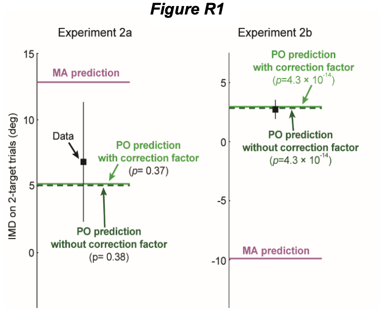
      We appreciate the comment. There are many ways we could have run these analyses and, in fact, in other papers we have done it differently, for example by splitting each look in 3, irrespective of its duration (Phillips et al., 2023).

      However, one aspect we took into account was the observation that 5-month-old infants exhibited more shorter looks compared to older infants. We recognized that dividing each into 3 parts, regardless of its duration, might have impacted the results. Presumably, the activity during the middle and termination phases of a 1.5-second look differs from that of a look lasting over 7 seconds.

      Two additional factors that provided us with confidence in our approach were: 1) while the definition of "middle" was somewhat arbitrary, it allowed us to maintain consistency in our analyses across different age points. And, 2) we obtained a comparable amount of observations across the two time points (e.g. “middle” at 5 months we had 172 events at 5 months, and 194 events at 10 months).
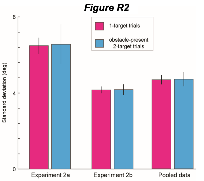
      b. It is recommended not to interpret lower-level interactions if more complex interactions are not significant. How are the interaction effects in a simpler model in which the 3-way interaction is removed? 

      We appreciate the comment. We tried to follow the same steps as in (Xie et al., 2018). However, we have re-analysed the data removing the 3-way interaction and the significance of the results stayed the same. Please see Author response image 2 below (first: new analyses without the 3-way interactions, second: original analyses that included the 3-way interaction).

      Author response image 2.

      (3) Figure S1: there seems to be an outlier in the bottom-right panel. Do results hold excluding it? 

      We re-run these analyses as per this suggestion and the results stayed the same (refer to SM pg. 2).

      (4) Figure S2 should refer to 10 months instead of 12.

      We thank the reviewer for noticing this typo, we have changed it in the reviewed manuscript (see SM pg. 3). 

      (5) In the 2nd paragraph of the discussion, I found this sentence unclear: "From Analysis 1 we found that infants at both ages showed a preferred modal reorientation rate". 

      We clarified this in the reviewed manuscript in pg10

      (6) Discussion: many (infant) studies have used theta in anticipation of receiving information (Begus et al., 2016) surprising events (Meyer et al., 2023), and especially exploration (Begus et al., 2015). Can you make a broader point on how these findings inform our interpretation of theta in the infant population (go more from description to underlying mechanisms)? 

      We have extended on this point on interpreting frequency bands in pg13 of the reviewed manuscript and thank the reviewer for bringing it up.

      Begus, K., Gliga, T., & Southgate, V. (2016). Infants' preferences for native speakers are associated with an expectation of information. Proceedings of the National Academy of Sciences, 113(44), 12397-12402.

      Meyer, M., van Schaik, J. E., Poli, F., & Hunnius, S. (2023). How infant‐directed actions enhance infants' attention, learning, and exploration: Evidence from EEG and computational modeling. Developmental Science, 26(1), e13259.

      Begus, K., Southgate, V., & Gliga, T. (2015). Neural mechanisms of infant learning: differences in frontal theta activity during object exploration modulate subsequent object recognition. Biology letters, 11(5), 20150041.

      (7) 2nd page of discussion, last paragraph: "preferred modal reorientation timer" is not a neural/cognitive mechanism, just a resulting behaviour. 

      We agree with this comment and thank the reviewer for bringing it out to our attention. We clarified this in in pg12 and pg13 of the reviewed manuscript.

      Reviewer #2 (Recommendations For The Authors):

      I have a few comments and questions that I think the authors should consider addressing in a revised version. Please see below:

      (1) During preprocessing (steps 5 and 6), it seems like the "noisy channels" were rejected using the pop_rejchan.m function and then interpolated. This procedure is common in infant EEG analysis, but a concern arises: was there no upper limit for channel interpolation? Did the authors still perform bad channel interpolation even when more than 30% or 40% of the channels were identified as "bad" at the beginning with the continuous data? 

      We did state in the original manuscript that “participants with fewer than 30% channels interpolated at 5 months and 25% at 10 months made it to the final step (ICA) and final analyses”. In the revised version we have re-written this section in order to make this more clear (pg. 17).

      (2) I am also perplexed about the sequencing of the ICA pruning step. If the intention of ICA pruning is to eliminate artificial components, would it be more logical to perform this procedure before the conventional artifacts' rejection (i.e., step 7), rather than after? In addition, what was the methodology employed by the authors to identify the artificial ICA components? Was it done through manual visual inspection or utilizing specific toolboxes? 

      We agree that the ICA is often run before, however, the decision to reject continuous data prior to ICA was to remove the very worst sections of data (where almost all channels were affected), which can arise during times when infants fuss or pull the caps. Thus, this step was applied at this point in the pipeline so that these sections of really bad data were not inputted into the ICA. This is fairly widespread practice in cleaning infant data.

      Concerning the reviewer’s second question, of how ICA components were removed – the answer to this is described in considerable detail in the paper that we refer to in that setion of the manuscript. This was done by training a classifier specially designed to clean naturalistic infant EEG data (Haresign et al., 2021) and has since been employed in similar studies (e.g. Georgieva et al., 2020; Phillips et al., 2023).

      (3) Please clarify how the relative power was calculated for the theta (3-6Hz) and alpha (6-9Hz) bands. Were they calculated by dividing the ratio of theta or alpha power to the power between 3 and 9Hz, or the total power between 1 (or 3) and 20 Hz? In other words, what does the term "all frequency bands" refer to in section 4.3.7? 

      We thank the reviewer for this comment, we have now clarified this in pg. 22.

      (4) One of the key discoveries presented in this paper is the observation that attention shifts are accompanied by a subsequent enhancement in theta band power shortly after the shifts occur. Is it possible that this effect or alteration might be linked to infants' saccades, which are used as indicators of attention shifts? Would it be feasible to analyze the disparities in amplitude between the left and right frontal electrodes (e.g., Fp1 and Fp2, which could be viewed as virtual horizontal EOG channels) in relation to theta band power, in order to eliminate the possibility that the augmentation of theta power was attributable to the intensity of the saccades? 

      We appreciate the concern. Average saccade duration in infants is about 40ms (Garbutt et al., 2007). Our finding that the positive cross-correlation between theta and look duration is present not only when we examine zero-lag data but also when we examine how theta forwards-predicts attention 1-2 seconds afterwards seems therefore unlikely to be directly attributable to saccade-related artifact. Concerning the reviewer’s suggestion – this is something that we have tried in the past. Unfortunately, however, our experience is that identifying saccades based on the disparity between Fp1 and Fp2 is much too unreliable to be of any use in analysing data. Even if specially positioned HEOG electrodes are used, we still find the saccade detection to be insufficiently reliable. In ongoing work we are tracking eye movements separately, in order to be able to address this point more satisfactorily.

      (5) The following question is related to my previous comment. Why is the duration of the relationship between theta power and moment-to-moment changes in attention so short? If theta is indeed associated with attention and information processing, shouldn't the relationship between the two variables strengthen as the attention episode progresses? Given that the authors themselves suggest that "One possible interpretation of this is that neural activity associates with the maintenance more than the initiation of attentional behaviors," it raises the question of (is in contradiction to) why the duration of the relationship is not longer but declines drastically (Figure 6). 

      We thank the reviewer for raising this excellent point. Certainly we argue that this, together with the low autocorrelation values for theta documented in Fig 7A and 7D challenge many conventional ways of interpreting theta. We are continuing to investigate this question in ongoing work.

      (6) Have the authors conducted a comparison of alpha relative power and HR deceleration durations between 5 and 10-month-old infants? This analysis could provide insights into whether the differences observed between the two age groups were partly due to varying levels of general arousal and engagement during free play.

      We thank the reviewer for this suggestion. Indeed, this is an aspect we investigated but ultimately, given that our primary emphasis was on the theta frequency, and considering the length of the manuscript, we decided not to incorporate. However, we attached Author response image 3 below showing there was no significant interaction between HR and alpha band.

      Author response image 3.

      Reviewer #3 (Recommendations For The Authors):

      (1) In reading the manuscript, the language used seems to imply longitudinal data or at the very least the ability to detect change or maturation. Given the cross-sectional nature of the data, the language should be tempered throughout. The data are illustrative but not definitive. 

      We thank the reviewer for this comment. We have now clarified that “Data was analysed in a cross-sectional manner” in pg15.

      (2) The sample size is quite modest, particularly in the specific age groups. This is likely tempered by the sheer number of data points available. This latter argument is implied in the text, but not as explicitly noted. (However, I may have missed this as the text is quite dense). I think more notice is needed on the reliability and stability of the findings given the sample. 

      We have clarified this in pg16.

      (3) On a related note, how was the sample size determined? Was there a power analysis to help guide decision-making for both recruitment and choosing which analyses to proceed with? Again, the analytic approach is quite sophisticated and the questions are of central interest to researchers, but I was left feeling maybe these two aspects of the study were out-sprinting the available data. The general impression is that the sample is small, but it is not until looking at table s7, that it is in full relief. I think this should be more prominent in the main body of the study.

      We have clarified this in pg16.

      (4) The devotes a few sentences to the relation between looking and attention. However, this distinction is central to the design of the study, and any philosophical differences regarding what take-away points can be generated. In my reading, I think this point needs to be more heavily interrogated. 

      This distinction between looking and paying attention is clearer now in the reviewed manuscript as per R1 and R3’s suggestions. We have also added a paragraph in the Introduction to clarify it and pointed out its limitations (see pg.5).

      (5) I would temper the real-world attention language. This study is certainly a great step forward, relative to static faces on a computer screen. However, there are still a great number of artificial constraints that have been added. That is not to say that the constraints are bad--they are necessary to carry out the work. However, it should be acknowledged that it constrains the external validity. 

      We have added a paragraph to acknowledged limitations of the setup in pg. 14.

      (6) The kappa on the coding is not strong. The authors chose to proceed nonetheless. Given that, I think more information is needed on how coders were trained, how they were standardized, and what parameters were used to decide they were ready to code independently. Again, with the sample size and the kappa presented, I think more discussion is needed regarding the robustness of the findings. 

      We appreciate the concern. As per our answer to R1, we chose to report the most stringent calculator of inter-rater reliability, but other calculation methods (i.e., percent agreement) return higher scores (see response to R1).

      As per the training, we wrote an extensively detailed coding scheme describing exactly how to code each look that was handed to our coders. Throughout the initial months of training, we meet with the coders on a weekly basis to discuss questions and individual frames that looked ambiguous. After each session, we would revise the coding scheme to incorporate additional details, aiming to make the coding process progressively less subjective. During this period, every coder analysed the same interactions, and inter-rater reliability (IRR) was assessed weekly, comparing their evaluations with mine (Marta). With time, the coders had fewer questions and IRR increased. At that point, we deemed them sufficiently trained, and began assigning them different interactions from each other. Periodically, though, we all assessed the same interaction and meet to review and discuss our coding outputs.

    1. Author Response

      The following is the authors’ response to the original reviews.

      eLife assessment

      These ingenious and thoughtful studies present important findings concerning how people represent and generalise abstract patterns of sensory data. The issue of generalisation is a core topic in neuroscience and psychology, relevant across a wide range of areas, and the findings will be of interest to researchers across areas in perception, learning, and cognitive science. The findings have the potential to provide compelling support for the outlined account, but there appear other possible explanations, too, that may affect the scope of the findings but could be considered in a revision.

      Thank you for sending the feedback from the three peer reviewers regarding our paper. Please find below our detailed responses addressing the reviewers' comments. We have incorporated these suggestions into the paper and provided explanations for the modifications made.

      We have specifically addressed the point of uncertainty highlighted in eLife's editorial assessment, which concerned alternative explanations for the reported effect. In response to Reviewer #1, we have clarified how Exp. 2c and Exp. 3c address the potential alternative explanation related to "attention to dimensions." Further, we present a supplementary analysis to account for differences in asymptotic learning, as noted by Reviewer #2. We have also clarified how our control experiments address effects associated with general cognitive engagement in the task. Lastly, we have further clarified the conceptual foundation of our paper, addressing concerns raised by Reviewers #2 and #3.

      Reviewer #1 (Public Review):

      Summary:

      This manuscript reports a series of experiments examining category learning and subsequent generalization of stimulus representations across spatial and nonspatial domains. In Experiment 1, participants were first trained to make category judgments about sequences of stimuli presented either in nonspatial auditory or visual modalities (with feature values drawn from a two-dimensional feature manifold, e.g., pitch vs timbre), or in a spatial modality (with feature values defined by positions in physical space, e.g., Cartesian x and y coordinates). A subsequent test phase assessed category judgments for 'rotated' exemplars of these stimuli: i.e., versions in which the transition vectors are rotated in the same feature space used during training (near transfer) or in a different feature space belonging to the same domain (far transfer). Findings demonstrate clearly that representations developed for the spatial domain allow for representational generalization, whereas this pattern is not observed for the nonspatial domains that are tested. Subsequent experiments demonstrate that if participants are first pre-trained to map nonspatial auditory/visual features to spatial locations, then rotational generalization is facilitated even for these nonspatial domains. It is argued that these findings are consistent with the idea that spatial representations form a generalized substrate for cognition: that space can act as a scaffold for learning abstract nonspatial concepts.

      Strengths:

      I enjoyed reading this manuscript, which is extremely well-written and well-presented. The writing is clear and concise throughout, and the figures do a great job of highlighting the key concepts. The issue of generalization is a core topic in neuroscience and psychology, relevant across a wide range of areas, and the findings will be of interest to researchers across areas in perception and cognitive science. It's also excellent to see that the hypotheses, methods, and analyses were pre-registered.

      The experiments that have been run are ingenious and thoughtful; I particularly liked the use of stimulus structures that allow for disentangling of one-dimensional and two-dimensional response patterns. The studies are also well-powered for detecting the effects of interest. The model-based statistical analyses are thorough and appropriate throughout (and it's good to see model recovery analysis too). The findings themselves are clear-cut: I have little doubt about the robustness and replicability of these data.

      Weaknesses:

      I have only one significant concern regarding this manuscript, which relates to the interpretation of the findings. The findings are taken to suggest that "space may serve as a 'scaffold', allowing people to visualize and manipulate nonspatial concepts" (p13). However, I think the data may be amenable to an alternative possibility. I wonder if it's possible that, for the visual and auditory stimuli, participants naturally tended to attend to one feature dimension and ignore the other - i.e., there may have been a (potentially idiosyncratic) difference in salience between the feature dimensions that led to participants learning the feature sequence in a one-dimensional way (akin to the 'overshadowing' effect in associative learning: e.g., see Mackintosh, 1976, "Overshadowing and stimulus intensity", Animal Learning and Behaviour). By contrast, we are very used to thinking about space as a multidimensional domain, in particular with regard to two-dimensional vertical and horizontal displacements. As a result, one would naturally expect to see more evidence of two-dimensional representation (allowing for rotational generalization) for spatial than nonspatial domains.

      In this view, the impact of spatial pre-training and (particularly) mapping is simply to highlight to participants that the auditory/visual stimuli comprise two separable (and independent) dimensions. Once they understand this, during subsequent training, they can learn about sequences on both dimensions, which will allow for a 2D representation and hence rotational generalization - as observed in Experiments 2 and 3. This account also anticipates that mapping alone (as in Experiment 4) could be sufficient to promote a 2D strategy for auditory and visual domains.

      This "attention to dimensions" account has some similarities to the "spatial scaffolding" idea put forward in the article, in arguing that experience of how auditory/visual feature manifolds can be translated into a spatial representation helps people to see those domains in a way that allows for rotational generalization. Where it differs is that it does not propose that space provides a scaffold for the development of the nonspatial representations, i.e., that people represent/learn the nonspatial information in a spatial format, and this is what allows them to manipulate nonspatial concepts. Instead, the "attention to dimensions" account anticipates that ANY manipulation that highlights to participants the separable-dimension nature of auditory/visual stimuli could facilitate 2D representation and hence rotational generalization. For example, explicit instruction on how the stimuli are constructed may be sufficient, or pre-training of some form with each dimension separately, before they are combined to form the 2D stimuli.

      I'd be interested to hear the authors' thoughts on this account - whether they see it as an alternative to their own interpretation, and whether it can be ruled out on the basis of their existing data.

      We thank the Reviewer for their comments. We agree with the Reviewer that the “attention to dimensions” hypothesis is an interesting alternative explanation. However, we believe that the results of our control experiments Exp. 2c and Exp. 3c are incompatible with this alternative explanation.

      In Exp. 2c, participants are pre-trained in the visual modality and then tested in the auditory modality. In the multimodal association task, participants have to associate the auditory stimuli and the visual stimuli: on each trial, they hear a sound and then have to click on the corresponding visual stimulus. It is thus necessary to pay attention to both auditory dimensions and both visual dimensions to perform the task. To give an example, the task might involve mapping the fundamental frequency and the amplitude modulation of the auditory stimulus to the colour and the shape of the visual stimulus, respectively. If participants pay attention to only one dimension, this would lead to a maximum of 25% accuracy on average (because they would be at chance on the other dimension, with four possible options). We observed that 30/50 participants reached an accuracy > 50% in the multimodal association task in Exp. 2c. This means that we know for sure that at least 60% of the participants paid attention to both dimensions of the stimuli. Nevertheless, there was a clear difference between participants that received a visual pre-training (Exp. 2c) and those who received a spatial pre-training (Exp. 2a) (frequency of 1D vs 2D models between conditions, BF > 100 in near transfer and far transfer). In fact, only 3/50 participants were best fit by a 2D model when vision was the pre-training modality compared to 29/50 when space was the pre-training modality. Thus, the benefit of the spatial pre-training cannot be due solely to a shift in attention toward both dimensions.

      This effect was replicated in Exp. 3c. Similarly, 33/48 participants reached an accuracy > 50% in the multimodal association task in Exp. 3c, meaning that we know for sure that at least 68% of the participants actually paid attention to both dimensions of the stimuli. Again, there was a clear difference between participants who received a visual pre-training (frequency of 1D vs 2D models between conditions, Exp. 3c) and those who received a spatial pre-training (Exp. 3a) (BF > 100 in near transfer and far transfer).

      Thus, we believe that the alternative explanation raised by the Reviewer is not supported by our data. We have added a paragraph in the discussion:

      “One alternative explanation of this effect could be that the spatial pre-training encourages participants to attend to both dimensions of the non-spatial stimuli. By contrast, pretraining in the visual or auditory domains (where multiple dimensions of a stimulus may be relevant less often naturally) encourages them to attend to a single dimension. However, data from our control experiments Exp. 2c and Exp. 3c, are incompatible with this explanation. Around ~65% of the participants show a level of performance in the multimodal association task (>50%) which could only be achieved if they were attending to both dimensions (performance attending to a single dimension would yield 25% and chance performance is at 6.25%). This suggests that participants are attending to both dimensions even in the visual and auditory mapping case.”

      Reviewer #2 (Public Review):

      Summary:

      In this manuscript, L&S investigates the important general question of how humans achieve invariant behavior over stimuli belonging to one category given the widely varying input representation of those stimuli and more specifically, how they do that in arbitrary abstract domains. The authors start with the hypothesis that this is achieved by invariance transformations that observers use for interpreting different entries and furthermore, that these transformations in an arbitrary domain emerge with the help of the transformations (e.g. translation, rotation) within the spatial domain by using those as "scaffolding" during transformation learning. To provide the missing evidence for this hypothesis, L&S used behavioral category learning studies within and across the spatial, auditory, and visual domains, where rotated and translated 4-element token sequences had to be learned to categorize and then the learned transformation had to be applied in new feature dimensions within the given domain. Through single- and multiple-day supervised training and unsupervised tests, L&S demonstrated by standard computational analyses that in such setups, space and spatial transformations can, indeed, help with developing and using appropriate rotational mapping whereas the visual domain cannot fulfill such a scaffolding role.

      Strengths:

      The overall problem definition and the context of spatial mapping-driven solution to the problem is timely. The general design of testing the scaffolding effect across different domains is more advanced than any previous attempts clarifying the relevance of spatial coding to any other type of representational codes. Once the formulation of the general problem in a specific scientific framework is done, the following steps are clearly and logically defined and executed. The obtained results are well interpretable, and they could serve as a good stepping stone for deeper investigations. The analytical tools used for the interpretations are adequate. The paper is relatively clearly written.

      Weaknesses:

      Some additional effort to clarify the exact contribution of the paper, the link between analyses and the claims of the paper, and its link to previous proposals would be necessary to better assess the significance of the results and the true nature of the proposed mechanism of abstract generalization.

      (1) Insufficient conceptual setup: The original theoretical proposal (the Tolman-Eichenbaum-Machine, Whittington et al., Cell 2020) that L&S relate their work to proposes that just as in the case of memory for spatial navigation, humans and animals create their flexible relational memory system of any abstract representation by a conjunction code that combines on the one hand, sensory representation and on the other hand, a general structural representation or relational transformation. The TEM also suggests that the structural representation could contain any graph-interpretable spatial relations, albeit in their demonstration 2D neighbor relations were used. The goal of L&S's paper is to provide behavioral evidence for this suggestion by showing that humans use representational codes that are invariant to relational transformations of non-spatial abstract stimuli and moreover, that humans obtain these invariances by developing invariance transformers with the help of available spatial transformers. To obtain such evidence, L&S use the rotational transformation. However, the actual procedure they use actually solved an alternative task: instead of interrogating how humans develop generalizations in abstract spaces, they demonstrated that if one defines rotation in an abstract feature space embedded in a visual or auditory modality that is similar to the 2D space (i.e. has two independent dimensions that are clearly segregable and continuous), humans cannot learn to apply rotation of 4-piece temporal sequences in those spaces while they can do it in 2D space, and with co-associating a one-to-one mapping between locations in those feature spaces with locations in the 2D space an appropriate shaping mapping training will lead to the successful application of rotation in the given task (and in some other feature spaces in the given domain). While this is an interesting and challenging demonstration, it does not shed light on how humans learn and generalize, only that humans CAN do learning and generalization in this, highly constrained scenario. This result is a demonstration of how a stepwise learning regiment can make use of one structure for mapping a complex input into a desired output. The results neither clarify how generalizations would develop in abstract spaces nor the question of whether this generalization uses transformations developed in the abstract space. The specific training procedure ensures success in the presented experiments but the availability and feasibility of an equivalent procedure in a natural setting is a crucial part of validating the original claim and that has not been done in the paper.

      We thank the Reviewer for their detailed comments on our manuscript. We reply to the three main points in turn.

      First, concerning the conceptual grounding of our work, we would point out that the TEM model (Whittington et al., 2020), however interesting, is not our theoretical starting point. Rather, as we hope the text and references make clear, we ground our work in theoretical work from the 1990/2000s proposing that space acts as a scaffold for navigating abstract spaces (such as Gärdenfors, 2000). We acknowledge that the TEM model and other experimental work on the implication of the hippocampus, the entorhinal cortex and the parietal cortex in relational transformations of nonspatial stimuli provide evidence for this general theory. However, our work is designed to test a more basic question: whether there is behavioural evidence that space scaffolds learning in the first place. To achieve this, we perform behavioural experiments with causal manipulation (spatial pre-training vs no spatial pre-training) have the potential to provide such direct evidence. This is why we claim that:

      “This theory is backed up by proof-of-concept computational simulations [13], and by findings that brain regions thought to be critical for spatial cognition in mammals (such as the hippocampal-entorhinal complex and parietal cortex) exhibit neural codes that are invariant to relational transformations of nonspatial stimuli. However, whilst promising, this theory lacks direct empirical evidence. Here, we set out to provide a strong test of the idea that learning about physical space scaffolds conceptual generalisation.“

      Second, we agree with the Reviewer that we do not provide an explicit model for how generalisation occurs, and how precisely space acts as a scaffold for building representations and/or applying the relevant transformations to non-spatial stimuli to solve our task. Rather, we investigate in our Exp. 2-4 which aspects of the training are necessary for rotational generalisation to happen (and conclude that a simple training with the multimodal association task is sufficient for ~20% participants). We now acknowledge in the discussion the fact that we do not provide an explicit model and leave that for future work:

      “We acknowledge that our study does not provide a mechanistic model of spatial scaffolding but rather delineate which aspects of the training are necessary for generalisation to happen.”

      Finally, we also agree with the Reviewer that our task is non-naturalistic. As is common in experimental research, one must sacrifice the naturalistic elements of the task in exchange for the control and the absence of prior knowledge of the participants. We have decided to mitigate as possible the prior knowledge of the participants to make sure that our task involved learning a completely new task and that the pre-training was really causing the better learning/generalisation. The effects we report are consistent across the experiments so we feel confident about them but we agree with the Reviewer that an external validation with more naturalistic stimuli/tasks would be a nice addition to this work. We have included a sentence in the discussion:

      “All the effects observed in our experiments were consistent across near transfer conditions (rotation of patterns within the same feature space), and far transfer conditions (rotation of patterns within a different feature space, where features are drawn from the same modality). This shows the generality of spatial training for conceptual generalisation. We did not test transfer across modalities nor transfer in a more natural setting; we leave this for future studies.”

      (2) Missing controls: The asymptotic performance in experiment 1 after training in the three tasks was quite different in the three tasks (intercepts 2.9, 1.9, 1.6 for spatial, visual, and auditory, respectively; p. 5. para. 1, Fig 2BFJ). It seems that the statement "However, our main question was how participants would generalise learning to novel, rotated exemplars of the same concept." assumes that learning and generalization are independent. Wouldn't it be possible, though, that the level of generalization depends on the level of acquiring a good representation of the "concept" and after obtaining an adequate level of this knowledge, generalization would kick in without scaffolding? If so, a missing control is to equate the levels of asymptotic learning and see whether there is a significant difference in generalization. A related issue is that we have no information on what kind of learning in the three different domains was performed, albeit we probably suspect that in space the 2D representation was dominant while in the auditory and visual domains not so much. Thus, a second missing piece of evidence is the model-fitting results of the ⦰ condition that would show which way the original sequences were encoded (similar to Fig 2 CGK and DHL). If the reason for lower performance is not individual stimulus difficulty but the natural tendency to encode the given stimulus type by a combo of random + 1D strategy that would clarify that the result of the cross-training is, indeed, transferring the 2D-mapping strategy.

      We agree with the Reviewer that a good further control is to equate performance during training. Thus, we have run a complementary analysis where we select only the participants that reach > 90% accuracy in the last block of training in order to equate asymptotic performance after training in Exp. 1. The results (see Author response image 1) replicates the results that we report in the main text: there is a large difference between groups (relative likelihood of 1D vs. 2D models, all BF > 100 in favour of a difference between the auditory and the spatial modalities, between the visual and the spatial modalities, in both near and far transfer, “decisive” evidence). We prefer not to include this figure in the paper for clarity, and because we believe this result is expected given the fact that 0/50 and 0/50 of the participants in the auditory and visual condition used a 2D strategy – thus, selecting subgroups of these participants cannot change our conclusions.

      Author response image 1.

      Results of Exp. 1 when selecting participants that reached > 90% accuracy in the last block of training. Captions are the same as Figure 2 of the main text.

      Second, the Reviewer suggested that we run the model fitting analysis only on the ⦰ condition (training) in Exp. 1 to reveal whether participants use a 1D or a 2D strategy already during training. Unfortunately, we cannot provide the model fits only in the ⦰ condition in Exp. 1 because all models make the same predictions for this condition (see Fig S4). However, note that this is done by design: participants were free to apply whatever strategy they want during training; we then used the generalisation phase with the rotated stimuli precisely to reveal this strategy. Further, we do believe that the strategy used by the participants during training and the strategy during transfer are the same, partly because – starting from block #4 – participants have no idea whether the current trial is a training trial or a transfer trial, as both trial types are randomly interleaved with no cue signalling the trial type. We have made this clear in the methods:

      “They subsequently performed 105 trials (with trialwise feedback) and 105 transfer trials including rotated and far transfer quadruplets (without trialwise feedback) which were presented in mixed blocks of 30 trials. Training and transfer trials were randomly interleaved, and no clue indicated whether participants were currently on a training trial or a transfer trial before feedback (or absence of feedback in case of a transfer trial).”

      Reviewer #3 (Public Review):

      Summary:

      Pesnot Lerousseau and Summerfield aimed to explore how humans generalize abstract patterns of sensory data (concepts), focusing on whether and how spatial representations may facilitate the generalization of abstract concepts (rotational invariance). Specifically, the authors investigated whether people can recognize rotated sequences of stimuli in both spatial and nonspatial domains and whether spatial pre-training and multi-modal mapping aid in this process.

      Strengths:

      The study innovatively examines a relatively underexplored but interesting area of cognitive science, the potential role of spatial scaffolding in generalizing sequences. The experimental design is clever and covers different modalities (auditory, visual, spatial), utilizing a two-dimensional feature manifold. The findings are backed by strong empirical data, good data analysis, and excellent transparency (including preregistration) adding weight to the proposition that spatial cognition can aid abstract concept generalization.

      Weaknesses:

      The examples used to motivate the study (such as "tree" = oak tree, family tree, taxonomic tree) may not effectively represent the phenomena being studied, possibly confusing linguistic labels with abstract concepts. This potential confusion may also extend to doubts about the real-life applicability of the generalizations observed in the study and raises questions about the nature of the underlying mechanism being proposed.

      We thank the Reviewer for their comments. We agree that we could have explained ore clearly enough how these examples motivate our study. The similarity between “oak tree” and “family tree” is not just the verbal label. Rather, it is the arrangement of the parts (nodes and branches) in a nested hierarchy. Oak trees and family trees share the same relational structure. The reason that invariance is relevant here is that the similarity in relational structure is retained under rigid body transformations such as rotation or translation. For example, an upside-down tree can still be recognised as a tree, just as a family tree can be plotted with the oldest ancestors at either top or bottom. Similarly, in our study, the quadruplets are defined by the relations between stimuli: all quadruplets use the same basic stimuli, but the categories are defined by the relations between successive stimuli. In our task, generalising means recognising that relations between stimuli are the same despite changes in the surface properties (for example in far transfer). We have clarify that in the introduction:

      “For example, the concept of a “tree” implies an entity whose structure is defined by a nested hierarchy, whether this is a physical object whose parts are arranged in space (such as an oak tree in a forest) or a more abstract data structure (such as a family tree or taxonomic tree). [...] Despite great changes in the surface properties of oak trees, family trees and taxonomic trees, humans perceive them as different instances of a more abstract concept defined by the same relational structure.”

      Next, the study does not explore whether scaffolding effects could be observed with other well-learned domains, leaving open the question of whether spatial representations are uniquely effective or simply one instance of a familiar 2D space, again questioning the underlying mechanism.

      We would like to mention that Reviewer #2 had a similar comment. We agree with both Reviewers that our task is non-naturalistic. As is common in experimental research, one must sacrifice the naturalistic elements of the task in exchange for the control and the absence of prior knowledge of the participants. We have decided to mitigate as possible the prior knowledge of the participants to make sure that our task involved learning a completely new task and that the pre-training was really causing the better learning/generalisation. The effects we report are consistent across the experiments so we feel confident about them but we agree with the Reviewer that an external validation with more naturalistic stimuli/tasks would be a nice addition to this work. We have included a sentence in the discussion:

      “All the effects observed in our experiments were consistent across near transfer conditions (rotation of patterns within the same feature space), and far transfer conditions (rotation of patterns within a different feature space, where features are drawn from the same modality). This shows the generality of spatial training for conceptual generalisation. We did not test transfer across modalities nor transfer in a more natural setting; we leave this for future studies.”

      Further doubt on the underlying mechanism is cast by the possibility that the observed correlation between mapping task performance and the adoption of a 2D strategy may reflect general cognitive engagement rather than the spatial nature of the task. Similarly, the surprising finding that a significant number of participants benefited from spatial scaffolding without seeing spatial modalities may further raise questions about the interpretation of the scaffolding effect, pointing towards potential alternative interpretations, such as shifts in attention during learning induced by pre-training without changing underlying abstract conceptual representations.

      The Reviewer is concerned about the fact that the spatial pre-training could benefit the participants by increasing global cognitive engagement rather than providing a scaffold for learning invariances. It is correct that the participants in the control group in Exp. 2c have poorer performances on average than participants that benefit from the spatial pre-training in Exp. 2a and 2b. The better performances of the participants in Exp. 2a and 2b could be due to either the spatial nature of the pre-training (as we claim) or a difference in general cognitive engagement. .

      However, if we look closely at the results of Exp. 3, we can see that the general cognitive engagement hypothesis is not well supported by the data. Indeed, the participants in the control condition (Exp. 3c) have relatively similar performances than the other groups during training. Rather, the difference is in the strategy they use, as revealed by the transfer condition. The majority of them are using a 1D strategy, contrary to the participants that benefited from a spatial pre-training (Exp 3a and 3b). We have included a sentence in the results:

      “Further, the results show that participants who did not experience spatial pre-training were still engaged in the task, but were not using the same strategy as the participants who experienced spatial pre-training (1D rather than 2D). Thus, the benefit of the spatial pre-training is not simply to increase the cognitive engagement of the participants. Rather, spatial pre-training provides a scaffold to learn rotation-invariant representation of auditory and visual concepts even when rotation is never explicitly shown during pre-training.”

      Finally, Reviewer #1 had a related concern about a potential alternative explanation that involved a shift in attention. We reproduce our response here: we agree with the Reviewer that the “attention to dimensions” hypothesis is an interesting (and potentially concerning) alternative explanation. However, we believe that the results of our control experiments Exp. 2c and Exp. 3c are not compatible with this alternative explanation.

      Indeed, in Exp. 2c, participants are pre-trained in the visual modality and then tested in the auditory modality. In the multimodal association task, participants have to associate the auditory stimuli and the visual stimuli: on each trial, they hear a sound and then have to click on the corresponding visual stimulus. It is necessary to pay attention to both auditory dimensions and both visual dimensions to perform well in the task. To give an example, the task might involve mapping the fundamental frequency and the amplitude modulation of the auditory stimulus to the colour and the shape of the visual stimulus, respectively. If participants pay attention to only one dimension, this would lead to a maximum of 25% accuracy on average (because they would be at chance on the other dimension, with four possible options). We observed that 30/50 participants reached an accuracy > 50% in the multimodal association task in Exp. 2c. This means that we know for sure that at least 60% of the participants actually paid attention to both dimensions of the stimuli. Nevertheless, there was a clear difference between participants that received a visual pre-training (Exp. 2c) and those who received a spatial pre-training (Exp. 2a) (frequency of 1D vs 2D models between conditions, BF > 100 in near transfer and far transfer). In fact, only 3/50 participants were best fit by a 2D model when vision was the pre-training modality compared to 29/50 when space was the pre-training modality. Thus, the benefit of the spatial pre-training cannot be due solely to a shift in attention toward both dimensions.

      This effect was replicated in Exp. 3c. Similarly, 33/48 participants reached an accuracy > 50% in the multimodal association task in Exp. 3c, meaning that we know for sure that at least 68% of the participants actually paid attention to both dimensions of the stimuli. Again, there was a clear difference between participants who received a visual pre-training (frequency of 1D vs 2D models between conditions, Exp. 3c) and those who received a spatial pre-training (Exp. 3a) (BF > 100 in near transfer and far transfer).

      Thus, we believe that the alternative explanation raised by the Reviewer is not supported by our data. We have added a paragraph in the discussion:

      “One alternative explanation of this effect could be that the spatial pre-training encourages participants to attend to both dimensions of the non-spatial stimuli. By contrast, pretraining in the visual or auditory domains (where multiple dimensions of a stimulus may be relevant less often naturally) encourages them to attend to a single dimension. However, data from our control experiments Exp. 2c and Exp. 3c, are incompatible with this explanation. Around ~65% of the participants show a level of performance in the multimodal association task (>50%) which could only be achieved if they were attending to both dimensions (performance attending to a single dimension would yield 25% and chance performance is at 6.25%). This suggests that participants are attending to both dimensions even in the visual and auditory mapping case.”

      Conclusions:

      The authors successfully demonstrate that spatial training can enhance the ability to generalize in nonspatial domains, particularly in recognizing rotated sequences. The results for the most part support their conclusions, showing that spatial representations can act as a scaffold for learning more abstract conceptual invariances. However, the study leaves room for further investigation into whether the observed effects are unique to spatial cognition or could be replicated with other forms of well-established knowledge, as well as further clarifications of the underlying mechanisms.

      Impact:

      The study's findings are likely to have a valuable impact on cognitive science, particularly in understanding how abstract concepts are learned and generalized. The methods and data can be useful for further research, especially in exploring the relationship between spatial cognition and abstract conceptualization. The insights could also be valuable for AI research, particularly in improving models that involve abstract pattern recognition and conceptual generalization.

      In summary, the paper contributes valuable insights into the role of spatial cognition in learning abstract concepts, though it invites further research to explore the boundaries and specifics of this scaffolding effect.

      Reviewer #1 (Recommendations For The Authors):

      Minor issues / typos:

      P6: I think the example of the "signed" mapping here should be "e.g., ABAB maps to one category and BABA maps to another", rather than "ABBA maps to another" (since ABBA would always map to another category, whether the mapping is signed or unsigned).

      Done.

      P11: "Next, we asked whether pre-training and mapping were systematically associated with 2Dness...". I'd recommend changing to: "Next, we asked whether accuracy during pre-training and mapping were systematically associated with 2Dness...", just to clarify what the analyzed variables are.

      Done.

      P13, paragraph 1: "only if the features were themselves are physical spatial locations" either "were" or "are" should be removed.

      Done.

      P13, paragraph 1: should be "neural representations of space form a critical substrate" (not "for").

      Done.

      Reviewer #2 (Recommendations For The Authors):

      The authors use in multiple places in the manuscript the phrases "learn invariances" (Abstract), "formation of invariances" (p. 2, para. 1), etc. It might be just me, but this feels a bit like 'sloppy' wording: we do not learn or form invariances, rather we learn or form representations or transformations by which we can perform tasks that require invariance over particular features or transformation of the input such as the case of object recognition and size- translation- or lighting-invariance. We do not form size invariance, we have representations of objects and/or size transformations allowing the recognition of objects of different sizes. The authors might change this way of referring to the phenomenon.

      We respectfully disagree with this comment. An invariance occurs when neurons make the same response under different stimulation patterns. The objects or features to which a neuron responds is shaped by its inputs. Those inputs are in turn determined by experience-dependent plasticity. This process is often called “representation learning”. We think that our language here is consistent with this status quo view in the field.

      Reviewer #3 (Recommendations For The Authors):

      • I understand that the objective of the present experiment is to study our ability to generalize abstract patterns of sensory data (concepts). In the introduction, the authors present examples like the concept of a "tree" (encompassing a family tree, an oak tree, and a taxonomic tree) and "ring" to illustrate the idea. However, I am sceptical as to whether these examples effectively represent the phenomena being studied. From my perspective, these different instances of "tree" do not seem to relate to the same abstract concept that is translated or rotated but rather appear to share only a linguistic label. For instance, the conceptual substance of a family tree is markedly different from that of an oak tree, lacking significant overlap in meaning or structure. Thus, to me, these examples do not demonstrate invariance to transformations such as rotations.

      To elaborate further, typically, generalization involves recognizing the same object or concept through transformations. In the case of abstract concepts, this would imply a shared abstract representation rather than a mere linguistic category. While I understand the objective of the experiments and acknowledge their potential significance, I find myself wondering about the real-world applicability and relevance of such generalizations in everyday cognitive functioning. This, in turn, casts some doubt on the broader relevance of the study's results. A more fitting example, or an explanation that addresses my concerns about the suitability of the current examples, would be beneficial to further clarify the study's intent and scope.

      Response in the public review.

      • Relatedly, the manuscript could benefit from greater clarity in defining key concepts and elucidating the proposed mechanism behind the observed effects. Is it plausible that the changes observed are primarily due to shifts in attention induced by the spatial pre-training, rather than a change in the process of learning abstract conceptual invariances (i.e., modifications to the abstract representations themselves)? While the authors conclude that spatial pre-training acts as a scaffold for enhancing the learning of conceptual invariances, it raises the question: does this imply participants simply became more focused on spatial relationships during learning, or might this shift in attention represent a distinct strategy, and an alternative explanation? A more precise definition of these concepts and a clearer explanation of the authors' perspective on the mechanism underlying these effects would reduce any ambiguity in this regard.

      Response in the public review.

      • I am wondering whether the effectiveness of spatial representations in generalizing abstract concepts stems from their special nature or simply because they are a familiar 2D space for participants. It is well-established that memory benefits from linking items to familiar locations, a technique used in memory training (method of loci). This raises the question: Are we observing a similar effect here, where spatial dimensions are the only tested familiar 2D spaces, while the other 2 spaces are simply unfamiliar, as also suggested by the lower performance during training (Fig.2)? Would the results be replicable with another well-learned, robustly encoded domain, such as auditory dimensions for professional musicians, or is there something inherently unique about spatial representations that aids in bootstrapping abstract representations?

      On the other side of the same coin, are spatial representations qualitatively different, or simply more efficient because they are learned more quickly and readily? This leads to the consideration that if visual pre-training and visual-to-auditory mapping were continued until a similar proficiency level as in spatial training is achieved, we might observe comparable performance in aiding generalization. Thus, the conclusion that spatial representations are a special scaffold for abstract concepts may not be exclusively due to their inherent spatial nature, but rather to the general characteristic of well-established representations. This hypothesis could be further explored by either identifying alternative 2D representations that are equally well-learned or by extending training in visual or auditory representations before proceeding with the mapping task. At the very least I believe this potential explanation should be explored in the discussion section.

      Response in the public review.

      I had some difficulty in following an important section of the introduction: "... whether participants can learn rotationally invariant concepts in nonspatial domains, i.e., those that are defined by sequences of visual and auditory features (rather than by locations in physical space, defined in Cartesian or polar coordinates) is not known." This was initially puzzling to me as the paragraph preceding it mentions: "There is already good evidence that nonspatial concepts are represented in a translation invariant format." While I now understand that the essential distinction here is between translation and rotation, this was not immediately apparent upon first reading. This crucial distinction, especially in the context of conceptual spaces, was not clearly established before this point in the manuscript. For better clarity, it would be beneficial to explicitly contrast and define translation versus rotation in this particular section and stress that the present study concerns rotations in abstract spaces.

      Done.

      • The multi-modal association is crucial for the study, however to my knowledge, it is not depicted or well explained in the main text or figures (Results section). In my opinion, the details of this task should be explained and illustrated before the details of the associated results are discussed.

      We have included an illustration of a multimodal association trial in Fig. S3B.

      Author response image 2.

      • The observed correlation between the mapping task performance and the adoption of a 2D strategy is logical. However, this correlation might not exclusively indicate the proposed underlying mechanism of spatial scaffolding. Could it also be reflective of more general factors like overall performance, attention levels, or the effort exerted by participants? This alternative explanation suggests that the correlation might arise from broader cognitive engagement rather than specifically from the spatial nature of the task. Addressing this possibility could strengthen the argument for the unique role of spatial representations in learning abstract concepts, or at least this alternative interpretation should be mentioned.

      Response in the public review.

      • To me, the finding that ~30% of participants benefited from the spatial scaffolding effect for example in the auditory condition merely through exposure to the mapping (Fig 4D), without needing to see the quadruplets in the spatial modality, was somewhat surprising. This is particularly noteworthy considering that only ~60% of participants adopted the 2D strategy with exposure to rotated contingencies in Experiment 3 (Fig 3D). How do the authors interpret this outcome? It would be interesting to understand their perspective on why such a significant effect emerged from mere exposure to the mapping task.

      • I appreciate the clarity Fig.1 provides in explaining a challenging experimental setup. Is it possible to provide example trials, including an illustration that shows which rotations produce the trail and an intuitive explanation that response maps onto the 1D vs 2D strategies respectively, to aid the reader in better understanding this core manipulation?

      • I like that the authors provide transparency by depicting individual subject's data points in their results figures (e.g. Figs. 2 B, F, J). However, with an n=~50 per condition, it becomes difficult to intuit the distribution, especially for conditions with higher variance (e.g., Auditory). The figures might be more easily interpretable with alternative methods of displaying variances, such as violin plots per data point, conventional error shading using 95%CIs, etc.

      • Why are the authors not reporting exact BFs in the results sections at least for the most important contrasts?

      • While I understand why the authors report the frequencies for the best model fits, this may become difficult to interpret in some sections, given the large number of reported values. Alternatives or additional summary statistics supporting inference could be beneficial.

      As the Reviewer states, there are a large number of figures that we can report in this study. We have chosen to keep this number at a minimum to be as clear as possible. To illustrate the distribution of individual data points, we have opted to display only the group's mean and standard error (the standard errors are included, but the substantial number of participants per condition provides precise estimates, resulting in error bars that can be smaller than the mean point). This decision stems from our concern that including additional details could lead to a cluttered representation with unnecessary complexity. Finally, we report what we believe to be the critical BFs for the comprehension of the reader in the main text, and choose a cutoff of 100 when BFs are high (corresponding to the label “decisive” evidence, some BFs are larger than 1012). All the exact BFs are in the supplementary for the interested readers.

    1. Author response:

      The following is the authors’ response to the original reviews.

      Reviewer #1 (Public Review):

      Summary:

      The manuscript considers a mechanistic extension of MacArthur's consumer-resource model to include chasing down food and potential encounters between the chasers (consumers) that lead to less efficient feeding in the form of negative feedback. After developing the model, a deterministic solution and two forms of stochastic solutions are presented, in agreement with each other. Finally, the model is applied to explain observed coexistence and rank-abundance data.

      We thank the reviewer for the accurate summary of our manuscript.

      Strengths:

      The application of the theory to natural rank-abundance curves is impressive. The comparison with the experiments that reject the competitive exclusion principle is promising. It would be fascinating to see if in, e.g. insects, the specific interference dynamics could be observed and quantified and whether they would agree with the model.

      The results are clearly presented; the methods adequately described; the supplement is rich with details.

      There is much scope to build upon this expansion of the theory of consumer-resource models. This work can open up new avenues of research.

      We appreciate the reviewer for the very positive comments. We have followed many of the suggestions raised by the reviewer, and the manuscript is much improved as a result.

      Following the reviewer’s suggestions, we have now used Shannon entropies to quantify the model comparison with experiments that reject the Competitive Exclusion Principle (CEP). Specifically, for each time point of each experimental or model-simulated community, we calculated the Shannon entropies using the formula:

      , where is the probability that a consumer individual belongs to species C<sub>i</sub> at the time stamp of t. The comparison of Shannon entropies in the time series between those of the experimental data and SSA results shown in Fig. 2D-E is presented in Appendix-fig. 7C-D. The time averages and standard deviations (δH) of the Shannon entropies for these experimental or SSA model-simulated communities are as follows:

      , ; ,

      , , .

      Meanwhile, we have calculated the time averages and standard deviations (δC<sub>i</sub>) of the species’ relative/absolute abundances for the experimental or SSA model-simulated communities shown in Fig. 2D-E, which are as follows:

      , ; , ; , , , , where the superscript “(R)” represents relative abundances.

      From the results of Shannon entropies shown in Author response image 1 (which are identical to those of Appendix-fig. 7C-D) and the quantitative comparison of the time average and standard deviation between the model and experiments presented above, it is evident that the model results in Fig. 2D-E exhibit good consistency with the experimental data. They share roughly identical time averages and standard deviations in both Shannon entropies and the species' relative/absolute abundances for most of the comparisons. All these analyses are included in the appendices and mentioned in the main text.

      Author response image 1.

      Shannon Entropies of the experimental data and SSA results in Fig. 2D-E, redrawn from Appendix-fig. 7C-D.

      Weaknesses:

      I am questioning the use of carrying capacity (Eq. 4) instead of using nutrient limitation directly through Monod consumption (e.g. Posfai et al. who the authors cite). I am curious to see how these results hold or are changed when Monod consumption is used.

      We thank the reviewer for raising this question. To explain it more clearly, the equation combining the third equation in Eq. 1 and Eq. 4 of our manuscript is presented below as Eq. R1:

      where x<sub>il</sub> represents the population abundance of the chasing pair C<sub>i</sub><sup>(P)</sup> ∨ R<sub>l</sub><sup>(P)</sup>, κ<sub>l</sub> stands for the steady-state population abundance of species R<sub>l</sub> (the carrying capacity) in the absence of consumer species. In the case with no consumer species, then x<sub>il</sub> \= 0 since C<sub>i</sub> \= 0 (i\=1,…,S<sub>C</sub>), thus R<sub>l</sub> = κ<sub>l</sub> when R<sub>l</sub> = 0.

      Eq. R1 for the case of abiotic resources is comparable to Eq. (1) in Posfai et al., which we present below as Eq. R2:

      where c<sub>i</sub> represents the concentration of nutrient i, and thus corresponds to our R<sub>l</sub> ; n<sub>σ</sub>(t) is the population of species σ, which corresponds to our C<sub>i</sub> ; s<sub>i</sub> stands for the nutrient supply rate, which corresponds to our ζl ; µi denotes the nutrient loss rate, corresponding to our is the coefficient of the rate of species σ for consuming nutrient i, which corresponds to our in Posfai et al. is the consumption rate of nutrient i by the population of species σ, which corresponds to our x<sub>il</sub>.

      In Posfai et al., is the Monod function: and thus

      In our model, however, since predator interference is not involved in Posfai et al., we need to analyze the form of x<sub>il</sub> presented in the functional form of x<sub>il</sub> ({R<sub>l</sub>},{C<sub>i</sub>}) in the case involving only chasing pairs. Specifically, for the case of abiotic resources, the population dynamics can be described by Eq. 1 combined with Eq. R1:

      where and . For convenience, we consider the case of S<sub>R</sub> \=1 where the Monod form was derived (Monod, J. (1949). Annu. Rev. Microbiol., 3, 371-394.). From , we have

      where , and l =1. If the population abundance of the resource species is much larger than that of all consumer species (i.e., ), then,

      and R<sub>l</sub><sup>(F)</sup> ≈ R<sub>l</sub>. Combined with R5, and noting that C<sub>i</sub> \= C<sub>i</sub>(F) + xil we can solve for x<sub>il</sub> :

      with l =1 since S<sub>R</sub> \=1. Comparing Eq. R6 with Eq. R3, and considering the symbol correspondence explained in the text above, it is now clear that our model can be reduced to the Monod consumption form in the case of S<sub>R</sub> \=1 where the Monod form was derived from.

      Following on the previous comment, I am confused by the fact that the nutrient consumption term in Eq. 1 and how growth is modeled (Eq. 4) are not obviously compatible and would be hard to match directly to experimentally accessible quantities such as yield (nutrient to biomass conversion ratio). Ultimately, there is a conservation of mass ("flux balance"), and therefore the dynamics must obey it. I don't quite see how conservation of mass is imposed in this work.

      We thank the reviewer for raising this question. Indeed, the population dynamics of our model must adhere to flux balance, with the most pertinent equation restated here as Eq. R7:

      Below is the explanation of how Eq. R7, and thus Eqs. 1 and 4 of our manuscript, adhere to the constraint of flux balance. The interactions and fluxes between consumer and resource species occur solely through chasing pairs. At the population level, the scenario of chasing pairs among consumer species C<sub>i</sub> and resource species R<sub>l</sub> is presented in the follow expression:

      where the superscripts "(F)" and "(P)" represent the freely wandering individuals and those involved in chasing pairs, respectively, "(+)" stands for the gaining biomass of consumer C<sub>i</sub> from resource R<sub>l</sub>. In our manuscript, we use x<sub>l</sub> to represent the population abundance (or equivalently, the concentration, for a well-mixed system with a given size) of the chasing pair C<sub>i</sub><sup>(P)</sup> ∨ R<sub>l</sub><sup>(P)</sup>, and thus, the net flow from resource species R<sub>l</sub> to consumer species C<sub>i</sub> per unit time is k<sub>il</sub>x<sub>il</sub>. Noting that there is only one R<sub>l</sub> individual within the chasing pair C<sub>i</sub><sup>(P)</sup> ∨ R<sub>l</sub><sup>(P)</sup>, then the net effect on the population dynamics of species is −k<sub>il</sub>x<sub>il</sub>. However, since a consumer individual from species C<sub>i</sub> could be much heavier than a species R<sub>l</sub> individual, and energy dissipation would be involved from nutrient conversion into biomass, we introduce a mass conversion ratio w<sub>l</sub> in our manuscript. For example, if a species C<sub>i</sub> individual is ten times the weight of a species R<sub>l</sub> individual, without energy dissipation, the mass conversion ratio wil should be 1/10 (i.e., wil \= 0.1 ), however, if half of the chemical energy is dissipated into heat from nutrient conversion into biomass, then w<sub>l</sub> \= 0.1 0.5× = 0.05. Consequently, the net effect of the flux from resource species _R_l to consumer species C<sub>i</sub> per unit time on the population dynamics is , and flux balance is clearly satisfied.

      For the population dynamics of a consumer species C<sub>i</sub>, we need to consider all the biomass influx from different resource species, and thus there is a summation over all species of resources, which leads to the term of in Eq. R7. Similarly, for the population dynamics of a resource species R<sub>l</sub>, we need to lump sum all the biomass outflow into different consumer species, resulting in the term of in Eq. R7.

      Consequently, Eq. R7 and our model satisfy the constraint of flux balance.

      These models could be better constrained by more data, in principle, thereby potential exists for a more compelling case of the relevance of this interference mechanism to natural systems.

      We thank the reviewer for raising this question. Indeed, our model could benefit from the inclusion of more experimental data. In our manuscript, we primarily set the parameters by estimating their reasonable range. Following the reviewer's suggestions, we have now specified the data we used to set the parameters. For example, in Fig. 2D, we set 𝐷<sub>2</sub>\=0.01 with τ=0.4 days, resulting in an expected lifespan of Drosophila serrata in our model setting of 𝜏⁄𝐷<sub>2</sub>\= 40 days, which roughly agrees with experimental data showing that the average lifespan of D. serrata is 34 days for males and 54 days for females (lines 321-325 in the appendices; reference: Narayan et al. J Evol Biol. 35: 657–663 (2022)). To explain biodiversity and quantitatively illustrate the rank-abundance curves across diverse communities, the competitive differences across consumer species, exemplified by the coefficient of variation of the mortality rates - a key parameter influencing the rank-abundance curve, were estimated from experimental data in the reference article (Patricia Menon et al., Water Research (2003) 37, 4151) using the two-sigma rule (lines 344-347 in the appendices).

      Still, we admit that many factors other than intraspecific interference, such as temporal variation, spatial heterogeneity, etc., are involved in breaking the limits of CEP in natural systems, and it is still challenging to differentiate each contribution in wild systems. However, for the two classical experiments that break CEP (Francisco Ayala, 1969; Thomas Park, 1954), intraspecific interference could probably be the most relevant mechanism, since factors such as temporal variation, spatial heterogeneity, cross-feeding, and metabolic tradeoffs are not involved in those two experimental systems.

      The underlying frameworks, B-D and MacArthur are not properly exposed in the introduction, and as a result, it is not obvious what is the specific contribution in this work as opposed to existing literature. One needs to dig into the literature a bit for that.

      The specific contribution exists, but it might be more clearly separated and better explained. In the process, the introduction could be expanded a bit to make the paper more accessible, by reviewing key features from the literature that are used in this manuscript.

      We thank the reviewer for these very insightful suggestions. Following these suggestions, we have now added a new paragraph and revised the introduction part of our manuscript (lines 51-67 in the main text) to address the relevant issues. Our paper is much improved as a result.

      Reviewer #2 (Public Review):

      Summary:

      The manuscript by Kang et al investigates how the consideration of pairwise encounters (consumer-resource chasing, intraspecific consumer pair, and interspecific consumer pair) influences the community assembly results. To explore this, they presented a new model that considers pairwise encounters and intraspecific interference among consumer individuals, which is an extension of the classical Beddington-DeAngelis (BD) phenomenological model, incorporating detailed considerations of pairwise encounters and intraspecific interference among consumer individuals. Later, they connected with several experimental datasets.

      Strengths:

      They found that the negative feedback loop created by the intraspecific interference allows a diverse range of consumer species to coexist with only one or a few types of resources. Additionally, they showed that some patterns of their model agree with experimental data, including time-series trajectories of two small in-lab community experiments and the rank-abundance curves from several natural communities. The presented results here are interesting and present another way to explain how the community overcomes the competitive exclusion principle.

      We appreciate the reviewer for the positive comments and the accurate summary of our manuscript.

      Weaknesses:

      The authors only explore the case with interspecific interference or intraspecific interference exists. I believe they need to systematically investigate the case when both interspecific and intraspecific interference exists. In addition, the text description, figures, and mathematical notations have to be improved to enhance the article's readability. I believe this manuscript can be improved by addressing my comments, which I describe in more detail below.

      We thank the reviewer for these valuable suggestions. We have followed many of the suggestions raised by the reviewer, and the manuscript is much improved as a result.

      (1) In nature, it is really hard for me to believe that only interspecific interference or intraspecific interference exists. I think a hybrid between interspecific interference and intraspecific interference is very likely. What would happen if both the interspecific and intraspecific interference existed at the same time but with different encounter rates? Maybe the authors can systematically explore the hybrid between the two mechanisms by changing their encounter rates. I would appreciate it if the authors could explore this route.

      We thank the reviewer for raising this question. Indeed, interspecific interference and intraspecific interference simultaneously exist in real cases. To differentiate the separate contributions of inter- and intra-specific interference on biodiversity, we considered different scenarios involving inter- or intra-specific interference. In fact, we have also considered the scenario involving both inter- and intra-specific interference in our old version for the case of S<sub>C</sub> = 2 and S<sub>R</sub> = 1, where two consumer species compete for one resource species (Appendix-fig. 5, and lines 147-148, 162-163 in the main text of the old version, or lines 160-161, 175-177 in the new version).

      Following the reviewer’s suggestions, we have now systematically investigated the cases of S<sub>C</sub> = 6, S<sub>R</sub> = 1, and S<sub>C</sub> = 20, S<sub>R</sub> = 1, where six or twenty consumer species compete for one resource species in scenarios involving chasing pairs and both inter- and intra-specific interference using both ordinary differential equations (ODEs) and stochastic simulation algorithm (SSA). These newly added ODE and SSA results are shown in Appendix-fig. 5 F-H, and we have added a new paragraph to describe these results in our manuscript (lines 212-215 in the main text). Consistent with our findings in the case of S<sub>C</sub> = 2 and S<sub>R</sub> = 1, the species coexistence behavior in the cases of both S<sub>C</sub> = 6, S<sub>R</sub> = 1, and S<sub>C</sub> = 20, S<sub>R</sub> = 1 is very similar to those without interspecific interference: all consumer species coexist with one type of resources at constant population densities in the ODE studies, and the SSA results fluctuate around the population dynamics of the ODEs.

      As for the encounter rates of interspecific and intraspecific interference, in fact, in a well-mixed system, these encounter rates can be derived from the mobility rates of the consumer species using the mean field method. For a system with a size of L2, the interspecific encounter rate between consumer species C<sub>i</sub> and C<sub>j</sub> (ij) is please refer to lines 100-102, 293-317 in the main text, and see also Appendix-fig. 1), where r<sup>(I)</sup> is the upper distance for interference, while v<sub>C<sub>i</sub></sub> and v<sub>C<sub>j</sub></sub> represent the mobility rates of species C<sub>i</sub> and C<sub>j</sub>, respectively. Meanwhile, the intraspecific encounter rates within species C<sub>i</sub> and species C<sub>j</sub> are and , respectively.

      Thus, once the intraspecific encounter rates a’<sub>ii</sub> are a’<sub>jj</sub> given, the interspecific encounter rate between species C<sub>i</sub> and C<sub>j</sub> is determined. Consequently, we could not tune the encounter rates of interspecific and intraspecific interference at will in our study, especially noting that for clarity reasons, we have used the mortality rate as the only parameter that varies among the consumer species throughout this study. Alternatively, we have made a systematic study on analyzing the influence of varying the separate rate and escape rate on species coexistence in the case of two consumers competing for a single type of resources (see Appendix-fig. 5A).

      (2) In the first two paragraphs of the introduction, the authors describe the competitive exclusion principle (CEP) and past attempts to overcome the CEP. Moving on from the first two paragraphs to the third paragraph, I think there is a gap that needs to be filled to make the transition smoother and help readers understand the motivations. More specifically, I think the authors need to add one more paragraph dedicated to explaining why predator interference is important, how considering the mechanism of predator interference may help overcome the CEP, and whether predator interference has been investigated or under-investigated in the past. Then building upon the more detailed introduction and movement of predator interference, the authors may briefly introduce the classical B-D phenomenological model and what are the conventional results derived from the classical B-D model as well as how they intend to extend the B-D model to consider the pairwise encounters.

      We thank the reviewer for these very insightful suggestions. Following these suggestions, we have added a new paragraph and revised the introduction part of our paper (lines 51-67 in the main text). Our manuscript is significantly improved as a result.

      (3) The notations for the species abundances are not very informative. I believe some improvements can be made to make them more meaningful. For example, I think using Greek letters for consumers and English letters for resources might improve readability. Some sub-scripts are not necessary. For instance, R^(l)_0 can be simplified to g_l to denote the intrinsic growth rate of resource l. Similarly, K^(l)_0 can be simplified to K_l. Another example is R^(l)_a, which can be simplified to s_l to denote the supply rate. In addition, right now, it is hard to find all definitions across the text. I would suggest adding a separate illustrative box with all mathematical equations and explanations of symbols.

      We thank the reviewer for these very useful suggestions. We have now followed many of the suggestions to improve the readability of our manuscript. Given that we have used many English letters for consumers and there are already many symbols of English and Greek letters for different variables and parameters in the appendices, we have opted to use Greek letters for parameters specific to resource species and English letters for those specific to consumer species. Additionally, we have now added Appendix-tables 1-2 in the appendices (pages 16-17 in the appendices) to illustrate the symbols used throughout our manuscript.

      (4) What is the f_i(R^(F)) on line 131? Does it refer to the growth rate of C_i? I noticed that f_i(R^(F)) is defined in the supplementary information. But please ensure that readers can understand it even without reading the supplementary information. Otherwise, please directly refer to the supplementary information when f_i(R^(F)) occurs for the first time. Similarly, I don't think the readers can understand \Omega^\prime_i and G^\prime_i on lines 135-136.

      We thank the reviewer for raising these questions. We apologize for not illustrating those symbols and functions clearly enough in our previous version of the manuscript. f<sub>i</sub>R<sup>(F)</sup>⟯ is a function of the variable R<sup>(F)</sup> with the index i, which is defined as and for i=2. Following the reviewer’s suggestions, we have now added clear definitions for symbols and functions and resolved these issues. The definitions of \Omega_i, \Omega^\prime_i, G, and G^\prime are overly complex, and hence we directly refer to the Appendices when they occur for the first time in the main text.

      Reviewer #3 (Public Review):

      Summary:

      A central question in ecology is: Why are there so many species? This question gained heightened interest after the development of influential models in theoretical ecology in the 1960s, demonstrating that under certain conditions, two consumer species cannot coexist on the same resource. Since then, several mechanisms have been shown to be capable of breaking the competitive exclusion principle (although, we still lack a general understanding of the relative importance of the various mechanisms in promoting biodiversity).

      One mechanism that allows for breaking the competitive exclusion principle is predator interference. The Beddington-DeAngelis is a simple model that accounts for predator interference in the functional response of a predator. The B-D model is based on the idea that when two predators encounter one another, they waste some time engaging with one another which could otherwise be used to search for resources. While the model has been influential in theoretical ecology, it has also been criticized at times for several unusual assumptions, most critically, that predators interfere with each other regardless of whether they are already engaged in another interaction. However, there has been considerable work since then which has sought either to find sets of assumptions that lead to the B-D equation or to derive alternative equations from a more realistic set of assumptions (Ruxton et al. 1992; Cosner et al. 1999; Broom et al. 2010; Geritz and Gyllenberg 2012). This paper represents another attempt to more rigorously derive a model of predator interference by borrowing concepts from chemical reaction kinetics (the approach is similar to previous work: Ruxton et al. 1992). The main point of difference is that the model in the current manuscript allows for 'chasing pairs', where a predator and prey engage with one another to the exclusion of other interactions, a situation Ruxton et al. (1992) do not consider. While the resulting functional response is quite complex, the authors show that under certain conditions, one can get an analytical expression for the functional response of a predator as a function of predator and resource densities. They then go on to show that including intraspecific interference allows for the coexistence of multiple species on one or a few resources, and demonstrate that this result is robust to demographic stochasticity.

      We thank the reviewer for carefully reading our manuscript and for the positive comments on the rigorously derived model of predator interference presented in our paper. We also appreciate the reviewer for providing a thorough introduction to the research background of our study, especially the studies related to the BeddingtonDeAngelis model. We apologize for our oversight in not fully appreciating the related study by Ruxton et al. (1992) at the time of our first submission. Indeed, as suggested by the reviewer, Ruxton et al. (1992) is relevant to our study in that we both borrowed concepts from chemical reaction kinetics. Now, we have reworked the introduction and discussion sections of our manuscript, cited, and acknowledged the contributions of related works, including Ruxton et al. (1992).

      Strengths:

      I appreciate the effort to rigorously derive interaction rates from models of individual behaviors. As currently applied, functional responses (FRs) are estimated by fitting equations to feeding rate data across a range of prey or predator densities. In practice, such experiments are only possible for a limited set of species. This is problematic because whether a particular FR allows stability or coexistence depends on not just its functional form, but also its parameter values. The promise of the approach taken here is that one might be able to derive the functional response parameters of a particular predator species from species traits or more readily measurable behavioral data.

      We appreciate the reviewer's positive comments regarding the rigorous derivation of our model. Indeed, all parameters of our model can be derived from measurable behavioral data for a specific set of predator species.

      Weaknesses:

      The main weakness of this paper is that it devotes the vast majority of its length to demonstrating results that are already widely known in ecology. We have known for some time that predator interference can relax the CEP (e.g., Cantrell, R. S., Cosner, C., & Ruan, S. 2004).

      While the model presented in this paper differs from the functional form of the B-D in some cases, it would be difficult to formulate a model that includes intraspecific interference (that increases with predator density) that does not allow for coexistence under some parameter range. Thus, I find it strange that most of the main text of the paper deals with demonstrating that predator interference allows for coexistence, given that this result is already well known. A more useful contribution would focus on the extent to which the dynamics of this model differ from those of the B-D model.

      We appreciate the reviewer for raising this question and apologize for not sufficiently clarifying the contribution of our manuscript in the context of existing knowledge upon our initial submission. We have now significantly revised the introduction part of our manuscript (lines 51-67 in the main text) to make this clearer. Indeed, with the application of the Beddington-DeAngelis (B-D) model, several studies (e.g., Cantrell, R. S., Cosner, C., & Ruan, S. 2004) have already shown that intraspecific interference promotes species coexistence, and it is certain that the mechanism of intraspecific interference could lead to species coexistence if modeled correctly. However, while we acknowledge that the B-D model is a brilliant phenomenological model of intraspecific interference, for the specific research topic of our manuscript on breaking the CEP and explaining the paradox of the plankton, it is highly questionable regarding the validity of applying the B-D model to obtain compelling results.

      Specifically, the functional response in the B-D model of intraspecific interference can be formally derived from the scenario involving only chasing pairs without consideration of pairwise encounters between consumer individuals (Eq. S8 in Appendices; related references: Gert Huisman, Rob J De Boer, J. Theor. Biol. 185, 389 (1997) and Xin Wang and Yang-Yu Liu, iScience 23, 101009 (2020)). Since we have demonstrated that the scenario involving only chasing pairs is under the constraint of CEP (see lines 139-144 in the main text and Appendix-fig. 3A-C; related references: Xin Wang and Yang-Yu Liu, iScience 23, 101009 (2020)), and given the identical functional response mentioned above, it is thus highly questionable regarding the validity of the studies relying on the B-D model to break CEP or explain the paradox of the plankton.

      Consequently, one of the major objectives of our manuscript is to resolve whether the mechanism of intraspecific interference can truly break CEP and explain the paradox of the plankton in a rigorous manner. By modeling intraspecific predator interference from a mechanistic perspective and applying rigorous mathematical analysis and numerical simulations, our work resolves these issues and demonstrates that intraspecific interference enables a wide range of consumer species to coexist with only one or a handful of resource species. This naturally breaks CEP, explains the paradox of plankton, and quantitatively illustrates a broad spectrum of experimental results.

      For intuitive understanding, we introduced a functional response in our model (presented as Eq. 5 in the main text), which indeed involves approximations. However, to rigorously break the CEP or explain the paradox of plankton, all simulation results in our study were directly derived from equations 1 to 4 (main text), without relying on the approximate functional response presented in Eq. 5.

      The formulation of chasing-pair engagements assumes that prey being chased by a predator are unavailable to other predators. For one, this seems inconsistent with the ecology of most predator-prey systems. In the system in which I work (coral reef fishes), prey under attack by one predator are much more likely to be attacked by other predators (whether it be a predator of the same species or otherwise). I find it challenging to think of a mechanism that would give rise to chased prey being unavailable to other predators. The authors also critique the B-D model: "However, the functional response of the B-D model involving intraspecific interference can be formally derived from the scenario involving only chasing pairs without predator interference (Wang and Liu, 2020; Huisman and De Boer, 1997) (see Eqs. S8 and S24). Therefore, the validity of applying the B-D model to break the CEP is questionable.".

      We appreciate the reviewer for raising this question. We fully agree with the reviewer that in many predator-prey systems (e.g., coral reef fishes as mentioned by the reviewer, wolves, and even microbial species such as Myxococcus xanthus; related references: Berleman et al., FEMS Microbiol. Rev. 33, 942-957 (2009)), prey under attack by one predator can be targeted by another predator (which we term as a chasing triplet) or even by additional predator individuals (which we define as higher-order terms). However, since we have already demonstrated in a previous study (Xin Wang, Yang-Yu Liu, iScience 23, 101009 (2020)) from a mechanistic perspective that a scenario involving chasing triplets or higher-order terms can naturally break the CEP, while our manuscript focuses on whether pairwise encounters between individuals can break the CEP and explain the paradox of plankton, we deliberately excluded confounding factors that are already known to promote biodiversity, just as we excluded prevalent factors such as cross-feeding and temporal variations in our model.

      However, the way "chasing pairs" are formulated does result in predator interference because a predator attacking prey interferes with the ability of other predators to encounter the prey. I don't follow the author's logic that B-D isn't a valid explanation for coexistence because a model incorporating chasing pairs engagements results in the same functional form as B-D.

      We thank the reviewer for raising this question, and we apologize for not making this point clear enough at the time of our initial submission. We have now revised the related part of our manuscript (lines 56-62 in the main text) to make this clearer.

      In our definition, predator interference means the pairwise encounter between consumer individuals, while a chasing pair is formed by a pairwise encounter between a consumer individual and a resource individual. Thus, in these definitions, a scenario involving only chasing pairs does not involve pairwise encounters between consumer individuals (which is our definition of predator interference).

      We acknowledge that there can be different definitions of predator interference, and the reviewer's interpretation is based on a definition of predator interference that incorporates indirect interference without pairwise encounters between consumer individuals. We do not wish to argue about the appropriateness of definitions. However, since we have proven that scenarios involving only chasing pairs are under the constraint of CEP (see lines 139-144 in the main text and Appendix-fig. 3A-C; related references: Xin Wang and Yang-Yu Liu, iScience 23, 101009 (2020)), while the functional response of the B-D model can be derived from the scenario involving only chasing pairs without consideration of pairwise encounters between consumer individuals (Eq. S8 in Appendices; related references: Gert Huisman, Rob J De Boer, J. Theor. Biol. 185, 389 (1997) and Xin Wang and Yang-Yu Liu, iScience 23, 101009 (2020)), it is thus highly questionable regarding the validity of applying the B-D model to break CEP.

      More broadly, the specific functional form used to model predator interference is of secondary importance to the general insight that intraspecific interference (however it is modeled) can allow for coexistence. Mechanisms of predator interference are complex and vary substantially across species. Thus it is unlikely that any one specific functional form is generally applicable.

      We thank the reviewer for raising this issue. We agree that the general insight that intraspecific predator interference can facilitate species coexistence is of great importance. We also acknowledge that any functional form of a functional response is unlikely to be universally applicable, as explicit functional responses inevitably involve approximations. However, we must reemphasize the importance of verifying whether intraspecific predator interference can truly break CEP and explain the paradox of plankton, which is one of the primary objectives of our study. As mentioned above, since the B-D model can be derived from the scenario involving only chasing pairs (Eq. S8 in Appendices; related references: Gert Huisman, Rob J De Boer, J. Theor. Biol. 185, 389 (1997) and Xin Wang and Yang-Yu Liu, iScience 23, 101009 (2020)), while we have demonstrated that scenarios involving only chasing pairs are subject to the constraint of CEP (see lines 139-144 in the main text and Appendix-fig. 3A-C; related references: Xin Wang and Yang-Yu Liu, iScience 23, 101009 (2020)), it is highly questionable regarding the validity of applying the B-D model to break CEP.

      Recommendations for the authors:

      Reviewer #1 (Recommendations For The Authors):

      I do not see any code or data sharing. They should exist in a prominent place. The authors should make their simulations and the analysis scripts freely available to download, e.g. by GitHub. This is always true but especially so in a journal like eLife.

      We appreciate the reviewer for these recommendations. We apologize for our oversight regarding the unsuccessful upload of the data in our initial submission, as the data size was considerable and we neglected to double-check for this issue. Following the reviewer’s recommendation, we have now uploaded the code and dataset to GitHub (accessible at https://github.com/SchordK/Intraspecific-predator-interference-promotesbiodiversity-in-ecosystems), where they are freely available for download.

      The introduction section should include more background, including about BD but also about consumer-resource models. Part of the results section could be moved/edited to the introduction. You should try that the results section should contain only "new" stuff whereas the "old" stuff should go in the introduction.

      We thank the reviewer for these recommendations. Following these suggestions, we have now reorganized our manuscript by adding a new paragraph to the introduction section (lines 51-62 in the main text) and revising related content in both the introduction and results sections (lines 63-67, 81-83 in the main text).

      I found myself getting a little bogged down in the general/formal description of the model before you go to specific cases. I found the most interesting part of the paper to be its second half. This is a dangerous strategy, a casual reader may miss out on the most interesting part of the paper. It's your paper and do what you think is best, but my opinion is that you could improve the presentation of the model and background to get to the specific contribution and specific use case quickly and easily, then immediately to the data. You can leave the more general formulation and the details to later in the paper or even the appendix. Ultimately, you have a simple idea and a beautiful application on interesting data-that is your strength I think, and so, I would focus on that.

      We appreciate the reviewer for the positive comments and valuable suggestions. Following these recommendations, we have revised the presentation of the background information to clarify the contribution of our manuscript, and we have refined our model presentation to enhance clarity. Meanwhile, as we need to address the concerns raised by other reviewers, we continue to maintain systematic investigations for scenarios involving different forms of pairwise encounters in the case of S<sub>C</sub> = 2 and S<sub>R</sub> = 1 before applying our model to the experimental data.

      Reviewer #2 (Recommendations For The Authors):

      (1) I believe the surfaces in Figs. 1F-H corresponds to the zero-growth isoclines. The authors should directly point it out in the figure captions and text descriptions.

      We thank the reviewer for this suggestion, and we have followed it to address the issue.

      (2) After showing equations 1 or 2, I believe it will help readers understand the mechanism of equations by adding text such as "(see Fig. 1B)" to the sentences following the equations.

      We appreciate the reviewer's suggestion, and we have implemented it to address the issue.

      (3) Lines 12, 129 143 & 188: "at steady state" -> "at a steady state"

      (4) Line 138: "is doom to extinct" -> "is doomed to extinct"

      (5) Line 170: "intraspecific interference promotes species coexistence along with stochasticity" -> "intraspecific interference still robustly promotes species coexistence when stochasticity is considered"

      (6) Line 190: "The long-term coexistence behavior are exemplified" -> "The long-term coexistence behavior is exemplified"

      (7) Line 227: "the coefficient of variation was taken round 0.3" -> "the coefficient of variation was taken around 0.3"?

      (8) Line 235: "tend to extinct" -> "tend to be extinct"

      We thank the reviewer for all these suggestions, and we have implemented each of them to revise our manuscript.

      Reviewer #3 (Recommendations For The Authors):

      I think this would be a much more useful paper if the authors focused on how the behavior of this model differs from existing models rather than showing that the new formation also generates the same dynamics as the existing theory.

      We thank the reviewers for this suggestion, and we apologize for not explaining the limitations of the B-D model and the related studies on the topic of CEP clearly enough at the time of our initial submission. As we have explained in the responses above, we have now revised the introduction part of our manuscript (lines 5167 in the main text) to make it clear that since the functional response in the B-D model can be derived from the scenario involving only chasing pairs without consideration of pairwise encounters between consumer individuals, while we have demonstrated that a scenario involving only chasing pairs is under the constraint of CEP, it is thus highly questionable regarding the validity of the studies relying on the B-D model to break CEP or explain the paradox of the plankton. Consequently, one of the major objectives of our manuscript is to resolve whether the mechanism of intraspecific interference can truly break CEP and explain the paradox of the plankton in a rigorous manner. By modeling from a mechanistic perspective, we resolve the above issues and quantitatively illustrate a broad spectrum of experimental results, including two classical experiments that violate CEP and the rank-abundance curves across diverse ecological communities.

      Things that would be of interest:

      What are the conditions for coexistence in this model? Presumably, it depends heavily on the equilibrium abundances of the consumers and resources as well as the engagement times/rates.

      We thank the reviewer for raising this question. We have shown that there is a wide range of parameter space for species coexistence in our model. Specifically, for the case involving two consumer species and one resource species (S<sub>C</sub> = 2 and S<sub>R</sub> \= 1), we have conducted a systematic study on the parameter region for promoting species coexistence. For clarity, we set the mortality rate 𝐷<sub>i</sub> (i = 1, 2) as the only parameter that varies with the consumer species, and the order of magnitude of all model parameters was estimated from behavioral data. The results for scenarios involving intraspecific predator interference are shown in Appendix-figs. 4B-D, 5A, 6C-D and we redraw some of them here as Fig. R2, including both ODEs and SSA results, wherein Δ = (𝐷<sub>1</sub>-𝐷<sub>2</sub>)/ 𝐷<sub>2</sub> represents the competitive difference between the two consumer species. For example, Δ =1 means that species C2 is twice the competitiveness of species C<sub>1</sub>. In Fig. R2 (see also Appendix-figs. 4B-D, 5A, 6C-D), we see that the two consumer species can coexist with a large competitive difference in either ODEs and SSA simulation studies.

      Author response image 2.

      The parameter region for two consumer species coexisting with one type of abiotic resource species (S<sub>C</sub> =2 and S<sub>R</sub> \=1). (A) The region below the blue surface and above the red surface represents stable coexistence of the three species at constant population densities. (B) The blue region represents stable coexistence at a steady state for the three species. (C) The color indicates (refer to the color bar) the coexisting fraction for long-term coexistence of the three species. Figure redrawn from Appendixfigs. 4B, 6C-D.

      For systems shown in Fig. 3A-D, where the number of consumer species is much larger than that of the resource species, we set each consumer species with unique competitiveness through a distinctive 𝐷<sub>i</sub> (i =1,…, S<sub>C</sub>). In Fig. 3A-D (see also Appendix fig. 10), we see that hundreds of consumer species may coexist with one or three types of resources when the coefficient of variation (CV) of the consumer species’ competitiveness was taken around 0.3, which indicates a large parameter region for promoting species coexistence.

      Is there existing data to estimate the parameters in the model directly from behavioral data? Do these parameter ranges support the hypothesis that predator interference is significant enough to allow for the coexistence of natural predator populations?

      We appreciate the reviewer for raising this question. Indeed, the parameters in our model were primarily determined by estimating their reasonable range from behavioral data. Following the reviewer's suggestions, we have now specified the data we used to set the parameters. For instance, in Fig. 2D, we set 𝐷<sub>2</sub>\=0.01 with τ=0.4 Day, resulting in an expected lifespan of Drosophila serrata in our model setting of 𝜏⁄𝐷<sub>2</sub>\= 40 days, which roughly agrees with experimental behavioral data showing that the average lifespan of D. serrata is 34 days for males and 54 days for females (lines 321325 in the appendices; reference: Narayan et al. J Evol Biol. 35: 657–663 (2022)). To account for competitive differences, we set the mortality rate as the only parameter that varies among the consumer species. As specified in the Appendices, the CV of the mortality rate is the only parameter that was used to fit the experiments within the range of 0.15-0.43. This parameter range (i.e., 0.15-0.43) was directly estimated from experimental data in the reference article (Patricia Menon et al., Water Research 37, 4151(2003)) using the two-sigma rule (lines 344-347 in the appendices).

      Given the high consistency between the model results and experiments shown in Figs. 2D-E and 3C-D, where all the key model parameters were estimated from experimental data in references, and considering that the rank-abundance curves shown in Fig. 3C-D include a wide range of ecological communities, there is no doubt that predator interference is significant enough to allow for the coexistence of natural predator populations within the parameter ranges estimated from experimental references.

      Bifurcation analyses for the novel parameters of this model. Does the fact that prey can escape lead to qualitatively different model behaviors?

      Author response image 3.

      Bifurcation analyses for the separate rate d’<sub>i</sub> and escape rate d<sub>i</sub> (i =1, 2) of our model in the case of two consumer species competing for one abiotic resource species (S<sub>C</sub> =2 and S<sub>R</sub> \=1). (A) A 3D representation: the region above the blue surface signifies competitive exclusion where C<sub>1</sub> species extinct, while the region below the blue surface and above the red surface represents stable coexistence of the three species at constant population densities. (B) a 2D representation: the blue region represents stable coexistence at a steady state for the three species. Figure redrawn from Appendix-fig. 4C-D.

      We appreciate the reviewer for this suggestion. Following this suggestion, we have conducted bifurcation analyses for the separate rate d’<sub>i</sub> and escape rate d<sub>i</sub> of our model in the case where two consumer species compete for one resource species (S<sub>C</sub> =2 and S<sub>R</sub> \=1). Both 2D and 3D representations of these results have been included in Appendix-fig. 4, and we redraw them here as Fig. R3. In Fig. R3, we set the mortality rate 𝐷<sub>i</sub> (i =1, 2) as the only parameter that varies between the consumer species, and thus Δ = _(D1-𝐷<sub>2</sub>)/𝐷<sub>2</sub> represents the competitive difference between the two species.

      As shown in Fig. R3A-B, the smaller the escape rate d<sub>i</sub>, the larger the competitive difference Δ tolerated for species coexistence at steady state. A similar trend is observed for the separate rate d’<sub>i</sub>. However, there is an abrupt change for both 2D and 3D representations at the area where d’<sub>i</sub> =0, since if d’<sub>i</sub> =0, all consumer individuals would be trapped in interference pairs, and then no consumer species could exist. On the contrary, there is no abrupt change for both 2D and 3D representations at the area where d<sub>i</sub>\=0, since even if d<sub>i</sub>\=0, the consumer individuals could still leave the chasing pair through the capture process.

      Figures: I found the 3D plots especially Appendix Figure 2 very difficult to interpret. I think 2D plots with multiple lines to represent predator densities would be more clear.

      We thank the reviewer for this suggestion. Following this suggestion, we have added a 2D diagram to Appendix-fig. 2.

    1. Author response:

      The following is the authors’ response to the original reviews.

      eLife Assessment 

      The work introduces a valuable new method for depleting the ribosomal RNA from bacterial single-cell RNA sequencing libraries and shows that this method is applicable to studying the heterogeneity in microbial biofilms. The evidence for a small subpopulation of cells at the bottom of the biofilm which upregulates PdeI expression is solid. However, more investigation into the unresolved functional relationship between PdeI and c-di-GMP levels with the help of other genes co-expressed in the same cluster would have made the conclusions more significant. 

      Many thanks for eLife’s assessment of our manuscript and the constructive feedback. We are encouraged by the recognition of our bacterial single-cell RNA-seq methodology as valuable and its efficacy in studying bacterial population heterogeneity. We appreciate the suggestion for additional investigation into the functional relationship between PdeI and c-di-GMP levels. We concur that such an exploration could substantially enhance the impact of our conclusions. To address this, we have implemented the following revisions: We have expanded our data analysis to identify and characterize genes co-expressed with PdeI within the same cellular cluster (Fig. 3F, G, Response Fig. 10); We conducted additional experiments to validate the functional relationships between PdeI and c-di-GMP, followed by detailed phenotypic analyses (Response Fig. 9B). Our analysis reveals that while other marker genes in this cluster are co-expressed, they do not significantly impact biofilm formation or directly relate to c-di-GMP or PdeI. We believe these revisions have substantially enhanced the comprehensiveness and context of our manuscript, thereby reinforcing the significance of our discoveries related to microbial biofilms. The expanded investigation provides a more thorough understanding of the PdeI-associated subpopulation and its role in biofilm formation, addressing the concerns raised in the initial assessment.

      Public Reviews: 

      Reviewer #1 (Public Review): 

      Summary: 

      In this manuscript, Yan and colleagues introduce a modification to the previously published PETRI-seq bacterial single-cell protocol to include a ribosomal depletion step based on a DNA probe set that selectively hybridizes with ribosome-derived (rRNA) cDNA fragments. They show that their modification of the PETRI-seq protocol increases the fraction of informative non-rRNA reads from ~4-10% to 54-92%. The authors apply their protocol to investigating heterogeneity in a biofilm model of E. coli, and convincingly show how their technology can detect minority subpopulations within a complex community. 

      Strengths: 

      The method the authors propose is a straightforward and inexpensive modification of an established split-pool single-cell RNA-seq protocol that greatly increases its utility, and should be of interest to a wide community working in the field of bacterial single-cell RNA-seq. 

      Weaknesses: 

      The manuscript is written in a very compressed style and many technical details of the evaluations conducted are unclear and processed data has not been made available for evaluation, limiting the ability of the reader to independently judge the merits of the method. 

      Thank you for your thoughtful and constructive review of our manuscript. We appreciate your recognition of the strengths of our work and the potential impact of our modified PETRI-seq protocol on the field of bacterial single-cell RNA-seq. We are grateful for the opportunity to address your concerns and improve the clarity and accessibility of our manuscript.

      We acknowledge your feedback regarding the compressed writing style and lack of technical details, which are constrained by the requirements of the Short Report format in eLife. We have addressed these issues in our revised manuscript as follows:

      (1) Expanded methodology section: We have provided a more comprehensive description of our experimental procedures, including detailed protocols for the ribosomal depletion step (lines 435-453) and data analysis pipeline (lines 471-528). This will enable readers to better understand and potentially replicate our methods.

      (2) Clarification of technical evaluations: We have elaborated on the specifics of our evaluations, including the criteria used for assessing the efficiency of ribosomal depletion (lines 99-120), and the methods employed for identifying and characterizing subpopulations (lines 155-159, 161-163 and 163-167).

      (3) Data availability: We apologize for the oversight in not making our processed data readily available. We have deposited all relevant datasets, including raw and source data, in appropriate public repositories (GEO: GSE260458) and provide clear instructions for accessing this data in the revised manuscript.

      (4) Supplementary information: To maintain the concise nature of the main text while providing necessary details, we have included additional supplementary information. This will cover extended methodology (lines 311-318, 321-323, 327-340, 450-453, 533, and 578-589), detailed statistical analyses (lines 492-493, 499-501 and 509-528), and comprehensive data tables to support our findings.

      We believe these changes significantly improved the clarity and reproducibility of our work, allowing readers to better evaluate the merits of our method.

      Reviewer #2 (Public Review): 

      Summary: 

      This work introduces a new method of depleting the ribosomal reads from the single-cell RNA sequencing library prepared with one of the prokaryotic scRNA-seq techniques, PETRI-seq. The advance is very useful since it allows broader access to the technology by lowering the cost of sequencing. It also allows more transcript recovery with fewer sequencing reads. The authors demonstrate the utility and performance of the method for three different model species and find a subpopulation of cells in the E.coli biofilm that express a protein, PdeI, which causes elevated c-di-GMP levels. These cells were shown to be in a state that promotes persister formation in response to ampicillin treatment. 

      Strengths: 

      The introduced rRNA depletion method is highly efficient, with the depletion for E.coli resulting in over 90% of reads containing mRNA. The method is ready to use with existing PETRI-seq libraries which is a large advantage, given that no other rRNA depletion methods were published for split-pool bacterial scRNA-seq methods. Therefore, the value of the method for the field is high. There is also evidence that a small number of cells at the bottom of a static biofilm express PdeI which is causing the elevated c-di-GMP levels that are associated with persister formation. Given that PdeI is a phosphodiesterase, which is supposed to promote hydrolysis of c-di-GMP, this finding is unexpected. 

      Weaknesses: 

      With the descriptions and writing of the manuscript, it is hard to place the findings about the PdeI into existing context (i.e. it is well known that c-di-GMP is involved in biofilm development and is heterogeneously distributed in several species' biofilms; it is also known that E.coli diesterases regulate this second messenger, i.e. https://journals.asm.org/doi/full/10.1128/jb.00604-15). 

      There is also no explanation for the apparently contradictory upregulation of c-di-GMP in cells expressing higher PdeI levels. Perhaps the examination of the rest of the genes in cluster 2 of the biofilm sample could be useful to explain the observed association. 

      Thank you for your thoughtful and constructive review of our manuscript. We are pleased that the reviewer recognizes the value and efficiency of our rRNA depletion method for PETRI-seq, as well as its potential impact on the field. We would like to address the points raised by the reviewer and provide additional context and clarification regarding the function of PdeI in c-di-GMP regulation.

      We acknowledge that c-di-GMP’s role in biofilm development and its heterogeneous distribution in bacterial biofilms are well studied. We appreciate the reviewer's observation regarding the seemingly contradictory relationship between increased PdeI expression and elevated c-di-GMP levels. This is indeed an intriguing finding that warrants further explanation.

      PdeI is predicted to function as a phosphodiesterase involved in c-di-GMP degradation, based on sequence analysis demonstrating the presence of an intact EAL domain, which is known for this function. However, it is important to note that PdeI also harbors a divergent GGDEF domain, typically associated with c-di-GMP synthesis. This dual-domain structure indicates that PdeI may play complex regulatory roles. Previous studies have shown that knocking out the major phosphodiesterase PdeH in E. coli results in the accumulation of c-di-GMP. Moreover, introducing a point mutation (G412S) in PdeI's divergent GGDEF domain within this PdeH knockout background led to decreased c-di-GMP levels2. This finding implies that the wild-type GGDEF domain in PdeI contributes to maintaining or increasing cellular c-di-GMP levels.

      Importantly, our single-cell experiments demonstrated a positive correlation between PdeI expression levels and c-di-GMP levels (Figure 4D). In this revision, we also constructed a PdeI(G412S)-BFP mutation strain. Notably, our observations of this strain revealed that c-di-GMP levels remained constant despite an increase in BFP fluorescence, which serves as a proxy for PdeI(G412S) expression levels (Figure 4D). This experimental evidence, coupled with domain analyses, suggests that PdeI may also contribute to c-di-GMP synthesis, rebutting the notion that it acts solely as a phosphodiesterase. HPLC LC-MS/MS analysis further confirmed that the overexpression of PdeI, induced by arabinose, resulted in increased c-di-GMP levels (Fig. 4E) . These findings strongly suggest that PdeI plays a pivotal role in upregulating c-di-GMP levels.

      Our further analysis indicated that PdeI contains a CHASE (cyclases/histidine kinase-associated sensory) domain. Combined with our experimental results showing that PdeI is a membrane-associated protein, we hypothesize that PdeI acts as a sensor, integrating environmental signals with c-di-GMP production under complex regulatory mechanisms.

      We understand your interest in the other genes present in cluster 2 of the biofilm and their potential relationship to PdeI and c-di-GMP. Upon careful analysis, we have determined that the other marker genes in this cluster do not significantly impact biofilm formation, nor have we identified any direct relationship between these genes, c-di-GMP, or PdeI. Our focus on PdeI within this cluster is justified by its unique and significant role in c-di-GMP regulation and biofilm formation, as demonstrated by our experimental results. While other genes in this cluster may be co-expressed, their functions appear unrelated to the PdeI-c-di-GMP pathway we are investigating. Therefore, we opted not to elaborate on these genes in our main discussion, as they do not contribute directly to our understanding of the PdeI-c-di-GMP association. However, we can include a brief mention of these genes in the manuscript, indicating their lack of relevance to the PdeI-c-di-GMP pathway. This addition will provide a more comprehensive view of the cluster's composition while maintaining our focus on the key findings related to PdeI and c-di-GMP.

      We have also included the aforementioned explanations and supporting experimental data within the manuscript to clarify this important point (lines 193-217). Thank you for highlighting this apparent contradiction, allowing us to provide a more detailed explanation of our findings.

      Recommendations for the authors:

      Reviewer #1 (Recommendations For The Authors): 

      Overall, I found the main text of the manuscript well written and easy to understand, though too compressed in parts to fully understand the details of the work presented, some examples are outlined below. The materials and methods appeared to be less carefully compiled and could use some careful proof-reading for spelling (e.g. repeated use of "minuts" for minutes, "datas" for data) and grammar and sentence fragments (e.g. "For exponential period E. coli data." Line 333). In general, the meaning is still clear enough to be understood. I also was unable to find figure captions for the supplementary figures, making these difficult to understand. 

      We appreciate your careful review, which has helped us improve the clarity and quality of our manuscript. We acknowledge that some parts of the main text may have been overly compressed due to Short Report format in eLife. We have thoroughly reviewed the manuscript and expanded on key areas to provide more comprehensive explanations. We have carefully revised the Materials and Methods section to address the following: Corrected all spelling and grammatical error, including "minuts" to "minutes" and "datas" to "data". Corrected grammatical issues and sentence fragments throughout the section. We sincerely apologize for the omission of captions for the supplementary figures. We have now added detailed captions for all supplementary figures to ensure they are easily understandable. We believe these revisions address your concerns and enhance the overall readability and comprehension of our work.

      General comments: 

      (1) To evaluate the performance of RiboD-PETRI, it would be helpful to have more details in general, particularly to do with the development of the sequencing protocol and the statistics shown. Some examples: How many reads were sequenced in each experiment? Of these, how many are mapped to the bacterial genome? How many reads were recovered per cell? Have the authors performed some kind of subsampling analysis to determine if their sequencing has saturated the detection of expressed genes? The authors show e.g. correlations between classic PETRI-seq and RiboD-PETRI for E. coli in Figure 1, but also have similar data for C. crescentus and S. aureus - do these data behave similarly? These are just a few examples, but I'm sure the authors have asked themselves many similar questions while developing this project; more details, hard numbers, and comparisons would be very much appreciated. 

      Thank you for your valuable feedback. To address your concerns, we have added a table in the supplementary material that clarifies the details of sequencing.

      The correlation values of PETRI-seq and RiboD-PETRI data in C. crescentus are relatively good. However, the correlation values between PETRI-seq and RiboD-PETRI data in SA data are relatively less high. The reason is that the sequencing depths of RiboD-PETRI and PETRI-seq are different, resulting in much higher gene expression in the RiboD-PETRI sequencing results than in PETRI-seq, and the calculated correlation coefficient is only about 0.47. This indicates that there is some positive correlation between the two sets of data, but it is not particularly strong. This indicates that there is a certain positive correlation between these two sets of data, but it is not particularly strong. However, we have counted the expression of 2763 genes in total, and even though the calculated correlation coefficient is relatively low, it still shows that there is some consistency between the two groups of samples.

      Author response image 1.

      Assessment of the effect of rRNA depletion on transcriptional profiles of (A) C. crescentus (CC) and (B) S. aureus (SA) . The Pearson correlation coefficient (r) of UMI counts per gene (log2 UMIs) between RiboD-PETRI and PETRI-seq was calculated for 4097 genes (A) and 2763 genes (B). The "ΔΔ" label represents the RiboD-PETRI protocol; The "Ctrl" label represents the classic PETRI-seq protocol we performed. Each point represents a gene.

      (2) Additionally, I think it is critical that the authors provide processed read counts per cell and gene in their supplementary information to allow others to investigate the performance of their method without going back to raw FASTQ files, as this can represent a significant hurdle for reanalysis. 

      Thank you for your suggestion. However, it's important to clarify that reads and UMIs (Unique Molecular Identifiers) are distinct concepts in single-cell RNA sequencing. Reads can be influenced by PCR amplification during library construction, making their quantity less stable. In contrast, UMIs serve as a more reliable indicator of the number of mRNA molecules detected after PCR amplification. Throughout our study, we primarily utilized UMI counts for quantification. To address your concern about data accessibility, we have included the UMI counts per cell and gene in our supplementary materials provided above (Table S7-15. Some of the files are too large in memory and are therefore stored in GEO: GSE260458). This approach provides a more accurate representation of gene expression levels and allows for robust reanalysis without the need to process raw FASTQ files.

      (3) Finally, the authors should also discuss other approaches to ribosomal depletion in bacterial scRNA-seq. One of the figures appears to contain such a comparison, but it is never mentioned in the text that I can find, and one could read this manuscript and come away believing this is the first attempt to deplete rRNA from bacterial scRNA-seq. 

      We have addressed this concern by including a comparison of different methods for depleting rRNA from bacterial scRNA-seq in Table S4 and make a short text comparison as follows: “Additionally, we compared our findings with other reported methods (Fig. 1B; Table S4). The original PETRI-seq protocol, which does not include an rRNA depletion step, exhibited an mRNA detection rate of approximately 5%. The MicroSPLiT-seq method, which utilizes Poly A Polymerase for mRNA enrichment, achieved a detection rate of 7%. Similarly, M3-seq and BacDrop-seq, which employ RNase H to digest rRNA post-DNA probe hybridization in cells, reported mRNA detection rates of 65% and 61%, respectively. MATQ-DASH, which utilizes Cas9-mediated targeted rRNA depletion, yielded a detection rate of 30%. Among these, RiboD-PETRI demonstrated superior performance in mRNA detection while requiring the least sequencing depth.” We have added this content in the main text (lines 110-120), specifically in relation to Figure 1B and Table S4. This addition provides context for our method and clarifies its position among existing techniques.

      Detailed comments: 

      Line 78: the authors describe the multiplet frequency, but it is not clear to me how this was determined, for which experiments, or where in the SI I should look to see this. Often this is done by mixing cultures of two distinct bacteria, but I see no evidence of this key experiment in the manuscript. 

      The multiplet frequency we discuss in the manuscript is not determined through experimental mixing of distinct bacterial cultures.The PETRI-seq and mirco-SPLIT articles have also done experiments mixing the two libraries to determine the single-cell rate, and both gave good results. Our technique is derived from these two articles (mainly PETRI-seq), and the biggest difference is the difference in the later RiboD part, so we did not do this experiment separately. So the multiple frequencies here are theoretical predictions based on our sequencing results, calculated using a Poisson distribution. We have made this distinction clearer in our manuscript (lines 93-97). The method is available in Materials and Methods section (lines 520-528). The data is available in Table S2. To elaborate:

      To assess the efficiency of single-cell capture in RiboD-PETRI, we calculated the multiplet frequency using a Poisson distribution based on our sequencing results

      (1) Definition: In our study, multiplet frequency is defined as the probability of a non-empty barcode corresponding to more than one cell.

      (2) Calculation Method: We use a Poisson distribution-based approach to calculate the predicted multiplet frequency. The process involves several steps:

      We first calculate the proportion of barcodes corresponding to zero cells: . Then, we calculate the proportion corresponding to one cell: . We derive the proportion for more than zero cells: P(≥1) = 1 - P(0). And for more than one cell: P(≥2) = 1 - P(1) - P(0). Finally, the multiplet frequency is calculated as:

      (3) Parameter λ: This is the ratio of the number of cells to the total number of possible barcode combinations. For instance, when detecting 10,000 cells, .

      Line 94: the concept of "percentage of gene expression" is never clearly defined. Does this mean the authors detect 99.86% of genes expressed in some cells? How is "expressed" defined - is this just detecting a single UMI? 

      The term "percentage gene expression" refers to the proportion of genes in the bacterial strain that were detected as expressed in the sequenced cell population. Specifically, in this context, it means that 99.86% of all genes in the bacterial strain were detected as expressed in at least one cell in our sequencing results. To define "expressed" more clearly: a gene is considered expressed if at least one UMI (Unique Molecular Identifier) detected in a cell in the population. This definition allows for the detection of even low-level gene expression. To enhance clarity in the manuscript, we have rephrased the sentence as “transcriptome-wide gene coverage across the cell population”.

      Line 98: The authors discuss the number of recovered UMIs throughout this paragraph, but there is no clear discussion of the number of detected expressed genes per cell. Could the authors include a discussion of this as well, as this is another important measure of sensitivity? 

      We appreciate your suggestion to include a discussion on the number of detected expressed genes per cell, as this is indeed another important measure of sensitivity. We would like to clarify that we have actually included statistics on the number of genes detected across all cells in the main text of our paper. This information is presented as percentages. However, we understand that you may be looking for a more detailed representation, similar to the UMI statistics we provided. To address this, we have now added a new analysis showing the number of genes detected per cell (lines 132-133, 138-139, 144-145 and 184-186, Fig. 2B, 3B and S2B). This additional result complements our existing UMI data and provides a more comprehensive view of the sensitivity of our method. We have included this new gene-per-cell statistical graph in the supplementary materials.

      Figure 1B: I presume ctrl and delta delta represent the classic PETRI-seq and RiboD protocols, respectively, but this is not specified. This should be clarified in the figure caption, or the names changed. 

      We appreciate you bringing this to our attention. We acknowledge that the labeling in the figure could have been clearer. We have now clarified this information in the figure caption. To provide more specificity: The "ΔΔ" label represents the RiboD-PETRI protocol; The "Ctrl" label represents the classic PETRI-seq protocol we performed. We have updated the figure caption to include these details, which should help readers better understand the protocols being compared in the figure.​

      Line 104: the authors claim "This performance surpassed other reported bacterial scRNA-seq methods" with a long number of references to other methods. "Performance" is not clearly defined, and it is unclear what the exact claim being made is. The authors should clarify what they're claiming, and further discuss the other methods and comparisons they have made with them in a thorough and fair fashion. 

      We appreciate your request for clarification, and we acknowledge that our definition of "performance" should have been more explicit. We would like to clarify that in this context, we define performance primarily in terms of the proportion of mRNA captured. Our improved method demonstrates a significantly higher rate of rRNA removal compared to other bacterial single-cell library construction methods. This results in a higher proportion of mRNA in our sequencing data, which we consider a key performance metric for single-cell RNA sequencing in bacteria. Additionally, when compared to our previous method, PETRI-seq, our improved approach not only enhances rRNA removal but also reduces library construction costs. This dual improvement in both data quality and cost-effectiveness is what we intended to convey with our performance claim.

      We recognize that a more thorough and fair discussion of other methods and their comparisons would be beneficial. We have summarized the comparison in Table S4 and make a short text discussion in the main text (lines 106-120). This addition provides context for our method and clarifies its position among existing techniques.

      Figure 1D: Do the authors have any explanation for the relatively lower performance of their C. crescentus depletion? 

      We appreciate your attention to detail and the opportunity to address this point. The lower efficiency of rRNA removal in C. crescentus compared to other species can be attributed to inherent differences between species. It's important to note that a single method for rRNA depletion may not be universally effective across all bacterial species due to variations in their genetic makeup and rRNA structures. Different bacterial species can have unique rRNA sequences, secondary structures, or associated proteins that may affect the efficiency of our depletion method. This species-specific variation highlights the challenges in developing a one-size-fits-all approach for bacterial rRNA depletion. While our method has shown high efficiency across several species, the results with C. crescentus underscore the need for continued refinement and possibly species-specific optimizations in rRNA depletion techniques. We thank you for bringing attention to this point, as it provides valuable insight into the complexities of bacterial rRNA depletion and areas for future improvement in our method.

      Line 118: The authors claim RiboD-PETRI has a "consistent ability to unveil within-population heterogeneity", however the preceding paragraph shows it detects potential heterogeneity, but provides no evidence this inferred heterogeneity reflects the reality of gene expression in individual cells. 

      We appreciate your careful reading and the opportunity to clarify this point. We acknowledge that our wording may have been too assertive given the evidence presented. We acknowledge that the subpopulations of cells identified in other species have not undergone experimental verification. Our intention in presenting these results was to demonstrate RiboD-PETRI's capability to detect “potential” heterogeneity consistently across different bacterial species, showcasing the method's sensitivity and potential utility in exploring within-population diversity. However, we agree that without further experimental validation, we cannot definitively claim that these detected differences represent true biological heterogeneity in all cases. We have revised this section to reflect the current state of our findings more accurately, emphasizing that while RiboD-PETRI consistently detects potential heterogeneity across species, further experimental validation would be required to confirm the biological significance of the observations (lines 169-171).

      Figure 1 H&I: I'm not entirely sure what I am meant to see in these figures, presumably some evidence for heterogeneity in gene expression. Are there better visualizations that could be used to communicate this? 

      We appreciate your suggestion for improving the visualization of gene expression heterogeneity. We have explored alternative visualization methods in the revised manuscript. Specifically, for the expression levels of marker genes shown in Figure 1H (which is Figure 2D now), we have created violin plots (Supplementary Fig. 4). These plots offer a more comprehensive view of the distribution of expression levels across different cell populations, making it easier to discern heterogeneity. However, due to the number of marker genes and the resulting volume of data, these violin plots are quite extensive and would occupy a significant amount of space. Given the space constraints of the main figure, we propose to include these violin plots as a Fig. S4 immediately following Figure 1 H&I (which is Figure 2D&E now). This arrangement will allow readers to access more detailed information about these marker genes while maintaining the concise style of the main figure.

      Regarding the pathway enrichment figure (Figure 2E), we have also considered your suggestion for improvement. We attempted to use a dot plot to display the KEGG pathway enrichment of the genes. However, our analysis revealed that the genes were only enriched in a single pathway. As a result, the visual representation using a dot plot still did not produce a particularly aesthetically pleasing or informative figure.

      Line 124: The authors state no significant batch effect was observed, but in the methods on line 344 they specify batch effects were removed using Harmony. It's unclear what exactly S2 is showing without a figure caption, but the authors should clarify this discrepancy. 

      We apologize for any confusion caused by the lack of a clear figure caption for Figure S2 (which is Figure S3D now). To address your concern, in addition to adding figure captions for supplementary figure, we would also like to provide more context about the batch effect analysis. In Supplementary Fig. S3, Panel C represents the results without using Harmony for batch effect removal, while Panel D shows the results after applying Harmony. In both panels A and B, the distribution of samples one and two do not show substantial differences. Based on this observation, we concluded that there was no significant batch effect between the two samples. However, we acknowledge that even subtle batch effects could potentially influence downstream analyses. Therefore, out of an abundance of caution and to ensure the highest quality of our results, we decided to apply Harmony to remove any potential minor batch effects. This approach aligns with best practices in single-cell analysis, where even small technical variations are often accounted for to enhance the robustness of the results.

      To improve clarity, we have revised our manuscript to better explain this nuanced approach: 1. We have updated the statement to reflect that while no major batch effect was observed, we applied batch correction as a precautionary measure (lines 181-182). 2. We have added a detailed caption to Figure S3, explaining the comparison between non-corrected and batch-corrected data. 3. We have modified the methods section to clarify that Harmony was applied as a precautionary step, despite the absence of obvious batch effects (lines 492-493).

      Figure 2D: I found this panel fairly uninformative, is there a better way to communicate this finding? 

      Thank you for your feedback regarding Figure 2D. We have explored alternative ways to present this information, using a dot plot to display the enrichment pathways, as this is often an effective method for visualizing such data. Meanwhile, we also provided a more detailed textual description of the enrichment results in the main text, highlighting the most significant findings.

      Figure 2I: the figure itself and caption say GFP, but in the text and elsewhere the authors say this is a BFP fusion. 

      We appreciate your careful review of our manuscript and figures. We apologize for any confusion this may have caused. To clarify: Both GFP (Green Fluorescent Protein) and BFP (Blue Fluorescent Protein) were indeed used in our experiments, but for different purposes: 1. GFP was used for imaging to observe location of PdeI in bacteria and persister cell growth, which is shown in Figure 4C and 4K. 2. BFP was used for cell sorting, imaging of location in biofilm, and detecting the proportion of persister cells which shown in Figure 4D, 4F-J. To address this inconsistency and improve clarity, we will make the following corrections: 1. We have reviewed the main text to ensure that references to GFP and BFP are accurate and consistent with their respective uses in our experiments. 2. We have added a note in the figure caption for Figure 4C to explicitly state that this particular image shows GFP fluorescence for location of PdeI. 3. In the methods section, we have provided a clear explanation of how both fluorescent proteins were used in different aspects of our study (lines 326-340).

      Line 156: The authors compare prices between RiboD and PETRI-seq. It would be helpful to provide a full cost breakdown, e.g. in supplementary information, as it is unclear exactly how the authors came to these numbers or where the major savings are (presumably in sequencing depth?) 

      We appreciate your suggestion to provide a more detailed cost breakdown, and we agree that this would enhance the transparency and reproducibility of our cost analysis. In response to your feedback, we have prepared a comprehensive cost breakdown that includes all materials and reagents used in the library preparation process. Additionally, we've factored in the sequencing depth (50G) and the unit price for sequencing (25¥/G). These calculations allow us to determine the cost per cell after sequencing. As you correctly surmised, a significant portion of the cost reduction is indeed related to sequencing depth. However, there are also savings in the library preparation steps that contribute to the overall cost-effectiveness of our method. We propose to include this detailed cost breakdown as a supplementary table (Table S6) in our paper. This table will provide a clear, itemized list of all expenses involved, including: 1. Reagents and materials for library preparation 2. Sequencing costs (depth and price per G) 3. Calculated cost per cell.

      Line 291: The design and production of the depletion probes are not clearly explained. How did the authors design them? How were they synthesized? Also, it appears the authors have separate probe sets for E. coli, C. crescentus, and S. aureus - this should be clarified, possibly in the main text.

      Thank you for your important questions regarding the design and production of our depletion probes. We included the detailed probe information in Supplementary Table S1, however, we didn’t clarify the information in the main text due to the constrains of the requirements of the Short Report format in eLife. We appreciate the opportunity to provide clarifications. ​

      The core principle behind our probe design is that the probe sequences are reverse complementary to the r-cDNA sequences. This design allows for specific recognition of r-cDNA. The probes are then bound to magnetic beads, allowing the r-cDNA-probe-bead complexes to be separated from the rest of the library. To address your specific questions: 1. Probe Design: We designed separate probe sets for E. coli, C. crescentus, and S. aureus. Each set was specifically constructed to be reverse complementary to the r-cDNA sequences of its respective bacterial species. This species-specific approach ensures high efficiency and specificity in rRNA depletion for each organism. The hybrid DNA complex wasthen removed by Streptavidin magnetic beads. 2. Probe Synthesis: The probes were synthesized based on these design principles. 3. Species-Specific Probe Sets: You are correct in noting that we used separate probe sets for each bacterial species. We have clarified this important point in the main text to ensure readers understand the specificity of our approach. To further illustrate this process, we have created a schematic diagram showing the principle of rRNA removal and clarified the design principle in figure legend, which we have included in the figure legend of Fig. 1A.

      Line 362: I didn't see a description of the construction of the PdeI-BFP strain, I assume this would be important for anyone interested in the specific work on PdeI. 

      Thank you for your astute observation regarding the construction of the PdeI-BFP strain. We appreciate the opportunity to provide this important information. The PdeI-BFP strain was constructed as follows: 1. We cloned the pdeI gene along with its native promoter region (250bp) into a pBAD vector. 2. The original promoter region of the pBAD vector was removed to avoid any potential interference. 3. This construction enables the expression of the PdeI-BFP fusion protein to be regulated by the native promoter of pdeI, thus maintaining its physiological control mechanisms. 4. The BFP coding sequence was fused to the pdeI gene to create the PdeI-BFP fusion construct. We have added a detailed description of the PdeI-BFP strain construction to our methods section (lines 327-334).

      Reviewer #2 (Recommendations For The Authors): 

      (1) General remarks: 

      Reconsider using 'advanced' in the title. It is highly generic and misleading. Perhaps 'cost-efficient' would be a more precise substitute. 

      Thank you for your valuable suggestion. After careful consideration, we have decided to use "improved" in the title. Firstly, our method presents an efficient solution to a persistent challenge in bacterial single-cell RNA sequencing, specifically addressing rRNA abundance. Secondly, it facilitates precise exploration of bacterial population heterogeneity. We believe our method encompasses more than just cost-effectiveness, justifying the use of the term "advanced."

      Consider expanding the introduction. The introduction does not explain the setup of the biological question or basic details such as the organism(s) for which the technique has been developed, or which species biofilms were studied. 

      Thank you for your valuable feedback regarding our introduction. We acknowledge our compressed writing style due to constrains of the requirements of the Short Report format in eLife. We appreciate opportunity to expand this crucial section of our manuscript, which will undoubtedly improve the clarity and impact of our manuscript's introduction.

      We revised our introduction (lines 53-80) according to following principles:

      (1) Initial Biological Question: We explained the initial biological question that motivated our research—understanding the heterogeneity in E. coli biofilms—to provide essential context for our technological development.

      (2) Limitations of Existing Techniques: We briefly described the limitations of current single-cell sequencing techniques for bacteria, particularly regarding their application in biofilm studies.

      (3) Introduction of Improved Technique: We introduced our improved technique, initially developed for E. coli.

      (4) Research Evolution: We highlighted how our research has evolved, demonstrating that our technique is applicable not only to E. coli but also to Gram-positive bacteria and other Gram-negative species, showcasing the broad applicability of our method.

      (5) Specific Organisms Studied: We provided examples of the specific organisms we studied, encompassing both Gram-positive and Gram-negative bacteria.

      (6) Potential Implications: Finally, we outlined the potential implications of our technique for studying bacterial heterogeneity across various species and contexts, extending beyond biofilms.

      (2) Writing remarks: 

      43-45 Reword: "Thus, we address a persistent challenge in bacterial single-cell RNA-seq regarding rRNA abundance, exemplifying the utility of this method in exploring biofilm heterogeneity.". 

      Thank you for highlighting this sentence and requesting a rewording. I appreciate the opportunity to improve the clarity and impact of our statement. We have reworded the sentence as: "Our method effectively tackles a long-standing issue in bacterial single-cell RNA-seq: the overwhelming abundance of rRNA. This advancement significantly enhances our ability to investigate the intricate heterogeneity within biofilms at unprecedented resolution." (lines 47-50)

      49 "Biofilms, comprising approximately 80% of chronic and recurrent microbial infections in the human body..." - probably meant 'contribute to'. 

      Thank you for catching this imprecision in our statement. We have reworded the sentence as: "​Biofilms contribute to approximately 80% of chronic and recurrent microbial infections in the human body...​"

      54-55 Please expand on "this". 

      Thank you for your request to expand on the use of "this" in the sentence. You're right that more clarity would be beneficial here. We have revised and expanded this section in lines 54-69.

      81-84 Unclear why these species samples were either at exponential or stationary phases. The growth stage can influence the proportion of rRNA and other transcripts in the population. 

      Thank you for raising this important point about the growth phases of the bacterial samples used in our study. We appreciate the opportunity to clarify our experimental design. To evaluate the performance of RiboD-PETRI, we designed a comprehensive assessment of rRNA depletion efficiency under diverse physiological conditions, specifically contrasting exponential and stationary phases. This approach allows us to understand how these different growth states impact rRNA depletion efficacy. Additionally, we included a variety of bacterial species, encompassing both gram-negative and gram-positive organisms, to ensure that our findings are broadly applicable across different types of bacteria. By incorporating these variables, we aim to provide insights into the robustness and reliability of the RiboD-PETRI method in various biological contexts. We have included this rationale in our result section (lines 99-106), providing readers with a clear understanding of our experimental design choices.

      86 "compared TO PETRI-seq " (typo). 

      We have corrected this typo in our manuscript.

      94 "gene expression collectively" rephrase. Probably this means coverage of the entire gene set across all cells. Same for downstream usage of the phrase. 

      Thank you for pointing out this ambiguity in our phrasing. Your interpretation of our intended meaning is accurate. We have rephrased the sentence as “transcriptome-wide gene coverage across the cell population”.

      97 What were the median UMIs for the 30,000 cell library {greater than or equal to}15 UMIs? Same question for the other datasets. This would reflect a more comparable statistic with previous studies than the top 3% of the cells for example, since the distributions of the single-cell UMIs typically have a long tail. 

      Thank you for this insightful question and for pointing out the importance of providing more comparable statistics. We agree that median values offer a more robust measure of central tendency, especially for datasets with long-tailed distributions, which are common in single-cell studies. The suggestion to include median Unique Molecular Identifier (UMI) counts would indeed provide a more comparable statistic with previous studies. We have analyzed the median UMIs for our libraries as follows and revised our manuscript according to the analysis (lines 126-130, 133-136, 139-142 and 175-180).

      (1) Median UMI count in Exponential Phase E. coli:

      Total: 102 UMIs per cell

      Top 1,000 cells: 462 UMIs per cell

      Top 5,000 cells: 259 UMIs per cell

      Top 10,000 cells: 193 UMIs per cell

      (2) Median UMI count in Stationary Phase S. aureus:

      Total: 142 UMIs per cell

      Top 1,000 cells: 378 UMIs per cell

      Top 5,000 cells: 207 UMIs per cell

      Top 8,000 cells: 167 UMIs per cell

      (3) Median UMI count in Exponential Phase C. crescentus:

      Total: 182 UMIs per cell

      Top 1,000 cells: 2,190 UMIs per cell

      Top 5,000 cells: 662 UMIs per cell

      Top 10,000 cells: 225 UMIs per cell

      (4) Median UMI count in Static E. coli Biofilm:

      Total of Replicate 1: 34 UMIs per cell

      Total of Replicate 2: 52 UMIs per cell

      Top 1,621 cells of Replicate 1: 283 UMIs per cell

      Top 3,999 cells of Replicate 2: 239 UMIs per cell

      104-105 The performance metric should again be the median UMIs of the majority of the cells passing the filter (15 mRNA UMIs is reasonable). The top 3-5% are always much higher in resolution because of the heavy tail of the single-cell UMI distribution. It is unclear if the performance surpasses the other methods using the comparable metric. Recommend removing this line. 

      We appreciate your suggestion regarding the use of median UMIs as a more appropriate performance metric, and we agree that comparing the top 3-5% of cells can be misleading due to the heavy tail of the single-cell UMI distribution. We have removed the line in question (104-105) that compares our method's performance based on the top 3-5% of cells in the revised manuscript. Instead, we focused on presenting the median UMI counts for cells passing the filter (≥15 mRNA UMIs) as the primary performance metric. This will provide a more representative and comparable measure of our method's performance. We have also revised the surrounding text to reflect this change, ensuring that our claims about performance are based on these more robust statistics (lines 126-130, 133-136, 139-142 and 175-180).

      106-108 The sequencing saturation of the libraries (in %), and downsampling analysis should be added to illustrate this point. 

      Thank you for your valuable suggestion. Your recommendation to add sequencing saturation and downsampling analysis is highly valuable and will help better illustrate our point. Based on your feedback, we have revised our manuscript by adding the following content:

      To provide a thorough evaluation of our sequencing depth and library quality, we performed sequencing saturation analysis on our sequencing samples. The findings reveal that our sequencing saturation is 100% (Fig. 8A & B), indicating that our sequencing depth is sufficient to capture the diversity of most transcripts. To further illustrate the impact of our downstream analysis on the datasets, we have demonstrated the data distribution before and after applying our filtering criteria (Fig. S1B & C). These figures effectively visualized the influence of our filtering process on the data quality and distribution. After filtering, we can have a more refined dataset with reduced noise and outliers, which enhances the reliability of our downstream analyses.

      We have also ensured that a detailed description of the sequencing saturation method is included in the manuscript to provide readers with a comprehensive understanding of our methodology. We appreciate your feedback and believe these additions significantly improve our work.

      122: Please provide more details about the biofilm setup, including the media used. I did not find them in the methods. 

      We appreciate your attention to detail, and we agree that this information is crucial for the reproducibility of our experiments. We propose to add the following information to our methods section (lines 311-318):

      "For the biofilm setup, bacterial cultures were grown overnight. The next day, we diluted the culture 1:100 in a petri dish. We added 2ml of LB medium to the dish. If the bacteria contain a plasmid, the appropriate antibiotic needs to be added to LB. The petri dish was then incubated statically in a growth chamber for 24 hours. After incubation, we performed imaging directly under the microscope. The petri dishes used were glass-bottom dishes from Biosharp (catalog number BS-20-GJM), allowing for direct microscopic imaging without the need for cover slips or slides. This setup allowed us to grow and image the biofilms in situ, providing a more accurate representation of their natural structure and composition.​"

      125: "sequenced 1,563 reads" missing "with" 

      Thank you for correcting our grammar. We have revisd the phrase as “sequenced with 1,563 reads”.

      126: "283/239 UMIs per cell" unclear. 283 and 239 UMIs per cell per replicate, respectively? 

      Thank you for correcting our grammar. We have revised the phrase as “283 and 239 UMIs per cell per replicate, respectively” (lines 184).

      Figure 1D: Please indicate where the comparison datasets are from. 

      We appreciate your question regarding the source of the comparison datasets in Figure 1D. All data presented in Figure 1D are from our own sequencing experiments. We did not use data from other publications for this comparison. Specifically, we performed sequencing on E. coli cells in the exponential growth phase using three different library preparation methods: RiboD-PETRI, PETRI-seq, and RNA-seq. The data shown in Figure 1D represent a comparison of UMIs and/or reads correlations obtained from these three methods. All sequencing results have been uploaded to the Gene Expression Omnibus (GEO) database. The accession number is GSE260458. We have updated the figure legend for Figure 1D to clearly state that all datasets are from our own experiments, specifying the different methods used.

      Figure 1I, 2D: Unable to interpret the color block in the data. 

      We apologize for any confusion regarding the interpretation of the color blocks in Figures 1I and 2D (which are Figure 2E, 3E now). The color blocks in these figures represent the p-values of the data points. The color scale ranges from red to blue. Red colors indicate smaller p-values, suggesting higher statistical significance and more reliable results. Blue colors indicate larger p-values, suggesting lower statistical significance and less reliable results. We have updated the figure legends for both Figure 2E and Figure 3E to include this explanation of the color scale. Additionally, we have added a color legend to each figure to make the interpretation more intuitive for readers.

      Figure1H and 2C: Gene names should be provided where possible. The locus tags are highly annotation-dependent and hard to interpret. Also, a larger size figure should be helpful. The clusters 2 and 3 in 2C are the most important, yet because they have few cells, very hard to see in this panel. 

      We appreciate your suggestions for improving the clarity and interpretability of Figures 1H and 2C (which is Figure 2D, 3D now). We have replaced the locus tags with gene names where possible in both figures. We have increased the size of both figures to improve visibility and readability. We have also made Clusters 2 and 3 in Figure 3D more prominent in the revised figure. Despite their smaller cell count, we recognize their importance and have adjusted the visualization to ensure they are clearly visible. We believe these modifications will significantly enhance the clarity and informativeness of Figures 2D and 3D.​

      (3) Questions to consider further expanding on, by more analyses or experiments and in the discussion: 

      What are the explanations for the apparently contradictory upregulation of c-di-GMP in cells expressing higher PdeI levels? How could a phosphodiesterase lead to increased c-di-GMP levels? 

      We appreciate the reviewer's observation regarding the seemingly contradictory relationship between increased PdeI expression and elevated c-di-GMP levels. This is indeed an intriguing finding that warrants further explanation.

      PdeI was predicted to be a phosphodiesterase responsible for c-di-GMP degradation. This prediction is based on sequence analysis where PdeI contains an intact EAL domain known for degrading c-di-GMP. However, it is noteworthy that PdeI also contains a divergent GGDEF domain, which is typically associated with c-di-GMP synthesis (Fig S8). This dual-domain architecture suggests that PdeI may engage in complex regulatory roles. Previous studies have shown that the knockout of the major phosphodiesterase PdeH in E. coli leads to the accumulation of c-di-GMP. Further, a point mutation on PdeI's divergent GGDEF domain (G412S) in this PdeH knockout strain resulted in decreased c-di-GMP levels2, implying that the wild-type GGDEF domain in PdeI contributes to the maintenance or increase of c-di-GMP levels in the cell. Importantly, our single-cell experiments showed a positive correlation between PdeI expression levels and c-di-GMP levels (Response Fig. 9B). In this revision, we also constructed PdeI(G412S)-BFP mutation strain. Notably, our observations of this strain revealed that c-di-GMP levels remained constant despite increasing BFP fluorescence, which serves as a proxy for PdeI(G412S) expression levels (Fig. 4D). This experimental evidence, along with domain analysis, suggests that PdeI could contribute to c-di-GMP synthesis, rebutting the notion that it solely functions as a phosphodiesterase. HPLC LC-MS/MS analysis further confirmed that PdeI overexpression, induced by arabinose, led to an upregulation of c-di-GMP levels (Fig. 4E). These results strongly suggest that PdeI plays a significant role in upregulating c-di-GMP levels. Our further analysis revealed that PdeI contains a CHASE (cyclases/histidine kinase-associated sensory) domain. Combined with our experimental results demonstrating that PdeI is a membrane-associated protein, we hypothesize that PdeI functions as a sensor that integrates environmental signals with c-di-GMP production under complex regulatory mechanisms.

      We have also included this explanation (lines 193-217) and the supporting experimental data (Fig. 4D & 4J) in our manuscript to clarify this important point. Thank you for highlighting this apparent contradiction, as it has allowed us to provide a more comprehensive explanation of our findings.

      What about the rest of the genes in cluster 2 of the biofilm? They should be used to help interpret the association between PdeI and c-di-GMP. 

      We understand your interest in the other genes present in cluster 2 of the biofilm and their potential relationship to PdeI and c-di-GMP. After careful analysis, we have determined that the other marker genes in this cluster do not have a significant impact on biofilm formation. Furthermore, we have not found any direct relationship between these genes and c-di-GMP or PdeI. Our focus on PdeI in this cluster is due to its unique and significant role in c-di-GMP regulation and biofilm formation, as demonstrated by our experimental results. While the other genes in this cluster may be co-expressed, their functions appear to be unrelated to the PdeI and c-di-GMP pathway we are investigating. We chose not to elaborate on these genes in our main discussion as they do not contribute directly to our understanding of the PdeI and c-di-GMP association. Instead, we could include a brief mention of these genes in the manuscript, noting that they were found to be unrelated to the PdeI-c-di-GMP pathway. This would provide a more comprehensive view of the cluster composition while maintaining focus on the key findings related to PdeI and c-di-GMP.

      Author response image 2.

      Protein-protein interactions of marker genes in cluster 2 of 24-hour static biofilms of E coli data.

      A verification is needed that the protein fusion to PdeI functional/membrane localization is not due to protein interactions with fluorescent protein fusion. 

      We appreciate your concern regarding the potential impact of the fluorescent protein fusion on the functionality and membrane localization of PdeI. It is crucial to verify that the observed effects are attributable to PdeI itself and not an artifact of its fusion with the fluorescent protein. To address this matter, we have incorporated a control group expressing only the fluorescent protein BFP (without the PdeI fusion) under the same promoter. This experimental design allows us to differentiate between effects caused by PdeI and those potentially arising from the fluorescent protein alone.

      Our results revealed the following key observations:

      (1) Cellular Localization: The GFP alone exhibited a uniform distribution in the cytoplasm of bacterial cells, whereas the PdeI-GFP fusion protein was specifically localized to the membrane (Fig. 4C).

      (2) Localization in the Biofilm Matrix: BFP-positive cells were distributed throughout the entire biofilm community. In contrast, PdeI-BFP positive cells localized at the bottom of the biofilm, where cell-surface adhesion occurs (Fig 4F).

      (3) c-di-GMP Levels: Cells with high levels of BFP displayed no increase in c-di-GMP levels. Conversely, cells with high levels of PdeI-BFP exhibited a significant increase in c-di-GMP levels (Fig. 4D).

      (4) Persister Cell Ratio: Cells expressing high levels of BFP showed no increase in persister ratios, while cells with elevated levels of PdeI-BFP demonstrated a marked increase in persister ratios (Fig. 4J).

      These findings from the control experiments have been included in our manuscript (lines 193-244, Fig. 4C, 4D, 4F, 4G and 4J), providing robust validation of our results concerning the PdeI fusion protein. They confirm that the observed effects are indeed due to PdeI and not merely artifacts of the fluorescent protein fusion.

      (!) Vrabioiu, A. M. & Berg, H. C. Signaling events that occur when cells of Escherichia coli encounter a glass surface. Proceedings of the National Academy of Sciences of the United States of America 119, doi:10.1073/pnas.2116830119 (2022). https://doi.org/10.1073/pnas.2116830119

      (2)bReinders, A. et al. Expression and Genetic Activation of Cyclic Di-GMP-Specific Phosphodiesterases in Escherichia coli. J Bacteriol 198, 448-462 (2016). https://doi.org:10.1128/JB.00604-15

    1. Author Response

      The following is the authors’ response to the original reviews.

      Major comments (Public Reviews)

      Generality of grid cells

      We appreciate the reviewers’ concern regarding the generality of our approach, and in particular for analogies in nonlinear spaces. In that regard, there are at least two potential directions that could be pursued. One is to directly encode nonlinear structures (such as trees, rings, etc.) with grid cells, to which DPP-A could be applied as described in our model. The TEM model [1] suggests that grid cells in the medial entorhinal may form a basis set that captures structural knowledge for such nonlinear spaces, such as social hierarchies and transitive inference when formalized as a connected graph. Another would be to use eigen-decomposition of the successor representation [2], a learnable predictive representation of possible future states that has been shown by Stachenfield et al. [3] to provide an abstract structured representation of a space that is analogous to the grid cell code. This general-purpose mechanism could be applied to represent analogies in nonlinear spaces [4], for which there may not be a clear factorization in terms of grid cells (i.e., distinct frequencies and multiple phases within each frequency). Since the DPP-A mechanism, as we have described it, requires representations to be factored in this way it would need to be modified for such purpose. Either of these approaches, if successful, would allow our model to be extended to domains containing nonlinear forms of structure. To the extent that different coding schemes (i.e., basis sets) are needed for different forms of structure, the question of how these are identified and engaged for use in a given setting is clearly an important one, that is not addressed by the current work. We imagine that this is likely subserved by monitoring and selection mechanisms proposed to underlie the capacity for selective attention and cognitive control [5], though the specific computational mechanisms that underlie this function remain an important direction for future research. We have added a discussion of these issues in Section 6 of the updated manuscript.

      (1) Whittington, J.C., Muller, T.H., Mark, S., Chen, G., Barry, C., Burgess, N. and Behrens, T.E., 2020. The Tolman-Eichenbaum machine: unifying space and relational memory through generalization in the hippocampal formation. Cell, 183(5), pp.1249-1263.

      (2) Dayan, P., 1993. Improving generalization for temporal difference learning: The successor representation. Neural computation, 5(4), pp.613-624.

      (3) Stachenfeld, K.L., Botvinick, M.M. and Gershman, S.J., 2017. The hippocampus as a predictive map. Nature neuroscience, 20(11), pp.1643-1653.

      (4) Frankland, S., Webb, T.W., Petrov, A.A., O'Reilly, R.C. and Cohen, J., 2019. Extracting and Utilizing Abstract, Structured Representations for Analogy. In CogSci (pp. 1766-1772).

      (5) Shenhav, A., Botvinick, M.M. and Cohen, J.D., 2013. The expected value of control: an integrative theory of anterior cingulate cortex function. Neuron, 79(2), pp.217-240. Biological plausibility of DPP-A

      We appreciate the reviewers’ interest in the biological plausibility of our model, and in particular the question of whether and how DPP-A might be implemented in a neural network. In that regard, Bozkurt et al. [1] recently proposed a biologically plausible neural network algorithm using a weighted similarity matrix approach to implement a determinant maximization criterion, which is the core idea underlying the objective function we use for DPP-A, suggesting that the DPP-A mechanism we describe may also be biologically plausible. This could be tested experimentally by exposing individuals (e.g., rodents or humans) to a task that requires consistent exposure to a subregion, and evaluating the distribution of activity over the grid cells. Our model predicts that high frequency grid cells should increase their firing rate more than low frequency cells, since the high frequency grid cells maximize the determinant of the covariance matrix of the grid cell embeddings. It is also worth noting that Frankland et al. [2] have suggested that the use of DPPs may also help explain a mutual exclusivity bias observed in human word learning and reasoning. While this is not direct evidence of biological plausibility, it is consistent with the idea that the human brain selects representations for processing that maximize the volume of the representational space, which can be achieved by maximizing the DPP-A objective function defined in Equation 6. We have added a comment to this effect in Section 6 of the updated manuscript.

      (1) Bozkurt, B., Pehlevan, C. and Erdogan, A., 2022. Biologically-plausible determinant maximization neural networks for blind separation of correlated sources. Advances in Neural Information Processing Systems, 35, pp.13704-13717.

      (2) Frankland, S. and Cohen, J., 2020. Determinantal Point Processes for Memory and Structured Inference. In CogSci.

      Simplicity of analogical problem and comparison to other models using this task

      First, we would like to point out that analogical reasoning is a signatory feature of human cognition, which supports flexible and efficient adaptation to novel inputs that remains a challenge for most current neural network architectures. While humans can exhibit complex and sophisticated forms of analogical reasoning [1, 2, 3], here we focused on a relatively simple form, that was inspired by Rumelhart’s parallelogram model of analogy [4,5] that has been used to explain traditional human verbal analogies (e.g., “king is to what as man is to woman?”). Our model, like that one, seeks to explain analogical reasoning in terms of the computation of simple Euclidean distances (i.e., A - B = C - D, where A, B, C, D are vectors in 2D space). We have now noted this in Section 2.1.1 of the updated manuscript. It is worth noting that, despite the seeming simplicity of this construction, we show that standard neural network architectures (e.g., LSTMs and transformers) struggle to generalize on such tasks without the use of the DPP-A mechanism.

      Second, we are not aware of any previous work other than Frankland et al. [6] cited in the first paragraph of Section 2.2.1, that has examined the capacity of neural network architectures to perform even this simple form of analogy. The models in that study were hardcoded to perform analogical reasoning, whereas we trained models to learn to perform analogies. That said, clearly a useful line of future work would be to scale our model further to deal with more complex forms of representation and analogical reasoning tasks [1,2,3]. We have noted this in Section 6 of the updated manuscript.

      (1) Holyoak, K.J., 2012. Analogy and relational reasoning. The Oxford handbook of thinking and reasoning, pp.234-259.

      (2) Webb, T., Fu, S., Bihl, T., Holyoak, K.J. and Lu, H., 2023. Zero-shot visual reasoning through probabilistic analogical mapping. Nature Communications, 14(1), p.5144.

      (3) Lu, H., Ichien, N. and Holyoak, K.J., 2022. Probabilistic analogical mapping with semantic relation networks. Psychological review.

      (4) Rumelhart, D.E. and Abrahamson, A.A., 1973. A model for analogical reasoning. Cognitive Psychology, 5(1), pp.1-28.

      (5) Mikolov, T., Chen, K., Corrado, G. and Dean, J., 2013. Efficient estimation of word representations in vector space. arXiv preprint arXiv:1301.3781.

      (6) Frankland, S., Webb, T.W., Petrov, A.A., O'Reilly, R.C. and Cohen, J., 2019. Extracting and Utilizing Abstract, Structured Representations for Analogy. In CogSci (pp. 1766-1772).

      Clarification of DPP-A attentional modulation

      We would like to clarify several concerns regarding the DPP-A attentional modulation. First, we would like to make it clear that ω is not meant to correspond to synaptic weights, and thank the reviewer for noting the possibility for confusion on this point. It is also distinct from a biasing input, which is often added to the product of the input features and weights. Rather, in our model ω is a vector, and diag (ω) converts it into a matrix with ω as the diagonal of the matrix, and the rest entries are zero. In Equation 6, diag(ω) is matrix multiplied with the covariance matrix V, which results in elementwise multiplication of ω with column vectors of V, and hence acts more like gates. We have noted this in Section 2.2.2 and have changed all instances of “weights (ω)” to “gates (ɡ)” in the updated manuscript. We have also rewritten the definition of Equation 6 and uses of it (as in Algorithm 1) to depict the use of sigmoid nonlinearity (σ) to , so that the resulting values are always between 0 and 1.

      Second, we would like to clarify that we don’t compute the inner product between the gates ɡ and the grid cell embeddings x anywhere in our model. The gates within each frequency were optimized (independent of the task inputs), according to Equation 6, to compute the approximate maximum log determinant of the covariance matrix over the grid cell embeddings individually for each frequency. We then used the grid cell embeddings belonging to the frequency that had the maximum within-frequency log determinant for training the inference module, which always happened to be grid cells within the top three frequencies. Author response image 1 (also added to the Appendix, Section 7.10 of the updated manuscript) shows the approximate maximum log determinant (on the y-axis) for the different frequencies (on the x-axis).

      Author response image 1.

      Approximate maximum log determinant of the covariance matrix over the grid cell embeddings (y-axis) for each frequency (x-axis), obtained after maximizing Equation 6.

      Third, we would like to clarify our interpretation of why DPP-A identified grid cell embeddings corresponding to the highest spatial frequencies, and why this produced the best OOD generalization (i.e., extrapolation on our analogy tasks). It is because those grid cell embeddings exhibited greater variance over the training data than the lower frequency embeddings, while at the same time the correlations among those grid cell embeddings were lower than the correlations among the lower frequency grid cell embeddings. The determinant of the covariance matrix of the grid cell embeddings is maximized when the variances of the grid cell embeddings are high (they are “expressive”) and the correlation among the grid cell embeddings is low (they “cover the representational space”). As a result, the higher frequency grid cell embeddings more efficiently covered the representational space of the training data, allowing them to efficiently capture the same relational structure across training and test distributions which is required for OOD generalization. We have added some clarification to the second paragraph of Section 2.2.2 in the updated manuscript. Furthermore, to illustrate this graphically, Author response image 2 (added to the Appendix, Section 7.10 of the updated manuscript) shows the results after the summation of the multiplication of the grid cell embeddings over the 2d space of 1000x1000 locations, with their corresponding gates for 3 representative frequencies (left, middle and right panels showing results for the lowest, middle and highest grid cell frequencies, respectively, of the 9 used in the model), obtained after maximizing Equation 6 for each grid cell frequency. The color code indicates the responsiveness of the grid cells to different X and Y locations in the input space (lighter color corresponding to greater responsiveness). Note that the dark blue area (denoting regions of least responsiveness to any grid cell) is greatest for the lowest frequency and nearly zero for the highest frequency, illustrating that grid cell embeddings belonging to the highest frequency more efficiently cover the representational space which allows them to capture the same relational structure across training and test distributions as required for OOD generalization.

      Author response image 2.

      Each panel shows the results after summation of the multiplication of the grid cell embeddings over the 2d space of 1000x1000 locations, with their corresponding gates for a particular frequency, obtained after maximizing Equation 6 for each grid cell frequency. The left, middle, and right panels show results for the lowest, middle, and highest grid cell frequencies, respectively, of the 9 used in the model. Lighter color in each panel corresponds to greater responsiveness of grid cells at that particular location in the 2d space.

      Finally, we would like to clarify how the DPP-A attentional mechanism is different from the attentional mechanism in the transformer module, and why both are needed for strong OOD generalization. Use of the standard self-attention mechanism in transformers over the inputs (i.e., A, B, C, and D for the analogy task) in place of DPP-A would lead to weightings of grid cell embeddings over all frequencies and phases. The objective function for the DPP-A represents an inductive bias, that selectively assigns the greatest weight to all grid cell embeddings (i.e., for all phases) of the frequency for which the determinant of the covariance matrix is greatest computed over the training space. The transformer inference module then attends over the inputs with the selected grid cell embeddings based on the DPP-A objective. We have added a discussion of this point in Section 6 of the updated manuscript.

      We would like to thank the reviewers for their recommendations. We have tried our best to incorporate them into our updated manuscript. Below we provide a detailed response to each of the recommendations grouped for each reviewer.

      Reviewer #1 (Recommendations for the authors)

      (1) It would be helpful to see some equations for R in the main text.

      We thank the reviewer for this suggestion. We have now added some equations explaining the working of R in Section 2.2.3 of the updated manuscript.

      (2) Typo: p 11 'alongwith' -> 'along with'

      We have changed all instances of ‘alongwith’ to ‘along with’ in the updated manuscript.

      (3) Presumably, this is related to equivariant ML - it would be helpful to comment on this.

      Yes, this is related to equivariant ML, since the properties of equivariance hold for our model. Specifically, the probability distribution after applying softmax remains the same when the transformation (translation or scaling) is applied to the scores for each of the answer choices obtained from the output of the inference module, and when the same transformation is applied to the stimuli for the task and all the answer choices before presenting as input to the inference module to obtain the scores. We have commented on this in Section 2.2.3 of the updated manuscript.

      Reviewer #2 (Recommendations for the authors)

      (1) Page 2 - "Webb et al." temporal context - they should also cite and compare this to work by Marc Howard on generalization based on multi-scale temporal context.

      While we appreciate the important contributions that have been made by Marc Howard and his colleagues to temporal coding and its role in episodic memory and hippocampal function, we would like to clarify that his temporal context model is unrelated to the temporal context normalization developed by Webb et al. (2020) and mentioned on Page 2. The former (Temporal Context Model) is a computational model that proposes a role for temporal coding in the functions of the medial temporal lobe in support of episodic recall, and spatial navigation. The latter (temporal context normalization) is a normalization procedure proposed for use in training a neural network, similar to batch normalization [1], in which tensor normalization is applied over the temporal instead of the batch dimension, which is shown to help with OOD generalization. We apologize for any confusion engendered by the similarity of these terms, and failure to clarify the difference between these, that we have now attempted to do in a footnote on Page 2.

      Ioffe, S. and Szegedy, C., 2015, June. Batch normalization: Accelerating deep network training by reducing internal covariate shift. In International conference on machine learning (pp. 448-456). pmlr.

      (2) page 3 - "known to be implemented in entorhinal" - It's odd that they seem to avoid citing the actual biology papers on grid cells. They should cite more of the grid cell recording papers when they mention the entorhinal cortex (i.e. Hafting et al., 2005; Barry et al., 2007; Stensola et al., 2012; Giocomo et al., 2011; Brandon et al., 2011).

      We have now cited the references mentioned below, on page 3 after the phrase “known to be implemented in entohinal cortex”.

      (1) Barry, C., Hayman, R., Burgess, N. and Jeffery, K.J., 2007. Experience-dependent rescaling of entorhinal grids. Nature neuroscience, 10(6), pp.682-684.

      (2) Stensola, H., Stensola, T., Solstad, T., Frøland, K., Moser, M.B. and Moser, E.I., 2012. The entorhinal grid map is discretized. Nature, 492(7427), pp.72-78.

      (3) Giocomo, L.M., Hussaini, S.A., Zheng, F., Kandel, E.R., Moser, M.B. and Moser, E.I., 2011. Grid cells use HCN1 channels for spatial scaling. Cell, 147(5), pp.1159-1170.

      (4) Brandon, M.P., Bogaard, A.R., Libby, C.P., Connerney, M.A., Gupta, K. and Hasselmo, M.E., 2011. Reduction of theta rhythm dissociates grid cell spatial periodicity from directional tuning. Science, 332(6029), pp.595-599.

      (3) To enhance the connection to biological systems, they should cite more of the experimental and modeling work on grid cell coding (for example on page 2 where they mention relational coding by grid cells). Currently, they tend to cite studies of grid cell relational representations that are very indirect in their relationship to grid cell recordings (i.e. indirect fMRI measures by Constaninescu et al., 2016 or the very abstract models by Whittington et al., 2020). They should cite more papers on actual neurophysiological recordings of grid cells that suggest relational/metric representations, and they should cite more of the previous modeling papers that have addressed relational representations. This could include work on using grid cell relational coding to guide spatial behavior (e.g. Erdem and Hasselmo, 2014; Bush, Barry, Manson, Burges, 2015). This could also include other papers on the grid cell code beyond the paper by Wei et al., 2015 - they could also cite work on the efficiency of coding by Sreenivasan and Fiete and by Mathis, Herz, and Stemmler.

      We thank the reviewer for bringing the additional references to our attention. We have cited the references mentioned below on page 2 of the updated manuscript.

      (1) Erdem, U.M. and Hasselmo, M.E., 2014. A biologically inspired hierarchical goal directed navigation model. Journal of Physiology-Paris, 108(1), pp.28-37.

      (2) Sreenivasan, S. and Fiete, I., 2011. Grid cells generate an analog error-correcting code for singularly precise neural computation. Nature neuroscience, 14(10), pp.1330-1337.

      (3) Mathis, A., Herz, A.V. and Stemmler, M., 2012. Optimal population codes for space: grid cells outperform place cells. Neural computation, 24(9), pp.2280-2317.

      (4) Bush, D., Barry, C., Manson, D. and Burgess, N., 2015. Using grid cells for navigation. Neuron, 87(3), pp.507-520

      (4) Page 3 - "Determinantal Point Processes (DPPs)" - it is rather annoying that DPP is defined after DPP-A is defined. There ought to be a spot where the definition of DPP-A is clearly stated in a single location.

      We agree it makes more sense to define Determinantal Point Process (DPP) before DPP-A. We have now rephrased the sentences accordingly. In the “Abstract”, the sentence now reads “Second, we propose an attentional mechanism that operates over the grid cell code using Determinantal Point Process (DPP), which we call DPP attention (DPP-A) - a transformation that ensures maximum sparseness in the coverage of that space.” We have also modified the second paragraph of the “Introduction”. The modified portion now reads “b) an attentional objective inspired from Determinantal Point Processes (DPPs), which are probabilistic models of repulsion arising in quantum physics [1], to attend to abstract representations that have maximum variance and minimum correlation among them, over the training data. We refer to this as DPP attention or DPP-A.” Due to this change, we removed the last sentence of the fifth paragraph of the “Introduction”.

      (1) Macchi, O., 1975. The coincidence approach to stochastic point processes. Advances in Applied Probability, 7(1), pp.83-122.

      (5) Page 3 - "the inference module R" - there should be some discussion about how this component using LSTM or transformers could relate to the function of actual brain regions interacting with entorhinal cortex. Or if there is no biological connection, they should state that this is not seen as a biological model and that only the grid cell code is considered biological.

      While we agree that the model is not construed to be as specific about the implementation of the R module, we assume that — as a standard deep learning component — it is likely to map onto neocortical structures that interact with the entorhinal cortex and, in particular, regions of the prefrontal-posterior parietal network widely believed to be involved in abstract relational processes [1,2,3,4]. In particular, the role of the prefrontal cortex in the encoding and active maintenance of abstract information needed for task performance (such as rules and relations) has often been modeled using gated recurrent networks, such as LSTMs [5,6], and the posterior parietal cortex has long been known to support “maps” that may provide an important substrate for computing complex relations [4]. We have added some discussion about this in Section 2.2.3 of the updated manuscript.

      (1) Waltz, J.A., Knowlton, B.J., Holyoak, K.J., Boone, K.B., Mishkin, F.S., de Menezes Santos, M., Thomas, C.R. and Miller, B.L., 1999. A system for relational reasoning in human prefrontal cortex. Psychological science, 10(2), pp.119-125.

      (2) Christoff, K., Prabhakaran, V., Dorfman, J., Zhao, Z., Kroger, J.K., Holyoak, K.J. and Gabrieli, J.D., 2001. Rostrolateral prefrontal cortex involvement in relational integration during reasoning. Neuroimage, 14(5), pp.1136-1149.

      (3) Knowlton, B.J., Morrison, R.G., Hummel, J.E. and Holyoak, K.J., 2012. A neurocomputational system for relational reasoning. Trends in cognitive sciences, 16(7), pp.373-381.

      (4) Summerfield, C., Luyckx, F. and Sheahan, H., 2020. Structure learning and the posterior parietal cortex. Progress in neurobiology, 184, p.101717.

      (5) Frank, M.J., Loughry, B. and O’Reilly, R.C., 2001. Interactions between frontal cortex and basal ganglia in working memory: a computational model. Cognitive, Affective, & Behavioral Neuroscience, 1, pp.137-160.

      (6) Braver, T.S. and Cohen, J.D., 2000. On the control of control: The role of dopamine in regulating prefrontal function and working memory. Control of cognitive processes: Attention and performance XVIII, (2000).

      (6) Page 4 - "Learned weighting w" - it is somewhat confusing to use "w" as that is commonly used for synaptic weights, whereas I understand this to be an attentional modulation vector with the same dimensionality as the grid cell code. It seems more similar to a neural network bias input than a weight matrix.

      We refer to the first paragraph of our response above to the topic “Clarification of DPP-A attentional modulation” under “Major comments (Public Reviews)”, which contains our response to this issue.

      (7) Page 4 - "parameterization of w... by two loss functions over the training set." - I realize that this has been stated here, but to emphasize the significance to a naïve reader, I think they should emphasize that the learning is entirely focused on the initial training space, and there is NO training done in the test spaces. It's very impressive that the parameterization is allowing generalization to translated or scaled spaces without requiring ANY training on the translated or scaled spaces.

      We have added the sentence “Note that learning of parameter occurs only over the training space and is not further modified during testing (i.e. over the test spaces)” to the updated manuscript.

      (8) Page 4 - "The first," - This should be specific - "The first loss function"

      We have changed it to “The first loss function” in the updated manuscript.

      (9) Page 4 - The analogy task seems rather simplistic when first presented (i.e. just a spatial translation to different parts of a space, which has already been shown to work in simulations of spatial behavior such as Erdem and Hasselmo, 2014 or Bush, Barry, Manson, Burgess, 2015). To make the connection to analogy, they might provide a brief mention of how this relates to the analogy space created by word2vec applied to traditional human verbal analogies (i.e. king-man+woman=queen).

      We agree that the analogy task is simple, and recognize that grid cells can be used to navigate to different parts of space over which the test analogies are defined when those are explicitly specified, as shown by Erdem and Hasselmo (2014) and Bush, Barry, Manson, and Burgess (2015). However, for the analogy task, the appropriate set of grid cell embeddings must be identified that capture the same relational structure between training and test analogies to demonstrate strong OOD generalization, and that is achieved by the attentional mechanism DPP-A. As suggested by the reviewer’s comment, our analogy task is inspired by Rumelhart’s parallelogram model of analogy [1,2] (and therefore similar to traditional human verbal analogies) in as much as it involves differences (i.e A - B = C - D, where A, B, C, D are vectors in 2D space). We have now noted this in Section 2.1.1 of the updated manuscript.

      (1) Rumelhart, D.E. and Abrahamson, A.A., 1973. A model for analogical reasoning. Cognitive Psychology, 5(1), pp.1-28.

      (2) Mikolov, T., Chen, K., Corrado, G. and Dean, J., 2013. Efficient estimation of word representations in vector space. arXiv preprint arXiv:1301.3781.

      (10) Page 5 - The variable "KM" is a bit confusing when it first appears. It would be good to re-iterate that K and M are separate points and KM is the vector between these points.

      We apologize for the confusion on this point. KM is meant to refer to an integer value, obtained by multiplying K and M, which is added to both dimensions of A, B, C and D, which are points in ℤ2, to translate them to a different region of the space. K is an integer value ranging from 1 to 9 and M is also an integer value denoting the size of the training region, which in our implementation is 100. We have clarified this in Section 2.1.1 of the updated manuscript.

      (11) Page 5 - "two continuous dimensions (Constantinescu et al._)" - this ought to give credit to the original study showing the abstract six-fold rotational symmetry for spatial coding (Doeller, Barry and Burgess).

      We have now cited the original work by Doeller et al. [1] along with Constantinescu et al. (2016) in the updated manuscript after the phrase “two continuous dimensions” on page 5.

      (1) Doeller, C.F., Barry, C. and Burgess, N., 2010. Evidence for grid cells in a human memory network. Nature, 463(7281), pp.657-661.

      (12) Page 6 - Np=100. This is done later, but it would be clearer if they right away stated that Np*Nf=900 in this first presentation.

      We have now added this sentence after Np=100. “Hence Np*Nf=900, which denotes the number of grid cells.”

      (13) Page 6 - They provide theorem 2.1 on the determinant of the covariance matrix of the grid code, but they ought to cite this the first time this is mentioned.

      We have cited Gilenwater et al. (2012) before mentioning theorem 2.1. The sentence just before that reads “We use the following theorem from Gillenwater et al. (2012) to construct :”

      (14) Page 6 - It would greatly enhance the impact of the paper if they could give neuroscientists some sense of how the maximization of the determinant of the covariance matrix of the grid cell code could be implemented by a biological circuit. OR at least to show an example of the output of this algorithm when it is used as an inner product with the grid cell code. This would require plotting the grid cell code in the spatial domain rather than the 900 element vector.

      We refer to our response above to the topic “Biological plausibility of DPP-A” and second, third, and fourth paragraphs of our response above to the topic “Clarification of DPP-A attentional modulation” under “Major comments (Public Reviews)”, which contain our responses to this issue.

      (15) Page 6 - "That encode higher spatial frequencies..." This seems intuitive, but it would be nice to give a more intuitive description of how this is related to the determinant of the covariance matrix.

      We refer to the third paragraph of our response above to the topic “Clarification of DPP-A attentional modulation” under “Major comments (Public Reviews)”, which contains our response to this issue.

      (16) Page 7 - log of both sides... Nf is number of frequencies... Would be good to mention here that they are referring to equation 6 which is only mentioned later in the paragraph.

      As suggested, we now refer to Equation 6 in the updated manuscript. The sentence now reads “This is achieved by maximizing the determinant of the covariance matrix over the within frequency grid cell embeddings of the training data, and Equation 6 is obtained by applying the log on both sides of Theorem 2.1, and in our case where refers to grid cells of a particular frequency.”

      (17) Page 7 - Equation 6 - They should discuss how this is proposed to be implemented in brain circuits.

      We refer to our response above to the topic “Biological plausibility of DPP-A” under “Major comments (Public Reviews)”, which contains our response to this issue.

      18) Page 9 - "egeneralize" - presumably this is a typo?

      Yes. We have corrected it to “generalize” in the updated manuscript.

      (19) Page 9 - "biologically plausible encoding scheme" - This is valid for the grid cell code, but they should be clear that this is not valid for other parts of the model, or specify how other parts of the model such as DPP-A could be biologically plausible.

      We refer to our response above to the topic “Biological plausibility of DPP-A” under “Major comments (Public Reviews)”, which contains our response to this issue.

      (20) Page 12 - Figure 7 - comparsion to one-hots or smoothed one-hots. The text should indicate whether the smoothed one-hots are similar to place cell coding. This is the most relevant comparison of coding for those knowledgeable about biological coding schemes.

      Yes, smoothed one-hots are similar to place cell coding. We now mention this in Section 5.3 of the updated manuscript.

      (21) Page 12 - They could compare to a broader range of potential biological coding schemes for the overall space. This could include using coding based on the boundary vector cell coding of the space, band cell coding (one dimensional input to grid cells), or egocentric boundary cell coding.

      We appreciate these useful suggestions, which we now mention as potentially valuable directions for future work in the second paragraph of Section 6 of the updated manuscript.

      (22) Page 13 - "transformers are particularly instructive" - They mention this as a useful comparison, but they might discuss further why a much better function is obtained when attention is applied to the system twice (once by DPP-A and then by a transformer in the inference module).

      We refer to the last paragraph of our response above to the topic “Clarification of DPP-A attentional modulation” under “Major comments (Public Reviews)”, which contains our response to this issue.

      (23) Page 13 - "Section 5.1 for analogy and Section 5.2 for arithmetic" - it would be clearer if they perhaps also mentioned the specific figures (Figure 4 and Figure 6) presenting the results for the transformer rather than the LSTM.

      We have now rephrased to also refer to the figures in the updated manuscript. The phrase now reads “a transformer (Figure 4 in Section 5.1 for analogy and Figure 6 in Section 5.2 for arithmetic tasks) failed to achieve the same level of OOD generalization as the network that used DPP-A.”

      (24) Page 14 - "statistics of the training data" - The most exciting feature of this paper is that learning during the training space analogies can so effectively generalize to other spaces based on the right attention DPP-A, but this is not really made intuitive. Again, they should illustrate the result of the xT w inner product to demonstrate why this work so effectively!

      We refer to the second, third, and fourth paragraphs of our response above to the topic “Clarification of DPP-A attentional modulation” under “Major comments (Public Reviews)”, which contains our response to this issue.

      (25) Bibliography - Silver et al., go paper - journal name "nature" should be capitalized. There are other journal titles that should be capitalized. Also, I believe eLife lists family names first.

      We have made the changes to the bibliography of the updated manuscript suggested by the reviewer.

    1. Author Response

      The following is the authors’ response to the original reviews.

      Public Reviews:

      Reviewer #1 (Public Review):

      Summary:

      The authors develop a method to fluorescently tag peptides loaded onto dendritic cells using a two-step method with a tetracystein motif modified peptide and labelling step done on the surface of live DC using a dye with high affinity for the added motif. The results are convincing in demonstrating in vitro and in vivo T cell activation and efficient label transfer to specific T cells in vivo. The label transfer technique will be useful to identify T cells that have recognised a DC presenting a specific peptide antigen to allow the isolation of the T cell and cloning of its TCR subunits, for example. It may also be useful as a general assay for in vitro or in vivo T-DC communication that can allow the detection of genetic or chemical modulators.

      Strengths:

      The study includes both in vitro and in vivo analysis including flow cytometry and two-photon laser scanning microscopy. The results are convincing and the level of T cell labelling with the fluorescent pMHC is surprisingly robust and suggests that the approach is potentially revealing something about fundamental mechanisms beyond the state of the art.

      Weaknesses:

      The method is demonstrated only at high pMHC density and it is not clear if it can operate at at lower peptide doses where T cells normally operate. However, this doesn't limit the utility of the method for applications where the peptide of interest is known. It's not clear to me how it could be used to de-orphan known TCR and this should be explained if they want to claim this as an application. Previous methods based on biotin-streptavidin and phycoerythrin had single pMHC sensitivity, but there were limitations to the PE-based probe so the use of organic dyes could offer advantages.

      We thank the reviewer for the valuable comments and suggestions. Indeed, we have shown and optimized this labeling technique for a commonly used peptide at rather high doses to provide a proof of principle for the possible use of tetracysteine tagged peptides for in vitro and in vivo studies. However, we completely agree that the studies that require different peptides and/or lower pMHC concentrations may require preliminary experiments if the use of biarsenical probes is attempted. We think it can help investigate the functional and biological properties of the peptides for TCRs deorphaned by techniques. Tetracysteine tagging of such peptides would provide a readily available antigen-specific reagent for the downstream assays and validation. Other possible uses for modified immunogenic peptides could be visualizing the dynamics of neoantigen vaccines or peptide delivery methods in vivo. For these additional uses, we recommend further optimization based on the needs of the prospective assay.

      Reviewer #2 (Public Review):

      Summary:

      The authors here develop a novel Ovalbumin model peptide that can be labeled with a site-specific FlAsH dye to track agonist peptides both in vitro and in vivo. The utility of this tool could allow better tracking of activated polyclonal T cells particularly in novel systems. The authors have provided solid evidence that peptides are functional, capable of activating OTII T cells, and that these peptides can undergo trogocytosis by cognate T cells only.

      Strengths:

      -An array of in vitro and in vivo studies are used to assess peptide functionality.

      -Nice use of cutting-edge intravital imaging.

      -Internal controls such as non-cogate T cells to improve the robustness of the results (such as Fig 5A-D).

      -One of the strengths is the direct labeling of the peptide and the potential utility in other systems.

      Weaknesses:

      1. What is the background signal from FlAsH? The baselines for Figure 1 flow plots are all quite different. Hard to follow. What does the background signal look like without FLASH (how much fluorescence shift is unlabeled cells to No antigen+FLASH?). How much of the FlAsH in cells is actually conjugated to the peptide? In Figure 2E, it doesn't look like it's very specific to pMHC complexes. Maybe you could double-stain with Ab for MHCII. Figure 4e suggests there is no background without MHCII but I'm not fully convinced. Potentially some MassSpec for FLASH-containing peptides.

      We thank the reviewer for pointing out a possible area of confusion. In fact, we have done extensive characterization of the background and found that it has varied with the batch of FlAsH, TCEP, cytometer and also due to the oxidation prone nature of the reagents. Because Figure 1 subfigures have been derived from different experiments, a combination of the factors above have likely contributed to the inconsistent background. To display the background more objectively, we have now added the No antigen+Flash background to the revised Fig 1.

      It is also worthwhile noting that nonspecific Flash incorporation can be toxic at increasing doses, and live cells that display high backgrounds may undergo early apoptotic changes in vitro. However, when these cells are adoptively transferred and tracked in vivo, the compromised cells with high background possibly undergo apoptosis and get cleared by macrophages in the lymph node. The lack of clearance in vitro further contributes to different backgrounds between in vitro and in vivo, which we think is also a possible cause for the inconsistent backgrounds throughout the manuscript. Altogether, comparison of absolute signal intensities from different experiments would be misleading and the relative differences within each experiment should be relied upon. We have added further discussion about this issue.

      1. On the flip side, how much of the variant peptides are getting conjugated in cells? I'd like to see some quantification (HPLC or MassSpec). If it's ~10% of peptides that get labeled, this could explain the low shifts in fluorescence and the similar T cell activation to native peptides if FlasH has any deleterious effects on TCR recognition. But if it's a high rate of labeling, then it adds confidence to this system.

      We agree that mass spectrometry or, more specifically tandem MS/MS, would be an excellent addition to support our claim about peptide labeling by FlAsH being reliable and non-disruptive. Therefore, we have recently undertaken a tandem MS/MS quantitation project with our collaborators. However, this would require significant time to determine the internal standard based calibration curves and to run both analytical and biological replicates. Hence, we have decided pursuing this as a follow up study and added further discussion on quantification of the FlAsH-peptide conjugates by tandem MS/MS.

      1. Conceptually, what is the value of labeling peptides after loading with DCs? Why not preconjugate peptides with dye, before loading, so you have a cleaner, potentially higher fluorescence signal? If there is a potential utility, I do not see it being well exploited in this paper. There are some hints in the discussion of additional use cases, but it was not clear exactly how they would work. One mention was that the dye could be added in real-time in vivo to label complexes, but I believe this was not done here. Is that feasible to show?

      We have already addressed preconjugation as a possible avenue for labeling peptides. In our hands, preconjugation resulted in low FlAsH intensity overall in both the control and tetracysteine labeled peptides (Author response image 1). While we don’t have a satisfactory answer as to why the signal was blunted due to preconjugation, it could be that the tetracysteine tagged peptides attract biarsenical compounds better intracellularly. It may be due to the redox potential of the intracellular environment that limits disulfide bond formation. (PMID: 18159092)

      Author response image 1.

      Preconjugation yields poor FlAsH signal. Splenic DCs were pulsed with peptide then treated with FlAsH or incubated with peptide-FlAsH preconjugates. Overlaid histograms show the FlAsH intensities on DCs following the two-step labeling (left) and preconjugation (right). Data are representative of two independent experiments, each performed with three biological replicates.

      1. Figure 5D-F the imaging data isn't fully convincing. For example, in 5F and 2G, the speeds for T cells with no Ag should be much higher (10-15micron/min or 0.16-0.25micron/sec). The fact that yours are much lower speeds suggests technical or biological issues, that might need to be acknowledged or use other readouts like the flow cytometry.

      We thank the reviewer for drawing attention to this technical point. We would like to point out that the imaging data in fig 5 d-f was obtained from agarose embedded live lymph node sections. Briefly, the lymph nodes were removed, suspended in 2% low melting temp agarose in DMEM and cut into 200 µm sections with a vibrating microtome. Prior to imaging, tissue sections were incubated in complete RPMI medium at 37 °C for 2 h to resume cell mobility. Thus, we think the cells resuming their typical speeds ex vivo may account for slightly reduced T cell speeds overall, for both control and antigen-specific T cells (PMID: 32427565, PMID: 25083865). We have added text to prevent the ambiguity about the technique for dynamic imaging. The speeds in Figure 2g come from live imaging of DC-T cell cocultures, in which the basal cell movement could be hampered by the cell density. Additionally, glass bottom dishes have been coated with Fibronectin to facilitate DC adhesion, which may be responsible for the lower average speeds of the T cells in vitro.

      Reviewer #1 (Recommendations For The Authors):

      Does the reaction of ReAsH with reactive sites on the surface of DC alter them functionally? Functions have been attributed to redox chemistry at the cell surface- could this alter this chemistry?

      We thank the reviewer for the insight. It is possible that the nonspecific binding of biarsenical compounds to cysteine residues, which we refer to as background throughout the manuscript, contribute to some alterations. One possible way biarsenicals affect the redox events in DCs can be via reducing glutathione levels (PMID: 32802886). Glutathione depletion is known to impair DC maturation and antigen presentation (PMID: 20733204). To avoid toxicity, we have carried out a stringent titration to optimize ReAsH and FlAsH concentrations for labeling and conducted experiments using doses that did not cause overt toxicity or altered DC function.

      Have the authors compared this to a straightforward approach where the peptide is just labelled with a similar dye and incubated with the cell to load pMHC using the MHC knockout to assess specificity? Why is this that involves exposing the DC to a high concentration of TCEP, better than just labelling the peptide? The Davis lab also arrived at a two-step method with biotinylated peptide and streptavidin-PE, but I still wonder if this was really necessary as the sensitivity will always come down to the ability to wash out the reagents that are not associated with the MHC.

      We agree with the reviewer that small undisruptive fluorochrome labeled peptide alternatives would greatly improve the workflow and signal to noise ratio. In fact, we have been actively searching for such alternatives since we have started working on the tetracysteine containing peptides. So far, we have tried commercially available FITC and TAMRA conjugated OVA323-339 for loading the DCs, however failed to elicit any discernible signal. We also have an ongoing study where we have been producing and testing various in-house modified OVA323-339 that contain fluorogenic properties. Unfortunately, at this moment, the ones that provided us with a crisp, bright signal for loading revealed that they have also incorporated to DC membrane in a nonspecific fashion and have been taken up by non-cognate T cells from double antigen-loaded DCs. We are actively pursuing this area of investigation and developing better optimized peptides with low/non-significant membrane incorporation.

      Lastly, we would like to point out that tetracysteine tags are visible by transmission electron microscopy without FlAsH treatment. Thus, this application could add a new dimension for addressing questions about the antigen/pMHCII loading compartments in future studies. We have now added more in-depth discussion about the setbacks and advantages of using tetracysteine labeled peptides in immune system studies.

      The peptide dosing at 5 µM is high compared to the likely sensitivity of the T cells. It would be helpful to titrate the system down to the EC50 for the peptide, which may be nM, and determine if the specific fluorescence signal can still be detected in the optimal conditions. This will not likely be useful in vivo, but it will be helpful to see if the labelling procedure would impact T cell responses when antigen is limited, which will be more of a test. At 5 µM it's likely the system is at a plateau and even a 10-fold reduction in potency might not impact the T cell response, but it would shift the EC50.

      We thank the reviewer for the comment and suggestion. We agree that it is possible to miss minimally disruptive effects at 5 µM and titrating the native peptide vs. modified peptide down to the nM doses would provide us a clearer view. This can certainly be addressed in future studies and also with other peptides with different affinity profiles. A reason why we have chosen a relatively high dose for this study was that lowering the peptide dose had costed us the specific FlAsH signal, thus we have proceeded with the lowest possible peptide concentration.

      In Fig 3b the level of background in the dsRed channel is very high after DC transfer. What cells is this associated with and does this appear be to debris? Also, I wonder where the ReAsH signal is in the experiments in general. I believe this is a red dye and it would likely be quite bright given the reduction of the FlAsH signal. Will this signal overlap with signals like dsRed and PHK-26 if the DC is also treated with this to reduce the FlAsH background?

      We have already shown that ReAsH signal with DsRed can be used for cell-tracking purposes as they don’t get transferred to other cells during antigen specific interactions (Author response image 2). In fact, combining their exceptionally bright fluorescence provided us a robust signal to track the adoptively transferred DCs in the recipient mice. On the other hand, the lipophilic membrane dye PKH-26 gets transferred by trogocytosis while the remaining signal contributes to the red fluorescence for tracking DCs. Therefore, the signal that we show to be transferred from DCs to T cells only come from the lipophilic dye. To address this, we have added a sentence to elaborate on this in the results section. Regarding the reviewer’s comment on DsRed background in Figure 3b., we agree that the cells outside the gate in recipient mice seems slightly higher that of the control mice. It may suggest that the macrophages clearing up debris from apoptotic/dying DCs might contribute to the background elicited from the recipient lymph node. Nevertheless, it does not contribute to any DsRed/ReAsH signal in the antigen-specific T cells.

      Author response image 2.

      ReAsH and DsRed are not picked up by T cells during immune synapse. DsRed+ DCs were labeled with ReAsH, pulsed with 5 μM OVACACA, labeled with FlAsH and adoptively transferred into CD45.1 congenic mice mice (1-2 × 106 cells) via footpad. Naïve e450-labeled OTII and e670-labeled polyclonal CD4+ T cells were mixed 1:1 (0.25-0.5 × 106/ T cell type) and injected i.v. Popliteal lymph nodes were removed at 42 h post-transfer and analyzed by flow cytometry. Overlaid histograms show the ReAsh/DsRed, MHCII and FlAsH intensities of the T cells. Data are representative of two independent experiments with n=2 mice per group.

      In Fig 5b there is a missing condition. If they look at Ea-specific T cells for DC with without the Ova peptide do they see no transfer of PKH-26 to the OTII T cells? Also, the FMI of the FlAsH signal transferred to the T cells seems very high compared to other experiments. Can the author estimate the number of peptides transferred (this should be possible) and would each T cell need to be collecting antigens from multiple DC? Could the debris from dead DC also contribute to this if picked up by other DC or even directly by the T cells? Maybe this could be tested by transferring DC that are killed (perhaps by sonication) prior to inoculation?

      To address the reviewer’s question on the PKH-26 acquisition by T cells, Ea-T cells pick up PKH-26 from Ea+OVA double pulsed DCs, but not from the unpulsed or single OVA pulsed DCs. OTII T cells acquire PKH-26 from OVA-pulsed DCs, whereas Ea T cells don’t (as expected) and serve as an internal negative control for that condition. Regarding the reviewer’s comment on the high FlAsH signal intensity of T cells in Figure 5b, a plausible explanation can be that the T cells accumulate pMHCII through serial engagements with APCs. In fact, a comparison of the T cell FlAsH intensities 18 h and 36-48 h post-transfer demonstrate an increase (Author response image 3) and thus hints at a cumulative signal. As DCs are known to be short-lived after adoptive transfer, the debris of dying DCs along with its peptide content may indeed be passed onto macrophages, neighboring DCs and eventually back to T cells again (or for the first time, depending on the T:DC ratio that may not allow all T cells to contact with the transferred DCs within the limited time frame). We agree that the number and the quality of such contacts can be gauged using fluorescent peptides. However, we think peptides chemically conjugated to fluorochromes with optimized signal to noise profiles and with less oxidation prone nature would be more suitable for quantification purposes.

      Author response image 3.

      FlAsH signal acquisition by antigen specific T cells becomes more prominent at 36-48 h post-transfer. DsRed+ splenic DCs were double-pulsed with 5 μM OVACACA and 5 μM OVA-biotin and adoptively transferred into CD45.1 recipients (2 × 106 cells) via footpad. Naïve e450-labeled OTII (1 × 106 cells) and e670-labeled polyclonal T cells (1 × 106 cells) were injected i.v. Popliteal lymph nodes were analyzed by flow cytometry at 18 h or 48 h post-transfer. Overlaid histograms show the T cell levels of OVACACA (FlAsH). Data are representative of three independent experiments with n=3 mice per time point

      Reviewer #2 (Recommendations For The Authors):

      As mentioned in weaknesses 1 & 2, more validation of how much of the FlAsH fluorescence is on agonist peptides and how much is non-specific would improve the interpretation of the data. Another option would be to preconjugate peptides but that might be a significant effort to repeat the work.

      We agree that mass spectrometry would be the gold standard technique to measure the percentage of tetracysteine tagged peptide is conjugated to FlAsH in DCs. However, due to the scope of such endevour this can only be addressed as a separate follow up study. As for the preconjugation, we have tried and unfortunately failed to get it to work (Reviewer Figure 1). Therefore, we have shifted our focus to generating in-house peptide probes that are chemically conjugated to stable and bright fluorophore derivates. With that, we aim to circumvent the problems that the two-step FlAsH labeling poses.

      Along those lines, do you have any way to quantify how many peptides you are detecting based on fluorescence? Being able to quantify the actual number of peptides would push the significance up.

      We think two step procedure and background would pose challenges to such quantification in this study. although it would provide tremendous insight on the antigen-specific T cell- APC interactions in vivo, we think it should be performed using peptides chemically conjugated to fluorochromes with optimized signal to noise profiles.

      In Figure 3D or 4 does the SA signal correlate with Flash signal on OT2 cells? Can you correlate Flash uptake with T cell activation, downstream of TCR, to validate peptide transfers?

      To answer the reviewer’s question about FlAsH and SA correlation, we have revised the Figure 3d to show the correlation between OTII uptake of FlAsH, Streptavidin and MHCII. We also thank the reviewer for the suggestion on correlating FlAsH uptake with T cell activation and/or downstream of TCR activation. We have used proliferation and CD44 expressions as proxies of activation (Fig 2, 6). Nevertheless, we agree that the early events that correspond to the initiation of T-DC synapse and FlAsH uptake would be valuable to demonstrate the temporal relationship between peptide transfer and activation. Therefore, we have addressed this in the revised discussion.

      Author response image 4.

      FlAsH signal acquisition by antigen specific T cells is correlates with the OVA-biotin (SA) and MHCII uptake. DsRed+ splenic DCs were double-pulsed with 5 μM OVACACA and 5 μM OVA-biotin and adoptively transferred into CD45.1 recipients (2 × 106 cells) via footpad. Naïve e450-labeled OTII (1 × 106 cells) and e670-labeled polyclonal T cells (1 × 106 cells) were injected i.v. Popliteal lymph nodes were analyzed by flow cytometry. Overlaid histograms show the T cell levels of OVACACA (FlAsH) at 48 h post-transfer. Data are representative of three independent experiments with n=3 mice.

      Minor:

      Figure 3F, 5D, and videos: Can you color-code polyclonal T cells a different color than magenta (possibly white or yellow), as they have the same look as the overlay regions of OT2-DC interactions (Blue+red = magenta).

      We apologize for the inconvenience about the color selection. We have had difficulty in assigning colors that are bright and distinct. Unfortunately, yellow and white have also been easily mixed up with the FlAsH signal inside red and blue cells respectively. We have now added yellow and white arrows to better point out the polyclonal vs. antigen specific cells in 3f and 5d.

    1. Author response:

      The following is the authors’ response to the current reviews.

      Reviewer #1 (Public Review):

      Comments on revisions:

      This revision addressed all my previous comments.

      Reviewer #3 (Public Review):

      Comments on revisions:

      The authors addressed my comments and it is ready for publication.

      We are grateful for the reviewers’ effort and are encouraged by their generally positive assessment of our manuscript.

      Reviewer #1 (Recommendations For The Authors):

      This revision addressed all my previous comments. The only new issue concerns the authors’ response to the following comment of reviewer 3:

      (2) Authors note ”monovalent positive salt ions such as Na+ can be attracted, somewhat counterintuitively, into biomolecular condensates scaffolded by positively-charged polyelectrolytic IDRs in the presence of divalent counterions”. This may be due to the fact that the divalent negative counterions present in the dense phase (as seen in the ternary phase diagrams) also recruit a small amount of Na+.

      Author reply: The reviewer’s comment is valid, as a physical explanation for this prediction is called for. Accordingly, the following sentence is added to p. 10, lines 27-29: ...

      Here are my comments on this issue. Most IDPs with a net positive charge still have negatively charged residues, which in theory can bind cations. In fact, Caprin1 has 3 negatively charged residues (same as A1-LCD). All-atom simulations of MacAinsh et al (ref 72) have shown that these negatively charged residues bind Na+; I assume this effect can be captured by the coarsegrained models in the present study. Moreover, all-atom simulations showed that Na+ has a strong tendency to be coordinated by backbone carbonyls, which of course are present on all residues. Suggestions:

      (a) The authors may want to analyze the binding partners of Na+. Are they predominantly the3 negatively charged residues, or divalent counterions, or both?

      (b) The authors may want to discuss the potential underestimation of Na+ inside Caprin1 condensates due to the lack of explicit backbone carbonyls that can coordinate Na+ in their models. A similar problem applies to backbone amides that can coordinate anions, but to a lesser extent (see Fig. 3A of ref 72).

      The reviewer’s comments are well taken. Regarding the statement in the revised manuscript “This phenomenon arises because the positively charge monovalent salt ions are attracted to the negatively charged divalent counterions in the protein-condensed phase.”, it should be first noted that the statement was inferred from the model observation that Na+ is depleted in condensed Caprin1 (Fig. 2a) when the counterion is monovalent (an observation that was stated almost immediately preceding the quoted statement). To make this logical connection clearer as well as to address the reviewer’s point about the presence of negatively charged residues in Caprin1, we have modified this statement in the Version of Record (VOR) as follows:

      “This phenomenon most likely arises from the attraction of the positively charge monovalent salt ions to the negatively charged divalent counterions in the proteincondensed phase because although the three negatively charged D residues in Caprin1 can attract Na+, it is notable that Na+ is depleted in condensed Caprin1 when the counterion is monovalent (Fig. 2a).”

      The reviewer’s suggestion (a) of collecting statistics of Na+ interactions in the Caprin1 condensate is valuable and should be attempted in future studies since it is beyond the scope of the present work. Thus far, our coarse-grained molecular dynamics has considered only monovalent Cl− counterions. We do not have simulation data for divalent counterions.

      Following the reviewer’s suggestion (b), we have now added the following sentence in Discussion under the subheading “Effects of salt on biomolecular LLPS”:

      “In this regard, it should be noted that positively and negatively charged salt ions can also coordinate with backbone carbonyls and amides, respectively, in addition to coordinating with charged amino acid sidechains (MacAinsh et al., eLife 2024). The impact of such effects, which are not considered in the present coarse-grained models, should be ascertained by further investigations using atomic simulations (MacAinsh et al., eLife 2024; Rauscher & Pom`es, eLife 2017; Zheng et al., J Phys Chem B 2020).”

      Here we have added a reference to Rauscher & Pom`es, eLife 2017 to more accurately reflect progress made in atomic simulations of biomolecular condensates.

      More generally, regarding the reviewer’s comments on the merits of coarse-grained versus atomic approaches, we re-emphasize, as stated in our paper, that these approaches are complementary. Atomic approaches undoubtedly afford structurally and energetically high-resolution information. However, as it stands, simulations of the assembly-disassembly process of biomolecular condensate are nonideal because of difficulties in achieving equilibration even for a small model system with < 10 protein chains (MacAinsh et al., eLife 2024) although well-equilibrated simulations are possible for a reasonably-sized system with ∼ 30 chains when the main focus is on the condensed phase (Rauscher & Pom`es, eLife 2017). In this context, coarse-grained models are valuable for assessing the energetic role of salt ions in the thermodynamic stability of biomolecular condensates of physically reasonable sizes under equilibrium conditions.

      In addition to the above minor additions, we have also added citations in the VOR to two highly relevant recent papers: Posey et al., J Am Chem Soc 2024 for salt-dependent biomolecular condensation (mentioned in Dicussion under subheadings “Tielines in protein-salt phase diagrams” and “Counterion valency” together with added references to Hribar et al., J Am Chem Soc 2002 and Nostro & Ninham, Chem Rev 2012 for the Hofmeister phenomena discussed by Posey et al.) and Zhu et al., J Mol Cell Biol 2024 for ATP-modulated reentrant behavior (mentioned in Introduction). We have also added back a reference to our previous work Lin et al., J Mol Liq 2017 to provide more background information for our formulation.

      Reviewer #2 (Recommendations For The Authors):

      The authors have done a great job addressing previous comments.

      We thank this reviewer for his/her effort and are encouraged by the positive assessment of our revised manuscript.

      ---

      The following is the authors’ response to the original reviews.

      Reviewer #1 (Public Review):

      Summary:

      The authors used multiple approaches to study salt effects in liquid-liquid phase separation (LLPS). Results on both wild-type Caprin1 and mutants and on different types of salts contribute to a comprehensive understanding.

      Strengths:

      The main strength of this work is the thoroughness of investigation. This aspect is highlighted by the multiple approaches used in the study, and reinforced by the multiple protein variants and different salts studied.

      We are encouraged by this positive overall assessment.

      Weaknesses: (1) The multiple computational approaches are a strength, but they’re cruder than explicit-solvent all-atom molecular dynamics (MD) simulations and may miss subtle effects of salts. In particular, all-atom MD simulations demonstrate that high salt strengthens pi-types of interactions (ref. 42 and MacAinsh et al, https://www.biorxiv.org/content/10.1101/2024.05.26.596000v3).

      The relative strengths and limitations of coarse-grained vs all-atom simulation are now more prominently discussed beginning at the bottom of p. 5 through the first 8 lines of p. 6 of the revised manuscript (page numbers throughout this letter refer to those in the submitted pdf file of the revised manuscript), with MacAinsh et al. included in this added discussion (cited as ref. 72 in the revised manuscript). The fact that coarse-grained simulation may not provide insights into more subtle structural and energetic effects afforded by all-atom simulations with regard to π-related interaction is now further emphasized on p. 11 (lines 23–30), with reference to MacAinsh et al. as well as original ref. 42 (Krainer et al., now ref. 50 in the revised manuscript).

      (2) The paper can be improved by distilling the various results into a simple set of conclusions. By example, based on salt effects revealed by all-atom MD simulations, MacAinsh et al. presented a sequence-based predictor for classes of salt dependence. Wild-type Caprin1 fits right into the “high net charg”e class, with a high net charge and a high aromatic content, showing no LLPS at 0 NaCl and an increasing tendency of LLPS with increasing NaCl. In contrast, pY-Caprin1 belongs to the “screening” class, with a high level of charged residues and showing a decreasing tendency of LLPS.

      This is a helpful suggestion. We have now added a subsection with heading “Overview of key observations from complementary approaches” at the beginning of the “Results” section on p. 6 (lines 18–37) and the first line of p. 7. In the same vein, a few concise sentences to summarize our key results are added to the first paragraph of “Discussion” (p. 18, lines 23– 26). In particular, the relationship of Caprin1 and pY-Caprin1 with the recent classification by MacAinsh et al. (ref. 72) in terms of “high net charge” and “screening” classes is now also stated, as suggested by this reviewer, on p. 18 under “Discussion” (lines 26–30).

      (3) Mechanistic interpretations can be further simplified or clarified. (i) Reentrant salt effects (e.g., Fig. 4a) are reported but no simple explanation seems to have been provided. Fig. 4a,b look very similar to what has been reported as strong-attraction promotor and weak-attraction suppressor, respectively (ref. 50; see also PMC5928213 Fig. 2d,b). According to the latter two studies, the “reentrant” behavior of a strong-attraction promotor, CL- in the present case, is due to Cl-mediated attraction at low to medium [NaCl] and repulsion between Cl- ions at high salt. Do the authors agree with this explanation? If not, could they provide another simple physical explanation? (ii) The authors attributed the promotional effect of Cl- to counterionbridged interchain contacts, based on a single instance. There is another simple explanation, i.e., neutralization of the net charge on Caprin1. The authors should analyze their simulation results to distinguish net charge neutralization and interchain bridging; see MacAinsh et al.

      The relationship of Cl− in bridging and neutralizing configurations, respectively, with the classification of “strong-attraction promoter” and “weak-attraction suppressor” by Zhou and coworkers is now stated on p. 13 (lines 29–31), with reference to original ref. 50 by Ghosh, Mazarakos & Zhou (now ref. 59 in the revised manuscript) as well as the earlier patchy particle model study PMC5928213 by Nguemaha & Zhou, now cited as ref. 58 in the revised manuscript. After receiving this referee report, we have conducted an extensive survey of our coarse-grained MD data to provide a quantitative description of the prevalence of counterion (Cl−) bridging interactions linking positively charged arginines (Arg+s) on different Caprin1 chains in the condensed phase (using the [Na+] = 0 case as an example). The newly compiled data is reported under a new subsection heading “Explicit-ion MD offers insights into counterion-mediated interchain bridging interactions among condensed Caprin1 molecules” on p. 12 (last five lines)–p. 14 (first 10 lines) [∼ 1_._5 additional page] as well as a new Fig. 6 to depict the statistics of various Arg+–Cl−–Arg+ configurations, with the conclusion that a vast majority (at least 87%) of Cl− counterions in the Caprin1-condensed phase engage in favorable condensation-driving interchain bridging interactions.

      (4) The authors presented ATP-Mg both as a single ion and as two separate ions; there is no explanation of which of the two versions reflects reality. When presenting ATP-Mg as a single ion, it’s as though it forms a salt with Na+. I assume NaCl, ATP, and MgCl2 were used in the experiment. Why is Cl- not considered? Related to this point, it looks like ATP is just another salt ion studied and much of the Results section is on NaCl, so the emphasis of ATP (“Diverse Roles of ATP” in the title is somewhat misleading.

      We model ATP and ATP-Mg both as single-bead ions (in rG-RPA) and also as structurally more realistic short multiple-bead polymers (in field-theoretic simulation, FTS). We have now added discussions to clarify our modeling rationale in using and comparing different models for ATP and ATP-Mg, as follows:

      p. 8 (lines 19–36):

      “The complementary nature of our multiple methodologies allows us to focus sharply on the electrostatic aspects of hydrolysis-independent role of ATP in biomolecular condensation by comparing ATP’s effects with those of simple salt. Here, Caprin1 and pY-Caprin1 are modeled minimally as heteropolymers of charged and neutral beads in rG-RPA and FTS. ATP and ATP-Mg are modeled as simple salts (singlebead ions) in rG-RPA whereas they are modeled with more structural complexity as short charged polymers (multiple-bead chains) in FTS, though the latter models are still highly coarse-grained. Despite this modeling difference, rG-RPA and FTS both rationalize experimentally observed ATP- and NaCl-modulated reentrant LLPS of Caprin1 and a lack of a similar reentrance for pY-Caprin1 as well as a prominent colocalization of ATP with the Caprin1 condensate. Consistently, the same contrasting trends in the effect of NaCl on Caprin1 and pY-Caprin1 are also seen in our coarse-grained MD simulations, though polymer field theories tend to overestimate LLPS propensity [99]. The robustness of the theoretical trends across different modeling platforms underscores electrostatics as a significant component in the diverse roles of ATP in the context of its well-documented ability to modulate biomolecular LLPS via hydrophobic and π-related effects [63, 65, 67].”

      Here, the last sentence quoted above addresses this reviewer’s question about our intended meaning in referring to “diverse roles of ATP” in the title of our paper. To make this point even clearer, we have also added the following sentence to the Abstract (p. 2, lines 12–13):

      “... The electrostatic nature of these features complements ATP’s involvement in π-related interactions and as an amphiphilic hydrotrope, ...”

      Moreover, to enhance readability, we have now added pointers in the rG-RPA part of our paper to anticipate the structurally more complex ATP and ATP-Mg models to be introduced subsequently in the FTS part, as follows:

      p. 9 (lines 13–15):

      “As mentioned above, in the present rG-RPA formulation, (ATP-Mg)<sup>2−</sup> and ATP<sup>4−</sup> are modeled minimally as a single-bead ion. They are represented by charged polymer models with more structural complexity in the FTS models below.”

      p. 11 (lines 8–11):

      These observations from analytical theory will be corroborated by FTS below with the introduction of structurally more realistic models of (ATP-Mg) <sup>2−</sup>, ATP<sup>4−</sup> together with the possibility of simultaneous inclusion of Na<sup>+</sup>, Cl−, and Mg<sup>2+</sup> in the FTS models of Caprin1/pY-Caprin1 LLPS systems.

      Reviewer #2 (Public Review):

      Summary:

      In this paper, Lin and colleagues aim to understand the role of different salts on the phase behavior of a model protein of significant biological interest, Caprin1, and its phosphorylated variant, pY-Caprin1. To achieve this, the authors employed a variety of methods to complement experimental studies and obtain a molecular-level understanding of ion partitioning inside biomolecular condensates. A simple theory based on rG-RPA is shown to capture the different salt dependencies of Caprin1 and pY-Caprin1 phase separation, demonstrating excellent agreement with experimental results. The application of this theory to multivalent ions reveals many interesting features with the help of multicomponent phase diagrams. Additionally, the use of CG model-based MD simulations and FTS provides further clarity on how counterions can stabilize condensed phases.

      Strengths:

      The greatest strength of this study lies in the integration of various methods to obtain complementary information on thermodynamic phase diagrams and the molecular details of the phase separation process. The authors have also extended their previously proposed theoretical approaches, which should be of significant interest to other researchers. Some of the findings reported in this paper, such as bridging interactions, are likely to inspire new studies using higher-resolution atomistic MD simulations.

      Weaknesses:

      The paper does not have any major issues.

      We are very encouraged by this reviewer’s positive assessment of our work.

      Reviewer #3 (Public Review):

      Authors first use rG-RPA to reproduce two observed trends. Caprin1 does not phase separate at very low salt but then undergoes LLPS with added salt while further addition of salt reduces its propensity to LLPS. On the other hand pY-Caprin1 exhibits a monotonic trend where the propensity to phase separate decreases with the addition of salt. This distinction is captured by a two component model and also when salt ions are explicitly modeled as a separate species with a ternary phase diagram. The predicted ternary diagrams (when co and counter ions are explicitly accounted for) also predict the tendency of ions to co-condense or exclude proteins in the dense phase. Predicted trends are generally in line with the measurement for Cparin1 [sic]. Next, the authors seek to explain the observed difference in phase separation when Arginines are replaced by Lysines creating different variants. In the current rG-RPA type models both Arginine (R) and Lysine (K) are treated equally since non-electrostatic effects are only modeled in a meanfield manner that can be fitted but not predicted. For this reason, coarse grain MD simulation is suitable. Moreover, MD simulation affords structural features of the condensates. They used a force field that is capable of discriminating R and K. The MD predicted degrees of LLPS of these variants again is consistent with the measurement. One additional insight emerges from MD simulations that a negative ion can form a bridge between two positively charged residues on the chain. These insights are not possible to derive from rG-RPA. Both rG-RPA and MD simulation become cumbersome when considering multiple types of ions such as Na, Cl, [ATP] and [ATP-Mg] all present at the same time. FTS is well suited to handle this complexity. FTS also provides insights into the co-localization of ions and proteins that is consistent with NMR. By using different combinations of ions they confirm the robustness of the prediction that Caprin1 shows salt-dependent reentrant behavior, adding further support that the differential behavior of Caprin1, and pY-Caprin1 is likely to be mediated by charge-charge interactions.

      We are encouraged by this reviewer’s positive assessment of our manuscript.

      Reviewer #1 (Recommendations For The Authors):

      Analysis:

      Analyze the simulation results to distinguish net charge neutralization and interchain bridging; see MacAinsh et al.

      Please see response above to points (3) and (4) under “Weaknesses” in this reviewer’s public review. We have now added a 1.5-page subsection starting from the bottom of p. 12 to the top of p. 14 to discuss a new extensive analysis of Arg<sup>+</sup>–Cl<sup>−</sup>–Arg<sup>+</sup> configurations to identify bridging interactions, with key results reported in a new Fig. 6 (p. 42). Recent results from MacAinsh, Dey & Zhou (cited now as ref. 72) are included in the added discussion. Relevant advances made in MacAinsh et al., including clarification and classification of salt-mediated interactions in the phase separation of A1-LCD are now mentioned multiple times in the revised manuscript (p. 5, lines 19–20; p. 6, lines 2–5; p. 11, line 30; p. 14, line 10; p. 18, lines 28–29; and p. 20, line 4).

      Writing and presentation

      (1) Cite subtle effects that may be missed by the coarser approaches in this study

      Please see response above to point (1) under “Weaknesses” in this reviewer’s public review.

      (2) Try to distill the findings into a simple set of conclusions

      Please see response above to point (2) under “Weaknesses” in this reviewer’s public review.

      (3) Clarify and simplify physical interpretations

      Please see response above to point (2) under “Weaknesses” in this reviewer’s public review.

      (4) Explain the treatment of ATP-Mg as either a single ion or two separate ions; reconsider modifying the reference to ATP in the title

      Please see response above to point (4) under “Weaknesses” in this reviewer’s public review.

      (5) Minor points:

      p. 4, citation of ref 56: this work shows ATP is a driver of LLPS, not merely a regulator (promotor or suppressor)

      This citation to original ref. 56 (now ref. 63) on p. 4 is now corrected (bottom line of p. 4).

      p. 7 and throughout: “using bulk [Caprin1]” – I assume this is the initial overall Caprin1 concentration. It would avoid confusion to state such concentrations as “initial” or “initial overall”

      We have now added “initial overall concentration” in parentheses on p. 8 (line 4) to clarify the meaning of “bulk concentration”.

      p. 7 and throughout: both mM (also uM) and mg/ml have been used as units of protein concentration and that can cause confusion. Indeed, the authors seem to have confused themselves on p. 9, where 400 (750) mM is probably 400 (750) mg/ml. The same with the use of mM and M for salt concentrations (400 mM Mg2+ but 0.1 and 1.0 M Na+)

      Concentrations are now given in both molarity and mass density in Fig. 1 (p. 37), Fig. 2 (p. 38), Fig. 4 (p. 40), and Fig. 7 (p. 43), as noted in the text on p. 8 (lines 4–5). Inconsistencies and errors in quoting concentrations are now corrected (p. 10, line 18, and p. 11, line 2).

      p. 7, “LCST-like”: isn’t this more like a case of a closed coexistence curve that contains both UCST and LCST?

      The discussion on p. 8 around this observation from Fig. 1d is now expanded, including alluding to the theoretical possibility of a closed co-existence curve mentioned by this reviewer, as follows:

      “Interestingly, the decrease in some of the condensed-phase [pY-Caprin1]s with decreasing T (orange and green symbols for ≲ 20◦C in Fig. 1d trending toward slightly lower [pY-Caprin1]) may suggest a hydrophobicity-driven lower critical solution temperature (LCST)-like reduction of LLPS propensity as temperature approaches ∼ 0◦C as in cold denaturation of globular proteins [7,23] though the hypothetical LCST is below 0◦C and therefore not experimentally accessible. If that is the case, the LLPS region would resemble those with both an UCST and a LCST [4]. As far as simple modeling is concerned, such a feature may be captured by a FH model wherein interchain contacts are favored by entropy at intermediate to low temperatures and by enthalpy at high temperatures, thus entailing a heat capacity contribution in χ(T), with [7,109,110] beyond the temperature-independent ϵ<sub>h</sub> and ϵ<sub>s</sub> used in Fig. 1c,d and Fig. 2. Alternatively, a reduction in overall condensed-phase concentration can also be caused by formation of heterogeneous locally organized structures with large voids at low temperatures even when interchain interactions are purely enthalpic (Fig. 4 of ref. [111]).”

      p. 8 “Caprin1 can undergo LLPS without the monovalent salt (Na+) ions (LLPS regions extend to [Na+] = 0 in Fig. 2e,f”: I don’t quite understand what’s going on here. Is the effect caused by a small amount of counterion (ATP-Mg) that’s calculated according to eq 1 (with z s set to 0)?

      The discussion of this result in Fig. 2e,f is now clarified as follows (p. 10, lines 8–14 in the revised manuscript):

      “The corresponding rG-RPA results (Fig. 2e–h) indicate that, in the present of divalent counterions (needed for overall electric neutrality of the Caprin1 solution), Caprin1 can undergo LLPS without the monvalent salt (Na+) ions (LLPS regions extend to [Na+] = 0 in Fig. 2e,f; i.e., ρs \= 0, ρc > 0 in Eq. (1)), because the configurational entropic cost of concentrating counterions in the Caprin1 condensed phase is lesser for divalent (zc \= 2) than for monovalent (zc \= 1) counterions as only half of the former are needed for approximate electric neutrality in the condensed phase.”

      p. 9 “Despite the tendency for polymer field theories to overestimate LLPS propensity and condensed-phase concentrations”: these limitations should be mentioned earlier, along with the very high concentrations (e.g., 1200 mg/ml) in Fig. 2

      This sentence (now on p. 11, lines 11–18) is now modified to clarify the intended meaning as suggested by this reviewer:

      “Despite the tendency for polymer field theories to overestimate LLPS propensity and condensed-phase concentrations quantitatively because they do not account for ion condensation [99]—which can be severe for small ions with more than ±1 charge valencies as in the case of condensed [Caprin1] ≳ 120 mM in Fig. 2i–l, our present rG-RPA-predicted semi-quantitative trends are consistent with experiments indicating “

      In addition, this limitation of polymer field theories is also mentioned earlier in the text on p. 6, lines 30–31.

      Reviewer #2 (Recommendations For The Authors):

      (1) he current version of the paper goes through many different methodologies, but how these methods complement or overlap in terms of their applicability to the problem at hand may not be so clear. This can be especially difficult for readers not well-versed in these methods. I suggest the authors summarize this somewhere in the paper.

      As mentioned above in response to Reviewer #1, we have now added a subsection with heading “Overview of key observations from complementary approaches” at the beginning of the “Results” section on p. 6 (lines 18–37) and the first line of p. 7 to make our paper more accessible to readers who might not be well-versed in the various theoretical and computational techniques. A few sentences to summarize our key results are added as well to the first paragraph of “Discussion” (p. 18, lines 23–26).

      (2) It wasn’t clear if the authors obtained LCST-type behavior in Figure 1d or if another phenomenon is responsible for the non-monotonic change in dense phase concentrations. At the very least, the authors should comment on the possibility of observing LCST behavior using the rG-RPA model and if modifications are needed to make the theory more appropriate for capturing LCST.

      As mentioned above in response to Reviewer #1, the discussion regarding possible LCSTtype behanvior in Fig. 1d is now expanded to include two possible physical origins: (i) hydrophobicity-like temperature-dependent effective interactions, and (ii) formation of heterogeneous, more open structures in the condensed phase at low temperatures. Three additional references [109, 110, 111] (from the Dill, Chan, and Panagiotopoulos group respectively) are now included to support the expanded discussion. Again, the modified discussion is as follows:

      “Interestingly, the decrease in some of the condensed-phase [pY-Caprin1]s with decreasing T (orange and green symbols for ≲ 20◦C in Fig. 1d trending toward slightly lower [pY-Caprin1]) may suggest a hydrophobicity-driven lower critical solution temperature (LCST)-like reduction of LLPS propensity as temperature approaches ∼ 0◦C as in cold denaturation of globular proteins [7,23] though the hypothetical LCST is below 0◦C and therefore not experimentally accessible. If that is the case, the LLPS region would resemble those with both an UCST and a LCST [4]. As far as simple modeling is concerned, such a feature may be captured by a FH model wherein interchain contacts are favored by entropy at intermediate to low temperatures and by enthalpy at high temperatures, thus entailing a heat capacity contribution in χ(T), with [7,109,110] beyond the temperature-independent ϵ<sub>h</sub> and ϵ<sub>s</sub> used in Fig. 1c,d and Fig. 2. Alternatively, a reduction in overall condensed-phase concentration can also be caused by formation of heterogeneous locally organized structures with large voids at low temperatures even when interchain interactions are purely enthalpic (Fig. 4 of ref. [111]).”

      (3) In Figures 4c and 4d, ionic density profiles could be shown as a separate zoomed-in version to make it easier to see the results.

      This is an excellent suggestion. Two such panels are now added to Fig. 4 (p. 40) as parts (g) and (h).

      Reviewer #3 (Recommendations For The Authors):

      I would suggest authors make some minor edits as noted here.

      (1) Please note down the chi values that were used when fitting experimental phase diagrams with rG-RPA theory in Figure 2a,b. At present there aren’t too many such values available in the literature and reporting these would help to get an estimate of effective chi values when electrostatics is appropriately modeled using rG-RPA.

      The χ(T) values and their enthalpic and entropic components ϵh and ϵs used to fit the experimental data in Fig. 1c,d are now stated in the caption for Fig. 1 (p. 37). Same fitted χ(T) values are used in Fig. 2 (p. 38) as it is now stated in the revised caption for Fig. 2. Please note that for clarity we have now changed the notation from ∆h and ∆s in our originally submitted manuscript to ϵh and ϵs in the revised text (p. 7, last line) as well as in the revised figure captions to conform to the notation in our previous works [18, 71].

      (2) Authors note “monovalent positive salt ions such as Na+ can be attracted, somewhat counterintuitively, into biomolecular condensates scaffolded by positively-charged polyelectrolytic IDRs in the presence of divalent counterions”. This may be due to the fact that the divalent negative counterions present in the dense phase (as seen in the ternary phase diagrams) also recruit a small amount of Na+.

      The reviewer’s comment is valid, as a physical explanation for this prediction is called for. Accordingly, the following sentence is added to p. 10, lines 27–29:

      “This phenomenon arises because the positively charge monovalent salt ions are attracted to the negatively charged divalent counterions in the protein-condensed phase.”

      (3) In the discussion where authors contrast the LLPS propensity of Caprin1 against FUS, TDP43, Brd4, etc, they correctly note majority of these other proteins have low net charge and possibly higher non-electrostatic interaction that can promote LLPS at room temperature even in the absence of salt. It is also worth noting if some of these proteins were forced to undergo LLPS with crowding which is sometimes typical. A quick literature search will make this clear.

      A careful reading of the work in question (Krainer et al., ref. 50) does not suggest that crowders were used to promote LLPS for the proteins the authors studied. Nonetheless, the reviewer’s point regarding the potential importance of crowder effects is well taken. Accordingly, crowder effects are now mentioned briefly in the Introduction (p. 4, line 13), with three additional references on the impact of crowding on LLPS added [30–32] (from the Spruijt, Mukherjee, and Rakshit groups respectively). In this connection, to provide a broader historical context to the introductory discussion of electrostatics effects in biomolecular processes in general, two additional influential reviews (from the Honig and Zhou groups respectively) are now cited as well [15, 16].

    1. Author response:

      The following is the authors’ response to the original reviews.

      Reviewer #1 (Public Review):

      Summary:

      The authors used structural and biophysical methods to provide insight into Parkin regulation. The breadth of data supporting their findings was impressive and generally well-orchestrated. Still, the impact of their results builds on recent structural studies and the stated impact is based on these prior works.

      Strengths:

      (1) After reading through the paper, the major findings are:

      - RING2 and pUbl compete for binding to RING0.

      - Parkin can dimerize.

      - ACT plays an important role in enzyme kinetics.

      (2) The use of molecular scissors in their construct represents a creative approach to examining inter-domain interactions.

      (3) From my assessment, the experiments are well-conceived and executed.

      We thank the reviewer for their positive remark and extremely helpful suggestions.

      Weaknesses:

      The manuscript, as written, is NOT for a general audience. Admittedly, I am not an expert on Parkin structure and function, but I had to do a lot of homework to try to understand the underlying rationale and impact. This reflects, I think, that the work generally represents an incremental advance on recent structural findings.

      To this point, it is hard to understand the impact of this work without more information highlighting the novelty. There are several structures of Parkin in various auto-inhibited states, and it was hard to delineate how this is different.

      For the sake of the general audience, we have included all the details of Parkin structures and conformations seen (Extended Fig. 1). The structures in the present study are to validate the biophysical/biochemical experiments, highlighting key findings. For example, we solved the phospho-Parkin (complex with pUb) structure after treatment with 3C protease (Fig. 2C), which washes off the pUbl-linker, as shown in Fig 2B. The structure of the pUbl-linker depleted phospho-Parkin-pUb complex showed that RING2 returned to the closed state (Fig. 2C), which is confirmation of the SEC assay in Fig. 2B. Similarly, the structure of the pUbl-linker depleted phospho-Parkin R163D/K211N-pUb complex (Fig. 3C), was done to validate the SEC data showing displacement of pUbl-linker is independent of pUbl interaction with the basic patch on RING0 (Fig. 3B). In addition, the latter structure also revealed a new donor ubiquitin binding pocket in the linker (connecting REP and RING2) region of Parkin (Fig. 9). Similarly, trans-complex structure of phospho-Parkin (Fig. 4D) was done to validate the biophysical data (Fig. 4A-C, Fig. 5A-D) showing trans-complex between phospho-Parkin and native Parkin. The latter also confirmed that the trans-complex was mediated by interactions between pUbl and the basic patch on RING0 (Fig. 4D). Furthermore, we noticed that the ACT region was disordered in the trans-complex between phospho-Parkin (1-140 + 141-382 + pUb) (Fig. 8A) which had ACT from the trans molecule, indicating ACT might be present in the cis molecule. The latter was validated from the structure of trans-complex between phospho-Parkin with cis ACT (1-76 + 77-382 + pUb) (Fig. 8C), showing the ordered ACT region. The structural finding was further validated by biochemical assays (Fig. 8 D-F, Extended Data Fig. 9C-E).

      The structure of TEV-treated R0RBR (TEV) (Extended Data Fig. 4C) was done to ensure that the inclusion of TEV and treatment with TEV protease did not perturb Parkin folding, an important control for our biophysical experiments.

      As noted, I appreciated the use of protease sites in the fusion protein construct. It is unclear how the loop region might affect the protein structure and function. The authors worked to demonstrate that this did not introduce artifacts, but the biological context is missing.

      We thank the reviewer for appreciating the use of protease sites in the fusion protein construct.  Protease sites were used to overcome the competing mode of binding that makes interactions very transient and beyond the detection limit of methods such as ITC or SEC. While these interactions are quite transient in nature, they could still be useful for the activation of various Parkin isoforms that lack either the Ubl domain or RING2 domain (Extended Data Fig. 6, Fig. 10). Also, our Parkin localization assays also suggest an important role of these interactions in the recruitment of Parkin molecules to the damaged mitochondria (Fig. 6).

      While it is likely that the binding is competitive between the Ubl and RING2 domains, the data is not quantitative. Is it known whether the folding of the distinct domains is independent? Or are there interactions that alter folding? It seems plausible that conformational rearrangements may invoke an orientation of domains that would be incompatible. The biological context for the importance of this interaction was not clear to me.

      This is a great point. In the revised manuscript, we have included quantitative data between phospho-Parkin and untethered ∆Ubl-Parkin (TEV) (Fig. 5B) showing similar interactions using phospho-Parkin K211N and untethered ∆Ubl-Parkin (TEV) (Fig. 4B). Folding of Ubl domain or various combinations of RING domains lacking Ubl seems okay. Also, folding of the RING2 domain on its own appears to be fine. However, human Parkin lacking the RING2 domain seems to have some folding issues, majorly due to exposure of hydrophobic pocket on RING0, also suggested by previous efforts (Gladkova et al.ref. 24, Sauve et al. ref. 29).  The latter could be overcome by co-expression of RING2 lacking Parkin construct with PINK1 (Sauve et al. ref. 29) as phospho-Ubl binds on the same hydrophobic pocket on RING0 where RING2 binds. A drastic reduction in the melting temperature of phospho-Parkin (Gladkova et al.ref. 24), very likely due to exposure of hydrophobic surface between RING0 and RING2, correlates with the folding issues of RING0 exposed human Parkin constructs.

      From the biological context, the competing nature between phospho-Ubl and RING2 domains could block the non-specific interaction of phosphorylated-ubiquitin-like proteins (phospho-Ub or phospho-NEDD8) with RING0 (Lenka et al. ref. 33), during Parkin activation. 

      (5) What is the rationale for mutating Lys211 to Asn? Were other mutations tried? Glu? Ala? Just missing the rationale. I think this may have been identified previously in the field, but not clear what this mutation represents biologically.

      Lys211Asn is a Parkinson’s disease mutation; therefore, we decided to use the same mutation for biophysical studies.  

      I was confused about how the phospho-proteins were generated. After looking through the methods, there appear to be phosphorylation experiments, but it is unclear what the efficiency was for each protein (i.e. what % gets modified). In the text, the authors refer to phospho-Parkin (T270R, C431A), but not clear how these mutations might influence this process. I gather that these are catalytically inactive, but it is unclear to me how this is catalyzing the ubiquitination in the assay.

      This is an excellent question. Because different phosphorylation statuses would affect the analysis, we ensured complete phosphorylation status using Phos-Tag SDS-PAGE, as shown below.

      Author response image 1.

      Our biophysical experiments in Fig. 5C show that trans complex formation is mediated by interactions between the basic patch (comprising K161, R163, K211) on RING0 and phospho-Ubl domain in trans. These interactions result in the displacement of RING2 (Fig. 5C). Parkin activation is mediated by displacement of RING2 and exposure of catalytic C431 on RING2. While phospho-Parkin T270R/C431A is catalytically dead, the phospho-Ubl domain of phospho-Parkin T270R/C431would bind to the basic patch on RING0 of WT-Parkin resulting in activation of WT-Parkin as shown in Fig. 5E. A schematic figure is shown below to explain the same.

      Author response image 2.

      (7) The authors note that "ACT can be complemented in trans; however, it is more efficient in cis", but it is unclear whether both would be important or if the favored interaction is dominant in a biological context.

      First, this is an excellent question about the biological context of ACT and needs further exploration. While due to the flexible nature of ACT, it can be complemented both in cis and trans, we can only speculate cis interactions between ACT and RING0 could be more relevant from the biological context as during protein synthesis and folding, ACT would be translated before RING2, and thus ACT would occupy the small hydrophobic patch on RING0 in cis. Unpublished data shows the replacement of the ACT region by Biogen compounds to activate Parkin (https://doi.org/10.21203/rs.3.rs-4119143/v1). The latter finding further suggests the flexibility in this region.        

      (8) The authors repeatedly note that this study could aid in the development of small-molecule regulators against Parkin to treat PD, but this is a long way off. And it is not clear from their manuscript how this would be achieved. As stated, this is conjecture.

      As suggested by this reviewer, we have removed this point in the revised manuscript.

      Reviewer #2 (Public Review):

      This manuscript uses biochemistry and X-ray crystallography to further probe the molecular mechanism of Parkin regulation and activation. Using a construct that incorporates cleavage sites between different Parkin domains to increase the local concentration of specific domains (i.e., molecular scissors), the authors suggest that competitive binding between the p-Ubl and RING2 domains for the RING0 domain regulates Parkin activity. Further, they demonstrate that this competition can occur in trans, with a p-Ubl domain of one Parkin molecule binding the RING0 domain of a second monomer, thus activating the catalytic RING1 domain. In addition, they suggest that the ACT domain can similarly bind and activate Parkin in trans, albeit at a lower efficiency than that observed for p-Ubl. The authors also suggest from crystal structure analysis and some biochemical experiments that the linker region between RING2 and repressor elements interacts with the donor ubiquitin to enhance Parkin activity.<br /> Ultimately this manuscript challenges previous work suggesting that the p-Ubl domain does not bind to the Parkin core in the mechanism of Parkin activation. The use of the 'molecular scissors' approach to probe these effects is an interesting approach to probe this type of competitive binding. However, there are issues with the experimental approach manuscript that detract from the overall quality and potential impact of the work.

      We thank the reviewer for their positive remark and constructive suggestions.

      The competitive binding between p-Ubl and RING2 domains for the Parkin core could have been better defined using biophysical and biochemical approaches that explicitly define the relative affinities that dictate these interactions. A better understanding of these affinities could provide more insight into the relative bindings of these domains, especially as it relates to the in trans interactions.

      This is an excellent point regarding the relative affinities of pUbl and RING2 for the Parkin core (lacking Ubl and RING2). While we could purify p-Ubl, we failed to purify human Parkin (lacking RING2 and phospho-Ubl). The latter folding issues were likely due to the exposure of a highly hydrophobic surface on RING0 (as shown below) in the absence of pUbl and RING2 in the R0RB construct. Also, RING2 with an exposed hydrophobic surface would be prone to folding issues, which is not suitable for affinity measurements. A drastic reduction in the melting temperature of phospho-Parkin (Gladkova et al.ref. 24) also highlights the importance of a hydrophobic surface between RING0 and RING2 on Parkin folding/stability. A separate study would be required to try these Parkin constructs from different species and ensure proper folding before using them for affinity measurements.

      Author response image 3.

      I also have concerns about the results of using molecular scissors to 'increase local concentrations' and allow for binding to be observed. These experiments are done primarily using proteolytic cleavage of different domains followed by size exclusion chromatography. ITC experiments suggest that the binding constants for these interactions are in the µM range, although these experiments are problematic as the authors indicate in the text that protein precipitation was observed during these experiments. This type of binding could easily be measured in other assays. My issue relates to the ability of a protein complex (comprising the core and cleaved domains) with a Kd of 1 µM to be maintained in an SEC experiment. The off-rates for these complexes must be exceeding slow, which doesn't really correspond to the low µM binding constants discussed in the text. How do the authors explain this? What is driving the Koff to levels sufficiently slow to prevent dissociation by SEC? Considering that the authors are challenging previous work describing the lack of binding between the p-Ubl domain and the core, these issues should be better resolved in this current manuscript. Further, it's important to have a more detailed understanding of relative affinities when considering the functional implications of this competition in the context of full-length Parkin. Similar comments could be made about the ACT experiments described in the text.

      This is a great point. In the revised manuscript, we repeated ITC measurements in a different buffer system, which gave nice ITC data. In the revised manuscript, we have also performed ITC measurements using native phospho-Parkin. Phospho-Parkin and untethered ∆Ubl-Parkin (TEV) (Fig. 5B) show similar affinities as seen between phospho-Parkin K211N and untethered ∆Ubl-Parkin (TEV) (Fig. 4B). However, Kd values were consistent in the range of 1.0 ± 0.4 µM which could not address the reviewer’s point regarding slow off-rate. The crystal structure of the trans-complex of phospho-Parkin shows several hydrophobic and ionic interactions between p-Ubl and Parkin core, suggesting a strong interaction and, thus, justifying the co-elution on SEC. Additionally, ITC measurements between E2-Ub and P-Parkin-pUb show similar affinity (Kd = 0.9 ± 0.2 µM) (Kumar et al., 2015, EMBO J.), and yet they co-elute on SEC (Kumar et al., 2015, EMBO J.).

      Ultimately, this work does suggest additional insights into the mechanism of Parkin activation that could contribute to the field. There is a lot of information included in this manuscript, giving it breadth, albeit at the cost of depth for the study of specific interactions. Further, I felt that the authors oversold some of their data in the text, and I'd recommend being a bit more careful when claiming an experiment 'confirms' a specific model. In many cases, there are other models that could explain similar results. For example, in Figure 1C, the authors state that their crystal structure 'confirms' that "RING2 is transiently displaced from the RING0 domain and returns to its original position after washing off the p-Ubl linker". However, it isn't clear to me that RING2 ever dissociated when prepared this way. While there are issues with the work that I feel should be further addressed with additional experiments, there are interesting mechanistic details suggested by this work that could improve our understanding of Parkin activation. However, the full impact of this work won't be fully appreciated until there is a more thorough understanding of the regulation and competitive binding between p-Ubl and RIGN2 to RORB both in cis and in trans.

      We thank the reviewer for their positive comment. In the revised manuscript, we have included the reviewer’s suggestion. The conformational changes in phospho-Parkin were established from the SEC assay (Fig. 2A and Fig. 2B), which show displacement/association of phospho-Ubl or RING2 after treatment of phospho-Parkin with 3C and TEV, respectively. For crystallization, we first phosphorylated Parkin, where RING2 is displaced due to phospho-Ubl (as shown in SEC), followed by treatment with 3C protease, which led to pUbl wash-off. The Parkin core separated from phospho-Ubl on SEC was used for crystallization and structure determination in Fig. 2C, where RING2 returned to the RING0 pocket, which confirms SEC data (Fig. 2B).

      Reviewer #3 (Public Review):

      Summary:

      In their manuscript "Additional feedforward mechanism of Parkin activation via binding of phospho-UBL and RING0 in trans", Lenka et al present data that could suggest an "in trans" model of Parkin ubiquitination activity. Parkin is an intensely studied E3 ligase implicated in mitophagy, whereby missense mutations to the PARK2 gene are known to cause autosomal recessive juvenile parkinsonism. From a mechanistic point of view, Parkin is extremely complex. Its activity is tightly controlled by several modes of auto-inhibition that must be released by queues of mitochondrial damage. While the general overview of Parkin activation has been mapped out in recent years, several details have remained murky. In particular, whether Parkin dimerizes as part of its feed-forward signaling mechanism, and whether said dimerization can facilitate ligase activation, has remained unclear. Here, Lenka et al. use various truncation mutants of Parkin in an attempt to understand the likelihood of dimerization (in support of an "in trans" model for catalysis).

      Strengths:

      The results are bolstered by several distinct approaches including analytical SEC with cleavable Parkin constructs, ITC interaction studies, ubiquitination assays, protein crystallography, and cellular localization studies.

      We thank the reviewer for their positive remark.

      Weaknesses:

      As presented, however, the storyline is very confusing to follow and several lines of experimentation felt like distractions from the primary message. Furthermore, many experiments could only indirectly support the author's conclusions, and therefore the final picture of what new features can be firmly added to the model of Parkin activation and function is unclear.

      We thank the reviewer for their constructive criticism, which has helped us to improve the quality of this manuscript.

      Major concerns:

      (1) This manuscript solves numerous crystal structures of various Parkin components to help support their idea of in trans transfer. The way these structures are presented more resemble models and it is unclear from the figures that these are new complexes solved in this work, and what new insights can be gleaned from them.

      The structures in the present study are to validate the biophysical/biochemical experiments highlighting key findings. For example, we solved the phospho-Parkin (complex with pUb) structure after treatment with 3C protease (Fig. 2C), which washes off the pUbl-linker, as shown in Fig. 2B. The structure of pUbl-linker depleted phospho-Parkin-pUb complex showed that RING2 returned to the closed state (Fig. 2C), which is confirmation of the SEC assay in Fig. 2B. Similarly, the structure of the pUbl-linker depleted phospho-Parkin R163D/K211N-pUb complex (Fig. 3C), was done to validate the SEC data showing displacement of pUbl-linker is independent of pUbl interaction with the basic patch on RING0 (Fig. 3B). In addition, the latter structure also revealed a new donor ubiquitin binding pocket in the linker (connecting REP and RING2) region of Parkin (Fig. 9). Similarly, trans-complex structure of phospho-Parkin (Fig. 4D) was done to validate the biophysical data (Fig. 4A-C, Fig. 5A-D) showing trans-complex between phospho-Parkin and native Parkin. The latter also confirmed that the trans-complex was mediated by interactions between pUbl and the basic patch on RING0 (Fig. 4D). Furthermore, we noticed that the ACT region was disordered in the trans-complex between phospho-Parkin (1-140 + 141-382 + pUb) (Fig. 8A) which had ACT from the trans molecule, indicating ACT might be present in the cis molecule. The latter was validated from the structure of trans-complex between phospho-Parkin with cis ACT (1-76 + 77-382 + pUb) (Fig. 8C), showing the ordered ACT region. The structural finding was further validated by biochemical assays (Fig. 8 D-F, Extended Data Fig. 9C-E).

      The structure of TEV-treated R0RBR (TEV) (Extended Data Fig. 4C) was done to ensure that the inclusion of TEV and treatment with TEV protease did not perturb Parkin folding, an important control for our biophysical experiments.

      (2) There are no experiments that definitively show the in trans activation of Parkin. The binding experiments and size exclusion chromatography are a good start, but the way these experiments are performed, they'd be better suited as support for a stronger experiment showing Parkin dimerization. In addition, the rationale for an in trans activation model is not convincingly explained until the concept of Parkin isoforms is introduced in the Discussion. The authors should consider expanding this concept into other parts of the manuscript.

      We thank the reviewer for appreciating the Parkin dimerization. Our biophysical data in Fig. 5C shows that Parkin dimerization is mediated by interactions between phospho-Ubl and RING0 in trans, leading to the displacement of RING2. However, Parkin K211N (on RING0) mutation perturbs interaction with phospho-Parkin and leads to loss of Parkin dimerization and loss of RING2 displacement (Fig. 5C). The interaction between pUbl and K211 pocket on RING0 leads to the displacement of RING2 resulting in Parkin activation as catalytic residue C431 on RING2 is exposed for catalysis. The biophysical experiment is further confirmed by a biochemical experiment where the addition of catalytically in-active phospho-Parkin T270R/C431A activates autoinhibited WT-Parkin in trans using the mechanism as discussed (a schematic representation also shown in Author response image 2).

      We thank this reviewer regarding Parkin isoforms. In the revised manuscript, we have included Parkin isoforms in the results section, too.

      (2a) For the in trans activation experiment using wt Parkin and pParkin (T270R/C431A) (Figure 3D), there needs to be a large excess of pParkin to stimulate the catalytic activity of wt Parkin. This experiment has low cellular relevance as these point mutations are unlikely to occur together to create this nonfunctional pParkin protein. In the case of pParkin activating wt Parkin (regardless of artificial point mutations inserted to study specifically the in trans activation), if there needs to be much more pParkin around to fully activate wt Parkin, isn't it just more likely that the pParkin would activate in cis?

      To test phospho-Parkin as an activator of Parkin in trans, we wanted to use the catalytically inactive version of phospho-Parkin to avoid the background activity of p-Parkin. While it is true that a large excess of pParkin (T270R/C431A) is required to activate WT-Parkin in the in vitro set-up, it is not very surprising as in WT-Parkin, the unphosphorylated Ubl domain would block the E2 binding site on RING1. Also, due to interactions between pParkin (T270R/C431A) molecules, the net concentration of pParkin (T270R/C431A) as an activator would be much lower. However, the Ubl blocking E2 binding site on RING1 won’t be an issue between phospho-Parkin molecules or between Parkin isoforms (lacking Ubl domain or RING2).

      (2ai) Another underlying issue with this experiment is that the authors do not consider the possibility that the increased activity observed is a result of increased "substrate" for auto-ubiquitination, as opposed to any role in catalytic activation. Have the authors considered looking at Miro as a substrate in order to control for this?

      This is quite an interesting point. However, this will be only possible if Parkin is ubiquitinated in trans, as auto-ubiquitination is possible with active Parkin and not with catalytically dead (phospho-Parkin T270R, C431A) or autoinhibited (WT-Parkin). Also, in the previous version of the manuscript, where we used only phospho-Ubl as an activator of Parkin in trans, we tested Miro1 ubiquitination and auto-ubiquitination, and the results were the same (Author response image 4).

      Author response image 4.

      (2b) The authors mention a "higher net concentration" of the "fused domains" with RING0, and use this to justify artificially cleaving the Ubl or RING2 domains from the Parkin core. This fact should be moot. In cells, it is expected there will only be a 1:1 ratio of the Parkin core with the Ubl or RING2 domains. To date, there is no evidence suggesting multiple pUbls or multiple RING2s can bind the RING0 binding site. In fact, the authors here even show that either the RING2 or pUbl needs to be displaced to permit the binding of the other domain. That being said, there would be no "higher net concentration" because there would always be the same molar equivalents of Ubl, RING2, and the Parkin core.

      We apologize for the confusion. “Higher net concentration” is with respect to fused domains versus the domain provided in trans. Due to the competing nature of the interactions between pUbl/RING2 and RING0, the interactions are too transient and beyond the detection limit of the biophysical techniques. While the domains are fused (for example, RING0-RING2 in the same polypeptide) in a polypeptide, their effective concentrations are much higher than those (for example, pUbl) provided in trans; thus, biophysical methods fail to detect the interaction. Treatment with protease solves the above issue due to the higher net concentration of the fused domain, and trans interactions can be measured using biophysical techniques. However, the nature of these interactions and conformational changes is very transient, which is also suggested by the data. Therefore, Parkin molecules will never remain associated; rather, Parkin will transiently interact and activate Parkin molecules in trans.

      (2c) A larger issue remaining in terms of Parkin activation is the lack of clarity surrounding the role of the linker (77-140); particularly whether its primary role is to tether the Ubl to the cis Parkin molecule versus a role in permitting distal interactions to a trans molecule. The way the authors have conducted the experiments presented in Figure 2 limits the possible interactions that the activated pUbl could have by (a) ablating the binding site in the cis molecule with the K211N mutation; (b) further blocking the binding site in the cis molecule by keeping the RING2 domain intact. These restrictions to the cis parkin molecule effectively force the pUbl to bind in trans. A competition experiment to demonstrate the likelihood of cis or trans activation in direct comparison with each other would provide stronger evidence for trans activation.

      This is an excellent point. In the revised manuscript, we have performed experiments using native phospho-Parkin (Revised Figure 5), and the results are consistent with those in Figure 2 ( Revised Figure 4), where we used the K211N mutation.

      (3) A major limitation of this study is that the authors interpret structural flexibility from experiments that do not report directly on flexibility. The analytical SEC experiments report on binding affinity and more specifically off-rates. By removing the interdomain linkages, the accompanying on-rate would be drastically impacted, and thus the observations are disconnected from a native scenario. Likewise, observations from protein crystallography can be consistent with flexibility, but certainly should not be directly interpreted in this manner. Rigorous determination of linker and/or domain flexibility would require alternative methods that measure this directly.

      We also agree with the reviewer that these methods do not directly capture structural flexibility. Also, rigorous determination of linker flexibility would require alternative methods that measure this directly. However, due to the complex nature of interactions and technical limitations, breaking the interdomain linkages was the best possible way to capture interactions in trans. Interestingly, all previous methods that report cis interactions between pUbl and RING0 also used a similar approach (Gladkova et al.ref. 24, Sauve et al. ref. 29).  

      (4) The analysis of the ACT element comes across as incomplete. The authors make a point of a competing interaction with Lys48 of the Ubl domain, but the significance of this is unclear. It is possible that this observation could be an overinterpretation of the crystal structures. Additionally, the rationale for why the ACT element should or shouldn't contribute to in trans activation of different Parkin constructs is not clear. Lastly, the conclusion that this work explains the evolutionary nature of this element in chordates is highly overstated.

      We agree with the reviewer that the significance of Lys48 is unclear. We have presented this just as one of the observations from the crystal structure. As the reviewer suggested, we have removed the sentence about the evolutionary nature of this element from the revised manuscript.

      (5) The analysis of the REP linker element also seems incomplete. The authors identify contacts to a neighboring pUb molecule in their crystal structure, but the connection between this interface (which could be a crystallization artifact) and their biochemical activity data is not straightforward. The analysis of flexibility within this region using crystallographic and AlphaFold modeling observations is very indirect. The authors also draw parallels with linker regions in other RBR ligases that are involved in recognizing the E2-loaded Ub. Firstly, it is not clear from the text or figures whether the "conserved" hydrophobic within the linker region is involved in these alternative Ub interfaces. And secondly, the authors appear to jump to the conclusion that the Parkin linker region also binds an E2-loaded Ub, even though their original observation from the crystal structure seems inconsistent with this. The entire analysis feels very preliminary and also comes across as tangential to the primary storyline of in trans Parkin activation.

      We agree with the reviewer that crystal structure data and biochemical data are not directly linked. In the revised manuscript, we have also highlighted the conserved hydrophobic in the linker region at the ubiquitin interface (Fig. 9C and Extended Data Fig. 11A), which was somehow missed in the original manuscript. We want to add that a very similar analysis and supporting experiments identified donor ubiquitin-binding sites on the IBR and helix connecting RING1-IBR (Kumar et al., Nature Str. and Mol. Biol., 2017), which several other groups later confirmed. In the mentioned study, the Ubl domain of Parkin from the symmetry mate Parkin molecule was identified as a mimic of “donor ubiquitin” on IBR and helix connecting RING1-IBR.

      In the present study, a neighboring pUb molecule in the crystal structure is identified as a donor ubiquitin mimic (Fig. 9C) by supporting biophysical/biochemical experiments. First, we show that mutation of I411A in the REP linker of Parkin perturbs Parkin interaction with E2~Ub (donor) (Fig. 9F). Another supporting experiment was performed using a Ubiquitin-VS probe assay, which is independent of E2. Assays using Ubiquitin-VS show that I411A mutation in the REP-RING2 linker perturbs Parkin charging with Ubiquitin-VS (Extended Data Fig. 11 B). Furthermore, the biophysical data showing loss of Parkin interaction with donor ubiquitin is further supported by ubiquitination assays. Mutations in the REP-RING2 linker perturb the Parkin activity (Fig. 9E), confirming biophysical data. This is further confirmed by mutations (L71A or L73A) on ubiquitin (Extended Data Fig. 11C), resulting in loss of Parkin activity. The above experiments nicely establish the role of the REP-RING2 linker in interaction with donor ubiquitin, which is consistent with other RBRs (Extended Data Fig. 11A).

      While we agree with the reviewer that this appears tangential to the primary storyline in trans-Parkin activation, we decided to include this data because it could be of interest to the field.

      Recommendations for the authors:

      Reviewer #1 (Recommendations For The Authors):

      (1) For clarity, a schematic of the domain architecture of Parkin would be helpful at the outset in the main figures. This will help with the introduction to better understand the protein organization. This is lost in the Extended Figure in my opinion.

      We thank the reviewer for suggesting this, which we have included in Figure 1 of the revised manuscript.

      (2) Related to the competition between the Ubl and RING2 domains, can competition be shown through another method? SPR, ITC, etc? ITC was used in other experiments, but only in the context of mutations (Lys211Asn)? Can this be done with WT sequence?

      This is an excellent suggestion. In the revised Figure 5, we have performed ITC experiment using WT Parkin, and the results are consistent with what we observed using Lys211Asn Parkin.

      (3) The authors also note that "the AlphaFold model shows a helical structure in the linker region of Parkin (Extended Data Figure 10C), further confirming the flexible nature of this region"... but the secondary structure would not be inherently flexible. This is confusing.

      The flexibility is in terms of the conformation of this linker region observed under the open or closed state of Parkin. In the revised manuscript, we have explained this point more clearly.

      (4) The manuscript needs extensive revision to improve its readability. Minor grammatical mistakes were prevalent throughout.

      We thank the reviewer for pointing out this and we have corrected these in the revised manuscript.

      (5) The confocal images are nice, but inset panels may help highlight the regions of interest (ROIs).

      This is corrected in the revised manuscript.

      (6) Trans is misspelled ("tans") towards the end of the second paragraph on page 16.

      This is corrected in the revised manuscript.

      (7) The schematics are helpful, but some of the lettering in Figure 2 is very small.

      This is corrected in the revised manuscript.

      Reviewer #3 (Recommendations For The Authors):

      (1) A significant portion of the results section refers to the supplement, making the overall readability very difficult.

      We accept this issue as a lot of relevant data could not be added to the main figures and thus ended up in the supplement.  In the revised manuscript, we have moved some of the supplementary figures to the main figures.

      (2) Interpretation of the experiments utilizing many different Parkin constructs and cleavage scenarios (particularly the SEC and crystallography experiments) is extremely difficult. The work would benefit from a layout of the Parkin model system, highlighting cleavage sites, key domain terminology, and mutations used in the study, presented together and early on in the manuscript. Using this to identify a simpler system of referencing Parkin constructs would also be a large improvement.

      This is a great suggestion. We have included these points in the revised manuscript, which has improved the readability.

      (3) Lines 81-83; the authors say they "demonstrate the conformational changes in Parkin during the activation process", but fail to show any actual conformational changes. Further, much of what is demonstrated in this work (in terms of crystal structures) corroborates existing literature. The authors should use caution not to overstate their original conclusions in light of the large body of work in this area.

      We thank the reviewer for pointing out this. We have corrected the above statement in the revised manuscript to indicate that we meant it in the context of trans conformational changes.

      (4) Line 446 and 434; there is a discrepancy about which amino acid is present at residue 409. Is this a K408 typo? The authors also present mutational work on K416, but this residue is not shown in the structure panel.

      We thank the reviewer for pointing out this. In the revised manuscript, we have corrected these typos.

    1. Author response:

      The following is the authors’ response to the current reviews.

      Reviewer 1 (Public Review):

      I want to reiterate my comment from the first round of reviews: that I am insufficiently familiar with the intricacies of Maxwell’s equations to assess the validity of the assumptions and the equations being used by WETCOW. The work ideally needs assessing by someone more versed in that area, especially given the potential impact of this method if valid.

      We appreciate the reviewer’s candor. Unfortunately, familiarity with Maxwell’s equations is an essential prerequisite for assessing the veracity of our approach and our claims.

      Effort has been made in these revisions to improve explanations of the proposed approach (a lot of new text has been added) and to add new simulations. However, the authors have still not compared their method on real data with existing standard approaches for reconstructing data from sensor to physical space. Refusing to do so because existing approaches are deemed inappropriate (i.e. they “are solving a different problem”) is illogical.

      Without understanding the importance of our model for brain wave activity (cited in the paper) derived from Maxwell’s equations in inhomogeneous and anisotropic brain tissue, it is not possible to critically evaluate the fundamental difference between our method and the standard so-called “source localization” method which the Reviewer feels it is important to compare our results with. Our method is not “source localization” which is a class of techniques based on an inappropriate model for static brain activity (static dipoles sprinkled sparsely in user-defined areas of interest). Just because a method is “standard” does not make it correct. Rather, we are reconstructing a whole brain, time dependent electric field potential based upon a model for brain wave activity derived from first principles. It is comparing two methods that are “solving different problems” that is, by definition, illogical.

      Similarly, refusing to compare their method with existing standard approaches for spatio-temporally describing brain activity, just because existing approaches are deemed inappropriate, is illogical.

      Contrary to the Reviewer’s assertion, we do compare our results with three existing methods for describing spatiotemporal variations of brain activity.

      First, Figures 1, 2, and 6 compare the spatiotemporal variations in brain activity between our method and fMRI, the recognized standard for spatiotemporal localization of brain activity. The statistical comparison in Fig 3 is a quantitative demonstration of the similarity of the activation patterns. It is important to note that these data are simultaneous EEG/fMRI in order to eliminate a variety of potential confounds related to differences in experimental conditions.

      Second, Fig 4 (A-D) compares our method with the most reasonable “standard” spatiotemporal localization method for EEG: mapping of fields in the outer cortical regions of the brain detected at the surface electrodes to the surface of the skull. The consistency of both the location and sign of the activity changes detected by both methods in a “standard” attention paradigm is clearly evident. Further confirmation is provided by comparison of our results with simultaneous EEG/fMRI spatial reconstructions (E-F) where the consistency of our reconstructions between subjects is shown in Fig 5.

      Third, measurements from intra-cranial electrodes, the most direct method for validation, are compared with spatiotemporal estimates derived from surface electrodes and shown to be highly correlated.

      For example, the authors say that “it’s not even clear what one would compare [between the new method and standard approaches]”. How about:

      (1) Qualitatively: compare EEG activation maps. I.e. compare what you would report to a researcher about the brain activity found in a standard experimental task dataset (e.g. their gambling task). People simply want to be able to judge, at least qualitatively on the same data, what the most equivalent output would be from the two approaches. Note, both approaches do not need to be done at the same spatial resolution if there are constraints on this for the comparison to be useful.

      (2) Quantitatively: compare the correlation scores between EEG activation maps and fMRI activation maps

      These comparison were performed and already in the paper.

      (1) Fig 4 compares the results with a standard attention paradigm (data and interpretation from Co-author Dr Martinez, who is an expert in both EEG and attention). Additionally, Fig 12 shows detected regions of increased activity in a well-known brain circuit from an experimental task (’reward’) with data provided by Co-author Dr Krigolson, an expert in reward circuitry.

      (2) Correlation scores between EEG and fMRI are shown in Fig 3.

      (3) Very high correlation between the directly measured field from intra-cranial electrodes in an epilepsy patient and those estimated from only the surface electrodes is shown in Fig 9.

      There are an awful lot of typos in the new text in the paper. I would expect a paper to have been proof read before submitting.

      We have cleaned up the typos.

      The abstract claims that there is a “direct comparison with standard state-of-the-art EEG analysis in a well-established attention paradigm”, but no actual comparison appears to have been completed in the paper.

      On the contrary, as mentioned above, Fig 4 compares the results of our method with the state-of-the-art surface spatial mapping analysis, with the state-of-the-art time-frequency analysis, and with the state-of-the-art fMRI analysis

      Reviewer 2 (Public Review):

      This is a major rewrite of the paper. The authors have improved the discourse vastly.

      There is now a lot of didactics included but they are not always relevant to the paper.

      The technique described in the paper does in fact leverage several novel methods we have developed over the years for analyzing multimodal space-time imaging data. Each of these techniques has been described in detail in separate publications cited in the current paper. However, the Reviewers’ criticisms stated that the methods were non-standard and they were unfamiliar with them. In lieu of the Reviewers’ reading the original publications, we added a significant amount of text indeed intended to be didactic. However, we can assume the Reviewer that nothing presented was irrelevant to the paper. We certainly had no desire to make the paper any longer than it needed to be.

      The section on Maxwell’s equation does a disservice to the literature in prior work in bioelectromagnetism and does not even address the issues raised in classic text books by Plonsey et al. There is no logical “backwardness” in the literature. They are based on the relative values of constants in biological tissues.

      This criticism highlights the crux of our paper. Contrary to the assertion that we have ignored the work of Plonsey, we have referenced it in the new additional text detailing how we have constructed Maxwell’s Equations appropriate for brain tissue, based on the model suggested by Plonsey that allows the magnetic field temporal variations to be ignored but not the time-dependence electric fields.

      However, the assumption ubiquitous in the vast prior literature of bioelectricity in the brain that the electric field dynamics can be “based on the relative values of constants in biological tissues”, as the Reviewer correctly summarizes, is precisely the problem. Using relative average tissue properties does not take into account the tissue anisotropy necessary to properly account for correct expressions for the electric fields. As our prior publications have demonstrated in detail, taking into account the inhomogeneity and anisotropy of brain tissue in the solution to Maxwell’s Equations is necessary for properly characterizing brain electrical fields, and serves as the foundation of our brain wave theory. This led to the discovery of a new class of brain waves (weakly evanescent transverse cortical waves, WETCOW).

      It is this brain wave model that is used to estimate the dynamic electric field potential from the measurements made by the EEG electrode array. The standard model that ignores these tissue details leads to the ubiquitous “quasi-static approximation” that leads to the conclusion that the EEG signal cannot be spatial reconstructed. It is indeed this critical gap in the existing literature that is the central new idea in the paper.

      There are reinventions of many standard ideas in terms of physics discourses, like Bayesian theory or PCA etc.

      The discussion of Bayesian theory and PCA is in response to the Reviewer complaint that they were unfamiliar with our entropy field decomposition (EFD) method and the request that we compare it with other “standard” methods. Again, we have published extensively on this method (as referenced in the manuscript) and therefore felt that extensive elaboration was unnecessary. Having been asked to provide such elaboration and then being pilloried for it therefore feels somewhat inappropriate in our view. This is particularly disappointing as the Reviewer claims we are presenting “standard” ideas when in fact the EFD is new general framework we developed to overcome the deficiencies in standard “statistical” and probabilistic data analysis methods that are insufficient for characterizing non-linear, nonperiodic, interacting fields that are the rule, rather than the exception, in complex dynamical systems, such as brain electric fields (or weather, or oceans, or ....).

      The EFD is indeed a Bayesian framework, as this is the fundamental starting point for probability theory, but it is developed in a unique and more general fashion than previous data analysis methods. (Again, this is detailed in several references in the papers bibliography. The Reviewer’s requested that an explanation be included in the present paper, however, so we did so). First, Bayes Theorem is expressed in terms of a field theory that allows an arbitrary number of field orders and coupling terms. This generality comes with a penalty, which is that it’s unclear how to assess the significance of the essentially infinite number of terms. The second feature is the introduction of a method by which to determine the significant number of terms automatically from the data itself, via the our theory of entropy spectrum pathways (ESP), which is also detailed in a cited publication, and which produces ranked spatiotemporal modes from the data. Rather than being “reinventions of many standard ideas” these are novel theoretical and computational methods that are central to the EEG reconstruction method presented in the paper.

      I think that the paper remains quite opaque and many of the original criticisms remain, especially as they relate to multimodal datasets. The overall algorithm still remains poorly described. benchmarks.

      It’s not clear how to assess the criticisms that the algorithm is poorly described yet there is too much detail provided that is mistakenly assessed as “standard”. Certainly the central wave equations that are estimated from the data are precisely described, so it’s not clear exactly what the Reviewer is referring to.

      The comparisons to benchmark remain unaddressed and the authors state that they couldn’t get Loreta to work and so aborted that. The figures are largely unaltered, although they have added a few more, and do not clearly depict the ideas. Again, no benchmark comparisons are provided to evaluate the results and the performance in comparison to other benchmarks.

      As we have tried to emphasize in the paper, and in the Response to Reviewers, the standard so-called “source localization” methods are NOT a benchmark, as they are solving an inappropriate model for brain activity. Once again, static dipole “sources” arbitrarily sprinkled on pre-defined regions of interest bear little resemblance to observed brain waves, nor to the dynamic electric field wave equations produced by our brain wave theory derived from a proper solution to Maxwell’s equations in the anisotropic and inhomogeneous complex morphology of the brain.

      The comparison with Loreta was not abandoned because we couldn’t get it to work, but because we could not get it to run under conditions that were remotely similar to whole brain activity described by our theory, or, more importantly, by an rationale theory of dynamic brain activity that might reproduce the exceedingly complex electric field activity observed in numerous neuroscience experiments.

      We take issue with the rather dismissive mention of “a few more” figures that “do not clearly depict the idea” when in fact the figures that have been added have demonstrated additional quantitative validation of the method.


      The following is the authors’ response to the original reviews.

      Public Reviews:

      Reviewer 1 (Public Review):

      The paper proposes a new source reconstruction method for electroencephalography (EEG) data and claims that it can provide far superior spatial resolution than existing approaches and also superior spatial resolution to fMRI. This primarily stems from abandoning the established quasi-static approximation to Maxwell’s equations.<br /> The proposed method brings together some very interesting ideas, and the potential impact is high. However, the work does not provide the evaluations expected when validating a new source reconstruction approach. I cannot judge the success or impact of the approach based on the current set of results. This is very important to rectify, especially given that the work is challenging some long- standing and fundamental assumptions made in the field.

      We appreciate the Reviewer’s efforts in reviewing this paper and have included a significant amount of new text to address their concerns.

      I also find that the clarity of the description of the methods, and how they link to what is shown in the main results hard to follow.

      We have added significantly more detail on the methods, including more accessible explanations of the technical details, and schematic diagrams to visualize the key processing components.

      I am insufficiently familiar with the intricacies of Maxwell’s equations to assess the validity of the assumptions and the equations being used by WETCOW. The work therefore needs assessing by someone more versed in that area. That said, how do we know that the new terms in Maxwell’s equations, i.e. the time-dependent terms that are normally missing from established quasi-static-based approaches, are large enough to need to be considered? Where is the evidence for this?

      The fact that the time-dependent terms are large enough to be considered is essentially the entire focus of the original papers [7,8]. Time-dependent terms in Maxwell’s equations are generally not important for brain electrodynamics at physiological frequencies for homogeneous tissues, but this is not true for areas with stroung inhomogeneity and ansisotropy.

      I have not come across EFD, and I am not sure many in the EEG field will have. To require the reader to appreciate the contributions of WETCOW only through the lens of the unfamiliar (and far from trivial) approach of EFD is frustrating. In particular, what impact do the assumptions of WETCOW make compared to the assumptions of EFD on the overall performance of SPECTRE?

      We have added an entire new section in the Appendix that provides a very basic introduction to EFD and relates it to more commonly known methods, such as Fourier and Independent Components Analyses.

      The paper needs to provide results showing the improvements obtained when WETCOW or EFD are combined with more established and familiar approaches. For example, EFD can be replaced by a first-order vector autoregressive (VAR) model, i.e. y<sub>t</sub> = Ay<sub>t−1</sub> + e<sub>t</sub> (where y<sub>t</sub> is [num<sub>gridpoints</sub> ∗ 1] and A is [num<sub>gridpoints</sub> ∗ num<sub>gridpoints</sub>] of autoregressive parameters).

      The development of EFD, which is independent of WETCOW, stemmed from the necessity of developing a general method for the probabilistic analysis of finitely sampled non-linear interacting fields, which are ubiquitous in measurements of physical systems, of which functional neuroimaging data (fMRI, EEG) are excellent examples. Standard methods (such as VAR) are inadequate in such cases, as discussed in great detail in our EFD publications (e.g., [12,37]). The new appendix on EFD reviews these arguments. It does not make sense to compare EFD with methods which are inappropriate for the data.

      The authors’ decision not to include any comparisons with established source reconstruction approaches does not make sense to me. They attempt to justify this by saying that the spatial resolution of LORETA would need to be very low compared to the resolution being used in SPECTRE, to avoid compute problems. But how does this stop them from using a spatial resolution typically used by the field that has no compute problems, and comparing with that? This would be very informative. There are also more computationally efficient methods than LORETA that are very popular, such as beamforming or minimum norm.

      he primary reason for not comparing with ’source reconstruction’ (SR) methods is that we are are not doing source reconstruction. Our view of brain activity is that it involves continuous dynamical non-linear interacting fields througout the entire brain. Formulating EEG analysis in terms of reconstructing sources is, in our view, like asking ’what are the point sources of a sea of ocean waves’. It’s just not an appropriate physical model. A pre-chosen limited distribution of static dipoles is just a very bad model for brain activity, so much so that it’s not even clear what one would compare. Because in our view, as manifest in our computational implementation, one needs to have a very high density of computational locations throughout the entire brain, including white matter, and the reconstructed modes are waves whose extent can be across the entire brain. Our comments about the low resolution of computational methods for SR techniques really is expressing the more overarching concern that they are not capable of, or even designed for, detecting time-dependent fields of non-linear interacting waves that exist everywhere througout the brain. Moreover, the SR methods always give some answer, but in our view the initial conditions upon which those methods are based (pre-selected regions of activity with a pre-selected number of ’sources’) is a highly influential but artificial set of strong computational constraints that will almost always provide an answer consist with (i.e., biased toward) the expectations of the person formlating the problem, and is therefore potentially misleading.

      In short, something like the following methods needs to be compared:

      (1) Full SPECTRE (EFD plus WETCOW)

      (2) WETCOW + VAR or standard (“simple regression”) techniques

      (3) Beamformer/min norm plus EFD

      (4) Beamformer/min norm plus VAR or standard (“simple regression”) techniques

      The reason that no one has previously ever been able to solve the EEG inverse problem is due to the ubiquitous use of methods that are too ’simple’, i.e., are poor physical models of brain activity. We have spent a decade carefully elucidating the details of this statement in numerous highly technical and careful publications. It therefore serves no purpose to return to the use of these ’simple’ methods for comparison. We do agree, however, that a clearer overview of the advantages of our methods is warranted and have added significant additional text in this revision towards that purpose.

      This would also allow for more illuminating and quantitative comparisons of the real data. For example, a metric of similarity between EEG maps and fMRI can be computed to compare the performance of these methods. At the moment, the fMRI-EEG analysis amounts to just showing fairly similar maps.

      We disagree with this assessment. The correlation coefficient between the spatially localized activation maps is a conservative sufficient statistic for the measure of statistically significant similarity. These numbers were/are reported in the caption to Figure 5, and have now also been moved to, and highlighted in, the main text.

      There are no results provided on simulated data. Simulations are needed to provide quantitative comparisons of the different methods, to show face validity, and to demonstrate unequivocally the new information that SPECTRE can ’potentially’ provide on real data compared to established methods. The paper ideally needs at least 3 types of simulations, where one thing is changed at a time, e.g.:

      (1) Data simulated using WETCOW plus EFD assumptions

      (2) Data simulated using WETCOW plus e.g. VAR assumptions

      (3) Data simulated using standard lead fields (based on the quasi-static Maxwell solutions) plus e.g. VAR assumptions

      These should be assessed with the multiple methods specified earlier. Crucially the assessment should be quantitative showing the ability to recover the ground truth over multiple realisations of realistic noise. This type of assessment of a new source reconstruction method is the expected standard

      We have now provided results on simulated data, along with a discussion on what entails a meaningful simulation comparison. In short, our original paper on the WETCOW theory included a significant number of simulations of predicted results on several spatial and temporal scales. The most relevant simulation data to compare with the SPECTRE imaging results are the cortical wave loop predicted by WETCOW theory and demonstrated via numerical simulation in a realistic brain model derived from high resolution anatomical (HRA) MRI data. The most relevant data with which to compare these simulations are the SPECTRE recontruction from the data that provides the closest approximation to a “Gold Standard” - reconstructions from intra-cranial EEG (iEEG). We have now included results (new Fig 8) that demonstrate the ability of SPECTRE to reconstruct dynamically evolving cortical wave loops in iEEG data acquired in an epilepsy patient that match with the predicted loop predicted theoretically by WETCOW and demonstrated in realistic numerical simulations.

      The suggested comparison with simple regression techniques serves no purpose, as stated above, since that class of analysis techniques was not designed for non-linear, non-Gaussian, coupled interacting fields predicted by the WETCOW model. The explication of this statement is provided in great detail in our publications on the EFD approach and in the new appendix material provided in this revision. The suggested simulation of the dipole (i.e., quasi-static) model of brain activity also serves no purpose, as our WETCOW papers have demonstrated in great detail that is is not a reasonable model for dynamic brain activity.

      Reviewer 2 (Public Review):

      Strengths:

      If true and convincing, the proposed theoretical framework and reconstruction algorithm can revolutionize the use of EEG source reconstructions.

      Weaknesses:

      There is very little actual information in the paper about either the forward model or the novel method of reconstruction. Only citations to prior work by the authors are cited with absolutely no benchmark comparisons, making the manuscript difficult to read and interpret in isolation from their prior body of work.

      We have now added a significant amount of material detailing the forward model, our solution to the inverse problem, and the method of reconstruction, in order to remedy this deficit in the previous version of the paper.

      Recommendations for the authors:

      Reviewer 1 (Recommendations):

      It is not at all clear from the main text (section 3.1) and the caption, what is being shown in the activity patterns in Figures 1 and 2. What frequency bands and time points etc? How are the values shown in the figures calculated from the equations in the methods?

      We have added detailed information on the frequency bands reconstructed and the activity pattern generation and meaning. Additional information on the simultaneous EEG/fMRI acquisition details has been added to the Appendix.

      How have the activity maps been thresholded? Where are the color bars in Figures 1 and 2?

      We have now included that information in new versions of the figures. In addition, the quantitative comparison between fMRI and EEG are presented is now presented in a new Figure 2 (now Figure 3).

      P30 “This term is ignored in the current paper”. Why is this term ignored, but other (time-dependent) terms are not?

      These terms are ignored because they represent higher order terms that complicate the processing (and intepretation) but do not substatially change the main results. A note to this effect has been added to the text.

      The concepts and equations in the EFD section are not very accessible (e.g. to someone unfamiliar with IFT).

      We have added a lengthy general and more accessible description of the EFD method in the Appendix.

      Variables in equation 1, and the following equation, are not always defined in a clear, accessible manner. What is ?

      We have added additional information on how Eqn 1 (now Eqn 3) is derived, and the variables therein.

      In the EFD section, what do you mean conceptually by α, i.e. “the coupled parameters α”?

      This sentence has been eliminated, as it was superfluous and confusing.

      How are the EFD and WETCOW sections linked mathematically? What is ψ (in eqn 2) linked to in the WETCOW section (presumably ϕ<sub>ω</sub>?) ?

      We have added more introductory detail at the beginning of the Results to describe the WETCOW theory and how this is related to the inverse problem for EEG.

      What is the difference between data d and signal s in section 6.1.3? How are they related?

      We have added a much more detailed Appendix A where this (and other) details are provided.

      What assumptions have been made to get the form for the information Hamiltonian in eqn3?

      Eq 3 (now Eqn A.5) is actually very general. The approximations come in when constructing the interaction Hamiltonian H<sub>i</sub>.

      P33 “using coupling between different spatio-temporal points that is available from the data itself” I do not understand what is meant by this.

      This was a poorly worded sentence, but this section has now been replaced by Appendix A, which now contains the sentence that prior information “is contained within the data itself”. This refers to the fact that the prior information consists of correlations in the data, rather than some other measurements independent of the original data. This point is emphasized because in many Bayesian application, prior information consists of knowledge of some quantity that were acquired independently from the data at hand (e.g., mean values from previous experiments)

      Reviewer 2 (Recommendations):

      Abstract

      The first part presents validation from simultaneous EEG/fMRI data, iEEG data, and comparisons with standard EEG analyses of an attention paradigm. Exactly what constitutes adequate validation or what metrics were used to assess performance is surprisingly absent.

      Subsequently, the manuscript examines a large cohort of subjects performing a gambling task and engaging in reward circuits. The claim is that this method offers an alternative to fMRI.

      Introduction

      Provocative statements require strong backing and evidence. In the first paragraph, the “quasi-static” assumption which is dominant in the field of EEG and MEG imaging is questioned with some classic citations that support this assumption. Instead of delving into why exactly the assumption cannot be relaxed, the authors claim that because the assumption was proved with average tissue properties rather than exact, it is wrong. This does not make sense. Citations to the WETCOW papers are insufficient to question the quasi-static assumption.

      The introduction purports to validate a novel theory and inverse modeling method but poorly outlines the exact foundations of both the theory (WETCOW) and the inverse modeling (SPECTRE) work.

      We have added a new introductory subsection (“A physical theory of brain waves”) to the Results section that provides a brief overview of the foundations of the WETCOW theory and an explicit description of why the quasi-static approximation can be abandoned. We have expanded the subsequent subsection (“Solution to the inverse EEG problem”) to more clearly detail the inverse modeling (SPECTRE) method.

      Section 3.2 Validation with fMRI

      Figure 1 supposedly is a validation of this promising novel theoretical approach that defies the existing body of literature in this field. Shockingly, a single subject data is shown in a qualitative manner with absolutely no quantitative comparison anywhere to be found in the manuscript. While there are similarities, there are also differences in reconstructions. What to make out of these discrepancies? Are there distortions that may occur with SPECTRE reconstructions? What are its tradeoffs? How does it deal with noise in the data?

      It is certainly not the case that there are no quantitative comparisons. Correlation coefficients, which are the sufficient statistics for comparison of activation regions, are given in Figure 5 for very specific activation regions. Figure 9 (now Figure 11) shows a t-statistic demonstrating the very high significance of the comparison between multiple subjects. And we have now added a new Figure 7 demonstrating the strongly correlated estimates for full vs surface intra-cranial EEG reconstructions. To make this more clear, we have added a new section “Statistical Significance of the Results”.

      We note that a discussion of the discrepancies between fMRI and EEG was already presented in the Supplementary Material. Therein we discuss the main point that fMRI and EEG are measuring different physical quantities and so should not be expected to be identical. We also highlight the fact that fMRI is prone to significant geometrical distortions for magnetic field inhomogeities, and to physiological noise. To provide more visibility for this important issue, we have moved this text into the Discussion section.

      We do note that geometric distortions in fMRI data due to suboptimal acquisitions and corrections is all too common. This, coupled with the paucity of open source simultaneous fMRI-EEG data, made it difficult to find good data for comparison. The data on which we performed the quantitative statistical comparison between fMRI and EEG (Fig 5) was collected by co-author Dr Martinez, and was of the highest quality and therefore sufficient for comparison. The data used in Fig 1 and 2 was a well publicized open source dataset but had significant fMRI distortions that made quantitative comparison (i.e., correlation coefficents between subregions in the Harvard-Oxford atlas) suboptimal. Nevertheless, we wanted to demonstrate the method in more than one source, and feel that visual similarity is a reasonble measure for this data.

      Section 3.2 Validation with fMRI

      Figure 2 Are the sample slices being shown? How to address discrepancies? How to assume that these are validations when there are such a level of discrepancies?

      It’s not clear what “sample slices” means. The issue of discrepancies is addressed in the response to the previous query.

      Section 3.2 Validation with fMRI

      Figure 3 Similar arguments can be made for Figure 3. Here too, a comparison with source localization benchmarks is warranted because many papers have examined similar attention data.

      Regarding the fMRI/EEG comparison, these data are compared quantitatively in the text and in Figure 5.

      Regarding the suggestion to perform standard ’source localization’ analysis, see responses to Reviewer 1.

      Section 3.2 Validation with fMRI

      Figure 4 While there is consistency across 5 subjects, there are also subtle and not-so-subtle differences.

      What to make out of them?

      Discrepancies in activations patterns between individuals is a complex neuroscience question that we feel is well beyond the scope of this paper.

      Section 3.2 Validation with fMRI

      Figures 5 & 6 Figure 5 is also a qualitative figure from two subjects with no appropriate quantification of results across subjects. The same is true for Figure 6.

      On the contrary, Figure 5 contains a quantitative comparison, which is now also described in the text. A quantitative comparison for the epilepsy data in Fig 6 (and C.4-C.6) is now shown in Fig 7.

      Section 3.2 Validation with fMRI

      Given the absence of appropriate “validation” of the proposed model and method, it is unclear how much one can trust results in Section 4.

      We believe that the quantitative comparisons extant in the original text (and apparently missed by the Reviewer) along with the additional quantitative comparisons are sufficient to merit trust in Section 4.

      Section 3.2 Validation with fMRI

      What are the thresholds used in maps for Figure 7? Was correction for multiple comparisons performed? The final arguments at the end of section 4 do not make sense. Is the claim that all results of reconstructions from SPECTRE shown here are significant with no reason for multiple comparison corrections to control for false positives? Why so?

      We agree that the last line in Section 4 is misleading and have removed it.

      Section 3.2 Validation with fMRI

      Discussion is woefully inadequate in addition to the inconclusive findings presented here.

      We have added a significant amount of text to the Discussion to address the points brought up by the Reviewer. And, contrary to the comments of this Reviewer, we believe the statistically significant results presented are not “inconclusive”.

      Supplementary Materials

      This reviewer had an incredibly difficult time understanding the inverse model solution. Even though this has been described in a prior publication by the authors, it is important and imperative that all details be provided here to make the current manuscript complete. The notation itself is so nonstandard. What is Σ<sup>ij</sup>, δ<sup>ij</sup>? Where is the reference for equation (1)? What about the equation for <sup>ˆ</sup>(R)? There are very few details provided on the exact implementation details for the Fourier-space pseudo-spectral approach. What are the dimensions of the problem involved? How were different tissue compartments etc. handled? Equation 1 holds for the entire volume but the measurements are only made on the surface. How was this handled? What is the WETCOW brain wave model? I don’t see any entropy term defined anywhere - where is it?

      We have added more detail on the theoretical and numerical aspects of the inverse problem in two new subsections “Theory” and “Numerical Implementation” in the new section “Solution to the inverse EEG problem”.

      Supplementary Materials

      So, how can one understand even at a high conceptual level what is being done with SPECTRE?

      We have added a new subsection “Summary of SPECTRE” that provides a high conceptual level overview of the SPECTRE method outlined in the preceding sections.

      Supplementary Materials

      In order to understand what was being presented here, it required the reader to go on a tour of the many publications by the authors where the difficulty in understanding what they actually did in terms of inverse modeling remains highly obscure and presents a huge problem for replicability or reproducibility of the current work.

      We have now included more basic material from our previous papers, and simplified the presentation to be more accessible. In particular, we have now moved the key aspects of the theoretic and numerical methods, in a more readable form, from the Supplementary Material to the main text, and added a new Appendix that provides a more intuitive and accessible overview of our estimation procedures.

      Supplementary Materials

      How were conductivity values for different tissue types assigned? Is there an assumption that the conductivity tensor is the same as the diffusion tensor? What does it mean that “in the present study only HRA data were used in the estimation procedure?” Does that mean that diffusion MRI data was not used? What is SYMREG? If this refers to the MRM paper from the authors in 2018, that paper does not include EEG data at all. So, things are unclear here.

      The conductivity tensor is not exactly the same as the diffusion tensor in brain tissues, but they are closely related. While both tensors describe transport properties in brain tissue, they represent different physical processes. The conductivity tensor is often assumed to share the same eigenvectors as the diffusion tensor. There is a strong linear relationship between the conductivity and diffusion tensor eigenvalues, as supported by theoretical models and experimental measurements. For the current study we only used the anatomical data for estimatition and assignment of different tissue types and no diffusion MRI data was used. To register between different modalities, including MNI, HRA, function MRI, etc., and to transform the tissue assignment into an appropriate space we used the SYMREG registration method. A comment to the effect has been added to the text.

      Supplementary Materials

      How can reconstructed volumetric time-series of potential be thought of as the EM equivalent of an fMRI dataset? This sentence doesn’t make sense.

      This sentence indeed did not make sense and has been removed.

      Supplementary Materials

      Typical Bayesian inference does not include entropy terms, and entropy estimation doesn’t always lend to computing full posterior distributions. What is an “entropy spectrum pathway”? What is µ∗? Why can’t things be made clear to the reader, instead of incredible jargon used here? How does section 6.1.2 relate back to the previous section?

      That is correct that Bayesian inference typically does not include entropy terms. We believe that their introduction via the theory of entropy spectrum pathways (ESP) is a significant advance in Bayesian estimation as it provides highly relevent prior information from within the data itself (and therefore always available in spatiotemporal data) that facilitates a practical methodology for the analysis of complex non-linear dynamical system, as contained in the entropy field decomposition (EFD).

      Section 6.1.3 has now been replaced by a new Appendix A that discusses ESP in a much more intuitive and conceptual manner.

      Supplementary Materials

      Section 6.1.3 describes entropy field decomposition in very general terms. What is “non-period”? This section is incomprehensible. Without reference to exactly where in the process this procedure is deployed it is extremely difficult to follow. There seems to be an abuse of notation of using ϕ for eigenvectors in equation (5) and potentials earlier. How do equations 9-11 relate back to the original problem being solved in section 6.1.1? What are multiple modalities being described here that require JESTER?

      Section 6.1.3 has now been replaced by a new Appendix A that covers this material in a much more intuitive and conceptual manner.

      Supplementary Materials

      Section 6.3 discusses source localization methods. While most forward lead-field models assume quasistatic approximations to Maxwell’s equations, these are perfectly valid for the frequency content of brain activity being measured with EEG or MEG. Even with quasi-static lead fields, the solutions can have frequency dependence due to the data having frequency dependence. Solutions do not have to be insensitive to detailed spatially variable electrical properties of the tissues. For instance, if a FEM model was used to compute the forward model, this model will indeed be sensitive to the spatially variable and anisotropic electrical properties. This issue is not even acknowledged.

      The frequency dependence of the tissue properties is not the issue. Our theoretical work demonstrates that taking into account the anisotropy and inhomogeneity of the tissue is necessary in order to derive the existence of the weakly evanescent transverse cortical waves (WETCOW) that SPECTRE is detecting. We have added more details about the WETCOW model in the new Section “A physical theory of brain wave” to emphasize this point.

      Supplementary Materials

      Arguments to disambiguate deep vs shallow sources can be achieved with some but not all source localization algorithms and do not require a non-quasi-static formulation. LORETA is not even the main standard algorithm for comparison. It is disappointing that there are no comparisons to source localization and that this is dismissed away due to some coding issues.

      Again, we are not doing ’source localization’. The concept of localized dipole sources is anathema to our brain wave model, and so in our view comparing SPECTRE to such methods only propagates the misleading idea that they are doing the same thing. So they are definitely not dismissed due to coding issues. However, because of repeated requests to do compare SPECTRE with such methods, we attempted to run a standard source localization method with parameters that would at least provide the closest approximation to what we were doing. This attempt highlighted a serious computational issue in source localization methods that is a direct consequence of the fact that they are not attempting to do what SPECTRE is doing - describing a time-varying wave field, in the technical definition of a ’field’ as an object that has a value at every point in space-time.

    1. Author response:

      The following is the authors’ response to the original reviews.

      Public Reviews: 

      Reviewer #1 (Public Review): 

      Summary: 

      Bennion and colleagues present a careful examination of how an earlier set of memories can either interfere with or facilitate memories formed later. This impressive work is a companion piece to an earlier paper by Antony and colleagues (2022) in which a similar experimental design was used to examine how a later set of memories can either interfere with or facilitate memories formed earlier. This study makes contact with an experimental literature spanning 100 years, which is concerned with the nature of forgetting, and the ways in which memories for particular experiences can interact with other memories. These ideas are fundamental to modern theories of human memory, for example, paired-associate studies like this one are central to the theoretical idea that interference between memories is a much bigger contributor to forgetting than any sort of passive decay. 

      Strengths: 

      At the heart of the current investigation is a proposal made by Osgood in the 1940s regarding how paired associates are learned and remembered. In these experiments, one learns a pair of items, A-B (cue-target), and then later learns another pair that is related in some way, either A'-B (changing the cue, delta-cue), or A-B' (changing the target, delta-target), or A'-B' (changing both, delta-both), where the prime indicates that item has been modified, and may be semantically related to the original item. The authors refer to the critical to-be-remembered pairs as base pairs. Osgood proposed that when the changed item is very different from the original item there will be interference, and when the changed item is similar to the original item there will be facilitation. Osgood proposed a graphical depiction of his theory in which performance was summarized as a surface, with one axis indicating changes to the cue item of a pair and the other indicating changes to the target item, and the surface itself necessary to visualize the consequences of changing both. 

      In the decades since Osgood's proposal, there have been many studies examining slivers of the proposal, e.g., just changing targets in one experiment, just changing cues in another experiment. Because any pair of experiments uses different methods, this has made it difficult to draw clear conclusions about the effects of particular manipulations. 

      The current paper is a potential landmark, in that the authors manipulate multiple fundamental experimental characteristics using the same general experimental design. Importantly, they manipulate the semantic relatedness of the changed item to the original item, the delay between the study experience and the test, and which aspect of the pair is changed. Furthermore, they include both a positive control condition (where the exact same pair is studied twice), and a negative control condition (where a pair is only studied once, in the same phase as the critical base pairs). This allows them to determine when the prior learning exhibits an interfering effect relative to the negative control condition and also allows them to determine how close any facilitative effects come to matching the positive control. 

      The results are interpreted in terms of a set of existing theories, most prominently the memory-for-change framework, which proposes a mechanism (recursive reminding) potentially responsible for the facilitative effects examined here. One of the central results is the finding that a stronger semantic relationship between a base pair and an earlier pair has a facilitative effect on both the rate of learning of the base pair and the durability of the memory for the base pair. This is consistent with the memory-for-change framework, which proposes that this semantic relationship prompts retrieval of the earlier pair, and the two pairs are integrated into a common memory structure that contains information about which pair was studied in which phase of the experiment. When semantic relatedness is lower, they more often show interference effects, with the idea being that competition between the stored memories makes it more difficult to remember the base pair. 

      This work represents a major methodological and empirical advance for our understanding of paired-associates learning, and it sets a laudably high bar for future work seeking to extend this knowledge further. By manipulating so many factors within one set of experiments, it fills a gap in the prior literature regarding the cognitive validity of an 80-year-old proposal by Osgood. The reader can see where the observed results match Osgood's theory and where they are inconclusive. This gives us insight, for example, into the necessity of including a long delay in one's experiment, to observe potential facilitative effects. This point is theoretically interesting, but it is also a boon for future methodological development, in that it establishes the experimental conditions necessary for examining one or another of these facilitation or interference effects more closely. 

      We thank the reviewer for their thorough and positive comments -- thank you so much!

      Weaknesses: 

      One minor weakness of the work is that the overarching theoretical framing does not necessarily specify the expected result for each and every one of the many effects examined. For example, with a narrower set of semantic associations being considered (all of which are relatively high associations) and a long delay, varying the semantic relatedness of the target item did not reliably affect the memorability of that pair. However, the same analysis showed a significant effect when the wider set of semantic associations was used. The positive result is consistent with the memory-for-change framework, but the null result isn't clearly informative to the theory. I call this a minor weakness because I think the value of this work will grow with time, as memory researchers and theorists use it as a benchmark for new theory development. For example, the data from these experiments will undoubtedly be used to develop and constrain a new generation of computational models of paired-associates learning. 

      We thank the reviewer for this constructive critique. We agree that the experiments with a narrower set of semantic associations are less informative; in fact, we thought about removing these experiments from the current study, but given that we found results in the ΔBoth condition in Antony et al. (2022) using these stimuli that we did NOT find in the wider set, we thought it was worth including for a thorough comparison. We hope that the analyses combining the two experiment sets (Fig 6-Supp 1) are informative for contextualizing the results in the ‘narrower’ experiments and, as the reviewer notes, for informing future researchers.

      Reviewer #2 (Public Review): 

      Summary: 

      The study focuses on how relatedness with existing memories affects the formation and retention of new memories. Of core interest were the conditions that determine when prior memories facilitate new learning or interfere with it. Across a set of experiments that varied the degree of relatedness across memories as well as retention interval, the study compellingly shows that relatedness typically leads to proactive facilitation of new learning, with interference only observed under specific conditions and immediate test and being thus an exception rather than a rule. 

      Strengths: 

      The study uses a well-established word-pair learning paradigm to study interference and facilitation of overlapping memories. However it goes more in-depth than a typical interference study in the systematic variation of several factors: (1) which elements of an association are overlapping and which are altered (change target, change cue, change both, change neither); (2) how much the changed element differs from the original (word relatedness, with two ranges of relatedness considered); (3) retention period (immediate test, 2-day delay). Furthermore, each experiment has a large N sample size, so both significant effects as well as null effects are robust and informative. 

      The results show the benefits of relatedness, but also replicate interference effects in the "change target" condition when the new target is not related to the old target and when the test is immediate. This provides a reconciliation of some existing seemingly contradictory results on the effect of overlap on memory. Here, the whole range of conditions is mapped to convincingly show how the direction of the effect can flip across the surface of relatedness values. 

      Additional strength comes from supporting analyses, such as analyses of learning data, demonstrating that relatedness leads to both better final memory and also faster initial learning. 

      More broadly, the study informs our understanding of memory integration, demonstrating how the interdependence of memory for related information increases with relatedness. Together with a prior study or retroactive interference and facilitation, the results provide new insights into the role of reminding in memory formation. 

      In summary, this is a highly rigorous body of work that sets a great model for future studies and improves our understanding of memory organization. 

      We thank their reviewer for their thorough summary and very supportive words!

      Weaknesses: 

      The evidence for the proactive facilitation driven by relatedness is very convincing. However, in the finer scale results, the continuous relationship between the degree of relatedness and the degree of proactive facilitation/interference is less clear. This could be improved with some additional analyses and/or context and discussion. In the narrower range, the measure used was AS, with values ranging from 0.03-0.98, where even 0.03 still denotes clearly related words (pious - holy). Within this range from "related" to "related a lot", no relationship to the degree of facilitation was found. The wider range results are reported using a different scale, GloVe, with values from -0.14 to 0.95, where the lower end includes unrelated words (sap - laugh). It is possible that any results of facilitation/interference observed in the wider range may be better understood as a somewhat binary effect of relatedness (yes or no) rather than the degree of relatedness, given the results from the narrower condition. These two options could be more explicitly discussed. The report would benefit from providing clearer information about these measures and their range and how they relate to each other (e.g., not a linear transformation). It would be also helpful to know how the values reported on the AS scale would end up if expressed in the GloVe scale (and potentially vice-versa) and how that affects the results. Currently, it is difficult to assess whether the relationship between relatedness and memory is qualitative or quantitative. This is less of a problem with interdependence analyses where the results converge across a narrow and wider range. 

      We thank the reviewer for this point. While other analyses do show differences across the range of AS values we used, we agree in the case of the memorability analysis in the narrower stimulus set, 48-hr experiment (or combining across the narrower and wider stimulus sets), there could be a stronger influence of binary (yes/no) relatedness. We have now made this point explicitly (p. 26):

      “Altogether, these results show that PI can still occur with low relatedness, like in other studies finding PI in ΔTarget (A-B, A-D) paradigms (for a review, see Anderson & Neely, 1996), but PF occurs with higher relatedness. In fact, the absence of low relatedness pairs in the narrower stimulus set likely led to the strong overall PF in this condition across all pairs (positive y-intercept in the upper right of Fig 3A). In this particular instance, there may have been a stronger influence of a binary factor (whether they are related or not), though this remains speculative and is not the case for other analyses in our paper.”

      Additionally, we have also emphasized that the two relatedness metrics are not linear transforms of each other. Finally, as in addressing both your and reviewer #3’s comment below, we now graph relatedness values under a common GloVe metric in Fig 1-Supp 1C (p. 9):

      “Please note that GloVe is an entirely different relatedness metric and is not a linear transformation of AS (see Fig 1-Supp 1C for how the two stimulus sets compare using the common GloVe metric).”

      A smaller weakness is generalizability beyond the word set used here. Using a carefully crafted stimulus set and repeating the same word pairings across participants and conditions was important for memorability calculations and some of the other analyses. However, highlighting the inherently noisy item-by-item results, especially in the Osgood-style surface figures, makes it challenging to imagine how the results would generalize to new stimuli, even within the same relatedness ranges as the current stimulus sets. 

      We thank the reviewer for this critique. We have added this caveat in the limitations to suggest that future studies should replicate these general findings with different stimulus sets (p. 28):

      “Finally, future studies could ensure these effects are not limited to these stimuli and generalize to other word stimuli in addition to testing other domains (Baek & Papaj, 2024; Holding, 1976).”

      Reviewer #3 (Public Review): 

      Summary: 

      Bennion et al. investigate how semantic relatedness proactively benefits the learning of new word pairs. The authors draw predictions from Osgood (1949), which posits that the degree of proactive interference (PI) and proactive facilitation (PF) of previously learned items on to-be-learned items depends on the semantic relationships between the old and new information. In the current study, participants learn a set of word pairs ("supplemental pairs"), followed by a second set of pairs ("base pairs"), in which the cue, target, or both words are changed, or the pair is identical. Pairs were drawn from either a narrower or wider stimulus set and were tested after either a 5-minute or 48-hour delay. The results show that semantic relatedness overwhelmingly produces PF and greater memory interdependence between base and supplemental pairs, except in the case of unrelated pairs in a wider stimulus set after a short delay, which produced PI. In their final analyses, the authors compare their current results to previous work from their group studying the analogous retroactive effects of semantic relatedness on memory. These comparisons show generally similar, if slightly weaker, patterns of results. The authors interpret their results in the framework of recursive reminders (Hintzman, 2011), which posits that the semantic relationships between new and old word pairs promote reminders of the old information during the learning of the new to-be-learned information. These reminders help to integrate the old and new information and result in additional retrieval practice opportunities that in turn improve later recall. 

      Strengths: 

      Overall, I thought that the analyses were thorough and well-thought-out and the results were incredibly well-situated in the literature. In particular, I found that the large sample size, inclusion of a wide range of semantic relatedness across the two stimulus sets, variable delays, and the ability to directly compare the current results to their prior results on the retroactive effects of semantic relatedness were particular strengths of the authors' approach and make this an impressive contribution to the existing literature. I thought that their interpretations and conclusions were mostly reasonable and included appropriate caveats (where applicable). 

      We thank the reviewer for this kind, effective summary and highlight of the paper’s strengths!

      Weaknesses: 

      Although I found that the paper was very strong overall, I have three main questions and concerns about the analyses. 

      My first concern lies in the use of the narrow versus wider stimulus sets. I understand why the initial narrow stimulus set was defined using associative similarity (especially in the context of their previous paper on the retroactive effects of semantic similarity), and I also understand their rationale for including an additional wider stimulus set. What I am less clear on, however, is the theoretical justification for separating the datasets. The authors include a section combining them and show in a control analysis that there were no directional effects in the narrow stimulus set. The authors seem to imply in the Discussion that they believe there are global effects of the lower average relatedness on differing patterns of PI vs PF across stimulus sets (lines 549-553), but I wonder if an alternative explanation for some of their conflicting results could be that PI only occurs with pairs of low semantic relatedness between the supplemental and base pair and that because the narrower stimulus set does not include the truly semantically unrelated pairs, there was no evidence of PI. 

      We agree with the reviewer’s interpretation here, and we have now directly stated this in the discussion section (p. 26):

      “Altogether, these results show that PI can still occur with low relatedness, like in other studies finding PI in ΔTarget (A-B, A-D) paradigms (for a review see, Anderson & Neely, 1996), but PF occurs with higher relatedness. In fact, the absence of low relatedness pairs in the narrower stimulus set likely led to the strong overall PF in this condition across all pairs (positive y-intercept in the upper right of Fig 3A).”

      As for the remainder of this concern, please see our response to your elaboration on the critique below.

      My next concern comes from the additive change in both measures (change in Cue + change in Target). This measure is simply a measure of overall change, in which a pair where the cue changes a great deal but the target doesn't change is treated equivalently to a pair where the target changes a lot, but the cue does not change at all, which in turn are treated equivalently to a pair where the cue and target both change moderate amounts. Given that the authors speculate that there are different processes occurring with the changes in cue and target and the lack of relationship between cue+target relatedness and memorability, it might be important to tease apart the relative impact of the changes to the different aspects of the pair. 

      We thank the reviewer for this great point. First, we should clarify that we only added cue and target similarity values in the ΔBoth condition, which means that all instances of equivalence relate to non-zero values for both cue and target similarity. However, it is certainly possible cue and target similarity separately influence memorability or interdependence. We have now run this analysis separately for cue and target similarity (but within the ΔBoth condition). For memorability, neither cue nor target similarity independently predicted memorability within the ΔBoth condition in any of the four main experiments (all p > 0.23). Conversely, there were some relationships with interdependence. In the narrower stimulus set, 48-hr delay experiment, both cue and target similarity significantly or marginally predicted base-secondary pair interdependence (Cue: r = 0.30, p = 0.04; Target: r = 0.29, p = 0.054). Notably, both survived partial correlation analyses partialing out the other factor (Cue: r = 0.33, p = 0.03; Target: r = 0.32, p = 0.04). In the wider stimulus set, 48-hr delay experiment, only target similarity predicted interdependence (Cue: r = 0.09, p = 0.55; Target: r = 0.34, p = 0.02), and target similarity also predicted interdependence after partialing out cue similarity (r = 0.34, p = 0.02). Similarly, in the narrower stimulus set, 5-min delay experiment, only target similarity predicted interdependence (Cue: r = 0.01, p = 0.93; Target: r = 0.41, p = 0.005), and target similarity also predicted interdependence after partialing out cue similarity (r = 0.42, p = 0.005). Neither predicted interdependence in the wider stimulus set, 5-min delay experiment (Cue: r = -0.14, p = 0.36; Target: r = 0.09, p = 0.54). We have opted to leave this out of the paper for now, but we could include it if the reviewer believes it is worthwhile.

      Note that we address the multiple regression point raised by the reviewer in the critique below.

      Finally, it is unclear to me whether there was any online spell-checking that occurred during the free recall in the learning phase. If there wasn't, I could imagine a case where words might have accidentally received additional retrieval opportunities during learning - take for example, a case where a participant misspelled "razor" as "razer." In this example, they likely still successfully learned the word pair but if there was no spell-checking that occurred during the learning phase, this would not be considered correct, and the participant would have had an additional learning opportunity for that pair. 

      We did not use online spell checking. We agree that misspellings would be considered successful instances of learning (meaning that for those words, they would essentially have successful retrieval more than once). However, we do not have a reason to think that this would meaningfully differ across conditions, so the main learning results would still hold. We have included this in the Methods (p. 29-30):

      “We did not use spell checking during learning, meaning that in some cases pairs could have been essentially retrieved more than once. However, we do not believe this would differ across conditions to affect learning results.”

      Recommendations for the authors:

      Reviewer #1 (Recommendations For The Authors): 

      In terms of the framing of the paper, I think the paper would benefit from a clearer explication of the different theories at play in the introductory section. There are a few theories being examined. Memory-for-change is described in most detail in the discussion, it would help to describe it more deliberately in the intro. The authors refer to a PI account, and this is contrasted with the memory-for-change account, but it seems to me that these theories are not mutually exclusive. In the discussion, several theories are mentioned in passing without being named, e.g., I believe the authors are referring to the fan effect when they mention the difference between delta-cue and delta-target conditions. Perhaps this could be addressed with a more detailed account of the theory underlying Osgood's predictions, which I believe arise from an associative account of paired-associates memory. Osgood's work took place when there was a big debate between unlearning and interference. The current work isn't designed to speak directly to that old debate. But it may be possible to develop the theory a bit more in the intro, which would go a long way towards scaffolding the many results for the reader, by giving them a better sense up front of the theoretical implications. 

      We thank the reviewer for this comment and the nudge to clarify these points. First, we have now made the memory-for-change and remindings accounts more explicit in the introduction, as well as the fact that we are combining the two in forming predictions for the current study (p. 3):

      “Conversely, in favor of the PF account, we consider two main, related theories. The first is the importance of “remindings” in memory, which involve reinstating representations from an earlier study phase during later learning (Hintzman, 2011). This idea centers study-phase retrieval, which involves being able to mentally recall prior information and is usually applied to exact repetitions of the same material (Benjamin & Tullis, 2010; Hintzman et al., 1975; Siegel & Kahana, 2014; Thios & D’Agostino, 1976; Zou et al., 2023). However, remindings can occur upon the presentation of related (but not identical) material and can result in better memory for both prior and new information when memory for the linked events becomes more interdependent (Hintzman, 2011; Hintzman et al., 1975; McKinley et al., 2019; McKinley & Benjamin, 2020; Schlichting & Preston, 2017; Tullis et al., 2014; Wahlheim & Zacks, 2019). The second is the memory-for-change framework, which builds upon these ideas and argues that humans often retrieve prior experiences during new learning, either spontaneously by noticing changes from what was learned previously or by instruction (Jacoby et al., 2015; Jacoby & Wahlheim, 2013). The key advance of this framework is that recollecting changes is necessary for PF, whereas PI occurs without recollection. This framework has been applied to paradigms including stimulus changes, including common paired associate paradigms (e.g., A-B, A-D) that we cover extensively later. Because humans may be more likely to notice and recall prior information when it is more related to new information, these two accounts would predict that semantic relatedness instead promotes successful remindings, which would create PF and interdependence among the traces.”

      Second, as the reviewer suggests, we were referring to the fan effect in the discussion, and we have now made that more explicit (p. 26):

      “We believe these effects arise from the competing processes of impairments between competing responses at retrieval that have not been integrated versus retrieval benefits when that integration has occurred (which occurs especially often with high target relatedness). These types of competing processes appear operative in various associative learning paradigms such as retrieval-induced forgetting (Anderson & McCulloch, 1999; Carroll et al., 2007), and the fan effect (Moeser, 1979; Reder & Anderson, 1980).”

      Finally, our reading of Osgood’s proposal is as an attempt to summarize the qualitative effects of the scattered literature (as of 1949) and did not discuss many theories. For this reason, we generally focus on the directional predictions relating to Osgood’s surface, but we couch it in theories proposed since then.

      It strikes me that the advantage seen for items in the retroactive study compared to the proactive study is consistent with classic findings examining spontaneous recovery. These classic studies found that first-learned materials tended to recover to a level above second-learned materials as time passed. This could be consistent with the memory-for-change proposal presented in the text. The memory-for-change proposal provides a potential cognitive mechanism for the effect, here I'm just suggesting a connection that could be made with the spontaneous recovery literature. 

      We thank the reviewer for this suggestion. Indeed, we agree there is a meaningful point of connection here. We have added the following to the Discussion (p. 27):

      “Additionally, these effects partially resemble those on spontaneous recovery, whereby original associations tend to face interference after new, conflicting learning, but slowly recover over time (either absolutely or relative to the new learning) and often eventually eclipse memory for the new information (Barnes & Underwood, 1959; Postman et al., 1969; Wheeler, 1995). In both cases, original associations appear more robust to change over time, though it is unclear whether these similar outcomes stem from similar mechanisms.”

      Minor recommendations 

      Line 89: relative existing -> relative to existing. 

      Line 132: "line from an unrelated and identical target" -> from an unrelated to identical target (take a look, just needs rephrasing). 

      Line 340: (e.g. peace-shaverazor) I wasn't clear whether this was a typographical error, or whether the intent was to typographically indicate a unified representation. <br /> Line 383: effects on relatedness -> effects of relatedness. 

      We think the reviewer for catching these errors. We have fixed them, and for the third comment, we have clarified that we indeed meant to indicate a unified representation (p. 12):

      “[e.g., peace-shaverazor (written jointly to emphasize the unification)]”

      Page 24: Figure 8. I think the statistical tests in this figure are just being done between the pairs of the same color? Like in the top left panel, delta-cue pro and delta-target retro are adjacent and look equivalent, but there is no n.s. marking for this pair. Could consider keeping the connecting line between the linked conditions and removing the connecting lines that span different conditions. 

      Indeed, we were only comparing conditions with the same color. We have changed the connecting lines to reflect this.

      Page 26 line 612: I think this is the first mention that the remindings account is referred to as the memory-for-change framework, consider mentioning this in the introduction. 

      Thank you – we have now mentioned this in the introduction.

      Lines 627-630. Is this sentence referring to the fan effect? If so it could help the reader to name it explicitly. 

      We have now named this explicitly.

      Reviewer #2 (Recommendations For The Authors): 

      This is a matter of personal preference, but I would prefer PI and PF spelled out instead of the abbreviations. This was also true for RI and RF which are defined early but then not used for 20 pages before being re-used again. In contrast, the naming of the within-subject conditions was very intuitive. 

      We appreciate this perspective. However, we prefer to keep the terms PI and PF for the sake of brevity. We now re-introduce terms that do not return until later in the manuscript.

      Osgood surface in Figure 1A could be easier to read if slightly reformatted. For example, target and cue relatedness sides are very disproportional and I kept wondering if that was intentional. The z-axis could be slightly more exaggerated so it's easier to see the critical messages in that figure (e.g., flip from + to - effect along the one dimension). The example word pairs were extremely helpful. 

      Figures 1C and 1D were also very helpful. It would be great if they could be a little bigger as the current version is hard to read. 

      Figure 1B took a while to decipher and could use a little more anticipation in the body of the text. Any reason to plot the x-axis from high to low on this figure? It is confusing (and not done in the actual results figures). I believe the supplemental GloVe equivalent in the supplement also has a confusing x-axis. 

      Thank the reviewer for this feedback. We have modified Figure 1A to reduce the disproportionality and accentuate the z-axis changes. We have also made the text in C and D larger. Finally, we have flipped around the x-axis in B and in the supplement.

      The description of relatedness values was rather confusing. It is not intuitive to accept that AS values from 0.03-0.96 are "narrow", as that seems to cover almost the whole theoretical range. I do understand that 0.03 is still a value showing relatedness, but more explanation would be helpful. It is also not clear how the GloVe values compare to the AS values. If I am understanding the measures and ranges correctly, the "narrow" condition could also be called "related only" while the "wide" condition could be called "related and unrelated". This is somewhat verbalized but could be clearer. In general, please provide a straightforward way for a reader to explicitly or implicitly compare those conditions, or even plot the "narrow" condition using both AS values and GloVe values so one can really compare narrow and wider conditions comparing apples with apples. 

      We thank the reviewer for this critique. First, we have now sought to clarify this in the Introduction (p. 11-12):

      “Across the first four experiments, we manipulated two factors: range of relatedness among the pairs and retention interval before the final test. The narrower range of relatedness used direct AS between pairs using free association norms, such that all pairs had between 0.03-0.96 association strength. Though this encompasses what appears to be a full range of relatedness values, pairs with even low AS are still related in the context of all possible associations (e.g., pious-holy has AS = 0.03 but would generally be considered related) (Fig 1B). The stimuli using a wider range of relatedness spanned the full range of global vector similarity (Pennington et al., 2014) that included many associations that would truly be considered unrelated (Fig 1-Supp 1A). One can see the range of the wider relatedness values in Fig 1-Supp 1B and comparisons between narrower and wider relatedness values in Fig 1-Supp 1C.”

      Additionally, as noted in the text above, we have added a new subfigure to Fig 1-Supp 1 that compares the relatedness values in the narrower and wider stimulus sets using the common GloVe metric.

      Considering a relationship other than linear may also be beneficial (e.g., the difference between AS of 0.03 and 0.13 may not be equal to AS of .83 and .93; same with GloVe). I am assuming that AS and GloVe are not linear transforms of each other. Thus, it is not clear whether one should expect a linear (rather than curvilinear or another monotonic) relationship with both of them. It could be as simple as considering rank-order correlation rather than linear correlation, but just wanted to put this out for consideration. The linear approach is still clearly fruitful (e.g., interdependence), but limits further the utility of having both narrow and wide conditions without a straightforward way to compare them. 

      We thank the reviewer for this point. Indeed, AS and GloVe are not linear transforms of each other, but metrics derived from different sources (AS comes from human free associations; GloVe comes from a learned vector space language model). (We noted this in the text and in our response to your above comment.) However, we do have the ability to put all the word pairs into the GloVe metric, which we do in the Results section, “Re-assessing proactive memory and interdependence effects using a common metric”. In this analysis, we used a linear correlation that combined data sets with a similar retention interval and replicated our main findings earlier in the paper (p. 5):

      “In the 48-hr delay experiment, correlations between memorability and cue relatedness in the ΔCue condition [r2(44) > 0.29, p < 0.001] and target relatedness in the ΔTarget condition [r2(44) = 0.2, p < 0.001] were significant, whereas cue+target relatedness in the ΔBoth condition was not [r2(44) = 0.01, p = 0.58]. In all three conditions, interdependence increased with relatedness [all r2(44) > 0.16, p < 0.001].”

      Following the reviewer suggestion to test things out using rank order, we also re-created the combined analysis using rank order based on GloVe values rather than the raw GloVe values. The ranks now span 1-90 (because there were 45 pairs in each of the narrower and wider stimulus sets). All results qualitatively held.

      Author response image 1.

      Rank order results.

      Author response image 2.

      And the raw results in Fig 6-Supp 1 (as a reference).

      Reviewer #3 (Recommendations For The Authors):

      In regards to my first concern, the authors could potentially test whether the stimulus sets are different by specifically looking at pairs from the wider stimulus set that overlap with the range of relatedness from the narrow set and see if they replicate the results from the narrow stimulus set. If the results do not differ, the authors could simplify their results section by collapsing across stimulus sets (as they did in the analyses presented in Figure 6 - Supplementary Figure 1). If the authors opt to keep the stimulus sets separate, it would be helpful to include a version of Figure 1b/Figure 1 - Supplementary Figure 1 where the coverage of the two stimulus sets are plotted on the same figure using GloVe similarity so it is easier to interpret the results. 

      We have conducted this analysis in two ways, though we note that we will eventually settle upon keeping the stimulus sets separate. First, we examined memorability between the data sets by removing one pair at a time from the wider stimulus set until there was no significant difference (p > 0.05). We did this at the long delay because that was more informative for most of our analyses. Even after reducing the wider stimulus set, the narrow stimulus set still had significantly or marginally higher memorability in all three conditions (p < 0.001 for ΔCue; p < 0.001 for ΔTarget; p = 0.08 for ΔBoth. We reasoned that this was likely because the AS values still differed (all, p < 0.001), which would present a clear way for participants to associate words that may not be as strongly similar in vector space (perhaps due to polysemy for individual words). When we ran the analysis a different way that equated AS, we no longer found significant memorability differences (p \= 0.13 for ΔCue; p = 0.50 for ΔTarget; p = 0.18 for ΔBoth). However, equating the two data sets in this analysis required us to drop so many pairs to equate the wider stimulus data set (because only a few only had a direct AS connection; there were 3, 5, and 1 pairs kept in the ΔCue, ΔTarget, and ΔBoth conditions) that we would prefer not to report this result.

      Additionally, we now plot the two stimulus sets on the same plot (Reviewer 2 also suggested this).

      In regards to my second concern, one potential way the authors could disambiguate the effects of change in cue vs change in target might be to run a multiple linear regression with change in Cue, change in Target, and the change in Cue*change in Target interaction (potentially with random effects of subject identity and word pair identity to combine experiments and control for pair memorability/counterbalancing), which has the additional bonus of potentially allowing the authors to include all word pairs in a single model and better describe the Osgood-style spaces in Figure 6.

      This is a very interesting idea. We set this analysis up as the reviewer suggested, using fixed effects for ΔCue, ΔTarget, and ΔCue*ΔTarget, and random effects for subject and word ID. Because we had a binary outcome variable, we used mixed effects logistic regression. For a given pair, if it had the same cue or target, the corresponding change column received a 0, and if it had a different cue or target, it received a graded value (1 - GloVe value between the new and old cue or target). For this analysis, because we designed this analysis to indicate a treatment away from a repeat (as in the No Δ condition, which had no change for either cues and targets), we omitted control items. For items in the ΔBoth condition, we initially used positive values in both the Cue and Target columns too, with the multiplied ΔCue*ΔTarget value in its own column. We focused these analyses on the 48-hr delay experiments. In both experiments, running it this way resulted in highly significant negative effects of ΔCue and ΔTarget (both p < 0.001), but positive effects of ΔCue*ΔTarget (p < 0.001), presumably because after accounting for the negative independent predictions of both ΔCue and ΔTarget, ΔCue*ΔTarget values actually were better than expected.

      We thought that those results were a little strange given that generally there did not appear to be interactions with ΔCue*ΔTarget values, and the positive result was simply due to the other predictors in the model. To show that this is the case, we changed the predictors so that items in the ΔBoth condition had 0 in ΔCue and ΔTarget columns alongside their ΔCue*ΔTarget value. In this case, all three factors negatively predicted memory (all p < 0.001).

      We don't necessarily see this second approach as better, partly because it seems clear to us that any direction you go from identity is just hurting memory, and we felt the need to drop the control condition. We next flipped around the analysis to more closely resemble how we ran the other analyses, using similarity instead of distance. Here, identity along any dimension indicated a 1, a change in any part of the pair involved using that pair’s GloVe value (rather than the 1 – the GloVe value from above), and the control condition simply had zeros in all the columns. In this case, if we code the cue and target similarity values as themselves in the ΔBoth condition, in both 48-hr experiments, cue and target similarity significantly positively predicted memory (narrower set: cue similarity had p = 0.006, target similarity had p < 0.001; wider set: both p < 0.001) and the interaction term negatively predicted memory (p < 0.001 in both). If we code cue and target similarity values as 0s in the ΔBoth condition, all three factors tend to be positive (narrower, Cue: p = 0.11, Target and Interaction: p < 0.001; wider, Cue and Target p < 0.001; Interaction: p = 0.07).

      Ultimately, we would prefer to leave this out of the manuscript in the interest of simplicity and because we largely find that these analyses support our prior conclusions. However, we could include them if the reviewer prefers.

    1. Author response:

      eLife Assessment

      This valuable short paper is an ingenious use of clinical patient data to address an issue in imaging neuroscience. The authors clarify the role of face-selectivity in human fusiform gyrus by measuring both BOLD fMRI and depth electrode recordings in the same individuals; furthermore, by comparing responses in different brain regions in the two patients, they suggested that the suppression of blood oxygenation is associated with a decrease in local neural activity. While the methods are compelling and provide a rare dataset of potentially general importance, the presentation of the data in its current form is incomplete.

      We thank the Reviewing editor and Senior editor at eLife for their positive assessment of our paper. After reading the reviewers’ comments – to which we reply below - we agree that the presentation of the data could be completed. We provide additional presentation of data in the responses below and we will slightly modify Figure 2 of the paper. However, in keeping the short format of the paper, the revised version will have the same number of figures, which support the claims made in the paper.

      Reviewer #1 (Public review):

      Summary:

      Measurement of BOLD MR imaging has regularly found regions of the brain that show reliable suppression of BOLD responses during specific experimental testing conditions. These observations are to some degree unexplained, in comparison with more usual association between activation of the BOLD response and excitatory activation of the neurons (most tightly linked to synaptic activity) in the same brain location. This paper finds two patients whose brains were tested with both non-invasive functional MRI and with invasive insertion of electrodes, which allowed the direct recording of neuronal activity. The electrode insertions were made within the fusiform gyrus, which is known to process information about faces, in a clinical search for the sites of intractable epilepsy in each patient. The simple observation is that the electrode location in one patient showed activation of the BOLD response and activation of neuronal firing in response to face stimuli. This is the classical association. The other patient showed an informative and different pattern of responses. In this person, the electrode location showed a suppression of the BOLD response to face stimuli and, most interestingly, an associated suppression of neuronal activity at the electrode site.

      Strengths:

      Whilst these results are not by themselves definitive, they add an important piece of evidence to a long-standing discussion about the origins of the BOLD response. The observation of decreased neuronal activation associated with negative BOLD is interesting because, at various times, exactly the opposite association has been predicted. It has been previously argued that if synaptic mechanisms of neuronal inhibition are responsible for the suppression of neuronal firing, then it would be reasonable

      Weaknesses:

      The chief weakness of the paper is that the results may be unique in a slightly awkward way. The observation of positive BOLD and neuronal activation is made at one brain site in one patient, while the complementary observation of negative BOLD and neuronal suppression actually derives from the other patient. Showing both effects in both patients would make a much stronger paper.

      We thank reviewer #1 for their positive evaluation of our paper. Obviously, we agree with the reviewer that the paper would be much stronger if BOTH effects – spike increase and decrease – would be found in BOTH patients in their corresponding fMRI regions (lateral and medial fusiform gyrus) (also in the same hemisphere). Nevertheless, we clearly acknowledge this limitation in the (revised) version of the manuscript (p.8: Material and Methods section).

      In the current paper, one could think that P1 shows only increases to faces, and P2 would show only decreases (irrespective of the region). However, that is not the case since 11% of P1’s face-selective units are decreases (89% are increases) and 4% of P2’s face-selective units are increases. This has now been made clearer in the manuscript (p.5).

      As the reviewer is certainly aware, the number and position of the electrodes are based on strict clinical criteria, and we will probably never encounter a situation with two neighboring (macro-micro hybrid electrodes), one with microelectrodes ending up in the lateral MidFG, the other in the medial MidFG, in the same patient. If there is no clinical value for the patient, this cannot be done.

      The only thing we can do is to strengthen these results in the future by collecting data on additional patients with an electrode either in the lateral or the medial FG, together with fMRI. But these are the only two patients we have been able to record so far with electrodes falling unambiguously in such contrasted regions and with large (and comparable) measures.

      While we acknowledge that the results may be unique because of the use of 2 contrasted patients only (and this is why the paper is a short report), the data is compelling in these 2 cases, and we are confident that it will be replicated in larger cohorts in the future.

      Reviewer #2 (Public review):

      Summary:

      This is a short and straightforward paper describing BOLD fMRI and depth electrode measurements from two regions of the fusiform gyrus that show either higher or lower BOLD responses to faces vs. objects (which I will call face-positive and facenegative regions). In these regions, which were studied separately in two patients undergoing epilepsy surgery, spiking activity increased for faces relative to objects in the face-positive region and decreased for faces relative to objects in the face-negative region. Interestingly, about 30% of neurons in the face-negative region did not respond to objects and decreased their responses below baseline in response to faces (absolute suppression).

      Strengths:

      These patient data are valuable, with many recording sessions and neurons from human face-selective regions, and the methods used for comparing face and object responses in both fMRI and electrode recordings were robust and well-established. The finding of absolute suppression could clarify the nature of face selectivity in human fusiform gyrus since previous fMRI studies of the face-negative region could not distinguish whether face < object responses came from absolute suppression, or just relatively lower but still positive responses to faces vs. objects.

      Weaknesses:

      The authors claim that the results tell us about both 1) face-selectivity in the fusiform gyrus, and 2) the physiological basis of the BOLD signal. However, I would like to see more of the data that supports the first claim, and I am not sure the second claim is supported.

      (1) The authors report that ~30% of neurons showed absolute suppression, but those data are not shown separately from the neurons that only show relative reductions. It is difficult to evaluate the absolute suppression claim from the short assertion in the text alone (lines 105-106), although this is a critical claim in the paper.

      We thank reviewer #2 for their positive evaluation of our paper. We understand the reviewer’s point, and we partly agree. Where we respectfully disagree is that the finding of absolute suppression is critical for the claim of the paper: finding an identical contrast between the two regions in terms of RELATIVE increase/decrease of face-selective activity in fMRI and spiking activity is already novel and informative. Where we agree with the reviewer is that the absolute suppression could be more documented: it wasn’t, due to space constraints (brief report). We provide below an example of a neuron showing absolute suppression to faces. In the frequency domain, there is only a face-selective response (1.2 Hz and harmonics) but no significant response at 6 Hz (common general visual response). In the time-domain, relative to face onset, the response drops below baseline level. It means that this neuron has baseline (non-periodic) spontaneous spiking activity that is actively suppressed when a face appears.

      Author response image 1.

      (2) I am not sure how much light the results shed on the physiological basis of the BOLD signal. The authors write that the results reveal "that BOLD decreases can be due to relative, but also absolute, spike suppression in the human brain" (line 120). But I think to make this claim, you would need a region that exclusively had neurons showing absolute suppression, not a region with a mix of neurons, some showing absolute suppression and some showing relative suppression, as here. The responses of both groups of neurons contribute to the measured BOLD signal, so it seems impossible to tell from these data how absolute suppression per se drives the BOLD response.

      It is a fact that we find both kinds of responses in the same region.  We cannot tell with this technique if neurons showing relative vs. absolute suppression of responses are spatially segregated for instance (e.g., forming two separate sub-regions) or are intermingled. And we cannot tell from our data how absolute suppression per se drives the BOLD response. In our view, this does not diminish the interest and originality of the study, but the statement "that BOLD decreases can be due to relative, but also absolute, spike suppression in the human brain” will be rephrased in the revised manuscript, in the following way: "that BOLD decreases can be due to relative, or absolute (or a combination of both), spike suppression in the human brain”.

      Reviewer #3 (Public review):

      In this paper the authors conduct two experiments an fMRI experiment and intracranial recordings of neurons in two patients P1 and P2. In both experiments, they employ a SSVEP paradigm in which they show images at a fast rate (e.g. 6Hz) and then they show face images at a slower rate (e.g. 1.2Hz), where the rest of the images are a variety of object images. In the first patient, they record from neurons over a region in the mid fusiform gyrus that is face-selective and in the second patient, they record neurons from a region more medially that is not face selective (it responds more strongly to objects than faces). Results find similar selectivity between the electrophysiology data and the fMRI data in that the location which shows higher fMRI to faces also finds face-selective neurons and the location which finds preference to non faces also shows non face preferring neurons.

      Strengths:

      The data is important in that it shows that there is a relationship between category selectivity measured from electrophysiology data and category-selective from fMRI. The data is unique as it contains a lot of single and multiunit recordings (245 units) from the human fusiform gyrus - which the authors point out - is a humanoid specific gyrus.

      Weaknesses:

      My major concerns are two-fold:

      (i) There is a paucity of data; Thus, more information (results and methods) is warranted; and in particular there is no comparison between the fMRI data and the SEEG data.

      We thank reviewer #3 for their positive evaluation of our paper. If the reviewer means paucity of data presentation, we agree and we provide more presentation below, although the methods and results information appear as complete to us. The comparison between fMRI and SEEG is there, but can only be indirect (i.e., collected at different times and not related on a trial-by-trial basis for instance). In addition, our manuscript aims at providing a short empirical contribution to further our understanding of the relationship between neural responses and BOLD signal, not to provide a model of neurovascular coupling.

      (ii) One main claim of the paper is that there is evidence for suppressed responses to faces in the non-face selective region. That is, the reduction in activation to faces in the non-face selective region is interpreted as a suppression in the neural response and consequently the reduction in fMRI signal is interpreted as suppression. However, the SSVEP paradigm has no baseline (it alternates between faces and objects) and therefore it cannot distinguish between lower firing rate to faces vs suppression of response to faces.

      We understand the concern of the reviewer, but we respectfully disagree that our paradigm cannot distinguish between lower firing rate to faces vs. suppression of response to faces. Indeed, since the stimuli are presented periodically (6 Hz), we can objectively distinguish stimulus-related activity from spontaneous neuronal firing. The baseline corresponds to spikes that are non-periodic, i.e., unrelated to the (common face and object) stimulation. For a subset of neurons, even this non-periodic baseline activity is suppressed, above and beyond the suppression of the 6 Hz response illustrated on Figure 2. We mention it in the manuscript, but we agree that we do not present illustrations of such decrease in the time-domain for SU, which we did not consider as being necessary initially (please see below for such presentation).

      (1) Additional data: the paper has 2 figures: figure 1 which shows the experimental design and figure 2 which presents data, the latter shows one example neuron raster plot from each patient and group average neural data from each patient. In this reader's opinion this is insufficient data to support the conclusions of the paper. The paper will be more impactful if the researchers would report the data more comprehensively.

      We answer to more specific requests for additional evidence below, but the reviewer should be aware that this is a short report, which reaches the word limit. In our view, the group average neural data should be sufficient to support the conclusions, and the example neurons are there for illustration. And while we cannot provide the raster plots for a large number of neurons, the anonymized data will be made available upon publication of the final version of the paper.

      (a) There is no direct comparison between the fMRI data and the SEEG data, except for a comparison of the location of the electrodes relative to the statistical parametric map generated from a contrast (Fig 2a,d). It will be helpful to build a model linking between the neural responses to the voxel response in the same location - i.e., estimate from the electrophysiology data the fMRI data (e.g., Logothetis & Wandell, 2004).

      As mentioned above the comparison between fMRI and SEEG is indirect (i.e., collected at different times and not related on a trial-by-trial basis for instance) and would not allow to make such a model.

      (b) More comprehensive analyses of the SSVEP neural data: It will be helpful to show the results of the frequency analyses of the SSVEP data for all neurons to show that there are significant visual responses and significant face responses. It will be also useful to compare and quantify the magnitude of the face responses compared to the visual responses.

      The data has been analyzed comprehensively, but we would not be able to show all neurons with such significant visual responses and face-selective responses.

      (c) The neuron shown in E shows cyclical responses tied to the onset of the stimuli, is this the visual response?

      Correct, it’s the visual response at 6 Hz.

      If so, why is there an increase in the firing rate of the neuron before the face stimulus is shown in time 0?

      Because the stimulation is continuous. What is displayed at 0 is the onset of the face stimulus, with each face stimulus being preceded by 4 images of nonface objects.

      The neuron's data seems different than the average response across neurons; This raises a concern about interpreting the average response across neurons in panel F which seems different than the single neuron responses

      The reviewer is correct, and we apologize for the confusion. This is because the average data on panel F has been notch-filtered for the 6 Hz (and harmonic responses), as indicated in the methods (p.11):  ‘a FFT notch filter (filter width = 0.05 Hz) was then applied on the 70 s single or multi-units time-series to remove the general visual response at 6 Hz and two additional harmonics (i.e., 12 and 18 Hz)’.

      Here is the same data without the notch-filter (the 6Hz periodic response is clearly visible):

      Author response image 2.

      For sake of clarity, we prefer presenting the notch-filtered data in the paper, but the revised version will make it clear in the figure caption that the average data has been notch-filtered.

      (d) Related to (c) it would be useful to show raster plots of all neurons and quantify if the neural responses within a region are homogeneous or heterogeneous. This would add data relating the single neuron response to the population responses measured from fMRI. See also Nir 2009.

      We agree with the reviewer that this is interesting, but again we do not think that it is necessary for the point made in the present paper. Responses in these regions appear rather heterogenous, and we are currently working on a longer paper with additional SEEG data (other patients tested for shorter sessions) to define and quantify the face-selective neurons in the MidFusiform gyrus with this approach (without relating it to the fMRI contrast as reported here).

      (e) When reporting group average data (e.g., Fig 2C,F) it is necessary to show standard deviation of the response across neurons.

      We agree with the reviewer and have modified Figure 2 accordingly in the revised manuscript.

      (f) Is it possible to estimate the latency of the neural responses to face and object images from the phase data? If so, this will add important information on the timing of neural responses in the human fusiform gyrus to face and object images.

      The fast periodic paradigm to measure neural face-selectivity has been used in tens of studies since its original reports:

      - in EEG: Rossion et al., 2015: https://doi.org/10.1167/15.1.18

      - in SEEG: Jonas et al., 2016: https://doi.org/10.1073/pnas.1522033113

      In this paradigm, the face-selective response spreads to several harmonics (1.2 Hz, 2.4 Hz, 3.6 Hz, etc.) (which are summed for quantifying the total face-selective amplitude). This is illustrated below by the averaged single units’ SNR spectra across all recording sessions for both participants.

      Author response image 3.

      There is no unique phase-value, each harmonic being associated with a phase-value, so that the timing cannot be unambiguously extracted from phase values. Instead, the onset latency is computed directly from the time-domain responses, which is more straightforward and reliable than using the phase. Note that the present paper is not about the specific time-courses of the different types of neurons, which would require a more comprehensive report, but which is not necessary to support the point made in the present paper about the SEEG-fMRI sign relationship.

      g) Related to (e) In total the authors recorded data from 245 units (some single units and some multiunits) and they found that both in the face and nonface selective most of the recoded neurons exhibited face -selectivity, which this reader found confusing: They write “ Among all visually responsive neurons, we found a very high proportion of face-selective neurons (p < 0.05) in both activated and deactivated MidFG regions (P1: 98.1%; N = 51/52; P2: 86.6%; N = 110/127)’. Is the face selectivity in P1 an increase in response to faces and P2 a reduction in response to faces or in both it’s an increase in response to faces

      Face-selectivity is defined as a DIFFERENTIAL response to faces compared to objects, not necessarily a larger response to faces. So yes, face-selectivity in P1 is an increase in response to faces and P2 a reduction in response to faces.

      (1) Additional methods

      (a) it is unclear if the SSVEP analyses of neural responses were done on the spikes or the raw electrical signal. If the former, how is the SSVEP frequency analysis done on discrete data like action potentials?

      The FFT is applied directly on spike trains using Matlab’s discrete Fourier Transform function. This function is suitable to be applied to spike trains in the same way as to any sampled digital signal (here, the microwires signal was sampled at 30 kHz, see Methods).

      In complementary analyses, we also attempted to apply the FFT on spike trains that had been temporally smoothed by convolving them with a 20ms square window (Le Cam et al., 2023, cited in the paper ). This did not change the outcome of the frequency analyses in the frequency range we are interested in.

      (b) it is unclear why the onset time was shifted by 33ms; one can measure the phase of the response relative to the cycle onset and use that to estimate the delay between the onset of a stimulus and the onset of the response. Adding phase information will be useful.

      The onset time was shifted by 33ms because the stimuli are presented with a sinewave contrast modulation (i.e., at 0ms, the stimulus has 0% contrast). 100% contrast is reached at half a stimulation cycle, which is 83.33ms here, but a response is likely triggered before reaching 100% contrast. To estimate the delay between the start of the sinewave (0% contrast) and the triggering of a neural response, we tested 7 SEEG participants with the same images presented in FPVS sequences either as a sinewave contrast (black line) modulation or as a squarewave (i.e. abrupt) contrast modulation (red line).  The 33ms value is based on these LFP data obtained in response to such sinewave stimulation and squarewave stimulation of the same paradigm. This delay corresponds to 4 screen refresh frames (120 Hz refresh rate = 8.33ms by frame) and 35% of the full contrast, as illustrated below (please see also Retter, T. L., & Rossion, B. (2016). Uncovering the neural magnitude and spatio-temporal dynamics of natural image categorization in a fast visual stream. Neuropsychologia, 91, 9–28).

      Author response image 4.

      (2) Interpretation of suppression:

      The SSVEP paradigm alternates between 2 conditions: faces and objects and has no baseline; In other words, responses to faces are measured relative to the baseline response to objects so that any region that contains neurons that have a lower firing rate to faces than objects is bound to show a lower response in the SSVEP signal. Therefore, because the experiment does not have a true baseline (e.g. blank screen, with no visual stimulation) this experimental design cannot distinguish between lower firing rate to faces vs suppression of response to faces.

      The strongest evidence put forward for suppression is the response of non-visual neurons that was also reduced when patients looked at faces, but since these are non-visual neurons, it is unclear how to interpret the responses to faces.

      We understand this point, but how does the reviewer know that these are non-visual neurons? Because these neurons are located in the visual cortex, they are likely to be visual neurons that are not responsive to non-face objects. In any case, as the reviewer writes, we think it’s strong evidence for suppression.

      We thank all three reviewers for their positive evaluation of our paper and their constructive comments.

    1. Author response:

      Public Reviews:

      Reviewer #1 (Public review):

      Summary:

      This paper concerns mechanisms of foraging behavior in C. elegans. Upon removal from food, C. elegans first executes a stereotypical local search behavior in which it explores a small area by executing many random, undirected reversals and turns called "reorientations." If the worm fails to find food, it transitions to a global search in which it explores larger areas by suppressing reorientations and executing long forward runs (Hills et al., 2004). At the population level, the reorientation rate declines gradually. Nevertheless, about 50% of individual worms appear to exhibit an abrupt transition between local and global search, which is evident as a discrete transition from high to low reorientation rate (Lopez-Cruz et al., 2019). This observation has given rise to the hypothesis that local and global search correspond to separate internal states with the possibility of sudden transitions between them (Calhoun et al., 2014). The main conclusion of the paper is that it is not necessary to posit distinct internal states to account for discrete transitions from high to low reorientation rates. On the contrary, discrete transitions can occur simply because of the stochastic nature of the reorientation behavior itself.

      Strengths:

      The strength of the paper is the demonstration that a more parsimonious model explains abrupt transitions in the reorientation rate.

      Weaknesses:

      (1) Use of the Gillespie algorithm is not well justified. A conventional model with a fixed dt and an exponentially decaying reorientation rate would be adequate and far easier to explain. It would also be sufficiently accurate - given the appropriate choice of dt - to support the main claims of the paper, which are merely qualitative. In some respects, the whole point of the paper - that discrete transitions are an epiphenomenon of stochastic behavior - can be made with the authors' version of the model having a constant reorientation rate (Figure 2f).

      We apologize, but we are not sure what the reviewer means by “fixed dt”. If the reviewer means taking discrete steps in time (dt), and modeling whether a reorientation occurs, we would argue that the Gillespie algorithm is a better way to do this because it provides floating-point precision time resolution, rather than a time resolution limited by dt, which we hopefully explain in the comments below.

      The reviewer is correct that discrete transitions are an epiphenomenon of stochastic behavior as we show in Figure 2f. However, abrupt stochastic jumps that occur with a constant rate do not produce persistent changes in the observed rate because it is by definition, constant. The theory that there are local and global searches is based on the observation that individual worms often abruptly change their rates. But this observation is only true for a fraction of worms. We are trying to argue that the reason why this is not observed for all, or even most worms is because these are the result of stochastic sampling, not a sudden change in search strategy.

      (2) In the manuscript, the Gillespie algorithm is very poorly explained, even for readers who already understand the algorithm; for those who do not it will be essentially impossible to comprehend. To take just a few examples: in Equation (1), omega is defined as reorientations instead of cumulative reorientations; it is unclear how (4) follows from (2) and (3); notation in (5), line 133, and (7) is idiosyncratic. Figure 1a does not help, partly because the notation is unexplained. For example, what do the arrows mean, what does "*" mean?

      We apologize for this, you are correct,  is cumulative reorientations, and we will edit the text as follows:

      Experimentally, reorientation rate is measured as the number of reorientation events that occurred in an observational window. However, these are discrete stochastic events, so we should describe them in terms of propensity, i.e. the probability of observing a transitional event (in this case, a reorientation) is:

      Here, P(W+1,t) is the probability of observing a reorientation event at time t, and a<sub>1</sub> is the propensity for this event to occur. Observationally, the frequency of reorientations observed decays over time, so we can define the propensity as:

      Where α is the initial propensity at t=0.

      We can model this decay as the reorientation propensity coupled to a decaying factor (M):

      Where the propensity of this event (a<sub>2</sub>) is:

      Since M is a first-order decay process, when integrated, the cumulative M observed is:

      We can couple the probability of observing a reorientation to this decay by redefining (a<sub>1</sub> as:

      So that now:

      A critical detail should be noted. While reorientations are modeled as discrete events, the amount of M at time t\=0 is chosen to be large (M<sub>0</sub>←1,000), so that over the timescale of 40 minutes, the decay in M is practically continuous. This ensures that sudden changes in reorientations are not due to sudden changes in M, but due to the inherent stochasticity of reorientations.

      To model both processes, we can create the master equation:

      Since these are both Poisson processes, the probability density function for a state change i occurring in time t is:

      The probability that an event will not occur in time interval t is:

      The probability that no events will occur for ALL transitions in this time interval is:

      We can draw a random number (r<sub>1</sub> ∈[0,1]) that represents the probability of no events in time interval t, so that this time interval can be assigned by rearranging equation 11:

      where:

      This is the time interval for any event (W+1 or M-1) happening at t + t. The probability of which event occurs is proportional to its propensity:

      We can draw a second number (r<sub>2</sub> ∈[0,1]) that represents this probability so that which event occurs at time t + t is determined by the smallest n that satisfies:

      so that:

      The elegant efficiency of the Gillespie algorithm is two-fold. First, it models all transitions simultaneously, not separately. Second, it provides floating-point time resolution. Rather than drawing a random number, and using a cumulative probability distribution of interval-times to decide whether an event occurs at discrete steps in time, the Gillespie algorithm uses this distribution to draw the interval-time itself. The time resolution of the prior approach is limited by step size, whereas the Gillespie algorithm’s time resolution is limited by the floating-point precision of the random number that is drawn.

      We are happy to add this text to improve clarity.

      We apologize for the arrow notation confusion. Arrow notation is commonly used in pseudocode to indicate variable assignment, and so we used it to indicate variable assignment updates in the algorithm.

      We added Figure 2a to help explain the Gillespie algorithm for people who are unfamiliar with it, but you are correct, some notation, like probabilities, were left unexplained. We will address this to improve clarity.

      (3) In the model, the reorientation rate dΩ⁄dt declines to zero but the empirical rate clearly does not. This is a major flaw. It would have been easy to fix by adding a constant to the exponentially declining rate in (1). Perhaps fixing this obvious problem would mitigate the discrepancies between the data and the model in Figure 2d.

      You are correct that the model deviates slightly at longer times, but this result is consistent with Klein et al. that show a continuous decline of reorientations. However, we could add a constant to the model, since an infinite run length is likely not physiological.

      (4) Evidence that the model fits the data (Figure 2d) is unconvincing. I would like to have seen the proportion of runs in which the model generated one as opposed to multiple or no transitions in reorientation rate; in the real data, the proportion is 50% (Lopez). It is claimed that the "model demonstrated a continuum of switching to non-switching behavior" as seen in the experimental data but no evidence is provided.

      We should clarify that the 50% proportion cited by López-Cruz was based on an arbitrary difference in slopes, and by assessing the data visually. We sought to avoid this subjective assessment by plotting the distribution of slopes and transition times produced by the method used in López-Cruz. We should also clarify by what we meant by “a continuum of switching and non-switching” behavior. Both the transition time distributions and the slope-difference distributions do not appear to be the result of two distributions. This is unlike roaming and dwelling on food, where two distinct distributions of behavioral metrics can be identified based on speed and angular speed (Flavell et al, 2009, Fig S2a). We will add a permutation test to verify the mean differences in slopes and transition times between the experiment and model are not significant.

      (5) The explanation for the poor fit between the model and data (lines 166-174) is unclear. Why would externally triggered collisions cause a shift in the transition distribution?

      Thank you, we should rewrite the text to clarify this better. There were no externally triggered collisions; 10 animals were used per experiment. They would occasionally collide during the experiment, but these collisions were excluded from the data that were provided. However, worms are also known to increase reorientations when they encounter a pheromone trail, and it is unknown (from this dataset) which orientations may have been a result of this phenomenon.

      (6) The discussion of Levy walks and the accompanying figure are off-topic and should be deleted.

      Thank you, we agree that this topic is tangential, and we will remove it.

      Reviewer #2 (Public review):

      Summary:

      In this study, the authors build a statistical model that stochastically samples from a time-interval distribution of reorientation rates. The form of the distribution is extracted from a large array of behavioral data, and is then used to describe not only the dynamics of individual worms (including the inter-individual variability in behavior), but also the aggregate population behavior. The authors note that the model does not require assumptions about behavioral state transitions, or evidence accumulation, as has been done previously, but rather that the stochastic nature of behavior is "simply the product of stochastic sampling from an exponential function".

      Strengths:

      This model provides a strong juxtaposition to other foraging models in the worm. Rather than evoking a behavioral transition function (that might arise from a change in internal state or the activity of a cell type in the network), or evidence accumulation (which again maps onto a cell type, or the activity of a network) - this model explains behavior via the stochastic sampling of a function of an exponential decay. The underlying model and the dynamics being simulated, as well as the process of stochastic sampling, are well described and the model fits the exponential function (Equation 1) to data on a large array of worms exhibiting diverse behaviors (1600+ worms from Lopez-Cruz et al). The work of this study is able to explain or describe the inter-individual diversity of worm behavior across a large population. The model is also able to capture two aspects of the reorientations, including the dynamics (to switch or not to switch) and the kinetics (slow vs fast reorientations). The authors also work to compare their model to a few others including the Levy walk (whose construction arises from a Markov process) to a simple exponential distribution, all of which have been used to study foraging and search behaviors.

      Weaknesses:

      This manuscript has two weaknesses that dampen the enthusiasm for the results. First, in all of the examples the authors cite where a Gillespie algorithm is used to sample from a distribution, be it the kinetics associated with chemical dynamics, or a Lotka-Volterra Competition Model, there are underlying processes that govern the evolution of the dynamics, and thus the sampling from distributions. In one of their references, for instance, the stochasticity arises from the birth and death rates, thereby influencing the genetic drift in the model. In these examples, the process governing the dynamics (and thus generating the distributions from which one samples) is distinct from the behavior being studied. In this manuscript, the distribution being sampled is the exponential decay function of the reorientation rate (lines 100-102). This appears to be tautological - a decay function fitted to the reorientation data is then sampled to generate the distributions of the reorientation data. That the model performs well and matches the data is commendable, but it is unclear how that could not be the case if the underlying function generating the distribution was fit to the data.

      Thank you, we apologize that this was not clearer. In the Lotka-Volterra model, the density of predators and prey are being modeled, with the underlying assumption that rates of birth and death are inherently stochastic. In our model, the number of reorientations are being modeled, with the assumption (based on the experiments), that the occurrence of reorientations is stochastic, just like the occurrence (birth) of a prey animal is stochastic. However, the decay in M is phenomenological, and we speculate about the nature of M later in the manuscript.

      You are absolutely right that the decay function for M was fitted to the population average of reorientations and then sampled to generate the distributions of the reorientation data. This was intentional to show that the parameters chosen to match the population average would produce individual trajectories with comparable stochastic “switching” as the experimental data. All we’re trying to show really is that observed sudden changes in reorientation that appear persistent can be produced by a stochastic process without resorting to binary state assignments. In Calhoun, et al 2014 it is reported all animals produced switch-like behavior, but in Klein et al, 2017 it is reported that no animals showed abrupt transitions. López-Cruz et al seem to show a mix of these results, which can be easily explained by an underlying stochastic process.

      The second weakness is somewhat related to the first, in that absent an underlying mechanism or framework, one is left wondering what insight the model provides. Stochastic sampling a function generated by fitting the data to produce stochastic behavior is where one ends up in this framework, and the authors indeed point this out: "simple stochastic models should be sufficient to explain observably stochastic behaviors." (Line 233-234). But if that is the case, what do we learn about how the foraging is happening? The authors suggest that the decay parameter M can be considered a memory timescale; which offers some suggestion, but then go on to say that the "physical basis of M can come from multiple sources". Here is where one is left for want: The mechanisms suggested, including loss of sensory stimuli, alternations in motor integration, ionotropic glutamate signaling, dopamine, and neuropeptides are all suggested: these are basically all of the possible biological sources that can govern behavior, and one is left not knowing what insight the model provides. The array of biological processes listed is so variable in dynamics and meaning, that their explanation of what governs M is at best unsatisfying. Molecular dynamics models that generate distributions can point to certain properties of the model, such as the binding kinetics (on and off rates, etc.) as explanations for the mechanisms generating the distributions, and therefore point to how a change in the biology affects the stochasticity of the process. It is unclear how this model provides such a connection, especially taken in aggregate with the previous weakness.

      Providing a roadmap of how to think about the processes generating M, the meaning of those processes in search, and potential frameworks that are more constrained and with more precise biological underpinning (beyond the array of possibilities described) would go a long way to assuaging the weaknesses.

      Thank you, these are all excellent points. We should clarify that in López-Cruz et al, they claim that only 50% of the animals fit a local/global search paradigm. We are simply proposing there is no need for designating local and global searches if the data don’t really support it. The underlying behavior is stochastic, so the sudden switches sometimes observed can be explained by a stochastic process where the underlying rate is slowing down, thus producing the persistently slow reorientation rate when an apparent “switch” occurs. What we hope to convey is that foraging doesn’t appear to follow a decision paradigm, but instead a gradual change in reorientations which for individual worms, can occasionally produce reorientation trajectories that appear switch-like.

      As for M, you are correct, we should be more explicit. A decay in reorientation rate, rather than a sudden change, is consistent with observations made by López-Cruz et al.  They found that the neurons AIA and ADE redundantly suppress reorientations, and that silencing either one was sufficient to restore the large number of reorientations during early foraging. The synaptic output of AIA and ADE was inhibited over long timescales (tens of minutes) by presynaptic glutamate binding to MGL-1, a slow G-Protein coupled receptor expressed in AIA and ADE. Their results support a model where sensory neurons suppress the synaptic output of AIA and ADE, which in turn leads to a large number of reorientations early in foraging. As time passes, glutamatergic input from the sensory neurons decrease, which leads to disinhibition of AIA and ADE, and a subsequent suppression of reorientations.

      The sensory inputs into AIA and ADE are sequestered into two separate circuits, with AIA receiving chemosensory input and ADE receiving mechanosensory input. Since the suppression of either AIA or ADE is sufficient to increase reorientations, the decay in reorientations is likely due to the synaptic output of both of these neurons decaying in time. This correlates with an observed decrease in sensory neuron activity as well, so the timescale of reorientation decay could be tied to the timescale of sensory neuron activity, which in turn is influencing the timescale of AIA/ADE reorientation suppression. This implies that our factor “M” is likely the sum of several different sensory inputs decaying in time.

      The molecular basis of which sensory neuron signaling factors contribute to decreased AIA and ADE activity is made more complicated by the observation that the glutamatergic input provided by the sensory neurons was not essential, and that additional factors besides glutamate contribute to the signaling to AIA and ADE. In addition to this, it is simply not the sensory neuron activity that decays in time, but also the sensitivity of AIA and ADE to sensory neuron input that decays in time. Simply depolarizing sensory neurons after the animals had starved for 30 minutes was insufficient to rescue the reorientation rates observed earlier in the foraging assay. This observation could be due to decreased presynaptic vesicle release, and/or decreased receptor localization on the postsynaptic side.

      In summary, there are two neuronal properties that appear to be decaying in time. One is sensory neuron activity, and the other is decreased potentiation of presynaptic input onto AIA and ADE. Our factor “M” is a phenomenological manifestation of these numerous decaying factors.

      Reviewer #3 (Public review):

      Summary:

      This intriguing paper addresses a special case of a fundamental statistical question: how to distinguish between stochastic point processes that derive from a single "state" (or single process) and more than one state/process. In the language of the paper, a "state" (perhaps more intuitively called a strategy/process) refers to a set of rules that determine the temporal statistics of the system. The rules give rise to probability distributions (here, the probability for turning events). The difficulty arises when the sampling time is finite, and hence, the empirical data is finite, and affected by the sampling of the underlying distribution(s). The specific problem being tackled is the foraging behavior of C. elegans nematodes, removed from food. Such foraging has been studied for decades, and described by a transition over time from 'local'/'area-restricted' search'(roughly in the initial 10-30 minutes of the experiments, in which animals execute frequent turns) to 'dispersion', or 'global search' (characterized by a low frequency of turns). The authors propose an alternative to this two-state description - a potentially more parsimonious single 'state' with time-changing parameters, which they claim can account for the full-time course of these observations.

      Figure 1a shows the mean rate of turning events as a function of time (averaged across the population). Here, we see a rapid transient, followed by a gradual 4-5 fold decay in the rate, and then levels off. This picture seems consistent with the two-state description. However, the authors demonstrate that individual animals exhibit different "transition" statistics (Figure 1e) and wish to explain this. They do so by fitting this mean with a single function (Equations 1-3).

      Strengths:

      As a qualitative exercise, the paper might have some merit. It demonstrates that apparently discrete states can sometimes be artifacts of sampling from smoothly time-changing dynamics. However, as a generic point, this is not novel, and so without the grounding in C. elegans data, is less interesting.

      Weaknesses:

      (1) The authors claim that only about half the animals tested exhibit discontinuity in turning rates. Can they automatically separate the empirical and model population into these two subpopulations (with the same method), and compare the results?

      Thank you, we should clarify that the observation that about half the animals exhibit discontinuity was not made by us, but by López-Cruz et al. The observed fraction of 50% was based on a visual assessment of the dual regression method we described. To make the process more objective, we decided to simply plot the distributions of the metrics they used for this assessment to see if two distinct populations could be observed. However, the distributions of slope differences and transition times do not produce two distinct populations. Our stochastic approach, which does not assume abrupt state-transitions, also produces comparable distributions. To quantify this, we will perform permutation tests on the means and variances differences between experimental and model data.

      (2) The equations consider an exponentially decaying rate of turning events. If so, Figure 2b should be shown on a semi-logarithmic scale.

      We are happy to add this panel as well.

      (3) The variables in Equations 1-3 and the methods for simulating them are not well defined, making the method difficult to follow. Assuming my reading is correct, Omega should be defined as the cumulative number of turning events over time (Omega(t)), not as a "turn" or "reorientation", which has no derivative. The relevant entity in Figure 1a is apparently <Omega (t)>, i.e. the mean number of events across a population which can be modelled by an expectation value. The time derivative would then give the expected rate of turning events as a function of time.

      Thank you, you are correct. Please see response to Reviewer #1.

      (4) Equations 1-3 are cryptic. The authors need to spell out up front that they are using a pair of coupled stochastic processes, sampling a hidden state M (to model the dynamic turning rate) and the actual turn events, Omega(t), separately, as described in Figure 2a. In this case, the model no longer appears more parsimonious than the original 2-state model. What then is its benefit or explanatory power (especially since the process involving M is not observable experimentally)?

      Thank you, yes we see how as written this was confusing. In our response to Reviewer #1, we added an important detail:

      While reorientations are modeled as discrete events, which is observationally true, the amount of M at time t\=0 is chosen to be large (M<sub>0</sub>←1,000), so that over the timescale of 40 minutes, the decay in M is practically continuous. This ensures that sudden changes in reorientations are not due to sudden changes in M, but due to the inherent stochasticity of reorientations.

      However you are correct that if M was chosen to have a binary value of 0 or 1, then this would indeed be the two state model. Adding this as an additional model would be a good idea to compare how this matches the experimental data, and we are happy to add it.

      (5) Further, as currently stated in the paper, Equations 1-3 are only for the mean rate of events. However, the expectation value is not a complete description of a stochastic system. Instead, the authors need to formulate the equations for the probability of events, from which they can extract any moment (they write something in Figure 2a, but the notation there is unclear, and this needs to be incorporated here).

      Thank you, yes please see our response to Reviewer #1.

      (6) Equations 1-3 have three constants (alpha and gamma which were fit to the data, and M0 which was presumably set to 1000). How does the choice of M0 affect the results?

      Thank you, this is a good question. We will test this down to a binary state of M as mentioned in comment #4.

      (7) M decays to near 0 over 40 minutes, abolishing omega turns by the end of the simulations. Are omega turns entirely abolished in worms after 30-40 minutes off food? How do the authors reconcile this decay with the leveling of the turning rate in Figure 1a?

      Yes, reviewer #1 recommended adding a baseline reorientation rate which is likely more biologically plausible. However, we should also note that in Klein et al they observed a continuous decay over 50 minutes.

      (8) The fit given in Figure 2b does not look convincing. No statistical test was used to compare the two functions (empirical and fit). No error bars were given (to either). These should be added. In the discussion, the authors explain the discrepancy away as experimental limitations. This is not unreasonable, but on the flip side, makes the argument inconclusive. If the authors could model and simulate these limitations, and show that they account for the discrepancies with the data, the model would be much more compelling. To do this, I would imagine that the authors would need to take the output of their model (lists of turning times) and convert them into simulated trajectories over time. These trajectories could be used to detect boundary events (for a given size of arena), collisions between individuals, etc. in their simulations and to see their effects on the turn statistics.

      Thank you, we will add error bars and perform a permutation test on the mean and variance differences between experiment and model over the 40 minute window.

      (9) The other figures similarly lack any statistical tests and by eye, they do not look convincing. The exception is the 6 anecdotal examples in Figure 2e. Those anecdotal examples match remarkably closely, almost suspiciously so. I'm not sure I understood this though - the caption refers to "different" models of M decay (and at least one of the 6 examples clearly shows a much shallower exponential). If different M models are allowed for each animal, this is no longer parsimonious. Are the results in Figure 2d for a single M model? Can Figure 2e explain the data with a single (stochastic) M model?

      Thank you, yes, we will perform permutation tests on the mean and variance differences in the observed distributions in figure 2d. We certainly don’t want the panels in Figure 2e to be suspicious! These comparisons were drawn from calculating the correlations between all model traces and all experimental traces, and then choosing the top hits. Every time we run the simulation, we arrive at a different set of examples. Since it was recommended we add a baseline rate, these examples will be a completely different set when we run the simulation, again.

      We apologize for the confusion regarding M. Since the worms do not all start out with identical reorientation rates, we drew the initial M value from a distribution centered on M0 and a variance to match the initial distribution of observed experimental rates.

      (10) The left axes of Figure 2e should be reverted to cumulative counts (without the normalization).

      Thank you, we will add this. We want to clarify that we normalized it because we chose these examples based on correlation to show that the same types of sudden changes in search strategy can occur with a model that doesn’t rely on sudden rate changes.

      (11) The authors give an alternative model of a Levy flight, but do not give the obvious alternative models:

      a) the 1-state model in which P(t) = alpha exp (-gamma t) dt (i.e. a single stochastic process, without a hidden M, collapsing equations 1-3 into a single equation).

      b) the originally proposed 2-state model (with 3 parameters, a high turn rate, a low turn rate, and the local-to-global search transition time, which can be taken from the data, or sampled from the empirical probability distributions). Why not? The former seems necessary to justify the more complicated 2-process model, and the latter seems necessary since it's the model they are trying to replace. Including these two controls would allow them to compare the number of free parameters as well as the model results. I am also surprised by the Levy model since Levy is a family of models. How were the parameters of the Levy walk chosen?

      Thank you, we will remove this section completely, as it is tangential to the main point of the paper.

      (12) One point that is entirely missing in the discussion is the individuality of worms. It is by now well known that individual animals have individual behaviors. Some are slow/fast, and similarly, their turn rates vary. This makes this problem even harder. Combined with the tiny number of events concerned (typically 20-40 per experiment), it seems daunting to determine the underlying model from behavioral statistics alone.

      Thank you, yes we should have been more explicit in the reasoning behind drawing the initial M from a distribution (response to comment #9). We assume that not every worm starts out with the same reorientation rate, but that some start out fast (high M) and some start out slow (low M). However, we do assume M decays with the same kinetics, which seems sufficient to produce the observed phenomena.

      (13) That said, it's well-known which neurons underpin the suppression of turning events (starting already with Gray et al 2005, which, strangely, was not cited here). Some discussion of the neuronal predictions for each of the two (or more) models would be appropriate.

      Thank you, yes we will add Gray et al, but also the more detailed response to Reviewer #2.

      (14) An additional point is the reliance entirely on simulations. A rigorous formulation (of the probability distribution rather than just the mean) should be analytically tractable (at least for the first moment, and possibly higher moments). If higher moments are not obtainable analytically, then the equations should be numerically integrable. It seems strange not to do this.

      Thank you for suggesting this, we will add these analyses.

      In summary, while sample simulations do nicely match the examples in the data (of discontinuous vs continuous turning rates), this is not sufficient to demonstrate that the transition from ARS to dispersion in C. elegans is, in fact, likely to be a single 'state', or this (eq 1-3) single state. Of course, the model can be made more complicated to better match the data, but the approach of the authors, seeking an elegant and parsimonious model, is in principle valid, i.e. avoiding a many-parameter model-fitting exercise.

      As a qualitative exercise, the paper might have some merit. It demonstrates that apparently discrete states can sometimes be artifacts of sampling from smoothly time-changing dynamics. However, as a generic point, this is not novel, and so without the grounding in C. elegans data, is less interesting.

      Thank you, we agree that this is a generic phenomenon, which is partly why we did this. The data from López-Cruz seem to agree in part with Calhoun et al, that claim abrupt transitions occur, and Klein et al, which claim they do not occur. Since the underlying phenomenon is stochastic, we propose the mixed observations of sudden and gradual changes in search strategy are simply the result of a stochastic process, which can produce both phenomena for individual observations.

    1. In part, for this reason, the glorification of middle-classfamily life seems to have had the unplanned, paradoxical effect of sendingmarried women into the labor force in order to obtain the money necessaryto live up to the ideal.

      the ideal of domesticity was so expensive that women had to work to afford it. The American dream sold through TV and ads depended on consumerism — not just emotion. It’s a reminder that “togetherness” was also economic.

    1. Behaviors in Action Integrity: Always document findings with evidence; never cut corners. Dealer-Centric: Explain inspection results in plain language. Ownership: Treat dealer disputes with urgency, as if your name is on it Consistency: Follow national SOPs for inspections and communication. Growth: Share best practices with peers; mentor new inspectors. Why Culture Matters to Licensees Protects the brand you are investing in. Creates repeat dealer trust, which drives recurring revenue. Makes your business scalable — inspectors and admins know “the ReconCash way.” Positions you as part of a respected national standard. Cultural Pillars Integrity First Every inspection, every claim, every conversation is built on honesty. We protect both dealers and buyers by standing neutral and consistent. Dealer-Centric Service Deliver inspections that are clear, professional, and transparent. Make it easy for dealers to trust the process and return to ReconCash. Ownership Mindset Territory owners run their businesses with pride and accountability. We treat every inspection as if our own reputation is on the line. Consistency Nationwide Local independence, but one standard of fairness across all 272 territories. Reports, processes, and customer experience feel seamless nationwide. People Growth Train, mentor, and develop inspectors and admins for long-term success. Provide opportunity to grow into leadership and territory ownership.

      this section reads more like internal culture and values for employees or inspectors rather than a page aimed at prospective territory owners. On the operator page, the focus should be on their business opportunity, support, and what they gain, not the internal culture in so much detail.

      Here’s how to improve it:

      Operate with Integrity, Build Dealer Trust, and Grow Your Business

      Running a successful ReconCash territory isn’t just about inspections — it’s about building a reputation, creating repeat business, and scaling your operations.

      Key Principles for Operators:

      Integrity & Reliability Deliver honest, accurate inspections every time. Consistency builds dealer trust and strengthens your reputation.

      Dealer-Centric Service Communicate inspection results clearly and professionally. Happy dealers return for repeat inspections, driving recurring revenue.

      Operational Consistency Use our proven systems, SOPs, and branded processes to run your business efficiently. Scalability comes naturally when your team knows “the ReconCash way.”

      Growth & Leadership Leverage training, tools, and support to expand your network, develop your team, and increase your revenue potential.

      Why These Principles Matter to You:

      Protects the value of the territory you’re investing in.

      Encourages repeat business from dealers, which fuels revenue.

      Makes your business scalable and easier to manage.

      Positions you as part of a trusted national standard.

    1. Loved by people /* widget: Testimonial Carousel */ /* general styles */ .uc_quote_slider{ min-height:1px; } #uc_responsive_testemonial_carousel_elementor_534a33f *{ box-sizing:border-box; } #uc_responsive_testemonial_carousel_elementor_534a33f .uc_quote_info .uc_author_avatar { width: 100%; } #uc_responsive_testemonial_carousel_elementor_534a33f .uc_quote_info .uc_author { display: inline-flex; align-items: center; text-align:center; } #uc_responsive_testemonial_carousel_elementor_534a33f .uc_stars{ display:flex; } #uc_responsive_testemonial_carousel_elementor_534a33f .uc_quote_info{ display:flex; } #uc_responsive_testemonial_carousel_elementor_534a33f *{ outline:none; } #uc_responsive_testemonial_carousel_elementor_534a33f .ue-image{ flex-grow:0; flex-shrink:0; } #uc_responsive_testemonial_carousel_elementor_534a33f .uc_quote_info .uc_author_info .uc_company { color: ; } #uc_responsive_testemonial_carousel_elementor_534a33f .ue-image-spacing{ flex-grow:0; flex-shrink:0; } #uc_responsive_testemonial_carousel_elementor_534a33f .ue-icon{ display:inline-flex; justify-content:center; align-items:center; } #uc_responsive_testemonial_carousel_elementor_534a33f .ue-icon svg{ width:1em; height:1em; } #uc_responsive_testemonial_carousel_elementor_534a33f .uc_quote_item, #uc_responsive_testemonial_carousel_elementor_534a33f .ue-flip-item-content{ transition: all .3s; } /* end general styles */ /* carousel type owl */ #uc_responsive_testemonial_carousel_elementor_534a33f .owl-dots { overflow:hidden; } #uc_responsive_testemonial_carousel_elementor_534a33f .owl-dot { display:inline-block; } #uc_responsive_testemonial_carousel_elementor_534a33f .owl-nav .owl-prev, #uc_responsive_testemonial_carousel_elementor_534a33f .owl-nav .owl-next{ position:absolute; display:inline-block; text-align:center; } /* end carousel type owl */ Trey W., Georgia Their cosmetic inspection found damage that the auction missed completely. It paid for the service 10x over. Rebecca L., California Finally, an inspection service that protects the buyer. ReconCash should be the new standard. Tony N., Illinois This isn’t just an inspection — it’s a dealership profit tool. My margins are stronger every month. Alex R., Arizona I’ve recovered thousands in missed damages since switching to ReconCash. Their team catches what auction PSI doesn’t. Mia T., Nevada The first car they inspected earned me a $1,050 concession. I was sold right there. John M., Utah I used to dread arbitration. Now I don’t lift a finger — ReconCash inspects, files, and gets it done. Trey W., Georgia Their cosmetic inspection found damage that the auction missed completely. It paid for the service 10x over. Rebecca L., California Finally, an inspection service that protects the buyer. ReconCash should be the new standard. Tony N., Illinois This isn’t just an inspection — it’s a dealership profit tool. My margins are stronger every month. Alex R., Arizona I’ve recovered thousands in missed damages since switching to ReconCash. Their team catches what auction PSI doesn’t. Mia T., Nevada The first car they inspected earned me a $1,050 concession. I was sold right there. John M., Utah I used to dread arbitration. Now I don’t lift a finger — ReconCash inspects, files, and gets it done. /* widget: Testimonial Carousel */ /* general styles */ .uc_quote_slider{ min-height:1px; } #uc_responsive_testemonial_carousel_elementor_e1039fe *{ box-sizing:border-box; } #uc_responsive_testemonial_carousel_elementor_e1039fe .uc_quote_info .uc_author_avatar { width: 100%; } #uc_responsive_testemonial_carousel_elementor_e1039fe .uc_quote_info .uc_author { display: inline-flex; align-items: center; text-align:center; } #uc_responsive_testemonial_carousel_elementor_e1039fe .uc_stars{ display:flex; } #uc_responsive_testemonial_carousel_elementor_e1039fe .uc_quote_info{ display:flex; } #uc_responsive_testemonial_carousel_elementor_e1039fe *{ outline:none; } #uc_responsive_testemonial_carousel_elementor_e1039fe .ue-image{ flex-grow:0; flex-shrink:0; } #uc_responsive_testemonial_carousel_elementor_e1039fe .uc_quote_info .uc_author_info .uc_company { color: ; } #uc_responsive_testemonial_carousel_elementor_e1039fe .ue-image-spacing{ flex-grow:0; flex-shrink:0; } #uc_responsive_testemonial_carousel_elementor_e1039fe .ue-icon{ display:inline-flex; justify-content:center; align-items:center; } #uc_responsive_testemonial_carousel_elementor_e1039fe .ue-icon svg{ width:1em; height:1em; } #uc_responsive_testemonial_carousel_elementor_e1039fe .uc_quote_item, #uc_responsive_testemonial_carousel_elementor_e1039fe .ue-flip-item-content{ transition: all .3s; } /* end general styles */ /* carousel type owl */ #uc_responsive_testemonial_carousel_elementor_e1039fe .owl-dots { overflow:hidden; } #uc_responsive_testemonial_carousel_elementor_e1039fe .owl-dot { display:inline-block; } #uc_responsive_testemonial_carousel_elementor_e1039fe .owl-nav .owl-prev, #uc_responsive_testemonial_carousel_elementor_e1039fe .owl-nav .owl-next{ position:absolute; display:inline-block; text-align:center; } /* end carousel type owl */ Marcus D., Florida I thought arbitration was a waste of time… until ReconCash won me $825 on a frame issue I didn’t catch Sarah G., North Carolina The revenue share model is genius. I only pay when they win — and they usually do Chad P., Michigan They helped me unwind two bad purchases and saved me over $5,000 in one month Vanessa K., Texas They’re fast, professional, and they actually work for me — not the auction. It's really great! Luis H., Colorado I’ve stopped using auction PSIs entirely. ReconCash is cheaper and more effective James B., Ohioy Their portal makes it so easy to track what’s happening. I don’t chase emails or make calls anymore Marcus D., Florida I thought arbitration was a waste of time… until ReconCash won me $825 on a frame issue I didn’t catch Sarah G., North Carolina The revenue share model is genius. I only pay when they win — and they usually do Chad P., Michigan They helped me unwind two bad purchases and saved me over $5,000 in one month Vanessa K., Texas They’re fast, professional, and they actually work for me — not the auction. It's really great! Luis H., Colorado I’ve stopped using auction PSIs entirely. ReconCash is cheaper and more effective James B., Ohioy Their portal makes it so easy to track what’s happening. I don’t chase emails or make calls anymore

      Loved by Customers

    1. Author response:

      The following is the authors’ response to the original reviews.

      Reviewer #1 (Public review):

      Summary:

      The authors propose a new technique which they name "Multi-gradient Permutation Survival Analysis (MEMORY)" that they use to identify "Genes Steadily Associated with Prognosis (GEARs)" using RNA-seq data from the TCGA database. The contribution of this method is one of the key stated aims of the paper. The vast majority of the paper focuses on various downstream analyses that make use of the specific GEARs identified by MEMORY to derive biological insights, with a particular focus on lung adenocarcinoma (LUAD) and breast invasive carcinoma (BRCA) which are stated to be representative of other cancers and are observed to have enriched mitosis and immune signatures, respectively. Through the lens of these cancers, these signatures are the focus of significant investigation in the paper.

      Strengths:

      The approach for MEMORY is well-defined and clearly presented, albeit briefly. This affords statisticians and bioinformaticians the ability to effectively scrutinize the proposed methodology and may lead to further advancements in this field.

      The scientific aspects of the paper (e.g., the results based on the use of MEMORY and the downstream bioinformatics workflows) are conveyed effectively and in a way that is digestible to an individual who is not deeply steeped in the cancer biology field.

      Weaknesses:

      I was surprised that comparatively little of the paper is devoted to the justification of MEMORY (i.e., the authors' method) for the identification of genes that are important broadly for the understanding of cancer. The authors' approach is explained in the methods section of the paper, but no rationale is given for why certain aspects of the method are defined as they are. Moreover, no comparison or reference is made to any other methods that have been developed for similar purposes and no results are shown to illustrate the robustness of the proposed method (e.g., is it sensitive to subtle changes in how it is implemented).

      For example, in the first part of the MEMORY algorithm, gene expression values are dichotomized at the sample median and a log-rank test is performed. This would seemingly result in an unnecessary loss of information for detecting an association between gene expression and survival. Moreover, while dichotomizing at the median is optimal from an information theory perspective (i.e., it creates equally sized groups), there is no reason to believe that median-dichotomization is correct vis-à-vis the relationship between gene expression and survival. If a gene really matters and expression only differentiates survival more towards the tail of the empirical gene expression distribution, median-dichotomization could dramatically lower the power to detect group-wise differences.

      Thanks for these valuable comments!! We understand the reviewer’s concern regarding the potential loss of information caused by median-based dichotomization. In this study, we adopted the median as the cut-off value to stratify gene expression levels primarily for the purpose of data balancing and computational simplicity. This approach ensures approximately equal group sizes, which is particularly beneficial in the context of limited sample sizes and repeated sampling. While we acknowledge that this method may discard certain expression nuances, it remains a widely used strategy in survival analysis. To further evaluate and potentially enhance sensitivity, alternative strategies such as percentile-based cutoffs or survival models using continuous expression values (e.g., Cox regression) may be explored in future optimization of the MEMORY pipeline. Nevertheless, we believe that this dichotomization approach offers a straightforward and effective solution for the initial screening of survival-associated genes. We have now included this explanation in the revised manuscript (Lines 391–393).

      Specifically, the authors' rationale for translating the Significant Probability Matrix into a set of GEARs warrants some discussion in the paper. If I understand correctly, for each cancer the authors propose to search for the smallest sample size (i.e., the smallest value of k_{j}) were there is at least one gene with a survival analysis p-value <0.05 for each of the 1000 sampled datasets. I base my understanding on the statement "We defined the sampling size k_{j} reached saturation when the max value of column j was equal to 1 in a significant-probability matrix. The least value of k_{j} was selected". Then, any gene with a p-value <0.05 in 80% of the 1000 sampled datasets would be called a GEAR for that cancer. The 80% value here seems arbitrary but that is a minor point. I acknowledge that something must be chosen. More importantly, do the authors believe this logic will work effectively in general? Presumably, the gene with the largest effect for a cancer will define the value of K_{j}, and, if the effect is large, this may result in other genes with smaller effects not being selected for that cancer by virtue of the 80% threshold. One could imagine that a gene that has a small-tomoderate effect consistently across many cancers may not show up as a gear broadly if there are genes with more substantive effects for most of the cancers investigated. I am taking the term "Steadily Associated" very literally here as I've constructed a hypothetical where the association is consistent across cancers but not extremely strong. If by "Steadily Associated" the authors really mean "Relatively Large Association", my argument would fall apart but then the definition of a GEAR would perhaps be suboptimal. In this latter case, the proposed approach seems like an indirect way to ensure there is a reasonable effect size for a gene's expression on survival.

      Thank you for the comment and we apologize for the confusion! 𝐴<sub>𝑖𝑗</sub> refers to the value of gene i under gradient j in the significant-probability matrix, primarily used to quantify the statistical probability of association with patient survival for ranking purposes. We believe that GEARs are among the top-ranked genes, but there is no established metric to define the optimal threshold. An 80% threshold is previously employed as an empirical standard in studies related to survival estimates [1]. In addition, we acknowledge that the determination of the saturation point 𝑘<sub>𝑗</sub> is influenced by the earliest point at which any gene achieves consistent significance across 1000 permutations. We recognize that this may lead to the under representation of genes with moderate but consistent effects, especially in the presence of highly significant genes that dominate the statistical landscape. We therefore empirically used 𝐴<sub>𝑖𝑗</sub> > 0.8 the threshold to distinguish between GEARs and non-GEARs. Of course, this parameter variation may indeed result in the loss of some GEARs or the inclusion of non-GEARs. We also agree that future studies could investigate alternative metrics and more refined thresholds to improve the application of GEARs.

      Regarding the term ‘Steadily Associated’, we define GEARs based on statistical robustness across subsampled survival analyses within individual cancer types, rather than cross-cancer consistency or pan-cancer moderate effects. Therefore, our operational definition of “steadiness” emphasizes within-cancer reproducibility across sampling gradients, which does not necessarily exclude high-effect-size genes. Nonetheless, we agree that future extensions of MEMORY could incorporate cross-cancer consistency metrics to capture genes with smaller but reproducible pan-cancer effects.

      The paper contains numerous post-hoc hypothesis tests, statements regarding detected associations and correlations, and statements regarding statistically significant findings based on analyses that would naturally only be conducted in light of positive results from analyses upstream in the overall workflow. Due to the number of statistical tests performed and the fact that the tests are sometimes performed using data-driven subgroups (e.g., the mitosis subgroups), it is highly likely that some of the findings in the work will not be replicable. Of course, this is exploratory science, and is to be expected that some findings won't replicate (the authors even call for further research into key findings). Nonetheless, I would encourage the authors to focus on the quantification of evidence regarding associations or claims (i.e., presenting effect estimates and uncertainty intervals), but to avoid the use of the term statistical significance owing to there being no clear plan to control type I error rates in any systematic way across the diverse analyses there were performed.

      Thank you for the comment! We agree that rigorous control of type-I error is essential once a definitive list of prognostic genes is declared. The current implementation of MEMORY, however, is deliberately positioned as an exploratory screening tool: each gene is evaluated across 10 sampling gradients and 1,000 resamples per gradient, and the only quantity carried forward is its reproducibility probability (𝐴<sub>𝑖𝑗</sub>).

      Because these probabilities are derived from aggregate “votes” rather than single-pass P-values, the influence of any one unadjusted test is inherently diluted. In another words, whether or not a per-iteration BH adjustment is applied does not materially affect the ranking of genes by reproducibility, which is the key output at this stage. However, we also recognize that a clinically actionable GEARs catalogue will require extensive, large-scale multiple-testing adjustments. Accordingly, future versions of MEMORY will embed a dedicated false-positive control framework tailored to the final GEARs list before any translational application. We have added this point in the ‘Discussion’ in the revised manuscript (Lines 350-359).

      A prespecified analysis plan with hypotheses to be tested (to the extent this was already produced) and a document that defines the complete scope of the scientific endeavor (beyond that which is included in the paper) would strengthen the contribution by providing further context on the totality of the substantial work that has been done. For example, the focus on LUAD and BRCA due to their representativeness could be supplemented by additional information on other cancers that may have been investigated similarly but where results were not presented due to lack of space.

      We thank the reviewer for requesting greater clarity on the analytic workflow. The MEMORY pipeline was fully specified before any results were examined and is described in ‘Methods’ (Lines 386–407). By contrast, the pathway-enrichment and downstream network/mutation analyses were deliberately exploratory: their exact content necessarily depended on which functional categories emerged from the unbiased GEAR screen.

      Our screen revealed a pronounced enrichment of mitotic signatures in LUAD and immune signatures in BRCA.

      We then chose these two cancer types for deeper “case-study” analysis because they contained the largest sample sizes among all cancers showing mitotic- or immune-dominated GEAR profiles, and provided the greatest statistical power for follow-up investigations. We have added this explanation into the revised manuscript (Line 163, 219-220).

      Reviewer #2 (Public review):

      Summary:

      The authors are trying to come up with a list of genes (GEAR genes) that are consistently associated with cancer patient survival based on TCGA database. A method named "Multi-gradient Permutation Survival Analysis" was created based on bootstrapping and gradually increasing the sample size of the analysis. Only the genes with consistent performance in this analysis process are chosen as potential candidates for further analyses.

      Strengths:

      The authors describe in detail their proposed method and the list of the chosen genes from the analysis. The scientific meaning and potential values of their findings are discussed in the context of published results in this field.

      Weaknesses:

      Some steps of the proposed method (especially the definition of survival analysis similarity (SAS) need further clarification or details since it would be difficult if anyone tries to reproduce the results. In addition, the multiplicity (a large number of p-values are generated) needs to be discussed and/or the potential inflation of false findings needs to be part of the manuscript.

      Thank you for the reviewer’s insightful comments. Accordingly, in the revised manuscript, we have provided a more detailed explanation of the definition and calculation of Survival-Analysis Similarity (SAS) to ensure methodological clarity and reproducibility (Lines 411-428); and the full code is now publicly available on GitHub (https://github.com/XinleiCai/MEMORY). We have also expanded the ‘Discussion’ to clarify our position on false-positive control: future releases of MEMORY will incorporate a dedicated framework to control false discoveries in the final GEARs catalogue, where itself will be subjected to rigorous, large-scale multiple-testing adjustment.

      If the authors can improve the clarity of the proposed method and there is no major mistake there, the proposed approach can be applied to other diseases (assuming TCGA type of data is available for them) to identify potential gene lists, based on which drug screening can be performed to identify potential target for development.

      Thank you for the suggestion. All source code has now been made publicly available on GitHub for reference and reuse. We agree that the GEAR lists produced by MEMORY hold considerable promise for drugscreening and target-validation efforts, and the framework could be applied to any disease with TCGA-type data. Of course, we also notice that the current GEAR catalogue should first undergo rigorous, large-scale multipletesting correction to further improve its precision before broader deployment.

      Reviewer #3 (Public review):

      Summary:

      The authors describe a valuable method to find gene sets that may correlate with a patient's survival. This method employs iterative tests of significance across randomised samples with a range of proportions of the original dataset. Those genes that show significance across a range of samples are chosen. Based on these gene sets, hub genes are determined from similarity scores.

      Strengths:

      MEMORY allows them to assess the correlation between a gene and patient prognosis using any available transcriptomic dataset. They present several follow-on analyses and compare the gene sets found to previous studies.

      Weaknesses:

      Unfortunately, the authors have not included sufficient details for others to reproduce this work or use the MEMORY algorithm to find future gene sets, nor to take the gene findings presented forward to be validated or used for future hypotheses.

      Thank you for the reviewer’s comments! We apologize for the inconvenience and the lack of details.

      Followed the reviewer’s valuable suggestion, we have now made all source code and relevant scripts publicly available on GitHub to ensure full reproducibility and facilitate future use of the MEMORY algorithm for gene discovery and hypothesis generation.

      Reviewer #4 (Public review):

      The authors apply what I gather is a novel methodology titled "Multi-gradient Permutation Survival Analysis" to identify genes that are robustly associated with prognosis ("GEARs") using tumour expression data from 15 cancer types available in the TCGA. The resulting lists of GEARs are then interrogated for biological insights using a range of techniques including connectivity and gene enrichment analysis.

      I reviewed this paper primarily from a statistical perspective. Evidently, an impressive amount of work has been conducted, and concisely summarised, and great effort has been undertaken to add layers of insight to the findings. I am no stranger to what an undertaking this would have been. My primary concern, however, is that the novel statistical procedure proposed, and applied to identify the gene lists, as far as I can tell offers no statistical error control or quantification. Consequently, we have no sense of what proportion of the highlighted GEAR genes and networks are likely to just be noise.

      Major comments:

      (1) The main methodology used to identify the GEAR genes, "Multi-gradient Permutation Survival Analysis" does not formally account for multiple testing and offers no formal error control. Meaning we are left with no understanding of what the family-wise (aka type 1) error rate is among the GEAR lists, nor the false discovery rate. I would generally recommend against the use of any feature selection methodology that does not provide some form of error quantification and/or control because otherwise we do not know if we are encouraging our colleagues and/or readers to put resources into lists of genes that contain more noise than not. There are numerous statistical techniques available these days that offer error control, including for lists of p-values from arbitrary sets of tests (see expansion on this and some review references below).

      Thank you for your thoughtful and important comment! We fully agree that controlling type I error is critical when identifying gene sets for downstream interpretation or validation. As an exploratory study, our primary aim was to define and screen for GEARs by using the MEMORY framework; however, we acknowledge that the current implementation of MEMORY does not include a formal procedure for error control. Given that MEMORY relies on repeated sampling and counts the frequency of statistically significant p-values, applying standard p-value–based multiple-testing corrections at the individual test level would not meaningfully reduce the false-positive rate in this framework.

      We believe that error control should instead be applied at the level of the final GEAR catalogue. However, we also recognize that conventional correction methods are not directly applicable. In future versions of MEMORY, we plan to incorporate a dedicated and statistically appropriate false-positive control module tailored specifically to the aggregated outputs of the pipeline. We have clarified this point explicitly in the revised manuscript. (Lines 350-359)

      (2) Similarly, no formal significance measure was used to determine which of the strongest "SAS" connections to include as edges in the "Core Survival Network".

      We agree that the edges in the Core Survival Network (CSN) were selected based on the top-ranked SAS values rather than formal statistical thresholds. This was a deliberate design choice, as the CSN was intended as a heuristic similarity network to prioritize genes for downstream molecular classification and biological exploration, not for formal inference. To address potential concerns, we have clarified this intent in the revised manuscript, and we now explicitly state that the network construction was based on empirical ranking rather than statistical significance (Lines 422-425).

      (3) There is, as far as I could tell, no validation of any identified gene lists using an independent dataset external to the presently analysed TCGA data.

      Thank you for the comment. We acknowledge that no independent external dataset was used in the present study to validate the GEARs lists. However, the primary aim of this work was to systematically identify and characterize genes with robust prognostic associations across cancer types using the MEMORY framework. To assess the biological relevance of the resulting GEARs, we conducted extensive downstream analyses including functional enrichment, mutation profiling, immune infiltration comparison, and drug-response correlation. These analyses were performed across multiple cancer types and further supported by a wide range of published literature.

      We believe that this combination of functional characterization and literature validation provides strong initial support for the robustness and relevance of the GEARs lists. Nonetheless, we agree that validation in independent datasets is an important next step, and we plan to carry this out in future work to further strengthen the clinical application of MEMORY.

      (4) There are quite a few places in the methods section where descriptions were not clear (e.g. elements of matrices referred to without defining what the columns and rows are), and I think it would be quite challenging to re-produce some aspects of the procedures as currently described (more detailed notes below).

      We apologize for the confusion. In the revised manuscript, we have provided a clearer and more detailed description of the computational workflow of MEMORY to improve clarity and reproducibility.

      (5) There is a general lack of statistical inference offered. For example, throughout the gene enrichment section of the results, I never saw it stated whether the pathways highlighted are enriched to a significant degree or not.

      We apologize for not clearly stating this information in the original manuscript. In the revised manuscript, we have updated the figure legend to explicitly report the statistical significance of the enriched pathways (Line 870, 877, 879-880).

      Reviewer #1 (Recommendations for the authors):

      Overall, the paper reads well but there are numerous small grammatical errors that at times cost me non-trivial amounts of time to understand the authors' key messages.

      We apologize for the grammatical errors that hindered clarity. In response, we have thoroughly revised the manuscript for grammar, spelling, and overall language quality.

      Reviewer #2 (Recommendations for the authors):

      Major comments:

      (1) Line 427: survival analysis similarity (SAS) definition. Any reference on this definition and why it is defined this way? Can the SAS value be negative? Based on line 429 definition, if A and B are exactly the same, SAS ~ 1; completely opposite, SAS =0; otherwise, SAS could be any value, positive or negative. So it is hard to tell what SAS is measuring. It is important to make sure SAS can measure the similarity in a systematic and consistent way since it is used as input in the following network analysis.

      We apologize for the confusion caused by the ambiguity in the original SAS formula. The SAS metric was inspired by the Jaccard index, but we modified the denominator to increase contrast between gene pairs. Specifically, the numerator counts the number of permutations in which both genes are simultaneously significant (i.e., both equal to 1), while the denominator is the sum of the total number of significant events for each gene minus twice the shared significant count. An additional +1 term was included in the denominator to avoid division by zero. This formulation ensures that SAS is always non-negative and bounded between 0 and 1, with higher values indicating greater similarity. We have clarified this definition and updated the formula in the revised manuscript (Lines 405-425). 

      (2) For the method with high dimensional data, multiplicity adjustment needs to be discussed, but it is missing in the manuscript. A 5% p-value cutoff was used across the paper, which seems to be too liberal in this type of analysis. The suggestion is to either use a lower cutoff value or use False Discovery Rate (FDR) control methods for such adjustment. This will reduce the length of the gene list and may help with a more focused discussion.

      We appreciate the reviewer’s suggestion regarding multiplicity. MEMORY is intentionally positioned as an exploratory screen: each gene is tested across 10 sampling gradients and 1,000 resamples, and only its reproducibility probability (𝐴<sub>𝑖𝑗</sub>) is retained. Because this metric is an aggregate of 1,000 “votes” the influence of any single unadjusted P-value is already strongly diluted; adding a per-iteration BH/FDR step therefore has negligible impact on the reproducibility ranking that drives all downstream analyses.

      That said, we recognize that a clinically actionable GEARs catalogue must undergo formal, large-scale multipletesting correction. Future releases of MEMORY will incorporate an error control module applied to the consolidated GEAR list before any translational use. We have now added a statement to this effect in the revised manuscript (Lines 350-359).

      (3) To allow reproducibility from others, please include as many details as possible (software, parameters, modules etc.) for the analyses performed in different steps.

      All source codes are now publically available on GitHub. We have also added the GitHub address in the section Online Content.

      Minor comments or queries:

      (4) The manuscript needs to be polished to fix grammar, incomplete sentences, and missing figures.

      Thank you for the suggestion. We have thoroughly proofread the manuscript to correct grammar, complete any unfinished sentences, and restore or renumber all missing figure panels. All figures are now properly referenced in the text.

      (5) Line 131: "survival probability of certain genes" seems to be miss-leading. Are you talking about its probability of associating with survival (or prognosis)?

      Sorry for the oversight. What we mean is the probability that a gene is found to be significantly associated with survival across the 1,000 resamples. We have revised the statement to “significant probability of certain genes” (Line 102).

      (6) Lines 132, 133: "remained consistent": the score just needs to stay > 0.8 as the sample increases, or the score needs to be monotonously non-decreasing?

      We mean the score stay above 0.8. We understand “remained consistent” is confusing and now revised it to “remained above 0.8”.

      (7) Lines 168-170 how can supplementary figure 5A-K show "a certain degree of correlation with cancer stages"?

      Sorry for the confusion! We have now revised Supplementary Figure 5A–K to support the visual impression with formal statistics. For each cancer type, we built a contingency table of AJCC stage (I–IV) versus hub-gene subgroup (Low, Mid, High) and applied Pearson’s 𝑥<sup>2</sup> test (Monte-Carlo approximation, 10⁵ replicates when any expected cell count < 5). The 𝑥<sup>2</sup> statistic and p-value are printed beneath every panel; eight of the eleven cancers show a significant association (p-value < 0.05), while LUSC, THCA and PAAD do not.We have replaced the vague phrase “a certain degree of correlation” with this explicit statistical statement in the revised manuscript (Lines 141-143).

      (8) Lines 172-174: since the hub genes are a subset of GEAR genes through CSN construction, it is not a surprise of the consistency. any explanation about PAAD that is shown only in GOEA with GEARs but not with hub genes?

      Thanks for raising this interesting point! In PAAD the Core Survival Network is unusually diffuse: the top-ranked SAS edges are distributed broadly rather than converging on a single dense module. Because of this flat topology, the ten highest-degree nodes (our hub set) do not form a tightly interconnected cluster, nor are they collectively enriched in the mitosis-related pathway that dominates the full GEAR list. This might explain that the mitotic enrichment is evident when all PAAD GEARs were analyzed but not when the analysis is confined to the far smaller—and more functionally dispersed—hub-gene subset.

      (9) Lines 191: how the classification was performed? Tool? Cutoff values etc?

      The hub-gene-based molecular classification was performed in R using hierarchical clustering. Briefly, we extracted the 𝑙𝑜𝑔<sub>2</sub>(𝑇𝑃𝑀 +1) expression matrix of hub genes, computed Euclidean distances between samples, and applied Ward’s minimum variance method (hclust, method = "ward.D2"). The resulting dendrogram was then divided into three groups (cutree, k = 3), corresponding to low, mid, and high expression classes. These parameters were selected based on visual inspection of clustering structure across cancer types. We have added this information to the revised ‘Methods’ section (Lines 439-443).

      (10) Lines 210-212: any statistics to support the conclusion? The bar chat of Figure 3B seems to support that all mutations favor ML & MM.

      We agree that formal statistical support is important for interpreting groupwise comparisons. In this case, however, several of the driver events, such as ROS1 and ERBB2, had very small subgroup counts, which violate the assumptions of Pearson’s 𝑥<sup>2</sup> test. While we explored 𝑥<sup>2</sup> and Fisher’s exact tests, the results were unstable due to sparse counts. Therefore, we chose to present these distributions descriptively to illustrate the observed subtype preferences across different driver mutations (Figure 3B). We have revised the manuscript text to clarify this point (Lines 182-188).

      (11) Line 216: should supplementary Figure 6H-J be "6H-I"?

      We apologize for the mistake. We have corrected it in the revised manuscript.

      (12) Line 224: incomplete sentence starting with "To further the functional... ".

      Thanks! We have made the revision and it states now “To further expore the functional implications of these mutations, we enriched them using a pathway system called Nested Systems in Tumors (NeST)”.

      (13) Lines 261-263: it is better to report the median instead of the mean. Use log scale data for analysis or use non-parametric methods due to the long tail of the data.

      Thank you for the very helpful suggestion. In the revised manuscript, we now report the median instead of the mean to better reflect the distribution of the data. In addition, we have applied log-scale transformation where appropriate and replaced the original statistical tests with non-parametric Wilcoxon ranksum tests to account for the long-tailed distribution. These changes have been implemented in both the main text and figure legends (Lines 234–237, Figure 5F).

      (14) Line 430: why based on the first sampling gradient, i.e. k_1 instead of the k_j selected? Or do you mean k_j here?

      Thanks for this question! We deliberately based SAS on the vectors from the first sampling gradient ( 𝑘<sub>1</sub>, ≈ 10 % of the cohort). At this smallest sample size, the binary significance patterns still contain substantial variation, and many genes are not significant in every permutation. Based on this, we think the measure can meaningfully identify gene pairs that behave concordantly throughout the gradient permutation. 

      We have now added a sentence to clarify this in the Methods section (Lines 398–403).

      (15) Need clarification on how the significant survival network was built.

      Thank you for pointing this out. We have now provided a more detailed clarification of how the Survival-Analysis Similarity (SAS) metric was defined and applied in constructing the core survival network (CSN), including the rationale for key parameter choices (Lines 409–430). Additionally, we have made full source code publicly available on GitHub to facilitate transparency and reproducibility (https://github.com/XinleiCai/MEMORY).

      (16) Line 433: what defines the "significant genes" here? Are they the same as GEAR genes? And what are total genes, all the genes?

      We apologize for the inconsistency in terminology, which may have caused confusion. In this context,

      “significant genes” refers specifically to the GEARs (Genes Steadily Associated with Prognosis). The SAS values were calculated between each GEAR and all genes. We have revised the manuscript to clarify this by consistently using the term “GEARs” throughout.

      (17) Line 433: more detail on how SAS values were used will be helpful. For example, were pairwise SAS values fed into Cytoscape as an additional data attribute (on top of what is available in TCGA) or as the only data attribute for network building?

      The SAS values were used as the sole metric for defining connections (edges) between genes in the construction of the core survival network (CSN). Specifically, we calculated pairwise SAS values between each GEAR and all other genes, then selected the top 1,000 gene pairs with the highest SAS scores to construct the network. No additional data attributes from TCGA (such as expression levels or clinical features) were used in this step. These selected pairs were imported into Cytoscape solely based on their SAS values to visualize the CSN.

      (18) Line 434: what is "ranking" here, by degree? Is it the same as "nodes with top 10 degrees" at line 436?

      The “ranking” refers specifically to the SAS values between gene pairs. The top 1,000 ranked SAS values were selected to define the edges used in constructing the Core Survival Network (CSN).

      Once the CSN was built, we calculated the degree (number of connections) for each node (i.e., each gene). The

      “top 10 degrees” mentioned on Line 421 refers to the 10 genes with the highest node degrees in the CSN. These were designated as hub genes for downstream analyses.

      We have clarified this distinction in the revised manuscript (Line 398-403).

      (19) Line 435: was the network built in Cytoscape? Or built with other tool first and then visualized in Cytoscape?

      The network was constructed in R by selecting the top 1,000 gene pairs with the highest SAS values to define the edges. This edge list was then imported into Cytoscape solely for visualization purposes. No network construction or filtering was performed within Cytoscape itself. We have clarified this in the revised ‘Methods’ section (Lines 424-425).

      (20) Line 436: the degree of each note was calculated, what does it mean by "degree" here and is it the same as the number of edges? How does it link to the "higher ranked edges" in Line 165?

      The “degree” of a node refers to the number of edges connected to that node—a standard metric in graph theory used to quantify a node’s centrality or connectivity in the network. It is equivalent to the number of edges a gene shares with others in the CSN.

      The “higher-ranked edges” refer to the top 1,000 gene pairs with the highest SAS values, which we used to construct the Core Survival Network (CSN). The degree for each node was computed within this fixed network, and the top 10 nodes with the highest degree were selected as hub genes. Therefore, the node degree is largely determined by this pre-defined edge set.

      (21) Line 439: does it mean only 1000 SAS values were used or SAS values from 1000 genes, which should come up with 1000 choose 2 pairs (~ half million SAS values).

      We computed the SAS values between each GEAR gene and all other genes, resulting in a large number of pairwise similarity scores. Among these, we selected the top 1,000 gene pairs with the highest SAS values—regardless of how many unique genes were involved—to define the edges in the Core Survival Network (CSN). In another words, the network is constructed from the top 1,000 SAS-ranked gene pairs, not from all possible combinations among 1,000 genes (which would result in nearly half a million pairs). This approach yields a sparse network focused on the strongest co-prognostic relationships.

      We have clarified this in the revised ‘Methods’ section (Lines 409–430).

      (22) Line 496: what tool is used and what are the parameters set for hierarchical clustering if someone would like to reproduce the result?

      The hierarchical clustering was performed in R using the hclust function with Ward's minimum variance method (method = "ward.D2"), based on Euclidean distance computed from the log-transformed expression matrix (𝑙𝑜𝑔<sub>2</sub>(𝑇𝑃𝑀 +1)). Cluster assignment was done using the cutree function with k = 3 to define low, mid, and high expression subgroups. These settings have now been explicitly stated in the revised ‘Methods’ section (Lines 439–443) to facilitate reproducibility.

      (23) Lines 901-909: Figure 4 missing panel C. Current panel C seems to be the panel D in the description.

      Sorry for the oversights and we have now made the correction (Line 893).

      (24) Lines 920-928: Figure 6C: considering a higher bar to define "significant".

      We agree that applying a more stringent cutoff (e.g., p < 0.01) may reduce potential false positives. However, given the exploratory nature of this study, we believe the current threshold remains appropriate for the purpose of hypothesis generation.

      Reviewer #3 (Recommendations for the authors):

      (1) The title says the genes that are "steadily" associated are identified, but what you mean by the word "steadily" is not defined in the manuscript. Perhaps this could mean that they are consistently associated in different analyses, but multiple analyses are not compared.

      In our manuscript, “steadily associated” refers to genes that consistently show significant associations with patient prognosis across multiple sample sizes and repeated resampling within the MEMORY framework (Lines 65–66). Specifically, each gene is evaluated across 10 sampling gradients (from ~10% to 100% of the cohort) with 1,000 permutations at each level. A gene is defined as a GEAR if its probability of being significantly associated with survival remains ≥ 0.8 throughout the whole permutation process. This stability in signal under extensive resampling is what we refer to as “steadily associated.”

      (2) I think the word "gradient" is not appropriately used as it usually indicates a slope or a rate of change. It seems to indicate a step in the algorithm associated with a sampling proportion.

      Thank you for pointing out the potential ambiguity in our use of the term “gradient.” In our study, we used “gradient” to refer to stepwise increases in the sample proportion used for resampling and analysis. We have now revised it to “progressive”.

      (3) Make it clear that the name "GEARs" is introduced in this publication.

      Done.

      (4) Sometimes the document is hard to understand, for example, the sentence, "As the number of samples increases, the survival probability of certain genes gradually approaches 1." It does not appear to be calculating "gene survival probability" but rather a gene's association with patient survival. Or is it that as the algorithm progresses genes are discarded and therefore do have a survival probability? It is not clear.

      What we intended to describe is the probability that a gene is judged significant in the 1,000 resamples at a given sample-size step, that is, its reproducibility probability in the MEMORY framework. We have now revised the description (Lines 101-104).

      (5) The article lacks significant details, like the type of test used to generate p-values. I assume it is the log-rank test from the R survival package. This should be explicitly stated. It is not clear why the survminer R package is required or what function it has. Are the p-values corrected for multiple hypothesis testing at each sampling?

      We apologize for the lack of details. In each sampling iteration, we used the log-rank test (implemented via the survdiff function in the R survival package) to evaluate the prognostic association of individual genes. This information has now been explicitly added to the revised manuscript.

      The survminer package was originally included for visualization purposes, such as plotting illustrative Kaplan– Meier curves. However, since it did not contribute to the core statistical analysis, we have now removed this package from the Methods section to avoid confusion (Lines 386-407).

      As for multiple-testing correction, we did not adjust p-values in each iteration, because the final selection of GEARs is based on the frequency with which a gene is found significant across 1,000 resamples (i.e., its reproducibility probability). Classical FDR corrections at the per-sample level do not meaningfully affect this aggregate metric. That said, we fully acknowledge the importance of multiple-testing control for the final GEARs catalogue. Future versions of the MEMORY framework will incorporate appropriate adjustment procedures at that stage.

      (6) It is not clear what the survival metric is. Is it overall survival (OS) or progression-free survival (PFS), which would be common choices?

      It’s overall survival (OS).

      (7) The treatment of the patients is never considered, nor whether the sequencing was performed pre or posttreatment. The patient's survival will be impacted by the treatment that they receive, and many other factors like commodities, not just the genomics.

      We initially thought there exist no genes significantly associated with patient survival (GEARs) without counting so many different influential factors. This is exactly what motivated us to invent the

      MEMORY. However, this work proves “we were wrong”, and it demonstrates the real power of GEARs in determining patient survival. Of course, we totally agree with the reviewer that incorporating therapy variables and other clinical covariates will further improve the power of MEMORY analyses.

      (8) As a paper that introduces a new analysis method, it should contain some comparison with existing state of the art, or perhaps randomised data.

      Our understanding is --- the MEMORY presents as an exploratory and proof-of-concept framework. Comparison with regular survival analyses seems not reasonable. We have added some discussion in revised manuscript (Lines 350-359).

      (9) In the discussion it reads, "it remains uncertain whether there exists a set of genes steadily associated with cancer prognosis, regardless of sample size and other factors." Of course, there are many other factors that may alter the consistency of important cancer genes, but sample size is not one of them. Sample size merely determines whether your study has sufficient power to detect certain gene effects, it does not effect whether genes are steadily associated with cancer prognosis in different analyses. (Of course, this does depend on what you mean by "steadily".)

      We totally agree with reviewer that sample size itself does not alter a gene’s biological association with prognosis; it only affects the statistical power to detect that association. Because this study is exploratory and we were initially uncertain whether GEARs existed, we first examined the impact of sample-size variation—a dominant yet experimentally tractable source of heterogeneity—before considering other, less controllable factors.

      Reviewer #4 (Recommendations for the authors):

      Other more detailed comments:

      (1) Introduction

      L93: When listing reasons why genes do not replicate across different cohorts / datasets, there is also the simple fact that some could be false positives

      We totally agree that some genes may simply represent false-positive findings apart from biological heterogeneity and technical differences between cohorts. Although the MEMORY framework reduces this risk by requiring high reproducibility across 1,000 resamples and multiple sample-size tiers, it cannot eliminate false positives completely. We have added some discussion and explicitly note that external validation in independent datasets is essential for confirming any GEAR before clinical application.

      (2) Results Section

      L143: Language like "We also identified the most significant GEARs in individual cancer types" I think is potentially misleading since the "GEAR" lists do not have formal statistical significance attached.

      We removed “significant” ad revised it to “top 1” (Line 115).

      L153 onward: The pathway analysis results reported do not include any measures of how statistically significant the enrichment was.

      We have now updated the figure legends to clearly indicate that the displayed pathways represent the top significantly enriched results based on adjusted p-values from GO enrichment analyses (Lines 876-878).

      L168: "A certain degree of correlation with cancer stages (TNM stages) is observed in most cancer types except for COAD, LUSC and PRAD". For statements like this statistical significance should be mentioned in the same sentence or, if these correlations failed to reach significance, that should be explicitly stated.

      In the revised Supplementary Figure 5A–K, we now accompany the visual trends with formal statistical testing. Specifically, for each cancer type, we constructed a contingency table of AJCC stage (I–IV) versus hub-gene subgroup (Low, Mid, High) and applied Pearson’s 𝑥<sup>2</sup> test (using Monte Carlo approximation with 10⁵ replicates if any expected cell count was < 5). The resulting 𝑥<sup>2</sup> statistic and p-value are printed beneath each panel. Of the eleven cancer types analyzed, eight showed statistically significant associations (p < 0.05), while COAD, LUSC, and PRAD did not. Accordingly, we have make the revision in the manuscript (Line 137139).

      L171-176: When mentioning which pathways are enriched among the gene lists, please clarify whether these levels of enrichment are statistically significant or not. If the enrichment is significant, please indicate to what degree, and if not I would not mention.

      We agree that the statistical significance of pathway enrichment should be clearly stated and made the revision throughout the manuscript (Line 869, 875, 877).

      (3) Methods Section

      L406 - 418: I did not really understand, nor see it explained, what is the motivation and value of cycling through 10%, 20% bootstrapped proportions of patients in the "gradient" approach? I did not see this justified, or motivated by any pre-existing statistical methodology/results. I do not follow the benefit compared to just doing one analysis of all available samples, and using the statistical inference we get "for free" from the survival analysis p-values to quantify sampling uncertainty.

      The ten step-wise sample fractions (10 % to 100 %) allow us to transform each gene’s single log-rank P-value into a reproducibility probability: at every fraction we repeat the test 1,000 times and record the proportion of permutations in which the gene is significant. This learning-curve-style resampling not only quantifies how consistently a gene associates with survival under different power conditions but also produces the 0/1 vectors required to compute Survival-Analysis Similarity (SAS) and build the Core Survival Network. A single one-off analysis on the full cohort would yield only one P-value per gene, providing no binary vectors at all—hence no basis for calculating SAS or constructing the network. 

      L417: I assume p < 0.05 in the survival analysis means the nominal p-value, unadjusted for multiple testing. Since we are in the context of many tests please explicitly state if so.

      Yes, p < 0.05 refers to the nominal, unadjusted p-value from each log-rank test within a single permutation. In MEMORY these raw p-values are converted immediately into 0/1 “votes” and aggregated over 1 000 permutations and ten sample-size tiers; only the resulting reproducibility probability (𝐴<sub>𝑖𝑗</sub>) is carried forward. No multiple-testing adjustment is applied at the individual-test level, because a per-iteration FDR or BH step would not materially affect the final 𝐴<sub>𝑖𝑗</sub> ranking. We have revised the manuscript (Line 396)

      L419-426: I did not see defined what the rows are and what the columns are in the "significant-probability matrix". Are rows genes, columns cancer types? Consequently I was not really sure what actually makes a "GEAR". Is it achieving a significance probability of 0.8 across all 15 cancer subtypes? Or in just one of the tumour datasets?

      In the significant-probability matrix, each row represents a gene, and each column corresponds to a sampling gradient (i.e., increasing sample-size tiers from ~10% to 100%) within a single cancer type. The matrix is constructed independently for each cancer.

      GEAR is defined as achieving a significance probability of 0.8 within a single tumor type. Not need to achieve significance probability across all 15 cancer subtypes.

      L426: The significance probability threshold of 0.8 across 1,000 bootstrapped nominal tests --- used to define the GEAR lists --- has, as far as I can tell, no formal justification. Conceptually, the "significance probability" reflects uncertainty in the patients being used (if I follow their procedure correctly), but as mentioned above, a classical p-value is also designed to reflect sampling uncertainty. So why use the bootstrapping at all?

      Moreover, the 0.8 threshold is applied on a per-gene basis, so there is no apparent procedure "built in" to adapt to (and account for) different total numbers of genes being tested. Can the authors quantify the false discovery rate associated with this GEAR selection procedure e.g. by running for data with permuted outcome labels? And why do the gradient / bootstrapping at all --- why not just run the nominal survival p-values through a simple Benjamini-Hochberg procedure, and then apply and FDR threshold to define the GEAR lists? Then you would have both multiplicity and error control for the final lists. As it stands, with no form of error control or quantification of noise rates in the GEAR lists I would not recommend promoting their use. There is a long history of variable selection techniques, and various options the authors could have used that would have provided formal error rates for the final GEAR lists (see seminal reviews by eg Heinze et al 2018 Biometrical

      Journal, or O'Hara and Sillanpaa, 2009, Bayesian Analysis), including, as I say, simple application of a Benjamini-Hochberg to achive multiplicity adjusted FDR control.

      Thank you. We chose the 10 × 1,000 resampling scheme to ask a different question from a single Benjamini–Hochberg scan: does a gene keep re-appearing as significant when cohort composition and statistical power vary from 10 % to 100 % of the data? Converting the 1,000 nominal p-values at each sample fraction into a reproducibility probability 𝐴<sub>𝑖𝑗</sub> allows us to screen for signals that are stable across wide sampling uncertainty rather than relying on one pass through the full cohort. The 0.8 cut-off is an intentionally strict, empirically accepted robustness threshold (analogous to stability-selection); under the global null the chance of exceeding it in 1,000 draws is effectively zero, so the procedure is already highly conservative even before any gene-wise multiplicity correction [1]. Once MEMORY moves beyond this exploratory stage and a final, clinically actionable GEAR catalogue is required, we will add a formal FDR layer after the robustness screen, but for the present proof-of-concept study, we retain the resampling step specifically to capture stability rather than to serve as definitive error control.

      L427-433: I gathered that SAS reflects, for a particular pair of genes, how likely they are to be jointly significant across bootstraps. If so, perhaps this description or similar could be added since I found a "conceptual" description lacking which would have helped when reading through the maths. Does it make sense to also reflect joint significance across multiple cancer types in the SAS? Or did I miss it and this is already reflected?

      SAS is indeed meant to quantify, within a single cancer type, how consistently two genes are jointly significant across the 1,000 bootstrap resamples performed at a given sample-size tier. In another words, SAS is the empirical probability that the two genes “co-light-up” in the same permutation, providing a measure of shared prognostic behavior beyond what either gene shows alone. We have added this plain language description to the ‘Methods’ (Lines 405-418).

      In the current implementation SAS is calculated separately for each cancer type; it does not aggregate cosignificance across different cancers. Extending SAS to capture joint reproducibility across multiple tumor types is an interesting idea, especially for identifying pan-cancer gene pairs, and we note this as a potential future enhancement of the MEMORY pipeline.

      L432: "The SAS of significant genes with total genes was calculated, and the significant survival network was constructed" Are the "significant genes" the "GEAR" list extracted above according to the 0.8 threshold? If so, and this is a bit pedantic, I do not think they should be referred to as "significant genes" and that this phrase should be reserved for formal statistical significance.

      We have replaced “significant genes” with “GEAR genes” to avoid any confusion (Lines 421-422).

      L434: "some SAS values at the top of the rankings were extracted, and the SAS was visualized to a network by Cytoscape. The network was named core survival network (CSN)". I did not see it explicitly stated which nodes actually go into the CSN. The entire GEAR list? What threshold is applied to SAS values in order to determine which edges to include? How was that threshold chosen? Was it data driven? For readers not familiar with what Cytoscape is and how it works could you offer more of an explanation in-text please? I gather it is simply a piece of network visualisation/wrangling software and does not annotate additional information (e.g. external experimental data), which I think is an important point to clarify in the article without needing to look up the reference.

      We have now clarified these points in the revised ‘Methods’ section, including how the SAS threshold was selected and which nodes were included in the Core Survival Network (CSN). Specifically, the CSN was constructed using the top 1,000 gene pairs with the highest SAS values. This threshold was not determined by a fixed numerical cutoff, but rather chosen empirically after comparing networks built with varying numbers of edges (250, 500, 1,000, 2,000, 6,000, and 8,000; see Reviewer-only Figure 1). We observed that, while increasing the number of edges led to denser networks, the set of hub genes remained largely stable. Therefore, we selected 1,000 edges as a balanced compromise between capturing sufficient biological information and maintaining computational efficiency and interpretability.

      The resulting node list (i.e., the genes present in those top-ranked pairs) is provided in Supplementary Table 4. Cytoscape was used solely as a network visualization platform, and no external annotations or experimental data were added at this stage. We have added a brief clarification in the main text to help readers understand.

      L437: "The effect of molecular classification by hub genes is indicated that 1000 to 2000 was a range that the result of molecular classification was best." Can you clarify how "best" is assessed here, i.e. by what metric and with which data?

      We apologize for the confusion. Upon constructing the network, we observed that the number of edges affected both the selection of hub genes and the computational complexity. We analyzed the networks with 250, 500, 1,000, 2,000, 6,000 and 8,000 edges, and found that the differences in selected hub genes were small (Author response image 1). Although the networks with fewer edges had lower computational complexity, the choice of 1000 edges was a compromise to the balance between sufficient biological information and manageable computational complexity. Thus, we chose the network with 1,000 edges as it offered a practical balance between computational efficiency and the biological relevance of the hub genes.

      Author response image 1.

      The intersection of the network constructed by various number of edges.

      References

      (1) Gebski, V., Garès, V., Gibbs, E. & Byth, K. Data maturity and follow-up in time-to-event analyses.International Journal of Epidemiology 47, 850–859 (2018).

    1. Tools ostensibly sold for healthcare or fitness (e.g., smart watches) become monitoring and information-gathering tools for the firms that collect these data [80].

      This point really makes me question the true purpose behind popular health technologies. While smartwatches and fitness apps are marketed as tools to improve ourselves, it’s unsettling to realize they also serve as data collection devices for large companies. I’ve noticed how these devices constantly encourage users to share more information, which makes me wonder if health improvement is just a cover for a way to make profit. It’s a clear example of how convenience and self-tracking can blur into surveillance, raising important ethical questions about consent and corporate transparency.

    1. While user studies can tell you a lot about the usability problems in your interface and help you identify incremental improvements to your design, they can’t identify fundamental flaws and they can’t tell you whether your design is useful. This is because you define the tasks. If no one wants to complete those tasks in real life, or there are conditions that change the nature of those tasks in real life, your user study results will not reveal those things. The only way to find out if something would actually be used is to implement your design and give it to people to see if it offers real value (you’d know, because they wouldn’t want you to take it away).

      When thinking about designers perspectives and role this does not surprise me, however thinking from the users perspective it does as I always assumed user studies were the ultimate way to test a design, but considering what the author stated about them (at times) missing fundamental flaws which can change that perspective. It’s interesting how the author says that considering designers define the tasks, the results can’t show whether people would actually want to do those tasks in real life. It makes me realize how important it is to test a design’s real-world value, not just its usability from seeing if people would actually miss it if it were taken away.

    2. Usability tests can help you learn about lower level problems in a user interface (layout, labeling, flow, etc.), but they generally can’t help you learn about whether the design achieves its larger goals (whether it’s useful, valuable, meaningful, etc.). This is because a usability test doesn’t occur in the context of someone’s actual life, where those larger goals are relevant.

      Yeah, I totally agree with this quote as usability tests are awesome for catching stuff like confusing buttons, weird layouts, or a clunky flow. But they don’t really show if the design actually fits into someone’s real life or if it’s genuinely useful. It made me realize that even if something tests well in a lab, it might still fail to be meaningful in the real world. I think it’s a good reminder that good design is about more than just making things easy to use and it’s about making them worth using.

    3. For example, if you are designing a course planner for students, you would want to recruit students (but what kind of students)?If your representative users are challenging to recruit, you might have to get creative. I’ve often had to walk into coffee shops and ask random strangers, or spam mailing lists to ask people to participate. You have to be a bit bold and courageous to find participants, and find ways of compensating them for their time and attention. If you’re working for a company that invests in a whole team to find people to participate in user studies, you might be able to delegate this recruiting work to them.

      I like this point about how recruiting participants often requires creativity and courage, like approaching strangers or using mailing lists. It shows that good research isn’t just about having a solid plan; it’s also about being proactive and resourceful. I agree that finding representative users is one of the hardest parts of user research, since not everyone will fit the target audience or be easy to reach. This made me appreciate how much behind-the-scenes effort goes into designing a good study and how researchers often have to step outside their comfort zones to get meaningful results.

    1. San had more time for leisure, slept more, ate a more balanced diet, and worked less than their “more developed” farming neighbors. The San and other hunter-gatherers around the world know where they can find different resources, including food, shelter, and water, during the course of the year, and they migrate seasonally and purposely to find resources necessary for survival

      It’s honestly so eye-opening to see that the San work way fewer hours but still have everything they need, while people in “developed” countries are constantly stressed and overworked. It really makes me think that modern life isn’t necessarily better — it’s just different.

    1. What responsibility do you think social media platforms have for the mental health of their users?

      I think that extreme cases, such as 4chan's incel community, should just be removed. If it's an obvious cycle of harm that only causes more problems, it's their responsibility to rectify that harm or at the very least prevent more of it.

  10. social-media-ethics-automation.github.io social-media-ethics-automation.github.io
    1. Evolution of cetaceans. November 2023. Page Version ID: 1186568602. URL: https://en.wikipedia.org/w/index.php?title=Evolution_of_cetaceans&oldid=1186568602 (visited on 2023-12-08). [l2] Nobu Tamura. Spinops. 2023. URL: http://spinops.blogspot.com/ (visited on 2023-12-13). [l3] The Selfish Gene. December 2023. Page Version ID: 1188207750. URL: https://en.wikipedia.org/w/index.php?title=The_Selfish_Gene&oldid=1188207750 (visited on 2023-12-08). [l4] Meme. December 2023. Page Version ID: 1187840093. URL: https://en.wikipedia.org/w/index.php?title=Meme&oldid=1187840093#Etymology (visited on 2023-12-08). [l5] Oliver Tearle. Who Said, ‘A Lie Is Halfway Round the World Before the Truth Has Got Its Boots On’? June 2021. URL: https://interestingliterature.com/2021/06/lie-halfway-round-world-before-truth-boots-on-quote-origin-meaning/ (visited on 2023-12-08). [l6] Tom Standage. Writing on the Wall: Social Media - The First 2,000 Years. Bloomsbury USA, New York, 1st edition edition, October 2013. ISBN 978-1-62040-283-2. [l7] Chain letter. December 2023. Page Version ID: 1188532303. URL: https://en.wikipedia.org/w/index.php?title=Chain_letter&oldid=1188532303 (visited on 2023-12-08). [l8] Pyramid scheme. December 2023. Page Version ID: 1188350070. URL: https://en.wikipedia.org/w/index.php?title=Pyramid_scheme&oldid=1188350070 (visited on 2023-12-08). [l9] Chain Letters. November 1999. URL: https://cs.uwaterloo.ca/~mli/chain.html (visited on 2023-12-08). [l10] Janus Sandsgaard. Sourdough starter. April 2014. URL: https://commons.wikimedia.org/wiki/File:Sourdough.jpg (visited on 2023-12-08). [l11] Nutrition Health, Food Safety &. Dutch Oven sourdough bread. September 2020. URL: https://commons.wikimedia.org/wiki/File:Dutch_Oven_Sourdough_Bread_2.jpg (visited on 2023-12-08). [l12] Carl Griffith's sourdough starter. November 2022. Page Version ID: 1120864146. URL: https://en.wikipedia.org/w/index.php?title=Carl_Griffith%27s_sourdough_starter&oldid=1120864146 (visited on 2023-12-08). [l13] Monica Lewinsky. December 2023. Page Version ID: 1187944516. URL: https://en.wikipedia.org/w/index.php?title=Monica_Lewinsky&oldid=1187944516 (visited on 2023-12-08). [l14] Monica Lewinsky (she/her) [@MonicaLewinsky]. 👀. May 2021. URL: https://twitter.com/MonicaLewinsky/status/1395734868407984136 (visited on 2023-12-08). [l15] Clinton–Lewinsky scandal. November 2023. Page Version ID: 1187645037. URL: https://en.wikipedia.org/w/index.php?title=Clinton%E2%80%93Lewinsky_scandal&oldid=1187645037 (visited on 2023-12-08). [l16] Matt Stopera. Monica Lewinsky Has Been Making Jokes About The Clinton Impeachment For Years, And It Really Is Funny Every Single Time. BuzzFeed, September 2021. URL: https://www.buzzfeed.com/mjs538/monica-lewinsky-twitter-comebacks (visited on 2023-12-08). [l17] Aja Romano. This is why there are jokes about plums all over your Twitter feed. Vox, December 2017. URL: https://www.vox.com/2017/12/1/16723210/this-is-just-to-say-plums-twitter-baby-shoes (visited on 2023-12-08). [l18] Ecological niche. October 2023. Page Version ID: 1182139023. URL: https://en.wikipedia.org/w/index.php?title=Ecological_niche&oldid=1182139023 (visited on 2023-12-08). [l19] Tanya Chen. A 27-Year-Old Composer Has Inspired One Of The Most Epic And Delightful Duet Chains On TikTok. BuzzFeed News, October 2020. URL: https://www.buzzfeednews.com/article/tanyachen/epic-tiktok-chain-musical-fighting-in-a-grocery-store (visited on 2023-12-08). [l20] Natalie [@historyadjunct]. Without downloading any new pics, what’s your energy going into 2022? January 2022. URL: https://twitter.com/historyadjunct/status/1477282737430147073 (visited on 2023-12-09). [l21] Star Wars Kid. December 2008. URL: https://knowyourmeme.com/memes/star-wars-kid (visited on 2023-12-08). [l22] Rebecca Black - Friday. March 2011. URL: https://knowyourmeme.com/memes/rebecca-black-friday (visited on 2023-12-08). [l23] Bean Dad. January 2021. URL: https://knowyourmeme.com/memes/events/bean-dad (visited on 2023-12-08). [l24] Twitter's Main Character. September 2020. URL: https://knowyourmeme.com/memes/twitters-main-character (visited on 2023-12-08). [l25] Dennis Lee. I made that viral Spaghettio pie that everyone is crapping themselves over. January 2021. URL: https://foodisstupid.substack.com/p/i-made-that-viral-spaghettio-pie (visited on 2023-12-08). [l26] Gina Vaynshteyn. I Made The Viral SpaghettiO And Milk Pie So That You Don’t Have To. February 2021. URL: https://www.scarymommy.com/spotted/spaghettio-pie (visited on 2023-12-08). [l27] Ryan Broderick. Your Least Favorite Gross Viral Food Videos Are All Connected to This Guy. Eater, May 2021. URL: https://www.eater.com/2021/5/11/22430383/why-are-gross-viral-food-videos-popular-rick-lax-facebook-watch (visited on 2023-12-08). [l28] Rowland Manthorpe. It's the attention economy, stupid: why Trump represents the future whether we like it or not. Wired UK, 2016. URL: https://www.wired.co.uk/article/us-president-donald-trump-attention-economy (visited on 2023-12-08). [l29] Nat King Cole. Nature Boy. March 1948. URL: https://genius.com/Nat-king-cole-nature-boy-lyrics (visited on 2023-12-08). [l30] This Looks Like A Cavalcade Of Beggars Sin And Wine Lyrics. November 2021. URL: https://thegeniuslyrics.com/this-looks-like-a-cavalcade-of-beggars-sin-and-wine-lyrics/ (visited on 2023-12-08). [l31] Morgan Sung. Their children went viral. Now they wish they could wipe them from the internet. NBC News, November 2022. URL: https://www.nbcnews.com/pop-culture/influencers-parents-posting-kids-online-privacy-security-concerns-rcna55318 (visited on 2023-12-08). [l32] The Onion. ‘Do You Mind If I Put You In My TikTok?’ Asks Younger Cousin About To Ruin Your Life. The Onion, November 2019. URL: https://www.theonion.com/do-you-mind-if-i-put-you-in-my-tiktok-asks-younger-c-1840052744 (visited on 2023-12-08). [l33] Central Park birdwatching incident. December 2023. Page Version ID: 1188867291. URL: https://en.wikipedia.org/w/index.php?title=Central_Park_birdwatching_incident&oldid=1188867291 (visited on 2023-12-08). [l34] Murder of George Floyd. December 2023. Page Version ID: 1188546892. URL: https://en.wikipedia.org/w/index.php?title=Murder_of_George_Floyd&oldid=1188546892 (visited on 2023-12-08). [l35] Taylor Lorenz. Elon Musk: Memelord or Meme Lifter? The New York Times, May 2021. URL: https://www.nytimes.com/2021/05/07/style/elon-musk-memes.html (visited on 2023-12-08). [l36] Miles Klee. Tesla CEO Elon Musk stole my meme. SFGATE, April 2021. URL: https://www.sfgate.com/tech/article/2021-04-elon-musk-twitter-covid-19-meme-tesla-ceo-16118139.php (visited on 2023-12-08). [l37] Matt Novak. 18 Jokes Elon Musk Stole From His Fans On Twitter. URL: https://www.forbes.co

      I looked at [l48] “We Need to Talk About Digital Blackface in GIFs” from Teen Vogue (2017). This article really stood out to me because it explains how using GIFs of Black people to express exaggerated emotions can unintentionally repeat old stereotypes — similar to how blackface mocked Black expression in the past. What I found powerful was how it connected something as casual as sending a reaction GIF to deeper issues of race and representation online.

      This source made me think about how easy it is to participate in cultural appropriation without realizing it. It also connects to the chapter’s point about “copying” — that not all copying is harmless or funny; sometimes it carries history and meaning that needs to be respected. I think this article pushes readers to be more self-aware and ethical about what we share, even in small everyday actions on social media.

    1. Much of the internet has developed a culture of copying without necessarily giving attribution to where it came from. Often, unlike with Elon Musk, this copying also involves modifying the content, recontextualizing the content to give it new meaning, or combining it with other content

      Reading this section made me think about how normalized copying has become online. Platforms like TikTok, Twitter, and even meme pages thrive on remixing and reposting, but most people never think about who originally made something. Personally, I’ve shared memes and gifs without even realizing they came from artists who might want credit. I think Confucius’s idea of “li”—doing what’s proper and respectful—applies here: giving credit isn’t just a rule, it’s a way of showing respect for the creator and the community.

      At the same time, I agree with Michael Wesch’s point that remixing can be a form of cultural expression and creativity, not just theft. It’s tricky, though, when remixing turns into cultural appropriation—like when certain slang or imagery from Black culture is taken and used for jokes by people outside the culture. I think the line between cultural exchange and appropriation comes down to intent and respect. If you’re sharing something to appreciate and understand, that’s exchange. But if it’s just for clout or laughs, it’s exploitation.

      This section really made me rethink how I use memes and social media. I’m going to start paying more attention to where things come from—and maybe even give credit when I can, even if it’s just a tag or mention.

    1. Note: This preprint has been reviewed by subject experts for Review Commons. Content has not been altered except for formatting.

      Learn more at Review Commons


      Referee #2

      Evidence, reproducibility and clarity

      Summary:

      The manuscript by Shukla et al described the "chromatin states" in the bryophyte Marchantia polymorpha and compared it with that in Arabidopsis thaliana. They described the generally common features of chromatin states between these evolutionally distant plant species, but they also find some differences. The authors also studied the connection between chromatin states and TF bindings, mostly in Arabidopsis due to the scarcity of the TF binding data in Marchantia. Their analyses lead to interesting finding that specific transcription families tend to associate with specific chromatin state, which tend to associate with specific genomic regions such as promoter, TSS, gene body, and fucultative heterochromatin. Overall, the authors provide novel piece of information regarding the evolutional conservation of chromatin states and the relationship between chromatin states and TFs.

      Major comments:

      1. In the end of the abstract they state "The association with the +1 nucleosome defines a list of candidate pioneer factors we know little about in plants", which is one of their major points. This is based on the results Fig4F and 4G, described in P27 L16-17. Question is, is cluster 1 TFs really associated with the +1 nucleosome? From Fig. 1C, +1 nucleosome is characterized mostly by E1 state and also by E2, F3, F4. However, from Fig. 4F, cluster 1 TFs are not associated with E1/E2 and association is not particularly strong for F3/F4. Indeeed association with E1/E2 is much conspicuous for cluster 4 TFs. Therefore, authors should reconsider this point and consider rephrasing or showing further results of analyses.

      2. P17 last line to P18, they state "The facultative heterochromatin states were primarily associated with the intergenic states I1 to I3, based on their enrichment in H3K27me3 and H2AK121ub, low accessibility, and low gene expression". I'm not sure about this statement. How can they say "primarily associated" from the data they cite? As far as the PTMs and variants patterns, I1 to I3 and facultative heterochromatin look different. The authors should explain more or rephrase.

      3. P20 L15, the authors state "Contrary to Arabidopsis, the promoters of Marchantia defined by the region just upstream of the TSS showed enrichment of H2AUb and the elongation mark H3K36me3, along with other euchromatic marks. " I have a concern that the TSS annotation could be inaccurate in Marchantia compared to more rigorously tested annotation of Arabidopsis thaliana, so that the relationship between TSS and histone PTMs could be different between species. The authors should make sure this is not the case.

      4. P21 last line to P22, they analyzed only H3K27me3 and H2Aub in the mutants of E(z) (Fig. 2E) and states that "we analyzed chromatin landscape in the Marchantia...". Is analyzing two histone marks enough to say "chromatin landscape"? In addition, they state "These findings suggest a strong independence of the two Polycomb repressive pathways in Marchantia. " However, they did not analyzed the effect of loss of PRC1 on H3K27me3; the opposite way. Actually, in Arabidopsis loss of PRC1 causes loss of H2Aub AND H3K27me3 (Zhou et al (2017) Genome Biol: DOI 10.1186/s13059-017-1197-z).

      5. Related to the above comments, they states "To further compare the regulation by PRC2 in both species,". However, they did not describe the knowledge about regulation by PRC2 in Arabidopsis. They should consider describing.

      6. P25 L14: "With this method to estimate TF activity, the scores of TF occupancy and activity converged. To look at different patterns of chromatin preferences among TFs, we kept ChIP-seq and DAP-seq data for ~300 TFs in Arabidopsis (after filtering out TFs with low scores of occupancy and activity)." This part is a little hard to follow. Perhaps better to explain in more detail.

      7. In discussion section P30 L19-21: "This could be due to open chromatin, which is associated with highly expressed genes and permissive for TF binding, generating highly occupied target regions (HOT) with redundant or passive activity (19)." This part needs further explanation; espetially for the latter part, It's not clar what the authors claim.

      Minor comments:

      1. P17 L21: H2bUb should be H2Bub.

      2. Legend of Fig. 4D: later should be latter.

      3. Legend of Fig. 4G and H: "clusters defined in figure-H" should be "defined in Fig. 4F"?

      Referee cross-commenting

      Reviewer #1 raises thorough and important points that should be addressed before the manuscript is published. Particularly about the comparison of chromatin states between Arabidopsis and Marchantia, as this paper will make foundation for further research in the future and serve as a resource for community, the authors should thoroughly look into the points raised by reviewer #1 including annotation of transcriptional units.

      Significance

      Strength and limitation: Strength of this paper is the insights into chromatin-based transcriptional regulation by defining chromatin states using combination of many epigenome data and compare it with TF biding data. Limitation is lack of experimental support for their interesting claims by perturbing histone PTMs, for example. Also, a limitation is that comparing only two species can tell subjective "similar" or "different" between species.

      Advance comparing past literature: One clear advance is studying chromatin states in a plant other than Arabidopsis thaliana. Another one is revealing that TFs can be classified into a number of groups according to the relationships with chromatin-based transcription regulation. However, experimental tests for these are awaited.

      Audience: Epigenetics, chromatin, and transcription researchers, plant biologists interested in transcriptional regulation.

      My expertise: Epigenome, genetics, histone PTMs, plants

    1. There’s a gender issue. . . . It’s happened before and it’s with international students, male, andtheir respect for female instructors. ... The rules are different than they are in other culturesand it’s a problem for the student and for the instructor.... And it’s hard to confront. Notrespect as... it’s not a different sort of respect but just general respect for the teaching andlearning experience and sometimes that isn’t present.

      I think this means that male international students sometimes struggle with respecting female instructors in the same way that’s expected here. It’s not always intentional disrespect, but cultural differences in views on teaching and learning. This can cause problems and is hard to address.

    1. And what happened in the last five years is that virtually every respected institution in the United States disgraced itself. The health industry, the military, the Supreme Court, Congress — everybody face planted, boom. What that left is that a lot of normies were gobsmacked, saying: What happened to the America I grew up in? Everything blew up. Nobody’s making sense. And it’s the lockdowns, it’s the vaccines, it’s the trannies, it’s just — it’s clown world.

      says that the radical implementation of the modern times has brought upon people to reconsider concepts from the Bible

    2. Christendom that learns lessons from history. And some of those lessons that you learn from history, maybe the person who wrote that book or influenced this legislation, they may have been a feminist or liberal or whatever, but what’s important is whether it’s just and prudent and right. And if it is and it aligns with the Bible, then I’m more than happy to go with it.

      belives that Christiantiy can learn from those damn liberals in some aspects

    1. Noting the racially ambiguous design of the mgs series’ protagonist Snake,Hutchinson argues that the white-passing body welcomes Western playersto empathize with its message.

      I know that this is colonising, you don't have to shove it upon me... but isn't it a justified concession? Isn't the inherent peace-cooperation argument embeded in the game akin to the reparatory non-repetition argument that underlies historical memory?

      For me, it is not, and I say this having played a large chunk of the game while focusing on utilitarianist EA ethics. It is not, because it may avoid tokenisation, sure, but Sam Porter is not a slave, he is a hero. Not only that, with although it prefaces the quest of reaching white people with anti-war logics, the game has war, the game has fights, and its sequel does too. These are surrounded with mysticism and fantastic events which cloud the statements and leave them open to interpretation in a way that most players are sure to miss them. It's not provocative, it's a eco-tourism chore. The cutscences and events are a McGuffin to visit places and trek through them to feel epic.

      To influence a mass of players, and not just get critical acclaim it would have needed to be more straightforward.

    1. We were born for more than just to be groomed into consumers who don't care about other human beings.

      This line is a reminder of how easy it is to forget that so much of digital media is designed to keep us consuming. The algorithm constantly pushes new products, trends, and advertisements our way. People can be so hateful online. There's cyberbullying, judgment, unrealistic beauty standards, and idealized lives that create insecurities and comparisons. It's a reality check, reminding us that we were meant for more than just falling into the trap of algorithms. We need to stay aware, compassionate, and human. Using technology responsibly means not letting it define our values or dull our empathy.

    2. you are already primed to believe that what you're getting is true.

      This captures how easy it is to trust what we see online without questioning it. Algorithms present information in a way that looks confident and authoritative, which makes us assume that it's factual, even when it might be misleading or incomplete. I've noticed this especially on platforms like TikTok, Instagram, and even Google searches, where misinformation spreads quickly but feels believable because it's packaged so convincingly. It's dangerous because it shapes our beliefs and decisions without us realizing it, and it shows how much power these systems have over our understanding of the world. Technology doesn't just give us information; it also guides what we think is true.

    1. 12.2.1. Books# The book Writing on the Wall: Social Media - The First 2,000 Years [l6] describes how, before the printing press, when someone wanted a book, they had to find someone who had a copy and have a scribe make a copy. So books that were popular spread through people having scribes copy each other’s books. And with all this copying, there might be different versions of the book spreading around, because of scribal copying errors, added notes, or even the original author making an updated copy. So we can look at the evolution of these books: which got copied, and how they changed over time. 12.2.2. Chain letters# When physical mail was dominant in the 1900s, one type of mail that spread around the US was a chain letter [l7]. Chain letters were letters that instructed the recipient to make their own copies of the letter and send them to people they knew. Some letters gave the reason for people to make copies might be as part of a pyramid scheme [l8] where you were supposed to send money to the people you got the letter from, but then the people you send the letter to would give you money. Other letters gave the reason for people to make copies that if they made copies, good things would happen to them, and if not bad things would, like this: You will receive good luck within four days of receiving this letter, providing, you in turn send it on. […] An RAF officer received $70,000 […] Gene Walsh lost his wife six days after receiving the letter. He

      Reading this section about pre-internet virality really made me reflect on how deeply rooted our desire to share and connect is. The example of chain letters especially stood out to me — even without social media, people still felt compelled to pass messages along, sometimes out of fear, sometimes out of hope. It’s interesting that what motivated them was often emotional rather than logical. This reminds me of how similar patterns appear today on social media: people still share posts promising “good luck” or “positive energy,” and even I’ve occasionally reshared something because it felt comforting or meaningful at the moment. It makes me realize that virality isn’t just about algorithms or technology; it’s about human emotions — our longing to be part of something bigger, our belief that our small actions can ripple outward.

    1. This research is responding to current notions of the digital publicsphere as having become infected with ‘echo chambers’ and ‘filter bubbles’, as socialmedia and search engines feed users information tailored to what the algorithms say aretheir individual needs.

      The mention of echo chambers and filter bubbles really stood out to me because it shows how algorithms don't just reflect our interests, they shape them. On my own feeds, I've noticed that I mostly see content that I already like or agree with, rarely encountering perspectives that challenge me. Ytreberg points out that this isn't accidental. Instead it's a result of platforms optimizing for engagement and profit. This makes me think about how digital media can fragment public conversation, making it harder for people to connect over shared issues or understand different viewpoints. The internet nowadays feels less like a democratic space for discussion and more like a reflection of what we already think.

    2. A major change then came with the rise of social media, which forced the two into closercontact. Journalists were now compelled to let their news stories be distributed onnetworks like Twitter and Facebook, which meant being shared or ignored by users whowere now ‘curating’ their news diet via their news feeds. It also meant being promotedor marginalized by whatever algorithms the social media corporations were using.

      This section resonates with me because it captures a reality I've noticed firsthand as a student journalist. Ytreberg describes how journalists today are expected to constantly produce content across multiple platforms while working with fewer resources. Journalism isn't just about writing strong, thoughtful pieces anymore. It's about staying visible online, adapting to trends, and keeping up with social media's nonstop pace. During my high school I've been a part of the journalism program. While we do take time to write quality articles for print, most of our topics are driven by what's trending, and what's happening on social media. Furthering my experience. I recently started writing for publications outside of school, where I've seen this pessure even more clearly. There's a constant push to publish short, quick articles and write stories that will perform well and get views, rather than focusing purely on depth. Technology has definitely profoundly reshaped the field. While it has made news more accessible than ever, it has also made it more competitive and attention-driven. Journalism today feels like a careful balancing act between keeping people informed and keeping up with the pace of digital media.

    1. Can coding agents self-improve? - Summary

      Core Thesis

      • Inference-time vs training-time self-improvement:

        "If you could never update the weights, how would you have the model increase its performance on a specific task? I think of that as inference-time self-improvement"

      • Key finding:

        "The good news is that GPT-5 is a very good model for building developer utilities. The bad news is that it hates using the tools it creates! As it told me 'I'll be honest - I didn't need any of them.'"

      Experimental Setup

      • Testing methodology: Asked models (GPT-5 and Opus 4) to:

        1. Build tools they thought would help productivity
        2. Attempt tasks using those tools
        3. Self-reflect on tool improvements
      • Core hypothesis:

        "The most valuable use case of coding agents is being a vessel for LLMs to extract value out of their own latent spaces"

      • Comparison: Also tested Gemini 2.5 Pro and GPT-4.1, but focused on GPT-5 vs Opus 4 as only models that could keep up

      Tool Creation Results

      Task Manager Tool

      • GPT-5 implementation features:

        "Uses WAL to avoid issues with multiple agents writing at the same time"

        "Uses a graph of dependencies to prioritize tasks"

        "Created an append-only events stream that lets any agent see what every other agent is doing with good keywords like impact_conflict"

      • Opus 4 limitations:

        "didn't pick up on the notifications / stream functionality to keep everyone in sync"

      Codebase Standards Tool

      • Purpose:

        "analyze a codebase and extract different heuristics on how code should be written. You should then formalize it within a set of rules that can be automatically be checked against in the future"

      • Quality comparison:

        "I've found the GPT-5 one to be much more nuanced than Opus"

      Self-Proposed Tools

      GPT-5 tools (16 total):

      • doctor, bootstrap, code-map, csearch, tasks-graph, impact, seed, repro scaffold, e2e, preflight, preflight-smol, broker, flake, codemod, triage, trace, runbook

      • Design philosophy:

        "GPT-5 built all of them as unix utilities that are easy to use via cli"

      • Characterization:

        "GPT-5 was building utilities it could use itself without being too opinionated"

      Opus 4 tools (10 total):

      • Context Analyzer, Cross-Platform Test Generator, Implementation Proposal Analyzer, Full-Stack Change Impact Analyzer, Bug Pattern Recognition Engine, Security & Permission Auditor, Multi-Platform Feature Implementer, API Integration Assistant, Performance Optimization Toolkit, Task Complexity Estimator

      • Design approach:

        "all meant to be run as python some_tool.py"

      • Characterization:

        "Opus 4 was building tools that accomplish tasks and have a bit of anthromorphized feeling"

      Task Execution Results

      Test Task

      • Project: smol-podcaster migration from Flask to FastAPI + Next.js

      • Task complexity:

        "the task I tried would take me 4-5 hours to do"

      • Performance:

        "Both models were almost able to one-shot the task"

      Tool Usage Discovery

      • First attempt: Both models completed task successfully but

        "They both said they did not use ANY of the tools they had built, except for the tools they were already familiar with"

      • GPT-5 second attempt response:

        "Short answer: no — I didn't use the devtools in this run. [...] The failures were runtime/env issues (missing libs, API key instantiation timing, port in use, RabbitMQ not running). It was faster to fix directly."

      • Opus 4 insight:

        "Look, I built those tools with knowledge that I already have. When I am actually doing the task, it's easier for me to just do it rather than using the tools"

      Key Insights

      Model Behavior Patterns

      • Tool learning resistance:

        "Nathan Lambert saying that models quickly learn to NOT use a tool during RL process if they have early failures"

      • Scale vs scaffolding:

        "Noam Brown saying that scaffolding for agents will be washed away by scale [...] This was the first time I really felt what he meant first hand"

      • Enforcement need:

        "having them pickup new tools at inference time needs stronger enforcement than just prompting them to do it"

      AGI Asymptote Theory

      • Deceleration perception:

        "The perceived deceleration in model improvements is explained above. Until the AGI line is crossed, it will be harder and harder to perceive big jumps"

      • Arbitrage opportunity:

        "If that's the case, it means that in many tasks the performance of older models is almost AGI, except much cheaper and often open source"

      Conclusions

      • Current state:

        "For now, I think we are far from inference-time self-improving coding agents that really push the frontier"

      • Practical recommendation:

        "I still think it's a great idea to use models to improve your rule-based tools. Writing ESLint rules, tests, etc is always a good investment of tokens"

      • Future research direction:

        "I'd look into having the model perfect these tools and then do some sort of RL over them to really internalize them, and see if that would make a difference"

      References

    1. Cline: Open Source Code Agent - Research Summary

      Company Overview & Product

      • Cline is an open source coding agent as VS Code extension (also coming to JetBrains, NeoVim, CLI)

        "Cline's an open source coding agent. It's a VS Code extension right now, but it's coming to JetBrains and NeoVim and CLI."

      • Approaching 2 million downloads, launched January 2025

      • Announced $32M Series A funding
      • Vision: Infrastructure layer for agents

        "Cline is the kind of infrastructure layer for agents, for all open source agents, people building on top of this like agentic infrastructure."

      Core Innovation: Plan + Act Paradigm

      • Pioneered two-mode system for agent interaction

        "Cline was the first to sort of come up with this concept of having two modes for the developer to engage with."

      • Plan mode: Exploratory, read files, gather context, extract requirements from developer

        "in plan mode, the agents directed to be more exploratory, read more files, get more data"

      • Act mode: Execute on plan, run commands, edit files with optional auto-approve

        "when they switch to act mode, that's when the agent gets this directive to look at the plan and start executing on it"

      • Emerged organically from user behavior patterns observed in Discord community

      Technical Philosophy: Simplicity Over Complexity

      Against RAG for Coding

      • Article: Why I No Longer Recommend RAG for Code

        "RAG is a mind virus"

      • Critique of RAG approach:

        "the way rag works is you have to like chunk all these files across your entire repository and like chop them up in a small little piece. And then throw them into this hyper dimensional vector space, and then pull out these random chugs when you're searching for relevant code snippets. And it's like, fundamentally, it's like so schizo."

      • Prefers agentic search: mimics senior engineer exploration pattern

        "you look at the folder structure, you look through the files, oh, this file imports from this other file, let's go take a look at that. And you kind of agentically explore the repository."

      Fast Apply Models "Bitter Lesson'd"

      • Article: Fast Apply Models Are Dead
      • Fast apply: Fine-tuned small models to handle lazy code snippets from frontier models
      • Problems with fast apply:

        "now instead of worrying about one model messing things up, now you have to worry about two models messing things up"

        "At like when fast apply came out, that was way higher, that was like in the 20s and the 30s. Now we're down to 4%"

      • Claude Sonnet 4 achieved sub-5% diff edit failure rate, making fast apply obsolete

      • Founders of fast apply companies estimate 3-month relevance window

      Context Engineering Approach

      Dynamic Context Management

      • Provides maximum visibility into model actions: prompts, tool calls, errors

        "We try to give as much insight into what exactly the model is doing in each step in accomplishing a task."

      • Uses AST (Abstract Syntax Trees) for code navigation

        "there's a tool that lets it pull in all the sort of language from a directory. So, it could be the names of classes, the names of functions"

      • Incorporates open VS Code tabs as context hints

        "what tabs they have open in VS Code. That was actually in our internal kind of benchmarking that turned out to work very, very well."

      Narrative Integrity

      • Treats each task as story with coherent arc

        "every task and client is kind of like a story...how do we maintain that narrative integrity where every step of the way the agent can kind of predict the next token"

      • Context summarization by asking model what's relevant rather than naive truncation

      • To-do list tool experiment: maintains agent focus across 10x context window length

      Memory Systems

      • Memory Bank concept for tribal knowledge

        "how can we hold on to the tribal knowledge that these agents learn along the way that people aren't documenting or putting into rules files"

      • Scratch pad approach: passive tracking of work state

      • Separate rules files (cline_rules) from other tools preferred by founders

      MCP (Model Context Protocol) Integration

      Early Adoption & Marketplace

      • Launch partner for Anthropic's MCP
      • MCP Marketplace launched February 2025 with 150+ servers

        "we launched the MCP marketplace where you could actually go through and have this one-click install process"

      • System prompt initially heavily focused on teaching MCP to models

      Popular MCP Servers

      • File System MCP
      • Browser automation: Browser Tools, Playwright, Puppeteer
      • Git Tools
      • Context7: documentation retrieval across libraries
      • Perplexity Research
      • Slack, Unity, Ableton integrations

      Non-Technical Use Cases

      • Marketing automation: Reddit scraping → Twitter posting via MCPs

        "Nick Bauman, he uses it to connect to, you know, a Reddit MCP server, scrape content connected to an X MCP server and post tweets"

      • Presentation creation using SlideDev + Limitless transcription

      • Example workflow: automated PR review → Slack notification

        "pull down this PR...Pull in all that context, read the files around the diff, review it...approve it and then send a message in Slack"

      MCP Monetization & Security

      • 21st.dev Magic MCP: Monetizes via API keys for beautiful UI components

        "they have this library of beautiful components and they just inject relevant examples"

      • Security concerns: malicious code in forks, need for version locking

      • Stripe exploring unified payment layer for MCP tools
      • Future vision: agents paying for tool calls autonomously via stablecoins

      Business Model & Enterprise

      Open Source + BYOK (Bring Your Own API Key)

      • Direct connection to model providers (Anthropic, OpenAI, Bedrock, OpenRouter)

        "Right now, it's bringing an API key, essentially just whatever pre-commitment you might have to whatever inference provider"

      • No margin capture on inference

        "our thesis is inference is not the business"

      • Transparency in pricing and data routing builds trust

        "that level of transparency, that level of we're building the best product. We're not focused on sort of capturing margin"

      Enterprise Offering

      • Fortune 5 companies demanded enterprise features

        "we have hundreds of engineers using Cline within our organization and this is a massive problem for us...Please just like, let us give you money"

      • Features: governance, security guardrails, usage insights, invoicing

      • Self-hosted option with internal router (similar to OpenRouter architecture)
      • ROI metrics: lines of code, usage statistics for internal champions

      Fork Ecosystem

      • 6,000+ forks of Cline
      • Top 3 apps in OpenRouter usage are Cline variants
      • Samsung created isolated fork mentioned in Wall Street Journal
      • No regrets about open source approach

        "let them copy. We're the leaders in the space. We're kind of showing the way for the entire industry."

      Model Evolution & Evaluation

      • Started 10 days after Claude 3.5 Sonnet release (June 2024)
      • Anthropic's model card addendum on agentic coding capabilities inspired development

        "there was this section about agentic coding and how it was so much better at this step by step accomplishing tasks"

      • Focus on models' improved long-context understanding (needle in haystack)

      • Claude Sonnet 4: ~4% diff edit failure rate (down from 20-30%)

      Competitive Positioning

      IDE Integration Matrix

      • Visibility axis: How much insight into agent actions
      • Autonomy axis: How automated the process is
      • Cline position: High visibility, balanced autonomy for "serious engineering teams"

        "serious engineering teams where they can't really give everything over to the AI, at least not yet. And they need to have high visibility"

      • Complements other tools: Cursor for inline edits, Windsurf for developer experience

        "being an extension also gives us a lot more distribution. You have to use us or somebody else."

      Avoiding VS Code Fork

      • Chose extension over fork to avoid maintenance burden

        "Microsoft makes it like notoriously difficult to maintain these forks"

      • Benefits: broader distribution, focus on core agentic loop, compatibility with Cursor/Windsurf

      Future Modalities

      • Background agents (like Codex, Devin) complement interactive agents
      • Parallel agents (Kanban interfaces) for experimentation
      • CLI version enabling cloud deployment, GitHub actions

        "the CLI is really the form factor for these kind of fully autonomous agents"

      • SDK for building agents on Cline infrastructure

      Key Technical Insights

      Complexity Redefinition

      • Past complexity: Algorithmic challenges (now trivial for models)
      • Current complexity: Architectural decisions, vision, taste

        "what we might have considered complex a few years ago, algorithmic, you know, challenges, that's pretty trivial for models today"

        "architectural decisions are a lot more fun to think about than putting together algorithms"

      Course Correction Critical

      • Real-time feedback more valuable than autonomous completion

        "the course correcting part is so incredibly important and in getting work done, I think much more quickly than if you were to kind of give a sort of a background agent work"

      Anthropomorphization Benefits

      • Named personality ("Cline" - play on CLI + editor)
      • Humanization builds trust and improves results

        "the humanizing aspect of it, I think has been helpful to me personally...There's, there's kind of a, of a trust building"

        "it's actually really important, I think, to anthropomorphize agents in general, because everything they do is like a little story"

      Team & Culture

      • 20 people, aiming for 100 by end of year
      • Hiring primarily through network: friends of friends
      • Culture: "feels like we're all just like friends building something cool"
      • Open source creates goodwill with constructive user feedback
      • Activities: go-karting, kayaking alongside intense work

      Referenced Tools & Companies

      • Competitors/Alternatives: Cursor, Windsurf, Copilot, Ader, Codex, Devin (Cognition Labs), Replit, Lovable
      • Related Tools: OpenRouter, Sentry, Agents-927, Kiro, Warp 2.0, Charm Crush, Augment CLI
      • Technologies: VS Code, JetBrains, NeoVim, Claude models, GPT models, Gemini, DeepSeek
      • Services: Stripe, GitHub, Slack, Reddit, X/Twitter, Unity, Ableton, Cloudflare Workers
    1. ely. Ifteachers and parents can ac-knowledge that text speak isindeed appropriate in the digital world that stu-dents navigate daily, then perhaps we can see its usein school as a difference, rather than a d

      This sums it up perfectly—text speak isn’t a problem, it’s just a different language style. What matters is knowing when to flip the switch.

    2. Because digital language represents such a largepart of the primary discourse of today's adolescents(Prensky), it is not surprising that the style of elec-tronic communication is "seeping into their school-work

      She’s explaining why texting shows up in schoolwork, it’s what students do all day. It’s not bad writing, just habit, and that’s an important difference.

    1. Web2.0 ideology is the child of both Silicon Valley entrepreneurialcapitalism and activist subcultures like independent publishing, anti-globalization activism, Burning Man, cyberdelic rave culture, andFOSS.

      I think this line really captures why Silicon Valley is so confusing. There's this mix of idealism and business that doesn't quite fit together. As someone who's grown up here and become more interested in business, I've seen this firsthand. People talk about changing the world and making things better for everyone, but at the same tmie they're constantly chasing investors and profits. They want to seem different from traditional corporations, but in the end, they still just want money. It's visible everywhere today. AI companies claim to be ethical while competing to dominate the market. Startups talk about helping people but really just want funding and profit. Marwick's point about Web 2.0 being born out of activism and capitalism explains that contradiction so well. It's what makes Silicon Valley interesting but also kind of fake. It's built on a constant clash between wanting to do good and wanting to make money.

  11. Oct 2025
    1. ."However, I quickly realized that most texters,and especially those who were sitting in my class-room as students, did not view text speak as ademon sent to destroy Standard En

      She realizes her students don’t see texting as wrong. It’s just how people communicate now, which changes how teachers have to approach writing.

    1. Child pornography and non-consensual distribution of intimate images.

      This is a concept we need to explain more clearly to everyone—especially minors. Many don’t realize that even if you're underage yourself, sharing or possessing certain types of photos involving others can still be illegal and harmful. It’s not just about personal choices; it’s about understanding consent, privacy, and the law.

    2. Our online habits can affect the way our brains function and consolidate memories. Typical online behaviour involves performing quick searches and jumping quickly from page to page, while responding to messages and notifications that each set us off on yet another tangent. This feels good because human brains release dopamine as a reward for finding new information. However, as Nicholas Carr states, “living in this perpetual state of distraction/interruption … crowds out more contemplative, calmer modes of thinking” that are necessary for memory consolidation, learning, and knowledge synthesis (Epipheo, 2013). This constant consumption of content jeopardizes creativity, innovation, and higher-order thinking. In our attempts to prevent “boredom,” we immediately pull out our phone to fill any spare sliver of time, thus preventing the mind from the critical processes of reflection and daydreaming, which are not only relaxing, but are also known to lead to new insights and ideas.  Additionally, the behaviour of constantly checking social media and constantly consuming content has been linked, in several studies, to higher levels of stress, anxiety, and depression.

      I wish I could shout this from the rooftops. I personally know for a fact my anxiety is increased when I keep my nose stuck to my screen. Why is that? It's because of all the nonsense that is posted to public forums, it is because the horrible events are publicized more so than the good events. I have known several people who have taken a 'screen break' and come back from it so much healthier mentally, but get drug back into the same dark hole. As society, what would we do without technology and a screen? How different would YOUR life be if you came home from work and set your phone face down, and were just present in your home for the evening. Would your children be happier? Would you and your spouse bond more? I think it is something everyone should make a challenge to succeed.

    1. What should be discarded is the idea, prevalent in the mainstream media worldwide and even at the UN, that charging for the social cost of carbon and its “offsetting” can replace public planning for socio-technological transition.

      I think the argument being made here, is that just having a price by itself it's a gross oversimplification about what is needed.

      And just because a price has been useful in places where you have seen a transition away from fossil fuel use, it doesn't mean you should start with a price.

      The price is the thing that comes in once you have a clear alternative to the fossil-powered default, to make it less attractive.

    1. OpenAI Dev Day 2025: AgentKit & Platform Strategy

      Overview & Platform Vision

      • OpenAI positions developers as the distribution layer for AGI benefits: > "our mission at OpenAI is to, one, build AGI...and then...just as important is to bring the benefits of that to the entire world...we really need to rely on developers, other third parties to be able to do this"
      • Developer ecosystem growth: 4 million developers (up from ~3 million last year)
      • ChatGPT now 5th or 6th largest website globally with 800 million weekly active users
      • "Today we're going to open up ChatGPT for developers to build real apps inside of ChatGPT...with the Apps SDK, your apps can reach hundreds of millions of ChatGPT users" — Sam Altman

      Major Model Releases

      API Parity with Consumer Products: - GPT-5 Pro - flagship model now available via API - Sora 2 & Sora 2 Pro - video generation models released - Distilled models: - gpt-realtime-mini (70% cheaper) - gpt-audio-mini - gpt-image-1-mini (80% cheaper)

      Apps SDK & MCP Integration

      • Built on Model Context Protocol (MCP), first major platform to adopt it
      • "OpenAI adopted [MCP] so quickly, much less to now be the first to turn it into the basis of a full app store platform"

      • Technical innovations:
      • React component bundling for iframe targets with custom UI components
      • Live data flow (demonstrated with Coursera app allowing queries during video watching)
      • OpenAI joined MCP steering committee in March 2025, with Nick Cooper as representative
      • "they really treat it as an open protocol...they are not viewing it as this thing that is specific to Anthropic"

      AgentKit Platform Components

      Agent Builder

      • Visual workflow builder with drag-and-drop interface
      • "launched agent kit today, full set of solutions to build, deploy and optimize agents"

      • Supports both deterministic and LLM-driven workflows
      • Uses Common Expression Language (CEL) for conditional logic
      • Features: user approval nodes, transform/set state capabilities, templating system
      • Pre-built templates: customer support, document discovery, data enrichment, planning helper, structured data Q&A, document comparison, internal knowledge assistant

      Agent SDK

      • "allowing you to use [traces] in the evals product and be able to grade it...over the entirety of what it's supposed to be doing"

      • Supports MCP protocol integration
      • Enables code export from Agent Builder for standalone deployment
      • Built-in tracing capabilities for debugging and evaluation

      ChatKit

      • Consumer-grade embeddable chat interface
      • "ChatKit itself is like an embeddable iframe...if you are using ChatKit and we come up with new...a new model that reasons in a different way...you don't actually need to rebuild"

      • Designed by team that built Stripe Checkout
      • Provides "full stack" with widgets and custom UI components
      • Already powers help.openai.com customer support

      Connector Registry

      • First-party "sync connectors" that store state for re-ranking and optimization
      • Third-party MCP server support
      • "we end up storing quite a bit of state...we can actually end up doing a lot more creative stuff...when you're chatting with ChatGPT"

      • Tradeoffs between first-party depth vs third-party breadth discussed

      Evaluation Tools

      • Agent-specific eval capabilities for multi-step workflows
      • "how do you even evaluate a 20 minute task correctly? And it's like, it's a really hard problem"

      • Multi-model support including third-party models via OpenRouter integration
      • Automated prompt optimization with LM-as-judge rubrics
      • Future plans for component-level evaluation of complex traces

      Developer Experience Insights

      Prompt Engineering Evolution

      • "two years ago people were like, oh, at some point...prompting is going to be dead...And if anything, it is like become more and more entrenched"

      • Research advancing with GEPA (Databricks) and other optimization techniques
      • "it is like pretty difficult for us to manage all of these different [fine-tuning] snapshots...if there is a way to...do this like zero gradient like optimization via prompts...I'm all for it"

      Internal Codex Usage

      • Agent Builder built in under 2 months using Codex
      • "on their way to work, they're like kicking off like five Codex tasks because the bus takes 30 minutes...and it kind of helps you orient yourself for the day"

      • High-quality PR reviews from Codex widely adopted internally
      • Pattern shift: > "push yourself to like trust the model to do more and more...full YOLO mode, like trust it to like write the whole feature"

      Infrastructure & Reliability

      Service Health Dashboard

      • New org-scoped SLO tracking for API integrations
      • Monitors token velocity (TPM), throughput, response codes in real-time
      • "We haven't had one [major outage] that bad since...We think we've got reliability in a spot where we're comfortable kind of putting this out there"

      • Target: moving from 4 nines toward 5 nines availability (exponentially more work per nine)
      • Serving >6 billion tokens per minute (stat already outdated at time of interview)

      Strategic Partnerships

      • Apple Siri integration: ChatGPT account status determines model routing (free vs Plus/Pro)
      • Kakao (Korea's largest messenger app): Sign-in with ChatGPT integration
      • Jony Ive and Stargate announcements happening offstage

      Key Personalities

      • Sherwin Wu - Head of Engineering, OpenAI Platform
      • Christina Huang - Platform Experience, OpenAI
      • John Schulman - Now at xAI, launched Tinker API (low-level fine-tuning library he championed at both OpenAI and Anthropic)
      • Michelle Pokrass - Former API team (2024), championed "API = AGI" philosophy
      • Greg Brockman - Mentioned sustainable businesses built on Custom GPTs
      • Sam Altman - Delivered keynote, announced Apps SDK

      References & Tools

      Future Directions

      • Multimodal evals expansion
      • Voice modality for Agent Builder
      • Human-in-the-loop workflows over weeks, not just binary approvals
      • Bring-your-own-key (BYOK) for public agent deployments
      • Protocol standardization (responses API, agent workflows)
      • Enhanced widget ecosystem potentially user-contributed
    1. Author response:

      The following is the authors’ response to the original reviews.

      Recommendations for the Authors:

      (1) Clarify Mechanistic Interpretations

      (a) Provide stronger evidence or a more cautious interpretation regarding whether intracellular BK-CaV1.3 ensembles are precursors to plasma membrane complexes.

      This is an important point. We adjusted the interpretation regarding intracellular BKCa<sub>V</sub>1.3 hetero-clusters as precursors to plasma membrane complexes to reflect a more cautious stance, acknowledging the limitations of available data. We added the following to the manuscript.

      “Our findings suggest that BK and Ca<sub>V</sub>1.3 channels begin assembling intracellularly before reaching the plasma membrane, shaping their spatial organization and potentially facilitating functional coupling. While this suggests a coordinated process that may contribute to functional coupling, further investigation is needed to determine the extent to which these hetero-clusters persist upon membrane insertion.”

      (b) Discuss the limitations of current data in establishing the proportion of intracellular complexes that persist on the cell surface.

      We appreciate the suggestion. We expanded the discussion to address the limitations of current data in determining the proportion of intracellular complexes that persist on the cell surface. We added the following to the manuscript.

      “Our findings highlight the intracellular assembly of BK-Ca<sub>V</sub>1.3 hetero-clusters, though limitations in resolution and organelle-specific analysis prevent precise quantification of the proportion of intracellular complexes that ultimately persist on the cell surface. While our data confirms that hetero-clusters form before reaching the plasma membrane, it remains unclear whether all intracellular hetero-clusters transition intact to the membrane or undergo rearrangement or disassembly upon insertion. Future studies utilizing live cell tracking and high resolution imaging will be valuable in elucidating the fate and stability of these complexes after membrane insertion.”

      (2) Refine mRNA Co-localization Analysis

      (a) Include appropriate controls using additional transmembrane mRNAs to better assess the specificity of BK and CaV1.3 mRNA co-localization.

      We agree with the reviewers that these controls are essential. We explain better the controls used to address this concern. We added the following to the manuscript. 

      “To explore the origins of the initial association, we hypothesized that the two proteins are translated near each other, which could be detected as the colocalization of their mRNAs (Figure 5A and B). The experiment was designed to detect single mRNA molecules from INS-1 cells in culture. We performed multiplex in situ hybridization experiments using an RNAScope fluorescence detection kit to be able to image three mRNAs simultaneously in the same cell and acquired the images in a confocal microscope with high resolution. To rigorously assess the specificity of this potential mRNA-level organization, we used multiple internal controls. GAPDH mRNA, a highly expressed housekeeping gene with no known spatial coordination with channel mRNAs, served as a baseline control for nonspecific colocalization due to transcript abundance. To evaluate whether the spatial proximity between BK mRNA (KCNMA1) and Ca<sub>V</sub>1.3 mRNA (CACNA1D) was unique to functionally coupled channels, we also tested for Na<sup>V</sup>1.7 mRNA (SCN9A), a transmembrane sodium channel expressed in INS-1 cells but not functionally associated with BK. This allowed us to determine whether the observed colocalization reflected a specific biological relationship rather than shared expression context. Finally, to test whether this proximity might extend to other calcium sources relevant to BK activation, we probed the mRNA of ryanodine receptor 2 (RyR2), another Ca<sup>2+</sup> channel known to interact structurally with BK channels [32]. Together, these controls were chosen to distinguish specific mRNA colocalization patterns from random spatial proximity, shared subcellular distribution, or gene expression level artifacts.”

      (b) Quantify mRNA co-localization in both directions (e.g., BK with CaV1.3 and vice versa) and account for differences in expression levels.

      We thank the reviewer for this suggestion. We chose to quantify mRNA co-localization in the direction most relevant to the formation of functionally coupled hetero-clusters, namely, the proximity of BK (KCNMA1) mRNA to Ca<sub>V</sub>1.3 (CACNA1D) mRNA. Since BK channel activation depends on calcium influx provided by nearby Ca<sub>V</sub>1.3 channels, this directional analysis more directly informs the hypothesis of spatially coordinated translation and channel assembly. To address potential confounding effects of transcript abundance, we implemented a scrambled control approach in which the spatial coordinates of KCNMA1 mRNAs were randomized while preserving transcript count. This control resulted in significantly lower colocalization with CACNA1D mRNA, indicating that the observed proximity reflects a specific spatial association rather than expressiondriven overlap. We also assessed colocalization of CACNA1D with both KCNMA1, GAPDH mRNAs and SCN9 (NaV1.7); as you can see in the graph below these data support t the same conclusion but were not included in the manuscript.

      Author response image 1.

      (c) Consider using ER labeling as a spatial reference when analyzing mRNA localization

      We thank the reviewers for this suggestion. Rather than using ER labeling as a spatial reference, we assess BK and CaV1.3 mRNA localization using fluorescence in situ hybridization (smFISH) alongside BK protein immunostaining. This approach directly identifies BK-associated translation sites, ensuring that observed mRNA localization corresponds to active BK synthesis rather than general ER association. By evaluating BK protein alongside its mRNA, we provide a more functionally relevant measure of spatial organization, allowing us to assess whether BK is synthesized in proximity to CaV1.3 mRNA within micro-translational complexes. The results added to the manuscript is as follows.

      “To further investigate whether KCNMA1 and CACNA1D are localized in regions of active translation (Figure 7A), we performed RNAScope targeting KCNMA1 and CACNA1D alongside immunostaining for BK protein. This strategy enabled us to visualize transcript-protein colocalization in INS-1 cells with subcellular resolution. By directly evaluating sites of active BK translation, we aimed to determine whether newly synthesized BK protein colocalized with CACNA1D mRNA signals (Figure 7A). Confocal imaging revealed distinct micro-translational complex where KCNMA1 mRNA puncta overlapped with BK protein signals and were located adjacent to CACNA1D mRNA (Figure 7B). Quantitative analysis showed that 71 ± 3% of all KCNMA1 colocalized with BK protein signal which means that they are in active translation. Interestingly, 69 ± 3% of the KCNMA1 in active translation colocalized with CACNA1D (Figure 7C), supporting the existence of functional micro-translational complexes between BK and Ca<sub>V</sub>1.3 channels.”

      (3) Improve Terminology and Definitions

      (a) Clarify and consistently use terms like "ensemble," "cluster," and "complex," especially in quantitative analyses.

      We agree with the reviewers, and we clarified terminology such as 'ensemble,' 'cluster,' and 'complex' and used them consistently throughout the manuscript, particularly in quantitative analyses, to enhance precision and avoid ambiguity.  

      (b) Consider adopting standard nomenclature (e.g., "hetero-clusters") to avoid ambiguity.

      We agree with the reviewers, and we adapted standard nomenclature, such as 'heteroclusters,' in the manuscript to improve clarity and reduce ambiguity.

      (4) Enhance Quantitative and Image Analysis

      (a) Clearly describe how colocalization and clustering were measured in super-resolution data.

      We thank the reviewers for this suggestion. We have modified the Methods section to provide a clearer description of how colocalization and clustering were measured in our super-resolution data. Specifically, we now detail the image processing steps, including binary conversion, channel multiplication for colocalization assessment, and density-based segmentation for clustering analysis. These updates ensure transparency in our approach and improve accessibility for readers, and we added the following to the manuscript.

      “Super-resolution imaging: 

      Direct stochastic optical reconstruction microscopy (dSTORM) images of BK and 1.3 overexpressed in tsA-201 cells were acquired using an ONI Nanoimager microscope equipped with a 100X oil immersion objective (1.4 NA), an XYZ closed-loop piezo 736 stage, and triple emission channels split at 488, 555, and 640 nm. Samples were imaged at 35°C. For singlemolecule localization microscopy, fixed and stained cells were imaged in GLOX imaging buffer containing 10 mM β-mercaptoethylamine (MEA), 0.56 mg/ml glucose oxidase, 34 μg/ml catalase, and 10% w/v glucose in Tris-HCl buffer. Single-molecule localizations were filtered using NImOS software (v.1.18.3, ONI). Localization maps were exported as TIFF images with a pixel size of 5 nm. Maps were further processed in ImageJ (NIH) by thresholding and binarization to isolate labeled structures. To assess colocalization between the signal from two proteins, binary images were multiplied. Particles smaller than 400 nm<sup>2</sup> were excluded from the analysis to reflect the spatial resolution limit of STORM imaging (20 nm) and the average size of BK channels. To examine spatial localization preference, binary images of BK were progressively dilated to 20 nm, 40 nm, 60 nm, 80 nm, 100 nm, and 200 nm to expand their spatial representation. These modified images were then multiplied with the Ca<sub>V</sub>1.3 channel to quantify colocalization and determine BK occupancy at increasing distances from Ca<sub>V</sub>1.3. To ensure consistent comparisons across distance thresholds, data were normalized using the 200 nm measurement as the highest reference value, set to 1.”

      (b) Where appropriate, quantify the proportion of total channels involved in ensembles within each compartment.

      We thank the reviewers for this comment. However, our method does not allow for direct quantification of the total number of BK and Ca<sub>V</sub>1.3 channels expressed within the ER or ER exit sites, as we rely on proximity-based detection rather than absolute fluorescence intensity measurements of individual channels. Traditional methods for counting total channel populations, such as immunostaining or single-molecule tracking, are not applicable to our approach due to the hetero-clusters formation process. Instead, we focused on the relative proportion of BK and Ca<sub>V</sub>1.3 hetero-clusters within these compartments, as this provides meaningful insights into trafficking dynamics and spatial organization. By assessing where hetero-cluster preferentially localize rather than attempting to count total channel numbers, we can infer whether their assembly occurs before plasma membrane insertion. While this approach does not yield absolute quantification of ER-localized BK and Ca<sub>V</sub>1.3 channels, it remains a robust method for investigating hetero-cluster formation and intracellular trafficking pathways. To reflect this limitation, we added the following to the manuscript.

      “Finally, a key limitation of this approach is that we cannot quantify the proportion of total BK or Ca<sub>V</sub>1.3 channels engaged in hetero-clusters within each compartment. The PLA method provides proximity-based detection, which reflects relative localization rather than absolute channel abundance within individual organelles”.

      (5) Temper Overstated Claims

      (a) Revise language that suggests the findings introduce a "new paradigm," instead emphasizing how this study extends existing models.

      We agree with the reviewers, and we have revised the language to avoid implying a 'new paradigm.' The following is the significance statement.

      “This work examines the proximity between BK and Ca<sub>V</sub>1.3 molecules at the level of their mRNAs and newly synthesized proteins to reveal that these channels interact early in their biogenesis. Two cell models were used: a heterologous expression system to investigate the steps of protein trafficking and a pancreatic beta cell line to study the localization of endogenous channel mRNAs. Our findings show that BK and Ca<sub>V</sub>1.3 channels begin assembling intracellularly before reaching the plasma membrane, revealing new aspects of their spatial organization. This intracellular assembly suggests a coordinated process that contributes to functional coupling.”

      (b) Moderate conclusions where the supporting data are preliminary or correlative.

      We agree with the reviewers, and we have moderated conclusions in instances where the supporting data are preliminary or correlative, ensuring a balanced interpretation. We added the following to the manuscript. 

      “This study provides novel insights into the organization of BK and Ca<sub>V</sub>1.3 channels in heteroclusters, emphasizing their assembly within the ER, at ER exit sites, and within the Golgi. Our findings suggest that BK and Ca<sub>V</sub>1.3 channels begin assembling intracellularly before reaching the plasma membrane, shaping their spatial organization, and potentially facilitating functional coupling. While this suggests a coordinated process that may contribute to functional coupling, further investigation is needed to determine the extent to which these hetero-clusters persist upon membrane insertion. While our study advances the understanding of BK and Ca<sub>V</sub>1.3 heterocluster assembly, several key questions remain unanswered. What molecular machinery drives this colocalization at the mRNA and protein level? How do disruptions to complex assembly contribute to channelopathies and related diseases? Additionally, a deeper investigation into the role of RNA binding proteins in facilitating transcript association and localized translation is warranted”.

      (6) Address Additional Technical and Presentation Issues

      (a) Include clearer figure annotations, especially for identifying PLA puncta localization (e.g., membrane vs. intracellular).

      We agree with the reviewers, and we have updated the figures to include clearer annotations that distinguish PLA puncta localized at the membrane versus those within intracellular compartments.

      (b) Reconsider the scale and arrangement of image panels to better showcase the data.

      We agree with the reviewers, and we have adjusted the scale and layout of the image panels to enhance data visualization and readability. Enlarged key regions now provide better clarity of critical features.

      (c) Provide precise clone/variant information for BK and CaV1.3 channels used.

      We thank the reviewers for their suggestion, and we now provide precise information regarding the BK and Ca<sub>V</sub>1.3 channel constructs used in our experiments, including their Addgene plasmid numbers and relevant variant details. These have been incorporated into the Methods section to ensure reproducibility and transparency. We added the following to the manuscript. 

      “The Ca<sub>V</sub>1.3 α subunit construct used in our study corresponds to the rat Ca<sub>V</sub>1.3e splice variant containing exons 8a, 11, 31b, and 42a, with a deletion of exon 32. The BK channel construct used in this study corresponds to the VYR splice variant of the mouse BKα subunit (KCNMA1)”.

      (d) Correct typographical errors and ensure proper figure/supplementary labeling throughout.

      Typographical errors have been corrected, and figure/supplementary labeling has been reviewed for accuracy throughout the manuscript.

      (7) Expand the Discussion

      (a) Include a brief discussion of findings such as BK surface expression in the absence of CaV1.3.

      We thank the reviewers for their suggestion. We expanded the Discussion to include a brief analysis of BK surface expression in the absence of Ca<sub>V</sub>1.3. We included the following in the manuscript. 

      “BK Surface Expression and Independent Trafficking Pathways

      BK surface expression in the absence of Ca<sub>V</sub>1.3 indicates that its trafficking does not strictly rely on Ca<sub>V</sub>1.3-mediated interactions. Since BK channels can be activated by multiple calcium sources, their presence in intracellular compartments suggests that their surface expression is governed by intrinsic trafficking mechanisms rather than direct calcium-dependent regulation. While some BK and Ca<sub>V</sub>1.3 hetero-clusters assemble into signaling complexes intracellularly, other BK channels follow independent trafficking pathways, demonstrating that complex formation is not obligatory for all BK channels. Differences in their transport kinetics further reinforce the idea that their intracellular trafficking is regulated through distinct mechanisms. Studies have shown that BK channels can traffic independently of Ca<sub>V</sub>1.3, relying on alternative calcium sources for activation [13, 41]. Additionally, Ca<sub>V</sub>1.3 exhibits slower synthesis and trafficking kinetics than BK, emphasizing that their intracellular transport may not always be coordinated. These findings suggest that BK and Ca<sub>V</sub>1.3 exhibit both independent and coordinated trafficking behaviors, influencing their spatial organization and functional interactions”.

      (b) Clarify why certain colocalization comparisons (e.g., ER vs. ER exit sites) are not directly interpretable.

      We thank the reviewer for their suggestion. A clarification has been added to the result section and discussion of the manuscript explaining why colocalization comparisons, such as ER versus ER exit sites, are not directly interpretable. We included the following in the manuscript.

      “Result:

      ER was not simply due to the extensive spatial coverage of ER labeling, we labeled ER exit sites using Sec16-GFP and probed for hetero-clusters with PLA. This approach enabled us to test whether the hetero-clusters were preferentially localized to ER exit sites, which are specialized trafficking hubs that mediate cargo selection and direct proteins from the ER into the secretory pathway. In contrast to the more expansive ER network, which supports protein synthesis and folding, ER exit sites ensure efficient and selective export of proteins to their target destinations”.

      “By quantifying the proportion of BK and Ca<sub>V</sub>1.3 hetero-clusters relative to total channel expression at ER exit sites, we found 28 ± 3% colocalization in tsA-201 cells and 11 ± 2% in INS-1 cells (Figure 3F). While the percentage of colocalization between hetero-clusters and the ER or ER exit sites alone cannot be directly compared to infer trafficking dynamics, these findings reinforce the conclusion that hetero-clusters reside within the ER and suggest that BK and Ca<sub>V</sub>1.3 channels traffic together through the ER and exit in coordination”.

      “Colocalization and Trafficking Dynamics

      The colocalization of BK and Ca<sub>V</sub>1.3 channels in the ER and at ER exit sites before reaching the Golgi suggests a coordinated trafficking mechanism that facilitates the formation of multi-channel complexes crucial for calcium signaling and membrane excitability [37, 38]. Given the distinct roles of these compartments, colocalization at the ER and ER exit sites may reflect transient proximity rather than stable interactions. Their presence in the Golgi further suggests that posttranslational modifications and additional assembly steps occur before plasma membrane transport, providing further insight into hetero-cluster maturation and sorting events. By examining BK-Ca<sub>V</sub>1.3 hetero-cluster distribution across these trafficking compartments, we ensure that observed colocalization patterns are considered within a broader framework of intracellular transport mechanisms [39]. Previous studies indicate that ER exit sites exhibit variability in cargo retention and sorting efficiency [40], emphasizing the need for careful evaluation of colocalization data. Accounting for these complexities allows for a robust assessment of signaling complexes formation and trafficking pathways”.

      Reviewer #1 (Recommendations for the authors):

      In addition to the general aspects described in the public review, I list below a few points with the hope that they will help to improve the manuscript: 

      (1) Page 3: "they bind calcium delimited to the point of entry at calcium channels", better use "sources" 

      We agree with the reviewer. The phrasing on Page 3 has been updated to use 'sources' instead of 'the point of entry at calcium channels' for clarity.

      (2) Page 3 "localized supplies of intracellular calcium", I do not like this term, but maybe this is just silly.

      We agree with the reviewer. The term 'localized supplies of intracellular calcium' on Page 3 has been revised to “Localized calcium sources”

      (3) Regarding the definitions stated by the authors: How do you distinguish between "ensembles" corresponding to "coordinated collection of BK and Cav channels" and "assembly of BK clusters with Cav clusters"? I believe that hetero-clusters is more adequate. The nomenclature does not respond to any consensus in the protein biology field, and I find that it introduces bias more than it helps. I would stick to heteroclusters nomenclature that has been used previously in the field. Moreover, in some discussion sections, the term "ensemble" is used in ways that border on vague, especially when talking about "functional signaling complexes" or "ensembles forming early." It's still acceptable within context but could benefit from clearer language to distinguish ensemble (structural proximity) from complex (functional consequence).

      We agree with the reviewer, and we recognize the importance of precise nomenclature and have adopted hetero-clusters instead of ensembles to align with established conventions in the field. This term specifically refers to the spatial organization of BK and Ca<sub>V</sub>1.3 channels, while functional complexes denote mechanistic interactions. We have revised sections where ensemble was used ambiguously to ensure clear distinction between structure and function.

      The definition of "cluster" is clearly stated early but less emphasized in later quantitative analyses (e.g., particle size discussions in Figure 7). Figure 8 is equally confusing, graphs D and E referring to "BK ensembles" and "Cav ensembles", but "ensembles" should refer to combinations of both channels, whereas these seem to be "clusters". In fact, the Figure legend mentions "clusters".

      We agree with the reviewer. Terminology has been revised throughout the manuscript to ensure consistency, with 'clusters' used appropriately in quantitative analyses and figure descriptions.

      (4) Methods: how are clusters ("ensembles") analysed from the STORM data? What is the logarithm used for? More info about this is required. Equally, more information and discussion about how colocalization is measured and interpreted in superresolution microscopy are required.

      We thank the reviewer for their suggestion, and additional details have been incorporated into the Methods section to clarify how clusters ('ensembles') are analyzed from STORM data, including the role of the logarithm in processing. Furthermore, we have expanded the discussion to provide more information on how colocalization is measured and interpreted in super resolution microscopy. We include the following in the manuscript.

      “Direct stochastic optical reconstruction microscopy (dSTORM) images of BK and Ca<sub>V</sub>1.3 overexpressed in tsA-201 cells were acquired using an ONI Nanoimager microscope equipped with a 100X oil immersion objective (1.4 NA), an XYZ closed-loop piezo 736 stage, and triple emission channels split at 488, 555, and 640 nm. Samples were imaged at 35°C. For singlemolecule localization microscopy, fixed and stained cells were imaged in GLOX imaging buffer containing 10 mM β-mercaptoethylamine (MEA), 0.56 mg/ml glucose oxidase, 34 μg/ml catalase, and 10% w/v glucose in Tris-HCl buffer. Single-molecule localizations were filtered using NImOS software (v.1.18.3, ONI). Localization maps were exported as TIFF images with a pixel size of 5 nm. Maps were further processed in ImageJ (NIH) by thresholding and binarization to isolate labeled structures. To assess colocalization between the signal from two proteins, binary images were multiplied. Particles smaller than 400 nm<sup>2</sup> were excluded from the analysis to reflect the spatial resolution limit of STORM imaging (20 nm) and the average size of BK channels. To examine spatial localization preference, binary images of BK were progressively dilated to 20 nm, 40 nm, 60 nm, 80 nm, 100 nm, and 200 nm to expand their spatial representation. These modified images were then multiplied with the Ca<sub>V</sub>1.3 channel to quantify colocalization and determine BK occupancy at increasing distances from Ca<sub>V</sub>1.3. To ensure consistent comparisons across distance thresholds, data were normalized using the 200 nm measurement as the highest reference value, set to 1”.

      (5) Related to Figure 2:

      (a) Why use an antibody to label GFP when PH-PLCdelta should be a membrane marker? Where is the GFP in PH-PKC-delta (intracellular, extracellular? Images in Figure 2E are confusing, there is a green intracellular signal.

      We thank the reviewer for their feedback. To clarify, GFP is fused to the N-terminus of PH-PLCδ and primarily localizes to the inner plasma membrane via PIP2 binding. Residual intracellular GFP signal may reflect non-membrane-bound fractions or background from anti-GFP immunostaining. We added a paragraph explaining the use of the antibody anti GFP in the Methods section Proximity ligation assay subsection. 

      (b) The images in Figure 2 do not help to understand how the authors select the PLA puncta located at the plasma membrane. How do the authors do this? A useful solution would be to indicate in Figure 2 an example of the PLA signals that are considered "membrane signals" compared to another example with "intracellular signals". Perhaps this was intended with the current Figure, but it is not clear.

      We agree with the reviewer. We have added a sentence to explain how the number of PLA puncta at the plasma membrane was calculated. 

      “We visualized the plasma membrane with a biological sensor tagged with GFP (PHPLCδ-GFP) and then probed it with an antibody against GFP (Figure 2E). By analyzing the GFP signal, we created a mask that represented the plasma membrane. The mask served to distinguish between the PLA puncta located inside the cell and those at the plasma membrane, allowing us to calculate the number of PLA puncta at the plasma membrane”.

      (c) Figure 2C: What is the negative control? Apologies if it is described somewhere, but I seem not to find it in the manuscript.

      We thank the reviewer for their suggestion. For the negative control in Figure 2C, BK was probed using the primary antibody without co-staining for Ca<sub>V</sub>1.3 or other proteins, ensuring specificity and ruling out non-specific antibody binding or background fluorescence. A sentence clarifying the negative control for Figure 2C has been added to the Results section, specifying that BK was probed using the primary antibody without costaining for Ca<sub>V</sub>1.3 or other proteins to ensure specificity. 

      “To confirm specificity, a negative control was performed by probing only for BK using the primary antibody, ensuring that detected signals were not due to non-specific binding or background fluorescence”.

      (d) What is the resolution in z of the images shown in Figure 2? This is relevant for the interpretation of signal localization.

      The z-resolution of the images shown in Figure 2 was approximately 270–300 nm, based on the Zeiss Airyscan system’s axial resolution capabilities. Imaging was performed with a step size of 300 nm, ensuring adequate sampling for signal localization while maintaining optimal axial resolution.

      “In a different experiment, we analyzed the puncta density for each focal plane of the cell (step size of 300 nm) and compared the puncta at the plasma membrane to the rest of the cell”.

      (e) % of total puncta in PM vs inside cell are shown for transfected cells, what is this proportion in INS-1 cells?

      This quantification was performed for transfected cells; however, we have not conducted the same analysis in INS-1 cells. Future experiments could address this to determine potential differences in puncta distribution between endogenous and overexpressed conditions.

      (6) Related to Figure 3:

      (a) Figure 3B: is this antibody labelling or GFP fluorescence? Why do they use GFP antibody labelling, if the marker already has its own fluorescence? This should at least be commented on in the manuscript.

      We thank the reviewer for their concern. In Figure 3B, GFP was labeled using an antibody rather than relying on its intrinsic fluorescence. This approach was necessary because GFP fluorescence does not withstand the PLA protocol, resulting in significant fading. Antibody labeling provided stronger signal intensity and improved resolution, ensuring optimal signal-to-noise ratio for accurate analysis.

      A clarification regarding the use of GFP antibody labeling in Figure 3B has been added to the Methods section, explaining that intrinsic GFP fluorescence does not endure the PLA protocol, necessitating antibody-based detection for improved signal and resolution.We added the following to the manuscript. 

      “For PLA combined with immunostaining, PLA was followed by a secondary antibody incubation with Alexa Fluor-488 at 2 μg/ml for 1 hour at 21˚C. Since GFP fluorescence fades significantly during the PLA protocol, resulting in reduced signal intensity and poor image resolution, GFP was labeled using an antibody rather than relying on its intrinsic fluorescence”.

      (b) Why is it relevant to study the ER exit sites? Some explanation should be included in the main text (page 11) for clarification to non-specialized readers. Again, the quantification should be performed on the proportion of clusters/ensembles out of the total number of channels expressed at the ER (or ER exit sites).

      We thank the reviewer for their feedback. We have modified this section to include a more detailed explanation of the relevance of ER exit sites to protein trafficking. ER exit sites serve as specialized sorting hubs that regulate the transition of proteins from the ER to the secretory pathway, distinguishing them from the broader ER network, which primarily facilitates protein synthesis and folding. This additional context clarifies why studying ER exit sites provides valuable insights into ensemble trafficking dynamics.

      Regarding quantification, our method does not allow for direct measurement of the total number of BK and Ca<sub>V</sub>1.3 channels expressed at the ER or ER exit sites. Instead, we focused on the proportion of hetero-clusters localized within these compartments, which provides insight into trafficking pathways despite the limitation in absolute channel quantification. We included the following in the manuscript in the Results section. 

      “To determine whether the observed colocalization between BK–Ca<sub>V</sub>1.3 hetero-clusters and the ER was not simply due to the extensive spatial coverage of ER labeling, we labeled ER exit sites using Sec16-GFP and probed for hetero-clusters with PLA. This approach enabled us to test whether the hetero-clusters were preferentially localized to ER exit sites, which are specialized trafficking hubs that mediate cargo selection and direct proteins from the ER into the secretory pathway. In contrast to the more expansive ER network, which supports protein synthesis and folding, ER exit sites ensure efficient and selective export of proteins to their target destinations”.

      “By quantifying the proportion of BK and Ca<sub>V</sub>1.3 hetero-clusters relative to total channel expression at ER exit sites, we found 28 ± 3% colocalization in tsA-201 cells and 11 ± 2% in INS-1 cells (Figure 3F). While the percentage of colocalization between hetero-clusters and the ER or ER exit sites alone cannot be directly compared to infer trafficking dynamics, these findings reinforce the conclusion that hetero-clusters reside within the ER and suggest that BK and Ca<sub>V</sub>1.3 channels traffic together through the ER and exit in coordination”.

      (7) Related to Figure 4:

      A control is included to confirm that the formation of BK-Cav1.3 ensembles is not unspecific. Association with a protein from the Golgi (58K) is tested. Why is this control only done for Golgi? No similar experiment has been performed in the ER. This aspect should be commented on.

      We thank the reviewer for their suggestion. We selected the Golgi as a control because it represents the final stage of protein trafficking before proteins reach their functional destinations. If BK and Ca<sub>V</sub>1.3 hetero-cluster formation is specific at the Golgi, this suggests that their interaction is maintained throughout earlier trafficking steps, including within the ER. While we did not perform an equivalent control experiment in the ER, the Golgi serves as an effective checkpoint for evaluating specificity within the broader protein transport pathway. We included the following in the manuscript.

      “We selected the Golgi as a control because it represents the final stage of protein trafficking, ensuring that hetero-cluster interactions observed at this point reflect specificity maintained throughout earlier trafficking steps, including within the ER”.

      (8) How is colocalization measured, eg, in Figure 6? Are the images shown in Figure 6 representative? This aspect would benefit from a clearer description.

      We thank the reviewer for their suggestion. A section clarifying colocalization measurement and the representativeness of Figure 6 images has been added to the Methods under Data Analysis. We included the following in the manuscript.

      For PLA and RNAscope experiments, we used custom-made macros written in ImageJ. Processing of PLA data included background subtraction. To assess colocalization, fluorescent signals were converted into binary images, and channels were multiplied to identify spatial overlap.

      (9) The text should be revised for typographical errors, for example:

      (a) Summary "evidence of" (CHECK THIS ONE)

      We agree with the reviewer, and we corrected the typographical errors

      (b) Table 1, row 3: "enriches" should be "enrich"

      We agree with the reviewer. The term 'enriches' in Table 1, row 3 has been corrected to 'enrich'.

      (c) Figure 2B "priximity"

      We agree with the reviewer. The typographical errors in Figure 2B has been corrected from 'priximity' to 'proximity'.

      (d) Legend of Figure 7 (C) "size of BK and Cav1.3 channels". Does this correspond to individual channels or clusters?

      We agree with the reviewer. The legend of Figure 7C has been clarified to indicate that 'size of BK and Cav1.3 channels' refers to clusters rather than individual channels.

      (e) Methods: In the RNASCOPE section, "Fig.4-supp1" should be "Fig. 5-supp1"

      (f) Page 15, Figure 5B is cited, should be Figure 6B

      We agree with the reviewer. The reference in the RNASCOPE section has been updated from 'Fig.4-supp1' to 'Fig. 5-supp1,' and the citation on Page 15 has been corrected from Figure 5B to Figure 6B.

      Reviewer #2 (Recommendations for the authors):

      (1) The abstract could be more accessible for a wider readership with improved flow.

      We thank the reviewer for their suggestion. We modified the summary as follows to provide a more coherent flow for a wider readership. 

      “Calcium binding to BK channels lowers BK activation threshold, substantiating functional coupling with calcium-permeable channels. This coupling requires close proximity between different channel types, and the formation of BK–Ca<sub>V</sub>1.3 hetero-clusters at nanometer distances exemplifies this unique organization. To investigate the structural basis of this interaction, we tested the hypothesis that BK and Ca<sub>V</sub>1.3 channels assemble before their insertion into the plasma membrane. Our approach incorporated four strategies: (1) detecting interactions between BK and Ca<sub>V</sub>1.3 proteins inside the cell, (2) identifying membrane compartments where intracellular hetero-clusters reside, (3) measuring the proximity of their mRNAs, and (4) assessing protein interactions at the plasma membrane during early translation. These analyses revealed that a subset of BK and Ca<sub>V</sub>1.3 transcripts are spatially close in micro-translational complexes, and their newly synthesized proteins associate within the endoplasmic reticulum (ER) and Golgi. Comparisons with other proteins, transcripts, and randomized localization models support the conclusion that BK and Ca<sub>V</sub>1.3 hetero-clusters form before their insertion at the plasma membrane”.

      (2) Figure 2B - spelling of proximity.

      We agree with the reviewer. The typographical errors in Figure 2B has been corrected from 'priximity' to 'proximity'.

      Reviewer #3 (Recommendations for the authors):

      Minor issues to improve the manuscript:

      (1) For completeness, the authors should include a few sentences and appropriate references in the Introduction to mention that BK channels are regulated by auxiliary subunits.

      We agree with the reviewer. We have revised the Introduction to include a brief discussion of how BK channel function is modulated by auxiliary subunits and provided appropriate references to ensure completeness. These additions highlight the broader regulatory mechanisms governing BK channel activity, complementing the focus of our study. We included the following in the manuscript. 

      “Additionally, BK channels are modulated by auxiliary subunits, which fine-tune BK channel gating properties to adapt to different physiological conditions. β and γ subunits regulate BK channel kinetics, altering voltage sensitivity and calcium responsiveness [18]. These interactions ensure precise control over channel activity, allowing BK channels to integrate voltage and calcium signals dynamically in various cell types. Here, we focus on the selective assembly of BK channels with Ca<sub>V</sub>1.3 and do not evaluate the contributions of auxiliary subunits to BK channel organization.”

      (2) Insert a space between 'homeostasis' and the square bracket at the end of the Introduction's second paragraph.

      We agree with the reviewer. A space has been inserted between 'homeostasis' and the square bracket in the second paragraph of the Introduction for clarity.

      (3) The images presented in Figures 2-5 should be increased in size (if permitted by the Journal) to allow the reader to clearly see the puncta in the fluorescent images. This would necessitate reconfiguring the figures into perhaps a full A4 page per figure, but I think the quality of the images presented really do deserve to "be seen". For example, Panels A & B could be at the top of Figure 2, with C & D presented below them. However, I'll leave it up to the authors to decide on the most aesthetically pleasing way to show these.

      We agree with the reviewer. We have increased the size of Figures 2–8 to enhance the visibility of fluorescent puncta, as suggested. To accommodate this, we reorganized the panel layout for each figure—for example, in Figure 2, Panels A and B are now placed above Panels C and D to support a more intuitive and aesthetically coherent presentation. We believe this revised configuration highlights the image quality and improves readability while conforming to journal layout constraints.

      (4) I think that some of the sentences could be "toned down"

      (a) eg, in the first paragraph below Figure 2, the authors state "that 46(plus minus)3% of the puncta were localised on intracellular membranes" when, at that stage, no data had been presented to confirm this. I think changing it to "that 46(plus minus)3% of the puncta were localised intracellularly" would be more precise.

      (b) Similarly, please consider replacing the wording of "get together at membranes inside the cell" to "co-localise intracellularly".

      (c) In the paragraph just before Figure 5, the authors mention that "the abundance of KCNMA1 correlated more with the abundance of CACNA1D than ... with GAPDH." Although this is technically correct, the R2 value was 0.22, which is exceptionally poor. I don't think that the paper is strengthened by sentences such as this, and perhaps the authors might tone this down to reflect this.

      (d) The authors clearly demonstrate in Figure 8 that a significant number of BK channels can traffic to the membrane in the absence of Cav1.3. Irrespective of the differences in transcription/trafficking time between the two channel types, the authors should insert a few lines into their discussion to take this finding into account.

      We appreciate the reviewer’s feedback regarding the clarity and precision of our phrasing.

      Our responses for each point are below.

      (a) We have modified the statement in the first paragraph below Figure 2, changing '46 ± 3% of the puncta were localized on intracellular membranes' to '46 ± 3% of the puncta were localized ‘intracellularly’ to ensure accuracy in the absence of explicit data confirming membrane association.

      (b) Similarly, we have replaced 'get together at membranes inside the cell' with 'colocalize intracellularly' to maintain clarity and avoid unintended implications. 

      (c) Regarding the correlation between KCNMA1 and CACNA1D abundance, we recognize that the R² value of 0.22 is relatively low. To reflect this appropriately, we have revised the phrasing to indicate that while a correlation exists, it is modest. We added the following to the manuscript. 

      “Interestingly, the abundance of KCNMA1 transcripts correlated more with the abundance of CACNA1D transcripts than with the abundance of GAPDH, a standard housekeeping gene, though with a modest R² value.”

      (d) To incorporate the findings from Figure 8, we have added discussion acknowledging that a substantial number of BK channels traffic to the membrane independently of Ca<sub>V</sub>1.3. This addition provides context for potential trafficking mechanisms that operate separately from ensemble formation.

      (5) For clarity, please insert the word "total" in the paragraph after Figure 3 "..."63{plus minus}3% versus 50%{plus minus}6% of total PLA puncta were localised at the ER". I know this is explicitly stated later in the manuscript, but I think it needs to be clarified earlier.

      We agree with the reviewer. The word 'total' has been inserted in the paragraph following Figure 3 to clarify the percentage of PLA puncta localized at the ER earlier in the manuscript

      (6) In the discussion, I think an additional (short) paragraph needs to be included to clarify to the reader why the % "colocalization between ensembles and the ER or the ER exit sites can't be compared or used to understand the dynamics of the ensembles". This may permit the authors to remove the last sentence of the paragraph just before the results section, "BK and Cav1.3 ensembles go through the Golgi."

      We thank the reviewer for their suggestion. We have added a short paragraph in the discussion to clarify why colocalization percentages between ensembles and the ER or ER exit sites cannot be compared to infer ensemble dynamics. This allowed us to remove the final sentence of the paragraph preceding the results section ('BK and Cav1.3 ensembles go through the Golgi).

      (7) In the paragraph after Figure 6, Figure 5B is inadvertently referred to. Please correct this to Figure 6B.

      We agree with the reviewer. The reference to Figure 5B in the paragraph after Figure 6 has been corrected to Figure 6B.

      (8) In the discussion under "mRNA co-localisation and Protein Trafficking", please insert a relevant reference illustrating that "disruption in mRNA localization... can lead to ion channel mislocalization".

      We agree with the reviewer. We have inserted a relevant reference under 'mRNA Colocalization and Protein Trafficking' to illustrate that disruption in mRNA localization can lead to ion channel mislocalization.

      (9) The supplementary Figures appear to be incorrectly numbered. Please correct and also ensure that they are correctly referred to in the text.

      We agree with the reviewer. The numbering of the supplementary figures has been corrected, and all references to them in the text have been updated accordingly.

      (10) The final panels of the currently labelled Figure 5-Supplementary 2 need to have labels A-F included on the image.

      We agree with the reviewer. Labels A-F have been added to the final panels of Figure 5-Supplementary 2.

      References

      (1) Shah, K.R., X. Guan, and J. Yan, Structural and Functional Coupling of Calcium-Activated BK Channels and Calcium-Permeable Channels Within Nanodomain Signaling Complexes. Frontiers in Physiology, 2022. Volume 12 - 2021.

      (2) Chen, A.L., et al., Calcium-Activated Big-Conductance (BK) Potassium Channels Traffic through Nuclear Envelopes into Kinocilia in Ray Electrosensory Cells. Cells, 2023. 12(17): p. 2125.

      (3) Berkefeld, H., B. Fakler, and U. Schulte, Ca2+-activated K+ channels: from protein complexes to function. Physiol Rev, 2010. 90(4): p. 1437-59.

      (4) Loane, D.J., P.A. Lima, and N.V. Marrion, Co-assembly of N-type Ca2+ and BK channels underlies functional coupling in rat brain. J Cell Sci, 2007. 120(Pt 6): p. 98595.

      (5) Boncompain, G. and F. Perez, The many routes of Golgi-dependent trafficking. Histochemistry and Cell Biology, 2013. 140(3): p. 251-260.

      (6) Kurokawa, K. and A. Nakano, The ER exit sites are specialized ER zones for the transport of cargo proteins from the ER to the Golgi apparatus. The Journal of Biochemistry, 2019. 165(2): p. 109-114.

      (7) Chen, G., et al., BK channel modulation by positively charged peptides and auxiliary γ subunits mediated by the Ca2+-bowl site. Journal of General Physiology, 2023. 155(6).

    1. RAG is Dead, Context Engineering is King — with Jeff Huber of Chroma

      Core Thesis

      • Context Engineering over RAG: "RAG" as a term is fundamentally flawed and confusing

        "RAG. We never use the term rag. I hate the term rag... retrieval, augmented generation. Are three concepts put together into one thing? Like, that's just really confusing."

      • Context Engineering Definition: The job of determining optimal context window contents

        "Context engineering is the job of figuring out what should be in the context window any given LLM generation step. And there's both an inner loop, which is setting up the, you know, what should be in the context window this time. And there's the outer loop, which is how do you get better over time at filling the context window with only the relevant information."

      Context Rot Research

      • Models degrade with longer contexts: Performance is not invariant to token count

        "The performance of LLMs is not invariant to how many tokens you use. As you use more and more tokens, the model can pay attention to less and then also can reason sort of less effectively."

      • Needle in Haystack is misleading: Lab benchmarks don't reflect real-world usage

        "There was this bit of, like, this sort of implication where, like, oh, look, our model is perfect on this task, needle in a haystack. Therefore, the context window you can use for whatever you want. There was an implication there. And, well, I hope that that is true someday. That is not the case."

      • Claude Sonnet 4.5 performs best: Based on area under curve for context utilization

        "I don't have much commentary. That is what we found for this particular task... I think it shows here if this is true, that's a big explanation for why" developers love Claude

      Retrieval System Architecture

      First-Stage Retrieval (Hybrid Approach)

      • Multiple signals for initial culling: Dense vectors, lexical search, metadata filtering

        "One pattern is to use what a lot of people call first stage retrieval to do a big cull down... using signals like vector search, like full text search, like metadata filtering, metadata search, and others to go from, let's say 10,000 down to 300."

      • LLMs can handle more than 10 results: Unlike traditional search for humans

        "You don't have to give an LLM 10 blue links. You can brute force a lot more."

      Re-ranking with LLMs

      • LLM re-ranking is cost-effective and emerging: From 300 candidates down to 30

        "Using an LLM as a re-ranker and brute forcing from 300 down to 30, I've seen now emerging a lot, like a lot of people are doing this and it actually is like way more cost effective than I think a lot of people realize I've heard of people that are running models themselves that are getting like a penny per million input tokens"

      • Purpose-built re-rankers will decline: Like specialized hardware, only needed at extreme scale

        "I actually think that like probably purpose built re-rankers will go away. And the same way that like purpose built... if you're at extreme scale, extreme cost, yes, you'll care to optimize that... the same way that if you're running with hardware... you're just going to use a CPU or GPU. Unless you absolutely have to."

      Context Assembly Best Practices

      • Structured ingestion matters: Extract metadata and signals at write time

        "As much structured information as you can put into your write or your ingestion pipeline, you should. So all of the metadata you can extract, do it at ingestion. All of the chunk rewriting you can do, do it at ingestion."

      • Chunk rewriting for code: Generate natural language descriptions

        "Instead of just embedding the code, you first have an LLM generate like a natural language description of like what this code is doing. And either you embed like just the natural language description or you embed that and the code"

      Code Retrieval Strategies

      • Regex remains dominant: 85-90% of queries satisfied, but embeddings add value

        "My guess is that like for code today, it's something like 90% of queries or 85% of queries can be satisfactorily run with Regex... But you maybe can get like 15% or 10% or 5% improvement by also using embeddings."

      • Chroma supports native regex search: With indexing for scale

        "We've actually worked on now inside of Chroma, both single load and distributed, we support regex search natively. So you can do regex search inside of Chroma because we've seen that as like a very powerful tool for code search."

      • Fork-based indexing for versioning: Fast branch/commit-specific indexes

        "Another feature we added to Chroma is the ability to do forking. So you can take an existing index and you can create a copy of that index in under a hundred milliseconds for pennies... you now can like have an index for like different each commit."

      Generative Benchmarking

      • Small golden datasets are highly valuable: Few hundred examples sufficient

        "The returns to a very high-quality small label data set are so high. Everybody thinks you have to have, like, a million examples or whatever. No. Actually, just, like, a couple hundred even, like, high-quality examples is extremely beneficial."

      • Generate synthetic QA pairs: When you have chunks but need queries

        "We did a whole technical report around how do you teach an LLM to write good queries from chunks? Because, again, you want, like, chunk query pairs. And so if you have the chunks, you need the queries."

      • Data labeling parties work: Simple, practical approach

        "Thursday night, we're all going to be in the conference room. We're ordering pizza. And we're just going to have a data labeling party for a few hours. That's all it takes to bootstrap this."

      Memory and Context Engineering

      • Memory is context engineering's benefit: Same problem, different framing

        "Memory again is like the memory is the term that like everybody can understand... but what is memory under the hood? It's still just context engineering... the domain of how do you put the right information into the context window?"

      • Compaction enables offline improvement: Re-indexing and refinement

        "Offline processing is helpful, and I think that is also helpful in this case... You're taking data. You're like, oh, maybe those two data points should be merged. Maybe they should be split. Maybe they should be, like, rewritten."

      Future of Retrieval Systems

      • Stay in latent space: Avoid natural language round-trip

        "Why are we going back to natural language? Why aren't we just like passing the embeddings like directly to the models who are just going to functionally like re put it into latent space."

      • Continuous retrieval during generation: Not just one-shot before generation

        "For the longest time we've done one retrieval per generation... why are we not continually retrieving as we need to"

      • Current approaches are crude: Will seem primitive in 5-10 years

        "I think when we look back in things, this was like, like hilariously crude, the way we do things today."

      Chroma Product Philosophy

      • Developer experience is paramount: Zero-config, serverless approach

        "In the same way that you could run pip install ChromaDB and be up and running in five seconds... That same story had to be true for the cloud... It needed to be like zero config, zero knobs to tune. It should just be always fast, always very cost-effective and always fresh without you having to do or think about anything."

      • Usage-based billing: True serverless pricing

        "We only charge you for the minimal slice of compute that you use and like nothing more, which not all serverless databases can claim"

      • Slow, intentional hiring: Culture and craft over speed

        "The slope of our future growth is entirely dependent on the people that are here in this office... we've just really decided to hire very slowly and be really picky."

      Key Technical Reports

      1. Context Rot: LLM performance degradation with context length
      2. Generative Benchmarking: Synthetic QA pair generation for evaluation

      Referenced Papers/Technologies

      Company Details

      • Downloads: 5M+ monthly, 70M+ all-time on PyPI
      • GitHub: 21,000+ stars
      • Architecture: Rust-based, fully multi-tenant, separation of storage/compute
      • Open Source: Apache 2 license for core and distributed versions
      • Cloud: Serverless, usage-based, $5 free credits (~100K docs + queries)
    1. Author response:

      The following is the authors’ response to the original reviews.

      Reviewer #1 (Public Review):

      Lu & Golomb combined EEG, artificial neural networks, and multivariate pattern analyses to examine how different visual variables are processed in the brain. The conclusions of the paper are mostly well supported, but some aspects of methods and data analysis would benefit from clarification and potential extensions.

      The authors find that not only real-world size is represented in the brain (which was known), but both retinal size and real-world depth are represented, at different time points or latencies, which may reflect different stages of processing. Prior work has not been able to answer the question of real-world depth due to the stimuli used. The authors made this possible by assessing real-world depth and testing it with appropriate methodology, accounting for retinal and real-world size. The methodological approach combining behavior, RSA, and ANNs is creative and well thought out to appropriately assess the research questions, and the findings may be very compelling if backed up with some clarifications and further analyses.

      The work will be of interest to experimental and computational vision scientists, as well as the broader computational cognitive neuroscience community as the methodology is of interest and the code is or will be made available. The work is important as it is currently not clear what the correspondence between many deep neural network models and the brain is, and this work pushes our knowledge forward on this front. Furthermore, the availability of methods and data will be useful for the scientific community.

      Reviewer #2 (Public Review):

      Summary:

      This paper aims to test if neural representations of images of objects in the human brain contain a 'pure' dimension of real-world size that is independent of retinal size or perceived depth. To this end, they apply representational similarity analysis on EEG responses in 10 human subjects to a set of 200 images from a publicly available database (THINGS-EEG2), correlating pairwise distinctions in evoked activity between images with pairwise differences in human ratings of real-world size (from THINGS+). By partialling out correlations with metrics of retinal size and perceived depth from the resulting EEG correlation time courses, the paper claims to identify an independent representation of real-world size starting at 170 ms in the EEG signal. Further comparisons with artificial neural networks and language embeddings lead the authors to claim this correlation reflects a relatively 'high-level' and 'stable' neural representation.

      Strengths:

      The paper features insightful figures/illustrations and clear figures.

      The limitations of prior work motivating the current study are clearly explained and seem reasonable (although the rationale for why using 'ecological' stimuli with backgrounds matters when studying real-world size could be made clearer; one could also argue the opposite, that to get a 'pure' representation of the real-world size of an 'object concept', one should actually show objects in isolation).

      The partial correlation analysis convincingly demonstrates how correlations between feature spaces can affect their correlations with EEG responses (and how taking into account these correlations can disentangle them better).

      The RSA analysis and associated statistical methods appear solid.

      Weaknesses:

      The claim of methodological novelty is overblown. Comparing image metrics, behavioral measurements, and ANN activations against EEG using RSA is a commonly used approach to study neural object representations. The dataset size (200 test images from THINGS) is not particularly large, and neither is comparing pre-trained DNNs and language models, or using partial correlations.

      Thanks for your feedback. We agree that the methods used in our study – such as RSA, partial correlations, and the use of pretrained ANN and language models – are indeed well-established in the literature. We therefore revised the manuscript to more carefully frame our contribution: rather than emphasizing methodological novelty in isolation, we now highlight the combination of techniques, the application to human EEG data with naturalistic images, and the explicit dissociation of real-world size, retinal size, and depth representations as the primary strengths of our approach. Corresponding language in the Abstract, Introduction, and Discussion has been adjusted to reflect this more precise positioning:

      (Abstract, line 34 to 37) “our study combines human EEG and representational similarity analysis to disentangle neural representations of object real-world size from retinal size and perceived depth, leveraging recent datasets and modeling approaches to address challenges not fully resolved in previous work.”

      (Introduction, line 104 to 106) “we overcome these challenges by combining human EEG recordings, naturalistic stimulus images, artificial neural networks, and computational modeling approaches including representational similarity analysis (RSA) and partial correlation analysis …”

      (Introduction, line 108) “We applied our integrated computational approach to an open EEG dataset…”

      (Introduction, line 142 to 143) “The integrated computational approach by cross-modal representational comparisons we take with the current study…”

      (Discussion, line 550 to 552) “our study goes beyond the contributions of prior studies in several key ways, offering both theoretical and methodological advances: …”

      The claims also seem too broad given the fairly small set of RDMs that are used here (3 size metrics, 4 ANN layers, 1 Word2Vec RDM): there are many aspects of object processing not studied here, so it's not correct to say this study provides a 'detailed and clear characterization of the object processing process'.

      Thanks for pointing this out. We softened language in our manuscript to reflect that our findings provide a temporally resolved characterization of selected object features, rather than a comprehensive account of object processing:

      (line 34 to 37) “our study combines human EEG and representational similarity analysis to disentangle neural representations of object real-world size from retinal size and perceived depth, leveraging recent datasets and modeling approaches to address challenges not fully resolved in previous work.”

      (line 46 to 48) “Our research provides a temporally resolved characterization of how certain key object properties – such as object real-world size, depth, and retinal size – are represented in the brain, …”

      The paper lacks an analysis demonstrating the validity of the real-world depth measure, which is here computed from the other two metrics by simply dividing them. The rationale and logic of this metric is not clearly explained. Is it intended to reflect the hypothesized egocentric distance to the object in the image if the person had in fact been 'inside' the image? How do we know this is valid? It would be helpful if the authors provided a validation of this metric.

      We appreciate the comment regarding the real-world depth metric. Specifically, this metric was computed as the ratio of real-world size (obtained via behavioral ratings) to measured retinal size. The rationale behind this computation is grounded in the basic principles of perspective projection: for two objects subtending the same retinal size, the physically larger object is presumed to be farther away. This ratio thus serves as a proxy for perceived egocentric depth under the simplifying assumption of consistent viewing geometry across images.

      We acknowledge that this is a derived estimate and not a direct measurement of perceived depth. While it provides a useful approximation that allows us to analytically dissociate the contributions of real-world size and depth in our RSA framework, we agree that future work would benefit from independent perceptual depth ratings to validate or refine this metric. We added more discussions about this to our revised manuscript:

      (line 652 to 657) “Additionally, we acknowledge that our metric for real-world depth was derived indirectly as the ratio of perceived real-world size to retinal size. While this formulation is grounded in geometric principles of perspective projection and served the purpose of analytically dissociating depth from size in our RSA framework, it remains a proxy rather than a direct measure of perceived egocentric distance. Future work incorporating behavioral or psychophysical depth ratings would be valuable for validating and refining this metric.”

      Given that there is only 1 image/concept here, the factor of real-world size may be confounded with other things, such as semantic category (e.g. buildings vs. tools). While the comparison of the real-world size metric appears to be effectively disentangled from retinal size and (the author's metric of) depth here, there are still many other object properties that are likely correlated with real-world size and therefore will confound identifying a 'pure' representation of real-world size in EEG. This could be addressed by adding more hypothesis RDMs reflecting different aspects of the images that may correlate with real-world size.

      We thank the reviewer for this thoughtful and important point. We agree that semantic category and real-world size may be correlated, and that semantic structure is one of the plausible sources of variance contributing to real-world size representations. However, we would like to clarify that our original goal was to isolate real-world size from two key physical image features — retinal size and inferred real-world depth — which have been major confounds in prior work on this topic. We acknowledge that although our analysis disentangled real-world size from depth and retinal size, this does not imply a fully “pure” representation; therefore, we now refer to the real-world size representations as “partially disentangled” throughout the manuscript to reflect this nuance.

      Interestingly, after controlling for these physical features, we still found a robust and statistically isolated representation of real-world size in the EEG signal. This motivated the idea that realworld size may be more than a purely perceptual or image-based property — it may be at least partially semantic. Supporting this interpretation, both the late layers of ANN models and the non-visual semantic model (Word2Vec) also captured real-world size structure. Rather than treating semantic information as an unwanted confound, we propose that semantic structure may be an inherent component of how the brain encodes real-world size.

      To directly address the your concern, we conducted an additional variance partitioning analysis, in which we decomposed the variance in EEG RDMs explained by four RDMs: real-world depth, retinal size, real-world size, and semantic information (from Word2Vec). Specifically, for each EEG timepoint, we quantified (1) the unique variance of real-world size, after controlling for semantic similarity, depth, and retinal size; (2) the unique variance of semantic information, after controlling for real-world size, depth, and retinal size; (3) the shared variance jointly explained by real-world size and semantic similarity, controlling for depth and retinal size. This analysis revealed that real-world size explained unique variance in EEG even after accounting for semantic similarity. And there was also a substantial shared variance, indicating partial overlap between semantic structure and size. Semantic information also contributed unique explanatory power, as expected. These results suggest that real-world size is indeed partially semantic in nature, but also has independent neural representation not fully explained by general semantic similarity. This strengthens our conclusion that real-world size functions as a meaningful, higher-level dimension in object representation space.

      We now include this new analysis and a corresponding figure (Figure S8) in the revised manuscript:

      (line 532 to 539) “Second, we conducted a variance partitioning analysis, in which we decomposed the variance in EEG RDMs explained by three hypothesis-based RDMs and the semantic RDM (Word2Vec RDM), and we still found that real-world size explained unique variance in EEG even after accounting for semantic similarity (Figure S9). And we also observed a substantial shared variance jointly explained by real-world size and semantic similarity and a unique variance of semantic information. These results suggest that real-world size is indeed partially semantic in nature, but also has independent neural representation not fully explained by general semantic similarity.”

      The choice of ANNs lacks a clear motivation. Why these two particular networks? Why pick only 2 somewhat arbitrary layers? If the goal is to identify more semantic representations using CLIP, the comparison between CLIP and vision-only ResNet should be done with models trained on the same training datasets (to exclude the effect of training dataset size & quality; cf Wang et al., 2023). This is necessary to substantiate the claims on page 19 which attributed the differences between models in terms of their EEG correlations to one of them being a 'visual model' vs. 'visual-semantic model'.

      We argee that the choice and comparison of models should be better contextualized.

      First, our motivation for selecting ResNet-50 and CLIP ResNet-50 was not to make a definitive comparison between model classes, but rather to include two widely used representatives of their respective categories—one trained purely on visual information (ResNet-50 on ImageNet) and one trained with joint visual and linguistic supervision (CLIP ResNet-50 on image–text pairs). These models are both highly influential and commonly used in computational and cognitive neuroscience, allowing for relevant comparisons with existing work (line 181-187).

      Second, we recognize that limiting the EEG × ANN correlation analyses to only early and late layers may be viewed as insufficiently comprehensive. To address this point, we have computed the EEG correlations with multiple layers in both ResNet and CLIP models (ResNet: ResNet.maxpool, ResNet.layer1, ResNet.layer2, ResNet.layer3, ResNet.layer4, ResNet.avgpool; CLIP: CLIP.visual.avgpool, CLIP.visual.layer1, CLIP.visual.layer2, CLIP.visual.layer3, CLIP.visual.layer4, CLIP.visual.attnpool). The results, now included in Figure S4, show a consistent trend: early layers exhibit higher similarity to early EEG time points, and deeper layers show increased similarity to later EEG stages. We chose to highlight early and late layers in the main text to simplify interpretation.

      Third, we appreciate the reviewer’s point that differences in training datasets (ImageNet vs. CLIP's dataset) may confound any attribution of differences in brain alignment to the models' architectural or learning differences. We agree that the comparisons between models trained on matched datasets (e.g., vision-only vs. multimodal models trained on the same image–text corpus) would allow for more rigorous conclusions. Thus, we explicitly acknowledged this limitation in the text:

      (line 443 to 445) “However, it is also possible that these differences between ResNet and CLIP reflect differences in training data scale and domain.”

      The first part of the claim on page 22 based on Figure 4 'The above results reveal that realworld size emerges with later peak neural latencies and in the later layers of ANNs, regardless of image background information' is not valid since no EEG results for images without backgrounds are shown (only ANNs).

      We revised the sentence to clarify that this is a hypothesis based on the ANN results, not an empirical EEG finding:

      (line 491 to 495) “These results show that real-world size emerges in the later layers of ANNs regardless of image background information, and – based on our prior EEG results – although we could not test object-only images in the EEG data, we hypothesize that a similar temporal profile would be observed in the brain, even for object-only images.”

      While we only had the EEG data of human subjects viewing naturalistic images, the ANN results suggest that real-world size representations may still emerge at later processing stages even in the absence of background, consistent with what we observed in EEG under with-background conditions.

      The paper is likely to impact the field by showcasing how using partial correlations in RSA is useful, rather than providing conclusive evidence regarding neural representations of objects and their sizes.

      Additional context important to consider when interpreting this work:

      Page 20, the authors point out similarities of peak correlations between models ('Interestingly, the peaks of significant time windows for the EEG × HYP RSA also correspond with the peaks of the EEG × ANN RSA timecourse (Figure 3D,F)'. Although not explicitly stated, this seems to imply that they infer from this that the ANN-EEG correlation might be driven by their representation of the hypothesized feature spaces. However this does not follow: in EEG-image metric model comparisons it is very typical to see multiple peaks, for any type of model, this simply reflects specific time points in EEG at which visual inputs (images) yield distinctive EEG amplitudes (perhaps due to stereotypical waves of neural processing?), but one cannot infer the information being processed is the same. To investigate this, one could for example conduct variance partitioning or commonality analysis to see if there is variance at these specific timepoints that is shared by a specific combination of the hypothesis and ANN feature spaces.

      Thanks for your thoughtful observation! Upon reflection, we agree that the sentence – "Interestingly, the peaks of significant time windows for the EEG × HYP RSA also correspond with the peaks of the EEG × ANN RSA timecourse" – was speculative and risked implying a causal link that our data do not warrant. As you rightly points out, observing coincident peak latencies across different models does not necessarily imply shared representational content, given the stereotypical dynamics of evoked EEG responses. And we think even variance partitioning analysis would still not suffice to infer that ANN-EEG correlations are driven specifically by hypothesized feature spaces. Accordingly, we have removed this sentence from the manuscript to avoid overinterpretation. 

      Page 22 mentions 'The significant time-window (90-300ms) of similarity between Word2Vec RDM and EEG RDMs (Figure 5B) contained the significant time-window of EEG x real-world size representational similarity (Figure 3B)'. This is not particularly meaningful given that the Word2Vec correlation is significant for the entire EEG epoch (from the time-point of the signal 'arriving' in visual cortex around ~90 ms) and is thus much less temporally specific than the realworld size EEG correlation. Again a stronger test of whether Word2Vec indeed captures neural representations of real-world size could be to identify EEG time-points at which there are unique Word2Vec correlations that are not explained by either ResNet or CLIP, and see if those timepoints share variance with the real-world size hypothesized RDM.

      We appreciate your insightful comment. Upon reflection, we agree that the sentence – "'The significant time-window (90-300ms) of similarity between Word2Vec RDM and EEG RDMs (Figure 5B) contained the significant time-window of EEG x real-world size representational similarity (Figure 3B)" – was speculative. And we have removed this sentence from the manuscript to avoid overinterpretation. 

      Additionally, we conducted two analyses as you suggested in the supplement. First, we calculated the partial correlation between EEG RDMs and the Word2Vec RDM while controlling for four ANN RDMs (ResNet early/late and CLIP early/late) (Figure S8). Even after regressing out these ANN-derived features, we observed significant correlations between Word2Vec and EEG RDMs in the 100–190 ms and 250–300 ms time windows. This result suggests that

      Word2Vec captures semantic structure in the neural signal that is not accounted for by ResNet or CLIP. Second, we conducted an additional variance partitioning analysis, in which we decomposed the variance in EEG RDMs explained by four RDMs: real-world depth, retinal size, real-world size, and semantic information (from Word2Vec) (Figure S9). And we found significant shared variance between Word2Vec and real-world size at 130–150 ms and 180–250 ms. These results indicate a partially overlapping representational structure between semantic content and real-world size in the brain.

      We also added these in our revised manuscript:

      (line 525 to 539) “To further probe the relationship between real-world size and semantic information, and to examine whether Word2Vec captures variances in EEG signals beyond that explained by visual models, we conducted two additional analyses. First, we performed a partial correlation between EEG RDMs and the Word2Vec RDM, while regressing out four ANN RDMs (early and late layers of both ResNet and CLIP) (Figure S8). We found that semantic similarity remained significantly correlated with EEG signals across sustained time windows (100-190ms and 250-300ms), indicating that Word2Vec captures neural variance not fully explained by visual or visual-language models. Second, we conducted a variance partitioning analysis, in which we decomposed the variance in EEG RDMs explained by three hypothesis-based RDMs and the semantic RDM (Word2Vec RDM), and we still found that real-world size explained unique variance in EEG even after accounting for semantic similarity (Figure S9). And we also observed a substantial shared variance jointly explained by realworld size and semantic similarity and a unique variance of semantic information. These results suggest that real-world size is indeed partially semantic in nature, but also has independent neural representation not fully explained by general semantic similarity.”

      Reviewer #3 (Public Review):

      The authors used an open EEG dataset of observers viewing real-world objects. Each object had a real-world size value (from human rankings), a retinal size value (measured from each image), and a scene depth value (inferred from the above). The authors combined the EEG and object measurements with extant, pre-trained models (a deep convolutional neural network, a multimodal ANN, and Word2vec) to assess the time course of processing object size (retinal and real-world) and depth. They found that depth was processed first, followed by retinal size, and then real-world size. The depth time course roughly corresponded to the visual ANNs, while the real-world size time course roughly corresponded to the more semantic models.

      The time course result for the three object attributes is very clear and a novel contribution to the literature. However, the motivations for the ANNs could be better developed, the manuscript could better link to existing theories and literature, and the ANN analysis could be modernized. I have some suggestions for improving specific methods.

      (1) Manuscript motivations

      The authors motivate the paper in several places by asking " whether biological and artificial systems represent object real-world size". This seems odd for a couple of reasons. Firstly, the brain must represent real-world size somehow, given that we can reason about this question. Second, given the large behavioral and fMRI literature on the topic, combined with the growing ANN literature, this seems like a foregone conclusion and undermines the novelty of this contribution.

      Thanks for your helpful comment. We agree that asking whether the brain represents real-world size is not a novel question, given the existing behavioral and neuroimaging evidence supporting this. Our intended focus was not on the existence of real-world size representations per se, but the nature of these representations, particularly the relationship between the temporal dynamics and potential mechanisms of representations of real-world size versus other related perceptual properties (e.g., retinal size and real-world depth). We revised the relevant sentence to better reflect our focue, shifting from a binary framing (“whether or not size is represented”) to a more mechanistic and time-resolved inquiry (“how and when such representations emerge”):

      (line 144 to 149) “Unraveling the internal representations of object size and depth features in both human brains and ANNs enables us to investigate how distinct spatial properties—retinal size, realworld depth, and real-world size—are encoded across systems, and to uncover the representational mechanisms and temporal dynamics through which real-world size emerges as a potentially higherlevel, semantically grounded feature.”

      While the introduction further promises to "also investigate possible mechanisms of object realworld size representations.", I was left wishing for more in this department. The authors report correlations between neural activity and object attributes, as well as between neural activity and ANNs. It would be nice to link the results to theories of object processing (e.g., a feedforward sweep, such as DiCarlo and colleagues have suggested, versus a reverse hierarchy, such as suggested by Hochstein, among others). What is semantic about real-world size, and where might this information come from? (Although you may have to expand beyond the posterior electrodes to do this analysis).

      We thank the reviewer for this insightful comment. We agree that understanding the mechanisms underlying real-world size representations is a critical question. While our current study does not directly test specific theoretical frameworks such as the feedforward sweep model or the reverse hierarchy theory, our results do offer several relevant insights: The temporal dynamics revealed by EEG—where real-world size emerges later than retinal size and depth—suggest that such representations likely arise beyond early visual feedforward stages, potentially involving higherlevel semantic processing. This interpretation is further supported by the fact that real-world size is strongly captured by late layers of ANNs and by a purely semantic model (Word2Vec), suggesting its dependence on learned conceptual knowledge.

      While we acknowledge that our analyses were limited to posterior electrodes and thus cannot directly localize the cortical sources of these effects, we view this work as a first step toward bridging low-level perceptual features and higher-level semantic representations. We hope future work combining broader spatial sampling (e.g., anterior EEG sensors or source localization) and multimodal recordings (e.g., MEG, fMRI) can build on these findings to directly test competing models of object processing and representation hierarchy.

      We also added these to the Discussion section:

      (line 619 to 638) “Although our study does not directly test specific models of visual object processing, the observed temporal dynamics provide important constraints for theoretical interpretations. In particular, we find that real-world size representations emerge significantly later than low-level visual features such as retinal size and depth. This temporal profile is difficult to reconcile with a purely feedforward account of visual processing (e.g., DiCarlo et al., 2012), which posits that object properties are rapidly computed in a sequential hierarchy of increasingly complex visual features. Instead, our results are more consistent with frameworks that emphasize recurrent or top-down processing, such as the reverse hierarchy theory (Hochstein & Ahissar, 2002), which suggests that high-level conceptual information may emerge later and involve feedback to earlier visual areas. This interpretation is further supported by representational similarities with late-stage artificial neural network layers and with a semantic word embedding model (Word2Vec), both of which reflect learned, abstract knowledge rather than low-level visual features. Taken together, these findings suggest that real-world size is not merely a perceptual attribute, but one that draws on conceptual or semantic-level representations acquired through experience. While our EEG analyses focused on posterior electrodes and thus cannot definitively localize cortical sources, we see this study as a step toward linking low-level visual input with higher-level semantic knowledge. Future work incorporating broader spatial coverage (e.g., anterior sensors), source localization, or complementary modalities such as MEG and fMRI will be critical to adjudicate between alternative models of object representation and to more precisely trace the origin and flow of real-world size information in the brain.”

      Finally, several places in the manuscript tout the "novel computational approach". This seems odd because the computational framework and pipeline have been the most common approach in cognitive computational neuroscience in the past 5-10 years.

      We have revised relevant statements throughout the manuscript to avoid overstating novelty and to better reflect the contribution of our study.

      (2) Suggestion: modernize the approach

      I was surprised that the computational models used in this manuscript were all 8-10 years old. Specifically, because there are now deep nets that more explicitly model the human brain (e.g., Cornet) as well as more sophisticated models of semantics (e.g., LLMs), I was left hoping that the authors had used more state-of-the-art models in the work. Moreover, the use of a single dCNN, a single multi-modal model, and a single word embedding model makes it difficult to generalize about visual, multimodal, and semantic features in general.

      Thanks for your suggestion. Indeed, our choice of ResNet and CLIP was motivated by their widespread use in the cognitive and computational neuroscience area. These models have served as standard benchmarks in many studies exploring correspondence between ANNs and human brain activity. To address you concern, we have now added additional results from the more biologically inspired model, CORnet, in the supplementary (Figure S10). The results for CORnet show similar patterns to those observed for ResNet and CLIP, providing converging evidence across models.

      Regarding semantic modeling, we intentionally chose Word2Vec rather than large language models (LLMs), because our goal was to examine concept-level, context-free semantic representations. Word2Vec remains the most widely adopted approach for obtaining noncontextualized embeddings that reflect core conceptual similarity, as opposed to the contextdependent embeddings produced by LLMs, which are less directly suited for capturing stable concept-level structure across stimuli.

      (3) Methodological considerations

      (a) Validity of the real-world size measurement

      I was concerned about a few aspects of the real-world size rankings. First, I am trying to understand why the scale goes from 100-519. This seems very arbitrary; please clarify. Second, are we to assume that this scale is linear? Is this appropriate when real-world object size is best expressed on a log scale? Third, the authors provide "sand" as an example of the smallest realworld object. This is tricky because sand is more "stuff" than "thing", so I imagine it leaves observers wondering whether the experimenter intends a grain of sand or a sandy scene region. What is the variability in real-world size ratings? Might the variability also provide additional insights in this experiment?

      We now clarify the origin, scaling, and interpretation of the real-world size values obtained from the THINGS+ dataset.

      In their experiment, participants first rated the size of a single object concept (word shown on the screen) by clicking on a continuous slider of 520 units, which was anchored by nine familiar real-world reference objects (e.g., “grain of sand,” “microwave oven,” “aircraft carrier”) that spanned the full expected size range on a logarithmic scale. Importantly, participants were not shown any numerical values on the scale—they were guided purely by the semantic meaning and relative size of the anchor objects. After the initial response, the scale zoomed in around the selected region (covering 160 units of the 520-point scale) and presented finer anchor points between the previous reference objects. Participants then refined their rating by dragging from the lower to upper end of the typical size range for that object. If the object was standardized in size (e.g., “soccer ball”), a single click sufficed. These size judgments were collected across at least 50 participants per object, and final scores were derived from the central tendency of these responses. Although the final size values numerically range from 0 to 519 (after scaling), this range is not known to participants and is only applied post hoc to construct the size RDMs.

      Regarding the term “sand”: the THINGS+ dataset distinguished between object meanings when ambiguity was present. For “sand,” participants were instructed to treat it as “a grain of sand”— consistent with the intended meaning of a discrete, minimal-size reference object. 

      Finally, we acknowledge that real-world size ratings may carry some degree of variability across individuals. However, the dataset includes ratings from 2010 participants across 1854 object concepts, with each object receiving at least 50 independent ratings. Given this large and diverse sample, the mean size estimates are expected to be stable and robust across subjects. While we did not include variability metrics in our main analysis, we believe the aggregated ratings provide a reliable estimate of perceived real-world size.

      We added these details in the Materials and Method section:

      (line 219 to 230) “In the THINGS+ dataset, 2010 participants (different from the subjects in THINGS EEG2) did an online size rating task and completed a total of 13024 trials corresponding to 1854 object concepts using a two-step procedure. In their experiment, first, each object was rated on a 520unit continuous slider anchored by familiar reference objects (e.g., “grain of sand,” “microwave oven,” “aircraft carrier”) representing a logarithmic size range. Participants were not shown numerical values but used semantic anchors as guides. In the second step, the scale zoomed in around the selected region to allow for finer-grained refinement of the size judgment. Final size values were derived from aggregated behavioral data and rescaled to a range of 0–519 for consistency across objects, with the actual mean ratings across subjects ranging from 100.03 (‘grain of sand’) to 423.09 (‘subway’).”

      (b) This work has no noise ceiling to establish how strong the model fits are, relative to the intrinsic noise of the data. I strongly suggest that these are included.

      We have now computed noise ceiling estimates for the EEG RDMs across time. The noise ceiling was calculated by correlating each participant’s EEG RDM with the average EEG RDM across the remaining participants (leave-one-subject-out), at each time point. This provides an upper-bound estimate of the explainable variance, reflecting the maximum similarity that any model—no matter how complex—could potentially achieve, given the intrinsic variability in the EEG data.

      Importantly, the observed EEG–model similarity values are substantially below this upper bound. This outcome is fully expected: Each of our model RDMs (e.g., real-world size, ANN layers) captures only a specific aspect of the neural representational structure, rather than attempting to account for the totality of the EEG signal. Our goal is not to optimize model performance or maximize fit, but to probe which components of object information are reflected in the spatiotemporal dynamics of the brain’s responses.

      For clarity and accessibility of the main findings, we present the noise ceiling time courses separately in the supplementary materials (Figure S7). Including them directly in the EEG × HYP or EEG × ANN plots would conflate distinct interpretive goals: the model RDMs are hypothesis-driven probes of specific representational content, whereas the noise ceiling offers a normative upper bound for total explainable variance. Keeping these separate ensures each visualization remains focused and interpretable. 

      Reviewer #1 (Recommendations For The Authors)::

      Some analyses are incomplete, which would be improved if the authors showed analyses with other layers of the networks and various additional partial correlation analyses.

      Clarity

      (1) Partial correlations methods incomplete - it is not clear what is being partialled out in each analysis. It is possible to guess sometimes, but it is not entirely clear for each analysis. This is important as it is difficult to assess if the partial correlations are sensible/correct in each case. Also, the Figure 1 caption is short and unclear.

      For example, ANN-EEG partial correlations - "Finally, we directly compared the timepoint-bytimepoint EEG neural RDMs and the ANN RDMs (Figure 3F). The early layer representations of both ResNet and CLIP were significantly correlated with early representations in the human brain" What is being partialled out? Figure 3F says partial correlation

      We apologize for the confusion. We made several key clarifications and corrections in the revised version.

      First, we identified and corrected a labeling error in both Figure 1 and Figure 3F. Specifically, our EEG × ANN analysis used Spearman correlation, not partial correlation as mistakenly indicated in the original figure label and text. We conducted parital correlations for EEG × HYP and ANN × HYP. But for EEG × ANN, we directly calculated the correlation between EEG RDMs and ANN RDM corresponding to different layers respectively. We corrected these errors: (1) In Figure 1, we removed the erroneous “partial” label from the EEG × ANN path and updated the caption to clearly outline which comparisons used partial correlation. (2) In Figure 3F, we corrected the Y-axis label to “(correlation)”.

      Second, to improve clarity, we have now revised the Materials and Methods section to explicitly describe what is partialled out in each parital correlation analysis:

      (line 284 to 286) “In EEG × HYP partial correlation (Figure 3D), we correlated EEG RDMs with one hypothesis-based RDM (e.g., real-world size), while controlling for the other two (retinal size and real-world depth).”

      (line 303 to 305) “In ANN (or W2V) × HYP partial correlation (Figure 3E and Figure 5A), we correlated ANN (or W2V) RDMs with one hypothesis-based RDM (e.g., real-world size), while partialling out the other two.”

      Finally, the caption of Figure 1 has been expanded to clarify the full analysis pipeline and explicitly specify the partial correlation or correlation in each comparison.

      (line 327 to 332) “Figure 1 Overview of our analysis pipeline including constructing three types of RDMs and conducting comparisons between them. We computed RDMs from three sources: neural data (EEG), hypothesized object features (real-world size, retinal size, and real-world depth), and artificial models (ResNet, CLIP, and Word2Vec). Then we conducted cross-modal representational similarity analyses between: EEG × HYP (partial correlation, controlling for other two HYP features), ANN (or W2V) × HYP (partial correlation, controlling for other two HYP features), and EEG × ANN (correlation).”

      We believe these revisions now make all analytic comparisons and correlation types full clear and interpretable.

      Issues / open questions

      (2) Semantic representations vs hypothesized (hyp) RDMs (real-world size, etc) - are the representations explained by variables in hyp RDMs or are there semantic representations over and above these? E.g., For ANN correlation with the brain, you could partial out hyp RDMs - and assess whether there is still semantic information left over, or is the variance explained by the hyp RDMs?

      Thank for this suggestion. As you suggested, we conducted the partial correlation analysis between EEG RDMs and ANN RDMs, controlling for the three hypothesis-based RDMs. The results (Figure S6) revealed that the EEG×ANN representational similarity remained largely unchanged, indicating that ANN representations capture much more additional representational structure not accounted for by the current hypothesized features. This is also consistent with the observation that EEG×HYP partial correlations were themselves small, but EEG×ANN correlations were much greater.

      We also added this statement to the main text:

      (line 446 to 451) “To contextualize how much of the shared variance between EEG and ANN representations is driven by the specific visual object features we tested above, we conducted a partial correlation analysis between EEG RDMs and ANN RDMs controlling for the three hypothesis-based RDMs (Figure S6). The EEG×ANN similarity results remained largely unchanged, suggesting that ANN representations capture much more additional rich representational structure beyond these features. ”

      (3) Why only early and late layers? I can see how it's clearer to present the EEG results. However, the many layers in these networks are an opportunity - we can see how simple/complex linear/non-linear the transformation is over layers in these models. It would be very interesting and informative to see if the correlations do in fact linearly increase from early to later layers, or if the story is a bit more complex. If not in the main text, then at least in the supplement.

      Thank you for the thoughtful suggestion. To address this point, we have computed the EEG correlations with multiple layers in both ResNet and CLIP models (ResNet: ResNet.maxpool, ResNet.layer1, ResNet.layer2, ResNet.layer3, ResNet.layer4, ResNet.avgpool; CLIP:CLIP.visual.avgpool, CLIP.visual.layer1, CLIP.visual.layer2, CLIP.visual.layer3, CLIP.visual.layer4, CLIP.visual.attnpool). The results, now included in Figure S4 and S5, show a consistent trend: early layers exhibit higher similarity to early EEG time points, and deeper layers show increased similarity to later EEG stages. We chose to highlight early and late layers in the main text to simplify interpretation, but now provide the full layerwise profile for completeness.

      (4) Peak latency analysis - Estimating peaks per ppt is presumably noisy, so it seems important to show how reliable this is. One option is to find the bootstrapped mean latencies per subject.

      Thanks for your suggestion. To estimate the robustness of peak latency values, we implemented a bootstrap procedure by resampling the pairwise entries of the EEG RDM with replacement. For each bootstrap sample, we computed a new EEG RDM and recalculated the partial correlation time course with the hypothesis RDMs. We then extracted the peak latency within the predefined significant time window. Repeating this process 1000 times allowed us to get the bootstrapped mean latencies per subject as the more stable peak latency result. Notably, the bootstrapped results showed minimal deviation from the original latency estimates, confirming the robustness of our findings. Accordingly, we updated the Figure 3D and added these in the Materials and Methods section:

      (line 289 to 298) “To assess the stability of peak latency estimates for each subject, we performed a bootstrap procedure across stimulus pairs. At each time point, the EEG RDM was vectorized by extracting the lower triangle (excluding the diagonal), resulting in 19,900 unique pairwise values. For each bootstrap sample, we resampled these 19,900 pairwise entries with replacement to generate a new pseudo-RDM of the same size. We then computed the partial correlation between the EEG pseudo-RDM and a given hypothesis RDM (e.g., real-world size), controlling for other feature RDMs, and obtained a time course of partial correlations. Repeating this procedure 1000 times and extracting the peak latency within the significant time window yielded a distribution of bootstrapped latencies, from which we got the bootstrapped mean latencies per subject.”

      (5) "Due to our calculations being at the object level, if there were more than one of the same objects in an image, we cropped the most complete one to get a more accurate retinal size. " Did EEG experimenters make sure everyone sat the same distance from the screen? and remain the same distance? This would also affect real-world depth measures.

      Yes, the EEG dataset we used (THINGS EEG2; Gifford et al., 2022) was collected under carefully controlled experimental conditions. We have confirmed that all participants were seated at a fixed distance of 0.6 meters from the screen throughout the experiment. We also added this information in the method (line 156 to 157).

      Minor issues/questions - note that these are not raised in the Public Review

      (6) Title - less about rigor/quality of the work but I feel like the title could be improved/extended. The work tells us not only about real object size, but also retinal size and depth. In fact, isn't the most novel part of this the real-world depth aspect? Furthermore, it feels like the current title restricts its relevance and impact... Also doesn't touch on the temporal aspect, or processing stages, which is also very interesting. There may be something better, but simply adding something like"...disentangled features of real-world size, depth, and retinal size over time OR processing stages".

      Thanks for your suggestion! We changed our title – “Human EEG and artificial neural networks reveal disentangled representations and processing timelines of object real-world size and depth in natural images”.

      (7) "Each subject viewed 16740 images of objects on a natural background for 1854 object concepts from the THINGS dataset (Hebart et al., 2019). For the current study, we used the 'test' dataset portion, which includes 16000 trials per subject corresponding to 200 images." Why test images? Worth explaining.

      We chose to use the “test set” of the THINGS EEG2 dataset for the following two reasons:

      (1) Higher trial count per condition: In the test set, each of the 200 object images was presented 80 times per subject, whereas in the training set, each image was shown only 4 times. This much higher trial count per condition in the test set allows for substantially higher signal-tonoise ratio in the EEG data.

      (2) Improved decoding reliability: Our analysis relies on constructing EEG RDMs based on pairwise decoding accuracy using linear SVM classifiers. Reliable decoding estimates require a sufficient number of trials per condition. The test set design is thus better suited to support high-fidelity decoding and robust representational similarity analysis.

      We also added these explainations to our revised manuscript (line 161 to 164).

      (8) "For Real-World Size RDM, we obtained human behavioral real-world size ratings of each object concept from the THINGS+ dataset (Stoinski et al., 2022).... The range of possible size ratings was from 0 to 519 in their online size rating task..." How were the ratings made? What is this scale - do people know the numbers? Was it on a continuous slider?

      We should clarify how the real-world size values were obtained from the THINGS+ dataset.

      In their experiment, participants first rated the size of a single object concept (word shown on the screen) by clicking on a continuous slider of 520 units, which was anchored by nine familiar real-world reference objects (e.g., “grain of sand,” “microwave oven,” “aircraft carrier”) that spanned the full expected size range on a logarithmic scale. Importantly, participants were not shown any numerical values on the scale—they were guided purely by the semantic meaning and relative size of the anchor objects. After the initial response, the scale zoomed in around the selected region (covering 160 units of the 520-point scale) and presented finer anchor points between the previous reference objects. Participants then refined their rating by dragging from the lower to upper end of the typical size range for that object. If the object was standardized in size (e.g., “soccer ball”), a single click sufficed. These size judgments were collected across at least 50 participants per object, and final scores were derived from the central tendency of these responses. Although the final size values numerically range from 0 to 519 (after scaling), this range is not known to participants and is only applied post hoc to construct the size RDMs.

      We added these details in the Materials and Method section:

      (line 219 to 230) “In the THINGS+ dataset, 2010 participants (different from the subjects in THINGS EEG2) did an online size rating task and completed a total of 13024 trials corresponding to 1854 object concepts using a two-step procedure. In their experiment, first, each object was rated on a 520unit continuous slider anchored by familiar reference objects (e.g., “grain of sand,” “microwave oven,” “aircraft carrier”) representing a logarithmic size range. Participants were not shown numerical values but used semantic anchors as guides. In the second step, the scale zoomed in around the selected region to allow for finer-grained refinement of the size judgment. Final size values were derived from aggregated behavioral data and rescaled to a range of 0–519 for consistency across objects, with the actual mean ratings across subjects ranging from 100.03 (‘grain of sand’) to 423.09 (‘subway’).”

      (9) "For Retinal Size RDM, we applied Adobe Photoshop (Adobe Inc., 2019) to crop objects corresponding to object labels from images manually... " Was this by one person? Worth noting, and worth sharing these values per image if not already for other researchers as it could be a valuable resource (and increase citations).

      Yes, all object cropping were performed consistently by one of the authors to ensure uniformity across images. We agree that this dataset could be a useful resource to the community. We have now made the cropped object images publicly available https://github.com/ZitongLu1996/RWsize.

      We also updated the manuscript accordingly to note this (line 236 to 239).

      (10) "Neural RDMs. From the EEG signal, we constructed timepoint-by-timepoint neural RDMs for each subject with decoding accuracy as the dissimilarity index " Decoding accuracy is presumably a similarity index. Maybe 1-accuracy (proportion correct) for dissimilarity?

      Decoding accuracy is a dissimilarity index instead of a similarity index, as higher decoding accuracy between two conditions indicates that they are more distinguishable – i.e., less similar – in the neural response space. This approach aligns with prior work using classification-based representational dissimilarity measures (Grootswagers et al., 2017; Xie et al., 2020), where better decoding implies greater dissimilarity between conditions. Therefore, there is no need to invert the decoding accuracy values (e.g., using 1 - accuracy).

      Grootswagers, T., Wardle, S. G., & Carlson, T. A. (2017). Decoding dynamic brain patterns from evoked responses: A tutorial on multivariate pattern analysis applied to time series neuroimaging data. Journal of Cognitive Neuroscience, 29(4), 677-697.

      Xie, S., Kaiser, D., & Cichy, R. M. (2020). Visual imagery and perception share neural representations in the alpha frequency band. Current Biology, 30(13), 2621-2627.

      (11) Figure 1 caption is very short - Could do with a more complete caption. Unclear what the partial correlations are (what is being partialled out in each case), what are the comparisons "between them" - both in the figure and the caption. Details should at least be in the main text.

      Related to your comment (1). We revised the caption and the corresponding text.

      Reviewer #2 (Recommendations For The Authors):

      (1) Intro:

      Quek et al., (2023) is referred to as a behavioral study, but it has EEG analyses.

      We corrected this – “…, one recent study (Quek et al., 2023) …”

      The phrase 'high temporal resolution EEG' is a bit strange - isn't all EEG high temporal resolution? Especially when down-sampling to 100 Hz (40 time points/epoch) this does not qualify as particularly high-res.

      We removed this phrasing in our manuscript.

      (2) Methods:

      It would be good to provide more details on the EEG preprocessing. Were the data low-pass filtered, for example?

      We added more details to the manuscript:

      (line 167 to 174) “The EEG data were originally sampled at 1000Hz and online-filtered between 0.1 Hz and 100 Hz during acquisition, with recordings referenced to the Fz electrode. For preprocessing, no additional filtering was applied. Baseline correction was performed by subtracting the mean signal during the 100 ms pre-stimulus interval from each trial and channel separately. We used already preprocessed data from 17 channels with labels beginning with “O” or “P” (O1, Oz, O2, PO7, PO3, POz, PO4, PO8, P7, P5, P3, P1, Pz, P2) ensuring full coverage of posterior regions typically involved in visual object processing. The epoched data were then down-sampled to 100 Hz.”

      It is important to provide more motivation about the specific ANN layers chosen. Were these layers cherry-picked, or did they truly represent a gradual shift over the course of layers?

      We appreciate the reviewer’s concern and fully agree that it is important to ensure transparency in how ANN layers were selected. The early and late layers reported in the main text were not cherry-picked to maximize effects, but rather intended to serve as illustrative examples representing the lower and higher ends of the network hierarchy. To address this point directly, we have computed the EEG correlations with multiple layers in both ResNet and CLIP models (ResNet: ResNet.maxpool, ResNet.layer1, ResNet.layer2, ResNet.layer3, ResNet.layer4, ResNet.avgpool; CLIP: CLIP.visual.avgpool, CLIP.visual.layer1, CLIP.visual.layer2, CLIP.visual.layer3, CLIP.visual.layer4, CLIP.visual.attnpool). The results, now included in Figure S4, show a consistent trend: early layers exhibit higher similarity to early EEG time points, and deeper layers show increased similarity to later EEG stages.

      It is important to provide more specific information about the specific ANN layers chosen. 'Second convolutional layer': is this block 2, the ReLu layer, the maxpool layer? What is the 'last visual layer'?

      Apologize for the confusing! We added more details about the layer chosen:

      (line 255 to 257) “The early layer in ResNet refers to ResNet.maxpool layer, and the late layer in ResNet refers to ResNet.avgpool layer. The early layer in CLIP refers to CLIP.visual.avgpool layer, and the late layer in CLIP refers to CLIP.visual.attnpool layer.”

      Again the claim 'novel' is a bit overblown here since the real-world size ratings were also already collected as part of THINGS+, so all data used here is available.

      We removed this phrasing in our manuscript.

      Real-world size ratings ranged 'from 0 - 519'; it seems unlikely this was the actual scale presented to subjects, I assume it was some sort of slider?

      You are correct. We should clarify how the real-world size values were obtained from the THINGS+ dataset.

      In their experiment, participants first rated the size of a single object concept (word shown on the screen) by clicking on a continuous slider of 520 units, which was anchored by nine familiar real-world reference objects (e.g., “grain of sand,” “microwave oven,” “aircraft carrier”) that spanned the full expected size range on a logarithmic scale. Importantly, participants were not shown any numerical values on the scale—they were guided purely by the semantic meaning and relative size of the anchor objects. After the initial response, the scale zoomed in around the selected region (covering 160 units of the 520-point scale) and presented finer anchor points between the previous reference objects. Participants then refined their rating by dragging from the lower to upper end of the typical size range for that object. If the object was standardized in size (e.g., “soccer ball”), a single click sufficed. These size judgments were collected across at least 50 participants per object, and final scores were derived from the central tendency of these responses. Although the final size values numerically range from 0 to 519 (after scaling), this range is not known to participants and is only applied post hoc to construct the size RDMs.

      We added these details in the Materials and Method section:

      (line 219 to 230) “In the THINGS+ dataset, 2010 participants (different from the subjects in THINGS EEG2) did an online size rating task and completed a total of 13024 trials corresponding to 1854 object concepts using a two-step procedure. In their experiment, first, each object was rated on a 520unit continuous slider anchored by familiar reference objects (e.g., “grain of sand,” “microwave oven,” “aircraft carrier”) representing a logarithmic size range. Participants were not shown numerical values but used semantic anchors as guides. In the second step, the scale zoomed in around the selected region to allow for finer-grained refinement of the size judgment. Final size values were derived from aggregated behavioral data and rescaled to a range of 0–519 for consistency across objects, with the actual mean ratings across subjects ranging from 100.03 (‘grain of sand’) to 423.09 (‘subway’).”

      Why is conducting a one-tailed (p<0.05) test valid for EEG-ANN comparisons? Shouldn't this be two-tailed?

      Our use of one-tailed tests was based on the directional hypothesis that representational similarity between EEG and ANN RDMs would be positive, as supported by prior literature showing correspondence between hierarchical neural networks and human brain representations (e.g., Cichy et al., 2016; Kuzovkin et al., 2014). This is consistent with a large number of RSA studies which conduct one-tailed tests (i.e., testing the hypothesis that coefficients were greater than zero: e.g., Kuzovkin et al., 2018; Nili et al., 2014; Hebart et al., 2018; Kaiser et al., 2019; Kaiser et al., 2020; Kaiser et al., 2022). Thus, we specifically tested whether the similarity was significantly greater than zero.

      Cichy, R. M., Khosla, A., Pantazis, D., Torralba, A., & Oliva, A. (2016). Comparison of deep neural networks to spatio-temporal cortical dynamics of human visual object recognition reveals hierarchical correspondence. Scientific reports, 6(1), 27755.

      Kuzovkin, I., Vicente, R., Petton, M., Lachaux, J. P., Baciu, M., Kahane, P., ... & Aru, J. (2018). Activations of deep convolutional neural networks are aligned with gamma band activity of human visual cortex. Communications biology, 1(1), 107.

      Nili, H., Wingfield, C., Walther, A., Su, L., Marslen-Wilson, W., & Kriegeskorte, N. (2014). A toolbox for representational similarity analysis. PLoS computational biology, 10(4), e1003553.

      Hebart, M. N., Bankson, B. B., Harel, A., Baker, C. I., & Cichy, R. M. (2018). The representational dynamics of task and object processing in humans. Elife, 7, e32816.

      Kaiser, D., Turini, J., & Cichy, R. M. (2019). A neural mechanism for contextualizing fragmented inputs during naturalistic vision. elife, 8, e48182.

      Kaiser, D., Inciuraite, G., & Cichy, R. M. (2020). Rapid contextualization of fragmented scene information in the human visual system. Neuroimage, 219, 117045.

      Kaiser, D., Jacobs, A. M., & Cichy, R. M. (2022). Modelling brain representations of abstract concepts. PLoS Computational Biology, 18(2), e1009837.

      Importantly, we note that using a two-tailed test instead would not change the significance of our results. However, we believe the one-tailed test remains more appropriate given our theoretical prediction of positive similarity between ANN and brain representations.

      The sentence on the partial correlation description (page 11 'we calculated partial correlations with one-tailed test against the alternative hypothesis that the partial correlation was positive (greater than zero)') didn't make sense to me; are you referring to the null hypothesis here?

      We revised this sentence to clarify that we tested against the null hypothesis that the partial correlation was less than or equal to zero, using a one-tailed test to assess whether the correlation was significantly greater than zero.

      (line 281 to 284) “…, we calculated partial correlations and used a one-tailed test against the null hypothesis that the partial correlation was less than or equal to zero, testing whether the partial correlation was significantly greater than zero.”

      (3) Results:

      I would prevent the use of the word 'pure', your measurement is one specific operationalization of this concept of real-world size that is not guaranteed to result in unconfounded representations. This is in fact impossible whenever one is using a finite set of natural stimuli and calculating metrics on those - there can always be a factor or metric that was not considered that could explain some of the variance in your measurement. It is overconfident to claim to have achieved some form of Platonic ideal here and to have taken into account all confounds.

      Your point is well taken. Our original use of the term “pure” was intended to reflect statistical control for known confounding factors, but we recognize that this wording may imply a stronger claim than warranted. In response, we revised all relevant language in the manuscript to instead describe the statistically isolated or relatively unconfounded representation of real-world size, clarifying that our findings pertain to the unique contribution of real-world size after accounting for retinal size and real-world depth.

      Figure 2C: It's not clear why peak latencies are computed on the 'full' correlations rather than the partial ones.

      No. The peak latency results in Figure 2C were computed on the partial correlation results – we mentioned this in the figure caption – “Temporal latencies for peak similarity (partial Spearman correlations) between EEG and the 3 types of object information.”

      SEM = SEM across the 10 subjects?

      Yes. We added this in the figure caption.

      Figure 3F y-axis says it's partial correlations but not clear what is partialled out here.

      We identified and corrected a labeling error in both Figure 1 and Figure 3F. Specifically, our EEG × ANN analysis used Spearman correlation, not partial correlation as mistakenly indicated in the original figure label and text. We conducted parital correlations for EEG × HYP and ANN × HYP. But for EEG × ANN, we directly calculated the correlation between EEG RDMs and ANN RDM corresponding to different layers respectively. We corrected these errors: (1) In Figure 1, we removed the erroneous “partial” label from the EEG × ANN path and updated the caption to clearly outline which comparisons used partial correlation. (2) In Figure 3F, we corrected the Y-axis label to “(correlation)”.

      Reviewer #3 (Recommendations For The Authors):

      (1) Several methodologies should be clarified:

      (a) It's stated that EEG was sampled at 100 Hz. I assume this was downsampled? From what original frequency?

      Yes. We added more detailed about EEG data:

      (line 167 to 174) “The EEG data were originally sampled at 1000Hz and online-filtered between 0.1 Hz and 100 Hz during acquisition, with recordings referenced to the Fz electrode. For preprocessing, no additional filtering was applied. Baseline correction was performed by subtracting the mean signal during the 100 ms pre-stimulus interval from each trial and channel separately. We used already preprocessed data from 17 channels with labels beginning with “O” or “P” (O1, Oz, O2, PO7, PO3, POz, PO4, PO8, P7, P5, P3, P1, Pz, P2) ensuring full coverage of posterior regions typically involved in visual object processing. The epoched data were then down-sampled to 100 Hz.”

      (b) Why was decoding accuracy used as the human RDM method rather than the EEG data themselves?

      Thanks for your question! We would like to address why we used decoding accuracy for EEG RDMs rather than correlation. While fMRI RDMs are typically calculated using 1 minus correlation coefficient, decoding accuracy is more commonly used for EEG RDMs (Grootswager et al., 2017; Xie et al., 2020). The primary reason is that EEG signals are more susceptible to noise than fMRI data. Correlation-based methods are particularly sensitive to noise and may not reliably capture the functional differences between EEG patterns for different conditions. Decoding accuracy, by training classifiers to focus on task-relevant features, can effectively mitigate the impact of noisy signals and capture the representational difference between two conditions.

      Grootswagers, T., Wardle, S. G., & Carlson, T. A. (2017). Decoding dynamic brain patterns from evoked responses: A tutorial on multivariate pattern analysis applied to time series neuroimaging data. Journal of Cognitive Neuroscience, 29(4), 677-697.

      Xie, S., Kaiser, D., & Cichy, R. M. (2020). Visual imagery and perception share neural representations in the alpha frequency band. Current Biology, 30(13), 2621-2627.

      We added this explanation to the manuscript:

      (line 204 to 209) “Since EEG has a low SNR and includes rapid transient artifacts, Pearson correlations computed over very short time windows yield unstable dissimilarity estimates (Kappenman & Luck, 2010; Luck, 2014) and may thus fail to reliably detect differences between images. In contrast, decoding accuracy - by training classifiers to focus on task-relevant features - better mitigates noise and highlights representational differences.”

      (c) How were the specific posterior electrodes selected?

      The 17 posterior electrodes used in our analyses were pre-selected and provided in the THINGS EEG2 dataset, and corresponding to standard occipital and parietal sites based on the 10-10 EEG system. Specifically, we included all 17 electrodes with labels beginning with “O” or “P”, ensuring full coverage of posterior regions typically involved in visual object processing (Page 7).

      (d) The specific layers should be named rather than the vague ("last visual")

      Apologize for the confusing! We added more details about the layer information:

      (line 255 to 257) “The early layer in ResNet refers to ResNet.maxpool layer, and the late layer in ResNet refers to ResNet.avgpool layer. The early layer in CLIP refers to CLIP.visual.avgpool layer, and the late layer in CLIP refers to CLIP.visual.attnpool layer.”

      (line 420 to 434) “As shown in Figure 3F, the early layer representations of both ResNet and CLIP (ResNet.maxpool layer and CLIP.visual.avgpool) showed significant correlations with early EEG time windows (early layer of ResNet: 40-280ms, early layer of CLIP: 50-130ms and 160-260ms), while the late layers (ResNet.avgpool layer and CLIP.visual.attnpool layer) showed correlations extending into later time windows (late layer of ResNet: 80-300ms, late layer of CLIP: 70-300ms). Although there is substantial temporal overlap between early and late model layers, the overall pattern suggests a rough correspondence between model hierarchy and neural processing stages.

      We further extended this analysis across intermediate layers of both ResNet and CLIP models (from early to late, ResNet: ResNet.maxpool, ResNet.layer1, ResNet.layer2, ResNet.layer3, ResNet.layer4, ResNet.avgpool; from early to late, CLIP: CLIP.visual.avgpool, CLIP.visual.layer1, CLIP.visual.layer2, CLIP.visual.layer3, CLIP.visual.layer4, CLIP.visual.attnpool).”

      (e) p19: please change the reporting of t-statistics to standard APA format.

      Thanks for the suggestion. We changed the reporting format accordingly:

      (line 392 to 394) “The representation of real-word size had a significantly later peak latency than that of both retinal size, t(9)=4.30, p=.002, and real-world depth, t(9)=18.58, p<.001. And retinal size representation had a significantly later peak latency than real-world depth, t(9)=3.72, p=.005.”

      (2) "early layer of CLIP: 50-130ms and 160-260ms), while the late layer representations of twoANNs were significantly correlated with later representations in the human brain (late layer of ResNet: 80-300ms, late layer of CLIP: 70-300ms)."

      This seems a little strong, given the large amount of overlap between these models.

      We agree that our original wording may have overstated the distinction between early and late layers, given the substantial temporal overlap in their EEG correlations. We revised this sentence to soften the language to reflect the graded nature of the correspondence, and now describe the pattern as a general trend rather than a strict dissociation:

      (line 420 to 427) “As shown in Figure 3F, the early layer representations of both ResNet and CLIP (ResNet.maxpool layer and CLIP.visual.avgpool) showed significant correlations with early EEG time windows (early layer of ResNet: 40-280ms, early layer of CLIP: 50-130ms and 160-260ms), while the late layers (ResNet.avgpool layer and CLIP.visual.attnpool layer) showed correlations extending into later time windows (late layer of ResNet: 80-300ms, late layer of CLIP: 70-300ms). Although there is substantial temporal overlap between early and late model layers, the overall pattern suggests a rough correspondence between model hierarchy and neural processing stages.”

      (3) "Also, human brain representations showed a higher similarity to the early layer representation of the visual model (ResNet) than to the visual-semantic model (CLIP) at an early stage. "

      This has been previously reported by Greene & Hansen, 2020 J Neuro.

      Thanks! We added this reference.

      (4) "ANN (and Word2Vec) model RDMs"

      Why not just "model RDMs"? Might provide more clarity.

      We chose to use the phrasing “ANN (and Word2Vec) model RDMs” to maintain clarity and avoid ambiguity. In the literature, the term “model RDMs” is sometimes used more broadly to include hypothesis-based feature spaces or conceptual models, and we wanted to clearly distinguish our use of RDMs derived from artificial neural networks and language models. Additionally, explicitly referring to ANN or Word2Vec RDMs improves clarity by specifying the model source of each RDM. We hope this clarification justifies our choice to retain the original phrasing for clarity.

  12. drive.google.com drive.google.com
    1. Media literacy involves critical thinking. To think that it does not would make the study of medialiteracy a passive undertaking, rather than an engaged dynamic.

      This is a good reminder that being "media literate" isn't simply understanding how to use media; it's also about questioning and examining it. A lot of individuals look at social media or watch the news without thinking about bias or purpose. Being media literate entails asking why something was made, who profits from it, and what it says. It's not just about consuming; it's an active and thoughtful process.

    1. Student loan repayment was a major factor in Gen Z’s average score decline, according to FICO’s report.

      I think this is probably the root cause of a majority of financial struggles with young adults. It really is crazy just how much student tuition are now and going along with that just how much debt we obtain. I truly believe that student tuitions shouldn't be so expensive. I really don't understand what schools are doing with all of this money and don't think it's necessary how much they take with us.

    1. Some educators and administrators still see professional skillsas a bonus, or a logical outcome from learning technical skills.They also assume they’re too subjective to teach or measure(which we’ve proven is not the case thanks to tools like SJTs).But as this report has shown, the lack of professional skillsdevelopment has graduates struggling to communicate, adapt,and lead in today’s workforce—skills that are particularlyimportant in today’s AI-driven workforce.The Opportunity: Provide faculty and staff with professionaldevelopment that underscores the importance of professionalskills and equips them with effective methods to assess anddevelop these skills. By learning how to measure and developthese skills, faculty can better integrate professional skillsevaluation into coursework, and ensure graduates have thecompetencies employers demand

      Difficult to assess (and impossible at scale) is proving to be a myth. It's doable, we just have to want to.

    1. Note: This response was posted by the corresponding author to Review Commons. The content has not been altered except for formatting.

      Learn more at Review Commons


      Reply to the reviewers

      General Statements

      We would like to thank the referees for their time and effort in giving feedback on our work, and their overall positive attitude towards the manuscript. Most of the referees' points were of clarifying and textual nature. We have identified three points which we think require more attention in the form of additional analyses, simulations or significant textual changes:

      Within the manuscript we state that conserved non coding sequences (CNSs) are a proxy for cis regulatory elements (CREs). We proceed to use these terms interchangeably without explaining the underlying assumption, which is inaccurate. To improve on this point we ensured in the new text that we are explicit about when we mean CNS or CRE. Secondly, we added a section to the discussion (‘Limitations of CNSs as CREs’) dedicated to this topic. During stabilising selection (maintaining the target phenotype) DSD can occur fully neutrally, or through the evolution of either mutational or developmental robustness. We describe the evolutionary trajectories of our simulations as neutral once fitness mostly plateaued; however, as reviewer 3 points out, small gains in median fitness still occur, indicating that either development becomes more robust to noisy gene expression and tissue variation, and/or the GRNs become more robust to mutations. To discern between fully neutral evolution where the fitness distribution of the population does not change, and the higher-order emergence of robustness, we performed additional analysis of the given results. Preliminary results showed that many (near-)neutral mutations affect the mutational robustness and developmental robustness, both positively and negatively. To investigate this further we will run an additional set of simulations without developmental stochasticity, which will take about a week. These simulations should allow us to more closely examine the role of stabilising selection (of developmental robustness) in DSD by removing the need to evolve developmental robustness. Additionally, we will set up simulations in which we changed the total number of genes, and the number of genes under selection to investigate how this modelling choice influences DSD. In the section on rewiring (‘Network redundancy creates space for rewiring’) we will analyse the mechanism allowing for rewiring in more depth, especially in the light of gene duplications and redundancy. We will extend this section with an additional analysis aimed to highlight how and when rewiring is facilitated. We will describe the planned and incorporated revisions in detail below; we believe these have led to a greatly improved manuscript.

      Kind regards,

      Pjotr van der Jagt, Steven Oud and Renske Vroomans

      Description of the planned revisions

      Referee cross commenting (Reviewer 4)

      Reviewer 3's concern about DSD resulting from stabilising selection for robustness is something I missed -- this is important and should be addressed.

      We understand this concern, and agree that we should be more thorough in our analysis of DSD by assessing the higher-order effects of stabilising selection on mutational robustness and/or environmental (developmental) robustness (McColgan & DiFrisco 2024).

      We will 1) extend our analysis of fitness under DSD by computing the mutational and developmental robustness (similar to Figure 2F) over time for a number of ancestral lineages. By comparing these two measures over evolutionary time we will gain a much more fine grained image of the evolutionary dynamics and should be able to find adaptive trends through gain of either type of robustness. Preliminary results suggest that during the plateaued fitness phase both mutational robustness and developmental robustness undergo weak gains and losses, likely due to the pleiotropic nature of our GPM. Collectively, these weak gains and losses result in the gain observed in Figure S3. So, rather than fully neutral we should discern (near-)neutral regimes in which clear adaptive steps are absent, but in which the sum of them is a net gain. These are interesting findings we initially missed, and give insights into how this high-dimensional fitness landscape is traversed, and will be included in a future revised version of the manuscript.

      2) We will run extra simulations without stochasticity to investigate DSD in the absence of adaptation through developmental robustness, and include the comparison between these and our original simulations in a future revised version.

      Finally 3) we will address stabilising selection more prominently in the introduction and discussion to accommodate these additional simulations.

      Reviewer 3 suggests that the model construction may favor DSD because there are many genes (14) of which only two determine fitness. I agree that some discussion on this point is warranted, though I am not sure enough is known about "the possible difference in constraints between the model and real development" for such a discussion to be on firm biological footing. A genetic architecture commonly found in quantitative genetic studies is that a small number of genes have large effects on the phenotype/fitness, whereas a very large number of genes have effects that are individually small but collectively large (see, e.g. literature surrounding the "omnigenic model" of complex traits). Implementing such an architecture is probably beyond the scope of the study here. More generally, would be natural to assume that the larger the number of genes, and the smaller the number of fitness-determining genes, the more likely DSD / re-wiring is to occur. That being said, I think the authors' choice of a 14-gene network is biologically defensible. It could be argued that the restriction of many modeling studies to small networks (often including just 3 genes) on the ground of convenience artificially ensures that DSD will not occur in these networks.

      The choice of 14 genes does indeed stem from a compromise between constraining the number of available genes, but at the same time allowing for sufficient degrees of freedom and redundancy. We have added a ‘modelling choices’ section in the discussion in which we address this point. Additionally, it is important to note that, while the fitness criterion only measures the pattern of 2 genes, throughout the evolutionary lineage additional genes become highly important for the fitness of an individual, because these genes evolved to help generate the target pattern (see for example Figure 4); the other genes indeed reflect reviewer 4’s point that most genes have a small effect. Crucially, we observe that even the genes and interactions that are important for fitness undergo DSD.

      Nevertheless, we think it is interesting to investigate this point of the influence of this particular modelling choice on the potential for DSD, and have set up an extra set of simulations with fewer gene types, and one with additional fitness genes.

      Furthermore, we discuss the choice of our network architecture more in depth in a discussion section on our modelling choices: ‘Modelling assumptions and choices’.

      Reviewer 1

      The observation of DSD in the computational models remains rather high-level in the sense that no motifs, mechanisms, subgraphs, mutations or specific dynamics are reported to be associated to it ---with the exception of gene expression domains overlapping. Perhaps the authors feel it is beyond this study, but a Results section with a more in-depth "mechanistic" analysis on what enables DSD would (a) make a better case for the extensive and expensive computational models and (b) would push this paper to a next level. As a starting point, it could be nice to check Ohno's intuition that gene duplications are a creative "force" in evolution. Are they drivers of DSD? Or are TFBS mutations responsible for the majority of cases?

      We agree that some mechanistic analysis would strengthen the manuscript, and will therefore extend the section ‘Network redundancy creates space for rewiring’ to address how this redundancy is facilitated. For instance, in the rewiring examples given in Figure 4 we can highlight how this new interaction emerges, if this is through a gene mutation followed by rewiring and loss of a redundant gene, or if the gain, redundancy and loss are all on the level of TFBS mutations. Effectively we will investigate which route of the three in the following schematic is most prominent:

      Additionally, we will do analysis on the different effects of the transcription dynamics for each of these routes. (note that this is not an exhaustive schematic, and combinations could be possible).

      l171. You discuss an example here, would it be possible to generalize this analysis and quantify the amount of DSD amongst all cloned populations? And related question: of the many conserved interactions in Fig 4A, how many do the two clonal lineages share? None? All?

      We agree that this is a good idea. In a new supplementary figure, we will show the number of times a conserved interaction gets lost, and a new interaction is gained as a metric for DSD in every cloned population.

      The populations in Fig 4A are cloned at generation 50.000, any interaction starting before then and still present at a point in time is shared. Any interactions starting after 50.000 are unique (or independently gained at least).

      - l269. What about phenotypic plasticity due to stochastic gene expression? Does it play a role in DSD in your model? I am thinking about https://pubmed.ncbi.nlm.nih.gov/24884746/ and https://pubmed.ncbi.nlm.nih.gov/21211007/

      We agree that this is an interesting point which should be included into the discussion. Following the comments of reviewer 3 we have set up extra simulations to investigate this in more detail, we will make sure to include these citations in the revised discussion when we have the results of those simulations.

      Reviewer 3

      Issue One: Interpretation of fitness gains under stabilising selection

      A central issue concerns how the manuscript defines and interprets developmental systems drift (DSD) in relation to evolution on the fitness landscape. The authors define DSD as the conservation of a trait despite changes in its underlying genetic basis, which is consistent with the literature. However, the manuscript would benefit from clarifying the relationship between DSD, genotype-to-phenotype maps, and fitness landscapes. Very simply, we can say that (i) DSD can operate along neutral paths in the fitness landscape, (ii) DSD can operate along adaptive paths in the fitness landscape. During DSD, these neutral or adaptive paths along the fitness landscape are traversed by mutations that change the gene regulatory network (GRN) and consequent gene expression patterns whilst preserving the developmental outcome, i.e., the phenotype. While this connection between DSD and fitness landscapes is referenced in the introduction, it is not fully elaborated upon. A complete elaboration is critical because, when I read the manuscript, I got the impression that the manuscript claims that DSD is prevalent along neutral paths in the fitness landscape, not just adaptive ones. If I am wrong and this is not what the authors claim, it should be explicitly stated in the results and discussed. Nevertheless, claiming DSD operates along neutral paths is a much more interesting statement than claiming it operates along adaptive paths. However, it requires sufficient evidence, which I have an issue with.

      The issue I have is about adaptations under stabilising selection. Stabilising selection occurs when there is selection to preserve the developmental outcome. Stabilising selection is essential to the results because evolutionary change in the GRN under stabilising selection should be due to DSD, not adaptations that change the developmental outcome. To ensure that the populations are under stabilising selection, the authors perform clonal experiments for 100,000 generations for 8 already evolved populations, 5 clones for each population. They remove 10 out of 40 clones because the fitness increase is too large, indicating that the developmental outcome changes over the 100,000 generations. However, the remaining 30 clonal experiments exhibit small but continual fitness increases over 100,000 generations. The authors claim that the remaining 30 are predominantly evolving due to drift, not adaptations (in the main text, line 137: "indicating predominantly neutral evolution", and section M: "too shallow for selection to outweigh drift"). The author's evidence for this claim is a mathematical analysis showing that the fitness gains are too small to be caused by beneficial adaptations, so evolution must be dominated by drift. I found this explanation strange, given that every clone unequivocally increases in fitness throughout the 100,000 generations, which suggests populations are adapting. Upon closer inspection of the mathematical analysis (section M), I believe it will miss many kinds of adaptations possible in their model, as I now describe.

      The mathematical analysis treats fitness as a constant, but it's a random variable in the computational model. Fitness is a random variable because gene transcription and protein translation are stochastic (Wiener terms in Eqs. (1)-(5)) and cell positions change for each individual (Methods C). So, for a genotype G, the realised fitness F is picked from a distribution with mean μ_G and higher order moments (e.g., variance) that determine the shape of the distribution. I think these assumptions lead to two problems.

      The first problem with the mathematical analysis is that F is replaced by an absolute number f_q, with beneficial mutations occurring in small increments denoted "a", representing an additive fitness advantage. The authors then take a time series of the median population fitness from their simulations and treat its slope as the individual's additive fitness advantage "a". The authors claim that drift dominates evolution because this slope is lower than a drift-selection barrier, which they derive from the mathematical analysis. This analysis ignores that the advantage "a" is a distribution, not a constant, which means that it does not pick up adaptations that change the shape of the distribution. Adaptations that change the shape of the distribution can be adaptations that increase robustness to stochasticity. Since there are multiple sources of noise in this model, I think it is highly likely that robustness to noise is selected for during these 100,000 generations.

      The second problem is that the mathematical analysis ignores traits that have higher-order effects on fitness. A trait has higher-order effects when it increases the fitness of the lineage (e.g., offspring) but not the parent. One possible trait that can evolve in this model with higher-order effects is mutational robustness, i.e., traits that lower the expected mutational load of descendants. Since many kinds of mutations occur in this model (Table 2), mutational robustness may be also evolving.

      Taken together, the analysis in Section M is set up to detect only immediate, deterministic additive gains in a single draw of fitness. It therefore cannot rule out weak but persistent adaptive evolution of robustness (to developmental noise and/or to mutations), and is thus insufficient evidence that DSD is occurring along neutral paths instead of adaptive paths. The small but monotonic fitness increases observed in all 40 clones are consistent with such adaptation (Fig. S3). The authors also acknowledge the evolution of robustness in lines 129-130 and 290-291, but the possibility of these adaptations driving DSD instead of neutral evolution is not discussed.

      To address the issue I have with adaptations during stabilising selection, the authors should, at a minimum, state clearly in their results that DSD is driven by both the evolution of robustness and drift. Moreover, a paragraph in the discussion should be dedicated to why this is the case, and why it is challenging to separate DSD through neutral evolution vs DSD through adaptations such as those that increase robustness.

      [OPTIONAL] A more thorough approach would be to make significant changes to the manuscript by giving sufficient evidence that the experimental clones are evolving by drift, or changing the model construction. One possible way to provide sufficient evidence is to improve the mathematical analysis. Another way is to show that the fitness distributions (both without and with mutations, like in Fig. 2F) do not significantly change throughout the 100,000 generations in experimental clones. It seems more likely that the model construction makes it difficult to separate the evolution of robustness from evolution by drift in the stabilising selection regime. Thus, I think the model should be constructed differently so that robustness against mutations and noise is much less likely to evolve after a "fitness plateau" is reached. This could be done by removing sources of noise from the model or reducing the kinds of possible mutations (related to issue two). In fact, I could not find justification in the manuscript for why these noise terms are included in the model, so I assume they are included for biological realism. If this is why noise is included, or if there is a separate reason why it is necessary, please write that in the model overview and/or the methods.

      We agree that we should be more precise about whether DSD operates along neutral vs adaptive paths in the fitness landscape, and have expanded our explanation of this distinction in the introduction. We also agree that it is worthwhile to distinguish between neutral evolution that does not change the fitness distribution of the population (either through changes in developmental or mutational robustness), higher-order evolutionary processes that increase developmental robustness, and drift along a neutral path in the fitness landscape towards regions of greater connectivity, resulting in mutational robustness (as described in Huynen et al., 1999). We have performed a preliminary analysis to identify changes in mutational robustness and developmental robustness over evolutionary time in the populations in which the maximum fitness has already plateaued. This analysis shows frequent weak gains and losses, in which clear adaptive steps are absent but a net gain can be seen in robustness, as consistent with higher-order fitness effects.

      To investigate the role of stabilising selection more in depth we will run simulations without developmental noise in the form of gene expression noise and tissue connectivity variation, thus removing the effect of the evolution of developmental robustness. We will compare the evolutionary dynamics of the GRNs with our original set of simulations, and include both these types of analyses in a supplementary figure of the revised manuscript.

      Furthermore, we now discuss the limitations of the mathematical analysis with regard to adaptation vs neutrality in our simulations, in the supplementary section.

      Issue two: The model construction may favour DSD

      In this manuscript, fitness is determined by the expression pattern of two types of genes (genes 12 and 13 in Table 1). There are 14 types of genes in total that can all undergo many kinds of mutations, including duplications (Table 2). Thus, gene regulatory networks (GRNs) encoded by genomes in this model tend to contain large numbers of interactions. The results show that most of these interactions have minimal effect on reaching the target pattern in high fitness individuals (e.g. Fig. 2F). A consequence of this is that only a minimal number of GRN interactions are conserved through evolution (e.g. Fig. 2D). From these model constructions and results from evolutionary simulations, we can deduce that there are very few constraints on the GRN. By having very few constraints on the GRN, I think it makes it easy for a new set of pattern-producing traits to evolve and subsequently for an old set of pattern-producing traits to be lost, i.e., DSD. Thus, I believe that the model construction may favour DSD.

      I do not have an issue with the model favouring DSD because it reflects real multicellular GRNs, where it is thought that a minority fraction of interactions are critical for fitness and the majority are not. However, it is unknown whether the constraints GRNs face in the model are more or less constrained than real GRNs. Thus, it is not known whether the prevalence of DSD in this model applies generally to real development, where GRN constraints depend on so many factors. At a minimum, the possible difference in constraints between the model and real development should be discussed as a limitation of the model. A more thorough change to the manuscript would be to test the effect of changing the constraints on the GRN. I am sure there are many ways to devise such a test, but I will give my recommendation here.

      [OPTIONAL] My recommendation is that the authors should run additional simulations with simplified mutational dynamics by constraining the model to N genes (no duplications and deletions), of which M out of these N genes contribute to fitness via the specific pattern (with M=2 in the current model). The authors should then test the effect of changing N and M independently, and how this affects the prevalence of DSD. If the prevalence of DSD is robust to changes in N and M, it supports the authors argument that DSD is highly prevalent in developmental evolution. If DSD prevalence is highly dependent on M and/or N, then the claims made in the manuscript about the prevalence of DSD must change accordingly. I acknowledge that these simulations may be computationally expensive, and I think it would be great if the authors knew (or devised) a more efficient way to test the effect of GRN constraints on DSD prevalence. Nevertheless, these additional simulations would make for a potentially very interesting manuscript.

      We agree that these modelling choices likely influence the potential for DSD. We think that our model setup, where most transcription factors are not under direct selection for a particular pattern, more accurately reflects biological development, where the outcome of the total developmental process (a functional organism) is what is under selection, rather than each individual gene pattern. As also mentioned by the referee, in real multicellular development the majority of interactions is not crucial for fitness, similar to our model. We also observe that, as fitness increases, additional genes experience emergent selection for particular expression patterns or interaction structures in the GRN, resulting in their conservation. Nevertheless, we do agree that the effect of model construction on DSD is an unexplored avenue and this work lends itself to addressing this. We will run additional sets of simulations: one in which we reduce the size of the network (‘N’), and a second set where we double the number of fitness contributing genes (‘M’), and show the effect on the extent of DSD in a future supplementary figure.

      Description of the revisions that have already been incorporated in the transferred manuscript

      Referee cross commenting (Reviewer 4)

      Overall I agree with the comments of Reviewer 1, 2 and 3. I note that reviewers 1, 3, and 4 each pointed out the difficulties with assuming that CNSs = CREs, so this needs to be addressed. Two reviewers (3 and 4) also point out problems with equating bulk RNAseq with a conserved phenotype.

      We agree that caution is warranted with the assumption of CNSs = CREs. We have added a section to the discussion in which we discuss this more thoroughly, see ‘Limitations of CNSs as CREs’ in the revised manuscript.

      Additionally, we made textual changes to the statement of significance, abstract and results to better reflect when we talk about CNSs or CREs.

      I agree with Reviewer 1's hesitancy about the rhetorical framing of the paper potentially generalising too far from a computational model of plant meristem patterning.

      We agree that the title should reflect the scope of the manuscript, and our short title reflects that better than ubiquitous, which implies we investigated beyond plant (meristem) development. We have changed the title in the revised version, to ‘System drift in the evolution of plant meristem development’.

      Reviewer 1

      It is system drift, not systems drift (see True and Haag 2001). No 's' after system.

      Thank you for catching this – we corrected this throughout.

      - I am afraid I have a problem with the manuscript title. I think "Ubiquitoes" is misplaced, because it strongly suggests you have a long list of case studies across plants and animals, and some quantification of DSD in these two kingdoms. That would have been an interesting result, but it is not what you report. I suggest something along the lines of "System drift in the evolution of plant meristem development", similar to the short title used in the footer.

      - Alternatively, the authors may aim to say that DSD happens all over the place in computational models of development? In that case the title should reflect that the claim refers to modeling. (But what then about the data analysis part?)

      As remarked in the summary (point 2), we agree with this assessment and have changed the title to ‘System drift in the evolution of plant meristem development’’

      Multiple times in the Abstract and Introduction the authors make statements on "cis-regulatory elements" that are actually "conserved non-coding sequences" (CNS). Even if it is not uncommon for CNSs to harbor enhancers etc., I would be very hesitant to use the two as synonyms. As the authors state themselves, sequences, even non-coding, can be conserved for many reasons other than CREs. I would ask the authors to support better their use of "CREs" or adjust language. As roughly stated in their Discussion (lines 310-319), one way forward could be to show for a few CNS that are important in the analysis (of Fig 5), that they have experimentally-verified enhancers. Is that do-able or a bridge too far?

      We changed the text such that we use CNS instead of CRE when discussing the bioinformatic analysis. Additionally we added a section in the discussion to clarify the relationship between CNS and CRE.

      line 7. evo-devo is jargon

      We changed this to ‘…evolution of development (evo-devo) research…

      l9. I would think "using a computational model and data analysis"

      Yes, corrected.

      l13. Strictly speaking you did not look at CREs, but at conserved non-coding sequences.

      Indeed, we changed this to CNS.

      l14. "widespread" is exaggerated here, since you show for a single organ in a handful of plant species. You may extrapolate and argue that you do not see why it should not be widespread, but you did not show it. Or tie in all the known cases that can be found in literature.

      We understand that ‘widespread’ seems to suggest that we have investigated a broader range of species and organs. To be more accurate we changed the wording to ‘prevalent’.

      l16. "simpler" than what?

      We added the example of RNA folding.

      l27. Again the tension between CREs and non-coding sequence.

      Changed to conserved non coding sequence.

      l28. I don't understand the use of "necessarily" here.

      This is indeed confusing and unnecessary, removed

      l34-35. A very general biology statement is backed up by two modeling studies. I would have expected also a few based on comparative analyses (e.g., fossils, transcriptomics, etc).

      We added extra citations and a discussion of more experimental work

      l36. I was missing the work on "phenogenetic drift" by Weiss; and Pavlicev & Wagner 2012 on compensatory mutations.

      Changed the text to:

      This phenomenon is called developmental system drift (DSD) (True and Haag, 2001; McColgan and DiFrisco, 2024), or phenogenetic drift (Weiss and Fullerton, 2000), and can occur when multiple genotypes which are separated by few mutational steps encode the same phenotype, forming a neutral (Wagner, 2008a; Crombach et al., 2016); or adaptive path (Johnson and Porter, 2007; Pavlicev and Wagner, 2012) .

      l38. Kimura and Wagner never had a developmental process in mind, which is much bigger than a single nucleotide or a single gene, respectively. First paper that I am aware of that explicitly connects DSD to evolution on genotype networks is my own work (Crombach 2016), since the editor of that article (True, of True and Haag 2001) highlighted that point in our communications.

      Added citation and moved Kimura to the theoretical examples of protein folding DSD.

      l40. While Hunynen and Hogeweg definitely studied the GP map in many of their works, the term goes back to Pere Alberch (1991).

      Added citation.

      l54-55. I'm missing some motivation here. If one wants to look at multicellular structures that display DSD, vulva development in C. elegans and related worms is an "old" and extremely well-studied example. Also, studies on early fly development by Yogi Jaeger and his co-workers are not multicellular, but at least multi-nuclear. Obviously these are animal-based results, so to me it would make sense to make a contrast animal-plant regarding DSD research and take it from there.

      Indeed, DSD has been found in these species and we now reference some of this work; the principle is better known in animals. Nevertheless, within the theoretical literature there is a continuing debate on the importance/extent of DSD.

      Changed text:

      ‘For other GPMs, such as those resulting from multicellular development, it has been suggested that complex phenotypes are sparsely distributed in genotype space, and have low potential for DSD because the number of neutral mutations anti-correlates with phenotypic complexity (Orr, 2000; Hagolani et al., 2021). On the other hand, theoretical and experimental studies in nematodes and fruit flies have shown that DSD is present in a phenotypically complex context (Verster et al., 2014; Crombach et al., 2016; Jaeger, 2018). It therefore remains debated how much DSD actually occurs in species undergoing multicellular development. DSD in plants has received little attention. One multicellular structure which …’

      l66-86. It is a bit of a style-choice, but this is a looong summary of what is to come. I would not have done that. Instead, in the Introduction I would have expected a bit more digging into the concept of DSD, mention some of the old animal cases, perhaps summarize where in plants it should be expected. More context, basically.

      We extended the paragraph on empirical examples of DSD by adding the animal cases and condensed our summary.

      l108. Could you quantify the conserved interactions shared between the populations? Or is each simulation so different that they are pretty much unique?

      Each simulation here is independent of the other simulations, so a per interaction comparison would be uninformative. After cloning they do share ancestry, but that is much later in the manuscript and here the quantification of the conserved interactions would be the inverse of the divergence as shown in, for instance Figure 3B.

      l169. "DSD driving functional divergence" needs some context, since DSD is supposed to not affect function (of the final phenotype). Or am I misunderstanding?

      This is indeed a confusing sentence. We mean to say that DSD allows for divergence to such an extent that the underlying functional pathway is changed. So instead of a mere substitution of the underlying network, in which the topology and relative functions stay conserved, a different network structure is found. We have modified the line to read “Taken together, we found that DSD can drive functional divergence in the underlying GRN resulting in novel spatial expression dynamics of the genes not directly under selection.

      l176. Say which interaction it is. Is it 0->8, as mentioned in the next paragraph?

      It is indeed 0->8, we have clarified this in the text.

      l197. Bulk RNAseq has the problem of averaging gene expression over the population of cells. How do you think that impacts your test for rewiring? If you would do a similar "bulk RNA" style test on your computational models, would you pick up DSD?

      The rewiring is based on the CNSs, whereas the RNAseq is used as phenotype, so it does not impact the test for rewiring.

      The averaging of bulk RNAseq does however, mean that we cannot show conservation/divergence of the phenotype within the tissues, only between the different tissues.

      The most important implication of doing this in our model would be the definition of the ‘phenotype’ which undergoes DSD. Currently the phenotype is a gene expression pattern on a cellular level, for bulk RNA this phenotype would change to tissue-level gene expression.

      This change in what we measure as phenotype implicates how we interpret our results, but would not hinder us in picking up DSD, it just has a different meaning than DSD on a cellular - and single tissue scale.

      We added clarification of the roles of the datasets at the start of the paragraph.

      ‘The Conservatory Project collects conserved non-coding sequences (CNSs) across plant genomes, which we used to investigate the extent of GRN rewiring in flowering plants. Schuster et al. measured gene expression in different homologous tissues of several species via bulk RNAseq, which we used to test for gene expression (phenotype) conservation, and how this relates to the GRN rewiring inferred from the CNSs.’

      l202. I do not understand the "within" of a non-coding sequence within an orthogroup. How are non-coding sequences inside an orthogroup of genes?

      We clarify this sentence by saying ‘A CNS is defined as a non-coding sequence conserved within the upstream/downstream region of genes within an orthogroup’, to more clearly separate the CNS from the orthogroup of genes. We also updated Figure 5A to reflect this better.

      l207-217. This paragraph is difficult to read and would benefit of a rephrasing. Plant-specific jargon, numbers do not add up (line 211), statements are rather implicit (9 deeply conserved CNS are the 3+6? Where do I see them in Fig 5B? And where do I see the lineage-specific losses?).

      We added extra annotations to the figure to make the plant jargon (angiosperm, eudicot, Brassicaceae) clear, and show the loss more clearly in the figure. We also clarified the text by splitting up 9 to 3 and 6.

      l223. Looking at the shared CNS between SEP1-2, can you find a TF binding site or another property that can be interpreted as regulatory importance?

      Reliably showing an active TF binding site would require experimental data, which we don’t have. We do mention in the discussion the need for datasets which could help address this gap.

      l225. My intuition says that the continuity of the phenotype may not be necessary if its loss can be compensated for somehow by another part of the organism. I.e., DSD within DSD. It is a poorly elaborated thought, I leave it here for your information. Perhaps a Discussion point?

      Although very interesting we think this discussion might be outside of the scope of this work, and would benefit from a standalone discussion – especially since the capacity for such compensation might differ between animals and plants (which are more “modular” organisms). This is our interpretation:

      First, let’s take a step back from ‘genotype’ and ‘phenotype’ and redefine DSD more generally: in a system with multiple organisational levels, where a hierarchical mapping between them exists, DSD is changes on one organisational level which do not alter the outcome of the ‘higher’ organisational level. In other words, DSD can exist any many-to-one mapping in which a set of many (which map to the same one) are within a certain distance in space, which we generally define as a single mutational step.

      Within this (slightly) more general definition we can extend the definition of DSD to the level of phenotype and function, in which phenotype describes the ‘many’ layer, and multiple phenotypes can fulfill the same function. When we are freed from the constraint of ‘genotype’ and ‘phenotype’, and DSD is defined at the level of this mapping, than it becomes an easy exercise to have multiple mappings (genotype→phenotype→function) and thus ‘DSD within DSD’.

      l233. "rarely"? I don't see any high Pearson distances.

      True in the given example there are no high Pearson distances, however some of the supplementary figures do so rarely felt like the most honest description. We changed the text to refer to these supplementary figures.

      Fig 4. Re-order of panels? I was expecting B at C and vice versa.

      Agreed, we swapped the order of the panels

      Fig 5B. Red boxes not explained. Mention that it is an UpSetplot?

      We added clarification to the figure caption.

      Fig 5D. It would be nice to quantify the minor and major diffs between orthologs and paralogs.

      We quantify the similarities (and thus differences) in Figure F, but we do indeed not show orthologs vs paralogs explicitly. We have extended Figure F to distinguish which comparisons are between orthologs vs paralogs with different tick marks, which shows their different distributions quite clearly.

      - l247. Over-generalization. In a specific organ of plants...

      Changed to vascular plant meristem.

      - l249. Where exactly is this link between diverse expression patterns and the Schuster dataset made? I suggest the authors to make it more explicit in the Results.

      We are slightly overambitious in this sentence. The Schuster dataset confirms the preservation of expression where the CNS dataset shows rewiring. That this facilitates diversification of expression patterns in traits not under selection is solely an outcome of the computational model. We have changed the text to reflect this more clearly.

      - l268. Final sentence of the paragraph left me puzzled. Why talk about opposite function?

      The goal here was to highlight regulatory rewiring which, in the most extreme case, would achieve an opposite function for a given TF within development. We agree that this was formulated vaguely so we rewrote this to be more to the point.

      These examples demonstrate that whilst the function of pathways is conserved, their regulatory wiring often is not.

      - l269. What about time scales generated by the system? Looking at Fig 2C and 2D, the elbow pattern is pretty obvious. That means interactions sort themselves into either short-lived or long-lived. Worth mentioning?

      Added a sentence to highlight this.

      - l291. Evolution in a *constant* fitness landscape increases robustness.

      Changed

      - l296. My thoughts, for your info: I suspect morphogenesis as single parameters instead of as mechanisms makes for a brittle landscape, resulting in isolated parts of the same phenotype.

      We agree, and now include citations to different models in which morphogenesis evolves which seem to display a more connected landscape.

      Reviewer 2

      Every computational model necessarily makes some simplifying assumptions. It would be nice if the authors could summarise in a paragraph in the Discussion the main assumptions made by their model, and which of those are most worth revisiting in future studies. In the current draft, some assumptions are described in different places in the manuscript, which makes it hard for a non-expert to evaluate the limitations of this model.

      We added a section to the discussion: ‘Modelling assumptions and choices’

      I did not find any mention of potential energetic constraints or limitations in this model. For example, I would expect high levels of gene expression to incur significant energy costs, resulting in evolutionary trade-offs. Could the authors comment on how taking energy limitations into account might influence their results?

      This would put additional constraints on the evolution/fitness landscape. Some paths/regions of the fitness landscape which are currently accessible will not be traversable anymore. On the other hand, an energy constraint might reduce certain high fitness areas to a more even plane and thus make it more traversable. During analysis of our data there were no signs of extremely high gene expression levels.

      Figure 3C lists Gene IDs 1, 2, 8, and 11, but the caption refers to genes 1, 2, 4, and 11.

      Thank you for catching this.

      Reviewer 3

      The authors present an analysis correlating conserved non-coding sequence (CNS) composition with gene expression to investigate developmental systems drift. One flaw of this analysis is that it uses deeply conserved sequences as a proxy for the entire cis-regulatory landscape. The authors acknowledge this flaw in the discussion.

      Another potential flaw is equating the bulk RNA-seq data with a conserved phenotype. In lines 226-227 of the manuscript, it is written that "In line with our computational model, we compared gene expression patterns to measure changes in phenotype." I am not sure if there is an equivalence between the two. In the computational model, the developmental outcome determining fitness is a spatial pattern, i.e., an emergent product of gene expression and cell interactions. In contrast, the RNA-seq data shows bulk measurements in gene expression for different organs. It is conceivable that, despite having very similar bulk measurements, the developmental outcome in response to gene expression (such as a spatial pattern or morphological shape) changes across species. I think this difference should be explicitly addressed in the discussion. The authors may have intended to discuss this in lines 320-326, although it is unclear to me.

      It is correct that the CNS data and RNA-seq data has certain limitations, and the brief discussion of some of these limitations in lines 320-326 is not sufficient. We have been more explicit on this point in the discussion.

      The gene expression data used in this study represents bulk expression at the organ level, such as the vegetative meristem (Schuster et al., 2024). This limits our analysis of the phenotypic effects of rewiring to comparisons between organs, which is different to our computational simulations where we look at within organ gene expression. Additionally, the bulk RNA-seq does not allow us to discern whether the developmental outcome of similar gene expression is the same in all these species. More fine-grained approaches, such as single-cell RNA sequencing or spatial transcriptomics, will provide a more detailed understanding of how gene expression is modulated spatially and temporally within complex tissues of different organisms, allowing for a closer alignment between computational predictions and experimental observations.

      Can the authors justify using these six species in the discussion or the results? Are there any limitations with choosing four closely related and two distantly related species for this analysis, in contrast to, say, six distantly related species? If so, please elaborate in the discussion.

      The use of these six species is mainly limited by the datasets we have available. Nevertheless, the combination of four closely related species, and two more distantly related species gives a better insight into the short vs long term divergence dynamics than six distantly related species would. We have noted this when introducing the datasets:

      This set of species contains both closely (A. thaliana, A. lyrata, C. rubella, E. salsugineum) and more distantly related species (M. truncatula, B. distachyon), which should give insight in short and long term divergence.

      In Figure S7, some profiles show no conservation across the six species. Can we be sure that a stabilising selection pressure conserves any CNSs? Is it possible that the deeply conserved CNSs mentioned in the main text are conserved by chance, given the large number of total CNSs? A brief comment on these points in the results or discussion would be helpful.

      In our simulations, we find that even CREs that were under selection for a long time can disappear; however, in our neutral simulations, CREs were not conserved, suggesting that deep conservation is the result of selection. When it comes to CNSs, the assumption is that they often contain CREs that are under selection.We have added a more elaborate section on CNSs in the discussion. See ‘Limitations of CNSs as CREs

      Line 7-8: I thought this was a bit difficult to read. The connection between (i) evolvability of complex phenotypes, (ii) neutral/beneficial change hindered by deleterious mutations, and (iii) DSD might not be so simple for many readers, so I think it should be rewritten. The abstract was well written, though.

      We made the connection to DSD and evolvability clearer and removed the specific mutational outcomes:

      *A key open question in evolution of development (evo-devo) is the evolvability of complex phenotypes. Developmental system drift (DSD) may contribute to evolvability by exploring different genotypes with similar phenotypic outcome, but with mutational neighbourhoods that have different, potentially adaptive, phenotypes. We investigated the potential for DSD in plant development using a computational model and data analysis. *

      Line 274 vs 276: Is there a difference between regulatory dynamics and regulatory mechanisms?

      No, we should use the same terminology. We have changed this to be clearer.

      Figure S4: Do you expect the green/blue lines to approach the orange line in the long term? In some clonal experiments, it seems like it will. In others, it seems like it has plateaued. Under continual DSD, I assume they should converge. It would be interesting to see simulations run sufficiently long to see if this occurs.

      In principle yes, however this might take a considerable amount of time given that some conserved interactions take >75000 generations to be rewired.

      Line 27: Evolutionarily instead of evolutionary?

      Changed

      Line 67-68: References in brackets?

      Changed

      Line 144: Capitalise "fig"

      Changed

      Fig. 3C caption: correct "1, 2, 4, 11" (should be 8)

      Changed

      Line 192: Reference repeated

      Changed

      Fig. 5 caption: Capitalise "Supplementary figure"

      Changed

      Line 277: Correct "A previous model Johnson.."

      Changed

      Line 290: Brackets around reference

      Changed

      Line 299: Correct "will be therefore be"

      Changed

      Line 394: Capitalise "table"

      Changed

      Line 449: Correct "was build using"

      Changed

      Fig. 5B: explain the red dashed boxes in the caption

      Added explanation to the caption

      Some of the Figure panels might benefit from further elaboration in their respective captions, such as 3C and 5F.

      Improved the figure captions.

      Reviewer 4

      Statement of significance. The logical connection between the first two sentences is not clear. What does developmental system drift have to do with neutral/beneficial mutations?

      This is indeed an unclear jump. Changed such that the connection between evolvability of complex phenotypes and DSD is more clear:

      *A key open question in evolution of development (evo-devo) is the evolvability of complex phenotypes. Developmental system drift (DSD) contributes to evolvability by exploring different genotypes with similar phenotypic outcome, but with mutational neighbourhoods that have different, potentially adaptive, phenotypes..We investigated the potential for DSD in plant development using a computational model and data analysis. *

      l 41 - "DSD is found to ... explain the developmental hourglass." Caution is warranted here. Wotton et al 2015 claim that "quantitative system drift" explains the hourglass pattern, but it would be more accurate to say that shifting expression domains and strengths allows compensatory regulatory change to occur with the same set of genes (gap genes). It is far from clear how DSD could explain the developmental hourglass pattern. What does DSD imply about the causes of differential conservation of different developmental stages? It's not clear there is any connection here.

      We should indeed be more cautious here. DSD is indeed not in itself an explanation of the hourglass model, but only a mechanism by which the developmental divergence observed in the hourglass model could have emerged. As per Pavlicev and Wagner, 2012, compensatory changes resulting from other shifts would fall under DSD, and can explain how the patterning outcome of the gap gene network is conserved. However, this does not explain why some stages are under stronger selection than others. We changed the text to reflect this.

      ‘...be a possible evolutionary mechanism involved in the developmental hourglass model (Wotton et al., 2015; Crombach et al., 2016)...’

      ll 51-53 - "Others have found that increased complexity introduces more degrees of freedom, allowing for a greater number of genotypes to produce the same phenotype and potentially allowing for more DSD (Schiffman and Ralph, 2022; Greenbury et al., 2022)." Does this refer to increased genomic complexity or increased phenotypic complexity? It is not clear that increased phenotypic complexity allows a greater number of genotypes to produce the same phenotype. Please explain further.

      The paragraph discusses complexity in the GPM as a whole, where the first few examples in the paragraph regard phenotypic complexity, and the ones in l51-53 refer to genomic complexity. This is currently not clear so we clarified the text.

      ‘For other GPMs, such as those resulting from multicellular development, it has been suggested that complex phenotypes are sparsely distributed in genotype space, and have low potential for DSD because the number of neutral mutations anti-correlates with phenotypic complexity (Orr, 2000; Hagolani et al., 2021). Others have found that increased genomic complexity introduces more degrees of freedom, allowing for a greater number of genotypes to produce the same phenotype and potentially allowing for more DSD (Schiffman and Ralph, 2022; Greenbury et al., 2022).’

      It was not clear why some gene products in the model have the ability to form dimers. What does this contribute to the simulation results? This feature is introduced early on, but is not revisited. Is it necessary?

      *Fitness. The way in which fitness is determined in the model was not completely clear to me. *

      Dimers are not necessary, but as they have been found to play a role in actual SAM development we added them to increase the realism of the developmental simulations. In some simulations the patterning mechanism involves the dimer, in others it does not, suggesting that dimerization is not essential for DSD.

      We have made changes to the methods to clarify fitness.

      Lines 103-104 say: "Each individual is assigned a fitness score based on the protein concentration of two target genes in specific regions of the SAM: one in the central zone (CZ), and one in the organizing center (OC)." How are these regions positionally defined in the simulation?

      We have defined bounding boxes to define cells as either CZ, OC or both. We have added these bounds in the figure description and more clearly in the revised methods.

      F, one reads (l. 385): "Fitness depends on the correct protein concentration of the two fitness genes in each cell, pcz and poc respectively." This sounds like fitness is determined by the state of all cells rather than the state of the two specific regions of the SAM. Please clarify.

      A fitness penalty is given for incorrect expression so it is true that the fitness is determined by the state of all cells. We agree that it is phrased unclearly and have clarified this in the text.

      The authors use conserved non-coding sequences as a proxy for cis-regulatory elements. More specification of how CNSs were assigned to an orthogroup seems necessary in this section. Is assignment based on proximity to the coding region? Of course the authors will appreciate that regulatory elements can be located far from the gene they regulate. This data showed extensive gains and losses of CNS. It might be interesting to consider how much of this is down to transposons, in which case rapid rearrangement is not unexpected. A potential problem with the claim that the data supports the simulation results follows from the fact that DSD is genetic divergence despite trait conservation, but conserved traits appear to have only been defined or identified in the case of the SEP genes. It can't be ruled out that divergence in CNSs and in gene expression captured by the datasets is driven by straightforward phenotypic adaptation, thus not by DSD. Further caution on this point is needed.

      CNSs are indeed assigned based on proximity up to 50kb, the full methods are described in detail in Hendelman et al., (2021). CREs can be located further than 50kb, but evidence suggests that this is rare for species with smaller genomes.

      In the cases where both gene expression and the CNSs diverged it can indeed not be ruled out that there has been phenotypic adaptation. We clarified in the text that the lower Pearson distances are informative for DSD as they highlight conserved phenotypes.

      l. 290-291 - "However, evolution has been shown to increase mutational robustness over time, resulting in the possibility for more neutral change." It is doubtful that there is any such unrestricted trend. If mutational robustness only tended to increase, new mutations would not affect the phenotype, and phenotypes would be unable to adapt to novel environments. Consider rethinking this statement.

      We have reformulated this statement, since it is indeed not expected that this trend is indefinite. Infinite robustness would indeed result in the absence of evolvability; however, it has been shown for other genotype-phenotype maps that mutational robustness, where a proportion of mutations is neutral, aids the evolution of novel traits. The evolution of mutational robustness also depends on population size and mutation rate. This trend will, most probably, also be stronger in modelling work where the fitness function is fixed, compared to a real life scenario where ‘fitness’ is much less defined and subject to continuous change. We added ‘constant’ to the fitness landscape to highlight this disparity.

      ll. 316-317 "experimental work investigating the developmental role of CREs has shown extensive epistasis - where the effect of a mutation depends on the genetic background - supporting DSD." How does extensive epistasis support DSD? One can just as easily imagine scenarios where high interdependence between genes would prevent DSD from occurring. Please explain further.

      We should be more clear. Experimental work has shown that the effect of mutating a particular CRE strongly depends on the genetic background, also known as epistasis. Counterintuitively, this indirectly supports the presence of DSD, since it means that different species or strains have slightly different developmental mechanisms, resulting in these different mutational effects. We have shown how epistatic effects shift over evolutionary time.

      Overall I found the explanation of the Methods, especially the formal aspects, to be unclear at times and would recommend that the authors go back over the text to improve its clarity.

      We rewrote parts of the methods and some of the equations to be more clear and cohesive throughout the text.

      C. Tissue Generation. Following on the comment on fitness above, it would be advisable to provide further details on how cell positions are defined. How much do the cells move over the course of the simulation? What is the advantage of modelling the cells as "springs" rather than as a simple grid?

      The tissue generation is purely a process to generate a database of tissue templates: the random positions, springs and voronoi method serve the purpose of having similar but different tissues to prevent unrealistic overfitting of our GRNs on a single topology. For each individual’s development however, only one, unchanging template is used. We clarified this in the methods.

      E. Development of genotype into phenotype. The diffusion term in the SDE equations is hard to understand as no variable for spatial position (x) is included in the equation. It seems this equation should rather be an SPDE with a position variable and a specified boundary condition (i.e. the parabola shape). In eq. 5 it should be noted that the Wi are independent. Also please justify the choice of how much noise/variance is being stipulated here.

      We have rewritten parts of this section for clarity and added citations.

      F. Fitness function. I must say I found formula 7 to be unclear. It looks like fi is the fitness of cell(s) but, from Section G, fitness is a property of the individual. It seems formula 7 should define fi as a sum over the cell types or should capture the fitness contribution of the cell types.

      Correct. We have rewritten this equation. We’ll define fi as the fitness contribution of a cell, F as the sum of fi, so the fitness of an individual, and use F in function 8.

      What is the basis for the middle terms (fractions) in the equation? After plugging in the values for pcz and poc, this yields a number, but how does that number assign a cell to one of the types? If a reviewer closely scrutinizing this section cannot make sense of it, neither will readers. Please explain further.

      The cell type is assigned based on the spatial location of the cell, and the correct fitness function for each of these cell types is described in this equation. We have clarified the text and functions.

      A minor note: it would be best practice not to re-use variables to refer to different things within the same paper. For example p refers to protein concentration but also probability of mutation.

      Corrected

    2. Note: This preprint has been reviewed by subject experts for Review Commons. Content has not been altered except for formatting.

      Learn more at Review Commons


      Referee #4

      Evidence, reproducibility and clarity

      In "Ubiquitous system drift in the evolution of development," van der Jagt et al. report a large-scale simulation study of the evolution of gene networks controlling a developmental patterning process. The 14-gene simulation shows interesting results: continual rewiring of the network and establishment of essential genes which themselves are replaced on long time scales. The authors suggest that this result is validated by plant genome and expression data from some public datasets. Overall, this study lends support to the idea that developmental system drift may be more pervasive in the evolution of complex gene networks than is currently appreciated.

      I have a number of comments, mostly of a clarificatory nature, that the authors can consider in revision.

      1. Intro

      Statement of significance. The logical connection between the first two sentences is not clear. What does developmental system drift have to do with neutral/beneficial mutations?

      l 41 - "DSD is found to ... explain the developmental hourglass." Caution is warranted here. Wotton et al 2015 claim that "quantitative system drift" explains the hourglass pattern, but it would be more accurate to say that shifting expression domains and strengths allows compensatory regulatory change to occur with the same set of genes (gap genes). It is far from clear how DSD could explain the developmental hourglass pattern. What does DSD imply about the causes of differential conservation of different developmental stages? It's not clear there is any connection here.

      ll 51-53 - "Others have found that increased complexity introduces more degrees of freedom, allowing for a greater number of genotypes to produce the same phenotype and potentially allowing for more DSD (Schiffman and Ralph, 2022; Greenbury et al., 2022)." Does this refer to increased genomic complexity or increased phenotypic complexity? It is not clear that increased phenotypic complexity allows a greater number of genotypes to produce the same phenotype. Please explain further. 2. Model

      It was not clear why some gene products in the model have the ability to form dimers. What does this contribute to the simulation results? This feature is introduced early on, but is not revisited. Is it necessary?

      Fitness. The way in which fitness is determined in the model was not completely clear to me. Lines 103-104 say: "Each individual is assigned a fitness score based on the protein concentration of two target genes in specific regions of the SAM: one in the central zone (CZ), and one in the organizing center (OC)." How are these regions positionally defined in the simulation? In Methods section F, one reads (l. 385): "Fitness depends on the correct protein concentration of the two fitness genes in each cell, pcz and poc respectively." This sounds like fitness is determined by the state of all cells rather than the state of the two specific regions of the SAM. Please clarify. 3. Data

      The authors use conserved non-coding sequences as a proxy for cis-regulatory elements. More specification of how CNSs were assigned to an orthogroup seems necessary in this section. Is assignment based on proximity to the coding region? Of course the authors will appreciate that regulatory elements can be located far from the gene they regulate. This data showed extensive gains and losses of CNS. It might be interesting to consider how much of this is down to transposons, in which case rapid rearrangement is not unexpected. A potential problem with the claim that the data supports the simulation results follows from the fact that DSD is genetic divergence despite trait conservation, but conserved traits appear to have only been defined or identified in the case of the SEP genes. It can't be ruled out that divergence in CNSs and in gene expression captured by the datasets is driven by straightforward phenotypic adaptation, thus not by DSD. Further caution on this point is needed. 4. Discussion

      ll. 290-291 - "However, evolution has been shown to increase mutational robustness over time, resulting in the possibility for more neutral change." It is doubtful that there is any such unrestricted trend. If mutational robustness only tended to increase, new mutations would not affect the phenotype, and phenotypes would be unable to adapt to novel environments. Consider rethinking this statement.

      ll. 316-317 "experimental work investigating the developmental role of CREs has shown extensive epistasis - where the effect of a mutation depends on the genetic background - supporting DSD." How does extensive epistasis support DSD? One can just as easily imagine scenarios where high interdependence between genes would prevent DSD from occurring. Please explain further. 5. Methods

      Overall I found the explication of the Methods, especially the formal aspects, to be unclear at times and would recommend that the authors go back over the text to improve its clarity.

      C. Tissue Generation. Following on the comment on fitness above, it would be advisable to provide further details on how cell positions are defined. How much do the cells move over the course of the simulation? What is the advantage of modelling the cells as "springs" rather than as a simple grid?

      E. Development of genotype into phenotype. The diffusion term in the SDE equations is hard to understand as no variable for spatial position (x) is included in the equation. It seems this equation should rather be an SPDE with a position variable and a specified boundary condition (i.e. the parabola shape). In eq. 5 it should be noted that the Wi are independent. Also please justify the choice of how much noise/variance is being stipulated here.

      F. Fitness function. I must say I found formula 7 to be unclear. It looks like fi is the fitness of cell(s) but, from Section G, fitness is a property of the individual. It seems formula 7 should define fi as a sum over the cell types or should capture the fitness contribution of the cell types.

      What is the basis for the middle terms (fractions) in the equation? After plugging in the values for pcz and poc, this yields a number, but how does that number assign a cell to one of the types? If a reviewer closely scrutinizing this section cannot make sense of it, neither will readers. Please explain further.

      A minor note: it would be best practice not to re-use variables to refer to different things within the same paper. For example p refers to protein concentration but also probability of mutation.

      Referee cross-commenting

      Overall I agree with the comments of Reviewer 1, 2 and 3. I note that reviewers 1, 3, and 4 each pointed out the difficulties with assuming that CNSs = CREs, so this needs to be addressed. Two reviewers (3 and 4) also point out problems with equating bulk RNAseq with a conserved phenotype.

      I agree with Reviewer 1's hesitancy about the rhetorical framing of the paper potentially generalising too far from a computational model of plant meristem patterning.

      Reviewer 3's concern about DSD resulting from stabilising selection for robustness is something I missed -- this is important and should be addressed.

      Reviewer 3 suggests that the model construction may favor DSD because there are many genes (14) of which only two determine fitness. I agree that some discussion on this point is warranted, though I am not sure enough is known about "the possible difference in constraints between the model and real development" for such a discussion to be on firm biological footing. A genetic architecture commonly found in quantitative genetic studies is that a small number of genes have large effects on the phenotype/fitness, whereas a very large number of genes have effects that are individually small but collectively large (see, e.g. literature surrounding the "omnigenic model" of complex traits). Implementing such an architecture is probably beyond the scope of the study here. More generally, would be natural to assume that the larger the number of genes, and the smaller the number of fitness-determining genes, the more likely DSD / re-wiring is to occur. That being said, I think the authors' choice of a 14-gene network is biologically defensible. It could be argued that the restriction of many modeling studies to small networks (often including just 3 genes) on the ground of convenience artificially ensures that DSD will not occur in these networks.

      I agree with the other reviewers on the overall positive assessment of the significance of the manuscript. There are many points to address and revise, but the core setup and result of this study is sound and should be published.

      Significance

      In "Ubiquitous system drift in the evolution of development," van der Jagt et al. report a large-scale simulation study of the evolution of gene networks controlling a developmental patterning process. The 14-gene simulation shows interesting results: continual rewiring of the network and establishment of essential genes which themselves are replaced on long time scales. The authors suggest that this result is validated by plant genome and expression data from some public datasets. Overall, this study lends support to the idea that developmental system drift may be more pervasive in the evolution of complex gene networks than is currently appreciated.

    3. Note: This preprint has been reviewed by subject experts for Review Commons. Content has not been altered except for formatting.

      Learn more at Review Commons


      Referee #3

      Evidence, reproducibility and clarity

      Summary:

      This manuscript uses an Evo-Devo model of the plant apical meristem to explore the potential for developmental systems drift (DSD). DSD occurs when the genetic underpinnings of development change through evolution while reaching the same developmental outcome. The mechanisms underlying DSD are theoretically intriguing and highly relevant for our understanding of how multicellular species evolve. The manuscript shows that DSD occurs extensively and continuously in their evolutionary simulations whilst populations evolve under stabilising selection. The authors examine regulatory rewiring across plant angiosperms to link their theoretical model with real data. The authors claim that, despite the conservation of genetic wiring in angiosperm species over shorter evolutionary timescales, this genetic wiring changes over long evolutionary timescales due to DSD, which is consistent with their theoretical model.

      Major comments:

      I enjoyed reading the author's approach to understanding DSD and the link to empirical data. I think it is a very important line of investigation that deserves more theoretical and experimental attention. All the data and methods are clearly presented, and the software for the research is publicly available. Sufficient information is given to reproduce all results. However, I have two major issues relating to the theoretical part of the research.

      Issue One: Interpretation of fitness gains under stabilising selection

      A central issue concerns how the manuscript defines and interprets developmental systems drift (DSD) in relation to evolution on the fitness landscape. The authors define DSD as the conservation of a trait despite changes in its underlying genetic basis, which is consistent with the literature. However, the manuscript would benefit from clarifying the relationship between DSD, genotype-to-phenotype maps, and fitness landscapes. Very simply, we can say that (i) DSD can operate along neutral paths in the fitness landscape, (ii) DSD can operate along adaptive paths in the fitness landscape. During DSD, these neutral or adaptive paths along the fitness landscape are traversed by mutations that change the gene regulatory network (GRN) and consequent gene expression patterns whilst preserving the developmental outcome, i.e., the phenotype. While this connection between DSD and fitness landscapes is referenced in the introduction, it is not fully elaborated upon. A complete elaboration is critical because, when I read the manuscript, I got the impression that the manuscript claims that DSD is prevalent along neutral paths in the fitness landscape, not just adaptive ones. If I am wrong and this is not what the authors claim, it should be explicitly stated in the results and discussed. Nevertheless, claiming DSD operates along neutral paths is a much more interesting statement than claiming it operates along adaptive paths. However, it requires sufficient evidence, which I have an issue with. The issue I have is about adaptations under stabilising selection. Stabilising selection occurs when there is selection to preserve the developmental outcome. Stabilising selection is essential to the results because evolutionary change in the GRN under stabilising selection should be due to DSD, not adaptations that change the developmental outcome. To ensure that the populations are under stabilising selection, the authors perform clonal experiments for 100,000 generations for 8 already evolved populations, 5 clones for each population. They remove 10 out of 40 clones because the fitness increase is too large, indicating that the developmental outcome changes over the 100,000 generations. However, the remaining 30 clonal experiments exhibit small but continual fitness increases over 100,000 generations. The authors claim that the remaining 30 are predominantly evolving due to drift, not adaptations (in the main text, line 137: "indicating predominantly neutral evolution", and section M: "too shallow for selection to outweigh drift"). The author's evidence for this claim is a mathematical analysis showing that the fitness gains are too small to be caused by beneficial adaptations, so evolution must be dominated by drift. I found this explanation strange, given that every clone unequivocally increases in fitness throughout the 100,000 generations, which suggests populations are adapting. Upon closer inspection of the mathematical analysis (section M), I believe it will miss many kinds of adaptations possible in their model, as I now describe. The mathematical analysis treats fitness as a constant, but it's a random variable in the computational model. Fitness is a random variable because gene transcription and protein translation are stochastic (Wiener terms in Eqs. (1)-(5)) and cell positions change for each individual (Methods C). So, for a genotype G, the realised fitness F is picked from a distribution with mean μ_G and higher order moments (e.g., variance) that determine the shape of the distribution. I think these assumptions lead to two problems. The first problem with the mathematical analysis is that F is replaced by an absolute number f_q, with beneficial mutations occurring in small increments denoted "a", representing an additive fitness advantage. The authors then take a time series of the median population fitness from their simulations and treat its slope as the individual's additive fitness advantage "a". The authors claim that drift dominates evolution because this slope is lower than a drift-selection barrier, which they derive from the mathematical analysis. This analysis ignores that the advantage "a" is a distribution, not a constant, which means that it does not pick up adaptations that change the shape of the distribution. Adaptations that change the shape of the distribution can be adaptations that increase robustness to stochasticity. Since there are multiple sources of noise in this model, I think it is highly likely that robustness to noise is selected for during these 100,000 generations. The second problem is that the mathematical analysis ignores traits that have higher-order effects on fitness. A trait has higher-order effects when it increases the fitness of the lineage (e.g., offspring) but not the parent. One possible trait that can evolve in this model with higher-order effects is mutational robustness, i.e., traits that lower the expected mutational load of descendants. Since many kinds of mutations occur in this model (Table 2), mutational robustness may be also evolving. Taken together, the analysis in Section M is set up to detect only immediate, deterministic additive gains in a single draw of fitness. It therefore cannot rule out weak but persistent adaptive evolution of robustness (to developmental noise and/or to mutations), and is thus insufficient evidence that DSD is occurring along neutral paths instead of adaptive paths. The small but monotonic fitness increases observed in all 40 clones are consistent with such adaptation (Fig. S3). The authors also acknowledge the evolution of robustness in lines 129-130 and 290-291, but the possibility of these adaptations driving DSD instead of neutral evolution is not discussed. To address the issue I have with adaptations during stabilising selection, the authors should, at a minimum, state clearly in their results that DSD is driven by both the evolution of robustness and drift. Moreover, a paragraph in the discussion should be dedicated to why this is the case, and why it is challenging to separate DSD through neutral evolution vs DSD through adaptations such as those that increase robustness. [OPTIONAL] A more thorough approach would be to make significant changes to the manuscript by giving sufficient evidence that the experimental clones are evolving by drift, or changing the model construction. One possible way to provide sufficient evidence is to improve the mathematical analysis. Another way is to show that the fitness distributions (both without and with mutations, like in Fig. 2F) do not significantly change throughout the 100,000 generations in experimental clones. It seems more likely that the model construction makes it difficult to separate the evolution of robustness from evolution by drift in the stabilising selection regime. Thus, I think the model should be constructed differently so that robustness against mutations and noise is much less likely to evolve after a "fitness plateau" is reached. This could be done by removing sources of noise from the model or reducing the kinds of possible mutations (related to issue two). In fact, I could not find justification in the manuscript for why these noise terms are included in the model, so I assume they are included for biological realism. If this is why noise is included, or if there is a separate reason why it is necessary, please write that in the model overview and/or the methods.

      Issue two: The model construction may favour DSD

      In this manuscript, fitness is determined by the expression pattern of two types of genes (genes 12 and 13 in Table 1). There are 14 types of genes in total that can all undergo many kinds of mutations, including duplications (Table 2). Thus, gene regulatory networks (GRNs) encoded by genomes in this model tend to contain large numbers of interactions. The results show that most of these interactions have minimal effect on reaching the target pattern in high fitness individuals (e.g. Fig. 2F). A consequence of this is that only a minimal number of GRN interactions are conserved through evolution (e.g. Fig. 2D). From these model constructions and results from evolutionary simulations, we can deduce that there are very few constraints on the GRN. By having very few constraints on the GRN, I think it makes it easy for a new set of pattern-producing traits to evolve and subsequently for an old set of pattern-producing traits to be lost, i.e., DSD. Thus, I believe that the model construction may favour DSD. I do not have an issue with the model favouring DSD because it reflects real multicellular GRNs, where it is thought that a minority fraction of interactions are critical for fitness and the majority are not. However, it is unknown whether the constraints GRNs face in the model are more or less constrained than real GRNs. Thus, it is not known whether the prevalence of DSD in this model applies generally to real development, where GRN constraints depend on so many factors. At a minimum, the possible difference in constraints between the model and real development should be discussed as a limitation of the model. A more thorough change to the manuscript would be to test the effect of changing the constraints on the GRN. I am sure there are many ways to devise such a test, but I will give my recommendation here. [OPTIONAL] My recommendation is that the authors should run additional simulations with simplified mutational dynamics by constraining the model to N genes (no duplications and deletions), of which M out of these N genes contribute to fitness via the specific pattern (with M=2 in the current model). The authors should then test the effect of changing N and M independently, and how this affects the prevalence of DSD. If the prevalence of DSD is robust to changes in N and M, it supports the authors argument that DSD is highly prevalent in developmental evolution. If DSD prevalence is highly dependent on M and/or N, then the claims made in the manuscript about the prevalence of DSD must change accordingly. I acknowledge that these simulations may be computationally expensive, and I think it would be great if the authors knew (or devised) a more efficient way to test the effect of GRN constraints on DSD prevalence. Nevertheless, these additional simulations would make for a potentially very interesting manuscript.

      Minor comments:

      1. The authors present an analysis correlating conserved non-coding sequence (CNS) composition with gene expression to investigate developmental systems drift. One flaw of this analysis is that it uses deeply conserved sequences as a proxy for the entire cis-regulatory landscape. The authors acknowledge this flaw in the discussion. Another potential flaw is equating the bulk RNA-seq data with a conserved phenotype. In lines 226-227 of the manuscript, it is written that "In line with our computational model, we compared gene expression patterns to measure changes in phenotype." I am not sure if there is an equivalence between the two. In the computational model, the developmental outcome determining fitness is a spatial pattern, i.e., an emergent product of gene expression and cell interactions. In contrast, the RNA-seq data shows bulk measurements in gene expression for different organs. It is conceivable that, despite having very similar bulk measurements, the developmental outcome in response to gene expression (such as a spatial pattern or morphological shape) changes across species. I think this difference should be explicitly addressed in the discussion. The authors may have intended to discuss this in lines 320-326, although it is unclear to me.
      2. Can the authors justify using these six species in the discussion or the results? Are there any limitations with choosing four closely related and two distantly related species for this analysis, in contrast to, say, six distantly related species? If so, please elaborate in the discussion.
      3. In Figure S7, some profiles show no conservation across the six species. Can we be sure that a stabilising selection pressure conserves any CNSs? Is it possible that the deeply conserved CNSs mentioned in the main text are conserved by chance, given the large number of total CNSs? A brief comment on these points in the results or discussion would be helpful.
      4. Line 7-8: I thought this was a bit difficult to read. The connection between (i) evolvability of complex phenotypes, (ii) neutral/beneficial change hindered by deleterious mutations, and (iii) DSD might not be so simple for many readers, so I think it should be rewritten. The abstract was well written, though.
      5. Line 274 vs 276: Is there a difference between regulatory dynamics and regulatory mechanisms?
      6. Figure S4: Do you expect the green/blue lines to approach the orange line in the long term? In some clonal experiments, it seems like it will. In others, it seems like it has plateaued. Under continual DSD, I assume they should converge. It would be interesting to see simulations run sufficiently long to see if this occurs.
      7. Line 27: Evolutionarily instead of evolutionary?
      8. Line 67-68: References in brackets?
      9. Line 144: Capitalise "fig"
      10. Fig. 3C caption: correct "1, 2, 4, 11" (should be 8)
      11. Line 192: Reference repeated
      12. Fig. 5 caption: Capitalise "Supplementary figure"
      13. Line 277: Correct "A previous model Johnson.."
      14. Line 290: Brackets around reference
      15. Line 299: Correct "will be therefore be"
      16. Line 394: Capitalise "table"
      17. Line 449: Correct "was build using"
      18. Fig. 5B: explain the red dashed boxes in the caption
      19. Some of the Figure panels might benefit from further elaboration in their respective captions, such as 3C and 5F.

      Significance

      General Assessment:

      This manuscript tackles a fundamental evolutionary problem of developmental systems drift (DSD). Its primary strength lies in its integrative approach, combining a multiscale evo-devo model with a comparative genomic analysis in angiosperms. This integrative approach provides a new way of investigating how developmental mechanisms can evolve even while the resulting phenotype is conserved. The details of the theoretical model are well defined and succinctly combined across scales. The manuscript employs several techniques to analyse the conservation and divergence of the theoretical model's gene regulatory networks (GRNs), which are rigorous yet easy to grasp. This study provides a strong platform for further integrative approaches to tackle DSD and multicellular evolution.

      The study's main limitations are due to the theoretical model construction and the interpretation of the results. The central claim that DSD occurs extensively through predominantly neutral evolution is not sufficiently supported, as the analysis does not rule out an alternative: DSD is caused by adaptive evolution for increased robustness to developmental or mutational noise. Furthermore, constructing the model with a high-dimensional GRN space and a low-dimensional phenotypic target may create particularly permissive conditions for DSD, raising questions about the generality of the theoretical conclusions. However, these limitations could be resolved by changes to the model and further simulations, although these require extensive research. The genomic analysis uses cis-regulatory elements as a proxy for the entire regulatory landscape, a limitation the authors are aware of and discuss. The genomic analysis uses bulk RNA-seq as a proxy for the developmental outcome, which may not accurately reflect differences in plant phenotypes.

      Advance:

      The concept of DSD is well-established, but mechanistic explorations of its dynamics in complex multicellular models are still relatively rare. This study represents a mechanistic advance by providing a concrete example of how DSD can operate continuously under stabilising selection. I found the evolutionary simulations and subsequent analysis of mechanisms underlying DSD in the theoretical model interesting, and these simulations and analyses open new pathways for studying DSD in theoretical models. To my knowledge, the attempt to directly link the dynamics from such a complex evo-devo model to patterns of regulatory element conservation across a real phylogeny (angiosperms) is novel. However, I think that the manuscript does not have sufficient evidence to show a high prevalence of DSD through neutral evolution in their theoretical model, which would be a highly significant conceptual result. The manuscript does have sufficient evidence to show a high prevalence of DSD through adaptive evolution under stabilising selection, which is a conceptually interesting, albeit somewhat expected, result.

      Audience:

      This work will be of moderate interest to a specialised audience in the fields of evolutionary developmental biology (evo-devo), systems biology, and theoretical/computational biology. Researchers in these areas will be interested in the model and the dynamics of GRN conservation and divergence. The results may interest a broader audience across the fields of evolutionary biology and molecular evolution.

      Expertise:

      My expertise is primarily in theoretical and computational models of biology and biophysics. While I have sufficient background knowledge in bioinformatics to assess the logic of the authors' genomic analysis and its connection to their theoretical model, I do not have sufficient expertise to critically evaluate the technicalities of the bioinformatic methods used for the identification of conserved non-coding sequences (CNSs) or analysis of RNA-seq data. A reviewer with expertise in plant comparative genomics would be better suited to judge the soundness of these specific methods.

    1. To translate a text is to enter into the most intimate relationship with it possible. It is the translator’s body, almost more so than the translator’s mind, that is the vessel of transfer.

      Why it’s beautiful to me: This line feels beautiful because it turns the act of translation into something alive and human. Mounzer describes translation not as a mechanical task but as a relationship of empathy and feeling , almost like giving life to someone else’s experience inside your own body. As a reader, I find that image powerful because it shows that language connects people emotionally, and not just intellectually.

    1. Author response:

      The following is the authors’ response to the original reviews

      Public Reviews:

      Reviewer #1 (Public review):

      Summary

      Query: In this manuscript, the authors introduce Gcoupler, a Python-based computational pipeline designed to identify endogenous intracellular metabolites that function as allosteric modulators at the G protein-coupled receptor (GPCR) - Gα protein interface. Gcoupler is comprised of four modules:

      I. Synthesizer - identifies protein cavities and generates synthetic ligands using LigBuilder3

      II. Authenticator - classifies ligands into high-affinity binders (HABs) and low-affinity binders (LABs) based on AutoDock Vina binding energies

      III. Generator - trains graph neural network (GNN) models (GCM, GCN, AFP, GAT) to predict binding affinity using synthetic ligands

      IV. BioRanker - prioritizes ligands based on statistical and bioactivity data

      The authors apply Gcoupler to study the Ste2p-Gpa1p interface in yeast, identifying sterols such as zymosterol (ZST) and lanosterol (LST) as modulators of GPCR signaling. Our review will focus on the computational aspects of the work. Overall, we found the Gcoupler approach interesting and potentially valuable, but we have several concerns with the methods and validation that need to be addressed prior to publication/dissemination.

      We express our gratitude to Reviewer #1 for their concise summary and commendation of our work. We sincerely apologize for the lack of sufficient detail in summarizing the underlying methods employed in Gcoupler, as well as its subsequent experimental validations using yeast, human cell lines, and primary rat cardiomyocyte-based assays.

      We wish to state that substantial improvements have been made in the revised manuscript, every section has been elaborated upon to enhance clarity. Please refer to the point-by-point response below and the revised manuscript.

      Query: (1) The exact algorithmic advancement of the Synthesizer beyond being some type of application wrapper around LigBuilder is unclear. Is the grow-link approach mentioned in the methods already a component of LigBuilder, or is it custom? If it is custom, what does it do? Is the API for custom optimization routines new with the Synthesizer, or is this a component of LigBuilder? Is the genetic algorithm novel or already an existing software implementation? Is the cavity detection tool a component of LigBuilder or novel in some way? Is the fragment library utilized in the Synthesizer the default fragment library in LigBuilder, or has it been customized? Are there rules that dictate how molecule growth can occur? The scientific contribution of the Synthesizer is unclear. If there has not been any new methodological development, then it may be more appropriate to just refer to this part of the algorithm as an application layer for LigBuilder.

      We appreciate Reviewer #1's constructive suggestion. We wish to emphasize that

      (1) The LigBuilder software comprises various modules designed for distinct functions. The Synthesizer in Gcoupler strategically utilizes two of these modules: "CAVITY" for binding site detection and "BUILD" for de novo ligand design.

      (2) While both modules are integral to LigBuilder, the Synthesizer plays a crucial role in enabling their targeted, automated, and context-aware application for GPCR drug discovery.

      (3) The CAVITY module is a structure-based protein binding site detection program, which the Synthesizer employs for identifying ligand binding sites on the protein surface.

      (4) The Synthesizer also leverages the BUILD module for constructing molecules tailored to the target protein, implementing a fragment-based design strategy using its integrated fragment library.

      (5) The GROW and LINK methods represent two independent approaches encompassed within the aforementioned BUILD module.

      Author response image 1.

      Schematic representation of the key strategy used in the Synthesizer module of Gcoupler.

      Our manuscript details the "grow-link" hybrid approach, which was implemented using a genetic algorithm through the following stages:

      (1) Initial population generation based on a seed structure via the GROW method.

      (2) Selection of "parent" molecules from the current population for inclusion in the mating pool using the LINK method.

      (3) Transfer of "elite" molecules from the current population to the new population.

      (4) Population expansion through structural manipulations (mutation, deletion, and crossover) applied to molecules within the mating pool.

      Please note, the outcome of this process is not fixed, as it is highly dependent on the target cavity topology and the constraint parameters employed for population evaluation. Synthesizer customizes generational cycles and optimization parameters based on cavity-specific constraints, with the objective of either generating a specified number of compounds or comprehensively exploring chemical diversity against a given cavity topology.

      While these components are integral to LigBuilder, Synthesizer's innovation lies

      (1) in its programmatic integration and dynamic adjustment of these modules.

      (2) Synthesizer distinguishes itself not by reinventing these algorithms, but by their automated coordination, fine-tuning, and integration within a cavity-specific framework.

      (3) It dynamically modifies generation parameters according to cavity topology and druggability constraints, a capability not inherently supported by LigBuilder.

      (4) This renders Synthesizer particularly valuable in practical scenarios where manual optimization is either inefficient or impractical.

      In summary, Synthesizer offers researchers a streamlined interface, abstracting the technical complexities of LigBuilder and thereby enabling more accessible and reproducible ligand generation pipelines, especially for individuals with limited experience in structural or cheminformatics tools.

      Query: (2) The use of AutoDock Vina binding energy scores to classify ligands into HABs and LABs is problematic. AutoDock Vina's energy function is primarily tuned for pose prediction and displays highly system-dependent affinity ranking capabilities. Moreover, the HAB/LAB thresholds of -7 kcal/mol or -8 kcal/mol lack justification. Were these arbitrarily selected cutoffs, or was benchmarking performed to identify appropriate cutoffs? It seems like these thresholds should be determined by calibrating the docking scores with experimental binding data (e.g., known binders with measured affinities) or through re-scoring molecules with a rigorous alchemical free energy approach.

      We again express our gratitude to Reviewer #1 for these inquiries. We sincerely apologize for the lack of sufficient detail in the original version of the manuscript. In the revised manuscript, we have ensured the inclusion of a detailed rationale for every threshold utilized to prioritize high-affinity binders. Please refer to the comprehensive explanation below, as well as the revised manuscript, for further details.

      We would like to clarify that:

      (1) The Authenticator module is not solely reliant on absolute binding energy values for classification. Instead, it calculates binding energies for all generated compounds and applies a statistical decision-making layer to define HAB and LAB classes.

      (2) Rather than using fixed thresholds, the module employs distribution-based methods, such as the Empirical Cumulative Distribution Function (ECDF), to assess the overall energy landscape of the compound set. We then applied multiple statistical tests to evaluate the HAB and LAB distributions and determine an optimal, data-specific cutoff that balances class sizes and minimizes overlap.

      (3) This adaptive approach avoids rigid thresholds and instead ensures context-sensitive classification, with safeguards in place to maintain adequate representation of both classes for downstream model training, and in this way, the framework prioritizes robust statistical reasoning over arbitrary energy cutoffs and aims to reduce the risks associated with direct reliance on Vina scores alone.

      (4) To assess the necessity and effectiveness of the Authenticator module, we conducted a benchmarking analysis where we deliberately omitted the HAB and LAB class labels, treating the compound pool as a heterogeneous, unlabeled dataset. We then performed random train-test splits using the Synthesizer-generated compounds and trained independent models.

      (5) The results from this approach demonstrated notably poorer model performance, indicating that arbitrary or unstructured data partitioning does not effectively capture the underlying affinity patterns. These experiments highlight the importance of using the statistical framework within the Authenticator module to establish meaningful, data-driven thresholds for distinguishing High- and Low-Affinity Binders. The cutoff values are thus not arbitrary but emerge from a systematic benchmarking and validation process tailored to each dataset.

      Please note: While calibrating docking scores with experimental binding affinities or using rigorous methods like alchemical free energy calculations can improve precision, these approaches are often computationally intensive and reliant on the availability of high-quality experimental data, a major limitation in many real-world screening scenarios.

      In summary, the primary goal of Gcoupler is to enable fast, scalable, and broadly accessible screening, particularly for cases where experimental data is sparse or unavailable. Incorporating such resource-heavy methods would not only significantly increase computational overhead but also undermine the framework’s intended usability and efficiency for large-scale applications. Instead, our workflow relies on statistically robust, data-driven classification methods that balance speed, generalizability, and practical feasibility.

      Query: (3) Neither the Results nor Methods sections provide information on how the GNNs were trained in this study. Details such as node features, edge attributes, standardization, pooling, activation functions, layers, dropout, etc., should all be described in detail. The training protocol should also be described, including loss functions, independent monitoring and early stopping criteria, learning rate adjustments, etc.

      We again thank Reviewer #1 for this suggestion. We would like to mention that in the revised manuscript, we have added all the requested details. Please refer to the points below for more information.

      (1) The Generator module of Gcoupler is designed as a flexible and automated framework that leverages multiple Graph Neural Network architectures, including Graph Convolutional Model (GCM), Graph Convolutional Network (GCN), Attentive FP, and Graph Attention Network (GAT), to build classification models based on the synthetic ligand datasets produced earlier in the pipeline.

      (2) By default, Generator tests all four models using standard hyperparameters provided by the DeepChem framework (https://deepchem.io/), offering a baseline performance comparison across architectures. This includes pre-defined choices for node features, edge attributes, message-passing layers, pooling strategies, activation functions, and dropout values, ensuring reproducibility and consistency. All models are trained with binary cross-entropy loss and support default settings for early stopping, learning rate, and batch standardization where applicable.

      (3) In addition, Generator supports model refinement through hyperparameter tuning and k-fold cross-validation (default: 3 folds). Users can either customize the hyperparameter grid or rely on Generator’s recommended parameter ranges to optimize model performance. This allows for robust model selection and stability assessment of tuned parameters.

      (4) Finally, the trained models can be used to predict binding probabilities for user-supplied compounds, making it a comprehensive and user-adaptive tool for ligand screening.

      Based on the reviewer #1 suggestion, we have now added a detailed description about the Generator module of Gcoupler, and also provided relevant citations regarding the DeepChem workflow.

      Query: (4) GNN model training seems to occur on at most 500 molecules per training run? This is unclear from the manuscript. That is a very small number of training samples if true. Please clarify. How was upsampling performed? What were the HAB/LAB class distributions? In addition, it seems as though only synthetically generated molecules are used for training, and the task is to discriminate synthetic molecules based on their docking scores. Synthetic ligands generated by LigBuilder may occupy distinct chemical space, making classification trivial, particularly in the setting of a random split k-folds validation approach. In the absence of a leave-class-out validation, it is unclear if the model learns generalizable features or exploits clear chemical differences. Historically, it was inappropriate to evaluate ligand-based QSAR models on synthetic decoys such as the DUD-E sets - synthetic ligands can be much more easily distinguished by heavily parameterized ligand-based machine learning models than by physically constrained single-point docking score functions.

      We thank reviewer #1 for these detailed technical queries. We would like to clarify that:

      (1) The recommended minimum for the training set is 500 molecules, but users can add as many synthesized compounds as needed to thoroughly explore the chemical space related to the target cavity.

      (2) Our systematic evaluation demonstrated that expanding the training set size consistently enhanced model performance, especially when compared to AutoDock docking scores. This observation underscores the framework's scalability and its ability to improve predictive accuracy with more training compounds.

      (3) The Authenticator module initially categorizes all synthesized molecules into HAB and LAB classes. These labeled molecules are then utilized for training the Generator module. To tackle class imbalance, the class with fewer data points undergoes upsampling. This process aims to achieve an approximate 1:1 ratio between the two classes, thereby ensuring balanced learning during GNN model training.

      (4) The Authenticator module's affinity scores are the primary determinant of the HAB/LAB class distribution, with a higher cutoff for HABs ensuring statistically significant class separation. This distribution is also indirectly shaped by the target cavity's topology and druggability, as the Synthesizer tends to produce more potent candidates for cavities with favorable binding characteristics.

      (5) While it's true that synthetic ligands may occupy distinct chemical space, our benchmarking exploration for different sites on the same receptor still showed inter-cavity specificity along with intra-cavity diversity of the synthesized molecules.

      (6) The utility of random k-fold validation shouldn't be dismissed outright; it provides a reasonable estimate of performance under practical settings where class boundaries are often unknown. Nonetheless, we agree that complementary validation strategies like leave-class-out could further strengthen the robustness assessment.

      (7) We agree that using synthetic decoys like those from the DUD-E dataset can introduce bias in ligand-based QSAR model evaluations if not handled carefully. In our workflow, the inclusion of DUD-E compounds is entirely optional and only considered as a fallback, specifically in scenarios where the number of low-affinity binders (LABs) synthesized by the Synthesizer module is insufficient to proceed with model training.

      (8) The primary approach relies on classifying generated compounds based on their derived affinity scores via the Authenticator module. However, in rare cases where this results in a heavily imbalanced dataset, DUD-E compounds are introduced not as part of the core benchmarking, but solely to maintain minimal class balance for initial model training. Even then, care is taken to interpret results with this limitation in mind. Ultimately, our framework is designed to prioritize data-driven generation of both HABs and LABs, minimizing reliance on synthetic decoys wherever possible.

      Author response image 2.

      Scatter plots depicting the segregation of High/Low-Affinity Metabolites (HAM/LAM) (indicated in green and red) identified using Gcoupler workflow with 100% training data. Notably, models trained on lesser training data size (25%, 50%, and 75% of HAB/LAB) severely failed to segregate HAM and LAM (along Y-axis). X-axis represents the binding affinity calculated using IC4-specific docking using AutoDock.

      Based on the reviewer #1’s suggestion, we have now added all these technical details in the revised version of the manuscript.

      Query: (5) Training QSAR models on docking scores to accelerate virtual screening is not in itself novel (see here for a nice recent example: https://www.nature.com/articles/s43588-025-00777-x), but can be highly useful to focus structure-based analysis on the most promising areas of ligand chemical space; however, we are perplexed by the motivation here. If only a few hundred or a few thousand molecules are being sampled, why not just use AutoDock Vina? The models are trained to try to discriminate molecules by AutoDock Vina score rather than experimental affinity, so it seems like we would ideally just run Vina? Perhaps we are misunderstanding the scale of the screening that was done here. Please clarify the manuscript methods to help justify the approach.

      We acknowledge the effectiveness of training QSAR models on docking scores for prioritizing chemical space, as demonstrated by the referenced study (https://www.nature.com/articles/s43588-025-00777-x) on machine-learning-guided docking screen frameworks.

      We would like to mention that:

      (1) While such protocols often rely on extensive pre-docked datasets across numerous protein targets or utilize a highly skewed input distribution, training on as little as 1-10% of ligand-protein complexes and testing on the remainder in iterative cycles.

      (2) While powerful for ultra-large libraries, this approach can introduce bias towards the limited training set and incur significant overhead in data curation, pre-computation, and infrastructure.

      (3) In contrast, Gcoupler prioritizes flexibility and accessibility, especially when experimental data is scarce and large pre-docked libraries are unavailable. Instead of depending on fixed docking scores from external pipelines, Gcoupler integrates target-specific cavity detection, de novo compound generation, and model training into a self-contained, end-to-end framework. Its QSAR models are trained directly on contextually relevant compounds synthesized for a given binding site, employing a statistical classification strategy that avoids arbitrary thresholds or precomputed biases.

      (4) Furthermore, Gcoupler is open-source, lightweight, and user-friendly, making it easily deployable without the need for extensive infrastructure or prior docking expertise. While not a complete replacement for full-scale docking in all use cases, Gcoupler aims to provide a streamlined and interpretable screening framework that supports both focused chemical design and broader chemical space exploration, without the computational burden associated with deep learning docking workflows.

      (5) Practically, even with computational resources, manually running AutoDock Vina on millions of compounds presents challenges such as format conversion, binding site annotation, grid parameter tuning, and execution logistics, all typically requiring advanced structural bioinformatics expertise.

      (6) Gcoupler's Authenticator module, however, streamlines this process. Users only need to input a list of SMILES and a receptor PDB structure, and the module automatically handles compound preparation, cavity mapping, parameter optimization, and high-throughput scoring. This automation reduces time and effort while democratizing access to structure-based screening workflows for users without specialized expertise.

      Ultimately, Gcoupler's motivation is to make large-scale, structure-informed virtual screening both efficient and accessible. The model serves as a surrogate to filter and prioritize compounds before deeper docking or experimental validation, thereby accelerating targeted drug discovery.

      Query: (6) The brevity of the MD simulations raises some concerns that the results may be over-interpreted. RMSD plots do not reliably compare the affinity behavior in this context because of the short timescales coupled with the dramatic topological differences between the ligands being compared; CoQ6 is long and highly flexible compared to ZST and LST. Convergence metrics, such as block averaging and time-dependent MM/GBSA energies, should be included over much longer timescales. For CoQ6, the authors may need to run multiple simulations of several microseconds, identify the longest-lived metastable states of CoQ6, and perform MM/GBSA energies for each state weighted by each state's probability.

      We appreciate Reviewer #1's suggestion regarding simulation length, as it is indeed crucial for interpreting molecular dynamics (MD) outcomes. We would like to mention that:

      (1) Our simulation strategy varied based on the analysis objective, ranging from short (~5 ns) runs for preliminary or receptor-only evaluations to intermediate (~100 ns) and extended (~550 ns) runs for receptor-ligand complex validation and stability assessment.

      (2) Specifically, we conducted three independent 100 ns MD simulations for each receptor-metabolite complex in distinct cavities of interest. This allowed us to assess the reproducibility and persistence of binding interactions. To further support these observations, a longer 550 ns simulation was performed for the IC4 cavity, which reinforced the 100 ns findings by demonstrating sustained interaction stability over extended timescales.

      (3) While we acknowledge that even longer simulations (e.g., in the microsecond range) could provide deeper insights into metastable state transitions, especially for highly flexible molecules like CoQ6, our current design balances computational feasibility with the goal of screening multiple cavities and ligands.

      (4) In our current workflow, MM/GBSA binding free energies were calculated by extracting 1000 representative snapshots from the final 10 ns of each MD trajectory. These configurations were used to compute time-averaged binding energies, incorporating contributions from van der Waals, electrostatic, polar, and non-polar solvation terms. This approach offers a more reliable estimate of ligand binding affinity compared to single-point molecular docking, as it accounts for conformational flexibility and dynamic interactions within the binding cavity.

      (5) Although we did not explicitly perform state-specific MM/GBSA calculations weighted by metastable state probabilities, our use of ensemble-averaged energy estimates from a thermally equilibrated segment of the trajectory captures many of the same benefits. We acknowledge, however, that a more rigorous decomposition based on metastable state analysis could offer finer resolution of binding behavior, particularly for highly flexible ligands like CoQ6, and we consider this a valuable direction for future refinement of the framework.

      Reviewer #2 (Public review):

      Summary:

      Query: Mohanty et al. present a new deep learning method to identify intracellular allosteric modulators of GPCRs. This is an interesting field for e.g. the design of novel small molecule inhibitors of GPCR signalling. A key limitation, as mentioned by the authors, is the limited availability of data. The method presented, Gcoupler, aims to overcome these limitations, as shown by experimental validation of sterols in the inhibition of Ste2p, which has been shown to be relevant molecules in human and rat cardiac hypertrophy models. They have made their code available for download and installation, which can easily be followed to set up software on a local machine.

      Strengths:

      Clear GitHub repository

      Extensive data on yeast systems

      We sincerely thank Reviewer #2 for their thorough review, summary, and appreciation of our work. We highly value their comments and suggestions.

      Weaknesses:

      Query: No assay to directly determine the affinity of the compounds to the protein of interest.

      We thank Reviewer #2 for raising these insightful questions. During the experimental design phase, we carefully accounted for validating the impact of metabolites in the rescue response by pheromone.

      We would like to mention that we performed an array of methods to validate our hypothesis and observed similar rescue effects. These assays include:

      a. Cell viability assay (FDA/PI Flourometry-based)

      b. Cell growth assay

      c. FUN1<sup>TM</sup>-based microscopy assessment

      d. Shmoo formation assays

      e. Mating assays

      f. Site-directed mutagenesis-based loss of function

      g. ransgenic reporter-based assay

      h. MAPK signaling assessment using Western blot.

      i. And via computational techniques.

      Concerning the in vitro interaction studies of Ste2p and metabolites, we made significant efforts to purify Ste2p by incorporating a His tag at the N-terminal. Despite dedicated attempts over the past year, we were unsuccessful in purifying the protein, primarily due to our limited expertise in protein purification for this specific system. As a result, we opted for genetic-based interventions (e.g., point mutants), which provide a more physiological and comprehensive approach to demonstrating the interaction between Ste2p and the metabolites.

      Author response image 3.

      (a) Affinity purification of Ste2p from Saccharomyces cerevisiae. Western blot analysis using anti-His antibody showing the distribution of Ste2p in various fractions during the affinity purification process. The fractions include pellet, supernatant, wash buffer, and sequential elution fractions (1–4). Wild-type and ste2Δ strains served as positive and negative controls, respectively. (b) Optimization of Ste2p extraction protocol. Ponceau staining (left) and Western blot analysis using anti-His antibody (right) showing Ste2p extraction efficiency. The conditions tested include lysis buffers containing different concentrations of CHAPS detergent (0.5%, 1%) and glycerol (10%, 20%).

      Furthermore, in addition to the clarification above, we have added the following statement in the discussion section to tone down our claims: “A critical limitation of our study is the absence of direct binding assays to validate the interaction between the metabolites and Ste2p. While our results from genetic interventions, molecular dynamics simulations, and docking studies strongly suggest that the metabolites interact with the Ste2p-Gpa1 interface, these findings remain indirect. Direct binding confirmation through techniques such as surface plasmon resonance, isothermal titration calorimetry, or co-crystallization would provide definitive evidence of this interaction. Addressing this limitation in future work would significantly strengthen our conclusions and provide deeper insights into the precise molecular mechanisms underlying the observed phenotypic effects.”

      We request Reviewer #2 to kindly refer to the assays conducted on the point mutants created in this study, as these experiments offer robust evidence supporting our claims.

      Query: In conclusion, the authors present an interesting new method to identify allosteric inhibitors of GPCRs, which can easily be employed by research labs. Whilst their efforts to characterize the compounds in yeast cells, in order to confirm their findings, it would be beneficial if the authors show their compounds are active in a simple binding assay.

      We express our gratitude and sincere appreciation for the time and effort dedicated by Reviewer #2 in reviewing our manuscript. We are confident that our clarifications address the reviewer's concerns.

      Reviewer #3 (Public review):

      Summary:

      Query: In this paper, the authors introduce the Gcoupler software, an open-source deep learning-based platform for structure-guided discovery of ligands targeting GPCR interfaces. Overall, this manuscript represents a field-advancing contribution at the intersection of AI-based ligand discovery and GPCR signaling regulation.

      Strengths:

      The paper presents a comprehensive and well-structured workflow combining cavity identification, de novo ligand generation, statistical validation, and graph neural network-based classification. Notably, the authors use Gcoupler to identify endogenous intracellular sterols as allosteric modulators of the GPCR-Gα interface in yeast, with experimental validations extending to mammalian systems. The ability to systematically explore intracellular metabolite modulation of GPCR signaling represents a novel and impactful contribution. This study significantly advances the field of GPCR biology and computational ligand discovery.

      We thank and appreciate Reviewer #3 for vesting time and efforts in reviewing our manuscript and for appreciating our efforts.

      Recommendations for the authors:

      Reviewing Editor Comments:

      We encourage the authors to address the points raised during revision to elevate the assessment from "incomplete" to "solid" or ideally "convincing." In particular, we ask the authors to improve the justification for their methodological choices and to provide greater detail and clarity regarding each computational layer of the pipeline.

      We are grateful for the editors' suggestions. We have incorporated significant revisions into the manuscript, providing comprehensive technical details to prevent any misunderstandings. Furthermore, we meticulously explained every aspect of the computational workflow.

      Reviewer #2 (Recommendations for the authors):

      Query: Would it be possible to make the package itself pip installable?

      Yes, it already exists under the testpip repository and we have now migrated it to the main pip. Please access the link from here: https://pypi.org/project/gcoupler/

      Query: I am confused by the binding free energies reported in Supplementary Figure 8. Is the total DG reported that of the protein-ligand complex? If that is the case, the affinities of the ligands would be extremely high. They are also very far off from the reported -7 kcal/mol active/inactive cut-off.

      We thank Reviewer #2 for this query. We would like to mention that we have provided a detailed explanation in the point-by-point response to Reviewer #2's original comment. Briefly, to clarify, the -7 kcal/mol active/inactive cutoff mentioned in the manuscript refers specifically to the docking-based binding free energies (ΔG) calculated using AutoDock or AutoDock Vina, which are used for compound classification or validation against the Gcoupler framework.

      In contrast, the binding free energies reported in Supplementary Figure 8 are obtained through the MM-GBSA method, which provides a more detailed and physics-based estimate of binding affinity by incorporating solvation and enthalpic contributions. It is well-documented in the literature that MM-GBSA tends to systematically underestimate absolute binding free energies when compared to experimental values (10.2174/1568026616666161117112604; Table 1).

      Author response image 4.

      Scatter plot comparing the predicted binding affinity calculated by Docking and MM/GBSA methods, against experimental ΔG (10.1007/s10822-023-00499-0)

      Our use of MM-GBSA is not to match experimental ΔG directly, but rather to assess relative binding preferences among ligands. Despite its limitations in predicting absolute affinities, MM-GBSA is known to perform better than docking for ranking compounds by their binding potential. In this context, an MM-GBSA energy value still reliably indicates stronger predicted binding, even if the numerical values appear extremely higher than typical experimental or docking-derived cutoffs.

      Thus, the two energy values, docking-based and MM-GBSA, serve different purposes in our workflow. Docking scores are used for classification and thresholding, while MM-GBSA energies provide post hoc validation and a higher-resolution comparison of binding strength across compounds.

      To corroborate their findings, can the authors include direct binding affinity assays for yeast and human Ste2p? This will help in establishing whether the observed phenotypic effects are indeed driven by binding of the metabolites.

      We thank Reviewer #2 for raising these insightful questions. During the experimental design phase, we carefully accounted for validating the impact of metabolites in the rescue response by pheromone.

      We would like to mention that we performed an array of methods to validate our hypothesis and observed similar rescue effects. These assays include:

      a. Cell viability assay (FDA/PI Flourometry- based)

      b. Cell growth assay

      c. FUN1<sup>TM</sup>-based microscopy assessment

      d. Shmoo formation assays

      e. Mating assays

      f. Site-directed mutagenesis-based loss of function

      g. Transgenic reporter-based assay

      h. MAPK signaling assessment using Western blot.

      i. And via computational techniques.

      Concerning the in vitro interaction studies of Ste2p and metabolites, we made significant efforts to purify Ste2p by incorporating a His tag at the N-terminal. Despite dedicated attempts over the past year, we were unsuccessful in purifying the protein, primarily due to our limited expertise in protein purification for this specific system. As a result, we opted for genetic-based interventions (e.g., point mutants), which provide a more physiological and comprehensive approach to demonstrating the interaction between Ste2p and the metabolites.

      Furthermore, in addition to the clarification above, we have added the following statement in the discussion section to tone down our claims: “A critical limitation of our study is the absence of direct binding assays to validate the interaction between the metabolites and Ste2p. While our results from genetic interventions, molecular dynamics simulations, and docking studies strongly suggest that the metabolites interact with the Ste2p-Gpa1 interface, these findings remain indirect. Direct binding confirmation through techniques such as surface plasmon resonance, isothermal titration calorimetry, or co-crystallization would provide definitive evidence of this interaction. Addressing this limitation in future work would significantly strengthen our conclusions and provide deeper insights into the precise molecular mechanisms underlying the observed phenotypic effects.”

      We request Reviewer #2 to kindly refer to the assays conducted on the point mutants created in this study, as these experiments offer robust evidence supporting our claims.

      Did the authors perform expression assays to make sure the mutant proteins were similarly expressed to wt?

      We thank reviewer #2 for this comment. We would like to mention that:

      (1) In our mutants (S75A, T155D, L289K)-based assays, all mutants were generated using integration at the same chromosomal TRP1 locus under the GAL1 promoter and share the same C-terminal CYC1 terminator sequence used for the reconstituted wild-type (rtWT) construct, thus reducing the likelihood of strain-specific expression differences.

      (2) Furthermore, all strains were grown under identical conditions using the same media, temperature, and shaking parameters. Each construct underwent the same GAL1 induction protocol in YPGR medium for identical durations, ensuring uniform transcriptional activation across all strains and minimizing culture-dependent variability in protein expression.

      (3) Importantly, both the rtWT and two of the mutants (T155D, L289K) retained α-factor-induced cell death (PI and FUN1-based fluorometry and microscopy; Figure 4c-d) and MAPK activation (western blot; Figure 4e), demonstrating that the mutant proteins are expressed at levels sufficient to support signalling.

      Reviewer #3 (Recommendations for the authors):

      My comments that would enhance the impact of this method are:

      (1) While the authors have compared the accuracy and efficiency of Gcoupler to AutoDock Vina, one of the main points of Gcoupler is the neural network module. It would be beneficial to have it evaluated against other available deep learning ligand generative modules, such as the following: 10.1186/s13321-024-00829-w, 10.1039/D1SC04444C.

      Thank you for the observation. To clarify, our benchmarking of Gcoupler’s accuracy and efficiency was performed against AutoDock, not AutoDock Vina. This choice was intentional, as AutoDock is one of the most widely used classical techniques in computer-aided drug design (CADD) for obtaining high-resolution predictions of ligand binding energy, binding poses, and detailed atomic-level interactions with receptor residues. In contrast, AutoDock Vina is primarily optimized for large-scale virtual screening, offering faster results but typically with lower resolution and limited configurational detail.

      Since Gcoupler is designed to balance accuracy with computational efficiency in structure-based screening, AutoDock served as a more appropriate reference point for evaluating its predictions.

      We agree that benchmarking against other deep learning-based ligand generative tools is important for contextualizing Gcoupler’s capabilities. However, it's worth noting that only a few existing methods focus specifically on cavity- or pocket-driven de novo drug design using generative AI, and among them, most are either partially closed-source or limited in functionality.

      While PocketCrafter (10.1186/s13321-024-00829-w) offers a structure-based generative framework, it differs from Gcoupler in several key respects. PocketCrafter requires proprietary preprocessing tools, such as the MOE QuickPrep module, to prepare protein pocket structures, limiting its accessibility and reproducibility. In addition, PocketCrafter’s pipeline stops at the generation of cavity-linked compounds and does not support any further learning from the generated data.

      Similarly, DeepLigBuilder (10.1039/D1SC04444C) provides de novo ligand generation using deep learning, but the source code is not publicly available, preventing direct benchmarking or customization. Like PocketCrafter, it also lacks integrated learning modules, which limits its utility for screening large, user-defined libraries or compounds of interest.

      Additionally, tools like AutoDesigner from Schrödinger, while powerful, are not publicly accessible and hence fall outside the scope of open benchmarking.

      Author response table 1.

      Comparison of de novo drug design tools. SBDD refers to Structure-Based Drug Design, and LBDD refers to Ligand-Based Drug Design.

      In contrast, Gcoupler is a fully open-source, end-to-end platform that integrates both Ligand-Based and Structure-Based Drug Design. It spans from cavity detection and molecule generation to automated model training using GNNs, allowing users to evaluate and prioritize candidate ligands across large chemical spaces without the need for commercial software or advanced coding expertise.

      (2) In Figure 2, the authors mention that IC4 and IC5 potential binding sites are on the direct G protein coupling interface ("This led to the identification of 17 potential surface cavities on Ste2p, with two intracellular regions, IC4 and IC5, accounting for over 95% of the Ste2p-Gpa1p interface (Figure 2a-b, Supplementary Figure 4j-n)..."). Later, however, in Figure 4, when discussing which residues affect the binding of the metabolites the most, the authors didn't perform MD simulations of mutant STE2 and just Gpa1p (without metabolites present). It would be beneficial to compare the binding of G protein with and without metabolites present, as these interface mutations might be affecting the binding of G protein by itself.

      Thank you for this insightful suggestion. While we did not perform in silico MD simulations of the mutant Ste2-Gpa1 complex in the absence of metabolites, we conducted experimental validation to functionally assess the impact of interface mutations. Specifically, we generated site-directed mutants (S75A, L289K, T155D) and expressed them in a ste2Δ background to isolate their effects.

      As shown in the Supplementary Figure, these mutants failed to rescue cells from α-factor-induced programmed cell death (PCD) upon metabolite pre-treatment. This was confirmed through fluorometry-based viability assays, FUN1<sup>TM</sup> staining, and p-Fus3 signaling analysis, which collectively monitor MAPK pathway activation (Figure 4c–e).

      Importantly, the induction of PCD in response to α-factor in these mutants demonstrates that G protein coupling is still functionally intact, indicating that the mutations do not interfere with Gpa1 binding itself. However, the absence of rescue by metabolites strongly suggests that the mutated residues play a direct role in metabolite binding at the Ste2p–Gpa1p interface, thus modulating downstream signaling.

      While further MD simulations could provide structural insight into the isolated mutant receptor–G protein interaction, our experimental data supports the functional relevance of metabolite binding at the identified interface.

      (3) While the experiments, performed by the authors, do support the hypothesis that metabolites regulate GPCR signaling, there are no experiments evaluating direct biophysical measurements (e.g., dissociation constants are measured only in silicon).

      We thank Reviewer #3 for raising these insightful comments. We would like to mention that we performed an array of methods to validate our hypothesis and observed similar rescue effects. These assays include:

      a. Cell viability assay (FDA/PI Flourometry- based)

      b. Cell growth assay

      c. FUN1<sup>TM</sup>-based microscopy assessment

      d. Shmoo formation assays

      e. Mating assays

      f. Site-directed mutagenesis-based loss of function

      g. Transgenic reporter-based assay

      h. MAPK signaling assessment using Western blot.

      i. And via computational techniques.

      Concerning the direct biophysical measurements of Ste2p and metabolites, we made significant efforts to purify Ste2p by incorporating a His tag at the N-terminal, with the goal of performing Microscale Thermophoresis (MST) and Isothermal Titration Calorimetry (ITC) measurements. Despite dedicated attempts over the past year, we were unsuccessful in purifying the protein, primarily due to our limited expertise in protein purification for this specific system. As a result, we opted for genetic-based interventions (e.g., point mutants), which provide a more physiological and comprehensive approach to demonstrating the interaction between Ste2p and the metabolites.
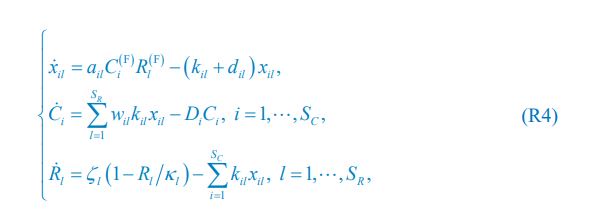
      Furthermore, in addition to the clarification above, we have added the following statement in the discussion section to tone down our claims: “A critical limitation of our study is the absence of direct binding assays to validate the interaction between the metabolites and Ste2p. While our results from genetic interventions, molecular dynamics simulations, and docking studies strongly suggest that the metabolites interact with the Ste2p-Gpa1 interface, these findings remain indirect. Direct binding confirmation through techniques such as surface plasmon resonance, isothermal titration calorimetry, or co-crystallization would provide definitive evidence of this interaction. Addressing this limitation in future work would significantly strengthen our conclusions and provide deeper insights into the precise molecular mechanisms underlying the observed phenotypic effects.”

      (4) The authors do not discuss the effects of the metabolites at their physiological concentrations. Overall, this manuscript represents a field-advancing contribution at the intersection of AI-based ligand discovery and GPCR signaling regulation.

      We thank reviewer #3 for this comment and for recognising the value of our work. Although direct quantification of intracellular free metabolite levels is challenging, several lines of evidence support the physiological relevance of our test concentrations.

      - Genetic validation supports endogenous relevance: Our genetic screen of 53 metabolic knockout mutants showed that deletions in biosynthetic pathways for these metabolites consistently disrupted the α-factor-induced cell death, with the vast majority of strains (94.4%) resisting the α-factor-induced cell death, and notably, a subset even displayed accelerated growth in the presence of α‑factor. This suggests that endogenous levels of these metabolites normally provide some degree of protection, supporting their physiological role in GPCR regulation.

      - Metabolomics confirms in vivo accumulation: Our untargeted metabolomics analysis revealed that α-factor-treated survivors consistently showed enrichment of CoQ6 and zymosterol compared to sensitive cells. This demonstrates that these metabolites naturally accumulate to protective levels during stress responses, validating their biological relevance.

    1. The foes of Charles the Fat and his uncle and predecessor, Charles the Bald, that helped end the Carolingian dynasty were the Vikings, a seafaring people originally from Scandinavia.

      It’s crazy to see that the Vikings didn’t just raid but they reshaped Europe and helped bring an end tot he powerful dynasty.

  13. social-media-ethics-automation.github.io social-media-ethics-automation.github.io
    1. Arvind Narayanan. TikTok’s Secret Sauce. Knight First Amendment Institute, December 2022. URL: http://knightcolumbia.org/blog/tiktoks-secret-sauce (visited on 2023-12-07).

      This article says TikTok’s recommendation system is not really “magic.” It works well because users can skip quickly, and the app learns fast from that. I agree with this idea. I also think it’s dangerous that people believe algorithms “know them,” when in fact it’s just smart design making people stay longer.

    1. Author response:

      The following is the authors’ response to the original reviews.

      Reviewer #1 (Public Review):

      In the current article, Octavia Soegyono and colleagues study "The influence of nucleus accumbens shell D1 and D2 neurons on outcome-specific Pavlovian instrumental transfer", building on extensive findings from the same lab. While there is a consensus about the specific involvement of the Shell part of the Nucleus Accumbens (NAc) in specific stimulus-based actions in choice settings (and not in General Pavlovian instrumental transfer - gPIT, as opposed to the Core part of the NAc), mechanisms at the cellular and circuitry levels remain to be explored. In the present work, using sophisticated methods (rat Cre-transgenic lines from both sexes, optogenetics, and the well-established behavioral paradigm outcome-specific PIT-sPIT), Octavia Soegyono and colleagues decipher the diNerential contribution of dopamine receptors D1 and D2 expressing spiny projection neurons (SPNs). 

      After validating the viral strategy and the specificity of the targeting (immunochemistry and electrophysiology), the authors demonstrate that while both NAc Shell D1- and D2SPNs participate in mediating sPIT, NAc Shell D1-SPNs projections to the Ventral Pallidum (VP, previously demonstrated as crucial for sPIT), but not D2-SPNs, mediates sPIT. They also show that these eNects were specific to stimulus-based actions, as valuebased choices were left intact in all manipulations. 

      This is a well-designed study, and the results are well supported by the experimental evidence. The paper is extremely pleasant to read and adds to the current literature.

      We thank the Reviewer for their positive assessment. 

      Reviewer 2 (Public Review):

      Summary: 

      This manuscript by Soegyono et al. describes a series of experiments designed to probe the involvement of dopamine D1 and D2 neurons within the nucleus accumbens shell in outcome-specific Pavlovian-instrumental transfer (osPIT), a well-controlled assay of cueguided action selection based on congruent outcome associations. They used an optogenetic approach to phasically silence NAc shell D1 (D1-Cre mice) or D2 (A2a-Cre mice) neurons during a subset of osPIT trials. Both manipulations disrupted cue-guided action selection but had no eNects on negative control measures/tasks (concomitant approach behavior, separate valued guided choice task), nor were any osPIT impairments found in reporter-only control groups. Separate experiments revealed that selective inhibition of NAc shell D1 but not D2 inputs to ventral pallidum was required for osPIT expression, thereby advancing understanding of the basal ganglia circuitry underpinning this important aspect of decision making.

      Strengths: 

      The combinatorial viral and optogenetic approaches used here were convincingly validated through anatomical tract-tracing and ex vivo electrophysiology. The behavioral assays are sophisticated and well-controlled to parse cue and value-guided action selection. The inclusion of reporter-only control groups is rigorous and rules out nonspecific eNects of the light manipulation. The findings are novel and address a critical question in the literature. Prior work using less decisive methods had implicated NAc shell D1 neurons in osPIT but suggested that D2 neurons may not be involved. The optogenetic manipulations used in the current study provide a more direct test of their involvement and convincingly demonstrate that both populations play an important role. Prior work had also implicated NAc shell connections to ventral pallidum in osPIT, but the current study reveals the selective involvement of D1 but not D2 neurons in this circuit. The authors do a good job of discussing their findings, including their nuanced interpretation that NAc shell D2 neurons may contribute to osPIT through their local regulation of NAc shell microcircuitry. 

      We thank the Reviewer for their positive assessment. 

      Weaknesses: 

      The current study exclusively used an optogenetic approach to probe the function of D1 and D2 NAc shell neurons. Providing a complementary assessment with chemogenetics or other appropriate methods would strengthen conclusions, particularly the novel demonstration of D2 NAc shell involvement. Likewise, the null result of optically inhibiting D2 inputs to the ventral pallidum leaves open the possibility that a more complete or sustained disruption of this pathway may have impaired osPIT.

      We acknowledge the reviewer's valuable suggestion that demonstrating NAc-S D1- and D2-SPNs engagement in outcome-specific PIT through another technique would strengthen our optogenetic findings. Several approaches could provide this validation. Chemogenetic manipulation, as the reviewer suggested, represents one compelling option. Alternatively, immunohistochemical assessment of phosphorylated histone H3 at serine 10 (P-H3) oMers another promising avenue, given its established utility in reporting striatal SPNs plasticity in the dorsal striatum (Matamales et al., 2020). We hope to complete such an assessment in future work since it would address the limitations of previous work that relied solely on ERK1/2 phosphorylation measures in NAc-S SPNs (Laurent et al., 2014). The manuscript was modified to report these future avenues of research (page 12). 

      Regarding the null result from optical silencing of D2 terminals in the ventral pallidum, we agree with the reviewer's assessment. While we acknowledge this limitation in the current manuscript (page 13), we aim to address this gap in future studies to provide a more complete mechanistic understanding of the circuit.

      Reviewer 3 (Public Review):

      Summary:

      The authors present data demonstrating that optogenetic inhibition of either D1- or D2MSNs in the NAc Shell attenuates expression of sensory-specific PIT while largely sparing value-based decision on an instrumental task. They also provide evidence that SS-PIT depends on D1-MSN projections from the NAc-Shell to the VP, whereas projections from D2-MSNs to the VP do not contribute to SS-PIT.

      Strengths:

      This is clearly written. The evidence largely supports the authors' interpretations, and these eNects are somewhat novel, so they help advance our understanding of PIT and NAc-Shell function.

      We thank the Reviewer for their positive assessment. 

      Weaknesses:

      I think the interpretation of some of the eNects (specifically the claim that D1-MSNs do not contribute to value-based decision making) is not fully supported by the data presented.

      We appreciate the reviewer's comment regarding the marginal attenuation of valuebased choice observed following NAc-S D1-SPN silencing. While this manipulation did produce a slight reduction in choice performance, the behavior remained largely intact. We are hesitant to interpret this marginal eMect as evidence for a direct role of NAc-S D1SPNs in value-based decision-making, particularly given the substantial literature demonstrating that NAc-S manipulations typically preserve such choice behavior (Corbit et al., 2001; Corbit & Balleine, 2011; Laurent et al., 2012). Furthermore, previous work has shown that NAc-S D1 receptor blockade impairs outcome-specific PIT while leaving value-based choice unaMected (Laurent et al., 2014). We favor an alternative explanation for our observed marginal reduction. As documented in Supplemental Figure 1, viral transduction extended slightly into the nucleus accumbens core (NAc-C), a region established as critical for value-based decision-making (Corbit et al., 2001; Corbit & Balleine, 2011; Laurent et al., 2012; Parkes et al., 2015). The marginal impairment may therefore reflect inadvertent silencing of a small number of  NAc-C D1-SPNs rather than a functional contribution from NAc-S D1-SPNs. Future studies specifically targeting larger NAc-C D1-SPN populations would help clarify this possibility and provide definitive resolution of this question.

      Reviewer 1 (Recommendations for the Author):

      My main concerns and comments are listed below.

      (1) Could the authors provide the "raw" data of the PIT tests, such as PreSame vs Same vs PreDiNerent vs DiNerent? Could the authors clarify how the Net responding was calculated? Was it Same minus PreSame & DiNerent minus PreDiNerent, or was the average of PreSame and PreDiNerent used in this calculation?

      The raw data for PIT testing across all experiments are now included in the Supplemental Figures (Supplemental Figures S1E, S2E, S3E, and S4E). Baseline responding was quantified as the average number of lever presses per minute for both actions during the two-minute period (i.e., average of PreSame and PreDiMerent) preceding each stimulus presentation. This methodology has been clarified in the revised manuscript (page 7).

      (2) While both sexes are utilized in the current study, no statistical analysis is provided. Can the authors please comment on this point and provide these analyses (for both training and tests)?

      As noted in the original manuscript, the final sample sizes for female and male rats were insuMicient to provide adequate statistical power for sex-based analyses (page 15). To address this limitation, we have now cited a previous study from our laboratory (Burton et al., 2014) that conducted such analyses with suMicient power in identical behavioural tasks. That study identified only marginal sex diMerences in performance, with female rats exhibiting slightly higher magazine entry rates during Pavlovian conditioning. Importantly, no diMerences were observed in outcome-specific PIT or value-based choice performance between sexes.

      (3) Regarding Figure 1 - Anterograde tracing in D1-Cre and A2a-Cre rats (from line 976), I have one major and one minor question:

      (3.1) I do not understand the rationale of showing anterograde tracing from the Dorsal Striatum (DS) as this region is not studied in the current work. Moreover, sagittal micrographs of D1-Cre and A2a-Cre would be relevant here. Could the authors please provide these micrographs and explain the rationale for doing tracing in DS?

      We included dorsal striatum (DS) tracing data as a reference because the projection patterns of D1 and D2 SPNs in this region are well-established and extensively characterized, in contrast to the more limited literature on these cell types in the NAc-S. Regarding the comment about sagittal micrographs, we are uncertain of the specific concern as these images are presented in Figure 1B.

      If the reviewer is requesting sagittal micrographs for NAc-S anterograde tracing, we did not employ this approach because: (1) the NAc-S and ventral pallidum are anatomically adjacent regions and (2) the medial-lateral coordinates of the ventral pallidum and lateral hypothalamus do not align optimally with those of the NAc-S, limiting the utility of sagittal analysis for these projections.

      (3.2) There is no description about how the quantifications were done: manually? Automatically? What script or plugin was used? If automated, what were the thresholding conditions? How many brain sections along the anteroposterior axis? What was the density of these subpopulations? Can the authors include a methodological section to address this point?

      We apologize for the omission of quantification methods used to assess viral transduction specificity. This methodological description has now been added to the revised manuscript (page 22). Briefly, we employed a manual procedure in two sections per rat, and cell counts were completed in a defined region of interest located around the viral infusion site.

      (4) Lex A & Hauber (2008) Dopamine D1 and D2 receptors in the nucleus accumbens core and shell mediate Pavlovian-instrumental transfer. Learning & memory 15:483- 491, should be cited and discussed. It also seems that the contribution of the main dopaminergic source of the brain, the ventral tegmental area, is not cited, while it has been investigated in PIT in at least 3 studies regarding sPIT only, notably the VP-VTA pathway (Leung & Balleine 2015, accurately cited already).

      We did not include the Lex & Hauber (2008) study because its experimental design (single lever and single outcome) prevents diMerentiation between the eMects of Pavlovian stimuli on action performance (general PIT) versus action selection (outcome-specific PIT, as examined in the present study). Drawing connections between their findings and our results would require speculative interpretations regarding whether their observed eMects reflect general or outcome-specific PIT mechanisms, which could distract from the core findings reported in the article.

      Several studies examining the role of the VTA in outcome-specific PIT were referenced in the manuscript's introduction. Following the reviewer's recommendation, these references have also been incorporated into the discussion section (page 13). 

      (5) While not directly the focus of this study, it would be interesting to highlight the accumbens dissociation between General vs Specific PIT, and how the dopaminergic system (diNerentially?) influences both forms of PIT.

      We agree with the reviewer that the double dissociation between nucleus accumbens core/shell function and general/specific PIT is an interesting topic. However, the present manuscript does not examine this dissociation, the nucleus accumbens core, or general PIT. Similarly, our study does not directly investigate the dopaminergic system per se. We believe that discussing these topics would distract from our core findings and substantially increase manuscript length without contributing novel data directly relevant to these areas. 

      (6) While authors indicate that conditioned response to auditory stimuli (magazine visits) are persevered in all groups, suggesting intact sensitivity to the general motivational properties of reward-predictive stimuli (lines 344, 360), authors can't conclude about the specificity of this behavior i.e. does the subject use a mental representation of O1 when experiencing S1, leading to a magazine visits to retrieve O1 (and same for S2-O2), or not? Two food ports would be needed to address this question; also, authors should comment on the fact that competition between instrumental & pavlovian responses does not explain the deficits observed.

      We agree with the Reviewer that magazine entry data cannot be used to draw conclusions about specificity, and we do not make such claims in our manuscript. We are therefore unclear about the specific concern being raised. Following the Reviewer’s recommendation, we have commented on the fact that response competition could not explain the results obtained (page 11, see also supplemental discussion). 

      The minor comments are listed below.

      (7) A high number of rats were excluded (> 32 total), and the number of rats excluded for NAc-S D1-SPNs-VP is not indicated.

      We apologize for omitting the number of rats excluded from the experiment examining NAc-S D1-SPN projections to the ventral pallidum. This information has been added to the revised manuscript (page 22).

      (7.1) Can authors please comment on the elevated number of exclusions?

      A total of 133 rats were used across the reported experiments, with 40 rats excluded based on post-mortem analyses. This represents an attrition rate of approximately 30%, which we consider reasonable given that most animals received two separate viral infusions and two separate fiber-optic cannula implantations, and that the inclusion of both female and male rats contributed to some variability in coordinates and so targeting. 

      (7.2) Can authors please present the performance of these animals during the tasks (OFF conditions, and for control ones, both ON & OFF conditions)?

      Rats were excluded after assessing the spread of viral infusions, placement of fibre-optic cannulas and potential damage due to the surgical procedures (page 21). The requested data are presented below and plotted in the same manner as in Figures 3-6. The pattern of performance in excluded animals was highly variable. 

      Author response image 1.


      (8) For tracing, only males were used, and for electrophysiology, only females were used.

      (8.1) Can authors please comment on not using both sexes in these experiments? 

      We agree that equal allocation of female and male rats in the experiments presented in Figures 1-2 would have been preferable. Animal availability was the sole factor determining these allocations. Importantly, both female and male D1-Cre and A2A-Cre rats were used for the NAc-S tracing studies, and no sex diMerences were observed in the projection patterns. The article describing the two transgenic lines of rats did not report any sex diMerence (Pettibone et al., 2019). 

      (8.2) Is there evidence in the literature that the electrophysiological properties of female versus male SPNs could diNer?

      The literature indicates that there is no sex diMerence in the electrophysiological properties of NAc-S SPNs (Cao et al., 2018; Willett et al., 2016).  

      (8.3) It seems like there is a discrepancy between the number of animals used as presented in the Figure 2 legend versus what is described in the main text. In the Figure legend, I understand that 5 animals were used for D1-Cre/DIO-eNpHR3.0 validation, and 7 animals for A2a-Cre/DIO-eNpHR3.0; however, the main text indicates the use of a total of 8 animals instead of the 12 presented in the Figure legend. Can authors please address this mismatch or clarify?

      The number of rats reported in the main text and Figure 2 legend was correct. However, recordings sometimes involved multiple cells from the same animal, and this aspect of the data was incorrectly reported and generated confusion. We have clarified the numbers in both the main text and Figure 2 legend to distinguish between animal counts and cell counts. 

      (9) Overall, in the study, have the authors checked for outliers?

      Performance across all training and testing stages was inspected to identify potential behavioral outliers in each experiment. Abnormal performance during a single session within a multi-session stage was not considered suMicient grounds for outlier designation. Based on these criteria, no subjects remaining after post-mortem analyses exhibited performance patterns warranting exclusion through statistical outlier analysis. However, we have conducted the specific analyses requested by the Reviewer, as described below. 

      (9.1) In Figure 3, it seems that one female in the eYFP group, in the OFF situation, for the diNerent condition, has a higher level of responding than the others. Can authors please confirm or refute this visual observation with the appropriate statistical analysis?

      Statistical analysis (z-score) confirmed the reviewer's observation regarding responding of the diMerent action in the OFF condition for this subject (|z| = 2.58). Similar extreme responding was observed in the ON condition (|z| = 2.03). Analyzing responding on the diMerent action in isolation is not informative in the context of outcome-specific PIT. Additional analyses revealed |z| < 2 when examining the magnitude of choice discrimination in outcome-specific PIT (i.e., net same versus net diMerent responding) in both ON and OFF conditions. Furthermore, this subject showed |z| < 2 across all other experimental stages. Based on these analyses, we conclude that the subject should be kept in all analyses. 

      (9.2) In Figure 5, it seems that one male, in the ON situation, in the diNerent condition, has a quite higher level of responding - is this subject an outlier? If so, how does it aNect the statistical analysis after being removed? And who is this subject in the OFF condition?

      The reviewer has identified two diMerent male rats infused with the eNpHR3.0 virus and has asked closer examination of their performance.

      The first rat showed outlier-level responding on the diMerent action in the ON condition (|z| = 2.89) but normal responding for all other measures across LED conditions (|z| < 2). Additional analyses revealed |z| = 2.55 when examining choice discrimination magnitude in outcome-specific PIT during the ON condition but not during the OFF condition (|z| = 0.62). This subject exhibited |z| < 2 across all other experimental stages.

      The second rat showed outlier-level responding on the same action in the OFF condition (|z| = 2.02) but normal responding for all other measures across LED conditions (|z| < 2). Additional analyses revealed |z| = 2.12 when examining choice discrimination magnitude in outcome-specific PIT during the OFF condition but not during the ON condition (|z| = 0.67). This subject also exhibited |z| < 2 across all other experimental stages.

      We excluded these two subjects and conducted the same analyses as described in the original manuscript. Baseline responding did not diMer between groups (p = 0.14), allowing to look at the net eMect of the stimuli. Overall lever presses were greater in the eYFP rats (Group: F(1,16) = 6.08, p < 0.05; η<sup>2</sup> = 0.28) and were reduced by LED activation (LED: F(1,16) = 9.52, p < 0.01; η<sup>2</sup> = 0.44) and this reduction depended on the group considered (Group x LED: F(1,16) = 12.125, p < 0.001; η<sup>2</sup> = 0.43). Lever press rates were higher on the action earning the same outcome as the stimuli compared to the action earning the diMerent outcome (Lever: F(1,16)= 49.32; η<sup>2</sup> = 0.76; p < 0.001), regardless of group (Group x Lever: p = 0.14). There was a Lever by LED light condition interaction (Lever x LED: F(1,16)= 5.25; η<sup>2</sup> = 0.24; p < 0.05) but no an interaction between group, LED light condition, and Lever during the presentation of the predictive stimuli (p = 0.10). Given the significant Group x LED and Lever x LED interactions, additional analyses were conducted to determine the source of these interactions. In eYFP rats, LED activation had no eMect (LED: p = 0.70) and lever presses were greater on the same action (Lever: (F(1,9) = 23.94, p < 0.001; η<sup>2</sup> = 0.79) regardless of LED condition (LED x Lever: p = 0.72). By contrast, in eNpHR3.0 rats, lever presses were reduced by LED activation (LED: F(1,9) = 23.97, p < 0.001; η<sup>2</sup> = 0.73), were greater on the same action (Lever: F(1,9) = 16.920, p < 0.001; η<sup>2</sup> = 0.65) and the two factors interacted (LED x Lever: F(1,9) = 9.12, p < 0.01; η<sup>2</sup> = 0.50). These rats demonstrated outcome-specific PIT in the OFF condition (F(1,9) = 27.26, p < 0.001; η<sup>2</sup> = 0.75) but not in the ON condition (p = 0.08).

      Overall, excluding these two rats altered the statistical analyses, but both the original and revised analyses yielded the same outcome: silencing the NAc-S D1-SPN to VP pathway disrupted PIT. More importantly, we do not believe there are suMicient grounds to exclude the two rats identified by the reviewer. These animals did not display outlier-level responding across training stages or during the choice test. Their potential classification as outliers would be based on responding during only one LED condition and not the other, with notably opposite patterns between the two rats despite belonging to the same experimental group. 

      (10) I think it would be appreciable if in the cartoons from Figure 5.A and 6.A, the SPNs neurons were color-coded as in the results (test plots) and the supplementary figures (histological color-coding), such as D1- in blue & D2-SPNs in red.

      Our current color-coding system uses blue for D1-SPNs transduced with eNpHR3.0 and red for D2-SPNs transduced with eNpHR3.0. The D1-SPNs and D2-SPNs shown in Figures 5A and 6A represent cells transduced with either eYFP (control) or eNpHR3.0 virus and therefore cannot be assigned the blue or red color, which is reserved for eNpHR3.0transduced cells specifically. The micrographs in the Supplemental Figures maintain consistency with the color-coding established in the main figures.

      (11) As there are (relatively small) variations in the control performance in term of Net responding (from ~3 to ~7 responses per min), I wonder what would be the result of pooling eYFP groups from the two first experiments (Figures 3 & 4) and from the two last ones (Figures 5 & 6) - would the same statically results stand or vary (as eYFP vs D1-Cre vs A2a-Cre rats)? In particular for Figures 3 & 4, with and without the potential outlier, if it's indeed an outlier.

      We considered the Reviewer’s recommendation but do not believe the requested analysis is appropriate. The Reviewer is requesting the pooling of data from subjects of distinct transgenic strains (D1-Cre and A2A-Cre rats) that underwent surgical and behavioral procedures at diMerent time points, sometimes months apart. Each experiment was designed with necessary controls to enable adequate statistical analyses for testing our specific hypotheses. 

      (12) Presence of cameras in operant cages is mentioned in methods, but no data is presented regarding recordings, though authors mention that they allow for real-time observations of behavior. I suggest removing "to record" or adding a statement about the fact that no videos were recorded or used in the present study.

      We have removed “to record” from the manuscript (page 18). 

      (13) In all supplementary Figures, "F" is wrongly indicated as "E".

      We thank the Reviewer for reporting these errors, which have been corrected. 

      (14) While the authors acknowledge that the eNicacy of optogenetic inhibition of terminals is questionable, I think that more details are required to address this point in the discussion (existing literature?). Maybe, the combination of an anterograde tracer from SPNs to VP, to label VP neurons (to facilitate patching these neurons), and the Credependent inhibitory opsin in the NAc Shell, with optogenetic illumination at the level of the VP, along with electrophysiological recordings of VP neurons, could help address this question but may, reasonably, seem challenging technically.

      Our manuscript does not state that optogenetic inhibition of terminals is questionable. It acknowledges that we do not provide any evidence about the eMicacy of the approach. Regardless, we have provided additional details and suggestions to address this lack of evidence (page 13). 

      (15) A nice addition could be an illustration of the proposed model (from line 374), but it may be unnecessary.

      We have carefully considered the reviewer's recommendation. The proposed model is detailed in three published articles, including one that is freely accessible, which we have cited when presenting the model in our manuscript (page 14). This reference should provide interested readers with easy access to a comprehensive illustration of the model.

      Reviewer 2 (Recommendations for the Author):

      As noted in my public comments, this is a truly excellent and compelling study. I have only a few minor comments.

      (1) I could not find the coordinates/parameters for the dorsal striatal AAV injections for that component of the tract tracing experiment.

      We apologize for this omission, which has now been corrected (page 16). 

      (2) Please add the final group sizes to the figure captions.

      We followed the Reviewer’s recommendation and added group sizes in the main figure captions. 

      (3) The discussion of group exclusions (p 21 line 637) seems to accidentally omit (n = X) the number of NAc-S D1-SPNs-VP mice excluded.

      We apologize for this omission, which has now been corrected (page 22). 

      (4) There were some labeling issues in the supplementary figures (perhaps elsewhere, too). Specifically, panel E was listed twice (once for F) in captions.

      We apologize for this error, which has now been corrected.  

      (5) Inspection of the magazine entry data from PIT tests suggests that the optogenetic manipulations may have had some eNects on this behavior and would encourage the authors to probe further. There was a significant group diNerence for D1-SPN inhibition and a marginal group eNect for D2-SPNs. The fact that these eNects were in opposite directions is intriguing, although not easily interpreted based on the canonical D1/D2 model. Of course, the eNects are not specific to the light-on trials, but this could be due to carryover into light-oN trials. An analysis of trial-order eNects seems crucial for interpreting these eNects. One might also consider normalizing for pre-test baseline performance. Response rates during Pavlovian conditioning seem to suggest that D2eNpHR mice showed slightly higher conditioned responding during training, which contrasts with their low entry rates at test. I don't see any of this as problematic -- but more should be done to interpret these findings.

      We thank the reviewer for raising this interesting point regarding magazine entry rates. Since these data are presented in the Supplemental Figures, we have added a section in the Supplemental Material file that elaborates on these findings. This section does not address trial order eMects, as trial order was fully counterbalanced in our experiments and the relevant statistical analyses would lack adequate power. Baseline normalization was not conducted because the reviewer's suggestion was based on their assumption that eNpHR3.0 rats in the D2-SPNs experiment showed slightly higher magazine entries during Pavlovian training. However, this was not the case. In fact, like the eNpHR3.0 rats in the D1-SPNs experiment, they tended to display lower magazine entries during training. The added section therefore focuses on the potential role of response competition during outcome-specific PIT tests. Although we concluded that response competition cannot explain our findings, we believe it may complicate interpretation of magazine entry behavior. Thus, we recommend that future studies examine the role of NAc-S SPNs using purely Pavlovian tasks. It is worth nothing that we have recently completed experiments (unpublished) examining NAc-S D1- and D2-SPN silencing during stimulus presentation in a Pavlovian task identical to the one used here. Silencing of either SPN population had no eMect on magazine entry behavior.

      Reviewer 3 (Recommendations for the Author):

      Broad comments:

      Throughout the manuscript, the authors draw parallels between the eNect established via pharmacological manipulations and those shown here with optogenetic manipulation. I understand using the pharmacological data to launch this investigation, but these two procedures address very diNerent physiological questions. In the case of a pharmacological manipulation, the targets are receptors, wherever they are expressed, and in the case of D2 receptors, this means altering function in both pre-synaptically expressed autoreceptors and post-synaptically expressed D2 MSN receptors. In the case of an optogenetic approach, the target is a specific cell population with a high degree of temporal control. So I would just caution against comparing results from these types of studies too closely.

      Related to this point is the consideration of the physiological relevance of the manipulation. Under normal conditions, dopamine acts at D1-like receptors to increase the probability of cell firing via Ga signaling. In contrast, dopamine binding of D2-like receptors decreases the cell's firing probability (signaling via Gi/o). Thus, shunting D1MSN activation provides a clear impression of the role of these cells and, putatively, the role of dopamine acting on these cells. However, inhibiting D2-MSNs more closely mimics these cells' response to dopamine (though optogenetic manipulations are likely far more impactful than Gi signaling). All this is to say that when we consider the results presented here in Experiment 2, it might suggest that during PIT testing, normal performance may require a halting of DA release onto D2-MSNs. This is highly speculative, of course, just a thought worth considering.

      We agree with the comments made by the Reviewer, and the original manuscript included statements acknowledging that pharmacological approaches are limited in the capacity to inform about the function of NAc-S SPNs (pages 4 and 9). As noted by the Reviewer, these limitations are especially salient when considering NAc-S D2-SPNs. Based on the Reviewer’s comment, we have modified our discussion to further underscore these limitations (page 12). Finally, we agree with the suggestion that PIT may require a halting of DA release onto D2-SPNs. This is consistent with the model presented, whereby D2-SPNs function is required to trigger enkephalin release (page 13).     

      Section-Specific Comments and Questions:

      Results:

      Anterograde tracing and ex vivo cell recordings in D1 Cre and A2a Cre rats: Why are there no statistics reported for the e-phys data in this section? Was this merely a qualitative demonstration? I realize that the A2a-Cre condition only shows 3 recordings, so I appreciate the limitations in analyzing the data presented.

      The reviewer is correct that we initially intended to provide a qualitative demonstration. However, we have now included statistical analyses for the ex vivo recordings. It is important to note that there were at least 5 recordings per condition, though overlapping data points may give the impression of fewer recordings in certain conditions. We have provided the exact number of recordings in both the main text (page 5) and figure legend. 

      What does trial by trial analysis look like, because in addition to the eNects of extinction, do you know if the responsiveness of the opsin to light stimulation is altered after repeated exposures, or whether the cells themselves become compromised in any way with repeated light-inhibition, particularly given the relatively long 2m duration of the trial.

      The Reviewer raises an interesting point, and we provide complete trial-by-trial data for each experiment below. As identified by the Reviewer, there is some evidence for extinction, although it remained modest. Importantly, the data suggest that light stimulation did not aMect the physiology of the targeted cells. In eNpHR3.0 rats, performance across OFF trials remained stable (both for Same and DiMerent) even though they were preceded by ON trials, indicating no carryover eMects from optical stimulation.

      Author response image 2.


      The statistics for the choice test are not reported for eNpHR-D1-Cre rats, but do show a weakening of the instrumental devaluation eNect "Group x Lever x LED: F1,18 = 10.04, p < 0.01, = 0.36". The post hoc comparisons showed that all groups showed devaluation, but it is evident that there is a weakening of this eNect when the LED was on (η<sup>2</sup> = 0.41) vs oN (η<sup>2</sup> = 0.78), so I think the authors should soften the claim that NAcS-D1s are not involved in value-based decision-making. (Also, there is a typo in the legend in Figure S1, where the caption for panel "F" is listed as "E".) I also think that this could be potentially interesting in light of the fact that with circuit manipulation, this same weakening of the instrumental devaluation eNect was not observed. To me, this suggests that D1-NAcS that project to a diNerent region (not VP) contribute to value-based decision making.

      This comment overlaps with one made in the Public Review, for which we have already provided a response. Given its importance, we have added a section addressing this point in the supplemental discussion of the Supplementary Material file, which aligns with the location of the relevant data. The caption labelling error has been corrected.

      Materials and Methods:

      Subjects:

      Were these heterozygous or homozygous rats? If hetero, what rats were used for crossbreeding (sex, strain, and vendor)? Was genotyping done by the lab or outsourced to commercial services? If genotyping was done within the lab, please provide a brief description of the protocol used. How was food restriction established and maintained (i.e., how many days to bring weights down, and was maintenance achieved by rationing or by limiting ad lib access to food for some period in the day)?

      The information requested by the Reviewer have been added to the subjects section (pages 15-16).  

      Were rats pair/group housed after implantation of optic fibers?

      We have clarified that rats were group houses throughout (see subjects section; pages 15-16). 

      Behavioral Procedures:

      How long did each 0.2ml sucrose infusion take? For pellets, for each US delivery, was it a single pellet or two in quick succession?

      We have modified the method section to indicate that the sucrose was delivered across 2 seconds and that a single pellet was provided (page 17). 

      The CS to ITI duration ratio is quite low. Is there a reason such a short ratio was used in training?

      These parameters are those used in all our previous experiments on outcome-specific PIT. There is no specific reason for using such a ratio, except that it shortens the length of the training session. 

      Relative to the end of training, when were the optical implantation surgeries conducted, and how much recovery time was given before initiating reminder training and testing?

      Fibre-optic implantation was conducted 3-4 days after training and another 3-4 days were given for recovery. This has been clarified in the Materials and methods section (pages 15-16).

      I think a diagram or schematic showing the timeline for surgeries, training, and testing would be helpful to the audience.

      We opted for a text-based experimental timeline rather than a diagram due to slight temporal variations across experiments (page 15).

      On trials, when the LED was on, was light delivered continuously or pulsed? Do these opto-receptors 'bleach' within such a long window?

      We apologize for the lack of clarity; the light was delivered continuously. We have modified the manuscript (pages 6 and 19) and figure legend accordingly. The postmortem analysis did not provide evidence for photobleaching (Supplemental Figures) and as noted above, the behavioural results do not indicate any negative physiological impact on cell function.  

      Immunofluorescence: The blocking solution used during IHC is described as "NHS"; is this normal horse serum?

      The Reviewer is correct; NHS stands for normal horse serum. This has been added (page 21). 

      Microscopy and imaging:

      For the description of rats excluded due to placement or viral spread problems, an n=X is listed for the NAc S D1 SPNs --> VP silencing group. Is this a typo, or was that meant to read as n=0? Also, was there a major sex diNerence in the attrition rate? If so, I think reporting the sex of the lost subjects might be beneficial to the scientific community, as it might reflect a need for better guidance on sex-specific coordinates for targeting small nuclei.

      We apologize for the error regarding the number of excluded animals. This error has been corrected (page 23). There were no major sex diMerences in the attrition rate. The manuscript has been updated to provide information about the sex of excluded animals (page 23). 

      References

      Cao, J., Willett, J. A., Dorris, D. M., & Meitzen, J. (2018). Sex DiMerences in Medium Spiny Neuron Excitability and Glutamatergic Synaptic Input: Heterogeneity Across Striatal Regions and Evidence for Estradiol-Dependent Sexual DiMerentiation. Front Endocrinol (Lausanne), 9, 173. https://doi.org/10.3389/fendo.2018.00173

      Corbit, L. H., Muir, J. L., Balleine, B. W., & Balleine, B. W. (2001). The role of the nucleus accumbens in instrumental conditioning: Evidence of a functional dissociation between accumbens core and shell. J Neurosci, 21(9), 3251-3260. http://eutils.ncbi.nlm.nih.gov/entrez/eutils/elink.fcgi?dbfrom=pubmed&id=11312 310&retmode=ref&cmd=prlinks

      Corbit, L. H., & Balleine, B. W. (2011). The general and outcome-specific forms of Pavlovian-instrumental transfer are diMerentially mediated by the nucleus accumbens core and shell. J Neurosci, 31(33), 11786-11794. https://doi.org/10.1523/JNEUROSCI.2711-11.2011

      Laurent, V., Bertran-Gonzalez, J., Chieng, B. C., & Balleine, B. W. (2014). δ-Opioid and Dopaminergic Processes in Accumbens Shell Modulate the Cholinergic Control of Predictive Learning and Choice. J Neurosci, 34(4), 1358-1369. https://doi.org/10.1523/JNEUROSCI.4592-13.2014

      Laurent, V., Leung, B., Maidment, N., & Balleine, B. W. (2012). μ- and δ-opioid-related processes in the accumbens core and shell diMerentially mediate the influence of reward-guided and stimulus-guided decisions on choice. J Neurosci, 32(5), 1875-1883. https://doi.org/10.1523/JNEUROSCI.4688-11.2012

      Matamales, M., McGovern, A. E., Mi, J. D., Mazzone, S. B., Balleine, B. W., & BertranGonzalez, J. (2020). Local D2- to D1-neuron transmodulation updates goal-directed learning in the striatum. Science, 367(6477), 549-555. https://doi.org/10.1126/science.aaz5751

      Parkes, S. L., Bradfield, L. A., & Balleine, B. W. (2015). Interaction of insular cortex and ventral striatum mediates the eMect of incentive memory on choice between goaldirected actions. J Neurosci, 35(16), 6464-6471. https://doi.org/10.1523/JNEUROSCI.4153-14.2015

      Pettibone, J. R., Yu, J. Y., Derman, R. C., Faust, T. W., Hughes, E. D., Filipiak, W. E., Saunders, T. L., Ferrario, C. R., & Berke, J. D. (2019). Knock-In Rat Lines with Cre Recombinase at the Dopamine D1 and Adenosine 2a Receptor Loci. eNeuro, 6(5). https://doi.org/10.1523/ENEURO.0163-19.2019

      Willett, J. A., Will, T., Hauser, C. A., Dorris, D. M., Cao, J., & Meitzen, J. (2016). No Evidence for Sex DiMerences in the Electrophysiological Properties and Excitatory Synaptic Input onto Nucleus Accumbens Shell Medium Spiny Neurons. eNeuro, 3(1), ENEURO.0147-15.2016. https://doi.org/10.1523/ENEURO.0147-15.2016

    1. This technique can get up to 108 ideas from six participants in just 30 minutes, and it’s great if you want to encourage every participant to generate ideas – especially if your team is predominantly introverts.

      I feel like this wouldn't suit me. What if there are multiple people that feel stumped early on? Also sounds like it takes a chunk of time to get to one cohesive idea.

    1. As should be obvious, you can’t have cinema without light. Light exposes the image and, of course, allows us to see it. But it’s the creative use of light, or lighting, is what makes it an element design. A cinematographer can illuminate a given scene with practical light, that is, light from lamps and other fixtures that are part of the set design, set lights, light fixtures that are off camera and specifically designed to light a film set, or even available light, light from the sun or whatever permanent fixtures are at a given location. But in each case, the cinematographer is not simply throwing a light switch, they are shaping that light, making it work for the scene and the story as a whole. They do this by emphasizing different aspects of lighting direction and intensity. A key light, for example, is the main light that illuminates a subject. A fill light fills out the shadows a strong key light might create. And a back light helps separate the subject from the background. And it’s the consistent use of a particular lighting design that makes it a powerful part of mise-en-scène.

      Lighting is more than just turning things on; it’s an art form that shapes the mood and meaning of a scene. Every choice with key, fill, or back light changes how we see characters and space, making light itself part of the story.

    1. As to your extraordinary Code of Laws, I cannot but laugh. We have been told that our Struggle has loosened the bands of Government every where. That Children and Apprentices were disobedient — that schools and Colledges were grown turbulent — that Indians slighted their Guardians and Negroes grew insolent to their Masters. But your Letter was the first Intimation that another Tribe more numerous and powerfull than all the rest were grown discontented. — This is rather too coarse a Compliment but you are so saucy, I wont blot it out.

      It's wild how he doesn't take his own wife seriously. It sounds like he's just saying "add it to the list of problems" or "now the women are complaining?"

    2. I find as much as I can do to manufacture cloathing for my family which would else be Naked. I know of but one person in this part of the Town who has made any, that is Mr. Tertias Bass as he is calld who has got very near an hundred weight which has been found to be very good.

      This as well as the rest of the paragraph shows that she is in touch with the town, as well as all she is doing for their family. Just goes to show it's ridiculous that women can fill this important role but cant have any rights outside of their home.

  14. inst-fs-iad-prod.inscloudgate.net inst-fs-iad-prod.inscloudgate.net
    1. I know that college is important but right now I have to focus on help-ing my family. Without papers there’s not much I can do. And it’s not the focus of our teachers. They just want us to learn English and so they don’t talk to us about how to apply to college. I think it’s best if I work and help my family

      This was the mentality of so many people i knew in middle school and highschool they chose to drop out of education in order to pursue work in trade or rap or whatever they could get their hands on because the education system failed them and denied them their ability to pursue something higher

    2. Seeing friends move forward punctuated our respondents’ own immo-bility. Confusion about the future constrained their decisions regarding the present. Ruben, from Seattle, explained to us that his entire future was turned upside down. You know, you grew up thinking, dreaming of your future. Like, “I’m going to be a fi refi ghter when I grow up”. You know, like that. I thought I could be something more. It’s hard to swallow realizing that you’re just an immigrant. How do you say? Undocumented? It really stopped me in my tracks

      From the perspective of immigrant students, this passage reveals how uncertainty about the future can deeply affect motivation and self-worth. Many undocumented students grow up believing in the same dreams as their peers—going to college, finding a good job, contributing to society—but later realize that their immigration status limits those possibilities. Seeing friends move forward while they remain stuck creates a painful sense of immobility and isolation. The confusion about what’s even possible makes it hard for them to plan or stay engaged in the present. For these students, education becomes a source of both hope and frustration—it represents opportunity but also reminds them of the barriers they face just to belong.

    1. Reviewer #1 (Public review):

      Summary:

      This manuscript investigates the interplay between spontaneous attention and melody formation during polyphonic music listening. The authors use EEG recordings during uninstructed listening to examine how attention bias influences melody processing, employing both behavioural measures and computational modelling with music transformers. The study introduces a very clever pitch-inversion manipulation design to dissociate high-voice superiority from melodic salience, and proposes a "weighted integration" model where attention dynamically modulates how multiple voices are combined into perceived melody.

      Strengths:

      (1) The attention bias findings (Figure 2) are compelling and methodologically sound, with convergent evidence from both behavioral and neural measures.

      (2) The pitch-inversion manipulation appears to super elegantly dissociate two competing factors (high-voice superiority vs melodic salience), moreover, the authors claim that the chosen music lends itself perfectly to his PolyInv condition. A claim I cannot really evaluate, but which would make it even more neat.

      (3) Nice bridge between hypotheses and operationalisations.

      Weaknesses:


      The results in Figure 3 are very striking, but I have a number of questions before I can consider myself convinced. 


      (1) Conceptual questions about surprisal analysis:


      The pattern of results seems backwards to me. Since the music is inherently polyphonic in PolyOrig, I'd expect the polyphonic model to fit the brain data better - after all, that's what the music actually is. These voices were composed to interact harmonically, so modeling them as independent monophonic streams seems like a misspecification. Why would the brain match this misspecified model better?
<br /> Conversely, it would seem to me the pitch inversion in PolyInv disrupts (at least to some extent) the harmonic coherence, so if anywhere, I'd a priori expect that in this condition, listeners would rather be processing streams separately - making the monophonic model fit better there (or less bad), not in PolyOrig. The current pattern is exactly opposite to what seems logical to me.


      (2) Missing computational analyses:


      If the transformer is properly trained, it should "understand" (i.e., predict/compress) the polyphonic music better, right? Can the authors demonstrate this via perplexity scores, bits-per-byte, or other prediction metrics, comparing how well each model (polyphonic vs monophonic) handles the music in both conditions? Similarly, if PolyInv truly maintains musical integrity as claimed, the polyphonic model should handle it as well as PolyOrig. But if the inversion does disrupt the music, we should see this reflected in degraded prediction scores. These metrics would validate whether the experimental manipulation works as intended. Also, how strongly are the surprisal streams correlated? There are many non-trivial modelling steps that should be reported in more detail.


      (3) Methodological inconsistencies:

      Why are the two main questions (Figures 2 and 3) answered with completely different analytical approaches? The switch from TRF to CCA with match-vs-mismatch classification seems unmotivated. I think it's very important to provide a simpler model comparison - just TRF with acoustic features plus either polyphonic or monophonic surprisal - evaluated on relevant electrodes or the full scalp. This would make the results more comparable and interpretable.

      (4) Presentation and methods:

      a) Coming from outside music/music theory, I found the paper somewhat abstract and hard to parse initially. The experimental logic becomes clearer with reflection, but you're doing yourselves a disservice with the jargon-heavy presentation. It would be useful to include example stimuli.

      b) The methods section is extremely brief - no details whatsoever are provided regarding the modelling: What specific music transformer architecture? Which implementation of this "anticipatory music transformer"? Pre-trained on what corpus - monophonic, polyphonic, Western classical only? What constituted "technical issues" for the 9 excluded participants? What were the channel rejection criteria?

    1. it is better to think of rubrics as roadmaps, displaying your destination, rather than a GPS system directing every move you make.

      Bouncing off my other annotation, while we should use the rubric to help us out on writings and assignments, we should rely too much on it, because that also can make it harder to write a successful paper. It's a "It's not the destination, but the journey," of a saying. As a writer, you shouldn't be tunneled into just hitting all the checkboxes to have a bare minimum piece, but to also explore and take your own paths, while still following the correct way.

    1. For every new field of study, you’re like a traveler visiting a foreign culture and learning how to get along

      This line is a metaphor, and to me, it's saying that writing is an immersive experience. It requires academic writing to have some sort of depth, curiosity emotion, and persistence. It shouldn't be the same every time, and also, some specifics are just not for every other person. Students should try to adapt to their writing skills and become “travelers learning new cultures," or learning how to write differently to become better and more vast.

    1. It’s important to remember that there is no “average user,” and so your choice of defaults will inevitably serve some people better than others. For example, if Google detects that a browser is in the United States, what language should it default too? Some might say English, but that prioritizes English-speaking people over others. But should it be Spanish? Or more dependent on a specific region?Or tied to a browser setting?

      Professor Amy makes a really good point because it talks about how small design choices like default choice can even reinforce inequality. This made me relize that how much bias can be built into everyday interfaces like on the devices we use. Like my own parents; since they only speak vietnamese, a lot of american interfaces are english by default which makes it confuse to look for the language option. This also reminded me that inclusive design isn't just about accessibility for people with disabilities but also about making sure products work for people with different language and cultural.

    2. If we adopt the aesthetic of designs being invisible, a good design would make the inputs, state, and outputs discoverable, clear, and efficient to use

      I really like how this chapter emphasizes that designing interfaces is more than just arranging visuals, it’s about shaping how people think and act through interaction. I found the discussion about gulfs of execution and evaluation especially insightful because it highlights how easily design can confuse users if not thoughtfully constructed. Overall, this reading deepened my understanding that great interface design is about empathy, clarity, and responsibility just as much as it is about aesthetics or functionality.

    3. clear affordances11 Rex Hartson (2003). Cognitive, physical, sensory, and functional affordances in interaction design. Behaviour & Information Technology. . An affordance is a relationship between a person and a property of what can be done to an interface in order to produce some effect. For example, a physical computer mouse can be clicked, which allows information to be communicated to a computer. However, these are just a property of a mouse; affordances arise when a person recognizes that opportunity and knows how to act upon it. To know that a user interface has an affordance, user interfaces provide signifiers, which are any sensory or cognitive indicator of the presence of an affordance. Consider, for example, how you know that a computer mouse can be clicked.

      I really agree with the idea in this passage about affordances — it makes so much sense when thinking about how we interact with interfaces every day. The point that affordances are not just about what something can do, but whether the user recognizes what can be done, feels super relevant. It’s one thing for a button to be clickable, but it’s another for users to know it’s clickable. I also like how the passage connects affordances to signifiers, like visual or sensory cues that guide users. It reminds me of how modern apps use animations, color changes, or shadows to make buttons feel “touchable.” It’s a small detail, but it really changes how intuitive something feels.

    1. Warner Bros. was a family-owned studio run by five brothers and smaller than some of the other larger companies like Universal and MGM. But one of those brothers, Sam, had a vision. Or rather, an ear. Up to that point, cinema was still a silent medium. But Sam was convinced that sound, and more specifically, sound that was synchronized to the image, was the future. And almost everyone thought he was crazy.

      Funny to think about people just sitting there in silence prior. Now it's so rare to get any silence at all, and when so it's concerning

    1. Designers use prototypes to resolve these uncertainties, iterate on their design based on feedback, and converge toward a design that best addresses the problem.

      I agree with this idea because it shows how important it is to view design as a process of learning rather than just building. Prototyping encourages creativity and flexibility, allowing designers to adapt based on real feedback instead of assumptions. I think this approach saves time and resources while leading to stronger, more user-centered outcomes. It reminds me that good design isn’t about getting it perfect the first time, it’s about improving through continuous discovery.

    2. As you can see, prototyping isn’t strictly about learning to make things, but also learning how to decide what prototype to make and what that prototype would teach you. These are judgements that are highly contextual because they depend on the time and resources you have and the tolerance for risk you have in whatever organization you’re in.

      I really agree with the reading’s point that prototyping isn’t just about building something; it’s about deciding what you need to build to learn the right thing at the right moment. That reminder shifts my perspective, because I used to think of prototypes as just early versions of the final product, but now I see them as experiments designed to answer specific questions. I think it's important to balance how much you don’t know with how much you can afford to discover.

    3. prototyping isn’t strictly about learning to make things, but also learning how to decide what prototype to make and what that prototype would teach you. These are judgements that are highly contextual because they depend on the time and resources you have and the tolerance for risk you have in whatever organization you’re in.You don’t always have to prototype. If the cost of just implementing the solution is less than prototyping, perhaps it’s worth it to just create it. That cost depends on the skills you have, the tools you have access to, and what knowledge you need from the prototype.

      I used to think prototyping was something you had to do in every design process, but this made me realize it’s more about thinking strategically than just building for the sake of it. The idea that prototyping helps you decide what to learn instead of just testing something random really stood out to me. I also find it super useful that it points out how sometimes it’s better to just go ahead and build the final version if it saves time or effort. Not every project needs multiple rounds of prototypes — it really depends on your goals, skills, and the level of uncertainty. Overall, I think this perspective helps designers (especially students like us) use their time more wisely and make smarter decisions about when and why to prototype.

  15. social-media-ethics-automation.github.io social-media-ethics-automation.github.io
    1. A disability is an ability that a person doesn’t have, but that their society expects them to have.[1] For example:

      I think this section really changed how I understand disability, it’s not just about what someone can or can’t do, but about what society assumes everyone should be able to do. The examples make it clear how design and environment can create barriers. It made me realize how important accessibility and inclusive design are in everyday life.

    2. A disability is an ability that a person doesn’t have, but that their society expects them to have.[1] For example: If a building only has staircases to get up to the second floor (it was built assuming everyone could walk up stairs), then someone who cannot get up stairs has a disability in that situation. If a physical picture book was made with the assumption that people would be able to see the pictures, then someone who cannot see has a disability in that situation. If tall grocery store shelves were made with the assumption that people would be able to reach them, then people who are short, or who can’t lift their arms up, or who can’t stand up, all would have a disability in that situation. If an airplane seat was designed with little leg room, assuming people’s legs wouldn’t be too long, then someone who is very tall, or who has difficulty bending their legs would have a disability in that situation. Which abilities are expected of people, and therefore what things are considered disabilities, are socially defined [j1]. Different societies and groups of people make different assumptions about what people can do, and so what is considered a disability in one group, might just be “normal” in another.

      I really appreciate how this section reframes disability as a social design issue rather than an individual problem. The examples about stairs and color vision made me realize how often our environments are built for a narrow idea of normal. I've never thought about how something as simple as shelf height or screen brightness can include or exclude people. This reminds me that accessibility isn't just a technical feature; it's an ethical responsibility. If design creates disability, them redesign can also remove it. It makes me wonder how many limitations in our world are actually design failures, not human ones.

    1. command pattern

      good question. they overlap a bit but they serve different purposes.

      command = intent

      event = outcome

      command pattern is about explicit control of an action. you create a Command object, pass it to an executor, and call execute() when you want. you know who asked for it, when it ran, and what the outcome was. it’s about invoking behavior in a controlled and traceable way.

      event-driven architecture is about reactions to things that already happened. an event is a statement of fact: “user.created”. it doesn’t command anyone to do something; it just signals that something occurred. listeners may respond or ignore it, you don’t control that directly.

      so:

      • use commands when you want deterministic, transactional actions with well-defined ownership and lifecycle (e.g. workflows, CQRS “write” side, retryable jobs).
      • use events when you want decoupled, asynchronous fan-out or notifications (e.g. “send welcome email” after user created).

      many systems use both. commands cause events. example: CreateUserCommand → executed → emits UserCreatedEvent.

    Annotators

    1. ever,the Transit Authority estimates passenger load on buses andon-time performance of trains and buses by using sampling.Proper sampling would provide a better indication of how“noisy” the system is

      This is another "will, not way" example. The TA says it's too hard to measure noise. But the author points out that they measure other things like passenger numbers all the time using the same method. They have the way, they just don't have the will.

    Annotators

    1. Looking as if she were alive. I call That piece a wonder, now: Frà Pandolf's hands

      It’s interesting how he begins so calmly, just describing a painting — but there’s already something unsettling underneath. It makes me curious about what really happened to the Duchess.

    1. In the middle, tucked away to keep them safe, are the photos from the onsen.

      im crashing out. this detail, ugh. you are just so good! so good. it's that balance of reading and imagining but also reading and remembering. like this shit actually happened. you're so good.

    2. Just a boy with large dreams and wavering self-confidence, loved by a boy with religion as a crutch for his crippling insecurities.

      "religion as a crutch for his crippling anxiety" oh my god. you've nailed it. the yunho characterization. the complex role of religion. oversharing, but when i first started learning more about yunho i was absolutely shocked and stumped by his faith. this is the parasocialism taking over but i genuinely, genuinely would think about it, turning over the idea of god and good and faith and why in the world ateez jeong yunho held onto it so strongly. i'd say even up to two years ago i never "got" religion. i remember in high school reading a book called "the god delusion" because i was raised absolutely devoid of faith and had so much trouble Believing in myself better yet something greater than me. but, things started to make sense. i think maybe that just takes time. but i remember being in agony wondering why the hell jeong yunho, who is good in every way i understand the word, needs religion. what's so wrong with him? i would ask myself. it's one thing to be born with faith, it's another to choose to hold onto, to come back to it. i had been taking that evil and sin class as well as that diary class and was deeply contemplating the role of confession in truth and why is it worth it to even say any of this out loud. and, well, it's because you get to be yourself after. after so much repression, so much secrecy, so much hating yourself for being who you are, in the end you're going to die so you might as die Yourself. thank you for this. it's like these past few years of my life have been articulated

    3. free from judgment and the threat of separation

      What is the world without judgment? What would we do? And does he perform in fear of judgment? Is that what it is? But from who? Mingi? Or himself. Because he hate himself for not being able to control this one thing... his want. It's proof of his undoing, his animal nature, his straying from God. God and religion being related to obedience, and Yunho not being able to tame his emotions.... making him just like the rest, meaning just like every other person. Human.

    1. For example, a building with stairs might also have ramps and elevators, so people with different mobility needs (e.g., people with wheelchairs, baby strollers, or luggage) can access each area. In the elevators the buttons might be at a height that both short and tall people can reach. The elevator buttons might have labels both drawn (for people who can see them) and in braille (for people who cannot), and the ground floor button may be marked with a star, so that even those who cannot read can at least choose the ground floor.

      Another good example of this I like are curb buts, those dips on sidewalks that go down to the street. It's said that they were originally designed just to help those with wheelchairs navigate off and on the street and sidewalk. But, as it turns out, it helped not only people in wheelchairs, but most people in general, like parents rolling their kids in strollers, people with wheeled carts trying to transport stuff, skateboarders and roller-skates. Whether this story is true or not, it has inspired the term the curb-cut effect, where something designed to aid a disabled person also aids everyone.

    1. Note: This response was posted by the corresponding author to Review Commons. The content has not been altered except for formatting.

      Learn more at Review Commons


      Reply to the reviewers

      Manuscript number: RC-2025-03130

      Corresponding author(s): Ellie S. Heckscher

      [The "revision plan" should delineate the revisions that authors intend to carry out in response to the points raised by the referees. It also provides the authors with the opportunity to explain their view of the paper and of the referee reports.

      • *

      The document is important for the editors of affiliate journals when they make a first decision on the transferred manuscript. It will also be useful to readers of the reprint and help them to obtain a balanced view of the paper.

      • *

      If you wish to submit a full revision, please use our "Full Revision" template. It is important to use the appropriate template to clearly inform the editors of your intentions.]

      1. General Statements [optional]

      We thank all three reviewers for their feedback on the paper. Reviewers stated that the paper was of broad interest to developmental biologists and neurobiologists. However, we want to ensure that our two key conceptual contributions are clear. We clarify in the following paragraph and include a revised abstract. We will update the introduction and paper to better reflect these advances. We also attach a supplemental table 1, which was inadvertently omitted from the previous submission due to our error.

      The first advance is that serially homologous neuroblasts follow a multimodal production model: In principle, stem cells can divide any number of times, from once to throughout the entire lifetime of the animal. And, on each division, a stem cell can generate either a proliferative daughter cell or a post-mitotic neuron. Together, therefore, there is a vast potential number of neurons any given stem cell could produce. From the literature on the vertebrate neocortex, we had the following models: (1) "random production" model, in which any number of neurons could be made by a stem cell; or (2) "unitary production" model, in which the same number of neurons (~eight) is produced by a stem cell regardless of context. Our data revealed an entirely new "multi-modal production" model, which could not have been predicted by prior literature. In the context of serially homologous neuroblasts arrayed along the Drosophila larval body axis, sets of five to seven neurons are produced in increments of one, two, or four. These increments correspond to units called temporal cohorts. Temporal cohorts are lineage fragments, or small set of neurons that share synaptic partners, making them lineage-based units of circuit assembly. Thus, in a multimodal production model, serially homologous stem cells produce different numbers of temporal cohorts depending on location. Our data advance the field by showing that stem cells produce circuit-relevant sets of neurons by adding or omitting temporal cohorts from a region, to meet regional needs.

      Key to understanding the second advance is that there are multiple types of temporal cohorts: early-born Notch OFF, early-born Notch ON, late-born Notch OFF, and late-born Notch ON. One temporal cohort type, the early-born Notch OFF, is found in every segment, which we term the "ubiquitous" temporal cohort. The other temporal cohort types can be produced in various combinations depending on the stem cell division pattern and segmental location. In a result that could not have been predicted, we found that the ubiquitous temporal cohorts are refined both in terms of the number of neurons and their connectivity, depending on body region. In contrast, when other temporal cohort types are produced, they are not refined to the same degree.

      The impact of this work is to advance how we think about stem cell-based circuit assembly.

      2. Description of the planned revisions

      Reviewer #1 (Evidence, reproducibility and clarity (Required)):

      *Summary: The study by Vasudevan et al intends to address how serially homologous neural progenitors generate different numbers and types of neurons depending on their location along the body axis. *

      Investigation of full repertoire of neurogenesis for these progenitors necessitates a precise ability to track the fates of both progenitors and their neuronal progeny making it extremely difficult in vertebrate paradigm. The authors used NB3-3 in the developing fly embryo as a model to investigate the full extent of the flexibility in neurogenesis from a single type of serially homologous stem cell. Previous work showed NB3-3 generates neurons including lateral interneurons that can be positively labeled by Even-skipped, but detailed characterization of the NB3-3 lineage mainly focused on 3 segments during embryogenesis. The authors defined the number of EL neurons in all segments of the central nervous system in early larvae after the completion of circuit formation and carried out clonal analyses to determine the proliferation pattern of NB3-3. They described the failure to express Eve in Notch OFF/B neurons as a new mechanism for controlling the number of EL neurons and PCD limits EL neurons in terminal segments.

      • *Thank you! In addition to the contributions highlighted by the reviewer, we also showed that all segments have ELs with early-born molecular identities, but only a subset have ELs with late-born identities (Figure 5). And we showed that early-born temporal cohorts can be mapped into different circuits depending on the axial region (Figure 6).

      *Major comments: The authors performed careful analyses of the NB3-3 lineage using EL neurons. My main concerns are limited applicability of their findings and lack of mechanisms as how NB3-3 generate various numbers of EL neurons. Their findings are exclusively relevant to the NB3-3 lineage despite their effort in highlighting that other NB lineages also generate temporal cohorts of EL neurons. *

        Thank you for raising these points. First, to clarify, as Reviewer 4 also mentioned, NB3-3 is the only lineage to produce EL neurons. We will ensure that this is clearly stated in the revised text.
      

      We agree that our findings might not apply beyond the NB3-3 lineage. However, as this is the first study of its kind, it is impossible to know a priori to what extent the concepts surfaced here are generalizable. In our opinion, this speaks to the novelty and impact of the study. A contribution is to motivate a need for future studies. We will make this explicit in our updated manuscript in the Discussion section.

        Our manuscript provides cell biological mechanisms that explain how stem cells give rise to different numbers of EL neurons in different regions, including stem cell division duration and type, neural cell death, identity gene expression, and differentiation state. If the reviewer is interested in genetic or molecular mechanisms, this is an interesting point. Several prior studies using NB3-3 as a model (e.g., Tsuji et al., 2008, Birkholz et al., 2013, Baumgardt et al., 2014) have elucidated the genetic regulation of specific cell biological processes. However, these studies provided fragmentary insight with regard to serially homologous stem cell development along the body axis. A comprehensive understanding of how the NB3-3 lineage, or any other serially homologous lineage, develops was missing. This is what makes our study both novel and needed. Without an analysis that both examines every segment and assays multiple cell biological processes, we would have missed key insights: that there is a ubiquitous type of temporal cohort, and that neurons within the ubiquitous temporal cohort are selectively refined post-mitotically (See General Statements for more details).
      

      *I disagreed with their conclusion that failure to express Eve as a mechanism for controlling EL neuron numbers when Eve serves as the marker for these neurons. Are there any other strategy to assess the fates and functions of these cells beside relying solely on Eve expression? I am not familiar with the significance of Eve expression on the functions of these neurons. Is it possible to perform clonal analyses of NB3-3 mutant for Eve and see if these neurons adopt different functionalities/identities? *

      • We agree that if Eve were only a marker, our logic would be circular. The Eve homolog, Evx1/2 is crucial for vertebrate interneuron cell fate (Moran-Rivard et al., 2001). Eve is essential for motor neuron morphology in Drosophila *(Fujioka et al., 2003). Eve is critical in Even-skipped for both the morphology and function of Even-skipped interneurons (Marshall et al., 2022). Hence, ELs cannot fully differentiate or incorporate into circuits without Eve. Thus, we use the failure to express Eve as a mechanism for controlling EL number. Furthermore, our prior study (Wang et al., 2022) showed that NB3-3 Notch OFF neurons in A1 that fail to express Eve have small soma and "stick-like" neurite projections that are typical of undifferentiated neurons. We will be sure to add this context to the revised manuscript.

      *If NB3-3 in the SEZ continually generate GMCs based on the interpretation of clonal analyses and depicted in Fig. 2A, why is the percent of clones that are 1:0 virtually at or near 100% from division 6-11 shown in 2G? *

      Admittedly, the ts-MARCM heat-shock-based lineage tracing experiments are inherently messy. This is part of the reason why we included the G-TRACE lineage tracing experiments in Figure 3. In Figure 3E, one can see that the number of Notch ON/A neurons in SEZ3 is equal to the number of ELs in that segment (Figure 1E). This is a second independent method that supports the assertion that in SEZ, NB3-3 stem cells continually generate GMCs. Given this independent observation, it leads us to believe that this question is most likely explained by technical issues inherent in ts-MARCM. These issues include but are not limited to: cell-type specific accessibility/success of heat-shock induced recombination; variably effective RNAi; and idiosyncrasies of the EL-GAL4 line used to detect recombination events. If the question is why the data is only reported for division 6-11, the answer is that the ts-MARCM dataset, which included SEZ clones only used later heat-shock time points (line from the paper "for the SEZ-containing dataset, inductions started at NB3-3's 5th division"). Along with this revision plan, we will include Supplemental Table 1, which was inadvertently omitted from the previous submission due to our error. This table shows all of the clonal data. We will include a section in the discussion to describe limitations in ts-MARCM.

      The authors also indicate that NB3-3 in the abdomen directly generate Notch OFF/B cells that assume EL neuronal identity. In this scenario, shouldn't the percent of 1:0 clones be 100% in later divisions in Fig. 2G? Based on the number of clones in abdomen shown in Fig. 2E, I cannot seem to understand how the authors come to the percent of 1:0 clones shown in Fig. 2G

        We agree that one might expect the 12th division to be 100% 1:0 clones in the abdomen. Unfortunately, we didn't sample that late in our dataset, and even when we sampled the inferred 11th division, we had a small sample size (Figure 2E). Other studies suggest that NB3-3 in the abdomen directly generates Notch OFF/B neurons (Baumgardt et al., 2014), which served as our starting point. We will revise the text to make this clearer. As you can see from Figure 3E, there is only one NB3-3 Notch ON/ A neuron produced in each abdominal segment in comparison to the number of NB3-3 Notch OFF/B/EL neurons (Figure 1E). According to two independent assessments, Figure 3 and Baumgardt et al., 2014, the data support the conclusion that NB3-3 in the abdomen directly generates Notch OFF/B cells that assume EL identity for all but one of their divisions. Again, we believe technical issues make the ts-MARCM dataset messy. We will include a section in the discussion to describe limitations in ts-MARCM.
      

      *There are many potentially interesting questions related to this study that can significantly broaden the impact of this study. For example, are other NB lineages that also generate distinct temporal cohorts of EL neurons display similar proliferation patterns (type 1 division in SEZ, early termination of cell division in thoracic segments and type 0 division in abdomen)? *

      • *NB3-3 is the only lineage that makes ELs; Many lineages switch proliferation fates along the body axis. Previous studies have described how this switch in division patterns produces the wedge-shaped CNS: Cobeta et al., 2017. In the revision, we will be sure to clarify both points.

      *Why does NB3-3 in the thoracic segment become quiescence so much sooner than SEZ and abdominal segments? *

      • *NB3-3 in the thorax enters quiescence due to Hox genes and temporal transcription factors (Tsuji et al., 2008). In the revision, we will be sure to clarify this point.

      The authors' observations suggest that NB3-3 in SEZ and abdomen generate a similar number of EL neurons despite the difference in their division patterns (type 1 vs type 0). Are the mechanisms that promote EL neuron generate in NB3-3 in SEZ and abdomen the same? Anything else is known beside Notch OFF?

      • We agree this is an interesting point. Previous work has detailed NB3-3 division patterns, showing Type 1 divisions in the thorax, and Type 1 to Type 0 switch in the abdomen (Baumgardt et al., 2014). However, the proliferation pattern of NB3-3 in the SEZ had not been addressed until our study. Figures 2 and 3 suggest the following (1) SEZ proliferates for the duration of embryonic neurogenesis; (2) It produces a GMC on each division; (3) the GMC divides to produce one EL Notch OFF neuron and one Notch ON neuron. In our revision, we will manipulate the Notch pathway using two mutants, sanpodo, which produces two Notch OFF cells, and numb*, which produces two Notch ON cells (Skeath et al., 1998), to specifically test how ELs in the SEZ are regulated by Notch signaling. The other difference we know of between the SEZ, and abdomen is Hox gene expression. In Figure S2, we show that a subset of ELs in the SEZ express the anterior Hox genes, Sex combs reduced (Scr). The role of Hox genes in this lineage is an interesting question, as addressed in the discussion. This is an important future direction that merits in-depth study and is beyond the scope of what of this study is trying to accomplish.

      Minor commentsThe authors' writing style is highly unusual especially in the result section. There is an overwhelming large amount of background information in the result section but very thin description on their observations. The background information portion also includes previously published observations. Since the nature of this study is not hypothesis-driven, it is very confusing to read in many places and difficult to distinguish their original observations from previously published results and making. One easily achievable improvement is to insert relevant figure numbers into the text more often.

      Thank you for this comment. It is invaluable. In the revision, we will expand the background into a more comprehensive introduction and present the results more clearly. We will certainly insert relevant figure numbers. In responding to the reviewer's comments above, we can see where our writing lacked clarity and will improve these areas. Thank you again.

      Reviewer #1 (Significance (Required)):

      The study by Vasudevan et al intends to address how serially homologous neural progenitors generate different numbers and types of neurons depending on their location along the body axis. Investigation of full repertoire of neurogenesis for these progenitors necessitates a precise ability to track the fates of both progenitors and their neuronal progeny making it extremely difficult in vertebrate paradigm. The authors used NB3-3 in the developing fly embryo as a model to investigate the full extent of the flexibility in neurogenesis from a single type of serially homologous stem cell. Previous work showed NB3-3 generates neurons including lateral interneurons that can be positively labeled by Even-skipped, but detailed characterization of the NB3-3 lineage mainly focused on 3 segments during embryogenesis. The authors defined the number of EL neurons in all segments of the central nervous system in early larvae after the completion of circuit formation and carried out clonal analyses to determine the proliferation pattern of NB3-3. They described the failure to express Eve in Notch OFF/B neurons as a new mechanism for controlling the number of EL neurons and PCD limits EL neurons in terminal segments.

      Because this text is the same as the summary, please see our response to that section.

      Reviewer #3 (Evidence, reproducibility and clarity (Required)):

      In this manuscript, Vasudevan et al provide a detailed characterisation of the different numbers and temporal birthdates of Even-skipped Lateral (EL) neurons produced at in different segments from the same neuroblast, NB3-3. The work highlights the differences in EL neuronal generation across segments is achieved through a combination of different division patterns, failure to upregulate EL marker Eve and segment-specific program cell death. For neurons born within the same window and segment, the authors describe additional heterogeneity in their circuit formation. The work underscores the large diversity that the same neuroblast can generate across segments.

      Thank you!

      Major comments:

      - Based on the ts-MARCM 1:0 clones representing 100% of the SEZ clones at any given inferred cell division, the authors conclude "NB3-3 neuroblasts generate proliferative daughter GMCs in the SEZ and thorax on most divisions". Figure 2G does not have any data for SEZ before inferred division 5, whereas there is data in other regions. The authors also state "In the SEZ and abdomen, ELs were labelled regardless of induction time." In reference to Fig 2F, which seems inaccurate given there are no SEZ clones before inferred division 5. There is no comment on this fact, which is surprising give their focus on temporal cohorts. The authors should explain this discrepancy, if known, or modify their statements to reflect the data.

      • *Thank you for raising this point. The reason is because we produced two ts-MARCM datasets. One had SEZ clones, the other did not. The dataset with SEZ clones used heat shock protocols only for later time points, because those were most informative. The text from the paper is "We combined a published ts-MARCM (Wang et al., 2022) dataset with a new one (Table S1). The differences between the datasets are (1) CNSs were imaged either at low resolution for all regions (SEZ to terminus) or higher resolution for nerve cords (thorax to terminus); (2) for the SEZ-containing dataset, inductions started at NB3-3's 5th division. The combined data includes ~12 different heat shock protocols, 80 CNS, and 234 clones (Table S2)". In response to this comment, however, we will further clarify this point. In addition, we are submitting Supplemental table 1, which contains all the clonal data, as you can see experiments a-h lack SEZ data and experiments i-k contain SEZ data.

      - The temporal cohort (early-born vs late-born) identity is exclusively examined based on markers. Given the absence of SEZ clones from early NB3-3 divisions, a time course showing that the SEZ generate early-born Els or some other complementary method would be desirable.

      Thank you for raising this point. We show early-born versus late-born identity using markers in Figure 5. We conducted the time-course experiment as suggested and can confirm that there are early-born ELs in the SEZ at stage 13. We will include a new Supplemental Figure that includes a time course of EL number at stages 11, 13, 15, and 17 for segments SEZ3 to Te2 in the revision. See figure below.

      - The authors repeatedly refer to their work as showing how a stem cell type can have "flexibility". Flexibility would imply that NB3-3 from one segment could adopt a different behaviour (different division pattern, or cell death or connectivity) if it were placed in a different segment. This is not what is being shown. In my opinion, "heterogeneity" of the same neuroblast across different segments would be more appropriate.

      • *Thank you for this comment. We will change the wording to heterogeneity in the revision.

      Minor comments:

      - Figure 2A depicts a combination of known data and conclusions from their own (mainly SEZ). The authors might consider editing the figure to highlight what is new. A possibility would be for figure A to be a diagram of the experimental design and their summary division pattern to be shown after the new data instead of being panel A.

      Thank you for this suggestion. We will make the suggested change.

      - The authors state that they combined published ts-MARCM with their new one, which differed in a number ways that they list, but they don't specify which limitations are associated with the published vs new dataset. Could the authors please clarify?

        We now include Supplemental Table 1, which shows the complete combined datasets. In the first dataset, experiments a-h, the CNS was imaged at high resolution, but in a smaller region. The limitation is that the SEZ is missing. In the second dataset, i-k, inductions started at NB3-3's 5th division. The limitation is that we fail to sample early time points. This was a strategic decision. There were two possible scenarios: (1) in the SEZ, NB3-3 divided early, made GMCs, but both daughters expressed Eve. (2) in the SEZ, NB3-3 divided for the entirety of the embryonic neurogenesis, making GMCs, with only the Notch OFF daughters expressing Eve-our data support (2). Only late heat shocks were needed to distinguish between these possibilities. As these experiments are labor-intensive, we focused our efforts on the later time points. We will make this clearer in our revised text.
      

      - The title refers exclusively to "temporal cohorts", which in the manuscript are defined quite narrowly and do not seem to apply to all segments.

      • *Thank you! This, in our opinion, is a central, not a minor point to raise, because the impact of this study involves temporal cohort biology. We outlined the essential concepts in Part 1 "general statements" section of this revision plan. We did not mean to use "temporal cohort" in a limited sense, and we can see how the writing of our results section led to this comment. We will revise to make this clear.

      - Several cited references are missing from the Reference list at the end. Could the authors please double check this? (e.g. Matsushita, 1997; Sweeney et al., 2018)

      • *Thank you, we will remedy this!

      - Legend for figure 2 is a bit confusing, there is a "(A)" within the legend for (D), which indicates that segments A1-A7 are shown (this seems inaccurate, as it only goes to A6).

      Thank you, we will remedy this!

      Reviewer #3 (Significance (Required)):

      This study provides a comprehensive analysis of different cell biological scenarios for a neuroblast to generate distinct progeny across repeating axial units. The strength is the detailed and systematic approach across segments and possible scenarios: different division patterns, cell death, molecular marker expression. While it focuses on one specific neuroblast of the ventral nerve cord of Drosophila, the authors have done extensive work to place their findings and interpretation in the context of other cell types and across model organisms both in the introduction and discussion. This makes the work of interest for developmental biologists in general, neurodevelopment research in particular and those interested in circuit assembly, beyond their specialised community. This point of view comes from someone working in vertebrate CNS development.

      Thank you!

      Reviewer #4 (Evidence, reproducibility and clarity (Required)):

      Summary

      This manuscript addresses the question of how the number of neurons produced by each progenitor in the nervous system is determined. To address this question the authors use the Drosophila embryo model. They focus on a single type of neural stem cell (neuroblast), with homologues in each hemisegment along the anterior-posterior axis.

      Using a combination of clonal labelling, antibody stainings, and blockade of programmed cell death, they provide a detailed description of segment-specific differences in the proliferation patterns of these neuroblasts, as well as in the fate and survival of their neuronal progeny.

      Furthermore, by employing trans-synaptic labelling, they demonstrate that neurons derived from the same progenitor type receive distinct patterns of synaptic input depending on their segmental origin, in part due to their temporal window origin.

      Overall this work shows that different mechanisms contribute to the final number and identity of the neuronal progeny arising from a single progenitor, even within homologous progenitors along the anterior posterior body axis.

      Thank you!

      Major Comments

      I would suggest adding line numbers to the text for future submissions, this massively helps providing comments.

        Thank you for this comment. We will definitely add line numbers to the revised manuscript. We also thank you for providing comments despite this oversight on our part. We appreciate your time, and did not mean to make extra work.
      

      *The authors propose that all neuroblasts produce the same type of temporal cohort (early born) and that, by changing the pattern of cell division, different temporal cohorts can be added. The way this this presented in the abstract sounds like an obvious thing, what would be the alternative scenario/s? *

        Thank you for raising the point that the abstract should be updated. We have included a revised abstract. The things that are obvious are: (1) changing a neuroblast's division pattern will change the number of neurons produced, and (2) if you have late-born neurons, the stem cell must at some point, have made early-born neurons. However, within those bounds is an extremely large parameter space. Each stem cell can choose to divide or not, and it can also choose to produce a proliferative daughter or not. The stem cell must navigate these choices at every division. The field had two models for what a stem cell might do - a "random production" model and a "unitary production" model. Our data support a third "multimodal production" model, which could not have been predicted based on prior literature or data.
      

      We had raised these points in the discussion as follows-

      "Under a null model, the durations and types of proliferation would vary stochastically across segments, resulting in a continuous and unstructured distribution of neuron numbers (Llorca et al., 2019). In a unitary production model, based on the vertebrate neocortex, there is a fixed neurogenic output of ~8-9 neurons per progenitor (Gao et al., 2014). However, our data support a third model, a multimodal production model. In a multimodal model, serially homologous neuroblasts generate different numbers of neurons depending on the segment."

      We will now update the text to address this concern.

      Here it's the late born neurons that lack in thoracic segments because of early NB quiescence, but it cannot be excluded that different neuroblast types adopt a different strategy.

      • *True. Neural development is complex. Other lineages could easily employ alternative strategies. Our study presents a new conceptual framework that should inspire future research.

      I found the ts-MARCM results confusing for 2 reasons:

      1- It's not clear to me why there are so many single cell clones in div 3 and 4 in abdominal segments. This is not compatible with the division model depicted for abdominal segments, unless GMCs are produced in those division window and the MARCM hits the GMC, as also mentioned in the legend for G. This aspect is important because, either the previous model by Baumgardt et al. - please correct cit. currently Gunnar et al. 2026 - is wrong, or something strange happens in this experiment, or the relative temporal order is incorrect.

      Thank you for raising this point. Having multiple single-cell (i.e., 1:0) clones in divisions 3 and 4 is not precisely what would be predicted by the model in Figure 2C. In part because heat-shock-based recombination methods in fly are stochastic and inherently "messy", we also conducted a second set of lineage tracing experiments, as shown in Figure 3, using G-TRACE. Figure 3E shows one Notch ON/A neuron in each abdominal segment, suggesting there is only one GMC present during lineage progression. But Figure 3E's result does not localize the GMC to any particular division. One possibility is that the GMC is generated once, but randomly throughout lineage progression. This possibility is consistent with the idea that the relative temporal order is incorrect and suggests that Baumgardt is erroneous. However, the Baumgardt data are strong, so we do not favor this idea. A second possibility, which we favor, is that something strange happened in this experiment. Here is how we envision the strange occurrence: heterogeneity in the EL driver. Ts-MARCM's recombination timing dictates the upper limit for the number of cells within a clone. However, recombination is detected by GAL4. So, if the GAL4 driver for some reason detects fewer cells than one expects, then one would see unusually small clones as is the case in question. To detect Ts-MARCM recombination in Figure 2, we used the EL-GAL4 driver. The EL-GAL4 driver is an enhancer fragment, ~400KB, meaning that it does not capture the full regulatory context of the eve locus. In our experience (e.g., Manning et al., 2012), drivers using small enhancers tend to give highly-specific, but somewhat variable expression, and this is the case for EL-GAL4 in our experience. We will update the discussion to discuss the ts-MARCM dataset and its limitations. And, we will correct the citation to Baumgardt et al., 2014, not Gunnar. Thank you!

      2- In segments other than abdomen, it is quite rare to hit proper clones, it appears that only GMCs are hit by recombination, with very few exceptions. Could the author please provide an explanation for this or at least mention this aspect?

      • *This is true. We cannot explain it. It could have something to do with the RNAi cassettes that are used in ts-MARCM, because in the original paper they mention that RNAi can be differently regulated in GMCs versus neuroblasts (Yu et al., 2009). We will mention it in the revised discussion about ts-MARCM limitations.

      It is also unclear whether in F the graph includes all types of clones (including 1:0 clones). This is important, because the timing of division for NBs and GMCs is different, and inclusion of 1:0 might lead to a wrong estimate of the NB proliferation window (longer than it actually is because GMCs divide for longer). This is particularly important for the SEZ, where most clones in normalised division 10 and 11 are with ratio 1:0, thus compatible with both terminal division as well as GMC division.

      • *The graph in F does include all types of clones. We provide Supplemental Table 1, which shows the full dataset. Unfortunately, we do not have enough data to analyze only NB clones. We agree that the estimate of the NB proliferation window is coarse using this analysis method and could overrepresent the division time by one cell division. We will mention this in the discussion and make sure that our results text is free from any overreaching claims about the precision of these measurements.

      To obtain an estimate of the timing of division, the authors normalise clone size to the size of the bigger clone in the abdomen. What happened to those samples where no abdominal clones were hit? Were they simply excluded from the analysis?

        From the analysis in Figure 2, we excluded the clones that were SEZ, thorax, or terminus only. They were rare. They are shown in Supplemental Table 1, which will now be added in our revision plan.
      

      It is proposed that in the thorax late temporal cohort neurons are not produced, yet the ts-MARCM experiment detects some 1:0 clones. What is the fate of these cells? Are they all derived from GMC division and therefore decoupled from the temporal identity window? Or is this a re-activation of division?

      Figure 2F shows at the inferred 11th NB3-3 division, 100% of thoracic clones are of the 1:0 type. This is an n=1 observation (Supplemental Table 1, row f-Jan20-2). When we look at the morphology of this thoracic EL, we can see that it is a fully differentiated neuron that crosses the midline and ascends to the CNS, which is similar to EL morphologies in A1, so we don't think it's a whole new cell type. We have no way of determining whether this neuron was derived from a GMC division. It is also possible that this is an infrequent event or a technical anomaly. To address the question of reactivation of the thoracic NB3-3 division, we plan to include a Supplemental Figure of EL number over developmental time (stages 11, 13, 15, 17) for segments SEZ3 to Te2. This is the same data that we mentioned to Reviewer 3. This will reveal the extent to which the thorax produces late-born ELs.

      *"in A1, a majority of segments had one Notch OFF/B neuron that failed to label with Eve" does "the majority" in this sentence mean that there were cases where all B neurons were labelled with Eve? If yes, where would this stochasticity come from? *

        • Yes, "the majority" in this sentence means that there were cases where all B neurons were labeled by Eve. In Figure 3F, for segment A1, that number is four. In contrast, there are 6 cases where B neurons failed to label with Eve. We can only speculate about the origin of the stochasticity. It could be biological (e.g., low level of Eve expression) or technical (e.g., poor antibody penetration). We plan to mention this in the discussion.

      Additionally, there is no evidence that it's the first born NotchOFF neuron in A1 that does not express Eve. The authors should clarify where this speculation comes from.

      • *The evidence that the first-born Notch OFF neuron in A1 does not express Eve comes from our ts-MARCM data: "So far, our ts-MARCM analyses grouped segments into regions (Figure 2A-C), however, EL number varies on a segment-by-segment basis (Figure 1). Therefore, we looked for segment-by-segment differences in ts-MARCM data (Table S1). The only detectable difference was between A1 and the other abdominal segments: When both A1 and another abdominal segment were labeled in a single CNS, a majority had smaller A1 clones. These data suggest that the production of ELs by NB3-3 neuroblasts lags in A1 compared to A2-A7." We will add a representation of these data to the ts-MARCM figure. As we stated above, we will add a Supplemental Figure of EL number over developmental time (stages 11, 13, 15, 17) for segments SEZ3 to Te2, which could strengthen this point.

      When discussing trends shared with other phyla:

      A- "In the mammalian spinal cord, more neurons are present in regions that control limbs (Francius et al., 2013). Analogously, EL numbers do not smoothly taper from anterior to posterior; instead, the largest number of ELs is found in two non-adjacent regions, SEZ and the abdomen." It's unclear what is the link between the figure in the mammalian spinal cord and the Drosophila embryo. The embryo doesn't even have limbs and the number of neurons measured here refer only to a single lineage, while there could be (and in fact there are) lineage-to-lineage differences that could depict a different scenario.

      Thank you for this comment. We will rewrite this sentence, "in the mammalian spinal cord, more neurons are present in regions that control limbs (Francius et al., 2013)" to more accurately reflect the data in the Francius paper, and make the parallel more explicit. We will say "the size of columns of V3, V1, V2a, V2b, and V0v neurons differ at brachial compared to lumbar levels in the developing spinal cord." This removes the confusion about limbs and somewhat mitigates the concern about lineage-to-lineage differences, at least from the perspective of the spinal cord.

      B- The parallelism between V1 mouse neurons and EL Drosophila neurons is also unclear to me. The similarity in fold change across segments could be a pure coincidence and, from what I understand, the two cell types are not functionally linked.

        Thank you for this comment. We believe this is the sentence in question (sorry about no line numbers). "(3) In the mouse spinal cord, ~10-fold differences in molecular subtypes for V1 neurons (Sweeney et al., 2018). In *Drosophila*, NB3-3 neuroblasts show differences in EL number, depending on region, with similar fold changes, suggesting this trait is shared across phyla."  The emphasis was intended to be on the fold-changes, not cell types. Coincidence or not, it is parallel. We will update the sentence to say "(3) In the mouse spinal cord, ~10-fold differences in molecular subtypes for V1 neurons (Sweeney et al., 2018). Although V1 neurons are not direct homologs of EL neurons, the number also varies ~10-fold depending on the region. One possibility is that this trait is shared across phyla." And, we will remove the final part of the paragraph, which distracts from the point "Thus, for this study and future research, NB3-3 development now offers a uniquely tractable, detailed, and comprehensive model for studying how stem cells flexibly produce neurons."
      

      Minor comments:

      I found the manuscript somewhat difficult to follow, even though I am familiar with both the model and the topic. For non-specialist readers, I expect it will be even more challenging. The presentation of the results often feels fragmented, at times resembling a sequence of brief statements rather than a continuous narrative. I would encourage the authors to provide more synthesis and interpretation, for example by summarising key findings, rather than listing in detail the number of neurons labelled in each segment for every experiment. This would make the results more accessible and easier to digest.

      • *Thank you for this comment. We will provide more synthesis and interpretation in results by summarizing key findings.

      From the way the MS is written it's not clear from the beginning that the work focuses exclusively on embryonic-born neurons. Since in Drosophila neuronal stem cells undergo two rounds of neurogenesis, one in the embryo and one in the larva, this omission could lead to confusion.

        Thank you for this comment. We will mention this in the abstract, introduction and discussion.
      

      In the abstract, what would be the other temporal cohorts generated in specific regions? (ref to: "In specific regions, NB3-3 neuroblasts produce additional types of temporal cohorts, including but not limited to the late-born EL temporal cohort.")

        In this manuscript, we use lineage tracing to identify four types of temporal cohorts- early-born Notch ON, early-born Notch OFF, late-born Notch ON, and late-born Notch OFF. This is now reflected in the revised abstract. ELs are early-born Notch OFF and/or late-born Notch OFF.
      

      This sentence in the introduction is inaccurate: "The Drosophila CNS is

      organized into an anterior hindbrain-like subesophageal zone (SEZ) and a posterior spinal cord-like nerve cord". The anterior hindbrain-like portion of the CNS is in fact the supraesophageal ganglion (or cerebrum), while the SEZ is a posterior-like region.

        Thank you. We will change this sentence to: "The *Drosophila* CNS is
      

      organized into a hindbrain-like subesophageal zone (SEZ) and a spinal cord-like nerve cord".

      Fig 1E: the encoding of the significance is not immediately clear. In the legend the 4 stars could also be arranged in the same way for clarity.

      • *Thank you. We will change it for clarity.

      Fig 2E legend: it is mentioned that B corresponds to a 1:4 clone, however the MARCM example is shown for C and it's a 1:5.

      Thank you. We will fix this.

      The occurrence of "undifferentiated" neurons in Th segments is in less than 10% of the clones, I wonder if this a stochastic or deterministic event and to what extent small cell bodies could just be the consequence of local differences in tissue architecture.

      • Because we are using a stochastic technique, it is difficult for us to determine whether the occurrence of neurons with small somas is a stochastic or deterministic event. Several papers suggest neurons with small axons are found across insect species (Pearson and Fourtner, 1975; Burrows, 1996). Neurons with a small soma and short axons/ axonless are found in the Drosophila embryonic abdominal nerve cord (Lacin et al., 2009). In our unpublished work from the Drosophila* nerve cord at a first instar larval stage, we found small somas with short axons in segment A1 (see Figure 4.6 below). This leads us to believe it is not a consequence of local tissue architecture.

      Fig 2I: it's unclear what the purple means (I suppose it might be Eve expression) and why in J there should be one purple cell not labelled by the ts-MARCM when this is not present in H and I.

      Purple is Eve. We will add labels for stains used in H and I, and remove the extra purple cell from the illustration in J.

      "When synapses do occur, they are numerically similar from segment to segment". It's unclear where the evidence for this statement comes from, please clarify or remove the sentence.

      We calibrated our trans-Tango data against available connectomic data using segment A1 as a reference. We learned that the trans-tango method only identifies strongly (>15 synapses) connected neurons.

      "First, we calibrated trans-Tango for use in larval Drosophila, focusing on segment A1, where connectome data are available (Wang et al., 2022). In the connectome, of the five early-born ELs in A1, three are strongly connected to CHOs (>15 synapses), two are weakly connected (15 synapses) connected to somatosensory neurons."

        We will modify this sentence to say "when synapses do occur they are of similar strengths from segment to segment"
      

      "In SEZ2, NB3-3 divides 10 times (Figure 2F)". Figure 2F does not support this statement and Figure 7 shows 12 divisions. Possibly SEZ2 and 3 have been inverted in this statement, please clarify.

      Thank you for pointing this out. We will correct it!

      **Referees cross-commenting**

      I agree with most of the comments/suggestions provided by the other two reviewers.

      In particular:

      I agree with reviewer #1's comment about failure to express Eve being a mechanism for controlling neurons number, as this is a circular argument.

      • *We address this earlier and direct you to that text. Briefly, Eve is not just a marker, but a key differentiation gene for ELs.

      I agree with reviewer #2's concern about the use of the word "flexibility"; "heterogeneity" would be a more appropriate term, as I would associate the word "flexibility" to the ability of a single neuroblast in a single segment to produce neurons with different fates under, for example, unusual growth conditions. Here no genetic/epigenetic manipulations were performed to address flexibility and the observed (stereotypical) differences result from axial patterning.

      • *We will change this, thank you.

      *As a note, Reviewer #1 asks about other temporal cohorts of EL neurons produced by other lineages, but these neurons are specifically generated from NB3-3. *

      • *Thank you for adding this clarification.

      To generalise the observations reported in this study, the authors would need to focus on other molecularly defined temporal cohorts or, more generally, on other lineages, which, however, are likely to adopt different combinations of mecahnisms to tune progeny number across segments.

      • *We agree that further studies are needed to assess the generalizability of our findings.

      Reviewer #4 (Significance (Required)):

      In Drosophila melanogaster, the relationship between neural progenitors and their neuronal progeny has been studied in great detail. This work has provided a comprehensive description of the number of progenitors present in each embryonic segment, their molecular identities, the number of neurons they produce, and the temporal transcriptional cascades that couple progenitor temporal identity to neuronal fate.

      This work adds to the existing knowledge a detailed characterisation of intersegmental differences in the pattern of proliferation of a single type of neuronal progenitor as well as in post-divisional fate depending on anterior-posterior position in the body axis (i.e. programmed cell death and Notch signalling activation). This is a first step towards understanding the cellular and molecular mechanisms underlying such differences, but it's not disclosing them.

      We have disclosed the cellular mechanisms- stem cell division duration and type, neural cell death, identity gene expression, and differentiation state -unless something else is envisaged by this comment. The molecular mechanisms are beyond the scope of this paper.

      That homologous neuroblasts can generate variable numbers of progeny neurons depending on their segmental position has been established previously. What this manuscript adds is the demonstration that these differences arise through a combination of altered division patterns and differential programmed cell death, thereby revealing a more complex and less predictable scenario than could have been anticipated from existing knowledge in other contexts. The advance provided by this study is therefore incremental, refining rather than overturning our understanding of how segmental diversity in neuroblast lineages is achieved.

      The key conceptual advances provided by this study are described in the General Statements section above. We don't overturn, but we advance the field.

      By touching on the general question of how progenitors generate diversity, this work could be of broad interest to developmental neuroscientists beyond the fly field. However, the way it is currently written does not make it very accessible to non-specialists.

      Thank you for this comment. We will endeavor to make it more accessible in the revised manuscript. Reviewer 3, an expert in vertebrate neurobiology, agreed that our work was of broad interest.

      My expertise: Drosophila neurodevelopment, nerve cord, cell types specification

      3. Description of the revisions that have already been incorporated in the transferred manuscript

      Please insert a point-by-point reply describing the revisions that were already carried out and included in the transferred manuscript. If no revisions have been carried out yet, please leave this section empty.

      With this Revision Plan, we submit a revised abstract, and a supplemental table 1. We plan to address every point raised by the reviewers.

      4. Description of analyses that authors prefer not to carry out

      Please include a point-by-point response explaining why some of the requested data or additional analyses might not be necessary or cannot be provided within the scope of a revision. This can be due to time or resource limitations or in case of disagreement about the necessity of such additional data given the scope of the study. Please leave empty if not applicable.

    2. Note: This preprint has been reviewed by subject experts for Review Commons. Content has not been altered except for formatting.

      Learn more at Review Commons


      Referee #3

      Evidence, reproducibility and clarity

      Summary

      This manuscript addresses the question of how the number of neurons produced by each progenitor in the nervous system is determined. To address this question the authors use the Drosophila embryo model. They focus on a single type of neural stem cell (neuroblast), with homologues in each hemisegment along the anterior-posterior axis.

      Using a combination of clonal labelling, antibody stainings, and blockade of programmed cell death, they provide a detailed description of segment-specific differences in the proliferation patterns of these neuroblasts, as well as in the fate and survival of their neuronal progeny. Furthermore, by employing trans-synaptic labelling, they demonstrate that neurons derived from the same progenitor type receive distinct patterns of synaptic input depending on their segmental origin, in part due to their temporal window origin. Overall this work shows that different mechanisms contribute to the final number and identity of the neuronal progeny arising from a single progenitor, even within homologous progenitors along the anterior posterior body axis.

      Major Comments

      I would suggest adding line numbers to the text for future submissions, this massively helps providing comments.

      The authors propose that all neuroblasts produce the same type of temporal cohort (early born) and that, by changing the pattern of cell division, different temporal cohorts can be added. The way this this presented in the abstract sounds like an obvious thing, what would be the alternative scenario/s? Here it's the late born neurons that lack in thoracic segments because of early NB quiescence, but it cannot be excluded that different neuroblast types adopt a different strategy.

      I found the ts-MARCM results confusing for 2 reasons:

      1. It's not clear to me why there are so many single cell clones in div 3 and 4 in abdominal segments. This is not compatible with the division model depicted for abdominal segments, unless GMCs are produced in those division window and the MARCM hits the GMC, as also mentioned in the legend for G. This aspect is important because, either the previous model by Baumgardt et al. - please correct cit. currently Gunnar et al. 2026 - is wrong, or something strange happens in this experiment, or the relative temporal order is incorrect.
      2. In segments other than abdomen, it is quite rare to hit proper clones, it appears that only GMCs are hit by recombination, with very few exceptions. Could the author please provide an explanation for this or at least mention this aspect? It is also unclear whether in F the graph includes all types of clones (including 1:0 clones). This is important, because the timing of division for NBs and GMCs is different, and inclusion of 1:0 might lead to a wrong estimate of the NB proliferation window (longer than it actually is because GMCs divide for longer). This is particularly important for the SEZ, where most clones in normalised division 10 and 11 are with ratio 1:0, thus compatible with both terminal division as well as GMC division.

      To obtain an estimate of the timing of division, the authors normalise clone size to the size of the bigger clone in the abdomen. What happened to those samples where no abdominal clones were hit? Were they simply excluded from the analysis?

      It is proposed that in the thorax late temporal cohort neurons are not produced, yet the ts-MARCM experiment detects some 1:0 clones. What is the fate of these cells? Are they all derived from GMC division and therefore decoupled from the temporal identity window? Or is this a re-activation of division?

      "in A1, a majority of segments had one Notch OFF/B neuron that failed to label with Eve" does "the majority" in this sentence mean that there were cases where all B neurons were labelled with Eve? If yes, where would this stochasticity come from? Additionally, there is no evidence that it's the first born NotchOFF neuron in A1 that does not express Eve. The authors should clarify where this speculation comes from. When discussing trends shared with other phyla:

      A- "In the mammalian spinal cord, more neurons are present in regions that control limbs (Francius et al., 2013). Analogously, EL numbers do not smoothly taper from anterior to posterior; instead, the largest number of ELs is found in two non-adjacent regions, SEZ and the abdomen." It's unclear what is the link between the figure in the mammalian spinal cord and the Drosophila embryo. The embryo doesn't even have limbs and the number of neurons measured here refer only to a single lineage, while there could be (and in fact there are) lineage-to-lineage differences that could depict a different scenario.

      B- The parallelism between V1 mouse neurons and EL Drosophila neurons is also unclear to me. The similarity in fold change across segments could be a pure coincidence and, from what I understand, the two cell types are not functionally linked.

      Minor comments:

      I found the manuscript somewhat difficult to follow, even though I am familiar with both the model and the topic. For non-specialist readers, I expect it will be even more challenging. The presentation of the results often feels fragmented, at times resembling a sequence of brief statements rather than a continuous narrative. I would encourage the authors to provide more synthesis and interpretation, for example by summarising key findings, rather than listing in detail the number of neurons labelled in each segment for every experiment. This would make the results more accessible and easier to digest.

      From the way the MS is written it's not clear from the beginning that the work focuses exclusively on embryonic-born neurons. Since in Drosophila neuronal stem cells undergo two rounds of neurogenesis, one in the embryo and one in the larva, this omission could lead to confusion.

      In the abstract, what would be the other temporal cohorts generated in specific regions? (ref to: "In specific regions, NB3-3 neuroblasts produce additional types of temporal cohorts, including but not limited to the late-born EL temporal cohort.")

      This sentence in the introduction is inaccurate: "The Drosophila CNS is organized into an anterior hindbrain-like subesophageal zone (SEZ) and a posterior spinal cord-like nerve cord". The anterior hindbrain-like portion of the CNS is in fact the supraesophageal ganglion (or cerebrum), while the SEZ is a posterior-like region.

      Fig 1E: the encoding of the significance is not immediately clear. In the legend the 4 stars could also be arranged in the same way for clarity.

      Fig 2E legend: it is mentioned that B corresponds to a 1:4 clone, however the MARCM example is shown for C and it's a 1:5.

      The occurrence of "undifferentiated" neurons in Th segments is in less than 10% of the clones, I wonder if this a stochastic or deterministic event and to what extent small cell bodies could just be the consequence of local differences in tissue architecture.

      Fig 2I: it's unclear what the purple means (I suppose it might be Eve expression) and why in J there should be one purple cell not labelled by the ts-MARCM when this is not present in H and I.

      "When synapses do occur, they are numerically similar from segment to segment". It's unclear where the evidence for this statement comes from, please clarify or remove the sentence.

      "In SEZ2, NB3-3 divides 10 times (Figure 2F)". Figure 2F does not support this statement and Figure 7 shows 12 divisions. Possibly SEZ2 and 3 have been inverted in this statement, please clarify.

      Referees cross-commenting

      I agree with most of the comments/suggestions provided by the other two reviewers. In particular: I agree with reviewer #1's comment about failure to express Eve being a mechanism for controlling neurons number, as this is a circular argument. I agree with reviewer #2's concern about the use of the word "flexibility"; "heterogeneity" would be a more appropriate term, as I would associate the word "flexibility" to the ability of a single neuroblast in a single segment to produce neurons with different fates under, for example, unusual growth conditions. Here no genetic/epigenetic manipulations were performed to address flexibility and the observed (stereotypical) differences result from axial patterning. As a note, Reviewer #1 asks about other temporal cohorts of EL neurons produced by other lineages, but these neurons are specifically generated from NB3-3. To generalise the observations reported in this study, the authors would need to focus on other molecularly defined temporal cohorts or, more generally, on other lineages, which, however, are likely to adopt different combinations of mecahnisms to tune progeny number across segments.

      Significance

      In Drosophila melanogaster, the relationship between neural progenitors and their neuronal progeny has been studied in great detail. This work has provided a comprehensive description of the number of progenitors present in each embryonic segment, their molecular identities, the number of neurons they produce, and the temporal transcriptional cascades that couple progenitor temporal identity to neuronal fate. This work adds to the existing knowledge a detailed characterisation of intersegmental differences in the pattern of proliferation of a single type of neuronal progenitor as well as in post-divisional fate depending on anterior-posterior position in the body axis (i.e. programmed cell death and Notch signalling activation). This is a first step towards understanding the cellular and molecular mechanisms underlying such differences, but it's not disclosing them.

      That homologous neuroblasts can generate variable numbers of progeny neurons depending on their segmental position has been established previously. What this manuscript adds is the demonstration that these differences arise through a combination of altered division patterns and differential programmed cell death, thereby revealing a more complex and less predictable scenario than could have been anticipated from existing knowledge in other contexts. The advance provided by this study is therefore incremental, refining rather than overturning our understanding of how segmental diversity in neuroblast lineages is achieved. By touching on the general question of how progenitors generate diversity, this work could be of broad interest to developmental neuroscientists beyond the fly field. However, the way it is currently written does not make it very accessible to non-specialists.

      My expertise: Drosophila neurodevelopment, nerve cord, cell types specification

    1. We're going back to the basics today for the non-technical people to explain “what is an “index” and why they are important to making your search engine work cost effectively at scale. Imagine you walked into a library back in the day before computers and asked the librarian to find you every book that mentioned the word "gazebo". You would probably get some pretty weird looks because it would be horribly inefficient for the librarian to go through every single book in the library to satisfy your obscure query. It would likely take months or even years to do a single query. Now imagine you asked them for every book in the library by “Hunter S Thompson”. That would be a piece of cake, but why? That’s because the library maintains an index of all the books that come in by title, author & etc. Each index is just a list of possible values that people would be searching for. In our example, the author index is an alphabetical list of author names and the specific book name/locations where you can find the whole book so you can get all the other information contained in the book. The index is built before any search is ever made. When a new book comes into the library the librarian breaks out those old index cards and adds it to the related indexes before the book ever hits the shelves. We do this same technique when working with data at scale. Let’s circle back to that first query for the word "gazebo". Why wouldn’t the library maintain an index for literally every word ever? Imagine a library filled with more index cards than books? It would be virtually unusable. Common words like the word “the” would likely contain the names of every book in the library rendering that index completely useless. I have seen databases where the indexes are twice the size of the data actually being indexed and it quickly has diminishing returns. It is a delicate balance for people like me to engineer these giant scalable search engines to walk to get the performance we need without flooding our virtual library (the database) with unneeded indexes.

      via u/schematical at https://reddit.com/user/schematical/comments/1oe41bx/what_is_a_database_index_as_explained_to_a_1930s/

      Perhaps it's a question of the "long search" versus the "short search"? Long searches with proper connecting tissue are more often the thing that produces innovation out of serendipity and this is the thing of greatest value versus "What time does the Superbowl start?". How do you build a database index to improve the "long search"?

      See, for example Keith Thomas' problem: https://hyp.is/DFLyZljJEe2dD-t046xWvQ/www.lrb.co.uk/the-paper/v32/n11/keith-thomas/diary