RRID:AB_11214448
DOI: 10.1016/j.molcel.2025.10.025
Resource: (Millipore Cat# 71591-3, RRID:AB_11214448)
Curator: @scibot
SciCrunch record: RRID:AB_11214448
RRID:AB_11214448
DOI: 10.1016/j.molcel.2025.10.025
Resource: (Millipore Cat# 71591-3, RRID:AB_11214448)
Curator: @scibot
SciCrunch record: RRID:AB_11214448
Dossier d'Information : La Quête de la Parentalité Idéale
Ce document synthétise une discussion radiophonique sur la notion de "bon parent", explorant les pressions, les doutes et les stratégies qui définissent la parentalité contemporaine.
Il ressort que l'idéal du parent parfait est une source de stress et de culpabilité, largement alimentée par la compétition sociale et un afflux de connaissances scientifiques qui peuvent être à la fois une aide et un fardeau.
Les intervenants s'accordent sur le fait que la parentalité est un exercice d'équilibriste constant, oscillant entre de grands succès et des échecs patents.
Les thèmes centraux incluent le conflit entre le désir de façonner un "enfant idéal" et la nécessité d'accepter l'enfant réel, la difficulté de se défaire de ses propres projections et traumatismes, et la charge mentale disproportionnée qui pèse souvent sur les mères.
La discussion met en lumière le concept de "parent suffisamment bon" de Donald Winnicott, qui valorise non pas la perfection, mais la capacité à répondre aux besoins de l'enfant tout en introduisant une frustration gérable, essentielle à son développement.
Finalement, la parentalité est présentée comme une expérience partagée, où l'échange, la reconnaissance de sa propre faillibilité et la capacité à "réparer" ses erreurs sont plus importants que la poursuite d'un idéal inaccessible.
--------------------------------------------------------------------------------
La question "Qu'est-ce qu'un bon parent ?" a fait l'objet d'une émission sur France Inter, réunissant des chroniqueurs, auteurs et parents pour partager leurs expériences et réflexions.
La discussion, présentée comme une conversation de "praticiens" plutôt que de spécialistes, a exploré les multiples facettes de la parentalité moderne.
Intervenants Principaux :
Nom
Rôle et Affiliation
Nombre d'enfants
Gwenaëlle Boulet
Rédactrice en chef (Popie, Pomme d'Api), autrice de la BD "Ma vie de parent"
Trois
Julien Bisson
Directeur des rédactions (Le 1 hebdo), chroniqueur "Ma vie de parent"
Un
Marie Pernaud
Chroniqueuse (La maison des maternels), animatrice du podcast "Very Important Parents"
Quatre
Sonia de Viller
Journaliste et parente intervenant au cours du débat
Deux (au moins)
Le débat a également été enrichi par les témoignages d'auditeurs, offrant des perspectives vécues sur les défis abordés.
La discussion s'ouvre sur un exercice d'auto-notation, demandant aux invités de s'évaluer sur une échelle de 1 (parent exécrable) à 10 (parent parfait).
Les réponses révèlent immédiatement la complexité et la variabilité de la perception de soi en tant que parent.
• Gwenaëlle Boulet se donne un 8/10, justifiant cette note élevée par le fait que ses enfants n'ont pas été maltraités et vont globalement bien, tout en admettant leur laisser "suffisamment de quoi aller chez le psy plus tard".
• Julien Bisson souligne la fluctuation de sa performance : il s'évalue à 9/10 la veille au soir après un jeu de société, mais à 2/10 le matin même après avoir "hurlé sur son fils". Sa moyenne se situe donc autour de 5,5/10.
• Marie Pernaud abonde dans ce sens, affirmant que la qualité de sa parentalité varie selon les moments de la journée, notant que "le matin, c'est compliqué quand même".
• Florence, une auditrice de Haute-Savoie, se donne une moyenne de 7,5/10, reconnaissant que sa performance dépend des "circonstances de la vie".
Cette variabilité démontre que la parentalité n'est pas une compétence statique, mais un effort constant et situationnel.
Un thème majeur émerge rapidement : la tension entre l'enfant que les parents désirent et l'enfant qu'ils ont réellement.
• Florence, l'auditrice, définit le bon parent comme celui qui, dès la naissance, considère son enfant "comme un être à part entière" et non "comme sa possession".
L'objectif est de l'aider à se réaliser "selon ce qu'il est lui et non pas ce que je voulais moi, ce qui soit".
• Gwenaëlle Boulet confesse que c'est le "combat de sa vie".
Elle illustre cette lutte avec son désir que ses enfants aiment la littérature, un désir qui s'est heurté à leur indifférence et s'est avéré "contreproductif à souhait".
Elle trouve "hyper dur" d'accepter que son enfant puise "dans d'autres sources que les tiennes pour grandir".
• Julien Bisson conclut que pour s'approcher du "parent idéal", il faut d'abord "éviter de vouloir un enfant idéal".
Cet enfant idéal est celui sur lequel on projette ses propres attentes psychologiques et d'accomplissement.
• Marie Pernaud résume : être un bon parent, "c'est vraiment faire le deuil de l'enfant qu'on aurait voulu avoir".
Face à un conflit, la question à se poser est : "quel est l'enfant qu'on a en fait et comment on doit réagir par rapport à l'enfant qu'on a".
Sonia de Viller ajoute une nuance importante : on n'est pas le même parent pour chaque enfant.
"Je suis pas la même mère avec mon fils aîné et mon cadet et d'ailleurs il me le reproche".
Marie Pernaud confirme que chaque enfant révèle des facettes différentes, positives comme négatives, chez le parent.
La discussion met en évidence que la parentalité contemporaine est soumise à une série de pressions externes et internes qui complexifient la tâche.
L'accès à une masse d'informations sur le développement de l'enfant est perçu comme une arme à double tranchant.
• Gwenaëlle Boulet utilise l'analogie de l'effet Dunning-Kruger :
1. La "montagne de la stupidité" : Fin 19e/début 20e, les exigences se limitaient à s'assurer que l'enfant ne meure pas.
2. La "vallée de l'humilité" : L'arrivée de la psychanalyse et des neurosciences a fait chuter la confiance des parents, écrasés par les connaissances sur ce qu'il "faut surtout pas faire".
3. Le "plateau de la consolidation" : L'objectif est de remonter en faisant correspondre sa confiance et ses compétences, en utilisant ces connaissances tout en se faisant confiance.
• Julien Bisson qualifie les sciences de l'éducation de "bénédiction et malédiction".
Une bénédiction pour les savoirs apportés, une malédiction car elles "ont creusé énormément la distance entre le parent qu'on a l'impression d'être et le parent qu'on pense devoir être", créant un "mal-être parental énorme".
La société moderne impose une dynamique de comparaison et d'individualisme qui affecte directement les parents.
• La Compétition Parentale : Gwenaëlle Boulet décrit une "compète" ressentie dès la maternité (choisir la "super maternité") et qui se poursuit avec la scolarité (l'âge d'apprentissage de la lecture).
• L'Isolement : Julien Bisson lie cette compétition à une société avec "plus d'individualisme, plus d'isolement", ce qui renforce le sentiment d'être "seul" et "désarmé".
• Témoignage de Charlotte : Une auditrice d'Aix-en-Provence exprime sa difficulté à "créer une communauté de parents".
Elle se sent comme une "extraterrestre" lorsqu'elle propose des initiatives collectives ou parle de l'éducation au "vivre ensemble".
La recherche de la perfection parentale a un coût direct sur le bien-être des parents.
• Marie Pernaud alerte sur le risque d'épuisement face aux "injonctions". Les parents reçoivent une multitude d'informations et pensent devoir "absolument tout faire".
Elle rappelle le propos d'une Danoise : tant qu'il n'y a ni maltraitance et qu'il y a de l'amour, il ne peut y avoir de mauvaise éducation.
• Julien Bisson cite des chiffres issus d'un numéro du 1 hebdo sur la santé mentale des parents :
◦ Le mal-être parental touche 1 parent sur 5 (20%).
◦ Le burnout parental affecte 6 à 8 % des parents.
◦ Les femmes sont plus touchées, non par fragilité, mais parce qu'elles "portent encore aujourd'hui une charge parentale beaucoup plus importante que les hommes".
Face à l'idéal inaccessible, la discussion propose une approche plus réaliste et bienveillante, inspirée du concept du psychanalyste Donald Winnicott.
• Définition : Un parent suffisamment bon répond aux besoins de l'enfant sans être parfait et sans "faire trop".
• Évolution :
1. Nourrisson : Le parent répond immédiatement et exactement aux besoins du bébé (faim, réconfort).
2. Enfant : Le parent instaure progressivement "de la frustration gérable".
Il apprend à l'enfant à différer ses désirs, ce qui l'aide à grandir et à "vivre en société".
• Risque de l'anticipation : Anticiper systématiquement les besoins de l'enfant peut freiner son autonomie et son développement émotionnel.
L'erreur n'est pas seulement inévitable, elle est une composante de la relation.
• Reconnaître ses erreurs : Gwenaëlle Boulet insiste sur l'importance de pouvoir revenir vers son enfant et dire :
"Je suis désolé, je me suis emballée [...] j'avais pas envie de réagir comme ça". Cela permet de "réparer beaucoup de choses".
• Déculpabiliser l'enfant : Julien Bisson ajoute que cela aide l'enfant à comprendre que ce n'est "pas toujours de sa faute", car son objectif principal est de satisfaire ses parents.
• Le "Faux Choix" : Gwenaëlle Boulet partage une technique concrète : au lieu de demander "Tu veux prendre ta douche ?", poser la question "Tu veux prendre ta douche maintenant ou dans 5 minutes ?".
Cela offre à l'enfant un "terrain d'expérimentation du choix" tout en atteignant l'objectif du parent.
• L'Influence Partagée : Julien Bisson utilise la métaphore du "buffet" : le parent offre un buffet, mais ne contrôle pas ce que l'enfant va choisir.
De plus, il n'est "pas le seul à le nourrir" (grands-parents, amis, etc.). Il ne faut pas surestimer sa propre influence.
• Le Duo Parental : L'ajustement entre les deux parents, avec leurs bagages respectifs, est un défi mais aussi ce qui "sauve", permettant de prendre de la distance.
Intervenant/Source
Citation ou Idée Clé
Fiva (auditeur)
"Le parent parfait existe mais il n'a pas encore d'enfant."
Cécile Dancy (auditeur)
"Être un bon parent, c'est déjà être capable de travailler ses propres failles pour ne pas les faire peser sur nos enfants."
Peter Ustinov (cité)
"Les parents sont les os sur lesquelles les enfants se font les dents."
Russell Show (cité)
"Si nous accordons à nos enfants notre confiance, si nous les laissons suivre leur propre voix (...) nous allégerons notre vie tout en leur donnant les moyens de s'épanouir."
Ivan (auditeur)
Témoigne avec une grande émotion de sa souffrance en tant que père de deux adolescents.
Il reconnaît avoir projeté des attentes élevées sur son fils aîné, en réaction à sa propre relation difficile avec son père, ce qui a mené à une "cassure".
Il exprime son désarroi face à une situation complexe, concluant : "un bon parent, je ne sais pas ce que c'est [...] c'est simplement essayer de faire du mieux que je peux".
Le témoignage d'Ivan illustre de manière poignante le poids du passé, le risque de la surprotection et le sentiment de désarroi que peuvent ressentir les parents, même avec la volonté de bien faire.
Sa démarche de s'interroger, selon les intervenants, est déjà la preuve qu'il est "probablement un bon parent".
I would take time to decide whether I should finish my education or have a kid to start a family because I can always go back to school to finish or maybe have a kid while I'm still in college I would try to find a outcome that won't effect each other
Would need to decide whether i need four year degree for my career, understand the skills it would give me to consider the financial and time demands, think about how it will affect starting a family, and compare job options with two year vs four year degree and determine what support I would need to continue my education.
1)Have I used generative AI in a fashion to ensure that theprimary ideas, insights, interpretations, and critical anal-yses my own? (2) Have I used generative AI in a fashionto ensure that humans will maintain competency in coreresearch and writing skills? (3) Have I double checked toensure that all the content (and references) in my manu-script are accurate, reliable, and free of bias? and (4) HaveI disclosed exactly how generative AI tools were used inwriting the manuscript, and which parts of the manu-script involved the use of generative AI?
Together, these questions provide a practical self-check system that helps authors use AI without compromising academic integrity. They highlight key responsibilities: ensuring true intellectual ownership, protecting human learning and critical thinking, verifying the accuracy and fairness of all AI-generated material, and openly reporting how AI was used. If any answer is “no,” it signals that the author may be misusing AI or relying on it too heavily, and must adjust their approach before continuing.
<theme> List of 2 $ axis.text.x : <ggplot2::element_text> ..@ family : NULL ..@ face : NULL ..@ italic : chr NA ..@ fontweight : num NA ..@ fontwidth : num NA ..@ colour : NULL ..@ size : NULL ..@ hjust : num 1 ..@ vjust : NULL ..@ angle : num 45 ..@ lineheight : NULL ..@ margin : NULL ..@ debug : NULL ..@ inherit.blank: logi FALSE $ panel.spacing: 'simpleUnit' num 1lines ..- attr(*, "unit")= int 3 @ complete: logi FALSE @ validate: logi TRUE
get rid of this output
Very good thanks
To achieve these goals, the policy Plan of Action includes the following steps:
to initiate the BioNETWORK and use its structure to fulfill economic goals and create industrial growth opportunities within its three themes:
Three themes: 1. Provide alternative supply chain pathways 2. Explore distributed biomanufacturing innovation to enhance supply chain resilience 3. Address standards and data infrastructure to support biotech and biomanufacturing commercialization and trade
Reviewer #2 (Public review):
Summary:
The authors set out to test whether a TMS-induced reduction in excitability of the left Superior Frontal Sulcus influenced evidence integration in perceptual and value-based decisions. They directly compared behaviour-including fits to a computational decision process model---and fMRI pre and post TMS in one of each type of decision-making task. Their goal was to test domain-specific theories of the prefrontal cortex by examining whether the proposed role of the SFS in evidence integration was selective for perceptual but not value-based evidence.
Strengths:
The paper presents multiple credible sources of evidence for the role of the left SFS in perceptual decision making, finding similar mechanisms to prior literature and a nuanced discussion of where they diverge from prior findings. The value-based and perceptual decision-making tasks were carefully matched in terms of stimulus display and motor response, making their comparison credible.
Weaknesses:
-I was confused about the model specification in terms of the relationship between evidence level and drift rate. While the methods (and e.g. supplementary figure 3) specify a linear relationship between evidence level and drift rate, suggesting, unless I misunderstood, that only a single drift rate parameter (kappa) is fit. However, the drift rate parameter estimates in the supplementary tables (and response to reviewers) do not scale linearly with evidence level.
-The fit quality for the value-based decision task is not as good as that for the PDM, and this would be worth commenting on in the paper.
Author response:
The following is the authors’ response to the original reviews
Public Reviews:
Reviewer #1 (Public Review):
Summary:
In this study, participants completed two different tasks. A perceptual choice task in which they compared the sizes of pairs of items and a value-different task in which they identified the higher value option among pairs of items with the two tasks involving the same stimuli. Based on previous fMRI research, the authors sought to determine whether the superior frontal sulcus (SFS) is involved in both perceptual and value-based decisions or just one or the other. Initial fMRI analyses were devised to isolate brain regions that were activated for both types of choices and also regions that were unique to each. Transcranial magnetic stimulation was applied to the SFS in between fMRI sessions and it was found to lead to a significant decrease in accuracy and RT on the perceptual choice task but only a decrease in RT on the value-different task. Hierarchical drift-diffusion modelling of the data indicated that the TMS had led to a lowering of decision boundaries in the perceptual task and a lower of non-decision times on the value-based task. Additional analyses show that SFS covaries with model-derived estimates of cumulative evidence and that this relationship is weakened by TMS.
Strengths:
The paper has many strengths including the rigorous multi-pronged approach of causal manipulation, fMRI and computational modelling which offers a fresh perspective on the neural drivers of decision making. Some additional strengths include the careful paradigm design which ensured that the two types of tasks were matched for their perceptual content while orthogonalizing trial-to-trial variations in choice difficulty. The paper also lays out a number of specific hypotheses at the outset regarding the behavioural outcomes that are tied to decision model parameters and are well justified.
Weaknesses:
(1.1) Unless I have missed it, the SFS does not actually appear in the list of brain areas significantly activated by the perceptual and value tasks in Supplementary Tables 1 and 2. Its presence or absence from the list of significant activations is not mentioned by the authors when outlining these results in the main text. What are we to make of the fact that it is not showing significant activation in these initial analyses?
You are right that the left SFS does not appear in our initial task-level contrasts. Those first analyses were deliberately agnostic to evidence accumulation (i.e., average BOLD by task, irrespective of trial-by-trial evidence). Consistent with prior work, SFS emerges only when we model the parametric variation in accumulated perceptual evidence.
Accordingly, we ran a second-level GLM that included trial-wise accumulated evidence (aE) as a parametric modulator. In that analysis, the left SFS shows significant aE-related activity specifically during perceptual decisions, but not during value-based decisions (SVC in a 10-mm sphere around x = −24, y = 24, z = 36).
To avoid confusion, we now:
(i) explicitly separate and label the two analysis levels in the Results; (ii) state up front that SFS is not expected to appear in the task-average contrast; and (iii) add a short pointer that SFS appears once aE is included as a parametric modulator. We also edited Methods to spell out precisely how aE is constructed and entered into GLM2. This should make the logic of the two-stage analysis clearer and aligns the manuscript with the literature where SFS typically emerges only in parametric evidence models.
(1.2) The value difference task also requires identification of the stimuli, and therefore perceptual decision-making. In light of this, the initial fMRI analyses do not seem terribly informative for the present purposes as areas that are activated for both types of tasks could conceivably be specifically supporting perceptual decision-making only. I would have thought brain areas that are playing a particular role in evidence accumulation would be best identified based on whether their BOLD response scaled with evidence strength in each condition which would make it more likely that areas particular to each type of choice can be identified. The rationale for the authors' approach could be better justified.
We agree that both tasks require early sensory identification of the items, but the decision-relevant evidence differs by design (size difference vs. value difference), and our modelling is targeted at the evidence integration stage rather than initial identification.
To address your concern empirically, we: (i) added session-wise plots of mean RTs showing a general speed-up across the experiment (now in the Supplement); (ii) fit a hierarchical DDM to jointly explain accuracy and RT. The DDM dissociates decision time (evidence integration) from non-decision time (encoding/response execution).
After cTBS, perceptual decisions show a selective reduction of the decision boundary (lower accuracy, faster RTs; no drift-rate change), whereas value-based decisions show no change to boundary/drift but a decrease in non-decision time, consistent with faster sensorimotor processing or task familiarity. Thus, the TMS effect in SFS is specific to the criterion for perceptual evidence accumulation, while the RT speed-up in the value task reflects decision-irrelevant processes. We now state this explicitly in the Results and add the RT-by-run figure for transparency.
(1.2.1) The value difference task also requires identification of the stimuli, and therefore perceptual decision-making. In light of this, the initial fMRI analyses do not seem terribly informative for the present purposes as areas that are activated for both types of tasks could conceivably be specifically supporting perceptual decision-making only.
Thank you for prompting this clarification.
The key point is what changes with cTBS. If SFS supported generic identification, we would expect parallel cTBS effects on drift rate (or boundary) in both tasks. Instead, we find: (a) boundary decreases selectively in perceptual decisions (consistent with SFS setting the amount of perceptual evidence required), and (b) non-decision time decreases selectively in the value task (consistent with speed-ups in encoding/response stages). Moreover, trial-by-trial SFS BOLD predicts perceptual accuracy (controlling for evidence), and neural-DDM model comparison shows SFS activity modulates boundary, not drift, during perceptual choices.
Together, these converging behavioral, computational, and neural results argue that SFS specifically supports the criterion for perceptual evidence accumulation rather than generic visual identification.
(1.2.2) I would have thought brain areas that are playing a particular role in evidence accumulation would be best identified based on whether their BOLD response scaled with evidence strength in each condition which would make it more likely that areas particular to each type of choice can be identified. The rationale for the authors' approach could be better justified.
We now more explicitly justify the two-level fMRI approach. The task-average contrast addresses which networks are generally more engaged by each domain (e.g., posterior parietal for PDM; vmPFC/PCC for VDM), given identical stimuli and motor outputs. This complements, but does not substitute for, the parametric evidence analysis, which is where one expects accumulation-related regions such as SFS to emerge. We added text clarifying that the first analysis establishes domain-specific recruitment at the task level, whereas the second isolates evidence-dependent signals (aE) and reveals that left SFS tracks accumulated evidence only for perceptual choices. We also added explicit references to the literature using similar two-step logic and noted that SFS typically appears only in parametric evidence models.
(1.3) TMS led to reductions in RT in the value-difference as well as the perceptual choice task. DDM modelling indicated that in the case of the value task, the effect was attributable to reduced non-decision time which the authors attribute to task learning. The reasoning here is a little unclear.
(1.3.1) Comment: If task learning is the cause, then why are similar non-decision time effects not observed in the perceptual choice task?
Great point. The DDM addresses exactly this: RT comprises decision time (DT) plus non-decision time (nDT). With cTBS, PDM shows reduced DT (via a lower boundary) but stable nDT; VDM shows reduced nDT with no change to boundary/drift. Hence, the superficially similar RT speed-ups in both tasks are explained by different latent processes: decision-relevant in PDM (lower criterion → faster decisions, lower accuracy) and decision-irrelevant in VDM (faster encoding/response). We added explicit language and a supplemental figure showing RT across runs, and we clarified in the text that only the PDM speed-up reflects a change to evidence integration.
(1.3.2) Given that the value-task actually requires perceptual decision-making, is it not possible that SFS disruption impacted the speed with which the items could be identified, hence delaying the onset of the value-comparison choice?
We agree there is a brief perceptual encoding phase at the start of both tasks. If cTBS impaired visual identification per se, we would expect longer nDT in both tasks or a decrease in drift rate. Instead, nDT decreases in the value task and is unchanged in the perceptual task; drift is unchanged in both. Thus, cTBS over SFS does not slow identification; rather, it lowers the criterion for perceptual accumulation (PDM) and, separately, we observe faster non-decision components in VDM (likely familiarity or motor preparation). We added a clarifying sentence noting that item identification was easy and highly overlearned (static, large food pictures), and we cite that nDT is the appropriate locus for identification effects in the DDM framework; our data do not show the pattern expected of impaired identification.
(1.4) The sample size is relatively small. The authors state that 20 subjects is 'in the acceptable range' but it is not clear what is meant by this.
We have clarified what we mean and provided citations. The sample (n = 20) matches or exceeds many prior causal TMS/fMRI studies targeting perceptual decision circuitry (e.g., Philiastides et al., 2011; Rahnev et al., 2016; Jackson et al., 2021; van der Plas et al., 2021; Murd et al., 2021). Importantly, we (i) use within-subject, pre/post cTBS differences-in-differences with matched tasks; (ii) estimate hierarchical models that borrow strength across participants; and (iii) converge across behavior, latent parameters, regional BOLD, and connectivity. We now replace the vague phrase with a concrete statement and references, and we report precision (HDIs/SEs) for all main effects.
Reviewer #2 (Public Review):
Summary:
The authors set out to test whether a TMS-induced reduction in excitability of the left Superior Frontal Sulcus influenced evidence integration in perceptual and value-based decisions. They directly compared behaviour - including fits to a computational decision process model - and fMRI pre and post-TMS in one of each type of decision-making task. Their goal was to test domain-specific theories of the prefrontal cortex by examining whether the proposed role of the SFS in evidence integration was selective for perceptual but not value-based evidence.
Strengths:
The paper presents multiple credible sources of evidence for the role of the left SFS in perceptual decision-making, finding similar mechanisms to prior literature and a nuanced discussion of where they diverge from prior findings. The value-based and perceptual decision-making tasks were carefully matched in terms of stimulus display and motor response, making their comparison credible.
Weaknesses:
(2.1) More information on the task and details of the behavioural modelling would be helpful for interpreting the results.
Thank you for this request for clarity. In the revision we explicitly state, up front, how the two tasks differ and how the modelling maps onto those differences.
(1) Task separability and “evidence.” We now define task-relevant evidence as size difference (SD) for perceptual decisions (PDM) and value difference (VD) for value-based decisions (VDM). Stimuli and motor mappings are identical across tasks; only the evidence to be integrated changes.
(2) Behavioural separability that mirrors task design. As reported, mixed-effects regressions show PDM accuracy increases with SD (β=0.560, p<0.001) but not VD (β=0.023, p=0.178), and PDM RTs shorten with SD (β=−0.057, p<0.001) but not VD (β=0.002, p=0.281). Conversely, VDM accuracy increases with VD (β=0.249, p<0.001) but not SD (β=0.005, p=0.826), and VDM RTs shorten with VD (β=−0.016, p=0.011) but not SD (β=−0.003, p=0.419).
(3 How the HDDM reflects this. The hierarchical DDM fits the joint accuracy–RT distributions with task-specific evidence (SD or VD) as the predictor of drift. The model separates decision time from non-decision time (nDT), which is essential for interpreting the different RT patterns across tasks without assuming differences in the accumulation process when accuracy is unchanged.
These clarifications are integrated in the Methods (Experimental paradigm; HDDM) and in Results (“Behaviour: validity of task-relevant pre-requisites” and “Modelling: faster RTs during value-based decisions is related to non-decision-related sensorimotor processes”).
(2.2) The evidence for a choice and 'accuracy' of that choice in both tasks was determined by a rating task that was done in advance of the main testing blocks (twice for each stimulus). For the perceptual decisions, this involved asking participants to quantify a size metric for the stimuli, but the veracity of these ratings was not reported, nor was the consistency of the value-based ones. It is my understanding that the size ratings were used to define the amount of perceptual evidence in a trial, rather than the true size differences, and without seeing more data the reliability of this approach is unclear. More concerning was the effect of 'evidence level' on behaviour in the value-based task (Figure 3a). While the 'proportion correct' increases monotonically with the evidence level for the perceptual decisions, for the value-based task it increases from the lowest evidence level and then appears to plateau at just above 80%. This difference in behaviour between the two tasks brings into question the validity of the DDM which is used to fit the data, which assumes that the drift rate increases linearly in proportion to the level of evidence.
We thank the reviewer for raising these concerns, and we address each of them point by point:
2.2.1. Comment: It is my understanding that the size ratings were used to define the amount of perceptual evidence in a trial, rather than the true size differences, and without seeing more data the reliability of this approach is unclear.
That is correct—we used participants’ area/size ratings to construct perceptual evidence (SD).
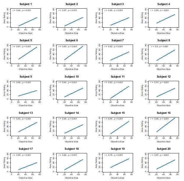
To validate this choice, we compared those ratings against an objective image-based size measure (proportion of non-black pixels within the bounding box). As shown in Author response image 3, perceptual size ratings are highly correlated with objective size across participants (Pearson r values predominantly ≈0.8 or higher; all p<0.001). Importantly, value ratings do not correlate with objective size (Author response image 2), confirming that the two rating scales capture distinct constructs. These checks support using participants’ size ratings as the participant-specific ground truth for defining SD in the PDM trials.
Author response image 1.
Objective size and value ratings are unrelated. Scatterplots show, for each participant, the correlation between objective image size (x-axis; proportion of non-black pixels within the item box) and value-based ratings (y-axis; 0–100 scale). Each dot is one food item (ratings averaged over the two value-rating repetitions). Across participants, value ratings do not track objective size, confirming that value and size are distinct constructs.
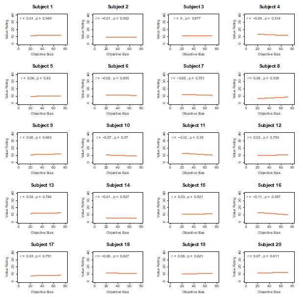
Author response image 2.
Perceptual size ratings closely track objective size. Scatterplots show, for each participant, the correlation between objective image size (x-axis) and perceptual area/size ratings (y-axis; 0–100 scale). Each dot is one food item (ratings averaged over the two perceptual ratings). Perceptual ratings are strongly correlated with objective size for nearly all participants (see main text), validating the use of these ratings to construct size-difference evidence (SD).
(2.2.2) More concerning was the effect of 'evidence level' on behaviour in the value-based task (Figure 3a). While the 'proportion correct' increases monotonically with the evidence level for the perceptual decisions, for the value-based task it increases from the lowest evidence level and then appears to plateau at just above 80%. This difference in behaviour between the two tasks brings into question the validity of the DDM which is used to fit the data, which assumes that the drift rate increases linearly in proportion to the level of evidence.
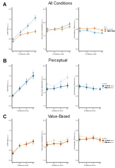
We agree that accuracy appears to asymptote in VDM, but the DDM fits indicate that the drift rate still increases monotonically with evidence in both tasks. In Supplementary figure 11, drift (δ) rises across the four evidence levels for PDM and for VDM (panels showing all data and pre/post-TMS). The apparent plateau in proportion correct during VDM reflects higher choice variability at stronger preference differences, not a failure of the drift–evidence mapping. Crucially, the model captures both the accuracy patterns and the RT distributions (see posterior predictive checks in Supplementary figures 11-16), indicating that a monotonic evidence–drift relation is sufficient to account for the data in each task.
Author response image 3.
HDDM parameters by evidence level. Group-level posterior means (± posterior SD) for drift (δ), boundary (α), and non-decision time (τ) across the four evidence levels, shown (a) collapsed across TMS sessions, (b) for PDM (blue) pre- vs post-TMS (light vs dark), and (c) for VDM (orange) pre- vs post-TMS. Crucially, drift increases monotonically with evidence in both tasks, while TMS selectively lowers α in PDM and reduces τ in VDM (see Supplementary Tables for numerical estimates).
(2.3) The paper provides very little information on the model fits (no parameter estimates, goodness of fit values or simulated behavioural predictions). The paper finds that TMS reduced the decision bound for perceptual decisions but only affected non-decision time for value-based decisions. It would aid the interpretation of this finding if the relative reliability of the fits for the two tasks was presented.
We appreciate the suggestion and have made the quantitative fit information explicit:
(1) Parameter estimates. Group-level means/SDs for drift (δ), boundary (α), and nDT (τ) are reported for PDM and VDM overall, by evidence level, pre- vs post-TMS, and per subject (see Supplementary Tables 8-11).
(2) Goodness of fit and predictive adequacy. DIC values accompany each fit in the tables. Posterior predictive checks demonstrate close correspondence between simulated and observed accuracy and RT distributions overall, by evidence level, and across subjects (Supplementary Figures 11-16).
Together, these materials document that the HDDM provides reliable fits in both tasks and accurately recovers the qualitative and quantitative patterns that underlie our inferences (reduced α for PDM only; selective τ reduction in VDM).
(2.4) Behaviourally, the perceptual task produced decreased response times and accuracy post-TMS, consistent with a reduced bound and consistent with some prior literature. Based on the results of the computational modelling, the authors conclude that RT differences in the value-based task are due to task-related learning, while those in the perceptual task are 'decision relevant'. It is not fully clear why there would be such significantly greater task-related learning in the value-based task relative to the perceptual one. And if such learning is occurring, could it potentially also tend to increase the consistency of choices, thereby counteracting any possible TMS-induced reduction of consistency?
Thank you for pointing out the need for a clearer framing. We have removed the speculative label “task-related learning” and now describe the pattern strictly in terms of the HDDM decomposition and neural results already reported:
(1) VDM: Post-TMS RTs are faster while accuracy is unchanged. The HDDM attributes this to a selective reduction in non-decision time (τ), with no change in decision-relevant parameters (α, δ) for VDM (see Supplementary Figure 11 and Supplementary Tables). Consistent with this, left SFS BOLD is not reduced for VDM, and trialwise SFS activity does not predict VDM accuracy—both observations argue against a change in VDM decision formation within left SFS.
(2) PDM: Post-TMS accuracy decreases and RTs shorten, which the HDDM captures as a lower decision boundary (α) with no change in drift (δ). Here, left SFS BOLD scales with accumulated evidence and decreases post-TMS, and trialwise SFS activity predicts PDM accuracy, all consistent with a decision-relevant effect in PDM.
Regarding the possibility that faster VDM RTs should increase choice consistency: empirically, consistency did not change in VDM, and the HDDM finds no decision-parameter shifts there. Thus, there is no hidden counteracting increase in VDM accuracy that could mask a TMS effect—the absence of a VDM accuracy change is itself informative and aligns with the modelling and fMRI.
Reviewer #3 (Public Review):
Summary:
Garcia et al., investigated whether the human left superior frontal sulcus (SFS) is involved in integrating evidence for decisions across either perceptual and/or value-based decision-making. Specifically, they had 20 participants perform two decision-making tasks (with matched stimuli and motor responses) in an fMRI scanner both before and after they received continuous theta burst transcranial magnetic stimulation (TMS) of the left SFS. The stimulation thought to decrease neural activity in the targeted region, led to reduced accuracy on the perceptual decision task only. The pattern of results across both model-free and model-based (Drift diffusion model) behavioural and fMRI analyses suggests that the left SLS plays a critical role in perceptual decisions only, with no equivalent effects found for value-based decisions. The DDM-based analyses revealed that the role of the left SLS in perceptual evidence accumulation is likely to be one of decision boundary setting. Hence the authors conclude that the left SFS plays a domain-specific causal role in the accumulation of evidence for perceptual decisions. These results are likely to add importance to the literature regarding the neural correlates of decision-making.
Strengths:
The use of TMS strengthens the evidence for the left SFS playing a causal role in the evidence accumulation process. By combining TMS with fMRI and advanced computational modelling of behaviour, the authors go beyond previous correlational studies in the field and provide converging behavioural, computational, and neural evidence of the specific role that the left SFS may play.
Sophisticated and rigorous analysis approaches are used throughout.
Weaknesses:
(3.1) Though the stimuli and motor responses were equalised between the perception and value-based decision tasks, reaction times (according to Figure 1) and potential difficulty (Figure 2) were not matched. Hence, differences in task difficulty might represent an alternative explanation for the effects being specific to the perception task rather than domain-specificity per se.
We agree that RTs cannot be matched a priori, and we did not intend them to be. Instead, we equated the inputs to the decision process and verified that each task relied exclusively on its task-relevant evidence. As reported in Results—Behaviour: validity of task-relevant pre-requisites (Fig. 1b–c), accuracy and RTs vary monotonically with the appropriate evidence regressor (SD for PDM; VD for VDM), with no effect of the task-irrelevant regressor. This separability check addresses differences in baseline RTs by showing that, for both tasks, behaviour tracks evidence as designed.
To rule out a generic difficulty account of the TMS effect, we relied on the within-subject differences-in-differences (DID) framework described in Methods (Differences-in-differences). The key Task × TMS interaction compares the pre→post change in PDM with the pre→post change in VDM while controlling for trialwise evidence and RT covariates. Any time-on-task or unspecific difficulty drift shared by both tasks is subtracted out by this contrast. Using this specification, TMS selectively reduced accuracy for PDM but not VDM (Fig. 3a; Supplementary Fig. 2a,c; Supplementary Tables 5–7).
Finally, the hierarchical DDM (already in the paper) dissociates latent mechanisms. The post-TMS boundary reduction appears only in PDM, whereas VDM shows a change in non-decision time without a decision-relevant parameter change (Fig. 3c; Supplementary Figs. 4–5). If unmatched difficulty were the sole driver, we would expect parallel effects across tasks, which we do not observe.
(3.2) No within- or between-participants sham/control TMS condition was employed. This would have strengthened the inference that the apparent TMS effects on behavioural and neural measures can truly be attributed to the left SFS stimulation and not to non-specific peripheral stimulation and/or time-on-task effects.
We agree that a sham/control condition would further strengthen causal attribution and note this as a limitation. In mitigation, our design incorporates several safeguards already reported in the manuscript:
· Within-subject pre/post with alternating task blocks and DID modelling (Methods) to difference out non-specific time-on-task effects.
· Task specificity across levels of analysis: behaviour (PDM accuracy reduction only), computational (boundary reduction only in PDM; no drift change), BOLD (reduced left-SFS accumulated-evidence signal for PDM but not VDM; Fig. 4a–c), and functional coupling (SFS–occipital PPI increase during PDM only; Fig. 5).
· Matched stimuli and motor outputs across tasks, so any peripheral sensations or general arousal effects should have influenced both tasks similarly; they did not.
Together, these converging task-selective effects reduce the likelihood that the results reflect non-specific stimulation or time-on-task. We will add an explicit statement in the Limitations noting the absence of sham/control and outlining it as a priority for future work.
(3.3) No a priori power analysis is presented.
We appreciate this point. Our sample size (n = 20) matched prior causal TMS and combined TMS–fMRI studies using similar paradigms and analyses (e.g., Philiastides et al., 2011; Rahnev et al., 2016; Jackson et al., 2021; van der Plas et al., 2021; Murd et al., 2021), and was chosen a priori on that basis and the practical constraints of cTBS + fMRI. The within-subject DID approach and hierarchical modelling further improve efficiency by leveraging all trials.
To address the reviewer’s request for transparency, we will (i) state this rationale in Methods—Participants, and (ii) ensure that all primary effects are reported with 95% CIs or posterior probabilities (already provided for the HDDM as pmcmcp_{\mathrm{mcmc}}pmcmc). We also note that the design was sensitive enough to detect RT changes in both tasks and a selective accuracy change in PDM, arguing against a blanket lack of power as an explanation for null VDM accuracy effects. We will nevertheless flag the absence of a formal prospective power analysis in the Limitations.
Recommendations for the Authors:
Reviewer #1 (Recommendations For The Authors):
Some important elements of the methods are missing. How was the site for targeting the SFS with TMS identified? The methods described how M1 was located but not SFS.
Thank you for catching this omission. In the revised Methods we explicitly describe how the left SFS target was localized. Briefly, we used each participant’s T1-weighted anatomical scan and frameless neuronavigation to place a 10-mm sphere at the a priori MNI coordinates (x = −24, y = 24, z = 36) derived from prior work (Heekeren et al., 2004; Philiastides et al., 2011). This sphere was transformed to native space for each participant. The coil was positioned tangentially with the handle pointing posterior-lateral, and coil placement was continuously monitored with neuronavigation throughout stimulation. (All of these procedures mirror what we already report for M1 and are now stated for SFS as well.)
Where to revise the manuscript:
Methods → Stimulation protocol. After the first sentence naming cTBS, insert:<br /> “The left SFS target was localized on each participant’s T1-weighted anatomical image using frameless neuronavigation. A 10-mm radius sphere was centered at the a priori MNI coordinates x = −24, y = 24, z = 36 (Heekeren et al., 2004; Philiastides et al., 2011), then transformed to native space. The MR-compatible figure-of-eight coil was positioned tangentially over the target with the handle oriented posterior-laterally, and its position was tracked and maintained with neuronavigation during stimulation.”
It is not clear how participants were instructed that they should perform the value-difference task. Were they told that they should choose based on their original item value ratings or was it left up to them?
We agree the instruction should be explicit. Participants were told_: “In value-based blocks, choose the item you would prefer to eat at the end of the experiment.”_ They were informed that one VDM trial would be randomly selected for actual consumption, ensuring incentive-compatibility. We did not ask them to recall or follow their earlier ratings; those ratings were used only to construct evidence (value difference) and to define choice consistency offline.
Where to revise the manuscript:
Methods → Experimental paradigm.
Add a sentence to the VDM instruction paragraph:
“In value-based (LIKE) blocks, participants were instructed to choose the item they would prefer to consume at the end of the experiment; one VDM trial was randomly selected and implemented, making choices incentive-compatible. Prior ratings were used solely to construct value-difference evidence and to score choice consistency; participants were not asked to recall or match their earlier ratings.”
Line 86 Introduction, some previous studies were conducted on animals. Why it is problematic that the studies were conducted in animals is not stated. I assume the authors mean that we do not know if their findings will translate to the human brain? I think in fairness to those working with animals it might be worth an extra sentence to briefly expand on this point.
We appreciate this and will clarify that animal work is invaluable for circuit-level causality, but species differences and putative non-homologous areas (e.g., human SFS vs. rodent FOF) limit direct translation. Our point is not that animal studies are problematic, but that establishing causal roles in humans remains necessary.
Revision:
Introduction (paragraph discussing prior animal work). Replace the current sentence beginning “However, prior studies were largely correlational”
“Animal studies provide critical causal insights, yet direct translation to humans can be limited by species-specific anatomy and potential non-homologies (e.g., human SFS vs. frontal orienting fields in rodents). Therefore, establishing causal contributions in the human brain remains essential.”
Line 100-101: "or whether its involvement is peripheral and merely functionally supporting a larger system" - it is not clear what you mean by 'supporting a larger system'
We meant that observed SFS activity might reflect upstream/downstream support processes (e.g., attentional control or working-memory maintenance) rather than the computation of evidence accumulation itself. We have rephrased to avoid ambiguity.
Revision:
Introduction. Replace the phrase with:
“or whether its observed activity reflects upstream or downstream support processes (e.g., attention or working-memory maintenance) rather than the accumulation computation per se.”
The authors do have to make certain assumptions about the BOLD patterns that would be expected of an evidence accumulation region. These assumptions are reasonable and have been adopted in several previous neuroimaging studies. Nevertheless, it should be acknowledged that alternative possibilities exist and this is an inevitable limitation of using fMRI to study decision making. For example, if it turns out that participants collapse their boundaries as time elapses, then the assumption that trials with weaker evidence should have larger BOLD responses may not hold - the effect of more prolonged activity could be cancelled out by the lower boundaries. Again, I think this is just a limitation that could be acknowledged in the Discussion, my opinion is that this is the best effort yet to identify choice-relevant regions with fMRI and the authors deserve much credit for their rigorous approach.
Agreed. We already ground our BOLD regressors in the DDM literature, but acknowledge that alternative mechanisms (e.g., time-dependent boundaries) can alter expected BOLD–evidence relations. We now add a short limitation paragraph stating this explicitly.
Revision:
Discussion (limitations paragraph). Add:
“Our fMRI inferences rest on model-based assumptions linking accumulated evidence to BOLD amplitude. Alternative mechanisms—such as time-dependent (collapsing) boundaries—could attenuate the prediction that weaker-evidence trials yield longer accumulation and larger BOLD signals. While our behavioural and neural results converge under the DDM framework, we acknowledge this as a general limitation of model-based fMRI.”
Reviewer #2 (Recommendations For The Authors):
Minor points
I suggest the proportion of missed trials should be reported.
Thank you for the suggestion. In our preprocessing we excluded trials with no response within the task’s response window and any trials failing a priori validity checks. Because non-response trials contain neither a choice nor an RT, they are not entered into the DDM fits or the fMRI GLMs and, by design, carry no weight in the reported results. To keep the focus on the data that informed all analyses, we now (i) state the trial-inclusion criteria explicitly and (ii) report the number of analysed (valid) trials per task and run. This conveys the effective sample size contributing to each condition without altering the analysis set.
Revision:
Methods → (at the end of “Experimental paradigm”): “Analyses were conducted on valid trials only, defined as trials with a registered response within the task’s response window and passing pre-specified validity checks; trials without a response were excluded and not analysed.”
Results → “Behaviour: validity of task-relevant pre-requisites” (add one sentence at the end of the first paragraph): “All behavioural and fMRI analyses were performed on valid trials only (see Methods for inclusion criteria).”
Figure 4 c is very confusing. Is the legend or caption backwards?
Thanks for flagging. We corrected the Figure 4c caption to match the colouring and contrasts used in the panel (perceptual = blue/green overlays; value-based = orange/red; ‘post–pre’ contrasts explicitly labeled). No data or analyses were changed, just the wording to remove ambiguity.
Revision:
Figure 4 caption (panel c sentence). Replace with:
“(c) Post–pre contrasts for the trialwise accumulated-evidence regressor show reduced left-SFS BOLD during perceptual decisions (green overlay), with a significantly stronger reduction for perceptual vs value-based decisions (blue overlay). No reduction is observed for value-based decisions.”
Even if not statistically significant it may be of interest to add the results for Value-based decision making on SFS in Supplementary Table 3.
Done. We now include the SFS small-volume results for VDM (trialwise accumulated-evidence regressor) alongside the PDM values in the same table, with exact peak, cluster size, and statistics.
Revision:
Supplementary Table 3 (title):
“Regions encoding trialwise accumulated evidence (parametric modulation) during perceptual and value-based decisions, including SFS SVC results for both tasks.”
Model comparisons: please explain how model complexity is accounted for.
We clarify that model evidence was compared using the Deviance Information Criterion (DIC), which penalizes model fit by an effective number of parameters (pD). Lower DIC indicates better out-of-sample predictive performance after accounting for model complexity.
Revision:
Methods → Hierarchical Bayesian neural-DDM (last paragraph). Add:
“Model comparison used the Deviance Information Criterion (DIC = D̄ + pD), where pD is the effective number of parameters; thus DIC penalizes model complexity. Lower DIC denotes better predictive accuracy after accounting for complexity.”
Reviewer #3 (Recommendations For The Authors):
The following issues would benefit from clarification in the manuscript:
- It is stated that "Our sample size is well within acceptable range, similar to that of previous TMS studies." The sample size being similar to previous studies does not mean it is within an acceptable range. Whether the sample size is acceptable or not depends on the expected effect size. It is perfectly possible that the previous studies cited were all underpowered. What implications might the lack of an a priori power analysis have for the interpretation of the results?
We agree and have revised our wording. We did not conduct an a priori power analysis. Instead, we relied on a within-participant design that typically yields higher sensitivity in TMS–fMRI settings and on convergence across behavioural, computational, and neural measures. We now acknowledge that the absence of formal power calculations limits claims about small effects (particularly for null findings in VDM), and we frame those null results cautiously.
Revision:
Discussion (limitations). Add:
“The within-participant design enhances statistical sensitivity, yet the absence of an a priori power analysis constrains our ability to rule out small effects, particularly for null results in VDM.”
- I was confused when trying to match the results described in the 'Behaviour: validity of task-relevant pre-requisites' section on page 6 to what is presented in Figure 1. Specifically, Figure 1C is cited 4 times but I believe two of these should be citing Figure 1B?
Thank you—this was a citation mix-up. The two places that referenced “Fig. 1C” but described accuracy should in fact point to Fig. 1B. We corrected both citations.
Revision:
Results → Behaviour: validity… Change the two incorrect “Fig. 1C” references (when describing accuracy) to “Fig. 1B”.
- Also, where is the 'SD' coefficient of -0.254 (p-value = 0.123) coming from in line 211? I can't match this to the figure.
This was a typographical error in an earlier draft. The correct coefficients are those shown in the figure and reported elsewhere in the text (evidence-specific effects: for PDM RTs, SD β = −0.057, p < 0.001; for VDM RTs, VD β = −0.016, p = 0.011; non-relevant evidence terms are n.s.). We removed the erroneous value.
Revision:
Results → Behaviour: validity… (sentence with −0.254). Delete the incorrect value and retain the evidence-specific coefficients consistent with Fig. 1B–C.
- It is reported that reaction times were significantly faster for the perceptual relative to the value-based decision task. Was overall accuracy also significantly different between the two tasks? It appears from Figure 3 that it might be, But I couldn't find this reported in the text.
To avoid conflating task with evidence composition, we did not emphasize between-task accuracy averages. Our primary tests examine evidence-specific effects and TMS-induced changes within task. For completeness, we now report descriptive mean accuracies by task and point readers to the figure panels that display accuracy as a function of evidence (which is the meaningful comparison in our matched-evidence design). We refrain from additional hypothesis testing here to keep the analyses aligned with our preregistered focus.
Revision:
Results → Behaviour: validity… Add:
“For completeness, group-mean accuracies by task are provided descriptively in Fig. 3a; inferential tests in the manuscript focus on evidence-specific effects and TMS-induced changes within task.”
Author response:
The following is the authors’ response to the original reviews
Public Reviews:
Reviewer #1 (Public review):
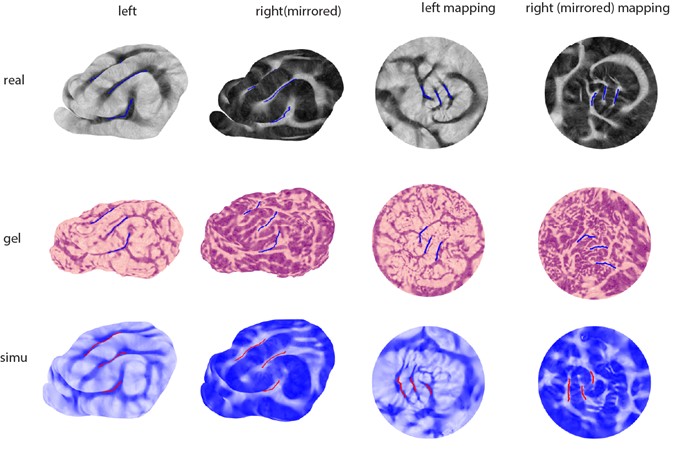
The manuscript by Yin and colleagues addresses a long-standing question in the field of cortical morphogenesis, regarding factors that determine differential cortical folding across species and individuals with cortical malformations. The authors present work based on a computational model of cortical folding evaluated alongside a physical model that makes use of gel swelling to investigate the role of a two-layer model for cortical morphogenesis. The study assesses these models against empirically derived cortical surfaces based on MRI data from ferret, macaque monkey, and human brains.
The manuscript is clearly written and presented, and the experimental work (physical gel modeling as well as numerical simulations) and analyses (subsequent morphometric evaluations) are conducted at the highest methodological standards. It constitutes an exemplary use of interdisciplinary approaches for addressing the question of cortical morphogenesis by bringing together well-tuned computational modeling with physical gel models. In addition, the comparative approaches used in this paper establish a foundation for broad-ranging future lines of work that investigate the impact of perturbations or abnormalities during cortical development.
The cross-species approach taken in this study is a major strength of the work. However, correspondence across the two methodologies did not appear to be equally consistent in predicting brain folding across all three species. The results presented in Figures 4 (and Figures S3 and S4) show broad correspondence in shape index and major sulci landmarks across all three species. Nevertheless, the results presented for the human brain lack the same degree of clear correspondence for the gel model results as observed in the macaque and ferret. While this study clearly establishes a strong foundation for comparative cortical anatomy across species and the impact of perturbations on individual morphogenesis, further work that fine-tunes physical modeling of complex morphologies, such as that of the human cortex, may help to further understand the factors that determine cortical functionalization and pathologies.
We thank the reviewer for positive opinions and helpful comments. Yes, the physical gel model of the human brain has a lower similarity index with the real brain. There are several reasons.
First, the highly convoluted human cortex has a few major folds (primary sulci) and a very large number of minor folds associated with secondary or tertiary sulci (on scales of order comparable to the cortical thickness), relative to the ferret and macaque cerebral cortex. In our gel model, the exact shapes, positions, and orientations of these minor folds are stochastic, which makes it hard to have a very high similarity index of the gel models when compared with the brain of a single individual.
Second, in real human brains, these minor folds evolve dynamically with age and show differences among individuals. In experiments with the gel brain, multiscale folds form and eventually disappear as the swelling progresses through the thickness. Our physical model results are snapshots during this dynamical process, which makes it hard to have a concrete one-to-one correspondence between the instantaneous shapes of the swelling gel and the growing human brain.
Third, the growth of the brain cortex is inhomogeneous in space and varying with time, whereas, in the gel model, swelling is relatively homogeneous.
We agree that further systematic work, based on our proposed methods, with more fine-tuned gel geometries and properties, might provide a deeper understanding of the relations between brain geometry, and growth-induced folds and their functionalization and pathologies. Further analysis of cortical pathologies using computational and physical gel models can be found in our companion paper (Choi et al., 2025), also published in eLife:
G. P. T. Choi, C. Liu, S. Yin, G. Séjourné, R. S. Smith, C. A. Walsh, L. Mahadevan, Biophysical basis for brain folding and misfolding patterns in ferrets and humans. eLife, 14, RP107141, 2025. doi:10.7554/eLife.107141
Reviewer# 2 (Public review):
This manuscript explores the mechanisms underlying cerebral cortical folding using a combination of physical modelling, computational simulations, and geometric morphometrics. The authors extend their prior work on human brain development (Tallinen et al., 2014; 2016) to a comparative framework involving three mammalian species: ferrets (Carnivora), macaques (Old World monkeys), and humans (Hominoidea). By integrating swelling gel experiments with mathematical differential growth models, they simulate sulcification instability and recapitulate key features of brain folding across species. The authors make commendable use of publicly available datasets to construct 3D models of fetal and neonatal brain surfaces: fetal macaque (ref. [26]), newborn ferret (ref. [11]), and fetal human (ref. [22]).
Using a combination of physical models and numerical simulations, the authors compare the resulting folding morphologies to real brain surfaces using morphometric analysis. Their results show qualitative and quantitative concordance with observed cortical folding patterns, supporting the view that differential tangential growth of the cortex relative to the subcortical substrate is sufficient to account for much of the diversity in cortical folding. This is a very important point in our field, and can be used in the teaching of medical students.
Brain folding remains a topic of ongoing debate. While some regard it as a critical specialization linked to higher cognitive function, others consider it an epiphenomenon of expansion and constrained geometry. This divergence was evident in discussions during the Strungmann Forum on cortical development (Silver¨ et al., 2019). Though folding abnormalities are reliable indicators of disrupted neurodevelopmental processes (e.g., neurogenesis, migration), their relationship to functional architecture remains unclear. Recent evidence suggests that the absolute number of neurons varies significantly with position-sulcus versus gyrus-with potential implications for local processing capacity (e.g., https://doi.org/10.1002/cne.25626). The field is thus in need of comparative, mechanistic studies like the present one.
This paper offers an elegant and timely contribution by combining gel-based morphogenesis, numerical modelling, and morphometric analysis to examine cortical folding across species. The experimental design - constructing two-layer PDMS models from 3D MRI data and immersing them in organic solvents to induce differential swelling - is well-established in prior literature. The authors further complement this with a continuum mechanics model simulating folding as a result of differential growth, as well as a comparative analysis of surface morphologies derived from in vivo, in vitro, and in silico brains.
We thank the reviewer for the very positive comments.
I offer a few suggestions here for clarification and further exploration:
Major Comments
(1) Choice of Developmental Stages and Initial Conditions
The authors should provide a clearer justification for the specific developmental stages chosen (e.g., G85 for macaque, GW23 for human). How sensitive are the resulting folding patterns to the initial surface geometry of the gel models? Given that folding is a nonlinear process, early geometric perturbations may propagate into divergent morphologies. Exploring this sensitivity-either through simulations or reference to prior work-would enhance the robustness of the findings.
The initial geometry is one of the important factors that decides the final folding pattern. The smooth brain in the early developmental stage shows a broad consistency across individuals, and we expect the main folds to form similarly across species and individuals.
Generally, we choose the initial geometry when the brain cortex is still relatively smooth. For the human, this corresponds approximately to GW23, as the major folds such as the Rolandic fissure (central sulcus), arise during this developmental stage. For the macaque brain, we chose developmental stage G85, primarily because of the availability of the dataset corresponding to this time, which also corresponds to the least folded.
We expect that large-scale folding patterns are strongly sensitive to the initial geometry but fine-scale features are not. Since our goal is to explain the large-scale features, we expect sensitivity to the initial shape.
Below are some references of other researchers that are consistent with this idea. Figure 4 from Wang et al. shows some images of simulations obtained by perturbing the geometry of a sphere to an ellipsoid. We see that the growth-induced folds mostly maintain their width (wavelength), but change their orientations.
Reference:
Wang, X., Lefévre, J., Bohi, A., Harrach, M.A., Dinomais, M. and Rousseau, F., 2021. The influence of biophysical parameters in a biomechanical model of cortical folding patterns. Scientific Reports, 11(1), p.7686.
Related results from the same group show that slight perturbations of brain geometry, cause these folds also tend to change their orientations but not width/wavelength (Bohi et al., 2019).
Reference:
Bohi, A., Wang, X., Harrach, M., Dinomais, M., Rousseau, F. and Lefévre, J., 2019, July. Global perturbation of initial geometry in a biomechanical model of cortical morphogenesis. In 2019 41st Annual International Conference of the IEEE Engineering in Medicine and Biology Society (EMBC) (pp. 442-445). IEEE.
Finally, a systematic discussion of the role of perturbations on the initial geometries and physical properties can be seen in our work on understanding a different system, gut morphogenesis (Gill et al., 2024).
We have added the discussion about geometric sensitivity in the section Methods-Numerical Simulations:
“Small perturbations on initial geometry would affect minor folds, but the main features of major folds, such as orientations, width, and depth, are expected to be conserved across individuals [49, 50]. For simplicity, we do not perturb the fetal brain geometry obtained from datasets.”
(2) Parameter Space and Breakdown Points
The numerical model assumes homogeneous growth profiles and simplifies several aspects of cortical mechanics. Parameters such as cortical thickness, modulus ratios, and growth ratios are described in Table II. It would be informative to discuss the range of parameter values for which the model remains valid, and under what conditions the physical and computational models diverge. This would help delineate the boundaries of the current modelling framework and indicate directions for refinement.
Exploring the valid parameter space is a key problem. We have tested a series of growth parameters and will state them explicitly in our revision. In the current version, we chose the ones that yield a relatively high similarity index to the animal brains. More generally, folding patterns are largely regulated by geometry as well as physical parameters, such as cortical thickness, modulus ratios, growth ratios, and inhomogeneity. In our previous work on a different system, gut morphogenesis, where similar folding patterns are seen, we have explored these features (Gill et al., 2024).
Reference:
Gill, H.K., Yin, S., Nerurkar, N.L., Lawlor, J.C., Lee, C., Huycke, T.R., Mahadevan, L. and Tabin, C.J., 2024. Hox gene activity directs physical forces to differentially shape chick small and large intestinal epithelia. Developmental Cell, 59(21), pp.2834-2849.
(3) Neglected Regional Features: The Occipital Pole of the Macaque
One conspicuous omission is the lack of attention to the occipital pole of the macaque, which is known to remain smooth even at later gestational stages and has an unusually high neuronal density (2.5× higher than adjacent cortex). This feature is not reproduced in the gel or numerical models, nor is it discussed. Acknowledging this discrepancy-and speculating on possible developmental or mechanical explanationswould add depth to the comparative analysis. The authors may wish to include this as a limitation or a target for future work.
Yes, we have added that the omission of the Occipital Pole of the macaque is one of our paper’s limitations. Our main aim in this paper is to explore the formation of large-scale folds, so the smooth region is not discussed. But future work could include this to make the model more complete.
The main text has been modified in Methods, Numerical simulations:
“To focus on fold formation, we did not discuss the relatively smooth region, such as the Occipital Pole of the macaque.”
and also in the caption of Figure 4: “... The occipital pole region of macaque brains remains smooth in real and simulated brains.”
(4) Spatio-Temporal Growth Rates and Available Human Data
The authors note that accurate, species-specific spatio-temporal growth data are lacking, limiting the ability to model inhomogeneous cortical expansion. While this may be true for ferret and macaque, there are high-quality datasets available for human fetal development, now extended through ultrasound imaging (e.g., https://doi.org/10.1038/s41586-023-06630-3). Incorporating or at least referencing such data could improve the fidelity of the human model and expand the applicability of the approach to clinical or pathological scenarios.
We thank the reviewer for pointing out the very useful datasets that exist for the exploration of inhomogeneous growth driven folding patterns. We have referred to this paper to provide suggestions for further work in exploring the role of growth inhomogeneities.
We have referred to this high-quality dataset in our main text, Discussion:
“...the effect of inhomogeneous growth needs to be further investigated by incorporating regional growth of the gray and white matter not only in human brains [29, 31] based on public datasets [45], but also in other species.”
A few works have tried to incorporate inhomogeneous growth in simulating human brain folding by separating the central sulcus area into several lobes (e.g., lobe parcellation method, Wang, PhD Thesis, 2021). Since our goal in this paper is to explain the large-scale features of folding in a minimal setting, we have kept our model simple and show that it is still capable of capturing the main features of folding in a range of mammalian brains.
Reference:
Xiaoyu Wang. Modélisation et caractérisation du plissement cortical. Signal and Image Processing. Ecole nationale superieure Mines-Télécom Atlantique, 2021. English. 〈NNT : 2021IMTA0248〉.
(5) Future Applications: The Inverse Problem and Fossil Brains
The authors suggest that their morphometric framework could be extended to solve the inverse growth problem-reconstructing fetal geometries from adult brains. This speculative but intriguing direction has implications for evolutionary neuroscience, particularly the interpretation of fossil endocasts. Although beyond the scope of this paper, I encourage the authors to elaborate briefly on how such a framework might be practically implemented and validated.
For the inverse problem, we could use the following strategies:
a. Perform systematic simulations using different geometries and physical parameters to obtain the variation in morphologies as a function of parameters.
b. Using either supervised training or unsupervised training (physics-informed neural networks, PINNs) to learn these characteristic morphologies and classify their dependence on the parameters using neural networks. These can then be trained to determine the possible range of geometrical and physical parameters that yield buckled patterns seen in the systematic simulations.
c. Reconstruct the 3D surface from fossil endocasts. Using the well-trained neural network, it should be possible to predict the initial shape of the smooth brain cortex, growth profile, and stiffness ratio of the gray and white matter.
As an example in this direction, supervised neural networks have been used recently to solve the forward problem to predict the buckling pattern of a growing two-layer system (Chavoshnejad et al., 2023). The inverse problem can then be solved using machine-learning methods when the training datasets are the folded shape, which are then used to predict the initial geometry and physical properties.
Reference:
Chavoshnejad, P., Chen, L., Yu, X., Hou, J., Filla, N., Zhu, D., Liu, T., Li, G., Razavi, M.J. and Wang, X., 2023. An integrated finite element method and machine learning algorithm for brain morphology prediction. Cerebral Cortex, 33(15), pp.9354-9366.
Conclusion
This is a well-executed and creative study that integrates diverse methodologies to address a longstanding question in developmental neurobiology. While a few aspects-such as regional folding peculiarities, sensitivity to initial conditions, and available human data-could be further elaborated, they do not detract from the overall quality and novelty of the work. I enthusiastically support this paper and believe that it will be of broad interest to the neuroscience, biomechanics, and developmental biology communities.
Note: The paper mentions a companion paper [reference 11] that explores the cellular and anatomical changes in the ferret cortex. I did not have access to this manuscript, but judging from the title, this paper might further strengthen the conclusions.
The companion paper (Choi et al., 2025) has also been submitted to eLife and can be found here:
G. P. T. Choi, C. Liu, S. Yin, G. Séjourné, R. S. Smith, C. A. Walsh, L. Mahadevan, Biophysical basis for brain folding and misfolding patterns in ferrets and humans. eLife, 14, RP107141, 2025. doi:10.7554/eLife.107141
Recommendations for the authors:
Reviewer #1 (Recommendations for the authors):
This study was conducted and presented to the highest methodological standards. It is clearly written, and the results are thoroughly presented in the main manuscript and supplementary materials. Nevertheless, I would present the following minor points and comments for consideration by the authors prior to finalizing their work:
We thank the reviewer for positive opinions and helpful comments.
(1) Where did the MRI-based cortical surface data come from? Specifically, it would be helpful to include more information regarding whether the surfaces were reconstructed based on individual- or group-level data. It appears the surfaces were group-level, and, if so, accounting for individual-level cortical folding may be a fruitful direction for future work.
The surface data come from public database, which are stated in the Methods Section. “We used a publicly available database for all our 3d reconstructions: fetal macaque brain surfaces are obtained from Liu et al. (2020); newborn ferret brain surfaces are obtained from Choi et al. (2025); and fetal human brain surfaces are obtained from Tallinen et al. (2016).”
These surfaces are reconstructed based on group-level data. Specifically, the macaque atlas images are constructed for brains at gestational ages of 85 days (G85, N \=18_, 9 females), 110 days (G110, _N \=10_, 7 females) and 135 days (G135, _N \=16_,_ 7 females). And yes, future work may focus on individual-level cortical folding, and we expect that more specific results could be found.
(2) One methodological approach for assessing consistency of cortical folding within species might be an evaluation of cross-hemispheric symmetry. I would find this particularly interesting with respect to the gel models, as it could complement the quantification of variation with respect to the computationally derived and real surfaces.
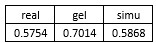
Yes, the cross-hemispheric symmetry comparison can be done by our morphometric analysis method. We have added the results of ferret brain’s left-right symmetry for gel models, simulations, and real surfaces in the supplementary material. A typical conformal mapping figure and the similarity index table are shown here.
(3) Was there a specific reason to reorder the histogram plots in Figure 4c to macaque, ferret, human rather than to maintain the order presented in Figure 4a/b of ferret, macaque, human? I appreciate that this is a minor concern, and all subplots are indeed properly titled, but consistent order may improve clarity.
We have reordered the histogram plots to make all the figure orders consistent.
Reviewer #2 (Recommendations for the authors):
(1) Please consider revising the caption of Figure 1 (or equivalent figures) to explicitly state whether features such as the macaque occipital flatness were reproduced or not.
We thank the reviewer for pointing out the macaque occipital flatness.
Author response table 1.
Left-right similarity index evaluated by comparing the shape index of ferret brains, calculated with vector P-NORM p\=2,
Author response image 1.
Left-right similarity index of ferret brains
Occipital Pole of the macaque remains relatively smooth in both real brains and computational models. But our main aim in this paper is to explore the large-scale folds formation, so the smooth region is not discussed in depth. But future work could include this to make the model more complete.
(2) Some figures could benefit from clearer labelling to distinguish between in vivo, in vitro, and in silico results.
We have supplemented some texts in panels to make the labelling clearer.
(3) The manuscript would benefit from a short paragraph in the Discussion reflecting on how future incorporation of regional heterogeneities might improve model fidelity.
We have added a sentence in the Discussion Section about improving the model fidelity by considering regional heterogeneities.
“Future more accurate models incorporating spatio-temporal inhomogeneous growth profiles and mechanical properties, such as varying stiffness, would make the folding pattern closer to the real cortical folding. This relies on more in vivo measurements of the brain’s physical properties and cortical expansion.”
(4) Suggestions for improved or additional experiments, data, or analyses.
(5) Clarify and justify the selection of developmental stages: The authors should explain why particular gestational stages (e.g., G85 for macaque, GW23 for human) were chosen as starting points for the physical and computational models. A discussion of how sensitive the folding patterns are to the initial geometry would help assess the robustness of the model. If feasible, a brief sensitivity analysis-varying initial age or surface geometry-would strengthen the conclusions.
The initial geometry is one of the important factors that decides the final folding pattern. The smooth brain in the early developmental stage shows a broad consistency across individuals, and we expect the main folds to form similarly across species and individuals.
Generally, we choose the initial geometry when the brain cortex is still relatively smooth. For the human, this corresponds approximately to GW23, as the major folds such as the Rolandic fissure (central sulcus), arise during this developmental stage. For the macaque brain, we chose developmental stage G85, primarily because of the availability of the dataset corresponding to this time, which also corresponds to the least folded.
We expect that large-scale folding patterns are strongly sensitive to the initial geometry but fine-scale features are not. Since our goal is to explain the large-scale features, we expect sensitivity to the initial shape.
We have added the discussion about geometric sensitivity in the section Methods-Numerical Simulations: “Small perturbations on initial geometry would affect minor folds, but the main features of major folds, such as orientations, width, and depth, are expected to be conserved across individuals [49, 50]. For simplicity, we do not perturb the fetal brain geometry obtained from datasets.”
(6) Explore parameter boundaries more explicitly: The paper would benefit from a clearer account of the ranges of mechanical and geometric parameters (e.g., growth ratios, cortical thickness) for which the model holds. Are there specific conditions under which the physical and numerical models diverge? Identifying breakdown points would help readers understand the model’s limitations and applicability.
Exploring the valid parameter space is a key problem. We have tested a series of growth parameters and will state them explicitly in our revision. In the current version, we chose the ones that yield a relatively high similarity index to the animal brains. More generally, folding patterns are largely regulated by geometry as well as physical parameters, such as cortical thickness, modulus ratios, and growth ratios and inhomogeneity. In our previous work on a different system, gut morphogenesis, where similar folding patterns are seen, we have explored these features (Gill et al., 2024).
(7) Address species-specific cortical peculiarities: A striking omission is the flat occipital pole of the macaque, which is not reproduced in the physical or computational models. Given its known anatomical and cellular distinctiveness, this discrepancy warrants discussion. Even if not explored experimentally, the authors could speculate on what developmental or mechanical conditions would be needed to reproduce such regional smoothness.
Please refer to our answer to the public reviewer 2, question (3). From our results, the formation of smooth Occipital Pole might indicate that the spatio-temporal growth rate of gray and white matter are consistent in this region, such that there’s no much differential growth.
(8) Consider integration of available human growth data: While the authors note the lack of spatiotemporal growth data across species, such datasets exist for human fetal brain development, including those from MRI and ultrasound studies (e.g., Nature 2023). Incorporating these into the human model-or at least discussing their implications-would enhance biological relevance.
Yes, some datasets for fetal human brains have provided very comprehensive measurements on brain shapes at many developmental stages. This can surely be implemented in our current model by calculating the spatio-temporal growth rate from regional cortical shapes at different stages.
(9) Recommendations for improving the writing and presentation:
a) The manuscript is generally well-written, but certain sections would benefit from more explicit linksbetween the biological phenomena and the modeling framework. For instance, the Introduction and Discussion could more clearly articulate how mechanical principles interface with genetic or cellular processes, especially in the context of evolution and developmental variation.
We have briefly discussed the gene-regulated cellular process and the induced changes of mechanical properties and growth rules in SI, table S1. In the main text, to be clearer, we have added a sentence:
“Many malformations are related to gene-regulated abnormal cellular processes and mechanical properties, which are discussed in SI”
b) The Discussion could better acknowledge limitations and future directions, including regional dif-ferences in folding, inter-individual variability, and the model’s assumptions of homogeneous material properties and growth.
In the discussion section, we have pointed out four main limitations and open directions based on our current model, including the discussion on spatiotemporal growth and property. To be more complete, we have supplemented other limitations on the regional differences in folding and the interindividual variability. In the main text, we added the following sentence:
“In addition to the homogeneity assumption, we have not investigated the inter-individual variability and regional differences in folding. More accurate and specific work is expected to focus on these directions.”
c) The authors briefly mention the potential for addressing the inverse growth problem. Expanding this idea in a short paragraph - perhaps with hypothetical applications to fossil brain reconstructions-would broaden the paper’s appeal to evolutionary neuroscientists.
We have stated general steps in the response to public reviewer 2, question (5).
(10) Minor corrections to the text and figures:
a) Figures:
Label figures more clearly to distinguish between in vivo, in vitro, and in silico brain representations.– Ensure that the occipital pole of the macaque is visible or annotated, especially if it lacks the expected smoothness.
Add scale bars where missing for clarity in morphometric comparisons.
We thank the reviewer for suggestions to improve the readability of our manuscript.
The in vivo (real), in vitro (gel), and in silico (simulated) results are both distinguished by their labels and different color scheme: gray-white for real brain, pink-white for gel model, and blue-white for simulations, respectively.
The occipital pole of the macaque brain remains relatively smooth in our computational model but notin our physical gel model. We have clarified this in the main text: “To focus on fold formation, we did not discuss the relatively smooth region, such as the Occipital Pole of the macaque.”
All the brain models are rescaled to the same size, where the distance between the anterior-most pointof the frontal lobe and the posterior-most point of the occipital lobe is two units.
b) Text:
Consider revising figure captions to explicitly mention whether specific regional features (e.g., flatoccipital pole) were observed or absent in models.
In Table II (and relevant text), ensure parameter definitions are consistent and explained clearly for across-disciplinary audience.
Add citations to recent human fetal growth imaging work (e.g., ultrasound-based studies) to support claims about available data.
We have added some descriptions of the characters of the folding pattern in the caption of Figure 4,including major folds and smooth regions.
“Three or four major folds of each brain model are highlighted and served as landmarks. The occipital pole region of macaque brains remains smooth in real and simulated brains.”
We have clarified the definition of growth ratio gMsub>g</sub>/g<sub>w</sub> and stiffness ratio µ<sub>g</sub>/µ<sub>w</sub> between gray matter and white matter, and the normalized cortical thickness h/L in Table 2.
We have referred to a high-quality dataset of fetal brain imaging work, the ultrasound-imaging method(Namburete et al. 2023), in our main text, Discussion:
“...the effect of inhomogeneous growth needs to be further investigated by incorporating regional growth of the gray and white matter not only in human brains [29, 31] based on public datasets [45], but also in other species.”
3 Import
Import should be in the results section, so double ##Import
Author response:
The following is the authors’ response to the original reviews.
Reviewer #1 (Public review):
Lack of Sensitivity Analyses for some Key Methodological Decisions: Certain methodological choices in this manuscript diverge from approaches used in previous works. In these cases, I recommend the following: (i) The authors could provide a clear and detailed justification for these deviations from established methods, and (ii) supplementary sensitivity analyses could be included to ensure the robustness of the findings, demonstrating that the results are not driven primarily by these methodological changes. Below, I outline the main areas where such evaluations are needed:
This detailed guidance is incredibly valuable, and we are grateful. Work of this kind is in its relative infancy, and there are so many design choices depending on the data available, questions being addressed, and so on. Help us navigate that has been extremely useful. In our revised manuscript we are very happy to add additional justification for design choices made, and wherever possible test the impact of those choices. It is certainly the case that different approaches have been used across the handful of papers published in this space, and, unlike in other areas of systems neuroscience, we have yet to reach the point where any of these approaches are established. We agree with the reviewer that wherever possible these design choices should be tested.
Use of Communicability Matrices for Structural Connectivity Gradients: The authors chose to construct structural connectivity gradients using communicability matrices, arguing that diffusion map embedding "requires a smooth, fully connected matrix." However, by definition, the creation of the affinity matrix already involves smoothing and ensures full connectedness. I recommend that the authors include an analysis of what happens when the communicability matrix step is omitted. This sensitivity test is crucial, as it would help determine whether the main findings hold under a simpler construction of the affinity matrix. If the results significantly change, it could indicate that the observations are sensitive to this design choice, thereby raising concerns about the robustness of the conclusions. Additionally, if the concern is related to the large range of weights in the raw structural connectivity (SC) matrix, a more conventional approach is to apply a log-transformation to the SC weights (e.g., log(1+𝑆𝐶<sub>𝑖𝑗</sub>)), which may yield a more reliable affinity matrix without the need for communicability measures.
The reason we used communicability is indeed partly because we wanted to guarantee a smooth fully connected matrix, but also because our end goal for this project was to explore structure-function coupling in these low-dimensional manifolds. Structural communicability – like standard metrics of functional connectivity – includes both direct and indirect pathways, whereas streamline counts only capture direct communication. In essence we wanted to capture not only how information might be routed from one location to another, but also the more likely situation in which information propagates through the system.
In the revised manuscript we have given a clearer justification for why we wanted to use communicability as our structural measure (Page 4, Line 179):
“To capture both direct and indirect paths of connectivity and communication, we generated weighted communicability matrices using SIFT2-weighted fibre bundle capacity (FBC). These communicability matrices reflect a graph theory measure of information transfer previously shown to maximally predict functional connectivity (Esfahlani et al., 2022; Seguin et al., 2022). This also foreshadowed our structure-function coupling analyses, whereby network communication models have been shown to increase coupling strength relative to streamline counts (Seguin et al., 2020)”.
We have also referred the reader to a new section of the Results that includes the structural gradients based on the streamline counts (Page 7, line 316):
“Finally, as a sensitivity analysis, to determine the effect of communicability on the gradients, we derived affinity matrices for both datasets using a simpler measure: the log of raw streamline counts. The first 3 components derived from streamline counts compared to communicability were highly consistent across both NKI (r<sub>s</sub> = 0.791, r<sub>s</sub> = 0.866, r<sub>s</sub> = 0.761) and the referred subset of CALM (r<sub>s</sub> = 0.951, r<sub>s</sub> = 0.809, r<sub>s</sub> = 0.861), suggesting that in practice the organisational gradients are highly similar regardless of the SC metric used to construct the affinity matrices”.
Methodological ambiguity/lack of clarity in the description of certain evaluation steps: Some aspects of the manuscript’s methodological description are ambiguous, making it challenging for future readers to fully reproduce the analyses based on the information provided. I believe the following sections would benefit from additional detail and clarification:
Computation of Manifold Eccentricity: The description of how eccentricity was computed (both in the results and methods sections) is unclear and may be problematic. The main ambiguity lies in how the group manifold origin was defined or computed. (1) In the results section, it appears that separate manifold origins were calculated for the NKI and CALM groups, suggesting a dataset-specific approach. (2) Conversely, the methods section implies that a single manifold origin was obtained by somehow combining the group origins across the three datasets, which seems contradictory. Moreover, including neurodivergent individuals in defining the central group manifold origin in conceptually problematic. Given that neurodivergent participants might exhibit atypical brain organization, as suggested by Figure 1, this inclusion could skew the definition of what should represent a typical or normative brain manifold. A more appropriate approach might involve constructing the group manifold origin using only the neurotypical participants from both the NKI and CALM datasets. Given the reported similarity between group-level manifolds of neurotypical individuals in CALM and NKI, it would be reasonable to expect that this combined origin should be close to the origin computed within neurotypical samples of either NKI or CALM. As a sanity check, I recommend reporting the distance of the combined neurotypical manifold origin to the centres of the neurotypical manifolds in each dataset. Moreover, if the manifold origin was constructed while utilizing all samples (including neurodivergent samples) I think this needs to be reconsidered.
This is a great point, and we are very happy to clarify. Separate manifolds were calculated for the NKI and CALM participants, hence a dataset-specific approach. Indeed, in the long-run our goal was to explore individual differences in these manifolds, relative to the respective group-level origins, and their intersection across modalities, so manifold eccentricity was calculated at an individual level for subsequent analyses. At the group level, for each modality, we computed 3 manifold origins: one for NKI, one for the referred subset of CALM, and another for the neurotypical portion of CALM. Crucially, because the manifolds are always normal, in each case the manifold origin point is near-zero (extremely near-zero, to the 6<sup>th</sup> or 7<sup>th</sup> decimal place). In other words, we do indeed calculate the origin separately each time we calculate the gradients, but the origin is zero in every case. As a result, differences in the origin point cannot be the source of any differences we observe in manifold eccentricity between groups or individuals. We have updated the Methods section with the manifold origin points for each dataset and clarified our rationale (Page 16, Line 1296):
“Note that we used a dataset-specific approach when we computed manifold eccentricity for each of the three groups relative to their group-level origin: neurotypical CALM (SC origin = -7.698 x 10<sup>-7</sup>, FC origin = 6.724 x 10<sup>-7</sup>), neurodivergent CALM (SC origin = -6.422 x 10 , FC origin = 1.363 x 10 ), and NKI (SC origin = -7.434 x 10 , FC origin = 4.308 x 10<sup>-6</sup>). Eccentricity is a relative measure and thus normalised relative to the origin. Because of this normalisation, each time gradients are constructed the manifold origin is necessarily near-zero, meaning that differences in manifold eccentricity of individual nodes, either between groups or individuals, are stem from the eccentricity of that node rather than a difference in origin point”.
We clarified the computation of the respective manifold origins within the Results section, and referred the reader to the relevant Methods section (Page 9, line 446):
“For each modality (2 levels: SC and FC) and dataset (3 levels: neurotypical CALM, neurodivergent CALM, and NKI), we computed the group manifold origin as the mean of their respective first three gradients. Because of the normal nature of the manifolds this necessarily means that these origin points will be very near-zero, but we include the exact values in the ‘Manifold Eccentricity’ methodology sub-section”.
Individual-Level Gradients vs. Group-Level Gradients: Unlike previous studies that examined alterations in principal gradients (e.g., Xia et al., 2022; Dong et al., 2021), this manuscript focuses on gradients derived directly from individual-level data. In contrast, earlier works have typically computed gradients based on grouped data, such as using a moving window of individuals based on age (Xia et al.) or evaluating two distinct age groups (Dong et al.). I believe it is essential to assess the sensitivity of the findings to this methodological choice. Such an evaluation could clarify whether the observed discrepancies with previous reports are due to true biological differences or simply a result of different analytical strategies.
This is a brilliant point. The central purpose of our project was to test how individual differences in these gradients, and their intersection across modalities, related to differences in phenotype (e.g. cognitive difficulties). These necessitated calculating gradients at the level of individuals and building a pipeline to do so, given that we could find no other examples. Nonetheless, despite this different goal and thus approach, we had expected to replicate a couple of other key findings, most prominently the ‘swapping’ of gradients shown by Dong et al. (2021). We were also surprised that we did not find this changing in order. The reviewer is right and there could be several design features that produce the difference, and in the revised manuscript we test several of them. We have added the following text to the manuscript as a sensitivity analysis for the Results sub-section titled “Stability of individual-level gradients across developmental time” (Page 7, Line 344 onwards):
“One possibility is that our observation of gradient stability – rather than a swapping of the order for the first two gradients (Dong et al., 2021) – is because we calculated them at an individual level. To test this, we created subgroups and contrasted the first two group-level structural and functional gradients derived from children (younger than 12 years old) versus those from adolescents (12 years old and above), using the same age groupings as prior work (Dong et al., 2021). If our use of individually calculated gradients produces the stability, then we should observe the swapping of gradients in this sensitivity analysis. Using baseline scans from NKI, the primary structural gradient in childhood (N = 99) as shown in Figure 1f, this was highly correlated (r<sub>s</sub> = 0.995) with those derived from adolescents (N = 123). Likewise, the secondary structural gradient in childhood was highly consistent in adolescence (r<sub>s</sub> = 0.988). In terms of functional connectivity, the principal gradient in childhood (N = 88) was highly consistent in adolescence (r<sub>s</sub> = 0.990, N = 125). The secondary gradient in childhood was again highly similar in adolescence (r<sub>s</sub> = 0.984). The same result occurred in the CALM dataset: In the baseline referred subset of CALM, the primary and secondary communicability gradients derived from children (N = 258) and adolescents (N = 53) were near-identical (r<sub>s</sub> = 0.991 and r<sub>s</sub> = 0.967, respectively). Alignment for the primary and secondary functional gradients derived from children (N = 130) and adolescents (N = 43) were also near-identical (r<sub>s</sub> = 0.972 and r<sub>s</sub> = 0.983, respectively). These consistencies across development suggest that gradients of communicability and functional connectivity established in childhood are the same as those in adolescence, irrespective of group-level or individual-level analysis. Put simply, our failure to replicate the swapping of gradient order in Dong et al. (2021) is not the result of calculating gradients at the level of individual participants.”
Procrustes Transformation: It is unclear why the authors opted to include a Procrustes transformation in this analysis, especially given that previous related studies (e.g., Dong et al.) did not apply this step. I believe it is crucial to evaluate whether this methodological choice influences the results, particularly in the context of developmental changes in organizational gradients. Specifically, the Procrustes transformation may maximize alignment to the group-level gradients, potentially masking individual-level differences. This could result in a reordering of the gradients (e.g., swapping the first and second gradients), which might obscure true developmental alterations. It would be informative to include an analysis showing the impact of performing vs. omitting the Procrustes transformation, as this could help clarify whether the observed effects are robust or an artifact of the alignment procedure. (Please also refer to my comment on adding a subplot to Figure 1). Additionally, clarifying how exactly the transformation was applied to align gradients across hemispheres, individuals, and/or datasets would help resolve ambiguity.
The current study investigated individual differences in connectome organisation, rather than group-level trends (Dong et al., 2021). This necessitates aligning individual gradients to the corresponding group-level template using a Procrustes rotation. Without a rotation, there is no way of knowing if you are comparing ‘like with like’: the manifold eccentricity of a given node may appear to change across individuals simply due to subtle differences in the arbitrary orientation of the underlying manifolds. We also note that prior work examining individual differences in principal alignment have used Procrustes (Xia et al., 2022), who demonstrated emergence of the principal gradient across development, albeit with much smaller effects than Dong and colleagues (2021). Nonetheless, we agree, the Procrustes rotation could be another source of the differences we observed with the previous paper (Dong et al. 2021). We explored the impact of the Procrustes rotation on individual gradients as our next sensitivity analysis. We recalculated everyone’s gradients without Procrustes rotation. We then tested the alignment of each participant with the group-level gradients using Spearman’s correlations, followed by a series of generalised linear models to predict principal gradient alignment using head motion, age, and sex. The expected swapping of the first and second functional gradient (Dong et al., 2021) would be represented by a decrease in the spatial similarity of each child’s principal functional gradient to the principal childhood group-level gradient, at the onset of adolescence (~age 12). However, there is no age effect on this unrotated alignment, suggesting that the lack of gradient swapping in our data does not appear to be the result of the Procrustes rotation. When you use unrotated individual gradients the alignment is remarkably consistent across childhood and adolescence. Alignment is, however, related to head motion, which is often related to age. To emphasise the importance of motion, particularly in relation to development, we conducted a mediation analysis between the relationship between age and principal alignment (without correcting for motion), with motion as a mediator, within the NKI dataset. Before accounting for motion, the relationship between age and principal alignment is significant, but this can be entirely accounted for by motion. In our revised manuscript we have included this additional analysis in the Results sub-section titled “Stability of individual-level gradients across developmental time”, following on from the above point about the effect of group-level versus individual-level analysis (Page 8, Line 400):
“A second possible discrepancy between our results and that of prior work examining developmental change in group-level functional gradients (Dong et al., 2021) was the use of Procrustes alignment. Such alignment of individual-level gradients to group-level templates is a necessary step to ensure valid comparisons between corresponding gradients across individuals, and has been implemented in sliding-window developmental work tracking functional gradient development (Xia et al., 2022). Nonetheless, we tested whether our observation of stable principal functional and communicability gradients may be an artefact of the Procrustes rotation. We did this by modelling how individual-level alignment without Procrustes rotation to the group-level templates varies with age, head motion, and sex, as a series of generalised linear models. We included head motion as the magnitude of the Procrustes rotation has been shown to be positively correlated with mean framewise displacement (Sasse et al., 2024), and prior group-level work (Dong et al., 2021) included an absolute motion threshold rather than continuous motion estimates. Using the baseline referred CALM sample, there was no significant relationship between alignment and age (β = -0.044, 95% CI = [-0.154, 0.066], p = 0.432) after accounting for head motion and sex. Interestingly, however head motion was significantly associated with alignment ( β = -0.318, 95% CI = [-0.428, -.207], p = 1.731 x 10<sup>-8</sup>), such that greater head motion was linked to weaker alignment. Note that older children tended to have exhibit less motion for their structural scans (r<sub>s</sub> = 0.335, p < 0.001). We observed similar trends in functional alignment, whereby tighter alignment was significantly predicted by lower head motion (β = -0.370, 95% CI = [-0.509, -0.231], p = 1.857 x 10<sup>-7</sup>), but not by age (β= 0.049, 95% CI = [-0.090, 0.187], p = 0.490). Note that age and head motion for functional scans were not significantly related (r<sub>s</sub> = -0.112, p = 0.137). When repeated for the baseline scans of NKI, alignment with the principal structural gradient was not significantly predicted by either scan age (β = 0.019, 95% CI = [-0.124, 0.163], p = 0.792) or head motion (β = -0.133, 95% CI = [-0.175, 0.009], p = 0.067) together in a single model, where age and motion were negatively correlated (r<sub>s</sub> = -0.355, p < 0.001). Alignment with the principal functional gradient was significantly predicted by head motion (β = -0.183, 95% CI = [-0.329, -0.036], p = 0.014) but not by age (β= 0.066, 95% CI = [-0.081, 0.213], p = 0.377), where age and motion were also negatively correlated (r<sub>s</sub> = -0.412, p < 0.001). Across modalities and datasets, alignment with the principal functional gradient in NKI was the only example in which there was a significant correlation between alignment and age (r<sub>s</sub> = 0.164, p = 0.017) before accounting for head motion and sex. This suggests that apparent developmental effects on alignment are minimal, and where they do exist they are removed after accounting for head motion. Put together this suggests that the lack of order swapping for the first two gradients is not the result of the Procrustes rotation – even without the rotation there is no evidence for swapping”.
“To emphasise the importance of head motion in the appearance of developmental change in alignment, we examined whether accounting for head motion removes any apparent developmental change within NKI. Specifically, we tested whether head motion mediates the relationship between age and alignment (Figure 1X), controlling for sex, given that higher motion is associated with younger children (β= -0.429, 95% CI = [0.552, -0.305], p = 7.957 x 10<sup>-11</sup>), and stronger alignment is associated with reduced motion (β = -0.211, 95% CI = [-0.344, -0.078], p = 2.017 x 10<sup>-3</sup>). Motion mediated the relationship between age and alignment (β = 0.078, 95% CI = [0.006, 0.146], p = 1.200 x 10<sup>-2</sup>), accounting for 38.5% variance in the age-alignment relationship, such that the link between age and alignment became non-significant after accounting for motion (β = 0.066, 95% CI = [-0.081, 0.214], p = 0.378). This firstly confirms our GLM analyses, where we control for motion and find no age associations. Moreover, this suggests that caution is required when associations between age and gradients are observed. In our analyses, because we calculate individual gradients, we can correct for individual differences in head motion in all our analyses. However, other than using an absolute motion threshold and motion-matched child and adolescent groups, individual differences in motion were not accounted for by prior work which demonstrated a flipping of the principal functional gradients with age (Dong et al., 2021)”.
We further clarify the use of Procrustes rotation as a separate sub-section within the Methods (Page 25, Line 1273):
“Procrustes Rotation
For group-level analysis, for each hemisphere we constructed an affinity matrix using a normalized angle kernel and applied diffusion-map embedding. The left hemisphere was then aligned to the right using a Procrustes rotation. For individual-level analysis, eigenvectors for the left hemisphere were aligned with the corresponding group-level rotated eigenvectors. No alignment was applied across datasets. The only exception to this was for structural gradients derived from the referred CALM cohort. Specifically, we aligned the principal gradient of the left hemisphere to the secondary gradient of the right hemisphere: this was due to the first and second gradients explaining a very similar amount of variance, and hence their order was switched”.
SC-FC Coupling Metric: The approach used to quantify nodal SC-FC coupling in this study appears to deviate from previously established methods in the field. The manuscript describes coupling as the "Spearman-rank correlation between Euclidean distances between each node and all others within structural and functional manifolds," but this description is unclear and lacks sufficient detail. Furthermore, this differs from what is typically referred to as SC-FC coupling in the literature. For instance, the cited study by Park et al. (2022) utilizes a multiple linear regression framework, where communicability, Euclidean distance, and shortest path length are independent variables predicting functional connectivity (FC), with the adjusted R-squared score serving as the coupling index for each node. On the other hand, the Baum et al. (2020) study, also cited, uses Spearman correlation, but between raw structural connectivity (SC) and FC values. If the authors opt to introduce a novel coupling metric, it is essential to demonstrate its similarity to these previous indices. I recommend providing an analysis (supplementary) showing the correlation between their chosen metric and those used in previous studies (e.g., the adjusted R-squared scores from Park et al. or the SC-FC correlation from Baum et al.). Furthermore, if the metrics are not similar and results are sensitive to this alternative metric, it raises concerns about the robustness of the findings. A sensitivity analysis would therefore be helpful (in case the novel coupling metric is not like previous ones) to determine whether the reported effects hold true across different coupling indices.
This is a great point, and we are happy to take the reviewer’s recommendation. There are multiple different ways of calculating structure-function coupling. For our set of questions, it was important that our metric incorporated information about the structural and functional manifolds, rather than being a separate approach that is unrelated to these low-dimensional embeddings. Put simply, we wanted our coupling measure to be about the manifolds and gradients outlined in the early sections of the results. We note that the multiple linear regression framework was developed by Vázquez-Rodríguez and colleagues (2019), whilst the structure-function coupling computed in manifold space by Park and colleagues (2022) was operationalised as a linear correlation between z-transformed functional connectomes and structural differentiation eigenvectors. To clarify how this coupling was calculated, and to justify why we developed a new coupling method based on manifolds rather than borrow an existing approach from the literature, we have revised the manuscript to make this far clearer for readers (Page 13, line 604):
“To examine the relationship between each node’s relative position in structural and functional manifold space, we turned our attention to structure-function coupling. Whilst prior work typically computed coupling using raw streamline counts and functional connectivity matrices, either as a correlation (Baum et al., 2020) or through a multiple linear regression framework (Vázquez-Rodríguez et al., 2019), we opted to directly incorporate low-dimensional embeddings within our coupling framework. Specifically, as opposed to correlating row-wise raw functional connectivity with structural connectivity eigenvectors (Park et al., 2022), our metric directly incorporates the relative position of each node in low-dimensional structural and functional manifold spaces. Each node was situated in a low-dimensional 3D space, the axes of which were each participant’s gradients, specific to each modality. For each participant and each node, we computed the Euclidean distance with all other nodes within structural and functional manifolds separately, producing a vector of size 200 x 1 per modality. The nodal coupling coefficient was the Spearman correlation between each node’s Euclidean distance to all other nodes in structural manifold space, and that in functional manifold space. Put simply, a strong nodal coupling coefficient suggests that that node occupies a similar location in structural space, relative to all other nodes, as it does in functional space”.
We also agree with the reviewer’s recommendation to compare this to some of the more standard ways of calculating coupling. We compare our metric with 3 others (Baum et al., 2020; Park et al., 2022; VázquezRodríguez et al., 2019), and find that all metrics capture the core developmental sensorimotor-to-association axis (Sydnor et al., 2021). Interestingly, manifold-based coupling measures captured this axis more strongly than non-manifold measures. We have updated the Results accordingly (Page 14, Line 638):
“To evaluate our novel coupling metric, we compared its cortical spatial distribution to three others (Baum et al., 2020; Park et al., 2022; Vázquez-Rodríguez et al., 2019), using the group-level thresholded structural and functional connectomes from the referred CALM cohort. As shown in Figure 4c, our novel metric was moderately positively correlated to that of a multi-linear regression framework (r<sub>s</sub> = 0.494, p<sub>spin</sub> = 0.004; Vázquez-Rodríguez et al., 2019) and nodal correlations of streamline counts and functional connectivity (r<sub>s</sub> = 0.470, p<sub>spin</sub> = 0.005; Baum et al., 2020). As expected, our novel metric was strongly positively correlated to the manifold-derived coupling measure (r<sub>s</sub> = 0.661, p<sub>spin</sub> < 0.001; Park et al., 2022), more so than the first (Z(198) = 3.669, p < 0.001) and second measure (Z(198) = 4.012, p < 0.001). Structure-function coupling is thought to be patterned along a sensorimotor-association axis (Sydnor et al., 2021): all four metrics displayed weak-tomoderate alignment (Figure 4c). Interestingly, the manifold-based measures appeared most strongly aligned with the sensorimotor-association axis: the novel metric was more strongly aligned than the multi-linear regression framework (Z(198) = -11.564, p < 0.001) and the raw connectomic nodal correlation approach (Z(198) = -10.724, p < 0.001), but the previously-implemented structural manifold approach was more strongly aligned than the novel metric (Z(198) = -12.242, p < 0.001). This suggests that our novel metric exhibits the expected spatial distribution of structure-function coupling, and the manifold approach more accurately recapitulates the sensorimotor-association axis than approaches based on raw connectomic measures”.
We also added the following to the legend of Figure 4 on page 15:
“d. The inset Spearman correlation plot of the 4 coupling measures shows moderate-to-strong correlations (p<sub>spin</sub> < 0.005 for all spatial correlations). The accompanying lollypop plot shows the alignment between the sensorimotor-to-association axis and each of the 4 coupling measures, with the novel measure coloured in light purple (p<sub>spin</sub> < 0.007 for all spatial correlations)”.
Prediction vs. Association Analysis: The term “prediction” is used throughout the manuscript to describe what appear to be in-sample association tests. This terminology may be misleading, as prediction generally implies an out-of-sample evaluation where models trained on a subset of data are tested on a separate, unseen dataset. If the goal of the analyses is to assess associations rather than make true predictions, I recommend refraining from the term “prediction” and instead clarifying the nature of the analysis. Alternatively, if prediction is indeed the intended aim (which would be more compelling), I suggest conducting the evaluations using a k-fold cross-validation framework. This would involve training the Generalized Additive Mixed Models (GAMMs) on a portion of the data and training their predictive accuracy on a held-out sample (i.e. different individuals). Additionally, the current design appears to focus on predicting SC-FC coupling using cognitive or pathological dimensions. This is contrary to the more conventional approach of predicting behavioural or pathological outcomes from brain markers like coupling. Could the authors clarify why this reverse direction of analysis was chosen? Understanding this choice is crucial, as it impacts the interpretation and potential implications of the findings.
We have replaced “prediction” with “association” across the manuscript. However, for analyses corresponding to Figure 5, which we believe to be the most compelling, we conducted a stratified 5-fold cross-validation procedure, outlined below, repeated 100 times to account for random variation in the train-test splits. To assess whether prediction accuracy in the test splits was significantly greater than chance, we compared our results to those derived from a null dataset in which cognitive factor 2 scores had been permuted across participants. To account for the time-series element and block design of our data, in that some participants had 2 or more observations, we permuted entire participant blocks of cognitive factor 2 scores, keeping all other variables, including covariates, the same. Included in our manuscript are methodological details and results pertaining to this procedure. Specifically, the following has been added to the Results (Page 16, Line 758):
“To examine the predictive value of the second cognitive factor for global and network-level structure-function coupling, operationalised as a Spearman rank correlation coefficient, we implemented a stratified 5-fold crossvalidation framework, and predictive accuracy compared with that of a null data frame with cognitive factor 2 scores permuted across participant blocks (see ‘GAMM cross-validation’ in the Methods). This procedure was repeated 100 times to account for randomness in the train-test splits, using the same model specification as above. Therefore, for each of the 5 network partitions in which an interaction between the second cognitive factor and age was a significant predictor of structure-function coupling (global, visual, somato-motor, dorsal attention, and default-mode), we conducted a Welch’s independent-sample t-test to compare 500 empirical prediction accuracies with 500 null prediction accuracies. Across all 5 network partitions, predictive accuracy of coupling was significantly higher than that of models trained on permuted cognitive factor 2 scores (all p < 0.001). We observed the largest difference between empirical (M = 0.029, SD = 0.076) and null (M = -0.052, SD = 0.087) prediction accuracy in the somato-motor network [t (980.791) = 15.748, p < 0.001, Cohen’s d = 0.996], and the smallest difference between empirical (M = 0.080, SD = 0.082) and null (M = 0.047, SD = 0.081) prediction accuracy in the dorsal attention network [t (997.720) = 6.378, p < 0.001, Cohen’s d = 0.403]. To compare relative prediction accuracies, we ordered networks by descending mean accuracy and conducted a series of Welch’s independent sample t-tests, followed by FDR correction (Figure 5X). Prediction accuracy was highest in the default-mode network (M = 0.265, SD = 0.085), two-fold that of global coupling (t(992.824) = 25.777, p<sub>FDR</sub> = 5.457 x 10<sup>-112</sup>, Cohen’s d = 1.630, M = 0.131, SD = 0.079). Global prediction accuracy was significantly higher than the visual network (t (992.644) = 9.273, p<sub>FDR</sub> = 1.462 x 10<sup>-19</sup>, Cohen’s d = 0.586, M = 0.083, SD = 0.085), but visual prediction accuracy was not significantly higher than within the dorsal attention network (t (997.064) = 0.554, p<sub>FDR</sub> = 0.580, Cohen’s d = 0.035, M = 0.080, SD = 0.082). Finally, prediction accuracy within the dorsal attention network was significantly stronger than that of the somato-motor network [t (991.566) = 10.158, p<sub>FDR</sub> = 7.879 x 10<sup>-23</sup>, Cohen’s d = 0.642 M = 0.029, SD = 0.076]. Together, this suggests that out-of-sample developmental predictive accuracy for structure-function coupling, using the second cognitive factor, is strongest in the higher-order default-mode network, and lowest in the lower-order somatosensory network”.
We have added a separate section for GAMM cross-validation in the Methods (Page 27, Line 1361):
GAMM cross-validation
“We implemented a 5-fold cross validation procedure, stratified by dataset (2 levels: CALM or NKI). All observations from any given participant were assigned to either the testing or training fold, to prevent data leakage, and the cross-validation procedure was repeated 100 times, to account for randomness in data splits. The outcome was predicted global or network-level structure-function coupling across all test splits, operationalised as the Spearman rank correlation coefficient. To assess whether prediction accuracy exceeded chance, we compared empirical prediction accuracy with that of GAMMs trained and tested on null data in which cognitive factor 2 scores were permuted across subjects. The number of observations formed 3 exchangeability blocks (N = 320 with one observation, N = 105 with two observations, and N = 33 with three observations), whereby scores from a participant with two observations were replaced by scores from another participant with two observations, with participant-level scores kept together, and so on for all numbers of observations. We compared empirical and null prediction accuracies using independent sample t-tests as, although the same participants were examined, the shuffling meant that the relative ordering of participants within both distributions was not preserved. For parallelisation and better stability when estimating models fit on permuted data, we used the bam function from the mgcv R package (Wood, 2017)”.
We also added a justification for why we predicted coupling using behaviour or psychopathology, rather than vice versa (Page 27, Line 1349):
“When using our GAMMs to test for the relationship between cognition and psychopathology and our coupling metrics, we opted to predict structure-function coupling using cognitive or psychopathological dimensions, rather than vice versa, to minimise multiple comparisons. In the current framework, we corrected for 8 multiple comparisons within each domain. This would have increased to 16 multiple comparison corrections for predicting two cognitive dimensions using network-level coupling, and 24 multiple comparison corrections for predicting three psychopathology dimensions. Incorporating multiple networks as predictors within the same regression framework introduces collinearity, whilst the behavioural dimensions were orthogonal: for example, coupling is strongly correlated between the somato-motor and ventral attention networks (r<sub>s</sub> = 0.721), between the default-mode and frontoparietal networks (r<sub>s</sub> = 0.670), and between the dorsal attention and fronto-parietal networks (r<sub>s</sub> = 0.650)”.
Finally, we noticed a rounding error in the ages of the data frame containing the structure-function coupling values and the cognitive/psychopathology dimensions. We rectified this and replaced the GAMM results, which largely remained the same.
In typical applications of diffusion map embedding, sparsification (e.g., retaining only the top 10 of the strongest connections) is often employed at the vertex-level resolution to ensure computational feasibility. However, since the present study performs the embedding at the level of 200 brain regions (a considerably coarser resolution), this step may not be necessary or justifiable. Specifically, for FC, it might be more appropriate to retain all positive connections rather than applying sparsification, which could inadvertently eliminate valuable information about lower-strength connections. Whereas for SC, as the values are strictly non-negative, retaining all connections should be feasible and would provide a more complete representation of the structural connectivity patterns. Given this, it would be helpful if the authors could clarify why they chose to include sparsification despite the coarser regional resolution, and whether they considered this alternative approach (using all available positive connections for FC and all non-zero values for SC). It would be interesting if the authors could provide their thoughts on whether the decision to run evaluations at the resolution of brain regions could itself impact the functional and structural manifolds, their alteration with age, and or their stability (in contrast to Dong et al. which tested alterations in highresolution gradients).
This is another great point. We could retain all connections, but we usually implement some form of sparsification to reduce noise, particularly in the case of functional connectivity. But we nonetheless agree with the reviewer’s point. We should check what impact this is having on the analysis. In brief, we found minimal effects of thresholding, suggesting that the strongest connections are driving the gradient (Page 7, Line 304):
“To assess the effect of sparsity on the derived gradients, we examined group-level structural (N = 222) and functional (N = 213) connectomes from the baseline session of NKI. The first three functional connectivity gradients derived using the full connectivity matrix (density = 92%) were highly consistent with those obtained from retaining the strongest 10% of connections in each row (r<sub>1</sub> = 0.999, r<sub>2</sub> = 0.998, r<sub>3</sub> < 0.999, all p < 0.001). Likewise, the first three communicability gradients derived from retaining all streamline counts (density = 83%) were almost identical to those obtained from 10% row-wise thresholding (r<sub>1</sub> = 0.994, r<sub>2</sub> = 0.963, r<sub>3</sub> = 0.955, all p < 0.001). This suggests that the reported gradients are driven by the strongest or most consistent connections within the connectomes, with minimal additional information provided by weaker connections. In terms of functional connectivity, such consistency reinforces past work demonstrating that the sensorimotor-toassociation axis, the major axis within the principal functional connectivity gradient, emerges across both the top- and bottom-ranked functional connections (Nenning et al., 2023)”.
Furthermore, we appreciate the nudge to share our thoughts on whether the difference between vertex versus nodal metrics could be important here, particularly regarding thresholds. To combine this point with R2’s recommendation to expand the Discussion, we have added the following paragraph (Page 19, Line 861):
“We consider the role of thresholding, cortical resolution, and head motion as avenues to reconcile the present results with select reports in the literature (Dong et al., 2021; Xia et al., 2022). We would suggest that thresholding has a greater effect on vertex-level data, rather than parcel-level. For example, a recent study revealed that the emergence of principal vertex-level functional connectivity gradients in childhood and adolescence are indeed threshold-dependent (Dong et al., 2024). Specifically, the characteristic unimodal organisation for children and transmodal organisation for adolescents only emerged at the 90% threshold: a 95% threshold produced a unimodal organisation in both groups, whilst an 85% threshold produced a transmodal organisation in both groups. Put simply, the ‘swapping’ of gradient orders only occurs at certain thresholds. Furthermore, our results are not necessarily contradictory to this prior report (Dong et al., 2021): developmental changes in high-resolution gradients may be supported by a stable low-dimensional coarse manifold. Indeed, our decision to use parcellated connectomes was partly driven by recent work which demonstrated that vertex-level functional gradients may be derived using biologically-plausible but random data with sufficient spatial smoothing, whilst this effect is minimal at coarser resolutions (Watson & Andrews, 2023). We observed a gradual increase in the variance of individual connectomes accounted for by the principal functional connectivity gradient in the referred subset of CALM, in line with prior vertex-level work demonstrating a gradual emergence of the sensorimotor-association axis as the principal axis of connectivity (Xia et al., 2022), as opposed to a sudden shift. It is also possible that vertex-level data is more prone to motion artefacts in the context of developmental work. Transitioning from vertex-level to parcel-level data involves smoothing over short-range connectivity, thus greater variability in short-range connectivity can be observed in vertex-level data. However, motion artefacts are known to increase short-range connectivity and decrease long-range connectivity, mimicking developmental changes (Satterthwaite et al., 2013). Thus, whilst vertexlevel data offers greater spatial resolution in representation of short-range connectivity relative to parcel-level data, it is possible that this may come at the cost of making our estimates of the gradients more prone to motion”.
Evaluating the consistency of gradients across development: the results shown in Figure 1e are used as evidence suggesting that gradients are consistent across ages. However, I believe additional analyses are required to identify potential sources of the observed inconsistency compared to previous works. The claim that the principal gradient explains a similar degree of variance across ages does not necessarily imply that the spatial structure remains the same. The observed variance explanation is hence not enough to ascertain inconsistency with findings from Dong et al., as the spatial configuration of gradients may still change over time. I suggest the following additional analyses to strengthen this claim. Alignment to group-level gradients: Assess how much of the variance in individual FC matrices is explained by each of the group-level gradients (G1, G2, and G3, for both FC and SC). This analysis could be visualized similarly to Figure 1e, with age on the x-axis and variance explained on the y-axis. If the explained variance varies as a function of age, it may indicate that the gradients are not as consistent as currently suggested.
This is another great suggestion. In the additional analyses above (new group-level analyses and unrotated gradient analyses) we rule-out a couple of the potential causes of the different developmental trends we observe in our data – namely the stability of the gradients over time. The suggested additional analysis is a great idea, and we have implemented it as follows (Page 8, Line 363):
“To evaluate the consistency of gradients across development, across baseline participants with functional connectomes from the referred CALM cohort (N = 177), we calculated the proportion of variance in individuallevel connectomes accounted for by group-level functional gradients. Specifically, we calculated the proportion of variance in an adjacency matrix A accounted for by the vector v<sub>i</sub> as the fraction of the square of the scalar projection of v<sub>i</sub> onto A, over the Frobenius norm of A. Using a generalised linear model, we then tested whether the proportion of variance explained varies systematically with age, controlling for sex and headmotion. The variance in individual-level functional connectomes accounted for by the group-level principal functional gradient gradually increased with development (β= 0.111, 95% CI = [0.022, 0.199], p = 1.452 x 10<sup>-2</sup>, Cohen’s d = 0.367), as shown in Figure 1g, and decreased with higher head motion ( β = -10.041, 95% CI = [12.379, -7.702], p = 3.900 x 10<sup>-17</sup>), with no effect of sex (β= 0.071, 95% CI = [-0.380, 0.523], p = 0.757). We observed no developmental effects on the variance explained by the second (r<sub>s</sub> = 0.112, p = 0.139) or third (r<sub>s</sub> = 0.053, p = 0.482) group-level functional gradient. When repeated with the baseline functional connectivity for NKI (N = 213), we observed no developmental effects (β = 0.097, 95% CI = [-0.035, 0.228], p = 0.150) on the variance explained by the principal functional gradient after accounting for motion (β= -3.376, 95% CI = [8.281, 1.528], p = 0.177) and sex (β = -0.368, 95% CI = [-1.078, 0.342], p = 0.309). However, we observed significant developmental correlations between age and variance (r<sub>s</sub> = 0.137, p = 0.046) explained before accounting for head motion and sex. We observed no developmental effects on the variance explained by the second functional gradient (r<sub>s</sub> = -0.066, p = 0.338), but a weak negative developmental effect on the variance explained by the third functional gradient (r<sub>s</sub> = -0.189, p = 0.006). Note, however, the magnitude of the variance accounted for by the third functional gradient was very small (all < 1%). When applied to communicability matrices in CALM, the proportion of variance accounted for by the group-level communicability gradient was negligible (all < 1%), precluding analysis of developmental change”.
“To further probe the consistency of gradients across development, we examined developmental changes in the standard deviation of gradient values, corresponding to heterogeneity, following prior work examining morphological (He et al., 2025) and functional connectivity gradients (Xia et al., 2022). Using a series of generalised linear models within the baseline referred subset of CALM, correcting for head motion and sex, we found that gradient variation for the principal functional gradient increased across development (= 0.219, 95% CI = [0.091, 0.347], p = 0.001, Cohen’s d = 0.504), indicating greater heterogeneity (Figure 1h), whilst gradient variation for the principal communicability gradient decreased across development (β = -0.154, 95% CI = [-0.267, -0.040], p = 0.008, Cohen’s d = -0.301), indicating greater homogeneity (Figure 1h). Note, a paired t-test on the 173 common participants demonstrated a significant effect of modality on gradient variability (t(172) = -56.639, p = 3.663 x 10<sup>-113</sup>), such that the mean variability of communicability gradients (M = 0.033, SD = 0.001) was less than half that of functional connectivity (M = 0.076, SD = 0.010). Together, this suggests that principal functional connectivity and communicability gradients are established early in childhood and display age-related refinement, but not replacement”.
The Issue of Abstraction and Benefits of the Gradient-Based View: The manuscript interprets the eccentricity findings as reflecting changes along the segregation-integration spectrum. Given this, it is unclear why a more straightforward analysis using established graph-theory metrics of segregationintegration was not pursued instead. Mapping gradients and computing eccentricity adds layers of abstraction and complexity. If similar interpretations can be derived directly from simpler graph metrics, what additional insights does the gradient-based framework offer? While the manuscript argues that this approach provides “a more unifying account of cortical reorganization”, it is not evident why this abstraction is necessary or advantageous over traditional graph metrics. Clarifying these benefits would strengthen the rationale for using this method.
This is a great point, and something we spent quite a bit of time considering when designing the analysis. The central goal of our project was to identify gradients of brain organisation across different datasets and modalities and then test how the organisational principles of those modalities align. In other words, how do structural and functional ‘spaces’ intersect, and does this vary across the cortex? That for us was the primary motivation for operationalising organisation as nodal location within a low-dimensional manifold space (Bethlehem et al., 2020; Gale et al., 2022; Park et al., 2021), using a simple composite measure to achieve compression, rather than as a series of graph metrics. The reason we subsequently calculated those graph metrics and tested for their association was simply to help us interpret what eccentricity within that lowdimensional space means. Manifold eccentricity was moderately positively correlated to graph-theory metrics of integration, leaving a substantial portion of variance unaccounted for, but that association we think is nonetheless helpful for readers trying to interpret eccentricity. However, since ME tells us about the relative position of a node in that low-dimensional space, it is also likely capturing elements of multiple graph theory measures. Following the Reviewer’s question, this is something we decided to test. Specifically, using 4 measures of segregation, including two new metrics requested by the Reviewer in a minor point (weighted clustering coefficient and normalized degree centrality), we conducted a dominance analysis (Budescu, 1993) with normalized manifold eccentricity of the group-level referred CALM structural connectome. We also detail the use of gradient measures in developmental contexts, and how they can be complementary to traditional graph theory metrics.
We have added the following to the Results section (Page 10, Lines 472 onwards):
“To further contextualise manifold eccentricity in terms of integration and segregation beyond simple correlations, we conducted a multivariate dominance analysis (Budescu, 1993) of four graph theory metrics of segregation as predictors of nodal normalized manifold eccentricity within the group-level referred CALM structural and functional connectomes (Figure 2c). A dominance analysis assesses the relative importance of each predictor in a multilinear regression framework by fitting 2<sup>n</sup> – 1 models (where n is the number of predictors) and calculating the relative increase in adjusted R2 caused by adding each predictor to the model across both main effects and interactions. A multilinear regression model including weighted clustering coefficient, within-module degree Z-score, participation coefficient and normalized degree centrality accounted for 59% of variance in nodal manifold eccentricity in the group-level CALM structural connectome. Withinmodule degree Z score was the most important predictor (40.31% dominance), almost twice that of the participation coefficient (24.03% dominance) and normalized degree centrality (24.05% dominance) which made roughly equal contributions. The least important predictor was the weighted clustering coefficient (11.62% dominance). When the same approach was applied for the group-level referred CALM functional connectome, the 4 predictors accounted for 52% variability. However, in contrast to the structural connectome, functional manifold eccentricity seemed to incorporate the same graph theory metrics in different proportions. Normalized degree centrality was the most important predictor (47.41% dominance), followed by withinmodule degree Z-score (24.27%), and then the participation coefficient (15.57%) and weighted clustering coefficient (12.76%) which made approximately equal contributions. Thus, whilst structural manifold eccentricity was dominated most by within-module degree Z-score and least by the weighted clustering coefficient, functional manifold eccentricity was dominated most by normalized degree centrality and least by the weighted clustering coefficient. This suggests that manifold mapping techniques incorporate different aspects of integration dependent on modality. Together, manifold eccentricity acts as a composite measure of segregation, being differentially sensitive to different aspects of segregation, without necessitating a priori specification of graph theory metrics. Further discussion of the value of gradient-based metrics in developmental contexts and as a supplement to traditional graph theory analyses is provided in the ‘Manifold Eccentricity’ methodology sub-section”.
We added further justification to the manifold eccentricity Methods subsection (Page 26, line 1283):
“Gradient-based measures hold value in developmental contexts, above and beyond traditional graph theory metrics: within a sample of over 600 cognitively-healthy adults aged between 18 and 88 years old, sensitivity of gradient-based within-network functional dispersion to age were stronger and more consistent across networks compared to segregation (Bethlehem et al., 2020). In the context of microstructural profile covariance, modules resolved by Louvain community detection occupied distinct positions across the principal two gradients, suggesting that gradients offer a way to meaningfully order discrete graph theory analyses (Paquola et al., 2019)”.
We added the following to the Introduction section outlining the application of gradients as cortex-wide coordinate systems (Page 3, Line 121):
“Using the gradient-based approach as a compression tool, thus forgoing the need to specify singular graph theory metrics a priori, we operationalised individual variability in low-dimensional manifolds as eccentricity (Gale et al., 2022; Park et al., 2021). Crucially, such gradients appear to be useful predictors of phenotypic variation, exceeding edge-level connectomics. For example, in the case of functional connectivity gradients, their predictive ability for externalizing symptoms and general cognition in neurotypical adults surpassed that of edge-level connectome-based predictive modelling (Hong et al., 2020), suggesting that capturing lowdimensional manifolds may be particularly powerful biomarkers of psychopathology and cognition”.
We also added the following to the Discussion section (Page 18, Line 839):
“By capitalising on manifold eccentricity as a composite measure of segregation across development, we build upon an emerging literature pioneering gradients as a method to establish underlying principles of structural (Paquola et al., 2020; Park et al., 2021) and functional (Dong et al., 2021; Margulies et al., 2016; Xia et al., 2022) brain development without a priori specification of specific graph theory metrics of interest”.
It is unclear whether the statistical tests finding significant dataset effects are capturing effects of neurotypical vs. Neurodivergent, or simply different scanners/sites. Could the neurotypical portion of CALM also be added to distinguish between these two sources of variability affecting dataset effects (i.e. ideally separating this to the effect of site vs. neurotypicality would better distinguish the effect of neurodivergence).
At a group-level, differences in the gradients between the two cohorts are very minor. Indeed, in the manuscript we describe these gradients as being seemingly ‘universal’. But we agree that we should test whether we can directly attribute any simple main effects of ‘dataset’ are resulting from the different site or the phenotype of the participants. The neurotypical portion of CALM (collected at the same site on the same scanner) helped us show that any minor differences in the gradient alignments is likely due to the site/scanner differences rather than the phenotype of the participants. We took the same approach for testing the simple main effects of dataset on manifold eccentricity. To better parse neurotypicality and site effects at an individual-level, we conducted a series of sensitivity analyses. First, in response to the reviewer’s earlier comment, we conducted a series of nodal generalized linear models for communicability and FC gradients derived from neurotypical and neurodivergent portions of CALM, alongside NKI, and tested for an effect of neurotypicality above and beyond scanner. As at the group level, having those additional scans on a ‘comparison’ sample for CALM is very helpful in teasing apart these effects. We find that neurotypicality affects communicability gradient expression to a greater degree than functional connectivity. We visualised these results and added them to Figure 1. Second, we used the same approach but for manifold eccentricity. Again, we demonstrate greater sensitivity of neurotypicality to communicability at a global-level, but we cannot pin these effects down to specific networks because the effects do not survive the necessary multiple comparison correction. We have added these analyses to the manuscript (Page 13, Line 583):
“Much as with the gradients themselves, we suspected that much of the simple main effect of dataset could reflect the scanner / site, rather than the difference in phenotype. Again, we drew upon the CALM comparison children to help us disentangle these two explanations. As a sensitivity analysis to parse effects of neurotypicality and dataset on manifold eccentricity, we conducted a series of generalized linear models predicting mean global and network-level manifold eccentricity, for each modality. We did this across all the baseline data (i.e. including the neurotypical comparison sample for CALM) using neurotypicality (2 levels: neurodivergent or neurotypical), site (2 levels: CALM or NKI), sex, head motion, and age at scan (Figure 3X). We restricted our analysis to baseline scans to create more equally-balanced groups. In terms of structural manifold eccentricity (N = 313 neurotypical, N = 311 neurodivergent), we observed higher manifold eccentricity in the neurodivergent participants at a global level (β = 0.090, p = 0.019, Cohen’s d = 0.188) but the individual network level effects did not survive the multiple comparison correction necessary for looking across all seven networks, with the default-mode network being the strongest (β = 0.135, p = 0.027, p<sub>FDR</sub> = 0.109, Cohen’s d = 0.177). There was no significant effect of neurodiversity on functional manifold eccentricity (N = 292 neurotypical and N = 177 neurodivergent). This suggests that neurodiversity is significantly associated with structural manifold eccentricity, over and above differences in site, but we cannot distinguish these effects reliably in the functional manifold data”.
Third, we removed the Scheirer-Ray-Hare test from the results for two reasons. First, its initial implementation did not account for repeated measures, and therefore non-independence between observations, as the same participants may have contributed both structural and functional data. Second, if we wanted to repeat this analysis in CALM using the referred and control portions, a significant difference in group size existed, which may affect the measures of variability. Specifically, for baseline CALM, 311 referred and 91 control participants contributed SC data, whilst 177 referred and 79 control participants contributed FC data. We believe that the ‘cleanest’ parsing of dataset and site for effects of eccentricity is achieved using the GLMs in Figure 3.
We observed no significant effect of neurodivergence on the magnitude of structure-function coupling across development, and have added the following text (Page 14, Line 632):
“To parse effects of neurotypicality and dataset on structure-function coupling, we conducted a series of generalized linear models predicting mean global and network-level coupling using neurotypicality, site, sex, head motion, and age at scan, at baseline (N = 77 CALM neurotypical, N = 173 CALM neurodivergent, and N = 170 NKI). However, we found no significant effects of neurotypicality on structure-function coupling across development”.
Since we demonstrated no significant effects of neurotypicality on structure-function coupling magnitude across development, but found differential dataset-specific effects of age on coupling development, we added the following sentence at the end of the coupling trajectory results sub-section (Page 14, line 664):
“Together, these effects demonstrate that whilst the magnitude of structure-function coupling appears not to be sensitive to neurodevelopmental phenotype, its development with age is, particularly in higher-order association networks, with developmental change being reduced in the neurodivergent sample”.
Figure 1.c: A non-parametric permutation test (e.g. Mann-Whitney U test) could quantitatively identify regions with significant group differences in nodal gradient values, providing additional support for the qualitative findings.
This is a great idea. To examine the effect of referral status on nodal gradient values, whilst controlling for covariates (head motion and sex), we conducted a series of generalised linear models. We opted for this instead of a Mann-Whitney U test, as the former tests for differences in distributions, whilst the direction of the t-statistic for referral status from the GLM would allow us to specify the magnitude and direction of differences in nodal gradient values between the two groups. Again, we conducted this in CALM (referred vs control), at an individual-level, as downstream analyses suggested a main effect of dataset (which is reflected in the highly-similar group-level referred and control CALM gradients). We have updated the Results section with the following text (Page 6, Line 283):
“To examine the effect of referral status on participant-level nodal gradient values in CALM, we conducted a series of generalized linear models controlling for head motion, sex and age at scan (Figure 1d). We restricted our analyses to baseline scans to reduce the difference in sample size for the referred (311 communicability and 177 functional gradients, respectively) and control participants (91 communicability and 79 functional gradients, respectively), and to the principal gradients. For communicability, 42 regions showed a significant effect (p < 0.05) of neurodivergence before FDR correction, with 9 post FDR correction. 8 of these 9 regions had negative t-statistics, suggesting a reduced nodal gradient value and representation in the neurodivergent children, encompassing both lower-order somatosensory cortices alongside higher-order fronto-parietal and default-mode networks. The largest reductions were observed within the prefrontal cortices of the defaultmode network (t = -3.992, p = 6.600 x 10<sup>-5</sup>, p<sub>FDR</sub> = 0.013, Cohen’s d = -0.476), the left orbitofrontal cortex of the limbic network (t = -3.710, p = 2.070 x 10<sup>-4</sup>, p<sub>FDR</sub> = 0.020, Cohen’s d = -0.442) and right somato-motor cortex (t = -3.612, p = 3.040 x 10<sup>-4</sup>, p<sub>FDR</sub> = 0.020, Cohen’s d = -0.431). The right visual cortex was the only exception, with stronger gradient representation within the neurotypical cohort (t = 3.071, p = 0.002, p<sub>FDR</sub> = 0.048, Cohen’s d = 0.366). For functional connectivity, comparatively fewer regions exhibited a significant effect (p < 0.05) of neurotypicality, with 34 regions prior to FDR correction and 1 post. Significantly stronger gradient representation was observed in neurotypical children within the right precentral ventral division of the defaultmode network (t = 3.930, p = 8.500 x 10<sup>-5</sup>, p<sub>FDR</sub> = 0.017, Cohen’s d = 0.532). Together, this suggests that the strongest and most robust effects of neurodivergence are observed within gradients of communicability, rather than functional connectivity, where alterations in both affect higher-order associative regions”.
In the harmonization methodology, it is mentioned that “if harmonisation was successful, we’d expect any significant effects of scanner type before harmonisation to be non-significant after harmonisation”. However, given that there were no significant effects before harmonization, the results reported do not help in evaluating the quality of harmonization.
We agree with the Reviewer, and have removed the post-harmonisation GLMs, and instead stating that there were no significant effects of scanner type before harmonization.
Figure 3: It would be helpful to include a plot showing the GAMM predictions versus real observations of eccentricity (x-axis: predictions, y-axis: actual values).
To plot the GAMM-predicted smooth effects of age, which we used for visualisation purposes only, we used the get_predictions function from the itsadug R package. This creates model predictions using the median value of nuisance covariates. Thus, whilst we specified the entire age range, the function automatically chooses the median of head motion, alongside controlling for sex (default level: male) and, for each dataset-specific trajectory. Since the gamm4 package separates the fitted model into a gam and linear mixed effects model (which accounts for participant ID as a random effect), and the get_predictions function only uses gam, random effects are not modelled in the predicted smooths. Therefore, any discrepancy between the observed and predicted manifold eccentricity values is likely due to sensitivity to default choices of covariates other than age, or random effects. To prevent Figure 3 being too over-crowded, we opted to not include the predictions: these were strongly correlated with real structural manifold data, but less for functional manifold data especially where significant developmental change was absent.
The 30mm threshold for filtering short streamlines in tractography is uncommon. What is the rationale for using such a large threshold, given the potential exclusion of many short-range association fibres?
A minimum length of 30mm was the default for the MRtrix3 reconstruction workflow, and something we have previously used. In a previous project, we systematically varied the minimum fibre length and found that this had minimal impact on network organisation (e.g. Mousley et al. 2025). However, we accept that short-range association fibres may have been excluded and have included this in the Discussion as a methodological limitation, alongside our predictions for how the gradients and structure-function coupling may’ve been altered had we included such fibres (Page 20, Line 955):
“A potential methodological limitation in the construction of structural connectomes was the 30mm tract length threshold which, despite being the QSIprep reconstruction default (Cieslak et al., 2021), may have potentially excluded short-range association fibres. This is pertinent as tracts of different lengths exhibit unique distributions across the cortex and functional roles (Bajada et al., 2019) : short-range connections occur throughout the cortex but peak within primary areas, including the primary visual, somato-motor, auditory, and para-hippocampal cortices, and are thought to dominate lower-order sensorimotor functional resting-state networks, whilst long-range connections are most abundant in tertiary association areas and are recruited alongside tracts of varying lengths within higher-order functional resting-state networks. Therefore, inclusion of short-range association fibres may have resulted in a relative increase in representation of lower-order primary areas and functional networks. On the other hand, we also note the potential misinterpretation of short-range fibres: they may be unreliably distinguished from null models in which tractography is restricted by cortical gyri only (Bajada et al., 2019). Further, prior (neonatal) work has demonstrated that the order of connectivity of regions and topological fingerprints are consistent across varying streamline thresholds (Mousley et al., 2025), suggesting minimal impact”.
Given the spatial smoothing of fMRI data (6mm FWHM), it would be beneficial to apply connectome spatial smoothing to structural connectivity measures for consistent spatial smoothness.
This is an interesting suggestion but given we are looking at structural communicability within a parcellated network, we are not sure that it would make any difference. The data structural data are already very smooth. Nonetheless we have added the following text to the Discussion (Page 20, Line 968):
“Given the spatial smoothing applied to the functional connectivity data, and examining its correspondence to streamline-count connectomes through structure-function coupling, applying the equivalent smoothing to structural connectomes may improve the reliability of inference, and subsequent sensitivity to cognition and psychopathology. Connectome spatial smoothing involves applying a smoothing kernel to the two streamline endpoints, whereby variations in smoothing kernels are selected to optimise the trade-off between subjectlevel reliability and identifiability, thus increasing the signal-to-noise ratio and the reliability of statistical inferences of brain-behaviour relationships (Mansour et al., 2022). However, we note that such smoothing is more effective for high-resolution connectomes, rather than parcel-level, and so have only made a modest improvement (Mansour et al., 2022)”.
Why was harmonization performed only within the CALM dataset and not across both CALM and NKI datasets? What was the rationale for this decision?
We thought about this very carefully. Harmonization aims to remove scanner or site effects, whilst retaining the crucial characteristics of interest. Our capacity to retain those characteristics is entirely dependent on them being *fully* captured by covariates, which are then incorporated into the harmonization process. Even with the best set of measures, the idea that we can fully capture ‘neurodivergence’ and thus preserve it in the harmonisation process is dubious. Indeed, across CALM and NKI there are limited number of common measures (i.e. not the best set of common measures), and thus we are limited in our ability to fully capture the neurodivergence with covariates. So, we worried that if we put these two very different datasets into the harmonisation process we would essentially eliminate the interesting differences between the datasets. We have added this text to the harmonization section of the Methods (Page 24, Line 1225):
“Harmonization aims to retain key characteristics of interest whilst removing scanner or site effects. However, the site effects in the current study are confounded with neurodivergence, and it is unlikely that neurodivergence may be captured fully using common covariates across CALM and NKI. Therefore, to preserve variation in neurodivergence, whilst reducing scanner effects, we harmonized within the CALM dataset only”.
The exclusion of subcortical areas from connectivity analyses is not justified.
This is a good point. We used the Schaefer atlas because we had previously used this to derive both functional and structural connectomes, but we agree that it would have been good to include subcortical areas (Page 20, Line 977).
“A potential limitation of our study was the exclusion of subcortical regions. However, prior work has shed light on the role of subcortical connectivity in structural and functional gradients, respectively, of neurotypical populations of children and adolescents (Park et al., 2021; Xia et al., 2022). For example, in the context of the primary-to-transmodal and sensorimotor-to-visual functional connectivity gradients, the mean gradient scores within subcortical networks were demonstrated to be relatively stable across childhood and adolescence (Xia et al., 2022). In the context of structural connectivity gradients derived from streamline counts, which we demonstrated were highly consistent with those derived from communicability, subcortical structural manifolds weighted by their cortical connectivity were anchored by the caudate and thalamus at one pole, and by the hippocampus and nucleus accumbens at the opposite pole, with significant age-related manifold expansion within the caudate and thalamus (Park et al., 2021)”.
In the KNN imputation method, were uniform weights used, or was an inverse distance weighting applied?
Uniform weights were used, and we have updated the manuscript appropriately.
The manuscript should clarify from the outset that the reported sample size (N) includes multiple longitudinal observations from the same individuals and does not reflect the number of unique participants.
We have rectified the Abstract (Page 2, Line 64) and Introduction (Page 3, Line 138):
“We charted the organisational variability of structural (610 participants, N = 390 with one observation, N = 163 with two observations, and N = 57 with three) and functional (512 participants, N = 340 with one observation, N = 128 with two observations, and N = 44 with three)”.
The term “structural gradients” is ambiguous in the introduction. Clarify that these gradients were computed from structural and functional connectivity matrices, not from other structural features (e.g. cortical thickness).
We have clarified this in the Introduction (Page 3, Line 134):
“Applying diffusion-map embedding as an unsupervised machine-learning technique onto matrices of communicability (from streamline SIFT2-weighted fibre bundle capacity) and functional connectivity, we derived gradients of structural and functional brain organisation in children and adolescents…”
Page 5: The sentence, “we calculated the normalized angle of each structural and functional connectome to derive symmetric affinity matrices” is unclear and needs clarification.
We have clarified this within the second paragraph of the Results section (Page 4, Line 185):
“To capture inter-nodal similarity in connectivity, using a normalised angle kernel, we derived individual symmetric affinity matrices from the left and right hemispheres of each communicability and functional connectivity matrix. Varying kernels capture different but highly-related aspects of inter-nodal similarity, such as correlation coefficients, Gaussian kernels, and cosine similarity. Diffusion-map embedding is then applied on the affinity matrices to derive gradients of cortical organisation”.
Figure 1.a: “Affine A” likely refers to the affinity matrix. The term “affine” may be confusing; consider using a clearer label. It would also help to add descriptive labels for rows and columns (e.g. region x region).
Thank you for this suggestion! We have replaced each of the labels with “pairwise similarity”. We also labelled the rows and columns as regions.
Figure 1.d: Are the cross-group differences statistically significant? If so, please indicate this in the figure.
We have added the results of a series of linear mixed effects models to the legend of Figure 1 (Page 6, line 252):
“indicates a significant effect of dataset (p < 0.05) on variance explained within a linear mixed effects model controlling for head motion, sex, and age at scan”.
The sentence “whose connectomes were successfully thresholded” in the methods is unclear. What does “successfully thresholded” mean? Additionally, this seems to be the first mention of the Schaefer 100 and Brainnetome atlas; clarify where these parcellations are used.
We have amended the Methodology section (Page 23, Line 1138):
“For each participant, we retained the strongest 10% of connections per row, thus creating fully connected networks required for building affinity matrices. We excluded any connectomes in which such thresholding was not possible due to insufficient non-zero row values. To further ensure accuracy in connectome reconstruction, we excluded any participants whose connectomes failed thresholding in two alternative parcellations: the 100node Schaefer 7-network (Schaefer et al., 2018) and Brainnetome 246-node (Fan et al., 2016) parcellations, respectively”.
We have also specified the use of the Schaefer 200-node parcellation in the first sentence on the second Results paragraph.
The use of “streamline counts” is misleading, as the method uses SIFT2-weighted fibre bundle capacity rather than raw streamline counts. It would be better to refer to this measure as “SIFT2-weighted fibre bundle capacity” or “FBC”.
We replaced all instances of “streamline counts” with “SIFT2-weighted fibre bundle capacity” as appropriate.
Figure 2.c: Consider adding plots showing changes in eccentricity against (1) degree centrality, and (2) weighted local clustering coefficient. Additionally, a plot showing the relationship between age and mean eccentricity (averaged across nodes) at the individual level would be informative.
We added the correlation between eccentricity and both degree centrality and the weighted local clustering coefficient and included them in our dominance analysis in Figure 2. In terms of the relationship between age and mean (global) eccentricity, these are plotted in Figure 3.
Figure 2.b: Considering the results of the following sections, it would be interesting to include additional KDE/violin plots to show group differences in the distribution of eccentricity within 7 different functional networks.
As part of our analysis to parse neurotypicality and dataset effects, we tested for group differences in the distribution of structural and functional manifold eccentricity within each of the 7 functional networks in the referred and control portions of CALM and have included instances of significant differences with a coloured arrow to represent the direction of the difference within Figure 3.
Figure 3: Several panels lack axis labels for x and y axes. Adding these would improve clarity.
To minimise the amount of text in Figure 3, we opted to include labels only for the global-level structural and functional results. However, to aid interpretation, we added a small schematic at the bottom of Figure 3 to represent all axis labels.
The statement that “differences between datasets only emerged when taking development into account” seems inaccurate. Differences in eccentricity are evident across datasets even before accounting for development (see Fig 2.b and the significance in the Scheirer-Ray-Hare test).
We agree – differences in eccentricity across development and datasets are evident in structural and functional manifold eccentricity, as well as within structure-function coupling. However, effects of neurotypicality were particularly strong for the maturation of structure-function coupling, rather than magnitude. Therefore, we have rephrased this sentence in the Discussion (page 18, line 832):
“Furthermore, group-level structural and functional gradients were highly consistent across datasets, whilst differences between datasets were emphasised when taking development into account, through differing rates of structural and functional manifold expansion, respectively, alongside maturation of structure-function coupling”.
The handling of longitudinal data by adding a random effect for individuals is not clear in the main text. Mentioning this earlier could be helpful.
We have included this detail in the second sentence of the “developmental trajectories of structural manifold contraction and functional manifold expansion” results sub-section (page 11, line 503):
“We included a random effect for each participant to account for longitudinal data”.
Figure 4.b: Why were ranks shown instead of actual coefficient of variation values? Consider including a cortical map visualization of the coefficients in the supplementary material.
We visualised the ranks, instead of the actual coefficient of variation (CV) values, due to considerable variability and skew in the magnitude of the CV, ranging from 28.54 (in the right visual network) to 12865.68 (in the parietal portion of the left default-mode network), with a mean of 306.15. If we had visualised the raw CV values, these larger values would’ve been over-represented. We’ve also noticed and rectified an error in the labelling of the colour bar for Figure 4b: the minimum should be most variable (i.e. a rank of 1). To aid contextualisation of the ranks, we have added the following to the Results (page 14, line 626):
“The distribution of cortical coefficients of variation (CV) varied considerably, with the largest CV (in the parietal division of the left default-mode network) being over 400 times that of the smallest (in the right visual network). The distribution of absolute CVs was positively skewed, with a Fisher skewness coefficient g<sub>1</sub> of 7.172, meaning relatively few regions had particularly high inter-individual variability, and highly peaked, with a kurtosis of 54.883, where a normal distribution has a skewness coefficient of 0 and a kurtosis of 3”.
Reviewer #2 (Public review):
Some differences in developmental trajectories between CALM and NKI (e.g. Figure 4d) are not explained. Are these differences expected, or do they suggest underlying factors that require further investigation?
This is a great point, and we appreciate the push to give a fuller explanation. It is very hard to know whether these effects are expected or not. We certainly don’t know of any other papers that have taken this approach. In response to the reviewer’s point, we decided to run some more analyses to better understand the differences. Having observed stronger age effects on structure-function coupling within the neurotypical NKI dataset, compared to the absent effects in the neurodivergent portion of CALM, we wanted to follow up and test that it really is that coupling is more sensitive to the neurodivergent versus neurotypical difference between CALM and NKI (rather than say, scanner or site effects). In short, we find stronger developmental effects of coupling within the neurotypical portion of CALM, rather than neurodivergent, and have added this to the Results (page 15, line 701):
“To further examine whether a closer correspondence of structure-function coupling with age is associated with neurotypicality, we conducted a follow-up analysis using the additional age-matched neurotypical portion of CALM (N = 77). Given the widespread developmental effects on coupling within the neurotypical NKI sample, compared to the absent effects in the neurodivergent portion of CALM, we would expect strong relationships between age and structure-function coupling with the neurotypical portion of CALM. This is indeed what we found: structure-function coupling showed a linear negative relationship with age globally (F = 16.76, p<sub>FDR</sub> < 0.001, adjusted R<sup>2</sup> = 26.44%), alongside fronto-parietal (F = 9.24, p<sub>FDR</sub> = 0.004, adjusted R<sup>2</sup> = 19.24%), dorsalattention (F = 13.162, p<sub>FDR</sub> = 0.001, adjusted R<sup>2</sup>= 18.14%), ventral attention (F = 11.47, p<sub>FDR</sub> = 0.002, adjusted R<sup>2</sup>= 22.78), somato-motor (F = 17.37, p<sub>FDR</sub> < 0.001, adjusted R<sup>2</sup>= 21.92%) and visual (F = 11.79, p<sub>FDR</sub> = 0.002, adjusted R<sup>2</sup>= 20.81%) networks. Together, this supports our hypothesis that within neurotypical children and adolescents, structure-function coupling decreases with age, showing a stronger effect compared to their neurodivergent counterparts, in tandem with the emergence of higher-order cognition. Thus, whilst the magnitude of structure-function coupling across development appeared insensitive to neurotypicality, its maturation is sensitive. Tentatively, this suggests that neurotypicality is linked to stronger and more consistent maturational development of structure-function coupling, whereby the tethering of functional connectivity to structure across development is adaptive”.
In conjunction with the Reviewer’s later request to deepen the Discussion, we have included an additional paragraph attempting to explain the differences in neurodevelopmental trajectories of structure-function coupling (Page 19, Line 924):
“Whilst the spatial patterning of structure-function coupling across the cortex has been extensively documented, as explained above, less is known about developmental trajectories of structure-function coupling, or how such trajectories may be altered in those with neurodevelopmental conditions. To our knowledge, only one prior study has examined differences in developmental trajectories of (non-manifold) structure-function coupling in typically-developing children and those with attention-deficit hyperactivity disorder (Soman et al., 2023), one of the most common conditions in the neurodivergent portion of CALM. Namely, using cross-sectional and longitudinal data from children aged between 9 and 14 years old, they demonstrated increased coupling across development in higher-order regions overlapping with the defaultmode, salience, and dorsal attention networks, in children with ADHD, with no significant developmental change in controls, thus encompassing an ectopic developmental trajectory (Di Martino et al., 2014; Soman et al., 2023). Whilst the current work does not focus on any condition, rather the broad mixed population of young people with neurodevelopmental symptoms (including those with and without diagnoses), there are meaningful individual and developmental differences in structure-coupling. Crucially, it is not the case that simply having stronger coupling is desirable. The current work reveals that there are important developmental trajectories in structure-function coupling, suggesting that it undergoes considerable refinement with age. Note that whilst the magnitude of structure-function coupling across development did not differ significantly as a function of neurodivergence, its relationship to age did. Our working hypothesis is that structural connections allow for the ordered integration of functional areas, and the gradual functional modularisation of the developing brain. For instance, those with higher cognitive ability show a stronger refinement of structurefunction coupling across development. Future work in this space needs to better understand not just how structural or functional organisation change with time, but rather how one supports the other”.
The use of COMBAT may have excluded extreme participants from both datasets, which could explain the lack of correlations found with psychopathology.
COMBAT does not exclude participants from datasets but simply adjusts connectivity estimates. So, the use of COMBAT will not be impacting the links with psychopathology by removing participants. But this did get us thinking. Excluding participants based on high motion may have systematically removed those with high psychopathology scores, meaning incomplete coverage. In other words, we may be under-representing those at the more extreme end of the range, simply because their head-motion levels are higher and thus are more likely to be excluded. We found that despite certain high-motion participants being removed, we still had good coverage of those with high scores and were therefore sensitive within this range. We have added the following to the revised Methods section (Page 26, Line 1338):
“As we removed participants with high motion, this may have overlapped with those with higher psychopathology scores, and thus incomplete coverage. To examine coverage and sensitivity to broad-range psychopathology following quality control, we calculated the Fisher-Pearson skewness statistic g<sub>1</sub> for each of the 6 Conners t-statistic measures and the proportion of youth with a t-statistic equal to or greater than 65, indicating an elevated or very elevated score. Measures of inattention (g<sub>1</sub> = 0.11, 44.20% elevated), hyperactivity/impulsivity (g<sub>1</sub> = 0.48, 36.41% elevated), learning problems (g<sub>1</sub> = 0.45, 37.36% elevated), executive functioning (g<sub>1</sub> = 0.27, 38.16% elevated), aggression (g<sub>1</sub> = 1.65, 15.58% elevated), and peer relations (g<sub>1</sub> = 0.49, 38% elevated) were positively skewed and comprised of at least 15% of children with elevated or very elevated scores, suggesting sufficient coverage of those with extreme scores”.
There is no discussion of whether the stable patterns of brain organization could result from preprocessing choices or summarizing data to the mean. This should be addressed to rule out methodological artifacts.
This is a brilliant point. We are necessarily using a very lengthy pipeline, with many design choices to explore structural and functional gradients and their intersection. In conjunction with the Reviewer’s later suggestion to deepen the Discussion, we have added the following paragraph which details the sensitivity analyses we carried out to confirm the observed stable patterns of brain organization (Page 18, Line 863):
“That is, whilst we observed developmental refinement of gradients, in terms of manifold eccentricity, standard deviation, and variance explained, we did not observe replacement. Note, as opposed to calculating gradients based on group data, such as a sliding window approach, which may artificially smooth developmental trends and summarise them to the mean, we used participant-level data throughout. Given the growing application of gradient-based analyses in modelling structural (He et al., 2025; Li et al., 2024) and functional (Dong et al., 2021; Xia et al., 2022) brain development, we hope to provide a blueprint of factors which may affect developmental conclusions drawn from gradient-based frameworks”.
Although imputing missing data was necessary, it would be useful to compare results without imputed data to assess the impact of imputation on findings.
It is very hard to know the impact of imputation without simply removing those participants with some imputed data. Using a simulation experiment, we expressed the imputation accuracy as the root mean squared error normalized by the range of observable data in each scale. This produced a percentage error margin. We demonstrate that imputation accuracy across all measures is at worst within approximately 11% of the observed data, and at best within approximately 4% of the observed data, and have included the following in the revised Methods section (Page 27, Line 1348):
“Missing data
To avoid a loss of statistical power, we imputed missing data. 27.50% of the sample had one or more missing psychopathology or cognitive measures (equal to 7% of all values), and the data was not missing at random: using a Welch’s t-test, we observed a significant effect of missingness on age [t (264.479) = 3.029, p = 0.003, Cohen’s d = 0.296], whereby children with missing data (M = 12.055 years, SD = 3.272) were younger than those with complete data (M = 12.902 years, SD = 2.685). Using a subset with complete data (N = 456), we randomly sampled 10% of the values in each column with replacement and assigned those as missing, thereby mimicking the proportion of missingness in the entire dataset. We conducted KNN imputation (uniform weights) on the subset with complete data and calculated the imputation accuracy as the root mean squared error normalized by the observed range of each measure. Thus, each measure was assigned a percentage which described the imputation margin of error. Across cognitive measures, imputation was within a 5.40% mean margin of error, with the lowest imputation error in the Trail motor speed task (4.43%) and highest in the Trails number-letter switching task (7.19%). Across psychopathology measures, imputation exhibited a mean 7.81% error margin, with the lowest imputation error in the Conners executive function scale (5.75%) and the highest in the Conners peer relations scale (11.04%). Together, this suggests that imputation was accurate”.
The results section is extensive, with many reports, while the discussion is relatively short and lacks indepth analysis of the findings. Moving some results into the discussion could help balance the sections and provide a deeper interpretation.
We agree with the Reviewer and appreciate the nudge to expand the Discussion section. We have added 4 sections to the Discussion. The first explores the importance of the default-mode network as a region whose coupling is most consistently predicted by working memory across development and phenotypes, in terms of its underlying anatomy (Paquola et al., 2025) (Page 20, Line 977):
“An emerging theme from our work is the importance of the default-mode network as a region in which structure-function coupling is reliably predicted by working memory across neurodevelopmental phenotypes and datasets during childhood and adolescence. Recent neurotypical adult investigations combining highresolution post-mortem histology, in vivo neuroimaging, and graph-theory analyses have revealed how the underlying neuroanatomy of the default-mode network may support diverse functions (Paquola et al., 2025), and thus exhibit lower structure-function coupling compared to unimodal regions. The default-mode network has distinct neuroanatomy compared to the remaining 6 intrinsic resting-state functional networks (Yeo et al., 2011), containing a distinctive combination of 5 of the 6 von Economo and Koskinas cell types (von Economo & Koskinas, 1925), with an over-representation of heteromodal cortex, and uniquely balancing output across all cortical types. A primary cytoarchitectural axis emerges, beyond which are mosaic-like spatial topographies. The duality of the default-mode network, in terms of its ability to both integrate and be insulated from sensory information, is facilitated by two microarchitecturally distinct subunits anchored at either end of the cytoarchitectural axis (Paquola et al., 2025). Whilst beyond the scope of the current work, structure-function coupling and their predictive value for cognition may also differ across divisions within the default-mode network, particularly given variability in the smoothness and compressibility of cytoarchitectural landscapes across subregions (Paquola et al., 2025)”.
The second provides a deeper interpretation and contextualisation of greater sensitivity of communicability, rather than functional connectivity, to neurodivergence (Page 19, Lines 907):
“We consider two possible factors to explain the greater sensitivity of neurodivergence to gradients of communicability, rather than functional connectivity. First, functional connectivity is likely more sensitive to head motion than structural-based communicability and suffers from reduced statistical power due to stricter head motion thresholds, alongside greater inter-individual variability. Second, whilst prior work contrasting functional connectivity gradients from neurotypical adults with those with confirmed ASD diagnoses demonstrated vertex-level reductions in the default-mode network in ASD and marginal increases in sensorymotor communities (Hong et al., 2019), indicating a sensitivity of functional connectivity to neurodivergence, important differences remain. Specifically, whilst the vertex-level group-level differences were modest, in line with our work, greater differences emerged when considering step-wise functional connectivity (SFC); in other words, when considering the dynamic transitions of or information flow through the functional hierarchy underlying the static functional connectomes, such that ASD was characterised by initial faster SFC within the unimodal cortices followed by a lack of convergence within the default-mode network (Hong et al., 2019). This emphasis on information flow and dynamic underlying states may point towards greater sensitivity of neurodivergence to structural communicability – a measure directly capturing information flow – than static functional connectivity”.
The third paragraph situates our work within a broader landscape of reliable brain-behaviour relationships, focusing on the strengths of combining clinical and normative samples to refine our interpretation of the relationship between gradients and cognition, as well as the importance of equifinality in developmental predictive work (Page 20, line 994):
“In an effort to establish more reliable brain-behaviour relationships despite not having the statistical power afforded by large-scale, typically normative, consortia (Rosenberg & Finn, 2022), we demonstrated the development-dependent link between default-mode structure-function coupling and working memory generalised across clinical (CALM) and normative (NKI) samples, across varying MRI acquisition parameters, and harnessing within- and across-participant variation. Such multivariate associations are likely more reliable than their univariate counterparts (Marek et al., 2022), but can be further optimised using task-related fMRI (Rosenberg & Finn, 2022). The consistency, or lack of, of developmental effects across datasets emphasises the importance of validating brain-behaviour relationships in highly diverse samples. Particularly evident in the case of structure-function coupling development, through our use of contrasting samples, is equifinality (Cicchetti & Rogosch, 1996), a key concept in developmental neuroscience: namely, similar ‘endpoints’ of structure-function coupling may be achieved through different initialisations dependent on working memory.
The fourth paragraph details methodological limitations in response to Reviewer 1’s suggestions to justify the exclusion of subcortical regions and consider the role of spatial smoothing in structural connectome construction as well as the threshold for filtering short streamlines”.
While the methods are thorough, it is not always clear whether the optimal approaches were chosen for each step, considering the available data.
In response to Reviewer 1’s concerns, we conducted several sensitivity analyses to evaluate the robustness of our results in terms of procedure. Specifically, we evaluated the impact of thresholding (full or sparse), level of analysis (individual or group gradients), construction of the structural connectome (communicability or fibre bundle capacity), Procrustes rotation (alignment to group-level gradients before Procrustes), tracking the variance explained in individual connectomes by group-level gradients, impact of head motion, and distinguishing between site and neurotypicality effects. All these analyses converged on the same conclusion: whilst we observe some developmental refinement in gradients, we do not observe replacement. We refer the reviewer to their third point, about whether stable patterns of brain organization were artefactual.
The introduction is overly long and includes numerous examples that can distract readers unfamiliar with the topic from the main research questions.
We have removed the following from the Introduction, reducing it to just under 900 words:
“At a molecular level, early developmental patterning of the cortex arises through interacting gradients of morphogens and transcription factors (see Cadwell et al., 2019). The resultant areal and progenitor specialisation produces a diverse pool of neurones, glia, and astrocytes (Hawrylycz et al., 2015). Across childhood, an initial burst in neuronal proliferation is met with later protracted synaptic pruning (Bethlehem et al., 2022), the dynamics of which are governed by an interplay between experience-dependent synaptic plasticity and genomic control (Gottlieb, 2007)”.
“The trends described above reflect group-level developmental trends, but how do we capture these broad anatomical and functional organisational principles at the level of an individual?”
We’ve also trimmed the second Introduction paragraph so that it includes fewer examples, such as removal of the wiring-cost optimisation that underlies structural brain development, as well as removing specific instances of network segregation and integration that occur throughout childhood.
Reviewer #3 (Public Review):
In this manuscript, Verma et al. set out to visualize cytoplasmic dynein in living cells and describe their behaviour. They first generated heterozygous CRISPR-Cas9 knock-ins of DHC1 and p50 subunit of dynactin and used spinning disk confocal microscopy and TIRF microscopy to visualize these EGFP-tagged molecules. They describe robust localization and movement of DHC and p50 at the plus tips of MTs, which was abrogated using SiR tubulin to visualize the pool of DHC and p50 on the MTs. These DHC and p50 punctae on the MTs showed similar, highly processive movement on MTs. Based on comparison to inducible EGFP-tagged kinesin-1 intensity in Drosophila S2 cells, the authors concluded that the DHC and p50 punctae visualized represented 1 DHC-EGFP dimer+1 untagged DHC dimer and 1 p50-EGFP+3 untagged p50 molecules.
Author response:
The following is the authors’ response to the original reviews.
Reviewer #1 (Public Review):
Strengths:
The work uses a simple and straightforward approach to address the question at hand: is dynein a processive motor in cells? Using a combination of TIRF and spinning disc confocal microscopy, the authors provide a clear and unambiguous answer to this question.
Thank you for the recognition of the strength of our work
Weaknesses:
My only significant concern (which is quite minor) is that the authors focus their analysis on dynein movement in cells treated with docetaxol, which could potentially affect the observed behavior. However, this is likely necessary, as without it, motility would not have been observed due to the 'messiness' of dynein localization in a typical cell (e.g., plus end-tracking in addition to cargo transport).
You are exactly correct that this treatment was required to provided us a clear view of motile dynein and p50 puncta. One concern about the treatment that we had noted in our original submission was that the docetaxel derivative SiR tubulin could increase microtubule detyrosination, which has been implicated in affecting the initiation of dynein-dynactin motility but not motility rates (doi: 10.15252/embj.201593071). In response to a comment from reviewer 2 we investigated whether there was a significant increase in alpha-tubulin detyrosination in our treatment conditions and found that there was not. We have removed the discussion of this possibility from the revised version. Please also see response to comments raised by reviewer 2.
Reviewer 1 (Recommendations for the authors):
Major points:
(1) The authors measured kinesin-1-GFP intensities in a different cell line (drosophila S2 cells) than what was used for the DHC and p50 measurements (HeLa cells). It is unclear if this provides a fair comparison given the cells provide different environments for the GFP. Although the differences may in fact be trivial, without somehow showing this is indeed a fair comparison, it should at least be noted as a caveat when interpreting relative intensity differences. Alternatively, the authors could compare DHC and p50 intensities to those measured from HeLa cells treated with taxol.
Thank you for this suggestion. We conducted new rounds of imaging with the DHCEGFP and p50-EGFP clones in conjunction with HeLa cells transiently expressing the human kinesin-1-EGFP and now present the datasets from the new experiments. Importantly, our new data was entirely consistent with the prior analyses as there was not a significant difference between the kinesin-1-EGFP dimer intensities and the DHC-EGFP puncta intensities and there was a statistically significant difference in the intensity of p50 puncta, which were approximately half the intensity of the kinesin-1 and DHC. We have moved the old data comparing the intensities in S2 cells expressing kinesin-1-EGFP to Figure 3 - figure supplement 2 A-D and the new HeLa cell data is now shown in Figure 3 D-G.
(2) Given the low number of observations (41-100 puncta), I think a scatter plot showing all data points would offer readers a more transparent means of viewing the single-molecule data presented in Figures 3A, B, C, and G. I also didn't see 'n' values for plots shown in Figure 3.
The box and whisker plots have now been replaced with scatter plots showing all data points. The accompanying ‘n’ values have been included in the figure 3 legend as well as the histograms in figures 1 and 2 that are represented in the comparative scatter plots.
(3) Given the authors have produced a body of work that challenges conclusions from another pre-print (Tirumala et al., 2022 bioRxiv) - specifically, that dynein is not processive in cells - I think it would be useful to include a short discussion about how their work challenges theirs. For example, one significant difference between the two experimental systems that may account for the different observations could simply be that the authors of the Tirumala study used a mouse DHC (in HeLa cells), which may not have the ability to assemble into active and processive dynein-dynactin-adaptor complexes.
Thank you for pointing this out! At the time we submitted our manuscript we were conflicted about citing a pre-print that had not been peer reviewed simply to point out the discrepancy. If we had done so at that time we would have proposed the exact potential technical issue that you have proposed here. However, at the time we felt it would be better for these issues to be addressed through the review process. Needless to say, we agree with your interpretation and now that the work is published (Tirumala et al. JCB, 2024) it is entirely appropriate to add a discussion on Tirumala et al. where contradictory observations were reported.
The following statement has been added to the manuscript:
“In contrast, a separate study (Tirumala et al., 2024) reported that dynein is not highly processive, typically exhibiting runs of very short duration (~0.6 s) in HeLa cells. A notable technical difference that may account for this discrepancy is that our study visualizes endogenously tagged human DHC, whereas Tirumala et al. characterized over-expressed mouse DHC in HeLa cells. Over-expression of the DHC may result in an imbalance of the subunits that comprise the active motor complex, leading to inactive, or less active complexes. Similarly, mouse DHC may not have the ability to efficiently assemble into active and processive dynein-dynactin-adaptor complexes to the same extent as human DHC.”
Minor points:
(1) "Specifically, the adaptor BICD2 recruited a single dynein to dynactin while BICDR1 and HOOK3 supported assembly of a "double dynein" complex." It would be more accurate to say that dynein-dynactin complexes assembled with Bicd2 "tend to favor single dynein, and the Bicdr1 and Hook3 tend to favor two dyneins" since even Bicd2 can support assembly of 2 dynein-1 dynactin complexes (see Urnavicius et al, Nature 2018).
Thank you, the manuscript has been edited to reflect this point.
(2) "Human HeLa cells were engineered using CRISPR/Cas9 to insert a cassette encoding FKBP and EGFP tags in the frame at the 3' end of the dynein heavy chain (DYNC1H1) gene (SF1)." It is unclear to what "SF1" is referring.
SF1 is supplementary figure 1, which we have now clarified as being Figure 1 – figure supplement 1A.
(3) "The SiR-Tubulin-treated cells were subjected to two-color TIRFM to determine if the DHC puncta exhibited motility and; indeed, puncta were observed streaming along MTs..." This sentence is strangely punctuated (the ";" is likely a typo?).
Thank you for pointing this out, the typo has been corrected and the sentence now reads:
“The SiR-Tubulin-treated cells were subjected to two-color TIRFM and DHC-EGFP puncta were clearly observed streaming on Sir-Tubulin labeled MTs, which was especially evident on MTs that were pinned between the nucleus and the plasma membrane (Video 3)”
(4) I am unfamiliar with the "MK" acronym shown above the molecular weight ladders in Figure 3H and I. Did the authors mean to use "MW" for molecular weight?
We intended this to mean MW and the typo has been corrected.
(5) "This suggests that the cargos, which we presume motile dynein-dynactin puncta are bound to, any kinesins..." This sentence is confusing as written. Did the authors mean "and kinesins"?
Agreed. We have changed this sentence to now read:
“The velocity and low switching frequency of motile puncta suggest that any kinesin motors associated with cargos being transported by the dynein-dynactin visualized here are inactive and/or cannot effectively bind the MT lattice during dynein-dynactin-mediated transport in interphase HeLa cells.”
Reviewer 2 (Recommendations for the authors):
(1) I am confused as to why the authors introduced an FKBP tag to the DHC and no explanation is given. Is it possible this tag induces artificial dimerization of the DHC?
FKBP was tagged to DHC for potential knock sideways experiments. Since the current cell line does not express the FKBP counterpart FRB, having FKBP alone in the cell line would not lead to artificial dimerization of DHC.
(2) The authors use a high concentration of SiR-tubulin (1uM) before washing it out. However, they observe strong effects on MT dynamics. The manufacturer states that concentrations below 100nM don't affect MT dynamics, so I am wondering why the authors are using such a high amount that leads to cellular phenotypes.
We would like to note that in our hands even 100 nM SiR-tubulin impacted MT dynamics if it was incubated for enough time to get a bright signal for imaging, which makes sense since drugs like docetaxel and taxol become enriched in cells over time. Thus, it was a trade-off between the extent/brightness of labeling and the effects on MT dynamics. We opted for shorter incubation with a higher concentration of Sir-Tubulin to achieve rapid MT labeling and efficient suppression of plus-end MT polymerization. This approach proved useful for our needs since the loss of the tip-tacking pool of DHC provided a clearer view of the motile population of MT-associated DHC.
(3) The individual channels should be labeled in the supplemental movies.
They have now been labelled.
(4) I would like to see example images and kymographs of the GFP-Kinesin-1 control used for fluorescent intensity analysis. Further, the authors use the mean of the intensity distribution, but I wonder why they don't fit the distribution to a Gaussian instead, as that seems more common in the field to me. Do the data fit well to a Gaussian distribution?
Example images and kymographs of the kinesin-1-EGFP control HeLa cells used for the updated fluorescent intensity analysis have been now added to the manuscript in Figure 3 - figure supplement 1. The kinesin-1-EGFP transiently expressed in HeLa cells exhibited a slower mean velocity and run length than the endogenously tagged HeLa dynein-dynactin. Regarding the distribution, we applied 6 normality tests to the new datasets acquired with DHC and p50 in comparison to human kinesin-EGFP in HeLa cells. While we are confident concluding that the data for p50 was normally distributed (p > 0.05 in 6/6), it was more difficult to reach conclusions about the normality of the datasets for kinesin-1 (p > 0.05 in 4/6) and DHC (p > 0.5 in 1/6). We have decided to report the data as scatter plots (per the suggestion in major point 1 by reviewer 1) in the new Figure 3G since it could be misleading to fit a non-normal distribution with a single Gaussian. We note that the likely non-normal distribution of the DHC data (since it “passed” only 1/6 normality tests) could reflect the presence of other populations (e.g. 1 DHC-EGFP in a motile puncta), but we could also not confidently conclude this since attempting to fit the data with a double Gaussian did not pass statistical muster. Indeed, as stated in the text, on lines 197-198 we do not exclude that the range of DHC intensities measured here may include sub-populations of complexes containing a single dynein dimer with one DHC-EGFP molecule.
Ultimately, we feel the safest conclusion is that there was not a statically significant difference between the DHC and kinesin-1 dimers (p = 0.32) but there was a statistically significant difference between both the DHC and kinesin-1 dimers compared to the p50 (p values < 0.001), which was ~50% the intensity of DHC and kinesin-1. Altogether this leads us to the fairly conservative conclusion that DHC puncta contain at least one dimer while the p50 puncta likely contain a single p50-EGFP molecule.
(5) The authors suggest the microtubules in the cells treated with SiR-tubulin may be more detyrosinated due to the treatment. Why don't they measure this using well-characterized antibodies that distinguish tyrosinated/detyrosinated microtubules in cells treated or not with SiR-tubulin?
At your suggestion, we carried out the experiment and found that under our labeling conditions there was not a notable difference in microtubule detyrosination between DMSO- and SiR-Tubulin-treated cells. Thus, we have removed this caveat from the revised manuscript.
(6) "While we were unable to assess the relative expression levels of tagged versus untagged DHC for technical reasons." Please describe the technical reasons for the inability to measure DHC expression levels for the reader.
We made several attempts to quantify the relative amounts of untagged and tagged protein by Western blotting. The high molecular weight of DHC (~500kDa) makes it difficult to resolve it on a conventional mini gel. We attempted running a gradient mini gel (4%-15%), and doing a western blot; however, we were still unable to detect DHC. To troubleshoot, the experiments were repeated with different dilutions of a commercially available antibody and varying concentrations of cell lysate; however, we were unable to obtain a satisfactory result.
We hold the view that even if it had it worked it would have been difficult to detect a relatively small difference between the untagged (MW = 500kDa) and tagged DHC (MW = 527kDa) by western blot. We have added language to this effect in the revised manuscript.
Reviewer #3 (Public Review):
(1). CRISPR-edited HeLa clones:
(i) The authors indicate that both the DHC-EGFP and p50-EGFP lines are heterozygous and that the level of DHC-EGFP was not measured due to technical difficulties. However, quantification of the relative amounts of untagged and tagged DHC needs to be performed - either using Western blot, immunofluorescence or qPCR comparing the parent cell line and the cell lines used in this work.
See response to reviewer 2 above.
(ii) The localization of DHC predominantly at the plus tips (Fig. 1A) is at odds with other work where endogenous or close-to-endogenous levels of DHC were visualized in HeLa cells and other non-polarized cells like HEK293, A-431 and U-251MG (e.g.: OpenCell (https://opencell.czbiohub.org/target/CID001880), Human Protein Atlas ), https://www.biorxiv.org/content/10.1101/2021.04.05.438428v3). The authors should perform immunofluorescence of DHC in the parental cells and DHC-EGFP cells to confirm there are no expression artifacts in the latter. Additionally, a comparison of the colocalization of DHC with EB1 in the parental and DHC-EGFP and p50-EGFP lines would be good to confirm MT plus-tip localisation of DHC in both lines.
The microtubule (MT) plus-tip localization of DHC was already observed in the 1990s, as evidenced by publications such as (PMID:10212138) and (PMID:12119357), which were further confirmed by Kobayashi and Murayama in 2009 (PMID:19915671). We hold the view that further investigation into this localization is not worthwhile since the tip-tracking behavior of DHC-dynactin has been long-established in the field.
(iii) It would also be useful to see entire fields of view of cells expressing DHC-EGFP and p50EGFP (e.g. in Spinning Disk microscopy) to understand if there is heterogeneity in expression. Similarly, it would be useful to report the relative levels of expression of EGFP (by measuring the total intensity of EGFP fluorescence per cell) in those cells employed for the analysis in the manuscript.
Representative images of fields have been added as Figure 1 - figure supplement 1B and Figure 2 – figure supplement 1 in the revised manuscript. We did not see drastic cell-tocell variation of expression within the clonal cell lines.
(iv) Given that the authors suspect there is differential gene regulation in their CRISPR-edited lines, it cannot be concluded that the DHC-EGFP and p50-EGFP punctae tracked are functional and not piggybacking on untagged proteins. The authors could use the FKBP part of the FKBPEGFP tag to perform knock-sideways of the DHC and p50 to the plasma membrane and confirm abrogation of dynein activity by visualizing known dynein targets such as the Golgi (Golgi should disperse following recruitment of EGFP-tagged DHC-EGFP or p50-EGFP to the PM), or EGF (movement towards the cell center should cease).
Despite trying different concentrations and extensive troubleshooting, we were not able to replicate the reported observations of Ciliobrevin D or Dynarrestin during mitosis. We would like to emphasize that the velocity (1.2 μm/s) of dynein-dynactin complexes that we measured in HeLa cells was comparable to those measured in iNeurons by Fellows et al. (PMID: 38407313) and for unopposed dynein under in vitro conditions.
(2) TIFRM and analysis:
(i) What was the rationale for using TIRFM given its limitation of visualization at/near the plasma membrane? Are the authors confident they are in TIRF mode and not HILO, which would fit with the representative images shown in the manuscript?
To avoid overcrowding, it was important to image the MT tracks that that were pinned between the nucleus and the plasma membrane. It is unclear to us why the reviewer feels that true TIRFM could not be used to visualize the movement of dynein-dynactin on this population of MTs since the plasma membrane is ~ 3-5 nm and a MT is ~25-27 nm all of which would fall well within the 100-200 nm excitable range of the evanescent wave produced by TIRF. While we feel TIRF can effectively visualize dynein-dynactin motility in cells, we have mentioned the possibility that some imaging may be HILO microscopy in the materials and methods.
(ii) At what depth are the authors imaging DHC-EGFP and p50-EGFP?
The imaging depth of traditional TIRFM is limited to around 100-200 nm. In adherent interphase HeLa cells the nucleus is in very close proximity (nanometer not micron scale) to the plasma membrane with some cytoskeletal filaments (actin) and microtubules positioned between the plasma membrane and the nuclear membrane. The fact that we were often visualizing MTs positioned between the nucleus and the membrane makes us confident that we were imaging at a depth (100 - 200nm) consistent with TIRFM.
(iii) The authors rely on manual inspection of tracks before analyzing them in kymographs - this is not rigorous and is prone to bias. They should instead track the molecules using single particle tracking tools (eg. TrackMate/uTrack), and use these traces to then quantify the displacement, velocity, and run-time.
Although automated single particle tracking tools offer several benefits, including reduced human effort, and scalability for large datasets, they often rely on specialized training datasets and do not generalize well to every dataset. The authors contend that under complex cellular environments human intervention is often necessary to achieve a reliable dataset. Considering the nature of our data we felt it was necessary to manually process the time-lapses.
(iv) It is unclear how the tracks that were eventually used in the quantification were chosen. Are they representative of the kind of movements seen? Kymographs of dynein movement along an entire MT/cell needs to be shown and all punctae that appear on MTs need to be tracked, and their movement quantified.
Considering the densely populated environment of a cell, it will be nearly impossible to quantity all the datasets. We selected tracks for quantification, focusing on areas where MTs were pinned between the nucleus and plasma membrane where we could track the movement of a single dynein molecule and where the surroundings were relatively less crowded.
(v) What is the directionality of the moving punctae?
In our experience, cells rarely organized their MTs in the textbook radial MT array meaning that one could not confidently conclude that “inward” movements were minus-end directed. Microtubule polarity was also not able to be determined for the MTs positioned between the plasma membrane and the nucleus on which many of the puncta we quantified were moving. It was clear that motile puncta moving on the same MT moved in the same direction with the exception of rare and brief directional switching events. What was more common than directional switching on the same MT were motile puncta exhibiting changes in direction at sharp (sometimes perpendicular) angles indicative of MT track switching, which is a well-characterized behavior of dynein-dynactin (See DOI: 10.1529/biophysj.107.120014).
(vi) Since all the quantification was performed on SiR tubulin-treated cells, it is unclear if the behavior of dynein observed here reflects the behavior of dynein in untreated cells. Analysis of untreated cells is required.
It was important to quantify SiR tubulin-treated cells because SiR-Tubulin is a docetaxel derivative, and its addition suppressed plus-end MT polymerization resulting in a significant reduction in the DHC tip-tracking population and a clearer view of the motile population of MT-associated DHC puncta. Otherwise, it was challenging to reliably identify motile puncta given the abundance of DHC tip-tracking populations in untreated cells.
(3) Estimation of stoichiometry of DHC and p50
Given that the punctae of DHC-EGFP and p50 seemingly bleach on MT before the end of the movie, the authors should use photobleaching to estimate the number of molecules in their punctae, either by simple counting the number of bleaching steps or by measuring single-step sizes and estimating the number of molecules from the intensity of punctae in the first frame.
Comparing the fluorescence intensity of a known molecule (in our case a kinesin-1EGFP dimer) to calculate the numbers of an unknown protein molecule (in our case Dynein or p50) is a widely accepted technique in the field. For example, refer to PMID: 29899040. To accurately estimate the stoichiometry of DHC and p50 and address the concerns raised by other reviewers, we expressed the human kinesin-EGFP in HeLa cells and analyzed the datasets from new experiments. We did not observe any significant differences between our old and new datasets.
(4) Discussion of prior literature
Recent work visualizing the behavior of dyneins in HeLa cells (DOI: 10.1101/2021.04.05.438428), which shows results that do not align with observations in this manuscript, has not been discussed. These contradictory findings need to be discussed, and a more objective assessment of the literature in general needs to be undertaken.
Author response:
The following is the authors’ response to the original reviews
Reviewer #1 (Public Review):
Overall, it's a well-performed study, however, causality between Plscr1 and Ifnlr1 expression needs to be more firmly established. This is because two recent studies of PLSCR1 KO cells infected with different viruses found no major differences in gene expression levels compared with their WT controls (Xu et al. Nature, 2023; LePen et al. PLoS Biol, 2024). There were also defects in the expression of other cytokines (type I and II IFNs plus TNF-alpha) so a clear explanation of why Ifnlr1 was chosen should also be given.
We appreciate the reviewer’s reference to the two recently published research on PLSCR1’s role in SARS-CoV-2 infections. We have also discussed those studies in the Introduction and Discussion sections of this manuscript. Here, we would like to clarify ourselves for the rationale of investigating Ifn-λr1 signaling.
The reviewer mentioned “defects in the expression of other cytokines (type I and II IFNs plus TNF-alpha)” and requested a clearer explanation of why Ifnlr1 was chosen for study. In our investigation of IAV infection, we observed no defects in the expression of type I and II IFNs or TNF-α in Plscr1<sup>-/-</sup> mice; rather, these cytokines were expressed at even higher levels compared to WT controls (Figures 2D and 3A). This indicates that the type I and II IFN and TNF-α signaling pathways remain intact and are not negatively affected by the loss of Plscr1. Notably, Ifn-λr1 expression is the only one among all IFNs and their receptors that is significantly impaired in Plscr1<sup>-/-</sup> mice (Figure 3A), justifying our focused investigation of this receptor. To further clarify this point, we have expanded the explanation under the section titled “Plscr1 Binds to Ifn-λr1 Promoter and Activates Ifn-λr1 Transcription in IAV Infection” within the Results. The reviewer noted that previously published studies “found no major differences in gene expression levels compared with their WT controls”, but neither study examined Ifn-λr1 expression.
(1) The authors propose that Plscr1 restricts IAV infection by regulating the type III IFN signaling pathway. While the data show a positive correlation between Ifnlr1 and Plscr1 levels in both mouse and cell culture models, additional evidence is needed to establish causality between the impaired type III IFN pathway, and the increased susceptibility observed in Plscr1-KO mice. To strengthen this conclusion, the following experiments could be undertaken: (i) Measure IAV titers in WT, Plscr1-KO, Ifnlr1-KO, and Plscr1/ Ifnlr1-double KO cells. If the antiviral activity of Plscr1 is highly dependent on Ifnlr1, there should be no further increase in IAV titers in double KO cells compared to single KO cells; (ii) over-express Plscr1 in Ifnlr1-KO cells to determine if it still inhibits IAV infection. If Plscr1's main action is to upregulate Ifnlr1, then it should not be able to rescue susceptibility since Ifnlr1 cannot be expressed in the KO background. If Plscr1 over-expression rescues viral susceptibility, then there are Ifnlr1-independent mechanisms involved. These experiments should help clarify the relative contribution of the type III IFN pathway to Plscr1-mediated antiviral immunity.
We agree with the reviewer that additional evidence is necessary to establish causality between the impaired type III IFN pathway and the increased susceptibility observed in Plscr1-KO mice. As requested by the reviewer, and one step further, we have measured IAV titers in Wt, Plscr1<sup>-/-</sup>, Ifn-λr1<sup>-/-</sup>, and Plscr1<sup>-/-</sup>Ifn-λr1<sup>-/-</sup> mouse lungs, which provided us with more comprehensive information at the tissue and organismal level compared to cell culture models. Our results are detailed under “The Anti-Influenza Activity of Plscr1 Is Highly Dependent on Ifn-λr1” within “Results” section and in Supplemental Figure 5. Importantly, there was no further increase in weight loss (Supplemental Figure 5B), total BAL cell counts (Supplemental Figure 5C), neutrophil percentages (Supplemental Figure 5D), and IAV titers (Supplemental Figure 5E) in Plscr1<sup>-/-</sup>Ifn-λr1<sup>-/-</sup> mouse lungs compared to Ifn-λr1<sup>-/-</sup> mouse lungs. These findings indicate that the antiviral activity of Plscr1 is largely dependent on Ifn-λr1.
We agree that overexpression of Plscr1 on an Ifn-λr1<sup>-/-</sup> background would provide additional evidence to support our conclusion from the Plscr1<sup>-/-</sup>Ifn-λr1<sup>-/-</sup> mice. In future studies, we plan to specifically overexpress Plscr1 in ciliated epithelial cells on the Ifn-λr1<sup>-/-</sup> background by breeding Plscr1<sup>floxStop</sup>Foxj1-Cre<sup>+</sup>Ifn-λr1<sup>-/-</sup> mice. In addition, ciliated epithelial cells isolated from Ifn-λr1<sup>-/-</sup> murine airways could be transduced with a Plscr1 construct for overexpression. We hypothesize that overexpression of Plscr1 in ciliated epithelial cells will not rescue susceptibility in Ifn-λr1<sup>-/-</sup> mice or cells, since our Plscr1<sup>-/-</sup>Ifn-λr1<sup>-/-</sup> mouse model suggest that Ifn-λr1-independent anti-influenza functions of Plscr1 are likely minor compared to its role in upregulating Ifn-λr1. These future plans have been added to the “Discussion” section, and we look forward to presenting our results in a forthcoming publication.
(3) In Figure 4, the authors demonstrate the interaction between Plscr1 and Ifnlr1. They suggest that this interaction modulates IFN-λ signaling. However, Figures 5C-E show that the 5CA mutant, which lacks surface localization and the ability to bind Ifnlr1, exhibits similar anti-flu activity to WT Plscr1. Does this mean the interaction between Plscr1 and Ifnlr1 is dispensable for Plscr1-mediated antiviral function? Can the authors compare the activation of IFN-λ signaling pathway in Plscr1-KO cells expressing empty vector, WT Plscr1, and 5CA mutant? This could be done by measuring downstream ISG expression or using an ISRE-luciferase reporter assay upon IFN-λ treatment.
We agree with the reviewer that downstream activation of the IFN-λ signaling pathway is a critical component of the proposed regulatory role of PLSCR1. As suggested, we attempted to perform an ISRE-luciferase reporter assay following IFN-λ treatment in PLSCR1 rescue cell lines by transfecting the cells with hGAPDH-rLuc (Addgene #82479) and pGL4.45 [luc2P/ISRE/Hygro] (Promega #E4041).
Despite extensive efforts over several months, we were unable to achieve expression of pGL4.45 [luc2P/ISRE/Hygro] in PLSCR1 rescue cells using either Lipofectamine 3000 or electroporation, as no firefly luciferase activity was detected at baseline or following IFN-λ treatment. In contrast, hGAPDH-rLuc was robustly expressed in these cells.
The pGL4.45 [luc2P/ISRE/Hygro] plasmid was obtained directly from Promega as a purified product, and its sequence was confirmed via whole plasmid sequencing. Additionally, both hGAPDH-rLuc and pGL4.45 [luc2P/ISRE/Hygro] were successfully expressed in 293T cells, indicating that neither the plasmids nor the transfection protocols are inherently faulty.
We suspect that prior modifications to the PLSCR1 rescue cells—such as CRISPR-mediated knockout and lentiviral transduction—may interfere with successful transfection of pGL4.45 [luc2P/ISRE/Hygro] through an as-yet-unknown mechanism. Although these results are disappointing, we will continue troubleshooting and plan to communicate in a separate manuscript once the luciferase assay is successfully established.
Reviewer #1 (Recommendations):
(1) In the introduction, the linkage between the paragraph discussing type III IFN and PLSCR1 needs to be better established. The mention of PLSCR1 being an ISG at the outset may help connect these two paragraphs and make the text appear more logical.
We apologize for the lack of linkage and logic between type 3 IFN and PLSCR1. We have introduced PLSCR1 as an ISG at the beginning of its paragraph as recommended.
(2) The statement that, “Intriguingly, PLSCR1 is also an antiviral ISG, as its expression can be highly induced by type 1 and 2 interferons in various viral infections[15, 16]. However, whether its expression can be similarly induced by type 3 interferon has not been studied yet.” is incorrect. Xu et al. tested the role of PLSCR1 in type III IFN-induced control of SARS-CoV-2 (ref. 24). This needs to be revised.
We apologize for the incorrect information in the introduction and have revised the paragraph with the proper citation.
(3) In Figure 3B, can the authors provide a comprehensive heatmap that includes all ISGs above the threshold, rather than only a subset? This would offer a more complete overview of the changes in type I, II, and III IFN pathways in Plscr1-KO mice.
As suggested by the reviewer, we have provided a comprehensive heatmap that includes all ISGs above the threshold in Figure 3C (previously Figure 3B). We identified a total of 1,113 ISGs in our dataset with a fold change ≥2. Enlarged heatmaps with gene names are provided in Supplemental Figure 1. Among those ISGs, 584 are regulated exclusively by type 1 IFNs, and 488 are regulated by both type 1 and type 2 interferons. Unfortunately, the Interferome database does not include information on type 3 IFN-inducible genes in mice[1]. Although many ISGs were robustly upregulated in Plscr1<sup>-/-</sup> infected lungs, consistent with inflammation data, a large subset of ISGs failed to be transcribed when Ifn-λr1 function was impaired, especially at 7 dpi. We suspect that those non-transcribed ISGs in Plscr1<sup>-/-</sup> mice may be specifically regulated by type 3 IFN and represent interesting targets for future research. These results have been added to “Plscr1 Binds to Ifn-λr1 Promoter and Activates Ifn-λr1 Transcription in IAV Infection” within “Results” section.
(4) In Figure 3C, 5B and 7H, immunoblots should also be included to measure changes of Ifnlr1/IFNLR1 protein level.
As requested by the reviewer, we have provided western blots measuring Ifn-λr1/IFN-λR1 protein level in Figure 5B and 7I. The protein expressions were consistent with the PCR results.
(5) In Figure 3H, the amount of RPL30 is also low in the anti-PLSCR1-treated and IgG samples, making it difficult to estimate if ChIP binding is genuinely impacted.
RPL30 Exon 3 serves as a negative control in the ChIP experiment and is not expected to bind either the anti-PLSCR1-treated or the IgG control samples. Anti-Histone H3 treatment is a positive control, with the treated sample expected to show binding to RPL30 Exon 3. We hope this clarification has addressed any further potential confusion from the reviewer.
(6) In Figure 4A, can the authors show a larger slice of the gel with molecular weight markers for both Plscr1 and Ifnlr1. In the coIP, the binding may be indirect through intermediate partners. Proximity ligation assay is a more direct assay for interaction and can be stated as such.
As suggested by the reviewer, we have included whole gel images of Figure 4A with molecular weight markers for both Plscr1 and Ifnlr1 in Supplemental Figure 3. We appreciate the reviewer’s affirmation of proximity ligation assay and have stated it as a more direct assay for interaction under “Plscr1 Interacts with Ifn-λr1 on Pulmonary Epithelial Cell Membrane in IAV Infection” in “Results” section.
(7) In Figure 5A, how is the expression of PLSCR1 WT and mutants driven by an EF-1α promoter can be further upregulated by IAV infection? Can the authors also use immunoblots to examine the protein level of PLSCR1?
We apologize for the confusion and appreciate the reviewer’s careful observation. We were initially surprised by this finding as well, but upon further investigation, we found out that the human PLSCR1 primers used in our qRT-PCR assay can still detect the transcription from the undisturbed portion of the endogenous PLSCR1 mRNA, even in PLSCR1<sup>-/-</sup> cells. In the original Figure 5A, data for vector-transduced PLSCR1<sup>-/-</sup> were not included because PCR was not performed on those samples at the time. After conducting PCR for vector-transduced PLSCR1<sup>-/-</sup> cells, we detected transcription of PLSCR1, which confirms that the signaling originates from endogenous DNA, but not from the EF-1α promoter-driven PLSCR1 plasmid. Please see Author response image 1 below.
Author response image 1.
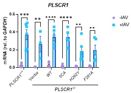
The forward human PLSCR1 primer we used matches 15-34 nt of Wt PLSCR1, and the reverse primer matches 224-244 nt of Wt PLSCR1. CRISPR-Cas9 KO of PLSCR1 was mediated by sgRNAs in A549 cells and was performed by Xu et al[2]. sgRNA #1 matches 227-246 nt, sgRNA #2 matches 209-228 nt, and sgRNA #3 matches 689-708 nt of Wt PLSCR1. The sgRNAs likely introduced a short deletion or insertion that does not affect transcription. However, those endogenous mRNA transcripts cannot be translated to functional and detectable PLSCR1 proteins, as validated by our western blot (below), as well as western blots performed by Xu et al[2]. Therefore, our primers could amplify endogenous PLSCR1 transcripts upregulated by IAV infection, if 15-244 nt was not disturbed by CRISPR-Cas9 KO. By western blot, we confirmed that only endogenous PLSCR1 expression is upregulated by IAV infection, and exogenous protein expression of PLSCR1 plasmids driven by an EF-1α promoter are not upregulated by IAV infection.
Author response image 2.
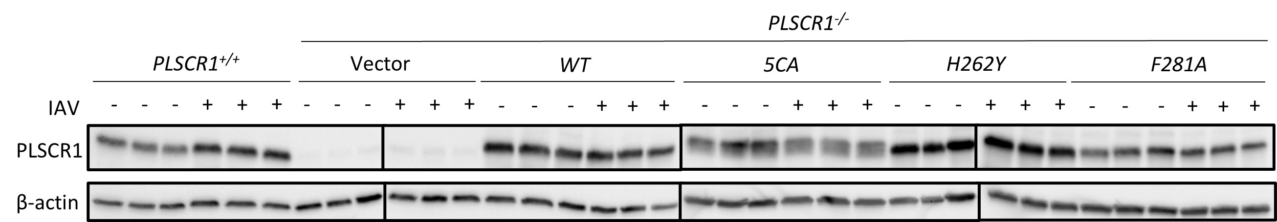
To avoid confusion, we have removed the original Figure 5A from the manuscript.
(8) In Figure 5C, the loss of anti-flu activity with the H262Y mutant is modest, suggesting the loss of ifnlr1 transcription is only partly responsible for the susceptibility of Plscr1 KO cells. The anti-flu activity being independent of scramblase activity resembles the earlier discovery of SARS-CoV-2 (Xu et al., 2024). This could be stated in the results since it is an important point that scramblase activity is dispensable for several major human viruses and shifts the emphasis regarding mechanism. It has been appropriately noted in the discussion.
We appreciated the comments and have acknowledged the consistency of our results with those of Xu et al. under “Both Cell Surface and Nuclear PLSCR1 Regulates IFN-λ Signaling and Limits IAV Infection Independent of Its Enzymatic Activity” in the “Results” section.
Reviewer #2 (Recommendations):
(1) The statement that type I interferons are expressed by “almost all cells” is inaccurate (line 61). Type I IFN production is also context-dependent and often restricted to specific cell types upon infection or stimulation.
We apologize for the inaccurate description of the expression pattern of type 1 IFNs and have corrected the restricted cellular sources of type 1 IFNs in the “Introduction”.
(2) The antiviral response is assessed solely through flu M gene expression. Incorporating infectious virus titers (e.g., TCID50 or plaque assay) would provide a more robust and direct measure of antiviral activity.
As requested by the reviewer, we have performed plaque assays on all experiments where flu M gene expression levels were measured (Figure 1G, 5E and 7F, and Supplemental Figure 6E). The plaque assay results are consistent with the flu M gene expressions.
(3) While mRNA expression of interferons is measured, protein levels (e.g., through ELISA) should also be quantified to establish the functional relevance of IFN expression changes.
As requested by the reviewer, we have quantified the protein level of IFN-λ in mouse BAL with ELISA (Figure 2E). The ELISA results are consistent with the mRNA expressions of IFN-λ.
(4) It is unclear whether reduced IFNLR1 expression translates to defective downstream signaling or antiviral responses after IFN-λ treatment in PLSCR1-deficient cells. This is particularly pertinent given the increase in IFN-λ ligand in vivo, which might compensate for receptor downregulation.
We agree with the reviewer that downstream activation of the IFN-λ signaling pathway is a critical aspect of PLSCR1’s proposed regulatory role. To investigate this, we attempted an ISRE-luciferase reporter assay to assess downstream signaling following IFN-λ treatment in PLSCR1 rescue cells. Unfortunately, the experiment encountered unforeseen technical issues. For additional context, please refer to our response to Reviewer #1’s public review #3.
(5) Detailed gating strategies for immune cell subsets are absent and should be included for clarity and reproducibility.
We would like to clarify that the immune cell subsets in BAL fluids were counted manually following cytospin preparation and Diff-Quik staining (Figure 2B and 7H, and Supplemental Figures 2C, 5D, and 8D), rather than by flow cytometry. We hope this resolves the reviewer’s confusion.
(6) The study does not definitively establish that reduced IFN-λ signaling causes the observed in vivo phenotype. Increased morbidity and mortality in PLSCR1-deficient mice could also stem from elevated TNF-α levels and lung damage, as proinflammatory cytokines and/or enhanced lung damage are known contributors to influenza morbidity and mortality. This point warrants detailed discussions.
We agreed with the reviewer that this study does not guarantee a definitive causality between reduced IFN-λ signaling and increased morbidity of Plscr1<sup>-/-</sup> mice and more experiments are needed to reach the conclusion. We have acknowledged this limitation of our study in the “Discussion”, as requested by the reviewer. We hope to fully eliminate the confounding elements and definitively establish the proposed causality in future studies.
Reviewer #3 (Public review):
Summary:
Yang et al. have investigated the role of PLSCR1, an antiviral interferon-stimulated gene (ISG), in host protection against IAV infection. Although some antiviral effects of PLSCR1 have been described, its full activity remains incompletely understood.
This study now shows that Plscr1 expression is induced by IAV infection in the respiratory epithelium, and Plscr1 acts to increase Ifn-λr1 expression and enhance IFN-λ signaling possibly through protein-protein interactions on the cell membrane.
Strengths:
The study sheds light on the way Ifnlr1 expression is regulated, an area of research where little is known. The study is extensive and well-performed with relevant genetically modified mouse models and tools.
Weaknesses:
There are some issues that need to be clarified/corrected in the results and figures as presented.
Also, the study does not provide much information about the role of PLSCR1 in the regulation of Ifn-λr1 expression and function in immune cells. This would have been a plus.
We would like to thank the reviewer for the positive feedback and insightful comment regarding the roles of PLSCR1 and IFN-λR1 in immune cells. It is important to note that IFN-λR1 expression is highly restricted in immune cells and is primarily limited to neutrophils and dendritic cells[3]. While dendritic cells were not the focus of this study, we did examine all immune cell subsets in our single cell RNA seq data and performed infection experiments in Plscr1<sup>floxStop</sup>/LysM-Cre<sup>+</sup> mice. We have not observed any significant findings in these populations. On the other hand, we do have some interesting preliminary data suggesting a role for PLSCR1 in regulating Ifn-λr1 expression and function in neutrophils. These findings are discussed in detail in our response to reviewer #3’s recommendation #12.
Reviewer #3 (Recommendations):
(1) In Figure 1B, the Plscr1 label should be moved to the y-axis so that readers don't confuse it with the Plscr1-/- mice used in the other figure panels. The fact that WT mice were used should be added in the figure legend.
We apologize for the confusion in the figures. We have moved Plscr1 label to the y-axis in Figure 1B and have mentioned Wt mice were used in the figure legend.
(2) In Figure 1C and D, the type of dose leading to the presented data should be added to help the reader. Also, shouldn't statistics be added?
We appreciate the suggestion and have added doses to Figure 1C and 1D. We are confused about the request of adding statistics by the reviewer, as two-way ANOVA tests were used to compare weight losses, and the significance was labeled on the figures.
(3) In Figures 1, F, and G, it is not indicated whether sublethal or lethal dose was used for the IAV infection. This should be very clear in the figure and figure legend.
We apologize for the confusion of infection doses used in the figures. We have added doses to Figure 1F, 1G and 1H.
(4) In Figure 1, the CTCF abbreviation should be explained in the Figure legend.
We have explained CTCF in the figure legend as requested.
(5) In Figure 2B, this is percentages of what?
Figure 2B shows the percentages of each immune cell type within total BAL cells.
(6) In Figures 3A and B, transcriptomes for each condition are from how many mice? Also, what do heatmaps show? Fold induction, differences, etc, and from what? What is compared with what? In addition, is there a discordance between the RNAseq data of Figure 3A and the qPCR data of Fig. 3C in terms of Ifnlr1 expression?
In Figure 3A and 3C (previously 3B), RNA from the whole lungs of 9 mice per PBS-treated group and 4 mice per IAV-infected group were pooled for transcriptomic analysis. Figure 3A represents a heatmap of differential gene expression, while Figure 3C (previously 3B) represents fold changes in gene expression relative to uninfected controls. In both heatmaps, gene expression values are color-coded from row minimum (blue) to row maximum (red), enabling comparison across groups within each gene (row). The major comparison of interest in these heatmaps is between Wt infected mice versus Plscr1<sup>-/-</sup> infected mice. We have added this information to the figure legend.
We also acknowledge the reviewer’s observation regarding the discordance between the RNA seq data of Figure 3A and the qPCR data of Figure 3B (previously 3C) for Ifnlr1 expression. To address this, we have repeated the qRT-PCR experiment with additional samples at 7 dpi. In the updated results, Wt mice consistently show significantly higher Ifn-λr1 expression than Plscr1<sup>-/-</sup> infected mice at both 3 dpi and 7 dpi, consistent with the RNA seq data. However, a time-dependent discrepancy between the RNA-seq and qRT-PCR datasets remains: Ifn-λr1 expression continues to increase at 7 dpi in the RNA-seq data (Figure 3A), whereas it declines in the qRT-PCR results (Figure 3B). The reason for this discrepancy remains unclear and has been addressed in the Discussion section.
(7) In Figure 3D, have the authors checked whether the Ifnlr1 antibody they use is indeed specific for Ifnlr1? Have they used any blocking peptide for the anti-mouse Ifn-λr1 polyclonal antibody they are using? Also, in Figure 3E, the marker used for staining should be indicated in the pictures of the lung section.
Unfortunately, a blocking peptide is not available for the anti-mouse Ifn-λr1 polyclonal antibody used in our study. To assess antibody specificity, we have performed immunofluorescence staining of Ifn-λr1 on lung tissues from Ifn-λr1<sup>-/-</sup> mice using the same antibody. No signal was detected (Supplemental Figure 5A), supporting the specificity of the antibody for Ifn-λr1.
As requested by the reviewer, we have added the marker (Ifn-λr1) to the pictures of the lung section in Figure 3E.
(8) In Figure 5, it's better to move each graph's label that stands to the top (e.g. PLSCR1, IFN-λR1 etc) to the y-axis label so that it doesn't get confused with the mouse -/- label.
We apologize for the confusion and have moved the top label to the y-axis in Figure 5.
(9) In Figure 6A, it is claimed that the 'two-dimensional UMAP demonstrated that these main lung cell populations (epithelial, endothelial, mesenchymal, and immune) were dynamic over the course of infection.'. This is not clear by the data. The percentage of cells per cluster should be calculated.
As requested by the reviewer, the proportion (Supplemental Figure 6A) and cell count (Supplemental Figure 6B) of each cluster have been calculated and included in “PLSCR1 Expression Is Upregulated in the Ciliated Airway Epithelial Compartment of Mice following Flu Infection” under “Results” section. Together with the two-dimensional UMAP (Figure 6A), these data demonstrate that the main lung cell populations (epithelial, endothelial, mesenchymal, and immune) were dynamic over the course of infection. Following infection, many populations emerged, particularly within the immune cell clusters. At the same time, some clusters were initially depleted and later restored, such as microvascular endothelial cells (cluster 2). Other populations, such as interferon-responsive fibroblasts (cluster 20), showed a dramatic yet transient expansion during acute infection and disappeared after infection resolved.
(10) In Figure 6 B and C, the legend should indicate that these are Violin plots. Also, if AT2 cells don't express Plscr1, does that indicate that in these cells Plscr1 is not needed for IFN-λR1 expression?
As requested, we have indicated in the legend of Figure 6B and 6C that these are violin plots. Plscr1 is expressed at low levels in AT2 cells. However, it is unclear whether Plscr1 is needed for Ifn-λr1 expression in AT2 cells, and it would be interesting to investigate further.
(11) In lines 302-304, it is stated that 'Among the various epithelial populations, ciliated epithelial cells not only had 303 the highest aggregated expression of Plscr1, but also were the only epithelial cell 304 population in which significantly more Plscr1 was induced in response to IAV infection.'. Which data/ figure support this statement?
Figure 6B shows that among the various epithelial populations, ciliated epithelial cells had the highest aggregated expression of Plscr1. To better illustrate this statement, we have rearranged the order of cell clusters from highest to lowest Plscr1 expression, and added red dots to indicate the mean expression levels for each cluster in Figure 6B.
Ciliated epithelial cells also had the most significant increase in Plscr1 expression (p < 2.22e-16 and p = 6.7e-05) in early IAV infection at 3 dpi (Figure 6C and Supplemental Figure 7A-7K). In comparison, AT1 cells were the only other epithelial cluster to show Plscr1 upregulation at 3dpi, but to a much less extent (p = 0.033, Supplemental Figure 7J). Supplemental Figure 7 was added to better support the statement and the explanation was added to “PLSCR1 Expression Is Upregulated in the Ciliated Airway Epithelial Compartment of Mice following Flu Infection” under “Results” section.
(12) As earlier, if Plscr1 is not expressed in neutrophils (Figure 6F), does that mean IFN-λR1 expression does not require Plscr1 in these cells?
Although Plscr1 is expressed at lower levels in neutrophils compared to epithelial cells, it is still detectable. In fact, our preliminary data suggest that IFN-λR1 expression in neutrophils is dependent on Plscr1. We have isolated neutrophils from peripheral blood and BAL of IAV-infected Wt and Plscr1<sup>-/-</sup> mice using a mouse neutrophil enrichment kit. Quantitative PCR results showed that Plscr1<sup>-/-</sup> neutrophils exhibit significantly lower expression of Ifn-λr1, alongside elevated levels of Il-1β, Il-6 and Tnf-α in IAV infection (see figures below). These findings suggest that Plscr1 may play an anti-inflammatory role in neutrophils by upregulating Ifn-λr1. These data were not included in the current manuscript because they are beyond the scope of current study, but we hope to address the role of PLSCR1 in regulating IFN-λR1 expression and function in neutrophils in a future study.
Author response image 3.
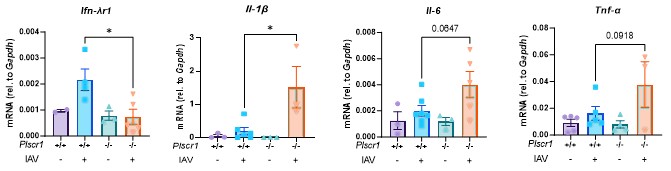
(13) The Figure 7A legend is not well stated. Something like ' Schematic representation of the experimental design of...' should be included. Also, Figure 7J is not referenced in the text.
We apologize for the unclear Figure 7A legend and have changed it to “Schematic representation of the experimental design of ciliated epithelial cell conditional Plscr1 KI mice.” Figure 8 (previously Figure 7J) has now been referenced in the text.
(14) In the Methods, more specific information in some parts should be provided. For example, the clones of the antibodies used should be included.
Apart from the 10x technology, the kits used and the type of the Illumina sequencing should be provided. Information on how the QC was performed (threshold for reads/cell, detected genes/per cells, and % of mitochondrial genes etc) should be added.
We apologize for the missing information in the “Methods”. We have now provided the clones of the antibodies used, the kit used to generate single-cell transcriptomic libraries, the type of the Illumina sequencing, and the QC performance data.
References
(1) Rusinova, I., et al., Interferome v2.0: an updated database of annotated interferon-regulated genes. Nucleic Acids Res, 2013. 41(Database issue): p. D1040-6.
(2) Xu, D., et al., PLSCR1 is a cell-autonomous defence factor against SARS-CoV-2 infection. Nature, 2023. 619(7971): p. 819-827.
(3) Donnelly, R.P., et al., The expanded family of class II cytokines that share the IL-10 receptor-2 (IL-10R2) chain. J Leukoc Biol, 2004. 76(2): p. 314-21.
Author response:
The following is the authors’ response to the original reviews.
Reviewer #1 (Public Review):
Here the authors discuss mechanisms of ligand binding and conformational changes in GlnBP (a small E Coli periplasmic binding protein, which binds and carries L-glutamine to the inner membrane ATP-binding cassette (ABC) transporter). The authors have distinguished records in this area and have published seminal works. They include experimentalists and computational scientists. Accordingly, they provide comprehensive, high-quality, experimental and computational work. They observe that apo- and holo- GlnBP does not generate detectable exchange between open and (semi-) closed conformations on timescales between 100 ns and 10 ms. Especially, the ligand binding and conformational changes in GlnBP that they observe are highly correlated. Their analysis of the results indicates a dominant induced-fit mechanism, where the ligand binds GlnBP prior to conformational rearrangements. They then suggest that an approach resembling the one they undertook can be applied to other protein systems where the coupling mechanism of conformational changes and ligand binding. They argue that the intuitive model where ligand binding triggers a functionally relevant conformational change was challenged by structural experiments and MD simulations revealing the existence of unliganded closed or semi-closed states and their dynamic exchange with open unbound conformations, discuss alternative mechanisms that were proposed, their merits and difficulties, concluding that the findings were controversial, which, they suggest is due to insufficient availability of experimental evidence to distinguish them. As to further specific conclusions they draw from their results, they determine that a conformational selection mechanism is incompatible with their results, but induced fit is. They thus propose induced fit as the dominant pathway for GlnBP, further supported by the notion that the open conformation is much more likely to bind substrate than the closed one based on steric arguments. Considering the landscape of substrate-free states, in my view, the closed state is likely to be the most stable and, thus most highly populated. As the authors note and I agree that state can be sterically infeasible for a deep-pocketed substrate. As indeed they also underscore, there is likely to be a range of open states. If the populations of certain states are extremely low, they may not be detected by the experimental (or computational) methods. The free energy landscape of the protein can populate all possible states, with the populations determined by their relative energies. In principle, the protein can visit all states. Whether a particular state is observed depends on the time the protein spends in that state. The frequencies, or propensities, of the visits can determine the protein function. As to a specific order of events, in my view, there isn't any. It is a matter of probabilities which depend on the populations (energies) of the states. The open conformation that is likely to bind is the most favorable, permitting substrate access, followed by minor, induced fit conformational changes. However, a key factor is the ligand concentration. Ligand binding requires overcoming barriers to sustain the equilibrium of the unliganded ensemble, thus time. If the population of the state is low, and ligand concentration is high (often the case in in vitro experiments, and high drug dosage scenarios) binding is likely to take place across a range of available states. This is however a personal interpretation of the data. The paper here, which clearly embodies massive careful, and high-quality work, is extensive, making use of a range of experimental approaches, including isothermal titration calorimetry, single-molecule Förster resonance energy transfer, and surface-plasmon resonance spectroscopy. The problem the authors undertake is of fundamental importance.
Reviewer #2 (Public Review):
The manuscript by Han et al and Cordes is a tour-de-force effort to distinguish between induced fit and conformational selection in glutamine binding protein (GlnBP).
We thank the referee for the recognition of the work and effort that has gone into this manuscript.
It is important to say that I don't agree that a decision needs to be made between these two limiting possibilities in the sense that whether a minor population can be observed depends on the experiment and the energy difference between the states. That said, the authors make an important distinction which is that it is not sufficient to observe both states in the ligand-free solution because it is likely that the ligand will not bind to the already closed state. The ligand binds to the open state and the question then is whether the ligand sufficiently changes the energy of the open state to effectively cause it to close. The authors point out that this question requires both a kinetic and a thermodynamic answer. Their "method" combines isothermal titration calorimetry, single-molecule FRET including key results from multi-parameter photon-by-photon hidden Markov modelling (mpH2MM), and SPR. The authors present this "method" of combination of experiments as an approach to definitively differentiate between induced fit and conformational selection. I applaud the rigor with which they perform all of the experiments and agree that others who want to understand the exact mechanism of protein conformational changes connected to ligand binding need to do such a multitude of different experiments to fully characterize the process. However, the situation of GlnBP is somewhat unique in the high affinity of the Gln (slow offrate) as compared to many small molecule binding situations such as enzyme-substrate complexes. It is therefore not surprising that the kinetics result in an induced fit situation.
For us these comments are an essential part of the conceptual aspects of our work and the resulting research. From a descriptive viewpoint, it is essential for us (and we tried to further highlight and stress this in the updated version of our paper) that IF and CS are two kinetic mechanisms of ligand binding. They imply – if active in a biomolecular system – a temporal order and timescale separation of ligand binding and conformational changes. Since we found many conflicting results for the binding mechanism of GlnBP, but also other SPBs, we decided to assess the situation in GlnBP.
In the case of the E-S complexes I am familiar with, the dissociation is much more rapid because the substrate binding affinity is in the micromolar range and therefore the re-equilibration of the apo state is much faster. In this case, the rate of closing and opening doesn't change much whether ligand is present or not. Here, of course, once the ligand is bound the re-equilibration is slow. Therefore, I am not sure if the conclusions based on this single protein are transferrable to most other protein-small molecule systems.
We do not argue that our results and interpretations are valid for most other protein-ligand systems may those be enzymes or simple ligand binders. Yet, based on the conservation of ABC-related SBPs and the fact that quite a few of them show sub-µM Kds, we render it likely to find many analogous situations as for GlnBP also based on our previous results e.g., from de Boer et al., eLife (2019).
I am also not sure if they are transferrable to protein-protein systems where both molecules the ligand and the receptor are expected to have multiscale dynamics that change upon binding.
As we argue above the two mechanisms IF/CS imply a clear temporal order and separation of timescales for ligand binding and conformational changes. These mechanisms are simple and extreme cases that we tested before more complex kinetic schemes are inferred for the description of ligand binding and conformational changes (which might not be necessary).
Strengths:
The authors provide beautiful ITC data and smFRET data to explore the conformational changes that occur upon Gln binding. Figure 3D and Figure 4 (mpH2MM data) provide the really critical data. The multi-parameter photon-by-photon hidden Markov modelling (mpH2MM) data. In the presence of glutamine concentrations near the Kd, two FRET-active sub-populations are identified that appear to interconvert on timescales slower than 10 ms. They then do a whole bunch of control experiments to look for faster dynamics (Figure 5). They also do TIRF smFRET to try to compare their results to those of previous publications. Here, they find several artifacts are occurring including inactivation of ~50% of the proteins. They also perform SPR experiments to measure the association rate of Gln and obtain expectedly rapid association rates on the order of 10<sup>^</sup>8 M-1s-1.
Thank you.
Weaknesses:
Looking at the traces presented in the supplementary figures, one can see that several of the traces have more than one molecule present. The authors should make sure that they use only traces with a single photobleaching event for each fluorophore. One can see steps in some of the green traces that indicate two green fluorophors (likely from 2 different molecules) in the traces. This is one of the frequent problems with TIRF smFRET with proteins, that only some of the spots represent single molecules and the rest need to be filtered out of the analysis.
We have inspected all TIRF data provided with the manuscript and assume that the referee refers to data shown in current Appendix Figure 4/5. We agree that those traces in which no photo bleaching occurs could potentially be questioned, yet they would not change our interpretations and thus decided to leave the figure as is.
The NMR experiments that the authors cite are not in disagreement with the work presented here. NMR is capable of detecting "invisible states" that occur in 1-5% of the population. SmFRET is not capable of detecting these very minor states. I am quite sure that if NMR spectroscopists could add very high concentrations of Gln they would also see a conversion to the closed population.
We agree with the referee that NMR is capable of detecting invisible states that occur in 1-5% of the population (see e.g., the paper cited in our manuscript by Tang, C et al., Open-to-closed transition in apo maltose-binding protein observed by paramagnetic NMR. Nature 2007, 449, 1078). Yet, we see a strong disagreement between our work and papers on GlnBP, where a combination of NMR, FRET and MD was used (Feng, Y. et al., Conformational Dynamics of apo‐GlnBP Revealed by Experimental and Computational Analysis. Angewandte Chemie 2016, 55, 13990; Zhang, L. et al., Ligand-bound glutamine binding protein assumes multiple metastable binding sites with different binding affinities. Communications biology 2020, 3, 1). These inconsistencies were also noted by others in the field (Kooshapur, H. et al., NMR Analysis of Apo Glutamine‐Binding Protein Exposes Challenges in the Study of Interdomain Dynamics. Angewandte Chemie 2019, 58, 16899) and we reemphasize that this latest NMR publication comes to similar conclusions as we present in our manuscript.
Reviewer #1 (Recommendations For The Authors):
The paper embodies massive careful and high-quality work, and is extensive, making use of a range of experimental approaches, including isothermal titration calorimetry, single-molecule Förster resonance energy transfer, and surface-plasmon resonance spectroscopy. Considering this extensiveness, I do not see what more the authors can do.
We very much appreciate the assessment and positive comments of the referee, but still tried to incorporate simulation data to support our interpretations.
Reviewer #2 (Recommendations For The Authors):
(1) Looking at the traces presented in the supplementary figures, one can see that several of the traces have more than one molecule present. The authors should make sure that they use only traces with a single photobleaching event for each fluorophore. One can see steps in some of the green traces that indicate two green fluorophors (likely from 2 different molecules) in the traces. This is one of the frequent problems with TIRF smFRET with proteins, that only some of the spots represent single molecules and the rest need to be filtered out of the analysis.
See response above for iteration of TIRF data selection and analysis.
(2) The NMR experiments that the authors cite are not in disagreement with the work presented here. NMR is capable of detecting "invisible states" that occur in 1-5% of the population. SmFRET is not capable of detecting these very minor states. I am quite sure that if NMR spectroscopists could add very high concentrations of Gln they would also see a conversion to the closed population.
See response above.
Minor point:
(1) It is difficult to see what is going on between apo and holo in Figure 1B. Could the authors make Figure 1a, 1b apo, and 1b holo in the same orientation (by aligning D2 or D1 to each other in all figures) so one can see which helices are in the same place and which have moved?
We respectfully disagree and decided to keep this figure as it is
Reviewer #2 (Public review):
Summary:
In the manuscript by Mahen et al., entitled "Gut Microbe-Derived Trimethylamine Shapes Circadian Rhythms Through the Host Receptor TAAR5," the authors investigate the interplay between a host G protein-coupled receptor (TAAR5), the gut microbiota-derived metabolite trimethylamine (TMA), and the host circadian system. Using a combination of genetically engineered mouse and bacterial models, the study demonstrates a link between microbial signaling and circadian regulation, particularly through effects observed in the olfactory system. Overall, this manuscript presents a novel and valuable contribution to our understanding of host-microbe interactions and circadian biology. The addition of new data following revision adds mechanistic depth to more fully support the authors' conclusions.
Strengths:
(1) The manuscript addresses an important and timely topic in host-microbe communication and circadian biology.
(2) The studies employ multiple complementary models, e.g., Taar5 knockout mice, microbial mutants, which enhances the depth of the investigation.
(3) The integration of behavioral, hormonal, microbial, and transcript-level data provides a multifaceted view of the observed phenotype.
(4) Inclusion of rhythmic analysis of a defined microbial community adds novelty and strength to the overall findings.
(5) The identification of olfactory-linked circadian changes in the context of gut microbes adds a novel perspective to the field.
Weaknesses:
(1) While the authors suggest a causal role for TAAR5 and its ligand in circadian regulation, some of the data remain correlative in this context; however, the authors have appropriately tempered these claims, and mechanistic experiments are proposed to expand upon their compelling findings in future work.
Reviewer #3 (Public review):
Summary:
Deletion of the TMA-sensor TAAR5 results in circadian alterations in the gene expression, particularly in the olfactory bulb; plasma hormones; and neurobehaviors.
Strengths:
Genetic background was rigorously controlled.
Comprehensive characterization.
Impact:
These data add to the growing literature pointing to a role for the TMA/TMAO pathway in olfaction and neurobehavior.
Author response:
The following is the authors’ response to the original reviews.
Reviewer #1 (Public review):
Summary:
This study focuses on the bacterial metabolite TMA, generated from dietary choline. These authors and others have previously generated foundational knowledge about the TMA metabolite TMAO, and its role in metabolic disease. This study extends those findings to test whether TMAO's precursor, TMA, and its receptor TAAR5 are also involved and necessary for some of these metabolic phenotypes. They find that mice lacking the host TMA receptor (Taar5-/-) have altered circadian rhythms in gene expression, metabolic hormones, gut microbiome composition, and olfactory and innate behavior. In parallel, mice lacking bacterial TMA production or host TMA oxidation have altered circadian rhythms.
Strengths:
These authors use state-of-the-art bacterial and murine genetics to dissect the roles of TMA, TMAO, and their receptor in various metabolic outcomes (primarily measuring plasma and tissue cytokine/gene expression). They also follow a unique and unexpected behavioral/olfactory phenotype. Statistics are impeccable.
Weaknesses:
Enthusiasm for the manuscript is dampened by some ambiguous writing and the presentation of ideas in the introduction, both of which could easily be improved upon revision.
We apologize for the abbreviated and ambiguous writing style in our original submission. Given Reviewer 2 also suggested reorganizing and rewriting certain parts, we have spent time to remove ambiguity by adding additional points of clarification and adding more historical context to justify studying TMA-TAAR5 signaling in regulating host circadian rhythms. We have also reorganized the presentation of data aligned with this.
Reviewer #2 (Public review):
Summary:
In the manuscript by Mahen et al., entitled "Gut Microbe-Derived Trimethylamine Shapes Circadian Rhythms Through the Host Receptor TAAR5," the authors investigate the interplay between a host G protein-coupled receptor (TAAR5), the gut microbiota-derived metabolite trimethylamine (TMA), and the host circadian system. Using a combination of genetically engineered mouse and bacterial models, the study demonstrates a link between microbial signaling and circadian regulation, particularly through effects observed in the olfactory system. Overall, this manuscript presents a novel and valuable contribution to our understanding of hostmicrobe interactions and circadian biology. However, several sections would benefit from improved clarity, organization, and mechanistic depth to fully support the authors' conclusions.
Strengths:
(1) The manuscript addresses an important and timely topic in host-microbe communication and circadian biology.
(2) The studies employ multiple complementary models, e.g., Taar5 knockout mice, microbial mutants, which enhance the depth of the investigation.
(3) The integration of behavioral, hormonal, microbial, and transcript-level data provides a multifaceted view of the observed phenotype.
(4) The identification of olfactory-linked circadian changes in the context of gut microbes adds a novel perspective to the field.
Weaknesses:
While the manuscript presents compelling data, several weaknesses limit the clarity and strength of the conclusions.
(1) The presentation of hormonal, cytokine, behavioral, and microbiome data would benefit from clearer organization, more detailed descriptions, and functional grouping to aid interpretation.
We appreciate this comment and have reorganized the data to improve functional grouping and readability. We have also added additional detail to descriptions of the data in the revised figure legends and results.
(2) Some transitions-particularly from behavioral to microbiome data-are abrupt and would benefit from better contextual framing.
We agree with this comment, and have added additional language to provide smoother transitions. This in many cases brings in historical context of why we focused on both behavioral and microbiome alterations in this body of work.
(3) The microbial rhythmicity analyses lack detail on methods and visualization, and the sequencing metadata (e.g., sample type, sex, method) are not clearly stated.
We apologize for this, and have now added more detail in our methods, figures, and figure legends to ensure the reader can easily understand sample type, sex, and the methods used.
(4) Several figures are difficult to interpret due to dense layouts or vague legends, and key metabolites and gene expression comparisons are either underexplained or not consistently assessed across models.
Aligned with the last comment we now added more detail in our methods, figures, and figure legends to provide clear information. We have now provided additional data showing the same key metabolites, hormones, and gene expression alterations in each model if the same endpoints were measured.
(5) Finally, while the authors suggest a causal role for TAAR5 and its ligand in circadian regulation, the current data remain correlative; mechanistic experiments or stronger disclaimers are needed to support these claims.
We agree with this comment, and as a result have removed any language causally linking TMA and TAAR5 together in circadian regulation. Instead, we only state finding in each model and refrain from overinterpreting.
Reviewer #3 (Public review):
Summary:
Deletion of the TMA-sensor TAAR5 results in circadian alterations in gene expression, particularly in the olfactory bulb, plasma hormones, and neurobehaviors.
Strengths:
Genetic background was rigorously controlled.
Comprehensive characterization.
Weaknesses:
The weaknesses identified by this reviewer are minor.
Overall, the studies are very nicely done. However, despite careful experimentation, I note that even the controls vary considerably in their gene expression, etc, across time (eg, compare control graphs for Cry 1 in IB, 4B). It makes me wonder how inherently noisy these measurements are. While I think that the overall point that the Taar5 KO shows circadian changes is robust, future studies to dissect which changes are reproducible over the noise would be helpful.
We thank the reviewer for this insightful comment. We completely agree that there are clear differences in the circadian data in experiments from Taar5<sup>-/-</sup> mice and those from gnotobiotic mice where we have genetically deleted CutC. Although the data from Taar5<sup>-/-</sup> mice show nice robust circadian rhythms, the data from mice where microbial CutC is altered have inherently more “noise”. We attribute some of this to the fact that the Taar5<sup>-/-</sup> mouse experiment have a fully intact and diverse gut microbiome . Whereas, the gnotobiotic study with CutC manipulation includes only a 6 member microbiome community that does not represent the normal microbiome diversity in the gut. This defined synthetic community was used as a rigorous reductionist approach, but likely affected the normal interactions between a complex intact gut microbiome and host circadian rhythms. We have added some additional discussion to indicate this in the limitations section of the manuscript.
Impact:
These data add to the growing literature pointing to a role for the TMA/TMAO pathway in olfaction and neurobehavioral.
Reviewer #1 (Recommendations for the authors):
I suggest a revision of the writing and organization. The potential impact of the study after reading the introduction is unclear. One example, in the intro, " TMAO levels are associated with many human diseases including diverse forms of CVD5-12, obesity13,14, type 2 diabetes15,16, chronic kidney disease (CKD)17,18, neurodegenerative conditions including Parkinson's and Alzheimer's disease19,20, and several cancers21,22" It would be helpful to explain how the previous literature has distinguished that the driver of these phenotypes is TMA/TMAO and not increased choline intake. Basically, for a TMA/O novice reader, a more detailed intro would be helpful.
We appreciate this insightful comment and have now provided a more expansive historical context for the reader regarding the effects of choline consumption (which impacts many things, including choline, acetylcholine, phosphatidylcholine, TMA, TMAO, etc) versus the primary effects of TMA and TMAO.
There were also many uses of vague language (regulation/impact/etc). Directionality would be super helpful.
We thank the reviewer for this recommendation and have improved language as suggested to show directionality of our findings. The terms regulation, impact, shape etc. are used only when we describe multiple variable changing at the same time over the time course of a 24-hour circadian period (some increased and some decreased).
Reviewer #2 (Recommendations for the authors):
In the manuscript by Mahen et al., entitled "Gut Microbe-Derived Trimethylamine Shapes Circadian Rhythms Through the Host Receptor TAAR5," the authors investigate the interplay between a host G protein-coupled receptor (TAAR5), the gut microbiota-derived metabolite trimethylamine (TMA), and the host circadian system. Using a combination of genetically engineered mouse and bacterial models, the study demonstrates a link between microbial signaling and circadian regulation, particularly through effects observed in the olfactory system. Overall, this manuscript presents a novel and valuable contribution to our understanding of hostmicrobe interactions and circadian biology. However, several sections would benefit from improved clarity, organization, and mechanistic depth to fully support the authors' conclusions. Below are specific major and minor suggestions intended to enhance the presentation and interpretation of the data.
Major suggestions:
(1) Consider adding a schematic/model figure as Panel A early in the manuscript to help readers understand the experimental conditions and major comparisons being made.
We thank the reviewer for this recommendation and have added a graphical abstract figure to help the reader understand the major comparisons being made.
(2) Could the authors present body weight and food intake characteristics in Taar5 KO vs. WT animals?
We have added body weight data as requested in Figure 1, Figure supplement 1. Although we have not stressed these mice with a high fat diet for these behavioral studies, under chow-fed conditions studied here we did not find any significant differences in body weight. Given no difference in body weight, we did not collect data on food consumption and have mentioned this as a limitation in the discussion.
(3) Several figures, especially Figures 3 and 4, and Supplemental Figures, would benefit from more structured organization and expanded legends. Grouping related data into thematic panels (e.g., satiety vs. appetite hormones, behavioral domains) may help improve readability.
We appreciate the reviewer’s thoughtful comments and agree that reorganization would improve clarity. We have reorganized figures to improve clarity and have expanded the figure legends to provide more detail on experimental methods.
(4) Clarify and expand the description of hormonal and cytokine changes. For instance, the phrase "altered rhythmic levels" is vague - do the authors mean dampened, phase-shifted, enhanced, etc., relative to WT controls?
Given a similar suggestion was made by Reviewer 1, we have provided more precise language focused on directionality and which specific endpoints we are referring to. For anything looking at circadian rhythms, the revised manuscript includes specific indications when we are discussing mesor, amplitude, and acrophase alterations. The terms regulation, impact, shape etc. are used only when we describe multiple complex variables changing at the same time over the time course of a 24-hour circadian period (some increased and some decreased).
(5) Consider grouping hormones and cytokines functionally (e.g., satiety vs. appetite-stimulating, pro- vs. antiinflammatory) to better interpret how these changes relate to the KO phenotype.
We thank the reviewer for this recommendation, and have re-organized figure panels to reflect this.
(6) Please provide a more detailed description of the behavioral results, particularly those in Supplemental Figure 2.
We have both expanded the methods description in the revised figure legends, but have also added a more detailed description of the behavioral results.
(7) As with hormonal data, behavioral outcomes would be easier to follow if organized thematically (e.g., locomotor activity, anxiety-like behavior, circadian-related behavior), especially for readers less familiar with behavioral assays.
We appreciate this reviewer’s comment and agree that we can better group our data to show how each test is associated with the type of behavior it assesses. As a result we have reorganized the behavioral data into broad categories such as olfactory-related, innate, cognitive, depressive/anxiety-like, or social behaviors. We have also new data in each of these behavioral categories to provide a more comprehensive understanding of behavioral alterations seen in Taar5<sup>-/-</sup> mice.
(8) The following statement needs clarification: "Also, it is important to note that many behavioral phenotypes examined, including tests not shown, were unaltered in Taar5-/- mice (Figures S2G, S2H, and S2I)." Consider rephrasing to explicitly state the intended message: are the authors emphasizing a lack of behavioral phenotype, or highlighting specific unaltered aspects?
We apologize for this confusing statement, and have changed the verbiage to improve readability. To expand the comprehensive nature of this study, we also now include the tests that were “not shown” in the original submission to provide a more comprehensive understanding of behavioral alterations seen in Taar5<sup>-/-</sup> mice. These new data are included as 6 different figure supplements to main Figure 2.
(9) The transition from behavior to microbiome data feels abrupt. Can the authors better explain whether the behavioral changes are thought to result from gut microbial function, independent of TMA-Taar5 signaling?
We apologize for the poor transitions in our writing style. We have spent time to explain the previous findings linking the TMA pathway to circadian reorganization of the gut microbiome (mostly coming from our original paper Schugar R, et al. 2022, eLife) and how this correlates with behavioral phenotypes. Although at this point it is difficult to know whether the microbiome changes are driving behavioral changes, or vice versa it could be central TAAR5 signaling is altering oscillations in gut microbiome, we present our findings here as a framework for follow up studies to more precisely get at these questions. It is important to note that our experiment using defined community gnotobiotic mice with or without the capacity to produce TMA (i.e. CutC-null community) shows that clearly microbial TMA production can impact host circadian rhythms in the olfactory bulb. Additional experiments beyond the scope of this work will be required to test which phenotypes originate from TMA-TAAR5 signaling versus more broad effects of the restructured gut microbiome.
(10) For Figure 3A, please expand the microbiome results with more granularity:
(a) Indicate in the Results section whether the sequencing method was 16S amplicon or metagenomic.
Sequencing was done using 16S rRNA amplicon sequencing using methods published by our group (PMID: 36417437, PMID: 35448550).
(b) State whether samples were from males, females, or a mix.
We have indicated that all mice from Figure 1 were male mice in the revised figure legend.
(c) Clarify whether beta diversity is based on phylogenetic or non-phylogenetic metrics. Consider using both types if not already done.
Beta diversity was analyzed using the Bray-Curtis dissimilarity index as the metric. Details have been included in the methods section.
(d) Make lines partially transparent in the Beta-diversity plot so that individual points are visible.
We have now updated the Beta-diversity plot with individual points visualized.
(e) Clarify what percentage of variation in the Beta-diversity plot is explained by CCA1, and whether this low percentage suggests minimal community-level differences.
We have updated the Beta-diversity plot to include the R<sup>2</sup> and p-values associated with these data.
(f) Confirm if the y-axis on the Beta-diversity plot should be labeled CCA2 rather than "CCAA 1".
We appreciate this comments, given it identified a typographical error in the plot. The revised figure now include the proper label of CCA2 instead of CCAA 1.
(11) For Figure 3B:
(a) Provide a description of the taxonomy plot in the results.
We have added a description of the taxonomy plot in the revised results section.
(b) Add phylum-level labels and enlarge the legend to improve the readability of genus-level data.
We agree this is a good suggestion so have enlarged the legend for the genus-level data and have also added phylum-level plots as well in the revised manuscript in Figure 3, figure supplement 1.
(12) Rhythmicity of the microbiome is central to the manuscript. The current approach of comparing relative abundance at discrete time points is limiting.
We thank the reviewer for this comment. We agree with this statement that discrete timepoint are not enough to describe circadian rhythmicity. In addition to comparing genotypes at discrete time points, we also used a rigorous cosinor analysis to plot the data over a 24-hour time period, and those differences are shown in the figure itself as well as Table 1.
(a) Please describe how rhythmicity was determined, e.g., what data or statistical method supports the statement: "Taar5-/- mice showed loss of the normal rhythmicity for Dubosiella and Odoribacter genera yet gained in amplitude of rhythmicity for Bacteroides genera (Figure 3 and S3)."
We appreciate this reviewer comment. Rhythmicity was determined using a cosinor analysis by use of an R program. Cosinor analysis is a statistical method used to model and analyze rhythmic patterns in time-series data, typically assuming a sinusoidal (cosine) shape. It estimates key parameters like mesor (mean level), amplitude (height of oscillation), and acrophase (timing of the peak), making it especially useful in fields like chronobiology and circadian rhythm research. We have used this in previous research to describe circadian rhythms. We do plan to improve language considering directionality of these circadian changes.
(b) Supplemental Figure S3 needs reorganization to highlight key findings. It's not currently clear how taxa are arranged or what trends are being shown.
The data in Figure S3 show the entire 24-hour time course of the cecal taxa that were significantly altered for at least one time point between Taar5<sup>+/+</sup> and Taar5<sup>-/-</sup> mice. Given we showed time pointspecific alterations in the Main Figure 3, we thought these more expansive plots would be important to show to depict how the circadian rhythms were altered.
(c) Supplemental Table 1, which includes 16S features, should be referenced and discussed in the microbiome section.
We have now referenced and discussed Supplemental Table 1 which includes all cosinor statistics for microbiome and other data presented in circadian time point studies.
(13) Did the authors quantify the 16S rRNA gene via RT-PCR to determine if this was similar between KO and WT over the 24-hour period?
We did not quantify 16S rRNA gene via RT-PCR, but do not think adding this will change our overall interpretations.
(14) Reorganize Figure 4 to align with the order of results discussed-starting with TMA and TMAO, followed by related metabolites like choline, L-carnitine, and gamma-butyrobetaine.
We thank the reviewer for this comment. We have chosen this organization because it is ordered from substrates (choline, L-carnitine, and betaine) to the microbe-associated products (TMA then TMAO). We will improve the writing associated with this figure to clearly explain this organization.
(a) Although the changes in the latter metabolites are more modest, they may still have physiological relevance. Could the authors comment on their significance?
We appreciate this reviewer comment and agree. We have expanded the results and discussion to address this.
(15) The authors note similarities in circadian gene expression between Taar5 KO mice and Clostridium sporogenes WT vs. ΔcutC mice, but the gene patterns are not consistent.
(a) Can the authors clarify what conclusions can reasonably be drawn from this comparison?
We hesitate to make definitive conclusions in the manuscript on why the gene patterns are not consistent, because it would be speculation. However, one major factor likely driving differences is the status of the diversity of the gut microbiome in the different studies. For instance, in the studies using Taar5<sup>+/+</sup> and Taar5<sup>-/-</sup> mice there is a very diverse microbiome in these conventionally housed mice. In contrast, by design the experiment using Clostridium sporogenes WT vs. ΔcutC communities is a reductionist approach that allows us to genetically define TMA production. In these gnotobiotic mice, the simplified community has very limited diversity and this likely alters the host circadian rhythms in gene expression quite dramatically. Although it is impossible to directly compare the results between these experiments given the difference microbiome diversity, there are clearly alterations in host gene expression when we manipulate TMA production (i.e. ΔcutC community) or TMA sensing (i.e. Taar5<sup>-/-</sup>).
(16) Were circadian and metabolic genes (e.g., Arntl, Cry1, Per2, Pemt, Pdk4) also analyzed in brown adipose tissue of Taar5 KO mice, and how do these results compare to the Clostridium models?
We thank the reviewer for this comment. Unfortunately, we did not collect brown adipose tissue in our original Taar5 study. We plan on doing this in future follow up studies studying cold-induced thermogenesis that are beyond the scope of this manuscript. However, we have decided to include data from our two timepoint Taar5 study which looks at ZT2 (9am) and ZT14 (9pm). There are clear differences in circadian genes between these timepoints.
(17) To allow a more direct comparison, please ensure the same cytokines (e.g., IL-1β, IL-2, TNF-α, IFN-γ, IL6, IL-33) are reported for both the Taar5 KO and microbial models.
We thank the reviewer for this comment and now include data from the same cytokines for each study.
(18) What was the defined microbial community used to colonize germ-free mice with C. sporogenes strains? Did this community exhibit oscillatory behavior?
To define TMA levels using a genetically-tractable model of a defined microbial community, we leveraged access to the community originally described by our collaborator Dr. Federico Rey (University of Wisconsin – Madison) (PMID: 25784704). We chose this community because it provide some functional metabolic diversity and is well known to allow for sufficient versus deficient TMA production. We are thankful for the reviewer comments about oscillatory behavior of this defined community, and to be responsive have performed sequencing to detect the species over time. These data are now included in the revised manuscript and show that there are clear differences in the oscillatory behavior of the defined community members. These data provide additional support that bacterial TMA production not only alters host circadian rhythms, but also the rhythmic behavior of gut bacteria themselves which has never been described before.
(19) Can the authors explain the rationale for measuring additional metabolites such as tryptophan, indole acetic acid, phenylacetic acid, and phenylacetylglycine? How are these linked to CutC gene function or Taar5 signaling?
We appreciate that this could be confusing, but have included other gut microbial metabolites to be as comprehensive as possible. This is important to include because we have found in other gnotobiotic studies where we have genetically altered metabolite production, if we alter one gut microbe-derived metabolite there can be unexpected alterations in other distinct classes of microbe-derived metabolites (PMID: 37352836). This is likely due to the fact that complex microbe-microbe and microbehost interactions work together to define systemic levels of circulating metabolites, influencing both the production and turnover of distinct and unrelated metabolites.
(20) The authors make several strong claims suggesting that loss of Taar5 or disruption of its ligand directly alters the circadian gene network. However, the current data are correlative. The authors should clarify that these findings demonstrate associations rather than direct causal effects, unless additional mechanistic evidence is provided. Approaches such as studies conducted in constant darkness, measurements of wheelrunning behavior, or analyses that control for potential confounding factors, e.g., inflammation or metabolic disruption, would help establish whether the observed changes in clock gene expression are primary or secondary effects. The authors are encouraged to either soften these causal claims or acknowledge this limitation explicitly in the discussion.
We thank the reviewer for this comment. We agree and have softened our language about direct effects of TMA via TAAR5 because we agree the data presented here are correlative only.
Minor suggestions:
(1) Avoid repetitive phrases such as "it is important to note..." for improved flow. Rephrasing these instances will enhance readability.
We thank the reviewer for this suggestion and have deleted such repetitive phrases.
(2) For Figure 2, remove interpretations above he graphs and use simple, descriptive panel labels, similar to those in Supplemental Figure 2.
We have removed these interpretations as suggested, but have retained descriptive panel labels to help the reader understand what type of data are being presented.
Reviewer #3 (Recommendations for the authors):
Minor:
In Figure 1D, UCP1 does not appear to be significantly changed.
We thank the reviewer for this comment and agree that UCP1 gene expression is not significantly altered . However, given the key role that UCP1 plays in white adipose tissue beiging, which is suppressed by the TMAO pathway, we think it is critical to show that this effect appears unaffected by perturbed TMA-TAAR5 signaling.
It would be helpful, in the discussion, to summarize any consistent changes across Taar5 KO, CutC deletion, and FMO3 deletion.
We have added this to the discussion, but as discussed above we hesitate to make strong interpretations about consistency between the models because the microbiome diversity is so different between the studies, and we did not measure all endpoints in both models.
For the Cosinor analysis, it may be helpful to remove the p-values that are >0.05 from the figures.
We have now removed any non-significant p-values that are associated with our figures.
For Figure 2, Supplement 1E, what are the two bars for each genotype?
We appreciate the reviewer pointing this out and will further explain this test in the figure with labels and in the legend.
Author response:
The following is the authors’ response to the previous reviews.
Editors comments:
I would encourage you to submit a revised version that addresses the following two points:
[a] The point from Reviewer #1 about a possible major confounding factor. The following article might be germane here: Baas and Fennell, 2019: https://papers.ssrn.com/sol3/papers.cfm?abstract_id=3339568
I don’t believe that the point raised by reviewer 1 is a confounder, see my response below.
This article highlighted was in my reading list, but I did not cite it because I was confused by its methods.
The point from Reviewer #4 about the abstract. It is important that the abstract says something about how reviewers reacted to the original versions of articles in which they were cited (ie, the odds ratio = 0.84, etc result), before going on to discuss how they reacted to revised articles (ie, the odds ratio = 1.61, etc result). I would suggest doing this along the following lines - but please feel free to reword the passage "but this effect was not strong/conclusive":
When reviewers were cited in the original version of the article under review, they were less likely to approve the article compared with reviewers who were not cited, but this effect was not strong/conclusive (odds ratio = 0.84; adjusted 99.4% CI: 0.69-1.03). However, when reviewers were cited in the revised version of the article, they were more likely to approve compared with reviewers who were not cited (odds ratio = 1.61; adjusted 99.4% CI: 1.16-2.23).
I have changed the abstract to include the odds ratios for version 1 and have used the same wording as from the main text.
Reviewer #1 (Public review):
Summary:
The work used open peer reviews and followed them through a succession of reviews and author revisions. It assessed whether a reviewer had requested the author include additional citations and references to the reviewers' work. It then assessed whether the author had followed these suggestions and what the probability of acceptance was based on the authors decision. Reviewers who were cited were more likely to recommend the article for publication when compared with reviewers that were not cited. Reviewers who requested and received a citation were much likely to accept than reviewers that requested and did not receive a citation.
Strengths and weaknesses:
The work's strengths are the in-depth and thorough statistical analysis it contains and the very large dataset it uses. The methods are robust and reported in detail.
I am still concerned that there is a major confounding factor: if you ignore the reviewers requests for citations are you more likely to have ignored all their other suggestions too? This has now been mentioned briefly and slightly circuitously in the limitations section. I would still like this (I think) major limitation to be given more consideration and discussion, although I am happy that it cannot be addressed directly in the analysis.
This is likely to happen, but I do not think it’s a confounder. A confounder needs to be associated with both the outcome and the exposure of interest. If we consider forthright authors who are more likely to rebuff all suggestions, then they would receive just as many citation and self-citation requests as authors who were more compliant. The behaviour of forthright authors would likely only reduce the association seen in most authors which would be reflected in the odds ratios.
Reviewer #2 (Public review):
Summary:
This article examines reviewer coercion in the form of requesting citations to the reviewer's own work as a possible trade for acceptance and shows that, under certain conditions, this happens.
Strengths:
The methods are well done and the results support the conclusions that some reviewers "request" self-citations and may be making acceptance decisions based on whether an author fulfills that request.
Weakness:
I thank the author for addressing my comments about the original version.
Reviewer #3 (Public review):
Summary:
In this article, Barnett examines a pressing question regarding citing behavior of authors during the peer review process. In particular, the author studies the interaction between reviewers and authors, focusing on the odds of acceptance, and how this may be affected by whether or not the authors cited the reviewers' prior work, whether the reviewer requested such citations be added, and whether the authors complied/how that affected the reviewer decision-making.
Strengths:
The author uses a clever analytical design, examining four journals that use the same open peer review system, in which the identities of the authors and reviewers are both available and linkable to structured data. Categorical information about the approval is also available as structured data. This design allows a large scale investigation of this question.
Weaknesses:
My original concerns have been largely addressed. Much more detail is provided about the number of documents under consideration for each analysis, which clarifies a great deal.
Much of the observed reviewer behavior disappears or has much lower effect sizes depending on whether "Accept with Reservations" is considered an Accept or a Reject. This is acknowledged in the results text. Language has been toned down in the revised version.
The conditional analysis on the 441 reviews (lines 224-228) does support the revised interpretation as presented.
No additional concerns are noted.
Reviewer #4 (Public review):
Summary:
This work investigates whether a citation to a referee made by a paper is associated with a more positive evaluation by that referee for that paper. It provides evidence supporting this hypothesis. The work also investigates the role of self-citations by referees where the referee would ask authors to cite the referee's paper.
Strengths:
This is an important problem: referees for scientific papers must provide their impartial opinions rooted in core scientific principles. Any undue influence due to the role of citations breaks this requirement. This work studies the possible presence and extent of this.
The methods are solid and well done. The work uses a matched pair design which controls for article-level confounding and further investigates robustness to other potential confounds.
Weaknesses:
The authors have addressed most concerns in the initial review. The only remaining concern is the asymmetric reporting and highlighting of version 1 (null result) versus version 2 (rejecting null). For example the abstract says "We find that reviewers who were cited in the article under review were more likely to recommend approval, but only after the first version (odds ratio = 1.61; adjusted 99.4% CI: 1.16 to 2.23)" instead of a symmetric sentence "We find ... in version 1 and ... in version 2".
The latest version now includes the results for both versions.
Joint Public Review:
From Reviewer 3 previously: Barnett examines a pressing question regarding citing behavior of authors during the peer review process. In particular, the author studies the interaction between reviewers and authors, focusing on the odds of acceptance, and how this may be affected by whether or not the authors cited the reviewers' prior work, whether the reviewer requested such citations be added, and whether the authors complied/how that affected the reviewer decision-making.
Key findings are a) that reviewers were more likely to approve an article if cited in the submission, b) reviewers who requested a citation in an updated version were less likely to approve, and c) reviewers who requested and received a citation were more likely to approve the revised version.
Comment from the Reviewing Editor about the latest version:
This is the third version of this article. Comments made during the peer review of the second version, along with author's responses to these comments, are available below.
Comments made during the peer review of the first version, along with author's responses to these comments, are available with previous versions of the article.
Reviewer #3 (Public review):
In this paper, the authors investigate how the RNA-binding protein Ssd1 and calorie restriction (CR) influence yeast replicative lifespan, with a particular focus on age-dependent iron uptake and activation of the iron regulon. For this, they use microfluidics-based single-cell imaging to monitor replicative lifespan, protein localization, and intracellular iron levels across aging cells. They show that both Ssd1 overexpression and CR act through a shared pathway to prevent the nuclear translocation of the iron-regulon regulator Aft1 and the subsequent induction of high-affinity iron transporters. As a result, these interventions block the age-related accumulation of intracellular free iron, which otherwise shortens lifespan. Genetic and chemical epistasis experiments further demonstrate that suppression of iron regulon activation is the key mechanism by which Ssd1 and CR promote replicative longevity.
Overall, the paper is technically rigorous, and the main conclusions are supported by a substantial body of experimental data. The microfluidics-based assays in particular provide compelling single-cell evidence for the dynamics of Ssd1 condensates and iron homeostasis.
My main concern, however, is that the central reasoning of the paper-that Ssd1 overexpression and CR prevent the activation of the iron regulon-appears to be contradicted by previous findings, and the authors may actually be misrepresenting these studies, unless I am mistaken. In the manuscript, the authors state on two occasions:
"Intriguingly, transcripts that had altered abundance in CR vs control media and in SSD1 vs ssd1∆ yeast included the FIT1, FIT2, FIT3, and ARN1 genes of the iron regulon (8)"
"Ssd1 and CR both reduce the levels of mRNAs of genes within the iron regulon: FIT1, FIT2, FIT3 and ARN1 (8)"
However, reference (8) by Kaeberlein et al. actually says the opposite:
"Using RNA derived from three independent experiments, a total of 97 genes were observed to undergo a change in expression >1.5-fold in SSD1-V cells relative to ssd1-d cells (supplemental Table 1 at http://www.genetics.org/supplemental/). Of these 97 genes, only 6 underwent similar transcriptional changes in calorically restricted cells (Table 2). This is only slightly greater than the number of genes expected to overlap between the SSD1-V and CR datasets by chance and is in contrast to the highly significant overlap in transcriptional changes observed between CR and HAP4 overexpression (Lin et al. 2002) or between CR and high external osmolarity (Kaeberlein et al. 2002). Intriguingly, of the 6 genes that show similar transcriptional changes in calorically restricted cells and SSD1-V cells, 4 are involved in iron-siderochrome transport: FIT1, FIT2, FIT3, and ARN1 (supplemental Table 1 at http://www.genetics.org/supplemental/)."
Although the phrasing might be ambiguous at first reading, this interpretation is confirmed upon reviewing Matt Kaeberlein's PhD thesis: https://dspace.mit.edu/handle/1721.1/8318
(page 264 and so on)
Moreover, consistent with this, activation of the iron regulon during calorie restriction (or the diauxic shift) has also been observed in two other articles:
https://doi.org/10.1016/S1016-8478(23)13999-9
https://doi.org/10.1074/jbc.M307447200
Taken together, these contradictory data might blur the proposed model and make it unclear how to reconcile the results.
Comments on revisions:
The authors successfully addressed my requests and concerns
Author response:
The following is the authors’ response to the original reviews.
Reviewer #2 (Public review):
(1) Why would BPS not reduce RLS in WT cells? The authors could test whether OE of FIT2 reduces RLS in WT cells.
Our data indicate that the iron regulon gets turned on naturally in old cells, presumably due to reduced iron sensing, limiting their lifespan. Although we haven’t tested it experimentally, BPS would also turn on the iron regulon presumably in wild type cells and therefore would have a redundant effect with the activation of the iron regulon that occurs naturally during normal aging. It may be interesting in the future to see if higher levels of BPS can shorten the lifespan of wildtype cells. Similarly, we would predict that overexpression of FIT2 may reduce the lifespan, as its deletion has been shown to extend RLS.
(2) The authors should add a brief explanation for why the GDP1 promoter was chosen for Ssd1 OE.
We used the same promoter that was used to overexpress Ssd1 in all previous studies. This is now stated in the text along with the relevant citations.
(3) On page 12, growth to saturation was described as glucose starvation. This is more accurately described as nutrient deprivation. Referring to it as glucose starvation is akin to CR, which growing to saturation is not. Ssd1 OE formed condensates upon saturation but not in CR. Why do the authors think Ssd1 OE did not form condensates upon CR?
Too mild a stress?
This is a fair comment, and we have now changed glucose starvation to nutrient deprivation, as it is more accurate. The effects of nutrient starvation are profound: the cell cycle stops, autophagy is induced, cells undergo the diauxic shift, metabolism changes. None of these changes occur during calorie restriction (0.05% glucose) such that it is not too surprising that Ssd1 does not form condensates during CR. We speculate that the stress is just too mild.
(4) The authors conclude that the main mechanism for RLS extension in CR and Ssd1 OE is the inhibition of the iron regulon in aging cells. The data certainly supports this. However, this may be an overstatement as other mutations block CR, such as mutations that impair respiration. The authors do note that induction of the iron regulon in aging cells could be a response to impaired mitochondrial function. Thus, it seems that the main goal of CR and Ssd1 OE may be to restore mitochondrial function in aging cells, one way being inactivation of the iron regulon. A discussion of how other mutations impact CR would be of benefit.
While some labs have shown that respiration impacts CR, this is not the case in other studies. For example, an impactful paper by Kaeberlein et al., PLOS Genetics 2005 showed that CR does extend lifespan in respiratory deficient strains using many different strain backgrounds.
(5) The cell cycle regulation of Ssd1 OE condensates is very interesting. There does not appear to be literature linking Ssd1 with proteasome-dependent protein turnover. Many proteins involved in cell cycle regulation and genome stability are regulated through ubiquitination. It is not necessary to do anything here about it, but it would be interesting to address how Ssd1 condensates may be regulated with such precision.
we see no evidence of changes in Ssd1 protein intensity during the cell cycle. The difference therefore we speculate is at the post translational level rather than Ssd1 degradation and there are known cell cycle regulated phosphatase and kinase that regulates Ssd1 phosphorylation and condensation state whose timing of function match when the Ssd1 condensates appear and dissolve in the cell cycle. We have now discussed this and elude to it in the model.
(6) While reading the draft, I kept asking myself what the relevance to human biology was. I was very impressed with the extensive literature review at the end of the discussion, going over how well conserved this strategy is in yeast with humans. I suggest referring to this earlier, perhaps even in the abstract. This would nail down how relevant this model is for understanding human longevity regulation.
Thank you, we have now mentioned in the abstract the relevance to human work.
In conclusion, I enjoyed reading this manuscript, describing how Ssd1 OE and CR lead to RLS increases, using different mechanisms. However, since the 2 strategies appear to be using redundant mechanisms, I was surprised that synergism was not observed.
We thank the reviewer for their kind comment. We propose that Ssd1 overexpression impacts the levels of the iron regulon transcripts, which would be downstream of the point in the pathway that is affected by CR, i.e., nuclear localization of Aft1. The lack of synergy fits with this model, as Ssd1 overexpression cannot impact the iron regulon transcripts if they are not induced due to CR. We have now improved the model to make the impact of these different anti-aging interventions on activation of the iron regulon more clear.
Reviewer #3 (Public review):
My main concern is that the central reasoning of the paper-that Ssd1 overexpression and CR prevent the activation of the iron regulon-appears to be contradicted by previous findings, and the authors may actually be misrepresenting these studies, unless I am mistaken. In the manuscript, the authors state on two occasions:
"Intriguingly, transcripts that had altered abundance in CR vs control media and in SSD1 vs ssd1∆ yeast included the FIT1, FIT2, FIT3, and ARN1 genes of the iron regulon (8)"
"Ssd1 and CR both reduce the levels of mRNAs of genes within the iron regulon: FIT1, FIT2, FIT3 and ARN1 (8)"
However, reference (8) by Kaeberlein et al. actually says the opposite:
"Using RNA derived from three independent experiments, a total of 97 genes were observed to undergo a change in expression >1.5-fold in SSD1-V cells relative to ssd1d cells (supplemental Table 1 at http://www.genetics.org/supplemental/). Of these 97 genes, only 6 underwent similar transcriptional changes in calorically restricted cells (Table 2). This is only slightly greater than the number of genes expected to overlap between the SSD1-V and CR datasets by chance and is in contrast to the highly significant overlap in transcriptional changes observed between CR and HAP4 overexpression (Lin et al. 2002) or between CR and high external osmolarity (Kaeberlein et al. 2002). Intriguingly, of the 6 genes that show similar transcriptional changes in calorically restricted cells and SSD1-V cells, 4 are involved in ironsiderochrome transport: FIT1, FIT2, FIT3, and ARN1 (supplemental Table 1 at http://www.genetics.org/supplemental/)."
Although the phrasing might be ambiguous at first reading, this interpretation is confirmed upon reviewing Matt Kaeberlein's PhD thesis: https://dspace.mit.edu/handle/1721.1/8318 (page 264 and so on).
Moreover, consistent with this, activation of the iron regulon during calorie restriction (or the diauxic shift) has also been observed in two other articles:
https://doi.org/10.1016/S1016-8478(23)13999-9
https://doi.org/10.1074/jbc.M307447200
Taken together, these contradictory data might blur the proposed model and make it unclear how to reconcile the results.
We thank the reviewer for pointing this out. Upon further consideration, we have now removed all mention of this paper from our manuscript as it is irrelevant to our situation, because the mRNA abundance studies during CR or with and without Ssd1 were not performed in situations in which the iron regulon is even activated such as aging, so there would not be any opportunity to detect reduced transcript levels due to CR or Ssd1 presence. Also, none of these studies were performed with Ssd1 overexpression which is the situation we are examining. Our data clearly show that Ssd1 overexpression and CR reduced / prevented, respectively, production of proteins from the iron regulon during aging.
We do not feel that the iron regulon being activated by nutrient depletion at the diauxic shift is a fair comparison to the situation in cells happily dividing during CR. The levels of nutrient deprivation used in those studies have profound effects including arresting cell growth, activating autophagy, altering metabolism. The levels of CR that we use (0.05% glucose) does not activate any of these changes nor the iron regulon in young cells or old cells (Fig. 4).
Reviewer #1 (Recommendations for the authors):
(1) The role of Ssd1 condensate formation in mRNA sequestration and lifespan expansion remains unclear. Thus, the study involves two parts (Ssd1 condensate formation and lifespan expansion via limiting Fe2+ accumulation), which are poorly linked. The study will therefore benefit from further data linking the two aspects.
Future experiments are planned to determine what mRNAs reside in the age-induced Ssd1 overexpression condensates, to determine if they include the iron regulon transcripts. This will require us to optimize isolation of old cells and isolation of the Ssd1 condensates from them, and is beyond the scope of the present study.
(2) The beneficial effects of Ssd1 overexpression and calorie restriction (CR) on lifespan are epistatic, yet the claim that both experimental conditions act via the same pathway should be further documented. It is recommended to combine Ssd1 overexpression with a well-defined condition that expands lifespan through a mechanism not involving changes in Fe2+ levels. A further increase in lifespan upon combining such conditions would at least indirectly support the authors' claim.
We have more than epistatic evidence to indicate that Ssd1 overexpression and CR are in the same pathway. Ssd1 overexpression and CR result in failure to properly induce the iron regulon during aging and subsequent reduced levels of iron, resulting in lifespan extension, supporting that they act via the same pathway. We do appreciate the point though and epistasis analyses are on our list for future studies.
(3) It is highly recommended to analyze ssd1 knockout cells: Is the shortened lifespan caused by intracellular Fe2+ accumulation, as predicted by the model? Does the knockout lead to an overactivation of the iron regulon? Such analysis will also document the physiological relevance of authentic Ssd1 levels in controlling yeast lifespan. The authors could test this possibility by determining intracellular Fe2+ levels (as done in Figure 5) and testing whether the mutant cells are partially rescued by the presence of an iron chelator (as done in Figure 5C).
We don’t think the normal role of Ssd1 is to sequester the iron regulon mRNAs to prevent its activation, given that wild type yeast with endogenous Ssd1 activates the iron regulon during aging. Rather, the failure to activate the iron regulon during aging is unique to when Ssd1 is overexpressed not at endogenous Ssd1 levels. As such, it may not be the case that the short lifespan of ssd1 yeast is due to iron accumulation (if that happens); yeast lacking SSD1 also have cell wall biogenesis problems and the defects in cell wall biogenesis shorten the replicative lifespan (Molon et al., Biogerentology 2018 PMID 29189912).
(4) Figure 4: The authors could not analyze the impact of Ssd1 overexpression on the localization of GFP-Aft1 due to synthetic sickness. This was not observed under calorie restriction (CR) conditions and is therefore unexpected. Why should Ssd1 overexpression and CR have such diverse impacts on cellular physiology when combined with GFP-Aft1? Isn`t that observation arguing against CR and increased Ssd1 levels acting through the same pathway? A further clarification of this point is necessary.
Without further experimentation, we can only speculate that cellular changes that are unique to overexpression of Ssd1 and not shared with CR cause a negative interaction with GFP-Aft1. Of note, Aft1 has functions in addition to its role in activating the iron regulon (aft1∆ strains have a growth defect independent from its role in iron regulon activation [27]) and we have shown previously that overexpressed Ssd1 has a reduction in global protein translation. Future experiments would be necessary to delineate the basis for this synthetic sickness.
(5) Lowering Fe2+ levels upon Ssd1 overexpression is predicted to reduce oxidative stress. It is suggested to determine ROS levels upon Ssd1 overexpression to bolster that point.
This is a great suggestion. The lowering of Fe2+ in the Ssd1 mutants is something that happens at the end of the lifespan and therefore we would need to do experiments to detect reduced ROS using a live dye on our microfluidics platform. We are not aware of any live fluorescent reporters of ROS.
Reviewer #2 (Recommendations for the authors):
(1) Page 6, 7th line of Replicative lifespan analyses, there is a double bracket.
This has been corrected. Thank you
(2) Page 18, line 6 of "failure to activate..." section, "revered" should be replaced with "reversed".
This has been corrected. Thank you
(3) Page 23, fix writing on line 2 of "Effects of CR..." section.
This has been corrected. Thank you
(4) Page 24, Author contributions section, replace "performed devised" with "designed".
This has been corrected. Thank you
Reviewer #3 (Recommendations for the authors):
(1) Figure 3C: The panel legend is somewhat confusing due to the color scheme and the scattering of labels across panels. A more consistent labeling strategy would help readability.
We agree, and the labelling has now been improved. Thank you.
(2) Figure 3D vs Figure 3B: it appears that Fit2 activation occurs substantially earlier than Aft1 translocation, which reduces the predictive value of Fit2 compared to Aft1. This is puzzling given that Fit2 is expected to be a direct target of Aft1. Could this discrepancy be related to the thresholding used for Fit2-mCherry display? The color scale in Figure 3D is also somewhat misleading, as most of the segments appear greenish. A continuous color gradient, perhaps restricted to the [10-120] interval, might give a clearer picture of iron regulon activation.
For the Aft1-mcherry experiment, we are only able to accurately annotate nuclear localization when Aft1 has been fully (or mostly) translocated into the nucleus from the cytoplasm such that this data is likely to be on the conservative side. However, activation of the iron regulon likely occurs as Aft1 is translocated into the nucleolus, so a minimal initial amount of Aft1 (for which we don’t have enough resolution in this system to detect) could be enough for FIT2 and ARN1 induction. By contrast, the Fit2 and Arn1 signal is measuring increase over a background of nothing, so is very easy to detect even at low level induction. To allow the readers to see all our data without over thresholding, we prefer to present the induction of Fit2 and Arn1 at all intensity levels even the very low level induction (green).
(3) "In control strains, expression of Fit2 and Arn1 varied across the population, but generally increased with age": for the right panel, normalization might be more appropriate. What is the fold change in fluorescence during lifespan? Reporting ΔmCherry intensity alone does not provide a quantitative measure of induction.
We have changed the figure to show quantitation as fold change, as suggested.
(4) Figure 6 (model): The model figure is conceptually useful but not easy to follow in its current form; a revised schematic with a clearer depiction of the pathway activations at different replicative ages would be helpful.
We have changed the figure to make the model more clear, as suggested.
Suplementy, które MUSISZ brać, i które ZASZKODZĄ. Ranking 15 🏆Tap to unmute2xSuplementy, które MUSISZ brać, i które ZASZKODZĄ. Ranking 15 🏆Dr Bartek Kulczyński 350,605 views 1 month agoSearchCopy linkInfoShoppingIf playback doesn't begin shortly, try restarting your device.Pull up for precise seekingGroup No. 4Mute5:26Group No. 4•Up nextLiveUpcomingCancelPlay nowYou're signed outVideos that you watch may be added to the TV's watch history and influence TV recommendations. To avoid this, cancel and sign in to YouTube on your computer.CancelConfirmDr Bartek KulczyńskiSubscribeSubscribedTu dietetyk dr Bartek Kulczyński. Na tym kanale opowiadam, jak powinna wyglądać zdrowa dieta, aby zażegnać choroby, zmniejszyć ich ryzyko. Poprzez zdrowy styl życia, włączenie do diety niektórych produktów i wykluczenie takich, które nam nie służą, możemy poprawić swoje zdrowie. Na kanale omawia takie tematy jak cukrzyca typu 2, odchudzanie (jak schudnąć zdrowo), jakie zdrowe produkty warto jeść, jakich produktów unikać i jak radzić sobie z chorobami. Pojawia się też gotowanie i zdrowe przepisy. W dorobku mam 67 publikacji naukowych o zasięgu krajowym i międzynarodowym, w takich wydawnictwach jak Elsevier, Springer czy Taylor & Francis. W latach 2015-2019 byłem redaktorem czasopisma naukowego „Postępy Dietetyki w Geriatrii i Gerontologii”. Napisałem około 300 artykułów popularno-naukowych o dietetyce. Od 2018 jestem zatrudniony przez Uniwersytet Przyrodniczy, gdzie prowadzę zajęcia ze studentami dietetyki i technologii żywności. Stopień doktora mam z technologii żywności i żywienia. Najsilniejszy odtruwacz organizmu. Tak zwiększysz jego poziom w ciele16:03HideShareInclude playlistAn error occurred while retrieving sharing information. Please try again later. 20:2020:20 / 21:43Live (21:20)•Watch full video ON OFF •Group No. 1Group No. 1•1:33:271 Bio-Hacker vs 20 Skeptics (ft. Bryan Johnson) | SurroundedJubilee and Bryan Johnson762k views • 4 days agoLivePlaylist ()Mix (50+)25:18The Matterhorn // Europe's Most DEADLY Mountain... SoloMagnus Midtbø2.5m views • 1 month agoLivePlaylist ()Mix (50+)15:26Gut Microbiome WARRIORS - Fighting Cancer NaturallyDr. Dino Prato Podcast252 views • 10 hours agoLivePlaylist ()Mix (50+)16:45HEAVY is the KILL [EP]KILL17k views • 5 months agoLivePlaylist ()Mix (50+)11:03Najważniejsze suplementy, które powinieneś brać do śniadania 🥗Jakub Mauricz82k views • 3 weeks agoLivePlaylist ()Mix (50+)1:16:26"ILE POWINIEN TRWAĆ SEKS I CO SIĘ DZIEJE GDY JEST ZA KRÓTKI" GINEKOLOG O PROBLEMACH W ŁÓŻKUBez Tajemnic926k views • 6 months agoLivePlaylist ()Mix (50+)19:42I Hired a Rental Japanese BOYFRIEND in Tokyo 💘seerasan831k views • 3 months agoLivePlaylist ()Mix (50+)18:15I taught an octopus piano (It took 6 months)Mattias Krantz5m views • 2 weeks agoLivePlaylist ()Mix (50+)11:58You're More Stressed Than Ever - Let's Change ThatKurzgesagt – In a Nutshell3.1m views • 9 days agoLivePlaylist ()Mix (50+)55:50Niedobór TESTOSTERONU u mężczyzn po 40-tce – prawda o spadku energii i libido – Tomasz WaligóraDzień Dobry Długowieczność78 views • 18 hours agoLivePlaylist ()Mix (50+)25:04Why Mastering Your Communication Will Make You Rich!Vinh Giang90k views • 6 days agoLivePlaylist ()Mix (50+)15:378 suplementów, których nigdy nie kupię ⚠️ Nr 2 wręcz szkodliwyDr Bartek Kulczyński716k views • 2 years agoLivePlaylist ()Mix (50+)Speed: 1.4 Suplementy, które MUSISZ brać, i które ZASZKODZĄ. Ranking 15 🏆
Wprowadzenie: Film przedstawia ranking 15 popularnych suplementów diety, podzielonych na cztery grupy w zależności od ich udowodnionej skuteczności i uniwersalności zastosowania [00:00:40].
GRUPA 1: Warto przyjmować codziennie
GRUPA 2: Szeroki, korzystny wpływ na zdrowie
GRUPA 3: Potwierdzona skuteczność, ale wąskie zastosowanie
GRUPA 4: Znikoma skuteczność działania, niepolecane
Miliony nowych komórek MÓZGU i mniejsze ryzyko DEMENCJI o 50%
Reviewer #2 (Public review):
Summary:
This study examines the dynamic interplay between infant attention and hierarchical maternal behaviors from a social information processing perspective. By employing a comprehensive naturalistic framework, the author quantified interactions across both low-level (sensory) and high-level (semantic) features. With correlation analysis with these features, they found that within social contexts, behaviors such as joint attention - shaped by mutual interaction - exhibit patterns distinct from unilateral responding or mimicry. In contrast to traditional semi-structured behavioral observation and coding, the methods employed in this study were designed to consciously and sensitively capture these dynamic features and relate them temporally. This approach contributes to a more integrated understanding of the developmental principles underlying capacities like joint action and communication.
Strengths:
The manuscript's core strength lies in its innovative, dynamic, and hierarchical framework for investigating early social attention. The findings reveal complex adaptive scaffolding strategies: for instance, when infants focus on objects, mothers reduce low-level sensory input, minimising distractions. Furthermore, the results indicate that, even from early development, maternal behaviors are both driven by and predictive of infant attention, confirming that attention involves complex interactive processes that unfold across multiple levels, from salience to semantics.
From a methodological standpoint, the use of unstructured play situations, combined with multi-channel, high-precision time-series analyses, undoubtedly required substantial effort in both data collection and coding. Compared to the relatively two-dimensional analytical approaches common in prior research, this study's introduction of lower-level and higher-level features to explore the hierarchical organization of processing across development is highly plausible. The psychological processes reflected by these quantified physical features span multiple domains - including emotion, motion, and phonetics - and the high temporal sampling rate ensures fine-grained resolution.
Critically, these features are extracted through a suite of advanced machine learning and computational methods, which automate the extraction of objective metrics from audiovisual data. Consequently, the methodological flow significantly enhances data utilization and offers valuable inspiration for future behavioral coding research aiming for high ecological validity.
Weaknesses:
The conclusion of this paper is generally supported by the data and analysis, but some aspects of data analysis need to be clarified and extended.
(1) A more explicit justification for the selection and theoretical categorization of the eight interaction features may be needed. The paper introduces a distinction between "lower-level" and "higher-level" features but does not clearly articulate the criteria underpinning this classification. While a continuum is acknowledged, the practical division requires a principled rationale. For instance, is the classification based on the temporal scale of the features, the degree of cognitive processing required for their integration, or their proximity to sensory input versus semantic meaning?
(2) The claims regarding age-related differences in Predictions 2 are not fully substantiated by the current analyses. The findings primarily rely on observing that an effect is significant in one age group but not the other (e.g., the association between object naming and attention is significant at 15 months but not at 5 months). However, this pattern alone does not constitute evidence about whether the two age groups differ significantly from each other. The absence of a direct statistical comparison (e.g., an interaction test in a model that includes age as a factor) creates an inferential gap. To robustly support developmental change, formal tests of the Age × Feature interaction on infant attention are required.
(3) Another potential methodological issue concerns the potential confounding effect of parents' use of the infant's name. The analysis of "object naming" does not clarify whether utterances containing object words (e.g., "panda") were distinct from those that also incorporated the infant's name (e.g., "Look, Sarah, the panda!"). Given that a child's own name is a highly salient social cue known to robustly capture infant attention, its co-occurrence with object labels could potentially inflate or confound the measured effect of object naming itself. It would be important to know whether and how frequently infants' names were called, whether this variable was analyzed separately, and if its effect was statistically disentangled from that of pure object labeling.
(4) Interpretation of results requires clarification regarding the extended temporal lags reported, specifically the negative correlation between maternal vocal spectral flux and infant attention at 6.54 to 9.52 seconds (Figure 4C). The authors interpret this as a forward-prediction, suggesting that a decrease in acoustic variability leads to increased infant attention several seconds later. However, a lag of such duration seems unusually long for a direct, contingent infant response to a specific vocal feature. Is there existing empirical evidence from infant research to support such a prolonged response latency? Alternatively, could this signal suggest a slower, cyclical pattern of the interaction rather than a direct causal link?
Reviewer #3 (Public review):
Summary:
This manuscript presents an ambitious integration of multiple artificial intelligence technologies to examine social learning in naturalistic mother-infant interactions. The authors aimed to quantify how information flows between mothers and infants across different communicative modalities and timescales, using speech analysis (Whisper), pose detection (MMPose), facial expression recognition, and semantic modeling (GPT-2) in a unified analytical framework. Their goal was to provide unprecedented quantitative precision in measuring behavioral coordination and information transfer patterns during social learning, moving beyond traditional observational coding approaches to examine cross-modal coordination patterns and semantic contingencies in real-time across multiple temporal scales.
Strengths:
The integration of multiple AI tools into a coherent analytical framework represents a genuine methodological breakthrough that advances our capabilities for studying complex social phenomena. The authors successfully analyzed naturalistic interactions at a scale and level of detail that was not previously possible, examining 33 5-month-old and 34 15-month-old dyads across multiple modalities simultaneously. This sophisticated analytical pipeline, combining speech analysis, semantic modeling, pose detection, and facial expression recognition, provides new capabilities for studying social interactions that extend far beyond what traditional observational coding could achieve.
The specific findings about hierarchical information flow patterns across different timescales are particularly valuable and would not have been possible without this sophisticated analytical approach. The discovery that mothers reduce low-level sensory input when infants focus on objects, while increases in object naming and information rate associate with sustained attention, provides new empirical insights into how social learning unfolds in naturalistic settings. The temporal dynamics analyses reveal interesting patterns of behavioral coordination that extend our understanding of how caregivers adaptively modify their responses to support infant attention across multiple communicative channels simultaneously.
The scale of data collection and the comprehensive multi-modal approach are impressive, opening up new possibilities for understanding social learning processes. The methodological innovations demonstrate how modern computational tools can be systematically integrated to reveal new quantitative aspects of well-established developmental phenomena. The computational features developed for this study represent innovative applications of information theory and computer vision to developmental research.
Weaknesses:
Several major limitations affect the reliability and interpretability of the findings. The sample sizes of 33-34 dyads per age group are relatively modest for the complexity of analyses performed, which include eight different features examined across various time lags with extensive statistical comparisons. The study lacks adequate power analysis to demonstrate whether these sample sizes are sufficient to detect meaningful effect sizes, which is particularly concerning given the multiple comparison burden inherent in this type of multi-modal, multi-timescale analysis.
The statistical framework presents several concerns that limit confidence in the findings. Inter-rater reliability for gaze coding shows substantial but not excellent agreement (κ = 0.628), with only 22% of the data undergoing double coding. Given that gaze coding forms the foundation for all subsequent analyses of joint attention and information flow, this reliability level may systematically influence findings. The multiple comparison correction strategies vary inconsistently across different analyses, with some using FDR correction and others treating lower-level and higher-level features separately. Additionally, object naming analyses employed one-sided tests (p<0.05) while others used two-sided tests (p<0.025) without clear theoretical or methodological justification for these differences.
The validation of AI tools in the specific context of mother-infant interactions is insufficient and represents a critical limitation. The performance characteristics of Whisper with infant-directed speech, the precision of MMPose for detecting facial landmarks in young children, and the accuracy of facial expression recognition tools in infant contexts are not adequately validated for this population. These sophisticated tools may not perform optimally in the specific context of mother-infant interactions, where speech patterns, facial expressions, and body movements may differ substantially from their training data.
The theoretical positioning requires substantial refinement to better acknowledge the extensive existing literature. The authors are working within a well-established theoretical framework that has long recognized social learning as an active, bidirectional process. The joint attention literature, beginning with foundational work by Bruner (1983) and continuing through contemporary theories of social cognition by researchers like Tomasello (1995), has emphasized the communicative and adaptive nature of attentional processes. The scaffolding literature, including seminal work by Wood, Bruner, and Ross (1976), has demonstrated how parents adjust their support based on children's developing competencies. Moreover, there is a substantial body of micro-analytic research that has employed sophisticated quantitative methods to study social interactions, including work by Stern (1985) on microsecond-level interactions and research using time-series methods to examine dyadic coordination patterns.
The cross-correlation analyses have inherent limitations for causal inference that are not adequately acknowledged. The interpretation of temporal correlation patterns in terms of directional influence requires more cautious consideration, as observational data have fundamental constraints for establishing causality. The ecological validity is also questionable due to the laboratory tabletop interaction paradigm and the sample's demographic homogeneity, consisting primarily of white, highly educated, high-income mothers.
Reviewer #1 (Public review):
Summary:
Lumen formation is a fundamental morphogenetic event essential for the function of all tubular organs, notably the vertebrate vascular network, where continuous and patent conduits ensure blood flow and tissue perfusion. The mechanisms by which endothelial cells organize to create and maintain luminal space have historically been categorized into two broad strategies: cell shape changes, which involve alterations in apical-basal polarity and cytoskeletal architecture, and cell rearrangements, wherein intercellular junctions and positional relationships are remodeled to form uninterrupted conduits. The study presented here focuses on the latter process, highlighting a unique morphogenetic module, junction-based lamellipodia (JBL), as the driver for endothelial rearrangements.
Strengths:
The key mechanistic insight from this work is the requirement of the Arp2/3 complex, the classical nucleator of branched actin filament networks, for JBL protrusion. This implicates Arp2/3-mediated actin polymerization in pushing force generation, enabling plasma membrane advancement at junctional sites. The dependence on Arp2/3 positions JBL within the family of lamellipodia-like structures, but the junctional origin and function distinguish them from canonical, leading-edge lamellipodia seen in cell migration.
Weaknesses:
The study primarily presents descriptive observations and includes limited quantitative analyses or genetic modifications. Molecular mechanisms are typically interrogated through the use of pharmacological inhibitors rather than genetic approaches. Furthermore, the precise semantic distinction between JAIL and JBL requires additional clarification, as current evidence suggests their biological relevance may substantially overlap.
Reviewer #2 (Public review):
Summary:
In Maggi et al., the authors investigated the mechanisms that regulate the dynamics of a specialized junctional structure called junction-based lamellipodia (JBL), which they have previously identified during multicellular vascular tube formation in the zebrafish. They identified the Arp2/3 complex to dynamically localize at expanding JBLs and showed that the chemical inhibition of Arp2/3 activity slowed junctional elongation. The authors therefore concluded that actin polymerization at JBLs pushes the distal junction forward to expand the JBL. They further revealed the accumulation of Myl9a/Myl9b (marker for MLC) at the junctional pole, at interjunctional regions, suggesting that contractile activity drives the merging of proximal and distal junctions. Indeed, chemical inhibition of ROCK activity decreased junctional mergence. With these new findings, the authors added new molecular and cellular details into the previously proposed clutch mechanism by proposing that Arp2/3-dependent actin polymerization provides pushing forces while actomyosin contractility drives the merging of proximal and distal junctions, explaining the oscillatory protrusive nature of JBLs.
Strengths:
The authors provide detailed analyses of endothelial cell-cell dynamics through time-lapse imaging of junctional and cytoskeletal components at subcellular resolution. The use of zebrafish as an animal model system is invaluable in identifying novel mechanisms that explain the organizing principles of how blood vessels are formed. The data is well presented, and the manuscript is easy to read.
Weaknesses:
While the data generally support the conclusions reached, some aspects can be strengthened. For the untrained eye, it is unclear where the proximal and distal junctions are in some images, and so it is difficult to follow their dynamics (especially in experiments where Cdh5 is used as the junctional marker). Images would benefit from clear annotation of the two junctions. All perturbation experiments were done using chemical inhibitors; this can be further supported by genetic perturbations.
Reviewer #3 (Public review):
The paper by Maggi et al. builds on earlier work by the team (Paatero et al., 2018) on oriented junction-based lamellipodia (JBL). They validate the role of JBLs in guiding endothelial cell rearrangements and utilise high-resolution time-lapse imaging of novel transgenic strains to visualise the formation of distal junctions and their subsequent fusion with proximal junctions. Through functional analyses of Arp2/3 and actomyosin contractility, the study identifies JBLs as localized mechanical hubs, where protrusive forces drive distal junction formation, and actomyosin contractility brings together the distal and proximal junctions. This forward movement provides a unique directionality which would contribute to proper lumen formation, EC orientation, and vessel stability during these early stages of vessel development.
Time-lapse live imaging of VEC, ZO-1, and actin reveals that VEC and ZO-1 are initially deposited at the distal junction, while actin primarily localizes to the region between the proximal and distal sites. Using a photoconvertible Cdh5-mClav2 transgenic line, the origin of the VEC aggregates was examined. This convincingly shows that VE-cadherin was derived from pools outside the proximal junctions. However, in addition to de novo VEC derived from within the photoconverted cell, could some VEC also be contributed by the neighbouring endothelial cell to which the JBL is connected?
As seen for JAILs in cultured ECs, the study reveals that Arp2/3 is enhanced when JBLs form by live imaging of Arpc1b-Venus in conjunction with ZO-1 and actin. Therefore Arp2/3 likely contributes to the initial formation of the distal junction in the lamellopodium.
Inhibiting Arp2/3 with CK666 prevents JBL formation, and filopodia form instead of lamellopodia. This loss of JBLs leads to impaired EC rearrangements.
Is the effect of CK666 treatment reversible? Since only a short (30 min) treatment is used, the overall effect on the embryo would be minimal, and thus washing out CK666 might lead to JBL formation and normalized rearrangements, which would further support the role of Arp2/3.
From the images in Figure 4d it appears that ZO-1 levels are increased in the ring after CK666 treatment. Has this been investigated, and could this overall stabilization of adhesion proteins further prevent elongation of the ring?
To explore how the distal and proximal junctions merge, imaging of spatiotemporal imaging of Myl9 and VEC is conducted. It indicates that Myl9 is localized at the interjunctional fusion site prior to fusion. This suggests pulling forces are at play to merge the junctions, and indeed Y 27632 treatment reduces or blocks the merging of these junctions.
For this experiment, a truncated version of VEC was use,d which lacks the cytoplasmic domain. Why have the authors chosen to image this line, since lacking the cytoplasmic domain could also impair the efficiency of tension on VEC at both junction sites? This is as described in the discussion (lines 328-332).
Since the time-lapse movies involve high-speed imaging of rather small structures, it is understandable that these are difficult to interpret. Adding labels to indicate certain structures or proteins at essential timepoints in the movies would help the readers understand these.
Reviewer #1 (Public Review):
Summary:
Ravichandran et al investigate the regulatory panels that determine the polarization state of macrophages. They identify regulatory factors involved in M1 and M2 polarization states by using their network analysis pipeline. They demonstrate that a set of three regulatory factors (RFs) i.e., CEBPB, NFE2L2, and BCL3 can change macrophage polarization from the M1 state to the M2 state. They also show that siRNA-mediated knockdown of those 3-RF in THP1-derived M0 cells, in the presence of M1 stimulant increases the expression of M2 markers and showed decreased bactericidal effect. This study provides an elegant computational framework to explore the macrophage heterogeneity upon different external stimuli and adds an interesting approach to understanding the dynamics of macrophage phenotypes after pathogen challenge.
Strengths:
This study identified new regulatory factors involved in M1 to M2 macrophage polarization. The authors used their own network analysis pipeline to analyze the available datasets. The authors showed 13 different clusters of macrophages that encounter different external stimuli, which is interesting and could be translationally relevant as in physiological conditions after pathogen challenge, the body shows dynamic changes in different cytokines/chemokines that could lead to different polarization states of macrophages. The authors validated their primary computational findings with in vitro assays by knocking down the three regulatory factors-NCB.
Author response:
The following is the authors’ response to the original reviews.
Reviewer #1 (Public Review):
Summary:
Ravichandran et al investigate the regulatory panels that determine the polarization state of macrophages. They identify regulatory factors involved in M1 and M2 polarization states by using their network analysis pipeline. They demonstrate that a set of three regulatory factors (RFs) i.e., CEBPB, NFE2L2, and BCL3 can change macrophage polarization from the M1 state to the M2 state. They also show that siRNA-mediated knockdown of those 3-RF in THP1-derived M0 cells, in the presence of M1 stimulant increases the expression of M2 markers and showed decreased bactericidal effect. This study provides an elegant computational framework to explore the macrophage heterogeneity upon different external stimuli and adds an interesting approach to understanding the dynamics of macrophage phenotypes after pathogen challenge.
Strengths:
This study identified new regulatory factors involved in M1 to M2 macrophage polarization. The authors used their own network analysis pipeline to analyze the available datasets. The authors showed 13 different clusters of macrophages that encounter different external stimuli, which is interesting and could be translationally relevant as in physiological conditions after pathogen challenge, the body shows dynamic changes in different cytokines/chemokines that could lead to different polarization states of macrophages. The authors validated their primary computational findings with in vitro assays by knocking down the three regulatory factors-NCB.
We thank the reviewer for reading our manuscript and for the encouraging comments.
Weaknesses:
One weakness of the paper is the insufficient analysis performed on all the clusters. They used macrophages treated with 28 distinct stimuli, which included a very interesting combination of pro- and anti-inflammatory cytokines/factors that can be very important in the context of in vivo pathogen challenge, but they did not characterize the full spectrum of clusters.
We have performed a functional enrichment analysis of all the clusters and added a section describing the results (Fig 1B). We believe this work will provide a basis for future experiments to characterize other clusters.
We have also performed a Principal Component Analysis (PCA) using hall mark genes of inflammation and the NCB panel alone to show the relative position of all clusters with respect to each other
Although they mentioned that their identified regulatory panels could determine the precise polarization state, they restricted their analysis to only the two well-established macrophage polarization states, M1 and M2. Analyzing the other states beyond M1 and M2 could substantially advance the field. They mentioned the regulatory factors involved in individual clusters but did not study the potential pathway involving the target genes of these regulatory factors, which can show the importance of different macrophage polarization states. Importantly, these findings were not validated in primary cells or using in vivo models.
We agree it would be useful to demonstrate the polarization switch in other systems as well. However, it is currently infeasible for us to perform these experiments.
Reviewer #2 (Public Review):
Summary:
The authors of this manuscript address an important question regarding how macrophages respond to external stimuli to create different functional phenotypes, also known as macrophage polarization. Although this has been studied extensively, the authors argue that the transcription factors that mediate the change in state in response to a specific trigger remain unknown. They create a "master" human gene regulatory network and then analyze existing gene expression data consisting of PBMC-derived macrophage response to 28 stimuli, which they sort into thirteen different states defined by perturbed gene expression networks. They then identify the top transcription factors involved in each response that have the strongest predicted association with the perturbation patterns they identify. Finally, using S. aureus infection as one example of a stimulus that macrophages respond to, they infect THP-1 cells while perturbing regulatory factors that they have identified and show that these factors have a functional effect on the macrophage response.
Strengths:
The computational work done to create a "master" hGRN, response networks for each of the 28 stimuli studied, and the clustering of stimuli into 13 macrophage states is useful. The data generated will be a helpful resource for researchers who want to determine the regulatory factors involved in response to a particular stimulus and could serve as a hypothesis generator for future studies.
The streamlined system used here - macrophages in culture responding to a single stimulus - is useful for removing confounding factors and studying the elements involved in response to each stimulus.
The use of a functional study with S. aureus infection is helpful to provide proof of principle that the authors' computational analysis generates data that is testable and valid for in vitro analysis.
We thank the reviewer for reading our manuscript and for the encouraging comments
Weaknesses:
Although a streamlined system is helpful for interrogating responses to a stimulus without the confounding effects of other factors, the reality is that macrophages respond to these stimuli within a niche and while interacting with other cell types. The functional analysis shown is just the first step in testing a hypothesis generated from this data and should be followed with analysis in primary human cells or in an in vivo model system if possible.
It would be helpful for the authors to determine whether the effects they see in the THP-1 immortalized cell line are reproduced in another macrophage cell line, or ideally in PBMC-derived macrophages.
We agree; It would be useful in the future to demonstrate the polarization switch in other systems as well. We believe the results we provide here will inform future studies on other systems.
The paper would benefit from an expanded explanation of the network mining approach used, as well as the cluster stability analysis and the Epitracer analysis. Although these approaches may be published elsewhere, readers with a non-computational background would benefit from additional descriptions.
We have elaborated on the network mining approach and added a schematic diagram (Fig S13) to describe the EpiTracer algorithm.
Although the authors identify 13 different polarization states, they return to the iM0/M1/M2 paradigm for their validation and functional assays. It would be useful to comment on the broader applications of a 13-state model.
We have included a new figure panel describing the functional enrichment analysis of all the clusters (Fig 1B) and added a section describing the results. We have also performed a Principal Component Analysis (PCA) using hallmark gene of inflammation and the NCB panel alone to show the relative position of all clusters with respect to each other. The PCA plot shows that C11(M1) and C3(M2) are roughly at two extreme ends, with other clusters between them, forming something resembling a punctuated continuum of states.
The relative contributions of each "switching factor" to the phenotype remain unclear, especially as knocking out each individual factor changes different aspects of the model (Fig. S5).
Fig S5 shows the effect on phenotype upon individual knockdown of the switching factors, from which we deduce that CEBPB has the largest contribution in determining the phenotype. However, we maintain that all three genes are necessary as a panel for M1/M2 switching.
Reviewer #1 (Recommendations For The Authors):
The manuscript by Ravichandran et al describes the networks of genes that they named j"RF" associated with M1 to M2 polarization of macrophages by using their computational pipelines. They have shown 13 clusters of human macrophage polarization state by using an available database of different combinatorial treatments with cytokines, endotoxin, or growth factors, which is interesting and could be useful in the research field. However, there are a few comments which will help to understand the subject more precisely.
(1,2) The authors claimed to identify key regulatory factors involved in the human macrophage polarization from M1 to M2. However, recent advances suggest that macrophage polarization cannot be restricted to M1 and M2 only, which is also supported by the authors' data that shows 13 clusters of macrophages. However, they only focused on the difference between clusters 11 and 3 considering conventional M1 and M2. It will be more interesting to analyze the other clusters and how they relate to the established and simplistic M1 and M2 paradigms.
It will be interesting to know if they found any difference in the enriched pathways among these different clusters considering the exclusive regulatory factors and their targets.
We appreciate the point and have addressed it as follows. In the revised manuscript, we have discussed the clusters in detail and have provided the key regulatory factors (RF) combinations and target genes that define distinct macrophage population states (Please refer: Data file S2, S3). We have also discussed the associated immunological processes with each cluster, particularly in relation to the C11 and C3 clusters. We have added a new panel in Fig 1 to illustrate a heatmap indicating the enrichment of pathways relevant to inflammation in each of the clusters (Fig 1B). Indeed, there is a substantial difference in the enrichment terms between the extreme ends (M1, M2) and significant differences in some of the pathways between clusters.
(3) The authors have shown the involvement of NCB at 72h post LPS treatment. Are these RF involved in late response genes or act at the earlier time point of LPS treatment? Understanding the RF involvement in the dynamic response of macrophages to any stimulant will be important.
Using the data available for different time points (30 mins to 72 hours), we plotted the fold change (with respect to unstimulated cells) in M1 and M2 clusters for each of the NCB genes and observe clear divergence in the trend at 24 hours and have provided them as newly added (Supplementary Figure 9 A, B, C).
(4) The authors showed that the knockdown of RF- NCB can switch the M1 to M2. However, they showed a few conventional markers known to be M2 markers. What happens if NCB is overexpressed or knocked down in other treatment conditions/other clusters? Is the RF-NCB only involved in these two specific stimulations or their overexpression can promote M2 polarization in any given stimuli?
It is an interesting question but for practical reasons, experimental work was limited to M1 and M2 clusters as the aim was to establish proof of concept and could not be scaled up for all clusters, which would require a large amount of work and possibly a separate study. We believe the description of the clusters that we have provided will enable the design of future experiments that will throw light on the significance of the intermediate clusters.
(5) The authors have shown that knockdown of RF- NCB decreases pathogen clearance, but what are their altered functions? Are they more efficient in cellular debris clearance or resolution of inflammation? The authors can check the mRNA expression of markers/cytokines involved in those processes, in the NCB knockdown condition.
Indeed. Expression levels were measured for the following genes: CXCL2, IL1B, iNOS, SOCS3 (which are pro-inflammatory markers), as well as MRC1, ARG1, TGFB, IL10 (anti-inflammatory markers), as shown in Fig 4B.
Minor comments:
(1, 2). How the authors evaluate the performance of their knowledge-based gene network. The authors should write the methods in detail, how they generated the simulated network, and evaluated the simulated dataset.
Gene network construction and module detection have many tools available. The authors need to mention which one they used. The authors should show whether their findings are consistent with at least another two module-detection methods (eg; "RedeR") to strengthen their claim.
We have added a schematic figure (Supplementary Fig S11) and detailed description of network construction and mining in the Methods section, as follows: We have reconstructed a comprehensive knowledge-based human Gene Regulatory Network (hGRN), which consists of Regulatory Factors (RF) to Target Gene (TG) and RF to RF interactions. To achieve this, we curated experimentally determined regulatory interactions (RF-TG, RF-RF) associated with human regulatory factors (Wingender et al., 2013). These interactions were sourced from several resources, including: (a) literature-curated resources like the Human Transcriptional Regulation Interactions database (HTRIdb) (Bovolenta et al., 2012), Regulatory Network Repository (RegNetwork) (Liu et al., 2015), Transcriptional Regulatory Relationships Unraveled by Sentence-based Text-mining (TRRUST) (Han et al., 2015), and the TRANSFAC resource from Harmonizome (Rouillard et al., 2016); (b) ChEA3, which contains ChIP-seq determined interactions (Keenan et al., 2019); and (c) high-confidence protein-protein binding interactions (RF-RF) from the human protein-protein interaction network-2 (hPPiN2) (Ravichandran et al., 2021). As a result, our hGRN comprises 27,702 nodes and 890,991 interactions. It is important to note that none of the edges/interactions in the hGRN are data-driven. We utilized this extensive hGRN, which encompasses the experimentally determined interactions/edges, to infer stimulant-specific hGRNs and top paths using our in-house network mining algorithm, ResponseNet. We have previously demonstrated that ResponseNet, which utilizes a knowledge-based network and a sensitive interrogation algorithm, outperformed data-driven network inference methods in capturing biologically relevant processes and genes, whose validation is reported earlier (Ravichandran and Chandra, 2019; Sambaturu et al., 2021).
We utilized our in-house response network approach to identify the stimulant-specific top active and repressed perturbations (Ravichandran and Chandra, 2019; Sambaturu et al., 2021). This is clearly described in the revised manuscript. To summarize, we generated stimulant-specific Gene Regulatory Networks (GRNs) by applying weights to the master human Gene Regulatory Network (hGRN) based on differential transcriptomic responses to stimulants (i.e., comparing stimulant-treated conditions to baseline). We then produced individually weighted networks for each stimulant and implemented a refined network mining technique to extract the most significant pathways. Furthermore, we have previously conducted a systematic comparison of our network mining strategy with other data-driven module detection methods, including jActiveModules (Ideker et al, 2002), WGCNA (Langfelder et al, 2008), and ARACNE (Margolin et al, 2006). Our findings demonstrated that our approach outperformed conventional data-driven network inference methods in capturing the biologically pertinent processes and genes (Ravichandran and Chandra, 2019). Since we have experimentally validated what we predicted from the network analysis, we do not see a need for performing the computational analysis with another algorithm. Moreover, different network analyses are based on different aspects of identifying functionally relevant genes or subnetworks. While each of them output useful information, given the scale of the network and the number of different biologically significant subnetworks and genes that could be present in an unbiased network such as what we have used, the output from different methods need not agree with each other as they may capture different aspects all together and hence is not guaranteed to be informative.
(3) Representation of Fig 2B is difficult to understand the authors' interpretation of 'the 3-RF combination has 1293 targets, 359 covering about 53% of the top-perturbed network' for general readers. If the authors can simplify the interpretation will be helpful for the readers.
This is replaced with clearer figures in the revised manuscript (Figure 2A, 2B), and the associated text is also rephrased for clarity.
Reviewer #2 (Recommendations For The Authors):
Major comments:
(1) It would be helpful for the authors to determine whether the effects they see in the THP-1 immortalized cell line are reproduced in another macrophage cell line, or ideally in PBMC-derived macrophages if this is feasible. If using PBMC- or bone marrow-derived macrophages is beyond the scope of what the authors can reasonably perform, they could consider using another macrophage cell line such as RAW 264.7 cells, which would also provide orthogonal validation from a mouse model.
At this point of time, it is unfortunately infeasible for us to perform these experiments, due to resource limitation. Moreover, it would require a lot of time. We hope that our work provides pointers for anyone working on mouse models or other model systems to design their studies on regulatory controls and the aspect of generalizability of our findings in Thp-1 cell lines to other systems will eventually emerge.
(2) It would be helpful for the authors to provide an expanded explanation of the network mining approach used, as well as the cluster stability analysis and the Epitracer analysis. Although these approaches may be published elsewhere, readers with a non-computational background would benefit from additional descriptions. A schematic figure would also be helpful to clarify their approach.
We have added a new schematic diagram in Supplementary figures (S13) and a detailed text in the Methods section describing the network mining analysis and epitracer identification in the revised manuscript.
(3) It would be helpful for the authors to comment on whether the thirteen polarization states that they identify align with other analyses that have been performed using data collected from stimulated macrophages, or whether this is a novel finding, especially as the original paper from which the primary data are derived identified 9 clusters. More broadly, since the authors eventually return to the M1-M2 paradigm, it is unclear whether there is any functional support for a 13-state model - it is also possible that macrophages exist along a continuum of stimulation states rather than in discrete clusters. This at least merits further discussion, which could focus on different axes of polarization as discussed and shown in the original paper.
As described in the manuscript, Clustering based on the differential transcriptome profile of RF-set1, which contains 265 transcription factors (TFs), in response to 28 stimulants, resulted in 13 distinct clusters. The cluster member associations inferred from RF-set1 were similar in number and pattern to those inferred from the entire differential transcriptome (n=12,164; Fig. S2, cophenetic coefficient = 0.68; p-value = 1.25e−51). Furthermore, the inferred cluster pattern largely matched the clustering pattern previously described for the same dataset (Xue et al., 2014). Our contribution: The pattern we observed from the top-ranked epicenters in each cluster suggests that a subset of differentially expressed genes (DEGs) present in our top networks is sufficient for achieving differentiation. Our gene-regulatory models suggest that saturated (SA and PA) and unsaturated (LA, LiA, and OA) fatty acids, which were previously grouped together, mediate distinct modes of resolution and are now separated into two sub-branches. Similarly, the effects of IFNγ and sLPS, previously combined, are now distinctly resolved, aligning with known regulatory differences (Hoeksema et al., 2015; Kang et al., 2019).
The principal takeaway from this analysis is not the exact number of clusters but rather the molecular basis it provides for the differentiation of functional states, with M1 and M2 representing two ends of the spectrum. Several other states are dispersed within the polarization spectrum, which we describe as a punctuated continuum. For our switching studies, we focused on clusters C11 (M1-like) and C2 (M2-like) due to their established functional relevance. However, future studies are required to explore the functional relevance of other clusters. We have added a discussion on this aspect as suggested.
(4) It would be helpful to define the contribution of each component of the NCB group to M1 polarization.
We assessed the impact of CEBPB, NFE2L2, and BCL3 on C2 (M1-like) polarization states by quantifying the expression levels of M1 and M2 markers. Our findings indicate that knocking down CEBPB led to a significant downregulation in the expression of M1 markers and an increase in M2 marker expression. In contrast, NFE2L2 and BCL3 knockdown resulted in decreased expression of M1 markers without a corresponding significant increase in M2 markers. These results suggest that CEBPB is crucial for M1 to the M2 transition. We have added a note on pg 22 to emphasize this better.
(5) NRF2, CEBPb, and BCL3 all have well-described roles in macrophage polarization. To add clarity to their discussion, the authors should cite relevant literature (eg PMIDs 15465827, 27211851, and others) and discuss how their findings extend what is currently known about the contribution of these individual proteins to macrophage responses.
The role of NFE2L2, CEBPB and BCL3 in macrophage polarization and state transition are described in the discussion section. The PMIDs mentioned by the reviewer are added as well.
(6) The effect size of NCB knockdown in the in vitro Staph aureus model shown in 4C is fairly small - bacterial killing assays typically require at least a log of difference to demonstrate a convincing effect. It would be helpful for the authors to include a positive control for this experiment (for example, STAT4) to frame the magnitude of their effect.
We thank the reviewer for the comment, however, we would like to point out that the difference in CFU plotted in log<sub>10</sub> scale, as per common practice. The CFUs are therefore almost halved due to the knockdown in absolute scale and reproduced multiple times with statistically significant results (p-value <0.01). We feel it is sufficient to demonstrate that the NCB geneset by themselves bring out a change in polarization and hence the killing effect. We have used STAT4 as a control for marker measurements as shown in Fig 3C. While carrying out CFU with siSTAT4 may add additional information, we have proceeded to perform the infection experiments with and without the NCB knockdown as that remains the main focus of the study.
Minor recommendations:
(1) Is there a difference between the data represented in Figure 1A-B and Figure S1? If this is the same data, there is no need to repeat it, and Figure 1 could be composed only of the current panels C and D.
We have removed Figure1 A and B as it illustrates the same point as Figure S1. We have retained Figures C and D and renamed them as new Figure 1A and C. In addition, we have added a new panel Fig 1B (in response to earlier points).
(2) Could Figure 2B be represented in a different way? The circles do not contain any readable information about the genes, and it may be less visually overwhelming to represent this with just the large and small triangles. Perhaps the individual genes represented by the circles could be listed in a supplemental table or Excel file.
We have provided a new Figure 2 A and B panels for the M1 and M2 clusters respectively, which has only the barcode genes along with a functional annotation. The full network is already provided in supplementary data.
(3) When indicating the N for all experiments performed in the figure legends, the authors should indicate whether these were technical or biological replicates.
We appreciate the reviewers for the suggestion. We have indicated what N is for all figure legends.
(4) Fig 3B: the y-axis is confusing - it appears that normalization is actually to the untreated cells.
Yes indeed. The normalization is with respect to the untreated cells as per standard practice. We have indicated this clearly in the legend.
(5) The 72-hour time point in Fig S8 shows unexpected results. Could the authors explain or propose a hypothesis for why CXCL2 and IL1b abruptly decrease while iNOS and MRC1 abruptly increase?
The purpose of the mentioned experiment was to standardize the time point of M1 polarization post S. aureus infection. In this regard, we profiled the expression levels of markers at various time points. We chose to study the 24 hour time point for all the future experiments based on the significant upregulation of NCB seen in the macrophages. We believe that the 72 hour time point may show effects that are different since the initial immune response would have waned leading to differences in cytokine dynamics. However, as this is not the focus of our study, we are not discussing this aspect further.
Reviewer #1 (Public review):
Summary:
Crohn's disease is a prevalent inflammatory bowel disease that often results in patient relapse post anti-TNF blockades. This study employs a multifaceted approach utilizing single-cell RNA sequencing, flow cytometry, and histological analyses to elucidate the cellular alterations in pediatric Crohn's disease patients pre and post anti-TNF treatment and comparing them with non-inflamed pediatric controls. Utilizing an innovative clustering approach, , the research distinguishes distinct cellular states that signify the disease's progression and response to treatment. Notably, the study suggests that the anti-TNF treatment pushes pediatric patients towards a cellular state resembling adult patients with persistent relapse. This study's depth offers a nuanced understanding of cell states in CD progression that might forecast the disease trajectory and therapy response.
Robust Data Integration: The authors adeptly integrate diverse data types: scRNA-seq, histological images, flow cytometry, and clinical metadata, providing a holistic view of the disease mechanism and response to treatment.
Novel Clustering Approach: The introduction and utilization of ARBOL, a tiered clustering approach, enhances the granularity and reliability of cell type identification from scRNA-seq data.
Clinical Relevance: By associating scRNA-seq findings with clinical metadata, the study offers potentially significant insights into the trajectory of disease severity and anti-TNF response; might help with the personalized treatment regimens.
Treatment Dynamics: The transition of the pediatric cellular ecosystem towards an adult, more treatment-refractory state upon anti-TNF treatment is a significant finding. It would be beneficial to probe deeper into the temporal dynamics and the mechanisms underlying this transition.
Comparative Analysis with Adult CD: The positioning of on-treatment biopsies between treatment-naïve pediCD and on-treatment adult CD is intriguing. A more in-depth exploration comparing pediatric and adult cellular ecosystems could provide valuable insights into disease evolution.
Areas of improvement:
(1) The legends accompanying the figures are quite concise. It would be beneficial to provide a more detailed description within the legends, incorporating specifics about the experiments conducted and a clearer representation of the data points.
(2) Statistical significance is missing from Fig. 1c WBC count plot, Fig. 2 b-e panels. Please provide even if its not significant. Also, legend should have the details of stat test used.
(3) In the study, the NOA group is characterized by patients who, after thorough clinical evaluations, were deemed to exhibit milder symptoms, negating the need for anti-TNF prescriptions. This mild nature could potentially align the NOA group closer to FIGD-a condition intrinsically defined by its low to non-inflammatory characteristics. Such an alignment sparks curiosity: is there a marked correlation between these two groups? A preliminary observation suggesting such a relationship can be spotted in Figure 6, particularly panels A and B. Given the prevalence of FIGD among the pediatric population, it might be prudent for the authors to delve deeper into this potential overlap, as insights gained from mild-CD cases could provide valuable information for managing FIGD.
(4) Furthermore, Figure 7 employs multi-dimensional immunofluorescence to compare CD, encompassing all its subtypes, with FIGD. If the data permits, subdividing CD into PR, FR, and NOA for this comparison could offer a more nuanced understanding of the disease spectrum. Such a granular perspective is invaluable for clinical assessments. The key question then remains: do the sample categorizations for the immunofluorescence study accommodate this proposed stratification?
(5) The study's most captivating revelation is the proximity of anti-TNF treated pediatric CD (pediCD) biopsies to adult treatment-refractory CD. Such an observation naturally raises the question: How does this alignment compare to a standard adult colon, and what proportion of this similarity is genuinely disease-specific versus reflective of an adult state? To what degree does the similarity highlight disease-specific traits?
Delving deeper, it will be of interest to see whether anti-TNF treatment is nudging the transcriptional state of the cells towards a more mature adult stage or veering them into a treatment-resistant trajectory. If anti-TNF therapy is indeed steering cells toward a more adult-like state, it might signify a natural maturation process; however, if it's directing them toward a treatment-refractory state, the long-term therapeutic strategies for pediatric patients might need reconsideration.
Comments on revisions:
I have no further comments. I am satisfied with the revisions.
Author response:
The following is the authors’ response to the original reviews.
Reviewer #1 (Public Review):
Summary:
Crohn's disease is a prevalent inflammatory bowel disease that often results in patient relapse post anti-TNF blockades. This study employs a multifaceted approach utilizing single-cell RNA sequencing, flow cytometry, and histological analyses to elucidate the cellular alterations in pediatric Crohn's disease patients pre and post-anti-TNF treatment and comparing them with non-inflamed pediatric controls. Utilizing an innovative clustering approach, the research distinguishes distinct cellular states that signify the disease's progression and response to treatment. Notably, the study suggests that the anti-TNF treatment pushes pediatric patients towards a cellular state resembling adult patients with persistent relapses. This study's depth offers a nuanced understanding of cell states in CD progression that might forecast the disease trajectory and therapy response.
Robust Data Integration: The authors adeptly integrate diverse data types: scRNA-seq, histological images, flow cytometry, and clinical metadata, providing a holistic view of the disease mechanism and response to treatment.
Novel Clustering Approach: The introduction and utilization of ARBOL, a tiered clustering approach, enhances the granularity and reliability of cell type identification from scRNA-seq data.
Clinical Relevance: By associating scRNA-seq findings with clinical metadata, the study offers potentially significant insights into the trajectory of disease severity and anti-TNF response; which might help with the personalized treatment regimens.
Treatment Dynamics: The transition of the pediatric cellular ecosystem towards an adult, more treatment-refractory state upon anti-TNF treatment is a significant finding. It would be beneficial to probe deeper into the temporal dynamics and the mechanisms underlying this transition.
Comparative Analysis with Adult CD: The positioning of on-treatment biopsies between treatment-naïve pediCD and on-treatment adult CD is intriguing. A more in-depth exploration comparing pediatric and adult cellular ecosystems could provide valuable insights into disease evolution.
Areas of improvement:
(1) The legends accompanying the figures are quite concise. It would be beneficial to provide a more detailed description within the legends, incorporating specifics about the experiments conducted and a clearer representation of the data points.
We agree that it is beneficial to have descriptive figure legends that balance elements of experimental design, methodology, and statistical analyses employed in order to have a clear understanding throughout the manuscript. We have gone through and clarified areas throughout.
(2) Statistical significance is missing from Fig. 1c WBC count plot, Fig. 2 b-e panels. Please provide it even if it's not significant. Also, the legend should have the details of stat test used.
We have now added details of statistical significance data in the Figure 1 legends. Please note that Mann-Whitney U-test was used for clinical categorical data.
(3) In the study, the NOA group is characterized by patients who, after thorough clinical evaluations, were deemed to exhibit milder symptoms, negating the need for anti-TNF prescriptions. This mild nature could potentially align the NOA group closer to FGID-a condition intrinsically defined by its low to non-inflammatory characteristics. Such an alignment sparks curiosity: is there a marked correlation between these two groups? A preliminary observation suggesting such a relationship can be spotted in Figure 6, particularly panels A and B. Given the prevalence of FGID among the pediatric population, it might be prudent for the authors to delve deeper into this potential overlap, as insights gained from mild-CD cases could provide valuable information for managing FGID.
Thank you for this insightful point. On histopathology and endoscopy, the NOA exhibited microscopic and macroscopic inflammation which landed these patients with the CD diagnosis, albeit mild on both micro and macro accounts. By contrast, the FGID group by definition will not have inflammation of microscopic and macroscopic evaluation. There is great interest in the field of adult and pediatric gastroenterology to understand why patients develop symptoms without evidence of inflammation. However, in 2023 the diagnostic tools of endoscopy with biopsy and histopathology is not sensitive enough to detect transcript level inflammation, positioning single-cell technology to be able to reveal further information in both disease processes.
Based on the reviewer’s suggestions, we have calculated a heatmap of overlapping NOA and FGID cell states along the Figure 6a joint-PC1, showing where NOA CD patients and FGID patients overlap in terms of cell states. This is displayed in Supplemental Figure 15d. This revealed a set of T, Myeloid, and Epithelial cell states that were most important in describing variance along the FGID-CD axis, allowing us to hone in on similarities at the boundary between FGID and CD. By comparing the joint cell states with CD atlas curated cluster names, we identified CCR7-expressing T cell states and GSTA2-expressing epithelial states associated with this overlap.
(4) Furthermore, Figure 7 employs multi-dimensional immunofluorescence to compare CD, encompassing all its subtypes, with FGID. If the data permits, subdividing CD into PR, FR, and NOA for this comparison could offer a more nuanced understanding of the disease spectrum. Such a granular perspective is invaluable for clinical assessments. The key question then remains: do the sample categorizations for the immunofluorescence study accommodate this proposed stratification?
Thank you for the thoughtful discussion. We agree that stratifying Crohn’s disease by PR, FR, and NOA would provide valuable clinical insight. Unfortunately our multiplex IF cohort was designed to maximize overall CD versus FGID comparisons and does not contain enough samples in patient subgroups to power such an analysis. We have highlighted this limitation in the text.
(5)The study's most captivating revelation is the proximity of anti-TNF-treated pediatric CD (pediCD) biopsies to adult treatment-refractory CD. Such an observation naturally raises the question: How does this alignment compare to a standard adult colon, and what proportion of this similarity is genuinely disease-specific versus reflective of an adult state? To what degree does the similarity highlight disease-specific traits?
Delving deeper, it will be of interest to see whether anti-TNF treatment is nudging the transcriptional state of the cells towards a more mature adult stage or veering them into a treatment-resistant trajectory. If anti-TNF therapy is indeed steering cells toward a more adult-like state, it might signify a natural maturation process; however, if it's directing them toward a treatment-refractory state, the long-term therapeutic strategies for pediatric patients might need reconsideration.
Thank you to the reviewer for another insightful point. We agree that age-matched samples are critical to evaluate disease cell states and hence we have age-matched controls in our pediatric cohort. Our timeline of follow-up only spans 3 years and patients remain in the pediatric age range at times of follow-up endoscopy and biopsy and would not be reflective of an adult GI state. We believe that the cellular behavior from naïve to treatment biopsy to on treatment biopsy is reflective of disease state rather than movement towards and adult-like state. We would also like to point out that pediatric onset IBD (Crohn’s and ulcerative colitis) traditionally has been harder to treat and presents with more extensive disease state (PMID: 22643596) and the ability to detect need for therapy escalation/change would be an invaluable tool for clinicians.
We share the reviewer’s interest in disentangling a natural maturation process from disease and treatment-specific changes. Because the patients who were not given treatment did not move towards the adult-like phenotype, it could point to a push towards a treatment-resistant trajectory. To further support these findings, we generated a new disease-pseudotime figure Supplemental Figure 17, using cross-validation methods and the TradeSeq package. This figure was designed to track how each pediatric sample shifts from the treatment-naïve state through antiTNF therapy and to test the robustness of these shifts across samples. The new visualizations show patterns that do not recapitulate natural aging processes but rather shifts across all cell types associated with antiTNF treatment.
Reviewer #2 (Public Review):
Summary:
Through this study, the authors combine a number of innovative technologies including scRNAseq to provide insight into Crohn's disease. Importantly samples from pediatric patients are included. The authors develop a principled and unbiased tiered clustering approach, termed ARBOL. Through high-resolution scRNAseq analysis the authors identify differences in cell subsets and states during pediCD relative to FGID. The authors provide histology data demonstrating T cell localisation within the epithelium. Importantly, the authors find anti-TNF treatment pushes the pediatric cellular ecosystem toward an adult state.
Strengths:
This study is well presented. The introduction clearly explains the important knowledge gaps in the field, the importance of this research, the samples that are used, and study design.
The results clearly explain the data, without overstating any findings. The data is well presented. The discussion expands on key findings and any limitations to the study are clearly explained.
I think the biological findings from, and bioinformatic approach used in this study, will be of interest to many and significantly add to the field.
Weaknesses:
(1) The ARBOL approach for iterative tiered clustering on a specific disease condition was demonstrated to work very well on the datasets generated in this study where there were no obvious batch effects across patients. What if strong batch effects are present across donors where PCA fails to mitigate such effects? Are there any batch correction tools implemented in ARBOL for such cases?
We thank the reviewer for their insightful point, the full extent to which ARBOL can address batch effects requires further study. To this end we integrated Harmony into the ARBOL architecture and used it in the paper to integrate a previous study with the data presented (Figure 8). We have added to ARBOL’s github README how to use Harmony with the automated clustering method. With ARBOL, as well as traditional clustering methods, batch effects can cause artifactual clustering at any tier of clustering. Due to iteration, this can cause batch effects to present themselves in a single round of clustering, followed by further rounds of clustering that appear highly similar within each batch subset. Harmony addresses this issue, removing these batch-related clustering rounds. The later arrangement of fine-grained clusters using the bottom-up approach can use the batch-corrected latent space to calculate relationships between cell states, removing the effects from both sides of the algorithm. As stated, the extent to which ARBOL can be used to systematically address these batch effects requires further research, but the algorithmic architecture of ARBOL is well suited to address these effects.
(2) The authors mentioned that the clustering tree from the recursive sub-clustering contained too much noise, and they therefore used another approach to build a hierarchical clustering tree for the bottom-level clusters based on unified gene space. But in general, how consistent are these two trees?
Thank you for this thoughtful question. The two tree methodologies are not consistent due to their algorithmic differences, but both are important for several reasons:
(1) The clustering tree is top-down, meaning low resolution lineage-related clusters are calculated first. Doublets and quality differences can cause very small clusters of different lineages (endothelial vs fibroblast) to fall under the incorrect lineage at first in the sub clustering tree, but these are recaptured during further sub clustering rounds, and then disentangled by the cluster-centroid tree.
(2) The hierarchical tree is a rose tree, meaning each branching point can contain several daughter branches, while taxonomies based on distances between species (or cell types in this case) are binary trees with only 2 branches per branching point, because distances between each cluster are unique. Because this taxonomy, or bottom-up, is different from the top-down approach, it is useful to then look at how these bottom-level clusters are similar. To that end, we performed pair-wise differential expression between all end clusters and clustered based on those genes.
(3) Calculation of a binary tree represents a quantitative basis for comparing the transcriptomic distance between clusters as opposed to relying on distances calculated within a heuristic manifold such as UMAP or algorithmic similarity space such as cluster definitions based on KNN graphs.
In practice, this dual view rescues small clusters that may have been mis-grouped by technical artifacts and gives a quantitative distance based hierarchy that can be compared across metadata covariates.
Author response:
The following is the authors’ response to the original reviews.
Reviewer #1 (Public review):
Summary:
In their previous publication (Dong et al. Cell Reports 2024), the authors showed that citalopram treatment resulted in reduced tumor size by binding to the E380 site of GLUT1 and inhibiting the glycolytic metabolism of HCC cells, instead of the classical citalopram receptor. Given that C5aR1 was also identified as the potential receptor of citalopram in the previous report, the authors focused on exploring the potential of the immune-dependent anti-tumor effect of citalopram via C5aR1. C5aR1 was found to be expressed on tumor-associated macrophages (TAMs) and citalopram administration showed potential to improve the stability of C5aR1 in vitro. Through macrophage depletion and adoptive transfer approaches in HCC mouse models, the data demonstrated the potential importance of C5aR1-expressing macrophage in the anti-tumor effect of citalopram in vivo. Mechanistically, their in vitro data suggested that citalopram may regulate the phagocytosis potential and polarization of macrophages through C5aR1. Next, they tried to investigate the direct link between citalopram and CD8+T cells by including an additional MASH-associated HCC mouse model. Their data suggest that citalopram may upregulate the glycolytic metabolism of CD8+T cells, probability via GLUT3 but not GLUT1-mediated glucose uptake. Lastly, as the systemic 5-HT level is down-regulated by citalopram, the authors analyzed the association between a low 5-HT and a superior CD8+T cell function against a tumor. Although the data is informative, the rationale for working on additional mechanisms and logical links among different parts is not clear. In addition, some of the conclusion is also not fully supported by the current data.
We thank the reviewer for their comprehensive summary of our study and appreciate the valuable feedback. We have made improvements based on these comments, and a detailed response addressing each point is presented below.
Strengths:
The idea of repurposing clinical-in-used drugs showed great potential for immediate clinical translation. The data here suggested that the anti-depression drug, citalopram displayed an immune regulatory role on TAM via a new target C5aR1 in HCC.
We thank the reviewer for recognizing the strengths of our study.
Weaknesses:
(1) The authors concluded that citalopram had a 'potential immune-dependent effect' based on the tumor weight difference between Rag-/- and C57 mice in Figure 1. However, tumor weight differences may also be attributed to a non-immune regulatory pathway. In addition, how do the authors calculate relative tumor weight? What is the rationale for using relative one but not absolute tumor weight to reflect the anti-tumor effect?
We appreciate your insights into the potential contributions of non-immune regulatory pathways to the observed tumor weight differences between Rag1<sup>-/- </sup>and wild type C57BL/6 mice. Indeed, the anti-tumor effects of citalopram involve non-immune mechanisms. Previously, we have demonstrated the direct effects of citalopram on cancer cell proliferation, apoptosis, and metabolic processes (PMID: 39388353). In this study, we focused on immune-dependent mechanisms, utilizing Rag1<sup>-/- </sup> mice to investigate a potential immune-mediated effect. The relative tumor weight was calculated by assigning an arbitrary value of 1 to the Rag1<sup>-/- </sup> mice in the DMSO treatment group, with all other tumor weights expressed relative to this baseline. As suggested, we have included absolute tumor weight data in the revised Figure 1B, 1E, 1F, and 3B.
(2) The authors used shSlc6a4 tumor cell lines to demonstrate that citalopram's effects are independent of the conventional SERT receptor (Figure 1C-F). However, this does not entirely exclude the possibility that SERT may still play a role in this context, as it can be expressed in other cells within the tumor microenvironment. What is the expression profiling of Slc6a4 in the HCC tumor microenvironment? In addition, in Figure 1F, the tumor growth of shSlc6a4 in C57 mice displayed a decreased trend, suggesting a possible role of Slc6a4.
As suggested, we probed the expression pattern of SERT in HCC and its tumor microenvironment. Using a single cell sequencing dataset of HCC (GSE125449), we revealed that SERT is also expressed by T cells, tumor-associated endothelial cells, and cancer-associated fibroblasts (see revised Figure S2G). Therefore, we cannot fully rule out the possibility that citalopram may influence these cellular components within the TME and contribute to its therapeutic effects. In the revised manuscript, we have included and discussed this result. In Figure 1F, SERT knockdown led to a 9% reduction in tumor growth, however, this difference was not statistically significant (0.619 ± 0.099 g vs. 0.594 ± 0.129 g; p = 0.75).
(3) Why did the authors choose to study phagocytosis in Figures 3G-H? As an important player, TAM regulates tumor growth via various mechanisms.
We choose to investigate phagocytosis because citalopram targets C5aR1-expressing TAM. C5aR1 is a receptor for the complement component C5a, which plays a crucial role in mediating the phagocytosis process in macrophages. In the revised manuscript, we have highlighted this rationale.
(4) The information on unchanged deposition of C5a has been mentioned in this manuscript (Figures 3D and 3F), the authors should explain further in the manuscript, for example, C5a could bind to receptors other than C5aR1 and/or C5a bind to C5aR1 by different docking anchors compared with citalopram.
Thank you for your insightful comment. In Figure 3D, tumor growth was attenuated in C5ar1<sup>-/-</sup> recipients compared with C5ar1<sup>-/-</sup> recipients, whereas C5a deposition remained unchanged. This suggests that while C5a is still present, its interaction with C5aR1 is critical for influencing tumor growth dynamics. In Figure 3F, C5a deposition was not affected by citalopram treatment. Indeed, docking analysis and DARTS assay revealed that citalopram binds to the D282 site of C5aR1. Previous report has shown that mutations on E199 and D282 reduce C5a binding affinity to C5aR1 (PMID: 37169960). Therefore, the impact of citalopram is primarily on C5a/C5aR1 interactions and downstream signaling pathways, rather than on altering C5a levels. In the revised manuscript, we have included this interpretation.
(5) Figure 3I-M - the flow cytometry data suggested that citalopram treatment altered the proportions of total TAM, M1 and M2 subsets, CD4<sup>+</sup> and CD8<sup>+</sup>T cells, DCs, and B cells. Why does the author conclude that the enhanced phagocytosis of TAM was one of the major mechanisms of citalopram? As the overall TAM number was regulated, the contribution of phagocytosis to tumor growth may be limited.
We thank the reviewer’s valuable input. Indeed, recent studies have demonstrated that targeting C5aR1<sup>+</sup> TAMs can induce many anti-tumor effects, such as macrophage polarization and CD8<sup>+</sup> T cell infiltration (PMID: 30300579, PMID: 38331868, and PMID: 38098230). In the revised manuscript, we have clarified our conclusion to better articulate the relationship between citalopram treatment, TAM populations, and their phagocytic activity, with particular emphasis on the role of CD8<sup>+</sup> T cells. For macrophage phagocytosis, one possible explanation is that citalopram targets C5aR1 to enhance macrophage phagocytosis and subsequent antigen presentation and/or cytokine production, which promotes T cell recruitment and activity as well as modulate other aspects of tumor immunity. Given that the anti-tumor effects of citalopram are largely dependent on CD8<sup>+</sup> T cells, we conclude that CD8<sup>+</sup> T cells are essential for the effector mechanisms of citalopram.
(6) Figure 4 - what is the rationale for using the MASH-associated HCC mouse model to study metabolic regulation in CD8<sup>+</sup> T cells? The tumor microenvironment and tumor growth would be quite different. In addition, how does this part link up with the mechanisms related to C5aR1 and TAM? The authors also brought GLUT1 back in the last part and focused on CD8<sup>+</sup> T cell metabolism, which was totally separated from previous data.
We chose the MASH-associated HCC mouse model because it closely mimics the etiology of metabolic-associated fatty liver disease (MAFLD), which is a significant contributor to the development of cirrhosis and HCC. In addition to the MASH-associated HCC mouse model, the study also incorporated the orthotopic Hepa1-6 tumor model. In our previous publication (Dong et al., Cell Reports 2024), we employed both of these HCC models. Therefore, we utilized the same two mouse models in this study. The inclusion of CD8<sup>+</sup> T cells in our study is based on the understanding that citalopram targets GLUT1, which plays a crucial role in glucose uptake (PMID: 39388353). CD8<sup>+</sup>T cell function is heavily reliant on glycolytic metabolism, making it essential to investigate how citalopram’s effects on GLUT1 influence the metabolic pathways and functionality of these immune cells. In this study, we identified that the primary glucose transporter in CD8<sup>+</sup> T cells is GLUT3, rather than GLUT1. The data presented in Figure 4 aim to illustrate the additional effect of citalopram on peripheral 5-HT levels, which, in turn, influences CD8<sup>+</sup> T cell functionality. By linking these findings, we clarify how citalopram impacts both TAMs and CD8<sup>+</sup> T cells. CD8<sup>+</sup> T cells can be influenced by citalopram through various mechanisms, including TAM-dependent mechanisms, reduced systemic serum 5-HT concentrations, and unidentified direct effects. In the revised manuscript, we have enhanced the background information to avoid any gaps.
(7) Figure 5, the authors illustrated their mechanism that citalopram regulates CD8<sup>+</sup> T cell anti-tumor immunity through proinflammatory TAM with no experimental evidence. Using only CD206 and MHCII to represent TAM subsets obviously is not sufficient.
Thank you for your valuable comments. As noted by the reviewer, TAMs can influence CD8<sup>+</sup> T cell anti-tumor immunity through various mechanisms. In this study, we focused on elucidating the impact of citalopram on pro-inflammatory TAMs, which in turn affect CD8<sup>+</sup> T cell anti-tumor immunity and ultimately influence tumor outcomes. Therefore, in the mechanistic diagram, we highlighted the effect of citalopram on pro-inflammatory TAMs, while the causal relationship between TAMs and CD8<sup>+</sup> T cell anti-tumor immunity was indicated with a dotted line due to the limited evidence presented in this study. Additionally, we have expanded our discussion on how citalopram regulates CD8<sup>+</sup> T cell anti-tumor immunity through pro-inflammatory TAMs.
For the analysis of TAMs, we initially sorted CD45<sup>+</sup>F4/80<sup>+</sup>CD11b<sup>+</sup> cells and assessed M1/M2 polarization by measuring CD206 and MHCII expression. As an added strength, we isolated TAMs from the orthotopic GLUT1<sup>KD</sup> Hepa1-6 model using CD11b microbeads and conducted real-time qPCR analysis of M1-oriented (Il6, Ifnb1, and Nos2) and M2-oriented (Mrc1, Il10, and Arg1) markers. Consistent with our flow cytometry data, the qPCR results confirmed that citalopram induces a pro-inflammatory TAM phenotype (revised Figure S9A).
Reviewer #2 (Public review): Summary:
Dong et al. present a thorough investigation into the potential of repurposing citalopram, an SSRI, for hepatocellular carcinoma (HCC) therapy. The study highlights the dual mechanisms by which citalopram exerts anti-tumor effects: reprogramming tumor-associated macrophages (TAMs) toward an anti-tumor phenotype via C5aR1 modulation and suppressing cancer cell metabolism through GLUT1 inhibition while enhancing CD8+ T cell activation. The findings emphasize the potential of drug repurposing strategies and position C5aR1 as a promising immunotherapeutic target. However, certain aspects of experimental design and clinical relevance could be further developed to strengthen the study's impact.
We thank the reviewer’s thoughtful review and constructive feedback. As suggested, we have made improvements based on the feedback provided.
Strength:
It provides detailed evidence of citalopram's non-canonical action on C5aR1, demonstrating its ability to modulate macrophage behavior and enhance CD8+ T cell cytotoxicity. The use of DARTS assays, in silico docking, and gene signature network analyses offers robust validation of drug-target interactions. Additionally, the dual focus on immune cell reprogramming and metabolic suppression presents a thorough strategy for HCC therapy. By emphasizing the potential for existing drugs like citalopram to be repurposed, the study also underscores the feasibility of translational applications.
We sincerely appreciate the reviewer’s recognition of the detailed evidence supporting citalopram’s non-canonical action on C5aR1, along with the innovative methodologies employed and the promising potential for repurposing existing drugs in HCC therapy.
Major weaknesses/suggestions:
The dataset and signature database used for GSEA analyses are not clearly specified, limiting reproducibility. The manuscript does not fully explore the potential promiscuity of citalopram's interactions across GLUT1, C5aR1, and SERT1, which could provide a deeper understanding of binding selectivity. The absence of GLUT1 knockdown or knockout experiments in macrophages prevents a complete assessment of GLUT1's role in macrophage versus tumor cell metabolism. Furthermore, there is minimal discussion of clinical data on SSRI use in HCC patients. Incorporating survival outcomes based on SSRI treatment could strengthen the study's translational relevance.
By addressing these limitations, the manuscript could make an even stronger contribution to the fields of cancer immunotherapy and drug repurposing.
We appreciate the reviewer’s valuable suggestions. As suggested, we have included the following revisions:
(a) GSEA analyses: For GSEA analyses, we conducted RNA sequencing (RNA-seq) analysis on HCC-LM3 cells treated with citalopram or fluvoxamine, which led to the identification of 114 differentially expressed genes (DEGs; 80 co-upregulated and 34 co-downregulated), as reported previously (PMID: 39388353). These DEGs were then utilized to create an SSRI-related gene signature. Subsequently, we analyzed RNA-seq data from liver HCC (LIHC) samples in The Cancer Genome Atlas (TCGA) cohort, comprising 371 samples, categorizing them into high and low expression groups based on the median expression levels of each candidate target gene (such as C5AR1). Finally, we performed GSEA on the grouped samples (C5AR1-high versus C5AR1-low) using the SSRI-related gene signature. In the revised manuscript, we have included this information in the “Materials and Methods” section.
(b) Exploration of binding selectivity: We acknowledge the importance of exploring the potential promiscuity of citalopram’s interactions across GLUT1, C5aR1, and SERT1. While we cannot provide further experimental data to support this aspect, we have included the following points in the revised manuscript: 1) We emphasize the significance of exploring the relative binding affinities of citalopram to GLUT1, C5aR1, and SERT, as varying affinities could influence the drug’s overall efficacy. As highlighted in the current manuscript and our previous publication (PMID: 39388353), citalopram interacts with C5aR1 and GLUT1 through distinct binding sites and mechanisms, whereas its interaction with SERT is characterized by a more direct inhibition of serotonin binding (PMID: 27049939). To gain deeper insights into these interactions, employing techniques such as surface plasmon resonance or biolayer interferometry could provide valuable quantitative data on binding kinetics and affinities for each target. 2) We discuss how citalopram’s interactions with multiple targets may contribute to its therapeutic effects, particularly in the context of immune modulation and tumor progression. The potential for citalopram to exhibit diverse mechanisms of action through its interactions with these proteins warrants further investigation. A comprehensive understanding of these pathways could lead to the development of improved therapeutic strategies.
(c) GLUT1 knockdown in macrophages: In the revised manuscript, we revealed that TAMs predominantly express GLUT3 but not GLUT1 (Figures S8B and S8C). GLUT1 knockdown in THP-1 cells did not significantly impact their glycolytic metabolism (Figure S8D), whereas GLUT3 knockdown led to a marked reduction in glycolysis in THP-1 cells.
(d) Clinical data on SSRI use in HCC patients: Previously, we have reported that SSRIs use is associated with reduced disease progression in HCC patients (PMID: 39388353) (Cell Rep. 2024 Oct 22;43(10):114818.). As detailed below:
“We determined whether SSRIs for alleviating HCC are supported by real-world data. A total of 3061 patients with liver cancer were extracted from the Swedish Cancer Register. Among them, 695 patients had been administrated with post-diagnostic SSRIs. The Kaplan-Meier survival analysis suggested that patients who utilized SSRIs exhibited a significantly improved metastasis-free survival compared to those who did not use SSRIs, with a P value of log-rank test at 0.0002. Cox regression analysis showed that SSRI use was associated with a lower risk of metastasis (HR = 0.78; 95% CI, 0.62-0.99)”.
Reviewer #1 (Recommendations for the authors):
(1) Add experiments to address the questions listed in the weaknesses.
As suggested, related experiments are performed to strengthen the conclusions.
(2) It would be appreciated to show the expression profile of SERT or employ KO mouse models to eliminate the effect of SERT.
As suggested, analysis of a single-cell sequencing dataset of HCC (GSE125449) revealed that SERT is expressed not only in HCC cells but also in T cells, tumor-associated endothelial cells, and cancer-associated fibroblasts (Figure S2G). Consistently, SERT has been reported as an immune checkpoint restricting CD8 T cell antitumor immunity (PMID: 40403728). Furthermore, SERT KO mice (Cyagen Biosciences, S-KO-02549) was employed to investigate the effects of citalopram. However, the Slc6a4 gene knockout in mice resulted in a significant decrease in 5-HT levels in the brain and a lack of cortical columnar structures. Importantly, the mice exhibited an intolerance to citalopram treatment. Therefore, we did not pursue further investigation into the effects of citalopram in SERT KO mice.
(3) Due to the concern of specificity and animal health, it would be more direct if the authors could use, for example, C5ar1-fl/fl x Adgre1-Cre mouse models.
Thank you for your valuable suggestion. We fully agree with your comment regarding the value of introducing C5ar1-fl/fl and Adgre1-Cre mouse models, along with the necessary experimental setups, to substantiate this point. However, in our study, the C5ar1 KO mice exhibited normal overall appearance and viability, indicating that the model is generally healthy. Furthermore, we have validated the specific role of C5aR1 in macrophages through bone marrow reconstitution experiments, reinforcing the importance of C5aR1 in these cells. Therefore, we chose the current model to balance experimental effectiveness with considerations for animal health.
(4) For example, a GSEA or GO analysis of comparison of macrophages from C5ar1-/- or C5ar1+/- mice may point to the enriched pathway of phagocytosis in macrophages derived from C5ar1-/- rather than C5ar1+/- mice, and this information is helpful for the integrity of this work. Besides, it would be more reliable if a nucleus staining is included in Figures 3G and 3H.
As suggested, macrophages were isolated from tumor-bearing C5ar1<sup>-/-</sup> and C5ar1<sup>+/-</sup> mice and subsequently analyzed using RNA sequencing. The Gene Set Enrichment Analysis (GSEA) revealed a significant enrichment of the phagocytosis pathway in macrophages derived from C5ar1<sup>-/-</sup> mice compared to those from C5ar1<sup>+/-</sup> mice (see revised Figure S6A). While we acknowledge that the addition of a nucleus staining would enhance reliability, we would like to point out that this style of presentation is also commonly found in articles related to phagocytosis. Furthermore, this experiment involved a significant number of experimental mice, and in accordance with the 3Rs principle for animal experiments, we did not obtain additional sorted TAMs to perform the phagocytosis assay. Thank you for your understanding.
(5) In line 122, there is a typo, and it should be 'analysis'.
Thank you for pointing out the typo. It has been corrected to "analysis" in the revised manuscript.
(6) In line 217, there is no causal relationship between the contexts, and using 'as a result' may lead to misunderstanding.
As suggested, ‘as a result’ has been removed to avoid any misunderstanding.
(7) In line 322, please make sure if it should be HBS or PBS.
It is PBS, and revisions have been made.
(8) Figure S7, the calculation of cell proportions needs to use a consistent denominator.
As suggested, we calculated cell proportions using a consistent denominator (CD45<sup>+</sup> cells).
(9) Figure 4C, label error.
Thanks for your careful review. It has been corrected to "MASH".
Reviewer #2 (Recommendations for the authors):
Dong et al. present compelling evidence for repurposing citalopram, a selective serotonin reuptake inhibitor (SSRI), as a potential therapeutic for hepatocellular carcinoma (HCC). While the concept of SSRI repurposing is not novel, this manuscript provides valuable insights into the drug's dual mechanisms: targeting tumor-associated macrophages (TAMs) via C5aR1 modulation and enhancing CD8+ T cell activity, alongside inhibiting cancer cell metabolism through GLUT1 suppression. The findings underscore the promise of drug repurposing strategies and identify C5aR1 as a noteworthy immunotherapeutic target. Addressing the following points will enhance the manuscript's impact and relevance to cancer immunotherapy.
Specific Comments:
(1) The authors identify C5aR1 on TAMs as a direct target of citalopram, independent of its classical SERT target, using drug-induced gene signature network analysis and co-immunofluorescence of CD163+ macrophages with C5aR1. The DARTS assay further supports the binding of C5aR1 to citalopram, complemented by in silico docking analysis adapted from their previous GLUT1 study. Since GLUT1 and SERT1 are transporter proteins while C5aR1 is a GPCR, these heterogeneous binding interactions suggest potential promiscuity in SSRI-target engagement.
(a) Figure 2A: The authors identify C5aR1 as a target using GSEA but do not specify the dataset used (e.g., cancer or immune cells) or the signature database consulted. Providing this context would enhance reproducibility.
For GSEA, we performed RNA sequencing (RNA-seq) on HCC-LM3 cells treated with citalopram or fluvoxamine and identified 114 differentially expressed genes (DEGs), which included 80 genes that were co-upregulated and 34 that were co-downregulated, as previously documented (PMID: 39388353). These DEGs were subsequently used to develop an SSRI-related gene signature. We then employed the RNA-seq data from liver hepatocellular carcinoma (LIHC) samples within The Cancer Genome Atlas (TCGA) cohort, which included 371 samples. HCC samples in the TCGA cohort were categorized into high and low expression groups based on the median expression levels of each candidate target gene, such as C5AR1. Finally, we conducted GSEA on the grouped samples (such as C5AR1-high versus C5AR1-low) using the SSRI-related gene signature. For reproducibility, detailed information has been added to the “Materials and Methods” section of the revised manuscript.
(b) Figure 2F: Given citalopram's reported role in inhibiting GLUT1, a comparative discussion on the relative contributions of GLUT1 inhibition versus C5aR1 modulation in tumor suppression is warranted. Performing a DARTS assay for GLUT1 in THP-1 cells, which express high GLUT1 levels and exhibit upregulation in M1 macrophages (https://doi.org/10.1038/s41467-022-33526-z), would clarify SSRI interactions with macrophage metabolism.
As suggested, we first investigated citalopram treatment in THP-1 cells. The result showed the glycolytic metabolism of THP-1 cells remained largely unaffected following citalopram treatment, as evidenced by glucose uptake, lactate release, and extracellular acidification rate (ECAR) (Figure S8A). Next, we mined a single cell sequencing datasets of HCC and revealed that TAMs predominantly express GLUT3 but not GLUT1 (Figure S8B). Consistently, Western blotting analysis showed a higher expression of GLUT3 and minimal levels of GLUT1 in THP-1 cells (Figure S8C). Consistently, it has been well documented that GLUT1 expression increased after M1 polarization stimuli an GLUT3 expression increased after M2 stimulation in macrophages (PMID: 37721853, PMID: 36216803). GLUT1 knockdown in THP-1 cells did not significantly impact their glycolytic metabolism (Figure S8D), whereas GLUT3 knockdown led to a marked reduction in glycolysis in THP-1 cells. Based on these findings, we conclude that the effects of citalopram on macrophages are primarily mediated through targeting C5aR1 rather than GLUT1.
(c) Figures 2H-I: A comparison of drug-protein interactions across GLUT1, C5aR1, and SERT1 would be valuable to identify potential shared or distinct binding features.
Citalopram exhibits distinct binding characteristics across its various targets, including GLUT1, C5aR1, and its classical target, SERT. In the case of C5aR1, our in silico docking analysis identified two key binding conformations at the orthosteric site. The interactions involved significant electrostatic contacts between citalopram’s amino group and negatively charged residues like E199 and D282. Notably, D282’s accessibility and orientation towards the binding cavity suggest it plays a crucial role in citalopram binding, highlighting the importance of specific amino acid interactions at this site. For GLUT1 (PMID: 39388353), citalopram’s interaction also demonstrated notable hydrophobic contacts, particularly through the fluorophenyl group with residues V328, P385, and L325. The cyanophtalane group penetrated the substrate-binding cavity, indicating that citalopram could occupy a similar binding site as glucose, which is distinct from the binding mechanism observed in C5aR1. The involvement of E380 in both poses for GLUT1 further emphasizes the role of electrostatic interactions in mediating citalopram’s binding to this transporter. In contrast, for SERT (PMID: 27049939), citalopram locks the transporter in an outward-open conformation by occupying the central binding site, which is located between transmembrane helices 1, 3, 6, 8 and 10. This binding directly obstructs serotonin from accessing its binding site, illustrating a more definitive blockade mechanism. Additionally, the allosteric site at SERT, positioned between extracellular loops 4 and 6 and transmembrane helices 1, 6, 10, and 11, enhances this blockade by sterically hindering ligand unbinding, thus providing a clear explanation for the allosteric modulation of serotonin transport. In summary, while citalopram interacts with C5aR1 and GLUT1 through distinct binding sites and mechanisms, its interaction with SERT is characterized by a more straightforward blockade of serotonin binding. The unique structural and functional attributes of each target highlight the versatility of citalopram and suggest that its pharmacological effects may vary significantly depending on the specific protein being targeted. In the revised manuscript, we have included detailed information in the revised manuscript.
(2) The manuscript presents evidence that citalopram reprograms TAMs to an anti-tumor phenotype, enhancing their phagocytic capacity.
(a) Bone Marrow Reconstitution Experiments (Figure 3): The use of donor (dC5aR1) and recipient (rC5aR1) mice is significant but requires clarification. Explicitly defining donor and recipient terminology and including a schematic of the experimental design would improve reader comprehension.
We appreciate your valuable feedback. As suggested, the terminology for donor (dC5aR1) and recipient (rC5aR1) mice was defined: “we injected GLUT1<sup>KD</sup> Hepa1-6 cells into syngeneic recipient C5ar1<sup>-/-</sup> (rC5ar1<sup>-/-</sup> ) mice that had been reconstituted with donor C5ar1<sup>+/-</sup> (dC5ar1<sup>+/-</sup>) or C5ar1<sup>-/-</sup> (dC5ar1<sup>-/-</sup>) bone marrow (BM) cells to analyze the therapeutic effect of citalopram”. Additionally, we have included a schematic of the experimental design to enhance reader comprehension (see revised Figure 3E).
(b) GLUT1 Knockdown (KD) Tumor Cells: While GLUT1 KD tumor cells are utilized, the authors do not assess GLUT1 KD or knockout (KO) in macrophages. Testing the effect of citalopram on macrophages with GLUT1 KO/KD would help determine the relative importance of C5aR1 versus GLUT1 in mediating SSRI effects.
As responded above, GLUT1 knockdown in THP-1 cells did not significantly alter their glycolytic metabolism (Figure S8D). This observation can be explained by the predominant expression of GLUT3 in TAMs rather than GLUT1 (Figures S8B and S8C). Indeed, knockdown of GLUT3 led to a significant reduction in glycolysis in THP-1 cells (Figure S8C).
(c) C5aR1's Pro-Tumoral Role: The authors state that C5aR1 fosters an immunosuppressive microenvironment but omit a discussion of current literature on C5aR1's pro-tumoral role (e.g., https://doi.org/10.1038/s41467-024-48637-y, https://www.nature.com/articles/s41419-024-06500-4, https://doi.org/10.1016/j.ymthe.2023.12.010). Including this background in both the introduction and discussion would contextualize their findings.
Thanks for your valuable feedback. As suggested, we have revised the manuscript to include discussions on C5aR1’s pro-tumoral role, referencing the suggested studies in both the introduction and discussion sections for better context. As detailed below:
(1) Targeting C5aR1<sup>+</sup> TAMs effectively reverses tumor progression and enhances anti-tumor response;
(2) Targeting C5aR1 reprograms TAMs from a protumor state to an antitumor state, promoting the secretion of CXCL9 and CXCL10 while facilitating the recruitment of cytotoxic CD8<sup>+</sup> T cells;
(3) Moreover, citalopram induces TAM phenotypic polarization towards to a M1 proinflammatory state, which supports anti-tumor immune response within the TME.
(d) C5aR1 Expression in TAMs: Is C5aR1 expression constitutive in TAMs? Further details on C5aR1 expression dynamics in TAMs under different conditions could strengthen the discussion. Public datasets on TAMs in various states (e.g., https://www.nature.com/articles/s41586-023-06682-5, https://www.cell.com/cell/abstract/S0092-8674(19)31119-5, https://pubmed.ncbi.nlm.nih.gov/36657444/) may offer useful insights.
Thank you for your valuable suggestions. As suggested, we investigated the expression patterns of C5aR1 in TAMs using a HCC cohort (http://cancer-pku.cn:3838/HCC/). In the study conducted by Qiming Zhang et al. (PMID: 31675496), six distinct macrophage subclusters were identified, with M4-c1-THBS1 and M4-c2-C1QA showing significant enrichment in tumor tissues. M4-c1-THBS1 was enriched with signatures indicative of myeloid-derived suppressor cells (MDSCs), while M4-c2-C1QA exhibited characteristics that resembled those of TAMs as well as M1 and M2 macrophages. Our subsequent analysis revealed that C5aR1 is highly expressed in these two clusters, while expression levels in the other macrophage clusters were notably lower (see revised Figure S3).
(3) The manuscript shows that citalopram-induced reductions in systemic serotonin levels enhance CD8+ T cell activation and cytotoxicity, as evidenced by increased glycolytic metabolism and elevated IFN-γ, TNF-α, and GZMB expression.
(a) How CD8+ T cell activation is done in serotonin-deficient environments?
As reported (PMID: 34524861), one possible explanation is that serotonin may enhance PD-L1 expression on cancer cells, thereby impairing CD8<sup>+</sup> T cell function. A deficiency of serotonin in the tumor microenvironment can delay tumor growth by promoting the accumulation and effector functions of CD8<sup>+</sup> T cells while reducing PD-L1 expression. In addition to the SERT-mediated transport and 5-HT receptor signaling, CD8<sup>+</sup> T cells can express TPH1 (PMID: 38215751, PMID: 40403728), enabling them to synthesize endogenous 5-HT, which activates their activity through serotonylation-dependent mechanisms (PMID: 38215751). In the revised manuscript, we have incorporated these interpretations.
(4) Suggestions for the model figure revision-C5aR1 in TAMs without Citalopram (Figure 5).
(a) Including a control scenario depicting receptor status and function in TAMs without citalopram treatment would provide a clearer baseline for understanding citalopram's effects.
Thank you for your valuable input regarding the model figure revision. We have included a revised mechanism model that depicts the receptor status and function of C5aR1 in TAMs without citalopram treatment, as you suggested.
(5) Suggestions for addressing clinical relevance.
The study predominantly uses preclinical mouse models, although some human HCC data is analyzed (Figures 2B and 3O). However, there is no discussion of clinical data on SSRI use in HCC patients.
Incorporating an analysis of patient survival outcomes based on SSRI treatment (e.g., https://pmc.ncbi.nlm.nih.gov/articles/PMC5444756/, https://pmc.ncbi.nlm.nih.gov/articles/PMC10483320/) would enhance the translational relevance of the findings.
Previously, we reported that the use of SSRIs is associated with reduced disease progression in HCC patients, based on real-world data from the Swedish Cancer Register (PMID: 39388353). As suggested, we have further discussed the clinical relevance of SSRIs in the revised manuscript. As detailed below:
“In a study involving 308,938 participants with HCC, findings indicated that the use of antidepressants following an HCC diagnosis was linked to a decreased risk of both overall mortality and cancer-specific mortality (PMID: 37672269). These associations were consistently observed across various subgroups, including different classes of antidepressants and patients with comorbidities such as hepatitis B or C infections, liver cirrhosis, and alcohol use disorders. Similarly, our analysis of real-world data from the Swedish Cancer Register demonstrated that SSRIs are correlated with slower disease progression in HCC patients (PMID: 39388353). Given these insights, antidepressants, especially SSRIs, show significant potential as anticancer therapies for individuals diagnosed with HCC”.
Santé Mentale : Fausses Promesses et Solutions Collectives – Synthèse du Briefing
Ce document synthétise les analyses et propositions issues d'une table ronde sur la santé mentale, organisée par Psycom au ministère de la Santé.
Le constat central est la nécessité urgente de dépasser une vision individualiste de la santé mentale, où le fardeau repose sur l'individu et la psychiatrie, pour adopter une approche collective et systémique.
Les discussions ont mis en lumière plusieurs problématiques majeures : * l'expansion d'un marché du "bien-être" non réglementé, proposant des solutions pseudoscientifiques dangereuses qui engendrent une "perte de chance" pour les personnes en souffrance ; * la montée des dérives sectaires qui exploitent les vulnérabilités psychiques à des fins financières et d'emprise ; et * l'impact prépondérant sur la santé psychique (estimé à 50 %) des déterminants socio-économiques tels que * la précarité, * les discriminations ou * le logement
Face à ces défis, les experts proposent des solutions multi-niveaux.
Celles-ci incluent un renforcement de la régulation des pratiques non conventionnelles et des titres de "thérapeutes", le développement de l'esprit critique et de la métacognition au sein de la population, et une transformation profonde du soin psychiatrique vers des modèles plus humains, participatifs et moins coercitifs, à l'image de l'approche "Open Dialogue".
Enfin, le rôle crucial des collectivités locales est souligné, celles-ci pouvant agir concrètement sur l'environnement social et urbain pour promouvoir le bien-être et recréer du lien, incarnant ainsi le passage d'une "société du soin" à une "société du prendre soin" attentive aux inégalités et aux vulnérabilités.
--------------------------------------------------------------------------------
La présente analyse se fonde sur les échanges d'une table ronde filmée en septembre 2025 au ministère de la Santé, lors de la journée "Full Santé Mentale :
de l'intime au collectif" organisée par Psycom, un organisme public de lutte contre la stigmatisation en santé mentale.
Question centrale :
Comment sortir d’une vision trop individualiste de la santé mentale pour aller vers une réflexion plus collective ?
Comment passer d’une société du soin à une société du "prendre soin", attentive aux vulnérabilités et aux inégalités ?
Participants :
Nom
Fonction
Organisation
Sophia Feuillère
Responsable de l'innovation pédagogique
Psychom
Elisabeth Fetti
Documentariste, créatrice du podcast sur la métacognition
Méta de Choc
Samir Calfa
Conseiller santé
Miviludes (Mission interministérielle de vigilance)
Maeva Musso
Psychiatre, présidente de l'association des jeunes psychiatres
Hôpitaux Paris Est Val-de-Marne / AJPJA
Marie-Christine Sanier Coavran
Adjointe à la santé et à la lutte contre les exclusions, vice-présidente du réseau Ville Santé
Ville de Lille
Sophia Feuillère identifie trois idées reçues persistantes qui freinent une approche collective :
1. La frontière rigide entre santé mentale et psychiatrie : Le public perçoit souvent la psychiatrie comme un état figé réservé aux "malades", et la santé mentale comme un état tout aussi figé pour les "bien-portants".
Pour contrer cela, Psychom promeut une notion de mouvement et de rétablissement, notamment via son outil de la "boussole de la santé mentale".
2. La seule responsabilité de l'individu : Une croyance répandue veut qu'il suffirait d'outiller les individus (cohérence cardiaque, compétences psychosociales) pour qu'ils prennent soin d'eux. Cette vision omet les déterminants extérieurs.
L'approche systémique, illustrée par l'outil du "cosmos mental", est donc essentielle pour réintégrer le contexte collectif.
3. L'exclusivité de l'expertise médicale : L'idée que seuls les soignants peuvent parler de santé mentale reste forte.
Il est crucial de légitimer la posture du "prendre soin", que chaque citoyen peut adopter, distincte de celle du "soin", qui relève des professionnels qualifiés.
Elisabeth Fetti observe une explosion des offres de "bien-être" sur les médias sociaux, portées par des influenceurs souvent sans expertise.
• Narratif dominant : Le discours s'appuie sur l'expérience personnelle ("J'ai touché le fond et j'ai rebondi, donc faites comme moi"), mêlant développement personnel (sans fondement scientifique) et spiritualité.
• instrumentalisation de la science : Des termes comme "neurosciences" ou "physique quantique" sont utilisés pour conférer une fausse légitimité aux discours.
• Mécanismes de persuasion : L'"effet Barnum" est massivement utilisé.
Il s'agit de formuler des généralités vagues dans lesquelles chacun peut se reconnaître ("Tu veux réussir mais parfois tu te sens empêché"), créant un sentiment de confiance et de compréhension.
• Risques avérés :
◦ Perte de chance : Le risque le plus grave est le retard de diagnostic et de prise en charge adéquate pour des pathologies réelles (dépression, endométriose, addictions).
◦ Escalade de l'engagement : Les clients sont entraînés dans un cycle d'engagement financier et émotionnel croissant (séance gratuite, puis livre, puis stage, etc.), rendant difficile la remise en question et la réorientation.
◦ Culpabilisation : En cas d'échec, la responsabilité est retournée contre l'individu :
"Si ça ne marche pas, c'est que tu n'as pas assez travaillé sur toi".
◦ Effets paradoxaux : Certaines pratiques, comme la "pensée positive", peuvent aggraver l'anxiété chez les personnes les plus vulnérables, comme le montrent des études scientifiques.
Samir Calfa alerte sur l'émergence d'un "système de santé parallèle" où les dérives sectaires prolifèrent, notamment dans le champ de la santé mentale qui représente 40 % des signalements à la Miviludes.
• Mécanisme central : Il ne peut y avoir de dérive sectaire sans emprise mentale, une relation singulière entre le gourou et sa victime.
• Vide juridique : N'importe qui peut aujourd'hui inventer et proposer une méthode de prise en charge psychologique sans réglementation.
• Profil des victimes et motivations des gourous : Neuf victimes sur dix sont des femmes.
Les gourous recherchent systématiquement trois choses : l'argent, les faveurs sexuelles et le travail dissimulé (les victimes devenant des "sergents recruteurs").
• Double impact psychologique : La vulnérabilité psychique est une porte d'entrée vers ces dérives, et la sortie de l'emprise laisse des séquelles psychologiques profondes et durables ("l'organisation sectaire ne sort jamais de votre tête").
Une augmentation des suicides liés à ces phénomènes est constatée.
Maeva Musso insiste sur le poids des facteurs environnementaux et sociaux.
Elle prend l'exemple des enfants placés, qui agit comme une "loupe" sur ces phénomènes :
• Statistiques alarmantes : Cette population présente 8 fois plus de handicaps, 5 fois plus de troubles psychiques graves, compose un quart de la population SDF à 25 ans et a une espérance de vie inférieure de 20 ans à la moyenne générale.
• Répartition des facteurs de troubles psychiques :
◦ 50 % : Déterminants socio-économiques (précarité, logement, discriminations).
◦ 25 % : Résilience du système de santé.
◦ 25 % : Facteurs individuels (génétique, biologie), eux-mêmes influencés par l'environnement via l'épigénétique.
• Nécessité d'une approche interministérielle : Pour agir sur ces déterminants, une collaboration entre les ministères de la Santé, de l'Éducation, de la Justice, etc., est indispensable, via un délégué interministériel dédié.
Marie-Christine Sanier Coavran démontre comment les politiques locales peuvent directement influencer la santé mentale de la population, en s'appuyant sur l'exemple de la ville de Lille.
• Urbanisme et logement : La conception des habitations (éviter les grandes tours, intégrer balcons et jardins) et des espaces publics (créer des îlots de verdure avec bancs et jeux) est pensée pour favoriser les interactions sociales et réduire le stress environnemental (bruit, pollution).
• Mobilité : Des mesures comme la limitation de vitesse à 30 km/h et le développement des pistes cyclables réduisent le bruit et la pollution tout en encourageant l'activité physique, bénéfique pour la santé mentale.
• Inclusion sociale : L'accompagnement vers l'emploi est complété par la valorisation d'autres formes d'engagement, comme le bénévolat, qui permettent aux individus de retrouver une place et une reconnaissance dans la société.
Face à la prolifération des offres dangereuses, une réponse ferme de la puissance publique est nécessaire.
• Actions de la Miviludes (Samir Calfa) : La mission mène des actions de sensibilisation auprès des élus et des professionnels de santé, publie des guides, et travaille en partenariat avec les ordres professionnels. 19,6 % des signalements concernent des professionnels de santé déviants.
• Cadre légal (Samir Calfa) : La loi du 10 mai 2024 constitue une avancée majeure, punissant d'un an de prison et 30 000 € d'amende la promotion de pratiques non éprouvées ou l'incitation à l'abandon de soins.
• Appel à la réglementation (Samir Calfa) : Un encadrement strict des appellations comme "psychopraticien", "psy-conseil" ou "coach" est indispensable, tout comme un contrôle des structures d'accueil qui échappent actuellement à la supervision des Agences Régionales de Santé (ARS).
Maeva Musso plaide pour une réforme des pratiques psychiatriques, en s'inspirant de modèles innovants.
• L'approche "Open Dialogue" :
◦ Principes : Intervention systématique en binôme de professionnels, implication du réseau social du patient (famille, amis), transparence totale des discussions et décisions, et réactivité (prise en charge sous 24-48h). ◦
Résultats observés : Réduction du recours à la coercition (isolement, contention) et aux prescriptions médicamenteuses à long terme.
Forte déstigmatisation au niveau communautaire, car une large part de la population finit par participer à ces réunions.
• Revendications de l'AJPJA :
◦ Faire des usagers des acteurs : Les intégrer à tous les niveaux (politique, formation des internes, recherche participative).
◦ Abolir les pratiques coercitives : Mettre fin à l'isolement et à la contention.
◦ Reconnaître la responsabilité collective : Le véritable tabou actuel est la responsabilité collective dans l'augmentation des troubles psychiques.
Le développement d'une culture partagée de la santé mentale passe par l'éducation et l'outillage de la population.
• Pédagogie et intelligence collective (Sophia Feuillère) : Les solutions doivent être co-construites ("tous ensemble"), en écoutant les singularités et les "points de vue situés" de chacun.
Les méthodes d'intelligence collective sont un levier puissant pour y parvenir.
• Métacognition et esprit critique (Elisabeth Fetti) : Il est crucial de développer la capacité à appliquer l'esprit critique à ses propres pensées.
Cela passe par la connaissance des mécanismes cognitifs et par l'étude de parcours de vie où des personnes ont radicalement changé de croyances, afin de "rendre désirable le questionnement sur soi".
Marie-Christine Sanier Coavran souligne le potentiel immense des municipalités et des réseaux de villes.
• Rôle de catalyseur : Les villes ont la capacité d'écouter les besoins, de mobiliser tous les acteurs (associations, professionnels, habitants) et de coordonner l'action.
• Actions concrètes : Le réseau Ville Santé recense de nombreuses initiatives, comme la gratuité des transports (Dunkerque), le maintien au logement (Metz), ou l'accès à la culture et au sport comme outils de bien-être (Lille, Poitiers).
• Formation citoyenne : Les villes peuvent financer des formations comme les "Premiers Secours en Santé Mentale" ou la création d'"ambassadeurs santé" pour doter la population de réflexes de base.
• Rôle d'interpellation : Face à la pénurie de soignants (18 mois d'attente dans certains CMP), les élus locaux ont le devoir d'interpeller l'État pour obtenir plus de psychiatres et une meilleure reconnaissance des psychologues cliniciens.
La table ronde conclut unanimement que la santé mentale est une question éminemment politique.
Le véritable tabou n'est plus la souffrance psychique elle-même, mais le refus de reconnaître la responsabilité collective dans l'augmentation des troubles.
La sortie de la crise passe par un engagement politique fort, une action interministérielle coordonnée et une implication de toutes les strates de la société.
Le passage d'une logique de soin individuel à une culture partagée du "prendre soin" collectif est la condition sine qua non pour construire une société plus résiliente et attentive à la santé psychique de toutes et tous.
174820
DOI: 10.1186/s13059-025-03849-3
Resource: RRID:Addgene_174820
Curator: @olekpark
SciCrunch record: RRID:Addgene_174820
138489
DOI: 10.1186/s13059-025-03849-3
Resource: RRID:Addgene_138489
Curator: @olekpark
SciCrunch record: RRID:Addgene_138489
112093
DOI: 10.1186/s13059-025-03849-3
Resource: RRID:Addgene_112093
Curator: @olekpark
SciCrunch record: RRID:Addgene_112093
48139
DOI: 10.1186/s12985-025-03002-3
Resource: RRID:Addgene_48139
Curator: @olekpark
SciCrunch record: RRID:Addgene_48139
154754
DOI: 10.1186/s12879-025-12038-3
Resource: RRID:Addgene_154754
Curator: @olekpark
SciCrunch record: RRID:Addgene_154754
smf-3(ok1035)
DOI: 10.1101/2024.12.20.629725
Resource: None
Curator: @Apiekniewska
SciCrunch record: RRID:WB-STRAIN:WBStrain00031779
27097
DOI: 10.1038/s42004-025-01744-3
Resource: RRID:Addgene_27097
Curator: @olekpark
SciCrunch record: RRID:Addgene_27097
RRID:AB_10949503
DOI: 10.1038/s42004-025-01744-3
Resource: (Cell Signaling Technology Cat# 8173, RRID:AB_10949503)
Curator: @scibot
SciCrunch record: RRID:AB_10949503
RRID:AB_2798712
DOI: 10.1038/s42004-025-01744-3
Resource: (Cell Signaling Technology Cat# 15115, RRID:AB_2798712)
Curator: @scibot
SciCrunch record: RRID:AB_2798712
RRID:AB_2819160
DOI: 10.1038/s42004-025-01744-3
Resource: (Abcam Cat# ab205718, RRID:AB_2819160)
Curator: @scibot
SciCrunch record: RRID:AB_2819160
RRID:AB_2895667
DOI: 10.1038/s42004-025-01744-3
Resource: None
Curator: @scibot
SciCrunch record: RRID:AB_2895667
RRID:AB_2242334
DOI: 10.1038/s42004-025-01744-3
Resource: (Cell Signaling Technology Cat# 3700, RRID:AB_2242334)
Curator: @scibot
SciCrunch record: RRID:AB_2242334
RRID:AB_306848
DOI: 10.1038/s42004-025-01744-3
Resource: (Abcam Cat# ab8898, RRID:AB_306848)
Curator: @scibot
SciCrunch record: RRID:AB_306848
RRID:AB_2895668
DOI: 10.1038/s42004-025-01744-3
Resource: None
Curator: @scibot
SciCrunch record: RRID:AB_2895668
RRID:AB_10947236
DOI: 10.1038/s42004-025-01744-3
Resource: (Santa Cruz Biotechnology Cat# sc-373750, RRID:AB_10947236)
Curator: @scibot
SciCrunch record: RRID:AB_10947236
RRID:AB_10544537
DOI: 10.1038/s42004-025-01744-3
Resource: (Cell Signaling Technology Cat# 4499, RRID:AB_10544537)
Curator: @scibot
SciCrunch record: RRID:AB_10544537
RRID:AB_2217020
DOI: 10.1038/s42004-025-01744-3
Resource: (Cell Signaling Technology Cat# 2368, RRID:AB_2217020)
Curator: @scibot
SciCrunch record: RRID:AB_2217020
RRID:Addgene_22011
DOI: 10.1038/s42004-025-01744-3
Resource: RRID:Addgene_22011
Curator: @scibot
SciCrunch record: RRID:Addgene_22011
RRID:AB_2797703
DOI: 10.1038/s42004-025-01744-3
Resource: (Cell Signaling Technology Cat# 9449, RRID:AB_2797703)
Curator: @scibot
SciCrunch record: RRID:AB_2797703
RRID:AB_914704
DOI: 10.1038/s42004-025-01744-3
Resource: (GenScript Cat# A00186, RRID:AB_914704)
Curator: @scibot
SciCrunch record: RRID:AB_914704
RRID:AB_2755049
DOI: 10.1038/s42004-025-01744-3
Resource: (Abcam Cat# ab205719, RRID:AB_2755049)
Curator: @scibot
SciCrunch record: RRID:AB_2755049
Caenorhabditis Genetics Center
DOI: 10.1038/s42003-024-07042-3
Resource: Caenorhabditis Genetics Center (RRID:SCR_007341)
Curator: @Apiekniewska
SciCrunch record: RRID:SCR_007341
225963
DOI: 10.1038/s41467-025-66058-3
Resource: None
Curator: @olekpark
SciCrunch record: RRID:Addgene_225963
225962
DOI: 10.1038/s41467-025-66058-3
Resource: None
Curator: @olekpark
SciCrunch record: RRID:Addgene_225962
225961
DOI: 10.1038/s41467-025-66058-3
Resource: None
Curator: @olekpark
SciCrunch record: RRID:Addgene_225961
225960
DOI: 10.1038/s41467-025-66058-3
Resource: None
Curator: @olekpark
SciCrunch record: RRID:Addgene_225960
225959
DOI: 10.1038/s41467-025-66058-3
Resource: None
Curator: @olekpark
SciCrunch record: RRID:Addgene_225959
Supplementary Information
DOI: 10.1038/s41467-024-55013-3
Resource: (WB Cat# WBStrain00024040,RRID:WB-STRAIN:WBStrain00024040)
Curator: @Apiekniewska
SciCrunch record: RRID:WB-STRAIN:WBStrain00024040
Supplementary Information
DOI: 10.1038/s41467-024-55013-3
Resource: None
Curator: @Apiekniewska
SciCrunch record: RRID:WB-STRAIN:WBStrain00035650
Supplementary Information
DOI: 10.1038/s41467-024-55013-3
Resource: RRID:WB-STRAIN:WBStrain00034895
Curator: @Apiekniewska
SciCrunch record: RRID:WB-STRAIN:WBStrain00034895
Supplementary Information
DOI: 10.1038/s41467-024-55013-3
Resource: (WB Cat# WBStrain00000001,RRID:WB-STRAIN:WBStrain00000001)
Curator: @Apiekniewska
SciCrunch record: RRID:WB-STRAIN:WBStrain00000001
Supplementary Information
DOI: 10.1038/s41467-024-55013-3
Resource: (WB Cat# WBStrain00034065,RRID:WB-STRAIN:WBStrain00034065)
Curator: @Apiekniewska
SciCrunch record: RRID:WB-STRAIN:WBStrain00034065
Supplementary Information
DOI: 10.1038/s41467-024-55013-3
Resource: (WB Cat# WBStrain00034068,RRID:WB-STRAIN:WBStrain00034068)
Curator: @Apiekniewska
SciCrunch record: RRID:WB-STRAIN:WBStrain00034068
Supplementary Information
DOI: 10.1038/s41467-024-55013-3
Resource: None
Curator: @Apiekniewska
SciCrunch record: RRID:WB-STRAIN:WBStrain00007661
Supplementary Information
DOI: 10.1038/s41467-024-55013-3
Resource: None
Curator: @Apiekniewska
SciCrunch record: RRID:WB-STRAIN:WBStrain00032346
Supplementary Information
DOI: 10.1038/s41467-024-55013-3
Resource: None
Curator: @Apiekniewska
SciCrunch record: RRID:WB-STRAIN:WBStrain00036038
Supplementary Information
DOI: 10.1038/s41467-024-55013-3
Resource: None
Curator: @Apiekniewska
SciCrunch record: RRID:WB-STRAIN:WBStrain00031898
Supplementary Information
DOI: 10.1038/s41467-024-55013-3
Resource: None
Curator: @Apiekniewska
SciCrunch record: RRID:WB-STRAIN:WBStrain00031164
Caenorhabditis Genetics Center
DOI: 10.1038/s41467-024-54362-3
Resource: Caenorhabditis Genetics Center (RRID:SCR_007341)
Curator: @Apiekniewska
SciCrunch record: RRID:SCR_007341
CB4856
DOI: 10.1016/j.cell.2024.11.037
Resource: (WB Cat# WBStrain00004602,RRID:WB-STRAIN:WBStrain00004602)
Curator: @Apiekniewska
SciCrunch record: RRID:WB-STRAIN:WBStrain00004602
N2
DOI: 10.1016/j.cell.2024.11.037
Resource: (WB Cat# WBStrain00000001,RRID:WB-STRAIN:WBStrain00000001)
Curator: @Apiekniewska
SciCrunch record: RRID:WB-STRAIN:WBStrain00000001
Reviewer #2 (Public review):
Summary:
This is a well-conducted and clearly written manuscript addressing the link between population receptive fields (pRFs) and visual behavior. The authors test whether developmental prosopagnosia (DP) involves atypical pRFs in face-selective regions, a hypothesis suggested by prior work with a small DP sample. Using a larger cohort of DPs and controls, robust pRF mapping with appropriate stimuli and CSS modeling, and careful in-scanner eye tracking, the authors report no group differences in pRF properties across the visual processing hierarchy. These results suggest that reduced spatial integration is unlikely to account for holistic face processing deficits in DP.
Strengths:
The dataset quality, sample size, and methodological rigor are notable strengths.
Weaknesses:
The primary concern is the interpretation of the results.
(1) Relationship between pRFs and spatial integration
While atypical pRF properties could contribute to deficits in spatial integration, impairments in holistic processing in DPs are not necessarily caused by pRF abnormalities. The discussion could be strengthened by considering alternative explanations for reduced spatial integration, such as altered structural or functional connectivity in the face network, which has been reported to underlie DP's difficulties in integrating facial features.
(2) Beyond the null hypothesis testing framework
The title claims "normal spatial integration," yet this conclusion is based on a failure to reject the null hypothesis, which does not justify accepting the alternative hypothesis. To substantiate a claim of "normal," the authors would need to provide analyses quantifying evidence for the absence of effects, e.g., using a Bayesian framework.
(3) Face-specific or broader visual processing
Prior work from the senior author's lab (Jiahui et al., 2018) reported pronounced reductions in scene selectivity and marginal reductions in body selectivity in DPs, suggesting that visual processing deficits in DPs may extend beyond faces. While the manuscript includes PPA as a high-level control region for scene perception, scene selectivity was not directly reported. The authors could also consider individual differences and potential data-quality confounds (tSNR difference between and within groups, several obvious outliers in the figures, etc). For instance, examining whether reduced tSNR in DPs contributed to lower face selectivity in the DP group in this dataset.
(4) Linking pRF properties to behavior
The manuscript aims to examine the relationship between pRF properties and behavior, but currently reports only one aspect of pRF (size) in relation to a single behavioral measure (CFMT), without full statistical reporting:
"We found no significant association between participants' CFMT scores and mean pRF size in OFA, pFUS, or mFUS."
For comprehensive reporting, the authors could examine additional pRF properties (e.g., center, eccentricity, scaling between eccentricity and pRF size, shape of visual field coverage, etc), additional ROIs (early, intermediate, and category-selective areas), and relate them to multiple behavioral measures (e.g., HEVA, PI20, FFT). This would provide a full picture of how pRF characteristics relate to behavioral performance in DP.
Author response:
Reviewer #1 (Public review):
Summary:
The authors examine the neural correlates of face recognition deficits in individuals with Developmental Prosopagnosia (DP; 'face blindness'). Contrary to theories that poor face recognition is driven by reduced spatial integration (via smaller receptive fields), here the authors find that the properties of receptive fields in face-selective brain regions are the same in typical individuals vs. those with DP. The main analysis technique is population Receptive Field (pRF) mapping, with a wide range of measures considered. The authors report that there are no differences in goodness-of-fit (R2), the properties of the pRFs (neither size, location, nor the gain and exponent of the Compressive Spatial Summation model), nor their coverage of the visual field. The relationship of these properties to the visual field (notably the increase in pRF size with eccentricity) is also similar between the groups. Eye movements do not differ between the groups.
Strengths:
Although this is a null result, the large number of null results gives confidence that there are unlikely to be differences between the two groups. Together, this makes a compelling case that DP is not driven by differences in the spatial selectivity of face-selective brain regions, an important finding that directly informs theories of face recognition. The paper is well written and enjoyable to read, the studies have clearly been carefully conducted with clear justification for design decisions, and the analyses are thorough.
Weaknesses:
One potential issue relates to the localisation of face-selective regions in the two groups. As in most studies of the neural basis of face recognition, localisers are used to find the face-selective Regions of Interest (ROIs) - OFA, mFus, and pFus, with comparison to the scene-selective PPA. To do so, faces are contrasted against other objects to find these regions (or scenes vs. others for the PPA). The one consistent difference that does emerge between groups in the paper is in the selectivity of these regions, which are less selective for faces in DP than in typical individuals (e.g., Figure 1B), as one might expect. 6/20 prosopagnosic individuals are also missing mFus, relative to only 2/20 typical individuals. This, to me, raises the question of whether the two groups are being compared fairly. If the localised regions were smaller and/or displaced in the DPs, this might select only a subset of the neural populations typically involved in face recognition. Perhaps the difference between groups lies outside this region. In other words, it could be that the differences in prosopagnosic face recognition lie in the neurons that are not able to be localised by this approach. The authors consider in the discussion whether their DPs may not have been 'true DPs', which is convincing (p. 12). The question here is whether the regions selected are truly the 'prosopagnosic brain areas' or whether there is a kind of survivor bias (i.e., the regions selected are normal, but perhaps the difference lies in the nature/extent of the regions. At present, the only consideration given to explain the differences in prosopagnosia is that there may be 'qualitative' differences between the two (which may be true), but I would give more thought to this.
We acknowledge that face-selective ROIs in DPs, relative to controls, may be smaller, less selective, or altogether missing when traditional methods of localization with fixed thresholds are used (Furl et al, 2011). For this reason - to circumvent potential survivor bias and ensure ROI voxel counts across participants are equated - we used a method of ROI definition whereby each subject’s individual statistical map from the localizer was intersected with a generously-sized group mask for each ROI and the top 20% most category-selective voxels were retained for the pRF analysis (Norman-Haignere et al., 2013; Jiahui et al., 2018). This means that the raw number of voxels per ROI was equal across all participants with respect to the common group space, thereby ensuring a fair comparison even in cases where one group shows diminished category-selectivity. The details of the ROI definition are provided in the Methods at the end of the manuscript. To ensure readers understand our approach, we will also make more explicit mention of this in the main body of the manuscript.
With regard to the question of whether face-selective ROIs may be displaced in DPs compared to controls, previous work from the senior author’s lab (Jiahui et al., 2018) shows that, despite exhibiting weaker activations, the peak coordinates of significant clusters in DPs occupy very similar locations to those of controls. And, even if there were indeed slight displacements of face-selective ROIs for some subjects, the group-defined masks used in the present analysis were large enough to capture the majority of the top voxels. In the supplemental materials section, we will include a diagram of the group masks used in our study.
The reviewer here also points out that more DPs than controls were missing the mFUS region (6/20 DPs vs 2/20 controls; Figure 1C). However, ‘missing’ in this context was not based on face-selectivity but rather a lack of retinotopic tuning. PRFs were fit to all voxels within each ROI - with all subjects starting out with equal voxel counts - and thereafter, voxels for which the variance explained by the pRF model was below 20% were excluded from subsequent analysis. We decided that any ROI with fewer than 10 voxels remaining after thresholding on the pRF fit should be deemed ‘missing’ since we considered the amount of data insufficient to reliably characterize the region’s retinotopic profile. While it may be somewhat interesting that four more DPs than controls were ‘missing’ left mFUS, using this particular set of decision criteria, it is important to keep in mind that left mFUS was just one of six face-selective regions under study. The other five regions, many of which evinced strong fits by the pRF model, were represented comparably in DPs and controls and showed high similarity in the pRF parameters. Furthermore, across most participants, mFUS exhibited a low proportion of retinotopically modulated voxels (defined as voxels with pRF R squared greater than 20%, see Figure 1D). A follow-up analysis showed that the count of voxels surviving pRF R squared thresholding in left mFUS was not significantly correlated with mean pRF size (r(30)=0.23, t=1.28, p=0.21) indicating that the greater exclusion of DPs in this region is unlikely to have biased the group’s average pRF size.
The discussion considers the differences between the current study and an unpublished preprint (Witthoft et al, 2016), where DPs were found to have smaller pRFs than typical individuals. The discussion presents the argument that the current results are likely more robust, given the use of images within the pRF mapping stimuli here (faces, objects, etc) as opposed to checkerboards in the prior work, and the use of the CSS model here as opposed to a linear Gaussian model previously. This is convincing, but fails to address why there is a lack of difference in the control vs. DP group here. If anything, I would have imagined that the use of faces in mapping stimuli would have promoted differences between the groups (given the apparent difference in selectivity in DPs vs. controls seen here), which adds to the reliability of the present result. Greater consideration of why this should have led to a lack of difference would be ideal. The latter point about pRF models (Gaussian vs. CSS) does seem pertinent, for instance - could the 'qualitative' difference lead to changes in the shape of these pRFs in prosopagnosia that are better characterised by the CSS model, perhaps? Perhaps more straightforwardly, and related to the above, could differences in the localisation of face-selective regions have driven the difference in prior work compared to here?
We agree that the use of high-level mapping stimuli (including faces) adds to the reliability of the present results for DPs and could have further emphasized differences between the groups if true differences did, in fact, exist. We speculate on the extent to which the type of mapping stimuli and various other methodological factors (e.g. stimulus size, aperture design, pRF model) could have explained the divergent findings in our study versus that of Witthoft et al. (2016) in the section of the Discussion titled, “What factors may have contributed to the different results for the present study and Witthoft et al. (2016)”. In brief, our use of more colorful, naturalistic stimuli targeting higher-level visual areas elicited better model fits than the black and white checkerboard pattern used by Witthoft et al. (2016). The CSS model we used is better suited for higher-level regions and makes fewer assumptions than the linear pRF model. The field of view of our stimulus was smaller but still relevant for real-world perception of faces. Finally, our aperture design and longer run length likely also improved reliability. Overall, these methodological improvements, along with our larger sample size, provide stronger evidence for our findings. These are our best attempts to make sense of the divergent findings, but it is not possible to come to a definitive explanation. Examples abound of exaggerated or spurious effects from small-scale studies that ultimately fail to replicate in the related field of dyslexia research (Jednorog et al., 2015; Ramus et al., 2018) and neuroimaging research more generally (Turner et al., 2018; Poldrack et al., 2017). Sometimes there are clear explanations for a lack of replicability (e.g. software bugs, overly flexible preprocessing methods, etc.), but many times the real reason cannot be determined.
Regarding the type of pRF model deployed, our use of a non-linear exponent (versus a linear model as in the Witthoft et al. (2016) preprint) is unlikely to explain the similarity we observed between the groups in terms of pRF size. Specifically, the groups did not show substantial differences in the exponent by ROI, as seen in Figure 1E, so the use of a linear model should, in theory, produce similar outcomes for the two groups. We will mention this point in the main text.
Finally, the lack of variations in the spatial properties of these brain regions is interesting in light of the theories that spatial integration is a key aspect of effective face recognition. In this context, it is interesting to note the marked drop in R2 values in face-selective regions like mFus relative to earlier cortex. The authors note in some sense that this is related to the larger receptive field size, but is there a broader point here that perhaps the receptive field model (even with Compressive Spatial Summation) is simply a poor fit for the function of these areas? Could it be that these areas are simply not spatial at all? A broader link between the null results presented here and their implications for theories of face recognition would be ideal.
The weaker pRF fits found in mFUS, to us, raise the question of whether there is a more effective pRF stimulus for these more anterior regions. For example, it might be possible to obtain higher and more reliable responses there using single isolated faces (Cf. Kay, Weiner, Grill-Spector, 2015). More broadly, though, we agree that it is important to acknowledge that the receptive field model might ultimately be a coarse and incomplete characterization of neural function in these areas. As the other reviewer suggests, one possibility is that other brain processes (e.g. functional or structural connectivity between ROIs) may give rise to holistic face processing in ways that are not captured by pRF properties.
Reviewer #2 (Public review):
Summary:
This is a well-conducted and clearly written manuscript addressing the link between population receptive fields (pRFs) and visual behavior. The authors test whether developmental prosopagnosia (DP) involves atypical pRFs in face-selective regions, a hypothesis suggested by prior work with a small DP sample. Using a larger cohort of DPs and controls, robust pRF mapping with appropriate stimuli and CSS modeling, and careful in-scanner eye tracking, the authors report no group differences in pRF properties across the visual processing hierarchy. These results suggest that reduced spatial integration is unlikely to account for holistic face processing deficits in DP.
Strengths:
The dataset quality, sample size, and methodological rigor are notable strengths.
Weaknesses:
The primary concern is the interpretation of the results.
(1) Relationship between pRFs and spatial integration
While atypical pRF properties could contribute to deficits in spatial integration, impairments in holistic processing in DPs are not necessarily caused by pRF abnormalities. The discussion could be strengthened by considering alternative explanations for reduced spatial integration, such as altered structural or functional connectivity in the face network, which has been reported to underlie DP's difficulties in integrating facial features.
We agree the Discussion section could benefit from mentioning that alterations to other neural mechanisms, besides pRF organization, could produce deficits in holistic processing. This could take the form of altered functional connectivity (Rosenthal et al., 2017; Lohse et al., 2016; Avidan et al., 2014) or altered structural connectivity (Gomez et al., 2015; Song et al., 2015)
(2) Beyond the null hypothesis testing framework
The title claims "normal spatial integration," yet this conclusion is based on a failure to reject the null hypothesis, which does not justify accepting the alternative hypothesis. To substantiate a claim of "normal," the authors would need to provide analyses quantifying evidence for the absence of effects, e.g., using a Bayesian framework.
We acknowledge that, using frequentist statistical methods, failing to reject the null hypothesis is not sufficient to claim equivalence. For the revision, we will look into additional analyses that could quantify evidence for the null hypothesis. And we will adjust the wording of the title in this regard.
(3) Face-specific or broader visual processing
Prior work from the senior author's lab (Jiahui et al., 2018) reported pronounced reductions in scene selectivity and marginal reductions in body selectivity in DPs, suggesting that visual processing deficits in DPs may extend beyond faces. While the manuscript includes PPA as a high-level control region for scene perception, scene selectivity was not directly reported. The authors could also consider individual differences and potential data-quality confounds (tSNR difference between and within groups, several obvious outliers in the figures, etc). For instance, examining whether reduced tSNR in DPs contributed to lower face selectivity in the DP group in this dataset.
Thank you for this suggestion - we will compare tSNR between the groups as a measure of data quality and we will include these comparisons. A preliminary look indicates that both groups possessed similar distributions of tSNR across many of the face-selective regions investigated here.
(4) Linking pRF properties to behavior
The manuscript aims to examine the relationship between pRF properties and behavior, but currently reports only one aspect of pRF (size) in relation to a single behavioral measure (CFMT), without full statistical reporting:
"We found no significant association between participants' CFMT scores and mean pRF size in OFA, pFUS, or mFUS."
For comprehensive reporting, the authors could examine additional pRF properties (e.g., center, eccentricity, scaling between eccentricity and pRF size, shape of visual field coverage, etc), additional ROIs (early, intermediate, and category-selective areas), and relate them to multiple behavioral measures (e.g., HEVA, PI20, FFT). This would provide a full picture of how pRF characteristics relate to behavioral performance in DP.
We will report the full statistical values (r, p) for the (albeit non-significant) relationship between CFMT score and pRF size - thank you for bringing that to our attention. Additionally, we will add other analyses assessing the relationship between a wider array of pRF measures and the other behavioral tests administered to provide a more comprehensive picture of the relation between pRFs and behavior.
References:
Avidan, G., Tanzer, M., Hadj-Bouziane, F., Liu, N., Ungerleider, L. G., & Behrmann, M. (2014). Selective Dissociation Between Core and Extended Regions of the Face Processing Network in Congenital Prosopagnosia. Cerebral Cortex, 24(6), 1565–1578. https://doi.org/10.1093/cercor/bht007
Furl, N., Garrido, L., Dolan, R. J., Driver, J., & Duchaine, B. (2011). Fusiform gyrus face selectivity relates to individual differences in facial recognition ability. Journal of Cognitive Neuroscience, 23(7), 1723–1740. https://doi.org/10.1162/jocn.2010.21545
Gomez, J., Pestilli, F., Witthoft, N., Golarai, G., Liberman, A., Poltoratski, S., Yoon, J., & Grill-Spector, K. (2015). Functionally Defined White Matter Reveals Segregated Pathways in Human Ventral Temporal Cortex Associated with Category-Specific Processing. Neuron, 85(1), 216–227. https://doi.org/10.1016/j.neuron.2014.12.027
Jednoróg, K., Marchewka, A., Altarelli, I., Monzalvo Lopez, A. K., van Ermingen-Marbach, M., Grande, M., Grabowska, A., Heim, S., & Ramus, F. (2015). How reliable are gray matter disruptions in specific reading disability across multiple countries and languages? Insights from a large-scale voxel-based morphometry study. Human Brain Mapping, 36(5), 1741–1754. https://doi.org/10.1002/hbm.22734
Jiahui, G., Yang, H., & Duchaine, B. (2018). Developmental prosopagnosics have widespread selectivity reductions across category-selective visual cortex. Proceedings of the National Academy of Sciences of the United States of America, 115(28), E6418–E6427. https://doi.org/10.1073/pnas.1802246115
Kay, K. N., Weiner, K. S., Kay, K. N., & Weiner, K. S. (2015). Attention Reduces Spatial Uncertainty in Human Ventral Temporal Cortex Attention Reduces Spatial Uncertainty in Human Ventral Temporal Cortex. Current Biology, 25(5), 595–600. https://doi.org/10.1016/j.cub.2014.12.050
Lohse, M., Garrido, L., Driver, J., Dolan, R. J., Duchaine, B. C., & Furl, N. (2016). Effective connectivity from early visual cortex to posterior occipitotemporal face areas supports face selectivity and predicts developmental prosopagnosia. Journal of Neuroscience, 36(13), 3821–3828. https://doi.org/10.1523/JNEUROSCI.3621-15.2016
Norman-Haignere, S., Kanwisher, N., & McDermott, J. H. (2013). Cortical pitch regions in humans respond primarily to resolved harmonics and are located in specific tonotopic regions of anterior auditory cortex. Journal of Neuroscience, 33(50), 19451–19469. https://doi.org/10.1523/JNEUROSCI.2880-13.2013
Poldrack, R. A., Baker, C. I., Durnez, J., Gorgolewski, K. J., Matthews, P. M., Munafò, M. R., Nichols, T. E., Poline, J. B., Vul, E., & Yarkoni, T. (2017). Scanning the horizon: Towards transparent and reproducible neuroimaging research. Nature Reviews Neuroscience, 18(2), 115–126. https://doi.org/10.1038/nrn.2016.167
Ramus, F., Altarelli, I., Jednoróg, K., Zhao, J., & Scotto di Covella, L. (2018). Neuroanatomy of developmental dyslexia: Pitfalls and promise. Neuroscience and Biobehavioral Reviews, 84(July 2017), 434–452. https://doi.org/10.1016/j.neubiorev.2017.08.001
Rosenthal, G., Tanzer, M., Simony, E., Hasson, U., Behrmann, M., & Avidan, G. (2017). Altered topology of neural circuits in congenital prosopagnosia. ELife, 6, 1–20. https://doi.org/10.7554/eLife.25069
Song, S., Garrido, L., Nagy, Z., Mohammadi, S., Steel, A., Driver, J., Dolan, R. J., Duchaine, B., & Furl, N. (2015). Local but not long-range microstructural differences of the ventral temporal cortex in developmental prosopagnosia. Neuropsychologia, 78, 195–206. https://doi.org/10.1016/j.neuropsychologia.2015.10.010
Turner, B. O., Paul, E. J., Miller, M. B., & Barbey, A. K. (2018). Small sample sizes reduce the replicability of task-based fMRI studies. Communications Biology, 1(1). https://doi.org/10.1038/s42003-018-0073-z
Witthoft, N., Poltoratski, S., Nguyen, M., Golarai, G., Liberman, A., LaRocque, K., Smith, M., & Grill-Spector, K. (2016). Reduced spatial integration in the ventral visual cortex underlies face recognition deficits in developmental prosopagnosia. BioRxiv, 1–26.
For example, according to NASA scientists, 2020 essentially tied with 2016 as the warmest year on record, continuing the overall trend of increasing worldwide temperatures (NASA 2021).
Most recently, NASA has recorded the current hottest year on record, 2024. July 22, 2024, is also the hottest day ever.
Reviewer #1 (Public review):
Summary:
This paper reports model simulations and a human behavioral experiment studying predictive learning in a multidimensional environment. The authors claim that semantic biases help people resolve ambiguity about predictive relationships due to spurious correlations.
Strengths:
(1) The general question addressed by the paper is important.
(2) The paper is clearly written.
(3) Experiments and analyses are rigorously executed.
Weaknesses:
(1) Showing that people can be misled by spurious correlations, and that they can overcome this to some extent by using semantic structure, is not especially surprising to me. Related literature already exists on illusory correlation, illusory causation, superstitious behavior, and inductive biases in causal structure learning. None of this work features in the paper, which is rather narrowly focused on a particular class of predictive representations, which, in fact, may not be particularly relevant for this experiment. I also feel that the paper is rather long and complex for what is ultimately a simple point based on a single experiment.
(2) Putting myself in the shoes of an experimental subject, I struggled to understand the nature of semantic congruency. I don't understand why the builder and terminal robots should have similar features is considered a natural semantic inductive bias. Humans build things all the time that look different from them, and we build machines that construct artifacts that look different from the machines. I think the fact that the manipulation worked attests to the ability of human subjects to pick up on patterns rather than supporting the idea that this reflects an inductive bias they brought to the experiment.
(3) As the authors note, because the experiment uses only a single transition, it's not clear that it can really test the distinctive aspects of the SR/SF framework, which come into play over longer horizons. So I'm not really sure to what extent this paper is fundamentally about SFs, as it's currently advertised.
(4) One issue with the inductive bias as defined in Equation 15 is that I don't think it will converge to the correct SR matrix. Thus, the bias is not just affecting the learning dynamics, but also the asymptotic value (if there even is one; that's not clear either). As an empirical model, this isn't necessarily wrong, but it does mess with the interpretation of the estimator. We're now talking about a different object from the SR.
(5) Some aspects of the empirical and model-based results only provide weak support for the proposed model. The following null effects don't agree with the predictions of the model:
(a) No effect of condition on reward.
(b) No effect of condition on composition spurious predictiveness.
(c) No effect of condition on the fitted bias parameter. The authors present some additional exploratory analyses that they use to support their claims, but this should be considered weaker support than the results of preregistered analyses.
(6) I appreciate that the authors were transparent about which predictions weren't confirmed. I don't think they're necessarily deal-breakers for the paper's claims. However, these caveats don't show up anywhere in the Discussion.
(7) I also worry that the study might have been underpowered to detect some of these effects. The preregistration doesn't describe any pilot data that could be used to estimate effect sizes, and it doesn't present any power analysis to support the chosen sample sizes, which I think are on the small side for this kind of study.
Reviewer #2 (Public review):
Summary:
This work by Prentis and Bakkour examines how predictive memory can become distorted in multidimensional environments and how inductive biases may mitigate these distortions. Using both computational simulations and an original human-robot building task with manipulated semantic congruency, the authors show that spurious observations can amplify noise throughout memory. They hypothesize, and preliminarily support, that humans deploy inductive biases to suppress such spurious information.
Strengths:
(1) The manuscript addresses an interesting and understudied question-specifically, how learning is distorted by spurious observations in high-dimensional settings.
(2) The theoretical modeling and feature-based successor representation analyses are methodologically sound, and simulations illustrate expected memory distortions due to multidimensional transitions.
(3) The behavioral experiment introduces a creative robot-building paradigm and manipulates transitions to test the effect of semantic congruency (more so category part congruency as explained below).
Weaknesses:
(1) The semantic manipulation may be more about category congruence (e.g., body part function) than semantic meaning. The robot-building task seems to hinge on categorical/functional relationships rather than semantic abstraction. Strong evidence for semantic learning would require richer, more genuinely semantic manipulations.
(2) The experimental design remains limited in dimensionality and depth. Simulated higher-dimensional or deeper tasks (or empirical follow-up) would strengthen the interpretation and relevance for real-world memory distortion.
(3) The identification of idiosyncratic biases appears to reflect individual variation in categorical mapping rather than semantic processing. The lack of conjunctive learning may simply reflect variability in assumed builder-target mappings, not a principled semantic effect.
Additional Comments:
(1) It is unclear whether this task primarily probes memory or reinforcement learning, since the graded reward feedback in the current design closely aligns with typical reinforcement learning paradigms.
(2) It may be unsurprising that the feature-based successor model fits best given task structure, so broader model comparisons are encouraged.
(3) Simulation-only work on higher dimensionality (lines 514-515) falls short; an empirical follow-up would greatly enhance the claims.
Reviewer #3 (Public review):
The article's main question is how humans handle spurious transitions between object features when learning a predictive model for decision-making. The authors conjecture that humans use semantic knowledge about plausible causal relations as an inductive bias to distinguish true from spurious links.
The authors simulate a successor feature (SF) model, demonstrating its susceptibility to suboptimal learning in the presence of spurious transitions caused by co-occurring but independent causal factors. This effect worsens with an increasing number of planning steps and higher co-occurrence rates. In a preregistered study (N=100), they show that humans are also affected by spurious transitions, but perform somewhat better when true transitions occur between features within the same semantic category. However, no evidence for the benefits of semantic congruency was found in test trials involving novel configurations, and attempts to model these biases within an SF framework remained inconclusive.
Strengths:
(1) The authors tackle an important question.
(2) Their simulations employ a simple yet powerful SF modeling framework, offering computational insights into the problem.
(3) The empirical study is preregistered, and the authors transparently report both positive and null findings.
(4) The behavioral benefit during learning in the congruent vs incongruent condition is interesting
Weaknesses:
(1) A major issue is that approximately one quarter of participants failed to learn, while another quarter appeared to use conjunctive or configural learning strategies. This raises questions about the appropriateness of the proposed feature-based learning framework for this task. Extensive prior research suggests that learning about multi-attribute objects is unlikely to involve independent feature learners (see, e.g., the classic discussion of configural vs. elemental learning in conditioning: Bush & Mosteller, 1951; Estes, 1950).
(2) A second concern is the lack of explicit acknowledgment and specification of the essential role of the co-occurrence of causal factors. With sufficient training, SF models can develop much stronger representations of reliable vs. spurious transitions, and simple mechanisms like forgetting or decay of weaker transitions would amplify this effect. This should be clarified from the outset, and the occurrence rates used in all tasks and simulations need to be clearly stated.
(3) Another problem is that the modeling approach did not adequately capture participant behavior. While the authors demonstrate that the b parameter influences model behavior in anticipated ways, it remains unclear how a model could account for the observed congruency advantage during learning but not at test.
(4) Finally, the conceptualization of semantic biases is somewhat unclear. As I understand it, participants could rely on knowledge such as "the shape of a building robot's head determines the kind of head it will build," while the type of robot arm would not affect the head shape. However, this assumption seems counterintuitive - isn't it plausible that a versatile arm is needed to build certain types of robot heads?
Author response:
We would like to thank the reviewers for their valuable feedback on this research.
Based on the limitations identified across the reviews, we will make four major revisions to this work. We will: (1) run a multi-step experiment to better test the successor representation framework and the predictions made by our model simulations; (2) include a task to explicitly gauge participants’ judgements about the relatedness of the robot features; (3) test additional computational models that may better capture participants’ behavior; and (4) clarify and expand the definition of the inductive bias studied in this work.
(1) The reviews raised the concern that while we frame our results as being about predictive learning within the successor representation framework, we investigated participants’ behavior on a one-step task that is not well suited to characterizing this form of predictive representation. Moreover, our simulations make predictions about how learning may differ in relatively more naturalistic environments, yet we do not test human participants in these more complex learning contexts. Finally, we found several null results for effects that were predicted by our simulations. This may be because the benefits of the bias are predicted to be more limited in simpler learning environments, and our experiment may not have been sufficiently powered to detect these smaller effects. To address these limitations, we will run a new experiment with a multi-step causal structure, allowing us to better test the SR framework while more comprehensively investigating the predictions of the simulations and improving our power to detect effects that were null in the one-step experiment.
(2) We argued that the causal-bias parameter may capture idiosyncratic differences in participants’ semantic memory that had an ensuing effect on their learning. However, the reviews identified that we did not explicitly measure participants’ judgements about the relatedness of the robot features to verify that existing conceptual knowledge drove these individual differences. In the new experiment, we will therefore include a task to quantify participants’ individual judgements about the relatedness of the robot features.
(3) The reviews questioned the suitability of the feature-based model for explaining behavior in the task given that only a subset of participants were best fit by the model, and not all of the model’s behavioral predictions were observed in the human subjects experiment. The reviews suggested alternative models could more validly capture behavior. In the revision, we will therefore consider alternative models (e.g., model-based planning, successor features with decay on weak associations).
(4) The reviews requested some clarity around our conceptualization of the inductive bias studied in this work, and questioned whether the task sufficiently captured the richness of semantic knowledge that may be required for a “semantic bias.” We acknowledge that the term semantic bias may not be an accurate descriptor of the inductive bias we measured. Instead, a more general “conceptual bias” term may better capture how any hierarchical conceptual knowledge – semantic or otherwise – may drive the studied bias. We will clarify our terminology in the revision.
In addition to these major revisions, we will address more minor critiques and suggestions raised by individual reviewers.
Reviewer #1 (Public review):
The authors found that high concentrations of a series of monovalent cations, NaCl, KCl, RbCl, and CsCl (although not LiCl), but not equal high osmolarity treatment of cultured cells induced rapid loss of phosphate from pT774 in the activation loop (AL) of the PKN1 Ser/Thr protein kinase, as well the cognate AL phosphoresidue in other related AGC family kinases, including PKCζ, PKCλ, and p70 S6 kinase. Focusing on PKN1, they showed that restoration of the extracellular salt concentration to physiological levels resulted in equally rapid recovery of AL phosphorylation. Using both okadaic acid PP1/PP2A inhibitor, and a selective PP2A inhibitor, PP2A was implicated as the protein phosphatase required for the rapid dephosphorylation of PIN1 pT774 in response to high salt. By making PKN1 T778A knock-in mouse fibroblast cells and re-expressing WT and a kinase-dead mutant PKN1, as well as use of PDK1 KO MEFs, they showed that recovery of T774 phosphorylation did not require PDK1, the protein kinase known to phosphorylate this site in cells, or the kinase activity of PKN1 itself. Surprisingly, they found that dephosphorylation of the PKN1 AL site also occurred when cell lysates were adjusted to high salt, with re-phosphorylation of T774 occurring rapidly when physiological salt level was restored by dilution. Their in vitro lysate experiments also demonstrated that depletion of ATP by apyrase treatment or sequestration of Mg2+ by EDTA did not prevent T744 re-phosphorylation, which would rule out a conventional protein kinase. Various GST-tagged fragments of PKN1, including a 767-780 AL 14-mer peptide,e exhibited the same curious de- and re-phosphorylation effect when mixed with cell lysates and exposed to high KCl followed by dilution. Using 32P γ-ATP and PDK1 to generate 32P-labeled phospho-GST-PKN1 (767-788). They showed the 32P signal was lost from GST-PKN1 (767-788) in lysates exposed to high salt, and restored again upon dilution. Similar results were obtained with unlabeled samples using PhosTag analysis to resolve phosphospecies.
They went on to test three possible models to explain their data:
(1) Model 1. Intramolecular transfer of the pT774 phosphate group, where the pT774 phosphate is reversibly transferred onto another residue in the same PKN1 molecule in response to high and normal salt concentrations. They attempted to rule out this model by mutating possible noncanonical phosphate acceptors in the 776GYGDRTSTFCGTPE788 peptide, making C776, D770A, R771A, and E780A mutant peptides, without observing any effect on the dephosphorylation/re-phosphorylation phenomenon.
(2) Model 2. Re-phosphorylation of T774 involves an unidentified phosphate donor, distinct from ATP or phospho-PKN1. This model was ruled out in several ways, including by demonstrating that added 32P-labeled PKN1 lost its 32P signal in high salt-exposed lysates, with the 32P signal being recovered upon dilution even in the presence of excess unlabeled ATP.
(3) Model 3. Reversible transfer of the pT774 phosphate group onto an intermediary factor (X) in the presence of high salt and re-phosphorylation in cis by phospho-X upon dilution, which is the model they favored. In support of this model, they showed that the pT774 phosphate could not be transferred onto another PKN1 fragment of a different size, nor did GST-PKN1 767-788 pretreated with λ-phosphatase regain phosphate. In the end, however, they were unable to identify the hypothetical factor X, and no 32P-labeled protein was observed in the experiment with 32P-labeled PKN1 upon high salt-induced dephosphorylation.
This is an intriguing and unexpected set of findings that could herald a new protein kinase regulatory mechanism, but ultimately, we are left with an intriguing observation without a clear-cut explanation. The authors have been very methodical in their analysis of this odd phenomenon, and their data and conclusions, for the most part, seem convincing, although some of the blot signals are rather weak. However, despite all their efforts, the identity of the hypothetical factor X, which can transiently accept a phosphate from pT774 in the PKN1 activation loop in response to supraphysiological alkali metal cation concentrations and then donate it back again to T774 in cis, when physiological salt concentrations are restored, remains unclear.
As it stands, there are several unresolved issues that need to be addressed.
(1) The real conundrum, as their data show, is that phospho-X cannot phosphorylate PKN1 in trans, and therefore has to act in cis, meaning that phospho-X must somehow remain associated with the same dephosphorylated PKN1 molecule that the phosphate came from. Because a small molecule would rapidly diffuse away from PKN1, the only reasonable model is that X is a protein and not a small molecule, such as creatine (the authors considered X unlikely to be a small molecule for other reasons). However, if X were a protein, then it should have been labeled and detectable on the gel in the 32P-experiment shown in Figure 6C, but no other 32P-labeled band was observed in lane 5. Even if phospho-X has a labile phosphate linkage that would be lost upon SDS-gel electrophoresis, it is unclear how phospho-X would remain associated with the very short 14-mer PKN1 activation loop peptide, especially under the extremely dilute conditions of a cell lysate.
(2) The evidence that PP2A is required in PKN1 dephosphorylation is reasonable, and in the Discussion, the authors consider various scenarios in which PP2A could be involved in generating the hypothetical phospho-X needed for T774 re-phosphorylation, most of which do not seem very plausible. In the end, it remains unclear how free phosphate released from pT774 in PKN1 by PP2A, which does not employ a phosphoenzyme intermediate, ends up covalently attached to molecule X.
(3) The interpretation of the in vitro data is complicated by the fact that cell lysis results in a massive dilution of both proteins and any small molecules present in the cell (apparently dilution with lysis buffer was at least 10-fold initially, and then a further 2-fold to restore normal salt levels), making it hard to imagine how a large or small molecule would remain tightly associated with a PKN1 molecule, i.e. Model 3 really only works if re-phosphorylation of T774 is a zero order/intramolecular reaction. Moreover, the re-phosphorylation reaction rates would be expected to fall dramatically upon dilution of both the dephosphorylated GST-PKN1 767-788 protein and phospho-X during restoration of normal salt, meaning that the kinetics of T774 re-phosphorylation should be significantly slower in vitro. In this connection, it would be informative if the authors carried out a lysate dilution series to test the extent to which the observed phenomenon is dilution-independent.
(4) Another issue is that most of the results, apart from the 32P-labeling experiment, are dependent on the specificity of the anti-pT774 PKN1 antibodies they used. The fact that the C776A mutant peptide gave a weaker anti-pT774 signal might be because phospho-Ab binding is, in part, dependent on recognition of Cys776. In turn, this suggests the possibility that reversible oxidation of C776 might cause the loss and regain of the pT774 signal at high and low salt concentrations, as a result of the oxidized form of C776 preventing anti-pT774 antibody binding. The Cell Signaling Technology phospho-PRK1 (Thr774)/PRK2 (Thr816) antibody (#2611) that was used here was generated against a synthetic peptide containing pT774, and while the exact antigenic peptide sequence is not given in the CST catalogue, presumably it had 4 or 5 residues on either side of pT774 (GYGDRTSTFCGTPE) (although C776 might have been substituted in the antigenic peptide because of issues with Cys oxidation).
(5) Perhaps the most important deficiency is that the target for the monovalent cation that induces PKN1 activation loop dephosphorylation was not established. Is this somehow a direct effect of cations on PKN1 itself - this seems unlikely, since this effect is observed with a 14-mer PKN1 activation loop peptide - or is this an indirect effect? In terms of possible indirect mechanisms, high salt treatment of cells is known to induce elevated ROS as a result of mitochondrial damage, which could lead to oxidative modification of cysteines, such as C776, in the activation loop and might interfere with anti-pT774 antibody recognition.
In summary, the authors have put a great deal of thought and resources into trying to solve this intriguing puzzle, but despite a lot of effort, have not convincingly elucidated how this dephosphorylation/re-phosphorylation process works. For this, they need to identify phospho-X and define how it remains associated with the original pT774 PKN1 molecule in order to carry out re-phosphorylation.
Reviewer #3 (Public review):
This is an intriguing paper that reports a potentially novel mechanism of reversible phosphorylation of AGC kinase activation segments by changes in sodium and potassium ion concentrations. The authors show for a variety of AGC kinases that incubating diverse eukaryotic cell types in 450 and 600 mM NaCl results in dephosphorylation of the activation segment. In contrast, phosphorylation of the activation segment for p38 kinases increases. No dephosphorylation of AGC kinases activation segment occurs with sorbitol, thus dephosphorylation is independent of osmotic pressure. This effect is rapidly reversed when cells are returned to normal media and the AGC kinase is re-phosphorylated. This phenomenon is also observed for eukaryotic cell-free extracts, and is induced by other alkali metal ions but not lithium. Importantly, no dephosphorylation is observed in the E. coli cell extract.
The authors also make the following observations:
(1) Dephosphorylation is dependent on PP2A.
(2) Re-phosphorylation is not dependent on PDK1, ATP, and Mg2+.
(3) The K/Na-dependent dephosphorylation/phosphorylation is observed even for relatively short protein segments that incorporate the activation segment.
(4) The phosphorylation observed occurs in cis, i.e., only the activation segment of the protein that is dephosphorylated becomes phosphorylated on reduced KCl. An activation segment from a different length protein is not phosphorylated.
(5) No evidence for auto(de)phosphorylation.
(6) The authors propose three models to explain the dephosphorylation/phosphorylation mechanism. Their experimental data suggest that an acceptor molecule is responsible for accepting the phosphate group and then transferring it back to the activation segment.
Comments on results and experiments:
(1) Are these results an artefact of their assay? The authors mainly use immunoblotting to assess the phosphorylation status of AGC kinase. However, an assay artefact would not show a difference between control and okadaic-acid-treated cells (Figure 3A). Moreover, the authors show dephosphorylation/phosphorylation using radiolabelling (Figure 6C).
(2) Preferably, the authors would have a control to test dephosphorylation/phosphorylation does not occur in the absence of cell extract. The E. coli extract shows that dephosphorylation/phosphorylation is specific to eukaryotic cell extracts.
(3) The authors should show that dephosphorylation/phosphorylation occurs on the same residue of the activation segment (by mass spec).
(4) Since phosphorylation levels are assessed using immunoblots, the levels of dephosphorylation/phosphorylation are not quantified. What proportion of AGC kinase is phosphorylated initially (before Na/K-induced dephosphorylation)?
(5) The experiment to test autophosphorylation (Figure 4, Figure supplement 1B) is not completely convincing because the authors use a cell line with a PKN1 mutant knock-in. Possibly PKN2 or another AGC kinase could phosphorylate the proteins expressed from the transfection vector - although the authors do test with AGC kinase inhibitors.
(6) What are the two bands in Figure 6C (lanes 'Con' and 'diluted)? Only one band disappears with KCl. There is one band in Figure 6 Supplement 2.
In summary, the results presented in this paper are highly unusual. Generally, the manuscript is well written and the figures are clear. The authors have performed numerous experiments to understand this process. These appear robust, and most of their data lend credence to their model in Figure 6Aiii. The idea that a phosphate group can be transferred by an enzyme onto/between molecule(s) is not unprecedented, i.e., phosphoglycerate mutase catalyses 3-phosphoglycerate isomerisation through a phosphorylenzyme intermediate. It will be important to identify this transfer enzyme. One observation that does not fit easily with their model is the role of PP2A. Since protein dephosphorylation by PP2A does not involve a phosphorylenzyme intermediate, if the initial dephosphorylation reaction is catalysed by PP2A, it is very difficult to envision how the free phosphate is then used to phosphorylate the activation segment.
Author response:
We thank you and the reviewers for the careful assessment and for the thoughtful public reviews of our manuscript. We are encouraged that the novelty of the observations and the systematic nature of our approach are recognised, and we fully appreciate the concerns raised regarding potential artefacts and the incompletely defined mechanism.
(1) Context for funding (Reviewer #2)
In response to Reviewer #2’s note that this study is personally funded by one of the authors, we would like to provide some context. When wefirst observed that high-NaCl treatment caused a reversible loss ofactivation-loop phospho-signal for PKN1, we recognised its potential importance and submitted grant applications specifically to investigate this phenomenon. Unfortunately, these applications were not funded. As a result, as Reviewer #2 correctly points out, we have continued this work only modestly, using a personal donation from one of the authors to the university.
Our initial view that this phenomenon merited detailed study was based mainly on three points:
(i) Phosphorylation of the activation-loop threonine is critical for the catalytic activity of these kinases.
(ii) In previous work on PKN, no stress signal had been identified that could induce such a prominent and rapid change in activation-loop threonine phosphorylation.
(iii) Although the phenomenon was originally detected under high Na⁺ conditions, if it simply reflected the balance between phosphorylation and dephosphorylation, then it seemed plausible that more physiological changes in ion concentrations might drive signals in cells.
To explore point (iii), we initially attempted to define the ion concentrations that trigger dephosphorylation under conditions where re-phosphorylation was blocked. However, even with potent kinase inhibitors, we were unable to prevent recovery of the phospho-signal.This unexpected result prompted us to investigate the underlying mechanism of this unusual behaviour in more depth.
(2) Hidden artefacts and mass-spectrometric approaches We fully share the reviewers’ concern expressed as “We remain concerned about hidden artifacts.” Throughout this work, we have repeatedly asked ourselves whether the phenomenon could arise from something as trivial as an artefact inherent to immunoblotting or from an unrecognised flaw in our experimental design, or whether it might ultimately be explainable in terms of conventional rules of protein phosphorylation' and 'dephosphorylation'.
To capture the phenomenon from an additional, independent angle, we agree with the reviewers’ suggestion to attempt mass spectrometry–based analysis. However, there are several substantial technical hurdles:
(i) At present, the phenomenon strictly requires the presence of animal cell extracts; we have not been able to reproduce it in their absence.
(ii) When we attempt to repurify the activation-loop fragments after ion treatment, the phosphate group is re-acquired during the wash steps, even when we use the same high-salt buffer employed for ion treatment.
(iii) In global phosphoproteomic analyses, reliably detecting a specific change in phosphorylation at a defined site is technically demanding and costly.
We therefore hope to identify conditions under which we can both (a)preserve the phosphorylation state established by the ion treatmentduring sample handling, and (b) achieve sufficient purification for informative mass spectrometric analysis. Reviewer #3 raised an important question regarding the origin of the two bands observed in Figure 6C. At present, we do not have data that would allow us to address this point in a well-founded manner. We hope that successful mass spectrometric analysis will also enable us to comment more concretely on this issue.
(3) Role of PP2A and reconstitution experimentsAs emphasised by Reviewers #1 and #3, although PP2A appears to beessential for the phenomenon, we have not yet been able to formulate a mechanistically plausible model that incorporates PP2A in a satisfactory way, and we share the reviewers’ concern on this point. We performed preliminary in vitro reconstitution experiments using recombinant PP2A purified from Sf9 cells (comprising the catalytic C subunit, the scaffold A subunit, and GST-fused PR130 as a B subunit) together with purified PKN1 activation loop fragments, to test whether the phenomenon can be reconstituted under low- and high-KCl conditions. Under the conditions tested so far, we have not yet succeeded in reconstituting the salt-dependent loss and recovery of activation loop phosphorylation. In vivo, PP2A holoenzymes exhibit substantial diversity in their subunit composition, particularly in the B subunit, and it is therefore unclear whether the particular complex we used is the one responsible for the behaviour observed in lysates. We plan to test additional PP2A complexes and, in parallel, to examine the effect of adding bacterial cell extracts—which by themselves do not induce changes in activation-loop phosphorylation in our system—in order to determine whether additional eukaryotic factors are required for reconstitution.
Through these experiments, we hope to move closer to constructing amechanistic scheme that explicitly includes PP2A and clarifies its role in this unusual process of phosphate loss and reacquisition.
We are grateful for the constructive feedback and believe these planned revisions will strengthen the clarity, balance, and rigour of our study.
Reviewer #3 (Public review):
Ji et al. report a novel and interesting light-induced transcriptional response pathway in the eyeless roundworm Caenorhabditis elegans that involves a cytochrome P450 family protein (CYP-14A5) and functions independently from previously established photosensory mechanisms. Although the exact mechanisms underlying photoactivation of this pathway remain unclear, light-dependent induction of CYP-14A5 requires bZIP transcription factors ZIP-2 and CEBP-2 that have been previously implicated in worm responses to pathogens. The authors then suggest that light-induced CYP-14A5 activity in the C. elegans hypoderm can unexpectedly and cell-non-autonomously contribute to retention of an olfactory memory. Finally, the authors demonstrate the potential for this pathway to enable robust light-induced control of gene expression and behavior, albeit with some restrictions. Overall, the evidence supporting the claims of the authors is convincing, and the authors' work suggests numerous interesting lines of future inquiry.
(1) The authors determine that light, but not several other stressors tested (temperature, hypoxia, and food deprivation), can induce transcription of cyp-15A5. The authors use these experiments to suggest the potential specificity of the induction of CYP-14A5 by light. Given the established relationship between light and oxidative stress and the authors' later identification of ZIP-2, testing the effect of an oxidative stressor or pathogen exposure on transcription of cyp-14A5 would further strengthen the validity of this statement and potentially shed some insight into the underlying mechanisms.
(2) The authors suggest that short-wavelength light more robustly increases transcription of cyp-14A5 compared to equally intense longer wavelengths (Figure 2F and 2G). Here, however, the authors report intensities in lux of wavelengths tested. Measurements of and reporting the specific spectra of the incident lights and their corresponding irradiances (ideally, in some form of mW/mm2 - see Ward et al., 2008, Edwards et al., 2008, Bhatla and Horvitz, 2015, De Magalhaes Filho et al., 2018, Ghosh et al., 2021, among others, for examples) is critical for appropriate comparisons across wavelengths and facilitates cross-checking with previous studies of C. elegans light responses. On a related and more minor note, the authors place an ultraviolet shield in front of a visible light LED to test potential effects of ultraviolet light on transcription of cyp-14A5. A measurement of the spectrum of the visible light LED would help confirm if such an experiment was required. Regardless, the principal conclusions the authors made from these experiments will likely remain unchanged.
(3) The authors report an interesting observation that animals exposed to ambient light (~600 lux) exhibit significantly increased memory retention compared to those maintained in darkness (Figure 4). Furthermore, light deprivation within the first 2-4 hours after learning appears to eliminate the effect of light on memory retention. These processes depend on CYP-14A5, loss of which can be rescued by re-expression of cyp-14A5 in mutant animals using a hypoderm-specific- and non-light-inducible- promoter. Taken together, the authors argue convincingly that hypodermal expression of cyp-14A5 can contribute to the retention of the olfactory memory. More broadly, these experiments suggest that cell-non-autonomous signaling can enhance retention of olfactory memory. How retention of the olfactory memory is enhanced by light generally remains unclear. In addition, the authors' experiments in Figure 1B demonstrate - at least by use of the transcriptional reporter - that light-dependent induction of cyp-14A5 transcription at 500 - 1000 lux is minimal and especially so at short duration exposures. Additional experiments, including verification of light-dependent changes in CYP-14A5 levels in the olfactory memory behavioral setup, would help further interpret these otherwise interesting results.
(4) The experiments in Figure 4 nicely validate the usage of the cyp-14A5 promoter as a potential tool for light-dependent induction of gene expression. Despite the limitations of this tool, including those presented by the authors, it could prove useful for the community.
Reviewer #1 (Public review):
Summary:
This paper applies ScaiVision, a convolutional neural network (CNN)-based supervised representation learning method, to single-cell RNA sequencing (scRNA-seq) data from six carcinoma types. The goal is to identify a pan-cancer gene expression signature of brain metastasis (BrM) that is both interpretable and clinically useful. The authors report:
(1) High classification accuracy for distinguishing primary tumours from brain metastases (AUC > 0.9 in training, > 0.8 in validation).
(2) Discovery of a 173-gene BrM signature, with a robust top-20 core.
(3) Evidence that the BrM signature is detectable in tumour-educated platelets (TEPs), enabling a potential non-invasive biomarker.
(4) Mechanistic analyses implicating VEGF-VEGFR1 signaling and ETS1 as central drivers of BrM.
(5) A computational drug repurposing screen highlighting pazopanib as a candidate therapeutic.
Strengths:
(1) Biological scope:
Integration of six tumour types highlights shared mechanisms of brain metastasis, beyond tumour-specific studies.
(2) Interpretability:
Use of integrated gradients on ScaiVision models identifies genes that drive classification, linking predictions to interpretable biology.
(3) Multi-modal validation:
BrM signature validated across scRNA-seq, spatial transcriptomics, pseudotime analyses, and liquid biopsy data.
(4) Translational potential:
Detection in TEPs provides a promising path toward a blood-based biomarker.
(5) Therapeutic angle:
Drug repurposing analysis identifies VEGF-targeting compounds, with pazopanib highlighted.
Weaknesses:
(1) Methodological contribution is limited:
ScaiVision is an existing proprietary framework; the paper does not introduce a new method.
No baseline comparisons (e.g., logistic regression, random forest, scVI, simple MLP) are presented, so the added value of CNNs over simpler models is unclear.
(2) Data constraints:
The dataset size is modest (115 samples, of which 21 are BrM), though thousands of cells per sample.
Training relies on patient-level labels, with subsampling to generate examples - a multi-instance learning setup that could be benchmarked more explicitly.
(3) Validation gaps:
Biomarker detection in platelets is based on retrospective bulk RNA-seq; no prospective patient validation is included.
Mechanistic claims (ETS1, VEGF) are computational inferences without wet-lab validation.
Reviewer #2 (Public review):
Summary:
This important study describes a deep learning framework that analyzes single-cell RNA data to identify tumor-agnostic gene signature associated with brain metastases. The identified signature uncovers key molecular mechanisms like VEGF signaling and highlights its potential therapeutic targets. It also assessed the performance of the gene signature in liquid biopsy and showed that the brain metastases signature yields a robust, metastasis-specific transcriptional signal in circulating platelets, suggesting potential for non-invasive diagnostics.
Strengths:
(1) The approach is multi-cancer, identifying mechanisms shared across diseases beyond tumor-specific constraints.
(2) Robust and explainable deep learning method workflow that utilized scRNA-seq data from various cancer types, demonstrating solid predictive accuracy.
(3) The detection of the BrM signature in tumor-educated platelets (TEPs) indicates a promising avenue for developing liquid biopsy assays, which could significantly enhance early detection capabilities.
Weaknesses:
(1) The paper lacks a thorough comparison with other reported signatures in the literature, which could help contextualize the performance and uniqueness of the authors' findings.
(2) The model training focused solely on epithelial cells, potentially overlooking critical contributions from stromal and immune cell types, which could provide a more comprehensive understanding of the tumor microenvironment.
(3) While the results are promising, there is a need for validation across tumor types not included in the training set to assess the generalizability of the signature.
Achievements:
The authors have made significant progress toward their aims, successfully identifying a transcriptional signature that is associated with brain metastasis across multiple cancer types. The results support their conclusions, showcasing the BrM signature's ability to distinguish between metastatic and primary tumor cells and its potential usability as a non-invasive biomarker.
This study has the potential to make a substantial impact in oncological research and clinical practice, particularly in the management of patients at risk for brain metastasis. The identification of a gene signature applicable across various tumor types could lead to the development of standardized diagnostic tools for early detection. Moreover, the emphasis on non-invasive diagnostic techniques aligns well with the current trends in precision medicine, making the findings highly relevant for the broader medical community.
Reviewer #3 (Public review):
Summary:
The article develops a CNN-based metastasis scoring system to distinguish cell subsets with high brain metastatic potential and validates its performance using patient platelet data. The robustness of this approach is further demonstrated across diverse single-cell and spatial datasets from multiple cancers, supported by transcription factor and gene set analyses, as well as novel drug identification pipelines. Together, these findings provide strong evidence that reinforces the central theme of the study.
Strengths:
Development of a CNN-based scoring system to reveal the potential of brain metastasis that is robust across multiple cancer cell types, validated by multiple datasets. Other approaches, including transcription factor analyses, cell-cell communication analysis, and spatial transcriptomic, etc., were included to strengthen the work.
Weaknesses:
The author could identify/validate more signaling pathways beyond the VEGF pathway since it's well known in metastasis.
Comment from Yrsa
Pin the Hypothesis extension in Chrome (1 and 2), then activate the sidebar by clicking the button in the location bar (3).
Ara here from Miami, Fl
Is Sauna ACTUALLY Good For You? (90-Day Experiment)
Summary: - Finnish research links 4+ dry sauna sessions per week to a 40% reduction in all-cause mortality—this outpaces even regular exercise or a Mediterranean diet. - Bryan Johnson’s 90-day experiment: 20-minute dry sauna sessions at 200°F (93°C), up to 7 times weekly, following protocols based on Finnish studies. - Initial issues included severe muscle cramps and poor sleep, traced to dehydration and electrolyte loss from sweating; resolved by increasing electrolyte consumption before and after each session. - Cardiovascular benefits included a rapid reduction of central systolic blood pressure and improved arterial flexibility, due to heat-induced vasodilation. - Body detoxification: After multiple sessions, significant reductions in body toxin levels were observed, especially when showering after each sauna. - Fertility markers: Using an ice pack on the testes during sauna preserved and even improved fertility by 31% over 21 days; discontinuing ice resulted in a 50% drop in fertility markers, highlighting the importance of testicular cooling for men during regular sauna use. - Most studied health benefits are linked to dry saunas at high heat, rather than infrared or steam saunas. - Other improvements included lowered resting heart rate, healthier arteries (biologically ~10 years younger), and increased VEF (a growth signal for blood vessels and organ health). - Protocol recommendations: 3–5 dry sauna sessions per week, 15–20 minutes at 175–200°F (80–93°C); drink electrolytes, wear natural fibers, ice for male fertility, and shower promptly afterward. - Best stacked with exercise for additive benefits; if sauna isn’t available, vigorous exercise also induces similar cardiovascular adaptations. - Safety tips: Gradually work up to higher temperatures, stay hydrated, and avoid sauna if pregnant or with certain health conditions. - Fertility markers were restorable—“icing the boys” reversed the heat-related decline when restarted. - Conclusion: When combined with proper hydration, electrolyte replacement, and safety strategies (especially for male fertility), sauna is highly beneficial for cardiovascular health, detoxification, and overall recovery.
Results: - arteliar flexibility: +25-50% - vascular de-aging effect: ≈ 10 years younger - vascular age equivalent: ≈ 20-year-old level
Sauna Checklist: - Frequency: 3-5 sessions per week - Duration: 15-20 min per session - Temperature: 80-93°C - Type: dry sauna - After exercise: stronger effects - Stay hydrated with sufficient electrolytes - Coll the boys 🥚🥚 with non-toxic, BPA-free ice packs - To avoid toxins, wear cotton, bamboo, naked. Avoid synthetic fabrics - Don't put water on the rocks to avoid toxins getting into the air - After sauna do shower to wash off the toxins - If you don't have access to sauna, exercise as it also increases the body heat
How To Increase Your HRV In 6 Month (59→155)
Note: This preprint has been reviewed by subject experts for Review Commons. Content has not been altered except for formatting.
Learn more at Review Commons
This manuscript investigates the role of DOT1L and its H3K79 methyltransferase activity in dendritic cell (DC) differentiation. The authors employ a combination of in vitro FLT3L/SCF bone marrow culture systems, in vivo inducible knockout models, and genome-wide H3K79me2 ChIP-seq and RNA-seq analyses to demonstrate that DOT1L influences the balance between pDC and cDC2 differentiation, while leaving cDC1 development largely unaffected. The study further identifies transcriptional and epigenetic programs associated with these changes, linking DOT1L deficiency to altered antigen presentation pathways and loss of pDC-associated transcription factors. The paper provides valuable insights into DC biology. However, some of the key conclusions rely heavily on in vitro systems and short-term tamoxifen deletion models, which limit the interpretation of the in vivo data. Strengthening or clearly defining these limitations would substantially improve the paper's impact and clarity.
Major Comments
(1) Validate their in vitro observations through in vivo experiments, or
(2) Focus on deepening and refining their in vitro findings, moving the limited in vivo data to the supplementary material and explicitly acknowledging the limitations of the tamoxifen-inducible system.
Strategy 1 - Strengthen in vivo validation
-   The experiments presented in Figures 3 and 5 could be repeated in a competitive bone marrow chimera setting (e.g. CD45.1/CD45.2 irradiated hosts reconstituted with a 1:1 mix of WT CD45.1⁺ and Dot1l-KO CD45.2⁺ cells).
-   This design would allow dissection of direct (cell-intrinsic) versus indirect effects of DOT1L deficiency and could mitigate confounding effects of incomplete or asynchronous deletion.
-   After reconstitution, mice could be maintained on tamoxifen-supplemented chow for a longer period to ensure efficient recombination and adequate time for observing phenotypic consequences.
-   Flow cytometric analysis of spleen and bone marrow should use more refined panels to explore DC precursor and subset deficiencies. Suggested reference panels: Rodrigues et al., Immunity 2024; Minutti et al., Nat. Immunol. 2024; Zhu et al., Nat. Immunol. 2015.
Strategy 2 - Refine in vitro system and reposition in vivo data - The authors could replicate their differentiation assays under conditions that emulate the chimera approach by co-culturing WT (CD45.1⁺) and Dot1l-KO (CD45.2⁺) bone marrow cells. - This would reveal potential competition or cross-talk between WT and mutant cells and provide clearer mechanistic insight into cell-intrinsic versus extrinsic effects. - The authors should examine how tamoxifen itself affects differentiation and measure the kinetics of deletion and H3K79me loss to better contextualize the dynamic response. - It would also be valuable to assess which cDC2 subtypes (A vs. B) are preferentially affected by Dot1l deficiency, again using more sophisticated flow cytometry panels (see references above). If this in vitro-focused strategy is adopted, the in vivo data could be moved to the supplementary material, with explicit acknowledgment that the inducible deletion model and the gradual nature of H3K79me dilution limit the interpretation of the in vivo findings. 2. In Figures 2 and 3, the efficiency of H3K79me2 depletion following Dot1l excision should be assessed directly. Although DOT1L is the sole H3K79 methyltransferase, the dilution kinetics of H3K79me2 can vary depending on the proliferation rate. Quantifying the H3K79me2 signal in bone marrow-derived cell culture samples would clarify whether the deletion window allowed complete loss of the methylation mark. 3. Several observations are not discussed in sufficient depth: - The finding that Dot1l deletion increases antigen-presentation signatures might reflect stress or activation rather than lineage fate change. - The authors could also acknowledge that DOT1L's effect might be indirect, acting through cytokine feedback loops or altered progenitor proliferation, especially given the co-expression of Kit, Flt3, and Irf8 in early DC progenitors. - Moreover, because H3K79 methylation is primarily associated with transcriptional elongation rather than initiation, the observed transcriptional changes could result from broader alterations in chromatin accessibility or polymerase processivity, rather than direct promoter regulation. Discussing this mechanistic aspect would help clarify whether DOT1L's role in DC differentiation reflects a direct control of lineage-defining gene expression or a secondary consequence of disrupted transcriptional elongation dynamics.
Minor Comments
This study provides important insights into the epigenetic regulation of DC differentiation by DOT1L. The conclusions would be more compelling if supported by in vivo validation or, alternatively, if the limitations of the current in vivo data were transparently acknowledged and the focus shifted toward mechanistic in vitro depth.
With these revisions, the manuscript would represent a valuable contribution to understanding how chromatin modification integrates with transcriptional control in shaping dendritic cell fate.
Note: This preprint has been reviewed by subject experts for Review Commons. Content has not been altered except for formatting.
Learn more at Review Commons
Summary:
In this study, Bouma et al. investigate the epigenetic mechanisms involved in dendritic cell (DC) development, focusing on the role of the lysine methyltransferase DOT1L, which mediates histone H3 lysine 79 (H3K79) methylation. The authors first show that Dot1l is expressed across most DC subsets and their progenitors. Consistently, DOT1L activity was detected in these subsets, as ChIP-seq analysis revealed an enrichment of H3K79 methylation marks around the transcription start sites of numerous genes that regulate DC fate. These marks were associated with active transcription, as confirmed by RNA sequencing. To assess the functional role of Dot1l in DC development, the authors used Rosa26Cre-ERT2 × Dot1l^flox/flox mice. Bone marrow (BM) cells from these mice were treated in vitro with tamoxifen and cultured with FLT3L and SCF to induce DC differentiation. Dot1l deletion impaired the development of plasmacytoid DCs (pDCs) and enhanced the generation of conventional DC2 (cDC2), while leaving cDC1 development unaffected. Similarly, in vivo tamoxifen treatment of Rosa26Cre-ERT2 × Dot1l^flox/flox mice for three days led to a comparable impairment of DC development upon in vitro culture of BM cells. Beyond mature DCs, Dot1l deletion also disrupted the ability of BM cells to generate common myeloid progenitors (CMPs), monocyte-dendritic cell progenitors (MDPs), and common DC progenitors (CDPs). These effects were attributed to the methyltransferase activity of DOT1L, as pharmacological inhibition of DOT1L produced similar outcomes. Interestingly, while in vivo tamoxifen treatment altered the frequencies of progenitor populations (MDP, CDP, CMP) in the BM, it did not significantly change the frequency of pDCs in the BM or spleen. Moreover, an increase in the cDC2 population was observed only in the BM, with no effect detected in the spleen. With these findings the authors claim that epigenetic regulation of gene expression by DOT1L is important for proper dendritic cell development.
Major comments.
While this study demonstrates that DOT1L regulates DC development in vitro, its inducible deletion in vivo using tamoxifen does not appear to significantly affect the overall distribution or function of DCs. Therefore, further investigation is needed to clarify the role of DOT1L in regulating DC fate under physiological conditions. The authors analyzed DC populations at only two time points (3 and 12 days) following tamoxifen-induced Dot1l deletion. As noted in the discussion, these time points are relatively early considering the lifespan of DCs, which often extends beyond this period. It would thus be important to assess the effects of Dot1l deletion over a longer duration (e.g., at least one month) to fully evaluate its impact on DC development. In addition to the BM, an extensive analysis of DCs population should be carried in the spleen as well as lymph nodes. Given the broad activity of the Rosa26-Cre system, prolonged deletion may affect overall mouse health and/or the function of other cell types that contribute to DC development; therefore, using a DC-specific Cre driver (e.g., CD11c-Cre) would provide a more targeted approach. Alternatively, competitive BM chimera experiments could be performed by reconstituting irradiated control mice with a 1:1 mixture of BM cells from Rosa26Cre-ERT2 × Dot1l^flox/flox and Rosa26Cre-ERT2 × Dot1l^wt/flox mice, both pre-treated with tamoxifen in vitro. Such experiments would offer more definitive evidence for the role of DOT1L in DC development in vivo. Aside from this point, the data and methods are clearly presented, and the figures are largely self-explanatory. All experiments were adequately replicated three times. Statistical analyses were primarily performed using t-tests, and ANOVA with multiple comparisons when appropriate. Since these are parametric tests that assume a normal distribution, it would be important to confirm whether the analyzed samples meet this assumption. If not, non-parametric tests should be used instead.
Minor comments.
It would be informative to show how specific Dot1l expression is in DCs and their progenitors compared with other immune lineages (e.g., lymphocytes) and their precursors. The data suggest that DOT1L regulates H3K79 methylation of both shared and subset-specific genes among DC populations. The authors could elaborate on how this regulation achieves cell-type specificity-perhaps through differential Dot1l expression levels across DC subsets.
Interestingly, Dot1l deletion both in vitro and in vivo markedly reduces the frequency of common DC progenitors (CDPs), which give rise to cDC1 and cDC2. The authors should discuss how such a substantial loss of progenitors does not proportionally affect downstream cDC populations. Although in vivo tamoxifen-induced deletion of Dot1l in Rosa26Cre-ERT2 × Dot1l^flox/flox mice does not significantly alter the overall distribution of DC subsets (pDCs and cDCs), it appears to modify their phenotype. It would therefore be valuable to examine how Dot1l loss impacts the functional properties of individual DC subsets. While pDC responsiveness to CpG stimulation seems preserved in the absence of Dot1l, assessing how cDCs respond to TLR3 and TLR4 stimulation and their capacity to activate T cells would provide important additional insights.
General assessment: Bouma et al. present compelling evidence that DOT1L is an important regulator of DC differentiation in vitro from bone marrow-derived cells. They further demonstrate that DOT1L regulates DC development through its lysine methyltransferase activity, mediating histone H3K79 methylation. While these in vitro findings are robust and well supported, the physiological relevance of DOT1L function in vivo remains less clearly established. Additional experiments would help to strengthen the conclusions regarding its role under physiological conditions.
Advance: While numerous transcription factors have been described as key regulators of DC subset development and fate, the role of epigenetic regulation in this process remains relatively understudied and poorly understood. This study addresses this important gap in the literature and provides novel insights into the role of H3K79 methylation mediated by DOT1L in controlling DC development.
Audience: This paper will be of interest for a specialized audience in the field of the regulation of dendritic cell ontogeny. This work could influence additional research to investigate the epigenitc regulation of DCs development.
While performing the osteotomy, attention should be paid to thedistance to the adjacent teeth and anatomical structures(minimum 2 mm distance to the adjacent tooth roots and at least3 mm distance between implants)
While performing the osteotomy, attention should be paid to the distance to the adjacent teeth and anatomical structures Osteotomi yapılırken, komşu dişlere ve anatomik yapılara olan mesafeye dikkat edilmelidir
🟠 (②) (minimum 2 mm distance to the adjacent tooth roots and at least 3 mm distance between implants). (Komşu diş köklerine en az 2 mm, implantlar arasında en az 3 mm mesafe bırakılmalıdır)
*If the serum CTx level is < 150 pg/ml, it is necessary to interrupt the drug as approved by thedoctor and follow up every 3 months until the CTx level is > 150 pg/ml.
If the serum CTx level is < 150 pg/ml, it is necessary to interrupt the drug as approved by the doctor Serum CTx seviyesi < 150 pg/ml ise, ilaç doktor onayıyla kesilmelidir 🟠 (③) and follow up every 3 months until the CTx level is > 150 pg/ml. ve CTx seviyesi > 150 pg/ml olana kadar her 3 ayda bir takip edilmelidir.
he bisphosphonates should be discontinued 3 months before the surgery, the drug should bestarted again 3 months after the surgery, and this process should be approved by the patient'sdoctor
The bisphosphonates should be discontinued 3 months before the surgery, Bisfosfonatlar, cerrahiden 3 ay önce kesilmelidir,
🟠 (②) the drug should be started again 3 months after the surgery, ilaç, cerrahiden 3 ay sonra tekrar başlanmalıdır,
🟠 (③) and this process should be approved by the patient's doctor. ve bu süreç, hastanın doktoru tarafından onaylanmalıdır.
Author response:
The following is the authors’ response to the current reviews.
I thank the authors for their clarifications. The manuscript is much improved now, in my opinion. The new power spectral density plots and revised Figure 1 are much appreciated. However, there is one remaining point that I am unclear about. In the rebuttal, the authors state the following: "To directly address the question of whether the auditory signal was distracting, we conducted a follow-up MEG experiment. In this study, we observed a significant reduction in visual accuracy during the second block when the distractor was present (see Fig. 7B and Suppl. Fig. 1B), providing clear evidence of a distractor cost under conditions where performance was not saturated."
I am very confused by this statement, because both Fig. 7B and Suppl. Fig. 1B show that the visual- (i.e., visual target presented alone) has a lower accuracy and longer reaction time than visual+ (i.e., visual target presented with distractor). In fact, Suppl. Fig. 1B legend states the following: "accuracy: auditory- - auditory+: M = 7.2 %; SD = 7.5; p = .001; t(25) = 4.9; visual- - visual+: M = -7.6%; SD = 10.80; p < .01; t(25) = -3.59; Reaction time: auditory- - auditory +: M = -20.64 ms; SD = 57.6; n.s.: p = .08; t(25) = -1.83; visual- - visual+: M = 60.1 ms ; SD = 58.52; p < .001; t(25) = 5.23)."
These statements appear to directly contradict each other. I appreciate that the difficulty of auditory and visual trials in block 2 of MEG experiments are matched, but this does not address the question of whether the distractor was actually distracting (and thus needed to be inhibited by occipital alpha). Please clarify.
We apologize for mixing up the visual and auditory distractor cost in our rebuttal. The reviewer is right in that our two statements contradict each other.
To clarify: In the EEG experiment, we see significant distractor cost for auditory distractors in the accuracy (which can be seen in SUPPL Fig. 1A). We also see a faster reaction time with auditory distractors, which may speak to intersensory facilitation. As we used the same distractors for both experiments, it can be assumed that they were distracting in both experiments.
In our follow-up MEG-experiment, as the reviewer stated, performance in block 2 was higher than in block 1, even though there were distractors present. In this experiment, distractor cost and learning effects are difficult to disentangle. It is possible that participants improved over time for the visual discrimination task in Block 1, as performance at the beginning was quite low. To illustrate this, we divided the trials of each condition into bins of 10 and plotted the mean accuracy in these bins over time (see Author response image 1). Here it can be seen that in Block 2, there is a more or less stable performance over time with a variation < 10 %. In Block 1, both for visual as well as auditory trials, an improvement over time can be seen. This is especially strong for visual trials, which span a difference of > 20%. Note that the mean performance for the 80-90 trial bin was higher than any mean performance observed in Block 2.
Additionally, the same paradigm has been applied in previous investigations, which also found distractor costs for the here-used auditory stimuli in blocked and non-blocked designs. See:
Mazaheri, A., van Schouwenburg, M. R., Dimitrijevic, A., Denys, D., Cools, R., & Jensen, O. (2014). Region-specific modulations in oscillatory alpha activity serve to facilitate processing in the visual and auditory modalities. NeuroImage, 87, 356–362. https://doi.org/10.1016/j.neuroimage.2013.10.052
Van Diepen, R & Mazaheri, A 2017, 'Cross-sensory modulation of alpha oscillatory activity: suppression, idling and default resource allocation', European Journal of Neuroscience, vol. 45, no. 11, pp. 1431-1438. https://doi.org/10.1111/ejn.13570
Author response image 1.
Accuracy development over time in the MEG experiment. During block 1, a performance increase over time can be observed for visual as well as for auditory stimuli. During Block 2, performance is stable over time. Data are presented as mean ± SEM. N = 27 (one participant was excluded from this analysis, as their trial count in at least one condition was below 90 trials).
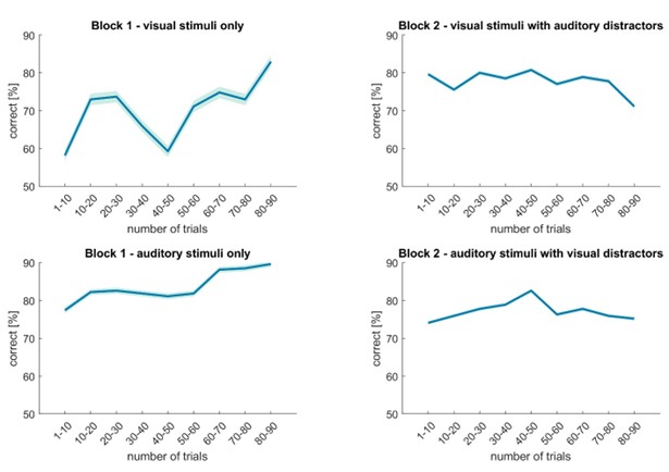
The following is the authors’ response to the previous reviews
Reviewer #1 (Public review):
In this study, Brickwedde et al. leveraged a cross-modal task where visual cues indicated whether upcoming targets required visual or auditory discrimination. Visual and auditory targets were paired with auditory and visual distractors, respectively. The authors found that during the cue-to-target interval, posterior alpha activity increased along with auditory and visual frequency-tagged activity when subjects were anticipating auditory targets. The authors conclude that their results disprove the alpha inhibition hypothesis, and instead implies that alpha "regulates downstream information transfer." However, as I detail below, I do not think the presented data irrefutably disproves the alpha inhibition hypothesis. Moreover, the evidence for the alternative hypothesis of alpha as an orchestrator for downstream signal transmission is weak. Their data serves to refute only the most extreme and physiologically implausible version of the alpha inhibition hypothesis, which assumes that alpha completely disengages the entire brain area, inhibiting all neuronal activity.
We thank the reviewer for taking the time to provide additional feedback and suggestions and we improved our manuscript accordingly.
(1) Authors assign specific meanings to specific frequencies (8-12 Hz alpha, 4 Hz intermodulation frequency, 36 Hz visual tagging activity, 40 Hz auditory tagging activity), but the results show that spectral power increases in all of these frequencies towards the end of the cue-to-target interval. This result is consistent with a broadband increase, which could simply be due to additional attention required when anticipating auditory target (since behavioral performance was lower with auditory targets, we can say auditory discrimination was more difficult). To rule this out, authors will need to show a power spectral density curve with specific increases around each frequency band of interest. In addition, it would be more convincing if there was a bump in the alpha band, and distinct bumps for 4 vs 36 vs 40 Hz band.
This is an interesting point with several aspects, which we will address separately
Broadband Increase vs. Frequency-Specific Effects:
The suggestion that the observed spectral power increases may reflect a broadband effect rather than frequency-specific tagging is important. However, Supplementary Figure 11 shows no difference between expecting an auditory or visual target at 44 Hz. This demonstrates that (1) there is no uniform increase across all frequencies, and (2) the separation between our stimulation frequencies was sufficient to allow differentiation using our method.
Task Difficulty and Performance Differences:
The reviewer suggests that the observed effects may be due to differences in task difficulty, citing lower performance when anticipating auditory targets in the EEG study. This issue was explicitly addressed in our follow-up MEG study, where stimulus difficulty was calibrated. In the second block—used for analysis—accuracy between auditory and visual targets was matched (see Fig. 7B). The replication of our findings under these controlled conditions directly rules out task difficulty as the sole explanation. This point is clearly presented in the manuscript.
Power Spectrum Analysis:
The reviewer’s suggestion that our analysis lacks evidence of frequency-specific effects is addressed directly in the manuscript. While we initially used the Hilbert method to track the time course of power fluctuations, we also included spectral analyses to confirm distinct peaks at the stimulation frequencies. Specifically, when averaging over the alpha cluster, we observed a significant difference at 10 Hz between auditory and visual target expectation, with no significant differences at 36 or 40 Hz in that cluster. Conversely, in the sensor cluster showing significant 36 Hz activity, alpha power did not differ, but both 36 Hz and 40 Hz tagging frequencies showed significant effects These findings clearly demonstrate frequency-specific modulation and are already presented in the manuscript.
(2) For visual target discrimination, behavioral performance with and without the distractor is not statistically different. Moreover, the reaction time is faster with distractor. Is there any evidence that the added auditory signal was actually distracting?
We appreciate the reviewer’s observation regarding the lack of a statistically significant difference in behavioral performance for visual target discrimination with and without the auditory distractor. While this was indeed the case in our EEG experiment, we believe the absence of an accuracy effect may be attributable to a ceiling effect, as overall visual performance approached 100%. This high baseline likely masked any subtle influence of the distractor.
To directly address the question of whether the auditory signal was distracting, we conducted a follow-up MEG experiment. In this study, we observed a significant reduction in visual accuracy during the second block when the distractor was present (see Fig. 7B and Suppl. Fig. 1B), providing clear evidence of a distractor cost under conditions where performance was not saturated.
Regarding the faster reaction times observed in the presence of the auditory distractor, this phenomenon is consistent with prior findings on intersensory facilitation. Auditory stimuli, which are processed more rapidly than visual stimuli, can enhance response speed to visual targets—even when the auditory input is non-informative or nominally distracting (Nickerson, 1973; Diederich & Colonius, 2008; Salagovic & Leonard, 2021). Thus, while the auditory signal may facilitate motor responses, it can simultaneously impair perceptual accuracy, depending on task demands and baseline performance levels.
Taken together, our data suggest that the auditory signal does exert a distracting influence, particularly under conditions where visual performance is not at ceiling. The dual effect—facilitated reaction time but reduced accuracy—highlights the complexity of multisensory interactions and underscores the importance of considering both behavioral and neurophysiological measures.
(3) It is possible that alpha does suppress task-irrelevant stimuli, but only when it is distracting. In other words, perhaps alpha only suppresses distractors that are presented simultaneously with the target. Since the authors did not test this, they cannot irrefutably reject the alpha inhibition hypothesis.
The reviewer’s claim that we did not test whether alpha suppresses distractors presented simultaneously with the target is incorrect. As stated in the manuscript and supported by our data (see point 2), auditory distractors were indeed presented concurrently with visual targets, and they were demonstrably distracting. Therefore, the scenario the reviewer suggests was not only tested—it forms a core part of our design.
Furthermore, it was never our intention to irrefutably reject the alpha inhibition hypothesis. Rather, our aim was to revise and expand it. If our phrasing implied otherwise, we have now clarified this in the manuscript. Specifically, we propose that alpha oscillations:
(a) Exhibit cyclic inhibitory and excitatory dynamics;
(b) Regulate processing by modulating transfer pathways, which can result in either inhibition or facilitation depending on the network context.
In our study, we did not observe suppression of distractor transfer, likely due to the engagement of a supramodal system that enhances both auditory and visual excitability. This interpretation is supported by prior findings (e.g., Jacoby et al., 2012), which show increased visual SSEPs under auditory task load, and by Zhigalov et al. (2020), who found no trial-by-trial correlation between alpha power and visual tagging in early visual areas, despite a general association with attention.
Recent evidence (Clausner et al., 2024; Yang et al., 2024) further supports the notion that alpha oscillations serve multiple functional roles depending on the network involved. These roles include intra- and inter-cortical signal transmission, distractor inhibition, and enhancement of downstream processing (Scheeringa et al., 2012; Bastos et al., 2015; Zumer et al., 2014). We believe the most plausible account is that alpha oscillations support both functions, depending on context.
To reflect this more clearly, we have updated Figure 1 to present a broader signal-transfer framework for alpha oscillations, beyond the specific scenario tested in this study.
We have now revised Figure 1 and several sentences in the introduction and discussion, to clarify this argument.
L35-37: Previous research gave rise to the prominent alpha inhibition hypothesis, which suggests that oscillatory activity in the alpha range (~10 Hz) plays a mechanistic role in selective attention through functional inhibition of irrelevant cortical areas (see Fig. 1; Foxe et al., 1998; Jensen & Mazaheri, 2010; Klimesch et al., 2007).
L60-65: In contrast, we propose that functional and inhibitory effects of alpha modulation, such as distractor inhibition, are exhibited through blocking or facilitating signal transmission to higher order areas (Peylo et al., 2021; Yang et al., 2023; Zhigalov & Jensen, 2020; Zumer et al., 2014), gating feedforward or feedback communication between sensory areas (see Fig. 1; Bauer et al., 2020; Haegens et al., 2015; Uemura et al., 2021).
L482-485: This suggests that responsiveness of the visual stream was not inhibited when attention was directed to auditory processing and was not inhibited by occipital alpha activity, which directly contradicts the proposed mechanism behind the alpha inhibition hypothesis.
L517-519: Top-down cued changes in alpha power have now been widely viewed to play a functional role in directing attention: the processing of irrelevant information is attenuated by increasing alpha power in areas involved with processing this information (Foxe, Simpson, & Ahlfors, 1998; Hanslmayr et al., 2007; Jensen & Mazaheri, 2010).
L566-569: As such, it is conceivable that alpha oscillations can in some cases inhibit local transmission, while in other cases, depending on network location, connectivity and demand, alpha oscillation can facilitate signal transmission. This mechanism allows to increase transmission of relevant information and to block transmission of distractors.
(4) In the abstract and Figure 1, the authors claim an alternative function for alpha oscillations; that alpha "orchestrates signal transmission to later stages of the processing stream." In support, the authors cite their result showing that increased alpha activity originating from early visual cortex is related to enhanced visual processing in higher visual areas and association areas. This does not constitute a strong support for the alternative hypothesis. The correlation between posterior alpha power and frequency-tagged activity was not specific in any way; Fig. 10 shows that the correlation appeared on both 1) anticipating-auditory and anticipating-visual trials, 2) the visual tagged frequency and the auditory tagged activity, and 3) was not specific to the visual processing stream. Thus, the data is more parsimonious with a correlation than a causal relationship between posterior alpha and visual processing.
Again, the reviewer raises important points, which we want to address
The correlation between posterior alpha power and frequency-tagged activity was not specific, as it is present both when auditory and visual targets are expected:
If there is a connection between posterior alpha activity and higher-order visual information transfer, then it can be expected that this relationship remains across conditions and that a higher alpha activity is accompanied by higher frequency-tagged activity, both over trials and over conditions. However, it is possible that when alpha activity is lower, such as when expecting a visual target, the signal-to-noise ratio is affected, which may lead to higher difficulty to find a correlation effect in the data when using non-invasive measurements.
The connection between alpha activity and frequency-tagged activity appears both for auditory as well as visual stimuli and The correlation is not specific to the visual processing stream:
While we do see differences between conditions (e.g. in the EEG-analysis, mostly 36 Hz correlated with alpha activity and only in one condition 40 Hz showed a correlation as well), it is true that in our MEG analysis, we found correlations both between alpha activity and 36 Hz as well as alpha activity and 40 Hz.
We acknowledge that when analysing frequency-tagged activity on a trial-by-trial basis, where removal of non-timelocked activity through averaging (which we did when we tested for condition differences in Fig. 4 and 9) is not possible, there is uncertainty in the data. Baseline-correction can alleviate this issue, but it cannot offset the possibility of non-specific effects. We therefore decided to repeat the analysis with a fast-fourier calculated power instead of the Hilbert power, in favour of a higher and stricter frequency-resolution, as we averaged over a time-period and thus, the time-domain was not relevant for this analysis. In this more conservative analysis, we can see that only 36 Hz tagged activity when expecting an auditory target correlated with early visual alpha activity.
Additionally, we added correlation analyses between alpha activity and frequency-tagged activity within early visual areas, using the sensor cluster which showed significant condition differences in alpha activity. Here, no correlations between frequency-tagged activity and alpha activity could be found (apart from a small correlation with 40 Hz which could not be confirmed by a median split; see SUPPL Fig. 14 C). The absence of a significant correlation between early visual alpha and frequency-tagged activity has previously been described by others (Zhigalov & Jensen, 2020) and a Bayes factor of below 1 also indicated that the alternative hypotheses is unlikely.
Nonetheless, a correlation with auditory signal is possible and could be explained in different ways. For example, it could be that very early auditory feedback in early visual cortex (see for example Brang et al., 2022) is transmitted alongside visual information to higher-order areas. Several studies have shown that alpha activity and visual as well as auditory processing are closely linked together (Bauer et al., 2020; Popov et al., 2023). Inference on whether or how this link could play out in the case of this manuscript expands beyond the scope of this study.
To summarize, we believe the fact that 36 Hz activity within early visual areas does not correlate with alpha activity on a trial-by-trial basis, but that 36 Hz activity in other areas does, provides strong evidence that alpha activity affects down-stream signal processing.
We mention this analysis now in our discussion:
L533-536: Our data provides evidence in favour of this view, as we can show that early sensory alpha activity does not covary over trials with SSEP magnitude in early visual areas, but covaries instead over trials with SSEP magnitude in higher order sensory areas (see also SUPPL. Fig. 14).
Reviewer #1 (Recommendations for the authors):
The evidence for the alternative hypothesis, that alpha in early sensory areas orchestrates downstream signal transmission, is not strong enough to be described up front in the abstract and Figure 1. I would leave it in the Discussion section, but advise against mentioning it in the abstract and Figure 1.
We appreciate the reviewer’s concern regarding the inclusion of the alternative hypothesis—that alpha activity in early sensory areas orchestrates downstream signal transmission—in the abstract and Figure 1. While we agree that this interpretation is still developing, recent studies (Keitel et al., 2025; Clausner et al., 2024; Yang et al., 2024) provide growing support for this framework.
In response, we have revised the introduction, discussion, and Figure 1 to clarify that our intention is not to outright dismiss the alpha inhibition hypothesis, but to refine and expand it in light of new data. This revision does not invalidate the prior literature on alpha timing and inhibition; rather, it proposes an updated mechanism that may better account for observed effects.
We have though retained Figure 1, as it visually contextualizes the broader theoretical landscape. while at the same time added further analyses to strengthen our empirical support for this emerging view.
References:
Bastos, A. M., Litvak, V., Moran, R., Bosman, C. A., Fries, P., & Friston, K. J. (2015). A DCM study of spectral asymmetries in feedforward and feedback connections between visual areas V1 and V4 in the monkey. NeuroImage, 108, 460–475. https://doi.org/10.1016/j.neuroimage.2014.12.081
Bauer, A. R., Debener, S., & Nobre, A. C. (2020). Synchronisation of Neural Oscillations and Cross-modal Influences. Trends in cognitive sciences, 24(6), 481–495. https://doi.org/10.1016/j.tics.2020.03.003
Brang, D., Plass, J., Sherman, A., Stacey, W. C., Wasade, V. S., Grabowecky, M., Ahn, E., Towle, V. L., Tao, J. X., Wu, S., Issa, N. P., & Suzuki, S. (2022). Visual cortex responds to sound onset and offset during passive listening. Journal of neurophysiology, 127(6), 1547–1563. https://doi.org/10.1152/jn.00164.2021
Clausner T., Marques J., Scheeringa R. & Bonnefond M (2024). Feature specific neuronal oscillations in cortical layers BioRxiv :2024.07.31.605816. https://doi.org/10.1101/2024.07.31.605816
Diederich, A., & Colonius, H. (2008). When a high-intensity "distractor" is better then a low-intensity one: modeling the effect of an auditory or tactile nontarget stimulus on visual saccadic reaction time. Brain research, 1242, 219–230. https://doi.org/10.1016/j.brainres.2008.05.081
Haegens, S., Nácher, V., Luna, R., Romo, R., & Jensen, O. (2011). α-Oscillations in the monkey sensorimotor network influence discrimination performance by rhythmical inhibition of neuronal spiking. Proceedings of the National Academy of Sciences of the United States of America, 108(48), 19377–19382. https://doi.org/10.1073/pnas.1117190108
Jacoby, O., Hall, S. E., & Mattingley, J. B. (2012). A crossmodal crossover: opposite effects of visual and auditory perceptual load on steady-state evoked potentials to irrelevant visual stimuli. NeuroImage, 61(4), 1050–1058. https://doi.org/10.1016/j.neuroimage.2012.03.040
Keitel, A., Keitel, C., Alavash, M., Bakardjian, K., Benwell, C. S. Y., Bouton, S., Busch, N. A., Criscuolo, A., Doelling, K. B., Dugue, L., Grabot, L., Gross, J., Hanslmayr, S., Klatt, L.-I., Kluger, D. S., Learmonth, G., London, R. E., Lubinus, C., Martin, A. E., … Kotz, S. A. (2025). Brain rhythms in cognition – controversies and future directions. ArXiv. https://doi.org/10.48550/arXiv.2507.15639
Nickerson R. S. (1973). Intersensory facilitation of reaction time: energy summation or preparation enhancement?. Psychological review, 80(6), 489–509. https://doi.org/10.1037/h0035437
Popov, T., Gips, B., Weisz, N., & Jensen, O. (2023). Brain areas associated with visual spatial attention display topographic organization during auditory spatial attention. Cerebral cortex (New York, N.Y. : 1991), 33(7), 3478–3489. https://doi.org/10.1093/cercor/bhac285
Salagovic, C. A., & Leonard, C. J. (2021). A nonspatial sound modulates processing of visual distractors in a flanker task. Attention, perception & psychophysics, 83(2), 800–809. https://doi.org/10.3758/s13414-020-02161-5
Scheeringa, R., Petersson, K. M., Kleinschmidt, A., Jensen, O., & Bastiaansen, M. C. (2012). EEG α power modulation of fMRI resting-state connectivity. Brain connectivity, 2(5), 254–264. https://doi.org/10.1089/brain.2012.0088
Spaak, E., Bonnefond, M., Maier, A., Leopold, D. A., & Jensen, O. (2012). Layer-specific entrainment of γ-band neural activity by the α rhythm in monkey visual cortex. Current biology : CB, 22(24), 2313–2318. https://doi.org/10.1016/j.cub.2012.10.020
Yang, X., Fiebelkorn, I. C., Jensen, O., Knight, R. T., & Kastner, S. (2024). Differential neural mechanisms underlie cortical gating of visual spatial attention mediated by alpha-band oscillations. Proceedings of the National Academy of Sciences of the United States of America, 121(45), e2313304121. https://doi.org/10.1073/pnas.2313304121
Zhigalov, A., & Jensen, O. (2020). Alpha oscillations do not implement gain control in early visual cortex but rather gating in parieto-occipital regions. Human brain mapping, 41(18), 5176–5186. https://doi.org/10.1002/hbm.25183
Zumer, J. M., Scheeringa, R., Schoffelen, J. M., Norris, D. G., & Jensen, O. (2014). Occipital alpha activity during stimulus processing gates the information flow to object-selective cortex. PLoS biology, 12(10), e1001965. https://doi.org/10.1371/journal.pbio.1001965
Note: This response was posted by the corresponding author to Review Commons. The content has not been altered except for formatting.
Learn more at Review Commons
We would like to thank all the reviewers for their valuable comments and criticisms. We have thoroughly revised the manuscript and the resource to address all the points raised by the reviewers. Below, we provide a point-by-point response for the sake of clarity.
Reviewer #1
__Evidence, reproducibility and clarity __
Summary: This manuscript, "MAVISp: A Modular Structure-Based Framework for Protein Variant Effects," presents a significant new resource for the scientific community, particularly in the interpretation and characterization of genomic variants. The authors have developed a comprehensive and modular computational framework that integrates various structural and biophysical analyses, alongside existing pathogenicity predictors, to provide crucial mechanistic insights into how variants affect protein structure and function. Importantly, MAVISp is open-source and designed to be extensible, facilitating reuse and adaptation by the broader community.
Major comments: - While the manuscript is formally well-structured (with clear Introduction, Results, Conclusions, and Methods sections), I found it challenging to follow in some parts. In particular, the Introduction is relatively short and lacks a deeper discussion of the state-of-the-art in protein variant effect prediction. Several methods are cited but not sufficiently described, as if prior knowledge were assumed. OPTIONAL: Extend the Introduction to better contextualize existing approaches (e.g., AlphaMissense, EVE, ESM-based predictors) and clarify what MAVISp adds compared to each.
We have expanded the introduction on the state-of-the-art of protein variant effects predictors, explaining how MAVISp departs from them.
- The workflow is summarized in Figure 1(b), which is visually informative. However, the narrative description of the pipeline is somewhat fragmented. It would be helpful to describe in more detail the available modules in MAVISp, and which of them are used in the examples provided. Since different use cases highlight different aspects of the pipeline, it would be useful to emphasize what is done step-by-step in each.
We have added a concise, narrative description of the data flow for MAVISp, as well as improved the description of modules in the main text. We will integrate the results section with a more comprehensive description of the available modules, and then clarify in the case studies which modules were applied to achieve specific results.
OPTIONAL: Consider adding a table or a supplementary figure mapping each use case to the corresponding pipeline steps and modules used.
We have added a supplementary table (Table S2) to guide the reader on the modules and workflows applied for each case study
We also added Table S1 to map the toolkit used by MAVISp to collect the data that are imported and aggregated in the webserver for further guidance.
- The text contains numerous acronyms, some of which are not defined upon first use or are only mentioned in passing. This affects readability. OPTIONAL: Define acronyms upon first appearance, and consider moving less critical technical details (e.g., database names or data formats) to the Methods or Supplementary Information. This would greatly enhance readability.
We revised the usage of acronyms following the reviewer’s directions of defying them at first appearance.
We thank the reviewer for noticing and praising the availability of the tools of MAVISp. Our MAVISp framework utilizes methods and scores that incorporate machine learning features (such as EVE or RaSP), but does not employ machine learning itself. Specifically, we do not use PyTorch and do not utilize features in a machine learning sense. We do extract some information from the AlphaFold2 models that we use (such as the pLDDT score and their secondary structure content, as calculated by DSSP), and those are available in the MAVISp aggregated csv files for each protein entry and detailed in the Documentation section of the MAVISp website.
We have removed this section and included a mention in the conclusions as part of the future directions.
Minor comments: - Most relevant recent works are cited, including EVE, ESM-1v, and AlphaFold-based predictors. However, recent methods like AlphaMissense (Cheng et al., 2023) could be discussed more thoroughly in the comparison.
We have revised the introduction to accommodate the proper space for this comparison.
We have revised Figure 2 and presented only one case study to simplify its readability. We have also changed Figure 3, whereas retained the other previous figures since they seemed less problematic.
We have done a proofreading of the entire article, including the points above
Significance
General assessment: the strongest aspects of the study are the modularity, open-source implementation, and the integration of structural information through graph neural networks. MAVISp appears to be one of the few publicly available frameworks that can easily incorporate AlphaFold2-based features in a flexible way, lowering the barrier for developing custom predictors. Its reproducibility and transparency make it a valuable resource. However, while the technical foundation is solid and the effort substantial, the scientific narrative and presentation could be significantly improved. The manuscript is dense and hard to follow in places, with a heavy use of acronyms and insufficient explanation of key design choices. Improving the descriptive clarity, especially in the early sections, would greatly enhance the impact of this work.
Advance
to the best of my knowledge, this is one of the first modular platforms for protein variant effect prediction that integrates structural data from AlphaFold2 with bioinformatic annotations and even clinical data in an extensible fashion. While similar efforts exist (e.g., ESMfold, AlphaMissense), MAVISp distinguishes itself through openness and design for reusability. The novelty is primarily technical and practical rather than conceptual.
Audience
this study will be of strong interest to researchers in computational biology, structural bioinformatics, and genomics, particularly those developing variant effect predictors or analyzing the impact of mutations in clinical or functional genomics contexts. The audience is primarily specialized, but the open-source nature of the tool may diffuse its use among more applied or translational users, including those working in precision medicine or protein engineering.
Reviewer expertise: my expertise is in computational structural biology, molecular modeling, and (rather weak) machine learning applications in bioinformatics. I am familiar with graph-based representations of proteins, AlphaFold2, and variant effects based on Molecular Dynamics simulations. I do not have any direct expertise in clinical variant annotation pipelines.
Reviewer #2
__Evidence, reproducibility and clarity __
Summary: The authors present a pipeline and platform, MAVISp, for aggregating, displaying and analysis of variant effects with a focus on reclassification of variants of uncertain clinical significance and uncovering the molecular mechanisms underlying the mutations.
Major comments: - On testing the platform, I was unable to look-up a specific variant in ADCK1 (rs200211943, R115Q). I found that despite stating that the mapped refseq ID was NP_001136017 in the HGVSp column, it was actually mapped to the canonical UniProt sequence (Q86TW2-1). NP_001136017 actually maps to Q86TW2-3, which is missing residues 74-148 compared to the -1 isoform. The Uniprot canonical sequence has no exact RefSeq mapping, so the HGVSp column is incorrect in this instance. This mapping issue may also affect other proteins and result in incorrect HGVSp identifiers for variants.
We would like to thank the reviewer for pointing out these inconsistencies. We have revised all the entries and corrected them. If needed, the history of the cases that have been corrected can be found in the closed issues of the GitHub repository that we use for communication between biocurators and data managers (https://github.com/ELELAB/mavisp_data_collection). We have also revised the protocol we follow in this regard and the MAVISp toolkit to include better support for isoform matching in our pipelines for future entries, as well as for the revision/monitoring of existing ones, as detailed in the Method Section. In particular, we introduced a tool, uniprot2refseq, which aids the biocurator in identifying the correct match in terms of sequence length and sequence identity between RefSeq and UniProt. More details are included in the Method Section of the paper. The two relevant scripts for this step are available at: https://github.com/ELELAB/mavisp_accessory_tools/
- The paper lacks a section on how to properly interpret the results of the MAVISp platform (the case-studies are helpful, but don't lay down any global rules for interpreting the results). For example: How should a variant with conflicts between the variant impact predictors be interpreted? Are specific indicators considered more 'reliable' than others?
We have added a section in Results to clarify how to interpret results from MAVISp in the most common use cases.
We thank the reviewer for spotting this inconsistency. This part in the main text was left over from a previous and preliminary version of the pre-print, we have revised the main text. Supplementary Text S4 includes the correct reference for the value in light of the benchmarking therewithin.
We have changed the structure of the webserver in such a way that now the whole website opens as its own separate window, instead of being confined within the size permitted by the website at DTU. This solves the fixed window size issue. Hopefully, this will improve the user experience.
We have refactored the web app by adding filtering functionality, both for the main protein table (that can now be filtered by UniProt AC, gene name or RefSeq ID) and the mutations table. Doing this required a general overhaul of the table infrastructure (we changed the underlying engine that renders the tables).
The table overhauls fixed both of these issues
We clarified the meaning of the reference column in the Documentation on the MAVISp website, as we realized it had confused the reviewer. The reference column is meant to cite the papers where the computationally-generated MAVISp data are used, not external sources. Since we also have the experimental data module in the most recent release, we have also refactored the MAVISp website by adding a “Datasets and metadata” page, which details metadata for key modules. These include references to data from external sources that we include in MAVISp on a case-by-case basis (for example the results of a MAVE experiment). Additionally, we have verified that the papers using MAVISp data are updated in https://elelab.gitbook.io/mavisp/overview/publications-that-used-mavisp-data and in the csv file of the interested proteins.
Here below the current references that have been included in terms of publications using MAVISp data:
SMPD1
ASM variants in the spotlight: A structure-based atlas for unraveling pathogenic mechanisms in lysosomal acid sphingomyelinase
Biochim Biophys Acta Mol Basis Dis
38782304
https://doi.org/10.1016/j.bbadis.2024.167260
TRAP1
Point mutations of the mitochondrial chaperone TRAP1 affect its functions and pro-neoplastic activity
Cell Death & Disease
40074754
https://doi.org/10.1038/s41419-025-07467-6
BRCA2
Saturation genome editing-based clinical classification of BRCA2 variants
Nature
39779848
0.1038/s41586-024-08349-1
TP53, GRIN2A, CBFB, CALR, EGFR
TRAP1 S-nitrosylation as a model of population-shift mechanism to study the effects of nitric oxide on redox-sensitive oncoproteins
Cell Death & Disease
37085483
10.1038/s41419-023-05780-6
KIF5A, CFAP410, PILRA, CYP2R1
Computational analysis of five neurodegenerative diseases reveals shared and specific genetic loci
Computational and Structural Biotechnology Journal
38022694
https://doi.org/10.1016/j.csbj.2023.10.031
KRAS
Combining evolution and protein language models for an interpretable cancer driver mutation prediction with D2Deep
Brief Bioinform
39708841
https://doi.org/10.1093/bib/bbae664
OPTN
Decoding phospho-regulation and flanking regions in autophagy-associated short linear motifs
Communications Biology
40835742
10.1038/s42003-025-08399-9
DLG4,GRB2,SMPD1
Deciphering long-range effects of mutations: an integrated approach using elastic network models and protein structure networks
JMB
40738203
doi: 10.1016/j.jmb.2025.169359
Entering multiple mutants in the "mutations to be displayed" window is time-consuming for more than a handful of mutants. Suggestion: Add a box where multiple mutants can be pasted in at once from an external document.
During the table overhaul, we have revised the user interface to add a text box that allows free copy-pasting of mutation lists. While we understand having a single input box would have been ideal, the former selection interface (which is also still available) doesn’t allow copy-paste. This is a known limitation in Streamlit.
Minor comments
We have done proofreading on the final version of the manuscript
Yes, we are aware of this. It is far from trivial to properly import the datasets from multiplex assays. They often need to be treated on a case-by-case basis. We are in the process of carefully compiling locally all the MAVE data before releasing it within the public version of the database, so this is why they are missing. We are giving priorities to the ones that can be correlated with our predictions on changes in structural stability and then we will also cover the rest of the datasets handling them in batches. Having said this, we have checked the dataset for BRCA1, HRAS, and PPARG. We have imported the ones for PPARG and BRCA1 from ProtGym, referring to the studies published in 10.1038/ng.3700 and 10.1038/s41586-018-0461-z, respectively. Whereas for HRAS, checking in details both the available data and literature, while we did identify a suitable dataset (10.7554/eLife.27810), we struggled to understand what a sensible cut-off for discriminating between pathogenic and non-pathogenic variants would be, and so ended up not including it in the MAVISp dataset for now. We will contact the authors to clarify which thresholds to apply before importing the data.
In the KRAS case study presented in MAVISP, we utilized the protein abundance dataset reported in (http://dx.doi.org/10.1038/s41586-023-06954-0) and made available in the ProteinGym repository (specifically referenced at https://github.com/OATML-Markslab/ProteinGym/blob/main/reference_files/DMS_substitutions.csv#L153). We adopted the precalculated thresholds as provided by the ProteinGym authors. In this regard, we are not really sure the reviewer is referring to this dataset or another one on KRAS.
We improved the description of our classification strategies for both modules in the Documentation page of our website. Also, we explained more clearly the possible sources of ‘uncertain’ annotations for the two modules in both the web app (Documentation page) and main text. Briefly, in the STABILITY module, we consider FoldX and either Rosetta or RaSP to achieve a final classification. We first classify one and the other independently, according to the following strategy:
If DDG ≥ 3, the mutation is Destabilizing If DDG ≤ −3, the mutation is Stabilizing If −2 We then compare the classifications obtained by the two methods: if they agree, then that is the final classification, if they disagree, then the final classification is Uncertain. The thresholds were selected based on a previous study, in which variants with changes in stability below 3 kcal/mol were not featuring a markedly different abundance at cellular level [10.1371/journal.pgen.1006739, 10.7554/eLife.49138]
Regarding the LOCAL_INTERACTION module, it works similarly as for the Stability module, in that Rosetta and FoldX are considered independently, and an implicit classification is performed for each, according to the rules (values in kcal/mol)
If DDG > 1, the mutation is Destabilizing. If DDG Each mutation is therefore classified for both methods. If the methods agree (i.e., if they classify the mutation in the same way), their consensus is the final classification for the mutation; if they do not agree, the final classification will be Uncertain.
If a mutation does not have an associated free energy value, the relative solvent accessible area is used to classify it: if SAS > 20%, the mutation is classified as Uncertain, otherwise it is not classified.
Thresholds here were selected according to best practices followed by the tool authors and more in general in the literature, as the reviewer also noticed.
The last of these points is not an application of MAVISp, but rather a way in which external data can help validate MAVISp results. Furthermore, none of the examples given demonstrate an application in benchmarking (what is being benchmarked?).
We have revised the statements to avoid this confusion in the reader.
We have removed this section and included a mention in the conclusions as part of the future directions.
The reviewer’s interpretation on the second legend is correct - it does refer to the ClinVar classification. Nonetheless, we understand the positioning of the legend makes understanding what the legend refers to not obvious. We also revised the captions of the figures in the main text. On the web app, we have changed the location of the figure legend for the ClinVar effect category and added a label to make it clear what the classification refers to.
We have corrected this in the text and the statements related to it.
Significance
Platforms that aggregate predictors of variant effect are not a new concept, for example dbNSFP is a database of SNV predictions from variant effect predictors and conservation predictors over the whole human proteome. Predictors such as CADD and PolyPhen-2 will often provide a summary of other predictions (their features) when using their platforms. MAVISp's unique angle on the problem is in the inclusion of diverse predictors from each of its different moules, giving a much wider perspective on variants and potentially allowing the user to identify the mechanistic cause of pathogenicity. The visualisation aspect of the web app is also a useful addition, although the user interface is somewhat awkward. Potentially the most valuable aspect of this study is the associated gitbook resource containing reports from biocurators for proteins that link relevant literature and analyse ClinVar variants. Unfortunately, these are only currently available for a small minority of the total proteins in the database with such reports. For improvement, I think that the paper should focus more on the precise utility of the web app / gitbook reports and how to interpret the results rather than going into detail about the underlying pipeline.
We appreciate the interest in the gitbook resource that we also see as very valuable and one of the strengths of our work. We have now implemented a new strategy based on a Python script introduced in the mavisp toolkit to generate a template Markdown file of the report that can be further customized and imported into GitBook directly (https://github.com/ELELAB/mavisp_accessory_tools/). This should allow us to streamline the production of more reports. We are currently assigning proteins in batches for reporting to biocurator through the mavisp_data_collection GitHub to expand their coverage. Also, we revised the text and added a section on the interpretation of results from MAVISp. with a focus on the utility of the web-app and reports.
In terms of audience, the fast look-up and visualisation aspects of the web-platform are likely to be of interest to clinicians in the interpretation of variants of unknown clinical significance. The ability to download the fully processed dataset on a per-protein database would be of more interest to researchers focusing on specific proteins or those taking a broader view over multiple proteins (although a facility to download the whole database would be more useful for this final group).
While our website only displays the dataset per protein, the whole dataset, including all the MAVISp entries, is available at our OSF repository (https://osf.io/ufpzm/), which is cited in the paper and linked on the MAVISp website. We have further modified the MAVISp database to add a link to the repository in the modes page, so that it is more visible.
My expertise. - I am a protein bioinformatician with a background in variant effect prediction and large-scale data analysis.
Reviewer #3 (Evidence, reproducibility and clarity (Required)):
Evidence, reproducibility and clarity:
Summary:
The authors present MAVISp, a tool for viewing protein variants heavily based on protein structure information. The authors have done a very impressive amount of curation on various protein targets, and should be commended for their efforts. The tool includes a diverse array of experimental, clinical, and computational data sources that provides value to potential users interested in a given target.
Major comments:
Unfortunately I was not able to get the website to work correctly. When selecting a protein target in simple mode, I was greeted with a completely blank page in the app window. In ensemble mode, there was no transition away from the list of targets at all. I'm using Firefox 140.0.2 (64-bit) on Ubuntu 22.04. I would like to explore the data myself and provide feedback on the user experience and utility.
We have tried reproducing the issue mentioned by the reviewer, using the exact same Ubuntu and Firefox versions, but unfortunately failed to produce it. The website worked fine for us under such an environment. The issue experienced by the reviewer may have been due to either a temporary issue with the web server or a problem with the specific browser environment they were working in, which we are unable to reproduce. It would be useful to know the date that this happened to verify if it was a downtime on the DTU IT services side that made the webserver inaccessible.
I have some serious concerns about the sustainability of the project and think that additional clarifications in the text could help. Currently is there a way to easily update a dataset to add, remove, or update a component (for example, if a new predictor is published, an error is found in a predictor dataset, or a predictor is updated)? If it requires a new round of manual curation for each protein to do this, I am worried that this will not scale and will leave the project with many out of date entries. The diversity of software tools (e.g., three different pipeline frameworks) also seems quite challenging to maintain.
We appreciate the reviewer’s concerns about long-term sustainability. It is a fair point that we consider within our steering group, who oversee and plans the activities and meet monthly. Adding entries to MAVISp is moving more and more towards automation as we grow. We aim to minimize the manual work where applicable. Still, an expert-based intervention is really needed in some of the steps, and we do not want to renounce it. We intend to keep working on MAVISp to make the process of adding and updating entries as automated as possible, and to streamline the process when manual intervention is necessary. From the point of view of the biocurators, they have three core workflows to use for the default modules, which also automatically cover the source of annotations. We are currently working to streamline the procedures behind LOCAL_INTERACTION, which is the most challenging one. On the data manager and maintainers' side, we have workflows and protocols that help us in terms of automation, quality control, etc, and we keep working to improve them. Among these, we have workflows to use for the old entries updates. As an example, the update of erroneously attributed RefSeq data (pointed out by reviewer 2) took us only one week overall (from assigning revisions and importing to the database) because we have a reduced version of Snakemake for automation that can act on only the affected modules. Also, another point is that we have streamlined the generation of the templates for the gitbook reports (see also answer to reviewer 2).
The update of old entries is planned and made regularly. We also deposit the old datasets on OSF for transparency, in case someone needs to navigate and explore the changes. We have activities planned between May and August every year to update the old entries in relation to changes of protocols in the modules, updates in the core databases that we interact with (COSMIC, Clinvar etc). In case of major changes, the activities for updates continue in the Fall. Other revisions can happen outside these time windows if an entry is needed or a specific research project and needs updates too.
Furthermore, the community of people contributing to MAVISp as biocurators or developers is growing and we have scientists contributing from other groups in relation to their research interest. We envision that for this resource to scale up, our team cannot be the only one producing data and depositing it to the database. To facilitate this we launched a pilot for a training event online (see Event page on the website) and we will repeat it once per year. We also organize regular meetings with all the active curators and developers to plan the activities in a sustainable manner and address the challenges we encounter.
As stated in the manuscript, currently with the team of people involved, automatization and resources that we have gathered around this initiative we can provide updates to the public database every third month and we have been regularly satisfied with them. Additionally, we are capable of processing from 20 to 40 proteins every month depending also on the needs of revision or expansion of analyses on existing proteins. We also depend on these data for our own research projects and we are fully committed to it.
Additionally, we are planning future activities in these directions to improve scale up and sustainability:
We thank the reviewer for this comment - we are aware of the upcoming EOL of Python 3.9. We tested MAVISp, both software package and web server, using Python 3.10 (which is the minimum supported version going forward) and Python 3.13 (which is the latest stable release at the time of writing) and updated the instructions in the README file on the MAVISp GitHub repository accordingly.
We plan on keeping track of Python and library versions during our testing and updating them when necessary. In the future, we also plan to deploy Continuous Integration with automated testing for our repository, making this process easier and more standardized.
I appreciate that the authors have made their code and data available. These artifacts should also be versioned and archived in a service like Zenodo, so that researchers who rely on or want to refer to specific versions can do so in their own future publications.
Since 2024, we have been reporting all previous versions of the dataset on OSF, the repository linked to the MAVISp website, at https://osf.io/ufpzm/files/osfstorage (folder: previous_releases). We prefer to keep everything under OSF, as we also use it to deposit, for example, the MD trajectory data.
Additionally, in this GitHub page that we use as a space to interact between biocurators, developers, and data managers within the MAVISp community, we also report all the changes in the NEWS space: https://github.com/ELELAB/mavisp_data_collection
Finally, the individual tools are all available in our GitHub repository, where version control is in place (see Table S1, where we now mapped all the resources used in the framework)
In the introduction of the paper, the authors conflate the clinical challenges of variant classification with evidence generation and it's quite muddled together. They should strongly consider splitting the first paragraph into two paragraphs - one about challenges in variant classification/clinical genetics/precision oncology and another about variant effect prediction and experimental methods. The authors should also note that they are many predictors other than AlphaMissense, and may want to cite the ClinGen recommendations (PMID: 36413997) in the intro instead.
We revised the introduction in light of these suggestions. We have split the paragraph as recommended and added a longer second paragraph about VEPs and using structural data in the context of VEPs. We have also added the citation that the reviewer kindly recommended.
Also in the introduction on lines 21-22 the authors assert that "a mechanistic understanding of variant effects is essential knowledge" for a variety of clinical outcomes. While this is nice, it is clearly not the case as we can classify variants according to the ACMG/AMP guidelines without any notion of specific mechanism (for example, by combining population frequency data, in silico predictor data, and functional assay data). The authors should revise the statement so that it's clear that mechanistic understanding is a worthy aspiration rather than a prerequisite.
We revised the statement in light of this comment from the reviewer
In the structural analysis section (page 5, lines 154-155 and elsewhere), the authors define cutoffs with convenient round numbers. Is there a citation for these values or were these arbitrarily chosen by the authors? I would have liked to see some justification that these assignments are reasonable. Also there seems to be an error in the text where values between -2 and -3 kcal/mol are not assigned to a bin (I assume they should also be uncertain). There are other similar seemingly-arbitrary cutoffs later in the section that should also be explained.
We have revised the text making the two intervals explicit, for better clarity.
On page 9, lines 294-298 the authors talk about using the PTEN data from ProteinGym, rather than the actual cutoffs from the paper. They get to the latter later on, but I'm not sure why this isn't first? The ProteinGym cutoffs are somewhat arbitrarily based on the median rather than expert evaluation of the dataset, and I'm not sure why it's even worth mentioning them when proper classifications are available. Regarding PTEN, it would be quite interesting to see a comparison of the VAMP-seq PTEN data and the Mighell phosphatase assay, which is cited on page 9 line 288 but is not actually a VAMP-seq dataset. I think this section could be interesting but it requires some additional attention.
We have included the data from Mighell’s phosphatase assay as provided by MAVEdb in the MAVISp database, within the experimental_data module for PTEN, and we have revised the case study, including them and explaining better the decision of supporting both the ProteinGym and MAVEdb classification in MAVISp (when available). See revised Figure3, Table 1 and corresponding text.
The authors mention "pathogenicity predictors" and otherwise use pathogenicity incorrectly throughout the manuscript. Pathogenicity is a classification for a variant after it has been curated according to a framework like the ACMG/AMP guidelines (Richards 2015 and amendments). A single tool cannot predict or assign pathogenicity - the AlphaMissense paper was wrong to use this nomenclature and these authors should not compound this mistake. These predictors should be referred to as "variant effect predictors" or similar, and they are able to produce evidence towards pathogenicity or benignity but not make pathogenicity calls themselves. For example, in Figure 4e, the terms "pathogenic" and "benign" should only be used here if these are the classifications the authors have derived from ClinVar or a similar source of clinically classified variants.
The reviewer is correct, we have revised the terminology we used in the manuscript and refers to VEPs (Variant Effect Predictors)
Minor comments:
The target selection table on the website needs some kind of text filtering option. It's very tedious to have to find a protein by scrolling through the table rather than typing in the symbol. This will only get worse as more datasets are added.
We have revised the website, adding a filtering option. In detail, we have refactored the web app by adding filtering functionality, both for the main protein table (that can now be filtered by UniProt AC, gene name, or RefSeq ID) and the mutations table. Doing this required a general overhaul of the table infrastructure (we changed the underlying engine that renders the tables).
The data sources listed on the data usage section of the website are not concordant with what is in the paper. For example, MaveDB is not listed.
We have revised and updated the data sources on the website, adding a metadata section with relevant information, including MaveDB references where applicable.
Figure 2 is somewhat confusing, as it partially interleaves results from two different proteins. This would be nicer as two separate figures, one on each protein, or just of a single protein.
As suggested by the reviewer, we have now revised the figure and corresponding legends and text, focusing only on one of the two proteins.
Figure 3 panel b is distractingly large and I wonder if the authors could do a little bit more with this visualization.
We have revised Figure 3 to solve these issues and integrating new data from the comparison with the phosphatase assay
Capitalization is inconsistent throughout the manuscript. For example, page 9 line 288 refers to VampSEQ instead of VAMP-seq (although this is correct elsewhere). MaveDB is referred to as MAVEdb or MAVEDB in various places. AlphaMissense is referred to as Alphamissense in the Figure 5 legend. The authors should make a careful pass through the manuscript to address this kind of issues.
We have carefully proofread the paper for these inconsistencies
MaveDB has a more recent paper (PMID: 39838450) that should be cited instead of/in addition to Esposito et al.
We have added the reference that the reviewer recommended
On page 11, lines 338-339 the authors mention some interesting proteins including BLC2, which has base editor data available (PMID: 35288574). Are there plans to incorporate this type of functional assay data into MAVISp?
The assay mentioned in the paper refers to an experimental setup designed to investigate mutations that may confer resistance to the drug venetoclax. We started the first steps to implement a MAVISp module aimed at evaluating the impact of mutations on drug binding using alchemical free energy perturbations (ensemble mode) but we are far from having it complete. We expect to import these data when the module will be finalized since they can be used to benchmark it and BCL2 is one of the proteins that we are using to develop and test the new module.
Reviewer #3 (Significance (Required)):
Significance:
General assessment:
This is a nice resource and the authors have clearly put a lot of effort in. They should be celebrated for their achievments in curating the diverse datasets, and the GitBooks are a nice approach. However, I wasn't able to get the website to work and I have raised several issues with the paper itself that I think should be addressed.
Advance:
New ways to explore and integrate complex data like protein structures and variant effects are always interesting and welcome. I appreciate the effort towards manual curation of datasets. This work is very similar in theme to existing tools like Genomics 2 Proteins portal (PMID: 38260256) and ProtVar (PMID: 38769064). Unfortunately as I wasn't able to use the site I can't comment further on MAVISp's position in the landscape.
We have expanded the conclusions section to add a comparison and cite previously published work, and linked to a review we published last year that frames MAVISp in the context of computational frameworks for the prediction of variant effects. In brief, the Genomics 2 Proteins portal (G2P) includes data from several sources, including some overlapping with MAVISp such as Phosphosite or MAVEdb, as well as features calculated on the protein structure. ProtVar also aggregates mutations from different sources and includes both variant effect predictors and predictions of changes in stability upon mutation, as well as predictions of complex structures. These approaches are only partially overlapping with MAVISp. G2P is primarily focused on structural and other annotations of the effect of a mutation; it doesn’t include features about changes of stability, binding, or long-range effects, and doesn’t attempt to classify the impact of a mutation according to its measurements. It also doesn’t include information on protein dynamics. Similarly, ProtVar does include information on binding free energies, long effects, or dynamical information.
Audience:
MAVISp could appeal to a diverse group of researchers who are interested in the biology or biochemistry of proteins that are included, or are interested in protein variants in general either from a computational/machine learning perspective or from a genetics/genomics perspective.
My expertise:
I am an expert in high-throughput functional genomics experiments and am an experienced computational biologist with software engineering experience.
Note: This preprint has been reviewed by subject experts for Review Commons. Content has not been altered except for formatting.
Learn more at Review Commons
Summary:
The authors present MAVISp, a tool for viewing protein variants heavily based on protein structure information. The authors have done a very impressive amount of curation on various protein targets, and should be commended for their efforts. The tool includes a diverse array of experimental, clinical, and computational data sources that provides value to potential users interested in a given target.
Major comments:
Unfortunately I was not able to get the website to work properly. When selecting a protein target in simple mode, I was greeted with a completely blank page in the app window, and in ensemble mode, there was no transition away from the list of targets at all. I'm using Firefox 140.0.2 (64-bit) on Ubuntu 22.04. I would have liked to be able to explore the data myself and provide feedback on the user experience and utility.
I have some serious concerns about the sustainability of the project and think that additional clarifications in the text could help. Currently is there a way to easily update a dataset to add, remove, or update a component (for example, if a new predictor is published, an error is found in a predictor dataset, or a predictor is updated)? If it requires a new round of manual curation for each protein to do this, I am worried that this will not scale and will leave the project with many out of date entries. The diversity of software tools (e.g., three different pipeline frameworks) also seems quite challenging to maintain.
On the same theme, according to the GitHub repository, the program relies on Python 3.9, which reaches end of life in October 2025. It has been tested against Ubuntu 18.04, which left standard support in May 2023. The authors should update the software to more modern versions of Python to promote the long-term health and maintainability of the project.
I appreciate that the authors have made their code and data available. These artifacts should also be versioned and archived in a service like Zenodo, so that researchers who rely on or want to refer to specific versions can do so in their own future publications.
In the introduction of the paper, the authors conflate the clinical challenges of variant classification with evidence generation and it's quite muddled together. The y should strongly consider splitting the first paragraph into two paragraphs - one about challenges in variant classification/clinical genetics/precision oncology and another about variant effect prediction and experimental methods. The authors should also note that they are many predictors other than AlphaMissense, and may want to cite the ClinGen recommendations (PMID: 36413997) in the intro instead.
Also in the introduction on lines 21-22 the authors assert that "a mechanistic understanding of variant effects is essential knowledge" for a variety of clinical outcomes. While this is nice, it is clearly not the case as we are able to classify variants according to the ACMG/AMP guidelines without any notion of specific mechanism (for example, by combining population frequency data, in silico predictor data, and functional assay data). The authors should revise the statement so that it's clear that mechanistic understanding is a worthy aspiration rather than a prerequisite.
In the structural analysis section (page 5, lines 154-155 and elsewhere), the authors define cutoffs with convenient round numbers. Is there a citation for these values or were these arbitrarily chosen by the authors? I would have liked to see some justification that these assignments are reasonable. Also there seems to be an error in the text where values between -2 and -3 kcal/mol are not assigned to a bin (I assume they should also be uncertain). There are other similar seemingly-arbitrary cutoffs later in the section that should also be explained.
On page 9, lines 294-298 the authors talk about using the PTEN data from ProteinGym, rather than the actual cutoffs from the paper. They get to the latter later on, but I'm not sure why this isn't first? The ProteinGym cutoffs are somewhat arbitrarily based on the median rather than expert evaluation of the dataset and I'm not sure why it's even worth mentioning them when proper classifications are available. Regarding PTEN, it would be quite interesting to see a comparison of the VAMP-seq PTEN data and the Mighell phosphatase assay, which is cited on page 9 line 288 but is not actually a VAMP-seq dataset. I think this section could be interesting but it requires some additional attention.
The authors mention "pathogenicity predictors" and otherwise use pathogenicity incorrectly throughout the manuscript. Pathogenicity is a classification for a variant after it has been curated according to a framework like the ACMG/AMP guidelines (Richards 2015 and amendments). A single tool cannot predict or assign pathogenicity - the AlphaMissense paper was wrong to use this nomenclature and these authors should not compound this mistake. These predictors should be referred to as "variant effect predictors" or similar, and they are able to produce evidence towards pathogenicity or benignity but not make pathogenicity calls themselves. For example, in Figure 4e, the terms "pathogenic" and "benign" should only be used here if these are the classifications the authors have derived from ClinVar or a similar source of clinically classified variants.
Minor comments:
The target selection table on the website needs some kind of text filtering option. It's very tedious to have to find a protein by scrolling through the table rather than typing in the symbol. This will only get worse as more datasets are added.
The data sources listed on the data usage section of the website are not concordant with what is in the paper. For example, MaveDB is not listed.
I found Figure 2 to be a bit confusing in that it partially interleaves results from two different proteins. I think this would be nicer as two separate figures, one on each protein, or just of a single protein.
Figure 3 panel b is distractingly large and I wonder if the authors could do a little bit more with this visualization.
Capitalization is inconsistent throughout the manuscript. For example, page 9 line 288 refers to VampSEQ instead of VAMP-seq (although this is correct elsewhere). MaveDB is referred to as MAVEdb or MAVEDB in various places. AlphaMissense is referred to as Alphamissense in the Figure 5 legend. The authors should make a careful pass through the manuscript to address this kind of issues.
MaveDB has a more recent paper (PMID: 39838450) that should be cited instead of/in addition to Esposito et al.
On page 11, lines 338-339 the authors mention some interesting proteins including BLC2, which has base editor data available (PMID: 35288574). Are there plans to incorporate this type of functional assay data into MAVISp?
General assessment:
This is a nice resource and the authors have clearly put a lot of effort in. They should be celebrated for their achievments in curating the diverse datasets, and the GitBooks are a nice approach. However, I wasn't able to get the website to work and I have raised several issues with the paper itself that I think should be addressed.
Advance:
New ways to explore and integrate complex data like protein structures and variant effects are always interesting and welcome. I appreciate the effort towards manual curation of datasets. This work is very similar in theme to existing tools like Genomics 2 Proteins portal (PMID: 38260256) and ProtVar (PMID: 38769064). Unfortunately as I wasn't able to use the site I can't comment further on MAVISp's position in the landscape.
Audience:
MAVISp could appeal to a diverse group of researchers who are interested in the biology or biochemistry of proteins that are included, or are interested in protein variants in general either from a computational/machine learning perspective or from a genetics/genomics perspective.
My expertise:
I am an expert in high-throughput functional genomics experiments and am an experienced computational biologist with software engineering experience.
Note: This preprint has been reviewed by subject experts for Review Commons. Content has not been altered except for formatting.
Learn more at Review Commons
Summary:
The authors present a pipeline and platform, MAVISp, for aggregating, displaying and analysis of variant effects with a focus on reclassification of variants of uncertain clinical significance and uncovering the molecular mechanisms underlying the mutations.
Major comments:
Minor comments
The last of these points is not an application of MAVISp, but rather a way in which external data can help validate MAVISp results. Furthermore, none of the examples given demonstrate an application in benchmarking (what is being benchmarked?). - Transcription factors section. This section describes an intended future expansion to MAVISp, not a current feature, and presents no results. As such, it should probably be moved to the conclusions/future directions section. - Figures. The dot-plots generated by the web app, and in Figures 4, 5 and 6 have 2 legends. After looking at a few, it is clear that the lower legend refers to the colour of the variant on the X-axis - most likely referencing the ClinVar effect category. This is not, however, made clear either on the figures or in the app. - "We identified ten variants reported in ClinVar as VUS (E102K, H86D, T29I, V91I, P2R, L44P, L44F, D56G, R11L, and E25Q, Fig.5a)"
E25Q is benign in ClinVar and has had that status since first submitted.
Platforms that aggregate predictors of variant effect are not a new concept, for example dbNSFP is a database of SNV predictions from variant effect predictors and conservation predictors over the whole human proteome. Predictors such as CADD and PolyPhen-2 will often provide a summary of other predictions (their features) when using their platforms. MAVISp's unique angle on the problem is in the inclusion of diverse predictors from each of its different moules, giving a much wider perspective on variants and potentially allowing the user to identify the mechanistic cause of pathogenicity. The visualisation aspect of the web app is also a useful addition, although the user interface is somewhat awkward. Potentially the most valuable aspect of this study is the associated gitbook resource containing reports from biocurators for proteins that link relevant literature and analyse ClinVar variants. Unfortunately, these are only currently available for a small minority of the total proteins in the database with such reports.
For improvement, I think that the paper should focus more on the precise utility of the web app / gitbook reports and how to interpret the results rather than going into detail about the underlying pipeline.
In terms of audience, the fast look-up and visualisation aspects of the web-platform are likely to be of interest to clinicians in the interpretation of variants of unknown clinical significance. The ability to download the fully processed dataset on a per-protein database would be of more interest to researchers focusing on specific proteins or those taking a broader view over multiple proteins (although a facility to download the whole database would be more useful for this final group).
My expertise.
Note: This preprint has been reviewed by subject experts for Review Commons. Content has not been altered except for formatting.
Learn more at Review Commons
Summary: This manuscript, "MAVISp: A Modular Structure-Based Framework for Protein Variant Effects," presents a significant new resource for the scientific community, particularly in the interpretation and characterization of genomic variants. The authors have developed a comprehensive and modular computational framework that integrates various structural and biophysical analyses, alongside existing pathogenicity predictors, to provide crucial mechanistic insights into how variants affect protein structure and function. Importantly, MAVISp is open-source and designed to be extensible, facilitating reuse and adaptation by the broader community.
Major comments:
Minor comments:
Page 3, line 46: "MAVISp perform" -> "MAVISp performs"
Page 3, line 56: "automatically as embedded" -> "automatically embedded"
Page 3, line 57: "along with to enhance" -> unclear; please revise
Page 4, line 96: "web app interfaces with the database and present" -> "presents"
Page 6, line 210: "to investigate wheatear" -> "whether"
Page 6, lines 215-216: "We have in queue for processing with MAVISp proteins from datasets relevant to the benchmark of the PTM module." -> unclear sentence; please clarify
Page 15, line 446: "Both the approaches" -> "Both approaches"
Page 20, line 704: "advantage of multi-core system" -> "multi-core systems"
General assessment: the strongest aspects of the study are the modularity, open-source implementation, and the integration of structural information through graph neural networks. MAVISp appears to be one of the few publicly available frameworks that can easily incorporate AlphaFold2-based features in a flexible way, lowering the barrier for developing custom predictors. Its reproducibility and transparency make it a valuable resource. However, while the technical foundation is solid and the effort substantial, the scientific narrative and presentation could be significantly improved. The manuscript is dense and hard to follow in places, with a heavy use of acronyms and insufficient explanation of key design choices. Improving the descriptive clarity, especially in the early sections, would greatly enhance the impact of this work.
Advance: to the best of my knowledge, this is one of the first modular platforms for protein variant effect prediction that integrates structural data from AlphaFold2 with bioinformatic annotations and even clinical data in an extensible fashion. While similar efforts exist (e.g., ESMfold, AlphaMissense), MAVISp distinguishes itself through openness and design for reusability. The novelty is primarily technical and practical rather than conceptual.
Audience: this study will be of strong interest to researchers in computational biology, structural bioinformatics, and genomics, particularly those developing variant effect predictors or analyzing the impact of mutations in clinical or functional genomics contexts. The audience is primarily specialized, but the open-source nature of the tool may diffuse its use among more applied or translational users, including those working in precision medicine or protein engineering.
Reviewer expertise: my expertise is in computational structural biology, molecular modeling, and (rather weak) machine learning applications in bioinformatics. I am familiar with graph-based representations of proteins, AlphaFold2, and variant effects based on Molecular Dynamics simulations. I do not have any direct expertise in clinical variant annotation pipelines.
cross all studies, controlling for within-study effect size correlations, the mean effect size for the association of parent training with communication, engagement, and language outcomes was moderate (mean [SE] Hedges g, 0.33 [0.06], P < .001) (Table 3). The sensitivity analysis demonstrated stable outcomes across ρ values (range, 0.3425-0.3427). The between-study heterogeneity was small (τ2 = 0.05), and 18% of the unexplained variability was attributable to true and explainable heterogeneity between studies. Children with ASD had consistent and moderate outcomes across all measures (range of mean [SE] Hedges g, 0.09-0.55 [0.06-0.24]). Children with developmental language disorder (DLD) had the largest social communication outcomes (mean [SE] Hedges g, 0.37 [0.17]); large and significant associations were observed for receptive (mean [SE] Hedges g, 0.92 [0.30]) and expressive language (mean [SE] Hedges g, 0.83 [0.20]), whereas all other measure types were not reported for this population. Children at risk for language impairments had moderate effect sizes across receptive language (mean [SE] Hedges g, 0.28 [0.15]) and engagement outcomes (mean [SE] Hedges g, 0.36 [0.17]). All the outcomes reported for each study are available in eTable 5 in the Supplement.
children with devilment language disorder had the largest social communication outcome
Parts 1 and 2
chs. 1-3
Part 3 of this textbook
ch. 4 of Pandas
Author response:
The following is the authors’ response to the original reviews.
Reviewer #1 (Public review):
Summary:
The paper by Boch and colleagues, entitled Comparative Neuroimaging of the Carnivore Brain: Neocortical Sulcal Anatomy, compares and describes the cortical sulci of eighteen carnivore species, and sets a benchmark for future work on comparative brains.
Based on previous observations, electrophysiological, histological and neuroimaging studies and their own observations, the authors establish a correspondence between the cortical sulci and gyri of these species. The different folding patterns of all brain regions are detailed, put into perspective in relation to their phylogeny as well as their potential involvement in cortical area expansion and behavioral differences.
Strengths:
This is a pioneering article, very useful for comparative brain studies and conducted with great seriousness and based on many past studies. The article is well-written and very didactic. The different protocols for brain collection, perfusion, and scanning are very detailed. The images are self-explanatory and of high quality. The authors explain their choice of nomenclature and labels for sulci and gyri on all species, with many arguments. The opening on ecology and social behavior in the discussion is of great interest and helps to put into perspective the differences in folding found at the level of the different cortexes. In addition, the authors do not forget to put their results into the context of the laws of allometry. They explain, for example, that although the largest brains were the most folded and had the deepest folds in their dataset, they did not necessarily have unique sulci, unlike some of the smaller, smoother brains.
Weaknesses:
The article is aware of its limitations, not being able to take into account interindividual variability within each species, inter-hemispheric asymmetries, or differences between males and females. However, this does not detract from their aim, which is to lay the foundations for a correspondence between the brains of carnivores so that navigation within the brains of these species can be simplified for future studies. This article does not include comparisons of morphometric data such as sulci depth, sulci wall surface, or thickness of the cortical ribbon around the sulci.
We thank the reviewer for their overwhelmingly positive evaluation of our work. As noted by the reviewer, our primary aim was to establish a framework for navigating carnivoran brains to lay the foundation for future research. We are pleased that this objective has been successfully achieved.
Individual differences
As the reviewer points out, we do not quantify within-species intraindividual differences, which was a conscious choice. We aimed to emphasise the breadth of species over individuals, as is standard in large-scale comparative anatomy (cf. Heuer et al., 2023, eLife; Suarez et al., 2022, eLife). Following the logic of phylogenetic relationships, the presence of a particular sulcus across related species is also a measure of reliability. We felt safe in this choice, as previous work in both primates and carnivorans has shown that differences across major sulci across individuals are a matter of degree rather than a case of presence or absence (Connolly, 1950, External morphology of the primate brain, C.C. Thomas; Hecht et al., 2019 J Neurosci; Kawamuro 1971 Acta Anat., Kawamuro & Naito, 1977, Acta Anat.).
In our revised manuscript, we now include additional individuals for six different species, representing both carnivoran suborders (Feliformia and Caniformia), and within Caniformia, both Arctoidea and Canidae (see revised Table 1 and main changes in text below). These additions confirm that intra-species variation primarily affects sulcal shape rather than the presence or absence of major sulci. Furthermore, the inclusion of additional individuals helped validate some initial observations, for example, confirming that the brown bear's proreal sulcus is more accurately characterised as a branch of the presylvian sulcus.
Main changes in the revised manuscript:
Results and discussion, p. 13-14: Presylvian sulcus. Rostral to the pseudo-sylvian fissure, the perisylvian sulcus originates from or close to the rostral lateral rhinal fissure (see Supplementary Note 1 and Figure S2 for ventral view). The sulcus extends dorsally, and we observed a gentle caudal curve in the majority of the species (Figures 2-3, white).
There were no major variations across species, but we noted a shortened sulcus in the meerkat and Egyptian mongoose and the presence of a secondary branch at the dorsal end that extended rostrally in the Eurasian badger and South American coati brain. The brown bear exhibited an additional sulcus in the frontal lobe, previously labelled as the proreal sulcus (see, e.g., Sienkiewicz et al., 2019); however, its shape closely resembled the secondary branches of the perisylvian sulcus seen in the South American coati and Eurasian badger. Sienkiewicz et al. (2019) also noted that this sulcus merges with the presylvian sulcus in their specimen, consistent with our findings in the left hemisphere of the brown bear and bilaterally in the Ussuri brown bear (see Supplementary Figure S3A, S5A). Given the known gyrencephaly of Ursidae brains with frequent secondary and tertiary sulci (Lyras et al., 2023), we propose that this sulcus represents a branch of the perisylvian sulcus.
General Discussion, p. 23-24:Regarding individual variability in external brain morphology, previous work in primates and carnivorans has shown that differences across individuals typically affect sulcal shape, depth, or extent, but not the presence of major sulci. This has been reported in diverse contexts, including comparisons between captive and (semi-)wild macaque (Sallet et al., 2011; Testard et al., 2022), different dog breeds (Hecht et al., 2019), domestic cats (Kawamura, 1971b), or selectively bred foxes (Hecht et al., 2021). By including additional individuals for selected species, we extend these findings to a broader range of carnivorans. Notably, we observed no major sulcal differences between closely related species, even when specimens were acquired using different extraction and scanning protocols, for example, across felid clades or among wolf-like canids, further suggesting that substantial within-species variation is unlikely. While a full analysis of interindividual variability lies beyond the scope of this study, our findings support the reliability of the major sulcal patterns described.
Interhemispheric differences
Regarding potential inter-hemispheric differences, we have now also created digital atlases of all identified sulci in both hemispheres, which are publicly available at https://git.fmrib.ox.ac.uk/neuroecologylab/carnivore-surfaces. While the manuscript continues to focus primarily on descriptions of the right hemisphere, we now also report observed inter-hemispheric differences where applicable. These differences remain minor and, again, a matter of degree. For example, the complementary quantitative analyses investigating covariation between sulcal length and behavioural traits conducted in the right hemisphere were replicated in the left (Supplementary Figure S6 and related Supplementary tables S1-S3).
Main changes in the revised manuscript:
Materials and Methods, p. 33: We focused on the major lateral and dorsal sulci of the carnivoran brain, but the medial wall and ventral view of the sulci are also described. For consistency, we started by labelling the right hemispheres on the mid-thickness surfaces; these are the hemispheres presented in the manuscript. An exception was made for the jungle cat, for which only the left hemisphere was available and is therefore shown. We aimed to facilitate interspecies comparisons and the exploration of previously undescribed carnivoran brains. To this end, we first created standardized criteria (henceforth referred to as recipes) for identifying each sulcus, drawing from existing literature on carnivoran neuroanatomy, particularly in paleoneurology (Lyras et al., 2023), and our own observations. In addition, we created digital sulcal masks for both hemispheres, which allowed us to test whether the same patterns were observable bilaterally and to further facilitate future research building on our framework. For the Egyptian mongoose, only the right hemisphere was available, and thus, a bilateral comparison was not possible for this species. Anatomical nomenclature primarily follows the recommendations of Czeibert et al (2018); if applicable, alternative names of sulci are provided once.
Materials and Methods, p. 34-35: We first briefly illustrated the gyri of the carnivoran brain with a focus on gyri that are not present in some species as a consequence of absent sulci to complement our observations. We then summarised the key differences and similarities in sulcal anatomy between species and related them to their ecology and behaviour. To complement this qualitative description, we conducted an initial quantitative analysis of sulcal length data from both hemispheres.
To test whether sulcal length covaries with behavioural traits, we fit linear models predicting the relative length of the three target sulci (cruciate, postcruciate, proreal) as a function of forepaw dexterity (low vs.
high) and sociality (solitary vs cooperative hunting). We measured the absolute length of each sulcus using the wb_command -border-length function from the Connectome Workbench toolkit (Marcus et al., 2011) applied to the manually defined sulcal masks (i.e., border files). Relative sulcal length was calculated by dividing the length of each target sulcus by that of a reference sulcus in the same hemisphere, reducing interspecies variation in brain or sulcal size. Reference sulci were required to be present in all species within a hemisphere and excluded if they were a target sulcus, part of the same functional system (e.g., somatosensory/motor), or anatomically atypical (e.g., the pseudosylvian fissure). This resulted in seven reference sulci for the proreal sulcus (ansate, coronal, marginal, presylvian, retrosplenial, splenial, suprasylvian) and four for the cruciate and postcruciate sulci (marginal, retrosplenial, splenial, suprasylvian). For each target-reference pair, we fit the following linear model: relative length ~ forepaw dexterity + sociality. Models were run separately for left and right hemispheres, with the left serving as a replication test. Associations were considered meaningful if the predictor reached statistical significance (p ≤ .05) in ≥ 75% of reference sulcus models per hemisphere. Additional individuals were not included in the analysis.
Data and code availability statement, p. 35-36: Generated surfaces of all species and T1-like contrast images of post-mortem samples obtained by the C Generated surfaces of all species and T1-like contrast images of post-mortem samples obtained by the Copenhagen Zoo and the Zoological Society of London (see Table 1) are available at the Digital Brain Zoo of the University of Oxford (Tendler et al., 2022) (https://open.win.ox.ac.uk/DigitalBrainBank/#/datasets/zoo). For all other species, except the domestic cat, the cortical surface reconstructions are available through the same resource. In-vivo data for the domestic cat is available upon request.
We created, extracted and analysed sulcal length data using the Connectome Workbench toolkit (Marcus et al., 2011), R 4.4.0 (R Core Team, 2023) and Python 3.9.7. Sulcal masks, along with the associated midthickness cortical surface reconstructions for all 32 animals, species-specific behavioural data, and the code used to extract sulcal lengths and perform the statistical analyses are available at: https://git.fmrib.ox.ac.uk/neuroecologylab/carnivore-surfaces.
Further brain measures
We feel that sulci depth, sulci wall surface, or thickness of the cortical ribbon are measures that vary more across individuals, and we have therefore not included them in the study. In addition, these are measures that are not generally used as betweenspecies comparative measures, whereas sulcal patterning is (cf. Amiez et al., 2019, Nat Comms; Connolly, 1950; Miller et al., 2021, Brain Behav Evol; Radinsky 1975, J Mammal; Radinsky 1969, Ann N Y Acad Sci; Welker & Campos 1963 J. Comp Neurol).
We, therefore, added them as suggestions for future directions, building on our work.
Major changes in the revised manuscript:
Limitations and future directions, p. 25-26: Our findings represent a critical first step for linking brains within and across species for interspecies insights. The present analyses are based on multiple individuals pooled into families and genera, primarily focusing on single representatives per species. Additional individuals for selected species confirmed that intra-species variation is a matter of degree rather than a case of presence or absence of major sulci, but we do not provide an extensive account of the possible range of sulcal shape or other anatomical features. Future studies will aim to systematically investigate interindividual variability in sulcal shape, depth, surface area, or thickness of the cortical ribbon surrounding the sulci, and will extend to more detailed investigations of the medial part of the cortex, as well as the subcortical structures and the cerebellum.The present framework and resulting database also provides the foundation to guide and facilitate future investigations of inter- and intra-species variation in regional brain size.
Reviewer #2 (Public review):
Summary:
The authors have completed MRI-based descriptions of the sulcal anatomy of 18 carnivoran species that vary greatly in behaviour and ecology. In this descriptive study, different sulcal patterns are identified in relation to phylogeny and, to some extent, behaviour. The authors argue that the reported differences across families reflect behaviour and electrophysiology, but these correlations are not supported by any analyses.
Strengths:
A major strength of this paper is using very similar imaging methods across all specimens. Often papers like this rely on highly variable methods so that consistency reduces some of the variability that can arise due to methodology.
The descriptive anatomy was accurate and precise. I could readily follow exactly where on the cortical surface the authors referring. This is not always the case for descriptive anatomy papers, so I appreciated the efforts the authors took to make the results understandable for a broader audience.
I also greatly appreciate the authors making the images open access through their website.
Weaknesses:
Although I enjoyed many aspects of this manuscript, it is lacking in any quantitative analyses that would provide more insights into what these variations in sulcal anatomy might mean. The authors do discuss inter-clade differences in relation to behaviour and older electrophysiology papers by Welker, Campos, Johnson, and others, but it would be more biologically relevant to try to calculate surface areas or volumes of cortical fields defined by some of these sulci. For example, something like the endocast surface area measurements used by Sakai and colleagues would allow the authors to test for differences among clades, in relation to brain/body size, or behaviour. Quantitative measurements would also aid significantly in supporting some of the potential correlations hinted at in the Discussion.
Although quantitative measurements would be helpful, there are also some significant concerns in relation to the specimens themselves. First, almost all of these are captive individuals. We know that environmental differences can alter neocortical development and humans and nonhuman animals and domestication affects neocortical volume and morphology. Whether captive breeding affects neocortical anatomy might not be known, but it can affect other brain regions and overall brain size and could affect sulcal patterns. Second, despite using similar imaging methods across specimens, fixation varied markedly across specimens. Fixation is unlikely to affect the ability to recognize deep sulci, but variations in shrinkage could nevertheless affect overall brain size and morphology, including the ability to recognize shallow sulci. Third, the sample size = 1 for every species examined. In humans and nonhuman animals, sulcal patterns can vary significantly among individuals. In domestic dogs, it can even vary greatly across breeds. It, therefore, remains unclear to what extent the pattern observed in one individual can be generalized for a species, let alone an entire genus or family. The lack of accounting for inter-individual variability makes it difficult to make any firm conclusions regarding the functional relevance of sulcal patterns.
We thank the reviewer for their assessment of our work. The primary aim of this study was to establish a framework for navigating carnivoran brains by providing a comprehensive overview of all major neocortical sulci across eighteen different species. Given the inconsistent nomenclature in the literature and the lack of standardized criteria (“recipes”) for identifying the major sulci, we specifically focused on homogenizing the terminology and creating recipes for their identification. In addition to generating digital cortical surfaces for all brains, we have now also added sulcal masks to further support future research building on this framework. We are pleased that our primary objective is seen as successfully achieved and are delighted to report that, following the reviewer’s recommendations, we have further expanded the dataset by including eight additional species and a second individual for six species, yielding a total of 32 carnivorans from eight carnivoran families (see revised Table 1 for a detailed list).
The present dataset constitutes the most comprehensive collection of fissiped carnivoran brains to date, encompassing a wide range of land-dwelling species from eight families. It includes diverse representatives, such as both social and solitary mongooses, weasel-like and non-weasel mustelids, and a broad spectrum of canids including wolf-like, fox-like, and more basal forms. Further expanding this already extensive dataset has even led to novel discoveries, such as the felid-specific diagonal sulcus and the unique occipito-temporal sulcal configuration shared by herpestids and hyaenids.
Major changes in the revised manuscript:
Results and discussion, p. 4-5: We labelled the neocortical sulci of twenty-six carnivoran species (see Figure 1) based on reconstructed surfaces and developed standardised criteria (“recipes”) for identifying each major sulcus. For each sulcus, we also created corresponding digital masks. Our study included eleven Feliformia and fifteen Caniformia species from eight different carnivoran families. Within the suborder Caniformia, we examined eight Canidae and seven Arctoidea species. In addition, we describe relative intra-species variation in sulcal shape based on supplementary specimens from six species (see Table 1).
Overall, of the carnivorans studied, Canidae brains exhibited the largest number of unique major sulci, while the brown bear brain was the most gyrencephalic, with the deepest folds and many secondary sulci (see Figures 2-3; brains are arranged by descending number of major sulci). The brown bear was also the largest animal in the sample. The brains of the smaller species, such as the fennec fox, meerkat or ferret, were the most lissencephalic, with the sulci having fewer undulations or indentations compared to the other species. A similar trend has also been observed in the sulci of the prefrontal cortex in primates (Amiez et al., 2023, 2019). The meerkat and Egyptian mongoose exhibited the smallest number of major sulci but possessed, along with the striped hyena, a unique configuration of sulci in the occipito-temporal cortex. In the following, we describe each sulcus' appearance, the recipes on how to identify them, and provide an overview of the most significant differences across species.
Results and discussion, p. 11: Diagonal sulcus. The diagonal sulcus is oriented nearly perpendicularly to the rostral portion of the suprasylvian sulcus (Figure 2, Supplementary Figure S2, red). We identified it in all Felidae and in the striped hyena, but it was absent in Herpestidae and all Caniformia species.
In our sample, the sulcus showed moderate variation in shape and continuity. In the caracal and the second sand cat, it appeared as a detached continuation of the rostral suprasylvian sulcus (Supplementary Figure S3). In the Amur and Persian leopards, the diagonal sulcus merged with the rostral ectosylvian sulcus on the right hemisphere, forming a continuous or bifurcated groove. Similar individual variation has been described in domestic cats (Kawamura, 1971b).
We respectfully disagree with the reviewer on two accounts, where we believe the revieweris not judging the scope of the current work
(1) Intra-individual differences & potential confounding factors
The first is with respect to individual differences relationships. To the best of our knowledge, differences between captive and wild animals, or indeed between individuals, do not affect the presence or absence of any major sulci. No differences in sulcal patterns were detected between captive and (semi-)wild macaques (cf. Sallet et al., 2011, Science; Testard et al., 2022, Sci Adv), different dog breeds (Hecht et al., 2019 J Neurosci) or foxes selectively bred to simulate domestication, compared to controls (Hecht et al., 2021 J. Neurosci).
By including additional individuals for selected species in the revised version of our manuscript, we confirm and extend these findings to a broader range of carnivorans. Indeed, we also did not observe major differences between closely related species, even when specimens were collected using different extraction and scanning protocols - for example, across felid clades or wolf-like canids - making substantial individual variation within a species even less likely. Thus, while a comprehensive analysis of interindividual variability is beyond the scope of this study, our observations support the robustness of the major sulcal patterns described here. Moreover, the inclusion of additional individuals also helped validate some initial observations, for example, confirming that the brown bear's proreal sulcus is more accurately characterised as a branch of the presylvian sulcus.
We do, however, agree with the reviewer that building up a database like ours benefits from providing as much information about the samples as possible to enable these issues to be tested. We, therefore, made sure to include as detailed information as possible, including whether the animals were from captive or wild populations, in our manuscript.
Main changes in the revised manuscript:
Results and discussion, p. 13-14: Presylvian sulcus. There were no major variations across species, but we noted a shortened sulcus in the meerkat and Egyptian mongoose and the presence of a secondary branch at the dorsal end that extended rostrally in the Eurasian badger and South American coati brain. The brown bear exhibited an additional sulcus in the frontal lobe, previously labelled as the proreal sulcus (see, e.g., Sienkiewicz et al., 2019); however, its shape closely resembled the secondary branches of the perisylvian sulcus seen in the South American coati and Eurasian badger. Sienkiewicz et al. (2019) also noted that this sulcus merges with the presylvian sulcus in their specimen, consistent with our findings in the left hemisphere of the brown bear and bilaterally in the Ussuri brown bear (see Supplementary Figure S3A, S5A). Given the known gyrencephaly of Ursidae brains with frequent secondary and tertiary sulci (Lyras et al., 2023), we propose that this sulcus represents a branch of the perisylvian sulcus.
Results and discussion, p. 23-24: Regarding individual variability in external brain morphology, previous work in primates and carnivorans has shown that differences across individuals typically affect sulcal shape, depth, or extent, but not the presence of major sulci. This has been reported in diverse contexts, including comparisons between captive and (semi-)wild macaque (Sallet et al., 2011; Testard et al., 2022), different dog breeds (Hecht et al., 2019), domestic cats (Kawamura, 1971b), or selectively bred foxes (Hecht et al., 2021). By including additional individuals for selected species, we extend these findings to a broader range of carnivorans. Notably, we observed no major sulcal differences between closely related species, even when specimens were acquired using different extraction and scanning protocols, for example, across felid clades or among wolf-like canids, further suggesting that substantial within-species variation is unlikely. While a full analysis of interindividual variability lies beyond the scope of this study, our findings support the reliability of the major sulcal patterns described.
Limitations and future directions, p. 25-26: Our findings represent a critical first step for linking brains within and across species for interspecies insights. The present analyses are based on multiple individuals pooled into families and genera, primarily focusing on single representatives per species. Additional individuals for selected species confirmed that intra-species variation is a matter of degree rather than a case of presence or absence of major sulci, but we do not provide an extensive account of the possible range of sulcal shape or other anatomical features.
Future studies will aim to systematically investigate interindividual variability in sulcal shape, depth, surface area, or thickness of the cortical ribbon surrounding the sulci, and will extend to more detailed investigations of the medial part of the cortex, as well as the subcortical structures and the cerebellum.The present framework and resulting database also provides the foundation to guide and facilitate future investigations of inter- and intra-species variation in regional brain size.
(2) Quantification of structure/function relationships
The second is in the quantification of structure/function relationships. We believe the cortical surfaces, detailed sulci descriptions, and atlases themselves are the main deliverables of this project. We felt it prudent to include some qualitative descriptions of the relationship between sulci as we observed them and behaviours as known from the literature, as a way to illustrate the possibilities that this foundational work opens up. This approach also allowed us to confirm and extend previous findings based on observations from a less diverse range of carnivoran species and families (Radinsky 1968 J Comp Neurol; Radinsky 1969, Ann N Y Acad Sci; Welker & Campos 1963 J Comp Neurol; Welker & Seidenstein, 1959 J Comp Neurol).
However, a full statistical framework for analysis is beyond the scope of this paper. Our group has previously worked on methods to quantitatively compare brain organization across species - indeed, we have developed a full framework for doing so (Mars et al., 2021, Annu Rev Neurosci), based on the idea that brains that differ in size and morphology should be compared based on anatomical features in a common feature space. Previously, we have used white matter anatomy (Mars et al., 2018, eLife) and spatial transcriptomics (Beauchamp et al., 2021, eLife). The present work presents the foundation for this approach to be expanded to sulcal anatomy, but the full development of it will be the topic of future communications.
Nevertheless, we now include a preliminary quantitative analysis of the relationship between the relative length of specific sulci and the two behavioural traits of interest. These analyses, which complement the qualitative observations in Figure 5, show that the relative length of the proreal sulcus was consistently greater in highly social, cooperatively hunting species, while no effect of forepaw dexterity was found (Supplementary Table S1). In contrast, both the cruciate and postcruciate sulci were significantly longer in species with high forepaw dexterity, but not related to sociality (Supplementary Tables S2–S3). These findings were consistent across reference sulci used to compute relative sulcal length and replicated in the left hemisphere (see Supplementary Figure S6).
We also would like to emphasize that we strongly believe that looking at measures of brain organization at a more detailed level than brain size or relative brain size is informative. Although studies correlating brain size with behavioural variables are prominent in the literature, they often struggle to distinguish between competing behavioural hypotheses (Healy, 2021, Adaptation and the Brain, OUP). In contrast, connectivity has a much more direct relationship to behavioural differences across species (Bryant et al., 2024, JoN), as does sulcal anatomy (Amiez et al., 2019, Nat Comms; Miller et al., 2021, Brain Behav Evol). Using our sulcal framework, we observed lineage-specific variations that would be overlooked by analyses focused solely on brain size. Moreover, such measures are less sensitive to the effects of fixation since that will affect brain size but not the presence or absence of a sulcus.
Main changes in the revised manuscript:
Results and discussion, p. 16-17: In the raccoon, red panda, coati, and ferret, considerably larger portions of the postcruciate gyrus S1 area appeared to be allocated to representing the forepaw and forelimbs (McLaughlin et al., 1998; Welker and Campos, 1963; Welker and Seidenstein, 1959) when compared to the domestic cat or dog (Dykes et al., 1980; Pinto Hamuy et al., 1956). This aligns with the observation that all species in the present sample with more complex or elongated postcruciate and cruciate sulci configurations display a preference for using their forepaws when manipulating their environment (see e.g., Iwaniuk et al., 1999; Iwaniuk and Whishaw, 1999; Radinsky, 1968; and Figure 5A). Complementary quantitative analyses further support this link, revealing a positive relationship between the relative length of the cruciate and postcruciate sulci and high forepaw dexterity (see Supplementary Figure S6, Tables S2-S3). This is suggestive of a potential link between sulcal morphology and a behavioural specialization in Arctoidea, consistent with earlier observations in otter species (Radinsky, 1968).
Results and discussion, p. 21: A distinct proreal sulcus was observed in the frontal lobe of the domestic dog, the African wild dog, wolf, dingo, and bush dog. This may indicate an expansion of frontal cortex in these animals compared to the other species in our sample (Figure 5-6). This aligns with findings from a comprehensive study comparing canid endocasts revealing an expanded proreal gyrus in these animals compared to the fennec fox, red fox and other species of the genus Vulpes (Lyras and Van Der Geer, 2003). The canids with a proreal sulcus also exhibit complex social structures compared to the primarily solitary living foxes (Nowak, 2005; Wilson and Mittermeier, 2009; Wilson, 2000, and see Figure 5).Despite living in social groups, the bat-eared fox, an insectivorous canid, does not possess a proreal sulcus. Its foraging behaviour is best described as spatially or communally coordinated rather than truly cooperative (Macdonald and Sillero-Zubiri, 2004), suggesting that the relationship between sulcal morphology and sociality may be specific to species engaging in active cooperative hunting. Supplementary quantitative analyses also confirm an increase in the relative length of the proreal sulcus
in cooperatively hunting species Moreover, a previous investigation of Canidae and Felidae brain evolution, using endocasts of extant and extinct species, also suggested a link between the emergence of pack structures and the proreal sulcus in Canidae (Radinsky, 1969). Despite being highly social and living in large social groups (i.e., mobs), meerkats appear to have a relatively small frontal lobe and no proreal sulcus compared to the social Canids (Figure 5), which would suggest that if the presence of a proreal sulcus correlates with complex social behaviour, this is canid-specific.
General discussion, p. 22-23: Our results revealed several interesting patterns of local variation in sulcal morphology between and within different lineages, and successfully replicate and expand upon prior observations based on more limited sets of species (Radinsky, 1969, 1968; Welker and Campos, 1963; Welker and Seidenstein, 1959). For example, Arctoidea showed relatively complex sulcal anatomy in the somatosensory cortex but low complexity in the occipito-temporal regions. In Canidae and Felidae, we found more complex occipito-temporal sulcal patterns indicative of changes in the amount of cortex devoted to visual and auditory processing in these regions. These observations may be linked to social or ecological factors, such as how the animals interact with objects or each other and their varied foraging strategies. Another example was the differential relative expansion of the neocortex surrounding the cruciate sulcus, which was particularly complex in Arctoidea species that are known to use their paws to manipulate their environment. Consistent with this observation, complementary quantitative analyses of both hemispheres revealed that species with high forepaw dexterity tended to have longer cruciate and postcruciate sulci. Although it has been argued that the cruciate sulcus appeared independently in different lineages and its exact relationship to the location of primary motor areas varies (Radinsky, 1971), our results provide a detailed exploration of the relationship between brain morphology and behavioural preferences across such a range of species.
Materials and Methods, p. 33: We focused on the major lateral and dorsal sulci of the carnivoran brain, but the medial wall and ventral view of the sulci are also described. For consistency, we started by labelling the right hemispheres on the mid-thickness surfaces; these are the hemispheres presented in the manuscript. An exception was made for the jungle cat, for which only the left hemisphere was available and is therefore shown. We aimed to facilitate interspecies comparisons and the exploration of previously undescribed carnivoran brains. To this end, we first created standardized criteria (henceforth referred to as recipes) for identifying each sulcus, drawing from existing literature on carnivoran neuroanatomy, particularly in paleoneurology (Lyras et al., 2023), and our own observations.In addition, we created digital sulcal masks for both hemispheres, which allowed us to test whether the same patterns were observable bilaterally and to further facilitate future research building on our framework. For the Egyptian mongoose, only the right hemisphere was available, and thus, a bilateral comparison was not possible for this species. Anatomical nomenclature primarily follows the recommendations of Czeibert et al (2018); if applicable, alternative names of sulci are provided once.
Materials and Methods, p. 34-35: We first briefly illustrated the gyri of the carnivoran brain with a focus on gyri that are not present in some species as a consequence of absent sulci to complement our observations. We then summarised the key differences and similarities in sulcal anatomy between species and related them to their ecology and behaviour. To complement this qualitative description, we conducted an initial quantitative analysis of sulcal length data from both hemispheres. To test whether sulcal length covaries with behavioural traits, we fit linear models predicting the relative length of the three target sulci (cruciate, postcruciate, proreal) as a function of forepaw dexterity (low vs.high) and sociality (solitary vs cooperative hunting). We measured the absolute length of each sulcus using the wb_command -border-length function from the Connectome Workbench toolkit (Marcus et al., 2011) applied to the manually defined sulcal masks (i.e., border files). Relative sulcal length was calculated by dividing the length of each target sulcus by that of a reference sulcus in the same hemisphere, reducing interspecies variation in brain or sulcal size. Reference sulci were required to be present in all species within a hemisphere and excluded if they were a target sulcus, part of the same functional system (e.g., somatosensory/motor), or anatomically atypical (e.g., the pseudosylvian fissure). This resulted in seven reference sulci for the proreal sulcus (ansate, coronal, marginal, presylvian, retrosplenial, splenial, suprasylvian) and four for the cruciate and postcruciate sulci (marginal, retrosplenial, splenial, suprasylvian). For each target-reference pair, we fit the following linear model: relative length ~ forepaw dexterity + sociality. Models were run separately for left and right hemispheres, with the left serving as a replication test. Associations were considered meaningful if the predictor reached statistical significance (p ≤ .05) in ≥ 75% of reference sulcus models per hemisphere. Additional individuals were not included in the analysis.
Data and code availability statement, p. 35-36: Generated surfaces of all species and T1-like contrast images of post-mortem samples obtained by the C Generated surfaces of all species and T1-like contrast images of post-mortem samples obtained by the Copenhagen Zoo and the Zoological Society of London (see Table 1) are available at the Digital Brain Zoo of the University of Oxford (Tendler et al., 2022) (https://open.win.ox.ac.uk/DigitalBrainBank/#/datasets/zoo). For all other species, except the domestic cat, the cortical surface reconstructions are available through the same resource. In-vivo data for the domestic cat is available upon request.
We created, extracted and analysed sulcal length data using the Connectome Workbench toolkit (Marcus et al., 2011), R 4.4.0 (R Core Team, 2023) and Python 3.9.7. Sulcal masks, along with the associated midthickness cortical surface reconstructions for all 32 animals, species-specific behavioural data, and the code used to extract sulcal lengths and perform the statistical analyses are available at:
https://git.fmrib.ox.ac.uk/neuroecologylab/carnivore-surfaces.
Reviewer #1 (Recommendations for the authors):
I was convinced by your model of labels in the temporal region and the nomenclature used, thanks to your argument concerning the primary auditory area in ferrets located in the gyrus called ectosylvian even though they have no ectosylvian sulcus. While this region raises questions, it seems to me that you make a good case for your labelling.
However, I don't understand your arguments in the occipital region regarding the ectomarginal sulcus. In the bear, for example, I don't understand why the caudal part of the marginal sulcus is not referred to as ectomarginal? You say that this sulci is specific to canids.
Whether in the paragraph describing the ectomarginal sulcus, the marginal sulcus, in the paragraphs on the gyri, or in the paragraph concerning the potential relationship to function, I don't see any argument to support your hypothesis. Especially as there is no information in the literature on the functions in this area of the bear brain as in that of the dog or other related species.
You just mention that in Canidae, the ectomarginal "runs between the suprasylvian and marginal sulcus", and I don't see why this is an argument.
Could you explain in more detail your choice of label and the specificity you claim to have in the canids of this region?
We have now expanded our rationale in the revised manuscript, particularly in the section describing the marginal sulcus, which directly follows the description of the ectomarginal sulcus. In brief, across our sample, including Ursidae and Canidae, we observed variation in whether the caudal marginal sulcus was detached or continuous, or extended further caudally vs ventrally, but no separate additional sulcus resembling the ectomarginal sulcus was seen in any species outside the canid family. We therefore reserve the label ectomarginal sulcus for the distinct structure consistently observed in Canidae and avoid applying it to the detached caudal marginal sulcus observed in Ursidae.
Main changes in the revised manuscript:
Results and discussion, p. 10-11: In several species, including the dingo, domestic cat, brown bear and South American coati and further supplementary individuals (Supplementary figure S3B), the caudal portion of the marginal sulcus was detached in one or both hemispheres, which is a frequently reported occurrence (England, 1973; Kawamura, 1971a; Kawamura and Naito, 1978). Potentially due to the similar caudal bend, some authors have labelled the (detached) caudal portion of the marginal sulcus in Ursidae as the ectomarginal sulcus (Lyras et al., 2023, but see e.g., Sienkiewicz et al., 2019);
The (detached) caudal marginal sulcus in Ursidae continues the course of the marginal sulcus caudally and/or ventrally and is topologically continuous with it. In contrast, the ectomarginal sulcus in Canidae is an entirely separate sulcus that runs between the suprasylvian and marginal sulci, forming a small, additional arch that is rarely connected to the marginal sulcus (Kawamura and Naito, 1978). This distinction is illustrated, for example, in the dingo and grey wolf. In the dingo, we observed both a detached caudal extension of the marginal sulcus and a distinct ectomarginal sulcus. In both grey wolf specimens, the marginal sulcus extended ventrally in a way that resembled the brown bear, but they also exhibited a clearly separate ectomarginal sulcus, confirming that the two features are not equivalent. In contrast, in the brown bear and Ussuri brown bear (Supplementary Figure S3B), we observed variation in whether the marginal sulcus was detached or continuous, but no separate sulcus resembling the ectomarginal sulcus seen in Canidae.
Reviewer #2 (Recommendations for the authors):
Although I indicated this already, I stress that the lack of quantification is problematic. In its current format, this is a classic descriptive study suitable for an anatomy journal, but even then, the conclusions are highly speculative. I would advise including some quantification of sulcal lengths or depths and surface areas or volumes of individual regions and relate all of those to overall brain size and potential clade differences. Figure 5 hints at some of these putative correlations, but is not an analysis. Some of these correlations are discussed in the manuscript, but without quantification, it is simply more descriptions and some speculative associations that largely parallel and corroborate findings from Radinsky's papers. In addition to quantification, the authors should consider a more fulsome explanation of the potential confounds and limitations of their data. As alluded to above, there are many sources of variation that were not sufficiently discussed but are critically important for interpreting any putative differences among and within clades.
We would like to reiterate that the primary aim of our study was to establish a comprehensive sulcal framework for carnivoran brains. The behavioural and ecological associations were secondary and exploratory, arising from a first application of this framework, and will require further investigation in future studies.
We already acknowledged in the initial version of the manuscript that many of our observations were consistent with those previously reported by Radinsky in more limited sets of species. However, we recognise that this point may not have come across clearly. We carefully revised our manuscript to further emphasise that our findings replicate and extend Radinsky’s work in a larger cross-species comparison, showing that our framework also successfully replicates and expands prior work.
As detailed in the public reviews, we did not measure overall or relative brain sizes. However, in the revised version of the manuscript, we have now quantified the relationship between sulcal length and its association with forepaw dexterity and sociality to complement the qualitative observations in Figure 5. Although preliminary, we believe that these analyses further showcase the strength of our sulcal framework and its potential for future investigations.
We also revised our discussion section to highlight the potential for future studies to build on our framework to systematically investigate interindividual variability in sulcal shape, depth, surface area, or thickness of the cortical ribbon surrounding the sulci. We also added that our framework and accompanying dataset can facilitate and guide future investigations into both inter- and intra-species variation in regional brain size.
Main changes in the revised manuscript:
General discussion, p. 22-23: Our results revealed several interesting patterns of local variation in sulcal morphology between and within different lineages, and successfully replicate and expand upon prior observations based on more limited sets of species (Radinsky, 1969, 1968; Welker and Campos, 1963; Welker and Seidenstein, 1959). For example, Arctoidea showed relatively complex sulcal anatomy in the somatosensory cortex but low complexity in the occipito-temporal regions. In Canidae and Felidae, we found more complex occipito-temporal sulcal patterns indicative of changes in the amount of cortex devoted to visual and auditory processing in these regions. These observations may be linked to social or ecological factors, such as how the animals interact with objects or each other and their varied foraging strategies. Another example was the differential relative expansion of the neocortex surrounding the cruciate sulcus, which was particularly complex in Arctoidea species that are known to use their paws to manipulate their environment. Consistent with this observation, complementary quantitative analyses of both hemispheres revealed that species with high forepaw dexterity tended to have longer cruciate and postcruciate sulci. Although it has been argued that the cruciate sulcus appeared independently in different lineages and its exact relationship to the location of primary motor areas varies (Radinsky, 1971), our results provide a detailed exploration of the relationship between brain morphology and behavioural preferences across such a range of species.
Limitations and future directions, p. 25-26: Our findings represent a critical first step for linking brains within and across species for interspecies insights. The present analyses are based on multiple individuals pooled into families and genera, primarily focusing on single representatives per species. Additional individuals for selected species confirmed that intra-species variation is a matter of degree rather than a case of presence or absence of major sulci, but we do not provide an extensive account of the possible range of sulcal shape or other anatomical features. Future studies will aim to systematically investigate interindividual variability in sulcal shape, depth, surface area, or thickness of the cortical ribbon surrounding the sulci, and will extend to more detailed investigations of the medial part of the cortex, as well as the subcortical structures and the cerebellum. The present framework and resulting database also provides the foundation to guide and facilitate future investigations of inter- and intra-species variation in regional brain size.
Another point that I did not see raised in the Discussion, but would be important and useful to include is that the authors are lacking specimens for several clades that could show additional differences in neocortical anatomy. For example, no hyaenids or viverrids were represented and an otter and badger are not necessarily representative of all mustelids, the majority of which are weasel-like. One could even argue that the meerkat is not necessarily representative of all herpestids given its behaviour and ecology. Of course, there are also pinnipeds, but they are divergent in many ways, and restricting the analyses to fissiped carnivorans is completely reasonable. Please note that I am not suggesting that the authors go back and try to procure even more species; rather they should emphasize that this is an incomplete survey of fissiped carnivorans.
The reviewer’s comments prompted us to further expand our carnivoran brain collection to include a broader range of species, representatives, and individual specimens. Notably, the collection now includes a hyaenid representative, the striped hyena. In addition to the otter and badger, we have added a weasel-like mustelid, the ferret, as well as the solitary Egyptian mongoose to complement the highly social meerkat within Herpestidae. Our felid dataset has also been expanded to include additional small and large wild cats, such as the sand cat and the Bengal tiger. As described above, these additions have led to the discovery of novel sulcal patterns, including the felid-specific diagonal sulcus.
We now also specify the fissiped families currently missing from the collection, which can be readily incorporated using our existing sulcal framework. The same applies to pinniped species, which we are currently investigating to support broader macro-level comparisons across the order.
Main changes in the revised manuscript:
General discussion, p. 23: Comparative neuroimaging requires balancing the level of anatomical detail with the breadth of species. The present sample represents the most comprehensive collection of fissiped carnivoran brains to date, encompassing a wide range of land-dwelling species from eight families. It includes diverse representatives, such as both social and solitary mongooses, weasel-like and non-weasel mustelids, and a broad array of canids, including wolf-like, fox-like, and more basal forms of canids. The framework and detailed protocols developed in this study are designed to facilitate navigation of additional fissiped species, such as Viverridae, Eupleridae, Mephitidae, Nandiniidae, and
Prionodontidae. Moreover, the approach can be readily extended to aquatic carnivorans, enabling broader macro-level comparisons across the order.
Apart from these broader issues, I also found some of the figures difficult to interpret in many instances. For example, the colour scheme used to highlight sulci is not colourblind friendly for Figures 2 and 3. It was also difficult for me to glean much information from Figure 6. I understand that functional regions of the cortex are shown for those species that were subject to electrophysiological studies in the past, but I could not work out how to transfer that data to the other brains. One suggestion for improving this would be to highlight putative cortical regions on the other brains in a lighter shade of the same colours.
We have carefully revised our figures to improve clarity and accessibility, particularly for individuals with colour vision deficiencies. Specifically, we have added numerical labels alongside the coloured sulci labels in Figures 2 and 3, as well as in all related supplementary figures (see examples on the following pages). For sulci that merge, such as the marginal, ansate, and coronal sulci, we have used colour combinations that are distinguishable across all major types of colour-blindness. Figure 4 has also been updated with a colour-blind-friendly palette and additional numerical labels for the gyri to further enhance interpretability.
Regarding Figure 6, we have updated the colour palette to ensure accessibility and have labelled all landmark sulci discussed in the main text using acronyms (e.g., the postcruciate sulcus as the boundary between S1 and M1). This is intended to facilitate the transfer of information between brains and guide orientation for readers less familiar with these structures. While we appreciate the suggestion to highlight putative cortical regions on other brains, we have opted not to do so. Our concern is that such visual cues, even when rendered in lighter shades, may be misinterpreted as established rather than hypothetical regional boundaries. We believe this more conservative approach appropriately reflects the current evidence base and avoids unintentionally overstating the certainty of functional homologies.
Reviewer #3 (Public review):
Summary:
The authors examine how distinct cellular environments differentially control Mtb following BCG vaccination. The key findings are that IL17 producing PMNs harbor a significant Mtb load in both wild type and IFNg-/- mice. Targeting IL17, Cox2, and Rorgt, improved disease in combination but not alone and enhances BCG efficacy over 12 weeks and neutrophils/IL17 are associated with treatment failure in humans. The authors suggest that targeting these pathways, especially in MSMD patients may improve disease outcomes.
Strengths:
The experimental approach is generally sound and consists of low dose aerosol infections with distinct readouts including cell sorting followed by CFU, histopathology and RNA sequencing analysis. By combining genetic approaches and chemical/antibody treatments, the authors can probe these pathways effectively.
Understanding how distinct inflammatory pathways contribute to control or worsen Mtb disease is important and thus, the results will be of great interest to the Mtb field.
Uncovering a neutrophil population that is refractory to BCG-mediated control can help to better define key markers for vaccine efficacy
Weaknesses:
Several of the key findings in mice have previously been shown (albeit with less sophisticated experimentation) and human disease and neutrophils are well described - thus the real new finding is how intracellular Mtb in neutrophils are more refractory to BCG-mediated control and modulating IL17 and inflammation can alter this.
There is a lack of direct evidence that the neutrophils are producing IL-17 or showing that specifically removing IL17 neutrophils has an effect on disease. Thus, many of these data are correlative, or have modest phenotypes. For example if blocking IL17 or alone does not impact disease alone the conclusion that these IL17+ neutrophils limits protection as noted in the title is is not fully supported. The inhibitors used are not cell-type specific.
Author response:
The following is the authors’ response to the original reviews.
Reviewer #1 (Public review):
Summary:
Recruitment of neutrophils to the lungs is known to drive susceptibility to infection with M. tuberculosis. In this study, the authors present data in support of the hypothesis that neutrophil production of the cytokine IL-17 underlies the detrimental effect of neutrophils on disease. They claim that neutrophils harbor a large fraction of Mtb during infection, and are a major source of IL-17. To explore the effects of blocking IL-17 signaling during primary infection, they use IL-17 blocking antibodies, SR221 (an inverse agonist of Th17 differentiation), and celecoxib, which they claim blocks Th17 differentiation, and observe modest improvements in bacterial burdens in both WT and IFN-γ deficient mice using the combination of IL-17 blockade with celecoxib during primary infection. Celecoxib enhances control of infection after BCG vaccination.
Thank you for the summary.
Strengths:
The most novel finding in the paper is that treatment with celecoxib significantly enhances control of infection in BCG-vaccinated mice that have been challenged with Mtb. It was already known that NSAID treatments can improve primary infection with Mtb.
Thank you.
Weaknesses:
The major claim of the manuscript - that neutrophils produce IL-17 that is detrimental to the host - is not strongly supported by the data. Data demonstrating neutrophil production of IL17 lacks rigor.
Our response: Neutrophil production of IL-17 is supported by two independent methods/ techniques in the current version:
(1) Through Flow cytometry- a large fraction of Ly6G<sup>+</sup>CD11b<sup>+</sup> cells from the lungs of Mtb-infected mice were also positive for IL-17 (Fig. 3C).
(2) IFA co-staining of Ly6G <SUP>+</SUP> cells with IL-17 in the lung sections from Mtb-infected mice (Fig. 3 E_G and Fig. 4H, Fig. 5I). For most of these IFA data, we provide quantified plots to show IL17<SUP>+</SUP>Ly6G<SUP>+</SUP> cells.
(3) Most importantly, conditions that inhibited IL-17 levels and controlled infection also showed a decline in IL-17 staining in Ly6G<SUP>+</SUP> cells.
Our efforts on IL-17 ELISPOT assay were not very successful and it needs further standardization.
Several independent publications support the production of IL-17 by neutrophils (Li et al. 2010; Katayama et al. 2013; Lin et al. 2011). For example, neutrophils have been identified as a source of IL-17 in human psoriatic lesions (Lin et al. 2011), in neuroinflammation induced by traumatic brain injury (Xu et al. 2023) and in several mouse models of infectious and autoimmune inflammation (Ferretti et al. 2003; Hoshino et al. 2008) (Li et al. 2010).
The experiments examining the effects of inhibitors of IL-17 on the outcome of infection are very difficult to interpret. First, treatment with IL-17 inhibitors alone has no impact on bacterial burdens in the lung, either in WT or IFN-γ KO mice. This suggests that IL-17 does not play a detrimental role during infection. Modest effects are observed using the combination of IL-17 blocking drugs and celecoxib, however, the interpretation of these results mechanistically is complicated. Celecoxib is not a specific inhibitor of Th17. Indeed, it affects levels of PGE2, which is known to have numerous impacts on Mtb infection separate from any effect on IL-17 production, as well as other eicosanoids.
The reviewer correctly says that Celecoxib is not a specific inhibitor of Th17. However, COX2 inhibition does have an effect on IL-17 levels, and numerous reports support this observation (Paulissen et al. 2013; Napolitani et al. 2009; Lemos et al. 2009).
(1) The detrimental role of IL-17 is obvious in the IFNγ KO experiment, where IL-17 neutralization led to a significant improvement in the lung pathology.
(2) In the highly susceptible IFNγ KO mice, IL-17 neutralization alone extended the survival of mice by ~10 days.
(3) IL-17 production independent of IL-23 is known to require PGE2 (Paulissen et al. 2013; Polese et al. 2021). In either WT or IFNγ KO mice, in contrast to IL-17 levels, we observed a decline in IL-23 levels. The PGE2 dependence of IL-17 production is obvious in the WT mice, where celecoxib abrogated IL-17 production.
(4) While deciding the impact of celecoxib or IL17 inhibition, looking at the cumulative readout of lung CFU, spleen CFU, Ly6G<sup>+</sup> cell recruitment, Ly6G<sup>+</sup> cell-resident Mtb pool and overall pathology, the effects are quite significant.
(5) Finally, in the revised manuscript, we provide additional results on the effect of SR2211 in BCG-vaccinated animals. It shows the direct impact of IL-17 inhibition on the BCG vaccine efficacy in WT mice.
Finally, the human data simply demonstrates that neutrophils and IL-17 both are higher in patients who experience relapse after treatment for TB, which is expected and does not support their specific hypothesis.
We disagree with the above statement. It also contradicts reviewers’ own assessments in one of the comments below, where a protective role of IL-17 is referred to. The literature lacks consensus in terms of a protective or pathological role of IL-17 in TB. Therefore, it was not expected to see higher IL-17 in patients who experienced relapse, death, or failed treatment outcomes. We do not have evidence from human subjects whether neutrophil-derived IL-17 has a similar pathological role as observed in mice. However, higher IL-17 in failed outcome cases confirm the central theme that IL-17 is pathological in both human and mouse models.
The use of genetic ablation of IL-17 production specifically in neutrophils and/or IL-17R in mice would greatly enhance the rigor of this study.
The reviewer’s point is well-taken. Having a genetic ablation of IL-17 production, specifically in the neutrophils, would be excellent. At present, however, we lack this resource. For the revised manuscript, we include the data with SR2211, a direct inhibitor of RORgt and, therefore, IL-17, in BCG-vaccinated mice.
The authors do not address the fact that numerous studies have shown that IL-17 has a protective effect in the mouse model of TB in the context of vaccination.
Yes, there are a few articles that talk about the protective effect of IL-17 in the mouse model of TB in the context of vaccination (Khader et al. 2007; Desel et al. 2011; Choi et al. 2020). This part was discussed in the original manuscript (in the Introduction section). For the revised manuscript, we also provide results from the experiment where we blocked IL-17 production by inhibiting RORgt using SR2211 in BCG-vaccinated mice. The results clearly show IL-17 as a negative regulator of BCG-mediated protective immunity. We believe some of the reasons for the observed differences could be 1) in our study, we analysed IL-17 levels in the lung homogenates at late phases of infection, and 2) most published studies rely on ex vivo stimulation of immune cells to measure cytokine production, whereas we actually measured the cytokine levels in the lung homogenates. We will elaborate on these points in the revised version.
Finally, whether and how many times each animal experiment was repeated is unclear.
We provide the details of the number of experiments in the revised version. Briefly, the BCG vaccination experiment (Figure 1) and BCG vaccination with Celecoxib treatment experiment (Figure 6) were performed twice and thrice, respectively. The IL-17 neutralization experiment (Figure 4) and the SR2211 treatment experiment (Figure 5) were done once. We will add another SR2211 experiment data in the revised version.
Reviewer #2 (Public review):
Summary:
In this study, Sharma et al. demonstrated that Ly6G+ granulocytes (Gra cells) serve as the primary reservoirs for intracellular Mtb in infected wild-type mice and that excessive infiltration of these cells is associated with severe bacteremia in genetically susceptible IFNγ/- mice. Notably, neutralizing IL-17 or inhibiting COX2 reversed the excessive infiltration of Ly6G+Gra cells, mitigated the associated pathology, and improved survival in these susceptible mice. Additionally, Ly6G+Gra cells were identified as a major source of IL-17 in both wild-type and IFNγ-/- mice. Inhibition of RORγt or COX2 further reduced the intracellular bacterial burden in Ly6G+Gra cells and improved lung pathology.
Of particular interest, COX2 inhibition in wild-type mice also enhanced the efficacy of the BCG vaccine by targeting the Ly6G+Gra-resident Mtb population.
Thank you for the summary.
Strengths:
The experimental results showing improved BCG-mediated protective immunity through targeting IL-17-producing Ly6G+ cells and COX2 are compelling and will likely generate significant interest in the field. Overall, this study presents important findings, suggesting that the IL-17-COX2 axis could be a critical target for designing innovative vaccination strategies for TB.
Thank you for highlighting the overall strengths of the study.
Weaknesses:
However, I have the following concerns regarding some of the conclusions drawn from the experiments, which require additional experimental evidence to support and strengthen the overall study.
Major Concerns:
(1) Ly6G+ Granulocytes as a Source of IL-17: The authors assert that Ly6G+ granulocytes are the major source of IL17 in wild-type and IFN-γ KO mice based on colocalization studies of Ly6G and IL-17. In Figure 3D, they report approximately 500 Ly6G+ cells expressing IL-17 in the Mtb-infected WT lung. Are these low numbers sufficient to drive inflammatory pathology? Additionally, have the authors evaluated these numbers in IFN-γ KO mice?
Thank you for pointing out the numbers in Fig. 3D It was our oversight to label the axis as No. of. For the observation that Ly6G<sup>+</sup> Gra are the major source of IL-17 in TB, we have used two separate strategies- a) IFA and b) FACS IL17<SUP>+</SUP> Ly6G<SUP>+</SUP> Gra/lung. For this data, only a part of the lung was used. For the revised manuscript, we provide the number of these cells at the whole lung level from Mtb-infected WT mice. Unfortunately, we did not evaluate these numbers in IFN-γ KO mice through FACS..
Our efforts to perform the IL-17 ELISpot assay on the sorted Ly6G<SUP>+</SUP>Gra from the lungs of Mtbinfected WT mice were unsuccessful. However, we provide a quantified representation of IFA of the tissue sections to stress upon the role of Ly6G<SUP>+</SUP> cells in IL-17 production in TB pathogenesis.
(2) Role of IL-17-Producing Ly6G Granulocytes in Pathology: The authors suggest that IL-17producing Ly6G granulocytes drive pathology in WT and IFN-γ KO mice. However, the data presented only demonstrate an association between IL-17<SUP>+</SUP> Ly6G cells and disease pathology. To strengthen their conclusion, the authors should deplete neutrophils in these mice to show that IL-17 expression, and consequently the pathology, is reduced.
Thank you for this suggestion. Neutrophil depletion studies in TB remain inconclusive. In some studies, neutrophil depletion helps the pathogen (Rankin et al. 2022; Pedrosa et al. 2000; Appelberg et al. 1995), and in others, it helps the host (Lovewell et al. 2021; Mishra et al. 2017). One reason for this variability is the stage of infection when neutrophil depletion was done. However, another crucial factor is the heterogeneity in the neutrophil population. There are reports that suggest neutrophil subtypes with protective versus pathological trajectories (Nwongbouwoh Muefong et al. 2022; Lyadova 2017; Hellebrekers, Vrisekoop, and Koenderman 2018; Leliefeld et al. 2018). Depleting the entire population using anti-Ly6G could impact this heterogeneity and may impact the inferences drawn.
A better approach would be to characterise this heterogeneous population, efforts towards which could be part of a separate study. Another direct approach could be Ly6G<SUP>+</SUP>-specific deletion of IL-17 function as part of a separate study.
For the revised manuscript, we provide results from the SR2211 experiment in BCG-vaccinated mice and other results to show the role of IL-17-producing Ly6G<SUP>+</SUP> Gra in TB pathology.
(3) IL-17 Secretion by Mtb-Infected Neutrophils: Do Mtb-infected neutrophils secrete IL-17 into the supernatants? This would serve as confirmation of neutrophil-derived IL-17. Additionally, are Ly6G<SUP>+</SUP> cells producing IL-17 and serving as pathogenic agents exclusively in vivo? The authors should provide comments on this.
Secretion of IL-17 by Mtb-infected neutrophils in vitro has been reported earlier (Hu et al. 2017). Our efforts to do a neutrophil IL-17 ELISPOT assay were not successful, and we are still standardising it. Whether there are a few neutrophil roles exclusively seen under in vivo conditions is an interesting proposition.
(4) Characterization of IL-17-Producing Ly6G+ Granulocytes: Are the IL-17-producing Ly6G+ granulocytes a mixed population of neutrophils and eosinophils, or are they exclusively neutrophils? Sorting these cells followed by Giemsa or eosin staining could clarify this.
This is a very important point. While usually eosinophils do not express Ly6G markers in laboratory mice, under specific contexts, including infections, eosinophils can express Ly6G. Since we have not characterized these potential Ly6G<SUP>+</SUP> sub-populations, that is one of the reasons we refer to the cell types as Ly6G<SUP>+</SUP> granulocytes, which do not exclude Ly6G<SUP>+</SUP> eosinophils. A detailed characterization of these subsets could be taken up as a separate study.
Reviewer #3 (Public review):
Summary:
The authors examine how distinct cellular environments differentially control Mtb following BCG vaccination. The key findings are that IL17-producing PMNs harbor a significant Mtb load in both wild-type and IFNg<sup>-/-</sup> mice. Targeting IL17 and Cox2 improved disease and enhanced BCG efficacy over 12 weeks and neutrophils/IL17 are associated with treatment failure in humans. The authors suggest that targeting these pathways, especially in MSMD patients may improve disease outcomes.
Thank you.
Strengths:
The experimental approach is generally sound and consists of low-dose aerosol infections with distinct readouts including cell sorting followed by CFU, histopathology, and RNA sequencing analysis. By combining genetic approaches and chemical/antibody treatments, the authors can probe these pathways effectively.
Understanding how distinct inflammatory pathways contribute to control or worsen Mtb disease is important and thus, the results will be of great interest to the Mtb field
Thank you.
Weaknesses:
A major limitation of the current study is overlooking the role of non-hematopoietic cells in the IFNg/IL17/neutrophil response. Chimera studies from Ernst and colleagues (Desvignes and Ernst 2009) previously described this IDO-dependent pathway following the loss of IFNg through an increased IL17 response. This study is not cited nor discussed even though it may alter the interpretation of several experiments.
Thank you for pointing out this earlier study, which we concede, we missed discussing. We disagree on the point that results from that study may alter the interpretation of several experiments in our study. On the contrary, the main observation that loss of IFNγ causes severe IL-17 levels is aligned in both studies.
IDO1 is known to alter T-helper cell differentiation towards Tregs and away from Th17 (Baban et al. 2009). It is absolutely feasible for the non-hematopoietic cells to regulate these events. However, that does not rule out the neutrophil production of IL-17 and the downstream pathological effect shown in this study. We have discussed and cited this study in the revised manuscript.
Several of the key findings in mice have previously been shown (albeit with less sophisticated experimentation) and human disease and neutrophils are well described - thus the real new finding is how intracellular Mtb in neutrophils are more refractory to BCG-mediated control. However, given there are already high levels of Mtb in PMNs compared to other cell types, and there is a decrease in intracellular Mtb in PMNs following BCG immunization the strength of this finding is a bit limited.
The reviewer’s interpretation of the BCG-refractory Mtb population in the neutrophil is interesting. The reviewer is right that neutrophils had a higher intracellular Mtb burden, which decreased in the BCG-vaccinated animals. Thus, on that account, the reviewer rightly mentions that BCG is able to control Mtb even in neutrophils. However, BCG almost clears intracellular burden from other cell types analysed, and therefore, the remnant pool of intracellular Mtb in the lungs of BCG-vaccinated animals could be mostly those present in the neutrophils. This is a substantial novel development in the field and attracts focus towards innate immune cells for vaccine efficacy.
References:
Appelberg, R., A. G. Castro, S. Gomes, J. Pedrosa, and M. T. Silva. 1995. 'SuscepBbility of beige mice to Mycobacterium avium: role of neutrophils', Infect Immun, 63: 3381-7.
Baban, B., P. R. Chandler, M. D. Sharma, J. Pihkala, P. A. Koni, D. H. Munn, and A. L. Mellor. 2009. 'IDO acBvates regulatory T cells and blocks their conversion into Th17-like T cells', J Immunol, 183: 2475-83.
Choi, H. G., K. W. Kwon, S. Choi, Y. W. Back, H. S. Park, S. M. Kang, E. Choi, S. J. Shin, and H. J. Kim. 2020. 'AnBgen-Specific IFN-gamma/IL-17-Co-Producing CD4(+) T-Cells Are the Determinants for ProtecBve Efficacy of Tuberculosis Subunit Vaccine', Vaccines (Basel), 8.
Cruz, A., A. G. Fraga, J. J. Fountain, J. Rangel-Moreno, E. Torrado, M. Saraiva, D. R. Pereira, T. D. Randall, J. Pedrosa, A. M. Cooper, and A. G. Castro. 2010. 'Pathological role of interleukin 17 in mice subjected to repeated BCG vaccinaBon afer infecBon with Mycobacterium tuberculosis', J Exp Med, 207: 1609-16.
Desel, C., A. Dorhoi, S. Bandermann, L. Grode, B. Eisele, and S. H. Kaufmann. 2011. 'Recombinant BCG DeltaureC hly+ induces superior protecBon over parental BCG by sBmulaBng a balanced combinaBon of type 1 and type 17 cytokine responses', J Infect Dis, 204: 1573-84.
Desvignes, L., and J. D. Ernst. 2009. 'Interferon-gamma-responsive nonhematopoieBc cells regulate the immune response to Mycobacterium tuberculosis', Immunity, 31: 974-85.
Ferreg, S., O. Bonneau, G. R. Dubois, C. E. Jones, and A. Trifilieff. 2003. 'IL-17, produced by lymphocytes and neutrophils, is necessary for lipopolysaccharide-induced airway neutrophilia: IL-15 as a possible trigger', J Immunol, 170: 2106-12.
Hellebrekers, P., N. Vrisekoop, and L. Koenderman. 2018. 'Neutrophil phenotypes in health and disease', Eur J Clin Invest, 48 Suppl 2: e12943.
Hoshino, A., T. Nagao, N. Nagi-Miura, N. Ohno, M. Yasuhara, K. Yamamoto, T. Nakayama, and K. Suzuki. 2008. 'MPO-ANCA induces IL-17 producBon by acBvated neutrophils in vitro via classical complement pathway-dependent manner', J Autoimmun, 31: 79-89.
Hu, S., W. He, X. Du, J. Yang, Q. Wen, X. P. Zhong, and L. Ma. 2017. 'IL-17 ProducBon of Neutrophils Enhances AnBbacteria Ability but Promotes ArthriBs Development During Mycobacterium tuberculosis InfecBon', EBioMedicine, 23: 88-99.
Hult, C., J. T. Magla, H. P. Gideon, J. J. Linderman, and D. E. Kirschner. 2021. 'Neutrophil Dynamics Affect Mycobacterium tuberculosis Granuloma Outcomes and DisseminaBon', Front Immunol, 12: 712457.
Katayama, M., K. Ohmura, N. Yukawa, C. Terao, M. Hashimoto, H. Yoshifuji, D. Kawabata, T. Fujii, Y. Iwakura, and T. Mimori. 2013. 'Neutrophils are essenBal as a source of IL-17 in the effector phase of arthriBs', PLoS One, 8: e62231.
Khader, S. A., G. K. Bell, J. E. Pearl, J. J. Fountain, J. Rangel-Moreno, G. E. Cilley, F. Shen, S. M. Eaton, S. L. Gaffen, S. L. Swain, R. M. Locksley, L. Haynes, T. D. Randall, and A. M. Cooper. 2007. 'IL-23 and IL-17 in the establishment of protecBve pulmonary CD4+ T cell responses afer vaccinaBon and during Mycobacterium tuberculosis challenge', Nat Immunol, 8: 369-77.
Leliefeld, P. H. C., J. Pillay, N. Vrisekoop, M. Heeres, T. Tak, M. Kox, S. H. M. Rooijakkers, T. W. Kuijpers, P. Pickkers, L. P. H. Leenen, and L. Koenderman. 2018. 'DifferenBal anBbacterial control by neutrophil subsets', Blood Adv, 2: 1344-55.
Lemos, H. P., R. Grespan, S. M. Vieira, T. M. Cunha, W. A. Verri, Jr., K. S. Fernandes, F. O. Souto, I. B. McInnes, S. H. Ferreira, F. Y. Liew, and F. Q. Cunha. 2009. 'Prostaglandin mediates IL-23/IL-17induced neutrophil migraBon in inflammaBon by inhibiBng IL-12 and IFNgamma producBon', Proc Natl Acad Sci U S A, 106: 5954-9.
Li, L., L. Huang, A. L. Vergis, H. Ye, A. Bajwa, V. Narayan, R. M. Strieter, D. L. Rosin, and M. D. Okusa. 2010. 'IL-17 produced by neutrophils regulates IFN-gamma-mediated neutrophil migraBon in mouse kidney ischemia-reperfusion injury', J Clin Invest, 120: 331-42.
Lin, A. M., C. J. Rubin, R. Khandpur, J. Y. Wang, M. Riblen, S. Yalavarthi, E. C. Villanueva, P. Shah, M. J. Kaplan, and A. T. Bruce. 2011. 'Mast cells and neutrophils release IL-17 through extracellular trap formaBon in psoriasis', J Immunol, 187: 490-500.
Lovewell, R. R., C. E. Baer, B. B. Mishra, C. M. Smith, and C. M. Sasseg. 2021. 'Granulocytes act as a niche for Mycobacterium tuberculosis growth', Mucosal Immunol, 14: 229-41.
Lyadova, I. V. 2017. 'Neutrophils in Tuberculosis: Heterogeneity Shapes the Way?', Mediators Inflamm, 2017: 8619307.
Mishra, B. B., R. R. Lovewell, A. J. Olive, G. Zhang, W. Wang, E. Eugenin, C. M. Smith, J. Y. Phuah, J. E. Long, M. L. Dubuke, S. G. Palace, J. D. Goguen, R. E. Baker, S. Nambi, R. Mishra, M. G. Booty, C. E. Baer, S. A. Shaffer, V. Dartois, B. A. McCormick, X. Chen, and C. M. Sasseg. 2017. 'Nitric oxide prevents a pathogen-permissive granulocyBc inflammaBon during tuberculosis', Nat Microbiol, 2: 17072.
Napolitani, G., E. V. Acosta-Rodriguez, A. Lanzavecchia, and F. Sallusto. 2009. 'Prostaglandin E2 enhances Th17 responses via modulaBon of IL-17 and IFN-gamma producBon by memory CD4+ T cells', Eur J Immunol, 39: 1301-12.
Nwongbouwoh Muefong, C., O. Owolabi, S. Donkor, S. Charalambous, A. Bakuli, A. Rachow, C. Geldmacher, and J. S. Sutherland. 2022. 'Neutrophils Contribute to Severity of Tuberculosis
Pathology and Recovery From Lung Damage Pre- and Posnreatment', Clin Infect Dis, 74: 175766.
Paulissen, S. M., J. P. van Hamburg, N. Davelaar, P. S. Asmawidjaja, J. M. Hazes, and E. Lubberts. 2013. 'Synovial fibroblasts directly induce Th17 pathogenicity via the cyclooxygenase/prostaglandin E2 pathway, independent of IL-23', J Immunol, 191: 1364-72.
Pedrosa, J., B. M. Saunders, R. Appelberg, I. M. Orme, M. T. Silva, and A. M. Cooper. 2000. 'Neutrophils play a protecBve nonphagocyBc role in systemic Mycobacterium tuberculosis infecBon of mice', Infect Immun, 68: 577-83.
Polese, B., B. Thurairajah, H. Zhang, C. L. Soo, C. A. McMahon, G. Fontes, S. N. A. Hussain, V. Abadie, and I. L. King. 2021. 'Prostaglandin E(2) amplifies IL-17 producBon by gammadelta T cells during barrier inflammaBon', Cell Rep, 36: 109456.
Rankin, A. N., S. V. Hendrix, S. K. Naik, and C. L. Stallings. 2022. 'Exploring the Role of Low-Density Neutrophils During Mycobacterium tuberculosis InfecBon', Front Cell Infect Microbiol, 12: 901590.
Xu, X. J., Q. Q. Ge, M. S. Yang, Y. Zhuang, B. Zhang, J. Q. Dong, F. Niu, H. Li, and B. Y. Liu. 2023. 'Neutrophil-derived interleukin-17A parBcipates in neuroinflammaBon induced by traumaBc brain injury', Neural Regen Res, 18: 1046-51.
Reviewer #1 (Recommendations for the authors):
All figures: Clear information about the number of repeat experiments for each figure must be included.
We have provided the details of the number of repeat experiments in the revised version.
Figure 1: The claim that neutrophils are a dominant cell type infected during Mtb infection of the lungs is undermined by the limited number of markers used to identify cell types. The gating strategy used to initially identify what cells are infected with Mtb divided cells into three categories; granulocytes (Ly6G<SUP>+</SUP> Cd11b<SUP>+</SUP>), CD64+MerTK+ macrophages, or Sca1+CD90.1+CD73+ (mesenchymal stem cells). This strategy leaves out monocyte populations that have been shown to be the dominant infected cells in other strategies (most recently, PMID: 36711606).
Thank you for this important point. We agree that we did not assess the infected monocyte population, specifically the Cd11c<SUP>+</SUP> population. Both CD11c<SUP>Hi</SUP> and CD11c<SUP>Lo</SUP> monocyte cells appear to be important for Mtb infection, in different studies (Lee et al., 2020), (Zheng et al., 2024). Therefore, leaving out the CD11c<SUP>+</SUP> population in our assays was a conscious decision to ensure the clarity of the cell types being studied.
In addition, substantial evidence from multiple studies indicates that Ly6G⁺ granulocytes constitute the predominant infected population in the Mtb-infected lungs of both mice and humans (Lovewell et al., 2021) (Eum et al., 2010). While monocytes may contribute to Mtb infection dynamics, our findings align with a growing body of research emphasizing the significant role of neutrophils as a dominant infected cell type in the lungs during TB pathology.
Figure 1: Putting the data from separate panels together, it appears that very few bacteria are isolated from the three cell types in the lung, suggesting there may be some loss in the preparation steps. Why is the total sorted CFU from neutrophils, macrophages, and MSCs so low, <400 bacteria total, when the absolute CFU is so high? Is it because only a fraction of the lung is being sorted/plated?
Yes, only a fraction of the lung was used for cell sorting and subsequent plating. The CFU plating from sorted cells also does not account for any bacteria growing extracellularly.
Figure 3C: It is difficult to ascertain whether the gating on IL-17<SUP>+</SUP> cells is accurately identifying IL-17 producing cells. It is surprising, based on other published work, that the authors claim that almost half of CD45+CD11b-Ly6G- cells produce IL-17 in WT mice. It would be informative to show cell type-specific production of IL-17 in both WT and IFN-γ KO mice for comparison with the literature. Unstained/isotype controls for IL-17 staining should be shown. With this in mind, it is difficult to interpret the authors' claim that 80% of neutrophils produce IL-17.
Thank you for the points above. We do agree that we were surprised to see ~50% of CD45<SUP>+</SUP> CD11b<SUP>-</SUP>Ly6G<SUP>-</SUP> cells producing IL-17. We have now done multiple experiments to confirm that this number is actually less than 1% (~90 cells) in the uninfected mice and less than 4% (~4000) in the Mtb-infected mice.
Neutrophil-derived IL-17 production in Mtb-infected lungs is supported by two independent techniques in our current study: Flow Cytometry and Immunofluorescence assay. While Neutrophil production of IL-17 is rarely studied in the context of TB, in several other settings it has been widely reported (Gonzalez-Orozco et al., 2019; Li et al., 2010; Ramirez-Velazquez et al., 2013). We consistently get >60% IL-17 positive cells in the CD11b<SUP>+</SUP> Ly6G<SUP>+</SUP> population, specifically in the infected samples.
To specifically address the reviewer’s concerns, we have now used an isotype control for IL17 staining and show the specificity of IL-17A antibody binding. The Author response image 1 is from the uninfected mice, 8 weeks age.
Unfortunately, our efforts to establish an IL-17 ELISPOT assay from neutrophils were not very successful and need further standardisation. The new results are included in Fig. 3C-D and Fig. S2F-G in the revised manuscript.
Author response image 1.
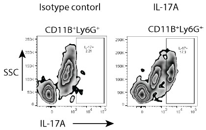
Figure 3 D-H. Quantification of immunofluorescence microscopy should be provided.
In the revised manuscript, we provide the quantification of IFA results.
Figure 4: Effects on neutrophil numbers in IFN-γ Kos do not correlate with CFU reductions, suggesting there may be a neutrophilindependent mechanism.
In the IFN-γ KO, we agree that the effect was less than dramatic. The immune dysfunction in the IFN-γ KO mice is too severe to see a strong reversal in the phenotype through interventions.
While we do not rule out any neutrophil-independent mechanism, in the context of following observations, neutrophil-dependent mechanisms certainly appear to play an important role-
(a) Improved pathology and survival upon IL-17 neutralization, which further improves with the inclusion of celecoxib.
(b) Loss of IL17<sup>+</sup>-Ly6G<sup>+</sup> cells upon IL-17 neutralization, which is further exacerbated when combined with celecoxib.
(c) Significant reduction in PMN number (shown by FACS) without any major impact on Th17 cell population upon IL-17 neutralization.
Finally, we believe some of the observations may become stronger once we characterize the specific sub-population among the Ly6G+ cells that correlates with pathology. For example, as shown in Figure 4I, FACS analysis of the Ly6G<sup>⁺</sup> cell population in Mtb-infected IFNγ<sup>⁻/⁻</sup> mice revealed a substantial subset of CD11b<sup>mid</sup> Ly6G<sup>ʰⁱ</sup> cells, indicative of an immature neutrophil population (Scapini et al., 2016). Efforts are currently underway to identify these important subpopulations.
Figure 4: Differences observed in the spleen cannot be connected to dissemination per se but instead could be a result of enhanced immune control in the spleen.
Thank you for this important point. We have revised this section. The role of neutrophils in Mtb dissemination is an emerging area of research, with growing evidence suggesting that these cells contribute to the spread of Mtb beyond the lungs (Hult et al., 2021). We highlight that the observed correlation could be speculative at this juncture.
Figure 4, 5: IL-17 neutralization alone has no effect on CFU in the lungs of Mtb-infected mice. While the combination of IL-17 neutralization and celecoxib has a very modest effect on CFU, the mechanism behind this observation is unclear. Further, the experiment shown has only 3 mice per group and it is unclear whether this (or any other) mouse experiment was repeated.
For Fig. 4, the experiment was done with 3 mice/group. The IFN KO mice were used to help identify the mechanism. IL-17 neutralisation or Celecoxib treatment alone did not have any significant effect on the bacterial burden (in lungs or isolated PMNs). However, it did show a significant effect on the number of PMNs recruited. Combination of IL-17 neutralisation and celecoxib led to about a one-log decrease in CFU, which is significant.
For Fig. 5, we used SR2211 instead of anti-IL-17 Ab for the experiment. This experiment had WT mice and 5 animals/group. Here, celecoxib and SR2211 alone showed a significant decline in PMN-resident Mtb pool as well as spleen burden. Only in the lungs, the impact of SR2211 alone was not significant.
Figure 6: The decreases in CFU correlate with a decrease in neutrophils; nothing connects this to neutrophil production of IL-17.
We now show quantification of observation in Fig. 5I, where in the WT mice, treatment with Celecoxib reduces the frequency of IL-17-producing Ly6G+ cells. In the revised manuscript, we also show direct evidence of SR2211 activity on BCG vaccine efficacy, which causes a significant decline in the Mtb burden in whole lung or in the isolated PMNs.
Figure 7. The Human data shows that elevated neutrophil levels and elevated IL-17 levels are associated with treatment failure in TB patients. This is expected, and does not
The literature lacks consensus in terms of a protective or pathological role of IL-17 in TB. Therefore, it was not expected to see higher IL-17 in patients who experienced relapse, death, or failed treatment outcomes. We do not have evidence from human subjects whether neutrophil derived IL-17 has a similar pathological role as observed in mice. However, higher IL-17 in failed outcome cases confirm the central theme that IL-17 is pathological in both human and mouse models.
Reviewer #2 (Recommendations for the authors):
(1) Survival of IFN-γ-/- Mice: The survival of IFN-γ-/- mice up to 100 days following a challenge with ~100 CFU of H37Rv is quite unusual. Have the authors checked PDIM expression in their Mtb strain, given that several studies report earlier mortality in these mice?
As shown in Fig. 4F, H37Rv-infected IFN-γ⁻/⁻ mice survived up to a little over 80 days. These figures are not unusual in the light of the following:
(1) In one study, IFNγ⁻/⁻ survived for about 40 days when the hypervirulent Mtb strain was used to infect these mice at 100-200 CFU using nose-only aerosol exposure (Nandi and Behar, 2011)
(2) In yet another study, IFNγ⁻/⁻ mice survived for ~50 days, however, they used H37Rv at 1-3x10<sup>5</sup> CFU to infect through intravenous injection (Kawakami et al., 2004)
Thus, compared with the above observations, where IFN-γ<sup>-/-</sup> mice survived for maximum 50 days due to hypervirulent infection or a very high dose infection, infection with H37Rv at ~100 CFU through the aerosol route and surviving for ~80 days is not unusual. The H37Rv cultures used in our study are always animal-passaged to ensure PDIM integrity.
(2) Granuloma Scoring: The granuloma scores appear to represent the percentage of lesion area. Please clarify and, if necessary, amend this in the manuscript.
The granuloma score is based on the calculation of the number of granulomatous infiltration and their severity. These are not % lesion area. We have added this detail in the revised manuscript.
(3) Pathology Comparison in Figures 4F and 4G: Does the pathology shown in Figure 4G correspond to the same groups as in Figure 4F? The celecoxib group in Figure 4F and the WT group in Figure 4G seem to be missing. Please clarify.
Figures 4F and 4G depict two independent experiments. For the time-to-death experiment, we had to leave the animals. The rest of the panels in Fig. 4 represent animals from the same experiment.
(4) Effect of Celecoxib on Ly6G+ Cells: The authors demonstrated that celecoxib treatment reduces Ly6G+ cells and IL-17-producing Ly6G+ cells. Do Ly6G+ cells express EP2/EP4 receptors? Alternatively, could the reduction in IL-17-producing Ly6G+ cells be due to an improved bactericidal response in other innate cells? The authors should discuss this possibility.
Yes, Ly6G<sup>⁺</sup> granulocytes express EP2/EP4 receptors (Lavoie et al., 2024), which mediate PGE₂ signaling. Prostaglandin E<sub>₂</sub> (PGE<sub>₂</sub>) is known to regulate neutrophil function and can enhance IL-17 production in various immune cells (Napolitani et al., 2009). However, the expression and functional role of EP2/EP4 receptors specifically on Ly6G<sup>⁺</sup> granulocytes in the context of Mtb infection require further investigation.
The alternate suggestion by the reviewer that the reduction in IL-17-producing Ly6G<sup>⁺</sup> cells following celecoxib treatment could be attributed to an improved bactericidal response in other innate immune cells is attractive. While we did not experimentally rule out this possibility, since reduced IL-17 invariably associated with reduced neutrophil-resident Mtb population, a cell-autonomous mechanism operational in Ly6G+ granulocytes is a highly likely mechanism.
(5) Culture Conditions: The methods section indicates that bacteria were cultured in 7H9+ADC. Is there a specific reason why the Oleic acid supplement was not added, given that standard Mtb culture conditions typically use 7H9+OADC supplements? Please comment on this choice.
It is a standard microbiological experimental procedure to use 7H9+ADC for broth culture, while 7H11+OADC for solid culture. Compared to broth culture, solid media are usually more stressful for bacteria because of hypoxia inside the growing colonies. Therefore, the media used are enriched in casein hydrolysate (like 7H11) and oleic acid (OADC).
Reviewer #3 (Recommendations for the authors):
Major suggestion: To really determine the role of neutrophil IL17 will require depletion studies and chimera experiments. These are clearly a major undertaking. I believe making significant re-writes to alter the conclusions or reanalyze any data to determine the role of nonhematopoietic and hematopoietic cells in IL17 is needed. If the conclusions are left as is, further experimentation is needed to fully support those conclusions.
Thank you for the suggestion. We have embarked on the specific deletion studies; however, as mentioned, this is a major undertaking and will take time. As suggested, we have discussed the results in accordance with the strength of evidence currently provided.
Eum, S.Y., J.H. Kong, M.S. Hong, Y.J. Lee, J.H. Kim, S.H. Hwang, S.N. Cho, L.E. Via, and C.E. Barry, 3rd. 2010. Neutrophils are the predominant infected phagocyGc cells in the airways of paGents with acGve pulmonary TB. Chest 137:122-128.
Gonzalez-Orozco, M., R.E. Barbosa-Cobos, P. Santana-Sanchez, L. Becerril-Mendoza, L. Limon-
Camacho, A.I. Juarez-Estrada, G.E. Lugo-Zamudio, J. Moreno-Rodriguez, and V. OrGzNavarrete. 2019. Endogenous sGmulaGon is responsible for the high frequency of IL-17Aproducing neutrophils in paGents with rheumatoid arthriGs. Allergy Asthma Clin Immunol 15:44.
References
Hult, C., J.T. Ma[la, H.P. Gideon, J.J. Linderman, and D.E. Kirschner. 2021. Neutrophil Dynamics Affect Mycobacterium tuberculosis Granuloma Outcomes and DisseminaGon. Front Immunol 12:712457.
Kawakami, K., Y. Kinjo, K. Uezu, K. Miyagi, T. Kinjo, S. Yara, Y. Koguchi, A. Miyazato, K. Shibuya, Y. Iwakura, K. Takeda, S. Akira, and A. Saito. 2004. Interferon-gamma producGon and host protecGve response against Mycobacterium tuberculosis in mice lacking both IL-12p40 and IL-18. Microbes Infect 6:339-349.
Lavoie, J.C., M. Simard, H. Kalkan, V. Rakotoarivelo, S. Huot, V. Di Marzo, A. Cote, M. Pouliot, and N. Flamand. 2024. Pharmacological evidence that the inhibitory effects of prostaglandin E2 are mediated by the EP2 and EP4 receptors in human neutrophils. J Leukoc Biol 115:1183-1189.
Lee, J., S. Boyce, J. Powers, C. Baer, C.M. Sasse[, and S.M. Behar. 2020. CD11cHi monocyte-derived macrophages are a major cellular compartment infected by Mycobacterium tuberculosis. PLoS Pathog 16:e1008621.
Li, L., L. Huang, A.L. Vergis, H. Ye, A. Bajwa, V. Narayan, R.M. Strieter, D.L. Rosin, and M.D. Okusa. 2010. IL-17 produced by neutrophils regulates IFN-gamma-mediated neutrophil migraGon in mouse kidney ischemia-reperfusion injury. J Clin Invest 120:331-342.
Lovewell, R.R., C.E. Baer, B.B. Mishra, C.M. Smith, and C.M. Sasse[. 2021. Granulocytes act as a niche for Mycobacterium tuberculosis growth. Mucosal Immunol 14:229-241.
Nandi, B., and S.M. Behar. 2011. RegulaGon of neutrophils by interferon-gamma limits lung inflammaGon during tuberculosis infecGon. The Journal of experimental medicine 208:22512262.
Napolitani, G., E.V. Acosta-Rodriguez, A. Lanzavecchia, and F. Sallusto. 2009. Prostaglandin E2 enhances Th17 responses via modulaGon of IL-17 and IFN-gamma producGon by memory CD4+ T cells. Eur J Immunol 39:1301-1312.
Ramirez-Velazquez, C., E.C. CasGllo, L. Guido-Bayardo, and V. OrGz-Navarrete. 2013. IL-17-producing peripheral blood CD177+ neutrophils increase in allergic asthmaGc subjects. Allergy Asthma Clin Immunol 9:23.
Sadikot, R.T., H. Zeng, A.C. Azim, M. Joo, S.K. Dey, R.M. Breyer, R.S. Peebles, T.S. Blackwell, and J.W. Christman. 2007. Bacterial clearance of Pseudomonas aeruginosa is enhanced by the inhibiGon of COX-2. Eur J Immunol 37:1001-1009.
Zheng, W., I.C. Chang, J. Limberis, J.M. Budzik, B.S. Zha, Z. Howard, L. Chen, and J.D. Ernst. 2023. Mycobacterium tuberculosis resides in lysosome-poor monocyte-derived lung cells during chronic infecGon. bioRxiv
Zheng, W., I.C. Chang, J. Limberis, J.M. Budzik, B.S. Zha, Z. Howard, L. Chen, and J.D. Ernst. 2024. Mycobacterium tuberculosis resides in lysosome-poor monocyte-derived lung cells during chronic infecGon. PLoS Pathog 20:e1012205.
Reviewer #3 (Public review):
Summary:
This manuscript examines how locus coeruleus (LC) activity relates to hippocampal ripple events across behavioral states in freely moving rats. Using multi-site electrophysiological recordings, the authors report that LC activity is suppressed prior to ripple events, with the magnitude of suppression depending on the ripple subtype. Suppression is stronger during wakefulness than during NREM sleep and is least pronounced for ripples coupled to spindles.
Strengths:
The study is technically competent and addresses an important question regarding how LC activity interacts with hippocampal and thalamocortical network events across vigilance states.
Weaknesses:
The results are interesting, but entirely observational. Also, the study in its current form would benefit from optimization of figure labeling and presentation, and more detailed result descriptions to make the findings fully interpretable. Also, it would be beneficial if the authors could formulate the narrative and central hypothesis more clearly to ease the line of reasoning across sections.
Comments:
(1) Stronger evidence that recorded units represent noradrenergic LC neurons would reinforce the conclusions. While direct validation may not be possible, showing absolute firing rates (Hz) across quiet wake, active wake, NREM, and REM, and comparing them to published LC values, would help.
(2) The analyses rely almost exclusively on z-scored LC firing and short baselines (~4-6 s), which limits biological interpretation. The authors should include absolute firing rates alongside normalized values for peri-ripple and peri-spindle analyses and extend pre-event windows to at least 20-30 s to assess tonic firing evolution. This would clarify whether differences across ripple subtypes arise from ceiling or floor effects in LC activity; if ripples require LC silence, the relative drop will appear larger during high-firing wake states. This limitation should be discussed and, if possible, results should be shown based on unnormalized firing rates.
(3) Because spindles often occur in clusters, the timing of ripple occurrence within these clusters could influence LC suppression. Indicate whether this structure was considered or discuss how it might affect interpretation (e.g., first vs. subsequent ripples within a spindle cluster).
(4) While the observational approach is appropriate here, causal tests (e.g., optogenetic or chemogenetic manipulation of LC around ripple events and in memory tasks) would considerably strengthen the mechanistic conclusions. At a minimum, a discussion of how such approaches could address current open questions would improve the manuscript.
(5) Please show how "Synchronization Index" (SI) differs quantitatively across behavioral states (wake, NREM, REM) and discuss whether it could serve as a state classifier. This would strengthen interpretations of the correlations between SI, ripple occurrence, and LC activity.
(6) The current use of SI to denote a delta/gamma power ratio is unconventional, as "SI" typically refers to phase-locking metrics. Consider adopting a more standard term, such as delta/gamma power ratio. Similarly, it would be easier to follow if you use common terminology (AUC) to describe the drop in LC-MUA rather than using "MI" and "sub-MI".
(7) The logic in Figure 3 is difficult to follow. The brain state (delta/gamma ratio) appears unchanged relative to surrogate events (3C), while LC activity that is supposedly negatively correlated to delta/gamma changes markedly (3D-E). Could this discrepancy reflect the low temporal resolution (4-s windows) used to calculate delta/gamma when the changes occur on a shorter time scale?
(8) There are apparent inconsistencies between Figures 4B and 4C-D. In B, it seems that the difference between the 10th and 90th percentile is mostly in higher frequencies, but in C and D, the only significant difference is in the delta band.
(9) Because standard sleep scoring is based on EEG and EMG signals, please include an example of sleep scoring alongside the data used for state classification. It would also be relevant to include the delta/gamma power ratio in such an example plot.
(10) Can variability in modulation index (subMI) across ripple subsets reflect differences in recording quality? Please report and compare mean LC firing rates across subsets to confirm this is not a confounding factor.
(11) Figure 6B: If the brown trace represents LC-MUA activity around random time points, why would there be a coinciding negative peak as relative to real sleep spindles? Or is it the subtracted trace?
(12) On page 8, lines 207-209, the authors write "Importantly, neither the LC-MUA rate nor SIs differed during a 2-sec time window preceding either group of spindles". It is unclear which data they refer to, but the statement seems to contradict Figure 6E as well as the following sentence: "Across sessions, MI values exceeded 95% CI in 17/20 datasets for isoSpindles and only 3/20 for ripSpindles". This should be clarified.
(13) The results in Figures 5C and 6F do not align. It seems surprising that ripple-coupled spindles show a considerably higher LC modulation than spindle-coupled ripples, as these events should overlap. Could the discrepancy be due to Z-score normalization as mentioned above? Please include a discussion of this to help the interpretation of the results.
(14) The text implies that 8 recordings came from one rat and two each from six others. This should be confirmed, and it should be explained how the recordings were balanced and analyzed across animals.
Author response:
Reviewer #1 (Public review):
Summary:
The manuscript by Yang et al. investigates the relationship between multi-unit activity in the locus coeruleus, putatively noradrenergic locus coeruleus, hippocampus (HP), sharp-wave ripples (SWR), and spindles using multi-site electrophysiology in freely behaving male rats. The study focuses on SWR during quiet wake and non-REM sleep, and their relation to cortical states (identified using EEG recordings in frontal areas) and LC units.
The manuscript highlights differential modulation of LC units as a function of HP-cortical communication during wake and sleep. They establish that ripples and LC units are inversely correlated to levels of arousal: wake, i.e., higher arousal correlates with higher LC unit activity and lower ripple rates. The authors show that LC neuron activity is strongly inhibited just before SWR is detected during wake. During non-REM sleep, they distinguish "isolated" ripples from SWR coupled to spindles and show that inhibition of LC neuron activity is absent before spindle-coupled ripples but not before isolated ripples, suggesting a mechanism where noradrenaline (NA) tone is modulated by HP-cortical coupling. This result has interesting implications for the roles of noradrenaline in the modulation of sleep-dependent memory consolidation, as ripple-spindle coupling is a mechanism favoring consolidation. The authors further show that NA neuronal activity is downregulated before spindles.
Strengths:
In continuity with previous work from the laboratory, this work expands our understanding of the activity of neuromodulatory systems in relation to vigilance states and brain oscillations, an area of research that is timely and impactful. The manuscript presents strong results suggesting that NA tone varies differentially depending on the coupling of HP SWR with cortical spindles. The authors place their findings back in the context of identified roles of HP ripples and coupling to cortical oscillations for memory formation in a very interesting discussion. The distinction of LC neuron activity between awake, ripple-spindle coupled events and isolated ripples is an exciting result, and its relation to arousal and memory opens fascinating lines of research.
Weaknesses:
I regretted that the paper fell short of trying to push this line of idea a bit further, for example, by contrasting in the same rats the LC unit-HP ripple coupling during exploration of a highly familiar context (as seemingly was the case in their study) versus a novel context, which would increase arousal and trigger memory-related mechanisms. Any kind of manipulation of arousal levels and investigation of the impact on awake vs non-REM sleep LC-HP ripple coordination would considerably strengthen the scope of the study.
We agree that conducting specific behavioral tests before electrophysiological recordings, as well as manipulating arousal during the recording session, would strengthen the study. These experiments are planned for future work, and we will acknowledge this point in the discussion.
The main result shows that LC units are not modulated during non-REM sleep around spindle-coupled ripples (named spRipples, 17.2% of detected ripples); they also show that LC units are modulated around ripple-coupled spindles (ripSpindles, proportion of detected spindles not specified, please add). These results seem in contradiction; this point should be addressed by the authors.
We found that LC suppression was generally weak around both types of coupled events (spRipples and ripSpindles). Specifically, session-averaged spRipple-associated LC suppression reached a significance level (exceeding 95% CI) in 4 (n = 3 rats) out of 20 sessions (Line 177). The significant ripSpindle-associated LC suppression was observed in 3 (n = 2 animals) out of 20 sessions (Line 213). When comparing the modulation index (MI) around spRipples and ripSpindles, we found a significant correlation (Pearson r = 0.72, p = 0.0003). As shown in Author response image 1 below, the three sessions (blue square, MI < 95%CI) with significant ripSpindle-associated LC suppression coincide with those sessions showing LC modulation around spRipples. Although, the detection of coupled events was performed independently, some overlap can not be excluded. We will be happy to provide this additional information in the results section.
Author response image 1.
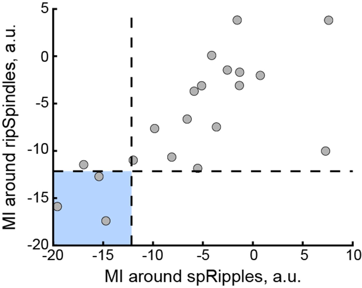
Results are displayed per recording session, with 20 sessions total recorded from 7 rats (2 to 8 sessions per rat), which implies that one of the rats accounts for 40% of the dataset. Authors should provide controls and/or data displayed as average per rat to ensure that results are now skewed by the weight of that single rat in the results.
Since high-quality recordings from the LC in behaving rats are challenging and rare, we used all valid sessions for this study. In Author response image 2 below, we plotted the average MIs for each animal (A) and each session (B). The dashed lines indicate the mean ± 2 standard deviations across all sessions. The rat ID and number of sessions is indicated in parentheses in A. All animal-averaged MIs fall within this range, indicating that the MI distribution is not driven by a single animal (rat 1101, 8 sessions). The MIs of eight sessions from rat1101 are shown in grey-filled triangles (B). Comparison of the MI distribution for these eight sessions versus the remaining 12 sessions from six other animals revealed no significant difference (Kolmogorov-Smirnov test, p = 0.969). We will be happy to provide this additional information in the Results section.
Author response image 2.
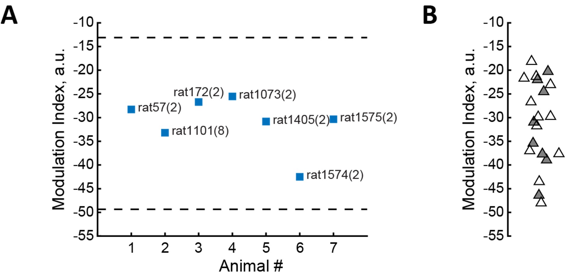
In its current form, the manuscript presents a lack of methodological detail that needs to be addressed, as it clouds the understanding of the analysis and conclusions. For example, the method to account for the influence of cortical state on LC MUA is unclear, both for the exact methods (shuffling of the ripple or spindle onset times) and how this minimizes the influence of cortical states; this should be better described. If the authors wish to analyze unit modulation as a function of cortical state, could they also identify/sort based on cortical states and then look at unit modulation around ripple onset? For the first part of the paper, was an analysis performed on quiet wake, non-REM sleep, or both?
As shown in Figure 3A and described in the main text (Lines 113–116), LC firing rate was negatively correlated with cortical arousal as quantified by Synchronisation Index (SI), whereas ripple rate was positively correlated with arousal. When computing LC activity (0.05 sec bins) aligned to the ripple onset over a longer time window ([–12, 12] sec), we observed a slow decrease in the LC firing rate beginning as early as 10 s before the ripple onset. In Author response image 3 below, a blue trace shows this slower temporal dynamic in a representative session. In addition to LC activity modulation at this relatively slow temporal scale, we also observed a much sharper drop in the LC firing rate ~ 2 s before the ripple onset. Considering two temporal scales, we hypothesized that slow modulation of LC activity might be related to fluctuations of the global brain state. Specifically, a higher SI (more synchronized cortical population activity) corresponded to a lower arousal state and reduced LC tonic firing; this brain state was associated with a higher ripple activity. Thus, slow LC modulation was likely driven by cortical state transitions. To correct for the influence of the global brain state on the LC/ripple temporal dynamics, we generated surrogate events by jittering the times of detected ripples (Lines 415–421). First, we confirmed that the cortical state did not differ around ripples and surrogate events (Figure 3C), while triggering the hippocampal LFP on the surrogate events lacked the ripple-specific frequency component (Figure 3B,). Thus, LC activity around surrogate evens captured its cortical state dependent dynamics (see orange trace in Author response image 3 below). Finally, to characterize state-independent ripple-related LC activity, we subtracted the state-related LC activity (orange trace in Author response image 3 below) from the ripple-triggered LC activity (blue trace). This yielded a corrected estimate of ripple-associated LC activity that was largely free from the confounding influence of cortical state transitions.
Author response image 3.
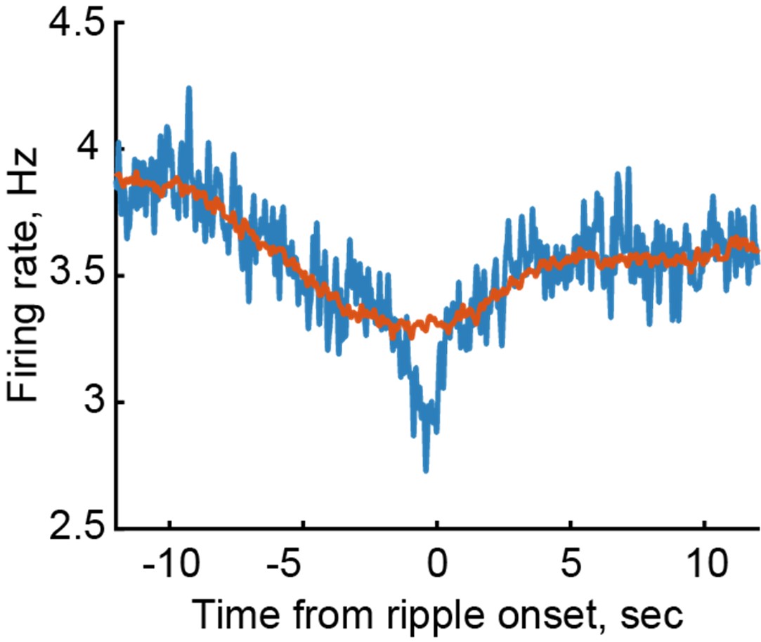
In the results subsection “LC-NE neuron spiking is suppressed around hippocampal ripples”, we reported LC modulation without accounting for the cortical state. The state-dependent effects were instead examined in the subsequent subsection, “Peri-ripple LC modulation depends on the cortical–hippocampal interaction,” where we characterized LC activity around ripples across different cortical states (quite awake and NREM sleep). We will provide more methodological details and a rationale for each analysis, as requested.
Reviewer #2 (Public review):
Summary:
In this study, the authors studied the synchrony between ripple events in the Hippocampus, cortical spindles, and Locus Coeruleus spiking. The results in this study, together with the established literature on the relationship of hippocampal ripples with widespread thalamic and cortical waves, guided the authors to propose a role for Locus Coeruleus spiking patterns in memory consolidation. The findings provided here, i.e., correlations between LC spiking activity and Hippocampal ripples, could provide a basis for future studies probing the directional flow or the necessity of these correlations in the memory consolidation process. Hence, the paper provides enough scientific advances to highlight the elusive yet important role of Norepinephrine circuitry in the memory processes.
Strengths:
The authors were able to demonstrate correlations of Locus Coeruleus spikes with hippocampal ripples as well as with cortical spindles. A specific strength of the paper is in the demonstration that the spindles that activate with the ripples are comparatively different in their correlations with Locus Coeruleus than those that do not.
Weaknesses:
The claims regarding the roles of these specific interactions were mostly derived from the literature that these processes individually contribute to the memory process, without any evidence of these specific interactions being necessary for memory processes. There are also issues with the description of methods, validation of shuffling procedures, and unclear presentation and the interpretation of the findings, which are described in the points that follow. I believe addressing these weaknesses might improve and add to the strength of the findings.
We believe that our responses to the Reviewer 1 and planned revisions as described above will adequately address the issues raised by the Reviewer 2.
Reviewer #3 (Public review):
Summary:
This manuscript examines how locus coeruleus (LC) activity relates to hippocampal ripple events across behavioral states in freely moving rats. Using multi-site electrophysiological recordings, the authors report that LC activity is suppressed prior to ripple events, with the magnitude of suppression depending on the ripple subtype. Suppression is stronger during wakefulness than during NREM sleep and is least pronounced for ripples coupled to spindles.
Strengths:
The study is technically competent and addresses an important question regarding how LC activity interacts with hippocampal and thalamocortical network events across vigilance states.
Weaknesses:
The results are interesting, but entirely observational. Also, the study in its current form would benefit from optimization of figure labeling and presentation, and more detailed result descriptions to make the findings fully interpretable. Also, it would be beneficial if the authors could formulate the narrative and central hypothesis more clearly to ease the line of reasoning across sections.
We will do our best to optimize presentation, revise the main text and figure labelling. When appropriate, we will add specific hypotheses and a rationale for specific analyses.
Comments:
(1) Stronger evidence that recorded units represent noradrenergic LC neurons would reinforce the conclusions. While direct validation may not be possible, showing absolute firing rates (Hz) across quiet wake, active wake, NREM, and REM, and comparing them to published LC values, would help.
We will provide the requested data in the revised manuscript.
(2) The analyses rely almost exclusively on z-scored LC firing and short baselines (~4-6 s), which limits biological interpretation. The authors should include absolute firing rates alongside normalized values for peri-ripple and peri-spindle analyses and extend pre-event windows to at least 20-30 s to assess tonic firing evolution. This would clarify whether differences across ripple subtypes arise from ceiling or floor effects in LC activity; if ripples require LC silence, the relative drop will appear larger during high-firing wake states. This limitation should be discussed and, if possible, results should be shown based on unnormalized firing rates.
We can provide absolute firing rates alongside normalized values for peri-ripple and peri-spindle analyses for isolated single LC units. However, we are reluctant to average absolute firing rates for multiunit activity, as it is unknown how many neurons contributed to each MUA recording. We can add the plots with extended pre-event windows ([–12, 12] sec). Please see our response to the Reviewer 1 about the two temporal scales of LC modulation.
(3) Because spindles often occur in clusters, the timing of ripple occurrence within these clusters could influence LC suppression. Indicate whether this structure was considered or discuss how it might affect interpretation (e.g., first vs. subsequent ripples within a spindle cluster).
We did not consider spindle clusters and classified the event as ripple coupled spindle if the ripple occurred between the spindle on- and offset. We will clarify this point in the Method section.
(4) While the observational approach is appropriate here, causal tests (e.g., optogenetic or chemogenetic manipulation of LC around ripple events and in memory tasks) would considerably strengthen the mechanistic conclusions. At a minimum, a discussion of how such approaches could address current open questions would improve the manuscript.
We agree that conducting causal tests would strengthen the study. We will acknowledge in the discussion that our results shall inspire future studies addressing many open questions.
(5) Please show how "Synchronization Index" (SI) differs quantitatively across behavioral states (wake, NREM, REM) and discuss whether it could serve as a state classifier. This would strengthen interpretations of the correlations between SI, ripple occurrence, and LC activity.
We will add the plot showing the average SI values across behavioral states. Although SI could potentially serve as a classifier, we have chosen not to discuss this in detail to maintain focus in the discussion.
(6) The current use of SI to denote a delta/gamma power ratio is unconventional, as "SI" typically refers to phase-locking metrics. Consider adopting a more standard term, such as delta/gamma power ratio. Similarly, it would be easier to follow if you use common terminology (AUC) to describe the drop in LC-MUA rather than using "MI" and "sub-MI".
The ranges of delta and gamma bands might vary across studies; therefore, we prefer using SI, as defined here and in our previous publications (Yang, 2019; Novitskaya, 2012). We calculated the modulation index (MI) as the area under the curve of the peri-event time histogram within the 1 second preceding ripple onset. To avoid potential confusion with the AUC calculated over the entire signal window, we opted to use MI.
(7) The logic in Figure 3 is difficult to follow. The brain state (delta/gamma ratio) appears unchanged relative to surrogate events (3C), while LC activity that is supposedly negatively correlated to delta/gamma changes markedly (3D-E). Could this discrepancy reflect the low temporal resolution (4-s windows) used to calculate delta/gamma when the changes occur on a shorter time scale?
Figure 3D and 3E show the 'state-corrected' ripple-related LC activity. Specifically, the cortical state related LC modulation was subtracted from the non-corrected ripple-associated LC activity. Please, see our detailed response to the Reviewer 1. We will revise the results and Figure 3 legend to clarify this point.
(8) There are apparent inconsistencies between Figures 4B and 4C-D. In B, it seems that the difference between the 10th and 90th percentile is mostly in higher frequencies, but in C and D, the only significant difference is in the delta band.
We will re-do this analysis and clarify this inconsistency.
(9) Because standard sleep scoring is based on EEG and EMG signals, please include an example of sleep scoring alongside the data used for state classification. It would also be relevant to include the delta/gamma power ratio in such an example plot.
We removed ‘standard’ and will add a supplementary Figure illustrating sleep scoring.
(10) Can variability in modulation index (subMI) across ripple subsets reflect differences in recording quality? Please report and compare mean LC firing rates across subsets to confirm this is not a confounding factor.
We will plot this result averaged per rat.
(11) Figure 6B: If the brown trace represents LC-MUA activity around random time points, why would there be a coinciding negative peak as relative to real sleep spindles? Or is it the subtracted trace?
We will clarify this point in the figure legend.
(12) On page 8, lines 207-209, the authors write "Importantly, neither the LC-MUA rate nor SIs differed during a 2-sec time window preceding either group of spindles". It is unclear which data they refer to, but the statement seems to contradict Figure 6E as well as the following sentence: "Across sessions, MI values exceeded 95% CI in 17/20 datasets for isoSpindles and only 3/20 for ripSpindles". This should be clarified.
We will clarify the description of this result.
(13) The results in Figures 5C and 6F do not align. It seems surprising that ripple-coupled spindles show a considerably higher LC modulation than spindle-coupled ripples, as these events should overlap. Could the discrepancy be due to Z-score normalization as mentioned above? Please include a discussion of this to help the interpretation of the results.
We will clarify this point in the revised manuscript. Please, also see our response to the Reviewer 1.
(14) The text implies that 8 recordings came from one rat and two each from six others. This should be confirmed, and it should be explained how the recordings were balanced and analyzed across animals.
Since high-quality recordings from LC in behaving animals are challenging and rare, we used all valid sessions. We will also present the main results averaged per rat, as also requested by the Reviewer 1.
By the late thirteenth century, Glastonbury -- some twelve miles from Cadbury -- was already a place with strong Arthurian connections. Identified by Geoffrey of Monmouth as the site of the legendary Avalon, resting-place of Joseph of Arimathea who took possession of the Holy Grail after the Crucifixion, it had already attracted the attention of Henry II and Richard I.(2) However, it was Edward I whose interest in the Glastonbury legend was particularly strong. He owned a prose Tristan, conducted Arthurian-inspired tournaments, linked his Welsh and Scottish campaigns to the legend, and created festivals which he called `Round Tables' in emulation of his mythical role-model.(3) His most conspicuous act in this regard was to order that the alleged tomb of Arthur and Guinevere, `discovered' at Glastonbury in the twelfth century, be opened and that the remains be removed from their resting-place in the lady chapel and then re-interred in the main church
Good quote for background of Edward I's obsession with Arthur
Reviewer #1 (Public review):
Summary:
Syed et al. investigate the circuit underpinnings for leg grooming in the fruit fly. They identify two populations of local interneurons in the right front leg neuromere of ventral nerve cord, i.e. 62 13A neurons and 64 13B neurons. Hierarchical clustering analysis identifies each 10 morphological classes for both populations. Connectome analysis reveals their circuit interactions: these GABAergic interneurons provide synaptic inhibition either between the two subpopulations, i.e. 13B onto 13A, or among each other, i.e. 13As onto other 13As, and/or onto leg motoneurons, i.e. 13As and 13Bs onto leg motoneurons. Interestingly, 13A interneurons fall into two categories with one providing inhibition onto a broad group of motoneurons, being called "generalists", while others project to few motoneurons only, being called "specialists". Optogenetic activation and silencing of both subsets strongly effects leg grooming. As well activating or silencing subpopulations, i.e. 3 to 6 elements of the 13A and 13B groups has marked effects on leg grooming, including frequency and joint positions and even interrupting leg grooming. The authors present a computational model with the four circuit motifs found, i.e. feed-forward inhibition, disinhibition, reciprocal inhibition and redundant inhibition. This model can reproduce relevant aspects of the grooming behavior.
Strengths:
The authors succeeded in providing evidence for neural circuits interacting by means of synaptic inhibition to play an important role in the generation of a fast rhythmic insect motor behavior, i.e. grooming. Two populations of local interneurons in the fruit fly VNC comprise four inhibitory circuit motifs of neural action and interaction: feed-forward inhibition, disinhibition, reciprocal inhibition and redundant inhibition. Connectome analysis identifies the similarities and differences between individual members of the two interneuron populations. Modulating the activity of small subsets of these interneuron populations markedly affects generation of the motor behavior thereby exemplifying their important role for generating grooming. The authors carefully discuss strengths and limitations of their approaches and place their findings into the broader context of motor control.
Weaknesses:
Effects of modulating activity in the interneuron populations by means of optogenetics were conducted in the so-called closed-loop condition. This does not allow to differentiate between direct and secondary effects of the experimental modification in neural activity, as feedforward and feedback effects cannot be disentangled. To do so open loop experiments, e.g. in deafferented conditions, would be important. Given that many members of the two populations of interneurons do not show one, but two or more circuit motifs, it remains to be disentangled which role the individual circuit motif plays in the generation of the motor behavior in intact animals.
Comments on revisions:
The careful revision of the manuscript improved the clarity of presentation substantially.
Reviewer #2 (Public review):
Summary:
This manuscript by Syed et al. presents a detailed investigation of inhibitory interneurons, specifically from the 13A and 13B hemilineages, which contribute to the generation of rhythmic leg movements underlying grooming behavior in Drosophila. After performing a detailed connectomic analysis, which offers novel insights into the organization of premotor inhibitory circuits, the authors build on this anatomical framework by performing optogenetic perturbation experiments to functionally test predictions derived from the connectome. Finally, they integrate these findings into a computational model that links anatomical connectivity with behavior, offering a systems-level view of how inhibitory circuits may contribute to grooming pattern generation.
Strengths:
(1) Performing an extensive and detailed connectomic analysis, which offers novel insights into the organization of premotor inhibitory circuits.
(2) Making sense of the largely uncharacterized 13A/13B nerve cord circuitry by combining connectomics and optogenetics is very impressive and will lay the foundation for future experiments in this field.
(3) Testing the predictions from experiments using a simplified and elegant model.
Weaknesses:
(1) In Figure 4-figure supplement 1, the inclusion of walking assays in dusted flies is problematic, as these flies are already strongly biased toward grooming behavior and rarely walk. To assess how 13A neuron activation influences walking, such experiments should be conducted in undusted flies under baseline locomotor conditions.
(2) Regarding Fig 5: The 70ms on/off stimulation with a slow opsin seems problematic. CsChrimson off kinetics are slow and unlikely to cause actual activity changes in the desired neurons with the temporal precision the authors are suggesting they get. Regardless, it is amazing the authors get the behavior! It would still be important for authors to mention the optogentics caveat, and potentially supplement the data with stimulation at different frequencies, or using faster opsins like ChrimsonR.
Overall, I think the strengths outweigh the weaknesses, and I consider this a timely and comprehensive addition to the field.
Reviewer #3 (Public review):
Summary:
The authors set out to determine how GABAergic inhibitory premotor circuits contribute to the rhythmic alternation of leg flexion and extension during Drosophila grooming. To do this, they first mapped the ~120 13A and 13B hemilineage inhibitory neurons in the prothoracic segment of the VNC and clustered them by morphology and synaptic partners. They then tested the contribution of these cells to flexion and extension using optogenetic activation and inhibition and kinematic analyses of limb joints. Finally, they produced a computational model representing an abstract version of the circuit to determine how the connectivity identified in EM might relate to functional output. The study makes important contributions to the literature.
The authors have identified an interesting question and use a strong set of complementary tools to address it:
They analysed serial‐section TEM data to obtain reconstructions of every 13A and 13B neuron in the prothoracic segment. They manually proofread over 60 13A neurons and 64 13B neurons, then used automated synapse detection to build detailed connectivity maps and cluster neurons into functional motifs.
They used optogenetic tools with a range of genetic driver lines in freely behaving flies to test the contribution of subsets of 13A and 13B neurons.
They used a connectome-constrained computational model to determine how the mapped connectivity relates to the rhythmic output of the behavior.
Author response:
The following is the authors’ response to the original reviews.
Reviewer #1 (Public review):
Summary:
Syed et al. investigate the circuit underpinnings for leg grooming in the fruit fly. They identify two populations of local interneurons in the right front leg neuromere of ventral nerve cord, i.e. 62 13A neurons and 64 13B neurons. Hierarchical clustering analysis identifies 10 morphological classes for both populations. Connectome analysis reveals their circuit interactions: these GABAergic interneurons provide synaptic inhibition either between the two subpopulations, i.e., 13B onto 13A, or among each other, i.e., 13As onto other 13As, and/or onto leg motoneurons, i.e., 13As and 13Bs onto leg motoneurons. Interestingly, 13A interneurons fall into two categories, with one providing inhibition onto a broad group of motoneurons, being called "generalists", while others project to a few motoneurons only, being called "specialists". Optogenetic activation and silencing of both subsets strongly affect leg grooming. As well aas ctivating or silencing subpopulations, i.e., 3 to 6 elements of the 13A and 13B groups, has marked effects on leg grooming, including frequency and joint positions, and even interrupting leg grooming. The authors present a computational model with the four circuit motifs found, i.e., feed-forward inhibition, disinhibition, reciprocal inhibition, and redundant inhibition. This model can reproduce relevant aspects of the grooming behavior.
Strengths:
The authors succeeded in providing evidence for neural circuits interacting by means of synaptic inhibition to play an important role in the generation of a fast rhythmic insect motor behavior, i.e., grooming. Two populations of local interneurons in the fruit fly VNC comprise four inhibitory circuit motifs of neural action and interaction: feed-forward inhibition, disinhibition, reciprocal inhibition, and redundant inhibition. Connectome analysis identifies the similarities and differences between individual members of the two interneuron populations. Modulating the activity of small subsets of these interneuron populations markedly affects the generation of the motor behavior, thereby exemplifying their important role in generating grooming.
We thank the reviewer for their thoughtful and constructive evaluation of our work.
Weaknesses:
Effects of modulating activity in the interneuron populations by means of optogenetics were conducted in the so-called closed-loop condition. This does not allow for differentiation between direct and secondary effects of the experimental modification in neural activity, as feedforward and feedback effects cannot be disentangled. To do so, open loop experiments, e.g., in deafferented conditions, would be important. Given that many members of the two populations of interneurons do not show one, but two or more circuit motifs, it remains to be disentangled which role the individual circuit motif plays in the generation of the motor behavior in intact animals.
Our optogenetic experiments show a role for 13A/B neurons in grooming leg movements – in an intact sensorimotor system - but we cannot yet differentiate between central and reafferent contributions. Activation of 13As or 13Bs disinhibits motor neurons and that is sufficient to induce walking/grooming. Therefore, we can show a role for the disinhibition motif.
Proprioceptive feedback from leg movements could certainly affect the function of these reciprocal inhibition circuits. Given the synapses we observe between leg proprioceptors and 13A neurons, we think this is likely.
Our previous work (Ravbar et al 2021) showed that grooming rhythms in dusted flies persist when sensory feedback is reduced, indicating that central control is possible. In those experiments, we used dust to stimulate grooming and optogenetic manipulation to broadly silence sensory feedback. We cannot do the same here because we do not yet have reagents to separately activate sparse subsets of inhibitory neurons while silencing specific proprioceptive neurons. More importantly, globally silencing proprioceptors would produce pleiotropic effects and severely impair baseline coordination, making it difficult to distinguish whether observed changes reflect disrupted rhythm generation or secondary consequences of impaired sensory input. Therefore, the reviewer is correct – we do not know whether the effects we observe are feedforward (central), feedback sensory, or both. We have included this in the revised results and discussion section to describe these possibilities and the limits of our current findings.
Additionally, we have used a computational model to test the role of each motif separately and we show that in the results.
Reviewer #2 (Public review):
Summary:
This manuscript by Syed et al. presents a detailed investigation of inhibitory interneurons, specifically from the 13A and 13B hemilineages, which contribute to the generation of rhythmic leg movements underlying grooming behavior in Drosophila. After performing a detailed connectomic analysis, which offers novel insights into the organization of premotor inhibitory circuits, the authors build on this anatomical framework by performing optogenetic perturbation experiments to functionally test predictions derived from the connectome. Finally, they integrate these findings into a computational model that links anatomical connectivity with behavior, offering a systems-level view of how inhibitory circuits may contribute to grooming pattern generation.
Strengths:
(1) Performing an extensive and detailed connectomic analysis, which offers novel insights into the organization of premotor inhibitory circuits.
(2) Making sense of the largely uncharacterized 13A/13B nerve cord circuitry by combining connectomics and optogenetics is very impressive and will lay the foundation for future experiments in this field.
(3) Testing the predictions from experiments using a simplified and elegant model.
We thank the reviewer for their thoughtful and encouraging evaluation of our work.
Weaknesses:
(1) In Figure 4, while the authors report statistically significant shifts in both proximal inter-leg distance and movement frequency across conditions, the distributions largely overlap, and only in Panel K (13B silencing) is there a noticeable deviation from the expected 7-8 Hz grooming frequency. Could the authors clarify whether these changes truly reflect disruption of the grooming rhythm?
We reanalyzed the dataset with Linear Mixed Models. We find significant differences in mean frequencies upon silencing these neurons but not upon activation. The experimental groups are also significantly more variable. We revised these panels with updated analysis. We think these data do support our interpretation that the grooming rhythms are disrupted.
More importantly, all this data would make the most sense if it were performed in undusted flies (with controls) as is done in the next figure.
In our assay conditions, undusted flies groom infrequently. We used undusted flies for some optogenetic activation experiments, where the neuron activation triggers behavior initiation, but we chose to analyze the effect of silencing inhibitory neurons in dusted flies because dust reliably activates mechanosensory neurons and elicits robust grooming behavior enabling us to assess how manipulation of 13A/B neurons alters grooming rhythmicity and leg coordination.
(2) In Figure 4-Figure Supplement 1, the inclusion of walking assays in dusted flies is problematic, as these flies are already strongly biased toward grooming behavior and rarely walk. To assess how 13A neuron activation influences walking, such experiments should be conducted in undusted flies under baseline locomotor conditions.
We agree that there are better ways to assay potential contributions of 13A/13B neurons to walking. We intended to focus on how normal activity in these inhibitory neurons affects coordination during grooming, and we included walking because we observed it in our optogenetic experiments and because it also involves rhythmic leg movements. The walking data is reported in a supplementary figure because we think this merits further study with assays designed to quantify walking specifically. We will make these goals clearer in the revised manuscript and we are happy to share our reagents with other research groups more equipped to analyze walking differences.
(3) For broader lines targeting six or more 13A neurons, the authors provide specific predictions about expected behavioral effects-e.g., that activation should bias the limb toward flexion and silencing should bias toward extension based on connectivity to motor neurons. Yet, when using the more restricted line labeling only two 13A neurons (Figure 4 - Figure Supplement 2), no such prediction is made. The authors report disrupted grooming but do not specify whether the disruption is expected to bias the movement toward flexion or extension, nor do they discuss the muscle target. This is a missed opportunity to apply the same level of mechanistic reasoning that was used for broader manipulations.
Because we cannot unambiguously identify one of the neurons from our sparsest 13A splitGAL4 lines in FANC, we cannot say with certainty which motor neurons they target. That limits the accuracy of any functional predictions.
(4) Regarding Figure 5: The 70ms on/off stimulation with a slow opsin seems problematic. CsChrimson off kinetics are slow and unlikely to cause actual activity changes in the desired neurons with the temporal precision the authors are suggesting they get. Regardless, it is amazing that the authors get the behavior! It would still be important for the authors to mention the optogenetics caveat, and potentially supplement the data with stimulation at different frequencies, or using faster opsins like ChrimsonR.
We were also intrigued by the behavioral consequences of activating these inhibitory neurons with CsChrimson. We appreciate the reviewer’s point that CsChrimson’s slow off-kinetics limit precise temporal control. To address this, we repeated our frequency analysis using a range of pulse durations (10/10, 50/50, 70/70, 110/110, and 120/120 ms on/off) and compared the mean frequency of proximal joint extension/flexion cycles across conditions. We found no significant difference in frequency (LLMS, p > 0.05), suggesting that the observed grooming rhythm is not dictated by pulse period but instead reflects an intrinsic property of the premotor circuit once activated. We now include these results in ‘Figure 5—figure supplement 1’ and clarify in the text that we interpret pulsed activation as triggering, rather than precisely pacing, the endogenous grooming rhythm. We continue to note in the manuscript that CsChrimson’s slow off-kinetics may limit temporal precision. We will try ChrimsonR in future experiments.
Overall, I think the strengths outweigh the weaknesses, and I consider this a timely and comprehensive addition to the field.
Reviewer #3 (Public review):
Summary:
The authors set out to determine how GABAergic inhibitory premotor circuits contribute to the rhythmic alternation of leg flexion and extension during Drosophila grooming. To do this, they first mapped the ~120 13A and 13B hemilineage inhibitory neurons in the prothoracic segment of the VNC and clustered them by morphology and synaptic partners. They then tested the contribution of these cells to flexion and extension using optogenetic activation and inhibition and kinematic analyses of limb joints. Finally, they produced a computational model representing an abstract version of the circuit to determine how the connectivity identified in EM might relate to functional output. The study, in its current form, makes an important but overclaimed contribution to the literature due to a mismatch between the claims in the paper and the data presented.
Strengths:
The authors have identified an interesting question and use a strong set of complementary tools to address it:
(1) They analysed serial‐section TEM data to obtain reconstructions of every 13A and 13B neuron in the prothoracic segment. They manually proofread over 60 13A neurons and 64 13B neurons, then used automated synapse detection to build detailed connectivity maps and cluster neurons into functional motifs.
(2) They used optogenetic tools with a range of genetic driver lines in freely behaving flies to test the contribution of subsets of 13A and 13B neurons.
(3) They used a connectome-constrained computational model to determine how the mapped connectivity relates to the rhythmic output of the behavior.
Weaknesses:
The manuscript aims to reveal an instructive, rhythm-generating role for premotor inhibition in coordinating the multi-joint leg synergies underlying grooming. It makes a valuable contribution, but currently, the main claims in the paper are not well-supported by the presented evidence.
Major points
(1) Starting with the title of this manuscript, "Inhibitory circuits generate rhythms for leg movements during Drosophila grooming", the authors raise the expectation that they will show that the 13A and 13B hemilineages produce rhythmic output that underlies grooming. This manuscript does not show that. For instance, to test how they drive the rhythmic leg movements that underlie grooming requires the authors to test whether these neurons produce the rhythmic output underlying behavior in the absence of rhythmic input. Because the optogenetic pulses used for stimulation were rhythmic, the authors cannot make this point, and the modelling uses a "black box" excitatory network, the output of which might be rhythmic (this is not shown). Therefore, the evidence (behavioral entrainment; perturbation effects; computational model) is all indirect, meaning that the paper's claim that "inhibitory circuits generate rhythms" rests on inferred sufficiency. A direct recording (e.g., calcium imaging or patch-clamp) from 13A/13B during grooming - outside the scope of the study - would be needed to show intrinsic rhythmogenesis. The conclusions drawn from the data should therefore be tempered. Moreover, the "black box" needs to be opened. What output does it produce? How exactly is it connected to the 13A-13B circuit?
We modified the title to better reflect our strongest conclusions: “Inhibitory circuits control leg movements during Drosophila grooming”
Our optogenetic activation was delivered in a patterned (70 ms on/off) fashion that entrains rhythmic movements, but this does not rule out the possibility that the rhythm is imposed externally. In the manuscript, we state that we used pulsed light to mimic a flexion-extension cycle and note that this approach tests whether inhibition is sufficient to drive rhythmic leg movements when temporally patterned. While this does not prove that 13A/13B neurons are intrinsic rhythm generators, it does demonstrate that activating subsets of inhibitory neurons is sufficient to elicit alternating leg movements resembling natural grooming and walking.
Our goal with the model was to demonstrate that it is possible to produce rhythmic outputs with this 13A/B circuit, based on the connectome. The “black box” is a small recurrent neural network (RNN) consisting of 40 neurons in its hidden layer. The inputs are the “dust” levels from the environment (the green pixels in Figure 6I), the “proprioceptive” inputs (“efference copy” from motor neurons), and the amount of dust accumulated on both legs. The outputs (all positive) connect to the 13A neurons, the 13B neurons, and to the motor neurons. We refer to it as the “black box” because we make no claims about the actual excitatory inputs to these circuits. Its function is to provide input, needed to run the network, that reflects the distribution of “dust” in the environment as well as the information about the position of the legs.
The output of the “black box” component of the model might be rhythmic. In fact, in most instances of the model implementation this is indeed the case. However, as mentioned in the current version of the manuscript: “But the 13A circuitry can still produce rhythmic behavior even without those external inputs (or when set to a constant value), although the legs become less coordinated.” Indeed, when we refine the model (with the evolutionary training) without the “black box” (using a constant input of 0.1) the behavior is still rhythmic and sustained. Therefore, the rhythmic activity and behavior can emerge from the premotor circuitry itself without a rhythmic input.
The context in which the 13A and 13B hemilineages sit also needs to be explained. What do we know about the other inputs to the motorneurons studied? What excitatory circuits are there?
We agree that there are many more excitatory and inhibitory, direct and indirect, connections to motor neurons that will also affect leg movements for grooming and walking. 13A neurons provide a substantial fraction of premotor input. For example, 13As account for ~17.1% of upstream synapses for one tibia extensor (femur seti) motor neuron and ~14.6% for another tibia extensor (femur feti) motor neuron. Our goal was to demonstrate what is possible from a constrained circuit of inhibitory neurons that we mapped in detail, and we hope to add additional components to better replicate the biological circuit as behavioral and biomechanical data is obtained by us and others.
Furthermore, the introduction ignores many decades of work in other species on the role of inhibitory cell types in motor systems. There is some mention of this in the discussion, but even previous work in Drosophila larvae is not mentioned, nor crustacean STG, nor any other cell types previously studied. This manuscript makes a valuable contribution, but it is not the first to study inhibition in motor systems, and this should be made clear to the reader.
We thank the reviewer for this important reminder. Previous work on the contribution of inhibitory neurons to invertebrate motor control certainly influenced our research. We have expanded coverage of the relevant history and context in our revised discussion.
(2) The experimental evidence is not always presented convincingly, at times lacking data, quantification, explanation, appropriate rationales, or sufficient interpretation.
We are committed to improving the clarity, rationale, and completeness of our experimental descriptions. We have revisited the statistical tests applied throughout the manuscript and expanded the Methods.
(3) The statistics used are unlike any I remember having seen, essentially one big t-test followed by correction for multiple comparisons. I wonder whether this approach is optimal for these nested, high‐dimensional behavioral data. For instance, the authors do not report any formal test of normality. This might be an issue given the often skewed distributions of kinematic variables that are reported. Moreover, each fly contributes many video segments, and each segment results in multiple measurements. By treating every segment as an independent observation, the non‐independence of measurements within the same animal is ignored. I think a linear mixed‐effects model (LMM) or generalized linear mixed model (GLMM) might be more appropriate.
We thank the reviewer for raising this important point regarding the statistical treatment of our segmented behavioral data. Our initial analysis used independent t-tests with Bonferroni correction across behavioral classes and features, which allowed us to identify broad effects. However, we acknowledge that this approach does not account for the nested structure of the data. To address this, we re-analyzed key comparisons using linear mixed-effects models (LMMs) as suggested by the reviewer. This approach allowed us to more appropriately model within-fly variability and test the robustness of our conclusions. We have updated the manuscript based on the outcomes of these analyses.
(4) The manuscript mentions that legs are used for walking as well as grooming. While this is welcome, the authors then do not discuss the implications of this in sufficient detail. For instance, how should we interpret that pulsed stimulation of a subset of 13A neurons produces grooming and walking behaviours? How does neural control of grooming interact with that of walking?
We do not know how the inhibitory neurons we investigated will affect walking or how circuits for control of grooming and walking might compete. We speculate that overlapping pre-motor circuits may participate because both have similar extension flexion cycles at similar frequencies, but we do not have hard experimental data to support. This would be an interesting area for future research. Here, we focused on the consequences of activating specific 13A/B neurons during grooming because they were identified through a behavioral screen for grooming disruptions, and we had developed high-resolution assays and familiarity with the normal movements in this behavior.
(5) The manuscript needs to be proofread and edited as there are inconsistencies in labelling in figures, phrasing errors, missing citations of figures in the text, or citations that are not in the correct order, and referencing errors (examples: 81 and 83 are identical; 94 is missing in text).
We have proofread the manuscript to fix figure labeling, citation order, and referencing errors.
Reviewing Editor Comments:
In addition to the recommendations listed below, a common suggestion, given the lack of evidence to support that 13A and 13B are rhythm-generating, is to tone down the title to something like, for example, "Inhibitory circuits control leg movements during grooming in Drosophila" (or similar).
We changed the title to Inhibitory circuits control leg movements during Drosophila grooming
Reviewer #1 (Recommendations for the authors):
(1) Naming of movements of leg segments:
The authors refer to movements of leg segments across the leg, i.e., of all joints, as "flexion" and "extension". For example, in Figure 4A and at many other places. This naming is functionally misleading for two reasons: (i) the anatomical organization of an insect leg differs in principle from the organization of the mammalian leg, which the manuscript often refers to. While the organization of a mammalian limb is planar the organization of the insect limb shows a different plane as compared to the body length axis (for detailed accounts see Ritzmann et al. 2004; Büschges & Ache, 2024); (ii) the reader cannot differentiate between places in the text, where "flexion" and "extension" refer to movements of the tibia of the femur-tibia joint, e.g. in the graphical abstract, in Figure 3 and its supplements, and other places, e.g. Figure 4 and its supplements, where these two words refer to movements of leg segments of other joints, e.g. thorax-coxa, coxa-trochanter and tarsal joints. The reviewer strongly suggests naming the movements of the leg segments according to the individual joint and its muscles.
We accept this helpful suggestion. We now include a description of the leg segments and joints in the revised Introduction and refer to which leg segments we mean
“The adult Drosophila leg consists of serially arranged joints—bodywall/thoraco-coxal (Th-C), coxa–trochanter (C-Tr), trochanter–femur (Tr-F), femur–tibia (F-Ti), tibia–tarsus (Ti-Ta)—each powered by opposing flexor and extensor muscles that transmit force through tendons (Soler et al., 2004). The proximal joints, Th-C and C-Tr, mediate leg protraction–retraction and elevation–depression, respectively (Ritzmann et al., 2004; Büschges & Ache, 2025). The medial joint, F-Ti, acts as the principal flexion–extension hinge and is controlled by large tibia extensor motor neurons and flexor motor neurons (Soler et al., 2004; Baek and Mann 2009; Brierley et al., 2012; Azevedo et al., 2024; Lesser et al., 2024). By contrast, distal joints such as Ti-Ta and the tarsomeres contribute to fine adjustments, grasping, and substrate attachment (Azevedo et al., 2024).”
We also clarified femur-tibia joints in the graphical abstract, modified Figure 3 legend and added joints at relevant places.
(2) Figures 3, 4, and 5 with supplements:
The authors optogenetically silence and activate (sub)populations of 13A and 13B interneurons. Changes in frequency of movements and distance between legs or leg movements are interpreted as the effect of these experimental paradigms. No physiological recordings from leg motoneurons or leg muscles are shown. While I understand the notion of the authors to interpret a movement as the outcome of activity in a muscle, it needs to be remembered that it is well known that fast cyclic leg movements, including those for grooming, cannot be used to conclude on the underlying neural activity. Zakotnik et al. (2006) and others provided evidence that such fast cyclic movements can result from the interaction of the rhythmic activity of one leg muscle only, together with the resting tension of its silent antagonist. Given that no physiological recordings are presented, this needs to be mentioned in the discussion, e.g., in the section "Inhibitory Innervation Imbalance.......".
Added studies from Heitler, 1974; Bennet-Clark, 1975; Zakotnik et al., 2006; Page et al., 2008 in discussion.
(3) Introduction and Discussion:
The authors refer extensively to work on the mammalian spinal cord and compare their own work with circuit elements found in the spinal cord. From the perspective of the reviewer this notion is in conflict with acknowledging prior research work on the role of inhibitory network interactions for other invertebrates and lower vertebrates: such are locust flight system (for feedforward inhibition, disinhibition), crustacean stomatogastric nervous system (reciprocal inhibition), clione swimming system (reciprocal inhibition, feedforward inhibition, disinhibition), leech swimming system (reciprocal inhibition, disinhibition, feedforward inhibition), xenopus swimming system (reciprocal inhibition). The next paragraph illustrates this criticism/suggestion for stick insect neural circuits for leg stepping.
(4) Discussion:
"Feedforward inhibition" and "Disinhibition": it is already been described that rhythmic activity of antagonistic insect leg motoneuron pools arises from alternating synaptic inhibition and disinhibition of the motoneurons from premotor central pattern generating networks, e.g., Büschges (1998); Büschges et al. (2004); Ruthe et al. (2024).
We have added these references to the revised Discussion.
(5) Circuit motifs of the simulation, i.e., mutual inhibition between interneurons and onto motoneurons and sensory feedback influences and pathways share similarities to those formerly used by studies simulating rhythmic insect leg movements, for example, Schilling & Cruse 2020, 2023 or Toth et al. 2012. For the reader, it appears relevant that the progress of the new simulation is explained in the light of similarities and differences to these former approaches with respect to the common circuit motifs used.
We now put our work in the context of other models in the Discussion section: “Similar circuit motifs, namely reciprocal inhibitions between pre-motor neurons and the sensory feedback have been modeled before, in particular neuroWalknet, and such simple motifs do not require a separate CPG component to generate rhythmic behavior in these models (Schilling & Cruse 2020, 2023). However, our model is much simpler than the neuroWalknet - it controls a 2D agent operating on an abstract environment (the dust distribution), without physics. In real animals or complex mechanical models such as NeuroMechFly (Lobato-Rios et al), a more explicit central rhythm generation may be advantageous for the coordination across many more degrees of freedom.”
Reviewer #2 (Recommendations for the authors):
I might have missed this, but I couldn't find any mention of how the grooming command pathways, described by previous work from the authors' lab, recruit these predicted grooming pattern-generating neurons. This should be mentioned in the connectome analysis and also discussed later in the discussion.
13A neurons are direct downstream targets of previously described grooming command neurons. Specifically, the antennal grooming command neuron aDN (Hampel et al., 2015) synapses onto two primary 13As (γ and α; 13As-i) that connect to proximal extensor and medial flexor motor neurons, as well as four other 13As (9a, 9c, 9i, 6e) projecting to body wall extensor motor neurons. The 13As-i also form reciprocal connections with 13As-ii, providing a potential substrate for oscillatory leg movements. aDN connects to homologous 13As on both sides, consistent with the bilateral coordination needed for antennal sweeping.
The head grooming/leg rubbing command neuron DNg12 (Guo et al., 2022) synapses directly onto ~50 13As, predominantly those connected to proximal motor neurons.
While sometimes the structural connectivity suggests pathways for generating rhythmic movements, the extensive interconnections among command neurons and premotor circuits indicate that multiple motifs could contribute to the observed behaviors. Further work will be needed to determine how these inputs are dynamically engaged during normal grooming sequences. We have now added it to the discussion.
I encourage the authors to be explicit about caveats wherever possible: e.g., ectopic expression in genetic tools, potential for other unexplored neurons as rhythm generators (rather than 13A/B), given that the authors never get complete silencing phenotypes, CsChrimson kinetics, neurotransmitter predictions, etc.
We now explain these caveats as follows: Ectopic expression is noted in Figure 1—figure supplement 1, and we added the following to the Discussion: “While our experiments with multiple genetic lines labeling 13A/B neurons consistently implicate these cells in leg coordination, ectopic expression in some lines raises the possibility that other neurons may also contribute to this phenotype. In addition, other excitatory and inhibitory neural circuits, not yet identified, may also contribute to the generation of rhythmic leg movements. Future studies should identify such neurons that regulate rhythmic timing and their interactions with inhibitory circuits.”
We also added a caveat regarding CsChrimson kinetics in the Results. Finally, our identification of these neurons as inhibitory is based on genetic access to the GABAergic population (we use GAD-spGAL4 as part of the intersection which targets them), rather than on predictions of neurotransmitter identity.
Reviewer #3 (Recommendations for the authors):
Detailed list of figure alterations:
(1) Figure 1:
(a) Figure 1B and Figure 1 - Figure Supplement 1 lack information on individual cells - how can we tell that the cells targeted are indeed 13A and 13B, and which ones they are? Since off-target expression in neighboring hemilineages isn't ruled out, the interpretation of results is not straightforward.
The neurons labeled by R35G04-DBD and GAD1-AD are identified as 13A and 13B based on their stereotyped cell body positions and characteristic neurite projections into the neuropil, which match those of 13A and 13B neurons reconstructed in the FANC and MANC connectome. While we have not generated flip-out clones in this genotype, we do isolate 13A neurons more specifically later in the manuscript using R35G04-DBD intersected with Dbx-AD, and show single-cell morphology consistent with identified 13A neurons. The purpose of including this early figure was to motivate the study by showing that silencing this population, which includes 13A/13B neurons, strongly reduces grooming in dusted flies.
Regarding Figure 1—Figure Supplement 1:
This figure showed the expression patterns of all lines used throughout the manuscript. Panels C and D illustrated lines with minimal to no ectopic expression. Panels A and B show neurons with posterior cell bodies that may correspond to 13A neurons not reconstructed in our dataset but described in Soffers et al., 2025 and Marin et al., 2025 and we have provided detailed information about all VNC expressions in the figure legend.
(b) Figure 1D lacks explanation of boxplots, asterisks, genotypes/experimental design.
Added.
(c) Figures 1E-F and video 1 lack quantification, scale bars.
Added quantification.
(2) Figure 2:
(a) Figure 2A, Figure 2 - Supplement 3: What are the details of the hierarchical clustering? What metric was used to decide on the number of clusters?
We have used FANC packages to perform NBLAST clustering (Azevedo et al., 2024, Nature). We now include the full protocol in Methods. The details are as follows:
We performed hierarchical clustering on pairwise NBLAST similarity scores computed using navis.nblast_allbyall(). The resulting similarity matrix was symmetrized by averaging it with its transpose, and converted into a distance matrix using the transformation:
distance=(1−similarity)\text{distance} = (1 - \text{similarity})distance=(1−similarity)
This ensures that a perfect NBLAST match (similarity = 1) corresponds to a distance of 0.
Clustering was performed using Ward’s linkage method (method='ward' in scipy.cluster.hierarchy.linkage), which minimizes the total within-cluster variance and is well-suited for identifying compact, morphologically coherent clusters.
We did not predefine the number of clusters. Instead, clusters were visualized using a dendrogram, where branch coloring is based on the default behavior of scipy.cluster.hierarchy.dendrogram(). By default, this function applies a visual color threshold at 70% of the maximum linkage distance to highlight groups of similar elements. In our dataset, this corresponded to a linkage distance of approximately 1–1.5, which visually separated morphologically distinct neuron types (Figures 2A and Figure 2—figure supplement 3A). This threshold was used only as a visual aid and not as a hard cutoff for quantitative grouping.
The Methods section says that the classification "included left-right comparisons". What does that mean? What are the implications of the authors only having proofread a subset of neurons in T1L (see below)?
All adult leg motor neurons and 13A neurons (except one, 13A-ε) have neurite arbors restricted to the local, ipsilateral neuropil associated with the nearest leg. Although 13B neurons have contralateral cell bodies, their projections are also entirely ipsilateral. The Tuthill Lab, with contributions from our group, focused proofreading efforts on the left front neuropil (T1L) in FANC. This is also where the motor neuron to muscle mapping has been most extensively done. We reconstructed/proofread the 13A and 13B neurons from the right side as well (T1R). We see similar clustering based on morphology and connectivity here as well.
Reconstructions lack scale bars and information on orientation (also in other figures), and the figures for the 13B analysis are not consistent with the main figure (e.g., labelling of clusters in panel B along x,y axes).
Added.
(b) Figure 2B: Since the cosine similarity matrix's values should go from -1 to 1, why was a color map used ranging from 0 to 1?
While cosine similarity values can theoretically range from -1 to 1, in our case, all vector entries (i.e., synaptic weights) are non-negative, as they reflect the number of synapses from each 13A neuron to its downstream targets. This means all pairwise cosine similarities fall within the 0 to 1 range.
Why are some neurons not included in this figure, like 1g, 2b, 3c-f (also in Supplement 3)?
The few 13A neurons that don’t connect to motor neurons are not shown in the figure.
(c) Figures 2C and D: the overlaid neurites are difficult to distinguish from one another. If the point here is to show that each 13A neuron class innervates specific motor neurons, then this is not the clearest way of doing that. For instance, the legend indicates that extensors are labelled in red, and that MNs with the highest number of synapses are highlighted in red - does that work? I could not figure out what was going on. On a more general point: if two cells are connected, does that not automatically mean that they should overlap in their projection patterns?
We intended these panels to illustrate that 13A neurons synapse onto overlapping regions of motor neurons, thereby creating a spatial representation of muscle targets. However, we agree that overlapping multiple neurons in a single flat projection makes the figure difficult to interpret. We have therefore removed Figures 2C and 2D.
While neurons must overlap at least somewhere if they form a synaptic connection, the amount of their neurites that overlap can vary, and more extensive overlap suggests more possible connections. Because the synapses are computationally predicted, examining the overlap helps to confirm that these predictions are consistent.
While connected neurons must overlap locally at their synaptic sites, they do not necessarily show extensive or spatially structured overlap of their projections. For example, descending neurons or 13B interneurons may form synapses onto motor neurons without exhibiting a topographically organized projection pattern. In contrast, 13A→MN connectivity is organized in a structured manner: specialist 13A neurons align with the myotopic map of MN dendrites, whereas generalist 13As project more broadly and target MN groups across multiple leg segments, reflecting premotor synergies. This spatial organization—combining both joint-specific and multi-joint representations—was a key finding we wished to highlight, and we have revised the Results text to make this clearer.
(d) Figure 2 - Figure Supplement 1: Why are these results presented in a way that goes against the morphological clustering results, but without explanation? Clusters 1-3 seem to overlap in their connectivity, and are presented in a mixed order. Why is this ignored? Are there similar data for 13B?
The morphological clusters 1–3 do exhibit overlapping connectivity, but this is consistent with both their anatomical similarity and premotor connectivity. Specifically, Cluster 1 neurons connect to SE and TrE motor neurons, Cluster 2 connects only to TrE motor neurons, and Cluster 3 targets multiple motor pools, including SE and TrE (Figure 2—Figure Supplement 1B). This overlap is also reflected in the high pairwise cosine similarity among Clusters 1–3 shown in Figure 2B. Thus, their similar connectivity profiles align with their proximity in the NBLAST dendrogram.
Regarding 13B neurons: there is no clear correlation between morphological clusters and downstream motor targets, as shown in the cosine similarity matrix (Figure 2—figure supplement 3). Moreover, even premotor 13B neurons that fall within the same morphological cluster do not connect to the same set of motor neurons (Figure 3—figure supplement 1F). For example, 13B-2a connects to LTrM and tergo-trochanteral MNs, 13B-2b connects to TiF MNs, and 13B-2g connects to Tr-F, TiE, and tergo-T MNs. Together, these results demonstrate that 13A neurons are spatially organized in a manner that correlates with their motor neuron targets, whereas 13B neurons lack such spatially structured organization, suggesting distinct principles of connectivity for these two inhibitory premotor populations.
(e) Figure 2 - Figure Supplement 2: A comparison is made here between T1R (proofread) and T1L (largely not proofread). A general point is made here that there are "similar numbers of neurons and cluster divisions". First, no quantitative comparison is provided, making it difficult to judge whether this point is accurate. Second, glancing at the connectivity diagram, I can identify a large number of discrepancies. How should we interpret those? Can T1L be proofread? If this is too much of a burden, results should be presented with that as a clear caveat.
The 13A and 13B neurons in the T1L hemisegment are fully proofread (Lesser et al, 2024, current publication); the T1R has been extensively analyzed as well. To compare the clustering and match identities of 13A and 13B neurons on the left and the right, We mirrored the 13A neurons from the left side and used NBLAST to match them with their counterparts on the right.
While individual synaptic counts differ between sides in the FANC dataset (T1L generally showing higher counts), the number of 13A neurons, their clustering, and the overall patterns of connectivity are largely conserved between T1L and T1R.
Importantly, each 13A cluster targets the same subset of motor neurons on both sides, preserving the overall pattern of connectivity. The largest divergence is seen in cluster 9, which shows more variable connectivity.
(f) Figure 2 - Figure Supplements 4 & 5: Why did the authors choose to present the particular cell type in Supplement 4? Why are the cell types in Supplement 5 presented differently? Labels in Supplement 5 are illegible, but I imagine this is due to the format of the file presented to reviewers. Why are there no data for 13B?
We chose to present the particular cell type in Supplement 4 because it corresponds to cell types targeted in the genetic lines used in our behavioral experiments. The 13A neuron shown is also one of the primary neurons in this lineage. This example illustrates its broader connectivity beyond the inhibitory and motor connections emphasized in the main figures.
In Supplement 5, we initially aimed to highlight that the major downstream targets of 13A neurons are motor neurons. We have now removed this figure and instead state in the text that the major downstream targets are MNs.
We did not present 13B neurons in the same format because their major downstream targets are not motor neurons. Instead, we emphasize their role in disinhibition and their connections to 13A neurons, as shown in a specific example in Figure 3—figure supplement 2. This 13B neuron also corresponds to a cell type targeted in the genetic line used in our behavioral experiments.
(3) Figure 3:
(a) Figure 3A: the collection of diagrams is not clear. I'd suggest one diagram with all connections included repeated for each subpanel, with each subpanel highlighting relevant connections and greying out irrelevant ones to the type of connection discussed. The nomenclature should be consistent between the figure and the legend (e.g., feedforward inhibition vs direct MN inhibition in A1.
The intent of Figure 3A is to highlight individual circuit motifs by isolating them in separate panels. Including all connections in every sub panel would likely reduce clarity and make it harder to follow each motif. For completeness, we show the full set of connections together in Panel D. We updated the nomenclature as suggested.
(b) Figure 3B: Why was the medial joint discussed in detail? Do the thicknesses of the lines represent the number of synapses? There should be a legend, in that case. Why are the green edges all the same thickness? Are they indeed all connected with a similarly low number of synapses?
We focused on the medial joint (femur-tibia joint) because it produces alternating flexion and extension of the tibia during both head sweeps and leg rubbing, which are the main grooming actions we analyzed. During head grooming, the tarsus is typically suspended in the air, so the cleaning action is primarily driven by tibial movements generated at the medial joint.
The thickness of the edges represents the number of synapses, and we have now clarified this in the legend. The green edges represent connections from 13B neurons, which were manually added to the graph, as described in the Methods section. 13B neurons are smaller than 13A neurons and form significantly fewer total downstream synapses. For example, the 13B neuron shown in Figure 3—figure supplement 2 makes a total of 155 synapses to all downstream neurons, with only 22 synapses to its most strongly connected partner, a 13A neuron. The relatively sparse connectivity of 13B neurons is shown in thinner or uniform edge weights in this graph.
(C) Figure 3C: This is a potentially important panel, but the connections are difficult to interpret. Moreover, the text says, "This organizational motif applies to multiple joints within a leg as reciprocal connections between generalist 13A neurons suggest a role in coordinating multi-joint movements in synergy". To what extent is this a representative result? The figure also has an error in the legend (it is not labelled as 3C).
This statement is true and based on the connectivity of these neurons. We now added
“Data for 13A-MN connections shown in Figure 2—figure supplement 1 I9, I6, I7, H9, H4, and H5; 13A-13A connections shown in Figure 3—figure supplement 1C.” to the figure legend.
Thanks, we fixed the labelling error.
(d) Figure 3 - Figure Supplement 1: Panel A is very difficult to interpret. Could a hierarchical diagram be used, or some other representation that is easier to digest?
Panel A provides a consolidated view of all upstream and downstream interconnections among individual 13A and 13B neurons, allowing readers to quickly assess which neurons connect to which others without having to examine all subpanels. For a hierarchical representation, we have provided individual neuron-level diagrams in Panels C–F.
(e) Figure 3 - Figure Supplement 2: Why was this cell type selected?
We selected this 13B because it is involved in the disinhibition of 13A neurons and is also present in the genetic line used for our behavioral experiments.
(f) Figure 3 - Figure Supplement 3: The diagram is confusing, with text aligned randomly, and colors lacking some explanations. Legend has odd formatting.
The diagram layout and text alignment are designed to reflect the logical grouping of proprioceptors, 13A neurons, and motor neurons. To improve clarity, we have added node colors, included a written explanation for edge colors, and corrected the formatting of the figure legend.
(4) Figure 4:
(a) Figure 4A: This has no quantification, poor labelling, and odd units (centiseconds?). The colours between the left and right panels also don't align.
We have fixed these issues.
(b) Figure 4D-K: The ranges on the different axes are not the same (e.g., y axis on box plots, x axis on histograms). This obscures the fact that the differences between experimental and control, which in many cases are not big, are not consistent between the various controls. Moreover, the data that are plotted are, as far as I can tell (which is also to say: this should be explained), one value per frame. With imaging at 100Hz, this means that an enormous number of values are used in each analysis. Very small differences can therefore be significant in a statistical sense. However, how different something is between conditions is important (effect size), and this is not taken int account in this manuscript. For instance, in 4D-J, the differences in the mean seem to be minimal. Should that not be taken into consideration? A point in case is panel D in Figure 4 - Figure Supplement 1: even with near identical distributions, a statistically significant difference is detected. The same applies to Figure 4 - Figure Supplements 1-3. Also, what do the boxes and whiskers in the box plots show, exactly?
We have re-plotted all summary panels using linear mixed-effects models (LMMs) as suggested. In the updated plots, each dot represents the mean value for a single animal, and bar height represents the group mean. Whiskers indicate the 95% confidence interval around the group mean. This approach avoids inflating sample size by using per-frame values and provides a more accurate view of both variability and effect size.
(e) Figure 4 - Figure Supplement 1: There are 6 cells labelled in the split line; only 4 are shown in A3. Is cluster 6 a convincing match between EM and MCFO?
We indeed report four neurons targeted by the split-GAL4 line in flip out clones. Generating these clones was technically challenging. In our sample (n=23), we may not have labeled all of the neurons. Alternatively, two neurons may share very similar morphology and connectivity, making it difficult to tell them apart. We have added this clarification to the revised figure legend.
It is interesting to see data on walking in panel K, but why were these analyses not done on any of the other manipulations? What defect produced the reduction in velocity, exactly? How should this be interpreted?
Our primary focus was on grooming, but we did observe changes in walking, so we report illustrative examples. We initially included a panel showing increased walking velocity upon 13A activation, but this effect did not survive FDR correction and was removed in the revised version. We instead included data for 13A silencing which did not affect the frequency of joint movements during walking. However, spatial aspects of walking were affected: the distance between front leg tips during stance was reduced, indicating that although flies continued to walk rhythmically, the positioning of the legs was altered. This suggests that these specific 13A neurons may influence coordination and limb placement during walking without disrupting basic rhythmicity. As reviewer #2 also noted, dust may itself affect walking, so we have chosen not to further pursue this aspect in the current study.
(f) Figure 4 - Figure Supplement 2: panel A is identical to Figure 1 - Figure Supplement 1C. This figure needs particular attention, both in content and style. Why present data on silencing these neurons in C-D, but not in E-F?
We removed the panel Figure 1 - Figure Supplement 1C and kept it in Figure 4 - Figure Supplement 2 A. E-F also shows data on silencing, as C’.
(g) Figure 4 - Figure Supplement 3: In panel B, the authors should more clearly demonstrate the identity of 4b and 4a. Why present such a limited number of parameters in F and G?
The cells shown in panel B represent the best matches we could identify between the light-level expression pattern and EM reconstructions. In panels F and G, we focused on bout duration, as leg position/inter-leg distance and frequency were already presented (in Figure 4). Together, these parameters demonstrate the role of 13B neurons in coordinating leg movements. Maximum angular velocity of proximal joints was not significantly affected and is therefore not included.
(5) Figure 5:
(a) Figure 5B: Lacks a quantification of the periodic nature of the behavior, which is required to compare to experimental conditions, e.g., in panel C.
Added
(b) Figure 5C: Requires a quantification; stimulus dynamics need to be incorporated.
Added
(c) Figure 5D: More information is needed. Does "Front leg" mean "leg rub", and "Head" "head sweep"? How do the dynamics in these behaviors compare to normal grooming behavior?
Yes, head grooming is head sweeps and Front leg grooming is leg rub. Comparison added, shown in 5E-F
(d) Figure 5E: How should we interpret these plots? Do these look like normal grooming/walking?
We have now included the comparison.
(e) Figure 5F: Needs stats to compare it to 5B'.
Done
(6) Figure 6:
(a) Figure 6A: I think the circuit used for the model is lacking the claw/hook extension - 13Bs connection. Any other changes? What is the rationale?
13Bs upstream of these particular 13As do not receive significant connections from claw/hook neurons (there’s only one ~5 synapses connection from one hook extension to one 13B neurons, which we neglected for the modeling purpose).
(b) Figure 6B and C: Needs labels, legend; where is 13B?
In the figure legend we now added: “The 13B neurons in this model do not connect to each other, receive excitatory input from the black box, and only project to the 13As (inhibitory). Their weight matrix, with only two values, is not shown.” We added the colorbar and corrected the color scheme.
(c) Figure 6D-H: plots are very difficult to interpret. Units are also missing (is "Time" correct?).
The units are indeed Time in frames (of simulation). We added this to the figure and the legend. We clarified the units of all variables in these panels. Corrected the color scheme and added their meaning to the legend text.
(d) Figure 6I: I think the authors should consider presenting this in a different format.
(e) Figure 6 J and K (also Figure Supplement): lacks labels.
We added labels for the three joints, increased the size of fonts for clarity, and added panel titles on the top.
More specific suggestions:
(1) It would be helpful if the titles of all figures reflected the take-away message, like in Figure 2.
(2) "Their dendrites occupy a limited region of VNC, suggesting common pre-synaptic inputs" - all dendrites do, so I'd suggest rephrasing to be more precise.
(3) "We propose that the broadly projecting primary neurons are generalists, likely born earlier, while specialists are mostly later-born secondary neurons" - this needs to be explained.
We added the explanation.
We propose that the broadly projecting primary neurons are generalists, likely born earlier, while specialists are mostly later-born secondary neurons. This is consistent with the known developmental sequence of hemilineages, where early-born primary neurons typically acquire larger arbors and integrate across broader premotor and motor targets, whereas later-born secondary neurons often have more spatially restricted projections and specialized roles[18,19,81,82,85]. Our morphological clustering supports this idea: generalist 13As have extensive axonal arbors spanning multiple leg segments, whereas specialist neurons are more narrowly tuned, connecting to a few MN targets within a segment. Thus, both their morphology and connectivity patterns align with the expectation from birth-order–dependent diversification within hemilineages.
(4) "We did not find any correlation between the morphology of premotor 13B and motor connections" - this needs to be explained, as morphology constrains connectivity.
We agree that morphology often constrains connectivity. However, in contrast to 13A neurons—where morphological clusters strongly predict MN connectivity—we did not observe such a correlation for 13B neurons. As we noted in our response to comment 2d, 13B neurons can form synapses onto MNs without exhibiting extensive or spatially structured overlap of their axonal projections with MN dendrites. This suggests that 13B→MN connectivity may be governed by more local, synapse-specific rules rather than by large-scale morphological positioning, in contrast to the spatially organized premotor map we observe for 13As.
(5) "Based on their connectivity, we hypothesized that continuously activating them might reduce extension and increase flexion. Conversely, silencing them might increase extension and reduce flexion." - these clear predictions are then not directly addressed in the results that follow.
We have now expanded this section.
(6) "Thus, 13A neurons regulate both spatial and temporal aspects of leg coordination" "Together, 13A and 13B neurons contribute to both spatial and temporal coordination during grooming" - are these not intrinsically linked? This needs to be explained/justified.
The spatial (leg positioning, joint angles) and temporal (frequency, rhythm) aspects are often linked, but they can be at least partially dissociated. This has been shown in other systems: for example, Argentine ants reduce walking speed on uneven terrain primarily by decreasing stride frequency while maintaining stride length (Clifton et al., 2020), and Drosophila larvae adjust crawling speed mainly by modulating cycle period rather than the amplitude of segmental contractions (Heckscher et al., 2012). Consistent with these findings, we observe that 13A neuron manipulation in dusted flies significantly alters leg positioning without changing the frequency of walking cycles. Thus, leg positioning can be perturbed while the number of extension–flexion cycles per second remains constant, supporting the view that spatial and temporal features are at least partially dissociable.
(7) "Connectome data revealed that 13B neurons disinhibit motor pools (...) One of these 13B neurons is premotor, inhibiting both proximal and tibia extensor MN" - these are not possible at the same time.
We show that the 13B population contains neurons with distinct connectivity motifs:
some inhibit premotor 13A neurons (leading to disinhibition of motor pools), while others directly inhibit motor neurons. The split-GAL4 line we use labels three 13B neurons—two that inhibit the primary 13A neuron 13A-9d-γ (which targets proximal extensor and medial flexor MNs) and one that is premotor, directly inhibiting both proximal and tibia extensor MNs. Although these functions may appear mutually exclusive, their combined action could converge to a similar outcome: disinhibition of proximal extensor and medial flexor MNs while simultaneously inhibiting medial extensor MNs. This suggests that the labeled 13B neurons act in concert to bias the network toward a specific motor state rather than producing contradictory effects.
(8) "we often observed that one leg became locked in flexion while the other leg remained extended, (indicating contribution from additional unmapped left right coordination circuits)." - Are these results not informative? I'd suggest the authors explain the implications of this more, rather than mentioning it within brackets like this.
We agree with the reviewer that these results are highly informative. The observation that one leg can remain locked in flexion while the other stays extended suggests that additional left–right coordination circuits are engaged during grooming. This cross-talk is likely mediated by commissural interneurons downstream of inhibitory premotor neurons, which have not yet been systematically studied. Dissecting these circuits will require a dedicated project combining bilateral connectomic reconstruction, studying downstream targets of these commissural neurons, and functional interrogation, which is beyond the scope of the current study.
(9) "Indeed, we observe that optogenetic activation of specific 13A and 13B neurons triggers grooming movements. We also discover that" - this phrasing suggests that this has already been shown.external
We replaced ‘indeed’ with “Consistent with this connectivity,”
(10) "But the 13A circuitry can still produce rhythmic behavior even without those sensory inputs (or when set to a constant value), although the legs become less coordinated." - what does this mean?
We can train (fine-tune) the model without the descending inputs from the “black box” and the behavior will still be rhythmic, meaning that our modeled 13A circuit alone can produce rhythmic behavior, i.e. the rhythm is not generated externally (by the “black box”). We added Figure 7 to the MS and re-wrote this paragraph. In the revised manuscript we now state: “But the 13A circuitry can still produce rhythmic behavior even without those excitatory inputs from the “black box” (or when set to a constant value), although the legs become less coordinated (because they are “unaware” of each other’s position at any time). Indeed, when we refine the model (with the evolutionary training) without the “black box” (using instead a constant input of 0.1) the behavior is still rhythmic although somewhat less sustained (Figure 7). This confirms that the rhythmic activity and behavior can emerge from the modeled pre-motor circuitry itself, without a rhythmic input.”
(11) "However, to explore the possibility of de novo emergent periodic behavior (without the direct periodic descending input) we instead varied the model's parameters around their empirically obtained values." - why do the authors not show how the model performs without tuning it first? What are the changes exactly that are happening as a result of the tuning? Are there specific connections that are lost? Do I interpret Figure 6B and C correctly when I think that some connections are lost (e.g., an SN-MN connection)? How does that compare to the text, which states that "their magnitudes must be at least 80% of the empirical weights"?
Without the fine-tuning we do not get any behavior (the activation levels saturate). So, we tolerate 20% divergence from the empirically established weights and we keep the signs the same. However, in the previous version we allowed the weights to decrease below 20% of the empirical weight (as long as the sign didn’t change) but not above (the signs were maintained and synapses were not added or removed). We thank the reviewer for observing this important discrepancy. In the current version we ensured that the model’s weights are bounded in both directions (the tolerance = 0.2), but we also partially relaxed the constraint on adjacency matrix re-scaling (see Methods, the “The fine-tuning of the synaptic weights” section, where we now clarify more precisely how the evolving model is fitted to the connectome constraints). We then re-ran the fine-tuning process. The Figure 6B and C is now corrected with the properly constrained model, as well as other panels in the figure. We also applied a better color scheme (now, blue is inhibitory and red is excitatory) for Fig. 6B and C.
(12) "Interestingly, removing 13As-ii-MN connections to the three MNs (second row of the 13A → MN matrices in Figures 6B and C) does not have much effect on the leg movement (data not shown). It seems sufficient for this model to contract only one of the two antagonistic muscles per joint, while keeping the other at a steady state." - this is not clear.
We repeated this test with the newly fine-tuned model and re-wrote the result as follows: “...when we remove just the 13A-i-MN connections (which control the flexors of the right leg) we likewise get a complete paralysis of the leg. However, removing the 13A-ii-MN (which control the extensors of the right leg) has only a modest effect on the leg movement. So, we need the 13A-i neurons to inhibit the flexors (via motor neurons), but not extensors, in order to obtain rhythmic movements.”
(13) The Discussion needs to reference the specific Results in all relevant sections.
We have revised the discussion to explicitly reference the specific results.
(14) "Flexors and extensors should alternate" - there are circumstances in which flexors and extensors should co-contract. For instance, co-contraction modulates joint stiffness for postural stability and helps generate forces required for fast movements.
Thanks for pointing this out. We added “However, flexor–extensor co-contraction can also be functionally relevant, such as for modulating joint stiffness during postural stabilization or for generating large forces required for fast movements (Zakotnik et al., 2006; Günzel et al., 2022; Ogawa and Yamawaki 2025). Some generalist 13A neurons could facilitate co-contraction across different leg segments, but none target antagonistic motor neurons controlling the same joint. Therefore, co-contraction within a single joint would require the simultaneous activation of multiple 13A neurons.”
(15) "While legs alternate between extension and flexion, they remain elevated during grooming. To maintain this posture, some MNs must be continuously activated while their antagonists are inactivated." - this is not necessarily correct. Small limbs, like those of Drosophila, can assume gravity-independent rest angles (10.1523/JNEUROSCI.5510-08.2009).
We added it to discussion
(16) The discussion "Spatial Mapping of premotor neurons in the nerve cord" seems to me to be making obvious points, and does not need to be included.
We have now revised this section to highlight the significance of 13A spatial organization, emphasizing premotor topographic mapping, multi-joint movement modules, and parallels to myotopic, proprioceptive, and vertebrate spinal maps.
(17) Key point, albeit a small one: "Normal activity of these inhibitory neurons is critical for grooming" - the use of the word critical is problematic, and perhaps typical of the tone of the manuscript. These animals still groom when many of these neurons are manipulated, so what does "critical" really mean?
In this instance, we now changed “critical” to “important”. We observed that silencing or activating a large number (>8) 13A neurons or few 13A and B neurons together completely abolishes grooming in dusted flies as flies get paralyzed or the limbs get locked in extreme poses. Therefore we think we have a justification for the statement that these neurons are critical for grooming. These neurons may contribute to additional behaviors, and there may be partially redundant circuits that can also support grooming. We have revised the manuscript with the intention of clarifying both what we have observed and the limits.
Reviewer #1 (Public review):
Summary and strengths:
In this manuscript, the authors endeavor to capture the dynamics of emotion-related brain networks. They employ slice-based fMRI combined with ICA on fMRI time series recorded while participants viewed a short movie clip. This approach allowed them to track the time course of four non-noise independent components at an effective 2s temporal resolution at the BOLD level. Notably, the authors report a temporal sequence from input to meaning, followed by response, and finally default mode networks, with significant overlap between stages. The use of ICA offers a data-driven method to identify large-scale networks involved in dynamic emotion processing. Overall, this paradigm and analytical strategy mark an important step forward in shifting affective neuroscience toward investigating temporal dynamics rather than relying solely on static network assessments.
(1) One of the main advantages highlighted is the improved temporal resolution offered by slice-based fMRI. However, the manuscript does not clearly explain how this method achieves a higher effective resolution, especially since the results still show a 2s temporal resolution-comparable to conventional methods. Clarification on this point would help readers understand the true benefit of the approach.
(2) While combining ICA with task fMRI is an innovative approach to study the spatiotemporal dynamics of emotion processing, task fMRI typically relies on modeling the hemodynamic response (e.g., using FIR or IR models) to mitigate noise and collinearity across adjacent trials. The current analysis uses unmodeled BOLD time series, which might risk suffering from these issues.
(3) The study's claims about emotion dynamics are derived from fMRI data, which are inherently affected by the hemodynamic delay. This delay means that the observed time courses may differ substantially from those obtained through electrophysiology or MEG studies. A discussion on how these fMRI-derived dynamics relate to-or complement-is critical for the field to understand the emotion dynamics.
(4) Although using ICA to differentiate emotion elements is a convenient approach to tell a story, it may also be misleading. For instance, the observed delayed onset and peak latency of the 'response network' might imply that emotional responses occur much later than other stages, which contradicts many established emotion theories. Given the involvement of large-scale brain regions in this network, the underlying reasons for this delay could be very complex.
Added after revision: In the response letter, the authors have provided clear responses to these comments and improved the manuscript.
Author response:
The following is the authors’ response to the original reviews.
Reviewer #1 (Public review):
Summary:
In this manuscript, the authors endeavor to capture the dynamics of emotion-related brain networks. They employ slice-based fMRI combined with ICA on fMRI time series recorded while participants viewed a short movie clip. This approach allowed them to track the time course of four non-noise independent components at an effective 2s temporal resolution at the BOLD level. Notably, the authors report a temporal sequence from input to meaning, followed by response, and finally default mode networks, with significant overlap between stages. The use of ICA offers a data-driven method to identify large-scale networks involved in dynamic emotion processing. Overall, this paradigm and analytical strategy mark an important step forward in shifting affective neuroscience toward investigating temporal dynamics rather than relying solely on static network assessments
Strengths:
(1) One of the main advantages highlighted is the improved temporal resolution offered by slice-based fMRI. However, the manuscript does not clearly explain how this method achieves a higher effective resolution, especially since the results still show a 2s temporal resolution, comparable to conventional methods. Clarification on this point would help readers understand the true benefit of the approach.
(2) While combining ICA with task fMRI is an innovative approach to study the spatiotemporaldynamics of emotion processing, task fMRI typically relies on modeling the hemodynamic response (e.g., using FIR or IR models) to mitigate noise and collinearity across adjacent trials. The current analysis uses unmodeled BOLD time series, which might risk suffering from these issues.
(3) The study's claims about emotion dynamics are derived from fMRI data, which are inherently affected by the hemodynamic delay. This delay means that the observed time courses may differ substantially from those obtained through electrophysiology or MEG studies. A discussion on how these fMRI-derived dynamics relate to - or complement - is critical for the field to understand the emotion dynamics.
(4) Although using ICA to differentiate emotion elements is a convenient approach to tell a story, it may also be misleading. For instance, the observed delayed onset and peak latency of the 'response network' might imply that emotional responses occur much later than other stages, which contradicts many established emotion theories. Given the involvement of largescale brain regions in this network, the underlying reasons for this delay could be very complex.
Concerns and suggestions:
However, I have several concerns regarding the specific presentation of temporal dynamics in the current manuscript and offer the following suggestions.
(1) One selling point of this work regarding the advantages of testing temporal dynamics is the application of slice-based fMRI, which, in theory, should improve the temporal resolution of the fMRI time course. Improving fMRI temporal resolution is critical for a research project on this topic. The authors present a detailed schematic figure (Figure 2) to help readers understand it. However, I have difficulty understanding the benefits of this method in terms of temporal resolution.
(a) In Figure 2A, if we examine a specific voxel in slice 2, the slice acquisitions occur at 0.7s, 2.7s, and 4.7s, which implies a temporal resolution of 2s rather than 0.7s. I am unclear on how the temporal resolution could be 0.7s for this specific voxel. I would prefer that the authors clarify this point further, as it would benefit readers who are not familiar with this technology.
We very much appreciate these concerns as they highlight shortcomings in our explanation of the method. Please note that the main explanation of the method (and comparison with expected HRF and FIR based methods) is done in Janssen et al. (2018, NeuroImage; see further explanations in Janssen et al., 2020). However, to make the current paper more selfcontained, we provided further explanation of the Slice-Based method in Figure 2. With respect to the specific concern of the reviewer, in the hypothetical example used in Figure 2, the temporal resolution of the voxel on slice 2 is 0.7s because it combines the acquisitions from stimulus presentations across all trials. Specifically, given the specific study parameters as outlined in Figures 2A and B, slice 2 samples the state of the brain exactly 0s after stimulus presentation on trial 1 (red color), 0.7s after stimulus presentation on trial 3 (green color), and 1.3s after stimulus presentation on trial 2 (yellow color). Thus after combining data acquisitions across these three 3 stimuli presentations, slice 2 has sampled the state of the brain at timepoints that are multiples of 0.7s starting from stimulus onset. This is why we say that the theoretical maximum temporal resolution is equal to the TR divided by the number of slices (in the example 2/3 = 0.7s, in the actual experiment 3/39 = 0.08s). In the current study we used temporal binning across timepoints to reduce the temporal resolution (to 2 seconds) and improve the tSNR.
We have updated the legend of Figure 3 to more clearly explain this issue.
(b) Even with the claim of an increased temporal resolution (0.7s), the actual data (Figure 3) still appears to have a 2s resolution. I wonder what specific benefit slice-based fMRI brings in terms of testing temporal dynamics, aside from correcting the temporal distortions that conventional fMRI exhibits.
This is a good point. In the current experiment, the TR was 3s, but we extracted the fMRI signal at 2s temporal resolution, which means an increment of 33%. In this study we did not directly compare the impact of different temporal resolutions on the efficacy of detection of network dynamics. Indeed, we agree with the reviewer that there remain many unanswered questions about the issue of temporal resolution of the extracted fMRI signal and the impact on the ability to detect fMRI network dynamics. We think that questions such as those posed by the reviewer should be addressed in future studies that are directly focused on this issue. We have updated our discussion section (page 21-22) to more clearly reflect this point of view.
(2) In task-fMRI, the hemodynamic response is usually estimated using a specific model (e.g., FIR, IR model; see Lindquist et al., 2009). These models are effective at reducing noise and collinearity across adjacent trials. The current method appears to be conducted on unmodeled BOLD time series.
(a) I am wondering how the authors avoid the issues that are typically addressed by these HRF modeling approaches. For example, if we examine the baseline period (say, -4 to 0s relative to stimulus onset), the activation of most networks does not remain around zero, which could be due to delayed influences from the previous trial. This suggests that the current time course may not be completely accurate.
We thank the reviewer for highlighting this issue. Let us start by reiterating what we stated above: That there are many issues related to BOLD signal extraction and fMRI network discovery in task-based fMRI that remain poorly understood and should be addressed in future work. Such work should explore, for example, the impact of using a FIR vs Slice-based method on the discovery of networks in task-fMRI. These studies should also investigate the impact of different types of baselines and baseline durations on the extraction of the BOLD signal and network discovery. For the present purposes, our goal was not to introduce a new technique of fMRI signal extraction, but to show that the slice-based technique, in combination with ICA, can be used to study the brain’s networks dynamics in an emotional task. In other words, while we clearly appreciate the reviewer’s concerns and have several other studies underway that directly address these concerns, we believe that such concerns are better addressed in independent research. See our discussion on page 21-22 that addresses this issue.
(b) A related question: if the authors take the spatial map of a certain network and apply a modeling approach to estimate a time series within that network, would the results be similar to the current ICA time series?
Interesting point. Typically in a modeling approach the expected HRF (e.g., the double gamma function) is fitted to the fMRI data. Importantly, this approach produces static maps of the fit between the expected HRF and the data. By contrast, model-free approaches such as FIR or slice-based methods extract the fMRI signal directly from the data without making apriori assumptions about the expected shape of the signal. These approaches do not produce static maps but instead are capable of extracting the whole-brain dynamics during the execution of a task (event-related dynamics). These data-driven approaches (FIR, SliceBased, etc) are therefore a necessary first step in the analyses of the dynamics of brain activity during a task. The subsequent step involves the analyses of these complex eventrelated brain dynamics. In the current paper we suggest that a straightforward way to do this is to use ICA which produces spatial maps of voxels with similar time courses, and hence, yields insights into the temporal dynamics of whole-brain fMRI networks. As we mentioned above, combining ICA with a high temporal resolution data-driven signal is new and there are many new avenues for research in this burgeoning new field.
(3) Human emotion should be inherently fast to ensure survival, as shown in many electrophysiology and MEG studies. For example, the dynamics of a fearful face can occur within 100ms in subcortical regions (Méndez-Bértolo et al., 2016), and general valence and arousal effects can occur as early as 200ms (e.g., Grootswagers et al., 2020; Bo et al., 2022). In contrast, the time-to-peak or onset timing in the BOLD time series spans a much larger time range due to the hemodynamic delay. fMRI findings indeed add spatial precision to our understanding of the temporal dynamics of emotion, but could the authors comment on how the current temporal dynamics supplement those electrophysiology studies that operate on much finer temporal scales?
We really like this point. One way that EEG and fMRI are typically discussed is that these two approaches are said to be complementary. While EEG is able to provide information on temporal dynamics, but not spatial localization of brain activity, fMRI cannot provide information on the temporal dynamics, but can provide insights into spatial localization. Our study most directly challenges the latter part of this statement. We believe that by using tasks that highlight “slow” cognition, fMRI can be used to reveal not only spatial but also temporal information of brain activity. The movie task that we used presumably relies on a kind of “slow” cognition that takes place on longer time scales (e.g., the construction of the meaning of the scene). Our results show that with such tasks, whole-brain networks with different temporal dynamics can be separated by ICA, at odds with the claim that fMRI is only good for spatial information. One avenue of future research would be to attempt such “slow” tasks directly with EEG and try to find the electrical correlates of the networks detected in the current study.
We hope to have answered the concerns of the reviewer.
(4) The response network shows activation as late as 15 to 20s, which is surprising. Could the authors discuss further why it takes so long for participants to generate an emotional response in the brain?
We thank the reviewer for this question. Our study design was such that there was an initial movie clip that lasted 12.5s, which was then followed by a two-alternative forced-choice decision task (including a button press, 2.5s), and finally followed by a 10s rest period. We extracted the fMRI signal across this entire 25s period (actually 28s because we also took into account some uncertainty in BOLD signal duration). Network discovery using ICA then showed various networks with distinct time courses (across the 25s period), including one network (IC2 response) that showed a peak around 21s (see Figure 3). Given the properties of the spatial map (eg., activity in primary motor areas, Figure 4), as well as the temporal properties of its timecourse (e.g., peak close to the response stage of the task), we interpreted this network as related to generating the manual response in the two-alternative forced-choice decision task. Further analyses showed that this aspect of the task (e.g., deciding the emotion of the character in the movie clip) was also sensitive to the emotional content of the earlier movie clip (Figure 6 and 7).
We have further clarified this aspect of our results (see pages 16-17). We thank the reviewer for pointing this out.
(5) Related to 4. In many theories, the emotion processing stages-including perception, valuation, and response-are usually considered iterative processes (e.g., Gross, 2015), especially in real-world scenarios. The advantage of the current paradigm is that it incorporates more dynamic elements of emotional stimuli and is closer to reality. Therefore, one might expect some degree of dynamic fluctuation within the tested brain networks to reflect those potential iterative processes (input, meaning, response). However, we still do not observe much brain dynamics in the data. In Figure 5, after the initial onset, most network activations remain sustained for an extended period of time. Does this suggest that emotion processing is less dynamic in the brain than we thought, or could it be related to limitations in temporal resolution? It could also be that the dynamics of each individual trial differ, and averaging them eliminates these variations. I would like to hear the authors' comments on this topic.
We thank the reviewer for this interesting question. We are assuming the reviewer is referring to Figure 3 and not Figure 5. Indeed what Figure 3 shows is the average time course of each detected network across all subjects and trial types. This figure therefore does not directly show the difference in dynamics between the different emotions. However, as we show in further analyses that examine how emotion modulates specific aspects of the fMRI signal dynamics (time to peak, peak value, duration) of different networks, there are differences in the dynamics of these networks depending on the emotion (Figure 6 and 7). Thus, our results show that different emotions evoked by movie clips differ in their dynamics. Obviously, generalizing this to say that in general, different emotions have different brain dynamics is not straightforward and would require further study (probably using other tasks, and other emotions). We have updated the discussion section as well as the caption of Figure 3 to better explain this issue (see also comments by reviewer 2).
(6) The activation of the default mode network (DMN), although relatively late, is very interesting. Generally, one would expect a deactivation of this network during ongoing external stimulation. Could this suggest that participants are mind-wandering during the later portion of the task?
Very good point. Indeed this is in line with our interpretation. The late activity of the default mode network could reflect some further processing of the previous emotional experience. More work is required to clarify this further in terms of reflective, mind-wandering or regulatory processing. We have updated our discussion section to better highlight this issue (see page 19).
We thank the reviewer for their really insightful comments and suggestions!
Reviewer #2 (Public review):
Summary:
This manuscript examined the neural correlates of the temporal-spatial dynamics of emotional processing while participants were watching short movie clips (each 12.5 s long) from the movie "Forrest Gump". Participants not only watched each film clip, but also gave emotional responses, followed by a brief resting period. Employing fMRI to track the BOLD responses during these stages of emotional processing, the authors found four large-scale brain networks (labeled as IC0,1,2,4) were differentially involved in emotional processing. Overall, this work provides valuable information on the neurodynamics of emotional processing.
Strengths:
This work employs a naturalistic movie watching paradigm to elicit emotional experiences. The authors used a slice-based fMRI method to examine the temporal dynamics of BOLD responses. Compared to previous emotional research that uses static images, this work provides some new data and insights into how the brain supports emotional processing from a temporal dynamics view.
Thank you!
Weaknesses:
Some major conclusions are unwarranted and do not have relevant evidence. For example, the authors seemed to interpret some neuroimaging results to be related to emotion regulation. However, there were no explicit instructions about emotional regulation, and there was no evidence suggesting participants regulated their emotions. How to best interpret the corresponding results thus requires caution.
We thank the reviewer for pointing this out. We have updated the limitations section of our Discussion section (page 20) to better qualify our interpretations.
Relatedly, the authors argued that "In turn, our findings underscore the utility of examining temporal metrics to capture subtle nuances of emotional processing that may remain undetectable using standard static analyses." While this sentence makes sense and is reasonable, it remains unclear how the results here support this argument. In particular, there were only three emotional categories: sad, happy, and fear. These three emotional categories are highly different from each other. Thus, how exactly the temporal metrics captured the "subtle nuances of emotional processing" shall be further elaborated.
This is an important point. We also discuss this limitation in the “limitations” section of our Discussion (page 20). We again thank the reviewer for pointing this out.
The writing also contained many claims about the study's clinical utility. However, the authors did not develop their reasoning nor elaborate on the clinical relevance. While examining emotional processing certainly could have clinical relevance, please unpack the argument and provide more information on how the results obtained here can be used in clinical settings.
We very much appreciate this comment. Note that we did not intend to motivate our study directly from a clinical perspective (because we did not test our approach on a clinical population). Instead, our point is that some researchers (e.g., Kuppens & Verduyn 2017; Waugh et al., 2015) have conceptualized emotional disorders frequently having a temporal component (e.g., dwelling abnormally long on negative thoughts) and that our technique could be used to examine if temporal dynamics of networks are affected in such disorders. However, as we pointed out, this should be verified in future work. We have updated our final paragraph (page 22) to more clearly highlight this issue. We thank the reviewer for pointing this out.
Importantly, how are the temporal dynamics of BOLD responses and subjective feelings related? The authors showed that "the time-to-peak differences in IC2 ("response") align closely with response latency results, with sad trials showing faster response latencies and earlier peak times". Does this mean that people typically experience sad feelings faster than happy or fear? Yet this is inconsistent with ideas such that fear detection is often rapid, while sadness can be more sustained. Understandably, the study uses movie clips, which can be very different from previous work, mostly using static images (e.g., a fearful or a sad face). But the authors shall explicitly discuss what these temporal dynamics mean for subjective feelings.
Excellent point! Our results indeed showed that sad trials had faster reaction times compared to happy and fearful trials, and that this result was reflected in the extracted time-to-peak measures of the fMRI data (see Figure 8D). To us, this primarily demonstrates that, as shown in other studies (e.g., Menon et al., 1997), that gross differences detected in behavioral measures can be directly recovered from temporal measures in fMRI data, which is not trivial. However, we do not think we are allowed to make interpretations of the sort suggested by the reviewer (and to be clear: we do not make such interpretations in the paper). Specifically, the faster reaction times on sad trials likely reflect some audio/visual aspect of the movie clips that result in faster reaction times instead of a generalized temporal difference in the subjective experience of sad vs happy/fearful emotions. Presumably the speed with which emotional stimuli influence the brain depends on the context. Perhaps future studies that examine emotional responses while controlling for the audio/visual experience could shed further light on this issue. We have updated the discussion section to address the reviewer’s concern.
We thank the reviewer for the interesting points which have certainly improved our manuscript!
Reviewer #1 (Recommendations for the authors):
Minor:
(1) Please add the unit to the y-axis in Figure 7, if applicable.
Done. We have added units.
(2) Adding a note in the legend of Figure 3 regarding the meaning of the amplitude of the timeseries would be helpful.
Done. We have added a sentence further explaining the meaning of the timecourse fluctuations.
Related references:
(1) Lindquist, M. A., Loh, J. M., Atlas, L. Y., & Wager, T. D. (2009). Modeling the hemodynamic response function in fMRI: efficiency, bias, and mis-modeling. Neuroimage, 45(1), S187-S198.
(2) Méndez-Bértolo, C., Moratti, S., Toledano, R., Lopez-Sosa, F., Martínez-Alvarez, R., Mah, Y. H., ... & Strange, B. A. (2016). A fast pathway for fear in human amygdala. Nature neuroscience, 19(8), 1041-1049.
(3) Bo, K., Cui, L., Yin, S., Hu, Z., Hong, X., Kim, S., ... & Ding, M. (2022). Decoding the temporal dynamics of affective scene processing. NeuroImage, 261, 119532.
(4) Grootswagers, T., Kennedy, B. L., Most, S. B., & Carlson, T. A. (2020). Neural signatures of dynamic emotion constructs in the human brain. Neuropsychologia, 145, 106535.
(5) Gross, J. J. (2015). The extended process model of emotion regulation: Elaborations, applications, and future directions. Psychological inquiry, 26(1), 130-137.
Author response:
The following is the authors’ response to the original reviews.
Reviewer #1 (Public review):
“Ejdrup, Gether, and colleagues present a sophisticated simulation of dopamine (DA) dynamics based on a substantial volume of striatum with many DA release sites. The key observation is that a reduced DA uptake rate in the ventral striatum (VS) compared to the dorsal striatum (DS) can produce an appreciable "tonic" level of DA in VS and not DS. In both areas they find that a large proportion of D2 receptors are occupied at "baseline"; this proportion increases with simulated DA cell phasic bursts but has little sensitivity to simulated DA cell pauses. They also examine, in a separate model, the effects of clustering dopamine transporters (DAT) into nanoclusters and say this may be a way of regulating tonic DA levels in VS. I found this work of interest and I think it will be useful to the community. At the same time, there are a number of weaknesses that should be addressed, and the authors need to more carefully explain how their conclusions are distinct from those based on prior models.
We appreciate that the reviewer finds our work interesting and useful to the community. However, we acknowledge it is important to discuss how our conclusions are different from those reached based on previous model. Already in the original version of the manuscript we discussed our findings in relation to earlier models; however, this discussion has now been expanded. In particular, we would argue that our simulations, which included updated parameters, represent more accurate portrayals of in vivo conditions as it is now specifically stated in lines 466-487. Compared to previous models our data highlight the critical importance of different DAT expression across striatal subregions as a key determinant of differential DA dynamics and differential tonic levels in DS compared to VS. We find that these conclusions are already highlighted in the Abstract and Discussion.
(1) The conclusion that even an unrealistically long (1s) and complete pause in DA firing has little effect on DA receptor occupancy is potentially important. The ability to respond to DA pauses has been thought to be a key reason why D2 receptors (may) have high affinity. This simulation instead finds evidence that DA pauses may be useless. This result should be highlighted in the abstract and discussed more.“
This is an interesting point. We have accordingly carried out new simulations across a range of D2R affinities to assess how this will affect the finding that even a long pause in DA firing has little effect on DR2 receptor occupancy. Interestingly, the simulations demonstrate that this finding is indeed robust across an order of magnitude in affinity, although the sensitivity to a one-second pause goes up as the affinity reaches 20 nM. The data are shown in a revised Figure S1H. For description of the results, please see revised text lines 195-197. The topic is now mentioned in the abstract as well as further commented in the Discussion in lines 500-504.
“(2) The claim of "DAT nanoclustering as a way to shape tonic levels of DA" is not very well supported at present. None of the panels in Figure 4 simply show mean steady-state extracellular DA as a function of clustering. Perhaps mean DA is not the relevant measure, but then the authors need to better define what is and why. This issue may be linked to the fact that DAT clustering is modeled separately (Figure 4) to the main model of DA dynamics (Figures 1-3) which per the Methods assumes even distribution of uptake. Presumably, this is because the spatial resolution of the main model is too coarse to incorporate DAT nanoclusters, but it is still a limitation.”
We agree with the reviewer that steady-state extracellular DA as a function of DAT clustering is a useful measure. We have therefore simulated the effects of different nanoclustering scenarios on this measure. We found that the extracellular concentrations went from approximately 15 nM for unclustered DAT to more than 30 nM in the densest clustering scenario. These results are shown in revised Figure 4F and described in the revised text in lines 337-349.
Further, we fully agree that the spatial resolution of the main model is a limitation and, ideally, that the nanoclustering should be combined with the large-scale release simulations. Unfortunately, this would require many orders of magnitude more computational power than currently available.
“As it stands it is convincing (but too obvious) that DAT clustering will increase DA away from clusters, while decreasing it near clusters. I.e. clustering increases heterogeneity, but how this could be relevant to striatal function is not made clear, especially given the different spatial scales of the models.”
Thank you for raising this important point. While it is true that DAT clustering increases heterogeneity in DA distribution at the microscopic level, the diffusion rate is, in most circumstances, too fast to permit concentration differences on a spatial scale relevant for nearby receptors. Accordingly, we propose that the primary effect of DAT nanoclustering is to decrease the overall uptake capacity, which in turn increases overall extracellular DA concentrations. Thus, homogeneous changes in extracellular DA concentrations can arise from regulating heterogenous DAT distribution. An exception to this would be the circumstance where the receptor is located directly next to a dense cluster – i.e. within nanometers. In such cases, local DA availability may be more directly influenced by clustering effects. Please see revised text in lines 354-362 for discussion of this matter.
“(3) I question how reasonable the "12/40" simulated burst firing condition is, since to my knowledge this is well outside the range of firing patterns actually observed for dopamine cells. It would be better to base key results on more realistic values (in particular, fewer action potentials than 12).”
We fully agree that this typically is outside the physiological range. The values are included in addition to more realistic values (3/10 and 6/20) to showcase what extreme situations would look like.
“(4) There is a need to better explain why "focality" is important, and justify the measure used.”
We have expanded on the intention of this measure in the revised manuscript (please see lines 266-268). Thank you for pointing out this lack of clarification.
“(5) Line 191: " D1 receptors (-Rs) were assumed to have a half maximal effective concentration (EC50) of 1000 nM" The assumptions about receptor EC50s are critical to this work and need to be better justified. It would also be good to show what happens if these EC50 numbers are changed by an order of magnitude up or down.”
We agree that these assumptions are critical. Simulations on effective off-rates across a range of EC50 values has now been included in the revised version in Figure 1I and is referred to in lines 188-189.
“(6) Line 459: "we based our receptor kinetics on newer pharmacological experiments in live cells (Agren et al., 2021) and properties of the recently developed DA receptor-based biosensors (Labouesse & Patriarchi, 2021). Indeed, these sensors are mutated receptors but only on the intracellular domains with no changes of the binding site (Labouesse & Patriarchi, 2021)"
This argument is diminished by the observation that different sensors based on the same binding site have different affinities (e.g. in Patriarchi et al. 2018, dLight1.1 has Kd of 330nM while dlight1.3b has Kd of 1600nM).”
We sincerely thank the reviewer for highlighting this important point. We fully recognize the fundamental importance of absolute and relative DA receptor kinetics for modeling DA actions and acknowledge that differences in affinity estimates from sensor-based measurements highlight the inherent uncertainty in selecting receptor kinetics parameters. While we have based our modeling decisions on what we believe to be the most relevant available data, we acknowledge that the choice of receptor kinetics is a topic of ongoing debate. Importantly, we are making our model available to the research community, allowing others to test their own estimates of receptor kinetics and assess their impact on the model’s behavior. In the revised manuscript, we have further elaborated the rationale behind our parameter choices. Please see revised text in lines in lines 177-178 of the Results section and in lines 481-486 of the Discussion.
“(7) Estimates of Vmax for DA uptake are entirely based on prior fast-scan voltammetry studies (Table S2). But FSCV likely produces distorted measures of uptake rate due to the kinetics of DA adsorption and release on the carbon fiber surface.”
We fully agree that this is a limitation of FSCV. However, most of the cited papers attempt to correct for this by way of fitting the output to a multi-parameter model for DA kinetics. If newer literature brings the Vmax values estimated into question, we have made the model publicly available to rerun the simulations with new parameters.
“(8) It is assumed that tortuosity is the same in DS and VS - is this a safe assumption?”
The original paper cited does not specify which region the values are measured in. However, a separate paper estimates the rat cerebellum has a comparable tortuosity index (Nicholson and Phillips, J Physiol. 1981), suggesting it may be a rather uniform value across brain regions. This is now mentioned in lines 98-99 and the reference has been included.
“(9) More discussion is needed about how the conclusions derived from this more elaborate model of DA dynamics are the same, and different, to conclusions drawn from prior relevant models (including those cited, e.g. from Hunger et al. 2020, etc)”.
As part of our revision, we have expanded the current discussion of our finding in the context of previous models in the manuscript in lines 466-487.
Reviewer #2 (Public review):
The work presents a model of dopamine release, diffusion, and reuptake in a small (100 micrometers^2 maximum) volume of striatum. This extends previous work by this group and others by comparing dopamine dynamics in the dorsal and ventral striatum and by using a model of immediate dopamine-receptor activation inferred from recent dopamine sensor data. From their simulations, the authors report two main conclusions. The first is that the dorsal striatum does not appear to have a sustained, relatively uniform concentration of dopamine driven by the constant 4Hz firing of dopamine neurons; rather that constant firing appears to create hotspots of dopamine. By contrast, the lower density of release sites and lower rate of reuptake in the ventral striatum creates a sustained concentration of dopamine. The second main conclusion is that D1 receptor (D1R) activation is able to track dopamine concentration changes at short delays but D2 receptor activation cannot.
The simulations of the dorsal striatum will be of interest to dopamine aficionados as they throw some doubt on the classic model of "tonic" and "phasic" dopamine actions, further show the disconnect between dopamine neuron firing and consequent release, and thus raise issues for the reward-prediction error theory of dopamine.
There is some careful work here checking the dependence of results on the spatial volume and its discretisation. The simulations of dopamine concentration are checked over a range of values for key parameters. The model is good, the simulations are well done, and the evidence for robust differences between dorsal and ventral striatum dopamine concentration is good.
However, the main weakness here is that neither of the main conclusions is strongly evidenced as yet. The claim that the dorsal striatum has no "tonic" dopamine concentration is based on the single example simulation of Figure 1 not the extensive simulations over a range of parameters. Some of those later simulations seem to show that the dorsal striatum can have a "tonic" dopamine concentration, though the measurement of this is indirect. It is not clear why the reader should believe the example simulation over those in the robustness checks, for example by identifying which range of parameter values is more realistic.”
We appreciate that the reviewer finds our work interesting and carefully performed.The reviewer is correct that DA dynamics, including the presence and level of tonic DA, are parameter-dependent in both the dorsal striatum (DS) and ventral striatum (VS). Indeed, our simulations across a broad range of biological parameters were intended to help readers understand how such variation would impact the model’s outcomes, particularly since many of the parameters remain contested. Naturally, altering these parameters results in changes to the observed dynamics. However, to derive possible conclusions, we selected a subset of parameters that we believe best reflect the physiological conditions, as elaborated in the manuscript. In response to the reviewer’s comment, we have placed greater emphasis on clarifying which parameter values we believe reflect the physiological conditions the most (see lines 155-157 and 254-255). Additionally, we have underscored that the distinction between tonic and non-tonic states is not a binary outcome but a parameter-dependent continuum (lines 222-225)—one that our model now allows researchers to explore systematically. Finally, we have highlighted how our simulations across parameter space not only capture this continuum but also identify the regimes that produce the most heterogeneous DA signaling, both within and across striatal regions (lines 266-268).
“The claim that D1Rs can track rapid changes in dopamine is not well supported. It is based on a single simulation in Figure 1 (DS) and 2 (VS) by visual inspection of simulated dopamine concentration traces - and even then it is unclear that D1Rs actually track dynamics because they clearly do not track rapid changes in dopamine that are almost as large as those driven by bursts (cf Figure 1i).”
We would like to draw the attention to Figure 1I, where the claim that D1R track rapid changes is supported in more depth (Figure S1 in original manuscript - moved to main figure to highlight this in the revised manuscript). According to this figure, upon coordinated burst firing, the D1R occupancy rapidly increased as diffusion no longer equilibrated the extracellular concentrations on a timescale faster than the receptors – and D1R receptor occupancy closely tracked extracellular DA with a delay on the order of tens of milliseconds. Note that the brief increases in [DA] from uncoordinated stochastic release events from tonic firing in Figure 1H are too brief to drive D1 signaling, as the DA concentration diffuses into the remaining extracellular space on a timescale of 1-5 ms. This is faster than the receptors response rate and does not lead to any downstream signaling according to our simulations. This means D1 kinetics are rapid enough to track coordinated signaling on a ~50 ms timescale and slower, but not fast enough to respond to individual release events from tonic activity.
“The claim also depends on two things that are poorly explained. First, the model of binding here is missing from the text. It seems to be a simple bound-fraction model, simulating a single D1 or D2 receptor. It is unclear whether more complex models would show the same thing.”
We realize that this is not made clear in the methods and, accordingly, we have updated the method section to elaborate on how we model receptor binding. The model simulates occupied fraction of D1R and D2R in every single voxel of the simulation space. Please see lines 546-555.
“Second, crucial to the receptor model here is the inference that D1 receptor unbinding is rapid; but this inference is made based on the kinetics of dopamine sensors and is superficially explained - it is unclear why sensor kinetics should let us extrapolate to receptor kinetics, and unclear how safe is the extrapolation of the linear regression by an order of magnitude to get the D1 unbinding rate.”
We chose to use the sensors because it was possible to estimate precise affinities/off-rates from the fluorescent measurements. Although there might some variation in affinities that could be attributable to the mutations introduced in the sensors, the data clearly separated D1R and D2R with a D1R affinity of ~1000 nM and a D2R affinity of ~7 nM (Labouesse & Patriarchi, 2021) consistent with earlier predictions of receptor affinities. From our assessment of the literature, we found that this was the most reasonable way to estimate affinities and thereby off-rates. Importantly, the model has been made publicly available, so should new measurements arise, the simulations can be rerun with tweaks to the input parameters. To address the concern, we have also expanded a bit on the logic applied in the updated manuscript (please see lines 177-178).
Reviewing editor Comments :
The paper could benefit from a critical confrontation not only with existing modeling work as mentioned by the reviewers, but also with existing empirical data on pauses, D2 MSN excitability, and plasticity/learning.”
We thank both the editor and the reviewers for their suggestions on how to improve the manuscript. We have incorporated further modelling on D1R and D2R response to pauses and bursts and expanded our discussion of the results in relation to existing evidence (please see our responses to the reviewers above and the revised text in the manuscript).
Reviewer #1 (Recommendations for the authors):
“(1) Many figure panels are too small to read clearly - e.g. "cross-section over time" plots.”
We agree with the reviewer and have increased the size of panels in several of the figures.
(2) Supplementary Videos of the model in action might be useful (and fun to watch).”
Great idea. We have generated videos of both bursts in the 3D projections and the resulting D1R and D2R occupancy in 2D. The videos are included as supplementary material as Videos S1 and S2 and referred to in the text of the revised manuscript.
” (3) Line 305: " Further, the cusp-like behaviour of Vmax in VS was independent of both Q and R%..."
It is not clear what the "cusp" refers to here.”
We agree this is a confusing sentence. We have rewritten and eliminated the use of the vague “cusp” terminology in the manuscript.
” (4) Line 311: "We therefore reanalysed data from our previously published comparison of fibre photometry and microdialysis and found evidence of natural variations in the release-uptake balance of the mice (Figure 5F,G)" This figure seems to be missing altogether.”
The manuscript missed “S” in the mentioned sentence to indicate a supplementary figure. We apologies for the confusion and have corrected the text.
(5) Figure 1:
1b: need numbers on the color scale.”
We have added numbers in the updated manuscript.
”1c: adding an earlier line (e.g. 2ms) could be helpful?”
We have added a 2 ms line to aid the readers.
”1d: do the colors show DA concentration on the visible surfaces of the cube or some form of projection?”
The colors show concentrations on the surface. We have expanded the text to clarify this.
”1e: is this "cross-section" a randomly-selected line (i.e. 1D) through the cube?”
The cross-section is midway through the cube. We have clarified this in the text.
”1f: "density" misspelled.”
We thank the reviewer for the keen eye. The error has been corrected.
”1g: color bars indicating stimulation time would be improved if they showed the individual stimulation pulses instead.”
The burst is simulated as a Poisson distribution and individual pulses may therefore be misleading.
” Why does the burst simulation include all release sites in a 10x10x10µm cube? Please justify this parameter choice.
1h: "1/10" - the "10" is meaningless for a single pulse, right?”
Yes, we agree.
”1i: is this the concentration for a single voxel? Or the average of voxels that are all 1µm from one specific release site?”
Thank you for pointing out the confusing language. The figure is for a voxel containing a release site (with a voxel size of 1 um in diameter).
The legend seems a bit different from the description in the main text ("within 1µm"). As it stands, I also can't tell whether the small DA peaks are related to that particular release site, or to others.
We have updated the text to clear up the confusing language.
” (6) Figure 2:
2h: I'm not sure that the "relative occupancy" normalized measure is the most helpful here.”
We believe the figure aids to illustrate the sphere of influence on receptors from a single burst is greater in VS than DS, suggesting DS can process information with tighter spatial control. Using a relative measure allows for more accessible comparison of the sphere of influence in a single figure.
” (7) Figure 3:
The schematics need improvement.
3a – would be more useful if it corresponded better to the actual simulation (e.g. we had a spatial scale shown).
3d – is this really useful, given the number of molecules shown is so much lower than in the simulation?
3h, 3j – need more explanation, e.g. axis labels. ”
The schematics are intended to quickly inform the readers what parameters are tuned in the following figures, and not to be exact representations. However, we agree Figures 3h and 3j need axis labels, and we have accordingly added these.
(8) Figure 4:
4m, n were not clearly explained.
We agree and have elaborated the explanation of these figures in the manuscript (lines 374-377.
” (9) From Figure S1 it appears that the definition of "DS" and "VS" used is above and below the anterior commissure, respectively. This doesn't seem reasonable - many if not most studies of "VS" have examined the nucleus accumbens core, which extends above the anterior commissure. Instead, it seems like the DAT expression difference observed is primarily a difference between accumbens Shell and the rest of the striatum, rather than DS vs VS.”
We assume that the reviewer refers to Figure S3 and not S1. First, we would like to highlight that we had mislabeled VMAT2 and DAT in Figure S3C (now corrected). Apologies for the confusion. Second, as for striatal subregions, we have intentionally not distinguished between different subregions of the ventral striatum. The majority of literature we base our parameters on do not specify between e.g., NAcC vs. NAcS or DLS vs. DMS. The four slices we examined in Figure 3A-C were not perfectly aligned in the accumbal region, and we therefore do not believe we can draw any conclusions between core and shell.
Reviewer #2 (Recommendations for the authors):
(1) Modelling assumptions:
The burst activity simulations seem conceptually flawed. How were release sites assigned to the 150 neurons? The burst activity simulations such as Figure 1g show a spatially localised release, but this means either (1) the release sites for one DA neuron are all locally clustered, or (2) only some release sites for each DA neuron are receiving a burst of APs, those release sites are close together, and the DA neurons' other release sites are not receiving the burst. Either way, this is not plausible.”
We apologize for the confusion; however, we disagree that the simulations seem conceptually flawed. It is important to note that the burst simulation is spatially restricted to investigate local DA dynamics and how well different parts of the striatum can gate spill-over and receptor activation. The conditions may mimic local action potentials generated by nicotinic receptor activation (see e.g. Liu et al. Science 2022 or Matityahu et al, Nature Comm 2023), We have accordingly expanded on this is the manuscript on lines 148-151.
(2) Data and its reporting:
Comparison to May and Wightman data: if we're meant to compare DS and VS concentrations, then plot them together; what were the experimental results (just says "closely resembled the earlier findings")?”
Unfortunately, the quantitative values of the May and Wightman (1989) data are not publicly available. We are therefore limited to visual comparison and cannot replot the values.
” Figures S3b and c do not agree: Figure S3b shows DAT staining dropping considerably in VS; Fig 3c does not, and neither do the quoted statistics.”
We had accidentally mixed up the labels in Figure S3c. Thank you for spotting this. We have corrected this in the updated manuscript.
” How robust are the results of simulations of the same parameter set? Figures S3D and E imply 5 simulations per burst paradigm, but these are not described.”
The bursts are simulated with a Poisson distribution as described in Methods under Three-dimensional finite difference model. This induces a stochastic variation in the simulations that mimics the empirical observations (see Dreyer et al., J. Neurosci., 2010).
” I found it rather odd that the robustness of the receptor binding results is not checked across the changes in model parameters. This seems necessary because most of the changes, such as increasing the quantal release or the number of sites, will obviously increase dopamine concentration, but they do not necessarily meaningfully increase receptor activation because of saturation (and, in more complex receptor binding models, because of the number of available receptors).”
This is an excellent point. However, we decided not to address this in the present study as we would argue that such additional simulations are not a necessity for our main conclusions. Instead, we decided in the revised version to focus on simulations mirroring a range of different receptor affinities as described in detail above.
” Figure 4H: how can unclustered simulations have a different concentration at the centre of a "cluster" than outside, when the uptake is homogenous? Why is clustering of DAT "efficient"? [line 359]”
This is a great observation. The drop is compared to the average of the simulation space. Despite no clusters, the uniform scenario still has a concentration gradient towards the surface of the varicosity. We have elaborated on this in the manuscript on lines 346-349.
” The Discussion conclusions about what D1Rs and D2Rs cannot track are not tested in the paper (e.g. ramps). Either test them or make clear what is speculation.”
An excellent point that some of the claims in the discussion were not fully supported. We have added a simulation with a chain of burst firings to highlight how the temporal integration differs between the two receptors and updated the wording in the discussion to exclude ramps as this was not explicitly tested. See lines 191-193 and Figure S1G.
” (3) Organisation of paper:
Consistency of terminology. These terms seem to be used to describe the same thing, but it is unclear if they are: release sites, active terminals (Table 1), varicosity density. Likewise: release probability, release fraction.”
Thank you for pointing this out. We have revised the manuscript and cleared up terminology on release sites. However, release probability and release-capable fraction of varicosities are two separate concepts.
” The references to the supplementary figure are not in sequence, and the panels assigned to the supplemental figures seem arbitrary in what is assigned to each figure and their ordering. As Figures 1 and 2 are to be directly compared, so plot the same results in each. Figure S1F is discussed as a key result, but is in a supplemental figure. ”
Thank you for identifying this. We have updated figure references and further moved Figure S1F into the main as we agree this is a main finding.
” The paper frequently reads as a loose collection of observations of simulations. For example, why look at the competitive inhibition of DA by cocaine [Fig 3H-I]? The nanoclustering of DAT (Figure 4) seems to be partial work from a different paper - it is unclear why the Vmax results warrant that detailed treatment here, especially as no rationale is offered for why we would want Vmax to change.”
We apologize if the paper reads as a loose collection of observations of simulations. This is certainly not the case. As for the cocaine competition, we used this because this modulates the Km value for DA and because we wanted to examine how dependent the dopamine dynamics are to changing different parameters in the model (Km in this case). We noticed Vmax had a separate effect between DS and VS. Accordingly, we gave it particular focus because it is physiological parameter than be modified and, if modified, it can have potential large impact on striatal DA dynamics. Importantly, it is well known that the DA transporter (DAT) is subject to cellular regulation of its surface expression e.g. by internalization /recycling and thereby of uptake capacity (Vmax). Furthermore, we demonstrate in the present study evidence that uptake capacity on a much faster time scale can be modulated by nanoclustering, which posits a potentially novel type of synaptic plasticity. We find this rather interesting and decided therefore to focus on this in the manuscript.
” What are the axes in Figure 3H and Figure 3J?”
We have updated the figures to include axis. Thank you for pointing out this omission.
” Much is made of the sensitivity to Vmax in VS versus DS, but this was hard work to understand. It took me a while to work out that Figure 3K was meant to indicate the range of Vmax that would be changed in VS and DS respectively. "Cusp-like behaviour" (line 305) is unclear.”
We agree that the original language was unclear – including the terminology “cusplike behavior”. We have updated the description and cut the confusion terminology. See line 366.
” The treatment of highly relevant prior work, especially that of Hunger et al 2020 and Dreyer et al (2010, 2014), is poor, being dismissed in a single paragraph late in the Discussion rather than explicating how the current paper's results fit into the context of that work. The authors may also want to discuss the anticipation of their conclusions by Wickens and colleagues, including dopamine hotspots (https://doi.org/10.1016/j.tins.2006.12.003) and differences between DS and VS dopamine release (https://doi.org/10.1196/annals.1390.016).”
We thank the reviewer for the suggested discussion points and have included and discussed references to the work by Wickens and colleagues (see lines 407-411 and 418-420).
” (4) Methods:
Clarify the FSCV simulations: the function I_FSCV was convolved with the simulated [DA] signal?”
Yes. We have clarified this in the method section on lines 593-594.
Reviewer #2 (Public review):
Summary:
The submitted manuscript aims to characterize the role of mast cells in TB granuloma. The manuscript reports heterogeneity in mast cell populations present within the granulomas of tuberculosis patients. With the help of previously published scRNAseq data, the authors identify transcriptional signatures associated with distinct subpopulations.
Strengths:
(1) The authors have carried out sufficient literature review to establish the background and significance of their study.
(2) The manuscript utilizes a mast cell-deficient mouse model, which demonstrates improved lung pathology during Mtb infection, suggesting mast cells as a potential novel target for developing host-directed therapies (HDT) against tuberculosis.
Weaknesses:
(1) The manuscript requires significant improvement, particularly in the clarity of the experimental design, as well as in the interpretation and discussion of the results. Enhanced focus on these areas will provide better coherence and understanding for the readers.
(2) The results discussed in the paper add only a slight novel aspect to the field of tuberculosis. While the authors have used multiple models to investigate the role of Mast cells in TB, majority of the results discussed in the Figure 1-2 are already known and are re-validation of previous literature.
(3) The claims made in the manuscript are only partially supported by the presented data. However, additional extensive experiments are necessary to strengthen the findings and enhance the overall scientific contribution of the work.
Comments on revisions:
While most of the comments have been addressed by the authors, a few important concerns pertaining to the data interpretation remain unanswered.
(1) The discrepancy between published studies and the current study on function of mast cells during TB remains. The authors could not justify the reason behind differences in results obtained during Mtb infection in humans vs macaques.
(2) To address the concern regarding immune alterations in mast cells deficient mice, the authors carried out adoptive transfer of mast cells to WT mice. However, they do not observe any changes in mycobacterial lung burden and inflammation, diluting their conclusions throughout the study.
(3) Additionally, as the authors propose mast cells as players in LTBI to PTB conversion, the adoptive transfer experiment could be conducted in a low-dosage model of TB. This would aid in assessing its role in TB reactivation.
Author response:
The following is the authors’ response to the original reviews.
Reviewer #1 (Public review):
Summary:
The study by Gupta et al. investigates the role of mast cells (MCs) in tuberculosis (TB) by examining their accumulation in the lungs of M. tuberculosis-infected individuals, non-human primates, and mice. The authors suggest that MCs expressing chymase and tryptase contribute to the pathology of TB and influence bacterial burden, with MC-deficient mice showing reduced lung bacterial load and pathology.
Strengths:
(1) The study addresses an important and novel topic, exploring the potential role of mast cells in TB pathology.
(2) It incorporates data from multiple models, including human, non-human primates, and mice, providing a broad perspective on MC involvement in TB.
(3) The finding that MC-deficient mice exhibit reduced lung bacterial burden is an interesting and potentially significant observation.
Weaknesses:
(1) The evidence is inconsistent across models, leading to divergent conclusions that weaken the overall impact of the study.
The strength of the study is the use of multiple models including mouse, nonhuman primate as well as human samples. The conclusions have now been refined to reflect the complexity of the disease and the use of multiple models.
(2) Key claims, such as MC-mediated cytokine responses and conversion of MC subtypes in granulomas, are not well-supported by the data presented.
To address the reviewer’ s comments we will carry out further experimentation to strengthen the link between MC subtypes and cytokine responses.
(3) Several figures are either contradictory or lack clarity, and important discrepancies, such as the differences between mouse and human data, are not adequately discussed.
We will further clarify the figures and streamline the discussions between the different models used in the study.
(4) Certain data and conclusions require further clarification or supporting evidence to be fully convincing.
We will either provide clarification or supporting evidence for some of the key conclusions in the paper.
Reviewer #2 (Public review):
Summary:
The submitted manuscript aims to characterize the role of mast cells in TB granuloma. The manuscript reports heterogeneity in mast cell populations present within the granulomas of tuberculosis patients. With the help of previously published scRNAseq data, the authors identify transcriptional signatures associated with distinct subpopulations.
Strengths:
(1) The authors have carried out a sufficient literature review to establish the background and significance of their study.
(2) The manuscript utilizes a mast cell-deficient mouse model, which demonstrates improved lung pathology during Mtb infection, suggesting mast cells as a potential novel target for developing host-directed therapies (HDT) against tuberculosis.
Weaknesses:
(1) The manuscript requires significant improvement, particularly in the clarity of the experimental design, as well as in the interpretation and discussion of the results. Enhanced focus on these areas will provide better coherence and understanding for the readers.
The strength of the study is the use of multiple models including mouse, nonhuman primate as well as human samples. The conclusions have now been refined to reflect the complexity of the disease and the use of multiple models.
(2) Throughout the manuscript, the authors have mislabelled the legends for WT B6 mice and mast cell-deficient mice. As a result, the discussion and claims made in relation to the data do not align with the corresponding graphs (Figure 1B, 3, 4, and S2). This discrepancy undermines the accuracy of the conclusions drawn from the results.
We apologize for the discrepancy which will be corrected in the revised manuscript
(3) The results discussed in the paper do not add a significant novel aspect to the field of tuberculosis, as the majority of the results discussed in Figure 1-2 are already known and are a re-validation of previous literature.
This is the first study which has used mouse, NHP and human TB samples from Mtb infection to characterize and validate the role of MC in TB. We believe the current study provides significant novel insights into the role of MC in TB.
(4) The claims made in the manuscript are only partially supported by the presented data. Additional extensive experiments are necessary to strengthen the findings and enhance the overall scientific contribution of the work.
We will either provide clarification or supporting evidence for some of the key conclusions in the paper.
Reviewer #1 (Recommendations for the authors):
In the study by Gupta et al., the authors report an accumulation of mast cells (MCs) expressing the proteases chymase and tryptase in the lungs of M. tuberculosis-infected individuals and non-human primates, as compared to healthy controls and latently infected individuals. They also MCs appear to play a pathological role in mice. Notably, MC-deficient mice show reduced lung bacterial burden and pathology during infection.
While the topic is of interest, the study is overall quite preliminary, and many conclusions are not wellsupported by the presented data. The reliance on three different models, each suggesting divergent outcomes, weakens the ability to draw definitive conclusions. Specifically, the claim that "MCs (...) mediate cytokine responses to drive pathology and promote Mtb susceptibility and dissemination during TB" is not substantiated by the data.
Major comments
(1) In human samples, the authors conclude that "While MCTCs accumulated in early immature granulomas within TB lesions, MCCs accumulated in late granulomas in TB patients" and that MCTs "likely convert first to MCTCs in early granulomas before becoming MCCs in late mature granulomas with necrotic cores." However, Figure 1B shows the opposite. Furthermore, the assertion that MCTs "convert" into MCTCs is not justified by the data.
Corrections have been made to the figures to ensure clarity for the reader. We demonstrate accumulation of tryptase-expressing MCs in healthy individuals, while the dual tryptase and chymaseexpressing MCs were seen in early granulomas, and only chymase-associated MCs were observed in late granulomas depicting more pathology of the disease. We have removed the line as advised by the reviewer.
(2) In Figure 2 I and J, the panels do not demonstrate co-expression of chymase and tryptase in clusters 0, 1, and 3 in PTB samples, which contradicts the histology data. This discrepancy is left unaddressed and raises concerns about the conclusions drawn from Figures 1 and 2.
We thank the reviewer for pointing this out. We revisited the data and now show the coexpression of the dual expressing cells in the data (Figure 2H). This discrepancy stemmed from the crossspecies nature of the dataset. It turns out the there is a considerable diversity in sequence similarity and tryptase function between human and NHPs (Trivedi et al., 2007). We explain this in the section now (line 313-364). Briefly, while humans express TPSG1 (encoding tryptase) and TPSD1 (encoding tryptase) and have the same gene name in NHP, the gene name for more widely expressed TPSAB1(encoding / tryptase) is different for NHP and the gene names are not shared as they are still predicated putative protein. The putative genes from NHP that map to human TPSAB1 is LOC699599 for M. mulatta and LOC102139613 for M. fasicularis, respectively. Thus, looking for TPSAB1 gene yielded no result in our previous analysis but examining these orthologous gene names, now phenocopy the results we see in the histology data. To strengthen our findings, we have now analyzed an additional single-cell dataset from the lungs of NHP M. fasicularis (Figure 2J-L) and found the co-expression of chymase and tryptase, adding an important validation to our histological findings.
(3) Figure 2 serves more as a resource and contributes little to the core findings of the study. It might be better suited as supplementary material.
We thank the reviewer for the suggestion; however, we believe that Figure 2 serves as an independent validation in a different species (NHP), showing heterogeneity in MCs across species in a TB model. The figure adds value as there are only a handful of studies (Tauber et al., 2023, Derakhshan et al., 2022, Cildir et al., 2021) but none in TB, describing MCs at single cell level, of which one is published from our group showing MC cluster in Mtb infected macaques (Esaulova et al., 2021). We feel strongly that dissecting MCs as specifically done here provides an important insight into the transcriptional heterogeneity of these cells linked to disease states. We have also added an additional NHP lung single cell dataset (Gideon et al., 2022) to complement our analysis, thus adding another validation, strengthening these findings. So, we believe in retaining the figure as an integral part of the main paper.
(4) In lines 275-277, the data referenced should be shown to support the claims.
We thank the reviewer for the suggestion. The text originally noted by the reviewer now appears in the revised manuscript at line 370-372 and the corresponding data has now been included as supplementary Figure S3.
(5) In Figure 3B, the difference between the two mouse strains becomes non-significant by day 150 pi, weakening the overall conclusion that MCs contribute to the bacterial burden.
At 100 dpi, MC-deficient mice exhibit lower Mtb CFU in both the lung and spleen, indicating improved protection. By 150 dpi, lung CFU differences are no longer significant; however, dissemination to the spleen remains reduced in MC-deficient mice. Thus, the overall conclusion that MCs contribute to increased bacterial burden remains valid, particularly with respect to dissemination. This conclusion is further supported by new data showing that adoptive transfer of MCs into B6 Mtb-infected mice increased Mtb dissemination to the spleen (Figure 5E).
(6) Figures 3D and E are not particularly convincing.
Figures 3D and 3E illustrate lung inflammation in MC-deficient mice compared to wild-type which more distinctly show that MC-deficient mice exhibit significantly less inflammation at 150 dpi, supporting the role of MCs in driving lung.
(7) In Figures 4 and S3, the color coding in panels A-F appears incorrect but is accurate in G. This inconsistency is confusing.
We thank the reviewer for noting this. The color coding has been corrected to ensure consistency across all figures.
(8) In the mouse model, MCs seem to disappear during infection, in contrast to observations in human and macaque samples. This discrepancy is not discussed in the paper.
We thank the reviewer for this important observation. In response, we performed a new analysis of lung MCs at baseline in wild-type and MC-deficient mice. Our data show that naïve wild-type lungs contain a small population of MCs, which is further reduced in MC-deficient mice. Following Mtb infection, MCs progressively accumulate in wild-type mice, whereas this accumulation is significantly impaired in MC-deficient mice. These new data are now included in Figure (Figure 4A) and also updated in the text (line 395-403).
(9) In lines 306-307, data should be shown to support the claims.
We thank the reviewer for the suggestion. The text originally noted by the reviewer now appears in the revised manuscript at line 399-400 and the corresponding data has now been included as supplementary Figure S4.
Minor comments
(1) What does "granuloma-associated" cells mean in samples from healthy controls?
We thank the reviewer for this point. The language has been revised to accurately refer to cells in the lung parenchyma in the Figure 1, rather than “granuloma associated” cells.
(2) In line 229, it is unclear what "these cells" refers to.
The phrase “these cells” refers to tryptase-expressing mast cells. This has now been clarified in the revised manuscript (line 276-277).
(3) The citation of Figure 3A in lines 284-285 is misplaced in the text and should be corrected.
The figure citation has been corrected in the text in the revised manuscript (lines 376-379).
Reviewer #2 (Recommendations for the authors):
(1) The data presented in Figure 1 seems to be a re-validation of the already known aspects of mast cells in TB granulomas. While distinct roles for mast cells in regulating Mtb infection have been reported, the manuscript appears to be a failed opportunity to characterize the transcriptional signatures of the distinct subsets and identify their role in previously reported processes towards controlling TB disease progression.
We thank the reviewer for the insight. While it was not our intent to investigate the bulk transcriptome, owing to the high number of cells required to get enough RNA for transcriptomic sequencing, it is technically challenging due to the low abundance of mast cells during TB infection (Figure 2). The motivation for Figure 2, that we utilized a more sensitive transcriptomic analysis to find the different transcriptional states in the distinct TB disease states. We believe that this analysis captures the essence of what the reviewer and provides meaningful insights into mast cell heterogeneity during TB.
(2) The experiments lack uniformity with respect to the strains of Mtb used for experimentation. For eg: Mtb strain HN878 was used for aerosol infection of mice while Mtb CDC1551 was used for macaques. If there were experimental constraints with respect to the choice, the same should be mentioned.
We thank the reviewer for this comment. The Mtb strain usage has been consistent within each species: HN878 for mice and CDC1551 for non-human primates (NHPs), in line with prior studies from our lab. The species-specific choice reflects the differences in pathogenicity of these strains in mice versus NHPs. CDC1551, which exhibits lower virulence, allows the development of a macaque model that recapitulates human latent to chronic TB when administered via aerosol at low to moderate doses (Kaushal et al., 2015; Sharan et al., 2021; Singh et al., 2025). In contrast, the more virulent HN878 strain leads to severe disease and high mortality in NHPs and is therefore not suitable for these models. Using CDC1551 in macaques provides a controlled and clinically relevant platform to study immunological and pathophysiological mechanisms of TB, justifying its use in the current study. This explanation has now been added to the manuscript method section (lines 109-114).
(3) Line 84- 85, the authors state that "Chymase positive MCs contribute to immune pathology and reduced Mtb control". Previous reports including Garcia-Rodriguez et al., 2021 associate high MCTCs with improved lung function. Additionally, in the macaques model of latent TB infection reported in the manuscript, the number of chymase-expressing MCs seems to significantly decrease. The authors should justify the same.
We thank the reviewer for this comment. In Garcia-Rodriguez et al., 2021, chymase-expressing MCs accumulate in fibrotic lung lesions. Fibrosis is a result of excessive inflammation in TB infection and is associated with lung damage. Similarly, in idiopathic pulmonary fibrosis, higher density and percentage of chymase-expressing MCs correlate positively with fibrosis severity (Andersson et al., 2011). In our study, although fibrosis was not directly assessed, chymase-positive MCs increased in late lung granulomas, consistent with advanced inflammatory disease. Therefore, our conclusion that chymaseproducing MCs contribute to lung pathology is justified and aligns with prior observations.
(4) The manuscript would benefit from a brief description of the experimental conditions for the previously published scRNAseq data used in the current study.
We thank the reviewer for the suggestion, and the information has been included in the final manuscript (lines 294-297) and represented as Figure 2A.
(5) The authors have not mentioned the criteria used to categorize early and late granulomas in TB patients. A lucid description of the same is necessary.
Based on reviewer’s comment the detailed categorization of early and late granulomas in TB patients is now included in the revised manuscript (line 256-260). Early granulomas: Discrete conglomerates of immune cells and resident stromal cells with defined borders and absence of central necrosis, and Late granulomas: Large and dense clusters of immune cells and resident cells with an evident necrotic center containing bacteria and dead neutrophils and lymphocytic infiltrating cells on the periphery of the necrotic center. MCs were measured in the periphery and inside early granulomas, while in the late granulomas, they were mainly quantified in the periphery.
(6) The authors mention that "While MCTCs accumulated in early immature granulomas within TB lesions, MCCs accumulated in late granulomas in TB patients". While this is evident from the representative, the quantification in Figure 1B seems to indicate otherwise.
We thank the reviewer for pointing this out. The labeling in the quantitative analysis shown in Figure 1B has been corrected in the revised manuscript to accurately reflect the accumulation of MC<sub>TC</sub>s in early granulomas and MC<sub>C</sub>s in late granulomas.
(7) The labelling followed in Figures 3, 4 and S2 do not match with the discussion. Such errors should be rectified to minimize any ambiguity within the text of the manuscript.
We thank the reviewer for noting this. The color coding has been corrected to ensure consistency across all figures.
(8) The mast cell deficient mice model has a differential number of immune cells at the site of granuloma as reported in the manuscript. This could contribute to the altered mycobacterial survival and inflammation cytokine production in the lung and hence might not be a direct effect of mast cell depletion. The authors can consider reconstituting mast cell populations to analyze the mast cell function.
We thank the reviewers for this suggestion. In the revised manuscript, we have adoptively transferred MCs into WT mice before Mtb challenge to assess if this would increase inflammation and Mtb CFU in the lung and spleen. Our results show that while lung inflammation was not impacted, we found that the dissemination to the spleen and the frequency of neutrophils in the lung were increased in WT mice that received MCs (Figure 5, lines 429-443).
(9) Line 295- 297, the authors state "MCs continued to accumulate in the lung up to 100 dpi in CgKitWsh mice, following which the MC numbers decreased at later stages". However, the quantification in Figure 4A does not reflect the same. This should be addressed.
In response to the reviewers' comments, we conducted a new analysis of lung MCs at baseline, comparing wild-type and MC-deficient mice. The revised data show that MC-deficient mice have fewer mast cells at baseline compared to B6 mice. Furthermore, mast cell numbers increase during infection, peaking at 100 days post-infection (dpi) and subsequently stabilize by 150 dpi. The revised data has been included in Figure 4A and text line 395-403.
(10) Additionally, while the scRNAseq data reflects a lower production of TNF in pulmonary TB granulomas, the mice deficient in mast cells are discussed to have a lower production of proinflammatory cytokines.
Mast cells increasing and contributing to the TB pathogenesis is the theme of the paper and as such we see and increase in the IFNG pathway genes and similar reduction in the production of pro- inflammatory cytokines. The relative decrease in the TNF pathway gene expression can be reconciled by the fact that less TNF gene expression in PTB could also represent loss of Mtb control and increased pathogenesis (Yuk et al., 2024), which is maintained in the LTBI/HC clusters. Higher bacterial burden of Mtb can also decrease the host TNF production, which is in line with what we observe here (Olsen et al., 2016, Reed et al., 2004, Kurtz et al., 2006).
(11) The authors have not annotated Figure 2 I and J in the text while describing their results and interpretation.
We thank the reviewer for noting this and the figure 2 has been revised and the results as pointed out have been added to the revised manuscript.
(12) In line 284, the authors have discussed the results pertaining to Figure 3B, however, mentioned it as Figure 3A in the text.
We thank the reviewer for noting this and the corrections have been made in the revised manuscript (lines 379-384).
References
ANDERSSON, C. K., ANDERSSON-SJOLAND, A., MORI, M., HALLGREN, O., PARDO, A., ERIKSSON, L., BJERMER, L., LOFDAHL, C. G., SELMAN, M., WESTERGREN-THORSSON, G. & ERJEFALT, J. S. 2011. Activated MCTC mast cells infiltrate diseased lung areas in cystic fibrosis and idiopathic pulmonary fibrosis. Respir Res, 12, 139.
CILDIR, G., YIP, K. H., PANT, H., TERGAONKAR, V., LOPEZ, A. F. & TUMES, D. J. 2021. Understanding mast cell heterogeneity at single cell resolution. Trends Immunol, 42, 523-535.
DERAKHSHAN, T., BOYCE, J. A. & DWYER, D. F. 2022. Defining mast cell differentiation and heterogeneity through single-cell transcriptomics analysis. J Allergy Clin Immunol, 150, 739-747.
ESAULOVA, E., DAS, S., SINGH, D. K., CHORENO-PARRA, J. A., SWAIN, A., ARTHUR, L., RANGEL-MORENO, J., AHMED, M., SINGH, B., GUPTA, A., FERNANDEZ-LOPEZ, L. A., DE LA LUZ GARCIA-HERNANDEZ, M., BUCSAN, A., MOODLEY, C., MEHRA, S., GARCIA-LATORRE, E., ZUNIGA, J., ATKINSON, J., KAUSHAL, D., ARTYOMOV, M. N. & KHADER, S. A. 2021. The immune landscape in tuberculosis reveals populations linked to disease and latency. Cell Host Microbe, 29, 165-178 e8.
GARCIA-RODRIGUEZ, K. M., BINI, E. I., GAMBOA-DOMINGUEZ, A., ESPITIA-PINZON, C. I., HUERTA-YEPEZ, S., BULFONE-PAUS, S. & HERNANDEZ-PANDO, R. 2021. Differential mast cell numbers and characteristics in human tuberculosis pulmonary lesions. Sci Rep, 11, 10687.
GIDEON, H. P., HUGHES, T. K., TZOUANAS, C. N., WADSWORTH, M. H., 2ND, TU, A. A., GIERAHN, T. M., PETERS, J. M., HOPKINS, F. F., WEI, J. R., KUMMERLOWE, C., GRANT, N. L., NARGAN, K., PHUAH, J. Y., BORISH, H. J., MAIELLO, P., WHITE, A. G., WINCHELL, C. G., NYQUIST, S. K., GANCHUA, S. K. C., MYERS, A., PATEL, K. V., AMEEL, C. L., COCHRAN, C. T., IBRAHIM, S., TOMKO, J. A., FRYE, L. J., ROSENBERG, J. M., SHIH, A., CHAO, M., KLEIN, E., SCANGA, C. A., ORDOVAS-MONTANES, J., BERGER, B., MATTILA, J. T., MADANSEIN, R., LOVE, J. C., LIN, P. L., LESLIE, A., BEHAR, S. M., BRYSON, B., FLYNN, J. L., FORTUNE, S. M. & SHALEK, A. K. 2022. Multimodal profiling of lung granulomas in macaques reveals cellular correlates of tuberculosis control. Immunity, 55, 827846 e10.
KAUSHAL, D., FOREMAN, T. W., GAUTAM, U. S., ALVAREZ, X., ADEKAMBI, T., RANGEL-MORENO, J., GOLDEN, N. A., JOHNSON, A. M., PHILLIPS, B. L., AHSAN, M. H., RUSSELL-LODRIGUE, K. E., DOYLE, L. A., ROY, C. J., DIDIER, P. J., BLANCHARD, J. L., RENGARAJAN, J., LACKNER, A. A., KHADER, S. A. & MEHRA, S. 2015. Mucosal vaccination with attenuated Mycobacterium tuberculosis induces strong central memory responses and protects against tuberculosis. Nat Commun, 6, 8533.
KURTZ, S., MCKINNON, K. P., RUNGE, M. S., TING, J. P. & BRAUNSTEIN, M. 2006. The SecA2 secretion factor of Mycobacterium tuberculosis promotes growth in macrophages and inhibits the host immune response. Infect Immun, 74, 6855-64.
OLSEN, A., CHEN, Y., JI, Q., ZHU, G., DE SILVA, A. D., VILCHEZE, C., WEISBROD, T., LI, W., XU, J., LARSEN, M., ZHANG, J., PORCELLI, S. A., JACOBS, W. R., JR. & CHAN, J. 2016. Targeting Mycobacterium tuberculosis Tumor Necrosis Factor Alpha-Downregulating Genes for the Development of Antituberculous Vaccines. mBio, 7.
REED, M. B., DOMENECH, P., MANCA, C., SU, H., BARCZAK, A. K., KREISWIRTH, B. N., KAPLAN, G. & BARRY, C. E., 3RD 2004. A glycolipid of hypervirulent tuberculosis strains that inhibits the innate immune response. Nature, 431, 84-7.
SHARAN, R., SINGH, D. K., RENGARAJAN, J. & KAUSHAL, D. 2021. Characterizing Early T Cell Responses in Nonhuman Primate Model of Tuberculosis. Front Immunol, 12, 706723.
SINGH, D. K., AHMED, M., AKTER, S., SHIVANNA, V., BUCSAN, A. N., MISHRA, A., GOLDEN, N. A., DIDIER, P. J., DOYLE, L. A., HALL-URSONE, S., ROY, C. J., ARORA, G., DICK, E. J., JR., JAGANNATH, C., MEHRA, S., KHADER, S. A. & KAUSHAL, D. 2025. Prevention of tuberculosis in cynomolgus macaques by an attenuated Mycobacterium tuberculosis vaccine candidate. Nat Commun, 16, 1957.
TAUBER, M., BASSO, L., MARTIN, J., BOSTAN, L., PINTO, M. M., THIERRY, G. R., HOUMADI, R., SERHAN, N., LOSTE, A., BLERIOT, C., KAMPHUIS, J. B. J., GRUJIC, M., KJELLEN, L., PEJLER, G., PAUL, C., DONG, X., GALLI, S. J., REBER, L. L., GINHOUX, F., BAJENOFF, M., GENTEK, R. & GAUDENZIO, N. 2023. Landscape of mast cell populations across organs in mice and humans. J Exp Med, 220.
TRIVEDI, N. N., TONG, Q., RAMAN, K., BHAGWANDIN, V. J. & CAUGHEY, G. H. 2007. Mast cell alpha and beta tryptases changed rapidly during primate speciation and evolved from gamma-like transmembrane peptidases in ancestral vertebrates. J Immunol, 179, 6072-9.
YUK, J. M., KIM, J. K., KIM, I. S. & JO, E. K. 2024. TNF in Human Tuberculosis: A Double-Edged Sword. Immune Netw, 24, e4.
AI tools can enhance learningoutcomes by providing personalised instruction and immediate feedback, thus supportingskill acquisition and knowledge retention [ 2 ,3]. However, growing evidence shows thatover-reliance on these tools can lead to cognitive offloading
With things like ChatGPT and other gen AI, it is causing the average person to think and apply themselves less and less which is lowering our abilities and stopping us from reaching our potential.
dweb.link This IPFS link is linking to a given state of a file it is immutable name for immutable content
It give no indication of the context the folder structure where it was store when the hasn the Conted ID CID for the resource been created
/
🧊/
♖/
hyperpost/
~/
indyweb/
2025-11
A Peergos secret link is one that can retrieve the resource identified by i. It is like IPNS that resolves an opque resource identifier to mutable content.
Unlike IPFS it actually shows the folder trail for all its parents rooted at a Peergos Account's name
Author response:
The following is the authors’ response to the previous reviews
Reviewer #1 (Public Review):
Summary:
The authors of this study sought to define a role for IgM in responses to house dust mites in the lung.
Strengths:
Unexpected observation about IgM biology
Combination of experiments to elucidate function
Weaknesses:
Would love more connection to human disease
We thank the reviewer for these comments. At the time of this publication, we have not made a concrete link with human disease. While there is some anecdotal evidence of diseases such as Autoimmune glomerulonephritis, Hashimoto’s thyroiditis, Bronchial polyp, SLE, Celiac disease and other diseases in people with low IgM. Allergic disorders are also common in people with IgM deficiency, other studies have reported as high as 33-47%. The mechanisms for the high incidence of allergic diseases are unclear as generally, these patients have normal IgG and IgE levels. IgM deficiency may represent a heterogeneous spectrum of genetic defects, which might explain the heterogeneous nature of disease presentations.
Reviewer #2 (Public Review):
Summary:
The manuscript by Hadebe and colleagues describes a striking reduction in airway hyperresponsiveness in Igm-deficient mice in response to HDM, OVA and papain across the B6 and BALB-c backgrounds. The authors suggest that the deficit is not due to improper type 2 immune responses, nor an aberrant B cell response, despite a lack of class switching in these mice. Through RNA-Seq approaches, the authors identify few di]erences between the lungs of WT and Igm-deficient mice, but see that two genes involved in actin regulation are greatly reduced in IgM-deficient mice. The authors target these genes by CRISPR-Cas9 in in vitro assays of smooth muscle cells to show that these may regulate cell contraction. While the study is conceptually interesting, there are a number of limitations, which stop us from drawing meaningful conclusions.
Strengths:
Fig. 1. The authors clearly show that IgMKO mice have striking reduced AHR in the HDM model, despite the presence of a good cellular B cell response.
Weaknesses:
Fig. 2. The authors characterize the cd4 t cell response to HDM in IGMKO mice.They have restimulated medLN cells with antiCD3 for 5 days to look for IL-4 and IL-13, and find no discernible di]erence between WT and KO mice. The absence of PBStreated WT and KO mice in this analysis means it is unclear if HDM-challenged mice are showing IL-4 or IL-13 levels above that seen at baseline in this assay.
We thank the Reviewer for this comment. We would like to mention that a very minimal level of IL-4 and IL-13 in PBS mice was detected. We have indicated with a dotted line on the Figure 2B to show levels in unstimulated or naïve cytokines. Please see Author response image 1 below from anti-CD3 stimulated cytokine ELISA data. The levels of these cytokines are very low (not detectable) and are not changed in control WT and IgM- KO mice challenge with PBS, this is also true for PMA/ionomycin-stimulated cells
Author response image 1.
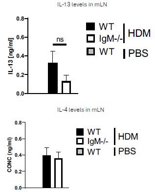
The choice of 5 days is strange, given that the response the authors want to see is in already primed cells. A 1-2 day assay would have been better.
We agree with the reviewer that a shorter stimulation period would work. Over the years we have settled for 5-day re-stimulation for both anti-CD3 and HDM. We have tried other time points, but we consistently get better secretion of cytokines after 5 days.
It is concerning that the authors state that HDM restimulation did not induce cytokine production from medLN cells, since countless studies have shown that restimulation of medLN would induce IL-13, IL-5 and IL-10 production from medLN. This indicates that the sensitization and challenge model used by the authors is not working as it should.
We thank the reviewer for this observation. In our recent paper showing how antigen load a]ects B cell function, we used very low levels of HDM to sensitise and challenge mice (1 ug and 3 ug respectively). See below article, Hadebe et al., 2021 JACI. This is because Labs that have used these low HDM levels also suggested that antigen load impacts B cell function, especially in their role in germinal centres. We believe the reason we see low or undetectable levels of cytokines is because of this low antigen load sensitisation and challenge. In other manuscripts we have published or about to publish, we have shown that normal HDM sensitisation load (1 ug or 100 ug) and challenge (10 ug) do induce cytokine release upon restimulation with HDM. See the below article by Khumalo et al, 2020 JCI Insight (Figure 4A).
Sabelo Hadebe*, Jermaine Khumalo, Sandisiwe Mangali, Nontobeko Mthembu, Hlumani Ndlovu, Amkele Ngomti, Martyna Scibiorek, Frank Kirstein, Frank Brombacher*. Deletion of IL-4Ra signalling on B cells limits hyperresponsiveness depending on antigen load. doi.org/10.1016/j.jaci.2020.12.635).
Jermaine Khumalo, Frank Kirstein, Sabelo Hadebe*, Frank Brombacher*. IL-4Rα signalling in regulatory T cells is required for dampening allergic airway inflammation through inhibition of IL-33 by type 2 innate lymphoid cells. JCI Insight. 2020 Oct 15;5(20):e136206. doi: 10.1172/jci.insight.136206
The IL-13 staining shown in panel c is also not definitive. One should be able to optimize their assays to achieve a better level of staining, to my mind.
We agree with the reviewer that much higher IL-13-producing CD4 T cells should be observed. We don’t think this is a technical glitch or non-optimal set-up as we see much higher levels of IL-13-producing CD4 T cells when using higher doses of HDM to sensitise and challenge, say between 7 -20% in WT mice (see Author response image 2 of lung stimulated with PMA/ionomycin+Monensin, please note this is for illustration purposes only and it not linked to the current manuscript, its merely to demonstrate a point from other experiments we have conducted in the lab).
Author response image 2.
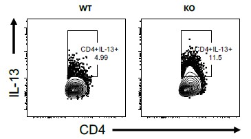
In d-f, the authors perform a serum transfer, but they only do this once. The half life of IgM is quite short. The authors should perform multiple naïve serum transfers to see if this is enough to induce FULL AHR.
We thank the reviewer for this comment. We apologise if this was not clear enough on the Figure legend and method, we did transfer serum 3x, a day before sensitisation, on the day of sensitisation and a day before the challenge to circumvent the short life of IgM. In our subsequent experiments, we have now used busulfan to deplete all bone marrow in IgM-deficient mice and replace it with WT bone marrow and this method restores AHR (Figure 3B).
This now appears in line 515 to 519 and reads
Adoptive transfer of naïve serum
Naïve wild-type mice were euthanised and blood was collected via cardiac puncture before being spun down (5500rpm, 10min, RT) to collect serum. Serum (200µL) was injected intraperitoneally into IgM-deficient mice. Serum was injected intraperitoneally at day -1, 0, and a day before the challenge with HDM (day 10).
The presence of negative values of total IgE in panel F would indicate some errors in calculation of serum IgE concentrations.
We thank the reviewer for this observation. For better clarity, we have now indicated these values as undetected in Figure 2F, as they were below our detection limit.
Overall, it is hard to be convinced that IgM-deficiency does not lead to a reduction in Th2 inflammation, since the assays appear suboptimal.
We disagree with the reviewer in this instance, because we have shown in 3 di]erent models and in 2 di]erent strains and 2 doses of HDM (high and low) that no matter what you do, Th2 remains intact. Our reason for choosing low dose HDM was based on our previous work and that of others, which showed that depending on antigen load, B cells can either be redundant or have functional roles. Since our interest was to tease out the role of B cells and specifically IgM, it was important that we look at a scenario where B cells are known to have a function (low antigen load). We did find similar findings at high dose of HDM load, but e]ects on AHR were not as strong, but Th2 was not changed, in fact in some instances Th2 was higher in IgM-deficient mice.
Fig. 3. Gene expression di]erences between WT and KO mice in PBS and HDM challenged settings are shown. PCA analysis does not show clear di]erences between all four groups, but genes are certainly up and downregulated, in particular when comparing PBS to HDM challenged mice. In both PBS and HDM challenged settings, three genes stand out as being upregulated in WT v KO mice. these are Baiap2l1, erdr1 and Chil1.
Noted
Fig. 4. The authors attempt to quantify BAIAP2L1 in mouse lungs. It is di]icult to know if the antibody used really detects the correct protein. A BAIAP2L1-KO is not used as a control for staining, and I am not sure if competitive assays for BAIAP2L1 can be set up. The flow data is not convincing. The immunohistochemistry shows BAIAP2L1 (in red) in many, many cells, essentially throughout the section. There is also no discernible di]erence between WT and KO mice, which one might have expected based on the RNA-Seq data. So, from my perspective, it is hard to say if/where this protein is located, and whether there truly exists a di]erence in expression between wt and ko mice.
We thank the reviewer for this comment. We are certain that the antibody does detect BAIAP2L1, we have used it in 3 assays, which we admit may show varying specificities since it’s a Polyclonal antibody. However, in our western blot (Figure 5A), the antibody detects a band at 56.7kDa, apart from what we think are isoforms. We agree that BAIAP2L1 is expressed by many cell types, including CD45+ cells and alpha smooth muscle negative cells and we show this in our Figure 5 – figure supplement 1A and B. Where we think there is a di]erence in expression between WT and IgM-deficient mice is in alpha-smooth muscle-positive cells. We have tested antibodies from di]erent companies (Proteintech and Abcam), and we find similar findings. We do not have access to BAIAP2L1 KO mice and to test specificity, we have also used single stain controls with or without secondary antibody and isotype control which show no binding in western blot and Immunofluorescence assays and Fluorescence minus one antibody in Flow cytometry, so that way we are convinced that the signal we are seeing is specific to BAIAP2L1.
Here we have also added additional Flow cytometry images using anti-BAIAP2L1 (clone 25692-1-AP) from Proteintech
Author response image 3.
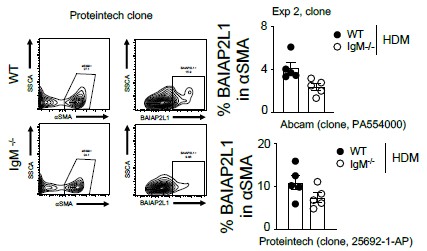
Figure similar to Figure 5C and Figure 5 -figure supplement 1A and B.
Fig. 5 and 6. The authors use a single cell contractility assay to measure whether BAIAP2L1 and ERDR1 impact on bronchial smooth muscle cell contractility. I am not familiar with the assay, but it looks like an interesting way of analysing contractility at the single cell level.
The authors state that targeting these two genes with Cas9gRNA reduces smooth muscle cell contractility, and the data presented for contractility supports this observation. However, the e]iciency of Cas9-mediated deletion is very unclear. The authors present a PCR in supp fig 9c as evidence of gene deletion, but it is entirely unclear with what e]iciency the gene has been deleted. One should use sequencing to confirm deletion. Moreover, if the antibody was truly working, one should be able to use the antibody used in Fig 4 to detect BAIAP2L1 levels in these cells. The authors do not appear to have tried this.
We thank the reviewer for these observations. We are in a process to optimise this using new polyclonal BAIAP2L1 antibodies from other companies, since the one we have tried doesn’t seem to work well on human cells via western blot. So hopefully in our new version, we will be able to demonstrate this by immunofluorescence or western blot.
Other impressions:
The paper is lacking a link between the deficiency of IgM and the e]ects on smooth muscle cell contraction.
The levels of IL-13 and TNF in lavage of WT and IGMKO mice could be analysed.
We have measured Th2 cytokine IL-13 in BAL fluid and found no di]erences between IgM-deficient mice and WT mice challenged with HDM (Author response image 4 below). We could not detected TNF-alpha in the BAL fluid, it was below detection limit.
Figure legend. IL-13 levels are not changed in IgM-deficient mice in the lung. Bronchoalveolar lavage fluid in WT or IgM-deficient mice sensitised and challenged with HDM. TNF-a levels were below the detection limit.
Author response image 4.
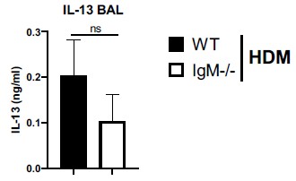
Moreover, what is the impact of IgM itself on smooth muscle cells? In the Fig. 7 schematic, are the authors proposing a direct role for IgM on smooth muscle cells? Does IgM in cell culture media induce contraction of SMC? This could be tested and would be interesting, to my mind.
We thank the Reviewer for these comments. We are still trying to test this, unfortunately, we have experienced delays in getting reagents such as human IgM to South Africa. We hope that we will be able to add this in our subsequent versions of the article. We agree it is an interesting experiment to do even if not for this manuscript but for our general understanding of this interaction at least in an in vitro system.
Reviewer #3 (Public Review):
Summary:
This paper by Sabelo et al. describes a new pathway by which lack of IgM in the mouse lowers bronchial hyperresponsiveness (BHR) in response to metacholine in several mouse models of allergic airway inflammation in Balb/c mice and C57/Bl6 mice. Strikingly, loss of IgM does not lead to less eosinophilic airway inflammation, Th2 cytokine production or mucus metaplasia, but to a selective loss of BHR. This occurs irrespective of the dose of allergen used. This was important to address since several prior models of HDM allergy have shown that the contribution of B cells to airway inflammation and BHR is dose dependent.
After a description of the phenotype, the authors try to elucidate the mechanisms. There is no loss of B cells in these mice. However, there is a lack of class switching to IgE and IgG1, with a concomitant increase in IgD. Restoring immunoglobulins with transfer of naïve serum in IgM deficient mice leads to restoration of allergen-specific IgE and IgG1 responses, which is not really explained in the paper how this might work. There is also no restoration of IgM responses, and concomitantly, the phenotype of reduced BHR still holds when serum is given, leading authors to conclude that the mechanism is IgE and IgG1 independent. Wild type B cell transfer also does not restore IgM responses, due to lack of engraftment of the B cells. Next authors do whole lung RNA sequencing and pinpoint reduced BAIAP2L1 mRNA as the culprit of the phenotype of IgM-/- mice. However, this cannot be validated fully on protein levels and immunohistology since di]erences between WT and IgM KO are not statistically significant, and B cell and IgM restoration are impossible. The histology and flow cytometry seems to suggest that expression is mainly found in alpha smooth muscle positive cells, which could still be smooth muscle cells or myofibroblasts. Next therefore, the authors move to CRISPR knock down of BAIAP2L1 in a human smooth muscle cell line, and show that loss leads to less contraction of these cells in vitro in a microscopic FLECS assay, in which smooth muscle cells bind to elastomeric contractible surfaces.
Strengths:
(1) There is a strong reduction in BHR in IgM-deficient mice, without alterations in B cell number, disconnected from e]ects on eosinophilia or Th2 cytokine production.
(2) BAIAP2L1 has never been linked to asthma in mice or humans
Weaknesses:
(1) While the observations of reduced BHR in IgM deficient mice are strong, there is insu]icient mechanistic underpinning on how loss of IgM could lead to reduced expression of BAIAP2L1. Since it is impossible to restore IgM levels by either serum or B cell transfer and since protein levels of BAIAP2L1 are not significantly reduced, there is a lack of a causal relationship that this is the explanation for the lack of BHR in IgMdeficient mice. The reader is unclear if there is a fundamental (maybe developmental) di]erence in non-hematopoietic cells in these IgM-deficient mice (which might have accumulated another genetic mutation over the years). In this regard, it would be important to know if littermates were newly generated, or historically bred along with the KO line.
We thank the reviewer for asking this question and getting us to think of this in a di]erent way. This prompted us to use a di]erent method to try and restore IgM function and since our animal facility no longer allows irradiation, we opted for busulfan. We present this data as new data in Figure 3. We had to go back and breed this strain and then generated bone marrow chimeras. What we have shown now with chimeras is that if we can deplete bone marrow from IgM-deficient mice and replace it with congenic WT bone marrow when we allow these mice to rest for 2 months before challenge with HDM (Figure 3 -figure supplement 1A-C) We also show that AHR (resistance and elastance) is partially restored in this way (Figure 3A and B) as mice that receive congenic WT bone marrow after chemical irradiation can mount AHR and those that receive IgM-deficient bone marrow, can’t mount AHR upon challenge with HDM. If the mice had accumulated an unknown genetic mutation in non-hematopoietic cells, the transfer of WT bone marrow would not make a di]erence. So, we don’t believe the colony could have gained a mutation that we are unaware of. We have also shipped these mice to other groups and in their hands, this strains still only behaves as an IgM only knockout mice. See their publication below.
Mark Noviski, James L Mueller, Anne Satterthwaite, Lee Ann Garrett-Sinha, Frank Brombacher, Julie Zikherman 2018. IgM and IgD B cell receptors di]erentially respond to endogenous antigens and control B cell fate. eLife 2018;7:e35074. DOI: https://doi.org/10.7554/eLife.35074
we have also added methods for bone marrow chimaeras and added results sections and new Figures related to these methods.
Methods appear in line 521-532 of the untracked version of the article.
Busulfan Bone marrow chimeras
WT (CD45.2) and IgM<sup>-/-</sup> (CD45.2) congenic mice were treated with 25 mg/kg busulfan (Sigma-Aldrich, Aston Manor, South Africa) per day for 3 consecutive days (75 mg/kg in total) dissolved in 10% DMSO and Phosphate bu]ered saline (0.2mL, intraperitoneally) to ablate bone marrow cells. Twenty-four hours after last administration of busulfan, mice were injected intravenously with fresh bone marrow (10x10<sup>6</sup> cells, 100µL) isolated from hind leg femurs of either WT (CD45.1) or IgM<sup>-/-</sup> mice [33]. Animals were then allowed to complement their haematopoietic cells for 8 weeks. In some experiments the level of bone marrow ablation was assessed 4 days post-busulfan treatment in mice that did not receive donor cells. At the end of experiment level of complemented cells were also assessed in WT and IgM<sup>-/-</sup> mice that received WT (CD45.1) bone marrow.
Results appear in line 198-228 of the untracked version of the article
Replacement of IgM-deficient mice with functional hematopoietic cells in busulfan mice chimeric mice restores airway hyperresponsiveness.
We then generated bone marrow chimeras by chemical radiation using busulfan (Montecino-Rodriguez and Dorshkind, 2020). We treated mice three times with busulfan for 3 consecutive days and after 24 hrs transferred naïve bone marrow from congenic CD45.1 WT mice or CD45.2 IgM KO mice (Figure 3A and Figure 3 -figure supplement 1A). We showed that recipient mice that did not receive donor bone marrow after 4 days post-treatment had significantly reduced lineage markers (CD45<sup>+</sup>Sca-1<sup>+</sup>) or lineage negative (Lin<sup>-</sup>) cells in the bone marrow when compared to untreated or vehicle (10% DMSO) treated mice (Figure 3 -figure supplements 1B-C). We allowed mice to reconstitute bone marrow for 8 weeks before sensitisation and challenge with low dose HDM (Figure 3A). We showed that WT (CD45.2) recipient mice that received WT (CD45.1) donor bone marrow had higher airway resistance and elastance and this was comparable to IgM KO (CD45.2) recipient mice that received donor WT (CD45.1) bone marrow (Figure 3B). As expected, IgM KO (CD45.2) recipient mice that received donor IgM KO (CD45.2) bone marrow had significantly lower AHR compared to WT (CD45.2) or IgM KO (CD45.2) recipient mice that received WT (CD45.1) bone marrow (Figure 3B). We confirmed that the di]erences observed were not due to di]erences in bone marrow reconstitution as we saw similar frequencies of CD45.1 cells within the lymphocyte populations in the lungs and other tissues (Figure 3 -figure supplement 1D). We observed no significant changes in the lung neutrophils, eosinophils, inflammatory macrophages, CD4 T cells or B cells in WT or IgM KO (CD45.2) recipient mice that received donor WT (CD45.1/CD45.2) or IgM KO (CD45.2) bone marrow when sensitised and challenged with low dose HDM (Figure 3C).
Restoring IgM function through adoptive reconstitution with congenic CD45.1 bone marrow in non-chemically irradiated recipient mice or sorted B cells into IgM KO mice (Figure 2 -figure supplement 1A) did not replenish IgM B cells to levels observed in WT mice and as a result did not restore AHR, total IgE and IgM in these mice (Figure 2 -figure supplements 1B-C).
The 2 new figures are Figure 3 which moved the rest of the Figures down and Figure 3- figure supplement 1AD), which also moved the rest of the supplementary figures down.
Discussion appears in line 410-419 of the untracked version of the article.To resolve other endogenous factors that could have potentially influenced reduced AHR in IgM-deficient mice, we resorted to busulfan chemical irradiation to deplete bone marrow cells in IgM-deficient mice and replace bone marrow with WT bone marrow. While it is well accepted that busulfan chemical irradiation partially depletes bone marrow cells, in our case it was not possible to pursue other irradiation methods due to changes in ethical regulations and that fact that mice are slow to recover after gamma rays irradiation. Busulfan chemical irradiation allowed us to show that we could mostly restore AHR in IgM-deficient recipient mice that received donor WT bone marrow when challenged with low dose HDM.
(2) There is no mention of the potential role of complement in activation of AHR, which might be altered in IgM-deficient mice
We thank the reviewer for this comment. We have not directly looked at complement in this instance, however, from our previous work on C3 knockout mice, there have been comparable AHR to WT mice under the HDM challenge.
(3) What is the contribution of elevated IgD in the phenotype of the IgM-deficient mice. It has been described by this group that IgD levels are clearly elevated
We thank the reviewer for this question. We believe that IgD is essentially what drives partial class switching to IgG, we certainly have shown that in the case of VSV virus and Trypanosoma congolense and Trypanosoma brucei brucei that elevated IgD drive delayed but e]ective IgG in the absence of IgM (Lutz et al, 2001, Nature). This is also confirmed by Noviski et al., 2018 eLife study where they show that both IgM and IgD do share some endogenous antigens, so its likely that external antigens can activate IgD in a similar manner to prompt class switching.
(4) How can transfer of naïve serum in class switching deficient IgM KO mice lead to restoration of allergen specific IgE and IgG1?
We thank the Reviewer for these comments, we believe that naïve sera transferred to IgM deficient mice is able to bind to the surface of B cells via IgM receptors (FcμR / Fcα/μR), which are still present on B cells and this is su]icient to facilitate class switching. Our IgM KO mouse lacks both membrane-bound and secreted IgM, and transferred serum contains at least secreted IgM which can bind to surfaces via its Fc portion. We measured HDM-specific IgE and we found very low levels, but these were not di]erent between WT and IgM KO adoptively transferred with WT serum. We also detected HDM-specific IgG1 in IgM KO transferred with WT sera to the same level as WT, confirming a possible class switching, of course, we can’t rule out that transferred sera also contains some IgG1. We also can’t rule out that elevated IgD levels can partially be responsible for class switched IgG1 as discussed above.
In the discussion line 463-464, we also added the following
“We speculate that IgM can directly activate smooth muscle cells by binding a number of its surface receptors including FcμR, Fcα/μR and pIgR (Liu et al., 2019; Nguyen et al., 2017b; Shibuya et al., 2000). IgM binds to FcμR strictly, but shares Fcα/μR and pIgR with IgA (Liu et al., 2019; Michaud et al., 2020; Nguyen et al., 2017b). Both Fcα/μR and pIgR can be expressed by non-structural cells at mucosal sites (Kim et al., 2014; Liu et al., 2019). We would not rule out that the mechanisms of muscle contraction might be through one of these IgM receptors, especially the ones expressed on smooth muscle cells(Kim et al., 2014; Liu et al., 2019). Certainly, our future studies will be directed towards characterizing the mechanism by which IgM potentially activates the smooth muscle.”
We have discussed this section under Discussion section, line 731 to 757. In addition, since we have now performed bone marrow chimaeras we have further added the following in our discussion in line 410-419.
To resolve other endogenous factors that could have potentially influenced reduced AHR in IgM-deficient mice, we resorted to busulfan chemical irradiation to deplete bone marrow cells in IgM-deficient mice and replace bone marrow with WT bone marrow. While it is well accepted that busulfan chemical irradiation partially depletes bone marrow cells, in our case it was not possible to pursue other irradiation methods due to changes in ethical regulations and that fact that mice are slow to recover after gamma rays irradiation. Busulfan chemical irradiation allowed us to show that we could mostly restore AHR in IgM-deficient recipient mice that received donor WT bone marrow when challenged with low dose HDM.
We removed the following lines, after performing bone marrow chimaeras since this changed some aspects.
Our efforts to adoptively transfer wild-type bone marrow or sorted B cells into IgMdeficient mice were also largely unsuccessful partly due to poor engraftment of wildtype B cells into secondary lymphoid tissues. Natural secreted IgM is mainly produced by B1 cells in the peritoneal cavity, and it is likely that any transfer of B cells via bone marrow transfer would not be su]icient to restore soluble levels of IgM<sup>3,10</sup>.
(5) lpha smooth muscle antigen is also expressed by myofibroblasts. This is insu]iciently worked out. The histology mentions "expression in cells in close contact with smooth muscle". This needs more detail since it is a very vague term. Is it in smooth muscle or in myofibroblasts.
We appreciate that alpha-smooth muscle actin-positive cells are a small fraction in the lung and even within CD45 negative cells, but their contribution to airway hyperresponsiveness is major. We also concede that by immunofluorescence BAIAP2L1 seems to be expressed by cells adjacent to alpha-smooth muscle actin (Figure 5B), however, we know that cells close to smooth muscle (such as extracellular matrix and myofibroblasts) contribute to its hypertrophy in allergic asthma.
James AL, Elliot JG, Jones RL, Carroll ML, Mauad T, Bai TR, et al. Airway Smooth Muscle Hypertrophy and Hyperplasia in Asthma. Am J Respir Crit Care Med [Internet]. 2012; 185:1058–64. Available from: https://doi.org/10.1164/rccm.201110-1849OC
(6) Have polymorphisms in BAIAP2L1 ever been linked to human asthma?
No, we have looked in asthma GWAS studies, at least summary statistics and we have not seen any SNPs that could be associated with human asthma.
(7) IgM deficient patients are at increased risk for asthma. This paper suggests the opposite. So the translational potential is unclear
We thank the reviewer for these comments. At the time of this publication, we have not made a concrete link with human disease. While there is some anecdotal evidence of diseases such as Autoimmune glomerulonephritis, Hashimoto’s thyroiditis, Bronchial polyp, SLE, Celiac disease and other diseases in people with low IgM. Allergic disorders are also common in people with IgM deficiency as the reviewer correctly points out, other studies have reported as high as 33-47%. The mechanisms for the high incidence of allergic diseases are unclear as generally, these patients have normal or higher IgG and IgE levels. IgM deficiency may represent a heterogeneous spectrum of genetic defects, which might explain the heterogeneous nature of disease presentations.
Reviewer #2 (Public review):
Summary:
Lamothe et al. collected fMRI responses to many voice stimuli in 3 subjects. The authors trained two different autoencoders on voice audio samples and predicted latent space embeddings from the fMRI responses, allowing the voice spectrograms to be reconstructed. The degree to which reconstructions from different auditory ROIs correctly represented speaker identity, gender or age was assessed by machine classification and human listener evaluations. Complementing this, the representational content was also assessed using representational similarity analysis. The results broadly concur with the notion that temporal voice areas are sensitive to different types of categorical voice information.
Strengths:
The single-subject approach that allow thousands of responses to unique stimuli to be recorded and analyzed is powerful. The idea of using this approach to probe cortical voice representations is strong and the experiment is technically solid.
Reviewer #3 (Public review):
Summary:
In this manuscript, Lamothe et al. sought to identify the neural substrates of voice identity in the human brain by correlating fMRI recordings with the latent space of a variational autoencoder (VAE) trained on voice spectrograms. They used encoding and decoding models, and showed that the "voice" latent space (VLS) of the VAE performs, in general, (slightly) better than a linear autoencoder's latent space. Additionally, they showed dissociations in the encoding of voice identity across the temporal voice areas.
Strengths:
The geometry of the neural representations of voice identity has not been studied so far. Previous studies on the content of speech and faces in vision suggest that such geometry could exist. This study demonstrates this point systematically, leveraging a specifically trained variational autoencoder.
The size of the voice dataset and the length of the fMRI recordings ensure that the findings are robust.
Comments on revisions:
The authors addressed my previous recommendations.
Author response:
The following is the authors’ response to the original reviews.
Reviewer #1 (Public Review):
Summary:
In this study, the authors trained a variational autoencoder (VAE) to create a high-dimensional "voice latent space" (VLS) using extensive voice samples, and analyzed how this space corresponds to brain activity through fMRI studies focusing on the temporal voice areas (TVAs). Their analyses included encoding and decoding techniques, as well as representational similarity analysis (RSA), which showed that the VLS could effectively map onto and predict brain activity patterns, allowing for the reconstruction of voice stimuli that preserve key aspects of speaker identity.
Strengths:
This paper is well-written and easy to follow. Most of the methods and results were clearly described. The authors combined a variety of analytical methods in neuroimaging studies, including encoding, decoding, and RSA. In addition to commonly used DNN encoding analysis, the authors performed DNN decoding and resynthesized the stimuli using VAE decoders. Furthermore, in addition to machine learning classifiers, the authors also included human behavioral tests to evaluate the reconstruction performance.
Weaknesses:
This manuscript presents a variational autoencoder (VAE) to evaluate voice identity representations from brain recordings. However, the study's scope is limited by testing only one model, leaving unclear how generalizable or impactful the findings are. The preservation of identity-related information in the voice latent space (VLS) is expected, given the VAE model's design to reconstruct original vocal stimuli. Nonetheless, the study lacks a deeper investigation into what specific aspects of auditory coding these latent dimensions represent. The results in Figure 1c-e merely tested a very limited set of speech features. Moreover, there is no analysis of how these features and the whole VAE model perform in standard speech tasks like speech recognition or phoneme recognition. It is not clear what kind of computations the VAE model presented in this work is capable of. Inclusion of comparisons with state-of-the-art unsupervised or self-supervised speech models known for their alignment with auditory cortical responses, such as Wav2Vec2, HuBERT, and Whisper, would strengthen the validation of the VAE model and provide insights into its relative capabilities and limitations.
The claim that the VLS outperforms a linear model (LIN) in decoding tasks does not significantly advance our understanding of the underlying brain representations. Given the complexity of auditory processing, it is unsurprising that a nonlinear model would outperform a simpler linear counterpart. The study could be improved by incorporating a comparative analysis with alternative models that differ in architecture, computational strategies, or training methods. Such comparisons could elucidate specific features or capabilities of the VLS, offering a more nuanced understanding of its effectiveness and the computational principles it embodies. This approach would allow the authors to test specific hypotheses about how different aspects of the model contribute to its performance, providing a clearer picture of the shared coding in VLS and the brain.
The manuscript overlooks some crucial alternative explanations for the discriminant representation of vocal identity. For instance, the discriminant representation of vocal identity can be either a higher-level abstract representation or a lower-level coding of pitch height. Prior studies using fMRI and ECoG have identified both types of representation within the superior temporal gyrus (STG) (e.g., Tang et al., Science 2017; Feng et al., NeuroImage 2021). Additionally, the methodology does not clarify whether the stimuli from different speakers contained identical speech content. If the speech content varied across speakers, the approach of averaging trials to obtain a mean vector for each speaker-the "identity-based analysis"-may not adequately control for confounding acoustic-phonetic features. Notably, the principal component 2 (PC2) in Figure 1b appears to correlate with absolute pitch height, suggesting that some aspects of the model's effectiveness might be attributed to simpler acoustic properties rather than complex identity-specific information.
Methodologically, there are issues that warrant attention. In characterizing the autoencoder latent space, the authors initialized logistic regression classifiers 100 times and calculated the tstatistics using degrees of freedom (df) of 99. Given that logistic regression is a convex optimization problem typically converging to a global optimum, these multiple initializations of the classifier were likely not entirely independent. Consequently, the reported degrees of freedom and the effect size estimates might not accurately reflect the true variability and independence of the classifier outcomes. A more careful evaluation of these aspects is necessary to ensure the statistical robustness of the results.
We thank Reviewer #1 for their thoughtful and constructive comments. Below, we address the key points raised:
New comparitive models. We agree there are still many open questions on the structure of the VLS and the specific aspects of auditory coding that its latent dimensions represent. The features tested in Figure 1c-e are not speech features, but aspects related to speaker identity: age, gender and unique identity. Nevertheless we agree the VLS could be compared to recent speech models (not available when we started this project): we have now included comparisons with Wav2Vec and HuBERT in the encoding section (new Figure 2-S3). The comparison of encoding results based on LIN, the VLS, Wav2Vec and HuBERT (new Fig2S3) indicates no clear superiority of one model over the others; rather, different sets of voxels are better explained by the different models. Interestingly all four models yielded best encoding results for the m and a TVA, indicating some consistency across models.
On decoding directly from spectrograms. We have now added decoding results obtained directly from spectrograms, as requested in the private review. These are presented in the revised Figure 4, and allow for comparison with the LIN- and VLS-based reconstructions. As noted, spectrogram-based reconstructions sounded less vocal-like and faithful to the original, confirming that the latent spaces capture more abstract and cerebral-like voice representations.
On the number and length of stimuli. The rationale for using a large number of brief, randomly spliced speech excerpts from different languages was to extract identity features independent of specific linguistic cues. Indeed, the PC2 could very well correlate with pitch; we were not able to extract reliable f0 information from the thousands of brief stimuli, many of which are largely inharmonic (e.g., fricatives), such that this assumption could not be tested empirically. But it would be relevant that the weight of PC2 correlates with pitch: although the average fundamental frequency of phonation is not a linguistic cue, it is a major acoustical feature differentiating speaker identities.
Statistics correction. To address the issue of potential dependence between multiple runs of logistic regression, we replaced our previous analysis with a Wilcoxon signedrank test comparing decoding accuracies to chance. The results remain significant across classifications, and the revised figure and text reflect this change.
Reviewer #2 (Public Review):
Summary:
Lamothe et al. collected fMRI responses to many voice stimuli in 3 subjects. The authors trained two different autoencoders on voice audio samples and predicted latent space embeddings from the fMRI responses, allowing the voice spectrograms to be reconstructed. The degree to which reconstructions from different auditory ROIs correctly represented speaker identity, gender, or age was assessed by machine classification and human listener evaluations. Complementing this, the representational content was also assessed using representational similarity analysis. The results broadly concur with the notion that temporal voice areas are sensitive to different types of categorical voice information.
Strengths:
The single-subject approach that allows thousands of responses to unique stimuli to be recorded and analyzed is powerful. The idea of using this approach to probe cortical voice representations is strong and the experiment is technically solid.
Weaknesses:
The paper could benefit from more discussion of the assumptions behind the reconstruction analyses and the conclusions it allows. The authors write that reconstruction of a stimulus from brain responses represents 'a robust test of the adequacy of models of brain activity' (L138). I concur that stimulus reconstruction is useful for evaluating the nature of representations, but the notion that they can test the adequacy of the specific autoencoder presented here as a model of brain activity should be discussed at more length. Natural sounds are correlated in many feature dimensions and can therefore be summarized in several ways, and similar information can be read out from different model representations. Models trained to reconstruct natural stimuli can exploit many correlated features and it is quite possible that very different models based on different features can be used for similar reconstructions. Reconstructability does not by itself imply that the model is an accurate brain model. Non-linear networks trained on natural stimuli are arguably not tested in the same rigorous manner as models built to explicitly account for computations (they can generate predictions and experiments can be designed to test those predictions). While it is true that there is increasing evidence that neural network embeddings can predict brain data well, it is still a matter of debate whether good predictability by itself qualifies DNNs as 'plausible computational models for investigating brain processes' (L72). This concern is amplified in the context of decoding and naturalistic stimuli where many correlated features can be represented in many ways. It is unclear how much the results hinge on the specificities of the specific autoencoder architectures used. For instance, it would be useful to know the motivations for why the specific VAE used here should constitute a good model for probing neural voice representations.
Relatedly, it is not clear how VAEs as generative models are motivated as computational models of voice representations in the brain. The task of voice areas in the brain is not to generate voice stimuli but to discriminate and extract information. The task of reconstructing an input spectrogram is perhaps useful for probing information content, but discriminative models, e.g., trained on the task of discriminating voices, would seem more obvious candidates. Why not include discriminatively trained models for comparison?
The autoencoder learns a mapping from latent space to well-formed voice spectrograms. Regularized regression then learns a mapping between this latent space and activity space. All reconstructions might sound 'natural', which simply means that the autoencoder works. It would be good to have a stronger test of how close the reconstructions are to the original stimulus. For instance, is the reconstruction the closest stimulus to the original in latent space coordinates out of using the experimental stimuli, or where does it rank? How do small changes in beta amplitudes impact the reconstruction? The effective dimensionality of the activity space could be estimated, e.g. by PCA of the voice samples' contrast maps, and it could then be estimated how the main directions in the activity space map to differences in latent space. It would be good to get a better grasp of the granularity of information that can be decoded/ reconstructed.
What can we make of the apparent trend that LIN is higher than VLS for identity classification (at least VLS does not outperform LIN)? A general argument of the paper seems to be that VLS is a better model of voice representations compared to LIN as a 'control' model. Then we would expect VLS to perform better on identity classification. The age and gender of a voice can likely be classified from many acoustic features that may not require dedicated voice processing.
The RDM results reported are significant only for some subjects and in some ROIs. This presumably means that results are not significant in the other subjects. Yet, the authors assert general conclusions (e.g. the VLS better explains RDM in TVA than LIN). An assumption typically made in single-subject studies (with large amounts of data in individual subjects) is that the effects observed and reported in papers are robust in individual subjects. More than one subject is usually included to hint that this is the case. This is an intriguing approach. However, reports of effects that are statistically significant in some subjects and some ROIs are difficult to interpret. This, in my view, runs contrary to the logic and leverage of the single-subject approach. Reporting results that are only significant in 1 out of 3 subjects and inferring general conclusions from this seems less convincing.
The first main finding is stated as being that '128 dimensions are sufficient to explain a sizeable portion of the brain activity' (L379). What qualifies this? From my understanding, only models of that dimensionality were tested. They explain a sizeable portion of brain activity, but it is difficult to follow what 'sizable' is without baseline models that estimate a prediction floor and ceiling. For instance, would autoencoders that reconstruct any spectrogram (not just voice) also predict a sizable portion of the measured activity? What happens to reconstruction results as the dimensionality is varied?
A second main finding is stated as being that the 'VLS outperforms the LIN space' (L381). It seems correct that the VAE yields more natural-sounding reconstructions, but this is a technical feature of the chosen autoencoding approach. That the VLS yields a 'more brain-like representational space' I assume refers to the RDM results where the RDM correlations were mainly significant in one subject. For classification, the performance of features from the reconstructions (age/ gender/ identity) gives results that seem more mixed, and it seems difficult to draw a general conclusion about the VLS being better. It is not clear that this general claim is well supported.
It is not clear why the RDM was not formed based on the 'stimulus GLM' betas. The 'identity GLM' is already biased towards identity and it would be stronger to show associations at the stimulus level.
Multiple comparisons were performed across ROIs, models, subjects, and features in the classification analyses, but it is not clear how correction for these multiple comparisons was implemented in the statistical tests on classification accuracies.
Risks of overfitting and bias are a recurrent challenge in stimulus reconstruction with fMRI. It would be good with more control analyses to ensure that this was not the case. For instance, how were the repeated test stimuli presented? Were they intermingled with the other stimuli used for training or presented in separate runs? If intermingled, then the training and test data would have been preprocessed together, which could compromise the test set. The reconstructions could be performed on responses from independent runs, preprocessed separately, as a control. This should include all preprocessing, for instance, estimating stimulus/identity GLMs on separately processed run pairs rather than across all runs. Also, it would be good to avoid detrending before GLM denoising (or at least testing its effects) as these can interact.
We appreciate Reviewer #2’s careful reading and numerous suggestions for improving clarity and presentation. We have implemented the suggested text edits, corrected ambiguities, and clarified methodological details throughout the manuscript. In particular, we have toned down several sentences that we agree were making strong claims (L72, L118, L378, L380-381).
Clarifications, corrections and additional information:
We streamlined the introduction by reducing overly specific details and better framing the VLS concept before presenting specifics.
Clarified the motivation for the age classification split and corrected several inaccuracies and ambiguities in the methods, including the hearing thresholds, balancing of category levels, and stimulus energy selection procedure.
Provided additional information on the temporal structure of runs and experimental stimuli selection.
Corrected the description of technical issues affecting one participant and ensured all acronyms are properly defined in the text and figure legends.
Confirmed that audiograms were performed repeatedly to monitor hearing thresholds and clarified our use of robust scaling and normalization procedures.
Regarding the test of RDM correlations, we clarified in the text that multiple comparisons were corrected using a permutation-based framework.
Reviewer #3 (Public Review):
Summary:
In this manuscript, Lamothe et al. sought to identify the neural substrates of voice identity in the human brain by correlating fMRI recordings with the latent space of a variational autoencoder (VAE) trained on voice spectrograms. They used encoding and decoding models, and showed that the "voice" latent space (VLS) of the VAE performs, in general, (slightly) better than a linear autoencoder's latent space. Additionally, they showed dissociations in the encoding of voice identity across the temporal voice areas.
Strengths:
The geometry of the neural representations of voice identity has not been studied so far. Previous studies on the content of speech and faces in vision suggest that such geometry could exist. This study demonstrates this point systematically, leveraging a specifically trained variational autoencoder.
The size of the voice dataset and the length of the fMRI recordings ensure that the findings are robust.
Weaknesses:
Overall, the VLS is often only marginally better than the linear model across analysis, raising the question of whether the observed performance improvements are due to the higher number of parameters trained in the VAE, rather than the non-linearity itself. A fair comparison would necessitate that the number of parameters be maintained consistently across both models, at least as an additional verification step.
The encoding and RSM results are quite different. This is unexpected, as similar embedding geometries between the VLS and the brain activations should be reflected by higher correlation values of the encoding model.
The consistency across participants is not particularly high, for instance, S1 seemed to have demonstrated excellent performances, while S2 showed poor performance.
An important control analysis would be to compare the decoding results with those obtained by a decoder operating directly on the latent spaces, in order to further highlight the interest of the non-linear transformations of the decoder model. Currently, it is unclear whether the non-linearity of the decoder improves the decoding performance, considering the poor resemblance between the VLS and brain-reconstructed spectrograms.
We thank Reviewer #3 for their comments. In response:
Code and preprocessed data are now available as indicated in the revised manuscript.
While we appreciate the suggestion to display supplementary analyses as boxplots split by hemisphere, we opted to retain the current format as we do not have hypotheses regarding hemispheric lateralization, and the small sample size per hemisphere would preclude robust conclusions.
Confirmed that the identities in Figure 3a are indeed ordered by age and have clarified this in the legend.
The higher variance observed in correlations for the aTVA in Figure 3b reflects the small number of data points (3 participants × 2 hemispheres), and this is now explained.
Regarding the cerebral encoding of gender and age, we acknowledge this interesting pattern. Prior work (e.g., Charest et al., 2013) found overlapping processing regions for voice gender without clear subregional differences in the TVAs. Evidence on voice age encoding remains sparse, and we highlight this novel finding in our discussion.
We again thank the reviewers for their insightful comments, which have greatly improved the quality and clarity of our work.
Reviewer #1 (Recommendations For The Authors):
(1) A set of recent advances have shown that embeddings of unsupervised/self-supervised speech models aligned to auditory responses to speech in the temporal cortex (e.g. Wav2Vec2: Millet et al NeurIPS 2022; HuBERT: Li et al. Nat Neurosci 2023; Whisper: Goldstein et al.bioRxiv 2023). These models are known to preserve a variety of speech information (phonetics, linguistic information, emotions, speaker identity, etc) and perform well in a variety of downstream tasks. These other models should be evaluated or at least discussed in the study.
We fully agree - the pace of progress in this area of voice technology has been incredible. Many of these models were not yet available at the time this work started so we could not use them in our comparison with cerebral representations.
We have now implemented Reviewer #1’s suggestion and evaluated Wav2Vec and HuBERT. The results are presented in supplementary Figure 2-S3. Correlations between activity predicted by the model and the real activity were globally comparable with those obtained with the LIN and VLS models. Interestingly both HuBERT and Wav2Vec yielded highest correlations in the mTVA, and to a lesser extent, the aTVA, as the LIN and VLS models.
(2) The test statistics of the results in Fig 1c-e need to be revised. Given that logistic regression is a convex optimization problem typically converging to a global optimum, these multiple initializations of the classifier were likely not entirely independent. Consequently, the reported degrees of freedom and the effect size estimates might not accurately reflect the true variability and independence of the classifier outcomes. A more careful evaluation of these aspects is necessary to ensure the statistical robustness of the results.
We thank Reviewer #1 for pointing out this important issue regarding the potential dependence between multiple runs of the logistic regression model. To address this concern, we have revised our analyses and used a Wilcoxon signed-rank test to compare the decoding accuracy to chance level. The results showed that the accuracy was significantly above chance for all classifications (Wilcoxon signed-rank test, all W=15, p=0.03125). We updated Figure 1c-e and the corresponding text (L154-L155) to reflect the revised analysis. Because the focus of this section is to probe the informational content of the autoencoder’s latent spaces, and since there are only 5 decoding accuracy values per model, we dropped the inter-model statistical test.
(3) In Line 198, the authors discuss the number of dimensions used in their models. To provide a comprehensive comparison, it would be informative to include direct decoding results from the original spectrograms alongside those from the VLS and LIN models. Given the vast diversity in vocal speech characteristics, it is plausible that the speaker identities might correlate with specific speech-related features also represented in both the auditory cortex and the VLS. Therefore, a clearer understanding of the original distribution of voice identities in the untransformed auditory space would be beneficial. This addition would help ascertain the extent to which transformations applied by the VLS or LIN models might be capturing or obscuring relevant auditory information.
We have now implemented Reviewer #1’s suggestion. The graphs on the right panel b of revised Figure 4 now show decoding results obtained from the regression performed directly on the spectrograms, rather than on representations of them, for our two example test stimuli. They can be listened to and compared to the LIN- and VLS-based reconstructions in Supplementary Audio 2. Compared to the LIN and VLS, the SPEC-based reconstructions sounded much less vocal or similar to the original, indicating that the latent spaces indeed capture more abstract voice representations, more similar to cerebral ones.
Reviewer #2 (Recommendations For The Authors):
L31: 'in voice' > consider rewording (from a voice?).
L33: consider splitting sentence (after interactions).
L39: 'brain' after parentheses.
L45-: certainly DNNs 'as a powerful tool' extend to audio (not just image and video) beyond their use in brain models.
L52: listened to / heard.
L63: use second/s consistently.
L64: the reference to Figure 5D is maybe a bit confusing here in the introduction.
We thank Reviewer #2 for these recommendations, which we have implemented.
L79-88: this section is formulated in a way that is too detailed for the introduction text (confusing to read). Consider a more general introduction to the VLS concept here and the details of this study later.
L99-: again, I think the experimental details are best saved for later. It's good to provide a feel for the analysis pipeline here, but some of the details provided (number of averages, denoising, preprocessing), are anyway too unspecific to allow the reader to fully follow the analysis.
Again, thank you for these suggestions for improving readability: we have modified the text accordingly.
L159: what was the motivation for classifying age as a 2-class classification problem? Rather than more classes or continuous prediction? How did you choose the age split?
The motivation for the 2 age classes was to align on the gender classification task for better comparison. The cutoff (30 years) was not driven by any scientific consideration, but by practical ones, based on the median age in our stimulus set. This is now clarified in the manuscript (L149).
L263: Is the test of RDM correlation>0 corrected for multiple comparisons across ROIs, subjects, and models?
The test of RDM correlation>0 was indeed corrected for multiple comparisons for models using the permutation-based ‘maximum statistics’ framework for multiple comparison correction (described in Giordano et al., 2023 and Maris & Oostenveld, 2007). This framework was applied for each ROI and subject. It was described in the Methods (L745) but not clearly enough in the text—we thank Reviewer #2 and clarified it in the text (L246, L260-L261).
L379: 'these stimuli' - weren't the experimental stimuli different from those used to train the V/AE?
We thank Reviewer #2 for spotting this issue. Indeed, the experimental stimuli are different from those used to train the models. We corrected the text to reflect this distinction (L84-L85).
L443: what are 'technical issues' that prevented subject 3 from participating in 48 runs??
We thank Reviewer #2 for pointing out the ambiguity in our previous statement. Participant 3 actually experienced personal health concerns that prevented them from completing the whole number of runs. We corrected this to provide a more accurate description (L442-L443).
L444: participants were instructed to 'stay in the scanner'!? Do you mean 'stay still', or something?
We thank the Reviewer for spotting this forgotten word. We have corrected the passage (L444).
L463: Hearing thresholds of 15 dB: do you mean that all had thresholds lower than 15 dB at all frequencies and at all repeated audiogram measurements?
We thank Reviewer #2 for spotting this error: we meant thresholds below 15dB HL. This has been corrected (L463). Indeed participants were submitted to several audiograms between fMRI sessions, to ensure no hearing loss could be caused by the scanner noise in these repeated sessions.
L472: were the 4 category levels balanced across the dataset (in number of occurrences of each category combination)?
The dataset was fully balanced, with an equal number of samples for each combination of language, gender, age, and identity. Furthermore, to minimize potential adaptation effects, the stimuli were also balanced within each run according to these categories, and identity was balanced across sessions. We made this clearer in Main voice stimuli (L492-L496).
L482: the test stimuli were selected as having high energy by the amplitude envelope. It is unclear what this means (how is the envelope extracted, what feature of it is used to measure 'high energy'?)
The selection of sounds with high energy was based on analyzing the amplitude envelope of each signal, which was extracted using the Hilbert transform and then filtered to refine the envelope. This envelope, which represents the signal's intensity over time, was used to measure the energy of each stimulus, and those that exceeded an arbitrary threshold were selected. From this pool of high-energy stimuli, likely including vowels, we selected six stimuli to be repeated during the scanning session, then reconstructed via decoding. This has been clarified in the text (L483-L484).
L500 was the audio filtered to account for the transfer function of the Sensimetrics headphones?
We did not perform any filtering, as the transfer function of the Sensimetrics is already very satisfactory as is. This has been clarified in the text (L503).
L500: what does 'comfortable level' correspond to and was it set per session (i.e. did it vary across sessions)?
By comfortable we mean around 85 dB SPL. The audio settings were kept similar across sessions. This has been added to the text (L504).
L526- does the normalization imply that the reconstructed spectrograms are normalized? Were the reconstructions then scaled to undo the normalization before inversion?
The paragraph on spectrogram standardization was not well placed inducing confusion. We have placed this paragraph in its more suitable location, in the Deep learning section (L545L550)
L606: does the identity GLM model the denoised betas from the first GLM or simply the BOLD data? The text indicates the latter, but I suspect the former.
Indeed: this has been clarified (L601-L602).
L704: could you unpack this a bit more? It is not easy to see why you specify the summing in the objective. Shouldn't this just be the ridge objective for a given voxel/ROI? Then you could just state it in matrix notation.
Thanks for pointing this out: we kept the formula unchanged but clarified the text, in particular specified that the voxel id is the ith index (L695).
L716: you used robust scaling for the classifications in latent space but haven't mentioned scaling here. Are we to assume that the same applies?
Indeed we also used robust scaling here, this is now made clear (L710-L711).
L720: Pearson correlation as a performance metric and its variance will depend on the choice of test/train split sizes. Can you show that the results generalize beyond your specific choices? Maybe the report explained variance as well to get a better idea of performance.
We used a standard 80/20 split. We think it is beyond the scope of this study to examine the different possible choices of splits, and prefer not to spend additional time on this point which we think is relatively minor.
Could you specify (somewhere) the stimulus timing in a run? ISI and stimulus duration are mentioned in different places, but it would be nice to have a summary of the temporal structure of runs.
This is now clarified at the beginning of the Methods section (L437-441)
Reviewer #3 (Recommendations For The Authors):
Code and data are not currently available.
Code and preprocessed data are now available (L826-827).
In the supplementary material, it would be beneficial to present the different analyses as boxplots, as in the main text, but with the ROIs in the left and right hemispheres separated, to better show potential hemispheric effect. Although this information is available in the Supplementary Tables, it is currently quite tedious to access it.
Although we provide the complete data split by hemisphere in the Tables, we do not believe it is relevant to illustrate left/right differences, as we do not have any hypotheses regarding hemispheric lateralization–and we would be underpowered in any case to test them with only three points by hemisphere.
In Figure 3a, it might be beneficial to order the identities by age for each gender in order to more clearly illustrate the structure of the RDMs,
The identities are indeed already ordered by increasing age: we now make this clear.
In Figure 3b, the variance for the correlations for the aTVA is higher than in other regions, why?
Please note that the error bar indicates variance across only 6 data points (3 subjects x 2 hemispheres) such that some fluctuations are to be expected.
Please make sure that all acronyms are defined, and that they are redefined in the figure legends.
This has been done.
Gender and age are primarily encoded by different brain regions (Figure 5, pTVA vs aTVA). How does this finding compare with existing literature?
This interesting finding was not expected. The cerebral processing of voice gender has been investigated by several groups including ours (Charest et al., 2013, Cerebral Cortex). Using an fMRI-adaptation design optimized using a continuous carry-over protocol and voice gender continua generated by morphing, we found that regions dealing with acoustical differences between voices of varying gender largely overlapped with the TVAs, without clear differentiation between the different subparts. Evidence for the role of the different TVAs in voice age processing remains scarce.
Reviewer #4 (Public review):
Summary:
In this study Tateishi et al. used TnSeq to identify 131 shared essential or growth defect-associated genes in eight clinical MAC-PD isolates and the type strain ATCC13950 of Mycobacterium intracellulare which are proposed as potential drug targets. Genes involved in gluconeogenesis and the type VII secretion system which are required for hypoxic pellicle-type biofilm formation in ATCC13950 also showed increased requirement in clinical strains under standard growth conditions. These findings were further confirmed in a mouse lung infection model.
Strengths:
This study has conducted TnSeq experiments in reference and 8 different clinical isolates of M. intracellulare thus producing large number of datasets which itself is a rare accomplishment and will greatly benefit the research community.
Weaknesses:
(1) Comparative growth study of pure and mixed cultures of clinical and reference strains under hypoxia will be helpful in supporting the claim that clinical strains adapt better to such conditions. This should be mentioned as future directions in the discussion section along with testing the phenotype of individual knockout strains.
(2) Authors should provide the quantitative value of read counts for classifying a gene as "essential" or "non-essential" or "growth-defect" or "growth-advantage". Merely mentioning "no insertions in all or most of their TA sites" or "unusually low read counts" or "unusually high low read counts" is not clear.
(3) One of the major limitations of this study is the lack of validation of TnSeq results with individual gene knockouts. Authors should mention this in the discussion section.
Comments on revisions:
The revised version has satisfactorily addressed my initial comments in the discussion section.
Reviewer #5 (Public review):
Summary:
In the research article, "Functional genomics reveals strain-specific genetic requirements conferring hypoxic growth in Mycobacterium intracellulare" Tateshi et al focussed their research on pulmonary disease caused by Mycobacterium avium-intracellulare complex which has recently become a major health concern. The authors were interested in identifying the genetic requirements necessary for growth/survival within host and used hypoxia and biofilm conditions that partly replicate some of the stress conditions experienced by bacteria in vivo. An important finding of this analysis was the observation that genes involved in gluconeogenesis, type VII secretion system and cysteine desulphurase were crucial for the clinical isolates during standard culture while the same were necessary during hypoxia in the ATCC type strain.
Strength of the study:
Transposon mutagenesis has been a powerful genetic tool to identify essential genes/pathways necessary for bacteria under various in vitro stress conditions and for in vivo survival. The authors extended the TnSeq methodology not only to the ATCC strain but also to the recently clinical isolates to identify the differences between the two categories of bacterial strains. Using this approach they dissected the similarities and differences in the genetic requirement for bacterial survival between ATCC type strains and clinical isolates. They observed that the clinical strains performed much better in terms of growth during hypoxia than the type strain. These in vitro findings were further extended to mouse infection models and similar outcomes were observed in vivo further emphasising the relevance of hypoxic adaptation crucial for the clinical strains which could be explored as potential drug targets.
Weakness:
The authors have performed extensive TnSeq analysis but fail to present the data coherently. The data could have been well presented both in Figures and text. In my view this is one of the major weakness of the study.
Comments on revisions:
There is quite a lot of data and this could have been a really impactful study if the the authors had channelized the Tn mutagenesis by focussing on one pathway or network. It looks scattered. However, from the previous version, the authors have made significant improvements to the manuscript and have provided comments that fairly address my questions.
Author response:
The following is the authors’ response to the previous reviews.
Reviewer #1 (Public review):
Summary:
In this descriptive study, Tateishi et al. report a Tn-seq based analysis of genetic requirements for growth and fitness in 8 clinical strains of Mycobacterium intracellulare Mi), and compare the findings with a type strain ATCC13950. The study finds a core set of 131 genes that are essential in all nine strains, and therefore are reasonably argued as potential drug targets. Multiple other genes required for fitness in clinical isolates have been found to be important for hypoxic growth in the type strain.
Strengths:
The study has generated a large volume of Tn-seq datasets of multiple clinical strains of Mi from multiple growth conditions, including from mouse lungs. The dataset can serve as an important resource for future studies on Mi, which despite being clinically significant remains a relatively understudied species of mycobacteria.
Thank you for the comment on the significance of our manuscript on the basic research of non-tuberculous mycobacteria.
Weaknesses:
The primary claim of the study that the clinical strains are better adapted for hypoxic growth is yet to be comprehensively investigated. However, this reviewer thinks such an investigation would require a complex experimental design and perhaps forms an independent study
Thank you for the comment on the issue of the claim of better adaptation for hypoxic growth in the clinical strains being not completely revealed. We agree the reviewer’s comment that comprehensive investigation of adaptation for hypoxic growth in the clinical strains should be a future project in terms of the complexity of an experimental design.
Reviewer #4 (Public review):
Summary:
In this study Tateishi et al. used TnSeq to identify 131 shared essential or growth defect-associated genes in eight clinical MAC-PD isolates and the type strain ATCC13950 of Mycobacterium intracellulare which are proposed as potential drug targets. Genes involved in gluconeogenesis and the type VII secretion system which are required for hypoxic pellicle-type biofilm formation in ATCC13950 also showed increased requirement in clinical strains under standard growth conditions. These findings were further confirmed in a mouse lung infection model.
Strengths:
This study has conducted TnSeq experiments in reference and 8 different clinical isolates of M. intracellulare thus producing large number of datasets which itself is a rare accomplishment and will greatly benefit the research community
Thank you for the comment on the significance of our manuscript on the basic research of non-tuberculous mycobacteria.
Weaknesses:
(1) A comparative growth study of pure and mixed cultures of clinical and reference strains under hypoxia will be helpful in supporting the claim that clinical strains adapt better to such conditions. This should be mentioned as future directions in the discussion section along with testing the phenotype of individual knockout strains.
Thank you for the comment on the idea of a comparative growth assay of pure and mixed cultures of clinical and reference strains under hypoxia. We appreciate the idea that showing the phenomenon of advantage of bacterial growth of the clinical strains under hypoxia in mixed culture with the ATCC strain would be important to strengthen the claim of better adaptation for hypoxic growth in the clinical strains. However, co-culture conditions introduce additional variables, including inter-strain competition or synergy, which can obscure the specific contributions of hypoxic adaptation in each strain. Therefore, we consider that our current approach using monoculture growth curves under defined oxygen conditions offers a clearer interpretation of strain-specific hypoxic responses.
Following the comment, we have added the mention of the mixed culture experiment and the growth assay using individual knockout strains as future directions (page 35 lines 614-632 in the revised manuscript).
“We have provided the data suggesting the preferential hypoxic adaptation in clinical strains compared to the ATCC type strain by the growth assay of individual strains. To strengthen our claim, several experiments are suggested including mixed culture experiments of clinical and reference strains under hypoxia. However, co-culture conditions introduce additional variables, including inter-strain competition or synergy, which can obscure the specific contributions of hypoxic adaptation in each strain. Therefore, we took the current approach using monoculture growth curves under defined oxygen conditions, which offers a clearer interpretation of strainspecific hypoxic responses. Furthermore, one of the limitations of this study is the lack of validation of TnSeq results with individual gene knockouts. Contrary to the case of Mtb, the technique of constructing knockout mutants of slow-growing NTM including M. intracellulare has not been established long time. We have just recently succeeded in constructing the vector plasmids for making knockout mutants of M intracellulare (Tateishi. Microbiol Immunol. 2024). Growth assay of individual knockout strains of genes showing increased genetic requirements such as pckA, glpX, csd, eccC5 and mycP5 in the clinical strains is suggested to provide the direct involvement of these genes on the preferential hypoxic adaptation in clinical strains. We have a future plan to construct knockout mutants of these genes to confirm the involvement of these genes on preferential hypoxic adaptation.”
Reference
Tateishi, Y., Nishiyama, A., Ozeki, Y. & Matsumoto, S. Construction of knockoutmutants in Mycobacterium intracellulare ATCC13950 strain using a thermosensitive plasmid containing negative selection marker rpsL<sup>+</sup>. Microbiol Immunol 68, 339-347 (2024).
(2) Authors should provide the quantitative value of read counts for classifying a gene as "essential" or "non-essential" or "growth-defect" or "growthadvantage". Merely mentioning "no insertions in all or most of their TA sites" or "unusually low read counts" or "unusually high low read counts" is not clear
Thank you for the comment on the issue of not providing the quantitative value of read counts for classifying the gene essentiality. In this study, we used an Hidden Markov Model (HMM) to predict gene essentiality. The HMM does not classify the 4 gene essentiality uniquely by the quantitative number of read counts but uses a probabilistic model to estimate the state at each TA based on the read counts and consistency with adjacent sites (Ioerger. Methods Mol Biol 2022).
The HMM uses consecutive data of read counts and calculates transition probability for predicting gene essentiality across the genome. The HMM allows for the clustering of insertion sites into distinct regions of essentiality across the entire genome in a statistically rigorous manner, while also allowing for the detection of growth-defect and growth-advantage regions. The HMM can smooth over individual outlier values (such as an isolated insertion in any otherwise empty region, or empty sites scattered among insertion in a non-essential region) and make a call for a region/gene that integrates information over multiple sites. The gene-level calls are made based on the majority call among the TA sites within each gene. The HMM automatically tunes its internal parameters (e.g. transition probabilities) to the characteristics of the input datasets (saturation and mean insertion counts) and can work over a broad range of saturation levels (as low as 20%) (DeJesus. BMC Bioinformatics 2013). Thus, HMM can represent the more nuanced ways the growth of an organism might be affected by the disruption of its genes (https://orca1.tamu.edu/essentiality/Tn-HMM/index.html)
Thus, the prediction of gene essentiality by the HMM does not rely on the quantitative threshold of Tn insertion reads independently at each TA site, but rather it is the most probable states for the whole sequence taken together (computed using Vitebri algorithm). Of the statistical methods, the HMM is a standard method for predicting gene essentiality in TnSeq (Ioerger TR. Methods Mol Biol. 2022) since a substantial number of TnSeq studies adopt this method for predicting gene essentiality (Akusobi. mBio 2025, DeJesus. mBio 2017, Dragset mSystems 2019, Mendum. BCG Genomics 2019). The HMM can be applied in many bioinformatics fields such as profiling functional protein families, identifying functional domains, sequence motif discoveries and gene prediction.
Taken together, we do not have the quantitative value of read counts for classifying gene essentiality by an HMM because the statistical methods for predicting gene essentiality do not uniquely use the quantitative value of read counts but use the transition of the read counts across the genome.
Reference
Ioerger TR. Analysis of Gene Essentiality from TnSeq Data Using Transit. Methods Mol Biol. 2022 ; 2377: 391–421. doi:10.1007/978-1-0716-1720-5_22.
DeJesus MA, Ioerger TR (2013) A Hidden Markov Model for identifying essential and 5 growth-defect regions in bacterial genomes from transposon insertion sequencing data. BMC Bioinformatics 14:303 [PubMed: 24103077]
Website by Ioerger: A Hidden Markov Model for identifying essential and growthdefect regions in bacterial genomes from transposon insertion sequencing data. https://orca1.tamu.edu/essentiality/Tn-HMM/index.html
Akusobi. C. et al. Transposon-sequencing across multiple Mycobacterium abscessus isolates reveals significant functional genomic diversity among strains. mBio 6, e0337624 (2025).
DeJesus, M.A. et al. Comprehensive essentiality analysis of the Mycobacterium tuberculosis genome via saturating transposon mutagenesis. mBio 8, e02133-16 (2017).
Dragset, M.S., et al. Global assessment of Mycobacterium avium subsp. hominissuis genetic requirement for growth and virulence. mSystems 4, e00402-19 (2019). Mendum T.A., et al. Transposon libraries identify novel Mycobacterium bovis BCG genes involved in the dynamic interactions required for BCG to persist during in vivo passage in cattle. BMC Genomics 20, 431 (2019)
(3) One of the major limitations of this study is the lack of validation of TnSeq results with individual gene knockouts. Authors should mention this in the discussion section.
Thank you for the comment on the issue of the lack of validation of TnSeq results by using individual knockout mutants. We agree that the lack of validation of TnSeq results is one of the limitations of this study. We have just recently succeeded in constructing the vector plasmids for making knockout mutants of M intracellulare (Tateishi. Microbiol Immunol. 2024). We will proceed to the validation experiment of TnSeq-hit genes by constructing knockout mutants.
Following the comment, we have added the description in the Discussion (page 35 lines 622-632 in the revised manuscript) as follows: “Furthermore, one of the limitations of this study is the lack of validation of TnSeq results with individual gene knockouts. Contrary to the case of Mtb, the technique of constructing knockout mutants of slow-growing NTM including M. intracellulare has not been established long time. We have just recently succeeded in constructing the vector plasmids for making knockout mutants of M intracellulare (Tateishi. Microbiol Immunol 2024). Growth assay of individual knockout strains of genes showing increased genetic requirements such as pckA, glpX, csd, eccC5 and mycP5 in the clinical strains is suggested to provide the direct involvement of these genes on the 6 preferential hypoxic adaptation in clinical strains. We have a future plan to construct knockout mutants of these genes to confirm the involvement of these genes on preferential hypoxic adaptation.”
Reference
Tateishi, Y., Nishiyama, A., Ozeki, Y. & Matsumoto, S. Construction of knockout mutants in Mycobacterium intracellulare ATCC13950 strain using a thermosensitive plasmid containing negative selection marker rpsL + . Microbiol Immunol 68, 339-347 (2024).
Reviewer #5 (Public review):
Summary:
In the research article, "Functional genomics reveals strain-specific genetic requirements conferring hypoxic growth in Mycobacterium intracellulare" Tateshi et al focussed their research on pulmonary disease caused by Mycobacterium avium-intracellulare complex which has recently become a major health concern. The authors were interested in identifying the genetic requirements necessary for growth/survival within host and used hypoxia and biofilm conditions that partly replicate some of the stress conditions experienced by bacteria in vivo. An important finding of this analysis was the observation that genes involved in gluconeogenesis, type VII secretion system and cysteine desulphurase were crucial for the clinical isolates during standard culture while the same were necessary during hypoxia in the ATCC type strain.
Strength of the study:
Transposon mutagenesis has been a powerful genetic tool to identify essential genes/pathways necessary for bacteria under various in vitro stress conditions and for in vivo survival. The authors extended the TnSeq methodology not only to the ATCC strain but also to the recently clinical isolates to identify the differences between the two categories of bacterial strains. Using this approach they dissected the similarities and differences in the genetic requirement for bacterial survival between ATCC type strains and clinical isolates. They observed that the clinical strains performed much better in terms of growth during hypoxia than the type strain. These in vitro findings were further extended to mouse 7 infection models and similar outcomes were observed in vivo further emphasising the relevance of hypoxic adaptation crucial for the clinical strains which could be explored as potential drug targets.
Thank you for the comment on the significance of our manuscript on the basic research of non-tuberculous mycobacteria.
Weakness:
The authors have performed extensive TnSeq analysis but fail to present the data coherently. The data could have been well presented both in Figures and text. In my view this is one of the major weakness of the study.
Thank you for the comment on the issue of data presentation. Our point-by-point response to the Reviewer’s comments is shown below.
Reviewer #5 (Recommendations for the authors):
Major comments:
(1) The result section could have been better organized by splitting into multiple sections with each section focusing on a particular aspect.
Thank you for the comment on the organization of the section. We have split into multiple sections with each section focusing on a particular aspect as follows:
(1) Common essential and growth-defect-associated genes representing the genomic diversity of M. intracellulare strains (page 6 lines 102-103 in the revised manuscript)
(2) The sharing of strain-dependent and accessory essential and growth-defectassociated genes with genes required for hypoxic pellicle formation in the type strain ATCC13950 (page 8 lines 129-131 in the revised manuscript)
(3) Partial overlap of the genes showing increased genetic requirements in clinical MAC-PD strains with those required for hypoxic pellicle formation in the type strain ATCC13950 (page 9 lines 151-153 in the revised manuscript)
(4) Minor role of gene duplication on reduced genetic requirements in clinical MACPD strains (page 11 lines 184-185 in the revised manuscript)
(5) Identification of genes in the clinical MAC-PD strains required for mouse lung infection (page 12 lines 210-211 in the revised manuscript) 8
(6) Effects of knockdown of universal essential or growth-defect-associated genes in clinical MAC-PD strains (page 17 lines 305-306 in the revised manuscript)
(7) Differential effects of knockdown of accessory/strain-dependent essential or growth-defect-associated genes among clinical MAC-PD strains (page 19 lines 325- 326 in the revised manuscript)
(8) Preferential hypoxic adaptation of clinical MAC-PD strains evaluated with bacterial growth kinetics (page 21 lines 365-366 in the revised manuscript)
(9) The pattern of hypoxic adaptation not simply determined by genotypes (page 22 line 386 in the revised manuscript)
(2) The different strains that were used in the study, how they were isolated and some information on their genotypes could have been mentioned in brief in the main text and a table of different strains included as a supplementary table
Thank you for the comment on the information on the clinically isolated strains used in this study. All clinical strains were isolated from sputum of MAC-PD patients (Tateishi. BMC Microbiol. 2021, BMC Microbiol. 2023). Sputum samples were treated by the standard method for clinical isolation of mycobacteria with 0.5% (w/v) Nacetyl-L-cysteine and 2% (w/v) sodium hydroxide and plated on 7H10/OADC agar plates. Single colonies were picked up for use in experiments as isolated strains.
Following the comment, we have added the description on the information of the strains (page 37 lines 652-660 in the revised manuscript). “All eleven clinical strains from MAC-PD patients in Japan were isolated from sputum (Tateishi. BMC Microbiol 2021, BMC Microbiol 2023). Sputum samples were treated by the standard method for clinical isolation of mycobacteria with 0.5% (w/v) N-acetyl-L-cysteine and 2% (w/v) sodium hydroxide and plated on 7H10/OADC agar. Single colonies were picked up for use in experiments as isolated strains. Of these strains, ATCC13950, M.i.198, M.i.27, M018, M005 and M016 belong to the typical M. intracellulare (TMI) genotype and M001, M003, M019, M021 and MOTT64 belong to the M. paraintracellulare-M. indicus pranii (MP-MIP) genotype (Fig. 1, new Supplementary Table 1)”
Moreover, we have added the Supplementary Table showing the information on genotypes of each strain and the purpose of the use of study strains as new Supplementary Table 1
References
Tateishi, Y. et al. Comparative genomic analysis of Mycobacterium intracellulare: implications for clinical taxonomic classification in pulmonary Mycobacterium aviumintracellulare complex disease. BMC Microbiol 21, 103 (2021). Tateishi, Y. et al. Virulence of Mycobacterium intracellulare clinical strains in a mouse model of lung infection - role of neutrophilic inflammation in disease severity. BMC Microbiol 23, 94 (2023).
(3) As stated by the previous reviews, an explanation for the variation in the Tn insertion across different strains has not been provided and how they derive conclusions when the Tn frequency was not saturating.
Thank you for the comment on how to predict gene essentiality from our TnSeq data under the variation in the Tn insertion reads with suboptimal levels of saturation without reaching full saturation of Tn insertion.
As for the overcome of the Tn insertion variation, we normalized data by using Beta-Geometric correction (BGC), a non-linear normalization method. BGC normalizes the datasets to fit an “ideal” geometric distribution with a variable probability parameter ρ, and BGC improves resampling by reducing the skew. On TRANSIT software, we set the replicate option as Sum to combine read counts. And we normalized the datasets by Beta-Geometric correction (BGC) to reduce variabilities and performed resampling analysis by using normalized datasets to compare the genetic requirements between strains.
Following the comment, we have explained the variation in the Tn insertion across different strains in the manuscript (pages 39-40, lines 700-708 in the revised manuscript). “The number of Tn insertion in our datasets varied between 1.3 to 5.8 million among strains. To reduce the variation in the Tn insertion across strains, we adopt a non-linear normalization method, Beta-Geometric correction (BGC). BGC normalizes the datasets to fit an “ideal” geometric distribution with a variable probability parameter ρ, and BGC improves resampling by reducing the skew. On TRANSIT software, we set the replicate option as Sum to combine read counts. And we normalized the datasets by BGC and performed resampling analysis by using normalized datasets to compare the genetic requirements between strains.”
As for the issue of saturation levels of Tn insertion in our Tn mutant libraries, we made a description in the Discussion in the 1st version of the revised manuscript (pages 33-35 lines 592-613 in the 2nd version of the revised manuscript). The saturation of our Tn mutant libraries became 62-79% as follows: ATCC13950: 67.6%, M001: 72.9%, M003: 63.0%, M018: 62.4%, M019: 74.5%, M.i.27: 76.6%, M.i.198: 68.0%, MOTT64: 77.6%, M021: 79.9% by combining replicates. That is, we calculated gene essentiality from the Tn mutant libraries with 62-79% saturation in each strain. The levels of saturation of transposon libraries in our study are similar to the very recent TnSeq anlaysis by Akusobi where 52-80% saturation libraries (so-called “high-density” transposon libraries) are used for HMM and resampling analyses (Supplemental Methods Table 1[merged saturation] in Akusobi. mBio. 2025). The saturation of Tn insertion in individual replicates of our libraries is also comparable to that reported by DeJesus (Table S1 in mBio 2017). Thus, we consider that our TnSeq method of identifying essential genes and detecting the difference of genetic requirements between clinical MAC-PD strains and ATCC13950 is acceptable.
As for the identification of essential or growth-defect-associated genes by an HMM analysis, we do not consider that we made a serious mistake for the classification of essentiality by an HMM method in most of the structural genes that encode proteins. Because, as DeJesus shows, the number essential genes identified by TnSeq are comparable in large genes possessing more than 10 TA sites between 2 and 14 TnSeq datasets, most of which seem to be structural genes (Supplementary Fig 2 in mBio 2017). If the reviewer intends to regard our libraries far less saturated due to the smaller replicates (n = 2 or 3) than the previous DeJesus’ and Rifat’s reports using 10-14 replicates obtained to acquire so-called “high-density” transposon libraries (DeJesus. mBio 2017, Rifat. mBio 2021), there is a possibility that not all genes could be detected as essential due to the incomplete 11 covering of Tn insertion at nonpermissive TA sites, especially the small genes including small regulatory RNAs. Even if this were the case, it would not detract from the findings of our current study
As for the identification of genetic requirements by a resampling analysis, we consider that our data is acceptable because we compared the normalized data between strains whose saturation levels are similar to the previous report by Akusobi with “high-density” transposon libraries as mentioned above.
References
DeJesus, M.A., Ambadipudi, C., Baker, R., Sassetti, C. & Ioerger, T.R. TRANSIT--A software tool for Himar1 TnSeq analysis. PLoS Comput Biol 11, e1004401 (2015). Akusobi. C. et al. Transposon-sequencing across multiple Mycobacterium abscessus isolates reveals significant functional genomic diversity among strains. mBio 6, e0337624 (2025).
DeJesus, M.A. et al. Comprehensive essentiality analysis of the Mycobacterium tuberculosis genome via saturating transposon mutagenesis. mBio 8, e02133-16 (2017).
Rifat, D., Chen L., Kreiswirth, B.N. & Nuermberger, E.L.. Genome-wide essentiality analysis of Mycobacterium abscessus by saturated transposon mutagenesis and deep sequencing. mBio 12, e0104921 (2021).
(4) ATCC strain is missing in the mouse experiment.
Thank you for the comment on the necessity of setting ATCC13950 as a control strain of mouse TnSeq experiment. To set ATCC13950 as a control strain in mouse infection experiments would be ideal. However, we have proved that ATCC13950 is eliminated within 4 weeks of infection in mice (Tateishi. BMC Microbiol 2023). To perform TnSeq, it is necessary to collect colonies at least the number of TA sites mathematically (Realistically, colonies with more than the number of TA sites are needed to produce biologically robust data.). That means, it is impossible to perform in vivo TnSeq study using ATCC13950 due to the inability to harvest sufficient number of colonies.
To make these things understood clearly, we have added the description of being unable to perform in vivo TnSeq in ATCC13950 in the result section (page 13 lines 221-222 in the revised manuscript).
“(It is impossible to perform TnSeq in lungs infected with ATCC13950 because ATCC13950 is eliminated within 4 weeks of infection) (Tateishi. BMC Microbiol 2023)”
Reference
Tateishi, Y. et al. Virulence of Mycobacterium intracellulare clinical strains in a mouse model of lung infection - role of neutrophilic inflammation in disease severity. BMC Microbiol 23, 94 (2023).
(5) The viability assays done in 96 well plate may not be appropriate given that mycobacterial cultures often clump without vigorous shaking. How did they control evaporation for 10 days and above?
Thank you for the comment on the issue of viability assay in terms of bacterial clumping. As described in the Methods (page 44 lines 778-781 in the revised manuscript), we have mixed the culture containing 250 μL by pipetting 40 times to loosen clumping every time before sampling 4 μL for inoculation on agar plates to count CFUs. By this method, we did not observe macroscopic clumping or pellicles like of Mtb or M. bovis BCG as seen in statistic culture.
We used inner wells for culture of bacteria in hypoxic growth assay. To control evaporation of the culture, we filled the distilled water in the outer wells and covered the plates with plastic lids. We cultured the plates with humidification at 37°C in the incubator.
(6) Fig. 7a many time points have only two data points and in few cases. The Y axis could have been kept same for better comparison for all strains and conditions.
Thank you for the comments on the data presentation of hypoxic growth assay in original Fig. 7a (new Fig 8a). The reason of many time points with only two data points is the close values of data in individual replicates. For example, the log10- transformed values of CFUs in ATCC13950 under aerobic culture are 4.716, 4.653, 4.698 at day 5, 4.949, 5.056, 4.954 at day 6, and 5.161, 5.190, 5.204 at day 8. We have added the numerical data of CFUs used for drawing growth curves as new Supplementary Table 19. Therefore, the data itself derives from three independent replicates.
Following the comment, we have revised the data presentation in new Fig 8a (original Fig. 7a) by keeping the same maximal value of Y axis across all graphs. In addition, we have revised the legend to designate clearly how we obtained the data of growth curves as follows (page 63 lines 1107-1108 in the revised manuscript): “Data on the growth curves are the means of three biological replicates from one experiment. Data from one experiment representative of three independent 13 experiments (N = 3) are shown.”
(7) The relevance of 7b is not well discussed and a suitable explanation for the difference in the profiles of M001 and MOTT64 between aerobic and hypoxia is not provided. Data representation should be improved for 7c with appropriate spacing.
Thank you for the comments on the relevance of original Fig. 7b (new Fig. 8b). In order to compare the pattern of logarithmic growth curves between strains quantitatively, we focused on time and slope at midpoint. The time at midpoint is the timing of entry to logarithmic growth phase. The earlier the strain enters logarithmic phase, the smaller the value of the time at midpoint becomes.
The two strains belonging to the MP-MIP subgroup, MOTT64 and M001 showed similar time at midpoint under aerobic conditions. However, the time at midpoint was significantly different between MOTT64 and M001 under hypoxia, the latter showing great delay of timing of entry to logarithmic phase. In contrast to the majority of the clinical strains that showed reduced growth rate at midpoint under hypoxia, neither strain showed such phenomenon under hypoxia. Although the implication in clinical situations has not been proven, strains without slow growth under hypoxia may have different (possibly strain-specific) mechanisms of hypoxic adaptation corresponding to the growth phenotypes under hypoxia.
Following the comment, we have added the explanation on the difference in the profiles of M001 and MOTT64 between aerobic and hypoxia in the Discussion (page 31 lines 552-557, page 32 lines 562-567 in the revised manuscript). “The two strains belonging to the MP-MIP subgroup, MOTT64 and M001 showed similar time at midpoint under aerobic conditions. However, the time at midpoint was significantly different between MOTT64 and M001 under hypoxia, the latter showing great delay of timing of entry to logarithmic phase. In contrast to the majority of the clinical strains that showed slow growth at midpoint under hypoxia, neither strain showed such phenomenon.”.
” Our inability to construct knockdown strains in M001 and MOTT64 prevented us from clarifying the factors that discriminate against the pattern of hypoxic adaptation. Although the implication in clinical situations has not been proven, strains without slow growth under hypoxia may have different (possibly strainspecific) mechanisms of hypoxic adaptation corresponding to the growth phenotypes under hypoxia.”
Following the comment, we have made the space between new Fig. 8b and 14 new Fig. 8c (original Fig. 7b and Fig. 7c).
(8) Fig. 8a, the antibiotic sensitivity at early and later time points do not seem to correlate. Any explanation?
Thank you for the comment on the uncorrelation of data of growth inhibition in knockdown strains of universal essential genes between early and later time points. The diminished effects of growth inhibition observed at Day 7 in knockdown strains may be due to the “escape” clones of knockdown strains under long-term culture by adding anhydrotetracycline (aTc) that induces sgRNA. As described in the Methods (pages 42-43 lines 754-758), we added aTc repeatedly every 48 h to maintain the induction of dCas9 and sgRNAs in experiments that extended beyond 48 h (Singh. Nucl Acid Res 2016). Such phenomenon has been reported by McNeil (Antimicrob Agent Chem. 2019) showing the increase in CFUs by day 9 with 100 ng/mL aTc with bacterial growth being detected between 2 and 3 weeks. These phenotypes of “escape” mutants is considered to be attributed to the promotor responsiveness to aTc.
Nevertheless, except for gyrB in M.i.27, the effect of growth inhibition at Day 7 in knockdown strains of universal essential genes was 10-1 or less of comparative growth rates of knockdown strains to vector control strains (y-axis of original Fig. 8). In this study, we judged the positive level of growth inhibition as 10-1 or less of comparative growth rates of knockdown strains to vector control strains (y-axis of new Fig. 7). Thus, we consider that the CRISPR-i data overall validated the essentiality of these genes.
References
Singh A.K., et al. Investigating essential gene function in Mycobacterium tuberculosis using an efficient CRISPR interference system, Nucl Acid Res 44, e143 (2016) McNeil M.B. &, Cook, G.M. Utilization of CRISPR interference to validate MmpL3 as a drug target in Mycobacterium tuberculosis. Antimicrob Agent Chem 63, e00629-19 (2019)
(9) Fig. 8b and c very data representation could have been improved. Some strains used in 7 are missing. The authors refer to technical challenge with respect to M001. Is it the same for others as well (MOTT64). The interpretation of data in result and discussion section is difficult to follow. Is the data subjected to statistical analysis?
Thank you for the comment on data presentation in original Fig. 8b (new Fig 7b). As 15 mentioned in the Discussion (page 18 lines 316-31 in the revised manuscript), the reason of missing M001 and MOTT64 in CRISPR-i experiment in original Fig. 7 (new Fig. 8) was we were unable to construct the knockdown strains in M001 and MOTT64. We consider these are the same technical challenges between M001 and MOTT64.
Following the comment, we have added the explanation of the technical challenge with respect to M001 and MOTT64 in the Discussion (page 32 lines 561- 566 in the revised manuscript). ”Our inability to construct knockdown strains in M001 and MOTT64 prevented us from clarifying the factors that discriminate against the pattern of hypoxic adaptation. Although the implication in clinical situations has not been proven, strains without slow growth under hypoxia may have different (possibly strain-specific) mechanisms of hypoxic adaptation corresponding to the growth phenotypes under hypoxia.”
As for the interpretation of growth suppression in knockdown experiments described in original Fig. 8 (new Fig. 7), We judged the positive level of growth inhibition as 10-1 or less of comparative growth rates of knockdown strains to vector control strains (y-axis of new Fig. 7). We interpreted the results based on whether the level of growth inhibition was positive or not (i.e. the comparative growth rates of knockdown strains to vector control strains became below 10-1 or not). Since our aim was to investigate whether knockdown of the target genes in each strain leads to growth inhibition, we did not perform statistical analysis between strains or target genes.
The major weakness of the study is the organization and data representation. It became very difficult to connect the role of gluconeogenesis, secretion system and others identified by authors to hypoxia, pellicle formation. The authors may consider rephrasing the results and discussion sections.
Thank you for the comments on the issue of organization and data presentation. Following the comment, we have revised the manuscript to indicate the relevance of the role of gluconeogenesis, secretion system and others defined by us more clearly (page 23 lines 404-408 in the revised manuscript).
“Because the profiles of genetic requirements reflect the adaptation to the environment in which bacteria habits, it is reasonable to assume that the increase of genetic requirements in hypoxia-related genes such as gluconeogenesis (pckA, glpX), type VII secretion system (mycP5, eccC5) and cysteine desulfurase (csd) play an important role on the growth under hypoxia-relevant conditions in vivo.”
Following the comments, we have exchanged the order of data presentation as follows: in vitro TnSeq (pages 6-12 lines 102-208 in the revised manuscript) , Mouse TnSeq (pages 12-17 lines 210-303 in the revised manuscript), Knockdown experiment (pages 17-21 lines 305-363 in the revised manuscript), Hypoxic growth assay (pages 21-23 lines 365-408 in the revised manuscript).
In association with the exchange of the order of data presentation, we have changed the order of the contents of the Discussion as follows: Preferential carbohydrate metabolism under hypoxia such as pckA and glpX (pages 24-26 lines 424-466 in the revised manuscript), Cysteine desulfurase gene (csd) (pages 26-27 lines 467-482 in the revised manuscript), Conditional essential genes in vivo such as type VII secretion system (pages 27-28 lines 483-497 in the revised manuscript), Knockdown experiment (pages 28-30 lines 498-536 in the revised manuscript), Hypoxic growth pattern (pages 30-32 lines 537-571 in the revised manuscript), Failure of assay using PckA inhibitors (pages 32-33 lines 572-578 in the revised manuscript), Transformation efficiencies (page 33 lines 579-591 in the revised manuscript), Saturation of Tn insertion (pages 33-35 lines 592-613 in the revised manuscript), Suggested future experiment plan (pages 35-36 lines 614-632 in the revised manuscript).
Reviewer #1 (Public review):
Summary:
The authors performed an elegant investigation to clarify the roles of CHD4 in chromatin accessibility and transcription regulation. In addition to the common mechanisms of action through nucleosome repositioning and opening of transcriptionally active regions, the authors considered here a new angle of CHD4 action through modulating the off-rate of transcription factor binding. Their suggested scenario is that the action of CHD4 is context-dependent and is different for highly-active regions vs low-accessibility regions.
Strengths:
This is a very well-written paper that will be of interest to researchers working in this field. The authors performed a large amount of work with different types of NGS experiments and the corresponding computational analyses. The combination of biophysical measurements of the off-rate of protein-DNA binding with NGS experiments is particularly commendable.
Weaknesses:
This is a very strong paper. I have only very minor suggestions to improve the presentation:
(1) It might be good to further discuss potential molecular mechanisms for increasing the TF off rate (what happens at the mechanistic level).
(2) To improve readability, it would be good to make consistent font sizes on all figures to make sure that the smallest font sizes are readable.
(3) upDARs and downDARs - these abbreviations are defined in the figure legend but not in the main text.
4) Figure 3B - the on-figure legend is a bit unclear; the text legend does not mention the meaning of "DEG".
(5) The values of apparent dissociation rates shown in Figure 5 are a bit different from values previously reported in literature (e.g., see Okamoto et al., 20203, PMC10505915). Perhaps the authors could comment on this. Also, it would be helpful to add the actual equation that was used for the curve fitting to determine these values to the Methods section.
(6) Regarding the discussion about the functionality of low-affinity sites/low accessibility regions, the authors may wish to mention the recent debates on this (https://www.nature.com/articles/s41586-025-08916-0; https://www.biorxiv.org/content/10.1101/2025.10.12.681120v1).
(7) It may be worth expanding figure legends a bit, because the definitions of some of the terms mentioned on the figures are not very easy to find in the text.
Reviewer #2 (Public review):
This study leverages acute protein degradation of CHD4 to define its role in chromatin and gene regulation. Previous studies have relied on KO and/or RNA interference of this essential protein and, as such, are hampered by adaptation, cell population heterogeneity, cell proliferation, and indirect effects. The authors have established an AID2-based method to rapidly deplete the dMi-2 remodeller to circumvent these problems. CHD4 is gone within an hour, well before any effects on cell cycle or cell viability can manifest. This represents an important technical advance that, for the first time, allows a comprehensive analysis of the immediate and direct effect of CHD4 loss of function on chromatin structure and gene regulation.
Rapid CHD4 degradation is combined with ATAC-seq, CUT&RUN, (nascent) RNA-seq, and single-molecule microscopy to comprehensively characterise the impact on chromatin accessibility, histone modification, transcription, and transcription factor (NANOG, SOX2, KLF4) binding in mouse ES cells.
The data support the previously developed model that high levels of CHD4/NuRD maintain a degree of nucleosome density to limit TF binding at open regulatory regions (e.g., enhancers). The authors propose that CHD4 activity at these sites is an important prerequisite for enhancers to respond to novel signals that require an expanded or new set of TFs to bind.
What I find even more exciting and entirely novel is the finding that CHD4 removes TFs from regions of limited accessibility to repress cryptic enhancers and to suppress spurious transcription. These regions are characterised by low CHD4 binding and have so far never been thoroughly analysed. The authors correctly point out that the general assumption that chromatin regulators act on regions where they seem to be concentrated (i.e., have high ChIP-seq signals) runs the risk of overlooking important functions elsewhere. This insight is highly relevant beyond the CHD4 field and will prompt other chromatin researchers to look into low-level binding sites of chromatin regulators.
The biochemical and genomic data presented in this study are of high quality (I cannot judge single microscopy experiments due to my lack of expertise). This is an important and timely study that is of great interest to the chromatin field.
I have a number of comments that the authors might want to consider to improve the manuscript further:
(1) Figure 2 shows heat maps of RNA-seq results following a time course of CHD4 depletion (0, 1, 2 hours...). Usually, the red/blue colour scale is used to visualise differential expression (fold-difference). Here, genes are coloured in red or blue even at the 0-hour time point. This confused me initially until I discovered that instead of fold-difference, a z-score is plotted. I do not quite understand what it means when a gene that is coloured blue at the 0-hour time point changes to red at a later time point. Does this always represent an upregulation? I think this figure requires a better explanation.
(2) Figure 5D: NANOG, SOX2 binding at the KLF4 locus. The authors state that the enhancers 68, 57, and 55 show a gain in NANOG and SOX2 enrichment "from 30 minutes of CHD4 depletion". This is not obvious to me from looking at the figure. I can see an increase in signal from "WT" (I am assuming this corresponds to the 0 hours time point) to "30m", but then the signals seem to go down again towards the 4h time point. Can this be quantified? Can the authors discuss why TF binding seems to increase only temporarily (if this is the case)?
(3) The is no real discussion of HOW CHD4/NuRD counteracts TF binding (i.e. by what molecular mechanism). I understand that the data does not really inform us on this. Still, I believe it would be worthwhile for the authors to discuss some ideas, e.g., local nucleosome sliding vs. a direct (ATP-dependent?) action on the TF itself.
Reviewer #3 (Public review):
Summary:
In this manuscript, an inducible degron approach is taken to investigate the function of the CHD4 chromatin remodelling complex. The cell lines and approaches used are well thought out, and the data appear to be of high quality. They show that loss of CHD4 results in rapid changes to chromatin accessibility at thousands of sites. Of these locations at which chromatin accessibility is decreased are strongly bound by CHD4 prior to activation of the degron, and so likely represent primary sites of action. Somewhat surprisingly, while chromatin accessibility is reduced at these sites, transcription factor occupancy is little changed. Following CHD4 degradation, occupancy of the key pluripotency transcription factors NANOG and SOX2 increases at many locations genome-wide wide and at many of these sites, chromatin accessibility increases. These represent important new insights into the function of CHD4 complexes.
Strengths:
The experimental approach is well-suited to providing insight into a complex regulator such as CHD4. The data generated to characterise how cells respond to the loss of CHD4 is of high quality. The study reveals major changes in transcription factor occupancy following CHD4 depletion.
Weaknesses:
The main weakness can be summarised as relating to the fact that authors interpret all rapid changes following CHD4 degradation as being a direct effect of the loss of CHD4 activity. The possibility that rapid indirect effects arise does not appear to have been given sufficient consideration. This is especially pertinent where effects are reported at sites where CHD4 occupancy is initially low.
Author response:
Reviewer #1 (Public review):
(1) It might be good to further discuss potential molecular mechanisms for increasing the TF off rate (what happens at the mechanistic level).
This is now expanded in the Discussion
(2) To improve readability, it would be good to make consistent font sizes on all figures to make sure that the smallest font sizes are readable.
We have normalised figure text as much as is feasible.
(3) upDARs and downDARs - these abbreviations are defined in the figure legend but not in the main text.
We have removed references to these terms from the text and included a definition in the figure legend.
(4) Figure 3B - the on-figure legend is a bit unclear; the text legend does not mention the meaning of "DEG".
We have removed this panel as it was confusing and did not demonstrate any robust conclusion.
(5) The values of apparent dissociation rates shown in Figure 5 are a bit different from values previously reported in literature (e.g., see Okamoto et al., 20203, PMC10505915). Perhaps the authors could comment on this. Also, it would be helpful to add the actual equation that was used for the curve fitting to determine these values to the Methods section.
We have included an explanation of the curve fitting equation in the Methods as suggested.
The apparent dissociation rate observed is a sum of multiple rates of decay – true dissociation rate (𝑘<sub>off</sub>), signal loss caused by photobleaching 𝑘<sub>pb</sub>, and signal loss caused by defocusing/tracking error (𝑘<sub>tl</sub>).
k<sub>off</sub><sup>app</sup>= k<sub>off</sub> + K<sub>pb</sub> + k<sub>tl</sub>
We are making conclusions about relative changes in k<sub>off</sub><sup>app</sup> upon CHD4 depletion, not about the absolute magnitude of true k<sub>off</sub> or TF residence times. Our conclusions extend to true k<sub>off</sub> based on the assumption that K<sub>pb</sub> and k<sub>tl</sub> are equal across all samples imaged due to identical experimental conditions and analysis.
K<sub>pb</sub> and k<sub>tl</sub> vary hugely across experimental set-ups, especially with diZerent laser powers, so other k<sub>off</sub> or k<sub>off</sub><sup>app</sup> values reported in the literature would be expected to diZer from ours. Time-lapse experiments or independent determination of K<sub>pb</sub> (and k<sub>tl</sub>) would be required to make any statements about absolute values of k<sub>off</sub>.
(6) Regarding the discussion about the functionality of low-affinity sites/low accessibility regions, the authors may wish to mention the recent debates on this (https://www.nature.com/articles/s41586-025-08916-0; https://www.biorxiv.org/content/10.1101/2025.10.12.681120v1).
We have now included a discussion of this point and referenced both papers.
(7) It may be worth expanding figure legends a bit, because the definitions of some of the terms mentioned on the figures are not very easy to find in the text.
We have endeavoured to define all relevant terms in the figure legends.
Reviewer #2 (Public review):
(1) Figure 2 shows heat maps of RNA-seq results following a time course of CHD4 depletion (0, 1, 2 hours...). Usually, the red/blue colour scale is used to visualise differential expression (fold-difference). Here, genes are coloured in red or blue even at the 0-hour time point. This confused me initially until I discovered that instead of folddifference, a z-score is plotted. I do not quite understand what it means when a gene that is coloured blue at the 0-hour time point changes to red at a later time point. Does this always represent an upregulation? I think this figure requires a better explanation.
The heatmap displays z-scores, meaning expression for each gene has been centred and scaled across the entire time course. As a result, time zero is not a true baseline, it simply shows whether the gene’s expression at that moment is above or below its own mean. A transition from blue to red therefore indicates that the gene increases relative to its overall average, which typically corresponds to upregulation, but it doesn’t directly represent fold-change from the 0-hour time point. We have now included a brief explanation of this in the figure legend to make this point clear.
(2) Figure 5D: NANOG, SOX2 binding at the KLF4 locus. The authors state that the enhancers 68, 57, and 55 show a gain in NANOG and SOX2 enrichment "from 30 minutes of CHD4 depletion". This is not obvious to me from looking at the figure. I can see an increase in signal from "WT" (I am assuming this corresponds to the 0 hours time point) to "30m", but then the signals seem to go down again towards the 4h time point. Can this be quantified? Can the authors discuss why TF binding seems to increase only temporarily (if this is the case)?
We have edited the text to more accurately reflect what is going on in the screen shot. We have also replaced “WT” with “0” as this more accurately reflects the status of these cells.
(3) The is no real discussion of HOW CHD4/NuRD counteracts TF binding (i.e. by what molecular mechanism). I understand that the data does not really inform us on this. Still, I believe it would be worthwhile for the authors to discuss some ideas, e.g., local nucleosome sliding vs. a direct (ATP-dependent?) action on the TF itself.
We now include more speculation on this point in the Discussion.
Reviewer #3 (Public review):
The main weakness can be summarised as relating to the fact that authors interpret all rapid changes following CHD4 degradation as being a direct effect of the loss of CHD4 activity. The possibility that rapid indirect effects arise does not appear to have been given sufficient consideration. This is especially pertinent where effects are reported at sites where CHD4 occupancy is initially low.
We acknowledge that we cannot definitively say any effect is a direct consequence of CHD4 depletion and have mitigated statements in the Results and Discussion.
Reviewing Editor Comments:
I am pleased to say all three experts had very complementary and complimentary comments on your paper - congratulations. Reviewer 3 does suggest toning down a few interpretations, which I suggest would help focus the manuscript on its greater strengths. I encourage a quick revision to this point, which will not go back to reviewers, before you request a version of record. I would also like to take this opportunity to thank all three reviewers for excellent feedback on this paper.
As advised we have mitigated the points raised by the reviewers.
Po roce 2020 došlo k násobnému nárůstu, který odráží především rozšíření programů SFŽP v oblasti energetických úspor a modernizace zdrojů tepla v domácnostech – zejména v souvislosti s implementací programu Nová zelená úsporám. 20152016201720182019202020212022202320240102030OdvětvíDávky pomoci v hmotné nouziDávky státní sociální podpory a dávky pěstounské péčeKomunální služby a územní rozvojOchrana ovzduší a klimatuOstatní činnost v oblasti bydlení, komunálních služeb a úz. rozv.Rozvoj bydlení a bytové hospodářstvíSlužby sociální prevenceZáležitosti těžebního průmyslu a energetikyVýdaje [mld. Kč].cls-1 {fill: #3f4f75;} .cls-2 {fill: #80cfbe;} .cls-3 {fill: #fff;}plotly-logomark {"x":{"data":[{"x":[2015,2016,2017,2018,2019,2020,2021,2022,2023,2024],"y":[3.1362012145199998,2.9167721326199998,2.42229314202,1.8933877991400001,1.5792528450799999,1.6272916878099999,1.76658297259,1.84017972437,1.694480889,1.6739637439999999],"text":["Rok: 2015 <br>Odvětví: Dávky pomoci v hmotné nouzi <br>Výdaje: 3.14 mld. Kč","Rok: 2016 <br>Odvětví: Dávky pomoci v hmotné nouzi <br>Výdaje: 2.92 mld. Kč","Rok: 2017 <br>Odvětví: Dávky pomoci v hmotné nouzi <br>Výdaje: 2.42 mld. Kč","Rok: 2018 <br>Odvětví: Dávky pomoci v hmotné nouzi <br>Výdaje: 1.89 mld. Kč","Rok: 2019 <br>Odvětví: Dávky pomoci v hmotné nouzi <br>Výdaje: 1.58 mld. Kč","Rok: 2020 <br>Odvětví: Dávky pomoci v hmotné nouzi <br>Výdaje: 1.63 mld. Kč","Rok: 2021 <br>Odvětví: Dávky pomoci v hmotné nouzi <br>Výdaje: 1.77 mld. Kč","Rok: 2022 <br>Odvětví: Dávky pomoci v hmotné nouzi <br>Výdaje: 1.84 mld. Kč","Rok: 2023 <br>Odvětví: Dávky pomoci v hmotné nouzi <br>Výdaje: 1.69 mld. Kč","Rok: 2024 <br>Odvětví: Dávky pomoci v hmotné nouzi <br>Výdaje: 1.67 mld. Kč"],"type":"scatter","mode":"lines","line":{"width":5.6692913385826778,"color":"rgba(17,49,68,1)","dash":"solid"},"hoveron":"points","name":"Dávky pomoci v hmotné nouzi","legendgroup":"Dávky pomoci v hmotné nouzi","showlegend":true,"xaxis":"x","yaxis":"y","hoverinfo":"text","frame":null},{"x":[2015,2016,2017,2018,2019,2020,2021,2022,2023,2024],"y":[9.1874478112700011,9.2896525793799984,8.6527129472500004,7.7153884478100005,7.1066980742899997,6.9721704018900006,6.64058688196,8.5408560970200007,17.890107087770001,20.330845674189998],"text":["Rok: 2015 <br>Odvětví: Dávky státní sociální podpory a dávky pěstounské péče <br>Výdaje: 9.19 mld. Kč","Rok: 2016 <br>Odvětví: Dávky státní sociální podpory a dávky pěstounské péče <br>Výdaje: 9.29 mld. Kč","Rok: 2017 <br>Odvětví: Dávky státní sociální podpory a dávky pěstounské péče <br>Výdaje: 8.65 mld. Kč","Rok: 2018 <br>Odvětví: Dávky státní sociální podpory a dávky pěstounské péče <br>Výdaje: 7.72 mld. Kč","Rok: 2019 <br>Odvětví: Dávky státní sociální podpory a dávky pěstounské péče <br>Výdaje: 7.11 mld. Kč","Rok: 2020 <br>Odvětví: Dávky státní sociální podpory a dávky pěstounské péče <br>Výdaje: 6.97 mld. Kč","Rok: 2021 <br>Odvětví: Dávky státní sociální podpory a dávky pěstounské péče <br>Výdaje: 6.64 mld. Kč","Rok: 2022 <br>Odvětví: Dávky státní sociální podpory a dávky pěstounské péče <br>Výdaje: 8.54 mld. Kč","Rok: 2023 <br>Odvětví: Dávky státní sociální podpory a dávky pěstounské péče <br>Výdaje: 17.89 mld. Kč","Rok: 2024 <br>Odvětví: Dávky státní sociální podpory a dávky pěstounské péče <br>Výdaje: 20.33 mld. Kč"],"type":"scatter","mode":"lines","line":{"width":5.6692913385826778,"color":"rgba(9,97,106,1)","dash":"solid"},"hoveron":"points","name":"Dávky státní sociální podpory a dávky pěstounské péče","legendgroup":"Dávky státní sociální podpory a dávky pěstounské péče","showlegend":true,"xaxis":"x","yaxis":"y","hoverinfo":"text","frame":null},{"x":[2018,2019,2020,2021,2022,2023,2024],"y":[1.67657141526,2.7964227882900001,3.15998356346,3.61070579615,2.8862273526500002,1.69988693084,0.82015937066],"text":["Rok: 2018 <br>Odvětví: Komunální služby a územní rozvoj <br>Výdaje: 1.68 mld. Kč","Rok: 2019 <br>Odvětví: Komunální služby a územní rozvoj <br>Výdaje: 2.8 mld. Kč","Rok: 2020 <br>Odvětví: Komunální služby a územní rozvoj <br>Výdaje: 3.16 mld. Kč","Rok: 2021 <br>Odvětví: Komunální služby a územní rozvoj <br>Výdaje: 3.61 mld. Kč","Rok: 2022 <br>Odvětví: Komunální služby a územní rozvoj <br>Výdaje: 2.89 mld. Kč","Rok: 2023 <br>Odvětví: Komunální služby a územní rozvoj <br>Výdaje: 1.7 mld. Kč","Rok: 2024 <br>Odvětví: Komunální služby a územní rozvoj <br>Výdaje: 0.82 mld. Kč"],"type":"scatter","mode":"lines","line":{"width":5.6692913385826778,"color":"rgba(2,146,144,1)","dash":"solid"},"hoveron":"points","name":"Komunální služby a územní rozvoj","legendgroup":"Komunální služby a územní rozvoj","showlegend":true,"xaxis":"x","yaxis":"y","hoverinfo":"text","frame":null},{"x":[2015,2016,2017,2018,2019,2020,2021,2022,2023,2024],"y":[1.6773676289600001,2.2493404589599999,3.1941818671500002,1.2126270560799999,2.1132997519700001,1.31701081322,0.97534286400000003,0.94263653754999999,2.2349673913600001,0.69131391674999998],"text":["Rok: 2015 <br>Odvětví: Ochrana ovzduší a klimatu <br>Výdaje: 1.68 mld. Kč","Rok: 2016 <br>Odvětví: Ochrana ovzduší a klimatu <br>Výdaje: 2.25 mld. Kč","Rok: 2017 <br>Odvětví: Ochrana ovzduší a klimatu <br>Výdaje: 3.19 mld. Kč","Rok: 2018 <br>Odvětví: Ochrana ovzduší a klimatu <br>Výdaje: 1.21 mld. Kč","Rok: 2019 <br>Odvětví: Ochrana ovzduší a klimatu <br>Výdaje: 2.11 mld. Kč","Rok: 2020 <br>Odvětví: Ochrana ovzduší a klimatu <br>Výdaje: 1.32 mld. Kč","Rok: 2021 <br>Odvětví: Ochrana ovzduší a klimatu <br>Výdaje: 0.98 mld. Kč","Rok: 2022 <br>Odvětví: Ochrana ovzduší a klimatu <br>Výdaje: 0.94 mld. Kč","Rok: 2023 <br>Odvětví: Ochrana ovzduší a klimatu <br>Výdaje: 2.23 mld. Kč","Rok: 2024 <br>Odvětví: Ochrana ovzduší a klimatu <br>Výdaje: 0.69 mld. Kč"],"type":"scatter","mode":"lines","line":{"width":5.6692913385826778,"color":"rgba(70,163,112,1)","dash":"solid"},"hoveron":"points","name":"Ochrana ovzduší a klimatu","legendgroup":"Ochrana ovzduší a klimatu","showlegend":true,"xaxis":"x","yaxis":"y","hoverinfo":"text","frame":null},{"x":[2015,2016,2017,2018,2019,2020,2021],"y":[0.66460017107000002,0.46405308710000004,0.19152440866000001,0,0,0,0],"text":["Rok: 2015 <br>Odvětví: Ostatní činnost v oblasti bydlení, komunálních služeb a úz. rozv. <br>Výdaje: 0.66 mld. Kč","Rok: 2016 <br>Odvětví: Ostatní činnost v oblasti bydlení, komunálních služeb a úz. rozv. <br>Výdaje: 0.46 mld. Kč","Rok: 2017 <br>Odvětví: Ostatní činnost v oblasti bydlení, komunálních služeb a úz. rozv. <br>Výdaje: 0.19 mld. Kč","Rok: 2018 <br>Odvětví: Ostatní činnost v oblasti bydlení, komunálních služeb a úz. rozv. <br>Výdaje: 0 mld. Kč","Rok: 2019 <br>Odvětví: Ostatní činnost v oblasti bydlení, komunálních služeb a úz. rozv. <br>Výdaje: 0 mld. Kč","Rok: 2020 <br>Odvětví: Ostatní činnost v oblasti bydlení, komunálních služeb a úz. rozv. <br>Výdaje: 0 mld. Kč","Rok: 2021 <br>Odvětví: Ostatní činnost v oblasti bydlení, komunálních služeb a úz. rozv. <br>Výdaje: 0 mld. Kč"],"type":"scatter","mode":"lines","line":{"width":5.6692913385826778,"color":"rgba(176,165,44,1)","dash":"solid"},"hoveron":"points","name":"Ostatní činnost v oblasti bydlení, komunálních služeb a úz. rozv.","legendgroup":"Ostatní činnost v oblasti bydlení, komunálních služeb a úz. rozv.","showlegend":true,"xaxis":"x","yaxis":"y","hoverinfo":"text","frame":null},{"x":[2015,2016,2017,2018,2019,2020,2021,2022,2023,2024],"y":[6.7056526725900003,6.1896334054099995,5.5863772922199999,5.4263460964599997,6.1337736404399994,6.9382058991499997,7.2597953133500006,6.96437401758,5.8336510214300006,4.9146220281000002],"text":["Rok: 2015 <br>Odvětví: Rozvoj bydlení a bytové hospodářství <br>Výdaje: 6.71 mld. Kč","Rok: 2016 <br>Odvětví: Rozvoj bydlení a bytové hospodářství <br>Výdaje: 6.19 mld. Kč","Rok: 2017 <br>Odvětví: Rozvoj bydlení a bytové hospodářství <br>Výdaje: 5.59 mld. Kč","Rok: 2018 <br>Odvětví: Rozvoj bydlení a bytové hospodářství <br>Výdaje: 5.43 mld. Kč","Rok: 2019 <br>Odvětví: Rozvoj bydlení a bytové hospodářství <br>Výdaje: 6.13 mld. Kč","Rok: 2020 <br>Odvětví: Rozvoj bydlení a bytové hospodářství <br>Výdaje: 6.94 mld. Kč","Rok: 2021 <br>Odvětví: Rozvoj bydlení a bytové hospodářství <br>Výdaje: 7.26 mld. Kč","Rok: 2022 <br>Odvětví: Rozvoj bydlení a bytové hospodářství <br>Výdaje: 6.96 mld. Kč","Rok: 2023 <br>Odvětví: Rozvoj bydlení a bytové hospodářství <br>Výdaje: 5.83 mld. Kč","Rok: 2024 <br>Odvětví: Rozvoj bydlení a bytové hospodářství <br>Výdaje: 4.91 mld. Kč"],"type":"scatter","mode":"lines","line":{"width":5.6692913385826778,"color":"rgba(245,158,14,1)","dash":"solid"},"hoveron":"points","name":"Rozvoj bydlení a bytové hospodářství","legendgroup":"Rozvoj bydlení a bytové hospodářství","showlegend":true,"xaxis":"x","yaxis":"y","hoverinfo":"text","frame":null},{"x":[2015,2016,2017,2018,2019,2020,2021,2022,2023,2024],"y":[0.017831,0.032006400999999997,0.023600388999999999,0.0082595670000000006,0.01070192675,0.10281950179999999,0.090053458209999993,0.013486108,0.014732843000000001,0.018406545],"text":["Rok: 2015 <br>Odvětví: Služby sociální prevence <br>Výdaje: 0.02 mld. Kč","Rok: 2016 <br>Odvětví: Služby sociální prevence <br>Výdaje: 0.03 mld. Kč","Rok: 2017 <br>Odvětví: Služby sociální prevence <br>Výdaje: 0.02 mld. Kč","Rok: 2018 <br>Odvětví: Služby sociální prevence <br>Výdaje: 0.01 mld. Kč","Rok: 2019 <br>Odvětví: Služby sociální prevence <br>Výdaje: 0.01 mld. Kč","Rok: 2020 <br>Odvětví: Služby sociální prevence <br>Výdaje: 0.1 mld. Kč","Rok: 2021 <br>Odvětví: Služby sociální prevence <br>Výdaje: 0.09 mld. Kč","Rok: 2022 <br>Odvětví: Služby sociální prevence <br>Výdaje: 0.01 mld. Kč","Rok: 2023 <br>Odvětví: Služby sociální prevence <br>Výdaje: 0.01 mld. Kč","Rok: 2024 <br>Odvětví: Služby sociální prevence <br>Výdaje: 0.02 mld. Kč"],"type":"scatter","mode":"lines","line":{"width":5.6692913385826778,"color":"rgba(241,135,56,1)","dash":"solid"},"hoveron":"points","name":"Služby sociální prevence","legendgroup":"Služby sociální prevence","showlegend":true,"xaxis":"x","yaxis":"y","hoverinfo":"text","frame":null},{"x":[2015,2016,2017,2018,2019,2020,2021,2022,2023,2024],"y":[0.70368427190999994,1.02549356101,1.58813889794,1.6295806145999998,1.8447968074100001,2.2908671036199997,2.8772400939499998,7.7262381892299992,29.393578740099997,33.00478224247],"text":["Rok: 2015 <br>Odvětví: Záležitosti těžebního průmyslu a energetiky <br>Výdaje: 0.7 mld. Kč","Rok: 2016 <br>Odvětví: Záležitosti těžebního průmyslu a energetiky <br>Výdaje: 1.03 mld. Kč","Rok: 2017 <br>Odvětví: Záležitosti těžebního průmyslu a energetiky <br>Výdaje: 1.59 mld. Kč","Rok: 2018 <br>Odvětví: Záležitosti těžebního průmyslu a energetiky <br>Výdaje: 1.63 mld. Kč","Rok: 2019 <br>Odvětví: Záležitosti těžebního průmyslu a energetiky <br>Výdaje: 1.84 mld. Kč","Rok: 2020 <br>Odvětví: Záležitosti těžebního průmyslu a energetiky <br>Výdaje: 2.29 mld. Kč","Rok: 2021 <br>Odvětví: Záležitosti těžebního průmyslu a energetiky <br>Výdaje: 2.88 mld. Kč","Rok: 2022 <br>Odvětví: Záležitosti těžebního průmyslu a energetiky <br>Výdaje: 7.73 mld. Kč","Rok: 2023 <br>Odvětví: Záležitosti těžebního průmyslu a energetiky <br>Výdaje: 29.39 mld. Kč","Rok: 2024 <br>Odvětví: Záležitosti těžebního průmyslu a energetiky <br>Výdaje: 33 mld. Kč"],"type":"scatter","mode":"lines","line":{"width":5.6692913385826778,"color":"rgba(237,113,99,1)","dash":"solid"},"hoveron":"points","name":"Záležitosti těžebního průmyslu a energetiky","legendgroup":"Záležitosti těžebního průmyslu a energetiky","showlegend":true,"xaxis":"x","yaxis":"y","hoverinfo":"text","frame":null}],"layout":{"margin":{"t":23.305936073059364,"r":7.3059360730593621,"b":24.690038964857905,"l":37.260273972602747},"paper_bgcolor":"rgba(255,255,255,1)","font":{"color":"rgba(0,0,0,1)","family":"","size":14.611872146118724},"xaxis":{"domain":[0,1],"automargin":true,"type":"linear","autorange":false,"range":[2014.55,2024.45],"tickmode":"array","ticktext":["2015","2016","2017","2018","2019","2020","2021","2022","2023","2024"],"tickvals":[2015,2016,2017,2018,2019,2020,2021,2022,2023,2024],"categoryorder":"array","categoryarray":["2015","2016","2017","2018","2019","2020","2021","2022","2023","2024"],"nticks":null,"ticks":"","tickcolor":null,"ticklen":3.6529680365296811,"tickwidth":0,"showticklabels":true,"tickfont":{"color":"rgba(77,77,77,1)","family":"","size":11.68949771689498},"tickangle":-45,"showline":false,"linecolor":null,"linewidth":0,"showgrid":true,"gridcolor":"rgba(235,235,235,1)","gridwidth":0,"zeroline":false,"anchor":"y","title":{"text":"","font":{"color":null,"family":null,"size":0}},"hoverformat":".2f"},"yaxis":{"domain":[0,1],"automargin":true,"type":"linear","autorange":false,"range":[-1.6502391121235001,34.655021354593501],"tickmode":"array","ticktext":["0","10","20","30"],"tickvals":[0,10,20,29.999999999999996],"categoryorder":"array","categoryarray":["0","10","20","30"],"nticks":null,"ticks":"","tickcolor":null,"ticklen":3.6529680365296811,"tickwidth":0,"showticklabels":true,"tickfont":{"color":"rgba(77,77,77,1)","family":"","size":11.68949771689498},"tickangle":-0,"showline":false,"linecolor":null,"linewidth":0,"showgrid":true,"gridcolor":"rgba(235,235,235,1)","gridwidth":0,"zeroline":false,"anchor":"x","title":{"text":"Výdaje [mld. Kč]","font":{"color":"rgba(0,0,0,1)","family":"","size":14.611872146118724}},"hoverformat":".2f"},"shapes":[{"type":"rect","fillcolor":null,"line":{"color":null,"width":0,"linetype":[]},"yref":"paper","xref":"paper","layer":"below","x0":0,"x1":1,"y0":0,"y1":1}],"showlegend":true,"legend":{"bgcolor":null,"bordercolor":null,"borderwidth":0,"font":{"color":"rgba(0,0,0,1)","family":"","size":11.68949771689498},"title":{"text":"Odvětví","font":{"color":null,"family":null,"size":0}},"orientation":"h"},"hovermode":"closest","barmode":"relative"},"config":{"doubleClick":"reset","modeBarButtonsToAdd":["hoverclosest","hovercompare"],"showSendToCloud":false},"source":"A","attrs":{"e303348632b":{"x":{},"y":{},"text":{},"colour":{},"type":"scatter"}},"cur_data":"e303348632b","visdat":{"e303348632b":["function (y) ","x"]},"highlight":{"on":"plotly_click","persistent":false,"dynamic":false,"selectize":false,"opacityDim":0.20000000000000001,"selected":{"opacity":1},"debounce":0},"shinyEvents":["plotly_hover","plotly_click","plotly_selected","plotly_relayout","plotly_brushed","plotly_brushing","plotly_clickannotation","plotly_doubleclick","plotly_deselect","plotly_afterplot","plotly_sunburstclick"],"base_url":"https://plot.ly"},"evals":[],"jsHooks":{"render":[{"code":"function(el){\n el.setAttribute('role','img');\n el.setAttribute('aria-label','Liniový graf výdajů státního rozpočtu na bydlení (včetně výdajů s nepřímým dopadem) v Česku v miliardách Kč podle odvětví. Zobrazuje se výše a složení výdajů na bydlení v čase od roku 2015. Popis dostupný v textu nad grafem v části Výdaje s nepřímým dopadem na bydlení.');\n }","data":null}]}}
V NZÚ byly taky vyhlašovány výzvy na zateplení bytových domů (v období 14-23 za cca 1 mld. Kč), průměrné výdaje na jednu akci jsou výrazně vyšší než pro rodinné domy (cca 800 tis. Kč)
atp-3(gk5653)
DOI: 10.1101/2024.07.09.602733
Resource: None
Curator: @Apiekniewska
SciCrunch record: RRID:WB-STRAIN:WBStrain00051266
RRID:AB_2923019
DOI: 10.1038/s41598-025-23812-3
Resource: (Elabscience Cat# E-AB-33121, RRID:AB_2923019)
Curator: @scibot
SciCrunch record: RRID:AB_2923019
RRID:AB_10856895
DOI: 10.1038/s41598-025-23812-3
Resource: None
Curator: @scibot
SciCrunch record: RRID:AB_10856895
CVCL_2957
DOI: 10.1038/s41419-025-07799-3
Resource: (RRID:CVCL_2957)
Curator: @scibot
SciCrunch record: RRID:CVCL_2957
RRID:CVCL_4381
DOI: 10.1038/s41419-025-07799-3
Resource: (RCB Cat# RCB1367, RRID:CVCL_4381)
Curator: @scibot
SciCrunch record: RRID:CVCL_4381
RRID:CVCL_0027
DOI: 10.1038/s41419-025-07799-3
Resource: (KCLB Cat# 88065, RRID:CVCL_0027)
Curator: @scibot
SciCrunch record: RRID:CVCL_0027
AB_10951811
DOI: 10.1016/j.isci.2025.113776
Resource: (MBL International Cat# M180-3, RRID:AB_10951811)
Curator: @scibot
SciCrunch record: RRID:AB_10951811
Reviewer #2 (Public review):
Summary:
This study by Dong et al. characterizes the roles of highly-expressed Rab GTPases Rab5, Rab7, and Rab11 in the development and wiring of olfactory projection neurons in Drosophila. This convincing descriptive study provides complementary approaches to Rab expression and localization profiling, conventional dominant-negative mutants, and clonal loss-of-function mutants to address the roles of different endosomal trafficking pathways across circuit development. They show distinct distributions and phenotypes for different Rabs. Overall, the study sets the stage for future mechanistic studies in this well-defined central neuron.
Strengths:
Beautiful imaging in central neurons demonstrates differential roles of 3 key Rab proteins in neuronal morphogenesis, as well as interesting patterns of subcellular endosome distribution. These descriptions will be critical for future mechanistic studies. The cell biology is well-written and explanatory, very accessible to a wide audience without sacrificing technical accuracy.
Weaknesses:
The Drosophila manipulations require more explanation in the main text to reach a wide audience.
Reviewer #3 (Public review):
Summary:
The authors aimed at a comprehensive phenotypic characterization of the roles of all Rab proteins expressed in PN neurons in the developing Drosophila olfactory system. Important data are shown for a number of these Rabs with small/no phenotypes (in the Supplements) as well as the main endosomal Rabs, Rab5, 7, and 11 in the main figures.
Strengths:
The mosaic analysis is a great strength, allowing visualization of small clones or single neuron morphologies. This also allows some assessment of the cell autonomy of the observed phenotypes. The impact of the work lies in the comprehensiveness of the experiments. The rescue experiments are a strength.
Weaknesses:
The main weakness is that the experiments do not address the mechanisms that are affected by the loss of these Rab proteins, especially in terms of the most significant cargos. The insights thus do not extend far beyond what is already known from other work in many systems.
Author response:
Reviewer #1 (Public review):
Summary:
Dong et al. present an in-depth analysis of mutant phenotypes of the Rab GTPases Rab5, Rab7, and Rab11 in Drosophila second-order olfactory neuron development. These three Rab GTPases are amongst the best-characterized Rab GTPases in eukaryotes and have been associated with major roles in early endosomes, late endosomes, and recycling endosomes, respectively. All three have been investigated in Drosophila neurons before; however, this study provides the most detailed characterization and comparison of mutant phenotypes for axonal and dendritic development of fly projection neurons to date. In addition, the authors provide excellent high-resolution data on the distribution of each of the three Rabs in developmental analyses.
Strengths:
The strength of the work lies in the detailed characterization and comparison of the different Rab mutants on projection neuron development, with clear differences for the three Rabs and by inference for the early, late, and recycling endosomal functions executed by each.
We would like to thank Reviewer #1 for their appreciation of our characterization of distinct Rab mutants.
Weaknesses:
Some weakness derives from the fact that Rab5, Rab7, and Rab11 are, as acknowledged by the authors, somewhat pleiotropic, and their actual roles in projection neuron development are not addressed beyond the characterization of (mostly adult) mutant phenotypes and developmental expression.
Prior to mid-pupal stage (around 48 hours after puparium formation), glomeruli in the antennal lobe have not yet assumed their stereotyped positions, which complicates analyses and interpretation; thus, many of our analyses are conducted at the adult stage. For Rab11 mutants we did perform many developmental analyses to evaluate the origins of the axonal development (Figure 6—figure supplement 1) and dendrite elaboration phenotypes (Figure 5 J–L) we observed at the adult stage. We realize that the development axonal analyses are in supplemental material where they could be missed. Given the reviewer’s comments, we will move these data to the main figures.
Further, we will extend our Rab5 analyses to evaluate the function of this protein during development in experiments we will add to the revised manuscript.
Reviewer #2 (Public review):
Summary:
This study by Dong et al. characterizes the roles of highly-expressed Rab GTPases Rab5, Rab7, and Rab11 in the development and wiring of olfactory projection neurons in Drosophila. This convincing descriptive study provides complementary approaches to Rab expression and localization profiling, conventional dominant-negative mutants, and clonal loss-of-function mutants to address the roles of different endosomal trafficking pathways across circuit development. They show distinct distributions and phenotypes for different Rabs. Overall, the study sets the stage for future mechanistic studies in this well-defined central neuron.
We appreciate Reviewer #2’s analysis of our work and thank them for their suggestions to improve the clarity of our manuscript.
Strengths:
Beautiful imaging in central neurons demonstrates differential roles of 3 key Rab proteins in neuronal morphogenesis, as well as interesting patterns of subcellular endosome distribution. These descriptions will be critical for future mechanistic studies. The cell biology is well-written and explanatory, very accessible to a wide audience without sacrificing technical accuracy.
Weaknesses:
The Drosophila manipulations require more explanation in the main text to reach a wide audience.
In our revised manuscript we will clarify the fly-specific manipulations and terminology to make our work more accessible to a broader audience.
Reviewer #3 (Public review):
Summary:
The authors aimed at a comprehensive phenotypic characterization of the roles of all Rab proteins expressed in PN neurons in the developing Drosophila olfactory system. Important data are shown for a number of these Rabs with small/no phenotypes (in the Supplements) as well as the main endosomal Rabs, Rab5, 7, and 11 in the main figures.
We appreciate Reviewer #3’s assessment and appreciation of our work.
Strengths:
The mosaic analysis is a great strength, allowing visualization of small clones or single neuron morphologies. This also allows some assessment of the cell autonomy of the observed phenotypes. The impact of the work lies in the comprehensiveness of the experiments. The rescue experiments are a strength.
Weaknesses:
The main weakness is that the experiments do not address the mechanisms that are affected by the loss of these Rab proteins, especially in terms of the most significant cargos. The insights thus do not extend far beyond what is already known from other work in many systems.
We understand this critique and are also interested in the specific cargos regulated by each Rab during development. We attempted to use antibodies to evaluate changes in cell-surface protein localization in response to disrupting individual Rabs but were unable to reliably distinguish(?) shifts in association with specific endosomal compartments. Many available antibodies label cell-surface proteins expressed in antennal lobe cells beyond projection neurons (such as olfactory receptor neurons, glia, or local interneurons) which complicates analyses. Further, although we have produced multiple ‘flp-on’ tags for PN cell-surface proteins, they cannot be used with the MARCM system. This prevents us from simultaneously perturbing individual Rabs and tracking corresponding changes in surface-protein localization with single cell resolution. Moreover, for proteins that are not highly endocytosed, it is difficult to separate plasma-membrane from endosomal localization, and we currently do not know which cell-surface proteins are most robustly endocytosed. Thus, while we share the reviewer’s interest in identifying candidate cargos, technological limitations make it difficult to achieve this goal within the scope of the current study.
Reviewer #1 (Public review):
Summary:
The authors show that targeted inhibition can turn on and off different sections of networks that produce sequential activity. These network sections may overlap under random assumptions, with the percent of gated neurons being the key parameter explored. The networks produce sequences of activity through drifting bump attractor dynamics embedded in 1D ring attractors or in 2D spaces. Derivations of eigenvalue spectra of the masked connectivity matrix are supported by simulations that include rate and spiking models. The paper is of interest to neuroscientists interested in sequences of activity and their relationship to neural manifolds and gating.
Strengths:
(1) The study convincingly shows preservation and switching of single sequences under inhibitory gating. It also explores overlap across stored subspaces.
(2) The paper deals with fast switching of cortical dynamics, on the scale of 10ms, which is commonly observed in experimental data, but rarely addressed in theoretical work.
(3) The introduction of winner-take-all dynamics is a good illustration of how such a mechanism could be leveraged for computations.
(4) The progression from simple 1D rate to 2D spiking models carries over well the intuitions.
(5) The derivations are clear, and the simulations support them. Code is publicly available.
Weaknesses:
(1) The inhibitory mechanism is mostly orthogonal to sequences: beyond showing that bump attractors survive partial silencing, the paper adds nothing on observed sequence properties or biological implications of these silenced sequences. The references clump together very different experimental sequences (from the mouse olfactory bulb to turtle spinal chord or rat hippocampus) with strongly varying spiking statistics and little evidence of targeted inhibitory gating. The study would benefit from focusing on fewer cases of sequences in more detail and what their mechanism would mean there.
(2) The paper does not address the simultaneous expression of sequences either in the results or the discussion. This seems biologically relevant (e.g., Dechery & MacLean, 2017) and potentially critical to the proposed mechanism as it could lead to severe interference and decoding limitations.
(3) The authors describe the mechanism as "rotating a neuronal space". In reality, it is not a rotation but a projection: a lossy transformation that skews the manifold. The two terms (rotation and projection) are used interchangeably in the text, which is misleading. It is also misrepresented in Figure 1de. Beyond being mathematically imprecise in the Results, this is a missed opportunity in the Discussion: could rotational dynamics in the data actually be projections introduced by inhibitory gating?
(4) The authors also refer to their mechanism as "blanket of inhibition with holes". That term typically refers to disinhibitory mechanisms (the holes; for instance, VIP-SOM interactions in Karnani et al, 2014). In reality, the inhibition in the paper targets the excitatory neurons (all schematics), which makes the terminology and links to SOM-VIP incorrect. Other terms like "clustered" and "selective" inhibition are also used extensively and interchangeably, but have many connotations in neuroscience (clustered synapses, feature selectivity). The paper would benefit from a single, consistent term for its targeted inhibition mechanism.
(5) Discussion of this mechanism in relation to theoretical work on gating of propagating signals (e.g., Vogels & Abbott 2009, among others) seems highly relevant but is missing.
(6) Schematics throughout give the wrong intuition about the network model: Colors and arrows suggest single E/I neurons that follow Dale's rule and have no autapses. None of this is true (Figure 2b W). Autapses are actually required for the eigenvalue derivation (Equation 11).
Reviewer #2 (Public review):
Summary:
In "Spatially heterogeneous inhibition projects sequential activity onto unique neural subspaces", Lehr et al. address the question of how neural circuits generate distinct low-dimensional, sequential neural dynamics that can shift to different neural subspaces on fast, behaviorally relevant timescales.
Lehr et al. propose a circuit architecture in which spatially heterogeneous inhibition constrains network dynamics to sequential activity on distinct neural subspaces and allows top-down sequence selection on fast timescales. Two types of inhibitory interneurons play separate roles. One class of interneuron balances excitation and contributes to sequence propagation. The second class of interneuron forms spatially heterogeneous, clustered inhibition that projects onto the sequence-generating portion of the circuit and suppresses all but a subset of the sequential activity, thus driving sequence selection. Due to the random nature of the inhibitory projections from each inhibitory cluster, the selected sequences exist on well-separated neural subspaces, provided the 'selection' inhibition is sufficiently dense. Lehr et al. use mathematical analysis and computational modeling to study this type of circuit mechanism in two contexts: a 1D ring network and a 2D, locally connected, spiking network. This work connects to previous literature, which considers the role of selective inhibition in shaping and restructuring sequential dynamics.
Strengths:
(1) This study makes testable predictions about the connectivity patterns for the two types of interneurons contributing to sequence generation and sequence selection.
(2) This study proposes a relatively simple circuit motif that can generate many distinct, low-dimensional neural sequences that can vary dynamically on fast, behaviorally relevant timescales. The authors make a clear analytical argument for the stability and structure of the dynamics of the sub-sequences.
(3) This study applies the inhibitory selection mechanisms in two different model network contexts: a 1D rate model and a 2D spiking model. Both settings have local connectivity patterns and two inhibitory pools but differ in several significant ways, which supports the generality of the proposed mechanism.
Weaknesses:
(1) Scaling synaptic weights to match the original sequence dynamics is a complex requirement for this mechanism. In the 2D network, the solution to this scaling issue is the saturation of single-unit firing rates. It is unclear if this is in a biologically relevant dynamical regime or to what degree the saturation dynamics of the sequences themselves are altered by the density of selective inhibition.
(2) In the 2D model, although the sequence-generating circuit is quite general, the heterogenous interneuron population requires a tuned connectivity structure paired with matched external inputs. In particular, the requirement that inhibitory pools project to shared but random excitatory neurons would benefit from a discussion about the biological feasibility of this architecture.
Reviewer #3 (Public review):
Summary:
The study investigates the control of the subspaces in which sequences propagate, through static external and dynamic self-generated inhibition. For this, it first uses a 1D ring model with an asymmetry in the weights to evoke a drift of its bump. This model is studied in detail, showing and explaining that the trajectories take place in different subspaces due to the inhibition of different sets of contributing neurons. Sequence propagation is preserved, even if large numbers of neurons are silenced. In this regime, trajectories are restricted to near-orthogonal subspaces of neuronal activity space. The last part of the results shows that similar phenomena can be observed in a 2D spiking neural network model.
Strengths:
The results are important and convincing, and the analyses give a good further insight into the phenomena. The interpretation of inhibited networks as near-circulant is very elucidating. The sparsening by dynamically maintained winner-takes-all inhibition and the transfer to a 2D spiking model are particularly nice results.
Weaknesses:
I see no major weaknesses, except that some crucial literature has not yet been mentioned and discussed. Further, Figure 2c might raise doubts whether the sequences are indeed reliable for the largest amount of sparsening inhibition considered, and it is not yet clear whether the dynamical regime of the 2D model is biologically plausible.
Reviewer #2 (Public review):
Summary:
Wang et al. engineered an optimized ACE2 mutant by introducing two mutations (T92Q and H374N) and fused this ACE2 mutant to human IgG1-Fc (B5-D3). Experimental results suggest that B5-D3 exhibits broad-spectrum neutralization capacity and confers effective protection upon intranasal administration in SARS-CoV-2-infected K18-hACE2 mice. Transcriptomic analysis suggests that B5-D3 induces early immune activation in lung tissues of infected mice. Fluorescence-based bio-distribution assay further indicates rapid accumulation of B5-D3 in the respiratory tract, particularly in airway macrophages. Further investigation shows that B5-D3 promotes viral phagocytic clearance by macrophages via an Fc-mediated effector function, namely antibody-dependent cellular phagocytosis (ADCP), while simultaneously blocking ACE2-mediated viral infection in epithelial cells. These results provide insights into improving decoy treatments against SARS-CoV-2 and other potential respiratory viruses.
Strengths:
The protective effect of this ACE2-Fc fusion protein against SARS-CoV-2 infection has been evaluated in a quite comprehensive way.
Weaknesses:
(1) The paper lacks an explanation regarding the reason for the combination of mutations listed in Supplementary Figure 2b. For example, for the mutations that enhance spike protein binding, B2-B6 does not fully align with the mutations listed in Table S1 of Reference 4, yet no specific criteria are provided. Second, for the mutations that abolished enzymatic activity, while D1 and D2, D3, D4, and D5 are cited from References 12, 11, and 33, respectively, the reason for combining D3 and D4 into A2, and D1 and D2 into A3 remains unexplained. It is also unclear whether some of these other possible combinations have been tested. Furthermore, for the B5-derived mutations, only double-mutant combinations with D1-D5 are tested, with no attempt made to evaluate triple mutations involving A2 or A3.
(2) Figures 1b, 1d, and 1e lack statistical analyses, making it difficult to determine whether B5 and D3 exhibit significant advantages. For Wuhan-Hu-1 strain, B2 and B5 are similar, and for D614G strain, B2, B3, B4, B5, and B6 display comparable results. However, only the glycosylation-related single mutant B5 is chosen for further combinatorial constructs. Moreover, for VOC/VOI strains, B5 is superior to B5-D3; for the Alpha strain, B5-D4 and B5-D5 are superior to B5-D3; and for the Delta and Lambda strains, B5-D5 is superior to B5-D3. These observations further highlight the need for a clearer explanation of the selection strategy.
(3) Figure 1e does not specify the construct form of the control hIgG1, namely whether it is an hIgG1 Fc fragment or a full-length hIgG1 protein. If the full-length form is used, the design of its Fab region should be clarified to ensure the accuracy and comparability of the experimental control.
(4) In Figure 2a, all three PBS control mice died, whereas in Figure 2f, three out of five PBS control mice died, with the remaining showing gradual weight recovery. This discrepancy may reflect individual immune variations within the control groups, and it is necessary to clarify whether potential autoimmune factors could have affected the comparability of the results. Also, the mouse experiments suffer from insufficient sample sizes, which affects the statistical power and reliability of the results. In Figure 2a, each group contains only 4 replicates, one of which was used for lung tissue sampling. As a result, body weight monitoring data is derived from only 3 mice per group (the figure legend indicating n=4 should be corrected to n=3). Such a small sample size limits the robustness of the conclusions. Similarly, in Figure 2f, although each group has 5 replicates, body weight data are presented for only 4 mice, with no explanation provided for the exclusion of the fifth mouse. Furthermore, the lung tissue experiments in Figure 3a include only 3 replicates, which is also inadequate.
(5) Compared to 6 hours, intranasal administration of B5-D3 at 24 hours before viral infection results in reduced protective efficacy. However, only survival and body weight data are provided, with no supporting evidence from virological assays such as viral titer measurement. Therefore, the long-term effectiveness lacks sufficient experimental validation.
(6) In Figures 3b and 3c, viral spike (S) and nucleocapsid (N) RNA relative expression levels are quantified by qPCR. The results show significant individual variation within the B5-D3-LALA treatment group: one mouse exhibits high S and N expression, while the other two show low expression. Viral load levels are also inconsistent: two mice have high viral loads, and one has a low viral load. Due to this variability, the available data are insufficient to robustly support the conclusion.
(7) Figure 3e: "H&E staining indicated alveolar thickening in all groups," including the Mock group. Since the Mock group did not receive virus or active drug treatment, this observed change may result from local tissue reaction induced by the intranasal inoculation procedure itself, rather than specific immune activation. A control group (no manipulation) should be set to rule out potential confounding effects of the experimental procedure on tissue morphology, thereby allowing a more accurate assessment of the drug's effects.
(8) In Supplementary Figure 11b, a considerable number of alveolar macrophages (AMs) are observed in both the PBS and B5-D3 groups. This makes it difficult to determine whether the observed accumulation is specifically induced by B5-D3.
(9) In the flow cytometry experiment shown in Figure 5, the PBS control group is not labeled with AF750, which necessarily results in a value of zero for "B5-D3+ cells" on the y-axis. An appropriate control (e.g., hIgG1-Fc labeled with AF750) should be included.
(10) The Methods section: a more detailed description of the experimental procedures involving HIV p24 and SARS-CoV-2 should be included.
Reviewer #3 (Public review):
Strengths:
The core strength of this study lies in its innovative demonstration that an engineered sACE2-Fc fusion redirects virus-decoy complexes to Fc-mediated phagocytosis and lysosomal clearance in macrophages, revealing a distinct antiviral mechanism beyond traditional neutralization. Its complete prophylactic protection in animal models and precise targeting of airway phagocytes establish a novel therapeutic paradigm against SARS-CoV-2 variants and future respiratory viruses.
Weaknesses:
The study attributes the complete antiviral protection to Fc-mediated phagocytic clearance, a central claim that requires more rigorous experimental validation. The observation that abrogating Fc functions compromises protection could be confounded by potential alterations in the protein's stability, half-life, or overall structure. To firmly establish this mechanism, it is crucial to include a control molecule with a mutated Fc region that lacks FcγR binding while preserving the Fc structure itself. Without this critical control, the conclusion that phagocytic clearance is the primary mechanism remains inadequately supported. The strategy of deliberately targeting virus-decoy complexes to phagocytes via Fc receptors inherently raises the question of Antibody-Dependent Enhancement (ADE) of disease. While the authors demonstrate a lack of productive infection in macrophages, this only addresses one facet of ADE. The risk of Fc-mediated exacerbation of inflammation (ADE) remains a critical concern. The manuscript would be significantly strengthened by a direct discussion of this risk and by including data, such as cytokine profiling from treated macrophages, to more comprehensively address the safety profile of this approach. The exclusive use of the K18-hACE2 mouse model, which exhibits severe disease, limits the generalizability of the findings. The "complete protection" observed may not translate to models with more robust and naturalistic immune responses or to human physiology. Furthermore, the lack of data on circulating SARS-CoV-2 variants is a concern. The concept of sACE2-Fc fusion proteins as decoy receptors is not novel, and numerous similar constructs have been previously reported. The manuscript would benefit from a clearer demonstration of how the optimized B5-D3 mutant represents a significant advance over existing sACE2-Fc designs. A direct comparative analysis with previously published benchmarks, particularly in terms of neutralizing potency, Fc effector function strength, and in vivo efficacy, is necessary to establish the incremental value and novelty of this specific agent.
Reviewer #1 (Public review):
Summary:
This study investigated the immunogenicity of a novel bivalent EABR mRNA vaccine for SARS-CoV-2 that expresses enveloped virus-like particles in pre-immune mice as a model for boosting the population that is already pre-immune to SARS-CoV-2. The study builds on promising data showing a monovalent EABR mRNA vaccine induced substantially higher antibody responses than a standard S mRNA vaccine in naïve mice. In pre-immune mice, the EABR booster increased the breadth and magnitude of the antibody response, but the effects were modest and often not statistically significant.
Strengths:
Evaluating a novel SARS-CoV-2 vaccine that was substantially superior in naive mice in pre-immune mice as a model for its potential in the pre-immune population.
Weaknesses:
(1) Overall, immune responses against Omicron variants were substantially lower than against the ancestral Wu-1 strain that the mice were primed with. The authors speculate this is evidence of immune imprinting, but don't have the appropriate controls (mice immunized 3 times with just the bivalent EABR vaccine) to discern this. Without this control, it's not clear if the lower immune responses to Omicron are due to immune imprinting (or original antigenic sin) or because the Omicron S immunogen is just inherently more poorly immunogenic than the S protein from the ancestral Wu-1 strain.
(2) The authors reported a statistically significant increase in antibody responses with the bivalent EABR vaccine booster when compared to the monovalent S mRNA vaccine, but consistently failed to show significantly higher responses when compared to the bivalent S mRNA vaccine, suggesting that in pre-immune mice, the EABR vaccine has no apparent advantage over the bivalent S mRNA vaccine which is the current standard. There were, however, some trends indicating the group sizes were insufficiently powered to see a difference. This is mostly glossed over throughout the manuscript. The discussion section needs to better acknowledge these limitations of their studies and the limited benefits of the EABR strategy in pre-immune mice vs the standard bivalent mRNA vaccine.
(3) The discussion would benefit from additional explanation about why they think the EABR S mRNA vaccine was substantially superior in naïve mice vs the standard S mRNA vaccine in their previously published work, but here, there is not much difference in pre-immune mice.
新增股权层级数据卡片:
管理层级数据卡片筛选:
显示清算、吊销、注销企业:
列表新增股权层级:逻辑同股权大屏
5. 调整列表数据统计: - (新增)列表企业统计:企业总数、控制范围企业、参股企业、上市企业 - 企业总数:包括所有控制范围企业+参股企业
控制范围企业:纯控股企业(也就是在股权结构里面填写的企业),即产权层次不为-1 的控股企业
参股企业:对外投资中的纯参股企业,即产权层次为-1的对外投资企业
result_depth=3):
Number of approximate nearest neighbors.
Ejercicio 1. : Determinar las configuraciones estereoquímicas de los centros quirales en las biomoléculas que se muestran a continuación. Ejercicio 2. : ¿Debe el enantiómero (R) del malato tener una cuña sólida o discontinua para el enlace C-O en la figura siguiente? Ejercicio 3. : Usando cuñas sólidas o discontinuas para mostrar
Cuál es la respuesta
d, the maker of the bed,and the painter
The 3 orders of truth: God (highest), the maker (second highest), artist (Last)
Note: This preprint has been reviewed by subject experts for Review Commons. Content has not been altered except for formatting.
Learn more at Review Commons
Meroni and colleagues present evidence that CIP2A is required to recruit the SMX complex to sites of replication stress in mitotic cells. Whilst the data generated when using U2OS cells seems to support a role for CIP2A in recruiting the SMX complex to sites of replication stress to facilitate MiDAS, as the authors point out, this pathway is not conserved in DLD1 cells. Although the authors suggest that this discrepancy in the data may relate to the fact that U2OS cells are ALT positive and the DLD1 cells are not, there is no experimental evidence to support this hypothesis. It would have been nice if the authors had backed up this hypothesis with data relating to how CIP2A regulates the SMX-MiDAS pathway in other ALT positive and negative cell lines. Taken together, after reading this manuscript, I am left wondering whether CIP2A is really important for SMX-dependent MiDAS or whether it is phenomenon that is found in some commonly used cancer cell lines and not others. Whilst it is important to publish conflicting results as they can explain why some research labs can reproduce published data and others can't, I think this manuscript would benefit from assessment of the role of CIP2A in mediating the recruitment of the SMX complex to carry out MiDAS in a variety of additional cancer cell lines and also non-cancer cell lines, such as RPE1-hTERT cells to obtain some sort of consensus about the importance of CIP2A in dealing with mitotic replication stress.
Comments:
As mentioned above, it is clear that the role of CIP2A in regulating the mitotic replication stress response by promoting recruitment of the SMX complex to sites of mitotic replication stress to promote MiDAS is complicated and may be specific to some cancer cell lines and not others. Whilst it is not clear what the underlying reason for this is, this manuscript would definitely benefit from additional analysis of this pathway in other cancer and non-cancer cell lines to obtain a consensus about the role of CIP2A.
This manuscript would appeal to fundamental research scientists interested in understanding the mechanisms underlying DNA damage repair, the replication stress response and mitotic regulation.
Note: This preprint has been reviewed by subject experts for Review Commons. Content has not been altered except for formatting.
Learn more at Review Commons
Summary:
In the manuscript entitled "CIP2A Mediates the Recruitment of the SLX4-MUS81-XPF Tri-Nuclease Complex in Mitosis and Protects Against Replication Stress" by Meroni et al the authors have characterized localization of the CIP2A-TopBP1 complex as well as some aspects of its function in U2OS and DLD1 cell lines exposed to different types of stress. They find that replication stress due to BRCA2 KO, APH or ATRi results in increased focus formation of the CIP2A-TopBP1 complex in mitotic cells. Moreover, the authors find significant decrease in EdU incorporartion in mitotic cells when disrupting CIP2A in (i) U2OS exposed to ATRi or Aph; (ii) in DLD1 BRCA2 KO; (iii) in one clone of DLD1 with Cip2A KO, and a non significant decrease the other DLD1 with Cip2A KO that they tested. Thus, under most of the tested conditions CIP2A is facilitating MiDAS. However, the authors find that expression of a previously characterised fragment of TopBP1 called B6L, which disrupts CIP2A-TopBP1 interaction, does not inhibit MiDAS in DLD1 cells.
Major comments:
It is convincing but not surprising that CIP2A-TopBP1 form more foci in mitotic cells after replication stress. The authors statement in the abstract: "We demonstrate that in the absence of CIP2A, cells fail to recruit the SLX4-MUS81-XPF (SMX) tri-nuclease complex to sites of under-replicated DNA in mitosis, resulting in a high incidence of lagging chromosomes during anaphase and subsequent micronuclei formation" is not supported by experiments. The authors indeed show that absence of CIP2A leads to lagging chromosomes during anaphase and subsequent micronuclei formation (which has previously been shown) but they have not shown that it is the failure to recruit the SMX complex that results in the phenotypes they mention. The authors should rephrase or remove this claim.
There is a discrepancy between the B6L-mediated disruption of TopBP1-CIP2A interaction having no effect on MiDAS in DLD1 cells (fig. 4F) whereas knockout of CIP2A in DLD1 cells seem to have an effect (fig 3E). The most obvious explanation for this observation is that the B6L peptide does not fully abolish TopBP1-CIP2A interaction and can still allow for some SLX4-MUS81 recruitment that is not visible as foci but still sufficient to induce MiDAS. To understand whether MiDAS in DLD1 expressing B6L is dependent on the fraction of TopBP1 that can still form foci (according to Fig 4D) the authors must co-stain for TopBP1 together with EdU detection to address whether they observe any colocalization of TopBP1 with MiDAS.
Many of the experiments are only performed with two independent replicates. The authors must perform 3 independent replicates. Also, it is not clear how many cells were analysed for each replicate. This should be clearly stated and the mean of each replicate should always be shown. Statistical analyses should be carried out using the means of the replicates. The authors must provide data showing the efficiency of CIP2A knockdown and CIP2A expression in the complementation assay (Fig. 2G)
Minor comments:
The authors should change "U-2 OS" in the figures to "U2OS" for consistency.
In figure 4D - is the increase with APH and S1 significant compared to S1 alone?
Figure 3 B and C. It is worrying that there is a huge difference in the EdU foci/mitotic cell in untreated condition from panel B to pabel C.
Fig 3F - is the increase in EdU incorporation after complementation significant?
For figure 3I representative images should be added
The data presented in the manuscript is of high quality but unfortunately does not present a big advance compared to current knowledge. Nevertheless, it is useful to have side-by-side comparison of different cell lines and conditions and IF localization studies. Given the therapeutic interest in the CIP2A-TopBP1 pathway it is important to get all the details right and researches with interest in DNA repair during mitosis will have interest in this work.
Moreover, in this manuscript the authors demonstrate that the impact of CIP2A disruption on MiDAS is variable across different cell lines-and even between individual clones. The concept of MiDAS is still clouded by considerable ambiguity, possibly due to earlier studies overstating the consequences of knockdown or knockout. It is therefore great that this manuscript presents clear, unbiased observations, highlighting both inter-cell line differences and the partial nature of the effects. This kind of nuanced reporting is valuable for the field.
Note: This preprint has been reviewed by subject experts for Review Commons. Content has not been altered except for formatting.
Learn more at Review Commons
Summary and Significance
This is a timely and exciting study that provides us with some new molecular insights into mitotic DNA repair. It builds on previous studies that identified the CIP2A-TOPBP1 complex as a molecular tether that connects broken DNA ends that get transmitted from interphase into mitosis (PMID: 30898438, 35842428, 35842428). The results are also largely complementary with those of Martin et al. (BioRxiv preprint at https://doi.org/10.1101/2024.11.12.621593) and de Haan et al. (BioRxiv preprint at https://www.biorxiv.org/content/10.1101/2025.04.03.647079v1).
The authors report three main findings, as summarized below.
1) The CIP2A oncoprotein is involved in the cellular response to replication stress in mitosis.
2) CIP2A is required for the recruitment of SLX4, MUS81, and XPF into foci during mitosis. SLX4 is a well-established protein scaffold for multiple DNA repair factors, including three structure-selective endonucleases called SLX1, MUS81-EME1, and XPF-ERCC1 that together, form the SMX tri-nuclease that removes DNA repair intermediates and chromosome entanglements during mitosis. In some cell lines, the SMX complex is required for mitotic DNA synthesis at sites of under-replicated DNA, thus ensuring complete DNA replication prior to cell division.
3) The role(s) of CIP2A in MiDAS are cell line-dependent/context-dependent.
In general, this is a solid body of microscopy-based work that includes appropriate cell models and experimental controls. The manuscript is well-written, and the data is presented coherently. The main findings will have important implications for researchers interested in mitotic DNA damage, genome stability, and cancer biology. After addressing the points below, I believe this manuscript will be suitable for publication.
Major comments
1) Figure 1C: The CIP2A-TOPBP1 PLA experiments are lacking critical controls, namely cells lacking or depleted of CIP2A and TOPBP1. These controls are necessary to provide confidence for the results presented in Figure 1C. If these controls are too expensive or time-demanding for the manuscript, then I recommend removing the PLA data from Figure 1C.
2) In Figure 2, the authors conclude that the loss of SLX4, XPF, and MUS81 foci in CIP2A depleted cells is synonymous with the loss of recruitment to DNA lesions. However, I can think of many other reasons that could explain the loss of foci. For example, do the authors know that the proteins are expressed to similar levels in cells with and without CIP2A (this should be tested by a simple western blot). Along the same vein, a biochemical fractionation and western blot of the soluble vs chromatin-bound fraction would complement and substantiate their microscopy-based assays in Figure 2. If the fractionation is not possible, then the text should be adjusted accordingly.
3) The experimental set-up in Figure 2 probes whether CIP2A mediates the recruitment of SMX subunits - SLX4, XPF, MUS81 - but not the SMX complex per se, which would require the study of SLX4 point mutants that selectively ablate the interactions with XPF or MUS81 (but not CIP2A). As such, I suggest that they rephrase their wording appropriately.
4) Western blots must be provided to substantiate the experiments performed with siRNA (Figure 1G-J, Figure 2A-E and 2H, Figure 3A-D, Figure 5B-D). Similarly, the authors should provide western blots to confirm the BRCA2 and CIP2A statuses in their KO cell lines, as well as the complementation cell lines. In the absence of this information, it is difficult for someone to make an independent and meaningful interpretation of their data.
5) Most of the data presented in this manuscript is derived from n = 2 biological replicates. All of the experiments reported in the study should be repeated for n = 3 biological replicates.
6) Since the authors report the median of their data, they should also report the interquartile range or confidence interval to display the uncertainty.
Minor comments
1) The references can be improved by acknowledging some of the foundational papers on SLX4 and the SMX tri-nuclease.
1.a) Page 3: Neither Minocherhomji et al. 2015 nor Pedersen et al. 2015 were the first to describe SLX4 as a scaffold for structure-selective endonucleases. The founding papers were published in 2009 (Svendsen et al. 2009, Munoz et al. 2009, Fekairi et al. 2009, Andersen et al. 2009) with important mechanistic studies on nuclease activation reported in 2013 (Wyatt et al. 2013, Castor et al. 2013) and 2017 (Wyatt et al. 2017).
1.b) Page 6: The authors should cite Wyatt et al. 2013, alongside Castor et al. 2013 and Garner et al. 2013 since these 3 articles were published at similar times. They may also want to acknowledge previous work from the Hickson and Rosselli labs showing that XPF-ERCC1 and MUS81-EME1 are recruited to fragile sites in mitosis.
2) To improve broad readability, the authors should remove the following abbreviations: Aph and WT.
3) In several figures, the authors show that a given treatment causes a very small change in the number of foci observed per mitotic cell. Although the values may be statistically different, it is important that they discuss the biological significance of these small effects - for example, I am not convinced that a difference of 2-3 foci per cell is sufficient to induce a robust cellular response.
4) The methods could be expanded to ensure reproducibility, particularly with respect to the drug treatments (e.g., timing, washes, etc.).
This is a timely and exciting study that provides us with some new molecular insights into mitotic DNA repair. It builds on previous studies that identified the CIP2A-TOPBP1 complex as a molecular tether that connects broken DNA ends that get transmitted from interphase into mitosis (PMID: 30898438, 35842428, 35842428). The results are also largely complementary with those of Martin et al. (BioRxiv preprint at https://doi.org/10.1101/2024.11.12.621593) and de Haan et al. (BioRxiv preprint at https://www.biorxiv.org/content/10.1101/2025.04.03.647079v1).
Doxing. December 2023. Page Version ID: 1189390304. URL: https://en.wikipedia.org/w/index.php?title=Doxing&oldid=1189390304 (visited on 2023-12-10). [q2] Roni Jacobson. I’ve Had a Cyberstalker Since I Was 12. Wired, 2016. URL: https://www.wired.com/2016/02/ive-had-a-cyberstalker-since-i-was-12/ (visited on 2023-12-10). [q3] Constance Grady. Chrissy Teigen’s fall from grace. Vox, June 2021. URL: https://www.vox.com/culture/22451970/chrissy-teigen-courtney-stodden-controversy-explained (visited on 2023-12-10). [q4] Dogpiling (Internet). November 2023. Page Version ID: 1187471785. URL: https://en.wikipedia.org/w/index.php?title=Dogpiling_(Internet)&oldid=1187471785 (visited on 2023-12-10). [q5] Emiliano De Cristofaro. 4chan raids: how one dark corner of the internet is spreading its shadows. The Conversation, November 2016. URL: http://theconversation.com/4chan-raids-how-one-dark-corner-of-the-internet-is-spreading-its-shadows-68394 (visited on 2023-12-10). [q6] Lone wolf attack. December 2023. Page Version ID: 1187839644. URL: https://en.wikipedia.org/w/index.php?title=Lone_wolf_attack&oldid=1187839644#Stochastic_terrorism (visited on 2023-12-10). [q7] Stochastic terrorism. October 2023. Page Version ID: 76245726. URL: https://en.wiktionary.org/w/index.php?title=stochastic_terrorism&oldid=76245726 (visited on 2023-12-10). [q8] Ellen Ioanes. An atmosphere of violence: Stochastic terror in American politics. Vox, November 2022. URL: https://www.vox.com/2022/11/5/23441858/violence-stochastic-terror-american-politics-trump-pelosi (visited on 2023-12-10). [q9] Ellie Hall. Twitter Data Has Revealed A Coordinated Campaign Of Hate Against Meghan Markle. BuzzFeed News, October 2021. URL: https://www.buzzfeednews.com/article/ellievhall/bot-sentinel-meghan-markle-prince-harry-twitter (visited on 2023-12-10). [q10] FBI–King suicide letter. November 2023. Page Version ID: 1184939326. URL: https://en.wikipedia.org/w/index.php?title=FBI%E2%80%93King_suicide_letter&oldid=1184939326 (visited on 2023-12-10). [q11] Hanna Ziady. One reason Meghan suffered racist UK coverage: The media is not diverse. CNN, March 2021. URL: https://www.cnn.com/2021/03/08/media/uk-media-meghan-race-diversity/index.html (visited on 2023-12-10). [q12] Amnesty Decoders. Troll Patrol Findings. URL: https://decoders.amnesty.org/projects/troll-patrol/findings (visited on 2023-12-10). [q13] Intersectionality. December 2023. Page Version ID: 1189426651. URL: https://en.wikipedia.org/w/index.php?title=Intersectionality&oldid=1189426651 (visited on 2023-12-10). [q14] Kimberlé Crenshaw. December 2023. Page Version ID: 1188130250. URL: https://en.wikipedia.org/w/index.php?title=Kimberl%C3%A9_Crenshaw&oldid=1188130250 (visited on 2023-12-10). [q15] Bell hooks. December 2023. Page Version ID: 1189289299. URL: https://en.wikipedia.org/w/index.php?title=Bell_hooks&oldid=1189289299 (visited on 2023-12-10). [q16] Alice E. Marwick. Morally Motivated Networked Harassment as Normative Reinforcement. Social Media + Society, 7(2):20563051211021378, April 2021. URL: https://doi.org/10.1177/20563051211021378 (visited on 2023-12-10), doi:10.1177/20563051211021378. [q17] Ku Klux Klan. December 2023. Page Version ID: 1189166211. URL: https://en.wikipedia.org/w/index.php?title=Ku_Klux_Klan&oldid=1189166211 (visited on 2023-12-10). [q18] Willennar Genealogy Center. Eckhart public library's online photo archive. URL: https://willennar.catalogaccess.com/ (visited on 2023-12-10). [q19] Camila Domonoske. On The Internet, Everyone Knows 'You're Racist': Twitter Account IDs Marchers. NPR, August 2017. URL: https://www.npr.org/sections/thetwo-way/2017/08/14/543418271/on-the-internet-everyone-knows-you-re-a-racist-twitter-account-ids-marchers (visited on 2023-12-10). [q20] Yes, You're Racist [@YesYoureRacist]. UPDATE: Cole White, the first person I exposed, no longer has a job 💁♂️ #GoodNightColeWhite #ExposeTheAltRight #Charlottesville. August 2017. URL: https://twitter.com/YesYoureRacist/status/896713553666871296 (visited on 2023-12-10). [q21] German Lopez. The debate over punching white nationalist Richard Spencer in the face, explained. Vox, January 2017. URL: https://www.vox.com/identities/2017/1/26/14369388/richard-spencer-punched-alt-right-trump (visited on 2023-12-10). [q22] Christina Capecchi and Katie Rogers. Killer of Cecil the Lion Finds Out That He Is a Target Now, of Internet Vigilantism. The New York Times, July 2015. URL: https://www.nytimes.com/2015/07/30/us/cecil-the-lion-walter-palmer.html (visited on 2023-12-10). [q23] Jane Dalton. Dentist who slaughtered Cecil the lion ‘hunts and kills protected wild ram’ just four years on. The Independent, July 2020. URL: https://www.independent.co.uk/news/world/asia/walter-palmer-cecil-lion-hunt-ram-sheep-mongolia-a9613856.html (visited on 2023-12-10). [q24] Punch up. August 2023. Page Version ID: 75836594. URL: https://en.wiktionary.org/w/index.php?title=punch_up&oldid=75836594 (visited on 2023-12-10). [q25] Index on Censorship. Interview with a troll. Index on Censorship, September 2011. URL: https://www.indexoncensorship.org/2011/09/interview-with-a-troll/ (visited on 2023-12-10). [q26] Gamergate (harassment campaign). December 2023. Page Version ID: 1189066559. URL: https://en.wikipedia.org/w/index.php?title=Gamergate_(harassment_campaign)&oldid=1189066559 (visited on 2023-12-10). [q27] Innuendo Studios. Why Are You So Angry? Part 1: A Short History of Anita Sarkeesian. URL: https://www.youtube.com/watch?v=6y8XgGhXkTQ&list=PLJA_jUddXvY62dhVThbeegLPpvQlR4CjF&index=2 (visited on 2023-12-10). [q28] Devin Coldewey. Study finds Reddit's controversial ban of its most toxic subreddits actually worked. TechCrunch, September 2017. URL: https://techcrunch.com/2017/09/11/study-finds-reddits-controversial-ban-of-its-most-toxic-subreddits-actually-worked/ (visited on 2023-12-10). [q29] Casey Newton. Why social networks like Clubhouse need better blocking tools. The Verge, February 2021. URL: https://www.theverge.com/2021/2/10/22275568/blocking-clubhouse-block-party-social-networks (visited on 2023-12-10). [q30] Joshua Adams. Quote Tweets Have Turned Us All Into Jerks. OneZero, November 2020. URL: https://onezero.medium.com/quote-tweets-have-turned-us-all-into-jerks-d5776c807942 (visited on 2023-11-18). [q31] Heather Schwedel. “Dunking” Is Delicious Sport. Slate, December 2017. URL: https://slate.com/technology/2017/12/dunking-is-delicious-and-also-probably-making-twitter-terrible.html (visited on 2023-12-05). [q32] Katherine Alejandra Cross. It's Not Your Fault You're a Jerk on Twitter. Wired, February 2022. URL: https://www.wired.com/story/social-media-harassment-platforms/ (visited on 2023-11-18). [q33] Kurt Wagner. Inside Twitter’s ambitious plan to clean up its platform. Vox, March 2019. URL: https://www.vox.com/2019/3/8/18245536/exclusive-twitter-healthy-conversations-dunking-research-product-incentives (visited on 2023-11-18). [q34] Nick Statt. Twitter tests a warning message that tells users to rethink offensive replies. The Verge, May 2020. URL: https://www.theverge.com/2020/5/5/21248201/twitter-reply-warning-harmful-language-revise-tweet-moderation (visited on 2023-11-18). [q35] James Vincent. Twitter updates offensive tweet warnings, accepts that you like to swear at your friends. The Verge, May 2021. URL: https://www.theverge.com/2021/5/5/22420586/twitter-offensive-tweet-warning-prompt-updated-success-rate (visited on 2023-11-18). [q36] Eugen Rochko (@Gargron@mastodon.social). I've made a deliberate choice against a quoting feature because it inevitably adds toxicity to people's behaviours. you are ... March 2018. URL: {https://mastodon.social/@Gargron/99662106175542726} (visited on 2023-11-18). [q37] Hilda Bastian. Quote Tweeting: Over 30 Studies Dispel Some Myths. Absolutely Maybe, January 2023. URL: https://absolutelymaybe.plos.org/2023/01/12/quote-tweeting-over-30-studies-dispel-some-myths/ (visited on 2023-11-18). [q38] Jon Pincus. Mastodon: a partial history (DRAFT). The Nexus Of Privacy, November 2022. URL: https://privacy.thenexus.today/mastodon-a-partial-history/ (visited on 2023-12-01). [q39] Dr. Johnathan Flowers (@shengokai@zirk.us). The quote tweet function in conjunction with the hashtag are what allow users to align with communities, and communities with conversations…. November 2022. URL: https://zirk.us/@shengokai/109347027270208314 (visited on 2023-11-18). [q40] Okereke, Mekka (@mekkaokereke@mastodon.cloud). @Gabadabs@is.nota.live i know that we can have more pleasant interactions on mastodon than on twitter. i already feel it. what i'm unsure... November 2022. URL: https://mastodon.cloud/@mekkaokereke/109334079258663352 (visited on 2023-11-18). [q41] Mekka Okereke. Content warning: Graphic example of reply visibility abuse. September 2023. URL: https://hachyderm.io/@mekkaokereke/111010421955145872 (visited on 2023-12-06). [q42] Mekka Okereke. @zachnfine @JamesWidman @Sablebadger @staidwinnow @Jorsh From your screenshot above, and the scenario I listed below, imagine if:1) the…. September 2023. URL: https://hachyderm.io/@mekkaokereke/111012743709881062 (visited on 2023-12-06). [q43] this barbie is a cackling hag [@lesliezye]. Hung out in this space for a few hours yesterday. it got weird. since twitter is still up i am now going to do discourse about it https://t.co/dq61qpNaat. November 2022. URL: https://twitter.com/lesliezye/status/1593631667037638660 (visited on 2023-11-18). [q44] jrm4 (@jrm4@mastodon.social). Here's the thing: twitter's ability to rapidly spread objectionable and distressing content is (was?) the *best* thing about it, not the... January 2023. URL: https://mastodon.social/@jrm4/109702486481162255 (visited on 2023-11-18). [q45] This You? June 2020. URL: https://knowyourmeme.com/memes/this-you (visited on 2023-11-18). [q46] FBI [@FBI]. On this 40th anniversary of #MLKDay as a federal holiday, the #FBI honors one of the most prominent leaders of the Civil Rights movement and reaffirms its commitment to Dr. King’s legacy of fairness and equal justice for all. https://t.co/yXqVRyicTU. January 2023. URL: https://twitter.com/FBI/status/1614986534318493696 (visited on 2023-11-18). [q47] Marc Lamont Hill [@marclamonthill]. This you? https://t.co/v7qXFbkq2s. January 2023. URL: https://twitter.com/marclamonthill/status/1615156250735435782 (visited on 2023-11-18). [q48] Eugen Rochko (@Gargron@mastodon.social). I don't feel as strongly about quote posts as i did in 2018. personally, i am not a fan, but there is clearly a lot of demand for it. we're considering it. January 2023. URL: https://mastodon.social/@Gargron/109623891328707089 (visited on 2023-11-18). [q49] Mastodon (@Mastodon@mastodon.social). You asked for it, and it’s coming. quote posts, search, and groups are on their way. in the meantime, check out the new onboarding experience launching today. https://blog.joinmastodon.org/2023/05/a-new-onboarding-experience-on-mastodon/. May 2023. URL: https://mastodon.social/@Mastodon/110294411952997299 (visited on 2023-11-18). [q50] Eugen Rochko. A new onboarding experience on Mastodon. May 2023. URL: https://blog.joinmastodon.org/2023/05/a-new-onboarding-experience-on-mastodon/ (visited on 2023-11-21). [q51] Justin Hendrix. The Whiteness of Mastodon. November 2022. URL: https://techpolicy.press/the-whiteness-of-mastodon/ (visited on 2023-11-18). [q52] Jon Pincus. Black Twitter, quoting, and white views of toxicity on Mastodon. The Nexus Of Privacy, December 2022. URL: https://privacy.thenexus.today/black-twitter-quoting-and-white-toxicity-on-mastodon/ (visited on 2023-11-18). [q53] Ally Perry. Woman Cooks for Neighbors, Somehow Offends People on the Internet. November 2022. URL: https://cheezburger.com/18473221/woman-cooks-for-neighbors-somehow-offends-people-on-the-internet (visited on 2023-11-21). [q54] Emily Heil. A woman made chili for neighbors, and outrage ensued. Was she wrong? Washington Post, November 2022. URL: https://www.washingtonpost.com/food/2022/11/18/chili-neighbors-twitter-etiquette/ (visited on 2023-11-21). { requestKernel: true, binderOptions: { repo: "binder-examples/jupyter-stacks-datascience", ref: "master", }, codeMirrorConfig: { theme: "abcdef", mode: "python" }, kernelOptions: { name: "python3", path: "./ch17_harassment" }, predefinedOutput: true } kernelName = 'python3'
After looking at the Wired article by Roni Jacobson, one thing that really stuck with me was how long-term and personal online harassment can get. The chapter talks about dogpiling and harassment in a kind of “big picture” way, but her story makes it feel way more real. She explains how a random person online basically followed her for years, posting rumors about her and trying to mess with her life even as she grew up.
What hit me the most was that she didn’t even do anything to “cause” it — she was literally a kid when it started. It shows how the internet gives people this power to fixate on someone and keep attacking them from behind a screen, and there’s not always an easy way to stop it.
It made me realize that harassment isn’t just about one bad moment online — sometimes it becomes a whole pattern that affects someone’s safety, their mental health, and how they see the internet in general. The chapter talks about vulnerability and marginalized groups, but this article adds another layer: sometimes it’s not even about identity, sometimes people get targeted for no reason at all. And that randomness honestly makes the internet feel a little more dangerous than I thought.
Anticholinergics—atropine, benztropine, diphenhydramine, scopolamine, trihexyphenidyl
Trihexyphenidyl is a muscarinic receptor antagonist
It works best for dystonia.
Important side effects: 1. Cognitive decline / confusion (elderly) 2. Hallucinations 3. Dry mouth + urinary retention + constipation
Reviewer #3 (Public review):
Summary:
Zhu et al. set out to elucidate how the moral emotions of guilt and shame emerge from specific cognitive antecedents - harm and responsibility - and how these emotions subsequently drive compensatory behavior. Consistent with their prediction derived from functionalist theories of emotion, their behavioral findings indicate that guilt is more influenced by harm, whereas shame is more influenced by responsibility. In line with previous research, their results also demonstrate that guilt has a stronger facilitating effect on compensatory behavior than shame. Furthermore, computational modeling and neuroimaging results suggest that individuals integrate harm and responsibility information into a composite representation of the individual's share of the harm caused. Brain areas such as the striatum, insula, temporoparietal junction, lateral prefrontal cortex, and cingulate cortex were implicated in distinct stages of the processing of guilt and/or shame. In general, this work makes an important contribution to the field of moral emotions. Its impact could be further enhanced by clarifying methodological details, offering a more nuanced interpretation of the findings, and discussing their potential practical implications in greater depth.
Strengths:
First, this work conceptualizes guilt and shame as processes unfolding across distinct stages (cognitive appraisal, emotional experience, and behavioral response) and investigates the psychological and neural characteristics associated with their transitions from one stage to the next.
Second, the well-designed experiment effectively manipulates harm and responsibility - two critical antecedents of guilt and shame.
Third, the findings deepen our understanding of the mechanisms underlying guilt and shame beyond what has been established in previous research.
Comments on revisions:
The authors have addressed the issues I raised in the previous review. I have no more comments on the manuscript.
Author response:
The following is the authors’ response to the original reviews.
Reviewer #1 (Public review):
Summary
This work provides important new evidence of the cognitive and neural mechanisms that give rise to feelings of shame and guilt, as well as their transformation into compensatory behavior. The authors use a well-designed interpersonal task to manipulate responsibility and harm, eliciting varying levels of shame and guilt in participants. The study combines behavioral, computational, and neuroimaging approaches to offer a comprehensive account of how these emotions are experienced and acted upon. Notably, the findings reveal distinct patterns in how harm and responsibility contribute to guilt and shame and how these factors are integrated into compensatory decision-making.
Strengths
(1) Investigating both guilt and shame in a single experimental framework allows for a direct comparison of their behavioral and neural effects while minimizing confounds.
(2) The study provides a novel contribution to the literature by exploring the neural bases underlying the conversion of shame into behavior.
(3) The task is creative and ecologically valid, simulating a realistic social situation while retaining experimental control.
(4) Computational modeling and fMRI analysis yield converging evidence for a quotient-based integration of harm and responsibility in guiding compensatory behavior.
We are grateful for your thoughtful summary of our work’s strengths and greatly appreciate these positive words.
We would like to note that, in accordance with the journal’s requirements, we have uploaded both a clean version of the revised manuscript and a version with all modifications highlighted in blue.
Weakness
(1) Post-experimental self-reports rely both on memory and on the understanding of the conceptual difference between the two emotions. Additionally, it is unclear whether the 16 scenarios were presented in random order; sequential presentation could have introduced contrast effects or demand characteristics.
Thank you for pointing out the two limitations of the experimental paradigm. We fully agree with your point. Participants recalled and reported their feelings of guilt and shame immediately after completing the task, which likely ensured reasonably accurate state reports. We acknowledge, however, that in-task assessments might provide greater precision. We opted against them to examine altruistic decision-making in a more natural context, as in-task assessments could have heightened participants’ awareness of guilt and shame and biased their altruistic decisions. Post-task assessments also reduced fMRI scanning time, minimizing discomfort from prolonged immobility and thereby preserving data quality.
In the present study, assessing guilt and shame required participants to distinguish conceptually between the two emotions. Most research with adult participants has adopted this approach, relying on direct self-reports of emotional intensity under the assumption that adults can differentiate between guilt and shame (Michl et al., 2014; Wagner et al., 2011; Zhu et al., 2019). However, we acknowledge that this approach may be less suitable for studies involving children, who may not yet have a clear understanding of the distinction between guilt and shame.
The limitations have been added into the Discussion section (Page 47): “This research has several limitations. First, post-task assessments of guilt and shame, unlike in-task assessments, rely on memory and may thus be less precise, although in-task assessments could have heightened participants’ awareness of these emotions and biased their decisions. Second, our measures of guilt and shame depend on participants’ conceptual understanding of the two emotions. While this is common practice in studies with adult participants (Michl et al., 2014; Wagner et al., 2011; Zhu et al., 2019), it may be less appropriate for research involving children.”
We apologize for the confusion. The 16 scenarios were presented in a random order. We have clarified this in the revised manuscript (Page 13): “After the interpersonal game, the outcomes of the experimental trials were re-presented in a random order.”
(2) In the neural analysis of emotion sensitivity, the authors identify brain regions correlated with responsibility-driven shame sensitivity and then use those brain regions as masks to test whether they were more involved in the responsibility-driven shame sensitivity than the other types of emotion sensitivity. I wonder if this is biasing the results. Would it be better to use a cross-validation approach? A similar issue might arise in "Activation analysis (neural basis of compensatory sensitivity)."
Thank you for this valuable comment. We replaced the original analyses with a leave-one-subject-out (LOSO) cross-validation approach, which minimizes bias in secondary tests due to non-independence (Esterman et al., 2010). The findings were largely consistent with the original results, except that two previously significant effects became marginally significant (one effect changed from P = 0.012 to P = 0.053; the other from P = 0.044 to P = 0.062). Although we believe the new results do not alter our main conclusions, marginally significant findings should be interpreted with caution. We have noted this point in the Discussion section (Page 48): “… marginally significant results should be viewed cautiously and warrant further examination in future studies with larger sample sizes.”
In the revised manuscript, we have described the cross-validation procedure in detail and reported the corresponding results. Please see the Method section, Page 23: “The results showed that the neural responses in the temporoparietal junction/superior temporal sulcus (TPJ/STS) and precentral cortex/postcentral cortex/supplementary motor area (PRC/POC/SMA) were negatively correlated with the responsibility-driven shame sensitivity. To test whether these regions were more involved in responsibilitydriven shame sensitivity than in other types of emotion sensitivity, we implemented a leave-one-subject-out (LOSO) cross-validation procedure (e.g., Esterman et al., 2010). In each fold, clusters in the TPJ/STS and PRC/POC/SMA showing significant correlations with responsibility-driven shame sensitivity were identified at the group level based on N-1 participants. These clusters, defined as regions of interest (ROI), were then applied to the left-out participant, from whom we extracted the mean parameter estimates (i.e., neural response values). If, in a given fold, no suprathreshold cluster was detected within the TPJ/STS or PRC/POC/SMA after correction, or if the two regions merged into a single cluster that could not be separated, the corresponding value was coded as missing. Repeating this procedure across all folds yielded an independent set of ROI-based estimates for each participant. In the LOSO crossvalidation procedure, the TPJ/STS and PRC/POC/SMA merged into a single inseparable cluster in two folds, and no suprathreshold cluster was detected within the TPJ/STS in one fold. These instances were coded as missing, resulting in valid data from 39 participants for the TPJ/STS and 40 participants for the PRC/POC/SMA. We then correlated these estimates with all four types of emotion sensitivities and compared the correlation with responsibility-driven shame sensitivity against those with the other sensitivities using Z tests (Pearson and Filon's Z).” and Page 24: “To directly test whether these regions were more involved in one of the two types of compensatory sensitivity, we applied the same LOSO cross-validation procedure described above. In this procedure, no suprathreshold cluster was detected within the LPFC in one fold and within the TP in 27 folds. These cases were coded as missing, resulting in valid data from 42 participants for the bilateral IPL, 41 participants for the LPFC, and 15 participants for the TP. The limited sample size for the TP likely reflects that its effect was only marginally above the correction threshold, such that the reduced power in cross-validation often rendered it nonsignificant. Because the sample size for the TP was too small and the results may therefore be unreliable, we did not pursue further analyses for this region. The independent ROI-based estimates were then correlated with both guilt-driven and shame-driven compensatory sensitivities, and the strength of the correlations was compared using Z tests (Pearson and Filon's Z).”
Please see the Results section, Pages 34 and 35: “To assess whether these brain regions were specifically involved in responsibility-driven shame sensitivity, we compared the Pearson correlations between their activity and all types of emotion sensitivities. The results demonstrated the domain specificity of these regions, by revealing that the TPJ/STS cluster had significantly stronger negative responses to responsibility-driven shame sensitivity than to responsibility-driven guilt sensitivity (Z = 2.44, P = 0.015) and harm-driven shame sensitivity (Z = 3.38, P < 0.001), and a marginally stronger negative response to harm-driven guilt sensitivity (Z = 1.87, P = 0.062) (Figure 4C; Supplementary Table 14). In addition, the sensorimotor areas (i.e., precentral cortex (PRC), postcentral cortex (POC), and supplementary motor area (SMA)) exhibited the similar activation pattern as the TPJ/STS (Figure 4B and 4C; Supplementary Tables 13 and 14).” and Page 35: “The results revealed that the left LPFC was more engaged in shame-driven compensatory sensitivity (Z = 1.93, P = 0.053), as its activity showed a marginally stronger positive correlation with shamedriven sensitivity than with guilt-driven sensitivity (Figure 5C). No significant difference was found in the Pearson correlations between the activity of the bilateral IPL and the two types of sensitivities (Supplementary Table 16). For the TP, the effective sample size was too small to yield reliable results (see Methods).”
(1) Regarding the traits of guilt and shame, I appreciate using the scores from the subscales (evaluations and action tendencies) separately for the analyses (instead of a composite score). An issue with using the actions subscales when measuring guilt and shame proneness is that the behavioral tendencies for each emotion get conflated with their definitions, risking circularity. It is reassuring that the behavior evaluation subscale was significantly correlated with compensatory behavior (not only the action tendencies subscale). However, the absence of significant neural correlates for the behavior evaluation subscale raises questions: Do the authors have thoughts on why this might be the case, and any implications?
We are grateful for this important comment. According to the Guilt and Shame Proneness Scale, trait guilt comprises two dimensions: negative behavior evaluations and repair action tendencies (Cohen et al., 2011). Behaviorally, both dimensions were significantly correlated with participants’ compensatory behavior (negative behavior evaluations: R = 0.39, P = 0.010; repair action tendencies: R = 0.33, P = 0.030). Neurally, while repair action tendencies were significantly associated with activity in the aMCC and other brain areas, negative behavior evaluations showed no significant neural correlates. The absence of significant neural correlates for negative behavior evaluations may be due to several factors. In addition to common explanations (e.g., limited sample size reducing the power to detect weak neural correlates or subtle effects obscured by fMRI noise), another possibility is that this dimension influences neural responses indirectly through intermediate processes not captured in our study (e.g., specific motivational states). We have added a discussion of the non-significant result to the revised manuscript (Page 47): “However, the neural correlates of negative behavior evaluations (another dimension of trait guilt) were absent. The reasons underlying the non-significant neural finding may be multifaceted. One possibility is that negative behavior evaluations influence neural responses indirectly through intermediate processes not captured in our study (e.g., specific motivational states).”
In addition, to avoid misunderstanding, the revised manuscript specifies at the appropriate places that the neural findings pertain to repair action tendencies rather than to trait guilt in general. For instance, see Pages 46 and 47: “Furthermore, we found neural responses in the aMCC mediated the relationship between repair action tendencies (one dimension of trait guilt) and compensation… Accordingly, our fMRI findings suggest that individuals with stronger tendency to engage in compensation across various moral violation scenarios (indicated by their repair action tendencies) are more sensitive to the severity of the violation and therefore engage in greater compensatory behavior.”
(2) Regarding the computational model finding that participants seem to disregard selfinterest, do the authors believe it may reflect the relatively small endowment at stake? Do the authors believe this behavior would persist if the stakes were higher?
Additionally, might the type of harm inflicted (e.g., electric shock vs. less stigmatized/less ethically charged harm like placing a hand in ice-cold water) influence the weight of self-interest in decision-making?
Taken together, the conclusions of the paper are well supported by the data. It would be valuable for future studies to validate these findings using alternative tasks or paradigms to ensure the robustness and generalizability of the observed behavioral and neural mechanisms.
Thank you for these important questions. As you suggested, we believe that the relatively small personal stakes in our task (a maximum loss of 5 Chinese yuan) likely explain why the computational model indicated that participants disregarded selfinterest. We also agree that when the harm to others is less morally charged, people may be more inclined to consider self-interest in compensatory decision-making. Overall, the more stigmatized the harm and the smaller the personal stakes, the more likely individuals are to disregard self-interest and focus solely on making appropriate compensation.
We have added the following passage to the Discussion section (Page 42): “Notably, in many computational models of social decision-making, self-interest plays a crucial role (e.g., Wu et al., 2024). However, our computational findings suggest that participants disregarded self-interest during compensatory decision-making. A possible explanation is that the personal stakes in our task were relatively small (a maximum loss of 5 Chinese yuan), whereas the harm inflicted on the receiver was highly stigmatized (i.e., an electric shock). Under conditions where the harm is highly salient and the cost of compensation is low, participants may be inclined to disregard selfinterest and focus solely on making appropriate compensation.”
Reviewer #2 (Public review):
Summary
The authors combined behavioral experiments, computational modeling, and functional magnetic resonance imaging (fMRI) to investigate the psychological and neural mechanisms underlying guilt, shame, and the altruistic behaviors driven by these emotions. The results revealed that guilt is more strongly associated with harm, whereas shame is more closely linked to responsibility. Compared to shame, guilt elicited a higher level of altruistic behavior. Computational modeling demonstrated how individuals integrate information about harm and responsibility. The fMRI findings identified a set of brain regions involved in representing harm and responsibility, transforming responsibility into feelings of shame, converting guilt and shame into altruistic actions, and mediating the effect of trait guilt on compensatory behavior.
Strengths
This study offers a significant contribution to the literature on social emotions by moving beyond prior research that typically focused on isolated aspects of guilt and shame. The study presents a comprehensive examination of these emotions, encompassing their cognitive antecedents, affective experiences, behavioral consequences, trait-level characteristics, and neural correlates. The authors have introduced a novel experimental task that enables such a systematic investigation and holds strong potential for future research applications. The computational modeling procedures were implemented in accordance with current field standards. The findings are rich and offer meaningful theoretical insights. The manuscript is well written, and the results are clearly and logically presented.
We are thankful for your considerate acknowledgment of our work’s strengths and truly value your positive comments.
We would like to note that, in accordance with the journal’s requirements, we have uploaded both a clean version of the revised manuscript and a version with all modifications highlighted in blue.
Weakness
In this study, participants' feelings of guilt and shame were assessed retrospectively, after they had completed all altruistic decision-making tasks. This reliance on memorybased self-reports may introduce recall bias, potentially compromising the accuracy of the emotion measurements.
Thank you for this crucial comment. We fully agree that measuring guilt and shame after the task may affect accuracy to some extent. However, because participants reported their emotions immediately after completing the task, we believe their recollections were reasonably accurate. In designing the experiment, we considered intask assessments, but this approach risked heightening participants’ awareness of guilt and shame and thereby interfering with compensatory decisions. After careful consideration, we ultimately chose post-task assessments of these emotions. A similar approach has been adopted in prior research on gratitude, where post-task assessments were also used (Yu et al., 2018).
In the revised manuscript, we have specified the limitations of both post-task and intask assessments of guilt and shame (Page 47): “… post-task assessments of guilt and shame, unlike in-task assessments, rely on memory and may thus be less precise, although in-task assessments could have heightened participants’ awareness of these emotions and biased their decisions.”.
In many behavioral economic models, self-interest plays a central role in shaping individual decision-making, including moral decisions. However, the model comparison results in this study suggest that models without a self-interest component (such as Model 1.3) outperform those that incorporate it (such as Model 1.1 and Model 1.2). The authors have not provided a satisfactory explanation for this counterintuitive finding.
Thank you for this important comment. In the revised manuscript, we have provided a possible explanation (Page 42): “Notably, in many computational models of social decision-making, self-interest plays a crucial role (e.g., Wu et al., 2024). However, our computational findings suggest that participants disregarded self-interest during compensatory decision-making. A possible explanation is that the personal stakes in our task were relatively small (a maximum loss of 5 Chinese yuan), whereas the harm inflicted on the receiver was highly stigmatized (i.e., an electric shock). Under conditions where the harm is highly salient and the cost of compensation is low, participants may be inclined to disregard self-interest and focus solely on making appropriate compensation.”
The phrases "individuals integrate harm and responsibility in the form of a quotient" and "harm and responsibility are integrated in the form of a quotient" appear in the Abstract and Discussion sections. However, based on the results of the computational modeling, it is more accurate to state that "harm and the number of wrongdoers are integrated in the form of a quotient." The current phrasing misleadingly suggests that participants represent information as harm divided by responsibility, which does not align with the modeling results. This potentially confusing expression should be revised for clarity and accuracy.
We sincerely thank you for this helpful suggestion and apologize for the confusion caused. We have removed expressions such as “harm and responsibility are integrated in the form of a quotient” from the manuscript. Instead, we now state more precisely that “harm and the number of wrongdoers are integrated in the form of a quotient.”
However, in certain contexts we continue to discuss harm and responsibility. Introducing “the number of wrongdoers” in these places would appear abrupt, so we have opted for alternative phrasing. For example, on Page 3, we now write:
“Computational modeling results indicated that the integration of harm and responsibility by individuals is consistent with the phenomenon of responsibility diffusion.” Similarly, on Page 49, we state: “Notably, harm and responsibility are integrated in a manner consistent with responsibility diffusion prior to influencing guilt-driven and shame-driven compensation.”
In the Discussion, the authors state: "Since no brain region associated with social cognition showed significant responses to harm or responsibility, it appears that the human brain encodes a unified measure integrating harm and responsibility (i.e., the quotient) rather than processing them as separate entities when both are relevant to subsequent emotional experience and decision-making." However, this interpretation overstates the implications of the null fMRI findings. The absence of significant activation in response to harm or responsibility does not necessarily imply that the brain does not represent these dimensions separately. Null results can arise from various factors, including limitations in the sensitivity of fMRI. It is possible that more finegrained techniques, such as intracranial electrophysiological recordings, could reveal distinct neural representations of harm and responsibility. The interpretation of these null findings should be made with greater caution.
Thank you for this reminder. In the revised manuscript, we have provided a more cautious interpretation of the results (Page 43): “Although the fMRI findings revealed that no brain region associated with social cognition showed significant responses to harm or responsibility, this does not suggest that the human brain encodes only a unified measure integrating harm and responsibility and does not process them as separate entities. Using more fine-grained techniques, such as intracranial electrophysiological recordings, it may still be possible to observe independent neural representations of harm and responsibility.”
Reviewer #3 (Public review):
Summary
Zhu et al. set out to elucidate how the moral emotions of guilt and shame emerge from specific cognitive antecedents - harm and responsibility - and how these emotions subsequently drive compensatory behavior. Consistent with their prediction derived from functionalist theories of emotion, their behavioral findings indicate that guilt is more influenced by harm, whereas shame is more influenced by responsibility. In line with previous research, their results also demonstrate that guilt has a stronger facilitating effect on compensatory behavior than shame. Furthermore, computational modeling and neuroimaging results suggest that individuals integrate harm and responsibility information into a composite representation of the individual's share of the harm caused. Brain areas such as the striatum, insula, temporoparietal junction, lateral prefrontal cortex, and cingulate cortex were implicated in distinct stages of the processing of guilt and/or shame. In general, this work makes an important contribution to the field of moral emotions. Its impact could be further enhanced by clarifying methodological details, offering a more nuanced interpretation of the findings, and discussing their potential practical implications in greater depth.
Strengths
First, this work conceptualizes guilt and shame as processes unfolding across distinct stages (cognitive appraisal, emotional experience, and behavioral response) and investigates the psychological and neural characteristics associated with their transitions from one stage to the next.
Second, the well-designed experiment effectively manipulates harm and responsibility - two critical antecedents of guilt and shame.
Third, the findings deepen our understanding of the mechanisms underlying guilt and shame beyond what has been established in previous research.
We truly appreciate your acknowledgment of our work’s strengths and your encouraging feedback.
We would like to note that, in accordance with the journal’s requirements, we have uploaded both a clean version of the revised manuscript and a version with all modifications highlighted in blue.
Weakness
Over the course of the task, participants may gradually become aware of their high error rate in the dot estimation task. This could lead them to discount their own judgments and become inclined to rely on the choices of other deciders. It is unclear whether participants in the experiment had the opportunity to observe or inquire about others' choices. This point is important, as the compensatory decision-making process may differ depending on whether choices are made independently or influenced by external input.
Thank you for pointing this out. We apologize for not making the experimental procedure sufficiently clear. Participants (as deciders) were informed that each decider performed the dot estimation independently and was unaware of the estimations made by the other deciders. We now have clarified this point in the revised manuscript (Pages 10 and 11): “Each decider indicated whether the number of dots was more than or less than 20 based on their own estimation by pressing a corresponding button (dots estimation period, < 2.5 s) and was unaware of the estimations made by other deciders”.
Given the inherent complexity of human decision-making, it is crucial to acknowledge that, although the authors compared eight candidate models, other plausible alternatives may exist. As such, caution is warranted when interpreting the computational modeling results.
Thank you for this comment. We fully agree with your opinion. Although we tried to build a conceptually comprehensive model space based on prior research and our own understanding, we did not include all plausible models, nor would it be feasible to do so. We acknowledge it as a limitation in the revised manuscript (Page 47): “... although we aimed to construct a conceptually comprehensive computational model space informed by prior research and our own understanding, it does not encompass all plausible models. Future research is encouraged to explore additional possibilities.”
I do not agree with the authors' claim that "computational modeling results indicated that individuals integrate harm and responsibility in the form of a quotient" (i.e., harm/responsibility). Rather, the findings appear to suggest that individuals may form a composite representation of the harm attributable to each individual (i.e., harm/the number of people involved). The explanation of the modeling results ought to be precise.
We appreciate your comment and apologize for the imprecise description. In the revised manuscript, we now use the expressions “… integrate harm and the number of wrongdoers in the form of a quotient.” and “… the integration of harm and responsibility by individuals is consistent with the phenomenon of responsibility diffusion.” For example, on Page 19, we state: “It assumes that individuals neglect their self-interest, have a compensatory baseline, and integrate harm and the number of wrongdoers in the form of a quotient.” On Page 3, we state: “Computational modeling results indicated that the integration of harm and responsibility by individuals is consistent with the phenomenon of responsibility diffusion.”
Many studies have reported positive associations between trait gratitude, social value orientation, and altruistic behavior. It would be helpful if the authors could provide an explanation about why this study failed to replicate these associations.
Thanks a lot for this important comment. We have now added an explanation into the revised manuscript (Page 47): “Although previous research has found that trait gratitude and SVO are significantly associated with altruistic behavior in contexts such as donation (Van Lange et al., 2007; Yost-Dubrow & Dunham, 2018) and reciprocity (Ma et al., 2017; Yost-Dubrow & Dunham, 2018), their associations with compensatory decisions in the present study were not significant. This suggests that the effects of trait gratitude and SVO on altruistic behavior are context-dependent and may not predict all forms of altruistic behavior.”
As the authors noted, guilt and shame are closely linked to various psychiatric disorders. It would be valuable to discuss whether this study has any implications for understanding or even informing the treatment of these disorders.
We are grateful for this advice. Although our study did not directly examine patients with psychological disorders, the findings offer insights into the regulation of guilt and shame. As these emotions are closely linked to various disorders, improving their regulation may help alleviate related symptoms. Accordingly, we have added a paragraph highlighting the potential clinical relevance (Pages 48 and 49): “Our study has potential practical implications. The behavioral findings may help counselors understand how cognitive interventions targeting perceptions of harm and responsibility could influence experiences of guilt and shame. The neural findings highlight specific brain regions (e.g., TPJ) as potential intervention targets for regulating these emotions. Given the close links between guilt, shame, and various psychological disorders (e.g., Kim et al., 2011; Lee et al., 2001; Schuster et al., 2021), strategies to regulate these emotions may contribute to symptom alleviation. Nevertheless, because this study was conducted with healthy adults, caution is warranted when considering applications to other populations.”
Reviewer #1 (Recommendations for the authors):
(1) Would it be interesting to explore other categories of behavior apart from compensatory behavior?
Thanks a lot for this insightful question. We focused on a classic form of altruistic behavior, compensation. Future studies are encouraged to adapt our paradigm to examine other behaviors associated with guilt and/or shame, such as donation (Xu, 2022), avoidance (Shen et al., 2023), or aggression (Velotti et al., 2014). Please see Page 48: “Future research could combine this paradigm with other cognitive neuroscience methods, such as electroencephalography (EEG) or magnetoencephalography (MEG), and adapt it to investigate additional behaviors linked to guilt and shame, including donation (Xu, 2022), avoidance (Shen et al., 2023), and aggression (Velotti et al., 2014).”
(2) Did the computational model account for the position of the block (slider) at the start of each decision-making response (when participants had to decide how to divide the endowment)? Or are anchoring effects not relevant/ not a concern?
Thank you for this interesting question. In our task, the initial position of the slider was randomized across trials, and participants were explicitly informed of this in the instructions. This design minimized stable anchoring effects across trials, as participants could not rely on a consistent starting point. Although anchoring might still have influenced individual trial responses, we believe it is unlikely that such effects systematically biased our results, since randomization would tend to cancel them out across trials. Additionally, prior research has shown that when multiple anchors are presented, anchoring effects are reduced if the anchors contradict each other (Switzer
III & Sniezek, 1991). Therefore, we did not attempt to model potential anchoring effects. Nevertheless, future research could systematically manipulate slider starting positions to directly examine possible anchoring influences. In the revised manuscript, we have added a brief clarification (Page 11): “The initial position of the block was randomized across trials, which helped minimize stable anchoring effects across trials.”
(3) Was there a real receiver who experienced the shocks and received compensation? I think it is not completely clear in the paper.
We are sorry for not making this clear enough. The receiver was fictitious and did not actually exist. We have supplemented the Methods section with the following description (Page 12): “We told the participant a cover story that the receiver was played by another college student who was not present in the laboratory at the time. … In fact, the receiver did not actually exist.”.
(4) What was the rationale behind not having participants meet the receiver?
Thank you for this question. Having participants meet the receiver (i.e., the victim), played by a confederate, might have intensified their guilt and shame and produced a ceiling effect. In addition, the current approach simplified the experimental procedure and removed the need to recruit an additional confederate. These reasons have been added to the Methods section (Page 12): “Not having participants meet the receiver helped prevent excessive guilt and shame that might produce a ceiling effect, while also eliminating the need to recruit an additional confederate.”
Minor edits:
(1) Line 49: "the cognitive assessment triggers them", I think a word is missing.
(2) Line 227: says 'Slide' instead of 'Slider'.
(3) Lines 867/868: "No brain response showed significant correlation with responsibility-driven guilt sensitivity, harm-driven shame sensitivity, or responsibilitydriven shame sensitivity." I think it should be harm-driven guilt sensitivity, responsibility-driven guilt sensitivity, and harm-driven shame sensitivity.
(4) Supplementary Information Line 12: I think there is a typo ( 'severs' instead of 'serves')
We sincerely thank you for patiently pointing out these typos. We have corrected them accordingly.
(1) “the cognitive assessment triggers them” has been revised to “the cognitive antecedents that trigger them” (Page 2).
(2) “SVO Slide Measure” has been revised to “SVO Slider Measure” (Page 8).
(3) “No brain response showed significant correlation with responsibility-driven guilt sensitivity, harm-driven shame sensitivity, or responsibility-driven shame sensitivity." has been revised to “No brain response showed significant correlation with harm-driven guilt sensitivity, responsibility-driven guilt sensitivity, and harm-driven shame sensitivity.” (Page 35).
(4) “severs” has been revised to “serves” (see Supplementary Information). In addition, we have carefully checked the entire manuscript to correct any remaining typographical errors.
Reviewer #2 (Recommendations for the authors):
The statement that trait gratitude and SVO were measured "for exploratory purposes" would benefit from further clarification regarding the specific questions being explored.
Thank you for this valuable suggestion. In the revised manuscript, we have illustrated the exploratory purposes (Page 9): “We measured trait gratitude and SVO for exploratory purposes. Previous research has shown that both are linked to altruistic behavior, particularly in donation contexts (Van Lange et al., 2007; Yost-Dubrow & Dunham, 2018) and reciprocity contexts (Ma et al., 2017; Yost-Dubrow & Dunham, 2018). Here, we explored whether they also exert significant effects in a compensatory context.”
In the Methods section, the authors state: "To confirm the relationships between κ and guilt-driven and shame-driven compensatory sensitivities, we calculated the Pearson correlations between them." However, the Results section reports linear regression results rather than Pearson correlation coefficients, suggesting a possible inconsistency. The authors are advised to carefully check and clarify the analysis approach used.
We thank you for the careful reviewing and apologize for this mistake. We used a linear mixed-effects regression instead of Pearson correlations for the analysis. The mistake has been revised (Page 25): “To confirm the relationships between κ and guiltdriven and shame-driven compensatory sensitivities, we conducted a linear mixedeffects regression. κ was regressed onto guilt-driven and shame-driven compensatory sensitivities, with participant-specific random intercepts and random slopes for each fixed effect included as random effects.”
A more detailed discussion of how the current findings inform the regulation of guilt and shame would further strengthen the contribution of this study.
Thank you for this suggestion. We have added a paragraph discussing the implications for the regulation of guilt and shame (Pages 48 and 49): “Our study has potential practical implications. The behavioral findings may help counselors understand how cognitive interventions targeting perceptions of harm and responsibility could influence experiences of guilt and shame. The neural findings highlight specific brain regions (e.g., TPJ) as potential intervention targets for regulating these emotions. Given the close links between guilt, shame, and various psychological disorders (e.g., Kim et al., 2011; Lee et al., 2001; Schuster et al., 2021), strategies to regulate these emotions may contribute to symptom alleviation. Nevertheless, because this study was conducted with healthy adults, caution is warranted when considering applications to other populations.”
As fMRI provides only correlational evidence, establishing a causal link between neural activity and guilt- or shame-related cognition and behavior would require brain stimulation or other intervention-based methods. This may represent a promising direction for future research.
Thank you for this advice. We also agree that it is important for future research to establish the causal relationships between the observed brain activity, psychological processes, and behavior. We have added a corresponding discussion in the revised manuscript (Pages 47 and 48): “… fMRI cannot establish causality. Future studies using brain stimulation techniques (e.g., transcranial magnetic stimulation) are needed to clarify the causal role of brain regions in guilt-driven and shame-driven altruistic behavior.”
Reviewer #3 (Recommendations for the authors):
It was mentioned that emotions beyond guilt and shame, such as indebtedness, may also drive compensation. Were any additional types of emotion measured in the study?
Thank you for this question. We did not explicitly measure emotions other than guilt and shame. However, the parameter κ from our winning computational model captures the combined influence of various psychological processes on compensation, which may reflect the impact of emotions beyond guilt and shame (e.g., indebtedness). We acknowledge that measuring other emotions similar to guilt and shame may help to better understand their distinct contributions. This point has been added into the revised manuscript (Page 48): “… we did not explicitly measure emotions similar to guilt and shame (e.g., indebtedness), which would have been helpful for understanding their distinct contributions.”
The experimental task is complicated, raising the question of whether participants fully understood the instructions. For instance, one participant's compensation amount was zero. Could this reflect a misunderstanding of the task instructions?
Thanks a lot for this question. In our study, after reading the instructions, participants were required to complete a comprehension test on the experimental rules. If they made any mistakes, the experimenter provided additional explanations. Only after participants fully understood the rules and correctly answered all comprehension questions did they proceed to the main experimental task. We have clarified this procedure in the revised manuscript (Page 13): “Participants did not proceed to the interpersonal game until they had fully understood the experimental rules and passed a comprehension test.”
Making identical choices across different trials does not necessarily indicate that participants misunderstood the rules. Similar patterns, where participants made the same choices across trials, have also been observed in previous studies (Zhong et al., 2016; Zhu et al., 2021).
Reference
Cohen, T. R., Wolf, S. T., Panter, A. T., & Insko, C. A. (2011). Introducing the GASP scale: a new measure of guilt and shame proneness. Journal of Personality and Social Psychology, 100(5), 947–966. https://doi.org/10.1037/a0022641
Esterman, M., Tamber-Rosenau, B. J., Chiu, Y. C., & Yantis, S. (2010). Avoiding nonindependence in fMRI data analysis: Leave one subject out. NeuroImage, 50(2), 572–576. https://doi.org/10.1016/j.neuroimage.2009.10.092
Kim, S., Thibodeau, R., & Jorgensen, R. S. (2011). Shame, guilt, and depressive symptoms: A meta-analytic review. Psychological Bulletin, 137(1), 68. https://doi.org/10.1037/a0021466
Lee, D. A., Scragg, P., & Turner, S. (2001). The role of shame and guilt in traumatic events: A clinical model of shame-based and guilt-based PTSD. British Journal of Medical Psychology, 74(4), 451–466. https://doi.org/10.1348/000711201161109
Ma, L. K., Tunney, R. J., & Ferguson, E. (2017). Does gratitude enhance prosociality?: A meta-analytic review. Psychological Bulletin, 143(6), 601–635. https://doi.org/10.1037/bul0000103
Michl, P., Meindl, T., Meister, F., Born, C., Engel, R. R., Reiser, M., & Hennig-Fast, K. (2014). Neurobiological underpinnings of shame and guilt: A pilot fMRI study. Social Cognitive and Affective Neuroscience, 9(2), 150–157.
Schuster, P., Beutel, M. E., Hoyer, J., Leibing, E., Nolting, B., Salzer, S., Strauss, B., Wiltink, J., Steinert, C., & Leichsenring, F. (2021). The role of shame and guilt in social anxiety disorder. Journal of Affective Disorders Reports, 6, 100208. https://doi.org/10.1016/j.jadr.2021.100208
Shen, B., Chen, Y., He, Z., Li, W., Yu, H., & Zhou, X. (2023). The competition dynamics of approach and avoidance motivations following interpersonal transgression. Proceedings of the National Academy of Sciences, 120(40), e2302484120. https://doi.org/10.1073/pnas.230248412
Switzer III, F. S., & Sniezek, J. A. (1991). Judgment processes in motivation: Anchoring and adjustment effects on judgment and behavior. Organizational Behavior and Human Decision Processes, 49(2), 208–229. https://doi.org/10.1016/0749-5978(91)90049-Y
Van Lange, P. A. M., Bekkers, R., Schuyt, T. N. M., & Van Vugt, M. (2007). From games to giving: Social value orientation predicts donations to noble causes. Basic and Applied Social Psychology, 29(4), 375–384. https://doi.org/10.1080/01973530701665223
Velotti, P., Elison, J., & Garofalo, C. (2014). Shame and aggression: Different trajectories and implications. Aggression and Violent Behavior, 19(4), 454–461. https://doi.org/10.1016/j.avb.2014.04.011
Wagner, U., N’Diaye, K., Ethofer, T., & Vuilleumier, P. (2011). Guilt-specific processing in the prefrontal cortex. Cerebral Cortex, 21(11), 2461–2470. https://doi.org/10.1093/cercor/bhr016
Wu, X., Ren, X., Liu, C., & Zhang, H. (2024). The motive cocktail in altruistic behaviors. Nature Computational Science, 4, 659–676. https://doi.org/10.1038/s43588-024-00685-6
Xu, J. (2022). The impact of guilt and shame in charity advertising: The role of self- construal. Journal of Philanthropy and Marketing, 27(1). https://doi.org/10.1002/nvsm.1709
Yost-Dubrow, R., & Dunham, Y. (2018). Evidence for a relationship between trait gratitude and prosocial behaviour. Cognition and Emotion, 32(2), 397–403. https://doi.org/10.1080/02699931.2017.1289153
Yu, H., Gao, X., Zhou, Y., & Zhou, X. (2018). Decomposing gratitude: Representation and integration of cognitive antecedents of gratitude in the brain. Journal of Neuroscience, 38(21), 4886–4898. https://doi.org/10.1523/JNEUROSCI.2944-17.2018
Zhong, S., Chark, R., Hsu, M., & Chew, S. H. (2016). Computational substrates of social norm enforcement by unaffected third parties. NeuroImage, 129, 95–104. https://doi.org/10.1016/j.neuroimage.2016.01.040
Zhu, R., Feng, C., Zhang, S., Mai, X., & Liu, C. (2019). Differentiating guilt and shame in an interpersonal context with univariate activation and multivariate pattern analyses. NeuroImage, 186, 476486. https://doi.org/10.1016/j.neuroimage.2018.11.012
Zhu, R., Xu, Z., Su, S., Feng, C., Luo, Y., Tang, H., Zhang, S., Wu, X., Mai, X., & Liu, C. (2021). From gratitude to injustice: Neurocomputational mechanisms of gratitude-induced injustice. NeuroImage, 245, 118730. https://doi.org/10.1016/j.neuroimage.2021.118730
Reviewer #3 (Public review):
Summary & Strengths:
This review by Yu-Tung Li sheds new light on the processes involved in leukocyte extravasation, with a focus on the inter between leukocytes and the extracellular matrix. In doing so, it presents a fresh perspective on the topic of leukocyte extravasation, which has been extensively covered in numerous excellent reviews. Notably, the role of the extracellular matrix in leukocyte extravasation has received relatively little attention until recently. This review synthesizes the substantial knowledge accumulated over the past two decades in a novel and compelling manner.
The author discusses the relevant barriers leukocytes face during extravasation, addresses interactions with and transmigrate through endothelial junctions, mechanisms supporting extravasation, and how minimal plasma leakage is achieved during this process. The question whether extravasation affects leukocyte differentiation and properties is original and thought-provoking and has received limited consideration thus far. The consequences leukocytes extracellular matrix interaction, non-linear responses to substrate stiffness and effects on macrophage polarization, efferocytosis and the outcome of inflammation are relevant topics raised. Finally, a unifying descriptive framework MIKA is introduced, which provides a tool for classifying macrophages based on their expression patterns and could inform the development of targeted therapies aimed at modulating macrophage identity and improving outcomes in inflammatory scenarios.
In summary, this review provides a stimulating perspective on leukocyte extravasation in the context of extracellular matrix biology.
Weaknesses:
One potential drawback of this review is that the attempt to integrate a vast amount of information has resulted in complex figures, which may lead to important details being overlooked by readers.
Author response:
The following is the authors’ response to the original reviews.
Public Reviews:
Reviewer #1 (Public review):
Summary:
In this review, the author covered several aspects of the inflammation response, mainly focusing on the mechanisms controlling leukocyte extravasation and inflammation resolution.
Strengths:
This review is based on an impressive number of sources, trying to comprehensively present a very broad and complex topic.
Weaknesses:
(1) This reviewer feels that, despite the title, this review is quite broad and not centred on the role of the extracellular matrix.
Since this review focuses on the whole extravasation journey of leukocyte, this topic is definitely quite broad and covers several related fields. The article highlights the involvement of extracellular matrices (ECM), which are important regulators in multiple phases of the process, as a common theme to thread together these related topics. In the revised manuscript, we have made further emphasis on the role of specific ECM where appropriate (see point 2 below) and reorganized the last section to fit to this theme (see point 3 below).
(2) The review will benefit from a stronger focus on the specific roles of matrix components and dynamics, with more informative subheadings.
ECM may exert their roles either as a collective structure or as individual components. In the latter case, though the concerned ECM are specifically named throughout the manuscript, they may not be sufficiently obvious since they were often not mentioned in subheadings. For sections discussing functions of a specific ECM protein or at least a specific class of ECM proteins, we have now included their names in the subheadings as well for clarity (section 5 and 8). For other sections discussing functions that involve ECM as a macrostructure, either in form of vascular basement membrane to enable force generation or contributing to the overall tissue stiffness to provide biophysical cues (section 7, 9-10), we have included the specific processes regulated in the subheadings like that in section 4.
In the newly added discussion about the effects of matrikines on lymphocytes, we have also focused on the roles of specific ECM (PGP and versican; line 396-408). We hope these measures have made the subheadings more informative and provided better clarity of the roles of specific ECM components.
(3) The macrophage phenotype section doesn't seem well integrated with the rest of the review (and is not linked to the ECM).
Section 10-11 concerns how macrophage phenotypes affect the tissue fate following inflammation, that is, either to resolve inflammation and regenerate damages incurred or to sustain inflammation. This fate decision is an important aspect of this review: By furthering our understanding on the processes and mechanisms involved, we hope to gain the capability to properly control tissue outcomes in inflammatory diseases.
In section 10, an emphasis is put on macrophage efferocytosis, for its documented efficiency to resolve tissue inflammation. Specific ECM components (type-V collagens and 𝑎2-laminins) could directly promote macrophage efferocytosis (line 494-499). On the other hand, changes in tissue stiffness, as a result of ECM turnover regulated by activities of leukocytes or other cell types like fibroblasts as described in section 9, also affects efferocytosis (line 504-507).
We acknowledge that section 11 does not integrate well to the rest of the review, this section is now restructured. First, we describe how the ECM-regulated efferocytosis may be leveraged in disease modulation (line 522-529) and the need for a unified system to describe macrophage states for disease modulation (line 527-533) such that the responsible cell states for producing ECM regulators / effectors can be clarified (line 533-535). Given means to control macrophage cell states, this clarification will be useful to modulate pathologies involving ECM malfunctioning, that might be hinted by emergence or expansion of those responsible macrophage states in pathology (line 577-579, 581-585). Next, we provide historic background of efforts to establish such a unified descriptive platform for macrophage states (line 538-548) and describe the recent solution offered by MIKA. MIKA is a pan-tissue archive for tissue macrophage cell states based on meta-analysis of published single-macrophage transcriptomes, we have described the establishment, the latest development (Supplementary Data 1-4) and how the complex tissue macrophage states are segmented to core and tissue-specific identities under this framework (line 548-560, Figure 5A). Under this identity framework, expression of different ECM regulators discussed in this review (either the ECM per se, fibroblastic growth factors or proteases or protease inhibitors that regulate ECM turnover or matrikine production) are examined and linked to specific macrophage identities to offer insights of their potential relevance in pathologies (line 561-586, Figure 5B).
(4) Table 1 is difficult to follow. It could be reformatted to facilitate reading and understanding
We apologize for the complex setup. Table 1 is now reformatted to horizontal orientation to have enough space for the columns and reorganized for much easier comprehension.
(5) Figure 2 appears very complex and broad.
The original Figure 2 is now split to 2 separate figures (Figure 3-4). Since many processes of diverse natures influence tissue decision of resolution/inflammation, Figure 3 serves to outline and summarise these processes. Figure 4 now focuses on the regulation and tissue-resolving roles of macrophage efferocytosis, which specific ECM components (type-V collagens and 2-laminins) or tissue stiffness contribute to acquisition of this cell state. We hope this split can better focus the messages and ease understanding.
(6) Spelling and grammar should be thoroughly checked to improve the readability.
The manuscript is now proofread again, with corrections made throughout the text.
Reviewer #2 (Public review):
Summary:
The manuscript is a timely and comprehensive review of how the extracellular matrix (ECM), particularly the vascular basement membrane, regulates leukocyte extravasation, migration, and downstream immune function. It integrates molecular, mechanical, and spatial aspects of ECM biology in the context of inflammation, drawing from recent advances. The framing of ECM as an active instructor of immune cell fate is a conceptual strength.
Strengths:
(1) Comprehensive synthesis of ECM functions across leukocyte extravasation and post-transmigration activity.
(2) Incorporation of recent high-impact findings alongside classical literature.
(3) Conceptually novel framing of ECM as an active regulator of immune function.
(4) Effective integration of molecular, mechanical, and spatial perspectives.
Weaknesses:
(1) Insufficient narrative linkage between the vascular phase (Sections 2-6) and the in-tissue phase (Sections 7-10).
A transition paragraph between these two phases is now added between Section 6 and Section 7 to provide a narrative that ECM interaction events during extravasation affect downstream leukocyte functions (line 300-307).
(2) Underrepresentation of lymphocyte biology despite mention in early sections.
Although lymphocytes follow a similar extravasation principle as described in earlier sections, their in-tissue activities differ much from innate leukocytes. Discussion of crosstalk amongst T cells, innate leukocytes and matrikines is now incorporated into section 8 (line 396-408). Functional effects of tissue stiffness on different T cell subsets are now discussed in section 9 (line 456-469).
(3) The MIKA macrophage identity framework is only loosely tied to ECM mechanisms.
The involved section 11 is now restructured to better integrate to the ECM topics with the associated Figure 3 changed to Figure 5. Specifically, under the MIKA framework, we have now linked specific macrophage identities to expression / production of ECM functional effectors or regulators discussed in this review to highlight their regulatory roles and potential relevance in pathologies. Reviewer #1 and #3 also have raised this issue, please refer to the response to point (3) of reviewer #1 for detailed description.
(4) Limited discussion of translational implications and therapeutic strategies.
Besides translational implications or therapeutic strategies included in the original manuscript (line 291-298, 375-377, 421-424, 427-429, 508-511, 512-516 of the current manuscript), we have now included additional discussion to enrich these aspects (line 356-358, line 396-398, 402-403, 428, 436-439, 467-469, 523-536, 579-586).
(5) Overly dense figure insets and underdeveloped links between ECM carryover and downstream immune phenotypes.
The original Figure 1 containing the insets is now split to Figure 1-2 to avoid too dense information fitting to a single figure and to better focus the message in each figure. To resolve the issue of overly dense insets, insets in Figure 1 are redrawn/ reorganized. The original Figure 1C is moved to Figure 2A. The inset showing platelet plugging, together with the issue of diapedesis overloading described in the original Figure 1B, is reorganized to Figure 2B. In this way, Figure 1 focuses on the vascular barrier organization, overview of extravasation, and the force related events during endothelial junctional remodelling. Figure 2 focuses on the low expression regions, and junctional sealing processes after diapedesis.
We have now expanded discussion on ECM carryovers and their reported or implicated effects on downstream leukocyte functions (line 329-335).
(6) Acronyms and some mechanistic details may limit accessibility for a broader readership.
A glossary explaining specialized terms that may be confusing to readers of different fields is now included as Appendix 1 to broaden accessibility (line 977).
Reviewer #3 (Public review):
Summary & Strengths:
This review by Yu-Tung Li sheds new light on the processes involved in leukocyte extravasation, with a focus on the interaction between leukocytes and the extracellular matrix. In doing so, it presents a fresh perspective on the topic of leukocyte extravasation, which has been extensively covered in numerous excellent reviews. Notably, the role of the extracellular matrix in leukocyte extravasation has received relatively little attention until recently, with a few exceptions, such as a study focusing on the central nervous system (J Inflamm 21, 53 (2024) doi.org/10.1186/s12950-024-00426-6) and another on transmigration hotspots (J Cell Sci (2025) 138 (11): jcs263862 doi.org/10.1242/jcs.263862). This review synthesizes the substantial knowledge accumulated over the past two decades in a novel and compelling manner.
The author dedicates two sections to discussing the relevant barriers, namely, endothelial cell-cell junctions and the basement membrane. The following three paragraphs address how leukocytes interact with and transmigrate through endothelial junctions, the mechanisms supporting extravasation, and how minimal plasma leakage is achieved during this process. The subsequent question of whether the extravasation process affects leukocyte differentiation and properties is original and thought-provoking, having received limited consideration thus far. The consequences of the interaction between leukocytes and the extracellular matrix, particularly regarding efferocytosis, macrophage polarization, and the outcome of inflammation, are explored in the subsequent three chapters. The review concludes by examining tissue-specific states of macrophage identity.
Weaknesses:
Firstly, the first ten sections provide a comprehensive overview of the topic, presenting logical and well-formulated arguments that are easily accessible to a general audience. In stark contrast, the final section (Chapter 11) fails to connect coherently with the preceding review and is nearly incomprehensible without prior knowledge of the author's recent publication in Cell. Mol. Life Sci. CMLS 772 82, 14 (2024). This chapter requires significantly more background information for the general reader, including an introduction to the Macrophage Identity Kinetics Archive (MIKA), which is not even introduced in this review, its basis (meta-analysis of published scRNA-seq data), its significance (identification of major populations), and the reasons behind the revision of the proposed macrophage states and their further development.
The issue of section 11 being not well-integrated to the rest of the review has also been pointed out by other reviewers. In response, this section and the associated Figure 3 are now restructured for better integration to the theme of ECM. In brief, we have now discussed the regulatory roles of specific macrophage identities under the MIKA framework on the ECM regulators described in this review. Please refer to the response to point (3) of reviewer #1 for further details.
Regarding the difficulties in understanding the MIKA framework without prior knowledge of our previous work, first, we thank the reviewer for pointing out this issue and for making suggestion to better introduce the framework in a way easy to comprehend. Accordingly, in the current structure of section 11, we have described the rationales behind the needs of a common descriptive platform for tissue macrophage states (line 523-536), previous historic efforts (line 538-548), have introduced MIKA with mentions of the establishment and significance (line 548-555), and also have explained the rationales behind further development (line 555-560).
Secondly, while the attempt to integrate a vast amount of information into fewer figures is commendable, it results in figures that resemble a complex puzzle. The author may consider increasing the number of figures and providing additional, larger "zoom-in" panels, particularly for the topics of clot formation at transmigration hotspots and the interaction between ECM/ECM fragments and integrins. Specifically, the color coding (purple for leukocyte α6-integrins, blue for interacting laminins, also blue for EC α6 integrins, and red for interacting 5-1-1 laminins) is confusing, and the structures are small and difficult to recognize.
We apologize for the figures being too dense. Other reviewers have also raised this issue (see response to point (5) of reviewer #2 and response to point (5) of reviewer #1). The original Figure 1 and 2 are now reorganized to Figure 1-2 and 3-4 respectively, with insets also redrawn / expanded. Figure 1 now focuses on the vascular barrier organization, overview of extravasation, and the force related events during endothelial junctional remodelling. Figure 2 focuses on the low expression regions, and junctional sealing processes after diapedesis. Figure 3 serves to outline and summarise the diverse processes influencing tissue decision of resolution/inflammation. Figure 4 focuses on the regulation and tissue-resolving roles of macrophage efferocytosis. The original Figure 3, mainly concerning the methodological aspects of update of MIKA, is now integrated to Supplementary Data 1. This figure is now replaced as Figure 5 concerning the specific macrophage identities producing ECM effectors / regulators discussed in this review.
The concerned colour-coding issue is now in Figure 2A. All integrins are now in sky blue and all laminins in red. VE-Cad is also in red but has a different size and shape than laminins. We hope these modifications have improved the figures avoiding confusion.
Recommendations for the authors:
As you will see, the reviewers thought your manuscript was interesting and timely. However, as part 11 and its corresponding Figure 3 seem somewhat detached from the rest of the manuscript, one recommendation would be to remove this part for improved clarity. Other recommendations can be found in the comments below.
Reviewer #2 (Recommendations for the authors):
(1) Improve narrative linkage between vascular extravasation (Sections 2-6) and in-tissue leukocyte activities (Sections 7-10) by adding explicit transition text that connects ECM changes during transmigration to downstream immune cell phenotypes.
A transition paragraph is now added between section 6 and 7 (line 300-307).
(2) Expand discussion of lymphocyte-ECM interactions, either within existing sections or as a dedicated subsection.
We have now added discussion of the effects of matrikine on in vivo T cell traffic (line 396-409) and how T cell functions are regulated by tissue stiffness (line 457-466).
(3) Strengthen integration of the MIKA macrophage identity framework with ECM-specific drivers (e.g., stiffness, matrikines) and reduce methodological detail in Fig. 3 to focus on biological relevance.
We thank the reviewer for this recommendation and have adopted accordingly. First, the methodological details in the original Fig.3 is now integrated to Supplementary Data 1. This figure is now replaced as Fig.5 serving to examine different macrophage identities’ contribution to ECM effectors / regulators (specifically, ECM per se, growth factors for ECM-producing fibroblasts, proteases and protease inhibitors) discussed in earlier sections. Relevant texts are on line 561-586.
(4) Consider adding a glossary of key terms (e.g., matrikines, efferocytosis) to aid accessibility.
A glossary explaining selected terms that may be confusing to the general readership is now added as Appendix 1 (line 977).
Reviewer #3 (Recommendations for the authors):
The discussion of fibrosis as a significant consequence of inflammatory activity is currently limited to skin keloids and bleomycin-induced lung fibrosis. Considering the substantial clinical relevance, it would be beneficial to include a mention of the various forms of liver fibrosis resulting from chronic inflammation.
Liver cirrhosis is now mentioned as further examples of stiffening tissues on line 428, 436-439.
While the manuscript is generally well-written, there are several minor language issues that could be easily addressed by a native speaker during revisions. Some examples are listed below:
We thank the reviewer for these very helpful suggestions. They are adopted with the relevant line number in the revised manuscript indicated below. In addition, the manuscript is proofread again, with other grammatical mistakes corrected throughout the text.
(1) Line 40: ... proliferative pathogen, can be timely eliminated.
line 40
(2) Line 79: It may be worthwhile pointing out that while Claudin 5 expression is highest in the BBB, it is also relevant in the BRB and expressed at lower levels in peripheral ECs. Similarly, ZO-1 is widely found to be expressed in peripheral endothelial cells.
Thanks for indicating this caution, it is now mentioned on line 79-82.
(3) Line 82: affects leukocyte traffic and...
line 84
(4) Line 125: ..., both neutrophil and lymphocyte extravasation were reduced by ~60%
line 125-126
5) Line 128: The term "paracellular endothelial junction" is odd, as junctions are per se paracellular, i.e., between cells.
line 129
(6) Line 147: ... VE-Cadherin, in which the FRET signal vanishes.
line 148
(7) Line 186: "activation by direct leukocyte pressing" might be rephrased to be clearer, e.g. "it might as well be activated by mechanical force exerted by leukocytes like it is the case for Piezo-1."
line 185-186
(8) Line 216: The phrasing "knockout analogy" is somewhat unfortunate. I would suggest "...a4 ko mice consequently largely lack a5 low expression regions and the resulting reduction in leukocyte extravasation confirms the facilitating role of the low a5 expression regions."
line 217-218
(9) Line 219: ...how the low expression regions form / are formed in the first place... The term construction implies active planning.
line 220
(10) Line 278: ... thrombocytopenic mice ...
line 279
(11) Line 294: ... use platelets as a drug delivery vehicle ...
line 295
(12) Line 304: instead of "could have changed", use "might change"
line 315
(13) Line 320: at the level of the monocyte
line 336-337
(14) Line 324: ... consistent with ...
line 340
(15) Line 335: ... progenitors
line 351
(16) Line 432: ... a considerable number of apoptotic neutrophils has (been) accumulated
line 480
(17) Line 442: ..., which promote killing responses, cross activate other leukocytes ..., or reduce tissue availability...
line 490-491
(18) Line 453: ...This macrophage is responsive to BMP...
This sentence is now rephrased on line 500-501.
(19) Line 454: ...involved in forming S1 macrophages.
line 502
(20) Line 476: ...numerous pathologies...
Points (20-22) concerns Section 11, which is now restructured (line 523-586).
21) Line 492: ...macrophages acquiring phenotypes specific to their residence tissue.
(22) Line 498: ...either - the tissue macrophage is of heterogeneous nature... or - tissue macrophages are of heterogeneous nature...
Reviewer #3 (Public review):
Summary:
In this article, Barnett examines a pressing question regarding citing behavior of authors during the peer review process. In particular, the author studies the interaction between reviewers and authors, focusing on the odds of acceptance, and how this may be affected by whether or not the authors cited the reviewers' prior work, whether the reviewer requested such citations be added, and whether the authors complied/how that affected the reviewer decision-making.
Strengths:
The author uses a clever analytical design, examining four journals that use the same open peer review system, in which the identities of the authors and reviewers are both available and linkable to structured data. Categorical information about the approval is also available as structured data. This design allows a large scale investigation of this question.
Weaknesses:
My original concerns have been largely addressed. Much more detail is provided about the number of documents under consideration for each analysis, which clarifies a great deal.
Much of the observed reviewer behavior disappears or has much lower effect sizes depending on whether "Accept with Reservations" is considered an Accept or a Reject. This is acknowledged in the results text. Language has been toned down in the revised version.
The conditional analysis on the 441 reviews (lines 224-228) does support the revised interpretation as presented.
No additional concerns are noted.
Author response:
The following is the authors’ response to the original reviews.
Public Reviews:
Reviewer #1 (Public review)::
Summary:
The work used open peer reviews and followed them through a succession of reviews and author revisions. It assessed whether a reviewer had requested the author include additional citations and references to the reviewers' work. It then assessed whether the author had followed these suggestions and what the probability of acceptance was based on the authors decision.
Strengths and weaknesses:
The work's strengths are the in-depth and thorough statistical analysis it contains and the very large dataset it uses. The methods are robust and reported in detail. However, this is also a weakness of the work. Such thorough analysis makes it very hard to read! It's a very interesting paper with some excellent and thought provoking references but it needs to be careful not to overstate the results and improve the readability so it can be disseminated widely. It should also discuss more alternative explanations for the findings and, where possible, dismiss them.
I have toned down the language including a more neutral title. To help focus on the main results, I have moved four paragraphs from the methods to the supplement. These are the sample size, the two sensitivity analyses on including co-reviewers and confounding by reviewers’ characteristics, and the analysis examining potential bias for the reviewers with no OpenAlex record.
Reviewer #2 (Public review):
Summary:
This article examines reviewer coercion in the form of requesting citations to the reviewer's own work as a possible trade for acceptance and shows that, under certain conditions, this happens.
Strengths:
The methods are well done and the results support the conclusions that some reviewers "request" self-citations and may be making acceptance decisions based on whether an author fulfills that request.
Weaknesses:
The author needs to be more clear on the fact that, in some instances, requests for selfcitations by reviewers is important and valuable.
This is a key point. I have included a new text analysis to examine this issue and have addressed this in the updated discussion.
Reviewer #3 (Public review):
Summary:
In this article, Barnett examines a pressing question regarding citing behavior of authors during the peer review process. In particular, the author studies the interaction between reviewers and authors, focusing on the odds of acceptance, and how this may be affected by whether or not the authors cited the reviewers' prior work, whether the reviewer requested such citations be added, and whether the authors complied/how that affected the reviewer decision-making.
Strengths:
The author uses a clever analytical design, examining four journals that use the same open peer review system, in which the identities of the authors and reviewers are both available and linkable to structured data. Categorical information about the approval is also available as structured data. This design allows a large scale investigation of this question.
Weaknesses:
My concerns pertain to the interpretability of the data as presented and the overly terse writing style.
Regarding interpretability, it is often unclear what subset of the data are being used both in the prose and figures. For example, the descriptive statistics show many more Version 1 articles than Version 2+. How are the data subset among the different possible methods?
I have now included the number of articles and reviews in the legends of each plot. There are more version 1 articles because some are “approved” at this stage and hence a second version is never submitted (I’ve now specifically mentioned this in the discussion).
Likewise, the methods indicate that a matching procedure was used comparing two reviewers for the same manuscript in order to control for potential confounds. However, the number of reviews is less than double the number of Version 1 articles, making it unclear which data were used in the final analysis. The methods also state that data were stratified by version. This raises a question about which articles/reviews were included in each of the analyses. I suggest spending more space describing how the data are subset and stratified. This should include any conditional subsetting as in the analysis on the 441 reviews where the reviewer was not cited in Version 1 but requested a citation for Version 2. Each of the figures and tables, as well as statistics provided in the text should provide this information, which would make this paper much more accessible to the reader.
[Note from editor: Please see "Editorial feedback" for more on this]
The numbers are now given in every figure legend, and show the larger sample size for the first versions.
The analysis of the 441 reviews was an unplanned analysis that is separate to the planned models. The sample size is much smaller than the main models due to the multiple conditions applied to the reviewers: i) reviewed both versions, ii) not cited in first version, iii) requested a self-citation in their first review.
Finally, I would caution against imputing motivations to the reviewers, despite the important findings provided here. This is because the data as presented suggest a more nuanced interpretation is warranted. First, the author observes similar patterns of accept/reject decisions whether the suggested citation is a citation to the reviewer or not (Figs 3 and 4). Second, much of the observed reviewer behavior disappears or has much lower effect sizes depending on whether "Accept with Reservations" is considered an Accept or a Reject. This is acknowledged in the results text, but largely left out of the discussion. The conditional analysis on the 441 reviews mentioned above does support a more cautious version of the conclusion drawn here, especially when considered alongside the specific comments left by reviewers that were mentioned in the results and information in Table S.3. However, I recommend toning the language down to match the strength of the data.
I have used more cautious language throughout, including a new title. The new text analysis presented in the updated version also supports a more cautious approach.
Reviewer #4 (Public review):
Summary:
This work investigates whether a citation to a referee made by a paper is associated with a more positive evaluation by that referee for that paper. It provides evidence supporting this hypothesis. The work also investigates the role of self citations by referees where the referee would ask authors to cite the referee's paper.
Strengths:
This is an important problem: referees for scientific papers must provide their impartial opinions rooted in core scientific principles. Any undue influence due to the role of citations breaks this requirement. This work studies the possible presence and extent of this.
Barring a few issues discussed below, the methods are solid and well done. The work uses a matched pair design which controls for article-level confounding and further investigates robustness to other potential confounds.
It is surprising that even in these investigated journals where referee names are public, there is prevalence of such citation-related behaviors.
Weaknesses:
Some overall claims are questionable:
"Reviewers who were cited were more likely to approve the article, but only after version 1" It also appears that referees who were cited were less likely to approve the article in version 1. This null or slightly negative effect undermines the broad claim of citations swaying referees. The paper highlights only the positive results while not including the absence (and even reversal) of the effect in version 1 in its narrative.
The reversed effect for version 1 is interesting, but the adjusted 99.4% confidence interval includes 1 and hence it’s hard to be confident that this is genuinely in the reverse direction. However, it is certainly far from the strongly positive association for versions 2+.
"To the best of our knowledge, this is the first analysis to use a matched design when examining reviewer citations" Does not appear to be a valid claim based on the literature reference [18]
This previous paper used a matched design but then did not used a matched analysis. Hence, I’ve changed the text in my paper to “first analysis to use a matched design and analysis”. This may seem a minor claim of novelty, but not using a matched analysis for matched data could discard much of the benefits of the matching.
It will be useful to have a control group in the analysis associated to Figure 5 where the control group comprises matched reviews that did not ask for a self citation. This will help demarcate words associated with approval under self citation (as compared to when there is no self citation). The current narrative appears to suggest an association of the use of these words with self citations but without any control.
Thanks for this useful suggestion. I have added a control group of reviewers who requested citations to articles other than their own. The words requested were very similar to the previous analysis, hence I’ve needed to reinterpret the results from the text analysis as “please” and “need” are not exclusively used by those requesting selfcitations. I also fixed a minor error in the text analysis concerning the exclusion of abstracts of shorter than 100 characters.
More discussion on the recommendations will help:
For the suggestion that "the reviewers initially see a version of the article with all references blinded and no reference list" the paper says "this involves more administrative work and demands more from peer reviewers". I am afraid this can also degrade the quality of peer review, given that the research cannot be contextualized properly by referees. Referees may not revert back to all their thoughts and evaluations when references are released afterwards.
This is an interesting point, but I don’t think it’s certain that this would happen. For example, revisiting the review may provide a fresh perspective and new ideas; this sometimes happens for me when I review the second version of an article. Ideally an experiment is needed to test this approach, as it is difficult to predict how authors and reviewers will react.
Recommendations for the Authors:
Editorial feedback:
I wonder if the article would benefit from a shorter title, such as the one suggested below. However, please feel free to not change the title if you prefer.
[i] Are peer reviewers influenced by their work being cited (or not)?
I like the slightly simpler: “Are peer reviewers influenced by their work being cited?”
[ii] To better reflect the findings in the article, please revise the abstract along the following lines:
Peer reviewers for journals sometimes write that one or more of their own articles should have been cited in the article under review. In some cases such comments are justified, but in other cases they are not. Here, using a sample of more than 37000 peer reviews for four journals that use open peer review and make all article versions available, we use a matched study design to explore this and other phenomena related to citations in the peer review process. We find that reviewers who were cited in the article under review were less likely to approve the original version of an article compared with reviewers who were not cited (odds ratio = 0.84; adjusted 99.4% CI: 0.69-1.03), but were more likely to approve a revised article in which they were cited (odds ratio = 1.61; adjusted 99.4% CI: 1.16-2.23). Moreover, for all versions of an article, reviewers who asked for their own articles to be cited were much less likely to approve the article compared with reviewers who did not do this (odds ratio = 0.15; adjusted 99.4% CI: 0.08-0.30). However, reviewers who had asked for their own articles to be cited were much more likely to approve a revised article that cited their own articles compared to a revised article that did not (odds ratio = 3.5; 95% CI: 2.0-6.1).
I have re-written the abstract along the lines suggested. I have not included the finding that cited reviewers were less likely to approve the article due to the adjusted 99.4% interval including 1.
[iii] The use of the phrase "self-citation" to describe an author citing an article by one of the reviewers is potentially confusing, and I suggest you avoid this phrase if possible.
I have removed “self-citation” everywhere and instead used “citations to their own articles”.
[iv] I think the captions for figures 2, 3 and 4 from benefit from rewording to more clearly describe what is being shown in the figure. Please consider revising the caption for figure 2 as follows, and revising the captions for figures 3 and 4 along similar lines. Please also consider replotting some of the panels so that the values on the horizontal axes of the top panel align with the values on the bottom panel.
I have aligned the odds and probability axes as suggested which better highlights the important differences. I have updated the figure captions as outlined.
Figure 2: Odds ratios and probabilities for reviewers giving a more or less favourable recommendation depending on whether they were cited in the article.
Top left: Odds ratios for reviewers giving a more favourable (Approved) or less favourable (Reservations or Not approved) recommendation depending on whether they were cited in the article. Reviewers who were cited in version 1 of the article (green) were less likely to make a favourable recommendation (odds ratio = 0.84; adjusted 99.4% CI: 0.691.03), but they were more likely to make a favourable recommendation (odds ratio = 1.61; adjusted 99.4% CI: 1.16-2.23) if they were cited in a subsequent version (blue). Top right: Same data as top left displayed in terms of probabilities. From the top, the lines show the probability of a reviewer approving: a version 1 article in which they are not cited (please give mean value and CI); a version 1 article in which they are cited (mean value and CI); a version 2 (or higher) article in which they are not cited (mean value and CI); and a version 2 (or higher) article in which they are cited (mean value and CI).
Bottom left: Same data as top left except that more favourable is now defined as Approved or Reservations, and less favourable is defined as Not approved. Again, reviewers who were cited in version 1 were less likely to make a favourable recommendation (odds ratio = 0.84; adjusted 99.4% CI: 0.57-1.23),and reviewers who were cited in subsequent versions were more likely to make a favourable recommendation (odds ratio = 1.12; adjusted 99.4% CI: 0.59-2.13).
Bottom right: Same data as bottom left displayed in terms of probabilities. From the top, the lines show the probability of a reviewer approving: a version 1 article in which they are not cited (please give mean value and CI); a version 1 article in which they are cited (mean value and CI); a version 2 (or higher) article in which they are not cited (mean value and CI); and a version 2 (or higher) article in which they are cited (mean value and CI).
This figure is based on an analysis of [Please state how many articles, reviewers, reviews etc are included in this analysis].
In all the panels a dot represents a mean, and a horizontal line represents an adjusted 99.4% confidence interval.
Reviewer #1 (Recommendations for the Authors):
A big recommendation to the author would be to consider putting a lot of the statistical analysis in an appendix and describing the methods and results in more accessible terms in the main text. This would help more readers see the baby through the bath water
I have moved four paragraphs from the methods to the supplement. These are the sample size, the two sensitivity analyses on including co-reviewers and confounding by reviewers’ characteristics, and the analysis examining potential bias for the reviewers with no OpenAlex record.
One possibility, that may have been accounted for, but it is hard to say given the density of the analysis, is the possibility that an author who follows the recommendations to cite the reviewer has also followed all the other reviewer requests. This could account for the much higher likelihood of acceptance. Conversely an author who has rejected the request to cite the reviewer may be more likely to have rejected many of the other suggestions leading to a rejection. I couldn't discern whether the analysis had accounted for this possibility. If it has it need to be said more prominently, if it hasn't this possibility at least needs to be discussed. It would be good to see other alternative explanations for the results discussed (and if possible dismissed) in the discussion section too.
This is an interesting idea. It’s also possible that authors more often accept and include any citation requests as it gives them more license to push back on other more involved changes that they would prefer not to make, e.g., running a new analysis. To examine this would require an analysis of the authors’ responses to the reviewers, and I have now added this as a limitation.
I hope this paper will have an impact on scientific publishing but I fear that it won't. This is no reflection on the paper but a more a reflection on the science publishing system.
I do not have any additional references (written by myself or others!) I would like the author to include
Thanks. I appreciate that extra thought is needed when peer reviewing papers on peer review. I do not know the reviewers’ names! I have added one additional reference suggested by the reviewers which had relevant results on previous surveys of coercive citations for the section on “Related research”.
Reviewer #2 (Recommendations for the Authors):
(1) Would it be possible for the author to control for academic discipline? Some disciplines cite at different rates and have different citation sub-cultures; for example, Wilhite and Fong (2012) show that editorial coercive citation differs among the social science and business disciplines. Is it possible that reviewers from different disciplines just take a totally different view of requesting self-citations?
Wilhite, A.W., & Fong, E.A. 2012. Coercive citation in academic publishing. Science, 335: 542-543.
This is an interesting idea, but the number of disciplines would need to be relatively broad to keep a sufficient sample size. The Catch-22 is then whether broad disciplines are different enough to show cultural differences. Overall, this is an idea for future work.
(2) I would like the author to be much more clear about their results in the discussion section. In line 214, they state that "Reviewers who requested a self-citation were much less likely to approve the article for all versions." Maybe in the discussion some language along the lines of "Although reviewers who requested self-citation were actually much less likely to approve an article, my more detailed analyses show that this was not the case when reviewers requested a self-citation without reason or with the inclusion of coercive language such as 'need' or 'please'." Again, word it as you like, but I think it should be made clear that requests for self-citation alone is not a problem. In fact, I would argue that what the author says in lines 250 to 255 in the discussion reflects that reviewers who request self-citations (maybe for good reasons) are more likely to be the real experts in the area and why those who did not request a self-cite did not notice the omission. It is my understanding that editors are trying to get warm bodies to review and thus reviewers are not all equally qualified. Could it be that requesting self-citations for a good reason is a proxy for someone who actually knows the literature better? I'm not saying this is s fact, but it is a possibility. I get this is said in the abstract, but worth fleshing out in the discussion.
I have updated the discussion after a new text analysis and have addressed this important question of whether self-citations are different from citations to other articles. The idea that some self-citers are more aware of the relevant literature is interesting, although this is very hard to test because they could also just be more aware of their own work. The question of whether self-citations are justified is a key question and one that I’ve tried to address in an updated discussion.
Reviewer #3 (Recommendations for the Authors):
Data and code availablility are in good shape. At a high level, I recommend:
Toning down the interpretation of reviewers' motivation, especially since some of this is mitigated by findings presented in the paper.
I have reworded the discussion and included a warning on the observational study design.
Devote more time detailing exactly what data are being presented in each figure/table and results section as described in more detail in the main review (n, selection criteria, conditional subsetting, etc.).
I agree and have provided more details in each figure legend.
Reviewer #4 (Recommendations for the Authors):
A few aspects of the paper are not clear:
I did not follow Figure 4. Are the "self citation" labels supposed to be "citation to other research"?
Thanks for picking up this error which has now been fixed.
I did not understand how to parse the left column of Figure 2
As per the editor’s suggestion, the figure legend has been updated.
Table 3: Please use different markers for the different curves so that it is clearly demarcated even in grayscale print
I presume you meant Figure 3 not Table 3. I’ve varied the symbols in all three odds ratio plots.
Supplementary S3: Typo "Approvep" Fixed, thanks.
OTHER CHANGES: As well as the four reviews, my paper was reviewed by an AI-reviewer which provided some useful suggestions. I have mentioned this review in the acknowledgements. I have reversed the order of figure 5 to show the probability of “Approved” as this is simpler to interpret.
Note: This response was posted by the corresponding author to Review Commons. The content has not been altered except for formatting.
Learn more at Review Commons
We thank the reviewers for their detailed comments, which have already helped us improve our manuscript. The responses below detail changes we have already made as part of the Review Commons revision plan, and further changes we expect to make in a longer revision period.
__Reviewer #1 __
Major points __ It is mentioned throughout the manuscript that 3 plates were evaluated per line. I believe these are independently differentiated plates. This detail is critical concerning rigor and reproducibility. This should be clearly stated in the Methods section and in the first description of the experimental system in the Results section for Figure 1.__
These experimental details have now been clarified. Unless otherwise stated, all findings were confirmed in three independently differentiated plates from the same line or at least one differentiation from each of three lines.
For the patient-specific lines - how many lines were derived per patient?
This has now been clarified in the methods. Microfluidic reprogramming of a small number of amniocytes produces one line per patient representing a pool of clones. Subcloning from individual cells would not be possible within the timeframe of a pregnancy.
Methods: For patient-specific iPSC lines, one independent iPSC line was obtained per patient following microfluidic mmRNA reprogramming.
Was the Vangl2 variant introduced by prime editing? Base editing? The details of the methods are sparse.
We have now expanded these details:
Methods: VANGL2 knock-in lines were generated using CRSIPR-Cas9 homology directed repair editing by Synthego (SO-9291367-1). The guide sequence was AUGAGCGAAGGGUGCGCAAG and the donor sequence was CAATGAGTACTACTATGAGGAGGCTGAGCATGAGCGA AGGGTGTGCAAGAGGAGGGCCAGGTGGGTCCCTGGGGGAGAAGAGGAGAG. Sequence modification was confirmed by Sanger sequencing before delivery of the modified clones, and Sanger sequencing was repeated after expansion of the lines (Supplementary Figure 5) as well as SNP arrays (Illumina iScan, not shown) confirming genomic stability.
Some additional suggestions for improvement. __ The abstract could be more clearly written to effectively convey the study's importance. Here are some suggestions.__
Line 26: Insert "apicobasal" before "elongation" - the way it is written, I initially interpreted it as anterior-posterior elongation.
Line 29: Please specify that the lines refer to 3 different established parent iPSC lines with distinct origins and established using different reprogramming methods, plus 2 control patient-derived lines. - The reproducibility of the cell behaviors is impressive, but this is not captured in the abstract.
Line 32: add that this mutation was introduced by CRISPR-Cas9 base/prime editing.
The last sentence of the abstract states that the study only links apical constriction to human NTDs, but also reveals that neural differentiation and apical-basal elongation were found. __ The introduction could also use some editing. __ Line 71: insert "that pulls actin filaments together" after "power strokes" __ Line 73: "apically localized," do you mean "mediolaterally" or "radially"? __ Line 75: Can you specify that PCP components promote "mediolaterally orientated" apical constriction __ Lines 127: Specify that NE functions include apical basal elongation and neurodifferentiation are disrupted in patient-derived models__
These text changes have all been made.
Reviewer #2:____ __ __Major comments: __ 1. Figure 1. The authors use F-actin to segment cell areas. Perhaps this could be done more accurately with ZO-1, as F-actin cables can cross the surface of a single cell. In any case, the authors need to show a measure of segmentation precision: segmented image vs. raw image plus a nuclear marker (DAPI, H2B-GFP), so we can check that the number of segmented cells matches the number of nuclei.__
We used ZO-1 to quantify apical areas of the VANGL2-konckin lines in Figure 3. Segmentation of neuroepithelial apical areas based on F-actin staining is commonplace in the field (e.g. Fig 9 of Bogart & Brooks 2025 as a recent example), and is generally robust because the cell junctions are much brighter than any apical fibres not associated with the apical cortex. However, we accept that at earlier stages of differentiation there may be more apical fibres when cells are cuboidal. We have therefore repeated our analysis of apical area using ZO-1 staining as suggested, shown in the new Supplementary Figure 1, analysing a more temporally-detailed time course in one iPSC line. This new analysis confirms our finding of lack of apical area change between days 2-4 of differentiation, then progressive reduction of apical area between days 4-8, further validating our system. Including nuclear images is not helpful because of the high nuclear index of pseudostratified epithelia (e.g. see Supplementary Figure 7) which means that nuclei overlap along the apicobasal axis. Individual nuclei cannot be related to their apical surface in projected images.
__2.Lines 156-166. The authors claim that changes in gene expression precede morphological changes. I am not convinced this is supported by their data. Fig. 1g (epithelial thickness) and Fig. 1k (PAX6 expression) seem to have similar dynamics. The authors can perform a cross-correlation between the two plots to see which Δt gives maximum correlation. If Δt __We are happy to do this analysis fully in revision. __Our initial analysis performing cross-correlation between apical area and CDH2 protein in one line shows the highest cross-correlation at Δt = -1, suggesting neuroepithelial CDH2 increases before apical area decreases. In contrast, the same analysis comparing apical area versus PAX6 shows Δt = 0, suggesting concurrence. This analysis will be expanded to include the other markers we quantified and the manuscript text amended accordingly. We are keen to undertake additional experiments to test whether these cells swap their key cadherins - CDH1 and CDH2 - before they begin to undergo morphological changes (see the response to Reviewer 3's minor comment 1 immediately below).
3. Figure 2d. The laser ablation experiment in the presence of ROCK inhibitor is clear, as I can easily see the cell outlines before and after the experiment. In the absence of ROCK inhibitor, the cell edges are blurry, and I am not convinced the outline that the authors drew is really the cell boundary. Perhaps the authors can try to ablate a larger cell patch so that the change in area is more defined.
The outlines on these images are not intended to show cell boundaries, but rather link landmarks visible at both timepoints to calculate cluster (not cell) change in area. This is as previously shown in Galea et al Nat Commun 2021 and Butler et al J Cell Sci 2019. We have now amended the visualisation of retraction in Figure 2 to make representation of differences between conditions more intuitive.
4. Figure 2d. Do the cells become thicker after recoil?
This is unlikely because the ablated surface remains in the focal plane. Unfortunately, we are unable to image perpendicularly to the direction of ablation to test whether their apical surface moves in Z even by a very small amount. This has now been clarified in the results:
Results: The ablated surface remained within the focal plane after ablation, indicating minimal movement along the apical-basal axis.
5. Figure 3. The authors mention their previous study in which they show that Vangl2 is not cell-autonomously required for neural closure. It will be interesting to study whether this also the case in the present human model by using mosaic cultures.
We agree with the reviewer that this is one of the exciting potential future applications of our model, which will first require us to generate stable fluorescently-tagged lines (to identify those cells which lack VANGL2). We will also need to extensively analyze controls to validate that mixing fluo-tagged and untagged lines does not alter the homogeneity of differentiation, or apical constriction, independently of VANGL2 deletion. As such, the reviewer is suggesting an altogether new project which carries considerable risk and will require us to secure dedicated funding to undertake.
6. Lines 403-415. The authors report poor neural induction and neuronal differentiation in GOSB2. As far as I understand, this phenotype does not represent the in vivo situation. Thus, it is not clear to what extent the in vitro 2D model describes the human patient.
The GOSB2 iPSC line we describe does represent the in vivo situation in Med24 knockout mouse embryos, but is clearly less severe because we are still able to detect MED24 protein expressed in this line. We do not have detailed clinical data of the patient from which this line was obtained to determine whether their neurological development is normal. However, it is well established that some individuals who have spina bifida also have abnormalities in supratentorial brain development. It is therefore likely that abnormalities in neuron differentiation/maturation are concomitant with spina bifida. Our findings in the GOSB2 line complement earlier studies which also identified deficiencies in the ability of patient-derived lines to form neurons, but were unable to functionally assess neuroepithelial cell behaviours we studied. This has now been clarified in the discussion:
Discussion: *Neuroepithelial cells of the GOSB2 line described here, which has partial loss of MED24, similarly produces a thinner neuroepithelium with larger apical areas. Although apical areas were not analysed in mouse models of Med24 deletion, these embryos also have shorter and non-pseudostratified neuroepithelium. *
Our GOSB2 line - which retains readily detectable MED24 protein - is clearly less severe than the mouse global knockout, and the clinical features of the patient from which this line was derived are milder than the phenotype of Med24 knockout embryos68. Mouse embryos lacking one of Med24's interaction partners in the mediator complex, Med1, also have thinner neuroepithelium and diminished neuronal differentiation but successfully close their neural tube85.
7.The experimental feat to derive cell lines from amniotic fluid and to perform experiments before birth is, in my view, heroic. However, I do not feel I learned much from the in vitro assays. There are many genetic changes that may cause the in vivo phenotype in the patient. The authors focus on MED24, but there is not enough convincing evidence that this is the key gene. I would like to suggest overexpression of MED24 as a rescue experiment, but I am not sure this is a single-gene phenotype. In addition, the fact that one patient line does not differentiate properly leads me to think that the patient lines do not strengthen the manuscript, and that perhaps additional clean mutations might contribute more.
We thank the reviewer for their praise of our personalised medicine approach and fully agree that neural tube defects are rarely monogenic. The patient lines we studied were not intended to provide mechanistic insight, but rather to demonstrate the future applicability of our approach to patient care. Our vision is that every patient referred for fetal surgery of spina bifida will have amniocytes (collected as part of routine cystocentesis required before surgery) reprogrammed and differentiated into neuroepithelial cells, then neural progenitors, to help stratify their post-natal care. One could also picture these cells becoming an autologous source for future cell-based therapies if they pass our reproducible analysis pipeline as functional quality control. This has now been clarified in the discussion:
Discussion____: The multi-genic nature of neural tube defect susceptibility, compounded by uncontrolled environmental risk factors (including maternal age and parity102), mean that patient-derived iPSC models are unlikely to provide mechanistic insight. They do provide personalised disease models which we anticipate will enable functional validation of genetic diagnoses for patients and their parents' recurrence risk in future pregnancies, and may eventually stratify patients' postnatal care. We also envision this model will enable quality control of patient-derived cells intended for future autologous cell replacement therapies, as is being developed in post-natal spinal cord injury103.
Minor comments: __ 1.Figure 1c. Text is cropped at the edge of the image.__
This image has been corrected.
Reviewer #2 (Significance (Required)): __ ...In addition, the model was unsuccessful in one of the two patient-derived lines, which limits generalizability and weakens claims of patient-specific predictive value.__
We disagree with the reviewer that "the model was unsuccessful in one of the two patient-derived lines". The GOSB1 line demonstrated deficiency of neuron differentiation independently of neuroepithelial biomechanical function, whereas the GOSB2 line showed earlier failure of neuroepithelial function. We also do not, at this stage, make patient-specific predictive claims: this will require longer-term matching of cell model findings with patient phenotypes over the next 5-10 years.
Reviewer #3: Major comments __ 1) One of my few concerns with this work is that the relative constriction of the apical surface with respect to the basal surface is not directly quantified for any of the experiments. This worry is slightly compounded by the 3D reconstructions Figure 1h, and the observation that overall cell volume is reduced and cell height increased simultaneously to area loss. Additionally, the net impact of apical constriction in tissues in vivo is to create local or global curvature change, but all the images in the paper suggest that the differentiated neural tissues are an uncurved monolayer even missing local buckles. I understand that these cells are grown on flat adherent surfaces limiting global curvature change, but is there evidence of localized buckling in the monolayer? While I believe-along with the authors-that their phenotypes are likely failures in apical constriction, I think they should work to strengthen this conclusion. I think the easiest way (and hopefully using data they already have) would be to directly compare apical area to basal area on a cell wise basis for some number of cells. Given the heterogeneity of cells, perhaps 30-50 cells per condition/line/mutant would be good? I am open to other approaches; this just seems like it may not require additional experiments.__
As the reviewer observes, our cultures cannot bend because they are adhered on a rigid surface. The apical and basal lengths of the cultures will therefore necessarily be roughly equal in length. Some inwards bending of the epithelium is expected at the edges of the dish, but these cannot be imaged. The live imaging we show in Figure 2 illustrates that, just as happens in vivo, apical constriction is asynchronous. This means not all cells will have 'bottle' shapes in the same culture. We now illustrate the evolution of these shapes in more detail in Supplementary Figure 1 (shown in point 2.1 above).
Additionally, the reviewer's comment motivated us to investigate local buckles in the apical surface of our cultures when their apical surfaces are dilated by ROCK inhibition. We hypothesised that the very straight apical surface in normal cultures is achieved by a balance of apical cell size and tension with pressure differences at the cell-liquid interface. Consistent with our expectation, the apical surface of ROCK-inhibited cultures becomes wrinkled (new Supplementary Figure 3). The VANGL2-KI lines do not develop this tortuous apical surface (as shown in Figure 3), which is to be expected given their modification is present throughout differentiation unlike the acute dilation caused by ROCK inhibition.
This new data complements our visualisation of apical constriction in live imaging, apical accumulation of phospho-myosin, and quantification of ROCK-dependent apical tension as independent lines of evidence that our cultures undergo apical constriction.
2) Another slight experimental concern I have regards the difference in laser ablation experiments detailed in Figure 3h-i from those of Figure 2d-e. It seems like WT recoil values in 3h-I are more variable and of a lower average than the earlier experiments and given that it appears significance is reached mainly by impact of the lower values, can the authors explain if this variability is expected to be due to heterogeneity in the tissue, i.e. some areas have higher local tension? If so, would that correspond with more local apical constriction?
There is no significant difference in recoil between the control lines in Figures 2 and 3, albeit the data in Figure 3 is more variable (necessitating more replicates: none were excluded). We also showed laser ablation recoil data in Supplementary Figure 10, in which we did identify a graphing error (now corrected, also no significant difference in recoil from the other control groups).
Minor comments __ 1) There seems to be a critical window at day 5 of the differentiation protocol, both in terms of cell morphology and the marker panel presented in Figure 1i. Do the authors have any data spanning the hours from day 5 to 6? If not, I don't think they need to generate any, but do I think this is a very interesting window worthy of further discussion for a couple of reasons. First, several studies of mouse neural tube closure have shown that various aspects of cell remodeling are temporally separable. For example, between Grego-Bessa et al 2016 and Brooks et al 2020 we can infer that apicobasal elongation rapidly increases starting at E8.5, whereas apical surface area reduction and constriction are apparent somewhat earlier at E8.0. I think it would be interesting to see if this separability is conserved in humans. Second, is there a sense of how the temporal correlation between the pluripotent and early neural fate marker data presented here corroborate or contradict the emerging set of temporally resolved RNA seq data sets of mouse development at equivalent early neural stages?__
Cell shape analysis between days 5 and 6 has now been added (see the response to point 2.1 below). As the reviewer predicted, this is a transition point when apical area begins to decrease and apicobasal elongation begins to increase.
We also thank the reviewer for this prompt to more closely compare our data to the previous mouse publications, which we have added to the discussion. The Grego-Bessa 2016 paper appears to show an increase in thickness between E7.75 and E8.5, but these are not statistically compared. Previous studies showed rapid apicobasal elongation during the period of neural fold elevation, when neuroepithelial cells apically constrict. This has now been added to the discussion:
Discussion In mice, neuroepithelial apicobasal thickness is spatially-patterned, with shorter cells at the midline under the influence of SHH signalling14,77,78. Apicobasal thickness of the cranial neural folds increases from ~25 µm at E7.75 to ~50 µm at E8.579: closely paralleling the elongation between days 2 and 8 of differentiation in our protocol. The rate of thickening is non-uniform, with the greatest increase occurring during elevation of the neural folds80, paralleled in our model by the rapid increase in thickness between days 4-6 as apical areas decrease. Elevation requires neuroepithelial apical constriction and these cells' apical area also decreases between E7.75 and E8.5 in mice79, but we and others have recently shown that this reduction is both region and sex-specific14,81. Specifically, apical constriction occurs in the lateral (future dorsal) neuroepithelium: this corresponds with the identity of the cells generated by the dual SMAD inhibition model we use56. More recently, Brooks et al82 showed that the rapid reduction in apical area from E8-E8.5 is associated with cadherin switching from CDH1 (E-cadherin) to CDH2 (N-cadherin). This is also directly paralleled in our human system, which shows low-level co-expression of CDH1 and CDH2 at day 4 of differentiation, immediately before apical area shrinks and apicobasal thickness increases.
Prompted by the in vivo data in Brooks et al (2025)82, we are keen to further explore the timing of CDH1/CDH2 switching versus apical constriction with new experimental data in revisions.
2) Can the authors elaborate a bit more on what is known regarding apicobasal thickening and pseudo-stratification and how their work fits into the current understanding in the discussion? This is a very interesting and less well studied mechanism critical to closure, which their model is well suited to directly address. I am thinking mainly of the Grego-Bessa at al., 2016 work on PTEN, though interestingly the work of Ohmura et al., 2012 on the NUAK kinases also shows reduced tissue thickening (and apical constriction) and I am sure I have missed others. Given that the authors identify MED24 as a likely candidate for the lack of apicobasal thickening in one of their patient derived lines, is there any evidence that it interacts with any of the known players?
We have now added further discussion on the mechanisms by which the neuroepithelium undergoes apicobasal elongation. Nuclear compaction is likely to be necessary to allow pseudostratification and apicobasal elongation. The reviewer's comment has led us to realise that diminished chromatin compaction is a potential outcome of MED24 down-regulation in our GOSB2 patient-derived line. Figure 4D suggests the nuclei of our MED24 deficient patient-derived line are less compacted than control equivalents and we propose to quantify nuclear volume in more detail to explore this possibility.
Additionally, we have already expanded our discussion as suggested by the reviewer:
Discussion: *Mechanistic separability of apical constriction and apicobasal elongation is consistent with biomechanical modelling of Xenopus neural tube closure showing that both are independently required for tissue bending61. Nonetheless, neuroepithelial apical constriction and apicobasal elongation are co-regulated in mouse models: for example, deletion of Nuak1/283, Cfl184, and Pten79 all produce shorter neuroepithelium with larger apical areas. Neuroepithelial cells of the GOSB2 line described here, which has partial loss of MED24, similarly produces a thinner neuroepithelium with larger apical areas. Although apical areas were not analysed in mouse models of Med24 deletion, these embryos also have shorter and non-pseudostratified neuroepithelium. *
Our GOSB2 line - which retains readily detectable MED24 protein - is clearly less severe than the mouse global knockout, and the clinical features of the patient from which this line was derived are milder than the phenotype of Med24 knockout embryos68. Mouse embryos lacking one of Med24's interaction partners in the mediator complex, Med1, also have thinner neuroepithelium and diminished neuronal differentiation but successfully close their neural tube85. As general regulators of polymerase activity, MED proteins have the potential to alter the timing or level of expression of many other genes, including those already known to influence pseudostratification or apicobasal elongation. MED depletion also causes redistribution of cohesion complexes86 which may impact chromatin compaction, reducing nuclear volume during differentiation.
3) Is there any indication that Vangl2 is weakly or locally planar polarized in this system? Figure 2F seems to suggest not, but Supplementary Figure 5 does show at least more supracellular cable like structures that may have some polarity. I ask because polarization seems to be one of the properties that differs along the anteroposterior axis of the neural plate, and I wonder if this offers some insight into the position along the axis that this system most closely models?
VANGL2 does not appear to be planar polarised in this system. This is similar to the mouse spinal neuroepithelium, in which apical VANGL2 is homogenous but F-actin is planar polarised (Galea et al Disease Models and Mechanisms 2018). We do observe local supracellular cable-like enrichments of F-actin in the apical surface of iPSC-derived neuroepithelial cells. _We propose to compare the length of F-actin cables and coherency of their orientation at the start and end of neuroepithelial differentiation, and in wild-type versus VANGL2-mutant epithelia._
4) I think some of the commentary on the strengths and limitations of the model found in the Results section should be collated and moved to the discussion in a single paragraph. For example ' This could also briefly touch on/compare to some of the other models utilizing hiPSCs (These are mentioned briefly in the intro, but this comparison could be elaborated on a bit after seeing all the great data in this work).
These changes have now been made:
__Discussion: __Some of these limitations, potentially including inclusion of environmental risk factors, can be addressed by using alternative iPSC-derived models93,94. For example, if patients have suspected causative mutations in genes specific to the surface (non-neural) ectoderm, such as GRHL2/3, 3D models described by Karzbrun et al49 or Huang et al95 may be informative. Characterisation of surface ectoderm behaviours in those models is currently lacking. These models are particularly useful for high-throughput screens of induced mutations95, but their reproducibility between cell lines, necessary to compare patient samples to non-congenic controls, remains to be validated. Spinal cell identities can be generated in human spinal cord organoids, although these have highly variable morphologies96,97. As such, each iPSC model presents limitations and opportunities, to which this study contributes a reductionist and highly reproducible system in which to quantitatively compare multiple neuroepithelial functions.
5) While the authors are generally good about labeling figures by the day post smad inhibition, in some figures it is not clear either from the images or the legend text. I believe this includes supplemental figures 2,5,6,8, and 10 (apologies if I simply missed it in one or more of them)
These have now been added.
6) The legend for Figure 2 refers to a panel that is not present and the remaining panel descriptions are off by a letter. I'm guessing this is a versioning error as the text itself seems largely correct, but it may be good to check for any other similar errors that snuck in
This has now been corrected.
7) The cell outlines in Figure 3d are a bit hard to see both in print and on the screen, perhaps increase the displayed intensity?
This has now been corrected.
8) The authors show a fascinating piece of data in Supplementary Figure 1, demonstrating that nuclear volume is halved by day 8. Do they have any indication if the DNA content remains constant (e.g., integrated DAPI density)? I suppose it must, and this is a minor point in the grand scheme, but this represents a significant nuclear remodeling and may impact the overall DNA accessibility.
We agree with the reviewer that the reduction in nuclear volume is important data both because it informs understanding of the reduction in total cell volume, and because it suggests active chromatin compaction during differentiation. Unfortunately, the thicker epithelium and superimposition of nuclei in the differentiated condition means the laser light path is substantially different, making direct comparisons of intensity uninterpretable. Additionally, the apical-most nuclei will mostly be in G2/M phase due to interkinetic nuclear migration. As such, the comparison of DAPI integrated density between epithelial morphologies would not be informative.
Note: This preprint has been reviewed by subject experts for Review Commons. Content has not been altered except for formatting.
Learn more at Review Commons
This manuscript by Ampartzidis et al., significantly extends the human induced pluripotent stem cell system originally characterized by the same group as a tool for examining cellular remodeling during differentiation stages consistent with those of human neural tube closure (Ampartzidis et al., 2023). Given that there are no direct ways to analyze cellular activity in human neural tube closure in vivo, this model represents an important platform for investigating neural tube defects which are a common and deleterious human developmental disease. Here, the authors carefully test whether this system is robust and reproducible when using hiPSC cells from different donors and pluripotency induction methods and find that despite all these variables the cellular remodeling programs that occur during early neural differentiation are statistically equivalent, suggesting that this system is a useful experimental substrate. Additionally, the carefully selected donor populations suggest these aspects of human neural tube closure are likely to be robust to sexual dimorphism and to reasonable levels of human genetic background variation, though more fully testing that proposition would require significant effort and be beyond the scope of the current work. Subsequent to this careful characterization, the authors next tested whether this system could be used to derive specific insights into cell remodeling during early neural differentiation. First, they used a reverse genetics approach to knock in a human point mutation in the critical regulator of planar cell polarity and apical constriction, Vangl2. Despite being identified in a patient, this R353C variant has not been directly functionally tested in a human system. The authors find that this variant, despite showing normal expression and phospho-regulation, leads to defects consistent with a failure in apical constriction, a key cell behavior required to drive curvature change during cranial closure. Finally, the authors test the utility of their hiPSC platform to understand human patient-specific defects by differentiating cells derived from two clinical spina bifida patients. The authors identify that one of these patients is likely to have a significant defect in fully establishing early proneural identity as well as defects in apicobasal thickening. While early remodeling occurs normally in the other patient, the authors observe significant defects in later neuronal induction and maturation. In addition, using whole exome sequencing the authors identify candidate variant loci that could underly these defects.
Major comments
1) One of my few concerns with this work is that the relative constriction of the apical surface with respect to the basal surface is not directly quantified for any of the experiments. This worry is slightly compounded by the 3D reconstructions Figure 1h, and the observation that overall cell volume is reduced and cell height increased simultaneously to area loss. Additionally, the net impact of apical constriction in tissues in vivo is to create local or global curvature change, but all the images in the paper suggest that the differentiated neural tissues are an uncurved monolayer even missing local buckles. I understand that these cells are grown on flat adherent surfaces limiting global curvature change, but is there evidence of localized buckling in the monolayer? While I believe-along with the authors-that their phenotypes are likely failures in apical constriction, I think they should work to strengthen this conclusion. I think the easiest way (and hopefully using data they already have) would be to directly compare apical area to basal area on a cell wise basis for some number of cells. Given the heterogeneity of cells, perhaps 30-50 cells per condition/line/mutant would be good? I am open to other approaches; this just seems like it may not require additional experiments.
2) Another slight experimental concern I have regards the difference in laser ablation experiments detailed in Figure 3h-i from those of Figure 2d-e. It seems like WT recoil values in 3h-I are more variable and of a lower average than the earlier experiments and given that it appears significance is reached mainly by impact of the lower values, can the authors explain if this variability is expected to be due to heterogeneity in the tissue, i.e. some areas have higher local tension? If so, would that correspond with more local apical constriction?
Minor comments
1) There seems to be a critical window at day 5 of the differentiation protocol, both in terms of cell morphology and the marker panel presented in Figure 1i. Do the authors have any data spanning the hours from day 5 to 6? If not, I don't think they need to generate any, but do I think this is a very interesting window worthy of further discussion for a couple of reasons. First, several studies of mouse neural tube closure have shown that various aspects of cell remodeling are temporally separable. For example, between Grego-Bessa et al 2016 and Brooks et al 2020 we can infer that apicobasal elongation rapidly increases starting at E8.5, whereas apical surface area reduction and constriction are apparent somewhat earlier at E8.0. I think it would be interesting to see if this separability is conserved in humans. Second, is there a sense of how the temporal correlation between the pluripotent and early neural fate marker data presented here corroborate or contradict the emerging set of temporally resolved RNA seq data sets of mouse development at equivalent early neural stages?
2) Can the authors elaborate a bit more on what is known regarding apicobasal thickening and pseudo-stratification and how their work fits into the current understanding in the discussion? This is a very interesting and less well studied mechanism critical to closure, which their model is well suited to directly address. I am thinking mainly of the Grego-Bessa at al., 2016 work on PTEN, though interestingly the work of Ohmura et al., 2012 on the NUAK kinases also shows reduced tissue thickening (and apical constriction) and I am sure I have missed others. Given that the authors identify MED24 as a likely candidate for the lack of apicobasal thickening in one of their patient derived lines, is there any evidence that it interacts with any of the known players?
3) Is there any indication that Vangl2 is weakly or locally planar polarized in this system? Figure 2F seems to suggest not, but Supplementary Figure 5 does show at least more supracellular cable like structures that may have some polarity. I ask because polarization seems to be one of the properties that differs along the anteroposterior axis of the neural plate, and I wonder if this offers some insight into the position along the axis that this system most closely models?
4) I think some of the commentary on the strengths and limitations of the model found in the Results section should be collated and moved to the discussion in a single paragraph. For example ' This could also briefly touch on/compare to some of the other models utilizing hiPSCs (These are mentioned briefly in the intro, but this comparison could be elaborated on a bit after seeing all the great data in this work).
5) While the authors are generally good about labeling figures by the day post smad inhibition, in some figures it is not clear either from the images or the legend text. I believe this includes supplemental figures 2,5,6,8, and 10 (apologies if I simply missed it in one or more of them)
6) The legend for Figure 2 refers to a panel that is not present and the remaining panel descriptions are off by a letter. I'm guessing this is a versioning error as the text itself seems largely correct, but it may be good to check for any other similar errors that snuck in
7) The cell outlines in Figure 3d are a bit hard to see both in print and on the screen, perhaps increase the displayed intensity?
8) The authors show a fascinating piece of data in Supplementary Figure 1, demonstrating that nuclear volume is halved by day 8. Do they have any indication if the DNA content remains constant (e.g., integrated DAPI density)? I suppose it must, and this is a minor point in the grand scheme, but this represents a significant nuclear remodeling and may impact the overall DNA accessibility.
Overall, I am enthusiastic about this work and believe it represents a significant step forward in the effort to establish precision medicine approaches for diagnoses of the patient-specific causative cellular defects underlying human neural tube closure defects. This work systematizes an important and novel tool to examine the cellular basis of neural tube defects. While other hiPSC models of neural tube closure capture some tissue level dynamics, which this model does not, they require complex microfluidic approaches and have limited accessibility to direct imaging of cell remodeling. Comparatively, the relative simplicity of the reported model and the work demonstrating its tractability as a patient-specific and reverse genetic platform make it unique and attractive. This work will be of interest to a broad cross section of basic scientists interested in the cellular basis of tissue remodeling and/or the early events of nervous system development as well as clinical scientists interested in modeling the consequences of patient specific human genetic deficits identified in neural tube defect pregnancies.
Note: This preprint has been reviewed by subject experts for Review Commons. Content has not been altered except for formatting.
Learn more at Review Commons
The authors' work focuses on studying cell morphological changes during differentiation of hPSCs into neural progenitors in a 2D monolayer setting. The authors use genetic mutations in VANGL2 and patient-derived iPSCs to show that (1) human phenotypes can be captured in the 2D differentiation assay, and (2) VANGL2 in humans is required for neural contraction, which is consistent with previous studies in animal models. The results are solid and convincing, the data are quantitative, and the manuscript is well written. The 2D model they present successfully addresses the questions posed in the manuscript. However, the broad impact of the model may be limited, as it does not contain NNE cells and does not exhibit tissue folding or tube closure, as seen in neural tube formation. Patient-derived lines are derived from amniotic fluid cells, and the experiments are performed before birth, which I find to be a remarkable achievement, showing the future of precision medicine.
Major comments:
1.Figure 1. The authors use F-actin to segment cell areas. Perhaps this could be done more accurately with ZO-1, as F-actin cables can cross the surface of a single cell. In any case, the authors need to show a measure of segmentation precision: segmented image vs. raw image plus a nuclear marker (DAPI, H2B-GFP), so we can check that the number of segmented cells matches the number of nuclei. 2.Lines 156-166. The authors claim that changes in gene expression precede morphological changes. I am not convinced this is supported by their data. Fig. 1g (epithelial thickness) and Fig. 1k (PAX6 expression) seem to have similar dynamics. The authors can perform a cross-correlation between the two plots to see which Δt gives maximum correlation. If Δt < 0, then it would suggest that gene expression precedes morphology, as they claim. Fig. 1j shows that NANOG drops before the morphological changes, but loss of NANOG is not specific to neural differentiation and therefore should not be related to the observed morphological changes. 3.Figure 2d. The laser ablation experiment in the presence of ROCK inhibitor is clear, as I can easily see the cell outlines before and after the experiment. In the absence of ROCK inhibitor, the cell edges are blurry, and I am not convinced the outline that the authors drew is really the cell boundary. Perhaps the authors can try to ablate a larger cell patch so that the change in area is more defined. 4.Figure 2d. Do the cells become thicker after recoil? 5.Figure 3. The authors mention their previous study in which they show that Vangl2 is not cell-autonomously required for neural closure. It will be interesting to study whether this also the case in the present human model by using mosaic cultures. 6.Lines 403-415. The authors report poor neural induction and neuronal differentiation in GOSB2. As far as I understand, this phenotype does not represent the in vivo situation. Thus, it is not clear to what extent the in vitro 2D model describes the human patient. 7.The experimental feat to derive cell lines from amniotic fluid and to perform experiments before birth is, in my view, heroic. However, I do not feel I learned much from the in vitro assays. There are many genetic changes that may cause the in vivo phenotype in the patient. The authors focus on MED24, but there is not enough convincing evidence that this is the key gene. I would like to suggest overexpression of MED24 as a rescue experiment, but I am not sure this is a single-gene phenotype. In addition, the fact that one patient line does not differentiate properly leads me to think that the patient lines do not strengthen the manuscript, and that perhaps additional clean mutations might contribute more.
Minor comments:
1.Figure 1c. Text is cropped at the edge of the image.
This study establishes a quantitative, reproducible 2D human iPSC-to-neural-progenitor platform for analyzing cell-shape dynamics during differentiation. Using VANGL2 mutations and patient-derived iPSCs, the work shows that (1) human phenotypes can be captured in a 2D differentiation assay and (2) VANGL2 is required for neural contraction (apical constriction), consistent with animal studies. The results are solid, the data are quantitative, and the manuscript is well written. Although the planar system lacks non-neural ectoderm and does not exhibit tissue folding or tube closure, it provides a tractable baseline for mechanistic dissection and genotype-phenotype mapping. The derivation of patient lines from amniotic fluid and execution of experiments before birth is a remarkable demonstration that points toward precision-medicine applications, while motivating rescue strategies and additional clean genetic models. However, overall I did not learn anything substantively new from this manuscript; the conclusions largely corroborate prior observations rather than extend them. In addition, the model was unsuccessful in one of the two patient-derived lines, which limits generalizability and weakens claims of patient-specific predictive value.
Note: This preprint has been reviewed by subject experts for Review Commons. Content has not been altered except for formatting.
Learn more at Review Commons
In this manuscript, Ampartzidis et al. report the establishment of an iPSC-derived neuroepithelial model to examine how mutations from spina bifida patients disrupt fundamental cellular properties that underlie neural tube closure. The authors utilize an adherent neural induction protocol that relies on dual SMAD inhibition to differentiate three previously established iPSC lines with different origins and reprogramming methods. The analysis is comprehensive and outstanding, demonstrating reproducible differentiation, apical-basal elongation, and apical constriction over an 8-day period among the 3 lines. In inhibitor studies, it is shown that apical constriction is dependent on ROCK and generates tension, which can be measured using an annular laser ablation assay. Since this pathway is dependent on PCP signaling, which is also implicated in neural tube defects, the authors investigated whether VANGL2 is required by generating 2 lines with a pathogenic patient-derived sequence variant. Both lines showed reduced apical constriction and reduced tension in the laser ablation assays. The authors then established lines obtained from amniocentesis, including 2 control and 2 spina bifida patient-derived lines. These remarkably exhibited different defects. One line showed defects in apical-basal elongation, while the other showed defects in neural differentiation. Both lines were sequenced to identify candidate variants in genes implicated in NTDs. While no smoking gun was found in the line that disrupts neural differentiation (as is often the case with NTDs), compound heterozygous MED24 variants were found in the patient whose cells were defective in apical-basal elongation. Since MED24 has been linked to this phenotype, this finding is especially significant.
Some details are missing regarding the method to evaluate the rigor and reproducibility of the study.
Major points
It is mentioned throughout the manuscript that 3 plates were evaluated per line. I believe these are independently differentiated plates. This detail is critical concerning rigor and reproducibility. This should be clearly stated in the Methods section and in the first description of the experimental system in the Results section for Figure 1. For the patient-specific lines - how many lines were derived per patient? Was the Vangl2 variant introduced by prime editing? Base editing? The details of the methods are sparse.<br /> Some additional suggestions for improvement.<br /> The abstract could be more clearly written to effectively convey the study's importance. Here are some suggestions Line 26: Insert "apicobasal" before "elongation" - the way it is written, I initially interpreted it as anterior-posterior elongation. Line 29: Please specify that the lines refer to 3 different established parent iPSC lines with distinct origins and established using different reprogramming methods, plus 2 control patient-derived lines. - The reproducibility of the cell behaviors is impressive, but this is not captured in the abstract. Line 32: add that this mutation was introduced by CRISPR-Cas9 base/prime editing The last sentence of the abstract states that the study only links apical constriction to human NTDs, but also reveals that neural differentiation and apical-basal elongation were found. The introduction could also use some editing. Line 71: insert "that pulls actin filaments together" after "power strokes" Line 73: "apically localized," do you mean "mediolaterally" or "radially"? Line 75: Can you specify that PCP components promote "mediolaterally orientated" apical constriction Lines 127: Specify that NE functions include apical basal elongation and neurodifferentiation are disrupted in patient-derived models
This paper is significant not only for verifying the cell behaviors necessary for neural tube closure in a human iPSC model, but also for establishing a robust assay for the functional testing of NTD-associated sequence variants. This will not only demonstrate that sequence variants result in loss of function but also determine which cellular behaviors are disrupted.
eLife Assessment
This study presents a valuable finding regarding the role of Arp2/3 and the actin nucleators N-WASP and WAVE complexes in myoblast fusion. The data presented is convincing, and the work will be of interest to biologists studying skeletal muscle stem cell biology in the context of skeletal muscle regeneration.
Reviewer #2 (Public review):
To fuse, differentiated muscle cells must rearrange their cytoskeleton and assemble actin-enriched cytoskeletal structures. These actin foci are proposed to generate mechanical forces necessary to drive close membrane apposition and the fusion pore formation. While the study of these actin-rich structures has been conducted mainly in drosophila and in vertebrate embryonic development, the present manuscript present clear evidence this mechanism is necessary for fusion of adult muscle stem cells in vivo, in mice. The data presented here clearly demonstrate that ARP2/3 and SCAR/WAVE complexes are required for differentiating satellite cells fusion into multinucleated myotubes, during skeletal muscle regeneration.
Reviewer #3 (Public review):
This manuscript addresses an important biological question regarding the mechanisms of muscle cell fusion during regeneration. The primary strength of this work lies in the clean and convincing experiments, with the major conclusions being well-supported by the data provided.
The authors have satisfactorily addressed my inquiries.
Author response:
The following is the authors’ response to the previous reviews.
Reviewer #3 (Public review):
The authors have satisfactorily addressed my inquiries. However, I had to look quite hard to find where they responded to my final comment regarding the potential role of Arpc2 post-fusion during myofiber growth and/or maintenance, which I eventually located on page 7. I would appreciate it if the authors could state this point more explicitly, perhaps by adding a sentence such as "However, we cannot rule out the possibility that Arpc2 may also play a role in....." to improve clarity of communication.
While I understood from the original version that this issue falls beyond the immediate scope of the study, I believe it is important to adopt a more cautious and rigorous interpretative framework, especially given the widespread use of this experimental approach. In particular, when a gene could potentially have additional roles in myofibers, it may be helpful to explicitly acknowledge that possibility. Even if Arpc2 may not necessarily be one of them, such roles cannot be fully excluded without direct testing.
We appreciate the reviewer’s comments and have included several sentences at the end of the “Branched actin polymerization is required for SCM fusion” section to address this question:
“The severe myoblast fusion defects observed in early stages of regeneration (e.g. dpi 4.5) provide a good explanation for the presence of thin muscle fibers in ArpC2 cKO mice at dpi 14 (Fig. 2B and 2C) and dpi 28 (Fig. S4A and S4B). These thin muscle fibers could be either elongated mononucleated muscle cells or multinucleated myofibers each containing a small number of nuclei due to occasional fusion events (comparable to those in Myomixer cKO muscles) (Fig. 2B and 2C; Fig. S4A and S4B). Whether Arp2/3 and branched actin polymerization play a role in the growth and/or maintenance of post-fusion multinucleated myofibers requires future loss-of-function studies in which ArpC2 cKO is generated using a myofiber-specific cre driver.”
Reviewer #1 (Public review):
The revised manuscript addresses several reviewer concerns, and the study continues to provide useful insights into how ZIP10 regulates zinc homeostasis and zinc sparks during fertilization in mice. The authors have improved the clarity of the figures, shifted emphasis in the abstract more clearly to ZIP10, and added brief discussion of ZIP6/ZIP10 interactions and ZIP10's role in zinc spark-calcium oscillation decoupling. However, some critical issues remain only partially addressed.
(1) Oocyte health confound: The use of Gdf9-Cre deletes ZIP10 during oocyte growth, meaning observed defects could result from earlier disruptions in zinc signaling rather than solely from the absence of zinc sparks at fertilization. The authors acknowledge this and propose transcriptome profiling as a future direction. However, since mRNA levels often do not accurately reflect protein levels and activity in oocytes, transcriptomics may not be particularly informative in this context. Proteomic approaches that directly assess the molecular effects of ZIP10 loss seem more promising. Although current sensitivity limitations make proteomics from small oocyte samples challenging, ongoing improvements in this area may soon allow for more detailed mechanistic insights.
(2) ZIP6 context and focus: The authors clarified the abstract to emphasize ZIP10, enhancing narrative clarity. This revision is appropriate and appreciated.
(3) Follicular development effects: The biological consequences of ZIP6 and ZIP10 knockout during folliculogenesis are still unknown. The authors now say these effects will be studied in the future, but this still leaves a major mechanistic gap unaddressed in the current version.
(4) Zinc spark imaging and probe limitations: The addition of calcium imaging enhances the clarity of Figure 3. However, zinc fluorescence remains inadequate, and the authors depend solely on FluoZin-3AM, a dye known for artifacts and limited ability to detect subcellular labile zinc. The suggestion that C57BL/6J mice may differ from CD1 in vesicle appearance is plausible but does not fully address concerns about probe specificity and resolution. As the authors acknowledge, future studies with more selective probes would increase confidence in both the spatial and quantitative analysis of zinc dynamics.
(5) Mechanistic insight remains limited: The revised discussion now recognizes the lack of detailed mechanistic understanding but does not significantly expand on potential signaling pathways or downstream targets of ZIP10. The descriptive data are useful, but the inability to pinpoint how ZIP10 mediates zinc spark regulation remains a key limitation. Again, proteomic profiling would probably be more informative than transcriptomic analysis for identifying ZIP10-dependent pathways once technical barriers to low-input proteomics are overcome.
Overall, the authors have reasonably revised and clarified key points raised by reviewers, and the manuscript now reads more clearly. However, the main limitation, lack of mechanistic insight and the inability to distinguish between developmental and fertilization-stage roles of ZIP10, remains unresolved. These should be explicitly acknowledged when framing the conclusions.
Comments on revisions: I have no further comments to add to this review.
Author response:
The following is the authors’ response to the previous reviews
Reviewer #1 (Public review):
The revised manuscript addresses several reviewer concerns, and the study continues to provide useful insights into how ZIP10 regulates zinc homeostasis and zinc sparks during fertilization in mice. The authors have improved the clarity of the figures, shifted emphasis in the abstract more clearly to ZIP10, and added brief discussion of ZIP6/ZIP10 interactions and ZIP10's role in zinc spark-calcium oscillation decoupling. However, some critical issues remain only partially addressed.
Thank you for your valuable inputs. We plan to address the issues that could not be clarified in this report going forward.
(1) Oocyte health confound: The use of Gdf9-Cre deletes ZIP10 during oocyte growth, meaning observed defects could result from earlier disruptions in zinc signaling rather than solely from the absence of zinc sparks at fertilization. The authors acknowledge this and propose transcriptome profiling as a future direction. However, since mRNA levels often do not accurately reflect protein levels and activity in oocytes, transcriptomics may not be particularly informative in this context. Proteomic approaches that directly assess the molecular effects of ZIP10 loss seem more promising. Although current sensitivity limitations make proteomics from small oocyte samples challenging, ongoing improvements in this area may soon allow for more detailed mechanistic insights.
Thank you for your suggestions. We will keep that in mind for the future.
(2) ZIP6 context and focus: The authors clarified the abstract to emphasize ZIP10, enhancing narrative clarity. This revision is appropriate and appreciated.
Thanks to your feedback, my paper has improved. Thank you for your evaluation.
(3) Follicular development effects: The biological consequences of ZIP6 and ZIP10 knockout during folliculogenesis are still unknown. The authors now say these effects will be studied in the future, but this still leaves a major mechanistic gap unaddressed in the current version.
As you mentioned, we have not been able to clarify the effects of ZIP6 and ZIP10 knockout on follicle formation. The effects of ZIP6 and ZIP10 knockout on follicle formation will be discussed in the future.
(4) Zinc spark imaging and probe limitations: The addition of calcium imaging enhances the clarity of Figure 3. However, zinc fluorescence remains inadequate, and the authors depend solely on FluoZin-3AM, a dye known for artifacts and limited ability to detect subcellular labile zinc. The suggestion that C57BL/6J mice may differ from CD1 in vesicle appearance is plausible but does not fully address concerns about probe specificity and resolution. As the authors acknowledge, future studies with more selective probes would increase confidence in both the spatial and quantitative analysis of zinc dynamics.
Thank you for your comment. Moving forward, we plan to conduct spatial and quantitative analyses of zinc dynamics using various other zinc probes.
(5) Mechanistic insight remains limited: The revised discussion now recognizes the lack of detailed mechanistic understanding but does not significantly expand on potential signaling pathways or downstream targets of ZIP10. The descriptive data are useful, but the inability to pinpoint how ZIP10 mediates zinc spark regulation remains a key limitation. Again, proteomic profiling would probably be more informative than transcriptomic analysis for identifying ZIP10-dependent pathways once technical barriers to low-input proteomics are overcome.
Thank you for your helpful advice. I'll use it as a reference for future analysis.
Future studies should assess the transcriptomic or proteomic profile of Zip10<sup>d/d</sup> mouse oocytes (P.11 Line 349-350).
Overall, the authors have reasonably revised and clarified key points raised by reviewers, and the manuscript now reads more clearly. However, the main limitation, lack of mechanistic insight and the inability to distinguish between developmental and fertilization-stage roles of ZIP10, remains unresolved. These should be explicitly acknowledged when framing the conclusions.
We have added the two limitations you pointed out to the conclusion section of the main text.
However, the role of ZIP6 remained uncertain. Additionally, the absence of mechanistic insight for zinc spark and the inability to distinguish between the developmental and fertilization stage roles of ZIP10 remain unresolved. These challenges necessitate further investigation (P.11-12 Line 354-357).
Joint Public Review:
Summary:
Sha K et al aimed at identifying mechanism of response and resistance to castration in the Pten knock out GEM model. They found elevated levels of TNF overexpressed in castrated tumors associated to an expansion of basal-like stem cells during recurrence, which they show occurring in prostate cancer cells in culture upon enzalutamide treatment. Further, the authors carry on timed dependent analysis of the role of TNF in regression and recurrence to show that TNF regulates both processes. Similarly, CCL2, which the authors had proposed as a chemokine secreted upon TNF induction following enzalutamide treatment, is also shown elevated during recurrence and associate it to the remodeling of an immunosuppressive microenvironment through depletion of T cells and recruitment of TAMs.
Strengths:
The paper exploits a well stablished GEM model to interrogate mechanisms of response to standard of care treatment. This of utmost importance since prostate cancer recurrence after ADT or ARSi marks the onset of an incurable disease stage for which limited treatments exist. The work is relevant in the confirmation that recurrent prostate cancer is mostly an immunologically "cold" tumor with an immunosuppressive immune microenvironment.
Comments on revised version:
The Reviewing Editor has reviewed the response letter and revised manuscript and has the following recommendations (all text revisions) prior to the Version of Record.
More information for Panel 4A:
For the most part, the authors have addressed the statistical concerns raised in the initial review through inclusion of p values in the relevant figure legends. One important exception is Fig 4A which includes some of the most impactful data in the paper. The response letter and the new Fig4A legend refers to statistical in Supp Table 3. I could not find this in the package. Because this is such an important panel, I would urge the authors to include the statistics in the main figure. The display should include a fourth panel with castration alone, as requested by at least one reviewer.
I would also urge the authors to place a schema of the experimental design at the top of the figure to clarify the timing of anti-TNF therapy and the fact that it is administered continuously rather than as a single dose (I was confused by this upon first reading). Last, it is hard to reconcile the curves in the day +3 panel with the conclusion that there is no effect (the red curve in particular).
Include a model cartoon of the TNF switch:
A key concept in the report is the concept of a "TNF switch". I recommend the authors include a model cartoon that lays out this out visually in an easily understandable format. The cartoon in Supp Fig 8 touches on this but is more biochemically focused and does not easily convey the "switch" concept.
Add a "study limitations" paragraph at the end of the discussion:
The authors noted that several other concerns expressed by the reviewers were considered beyond the scope of this report. These include the inclusion of additional tumor response endpoints beyond US-guided assessment of tumor volume (e.g., histology, proliferation markers, etc.) and the purely correlative association of macrophage and T cell infiltration with recurrence, in the absence of immune cell depletion experiments. To this point, the subheading "Immune suppression is a key consequence of increased tumor cell stemness" in the Discussion is too strongly worded.
Similarly, there is no experimental proof that CCL2 from stroma (vs from tumor cell) is required for late relapse. Prior to formal publication, I suggest the authors include a "limitations of the study" paragraph at the end of the discussions that delineates several of these points.
Other points:
For concerns that several reviewers raised about basal versus luminal cells and stemness, the authors have modified the text to soften the conclusions and not assign specific lineage identities.
The answer to the question regarding timing of castration (based on tumor size, not age) needs more detail. This is particularly relevant for the Hi-MYC model that is exquisitely castration sensitive and not known to relapse, except perhaps at very late time points (9-12 months). Surely the authors can include some information on the age range of the mice.
Author response:
The following is the authors’ response to the original reviews.
Reviewer #1 (Public Review):
Summary:
Sha K et al aimed at identifying the mechanism of response and resistance to castration in the Pten knockout GEM model. They found elevated levels of TNF overexpressed in castrated tumors associated with an expansion of basal-like stem cells during recurrence, which they show occurring in prostate cancer cells in culture upon enzalutamide treatment. Further, the authors carry on a timed dependent analysis of the role of TNF in regression and recurrence to show that TNF regulates both processes. Similarly, CCL2, which the authors had proposed as a chemokine secreted upon TNF induction following enzalutamide treatment, is also shown to be elevated during recurrence and associated with the remodeling of an immunosuppressive microenvironment through depletion of T cells and recruitment of TAMs.
Strengths:
The paper exploits a well-established GEM model to interrogate mechanisms of response to standard-of-care treatment. This is of utmost importance since prostate cancer recurrence after ADT or ARSi marks the onset of an incurable disease stage for which limited treatments exist. The work is relevant in the confirmation that recurrent prostate cancer is mostly an immunologically "cold" tumor with an immunosuppressive immune microenvironment
Weaknesses:
While the data is consistent and the conclusions are mostly supported and justified, the findings overall are incremental and of limited novelty. The role of TNF and NF-kB signaling in tumor progression and the role of the CCL2-CCR2 in shaping the immunosuppressive microenvironment are well established.
We contend there is novelty in: the experimental design; our finding of a TNF signaling ‘switch’ and the role of androgen-deprivation induced immunosuppression.
On the other hand, it is unclear why the authors decided to focus on the basal compartment when there is a wealth of literature suggesting that luminal cells are if not exclusively, surely one of the cells of origin of prostate cancer and responsible for recurrence upon antiandrogen treatment. As a result, most of the later shown data has to be taken with caution as it is not known if the same phenomena occur in the luminal compartment.
While we appreciate the reviewer’s interest in the cancer stem cell biology occurring in the tumor in response to androgen deprivation, our focus in this report is identifying mechanisms that account for a switch in TNF signaling. Specifically, our previous studies showed a rapid increase in TNF mRNA following castration (in the normal murine prostate) but in the current report we also observe an increase in TNF at late times post-castration (in a murine prostate cancer model). We propose that the increase in TNF at late times is due to plasticity (increased stemness) in the tumor cell population, rather than - for example - a change in signal-driven TNF mRNA transcription. While a possible mechanism is expansion of a recurrent tumor stem-cell population, a careful investigation is beyond the scope of this report. Therefore, in the revised manuscript, we have altered the text in multiple places to indicate a suggestive, rather than definitive, role for tumor stem cells. Indeed, we did include caveats regarding the role of tumor stem cells in the original discussion (lines 425-429 in the revised manuscript), and this is now made more explicit in the revised manuscript.
Reviewer #2 (Public Review):
Summary:
In this study, Sha and Zhang et al. reported that androgen deprivation therapy (ADT) induces a switch to a basal-stemness status, driven by the TNF-CCL2-CCR2 axis. Their results also reveal that enhanced CCL2 coincides with increased macrophages and decreased CD8 T cells, suggesting that ADT resistance may be related to the TNF/CCL2/CCR2-dependent immunosuppressive tumor microenvironment (TME). Overall, this is a very interesting study with a significant amount of data.
Strengths:
The strengths of the study include various clinically relevant models, cutting-edge technology (such as single-cell RNA-seq), translational potential (TNF and CCR2 inhibitors), and novel insights connecting stemness lineage switch to an immunosuppressive TME. Thus, I believe this work would be of significant interest to the field of prostate cancer and journal readership.
Weaknesses:
(1) One of the key conclusions/findings of this study is the ADT-induced basal-stemness lineage switch driving ADT resistance. However, most of the presented evidence supporting this conclusion only selects a couple of marker genes. What exacerbates this issue is that different basal-stemness markers were often selected with different results. For example, Figure S1A uses CD166/EZH2 as markers, while Figure S1B uses ITGb1/EZH2. In contrast, Figure 1D uses Sca1/CD49, and Figure 2B-C uses CD49/CD166. Since many basal-stemness lineage gene signatures have been previously established, the study should examine various basal-stemness gene signatures rather than a couple of selected markers. Moreover, why were none of the stemness/basal-gene signatures significantly changed in the GO enrichment analysis in Figure 6A/B?
Mice and human cells express similar but also partially distinct prostate stem cell markers. For example, Sca1 is predominantly used as a stem cell marker in mice but not in human prostate epithelial cells. CD166 and CD49f are expressed in both human and murine prostate epithelium and therefore we used these in both sets of studies. Also see the response to R1-2.
(2) A related weakness is the lack of functional results supporting the stemness lineage switch. Although the authors present colony formation assay results, these could be influenced simply by promoted cell proliferation, which is not a convincing indicator of stemness. To support this key conclusion, widely accepted stemness assays, such as the prostasphere formation assay (in vitro) and Extreme Limiting Dilution Analysis (ELDA) xenograft assay (in vivo), should be carried out.
See the response to R1-2 and R2-1, above.
(3) Another significant concern is that this study uses concurrency to demonstrate a causal relationship in many key results, which is entirely different. For example, Figure S4A and S4B only show increased CCL2 and TNF secretion simultaneously, which cannot support that CCL2 is dependent on TNF. Similarly, Figure 5A only shows that CCL2 increased coincidently with a rise in TNF, which cannot support a causal relationship. To support the causal relationship of this conclusion, it is necessary to show that TNF-KO/KD would abolish the increased CCL2 secretion.
Regarding Fig. S4A and S4B: We previously demonstrated (Sha et al, 2015; reference 10) that CCL2 secretion is dependent on TNF, in the same cell lines. We have added additional data (new Fig. S4B) in this report to confirm this dependency.
Regarding Fig 5: In Fig 5B we demonstrated that the increase in CCL2-staining cells in recurrent tumors from castrated animals (the equivalent of human CRPC in our model) was significantly inhibited in animals receiving etanercept, demonstrating TNF dependency for CCL2 in this context.
While the use of TNF KO cell lines and animals could provide additional insights, the creation of such cell lines and tumor models is arduous. Moreover, we previously demonstrated that administration of anti-TNF drugs such as etanercept are as effective as the KO phenotypes (Davis et al 2011; ref. 11).
(4) Some of the selective data presentations are not explained and are difficult to understand. For example, why does CD49 staining in Figure S3A have data for all four time points, while CD166 in Figure S3D only has data for the last time point (day 21)? Similarly, although several TNF_UP gene signatures were highlighted in Figure 4B, several TNF_DN signatures were also enriched in the same table, such as RUAN_RESPONSE_TO_TNF_DN. What is the explanation for these contrasting results?
Regarding Fig. S3A and S3D: The cell-staining studies in Fig. S3 are confirmatory of the FACS studies in Figs. 2 and 3. We were not able to stain all of the CD166 time-points for technical reasons (difficulty optimizing the automated staining protocol) but we were able to successfully stain key late time-points, so we have included this data in the supplementary figure. There was no attempt to selectively present data; this was just a practical limitation of the time and funds that we could devote to confirmatory studies.
Regarding Fig 4B: The highlighting identifies a common (i.e., identical) group of gene sets in the two GSEA analyses, demonstrating that these very same gene sets are all up-regulated in one instance, and down-regulated in the other. The ‘TNF DN’ genes were not identical in the two GSEA analyses and so we cannot draw any conclusions about these. Note that we are scoring the TNF-related genes sets with the 10 largest (positive or negative) normalized enrichment scores (NES), and are not relying on DN or UP designations in the gene set name (identifier). In this analysis up- and down-regulation refers to the sign and magnitude of the NES, not the gene set names.
Reviewer #3 (Public Review):
Summary:
The current manuscript evaluates the role of TNF in promoting AR targeted therapy regression and subsequent resistance through CCL2 and TAMs. The current evidence supports a correlative role for TNF in promoting cancer cell progression following AR inhibition. Weaknesses include a lack of descriptive methodology of the pre-clinical GEM model experiments and it is not well defined which cell types are impacted in this pre-clinical model which will be quite heterogenous with regards to cancer, normal, and microenvironment cells.
Strengths:
(1) Appropriate use of pre-clinical models and GEM models to address the scientific questions.
(2) Novel finding of TNF and interplay of TAMs in promoting cancer cell progression following AR inhibition.
(3) Potential for developing novel therapeutic strategies to overcome resistance to AR blockade.
Weaknesses:
(1) There is a lack of description regarding the GEM model experiments - the age at which mice experiments are started.
Table S1 in the supplementary data summarizes the salient characteristics of the GEM models. Note that as described in the M&M, we selected animals for experimental groups based on the tumor volume (determined by HFUS) and not based on the age of the mouse, since there is some variability in the kinetics of tumor growth in genetically identical mice, as shown by our HFUS observations of hundreds of mice harboring the genetic changes (PTEN loss, MYC gain) in the models we have studied most extensively. Although admittedly an imperfect criteria, we reasoned that tumor volume would be the best surrogate criteria for tumor biology.
(2) Tumor volume measurements are provided but in this context, there is no discussion on how the mixed cancer and normal epithelial and microenvironment is impacted by AR therapy which could lead to the subtle changes in tumor volume.
The reviewer’s criticism is well-founded - most of our studies involved bulk analysis, which makes it difficult to probe the cellular interactions within the TME. Future studies - beyond the scope of this report - using single cell technical approaches - are needed to investigate these subtle changes. We have added a statement to this effect to the manuscript (lines 464-468).
(3) There are no readouts for target inhibition across the therapeutic pre-clinical trials or dosing time courses.
The reviewer’s criticism is well-founded, since we cannot be 100% certain of drug delivery in the TNF and CCL2 blockade experiments. Two points in this regard. First, with the assistance of institutional veterinarian staff, we have had good success in training multiple scientists (PhD student, technicians) to deliver both biological and small molecule drugs i.p. Second, the observation that the drugs did ‘work’ in most animals in well-defined experimental protocols strongly suggests that the delivery methodology is reliable. If sporadic delivery failures do occur, this would tend to underestimate the magnitude of the ‘positive’ (i.e., blocking) effects rather than leading to false negatives.
(4) The terminology of regression and resistance appears arbitrary. The data seems to demonstrate a persistence of significant disease that progresses, rather than a robust response with minimal residual disease that recurs within the primary tumor.
We explain our rationale for the criteria defining regression and recurrence in the M&M and in the legend to Table S2. In the revised version of the manuscript, we now explicitly reference these descriptions in the relevant RESULTS section (lines 222-223). Note that we use the term ‘recurrence’ rather than ‘resistance’ as the former does not necessarily imply a particular biological mechanism.
(5) It is unclear if the increase in basal-like stem cells is from normal basal cells or cancer cells with a basal stem-like property.
See the response to R1-2 and R2-1.
(6) In the Hi-MYC model, MYC expression is regulated by AR inhibition and is profoundly ARi responsive at early time points.
We agree that this is the likely mechanism of castration-induced regression (so-called ‘MYC addiction’) but it is unclear what the reviewer’s concern is vis-a-vis our manuscript.
Reviewer #4 (Public Review):
In this manuscript by Sha et al. the authors test the role of TNFa in modulating tumor regression/recurrence under therapeutic pressure from castration (or enzalutamide) in both in vitro and in vivo models of prostate cancer. Using the PTEN-null genetic mouse model, they compare the effect of a TNFα ligand trap, etanercept, at various points pre- and post-castration. Their most interesting findings from this experiment were that etanercept given 3 days prior to castration prevented tumor regression, which is a common phenotype seen in these models after castration, but etanercept given 1 day prior to castration prevented prostate cancer recurrence after castration. They go on to perform RNA sequencing on tumors isolated from either sham or castrate mice from two time points post-castration to study acute and delayed transcriptional responses to androgen deprivation. They found enrichment of gene sets containing TNF-targets which initially decrease post-castration but are elevated by 35 days, the time at which tumors recur. The authors conduct a similar set of experiments using human prostate cancer cell lines treated with the androgen receptor inhibitor enzalutamide and observe that drug treatment leads to cells with basal stem-like features that express high levels of TNF. They noticed that CCL2 levels correlate with changes in TNF levels raising the possibility that CCL2 might be a critical downstream effector for disease recurrence. To this end, they treated PTEN-null and hi-MYC castrated mice with a CCR2-antagonist (CCR2a) because CCR2 is one receptor of CCL2 and monitors tumor growth dynamics. Interestingly, upon treatment with CCR2a, tumors did not recur according to their measurements. They go on to demonstrate that the tumors pre-treated with CCR2a had reduced levels of putative TAMs and increased CTLs in the context of TNF or CCR2 inhibition providing a cellular context associated with disease regression. Lastly, they perform single-cell RNA sequencing to further characterize the tumor microenvironment post-castration and report that the ratio of CTLs to TAMs is lower in a recurrent tumor.
While the concepts behind the study have merit, the data are incomplete and do not fully support the authors' conclusions. The author's definition of recurrence is subjective given that the amount of disease regression after castration is both variable (Figure 8) and relatively limited
See the response to R3-4, above.
particularly in the PTEN loss model. Critical controls are missing. For example, both drug experiments were completed without treating non-castrate plus drug controls
In these experiments, we are investigating the effect of anti-TNF or anti-CCL2 therapy on the response to the castration. The appropriate controls are castrated mice which received vehicle or no treatment. The response of intact animals (with tumors still increasing in size) is not only irrelevant to the question we are asking, but also impractical, as the tumor size would be too large for mouse viability.
which raises the question of how specific these findings are to castration resistance. No validation was performed to ensure that either the TNF ligand trap or the CCR2 agonist was acting on target.
See the response to R3-3, above.
The single-cell sequencing experiments were done without replicates which raises concern about its interpretation.
The goal in these experiments is to address a relatively narrow question concerning changes in a few key TAM-associated transcripts versus changes in a few CTL-associated transcripts. This is not meant to provide rigorous single cell transcriptomic analysis that is required - for example - to definitely assess the levels of various cell populations. As noted in R3-2 (and in the DISCUSSION , lines 467-468) future single cell analysis is ongoing, but beyond the scope of this manuscript.
At a conceptual level, the authors say that a major cause of disease recurrence in the immunosuppressive TME, but provide little functional data that macrophages and T cells are directly responsible for this phenotype.
The requirement for CCL2-CCR2 signaling for recurrence suggests that TAMs drive recurrence, presumably due to immunosuppression in the TME. However, CCR2 is expressed by other cell types. Therefore, in future studies we will need to examine the response to additional inhibitors and also employ single cell ‘omics to more thoroughly characterize the changes in the cellular components of the tumor immune microenvironment. Functional analysis of T-cell subsets is an even more formidable experimental challenge.
Statistical analyses were performed on only select experiments.
See the response to R1-3, below.
In summary, further work is recommended to support the conclusions of this story.
Reviewer #1 (Recommendations For The Authors):
I suggest the authors address the following:
(1) Throughout the figures, statistical analysis needs to be made clear including n numbers, replicates, and whether or not differences shown are statistically significant. These includes Figure 1c, and d,; Figure 2 A and B, Figure 3A; Figure 4A; Figure 5A, C and D; Figure 7B.
We thank the reviewer for identifying these issues and we have inserted statistical analyses into the text as follows:
Figure 1C-D: Statistical analysis added to the legend of Fig. 1.
FIgure 2A: Statistical analysis added to the legend of Fig. 2.
Figures 2B: These are representative FACS scatter plots – the corresponding statistical analysis is shown in Fig. 2C (left panel).
Figure 3A: Statistical comparisons are not relevant to this figure – the data is presented to document the cell sorting enrichment process.
Figure 4A and Figure 5C-D: For the small n, categorical data sets related to the studies using GEM prostate cancer models shown in Figures 4A, 5C and 5D, we employed the exact binomial test to determine the Clopper-Pearson confidence interval for the proportion and Fisher’s exact test to determine the p-values and now present these analyses in a new Supplementary Table 3. We have included this information in the M&M section and edited the Figure legends to direct the reader to the new Supplementary Table.
We would like to emphasize that the reported p-values are exact probabilities from Fisher’s exact test. Given the small sample sizes and the discrete nature of the distribution, these values should not be interpreted as if they strictly conform to conventional thresholds such as p<0.05. Instead, they represent the exact probability of observing data as extreme as (or more extreme than) what we obtained under the null hypothesis.
Figure 5A: The legend of Fig. 5A was edited to clarify the statistical analysis.
Figure 7B: The differences in CD8+ T cells and F4/80 macrophages due to CCR2a-35d treatment were not statistically different (p>0.05) - we have now stated this explicitly in the figure legend.
(2) Several experiments either lack appropriate controls or the choice of data presentation is confusing. In Figure 4A vehicle controls should
We have not observed any effect of IP administration of vehicle in any experiments across multiple published studies employing these GEMMs, and so we conclude that the injection of vehicle is very unlikely to modify the outcome of these experiments.
be included in the graphs and for ease of interpretation perhaps average tumor growth should be shown with individual tumor growth can be shown in the supplement. In Figure 5 the vehicle control is missing and in Figure 5D 4 out of 5 CX+vehicle tumors are said to have recurred but the trend line in the graph shows otherwise.
We thank the reviewer for noting this issue - the color designations were inadvertently reversed in the legend text. This error has been corrected in the revised version of the manuscript.
In Figure 8B flow cytometry would actually be more convincing than scRNAseq. If scRNAseq is chosen, a higher quality UMAP or t_SNE plot is needed with a broader color palette.
We did consider the FACS approach suggested by the reviewer, but decided against it as we could not readily identify and validate a TAM-specific antibody to allow such measurements.
Reviewer #3 (Recommendations For The Authors):
(1) A clear description of the GEM model experiments will be helpful in interpreting the data as it is unclear what age the PTEN or MYC mice were when therapy was started. PTEN are generally intrinsically resistant to ARi whereas MYC are robustly sensitive.
(2) Prostate organoid technology of the GEM prostate cell, and normal prostate cells may allow for a better evaluation of which basal stem-like cells are expressing TNF - dissecting out normal basal from cancer with basal-like properties.
(3) Experiments to demonstrate targeting inhibition should be performed for AR and TNF inhibition. Especially across the spectrum of TNF blockade timing given the differences in proposed responsiveness over an acute change in dosing schedule.
(4) Detailed histology and pathologic evaluation should be provided to characterize the impact on cancer and TME as well as normal prostate mixed in these tumors.
(5) Prostate organoid development with genetic manipulation (PTEN ko) and transplant back into immunocompetent mice may provide experiments to prove causality and address the impact on the immune microenvironment.
(6) The descriptive of regression and recurrence need to be defined as based on the kinetics and presented data this seems to be associated with minimal responsiveness and progression from a substantial volume of persistent cells.
(7) The authors should also explore the impact of TNF inhibition on the cancer cell directly and evaluate downstream PI3K signaling.
Responding to this set of recommendations: A number of these recommendations (R3-7, -9, -12) are similar or identical to those already noted in Reviewer 3’s public review and have been addressed above. The remaining recommendations (R3-8, -10, -11; organoids, histological approaches to the TME, etc.) are potentially interesting experimental approaches but beyond the scope of the current manuscript.
Reviewer #4 (Recommendations For The Authors):
Major comments:
(1) Figure 1A-B: While the decrease in tumor growth post-castration is apparent, the increase in tumor growth that has been designated as the point of androgen-independence is a mild increase from the 28 measurements and would benefit from statistical support. Further time points demonstrating that the tumors continue to increase in size would better support the claim that these tumors appropriately model disease recurrence.
This data meets our criteria for recurrence (outlined in the M&M and in the legend to Table S2).
(2) Figure 2A: Statistical analysis should be performed and why is this figure shown twice (also in the S2A right panel)?
We added statistical analysis to the legend of Fig. 2A. The data from Fig 2 (C4-2 cell line) is replicated in Supplementary Fig S2 to allow the reader to directly compare the response of the C4-2 cell line with the response of the LNCaP cell line.
(3) Figure 4A: Non-castrate + etan control is needed here. Also, the data should be statistically assessed.
Regarding non-castrate controls, see our response to R4-2. Statistical analysis has been added - see Supplementary Table S3.
(4) It appears that at least two of the mice shown in Figure 5C have the same level of disease recurrence as was demonstrated in Figure 1B, yet the analysis defines recurrence in 0/6 mice.
Again, similar to R4-7, None of the mice in Figure 5C meet our criteria for recurrence (outlined in the M&M and in the legend to Table S2).
(5) The text for Figure 5D states that vehicle-treated tumors (red) regress then recur while mice pre-treated with a CCR2 antagonist (blue) don't recur, but in the figure, these groups appear to be reversed. In addition, it would be good to have noncastrate + CCR2a control for Figure 5C and 5D.
We corrected the labeling error in the legend to Figure 5.
(6) It would be good to validate major RNAseq findings using orthogonal approaches.
We agree that it is valuable to validate our findings but these experiments are beyond the scope of the manuscript
(7) Figure 7B is quite puzzling. It appears to show the opposite of what was written.
We thank the reviewer for bringing this error to our attention. Our internal review of previous versions of the manuscript showed that the corresponding author (JJK) inadvertently mis-edited this figure when preparing the BioRxiv submission. Figure 7B has been corrected and now aligns with the Results text. We have also appended a PDF documenting the editing error/ mistake.
(8) Figure 8: This experiment appears to have been done without replicates making the current interpretation questionable.
A more detailed scRNAseq analysis of the GEMM response to castration (with replicated) is already underway. The analysis in Fig. 8 includes 1000’s of cells, capturing the variation in mRNA levels. However, it does not capture animal-to-animal variation. Given the supporting role of this data in this manuscript, we believe that the single animal approach is adequate in this case.
(9) The level of detail included in the mechanism described in Figure S8 is not supported by the work shown.
Fig. S8 is not presented as a summary of our findings but as a model that is consistent with our data - since it is by definition somewhat speculative, we present it in the supplementary data.
Minor Comments:
(1) Figure 6S title is written incorrectly.
We thank the reviewer for noticing this - we have corrected this in the revised manuscript.
(2) Images shown in Figure S7C need scale bars.
These images are at 40X magnification - this has been added to the legend.
Reviewer #1 (Public review):
Summary:
This paper investigates the physical basis of epithelial invagination in the morphogenesis of the ascidian siphon tube. The authors observe changes in actin and myosin distribution during siphon tube morphogenesis using fixed specimens and immunohistochemistry. They discover that there is a biphasic change in the actomyosin localization that correlates with changes in cell shapes. Initially, there is the well-known relocation of actomyosin from the lateral sides to the apical surface of cells that will invaginate, accompanied by a concomitant lengthening of the central cells within the invagination, but not a lot of invagination. Coincident with a second, more rapid, phase of invagination, the authors see a relocalization of actomyosin back to the lateral sides of the cells. This 2nd "bidirectional" relocation of actin appears to be important because optogenetic inhibition of myosin in the lateral domain after the initial invaginations phase resulted in a block of further invagination. Although not noted in the paper, that the second phase of siphon invagination is dependent on actomyosin is interesting and important because it has been shown that during Drosophila mesoderm invagination that a second "folding" phase of invagination is independent of actomyosin contraction (Guo et al. elife 2022), so there appear to be important differences between the Drosophila mesoderm system and the ascidian siphon tube systems.
Using the experimental data, the authors create a vertex model of the invagination, and simulations reveal a coupled mechanism of apicobasal tension imbalance and lateral contraction that creates the invagination. The resultant model appears to recapitulate many aspects of the observed cell behaviors, although there are some caveats to consider (described below).
Strengths:
The studies and presented results are well done and provide important insights into the physical forces of epithelial invagination, which is important because invaginations are how a large fraction of organs in multicellular organisms are formed.
Weaknesses:
(1) This reviewer has concerns about two aspects of the computational model. First, the model in Figure 5D shows a simulation of a flat epithelial sheet creating an invagination. However, the actual invagination is occurring in a small embryo that has significant curvature, such that nine or so cells occupy a 90-degree arc of the 360-degree circle that defines the embryo's cross-section (e.g., see Figure 1A). This curvature could have important effects on cell behavior.
(2) The second concern about the model is that Figure 5 D shows the vertex model developing significant "puckering" (bulging) surrounding the invagination. Such "puckering" is not seen in the in vivo invagination (Figure 1A, 2A). This issue is not discussed in the text, so it is unclear how big an issue this is for the developed model, but the model does not recapitulate all aspects of the siphon invagination system.
(3) In Figure 2A, Top View, and the schematic in Figure 2C, the developing invagination is surrounded by a ring of aligned cell edges characteristic of a "purse string" type actomyosin cable that would create pressure on the invaginating cells, which has been documented in multiple systems. Notably, the schematic in Figure 2C shows myosin II localizing to aligned "purse string" edges, suggesting the purse string is actively compressing the more central cells. If the purse string consistently appears during siphon invagination, a complete understanding of siphon invagination will require understanding the contributions of the purse string to the invagination process.
(4) The introduction and discussion put the work in the context of work on physical forces in invagination, but there is not much discussion of how the modeling fits into the literature.
Reviewer #2 (Public review):
Summary:
The authors propose that bidirectional translocation of actomyosin drives tissue invagination in Ciona siphon tube formation. They suggest a two-stage model where actomyosin first accumulates apically to drive a slow initial invagination, followed by translocation to lateral domains to accelerate the invagination process through cell shortening. They have shown that actomyosin activity is important for invagination - modulation of myosin activity through expression of myosin mutants altered the timing and speed of invagination; furthermore, optogenetic inhibition of myosin during the transition of the slow and fast stages disrupted invagination. The authors further developed a vertex model to validate the relationship between contractile force distribution and epithelial invagination.
Strengths:
(1) The authors employed various techniques to address the research question, including optogenetics, the use of MRLC mutants, and vertex modelling.
(2) The authors provide quantitative analyses for a substantial portion of their imaging data, including cell and tissue geometry parameters as well as actin and myosin distributions. The sample sizes used in these analyses appear appropriate.
(3) The authors combined experimental measurements with computer modeling to test the proposed mechanical models, which represents a strength of the study. It provides a framework to explore the mechanical principles underlying the observed morphogenesis.
Weaknesses:
(1) The concept of coordinated and sequential action of apical and lateral actomyosin in support of epithelial folding has been documented through a combination of experimental and modeling approaches in other contexts, such as ascidian endoderm invagination (PMID: 20691592) and gastrulation in Drosophila (PMIDs: 21127270, 22511944, 31273212). While the manuscript addresses an important question, related findings have been reported in these previous studies. This overlap reduces the degree of novelty, and it remains to be clarified how their work advances beyond these prior contributions.
(2) One of the central statements made by the authors is that the translocation of actomyosin between the apical and lateral domains mediates invagination. The use of the term "translocation" infers that the same actomyosin structures physically move from one location to another location, which is not demonstrated by the data. Given the time scale of the process (several hours), it is also possible that the observed spatiotemporal patterns of actomyosin intensity result from sequential activation/assembly and inactivation/disassembly at specific locations on the cell cortex, rather than from the physical translocation of actomyosin structures over time.
(3) Some aspects of the data on actomyosin localization require further clarification. (1) The authors state that actomyosin translocation is bidirectional, first moving from the lateral domain to the apical domain; however, the reduction of the lateral actomyosin at this step was not rigorously tested. (2) During the slow invagination stage, it is unclear whether myosin consistently localizes to the apical cell-cell borders or instead relocalizes to the medioapical domain, as suggested by the schematic illustration presented in Figure 2C. (3) It is unclear how many cells along the axis orthogonal to the furrow accumulate apical and lateral myosin.
(4) The overexpression of MRLC mutants appears to be rather patchy in some cases (e.g., in Figure 3A, 17.0 hpf, only cells located at the right side of the furrow appeared to express MRLC T18ES19E). It is unclear how such patchy expression would impact the phenotype.
(5) In the optogenetic experiment, it appears that after one hour of light stimulation, the apical side of the tissue underwent relaxation (comparing 17 hpf and 16 hpf in Figure 4B). It is therefore unclear whether the observed defect in invagination is due to apical relaxation or lack of lateral contractility, or both. Therefore, the phenotype is not sufficient to support the authors' statement that "redistribution of myosin contractility from the apical to lateral regions is essential for the development of invagination".
(6) The vertex model is designed to explore how apical and lateral tensions contribute to distinct morphological outcomes. While the authors raise several interesting predictions, these are not further tested, making it unclear to what extent the model provides new insights that can be validated experimentally. In addition, modeling the epithelium as a flat sheet and not accounting for cell curvature is a simplification that may limit the model's accuracy. Finally, the model does not fully recapitulate the deeply invaginated furrow configuration as observed in a real embryo (comparing 18 hpf in Figure 5D and 18 hpf in Figure 1A) and does not fully capture certain mutant phenotypes (comparing 18 hpf in Figure 5F and 18 hpf in Figure 3B right panel).
Reviewer #3 (Public review):
Summary:
In this manuscript by Qiao et al., the authors seek to uncover force and contractility dynamics that drive tissue morphogenesis, using the Ciona atrial siphon primordium as a model. Specifically, the authors perform a detailed examination of epithelial folding dynamics. Generally, the authors' claims were supported by their data, and the conceptual advances may have broader implications for other epithelial morphogenesis processes in other systems.
Strengths:
The strengths of this manuscript include the variety of experimental and theoretical methods, including generally rigorous imaging and quantitative analyses of actomyosin dynamics during this epithelial folding process, and the derivation of a mathematical model based on their empirical data, which they perturb in order to gain novel insights into the process of epithelial morphogenesis.
Weaknesses:
There are concerns related to wording and interpretations of results, as well as some missing descriptions and details regarding experimental methods.
Author response:
Reviewing Editor Comments:
Based on the feedback from the reviewers, a focus on the following major points has the potential to improve the overall assessment of the significance of the findings and the strength of the evidence:
(1) It would be helpful to clearly articulate how these findings advance the field beyond what has already been demonstrated or suggested in other systems.
We will revise the Introduction and Discussion to better contextualize our findings. We will provide a careful comparison of the Ciona atrial siphon invagination with the other established systems to elucidate the unique aspects of our model. Highlighting our discovery of a novel bidirectional "lateral-apical-lateral" contractility as a distinct mechanical paradigm for sequential morphogenesis.
(2) It would be helpful to clarify the meaning of "translocation" and more explicitly describe the temporal and spatial patterns of active myosin localization during the two steps of invagination.
We will replace “translocation” with the more accurate and conservative term “redistribution” throughout the manuscript, including in the title. We will also revise the text in Result and Discussion sections to avoid overinterpretation. To provide a more explicit description of the spatiotemporal patterns, we will add new quantitative analyses of active myosin intensity from earlier time points (13-14 hpf) to rigorously support the initial lateral-to-apical redistribution phase. Then, we will add high-resolution top-view images to unambiguously show the ring-like localization of myosin at the apical cell-cell junctions during the initial stage. Finally, we will correct the schematic in Figure 2C to accurately reflect the predominant localization of active myosin at the apical cell-cell borders.
(3) It would be helpful to explain how the optogenetic data support the conclusion that "redistribution of myosin contractility from the apical to lateral regions is essential for the development of invagination".
We acknowledge the limitation of the original global inhibition experiment. We will perform additional experiments that combine optogenetic inhibition with subsequent immunostaining of the active myosin. By quantitatively comparing the distribution of actomyosin in light-stimulated versus dark-control embryos, we will be able to demonstrate whether the inhibition prevents the establishment of the lateral contractility domain. This will allow us to refine our conclusion.
(4) It would be helpful to describe how the modeling work fits within the existing literature on modeling epithelial folding and to address discrepancies between the model and the actual biological observations, such as tissue curvature, limited invagination depth in the model, and the "puckering" surrounding the invagination. In addition, certain descriptions of the modeling results should be clarified, as suggested by Reviewer #3.
We fully agree that we should discuss the existing theoretical work on epithelial folding more clearly. Clarifying how physical forces contribute to invagination is central to interprete the underlying mechanisms, and we appreciate the opportunity to better connect our framework to existing studies. In the revision, we will expand the Introduction and Discussion to place our model in the appropriate theoretical context and highlight how it relates to and differs from previous approaches. At the same time, we will extend the model to a curved geometric framework to more accurately reproduce the experimental observations, which will improve its predictive value. We will also revise the descriptions and schematic representations of the modeling results to enhance clarity and better align them with the biological data.
(5) It would be helpful to elaborate on the methods for quantitative image analysis and statistical tests.
We will thoroughly expand the Methods section to provide a detailed step-by-step description of image quantification procedures, including precise definitions of the apical, lateral, and basal domains used for intensity measurements and the measurement of cell surface areas and invagination depths.
Reviewer #1 (Public review):
Summary:
This paper investigates the physical basis of epithelial invagination in the morphogenesis of the ascidian siphon tube. The authors observe changes in actin and myosin distribution during siphon tube morphogenesis using fixed specimens and immunohistochemistry. They discover that there is a biphasic change in the actomyosin localization that correlates with changes in cell shapes. Initially, there is the well-known relocation of actomyosin from the lateral sides to the apical surface of cells that will invaginate, accompanied by a concomitant lengthening of the central cells within the invagination, but not a lot of invagination. Coincident with a second, more rapid, phase of invagination, the authors see a relocalization of actomyosin back to the lateral sides of the cells. This 2nd "bidirectional" relocation of actin appears to be important because optogenetic inhibition of myosin in the lateral domain after the initial invaginations phase resulted in a block of further invagination. Although not noted in the paper, that the second phase of siphon invagination is dependent on actomyosin is interesting and important because it has been shown that during Drosophila mesoderm invagination that a second "folding" phase of invagination is independent of actomyosin contraction (Guo et al. elife 2022), so there appear to be important differences between the Drosophila mesoderm system and the ascidian siphon tube systems.
Using the experimental data, the authors create a vertex model of the invagination, and simulations reveal a coupled mechanism of apicobasal tension imbalance and lateral contraction that creates the invagination. The resultant model appears to recapitulate many aspects of the observed cell behaviors, although there are some caveats to consider (described below).
We sincerely thank you for this insightful comment and for bringing the important study by Guo et al. (2022) to our attention. We fully agree that a direct comparison between these two mechanisms is important of our findings. As you astutely point out, the fundamental difference lies in the autonomy and driving force of the second, rapid invagination phase. To highlight this important conceptual advance, we will add a dedicated paragraph in the Discussion section to explicitly discuss this point.
Strengths:
The studies and presented results are well done and provide important insights into the physical forces of epithelial invagination, which is important because invaginations are how a large fraction of organs in multicellular organisms are formed.
Thank you for this positive assessment and for recognizing the significance of our work in elucidating the physical mechanisms underlying fundamental morphogenetic processes. We have striven to provide a comprehensive and rigorous analysis, and are grateful for this encouraging feedback.
Weaknesses:
(1) This reviewer has concerns about two aspects of the computational model. First, the model in Figure 5D shows a simulation of a flat epithelial sheet creating an invagination. However, the actual invagination is occurring in a small embryo that has significant curvature, such that nine or so cells occupy a 90-degree arc of the 360-degree circle that defines the embryo's cross-section (e.g., see Figure 1A). This curvature could have important effects on cell behavior.
Thank you for bringing up the issue of tissue curvature. In this initial version of the model, we treated the tissue as flat because although the anterior epidermis indeed has significant curvature, the region that actually undergoes invagination occupies only a small arc of the embryo's cross-section—roughly 30-degree arc of the 360-degree circle. In addition, the embryo elongates anisotropically, and by 16.5 hpf the curvature has largely diminished (Fig.1A), leaving this local region effectively flattened. We agree that this simplification may overlook contributions from early curvature, and we will examine curvature changes more carefully in the data and incorporate curved geometry into the model to evaluate their impact.
(2) The second concern about the model is that Figure 5 D shows the vertex model developing significant "puckering" (bulging) surrounding the invagination. Such "puckering" is not seen in the in vivo invagination (Figure 1A, 2A). This issue is not discussed in the text, so it is unclear how big an issue this is for the developed model, but the model does not recapitulate all aspects of the siphon invagination system.
Thank you for pointing out the issue regarding the accuracy of the deformation pattern in our simulations. We do observe a mild puckering in vivo around 17 hpf (Fig. 1A), but it is clearly less pronounced than in the current model. The presence of such deformation suggests that bending stiffness of the epithelial sheet contributes to the mechanics of the invagination, which is included in our current model. While the discrepancy reflects limitations in our mechanical assumptions and geometric simplifications, including oversimplified interactions between the apical cell layer and the underlying basal cells, as well as the omission of tissue curvature. We will refine these aspects in the revised model to better reproduce the deformation patterns observed in vivo.
(3) In Figure 2A, Top View, and the schematic in Figure 2C, the developing invagination is surrounded by a ring of aligned cell edges characteristic of a "purse string" type actomyosin cable that would create pressure on the invaginating cells, which has been documented in multiple systems. Notably, the schematic in Figure 2C shows myosin II localizing to aligned "purse string" edges, suggesting the purse string is actively compressing the more central cells. If the purse string consistently appears during siphon invagination, a complete understanding of siphon invagination will require understanding the contributions of the purse string to the invagination process.
Thank you for this excellent observation. We agree that the ring-like actomyosin structure is a prominent feature during the initial stages of invagination, and its potential role warrants discussion. We carefully re-examined our data. Our analysis confirms that this myosin ring is most pronounced during the early initial invagination stage (approximately 13-14 hpf). This inward compression from the periphery would work in concert with apical constriction to help shape the initial invagination. However, this ring-like myosin pattern significantly diminishes in the accelerated invagination stage. We feel that the purse string may play a collaborative role in the early phase, however, its dissolution at the accelerated invagination stage indicates that Ciona atrial siphon invagination does not entirely rely on the sustained compression from the purse string of surrounding cells. These data will be included in the supplementary materials.
(4) The introduction and discussion put the work in the context of work on physical forces in invagination, but there is not much discussion of how the modeling fits into the literature.
We apologize for not providing sufficient context on how our theoretical framework relates to prior work on the mechanics of invagination. You are absolutely right that the Introduction and Discussion sessions should more clearly situate our model within the existing literature, including the classical formulations it builds upon and the more recent models that address similar morphogenetic processes. In the revision, we will expand this section to acknowledge relevant work, clarify how our approach connects to and differs from previous models, and explicitly discuss the strengths and limitations of our framework. We appreciate this helpful suggestion and will make these connections much clearer.
Reviewer #2 (Public review):
Summary:
The authors propose that bidirectional translocation of actomyosin drives tissue invagination in Ciona siphon tube formation. They suggest a two-stage model where actomyosin first accumulates apically to drive a slow initial invagination, followed by translocation to lateral domains to accelerate the invagination process through cell shortening. They have shown that actomyosin activity is important for invagination - modulation of myosin activity through expression of myosin mutants altered the timing and speed of invagination; furthermore, optogenetic inhibition of myosin during the transition of the slow and fast stages disrupted invagination. The authors further developed a vertex model to validate the relationship between contractile force distribution and epithelial invagination.
Thank you for your thoughtful and accurate summary of our work and for your constructive critique.
Strengths:
(1) The authors employed various techniques to address the research question, including optogenetics, the use of MRLC mutants, and vertex modelling.
(2) The authors provide quantitative analyses for a substantial portion of their imaging data, including cell and tissue geometry parameters as well as actin and myosin distributions. The sample sizes used in these analyses appear appropriate.
(3) The authors combined experimental measurements with computer modeling to test the proposed mechanical models, which represents a strength of the study. It provides a framework to explore the mechanical principles underlying the observed morphogenesis.
We are grateful for your positive assessment of the multidisciplinary approaches, quantitative analyses, and the integration of modeling with experiments.
Weaknesses:
(1) The concept of coordinated and sequential action of apical and lateral actomyosin in support of epithelial folding has been documented through a combination of experimental and modeling approaches in other contexts, such as ascidian endoderm invagination (PMID: 20691592) and gastrulation in Drosophila (PMIDs: 21127270, 22511944, 31273212). While the manuscript addresses an important question, related findings have been reported in these previous studies. This overlap reduces the degree of novelty, and it remains to be clarified how their work advances beyond these prior contributions.
We thank you for raising this important point regarding the novelty of our work and for directing us to the key literature on ascidian endoderm invagination (PMID: 20691592) and Drosophila gastrulation (PMIDs: 21127270, 22511944, 31273212). We agree with the reviewer that the sequential activation of contractility in different cellular domains is a fundamental mechanism driving epithelial morphogenesis, as elegantly demonstrated in these prior studies. Our work builds upon this foundational concept. However, we believe we reveals a novel and distinct mechanical model: The ascidian endoderm and the atrial siphon involve a sequential shift of actomyosin contractility. However, the spatial pattern and functional outcomes are fundamentally different. In the ascidian endoderm (PMID: 20691592), the transition is from apical constriction to basolateral contraction. Basolateral contraction works in concert with a persistent circumferential to overcome tissue resistance and drive invagination. In contrast, our study of the atrial siphon reveals a bidirectional actomyosin redistribution between the apical and lateral domains. The basal domain in our system appears to play a more passive, structural role. While, Drosophila gastrulation also involves apical and lateral myosin, the mechanisms and dependencies differ. As supported by recent work (Guo et al. elife 2022), ventral furrow invagination can proceed even when lateral contractility is compromised, indicating that it is not an absolute requirement. In our system, however, optogenetic inhibition and our vertex model strongly suggest that the acquisition of lateral contractility is essential for the accelerated invagination stage. We will revise the text to better articulate these points of distinction and novelty in the Introduction and Discussion sections.
(2) One of the central statements made by the authors is that the translocation of actomyosin between the apical and lateral domains mediates invagination. The use of the term "translocation" infers that the same actomyosin structures physically move from one location to another location, which is not demonstrated by the data. Given the time scale of the process (several hours), it is also possible that the observed spatiotemporal patterns of actomyosin intensity result from sequential activation/assembly and inactivation/disassembly at specific locations on the cell cortex, rather than from the physical translocation of actomyosin structures over time.
Your critique regarding the term "translocation" was well-founded. We will replace “translocation” with the more accurate and conservative term “redistribution” throughout the manuscript, including in the title. We will also revise the text in the Results and Discussion sections to avoid overinterpretation.
(3) Some aspects of the data on actomyosin localization require further clarification. (1) The authors state that actomyosin translocation is bidirectional, first moving from the lateral domain to the apical domain; however, the reduction of the lateral actomyosin at this step was not rigorously tested. (2) During the slow invagination stage, it is unclear whether myosin consistently localizes to the apical cell-cell borders or instead relocalizes to the medioapical domain, as suggested by the schematic illustration presented in Figure 2C. (3) It is unclear how many cells along the axis orthogonal to the furrow accumulate apical and lateral myosin.
Thank you for your insightful comments, which will help us significantly improve the clarity and rigor of our actomyosin localization analysis. To address the points raised, we will undertake several key revisions: First, we will add new quantitative analyses of active myosin intensity from earlier time points (13-14 hpf) to rigorously support the initial lateral-to-apical redistribution phase. Second, we will correct the schematic in Figure 2C to accurately reflect the predominant localization of active myosin at the apical cell-cell borders. Finally, we will clarify that the actomyosin redistribution occurs within a broader domain of approximately 15-20 cells in the invagination primordium, not being restricted to the single central cell on which our quantitative measurements were focused.
(4) The overexpression of MRLC mutants appears to be rather patchy in some cases (e.g., in Figure 3A, 17.0 hpf, only cells located at the right side of the furrow appeared to express MRLC T18ES19E). It is unclear how such patchy expression would impact the phenotype.
Thank you for your observation. We acknowledge that mosaic expression is common in Ciona electroporation. For all quantitative analyses, we only selected embryos in which the central cell, along with more than half of the surrounding cells in the primordium, showed clear expression of the plasmid.
(5) In the optogenetic experiment, it appears that after one hour of light stimulation, the apical side of the tissue underwent relaxation (comparing 17 hpf and 16 hpf in Figure 4B). It is therefore unclear whether the observed defect in invagination is due to apical relaxation or lack of lateral contractility, or both. Therefore, the phenotype is not sufficient to support the authors' statement that "redistribution of myosin contractility from the apical to lateral regions is essential for the development of invagination".
We agree that our optogenetic inhibition experiment does not distinguish between apical and lateral roles. To directly address this point, we will perform additional experiments in which we conduct the optogenetic inhibition and subsequently fix and stain the embryos for active myosin and F-actin. This will allow us to quantitatively compare the distribution of actomyosin in the light-stimulated experimental group versus the dark control group. We expect that light activation will have a more pronounced inhibitory effect on the lateral domains than on the apical domain, as the latter is naturally undergoing a reduction in contractility at this stage.
(6) The vertex model is designed to explore how apical and lateral tensions contribute to distinct morphological outcomes. While the authors raise several interesting predictions, these are not further tested, making it unclear to what extent the model provides new insights that can be validated experimentally. In addition, modeling the epithelium as a flat sheet and not accounting for cell curvature is a simplification that may limit the model's accuracy. Finally, the model does not fully recapitulate the deeply invaginated furrow configuration as observed in a real embryo (comparing 18 hpf in Figure 5D and 18 hpf in Figure 1A) and does not fully capture certain mutant phenotypes (comparing 18 hpf in Figure 5F and 18 hpf in Figure 3B right panel).
Thank you for raising these important points. We agree that several model predictions require stronger experimental grounding, and that the flat-sheet assumption is an oversimplification that likely contributes to the model not fully capturing certain morphological features. Our current simulations of myosin perturbation are largely consistent with the optogenetic experiments and the behavior of the myosin mutant. However, the predictions obtained by theoretically decoupling apical and lateral tension are difficult to validate experimentally, given the challenges of selectively manipulating these two components in vivo. Based on your helpful suggestions, we will extend the model to incorporate tissue curvature and examine how initial bending influences the mechanics of invagination, which we expect will improve the accuracy of the model’s morphological predictions.
Reviewer #3 (Public review):
Summary:
In this manuscript by Qiao et al., the authors seek to uncover force and contractility dynamics that drive tissue morphogenesis, using the Ciona atrial siphon primordium as a model. Specifically, the authors perform a detailed examination of epithelial folding dynamics. Generally, the authors' claims were supported by their data, and the conceptual advances may have broader implications for other epithelial morphogenesis processes in other systems.
Thank you for your positive summary and for recognizing the broader implications of our work.
Strengths:
The strengths of this manuscript include the variety of experimental and theoretical methods, including generally rigorous imaging and quantitative analyses of actomyosin dynamics during this epithelial folding process, and the derivation of a mathematical model based on their empirical data, which they perturb in order to gain novel insights into the process of epithelial morphogenesis.
Thank you for highlighting the strengths of our multidisciplinary methodology.
Weaknesses:
There are concerns related to wording and interpretations of results, as well as some missing descriptions and details regarding experimental methods.
We will revise the manuscript to address your concerns regarding wording and methodological details. Your feedback led us to improve clarity, precision, and the depth of methodological description throughout the text.
Reviewer #1 (Public review):
Summary:
In their paper, Shimizu and Baron describe the signaling potential of cancer gain-of-function Notch alleles using the Drosophila Notch transfected in S2 cells. These cells do not express Notch or the ligand Dl or Dx, which are all transfected. With this simple cellular system, the authors have previously shown that it is possible to measure Notch signaling levels by using a reporter for the 3 main types of signaling outputs, basal signaling, ligand-induced signaling and ligand-independent signaling regulated by deltex. The authors proceed to test 22 cancer mutations for the above-mentioned 3 outputs. The mutation is considered a cluster in the negative regulatory region (NRR) that is composed of 3 LNR repeats wrapping around the HD domain. This arrangement shields the S2 cleavage site that starts the activation reaction.
The main findings are:
(1) Figure 1: the cell system can recapture ectopic activation of 3 existing Drosophila alleles validated in vivo.
(2) Figure 2: Some of the HD mutants do show ectopic activation that is not induced by Dl or Dx, arguing that these mutations fully expose the S2 site. Some of the HD mutants do not show ectopic activation in this system, a fact that is suggested to be related to retention in the secretory pathway.
(3) Figure 3: Some of the LNR mutants do show ectopic activation that is induced by Dl or Dx, arguing that these might partially expose the S2 site.
(4) Figure 4-6: 3 sites of the LNR3 on the surface that are involved in receptor heterodimerization, if mutated to A, are found to cause ectopic activation that is induced by Dl or Dx. This is not due to changes in their dimerization ability, and these mutants are found to be expressed at a higher level than WT, possibly due to decreased levels of protein degradation.
Strengths and Weaknesses:
The paper is very clearly written, and the experiments are robust, complete, and controlled. It is somewhat limited in scope, considering that Figure 1 and 5 could be supplementary data (setup of the system and negative data). However, the comparative approach and the controlled and well-known system allow the extraction of meaningful information in a field that has struggled to find specific anticancer approaches. In this sense, the authors contribute limited but highly valuable information.
Reviewer #3 (Public review):
Summary:
Overall, the work is fine; however, I find it very preliminary. To the best of my understanding, to make any claims for altered Notch signaling from this study that is physiologically relevant remains to be discerned.
Strengths:
This manuscript systematically analyzes cancer-associated mutations in the Negative Regulatory Region (NRR) of Drosophila Notch to reveal diverse regulatory mechanisms with implications for cancer modelling and therapy development. The study introduces cancer-associated mutations equivalent to human NOTCH1 mutations, covering a broad spectrum across the LNR and HD domains. The authors use rigorous phenotypic assays to classify their functional outcomes. By leveraging the S2 cell-based assay platform, the work identifies mechanistic differences between mutations that disrupt the LNR-HD interface, core HD, and LNR surface domains, enhancing understanding of Notch regulation. The discovery that certain HD and LNR-HD interface mutations (e.g., R1626Q and E1705P) in Drosophila mirror the constitutive activation and synergy with PEST deletion seen in mammalian T-ALL is nice and provides a platform for future cancer modelling. Surface-exposed LNR-C mutations were shown to increase Notch protein stability and decrease turnover, suggesting a previously unappreciated regulatory layer distinct from canonical cleavage-exposure mechanisms. By linking mutant-specific mechanistic diversity to differential signaling properties, the work directly informs targeted approaches for modulating Notch activity in cancer cells.
Weaknesses:
While this is indeed an exciting set of observations, the work is entirely cell-line-based, and is the primary reason why this approach dampens the enthusiasm for the study. The analysis is confined to Drosophila S2 cells, which may not fully recapitulate tissue or organism-level regulatory complexity observed in vivo. Some Drosophila HD domain mutants accumulate in the secretory pathway and do not phenocopy human T-ALL mutations. Possibly due to limitations on physiological inputs that S2 cells cannot account for, or species-specific differences such as the absence of S1 cleavage.
Thus, the findings may not translate directly to understanding Notch 1 function in mammalian cancer models. While the manuscript highlights mechanistic variety, the functional significance of these mutations for hematopoietic malignancies or developmental contexts in live animals remains untested. Overall, the work does not yet provide evidence for altered Notch signaling that is physiologically relevant.
Reviewer #1 (Public review):
Summary:
In the paper, the authors investigate how the availability of genomic information and the timing of vaccine strain selection influence the accuracy of influenza A/H3N2 forecasting. The manuscript presents three key findings:
(1) Using real and simulated data, the authors demonstrate that shortening the forecasting horizon and reducing submission delays for sharing genomic data improve the accuracy of virus forecasting.
(2) Reducing submission delays also enhances estimates of current clade frequencies.
(3) Shorter forecasting horizons, for example allowed by the proposed use of "faster" vaccine platforms such as mRNA, result in the most significant improvements in forecasting accuracy.
Strengths:
The authors present a robust analysis, using statistical methods based on previously published genetic based techniques to forecast influenza evolution. Optimizing prediction methods is crucial from both scientific and public health perspectives. The use of simulated as well as real genetic data (collected between April 1, 2005, and October 1, 2019) to assess the effects of shorter forecasting horizons and reduced submission delays is valuable and provides a comprehensive dataset. Moreover, the accompanying code is openly available on GitHub and is well-documented.
Limitations of the authors genomic-data-only approach are discussed in depth and within the context of existing literature. In particular, the impact of subsampling, necessary for computational reasons in this study, or restriction to Northen/Southern Hemisphere data is explored and discussed.
Weaknesses:
Although the authors acknowledge these limitations in their discussion, the impact of the analysis is somewhat constrained by its exclusive reliance on methods using genomic information, without incorporating or testing the impact of phenotypic data. The analysis with respect to more integrative models remains open and the authors do not empirically validate how the inclusion of phenotypic information might alter or impact the findings. Instead, we must rely on the authors' expectation that their findings are expected to hold across different forecasting models, including those integrating both phenotypic and genetic data. This expectation, while reasonable, remains untested within the scope of the current study.
Comments on latest version:
Thanks to the authors for the revised version of the manuscript, which addresses and clarifies all of my previously raised points.
In particular, the exploration of how subsampling of genomic information, hemisphere-specific forecasting, and the check for time dependence potentially influence the findings is now included and adds to the discussion. The manuscript also benefits from a look at these limitations when relying only on genomic data.
The authors have carefully placed these limitations within the context of existing literature, especially on the raised concern to not include phenotypic data. As a minor comment, the conclusion that the findings potentially stay across different forecasting models, including those integrating both phenotypic and genetic data, rely on the author's expectation. While this expectation might be plausible, it remains to be validated empirically in future work.
Author response:
The following is the authors’ response to the original reviews.
Reviewer #1 (Public review)
Summary:
In the paper, the authors investigate how the availability of genomic information and the timing of vaccine strain selection influence the accuracy of influenza A/H3N2 forecasting. The manuscript presents three key findings:
(1) Using real and simulated data, the authors demonstrate that shortening the forecasting horizon and reducing submission delays for sharing genomic data improve the accuracy of virus forecasting.
(2) Reducing submission delays also enhances estimates of current clade frequencies.
(3) Shorter forecasting horizons, for example, allowed by the proposed use of "faster" vaccine platforms such as mRNA, resulting in the most significant improvements in forecasting accuracy.
Strengths:
The authors present a robust analysis, using statistical methods based on previously published genetic-based techniques to forecast influenza evolution. Optimizing prediction methods is crucial from both scientific and public health perspectives. The use of simulated as well as real genetic data (collected between April 1, 2005, and October 1, 2019) to assess the effects of shorter forecasting horizons and reduced submission delays is valuable and provides a comprehensive dataset. Moreover, the accompanying code is openly available on GitHub and is well-documented.
Thank you for this summary! We worked hard to make this analysis robust, reproducible, and open source.
Weaknesses:
While the study addresses a critical public health issue related to vaccine strain selection and explores potential improvements, its impact is somewhat constrained by its exclusive reliance on predictive methods using genomic information, without incorporating phenotypic data. The analysis remains at a high level, lacking a detailed exploration of factors such as the genetic distance of antigenic sites.
We are glad to see this acknowledgment of the critical public health issue we've addressed in this project. The goal for this study was to test effects of counterfactual scenarios with realistic public health interventions and not to introduce methodological improvements to forecasting methods. The final forecasting model we analyzed in this study (lines 301-330 and Figure 6) was effectively an "oracle" model that produced the optimal forecast for each given current and future timepoint. We expect any methodological improvements to forecasting models to converge toward the patterns we observed in this final section of the results.
We've addressed the reviewer's concerns in more detail in response to their numbered comments 4 and 5 below.
Another limitation is the subsampling of the available dataset, which reduces several tens of thousands of sequences to just 90 sequences per month with even sampling across regions. This approach, possibly due to computational constraints, might overlook potential effects of regional biases in clade distribution that could be significant. The effect of dataset sampling on presented findings remains unexplored. Although the authors acknowledge limitations in their discussion section, the depth of the analysis could be improved to provide a more comprehensive understanding of the underlying dynamics and their effects.
We have addressed this comment in the numbered comment 1 below.
Suggestions to enhance the depth of the manuscript:
Thank you again for these thoughtful suggestions. They have encouraged us to revisit aspects of this project that we had overlooked by being too close to it and have helped us improve the paper's quality.
(1) Subsampling and Sampling Strategies: It would be valuable to comment on the rationale behind the strong subsampling of the available GISAID data. A discussion of the potential effects of different sampling strategies is necessary. Additionally, assessing the stability of the results under alternative sequence sampling strategies would strengthen the robustness of the conclusions.
We agree with the reviewer's point that our subsampled sequences only represent a fraction of those available in the GISAID EpiFlu database and that a more complete representation would be ideal. We designed the subsampling approach we used in this study for two primary reasons.
(1) First, we sought to minimize known regional and temporal biases in sequence availability. For example, North America and Europe are strongly overrepresented in the GISAID EpiFlu database, while Africa and Asia are underrepresented (Figure 1A). Additionally, the number of sequences in the database has increased every year since 2010, causing later years in this study period to be overrepresented compared to earlier years. A major limitation of our original forecasting model from Huddleston et al. 2020 is its inability to explicitly estimate geographic-specific clade fitnesses. Because of this limitation, we trained that original model on evenly subsampled sequences across space and time. We used the same approach in this study to allow us to reuse that previously trained forecasting model. Despite this strong subsampling approach, we still selected an average of 50% of all available sequences across all 10 regions and the entire study period (Figure 1B). Europe and North America were most strongly downsampled with only 7% and 8% of their total sequences selected for the study, respectively. In contrast, we selected 91% of all sequences from Southeast Asia.
(2) Second, our forecasting model relies on the inference of time-scaled phylogenetic trees which are computationally intensive to infer. While new methods like CMAPLE (Ly-Trong et al. 2024) would allow us to rapidly infer divergence trees, methods to infer time trees still do not scale well to more than ~20,000 samples. The subsampling approach we used in this study allowed us to build the 35 six-year H3N2 HA trees we needed to test our forecasting model in a reasonable amount of time.
We have expanded our description of this rationale for our subsampling approach in the discussion and described the potential effects of geographic and temporal biases on forecasting model predictions (lines 360-376). Our original discussion read:
"Another immediate improvement would be to develop models that can use all available data in a way that properly accounts for geographic and temporal biases. Current models based on phylogenetic trees need to evenly sample the diversity of currently circulating viruses to produce unbiased trees in a reasonable amount of time. Models that could estimate sample fitness and compare predicted and future populations without trees could use more available sequence data and reduce the uncertainty in current and future clade frequencies."
The section now reads:
"Another immediate improvement would be to develop models that can use all available data in a way that properly accounts for geographic and temporal biases. For example, virus samples from North America and Europe are overrepresented in the GISAID EpiFlu database, while samples from Africa and Asia are underrepresented (McCarron et al. 2022). As new H3N2 epidemics often originate from East and Southeast Asia and burn out in North America and Europe (Bedford et al. 2015), models that do not account for this geographic bias are more likely to incorrectly predict the success of lower fitness variants circulating in overrepresented regions and miss higher fitness variants emerging from underrepresented regions. Additionally, the number of H3N2 HA sequences per year in the GISAID EpiFlu database has increased consistently since 2010, creating a temporal bias where any given season a model forecasts to will have more sequences available than the season from which forecasts occur. The model we used in this study does not explicitly account for geographic variability of viral fitness and relies on time-scaled phylogenetic trees which can be computationally costly to infer for large sample sizes. As a result, we needed to evenly sample the diversity of currently circulating viruses to produce unbiased trees in a reasonable amount of time. Models that could estimate viral fitness per geographic region without inferring trees could use more available sequence data and reduce the uncertainty in current and future clade frequencies."
We also added a brief explanation of our subsampling method to the corresponding section of the methods (lines 411-415). These lines read:
"This sampling approach accounts for known regional biases in sequence availability through time (McCarron et al. 2022) and makes inference of divergence and time trees computationally tractable. This approach also exactly matches our previous study where we first trained the forecast models used in this study (Huddleston et al. 2020), allowing us to reuse those previously trained models."
Although our forecast model is limited to a small proportion of sequences that we evenly sample across regions and time, we agree that we could improve the robustness of our conclusions by repeating our analysis for different subsets of the available data. To assess the stability of the results under alternative sequence sampling strategies, we ran a second replicate of our entire analysis of natural H3N2 populations with three times as many sequences per month (270) than our original replicate. With this approach, we selected between 17% (Europe) and 97% (Southeast Asia) of all sequences per region with an average of 72% and median of 83% (Figure 1C). We compared the effects of realistic interventions for this high-density subsampling analysis with the effects from the original subsampling analysis (Figure 6). We have added the results from this analysis to the main text (lines 313-321) which now reads:
"For natural A/H3N2 populations, the average improvement of the vaccine intervention was 1.1 AAs and the improvement of the surveillance intervention was 0.27 AAs or approximately 25% of the vaccine intervention. The average improvement of both interventions was only slightly less than additive at 1.28 AAs. To verify the robustness of these results, we replicated our entire analysis of A/H3N2 populations using a subsampling scheme that tripled the number of viruses selected per month from 90 to 270 (Figure 1—figure supplement 4C). We found the same pattern with this replication analysis, with average improvements of 0.93 AAs for the vaccine intervention, 0.21 AAs for the surveillance intervention, and 1.14 AAs for both interventions (Figure 6—figure supplement 2)."
We updated our revised manuscript to include the summary of sequences available and subsampled as Figure 1—figure supplement 4 and the effects of interventions with the high-density analysis as Figure 6—figure supplement 2. For reference, we have included Figure 2 showing both the original Figure 6 (original subsampling) and Figure 6—figure supplement 2 (high-density subsampling).
(2) Time-Dependent Effects: Are there time-dependent patterns in the findings? For example, do the effects of submission lag or forecasting horizon differ across time periods, such as [2005-2010, +2010-2015,2015-2018]? This analysis could be particularly interesting given the emergence of co-circulation of clades 3c.2 and 3c.3 around 2012, which marked a shift to less "linear" evolutionary patterns over many years in influenza A/H3N2.
This is an interesting question that we overlooked by focusing on the broader trends in the predictability of A/H3N2 evolution. The effects of realistic interventions that we report in Figure 6 span future timepoints of 2012-04-01 to 2019-10-01. Since H1N1pdm emerged in 2009 and 3c3 started cocirculating with 3c2 in 2012, we can't inspect effects for the specific epochs mentioned above. However, there have been many periods during this time span where the number of cocirculating clades varied in ways that could affect forecast accuracy. The streamgraph, Author response image 1, shows the variation in clade frequencies from the "full tree" that we used to define clades for A/H3N2 populations.
Author response image 1.
Streamgraph of clade frequencies for A/H3N2 populations demonstrating variability of clade cocirculation through time.
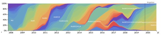
We might expect that forecasting models would struggle to accurately predict future timepoints with higher clade diversity, since much of that diversity would not have existed at the time of the forecast. We might also expect faster surveillance to improve our ability to detect that future variation by detecting those variants at low frequency instead of missing them completely.
To test this hypothesis, we calculated the Shannon entropy of clade frequencies per future timepoint represented in Figure 6 (under no submission lag) and plotted the change in optimal distance to the predicted future by the entropy per timepoint. If there was an effect of future clade complexity on forecast accuracy, we expected greater improvements from interventions to be associated with higher future entropy.
There was a trend for some of the greatest improvements per intervention to occur at higher future clade entropy timepoints, but we didn’t find a strong relationship between clade entropy and improvement in forecast accuracy by any intervention (Figure 4). The highest correlation was for improved surveillance (Pearson r=0.24).
We have added this figure to the revised manuscript as Figure 6—figure supplement 3 and updated the results (lines 321-323) to reflect the patterns we described above. The updated results (which partially includes our response to the next reviewer comment) read:
"These effects of realistic interventions appeared consistent across the range of genetic diversity at future timepoints (Figure 6—figure supplement 3) and for future seasons occurring in both Northern and Southern Hemispheres (Figure 6—figure supplement 4)."
(3) Hemisphere-Specific Forecasting: Do submission lags or forecasting horizons show different performance when predicting Northern versus Southern Hemisphere viral populations? Exploring this distinction could add significant value to the analysis, given the seasonal differences in influenza circulation.
Similar to the question above, we can replot the improvements in optimal distances to the future for the realistic interventions, grouping values by the hemisphere that has an active season in each future timepoint. Much like we expected forecasts to be less accurate when predicting into a highly diverse season, we might also expect forecasts to be less accurate when predicting into a season for a more densely populated hemisphere. Specifically, we expected that realistic interventions would improve forecast accuracy more for Northern Hemisphere seasons than Southern Hemisphere seasons. For this analysis, we labeled future timepoints that occurred in October or January as "Northern" and those that occurred in April or July as "Southern". We plotted effects of interventions on optimal distances to the future by intervention and hemisphere.
In contrast to our original expectation, we found a slightly higher median improvement for the Southern Hemisphere seasons under both of the interventions that improved the vaccine timeline (Figure 5). The median improvement for the combined intervention was 1.42 AAs in the Southern Hemisphere and 0.93 AAs in the Northern Hemisphere. Similarly, the improvement with the "improved vaccine" intervention was 1.03 AAs in the South and 0.74 AAs in the North. However, the range of improvements per intervention was greater for the Northern Hemisphere across all interventions. The median increase in forecast accuracy was similar for both hemispheres in the improved surveillance intervention, with a single Northern Hemisphere season showing an unusually greater improvement that was also associated with higher clade entropy (Figure 4). These results suggest that both an improved vaccine development timeline and more timely sequence submissions would most improve forecast accuracy for Southern Hemisphere seasons compared to Northern Hemisphere seasons.
We have added this figure to the revised manuscript as Figure 6—figure supplement 4 and updated the results (lines 321-326) to reflect the patterns we described above. The new lines in the results read:
"These effects of realistic interventions appeared consistent across the range of genetic diversity at future timepoints (Figure 6—figure supplement 3) and for future seasons occurring in both Northern and Southern Hemispheres (Figure 6—figure supplement 4). We noted a slightly greater median improvement in forecast accuracy associated with both improved vaccine interventions for the Southern Hemisphere seasons (1.03 and 1.42 AAs) compared to the Northern Hemisphere seasons (0.74 and 0.93 AAs)."
(4) Antigenic Sites and Submission Delays: It would be interesting to investigate whether incorporating antigenic site information in the distance metric amplifies or diminishes the observed effects of submission delays. Such an analysis could provide a first glance at how antigenic evolution interacts with forecasting timelines.
This would be an interesting area to explore. One hypothesis along these lines would be that if 1) viruses with more substitutions at antigenic sites are more likely to represent the future population and 2) viruses with more antigenic substitutions originate in specific geographic locations and 3) submissions of sequences for those viruses are more likely to be lagged due to their geographic origin, then 4) decreasing submission lags should improve our forecasting accuracy by detecting antigenically-important sequences earlier. If there is not a direct link between viruses that are more likely to represent the future and higher submission lags, we would not expect to see any additional effect of reducing submission lags for antigenic sites. Based on our work in Huddleston et al. 2020, it is also not clear that assumption 1 above is consistently true, since the specific antigenic sites associated with high fitness change over time. In that earlier work, we found that models based on these antigenic (or "epitope") sites could only accurately predict the future when the relevant sites for viral success were known in advance. This result was shown by our "oracle" model which accurately predicted the future during the model validation period when it knew which sites were associated with success and failed to predict the future in the test period when the relevant sites for success had changed (Figure 6).
To test the hypothesis above, we would need sequences to have submission lags that reflect their geographic origin. For this current study, we intentionally decoupled submission lags from geographic origin to allow inclusion of historical A/H3N2 HA sequences that were originally submitted as part of scientific publications and not as part of modern routine surveillance. As a result, the original submission dates for many sequences are unrealistically lagged compared to surveillance sequences.
(5) Incorporation of Phenotypic Data: The authors should provide a rationale for their choice of a genetic-information-only approach, rather than a model that integrates phenotypic data. Previous studies, such as Huddleston et al. (2020, eLife), demonstrate that models combining genetic and phenotypic data improve forecasts of seasonal influenza A/H3N2 evolution. It would be interesting to probe the here observed effects in a more recent model.
The primary goal of this study was not to test methodological improvements to forecasting models but to test the effects of realistic public health policy changes that could alter forecast horizons and sequence availability. Most influenza collaborating centers use a "sequence-first" approach where they sequence viral isolates first and use those sequences to prioritize viruses for phenotypic characterization (Hampson et al. 2017). The additional lag in availability of phenotypic data means that a forecasting model based on genetic and phenotypic data will necessarily have a greater lag in data availability than a model based on genetic data only. Since the policy changes we're testing in this study only affect the availability of sequence data and not phenotypic data, we chose to test the relative effects of policy changes on sequence-based forecasting models.
We have updated the abstract (lines 18-26 and 30-32), introduction (lines 87-88), and discussion (lines 332-334) to emphasize the focus of this study on effects of policy changes. The updated abstract lines read as follows with new content in bold:
"Despite continued methodological improvements to long-term forecasting models, these constraints of a 12-month forecast horizon and 3-month average submission lags impose an upper bound on any model's accuracy. The global response to the SARS-CoV-2 pandemic revealed that the adoption of modern vaccine technology like mRNA vaccines can reduce how far we need to forecast into the future to 6 months or less and that expanded support for sequencing can reduce submission lags to GISAID to 1 month on average. To determine whether these public health policy changes could improve long-term forecasts for seasonal influenza, we quantified the effects of reducing forecast horizons and submission lags on the accuracy of forecasts for A/H3N2 populations. We found that reducing forecast horizons from 12 months to 6 or 3 months reduced average absolute forecasting errors to 25% and 50% of the 12-month average, respectively. Reducing submission lags provided little improvement to forecasting accuracy but decreased the uncertainty in current clade frequencies by 50%. These results show the potential to substantially improve the accuracy of existing influenza forecasting models through the public health policy changes of modernizing influenza vaccine development and increasing global sequencing capacity."
The updated introduction now reads:
"These technological and public health policy changes in response to SARS-CoV-2 suggest that we could realistically expect the same outcomes for seasonal influenza."
The updated discussion now reads:
"In this work, we showed that realistic public health policy changes that decrease the time to develop new vaccines for seasonal influenza A/H3N2 and decrease submission lags of HA sequences to public databases could improve our estimates of future and current populations, respectively."
We have also updated the introduction (lines 57-65) and the discussion (lines 345-348) to specifically address the use of sequence-based models instead of sequence-and-phenotype models. The updated introduction now reads:
"For this reason, the decision process is partially informed by computational models that attempt to predict the genetic composition of seasonal influenza populations 12 months in the future (Morris et al. 2018). The earliest of these models predicted future influenza populations from HA sequences alone (Luksza and Lassig 2014, Neher et al. 2014, Steinbruck et al. 2014). Recent models include phenotypic data from serological experiments (Morris et al. 2018, Huddleston et al. 2020, Meijers et al. 2023, Meijers et al. 2025). Since most serological experiments occur after genetic sequencing (Hampson et al. 2017) and all forecasting models depend on HA sequences to determine the viruses circulating at the time of a forecast, sequence availability is the initial limiting factor for any influenza forecasts."
The updated discussion now reads:
"Since all models to date rely on currently available HA sequences to determine the clades to be forecasted, we expect that decreasing forecast horizons and submission lags will have similar relative effect sizes across all forecasting models including those that integrate phenotypic and genetic data."
Reviewer #2 (Public review):
Summary:
The authors have examined the effects of two parameters that could improve their clade forecasting predictions for A(H3N2) seasonal influenza viruses based solely on analysis of haemagglutinin gene sequences deposited on the GISAID Epiflu database. Sequences were analysed from viruses collected between April 1, 2005 and October 1, 2019. The parameters they investigated were various lag periods (0, 1, 3 months) for sequences to be deposited in GISAID from the time the viruses were sequenced. The second parameter was the time the forecast was accurate over projecting forward (for 3,6,9,12 months). Their conclusion (not surprisingly) was that "the single most valuable intervention we could make to improve forecast accuracy would be to reduce the forecast horizon to 6 months or less through more rapid vaccine development". This is not practical using conventional influenza vaccine production and regulatory procedures. Nevertheless, this study does identify some practical steps that could improve the accuracy and utility of forecasting such as a few suggested modifications by the authors such as "..... changing the start and end times of our long-term forecasts. We could change our forecasting target from the middle of the next season to the beginning of the season, reducing the forecast horizon from 12 to 9 months.'
Strengths:
The authors are very familiar with the type of forecasting tools used in this analysis (LBI and mutational load models) and the processes used currently for influenza vaccine virus selection by the WHO committees having participated in a number of WHO Influenza Vaccine Consultation meetings for both the Southern and Northern Hemispheres.
Weaknesses:
The conclusion of limiting the forecasting to 6 months would only be achievable from the current influenza vaccine production platforms with mRNA. However, there are no currently approved mRNA influenza vaccines, and mRNA influenza vaccines have also yet to demonstrate their real-world efficacy, longevity, and cost-effectiveness and therefore are only a potential platform for a future influenza vaccine. Hence other avenues to improve the forecasting should be investigated.
We recognize that there are no approved mRNA influenza vaccines right now. However, multiple mRNA vaccines have completed phase 3 trials indicating that these vaccines could realistically become available in the next few years. A primary goal of our study was to quantify the effects of switching to a vaccine platform with a shorter timeline than the status quo. Our results should further motivate the adoption of any modern vaccine platform that can produce safe and effective vaccines more quickly than the egg-passaged standard. We have updated the introduction (lines 88-91) to note the mRNA vaccines that have completed phase 3 trials. The new sentence in the introduction reads:
"Work on mRNA vaccines for influenza viruses dates back over a decade (Petsch et al. 2012, Brazzoli et al. 2016, Pardi et al. 2018, Feldman et al. 2019), and multiple vaccines have completed phase 3 trials by early 2025 (Soens et al. 2025, Pfizer 2022)."
While it is inevitable that more influenza HA sequences will become available over time a better understanding of where new influenza variants emerge would enable a higher weighting to be used for those countries rather than giving an equal weighting to all HA sequences.
This is definitely an important point to consider. The best estimates to date (Russell et al. 2008, Bedford et al. 2015) suggest that most successful variants emerge from East or Southeast Asia. In contrast, most available HA sequence data comes from Europe and North America (Figure 1A). Our subsampling method explicitly tries to address this regional bias in data availability by evenly sampling sequences from 10 different regions including four distinct East Asian regions (China, Japan/Korea, South Asia, and Southeast Asia). Instead of weighting all HA sequences equally, this sampling approach ensures that HA sequences from important distinct regions appear in our analysis.
We have updated our methods (lines 411-423) to better describe the motivation of our subsampling approach and proportions of regions sampled with our original approach (90 viruses per month) and a second high-density sampling approach (270 viruses per month). These new lines read:
"This sampling approach accounts for known regional biases in sequence availability through time (McCarron et al. 2022) and makes inference of divergence and time trees computationally tractable. This approach also exactly matches our previous study where we first trained the forecast models used in this study (Huddleston et al. 2020), allowing us to reuse those previously trained models. With this subsampling approach, we selected between 7% (Europe) and 91% (Southeast Asia) of all available sequences per region across the entire study period with an average of 50% and median of 52% across all 10 regions (Figure 1—figure Supplement 4). To verify the reproducibility and robustness of our results, we reran the full forecasting analysis with a high-density subsampling scheme that selected 270 sequences per month with the same even sampling across regions and time as the original scheme. With this approach, we selected between 17% (Europe) and 97% (Southeast Asia) of all available sequences per region with an average of 72% sampled and a median of 83% (Figure 1—figure Supplement 4C)."
We added Figure 1—figure Supplement 4 to document the regional biases in sequence availability and the proportions of sequences we selected per region and year.
Also, other groups are considering neuraminidase sequences and how these contribute to the emergence of new or potentially predominant clades.
We agree that accounting for antigenic evolution of neuraminidase is a promising path to improving forecasting models. We chose to focus on hemagglutinin sequences for several reasons, though. First, hemagglutinin is the only protein whose content is standardized in the influenza vaccine (Yamayoshi and Kawaoka 2019), so vaccine strain selection does not account for a specific neuraminidase. Additionally, as we noted in response to Reviewer 1 above, the goal of this study was to test effects of counterfactual scenarios with realistic public health interventions and not to introduce methodological improvements to forecasting models like the inclusion of neuraminidase sequences.
We have updated the introduction to provide the additional context about hemagglutinin's outsized role in the current vaccine development process (lines 40-44):
"The dominant influenza vaccine platform is an inactivated whole virus vaccine grown in chicken eggs (Wong and Webby, 2013) which takes 6 to 8 months to develop, contains a single representative vaccine virus per seasonal influenza subtype including A/H1N1pdm, A/H3N2, and B/Victoria (Morris et al., 2018), and for which only the HA protein content is standardized (Yamayoshi and Kawaoka, 2019)."
We have updated the abstract (lines 18-26 and 30-32), introduction (lines 87-88), and discussion (lines 332-334) to emphasize our goal of testing effects of public health policy changes on forecasting accuracy rather than methodological changes. The updated abstract lines read as follows with new content in bold:
"Despite continued methodological improvements to long-term forecasting models, these constraints of a 12-month forecast horizon and 3-month average submission lags impose an upper bound on any model's accuracy. The global response to the SARS-CoV-2 pandemic revealed that the adoption of modern vaccine technology like mRNA vaccines can reduce how far we need to forecast into the future to 6 months or less and that expanded support for sequencing can reduce submission lags to GISAID to 1 month on average. To determine whether these public health policy changes could improve long-term forecasts for seasonal influenza, we quantified the effects of reducing forecast horizons and submission lags on the accuracy of forecasts for A/H3N2 populations. We found that reducing forecast horizons from 12 months to 6 or 3 months reduced average absolute forecasting errors to 25% and 50% of the 12-month average, respectively. Reducing submission lags provided little improvement to forecasting accuracy but decreased the uncertainty in current clade frequencies by 50%. These results show the potential to substantially improve the accuracy of existing influenza forecasting models through the public health policy changes of modernizing influenza vaccine development and increasing global sequencing capacity."
The updated introduction now reads:
"These technological and public health policy changes in response to SARS-CoV-2 suggest that we could realistically expect the same outcomes for seasonal influenza."
The updated discussion now reads:
"In this work, we showed that realistic public health policy changes that decrease the time to develop new vaccines for seasonal influenza A/H3N2 and decrease submission lags of HA sequences to public databases could improve our estimates of future and current populations, respectively."
Figure 1a. I don't understand why the orange dot 1-month lag appears to be on the same scale as the 3-month/ideal timeline.
We apologize for the confusion with this figure. Our original goal was to show how the two factors in our study design (forecast horizons and sequence submission lags) interact with each other by showing an example of 3-month forecasts made with no lag (blue), ideal lag (orange), and realistic lag (green). To clarify these two factors, we have removed the two lines at the 3-month forecast horizon for the ideal and realistic lags and have updated the caption to reflect this simplification. The new figure looks like this:
The authors should expand on the line "The finding of even a few sequences with a potentially important antigenic substitution could be enough to inform choices of vaccine candidate viruses." While people familiar with the VCM process will understand the implications of this statement the average reader will not fully understand the implications of this statement. Not only will it inform but it will allow the early production of vaccine seeds and reassortants that can be used in conventional vaccine production platforms if these early predictions were consolidated by the time of the VCM. This is because of the time it takes to isolate viruses, make reassortants and test them - usually a month or more is needed at a minimum.
Thank you for pointing out this unclear section of the discussion. We have rewritten this section, dropping the mention of prospective measurements of antigenic escape which now feels off-topic and moving the point about early detection of important antigenic substitutions to immediately follow the description of the candidate vaccine development timeline. This new placement should clarify the direct causal relationship between early detection and better choices of vaccine candidates. The original discussion section read:
"For example, virologists must choose potential vaccine candidates from the diversity of circulating clades well in advance of vaccine composition meetings to have time to grow virus in cells and eggs and measure antigenic drift with serological assays (Morris et al., 2018; Loes et al., 2024). Similarly, prospective measurements of antigenic escape from human sera allow researchers to predict substitutions that could escape global immunity (Lee et al., 2019; Greaney et al., 2022; Welsh et al., 2023). The finding of even a few sequences with a potentially important antigenic substitution could be enough to inform choices of vaccine candidate viruses."
The new section (lines 386-391) now reads:
"For example, virologists must choose potential vaccine candidates from the diversity of circulating clades months in advance of vaccine composition meetings to have time to grow virus in cells and eggs and measure antigenic drift with serological assays (Morris et al. 2018; Loes et al. 2024). Earlier detection of viral sequences with important antigenic substitutions could determine whether corresponding vaccine candidates are available at the time of the vaccine selection meeting or not."
A few lines in the discussion on current approaches being used to add to just the HA sequence analysis of H3N2 viruses (ferret/human sera reactivity) would be welcome.
We have added the following sentences to the last paragraph (lines 391-397) to note recent methodological advances in estimating influenza fitness and the relationship these advances have to timely genomic surveillance.
"Newer methods to estimate influenza fitness use experimental measurements of viral escape from human sera (Lee et al., 2019; Welsh et al., 2024; Meijers et al., 2025; Kikawa et al., 2025), measurements of viral stability and cell entry (Yu et al., 2025), or sequences from neuraminidase, the other primary surface protein associated with antigenic drift (Meijers et al., 2025). These methodological improvements all depend fundamentally on timely genomic surveillance efforts and the GISAID EpiFlu database to identify relevant influenza variants to include in their experiments."
OP50
DOI: 10.1038/s44318-024-00123-3
Resource: (WB Cat# WBStrain00041969,RRID:WB-STRAIN:WBStrain00041969)
Curator: @Apiekniewska
SciCrunch record: RRID:WB-STRAIN:WBStrain00041969
JK2533
DOI: 10.1038/s44318-024-00123-3
Resource: None
Curator: @Apiekniewska
SciCrunch record: RRID:WB-STRAIN:WBStrain00022579
CGC32
DOI: 10.1038/s44318-024-00123-3
Resource: None
Curator: @Apiekniewska
SciCrunch record: RRID:WB-STRAIN:WBStrain00004963
N2
DOI: 10.1038/s44318-024-00123-3
Resource: (WB Cat# WBStrain00000001,RRID:WB-STRAIN:WBStrain00000001)
Curator: @Apiekniewska
SciCrunch record: RRID:WB-STRAIN:WBStrain00000001
HT115
DOI: 10.1038/s44318-024-00123-3
Resource: RRID:WB-STRAIN:WBStrain00041079
Curator: @Apiekniewska
SciCrunch record: RRID:WB-STRAIN:WBStrain00041079
Supplementary Data 3
DOI: 10.1038/s41467-024-50027-3
Resource: None
Curator: @Apiekniewska
SciCrunch record: RRID:WB-STRAIN:WBStrain00043589
Supplementary Data 3
DOI: 10.1038/s41467-024-50027-3
Resource: RRID:WB-STRAIN:WBStrain00040414
Curator: @Apiekniewska
SciCrunch record: RRID:WB-STRAIN:WBStrain00040414
Supplementary Data 3
DOI: 10.1038/s41467-024-50027-3
Resource: (WB Cat# WBStrain00000001,RRID:WB-STRAIN:WBStrain00000001)
Curator: @Apiekniewska
SciCrunch record: RRID:WB-STRAIN:WBStrain00000001