RRID:SCR_014210
DOI: 10.1186/s13024-025-00903-3
Resource: Image Lab Software (RRID:SCR_014210)
Curator: @scibot
SciCrunch record: RRID:SCR_014210
RRID:SCR_014210
DOI: 10.1186/s13024-025-00903-3
Resource: Image Lab Software (RRID:SCR_014210)
Curator: @scibot
SciCrunch record: RRID:SCR_014210
RRID:AB_144696
DOI: 10.1186/s13024-025-00903-3
Resource: (Molecular Probes Cat# A-11031, RRID:AB_144696)
Curator: @scibot
SciCrunch record: RRID:AB_144696
RRID:AB_2534102
DOI: 10.1186/s13024-025-00903-3
Resource: (Thermo Fisher Scientific Cat# A-11055, RRID:AB_2534102)
Curator: @scibot
SciCrunch record: RRID:AB_2534102
RRID:AB_10563566
DOI: 10.1186/s13024-025-00903-3
Resource: (Thermo Fisher Scientific Cat# A-11036, RRID:AB_10563566)
Curator: @scibot
SciCrunch record: RRID:AB_10563566
RRID:AB_331589
DOI: 10.1186/s13024-025-00903-3
Resource: (Cell Signaling Technology Cat# 9134, RRID:AB_331589)
Curator: @scibot
SciCrunch record: RRID:AB_331589
RRID:AB_2650633
DOI: 10.1186/s13024-025-00903-3
Resource: (BioLegend Cat# 848001, RRID:AB_2650633)
Curator: @scibot
SciCrunch record: RRID:AB_2650633
RRID:AB_305643
DOI: 10.1186/s13024-025-00903-3
Resource: (Abcam Cat# ab6673, RRID:AB_305643)
Curator: @scibot
SciCrunch record: RRID:AB_305643
RRID:AB_223647
DOI: 10.1186/s13024-025-00903-3
Resource: (Thermo Fisher Scientific Cat# MN1020, RRID:AB_223647)
Curator: @scibot
SciCrunch record: RRID:AB_223647
RRID:AB_324217
DOI: 10.1186/s13024-025-00903-3
Resource: (Bio-Rad Cat# MCA1957GA, RRID:AB_324217)
Curator: @scibot
SciCrunch record: RRID:AB_324217
RRID:AB_305808
DOI: 10.1186/s13024-025-00903-3
Resource: (Abcam Cat# ab7260, RRID:AB_305808)
Curator: @scibot
SciCrunch record: RRID:AB_305808
RRID:AB_142134
DOI: 10.1186/s13024-025-00903-3
Resource: (Molecular Probes Cat# A-11070, RRID:AB_142134)
Curator: @scibot
SciCrunch record: RRID:AB_142134
RRID:AB_94975
DOI: 10.1186/s13024-025-00903-3
Resource: (Millipore Cat# MAB386, RRID:AB_94975)
Curator: @scibot
SciCrunch record: RRID:AB_94975
RRID:AB_839504
DOI: 10.1186/s13024-025-00903-3
Resource: (Wako Cat# 019-19741, RRID:AB_839504)
Curator: @scibot
SciCrunch record: RRID:AB_839504
RRID:AB_2548607
DOI: 10.1186/s13024-025-00903-3
Resource: (Thermo Fisher Scientific Cat# PA5-31133, RRID:AB_2548607)
Curator: @scibot
SciCrunch record: RRID:AB_2548607
RRID:SCR_003070
DOI: 10.1186/s13024-025-00903-3
Resource: ImageJ (RRID:SCR_003070)
Curator: @scibot
SciCrunch record: RRID:SCR_003070
CVCL_0532
DOI: 10.1158/0008-5472.CAN-25-0977
Resource: (CLS Cat# 300342/p657_SK-OV-3, RRID:CVCL_0532)
Curator: @scibot
SciCrunch record: RRID:CVCL_0532
Reviewer #2 (Public review):
Summary:
In this manuscript, the authors investigate the mechanisms underlying the virulence of OMVs using a Drosophila model. They reveal a complex interplay between host defenses and OMV pathogenicity. Although the study enhances our understanding of Drosophila innate immunity, additional evidence is needed to strengthen the conclusions.
Strengths:
(1) In Figure 1, Toll pathway mutants infected with OMVs displayed three distinct phenotypic outcomes: mildly enhanced resistance to OMV infection, a response similar to that of the control, or increased susceptibility. Therefore, in addition to Imd and Kenny mutants from the Imd pathway, further mutants, such as Relish and PGRP-LC, should be examined to assess whether the Imd pathway is involved in host defense against OMVs.
(2) Plasmatocytes clear particles via phagocytosis or endocytosis. However, flies lacking all hemocytes showed increased resistance to OMV challenge, raising the question of whether hemocytes actually aid the pathogen. To explore this hypothesis, the uptake of fluorescently tagged OMVs should be examined.
(3) Hayan cleaves PPO into active PO. However, Hayan and PPO mutants exhibit opposite phenotypes upon OMV injection, raising the question of whether OMV-induced pathogenesis is linked to melanization.
(4) Puckered mRNA levels were used as a read-out for JNK pathway activity. A transient induction of the JNK pathway was observed in head and thorax tissues. It would be beneficial if the authors could directly examine JNK activation in neuronal cells using immunostaining for pJNK.
(5) In Figure 4B, the kayak was knocked down using the pan-neuronal driver elav-Gal4. To confirm the specificity and validity of this observation, the experiment should be repeated using another neural-specific driver.
Weaknesses:
It is unclear how many Serratia marcescens cells a 69 nL injection of 0.1 ng/nL OMVs corresponds to.
Reviewer #3 (Public review):
Summary:
The authors investigate deficiencies in various immune responses, and also the prtA toxin's role in OMV toxicity. Some key interpretations are that the Imd pathway contributes to preventing OMV toxicity, but not Toll, and that Hayan and Eater somehow mediate OMV or PrtA toxicity. This descriptive effort is a solid set of experiments, although some experimental results may require further validation.
Strengths:
The breadth of experiments tests multiple immune parameters, providing a systematic effort that ensures a number of potentially relevant interactions can be recovered. Certain findings, such as the PrtA toxicity to flies, appear solid, and some interesting findings regarding Hayan and eater will be of interest to the fly immunity field.
Weaknesses:
It appears almost all results rely on the use of a single mutant representing the deletion of the gene. It's not clear if the mutations are always in the same genetic background, but this can be clarified. There are a couple of results that are confusing and may be internally contradicting, and should be additionally validated and clarified.
Author response:
We thank the reviewers and editors for the careful evaluation of our manuscript. Below, we provide a first refutation of some of the concerns expressed by reviewers.
Both reviewer 1 &3 underscore the importance of controlling for genetic backgrounds. This is actually an issue only for a limited part of the study and this criticism should not apply to major findings of this study, with some exceptions, as detailed below.
It is important to note that we have identified ourselves several of the mutant lines we have been using. For instance, key and MyD88 mutant alleles have been identified in the Exelixis transposon insertion collection that we have screened in collaboration with this firm (e.g., [3, 4, 5]). This resource has been generated in a isogenized w [A5001] strain[6], which we are using as matched control for these mutants (Figs 1B,D). Of note, while they share a common genetic background, the phenotypes of key and MyD88 are opposite in terms of sensitivity to OMV challenge. The imd<sup>shadok</sup> null allele had been identified during our chemical mutagenesis screen with EMS in a yw cn bw background [5, 7, 8, 9], which was used as a control (FigS1A).
With respect to Hayan (Fig. 2C, Fig. S2C) and eater (Fig. S2A-B) mutants[10, 11, 12], we find a similarly strong phenotype with two independent mutants in distinct genetic backgrounds (actually three for Hayan, as we have not included in our original manuscript the Hayan<sup>SK3</sup>allele generated in the Lemaitre laboratory in which OMVs displayed also impaired virulence). We have shown that the Hayan mutants do display the expected phenotype in terms of PPO cleavage (Fig. S2D). Please, also note that in Fig. S2C the two mutant alleles are tested in the same experiment: even though there is some variation between the w<sup>1118</sup> and the w[A5001] strains, the two mutants behave in a remarkably similar manner. As regards the role of the cellular response, we note that we obtained results similar to those obtained with eater mutants using genetic ablation of hemocytes (Fig. 2A) or by saturating the phagocytosis apparatus (Fig. 2B), a confirmation by two totally-independent approaches.
Of note, the observed eater and Hayan phenotypes are strong and not relatively small and thus unlikely to be due to the genetic background.
The PPO mutants have been isogenized in the w<sup>1118</sup> by the lab of Bruno Lemaitre[13, 14] and are also validated biochemically in Fig. S2D. These mutants have been extensively tested in the Lemaitre laboratory[13, 14, 15].
With respect to RNAi silencing driven ubiquitously or in specific tissues using the UAS-Gal4 system, we have mostly used transgenes from the Trip collection and have used as a control the mCherry RNAi provided by this resource[16]. As the RNAi transgenes have been generated in the same genetic background, it follows that independently of the driver used, the genetic background used in mCherry and genes-of-interest (Duox, Nox, Jafrac2) silenced flies is controlled for (Fig. 3D,E).
For UAS-Gal4-mediated overexpression of fly superoxide dismutase genes, we have used SOD1 and SOD2 transgenes that have both been generated by the same laboratory (Phillips laboratory, University of Guelph) presumably in the same genetic background. Using two distinct drivers we find a strongly enhanced susceptibility phenotype when using UAS-SOD2 but not UAS-SOD1 transgenes (Fig. 3F, Fig. 4E). Importantly, the former is associated with mitochondria whereas the other is expressed in the endoplasmic reticulum: we independently confirm this phenotype using the mitoTempo mitochondrial ROS inhibitor.
We shall thus address the criticism with NOS mutants, where genetic background control is indeed critical and for the UAS-kay RNAi line using a Trip line and its associated mCherry RNAi control transgene.
With respect to the Toll pathway mutants, we agree that some of the variability of the phenotypes may be due to the genetic background, especially as regards tube and pelle. The SPE and grass mutants have been retrieved in a screen performed by the group of Jean-Marc Reichhart in our Research Unit. They thus have been generated in the same genetic background, yet grass displays a mildly decreased virulence of injected OMVs whereas SPE mutants display an opposite phenotype (compare Fig. S1E to S1I; the survival experiment shave been performed in the same set of experiments and have been separated for clarity). We do not intend to analyze further the mutants of the Toll pathway as our data suggest that the canonical Toll pathway, likely activated through psh (Fig. S1F) appears to be activated to detectable levels too late by comparison with the time course of OMV pathogenicity. In our opinion, the contribution of the Toll pathway in the host defense against OMV pathogenicity is minor, albeit we acknowledge that some of the findings, especially with SPE are puzzling.
With respect to the IMD pathway, we shall test also PGRP-LC and Relish mutants, as suggested by reviewers 2&3.
Reviewer 2 query: “It is unclear how many Serratia marcescens cells a 69 nL injection of 0.1 ng/nL OMVs corresponds to.”
OMVs were purified from 600 mL of SmDb11 cultures grown to an average OD<sub>600</sub> of 2.0. Based on a cell density of 0.8 × 10<sup>8</sup> cells/mL per OD unit, this corresponds to approximately 9.6 × 10<sup>10</sup> total bacterial cells.
Each OMV preparation was concentrated into a final volume of 400 µL, resulting in a concentration factor of ~1500× relative to the original culture. Therefore, an injection dose of 69 nL of OMVs is equivalent to 0.1 mL of the starting bacterial culture, which corresponds to:
0.2 OD units
Approximately 1.6 × 10<sup>7</sup> bacterial cells
It is likely that such high concentrations occur only toward the end of the infection, if OMVs are produced at the same rate in the host and in vitro.
With respect to other Reviewer 2 queries, we shall give a try at labeling OMVs with the FM4-64 lipophilic dye and examining whether they are taken up by hemocytes. However, an issue may arise with potentially high background, which has been encountered in cell culture. Of note, OMVs are known to attack cultured human THP1 cells, a monocyte cell line [17].Of note, determining whether OMVs are taken up by hemocytes may only be a starting point to understand how they promote the pathogenicity of OMVs. This question constitutes the topic of a full study that we are currently unable to undertake.
We shall also test whether we can document phospho-JNK expression in neural tissues.
Finally, we shall also confirm the data obtained with two elav-Gal4 drivers (including an inducible one) with the nsyb-Gal4 driver line.
References
(1) Xu R, et al. The Toll pathway mediates Drosophila resilience to Aspergillus mycotoxins through specific Bomanins. EMBO Rep 24, e56036 (2023).
(2) Huang J, et al. A Toll pathway effector protects Drosophila specifically from distinct toxins secreted by a fungus or a bacterium. Proc Natl Acad Sci U S A 120, e2205140120 (2023).
(3) Gobert V, et al. Dual Activation of the Drosophila Toll Pathway by Two Pattern Recognition Receptors. Science 302, 2126-2130 (2003).
(4) Gottar M, et al. Dual Detection of Fungal Infections in Drosophila via Recognition of Glucans and Sensing of Virulence Factors. Cell 127, 1425-1437 (2006).
(5) Gottar M, et al. The Drosophila immune response against Gram-negative bacteria is mediated by a peptidoglycan recognition protein. Nature 416, 640-644 (2002).
(6) Thibault ST, et al. A complementary transposon tool kit for Drosophila melanogaster using P and piggyBac. Nat Genet 36, 283-287 (2004).
(7) Rutschmann S, Jung AC, Hetru C, Reichhart J-M, Hoffmann JA, Ferrandon D. The Rel protein DIF mediates the antifungal, but not the antibacterial, response in Drosophila. Immunity 12, 569-580 (2000).
(8) Rutschmann S, Jung AC, Rui Z, Silverman N, Hoffmann JA, Ferrandon D. Role of Drosophila IKKg in a Toll-independent antibacterial immune response. Nat Immunology 1, 342-347 (2000).
(9) Jung A, Criqui M-C, Rutschmann S, Hoffmann J-A, Ferrandon D. A microfluorometer assay to measure the expression of ß-galactosidase and GFP reporter genes in single Drosophila flies. Biotechniques 30, 594- 601 (2001).
(10) Nam HJ, Jang IH, You H, Lee KA, Lee WJ. Genetic evidence of a redox-dependent systemic wound response via Hayan protease-phenoloxidase system in Drosophila. Embo J 31, 1253-1265 (2012).
(11) Kocks C, et al. Eater, a transmembrane protein mediating phagocytosis of bacterial pathogens in Drosophila. Cell 123, 335-346 (2005).
(12) Bretscher AJ, et al. The Nimrod transmembrane receptor Eater is required for hemocyte attachment to the sessile compartment in Drosophila melanogaster. Biology open 4, 355-363 (2015).
(13) Binggeli O, Neyen C, Poidevin M, Lemaitre B. Prophenoloxidase activation is required for survival to microbial infections in Drosophila. PLoS Pathog 10, e1004067 (2014).
(14) Dudzic JP, Kondo S, Ueda R, Bergman CM, Lemaitre B. Drosophila innate immunity: regional and functional specialization of prophenoloxidases. BMC Biol 13, 81 (2015).
(15) Dudzic JP, Hanson MA, Iatsenko I, Kondo S, Lemaitre B. More Than Black or White: Melanization and Toll Share Regulatory Serine Proteases in Drosophila. Cell reports 27, 1050-1061 e1053 (2019).
(16) Perkins LA, et al. The Transgenic RNAi Project at Harvard Medical School: Resources and Validation. Genetics 201, 843-852 (2015).
(17) Goman A, et al. Uncovering a new family of conserved virulence factors that promote the production of host-damaging outer membrane vesicles in gram-negative bacteria. J Extracell Vesicles 14, e270032 (2025).
Reviewer #2 (Public review):
Summary:
This work by Waltner et. al. provides a comprehensive single-cell multiomics analysis of plasticity in gene regulatory networks present in Ewing sarcoma using single-cell RNA-sequencing (scRNA-seq) and single-cell assay for transposase accessible chromatin with sequencing (scATAC-seq). They find that Ewing sarcoma cell line models have distinct patterns of chromatin accessibility compared to non-Ewing sarcoma models, and that there is significant variability across Ewing sarcoma cell lines, and sometimes within a single cell line. These differences across models are linked to 3 distinct gene regulatory modules, 2 of which are present across the range of model systems studied here. The first modules present across models are activated when the fusion is expressed and include genes enriched for the known EWSR1::FLI1 response element, GGAA microsatellites, along with other neural crest transcription factors. The other module primarily consists of genes repressed by EWSR1::FLI1, which are activated in EWSR1::FLI1-low states. Interestingly, EWSR1::FLI1-low cells have already been tied to more migratory and metastatic phenotypes, and the data here suggest these cells are more responsive to external signals from TGF-β, and this may be mediated through FOSL2-mediated gene regulation. While there are some minor additional validation studies that can be performed to strengthen a few individual analyses, this is a technically rigorous study, with a variety of different analytical techniques used to address similar questions, and this approach elevates confidence in the answers provided. This is further strengthened by the diverse set of model systems used, including patient-derived cell lines, cell line xenograft models, patient-derived xenografts, mining available single-cell data from patient samples, and validation of the gene modules identified in a larger set of patient microarray samples. In whole, this study provides a valuable resource for understanding heterogeneity, plasticity, and gene expression networks in Ewing sarcoma. This may be useful for future studies of metastatic disease and may also provide a framework for similar questions in other fusion-driven sarcomas.
Strengths:
There are a few core strengths in this study. First is the number and diversity of Ewing sarcoma models studied, spanning commonly used cell lines, patient-derived xenografts, and patient samples. The second is the large array of rigorous and orthogonal approaches used to uncover the identity and function of various gene modules. This includes an array of informatics techniques, as well as specific modulation of cell line models in culture. A third is confirmation that different gene expression programs are present in the same tumor using spatial transcriptomic analysis. Lastly, the authors have made all of their data and code accessible, enabling continued use of this dataset as a resource for others.
Weaknesses:
As highlighted by the authors, this study is somewhat limited by the small number of single-cell data from patient samples that are publicly available. Much of the analysis comes from cell lines. Additionally, they focus only on one type of signal that may modulate cell plasticity, and there are likely to be many others. Lastly, there are a few weak spots in the data. Some of this likely arises from the underlying complexity of the data, the generally sparse nature of scATAC data, and the biological heterogeneity present in the cell lines studied. The most pronounced weakness was in the analysis of transcription factors that dictate gene expression in the distinct modules, as well as the response to TGF-β. While some specific transcription factors showed module-specific expression consistent with the computational prediction in Figure 2, others did not likely due to additional factors not tested here. Likewise, the same transcription factors did not always show consistent enrichment in the gene modules that responded to TGF-β treatment when analyzed across cell lines. On the whole, these are relatively minor weaknesses and do not diminish the value of this study.
font-family: Verdana, Geneva, sans-serif;
3 opties v fonts: standaard fond windows, standaard font mac, Basic dat alles zoiso werkt
=> Gewoon om zeker te zijn.
Therefore, the first threestrategies listed below are pre-drafting activities.1. Determine your rhetorical situation.2. Review and analyze other multimodal texts.3. Gather content, media, and tools
in these lines three stategies listed below are pre drafting activities .mean before the drafting ,understanding of rhetorical situation ,analyz other multimodal texts,gather content ,media,and tools
TABLE 5 PROFICIENCY LEVEL AND TRANSLANGUAGING My high level of English proficiency and competence in English is a result of my instructor's use of Arabic in my English lessons. S/N Option Frequency Percent 1 Strongly Agree 77 48.4 2 Agree 31 19.5 3 Neutral 27 17 4 Disagree 15 9.4 5 Strongly Disagree 9 5.7
This is the proficiency for English with translanguage
Instead, overland trade in items like silk, porcelain, glass, wool, and horses flowed between Baghdad and Chang'an via Merv (Turkmenistan), Samarkand (Uzbekistan), Kashgar (China), and Dunhuang (China). By sea, goods including spices, ceramics, ivory, and silk flowed through Basra (Iraq), Siraf (Iran), Daybul (Pakistan), Gujarat (India), Malacca (Malaysia), and Guangzhou (China). The goods were carried between these markets by middlemen from the surrounding regions, who spoke Persian, Chinese, and Turkic languages as well as a "caravan bazaar" pidgin language of several hundred words that allowed traders to understand each other a bit. Universal tools like math using Indian-derived "Arabic" numerals and standardized weights established in Baghdad also facilitated trade.
Trade worked well because middlemen helped move goods between faraway places and used a simple shared language so everyone could understand a little. Standard weights and Arabic numbers made it easy to measure and price things correctly, letting merchants from different countries trade without confusion.
Baghdad became a center for not only imperial administration and scholarship, but Silk Road trade. As had been the case with the Silk Road contact between the Roman and Han empires, this was not a direct trading relationship between the Abbasids and the Chinese, although the Abbasids did acquire paper-making technology that led to an expansion of literacy in a battle against Tang forces at Talas (Kyrgyzstan) in 751.
Baghdad was a busy city for both government and learning. The Abbasids learned how to make paper from the Chinese, which let more people read and write, helping the empire run more smoothly and share knowledge.
Theodoric imagined himself as the restorer and protector of "Roman" order in the west; Justinian saw him as just another barbarian.
It’s interesting that Theodoric saw himself as restoring Roman order while Justinian viewed him as a barbarian. I find it fascinating how perspective shaped their reputations. I find it also funny
By 250 CE, between 1% and 5% of the empire's 60 million people were Christians (or, up to 3 million).
It’s surprising to learn that up to 3 million people, or 1–5% of the empire, were Christians by 250 CE. I find it interesting how quickly the faith was growing.
Ancient sources such as Xenophon and Plutarch described Spartan women as bold, athletic, and outspoken.
These sources help me see Spartan women as bold, athletic, and outspoken, which I didn’t expect and find really interesting. Learning this makes me want to explore more about how their roles differed from other Greek women.
There are two major sites regarded as temples in the city and 19 other temple complexes nearby in the Supe Valley.
The city had two main temple sites and 19 additional temple complexes nearby in the Supe Valley. This indicates a strong religious or ceremonial focus in the region. It reflects the importance of ritual in their society.
No battlements, weapons, or mutilated bodies have been found (as in other sites), but in one of the temples researchers found 32 flutes made of condor and pelican bones and 37 larger wind instruments carved from the bones of deer and llama.
I agree—that’s really fascinating! The absence of battlements or weapons suggests these sites weren’t focused on warfare. Instead, the discovery of so many flutes and wind instruments points to a strong emphasis on music and ritual. It really highlights the cultural and ceremonial importance in that society.
China's first urban culture, called Longshan, grew in the Yellow River Valley between 5,000 and 3,900 years ago. The earliest city, Liangchengzhen, had a population of about 40,000 at its peak about 4,500 years ago.
Absolutely! Longshan was truly China’s first urban culture, and Liangchengzhen’s population of around 40,000 shows how developed it was. It’s fascinating to see such early urban growth along the Yellow River. This highlights how complex societies emerged independently in different parts of the world.
The Indus Valley Civilization seems to have been more egalitarian than that of Egypt or Uruk, with no clear archaeological evidence of palaces, temples, or elite burials. Indus Valley cities have uniform housing and broad access to sanitary sewer systems.
I completely agree! The Indus Valley Civilization does seem remarkably egalitarian compared to Egypt or Uruk. Its uniform housing and advanced sewer systems suggest a society where resources and infrastructure were widely shared. It’s impressive how organized and community-focused their cities were.
By 5,800 years ago, Hierakonpolis had become Egypt's first city, with a local elite that gained control over trade routes to the Red Sea (for shells and obsidian) and the deserts (for gold and copper); and later more widely for luxury goods like cedar and lapis.
Yes, that makes sense! Hierakonpolis really was Egypt’s first city, with elites controlling key trade routes. They accessed resources like shells, obsidian, gold, and copper, and later even luxury goods like cedar and lapis. It shows how early urban centers were tied to both power and trade.
Often family descent was matrilineal, since it was easier to know who a person's mother was, than their father.
I wonder how this became, because is it like the mother is well known rather than the father but this is a interesting concept
In 1376 he executed several thousand officials convicted of corruption.
I wonder how executing thousands f officials affected the government and the people at the time.
A young orphan, Zhu Yuanzhang, who had lost his entire family to plague and famine, was sheltered at a White Lotus monastery around 1345.
It’s interesting that Zhu Yuanzhang became a future emperor survived the plague and famine as an orphan.
The Church, which was unable to either explain or prevent the plague, lost a lot of its prestige and power.
I find it interesting that the plague made people lose faith in the church because it couldn’t stop or explain the disease.
As I mentioned in the last chapter, the heirs of Genghis Khan's empire continued its expansion after his death in 1227.
An interesting point is that Genghis Khans empire didn’t stop growing after his death. It kept expanding under his heirs.
Such variability, as well as the presence of negative clearance rates, might be due both to local differences in bacterial concentration when sampling water aliquots and to actual changes in filtering activity and/or water transport by sponges over time [3], [14], [39].
With such great amounts of variability, would this sponge actually make a good candidate for bioremediation? Or would it fluctuate too much to truly help?
In particular, sponges can actively feed on bacteria [2], [3], [35] and good growth rates have been recorded using these micro-organisms as food sources [20], [36], [37]
Shows that bacteria are a natural food source for sponges and can support their growth, supporting the choice of E. coli as a tracer, which goes back to the first sentence of the paragraph.
Fig. 3: View of selected dividers in ZK 19: “Religion – Myth”, “Mythology pragmatic”, “Venus and her entourage”, “Ancient Superstition Afterlife”, “Mysteries”. © Warburg Institute

Somewhat curious of the dates/times of the creation of these tabbed cards. Surely made in the 20th century, but since Warburg was likely creating notes in the late 1800s, where does this sit with respect to the invention of the tab card in 1894 claimed by Progressive Indexing and Filing (Remington Rand, 1950, p205)?
Reviewer #2 (Public review):
Summary:
Using a gerbil model, the authors tested the hypothesis that loss of synapses between sensory hair cells and auditory nerve fibers (which may occur due to noise exposure or aging) affects behavioral discrimination of the rapid temporal fluctuations of sounds. In contrast to previous suggestions in the literature, their results do not support this hypothesis; young animals treated with a compound that reduces the number of synapses did not show impaired discrimination compared to controls. Additionally, their results from older animals showing impaired discrimination suggest that age-related changes aside from synaptopathy are responsible for the age-related decline in discrimination.
Strengths:
(1) The rationale and hypothesis are well-motivated and clearly presented.
(2) The study was well conducted with strong methodology for the most part, and good experimental control. The combination of physiological and behavioral techniques is powerful and informative. Reducing synapse counts fairly directly using ouabain is a cleaner design than using noise exposure or age (as in other studies), since these latter modifiers have additional effects on auditory function.
(3) The study may have a considerable impact on the field. The findings could have important implications for our understanding of cochlear synaptopathy, one of the most highly researched and potentially impactful developments in hearing science in the past fifteen years.
Weaknesses:
(1) I have concerns that the gerbils may not have been performing the behavioral task using temporal fine structure information.
Human studies using the same task employed a filter center frequency that was (at least) 11 times the fundamental frequency (Marmel et al., 2015; Moore and Sek, 2009). Moore and Sek wrote: "the default (recommended) value of the centre frequency is 11F0." Here, the center frequency was only 4 or 8 times the fundamental frequency (4F0 or 8F0). Hence, relative to harmonic frequency, the harmonic spacing was considerably greater in the present study. However, gerbil auditory filters are thought to be broader than those in human. In the revised version of the manuscript, the authors provide modelling results suggesting that the excitation patterns were discriminable for the 4F0 conditions, but may not have been for the 8F0 conditions. These results provide some reassurance that the 8F0 discriminations were dependent on temporal cues, but the description of the model lacks detail. Also, the authors state that "thus, for these two conditions with harmonic number N of 8 the gerbils cannot rely on differences in the excitation patterns but must solve the task by comparing the temporal fine structure." This is too strong. Pulsed tone intensity difference limens (the reference used for establishing whether or not the excitation pattern cues were usable) may not be directly comparable to profile-analysis-like conditions, and it has been argued that frequency discrimination may be more sensitive to excitation pattern cues than predicted from a simple comparison to intensity difference limens (Micheyl et al. 2013, https://doi.org/10.1371/journal.pcbi.1003336).
I'm also somewhat concerned that the masking noise used in the present study was too low in level to mask cochlear distortion products. Based on their excitation pattern modelling, the authors state (without citation) that "since the level of excitation produced by the pink noise is less than 30 dB below that produced by the complex tones, distortion products will be masked." The basis for this claim is not clear. In human, distortion products may be only ~20 dB below the levels of the primaries (referenced to an external sound masker / canceller, which is appropriate, assuming that the modelling reported in the present paper did not include middle-ear effects; see Norman-Haignere and McDermott, 2016, doi: 10.1016/j.neuroimage.2016.01.050). Oxenham et al. (2009, doi: 10.1121/1.3089220) provide further cautionary evidence on the potential use of distortion product cues when the background noise level is too low (in their case the relative level of the noise in the compromised condition was only a little below that used in the present study). The masking level used in the present study may have been sufficient, but it would be useful to have some further reassurance on this point.
(2) The synapse reductions in the high ouabain and old groups were relatively small (mean of 19 synapses per hair cell compared to 23 in the young untreated group). In contrast, in some mouse models of the effects of noise exposure or age, a 50% reduction in synapses is observed, and in the human temporal bone study of Wu et al. (2021, https://doi.org/10.1523/JNEUROSCI.3238-20.2021) the age-related reduction in auditory nerve fibres was ~50% or greater for the highest age group across cochlear location. It could be simply that the synapse loss in the present study was too small to produce significant behavioral effects. Hence, although the authors provide evidence that in the gerbil model the age-related behavioral effects are not due to synaptopathy, this may not translate to other species (including human).
(3) The study was not pre-registered, and there was no a priori power calculation, so there is less confidence in replicability than could have been the case. Only three old animals were used in the behavioral study, which raises concerns about the reliability of comparisons involving this group. Statistical analyses on very small samples can be unreliable due to problems of power, generalisability, and susceptibility to outliers.
Reviewer #3 (Public review):
This study is a part of the ongoing series of rigorous work from this group exploring neural coding deficits in the auditory nerve, and dissociating the effects of cochlear synaptopathy from other age-related deficits. They have previously shown no evidence of phase-locking deficits in the remaining auditory nerve fibers in quiet-aged gerbils. Here, they study the effects of aging on the perception and neural coding of temporal fine structure cues in the same Mongolian gerbil model.
They measure TFS coding in the auditory nerve using the TFS1 task which uses a combination of harmonic and tone-shifted inharmonic tones which differ primarily in their TFS cues (and not the envelope). They then follow this up with a behavioral paradigm using the TFS1 task in these gerbils. They test young normal hearing gerbils, aged gerbils, and young gerbils with cochlear synaptopathy induced using the neurotoxin ouabain to mimic synapse losses seen with age.
In the behavioral paradigm, they find that aging is associated with decreased performance compared to the young gerbils, whereas young gerbils with similar levels of synapse loss do not show these deficits. When looking at the auditory nerve responses, they find no differences in neural coding of TFS cues across any of the groups. However, aged gerbils show an increase in the representation of periodicity envelope cues (around f0) compared to young gerbils or those with induced synapse loss. The authors hence conclude that synapse loss by itself doesn't seem to be important for distinguishing TFS cues, and rather the behavioral deficits with age are likely having to do with the misrepresented envelope cues instead.
The manuscript is well written, and the data presented are robust. Some of the points below will need to be considered while interpreting the results of the study, in its current form. These considerations are addressable if deemed necessary, with some additional analysis in future versions of the manuscript.
Spontaneous rates - Figure S2 shows no differences in median spontaneous rates across groups. But taking the median glosses over some of the nuances there. Ouabain (in the Bourien study) famously affects low spont rates first, and at a higher degree than median or high spont rates. It seems to be the case (qualitatively) in figure S2 as well, with almost no units in the low spont region in the ouabain group, compared to the other groups. Looking at distributions within each spont rate category and comparing differences across the groups might reveal some of the underlying causes for these changes. Given that overall, the study reports that low-SR fibers had a higher ENV/TFS log-z-ratio, the distribution of these fibers across groups may reveal specific effects of TFS coding by group.
[Update: The revised manuscript has addressed these issues]
Threshold shifts - It is unclear from the current version if the older gerbils have changes in hearing thresholds, and whether those changes may be affecting behavioral thresholds. The behavioral stimuli appear to have been presented at a fixed sound level for both young and aged gerbils, similar to the single unit recordings. Hence, age-related differences in behavior may have been due to changes in relative sensation level. Approaches such as using hearing thresholds as covariates in the analysis will help explore if older gerbils still show behavioral deficits.
[Update: The issue of threshold shifts with aging gerbils is still unresolved in my opinion. From the revised manuscript, it appears that aged gerbils have a 36dB shift in thresholds. While the revised manuscript provides convincing evidence that these threshold shifts do not affect the auditory nerve tuning properties, the behavioral paradigm was still presented at the same sound level for young and aged animals. But a potential 36 dB change in sensation level may affect behavioral results. The authors may consider adding thresholds as covariates in analyses or present any evidence that behavioral thresholds are plateaued along that 30dB range].
Task learning in aged gerbils - It is unclear if the aged gerbils really learn the task well in two of the three TFS1 test conditions. The d' of 1 which is usually used as the criterion for learning was not reached in even the easiest condition for aged gerbils in all but one condition for the aged gerbils (Fig. 5H) and in that condition, there doesn't seem to be any age-related deficits in behavioral performance (Fig. 6B). Hence dissociating the inability to learn the task from the inability to perceive TFS 1 cues in those animals becomes challenging.
[Update: The revised manuscript sufficiently addresses these issues, with the caveat of hearing threshold changes affecting behavioral thresholds mentioned above].
Increased representation of periodicity envelope in the AN - the mechanisms for increased representation of periodicity envelope cues is unclear. The authors point to some potential central mechanisms but given that these are recordings from the auditory nerve what central mechanisms these may be is unclear. If the authors are suggesting some form of efferent modulation only at the f0 frequency, no evidence for this is presented. It appears more likely that the enhancement may be due to outer hair cell dysfunction (widened tuning, distorted tonotopy). Given this increased envelope coding, the potential change in sensation level for the behavior (from the comment above), and no change in neural coding of TFS cues across any of the groups, a simpler interpretation may be -TFS coding is not affected in remaining auditory nerve fibers after age-related or ouabain induced synapse loss, but behavioral performance is affected by altered outer hair cell dysfunction with age.
[Update: The revised manuscript has addressed these issues]
Emerging evidence seems to suggest that cochlear synaptopathy and/or TFS encoding abilities might be reflected in listening effort rather than behavioral performance. Measuring some proxy of listening effort in these gerbils (like reaction time) to see if that has changed with synapse loss, especially in the young animals with induced synaptopathy, would make an interesting addition to explore perceptual deficits of TFS coding with synapse loss.
[Update: The revised manuscript has addressed these issues]
Author response:
The following is the authors’ response to the current reviews.
Reviewer #2 (Public review):
Summary:
Using a gerbil model, the authors tested the hypothesis that loss of synapses between sensory hair cells and auditory nerve fibers (which may occur due to noise exposure or aging) affects behavioral discrimination of the rapid temporal fluctuations of sounds. In contrast to previous suggestions in the literature, their results do not support this hypothesis; young animals treated with a compound that reduces the number of synapses did not show impaired discrimination compared to controls. Additionally, their results from older animals showing impaired discrimination suggest that age-related changes aside from synaptopathy are responsible for the age-related decline in discrimination.
Strengths:
(1) The rationale and hypothesis are well-motivated and clearly presented.
(2) The study was well conducted with strong methodology for the most part, and good experimental control. The combination of physiological and behavioral techniques is powerful and informative. Reducing synapse counts fairly directly using ouabain is a cleaner design than using noise exposure or age (as in other studies), since these latter modifiers have additional effects on auditory function.
(3) The study may have a considerable impact on the field. The findings could have important implications for our understanding of cochlear synaptopathy, one of the most highly researched and potentially impactful developments in hearing science in the past fifteen years.
Weaknesses:
(1) I have concerns that the gerbils may not have been performing the behavioral task using temporal fine structure information.
Human studies using the same task employed a filter center frequency that was (at least) 11 times the fundamental frequency (Marmel et al., 2015; Moore and Sek, 2009). Moore and Sek wrote: "the default (recommended) value of the centre frequency is 11F0." Here, the center frequency was only 4 or 8 times the fundamental frequency (4F0 or 8F0). Hence, relative to harmonic frequency, the harmonic spacing was considerably greater in the present study. However, gerbil auditory filters are thought to be broader than those in human. In the revised version of the manuscript, the authors provide modelling results suggesting that the excitation patterns were discriminable for the 4F0 conditions, but may not have been for the 8F0 conditions. These results provide some reassurance that the 8F0 discriminations were dependent on temporal cues, but the description of the model lacks detail. Also, the authors state that "thus, for these two conditions with harmonic number N of 8 the gerbils cannot rely on differences in the excitation patterns but must solve the task by comparing the temporal fine structure." This is too strong. Pulsed tone intensity difference limens (the reference used for establishing whether or not the excitation pattern cues were usable) may not be directly comparable to profile-analysis-like conditions, and it has been argued that frequency discrimination may be more sensitive to excitation pattern cues than predicted from a simple comparison to intensity difference limens (Micheyl et al. 2013, https://doi.org/10.1371/journal.pcbi.1003336
We can assume that our conclusions based on the excitation patterns are adequate when putting gerbil auditory filter data, frequency difference limens and intensity difference limens together into perspective. Kittel et al. (2002) observed an about factor 2 larger auditory-filter bandwidth in the gerbil than in humans reducing the number of independent frequency channels in the analysis of excitation patterns. The gerbil frequency-difference limen for pure tones being an indicator for the sensitivity to make use of excitation patterns is more than an order of magnitude larger than the corresponding human frequency difference limen (Klinge and Klump 2009, https://doi.org/10.1121/1.3021315). Finally, the gerbil intensity-difference limen of 2.8 dB observed for 1-kHz pure tones is considerably larger than the 0.75 dB observed for humans in the same study (Sinnott et al. 1992). Thus, taken together these lines of evidence indicate that our conclusions regarding the potential use of excitation patterns are not too strong.
I'm also somewhat concerned that the masking noise used in the present study was too low in level to mask cochlear distortion products. Based on their excitation pattern modelling, the authors state (without citation) that "since the level of excitation produced by the pink noise is less than 30 dB below that produced by the complex tones, distortion products will be masked." The basis for this claim is not clear. In human, distortion products may be only ~20 dB below the levels of the primaries (referenced to an external sound masker / canceller, which is appropriate, assuming that the modelling reported in the present paper did not include middle-ear effects; see Norman-Haignere and McDermott, 2016, doi: 10.1016/j.neuroimage.2016.01.050). Oxenham et al. (2009, doi: 10.1121/1.3089220) provide further cautionary evidence on the potential use of distortion product cues when the background noise level is too low (in their case the relative level of the noise in the compromised condition was only a little below that used in the present study). The masking level used in the present study may have been sufficient, but it would be useful to have some further reassurance on this point.
In the method section, we provide the citation for estimating the size of the distortion products and the estimated signal-to-noise ratio making the basis for our estimates clear.
We consulted Oxenham et al. (2009, doi: 10.1121/1.3089220) who suggested that distortion products may have been used in human subjects. However, in Fig. 1 of their paper, they convincingly demonstrate that even for humans that have more narrow auditory filters than gerbils, spectral cues cannot be used to evaluate the frequency shift in harmonic complex tones. We are confident that the same limitation applies to gerbils that have wider auditory filters than humans and a lower ability to use spectral cues as indicated by their higher frequency-difference limens and intensity-difference limens compared to humans.
(2) The synapse reductions in the high ouabain and old groups were relatively small (mean of 19 synapses per hair cell compared to 23 in the young untreated group). In contrast, in some mouse models of the effects of noise exposure or age, a 50% reduction in synapses is observed, and in the human temporal bone study of Wu et al. (2021, https://doi.org/10.1523/JNEUROSCI.3238-20.2021) the age-related reduction in auditory nerve fibres was ~50% or greater for the highest age group across cochlear location. It could be simply that the synapse loss in the present study was too small to produce significant behavioral effects. Hence, although the authors provide evidence that in the gerbil model the age-related behavioral effects are not due to synaptopathy, this may not translate to other species (including human).
(3) The study was not pre-registered, and there was no a priori power calculation, so there is less confidence in replicability than could have been the case. Only three old animals were used in the behavioral study, which raises concerns about the reliability of comparisons involving this group.
Reviewer #3 (Public review):
This study is a part of the ongoing series of rigorous work from this group exploring neural coding deficits in the auditory nerve, and dissociating the effects of cochlear synaptopathy from other age-related deficits. They have previously shown no evidence of phase-locking deficits in the remaining auditory nerve fibers in quiet-aged gerbils. Here, they study the effects of aging on the perception and neural coding of temporal fine structure cues in the same Mongolian gerbil model.
They measure TFS coding in the auditory nerve using the TFS1 task which uses a combination of harmonic and tone-shifted inharmonic tones which differ primarily in their TFS cues (and not the envelope). They then follow this up with a behavioral paradigm using the TFS1 task in these gerbils. They test young normal hearing gerbils, aged gerbils, and young gerbils with cochlear synaptopathy induced using the neurotoxin ouabain to mimic synapse losses seen with age.
In the behavioral paradigm, they find that aging is associated with decreased performance compared to the young gerbils, whereas young gerbils with similar levels of synapse loss do not show these deficits. When looking at the auditory nerve responses, they find no differences in neural coding of TFS cues across any of the groups. However, aged gerbils show an increase in the representation of periodicity envelope cues (around f0) compared to young gerbils or those with induced synapse loss. The authors hence conclude that synapse loss by itself doesn't seem to be important for distinguishing TFS cues, and rather the behavioral deficits with age are likely having to do with the misrepresented envelope cues instead.
The manuscript is well written, and the data presented are robust. Some of the points below will need to be considered while interpreting the results of the study, in its current form. These considerations are addressable if deemed necessary, with some additional analysis in future versions of the manuscript.
Spontaneous rates - Figure S2 shows no differences in median spontaneous rates across groups. But taking the median glosses over some of the nuances there. Ouabain (in the Bourien study) famously affects low spont rates first, and at a higher degree than median or high spont rates. It seems to be the case (qualitatively) in figure S2 as well, with almost no units in the low spont region in the ouabain group, compared to the other groups. Looking at distributions within each spont rate category and comparing differences across the groups might reveal some of the underlying causes for these changes. Given that overall, the study reports that low-SR fibers had a higher ENV/TFS log-z-ratio, the distribution of these fibers across groups may reveal specific effects of TFS coding by group.
[Update: The revised manuscript has addressed these issues]
Threshold shifts - It is unclear from the current version if the older gerbils have changes in hearing thresholds, and whether those changes may be affecting behavioral thresholds. The behavioral stimuli appear to have been presented at a fixed sound level for both young and aged gerbils, similar to the single unit recordings. Hence, age-related differences in behavior may have been due to changes in relative sensation level. Approaches such as using hearing thresholds as covariates in the analysis will help explore if older gerbils still show behavioral deficits.
[Update: The issue of threshold shifts with aging gerbils is still unresolved in my opinion. From the revised manuscript, it appears that aged gerbils have a 36dB shift in thresholds. While the revised manuscript provides convincing evidence that these threshold shifts do not affect the auditory nerve tuning properties, the behavioral paradigm was still presented at the same sound level for young and aged animals. But a potential 36 dB change in sensation level may affect behavioral results. The authors may consider adding thresholds as covariates in analyses or present any evidence that behavioral thresholds are plateaued along that 30dB range].
Since we do not have behavioural detection thresholds from our individual animals, only CAP thresholds that represent the auditory-nerve data and cannot be translated to behavioural thresholds directly, we want to refrain from using these indirect measures as covariates in the present analysis. In addition, the study by Hamann et al. (2002, https://doi.org/10.1016/S0378-5955(02)00454-9) indicates that age-related behavioural threshold increases are smaller than threshold increases obtained from auditory brainstem response measurements. Finally, statistical analyses on very small samples can be unreliable due to problems of power, generalisability, and susceptibility to outliers.
Moore and Sek (2009) in their paper on the TFS1 test pointed out that the effect of signal level on the TFS1 threshold in normal hearing human subjects was small when the signal-to-noise ratio between the broadband masking noise and the complex tone was kept constant. Furthermore, the masking noise will raise the thresholds of normal hearing gerbils and old gerbils with an audibility threshold increase to about the same signal-to-noise ratio. Thus, as long as the signal remains audible to the behaviourally tested gerbil which can be expected at an overall signal level of 68 dB SPL, we expect little effect of raised audibility thresholds on the TFS1 threshold. The lack of temporal processing deficits in the auditory-nerve fibers of old, mildly hearing impaired gerbils compared to those in normal hearing young adult gerbils further strengthens this argument.
Task learning in aged gerbils - It is unclear if the aged gerbils really learn the task well in two of the three TFS1 test conditions. The d' of 1 which is usually used as the criterion for learning was not reached in even the easiest condition for aged gerbils in all but one condition for the aged gerbils (Fig. 5H) and in that condition, there doesn't seem to be any age-related deficits in behavioral performance (Fig. 6B). Hence dissociating the inability to learn the task from the inability to perceive TFS 1 cues in those animals becomes challenging.
[Update: The revised manuscript sufficiently addresses these issues, with the caveat of hearing threshold changes affecting behavioral thresholds mentioned above].
As we argued above, an audibility threshold increase in the old gerbils is unlikely to explain the raised TFS1 thresholds in the old gerbils.
Increased representation of periodicity envelope in the AN - the mechanisms for increased representation of periodicity envelope cues is unclear. The authors point to some potential central mechanisms but given that these are recordings from the auditory nerve what central mechanisms these may be is unclear. If the authors are suggesting some form of efferent modulation only at the f0 frequency, no evidence for this is presented. It appears more likely that the enhancement may be due to outer hair cell dysfunction (widened tuning, distorted tonotopy). Given this increased envelope coding, the potential change in sensation level for the behavior (from the comment above), and no change in neural coding of TFS cues across any of the groups, a simpler interpretation may be -TFS coding is not affected in remaining auditory nerve fibers after age-related or ouabain induced synapse loss, but behavioral performance is affected by altered outer hair cell dysfunction with age.
[Update: The revised manuscript has addressed these issues]
Emerging evidence seems to suggest that cochlear synaptopathy and/or TFS encoding abilities might be reflected in listening effort rather than behavioral performance. Measuring some proxy of listening effort in these gerbils (like reaction time) to see if that has changed with synapse loss, especially in the young animals with induced synaptopathy, would make an interesting addition to explore perceptual deficits of TFS coding with synapse loss.
[Update: The revised manuscript has addressed these issues]
Reviewer #3 (Recommendations for the authors):
Thank you for your revisions. They largely address most of my initial concerns. The issue of threshold shifts potentially affecting behavioral thresholds still remains unresolved in my opinion. The new data about unaltered tuning curves is convincing that the auditory nerve fiber recordings are unaffected by threshold shifts. But am I correct in my understanding that the threshold shift with age was 36 dB relative to the young (L168)? If so, wouldn't the fact that behavior was performed at 68 dB SPL regardless of group affect the behavioral thresholds with age? Is there any additional evidence that suggests that behavioral performance plateaus along that ~30dB range that the authors could include to strengthen this claim?
In our response above to reviewer #3 and to reviewer #2 we provided additional arguments why we think that an audibility threshold increase in old gerbils cannot explain their compromised TFS1 thresholds.
The following is the authors’ response to the original reviews.
Reviewer #1(Public review)
Summary:
The authors investigate the effects of aging on auditory system performance in understanding temporal fine structure (TFS), using both behavioral assessments and physiological recordings from the auditory periphery, specifically at the level of the auditory nerve. This dual approach aims to enhance understanding of the mechanisms underlying observed behavioral outcomes. The results indicate that aged animals exhibit deficits in behavioral tasks for distinguishing between harmonic and inharmonic sounds, which is a standard test for TFS coding. However, neural responses at the auditory nerve level do not show significant differences when compared to those in young, normalhearing animals. The authors suggest that these behavioral deficits in aged animals are likely attributable to dysfunctions in the central auditory system, potentially as a consequence of aging. To further investigate this hypothesis, the study includes an animal group with selective synaptic loss between inner hair cells and auditory nerve fibers, a condition known as cochlear synaptopathy (CS).CS is a pathology associated with aging and is thought to be an early indicator of hearing impairment. Interestingly, animals with selective CS showed physiological and behavioral TFS coding similar to that of the young normal-hearing group, contrasting with the aged group's deficits. Despite histological evidence of significant synaptic loss in the CS group, the study concludes that CS does not appear to affect TFS coding, either behaviorally or physiologically.
We agree with the reviewer’s summary.
Strengths:
This study addresses a critical health concern, enhancing our understanding of mechanisms underlying age-related difficulties in speech intelligibility, even when audiometric thresholds are within normal limits. A major strength of this work is the comprehensive approach, integrating behavioral assessments, auditory nerve (AN) physiology, and histology within the same animal subjects. This approach enhances understanding of the mechanisms underlying the behavioral outcomes and provides confidence in the actual occurrence of synapse loss and its effects. The study carefully manages controlled conditions by including five distinct groups: young normal-hearing animals, aged animals, animals with CS induced through low and high doses, and a sham surgery group. This careful setup strengthens the study's reliability and allows for meaningful comparisons across conditions. Overall, the manuscript is well-structured, with clear and accessible writing that facilitates comprehension of complex concepts.
Weaknesses:
The stimulus and task employed in this study are very helpful for behavioral research, and using the same stimulus setup for physiology is advantageous for mechanistic comparisons. However, I have some concerns about the limitations in auditory nerve (AN) physiology. Due to practical constraints, it is not feasible to record from a large enough population of fibers that covers a full range of best frequencies (BFs) and spontaneous rates (SRs) within each animal. This raises questions about how representative the physiological data are for understanding the mechanism in behavioral data. I am curious about the authors' interpretation of how this stimulus setup might influence results compared to methods used by Kale and Heinz (2010), who adjusted harmonic frequencies based on the characteristic frequency (CF) of recorded units. While, the harmonic frequencies in this study are fixed across all CFs, meaning that many AN fibers may not be tuned closely to the stimulus frequencies. If units are not responsive to the stimulus further clarification on detecting mistuning and phase locking to TFS effects within this setup would be valuable. Since the harmonic frequencies in this study are fixed across all CFs, this means that many AN fibers may not be tuned closely to the stimulus frequencies, adding sampling variability to the results.
We chose the stimuli for the AN recordings to be identical to the stimuli used in the behavioral evaluation of the perceptual sensitivity. Only with this approach can we directly compare the response of the population of AN fibers with perception measured in behavior.
The stimuli are complex, i.e., comprise of many frequency components AND were presented at 68 dB SPL. Thus, the stimuli excite a given fiber within a large portion of the fiber’s receptive field. Furthermore, during recordings, we assured ourselves that fibers responded to the stimuli by audiovisual control. Otherwise it would have cost valuable recording time to record from a nonresponsive AN fiber.
Given the limited number of units per condition-sometimes as few as three for certain conditions - I wonder if CF-dependent variability might impact the results of the AN data in this study and discussing this factor can help with better understanding the results. While the use of the same stimuli for both behavioral and physiological recordings is understandable, a discussion on how this choice affects interpretation would be beneficial. In addition a 60 dB stimulus could saturate high spontaneous rate (HSR) AN fibers, influencing neural coding and phase-locking to TFS. Potentially separating SR groups, could help address these issues and improve interpretive clarity.
A deeper discussion on the role of fiber spontaneous rate could also enhance the study. How might considering SR groups affect AN results related to TFS coding? While some statistical measures are included in the supplement, a more detailed discussion in the main text could help in interpretation. We do not think that it will be necessary to conduct any statistical analysis in addition to that already reported in the supplement.
We considered moving some supplementary information back into the main manuscript but decided against it. Our single-unit sample was not sufficient, i.e. not all subpopulations of auditory-nerve fibers were sufficiently sampled for all animal treatment groups, to conclusively resolve every aspect that may be interesting to explore. The power of our approach lies in the direct linkage of several levels of investigation – cochlear synaptic morphology, single-unit representation and behavioral performance – and, in the main manuscript, we focus on the core question of synaptopathy and its relation to temporal fine structure perception. This is now spelled out clearly in lines 197 - 203 of the main manuscript.
Although Figure S2 indicates no change in median SR, the high-dose treatment group lacks LSR fibers, suggesting a different distribution based on SR for different animal groups, as seen in similar studies on other species. A histogram of these results would be informative, as LSR fiber loss with CS-whether induced by ouabain in gerbils or noise in other animals-is well documented (e.g., Furman et al., 2013).
Figure S2 was revised to avoid overlap of data points and show the distributions more clearly. Furthermore, the sample sizes for LSR and HSR fibers are now provided separately.
Although ouabain effects on gerbils have been explored in previous studies, since these data already seems to be recorded for the animal in this study, a brief description of changes in auditory brainstem response (ABR) thresholds, wave 1 amplitudes, and tuning curves for animals with cochlear synaptopathy (CS) in this study would be beneficial. This would confirm that ouabain selectively affects synapses without impacting outer hair cells (OHCs). For aged animals, since ABR measurements were taken, comparing hearing differences between normal and aged groups could provide insights into the pathologies besides CS in aged animals. Additionally, examining subject variability in treatment effects on hearing and how this correlates with behavior and physiology would yield valuable insights. If limited space maybe a brief clarification or inclusion in supplementary could be good enough.
We thank the reviewer for this constructive suggestion. The requested data were added in a new section of the Results, entitled “Threshold sensitivity and frequency tuning were not affected by the synapse loss.” (lines 150 – 174). Our young-adult, ouabain-treated gerbils showed no significant elevations of CAP thresholds and their neural tuning was normal. Old gerbils showed the typical threshold losses for individuals of comparable age, and normal neural tuning, confirming previous reports. Thus, there was no evidence for relevant OHC impairments in any of our animal groups.
Another suggestion is to discuss the potential role of MOC efferent system and effect of anesthesia in reducing efferent effects in AN recordings. This is particularly relevant for aged animals, as CS might affect LSR fibers, potentially disrupting the medial olivocochlear (MOC) efferent pathway. Anesthesia could lessen MOC activity in both young and aged animals, potentially masking efferent effects that might be present in behavioral tasks. Young gerbils with functional efferent systems might perform better behaviorally, while aged gerbils with impaired MOC function due to CS might lack this advantage. A brief discussion on this aspect could potentially enhance mechanistic insights.
Thank you for this suggestion. The potential role of olivocochlear efferents is now discussed in lines 597 - 613.
Lastly, although synapse counts did not differ between the low-dose treatment and NH I sham groups, separating these groups rather than combining them with the sham might reveal differences in behavior or AN results, particularly regarding the significance of differences between aged/treatment groups and the young normal-hearing group.
For maximizing statistical power, we combined those groups in the statistical analysis. These two groups did not differ in synapse number, threshold sensitivity or neural tuning bandwidths.
Reviewer #2 (Public review):
Summary:
Using a gerbil model, the authors tested the hypothesis that loss of synapses between sensory hair cells and auditory nerve fibers (which may occur due to noise exposure or aging) affects behavioral discrimination of the rapid temporal fluctuations of sounds. In contrast to previous suggestions in the literature, their results do not support this hypothesis; young animals treated with a compound that reduces the number of synapses did not show impaired discrimination compared to controls. Additionally, their results from older animals showing impaired discrimination suggest that agerelated changes aside from synaptopathy are responsible for the age-related decline in discrimination.
We agree with the reviewer’s summary.
Strengths:
(1) The rationale and hypothesis are well-motivated and clearly presented.
(2) The study was well conducted with strong methodology for the most part, and good experimental control. The combination of physiological and behavioral techniques is powerful and informative. Reducing synapse counts fairly directly using ouabain is a cleaner design than using noise exposure or age (as in other studies), since these latter modifiers have additional effects on auditory function.
(3) The study may have a considerable impact on the field. The findings could have important implications for our understanding of cochlear synaptopathy, one of the most highly researched and potentially impactful developments in hearing science in the past fifteen years.
Weaknesses:
(1) My main concern is that the stimuli may not have been appropriate for assessing neural temporal coding behaviorally. Human studies using the same task employed a filter center frequency that was (at least) 11 times the fundamental frequency (Marmel et al., 2015; Moore and Sek, 2009). Moore and Sek wrote: "the default (recommended) value of the centre frequency is 11F0." Here, the center frequency was only 4 or 8 times the fundamental frequency (4F0 or 8F0). Hence, relative to harmonic frequency, the harmonic spacing was considerably greater in the present study. By my calculations, the masking noise used in the present study was also considerably lower in level relative to the harmonic complex than that used in the human studies. These factors may have allowed the animals to perform the task using cues based on the pattern of activity across the neural array (excitation pattern cues), rather than cues related to temporal neural coding. The authors show that mean neural driven rate did not change with frequency shift, but I don't understand the relevance of this. It is the change in response of individual fibers with characteristic frequencies near the lowest audible harmonic that is important here.
The auditory filter bandwidth of the gerbil is about double that of human subjects. Because of this, the masking noise has a larger overall level than in the human studies in the filter, prohibiting the use of distortion products. The larger auditory filter bandwidth precludes that the gerbils can use excitation patterns, especially in the condition with a center frequency of 1600 Hz and a fundamental of 200 Hz and in the condition with a center frequency of 3200 Hz and a fundamental of 400 Hz. In the condition with a center frequency of 1600 Hz and a fundamental of 400 Hz, it is possible that excitation patterns are exploited. We have now added modeling of the excitation patterns, and a new figure showing their change at the gerbils’ perception threshold, in the discussion of the revised version (lines 440 - 446 and Fig. 8).
The case against excitation pattern cues needs to be better made in the Discussion. It could be that gerbil frequency selectivity is broad enough for this not to be an issue, but more detail needs to be provided to make this argument. The authors should consider what is the lowest audible harmonic in each case for their stimuli, given the level of each harmonic and the level of the pink noise. Even for the 8F0 center frequency, the lowest audible harmonic may be as low as the 4th (possibly even the 3rd). In human, harmonics are thought to be resolvable by the cochlea up to at least the 8th.
This issue is now covered in the discussion, see response to the previous point.
(2) The synapse reductions in the high ouabain and old groups were relatively small (mean of 19 synapses per hair cell compared to 23 in the young untreated group). In contrast, in some mouse models of the effects of noise exposure or age, a 50% reduction in synapses is observed, and in the human temporal bone study of Wu et al. (2021, https://doi.org/10.1523/JNEUROSCI.3238-20.2021) the age-related reduction in auditory nerve fibres was ~50% or greater for the highest age group across cochlear location. It could be simply that the synapse loss in the present study was too small to produce significant behavioral effects. Hence, although the authors provide evidence that in the gerbil model the age-related behavioral effects are not due to synaptopathy, this may not translate to other species (including human). This should be discussed in the manuscript.
We agree that our results apply to moderate synaptopathy, which predominantly characterizes early stages of hearing loss or aged individuals without confounding noise-induced cochlear damage. This is now discussed in lines 486 – 498.
It would be informative to provide synapse counts separately for the animals who were tested behaviorally, to confirm that the pattern of loss across the group was the same as for the larger sample.
Yes, the pattern was the same for the subgroup of behaviorally tested animals. We have added this information to the revised version of the manuscript (lines 137 – 141).
(3) The study was not pre-registered, and there was no a priori power calculation, so there is less confidence in replicability than could have been the case. Only three old animals were used in the behavioral study, which raises concerns about the reliability of comparisons involving this group.
The results for the three old subjects differed significantly from those of young subjects and young ouabain-treated subjects. This indicates a sufficient statistical power, since otherwise no significant differences would be observed.
Reviewer #3 (Public review):
This study is a part of the ongoing series of rigorous work from this group exploring neural coding deficits in the auditory nerve, and dissociating the effects of cochlear synaptopathy from other agerelated deficits. They have previously shown no evidence of phase-locking deficits in the remaining auditory nerve fibers in quiet-aged gerbils. Here, they study the effects of aging on the perception and neural coding of temporal fine structure cues in the same Mongolian gerbil model.
They measure TFS coding in the auditory nerve using the TFS1 task which uses a combination of harmonic and tone-shifted inharmonic tones which differ primarily in their TFS cues (and not the envelope). They then follow this up with a behavioral paradigm using the TFS1 task in these gerbils. They test young normal hearing gerbils, aged gerbils, and young gerbils with cochlear synaptopathy induced using the neurotoxin ouabain to mimic synapse losses seen with age.
In the behavioral paradigm, they find that aging is associated with decreased performance compared to the young gerbils, whereas young gerbils with similar levels of synapse loss do not show these deficits. When looking at the auditory nerve responses, they find no differences in neural coding of TFS cues across any of the groups. However, aged gerbils show an increase in the representation of periodicity envelope cues (around f0) compared to young gerbils or those with induced synapse loss. The authors hence conclude that synapse loss by itself doesn't seem to be important for distinguishing TFS cues, and rather the behavioral deficits with age are likely having to do with the misrepresented envelope cues instead.
We agree with the reviewer’s summary.
The manuscript is well written, and the data presented are robust. Some of the points below will need to be considered while interpreting the results of the study, in its current form. These considerations are addressable if deemed necessary, with some additional analysis in future versions of the manuscript.
Spontaneous rates - Figure S2 shows no differences in median spontaneous rates across groups. But taking the median glosses over some of the nuances there. Ouabain (in the Bourien study) famously affects low spont rates first, and at a higher degree than median or high spont rates. It seems to be the case (qualitatively) in Figure S2 as well, with almost no units in the low spont region in the ouabain group, compared to the other groups. Looking at distributions within each spont rate category and comparing differences across the groups might reveal some of the underlying causes for these changes. Given that overall, the study reports that low-SR fibers had a higher ENV/TFS log-zratio, the distribution of these fibers across groups may reveal specific effects of TFS coding by group.
As the reviewer points out, our sample from the group treated with a high concentration of ouabain showed very few low-spontaneous-rate auditory-nerve fibers, as expected from previous work. However, this was also true, e.g., for our sample from sham-operated animals, and may thus well reflect a sampling bias. We are therefore reluctant to attach much significance to these data distributions. We now point out more clearly the limitations of our auditory-nerve sample for the exploration of interesting questions beyond our core research aim (see also response to Reviewer 1 above).
Threshold shifts - It is unclear from the current version if the older gerbils have changes in hearing thresholds, and whether those changes may be affecting behavioral thresholds. The behavioral stimuli appear to have been presented at a fixed sound level for both young and aged gerbils, similar to the single unit recordings. Hence, age-related differences in behavior may have been due to changes in relative sensation level. Approaches such as using hearing thresholds as covariates in the analysis will help explore if older gerbils still show behavioral deficits.
Unfortunately, we did not obtain behavioral thresholds that could be used here. We want to point out that the TFS 1 stimuli had an overall level of 68 dB SPL, and the pink noise masker would have increased the threshold more than expected from the moderate, age-related hearing loss in quiet. Thus, the masked thresholds for all gerbil groups are likely similar and should have no effect on the behavioral results.
Task learning in aged gerbils - It is unclear if the aged gerbils really learn the task well in two of the three TFS1 test conditions. The d' of 1 which is usually used as the criterion for learning was not reached in even the easiest condition for aged gerbils in all but one condition for the aged gerbils (Fig. 5H) and in that condition, there doesn't seem to be any age-related deficits in behavioral performance (Fig. 6B). Hence dissociating the inability to learn the task from the inability to perceive TFS 1 cues in those animals becomes challenging.
Even in the group of gerbils with the lowest sensitivity, for the condition 400/1600 the animals achieved a d’ of on average above 1. Furthermore, stimuli were well above threshold and audible, even when no discrimination could be observed. Finally, as explained in the methods, different stimulus conditions were interleaved in each session, providing stimuli that were easy to discriminate together with those being difficult to discriminate. This approach ensures that the gerbils were under stimulus control, meaning properly trained to perform the task. Thus, an inability to discriminate does not indicate a lack of proper training.
Increased representation of periodicity envelope in the AN - the mechanisms for increased representation of periodicity envelope cues is unclear. The authors point to some potential central mechanisms but given that these are recordings from the auditory nerve what central mechanisms these may be is unclear. If the authors are suggesting some form of efferent modulation only at the f0 frequency, no evidence for this is presented. It appears more likely that the enhancement may be due to outer hair cell dysfunction (widened tuning, distorted tonotopy). Given this increased envelope coding, the potential change in sensation level for the behavior (from the comment above), and no change in neural coding of TFS cues across any of the groups, a simpler interpretation may be -TFS coding is not affected in remaining auditory nerve fibers after age-related or ouabain induced synapse loss, but behavioral performance is affected by altered outer hair cell dysfunction with age.
A similar point was made by Reviewer #1. As indicated above, new data on threshold sensitivity and neural tuning were added in a new section of the Results which indirectly suggest that significant OHC pathologies were not a concern, neither in our young-adult, synaptopathic gerbils nor in the old gerbils.
Emerging evidence seems to suggest that cochlear synaptopathy and/or TFS encoding abilities might be reflected in listening effort rather than behavioral performance. Measuring some proxy of listening effort in these gerbils (like reaction time) to see if that has changed with synapse loss, especially in the young animals with induced synaptopathy, would make an interesting addition to explore perceptual deficits of TFS coding with synapse loss.
This is an interesting suggestion that we now explore in the revision of the manuscript. Reaction times can be used as a proxy for listening effort and were recorded for all responses. The the new analysis now reported in lines 378 - 396 compared young-adult control gerbils with young-adult gerbils that had been treated with the high concentration of ouabain. No differences in response latencies was found, indicating that listening effort did not change with synapse loss.
Reviewer #1 (Recommendations for the authors):
Figure 2: The y-axis labeled as "Frequency" is potentially misleading since there are additional frequency values on the right side of the panels. It would be helpful to clarify more in the caption what these right-side frequency values represent. Additionally, the legend could be positioned more effectively for clarity.
Thank you for your suggestion. The axis label was rephrased.
Figure 7: This figure is a bit unclear, as it appears to show two sets of gerbil data at 1500 Hz, yet the difference between them is not explained.
We added the following text to the figure legend: „The higher and lower thresholds shown for the gerbil data reflect thresholds at fc of 1600 Hz for fundamentals f0 of 200 Hz and 400 Hz, respectively.“
Maybe a short description of fmax that is used in Figure 4 could help or at least point to supplementary for finding the definition.
We thank the reviewer for pointing out this typo/inaccuracy. The correct terminology in line with the remainder of the manuscript is “fmaxpeak”. We corrected the caption of figure 5 (previously figure 4) and added the reference pointing to figure 11 (previously figure 9), which explains the terms.
I couldn't find information about the possible availability of data.
The auditory-nerve recordings reported in this paper are part of a larger study of single-unit auditorynerve responses in gerbils, formally described and published by Heeringa (2024) Single-unit data for sensory neuroscience: Responses from the auditory nerve of young-adult and aging gerbils. Scientific Data 11:411, https://doi.org/10.1038/s41597-024-03259-3. As soon as the Version of Record will be submitted, the raw single-unit data can be accessed directly through the following link: https://doi.org/10.5061/dryad.qv9s4mwn4. The data that are presented in the figures of the present manuscript and were statistically analyzed are uploaded to the Zenodo repository (https://doi.org/10.5281/zenodo.15546625).
Reviewer #2 (Recommendations for the authors):
L22. The term "hidden hearing loss" is used in many different ways in the literature, from being synonymous with cochlear synaptopathy, to being a description of any listening difficulties that are not accounted for by the audiogram (for which there are many other / older terms). The original usage was much more narrow than your definition here. It is not correct that Schaette and McAlpine defined HHL in the broad sense, as you imply. I suggest you avoid the term to prevent further confusion.
We eliminated the term hidden hearing loss.
L43. SNHL is undefined.
Thank you for catching that. The term is now spelled out.
L64. "whether" -> "that"
We corrected this issue.
L102. It would be informative to see the synapse counts (across groups) for the animals tested in the behavioral part of the study. Did these vary between groups in the same way?
Yes, the pattern was the same for the subgroup of behaviorally tested animals. We have added this information to the revised version of the manuscript (lines 137 – 141).
L108. How many tests were considered in the Bonferroni correction? Did this cover all reported tests in the paper?
The comparisons of synapse numbers between treatment groups were done with full Bonferroni correction, as in the other tests involving posthoc pair-wise comparisons after an ANOVA.
Figure 1 and 6 captions. Explain meaning of * and ** (criteria values).
The information was added to the figure legends of now Figs. 1 and 7.
L139. I don't follow the argument - the mean driven rate is not important. It is the rate at individual CFs and how that changes with frequency shift that provides the cue.
L142. I don't follow - individual driven rates might have been a cue (some going up, some down, as frequency was shifted).
Yes, theoretically it is possible that the spectral pattern of driven rates (i.e., excitation pattern) can be specifically used for profile analysis and subsequently as a strong cue for discriminating the TFS1 stimuli. In order to shed some light on this question with regard to the actual stimuli used in this study, we added a comprehensive figure showing simulated excitation patterns (figure 8). The excitation patterns were generated with a gammatone filter bank and auditory filter bandwidths appropriate for gerbils (Kittel et al. 2002). The simulated excitation patterns allow to draw some at least semi-quantitative conclusions about the possibility of profile analysis: 1. In the 200/1600 Hz and 400/3200 Hz conditions (i.e., harmonic number of fc is 8), the difference between all inharmonic excitation patterns and the harmonic reference excitation pattern is far below the threshold for intensity discrimination (Sinnott et al. 1992). 2. In the same conditions, the statistics of the pink noise make excitation patterns differences at or beyond the filter slopes (on both high and low frequency limits) useless for frequency shift discrimination. 3. In the 400/1600 Hz condition (i.e., harmonic number of fc is 4), there is a non-negligible possibility that excitation pattern differences were a main cue for discrimination. All of these conclusions are compatible with the results of our study.
L193. Is this p-value Bonferroni corrected across the whole study? If not, the finding could well be spurious given the number of tests reported.
Yes, it is Bonferroni corrected
L330. TFS is already defined.
L346. AN is already defined.
L408. "temporal fine structure" -> "TFS"
It was a deliberate decision to define these terms again in the Discussion, for readers who prefer to skip most of the detailed Results.
L364-366. This argument is somewhat misleading. Cochlear resolvability largely depends on the harmonic spacing (i.e., F0) relative to harmonic frequency (in other words, on harmonic rank). Marmel et al. (2015) and Moore and Sek (2009) used a center frequency (at least) 11 times F0. Here, the center frequency was only 4 or 8 times F0. In human, this would not be sufficient to eliminate excitation pattern cues.
We have now included results from modeling the excitation patterns in the discussion with a new figure demonstrating that at a center frequency of 8 times F0, excitation patterns provide no useful cue while this is a possibility at a center frequency of 4 times F0 (Fig. 8, lines 440 - 446).
L541. Was that a spectrum level of 20 dB SPL (level per 1-Hz wide band) at 1 kHz? Need to clarify.
The power spectral density of the pink noise at 1 kHz (i.e., the level in a 1 Hz wide band centered at 1 kHz) was 13.3 dB SPL. The total level of the pink noise (including edge filters at 100 Hz and 11 kHz) was 50 dB SPL.
L919. So was the correction applied across only the tests within each ANOVA? Don't you need to control the study-wise error rate (across all primary tests) to avoid spurious findings?
We added information about the family-wise error rate (line 1077 - 1078). Since the ANOVAs tested different specific research questions, we do not think that we need to control the study-wise error rate.
Reviewer #3 (Recommendations for the authors):
There was no difference in TFS sensitivity in the AN fiber activity across all the groups. Potential deficits with age were only sound in the behavioral paradigm. Given that, it might make it clearer to specify that the deficits or lack thereof are in behavior, in multiple instances in the manuscript where it says synaptopathy showed no decline in TFS sensitivity (For example Line 342-344).
We carefully went through the entire text and clarified a couple more instances.
L353 - this statement is a bit too strong. It implies causality when there is only a co-occurrence of increased f0 representation and age-related behavioral deficits in TFS1 task.
The statement was rephrased as “Thus, cue representation may be associated with the perceptual deficits, but not reduced synapse numbers, as originally proposed.”
L465-467 - while this may be true, I think it is hard to say this with the current dataset where only AN fibers are being recorded from. I don't think we can say anything about afferent central mechanisms with this data set.
We agree. However, we refer here to published data on central inhibition to provide a possible explanation.
Hearing thresholds with ABRs are mentioned in the methods, but that data is not presented anywhere. Would be nice to see hearing thresholds across the various groups to account or discount outer hair cell dysfunction.
This important point was made repeatedly and we thank the Reviewers for it. As indicated above, new data on threshold sensitivity and neural tuning were added in a new section of the Results which indirectly suggest that significant OHC pathologies were not a concern, neither in our young-adult, synaptopathic gerbils nor in the old gerbils.
Reliability of TCP-IP
FLUSSO CORRETTO DI COME FUNZIONA UNA RICHIESTA WEB 1. Trovi il computer remoto → IP
Il browser scopre l’IP del server (es. di google.com). Questo dice quale macchina contattare.
Il tuo computer apre una connessione TCP verso quell’IP.
TCP fa queste cose:
stabilisce la connessione,
spezza i dati in pacchetti,
garantisce che arrivino in ordine,
richiede ritrasmissioni se qualcosa si perde.
TCP è quindi il trasportatore affidabile dei dati.
Per parlare HTTP, il browser contatta la porta 80 (o 443).
IP = dov’è il computer
Porta = quale applicazione dentro quel computer
Il tuo computer usa anche lui una porta, ma una porta alta e temporanea (es. 51234). Serve per distinguere quella connessione da altre.
A questo punto TCP è solo il tubo che trasporta i dati. Dentro quel tubo ci metti un messaggio HTTP, tipo:
GET /index.html HTTP/1.1 Host: www.google.com
HTTP è il linguaggio della richiesta.
Il server ha un programma (Apache, Nginx, ecc.) che:
ascolta su porta 80,
riceve la richiesta HTTP,
la interpreta,
manda una risposta HTTP dentro la stessa connessione TCP.
Il tutto ritorna al tuo browser.
RIASSUNTO IN UNA FRASE PERFETTA
IP ti porta al computer giusto, TCP ti fornisce un canale affidabile, la porta ti collega all’applicazione giusta, HTTP è il linguaggio della richiesta e della risposta
Author response:
The following is the authors’ response to the original reviews
eLife Assessment
his valuable study presents a theoretical model of how punctuated mutations influence multistep adaptation, supported by empirical evidence from some TCGA cancer cohorts. This solid model is noteworthy for cancer researchers as it points to the case for possible punctuated evolution rather than gradual genomic change. However, the parametrization and systematic evaluation of the theoretical framework in the context of tumor evolution remain incomplete, and alternative explanations for the empirical observations are still plausible.
We thank the editor and the reviewers for their thorough engagement with our work. The reviewers’ comments have drawn our attention to several important points that we have addressed in the updated version. We believe that these modifications have substantially improved our paper.
There were two major themes in the reviewers’ suggestions for improvement. The first was that we should demonstrate more concretely how the results in the theoretical/stylized modelling parts of our paper quantitatively relate to dynamics in cancer.
To this end, we have now included a comprehensive quantification of the effect sizes of our results across large and biologically-relevant parameter ranges. Specifically, following reviewer 1’s suggestion to give more prominence to the branching process, we have added two figures (Fig S3-S4) quantifying the likelihood of multi-step adaptation in a branching process for a large range of mutation rates and birth-death ratios. Formulating our results in terms of birth-death ratios also allowed us to provide better intuition regarding how our results manifest in models with constant population size vs models of growing populations. In particular, the added figure (Fig S3) highlights that the effect size of temporal clustering on the probability of successful 2-step adaptation is very sensitive to the probability that the lineage of the first mutant would go extinct if it did not acquire a second mutation. As a result, the phenomenon we describe is biologically likely to be most effective in those phases during tumor evolution in which tumor growth is constrained. This important pattern had not been described sufficiently clearly in the initial version of our manuscript, and we thank both reviewers for their suggestions to make these improvements.
The second major theme in the reviewers’ suggestions was focused on how we relate our theoretical findings to readouts in genomic data, with both reviewers pointing to potential alternative explanations for the empirical patterns we describe.
We have now extended our empirical analyses following some of the reviewers’ suggestions. Specifically, we have included analyses investigating how the contribution of reactive oxygen species (ROS)-related mutation signatures correlates with our proxies for multi-step adaptation; and we have included robustness checks in which we use Spearman instead of Pearson correlations. Moreover, we have included more discussion on potential confounds and the assumptions going into our empirical analyses as well as the challenges in empirically identifying the phenomena we describe.
Below, we respond in detail to the individual comments made by each reviewer.
Public Reviews:
Reviewer #1 (Public review):
Summary:
Grasper et al. present a combined analysis of the role of temporal mutagenesis in cancer, which includes both theoretical investigation and empirical analysis of point mutations in TCGA cancer patient cohorts. They find that temporally elevated mutation rates contribute to cancer fitness by allowing fast adaptation when the fitness drops (due to previous deleterious mutations). This may be relevant in the case of tumor suppressor genes (TSG), which follow the 2-hit hypothesis (i.e., biallelic 2 mutations are necessary to deactivate TS), and in cases where temporal mutagenesis occurs (e.g., high APOBEC, ROS). They provide evidence that this scenario is likely to occur in patients with some cancer types. This is an interesting and potentially important result that merits the attention of the target audience. Nonetheless, I have some questions (detailed below) regarding the design of the study, the tools and parametrization of the theoretical analysis, and the empirical analysis, which I think, if addressed, would make the paper more solid and the conclusion more substantiated.
Strengths:
Combined theoretical investigation with empirical analysis of cancer patients.
Weaknesses:
Parametrization and systematic investigation of theoretical tools and their relevance to tumor evolution.
We sincerely thank Reviewer 1 for their comments. As communicated in more detail in the point-by-point replies to the “Recommendations for the authors”, we have revised the paper to address these comments in various ways. To summarize, Reviewer 1 asked for (1) more comprehensive analyses of the parameter space, especially in ranges of small fitness effects and low mutation rates; (2) additional clarifications on details of mechanisms described in the manuscript; and (3) suggested further robustness checks to our empirical analyses. We have addressed these points as follows: we have added detailed analyses of dynamics and effect sizes for branching processes (see Sections SI2 and SI3 in the Supplementary Information, as well as Figures S3 and S4). As suggested, these additions provide characterizations of effect sizes in biologically relevant parameter ranges (low mutation rates and smaller fitness effect sizes), and extend our descriptions to processes with dynamically changing population sizes. Moreover, we have added further clarifications at suggested points in the manuscript, e.g. to elaborate on the non-monotonicities in Fig 3. Lastly, we have undertaken robustness checks using Spearman rather than Pearson correlation coefficients to quantify relations between TSG deactivation and APOBEC signature contribution, and have performed analyses investigating dynamics of reactive oxygen species-associated mutagenesis instead of APOBEC.
Reviewer #2 (Public review):
This work presents theoretical results concerning the effect of punctuated mutation on multistep adaptation and empirical evidence for that effect in cancer. The empirical results seem to agree with the theoretical predictions. However, it is not clear how strong the effect should be on theoretical grounds, and there are other plausible explanations for the empirical observations.
Thank you very much for these comments. We have now substantially expanded our investigations of the parameter space as outlined in the response to the “eLife Assessment” above and in the detailed comments below (A(1)-A(3)) to convey more quantitative intuition for the magnitude of the effects we describe for different phases of tumor evolution. We agree that there could be potential additional confounders to our empirical investigations besides the challenges regarding quantification that we already described in our initial version of the manuscript. We have thus included further discussion of these in our manuscript (see replies to B(1)-B(3)), and we have expanded our empirical analyses as outlined in the response to the “eLife Assessment”.
For various reasons, the effect of punctuated mutation may be weaker than suggested by the theoretical and empirical analyses:
(A1) The effect of punctuated mutation is much stronger when the first mutation of a two-step adaptation is deleterious (Figure 2). For double inactivation of a TSG, the first mutation--inactivation of one copy--would be expected to be neutral or slightly advantageous. The simulations depicted in Figure 4, which are supposed to demonstrate the expected effect for TSGs, assume that the first mutation is quite deleterious. This assumption seems inappropriate for TSGs, and perhaps the other synergistic pairs considered, and exaggerates the expected effects.
Thank you for highlighting this discrepancy between Figure 2 and Figure 4. For computational efficiency and for illustration purposes, we had opted for high mutation rates and large fitness effects in Figure 2; however, our results are valid even in the setting of lower mutation rates and fitness effects. To improve the connection to Figure 4, and to address other related comments regarding parameter dependencies, we have now added more detailed quantification of the effects we describe (Figures SF3 and SF4) to the revised manuscript. These additions show that the effects illustrated in Figure 2 retain large effect sizes when going to much lower mutation rates and much smaller fitness effects. Indeed, while under high mutation rates we only see the large relative effects if the first mutation is highly deleterious, these large effects become more universal when going to low mutation rates.
In general, it is correct that the selective disadvantage (or advantage) conveyed by the first mutation affects the likelihood of successful 2-step adaptations. It is also correct that the magnitude of the ‘relative effect’  of temporal clustering on valley-crossing is highest if the lineage with only the first of the two mutations is vanishingly unlikely to produce a second mutant before going extinct. If the first mutation is strongly deleterious, the lineage of such a first mutant is likely to quickly go extinct – and therefore also more likely to do so before producing a second mutant.
However, this likelihood of producing the second mutant is also low if the mutation rate is low. As our added figure (Figure SF3) illustrates, at low mutation rates appropriate for cancer cells, is insensitive to the magnitude of the fitness disadvantage for large parts of the parameter space. Especially in populations of constant size (approximated by a birth/death ratio of 1), the relative effects for first mutations that reduce the birth rate by 0.5 or by 0.05 are indistinguishable (Figure SF3f).
Moreover, the absolute effect  , as we discuss in the paper (Figures SF2 and SF3) is largest in regions of the parameter space in which the first mutant is not infinitesimally unlikely to produce a second mutant (and 𝑓<sub>𝑘</sub> and 𝑓<sub>1</sub> would be infinitesimally small), but rather in parameter regions in which this first mutant has a non-negligible chance to produce a second mutant. The absolute effect therefore peaks around fitness-neutral first mutations. While the next comment (below) says that our empirical investigations more closely resemble comparisons of relative effects and not absolute effects, we would expect that the observations in our data come preferentially from multi-step adaptations with large absolute effect since the absolute effect is maximal when both 𝑓<sub>𝑘</sub> and 𝑓<sub>1</sub>are relatively high.
In summary, we believe Figure 2, while having exaggerated parameters for very defendable reasons, is not a misleading illustration of the general phenomenon or of its applicability in biological settings, as effect sizes remain large when moving to biologically realistic parameter ranges. To clarify this issue, we have largely rewritten the relevant paragraphs in the results section and have added two additional figures (Figures SF3 and SF4) as well as a section in the SI with detailed discussion (SI2).
(A2) More generally, parameter values affect the magnitude of the effect. The authors note, for example, that the relative effect decreases with mutation rate. They suggest that the absolute effect, which increases, is more important, but the relative effect seems more relevant and is what is assessed empirically.
Thank you for this comment. As noted in the replies to the above comments, we have now included extensive investigations of how sensitive effect sizes are to different parameter choices. We also apologize for insufficiently clearly communicating how the quantities in Figure 4 relate to the findings of our theoretical models.
The challenge in relating our results to single-timepoint sequencing data is that we only observe the mutations that a tumor has acquired, but we do not directly observe the mutation rate histories that brought about these mutations. As an alternative readout, we therefore consider (through rough proxies: TSGs and APOBEC signatures) the amount of 2-step adaptations per acquired/retained mutation. While we unfortunately cannot control for the average mutation rate in a sample, we motivate using this “TSG-deactivation score” by the hypothesis that for any given mutation rate, we expect a positive relationship between the amount of temporal clustering and the amount of 2-step adaptations per acquired/retained mutation. This hypothesis follows directly from our theoretical model where it formally translates to the statement that for a fixed , is increasing in .
However, while both quantities 𝑓<sub>𝑘</sub>/𝑓<sub>1</sub> or from our theoretical model relate to this hypothesis – both are increasing in 𝑘–, neither of them maps directly onto the formulation of our empirical hypothesis.
We have now rewritten the relevant passages of the manuscript to more clearly convey our motivation for constructing our TSG deactivation score in this form (P. 4-6).
(A3) Routes to inactivation of both copies of a TSG that are not accelerated by punctuation will dilute any effects of punctuation. An example is a single somatic mutation followed by loss of heterozygosity. Such mechanisms are not included in the theoretical analysis nor assessed empirically. If, for example, 90% of double inactivations were the result of such mechanisms with a constant mutation rate, a factor of two effect of punctuated mutagenesis would increase the overall rate by only 10%. Consideration of the rate of apparent inactivation of just one TSG copy and of deletion of both copies would shed some light on the importance of this consideration.
This is a very good point, thank you. In our empirical analyses, the main motivation was to investigate whether we would observe patterns that are qualitatively consistent with our theoretical predictions, i.e. whether we would find positive associations between valley-crossing and temporal clustering. Our aim in the empirical analyses was not to provide a quantitative estimate of how strongly temporally clustered mutation processes affect mutation accumulation in human cancers. We hence restricted attention to only one mutation process which is well characterized to be temporally clustered (APOBEC mutagenesis) and to only one category of (epi)genomic changes (SNPs, in which APOBEC signatures are well characterized). Of course, such an analysis ignores that other mutation processes (e.g. LOH, copy number changes, methylation in promoter regions, etc.) may interact with the mechanisms that we consider in deactivating Tumor suppressor genes.
We have now updated the text to include further discussion of this limitation and further elaboration to convey that our empirical analyses are not intended as a complete quantification of the effect of temporal clustering on mutagenesis in-vivo (P. 10,11).
Several factors besides the effects of punctuated mutation might explain or contribute to the empirical observations:
(B1) High APOBEC3 activity can select for inactivation of TSGs (references in Butler and Banday 2023, PMID 36978147). This selective force is another plausible explanation for the empirical observations.
Thank you for making this point. We agree that increased APOBEC3 activity, or any other similar perturbation, can change the fitness effect that any further changes/perturbations to the cell would bring about. Our empirical analyses therefore rely on the assumption that there are no major confounding structural differences in selection pressures between tumors with different levels of APOBEC signature contributions. We have expanded our discussion section to elaborate on this potential limitation (P. 10-11).
While the hypothesis that APOBEC3 activity selects for inactivation of TSGSs has been suggested, there remain other explanations. Either way, the ways in which selective pressures have been suggested to change would not interfere relevantly with the effects we describe. The paper cited in the comment argues that “high APOBEC3 activity may generate a selective pressure favoring” TSG mutations as “APOBEC creates a high [mutation] burden, so cells with impaired DNA damage response (DDR) due to tumor suppressor mutations are more likely to avert apoptosis and continue proliferating”. To motivate this reasoning, in the same passage, the authors cite a high prevalence of TP53 mutations across several cancer types with “high burden of APOBEC3-induced mutations”, but also note that “this trend could arise from higher APOBEC3 expression in p53-mutated tumors since p53 may suppress APOBEC3B transcription via p21 and DREAM proteins”.
Translated to our theoretical framework, this reasoning builds on the idea that APOBEC3 activity increases the selective advantage of mutants with inactivation of both copies of a TSG. In contrast, the mechanism we describe acts by altering the chances of mutants with only one TSG allele inactivated to inactivate the second allele before going extinct. If homozygous inactivation of TSGs generally conveys relatively strong fitness advantages, lineages with homozygous inactivation would already be unlikely to go extinct. Further increasing the fitness advantage of such lineages would thus manifest mostly in a quicker spread of these lineages, rather than in changes in the chance that these lineages survive. In turn, such a change would have limited effect on the “rate” at which such 2-step adaptations occur, but would mostly affect the speed at which they fixate. It would be interesting to investigate these effects empirically by quantifying the speed of proliferation and chance of going extinct for lineages that newly acquired inactivating mutations in TSGs.
Beyond this explicit mention of selection pressures, the cited paper also discusses high occurrences of mutations in TSGs in relation to APOBEC. These enrichments, however, are not uniquely explained by an APOBEC-driven change in selection pressures. Indeed, our analyses would also predict such enrichments.
(B2) Without punctuation, the rate of multistep adaptation is expected to rise more than linearly with mutation rate. Thus, if APOBEC signatures are correlated with a high mutation rate due to the action of APOBEC, this alone could explain the correlation with TSG inactivation.
Thank you for making this point. Indeed, an identifying assumption that we make is that average mutation rates are balanced between samples with a higher vs lower APOBEC signature contribution. We cannot cleanly test this assumption, as we only observe aggregate mutation counts but not mutation rates. However, the fact that we observe an enrichment for APOBEC-associated mutations among the set of TSG-inactivating mutations (see Figure 4F) would be consistent with APOBEC-mutations driving the correlations in Fig 4D, rather than just average mutation rates. We have now added a paragraph to our manuscript to discuss these points (P. 10-11).
(B3) The nature of mutations caused by APOBEC might explain the results. Notably, one of the two APOBEC mutation signatures, SBS13, is particularly likely to produce nonsense mutations. The authors count both nonsense and missense mutations, but nonsense mutations are more likely to inactivate the gene, and hence to be selected.
Thank you for making this point. We have included it in our discussion of potential confounders/limitations in the revised manuscript (P. 10-11).
Recommendations for the authors:
Reviewer #1 (Recommendations for the authors):
Specific questions/comments/suggestions:
(1) For the theoretical investigation, the authors use the Wright-Fisher model with specific parameters for the decrease/increase in the fitness (0.5,1.5). This model is not so relevant to cancer, because it assumes a constant population size, while in cancer, the population is dynamic (increasing, if the tumor grows). Although I see they mention relevance to the branching process (in SI), I think the branching process should be bold in the main text and the Wright-Fisher in SI (or even dropped).
Thank you for this comment. We agree that too little attention had been given to the branching process in the original version of our manuscript. While the Wright-Fisher process is computationally efficient to simulate and thus lends itself to clean simulations for illustrative examples, it did lead us to put undue emphasis on populations of constant size.
The added Figures SF2 and SF3 now focus on branching processes, and we have substantially expanded our discussion of how dynamics differ as a function of the population-size trajectory (constant vs growing; SI2, P. 4,9,10). Generally, we do believe that it is appropriate to consider both regimes. If tumors evolve from being confined within their site of origin to progressively invading adjacent tissues and organ compartments, they traverse different regions of the birth-death ratio parameter space. Moreover, the timing of transitions between phases of more or less constrained growth is likely closely tied to adaptation dynamics, since breaching barriers to expansion requires adapting to novel environments and selection pressures.
We hope that the revised version of the manuscript conveys these points more clearly, and thank you for alerting us to this imbalance in the original version of our manuscript.
(2) The parameters 0.5 (decrease in fitness) and 1.5 (increase in fitness) seem exaggerated (the typical values for the selective advantage are usually much lower (by an order of magnitude). The same goes for the mutation rate. The authors chose values of the order 0.001, while in cancer (and generally) it is much lower than that (10-5 - 10-6). I think that generally, the authors should present a more systematic analysis of the sensitivity of the results to these parameters.
Thank you very much for this very important comment. We have made this a major focus in our revisions (see our reply to the editor’s comments). As suggested, we have now added further analyses to explore more biologically relevant parameter regimes. Reviewer 2 has made a similar remark, and to avoid redundancies, we point for a more detailed response to our response to that comment (A1).
(3) In Figure 3, the authors explore the sensitivity to mu (mutation rate) and k (temporal clustering) and find a non-monotonic behavior (Figure 3C). However, this behavior is not well explained. I think some more explanations are required here.
Thank you for pointing this out. We had initially relegated the more detailed explanations to the SI2 (which in the revised manuscript became SI4), but are happy to provide more elaboration in the main text, and have done so now (P. 5).
For , the non-monotonicity reflects the exploration-exploitation tradeoff that this section is dedicated to very small values (little exploration) prevent the population from finding fitness peaks. In contrast, once a fitness peak is reached, excessively large values (little exploitation) scatter the population away from this peak to points of lower fitness.
For , the most relevant dynamic is that at high , the population becomes unable to find close-by fitness improvements (1-step adaptations) if it is not in a burst. As 𝑘 increases, this delay in adaptation (until a burst occurs) eventually comes to outweigh the benefits of high 𝑘 (better ability to undergo multi-step adaptations). Additionally, if 𝑘 ∙ μ becomes very large, clonal interference eventually leads to diminishing exploration-returns when 𝑘 is increased further (Fig 5C), as the per-cell likelihood of finding a specific fitness peak eventually saturates and increasing only causes multiple cells to find the same peak, rather than one cell finding this peak and its lineage fixating in the population.
(4) In Figure 5, where the authors show the accumulation of the first (red; deleterious mutation) and second (blue; advantageous mutation), it seems that the fraction of deleterious mutations is much lower than that of advantageous mutations. This is opposite to the case of cancer, where most of the mutations are 'passengers', (slightly) deleterious or neutral mutations. Can the author explain this discrepancy and generally the relation of their parametrization to deleterious vs. advantageous mutations?
Thank you for this comment. In general, we have focused attention in our paper on sequences of mutations that bring about a fitness increase. We call those sequences ‘adaptations’ and categorize these as one-step or multi-step, depending on whether or not they contain intermediates states with a fitness disadvantage.
In our modelling, we do not consider mutations that are simply deleterious and are not a necessary part of a multi-step adaptation sequence. The motivation for this abstraction is, firstly, to focus on adaptation dynamics, and secondly, that in certain limits (small mu and large constant population sizes), lineages with only deleterious mutations have a probability close to one of going extinct, so that any emerging deleterious mutant would likely be 'washed out’ of the population before a new mutation emerges.
However, whether the dynamics of how neutral or deleterious passenger mutations are acquired also vary relevantly with the extent of temporal clustering is a valid and interesting question that would warrant its own study. The types of theoretical arguments for such an investigation would be very similar to the ones we use in our paper.
(5) The theoretical investigation assumes a multi/2-step adaptation scenario where the first mutation is deleterious and the second is advantageous. I think this should be generalized and further explored. For example, what happens when there are multiple mutations that are slightly deleterious (as probably is the case in cancer) and only much later mutations confer a selective advantage? How stable is the "valley crossing" if more deleterious mutations occur after the 2 steps?
This is also an important point and relates in part to the previous comment (4). For discussion of interactions with deleterious mutations, please see the reply to comment (4).
Regarding generalizations of this valley-crossing scenario, note that any sequence of mutations that increases fitness can be decomposed into sequences of either one-step or multi-step adaptations, as defined in the paper. Therefore, if all intermediate states before the final selectively advantageous state have a selective disadvantage making the lineages of such cells likely to go extinct, then our derivations in S1 apply, and the relative effect of temporal clustering becomes  where n is the number of intermediate states. If, conversely, any of the intermediate states already had a selective advantage, then our model would consider the subsequence until this first mutation with a selective advantage as its individual (one-step or multi-step) “adaptation”.
The second question, “How stable is the "valley crossing" if more deleterious mutations occur after the 2 steps?”, touches on a different property of the population dynamics, namely on how the fate of a mutant lineage depends on how this lineage emerged. In our paper, we compare different levels of temporal clustering for a fixed average mutation rate. This choice implies that, if we assume that the mutant that emerges from a valley-crossing does not go extinct, then the number of deleterious mutations expected to occur in this lineage, once emerged, will not depend on the extent of temporal clustering. However, if in-burst mutation rates increased the expected burden of early acquired deleterious mutations sufficiently much to affect the probability that the lineage with a multi-step adaptation goes extinct before the burst ends, then there may indeed be an interaction between effects of deleterious passengers and temporal clustering. We would, however, expect effects on this probability of early extinction to be relatively minor, since such a lineage with a selective advantage would quickly grow to large cell-numbers implying that it would require a large number of co-occurring and sufficiently deleterious mutations across these cells for the lineage to go extinct.
(6) For the empirical analysis of TCGA cohorts, the authors focus on the contribution of APOBEC mutations (via signature analysis) to temporal mutagenesis. They find only a few cancer types (Figure 4D) that follow their prediction (in Figure 4C) of a correlation between TSG deactivation and temporal mutations in bursts. I think two main points should be addressed:
Thank you for this comment. We will respond in detail to the corresponding points below, but would like to note here that while we find this correlation “in only a few cancer types”, we also show that only few cancer types have relevant proportions of mutations caused by APOBEC, and it is precisely in these cancer types that we find a correlation. We have clarified this aspect in the revised version of the manuscript (P.7).
(i) APOBEC is not the only cause for temporal mutagenesis. For example, elevated ROS and hypoxia are also potential contributors - it might therefore be important to extend the signature analysis (to include more possible sources for temporal mutagenesis). Potentially, such an extension may show that more cancer types follow the author's prediction.
Thank you for this interesting suggestion. We have now included analogous analyses for contributions of signature SBS18 which is associated with ROS mutagenesis, and for the joint contribution of signatures SBS17a, SBS17b, SBS18 and SBS36, which all have been shown (some in a more context-dependent manner) to be associated with ROS mutagenesis. When doing so, we do not find a clear trend. However, we also do not find these signatures to account for substantial proportions of the acquired mutations, meaning that ROS mutagenesis likely also does not account for much of the variation in how temporally clustered the mutation rate trajectories of different tumors are. We have incorporated these results and their discussion in the manuscript (SI5 and Fig S8).
(ii) The TSG deactivation score used by the authors only counts the number of mutations and does not consider if the 2 mutations are biallelic, which is highly important in this case. There are ways to investigate the specific allele of mutations in TCGA data (for example, see Ciani et al. Cell Sys 2022 PMID: 34731645). Given the focus on TSG of this study, I think it is important to account for this in the analysis.
Thank you for making this point. We did initially consider inferring allele-specific mutation status, but decided against it as this would have shrunk our dataset substantially, thus potentially introducing unwanted biases. Determining whether two mutations lie on the same or on different alleles requires either (1) observing sequencing reads that either cover the loci of both mutations, or (2) tracing whether (sets of) other SNPs on the same gene co-occur exclusively with one of the two considered mutations. These requirements lead to a substantial filtering of the observed mutations. Moreover, this filtering would be especially strong for tumors with a small overall mutation burden, as these would have fewer co-occurring SNPs to leverage in this inference. We would have hence preferentially filtered out TSG-deactivating mutations in tumors with low mutation burden. We have modified the text to address this point (P.14).
(7) To continue point 4. I wonder why some known cancer types with high APOBEC signatures (e.g., lung, mentioned in the introduction) do not appear in the results of Figure 4. Can the author explain why it is missed?
We do provide complete results for all categories in Supplementary Figure 3. To not overwhelm the figure in the main text, we only show the four categories with the highest average APOBEC signature contribution, beyond those four, average APOBEC signature contributions quickly drop. Lung-related categories do not feature in these top four (Lung squamous cell carcinoma are fifth and Lung adenocarcinoma are eighth in this ordering).
Minors:
(1) It is worth mentioning the relevance to resistance to treatment (see https://www.nature.com/articles/s41588-025-02187-1).
Thank you for this suggestion. We have included a mention of the relation to this paper in the discussion section (P. 11).
(2) Some of the figures' resolution should be improved - specifically, Figures 4, S1, and S5, which are not clear/readable.
Thank you for pointing this out. This was the result of conversion to a word document. We will provide tif files in the revisions to have better resolution.
(3) Regarding Figure 3e,f. How come that moving from K=1 to K=I doesn't show any changes in fitness - it looks as if in both cases the value fluctuates around comparable mean fitness? Is that the case?
While fitness differences between simulations with different k manifest robustly over long time-horizons (see Fig 3C with results over generations), there are various sources of substantial stochasticity that make the fitness values in these short-term plots (Fig3D-F) imperfect illustrations of how long-term average fitness behaves. For instance, fitness landscapes are drawn randomly which introduces variability in how high and how close-by different fitness peaks are. Similarly, there is substantial randomness since both the type (direction on the 2-D fitness landscape) and the timing of mutation are stochastic.
The short-term plots in Fig3D-F are intended to showcase representative dynamics of transitions between points on the genotype space with different fitness values following a redrawing of the landscape – but not necessarily to provide a comparison between the height of the attained (local) fitness-maxima.
(4) Figures 4c,d - correlation should be Spearman, not Pearson (it's not a linear relationship).
Thank you for this comment. As a robustness check, we have generated the same figures using Spearman and not Pearson correlations and find results that are qualitatively consistent with the initially shown results. Indeed, using Spearman correlations, all four cancer types from Fig 4D have significant correlations.
(5) Typo for E) "...in samples of the cancer types in (C) were caused by APOBEC" - it should be D (not C) I guess.
Thank you for catching this. We fixed the typo.
(6) Figure 5 - the mutation rate is too high (0.001), sensitivity to that? Also the fitness change is exaggerated (0.5, 1.5), and the division of mutations to 100 and 100 (200 in total) loci is not clear.
Thank you for making this point. In this simulation setting it is unfortunately computationally prohibitively expensive to perform simulations at biologically realistic mutation rates. Therefore, we have scaled up the mutation rate while scaling down the population size. Moreover, the choice of model here is not meant to resemble a biologically realistic dynamic, but rather to create a stylized setting to be able to consider the interplay between clonal interference and facilitated valley-crossing in isolation. The key result from this figure is the separation of time scales at which low or high temporal clustering maximizes adaptability.
However, known parameter dependencies in these models allow us to reason about how tuning individual parameters of this stylized model would affect the relative importance of effects of clonal interference. This relative importance is largest when mutants are likely to co-occur on different competing clones in a population. The likelihood of such co-occurrences decreases substantially if decreasing the mutation rate to biologically realistic values. However, this likelihood also sensitively depends on the time that it takes a clone with a one-step adaptation to spread through the population. Smaller fitness advantages, as well as larger population sizes, slow down this process of taking over the population, which increases the likelihood of clonal interference. We now discuss these points in our revised manuscript (P. 8).
7) In the results text (last section) "Performing simulations for 2-step adaptations, we found that fixation rates are non-monotone in k. While at low k increasing k leads to a steep increase in the fixation rate, this trend eventually levels off and becomes negative, with further increases in k leading to a decrease in the fixation rate". Where are the results of this? It should be bold and apparent.
Thank you for alerting us that this is unclear. The relevant figure reference is indeed Fig 5C as in the preceding passage in the manuscript. However, we noticed that due to the presence of the steadily decreasing black line for 1-step adaptations, it is not easy to see that also the blue line is downward sloping. We have added a further reference to Fig 5C, and have adapted the grid spacing in the background of that figure-panel to make this trend more easily visible.
(8) Although not inconceivable, conclusions regarding resistance in the discussion are overstated. If you want to make this statement, you need to show that in resistant tumors, the temporal mutagenesis is responsible for progression vs. non-resistant/sensitive cases (is that the case), otherwise this should be toned down.
Thank you for pointing this out. We have tempered these conclusions in the revised version of the manuscript (P. 11).
Reviewer #2 (Recommendations for the authors):
(1) It might be useful to look specifically at X-linked TSGs. On the authors' interpretation, their relative inactivation rates should not be correlated with APOBEC signatures in males (but should be in females), though the size of the dataset may preclude any definite conclusions.
Thank you for this suggestion. Indeed, the size of the dataset unfortunately makes such analyses infeasible. Moreover, it is not clear whether X-linked TSGs might have structurally different fitness dynamics than TSGs on other chromosomes. However, this is an interesting suggestion worth following up on as more synergistic pairs confined to the X-chromosome are getting identified.
(2) Might there be value in distinguishing tumors that carry mutations expected to increase APOBEC expression from those that do not? Among several reasons, an APOBEC signature due to such a mutation and an APOBEC signature due to abortive viral infection may differ with respect to the degree of punctuation.
This is also an interesting suggestion for future investigations, but for which we unfortunately do not have sufficient information to build a meaningful analysis. In particular, it is unclear to what extent the degree and manifestation of episodicity/punctuation varies between these different mechanisms. Burst duration and intensity, as well as out-of-burst baseline rates of APOBEC mutagenesis likely differ in ways that are yet insufficiently characterized, which would make any result of analyses like these in Fig 4 hard to interpret.
(3) Also, in that paragraph, is "proportional to" used loosely to mean "an increasing function of"?
Thank you for this comment. We are not quite sure which paragraph is meant, but we use the term “proportional” in a literal sense at every point it is mentioned in the paper.
For the occurrences of the term on pages 3, 10 and 11, the word is used in reference to probabilities of reproduction (division in the branching process, or ‘being drawn to populate a spot in the next generation’ in the WF process) being “proportional” to fitness. These probabilities are constructed by dividing each individual cell’s fitness by the total fitness summed across all cells in the population. As the population acquires fitness-enhancing mutations, the resulting proportionality constant (1/total_fitness) changes, so that the mapping from ‘fitness’ to probability of reproduction in the next reproduction event changes over time. Nevertheless, this mapping always remains fitness-proportional.
On page 4, the term is used as follows: “the absolute rates 𝑓<sub>𝑘</sub> and 𝑓<sub>1</sub> are proportional to µ<sup>n+1”</sup>. Here, proportionality in the literal sense follows from the equations on page 20, when setting  , so that the second factor becomes µ<sup>n+1</sup>. We have included a clarifying sentence to address this in the derivations (SI1).
(4) It could be mentioned in the main text that the time between bursts (d) must not be too short in order for the effect to be substantial. I would think that the relevant timescale depends on how deleterious the initial mutation is.
Thank you for making this interesting and very relevant point. We have included a section (SI3) and Figure (Fig S4) in the supplement to investigate the dependence on d. In short, we find that effects are weaker for small inter-burst intervals. The sensitivity to the burst size is highest for inter-burst intervals that are sufficiently small so that the lineage of the first mutant has relevant probability of surviving long enough to experience multiple burst phases.
(5) Why not report that relative rate for Figure 2E as for 2D, as the former would seem to be more relevant to TSGs? And why was it assumed that the first inactivation is deleterious in the simulations in Figure 4 if the goal is to model TSGs?
Thank you for noting this. For how we revised the paper to better connect Figures 2 and 4, please see our comment (A1) above. In general, neither 2E nor 2D should serve as quantitative predictions for what effect size we should expect in real world data, but are rather curated illustrations of the general phenomenon that we describe: we chose high mutation rates and exaggerated fitness effects so that dynamics become visually tractable in small simulation examples.
For figure 4, assuming that the first inactivation is deleterious achieves that the branching process for the mutant lineage becomes subcritical, which keeps the simulation example simple and illustrative. For more comprehensive motivation of the approach in 4D, and especially the discussion of how fitness effects of different magnitudes may or may not be subject to the effects we describe depending on whether the population is in a phase of constant or growing population size, we refer the reader to our added section SI2, and the added discussion on pages 6 and 10.
(6) Figure 2, D and E. I'm not sure why heatmaps with height one were provided rather than simple plots over time. It is difficult, for example, to determine from a heatmap whether the increase is linear or the relative rates with and without punctuation.
Thank you for this comment. These are not heatmaps with height one, but rather for every column of pixels, different segments of that column correspond to different clones within that population. This approach is intended to convey the difference in dynamics between the results in Fig 2 and the analogous results for a branching process in Fig S1. In Fig 2, valley-crossings happen sequentially, with subsequent fixations of adapted mutants. In Fig S1, with a growing population size, multiple clones with different numbers of adaptations coexist. We have now adapted the caption of Fig 2 to clarify this point.
(7) Page 3: "High mutation rates are known to limit the rate of 1-step adaptations due to clonal interference." This is a bit misleading, as it makes it sound like increasing the mutation rate decreases the rate of one-step adaptations.
Thank you for alerting us to this poor phrasing. We have changed it in the revised version of the manuscript (P. 3).
(8) Page 4: "proportional to \mu^{n+1}" Is "proportional" being used loosely for "an increasing function of"?
It is meant in the literal mathematical sense (see response to comment (3))
(9) Page 5, near bottom: "at least two mutations across the population". In the same genome?
We counted mutations irrespective of whether they emerged in the same genome, to remain analogous to the TCGA analyses for which we also do not have single cell-resolved information.
(10) Page 6: "missense or nonsense mutation". What about indels? If these are not affected by APOBEC, omitting them will exaggerate the effect of punctuation.
Thank you for pointing out that this focus on single nucleotide substitutions conveys an exaggerated image of the importance of this effect of APOBEC-driven mutagenesis. There are of course several other classes of (epi)genomic alterations (e.g. chromatin modifications, methylation changes, copy number changes) that we do not consider in this part of our analysis. APOBEC mutagenesis serves as an example of a temporally clustered mutation process, which we investigate in its domain of action.
We have added further discussion (P. 10-11) to convey that our empirical results merely constitute an investigation of whether empirical patterns are consistent with our hypothesis, but that the narrow focus on only SNVs, only TSGs, and only APOBEC mutagenesis does not allow for a general quantitative statement about the in-vivo relevance of the phenomena we describe.
(11) Page 6: "normalized by the total number of single nucleotide substitutions." It is difficult to know how to normalize correctly, but I might think that the square of the number of substitutions would be more appropriate. Perhaps the total numbers are close enough that it matters little.
Thank you for noting this. In the revised manuscript we have now expanded this passage in the text to more clearly convey our motivations for why we normalize by the total number of single nucleotide substitutions. While the likelihood for crossing a fitness valley with 2 mutations is indeed proportional to the square of the mutation rate, we do not directly observe mutation rates from our data. Rather, we observe the number of acquired single nucleotide substitutions for every tumor sample, but since tumors in our data differ in the time since initiation and therefore differ in the numbers of divisions their cells have undergone before being sequenced, we cannot directly infer mutation rates. One way to phrase our main result about valley-crossing is that temporally clustered mutation processes have an increased rate of successful valley-crossings per attempted valley crossing. Our TSG deactivation score is constructed to reflect this idea. The number of TSGs serves as a proxy for successful valley-crossings and the total mutation burden serves as a proxy for attempted valley-crossings.
To convey these points more clearly, we have rewritten the first paragraph in the Section “Proxies for valley crossing and for temporal clustering found in patient data” (P.6)
(12) Perhaps embed links to the COSMIC web pages for SBS2 and SBS13 in the text.
Thank you for this suggestion. We have embedded the links at the first mention of SBS2 and SBS13 in the text.
Hvězdový stan od MITKO, tedy plná bezpečnost To, co skutečně odlišuje hvězdový stan od MITKO, je bezpečnost konstrukce. Stany Jehlan jsou navrženy pro použití v náročných venkovních podmínkách. Jejich hliníkové stožáry o průměru až 76 mm jsou pevnou oporou, která v kombinaci s velkými ocelovými základy zajišťuje stabilitu celé konstrukce. Při správném ukotvení stan odolává poryvům větru o rychlosti až 100 km/h, což z něj činí nejbezpečnější volbu pro venkovní akce bez ohledu na počasí. Není to jen efektní prvek programu, ale také promyšlená investice do komfortu a klidu organizátorů. Potvrzením kvality je 2letá záruka a 10letý pozáruční servis, díky kterému máte jistotu, že i po letech můžete počítat s technickou podporou a dostupností náhradních dílů. Navíc v MITKO můžete počítat s bezplatným grafickým návrhem a plnou podporou obchodníka v každé fázi procesu, od prvního dotazu po realizaci. To je záruka, že vše proběhne hladce a hotový stan bude přizpůsoben jak vašim potřebám, tak vizuální identitě značky. Hvězdový stan – efektní prostor, který je vidět zdaleka Pokud chcete být dobře viditelní a mít solidní pracovní prostor uvnitř, volba je jednoduchá – hvězdový stan od MITKO. Unikátní konstrukce s centrálním stožárem a rozložitými rameny přitahuje pozornost, ale stejně důležité je, že poskytuje až 227 m² zastřešení bez bočních podpěr. V praxi to znamená místo na lehátka, pódium, lavice – a stále spoustu volnosti. Skvěle se hodí na rozsáhlé plochy, náměstí a všude tam, kde záleží na prvním dojmu. Hvězdový stan, který pracuje pro vaše branding S hvězdovým stanem od MITKO se snadno odlišíte. Můžete na něj natisknout velké logo nebo grafiku – díky výšce přes 4 metry budou viditelné i z dálky. Umístěte vedle reklamní vlajky, které ještě lépe přitáhnou pozornost a pomohou návštěvníkům najít váš stánek. Chcete, aby se zastavili na déle? Přidejte lehátka s vlastním potiskem a reklamní slunečníky – celé to bude vypadat souvisle a profesionálně, bez nutnosti shánět prvky z různých zdrojů. Flexibilita konstrukce hvězdového stanu (Jehlan) – vybíráte verzi, která se hodí k události Nemusíte hádat, zda se hvězdový stan osvědčí na vaší akci. V MITKO nabízíme tři konfigurace Jehlana Base: s 1, 2 nebo 3 stožáry. Díky tomu si vybíráte konstrukci přesně podle potřeb události – od menších realizací po velké venkovní akce. Nejčastěji vybíraná verze s jedním stožárem je kompromisem mezi silným vizuálním efektem a efektivním provozem. Montáž trvá od 30 do 45 minut a vyžaduje pouze 2–3 osoby, v závislosti na velikosti stanu. V případě potřeby můžete konstrukci rozšířit o boční stěny, vstupní předsíňku nebo bezpečnostní sadu (kolíky, šňůry, kladivo) – všechny prvky jsou připraveny k okamžitému použití. Hvězdový stan bez zprostředkovatelů Místo řetězce subdodavatelů – jedno místo, plná kontrola. Každý hvězdový stan MITKO vzniká v Polsku. Sami jej šijeme, testujeme a odesíláme přímo k vám. Máte konkrétní termín? Realizujeme ho bez problémů – nic nemusí cestovat přes půl Evropy. Neobvyklé požadavky, např. stěny s oknem? U nás je to standard, nikoli „volitelná verze za 6 týdnů“. Pokud je potřeba úprava – nenarazíte na infolinku, ale mluvíte s lidmi, kteří tento stan skutečně vytvářejí.
it´s already written several times above, is it necessary?
Mini 1 Mini 2 Mini 3 Základna 1 Základna 2 Base 2 Scéna Základna 3
correct names: Mini 1, Mini 2, Mini 3, Base 1, Base 2, Base 2 - Stage, Base 3
I found it rather interesting that this story isn't about Timothy finding confidence in his identity, or acceptance from his close family and friends, as his best friends already accept him for who he is, and while they fight at times his mother accepts him too, despite her struggles with reconciling that acceptance with the demands of of society as a whole. This is instead, as the article states, about the town as a whole coming to tolerate, if not accept, homosexuality. while it was confusing for the first 1/3 of the movie or so as I had trouble understanding what the conflict could be, I believe this is actually a very important and often overlooked idea.
BIBLIOGRAPHIE [1] BAVELIER D., GREEN CS., DYE MWG. — Children, wired-for better and for worse. Neuron, 2010, 67 (5), 692-701. [2] CHAN PA., RABINOWITZ T. — A cross-sectional analysis of videogames and attention deficit hyperactivity disorder symptoms in adolescents. Ann. Gen. Psychiatry, 2006, 5, 16. [3] GENTILE DA., CHOO H., LIAU A., SIM T., LI D., FUNG D., KHOO A. — Pathological videogame use among youths : a two year longitudinal study. Pediatrics, 2011, 127 (2).
Bases réflexives sur laquelle s'est appuyer la séance
这是一个非常典型的“PNC(规控)选手误入CV(计算机视觉)深水区”的课表。
作为PNC架构师,我必须敲醒你:李沐老师的课虽然是神课,但他是讲CV和NLP通用的。如果你全看,至少浪费50%的时间。 对于PNC算法岗,你的核心战场是“时序预测”和“决策逻辑”,而不是教车子怎么“看图”。
以下是基于PNC高薪Offer标准的剪裁版学习指南:
优先级:S+ 理由:这是现代自动驾驶Prediction(预测)和End-to-End Planning(端到端规划)的基石。不懂这个,你只能做传统的规则代码,拿不到顶薪。
优先级:A 理由:PNC的输入是Perception发来的。你不需要会写检测算法,但你必须懂“输入数据”的特性,才能在规划层做鲁棒性处理(Safety Shield)。
优先级:C (Direct Pass) 理由:这是CV算法岗或者Infra架构师的活,PNC看了没用。
你的学习路径应该是这样的:
下一步建议: 学完 Transformer 后,不要去微调 BERT 做文本分类。 直接去找一篇自动驾驶轨迹预测的经典论文(比如 VectorNet 或 Trajectron++)的代码读一下,看看他们是怎么用 LSTM/Transformer 处理 (x,y) 坐标序列的。这才是把你学到的东西变现的唯一路径。
Reviewer #3 (Public review):
Summary:
This study investigates how various behavioral features are represented in the medial prefrontal cortex (mPFC) of rats engaged in a naturalistic foraging task. The authors recorded electrophysiological responses of individual neurons as animals transitioned between navigation, reward consumption, avoidance, and escape behaviors. Employing a range of computational and statistical methods, including artificial neural networks, dimensionality reduction, hierarchical clustering, and Bayesian classifiers, the authors sought to predict from neural activity distinct task variables (such as distance from the reward zone and the success or failure of avoidance behavior). The findings suggest that mPFC neurons alternate between at least two distinct functional modes, namely spatial encoding and threat evaluation, contingent on the specific location.
Strengths:
This study attempt to address an important question: understanding the role of mPFC across multiple dynamic behaviors. The authors highlight the diverse roles attributed to mPFC in previous literature and seek to explain this apparent heterogeneity. They designed an ethologically relevant foraging task that facilitated the examination of complex dynamic behavior, collecting comprehensive behavioral and neural data. The analyses conducted are both sound and rigorous.
Weaknesses:
Because the study still lacks experimental manipulation, the findings remain correlational. The authors have appropriately tempered their claims regarding the functional role of the mPFC in the task. The nature of the switch between functional modes encoding distinct task variables (i.e., distance to reward, and threat-avoidance behavior type) is not established. Moreover, the evidence presented to dissociate movement from these task variables is not fully convincing, particularly without single-session video analysis of movement. Specifically, while the new analyses in Figure 7 are informative, they may not fully account for all potential confounding variables arising from changes in context or behavior.
Comments on revisions:
The authors have addressed my previous recommendations.
Author response:
The following is the authors’ response to the original reviews
Public Reviews:
Reviewer #1 (Public review):
Summary:
In this study, Jeong and Choi examine neural correlates of behavior during a naturalistic foraging task in which rats must dynamically balance resource acquisition (foraging) with the risk of threat. Rats first learn to forage for sucrose reward from a spout, and when a threat is introduced (an attack-like movement from a "LobsterBot"), they adjust their behavior to continue foraging while balancing exposure to the threat, adopting anticipatory withdraw behaviors to avoid encounter with the LobsterBot. Using electrode recordings targeting the medial prefrontal cortex (PFC), they identify heterogenous encoding of task variables across prelimbic and infralimbic cortex neurons, including correlates of distance to the reward/threat zone and correlates of both anticipatory and reactionary avoidance behavior. Based on analysis of population responses, they show that prefrontal cortex switches between different regimes of population activity to process spatial information or behavioral responses to threat in a context-dependent manner. Characterization of the heterogenous coding scheme by which frontal cortex represents information in different goal states is an important contribution to our understanding of brain mechanisms underlying flexible behavior in ecological settings.
Strengths:
As many behavioral neuroscience studies employ highly controlled task designs, relatively less is generally known about how the brain organizes navigation and behavioral selection in naturalistic settings, where environment states and goals are more fluid. Here, the authors take advantage of a natural challenge faced by many animals - how to forage for resources in an unpredictable environment - to investigate neural correlates of behavior when goal states are dynamic. Related to his, they also investigate prefrontal cortex (PFC) activity is structured to support different functional "modes" (here, between a navigational mode and a threat-sensitive foraging mode) for flexible behavior. Overall, an important strength and real value of this study is the design of the behavioral experiment, which is trial-structured, permitting strong statistical methods for neural data analysis, yet still rich enough to encourage natural behavior structured by the animal's volitional goals. The experiment is also phased to measure behavioral changes as animals first encounter a threat, and then learn to adapt their foraging strategy to its presence. Characterization of this adaptation process is itself quite interesting and sets a foundation for further study of threat learning and risk management in the foraging context. Finally, the characterization of single-neuron and population dynamics in PFC in this naturalistic setting with fluid goal states is an important contribution to the field. Previous studies have identified neural correlates of spatial and behavioral variables in frontal cortex, but how these representations are structured, or how they are dynamically adjusted when animals shift their goals, has been less clear. The authors synthesize their main conclusions into a conceptual model for how PFC activity can support mode switching, which can be tested in future studies with other task designed and functional manipulations.
Weaknesses:
While the task design in this study is intentionally stimulus-rich and places minimal constraint on the animal to preserve naturalistic behavior, this also introduces confounds that limit interpretability of the neural analysis. For example, some variables which are the target of neural correlation analysis, such as spatial/proximity coding and coding of threat and threat-related behaviors, are naturally entwined. To their credit, the authors have included careful analyses and control conditions to disambiguate these variables and significantly improve clarity.
The authors also claim that the heterogenous coding of spatial and behavioral variables in PFC is structured in a particular way that depends on the animal's goals or context. As the authors themselves discuss, the different "zones" contain distinct behaviors and stimuli, and since some neurons are modulated by these events (e.g., licking sucrose water, withdrawing from the LobsterBot, etc.), differences in population activity may to some extent reflect behavior/event coding. The authors have included a control analysis, removing timepoints corresponding to salient events, to substantiate the claim that PFC neurons switch between different coding "modes." While this significantly strengthens evidence for their conclusion, this analysis still depends on relatively coarse labeling of only very salient events. Future experiment designs, which intentionally separate task contexts (e.g. navigation vs. foraging), could serve to further clarify the structure of coding across contexts and/or goal states.
Finally, while the study includes many careful, in-depth neural and behavioral analyses to support the notion that modal coding of task variables in PFC may play a role in organizing flexible, dynamic behavior, the study still lacks functional manipulations to establish any form of causality. This limitation is acknowledged in the text, and the report is careful not to over interpret suggestions of causal contribution, instead setting a foundation for future investigations.
Thank you for the positive comment. We also acknowledge the inherent drawbacks of studying naturalistic behavior. As you also mentioned in the second round of review, separating navigation and foraging tasks in a larger apparatus, such as the one illustrated below, could better distinguish neural activity patterns associated with these different task types. To address the limitations of the current study, we have revised the report to avoid overinterpretation or unwarranted assumptions, and we appreciate that you have recognized this effort.
Author response image 1.
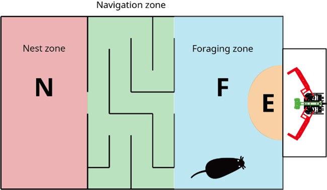
Reviewer #2 (Public review):
Summary:
Jeong & Choi (2023) use a semi-naturalistic paradigm to tackle the question of how the activity of neurons in the mPFC might continuously encode different functions. They offer two possibilities: either there are separate dedicated populations encoding each function, or cells alter their activity dependent on the current goal of the animal. In a threat-avoidance task rats procurred sucrose in an area of a chamber where, after remaining there for some amount of time, a 'Lobsterbot' robot attacked. In order to initiate the next trial rats had to move through the arena to another area before returning to the robot encounter zone. Therefore the task has two key components: threat avoidance and navigating through space. Recordings in the IL and PL of the mPFC revealed encoding that depended on what stage of the task the animal was currently engaged in. When animals were navigating, neuronal ensembles in these regions encoded distance from the threat. However, whilst animals were directly engaged with the threat and simultaneously consuming reward, it was possible to decode from a subset of the population whether animals would evade the threat. Therefore the authors claim that neurons in the mPFC switched between two functional modes: representing allocentric spatial information, and representing egocentric information pertaining to the reward and threat. Finally, the authors propose a conceptual model based on these data whereby this switching of population encoding is driven by either bottom-up sensory information or top-down arbitration.
Strengths:
Whilst these multiple functions of activity in the mPFC have generally been observed in tasks dedicated to the study of a singular function, less work has been done in contexts where animals continuously switch between different modes of behaviour in a more natural way. Being able to assess whether previous findings of mPFC function apply in natural contexts is very valuable to the field, even outside of those interested in the mPFC directly. This also speaks to the novelty of the work; although mixed selectivity encoding of threat assessment and action selection has been demonstrated in some contexts (e.g. Grunfeld & Likhtik, 2018) understanding the way in which encoding changes on-the-fly in a self-paced task is valuable both for verifying whether current understanding holds true and for extending our models of functional coding in the mPFC.
The authors are also generally thoughtful in their analyses and use a variety of approaches to probe the information encoded in the recorded activity. In particular, they use relatively close analysis of behaviour as well as manipulating the task itself by removing the threat to verify their own results. The use of such a rich task also allows them to draw comparisons, e.g. in different zones of the arena or different types of responses to threat, that a more reduced task would not otherwise allow. Additional in-depth analyses in the updated version of the manuscript, particularly the feature importance analysis, as well as complimentary null findings (a lack of cohesive place cell encoding, and no difference in location coding dependent on direction of trajectory) further support the authors' conclusion that populations of cells in the mPFC are switching their functional coding based on task context rather than behaviour per se. Finally, the authors' updated model schematic proposes an intriguing and testable implementation of how this encoding switch may be manifested by looking at differentiable inputs to these populations.
Weaknesses:
The main existing weakness of this study is that its findings are correlational (as the authors highlight in the discussion). Future work might aim to verify and expand the authors' findings - for example, whether the elevated response of Type 2 neurons directly contributes to the decision-making process or just represents fear/anxiety motivation/threat level - through direct physiological manipulation. However, I appreciate the challenges of interpreting data even in the presence of such manipulations and some of the additional analyses of behaviour, for example the stability of animals' inter-lick intervals in the E-zone, go some way towards ruling out alternative behavioural explanations. Yet the most ideal version of this analysis is to use a pose estimation method such as DeepLabCut to more fully measure behavioural changes. This, in combination with direct physiological manipulation, would allow the authors to fully validate that the switching of encoding by this population of neurons in the mPFC has the functional attributes as claimed here.
I wanted to add a minor comment about interpreting the two possible accounts presented in fig. 8 to suggest a third possibility: that both bottom-up sensory and top-down arbitration mechanisms can occur simultaneously to influence whether the activity of the population switches. Indeed, a model where these inputs are balanced or pitted against each other, so to speak, to continuously modulate encoding in the mPFC seems both adaptive and likely. Further, some speculation on the source of the 'arbitrator' in the top-down account would make this model more tractable for future testing of its validity.
We thank the reviewer for highlighting this important perspective. We fully agree that an intricate and recurrent interaction between bottom-up and top-down modulations is a highly plausible account of how the mPFC changes its encoding mode. In line with this suggestion, we have incorporated this idea as a third possibility in the revised Discussion, alongside an updated version of Figure 8 that explicitly illustrates this competitive model.
Although we were unable to identify a definitive study directly measuring how the mPFC switches encoding modes across tasks, we did find relevant human EEG and fMRI studies addressing this issue. Based on these findings, we now propose the anterior cingulate cortex (ACC) as a potential hub for top-down arbitration. We have added a paragraph in the Discussion describing this possibility and its implications for future testing.
“Which brain region might act as this arbitrator? Evidence from human neuroimaging studies implicates the anterior cingulate cortex (ACC) as a central hub for switching cognitive modes. During task switching, the ACC shows increased activation (Hyafil et al., 2009), enhances connectivity with task-specific regions (Aben et al., 2020), correlates with multitask performance (Kondo et al., 2004), and monitors the reliability of competing decision systems (Lee et al., 2014). Collectively, these findings point to a pivotal role for the ACC in coordinating task assignment. Rodent studies also link the ACC to strategic mode switching (Tervo et al., 2014), suggesting that the rodent ACC could similarly arbitrate between strategies, determining which task-relevant variables are represented in the ventral mPFC, including the PL and IL. Future studies combining multi-context tasks with causal manipulations will be essential to determine whether these functional shifts are driven primarily by top-down arbitration or by bottom-up sensory inputs.”
Reviewer #3 (Public review):
Summary:
This study investigates how various behavioral features are represented in the medial prefrontal cortex (mPFC) of rats engaged in a naturalistic foraging task. The authors recorded electrophysiological responses of individual neurons as animals transitioned between navigation, reward consumption, avoidance, and escape behaviors. Employing a range of computational and statistical methods, including artificial neural networks, dimensionality reduction, hierarchical clustering, and Bayesian classifiers, the authors sought to predict from neural activity distinct task variables (such as distance from the reward zone and the success or failure of avoidance behavior). The findings suggest that mPFC neurons alternate between at least two distinct functional modes, namely spatial encoding and threat evaluation, contingent on the specific location.
Strengths:
This study attempt to address an important question: understanding the role of mPFC across multiple dynamic behaviors. The authors highlight the diverse roles attributed to mPFC in previous literature and seek to explain this apparent heterogeneity. They designed an ethologically relevant foraging task that facilitated the examination of complex dynamic behavior, collecting comprehensive behavioral and neural data. The analyses conducted are both sound and rigorous.
Weaknesses:
Because the study still lacks experimental manipulation, the findings remain correlational. The authors have appropriately tempered their claims regarding the functional role of the mPFC in the task. The nature of the switch between functional modes encoding distinct task variables (i.e., distance to reward, and threat-avoidance behavior type) is not established. Moreover, the evidence presented to dissociate movement from these task variables is not fully convincing, particularly without single-session video analysis of movement. Specifically, while the new analyses in Figure 7 are informative, they may not fully account for all potential confounding variables arising from changes in context or behavior.
Regarding the claim of highly stereotyped behavior, there are some inconsistencies. While the authors assert this, Figure 1F shows inter-animal variability, and the PETHs, representing averaged activity, may not fully capture the variability of the behavior across sessions and animals. To strengthen this aspect, a more detailed analysis that examines the relationship between behavior and neural activity on a trial-by-trial basis, or at minimum, per session, could help.
We thank the reviewer for this thoughtful recommendation and the opportunity to clarify our use of the term “stereotyped behavior.” By this, we were specifically referring to the animals’ consistent licking behavior in the E-zone, rather than to the latency of head withdrawal, which indeed varied across trials and animals. Because licking tempo and body posture during sucrose consumption were highly consistent, the decision to avoid or stay (AW vs. EW) could not be predicted from overt behavior alone. This consistency strengthens our conclusion that the significant predictive power of the Bayesian decoding analysis reflects intrinsic firing patterns of the mPFC neural network, rather than simple behavioral correlates of avoidance.
We also note that the Bayesian model was conducted on a trial-by-trial basis, and the reported prediction accuracy of 73% represents the average across all individual trials (Figure 6B, C). Thus, the analysis inherently captures variability across trials and animals, directly addressing the reviewer’s concern.
The reviewer is correct that the PETHs shown in Figure 5 are based on session-averaged activity aligned to head-entry and head-withdrawal events. The purpose of this analysis was to illustrate that certain modulation patterns could be grouped into 2–3 distinct categories. While averaged activity can provide insight into collective responses to external events, we agree that trial-based analyses provide a more rigorous demonstration of the link between neural ensemble activity and behavioral decisions. This is precisely why we complemented the PETH analysis with Bayesian decoding, which provides stronger evidence that mPFC ensemble activity is predictive of the animal’s choice to avoid or stay.
Similarly, the claim regarding the limited scope of extraneous behavior (beyond licking) requires further substantiation. It would be more convincing to quantify potential variations in licking vigor and to provide evidence for the absence of significant postural changes.
To address this concern, we quantified licking vigor using the inter-lick interval (ILI) as an indirect index. A lick was defined as the period from tongue contact with the IR beam (Lick-On) to withdrawal (Lick-Off), and the ILI was calculated as the time between a Lick-Off and the subsequent Lick-On. Across all animals, ILIs were clustered within a narrow range with a median of 0.155 s (see Author response image 4, left panel).
We analyzed licking vigor at two levels: within trials and within sessions. Because reduced vigor or satiation would lengthen ILIs, comparing the first half and the last half of ILIs within a trial or within a session provides a sensitive proxy for licking consistency.
Within trials: For each of 2,820 trials, we compared the mean ILI of the first half of licks to that of the second half. The average difference was only ~ 17 ms (middle panel). Across sessions: Trial-averaged ILIs were compared between the first and last halves of each session, yielding a mean difference ~ 1.7 ms per session (right panel).
These analyses demonstrate that rats maintained stable licking vigor whenever they entered the E-zone, regardless of avoidance outcome.
Author response image 2.
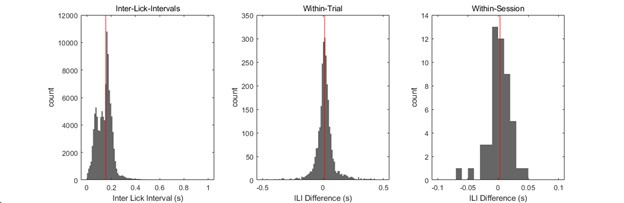
Concerning the ANN model, while I understand the choice of a 4-layer network for its performance, the study could have benefited from exploring simpler models. A model where weight corresponds directly to individual neurons could improve interpretability and facilitate the investigation of dynamic changes in neuronal 'modes' (i.e., weight adjustments) over time.
We fully agree with the reviewer on the importance of biologically interpretable models. While artificial neural networks (ANNs) share certain similarities with neural computation, they are not intended to capture biological realism. For example, the error correction mechanism used in ANNs, such as backpropagation has no direct counterpart in mammalian neural circuits. Although we considered approaches that would link each computational node more directly to the activity of individual neurons, building such a model would require temporally sensitive, mechanistic frameworks (e.g., leaky integrate-and-fire networks) and an extensive behavioral alignment effort, which is beyond the scope of the current study.
Our use of an ANN was intended solely as an analytical tool to uncover hidden patterns in multi-unit activity that may not be detectable with traditional methods. Among various machine-learning algorithms, we selected a four-layer ANN regressor because it achieved significantly lower decoding errors (Supplementary Figure S3) and showed robustness to hyperparameter variation (Glaser et al., 2020). To acknowledge the limitations of this approach and suggest future directions, we have revised the Results section to explicitly discuss these points.
“Among various machine learning algorithms, we selected a robust tool for decoding underlying patterns in the data, rather than to model the architecture of the mPFC. We implemented a four-layer artificial neural network regressor (ANN; see Materials and Methods for a detailed structure), as the ANN achieves significantly lower decoding errors (Supplementary Figure S3) and has robustness to hyperparameter changes (Glaser et al., 2020).”
Reviewer #3 (Public review):
Summary:
The authors convincingly demonstrate that a population of CCK+ spinal neurons in the deep dorsal horn express the G protein coupled estrogen receptor GPR30 to modulate pain sensitivity in the chronic constriction injury (CCI) model of neuropathic pain in mice. Using complementary pharmacological and genetic knockdown experiments they convincingly show that GPR30 inhibition or knockdown reverses mechanical, tactile and thermal hypersensitivity, conditioned place aversion, and c-fos staining in the spinal dorsal horn after CCI. They propose that GPR30 mediates an increase in postsynaptic AMPA receptors after CCI using slice electrophysiology which may underlie the increased behavioral sensitivity. They then use anterograde tracing approaches to show that CCK and GPR30 positive neurons in the deep dorsal horn may receive direct connections from primary somatosensory cortex. Chemogenetic activation of these dorsal horn neurons proposed to be connected to S1 increased nociceptive sensitivity in a GPR30 dependent manner. Overall, the data are very convincing and the experiments are well conducted and adequately controlled. The potential role of direct connections from S1 for descending modulation of pain and the endogenous mechanism(s) activating GPR30 will be interesting to test in future studies.
Strengths:
The experiments are very well executed and adequately controlled throughout the manuscript. The data are nicely presented and supportive of a role for GPR30 signaling in the spinal dorsal horn influencing nociceptive sensitivity following CCI. The authors also did an excellent job of using complementary approaches to rigorously test their hypothesis.
Weaknesses:
While the viral tracing demonstrates a potential connection between S1 and CCK+ or GPR30+ spinal neurons, no direct evidence is provided for S1 in facilitating any activity of these neurons in the dorsal horn.
Comments on the latest version:
The authors have done a good job addressing previous critiques and have appropriately revised the manuscript and conclusions.
Author response:
The following is the authors’ response to the previous reviews
Reviewer #1 (Public review):
In their revised manuscript, Chen et al. have added additional data that establishes GPR30 spinal neurons as a population of excitatory neurons, half of which express CCK. These data help to position GPR30 neurons in the existing framework of spinal neuron populations that contribute to neuropathic pain, strengthening the author's findings.
Thank you very much for your positive feedback and for recognizing the value of our additional data.
Reviewer #3 (Public review):
The authors did an excellent job addressing many of the critiques raised. Despite acknowledging that a direct functional corticospinal projection to CCK/GPR30+neurons is not supported by the data and revising the title, these claims still persist throughout the manuscript. Manipulating gene expression or the activity of postsynaptic neurons through a trans-synaptic labeling strategy does not directly support any claim that those upstream neurons are directly modulating spinal neurons through the proposed pathway. Indeed they might, but that is not demonstrated here.
We sincerely thank the reviewer for this critical insight. We fully agree that our trans-synaptic approach does not provide a direct functional connection. In response, we have revised the manuscript to remove any overstated claims of "direct" modulation and instead emphasize the critical role of spinal GPR30+ neurons. Moreover, we have added a statement in the Discussion to acknowledge this limitation and to highlight that the precise function role of this connection requires further investigation in further studies.
Reviewer #1 (Recommendations for the authors):
I recommend 2 minor corrections to the text and figures
(1) Line 131 : "What's more, near-universal CCK+ neurons were co-localized with GPR30 (Fig 2F and G)."
The additional quantification of the overlap between GPR30 and tdTomato provided by the authors is useful, but there are inconsistencies with how the data are reported in the figures and text, making them difficult to interpret. 2F supports the author's conclusion that approximately 90% of CCK⁺ neurons express GPR30, and about 50% of GPR30⁺ neurons co-express CCK. However, the x-axis labels in 2G appear to have been switched, and suggest that the opposite is true (i.e., most GRPR neurons are CCK+, while only 50% of CCK neurons are GPR30+). Please clarify which is correct throughout the results and discussion sections.
Thank you for identifying this important error. We apologized for the confusion caused by the mislabeled x-axis in Fig. 2G. The x-axis labels were indeed inadvertently switched. The correct data is that approximately 90% of CCK<sup>+</sup> neurons express GPR30. We have corrected the figure and have carefully reviewed the entire manuscript to ensure all related descriptions and discussions are consistent with the accurate quantification.
(2) The following sentence describing Figure 5 was hard to follow: Lines 190-192, "Consistent with prior observations, we found that these SDH downstream neurons exhibited colocalization with CCK+ neurons, with 28.1% of mCherry+ neurons expressing CCK (Fig 5I and J)." Since the authors are describing a common population of neurons, a statement describing the coexpression (rather than the colocalization" would more simply summarize their data.
We thank the reviewer for this helpful suggestion. We fully agree that "coexpression" is a more precise term for the description. We have revised the sentence on Lines 189-190 to read: "Consistent with prior observations, we found that 28.1% of mCherry+ S1-SDH downstream neurons coexpressed CCK (Fig 5I and J)."
Reviewer #3 (Recommendations for the authors):
Additional Recommendations
The authors did a commendable job revising the manuscript text to improve readability; however, several informal phrases from the original version still persist, or were added (e.g. "by the way").
We thank the reviewer for this valuable feedback regarding the language. We have conducted a line-by-line review of the entire manuscript to identify all remaining informal phrases, and replaced them with more appropriate phrasing.
It should be clearly mentioned that spontaneous E/IPSCs were recorded in Figure 4 and Fig S5.
We thank the reviewer for this helpful suggestion. We have now clearly indicated the spontaneous E/IPSCs in Fig. 4 and Fig. S5 and manuscript.
The rationale for recording EPSCs from GFP-labeled CCK+ neurons because "a significant proportion of spinal CCK+ neurons form excitatory synapses with upstream neurons" does not make any sense. Do the authors instead mean that CCK neurons receive excitatory inputs from other spinal neurons and intend to test if those synaptic connections are modulated by GPR30?
We thank the reviewer for this critical correction. Our intended meaning was indeed that CCK<sup>+</sup> neurons receive excitatory inputs from other neurons, and we aimed to test whether those synaptic connections are modulated by GPR30. To avoid confusion, we have revised the manuscript to remove the erroneous statement “Since CCK+ neurons mainly receive excitatory synaptic inputs from upstream neurons, we then intended to test whether GPR30 modulated these synaptic connections.”
I am confused by the statement on Page 8 "to examine whether GPCR30-mediated EPSCs depend on AMPA mediated currents." Given that sEPSCs were recorded at -70 mV in low Cl internal I'm not sure what other glutamate receptor would be involved. Perhaps the intention was to more directly test whether GPR30 activation acutely modulates AMPAR-mediated EPSCs? However, as the authors acknowledged, this experiment does not necessarily support a solely post-synaptic AMPAR-dependent mechanism.
We thank the reviewer for this insightful comment and apologize for the lack of clarity. Our intention was indeed to test whether GPR30 activation modulates AMPAR-mediated currents. We have revised the text. In addition, we also emphasize in the Discussion that our data did not rule out the potential pre-synaptic contributions to this effect.
An elevation in EPSCs within a cell does not necessarily mean that the cell is more excitable, only that it is receiving more excitatory inputs or has an increase in synaptic receptors. The cell may scale down its activity to compensate for this increase. I recommend only drawing conclusions from what the experiments actually tested.
We thank the reviewer for this crucial clarification. We have revised the manuscript to remove any claims that the cells were "more excitable". Our conclusions now strictly focus on the specific findings that GPR30 activation enhanced the excitatory transmission onto CCK<sup>+</sup> neurons.
Reviewer #3 (Public review):
Summary:
The study provides an interesting contribution to our understanding of Cryptovaranoides relationships, which is a matter of intensive debate among researchers. The authors have modified the manuscript according to most of my suggestions. My main concerns are about the wording of some statements but the authors have the right to put it as they want in the end. Overall the discussion and data are well prepared. I would recommend to publish the manuscript after very minor revisions.
Strengths:
Detailed analysis of the discussed characters. Illustrations of some comparative materials.
Weaknesses:
Abstract: "Our team challenged this identification and instead suggested †Cryptovaranoides had unclear affinities to living reptiles"
Unfortunately I have to disagree again. "unclear affinities to living reptiles" can mean anything including a crown lizard. First, the 2023 paper clearly rejected the squamate hypothesis and presented some evidence that potentially places Cryptovaranoides among Archosauromorpha. In this context "unclear where it would belong within the latter" does not really matter. Second, we are not discussing here if Cryptovaranoides is a squamate or a stem-squamate. We have many more options on the table, so "unclear affinities" is too imprecise. Please change it to "could be an archosauromorph or an indeterminate neodiapsid" in the abstract to show the scale of conflicting evidence.
Author response:
The following is the authors’ response to the original reviews.
Reviewer #1 (Public review):
In the Late Triassic and Early Jurassic (around 230 to 180 Ma ago), southern Wales and adjacent parts of England were a karst landscape. The caves and crevices accumulated remains of small vertebrates. These fossil-rich fissure fills are being exposed in limestone quarrying. In 2022 (reference 13 of the article), a partial articulated skeleton and numerous isolated bones from one fissure fill of end-Triassic age (just over 200 Ma) were named Cryptovaranoides microlanius and described as the oldest known squamate - the oldest known animal, by some 20 to 30 Ma, that is more closely related to snakes and some extant lizards than to other extant lizards. This would have considerable consequences for our understanding of the evolution of squamates and their closest relatives, especially for their speed and absolute timing, and was supported in the same paper by phylogenetic analyses based on different datasets.
In 2023, the present authors published a rebuttal (reference 18) to the 2022 paper, challenging anatomical interpretations and the irreproducible referral of some of the isolated bones to Cryptovaranoides. Modifying the datasets accordingly, they found Cryptovaranoides outside Squamata and presented evidence that it is far outside. In 2024 (reference 19), the original authors defended most of their original interpretation and presented some new data, some of it from newly referred isolated bones. The present article discusses anatomical features and the referral of isolated bones in more detail, documents some clear misinterpretations, argues against the widespread but not justifiable practice of referring isolated bones to the same species as long as there is merely no known evidence to the contrary, further argues against comparing newly recognized fossils to lists of diagnostic characters from the literature as opposed to performing phylogenetic analyses and interpreting the results, and finds Cryptovaranoides outside Squamata again.
Although a few of the character discussions and the discussion of at least one of the isolated bones can probably still be improved (and two characters are addressed twice), I see no sign that the discussion is going in circles or otherwise becoming unproductive. I can even imagine that the present contribution will end it.
We appreciate the positive response from reviewer 1!
Reviewer #2 (Public review):
Congratulations on this thorough manuscript on the phylogenetic affinities of Cryptovaranoides.
Thank you.
Recent interpretations of this taxon, and perhaps some others, have greatly changed the field's understanding of reptile origins- for better and (likely) for worse.
We agree, and note that while it is possible for challenges to be worse than the original interpretations, both the original and subsequent challenges are essential aspects of what make science, science.
This manuscript offers a careful review of the features used to place Cryptovaranoides within Squamata and adequately demonstrates that this interpretation is misguided, and therefore reconciles morphological and molecular data, which is an important contribution to the field of paleontology. The presence of any crown squamate in the Permian or Triassic should be met with skepticism, the same sort of skepticism provided in this manuscript.
We agree and add that every testable hypothesis requires skepticism and testing.
I have outlined some comments addressing some weaknesses that I believe will further elevate the scientific quality of the work. A brief, fresh read‑through to refine a few phrases, particularly where the discussion references Whiteside et al. could also give the paper an even more collegial tone.
We have followed Reviewer 2’s recommendations closely (see below) and have justified in our responses if we do not fully follow a particular recommendation.
This manuscript can be largely improved by additional discussion and figures, where applicable. When I first read this manuscript, I was a bit surprised at how little discussion there was concerning both non-lepidosauromorph lepidosaurs as well as stem-reptiles more broadly. This paper makes it extremely clear that Cryptovaranoides is not a squamate, but would greatly benefit in explaining why many of the characters either suggested by former studies to be squamate in nature or were optimized as such in phylogenetic analyses are rather widespread plesiomorphies present in crownward sauropsids such as millerettids, younginids, or tangasaurids. I suggest citing this work where applicable and building some of the discussion for a greatly improved manuscript. In sum:
(1) The discussion of stem-reptiles should be improved. Nearly all of the supposed squamate features in Cryptovaranoides are present in various stem-reptile groups. I've noted a few, but this would be a fairly quick addition to this work. If this manuscript incorporates this advice, I believe arguments regarding the affinities of Cryptovaranoides (at least within Squamata) will be finished, and this manuscript will be better off for it.
(2) I was also surprised at how little discussion there was here of putative stem-squamates or lepidosauromorphs more broadly. A few targeted comparisons could really benefit the manuscript. It is currently unclear as to why Cryptovaranoides could not be a stem-lepidosaur, although I know that the lepidosaur total-group in these manuscripts lacks character sampling due to their scarcity.
We are responding to (1) and (2) together. We agree with the Reviewer that a thorough comparison of Cryptovaranoides to non-lepidosaurian reptiles is critical. This is precisely what we did in our previous study: Brownstein et al. (2023)— see main text and supplementary information therein. As addressed therein, there is a substantial convergence between early lepidosaurs and some groups of archosauromorphs (our inferred position for Cryptovaranoides). Many of those points are not addressed in detail here in order to avoid redundancy and are simply referenced back to Brownstein et al. (2023). Secondly, stem reptiles (i.e., non-lepidosauromorphs and non-archosauromorphs), such as suggested above (millerettids, younginids, or tangasaurids), are substantially more distantly related to Cryptovaranoides (following any of the published hypotheses). As such, they share fewer traits (either symplesiomorphies or homoplasies), and so, in our opinion, we would risk directing losing the squamate-focus of our study.
We thus respectfully decline to engage the full scope of the problem in this contribution, but do note that this level of detailed work would make for an excellent student dissertation research program.
(3) This manuscript can be improved by additional figures, such as the slice data of the humerus. The poor quality of the scan data for Cryptovaranoides is stated during this paper several times, yet the scan data is often used as evidence for the presence or absence of often minute features without discussion, leaving doubts as to what condition is true. Otherwise, several sections can be rephrased to acknowledge uncertainty, and probably change some character scorings to '?' in other studies.
We strongly agree with the reviewer. Unfortunately, the original publication (Whiteside et al., 2021) did not make available the raw CT scan data to make this possible. As noted below in the Responses to Recommendations Section, we only have access to the mesh files for each segmented element. While one of us has observed the specimens personally, we have not had the opportunity to CT scan the specimens ourselves.
Reviewer #3 (Public review):
Summary:
The study provides an interesting contribution to our understanding of Cryptovaranoides relationships, which is a matter of intensive debate among researchers. My main concerns are in regard to the wording of some statements, but generally, the discussion and data are well prepared. I would recommend moderate revisions.
Strengths:
(1) Detailed analysis of the discussed characters.
(2) Illustrations of some comparative materials.
Thank you for noting the strengths inherent to our study.
Weaknesses:
Some parts of the manuscript require clarification and rewording.
One of the main points of criticism of Whiteside et al. is using characters for phylogenetic considerations that are not included in the phylogenetic analyses therein. The authors call it a "non-trivial substantive methodological flaw" (page 19, line 531). I would step down from such a statement for the reasons listed below:
(1) Comparative anatomy is not about making phylogenetic analyses. Comparative anatomy is about comparing different taxa in search of characters that are unique and characters that are shared between taxa. This creates an opportunity to assess the level of similarity between the taxa and create preliminary hypotheses about homology. Therefore, comparative anatomy can provide some phylogenetic inferences.
That does not mean that tests of congruence are not needed. Such comparisons are the first step that allows creating phylogenetic matrices for analysis, which is the next step of phylogenetic inference. That does not mean that all the papers with new morphological comparisons should end with a new or expanded phylogenetic matrix. Instead, such papers serve as a rationale for future papers that focus on building phylogenetic matrices.
We agree completely. We would also add that not every study presenting comparative anatomical work need be concluded with a phylogenetic analysis.
Our criticism of Whiteside et al. (2022) and (2024) is that these studies provided many unsubstantiated claims of having recovered synapomorphies between Cryptovaranoides and crown squamates without actually having done so through the standard empirical means (i.e., phylogenetic analysis and ancestral state reconstruction). Both Whiteside et al. (2022) and (2024) indicate characters presented as ‘shared with squamates’ along with 10 characters presented as synapomorphies (10). However, their actual phylogenetically recovered synapomorphies were few in number (only 3) and these were not discussed.
Furthermore, Whiteside et al. (2022) and (2024) comparative anatomy was restricted to comparing †Cryptovaranoides to crown squamates., based on the assumption that †Cryptovaranoides was a crown squamate and thus only needed to be compared to crown squamates.
In conclusion, we respectfully, we maintain such efforts are “non-trivial substantive methodological flaw(s)”.
(2) Phylogenetic matrices are never complete, both in terms of morphological disparity and taxonomic diversity. I don't know if it is even possible to have a complete one, but at least we can say that we are far from that. Criticising a work that did not include all the possibly relevant characters in the phylogenetic analysis is simply unfair. The authors should know that creating/expanding a phylogenetic matrix is a never-ending work, beyond the scope of any paper presenting a new fossil.
Respectfully, we did not criticize previous studies for including an incomplete phylogeny. Instead, we criticized the methodology behind the homology statements made in Whiteside et al. (2022) and Whiteside et al. (2024).
(3) Each additional taxon has the possibility of inducing a rethinking of characters. That includes new characters, new character states, character state reordering, etc. As I said above, it is usually beyond the scope of a paper with a new fossil to accommodate that into the phylogenetic matrix, as it requires not only scoring the newly described taxon but also many that are already scored. Since the digitalization of fossils is still rare, it requires a lot of collection visits that are costly in terms of time.
We agree on all points, but we are unsure of what the Reviewer is asking us to do relative to this study.
(4) If I were to search for a true flaw in the Whiteside et al. paper, I would check if there is a confirmation bias. The mentioned paper should not only search for characters that support Cryptovaranoides affinities with Anguimorpha but also characters that deny that. I am not sure if Whiteside et al. did such an exercise. Anyway, the test of congruence would not solve this issue because by adding only characters that support one hypothesis, we are biasing the results of such a test.
We would refer the Reviewer to their section (1) on comparative anatomy. As we and the Reviewer have pointed out, Whiteside et al. did not perform comparative anatomical statements outside of crown Squamata in their original study. More specifically, Whiteside et al. (2022, Fig. 8) presented a phylogeny where Cryptovaranoides formed a clade with Xenosaurus within the crown of Anguimorpha or what they termed “Anguiformes”, and made comparisons to the anatomies of the legless anguids, Pseudopus and Ophisaurus. Whiteside et al. (2024), abandoned “Anguiformes”, maintained comparisons to Pseudopus and emphasized affinities with Anguimorpha (but almost all of their phylogenies as published, they do not recover a monophyletic Angumimorpha unless amphisbaenians and snakes are considered to be anguimorphans. Thus, we agree that confirmation bias was inherent in their studies.
To sum up, there is nothing wrong with proposing some hypotheses about character homology between different taxa that can be tested in future papers that will include a test of congruence. Lack of such a test makes the whole argumentation weaker in Whiteside et al., but not unacceptable, as the manuscript might suggest. My advice is to step down from such strong statements like "methodological flaw" and "empirical problems" and replace them with "limitations", which I think better describes the situation.
We agree with the first sentence in this paragraph – there is nothing wrong with proposing character homologies between different taxa based on comparative anatomical studies. However, that is not what Whiteside et al. (2022) and (2024) did. Instead, they claimed that an ad hoc comparison of Cryptovaranoides to crown Squamata confirmed that Cryptovaranoides is in fact a crown squamate and likely a member of Anguimorpha. Their study did not recognize limitations, but rather, concluded that their new taxon pushed the age of crown Squamata into the Triassic.
As noted by Reviewer 2, such a claim, and the ‘data’ upon which it is based, should be treated with skepticism. We have elected to apply strong skepticism and stringent tests of falsification to our critique.
Reviewer #1 (Recommendations for the authors):
(1) Lines 596-598 promise the following: "we provide a long[-]form review of these and other features in Cryptovaranoides that compare favorably with non-squamate reptiles in Supplementary Material." You have kindly informed me that all this material has been moved into the main text; please amend this passage.
This has been deleted.
(2) Comments on science
41: I would rather say "an additional role".
This has been edited accordingly.
43: Reconstructing the tree entirely from extant organisms and adding fossils later is how Hennig imagined it, because he was an entomologist, and fossil insects are, on average,e extremely rare and usually very incomplete (showing a body outline and/or wing venation and little or nothing else). He was wrong, indeed wrong-headed. As a historical matter, phylogenetic hypotheses were routinely built on fossils by the mid-1860s, pretty much as soon as the paleontologists had finished reading On the Origin of Species, and this practice has never declined, let alone been interrupted. As a theoretical matter, including as many extinct taxa as possible in a phylogenetic analysis is desirable because it breaks up long branches (as most recently and dramatically shown by Mongiardino Koch & Parry 2020), and while some methods and some kinds of data are less susceptible to long-branch attraction and long-branch repulsion than others, none are immune; and while missing data (on average more common in fossils) can actively mislead parametric methods, this is not the case with parsimony, and even in Bayesian inference the problem is characters with missing data, not taxa with missing data. Some of you have, moreover, published tip-dated phylogenetic analyses. As a practical matter, molecular data are almost never available from fossils, so it is, of course, true that analyses which only use molecular data can almost never include fossils; but in the very rare exceptions, there is no reason to treat fossil evidence as an afterthought.
We agree and have changed “have become” to “is.”
49-50, 59: The ages of individual fissure fills can be determined by biostratigraphy; as far as I understand, all specimens ever referred to Cryptovaranoides [13, 19] come from a single fill that is "Rhaetian, probably late Rhaetian (equivalent of Cotham Member, Lilstock Formation)" [13: pp. 2, 15].
We appreciate this comment; the recent literature, however, suggests that variable ages are implied by the biostratigraphy at the English Fissure Fills, so we have chosen to keep this as is. Also note that several isolated bones were not recovered with the holotype but were discussed by Whiteside et al. (2024). The provenance of these bones was not clearly discussed in that paper.
59-60: Why "putative"? Just to express your disagreement? I would do that in a less misleading way, for example: "and found this taxon as a crown-group squamate (squamate hereafter) in their phylogenetic analyses." - plural because [19] presented four different analyses of two matrices just in the main paper.
We have removed this word.
121-124: The entepicondylar foramen is homologous all the way down the tree to Eusthenopteron and beyond. It has been lost a quite small number of times. The ectepicondylar foramen - i.e., the "supinator" (brachioradialis) process growing distally to meet the ectepicondyle, fusing with it and thereby enclosing the foramen - goes a bit beyond Neodiapsida and also occurs in a few other amniote clades (...as well as, funnily enough, Eusthenopteron in later ontogeny, but that's independent).
We agree. However, the important note here is that the features on the humerus of Cryptovaranoides are not comparable (differ in location and morphology) to the ent- and ectepondylar foramina in other reptiles, as we discuss at length. As such, we have kept this sentence as is.
153: Yes, but you [18] mistakenly wrote "strong anterior emargination of the maxillary nasal process, which is [...] a hallmark feature of archosauromorphs" in the main text (p. 14) - and you make the same mistake again here in lines 200-206! Also, the fact [19: Figure 2a-c] remains that Cryptovaranoides did not have an antorbital fenestra, let alone an antorbital fossa surrounding it (a fossa without a fenestra only occurs in some cases of secondary loss of the fenestra, e.g., in certain ornithischian dinosaurs). Unsurprisingly, therefore, Cryptovaranoides also does not have an orbital-as-opposed-to-nasal process on its maxilla [19: Figure 2a-c].
Line 243-249 (in original manuscript) deal with the emargination of maxillary nasal process (but this does not imply a full antorbital fenestra). We explicitly state that this feature alone "has limited utility" for supporting archosauromorph affinity.
158-173: The problem here is not that the capitellum is not preserved; from amniotes and "microsaurs" to lissamphibians and temnospondyls, capitella ossify late, and larger capitella attach to proportionately larger concave surfaces, so there is nothing wrong with "the cavity in which it sat clearly indicates a substantial condyle in life". Instead, the problem is a lack of quantification (...as has also been the case in the use of the exact same character in the debate on the origin of lissamphibians); your following sentence (lines 173-175) stands. The rest of the paragraph should be drastically shortened.
We appreciate this comment. We note that the ontogenetic variation of this feature is in part the issue with the interpretation provided by Whiteside et al. (2024). The issue is the lack of consistency on the morphology of the capitellum in that study. We are unclear on what the reviewer means by ‘quantification,’ as the character in question is binary.
250-252: It's not going to matter here, but in any different phylogenetic context, "sphenoid" would be confusing given the sphenethmoid, orbitosphenoid, pleurosphenoid, and laterosphenoid. I actually recommend "parabasisphenoid" as used in the literature on early amniotes (fusion of the dermal parasphenoid and the endochondral basisphenoid is standard for amniotes).
We have added "(=parabasisphenoid)" on first use but retain use of sphenoid because in the squamate and archosauromorph literature, sphenoid (or basisphenoid) is used more frequently.
314-315: Vomerine teeth are, of course, standard for sarcopterygians. Practically all extant amphibians have a vomerine toothrow, for example. A shagreen of denticles on the vomer is not as widespread but still reaches into the Devonian (Tulerpeton).
We agree, but vomerine teeth are rare in lepidosaurs and archosaurs and occur only in very recent clades e.g. anguids and one stem scincoid. Their presence in amphibians is not directly relevant to the phylogenetic placement of Cryptovaranoides among reptiles.
372: Fusion was not scored as present in [13], but as unknown (as "partial" uncertainty between states 0 and 1 [19:8]), and seemingly all three options were explored in [19].
We politely disagree with the reviewer; state 1 is scored in Whiteside et al. (2024).
377-383: Together with the partially fused NHMUK PV R37378 [13: Figure 4B, C; 19: 8], this is actually an argument that Cryptovaranoides is outside but close to Unidentata. The components of the astragalus fuse so early in extant amniotes that there is just a single ossification center in the already fused cartilage, but there are Carboniferous and Permian examples of astragali with sutures in the expected places; all of the animals in question (Diadectes, Hylonomus, captorhinids) seem to be close to but outside Amniota. (And yet, the astragalus has come undone in chamaeleons, indicating the components have not been lost.) - Also, if NHMUK PV R37378 doesn't belong to a squamate close to Unidentata, what does it belong to? Except in toothless beaks, premaxillary fusion is really rare; only molgin newts come to mind (and age, tooth size, and tooth number of NHMUK PV R37378 are wholly incompatible with a salamandrid).
The relevance of the astragalus is to the current discussion is unclear as we do not mention this element in our manuscript. We discuss the fusion in the premaxillae in response to previous comment.
471-474: That thing is concave. (The photo is good enough that you can enlarge it to 800% before it becomes too pixelated.) It could be a foramen filled with matrix; it does not look like a grain sticking to the outside of the bone. Also, spell out that you're talking about "suc.fo" in Figure 3j.
We are also a bit confused about this comment, as we state:
“Finally, we note here that Whiteside et al. [19] appear to have labeled a small piece of matrix attached to a coracoid that they refer to †C. microlanius as the supracoroacoid [sic] foramen in their figure 3, although this labeling is inferred because only “suc, supracoroacoid [sic]” is present in their figure 3 caption.” (L. 519-522, P. 17). We cannot verify that this structure is concave, as so we keep this text as is.
476-489: [19] conceded in their section 4.1 (pp. 11-12) that the atlas pleurocentrum, though fused to the dorsal surface of the axis intercentrum as usual for amniotes and diadectomorphs, was not fused to the axis pleurocentrum.
This is correct, as we note in the MS. The issue is whether these elements are clearly identifiable.
506-510: [19:12] did identify what they considered a possible ulnar patella, illustrated it (Figure 4d), scored it as unknown, and devoted the entire section 4.4 to it.<br /> 512-523: What I find most striking is that Whiteside et al., having just discovered a new taxon, feel so certain that this is the last one and any further material from that fissure must be referable to one of the species now known from there.
We agree with these points and believe we have devoted adequate text to addressing them. Note that the reviewer does not recommend any revisions to these sections.
553: Not that it matters, but I'm surprised you didn't use TNT 1.6; it came out in 2023 and is free like all earlier versions.
We have kept this as is following the reviewer comment, and because we were interested in replicating the analyses in the previous publications that have contributed to the debate about the identity of this taxon. For the present simple analyses both versions should perform identically, as the search algorithms for discrete characters are identical across these versions.
562: Is "01" a typo, or do you mean "0 or 1"? In that case, rather write "0/1" or "{01}".
This has been corrected to {01}
(3) Comments on nomenclature and terminology
55, 56: Delete both "...".
This has been corrected.
100: "ent- and ectepicondylar"
For clarity, we have kept the full words.
107-108: I understand that "high" is proximal and "low" is distal, but what is "the distal surface" if it is not the articular surface in the elbow joint?
This has been corrected.
120: "stem pan-lepidosaurs, and stem pan-squamates"; Lepidosauria and Squamata are crown groups that don't contain their stems
This has been corrected.
122, 123: Italics for Claudiosaurus and Delorhynchus.
This has been corrected.
130: Insert a space before "Tianyusaurus" (it's there in the original), and I recommend de-italicizing the two genus names to keep the contrast (as you did in line 162).
This has been corrected.
130, 131: Replace both "..." by "[...]", though you can just delete the second one.
This has been corrected.
174: Not a capitulum, but a grammatically even smaller (double diminutive) capitellum.
This has been corrected.
209, 224, Table 1: Both teams have consistently been doing this wrong. It's "recessus scalae tympani". The scala tympani ("ladder/staircase of the [ear]drum") isn't the recess, it's what the recess is for; therefore, the recess is named "recess of the scala tympani", and because there was no word for "of" in Classical Latin ("de" meant "off" and "about"), the genitive case was the only option. (For the same reason, the term contains "tympani", the genitive of "tympanum".)
This has been corrected.
415-425: This is a terminological nightmare. Ribs can have (and I'm not sure this is exhaustive): a) two separate processes (capitulum, tuberculum) that each bear an articulating facet, and a notch in between; b) the same, but with a non-articulating web of bone connecting the processes; c) a single uninterrupted elongate (even angled) articulating facet that articulates with the sutured or fused dia- and parapophysis; d) a single round articulating facet. Certainly, a) is bicapitate and d) is unicapitate, but for b) and c) all bets are off as to how any particular researcher is going to call them. This is a known source of chaos in phylogenetic analyses. I recommend writing a sentence or three on how the terms "unicapitate" & "bicapitate" lack fixed meanings and have caused confusion throughout tetrapod phylogenetics, and that the condition seen in Cryptovaranoides is nonetheless identical to that in archosauromorphs.
This has been added: “This confusion in part stems from the lack of a fixed meaning for uni- and bicapitate rib heads; in any case, †C. microlanius possesses a condition identical to archosauromorphs as we have shown.” (L.475-477, P.16).
439-440: Other than in archosaurs, some squamates and Mesosaurus, in which sauropsids are dorsal intercentra absent?
We are unclear about the relevance of the question to this section. The issue at hand is that some squamate lineages possess dorsal intercentra, so the absence of dorsal intercentra cannot be considered a squamate synapomorphy without the optimization of this feature along a phylogeny (which was not accomplished by Whiteside et al.).
458: prezygapophyses.
This has been corrected.
516: "[...]".
This has been corrected.
566: synapomorphies.
This has been corrected.
587: Macrocnemus.
This has been corrected.
585: I strongly recommend either taking off and nuking the name Reptilia from orbit (like Pisces) or using it the way it is defined in Phylonyms, namely as the crown group (a subset of Neodiapsida). Either would mean replacing "neodiapsid reptiles" with "neodiapsids".
This has been corrected to “neodiapsids.”
625: Replace "inclusive clades" by "included clades", "component clades", "subclades", or "parts," for example.
This has been kept as is because “inclusive clades” is common terminology and is used extensively in, for example, the PhyloCode.
659: Please update.
References are updated.
Fig. 8: Typo in Puercosuchus.
This has been corrected.
(4) Comments on style and spelling
You inconsistently use the past and the present tense to describe [13, 19], sometimes both in the same sentence (e.g., lines 323 vs. 325). I recommend speaking of published papers in the past tense to avoid ascribing past views and acts to people in their present state.
This has been corrected to be more consistent throughout the manuscript.
48: Remove the second comma.
This has been corrected.
91: Replace "[13] and WEA24" by "[13, 19]".
This has been corrected.
100: Commas on both sides of "in fact" or on neither
This has been corrected.
117: I recommend "the interpretation in [19]". I have nothing against the abbreviation "WEA24", but you haven't defined it, and it seems like a remnant of incomplete editing. - That said, eLife does not impose a format on such things. If you prefer, you can just bring citation by author & year back; in that case, this kind of abbreviation would make perfect sense (though it should still be explicitly defined).<br /> 129, 145: Likewise.
We have modified this [13] and [19] where necessary.
192-198: Surely this should be made part of the paragraph in lines 158-175, which has the exact same headline?
This has been corrected.
200-206: Surely this should be made part of the paragraph in lines 148-156, which has the exact same headline?
These sections deal with different issues pertaining to the analyses of Whiteside et al. (2024) and so we have kept to organization as is.
214: Delete "that".
This has been deleted.
312: "Vomer" isn't an adjective; I'd write "main vomer body" or "vomer's main body" or "main body of the vomer".
This has been corrected.
350: "figured"
This has been corrected.
400: Rather, "rearticulated" or "worked to rearticulate"? - And why "several"? Just write "two". "Several" implies larger numbers.
These issues have been corrected.
448, 500: As which? As what kind of feature? I'm aware that "as such" is fairly widely used for "therefore", but it still confuses me every time, and I have to suspect I'm not the only one. I recommend "therefore" or "for this reason" if that is what you mean.
“As such” has been deleted.
452: Adobe Reader doesn't let me check, but I think you have two spaces after "of".
This has been corrected.
514, 539, 546, 552, 588, Fig. 3, 5, 6, Table 1: "WEA24" strikes again.
This has been corrected.
515: Remove the parentheses.
This has been corrected.
531: Insert a space after the period.
This has been corrected.
532: Remove both commas and the second "that".
This has been corrected.
538: Remove the comma.
This has been kept as is because changing it would render the sentence grammatically incorrect.
545: "[...]" or, better, nothing.
This has been corrected.
547: Spaces on both sides of the dash or on neither (as in line 553).
This has been corrected.
552: Rather, "conducted a parsimony analysis".
This has been corrected.
556: Space after "[19]".
This has been corrected.
560: Comma after "narrow".
This has been corrected.
600: Comma after "above" to match the one in the preceding line - there's an insertion in the sentence that must be flanked by commas on both sides.
This has been corrected.
603: Compound adjectives like "alpha-taxonomic" need a hyphen to avoid tripping readers up.
This has been corrected.
612: Similarly, "ancestral-state reconstruction" needs one to make immediately clear it isn't a state reconstruction that is ancestral but a reconstruction of ancestral states.
This has been corrected.
613: If you want to keep this comma, you need to match it with another after "Cryptovaranoides" in line 611.
We have kept this as is, because removing this comma would render the sentence grammatically incorrect.
615: Likewise, you need a comma after "and" because "except for a few features" is an insertion. The other comma is actually optional; it depends on how much emphasis you want to place on what comes after it.
this has been added.
622: Comma after "[48, 49]".
this has been added.
672: Missing italics and two missing spaces.
This has been corrected.
678, 680-681, 693, 700-701, 734, 742, 747, 788, 797, 799, 803, 808, 810-811, 814, 817, 820, 823, 828, 841, 843: Missing italics.
This has been corrected.
683, 689: These are book chapters. Cite them accordingly.
This has been corrected.
737: Missing DOI.
No DOI is available.
793: Missing Bolosaurus major; and I'd rather cite it as "2024" than "in press", and "online early" instead of "n/a".
This has been corrected.
835: Hoffstetter, RJ?
This has been corrected.
836: Is there something missing?
This has been corrected.
839: This is the same reference as number 20 (lines 683-684), and it is miscited in a different way...!
This has been corrected.
Reviewer #2 (Recommendations for the authors):
(1) There is a brief mention of a phylogenetic analysis being re-run, but it is unclear if any modifications (changes in scoring) based on the very observations were made. Please state this explicitly.
This is explained from lines 600-622, P.20-21, in the section “Apomorphic characters not empirically obtained.” "In order to check the characters listed by Whiteside et al. [19] (p.19) as “two diagnostic characters” and “eight synapomorphies” in support of a squamate identity for †Cryptovaranoides, we conducted a parsimony analysis of the revised version of the dataset [32] provided by Whiteside et al. [19] in TNT v 1.5 [91]. We used Whiteside et al.’s [19] own data version"
(2) Line 20: There is almost no discussion of non‑lepidosaur lepidosauromorphs. I suggest including this, as the archosauromorph‑like features reported in Cryptovaranoides appear rather plastic. Furthermore, diagnostic features of Archosauromorpha in other datasets (e.g., Ezcurra 2016 or the works of Spiekman) are notably absent (and unsampled) in Cryptovaranoides. Expanding this comparison would greatly strengthen the manuscript.
The brief discussion (although not absent) of non-lepidosaur lepidosauromorphs is largely a function of the poor fossil record of this grade. But where necessary, we do discuss these taxa. Also see our previous study (Brownstein et al. 2023) for an extensive discussion of characters relevant to archosauromorphs.
(3) Line 38: I suggest removing "Archosauromorpha" from the keywords. The authors make a compelling case that Cryptovaranoides is not a squamate, yet they do not fully test its placement within Archosauromorpha (as they acknowledge). Perhaps use "Reptilia" instead?
We have removed this keyword.
(4) Line 99: The authors' points here are well made and largely valid. The presence of the ent‑ and ectepicondylar foramina is indeed an amniote plesiomorphy and cannot confirm a squamate identity. Their absence, however, can be informative - although it is unclear whether the CT scans of the humerus are of sufficient resolution, and Figure 4 of Brownstein et al. looks hastily reconstructed (perhaps owing to limited resolution). Moreover, the foramina illustrated by Whiteside do resemble those of other reptiles, albeit possibly over‑prepared and exaggerated.
The issue with the noted figure is indeed due to poor resolution from the scans. Although we agree with the reviewer, we hesitate to talk about absence in this taxon being phylogenetically informative given the confounding influence of ontogeny.
(5) I encourage the authors to provide slice data to support the claim that the foramina are absent (which could certainly be correct!); otherwise, the assertion remains unsubstantiated.
We only have access to the mesh files of segmented bones, not the raw (reconstructed slice) data.
(6) PLEASE NOTE - because the specimen is juvenile, the apparent absence of the ectepicondylar foramen is equivocal: the supinator process develops through ontogeny and encloses this foramen (see Buffa et al. 2025 on Thadeosaurus, for example).
See above.
(7) Line 122: Italicize 'Delorhynchus'
This has been corrected.
(8) Lines 131‑132: I'd suggest deleting the final sentence; it feels a little condescending, and your argument is already persuasive.
This has been corrected.
(9) Line 129: Please note that owenettid "parareptiles" also lack this process, as do several other stem‑saurians. Its absence is therefore not diagnostic of Squamata.<br /> Also: Such plasticity is common outside the crown. Milleropsis and Younginidae develop this process during ontogeny, even though a lower temporal bar never fully forms.
We appreciate this point. See discussion later in the manuscript.
(11) Line 172: Consider adding ontogeny alongside taphonomy and preservation. A juvenile would likely have a poorly developed radial condyle, if any. Acknowledging this possibility will add some needed nuance.
This sentence has been modified, but we have not added in discussion of ontogeny here because it is not immediately relevant to refuting the argument about inference of the presence of this feature when it is not preserved.
(12) Line 177: The "septomaxilla" in Whiteside et al. (2024, Figure 1C) resembles the contralateral premaxilla in dorsal view, with the maxillary process on the left and the palatal (or vomerine) process on the right (the dorsal process appears eroded). The foramen looks like a prepalatal foramen, common to many stem and crown reptiles. Consequently, scoring the septomaxilla as absent may be premature; this bone often ossifies late. In my experience with stem‑reptile aggregations, only one of several articulated individuals may ossify this element.
We agree that presence of a late-ossifying septomaxilla cannot be ruled out, but our point remains (and in agreement with Referee) that scoring the septomaxilla as present based on the amorphous fragments is premature.
(13) Line 200: Tomography data should be shown before citing it. The posterior margin of the maxilla appears rather straight, and the maxilla itself is tall for an archosauromorph. It would be more convincing to score this feature as present only after illustrating the relevant slices - and, as you note, the trait is widespread among non‑archosauromorphs.
See above and Brownstein et al. (2023).
(14) Line 208: Well argued: how could Whiteside et al. confidently assign a disarticulated element? Their "vagus" foramen actually resembles a standard hypoglossal foramen - identical to that seen in many stem reptiles, which often have one large and one small opening.
Thank you!
(15) Line 248: Again, please illustrate this region. One cannot argue for absence without showing the slice data. Note that millerettids and procolophonians - contemporaneous with Cryptovaranoides - possess an enclosed vidian canal, so the feature is broadly distributed.
See above.
(16) Line 258: The choanal fossa is intriguing: originally created for squamate matrices, yet present (to varying degrees) in nearly every reptile I have examined. It is strongly developed in millerettids (see Jenkins et al. 2025 on Milleropsis and Milleretta) and younginids, much like in squamates - Tiago appropriately scores it as present. Thus, it may be more of a "Neodiapsida + millerettids" character. In any case, the feature likely forms an ordered cline rather than a simple binary state.
We agree and look forward to future study of this feature.
(17) Line 283: Bolosaurids are not diapsids and, per Simões, myself, and others, "Diapsida" is probably invalid, at least how it is used here. Better to say "neodiapsids" for choristoderes and "stem‑reptiles" or "sauropsids" for bolosaurids. Jenkins et al.'s placement is largely a function of misidentifying the bolosaurid stapes as the opisthotic.
We are not entirely clear on this point since bolosaurids are not mentioned in this section.
(18) Line 298: Here, you note that the CT scans are rather coarse, which makes some earlier statements about absence/presence less certain (e.g., humeral foramina). It may strengthen the paper to make fewer definitive claims where resolution limits interpretation.
We appreciate this point. However, in the case of the humeral foramina the coarseness of the scans is one reason why we question Whiteside et al. scoring of the presence of these features.
(19) Line 314: Multiple rows of vomerine teeth are standard for amniotes; lepidosauromorphs such as Paliguana and Megachirella also exhibit them (though they may not have been segmented in the latter's description). Only a few groups (e.g., varanopids, some millerettids) have a single medial row.
We appreciate this point and have added in those citations into the following added sentence: “Multiple rows of vomerine teeth are common in reptiles outside of Squamata [76]; the presence of only one row is restricted to a handful of clades, including millerettids [77,78], †Tanystropheus [49], and some [79], but not all [71,80] choristoderes.” (L. 360-363, P. 12).
(20) Line 317: This is likely a reptile plesiomorphy - present in all millerettids (e.g., Milleropsis and Milleretta per Jenkins et al.). Citing these examples would clarify that it is not uniquely squamate. Could it be secondarily lost in archosauromorphs?
We appreciate this point and have cited Jenkins et al. here. It is out of the scope of this discussion to discuss the polarity of this feature relative to Archosauromorpha.
(21) Line 336: Unfortunately, a distinct quadratojugal facet is usually absent in Neodiapsids and millerettids; where present, the quadratojugal is reduced and simply overlaps the quadrate.
We appreciate this point but feel that reviewing the distribution of this feature across all reptiles is not relevant to the text noted.
(22) Line 357: Pterygoid‑quadrate overlap is likely a tetrapod plesiomorphy. Whiteside et al. do not define its functional or phylogenetic significance, and the overlap length is highly variable even among sister taxa.
We agree, but in any case this feature is impossible to assess in Cryptovaranoides.
(23) Line 365: Another well‑written section - clear and persuasive.
Thank you!
(24) Line 385: The cephalic condyle is widespread among neodiapsids, so it is not uniquely squamate.
We agree.
(25) Character 391: Note that the frontal underlapping the parietal is widespread, appearing in both millerettids and neodiapsids such as Youngina.
We appreciate this point, but the point here deals with the fact that this feature is not observable in the holotype of Cryptovaranoides.
(26) Line 415: The "anterior process" is actually common among crown reptiles, including sauropterygians, so it cannot by itself place Cryptovaranoides within Archosauromorpha.
We agree but also note that we do not claim this feature unambiguously unites Cryptovaranoides with Archosauromorpha.
(28) Line 460: Yes - Whiteside et al. appear to have relabeled the standard amniote coracoid foramen. Excellent discussion.
Thank you!
(29) Line 496: While mirroring Whiteside's structure, discussing this mandibular character earlier, before the postcrania, might aid readability.
We have chosen to keep this structure as is.
(30) Lines 486-588: This section oversimplifies the quadrate articulation.
We are unclear how this is an oversimplification.
(31) Both Prolacerta and Macrocnemus possess a cephalic condyle and some mobility (though less than many squamates). In Prolacerta (Miedema et al. 2020, Figure 4), the squamosal posteroventral process loosely overlaps the quadrate head.
We assume this comment refers to the section "Peg-in-notch articulation of quadrate head"; we appreciate clarification that this feature occurs in variable extent outside squamates, but this does not affect our statement that the material of Cryptovaranoides is too poorly preserved to confirm its presence.
(32) Where is this process in Cryptovaranoides? It is not evident in Whiteside's segmentation of the slender squamosal - please illustrate.
We are unclear as to which section this comment refers.
(33) Additionally, the quadrate "conch" of Cryptovaranoides is well developed, bearing lateral and medial tympanic crests; the lateral crest is absent in the cited archosauromorphs.
We note that no vertebrate has a medial tympanic crest (it is always laterally placed for the tympanic membrane, when present). If this is what the reviewer refers to, this is a feature commonly found across all tetrapods bearing a tympanum attached to the quadrate (e.g., most reptiles), and so it is not very relevant phylogenetically. Regarding its presence in Cryptovaranoides, the lateral margin of the quadrate is broken (Brownstein et al., 2023), so it cannot be determined. This incomplete preservation also makes an interpretation of a quadrate conch very hard to determine. But as currently preserved, there is no evidence whatsoever for this feature.
(34) Line 591: The cervical vertebrae of Cryptovaranoides are not archosauromorph‑like. Archosauromorph cervicals are elongate, parallelogram‑shaped, and carry long cervical ribs-none of which apply here. As the manuscript lacks a phylogenetic analysis, including these features seems unnecessary. Should they be added to other datasets, I suspect Cryptovaranoides would align along the lepidosaur stem (though that remains to be tested).
We politely disagree. The reviewer here mentions that the cervical vertebrae of archosauromorphs are generally shaped differently from those in Cryptovaranoides. The description provided (“elongate, parallelogram‑shaped, and carry long cervical ribs-none”) is basically limited to protorosaurians (e.g., tanystropheids, Macrocnemus) and early archosauriforms. We note that archosauromorph cervicals are notoriously variable in shape, especially in the crown, but also among early archosauromorphs. Further, the cervical ribs, are notoriously similar among early archosauromorphs (including protorosaurians) and Cryptovaranoides, as discussed and illustrated in Brownstein et al., 2023 (Figs. 2 and 3), especially concerning the presence of the anterior process.
Further, we do include a phylogenetic analysis of the matrix provided in Whiteside et al. (2024) as noted in our results section. In any case, we direct the reviewer to our previous study (Brownstein et al., 2023), in which we conduct phylogenetic analyses that included characters relevant to this note.
Reviewer #3 (Recommendations for the authors):
(1) The authors should use specimen numbers all over the text because we are talking about multiple individuals, and the authors contest the previous affinity of some of them. For example, on page 16, line 447, they mention an isolated vertebra but without any number. The specimen can be identified in the referenced article, but it would be much easier for the reader if the number were also provided here
Agreed and added.
(2) Abstract: "Our team questioned this identification and instead suggested Cryptovaranoides had unclear affinities to living reptiles."
That is very imprecise. The team suggested that it could be an archosauromorph or an indeterminate neodiapsid. Please change accordingly.
We politely disagree. We stated in our 2023 study that whereas our phylogenetic analyses place this taxon in Archosauromorpha, it remains unclear where it would belong within the latter. This is compatible with “unclear affinities to living reptiles”.
(3) Page 7, line 172: "Taphonomy and poor preservation cannot be used to infer the presence of an anatomical feature that is absent." Unfortunate wording. Taphonomy always has to be used to infer the presence or absence of anatomical features. Sometimes the feature is not preserved, but it leaves imprints/chemical traces or other taphonomic indicators that it was present in the organism. Please remove or rewrite the sentence.
We agree and have modified the sentence to read: “Taphonomy and poor preservation cannot be used alone to justify the inference that an anatomical feature was present when it is not preserved and there is no evidence of postmortem damage. In a situation when the absence of a feature is potentially ascribable to preservation, its presence should be considered ambiguous.” (L. 141-145, P.5).
(4) Page 4, line 91, please explain "WEA24" here, though it is unclear why this abbreviation is used instead of citation in the manuscript.
This has been corrected to Whiteside et al. [19].
(5) Page 6, line 144: "Together, these observations suggest that the presence of a jugal posterior process was incorrectly scored in the datasets used by WEA24 (type (ii) error)." That sentence is unclear. Why did the authors use "suggest"? Does it mean that they did not have access to the original data matrix to check it? If so, it should be clearly stated at the beginning of the manuscript.
See earlier; this has been modified and “suggest” has been removed.
(6) Page 7, line 174: "Finally, even in the case of the isolated humerus with a preserved capitulum, the condyle illustrated by Whiteside et al. [19] is fairly small compared to even the earliest known pan-squamates, such as Megachirella wachtleri (Figure 4)." Figure 4 does not show any humeri. Please correct.
The reference to figure 4 has been removed.
(7) Page 8, line 195-198: "This is not the condition specified in either of the morphological character sets that they cite [18,38], the presence of a distinct condyle that is expanded and is by their own description not homologous to the condition in other squamates." This is a bit unclear. Could the authors explain it a little bit further? How is the condition that is specified in the referred papers different compared to the Whiteside et al. description?
We appreciate this comment and have broken this sentence up into three sentences to clarify what we mean:
“The projection of the radial condyle above the adjacent region of the distal anterior extremity is not the condition specified in either of the morphological character sets that Whiteside et al. [19] cite [18,32]. The condition specified in those studies is the presence of a distinct condyle that is expanded. The feature described in Whiteside et al. [19] does not correspond to the character scored in the phylogenetic datasets.” (L.220-225, P.8).
(8) Page 16, line 446: "they observed in isolated vertebrae that they again refer to C. microlanius without justification". That is not true. The referred paper explains the attribution of these vertebrae to Cryptovaranoides (see section 5.3 therein). The authors do not have to agree with that justification, but they cannot claim that no justification was made. Please correct it here and throughout the text.
We have modified this sentence but note that the justification in Whiteside et al. (2024) lacked rigor. Whiteside et al. (2024) state: “Brownstein et al. [5] contested the affinities of three vertebrae, cervical vertebra NHMUK PV R37276, dorsal vertebra NHMUK PV R37277 and sacral vertebra NHMUK PV R37275. While all three are amphicoelous and not notochordal, the first two can be directly compared to the holotype. Cervical vertebra NHMUK PV R37276 is of the same form as the holotype CV3 with matching neural spine, ventral keel (=crest) and the posterior lateral ridges or lamina (figure 3c,d) shown by Brownstein et al. [5, fig. 1a]. The difference is that NHMUK PV R37276 has a fused neural arch to the pleurocentrum and a synapophysis rather than separate diapophysis and parapophysis of the juvenile holotype (figure 3c). Neurocentral fusion of the neural arch and centrum can occur late in modern squamates, ‘up to 82% of the species maximum size’ [28].
The dorsal surface of dorsal vertebra NHMUK PV R37277 (figure 3e) can be matched to the mid-dorsal vertebra in the †Cryptovaranoides holotype (figure 4d, dor.ve) and has the same morphology of wide, dorsally and outwardly directed, prezygapophyses, downwardly directed postzygapophyses and similar neural spine. It is also of similar proportions to the holotype when viewed dorsally (figures 3e and 4d), both being about 1.2 times longer anteroposteriorly than they are wide, measured across the posterior margin. The image in figure 4d demonstrates that the posterior vertebrae are part of the same spinal column as the truncated proximal region but the spinal column between the two parts is missing, probably lost in quarrying or fossil collection.”
This justification is based on pointing out the presence of supposed shared features between these isolated vertebrae and those in the holotype of Cryptovaranoides, even though none of these features are diagnostic for that taxon. We have changed the sentence in our manuscript to read:
“Whiteside et al. [19] concur with Brownstein et al. [18] that the diapophyses and parapophyses are unfused in the anterior dorsals of the holotype of †Cryptovaranoides microlanius, and restate that fusion of these structures is based on the condition they observed in isolated vertebrae that they refer to †C. microlanius based on general morphological similarity and without reference to diagnostic characters of †C. microlanius” (L. 502-507, P. 17).
(9) Figure 2. The figure caption lacks some explanations. Please provide information about affinity (e.g., squamate/gekkotan), ag,e and locality of the taxa presented. Are these left or right palatines? The second one seems to be incomplete, and maybe it is worth replacing it with something else?
The figure caption has been modified:
“Figure 2. Comparison of palatine morphologies. Blue shading indicates choanal fossa. Top image of †Cryptovaranoides referred left palatine is from Whiteside et al. [19]. Middle is the left palatine of †Helioscopos dickersonae (Squamata: Pan-Gekkota) from the Late Jurassic Morrison Formation [62]. Bottom is the right palatine of †Eoscincus ornatus (Squamata: Pan-Scincoidea) from the Late Jurassic Morrison Formation [31].”
(10) Figure 8. The abbreviations are not explained in the figure caption.
These have been added.
CGC
DOI: 10.21203/rs.3.rs-4796642/v1
Resource: Caenorhabditis Genetics Center (RRID:SCR_007341)
Curator: @Apiekniewska
SciCrunch record: RRID:SCR_007341
Supplementary Tables 1–3
DOI: 10.1038/s41556-024-01512-w
Resource: Caenorhabditis Genetics Center (RRID:SCR_007341)
Curator: @Apiekniewska
SciCrunch record: RRID:SCR_007341
Supplementary Tables 1–3
DOI: 10.1038/s41556-024-01512-w
Resource: RRID:WB-STRAIN:WBStrain00004055
Curator: @Apiekniewska
SciCrunch record: RRID:WB-STRAIN:WBStrain00004055
HT115
DOI: 10.1038/s41467-024-52556-3
Resource: RRID:WB-STRAIN:WBStrain00041079
Curator: @Apiekniewska
SciCrunch record: RRID:WB-STRAIN:WBStrain00041079
OP50
DOI: 10.1038/s41467-024-52556-3
Resource: (WB Cat# WBStrain00041969,RRID:WB-STRAIN:WBStrain00041969)
Curator: @Apiekniewska
SciCrunch record: RRID:WB-STRAIN:WBStrain00041969
DA1877
DOI: 10.1038/s41467-024-52556-3
Resource: RRID:WB-STRAIN:WBStrain00040995
Curator: @Apiekniewska
SciCrunch record: RRID:WB-STRAIN:WBStrain00040995
ATCCCat# HTB-77
DOI: 10.1016/j.celrep.2025.116593
Resource: (CLS Cat# 300342/p657_SK-OV-3, RRID:CVCL_0532)
Curator: @areedewitt04
SciCrunch record: RRID:CVCL_0532
RRID:AB_1279299
DOI: 10.1016/j.isci.2025.114303
Resource: (MBL International Cat# M162-3, RRID:AB_1279299)
Curator: @scibot
SciCrunch record: RRID:AB_1279299
Reviewer #3 (Public review):
Summary:
Ruppert et al. present a well-designed 2×2 factorial study directly comparing methionine restriction (MetR) and cold exposure (CE) across liver, iBAT, iWAT, and eWAT, integrating physiology with tissue-resolved RNA-seq. This approach allows a rigorous assessment of where dietary and environmental stimuli act additively, synergistically, or antagonistically. Physiologically, MetR progressively increases energy expenditure (EE) at 22{degree sign}C and lowers RER, indicating a lipid utilization bias. By contrast, a 24-hour 4 {degree sign}C challenge elevates EE across all groups and eliminates MetR-Ctrl differences. Notably, changes in food intake and activity do not explain the MetR effect at room temperature.
Strengths:
The data convincingly support the central claim: MetR enhances EE and shifts fuel preference to lipids at thermoneutrality, while CE drives robust EE increases regardless of diet and attenuates MetR-driven differences. Transcriptomic analysis reveals tissue-specific responses, with additive signatures in iWAT and CE-dominant effects in iBAT. The inclusion of explicit diet×temperature interaction modeling and GSEA provides a valuable transcriptomic resource for the field.
Comments on revisions:
The authors have addressed any concerns I had.
Author response:
The following is the authors’ response to the original reviews.
Reviewer #1 (Public review):
Summary:
Activation of thermogenesis by cold exposure and dietary protein restriction are two lifestyle changes that impact health in humans and lead to weight loss in model organisms - here, in mice. How these affect liver and adipose tissues has not been thoroughly investigated side by side. In mice, the authors show that the responses to methionine restriction and cold exposure are tissue-specific, while the effects on beige adipose are somewhat similar.
Strengths:
The strength of the work is the comparative approach, using transcriptomics and bioinformatic analyses to investigate the tissue-specific impact. The work was performed in mouse models and is state-of-the-art. This represents an important resource for researchers in the field of protein restriction and thermogenesis.
Weaknesses:
The findings are descriptive, and the conclusions remain associative. The work is limited to mouse physiology, and the human implications have not been investigated yet.
We thank Reviewer 1 for their thoughtful review and for highlighting the strength of our comparative, tissue-specific analyses. We acknowledge that our study is descriptive and limited to mouse physiology, and agree that translation to humans will be an important next step. By making these data broadly accessible, we aim to provide a useful resource for future mechanistic and translational studies on dietary amino acid restriction and thermogenesis.
Reviewer #2 (Public review):
Summary:
This study provides a library of RNA sequencing analysis from brown fat, liver, and white fat of mice treated with two stressors - cold challenge and methionine restriction - alone and in combination (interaction between diet and temperature). They characterize the physiologic response of the mice to the stressors, including effects on weight, food intake, and metabolism. This paper provides evidence that while both stressors increase energy expenditure, there are complex tissue-specific responses in gene expression, with additive, synergistic, and antagonistic responses seen in different tissues.
Strengths:
The study design and implementation are solid and well-controlled. Their writing is clear and concise. The authors do an admirable job of distilling the complex transcriptome data into digestible information for presentation in the paper. Most importantly, they do not overreach in their interpretation of their genomic data, keeping their conclusions appropriately tied to the data presented. The discussion is well thought out and addresses some interesting points raised by their results.
Weaknesses:
The major weakness of the paper is the almost complete reliance on RNA sequencing data, but it is presented as a transcriptomic resource.
We thank Reviewer 2 for their positive evaluation of our study and for highlighting the strengths of our design, analyses, and interpretation. We acknowledge the limitation of relying primarily on RNA-seq, and emphasize that our intent was to provide a comprehensive transcriptomic resource to guide future mechanistic work by the community.
Reviewer #3 (Public review):
Summary:
Ruppert et al. present a well-designed 2×2 factorial study directly comparing methionine restriction (MetR) and cold exposure (CE) across liver, iBAT, iWAT, and eWAT, integrating physiology with tissue-resolved RNA-seq. This approach allows a rigorous assessment of where dietary and environmental stimuli act additively, synergistically, or antagonistically. Physiologically, MetR progressively increases energy expenditure (EE) at 22{degree sign}C and lowers RER, indicating a lipid utilization bias. By contrast, a 24-hour 4 {degree sign}C challenge elevates EE across all groups and eliminates MetR-Ctrl differences. Notably, changes in food intake and activity do not explain the MetR effect at room temperature.
Strengths:
The data convincingly support the central claim: MetR enhances EE and shifts fuel preference to lipids at thermoneutrality, while CE drives robust EE increases regardless of diet and attenuates MetR-driven differences. Transcriptomic analysis reveals tissue-specific responses, with additive signatures in iWAT and CE-dominant effects in iBAT. The inclusion of explicit diet×temperature interaction modeling and GSEA provides a valuable transcriptomic resource for the field.
Weaknesses:
Limitations include the short intervention windows (7 d MetR, 24 h CE), use of male-only cohorts, and reliance on transcriptomics without complementary proteomic, metabolomic, or functional validation. Greater mechanistic depth, especially at the level of WAT thermogenic function, would strengthen the conclusions.
We thank Reviewer 3 for their thorough review and for recognizing the strengths of our factorial design, physiological assessments, and transcriptomic analyses. We acknowledge the limitations of short intervention windows, male-only cohorts, and the reliance on transcriptomics. Our aim was to generate a well-controlled comparative dataset as a resource, and we agree that future work incorporating longer interventions, both sexes, and additional mechanistic layers will be important to build on these findings.
Reviewer #1 (Recommendations for the authors):
In my opinion, the comparative analysis between tissues and treatments could be expanded.
We thank the reviewer for this suggestion. We included top30 DEG heatmaps for the comparison MetR_CEvsCtrl_RT for up and downregulated genes in the figures for each tissue. We also provide additional data in the supplementary, including top30 heatmaps for Ctrl_CEvsCtrl_RT, MetR_RTvsCtrl_RT, the interaction term, as well as one excel sheet per tissue for all DEGs (p<0.05 and FC +/- 1.5 and for all gene sets (GSEA).
Reviewer #3 (Recommendations for the authors):
(1) CE robustly increases food intake, yet MetR mice at room temperature, despite elevated EE, do not appear to increase feeding to maintain energy balance. The authors should discuss this discrepancy, as it represents an intriguing avenue for follow-up.
See answer below.
(2) CE raises EE to ~0.9 kcal/h irrespective of diet, suggesting that the additive weight loss seen with MetR+CE (Fig. 1H) must be due to reduced intake. This raises the possibility that MetR mice fail to appropriately sense negative energy balance, even under CE, and do not compensate with higher feeding.
We thank the reviewer for comments 1 and 2. We did not put an emphasis on this finding, as the literature on the effects on food intake under sulfur amino acid restriction are very inconsistent. Intial studies (e.g. by Gettys group) most often report on food intake per gram bodyweight and report an increase in caloric intake. We think that this reporting is flawed and should rather be reported as cumulative food intake. The recent paper by the Dixit group also reports that there is no effect on food intake, in line with our data. The recent paper by the Nudler group reports a decrease in food intake.
(3) Report effect sizes and sample sizes alongside p-values in all figure panels, and ensure the GEO accession (currently listed as "GSEXXXXXX") is provided.
We thank the reviewer for noticing this. So far we were unable to upload the datasets to GEO. We’re unable to connect to the NIH servers, presumably due to the US government shutdown. We are commited to sharing this dataset as soon as possible and will update the manuscript in the future accordingly. We included the sample size for experiment 1 and 2 in the figure legends and described our outlier detection method in the methods section. Significances are explained in the figure legends.
(4) Explicitly define the criteria for "additive," "synergistic," and "antagonistic" interactions (both at the gene and pathway levels) to help readers align the text with the figures.
We thank the reviewer for this helpful comment. We added an description of how we defined and computed the regulatory logic in the method section.
(5) Revise the introduction to address recent data from the Dixit group (ref. #38), which shows that EE induced by cysteine restriction and weight loss is independent of FGF21 and UCP1. As written, the introduction states: "Recent studies have shown that DIT via dietary MetR augments energy expenditure in a UCP1-dependent...fashion".
See answer below.
(6) "Mechanistically, MetR...results in secretion of FGF21. In turn, FGF21 augments EE by activating UCP1-driven thermogenesis in brown adipose tissue via β-adrenergic signaling (4,7)." This should be updated for accuracy and balance.
We thank the reviewers for both comments 5 and 6. Both recent publications by the Dixit and the Nudler groups (now ref 9 and 10) provide very interesting further mechanistic detail into the bodyweight loss in response to dietary sulfur amino acid restriction. However, there are also older papers by the Gettys group that in part contradict their findings, particularly, when it comes to the importance of UCP1 for the adaptation to sulfur amino acid restriction. Overall, we think that further work is required to determine the importance of UCP1-driven EE from alternative mechanisms that ultimately drive body and fat mass loss. We rewrote the referenced paragraph in the introduction to reflect this.
Reviewer #2 (Public review):
Summary:
This study aims to test the hypothesis that microsaccades are linked to the shifting of spatial attention, rather than the maintenance of attention at the cued location. In two experiments, participants were required to judge an orientation change at either a validly cued location (80% of the time) or an invalidly cued location (20% of the time). This change was presented at varying intervals (ranging from 500 to 3,200 ms) after cue onset. Accuracy and reaction times both showed attentional benefits at the valid versus invalid location across the different cue-target intervals. In contrast, microsaccade biases were time-dependent. The authors report a directional bias primarily observed around 400 ms after the cue, with later intervals (particularly in Experiment 2) exhibiting no biases in microsaccade direction towards the cued location. The authors argue that this finding supports their initial hypothesis that microsaccade biases reflect shifts in attention, but that maintaining attention at the cued location after an attention shift is not correlated with microsaccade direction.
Strengths:
The results are straightforward given the chosen experimental design. The manuscript is clearly written, and the presentation of the study and its visualisations are both of a high standard.
Weaknesses:
The major weakness of this paper is its incremental contribution to a widely studied phenomenon. The link between attention and microsaccades has been the subject of extensive research over the past two decades. This study merely provides a limited overview of the key insights gained from these papers and discussions. In fact, it attempts to summarise previous work by stating that many experiments found a link, while others did not, and provides only a relatively small number of references. To make a significant contribution, I believe the authors should evaluate the field more thoroughly, rather than merely scratching the surface.
The authors then present a potential solution to the conflicting past findings, arguing that attention should be considered a dynamic process that can be broken down into an attention shift and a sustained attention phase. Although the authors present this as a novel concept, I cannot think of anyone in the field who considers spatial attention to be a static entity. Nevertheless, I was curious to see how the authors would attempt to determine the precise timing of the attention shift and manipulate the different stages individually. However, the authors only varied the interval between the onset of the attention cue and the test stimulus, failing to further pinpoint their dynamic attention concept.
The current version of the experiment, therefore, takes a correlational approach, similar to initial studies by Engbert and Kliegl (2003) and Hafed and Clark (2002). Meanwhile, we have learned a great deal about the link between microsaccades and attention. Below, I will list just a few of these findings to demonstrate how much we already know. It is important to note that, while the present study cites some of these papers, it does not provide a clear overview of how the current study goes beyond previous research.
(1) Yuval-Greenberg and colleagues (2014) presented stimuli contingent on online-detected microsaccades. A postcue indicated the target for a visual task, and the target could be congruent or incongruent with the microsaccade direction. The authors showed higher visual accuracy in congruent trials. The authors cited that paper, but it is still important to emphasize how this study already tried to go beyond purely correlational links on a single trial level.
(2) The Desimone lab (Lower et al., 2018) showed that firing rates in monkey V4 and IT were increased when a microsaccade was generated in the direction of the attended target.
(3) However, attention can modulate responses in the superior colliculus even in the absence of microsaccades (Yu et al., 2022)
(4) Similarly, Poletti, Rucci & Carrasco (2017) observed attentional modulations in the absence of microsaccades, or comparable attention effects irrespective of whether a microsaccade occurred or not (Roberts & Carrasco, 2019).
Thus, in light of these insights, I believe the current study only adds incrementally to our understanding of the link between microsaccades and spatial attention.
In general, it is important to have an independent measure of the dynamics of an attention shift. I think a shift of 200-600 ms is quite long, and defining this interval is rather arbitrary. Why consider such a long delay as the shift? Rather than taking a data-driven approach to defining an interval for an attention shift, it would be more convincing to derive an interval of interest based on past research or an independent measure.
The present analyses report microsaccade statistics across all trials, but do not directly link single-trial microsaccades to accuracy. Similarly, reaction times and accuracy were analyzed only with respect to valid vs. invalid trials. Here, it would be important to link the findings between microsaccades and performance on a single-trial level. For instance, can the authors report reaction times and accuracy also separately for trials with vs. without microsaccades, and for trials with congruent vs. incongruent microsaccades?
The study would benefit greatly from including a neutral condition to substantiate claims of attentional benefits and costs. It is highly probable that invalid trials would also demonstrate costs in terms of reaction times and accuracy. It would be interesting to observe whether directional biases in microsaccades are also evident when compared to a neutral condition.
Material hope is one element of the critical hope that teachers can cultivate in their students, and it comes from the sense of control young people have when they are given the resources to “deal with the forces that affect their lives” (Syme, 2004, p. 3). It seems like a simple point, but teachers who want to build material hope must understand that quality teaching is the most signifi-cant “material” resource they have to offer youth. The best of the research in our field defines “quality” in teaching by our ability to produce student growth across assessment measures (grades, social development, test scores, student engagement, etc.). To accomplish this, we have to bust the false binary that suggests we must choose between an academically rigorous pedagogy and one geared toward social justice.
The discussion of Material Hope and the importance of teaching and teaching quality to its success are among the most significant points made by the author. The dedication of the teacher and the ability of the teacher to relate a topic or subject to the student on that student's level are critical to education, especially for students that feel alienated to the system. Dedication and a true desire to help the student is essential if a teacher wants to connect with the student on a personal level. Students can always detect and respond positively to a caring and passionate teacher. In the end, a teacher is only a guide, and a great teacher is one who can motivate the student to take control of their own development.
He argues that recent research into the importance of hope for life outcomes is a “major break-through in thinking” for scholars in public health and epidemiology (p. 3). Syme attributes the genesis of this breakthrough to the groundbreaking White-hall studies, which led to revelations that the distribution of “virtually every
Syme’s framing of hope as control of destiny really lands. It shifts the focus from pep talks to power. If unequal health tracks with class because control is uneven, schools can answer by giving students real agency over their learning and futures. That means clear and predictable systems, authentic choices in work, chances to revise, advisory that helps set and pursue goals, and concrete navigation help for college and aid. It also means reducing daily stressors with stable routines, mental health access, and help with basics so students can show up ready to learn. Do that and hope is not a mood. It is a capacity students practice every day.
Reviewer #1 (Public review):
Summary:
The authors report intracranial EEG findings from 12 epilepsy patients performing an associative recognition memory task under the influence of scopolamine. They show that scopolamine administered before encoding disrupts hippocampal theta phenomena and reduces memory performance, and that scopolamine administered after encoding but before retrieval impairs hippocampal theta phenomena (theta power, theta phase reset) and neural reinstatement but does not impair memory performance. This is an important study with exciting, novel results and translational implications. The manuscript is well-written, the analyses are thorough and comprehensive, and the results seem robust.
Strengths:
(1) Very rare experimental design (intracranial neural recordings in humans coupled with pharmacological intervention).
(2) Extensive analysis of different theta phenomena.
(3) Well-established task with different conditions for familiarity versus recollection.
(4) Clear presentation of findings and excellent figures.
(5) Translational implications for diseases with cholinergic dysfunction (e.g., AD).
(6) Findings challenge existing memory models, and the discussion presents interesting novel ideas.
Weaknesses:
(1) One of the most important results is the lack of memory impairment when scopolamine is administered after encoding but before retrieval (scopolamine block 2). The effect goes in the same direction as for scopolamine during encoding (p = 0.15). Could it be that this null effect is simply due to reduced statistical power (12 subjects with only one block per subject, while there are two blocks per subject for the condition with scopolamine during encoding), which may become significant with more patients? Is there actually an interaction effect indicating that memory impairment is significantly stronger when scopolamine is applied before encoding (Figure 1d)? Similar questions apply to familiarity versus recollection (lines 78-80). This is a very critical point that could alter major conclusions from this study, so more discussion/analysis of these aspects is needed. If there are no interaction effects, then the statements in lines 84-86 (and elsewhere) should be toned down.
(2) Further, could it simply be that scopolamine hadn't reached its major impact during retrieval after administration in block 2? Figure 2e speaks in favor of this possibility. I believe this is a critical limitation of the experimental design that should be discussed.
(3) It is not totally clear to me why slow theta was excluded from the reinstatement analysis. For example, despite an overall reduction in theta power, relative patterns may have been retained between encoding and recall. What are the results when using 1-128 Hz as input frequencies?
(4) In what way are the results affected by epileptic artifacts occurring during the task (in particular, IEDs)?
Author response:
Reviewer #1 (Public review):
Summary:
The authors report intracranial EEG findings from 12 epilepsy patients performing an associative recognition memory task under the influence of scopolamine. They show that scopolamine administered before encoding disrupts hippocampal theta phenomena and reduces memory performance, and that scopolamine administered after encoding but before retrieval impairs hippocampal theta phenomena (theta power, theta phase reset) and neural reinstatement but does not impair memory performance. This is an important study with exciting, novel results and translational implications. The manuscript is well-written, the analyses are thorough and comprehensive, and the results seem robust.
Strengths:
(1) Very rare experimental design (intracranial neural recordings in humans coupled with pharmacological intervention).
(2) Extensive analysis of different theta phenomena.
(3) Well-established task with different conditions for familiarity versus recollection.
(4) Clear presentation of findings and excellent figures.
(5) Translational implications for diseases with cholinergic dysfunction (e.g., AD).
(6) Findings challenge existing memory models, and the discussion presents interesting novel ideas.
Weaknesses:
(1) One of the most important results is the lack of memory impairment when scopolamine is administered after encoding but before retrieval (scopolamine block 2). The effect goes in the same direction as for scopolamine during encoding (p = 0.15). Could it be that this null effect is simply due to reduced statistical power (12 subjects with only one block per subject, while there are two blocks per subject for the condition with scopolamine during encoding), which may become significant with more patients? Is there actually an interaction effect indicating that memory impairment is significantly stronger when scopolamine is applied before encoding (Figure 1d)? Similar questions apply to familiarity versus recollection (lines 78-80). This is a very critical point that could alter major conclusions from this study, so more discussion/analysis of these aspects is needed. If there are no interaction effects, then the statements in lines 84-86 (and elsewhere) should be toned down.
The reviewer highlights important concerns regarding the statistical power of the behavioral effects. We address these concerns in the revised manuscript in two ways: (1) we provide a supplemental analysis using a matched number of blocks between the placebo and scopolamine conditions to avoid statistical bias related to differing trial counts, and (2) we include a supplemental figure illustrating paired comparisons between blocks.
(2) Further, could it simply be that scopolamine hadn't reached its major impact during retrieval after administration in block 2? Figure 2e speaks in favor of this possibility. I believe this is a critical limitation of the experimental design that should be discussed.
The reviewer raises an important methodological concern regarding the time required for scopolamine's effect to manifest and the subsequent impact on the study outcomes. Previous studies report that the average time to maximum serum concentration after intravenous (IV) scopolamine administration is approximately 5 minutes (Renner et al., 2005), with the corresponding clinical onset estimated at 10 minutes. In our study, the retrieval period in Block 2 commenced at 15 ± 0.2 post-injection across all subjects. Given this timing, there is sufficient reason to conclude that scopolamine had reached its major impact during the Block 2 retrieval phase. Furthermore, the observation of significant disruptions to theta oscillations during this same retrieval phase provides strong evidence that the drug was in full effect at that time.
(3) It is not totally clear to me why slow theta was excluded from the reinstatement analysis. For example, despite an overall reduction in theta power, relative patterns may have been retained between encoding and recall. What are the results when using 1-128 Hz as input frequencies?
Slow theta (2–4 Hz) was excluded from the reinstatement analysis to avoid potential confounding effects. Given the observed disruption to slow theta power following scopolamine administration, any subsequent changes in slow theta reinstatement would be causally ambiguous, potentially arising directly from the power effects. Therefore, we would be unable to determine whether changes in slow theta reinstatement were genuinely independent of changes in power.
(4) In what way are the results affected by epileptic artifacts occurring during the task (in particular, IEDs)?
To exclude abnormal events and interictal activity, a kurtosis threshold of 4 was applied to each trial, effectively filtering out segments exhibiting significant epileptic artifacts.
Reviewer #2 (Public review):
Summary:
In this study, performed in human patients, the authors aimed at dissecting out the role of cholinergic modulation in different types of memory (recollection-based vs familiarity and novelty-based) and during different memory phases (encoding and retrieval). Moreover, their goal was to obtain the electrophysiological signature of cholinergic modulation on network activity of the hippocampus and the entorhinal cortex.
Strengths:
The authors combined cognitive tasks and intracranial EEG recordings in neurosurgical epilepsy patients. The study confirms previous evidence regarding the deleterious effects of scopolamine, a muscarinic acetylcholine receptor antagonist, on memory performance when administered prior to the encoding phase of the task. During both encoding and retrieval phases, scopolamine disrupts the power of theta oscillations in terms of amplitude and phase synchronization. These results raise the question of the role of theta oscillations during retrieval and the meaning of scopolamine's effect on retrieval-associated theta rhythm without cognitive changes. The authors clearly discussed this issue in the discussion session. A major point is the finding that the scopolamine-mediated effect is selective for recollection-based memory and not for familiarity- and novelty-based memory.
The methodology used is powerful, and the data underwent a detailed and rigorous analysis.
Weaknesses:
A limited cohort of patients; the age of the patients is not specified in the table.
To comply with human subject privacy protection policies, age was not reported; however, we did not find any significant effects of age on the behavioral or neural measures.
Joint Public Review:
Summary
Non-alcoholic fatty liver disease (NAFLD) is a widespread metabolic disease associated with obesity. Endoplasmic reticulum and calcium dysregulation are hallmarks of NAFLD. Here, the authors explore whether the secreted liver protein transthyretin (TTR), which has been previously shown to modulate calcium signaling in the context of insulin resistance, could also impact NAFLD. The study is motivated by a small cohort of NASH patients who show elevated TTR levels. The authors then overexpress TTR in two mouse obesogenic models, which leads to elevated liver lipid deposition. In contrast, liver-specific TTR knockdown improves some liver lipid levels, reduces inflammation markers, and improves glucose tolerance, overall improving the NAFLD markers. These phenotypic findings are overall convincing and largely consistent in two different diet models.
Because of TTR's connection to calcium regulation, the authors then assess whether the knockdown affects ER stress and impacts SERCA2 expression. However, the direct mechanistic evidence supporting the central claim that TTR physically interacts with and inhibits the SERCA2 calcium pump is preliminary and requires further validation. Whether the broader effects on lipid accumulation, inflammation markers, and glucose tolerance are mechanistically connected remains to be determined.
Strengths
The premise of the study is built on prior work from the authors identifying a link between increased transthyretin secretion and the development of insulin resistance, a related obesity condition. The in vivo studies are comprehensive, using human NASH samples, two distinct diet-induced mouse models (HFD and GAN), and in vitro hepatocyte models. The phenotypic data showing that TTR knockdown alleviates steatosis, inflammation, and insulin resistance are robust and convincing across these systems.
Weaknesses
The mechanistic studies in Figures 6-9 are incomplete. There are several issues encompassing experimental design, rigor, and interpretation that, if properly addressed, would make the study much stronger.
(1) Exogenous TTR that is endocytosed by cells is unlikely to ever find itself inside the lumen of the ER. Conversely, endogenous TTR that is produced in cells and that has not yet been secreted is almost certain to have an ER lumenal localization (as in Figures 7B and 9A, and where an apparent colocalization with SERCA is likely to be incidental). In a model where TTR, acting as a hepatokine, has inhibitory effects on SERCA, these would almost certainly be realized from the cytosolic side of the ER membrane-a region inaccessible to lumenal endogenous TTR. It is possible that the overexpression and knockdown of endogenous TTR have the effects seen due to its secretion and uptake (that is, cell-non-autonomous effects), but this possibility was not directly tested through Transwell or similar assays. Given the identity of TTR as a secretory pathway client protein, the only localization data for TTR that are unexpected are those suggesting an ER localization of exogenously added TTR (Figure 7A), but this localization seems to involve only a minor population of TTR, is hindered by a technical issue with cell permeabilization (see below), and lacks orthogonal approaches to convincingly demonstrate meaningful localization of exogenous TTR at the ER membrane.
(2) The experimental logic in Figure 8 is problematic. The authors use Thapsigargin (Tg), a potent and specific SERCA inhibitor, to probe SERCA function. However, since both Tg and TTR are proposed to inhibit SERCA2, the design lacks a critical control to demonstrate that TTR's effects are indeed mediated through SERCA2. SERCA2 activity should, in principle, be fully and irreversibly inhibited by Tg treatment, especially using such a high concentration (5 µM). If TTR's effect on calcium flux is exclusively through SERCA2, then SERCA2 impairment by TTR should have no additional effect in the presence of Tg, as Tg would already be maximally inhibiting the pump. The current data (Figures 8G-H) showing an effect of TTR-KD even with Tg present is difficult to interpret and may suggest off-target or compensatory mechanisms.
(3) The coIP data in Figure 9 need to be better controlled, including by overexpression of FLAG- and MYC-tagged irrelevant proteins, ideally also localized to the ER. The coIP of overexpressed TTR with endogenous SERCA in Figure 9D, in addition to requiring a more rigorous control, is itself of relatively low quality, with the appearance of a possible gel/blotting artifact.
(4) The ER stress markers in Figure 6 are not convincing. Molecular weight markers and positive controls (for example, livers from animals injected with tunicamycin) are missing. In addition, the species of ATF6 that is purportedly being detected (cleaved or full-length) is not indicated, and this protein is also notoriously difficult to detect with convincing specificity in mouse tissues. As well, CHOP protein is usually not detectable in control normal diet mouse livers, raising questions of whether the band identified as CHOP is, in fact, CHOP. These issues, along with the observation that ER stress-regulated RNAs are not altered (Figure S5), raise the question of whether ER stress is involved at all. Likewise, the quantification of SERCA2 levels from Figure 6 requires more rigor. For all blots, it isn't clear that analyzing only 3 or 4 of the animals provides adequate and unbiased power to detect differences; in addition, in Figure 6C, at least the SERCA2 exposure (assuming SERCA2 is being specifically detected; see above) is well beyond the linear range of quantification.
In addition, the following important issues were raised:
(5) n=4 for overexpression might not provide adequate statistical power.
(6) The error for human NASH samples and controls in Figure 1A is surprisingly small. Larger gene expression data sets from NASH cohorts exist and should be used to test the finding in a larger population.
(7) For experiments involving two independent variables (e.g., diet and TTR manipulation, as in Figures 2, 3, 4, 5), a Two-way ANOVA must be used instead of One-way ANOVA or t-tests. Also, the ND-TTR-KD group is missing - these data are an essential control to show the specificity of the knockdown and its effects in a non-diseased state.
(8) Figure 7A: The co-localization signal between TTR-Alexa488 and the ER marker is not strong or convincing, which could be due to the inappropriate immunofluorescence protocol used, of permeabilization prior to fixation. The standard and recommended order is fixation first (to preserve cellular architecture), followed by permeabilization.
[image request *3]
images needed
correspondences
. Verb 일치하다, 부합하다 (=agree, tally)
2. Verb (~에) 해당[상응]하다 (=equivalent)
3. Verb formal (~와) 서신을 주고받다
Heading 3 Content Heading 3 Content Nullam quis erat in sapien facilisis efficitur. Phasellus id elit blandit, elementum velit eu, gravida est. Nullam pretium ante nec scelerisque finibus. Duis ut diam elementum, tempor elit sit amet, congue massa. Maecenas vestibulum tempor mi eget maximus. Maecenas facilisis nibh vel lorem ullamcorper, at fringilla felis semper. Nulla facilisi. Praesent et egestas tellus. Curabitur sed erat eu purus ornare suscipit in quis ex. Fusce sit amet neque eu mauris laoreet aliquam. Praesent vehicula sem nec augue.
Need to be removed
Under the U.S. Constitution, Article II, Section 1, Clause 3, as modified by the 12th Amendment (ratified in 1804), provides for the election of the President and Vice President through the Electoral College rather than by popular vote.
The Constitution uses the Electoral College as the method for choosing the President and Vice President. This means citizens don't elect the President instead, electors chosen by each state cast the votes.
When I first discovered earlier this year that Meta had trained its flagship large language model (LLM) Llama 3 on books from LibGen, one of the largest pirated libraries on the web, containing over 7.5 million books and 81 million research papers, I felt the same surge of betrayal as many authors. How dare this tech behemoth exploit the books into which we had poured our hearts--using them as training data without our consent, especially since such LLMs might one day pose an existential threat to our art.
Meta's use of AI that upset several authors because they used a pirated library
These tools are powerful applications designed to help generate, edit, and improve written content [2]. They use natural language processing (NLP) models, like Open AI’s GPT or Google’s BERT, to analyze and generate human-like text [3].
What AI does
books and scholarly articles. Academic books generally fall into three categories: (1) textbooks written with students in mind, (2) monographs which give an extended report on a large research project, and (3) edited-volumes in which each chapter is authored by different people. Scholarly articles appear in academic journals, which are published multiple times a year in order to share the latest research findings with scholars in the field.
Main forms of sources that are reliable
Note: This preprint has been reviewed by subject experts for Review Commons. Content has not been altered except for formatting.
Learn more at Review Commons
Summary
The authors report the construction and validation of a novel SOX2-TBXT dual-reporter mouse embryonic stem cell (mESC) line, a tool enabling the simultaneous, live visualization of SOX2 and TBXT expression. Using this line, they established an in vitro differentiation system that generates populations of SOX2/TBXT co-expressing cells which mimic neuromesodermal progenitors (NMPs). The authors combined clonal analysis to assess the fate potential of these cells and applied gastruloid models to dissect the functional consequences of gene expression dynamics on axis elongation. The central finding is that the level of TBXT expression predicts and directs lineage potential. This work identifies specific expression thresholds that bias progenitors toward a mesodermal fate.
Major comments
The study's conclusions would be substantially strengthened by more direct validation in an embryonic context. Could the authors quantify endogenous SOX2 and TBXT protein levels of the NMPs in the mouse embryos with immunofluorescence? This would test whether a similar heterogeneity in TBXT expression exists in vivo and whether it correlates with the cells' spatial position.
The role of SOX2 in the quantitative model seems underdeveloped. To justify the authors' claim, could the authors analyze their existing imaging data in more detail to disentangle if the absolute TBXT level is essential rather than the ratio of Sox2 to Tbxt is the driving factor for determining NMP fate?
It seems that SOX2 expression also appears heterogeneous from both in vitro differentiation and gastruloid models. Quantifications, and a discussion of this heterogeneity and whether it influences the fate-decision process would be helpful.
To support the authors' claim that the reporter line recapitulates endogenous protein expression in vivo (lines 121-128), please include a control immunostaining of wild-type embryo for SOX2 and TBXT to compare expression patterns side-by-side with those embryos shown in Figure 1B, Suppl. Fig. 1C, D. To substantiate the claims regarding cellular expression patterns within the embryo (line 125-128), the use of higher-resolution imaging, such as confocal microscopy, is recommended.
The differentiation trajectory described culminates in a double-negative (Sox2-mCherry-negative, Tbxt-GFP-negative) population (lines 246-247). To provide a more complete picture of this fate progression, could the authors perform qPCR for relevant lineage markers to validate the molecular identity of this terminal population?
Minor comments
Scale bars for micrographs are missing in Figure 1B, Suppl. Fig. 1C, and D. The claims regarding the dynamics of TBXT and SOX2 expression in gastruloids following WNT/NOTCH inhibition (Figure 4B, 4D, 4E) would be more compelling if the authors include supplementary videos of the time-lapse imaging.
In lines 322-324, the authors conclude that Tbxt-cells are the driving cells. Please elaborate on the interpretation that this is a cell-autonomous effect driven by TBXT levels. The observation that Sox2 levels increase ~10-15 hours after WNT/NOTCH inhibition is interesting (Figure 4D, 4E). Could the authors discuss this upregulation?
General Assessment
In the development of a novel dual Sox2/Tbxt reporter cell line, which provides a powerful tool for quantitatively understanding the dynamics of cell fate specification during gastrulation and potentially in other developmental contexts. However, a key limitation is the study's primary focus on in vitro models. The findings will require further validation in an in vivo context.
Advance
This study provides a technical advance that provides a new resource available to the field for stem cell and developmental biology.
Audience
This paper will primarily interest a specialized audience, particularly developmental and stem cell biologists who study the fundamental mechanisms of embryogenesis, cell fate specification, and axis elongation.
Field of expertise
Stem cell biology and developmental biology. I do not have the expertise to evaluate their mathematical modeling.
Note: This preprint has been reviewed by subject experts for Review Commons. Content has not been altered except for formatting.
Learn more at Review Commons
Summary:
In this manuscript, the authors generate a novel reporter mouse ESC line to track SOX2 and TBXT dynamics in neuromesodermal progenitors. The authors leverage multiple systems (in vitro differentiation, chimeric embryos and gastruloids) to address how SOX2/TBXT levels impact the contribution of neuromesodermal progenitors towards neural versus mesodermal fates. They show that the levels of TBXT can predict differentiation outcomes, whereby certain thresholds of TBXT influence the differentiation towards a mesodermal identity. In gastruloids, perturbing either WNT or NOTCH signalling coincides with diminished axial elongation. In vitro, the bias mediated by TBXT is also somewhat influenced by the substrate.
Major comments:
There are some key items to clarify that are important to resolve the interpretation of the results and clarify the main advances for a broader readership.
With respect to the mESC differentiation into NMPs (using an established protocol from Gouti et al 2014), after Day 3, cells are cultured in conditions where they are exposed to both CHIR and FGF for a further two days. As these extended CHIR/FGF conditions don't appear to be characterised by Gouti et al., 2014, what proportions and progenitors are generated in the dish under these conditions? The loss of SOX2 by day 5 suggests mesodermal progenitors are the main derivatives but further characterization (eg Meox1/Msgn1) would be needed to verify this claim.
Further validation of the generated derivatives would also be useful in the re-plating experiments (Figure 3) to test whether the double negative cells are transitioning to a mesodermal (eg Meox1/Msgn1) or neural derivative (eg Sox1/Pax6). Similarly, at day 5 and 6 of the differentiation, there appears to be a loss of Sox2 expression in some of the replated cells from the Sox2-positive population (see Figure 3D). Could the authors please clarify whether the double negative cells represent neural progenitors, and/or alternative cell types? Do the replated cells transiently adopt Tbxt? This would be possible by staining with neural (SOX1), or (pre)somitic mesoderm genes (MSGN1,MEOX1) or adjusting the text to reflect the uncertainty.
At line 172 "The cells posterior to the node expressed only TBXT." Do these cells have low SOX2 expression that is hard to detect? Are these TBXT-positive cells derived from the primitive streak? Would staining with the primitive streak marker TBX6 enable visualization of these distinct cell types, and/or could the authors please label the figure in more detail.
Could the authors please comment on the design of the reporter system in a bit more detail? For example, please clarify the necessity to generate a TBXT reporter that includes a H2B-GFP, unlike Sox2, which does not include a H2B. Can the authors distinguish between an increase in the threshold of TBXT, versus an increase detected due to the stability of the H2B-GFP? The low versus high TBXT cells may reflect early versus late TBXT expressing cells. Are the changes in TBXT expression (eg Supplementary Figure 2) significantly changed between the low versus high GFP populations? Additionally, why is the level of GFP similar across low and high GFP populations in Sup Fig 2? Could the in vivo data be used to quantify differences in TBXT (similar to what has been shown previously in Ivanovitch et al., 2021 PMID: 33999917)?
Optional
Minor comments:
Figure 3B - The SOX2+/TBXT- population only shows a moderate level of SOX1 by RT-qPCR. Using pre-neural markers (e.g. NKX1-2) might be helpful here to show progression towards a neural progenitor identity.
Line 310 - Can you comment on the general efficiency in generating elongating gastruloids compared to WT cells and/or previous literature?
Line 236 - Add "at constant SOX2 levels" (when comparing orange and yellow populations)
Figure 5
Fig5C and E take time to understand. Potentially expanding the figure legend slightly could be helpful to the reader.
Supplementary Figure 2
Line 864 - refer to Fig3A
Line 350 - The link with testing the different substrates is a bit abrupt. Please can you make it clearer by modifying the text to explain the hypothesis being tested here.
Line 363 - Could you comment in relation to what happens in the embryo to future mesoderm progenitors that seem to have a more motile phenotype compared to neural progenitors (eg Romanos et al 2021 PMID: 34607629)?
In this work, the authors have explored how the dynamics of SOX2/TBXT impact the decision process of neuromesodermal progenitors (NMPs). They have engineered and validated a novel dual fluorescent reporter ESC line to track SOX2 and TBXT. The work combines in vitro, in vivo and modelling approaches to understand how NMPs make decisions - a highly relevant and important question for multiple fields spanning developmental and quantitative biology, and the engineering of cell types in vitro from pluripotent cells. The authors propose a critically important finding: that discrete thresholds of TBXT influence the outcome of NMPs. However, further clarification is required to solidify these claims (discussed above).
The data generated from this study also suggests that in contrast to Tbxt, the level of Sox2 does not appear to impact the NMP fate decision. While these are interesting and important findings, it is not entirely clear in this version of the manuscript how these advances relate with previous studies that have highlighted critical roles mediated by Sox2 and its level of expression (including the work of Koch et al 2017 - PMID: 28826820 and Blassberg et al PMID: 35550614). We expect that a broader discussion will in turn broaden the general interest and value of the work to a wider readership.
Note: This preprint has been reviewed by subject experts for Review Commons. Content has not been altered except for formatting.
Learn more at Review Commons
The work of Binagui-Casas, Granes and colleagues, investigates in a rigorous way the origin and potential of murine NMPs. The authors first validated a dual reporter system, which monitors Sox2 and Tbxt expression. Next, they identified the location in the embryo and the sequence of gene activation (Sox2 first, then Tbxt) leading to NMPs specification. Importantly, the in vitro model faithfully mimics the in vivo ontogeny of NMPs. Among Sox2+ NMCs, the authors observed different levels of Tbxt, which they proposed mark different stages of mesoderm maturation, with high Tbxt corresponding to more mature mesodermal state. Through sorting and replating of different populations, the authors convincingly showed that Sox2+/Tbxt-low cells are still bipotent, while Sox2+/Tbxt-high are committed towards the mesoderm lineage. Using a gastruloid model, the authors then showed that Tbxt expression correlates with axis elongation, as both are reduced upon inhibition of either WNT or NOTCH Finally, single-cell sorting followed by differentiation in FGF/CHIR and high throughput microscopy confirmed that double Sox2/Tbxt positive cells behave as NMPs and that high levels of Tbxt predispose cells towards mesoderm differentiation. These conclusions were further supported by mathematical modelling. The manuscript is easy to read, and figures are very clear. I have only minor suggestions, as I find the manuscript quite solid and complete.
Minor points:
Referees cross-commenting
I agree with Reviewer #2 comment about "Further validation of the generated derivatives" by staining for additional markers.
I also made a comment related to GFP stability, as Reviewer #2 did (i.e. The low versus high TBXT cells may reflect early versus late TBXT expressing cells ).
Overall, the manuscript uses an elegant approach and address an important question about NMPs behaviour. The results presented are an important advance in knowledge of NMP biology. I am confident that both stem cell and developmental biologist would be interested in this manuscript. I am an expert of pluripotency, signaling and models of early mammalian development.
Reviewer #1 (Public review):
Summary:
The novel advance by Wang et al is in the demonstration that, relative to a standard extinction procedure, the retrieval-extinction procedure more effectively suppresses responses to a conditioned threat stimulus when testing occurs just minutes after extinction. The authors provide solid evidence to show that this "short-term" suppression of responding involves engagement of the dorsolateral prefrontal cortex.
Strengths:
Overall, the study is well-designed and the results are valuable. There are, however, a few issues in the way that it is introduced and discussed. It would have been useful if the authors could have more explicitly related the results to a theory - it would help the reader understand why the results should have come out the way that they did. More specific comments are presented below.
Please note: The authors appear to have responded to my original review twice. It is not clear that they observed the public review that I edited after the first round of revisions. As part of these edits, I removed the entire section titled Clarifications, Elaborations and Edits
Theory and Interpretation of Results
(1) It is difficult to appreciate why the first trial of extinction in a standard protocol does NOT produce the retrieval-extinction effect. This applies to the present study as well as others that have purported to show a retrieval-extinction effect. The importance of this point comes through at several places in the paper. E.g., the two groups in study 1 experienced a different interval between the first and second CS extinction trials; and the results varied with this interval: a longer interval (10 min) ultimately resulted in less reinstatement of fear than a shorter interval. Even if the different pattern of results in these two groups was shown/known to imply two different processes, there is nothing in the present study that addresses what those processes might be. That is, while the authors talk about mechanisms of memory updating, there is little in the present study that permits any clear statement about mechanisms of memory. The references to a "short-term memory update" process do not help the reader to understand what is happening in the protocol.
In reply to this point, the authors cite evidence to suggest that "an isolated presentation of the CS+ seems to be important in preventing the return of fear expression." They then note the following: "It has also been suggested that only when the old memory and new experience (through extinction) can be inferred to have been generated from the same underlying latent cause, the old memory can be successfully modified (Gershman et al., 2017). On the other hand, if the new experiences are believed to be generated by a different latent cause, then the old memory is less likely to be subject to modification. Therefore, the way the 1st and 2nd CS are temporally organized (retrieval-extinction or standard extinction) might affect how the latent cause is inferred and lead to different levels of fear expression from a theoretical perspective." This merely begs the question: why might an isolated presentation of the CS+ result in the subsequent extinction experiences being allocated to the same memory state as the initial conditioning experiences?<br /> This is not addressed in the paper. The study was not designed to address this question; and that the question did not need to be addressed for the set of results to be interesting. However, understanding how and why the retrieval-extinction protocol produces the effects that it does in the long-term test of fear expression would greatly inform our understanding of how and why the retrieval-extinction protocol has the effects that it does in the short-term tests of fear expression. To be clear; the results of the present study are very interesting - there is no denying that. I am not asking the authors to change anything in response to this point. It simply stands as a comment on the work that has been done in this paper and the area of research more generally.
(2) The discussion of memory suppression is potentially interesting but raises many questions. That is, memory suppression is invoked to explain a particular pattern of results but I, as the reader, have no sense of why a fear memory would be better suppressed shortly after the retrieval-extinction protocol compared to the standard extinction protocol; and why this suppression is NOT specific to the cue that had been subjected to the retrieval-extinction protocol. I accept that the present study was not intended to examine aspects of memory suppression, and that it is a hypothesis proposed to explain the results collected in this study. I am not asking the authors to change anything in response to this point. Again, it simply stands as a comment on the work that has been done in this paper.
(3) The authors have inserted the following text in the revised manuscript: "It should be noted that while our long-term amnesia results were consistent with the fear memory reconsolidation literatures, there were also studies that failed to observe fear prevention (Chalkia, Schroyens, et al., 2020; Chalkia, Van Oudenhove, et al., 2020; Schroyens et al., 2023). Although the memory reconsolidation framework provides a viable explanation for the long-term amnesia, more evidence is required to validate the presence of reconsolidation, especially at the neurobiological level (Elsey et al., 2018). While it is beyond the scope of the current study to discuss the discrepancies between these studies, one possibility to reconcile these results concerns the procedure for the retrieval-extinction training. It has been shown that the eligibility for old memory to be updated is contingent on whether the old memory and new observations can be inferred to have been generated by the same latent cause (Gershman et al., 2017; Gershman and Niv, 2012). For example, prevention of the return of fear memory can be achieved through gradual extinction paradigm, which is thought to reduce the size of prediction errors to inhibit the formation of new latent causes (Gershman, Jones, et al., 2013). Therefore, the effectiveness of the retrieval-extinction paradigm might depend on the reliability of such paradigm in inferring the same underlying latent cause." ***It is perfectly fine to state that "the effectiveness of the retrieval-extinction paradigm might depend on the reliability of such paradigm in inferring the same underlying latent cause..." This is not uninteresting; but it also isn't saying much. Ideally, the authors would have included some statement about factors that are likely to determine whether one is or isn't likely to see a retrieval-extinction effect, grounded in terms of the latent state theories that have been invoked here. Presumably, the retrieval-extinction protocol has variable effects because of procedural differences that affect whether subjects infer the same underlying latent cause when shifted into extinction. Surely, the clinical implications of any findings are seriously curtailed unless one understands when a protocol is likely to produce an effect; and why the effect occurs at all? This question is rhetorical. I am not asking the authors to change anything in response to this point. Again, it stands as a comment on the work that has been done in this paper; and remains a comment after insertion of the new text, which is acknowledged and appreciated.
(4) The authors find different patterns of responses to CS1 and CS2 when they were tested 30 min after extinction versus 24 h after extinction. On this basis, they infer distinct memory update mechanisms. However, I still can't quite see why the different patterns of responses at these two time points after extinction need to be taken to infer different memory update mechanisms. That is, the different patterns of responses at the two time points could be indicative of the same "memory update mechanism" in the sense that the retrieval-extinction procedure induces a short-term memory suppression that serves as the basis for the longer-term memory suppression (i.e., the reconsolidation effect). My pushback on this point is based on the notion of what constitutes a memory update mechanism; and is motivated by what I take to be a rather loose use of language/terminology in the reconsolidation literature and this paper specifically (for examples, see the title of the paper and line 2 of the abstract).
To be clear: I accept the authors' reply that "The focus of the current manuscript is to demonstrate that the retrieval-extinction paradigm can also facilitate a short-term fear memory deficit measured by SCR". However, I disagree with the claim that any short-term fear memory deficit must be indicative of "update mechanisms other than reconsolidation", which appears on Line 27 in the abstract and very much indicates the spirit of the paper. To make the point: the present study has examined the effectiveness of a retrieval-extinction procedure in suppressing fear responses 30 min, 6 hours and 24 hours after extinction. There are differences across the time points in terms of the level of suppression, its cue specificity, and its sensitivity to manipulation of activity in the dlPFC. This is perfectly interesting when not loaded with additional baggage re separable mechanisms of memory updating at the short and long time points: there is simply no evidence in this study or anywhere else that the short-term deficit in suppression of fear responses has anything whatsoever to do with memory updating. It can be exactly what is implied by the description: a short-term deficit in the suppression of fear responses. Again, this stands as a comment on the work that has been done; and remains a comment for the revised paper.
(5) It is not clear why thought control ability ought to relate to any aspect of the suppression that was evident in the 30 min tests - that is, I accept the correlation between thought control ability and performance in the 30 min tests but would have liked to know why this was looked at in the first place and what, if anything, it means. The issue at hand is that, as best as I can tell, there is no theory to which the result from the short- and long-term tests can be related. The attempts to fill this gap with reference to phenomena like retrieval-induced forgetting are appreciated but raise more questions than answers. This is especially clear in the discussion, where it is acknowledged/stated: "Inspired by the similarities between our results and suppression-induced declarative memory amnesia (Gagnepain et al., 2017), we speculate that the retrieval-extinction procedure might facilitate a spontaneous memory suppression process and thus yield a short-term amnesia effect. Accordingly, the activated fear memory induced by the retrieval cue would be subjected to an automatic fear memory suppression through the extinction training (Anderson and Floresco, 2022)." There is nothing in the subsequent discussion to say why this should have been the case other than the similarity between results obtained in the present study and those in the literature on retrieval induced forgetting, where the nature of the testing is quite different. Again, this is simply a comment on the work that has been done - no change is required for the revised paper.
Reviewer #2 (Public review):
Summary
The study investigated whether memory retrieval followed soon by extinction training results in a short-term memory deficit when tested - with a reinstatement test that results in recovery from extinction - soon after extinction training. Experiment 1 documents this phenomenon using a between-subjects design. Experiment 2 used a within-subject control and sees that the effect is also observed in a control condition. In addition, it also revealed that if testing is conducted 6 hours after extinction, there is not effect of retrieval prior to extinction as there is recovery from extinction independently of retrieval prior to extinction. A third Group also revealed that retrieval followed by extinction attenuates reinstatement when the test is conducted 24 hours later, consistent with previous literature. Finally, Experiment 3 used continuous theta-burst stimulation of the dorsolateral prefrontal cortex and assessed whether inhibition of that region (vs a control region) reversed the short-term effect revealed in Experiments 1 and 2. The results of control groups in Experiment 3 replicated the previous findings (short-term effect), and the experimental group revealed that these can be reversed by inhibition of the dorsolateral prefrontal cortex.
Strengths
The work is performed using standard procedures (fear conditioning and continuous theta-burst stimulation) and there is some justification of the sample sizes. The results replicate previous findings - some of which have been difficult to replicate and this needs to be acknowledged - and suggest that the effect can also be observed in a short-term reinstatement test.
The study establishes links between the memory reconsolidation and retrieval-induced forgetting (or memory suppression) literatures. The explanations that have been developed for these are distinct and the current results integrate these, by revealing that the DLPFC activity involved in retrieval-extinction short-term effect. There is thus some novelty in the present results, but numerous questions remain unaddressed.
Weakness
The fear acquisition data is converted to a differential fear SCR and this is what is analysed (early vs late). However, the figure shows the raw SCR values for CS+ and CS- and therefore it is unclear whether acquisition was successful (despite there being an "early" vs "late" effect - no descriptives are provided).
In Experiment 1 (Test results) it is unclear whether the main conclusion stems from a comparison of the test data relative to the last extinction trial ("we defined the fear recovery index as the SCR difference between the first test trial and the last extinction trial for a specific CS") or the difference relative to the CS- ("differential fear recovery index between CS+ and CS-"). It would help the reader assess the data if Fig 1e presents all the indexes (both CS+ and CS-). In addition, there is one sentence which I could not understand "there is no statistical difference between the differential fear recovery indexes between CS+ in the reminder and no reminder groups (P=0.048)". The p value suggests that there is a difference, yet it is not clear what is being compared here. Critically, any index taken as a difference relative to the CS- can indicate recovery of fear to the CS+ or absence of discrimination relative to the CS-, so ideally the authors would want to directly compare responses to the CS+ in the reminder and no-reminder groups. In the absence of such comparison, little can be concluded, in particular if SCR CS- data is different between groups. The latter issue is particularly relevant in Experiment 2, in which the CS- seems to vary between groups during the test and this can obscure the interpretation of the result.
In experiment 1, the findings suggest that there is a benefit of retrieval followed by extinction in a short-term reinstatement test. In Experiment 2, the same effect is observed to a cue which did not undergo retrieval before extinction (CS2+), a result that is interpreted as resulting from cue-independence, rather than a failure to replicate in a within-subjects design the observations of Experiment 1 (between-subjects). Although retrieval-induced forgetting is cue-independent (the effect on items that are supressed [Rp-] can be observed with an independent probe), it is not clear that the current findings are similar, and thus that the strong parallels made are not warranted. Here, both cues have been extinguished and therefore been equally exposed during the critical stage.
The findings in Experiment 2 suggest that the amnesia reported in experiment 1 is transient, in that no effect is observed when the test is delayed by 6 hours. The phenomena whereby reactivated memories transition to extinguished memories as a function of the amount of exposure (or number of trials) is completely different from the phenomena observed here. In the former, the manipulation has to do with the number of trials (or total amount of time) that the cues are exposed. In the current Experiment 2, the authors did not manipulate the number of trials but instead the retention interval between extinction and test. The finding reported here is closer to a "Kamin effect", that is the forgetting of learned information which is observed with intervals of intermediate length (Baum, 1968). Because the Kamin effect has been inferred to result from retrieval failure, it is unclear how this can be explained here. There needs to be much more clarity on the explanations to substantiate the conclusions.
There are many results (Ryan et al., 2015) that challenge the framework that the authors base their predictions on (consolidation and reconsolidation theory), therefore these need to be acknowledged. These studies showed that memory can be expressed in the absence of the biological machinery thought to be needed for memory performance. The authors should be careful about statements such as "eliminate fear memores" for which there is little evidence.
The parallels between the current findings and the memory suppression literature are speculated in the general discussion, and there is the conclusion that "the retrieval-extinction procedure might facilitate a spontaneous memory suppression process". Because one of the basic tenets of the memory suppression literature is that it reflects an "active suppression" process, there is no reason to believe that in the current paradigm the same phenomenon is in place, but instead it is "automatic". In other words, the conclusions make strong parallels with the memory suppression (and cognitive control) literature, yet the phenomena that they observed is thought to be passive (or spontaneous/automatic). Ultimately, it is unclear why 10 mins between the reminder and extinction learning will "automatically" supress fear memories. Further down in the discussion it is argued that "For example, in the well-known retrieval-induced forgetting (RIF) phenomenon, the recall of a stored memory can impair the retention of related long-term memory and this forgetting effect emerges as early as 20 minutes after the retrieval procedure, suggesting memory suppression or inhibition can occur in a more spontaneous and automatic manner". I did not follow with the time delay between manipulation and test (20 mins) would speak about whether the process is controlled or automatic. In addition, the links with the "latent cause" theoretical framework are weak if any. There is little reason to believe that one extinction trial, separated by 10 mins from the rest of extinction trials, may lead participants to learn that extinction and acquisition have been generated by the same latent cause.
Among the many conclusions, one is that the current study uncovers the "mechanism" underlying the short-term effects of retrieval-extinction. There is little in the current report that uncovers the mechanism, even in the most psychological sense of the mechanism, so this needs to be clarified. The same applies to the use of "adaptive".
Whilst I could access the data in the OFS site, I could not make sense of the Matlab files as there is no signposting indicating what data is being shown in the files. Thus, as it stands, there is no way of independently replicating the analyses reported.<br /> The supplemental material shows figures with all participants, but only some statistical analyses are provided, and sometimes these are different from those reported in the main manuscript. For example, the test data in Experiment 1 is analysed with a two-way ANOVA with main effects of group (reminder vs no-reminder) and time (last trial of extinction vs first trial of test) in the main report. The analyses with all participants in the sup mat used a mixed two-way ANOVA with group (reminder vs no reminder) and CS (CS+ vs CS-). This makes it difficult to assess the robustness of the results when including all participants. In addition, in the supplementary materials there are no figures and analyses for Experiment 3.
One of the overarching conclusions is that the "mechanisms" underlying reconsolidation (long term) and memory suppression (short term) phenomena are distinct, but memory suppression phenomena can also be observed after a 7-day retention interval (Storm et al., 2012), which then questions the conclusions achieved by the current study.
References:
Baum, M. (1968). Reversal learning of an avoidance response and the Kamin effect. Journal of Comparative and Physiological Psychology, 66(2), 495.<br /> Chalkia, A., Schroyens, N., Leng, L., Vanhasbroeck, N., Zenses, A. K., Van Oudenhove, L., & Beckers, T. (2020). No persistent attenuation of fear memories in humans: A registered replication of the reactivation-extinction effect. Cortex, 129, 496-509.<br /> Ryan, T. J., Roy, D. S., Pignatelli, M., Arons, A., & Tonegawa, S. (2015). Engram cells retain memory under retrograde amnesia. Science, 348(6238), 1007-1013.<br /> Storm, B. C., Bjork, E. L., & Bjork, R. A. (2012). On the durability of retrieval-induced forgetting. Journal of Cognitive Psychology, 24(5), 617-629.
Comments on revisions:
Thanks to the authors for trying to address my concerns.
(1 and 2) My point about evidence for learning relates to the fact that in none of the experiments an increase in SCR to the CSs+ is observed during training (in Experiment 1 CS+/CS- differences are even present from the outset), instead what happens is that participants learn to discriminate between the CS+ and CS- and decrease their SCR responding to the safe CS-. This begs the question as to what is being learned, given that the assumption is that the retrieval-extinction treatment is concerned with the excitatory memory (CS+) rather than the CS+/CS- discrimination. For example, Figures 6A and 6B have short/Long term amnesia in the right axes, but it is unclear from the data what memory is being targeted. In Figure 6C, the right panels depicting Suppression and Reconsolidation mechanisms suggest that it is the CS+ memory that is being targeted. Because the dependent measure (differential SCR) captures how well the discrimination was learned (this point relates to point 2 which the authors now acknowledge that there are differences between groups in responding to the CS-), then I struggle to see how the data supports these CS+ conclusions. The fact that influential papers have used this dependent measure (i.e., differential SCR) does not undermine the point that differences between groups at test are driven by differences in responding to the CS-.
(3, 4 and 5) The authors have qualified some of the statements, yet I fail to see some of these parallels. Much of the discussion is speculative and ultimately left for future research to address.
(6) I can now make more sense of the publicly available data, although the files would benefit from an additional column that distinguishes between participants that were included in the final analyses (passed the multiple criteria = 1) and those who did not (did not pass the criteria = 0). Otherwise, anyone who wants to replicate these analyses needs to decipher the multiple inclusion criteria and apply it to the dataset.
Author response:
The following is the authors’ response to the previous reviews
Reviewer #1 (Public review):
Introduction & Theory
(1) It is difficult to appreciate why the first trial of extinction in a standard protocol does NOT produce the retrieval-extinction effect. This applies to the present study as well as others that have purported to show a retrieval-extinction effect. The importance of this point comes through at several places in the paper. E.g., the two groups in Study 1 experienced a different interval between the first and second CS extinction trials; and the results varied with this interval: a longer interval (10 min) ultimately resulted in less reinstatement of fear than a shorter interval. Even if the different pattern of results in these two groups was shown/known to imply two different processes, there is nothing in the present study that addresses what those processes might be. That is, while the authors talk about mechanisms of memory updating, there is little in the present study that permits any clear statement about mechanisms of memory. The references to a "short-term memory update" process do not help the reader to understand what is happening in the protocol.
We agree with the reviewer that whether and how the retrieval-extinction paradigm works is still under debate. Our results provide another line of evidence that such a paradigm is effective in producing long term fear amnesia. The focus of the current manuscript is to demonstrate that the retrieval-extinction paradigm can also facilitate a short-term fear memory deficit measured by SCR. Our TMS study provided some preliminary evidence in terms of the brain mechanisms involved in the causal relationship between the dorsolateral prefrontal cortex (dlPFC) activity and the short-term fear amnesia and showed that both the retrieval interval and the intact dlPFC activity were necessary for the short-term fear memory deficit and accordingly were referred to as the “mechanism” for memory update. We acknowledge that the term “mechanism” might have different connotations for different researchers. We now more explicitly clarify what we mean by “mechanisms” in the manuscript (line 99) as follows:
“In theory, different cognitive mechanisms underlying specific fear memory deficits, therefore, can be inferred based on the difference between memory deficits.”
In reply to this point, the authors cite evidence to suggest that "an isolated presentation of the CS+ seems to be important in preventing the return of fear expression." They then note the following: "It has also been suggested that only when the old memory and new experience (through extinction) can be inferred to have been generated from the same underlying latent cause, the old memory can be successfully modified (Gershman et al., 2017). On the other hand, if the new experiences are believed to be generated by a different latent cause, then the old memory is less likely to be subject to modification. Therefore, the way the 1stand 2ndCS are temporally organized (retrieval-extinction or standard extinction) might affect how the latent cause is inferred and lead to different levels of fear expression from a theoretical perspective." This merely begs the question: why might an isolated presentation of the CS+ result in the subsequent extinction experiences being allocated to the same memory state as the initial conditioning experiences? This is not yet addressed in any way.
As in our previous response, this manuscript is not about investigating the cognitive mechanism why and how an isolated presentation of the CS+ would suppress fear expression in the long term. As the reviewer is aware, and as we have addressed in our previous response letters, both the positive and negative evidence abounds as to whether the retrieval-extinction paradigm can successfully suppress the long-term fear expression. Previous research depicted mechanisms instigated by the single CS+ retrieval at the molecular, cellular, and systems levels, as well as through cognitive processes in humans. In the current manuscript, we simply set out to test that in addition to the long-term fear amnesia, whether the retrieval-extinction paradigm can also affect subjects’ short-term fear memory.
(2) The discussion of memory suppression is potentially interesting but, in its present form, raises more questions than it answers. That is, memory suppression is invoked to explain a particular pattern of results but I, as the reader, have no sense of why a fear memory would be better suppressed shortly after the retrieval-extinction protocol compared to the standard extinction protocol; and why this suppression is NOT specific to the cue that had been subjected to the retrieval-extinction protocol.
Memory suppression is the hypothesis we proposed that might be able to explain the results we obtained in the experiments. We discussed the possibility of memory suppression and listed the reasons why such a mechanism might be at work. As we mentioned in the manuscript, our findings are consistent with the memory suppression mechanism on at least two aspects: 1) cue-independence and 2) thought-control ability dependence. We agree that the questions raised by the reviewer are interesting but to answer these questions would require a series of further experiments to disentangle all the various variables and conceptual questions about the purpose of a phenomenon, which we are afraid is out of the scope of the current manuscript. We refer the reviewer to the discussion section where memory suppression might be the potential mechanism for the short-term amnesia we observed (lines 562-569) as follows:
“Previous studies indicate that a suppression mechanism can be characterized by three distinct features: first, the memory suppression effect tends to emerge early, usually 10-30 mins after memory suppression practice and can be transient (MacLeod and Macrae, 2001; Saunders and MacLeod, 2002); second, the memory suppression practice seems to directly act upon the unwanted memory itself (Levy and Anderson, 2002), such that the presentation of other cues originally associated with the unwanted memory also fails in memory recall (cue-independence); third, the magnitude of memory suppression effects is associated with individual difference in control abilities over intrusive thoughts (Küpper et al., 2014).”
(3) Relatedly, how does the retrieval-induced forgetting (which is referred to at various points throughout the paper) relate to the retrieval-extinction effect? The appeal to retrieval-induced forgetting as an apparent justification for aspects of the present study reinforces points 2 and 3 above. It is not uninteresting but lacks clarification/elaboration and, therefore, its relevance appears superficial at best.
We brought the topic of retrieval-induced forgetting (RIF) to stress the point that memory suppression can be unconscious. In a standard RIF paradigm, unlike the think/no-think paradigm, subjects are not explicitly told to suppress the non-target memories. However, to successfully retrieve the target memory, the cognitive system actively inhibits the non-target memories, effectively implementing a memory suppression mechanism (though unconsciously). Therefore, it is possible our results might be explained by the memory suppression framework. We elaborated this point in the discussion section (lines 578-584):
“In our experiments, subjects were not explicitly instructed to suppress their fear expression, yet the retrieval-extinction training significantly decreased short-term fear expression. These results are consistent with the short-term amnesia induced with the more explicit suppression intervention (Anderson et al., 1994; Kindt and Soeter, 2018; Speer et al., 2021; Wang et al., 2021; Wells and Davies, 1994). It is worth noting that although consciously repelling unwanted memory is a standard approach in memory suppression paradigm, it is possible that the engagement of the suppression mechanism can be unconscious.”
(4) I am glad that the authors have acknowledged the papers by Chalkia, van Oudenhove & Beckers (2020) and Chalkia et al (2020), which failed to replicate the effects of retrieval-extinction reported by Schiller et al in Reference 6. The authors have inserted the following text in the revised manuscript: "It should be noted that while our long-term amnesia results were consistent with the fear memory reconsolidation literature, there were also studies that failed to observe fear prevention (Chalkia, Schroyens, et al., 2020; Chalkia, Van Oudenhove, et al., 2020; Schroyens et al., 2023). Although the memory reconsolidation framework provides a viable explanation for the long-term amnesia, more evidence is required to validate the presence of reconsolidation, especially at the neurobiological level (Elsey et al., 2018). While it is beyond the scope of the current study to discuss the discrepancies between these studies, one possibility to reconcile these results concerns the procedure for the retrieval-extinction training. It has been shown that the eligibility for old memory to be updated is contingent on whether the old memory and new observations can be inferred to have been generated by the same latent cause (Gershman et al., 2017; Gershman and Niv, 2012). For example, prevention of the return of fear memory can be achieved through gradual extinction paradigm, which is thought to reduce the size of prediction errors to inhibit the formation of new latent causes (Gershman, Jones, et al., 2013). Therefore, the effectiveness of the retrieval-extinction paradigm might depend on the reliability of such paradigm in inferring the same underlying latent cause." Firstly, if it is beyond the scope of the present study to discuss the discrepancies between the present and past results, it is surely beyond the scope of the study to make any sort of reference to clinical implications!!!
As we have clearly stated in our manuscript that this paper was not about discussing why some literature was or was not able to replicate the retrieval-extinction results originally reported by Schiller et al. 2010. Instead, we aimed to report a novel short-term fear amnesia through the retrieval-extinction paradigm, above and beyond the long-term amnesia reported before. Speculating about clinical implications of these finding is unrelated to the long-term, amnesia debate in the reconsolidation world. We now refer the reader to several perspectives and reviews that have proposed ways to resolve these discrepancies as follows (lines 642-673).
Secondly, it is perfectly fine to state that "the effectiveness of the retrieval-extinction paradigm might depend on the reliability of such paradigm in inferring the same underlying latent cause..." This is not uninteresting, but it also isn't saying much. Minimally, I would expect some statement about factors that are likely to determine whether one is or isn't likely to see a retrieval-extinction effect, grounded in terms of this theory.
Again, as we have responded many times, we simply do not know why some studies were able to suppress the fear expression using the retrieval-extinction paradigm and other studies weren’t. This is still an unresolved issue that the field is actively engaging with, and we now refer the reader to several papers dealing with this issue. However, this is NOT the focus of our manuscript. Having a healthy debate does not mean that every study using the retrieval-extinction paradigm must address the long-standing question of why the retrieval-extinction paradigm is effective (at least in some studies).
Clarifications, Elaborations, Edits
(5) Some parts of the paper are not easy to follow. Here are a few examples (though there are others):
(a) In the abstract, the authors ask "whether memory retrieval facilitates update mechanisms other than memory reconsolidation"... but it is never made clear how memory retrieval could or should "facilitate" a memory update mechanism.
We meant to state that the retrieval-extinction paradigm might have effects on fear memory, above and beyond the purported memory reconsolidation effect. Sentence modified (lines 25-26) as follows:
“Memory reactivation renders consolidated memory fragile and thereby opens the window for memory updates, such as memory reconsolidation.”
(b) The authors state the following: "Furthermore, memory reactivation also triggers fear memory reconsolidation and produces cue specific amnesia at a longer and separable timescale (Study 2, N = 79 adults)." Importantly, in study 2, the retrieval-extinction protocol produced a cue-specific disruption in responding when testing occurred 24 hours after the end of extinction. This result is interesting but cannot be easily inferred from the statement that begins "Furthermore..." That is, the results should be described in terms of the combined effects of retrieval and extinction, not in terms of memory reactivation alone; and the statement about memory reconsolidation is unnecessary. One can simply state that the retrieval-extinction protocol produced a cue-specific disruption in responding when testing occurred 24 hours after the end of extinction.
The sentence the reviewer referred to was in our original manuscript submission but had since been modified based on the reviewer’s comments from last round of revision. Please see the abstract (lines 30-35) of our revised manuscript from last round of revision:
“Furthermore, across different timescales, the memory retrieval-extinction paradigm triggers distinct types of fear amnesia in terms of cue-specificity and cognitive control dependence, suggesting that the short-term fear amnesia might be caused by different mechanisms from the cue-specific amnesia at a longer and separable timescale (Study 2, N = 79 adults).”
(c) The authors also state that: "The temporal scale and cue-specificity results of the short-term fear amnesia are clearly dissociable from the amnesia related to memory reconsolidation, and suggest that memory retrieval and extinction training trigger distinct underlying memory update mechanisms." ***The pattern of results when testing occurred just minutes after the retrieval-extinction protocol was different to that obtained when testing occurred 24 hours after the protocol. Describing this in terms of temporal scale is unnecessary; and suggesting that memory retrieval and extinction trigger different memory update mechanisms is not obviously warranted. The results of interest are due to the combined effects of retrieval+extinction and there is no sense in which different memory update mechanisms should be identified with the different pattern of results obtained when testing occurred either 30 min or 24 hours after the retrieval-extinction protocol (at least, not the specific pattern of results obtained here).
Again, we are afraid that the reviewer referred to the abstract in the original manuscript submission, instead of the revised abstract we submitted in the last round. Please see lines 37-39 of the revised abstract where the sentence was already modified (or the abstract from last round of revision).
The facts that the 30min, 6hr and 24hr test results are different in terms of their cue-specificity and thought-control ability dependence are, to us, an important discovery in terms of delineating different cognitive processes at work following the retrieval-extinction paradigm. We want to emphasize that the fear memories after going through the retrieval-extinction paradigm showed interesting temporal dynamics in terms of their magnitudes, cue-specificity and thought-control ability dependence.
(d) The authors state that: "We hypothesize that the labile state triggered by the memory retrieval may facilitate different memory update mechanisms following extinction training, and these mechanisms can be further disentangled through the lens of temporal dynamics and cue-specificities." *** The first part of the sentence is confusing around usage of the term "facilitate"; and the second part of the sentence that references a "lens of temporal dynamics and cue-specificities" is mysterious. Indeed, as all rats received the same retrieval-extinction exposures in Study 2, it is not clear how or why any differences between the groups are attributed to "different memory update mechanisms following extinction"
The term “facilitate” was used to highlight the fact that the short-term fear amnesia effect is also memory retrieval dependent, as study 1 demonstrated. The novelty of the short-term fear memory deficit can be distinguished from the long-term memory effect via cue-specificity and thought-control ability dependence. Sentence has been modified (lines 97-101) as follows:
“We hypothesize that the labile state triggered by the memory retrieval may facilitate different memory deficits following extinction training, and these deficits can be further disentangled through the lens of temporal dynamics and cue-specificities. In theory, different cognitive mechanisms underlying specific fear memory deficits, therefore, can be inferred based on the difference between memory deficits.”
Data
(6A) The eight participants who were discontinued after Day 1 in Study 1 were all from the no reminder group. The authors should clarify how participants were allocated to the two groups in this experiment so that the reader can better understand why the distribution of non-responders was non-random (as it appears to be).
(6B) Similarly, in study 2, of the 37 participants that were discontinued after Day 2, 19 were from Group 30 min and 5 were from Group 6 hours. The authors should comment on how likely these numbers are to have been by chance alone. I presume that they reflect something about the way that participants were allocated to groups: e.g., the different groups of participants in studies 1 and 2 could have been run at quite different times (as opposed to concurrently). If this was done, why was it done? I can't see why the study should have been conducted in this fashion - this is for myriad reasons, including the authors' concerns re SCRs and their seasonal variations.
As we responded in the previous response letters (as well as in the revised the manuscript), subjects were excluded because their SCR did not reach the threshold of 0.02 S when electric shock was applied. Subjects were assigned to different treatments daily (eg. Day 1 for the reminder group and Day 2 for no-reminder group) to avoid potential confusion in switching protocols to different subjects within the same day. We suspect that the non-responders might be related to the body thermal conditions caused by the lack of central heating for specific dates. Please note that the discontinued subjects (non-responders) were let go immediately after the failure to detect their SCR (< 0.02 S) on Day 1 and never invited back on Day 2, so it’s possible that the discontinued subjects were all from certain dates on which the body thermal conditions were not ideal for SCR collection. Despite the number of excluded subjects, we verified the short-term fear amnesia effect in three separate studies, which to us should serve as strong evidence in terms of the validity of the effect.
(6C) In study 2, why is responding to the CS- so high on the first test trial in Group 30 min? Is the change in responding to the CS- from the last extinction trial to the first test trial different across the three groups in this study? Inspection of the figure suggests that it is higher in Group 30 min relative to Groups 6 hours and 24 hours. If this is confirmed by the analysis, it has implications for the fear recovery index which is partly based on responses to the CS-. If not for differences in the CS- responses, Groups 30 min and 6 hours are otherwise identical. That is, the claim of differential recovery to the CS1 and CS2 across time may simply an artefact of the way that the recovery index was calculated. This is unfortunate but also an important feature of the data given the way in which the fear recovery index was calculated.
We have provided detailed analysis to this question in our previous response letter, and we are posting our previous response there:
Following the reviewer’s comments, we went back and calculated the mean SCR difference of CS- between the first test trial and the last extinction trial for all three studies (see Author response image 1 below). In study 1, there was no difference in the mean CS- SCR (between the first test trial and last extinction trial) between the reminder and no-reminder groups (Kruskal-Wallis test  , though both groups showed significant fear recovery even in the CS- condition (Wilcoxon signed rank test, reminder: P = 0.0043, no-reminder: P = 0.0037). Next, we examined the mean SCR for CS- for the 30min, 6h and 24h groups in study 2 and found that there was indeed a group difference (one-way ANOVA,F<sub>2.76</sub> = 5.3462, P = 0.0067, panel b), suggesting that the CS- related SCR was influenced by the test time (30min, 6h or 24h). We also tested the CS- related SCR for the 4 groups in study 3 (where test was conducted 1 hour after the retrieval-extinction training) and found that across TMS stimulation types (PFC vs. VER) and reminder types (reminder vs. no-reminder) the ANOVA analysis did not yield main effect of TMS stimulation type (F<sub>1.71</sub> = 0.322, P = 0.572) nor main effect of reminder type (F<sub>1.71</sub> = 0.0499, P = 0.824, panel c). We added the R-VER group results in study 3 (see panel c) to panel b and plotted the CS- SCR difference across 4 different test time points and found that CS- SCR decreased as the test-extinction delay increased (Jonckheere-Terpstra test, P = 0.00028). These results suggest a natural “forgetting” tendency for CS- related SCR and highlight the importance of having the CS- as a control condition to which the CS+ related SCR was compared with.
Author response image 1.
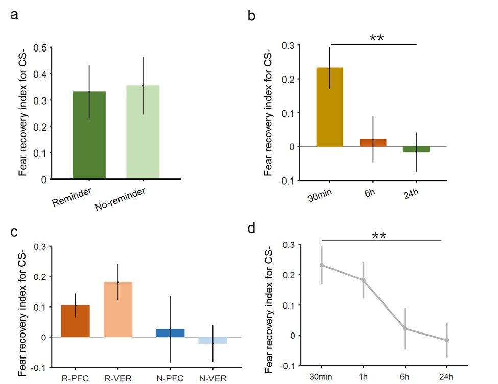
(6D) The 6 hour group was clearly tested at a different time of day compared to the 30 min and 24 hour groups. This could have influenced the SCRs in this group and, thereby, contributed to the pattern of results obtained.
Again, we answered this question in our previous response. Please see the following for our previous response:
For the 30min and 24h groups, the test phase can be arranged in the morning, in the afternoon or at night. However, for the 6h group, the test phase was inevitably in the afternoon or at night since we wanted to exclude the potential influence of night sleep on the expression of fear memory (see Author response table 1 below). If we restricted the test time in the afternoon or at night for all three groups, then the timing of their extinction training was not matched.
Author response table 1.
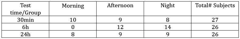
Nevertheless, we also went back and examined the data for the subjects only tested in the afternoon or at nights in the 30min and 24h groups to match with the 6h group where all the subjects were tested either in the afternoon or at night. According to the table above, we have 17 subjects for the 30min group (9+8),18 subjects for the 24h group (9 + 9) and 26 subjects for the 6h group (12 + 14). As Author response image 2 shows, the SCR patterns in the fear acquisition, extinction and test phases were similar to the results presented in the original figure.
Author response image 2.
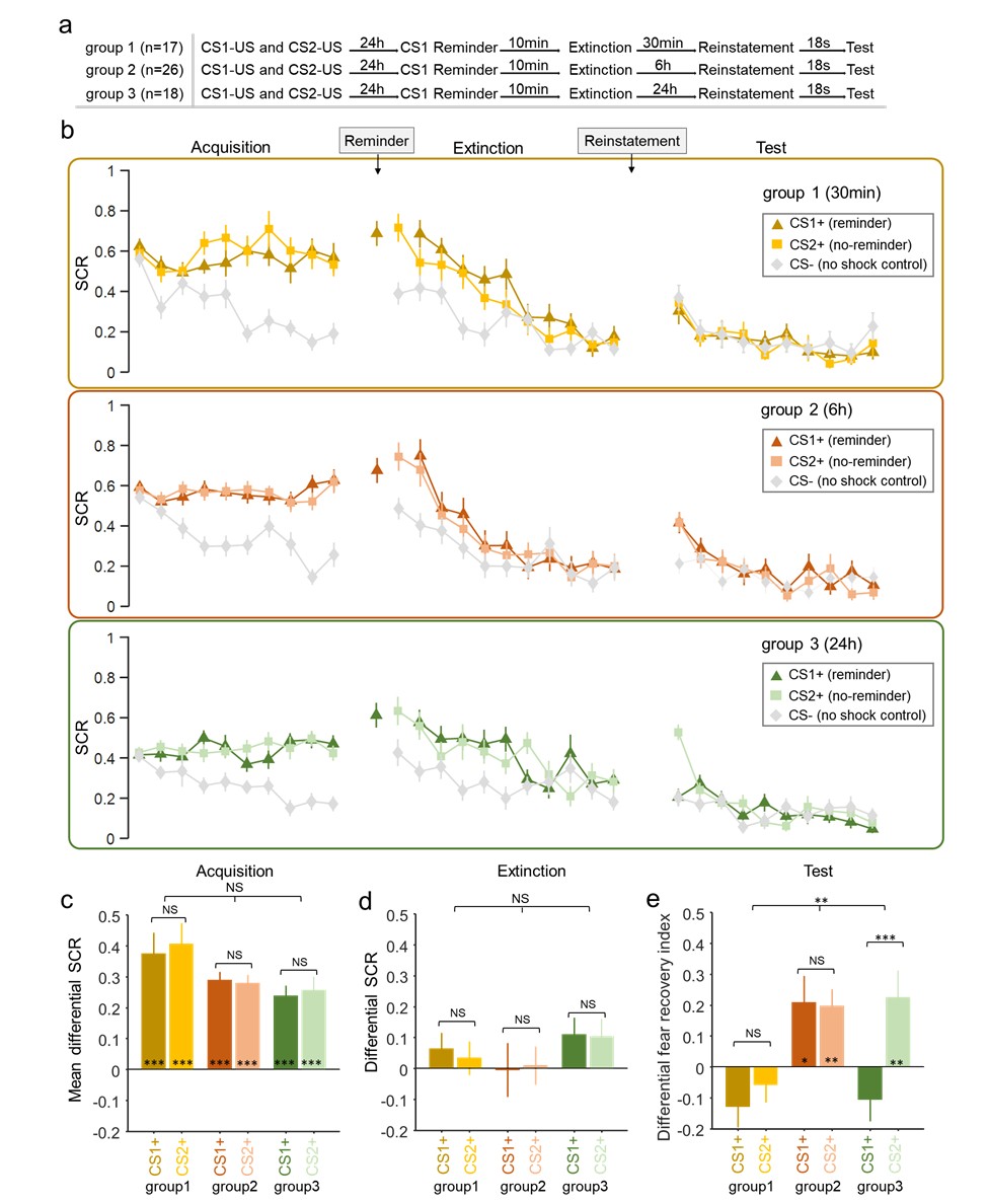
(6E) The authors find different patterns of responses to CS1 and CS2 when they were tested 30 min after extinction versus 24 h after extinction. On this basis, they infer distinct memory update mechanisms. However, I still can't quite see why the different patterns of responses at these two time points after extinction need to be taken to infer different memory update mechanisms. That is, the different patterns of responses at the two time points could be indicative of the same "memory update mechanism" in the sense that the retrieval-extinction procedure induces a short-term memory suppression that serves as the basis for the longer-term memory suppression (i.e., the reconsolidation effect). My pushback on this point is based on the notion of what constitutes a memory update mechanism; and is motivated by what I take to be a rather loose use of language/terminology in the reconsolidation literature and this paper specifically (for examples, see the title of the paper and line 2 of the abstract).
As we mentioned previously, the term “mechanism” might have different connotations for different researchers. We aim to report a novel memory deficit following the retrieval-extinction paradigm, which differed significantly from the purported reconsolidation related long-term fear amnesia in terms of its timescale, cue-specificity and thought-control ability. Further TMS study confirmed that the intact dlPFC function is necessary for the short-term memory deficit. It’s based on these results we proposed that the short-term fear amnesia might be related to a different cognitive “mechanism”. As mentioned above, we now clarify what we mean by “mechanism” in the abstract and introduction (lines 31-34, 97-101).
Reviewer #2 (Public review):
The fear acquisition data is converted to a differential fear SCR and this is what is analysed (early vs late). However, the figure shows the raw SCR values for CS+ and CS- and therefore it is unclear whether acquisition was successful (despite there being an "early" vs "late" effect - no descriptives are provided).
(1) There are still no descriptive statistics to substantiate learning in Experiment 1.
We answered this question in our previous response letter. We are sorry that the definition of “early” and “late” trials was scattered in the manuscript. For example, we wrote “the late phase of acquisition (last 5 trials)” (Line 375-376) in the results section. Since there were 10 trials in total for the acquisition stage, we define the first 5 trials and the last 5 trials as “early” and “late” phases of the acquisition stage and explicitly added them into the first occasion “early” and “late” terms appeared (lines 316-318).
In the results section, we did test whether the acquisition was successful in our previous manuscript (Line 316-325):
“To assess fear acquisition across groups (Figure 1B and C), we conducted a mixed two-way ANOVA of group (reminder vs. no-reminder) x time (early vs. late part of the acquisition; first 5 and last 5 trials, correspondingly) on the differential fear SCR. Our results showed a significant main effect of time (early vs. late; F<sub>1,55</sub> \= 6.545, P \= 0.013, η<sup>2</sup> \= 0.106), suggesting successful fear acquisition in both groups. There was no main effect of group (reminder vs. no-reminder) or the group x time interaction (group: F<sub>1,55</sub> \= 0.057, P \= 0.813, η<sup>2</sup> \= 0.001; interaction: F<sub>1,55</sub> \= 0.066, P \= 0.798, η<sup>2</sup> \= 0.001), indicating similar levels of fear acquisition between two groups. Post-hoc t-tests confirmed that the fear responses to the CS+ were significantly higher than that of CS- during the late part of acquisition phase in both groups (reminder group: t<sub>29</sub> \= 6.642, P < 0.001; no-reminder group: t<sub>26</sub> = 8.522, P < 0.001; Figure 1C). Importantly, the levels of acquisition were equivalent in both groups (early acquisition: t<sub>55</sub> \= -0.063, P \= 0.950; late acquisition: t<sub>55</sub> \= -0.318, P \= 0.751; Figure 1C).”
In Experiment 1 (Test results) it is unclear whether the main conclusion stems from a comparison of the test data relative to the last extinction trial ("we defined the fear recovery index as the SCR difference between the first test trial and the last extinction trial for a specific CS") or the difference relative to the CS- ("differential fear recovery index between CS+ and CS-"). It would help the reader assess the data if Fig 1e presents all the indexes (both CS+ and CS-). In addition, there is one sentence which I could not understand "there is no statistical difference between the differential fear recovery indexes between CS+ in the reminder and no reminder groups (P=0.048)". The p value suggests that there is a difference, yet it is not clear what is being compared here. Critically, any index taken as a difference relative to the CS- can indicate recovery of fear to the CS+ or absence of discrimination relative to the CS-, so ideally the authors would want to directly compare responses to the CS+ in the reminder and no-reminder groups. In the absence of such comparison, little can be concluded, in particular if SCR CS- data is different between groups. The latter issue is particularly relevant in Experiment 2, in which the CS- seems to vary between groups during the test and this can obscure the interpretation of the result.
(2) In the revised analyses, the authors now show that CS- changes in different groups (for example, Experiment 2) so this means that there is little to conclude from the differential scores because these depend on CS-. It is unclear whether the effects arise from CS+ performance or the differential which is subject to CS- variations.
There was a typo in the “P = 0.048” sentence and we have corrected it in our last response letter. Also in the previous response letter, we specifically addressed how the fear recovery index was defined (also in the revised manuscript).
In most of the fear conditioning studies, CS- trials were included as the baseline control. In turn, most of the analyses conducted also involved comparisons between different groups. Directly comparing CS+ trials across groups (or conditions) is rare. In our study 2, we showed that the CS- response decreased as a function of testing delays (30min, 1hr, 6hr and 24hr). Ideally, it would be nice to show that the CS- across groups/conditions did not change. However, even in those circumstances, comparisons are still based on the differential CS response (CS+ minus CS-), that is, the difference of difference. It is also important to note that difference score is important as CS+ alone or across conditions is difficult to interpret, especially in humans, due to noise, signal fluctuations, and irrelevant stimulus features; therefore trials-wise reference is essential to assess the CS+ in the context of a reference stimulus in each trial (after all, the baselines are different). We are listing a few influential papers in the field that the CS- responses were not particularly equivalent across groups/conditions and argue that this is a routine procedure (Kindt & Soeter 2018 Figs. 2-3; Sevenster et al., 2013 Fig. 3; Liu et al., 2014 Fig. 1; Raio et al., 2017 Fig. 2).
In experiment 1, the findings suggest that there is a benefit of retrieval followed by extinction in a short-term reinstatement test. In Experiment 2, the same effect is observed to a cue which did not undergo retrieval before extinction (CS2+), a result that is interpreted as resulting from cue-independence, rather than a failure to replicate in a within-subjects design the observations of Experiment 1 (between-subjects). Although retrieval-induced forgetting is cue-independent (the effect on items that are suppressed [Rp-] can be observed with an independent probe), it is not clear that the current findings are similar, and thus that the strong parallels made are not warranted. Here, both cues have been extinguished and therefore been equally exposed during the critical stage.
(3) The notion that suppression is automatic is speculative at best
We have responded the same question in our previous revision. Please note that our results from study 1 (the comparison between reminder and no-reminder groups) was not set up to test the cue-independence hypothesis for the short-term amnesia with only one CS+. Results from both study 2 (30min condition) and study 3 confirmed the cue-independence hypothesis and therefore we believe interpreting results from study 2 as “a failure to replicate in a within-subject design of the observations of Experiment 1” is not the case.
We agree that the proposal of automatic or unconscious memory suppression is speculative and that’s why we mentioned it in the discussion. The timescale, cue-specificity and the thought-control ability dependence of the short-term fear amnesia identified in our studies was reminiscent of the memory suppression effects reported in the previous literature. However, memory suppression typically adopted a conscious “suppression” treatment (such as the think/no-think paradigm), which was absent in the current study. However, the retrieval-induced forgetting (RIF), which is also considered a memory suppression paradigm via inhibitory control, does not require conscious effort to suppress any particular thought. Based on these results and extant literature, we raised the possibility of memory suppression as a potential mechanism. We make clear in the discussion that the suppression hypothesis and connections with RIF will require further evidence (lines 615-616):
“future research will be needed to investigate whether the short-term effect we observed is specifically related to associative memory or the spontaneous nature of suppression as in RIF (Figure 6C).”
(4) It still struggle with the parallels between these findings and the "limbo" literature. Here you manipulated the retention interval, whereas in the cited studies the number of extinction (exposure) was varied. These are two completely different phenomena.
We borrowed the “limbo” term to stress the transitioning from short-term to long-term memory deficits (the 6hr test group). Merlo et al. (2014) found that memory reconsolidation and extinction were dissociable processes depending on the extent of memory retrieval. They argued that there was a “limbo” transitional state, where neither the reconsolidation nor the extinction process was engaged. Our results suggest that at the test delay of 6hr, neither the short-term nor the long-term effect was present, signaling a “transitional” state after which the short-term memory deficit wanes and the long-term deficit starts to take over. We make this idea more explicit as follows (lines 622-626):
“These works identified important “boundary conditions” of memory retrieval in affecting the retention of the maladaptive emotional memories. In our study, however, we showed that even within a boundary condition previously thought to elicit memory reconsolidation, mnemonic processes other than reconsolidation could also be at work, and these processes jointly shape the persistence of fear memory.”
(5) My point about the data problematic for the reconsolidation (and consolidation) frameworks is that they observed memory in the absence of the brain substrates that are needed for memory to be observed. The answer did not address this. I do not understand how the latent cause model can explain this, if the only difference is the first ITI. Wouldn't participants fail to integrate extinction with acquisition with a longer ITI?
We take the sentence “they observed memory in the absence of the brain substrates that are needed for memory to be observed” as referring to the long-term memory deficit in our study. As we responded before, the aim of this manuscript was not about investigating the brain substrates involved in memory reconsolidation (or consolidation). Using a memory retrieval-extinction paradigm, we discovered a novel short-term memory effect, which differed from the purported reconsolidation effect in terms of timescale, cue-specificity and thought-control ability dependence. We further showed that both memory retrieval and intact dlPFC functions were necessary to observe the short-term memory deficit effect. Therefore, we conclude that the brain mechanism involved in such an effect should be different from the one related to the purported reconsolidation effect. We make this idea more explicit as follows (lines 546-547):
“Therefore, findings of the short-term fear amnesia suggest that the reconsolidation framework falls short to accommodate this more immediate effect (Figure 6A and B).”
Whilst I could access the data in the OFS site, I could not make sense of the Matlab files as there is no signposting indicating what data is being shown in the files. Thus, as it stands, there is no way of independently replicating the analyses reported.
(6) The materials in the OSF site are the same as before, they haven't been updated.
Last time we thought the main issue was the OSF site not being publicly accessible and thus made it open to all visitors. We have added descriptive file to explain the variables to help visitors to replicate the analyses we took.
(7) Concerning supplementary materials, the robustness tests are intended to prove that you 1) can get the same results by varying the statistical models or 2) you can get the same results when you include all participants. Here authors have done both so this does not help. Also, in the rebuttal letter, they stated "Please note we did not include non-learners in these analyses " which contradicts what is stated in the figure captions "(learners + non learners)"
In the supplementary materials, we did the analyses of varying the statistical models and including both learners and non-learners separately, instead of both. In fact, in the supplementary material Figs. 1 & 2, we included all the participants and performed similar analysis as in the main text and found similar results (learners + non-learners). Also, in the text of the supplementary material, we used a different statistical analysis method to only learners (analyzing subjects reported in the main text using a different method) and achieved similar results. We believe this is exactly what the reviewer suggested us to do. Also there seems to be a misunderstanding for the "Please note we did not include non-learners in these analyses" sentence in the rebuttal letter. As the reviewer can see, the full sentence read “Please note we did not include non-learners in these analyses (the texts of the supplementary materials)”. We meant to express that the Figures and texts in the supplementary material reflect two approaches: 1) Figures depicting re-analysis with all the included subjects (learners + non learners); 2) Text describing different analysis with learners. We added clarifications to emphasize these approaches in the supplementary materials.
(8) Finally, the literature suggesting that reconsolidation interference "eliminates" a memory is not substantiated by data nor in line with current theorising, so I invite a revision of these strong claims.
We agree and have toned down the strong claims.
Overall, I conclude that the revised manuscript did not address my main concerns.
In both rounds of responses, we tried our best to address the reviewer’s concerns. We hope that the clarifications in this letter and revisions in the text address the remaining concerns. Thank you for your feedback.
Reference:
Kindt, M. and Soeter, M. 2018. Pharmacologically induced amnesia for learned fear is time and sleep dependent. Nat Commun, 9, 1316.
Liu, J., Zhao, L., Xue, Y., Shi, J., Suo, L., Luo, Y., Chai, B., Yang, C., Fang, Q., Zhang, Y., Bao, Y., Pickens, C. L. and Lu, L. 2014. An unconditioned stimulus retrieval extinction procedure to prevent the return of fear memory. Biol Psychiatry, 76, 895-901.
Raio, C. M., Hartley, C. A., Orederu, T. A., Li, J. and Phelps, E. A. 2017. Stress attenuates the flexible updating of aversive value. Proc Natl Acad Sci U S A, 114, 11241-11246.
Sevenster, D., Beckers, T., & Kindt, M. 2013. Prediction error governs pharmacologically induced amnesia for learned fear. Science (New York, N.Y.), 339(6121), 830–833.
Reviewer #3 (Public review):
This study concerns how observers (human participants) detect changes in the statistics of their environment, termed regime shifts. To make this concrete, a series of 10 balls are drawn from an urn that contains mainly red or mainly blue balls. If there is a regime shift, the urn is changed over (from mainly red to mainly blue) at some point in the 10 trials. Participants report their belief that there has been a regime shift as a % probability. Their judgement should (mathematically) depend on the prior probability of a regime shift (which is set at one of three levels) and the strength of evidence (also one of three levels, operationalized as the proportion of red balls in the mostly-blue urn and vice versa). Participants are directly instructed of the prior probability of regime shift and proportion of red balls, which are presented on-screen as numerical probabilities. The task therefore differs from most previous work on this question in that probabilities are instructed rather than learned by observation, and beliefs are reported as numerical probabilities rather than being inferred from participants' choice behaviour (as in many bandit tasks, such as Behrens 2007 Nature Neurosci).
The key behavioural finding is that participants over-estimate the prior probability of regime change when it is low, and under estimate it when it is high; and participants over-estimate the strength of evidence when it is low and under-estimate it when it is high. In other words participants make much less distinction between the different generative environments than an optimal observer would. This is termed 'system neglect'. A neuroeconomic-style mathematical model is presented and fit to data.
Functional MRI results how that strength of evidence for a regime shift (roughly, the surprise associated with a blue ball from an apparently red urn) is associated with activity in the frontal-parietal orienting network. Meanwhile, at time-points where the probability of a regime shift is high, there is activity in another network including vmPFC. Both networks show individual differences effects, such that people who were more sensitive to strength of evidence and prior probability show more activity in the frontal-parietal and vmPFC-linked networks respectively.
Strengths
(1) The study provides a different task for looking at change-detection and how this depends on estimates of environmental volatility and sensory evidence strength, in which participants are directly and precisely informed of the environmental volatility and sensory evidence strength rather than inferring them through observation as in most previous studies<br /> (2) Participants directly provide belief estimates as probabilities rather than experimenters inferring them from choice behaviour as in most previous studies<br /> (3) The results are consistent with well-established findings that surprising sensory events activate the frontal-parietal orienting network whilst updating of beliefs about the word ('regime shift') activates vmPFC.
Weaknesses
(1) The use of numerical probabilities (both to describe the environments to participants, and for participants to report their beliefs) may be problematic because people are notoriously bad at interpreting probabilities presented in this way, and show poor ability to reason with this information (see Kahneman's classic work on probabilistic reasoning, and how it can be improved by using natural frequencies). Therefore the fact that, in the present study, people do not fully use this information, or use it inaccurately, may reflect the mode of information delivery.
(2) Although a very precise model of 'system neglect' is presented, many other models could fit the data.
For example, you would get similar effects due to attraction of parameter estimates towards a global mean - essentially application of a hyper-prior in which the parameters applied by each participant in each block are attracted towards the experiment-wise mean values of these parameters. For example, the prior probability of regime shift ground-truth values [0.01, 0.05, 0.10] are mapped to subjective values of [0.037, 0.052, 0.069]; this would occur if observers apply a hyper-prior that the probability of regime shift is about 0.05 (the average value over all blocks). This 'attraction to the mean' is a well-established phenomenon and cannot be ruled out with the current data (I suppose you could rule it out by comparing to another dataset in which the mean ground-truth value was different).
More generally, any model in which participants don't fully use the numerical information they were given would produce apparent 'system neglect'. Four qualitatively different example reasons are: 1. Some individual participants completely ignored the probability values given. 2. Participants did not ignore the probability values given, but combined them with a hyperprior as above. 3. Participants had a reporting bias where their reported beliefs that a regime-change had occurred tend to be shifted towards 50% (rather than reporting 'confident' values such 5% or 95%). 4. Participants underweighted probability outliers resulting in underweighting of evidence in the 'high signal diagnosticity' environment (10.1016/j.neuron.2014.01.020 )
In summary I agree that any model that fits the data would have to capture the idea that participants don't differentiate between the different environments as much as they should, but I think there are a number of qualitatively different reasons why they might do this - of which the above are only examples - hence I find it problematic that the authors present the behaviour as evidence for one extremely specific model.
(3) Despite efforts to control confounds in the fMRI study, including two control experiments, I think some confounds remain.
For example, a network of regions is presented as correlating with the cumulative probability that there has been a regime shift in this block of 10 samples (Pt). However, regardless of the exact samples shown, doesn't Pt always increase with sample number (as by the time of later samples, there have been more opportunities for a regime shift)? Unless this is completely linear, the effect won't be controlled by including trial number as a co-regressor (which was done).
On the other hand, two additional fMRI experiments are done as control experiments and the effect of Pt in the main study is compared to Pt in these control experiments. Whilst I admire the effort in carrying out control studies, I can't understand how these particular experiment are useful controls. For example in experiment 3 participants simply type in numbers presented on the screen - how can we even have an estimate of Pt from this task?
(4) The Discussion is very long, and whilst a lot of related literature is cited, I found it hard to pin down within the discussion, what the key contributions of this study are. In my opinion it would be better to have a short but incisive discussion highlighting the advances in understanding that arise from the current study, rather than reviewing the field so broadly.
Editors’ note: Reviewer #2 was unavailable to re-review the manuscript. Reviewer #3 was added for this round of review to ensure two reviewers and because of their expertise in the computational and modelling aspects of the work.
Author response:
The following is the authors’ response to the current reviews.
eLife Assessment<br /> This study offers valuable insights into how humans detect and adapt to regime shifts, highlighting distinct contributions of the frontoparietal network and ventromedial prefrontal cortex to sensitivity to signal diagnosticity and transition probabilities. The combination of an innovative task design, behavioral modeling, and model-based fMRI analyses provides a solid foundation for the conclusions; however, the neuroimaging results have several limitations, particularly a potential confound between the posterior probability of a switch and the passage of time that may not be fully controlled by including trial number as a regressor. The control experiments intended to address this issue also appear conceptually inconsistent and, at the behavioral level, while informing participants of conditional probabilities rather than requiring learning is theoretically elegant, such information is difficult to apply accurately, as shown by well-documented challenges with conditional reasoning and base-rate neglect. Expressing these probabilities as natural frequencies rather than percentages may have improved comprehension. Overall, the study advances understanding of belief updating under uncertainty but would benefit from more intuitive probabilistic framing and stronger control of temporal confounds in future work.
We thank the editors for the assessment. The editor added several limitations based on the new reviewer 3 in this round, which we address below.
With regard to temporal confounds, we clarified in the main text and response to Reviewer 3 that we had already addressed the potential confound between posterior probability of a switch and passage of time in GLM-2 with the inclusion of intertemporal prior. After adding intertemporal prior in the GLM, we still observed the same fMRI results on probability estimates. In addition, we did two other robustness checks, which we mentioned in the manuscript.
With regard to response mode (probability estimation rather than choice or indicating natural frequencies), we wish to point out that the in previous research by Massey and Wu (2005), which the current study was based on, the concern of participants showing system-neglect tendencies due to the mode of information delivery, namely indicating beliefs through reporting probability estimates rather than through choice or other response mode was addressed. Massy and Wu (2005, Study 3) found the same biases when participants performed a choice task that did not require them to indicate probability estimates.
With regard to the control experiments, the control experiments in fact were not intended to address the confounds between posterior probability and passage of time. Rather, they aimed to address whether the neural findings were unique to change detection (Experiment 2) and to address visual and motor confounds (Experiment 3). These and the results of the control experiments were mentioned on page 18-19.
Finally, we wish to highlight that we had performed detailed model comparisons after reviewer 2’s suggestions. Although reviewer 2 was unable to re-review the manuscript, we believe this provides insight into the literature on change detection. See “Incorporating signal dependency into system-neglect model led to better models for regime-shift detection” (p.27-30). The model comparison showed that system-neglect models that incorporate signal dependency are better models than the original system-neglect model in describing participants probability estimates. This suggests that people respond to change-consistent and change-inconsistent signals differently when judging whether the regime had changed. This was not reported in previous behavioral studies and was largely inspired by the neural finding on signal dependency in the frontoparietal cortex. It indicates that neural findings can provide novel insights into computational modeling of behavior.
Public Reviews:
Reviewer #1 (Public review):
Summary:
The study examines human biases in a regime-change task, in which participants have to report the probability of a regime change in the face of noisy data. The behavioral results indicate that humans display systematic biases, in particular, overreaction in stable but noisy environments and underreaction in volatile settings with more certain signals. fMRI results suggest that a frontoparietal brain network is selectively involved in representing subjective sensitivity to noise, while the vmPFC selectively represents sensitivity to the rate of change.
Strengths:
- The study relies on a task that measures regime-change detection primarily based on descriptive information about the noisiness and rate of change. This distinguishes the study from prior work using reversal-learning or change-point tasks in which participants are required to learn these parameters from experiences. The authors discuss these differences comprehensively.
- The study uses a simple Bayes-optimal model combined with model fitting, which seems to describe the data well. The model is comprehensively validated.
- The authors apply model-based fMRI analyses that provide a close link to behavioral results, offering an elegant way to examine individual biases.
We thank the reviewer for the comments.
Weaknesses:
The authors have adequately addressed most of my prior concerns.
We thank the reviewer for recognizing our effort in addressing your concerns.
My only remaining comment concerns the z-test of the correlations. I agree with the non-parametric test based on bootstrapping at the subject level, providing evidence for significant differences in correlations within the left IFG and IPS.
However, the parametric test seems inadequate to me. The equation presented is described as the Fisher z-test, but the numerator uses the raw correlation coefficients (r) rather than the Fisher-transformed values (z). To my understanding, the subtraction should involve the Fisher z-scores, not the raw correlations.
More importantly, the Fisher z-test in its standard form assumes that the correlations come from independent samples, as reflected in the denominator (which uses the n of each independent sample). However, in my opinion, the two correlations are not independent but computed within-subject. In such cases, parametric tests should take into account the dependency. I believe one appropriate method for the current case (correlated correlation coefficients sharing a variable [behavioral slope]) is explained here:
Meng, X.-l., Rosenthal, R., & Rubin, D. B. (1992). Comparing correlated correlation coefficients. Psychological Bulletin, 111(1), 172-175. https://doi.org/10.1037/0033-2909.111.1.172
It should be implemented here:
Diedenhofen B, Musch J (2015) cocor: A Comprehensive Solution for the Statistical Comparison of Correlations. PLoS ONE 10(4): e0121945. https://doi.org/10.1371/journal.pone.0121945
My recommendation is to verify whether my assumptions hold, and if so, perform a test that takes correlated correlations into account. Or, to focus exclusively on the non-parametric test.
In any case, I recommend a short discussion of these findings and how the authors interpret that some of the differences in correlations are not significant.
Thank you for the careful check. Yes. This was indeed a mistake from us. We also agree that the two correlations are not independent. Therefore, we modified the test that accounts for dependent correlations by following Meng et al. (1992) suggested by the reviewer.
We referred to the correlation between neural and behavioral sensitivity at change-consistent (blue) signals as , and that at change-inconsistent (red) signals as 𝑟<sub>𝑟𝑒𝑑</sub>. To statistically compare these two correlations, we adopted the approach of Meng et al. (1992), which specifically tests differences between dependent correlations according to the following equation
where is the number of subjects, 𝑧<sub>𝑟𝑖</sub> is the Fisher z-transformed value of 𝑟<sub>𝑖</sub>, 𝑟<sub>1</sub> = 𝑟<sub>𝑏𝑙𝑢𝑒</sub> and 𝑟<sub>2</sub> = 𝑟<sub>𝑟𝑒𝑑</sub>. 𝑟<sub>𝑥</sub> is the correlation between the neural sensitivity at change-consistent signals and change-inconsistent signals.
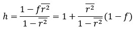
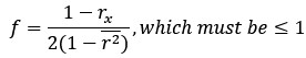
Where  is the mean of the
 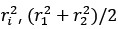 , and 𝑓 should be set to 1 if > 1.
We found that among the five ROIs in the frontoparietal network, two of them, namely the left IFG and left IPS, the difference in correlation was significant (one-tailed z test; left IFG: 𝑧 = 1.8908, 𝑝 = 0.0293; left IPS: 𝑧 = 2.2584, 𝑝 = 0.0049). For the remaining three ROIs, the difference in correlation was not significant (dmPFC: 𝑧 = 0.9522, 𝑝 = 0.1705; right IFG: 𝑧 = 0.9860, 𝑝 = 0.1621; right IPS: 𝑧 = 1.4833, 𝑝 = 0.0690). We chose one-tailed test because we already know the correlation under the blue signals was significantly greater than 0. These updated results are consistent with the nonparametric tests we had already performed and we will update them in the revised manuscript.
Reviewer #3 (Public review):
This study concerns how observers (human participants) detect changes in the statistics of their environment, termed regime shifts. To make this concrete, a series of 10 balls are drawn from an urn that contains mainly red or mainly blue balls. If there is a regime shift, the urn is changed over (from mainly red to mainly blue) at some point in the 10 trials. Participants report their belief that there has been a regime shift as a % probability. Their judgement should (mathematically) depend on the prior probability of a regime shift (which is set at one of three levels) and the strength of evidence (also one of three levels, operationalized as the proportion of red balls in the mostly-blue urn and vice versa). Participants are directly instructed of the prior probability of regime shift and proportion of red balls, which are presented on-screen as numerical probabilities. The task therefore differs from most previous work on this question in that probabilities are instructed rather than learned by observation, and beliefs are reported as numerical probabilities rather than being inferred from participants' choice behaviour (as in many bandit tasks, such as Behrens 2007 Nature Neurosci).
The key behavioural finding is that participants over-estimate the prior probability of regime change when it is low, and under estimate it when it is high; and participants over-estimate the strength of evidence when it is low and under-estimate it when it is high. In other words participants make much less distinction between the different generative environments than an optimal observer would. This is termed 'system neglect'. A neuroeconomic-style mathematical model is presented and fit to data.
Functional MRI results how that strength of evidence for a regime shift (roughly, the surprise associated with a blue ball from an apparently red urn) is associated with activity in the frontal-parietal orienting network. Meanwhile, at time-points where the probability of a regime shift is high, there is activity in another network including vmPFC. Both networks show individual differences effects, such that people who were more sensitive to strength of evidence and prior probability show more activity in the frontal-parietal and vmPFC-linked networks respectively.
We thank the reviewer for the overall descriptions of the manuscript.
Strengths:
(1) The study provides a different task for looking at change-detection and how this depends on estimates of environmental volatility and sensory evidence strength, in which participants are directly and precisely informed of the environmental volatility and sensory evidence strength rather than inferring them through observation as in most previous studies
(2) Participants directly provide belief estimates as probabilities rather than experimenters inferring them from choice behaviour as in most previous studies<br /> (3) The results are consistent with well-established findings that surprising sensory events activate the frontal-parietal orienting network whilst updating of beliefs about the word ('regime shift') activates vmPFC.
Thank you for these assessments.
Weaknesses:
(1) The use of numerical probabilities (both to describe the environments to participants, and for participants to report their beliefs) may be problematic because people are notoriously bad at interpreting probabilities presented in this way, and show poor ability to reason with this information (see Kahneman's classic work on probabilistic reasoning, and how it can be improved by using natural frequencies). Therefore the fact that, in the present study, people do not fully use this information, or use it inaccurately, may reflect the mode of information delivery.
We appreciate the reviewer’s concern on this issue. The concern was addressed in Massey and Wu (2005) as participants performed a choice task in which they were not asked to provide probability estimates (Study 3 in Massy and Wu, 2005). Instead, participants in Study 3 were asked to predict the color of the ball before seeing a signal. This was a more intuitive way of indicating his or her belief about regime shift. The results from the choice task were identical to those found in the probability estimation task (Study 1 in Massey and Wu). We take this as evidence that the system-neglect behavior the participants showed was less likely to be due to the mode of information delivery.
(2) Although a very precise model of 'system neglect' is presented, many other models could fit the data.
For example, you would get similar effects due to attraction of parameter estimates towards a global mean - essentially application of a hyper-prior in which the parameters applied by each participant in each block are attracted towards the experiment-wise mean values of these parameters. For example, the prior probability of regime shift ground-truth values [0.01, 0.05, 0.10] are mapped to subjective values of [0.037, 0.052, 0.069]; this would occur if observers apply a hyper-prior that the probability of regime shift is about 0.05 (the average value over all blocks). This 'attraction to the mean' is a well-established phenomenon and cannot be ruled out with the current data (I suppose you could rule it out by comparing to another dataset in which the mean ground-truth value was different).
We thank the reviewer for this comment. It is true that the system-neglect model is not entirely inconsistent with regression to the mean, regardless of whether the implementation has a hyper prior or not. In fact, our behavioral measure of sensitivity to transition probability and signal diagnosticity, which we termed the behavioral slope, is based on linear regression analysis. In general, the modeling approach in this paper is to start from a generative model that defines ideal performance and consider modifying the generative model when systematic deviations in actual performance from the ideal is observed. In this approach, a generative model with hyper-prior would be more complex to begin with, and a regression to the mean idea by itself does not generate a priori predictions.
More generally, any model in which participants don't fully use the numerical information they were given would produce apparent 'system neglect'. Four qualitatively different example reasons are: 1. Some individual participants completely ignored the probability values given. 2. Participants did not ignore the probability values given, but combined them with a hyperprior as above. 3. Participants had a reporting bias where their reported beliefs that a regime-change had occurred tend to be shifted towards 50% (rather than reporting 'confident' values such 5% or 95%). 4. Participants underweighted probability outliers resulting in underweighting of evidence in the 'high signal diagnosticity' environment (10.1016/j.neuron.2014.01.020 )
In summary I agree that any model that fits the data would have to capture the idea that participants don't differentiate between the different environments as much as they should, but I think there are a number of qualitatively different reasons why they might do this - of which the above are only examples - hence I find it problematic that the authors present the behaviour as evidence for one extremely specific model.
Thank you for raising this point. The modeling principle we adopt is the following. We start from the normative model—the Bayesian model—that defined what normative behavior should look like. We compared participants’ behavior with the Bayesian model and found systematic deviations from it. To explain those systematic deviations, we considered modeling options within the confines of the same modeling framework. In other words, we considered a parameterized version of the Bayesian model, which is the system-neglect model and examined through model comparison the best modeling choice. This modeling approach is not uncommon, and many would agree this is the standard approach in economics and psychology. For example, Kahneman and Tversky adopted this approach when proposing prospect theory, a modification of expected utility theory where expected utility theory can be seen as one specific model for how utility of an option should be computed.
(3) Despite efforts to control confounds in the fMRI study, including two control experiments, I think some confounds remain.
For example, a network of regions is presented as correlating with the cumulative probability that there has been a regime shift in this block of 10 samples (Pt). However, regardless of the exact samples shown, doesn't Pt always increase with sample number (as by the time of later samples, there have been more opportunities for a regime shift)? Unless this is completely linear, the effect won't be controlled by including trial number as a co-regressor (which was done).
Thank you for raising this concern. Yes, Pt always increases with sample number regardless of evidence (seeing change-consistent or change-inconsistent signals). This is captured by the ‘intertemporal prior’ in the Bayesian model, which we included as a regressor in our GLM analysis (GLM-2), in addition to Pt. In short, GLM-1 had Pt and sample number. GLM-2 had Pt, intertemporal prior, and sample number, among other regressors. And we found that, in both GLM-1 and GLM-2, both vmPFC and ventral striatum correlated with Pt.
To make this clearer, we updated the main text to further clarify this on p.18:
On the other hand, two additional fMRI experiments are done as control experiments and the effect of Pt in the main study is compared to Pt in these control experiments. Whilst I admire the effort in carrying out control studies, I can't understand how these particular experiment are useful controls. For example in experiment 3 participants simply type in numbers presented on the screen - how can we even have an estimate of Pt from this task?
We thank the reviewer for this comment. The purpose of Experiment 3 was to control for visual and motor confounds. In other words, if subjects saw the similar visual layout and were just instructed to press numbers, would we observe the vmPFC, ventral striatum, and the frontoparietal network like what we did in the main experiment (Experiment 1)?
The purpose of Experiment 2 was to establish whether what we found about Pt was unique to change detection. In Experiment 2, subjects estimated the probability that the current regime is the blue regime (just as they did in Experiment 1) except that there were no regime shifts involved. In other words, it is possible that the regions we identified were generally associated with probability estimation and not particularly about change detection. And we used Experiment 2 to examine whether this were true.
(4) The Discussion is very long, and whilst a lot of related literature is cited, I found it hard to pin down within the discussion, what the key contributions of this study are. In my opinion it would be better to have a short but incisive discussion highlighting the advances in understanding that arise from the current study, rather than reviewing the field so broadly.
Thank you. We received different feedbacks from previous reviews on what to include in Discussion. To address the reviewer’s concern, we will revise the Discussion to better highlight the key contributions of the current study at the beginning of Discussion.
Recommendations for the authors:
Reviewer #3 (Recommendations for the authors):
Many of the figures are too tiny - the writing is very small, as are the pictures of brains. I'd suggest adjusting these so they will be readable without enlarging.
Thank you. We will enlarge the figures to make them more readable.
The following is the authors’ response to the original reviews.
Public Reviews:
Reviewer #1 (Public review):
Summary:
The study examines human biases in a regime-change task, in which participants have to report the probability of a regime change in the face of noisy data. The behavioral results indicate that humans display systematic biases, in particular, overreaction in stable but noisy environments and underreaction in volatile settings with more certain signals. fMRI results suggest that a frontoparietal brain network is selectively involved in representing subjective sensitivity to noise, while the vmPFC selectively represents sensitivity to the rate of change.
Strengths:
(1) The study relies on a task that measures regime-change detection primarily based on descriptive information about the noisiness and rate of change. This distinguishes the study from prior work using reversal-learning or change-point tasks in which participants are required to learn these parameters from experiences. The authors discuss these differences comprehensively.
Thank you for recognizing our contribution to the regime-change detection literature and our effort in discussing our findings in relation to the experience-based paradigms.
(2) The study uses a simple Bayes-optimal model combined with model fitting, which seems to describe the data well.
Thank you for recognizing the contribution of our Bayesian framework and systemneglect model.
(3) The authors apply model-based fMRI analyses that provide a close link to behavioral results, offering an elegant way to examine individual biases.
Thank you for recognizing our execution of model-based fMRI analyses and effort in using those analyses to link with behavioral biases.
Weaknesses:
My major concern is about the correlational analysis in the section "Under- and overreactions are associated with selectivity and sensitivity of neural responses to system parameters", shown in Figures 5c and d (and similarly in Figure 6). The authors argue that a frontoparietal network selectively represents sensitivity to signal diagnosticity, while the vmPFC selectively represents transition probabilities. This claim is based on separate correlational analyses for red and blue across different brain areas. The authors interpret the finding of a significant correlation in one case (blue) and an insignificant correlation (red) as evidence of a difference in correlations (between blue and red) but don't test this directly. This has been referred to as the "interaction fallacy" (Niewenhuis et al., 2011; Makin & Orban de Xivry 2019). Not directly testing the difference in correlations (but only the differences to zero for each case) can lead to wrong conclusions. For example, in Figure 5c, the correlation for red is r = 0.32 (not significantly different from zero) and r = 0.48 (different from zero). However, the difference between the two is 0.1, and it is likely that this difference itself is not significant. From a statistical perspective, this corresponds to an interaction effect that has to be tested directly. It is my understanding that analyses in Figure 6 follow the same approach.
Relevant literature on this point is:
Nieuwenhuis, S, Forstmann, B & Wagenmakers, EJ (2011). Erroneous analyses of interactions in neuroscience: a problem of significance. Nat Neurosci 14, 11051107. https://doi.org/10.1038/nn.2886
Makin TR, Orban de Xivry, JJ (2019). Science Forum: Ten common statistical mistakes to watch out for when writing or reviewing a manuscript. eLife 8:e48175. https://doi.org/10.7554/eLife.48175
There is also a blog post on simulation-based comparisons, which the authors could check out: https://garstats.wordpress.com/2017/03/01/comp2dcorr/
I recommend that the authors carefully consider what approach works best for their purposes. It is sometimes recommended to directly compare correlations based on Monte-Carlo simulations (cf Makin & Orban). It might also be appropriate to run a regression with the dependent variable brain activity (Y) and predictors brain area (X) and the model-based term of interest (Z). In this case, they could include an interaction term in the model:
Y = \beta_0 + \beta_1 \cdot X + \beta_2 \cdot Z + \beta_3 \cdot X \cdot Z
The interaction term reflects if the relationship between the model term Z and brain activity Y is conditional on the brain area of interest X.
Thank you for the suggestion. In response, we tested for the difference in correlation both parametrically and nonparametrically. The results were identical. In the parametric test, we used the Fisher z transformation to transform the difference in correlation coefficients to the z statistic. That is, for two correlation coefficients, 𝑟<sub>1</sub> (with sample size 𝑛<sub>1</sub>) and 𝑟<sub>2</sub>, (with sample size 𝑛<sub>2</sub>), the z statistic of the difference in correlation is given by
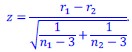
We referred to the correlation between neural and behavioral sensitivity at change-consistent (blue) signals as 𝑟<sub>𝑏𝑙𝑢𝑒</sub>, and that at change-inconsistent (red) signals as 𝑟<sub>𝑟𝑒𝑑</sub>. For the Fisher z transformation 𝑟<sub>1</sub>= 𝑟<sub>𝑏𝑙𝑢𝑒</sub> and 𝑟<sub>2</sub> \= 𝑟<sub>𝑟𝑒𝑑</sub>. We found that among the five ROIs in the frontoparietal network, two of them, namely the left IFG and left IPS, the difference in correlation was significant (one-tailed z test; left IFG: 𝑧 = 1.8355, 𝑝 =0.0332; left IPS: 𝑧 = 2.3782, 𝑝 = 0.0087). For the remaining three ROIs, the difference in correlation was not significant (dmPFC: 𝑧 = 0.7594, 𝑝 = 0.2238; right IFG: 𝑧 = 0.9068, 𝑝 = 0.1822; right IPS: 𝑧 = 1.3764, 𝑝 = 0.0843). We chose one-tailed test because we already know the correlation under the blue signals was significantly greater than 0.
In the nonparametric test, we performed nonparametric bootstrapping to test for the difference in correlation (Efron & Tibshirani, 1994). We resampled with replacement the dataset (subject-wise) and used the resampled dataset to compute the difference in correlation. We then repeated the above for 100,000 times so as to estimate the distribution of the difference in correlation coefficients, tested for significance and estimated p-value based on this distribution. Consistent with our parametric tests, here we also found that the difference in correlation was significant in left IFG and left IPS (left IFG: 𝑟<sub>𝑏𝑙𝑢𝑒</sub> − 𝑟<sub>𝑟𝑒𝑑</sub> \= 0.46, 𝑝 = 0.0496; left IPS: 𝑟<sub>𝑏𝑙𝑢𝑒</sub> − 𝑟<sub>𝑟𝑒𝑑</sub> \= 0.5306, 𝑝 = 0.0041), but was not significant in dmPFC, right IFG, and right IPS (dmPFC: 𝑟<sub>𝑏𝑙𝑢𝑒</sub> − 𝑟<sub>𝑟𝑒𝑑</sub> \= 0.1634, 𝑝 = 0.1919; right IFG: 𝑟<sub>𝑏𝑙𝑢𝑒</sub> − 𝑟<sub>𝑟𝑒𝑑</sub> \= 0.2123, 𝑝 = 0.1681; right IPS: 𝑟<sub>𝑏𝑙𝑢𝑒</sub> − 𝑟<sub>𝑟𝑒𝑑</sub> \= 0.3434, 𝑝 = 0.0631).
In summary, we found that neural sensitivity to signal diagnosticity in the frontoparietal network measured at change-consistent signals significantly correlated with individual subjects’ behavioral sensitivity to signal diagnosticity (𝑟<sub>𝑏𝑙𝑢𝑒</sub>). By contrast, neural sensitivity to signal diagnosticity measured at change-inconsistent did not significantly correlate with behavioral sensitivity (𝑟<sub>𝑟𝑒𝑑</sub>). The difference in correlation, 𝑟<sub>𝑏𝑙𝑢𝑒</sub> − 𝑟<sub>𝑟𝑒𝑑</sub>, however, was statistically significant in some (left IPS and left IFG) but not all brain regions within the frontoparietal network.
To incorporate these updates, we added descriptions of the methods and results in the revised manuscript. In the Results section (p.26-27):
“We further tested, for each brain region, whether the difference in correlation was significant using both parametric and nonparametric tests (see Parametric and nonparametric tests for difference in correlation coefficients in Methods). The results were identical. In the parametric test, we used the Fisher 𝑧 transformation to transform the difference in correlation coefficients to the 𝑧 statistic. We found that among the five ROIs in the frontoparietal network, two of them, namely the left IFG and left IPS, the difference in correlation was significant (one-tailed z test; left IFG: 𝑧 = 1.8355, 𝑝 = 0.0332; left IPS: 𝑧 = 2.3782, 𝑝 = 0.0087). For the remaining three ROIs, the difference in correlation was not significant (dmPFC: 𝑧 = 0.7594, 𝑝 = 0.2238; right IFG: 𝑧 = 0.9068, 𝑝 = 0.1822; right IPS: 𝑧 = 1.3764, 𝑝 = 0.0843). We chose one-tailed test because we already know the correlation under change-consistent signals was significantly greater than 0. In the nonparametric test, we performed nonparametric bootstrapping to test for the difference in correlation. We referred to the correlation between neural and behavioral sensitivity at change-consistent (blue) signals as 𝑟<sub>𝑏𝑙𝑢𝑒</sub>, and that at change-inconsistent (red) signals as 𝑟<sub>𝑟𝑒𝑑</sub>. Consistent with the parametric tests, we also found that the difference in correlation was significant in left IFG and left IPS (left IFG: 𝑟<sub>𝑏𝑙𝑢𝑒</sub> − 𝑟<sub>𝑟𝑒𝑑</sub> \= 0.46, 𝑝 = 0.0496; left IPS: 𝑟<sub>𝑏𝑙𝑢𝑒</sub> − 𝑟<sub>𝑟𝑒𝑑</sub> \= 0.5306, 𝑝 = 0.0041), but was not significant in dmPFC, right IFG, and right IPS (dmPFC: 𝑟<sub>𝑏𝑙𝑢𝑒</sub> − 𝑟<sub>𝑟𝑒𝑑</sub> \=0.1634, 𝑝 = 0.1919; right IFG: 𝑟<sub>𝑏𝑙𝑢𝑒</sub> − 𝑟<sub>𝑟𝑒𝑑</sub> \= 0.2123, 𝑝 = 0.1681; right IPS: 𝑟<sub>𝑏𝑙𝑢𝑒</sub> − 𝑟<sub>𝑟𝑒𝑑</sub> \= 0.3434, 𝑝 = 0.0631). In summary, we found that neural sensitivity to signal diagnosticity measured at change-consistent signals significantly correlated with individual subjects’ behavioral sensitivity to signal diagnosticity. By contrast, neural sensitivity to signal diagnosticity measured at change-inconsistent signals did not significantly correlate with behavioral sensitivity. The difference in correlation, however, was statistically significant in some (left IPS and left IFG) but not all brain regions within the frontoparietal network.”
In the Methods section, we added on p.53:
“Parametric and nonparametric tests for difference in correlation coefficients. We implemented both parametric and nonparametric tests to examine whether the difference in Pearson correlation coefficients was significant. In the parametric test, we used the Fisher 𝑧 transformation to transform the difference in correlation coefficients to the 𝑧 statistic. That is, for two correlation coefficients, 𝑟<sub>1</sub> (with sample size 𝑛<sub>2</sub>) and 𝑟<sub>2</sub>, (with sample size 𝑛<sub>1</sub>), the 𝑧 statistic of the difference in correlation is given by
We referred to the correlation between neural and behavioral sensitivity at changeconsistent (blue balls) signals as 𝑟<sub>𝑏𝑙𝑢𝑒</sub>, and that at change-inconsistent (red balls) signals as 𝑟<sub>𝑟𝑒𝑑</sub>. For the Fisher 𝑧 transformation, 𝑟<sub>1</sub> \= 𝑟 𝑟<sub>𝑏𝑙𝑢𝑒</sub> and 𝑟<sub>2</sub> \= 𝑟<sub>𝑟𝑒𝑑</sub>. In the nonparametric test, we performed nonparametric bootstrapping to test for the difference in correlation (Efron & Tibshirani, 1994). That is, we resampled with replacement the dataset (subject-wise) and used the resampled dataset to compute the difference in correlation. We then repeated the above for 100,000 times so as to estimate the distribution of the difference in correlation coefficients, tested for significance and estimated p-value based on this distribution.”
Another potential concern is that some important details about the parameter estimation for the system-neglect model are missing. In the respective section in the methods, the authors mention a nonlinear regression using Matlab's "fitnlm" function, but it remains unclear how the model was parameterized exactly. In particular, what are the properties of this nonlinear function, and what are the assumptions about the subject's motor noise? I could imagine that by using the inbuild function, the assumption was that residuals are Gaussian and homoscedastic, but it is possible that the assumption of homoscedasticity is violated, and residuals are systematically larger around p=0.5 compared to p=0 and p=1. Relatedly, in the parameter recovery analyses, the authors assume different levels of motor noise. Are these values representative of empirical values?
We thank the reviewer for this excellent point. The reviewer touched on model parameterization, assumption of noise, and parameter recovery analysis. We answered these questions point-by-point below.
On how our model was parameterized
We parameterized the model according to the system-neglect model in Eq. (2) and estimated the alpha parameter separately for each level of transition probability and the beta parameter separately for each level of signal diagnosticity. As a result, we had a total of 6 parameters (3 alpha and 3 beta parameters) in the model. The system-neglect model is then called by fitnlm so that these parameters can be estimated. The term ‘nonlinear’ regression in fitnlm refers to the fact that you can specify any model (in our case the system-neglect model) and estimate its parameters when calling this function. In our use of fitnlm, we assume that the noise is Gaussian and homoscedastic (the default option).
On the assumptions about subject’s motor noise
We actually never called the noise ‘motor’ because it can be estimation noise as well. In the context of fitnlm, we assume that the noise is Gaussian and homoscedastic.
On the possibility that homoscedasticity is violated
We take the reviewer’s point. In response, we separately estimated the residual standard deviation at different probability intervals ([0.0–0.2), [0.2–0.4), [0.4–0.6), [0.6– 0.8), and [0.8–1.0]). The result is shown in the figure below. The black data points are the average residual standard deviation (across subjects) and the error bars are the standard error of the mean. The residual standard deviation is indeed heteroscedastic— smallest at 0.1 probability and increasing as probability increases and asymptote at 0.5 (Fig. S4).
To examine how this would affect model fitting (parameter estimation), we performed parameter recovery analysis based on these empirically estimated, probabilitydependent residual standard deviation. That is, we simulated subjects’ probability estimates using the system-neglect model and added the heteroscedastic noise according to the empirical values and then estimated the parameter estimates of the system-neglect model. The recovered parameter estimates did not seem to be affected by the heteroscedasticity of the variance. The parameter recovery results were identical to the parameter recovery results when homoscedasticity was assumed. This suggested that although homoscedasticity was violated, it did not affect the accuracy of the parameter estimates (Fig.S4).
We added a section ‘Impact of noise homoscedasticity on parameter estimation’ in Methods section (p.47-48) and a figure in the supplement (Fig. S4) to describe this:
On whether the noise levels in parameter recovery analysis are representative of empirical values
To address the reviewer’s question, we conducted a new analysis using maximum likelihood estimation to simultaneously estimate the system-neglect model and the noise level of each individual subject. To estimate each subject’s noise level, we incorporated a noise parameter into the system-neglect model. We assumed that probability estimates are noisy and modeled them with a Gaussian distribution where the noise parameter (𝜎,-./&) is the standard deviation. At each period, a probability estimate of regime shift was computed according to the system-neglect model where Θ is the set of parameters including parameters in the system-neglect model and the noise parameter. The likelihood function, 𝐿(Θ), is the probability of observing the subject’s actual probability estimate at period 𝑡, 𝑝), given Θ, 𝐿(Θ) = 𝑃(𝑝)|Θ). Since we modeled the noisy probability estimates with a Gaussian distribution, we can therefore express 𝐿(Θ) as 𝐿(Θ)~𝑁(𝑝); 𝑝)*+, 𝜎,-./&) where 𝑝)*+ is the probability estimate predicted by the system-neglect (SN) model at period 𝑡. As a reminder, we referred to a ‘period’ as the time when a new signal appeared during a trial (for a given transition probability and signal diagnosticity). To find that maximum likelihood estimates of ΘMLE, we summed over all periods the negative natural logarithm of likelihood and used MATLAB’s fmincon function to find ΘMLE. Across subjects, we found that the mean noise estimate was 0.1735 and ranged from 0.1118 to 0.2704 (Supplementary Figure S3).”
Compared with our original parameter recovery analysis where the maximum noise level was set at 0.1, our data indicated that some subjects’ noise was larger than this value. Therefore, we expanded our parameter recovery analysis to include noise levels beyond 0.1 to up to 0.3. The results are now updated in Supplementary Fig. S3.
We updated the parameter recovery section (p. 47) in Methods:
The main study is based on N=30 subjects, as are the two control studies. Since this work is about individual differences (in particular w.r.t. to neural representations of noise and transition probabilities in the frontoparietal network and the vmPFC), I'm wondering how robust the results are. Is it likely that the results would replicate with a larger number of subjects? Can the two control studies be leveraged to address this concern to some extent?
We can address the issue of robustness through looking at the effect size. In particular, with respect to individual differences in neural sensitivity of transition probability and signal diagnosticity, since the significant correlation coefficients between neural and behavioral sensitivity were between 0.4 and 0.58 for signal diagnosticity in frontoparietal network (Fig. 5C), and -0.38 and -0.37 for transition probability in vmPFC (Fig. 5D), the effect size of these correlation coefficients was considered medium to large (Cohen, 1992).
It would be challenging to use the control studies to address the robustness concern. The two control studies did not allow us to examine individual differences – in particular with respect to neural selectivity of noise and transition probability – and therefore we think it is less likely to leverage the control studies. Having said that, it is possible to look at neural selectivity of noise (signal diagnosticity) in the first control experiment where subjects estimated the probability of blue regime in a task where there was no regime change (transition probability was 0). However, the fact that there were no regime shifts changed the nature of the task. Instead of always starting at the Red regime in the main experiment, in the first control experiment we randomly picked the regime to draw the signals from. It also changed the meaning and the dynamics of the signals (red and blue) that would appear. In the main experiment the blue signal is a signal consistent with change, but in the control experiment this is no longer the case. In the main experiment, the frequency of blue signals is contingent upon both noise and transition probability. In general, blue signals are less frequent than red signals because of small transition probabilities. But in the first control experiment, the frequency of blue signals may not be less frequent because the regime was blue in half of the trials. Due to these differences, we do not see how analyzing the control experiments could help in establishing robustness because we do not have a good prediction as to whether and how the neural selectivity would be impacted by these differences.
It seems that the authors have not counterbalanced the colors and that subjects always reported the probability of the blue regime. If so, I'm wondering why this was not counterbalanced.
We are aware of the reviewer’s concern. The first reason we did not do these (color counterbalancing and report blue/red regime balancing) was to not confuse the subjects in an already complicated task. Balancing these two variables also comes at the cost of sample size, which was the second reason we did not do it. Although we can elect to do these balancing at the between-subject level to not impact the task complexity, we could have introduced another confound that is the individual differences in how people respond to these variables. This is the third reason we were hesitant to do these counterbalancing.
Reviewer #2 (Public review):
Summary:
This paper focuses on understanding the behavioral and neural basis of regime shift detection, a common yet hard problem that people encounter in an uncertain world.
Using a regime-shift task, the authors examined cognitive factors influencing belief updates by manipulating signal diagnosticity and environmental volatility. Behaviorally, they have found that people demonstrate both over and under-reaction to changes given different combinations of task parameters, which can be explained by a unified system-neglect account. Neurally, the authors have found that the vmPFC-striatum network represents current belief as well as belief revision unique to the regime detection task. Meanwhile, the frontoparietal network represents cognitive factors influencing regime detection i.e., the strength of the evidence in support of the regime shift and the intertemporal belief probability. The authors further link behavioral signatures of system neglect with neural signals and have found dissociable patterns, with the frontoparietal network representing sensitivity to signal diagnosticity when the observation is consistent with regime shift and vmPFC representing environmental volatility, respectively. Together, these results shed light on the neural basis of regime shift detection especially the neural correlates of bias in belief update that can be observed behaviorally.
Strengths:
(1) The regime-shift detection task offers a solid ground to examine regime-shift detection without the potential confounding impact of learning and reward. Relatedly, the system-neglect modeling framework provides a unified account for both over or under-reacting to environmental changes, allowing researchers to extract a single parameter reflecting people's sensitivity to changes in decision variables and making it desirable for neuroimaging analysis to locate corresponding neural signals.
Thank you for recognizing our task design and our system-neglect computational framework in understanding change detection.
(2) The analysis for locating brain regions related to belief revision is solid. Within the current task, the authors look for brain regions whose activation covary with both current belief and belief change. Furthermore, the authors have ruled out the possibility of representing mere current belief or motor signal by comparing the current study results with two other studies. This set of analyses is very convincing.
Thank you for recognizing our control studies in ruling out potential motor confounds in our neural findings on belief revision.
(3) The section on using neuroimaging findings (i.e., the frontoparietal network is sensitive to evidence that signals regime shift) to reveal nuances in behavioral data (i.e., belief revision is more sensitive to evidence consistent with change) is very intriguing. I like how the authors structure the flow of the results, offering this as an extra piece of behavioral findings instead of ad-hoc implanting that into the computational modeling.
Thank you for appreciating how we showed that neural insights can lead to new behavioral findings.
Weaknesses:
(1) The authors have presented two sets of neuroimaging results, and it is unclear to me how to reason between these two sets of results, especially for the frontoparietal network. On one hand, the frontoparietal network represents belief revision but not variables influencing belief revision (i.e., signal diagnosticity and environmental volatility). On the other hand, when it comes to understanding individual differences in regime detection, the frontoparietal network is associated with sensitivity to change and consistent evidence strength. I understand that belief revision correlates with sensitivity to signals, but it can probably benefit from formally discussing and connecting these two sets of results in discussion. Relatedly, the whole section on behavioral vs. neural slope results was not sufficiently discussed and connected to the existing literature in the discussion section. For example, the authors could provide more context to reason through the finding that striatum (but not vmPFC) is not sensitive to volatility.
We thank the reviewer for the valuable suggestions.
With regard to the first comment, we wish to clarify that we did not find frontoparietal network to represent belief revision. It was the vmPFC and ventral striatum that we found to represent belief revision (delta Pt in Fig. 3). For the frontoparietal network, we identified its involvement in our task through finding that its activity correlated with strength of change evidence (Fig. 4) and individual subjects’ sensitivity to signal diagnosticity (Fig. 5). Conceptually, these two findings reflect how individuals interpret the signals (signals consistent or inconsistent with change) in light of signal diagnosticity. This is because (1) strength of change evidence is defined as signals (+1 for signal consistent with change, and -1 for signal inconsistent with change) multiplied by signal diagnosticity and (2) sensitivity to signal diagnosticity reflects how individuals subjectively evaluate signal diagnosticity. At the theoretical level, these two findings can be interpreted through our computational framework in that both the strength of change evidence and sensitivity to signal diagnosticity contribute to estimating the likelihood of change (Eqs. 1 and 2). We added a paragraph in Discussion to talk about this.
We added on p. 36:
“For the frontoparietal network, we identified its involvement in our task through finding that its activity correlated with strength of change evidence (Fig. 4) and individual subjects’ sensitivity to signal diagnosticity (Fig. 5). Conceptually, these two findings reflect how individuals interpret the signals (signals consistent or inconsistent with change) in light of signal diagnosticity. This is because (1) strength of change evidence is defined as signals (+1 for signal consistent with change, and −1 for signal inconsistent with change) multiplied by signal diagnosticity and (2) sensitivity to signal diagnosticity reflects how individuals subjectively evaluate signal diagnosticity. At the theoretical level, these two findings can be interpreted through our computational framework in that both the strength of change evidence and sensitivity to signal diagnosticity contribute to estimating the likelihood of change (Equations 1 and 2 in Methods).”
With regard to the second comment, we added a discussion on the behavioral and neural slope comparison. We pointed out previous papers conducting similar analysis (Vilares et al., 2011; Ting et al., 2015; Yang & Wu, 2020), their findings and how they relate to our results. Vilares et al. found that sensitivity to prior information (uncertainty in prior distribution) in the orbitofrontal cortex (OFC) and putamen correlated with behavioral measure of sensitivity to prior. In the current study, transition probability acts as prior in the system-neglect framework (Eq. 1) and we found that ventromedial prefrontal cortex represents subjects’ sensitivity to transition probability. Together, these results suggest that OFC (with vmPFC being part of OFC, see Wallis, 2011) is involved in the subjective evaluation of prior information in both static (Vilares et al., 2011) and dynamic environments (current study).
We added on p. 37-38:
“In the current study, our psychometric-neurometric analysis focused on comparing behavioral sensitivity with neural sensitivity to the system parameters (transition probability and signal diagnosticity). We measured sensitivity by estimating the slope of behavioral data (behavioral slope) and neural data (neural slope) in response to the system parameters. Previous studies had adopted a similar approach (Ting et al., 2015a; Vilares et al., 2012; Yang & Wu, 2020). For example, Vilares et al. (2012) found that sensitivity to prior information (uncertainty in prior distribution) in the orbitofrontal cortex (OFC) and putamen correlated with behavioral measure of sensitivity to the prior.
In the current study, transition probability acts as prior in the system-neglect framework (Eq. 2 in Methods) and we found that ventromedial prefrontal cortex represents subjects’ sensitivity to transition probability. Together, these results suggest that OFC (with vmPFC being part of OFC, see Wallis, 2011) is involved in the subjective evaluation of prior information in both static (Vilares et al., 2012) and dynamic environments (current study). In addition, distinct from vmPFC in representing sensitivity to transition probability or prior, we found through the behavioral-neural slope comparison that the frontoparietal network represents how sensitive individual decision makers are to the diagnosticity of signals in revealing the true state (regime) of the environment.”
(2) More details are needed for behavioral modeling under the system-neglect framework, particularly results on model comparison. I understand that this model has been validated in previous publications, but it is unclear to me whether it provides a superior model fit in the current dataset compared to other models (e.g., a model without \alpha or \beta). Relatedly, I wonder whether the final result section can be incorporated into modeling as well - i.e., the authors could test a variant of the model with two \betas depending on whether the observation is consistent with a regime shift and conduct model comparison.
Thank you for the great suggestion. We rewrote the final Results section to specifically focus on model comparison. To address the reviewer’s suggestion (separately estimate beta parameters for change-consistent and change-inconsistent signals), we indeed found that these models were better than the original system-neglect model.
To incorporate these new findings, we rewrote the entire final result section “Incorporating signal dependency into system-neglect model led to better models for regime-shift detection “(p.28-30).
Recommendations for the authors:
Reviewer #1 (Recommendations for the authors):
(1) Use line numbers for the next round of reviews.
We added line numbers in the revised manuscript.
(2) Figure 2b: Can the empirical results be reproduced by the system-neglect model? This would complement the analyses presented in Figure S4.
Yes. We now add Figure S6 based on system-neglect model fits. For each subject, we first computed period-by-period probability estimates based on the parameter estimates of the system-neglect model. Second, we computed index of overreaction (IO) for each combination of transition probability and signal diagnosticity. Third, we plot the IO like we did using empirical results in Fig. 2b. We found that the empirical results in Fig. 2b are similar to the system-neglect model shown in Figure S6, indicating that the empirical results can be reproduced by the model.
(3) Page 14: Instead of referring to the "Methods" in general, you could be more specific about where the relevant information can be found.
Fixed. We changed “See Methods” to “See System-neglect model in Methods”.
(4) Page 18: Consider avoiding the term "more significantly". Consider effect sizes if interested in comparing effects to each other.
Fixed. On page 19, we changed that to
“In the second analysis, we found that for both vmPFC and ventral striatum, the regression coefficient of 𝑃) was significantly different between Experiment 1 and Experiment 2 (Fig. 3C) and between Experiment 1 and Experiment 3 (Fig. 3D; also see Tables S5 and S6 in SI).”
(5) Page 30: Cite key studies using reversal-learning paradigms. Currently, readers less familiar with the literature might have difficulties with this.
We now cite key studies using reversal-learning paradigms on p.32:
“Our work is closely related to the reversal-learning paradigm—the standard paradigm in neuroscience and psychology to study change detection (Fellows & Farah, 2003; Izquierdo et al., 2017; O'Doherty et al., 2001; Schoenbaum et al., 2000; Walton et al., 2010). In a typical reversal-learning task, human or animal subjects choose between two options that differ in the reward magnitude or probability of receiving a reward. Through reward feedback the participants gradually learn the reward contingencies associated with the options and have to update knowledge about reward contingencies when contingencies are switched in order to maximize rewards.”
Reviewer #2 (Recommendations for the authors):
(1) Some literature on change detection seems missing. For example, the author should also cite Muller, T. H., Mars, R. B., Behrens, T. E., & O'Reilly, J. X. (2019). Control of entropy in neural models of environmental state. elife, 8, e39404. This paper suggests that medial PFC is correlated with the entropy of the current state, which is closely related to regime change and environmental volatility.
Thank you for pointing to this paper. We have now added it and other related papers in the Introduction and Discussion.
In Introduction, we added on p.5-6:
“Different behavioral paradigms, most notably reversal learning, and computational models were developed to investigate its neurocomputational substrates (Behrens et al., 2007; Izquierdo et al., 2017; Payzan-LeNestour et al., 2011, 2013; Nasser et al., 2010; McGuire et al., 2014; Muller et al., 2019). Key findings on the neural implementations for such learning include identifying brain areas and networks that track volatility in the environment (rate of change) (Behrens et al., 2007), the uncertainty or entropy of the current state of the environment (Muller et al., 2019), participants’ beliefs about change (Payzan-LeNestour et al., 2011; McGuire et al., 2014; Kao et al., 2020), and their uncertainty about whether a change had occurred (McGuire et al., 2014; Kao et al., 2020).”
In Discussion (p.35), we added a new paragraph:
“Related to OFC function in decision making and reinforcement learning, Wilson et al. (2014) proposed that OFC is involved in inferring the current state of the environment. For example, medial OFC had been shown to represent probability distribution on possible states of the environment (Chan et al., 2016), the current task state (Schuck et al., 2016) and uncertainty or entropy associated with the state of the environment (Muller et al., 2019). In the context of regime-shift detection, regimes can be regarded as states of the environment and therefore a change in regime indicates a change in the state of the environment. Muller et al. (2019) found that in dynamic environments where changes in the state of the environment happen regularly, medial OFC represented the level of uncertainty in the current state of the environment. Our finding that vmPFC represented individual participants’ probability estimates of regime shifts suggest that vmPFC and/or OFC are involved in inferring the current state of the environment through estimating whether the state has changed. Our finding that vmPFC represented individual participants’ sensitivity to transition probability further suggest that vmPFC and/or OFC contribute to individual participants’ biases in state inference (over- and underreactions to change) in how these brain areas respond to the volatility of the environment.”
(2) The language used when describing the selective relationship between frontoparietal network activation and change-consistent signal can be clearer. When describing separating those two signals, the authors refer to them as when the 'blue' signal shows up and when the 'red' signal shows up, assuming that the current belief state is blue. This is a little confusing cuz it is hard to keep in mind what is the default color in this example. It would be more intuitive if the author used language such as the 'change consistent' signal.
Thank you for the suggestion. We have changed the wording according to your suggestion. That is, we say ‘change-consistent (blue) signals’ and ‘change-inconsistent (red) signals’ throughout pages 22-28.
(3) Figure 4B highlights dmPFC. However, in the associated text, it says p = .10 so it is not significant. To avoid misleading readers, I would recommend pointing this out explicitly beyond saying 'most brain regions in the frontoparietal network also correlated with the intertemporal prior'.
Thank you for pointing this out. We now say on p.20
“With independent (leave-one-subject-out, LOSO) ROI analysis, we examined whether brain regions in the frontoparietal network (shown to represent strength of change evidence) correlated with intertemporal prior and found that all brain regions, with the exception of dmPFC, in the frontoparietal network correlated with the intertemporal prior.”
(4) There is a full paragraph in the discussion talking about the central opercular cortex, but this terminology has not shown up in the main body of the paper. If this is an important brain region to the authors, I would recommend mentioning it more often in the result section.
Thank you for this suggestion. We have now added central opercular cortex in the Results section (p.18):
“For 𝑃<sub>𝑡</sub>, we found that the ventromedial prefrontal cortex (vmPFC) and ventral striatum correlated with this behavioral measure of subjects’ belief about change. In addition, many other brain regions, including the motor cortex, central opercular cortex, insula, occipital cortex, and the cerebellum also significantly correlated with 𝑃<sub>𝑡</sub>.”
(5) The authors have claimed that people make more extreme estimates under high diagnosticity (Supplementary Figure 1). This is an interesting point because it seems to be different from what is shown in the main graph where it seems that people are not extreme enough compared to an ideal Bayesian observer. I understand that these are effects being investigated under different circumstances. It would be helpful if for Supplementary Figure 1 the authors could overlay, or generate a different figure showing what an ideal Bayesian observer would do in this situation.
We thank the reviewer for pointing this out. We wish to clarify that when we said “more extreme estimates under high diagnosticity” we meant compared with low diagnosticity and not with the ideal Bayesian observer. We clarified this point by rephrasing our sentence on p.11:
“We also found that subjects tended to give more extreme Pt under high signal diagnosticity than low diagnosticity (Fig. S1 in Supplementary Information, SI).”
When it comes to comparing subjects’ probability estimates with the normative Bayesian, subjects tended to “underreact” under high diagnosticity. This can be seen in Fig. 4B, which shows a trend of increasing underreaction (or decreasing overreaction) as diagnosticity increased (row-wise comparison for a given transition probability).
We see the reviewer’s point in overlaying the Bayesian on Fig. S1 and update it by adding the normative Bayesian in orange.
Dostupné typy stěn u stanů:
Typy bočnic nůžkových stanů 1) plná 2) poloviční 3) s oknem 4) se vstupem
Reviewer #1 (Public review):
Summary:
Silbaugh, Koster and Hansel investigated how the cerebellar climbing fiber (CF) signals influence neuronal activity and plasticity in mouse primary somatosensory (S1) cortex. They found that optogenetic activation of CFs in the cerebellum modulates responses of cortical neurons to whisker stimulation in a cell-type-specific manner and suppresses potentiation of layer 2/3 pyramidal neurons induced by repeated whisker stimulation. This suppression of plasticity by CF activation is mediated through modulation of VIP- and SST-positive interneurons. Using transsynaptic tracing and chemogenetic approaches, the authors identified a pathway from the cerebellum through the zona incerta and the thalamic posterior medial (POm) nucleus to the S1 cortex, which underlies this functional modulation.
The authors have addressed all the necessary points.
Reviewer #3 (Public review):
Summary:
The authors developed an interesting novel paradigm to probe the effects of cerebellar climbing fiber activation on short-term adaptation of somatosensory neocortical activity during repetitive whisker stimulation. Normally, RWS potentiated whisker responses in pyramidal cells and weakly suppressed them in interneruons, lasting for at least 1h. Crusii Optogenetic climbing fiber activation during RWS reduced or inverted these adaptive changes. This effect was generally mimicked or blocked with chemogenetic SST or VIP activation/suppression as predicted based on their "sign" in the circuit.
Strengths:
The central finding about CF modulation of S1 response adaptation is interesting, important, and convincing, and provides a jumping-off point for the field to start to think carefully about cerebellar modulation of neocortical plasticity.
Weaknesses:
The SST and VIP results appeared slightly weaker statistically, but I do not personally think this detracts from the importance of the initial finding (if there are multiple underlying mechanisms, modulating one may reproduce only a fraction of the effect size). I found the suggestion that zona incerta may be responsible for the cerebellar effects on S1 to be a more speculative result (it is not so easy with existing technology to effectively modulate this type of polysynaptic pathway), but this may be an interesting topic for the authors to follow up on in more detail in the future.
Comments on revisions:
The authors have appropriately addressed my comments.
Author response:
The following is the authors’ response to the original reviews
Public Reviews:
Reviewer #1 (Public review):
Summary:
Silbaugh, Koster, and Hansel investigated how the cerebellar climbing fiber (CF) signals influence neuronal activity and plasticity in mouse primary somatosensory (S1) cortex. They found that optogenetic activation of CFs in the cerebellum modulates responses of cortical neurons to whisker stimulation in a cell-type-specific manner and suppresses potentiation of layer 2/3 pyramidal neurons induced by repeated whisker stimulation. This suppression of plasticity by CF activation is mediated through modulation of VIP- and SST-positive interneurons. Using transsynaptic tracing and chemogenetic approaches, the authors identified a pathway from the cerebellum through the zona incerta and the thalamic posterior medial (POm) nucleus to the S1 cortex, which underlies this functional modulation.
Strengths:
This study employed a combination of modern neuroscientific techniques, including two-photon imaging, opto- and chemo-genetic approaches, and transsynaptic tracing. The experiments were thoroughly conducted, and the results were clearly and systematically described. The interplay between the cerebellum and other brain regions - and its functional implications - is one of the major topics in this field. This study provides solid evidence for an instructive role of the cerebellum in experience-dependent plasticity in the S1 cortex.
Weaknesses:
There may be some methodological limitations, and the physiological relevance of the CFinduced plasticity modulation in the S1 cortex remains unclear. In particular, it has not been elucidated how CF activity influences the firing patterns of downstream neurons along the pathway to the S1 cortex during stimulation.
Our study addresses the important question of whether CF signaling can influence the activity and plasticity of neurons outside the olivocerebellar system, and further identifies the mechanism through which this indeed occurs. We provide a detailed description of the involvement of specific neuron subtypes and how they are modulated by climbing fiber activation to impact S1 plasticity. We also identify at least one critical pathway from the cerebellar output to the S1 circuit. It is indeed correct that we did not investigate how the specific firing patterns of all of these downstream neurons are affected, or the natural behaviors in which this mechanism is involved. Now that it is established that CF signaling can impact activity and plasticity outside the olivocerebellar system -- and even in the primary somatosensory cortex -- these questions will be important to further investigate in future studies.
(1) Optogenetic stimulation may have activated a large population of CFs synchronously, potentially leading to strong suppression followed by massive activation in numerous cerebellar nuclear (CN) neurons. Given that there is no quantitative estimation of the stimulated area or number of activated CFs, observed effects are difficult to interpret directly. The authors should at least provide the basic stimulation parameters (coordinates of stim location, power density, spot size, estimated number of Purkinje cells included, etc.).
As discussed in the paper, we indeed expect that synchronous CF activation is needed to allow for an effect on S1 circuits under natural or optogenetic activation conditions. The basic optogenetic stimulation parameters (also stated in the methods) are as follows: 470 nm LED; Ø200 µm core, 0.39 NA rotary joint patch cable; absolute power output of 2.5 mW; spot size at the surface of the cortex 0.6 mm; estimated power density 8 mW/mm2. A serious estimate of the number of Purkinje cells that are activated is difficult to provide, in particular as ‘activation’ would refer to climbing fiber inputs, not Purkinje cells directly.
(2) There are CF collaterals directly innervating CN (PMID:10982464). Therefore, antidromic spikes induced by optogenetic stimulation may directly activate CN neurons. On the other hand, a previous study reported that CN neurons exhibit only weak responses to CF collateral inputs (PMID: 27047344). The authors should discuss these possibilities and the potential influence of CF collaterals on the interpretation of the results.
A direct activation of CN neurons by antidromic spikes in CF collaterals cannot be ruled out. However, we believe that this effect will not be substantial. The activation of the multi-synaptic pathway that we describe in this study is more likely to require a strong nudge as resulting from synchronized Purkinje cell input and subsequent rebound activation in CN neurons (PMID: 22198670), rather than small-amplitude input provided by CF collaterals (PMID: 27047344). A requirement for CF/PC synchronization would also set a threshold for activation of this suppressive pathway.
(3) The rationale behind the plasticity induction protocol for RWS+CF (50 ms light pulses at 1 Hz during 5 min of RWS, with a 45 ms delay relative to the onset of whisker stimulation) is unclear.
a) The authors state that 1 Hz was chosen to match the spontaneous CF firing rate (line 107); however, they also introduced a delay to mimic the CF response to whisker stimulation (line 108). This is confusing, and requires further clarification, specifically, whether the protocol was designed to reproduce spontaneous or sensory-evoked CF activity.
This protocol was designed to mimic sensory-evoked CF activity as reported in Bosman et al (J. Physiol. 588, 2010; PMID: 20724365).
b) Was the timing of delivering light pulses constant or random? Given the stochastic nature of CF firing, randomly timed light pulses with an average rate of 1Hz would be more physiologically relevant. At the very least, the authors should provide a clear explanation of how the stimulation timing was implemented.
Light pulses were delivered at a constant 1 Hz. Our goal was to isolate synchrony as the variable distinguishing sensory-evoked from spontaneous CF activity; additionally varying stochasticity, rate, or amplitude would have confounded this. Future studies could explore how these additional parameters shape S1 responses.
(4) CF activation modulates inhibitory interneurons in the S1 cortex (Figure 2): responses of interneurons in S1 to whisker stimulation were enhanced upon CF coactivation (Figure 2C), and these neurons were predominantly SST- and PV-positive interneurons (Figure 2H, I). In contrast, VIP-positive neurons were suppressed only in the late time window of 650-850 ms (Figure 2G). If the authors' hypothesis-that the activity of VIP neurons regulates SST- and PVneuron activity during RWS+CF-is correct, then the activity of SST- and PV-neurons should also be increased during this late time window. The authors should clarify whether such temporal dynamics were observed or could be inferred from their data.
Yes, we see a significant activity increase in PV neurons in this late time window (see updates to Data S2). Activity was also increased in SST neurons, though this did not reach statistical significance (Data S2). One reason might be that – given the small effect size overall – such an effect would only be seen in paired recordings. Chemogenetic activity modulation in VIP neurons, which provides a more crude test, shows, however, that SST- and PV-positive interneurons are indeed regulated via inhibition from VIP-positive interneurons (Fig. 5).
(5) Transsynaptic tracing from CN nicely identified zona incerta (ZI) neurons and their axon terminals in both POm and S1 (Figure 6 and Figure S7).
a) Which part of the CN (medial, interposed, or lateral) is involved in this pathway is unclear.
We used a dual-injection transsynaptic tracing approach to specifically label the outputs of ZI neurons that receive input from the deep cerebellar nuclei. The anterograde viral vector injected into the CN is unlabeled (no fluorophore) and therefore, it is not possible to reliably assess the extent of viral spread in those experiments as performed. However, we have previously performed similar injections into the deep cerebellar nuclei and post hoc histology suggest all three nuclei will have at least some viral expression (Koster and Sherman, 2024). Due to size and injection location, we will mostly have reached the lateral (dentate) nuclei, but cannot exclude partial transsynaptic tracing from the interposed and medial nuclei.
b) Were the electrophysiological properties of these ZI neurons consistent with those of PV neurons?
Although most recorded cells demonstrated electrophysiological properties consistent with PV+ interneurons in other brain regions (i.e. fast spiking, narrow spike width, non-adapting; see Tremblay et al., 2016), interneuron subtypes in the ZI have been incompletely characterized, with SST+ cells showing similar features to those typically associated with PV+ cells (if interested, compare Fig. 4 in DOI: 10.1126/sciadv.abf6709 vs. Fig. S10 in https://doi.org/10.1016/j.neuron.2020.04.027). Therefore, we did not attempt to delineate cell identity based on these characteristics.
c) There appears to be a considerable number of axons of these ZI neurons projecting to the S1 cortex (Figure S7C). Would it be possible to estimate the relative density of axons projecting to the POm versus those projecting to S1? In addition, the authors should discuss the potential functional role of this direct pathway from the ZI to the S1 cortex.
An absolute quantification is difficult to provide based on the images that we obtained. However, any crude estimate would indicate the relative density of projections to POm is higher than the density of projections to S1 (this is apparent from the images themselves). While the anatomical and functional connections from POm to S1 have been described in detail (Audette et al., 2018), this is not the case for the direct projections to ZI. A direct ZI to S1 projection would potentially involve a different recruitment of neurons in the S1 circuit. Any discussion on the specific consequences of the activation of this direct pathway would be purely speculative.
Reviewer #2 (Public review):
Summary:
The authors examined long-distance influence of climbing fiber (CF) signaling in the somatosensory cortex by manipulating whiskers through stimulation. Also, they examined CF signaling using two-photon imaging and mapped projections from the cerebellum to the somatosensory cortex using transsynaptic tracing. As a final manipulation, they used chemogenetics to perturb parvalbumin-positive neurons in the zona incerta and recorded from climbing fibers.
Strengths:
There are several strengths to this paper. The recordings were carefully performed, and AAVs used were selective and specific for the cell types and pathways being analyzed. In addition, the authors used multiple approaches that support climbing fiber pathways to distal regions of the brain. This work will impact the field and describes nice methods to target difficult-to-reach brain regions, such as the inferior olive.
Weaknesses:
There are some details in the methods that could be explained further. The discussion was very short and could connect the findings in a broader way.
In the revised manuscript, we provide more methodological details, as requested. We provided as simple as possible explanations in the discussion, so as not to bias further investigations into this novel phenomenon. In particular, we avoid an extended discussion of the gating effect of CF activity on S1 plasticity. While this is the effect on plasticity specifically observed here, we believe that the consequences of CF signaling on S1 activity may entirely depend on the contexts in which CF signals are naturally recruited, the ongoing activity of other brain regions, and behavioral state. Our key finding is that such modulation of neocortical plasticity can occur. How CF signaling controls plasticity of the neocortex in all contexts remains unknown, but needs to be thoughtfully tested in the future.
Reviewer #3 (Public review):
Summary:
The authors developed an interesting novel paradigm to probe the effects of cerebellar climbing fiber activation on short-term adaptation of somatosensory neocortical activity during repetitive whisker stimulation. Normally, RWS potentiated whisker responses in pyramidal cells and weakly suppressed them in interneurons, lasting for at least 1h. Crusii Optogenetic climbing fiber activation during RWS reduced or inverted these adaptive changes. This effect was generally mimicked or blocked with chemogenetic SST or VIP activation/suppression as predicted based on their "sign" in the circuit.
Strengths:
The central finding about CF modulation of S1 response adaptation is interesting, important, and convincing, and provides a jumping-off point for the field to start to think carefully about cerebellar modulation of neocortical plasticity.
Weaknesses:
The SST and VIP results appeared slightly weaker statistically, but I do not personally think this detracts from the importance of the initial finding (if there are multiple underlying mechanisms, modulating one may reproduce only a fraction of the effect size). I found the suggestion that zona incerta may be responsible for the cerebellar effects on S1 to be a more speculative result (it is not so easy with existing technology to effectively modulate this type of polysynaptic pathway), but this may be an interesting topic for the authors to follow up on in more detail in the future.
Our interpretation of the anatomical and physiological findings is that a pathway via the ZI is indeed critical for the observed effects. This pathway also represents perhaps the most direct pathway (i.e. least number of synapses connecting the cerebellar nuclei to S1). However, several other direct and indirect pathways are plausible as well and we expect distinct activation requirements and consequences for neurons in the S1 circuit. These are indeed interesting topics for future investigation.
Recommendations for the authors:
Reviewer #1 (Recommendations for the authors):
(1) Line 77: "CF transients" is not a standard or widely recognized term. Please use a more precise expression, such as "CF-induced calcium transients."
We now avoid the use of the term “CF transients” and replaced it with “CF-induced calcium transients.”
(2) Titer of AAVs injected should be provided.
AAV titers have been included in an additional data table (Data S9).
(3) Several citations to the figures are incorrect (for example, "Supplementary Data 2a (Line 398)" does not exist).
We apologize for the mistakes in this version of the article. Incorrect citations to the figures have been corrected.
(4) Line 627-628: "The tip of the patch cable was centered over Crus II in all optogenetic stimulation experiments." The stereotaxic coordinate of the tip position should be provided.
The stereotaxic coordinate of the tip position has been provided in the methods.
(5) Line 629: "Blue light pulses were delivered with a 470 nm Fiber-Coupled LED (Thorlabs catalog: M470F3)." The size of the light stim and estimated power density (W/mm^2) at the surface of the cortex should be provided.
The spot size and estimated power density at the surface of the cortex has been provided in the methods.
(6) Line 702-706: References for DCZ should be cited.
We now cited Nagai et al, Nat. Neurosci. 23 (2020) as the original reference.
(7) Two-photon image processing (Line 807-809): The rationale for normalizing ∆F/F traces to a pre-stimulus baseline is unclear because ∆F/F is, by definition, already normalized to baseline fluorescence: (Ft-F0)/F0. The authors should clarify why this additional normalization step was necessary and how it affected the interpretation of the data.
A single baseline fluorescence value (F₀) was computed for each neuron across the entire recording session, which lasted ~120-minutes. However, some S1 neurons exhibit fluctuations in baseline fluorescence over time—often related to locomotive activity or spontaneous network oscillations—which can obscure stimulus-evoked changes. To isolate fluorescence changes specifically attributable to whisker stimulation, we normalized each ∆F/F trace to the prestimulus baseline for that trial. This additional normalization allowed us to quantify potentiation or depression of sensory responses themselves, independently of spontaneous oscillations or locomotion-related changes in the ongoing neural activity.
Reviewer #2 (Recommendations for the authors):
(1) Did the climbing fiber stimulation for Figure 1 result in any changes to motor activity? Can you make any additional comments on other behaviors that were observed during these manipulations?
Acute CF stimulation did not cause any changes in locomotive or whisking activity. The CF stimulation also did not influence the overall level of locomotion or whisking during plasticity induction.
(2) Figure 3B and F- it is very difficult to see the SST+ neurons. Can this be enhanced?
We linearly adjusted the brightness and contrast for the bottom images in Figure 3B and F to improve visualization of SST+ neurons. Note the expression of both hM3D(Gq) and hM4D(Gi) in SST+ neurons is sparse, which was necessary to avoid off-target effects.
(3) Can you be more specific about the subregions of cerebellar nuclei and cell types that are targeted in the tracing studies? Discussions of the cerebellar nuclei subregions are missing and would be interesting, as others have shown discrete pathways between cerebellar nuclei subregions and long-distance projections.
See our response to comment 5a from Reviewer 1 (copied again here): we used a dual-injection transsynaptic tracing approach to specifically label the outputs of ZI neurons that receive input from the deep cerebellar nuclei. The anterograde viral vector injected into the CN is unlabeled (no fluorophone) and therefore, it is not possible to reliably assess the extent of viral spread in those experiments as performed. However, we have previously performed similar injections into the deep cerebellar nuclei and post hoc histology suggest all three nuclei will have at least some viral expression (Koster and Sherman, 2024). Due to size and injection location, we will mostly have reached the lateral (dentate) nuclei, but cannot exclude partial transsynaptic tracing from the interposed and medial nuclei.
It would indeed be interesting to further investigate the effect of CFs residing in different cerebellar lobules, which preferentially target different cerebellar nuclei, on targets of these nuclei.
(4) Did you see any connection to the ventral tegmental area? Can you comment on whether dopamine pathways are influenced by CF and in your manipulations?
We did not specifically look at these pathways and thus are not able to comment on this.
(5) These are intensive surgeries, do you think glia could have influenced any results?
This was not tested and seems unlikely, but we cannot exclude such possibility.
(6) It is unclear in the methods how long animals were recorded for in each experiment. Can you add more detail?
Additional detail was added to the methods. Recordings for all experimental configurations did not last more than 120 minutes in total. All data were analyzed across identical time windows for each experiment.
(7) In the methods it was mentioned that recording length can differ between animals. Can this influence the results, and if so, how was that controlled for?
There was a variance in recording length within experimental groups, but no systematic difference between groups.
(8) I do not see any mention of animal sex throughout this manuscript. If animals were mixed groups, were sex differences considered? Would it be expected that CF activity would be different in male and female mice?
As mentioned in the Methods (Animals), mice of either sex were used. No sex-dependent differences were observed.
(9) Transsynaptic tracing results of the zona incerta are very interesting. The zona incerta is highly understudied, but has been linked to feeding, locomotion, arousal, and novelty seeking. Do you think this pathway would explain some of the behavioral results found through other studies of cerebellar lobule perturbations? Some discussion of how this brain region would be important as a cerebellar connection in animal behavior would be interesting.
Since the multi-synaptic pathway from the cerebellum to S1 involves several brain regions with their own inputs and modulatory influences, it seems plausible to assume that behaviors controlled by these regions or affecting signaling pathways that regulate them would show some level of interaction. Our study does not address these interactions, but this will be an interesting question to be addressed in future work.
Reviewer #3 (Recommendations for the authors):
General comments on the data presentation:
I'm not a huge fan of taking areas under curves ('AUC' throughout the study) when the integral of the quantity has no physical meaning - 'normalizing' the AUC (1I,L etc) is even stranger, because of course if you instead normalize the AUC by the # of data points, you literally just get the mean (which is probably what should be used instead).
Indeed, AUC is equal to the average response in the time window used, multiplied by the window duration (thus, AUC is directly proportional to the mean). We choose to report AUC, a descriptive statistic, rather than the mean within this window. In 1I and L, we normalize the AUC across animals, essentially removing the variability across animals in the ‘Pre’ condition for visualization. Note the significance of these comparisons are consistent whether or not we normalize to the ‘Pre’ condition (non-normalized RWS data in I shows a significant increase in PN activity, p = 0.0068, signrank test; non-normalized RWS+CF data in I shows a significant decrease in PN activity, p = 0.0135, paired t-test; non-normalized RWS data in L shows a significant decrease in IN activity, p <0.001, paired t-test; non-normalized RWS+CF data in L shows no significant change in IN activity, p = 0.7789, paired t-test).
I think unadorned bar charts are generally excluded from most journals now. Consider replacing these with something that shows the raw datapoints if not too many, or the distribution across points.
We have replaced bar charts with box plots and violin plots. We have avoided plotting individual data points due to the quantity of points.
In various places, the statistics produce various questionable outcomes that will draw unwanted reader scrutiny. Many of the examples below involve tiny differences in means with overlapping error bars that are "significant" or a few cases of nonoverlapping error bars that are "not significant." I think replacing the bar charts may help to resolve things here if we can see the whole distribution or the raw data points. As importantly, I think a big problem is that the statistical tests all seem to be nonparametric (they are ambiguously described in Table S3 as "Wilcoxon," which should be clarified, since there is an unpaired Wilcoxon test [rank sum] and a paired Wilcoxon test [sign rank]), and thus based on differences in the *median* whereas the bar charts are based on the *mean* (and SEM rather than MAD or IQR or other medianappropriate measure of spread). This should be fixed (either change the test or change the plots), which will hopefully allay many of the items below.
We thank the reviewer for this important point. As mentioned in the Statistics and quantification section, Wilcoxon signed rank tests were used for non-normal data. We have replaced the bar charts with box plots which show the IQR and median, which indeed allays may of the items below.
Here are some specific points on the statistics presentation:
(1) 1G, the test says that following RWS+CF, the decrease in PN response is not significant. In 1I, the same data, but now over time, shows a highly significant decrease. This probably means that either the first test should be reconsidered (was this a paired comparison, which would "build in" the normalization subsequently used automatically?) or the second test should be reconsidered. It's especially strange because the n value in G, if based on cells, would seem to be ~50-times higher than that in I if based on mice.
In Figure 1G, the analysis tests whether individual pyramidal neurons significantly changed their responses before vs. after RWS+CF stimulation. This is a paired comparison at the single-cell level, and here indicates that the average per-neuron response did not reliably decrease after RWS+CF when comparing each cell’s pre- and post-values directly. In contrast, Figure 1I examines the same dataset analyzed across time bins using a two-way ANOVA, which tests for effects of time, group (RWS vs. RWS+CF), and their interaction. The analysis showed a significant group effect (p < 0.001), indicating that the overall level of activity across all time points differed between RWS and RWS+CF conditions. The difference in significance between these two analyses arises because the first test (Fig. 1G) assesses within-neuron changes (paired), whereas the second test (Fig. 1I) assesses overall population-level differences between groups over time (independent groups). Thus, the tests address related but distinct questions—one about per-cell response changes, the other about how activity differs across experimental conditions.
(2) 1J RWS+CF then shows a much smaller difference with overlapping error bars than the ns difference with nonoverlapping errors in 1G, but J gets three asterisks (same n-values).
Bar graphs have been replaced with box plots.
(3) 1K, it is very unclear what is under the asterisk could possibly be significant here, since the black and white dots overlap and trade places multiple times.
See response to point 1. A significant group effect will exist if the aggregate difference across all time bins exceeds within-group variability. The asterisk therefore reflects a statistically significant main group effect (RWS versus RWS+CF) rather than differences at any single time point. Note, however, the very small effect size here.
(4) 2B, 2G, 2H, 2I, 3G, 3H, 5C etc, again, significance with overlapping error bars, see suggestions above.
Bar graphs have been replaced with box plots.
(5) Time windows: e.g., L149-153 / 2B - this section reads weirdly. I think it would be less offputting to show a time-varying significance, if you want to make this point (there are various approaches to this floating around), or a decay rate, or something else.
Here, we wanted to understand the overall direction of influence of CFs on VIP activity. We find that CFs exert a suppressive effect on VIP activity, which is statistically significant in this later time window. The specific effect of CF modulation on the activity of S1 neurons across multiple time points will be described in more detail in future investigations.
(6) 4G, 6I, these asterisks again seem impossible (as currently presented).
Bar graphs have been replaced with box plots.
The writing is in generally ok shape, but needs tightening/clarifying:
(1) L45 "mechanistic capacity" not clear.
We have simplified this term to “capacity.” We use the term here to express that the central question we pose is whether CF signals are able to impact S1 circuits. We demonstrate CF signals indeed influence S1 circuits and further describe the mechanism through which this occurs, but we do not yet know all of the natural conditions in which this may occur. We feel that “capacity” describes the question we pose -- and our findings -- very well.
(2) L48-58 there's a lot of material here, not clear how much is essential to the present study.
We would like to give an overview of the literature on instructive CF signaling within the cerebellum. Here, we feel it is important to describe how CFs supervise learning in the cerebellum via coincident activation of parallel fiber inputs and CF inputs. Our results demonstrate CFs have the capacity to supervise learning in the neocortex in a similar manner, as coincident CF activation with sensory input modulates plasticity of S1 neurons.
(3) L59 "has the capacity to" maybe just "can".
This has been adopted. We agree that “can” is a more straightforward way of saying “has the capacity to” here. In this sentence, “can” and “has the capacity to” both mean a general ability to do something, without explicit knowledge about the conditions of use.
(4) L61-62 some of this is circular "observation that CF regulates plasticity in S1..has consequences for plasticity in S1".
We now changed this to read “…consequences for input processing in S1.”
(5) L91 "already existing whisker input" although I get it, strictly speaking, not clear what this means.
This sentence has been reworded for clarity.
(6) L94 "this form of plasticity" what form?
Edited to read “sensory-evoked plasticity.”
(7) L119 should say "to test the".
This has been corrected.
(8) L120 should say "well-suited to measure receptive fields".
We agree; this wording has been adopted.
(9) L130 should say "optical imaging demonstrated that receptive field".
This has been adopted.
(10) L138, the disclaimer is helpful, but wouldn't it be less confusing to just pick a different set of terms? Response potentiation etc.
Perhaps, but we want to stress that components of LTP and LTD (traditionally tested using electrophysiological methods to specifically measure synaptic gain changes) can be optically measured as long as it is specified what is recorded.
(11) L140, this whole section is not very clear. What was the experiment? What was done and how?
The text in this section has been updated.
(12) L154, 156, 158, 160, 960, what is a "basic response"? Is this supposed to contrast with RWS? If so, I would just say "we measured the response to whisker stimulation without first performing RWS, and compared this to the whisker stimulation with simultaneous CF activation."
What we meant by “basic response” was the acute response of S1 neurons to a single 100 ms air puff. Here, we indeed measured the acute responses of S1 neurons to whisker stimulation (100 ms air puff) and compared them to whisker stimulation with simultaneous CF activation (100 ms air puff with a 50 ms light pulse; the light pulse was delayed 45 ms with respect to the air puff). This paragraph has been reworded for clarity.
(13) L156 "comprised of a majority" unclear. You mean most of the nonspecific IN group is either PV or SST?
Yes, that was meant here. This paragraph has been reworded for clarity.
(14) L165 tense. "are activated" "we tested" prob should be "were activated."
This sentence was reworded.
(15) L173 Not requesting additional experiments, but demonstrating that the effect is mimicked by directly activating SST or suppressing VIP questions the specificity of CF activation per se, versus presumably many other pathways upstream of the same mechanisms, which might be worth acknowledging in the text.
We indeed observe that directly activating SST or suppressing VIP neurons in S1 is sufficient to mediate the effect of CF activation on S1 pyramidal neurons, implicating SST and VIP neurons as the local effectors of CF signaling. In the text, we wrote “...the notion of sufficiency does not exclude potential effects of plasticity processes elsewhere that might well modulate effector activation in this context and others not yet tested.” Here, we mean that CFs are certainly not the only modulators of the inhibitory network in S1. One example we highlight in the discussion is that projections from M1 are known to modulate this disinhibitory VIP-to-SST-to-PN microcircuit in S1. We conclude from our chemogenetic manipulation experiments that CFs ultimately have the capacity to modulate S1 interneurons, which must occur indirectly (either through the thalamus or “upstream” regions as this reviewer points out). The fact that many other brain regions may also modulate the interneuron network in S1 -- or be modulated by CF activity themselves -- only expands the capacity of CFs to exert a variety of effects on S1 neurons in different contexts.
(16) L247 "induced ChR2" awkward.
We changed this to read “we expressed ChR2.”
(17) 6C, what are the three colors supposed to represent?
We apologize for the missing labels in this version of the manuscript. Figure 6C and the figure legend have been updated.
第一梯队:必刷,且要深挖 (★★★★★) 这部分直接对应PNC的核心算法逻辑,面试必考,工作中常用。
为什么刷: 全局路径规划(Global Routing)完全依赖图搜索。
重点题目类型:
BFS / DFS (广度/深度优先搜索): 是一切搜索的基础。
最短路径 (Dijkstra / Floyd): 必须滚瓜烂熟。
拓扑排序 (Topological Sort): 处理任务依赖关系时偶尔用到。
(注:LeetCode上很少有直接的 A 题目,但你需要用 Dijkstra 的题去练习 A 的写法)
为什么刷: 自动驾驶处理的是矩阵、栅格地图(Grid Map)、点云。
重点题目类型:
二维矩阵操作: 比如“矩阵旋转”、“岛屿数量”(本质是搜索)、“搜索二维矩阵”。
前缀和 (Prefix Sum): 快速计算某段轨迹的累积代价。
为什么刷: 图片里可能把“堆”归类在了这里。你需要精通 std::priority_queue(最小堆/最大堆)。
重点题目类型: Top K 问题、合并K个排序链表(类似多路归并)。这直接对应 A* 算法中 OpenList 的维护。
第二梯队:选刷,理解思想 (★★★) 这部分有助于解决特定子问题,或者优化性能。
刷题策略: 不需要刷太偏太难的数学DP,重点刷“网格路径类”和“打家劫舍类”(相邻约束问题)。
刷题策略: 重点练习树的遍历(递归与非递归)、计算树的深度。这是为了让你理解如何在一个层级结构中快速查找数据。
场景: 比如你需要检查一条长轨迹中,是否存在一段连续的曲率过大的点。这就是一个滑动窗口问题。
第三梯队:可以直接跳过 / 浏览即可 (★) 这部分在PNC领域性价比极低,除非为了应付纯计算机类的通用面试,否则别浪费时间。
字符串 (String)理由: 自动驾驶处理的是坐标 $(x, y, z, v, a)$,不是文本。除了简单的日志解析,你基本不会遇到“回文串”、“括号匹配”这种问题。
链表 (Linked List)理由: 正如之前所说,链表内存不连续,对 Cache 不友好,在追求极致性能的 C++ PNC 代码中几乎被 std::vector 全面取代。面试手撕链表通常是为了考察指针操作能力,而不是因为工程中真这么用。会反转链表就行,别钻太深。
单调栈 (Monotonic Stack) / 回溯算法 (Backtracking)理由:回溯: 也就是暴力穷举。自动驾驶要求 10ms-100ms 必须出结果,回溯的时间复杂度通常是指数级的,工程上不可接受(除非解空间极小)。单调栈: 太针对特定题目,通用性不强。
There are three major diversification strategies: (1) concentric diversification, where the new business produces products that are technically similar to the company’s current product but that appeal to a new consumer group; (2) horizontal diversification, where the new business produces products that are totally unrelated to the company’s current product but that appeal to the same consumer group; and (3) conglomerate diversification, where the new business produces products that are totally unrelated to the company’s current product and that appeal to an entirely new consumer group.
Diversification Methods
__________________________________________________________________
You already know that studying full-time helps you finish faster but takes more money and time, while part-time or online classes are easier to balance but take longer. You also know that starting a family now may make school harder, and waiting could give you more stability. What you still need to know includes the exact cost of a four-year program, your financial aid options, how much a degree improves job opportunities, and how your work schedule can change. You can get this information by talking to your college adviser, checking financial aid offices, researching game-design careers, and discussing schedules with your wife. The pros of continuing school are better skills, more career options, and long-term growth; the cons are higher cost, more stress, and less free time. The pros of delaying school are more stability and less pressure, while the cons are slower career progress and fewer opportunities in the short term.
__________________________________________________________________
You have several good options for each part of the problem. For money, you could use financial aid or wait until you save more. For time, you could study part-time or full-time. To balance work and school, you could change your work hours or take fewer classes. For starting a family, you could begin now and move through school slowly, or wait until after you finish your degree. For your career, you could get the four-year degree for more skills, or learn through online courses and personal projects instead.
__________________________________________________________________
Here’s a small, clear paragraph:
The problem can be broken into a few manageable parts: figuring out the financial impact of continuing your education, understanding the time commitment needed for a four-year degree, determining how school will fit with your work and your wife’s schedule, considering how starting a family soon will affect your availability, and weighing how much a four-year degree will actually improve your chances of becoming a video game designer. By breaking it down this way, each part becomes easier to evaluate.
__________________________________________________________________
The core problem is deciding whether to pursue a four-year degree to better prepare for a career in video game design while also balancing work, finances, and plans to start a family soon. Related issues include the cost of more schooling, the time commitment, and how it will affect your home life and future stability. A successful solution must support your career goals, remain financially realistic, and still allow room for family responsibilities. A good metaphor for this situation is choosing between two paths—one easier and shorter now, and one longer but potentially leading to greater opportunities.
__________________________________________________________________
After doing three ten-minute brainstorming sessions with my group and comparing them to my own ideas, I noticed that the group came up with more ideas and they were generally more creative. Working together helped us build on each other’s suggestions, which made the ideas more unique and interesting. My individual ideas were simpler, while the group had more innovative ones.
c
この行以下3行にも結果に: がないようです
Explore Bartleby
Referencing code: [INT]: Personal comments, interpretations [STY]: Stylistic comments [SCH]: Scholarly comments
Scholarly Works Cited - Kuebrich, David. “Melville’s Doctrine of Assumptions: The Hidden Ideology of Capitalist Production in ‘Bartleby.’” The New England Quarterly, vol. 69, no. 3, 1996, pp. 381–405. - Ngai, Sianne. Ugly Feelings. Harvard UP, 2005. - Ngai, Sianne. Theory of the Gimmick. Harvard University Press, 2017 - Tseng, Chia-Chieh Mavis. “The Poetics of Refusal: Bartleby’s Language and the Violence of Signification in ‘Bartleby, the Scrivener.’” Journal of Interdisciplinary Cultural Studies, vol. 2, 2025, pp. 305–313. - Verdicchio, Massimo. “‘Bartleby the Scrivener’: An Allegory of Reading.” Canadian Review of Comparative Literature / Revue Canadienne de Littérature Comparée, Sept. 2018. - Žižek, Slavoj. The Parallax View. MIT Press, 2006.
CGC
DOI: 10.21203/rs.3.rs-7240678/v1
Resource: Caenorhabditis Genetics Center (RRID:SCR_007341)
Curator: @Apiekniewska
SciCrunch record: RRID:SCR_007341
CVCL_0532
DOI: 10.5483/BMBRep.2025-0137
Resource: (CLS Cat# 300342/p657_SK-OV-3, RRID:CVCL_0532)
Curator: @scibot
SciCrunch record: RRID:CVCL_0532
https://youtube.com/watch?v=TAQ7yBLRZ3U&feature=shared
Certainly! Here’s a detailed summary and key insights from the YouTube talk “Use.GPU - Declarative/Reactive 3D Graphics by Steven Wittens #LambdaConf2024” (link to video):
Steven Wittens introduces Use.GPU, a TypeScript library for driving WebGPU with a declarative and reactive programming model. The talk explores the motivation, design, and technical underpinnings of Use.GPU, emphasizing productivity, maintainability, and the bridging of web and graphics paradigms.
Use.GPU is a new TypeScript/WebGPU library that brings React-style declarative, reactive programming to 3D graphics in the browser. Built on the “Live” runtime, it enables maintainable, high-performance graphics apps with familiar web development patterns—potentially revolutionizing how interactive graphics are built on the web.
If you want a specific section of the talk summarized, or code examples from Use.GPU, let me know!
Citations: [1] watch?v=TAQ7yBLRZ3U https://www.youtube.com/watch?v=TAQ7yBLRZ3U
only by acquiring Standard English will most students have any opportunity to fulfill high aspirations; and (3) a standard form of any language is good because it leads to social cohesion, upward mobility, and literary continuity with the past.
Acquiring standard English gives one more opportunity to fulfill more.
☑️The most up to date version will be the canonical version that will point to the latest version using IPNS
all versions thus will be available via links
My to do list is on the annotation margins
use hypothesis search to see a reverse chronological listing of todo tasks
This annotation is at the top of that list when this annotation was made
Origo Folder for my hyperpost Peergos Account
No Groan Zome
but
Not just Converge but UpVerge in an autopoietic emregent upward spiral
Beyond all expectations
Imagined a whole new way what that leads to is beyond prior imaginings
Kanuck, Tuckahoe, Congressman, Cuff
Old terms for different ethnic and social groups: 1. Kanuck: Canadian 2. Tuckahoe: A term for people from the American South 3. Cuff: A racist old term for a Black man The point is that the grass grows the same for all.
Kanuck, Tuckahoe, Congressman, Cuff
Old terms for different ethnic and social groups: 1. Kanuck: Canadian 2. Tuckahoe: A term for people from the American South 3. Cuff: A racist old term for a Black man The point is that the grass grows the same for all.
: IDBR 08 - Índice de Operacionalidade em Relação à Média - CINDACTA I
Tentar usar o gráfico padrão de KPI para AD nesse caso juntando os dtceas. Verificar se tem os 3 anos.
Le droit des enfants à une justice adaptée : Synthèse du rapport 2025 du Défenseur des droits
Le rapport 2025 du Défenseur des droits, intitulé « Le droit des enfants à une justice adaptée », dresse un état des lieux critique de la justice pénale des mineurs en France. S'appuyant sur une vaste consultation de plus de 1 600 jeunes, le rapport réaffirme le principe fondamental selon lequel un enfant n'est pas un adulte, ce qui justifie une justice spécialisée, dont la primauté doit être éducative plutôt que répressive.
Les conclusions clés sont les suivantes :
• Un principe fondamental menacé :
La spécificité de la justice des mineurs, fondée sur l'atténuation de la responsabilité pénale et la recherche du relèvement éducatif, est fragilisée par des discours publics et des réformes législatives prônant un durcissement des sanctions, au mépris de l'intérêt supérieur de l'enfant et des engagements internationaux de la France.
• La délinquance, symptôme de vulnérabilités :
Loin d'être un phénomène isolé, la délinquance juvénile est intrinsèquement liée à des facteurs de vulnérabilité multiples : 55 % des mineurs délinquants sont suivis par la protection de l’enfance, souvent après avoir été victimes de maltraitances.
La pauvreté, l'échec scolaire, les troubles de santé mentale et l'exposition à la violence sont des déterminants majeurs.
• Un parcours pénal parsemé de défaillances :
De l'interpellation à l'incarcération, le rapport met en évidence des manquements systémiques au respect des droits des enfants.
Les contrôles d'identité discriminatoires, les violences lors des interpellations, les conditions de garde à vue inadaptées et les atteintes à la dignité en détention nourrissent une profonde défiance des jeunes envers les institutions.
• Une réponse judiciaire sous-dotée et incohérente :
Malgré les efforts des professionnels, le système souffre d'un manque criant de moyens.
Les mesures éducatives ne sont pas toujours mises en œuvre faute de personnel, et les conditions d'incarcération, qui devrait être l'ultime recours, compromettent gravement les chances de réinsertion en raison d'un accès insuffisant à l'éducation, aux soins et aux activités.
• La parole des jeunes, un appel à une justice plus humaine :
La consultation révèle une méconnaissance généralisée des droits et une perception négative de la justice chez les jeunes qui y ont été confrontés.
Ils appellent à une justice plus juste, compréhensible, préventive et bienveillante, qui prenne en compte leur vécu et leur offre une véritable seconde chance.
En conclusion, le rapport alerte sur le risque d'une justice qui, en privilégiant une approche exclusivement répressive, reproduirait l'exclusion qu'elle entend combattre.
Il formule 25 recommandations visant à sanctuariser les principes d'une justice adaptée, à renforcer la prévention en luttant contre les vulnérabilités, et à garantir le respect des droits des enfants à chaque étape de leur parcours pénal.
--------------------------------------------------------------------------------
Le rapport rappelle que la nécessité d'une justice pénale distincte pour les mineurs repose sur des principes juridiques, constitutionnels et scientifiques solides, bien que régulièrement remis en cause dans le débat public.
Le discernement, c'est-à-dire la capacité à comprendre et vouloir son acte, se développe progressivement.
Les neurosciences confirment que le cortex préfrontal, responsable du raisonnement et de la régulation des émotions, n'atteint sa pleine maturité qu'autour de 24-25 ans.
Les adolescents sont donc physiologiquement plus sujets à l'impulsivité, à l'influence du groupe et à une mauvaise évaluation des conséquences de leurs actes.
« On n’est pas assez mature, on n’a pas conscience de nos actes. » - Jeune consulté
Le Code de la justice pénale des mineurs (CJPM) de 2021 a instauré une présomption simple de non-discernement pour les enfants de moins de 13 ans.
Le Défenseur des droits estime cette mesure insuffisante et recommande d'inscrire dans la loi un principe de non-responsabilité pénale absolue en deçà de cet âge (Recommandation 1).
La justice des mineurs en France, héritière de l'ordonnance du 2 février 1945, repose sur des principes à valeur constitutionnelle :
• L'atténuation de la responsabilité pénale en fonction de l'âge.
• La primauté de l'éducatif sur le répressif, visant le « relèvement éducatif et moral » de l'enfant.
• La spécialisation des juridictions (juge des enfants, tribunal pour enfants) et des professionnels.
Ces principes sont conformes aux engagements internationaux de la France, notamment la Convention internationale des droits de l’enfant (CIDE).
Le rapport s'inquiète des récentes tentatives de les éroder, comme la loi du 23 juin 2025 qui visait initialement à instaurer une comparution immédiate pour les mineurs de plus de 16 ans, une mesure largement censurée par le Conseil constitutionnel.
La consultation nationale « J’ai des droits, entends-moi ! » révèle une fracture profonde :
• Les jeunes n'ayant jamais eu affaire à la justice ont une perception plutôt positive de son rôle protecteur.
• Ceux qui y ont été confrontés décrivent une expérience marquée par le déficit d'information, le sentiment de ne pas être écoutés et des pratiques discriminatoires, notamment pour les jeunes issus de quartiers prioritaires ou perçus comme d'origine étrangère.
« Dans la justice, y a une injustice : quand c’est des Blancs ou des Arabes c’est différent, ce n’est pas le même traitement. » - Jeune consulté
Globalement, les jeunes aspirent à une justice « compréhensible, éducative, préventive, cadrante mais bienveillante, accompagnante », qui répare et offre une seconde chance.
« Une justice adaptée, ce n’est pas seulement juger, c’est aider les jeunes dans leur souffrance. (...) Nous enfermer (...) n’est probablement pas la meilleure solution. Nous voulons être éduqués et obtenir une seconde chance. » - Lettre collective de mineurs incarcérés
Le rapport insiste sur le fait que la lutte contre la délinquance juvénile passe avant tout par un investissement massif dans la prévention et la protection des enfants contre les facteurs de vulnérabilité.
La délinquance est souvent la conséquence de parcours de vie marqués par des ruptures et des fragilités.
Données et Constats du Rapport
Situation familiale et sociale
55 % des mineurs délinquants sont suivis par la protection de l’enfance. 46 % de ceux en Centre Éducatif Fermé (CEF) ont un père absent.
La précarité socio-économique est citée par les jeunes comme la première cause du passage à l'acte.
Rupture scolaire
Le risque de délinquance est multiplié par huit en cas d'absentéisme scolaire. 72 % des jeunes suivis par la PJJ à Marseille sont ou ont été déscolarisés.
Santé mentale et handicap
90 % des jeunes en CEF présentent au moins un trouble psychiatrique. Le manque de structures de soins et d'accompagnement adapté aggrave leur fragilité.
Exposition à la violence
L'exposition à la violence (familiale, scolaire, numérique, sexuelle) favorise la reproduction des comportements violents. Le rapport note une augmentation de 77 % des mineurs mis en cause pour violences sexuelles entre 2017 et 2024.
Exploitation par des réseaux
Des mineurs, notamment les non-accompagnés (MNA), sont victimes de traite des êtres humains à des fins de délinquance forcée (trafic de stupéfiants, prostitution). Ils sont souvent traités comme des auteurs et non comme des victimes.
Pour contrer ces facteurs, le rapport préconise de renforcer plusieurs dispositifs.
• La prévention spécialisée : Les "éducateurs de rue" qui vont à la rencontre des jeunes en marge jouent un rôle capital. Cependant, ce secteur souffre d'un déploiement inégal sur le territoire et d'une pénurie de professionnels.
• Le soutien à la parentalité : Le rapport privilégie un accompagnement des familles en difficulté plutôt qu'une approche purement punitive, s'interrogeant sur l'efficacité des sanctions financières contre des parents souvent déjà précaires.
• La protection de l’enfance : L'articulation entre l'Aide Sociale à l'Enfance (ASE) et la Protection Judiciaire de la Jeunesse (PJJ) est jugée indispensable mais défaillante, entravant une prise en charge globale des jeunes.
Le rapport détaille, étape par étape, comment les droits spécifiques des mineurs sont mis à mal tout au long de la procédure pénale.
1. Premier Contact : Contrôles d'Identité et Interpellations
• Contrôles d'identité : Le rapport dénonce l'existence de pratiques discriminatoires, s'appuyant sur ses propres enquêtes qui montrent que les jeunes hommes perçus comme noirs ou arabes ont 12 fois plus de risques de subir un contrôle "poussé".
Ces pratiques, reconnues par la justice française (Cour de cassation, Conseil d'État) et européenne (CEDH), nourrissent un sentiment d'injustice et de défiance.
• Interpellations : Les témoignages de jeunes font état d'un usage disproportionné de la force, d'humiliations et de propos racistes, transformant l'interpellation en une expérience traumatisante.
« Ils cherchent à provoquer les jeunes lors des contrôles, pour que cela dérape et qu’ils puissent les embarquer. » - Jeune consulté
Bien que le CJPM prévoie des garanties fortes (droit à un avocat sans dérogation, enregistrement audiovisuel, information des parents), leur application est défaillante.
• Auditions : Des mineurs sont interrogés sans notification de leurs droits ou dans des conditions inadaptées.
• Garde à vue : Décrite comme une expérience traumatisante, avec des conditions matérielles souvent médiocres, un manque d'information et un isolement anxiogène. La situation des mineurs en situation de handicap est particulièrement préoccupante.
La réforme du CJPM a permis de réduire les délais de jugement (de 23 à 9,4 mois en moyenne), mais a engendré de nouvelles difficultés.
• Mise à l'épreuve éducative : Cette période entre l'audience de culpabilité et celle de sanction n'est souvent pas effective faute de moyens, vidant la réforme de son sens.
• Recours à l'audience unique : Prévue comme une exception, cette procédure qui statue en une seule fois sur la culpabilité et la sanction tend à se généraliser, au détriment de l'évaluation éducative.
• Compréhension : Les jeunes se plaignent d'un langage judiciaire inaccessible et du sentiment de ne pas être écoutés par les magistrats.
L'incarcération des mineurs, possible dès 13 ans, doit rester exceptionnelle. Le rapport alerte sur ses conséquences dramatiques.
• "Choc carcéral" et suicides : L'enfermement est un traumatisme majeur. Cinq adolescents se sont suicidés en détention entre octobre 2023 et août 2024.
• Conditions de détention :
◦ Éducation : L'accès à la scolarité est très insuffisant (bien en deçà des 12 à 20 heures hebdomadaires prévues) et entravé par les contraintes sécuritaires.
◦ Santé : La continuité des soins, notamment psychiatriques, est rompue.
◦ Coordination : La collaboration entre l'Administration Pénitentiaire (AP) et la PJJ est difficile, avec des logiques parfois contradictoires (sécurité vs. éducatif).
◦ Dignité : Les jeunes dénoncent la qualité et la quantité de la nourriture, le coût élevé des communications avec la famille, et des pratiques de fouilles intégrales jugées humiliantes et abusives.
« Mettre ensemble plusieurs jeunes “perturbateurs”, ça ne fait que rassembler des idées de perturbations encore plus grandes. » - Jeune incarcéré
La réinsertion n'est pas une simple étape post-sanction, mais un processus qui doit être engagé dès le début du parcours pénal.
• Préparer la sortie : Les fins de placement ou de détention sont des moments à haut risque de récidive.
Le rapport souligne le besoin crucial d'anticiper ces transitions en coordonnant l'action de tous les acteurs (PJJ, ASE, éducation, etc.).
• Le droit à l'oubli : L'effacement des condamnations du casier judiciaire est essentiel pour permettre aux jeunes de se reconstruire sans être stigmatisés.
Ce droit reste largement méconnu des principaux intéressés.
Les jeunes eux-mêmes insistent sur l'importance de l'accompagnement, du soutien à leurs projets et de la possibilité de rencontrer des pairs au parcours de réinsertion réussi, qui incarnent une source d'espoir.
« Nous devons avoir la possibilité de nous racheter sans être stigmatisés à vie. » - Jeune consulté
Parmi les 25 recommandations du rapport, plusieurs se distinguent par leur portée structurelle.
• Principes fondamentaux :
◦ Recommandation 1 : Inscrire dans la loi le principe de non-responsabilité pénale des mineurs de moins de 13 ans, sans exception.
◦ Recommandation 4 : Créer un code de l’enfance pour unifier et clarifier l'ensemble des dispositions civiles et pénales.
• Prévention :
◦ Recommandation 5 : Renforcer les moyens alloués à la prévention du décrochage scolaire (plus de psychologues, d'assistants sociaux, etc.).
◦ Recommandation 9 : Remettre la prévention spécialisée au cœur des politiques publiques avec un financement sécurisé et renforcé.
• Parcours Pénal :
◦ Recommandation 12 : Assurer la traçabilité des contrôles d’identité pour lutter contre les discriminations.
◦ Recommandation 18 : Rendre la justice compréhensible pour les enfants en formant les professionnels à l'usage d'un langage simple et clair.
• Détention et Réinsertion :
◦ Recommandation 21 : Garantir l'effectivité de l'accès à l'éducation, à la santé et au maintien des liens familiaux en détention.
◦ Recommandation 24 : Anticiper systématiquement la fin d’un placement ou d’une incarcération pour favoriser la réinsertion.
◦ Recommandation 25 : Rendre systématique l'information des mineurs sur les procédures d’effacement du casier judiciaire pour rendre effectif le droit à l’oubli.
Proposition pour une Réforme des Temps de l'Enfant : Synthèse Stratégique du Rapport de la Convention Citoyenne
La réforme de l'organisation des temps de l'enfant est devenue un impératif national.
Le modèle actuel, fragmenté et inadapté aux besoins fondamentaux de développement, de santé et d'apprentissage de millions d'enfants, fragilise notre cohésion sociale et hypothèque notre avenir collectif.
L'épuisement des élèves, la croissance des inégalités et la pression constante exercée sur les familles ne sont plus des signaux faibles, mais les symptômes d'une crise systémique qui appelle une action politique courageuse et structurée.
Comme le soulignait la lettre de saisine du Premier ministre, le système actuel est une superposition de « temps familial, temps scolaire et temps périscolaire » qui ne sont pas « pensés de façon articulée et globale ».
Face à cette fragmentation, la Convention Citoyenne sur les temps de l'enfant a été mandatée pour produire une vision d'ensemble cohérente, capable de réaligner les politiques publiques sur l'intérêt supérieur de l'enfant.
Cette démarche démocratique est inédite.
En confiant cette réflexion à 133 citoyennes et citoyens tirés au sort, qui ont délibéré pendant 21 jours, les pouvoirs publics ont permis l'émergence d'une parole authentique, libre de tout clivage politique et de tout intérêt corporatiste.
La légitimité des recommandations qui en émanent est donc particulièrement forte, car elle est le fruit d'un travail collectif, informé et représentatif de la diversité de la société française.
La présente note de synthèse a pour objectif de présenter de manière stratégique les conclusions de ce travail exceptionnel.
Elle exposera d'abord le diagnostic alarmant posé par la Convention, puis la vision directrice qui a guidé ses travaux, avant de détailler les axes de réforme concrets et les conditions impératives à leur succès.
La compréhension fine du diagnostic est en effet le fondement de la nécessité d'agir.
Les propositions de la Convention ne sont pas des opinions isolées ; elles reposent sur une analyse rigoureuse et partagée des dysfonctionnements profonds du système actuel.
Ce diagnostic met en lumière une crise systémique où les problèmes ne sont pas seulement additionnels mais s'aggravent mutuellement, créant un cercle vicieux qui pénalise en premier lieu les plus vulnérables.
Cinq constats centraux forment le socle de cette analyse.
• Une organisation subie : Les temps de l'enfant sont dictés par les contraintes des adultes et des institutions (horaires de travail, transports, logistique) et non par les besoins physiologiques, psychologiques et cognitifs de l'enfant.
• Des rythmes contre-productifs : Le rythme scolaire est en profond décalage avec les rythmes biologiques des enfants, ce qui nuit à leur concentration, altère leurs apprentissages et génère un déficit de sommeil chronique pour 20 à 30 % d'entre eux.
• Une pression constante : La densité des programmes scolaires, la place omniprésente des évaluations et la compétition génèrent anxiété et stress, dans une société qui valorise excessivement la performance et la productivité.
• L'érosion du temps libre : Le temps libre, essentiel au développement, se raréfie et se trouve dominé par une surexposition aux écrans, qui atteint près de 4h48 par jour en moyenne chez les 11-14 ans, avec des conséquences majeures sur la santé et les apprentissages.
• Un sous-investissement chronique : Le manque de moyens financiers et humains fragilise l'ensemble de la chaîne éducative et sociale, mettant en tension les professionnels (enseignants, animateurs, AESH) et dégradant la qualité de l'accompagnement.
Ces constats sont aggravés par quatre enjeux transversaux qui démontrent que les problèmes de rythme ont des conséquences sociales profondes : la montée des violences et du harcèlement, le manque d'inclusion des enfants à besoins spécifiques, la dégradation de la santé physique et mentale, et surtout l'aggravation des inégalités.
Sur ce dernier point, le rapport rappelle une réalité accablante : l'école française reste l'une des plus inégalitaires de l'OCDE, où l'origine sociale détermine encore massivement la réussite scolaire, comme en témoigne le fait que 71 % des enfants issus de familles modestes ne sont pas inscrits dans un club ou une association.
Face à ce diagnostic sévère et multidimensionnel, la Convention a stratégiquement refusé la voie des ajustements marginaux pour élaborer une vision d'avenir cohérente et désirable.
La Convention a correctement compris que la correction de défaillances systémiques exige une vision alternative convaincante, et non des solutions de fortune.
Pour être efficace, une réforme ne peut être un simple ajustement technique ; elle doit être portée par un projet global et humaniste, qui repositionne l'enfant de simple sujet des politiques publiques à leur finalité centrale.
La vision de la Convention s'articule autour de trois piliers fondamentaux.
Un socle commun élargi pour apprendre autrement
Ce pilier est une réponse directe au diagnostic d'un système qui génère une « pression constante » en survalorisant un ensemble restreint de compétences académiques.
La Convention propose de valoriser à égalité les apprentissages théoriques, concentrés le matin lorsque l'attention est maximale, et les apprentissages pratiques, artistiques, culturels et sportifs, développés l'après-midi.
Cette approche, qui intègre des ateliers de vie quotidienne concrets (bricolage, cuisine, couture, gestion du budget), vise à reconnaître toutes les formes d'intelligence, à redonner du sens et du plaisir aux apprentissages et à permettre à chaque enfant de se réaliser.
Une gouvernance équilibrée Pour s'attaquer aux « inégalités croissantes » identifiées dans le diagnostic, la Convention préconise un modèle de gouvernance à deux niveaux.
Un pilotage national fort doit fixer un cap clair, garantir le cadre commun et assurer l'égalité des chances sur tout le territoire.
Parallèlement, une mise en œuvre locale autonome doit permettre à chaque territoire d'adapter les politiques à ses spécificités, de mobiliser ses ressources propres (associations, acteurs culturels, environnement naturel) et de construire un projet éducatif pertinent et partagé, qui ne soit pas un mandat uniforme.
Des temps de vie de qualité
En réponse à « l'érosion du temps libre » et à la pression exercée sur les familles, ce pilier vise à redonner aux enfants du « temps libre vraiment libre », essentiel à leur développement personnel et à leur créativité, notamment en allégeant la charge des devoirs. Simultanément, la Convention appelle à soutenir une parentalité accompagnée, qui permette aux parents de retrouver du temps et de la sérénité dans leur relation avec leurs enfants, libérée de la surcharge logistique et de l'anxiété liées au système actuel.
C'est sur la base de cette vision que la Convention a structuré ses 20 propositions d'action, conçues comme un ensemble cohérent et interdépendant pour une transformation systémique.
Cette section constitue le cœur opérationnel de la proposition.
Les 20 recommandations adoptées par la Convention ne sont pas une simple liste de mesures, mais s'articulent logiquement en trois axes d'intervention complémentaires.
Ensemble, ils visent une transformation systémique de l'organisation des temps de l'enfant et de l'écosystème qui l'entoure.
Cet axe regroupe les propositions (1 à 11) qui ciblent stratégiquement les causes profondes de la fatigue et du stress identifiées dans le diagnostic.
En réalignant les rythmes de vie sur les besoins biologiques et psychologiques des enfants, il vise à transformer l'école d'une source de pression en un environnement structuré pour un développement sain.
La journée scolaire repensée Cette refonte de la journée scolaire s'attaque directement au décalage chronobiologique et à la fatigue chronique mis en évidence dans le diagnostic. Les mesures clés incluent :
• Le début des cours à 9h au collège et au lycée (Prop. 2) pour s'adapter au rythme de sommeil des adolescents.
• La réduction des cours à 45 minutes effectives dans le secondaire (Prop. 4) pour maintenir une attention optimale.
• Une pause déjeuner d'au moins 1h30 (Prop. 6 & 7), garantissant un temps de repas serein et un vrai temps de liberté.
• La réalisation des devoirs essentiellement à l'école (Prop. 8) pour alléger la charge de travail à la maison et réduire les inégalités.
La semaine et l'année rééquilibrées Pour garantir régularité et repos, conformément aux recommandations des chronobiologistes, la Convention propose :
• Le passage à la semaine de 5 jours pour tous les niveaux, du lundi au vendredi (Prop. 9), pour lisser les apprentissages.
• L'adoption d'un rythme annuel stable de 7 semaines de cours suivies de 2 semaines de vacances (Prop. 11), ce qui implique une réorganisation des zones de vacances.
Cet axe se concentre sur les propositions (12 à 17) visant à construire un environnement éducatif cohérent et des espaces de vie adaptés aux nouvelles ambitions pédagogiques, répondant ainsi au diagnostic d'un système fragmenté et d'infrastructures inadaptées.
Une gouvernance unifiée et déconcentrée La Convention propose une refonte de la gouvernance à double niveau : un Ministère de l'Enfance puissant au niveau national (Prop. 12) pour corriger les inégalités systémiques identifiées dans le diagnostic, et des Projets Éducatifs de Territoire (PEdT) "nouvelle génération" obligatoires (Prop. 13) pour garantir une mise en œuvre adaptée au contexte local et non un mandat uniforme.
Des espaces de vie adaptés La vision inclut la transformation des établissements en "campus des jeunes" via un plan bâtimentaire sur 20-30 ans (Prop. 14), avec des espaces flexibles, modulaires et ouverts sur l'extérieur (Prop. 15 & 16).
Cette ambition vise à créer des environnements de bien-être adaptés aux nouvelles pédagogies et au changement climatique.
Une mobilité facilitée et sécurisée Le "plan de mobilité jeunes" (Prop. 17) s'attaque directement à l'une des "contraintes des adultes" identifiées dans le diagnostic.
Il vise à limiter les temps de trajet à 45 minutes maximum et à promouvoir activement les mobilités douces, réduisant ainsi une source majeure de fatigue et de stress.
Cet axe répond aux défis modernes de l'éducation et de la vie familiale (Propositions 18 à 20), en s'attaquant directement aux nouvelles sources de pression et à l'érosion du temps libre diagnostiquées.
Encadrer l'usage des écrans Face à l'omniprésence du numérique, une double approche est proposée.
Elle consiste d'une part à informer, sensibiliser et accompagner les enfants et les parents (Prop. 18), et d'autre part à appliquer et renforcer la législation en vigueur (Prop. 19), notamment l'interdiction effective des réseaux sociaux avant 15 ans et le paramétrage par défaut des téléphones pour protéger les enfants.
Soutenir la parentalité Pour mieux concilier vie familiale et professionnelle et alléger la pression sur les familles, il est proposé de renforcer le cadre légal des aides à la parentalité (Prop. 20), reconnaissant le rôle essentiel des parents et leur besoin de soutien pour se libérer de la surcharge logistique et de l'anxiété.
Cependant, la Convention identifie lucidement que ces réformes ambitieuses sont conditionnées par un ensemble de prérequis structurels non négociables, qui doivent être abordés avec la même détermination.
La Convention a lucidement identifié que les réformes proposées, aussi pertinentes soient-elles, ne pourront porter leurs fruits sans la mise en place de leviers structurels indispensables.
Ces prérequis transforment la vision en un plan d'action réaliste pour les pouvoirs publics, en conditionnant le succès à des engagements clairs.
• Investissement et Stabilité : Il est impératif de rompre avec le sous-investissement chronique.
Cela exige un investissement financier pérenne et conséquent, sanctuarisé par une loi de programmation pluriannuelle.
De plus, il est crucial de « penser le temps long » pour garantir la stabilité des politiques éducatives et échapper aux cycles politiques courts qui paralysent les réformes de fond.
• Valorisation du Capital Humain : Aucune réforme ne réussira sans les professionnels qui la mettent en œuvre.
Il est donc impératif de réduire significativement les effectifs des classes et d'engager une revalorisation globale de l'ensemble des métiers de l'éducation (enseignants, animateurs, AESH, etc.), incluant les salaires, la formation continue et la reconnaissance de leur statut.
• Modernisation Pédagogique : Le changement de rythme doit s'accompagner d'une évolution des contenus.
Il est nécessaire de repenser les programmes scolaires pour les alléger et les aligner sur la nouvelle structure de la journée.
De plus, il faut garantir que les enfants, les jeunes et les professionnels soient systématiquement inclus dans les processus de décision qui les concernent.
• Adaptation des Infrastructures : Les conditions matérielles sont un prérequis au bien-être.
La réussite de la réforme dépend directement de l'adaptation du bâti scolaire (rénovation, végétalisation, modularité) et de la réduction effective des temps de trajet, qui ne sont pas des objectifs secondaires mais des conditions fondamentales à l'épanouissement des enfants.
La mise en œuvre de ces propositions, conditionnée par ces prérequis, constitue un projet de société ambitieux qui appelle une volonté politique sans faille.
La proposition de la Convention Citoyenne sur les temps de l'enfant suit une logique implacable : un diagnostic sévère sur l'état de notre système éducatif et social appelle une vision ambitieuse pour l'avenir de nos enfants.
Cette vision est traduite en un ensemble de réformes concrètes et interdépendantes, dont les conditions de succès sont clairement identifiées.
Nous disposons désormais d'une feuille de route cohérente, légitime et porteuse d'espoir.
Comme l'affirment avec force les citoyennes et citoyens dans leur manifeste, l'heure n'est plus aux constats mais à l'action :
Notre rapport ne doit pas être un rapport de plus, nous serons vigilants sur les suites données à notre travail. Nous attendons maintenant de nos décideurs politiques qu’ils prennent leurs responsabilités.
La mise en œuvre de ces réformes ne doit pas être perçue comme une dépense, mais comme l'investissement le plus stratégique pour l'avenir de la Nation.
Il s'agit de former des citoyens épanouis, en meilleure santé physique et mentale, capables de s'adapter aux défis de demain.
Il s'agit de réduire les fractures sociales et territoriales à la racine, en offrant à chaque enfant, où qu'il vive, les mêmes chances de se réaliser pleinement.
Il appartient désormais aux décideurs politiques de se montrer à la hauteur de cette ambition et de cet impératif démocratique.
Reviewer #3 (Public review):
Summary:
The authors recorded brain responses while participants viewed images and captions. The images and captions were taken from the COCO dataset, so each image has a corresponding caption and each caption has a corresponding image. This enabled the authors to extract features from either the presented stimulus or the corresponding stimulus in the other modality. The authors trained linear decoders to take brain responses and predict stimulus features. "Modality-specific" decoders were trained on brain responses to either images or captions while "modality-agnostic" decoders were trained on brain responses to both stimulus modalities. The decoders were evaluated on brain responses while the participants viewed and imagined new stimuli, and prediction performance was quantified using pairwise accuracy. The authors reported the following results:
(1) Decoders trained on brain responses to both images and captions can predict new brain responses to either modality.
(2) Decoders trained on brain responses to both images and captions outperform decoders trained on brain responses to a single modality.
(3) Many cortical regions represent the same concepts in vision and language.
(4) Decoders trained on brain responses to both images and captions can decode brain responses to imagined scenes.
Strengths:
This is an interesting study that addresses important questions about modality-agnostic representations. Previous work has shown that decoders trained on brain responses to one modality can be used to decode brain responses to another modality. The authors build on these findings by collecting a new multimodal dataset and training decoders on brain responses to both modalities.
To my knowledge, SemReps-8K is the first dataset of brain responses to vision and language where each stimulus item has a corresponding stimulus item in the other modality. This means that brain responses to a stimulus item can be modeled using visual features of the image, linguistic features of the caption, or multimodal features derived from both the image and the caption. The authors also employed a multimodal one-back matching task which forces the participants to activate modality-agnostic representations. Overall, SemReps-8K is a valuable resource that will help researchers answer more questions about modality-agnostic representations.
The analyses are also very comprehensive. The authors trained decoders on brain responses to images, captions, and both modalities, and they tested the decoders on brain responses to images, caption, and imagined scenes. They extracted stimulus features using a range of visual, linguistic, and multimodal models. The modeling framework appears rigorous and the results offer new insights into the relationship between vision, language, and imagery. In particular, the authors found that decoders trained on brain responses to both images and captions were more effective at decoding brain responses to imagined scenes than decoders trained on brain responses to either modality in isolation. The authors also found that imagined scenes can be decoded from a broad network of cortical regions.
Weaknesses:
The characterization of "modality-agnostic" and "modality-specific" decoders seems a bit contradictory. There are three major choices when fitting a decoder: the modality of the training stimuli, the modality of the testing stimuli, and the model used to extract stimulus features. However, the authors characterize their decoders based on only the first choice-"modality-specific" decoders were trained on brain responses to either images or captions while "modality-agnostic" decoders were trained on brain responses to both stimulus modalities. I think that this leads to some instances where the conclusions are inconsistent with the methods and results.
First, the authors suggest that "modality-specific decoders are not explicitly encouraged to pick up on modality-agnostic features during training" (line 137) while "modality-agnostic decoders may be more likely to leverage representations that are modality-agnostic" (line 140). However, whether a decoder is required to learn modality-agnostic representations depends on both the training responses and the stimulus features. Consider the case where the stimuli are represented using linguistic features of the captions. When you train a "modality-specific" decoder on image responses, the decoder is forced to rely on modality-agnostic information that is shared between the image responses and the caption features. On the other hand, when you train a "modality-agnostic" decoder on both image responses and caption responses, the decoder has access to the modality-specific information that is shared by the caption responses and the caption features, so it is not explicitly required to learn modality-agnostic features. As a result, while the authors show that "modality-agnostic" decoders outperform "modality-specific" decoders in most conditions, I am not convinced that this is because they are forced to learn more modality-agnostic features.
Second, the authors claim that "modality-specific decoders can be applied only in the modality that they were trained on" while "modality-agnostic decoders can be applied to decode stimuli from multiple modalities, even without knowing a priori the modality the stimulus was presented in" (line 47). While "modality-agnostic" decoders do outperform "modality-specific" decoders in the cross-modality conditions, it is important to note that "modality-specific" decoders still perform better than expected by chance (figure 5). It is also important to note that knowing about the input modality still improves decoding performance even for "modality-agnostic" decoders, since it determines the optimal feature space-it is better to decode brain responses to images using decoders trained on image features, and it is better to decode brain responses to captions using decoders trained on caption features.
Comments on revised version:
The revised version benefits from clearer claims and more precise terminology (i.e. classifying the decoders as "modality-agnostic" or "modality-specific" while classifying the representations as "modality-invariant" or "modality-dependent").
While the modality-agnostic decoders outperform the modality-specific decoders, I am still not convinced that this is because they are "explicitly trained to leverage the shared information in modality-invariant patterns of the brain activity". On one hand, the high-level feature spaces may each contain some amount of modality-invariant information, so even modality-specific decoders can capture some modality-invariant information. On the other hand, I do not see how training the modality-agnostic decoders on responses to both modalities necessitates that they learn modality-invariant representations beyond those that are learned by the modality-specific decoders.
Author response:
The following is the authors’ response to the original reviews
We would like to thank all reviewers for their constructive and in-depth reviews. Thanks to your feedback, we realized that the main objective of the paper was not presented clearly enough, and that our use of the same “modality-agnostic” terminology for both decoders and representations caused confusion. We addressed these two major points as outlined in the following.
In the revised manuscript, we highlight that the main contribution of this paper is to introduce modality-agnostic decoders. Apart from introducing this new decoder type, we put forward their advantages in comparison to modality-specific decoders in terms of decoding performance and analyze the modality-invariant representations (cf. updated terminology in the following paragraph) that these decoders rely on. The dataset that these analyses are based on is released as part of this paper, in the spirit of open science (but this dataset is only a secondary contribution for our paper).
Regarding the terminology, we clearly define modality-agnostic decoders as decoders that are trained on brain imaging data from subjects exposed to stimuli in multiple modalities. The decoder is not given any information on which modality a stimulus was presented in, and is therefore trained to operate in a modality-agnostic way. In contrast, modality-specific decoders are trained only on data from a single stimulus modality. These terms are explained in Figure 2. While these terms describe different ways of how decoders can be trained, there are also different ways to evaluate them afterwards (see also Figure 3); but obviously, this test-time evaluation does not change the nature of the decoder, i.e., there is no contradiction in applying a modality-specific decoder to brain data from a different modality.
Further, we identify representations that are relevant for modality-agnostic decoders using the searchlight analysis. We realized that our choice of using the same “modality-agnostic” term to describe these brain representations created unnecessary debate and confusion. In order to not conflate the terminology, in the updated manuscript we call these representations modality-invariant (and the opposite modality-dependent). Our methodology does not allow us to distinguish whether certain representations merely share representational structure to a certain degree, or are truly representations that abstract away from any modality-dependent information. However, in order to be useful for modality-agnostic decoding, a significant degree of shared representational structure is sufficient, and it is this property of brain representations that we now define as “modality-invariant”.
We updated the manuscript in line with this new terminology and focus: in particular, the first Related Work section on Modality-invariant brain representations, as well as the Introduction and Discussion.
Public Reviews:
Reviewer #1 (Public review):
Summary:
The authors introduce a densely-sampled dataset where 6 participants viewed images and sentence descriptions derived from the MS Coco database over the course of 10 scanning sessions. The authors further showcase how image and sentence decoders can be used to predict which images or descriptions were seen, using pairwise decoding across a set of 120 test images. The authors find decodable information widely distributed across the brain, with a left-lateralized focus. The results further showed that modality-agnostic models generally outperformed modality-specific models, and that data based on captions was not explained better by caption-based models but by modality-agnostic models. Finally, the authors decoded imagined scenes.
Strengths:
(1) The dataset presents a potentially very valuable resource for investigating visual and semantic representations and their interplay.
(2) The introduction and discussion are very well written in the context of trying to understand the nature of multimodal representations and present a comprehensive and very useful review of the current literature on the topic.
Weaknesses:
(1) The paper is framed as presenting a dataset, yet most of it revolves around the presentation of findings in relation to what the authors call modality-agnostic representations, and in part around mental imagery. This makes it very difficult to assess the manuscript, whether the authors have achieved their aims, and whether the results support the conclusions.
Thanks for this insightful remark. The dataset release is only a secondary contribution of our study; this was not clear enough in the previous version. We updated the manuscript to make the main objective of the paper more clear, as outlined in our general response to the reviews (see above).
(2) While the authors have presented a potential use case for such a dataset, there is currently far too little detail regarding data quality metrics expected from the introduction of similar datasets, including the absence of head-motion estimates, quality of intersession alignment, or noise ceilings of all individuals.
As already mentioned in the general response, the main focus of the paper is to introduce modality-agnostic decoders. The dataset is released in addition, this is why we did not focus on reporting extensive quality metrics in the original manuscript. To respond to your request, we updated the appendix of the manuscript to include a range of data quality metrics.
The updated appendix includes head motion estimates in the form of realignment parameters and framewise displacement, as well as a metric to assess the quality of intersession alignment. More detailed descriptions can be found in Appendix 1 of the updated manuscript.
Estimating noise ceilings based on repeated presentations of stimuli (as for example done in Allen et al. (2022)) requires multiple betas for each stimulus. All training stimuli were only presented once, so this could only be done for the test stimuli which were presented repeatedly. However, during our preprocessing procedure we directly calculated stimulus-specific betas based on data from all sessions using one single GLM, which means that we did not obtain separate betas for repeated presentations of the same stimulus. We will however share the raw data publicly, so that such noise ceilings can be calculated using an adapted preprocessing procedure if required.
Allen, E. J., St-Yves, G., Wu, Y., Breedlove, J. L., Prince, J. S., Dowdle, L. T., Nau, M., Caron, B., Pestilli, F., Charest, I., Hutchinson, J. B., Naselaris, T., & Kay, K. (2022). A massive 7T fMRI dataset to bridge cognitive neuroscience and artificial intelligence. Nature Neuroscience, 25(1), 116–126. https://doi.org/10.1038/s41593-021-00962-x
(3) The exact methods and statistical analyses used are still opaque, making it hard for a reader to understand how the authors achieved their results. More detail in the manuscript would be helpful, specifically regarding the exact statistical procedures, what tests were performed across, or how data were pooled across participants.
In the updated manuscript, we improved the level of detail for the descriptions of statistical analyses wherever possible (see also our response to your “Recommendations for the authors”, Point 6).
Regarding data pooling across participants:
Figure 8 shows averaged results across all subjects (as indicated in the caption)
Regarding data pooling for the estimation of the significance threshold of the searchlight analysis for modality-invariant regions: We updated the manuscript to clarify that we performed a permutation test, combined with a bootstrapping procedure to estimate a group-level null distribution: “For each subject, we evaluated the decoders 100 times with shuffled labels to create per-subject chance-level results. Then, we randomly selected one of the 100 chance-level results for each of the 6 subjects and calculated group-level statistics (TFCE values) the exact same way as described in the preceding paragraph. We repeated this procedure 10,000 times resulting in 10,000 permuted group-level results.”
Additionally, we indicated that the same permutation testing methods were applied to assess the significance threshold for the imagery decoding searchlight maps (Figure 10).
(4) Many findings (e.g., Figure 6) are still qualitative but could be supported by quantitative measures.
The Figures 6 and 7 are intentionally qualitative results to support the quantitative decoding results presented in Figures 4 and 5. (see also Reviewer 2 Comment 2)
Figures 4 and 5 show pairwise decoding accuracy as a quantitative measure for evaluation of the decoders. This metric is the main metric we used to compare different decoder types and features. Based on the finding that modality-agnostic decoders using imagebind features achieve the best score on this metric, we performed the additional qualitative analysis presented in Figures 6 and 7. (Note that we expanded the candidate set for the qualitative analysis in order to have a larger and more diverse set of images.)
(5) Results are significant in regions that typically lack responses to visual stimuli, indicating potential bias in the classifier. This is relevant for the interpretation of the findings. A classification approach less sensitive to outliers (e.g., 70-way classification) could avoid this issue. Given the extreme collinearity of the experimental design, regressors in close temporal proximity will be highly similar, which could lead to leakage effects.
It is true that our searchlight analysis revealed significant activity in regions outside of the visual cortex. However, it is assumed that the processing of visual information does not stop at the border of the visual cortex. The integration of information such as the semantics of the image is progressively processed in other higher-level regions of the brain. Recent studies have shown that activity in large areas of the cortex (including many outside of the visual cortex) can be related to visual stimulation (Solomon et al. 2024; Raugel et al. 2025). Our work confirms this finding and we therefore do not see reason to believe that this is due to a bias in our decoders.
Further, you are suggesting that we could replace our regression approach with a 70-way classification. However, this is difficult using our fMRI data as we do not see a straightforward way to assign the training and testing stimuli with class labels (the two datasets consist of non-overlapping sets of naturalistic images).
To address your concerns regarding the collinearity of the experimental design and possible leakage effects, we trained and evaluated a decoder for one subject after running a “null-hypothesis” adapted preprocessing. More specifically, for all sessions, we shifted the functional data of all runs by one run (moving the data of the last run to the very front), but leaving the design matrices in place. Thereby, we destroyed the relationship of stimuli and brain activity but kept the original data and design with its collinearity (and possible biases). We preprocessed this adapted data for subject 1, and ran a whole-brain decoding using Imagebind features and verified that the decoding performance was at chance level: Pairwise accuracy (captions): 0.43 | Pairwise accuracy (images): 0.47 | Pairwise accuracy (imagery): 0.50. This result provides evidence against the notion that potential collinearity or biases in our experimental design or evaluation procedure could have led to inflated results.
Raugel, J., Szafraniec, M., Vo, H.V., Couprie, C., Labatut, P., Bojanowski, P., Wyart, V. and King, J.R. (2025). Disentangling the Factors of Convergence between Brains and Computer Vision Models. arXiv preprint arXiv:2508.18226.
Solomon, S. H., Kay, K., & Schapiro, A. C. (2024). Semantic plasticity across timescales in the human brain. bioRxiv, 2024-02.
(6) The manuscript currently lacks a limitations section, specifically regarding the design of the experiment. This involves the use of the overly homogenous dataset Coco, which invites overfitting, the mixing of sentence descriptions and visual images, which invites imagery of previously seen content, and the use of a 1-back task, which can lead to carry-over effects to the subsequent trial.
Regarding the dataset CoCo: We agree that CoCo is somewhat homogenous, it is however much more diverse and naturalistic than the smaller datasets used in previous fMRI experiments with multimodal stimuli. Additionally, CoCo has been widely adopted as a benchmark dataset in the Machine Learning community, and features rich annotations for each image (e.g. object labels, segmentations, additional captions, people’s keypoints) facilitating many more future analyses based on our data.
Regarding the mixing of sentence descriptions and images: Subjects were not asked to visualize sentences and different techniques for the one-back tasks might have been used. Generally, we do not see it as problematic if subjects are performing visual imagery to some degree while reading sentences, and this might even be the case during normal reading as well. A more targeted experiment comparing reading with and without interleaved visual stimulation in the form of images and a one-back task would be required to assess this, but this was not the focus of our study. For now, it is true that we can not be sure that our results generalize to cases in which subjects are just reading and are less incentivized to perform mental imagery.
Regarding the use of a 1-back task: It was necessary to make some design choices in order to realize this large-scale data collection with approximately 10 hours of recording per subject. Specifically, the 1-back task was included in the experimental setup in order to assure continuous engagement of the participant during the rather long sessions of 1 hour. The subjects did indeed need to remember the previous stimulus to succeed at the 1-back task, which means that some brain activity during the presentation of a stimulus is likely to be related to the previous stimulus. We aimed to account for this confound during the preprocessing stage when fitting the GLM, which was fit to capture only the response to the presented image/caption, not the preceding one. Still, it might have picked up on some of the activity from preceding stimuli, causing some decrease of the final decoding performance.
We added a limitations section to the updated manuscript to discuss these important issues.
(7) I would urge the authors to clarify whether the primary aim is the introduction of a dataset and showing the use of it, or whether it is the set of results presented. This includes the title of this manuscript. While the decoding approach is very interesting and potentially very valuable, I believe that the results in the current form are rather descriptive, and I'm wondering what specifically they add beyond what is known from other related work. This includes imagery-related results. This is completely fine! It just highlights that a stronger framing as a dataset is probably advantageous for improving the significance of this work.
Thanks a lot for pointing this out. Based on this comment and feedback from the other reviewers we restructured the abstract, introduction and discussion section of the paper to better reflect the primary aim. (cf. general response above).
You further mention that it is not clear what our results add beyond what is known from related work. We list the main contributions here:
A single modality-agnostic decoder can decode the semantics of visual and linguistic stimuli irrespective of the presentation modality with a performance that is not lagging behind modality-specific decoders.
Modality-agnostic decoders outperform modality-specific decoders for decoding captions and mental imagery.
Modality-invariant representations are widespread across the cortex (a range of previous work has suggested they were much more localized (Bright et al. 2004; Jung et al. 2018; Man et al. 2012; Simanova et al. 2014).
Regions that are useful for imagery are largely overlapping with modality-invariant regions
Bright, P., Moss, H., & Tyler, L. K. (2004). Unitary vs multiple semantics: PET studies of word and picture processing. Brain and language, 89(3), 417-432.
Jung, Y., Larsen, B., & Walther, D. B. (2018). Modality-Independent Coding of Scene Categories in Prefrontal Cortex. Journal of Neuroscience, 38(26), 5969–5981.
Liuzzi, A. G., Bruffaerts, R., Peeters, R., Adamczuk, K., Keuleers, E., De Deyne, S., Storms, G., Dupont, P., & Vandenberghe, R. (2017). Cross-modal representation of spoken and written word meaning in left pars triangularis. NeuroImage, 150, 292–307. https://doi.org/10.1016/j.neuroimage.2017.02.032
Man, K., Kaplan, J. T., Damasio, A., & Meyer, K. (2012). Sight and Sound Converge to Form Modality-Invariant Representations in Temporoparietal Cortex. Journal of Neuroscience, 32(47), 16629–16636.
Simanova, I., Hagoort, P., Oostenveld, R., & van Gerven, M. A. J. (2014). Modality-Independent Decoding of Semantic Information from the Human Brain. Cerebral Cortex, 24(2), 426–434.
Reviewer #2 (Public review):
Summary:
This study introduces SemReps-8K, a large multimodal fMRI dataset collected while subjects viewed natural images and matched captions, and performed mental imagery based on textual cues. The authors aim to train modality-agnostic decoders--models that can predict neural representations independently of the input modality - and use these models to identify brain regions containing modality-agnostic information. They find that such decoders perform comparably or better than modality-specific decoders and generalize to imagery trials.
Strengths:
(1) The dataset is a substantial and well-controlled contribution, with >8,000 image-caption trials per subject and careful matching of stimuli across modalities - an essential resource for testing theories of abstract and amodal representation.
(2) The authors systematically compare unimodal, multimodal, and cross-modal decoders using a wide range of deep learning models, demonstrating thoughtful experimental design and thorough benchmarking.
(3) Their decoding pipeline is rigorous, with informative performance metrics and whole-brain searchlight analyses, offering valuable insights into the cortical distribution of shared representations.
(4) Extension to mental imagery decoding is a strong addition, aligning with theoretical predictions about the overlap between perception and imagery.
Weaknesses:
While the decoding results are robust, several critical limitations prevent the current findings from conclusively demonstrating truly modality-agnostic representations:
(1) Shared decoding ≠ abstraction: Successful decoding across modalities does not necessarily imply abstraction or modality-agnostic coding. Participants may engage in modality-specific processes (e.g., visual imagery when reading, inner speech when viewing images) that produce overlapping neural patterns. The analyses do not clearly disambiguate shared representational structure from genuinely modality-independent representations. Furthermore, in Figure 5, the modality-agnostic encoder did not perform better than the modality-specific decoder trained on images (in decoding images), but outperformed the modality-specific decoder trained on captions (in decoding captions). This asymmetry contradicts the premise of a truly "modality-agnostic" encoder. Additionally, given the similar performance between modality-agnostic decoders based on multimodal versus unimodal features, it remains unclear why neural representations did not preferentially align with multimodal features if they were truly modality-independent.
We agree that successful modality-agnostic and cross-modal decoding does not necessarily imply that abstract patterns were decoded. In the updated manuscript, we therefore refer to these representations as modality-invariant (see also the updated terminology explained in the general response above).
If participants are performing mental imagery when reading, and this is allowing us to perform cross-decoding, then this means that modality-invariant representations are formed during this mental imagery process, i.e. that the representations formed during this form of mental imagery are compatible with representations during visual perception (or, in your words, produce overlapping neural patterns). While we can not know to what extent people were performing mental imagery while reading (or having inner speech while viewing images), our results demonstrate that their brain activity allows for decoding across modalities, which implies that modality-invariant representations are present.
It is true that our current analyses can not disambiguate modality-invariant representations (or, in your words, shared representational structure) from abstract representations (in your words, genuinely modality-independent representations). As the main goal of the paper was to build modality-agnostic decoders, and these only require what we call “modality-invariant” representations (see our updated terminology in the general reviewer response above), we leave this question open for future work. We do however discuss this important limitation in the Discussion section of the updated manuscript.
Regarding the asymmetry of decoding results when comparing modality-agnostic decoders with the two respective modality-specific decoders for captions and images: We do not believe that this asymmetry contradicts the premise of a modality-agnostic decoder. Multiple explanations for this result are possible: (1) The modality-specific decoder for images might benefit from the more readily decodable lower-level modality-dependent neural activity patterns in response to images, which are less useful for the modality-agnostic decoder because they are not useful for decoding caption trials. The modality-specific decoders for captions might not be able to pick up on low-level modality-dependent neural activity patterns as these might be less easily decodable.
The signal-to-noise ratio for caption trials might be lower than for image trials (cf. generally lower caption decoding performance), therefore the addition of training data (even if it is from another modality) improves the decoding performance for captions, but not for images (which might be at ceiling already).
Regarding the similar performance between modality-agnostic decoders based on multimodal versus unimodal features: Unimodal features are based on rather high-level features of the respective modality (e.g. last-layer features of a model trained for semantic image classification), which can be already modality-invariant to some degree. Additionally, as already mentioned before, in the updated manuscript we only require representations to be modality-invariant and not necessarily abstract.
(2) The current analysis cannot definitively conclude that the decoder itself is modality-agnostic, making "Qualitative Decoding Results" difficult to interpret in this context. This section currently provides illustrative examples, but lacks systematic quantitative analyses.
The qualitative decoding results in Figures 6 and 7 present exemplary qualitative results for the quantitative results presented in Figures 4 and 5 (see also Reviewer 1 Comment 4).
Figures 4 and 5 show pairwise decoding accuracy as a quantitative measure for evaluation of the decoders. This metric is the main metric we used to compare different decoder types and features. Based on the finding that modality-agnostic decoders using imagebind features achieve the best score on this metric, we performed the additional qualitative analysis presented in Figures 6 and 7. (Note that we expanded the candidate set for the qualitative analysis in order to have a larger and more diverse set of images.)
(3) The use of mental imagery as evidence for modality-agnostic decoding is problematic.
Imagery involves subjective, variable experiences and likely draws on semantic and perceptual networks in flexible ways. Strong decoding in imagery trials could reflect semantic overlap or task strategies rather than evidence of abstraction.
It is true that mental imagery does not necessarily rely on modality-agnostic representations. In the updated manuscript we revised our terminology and refer to the analyzed representations as modality-invariant, which we define as “representations that significantly overlap between modalities”.
The manuscript presents a methodologically sophisticated and timely investigation into shared neural representations across modalities. However, the current evidence does not clearly distinguish between shared semantics, overlapping unimodal processes, and true modality-independent representations. A more cautious interpretation is warranted.
Nonetheless, the dataset and methodological framework represent a valuable resource for the field.
We fully agree with these observations, and updated our terminology as outlined in the general response.
Reviewer #3 (Public review):
Summary:
The authors recorded brain responses while participants viewed images and captions. The images and captions were taken from the COCO dataset, so each image has a corresponding caption, and each caption has a corresponding image. This enabled the authors to extract features from either the presented stimulus or the corresponding stimulus in the other modality.
The authors trained linear decoders to take brain responses and predict stimulus features.
"Modality-specific" decoders were trained on brain responses to either images or captions, while "modality-agnostic" decoders were trained on brain responses to both stimulus modalities. The decoders were evaluated on brain responses while the participants viewed and imagined new stimuli, and prediction performance was quantified using pairwise accuracy. The authors reported the following results:
(1) Decoders trained on brain responses to both images and captions can predict new brain responses to either modality.
(2) Decoders trained on brain responses to both images and captions outperform decoders trained on brain responses to a single modality.
(3) Many cortical regions represent the same concepts in vision and language.
(4) Decoders trained on brain responses to both images and captions can decode brain responses to imagined scenes.
Strengths:
This is an interesting study that addresses important questions about modality-agnostic representations. Previous work has shown that decoders trained on brain responses to one modality can be used to decode brain responses to another modality. The authors build on these findings by collecting a new multimodal dataset and training decoders on brain responses to both modalities.
To my knowledge, SemReps-8K is the first dataset of brain responses to vision and language where each stimulus item has a corresponding stimulus item in the other modality. This means that brain responses to a stimulus item can be modeled using visual features of the image, linguistic features of the caption, or multimodal features derived from both the image and the caption. The authors also employed a multimodal one-back matching task, which forces the participants to activate modality-agnostic representations. Overall, SemReps-8K is a valuable resource that will help researchers answer more questions about modality-agnostic representations.
The analyses are also very comprehensive. The authors trained decoders on brain responses to images, captions, and both modalities, and they tested the decoders on brain responses to images, captions, and imagined scenes. They extracted stimulus features using a range of visual, linguistic, and multimodal models. The modeling framework appears rigorous, and the results offer new insights into the relationship between vision, language, and imagery. In particular, the authors found that decoders trained on brain responses to both images and captions were more effective at decoding brain responses to imagined scenes than decoders trained on brain responses to either modality in isolation. The authors also found that imagined scenes can be decoded from a broad network of cortical regions.
Weaknesses:
The characterization of "modality-agnostic" and "modality-specific" decoders seems a bit contradictory. There are three major choices when fitting a decoder: the modality of the training stimuli, the modality of the testing stimuli, and the model used to extract stimulus features. However, the authors characterize their decoders based on only the first choice-"modality-specific" decoders were trained on brain responses to either images or captions, while "modality-agnostic" decoders were trained on brain responses to both stimulus modalities. I think that this leads to some instances where the conclusions are inconsistent with the methods and results.
In our analysis setup, a decoder is entirely determined by two factors: (1) the modality of the stimuli that the subject was exposed to, and (2) the machine learning model used to extract stimulus features.
The modality of the testing stimuli defines whether we are evaluating the decoder in a within-modality or cross-modality setting, but is not an inherent characteristic of a trained decoder
First, the authors suggest that "modality-specific decoders are not explicitly encouraged to pick up on modality-agnostic features during training" (line 137) while "modality-agnostic decoders may be more likely to leverage representations that are modality-agnostic" (line 140). However, whether a decoder is required to learn modality-agnostic representations depends on both the training responses and the stimulus features. Consider the case where the stimuli are represented using linguistic features of the captions. When you train a "modality-specific" decoder on image responses, the decoder is forced to rely on modality-agnostic information that is shared between the image responses and the caption features. On the other hand, when you train a "modality-agnostic" decoder on both image responses and caption responses, the decoder has access to the modality-specific information that is shared by the caption responses and the caption features, so it is not explicitly required to learn modality-agnostic features. As a result, while the authors show that "modality-agnostic" decoders outperform "modality-specific" decoders in most conditions, I am not convinced that this is because they are forced to learn more modality-agnostic features.
It is true that for example a modality-specific decoder trained on fmri data from images with stimulus features extracted from captions might also rely on modality-invariant features. We still call this decoder modality-specific, as it has been trained to decode brain activity recorded from a specific stimulus modality. In the updated manuscript we corrected the statement that “modality-specific decoders are not explicitly encouraged to pick up on modality-invariant features during training” to include the case of decoders trained on features from the other modality which might also rely on modality-invariant features.
It is true that a modality-agnostic decoder can also have access to modality-dependent information for captions and images. However, as it is trained jointly with both modalities and the modality-dependent features are not compatible, it is encouraged to rely on modality-invariant features. The result that modality-agnostic decoders are outperforming modality-specific decoders trained on captions for decoding captions confirms this, because if the decoder was only relying on modality-dependent features the addition of additional training data from another stimulus modality could not increase the performance. (Also, the lack of a performance drop compared to modality-specific decoders trained on images is only possible thanks to the reliance on modality-invariant features. If the decoder only relied on modality-dependent features the addition of data from another modality would equal an addition of noise to the training data which must result in a performance drop at test time.). We can not exclude the possibility that modality-agnostic decoders are also relying on modality-dependent features, but our results suggest that they are relying at least to some degree on modality-invariant features.
Second, the authors claim that "modality-specific decoders can be applied only in the modality that they were trained on, while "modality-agnostic decoders can be applied to decode stimuli from multiple modalities, even without knowing a priori the modality the stimulus was presented in" (line 47). While "modality-agnostic" decoders do outperform "modality-specific" decoders in the cross-modality conditions, it is important to note that "modality-specific" decoders still perform better than expected by chance (figure 5). It is also important to note that knowing about the input modality still improves decoding performance even for "modality-agnostic" decoders, since it determines the optimal feature space-it is better to decode brain responses to images using decoders trained on image features, and it is better to decode brain responses to captions using decoders trained on caption features.
Thanks for this important remark. We corrected this statement and now say that “modality-specific decoders that are trained to be applied only in the modality that they were trained on”, highlighting that their training process optimizes them for decoding in a specific modality. They can indeed be applied to the other modality at test time, this however results in a substantial performance drop.
It is true that knowing the input modality can improve performance even for modality-agnostic decoders. This can most likely be explained by the fact that in that case the decoder can leverage both, modality-invariant and modality-dependent features. We will not further focus on this result however as the main motivation to build modality-agnostic decoders is to be able to decode stimuli without knowing the stimulus modality a priori.
Recommendations for the authors:
Reviewer #1 (Recommendations for the authors):
I will list additional recommendations below in no specific order:
(1) I find the term "modality agnostic" quite unusual, and I believe I haven't seen it used outside of the ML community. I would urge the authors to change the terminology to be more common, or at least very early explain why the term is much better suited than the range of existing terms. A modality agnostic representation implies that it is not committed to a specific modality, but it seems that a representation cannot be committed to something.
In the updated manuscript we now refer to the identified brain patterns as modality-invariant, which has previously been used in the literature (Man et al. 2012; Devereux et al. 2013; Patterson et al. 2016; Deniz et al. 2019, Nakai et al. 2021) (see also the general response on top and the Introduction and Related Work sections of the updated manuscript).
We continue to refer to the decoders as modality-agnostic, as this is a new type of decoder, and describes the fact that they are trained in a way that abstracts away from the modality of the stimuli. We chose this term as we are not aware of any work in which brain decoders were trained jointly on multiple stimulus modalities and in order not to risk contradictions/confusions with other definitions.
Deniz, F., Nunez-Elizalde, A. O., Huth, A. G., & Gallant, J. L. (2019). The Representation of Semantic Information Across Human Cerebral Cortex During Listening Versus Reading Is Invariant to Stimulus Modality. Journal of Neuroscience, 39(39), 7722–7736. https://doi.org/10.1523/JNEUROSCI.0675-19.2019
Devereux, B. J., Clarke, A., Marouchos, A., & Tyler, L. K. (2013). Representational Similarity Analysis Reveals Commonalities and Differences in the Semantic Processing of Words and Objects. The Journal of Neuroscience, 33(48).
Nakai, T., Yamaguchi, H. Q., & Nishimoto, S. (2021). Convergence of Modality Invariance and Attention Selectivity in the Cortical Semantic Circuit. Cerebral Cortex, 31(10), 4825–4839. https://doi.org/10.1093/cercor/bhab125
Man, K., Kaplan, J. T., Damasio, A., & Meyer, K. (2012). Sight and Sound Converge to Form Modality-Invariant Representations in Temporoparietal Cortex. Journal of Neuroscience, 32(47), 16629–16636.
Patterson, K., & Lambon Ralph, M. A. (2016). The Hub-and-Spoke Hypothesis of Semantic Memory. In Neurobiology of Language (pp. 765–775). Elsevier. https://doi.org/10.1016/B978-0-12-407794-2.00061-4
(2) The table in Figure 1B would benefit from also highlighting the number of stimuli that have overlapping captions and images.
The number of overlapping stimuli is rather small (153-211 stimuli depending on the subject). We added this information to Table 1B.
(3) The authors wrote that training stimuli were presented only once, yet they used a one-back task. Did the authors also exclude the first presentation of these stimuli?
Thanks for pointing this out. It is indeed true that some training stimuli were presented more than once, but only for the case of one-back target trials. In these cases the second presentation of the stimulus was excluded, but not the first. As the subject can not be aware of the fact that the upcoming presentation is going to be a one-back target, the first presentation can not be affected by the presence of the subsequent repeated presentation. We updated the manuscript to clarify this issue.
(4) Coco has roughly 80-90 categories, so many image captions will be extremely similar (e.g., "a giraffe walking", "a surfer on a wave", etc.). How can people keep these apart?
It is true that some captions and images are highly similar even though they are not matching in the dataset. This might result in several false button presses because the subjects identified an image-caption pair as matching when in fact it wasn't intended to. However, as there was no feedback given on the task performance, this issue should not have had a major influence on the brain activity of the participants.
(5) Footnotes for statistics are quite unusual - could the authors integrate statistics into the text?
Thanks for this remark, in the updated manuscript all statistics are part of the main text.
(6) It may be difficult to achieve the assumptions of a permutation test - exchangeability, which may bias statistical results. It is not uncommon for densely sampled datasets to use bootstrap sampling on the predictions of the test data to identify if a given percentile of that distribution crosses 0. The lowest p-value is given by the number of bootstrap samples (e.g., if all 10,000 bootstrap samples are above chance, then p < 0.0001). This may turn out to be more effective.
Thanks for this comment. Our statistical procedure was in fact involving a bootstrapping procedure to generate a null distribution on the group-level. We updated the manuscript to describe this method in more detail. Here is the updated paragraph: “To estimate the statistical significance of the resulting clusters we performed a permutation test, combined with a bootstrapping procedure to estimate a group-level null distribution see also Stelzer et al., 2013). For each subject, we evaluated the decoders 100 times with shuffled labels to create per-subject chance-level results. Then, we randomly selected one of the 100 chance-level results for each of the 6 subjects and calculated group-level statistics (TFCE values) the exact same way as described in the preceding paragraph. We repeated this procedure 10,000 times resulting in 10,000 permuted group-level results. We ensured that every permutation was unique, i.e. no two permutations were based on the same combination of selected chance-level results. Based on this null distribution, we calculated p-values for each vertex by calculating the proportion of sampled permutations where the TFCE value was greater than the observed TFCE value. To control for multiple comparisons across space, we always considered the maximum TFCE score across vertices for each group-level permutation (Smith and Nichols, 2009).”
(7) The authors present no statistical evidence for some of their claims (e.g., lines 335-337). It would be good if they could complement this in their description. Further, the visualization in Figure 4 is rather opaque. It would help if the authors could add a separate bar for the average modality-specific and modality-agnostic decoders or present results in a scatter plot, showing modality-specific on the x-axis and modality-agnostic on the y-axis and color-code the modality (i.e., making it two scatter colors, one for images, one for captions). All points will end up above the diagonal.
We updated the manuscript and added statistical evidence for the claims made:
We now report results for the claim that when considering the average decoding performance for images and captions, modality-agnostic decoders perform better than modality-specific decoders, irrespective of the features that the decoders were trained on.
Additionally, we report the average modality-agnostic and modality-specific decoding accuracies corresponding to Figure 4. For modality-agnostic decoders the average value is 81.86\%, for modality-specific decoders trained on images 78.15\%, and for modality-specific decoders trained on captions 72.52\%. We did not add a separate bar to Figure 4 as this would add additional information to a Figure which is already very dense in its information content (cf. Reviewers 2’s recommendations for the authors). We therefore believe it is more useful to report the average values in the text and provide results for a statistical test comparing the decoder types. A scatter plot would make it difficult to include detailed information on the features, which we believe is crucial.
We further provide statistical evidence for the observation regarding the directionality of cross-modal decoding.
Reviewer #2 (Recommendations for the authors):
For achieving more evidence to support modality-agnostic representations in the brain, I suggest more thorough analyses, for example:
(1) Traditional searchlight RSA using different deep learning models. Through this approach, it might identify different brain areas that are sensitive to different formats of information (visual, text, multimodal); subsequently, compare the decoding performance using these ROIs.
(2) Build more dissociable decoders for information of different modality formats, if possible. While I do not have a concrete proposal, more targeted decoder designs might better dissociate representational formats (i.e., unimodal vs. modality-agnostic).
(3) A more detailed exploration of the "qualitative decoding results"--for example, quantitatively examining error types produced by modality-agnostic versus modality-specific decoders--would be informative for clarifying what specific content the decoder captures, potentially providing stronger evidence for modality-agnostic representations.
Thanks for these suggestions. As the main goal of the paper is to introduce modality-agnostic decoders (which should be more clear from the updated manuscript, see also the general response to reviews), we did not include alternative methods for identifying modality-invariant regions. Nonetheless, we agree that in order to obtain more in-depth insight into the nature of representations that were recorded, performing analyses with additional methods such as RSA, comparisons with more targeted decoder designs in terms of their target features will be indispensable, as well as more in-depth error type analyses. We leave these analyses as promising directions for future work.
The writing could be further improved in the introduction and, accordingly, the discussion. The authors listed a series of theories about conceptual representations; however, they did not systematically explain the relationships and controversies between them, and it seems that they did not aim to address the issues raised by these theories anyway. Thus, the extraction of core ideas is suggested. The difference between "modality-agnostic" and terms like "modality-independent," "modality-invariant," "abstract," "amodal," or "supramodal," and the necessity for a novel term should be articulated.
The updated manuscript includes an improved introduction and discussion section that highlight the main focus and contributions of the study.
We believe that a systematic comparison of theories on conceptual representations involving their relationships and controversies would require a dedicated review paper. Here, we focused on the aspects that are relevant for the study at hand (modality-invariant representations), for which we find that none of the considered theories can be rejected based on our results.
Regarding the terminology (modality-agnostic vs. modality-invariant, ..) please refer to the general response.
The figures also have room to improve. For example, Figures 4 and 5 present dense bar plots comparing multiple decoding settings (e.g., modality-specific vs. modality-agnostic decoders, feature space, within-modal vs. cross-modal, etc.); while comprehensive, they would benefit from clearer labels or separated subplots to aid interpretation. All figures are recommended to be optimized for greater clarity and directness in future revisions.
Thanks for this remark. We agree that the figures are quite dense in information. However, splitting them up into subplots (e.g. separate subplots for different decoder types) would make it much less straightforward to compare the accuracy scores between conditions. As the main goal of these figures is to compare features and decoder types, we believe that it is useful to keep all information in the same plot.
You are also suggesting to improve the clarity of the labels. It is true that the top left legend of Figures 4 and 5 was mixing information about decoder type and broad classes of features (vision/language/multimodal). To improve clarity, we updated the figures and clearly separated information on decoder type (the hue of different bars) and features (x-axis labels). The broad classes of features (vision/language/multimodal) are distinguished by alternating light gray background colors and additional labels at the very bottom of the plots.
The new plots allow for easy performance comparison of the different decoder types and additionally provide information on confidence intervals for the performance of modality-specific decoders, which was not available in the previous figures.
Reviewer #3 (Recommendations for the authors):
(1) As discussed in the Public Review, I think the paper would greatly benefit from clearer terminology. Instead of describing the decoders as "modality-agnostic" and "modality-specific", perhaps the authors could describe the decoding conditions based on the train and test modalities (e.g., "image-to-image", "caption-to-image", "multimodal-to-image") or using the terminology from Figure 3 (e.g., "within-modality", "cross-modality", "modality-agnostic").
We updated our terminology to be clearer and more accurate, as outlined in the general response. The terms modality-agnostic and modality-specific refer to the training conditions, and the test conditions are described in Figure 3 and are used throughout the paper.
(2) Line 244: I think the multimodal one-back task is an important aspect of the dataset that is worth highlighting. It seems to be a relatively novel paradigm, and it might help ensure that the participants are activating modality-agnostic representations.
It is true that the multimodal one-back task could play an important role for the activation of modality-invariant representations. Future work could investigate to what degree the presence of widespread modality-invariant representations is dependent on such a paradigm.
(3) Line 253: Could the authors elaborate on why they chose a random set of training stimuli for each participant? Is it to make the searchlight analyses more robust?
A random set of training stimuli was chosen in order to maximize the diversity of the training sets, i.e. to avoid bias based on a specific subsample of the CoCo dataset. Between-subject comparisons can still be made based on the test set which was shared for all subjects, with the limitation that performance differences due to individual differences or to the different training sets can not be disentangled. However, the main goal of the data collection was not to make between-subject comparisons based on common training sets, but rather to make group-level analyses based on a large and maximally diverse dataset.
(4) Figure 4: Could the authors comment more on the patterns of decoding performance in Figure 5? For instance, it is interesting that ResNet is a better target than ViT, and BERT-base is a better target than BERT-large.
A multitude of factors influence the decoding performance, such as features dimensionality, model architecture, training data, and training objective(s) (Conwell et al. 2023; Raugel et al. 2025). Bert-base might be better than bert-large because the extracted features are of lower dimension. Resnet might be better than ViT because of its architecture (CNN vs. Transformer). To dive deeper into these differences further controlled analysis would be necessary, but this is not the focus of this paper. The main objective of the feature comparison was to provide a broad overview over visual/linguistic/multimodal feature spaces and to identify the most suitable features for modality-agnostic decoding.
Conwell, C., Prince, J. S., Kay, K. N., Alvarez, G. A., & Konkle, T. (2023). What can 1.8 billion regressions tell us about the pressures shaping high-level visual representation in brains and machines? (p. 2022.03.28.485868). bioRxiv. https://doi.org/10.1101/2022.03.28.485868
Raugel, J., Szafraniec, M., Vo, H.V., Couprie, C., Labatut, P., Bojanowski, P., Wyart, V. and King, J.R. (2025). Disentangling the Factors of Convergence between Brains and Computer Vision Models. arXiv preprint arXiv:2508.18226.
(5) Figure 7: It is interesting that the modality-agnostic decoder predictions mostly appear traffic-related. Is there a possibility that the model always produces traffic-related predictions, making it trivially correct for the presented stimuli that are actually traffic-related? It could be helpful to include some examples where the decoder produces other types of predictions to dispel this concern.
The presented qualitative examples were randomly selected. To make sure that the decoder is not always predicting traffic-related content, we included 5 additional randomly selected examples in Figures 6 and 7 of the updated manuscript. In only one of the 5 new examples the decoder was predicting traffic-related content, and in this case the stimulus had actually been traffic-related (a bus).
Note: This response was posted by the corresponding author to Review Commons. The content has not been altered except for formatting.
Learn more at Review Commons
Manuscript number: RC-2025-03174
Corresponding author(s): Cristina, Tocchini and Susan, Mango
We thank the reviewers for their thoughtful and constructive comments. We were pleased that the reviewers found our study “rigorous”, “well presented”, “technically strong”, and “novel”. We are also grateful for their recognition that our work identifies a function for a HOT region in gene regulation and provides new insights into the role of the uHOT in controlling dlg-1 expression.
Point-by-point description of the revisions
We have addressed the reviewers’ concerns by clarifying and refining the text, particularly regarding the intron 1 results, improving the quantitation and statistical analyses, and making adjustments and additions to text and figures.
Specific responses to each point are provided below in blue.
Reviewer #1
In my view, their conclusions regarding the intronic HOT region are speculative and unconvincing. See below for main criticisms.*
We agree, and have made changes throughout the manuscript to make this point clearer. Specifically, we contextualize the role of intron 1 as a putative enhancer in reporter assays, but not in endogenous, physiological conditions. Some examples are:
Abstract: “(…) In contrast, the intronic region displays weak enhancer-like activity when tested in transcriptional reporter assays but is dispensable in transcriptional control when studied at the endogenous locus. Our findings reveal how HOT regions contribute to gene regulation during animal development and illustrate how regulatory potential identified in isolated contexts can be selectively deployed or buffered within the native genomic architecture.”
Background: “(…) The HOT region in the first intron possesses weak transcriptional capabilities that are restricted to epidermal cells as observed in transcriptional reporters, but seem to not be employed in physiological contexts.” As it will become clear reading this updated version of the manuscript, we cannot exclude at present a functional role during non-physiological conditions (e.g., stress)
Results and discussion: “(…) This is in contrast with what the reporter experiments showed, where intron 1 alone was permissive for transcription and slightly enhanced the FL transgene expression levels (Figure 1F,G and S4). (…)”
Other changes can be found highlighted in yellow in the manuscript.
We thank the reviewer for raising this concern. To avoid overstating our conclusions, we now frame the potential interaction between the two studied HOT regions strictly in the context of previously published ARC-C data (Huang et al., 2022). We clarify in the revised text that these interactions have been observed in earlier work during larval stages (Huang et al., 2022), but remain to be validated during embryogenesis, and we present them solely as contextual information rather than as a central conclusion.
In Results and discussion section we wrote: “(…) Although the presence of a fountain at this locus remains to be confirmed during embryogenesis, Accessible Region Conformation Capture (ARC-C), a method that maps chromatin contacts anchored at accessible regulatory elements, showed that the putative HOT region interacts with other DNA sequences, including the first intron of dlg-1 (1). (…)”
* The authors claim that not all the phenotypic effects seen from deleting the uHOT region are specific to the dlg-1 gene. This is an interesting model, but the authors show essentially no data to support this or any explanation of what other gene might be regulated.*
We appreciate the reviewer’s comment and have revised the manuscript to ensure that the possibility of additional regulatory effects from the uHOT region is presented as a hypothesis rather than a claim. Our study was designed to investigate HOT-region–based transcriptional regulation rather than chromatin interactions, and we now make this scope more explicit in the text. The revised discussion highlights that, although ARC-C data suggest the uHOT region may contact other loci, the idea that these interactions contribute to the observed phenotypes remains speculative and will require dedicated future work.
In Results and discussion section we wrote: “(…) Because, as previously shown, the upstream HOT region exhibits chromatin interactions with other genomic loci (1), its depletion might affect gene expression of beyond dlg-1 alone. An intriguing hypothesis is that these phenotypes do not arise only from the reduction in dlg-1 mRNA and DLG-1 protein levels, but also from synergistic, partial loss-of-function phenotypes involving other genes (24). (…)”
* Finally, some of the hypotheses in the text could be more accurately framed by the authors. They claim HOT regions are often considered non-functional (lines 189-191). Also, they claim that correct expression levels and patterning is usually regulation by elements within a few hundred basepairs of the CDS (lines 78-80). These claims are not generally accepted in the field, despite a relatively compact genome. Notably, both claims were tested and disproven by Chen et al (2014), Genome Research, where the authors specifically showed strong transcriptional activity from 10 out of 10 HOT regions located up to 4.7 kb upstream of their nearest gene. Chen et al. 2014 is cited by Tocchini et al. and it is, therefore, surprisingly inconsistent with the claims in this manuscript.*
We thank the reviewer for this comment and have revised the text to clarify our intended meaning and avoid framing discussion points as absolute claims. We changed “often” to “frequently” in both sentences so that they better reflect general trends rather than universal rules.
The revised text now reads: “Controversially, C. elegans sequences that dictate correct expression levels and patterning are frequently located within a few hundred base-pairs (bp) (maximum around 1,000–1,500 bp) from a gene’s CDS (3,13–15),”;
And: “HOT regions in C. elegans, as well as other systems, have been predominantly associated with promoters and were frequently considered non-functional or simply reflective of accessible chromatin (25).”
Regarding the comparison to Chen et al., 2014, we note that their reporters did not include a reference baseline for “strong” transcriptional activity, and only five of the ten tested HOT regions were located more than 1.5 kb from the nearest TSS. Therefore, our phrasing is consistent with their findings while describing general trends observed in the C. elegans genome rather than absolute rules. We have also ensured that these sentences are presented as discussion points rather than definitive claims. We hope these revisions make the framing and context clearer to the reader. The fluorescence expression from the intronic HOT region is not visible by eye and the quantification shows very little expression, suggestive of background fluorescence. Although the authors show statistical significance in Figure 1G, I would argue this is possibly based on inappropriate comparisons and/or a wrong choice statistical test. The fluorescence levels should be compared to a non-transgenic animal and/or to a transgenic animal with the tested region shuffled but in an equivalent
We understand the reviewer’s concern regarding the low fluorescence levels observed for the intronic HOT reporter. To address this, we have now included a Figure S4 with higher-exposure versions of the embryos shown in Figure 1. These panels confirm that the nuclear signal is genuine: embryos without a functional transcriptional transgene do not display any comparable fluorescence, aside from the characteristic cytoplasmic granules associated with embryonic autofluorescence. Similar reference images have also been added to Figure S3 to clarify the appearance of autofluorescence under the same imaging conditions.
Regarding the quantitation analyses, as suggested by the reviewers, we now consistently quantify fluorescence by calculating the mean intensity for each embryo (biological replicates) and performing statistical analyses on these values. This approach ensures that the statistical tests are applied to independent biological measurements.
* I would suggest the authors remove their claims about the intronic enhancer and the interaction between the two regions. And I would suggest softening the claims about the uHOT regulation of another putatitive gene.*
We have revised the manuscript to avoid definitive claims regarding the presence of an interaction between the two studied HOT regions. These points are now presented strictly as hypotheses within the discussion, suggested by previously published ARC-C data rather than by our own experimental evidence. Likewise, we have softened our statements regarding the possibility that the uHOT region may regulate additional gene(s). This idea is now framed as a speculative model that will require dedicated future studies, rather than as a conclusion of the present work. Quotes can be found in the previous points (#3 and #4) raised by Reviewer 1.
* The authors would need to demonstrate several things to support their current claims. The major experiments necessary are:*
In general, the minimal Δpes-10 promoter is specifically designed to have negligible basal transcriptional activity on its own, and this property has been extensively validated in previous studies (reference included in the revised manuscript).
* It is not very clear why the authors did not test intron 1 within the H2B of the transgene and just the minimal promoter in front of the transgene, but only in the context of the full-length promoter. The authors show a minor difference in expression levels for the full-length (FL) and full-length with intron 1 (FL-INT1) but show a large statistical differnce. The authors use an inappropriate statistical test (T-test) for this experiment and treat many datapoints from the same embryo as independent, which is clearly not the case. Even minor differences in staging, transgene silencing in early development, or variability would potentially bias their data collection.*
We thank the reviewer for this comment. Our goal was to assess the potential contribution of intron 1 in two complementary contexts: (i) on its own, upstream of a minimal promoter, to test whether it can in principle support transcription, and (ii) within the full-length promoter construct, which more closely reflects the endogenous configuration. For this reason, we did not generate an additional construct placing intron 1 within the H2B reporter driven only by the minimal promoter, as we considered this redundant with the information provided by the existing INT1 and FL-INT1 reporters.
Regarding the statistical analysis, we agree that treating multiple measurements from the same embryo as independent is not appropriate. In the revised manuscript, we now use the mean fluorescence intensity per embryo as a single biological replicate and perform all statistical tests on these independent values. This approach avoids pseudo-replication and ensures that the analysis is robust to variability in staging or transgene behavior. The conclusions remain the same.
* The authors claim, based on ARC-C data previously published by their lab (Huang et al. 2022) that the dlg-1 HOT region interacts with "other" genomic regions. This is potentially interesting but the evidence for this should be included in the manuscript itself, perhaps by re-analyzing data from the 2022 manuscript?*
We thank the reviewer for this suggestion. The chromatin-interaction data referred to in the manuscript originate from the work of Huang et al., 2022, published by the Ahringer lab. As these ARC-C datasets are already publicly available and thoroughly analyzed in the original publication, we felt that reproducing them in our manuscript was not necessary for supporting the limited contextual point we make. Our intent is simply to note that previous work reported contacts between the uHOT region and additional loci. To address the reviewer’s concern, we have revised the manuscript to make clear that we are referencing previously published ARC-C observations and that we do not present these interactions as new findings from our study.
For example, in Results and discussion section we wrote: “(…) Because, as previously shown, the upstream HOT region exhibits chromatin interactions with other genomic loci (1), its depletion might affect gene expression beyond dlg-1 alone. An intriguing hypothesis is that these phenotypes do not arise only from the reduction in dlg-1 mRNA and DLG-1 protein levels, but also from a synergistic, partial loss-of-function phenotypes involving other genes (24). (…)”
* The fluorescence quantification is difficult to interpret from the attached data file (Table S1). For the invidividual values, it is unclear how many indpendent experiments (different embryos) were conducted. The authors should clarify if every data value is from an independent embryo or if they used several values from the same embryo. If they did use several values from the same embryo, how did they do this? Did they take very cell? Or did they focus on specific cells? How did they ensure embryo staging?*
We thank the reviewer for pointing this out. To clarify the quantification procedure, we have expanded the description in the Methods section (“Live imaging: microscopy, quantitation, and analysis”). The revised text now specifies that each data point represents the normalized fluorescence value obtained from three nuclei (or five junctions, depending on the construct), all taken from the same anatomical positions across embryos. Two independent biological replicates were performed for each experiment, with each embryo contributing a single averaged value.
As noted in the figure legends, the specific nuclei used for quantification are indicated in each panel (with dashed outlines), and a reference nucleus marked with an asterisk allows unambiguous identification of the same positions across all conditions. We are happy to further refine this description if additional clarification is needed.
* The authors also do not describe how they validated single-copy insertions (partial transgene deletions in integrants are not infrequent and they only appear to use a single insertion for each strain). This should be described and or added as a caveat if no validation was performed.*
The authors also do not describe any validation for the CRISPR alleles, either deletions or insertion of the synthetic intron into dlg-1. How were accurate gene edits verified.
We thank the reviewer for highlighting the importance of validating the genetic constructs. We have now clarified this more explicitly in the revised Methods section and in Table S1. All single-copy transgene insertions and all CRISPR-generated alleles were verified by genotyping and Sanger sequencing to confirm correct integration and the absence of unintended rearrangements.
I am not convinced the statistical analysis of the fluorescence data is correct. Unless the authors show that every datapoint in the fluorescence quantification is independent, then I would argue they vastly overestimate the statistical significance. Even small differences are shown to have "***" levels of significance, which does not appear empirically plausible.
We thank the reviewer for highlighting this point. To ensure that each data point represents an independent measurement, we now calculate the mean fluorescence per embryo (from three nuclei or five junctions) and use these per-embryo means as biological replicates for statistical testing. Two independent experiments were performed for each condition. Statistical differences were evaluated using a one-tailed t-test on the per-embryo means, as indicated in the revised Methods section.
After this adjustment, the differences remain statistically significant, although less extreme than in the initial analysis (now p * *
This study is so closely related to the Chen et al study, that I believe this study should be discussed in more detail to put the data into context.
We thank the reviewer for this suggestion. While we refer to Chen et al., 2014 as a relevant prior study for context, we believe that our work addresses distinct questions and experimental approaches. Specifically, our study focuses on HOT region-based transcriptional regulation in the dlg-1 locus and its functional dissection in vivo, which is conceptually and methodologically different from the scope of Chen et al., 2014 where the author tested the functionality of HOT region-containing promoters in the context of single-copy integrated transcriptional reporters. We hope this is clearer to the reader in the revised manuscript.
* Add H2B to the mNG in Figure 1 in order to understand where the first intron was inserted.*
We thank the reviewer for this suggestion. A schematic representation of the transgene is already provided above the corresponding images to indicate the location of the first intron.
For additional clarity, we have now added the following sentence in the main text: “In the other, intron 1 was inserted in the FL transgene within the H2B coding sequence (at position 25 from the ATG), preserving the canonical splice junctions with AG at the end of the first exon and a G at the beginning of the second exon, so that it acted as a bona fide intron (FL-INT1) (Figure 1F).”
This should help readers understand the placement of the intron without requiring modifications to the figure itself.__ __
Reviewer #2
1) The authors suggest that the region upstream of the dlg-1 gene is a HOT region. Although they highlight that other broad studies pick up this region as a HOT region, it would be good that the authors dive into the HOT identity of the region and characterize it, as it is a major part of their study. In addition to multiple TFs binding to the site, there are different criteria by which a region would be considered a HOT region. E.g. is there increased signal on this region in the IgG ChIP-seq tracks? Is the area CpG dense?
We thank the reviewer for this suggestion. In the manuscript and Figure S1, we show several features of HOT regions, including transcription factor binding and chromatin marks. To further characterize the dlg-1 uHOT region, we have added the following sentence to the text: “The conserved region is positioned approximately four Kb from the CDS of dlg-1 in a CpG-dense sequence (2), and is overlapping and bordered by chromatin marks typically found in enhancers (5,16).”
This addition provides additional evidence supporting the identity of the region as a HOT region, complementing the features already presented.
* 2) When describing the HOT region, they refer to Pol II binding as 'confirming its role as a promoter': non-promoter regions can also have Pol II binding, especially enhancers. Having binding of Pol II does not confirm its role as promoter. On the contrary, seeing the K27ac and K4me1 would point towards it being an enhancer.*
The sentence has been revised to clarify the interpretation of Pol II binding: “This HOT site also contains RNA Pol II peaks during embryogenesis (Figure S1C), supporting its role as a promoter or enhancer (9).” This wording avoids overinterpreting Pol II binding alone, while acknowledging that the HOT region may have both promoter and enhancer characteristics.
We would like to note that the relevant chromatin marks (H3K27ac and H3K4me1), which are indicative of enhancer activity, are described in the text: “(…) Specifically, it is enriched in acetylated lysine 27 (H3K27ac) and mono- and di-methylated lysine 4 of histone H3 (H3K4me1/2), and depleted from tri-methylated lysine 4 of histone H3 (H3K4me3) (Figure S1D) (5,16). (…)”
These changes clarify that the HOT region may have enhancer characteristics and avoid overinterpreting the Pol II signal.
* 3) In S1B, the authors show TF binding tracks. They also have a diagram of the region subsets (HOT1-4) that were later tested. What is their criteria for dividing the HOT region into those fragments? From looking at Fig S1, the 'proper' HOT region (ie. Where protein binding occurs) seems to be divided into two (one chunk as part of HOT3 and one chunk as part of HOT4). Can the authors comment on the effects of this division?*
To clarify the criteria for dividing the HOT region into subregions, we have added the following sentence to the main text: “The subregions were chosen taking into account (i) enrichment of putative TF binding sites (uHOT1 for PHA-4, uHOT2 for YAP-1 and NHR-25, uHOT3 for ELT-3, and uHOT4 for PHA-4 and others (e.g., ELT-1 and ELT-3)), (ii) Pol II binding peaks, and (iii) histone modification peaks (Fig. S1C,D).”
This description explains the rationale behind the division and clarifies why the HOT region was split into these four fragments for functional testing.
* 4) For the reporter experiments, the first experiments carry the histone H2B sequence and the second set of experiments (where the HOT region is dissected) carry a minimal promoter Δ*pes-10 (MINp). The results could be affected by the addition of these sequences. Is there a reason for this difference? Can the authors please justify it?
The difference in reporter design reflects the distinct goals of the two sets of experiments. The H2B sequence, coupled to mNG, is used as a coding sequence throughout the first part of the study (reporter analysis). This is commonly used to (i) concentrate the fluorescence signal (mNG) into nuclei (H2B) and (ii) be able to identify specific cells more accurately for quantitation reasons (intensity and consistency). The Δpes-10 promoter is instead used to analyze whether specific sequences possess enhancer potential: this promoter alone possesses the sequences that can allow transcription only in the presence of transcription factors that bind to the studied sequence placed upstream it.
To clarify this distinction in the manuscript, we have added the following sentence: “(…) Each region was paired with the minimal promoter Δpes-10 (MINp) (Figure 1D) and generated four transcriptional reporters. Δpes-10 is commonly used to generate transcriptional reporter aimed at assessing candidate regulatory enhancer sequences (20). The minimal promoter drives expression only when transcription factors bind to the tested upstream sequence and test enhancer activity. (…)”
5) Regarding the H2B sequence: ' 137: first intron [...] inserted in the FL transgene within the H2B sequence, acting as an actual intron (FL-INT1)': how was the location of the insertion chosen? Does it disrupt H2B? can it be that the H2B sequence contributed to dampening down the expression of mNG and disrupting it makes it stronger? It would be important to run the first experiments with minimal promoters and not with the H2B sequence.
The location of the intron insertion within the H2B coding sequence was chosen to preserve proper splicing and avoid disrupting H2B protein. We added the following sentence to clarify this point: “(…) In the other, the intron was inserted in the FL transgene within the H2B coding sequence (at position 25 from the ATG), preserving the canonical splice junctions with AG at the end of the first exon and a G at the beginning of the second exon, so that it acted as a bona fide intron (FL-INT1) (Figure 1F). (…)”
* 6) Have the authors explored the features of the sequences underlying the different HOT subregions? (e.g. running a motif enrichment analysis)? Is there anything special about HOT3 that could make it a functional region? It would be good to compare uHOT3 vs the others that do not drive the correct pattern. Since it's a HOT region, it may not have a special feature, but it is important to look into it.*
We thank the reviewer for this suggestion. To clarify the rationale for dividing the HOT region into four subregions, we have added the following sentence to the main text: “(…) The subregions were chosen taking into account (i) enrichment of putative TF binding sites (uHOT1 for PHA-4, uHOT2 for YAP-1 and NHR-25, uHOT3 for ELT-3, and uHOT4 for PHA-4 and others (e.g., ELT-1 and ELT-3)), (ii) Pol II binding peaks, and (iii) histone modification peaks (Fig. S1C,D). (…)”
While uHOT3 does not appear to possess unique sequence features beyond these general HOT-region characteristics, this approach allowed us to systematically test which fragments contribute to transcriptional activity and patterning.
7) For comparisons, the authors run t-tests. Is the data parametric? Otherwise, it would be more suitable to use a non-parametric test.
To ensure that each data point represents an independent biological replicate, we now calculate the mean fluorescence intensity per embryo and perform statistical tests on these per-embryo means. The data meet the assumptions of parametric tests, and we use a one-tailed t-test as indicated in the Methods.
* 1) The authors work with C. elegans embryos at comma stage, according to the methods section. It would be good if the authors mentioned it in the main text so that the reader is informed.*
Thanks for this suggestion. We added this sentence in the main text: “(…) Live imaging and quantitation analyses on embryos at the comma stage (used throughout the study for consistency purposes) showed (…)”.
* 2) 'Notably, the upstream HOT region is located more than four kilo-bases (Kb) away the CDS, and the one in the first intron contains enhancer sites, too.': what do they mean by 'enhance sites, too'. Is the region known as a functional enhancer? If so, could you please provide the reference?*
Here the clarification from the revised text: “(…) Notably, the upstream HOT region is located more than four kilo-bases (Kb) away the CDS, and the one in the first intron does not only contain two TSS but also three enhancer sites (8). (…)”
* 3) 'We hypothesized the upstream HOT region is the main driver of dlg-1 transcriptional regulation.': this sentence needs more reasoning. What led to this hypothesis? Is it the fact of seeing multiple TFs binding there? The chromatin marks?*
The reasoning behind the hypothesis is described in the preceding paragraph, and to make this connection clearer, we have revised the sentence to begin with: “Considering all of this information, we hypothesized the upstream HOT region is the main driver of dlg-1 transcriptional regulation. (…)”.
This change explicitly links the hypothesis to the observed TF binding and chromatin marks described above.
* 4) The labels of S1B are too wide, as if they have stretched the image. Could the authors please correct this?*
Yes, we agree with Reviewer 2. We corrected this.
* 5) This sentence does not flow with the rest of the text '84 - cohesins have been shown to organize the DNA in a way that active enhancers make contacts in the 3D space forming "fountains" detectable in Hi-C data (17,18).': is there a reason to explain this? I would remove it if not, as it can confuse the reader.*
We thank the reviewer for this comment. We agree that the sentence could potentially interrupt the flow; however, it is important for introducing the concept of “fountains” in 3D genome organization, which is necessary to understand the subsequent statement: “(…) Although the presence of a fountain at this locus remains to be confirmed during embryogenesis, Accessible Region Conformation Capture (ARC-C), a method that maps chromatin contacts anchored at accessible regulatory elements, showed that the putative HOT region interacts with other DNA sequences, including the first intron of dlg-1 (1). (…)”.
Therefore, we have retained this sentence to provide the necessary background for readers.
* 6) The authors mentioned that 'ARC-C data showed the putative HOT region interacts with other DNA sequences, including the first intron of dlg': have the authors analysed the data from the previous paper? A figure with the relevant data could illustrate this interaction so that the reader knows which specific region has been shown to interact with which. This would also bring clarity as to why they chose intron1 for additional experiments.*
We thank the reviewer for this suggestion. We have examined the relevant ARC-C data from the previous publication (Huang et al., 2022). However, as these results are already published, we do not feel it is necessary to reproduce them in our manuscript. The mentioning of these interactions is intended only to introduce the concept for discussion and to provide context for why intron 1 was considered in subsequent experiments
* 7) 'two deletion sequences spanning from the beginning (uHOT) or the end (Short) of the HOT region until the dlg-1 CDS': From the diagrams of the figure, I understand that uHOT has the distal region deleted, and the short HOT has the distal and the upstream regions deleted. Is this correct? Could you clarify this in the text? E.g. 'we designed two reporters - one containing the sequence starting at the HOT region and ending at the dlg-1 CDS, and the other without the HOT region, but rather starting downstream of it until the dlg-1 CDS'.*
To clarify the design of the reporters, we have revised the text as follows: “(…) To test this idea, we generated three single-copy, integrated transcriptional reporters carrying a histone H2B sequence fused to an mNeon-Green (mNG) fluorescent protein sequence under the transcriptional control of the following dlg-1 upstream regions: (i) a full-length sequence (“FL” = Distal + uHOT + Proximal sequences), (ii) one spanning from the beginning of the HOT region to the dlg-1 CDS (“uHOT” = uHOT + Proximal sequences), and (iii) one starting at the end of the HOT region and ending at the dlg-1 CDS (“Short” = Proximal sequence) (Figure 1A-C). (…)”
This description clarifies which parts of the upstream region are included in each reporter and matches the schematics in Figure 1.
* 8) 'Specifically, it spanned from bp 5,475,070 to 5,475,709 on chromosome X and removed HOT2 and HOT2 sequences' - this is unclear to me. What sequences are removed? HOT2 and 3?*
Thanks for spotting this typo. It has now been corrected.
* 9) 'ARC-C' is not introduced. Please spell out what this is. Accessible Region Conformation Capture (ARC-C). It would be helpful to include a sentence of what it is, as it will not be known by many readers.*
You are right, we changed into: “(…) Although the presence of a fountain at this locus remains to be confirmed during embryogenesis, Accessible Region Conformation Capture (ARC-C), a method that maps chromatin contacts anchored at accessible regulatory elements, showed that the putative HOT region interacts with other DNA sequences, including the first intron of dlg-1 (1). (...)”
* 10) Fig 1 B, diagram on the right: the H2B sequence is missing. I see that is indicated in the legend as part of mNG but this can be misleading. Could the authors add it to the diagram for clarification?*
Yes, you are right. We added this in the figure.__ __
Reviewer #3
The authors' claims are generally supported by the data, thoug the last sentence of the abstract was a bit overstated. They state that they "reveal the function of HOT regions in animals development...."; it would be more accurate to state that they linked the role of an upstream HOT region to dlg-1 regulation, and their findings hint that this element could have additional regulatory functions. The authors can either temper their conclusions or try RNA-seq experiments to find additional genes that are misregulated by the delta-uHOT deletion allele. [OPTIONAL]. Another [OPTIONAL] experiment that would strengthen the claims is to perform RNAi knockdown or DLG-1 protein depletion and link that to phenotype to show that the dlg-1 mRNA and DLG-1 protein changes seen in the uHOT mutant do not explain the lethality observed.
We thank the reviewer for this comment. We have studied HOT region function in the context of a model organism, C. elegans; therefore, we believe that describing our findings as revealing a function of HOT regions in animal development is accurate. The sentence aims at noting that these observations may provide broader insights into HOT region regulation. We changed the last sentence of the abstract into: “(…) Our findings reveal how HOT regions contribute to gene regulation during animal development and illustrate how regulatory potential identified in isolated contexts can be selectively deployed or buffered within the native genomic architecture. (…)”.
We note that RNA-seq is beyond the scope of this study; our discussion of potential effects on other genes is intended only as a hypothesis for future work. RNAi of dlg-1 has been previously reported and is cited in the manuscript, providing context for the phenotypes observed and discussed.
* When printed out I cannot read what the tracks are in Fig S1. Adding larger text to indicate what those tracks are is necessary.* Yes, you are right. We changed this in the figure.
*
Line 79. I would change the word "usually" to "frequently" in the discussion about regulatory element position. While promoters ranging from a few hundred to 2000 basepairs are frequently used, there are numerous examples where important enhancers can be further away.*
Corrected.
* Line 93-95. The description of the reporters was very confusing. When referring to the deletion sequences it sounds like that is what is missing rather than what is included. Rather, if I understand correctly the uHOT is the sequence from the start of the uHOT to the CDS and Short starts at the end of uHOT (omitting it). Adding the promoter fragments to the figure would improve clarity.*
To clarify the design of the reporters, we have revised the text as follows: “(…) To test this idea, we generated three single-copy, integrated transcriptional reporters carrying a histone H2B sequence fused to an mNeon-Green (mNG) fluorescent protein sequence under the transcriptional control of the following dlg-1 upstream regions: (i) a full-length sequence (“FL” = Distal + uHOT + Proximal sequences), (ii) one spanning from the beginning of the HOT region to the dlg-1 CDS (“uHOT” = uHOT + Proximal sequences), and (iii) one starting at the end of the HOT region and ending at the dlg-1 CDS (“Short” = Proximal sequence) (Figure 1A-C). (…)”
This description clarifies which parts of the upstream region are included in each reporter and matches the schematics in Figure 1.
* Line 108. Re-work the phrase "increase majorly". Majorly increase would be better.*
We thank the reviewer for this suggestion. The verb is used here as an infinitive (“to increase majorly”), and in standard English the infinitive is usually not split. Therefore, we have kept the phrasing as it currently appears in the manuscript.
* Line 153-154. The deletion indicates that HOT2 and HOT2 were removed. Was one supposed to be HOT3?*
Thanks for spotting this typo. It has now been corrected.
* In the figure legends the number of animals scored and the number of biological repeats is missing.*
Added.
* Figure 1 title in the legend. Should read "main driver" not "man driver".*
Thanks for spotting this typo. It has now been corrected.
* The references need to be gone through carefully and cleaned up. There are numerous gene and species names that are not italicized. There are also extra elements added by the reference manager such as [Internet].*
Thanks for pointing it out. We used Zotero and the requested formatting from the journal of our choice. We will discuss with their team how to go through this issue.
Note: This preprint has been reviewed by subject experts for Review Commons. Content has not been altered except for formatting.
Learn more at Review Commons
High occupancy target (HOT) regions are genomic sequences in C. elegans that are bound by large numbers of transcription factors and emerged from systematic ChIP-seq studies. Whether they play physiologically important roles in gene regulation is not clear. in In this manuscript, Tocchini et al. examine the function of two HOT regions using a combination of promoter reporters, genome editing, and smFISH. One HOT region is upstream of the dlg-1 gene and other is in the first intron of dlg-1.
The claims about the impact of the upstream HOT region on dlg-1 expression are convincing. Omitting the sequence in a promoter reporter reduces expression, the element is sufficient to drive expression from a MINp::mNG reporter, and deletion of the element reduces dlg-1 expression and causes developmental defects. The claims about the intronic HOT region need to be tempered slightly. The element drives weak expression in a MINp::mNG reporter but the replacement of the dlg-1 first intron with a syntron had no effect on expression, limiting the claims that be made about this regulatory element. The authors' claims are generally supported by the data, thoug the last sentence of the abstract was a bit overstated. They state that they "reveal the function of HOT regions in animals development...."; it would be more accurate to state that they linked the role of an upstream HOT region to dlg-1 regulation, and their findings hint that this element could have additional regulatory functions. The authors can either temper their conclusions or try RNA-seq experiments to find additional genes that are misregulated by the delta-uHOT deletion allele. [OPTIONAL]. Another [OPTIONAL] experiment that would strengthen the claims is to perform RNAi knockdown or DLG-1 protein depletion and link that to phenotype to show that the dlg-1 mRNA and DLG-1 protein changes seen in the uHOT mutant do not explain the lethality observed.
There are elements of the manuscript that must be improved for clarity/accuracy.
Referee cross-commenting
I agree with the comments from the previous reviewers. The suggested experiments are reasonable. Reviewer 1's point about the Chen et al 2014 Genome Res paper is really important. I put the revision as unknown as it depended on whether they did the optional experiments I suggested. If they revise their text, tempering claims, adjusting statistical analyses, then that could be 1-3 months. If they did the RNA-seq that I suggested, that would be a longer timeline.
The study is generally rigorously done. Strengths are that this work finds a function for a HOT region in gene regulation. Limitations are that the work is currently very thorough regulatory element bashing. They convincingly demonstrate the role of uHOT in regulating dlg-1 and suggest that the reduction of DLG-1 levels does not explain the phenotype. This finding is of interest to basic researchers in gene regulation. Without going into that discrepancy more, the significance is limited. Linking HOT regions to novel regulatory mechanisms controlling multiple genes would be broadly interesting to the gene regulation and developmental biology.
I am a C. elegans molecular biologist with expertise in gene regulatory networks.
Note: This preprint has been reviewed by subject experts for Review Commons. Content has not been altered except for formatting.
Learn more at Review Commons
Summary:
The authors investigate the functionality of a HOT region located upstream of the dlg-1 gene in Caenorhabditis elegans. This region is bound by multiple proteins and enriched for H3K27ac and H3K4me1, features characteristic of enhancers. Using reporter assays, they dissect the region and identify a sub-fragment, HOT3, as responsible for driving gene expression in epidermis, with a pattern similar to that of dlg-1 itself. Deletion of this region leads to downregulation of dlg-1 and lethality before or shortly after hatching, in contrast to complete dlg-1 knockouts, which die at mid-embryogenesis. They further examine the role of the gene's first intron, previously reported to physically interact with the HOT region. Incorporating intron 1 into the reporter construct slightly increases expression, suggesting an additive regulatory effect. However, replacing intron 1 with a synthetic sequence at the endogenous locus does not cause major changes. Overall, this study demonstrates that HOT regions can play a functional role in gene regulation, challenging the prevailing view that they are largely non-functional.
Major comments:
Overall, the paper lacks to explain their reasoning on choosing certain conditions and it also lacks on discussions on relevant topics, highlighted below.
1) The authors suggest that the region upstream of the dlg-1 gene is a HOT region. Although they highlight that other broad studies pick up this region as a HOT region, it would be good that the authors dive into the HOT identity of the region and characterize it, as it is a major part of their study. In addition to multiple TFs binding to the site, there are different criteria by which a region would be considered a HOT region. E.g. is there increased signal on this region in the IgG ChIP-seq tracks? Is the area CpG dense?
2) When describing the HOT region, they refer to Pol II binding as 'confirming its role as a promoter': non-promoter regions can also have Pol II binding, especially enhancers. Having binding of Pol II does not confirm its role as promoter. On the contrary, seeing the K27ac and K4me1 would point towards it being an enhancer.
3) In S1B, the authors show TF binding tracks. They also have a diagram of the region subsets (HOT1-4) that were later tested. What is their criteria for dividing the HOT region into those fragments? From looking at Fig S1, the 'proper' HOT region (ie. Where protein binding occurs) seems to be divided into two (one chunk as part of HOT3 and one chunk as part of HOT4). Can the authors comment on the effects of this division?
4) For the reporter experiments, the first experiments carry the histone H2B sequence and the second set of experiments (where the HOT region is dissected) carry a minimal promoter Δpes-10 (MINp). The results could be affected by the addition of these sequences. Is there a reason for this difference? Can the authors please justify it?
5) Regarding the H2B sequence: ' 137: first intron [...] inserted in the FL transgene within the H2B sequence, acting as an actual intron (FL-INT1)': how was the location of the insertion chosen? Does it disrupt H2B? can it be that the H2B sequence contributed to dampening down the expression of mNG and disrupting it makes it stronger? It would be important to run the first experiments with minimal promoters and not with the H2B sequence.
6) Have the authors explored the features of the sequences underlying the different HOT subregions? (e.g. running a motif enrichment analysis)? Is there anything special about HOT3 that could make it a functional region? It would be good to compare uHOT3 vs the others that do not drive the correct pattern. Since it's a HOT region, it may not have a special feature, but it is important to look into it.
7) For comparisons, the authors run t-tests. Is the data parametric? Otherwise, it would be more suitable to use a non-parametric test.
Minor comments:
1) The authors work with C. elegans embryos at comma stage, according to the methods section. It would be good if the authors mentioned it in the main text so that the reader is informed.
2) 'Notably, the upstream HOT region is located more than four kilo-bases (Kb) away the CDS, and the one in the first intron contains enhancer sites, too.': what do they mean by 'enhance sites, too'. Is the region known as a functional enhancer? If so, could you please provide the reference?
3) 'We hypothesized the upstream HOT region is the main driver of dlg-1 transcriptional regulation.': this sentence needs more reasoning. What led to this hypothesis? Is it the fact of seeing multiple TFs binding there? The chromatin marks?
4) The labels of S1B are too wide, as if they have stretched the image. Could the authors please correct this?
5) This sentence does not flow with the rest of the text '84 - cohesins have been shown to organize the DNA in a way that active enhancers make contacts in the 3D space forming "fountains" detectable in Hi-C data (17,18).': is there a reason to explain this? I would remove it if not, as it can confuse the reader.
6) The authors mentioned that 'ARC-C data showed the putative HOT region interacts with other DNA sequences, including the first intron of dlg': have the authors analysed the data from the previous paper? A figure with the relevant data could illustrate this interaction so that the reader knows which specific region has been shown to interact with which. This would also bring clarity as to why they chose intron1 for additional experiments.
7) 'two deletion sequences spanning from the beginning (uHOT) or the end (Short) of the HOT region until the dlg-1 CDS': From the diagrams of the figure, I understand that uHOT has the distal region deleted, and the short HOT has the distal and the upstream regions deleted. Is this correct? Could you clarify this in the text? E.g. 'we designed two reporters - one containing the sequence starting at the HOT region and ending at the dlg-1 CDS, and the other without the HOT region, but rather starting downstream of it until the dlg-1 CDS'.
8) 'Specifically, it spanned from bp 5,475,070 to 5,475,709 on chromosome X and removed HOT2 and HOT2 sequences' - this is unclear to me. What sequences are removed? HOT2 and 3?
9) 'ARC-C' is not introduced. Please spell out what this is. Accessible Region Conformation Capture (ARC-C). It would be helpful to include a sentence of what it is, as it will not be known by many readers.
10) Fig 1 B, diagram on the right: the H2B sequence is missing. I see that is indicated in the legend as part of mNG but this can be misleading. Could the authors add it to the diagram for clarification?
HOT regions are thought to be artifacts from ChIP-seq experiments. This study provides evidence that at least some HOT regions can have a functional role in gene regulation, emphasizing that they should not be dismissed outright.
The findings will be of interest to researchers investigating the biological nature of HOT regions, as well as to those who have encountered HOT regions in their own sequencing datasets. In addition, researchers studying the regulation of dlg-1 in C. elegans may find this work particularly relevant. I work on gene regulation during embryonic development and my technical expertise is omics and fluorescence microscopy. Since I do not work in C. elegans, I cannot evaluate if the patterns/location of the signal is where they claim it to be, I do not know if the cells marked are epidermal cells.
Note: This preprint has been reviewed by subject experts for Review Commons. Content has not been altered except for formatting.
Learn more at Review Commons
Summary:
Provide a short summary of the findings and key conclusions (including methodology and model system(s) where appropriate).
In this manuscript, Tocchini et al. characterize two enhancer regions, one distal and one intronic, of the gene dlg-1 in C. elegans. The two enhancers are termed high-occupancy target (HOT) regions as defined by their binding of most transcription factors, as identified by the modENCODE project. The authors test transcriptional activity of the two HOT regions using single-copy transgene assays and assay their functional relevance by deleting the regions using CRISPR/Cas9 genome editing. The authors observe robust transcriptional activity and functional effects of the distal regulatory element and little evidence for enhancer activity from the intronic enhancer. From these assays, the authors conclude that the distal and intronic enhancers coordinate to fine tune gene expression in a cell-type specific manner.
Major comments:
Are the key conclusions convincing?
The results fully support the authors conclusions regarding the significant role of the upstream HOT region ("uHOT") with strong fluorescence activity and substantial phenotypic effects (i.e., the animals have very low brood sizes and rarely progress through hatching). This data is well presented and technically well done.
The fluorescence expression from the intronic HOT region is not visible by eye and the quantification shows very little expression, suggestive of background fluorescence. Although the authors show statistical significance in Figure 1G, I would argue this is possibly based on inappropriate comparisons and/or a wrong choice statistical test. The fluorescence levels should be compared to a non-transgenic animal and/or to a transgenic animal with the tested region shuffled but in an equivalent - Should the authors qualify some of their claims as preliminary or speculative, or remove them altogether?
Yes, I would suggest the authors remove their claims about the intronic enhancer and the interaction between the two regions. And I would suggest softening the claims about the uHOT regulation of another putatitive gene. - Would additional experiments be essential to support the claims of the paper? Request additional experiments only where necessary for the paper as it is, and do not ask authors to open new lines of experimentation.
Yes, the authors would need to demonstrate several things to support their current claims. The major experiments necessary are:
These experiments are not costly (two transgenes inserted by single-copy transgenesis) nor particularly time-consuming. With cloning, injection, and microscopy, these experiments can be conducted in 6 weeks with relatively few "hands on" hours. The cost should be very reasonably (reagents surely less than €500). - Are the data and the methods presented in such a way that they can be reproduced?
The data are not entirely clear and could benefit from additional details. This is a partial list but shows the general concern.
The fluorescence quantification is difficult to interpret from the attached data file (Table S1). For the invidividual values, it is unclear how many indpendent experiments (different embryos) were conducted. The authors should clarify if every data value is from an independent embryo or if they used several values from the same embryo. If they did use several values from the same embryo, how did they do this? Did they take very cell? Or did they focus on specific cells? How did they ensure embryo staging?
The authors also do not describe how they validated single-copy insertions (partial transgene deletions in integrants are not infrequent and they only appear to use a single insertion for each strain). This should be described and or added as a caveat if no validation was performed.
The authors also do not describe any validation for the CRISPR alleles, either deletions or insertion of the synthetic intron into dlg-1. How were accurate gene edits verified. - Are the experiments adequately replicated and statistical analysis adequate?
I am not convinced the statistical analysis of the fluorescence data is correct. Unless the authors show that every datapoint in the fluorescence quantification is independent, then I would argue they vastly overestimate the statistical significance. Even small differences are shown to have "***" levels of significance, which does not appear empirically plausible.
Minor comments:
This study is so closely related to the Chen et al study, that I believe this study should be discussed in more detail to put the data into context. - Are the text and figures clear and accurate?
Yes, the text and figurea are clear - Do you have suggestions that would help the authors improve the presentation of their data and conclusions?
Add H2B to the mNG in Figure 1 in order to understand where the first intron was inserted.
This manuscript shows an incremental advance in our understanding of HOT regions in C. elegans. The authors replicate similar data presented previously (enhancer assays on HOT regions, PMID: 24653213). Importantly, the authors funcationally validate their data with smFISH and CRISPR-mediated deletion of two enhancers (including the substitution of the intron for a synthetic intron), which is, to my knowledge, novel and advances the field. As such, the data presented validate and increase our confidence in prior results on HOT regions. Unfortunately, the more interesting conclusions about HOT region interactions and synergy to direct expression are less well supported. The work will likely be mainly of interest to C. elegans researchers working on transcriptional regulation. My own field of expertise is C. elegans gene regulation and my lab frequently uses transcriptional transgene assays to determine gene expression.
Reviewer #1 (Public review):
This work compiles a comprehensive atlas of ncORFs across mammalian tissues and cell types, derived from reanalysis of ~400 public ribosome profiling datasets. The authors then evaluate cross-species conservation and functional signatures, proposing that evolutionarily ancient ncORFs tend to have higher translation potential, stronger expression, and closer relationships with canonical coding sequences.
Strengths:
In general, the study provides a large-scale and timely resource of annotated ncORFs, which could be broadly useful for the community. The authors collected ~400 public ribosome profiling datasets for annotations of ncORFs, which, to my best knowledge, is the largest collection of data for such a purpose. The catalog could facilitate future investigations into ncORF biology and broaden understanding of the coding potential of the "non-coding" genome.
Weaknesses:
Based on the ncORF catalog, some of the analyses were not properly done. Some of the results are descriptive.
(1) Bias and representations of the data source. Public ribo-seq datasets are unevenly distributed across tissues and cell lines, raising concerns about heterogeneity and underrepresentation of certain contexts. This may limit the generalizability of the catalog.
(2) The discussion on modular domains of ncORFs is unclear, and the claim that they may originate via TE-related mechanisms is not well supported. Stronger evidence or clearer reasoning is needed.
(3) The conservation comparisons are not fully convincing. Figure S7 shows only mild differences between ncORFs and CDS, and statistical significance is not clearly demonstrated.<br /> Comparisons with other non-coding RNAs should be added, and overlapping sequences between ncORFs and CDS should be excluded to avoid bias.
(4) Figure 3 indicates that some ncORFs are subject to evolutionary constraints. This is not surprising. The authors should provide further analyses on more detailed features of these "conserved" ncORFs vs. the "non-conserved" ones. Some pretty informative works have been done in Drosophila, worms, mice, and humans. Figure 3 suggests some ncORFs are under evolutionary constraint, but this is not unexpected. More granular analyses contrasting "conserved" versus "non-conserved" ncORFs would be informative. In fact, small ORFs, especially uORFs, have been extensively studied for their functions and cross-species conservation. The authors should explicitly show what is new here in their analyses.
(5) Translation levels are reported using RPF counts. However, translation efficiency (normalized by RNA expression) is a more appropriate measure to account for expression heterogeneity.
(6) The correlation analyses between ncORF translation levels and PhyloCSF are confusing and largely descriptive. These sections need sharper framing and clearer conclusions.
(7) Public ribo-seq datasets, generated by different research labs, are known for their strong batch effects. Representations of tissues and cells are also very unbalanced. Therefore, the co-translation analysis between ncORFs and canonical CDS is not well controlled. This should be done by referring to a recent large-scale ribo-seq meta-analysis (Nat Biotechnol. 2025. doi: 10.1038/s41587-025-02718-5).
使用生物系分PM微板定义推定代谢物的一个优点是,输出基于四唑指示剂的还原,因此细胞分裂并非必需
Note: This response was posted by the corresponding author to Review Commons. The content has not been altered except for formatting.
Learn more at Review Commons
__Reviewer #1 (Evidence, reproducibility and clarity (Required)): __
This study explores chromatin organization around trans-splicing acceptor sites (TASs) in the trypanosomatid parasites Trypanosoma cruzi, T. brucei and Leishmania major. By systematically re-analyzing MNase-seq and MNase-ChIP-seq datasets, the authors conclude that TASs are protected by an MNase-sensitive complex that is, at least in part, histone-based, and that single-copy and multi-copy genes display differential chromatin accessibility. Altogether, the data suggest a common chromatin landscape at TASs and imply that chromatin may modulate transcript maturation, adding a new regulatory layer to an unusual gene-expression system.
I value integrative studies of this kind and appreciate the careful, consistent data analysis the authors implemented to extract novel insights. That said, several aspects require clarification or revision before the conclusions can be robustly supported. My main concerns are listed below, organized by topic/result section.
TAS prediction * Why were TAS predictions derived only from insect-stage RNA-seq data? Restricting TAS calls to one life stage risks biasing predictions toward transcripts that are highly expressed in that stage and may reduce annotation accuracy for lowly expressed or stage-specific genes. Please justify this choice and, if possible, evaluate TAS robustness using additional transcriptomes or explicitly state the limitation.
TAS predictions derived only from insect-stage RNA-seq data because in a previous study it was shown that there are no significant differences between stages in the 5'UTR procesing in T. cruzi life stages (https://doi.org/10.3389/fgene.2020.00166) We are not testing an additional transcriptome here, because the robustness of the software was already probed in the original article were UTRme was described (Radio S, 2018 doi:10.3389/fgene.2018.00671).
Results - "There is a distinctive average nucleosome arrangement at the TASs in TriTryps": * You state that "In the case of L. major the samples are less digested." However, Supplementary Fig. S1 suggests that replicate 1 of L. major is less digested than the T. brucei samples, while replicate 2 of L. major looks similarly digested. Please clarify which replicates you reference and correct the statement if needed.
The reviewer has a good point. We made our statement based on the value of the maximum peak of the sequenced DNA molecules, which in general is a good indicative of the extension of the digestion achieved by the sample (Cole H, NAR, 2011).
As the reviewer correctly points, we should have also considered the length of the DNA molecules in each percentile. However, in this case both, T. brucei's and L major's samples were gel purified before sequencing and it is hard to know exactly what fragments were left behind in each case. Therefore, it is better not to over conclude on that regard.
We have now comment on this in the main manuscript, and we have clarified in the figure legends which data set we used in each case in the figure legends and in Table S1.
* It appears you plot one replicate in Fig. 1b and the other in Suppl. Fig. S2. Please indicate explicitly which replicate is in each plot. For T. brucei, the NDR upstream of the TAS is clearer in Suppl. Fig. S2 while the TAS protection is less prominent; based on your digestion argument, this should correspond to the more-digested replicate. Please confirm.
The replicates used for the construction of each figure are explicitly indicated in Table S1. Although we have detailed in the table the original publication, the project and accession number for each data set, the reviewer is correct that in this case it was still not completely clear to which length distribution heatmap was each sample associated with. To avoid this confusion, we have now added the accession number for each data set to the figure legends and also clarified in Table S1. Regarding the reviewer's comment on the correspondence between the observed TAS protection and the extent of samples digestion, he/she is correct that for a more digested sample we would expect a clearer NDR. In this case, the difference in the extent of digestion between these two samples is minor, as observed the length of the main peak in the length distribution histogram for sequenced DNA molecules is the same. These two samples GSM5363006, represented in Fig1 b, and GSM5363007, represented in S2, belong to the same original paper (Maree et al 2017), and both were gel purified before sequencing. Therefore, any difference between them could not only be the result of a minor difference in the digestion level achieved in each experiment but could be also biased by the fragments included or not during gel purification. Therefore, I would not over conclude about TAS protection from this comparison. We have now included a brief comment on this, in the figure discussion
* The protected region around the TAS appears centered on the TAS in T. brucei but upstream in L. major. This is an interesting difference. If it is technical (different digestion or TAS prediction offset), explain why; if likely biological, discuss possible mechanisms and implications.
We appreciate the reviewer suggestion. We cannot assure if it is due to technical or biological reasons, but there is evidence that L. major 's genome has a different dinucleotide content and it might have an impact on nucleosome assembly. We have now added a comment about this observation in the final discussion of the manuscript.
Additionally, we analyzed DRIP-seq data for L. major, recently published doi: 10.1038/s41467-025-56785-y, and we observed that the R-loop footprint co-localized with the MNase-protected region upstream of the TAS (new S5 Fig), suggesting that the shift is not related to the MNase-seq technique.
Results - "An MNase sensitive complex occupies the TASs in T. brucei": * The definition of "MNase activity" and the ordering of samples into Low/Intermediate/High digestion are unclear. Did you infer digestion levels from fragment distributions rather than from controlled experimental timepoints? In Suppl. Fig. S3a it is not obvious how "Low digestion" was defined; that sample's fragment distribution appears intermediate. Please provide objective metrics (e.g., median fragment length, fraction 120-180 bp) used to classify digestion levels.
As the reviewer suggests, the ideal experiment would be to perform a time course of MNase reaction with all the samples in parallel, or to work with a fixed time point adding increasing amounts of MNase. However, even when making controlled experimental timepoints, you need to check the length distribution histogram of sequenced DNA molecules to be sure which level of digestion you have achieved.
In this particular case, we used public available data sets to make this analysis. We made an arbitrary definition of low, intermediate and high level of digestion, not as an absolute level of digestion, but as a comparative output among the tested samples. We based our definition on the comparison of __the main peak in length distribution heatmaps because this parameter is the best metric to estimate the level of digestion of a given sample. It represents the percentage of the total DNA sequenced that contains the predominant length in the sample tested. __Hence, we considered:
low digestion: when the main peak is longer than the expected protection for a nucleosome (longer than 150 bp). We expect this sample to contain additional longer bands that correspond to less digested material.
intermediate digestion, when the main peak is the expected for the nucleosome core-protection (˜146-150bp).
high digestion, when the main peak is shorter than that (shorter than 146 bp). This case, is normally accompanied by a bigger dispersion in fragment sizes.
To do this analysis, we chose samples that render different MNase protection of the TAS when plotting all the sequenced DNA molecules relative to this point and we used this protection as a predictor of the extent of sample digestion (Figure 2). To corroborate our hypothesis, that the degree of TAS protection was indeed related to the extent of the MNase digestion of a given sample, we looked at the length distribution histogram of the sequenced DNA molecules in each case. It is the best measurement of the extent of the digestion achieved, especially, when sequencing the whole sample without any gel purification and representing all the reads in the analysis as we did. The only caveat is with the sample called "intermediate digestion 1" that belongs to the original work of Mareé 2017, since only this data set was gel purified. To avoid this problem, we decided to remove this data from figures 2 and S3. In summary, the 3 remaining samples comes from the same lab, and belong to the same publication (Mareé 2022). These sample are the inputs of native MNase ChIp-seq, obtain the same way, totally comparable among each other.
* Several fragment distributions show a sharp cutoff at ~100-125 bp. Was this due to gel purification or bioinformatic filtering? State this clearly in Methods. If gel purification occurred, that can explain why some datasets preserve the MNase-sensitive region.
The sharp cutoff is neither due to gel purification or bioinformatic filtering, it is just due to the length of the paired-end read used in each case. In earlier works the most common was to sequence only 50bp, with the improvement of technologies it went up to 75,100 or 125 bp. We have now clarified in Table S1 the length of the paired-reads used in each case when possible.
* Please reconcile cases where samples labeled as more-digested contain a larger proportion of >200 bp fragments than supposedly less-digested samples; this ordering affects the inference that digestion level determines the loss/preservation of TAS protection. Based on the distributions I see, "Intermediate digestion 1" appears most consistent with an expected MNase curve - please confirm and correct the manuscript accordingly.
As explained above, it's a common observation in MNase digestion of chromatin that more extensive digestion can still result in a broad range of fragment sizes, including some longer fragments. This seemingly counter-intuitive result is primarily due to the non-uniform accessibility of chromatin and the sequence preference of the MNase enzyme, which has a preference for AT reach sequences.
The rationale of this is as follows: when you digest chromatin with MNase and the objective is to map nucleosomes genome-wide, the ideal situation would be to get the whole material contained in the mononucleosome band. Given that MNase is less efficient to digest protected DNA but, if the reaction proceeds further, it always ends up destroying part of it, the result is always far from perfect. The better situation we can get, is to obtain samples were ˜80% of the material is contained in the mononucloesome band. __And here comes the main point: __even in the best scenario, you always get some additional longer bands, such as those for di or tri nucleosomes. If you keep digesting, you will get less than 80 % in the nucleosome band and, those remaining DNA fragments that use to contain di and tri nucleosomes start getting digested as well, originating a bigger dispersion in fragments sizes. How do we explain persistence of Long Fragments? The longest fragments (di-, tri-nucleosomes) that persist in a highly digested sample are the ones that were originally most highly protected by proteins or higher-order structure, or by containing a poor AT sequence content, making their linker DNA extremely resistant to initial cleavage. Once the majority of the genome is fragmented, these few resistant longer fragments become a more visible component of the remaining population, contributing to a broader size dispersion. Hence, you end up observing a bigger dispersion in length distributions in the final material. Bottom line, it is not a good practice to work with under or over digested samples. Our main point, is to emphasize that especially when comparing samples, it important to compare those with comparable levels of digestion. Otherwise, a different sampling of the genome will be represented in the remaining sequenced DNA.
Results - "The MNase sensitive complexes protecting the TASs in T. brucei and T. cruzi are at least partly composed of histones": * The evidence that histones are part of the MNase-sensitive complex relies on H3 MNase-ChIP signal in subnucleosomal fragment bins. This seems to conflict with the observation (Fig. 1) that fragments protecting TASs are often nucleosome-sized. Please reconcile these points: are H3 signals confined to subnucleosomal fragments flanking the TAS while the TAS itself is depleted of H3? Provide plots that compare MNase-seq and H3 ChIP signals stratified by consistent fragment-size bins to clarify this.
What we learned from other eukaryotic organisms that were deeply studied, such as yeast, is that NDRs are normally generated at regulatory points in the genome. In this sense, yeast tRNA genes have a complex with a bootprint smaller than a nucleosome formed by TFIIIC-TFIIB (Nagarajavel, doi: 10.1093/nar/gkt611). On the other hand, many promotor regions have an MNase-sensitive complex with a nucleosome-size footprint, but it does not contain histones (Chereji, et al 2017, doi:10.1016/j.molcel.2016.12.009). The reviewer is right that from Figure 1 and S2 we could observe that the footprint of whatever occupies the TAS region, especially in T. brucei, is nucleosome-size. However, it only shows the size, but it doesn't prove the nature of its components. Nevertheless, those are only MNase-seq data sets. Since it does not include a precipitation with specific antibodies, we cannot confirm the protecting complex is made up by histones. In parallel, a complementary study by Wedel 2017, from Siegel's lab, shows that using a properly digested sample and further immunoprecipitating with a-H3 antibody, the TAS is not protected by nucleosomes at least not when analyzing nucleosome size-DNA molecules. Besides, Briggs et. al 2018 (doi: 10.1093/nar/gky928) showed that at least at intergenic regions H3 occupancy goes down while R-loops accumulation increases. We have now added a new figure 4 replotting R-loops and MNase-ChIP-seq for H3 relative to our predicted TAS showing this anti-correlation and how it partly correlates with MNase protection as well. As a control we show that Rpb9 trends resembles H3 as Siegel's lab have shown in Wedel 2018. Moreover, we analyzed redate from a recently published paper (doi: 10.1038/s41467-025-56785-y) added a new supplemental figure 5 showing that a similar correlation between MNase protection and R-loop footprint occurs in L. major (S5 Fig).
* Please indicate which datasets are used for each panel in Suppl. Fig. S4 (e.g., Wedel et al., Maree et al.), and avoid calling data from different labs "replicates" unless they are true replicates.
In most of our analysis we used real replicated experiments. Such is the case MNase-seq data used in Figure 1, with the corresponding replicate experiments used in Figure S2; T. cruzi MNase-ChIP-seq data used in Figure 3b and 4a with the respective replicate used in Figures S4 and S5 (now S6 in the revised manuscript). The only case in which we used experiments coming from two different laboratories, is in the case of MNase-ChIP-seq for H3 from T. brucei. Unfortunately, there are only two public data sets coming each of them from different laboratories. The samples used in Fig 3 (from Siegel's lab) whether the IP from H3 represented in S4 and S5 (S6 n the updated version) comes from another lab (Patterton's). To be more rigorous, we now call them data 1 and 2 when comparing these particular case.
The reviewer is right that in this particular case one is native chromatin (Pattertons') while the other one is crosslinked (Siegel's). We have now clarified it in the main text that unfortunately we do not count on a replicate but even under both condition the result remains the same, and this is compatible with my own experience, were crosslinking does not affect the global nucleosome patterns (compared nucleosome organization from crosslinked chromatin MNAse-seq inputs Chereji, Mol Cell, 2017 doi: 10.1016/j.molcel.2016.12.009 and native MNase-seq from Ocampo, NAR, 2016 doi: 10.1093/nar/gkw068).
* Several datasets show a sharp lower bound on fragment size in the subnucleosomal range (e.g., ~80-100 bp). Is this a filtering artifact or a gel-size selection? Clarify in Methods and, if this is an artifact, consider replotting after removing the cutoff.
We have only filtered adapter dimmer or overrepresented sequences when needed. In Figures 2 and S3 we represented all the sequenced reads. In other figures when we sort fragments sizes in silico, such as nucleosome range, dinucleosome or subnucleosome size, we make a note in the figure legends. What the reviewer points is related to the length of the sequence DNA fragment in each experiment. As we explained above, the older data-sets were performed with 50 bp paired-end reads, the newer ones are 75, 100 or 125bp. This is information is now clarified in Table S1.
__Results - "The TASs of single and multi-copy genes are differentially protected by nucleosomes": __
__ __* Please include T. brucei RNA-seq data in Suppl. Fig. S5b as you did for T. cruzi.
We have shown chromatin organization for T. brucei in previous S5b to illustrate that there is a similar trend. Unfortunately, we did not get a robust list of multi-copy genes for T. brucei as we did get for T. cruzi, therefore we do not want to over conclude showing the RNA-seq for these subsets of genes. The limitation is related to the fact that UTRme restrict the search and is extremely strict when calling sites at repetitive regions. Additionally, attending to the request of one reviewer we have now changed the UTR predictions for T. brucei using a different RNA-seq data set from Lister 427(detail in method section). Given that with the new predictions it was even harder to obtain the list of multicopy genes for T. brucei, we decided to remove that figure in the updated version of the manuscript.
* Discuss how low or absent expression of multigene families affects TAS annotation (which relies on RNA-seq) and whether annotation inaccuracies could bias the observed chromatin differences.
The mapping of occurrence and annotations that belong to repetitive regions has great complexity. UTRme is specially designed to avoid overcalling those sites. In other words, there is a chance that we could be underestimating the number of predicted TASs at multi-copy genes. Regarding the impact on chromatin analysis, we cannot rule out that it might have an impact, but the observation favors our conclusion, since even when some TASs at multi-copy genes can remain elusive, we observe more nucleosome density at those places.
* The statement that multi-copy genes show an "oscillation" between AT and GC dinucleotides is not clearly supported: the multi-copy average appears noisier and is based on fewer loci. Please tone down this claim or provide statistical support that the pattern is periodic rather than noisy.
We have fixed this now in the preliminary revised version
* How were multi-copy genes defined in T. brucei? Include the classification method in Methods.
This classification was done the same way it was explained for T. cruzi. However, decided to remove the supplemental figure that included this sorting.
Genomes and annotations: * If transcriptomic data for the Y strain was used for T. cruzi, please explain why a Y strain genome was not used (e.g., Wang et al. 2021 GCA_015033655.1), or justify the choice. For T. brucei, consider the more recent Lister 427 assembly (Tb427_2018) from TriTrypDB. Use strain-matched genomes and transcriptomes when possible, or discuss limitations.
The most appropriate way to analyze high throughput data, is to aline it to the same genome were the experiments were conducted. This was clearly illustrated in a previous publication from our group were we explained how should be analyzed data from the hybrid CL Brener strain. A common practice in the past was to use only Esmeraldo-like genome for simplicity, but this resulted in output artifacts. Therefore, we aligned it to CL Brener genome, and then focused the main analysis on the Esmeraldo haplotype (Beati Plos ONE, 2023). Ideally, we should have counted on transcriptomic data for the same strain (CL Brener or Esmeraldo). Since this was not the case at that moment, we used data from Y strain that belongs to the same DTU with Esmeraldo.
In the case of T. brucei, when we started our analysis and the software code for UTRme was written, the previous version of the genome was available. Upon 2018 version came up, we checked chromatin parameters and observed that it did not change the main observations. Therefore, we continue working with our previous setups.
Reproducibility and broader integration: * Please share the full analysis pipeline (ideally on GitHub/Zenodo) so the results are reproducible from raw reads to plots.
We are preparing a full pipeline in GitHub. We will make it available before manuscript full revision
* As an optional but helpful expansion, consider including additional datasets (other life stages, BSF MNase-seq, ATAC-seq, DRIP-seq) where available to strengthen comparative claims.
We are now including a new figure 4 and a supplemental figure 5 including DRIP-seq and Rp9 ChIP-seq for T. brucei (revised Fig 4) and DRIP-seq for L. major (S5 Fig). Additionally, we added FAIRE-seq data to previous Fig 4 now Fig 5 (revised Fig 5C).
We are analyzing ATAC-seq data for T. brucei.
Regarding BSF MNase-seq, the original article by Mareé 2017 claims that there is not significant difference for average chromatin organization between the two life forms; therefore, is not worth including that analysis.
Optional analyses that would strengthen the study: * Stratify single-copy genes by expression (high / medium / low) and examine average nucleosome occupancy at TASs for each group; a correlation between expression and NDR depth would strengthen the functional link to maturation.
We have now included a panel in suplemental figure 5 (now revised S6), showing the concordance for chromatin organization of stratified genes by RNA-seq levels relative to TAS.
__Minor / editorial comments: __ * In the Introduction, the sentence "transcription is initiated from dispersed promoters and in general they coincide with divergent strand switch regions" should be qualified: such initiation sites also include single transcription start regions.
We have clarified this in the preliminary revised version
* Define the dotted line in length distribution plots (if it is not the median, please clarify) and consider placing it at 147 bp across plots to ease comparison.
The dotted line is just to indicate where the maximum peak is located. It is now clarified in figure legends.
* In Suppl. Fig. 4b "Replicate2" the x-axis ticks are misaligned with labels - please fix.
We have now fixed the figure. Thanks for noticing this mistake.
* Typo in the Introduction: "remodellingremodeling" → "remodeling
Thanks for noticing this mistake, it is fixed in the current version of the manuscript
**Referee cross-commenting** Comment 1: I think Reviewer #2 and Reviewer #3 missed that they authors of this manuscript do cite and consider the results from Wedel at al. 2017. They even re-analysed their data (e.g. Figure 3a). I second Reviewer #2 comment indicating that the inclusion of a schematic figure to help readers visualize and better understand the findings would be an important addition.
Comment 2: I agree with Reviewer #3 that the use of different MNase digestion procedures in the different datasets have to be considered. On the other hand, I don't think there is a problem with figure 1 showing an MNase-protected TAS for T. brucei as it is based on MNase-seq data and reproduces the reported results (Maree et al. 2017). What the Siegel lab did in Wedel et al. 2017 was MNase-ChIPseq of H3 showing nucleosome depletion at TAS, but both results are not necessary contradictory: There could still be something else (which does not contain H3) sitting on the TAS protecting it from MNase digestion.
Reviewer #1 (Significance (Required)):
This study provides a systematic comparative analysis of chromatin landscapes at trans-splicing acceptor sites (TASs) in trypanosomatids, an area that has been relatively underexplored. By re-analyzing and harmonizing existing MNase-seq and MNase-ChIP-seq datasets, the authors highlight conserved and divergent features of nucleosome occupancy around TASs and propose that chromatin contributes to the fidelity of transcript maturation. The significance lies in three aspects: 1. Conceptual advance: It broadens our understanding of gene regulation in organisms where transcription initiation is unusual and largely constitutive, suggesting that chromatin can still modulate post-transcriptional processes such as trans-splicing. 2. Integrative perspective: Bringing together data from T. cruzi, T. brucei and L. major provides a comparative framework that may inspire further mechanistic studies across kinetoplastids. 3. Hypothesis generation: The findings open testable avenues about the role of chromatin in coordinating transcript maturation, the contribution of DNA sequence composition, and potential interactions with R-loops or RNA-binding proteins. Researchers in parasitology, chromatin biology, and RNA processing will find it a useful resource and a stimulus for targeted experimental follow-up.
My expertise is in gene regulation in eukaryotic parasites, with a focus on bioinformatic analysis of high-throughput sequencing data
__Reviewer #2 (Evidence, reproducibility and clarity (Required)): __
Siri et al. perform a comparative analysis using publicly available MNase-seq data from three trypanosomatids (T. brucei, T. cruzi, and Leishmania), showing that a similar chromatin profile is observed at TAS (trans-splicing acceptor site) regions. The original studies had already demonstrated that the nucleosome profile at TAS differs from the rest of the genome; however, this work fills an important gap in the literature by providing the most reliable cross-species comparison of nucleosome profiles among the tritryps. To achieve this, the authors applied the same computational analysis pipeline and carefully evaluated MNase digestion levels, which are known to influence nucleosome profiling outcomes.
In my view, the main conclusion is that the profiles are indeed similar-even when comparing T. brucei and T. cruzi. This was not clear in previous studies (and even appeared contradictory, reporting nucleosome depletion versus enrichment) largely due to differences in chromatin digestion across these organisms. The manuscript could be improved with some clarifications and adjustments:
- The authors state from the beginning that available MNase data indicate altered nucleosome occupancy around the TAS. However, they could also emphasize that the conclusions across the different trypanosomatids are inconsistent and even contradictory: NDR in T. cruzi versus protection-in different locations-in T. brucei and Leishmania.
We start our manuscript by referring to the first MNase-seq data sets publicly available for each TriTryp and we point that one of the main observations, in each of them, is the occurrence of a change in nucleosome density or occupancy at intergenic regions. In T. cruzi, in a previous publication from our group, we stablished that this intergenic drop in nucleosome density occurs near the trans-splicing acceptor site. In this work, we extend our study to the other members of TriTryps: T. brucei and L. major.
In T. brucei the papers from Patterton's lab and Siegel's lab came out almost simultaneously in 2017. Hence, they do not comment on each other's work. The first one claims the presence of a well-positioned nucleosome at the TAS by using MNase-seq, while the second one, shows an NDR at the TAS by using MNase-ChIP-seq. However, we do not think they are contradictory, or they have inconsistency. We brought them together along the manuscript because we think these works can provide complementary information.
On one hand, we infer data from Pattertons lab is slightly less digested than the sample from Siegel's lab. Therefore, we discuss that this moderate digestion must be the reason why they managed to detect an MNase protecting complex sitting at the TAS (Figure 1). On the other hand, Sigel's lab includes an additional step by performing MNase-ChIP-seq, showing that when analyzing nucleosome size fragments, histones are not detected at the TAS. Here, we go further in this analysis on figure 3, showing that only when looking at subnucleosome-size fragments, we can detect histone H3. And this is also true for T. cruzi.
By integrating every analysis in this work and the previous ones, we propose that TASs are protected by an MNase-sensitive complex (proved in Figure 2). This complex most likely is only partly formed by histones, since only when analyzing sub-nucleosomes size DNA molecules we can detect histone H3 (Figure 3). To be sure that the complex is not entirely made up by histones, future studies should perform an MNse-ChIP-seq with less digested samples. However, it was previously shown that R-loops are enriched at those intergenic NDRs (Briggs, 2018 doi: 10.1093/nar/gky928) and that R-loops have plenty of interacting proteins (Girasol, 2023 10.1093/nar/gkad836). Therefore, most likely, this MNase-sensitive complexed have a hybrid nature made up by H3 and some other regulatory molecules, possibly involved in trans-splicing. We have now added a new figure 4 showing R-loop co-localization with the NDR.
Regarding the comparison between different organisms, after explaining the sensitivity to MNase of the TAS protecting complex, we discuss that when comparing equally digested samples T. cruzi and T. brucei display a similar chromatin landscape with a mild NDR at the TAS (See T. cruzi represented in Figure 1 compared to T. brucei represented in Intermediate digestion 2 in Figure 2, intermediate digestion in the revised manuscript). Unfortunately, we cannot make a good comparison with L. major, since we do not count on a similar level of digestion. However, by analyzing a recently published DRIP-seq data-set for L. major we show that R-loop signal co localize with MNase-protection in a similar way (new S5 Fig).
Another point that requires clarification concerns what the authors mean in the introduction and discussion when they write that trypanosomes have "...poorly organized chromatin with nucleosomes that are not strikingly positioned or phased." On the other hand, they also cite evidence of organization: "...well-positioned nucleosome at the spliced-out region.. in Leishmania (ref 34)"; "...a well-positioned nucleosome at the TASs for internal genes (ref37)"; "...a nucleosome depletion was observed upstream of every gene (ref 35)." Aren't these examples of organized chromatin with at least a few phased nucleosomes? In addition, in ref 37, figure 4 shows at least two (possibly three to four) nucleosomes that appear phased. In my opinion, the authors should first define more precisely what they mean by "poorly organized chromatin" and clarify that this interpretation does not contradict the findings highlighted in the cited literature.
For a better understanding of nucleosome positioning and phasing I recommend the review: Clark 2010 doi:10.1080/073911010010524945, Figure 4. Briefly, in a cell population there are different alternative positions that a given nucleosome can adopt. However, some are more favorable. When talking about favorable positions, we refer to the coordinates in the genome that are most likely covered by a nucleosome and are predominant in the cell population. Additionally, nucleosomes could be phased or not. This refers not only the position in the genome, but to the distance relative to a given point. In yeast, or in highly transcribed genes of more complex eukaryotes, nucleosomes are regularly spaced and phased relative to the transcription start site (TSS) or to the +1 nucleosome (Ocampo, NAR, 2016, doi:10.1093/nar/gkw068). In trypanosomes, nucleosomes have some regular distribution when making a browser inspection but, given that they are not properly phased with respect to any point, it is almost impossible to make a spacing estimation from paired-end data. This is also consistent with a chromatin that is transcribed in an almost constitutive manner.
As the reviewer mention, we do site evidence of organization. We think the original observations are correct, but we do not fully agree with some of the original statements. In this manuscript our aim is to take the best we learned from their original works and to make a constructive contribution adding to the original discussions. In this regard, in trypanosomes there are some conserved patterns in the chromatin landscape, but their nucleosomes are far from being well-positioned or phased. For a better understanding, compare the variations observed in the y axis when representing av. nucleosome occupancy in yeast with those observed in trypanosomes and you will see that the troughs and peaks are much more prominent in yeast than the ones observed in any TryTryp member.
Following the reviewer's suggestion we have now clarified this in the main text.
The paper would also benefit from the inclusion of a schematic figure to help readers visualize and better understand the findings. What is the biological impact of having nucleosomes, di-nucleosomes, or sub-nucleosomes at TAS? This is not obvious to readers outside the chromatin field. For example, the following statement is not intuitive: "We observed that, when analyzing nucleosome-size (120-180 bp) DNA molecules or longer fragments (180-300 bp), the TASs of either T. cruzi or T. brucei are mostly nucleosome-depleted. However, when representing fragments smaller than a nucleosome-size (50-120 bp) some histone protection is unmasked (Fig. 3 and Fig. S4). This observation suggests that the MNase sensitive complex sitting at the TASs is at least partly composed of histones." Please clarify.
We appreciate the reviewer's suggestion to make a schematic figure. We have now added a new Figure 6.
Regarding the biological impact of having mono, di or subnucleosome fragments, it is important to unveil the fragment size of the protected DNA to infer the nature of the protecting complex. In the case of tRNA genes in yeast, at pol III promoters they found footprints smaller than a nucleosome size that ended up being TFIIB-TFIIC (Nagarajavel, doi: 10.1093/nar/gkt611). Therefore, detecting something smaller than a nucleosome might suggest the binding of trans-acting factors different than histones or involving histones in a mixed complex. These mixed complexes are also observed, and that is the case of the centromeric nucleosome which has a very peculiar composition (Ocampo and Clark, Cells Reports, 2015). On the other hand, if instead we detect bigger fragments, it could be indicative of the presence of bigger protecting molecules or that those regions are part of higher order chromatin organization still inaccessible for MNase linker digestions.
Here we show on 2Dplots, that complex or components protecting the TAS have nucleosome size, but we cannot assure they are entirely made up by histones, since, only when looking at subnucleosome-size fragments, we are able to detect histone H3. We have now added part of this explanation to the discussion.
By integrating every analysis in this work and the previous ones, we propose that the TAS is protected by an MNase-sensitive complex (Figure 2). This complex most likely is only partly formed by histones, since only when analyzing sub-nucleosomes size DNA molecules we can detect histone H3 (Figure 3). As explained above, to be sure that the complex is not entirely made up by histones, future studies should perform an MNse-ChIP-seq with less digested samples. However, it was previously shown that R-loops are enriched at those intergenic NDRs (Briggs 2018) and that R-loops have plenty of interacting proteins (Girasol, 2023). Therefore, most likely, this MNase-sensitive complexed have a hybrid nature made up by H3 and some other regulatory molecules. We have now added a new figure 4 showing R-loop partial co-localization with MNase protection.
Some references are missing or incorrect:
we will make a thorough revision
"In trypanosomes, there are no canonical promoter regions." - please check Cordon-Obras et al. (Navarro's group). Thank you for the appropiate suggestion.
Thank you for the appropriate suggestion. We have now added this reference
Please, cite the study by Wedel et al. (Siegel's group), which also performed MNase-seq analysis in T. brucei.
We understand that reviewer number 2# missed that we cited this reference and that we did used the raw data from the manuscript of Wedel et. al 2017 form Siegel's group. We used the MNase-ChIP-seq data set of histone H3 in our analysis for Figures 3, S4 and S6 (in the revised version), also detailed in table S1. To be even more explicit, we have now included the accession number of each data set in the figure legends.
Figure-specific comments: Fig. S3: Why does the number of larger fragments increase with greater MNase digestion? Shouldn't the opposite be expected?
This a good observation. As we also explained to reviewer#1:
It's a common observation in MNase digestion of chromatin that more extensive digestion can still result in a broad range of fragment sizes, including some longer fragments. This seemingly counter-intuitive result is primarily due to the non-uniform accessibility of chromatin and the sequence preference of the MNase enzyme.
The rationale of this is as follows: when you digest chromatin with MNase and the objective is to map nucleosomes genome-wide, the ideal situation would get the whole material contained in the mononucleosome band. Given that MNase is less efficient to digest protected DNA but, if the reaction proceeds further, it always ends up destroying part of it, the result is always far from perfect. The better situation we can get, is to obtain samples were ˜80% of the material is contained in the mononucloesome band. __And here comes the main point: __even in the best scenario, you always have some additional longer bands, such as those for di or tri nucleosomes. If you keep digesting, you will get less than 80 % in the nucleosome band and, those remaining DNA fragments that use to contain di and tri nucleosomes start getting digested as well originating a bigger dispersion in fragments sizes. How do we explain persistence of Long Fragments? The longest fragments (di-, tri-nucleosomes) that persist in a highly digested sample are the ones that were originally most highly protected by proteins or higher-order structure, making their linker DNA extremely resistant to initial cleavage. Once most of the genome is fragmented, these few resistant longer fragments become a more visible component of the remaining population, contributing to a broader size dispersion. Hence, there you end up having a bigger dispersion in length distributions in the final material. Bottom line, it is not a good practice to work with under or overdirected samples. Our main point is to emphasize that especially when comparing samples, it important to compare those with comparable levels of digestion. Otherwise, a different sampling of the genome will be represented in the remaining sequenced DNA.
Minor points:
There are several typos throughout the manuscript.
Thanks for the observation. We will check carefully.
Methods: "Dinucelotide frecuency calculation."
We will add a code in GitHub
Reviewer #2 (Significance (Required)):
In my view, the main conclusion is that the profiles are indeed similar-even when comparing T. brucei and T. cruzi. This was not clear in previous studies (and even appeared contradictory, reporting nucleosome depletion versus enrichment) largely due to differences in chromatin digestion across these organisms. Audience: basic science and specialized readers.
Expertise: epigenetics and gene expression in trypanosomatids.
__Reviewer #3 (Evidence, reproducibility and clarity (Required)): __
The authors analysed publicly accessible MNase-seq data in TriTryps parasites, focusing on the chromatin structure around trans-splicing acceptor sites (TASs), which are vital for processing gene transcripts. They describe a mild nucleosome depletion at the TAS of T. cruzi and L. major, whereas a histone-containing complex protects the TASs of T. brucei. In the subsequent analysis of T. brucei, they suggest that a Mnase-sensitive complex is localised at the TASs. For single-copy versus multi-copy genes, the authors show different di-nucleotide patterns and chromatin structures. Accordingly, they propose this difference could be a novel mechanism to ensure the accuracy of trans-splicing in these parasites.
Before providing an in- depth review of the manuscript, I note that some missing information would have helped in assessing the study more thoroughly; however, in the light of the available information, I provide the following comments for consideration.
The numbering of the figures, including the figure legends, is missing in the PDF file. This is essential for assessing the provided information.
We apologized for not including the figure numbers in the main text, although they are located in the right place when called in the text. The omission was unwillingly made when figure legends were moved to the bottom of the main text. This is now fixed in the updated version of the manuscript.
The publicly available Mnase- seq data are manyfold, with multiple datasets available for T. cruzi, for example. It is unclear from the manuscript which dataset was used for which figure. This must be clarified.
This was detailed in Table S1. We have now replaced the table by an improved version, and we have also included the accession number of each data set used in the figure legends.
Why do the authors start in figure 1 with the description of an MNase- protected TAS for T.brucei, given that it has been clearly shown by the Siegel lab that there is a nucleosome depletion similar to other parasites?
We did not want to ignore the paper from Patterton's lab because it was the first one to map nucleosomes genome-wide in T. brucei and the main finding of that paper claimed the existence of a well-positioned nucleosome at intergenic regions, what we though constitutes a point worth to be discussed. While Patterton's work use MNase-seq from gel-purified samples and provides replicated experiments sequenced in really good depth; Siegel's lab uses MNase-ChIP-seq of histone H3 but performs only one experiment and its input was not sequenced. So, each work has its own caveats and provides different information that together contributes to make a more comprehensive study. We think that bringing up both data sets to the discussion, as we have done in Figures 1 and 3, helps us and the community working in the field to enrich the discussion.
If the authors re- analyse the data, they should compare their pipeline to those used in the other studies, highlighting differences and potential improvements.
We are working on this point. We will provide a more detail description in the final revision.
Since many figures resemble those in already published studies, there seems little reason to repeat and compare without a detailed comparison of the pipelines and their differences.
Following the reviewer advice, we are now working on highlighting the main differences that justify analyzing the data the way we did and will be added in the finally revised method section.
At a first glance, some of the figures might look similar when looking at the original manuscripts comparing with ours. However, with a careful and detailed reading of our manuscripts you can notice that we have added several analyses that allow to unveil information that was not disclosed before.
First, we perform a systematic comparison analyzing every data set the same way from beginning to end, being the main difference with previous studies the thorough and precise prediction of TAS for the three organisms. Second, we represent the average chromatin organization relative to those predicted TASs for TriTryps and discuss their global patterns. Third, by representing the average chromatin into heatmaps, we show for the very first time, that those average nucleosome landscape are not just an average, they keep a similar organization in most of the genome. These was not done in any of the previous manuscripts except for our own (Beati, PLOS One 2023). Additionally, we introduce the discussion of how the extension of MNase reaction can affect the output of these experiments and we show 2D-plots and length distribution heatmaps to discuss this point (a point completely ignored in all the chromatin literature for trypanosomes). Furthermore, we made a far-reaching analysis by considering the contributions of each publish work even when addressed by different techniques. Finally, we discuss our findings in the context of a topic of current interest in the field, such as TriTryp's genome compartmentalization.
Several previous Mnase- seq analysis studies addressing chromatin accessibility emphasized the importance of using varying degrees of chromatin digestion, from low to high digestion (30496478, 38959309, 27151365).
The reviewer is correct, and this point is exactly what we intended to illustrate in figure number 2. We appreciate he/she suggests these references that we are now citing in the final discussion. Just to clarify, using varying degrees of chromatin digestion is useful to make conclusions about a given organism but when comparing samples, strains, histone marks, etc. It is extremely important to do it upon selection of similar digested samples.
No information on the extent of DNA hydrolysis is provided in the original Mnase- seq studies. This key information can not be inferred from the length distribution of the sequenced reads.
The reviewer is correct that "No information on the extent of DNA hydrolysis is provided in the original Mnase-seq studies" and this is another reason why our analysis is so important to be published and discussed by the scientific community working in trypanosomes. We disagree with the reviewer in the second statement, since the level of digestion of a sequenced sample is actually tested by representing the length distribution of the total DNA sequenced. It is true that before sequencing you can, and should, check the level of digestion of the purified samples in an agarose gel and/or in a bioanalyzer. It could be also tested after library preparation, but before sequencing, expecting to observe the samples sizes incremented in size by the addition of the library adapters. But, the final test of success when working with MNase digested samples is to analyze length of DNA molecules by representing the histograms with length distribution of the sequenced DNA molecules. Remarkably, on occasions different samples might look very similar when run in a gel, but they render different length distribution histograms and this is because the nucleosome core could be intact but they might have suffered a differential trimming of the linker DNA associated to it or even be chewed inside (see Cole Hope 2011, section 5.2, doi: 10.1016/B978-0-12-391938-0.00006-9, for a detailed explanation).
As the input material are selected, in part gel- purified mono- nucleosomal DNA bands. Furthermore the datasets are not directly comparable, as some use native MNase, while others employ MNase after crosslinking; some involve short digestion times at 37 {degree sign} C, while others involve longer digestion at lower temperatures. Combining these datasets to support the idea of an MNase- sensitive complex at the TAS of T. brucei therefore may not be appropriate, and additional experiments using consistent methodologies would strengthen the study's conclusions.
In my opinion, describing an MNase- sensitive complex based solely on these data is not feasible. It requires specifically designed experiments using a consistent method and well- defined MNase digestion kinetics.
As the reviewer suggests, the ideal experiment would be to perform a time course of MNase reaction with all the samples in parallel, or to work with a fix time point adding increasing amounts of MNase. However, the information obtained from the detail analysis of the length distribution histogram of sequenced DNA molecules the best test of the real outcome. In fact, those samples with different digestion levels were probably not generated on purpose.
The only data sets that were gel purified are those from Mareé 2017 (Patterton's lab), used in Figures 1, S1 and S2 and those from L. major shown in Fig 1. It was a common practice during those years, then we learned that is not necessary to gel purify, since we can sort fragment sizes later in silico when needed.
As we explained to reviewer #1, to avoid this conflict, we decided to remove this data from figures 2 and S3. In summary, the 3 remaining samples comes from the same lab, and belong to the same publication (Mareé 2022). These sample are the inputs of native MNase ChIp-seq, obtain the same way, totally comparable among each other.
Reviewer #3 (Significance (Required)):
Due to the lack of controlled MNase digestion, use of heterogeneous datasets, and absence of benchmarking against previous studies, the conclusions regarding MNase-sensitive complexes and their functional significance remain speculative. With standardized MNase digestion and clearly annotated datasets, this study could provide a valuable contribution to understanding chromatin regulation in TriTryps parasites.
As we have explained in the previous point our conclusions are valid since we do not compare in any figure samples coming from different treatments. The only exception to this comment could be in figure 3 when talking about MNase-ChIP-seq. We have now added a clear and explicit comment in the section and the discussion that despite having subtle differences in experimental procedures we arrive to the same results. This is the case for T. cruzi IP, run from crosslinked chromatin, compared to T. brucei's IP, run from native chromatin.
Along the years it was observed in the chromatin field that nucleosomes are so tightly bound to DNA that crosslinking is not necessary. However, it is still a common practice specially when performing IPs. In our own hands, we did not observe any difference at the global level neither in T. cruzi (unpublished) nor in my previous work with yeast (compared nucleosome organization from crosslinked chromatin MNAse-seq inputs Chereji, Mol Cell, 2017 doi:10.1016/j.molcel.2016.12.009 and native MNase-seq from Ocampo, NAR, 2016 doi: 10.1093/nar/gkw068).
Note: This preprint has been reviewed by subject experts for Review Commons. Content has not been altered except for formatting.
Learn more at Review Commons
The authors analysed publicly accessible MNase-seq data in TriTryps parasites, focusing on the chromatin structure around trans-splicing acceptor sites (TASs), which are vital for processing gene transcripts. They describe a mild nucleosome depletion at the TAS of T. cruzi and L. major, whereas a histone-containing complex protects the TASs of T. brucei. In the subsequent analysis of T. brucei, they suggest that a Mnase-sensitive complex is localised at the TASs. For single-copy versus multi-copy genes, the authors show different di-nucleotide patterns and chromatin structures. Accordingly, they propose this difference could be a novel mechanism to ensure the accuracy of trans-splicing in these parasites.
Before providing an in- depth review of the manuscript, I note that some missing information would have helped in assessing the study more thoroughly; however, in the light of the available information, I provide the following comments for consideration.
The numbering of the figures, including the figure legends, is missing in the PDF file. This is essential for assessing the provided information. The publicly available Mnase- seq data are manyfold, with multiple datasets available for T. cruzi, for example. It is unclear from the manuscript which dataset was used for which figure. This must be clarified. Why do the authors start in figure 1 with the description of an MNase- protected TAS for T.brucei, given that it has been clearly shown by the Siegel lab that there is a nucleosome depletion similar to other parasites? If the authors re- analyse the data, they should compare their pipeline to those used in the other studies, highlighting differences and potential improvements. Since many figures resemble those in already published studies, there seems little reason to repeat and compare without a detailed comparison of the pipelines and their differences. Several previous Mnase- seq analysis studies addressing chromatin accessibility emphasised the importance of using varying degrees of chromatin digestion, from low to high digestion (30496478, 38959309, 27151365). No information on the extent of DNA hydrolysis is provided in the original Mnase- seq studies. This key information can not be inferred from the length distribution of the sequenced reads. As the input material are selected, in part gel- purified mono- nucleosomal DNA bands. Furthermore the datasets are not directly comparable, as some use native MNase, while others employ MNase after crosslinking; some involve short digestion times at 37 {degree sign} C, while others involve longer digestion at lower temperatures. Combining these datasets to support the idea of an MNase- sensitive complex at the TAS of T. brucei therefore may not be appropriate, and additional experiments using consistent methodologies would strengthen the study's conclusions. In my opinion, describing an MNase- sensitive complex based solely on these data is not feasible. It requires specifically designed experiments using a consistent method and well- defined MNase digestion kinetics.
Due to the lack of controlled MNase digestion, use of heterogeneous datasets, and absence of benchmarking against previous studies, the conclusions regarding MNase-sensitive complexes and their functional significance remain speculative. With standardized MNase digestion and clearly annotated datasets, this study could provide a valuable contribution to understanding chromatin regulation in TriTryps parasites.
Note: This preprint has been reviewed by subject experts for Review Commons. Content has not been altered except for formatting.
Learn more at Review Commons
Siri et al. perform a comparative analysis using publicly available MNase-seq data from three trypanosomatids (T. brucei, T. cruzi, and Leishmania), showing that a similar chromatin profile is observed at TAS (trans-splicing acceptor site) regions. The original studies had already demonstrated that the nucleosome profile at TAS differs from the rest of the genome; however, this work fills an important gap in the literature by providing the most reliable cross-species comparison of nucleosome profiles among the tritryps. To achieve this, the authors applied the same computational analysis pipeline and carefully evaluated MNase digestion levels, which are known to influence nucleosome profiling outcomes.
In my view, the main conclusion is that the profiles are indeed similar-even when comparing T. brucei and T. cruzi. This was not clear in previous studies (and even appeared contradictory, reporting nucleosome depletion versus enrichment) largely due to differences in chromatin digestion across these organisms. The manuscript could be improved with some clarifications and adjustments:
"In trypanosomes, there are no canonical promoter regions." - please check Cordon-Obras et al. (Navarro's group).
Please, cite the study by Wedel et al. (Siegel's group), which also performed MNase-seq analysis in T. brucei.
Figure-specific comments:
Fig. S3: Why does the number of larger fragments increase with greater MNase digestion? Shouldn't the opposite be expected?
Fig. S5B: Why not use MNase conditions under which T. cruzi and T. brucei display comparable profiles at TAS? This would facilitate interpretation.
Minor points:
There are several typos throughout the manuscript.
Methods: "Dinucelotide frecuency calculation."
In my view, the main conclusion is that the profiles are indeed similar-even when comparing T. brucei and T. cruzi. This was not clear in previous studies (and even appeared contradictory, reporting nucleosome depletion versus enrichment) largely due to differences in chromatin digestion across these organisms.
Audience: basic science and specialized readers.
Expertise: epigenetics and gene expression in trypanosomatids.
Note: This preprint has been reviewed by subject experts for Review Commons. Content has not been altered except for formatting.
Learn more at Review Commons
This study explores chromatin organization around trans-splicing acceptor sites (TASs) in the trypanosomatid parasites Trypanosoma cruzi, T. brucei and Leishmania major. By systematically re-analyzing MNase-seq and MNase-ChIP-seq datasets, the authors conclude that TASs are protected by an MNase-sensitive complex that is, at least in part, histone-based, and that single-copy and multi-copy genes display differential chromatin accessibility. Altogether, the data suggest a common chromatin landscape at TASs and imply that chromatin may modulate transcript maturation, adding a new regulatory layer to an unusual gene-expression system.
I value integrative studies of this kind and appreciate the careful, consistent data analysis the authors implemented to extract novel insights. That said, several aspects require clarification or revision before the conclusions can be robustly supported. My main concerns are listed below, organized by topic/result section.
TAS prediction:
Results
Results
Genomes and annotations:
Reproducibility and broader integration:
Minor / editorial comments:
Referee cross-commenting
Comment 1: I think Reviewer #2 and Reviewer #3 missed that they authors of this manuscript do cite and consider the results from Wedel at al. 2017. They even re-analysed their data (e.g. Figure 3a). I second Reviewer #2 comment indicating that the inclusion of a schematic figure to help readers visualize and better understand the findings would be an important addition.
Comment 2: I agree with Reviewer #3 that the use of different MNase digestion procedures in the different datasets have to be considered. On the other hand, I don't think there is a problem with figure 1 showing an MNase-protected TAS for T. brucei as it is based on MNase-seq data and reproduces the reported results (Maree et al. 2017). What the Siegel lab did in Wedel et al. 2017 was MNase-ChIPseq of H3 showing nucleosome depletion at TAS, but both results are not necessary contradictory: There could still be something else (which does not contain H3) sitting on the TAS protecting it from MNase digestion.
This study provides a systematic comparative analysis of chromatin landscapes at trans-splicing acceptor sites (TASs) in trypanosomatids, an area that has been relatively underexplored. By re-analyzing and harmonizing existing MNase-seq and MNase-ChIP-seq datasets, the authors highlight conserved and divergent features of nucleosome occupancy around TASs and propose that chromatin contributes to the fidelity of transcript maturation.
The significance lies in three aspects:
My expertise is in gene regulation in eukaryotic parasites, with a focus on bioinformatic analysis of high-throughput sequencing data
Reading Time: 3–5 minutes This toolkit helps beginners understand exhibition accessibility through two practical tasks: writing alternative text and assessing visual clarity. In exhibitions, accessibility means all visitors—including blind or low-vision visitors, visitors who cannot read labels, and anyone unsure about how to look at art—can access essential visual information. Alt-text supports this by offering thin description: clear, objective statements of what is visible, without interpretation. No physical tools needed—just a pen or digital device.
This works very well.
Figura 2.25: Variação de Efetivo ATCO por Regional
Corrigir a variação do gráfico e diminuir para 3 anos a comparação.
Note: This preprint has been reviewed by subject experts for Review Commons. Content has not been altered except for formatting.
Learn more at Review Commons
Major criticisms
The manuscript by Chapa-y-Lazo et al. is confusing. It does not provide precise information about the three photostable monomers developed by different research groups. Please read the review (ref. 17) carefully. The monomeric version analyzed in this study was developed by Ivorra-Molla et al. and should be referred to as StayGold-E138D. This variant excels in dispersibility (monomericity), photostability, and molecular brightness (the product of the molar extinction coefficient and the fluorescence quantum yield). However, when analyzed in animal cells, StayGold-E138D is practically dim, and its brightness is poor. This can be seen in Figures 2, 3, S5, and S6 of the manuscript. The maturation efficiency of the chromophore is not so good in fly embryos. On the other hand, Ando et al. independently developed a monomeric version of StayGold called mStayGold at FPbase and Addgene. Therefore, I think that the authors should acknowledge that their analysis of StayGold monomer behavior is still incomplete. Additionally, the evolution tree of StayGold shown in Figure S2 is incorrect. The side-by side comparison of the three monomeric variants of StayGold, including StayGold-E138D and mStayGold, is documented in a recent preprint. Comparison of monomeric variants of StayGold | bioRxiv
Minor comments
Line 84 z-stacks were acquired using a spinning disc confocal microscope. Line 100 we collected a z-stack through each embryo. Line373 We analyzed the slices from 7 µm to 20.5 µm depth. Line 390 Depth 9 µm to 21 µm was analyzed. It is not clear what "z-stack" means in these sentences.
Nothing in particular.
Note: This preprint has been reviewed by subject experts for Review Commons. Content has not been altered except for formatting.
Learn more at Review Commons
Chapa-y-Lazo and colleagues report the detailed characterization of a number of different genetically-encoded fluorescent proteins in Drosophila embryos. The screening and selection of an appropriate fluorescent protein for imaging tasks is an important and often neglected part of experimental design, and datasets such as this one will be extremely useful in guiding decision making for other users. The manuscript is well-written and carefully controlled for different developmental stages and nicely compares the most pertinent properties of FPs such as brightness, photobleaching, and folding time. There would be a couple of additional experiments that would be nice to see but are not strictly necessary for improving the paper as-is, but might be helpful points to include in the discussion.
Comments:
1) All fluorophores in this study were fused to H2Av, at the same insertion site, which makes for a nice and easy comparison between lines. However, histone-binding proteins can sometimes behave unpredictably when tagged with different things and in addition it would be interesting to see if the fusion protein affects the FP properties in anyway. I.e. would sfGFP be brighter than mEmerald when bound to a CAAX sequence or some other organelle? It would be impractical for this study to re-do all the FPs, but the top two hits could be interesting and would potentially be quite interesting if there is a significant difference in behaviour between FPs when bound to different proteins/cellular compartments. Else maybe a mention in the discussion?
2) Another way to compare the fluorophore folding time would be to selectively bleach a portion of the embryo at the same developmental stage and measure the time it takes for each FP to recover to the same intensity as the rest of the embryo. This could potentially control for any delay for developmental reasons.
3) Some of the lines in the figure plots could be a bit thicker - purple and pink when overlapping are hard to distinguish.
This manuscript will be quite useful for those who are deciding between which fluorescent protein or combination to use for their live-imaging work, and additionally has created a number of useful fly strains in the process. It will hopefully also start a discussion about proper characterization and quantification of fluorescent reporters under different conditions, ideally before all the effort to generate an entirely new genetically modified animal is performed.
Note: This preprint has been reviewed by subject experts for Review Commons. Content has not been altered except for formatting.
Learn more at Review Commons
In this manuscript Saunders and colleagues benchmark the brightness, folding speed and photostability of a variety of red (8 versions) and green fluorescent proteins (9 versions), which have been widely used for in vivo imaging. They fused each protein to histone2Av, cloned the fusion into attP constructs and inserted them in the Drosophila genome at the same genetic location. Thus, expression levels can be compared. Nuclei at embryonic cycle 14 were imaged, segmented and fluorescence was quantified. At this early stage the maturation kinetics of the fluorophore can particularly influence its fluorescence intensity.
Additionally, stage 15-16 embryos were imaged at the dorsal side to quantify brightness. As the histone promoter is active in all cells, the fluorescence in the nuclei of all cell types can be quantified. Brightness differences between the different proteins vary a bit between both experiments, likely taking folding versus brightness into account. Generally, sfGFP, mEGFP, mEmerald as well as mStrawberry and mScarlet are the brightest. Next, developmental movies were recorded starting at gastrulation to estimate the folding rates of the different proteins. No large differences of the relative fluorescence increase over time were reported. To estimate photostability, embryos were imaged ventrally shortly before the onset of gastrulation for 2 or 4 hours with high laser intensity and the fluorescence intensity was recorded. Consistent with data in the literature, StayGold is the most photostable green protein, although it is not the brightest from the start, likely to also slower folding. From the red proteins mRFP and mCherry are good choices for long-term imaging.
In summary, these results do not bring huge surprises but are still valuable for future choice of protein tagging for imaging. Best green proteins are mEGFP, mNeonGreen, mStayGold with differences in brightness vs stability. For red, no protein is the clear winner, mScarlet-I is good in folding and brightness but others are better for photostability.
Major comments:
Minor comments:
Experiments are well performed and the finding are useful to guide the future choice of fluorophores in Drosophila and possibly other model organisms. Results are not very surprising, as the major finding that StayGold is photostable (but not the brightest) is not entirely new but still reassuring. It is particularly nice to have the differences confirmed by well controlled side-by-side measurements in Drosophila. This will likely guide many Drosophila researchers to tag their favourite protein with StayGold in the future.
Reviewer #1 (Public review):
Summary:
RNA modification has emerged as an important modulator of protein synthesis. Recent studies found that mRNA can be acetylated (ac4c), which can alter mRNA stability and translation efficiency. The role of ac4c mRNA in the brain has not been studied. In this paper, the authors convincingly show that ac4c occurs selectively on mRNAs localized at synapses, but not cell-wide. The ac4c "writer" NAT10 is highly expressed in hippocampal excitatory neurons. Using NAT10 conditional KO mice, decreasing levels of NAT10 resulted in decreases in ac4c of mRNAs and also showed deficits in LTP and spatial memory. These results reveal a potential role for ac4c mRNA in memory consolidation.
This is a new type of mRNA regulation that seems to act specifically at synapses, which may help elucidate the mechanisms of local protein synthesis in memory consolidation. Overall, the studies are well carried out and presented. There is some confusion over training/learning vs memory, and the precise mRNAs that require ac4c to carry out memory consolidation are not clear. The specificity of changes occurring only at the end of training, rather than after each day of training, is interesting and warrants some investigation. This timeframe is puzzling because the authors show that ac4c can dynamically increase within 1 hour after cLTP.
Strengths:
(1) The studies show that mRNA acetylation (ac4c) occurs selectively at mRNAs localized to synaptic compartments (using synaptoneurosome preps).
(2) The authors identify a few key mRNAs acetylated and involved in plasticity and memory - e.g., Arc.
(3) The authors show that Ac4c is induced by learning and neuronal activity (cLTP).
(4) The studies show that the ac4c "writer" NAT10 is expressed in hippocampal excitatory neurons and may be relocated to synapses after cLTP/learning induction.
(5) The authors used floxed NAT10 mice injected with AAV-Cre in the hippocampus (NAT10 cKO) to show that NAT10 may play a role in LTP maintenance and memory consolidation (using the Morris Water Maze).
Weaknesses:
(1) The authors use a confusing timeline for their behavioral experiments, i.e, day 1 is the first day of training in the MWM, and day 6 is the probe trial, but in reality, day 6 is the first day after the last training day. So this is really day 1 post-training, and day 20 is 14 days post-training.
(2) The authors inaccurately use memory as a term. During the training period in the MWM, the animals are learning, while memory is only probed on day 6 (after learning). Thus, day 6 reflects memory consolidation processes after learning has taken place.
(3) The NAT10 cKO mice are useful to test the causal role of NAT10 in ac4a and plasticity/memory, but all the experiments used AAV-CRE injections in the dorsal hippocampus that showed somewhat modest decreases in total NAT10 protein levels. For these experiments, it would be better to cross the NAT10 floxed animals to CRE lines where a better knockdown of NAT10 can be achieved, with less variability.
(4) Because knockdown is only modest (~50%), it is not clear if the remaining ac4c on mRNAs is due to remaining NAT10 protein or due to an alternative writer (as the authors pose).
Reviewer #2 (Public review):
This is an interesting study that shows that mRNA acetylation at synapses is dynamically regulated at synapses by spatial memory in the mouse hippocampus. The dynamic changes of ac4C-mRNAs regulated by memory were validated by methods including ac4C dot-blot and liquid 13 chromatography-tandem mass spectrometry (LC-MS/MS).
Here are some comments for consideration by readers and authors:
(1) It is known that synaptosomes are contaminated with glial tissue. In the study, the authors also show that NAT0 is expressed in glia. So the candidate mRNAs identified by acRIP-seq might also be mixed with glial mRNAs. Are the GO BP terms shown in Figure 3A specifically chosen, or unbiasedly listed for all top ones?
(2) Where does NAT10-mediated mRNA acetylation take place within cells generally? Is there evidence that NAT10 can catalyze mRNA acetylation in the cytoplasm?
(3) "The NAT10 proteins were significantly reduced in the cytoplasm (S2 fraction) but increased in the PSD fraction at day 6 after memory (Figures 5J and 5K)." The authors argue that the translocation of NAT10 from soma to synapses accounts for these changes. The increase of NAT10 protein in the PSD fraction can be understood. However, it is quite surprising that the NAT10 proteins were significantly reduced in the cytoplasm (S2 fraction), considering the amount of NAT10 in soma is much more abundant in synapses. The small increase in synaptic NAT10 might not be enough to cause a decrease in soma NAT10 protein level.
(4) It is difficult to separate the effect on mRNA acetylation and protein mRNA acetylation when doing the loss of function of NAT10.
Author response:
Reviewer #1:
Comment 1: The authors use a confusing timeline for their behavioral experiments, i.e., day 1 is the first day of training in the MWM, and day 6 is the probe trial, but in reality, day 6 is the first day after the last training day. So this is really day 1 post-training, and day 20 is 14 days post-training.
We thank this reviewer for pointing out the issue of the behavioral timeline. We will revise the behavioral timeline as suggested by this reviewer. Days 1–5 will be labeled as “Training phase day 1–5”. Day 6 will be labeled as the “Day 1 post-training” and Day 20 will be labeled as the “Day 14 post-training”.
Comment 2: The authors inaccurately use memory as a term. During the training period in the MWM, the animals are learning, while memory is only probed on day 6 (after learning). Thus, day 6 reflects memory consolidation processes after learning has taken place.
We will revise the manuscript to distinguish between "learning" and "memory." We will refer to the performance during the 5-day training period as "spatial learning" and restrict the term "memory" to the probe tests on Day 6, which reflect memory processes after learning has taken place.
Comment 3: The NAT10 cKO mice are useful... but all the experiments used AAV-CRE injections in the dorsal hippocampus that showed somewhat modest decreases... For these experiments, it would be better to cross the NAT10 floxed animals to CRE lines where a better knockdown of NAT10 can be achieved, with less variability.
We want to clarify the reason for using AAV-Cre injection rather than Cre lines. Indeed, we attempted to generate Nat10 conditional knockouts by crossing Nat10<sup>flox/flox</sup> mice with several CNS-specific Cre lines. Crossing with Nestin-Cre and Emx1-Cre resulted in embryonic and premature lethality, respectively, consistent with the essential housekeeping function of NAT10 during neurodevelopment. We are currently using the Camk2α-Cre line which starts to express Cre after postnatal 3 weeks specifically in hippocampal pyramidal neurons (Tsien et al., 1996).
Comment 4: Because knockdown is only modest (~50%), it is not clear if the remaining ac4c on mRNAs is due to remaining NAT10 protein or due to an alternative writer (as the authors pose).
Our results suggest the existence of alternative writers. As shown in Figure 6D, we identified a population of "NAT10-independent" MISA mRNAs (present in MISA but not downregulated in NASA). Remarkably, these mRNAs possess a consensus motif (RGGGCACTAACY) that is fundamentally different from the canonical NAT10 motif (AGCAGCTG). This distinct motif usage suggests that the residual ac4C signals are not merely due to incomplete knockdown of NAT10, but reflect the activity of other, as-yet-unidentified ac4C writers. Nonetheless, we think that generation of a Nat10 knockout line with completely loss of NAT10 proteins is useful to address this reviewer’s concern.
Reviewer #2:
Comment 1: It is known that synaptosomes are contaminated with glial tissue... So the candidate mRNAs identified by acRIP-seq might also be mixed with glial mRNAs. Are the GO BP terms shown in Figure 3A specifically chosen, or unbiasedly listed for all top ones?
It is true that some ac4C-mRNAs identified by acRIP-seq from the synaptosomes are highly expressed in astrocyte, such as Aldh1l1, ApoE, Sox9 and Aqp4 (Table S3, Fig. S6H). In agreement, we found that NAT10 was also expressed in astrocyte in addition to neurons. We will show representative image for the expression of NAT10-Cre in astrocytes in the revised MS. The BP items shown in Fig. 3A were chosen from top 30 and highly related with synaptic plasticity and memory. We will show the full list of significant BP items for MISA in the revised MS.
Comment 2: Where does NAT10-mediated mRNA acetylation take place within cells generally? Is there evidence that NAT10 can catalyze mRNA acetylation in the cytoplasm?
The previous studies from non-neuronal cells showed that NAT10 can catalyze mRNA acetylation in the cytoplasm and enhance translational efficiency (Arango et al., 2018; Arango et al., 2022). In this study, we showed that mRNA acetylation occurred both in the homogenates and synapses (see ac4C-mRNA lists in Table S2 and S3). However, spatial memory upregulated mRNA acetylation mainly in the synapses rather than in the homogenates (Fig. 2 and Fig. S2).
Comment 3: "The NAT10 proteins were significantly reduced in the cytoplasm (S2 fraction) but increased in the PSD fraction..." The small increase in synaptic NAT10 might not be enough to cause a decrease in soma NAT10 protein level.
We showed that the NAT10 protein levels were increased by one-fold in the PSD fraction, but were reduced by about 50% in the cytoplasm after memory formation (Fig. 5J and K). The protein levels of NAT10 in the homogenates and nucleus were not altered after memory formation (Fig. 5F and I). Due to these facts, we hypothesized that NAT10 proteins may have a relocation from cytoplasm to synapses after memory formation, which was also supported by the immunofluorescent results from cultured neurons (Fig. S4). However, we agree with this reviewer that drawing such a conclusion may require the time-lapse imaging of NAT10 protein trafficking in living animals, which is technically challenging at this moment.
Comment 4: It is difficult to separate the effect on mRNA acetylation and protein mRNA acetylation when doing the loss of function of NAT10.
This is a good point. We agree with this reviewer that NAT10 may acetylate both mRNA and proteins. We examined the acetylation levels of -tubulin and histone H3, two substrate proteins of NAT10 in the hippocampus of Nat10 cKO mice. As shown in Fig S5C, E, and F, the acetylation levels of -tubulin and histone H3 remained unchanged in the Nat10 cKO mice, likely due to the compensation by other protein acetyltransferases. In contrast, mRNA ac4C levels were significantly decreased in the Nat10 cKO mice (Figure S5G–H). These results suggest that the memory deficits seen in Nat10 cKO mice may be largely due to the impaired mRNA acetylation. Nonetheless, we believe that developing a new technology which enables selective erasure of mRNA acetylation would be helpful to address the function of mRNA. We discussed these points in the MS (line 585-592).
References
Arango, D., Sturgill, D., Alhusaini, N., Dillman, A. A., Sweet, T. J., Hanson, G., Hosogane, M., Sinclair, W. R., Nanan, K. K., & Mandler, M. D. (2018). Acetylation of cytidine in mRNA promotes translation efficiency. Cell, 175(7), 1872-1886. e1824.
Arango, D., Sturgill, D., Yang, R., Kanai, T., Bauer, P., Roy, J., Wang, Z., Hosogane, M., Schiffers, S., & Oberdoerffer, S. (2022). Direct epitranscriptomic regulation of mammalian translation initiation through N4-acetylcytidine. Molecular cell, 82(15), 2797-2814. e2711.
Tsien, J. Z., Chen, D. F., Gerber, D., Tom, C., Mercer, E. H., Anderson, D. J., Mayford, M., Kandel, E. R., & Tonegawa, S. (1996). Subregion-and cell type–restricted gene knockout in mouse brain. Cell, 87(7), 1317-1326.
Core business concepts (actor, movie) are modeled independently across multiple systems with no coordination
"Each system models these concepts differently and in isolation, with little coordination or shared understanding."
Data Quality Issues — Discrepancies and broken references hard to detect across microservices
"While identifiers and foreign keys exist, they are inconsistently modeled and poorly documented"
Limited Connectivity — Cross-system relationships effectively non-existent
Foundation for connected data in Content Engineering
"UDA enables teams to model domains once and represent them consistently across systems — powering automation, discoverability, and semantic interoperability."
Knowledge Graph — Built on RDF and SHACL
"We chose RDF and SHACL as the foundation for UDA's knowledge graph"
Named-graph-first information model — Each named graph conforms to a governing model
Language for formally describing domains and their concepts
"Upper is the metamodel for Connected Data in UDA — the model for all models"
Key properties:
Data connecting domain models to data containers
"A Mapping connects nodes in a subgraph of the domain model to nodes in a subgraph of a container representation"
Enable discovery by walking knowledge graph to find concept materializations
Produce concrete data containers (GraphQL schemas, Data Mesh sources)
"Each projection is a concrete realization of Upper's denotational semantics, ensuring semantic interoperability across all containers"
Transpilation targets: GraphQL, Avro (Data Mesh flavor)
Primary Data Management (PDM)
Uses SKOS (Simple Knowledge Organization System) W3C standard
"PDM uses Domain Models to integrate SKOS into the rest of Content Engineering's ecosystem"
Auto-generates: UI, Domain Graph Service, GraphQL APIs, Data Mesh pipelines, warehouse data products
Sphere
Self-service operational reporting tool
"Instead of specifying exact tables and join keys, users simply can search for familiar business concepts such as 'actors' or 'movies'"
Uses UDA knowledge graph for query generation via graph traversal
Supplementary Material
DOI: 10.21203/rs.3.rs-6886432/v1
Resource: None
Curator: @Apiekniewska
SciCrunch record: RRID:WB-STRAIN:WBStrain00040935
Supplementary Material
DOI: 10.21203/rs.3.rs-6886432/v1
Resource: None
Curator: @Apiekniewska
SciCrunch record: RRID:WB-STRAIN:WBStrain00031069
Supplement 3
DOI: 10.1101/2025.05.01.651706
Resource: (WB Cat# WBStrain00000001,RRID:WB-STRAIN:WBStrain00000001)
Curator: @Apiekniewska
SciCrunch record: RRID:WB-STRAIN:WBStrain00000001
Supplement 3
DOI: 10.1101/2025.05.01.651706
Resource: Caenorhabditis Genetics Center (RRID:SCR_007341)
Curator: @Apiekniewska
SciCrunch record: RRID:SCR_007341
Supplement 3
DOI: 10.1101/2025.05.01.651706
Resource: None
Curator: @Apiekniewska
SciCrunch record: RRID:WB-STRAIN:WBStrain00029904
RRID:AB_221448
DOI: 10.1038/s41467-025-65756-2
Resource: (Molecular Probes Cat# A-21271, RRID:AB_221448)
Curator: @scibot
SciCrunch record: RRID:AB_221448
RRID:AB_2535789
DOI: 10.1007/s00415-025-13512-3
Resource: (Thermo Fisher Scientific Cat# A-21203, RRID:AB_2535789)
Curator: @scibot
SciCrunch record: RRID:AB_2535789
RRID:AB_2762832
DOI: 10.1007/s00415-025-13512-3
Resource: (Thermo Fisher Scientific Cat# A32789, RRID:AB_2762832)
Curator: @scibot
SciCrunch record: RRID:AB_2762832
RRID:AB_2069575
DOI: 10.1007/s00415-025-13512-3
Resource: (Thermo Fisher Scientific Cat# MA3-920, RRID:AB_2069575)
Curator: @scibot
SciCrunch record: RRID:AB_2069575
RRID:AB_325496
DOI: 10.1007/s00415-025-13512-3
Resource: (Thermo Fisher Scientific Cat# MA3-913, RRID:AB_325496)
Curator: @scibot
SciCrunch record: RRID:AB_325496
RRID:CVCL_0030
DOI: 10.1007/s00415-025-13512-3
Resource: (BCRC Cat# 60005, RRID:CVCL_0030)
Curator: @scibot
SciCrunch record: RRID:CVCL_0030
RRID:SCR_025709
DOI: 10.1007/s00415-025-13512-3
Resource: None
Curator: @scibot
SciCrunch record: RRID:SCR_025709
RRID:AB_2183051
DOI: 10.1007/s00415-025-13512-3
Resource: (Abcam Cat# ab2868, RRID:AB_2183051)
Curator: @scibot
SciCrunch record: RRID:AB_2183051
RRID:AB_10615780
DOI: 10.1007/s00415-025-13512-3
Resource: (Millipore Cat# MAB2636, RRID:AB_10615780)
Curator: @scibot
SciCrunch record: RRID:AB_10615780
RRID:AB_2061279
DOI: 10.1007/s00415-025-13512-3
Resource: (Abcam Cat# ab2819, RRID:AB_2061279)
Curator: @scibot
SciCrunch record: RRID:AB_2061279
RRID:AB_303865
DOI: 10.1007/s00415-025-13512-3
Resource: (Abcam Cat# ab3516, RRID:AB_303865)
Curator: @scibot
SciCrunch record: RRID:AB_303865
RRID:SCR_013672
DOI: 10.1007/s00415-025-13512-3
Resource: ZEISS ZEN Microscopy Software (RRID:SCR_013672)
Curator: @scibot
SciCrunch record: RRID:SCR_013672
Classification of Files of the U. S. ExplosivePlant at Nitro, W. Va.By Miss J. L. Dillard
Dillard, J. L. 1919. “Subject and Classification Filing: Classification of Files in the U.S. Explosive Plant at Nitro, W. Va.” Filing: A Magazine on Indexing & Filing 3(2): 401–3. https://www.google.com/books/edition/Filing/nxFLAAAAYAAJ?hl=en&gbpv=1&pg=PA401&printsec=frontcover&dq=duplex (December 2, 2025).
ll correspondence is filed under the correspond-ent's number, unless it relates to branch offices orto a subject relating to some special division ofthe correspondent's business, for which it has beennecessary to assign a separate folder. In this casethey are assigned auxiliary numbers to the mainnumber. This is known as a Duplex Numericsystem of numbering.American Express Co. 52431234 Market St. , Phila., PaNew York City, N. Y.Pittsburgh , Pa.-1-2Rochester , N. Y. -3
620. Should further expansion be required, a third divisioncan be made by suffixing letters of the alphabet in rotation, e.g. :4-3 FIRE INSURANCE4-3a Losses4-3b Agents4-3c Rates4-3d Danger Zones
expanding numeric systems is quite easy
nd accessible only to registered users. To access the content, either sign in to your account or request access to this book. You can also set up your own Pressbooks
west anno
70.0
※小数点表示に注意 (小数点以下を2桁に指定したい時は%.2fとする)
for (i = 0; i < DIM; i++) { z[i] = x[i] - y[i];
ヒント
for文で入力される配列の動き
1週目: z[0] = x[0] - y[0] z[0] = 1 - 2
2週目: z[1] = x[1] - y[1] z[1] = (-2) - 0
3週目: z[2]= x[2] - y[2] z[2] = 1 - (-2)
このように,配列z[ ]に引き算の結果が入る.
Note: This response was posted by the corresponding author to Review Commons. The content has not been altered except for formatting.
Learn more at Review Commons
Manuscript number: RC-2025-03195R
Point-by-Point Response to Reviewers
We thank the reviewers for their thoughtful and constructive evaluations, which have helped us substantially improve the clarity, rigor, and balance of our manuscript. We are grateful for their recognition that our integrated ATAC-seq and RNA-seq analyses provide a valuable and technically sound contribution to understanding soxB1-2 function and regenerative neurogenesis in planarians.
We have carefully addressed the reviewers' major points as follows:
Reviewer #1 (Evidence, reproducibility and clarity (Required)):
Summary
The authors of this interesting study take the approach of combining RNAi, RNA-seq and ATAC-seq to try to build a regulatory network surrounding the function of a planarian SoxB1 ortholog, broadly required for neural specification during planarian regeneration. They find a number of chromatin regions that differentially accessible (measured by ATAC-seq), associate these with potential genes by proximity to the TSS. They then compare this set of genes with those that are differentially regulated (using RNA-seq), after SoxB1 RNAi mediated knockdown. This allows them the authors some focus on potential directly regulated targets of the planarian SoxB1. Two of these downstream targets, the mecom and castor transcription factors are then studied in greater detail.
Major Comments
I have no suggestions for new experiments that fit sensibly with the scope of the current work. There are other analyses that could be appropriate with the ATAC-seq data, but may not make sense in the content of SoxB1 acting as pioneer factor.
I would like to see motif enrichment analysis under the set of peaks to see if SoxB1 is opening chromatin for a restricted set of other transcription factors to then bind. Much of this could be taken from Neiro et al, eLife 2022 (which also used ATAC-seq) and matched planarians TF families to likely binding motifs. This could add some breadth to the regulatory network. It could be revealing for example if downstream TF also help regulate other targets that SoxB1 makes available, this is pattern often seen for cell specification (as I am sure the authors are aware). Alternatively, it may reveal other candidate regulators.
Thank you for this suggestion. We agree with the reviewers that this analysis should be done. We ran the motif enrichment analysis using the same methods as outlined in Neiro et al. eLife, 2022. We have included a new motif enrichment analysis in the supplement to contextualize possible co-regulators within the SoxB1-2 network.
Overall peak calling consistency with ATAC-sample would be useful to report as well, to give readers an idea of noise in the data. What was the correlation between samples?
__Excellent point. In response to this comment, we ran a Pearson correlation test on replicates within gfp and soxB1-2 RNAi replicates to get an idea of overall correlation between replicates. Additionally, we calculated percent overlap of peaks for biological replicates and between treatment groups. __
While it is logical to focus on downregulated genes, it would also be interesting to look at upregulated genes in some detail. In simple terms would we expect to see the representation of an alternate set of fate decisions being made by neoblast progeny?
This is also an important point that we considered but initially did not pursue it due to the lack of tools to test upregulated gene function. However, the reviewer is correct that this is straightforward to perform computationally. Thus, we have performed Gene Ontology analysis on the upregulated genes in all RNA-seq datasets (soxB1-2 RNAi, mecom RNAi, and castor RNAi). Both mecom and castor datasets did not reveal enrichment within the upregulated portion of the dataset. Genes upregulated after soxB1-2 RNAi were enriched for metabolic, xenobiotic detoxification, potassium homeostasis, and endocytic programs. Rather than indicating a shift toward alternative lineages, including non-ectodermal fates, these signatures are consistent with stress-responsive and homeostatic programs activated following loss of soxB1-2. We did not detect enrichment patterns strongly associated with alternative cell fates. We conclude that this analysis does not formally exclude potential shifts in lineage-specific transcriptional programs, but does support our hypothesis that soxB1-2 functions as a transcriptional activator.
Can the authors be explicit about whether they have evidence for co-expression of SoxB1/castor and SoxB1/mecom? I could find this clearly and it would be important to be clear whether this basic piece of evidence is in place or not at this stage.
We included co-expression plots for soxB1-2 with mecom and castor in the supplemental material. These plots were generated from previously published scRNA-seq data and demonstrate that cells expressing soxB1-2 also express mecom and castor. We have not done experiments showing co-expression via in situ at this time.
Minor comments
Formally loss of castor and mecom expression does mean these cells are absent, strictly the cell absence needs an independent method. It might be useful to clarify this with the evidence of be clear that cells are "very probably" not produced.
We agree that loss of castor and mecom expression does not formally demonstrate the physical absence of these cells, and that independent methods would be required to definitively confirm their loss. In response, we have revised our wording to indicate that castor- and mecom-expressing cells are very likely not being produced, rather than stating that they are absent.
Reviewer #1 (Significance (Required)):
Significance
Strengths and limitations.
The precise exploitation of the planarian system to identify potential targets, and therefore regulatory mechanisms, mediated by SoxB1 is an interesting contribution to the fi eld. We know almost nothing about the regulatory mechanisms that allow regeneration and how these might have evolved, and this work is well-executed step in that direction.
Advance
The paper makes a clear advance in our understanding of an important process in animals (neural specification) and how this happens in the context in the context during an example of animal regeneration. The methods are state-of-the-art with respect to what is possible in the planarian system.
Audience
This will be of wide interest to developmental biologists, particularly those studying regeneration in planarians and other regenerative systems,and those who study comparative neurodevelopment.
Expertise
I have expertise in functional genomics in the context of stem cells and regeneration, particularly in the planarian model system
Reviewer #2 (Evidence, reproducibility and clarity (Required)):
Review - Cathell, et al (RC-2025-03195)
Summary and Significance:
Understanding regenerative neurogenesis has been difficult due to the limited amount of neurogenesis that occurs after injury in most animal species. Planarians, with their adult neurogenesis and robust post-injury response, allow us to get a glimpse into regenerative neurogenesis. The Zayas laboratory previously revealed a key role for SoxB1-2 in maintenance and regeneration of a broad set of sensory and peripheral neurons in the planarian body. SoxB1-2 also has a role in many epidermal fates. Their previous work left open the tempting possibility that SoxB1-2 acts as a very upstream regulator of epidermal and neuronal fates, potentially acting as a pioneer transcription factor within these lineages. In the manuscript currently under review, Cathell and colleagues use ATAC-Seq and RNA-Seq to investigate chromatin changes after SoxB1-2(RNAi). With the experimental limitations in planarians, this is a strong first step toward testing their hypothesis that SoxB1-2acts as a pioneer within a set of planarian lineages. Beyond these cell types, this work is also important because planarian cell fates often rely on a suite of transcription factors, but the nature of transcription factor cooperation has been much less well understood. Indeed, the authors do show that loss of SoxB1-2 by RNAi causes changes in a number of accessible regions of the genome; many of these chromatin changes correspond to changes in gene expression of genes nearby these peaks. The authors also examine in more detail two genes that have genomic and transcriptomic changes after SoxB1-2(RNAi), mecom and castor. The authors completed RNA-Seq on mecom(RNAi) and castor(RNAi) animals, identifying genes downregulated after loss of either factor that are also seen in SoxB1-2(RNAi). The results in this paper are rigorous and very well presented. I will share two major limitations of the study and some suggestions for addressing them, but this work may also be acceptable without those changes at some journals.
Limitation 1:
The paper aims to test the hypothesis that SoxB1-2 is a pioneer transcription factor. Observation that SoxB1-2(RNAi) leads to loss of many accessible regions in the chromatin supports the hypothesis. However, an alternate possibility is that SoxB1-2 leads to transcription of another factor that is a pioneer factor or a chromatin remodeling enzyme; in either of these cases, the accessibility peak changes may not be due to SoxB1-2 directly but due to another protein that SoxB1-2 promotes. The authors describe how they can address this limitation in the future; in the meantime, is it known what the likely binding for SoxB1-2 would be (experimentally or based on homology)? If so, could the authors examine the relative abundance of SoxB1-2 binding sites in peaks that change after SoxB1-2(RNAi)? This could be compared to the abundance of the same binding sequence in non-changing peaks. Enrichment of SoxB1-2 binding sites in ATAC peaks that change after its RNAi would support the argument that chromatin changes are directly due to SoxB1-2.
We appreciate the feedback and agree that distinguishing between direct SoxB1-2 pioneer activity and indirect effects mediated through downstream regulators is an important consideration. While we did not perform a direct abundance analysis of potential chromatin-remodeling cofactors, we conducted a motif enrichment analysis following the approach of Neiro et al. (eLife, 2022), comparing control and soxB1-2(RNAi) peak sets. This analysis revealed that Sox-family motifs, particularly SoxB1-like motifs, were among the most enriched in regions that remain accessible in control animals relative to soxB1-2(RNAi) animals, consistent with a model in which SoxB1-2 directly contributes to establishing or maintaining accessibility at these loci. We have now included this analysis in the supplemental materials to further contextualize potential co-regulators and transcriptional partners within the SoxB1-2 regulatory network. We agree and acknowledge in the report that future studies assessing chromatin remodeling factor expression and abundance will be valuable to definitively separate direct and indirect pioneer activity.
Limitation 2:
The characterization of mecom and castor is somewhat preliminary relative to the deep work in the rest of the paper. I think this could be addressed with a few experiments. The authors could validate RNA-seq findings with ISH to show that cells are lost after reduction of either TF (this would support the model figure). The authors could also try to define whether loss of either TF causes behavioral phenotypes that might be similar to SoxB1-2(RNAi); this would be a second line of evidence that the TFs are downstream of key events in the SoxB1-2
pathway.
Thank you for this suggestion. We agree that additional validation of the mecom and castor RNA-seq results and further phenotypic characterization would strengthen this section. We are currently conducting in situ hybridization experiments to validate transcriptional changes in mecom and castor using the same experimental framework applied to soxB1-2 downstream candidates. We anticipate completing these studies within the next three months and will incorporate the results into future work.
Regarding behavioral phenotypes, we performed preliminary screening for robust behavioral responses, including mechanosensory responses, but did not observe overt defects. However, the lack of established, standardized behavioral assays in planarians presents a current limitation; such assays need to be developed de novo, and predicting specific behavioral phenotypes in advance remains challenging. We fully agree that functional behavioral assays represent an important next step and are actively exploring strategies to systematically develop and implement them going forward.
Other questions or comments for the authors:
Is it known how other Sox factors work as pioneer TFs? Are key binding partners known? I wondered if it would be possible to show that SoxB1-2 is co-expressed with the genes that encode these partners and/or if RNAi of these factors would phenocopy SoxB1-2. This is likely beyond the scope of this paper, but if the authors wanted to further support their argument about SoxB1-2 acting as a pioneer in planarians, this might be an additional way to do it.
In other systems, Sox pioneer factors often act together with POU family transcription factors (for example, Oct4 and Brn2) and PAX family members such as Pax6. In planarians, a POU homolog (pou-p1) is expressed in neoblasts and may represent an interesting candidate co-factor for future investigation in the context of SoxB1-2 pioneer activity. We have also previously examined the relationship between SoxB1-2 and the POU family transcription factors pou4-1 and pou4-2. Although RNAi of these factors does not fully phenocopy soxB1-2 knockdown, pou4-2(RNAi) results in loss of mechanosensation, suggesting that downstream POU factors may contribute to aspects of neural function regulated by SoxB1-2 (McCubbin et al. eLife 2025). We agree that co-expression and functional interaction studies with these candidates would be highly informative, and we view this as an exciting future direction beyond the scope of the current manuscript.
This paper is one of few to use ATAC-Seq in planarians. First, I think the authors should make a bigger deal of their generation of a dataset with this tool! Second, it would be great to know whether the ATAC-Seq data (controls and/or RNAi) will be browsable in any planarian databases or in a new website for other scientists. I believe that in addition to the data being used to test hypotheses about planarians, the data could also be a huge hypothesis generating resource in the planarian community, so I would encourage the authors to both self-promote their contribution and make plans to share it as widely and usably as possible.
Thank you very much for this encouraging feedback. We appreciate the suggestion and have strengthened the text to emphasize the significance of generating this ATAC-seq resource for the planarian field. We agree that these datasets represent a valuable community resource and are committed to making all control and soxB1-2(RNAi) ATAC-seq data publicly accessible.
Reviewer #2 (Significance (Required)):
This paper's strengths are that it addresses an important problem in regenerative biology in a rigorous manner. The writing and presentation of the data are excellent. The paper also provides excellent datasets that will be very useful to other researchers in the fi eld. Finally, the work is one of, if not the first to examine how the action of one transcription factor in planarians leads to changes in the cellular and chromatin environment that could then be acted upon by subsequent factors. This is an important contribution to the planarian fi eld, but also one that will be useful for other developmental neuroscientists and regenerative biologists.
I described a couple of limitations in the review above, but the strengths outweigh the weaknesses.
Reviewer #3 (Evidence, reproducibility and clarity (Required)):
The authors investigated the role of soxB1-2 in planarian neural and epidermal lineage specification. Using ATAC-seq and RNA-seq from head fragments after soxB1-2 RNAi, they identified regions of decreased chromatin accessibility and reduced gene expression, demonstrating that soxB1-2 induces neural and sensory programs. Integration of the datasets yielded 31 overlapping candidate targets correlating ATAC-seq and RNA-seq. Downstream analyses of transcription factors that had either/or differentially accessible regulatory region or showed differential expression (castor and mecom) implicated these transcription factors in mechanosensory and ciliary modules. The authors combined additional techniques, such as in situ hybridization to support the observations based on the ATACseq/RNAseq data. The manuscript is clearly written as well as data presentation in the main and supplementary figures. The major claim of the manuscript is that SoxB1-2 is likely a pioneer transcription factor that alters the accessibility of the chromatin, which if true, would be one of the first demonstrations of direct transcriptional regulation in planarians. As described below, I am not certain that this interpretation of the data is more valid than alternative interpretations.
Major comments
We agree that distinguishing between direct SoxB1-2 pioneer activity and indirect chromatin changes mediated by downstream factors is an important consideration. As suggested, examining the enrichment of SoxB1-2 binding motifs in regions that lose accessibility following soxB1-2(RNAi) can provide supporting evidence for direct regulation.
While we did not conduct a direct abundance analysis of all potential chromatin-remodeling cofactors, we performed a motif enrichment analysis following the methodology of Neiro et al. (eLife, 2022), comparing control-specific and soxB1-2(RNAi)-specific accessible peak sets. Consistent with a direct role for SoxB1-2 in chromatin regulation, Sox-family motifs, particularly SoxB1-like motifs, were among the most significantly enriched in regions that maintain accessibility in control animals relative to soxB1-2(RNAi) animals.
Evidence for pioneer activity. The authors correctly acknowledge that they do not present direct evidence of soxB1-2 binding or chromatin opening. However, the section title in the Discussion could be interpreted as implying otherwise. The claim of pioneer activity should remain explicitly tentative until supported (at least) by motif or binding data.
We have performed suggested motif analysis and changed the language in this section to better fit the data.
Replication and dataset comparability. Both ATAC-seq and soxB1-2 RNA-seq were performed on head fragments, but the number of replicates differ between assays (ATAC-seq n=2 per group, RNA-seq n=4-6). This is of course acceptable, but when interpreting the results, it should be taken into consideration that the statistical power is different when using data collected using different techniques and having a varied number of replicates.
Thank you for raising this important point regarding replication and comparability across datasets. We agree that the differing number of biological replicates between the ATAC-seq and RNA-seq experiments results in different statistical power across assays. We have now clarified this consideration in the manuscript text.
Minor comments
"Thousands of accessible chromatin sites". Please state the number of peaks and the thresholds for calling them. Ensure consistency between text (264 DA peaks) and Figure 1 legend (269 DA peaks).
__We have clarified specific peak numbers and will include the calling parameters in the methods section. Additionally, we will fix the discrepancies between differential peaks. __
Specify the y-axis normalization units in all coverage plots.
We have specified this across plots.
Clarify replicate numbers consistently in the text and figure legends.
We have identified and corrected discrepancies in the figure legends vs text and correct them and ensured they are included consistently across datasets.
Referees cross commenting
The reviews are highly consistent. They recognize the value of the work, and raise similar points. The main shared view is that the current data do not distinguish direct from indirect effects, and claims about pioneer activity should be softened, and further analysis of the differentially accessible peaks could strengthen the link between SoxB1-2 and the chromatin changes.
-I don't think that it's necessary to further characterize experimentally mecom or castor (as suggested), but of course that it could have value.
We thank all three reviewers for their positive assessment of the value of our work aiming to elucidate mechanisms by which SoxB1-2 programs planarian stem cells. In the revision, we have improved the presentation and carefully edited conclusions about the function of SoxB1-2. Performing motif analysis and GO annotation of upregulated genes has strengthened our observation that SoxB1-2 acts as an activator and has revealed putative binding sites.
The preliminary revision does not yet include further characterization of mecom and castor downstream genes. In response to Reviewer #2, we appreciate that additional validation of the mecom and castor RNA-seq results and further phenotypic characterization would strengthen this section. Although we are currently conducting in situ hybridization experiments to validate transcriptional changes in mecom and castor using the same experimental framework applied to soxB1-2 downstream candidates, we also reconsidered, as we did in our first revision, whether this is necessary or better suited for future investigations.
In the revision, we noted that our Discussion points were not balanced and that we emphasized the mecom and castor results in a manner that distracted from the major focus of the work, likely contributing to the impression that additional experimental evidence was required. Therefore, we have revised the section accordingly and streamlined the Discussion to avoid repetitive statements and to focus on the insights gained into the mechanism of SoxB1-2 function in planarian neurogenesis. We remain open to including these additional experiments if the reviewers or handling editors consider them essential; however, we agree that their inclusion is not absolutely necessary.
Reviewer #3 (Significance (Required)):
General assessment. The study offers valuable observations by combining chromatin and transcriptional analysis of planarian neural differentiation. The integration with in situ validation convincingly demonstrates effects on neural tissues and provides a solid resource for future functional work. However, mechanistic interpretation remains limited, partly because of technical limitations of the system. The data support an important role for soxB1-2 in neural and epidermal lineage regulation, but not direct binding or chromatin-opening activity. The authors have previously published analysis of soxB1-2 in planarians, so the addition of ATAC-seq data contributes to solving another piece of the puzzle.
__Advance. __
This is one of the first studies to couple ATAC-seq and RNA-seq in planarian tissue to dissect regulatory logic during regeneration. It identifies new candidate regulators of sensory and epidermal differentiation and identifies soxB1-2 as a likely upstream factor in ectodermal lineage networks. The work extends previous studies on soxB1-2 activity and neural cell production by integrating chromatin and transcriptional layers. In that respect the results are very solid, although the study remains correlative at the mechanistic level.
Audience.
This work will potentially interest researchers interested in regeneration and transcriptional networks. The datasets and gene lists will be valuable references for follow-up studies on planarian ectodermal lineages, and therefore will appeal to this community.
Note: This preprint has been reviewed by subject experts for Review Commons. Content has not been altered except for formatting.
Learn more at Review Commons
The authors investigated the role of soxB1-2 in planarian neural and epidermal lineage specification. Using ATAC-seq and RNA-seq from head fragments after soxB1-2 RNAi, they identified regions of decreased chromatin accessibility and reduced gene expression, demonstrating that soxB1-2 induces neural and sensory programs. Integration of the datasets yielded 31 overlapping candidate targets correlating ATAC-seq and RNA-seq. Downstream analyses of transcription factors that had either/or differentially accessible regulatory region or showed differential expression (castor and mecom) implicated these transcription factors in mechanosensory and ciliary modules. The authors combined additional techniques, such as in situ hybridization to support the observations based on the ATACseq/RNAseq data. The manuscript is clearly written as well as data presentation in the main and supplementary figures. The major claim of the manuscript is that SoxB1-2 is likely a pioneer transcription factor that alters the accessibility of the chromatin, which if true, would be one of the first demonstrations of direct transcriptional regulation in planarians. As described below, I am not certain that this interpretation of the data is more valid than alternative interpretations.
Major comments
Minor comments
"Thousands of accessible chromatin sites". Please state the number of peaks and the thresholds for calling them. Ensure consistency between text (264 DA peaks) and Figure 1 legend (269 DA peaks). Specify the y-axis normalization units in all coverage plots. Clarify replicate numbers consistently in the text and figure legends.
Referees cross commenting
The reviews are highly consistent. They recognize the value of the work, and raise similar points. The main shared view is that the current data do not distinguish direct from indirect effects, and claims about pioneer activity should be softened, and further analysis of the differentially accessible peaks could strengthen the link between SoxB1-2 and the chromatin changes.
General assessment. The study offers valuable observations by combining chromatin and transcriptional analysis of planarian neural differentiation. The integration with in situ validation convincingly demonstrates effects on neural tissues and provides a solid resource for future functional work. However, mechanistic interpretation remains limited, partly because of technical limitations of the system. The data support an important role for soxB1-2 in neural and epidermal lineage regulation, but not direct binding or chromatin-opening activity. The authors have previously published analysis of soxB1-2 in planarians, so the addition of ATAC-seq data contributes to solving another piece of the puzzle.
Advance. This is one of the first studies to couple ATAC-seq and RNA-seq in planarian tissue to dissect regulatory logic during regeneration. It identifies new candidate regulators of sensory and epidermal differentiation and identifies soxB1-2 as a likely upstream factor in ectodermal lineage networks. The work extends previous studies on soxB1-2 activity and neural cell production by integrating chromatin and transcriptional layers. In that respect the results are very solid, although the study remains correlative at the mechanistic level.
Audience. This work will potentially interest researchers interested in regeneration and transcriptional networks. The datasets and gene lists will be valuable references for follow-up studies on planarian ectodermal lineages, and therefore will appeal to this community.
.
genes with TE's in 5' and 3' ends experience increase in gene expression in tissues
Reverse engineering the neocortex to revolutionize AI
5.3 Diet
Diet can support well-being. By providing vitamin D through foods, especially in low-slight seasons, incorporating omega-3-rich fatty fish to reduce the risk of depression, eating fresh fruits and vegetables to boost happiness, and taking melatonin supplements when needed can support both mood and sleep regulation.
fluence and Impact Giving autonomy to persons and groups oo Freeing people to “do their thing Expressing own ideas and feelings as one aspect of the group data Facilitating learning Giving orders Directing subordinates’ behavior Keeping own ideas and feelings “close to the vest” Exercising authority over people and organizations Coercing when necessary Teaching, instructing, advising Evaluating others Stimulating independence in d action Delenuting: siving full responsibility Offering feedback and receiving it Encouraging and relying on self-evaluation Finding rewards in the achievements of others Being rewarded by own achievements > Pp Pp d control. NT . wee Douglas McGregor’s Human Side of eo theory X and theory Y.° They are not oppos ‘ poles views about work—including teaching and obs a ae ement and the assumptions underlying it. Ty nived from research in the social sciences. Three basic assumptions of theory X are ggests two approaches to management, oles on a continuum but two different Theory X applies to traditional s based on assumptions de- isli i id it if Th age human being has an inherent dislike of work and will avoi 4. The aver possible. e of this hu * threatened with punishment to get them to put forth adeq achievement of organizational objectives. i i ibility, e human being prefers to be directed, wishes to avoid responsibility 3. The averag i 1. has relatively little ambition, and wants security above al i e an ick” tivation fits reason- i “ d the stick” theory of mo indicates that the “carrot an oe OE te alan theory X. External rewards and punishments are mu monn ee The oer ‘quent direction and control does not recognize intrinsic ' ms Theory Y is more humanistic and is based on six assumptions: i sh. and mental effort in work is as natural as play or re 1. The expenditure of physical ly means for bringing i the on 2. External controls and the threat of punishment are not i i ise self- iectives. Human beings will exercise sof obi h they are committed. izational o t effort toward organiza s. n ‘ineotion and self-control in the service of objectives to wh Notes 121 3. Commitment to objectives is a function of the rewards associated with their achievement. 4. The average human being learns, under proper conditions, not only to accept but also to seek responsibility, 5. The capacity to exercise a relatively hi creativity in the solution of organizatio tributed in the population. 6. Under the conditions of modern industrial life, th average human being are only partially utilized. gh degree of imagination, ingenuity, and nal problems is widely, not natrowly, dis- e intellectual potentialities of the McGregor saw these assumptions leading to superior—subordinate relationships in which the subordinate would have greater influence over the activities in his or her own work and also have influence on the Superior’s actions. Through participatory manage- Inent, greater creativity and productivity are expected, and also a greater sense of personal accomplishment and satisfaction by the workers. Chris Argyris,”° Warren Bennis,2” and Rensis Likert” cite evidence that a participatory system of management can be more ef- fective than traditional management. Likert’s studies showed that high production can be achieved by people- rather than production-oriented managers. Mor cover, these high-production managers were willing to delegate; to allow subordinates to participate in decisions; to be relatively nonpunitive; and to use open, two-way communication patterns. High morale and effective planning were also characteristic of these “person-centered” managers. The results may be applied to the supervisory relationship in education as well as to industry. There have been at least two theory Z candi broached in Abraham Maslow’s Nature.” The other dealt with when they were applied to pos circles, cooperative learning, influenced by those theories. dates in more recent years. One was posthumous publication, The Farther Reaches of Human the success of ideas from the 1930s in the United States twar Japan following WWII. Innovations such as quality participatory management, and shared decision making were NOTES 1. Shwartz, T. ( 1996). What really matters: Searching for wis- 7. Hersey, P. and Blanchard, K, (1982). Management of organi- dom in America. New York: Bantam Books. zational behavior: Utilizing human resources. Englewood Cliffs, 2. Bales, R. F. (1976). Interaction process analysis: A method NJ: Prentice-Hall. Jor the study of small 8roups. Chicago: Midway Reprint, Univer- 8. Gregorc, A. F. (1986). Gregore style delineator. Gregorc sity of Chicago Press, Associates. 9. Myers-Briggs: Quenk, N. L. (2000). Essentials of Myers- Briges type indicator assessment. New York: John Wiley & Sons. 10. Keirsey, D., & Bates, M. (1978). Please understand me. Del 3, Cattell; See Hall, Lindsey, and Campbell, (1997). Theories of Personality. New York: John Wiley & Sons. 4, Murray, Rorschach: See Buros, O. (1970-1975). Personality tests and reviews (Vol. 1 & 2). Highland Park, NI: Gryphon Mar, CA: Prometheus Nemesis Book Company. Press, : 11. Keirsey, D. (1998). Please understand me TT; Temperament, 5. Amidon, E., & Flanders, N. (1967), Interaction analysis asa character, intelligence. Loughton, UK: Prometheus Books. feedba¢k system. In Interaction Analysis: Theory, Research, and Applica’ ; ‘ 12. Goldberg, L. R. http://www.ori.org/scientists/goldberg. htm! ton (pp. 122-124). Reading, MA: Addison-Wesley. 6.8 . ; 13. Spaulding, R. I. (1967). A coping analysis schedule for edu- o lumberg, A, (1974). Supervisors and teachers: A Private cational settings (CASES). In A. Simon & EG. Boyer (Eds.), ‘var Berkeley, CA: McCutchan, 1974. Mirrors for behavior. Philadelphia: Research for Better Schools.
I agree that most teachers need influence and impact, NOT power and control from their leadership!
114 Chapter6 Styles of Interperson al Communication in Clinical Supervision idea to a different situation 18 but one example; pointing to a logical consequence 1S at other. ¥ araphrasing can be OV erdone if to 0 many responses are similar, or if they are inap ee ing 60 miles an hour,” her says, “The car was going . : ed. For example, if a teac . . m obile was ED atta much to respond, “What you are saying 1S a rat to communi- : vel a mile a minute.” An effective paraphrase must bea.g eer: idea shows cate that we understand what the other person 1s a 7 sane Of course, it can be pur- cee ood is pursuing the thougnt. . er heard, understood, and is pu x’s. Generally, ea ar it ceases to be the teacher's idea and becomes the observe sue wev Vv. y y i is rewarding. however, having a person ou respect use your idea is re zg 3 NS COMMUNICATION TECHNIQUE 3: ASK CLARIFYING QUESTIO ify the observer’s understanding , ften need to be probed to clarify ot The Fea teacher vink carefully about inferences and decisions. “Tell me what you eacher to th s nk. 0 1 nat oF “Can you say a little more about that?” are examples. So is mean by idence that... .” | waist Ae © maunoes if we do not clarify, miscommunication 1s ne result woroceeds z someone will say, “You're absolutely right! Moreover ao oh cv Pet SO eel i ht you said. ; t opposite of what you thoug, aid on Oe anal st teay of a case of not listening at all, but a clarifying question avoids u stra’ . : ; . \ understandings. ; . wees stions took place in a high schoo Anexample of paraphrasing and asking clarifying que o fill out anonymously. here the principal gave the faculty an administrator appraisal stactlty meeting, “What you ‘After analyzing the compiled responses, the principal said 5 & would like.” Several aeeatobe ling me in this survey is that I'm not as accessible as you we id look like?” an id almost in unison, “Could you tell us what "being eS a ome ‘drop-in’ we which the ptincipal replied: “Well, I'd keep my door open me = oan ewer it briefly ae And if you stopped me in the hall and asked a question, I'd try cnats. . tone 3? a way to a meeting. ; ant ane and Clarified his iatentions in public, he was destined to become i nced an a Mi sev eesible” in the next few months. Of course he had some help from wags “ T. ing, “ ible?” t resist asking, “Are you feeling accessi station fe veal veints ca be made with this example: (1) the ee pears oft into lech and-blood behavior; (2) the clarifying question checked the per
this is important with the work I often do with teachers who speak english as a second language. We have to clarify and not make assumptions of understanding.
Note: This response was posted by the corresponding author to Review Commons. The content has not been altered except for formatting.
Learn more at Review Commons
Reviewer #1 (Evidence, reproducibility and clarity (Required)):
In this manuscript, the authors employed fast MAS NMR spectroscopy to investigate the gel aggregation of longer repeat (48×) RNAs, revealing inherent folding structures and interactions (i.e., G-quadruplex and duplex). The dynamic structure of the RNA gel was not resolved at high resolution, and only the structural features-namely, the coexistence of G-quadruplexes and duplexes-were inferred. The 1D and 2D NMR spectra were not assigned to specific atomic positions within the RNA, which makes it difficult to perform molecular dynamics (MD) modeling to elucidate the dynamic nature of the RNA gel. The following comments are provided for the authors' consideration:
Reviewer #1, Comment 1:
Figure 2E and Figure 3A: The data suggest that Ca²⁺ promotes stronger G-quadruplex formation within the RNA gel compared with Mg²⁺. This observation is somewhat puzzling, as Mg²⁺ is generally known to stabilize G-quadruplex structures. The authors should clarify this discrepancy.
__Response: __Mg2+ is also a stabilizer of double-stranded RNA. In most cases, Mg²⁺ stabilizes RNA duplexes more significantly than it stabilizes G-quadruplexes. When Mg2+ is removed and replaced for Ca2+, RNA duplex is destabilized more than G4 structures. We have added a clarification regarding that to the Conclusions section.
Reviewer #1, Comment 2:
Figures 2 and 3: The authors use the chemical shift at δN 144.1 ppm to distinguish between G-quadruplex and duplex structures. How was the reliability of this assignment evaluated? Chemical shifts of RNA atoms can be influenced by various factors such as intermolecular interactions, conformational stress, and local chemical environment, not only by higher-order structures. This point should be substantiated by citing relevant references or by analyzing additional RNA structures exhibiting δN 144.1 ppm signals using NMR spectroscopy.
Response: The assignment was made by comparing the chemical shifts with published data and by comparing the obtained spectra with existing datasets in the lab. We have added an explanation to the Results section and cited the literature. The 144.1 ppm was an illustrative value selected for guiding the discussion and we noted that it could sound too specific. We modified Figure 2 to outline the regions of chemical shifts in accordance with our interpretation of spectra.
Reviewer #1, Comment 3:
The authors state that "Our findings demonstrate that fast MAS NMR spectroscopy enables atomic-resolution monitoring of structural changes in GGGGCC repeat RNA of physiological lengths." This claim appears overstated, as no molecular model was constructed to define atomic coordinates based on NMR restraints.
Response: We agree and we have rewritten the conclusions to be more precise in wording. The new text does not mention “atomic-resolution” anymore.
Reviewer #1, Comment 4: Figure 3B: The experiment using nuclear extracts supplemented with Mg²⁺ to study RNA aggregation via 2D NMR may not accurately reflect intracellular conditions. It would be informative to perform a parallel experiment using nuclear extracts without additional Mg²⁺ to better simulate the native environment for RNA folding.
__Response: __We agree that we have not yet approached physiological conditions and that it would be interesting to obtain data for conditions at physiological Mg2+ concentrations in the range between 0.5 mM – 1 mM. The buffer of purchased nuclear extracts does not contain MgCl2, so some MgCl2 would still need to be added. In our opinion, nuclear extracts are actually not the optimal way to move forward, since they still differ from real in cell environment with the caveat that their composition is not well controlled. Full reconstitution with recombinant proteins might be a better approach because stoichiometry can be better regulated.
__Reviewer #1 (Significance (Required)): __ In this manuscript, the authors employed fast MAS NMR spectroscopy to investigate the gel aggregation of longer repeat (48×) RNAs, revealing inherent folding structures and interactions (i.e., G-quadruplex and duplex). The dynamic structure of the RNA gel was not resolved at high resolution, and only the structural features-namely, the coexistence of G-quadruplexes and duplexes-were inferred. The 1D and 2D NMR spectra were not assigned to specific atomic positions within the RNA, which makes it difficult to perform molecular dynamics (MD) modeling to elucidate the dynamic nature of the RNA gel.
Response: We agree that constraints for molecular dynamics cannot be derived from these data. The focus of this work is methodological: to demonstrate how 1H-15N 2D correlation spectra can be used to characterize G-G pairing in RNA gels directly. Such spectra could be used to study effects of small molecules or interacting proteins for example.
__Reviewer #2 (Evidence, reproducibility and clarity (Required)): __ The manuscript by Kragelj et al. has the potential to become a valuable study demonstrating the role and power of modern solid-state NMR spectroscopy in investigating molecular assemblies that are otherwise inaccessible to other structural biology techniques. However, due to poor experimental execution and incomplete data interpretation, the manuscript requires substantial revision before it can be considered for publication in any journal.
__Reviewer #2, Major Concern __Inspection of the analytical gels of the transcribed RNA clearly shows that the desired RNA product constitutes only about 10% of the total crude transcript. The RNA must therefore be purified, for example by preparative PAGE, before performing any NMR or other biophysical studies. As it stands, all spectra shown in the figures represent a combined signal of all products in the crude mixture rather than the intended 48 repeat RNA. Consequently, all analyses and conclusions currently refer to a heterogeneous mixture of transcripts rather than the specific target RNA.
Response: The estimate of 10% 48xG4C2 on the gel is an overstatement. While multiple bands are visible, they correspond to dimers or multimers of the 48xG4C2 RNA. Transcripts that are longer than 48xG4C2 cannot occur in our transcription conditions. Bands at lower masses than expected are folded RNA. The high repeat length and the presence of Mg²⁺ during transcription promote multimerization, which is not fully reversed by denaturation in urea. If shorter transcripts had arisen from early termination they would be still substantially longer than 24 repeats based of what is visible on the gel and would thus remain within the pathological length range. Therefore, the observed NMR spectra primarily report on 48 repeat lengths.
__Reviewer #2, Specific Comments 1: __The statements: "We show that a technique called NMR spectroscopy under fast Magic Angle Spinning (fast MAS NMR) can be used to obtain structural information on GGGGCC repeat RNAs of physiological lengths. Fast MAS NMR can be used to obtain structural information on biomolecules regardless of their size." on page 1 are not entirely correct. Firstly, not only fast MAS NMR but MAS NMR in general can provide structural information on biomolecules regardless of their size. Fast MAS primarily allows for ¹H-detected experiments, improves spectral resolution, and reduces the required sample amount. Conventional ¹³C-detected solid-state MAS NMR can provide very similar structural information. A more thorough review of relevant literature could help address this issue.
Response: We have clarified the distinction between MAS NMR and Fast MAS NMR in the introduction.
__Reviewer #2, Specific Comments 2: __Secondly, MAS NMR has already been applied to systems of comparable complexity - for instance, the (CUG)₉₇ repeat studied by the Goerlach group as early as 2005. That work provided a comprehensive structural characterization of a similar molecular assembly. The authors are strongly encouraged to cite these studies (e.g., Riedel et al., J. Biomol. NMR, 2005; Riedel et al., Angew. Chem., 2006).
Response: We added a mention of that study in the introduction.
Reviewer #2, Experimental Description 1: The experimental details are poorly documented and need to be described in sufficient detail for reproducibility. Specifically: 1. What was the transcription scale? What was the yield (e.g., xx mg RNA per 1 mL transcription reaction)?
Response: Between 3.5 mg and 4.5 mg per 10 ml transcription reaction. We’ve added this information to the methods.
Reviewer #2, Experimental Description 2: 2. Why was the transcription product not purified? Dialysis only removes small molecules, while all macromolecular impurities above the cutoff remain. What was the dialysis cutoff used?
Response: RNA was purified using dialysis and phenol-chloroform precipitation. We have added the information about molecular weight cutoff for dialysis membranes to the methods.
Reviewer #2, Experimental Description 3: 3. How much RNA was used for each precipitation experiment? Were the amounts normalized? For example, if 10 mg of pellet were obtained, what fraction of that mass corresponded to RNA? Was this ratio consistent across all samples?
Response: In the test gel formations, we used 180.0 µg per condition. We used 108.0 µg of RNA for gelation test in the presence of nuclear extracts. We have not determined the water content in the gels. We added this information to methods and results section.
Reviewer #2, Experimental Description 4: 4. Why is there a smaller amount of precipitate when nuclear extract (NE) or CaCl₂ is added?
Response: The apparent difference in pellet size may reflect variations in water content rather than RNA quantity. While the Figure 1 might entice to directly compare pellet weights across different ion series tests, our primary goal was to determine the minimal divalent-ion concentrations required to reproducibly obtain gels. We have added a clarification in the Results section and in the Figure 1 caption regarding the comparability of conditions
Reviewer #2, Experimental Description 5: 5. The authors should describe NE addition in more detail: What is the composition of NE? What buffer was used (particularly Mg²⁺ and salt concentrations)? Was a control performed with NE buffer-type alone (without NE)?
Response: We have added the full description of NE buffer to the methods section. Its composition is: 40 mM Tris pH 8.0, 100 mM KCl, 0.2 mM EDTA, 0.5 mM PMSF, 0.5 mM DTT, 25 % glycerol. After mixing the nuclear extract with RNA, the target buffer was: 20 mM Tris pH 8.0, 90 mM KCl, 0.1 mM EDTA, 0.25 mM PMSF, 0.75 mM DTT, 12.5% glycerol, and 10 mM MgCl2.
We have not performed a control with NE buffer-type alone but we confirmed separately that glycerol does not affect gel formation.
Reviewer #2, Experimental Description 6: 6. How much pellet/RNA material was actually packed into each MAS rotor?
Response: Starting with a 5 mg pellet, we packed a rotor with a volume of 3 µl. We added this information to the methods section.
Reviewer #2, Additional Clarifications: P5. What is meant by "selective" in the phrase "We recorded a selective 1D-¹H MAS NMR spectrum of 48×G₄C₂ RNA gels"?
Response: That was a typo. We meant imino-selective. It is now corrected.
__Reviewer #2, Additional Clarifications: __ There are also several contradictions between statements in the text and the corresponding figures. For example: • Page 4: The authors write that "The addition of at least 5 mM Mg²⁺ was required for significant 48×G₄C₂ aggregation." However, Figure 1E shows significant aggregation already at 3 mM MgCl₂ (NE−), and in samples containing NE, aggregation appears even at 1 mM MgCl₂. Was aggregation already present in the sample containing NE but without any added MgCl₂?
Response: We changed text in the results section to more closely align with what’s depicted on the figure. There was some aggregation present in the nuclear extracts but it was of different quantity and quality. We clarified this in the results section.
__Reviewer #2 (Significance (Required)): __ The manuscript by Kragelj et al. has the potential to become a valuable study demonstrating the role and power of modern solid-state NMR spectroscopy in investigating molecular assemblies that are otherwise inaccessible to other structural biology techniques.
In its current form, tthe manuscript has significant experimental concerns - particularly the lack of RNA purification and inadequate description of materials and methods. The data therefore cannot support the conclusions presented. I recommend extensive revision and repetition of the experiments using purified RNA material before further consideration for publication.
__Response: __We’ve addressed the concerns about RNA purification within the response to the first comment (Major concern).
__Reviewer #3 (Evidence, reproducibility and clarity (Required)): __ This is an interesting manuscript reporting evidence for formation of both hairpins and G-quadruplexes within RNA aggregates formed by ALS expansion repeats (GGGGCC)n. This is in line with literature but never directly confirmed. Given the novelty of the method (NMR magic angle) and of the data (NMR on aggregate), I believe this manuscript should be considered for publication. I also trust the methods are appropriately reported and reproducible.
Below are my main points:
Major points:
__Reviewer #3, Comment 1: __ 1) RNA aggregation of the GGGGCCn repeat has been reported for expansion as short as 6-8 repeats (see Raguseo et al. Nat Commun 2023), so the authors might not see aggregation under the conditions they use for these shorter repeats but this can happen under physiological conditions . The ionic strengths and the conditions used can vary heavily the phase diagram and the authors therefore should tone down significantly their conclusions. They characterise one aggregate that is likely to contain both secondary structures under the conditions used (in terms of ion and pHs). However, it has been shown in Raguseo et al that aggregates can arise by both intermolecular G4s and hairpins (or a mixture of them) depending on the ionic conditions used. This means that what the authors report might not be necessarily relevant in cells, which should be caveated in the manuscript.
__Response: __We toned down our statements regarding aggregation of shorter repeats in the introduction. We added the citation to Raguseo et al. Nat Commun 2023, which indeed provides useful insights about aggregation of GGGGCC repeats. In Supplementary Figure 1, we had data on gel formation with 8x and 24x repeats which showed these repeat lengths form gels to some extent. We oversimplified our conclusion and said there were no aggregates which needs correction, especially considering other studies reported in the literature have observed in vitro aggregation of these repeat lengths. We modified the results section to reflect this nuance.
__Reviewer #3, Comment 2: __ 2) It would be important to perform perturbation experiments that might promote/disrupt formation of the G4 or hairpin and see if this affect RNA aggregation, which has been already reported by Raguseo et al, and wether this can be appreciated spectroscopically in their assay. This can be done by taking advantage of some of the experiments reported in the manuscript mentioned above, such as: PDS treatment (favouring monomolecular G4s and preventing aggregation), Li vs K treatment (favouring hairpin over G4s), NMM photo-oxidation (disassembling G4s) or addition of ALS relevant RNA binding proteins (i.e. TDP-43). Not all of these controls need to be performed but it would be good to reconcile how the fraction of G4 vs hairpin reflect aggregates' properties, since the authors offer such a nice technique to measure this.
Response: We appreciate the reviewer’s suggestions and we would be eager to do the perturbation experiments in the future. However, these experiments would require additional optimization and waiting for approval and availability of measurement time on a high-field NMR spectrometer. Given that the primary goal of this manuscript is reporting on the methodological approach, we think the current data adequately demonstrate the technique’s utility.
__Reviewer #3, Comment 3: __ 3) I disagree with the speculation of the monomolecular G4 being formed within the condensates, as the authors have no evidence to support this. It has been shown that n=8 repeat forms multimolecular G4s that are responsible of aggregation, so the authors need to provide direct evidence to support this hypothesis if they want to keep it in the manuscript, as it would clash with previous reports (Raguseo et al Nat Commun 2023)
Response: We agree that multimolecular G4s contribute to aggregation in our 48xG4C2 gels. We also realized, after reading this comment, that the original presentation of data and schematics may have unintentionally suggested the presence of monomolecular G4 in our RNA gels. To address this, we have added a clarification to the results section, we modified Figure 2 and 3, and we included a new Supplementary Figure 4. For clarification, both multimolecular and monomolecular G4s in model oligonucleotides produce imino 1H and 15N chemical shifts in the same region and cannot be distinguished by the experiments used in our study. Based on the observations reported in the literature, we believe that G4s in 48xG4C2 form primarily intermolecularly, although direct experimental proof is not available with the present data.
Minor points:
__Reviewer #3, Comment 4: __ 4) An obvious omission in the literature is Raguseo et al Nat Commun 2023, extensively mentioned above. Given the relevance of the findings reported in this manuscript for this study, this should be appropriately referenced for clarity.
Response: We’ve added the citation to Raguseo et al Nat Commun 2023 to the introduction where in vitro aggregation is discussed.
__Reviewer #3, Comment 5: __ 5) The schematic in Figure 3 is somehow confusing and the structures reported and how they relate to aggregate formation is not clear. Given that in structural studies presentation and appearance is everything, I would strongly recommend to the authors to improve the clarity of the schematic for the benefit of the readers.
Response: We thank you for your comment. We’ve modified the figure, and we hope it is now clearer.
Providing that the authors can address the criticisms raised, I would be supportive of publication of this fine study.
Reviewer #3 (Significance (Required)):
The main strength of this paper is to provide direct evidence of DNA secondary structure formation within aggregates, which is something that has not been done before. This is important as it reconcile with the relevance of hairpin formation for the disease (reported by Disney and co-workers) and the relevance of G4-formation in the process of aggregation through multimolecular G4-formation (reported by Di Antonio and co-workers). Given the significance of the findings in this context and the novelty of the method applied to the study of RNA aggregation, this reviewer is supportive for publication of this manuscript and of its relevance to the field. I would be, however, more careful in the conclusions reported and would add additional controls to strengthen the conclusions.
Response: We thank the reviewer for the comment. In the conclusion section, we have added a statement highlighting the potential roles of both double-stranded and G4 structures in gel formation, in line with what has been reported in previous studies.
Note: This preprint has been reviewed by subject experts for Review Commons. Content has not been altered except for formatting.
Learn more at Review Commons
This is an interesting manuscript reporting evidence for formation of both hairpins and G-quadruplexes within RNA aggregates formed by ALS expansion repeats (GGGGCC)n. This is in line with literature but never directly confirmed. Given the novelty of the method (NMR magic angle) and of the data (NMR on aggregate), I believe this manuscript should be considered for publication. I also trust the methods are appropriately reported and reproducible.
Below are my main points:
Major points:
1) RNA aggregation of the GGGGCCn repeat has been reported for expansion as short as 6-8 repeats (see Raguseo et al. Nat Commun 2023), so the authors might not see aggregation under the conditions they use for these shorter repeats but this can happen under physiological conditions . The ionic strengths and the conditions used can vary heavily the phase diagram and the authors therefore should tone down significantly their conclusions. They characterise one aggregate that is likely to contain both secondary structures under the conditions used (in terms of ion and pHs). However, it has been shown in Raguseo et al that aggregates can arise by both intermolecular G4s and hairpins (or a mixture of them) depending on the ionic conditions used. This means that what the authors report might not be necessarily relevant in cells, which should be caveated in the manuscript.
2) It would be important to perform perturbation experiments that might promote/disrupt formation of the G4 or hairpin and see if this affect RNA aggregation, which has been already reported by Raguseo et al, and wether this can be appreciated spectroscopically in their assay. This can be done by taking advantage of some of the experiments reported in the manuscript mentioned above, such as: PDS treatment (favouring monomolecular G4s and preventing aggregation), Li vs K treatment (favouring hairpin over G4s), NMM photo-oxidation (disassembling G4s) or addition of ALS relevant RNA binding proteins (i.e. TDP-43). Not all of these controls need to be performed but it would be good to reconcile how the fraction of G4 vs hairpin reflect aggregates' properties, since the authors offer such a nice technique to measure this.
3) I disagree with the speculation of the monomolecular G4 being formed within the condensates, as the authors have no evidence to support this. It has been shown that n=8 repeat forms multimolecular G4s that are responsible of aggregation, so the authors need to provide direct evidence to support this hypothesis if they want to keep it in the manuscript, as it would clash with previous reports (Raguseo et al Nat Commun 2023)
Minor points:
4) An obvious omission in the literature is Raguseo et al Nat Commun 2023, extensively mentioned above. Given the relevance of the findings reported in this manuscript for this study, this should be appropriately referenced for clarity.
5) The schematic in Figure 3 is somehow confusing and the structures reported and how they relate to aggregate formation is not clear. Given that in structural studies presentation and appearance is everything, I would strongly recommend to the authors to improve the clarity of the schematic for the benefit of the readers.
Providing that the authors can address the criticisms raised, I would be supportive of publication of this fine study.
The main strength of this paper is to provide direct evidence of DNA secondary structure formation within aggregates, which is something that has not been done before. This is important as it reconcile with the relevance of hairpin formation for the disease (reported by Disney and co-workers) and the relevance of G4-formation in the process of aggregation through multimolecular G4-formation (reported by Di Antonio and co-workers). Given the significance of the findings in this context and the novelty of the method applied to the study of RNA aggregation, this reviewer is supportive for publication of this manuscript and of its relevance to the field. I would be, however, more careful in the conclusions reported and would add additional controls to strengthen the conclusions.
Note: This preprint has been reviewed by subject experts for Review Commons. Content has not been altered except for formatting.
Learn more at Review Commons
The manuscript by Kragelj et al. has the potential to become a valuable study demonstrating the role and power of modern solid-state NMR spectroscopy in investigating molecular assemblies that are otherwise inaccessible to other structural biology techniques. However, due to poor experimental execution and incomplete data interpretation, the manuscript requires substantial revision before it can be considered for publication in any journal.
Major Concern
Inspection of the analytical gels of the transcribed RNA clearly shows that the desired RNA product constitutes only about 10% of the total crude transcript. The RNA must therefore be purified, for example by preparative PAGE, before performing any NMR or other biophysical studies. As it stands, all spectra shown in the figures represent a combined signal of all products in the crude mixture rather than the intended 48× repeat RNA. Consequently, all analyses and conclusions currently refer to a heterogeneous mixture of transcripts rather than the specific target RNA.
Specific Comments
The statements: "We show that a technique called NMR spectroscopy under fast Magic Angle Spinning (fast MAS NMR) can be used to obtain structural information on GGGGCC repeat RNAs of physiological lengths. Fast MAS NMR can be used to obtain structural information on biomolecules regardless of their size." on page 1 are not entirely correct. Firstly, not only fast MAS NMR but MAS NMR in general can provide structural information on biomolecules regardless of their size. Fast MAS primarily allows for ¹H-detected experiments, improves spectral resolution, and reduces the required sample amount. Conventional ¹³C-detected solid-state MAS NMR can provide very similar structural information. A more thorough review of relevant literature could help address this issue. Secondly, MAS NMR has already been applied to systems of comparable complexity - for instance, the (CUG)₉₇ repeat studied by the Goerlach group as early as 2005. That work provided a comprehensive structural characterization of a similar molecular assembly. The authors are strongly encouraged to cite these studies (e.g., Riedel et al., J. Biomol. NMR, 2005; Riedel et al., Angew. Chem., 2006).
Experimental Description
The experimental details are poorly documented and need to be described in sufficient detail for reproducibility. Specifically:
How much pellet/RNA material was actually packed into each MAS rotor? Additional Clarifications P5. What is meant by "selective" in the phrase "We recorded a selective 1D-¹H MAS NMR spectrum of 48×G₄C₂ RNA gels"? There are also several contradictions between statements in the text and the corresponding figures. For example:
Page 4: The authors write that "The addition of at least 5 mM Mg²⁺ was required for significant 48×G₄C₂ aggregation." However, Figure 1E shows significant aggregation already at 3 mM MgCl₂ (NE−), and in samples containing NE, aggregation appears even at 1 mM MgCl₂. Was aggregation already present in the sample containing NE but without any added MgCl₂?
The manuscript by Kragelj et al. has the potential to become a valuable study demonstrating the role and power of modern solid-state NMR spectroscopy in investigating molecular assemblies that are otherwise inaccessible to other structural biology techniques.
In its current form, tthe manuscript has significant experimental concerns - particularly the lack of RNA purification and inadequate description of materials and methods. The data therefore cannot support the conclusions presented. I recommend extensive revision and repetition of the experiments using purified RNA material before further consideration for publication.
Note: This preprint has been reviewed by subject experts for Review Commons. Content has not been altered except for formatting.
Learn more at Review Commons
In this manuscript, the authors employed fast MAS NMR spectroscopy to investigate the gel aggregation of longer repeat (48×) RNAs, revealing inherent folding structures and interactions (i.e., G-quadruplex and duplex).
The dynamic structure of the RNA gel was not resolved at high resolution, and only the structural features-namely, the coexistence of G-quadruplexes and duplexes-were inferred. The 1D and 2D NMR spectra were not assigned to specific atomic positions within the RNA, which makes it difficult to perform molecular dynamics (MD) modeling to elucidate the dynamic nature of the RNA gel. The following comments are provided for the authors' consideration:
In this manuscript, the authors employed fast MAS NMR spectroscopy to investigate the gel aggregation of longer repeat (48×) RNAs, revealing inherent folding structures and interactions (i.e., G-quadruplex and duplex).
The dynamic structure of the RNA gel was not resolved at high resolution, and only the structural features-namely, the coexistence of G-quadruplexes and duplexes-were inferred. The 1D and 2D NMR spectra were not assigned to specific atomic positions within the RNA, which makes it difficult to perform molecular dynamics (MD) modeling to elucidate the dynamic nature of the RNA gel.
Reviewer #2 (Public review):
Summary:
The authors studied the excitability of layer 2/3 pyramidal neurons in response to layer four stimulation at temperatures ranging from 30 to 39{degree sign}C in P7-8, P12-P14, and P22-P24 animals. They also measure brain temperature and spiking in vivo in response to externally applied heat. Some pyramidal neurons continue to fire action potentials in response to stimulation at 39{degree sign}C and are referred to as "stay neurons." Stay neurons have unique properties, aided by the expression of the TRPV3 channel.
Strengths:
The authors focused on layer 2/3 neuronal excitability at three developmental stages: during the window of susceptibility to febrile seizures, before the window opens, and after it closes.
Electrophysiological experiments are rigorously performed and carefully interpreted.
The cellular electrophysiology is further confirmed. The authors compared the seizure susceptibility of TRPV3 knockout, heterozygous, and wild-type mice. EEG recording would have strengthened the study, but they are challenging in this age group.
Finally, the authors studied TRPV3 expression with immunohistochemistry.
Reviewer #3 (Public review):
Summary:
This important study combines in vitro and in vivo recording to determine how the firing of cortical and striatal neurons changes during a fever range temperature rise (37-40 oC). The authors found that certain neurons will start, stop, or maintain firing during these body temperature changes. The authors further suggested that the TRPV3 channel plays a role in maintaining cortical activity during fever.
Strengths:
The topic of how the firing pattern of neurons changes during fever is unique and interesting. The authors carefully used in vitro electrophysiology assays to study this interesting topic.
Weaknesses:
(1) In vivo recording is a strength of this study. However, data from in vivo recording is only shown in Fig 5A,B. This reviewer suggests the authors further expand on the analysis of the in vivo Neuropixels recording. For example, to show single spike waveforms and raster plots to provide more information on the recording. The authors can also separate the recording based on brain regions (cortex vs striatum) using the depth of the probe as a landmark to study the specific firing of cortical neurons and striatal neurons. It is also possible to use published parameters to separate the recording based on spike waveform to identify regular principal neurons vs fast-spiking interneurons. Since the authors studied E/I balance in brain slices, it would be very interesting to see whether the "E/I balance" based on the firing of excitatory neurons vs fast-spiking interneurons might be changed or not in the in vivo condition.
(2) The author should propose a potential mechanism for how TRPV3 helps to maintain cortical activity during fever. Would calcium influx-mediated change of membrane potential be the possible reason? Making a summary figure to put all the findings into perspective and propose a possible mechanism would also be appreciated.
(3) The author studied P7-8, P12-14, and P20-26 mice. How do these ages correspond to the human ages? it would be nice to provide a comparison to help the reader understand the context better.
Comments on revisions:
In this revised version, the authors nicely addressed my critiques. I have no more comments to make.
Author response:
The following is the authors’ response to the original reviews
Public Reviews:
Reviewer #1 (Public review):
The paper by Chen et al describes the role of neuronal themo-TRPV3 channels in the firing of cortical neurons at a fever temperature range. The authors began by demonstrating that exposure to infrared light increasing ambient temperature causes body temperature to rise to a fever level above 38{degree sign}C. Subsequently, they showed that at the fever temperature of 39{degree sign}C, the spike threshold (ST) increased in both populations (P12-14 and P7-8) of cortical excitatory pyramidal neurons (PNs). However, the spike number only decreased in P7-8 PNs, while it remained stable in P12-14 PNs at 39 degrees centigrade. In addition, the fever temperature also reduced the late peak postsynaptic potential (PSP) in P12-14 PNs. The authors further characterized the firing properties of cortical P12-14 PNs, identifying two types: STAY PNs that retained spiking at 30{degree sign}C, 36{degree sign}C, and 39{degree sign}C, and STOP PNs that stopped spiking upon temperature change. They further extended their analysis and characterization to striatal medium spiny neurons (MSNs) and found that STAY MSNs and PNs shared the same ST temperature sensitivity. Using small molecule tools, they further identified that themo-TRPV3 currents in cortical PNs increased in response to temperature elevation, but not TRPV4 currents. The authors concluded that during fever, neuronal firing stability is largely maintained by sensory STAY PNs and MSNs that express functional TRPV3 channels. Overall, this study is well designed and executed with substantial controls, some interesting findings, and quality of data. Here are some specific comments:
(1) Could the authors discuss, or is there any evidence of, changes in TRPV3 expression levels in the brain during the postnatal 1-4 week age range in mice?
This is an excellent question. To our knowledge, no published studies have documented changes in TRPV3 expression in the mouse brain during the first to fourth postnatal weeks. Research on TRPV3 expression has primarily relied on RT-PCR analysis of RNA from dissociated adult brain tissue (Jang et al., 2012; Kumar et al., 2018), largely due to the limited availability of effective antibodies for brain sections at the time. Furthermore, the Allen Brain Atlas does not provide data on TRPV3 expression in the developing or postnatal brain. To address this gap, we performed immunohistochemistry to examine TRPV3 expression at P7,
P14, and P21 (Figure 7). To confirm specificity, the TRPV3 antibody was co-incubated with a TRPV3 blocker (Figure 7A, top row, right panel). While immunohistochemistry is semiquantitative, we observed a trend toward increased TRPV3 expression in the cortex, striatum, hippocampus, and thalamus from P7 to P14.
(2) Are there any differential differences in TRPV3 expression patterns that could explain the different firing properties in response to fever temperature between the STAY- and STOP neurons?
This is another excellent question, and we plan to explore it in the future by developing reporter mice for TRPV3 expression and viral tools that leverage endogenous TRPV3 promoters to drive a fluorescent protein, enabling monitoring of cells with native TRPV3 expression. To our knowledge, such tools do not currently exist. Creating them will be challenging, as it requires identifying promoters that accurately reflect endogenous TRPV3 expression.
We have not yet quantified TRPV3 expression in STOP and STAY neurons. However, our analysis of evoked spiking at 30, 36, and 39 °C suggests that TRPV3 may mark a population of cortical pyramidal neurons that tend to remain active (“STAY”) as temperatures increase. While we have not directly compared TRPV3 expression between STAY and STOP neurons at feverrange temperatures, intracellular blockade of TRPV3 with forsythoside B (50 µM) significantly reduced the proportion of STAY neurons (Figure 9B). Consistently, spiking was also significantly reduced in Trpv3⁻/⁻ mice (Figure 10D).
In our immunohistochemical analysis, TRPV3 was detected in L4 barrels and in L2/3, where we observed a patchy distribution with some regions showing more intense staining (Figure 7B). It is possible that cells with higher TRPV3 levels correspond to STAY neurons, while those with lower levels correspond to STOP neurons. As we develop tools to monitor activity based on endogenous TRPV3 levels, we anticipate gaining deeper insight into this relationship.
(3) TRPV3 and TRPV4 can co-assemble to form heterotetrameric channels with distinct functional properties. Do STOP neurons exhibit any firing behaviors that could be attributed to the variable TRPV3/4 assembly ratio?
There is some evidence that TRPV3 and TRPV4 proteins can physically associate in HEK293 cells and native skin tissues (Hu et al., 2022).TRPV3 and TRPV4 are both expressed in the cortex (Kumar et al., 2018), but it remains unclear whether they are co-expressed and coassembled to form heteromeric channels in cortical excitatory pyramidal neurons. Examination of the I-V curve from HEK cells co-expressing TRPV3/4 heteromeric channels shows enhanced current at negative membrane potentials (Hu et al., 2022).
Currently, we cannot characterize cells as STOP or STAY and measure TRPV3 or TRPV4 currents simultaneously, as this would require different experimental setups and internal solutions. Additionally, the protocol involves a sequence of recordings at 30, 36, and 39°C, followed by cooling back to 30°C and re-heating to each temperature. Cells undergoing such a protocol will likely not survive till the end.
In our recordings of TRPV3 currents, which likely include both STOP and STAY cells, we do not observe a significant current at negative voltages, suggesting that TRPV3/4 heteromeric channels may either be absent or underrepresented, at least at a 1:1 ratio. However, the possibility that TRPV3/4 heteromeric channels could define the STOP cell population is intriguing and plausible.
(4) In Figure 7, have the authors observed an increase of TRPV3 currents in MSNs in response to temperature elevation?
We have not recorded TRPV3 currents in MSNs in response to elevated temperatures. Please note that the handling editor gave us the option to remove these data from the paper, and we elected to do so to develop them as a separate manuscript.
(5) Is there any evidence of a relationship between TRPV3 expression levels in D2+ MSNs and degeneration of dopamine-producing neurons?
This is an interesting question, though it falls outside our current research focus in the lab. A PubMed search yields no results connecting the terms TRPV3, MSNs, and degeneration. However, gain-of-function mutations in TRPV4 channel activity have been implicated in motor neuron degeneration (Sullivan et al., 2024) and axon degeneration (Woolums et al., 2020). Similarly, TRPV1 activation has been linked to developmental axon degeneration (Johnstone et al., 2019), while TRPV3 blockade has shown neuroprotective effects in models of cerebral ischemia/reperfusion injury in mice (Chen et al., 2022).
The link between TRPV activation and cell degeneration, however, may not be straightforward. For instance, TRPV1 loss has been shown to accelerate stress-induced degradation of axonal transport from retinal ganglion cells to the superior colliculus and to cause degeneration of axons in the optic nerve (Ward et al., 2014). Meanwhile, TRPV1 activation by capsaicin preserves the survival and function of nigrostriatal dopamine neurons in the MPTP mouse model of Parkinson's disease (Chung et al., 2017).
(6) Does fever range temperature alter the expressions of other neuronal Kv channels known to regulate the firing threshold?
This is an active line of investigation in our lab. The results of ongoing experiments will provide further insight into this question.
Reviewer #2 (Public review):
Summary:
The authors study the excitability of layer 2/3 pyramidal neurons in response to layer four stimulation at temperatures ranging from 30 to 39 Celsius in P7-8, P12-P14, and P22-P24 animals. They also measure brain temperature and spiking in vivo in response to externally applied heat. Some pyramidal neurons continue to fire action potentials in response to stimulation at 39 C and are called stay neurons. Stay neurons have unique properties aided by TRPV3 channel expression.
Strengths:
The authors use various techniques and assemble large amounts of data.
Weaknesses:
(1) No hyperthermia-induced seizures were recorded in the study.
The goal of this manuscript is to uncover age-related physiological changes that enable the brain to maintain function at fever-range temperatures, typically 38–40°C. Febrile seizures in humans are also typically induced within this temperature range. Given this context, we initially did not examine hyperthermia-induced seizures. However, as requested, we assessed the effects of reduced Trpv3 expression on hyperthermia-induced seizures in WT(Trpv3<sup>+/+</sup>), heterozygous (Trpv3<sup>+/-</sup>), and homozygous knockout (Trpv3<sup>-/-</sup>) P12 pups. Please see figure 10.
While T<sub>b</sub> at seizure onset and the rate of T<sub>b</sub> increase leading to seizure were not significantly different among genotypes, the time to seizure from the point of loss of postural control (LPC), defined as collapse and failure to maintain upright posture, was significantly longer in Trpv3<sup>+/-</sup> and Trpv3<sup>-/-</sup> mice. Together, these results indicate that reduced TRPV3 function enhances resistance to seizure initiation and/or propagation under febrile conditions, likely by decreasing neuronal depolarization and excitability.
(2) Febrile seizures in humans are age-specific, extending from 6 months to 6 years. While translating to rodents is challenging, according to published literature (see Baram), rodents aged P11-16 experience seizures upon exposure to hyperthermia. The rationale for publishing data on P7-8 and P22-24 animals, which are outside this age window, must be clearly explained to address a potential weakness in the study.
As requested, we have added an explanation in the “Introduction” for our rationale in including age ranges that flank the period of susceptibility to hyperthermia-induced seizures (see lines 80–100). In summary, we emphasize that this design provides negative controls, allowing us to determine whether the changes observed in the P12–14 window are specific to this developmental period.
(3) Authors evoked responses from layer 4 and recorded postsynaptic potentials, which then caused action potentials in layer 2/3 neurons in the current clamp. The post-synaptic potentials are exquisitely temperature-sensitive, as the authors demonstrate in Figures 3 B and 7D. Note markedly altered decay of synaptic potentials with rising temperature in these traces. The altered decays will likely change the activation and inactivation of voltage-gated ion channels, adjusting the action potential threshold.
The activation and inactivation of voltage-gated ion channels can modulate action potential threshold. Indeed, we have identified channels that contribute to the temperature-induced increase in spike threshold, including BK channels and Scn2a. However, Figure 4B represents a cell with no inhibition at 39°C, and thus the observed loss of the late postsynaptic potential (PSP). This primarily contributes to the prolonged decay of the synaptic potentials. By contrast, cells in which inhibition is retained, when exposed to the same thermal protocol, do not exhibit such extended decay.
(4) The data weakly supports the claim that the E-I balance is unchanged at higher temperatures. Synaptic transmission is exquisitely temperature-sensitive due to the many proteins and enzymes involved. A comprehensive analysis of spontaneous synaptic current amplitude, decay, and frequency is crucial to fully understand the effects of temperature on synaptic transmission.
We did not intend to imply that E-I balance is generally unchanged at higher temperatures. Our statements specifically referred to observations in experiments conducted during the P20–26 age range in cortical pyramidal neurons. We are conducting a parallel line of investigation examining the differential susceptibility of E-I balance across age and temperature, and we have observed age- and temperature-dependent effects. Recognizing that our earlier wording may have been misleading, we have removed this statement from the manuscript.
(5) It is unclear how the temperature sensitivity of medium spiny neurons is relevant to febrile seizures. Furthermore, the most relevant neurons are hippocampal neurons since the best evidence from human and rodent studies is that febrile seizures involve the hippocampus.
Thank you for the opportunity to provide clarification. The goal of this manuscript is to uncover age-related physiological changes that enable the brain to maintain stable, non-excessive neuronal firing at fever-range temperatures (typically 38–40°C). We hypothesize that these changes are a normal part of brain development, potentially explaining why most children do not experience febrile seizures. By understanding these mechanisms, we may identify points in the process that are susceptible to dysfunction, due to genetic mutations, developmental delays, or environmental factors, which could provide insight into the rare cases when seizures occur between 2–5 years of age.
Our aim was not to establish a link between medium spiny neuron (MSN) function and febrile seizures. MSNs were included in this study as a mechanistic comparison because they represent a non-pyramidal, non-excitatory neuronal subtype, allowing us to assess whether the physiological changes observed in L2/3 excitatory pyramidal neurons are unique to these cells. Please note that the handling editor gave us the option to remove these data from the manuscript, and we chose to do so, developing these findings into a separate manuscript.
(6) TRP3V3 data would be convincing if the knockout animals did not have febrile seizures.
We find that approximately equal numbers of excitatory neurons either start or stop firing at fever-range temperatures (typically 38–40 °C). Neurons that continue to fire (“STAY” cells), thus play a key role in maintaining stable, non-excessive network activity. While future studies will examine the mechanisms driving some neurons to initiate spiking, our findings suggest that a reduction in the number of STAY cells could influence more subtle aspects of seizure dynamics, such as time to onset, by decreasing overall network excitability. We assessed the effects of reduced Trpv3 expression on hyperthermia-induced seizures in WT(Trpv3<sup>+/+</sup>), heterozygous (Trpv3<sup>+/-</sup>), and homozygous knockout (Trpv3<sup>-/-</sup>) P12 pups. As you stated, these mice have hyperthermic seizures, however, we noted that the time to seizure from the point of loss of postural control (LPC), defined as collapse and failure to maintain upright posture, was significantly longer in Trpv3<sup>+/-</sup> and Trpv3<sup>-/-</sup> mice. Normally, seizures happen shortly after this point, but notably, Trpv3<sup>-/-</sup> mice took twice as long to reach seizure onset compared with wildtype mice. In an epileptic patient, this increased time may be sufficient for a caretaker to move the patient to a safer location, reducing the risk of injury during the seizure.
Consistent with findings that TRPV3 blockade using 50 µM forsythoside B reduces spiking in cortical L2/3 pyramidal neurons, we observed significantly reduced spiking in Trpv3<sup>-/-</sup> mice as well (Figure 10D). Analysis of postsynaptic potentials in these neurons showed that, in WT mice, PSP amplitude increased with temperature elevation into the febrile range, whereas this temperature-dependent depolarization was absent in Trpv3<sup>-/-</sup> mice (Figure 10E). Together, these results indicate that reduced TRPV3 function enhances resistance to seizure initiation and/or propagation under febrile conditions, likely by decreasing neuronal depolarization and excitability.
Reviewer #3 (Public review):
Summary:
This important study combines in vitro and in vivo recording to determine how the firing of cortical and striatal neurons changes during a fever range temperature rise (37-40 oC). The authors found that certain neurons will start, stop, or maintain firing during these body temperature changes. The authors further suggested that the TRPV3 channel plays a role in maintaining cortical activity during fever.
Strengths:
The topic of how the firing pattern of neurons changes during fever is unique and interesting. The authors carefully used in vitro electrophysiology assays to study this interesting topic.
Weaknesses:
(1) In vivo recording is a strength of this study. However, data from in vivo recording is only shown in Figures 5A,B. This reviewer suggests the authors further expand on the analysis of the in vivo Neuropixels recording. For example, to show single spike waveforms and raster plots to provide more information on the recording. The authors can also separate the recording based on brain regions (cortex vs striatum) using the depth of the probe as a landmark to study the specific firing of cortical neurons and striatal neurons. It is also possible to use published parameters to separate the recording based on spike waveform to identify regular principal neurons vs fast-spiking interneurons. Since the authors studied E/I balance in brain slices, it would be very interesting to see whether the "E/I balance" based on the firing of excitatory neurons vs fast-spiking interneurons might be changed or not in the in vivo condition.
As requested, we have included additional analyses and figures related to the in vivo recording experiments in Figure 5. Specifically, we added examples of multiunit and single-spike waveforms, as well as autocorrelation histograms (ACHs). ACHs were used because raster plots of individual single units would not be very informative given the long recording period. Additionally, Figure 5F was also aimed to replace raster plots as it helps to track changes in the firing rate of a single neurons over time.
Additionally, all recordings were conducted in the cortex at a depth of ~1 mm from the surface, and no recordings were performed in the striatum. Based on the reviewing editor’s suggestions, we decided to remove the striatal data from the manuscript and develop this aspect of the project for a separate publication.
Lastly, we used published parameters to classify recordings based on spike waveform into putative regular principal neurons and interneurons. To clarify this point, we have now included descriptions that were previously listed only in the “Methods” section into the “Results” section as well.
The paragraph below from the methods section describes this procedure.
“Following manual curation, based on their spike waveform duration, the selected single units (n= 633) were separated into putative inhibitory interneurons and excitatory principal cells (Barthóet al., 2004). The spike duration was calculated as the time difference between the trough and the subsequent waveform peak of the mean filtered (300 – 6000 Hz bandpassed) spike waveform. Durations of extracellularly recorded spikes showed a bimodal distribution (Hartigan’s dip test; p < 0.001) characteristic of the neocortex with shorter durations corresponding to putative interneurons (narrow spikes) and longer durations to putative principal cells (wide spikes). Next, k-means clustering was used to separate the single units into these two groups, which resulted in 140 interneurons (spike duration < 0.6 ms) and 493 principal cells (spike duration > 0.6 ms), corresponding to a typical 22% - 78% (interneuron – principal) cell ratio”.
As suggested, we calculated the E/I balance using the average firing rates of excitatory and inhibitory neurons in the in vivo condition. Our analysis revealed that the E/I balance remained unchanged (see Author response image 1). Nonetheless, following the option provided by the reviewing editor, we have chosen to remove the statement referencing E/I balance from the manuscript.
Author response image 1.
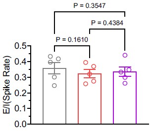
(2) The author should propose a potential mechanism for how TRPV3 helps to maintain cortical activity during fever. Would calcium influx-mediated change of membrane potential be the possible reason? Making a summary figure to put all the findings into perspective and propose a possible mechanism would also be appreciated.
Thank you for your helpful suggestion. In response, we have included a summary figure (Figure 11) illustrating the hypothesis described in the Discussion section. We agree with your assessment that Trpv3 most likely contributes to maintaining cortical activity during fever by promoting calcium influx and depolarizing the membrane potential.
(3) The author studied P7-8, P12-14, and P20-26 mice. How do these ages correspond to the human ages? it would be nice to provide a comparison to help the reader understand the context better.
Ideally, the mouse to human age comparison should depend on the specific process being studied. Per your suggestion, we have added additional references in the Introduction (Dobbing and Sands, 1973; Baram et al., 1997; Bender et al., 2004) to help readers better understand the correspondence between mouse and human ages.
Recommendations for the authors:
Reviewer #2 (Recommendations for the authors):
(3) Perform I-F curves to study the intrinsic properties of layer 2/3 neurons without the confound of evoked responses.
We performed F-I curve analyses (Figures 2H–I), as suggested by Reviewer 2, to study intrinsic properties of L2/3 neurons without evoked responses. Although rheobase increased at 39 °C compared to 30 °C, consistent with findings such as depolarized spike threshold and reduced input resistance, the mean number of spikes across current steps did not differ.
Reviewer #3 (Recommendations for the authors):
Some statistical descriptions are not clearly stated. For example, what statistical methods were used in Fig 2E? The effect size in Fig 2D seems to be quite small. The authors are advised to consider "nested analysis" to further increase the rigor of the analysis. Does each dot mean one neuron? Some of the data points might not be totally independent. The author should carefully check all figures to make sure the stats methods are provided for each panel.
We apologize for not including statistical details in Figure 2E. We have now added this information and verified that statistical descriptions are provided in all figure legends. In Figure 2D, each dot represents a cell, with measurements taken from the same cell at 30°C, 36°C, and 39°C. Given this design, the appropriate test is a one-way repeated-measures ANOVA.
Reports - Menu item for defining, requesting, and monitoring queries and reports. Fee - Menu item for setting and calculating fees. Automation - Menu item for managing scheduled processes, end-of-day, and start-of-day operations.
Ez a 3 menüpont kerüljön a Limit alá
Reviewer #3 (Public review):
The current paper investigates neural correlates of trust development in human-AI interaction, looking at EEG signatures locked to the moment that AI advice is presented. The key finding is that both human-response-locked EEG signatures (the CPP) and post-AI-advice signatures (N2, P3) are modulated by trust ratings. The study is interesting, however, it does have some clear and sometimes problematic weaknesses:
(1) The authors did not include "AI-advice". Instead, a manikin turned green or blue, which was framed as AI advice. It is unclear whether participants viewed this as actual AI advice.
(2) The authors did not include a "non-AI" control condition in their experiment, such that we cannot know how specific all of these effects are to AI, or just generic uncertain feedback processing.
(3) Participants perform the task at chance level. This makes it unclear to what extent they even tried to perform the task or just randomly pressed buttons. These situations likely differ substantially from a real-life scenario where humans perform an actual task (which is not impossible) and receive actual AI advice.
(4) Many of the conclusions in the paper are overstated or very generic.
Author response:
A major point all three reviewers raise is that the ‘human-AI collaboration’ in our experiment may not be true collaboration (as the AI does not classify images per se), but that it is only implied. The reviewers pointed out that whether participants were genuinely engaged in our experimental task is currently not sufficiently addressed. We plan to address this issue in the revised manuscript by including results from a brief interview we conducted after the experiment with each participant, which asked about the participant’s experience and decision-making processes while performing the task. Additionally, we also measured the participants’ propensity to trust in AI via a questionnaire before and after the experiment. The questionnaire and interview results will allow us to more accurately describe the involvement of our participants in the task. Additionally, we will conduct additional analyses of the behavioural data (e.g., response times) to show that participants genuinely completed the experimental task. Finally, we will work to sharpen our language and conclusions in the revised manuscript, following the reviewers’ recommendations.
Reviewer #1:
Summary:
In the study by Roeder and colleagues, the authors aim to identify the psychophysiological markers of trust during the evaluation of matching or mismatching AI decision-making. Specifically, they aim to characterize through brain activity how the decision made by an AI can be monitored throughout time in a two-step decision-making task. The objective of this study is to unfold, through continuous brain activity recording, the general information processing sequence while interacting with an artificial agent, and how internal as well as external information interact and modify this processing. Additionally, the authors provide a subset of factors affecting this information processing for both decisions.
Strengths:
The study addresses a wide and important topic of the value attributed to AI decisions and their impact on our own confidence in decision-making. It especially questions some of the factors modulating the dynamical adaptation of trust in AI decisions. Factors such as perceived reliability, type of image, mismatch, or participants' bias toward one response or the other are very relevant to the question in human-AI interactions.
Interestingly, the authors also question the processing of more ambiguous stimuli, with no real ground truth. This gets closer to everyday life situations where people have to make decisions in uncertain environments. Having a better understanding of how those decisions are made is very relevant in many domains.
Also, the method for processing behavioural and especially EEG data is overall very robust and is what is currently recommended for statistical analyses for group studies. Additionally, authors provide complete figures with all robustness evaluation information. The results and statistics are very detailed. This promotes confidence, but also replicability of results.
An additional interesting method aspect is that it is addressing a large window of analysis and the interaction between three timeframes (evidence accumulation pre-decision, decision-making, post-AI decision processing) within the same trials. This type of analysis is quite innovative in the sense that it is not yet a standard in complex experimental designs. It moves forward from classical short-time windows and baseline ERP analysis.
We appreciate the constructive appraisal of our work.
Weaknesses:
R1.1. This manuscript raises several conceptual and theoretical considerations that are not necessarily answered by the methods (especially the task) used. Even though the authors propose to assess trust dynamics and violations in cooperative human-AI teaming decision-making, I don't believe their task resolves such a question. Indeed, there is no direct link between the human decision and the AI decision. They do not cooperate per se, and the AI decision doesn't seem, from what I understood to have an impact on the participants' decision making. The authors make several assumptions regarding trust, feedback, response expectation, and "classification" (i.e., match vs. mismatch) which seem far stretched when considering the scientific literature on these topics.
This issue is raised by the other reviewers as well. The reviewer is correct in that the AI does not classify images but that the AI response is dependent on the participants’ choice (agree in 75% of trials, disagree in 25% of the trials). Importantly, though, participants were briefed before and during the experiment that the AI is doing its own independent image classification and that human input is needed to assess how well the AI image classification works. That is, participants were led to believe in a genuine, independent AI image classifier on this experiment.
Moreover, the images we presented in the experiment were taken from previous work by Nightingale & Farid (2022). This image dataset includes ‘fake’ (AI generated) images that are indistinguishable from real images.
What matters most for our work is that the participants were truly engaging in the experimental task; that is, they were genuinely judging face images, and they were genuinely evaluating the AI feedback. There is strong indication that this was indeed the case. We conducted and recorded brief interviews after the experiment, asking our participants about their experience and decision-making processes. The questions are as follows:
(1) How did you make the judgements about the images?
(2) How confident were you about your judgement?
(3) What did you feel when you saw the AI response?
(4) Did that change during the trials?
(5) Who do you think it was correct?
(6) Did you feel surprised at any of the AI responses?
(7) How did you judge what to put for the reliability sliders?
In our revised manuscript we will conduct additional analyses to provide detail on participants’ engagement in the task; both in the judging of the AI faces, as well as in considering the AI feedback. In addition, we will investigate the EEG signal and response time to check for effects that carry over between trials. We will also frame our findings more carefully taking scientific literature into account.
Nightingale SJ, and Farid H. "AI-synthesized faces are indistinguishable from real faces and more trustworthy." Proceedings of the National Academy of Sciences 119.8 (2022): e2120481119.
R1.2. Unlike what is done for the data processing, the authors have not managed to take the big picture of the theoretical implications of their results. A big part of this study's interpretation aims to have their results fit into the theoretical box of the neural markers of performance monitoring.
We indeed used primarily the theoretical box of performance monitoring and predictive coding, since the make-up of our task is similar to a more classical EEG oddball paradigm. In our revised manuscript, we will re-frame and address the link of our findings with the theoretical framework of evidence accumulation and decision confidence.
R1.3. Overall, the analysis method was very robust and well-managed, but the experimental task they have set up does not allow to support their claim. Here, they seem to be assessing the impact of a mismatch between two independent decisions.
Although the human and AI decisions are independent in the current experiment, the EEG results still shed light on the participant’s neural processes, as long as the participant considers the AI’s decision and believes it to be genuine. An experiment in which both decisions carry effective consequences for the task and the human-AI cooperation would be an interesting follow-up study.
Nevertheless, this type of work is very important to various communities. First, it addresses topical concerns associated with the introduction of AI in our daily life and decisions, but it also addresses methodological difficulties that the EEG community has been having to move slowly away from the static event-based short-timeframe analyses onto a more dynamic evaluation of the unfolding of cognitive processes and their interactions. The topic of trust toward AI in cooperative decision making has also been raised by many communities, and understanding the dynamics of trust, as well as the factors modulating it, is of concern to many high-risk environments, or even everyday life contexts. Policy makers are especially interested in this kind of research output.
Reviewer #2:
Summary:
The authors investigated how "AI-agent" feedback is perceived in an ambiguous classification task, and categorised the neural responses to this. They asked participants to classify real or fake faces, and presented an AI-agent's feedback afterwards, where the AI-feedback disagreed with the participants' response on a random 25% of trials (called mismatches). Pre-response ERP was sensitive to participants' classification as real or fake, while ERPs after the AI-feedback were sensitive to AI-mismatches, with stronger N2 and P3a&b components. There was an interaction of these effects, with mismatches after a "Fake" response affecting the N2 and those after "Real" responses affecting P3a&b. The ERPs were also sensitive to the participants' response biases, and their subjective ratings of the AI agent's reliability.
Strengths:
The researchers address an interesting question, and extend the AI-feedback paradigm to ambiguous tasks without veridical feedback, which is closer to many real-world tasks. The in-depth analysis of ERPs provides a detailed categorisation of several ERPs, as well as whole-brain responses, to AI-feedback, and how this interacts with internal beliefs, response biases, and trust in the AI-agent.
We thank the reviewer for their time in reading and reviewing our manuscript.
Weaknesses:
R2.1. There is little discussion of how the poor performance (close to 50% chance) may have affected performance on the task, such as by leading to entirely random guessing or overreliance on response biases. This can change how error-monitoring signals presented, as they are affected by participants' accuracy, as well as affecting how the AI feedback is perceived.
The images were chosen from a previous study (Nightingale & Farid, 2022, PNAS) that looked specifically at performance accuracy and also found levels around 50%. Hence, ‘fake’ and ‘real’ images are indistinguishable in this image dataset. Our findings agree with the original study.
Judging based on the brief interviews after the experiment (see answer to R.1.1.), all participants were actively and genuinely engaged in the task, hence, it is unlikely that they pressed buttons at random. As mentioned above, we will include a formal analysis of the interviews in the revised manuscript.
The response bias might indeed play a role in how participants responded, and this might be related to their initial propensity to trust in AI. We have questionnaire data available that might shed light on this issue: before and after the experiment, all participants answered the following questions with a 5-point Likert scale ranging from ‘Not True’ to ‘Completely True’:
(1) Generally, I trust AI.
(2) AI helps me solve many problems.
(3) I think it's a good idea to rely on AI for help.
(4) I don't trust the information I get from AI.
(5) AI is reliable.
(6) I rely on AI.
The propensity to trust questionnaire is adapted from Jessup SA, Schneider T R, Alarcon GM, Ryan TJ, & Capiola A. (2019). The measurement of the propensity to trust automation. International Conference on Human-Computer Interaction.
Our initial analyses did not find a strong link between the initial (before the experiment) responses to these questions, and how images were rated during the experiment. We will re-visit this analysis and add the results to the revised manuscript.
Regarding how error-monitoring (or the equivalent thereof in our experiment) is perceived, we will analyse interview questions 3 (“What did you feel when you saw the AI response”) and 6 (“Did you feel surprised at any of the AI responses”) and add results to the revised manuscript.
The task design and performance make it hard to assess how much it was truly measuring "trust" in an AI agent's feedback. The AI-feedback is yoked to the participants' performance, agreeing on 75% of trials and disagreeing on 25% (randomly), which is an important difference from the framing provided of human-AI partnerships, where AI-agents usually act independently from the humans and thus disagreements offer information about the human's own performance. In this task, disagreements are uninformative, and coupled with the at-chance performance on an ambiguous task, it is not clear how participants should be interpreting disagreements, and whether they treat it like receiving feedback about the accuracy of their choices, or whether they realise it is uninformative. Much greater discussion and justification are needed about the behaviour in the task, how participants did/should treat the feedback, and how these affect the trust/reliability ratings, as these are all central to the claims of the paper.
In our experiment, the AI disagreements are indeed uninformative for the purpose of making a correct judgment (that is, correctly classifying images as real or fake). However, given that the AI-generated faces are so realistic and indistinguishable from the real faces, the correctness of the judgement is not the main experimental factor in this study. We argue that, provided participants were genuinely engaged in the task, their judgment accuracy is less important than their internal experience when the goal is to examine processes occurring within the participants themselves. We briefed our participants as follows before the experiment:
“Technology can now create hyper-realistic images of people that do not exist. We are interested in your view on how well our AI system performs at identifying whether images of people’s faces are real or fake (computer-generated). Human input is needed to determine when a face looks real or fake. You will be asked to rate images as real or fake. The AI system will also independently rate the images. You will rate how reliable the AI is several times throughout the experiment.”
We plan to more fully expand the behavioural aspect and our participants’ experience in the revised manuscript by reporting the brief post-experiment interview (R.1.1.), the propensity to trust questionnaire (R.2.1.), and additional analyses of the response times.
There are a lot of EEG results presented here, including whole-brain and window-free analyses, so greater clarity on which results were a priori hypothesised should be given, along with details on how electrodes were selected for ERPs and follow-up tests.
We chose the electrodes mainly to be consistent across findings, and opted to use central electrodes (Pz and Fz), as long as the electrode was part of the electrodes within the reported cluster. We can in our revised manuscript also report on the electrodes with the maximal statistic, as part of a more complete and descriptive overview. We will also report on where we expected to see ERP components within the paper. In short, we did expect something like a P3, and we did also expect to see something before the response what we call the CPP. The rest of the work was more exploratory, with a more careful expectation that bias would be connected to the CPP, and the reliability ratings more to the P3; however, we find the opposite results. We will include this in our revised work as well.
We selected the electrodes primarily to maintain consistency across our findings and figures, and focused on central electrodes (Pz and Fz), provided they fell within the reported cluster. In the revised manuscript, we will also report the electrodes showing the maximal statistical effects to give a more complete and descriptive overview. Additionally, we will report where we expected specific ERP components to appear. In brief, we expected to see a P3 component post AI feedback, and a pre-response signal corresponding to the CPP. Beyond these expectations, the remaining analyses were more exploratory. Although we tentatively expected bias to relate to the CPP and reliability ratings to the P3, our results showed the opposite pattern. We will clarify this in the revised version of the manuscript.
Reviewer #3:
The current paper investigates neural correlates of trust development in human-AI interaction, looking at EEG signatures locked to the moment that AI advice is presented. The key finding is that both human-response-locked EEG signatures (the CPP) and post-AI-advice signatures (N2, P3) are modulated by trust ratings. The study is interesting, however, it does have some clear and sometimes problematic weaknesses:
(1) The authors did not include "AI-advice". Instead, a manikin turned green or blue, which was framed as AI advice. It is unclear whether participants viewed this as actual AI advice.
This point has been raised by the other reviewers as well, and we refer to the answers under R1.1., and under R2.1. We will address this concern by analysing the post-experiment interviews. In particular, questions 3 (“What did you feel when you saw the AI response”), 4 (“Did that change during the trials?”) and 6 (“Did you feel surprised at any of the AI responses”) will give critical insight. As stated above, our general impression from conducting the interviews is that all participants considered the robot icon as decision from an independent AI agent.
(2) The authors did not include a "non-AI" control condition in their experiment, such that we cannot know how specific all of these effects are to AI, or just generic uncertain feedback processing.
In the conceptualization phase of this study, we indeed considered different control conditions for our experiment to contrast different kinds of feedback. However, previous EEG studies on performance monitoring ERPs have reported similar results for human and machine supervision (Somon et al., 2019; de Visser et al., 2018). We therefore decided to focus on one aspect (the judgement of observation of an AI classification), also to prevent the experiment from taking too long and risking that participants would lose concentration and motivation to complete the experiment. Comparing AI vs non-AI feedback, is still interesting and would be a valuable follow-up study.
Somon B, et al. "Human or not human? Performance monitoring ERPs during human agent and machine supervision." NeuroImage 186 (2019): 266-277.
De Visser EJ, et al. "Learning from the slips of others: Neural correlates of trust in automated agents." Frontiers in human neuroscience 12 (2018): 309.
(3) Participants perform the task at chance level. This makes it unclear to what extent they even tried to perform the task or just randomly pressed buttons. These situations likely differ substantially from a real-life scenario where humans perform an actual task (which is not impossible) and receive actual AI advice.
This concern was also raised by the other two reviewers. As already stated in our responses above, we will add results from the post-experiment interviews with the participants, the propensity to trust questionnaire, and additional behavioural analyses in our revised manuscript.
Reviewer 1 (R1.3) also brought up the situation where decisions by the participant and the AI have a more direct link which carries consequences. This will be valuable follow-up research. In the revised manuscript, we will more carefully frame our approach.
(4) Many of the conclusions in the paper are overstated or very generic.
In the revised manuscript, we will re-phrase our discussion and conclusions to address the points raised in the reviewer’s recommendations to authors.
Reviewer #1 (Public review):
Summary:
This manuscript provides a comprehensive systematic analysis of envelope-containing Ty3/gypsy retrotransposons (errantiviruses) across metazoan genomes, including both invertebrates and ancient animal lineages. Using iterative tBLASTn mining of over 1,900 genomes, the authors catalog 1,512 intact retrotransposons with uninterrupted gag, pol, and env open reading frames. They show that these elements are widespread-present in most metazoan phyla, including cnidarians, ctenophores, and tunicates-with active proliferation indicated by their multicopy status. Phylogenetic analyses distinguish "ancient" and "insect" errantivirus clades, while structural characterization (including AlphaFold2 modeling) reveals two major env types: paramyxovirus F-like and herpesvirus gB-like proteins. Although bot envelope types were identified in previous analyses two decades ago, the evolutionary provenance of these envelope genes was almost rudimentary and anecdotal (I can say this because I authored one of these studies). The results in the present study support an ancient origin for env acquisition in metazoan Ty3/gypsy elements, with subsequent vertical inheritance and limited recombination between env and pol domains. The paper also proposes an expanded definition of 'errantivirus' for env-carrying Ty3/gypsy elements outside Drosophila.
Strengths:
(1) Comprehensive Genomic Survey:<br /> The breadth of the genome search across non-model metazoan phyla yields an impressive dataset covering evolutionary breadth, with clear documentation of search iterations and validation criteria for intact elements.
(2) Robust Phylogenetic Inference:<br /> The use of maximum likelihood trees on both pol and env domains, with thorough congruence analysis, convincingly separates ancient from lineage-specific elements and demonstrates co-evolution of env and pol within clades.
(3) Structural Insights:<br /> AlphaFold2-based predictions provide high-confidence structural evidence that both env types have retained fusion-competent architectures, supporting the hypothesis of preserved functional potential.
(4) Novelty and Scope:<br /> The study challenges previous assumptions of insect-centric or recent env acquisition and makes a compelling case for a Pre-Cambrian origin, significantly advancing our understanding of animal retroelement diversity and evolution. THIS IS A MAJOR ADVANCE.
(5) Data Transparency:<br /> I appreciate that all data, code, and predicted structures are made openly available, facilitating reproducibility and future comparative analyses.
Major Weaknesses
(1) Functional Evidence Gaps:<br /> The work rests largely on sequence and structure prediction. No direct expression or experimental validation of envelope gene function or infectivity outside Drosophila is attempted, which would be valuable to corroborate the inferred roles of these glycoproteins in non-insect lineages. At least for some of these species, there are RNA-seq datasets that could be leveraged.
(2) Horizontal Transfer vs. Loss Hypotheses:<br /> The discussion argues primarily for vertical inheritance, but the somewhat sporadic phylogenetic distributions and long-branch effects suggest that loss and possibly rare horizontal events may contribute more than acknowledged. Explicit quantitative tests for horizontal transfer, or reconciliation analyses, would strengthen this conclusion. It's also worth pointing out that, unlike retrotransposons that can be found in genomes, any potential related viral envelopes must, by definition, have a spottier distribution due to sampling. I don't think this challenges any of the conclusions, but it must be acknowledged as something that could affect the strength of this conclusion
(3) Limited Taxon Sampling for Certain Phyla:<br /> Despite the impressive breadth, some ancient lineages (e.g., Porifera, Echinodermata) are negative, but the manuscript does not fully explore whether this reflects real biological absence, assembly quality, or insufficient sampling. A more systematic treatment of negative findings would clarify claims of ubiquity. However, I also believe this falls beyond the scope of this study.
(4) Mechanistic Ambiguity:<br /> The proposed model that env-containing elements exploit ovarian somatic niches is plausible but extrapolated from Drosophila data; for most taxa, actual tissue specificity, lifecycle, or host interaction mechanisms remain speculative and, to me, a bit unreasonable.
Minor Weaknesses:
(1) Terminology and Nomenclature:<br /> The paper introduces and then generalizes the term "errantivirus" to non-insect elements. While this is logical, it may confuse readers familiar with the established, Drosophila-centric definition if not more explicitly clarified throughout. I also worry about changes being made without any input from the ICTV nomenclature committee, which just went through a thorough reclassification. Nevertheless, change is expected, and calling them all errantiviruses is entirely reasonable.
(2) Figures and Supplementary Data Navigation:<br /> Some key phylogenies and domain alignments are found only in supplementary figures, occasionally hindering readability for non-expert audiences. Selected main-text inclusion of representative trees would benefit accessibility.
(3) ORF Integrity Thresholds:<br /> The cutoff choices for defining "intact" elements (e.g., numbers/placement of stop codons, length ranges) are reasonable but only lightly justified. More rationale or sensitivity analysis would improve confidence in the inclusion criteria. For example, how did changing these criteria change the number of intact elements?
(4) Minor Typos/Formatting:<br /> The paper contains sporadic typographical errors and formatting glitches (e.g., misaligned figure labels, unrendered symbols) that should be addressed.
Reviewer #3 (Public review):
Summary and Significance:
In this work, Cary and Hayashi address the important question of when, in evolution, certain mobile genetic elements (Ty3/gypsy-like non-LTR retrotransposons) associated with certain membrane fusion proteins (viral glycoprotein F or B-like proteins), which could allow these mobile genetic elements to be transferred between individual cells of a given host. It is debated in the literature whether the acquisition of membrane fusion proteins by non-LTR retrotransposons is a rather recent phenomenon that separately occurred in the ancestors of certain host species or whether the association with membrane fusion proteins is a much more ancient one, pre-dating the Cambrian explosion. Obviously, this question also touches upon the origin of the retroviruses, which can spread between individuals of a given host but seem restricted to vertebrates. Based on convincing data, Cary and Hayashi argue that an ancient association of non-LTR retrotransposons with membrane fusion proteins is most probable.
Strengths:
The authors take the smart approach to systematically retrieve apparently complete, intact, and recently functional Ty3/gypsy-like non-LTR retrotransposons that, next to their characteristic gag and pol genes, additionally carry sequences that are homologous to viral glycoprotein F (env-F) or viral glycoprotein B (env-B). They then construct and compare phylogenetic trees of the host species and individual encoded proteins and protein domains, where 3D-structure calculations and other features explain and corroborate the clustering within the phylogenetic trees. Congruence of phylogenetic trees and correlation of structural features is then taken as evidence for an infrequent recombination and a long-term co-evolution of the reverse transcriptase (encoded by the pol gene) and its respective putative membrane fusion gene (encoded by env-F or env-B). Importantly, the env-F and env-B containing retrotransposons do not form a monophyletic group among the Ty3/gypsy-like non-LTR retrotransposons, but are scattered throughout, supporting the idea of an originally ancient association followed by a random loss of env-F/env-B in individual branches of the tree (and rather rare re-associations via more recent recombinations).
Overall, this is valuable, stimulating, and important work of general and fundamental interest, but still also somewhat incompletely explored, imprecisely explained, and insufficiently put into context for a more general audience.
Weaknesses:
Some points that might be considered and clarified:
(1) Imprecise explanations, terms, and definitions:
It might help to add a 'definitions box' or similar to precisely explain how the authors decided to use certain terms in this manuscript, and then use these terms consistently and with precision.
a) In particular, these are terms such as 'vertebrate retrovirus' vs 'retrovirus' vs 'endogenized retrovirus' vs 'endogenous retrovirus' vs 'non-LTR retrotransposon' and 'Ty3/gypsi-like retrotransposon' vs 'Ty3/gypsy retrotransposon' vs 'errantivirus'.
b) The comment also applies to the term 'env' used for both 'env-F' and 'env-B', where often it remains unclear which of the two protein types the authors refer to. This is confusing, particularly in the methods, where the search for the respective homologs is described.
c) Other examples are the use of the entire pol gene vs. pol-RT for the definition of the Ty3/gypsy clade and for the generation of phylogenetic trees (Methods and Figure S1), and the names for various portions of pol that appear without prior definition or explanation (e.g., 'pro' in Figure 1A, 'bridge' in Figure S1C, 'the chromodomain' in the text and Figure 7).
d) It is unclear from the main text which portions of pol were chosen to define pol-RT and why. The methods name the 'palm-and-fingers', 'thumb', and 'connections' domains to define RT. In the main text, the 'connection' domain is called 'tether' and is instead defined as part of the 'bridge' region following RT, which is not part of RT.
(2) Insufficient broader context:
a) The introduction does not state what defines Ty3/gypsy non-LTR retrotransposons as compared to their closest relatives (Ty1/copia retrotransposons, BEL/pao retrotransposons, vertebrate retroviruses). This makes it difficult to judge the significance and generality of the findings.
b) The various known compositions of Ty3/gypsi-like retrotransposons are not mentioned and explained in the introduction (open reading frames, (poly-)proteins and protein domains, and their variable arrangement, enzymatic activities, and putative functions), and the distribution of Ty3/gypsi-like retrotransposons among eukaryotes remains unclear. The introduction does not mention that Ty3/gypsi-like retrotransposons apparently are absent from vertebrates, and Figure 7 is not very clear about whether or not it includes sequences from plants ('Chromoviridae').
c) The known association of Ty3/gypsi-like retrotransposons from different metazoan phyla with putative membrane fusion proteins (env-like) genes is mentioned in the introduction, but literature information, whether such associations also occur in the context of other retrotransposons (e.g., Ty1/ copia or BEL/pao), is not provided. The abstract is somewhat misleading in this respect. Finally, the different known types of env-like genes are not mentioned and explained as part of the introduction ('env-f', 'env-B', 'retroviral env', others?)
d) Some key references and reviews might be added:
- Pelisson, A. et al. (1994) https://www.embopress.org/doi/abs/10.1002/j.1460-2075.1994.tb06760.x<br /> (next to Song et al. (1994), for the identification of env in Ty3/gypsy)
- Boeke, J.D. et al. (1999)<br /> In Virus Taxonomy: ICTV VIIth report. (ed. F.A. Murphy),. Springer-Verlag, New York.<br /> (cited by Malik et al. (2000) - for the definition and first use of the term 'errantivirus')
- Eickbush, T.H. and Jamburuthugoda, V.K. (2008) https://doi.org/10.1016/j.virusres.2007.12.010<br /> (on the classification of retrotransposons and their env-like genes)
- Hayward, A. (2017) https://doi.org/10.1016/j.coviro.2017.06.006<br /> (on scenarios of env acquisition)
(3) Incomplete analysis:
a) Mobile genetic elements are sometimes difficult to assemble correctly from short-read sequencing data. Did the authors confirm some of their newly identified elements by e.g., PCR analysis or re-identification in long-read sequencing data?
b) The authors mention somewhat on the side that there are Ty3/gypsy elements with a different arrangement (gag-env-pol instead of gag-pol-env). Why was this important feature apparently not used and correlated in the analysis? How does it map on the RT phylogenetic tree? Which type of env is found with either arrangement? Is there evidence for a loss of env also in the case of gag-env-pol elements?
c) Sankey plots are insufficiently explained. How would inconsistencies between trees (recombinations) show up here? Why is there no Sankey plot for the analysis of env-B in Figure 5?
d) Why are there no trees generated for env-F and env-B like proteins, including closely related homologous sequences that do NOT come from Ty3/gypsy retrotransposons (e.g., from the eukaryotic hosts, from other types of retrotransposons (Ty1/copia or BEL/pao), from viruses such as Herpesvirus and Baculovirus)? It would be informative whether the sequences from Ty3/gypsy cluster together in this case.
e) Did the authors identify any other env-like ORFs (apart from env-F and env-B) among Ty3/gypsy retrotransposons? Did they identify other, non-env-like ORFs that might help in the analysis? It is not quite clear from the methods if the searches for env-F and env-B - containing Ty3/gypsy elements were done separately and consecutively or somehow combined (the authors generally use 'env', and it is not clear which type of protein this refers to).
f) Why was the gag protein apparently not used to support the analysis? Are there different, unrelated types of gag among non-LTR retrotransposons? Does gag follow or break the pattern of co-evolution between RT and env-F/env-B?
g) Data availability. The link given in the paper does not seem to work (https://github.com/RippeiHayashi/errantiviruses_2025/tree/main). It would be useful for the community to have the sequences of the newly identified Ty3/gypsy retrotransposons listed readily available (not just genome coordinates as in table S1), together with the respective annotations of ORFs and features.
Author response:
We appreciate thorough and highly valuable feedback from the reviewers. We will take their suggestions on board and prepare a revised manuscript focusing on the following points:
(1) As reviewers pointed out, we did not evaluate horizontal transfer events of env-containing Ty3/gypsy elements. We consistently observed that elements found in the same phylum/class/superfamily cluster together in the POL phylogenetic tree, suggesting an ancient acquisition of env to the Ty3/gypsy elements—separation should not be as clear as we observed should they had been frequently gained from animals across different phylum/class/superfamilies. However, this does not exclude more recent horizontal transfer events that may occur between closely related species. We will perform gene-tree species-tree reconciliation analyses in clades that have enough elements and represented species to estimate the frequency of horizontal transfer events.
(2) We did not find env-containing Ty3/gypsy elements in some animal phyla such as Echinodermata and Porifera, but this could be due to the quality or number of available genome assemblies as reviewers suggested. To address this, we will mine GAG-POL gypsy elements in the genomes that were devoid of GAG-POL-ENV elements and compare their abundance with other genomes that carry GAG-POL-ENV elements. If GAG-POL gypsy elements were similarly abundantly identified, that would indicate that the observed absence of GAG-POL-ENV elements is not due to poor quality of genome assemblies.
(3) We will include F-type and HSV-gB type ENV proteins from known viruses in the phylogenetic analysis to investigate their ancestry and potential recombination events with env-containing Ty3/gypsy elements.
(4) Wherever relevant, we will clarify the terms using in the manuscript, provide rationale to our selection of POL domains used for structural and phylogenetic analyses, improve accessibility of figures, touch on gypsy elements in vertebrates, and make sure all concepts covered in the results are sufficiently introduced in the introduction.
Researchers from University College London and the University of Florida examined national data from 2003 to 2023 and found that the share of people who reported reading for pleasure on a given day fell to 16 percent in 2023 from a peak of 28 percent in 2004 — a drop of about 40 percent. It declined around 3 percent each year over those two decades.
statics (logos)
The Math of Why You Can't Focus at Work
“You come heah wid yo’ mouf full uh foolishness on uh busy day. Heah you got uh prop tuh lean on all yo’ bawn days, and big protection, and everybody got tuh tip dey hat tuh you and call you Mis’ Killicks, and you come worryin’ me ’bout love.” “But Nanny, Ah wants to want him sometimes. Ah don’t want him to do all de wantin’.”
Notice the contrasting views of Nanny and Janie.
Nanny has had a rougher early life compared with Janie, being a former slave, and as a result, she doesn't even care about love. Having someone like Logan as a husband would be unimaginably good to Nanny when she was Janie's age.
Janie never faced slavery, and takes personal safety for granted, so she wants personal fulfillment as well.
Husbands and wives always loved each other, and that was what marriage meant. It was just so.
Janie's current view on romance—marriage comes before love.
somatosensation
Rewsponds to stimuili like -temp -touch -pain -pressure -vibrayion
Écologie : Complexité, Paradoxes et Holisme — Synthèse de la Leçon Inaugurale de Franck Courchamp
Cette note de synthèse résume la leçon inaugurale de Franck Courchamp, titulaire de la chaire annuelle "Biodiversité et écosystèmes" au Collège de France.
La présentation articule l'étude de l'écologie autour de trois concepts fondamentaux : la complexité, les paradoxes et le holisme.
Franck Courchamp, directeur de recherche au CNRS et scientifique de renommée mondiale, démontre que la biodiversité est un système d'une richesse et d'une interconnexion extraordinaires, dont la compréhension ne peut être que partielle sans une approche globale.
Les points clés sont les suivants :
• La Biodiversité est une réalité multidimensionnelle et largement méconnue.
Définie à trois niveaux (spécifique, génétique, écosystémique), elle représente une richesse quantitative (potentiellement jusqu'à 10 milliards d'espèces de procaryotes) et qualitative (valeur utilitaire et intrinsèque) immense.
Cependant, la science n'a décrit qu'une infime fraction de cette diversité (2,3 millions d'espèces eucaryotes), alors même qu'un million d'espèces sont menacées d'extinction.
• La complexité est la caractéristique fondamentale des écosystèmes.
Le nombre vertigineux d'espèces (des dizaines de milliers dans une surface équivalente à une salle de conférence en forêt amazonienne) et la multitude d'interactions directes et indirectes entre elles et avec leur environnement créent des systèmes dynamiques et auto-organisés d'une complexité qui dépasse souvent l'intuition.
• De cette complexité naissent des paradoxes écologiques. De nombreux phénomènes observés en écologie sont contre-intuitifs.
Par exemple, l'ajout d'engrais peut appauvrir la diversité végétale, la prévention des incendies peut engendrer des méga-feux, et la réintroduction de prédateurs comme le loup peut paradoxalement rendre les routes plus sûres en modifiant le comportement de leurs proies.
• L'approche holistique est indispensable pour comprendre et agir.
Seule une vision globale de l'écosystème, intégrant toutes ses composantes et interactions, permet de déchiffrer ces paradoxes et d'éviter des interventions de conservation aux conséquences inverses de celles escomptées.
L'exemple de la réintroduction des loups à Yellowstone, qui a modifié jusqu'au cours des rivières, illustre parfaitement la puissance des effets en cascade qu'une approche holistique peut révéler.
La conférence conclut que ces trois concepts — complexité, paradoxes, holisme — sont des outils intellectuels essentiels pour naviguer dans le champ de l'écologie.
Ils formeront le fil conducteur des cours à venir, qui se concentreront sur la biologie des invasions, en adoptant une perspective résolument interdisciplinaire.
--------------------------------------------------------------------------------
La leçon inaugurale a été prononcée dans le cadre de la cinquième édition de la chaire annuelle "Biodiversité et écosystèmes" du Collège de France, une initiative soutenue par la Fondation Jean-François de Clermont-Tonnerre.
Cette chaire vise à promouvoir la recherche et à éclairer le débat public sur les enjeux du vivant.
Le titulaire de la chaire, Franck Courchamp, est une figure de premier plan dans le domaine de l'écologie. Ses qualifications incluent :
• Positions académiques : Directeur de recherche première classe au CNRS, il dirige une équipe à l'Université Paris-Saclay et est titulaire de la chaire AXA "Biologie des invasions".
• Reconnaissance internationale : Auteur de plus de 200 publications, il est l'un des scientifiques les plus cités au monde dans son domaine et contribue aux travaux de panels intergouvernementaux majeurs comme le GIEC et l'IPBES.
• Distinctions : Il a reçu de nombreuses récompenses, dont la médaille d'argent du CNRS (2011), a été nommé à l'Académie européenne des sciences (2014) et fait chevalier de l'Ordre national du Mérite (2021).
• Vulgarisation : Reconnu pour son talent de communicant, il a participé à des documentaires (notamment la série Une espèce à part sur Arte), et a publié des ouvrages grand public tels que L'Écologie pour les nuls et la bande dessinée La Guerre des fourmis.
La biodiversité, contraction de "diversité biologique", est classiquement analysée selon trois échelles interdépendantes :
1. La biodiversité spécifique : Le nombre d'espèces présentes dans un espace donné (ex. : 160 000 à 180 000 espèces de papillons dans le monde). C'est le niveau le plus couramment étudié.
2. La biodiversité génétique : La diversité au sein d'une même espèce (ex. : les 340 races de chiens). Une faible diversité génétique, comme chez le guépard, rend une espèce très vulnérable.
3. La biodiversité écosystémique : La variété des écosystèmes dans un paysage (ex. : un paysage avec forêt, lac et prairie a une plus grande diversité écosystémique qu'un récif corallien, même si ce dernier a une très grande diversité spécifique).
L'ampleur de la biodiversité sur Terre reste largement sous-estimée.
• Espèces décrites : La science a formellement décrit 2,3 millions d'espèces eucaryotes (animaux, plantes, champignons, protistes).
• Espèces inconnues : Les estimations suggèrent que la grande majorité des espèces reste à découvrir. Le tableau suivant, évoqué dans la conférence, illustre ce déficit de connaissance :
Pourcentage d'Espèces Inconnues (estimation)
Mammifères
Près de 10 %
Poissons
Près de 90 %
Insectes
Près de 90 %
Algues
Près de 90 %
Champignons
Plus de 90 %
Franck Courchamp souligne : "Nous vivons, sans le savoir, dans un monde de champignons et d'insectes."
De plus, les eucaryotes ne sont qu'une infime partie du vivant ; les procaryotes (bactéries et archées) pourraient représenter jusqu'à 10 milliards d'espèces.
La biodiversité est importante pour l'humanité de deux manières distinctes :
• La valeur utilitaire : Elle fournit des "biens" et des "services" essentiels.
◦ Biens : Alimentation (seulement 12 espèces végétales fournissent 75% de la nourriture mondiale), matériaux (bois, coton, laine), et médicaments (deux tiers des molécules pharmaceutiques proviennent directement des plantes).
◦ Services : Pollinisation (près de 80% de nos cultures), purification de l'eau et de l'air, fertilisation des sols et biodégradation.
• La valeur intrinsèque : Chaque espèce, écosystème ou individu possède une valeur propre, indépendamment de son utilité pour l'être humain.
Une Richesse Menacée
Cette richesse est en péril. Le rapport de l'IPBES de 2019 a établi qu'un million d'espèces animales et végétales sont menacées d'extinction au cours des prochaines décennies, avec une accélération notable du rythme des extinctions récentes.
L'écologie est la discipline scientifique qui étudie les interactions entre les organismes et leur environnement. Elle est intrinsèquement liée à la science de l'évolution. Comme le formule Franck Courchamp : "L'écologie observe la danse des espèces dans leur environnement [...]. L'évolution raconte l'histoire de cette danse."
L'écologie analyse des systèmes à différentes échelles, des individus à la biosphère. L'étude de la dynamique des populations offre une porte d'entrée.
L'exemple classique des cycles prédateur-proie entre le lynx et le lièvre arctique, documenté grâce aux registres de la Compagnie de la Baie d'Hudson, montre comment des modèles mathématiques simples (comme le modèle de Lotka-Volterra) peuvent décrire des dynamiques complexes.
Cependant, la réalité est celle de réseaux trophiques où chaque espèce interagit avec de nombreuses autres, créant des systèmes d'une complexité immense, auxquels s'ajoutent les interactions non-vivantes (cycles biogéochimiques du carbone, de l'azote, etc.).
Franck Courchamp propose une grille de lecture de l'écologie fondée sur trois concepts interdépendants.
La biodiversité est un système caractérisé par une richesse, une dynamicité et un nombre d'interactions extraordinairement élevés.
Un exercice de pensée illustre ce point : sur une surface équivalente à celle de la salle de conférence, une forêt amazonienne peut abriter entre 10 000 et 20 000 espèces différentes, dont 5 000 à 10 000 espèces d'insectes.
L'ensemble des interactions directes et indirectes entre ces milliers d'acteurs forme un système dynamique, auto-organisé (autopoïétique) et multiscalaire.
De cette complexité émergent des résultats qui défient l'intuition. Ces paradoxes sont omniprésents en écologie.
• Paradoxes généraux :
◦ Écologie des communautés : L'ajout d'engrais peut "tuer" les plantes en favorisant quelques espèces dominantes au détriment de la diversité globale, rendant l'écosystème moins stable.
◦ Écologie forestière : La suppression systématique des feux de faible intensité mène à l'accumulation de combustible et à des "méga-feux" dévastateurs.
◦ Biologie de la conservation : Le retour des loups dans certaines régions des États-Unis a réduit de près d'un quart les accidents de voiture impliquant des cerfs, non pas en diminuant leur population, mais en modifiant leur comportement (création d'un "paysage de la peur").
• Paradoxes issus des recherches de Franck Courchamp :
◦ Épidémiologie : Les chats infectés par le VIF (sida du chat) vivent plus longtemps, car le virus se transmet lors de combats entre les individus les plus dominants et les plus robustes.
◦ Effet Allee : Pour certaines espèces sociales (suricates, lycaons), c'est l'incapacité à coopérer en dessous d'un certain seuil d'effectif qui cause l'extinction, et non la compétition.
◦ Paradoxe de la rareté : La rareté d'une espèce augmente sa valeur sur le marché (chasse, collection), ce qui intensifie son exploitation et accélère sa disparition dans une boucle de rétroaction positive.
◦ Espèces charismatiques : Elles sont à la fois les plus aimées, les plus menacées, et leur omniprésence culturelle nous fait croire à tort qu'elles sont communes, ce qui freine les efforts de conservation.
La clé pour comprendre ces paradoxes et agir efficacement est l'adoption d'une approche holistique, qui considère l'écosystème dans son ensemble.
• Pour Comprendre : L'Exemple des Loups à Yellowstone La réintroduction du loup, un prédateur apical, a déclenché une cascade d'effets dans tout l'écosystème :
1. Contrôle des élans : Diminution de la pression de broutage sur la végétation.
2. Régénération de la végétation : Les saules et les peupliers ont pu repousser.
3. Retour des castors : Avec plus de bois, les populations de castors ont explosé, créant des barrages.
4. Modification des rivières : Les barrages ont modifié l'hydrologie et la morphologie des cours d'eau, créant des habitats pour d'autres espèces (poissons, amphibiens, oiseaux). Cet exemple montre qu'une seule action peut avoir des répercussions profondes et inattendues sur l'ensemble du système.
• Pour Agir : Biologie de la Conservation Une vision non-holistique peut mener à l'échec. La surprotection des éléphants dans certaines réserves, sans tenir compte du reste de l'écosystème, a conduit à la dégradation de la végétation et a nui à d'autres herbivores.
De même, l'interdiction totale du commerce de l'ivoire, bien qu'intentionnée, a créé un marché noir qui a pu intensifier le braconnage dans certaines zones.
La complexité, les paradoxes et le holisme ne sont pas de simples concepts académiques, mais des outils essentiels pour déchiffrer le fonctionnement du vivant et orienter l'action humaine.
Ces principes formeront la structure des cours à venir de Franck Courchamp, qui se concentreront sur la biologie des invasions.
Chaque cours sera enrichi par un séminaire mené par un spécialiste d'une autre discipline (économie, philosophie, épidémiologie, etc.), soulignant la nécessité d'une approche interdisciplinaire pour relever les défis environnementaux actuels.
La leçon se termine sur une citation de Carl Sagan, rappelant que la nature recèle encore d'innombrables merveilles à découvrir : "Quelque part, quelque chose d'incroyable attend d'être connu."
Specific words and images make your writing clearer, more precise, and often more interesting. Whenever possible, avoid overly general words in your writing; instead, try to replace general language with particular nouns, verbs, and modifiers that convey details and that bring yours words to life. Add words that provide color, texture, sound, and even smell to your writing.
This makes me realize that using specific words could make such a big difference.Adding small details like color or sound can suddenly make writing feel more alive.
You and 7 others reacted
Domsch suggests that for game choices to feel as if theypossess meaning, they must rely on three guiding principles:they must feel meaningful 1) by being difficult to achieve;2) by making their relevance ambiguous; and 3) by notproviding full gameplay information to the player, and onlysometimes providing full gameplay information. By presentingchoices with incomplete information, the player cannot applya mechanistic decision-making process to get the idealoutcome, and thus the choice feels more meaningful. Thisforces the player to rely on the game’s narrative structureand its broader fiction.
Scarcity, Novelty, and Unpredictableness to build a dramatic arc with ups and downs.
In part, this aspirational aspect was due to the financialsituation of the London-based Royal Africa Company (RAC)early on; those responsible for the fort were chronicallyunderfunded and typically owed money, as seen through anextensive correspondence by the chief factor, RobertPlunkett, requesting supplies in the early eighteenthcentury.3 Those who worked at Bunce were isolated by distanceand the time period from close oversight by their companyofficials.
About communication delay, which now is much uncommon, but still happens in some rural areas.
现有跨境支付存在渠道分散、结算效率低、成本较高、透明度不足等问题。各国跨境支付系统(SWIFT、CHIPS、SEPA)技术标准、运营时间、接口、数据格式不统一,导致跨境支付链路冗长,处理环节复杂;传统跨境支付依赖电报式报文传输,平均处理时间需1~3天;代理行费用叠加导致产生高额手续费,并且交易路径不透明,难以追踪支付状态。应对金融制裁风险,美国频繁使用 SWIFT 系统制裁相关国家,将金融基础设施武器化,使金融贸易体系面临金融霸权威胁。
建设CIPS系统的背景
As a colonial organization, See argues that “rather than borrowing only Irish and English political concerns, the Canadian Orangemen charted a course that addressed local issues and attempted to solve indigenous problems,” particularly in the wake of Irish−Catholic and French−Canadian migration into English Canada (See Citation1993, 75). The Orange Order thus established itself in Canada as a “bulwark of colonial Protestantism,” in the words of Smyth and Houston, a force for the maintenance of a British identity in the face of a significant French Catholic population. The Order opposed the extension of French culture into Ontario, particularly with regard to the use of the French language in schools, and insisted that “the movement of French colonists into Ontario had been a ‘popish plot’” (Houston and Smyth Citation1980, 3, 47).
Again, "specific COLONIAL context" but mirrors almost exactly the context of NI -> fight against French Catholicism. Says it is concerned w/ local issues but this is the same issue , just w/ added ethni-linguiustic edge.
Anyway, "Bulwarck of colonial Protestantism"
"As a colonial organization, See argues that “rather than borrowing only Irish and English political concerns, the Canadian Orangemen charted a course that addressed local issues and attempted to solve indigenous problems,” particularly in the wake of Irish−Catholic and French−Canadian migration into English Canada (See Citation1993, 75). The Orange Order thus established itself in Canada as a “bulwark of colonial Protestantism,” in the words of Smyth and Houston, a force for the maintenance of a British identity in the face of a significant French Catholic population. The Order opposed the extension of French culture into Ontario, particularly with regard to the use of the French language in schools, and insisted that “the movement of French colonists into Ontario had been a ‘popish plot’” (Houston and Smyth Citation1980, 3, 47)."
If the relationship between pressure and altitude were exactly exponential, this plot would be a straight line. It is not quite straight because the temperature of the atmosphere also comes into play, and temperature is also not constant with height. Pressure decreases with altitude less quickly where the atmosphere is warmer because the density is lower, and more quickly where the temperature is lower. However, these variations are not huge because the temperature range (in kelvin) is not large – about 213–288 K over the troposphere, for example – compared to pressure changes that span many orders of magnitude. We will look at temperature changes with altitude next.
pressure and altitude aren't exactly exponential because temperature has na impact Pressure decreases when the atmosphere is warmer as the density is lower, and increases when the temperature is lower as the density is higher These variations aren't huge because the temp range in kelvin is small, about 213-288K over the troposphere
The fundamental variables that can be measured in the atmosphere are often pressure and temperature, and height itself is derived from the pressure and temperature structure. In fact, meteorologists often plot the height of a given pressure surface as a dependent variable because it is related to the mean atmospheric temperature below that pressure level.
To get height of the atmosphere you take measurements from pressure and temperature structure
As discussed in the previous section, atmospheric pressure is high near the Earth’s surface and decreases with altitude. Figure 2.1.6 illustrates the way atmospheric pressure varies with altitude. The figure shows a global mean pressure profile, meaning it is an average over location and time of atmospheric pressure against height above sea level. It is based on climatological data for the lowest 50 km of the atmosphere.
Pressure is high and the surface and decreases with altitude
The values in Table 2.1.1 represent average values for the lower atmosphere, but the exact proportion of each gas can vary with location, both horizontally (latitude and longitude) and vertically (altitude), and with time between seasons. As you can see, the amount of water vapour in the air is very variable, so scientists usually deal with this constituent separately and refer to the other constituents as dry air. In the lower atmosphere, the three ‘essentially constant’ gases listed in Table 2.1.1 are well mixed by the winds and the churning of the atmosphere, and composition does not vary much from place to place. Higher layers of the atmosphere have similar proportions of the two main gases, oxygen and nitrogen, but they can have quite different proportions of the trace gases. A well-known example of a gas found in variable concentration in different parts of the atmosphere is ozone. Its mixing ratio is greatest in the stratosphere, and the amount of stratospheric ozone varies strongly because of chemical reactions in the atmosphere. This will be discussed further in Part 4 of this block.
the proportion of gas varies by location, horizontally (long lat) and vertically (alt) and between seasons Water vapor is very variable and its normally dealt with separation - other gases are classed as dry air three constant gases are mixed by winds and composition doesn't change much higher layers have similar portions of oxygen and nitrogen but different % of trace gases
This mixing ratio definition is based on the number of molecules and not their proportion by mass, which is called the mass mixing ratio. The mass mixing ratio is different from the volumetric mixing ratio because the molecules each have a different mass.
This is the number of molecules which is different from the mass
The mixing ratio of a gas is the number of molecules (or atoms of monatomic species, such as argon) of that gas divided by the total number of molecules of all gases present in a given volume. For trace gases, these are given as either parts per million (ppm; 1 ppm is a mixing ratio of 10 super negative six ), parts per billion (ppb; 1 ppb is a mixing ratio of 10 super negative nine ) or parts per trillion (ppt; 1 ppt is a mixing ratio of 10 super negative 12 ) as this is a more convenient way of expressing small mixing ratios. Note that, as a volume mixing ratio, the units are expressed as ppmv, ppbv and pptv, but these are also frequently shortened to ppm, ppb and ppt respectively. Although they have small mixing ratios, many trace gases play a vital role in atmospheric processes, as you will see later in this block.
Mixing ratio is the number of molecules/total number in a given volume Trace gases are given parts per million/billion/trillion Although small they play important role in atmospheric processes.
Table 2.1.1 lists the mixing ratios of some of the gases in air in the lower part of the atmosphere, including the most common gases and some trace gases you will encounter in this block. A trace gas is one that makes up only a small proportion of a sample of air, and tends to be more variable in its mixing ratio.
Trace gas make up a small % of the atmosphere and tends to be more variable in its mixing ratio
Many forms of life on Earth (all multicellular organisms and most single-celled ones) can use oxygen because they are able to break the oxygen-to-oxygen bond in the O2 molecule. In contrast, only a very few species can cleave the strong bond that binds the N atoms in the N2 molecule (e.g. certain specialised bacteria which can use atmospheric nitrogen in protein synthesis). Figure 2.1.2 is interactive and allows you to compare the basic molecular structure of O2 (a) and N2 (b).
All multicelluar and most single celled life forms can break down the OtoO bond and can use oxygen, but they can;t do that to the N.
The gas we call air is a mixture of many individual gases, but it is predominantly nitrogen with oxygen. Nitrogen makes up a little over 78% of the atmosphere (Table 2.1.1) and is in the form of nitrogen molecules – that is, a pair of nitrogen (N) atoms strongly bonded together. Atomic N has three unpaired electrons and is very reactive, hence the gas usually forms the triple-bonded molecular dinitrogen, or N2. Oxygen, which makes up 21% of the atmosphere, is composed of O2 molecules, in which two oxygen (O) atoms are bonded together, but with a double bond that is not as strong as the bond connecting the N atoms in N2 molecules.
Nitrogen makes us 78% of air, in the form of nitrogen molecules - a pair of N strongly bonded Atomic N has 3 unpaired electrons and is very reactive, so it normally forms triple bonded moleculer dinitrogen, or N2
Oxygen makes us 21%, composed of O2 molecules, two atoms that are bonded, less strongly than nitrogen