10,000 Matching Annotations
  1. Oct 2025
    1. Reviewer #2 (Public review):

      Summary:

      This work presents a valuable resource by generating a comprehensive bulk RNA sequencing catalogue of gene expression in the mouse duodenum and ileum during the first postnatal month. The central findings of this work are based on an analysis of this dataset. Specifically, the authors characterized molecular shifts that occur as the intestine matures from an immature to an adult-like state, investigating both temporal changes and regional differences between the proximal and distal small intestine. A key objective was to identify gene expression patterns relevant to understanding the region-specific susceptibility and resistance to necrotizing enterocolitis (NEC) observed in humans during the postnatal period. They also sought to validate key findings through complementary methods and to provide comparative context with human intestinal samples. This study will provide a solid reference dataset for the community of researchers studying postnatal gastrointestinal development and diseases that arise during these stages. However, the study lacks functional validation of the interpretations.

      Strengths:

      (1) The inclusion of numerous time points (day 0 through 4 weeks) and comparative analyses throughout the first postnatal month.

      (2) Validation of key interpretations of RNA-seq data by other methods.

      (3) Linking mouse postnatal development to human premature infant development, enhancing its clinical relevance, particularly for NEC research. The inclusion of human intestinal biopsy and organoid data for comparison further strengthens this link.

      (4) The investigation covers a wide array of developmental gene categories with known significance, including epithelial differentiation markers (e.g., Vil1, Muc2, Lyz1), intestinal stem cell markers (e.g., Lgr5, Olfm4, Ascl2), mesenchymal markers (e.g., Pdgfra, Vim), Wnt signaling components (e.g., Wnt3, Wnt5a, Ctnnb1), and various immune genes (e.g., defensins, T cell, B cell, ILC, macrophage markers).

      Weaknesses:

      (1) The primary limitation is that there is no functional validation. The study primarily focuses on the interpretation of RNA expression. This is a common limitation of transcriptomic "atlas" studies, but the functional and mechanistic relevance of these interpretations remains to be determined.

      (2) The data are derived from bulk RNA-Seq of full-thickness intestinal tissue. While this approach helps capture rare cell types and both epithelial and mesenchymal components simultaneously, it does not provide cell-type-specific gene expression profiles, which might obscure important nuances. Future investigations using single-cell sequencing would be a logical follow-up.

      (3) The day 4 samples were omitted due to quality issues, which might have led to missing some dynamic changes, especially given that some ISC genes show dynamic changes around day 6.

    2. Reviewer #3 (Public review):

      Summary:

      This study uses bulk mRNA sequencing to profile transcriptional changes in intestinal cells during the early postnatal period in mice - a developmental window that has received relatively little attention despite its importance. This developmental stage is particularly significant because it parallels late gestation in humans, a time when premature infants are highly vulnerable to necrotizing enterocolitis (NEC). By sampling closely spaced timepoints from birth through postnatal week four, the authors generate a resource that helps define transcriptional trajectories during this phase. Although the primary focus is on murine tissue, the authors also present limited data from human fetal intestinal biopsy samples and organoids. In addition, they discuss potential links between observed gene expression changes and factors that may contribute to NEC.

      Strengths:

      The close temporal sampling in mice offers a detailed view of dynamic transcriptional changes across the first four weeks after birth. The authors leverage these close timepoints to perform hierarchical clustering to define relationships between developmental stages. This is a useful approach, as it highlights when transcriptional states shift most dramatically and allows for functional predictions about classes of genes that vary over time. This high-level analysis provides an effective entry point into the dataset and will be useful for future investigations. The inclusion of human fetal intestinal samples, although limited, is especially notable given the scarcity of data from late fetal timepoints. The authors are generally careful in their presentation of results, acknowledging the limitations of their approach and avoiding over-interpretation. As they note, this dataset is intended as a foundation for their lab and others, with secondary approaches required to more fully explore the biological questions raised.

      Weaknesses:

      One limitation of the study is the use of bulk mRNA sequencing to draw conclusions about individual cell types. It has been documented that a few genes are exclusively expressed in single cell types. For instance, markers such as Lgr5 and Olfm4 are enriched in intestinal stem cells (ISCs), but they are also expressed at lower levels in other lineages and in differentiating cells. Using these markers as proxies for specific cell populations lowers confidence in the conclusions, particularly without complementary validation to confirm cell type-specific dynamics.

      Validation of the sequencing data was itself limited, relying primarily on qPCR, which measures expression at the same modality rather than providing orthogonal support. It is unclear how the authors selected the subset of genes for validation; many key genes highlighted in the sequencing data were not assessed. Moreover, the regional differences reported in Lgr5, Olfm4, and Ascl2, appearing much higher in proximal samples than in distal ones, were not recapitulated by qPCR validation of Olfm4, and this discrepancy was not addressed. Resolving such inconsistencies will be important for interpreting the dataset.

      The basis for linking particular gene sets to NEC susceptibility rests largely on their spatial restriction to the distal intestine and their temporal regulation between early (day 0-14) and later (weeks 3-4) developmental stages. While this is a reasonable approach for generating hypotheses, the correlations have limited interpretive power without experimental validation, which is not provided here. Many factors beyond NEC may drive regional and temporal differences in intestinal development.

      Finally, the contribution of human fetal biopsy samples is minimal. The central figure presenting these data (Figure 4A) shows immunofluorescence for LGR5, a single stem cell marker. The staining at day 35 is not convincing, and the conclusions that can be drawn are limited to confirming the localization of LGR5-positive cells to crypts as early as 26 weeks.

    1. Joint Public Review:

      In this study, the authors sought to characterize the relationship between the timescales of evidence integration in an auditory change detection task and neural activity dynamics in the rat posterior parietal cortex (PPC), an area that has been implicated in the accumulation of sensory evidence. Using the state-of-the-art Neuropixel recording techniques, they identified two subpopulations of neurons whose firing rates were positively and negatively modulated by auditory clicks. The timescale of click-related response was similar to the behaviorally measured timescale for evidence evaluation. The click-related response of positively modulated neurons also depended on when the clicks were presented, which the authors hypothesized to reflect a time-dependent gain change to implement an urgency signal. Using muscimol injections to inactivate the PPC, they showed that PPC inactivation affected the rats' choices and reaction times.

      There are several strengths of this study, including:

      (1) Compelling evidence for short temporal integration in behavioral and neural data for this task.

      (2) Well-executed and interpretable comparisons of psychophysical reverse correlation with single-trial, click-triggered neuronal analyses to relate behavior and neural activity.

      (3) Inactivation experiments to test for causality.

      (4) Characterization of neural subpopulations that allows for complex relationships between a brain region and behavior.

      (5) Experimental evidence for an interesting way to use sensory gain change to implement urgency signals.

      There are also some concerns, including:

      (1) The work could be better contextualized. From a normative Bayesian perspective, the observed adaptation of timescales and gain aligns closely with optimal strategies for change detection in noisy streams: placing greater weight on recent sensory samples and lowering evidence requirements as decision urgency grows. However, the manuscript could go further in explicitly connecting the experimental findings to normative models, such as leaky accumulator or dynamic belief-updating frameworks. This would strengthen the broader impact of the work by making clear how the observed PPC dynamics instantiate computationally optimal strategies.

      (2) It is unclear how the rats are performing the task, both in terms of the quality of performance (they only show hit rates, but the rats also seem to have high false alarm rates), and in terms of the underlying strategy that they seem to be using.

      (3) A major conceptual weakness lies in the claim that PPC "dynamically modulates evidence evaluation in a time-adaptive manner to suit the behavioral demands of a free-response change detection task." To support this claim, it would require direct comparison of neural activity between two task demands, either in two tasks or in one task with manipulations that promote the adoption of different timescales.

      (4) Some analyses of neural data are lacking or seem incomplete, without considering alternative interpretations.

      (5) The muscimol inactivation results did not provide a clear interpretation about the link between PPC activity and decision performance.

    1. Reviewer #1 (Public review):

      Summary:

      (1) Introduction Hybridogenesis involves one genome being clonally transmitted while the other is replaced by backcrossing. It results in high heterozygosity and balanced ancestry proportions in hybrids. Distinguishing it from other hybrid systems requires a combination of nuclear, mitochondrial, and population-genetic evidence. Hybridogenesis has been identified in only a few taxa (e.g., some fish, frogs, and stick insects), but no new cases have been reported in over a decade. Advancements in high-throughput sequencing now allow for the detection of high individual heterozygosity, which can indicate hybridization, but it is difficult to distinguish hybridogenesis from other similar asexual systems based solely on genome-wide data. To differentiate these systems, researchers look at several key indicators: Presence of pure-species offspring from hybrids (possible only in hybridogenesis); sex ratio (male presence in hybridogenetic systems); nuclear and mitochondrial haplotype sharing with co-distributed parental species; geographic distribution patterns, especially the lack of both parental species in hybrid populations.

      (2) What the authors were trying to achieve The paper studies Quasipaa Frogs. Q. robertingeri (narrowly endemic) and Q. boulengeri (widespread), which are morphologically similar and found sympatrically in parts of China. Preliminary RAD-seq data revealed bimodal heterozygosity in Q. boulengeri samples. Some individuals had extremely high heterozygosity, consistent across loci and suggestive of F1 hybrids. These high-heterozygosity individuals had one haplotype from each species. The study investigates the high heterozygosity observed in Quasipaa frogs, particularly in individuals morphologically resembling Q. boulengeri but genetically appearing to be F1 hybrids with Q. robertingeri. The goal is to determine whether these patterns are consistent with hybridogenesis, rather than other atypical reproductive modes. The authors also suggest the hypothesis that hybridogenesis could enable range expansion of an endemic species through hybridization with a widespread relative.

      (3) Methods A total of 107 individuals from 53 localities were collected for the study. This sample included 58 sexed adults-27 males and 31 females-as well as a majority of tadpoles. Of these individuals, 31 had previously determined karyotypes. DNA was extracted and sequenced. Individual heterozygosity and ancestry were estimated using bioinformatics tools. F1 hybrids were compared to one of the parental species to examine patterns of fixed heterozygous loci. Mitochondrial DNA was also extracted from sequencing data, and phylogenetic trees were constructed

      (4) Results Two groups of individuals were detected based on heterozygosity: one group exhibited high heterozygosity and consisted of F1 hybrids, while the other group showed low heterozygosity, representing pure-species types. The F1 hybrids demonstrated approximately equal ancestry from Q. robertingeri and Q. boulengeri, consistently maintaining a high proportion of heterozygous loci at around 16.7%. In contrast, pure individuals had much lower heterozygosity, approximately 2.9%. F1 hybrids were found across 21 different sites, including both male and female individuals. The presence of numerous fixed heterozygous loci in F1 hybrids confirmed their hybrid origin, and these loci were absent in pure Q. boulengeri samples. F1 individuals typically carried one haplotype from each parental species. There was minimal haplotype sharing between the two pure species, but extensive sharing was observed between F1 hybrids and co-occurring pure-species individuals. In fact, F1 types shared haplotypes with local Q. boulengeri in over 90% of cases, which supports the occurrence of local backcrossing and parental contribution. In terms of mitochondrial DNA, F1 hybrids possessed mitochondrial haplotypes that clustered with Q. boulengeri and often shared these haplotypes directly. Genetic structure and phylogenetic analyses, revealed three distinct genetic clusters corresponding to F1 hybrids, Q. boulengeri, and Q. robertingeri. The F1 hybrids positioned themselves intermediate between the two pure species. Neighbor-joining trees and TreeMix analyses confirmed a strong separation between pure-species types, with F1 hybrids clustering alongside local Q. boulengeri subpopulations, indicating local formation of hybrids.

      (5) Discussion In summary, the study reveals hybridogenesis (a reproductive system where hybrids clonally transmit one parental genome) in Quasipaa boulengeri and Q. robertingeri. Hybrids show high genetic heterozygosity and coexist with parental species, ruling out other reproductive modes like parthenogenesis or kleptogenesis. Evidence suggests hybridogenesis enables Q. robertingeri genomes to appear far outside their normal range, possibly aiding range expansion. Chromosomal abnormalities are linked to hybrid hybrids, supporting clonal genome transmission. The genetic divergence between parental species fits patterns seen in other hybridogenetic systems, highlighting a unique, understudied case in East Asia.

      Strengths:

      Overall, the authors carefully interpret their genetic data to support hybridogenesis as the reproductive mode in this system and propose that this mechanism may aid range expansion. They also appropriately acknowledge the need for further cytogenetic and ecological studies, demonstrating scientific caution. In summary, the discussion reasonably follows from the results, offering cautious interpretation where necessary.

      Weaknesses:

      Direct reproductive or cytological evidence is still lacking. While alternative reproductive modes are discussed and mostly ruled out logically, some require further empirical testing. The authors maintain a cautious interpretation, appropriately suggesting further research. Some outstanding questions remain.

      (1) The elevated heterozygosity and presence of fixed heterozygous loci in hybrids compared to parental species strongly indicate hybridogenesis. However, alternative explanations such as repeated F1 hybridization or some form of balanced polymorphism, while less likely, are not fully excluded.

      (2) The coexistence of hybrids and parental species, along with high nuclear and mitochondrial haplotype sharing between hybrids and Q. boulengeri, argues against reproductive modes like parthenogenesis, gynogenesis, or kleptogenesis. However, the assumption that hybrid sterility or multiple local hybrid origins are unlikely could be challenged if undetected local variation or cryptic reproductive strategies exist.

      (3) The presence of Q. robertingeri nuclear genomes far outside their known geographic range, genetically linked to nearby populations, fits a hybridogenetic-mediated dispersal model. Although the authors dismiss human-mediated or accidental transport as explanations, these scenarios are not necessarily unlikley.

    2. Reviewer #2 (Public review):

      This study describes F1 hybrid frog lineages that use an "unusual" form of reproduction, perhaps hybridogenesis. Identifying such species is important for understanding the biodiversity of reproduction in animals, and animals that do not reproduce via "canonical" sex can be useful model systems in ecology and evolution. The conclusion of the study are based on reduced representation sequencing (RAD-seq with a de-novo assembly of loci) of 107 wild-caught individuals from 53 localities (plus 4 outgroup individuals), including 27 males, 31 females, and 49 juveniles of unknown sex. Conclusive inferences of unusual forms of reproduction typically require breeding studies and parent-offspring genotype comparisons but such information is not available (and perhaps impossible to generate) for the focal frog lineages.

      (1) Conclusion 1: there are two pure species and F1 hybrids

      The authors infer that there are two lineages RR and BB (corresponding to two named species), and F1 interspecific hybrids RB. This inference is based on the results presented in Figure 1 (PCA, admixture, and heterozygosity analyses) as well as analyses of fixed SNP differences between R and B. I think that this conclusion is well supported; my only comment on this part is that it would be useful to have the admixture plots & cross-validation for the 107 samples with other k values (not only k=2) as a supplemental figure. The plots in the supplemental file S1 are for the subset of 55 inds inferred to be BB only.

      (2) Conclusion 2: F1 hybrids most likely reproduce via hybridogenesis

      This conclusion is based on the sex ratio of hybrids and haplotype sharing between species and lineages at different, ~150 bp long loci. Parthenogenesis (including sperm-dependent parthenogenesis) is unlikely to generate males, yet sexed F1 hybrid individuals include 18 females and 10 males which prompts the exclusion of parthenogenesis in the present paper. Specific haplotype-sharing patterns are also discussed in the study and used as further support, but these arguments (and the related main and supplementary figures) are difficult to read/interpret. To clarify the arguments related to haplotype sharing and haplotype diversities, I suggest that the authors phase the R and B haplotypes from all their hybrids by using their pure (RR and BB individuals) as references. The concatenated lineage-specific haplotypes can then be used to reconstruct a single phylogenetic tree for all loci (easier to visualize and interpret that the separate haplotype networks for the loci). The authors can then draw cartoon phylogenies for what would be the expected pattern for haplotype clustering and diversity for different reproductive modes, and discuss their observed phylogenies in this regard. Similarly, the migration weights (represented in Figure 4) can then also be computed for separate haplotypes in the hybrids.

      However, independently of the outcome of the phasing, it is important to note that there is no a priori reason why all F1 hybrid individuals would reproduce via the same reproductive mode. Notably, work by Barbara Mantovani and Valerio Scali on stick insects has shown that different F1 hybrid lineages involving the same parental species reproduce via hybridogenesis or parthenogenesis. I don't see how the presented data can allow excluding that some F1 hybrid frogs are parthenogenetic while others are hybridogenetic for example.

      (3) Conclusion 3: Crosses between hybridogenetic RB males and hybridogenetic RB females gave rise to a new population of RR individuals outside of the RR species range (this new population would correspond to location 30 from Figure 1).

      It is not entirely clear to me which data this conclusion is based on, I believe it is the combination of known species ranges for the species R (location 30 being outside of this) and the relatively low heterozygosity of RR individuals at location 30.

      However, as the authors point out, the study focuses on an understudied geographic range. Isolated or rare populations of the R species may easily have been overlooked in the past, especially since the R and B species are morphologically difficult to distinguish. Furthermore, an isolated, perhaps vestigial population may also likely be inbred/feature low diversity. It seems most appropriate to discuss different (equally likely) scenarios for the RR population at location 30 rather than implying a hybridogenetic origin of RR individuals. I would also choose a title that does not directly imply this scenario but reflects the solid (not speculative) findings of the study.

    3. Reviewer #3 (Public review):

      Summary:

      This work reports a new case of hybridogenetic reproduction in the frog genus Quasipaa. Only one other example of this peculiar reproductive mode is known in amphibians, and fewer than a dozen across the tree of life. Interestingly, a population of one of the parental species (Q. robertingeri) was found away from the core of its distribution, within the distribution of the hybridogens. This range expansion might have been mediated by hybridogenesis, whereby two copies of the same parental genome came together again after many generations of hybridogenesis.

      Strengths:

      Evidence for hybridogenesis is solid. The state of the art would be to genotype parents and offspring, but other known alternative scenarios have been considered carefully and can be ruled out convincingly. In addition, the authors are very careful in their phrasing and made sure to never overinterpret their data.

      The explicit predictions under different reproductive modes (and Table 1) are a useful resource for future studies and could inspire new findings of unusual reproductive modes in other taxa.

      The sampling is very impressive, with over 50 populations sampled across a very large area.

      The comparison of p-distances between pairs of species involved in hybridogenesis is interesting.

      Weaknesses:

      The current phylogenetic reconstruction with the F1s does not enable to infer the number of origins of hybridogenesis, nor whether the population of Q. robertingeri that was found far from the core of the species' distribution indeed derives from hybridogenesis. This is because some of the signal is driven by the Q. boulengeri haplome, which is replaced every generation and therefore does not reflect the evolutionary history of the lineage.

      All known reproductive modes except hybridogenesis can be excluded, but without genotyping parents and offspring, it is impossible to rule out another, yet undescribed reproductive mode.

    1. Analyse du "Bon Pays" : Mondialisation, Coopération et Intérêt National

      https://hyp.is/go?url=https%3A%2F%2Findex.goodcountry.org%2F&group=world

      Résumé

      Ce document de synthèse analyse les thèses centrales présentées par Simon Anholt concernant les défis de la mondialisation et la nécessité d'une nouvelle approche de la gouvernance mondiale.

      Le problème fondamental identifié est un décalage critique : alors que les problèmes les plus urgents de l'humanité (changement climatique, pandémies, crises économiques) sont mondialisés, les systèmes de gouvernance restent ancrés dans des cadres nationaux égoïstes.

      Trois obstacles majeurs à la coopération internationale sont identifiés : la demande des électeurs pour des politiques nationalistes, une forme de "psychopathie culturelle" qui limite l'empathie envers les étrangers, et la fausse croyance des dirigeants que les agendas nationaux et internationaux sont incompatibles.

      La solution proposée repose sur une découverte issue d'une analyse de données à grande échelle sur la perception des pays (l'Indice des Marques Nationales). Cette recherche révèle que les pays les plus admirés ne sont pas les plus riches ou les plus puissants, mais ceux perçus comme "bons" – c'est-à-dire ceux qui contribuent de manière significative au bien commun de l'humanité.

      Cette découverte lie directement la "bonté" d'un pays à son "intérêt personnel", car une réputation positive attire investissements, tourisme et talents, rendant la collaboration internationale un levier de compétitivité nationale.

      Pour matérialiser ce concept, Anholt a créé "l'Indice des Bons Pays", qui mesure la contribution de chaque nation à l'humanité.

      L'Irlande se classe au premier rang, démontrant qu'un pays peut honorer ses devoirs internationaux tout en gérant ses propres défis économiques.

      L'appel à l'action final est d'intégrer le terme "bon" (défini comme le contraire d'égoïste) dans le discours public et politique, afin de créer une pression citoyenne pour que les gouvernements adoptent des politiques plus collaboratives et tournées vers l'extérieur.

      1. Le Paradoxe de la Mondialisation : Problèmes Mondiaux, Solutions Nationales

      La mondialisation a profondément interconnecté le monde, créant un système où des événements locaux peuvent avoir des répercussions mondiales quasi instantanées. Des exemples frappants illustrent cette réalité :

      Sanitaire : "Il y a 20 ou 30 ans, si un poulet attrapait froid, éternuait et mourait dans un petit village d'Extrême-Orient, c'était tragique pour le poulet [...] mais c'était peu probable qu'on ait peur d'une pandémie mondiale".

      Économique : "si une banque américaine prêtait trop d'argent à des clients non solvables et que la banque faisait faillite, c'était néfaste [...] mais nous ne pensions pas que ça amènerait un effondrement du système économique pendant presque dix ans."

      Cette interconnexion a apporté des bénéfices, comme le succès des Objectifs du Millénaire, prouvant que "l'espèce humaine peut arriver à d'extraordinaires progrès en se montrant unie et persévérante".

      Cependant, la mondialisation a également amplifié les problèmes : réchauffement climatique, terrorisme, épidémies, trafic de drogue, et bien d'autres.

      Le problème central est que l'humanité n'a pas adapté ses structures de gouvernance à cette nouvelle réalité.

      L'organisation mondiale est toujours fragmentée en environ 200 États-nations dont les gouvernements sont programmés pour se concentrer quasi exclusivement sur leurs intérêts nationaux.

      Citation clé : "Il faut que nous arrivions à nous reprendre et trouver comment améliorer la mondialisation des solutions pour éviter de devenir une espèce victime de la mondialisation des problèmes."

      2. Les Obstacles à la Coopération Internationale

      Simon Anholt identifie trois raisons principales qui expliquent la lenteur des progrès sur les enjeux mondiaux et la persistance de l'approche nationaliste.

      2.1 La Demande des Électeurs

      La première raison est que les citoyens eux-mêmes exigent de leurs gouvernements une focalisation interne.

      En élisant ou en tolérant des gouvernements, le message envoyé est clair : la priorité est la prospérité, la croissance, la compétitivité et la justice à l'intérieur des frontières nationales.

      Les politiciens, en regardant "dans un microscope" plutôt que "dans un télescope", ne font que répondre à cette demande.

      2.2 La "Psychopathie Culturelle"

      Le deuxième obstacle est un biais psychologique collectif qu'Anholt nomme la "psychopathie culturelle".

      Il s'agit d'un manque de capacité à ressentir une véritable empathie pour les personnes qui sont culturellement différentes.

      • L'empathie fonctionne bien avec ceux qui "nous ressemblent, marchent, parlent, mangent, prient et s'habillent comme nous".

      • En revanche, les autres, ceux qui sont différents, sont souvent perçus comme des "personnages en carton", des figures bidimensionnelles plutôt que des êtres humains complexes.

      Ce manque d'empathie à grande échelle empêche une véritable solidarité mondiale.

      2.3 La Fausse Dichotomie des Agendas

      Le troisième obstacle est la croyance, particulièrement ancrée chez les dirigeants, que les agendas nationaux et internationaux sont mutuellement exclusifs. Anholt qualifie cette idée de "grand n'importe quoi".

      Fort de son expérience de conseiller politique auprès de nombreux gouvernements, il affirme n'avoir jamais vu "un seul problème national qui ne pouvait être résolu de façon plus inventive, plus efficace et plus rapide qu'en le traitant comme un problème international".

      3. L'Intérêt Personnel comme Levier du Changement

      Pour surmonter ces obstacles et la résistance naturelle de l'être humain au changement, il est nécessaire de démontrer qu'un comportement plus collaboratif sert l'intérêt personnel des nations. C'est le cœur de la découverte d'Anholt.

      3.1 La Recherche sur la Réputation des Nations

      En 2005, Anholt a lancé l'Indice des Marques Nationales, une étude à très grande échelle recueillant les perceptions du public mondial sur les différents pays.

      Cette base de données de 200 milliards de points de données a révélé un fait économique crucial :

      • Les pays dépendent "énormément de leurs réputations afin de survivre et de prospérer dans le monde".

      • Une bonne image (ex : Allemagne, Suède, Suisse) facilite tout : tourisme, investissements, exportation.

      • Une mauvaise image rend tout "difficile et [...] cher".

      3.2 La Découverte Clé : Admiration et "Bonté"

      En interrogeant cette base de données pour comprendre pourquoi certains pays sont plus admirés que d'autres, la réponse fut surprenante.

      Ce n'est ni la richesse, ni la puissance, ni la modernité qui est le facteur principal.

      Citation clé : "les pays que nous préférons sont les bons pays. [...] nous admirons surtout un pays parce qu'il est bon."

      Un "bon pays" est défini comme un pays qui "contribue au monde dans lequel nous vivons", le rendant "plus sûr, meilleur, plus riche ou plus juste".

      Cette découverte crée un lien direct et puissant entre l'altruisme et l'égoïsme : pour réussir économiquement (servir son intérêt national), un pays doit "faire le bien" et contribuer à l'humanité.

      "Plus vous collaborez, plus vous devenez compétitif."

      4. L'Indice des Bons Pays : Une Nouvelle Mesure du Succès

      Pour concrétiser cette idée, Anholt et son équipe ont développé l'Indice des Bons Pays ("The Good Country Index").

      Objectif : Mesurer la contribution exacte de chaque pays, non pas à ses propres habitants, mais au reste de l'humanité.

      Définition de "Bon" : Le terme n'a pas une connotation morale ("bon" vs "mauvais"), mais est utilisé comme le contraire de "égoïste".

      Un "bon" pays est un pays qui se préoccupe des intérêts de tous.

      4.1 Classement et Enseignements

      Les résultats de l'indice offrent des perspectives importantes :

      Rang

      Pays

      Observations Clés

      1

      Irlande

      Le pays qui, par habitant ou par dollar de PIB, contribue le plus au monde. Salué pour sa capacité à maintenir ses devoirs internationaux tout en se relevant d'une grave récession.

      2

      Finlande

      Très proche de l'Irlande, avec des scores globalement élevés.

      13

      Allemagne

      21

      États-Unis

      66

      Mexique

      95

      Russie

      Pays en développement focalisé sur sa construction interne.

      107

      Chine

      Pays en développement focalisé sur sa construction interne.

      Domination Européenne : Le top 10 est majoritairement composé de pays riches d'Europe occidentale (à l'exception de la Nouvelle-Zélande).

      L'Importance de l'Attitude : La présence du Kenya dans le top 30 est cruciale.

      Elle prouve que la contribution au monde n'est pas qu'une question d'argent, mais "d'attitude", de "culture" et de volonté politique de se tourner vers l'extérieur.

      Les données complètes de l'indice sont accessibles sur le site goodcountry.org.

      5. Appel à l'Action : Redéfinir le Discours Politique

      La finalité de ce projet n'est pas seulement de classer les pays, mais de changer radicalement le dialogue public et politique.

      5.1 Changer le Vocabulaire du Succès

      Anholt exprime sa lassitude face à un vocabulaire centré sur l'égoïsme national : "J'en ai assez d'entendre parler de compétitivité.

      J'en ai assez d'entendre parler de prospérité, de richesse, de croissance rapide. J'en ai assez d'entendre parler de pays heureux parce que ça reste quand même égoïste."

      Il propose de réinjecter le mot "bon" (au sens de "non-égoïste") dans la conversation.

      5.2 Un Outil pour les Citoyens

      Ce mot doit devenir un "bâton qui s'abattrait sur nos politiciens".

      Les citoyens sont invités à utiliser ce critère pour juger les politiques et les dirigeants en se posant la question :

      Question clé : "Est-ce qu'un bon pays ferait ça ?"

      L'objectif ultime est de faire évoluer les mentalités, pour que le désir principal des citoyens ne soit plus de vivre dans un pays riche ou compétitif, mais dans un "bon pays".

      Un pays dont on peut être fier à l'international, car il est reconnu pour sa contribution positive au monde entier.

    1. Synthèse du MIPEX 2025 : Politiques d'Intégration en France

      Résumé

      L'analyse des politiques d'intégration de la France dans le cadre du Migrant Integration Policy Index (MIPEX) 2025 révèle un tableau contrasté.

      Avec un score global de 56 sur 100, la France se positionne à mi-chemin, appliquant des politiques qui offrent des opportunités mais aussi des obstacles significatifs à l'intégration.

      Cette note, inchangée depuis 2019, masque des évolutions divergentes :

      des progrès notables dans le domaine de l'éducation sont contrebalancés par des reculs en matière d'accès aux soins de santé et de résidence permanente.

      L'approche française est classée comme "Intégration Temporaire", un modèle qui accorde des droits fondamentaux aux citoyens non-européens mais leur refuse la sécurité à long terme nécessaire pour s'établir durablement et participer pleinement à la vie citoyenne.

      Les points forts de la France résident dans son cadre législatif solide en matière de lutte contre les discriminations et dans les récentes améliorations de l'accès à l'enseignement supérieur.

      Cependant, ces avancées sont minées par des politiques restrictives concernant la résidence permanente, le regroupement familial et un processus d'accès à la nationalité jugé discrétionnaire et politisé.

      La loi "Immigration & Intégration" de janvier 2024 et les décrets d'application subséquents marquent un tournant vers une approche plus sélective et exigeante, renforçant les exigences linguistiques et civiques.

      Pour améliorer son modèle, il est recommandé à la France d'adopter une approche plus cohérente, alignant ses politiques sur un objectif d'intégration à long terme et traitant les immigrés comme de futurs citoyens plutôt que comme des résidents temporaires.

      Analyse Détaillée des Politiques d'Intégration

      Score Global et Classification

      Avec un score de 56 sur 100, les politiques d'intégration de la France sont jugées "à mi-chemin" (halfway to promote societal integration).

      Ce score place la France dans la catégorie de l'"Intégration Temporaire". Selon la typologie du MIPEX, ce modèle se caractérise par :

      • L'octroi de droits fondamentaux et de certaines mesures favorisant l'égalité des chances.

      • Le refus de la sécurité à long terme indispensable pour s'installer de manière permanente, investir dans l'intégration et participer pleinement en tant que citoyen.

      • La perpétuation d'une perception des immigrés comme étant partiellement égaux, mais restant fondamentalement des étrangers (outsiders).

      Cette approche contraste avec celle des pays du "Top Ten" du MIPEX, qui traitent les immigrés comme des égaux, des voisins et des citoyens potentiels, investissant dans l'intégration comme un processus mutuel bénéfique pour l'ensemble de la société.

      Évolutions Récentes des Politiques (Depuis 2019)

      Le score global de la France est stable depuis 2019, mais cette stabilité cache des changements contradictoires dans différents domaines politiques.

      Changements Positifs :

      Accès à l'enseignement supérieur : Des programmes ciblés ont été mis en place pour améliorer l'accès des migrants à l'enseignement supérieur.

      Intégration dans le corps enseignant : Des initiatives soutiennent l'intégration des migrants dans la profession d'enseignant.

      Projets spécifiques :

      AIMES+ (depuis 2023) : Vise à améliorer la qualité des cours de français pour les étudiants immigrés.   

      L'Université en Exil (UXIL) : Offre un parcours académique aux étudiants et chercheurs en exil.

      Changements Négatifs :

      Résidence permanente : Les conditions de renouvellement du statut de résident permanent ont été durcies, notamment par la réduction des périodes d'absence autorisées hors du territoire français.

      Accès aux soins de santé (depuis 2020) : Les demandeurs d'asile et les immigrés non-européens font face à des obstacles accrus, avec des conditions supplémentaires et des délais d'attente plus longs pour la couverture santé.

      Un changement juridique clé en 2019 a introduit un délai de carence de trois mois et une condition de résidence minimale pour l'éligibilité à la Protection Universelle Maladie (PUMa).

      Loi "Immigration & Intégration" (janvier 2024) : Cette loi, dont le score n'est pas encore intégré au MIPEX, a centralisé et renforcé les exigences en matière de langue, de civisme et d'emploi.

      Elle introduit des limites au renouvellement des titres de séjour temporaires et des tests de langue et de valeurs plus stricts pour la résidence et la citoyenneté.

      Les décrets et circulaires de mi-2024 et début 2025 ont activé ce cadre, augmentant la pression administrative et les obligations d'intégration.

      Analyse par Domaine Politique

      Domaine Politique

      Classification MIPEX

      Résumé des Constatations

      Mobilité sur le Marché du Travail

      Halfway favourable (Moyennement favorable)

      Les résidents permanents et les familles ont accès au marché du travail, mais sont exclus de plus de professions réglementées que dans tout autre pays.

      Les nouveaux arrivants ont accès aux services généraux d'emploi mais souvent pas à la reconnaissance de leurs diplômes ou à des bourses d'études.

      Regroupement Familial

      Halfway favourable (Moyennement favorable)

      Les exigences (économiques, logement) sont strictes et le processus peut être long et discrétionnaire.

      Cependant, une fois réunies, les familles bénéficient de droits socio-économiques égaux et d'un soutien à l'intégration, avec une augmentation des heures de cours de langue (jusqu'à 400h, et 600h pour les personnes analphabètes).

      Éducation

      Halfway favourable (Moyennement favorable)

      La France a renforcé son soutien, notamment via des programmes ciblés depuis 2015 (AIMES+, UXIL).

      Tous les élèves, quel que soit leur statut, ont les mêmes droits à l'éducation.

      Le point faible reste l'absence de valorisation de la diversité dans l'éducation à la citoyenneté.

      Santé

      Slightly favourable (Légèrement favorable)

      Le système de santé est inclusif, mais il ne répond que faiblement aux besoins spécifiques des patients migrants.

      Depuis 2020, les barrières à l'accès se sont renforcées pour les demandeurs d'asile et les immigrés non-UE (conditions plus strictes, délais d'attente allongés).

      Participation Politique

      Halfway favourable (Moyennement favorable)

      Les étrangers sont peu informés et consultés par les autorités.

      La France est l'un des rares grands pays de destination sans droit de vote local pour les étrangers.

      Une consultation accrue des groupes de réfugiés est notée au niveau national depuis 2018.

      Résidence Permanente

      Halfway favourable (Moyennement favorable)

      L'accès au statut sécurisé de 10 ans est conditionné par des exigences linguistiques, d'intégration et parfois économiques parmi les plus restrictives.

      Bien que le statut lui-même soit protecteur, il est très difficile à obtenir et à renouveler (notamment depuis 2024).

      Accès à la Nationalité

      Slightly favourable (Légèrement favorable)

      Le parcours est similaire à d'autres pays occidentaux (5 ans de résidence, double nationalité possible).

      Cependant, le processus est de plus en plus politisé, discrétionnaire et décourageant pour certains candidats.

      Les exigences strictes (stabilité financière, niveau B1 en langue, entretien d'assimilation subjectif) constituent des barrières importantes.

      Antidiscrimination

      Slightly favourable (Légèrement favorable)

      Il s'agit du plus grand point fort de la France en matière d'intégration.

      La législation est solide et l'organe de défense (Défenseur des Droits) est efficace pour informer le public et aider les victimes.

      Ces politiques semblent avoir eu un impact positif à long terme sur les mentalités publiques en Europe.

      Conclusions et Recommandations

      Le modèle d'intégration français est marqué par une incohérence fondamentale :

      ses forces reconnues en matière de lutte contre la discrimination et

      ses progrès dans l'éducation sont sapés par une approche restrictive et précaire concernant les piliers de l'intégration à long terme que sont la résidence, la famille et la nationalité.

      La trajectoire politique récente confirme cette tendance restrictive.

      La loi de 2024, les nouvelles instructions préfectorales sur la naturalisation (mai 2025) et une proposition de 2024 remettant en cause le droit du sol témoignent d'un changement de discours vers des politiques d'intégration plus exclusives.

      Pour renforcer son modèle, la France devrait :

      1. Adopter une Approche Cohérente : Aligner les politiques restrictives de résidence et de regroupement familial sur ses mesures plus inclusives en matière d'éducation et d'antidiscrimination.

      2. Sécuriser les Parcours d'Intégration : Réduire le caractère discrétionnaire et les exigences excessives dans les procédures d'accès à la résidence permanente et à la nationalité pour offrir la stabilité nécessaire à une intégration réussie.

      3. Traiter les Immigrés comme de Futurs Citoyens : Mettre en œuvre une vision de l'intégration comme un processus à double sens qui renforce la confiance mutuelle et bénéficie à l'ensemble de la société.

      Comme le démontrent 130 études scientifiques indépendantes utilisant les données du MIPEX, la manière dont les gouvernements traitent les immigrés est un facteur déterminant qui influence non seulement l'acceptation par le public, mais aussi le sentiment d'appartenance, la participation et même la santé des immigrés dans leur nouveau pays.

    1. <svg viewBox="100 100 1100 500" width="670" height="300" version="1.1" xmlns="http://www.w3.org/2000/svg"><rect width="1100" height="600" fill="#FFFFFF"></rect><g transform="translate(419,295)"><text text-anchor="middle" transform="translate(57, -102)" style="font-size: 70px; user-select: none; cursor: default; font-family: Lato; fill: rgb(0, 150, 210);">web</text><text text-anchor="middle" transform="translate(-55, -10)" style="font-size: 37.6px; user-select: none; cursor: default; font-family: Lato; fill: rgb(0, 150, 210);">save</text><text text-anchor="middle" transform="translate(-166, -27)" style="font-size: 37.6px; user-select: none; cursor: default; font-family: Lato; fill: rgb(0, 150, 210);">pages</text><text text-anchor="middle" transform="translate(58, -64)" style="font-size: 26.8px; user-select: none; cursor: default; font-family: Lato; fill: rgb(0, 150, 210);">folder</text><text text-anchor="middle" transform="translate(117, 49)" style="font-size: 26.8px; user-select: none; cursor: default; font-family: Lato; fill: rgb(0, 150, 210);">saved</text><text text-anchor="middle" transform="translate(-110, -111)" style="font-size: 26.8px; user-select: none; cursor: default; font-family: Lato; fill: rgb(0, 150, 210);">singlefile</text><text text-anchor="middle" transform="translate(-147, 91)" style="font-size: 26.8px; user-select: none; cursor: default; font-family: Lato; fill: rgb(0, 150, 210);">page</text><text text-anchor="middle" transform="translate(-29, -86)" style="user-select: none; cursor: default; font-family: Lato; fill: rgb(0, 150, 210);">gyuri's</text><text text-anchor="middle" transform="translate(-135, 30)" style="user-select: none; cursor: default; font-family: Lato; fill: rgb(0, 150, 210);">snarf</text><text text-anchor="middle" transform="translate(-209, 56)" style="user-select: none; cursor: default; font-family: Lato; fill: rgb(0, 150, 210);">week</text><text text-anchor="middle" transform="translate(-15, -56)" style="user-select: none; cursor: default; font-family: Lato; fill: rgb(76, 40, 130);">october</text><text text-anchor="middle" transform="translate(-145, 55)" style="user-select: none; cursor: default; font-family: Lato; fill: rgb(76, 40, 130);">links</text><text text-anchor="middle" transform="translate(29, 112)" style="user-select: none; cursor: default; font-family: Lato; fill: rgb(76, 40, 130);">view</text><text text-anchor="middle" transform="translate(-7, 141)" style="user-select: none; cursor: default; font-family: Lato; fill: rgb(76, 40, 130);">sandbox</text><text text-anchor="middle" transform="translate(117, 128)" style="user-select: none; cursor: default; font-family: Lato; fill: rgb(76, 40, 130);">purpose</text><text text-anchor="middle" transform="translate(-20, -149)" style="user-select: none; cursor: default; font-family: Lato; fill: rgb(76, 40, 130);">provide</text><text text-anchor="middle" transform="translate(48, -19)" style="user-select: none; cursor: default; font-family: Lato; fill: rgb(76, 40, 130);">space</text><text text-anchor="middle" transform="translate(-158, -75)" style="user-select: none; cursor: default; font-family: Lato; fill: rgb(76, 40, 130);">meta-reflective</text><text text-anchor="middle" transform="translate(140, -64)" style="user-select: none; cursor: default; font-family: Lato; fill: rgb(76, 40, 130);">discussion</text><text text-anchor="middle" transform="translate(154, -87)" style="user-select: none; cursor: default; font-family: Lato; fill: rgb(76, 40, 130);">dedicated</text><text text-anchor="middle" transform="translate(-92, 66)" style="user-select: none; cursor: default; font-family: Lato; fill: rgb(0, 236, 183);">snarfed</text><text text-anchor="middle" transform="translate(-154, -140)" style="user-select: none; cursor: default; font-family: Lato; fill: rgb(0, 236, 183);">copied</text><text text-anchor="middle" transform="translate(-79, -40)" style="user-select: none; cursor: default; font-family: Lato; fill: rgb(0, 236, 183);">without</text><text text-anchor="middle" transform="translate(84, -164)" style="user-select: none; cursor: default; font-family: Lato; fill: rgb(0, 236, 183);">explicit</text><text text-anchor="middle" transform="translate(-149, -3)" style="user-select: none; cursor: default; font-family: Lato; fill: rgb(0, 236, 183);">permission</text><text text-anchor="middle" transform="translate(169, 108)" style="user-select: none; cursor: default; font-family: Lato; fill: rgb(0, 236, 183);">private</text><text text-anchor="middle" transform="translate(-206, 95)" style="user-select: none; cursor: default; font-family: Lato; fill: rgb(0, 236, 183);">study</text><text text-anchor="middle" transform="translate(134, 87)" style="user-select: none; cursor: default; font-family: Lato; fill: rgb(0, 236, 183);">research</text><text text-anchor="middle" transform="translate(169, -113)" style="user-select: none; cursor: default; font-family: Lato; fill: rgb(0, 236, 183);">attributed</text><text text-anchor="middle" transform="translate(56, -43)" style="user-select: none; cursor: default; font-family: Lato; fill: rgb(0, 236, 183);">sharing</text><text text-anchor="middle" transform="translate(233, -93)" style="user-select: none; cursor: default; font-family: Lato; fill: rgb(231, 33, 153);">claiming</text><text text-anchor="middle" transform="translate(4, 8)" style="user-select: none; cursor: default; font-family: Lato; fill: rgb(231, 33, 153);">constitutin</text><text text-anchor="middle" transform="translate(-185, -99)" style="user-select: none; cursor: default; font-family: Lato; fill: rgb(231, 33, 153);">fair</text><text text-anchor="middle" transform="translate(36, -152)" style="user-select: none; cursor: default; font-family: Lato; fill: rgb(231, 33, 153);">use</text><text text-anchor="middle" transform="translate(166, 66)" style="user-select: none; cursor: default; font-family: Lato; fill: rgb(231, 33, 153);">usin</text><text text-anchor="middle" transform="translate(-102, 136)" style="user-select: none; cursor: default; font-family: Lato; fill: rgb(231, 33, 153);">browser</text><text text-anchor="middle" transform="translate(-65, 88)" style="user-select: none; cursor: default; font-family: Lato; fill: rgb(231, 33, 153);">extension</text><text text-anchor="middle" transform="translate(-44, -169)" style="user-select: none; cursor: default; font-family: Lato; fill: rgb(231, 33, 153);">designed</text><text text-anchor="middle" transform="translate(-226, -94)" style="user-select: none; cursor: default; font-family: Lato; fill: rgb(231, 33, 153);">form</text><text text-anchor="middle" transform="translate(-62, 117)" style="user-select: none; cursor: default; font-family: Lato; fill: rgb(231, 33, 153);">allows</text><text text-anchor="middle" transform="translate(-232, 2)" style="user-select: none; cursor: default; font-family: Lato; fill: rgb(135, 105, 214);">failthful</text><text text-anchor="middle" transform="translate(54, -185)" style="user-select: none; cursor: default; font-family: Lato; fill: rgb(135, 105, 214);">presentation</text><text text-anchor="middle" transform="translate(-203, 26)" style="user-select: none; cursor: default; font-family: Lato; fill: rgb(135, 105, 214);">looked</text><text text-anchor="middle" transform="translate(-198, -122)" style="user-select: none; cursor: default; font-family: Lato; fill: rgb(135, 105, 214);">time</text><text text-anchor="middle" transform="translate(184, 27)" style="user-select: none; cursor: default; font-family: Lato; fill: rgb(135, 105, 214);">saving</text><text text-anchor="middle" transform="translate(196, 139)" style="user-select: none; cursor: default; font-family: Lato; fill: rgb(135, 105, 214);">understand</text><text text-anchor="middle" transform="translate(-54, 28)" style="user-select: none; cursor: default; font-family: Lato; fill: rgb(135, 105, 214);">correctly</text><text text-anchor="middle" transform="translate(219, 95)" style="user-select: none; cursor: default; font-family: Lato; fill: rgb(135, 105, 214);">runs</text><text text-anchor="middle" transform="translate(149, -149)" style="user-select: none; cursor: default; font-family: Lato; fill: rgb(135, 105, 214);">jaacript</text><text text-anchor="middle" transform="translate(208, 6)" style="user-select: none; cursor: default; font-family: Lato; fill: rgb(135, 105, 214);">resultatnt</text></g></svg>

    2. <svg viewBox="0 0 1100 500" width="670" height="370" version="1.1" xmlns="http://www.w3.org/2000/svg"><rect width="1100" height="600" fill="#FFFFFF"></rect><g transform="translate(283.5,295)"><text text-anchor="middle" transform="translate(-87, 5)" style="font-size: 70px; user-select: none; cursor: default; font-family: Oswald; fill: rgb(166, 65, 130);">index</text><text text-anchor="middle" transform="translate(-57, -67)" style="font-size: 62.2857px; user-select: none; cursor: default; font-family: Oswald; fill: rgb(166, 65, 130);">page</text><text text-anchor="middle" transform="translate(-115, 64)" style="font-size: 62.2857px; user-select: none; cursor: default; font-family: Oswald; fill: rgb(166, 65, 130);">new</text><text text-anchor="middle" transform="translate(-81, -114)" style="font-size: 62.2857px; user-select: none; cursor: default; font-family: Oswald; fill: rgb(166, 65, 130);">html</text><text text-anchor="middle" transform="translate(-32, -178)" style="font-size: 46.8571px; user-select: none; cursor: default; font-family: Oswald; fill: rgb(166, 65, 130);">hyperpost</text><text text-anchor="middle" transform="translate(-37, 121)" style="font-size: 46.8571px; user-select: none; cursor: default; font-family: Oswald; fill: rgb(59, 50, 115);">link</text><text text-anchor="middle" transform="translate(127, 26)" style="font-size: 46.8571px; user-select: none; cursor: default; font-family: Oswald; fill: rgb(59, 50, 115);">peergos</text><text text-anchor="middle" transform="translate(3, -113)" style="font-size: 39.1429px; user-select: none; cursor: default; font-family: Oswald; fill: rgb(59, 50, 115);">add</text><text text-anchor="middle" transform="translate(63, 76)" style="font-size: 39.1429px; user-select: none; cursor: default; font-family: Oswald; fill: rgb(59, 50, 115);">path</text><text text-anchor="middle" transform="translate(39, -82)" style="font-size: 31.4286px; user-select: none; cursor: default; font-family: Oswald; fill: rgb(59, 50, 115);">gyuri</text><text text-anchor="middle" transform="translate(-1, 38)" style="font-size: 31.4286px; user-select: none; cursor: default; font-family: Oswald; fill: rgb(242, 236, 145);">view</text><text text-anchor="middle" transform="translate(38, -20)" style="font-size: 31.4286px; user-select: none; cursor: default; font-family: Oswald; fill: rgb(242, 236, 145);">sandbox</text><text text-anchor="middle" transform="translate(-103, 104)" style="font-size: 31.4286px; user-select: none; cursor: default; font-family: Oswald; fill: rgb(242, 236, 145);">https</text><text text-anchor="middle" transform="translate(34, 114)" style="font-size: 23.7143px; user-select: none; cursor: default; font-family: Oswald; fill: rgb(242, 236, 145);">week</text><text text-anchor="middle" transform="translate(72, 142)" style="font-size: 23.7143px; user-select: none; cursor: default; font-family: Oswald; fill: rgb(242, 236, 145);">hypothes</text><text text-anchor="middle" transform="translate(140, -143)" style="font-size: 23.7143px; user-select: none; cursor: default; font-family: Oswald; fill: rgb(242, 158, 109);">just</text><text text-anchor="middle" transform="translate(-19, 150)" style="font-size: 23.7143px; user-select: none; cursor: default; font-family: Oswald; fill: rgb(242, 158, 109);">change</text><text text-anchor="middle" transform="translate(93, -137)" style="font-size: 23.7143px; user-select: none; cursor: default; font-family: Oswald; fill: rgb(242, 158, 109);">copy</text><text text-anchor="middle" transform="translate(-138, 138)" style="font-size: 23.7143px; user-select: none; cursor: default; font-family: Oswald; fill: rgb(242, 158, 109);">appropriate</text><text text-anchor="middle" transform="translate(106, -11)" style="font-size: 23.7143px; user-select: none; cursor: default; font-family: Oswald; fill: rgb(242, 158, 109);">net</text><text text-anchor="middle" transform="translate(135, 126)" style="font-size: 23.7143px; user-select: none; cursor: default; font-family: Oswald; fill: rgb(242, 125, 114);">url</text><text text-anchor="middle" transform="translate(140, -39)" style="font-size: 23.7143px; user-select: none; cursor: default; font-family: Oswald; fill: rgb(242, 125, 114);">web</text><text text-anchor="middle" transform="translate(-144, -181)" style="user-select: none; cursor: default; font-family: Oswald; fill: rgb(242, 125, 114);">antate</text><text text-anchor="middle" transform="translate(1, 174)" style="user-select: none; cursor: default; font-family: Oswald; fill: rgb(242, 125, 114);">created</text></g></svg> x

    1. It makes it almost impossible for anyone to predict the outcome of the Generative AI creation and it adds layers of complexity to the creation by itself. Once the outcome is received at the users' end the AI receives feedback on its creation, this helps the AI in decision making and it learns from the mistake made in the past.3

      Because of the random nature of AI content generation, it can theoretically create anything and often needs guiding to avoid truly random creation.

    2. copyright law itself is a result of technology. It burgeoned only after the invention of the printing press- a technological development.3 It was introduced to censor the books that were sold in England and to regulate the book trade by governing the relationship between the publisher and the work by providing limited ownership to the publisher for reaping profits from the work.4

      The internet made copyright infringement way easier. Platforms such as YouTube needing to implement copyright for any unauthorized use of audio.

    1. Steps to Get Started

      There should be three steps to configuring "Prompt Firewall".

      1. Add AccuKnox Prompt Firewall as proxy
      2. Create Application on Control Plane
      3. Configure Prompt Firewall policies for the application and monitor it.
    1. the dietary intake of specific nutrients such as n-3 polyunsaturated fatty acids, B vitamins, zinc, and magnesium have been implicated in brain function

      Vitamins that are associated with brain function.

    1. nearly 3 degrees Celsius (5.4 degrees Fahrenheit) in the last 50 years.

      The Antarctic peninsula is one of the fastest warming regions on Earth, in the past 50 years, the temperatures have risen nearly 3 degrees, raising sea levels and in turn threatening animals who rely on that environment to survive.

    Annotators

    URL

    1. Table of Contents:INTRODUCTION . . . . . . . . . . . . . . . . . . . . . . . . . . . . . . . . . . . . . . . . . . . . . . 3QUALITIES FOR CUSTOMERS. . . . . . . . . . . . . . . . . . . . . . . . . . . . . . . . . 3-4QUALITIES FOR EMPLOYEES. . . . . . . . . . . . . . . . . . . . . . . . . . . . . . . . . 4-5COMMUNITY CONTACT. . . . . . . . . . . . . . . . . . . . . . . . . . . . . . . . . . . . . . 5-6CONCLUSION . . . . . . . . . . . . . . . . . . . . . . . . . . . . . . . . . . . . . . . . . . . . . . . . . 6

      Insert Table in Word to correctly align the columns of your numbers in your TOC.

    Annotators

    1. Consider the following sequence of events. Server 1, 2, and 3 are up; server 3crashes; server 1 and 2 form a new group; server 2 crashes. Now as we want to tolerate networkpartitions correctly, we forced server 1 to fail. However, this is too strict. If server 1 stays aliveand server 3 is restarted, server 1 and 3 can form a new group, because server 1 must have per-formed all the updates that server 2 could have performed. The rule in general is that twoservers can recover, if the server that did not fail has a higher sequence number, as in this case itis certain that the new member has not formed a group with the (now) unavailable member in themeantime. We will incorporate this improvement in our directory service in the near future.

      Нетривиальный корнейкейс: система заставляет Server 1 упасть, хотя он мог бы подождать Server 3 и нормально восстановиться... Решение очень элегантное: смотреть sequence numbers. Если у неупавшего сервера sequence number выше, он гарантированно видел все апдейты и может безопасно пересобрать группу

    1. Baidu Baijiahao, « 海卖云享国外媒体发稿 » (Haimai Yunxiang foreign mediarelease), accessed June 12, 2025. https://author.baidu.com/home?from=bjh_article&app_id=17431201508701474 Baidu Baijiahao, ’法国媒体发布介绍” (French Media Release Introduction),海卖云享国外媒体发稿 (Haimaiyunxiang Foreign Media Release), August 15, 2023, https://baijiahao.baidu.com/s?id=1774279612845909938

      these articles are nonsense

    1. Maggie attempted an audience analysis. However, she failed to adequately involve all audience members by choosing a traditionally female topic and tailoring the language to females in the class

      weakens credibility - violates ethical standards on inclusive speaking and proper sourcing

    1. ✔️ If x is greater than 2, it's always doubled, and then that result is always greater than 4, so it's set to 0 in the second if statement.

      ohhh

    1. The U.S. copyright office wrote in 1961 that fewer than 15% of copyrights from 1924-1961 had been renewed.

      This is a curious claim that I cannot substantiate. After looking around, I see the same claim in Wikipedia's article for Copyright renewal in the United States, but the cited source (Fishman, Stephen; 2010. The Public Domain: How to Find & Use Copyright-Free Writings, Music, Art & More) doesn't appear to provide a robust citation. (On page 287 in Chapter 15, Fishman writes, "The Copyright Office estimates that only about 15% of pre-1964 published works were ever renewed", unaccompanied by a footnote.) One also notices that 1961 and 1964 are not the same year.

      I stumble across a similar claim ("a 1961 report from the U.S. Copyright Office estimates that 85% of the books never had the copyrights renewed") on lcgsco.org, which disappointingly turns out to be the website for "Larimer County Genealogical Society", with no link to the report in question.

      The Copyright Office does make available its historical archive of annual reports at https://www.copyright.gov/history/annual_reports.html. Could its annual report be the one referred to? Searching for the string "renewal" in the 1961 annual report turns up two noteworthy occurrences (out of a reported nine):

      1. on page 2, a claim related to renewals mentioning a "15 percent" figure

      2. on page 16, a description of "Studies 29–31 [… including …] 31. Renewal of Copyright"

      The full sentence on page 2 where the "15 percent" figure appears is actually that "The year's increase in registrations was nearly 3 percent, this was counting a 15 percent decrease in renewal registrations, the result of the corresponding decrease in original regisrations 28 years previously." This is, troublingly, not the same thing as fewer than 15% of copyright registrations until 1961 being renewed. (It is not even the same as only 15% of registrations up for renewal in 1961 being renewed.) It is a 15% decrease in renewals relative to the prior year, i.e., number of renewals in 1961 compared to the number of renewals in 1960. If this is the report that the is meant to be the source for those claims of 85% non-renewal, it then it fails verification.

      I have also come across a reference for renewal figures in a 2008 article in D-Lib Magazine (Peter B. Hirtle, "Copyright Renewal, Copyright Restoration, and the Difficulty of Determining Copyright Status"). Footnote 4 there cites the same Study 31 (attributed to a Barbara Ringer). Interestingly, it is not cited as a way to substantiate the 15% claim, but instead that "only 7% of registered copyrighted books" were renewed. It's not clear from context whether that claim is meant to be about the full range of potential renewals up to 1961, or merely the subset of works up for renewal in 1961.

      At the time of this comment, I have not yet looked into Study 31 itself. I expect it to contain answers.

    1. Reviewer #1 (Public review):

      Liver cancer shows a high incidence in males than females with incompletely understood causes. This study utilized a mouse model that lacks the bile acid feedback mechanisms (FXR/SHP DKO mice) to study how dysregulation of bile acid homeostasis and a high circulating bile acid may underlie the gender-dependent prevalence and prognosis of HCC. By transcriptomics analysis comparing male and female mice, unique sets of gene signatures were identified and correlated with HCC outcomes in human patients. The study showed that ovariectomy procedure increased HCC incidence in female FXR/SHP DKO mice that were otherwise resistant to age-dependent HCC development, and that removing bile acids by blocking intestine bile acid absorption reduced HCC progression in FXR/SHP DKO mice. Based on these findings, the authors suggest that gender-dependent bile acid metabolism may play a role in the male-dominant HCC incidence, and that reducing bile acid level and signaling may be beneficial in HCC treatment. This study include many strengths: 1. Chronic liver diseases often proceed the development of liver and bile duct cancer. Advanced chronic liver diseases are often associated with dysregulation of bile acid homeostasis and cholestasis. This study takes advantage of a unique FXR/SHP DKO model that develop high organ bile acid exposure and spontaneous age-dependent HCC development in males but not females to identify unique HCC-associated gene signatures. The study showed that the unique gene signature in female DKO mice that had lower HCC incidence also correlated with lower grade HCC and better survival in human HCC patients. 2. The study also suggests that differentially regulated bile acid signaling or gender-dependent response to altered bile acids may contribute to gender-dependent susceptibility to HCC development and/or progression. 3. The sex-dependent differences in bile acid-mediated pathology clearly exist but are still not fully understood at the mechanistic level. Female mice have been shown to be more sensitive to bile acid toxicity in a few cholestasis models, while this study showed a male dominance of bile acid promotion of HCC. This study used ovariectomy to demonstrate that female hormones are possible underlying factors. Future studies are needed to understand the interaction of sex hormones, bile acids, and chronic liver diseases and cancer.

    1. Same problem can be found in tf.keras.layers.ZeroPadding3D. Here is the repo code: padding = 16 data_format = None __input___0_tensor = tf.random.uniform([1, 1, 2, 2, 3], minval=0.8510533546655319,maxval=3.0,dtype=tf.float64) __input___0 = tf.identity(__input___0_tensor) ZeroPadding3D_class = tf.keras.layers.ZeroPadding3D(padding=padding,data_format=data_format) layer = ZeroPadding3D_class inputs = __input___0 with tf.GradientTape() as g: g.watch(inputs) res = layer(inputs) print(res.shape) grad = g.jacobian(res, inputs) print(grad)
    1. Reviewer #2 (Public review):

      Summary:

      This manuscript presents a thoughtful and well-executed study of critical period plasticity in the Drosophila larval motor circuit. The authors examined how transient heat, 32 {degree sign}C, during the embryonic stage, altered network properties, showing that premotor interneurons A27h increase excitatory drive onto motoneurons, which respond with a reduction in excitability. At the NMJ, synaptic terminals expand and GluRIIA distribution shifts, yet synaptic transmission remains largely unaffected. Despite these local compensations, the treated larvae display slower crawling and prolonged recovery from seizures, indicating that the network is functionally compromised.

      Strengths:

      (1) One of the major strengths of this study is the elegant dissection of a defined circuit, tracking changes from premotor interneurons through motoneurons to the NMJ. The multimodal approach provides a comprehensive view of how connected elements respond to CP perturbations.

      (2) An interesting finding is that NMJ morphology changes dramatically without corresponding deficits in synaptic transmission, challenging the common assumption that larger boutons necessarily indicate stronger synapses.

      (3) Another intriguing result is that even with two layers of homeostatic compensation, locomotor behavior is still impaired, highlighting the limits of compensation and underscoring the critical role of CP timing.

      (4) Beyond these scientific insights, the study benefits from a well-defined, tractable system and simple experimental manipulations, which together make the results highly interpretable and reproducible.

      Weaknesses:

      There are a few areas where the manuscript could be strengthened.

      (1) Although A27h premotor neurons are well characterized, the claim that they are the causal driver of downstream changes would be strengthened by additional experiments or a clearer discussion of the temporal hierarchy.

      (2) While 32 {degree sign}C heat stress is presented as ecologically relevant, it produces maladaptive behavioral outcomes, raising questions about the ecological and mechanistic interpretation of the model. In particular, most experiments, with the exception of Figure 1, used prolonged (24h) heat treatments, which could introduce developmental effects beyond the CP itself. Comparing shorter and longer heat exposures would help clarify the specificity of the CP response.

      (3) While there are schematics for experimental procedures, a circuit diagram tracing information flow and indicating where structural and functional changes occur would help readers better understand the findings.

      (4) Finally, the main paradox of the study, that robust homeostatic compensations occur yet behavior remains impaired, could be explored in more depth in the Discussion.

    2. Reviewer #3 (Public review):

      Summary:

      During development, neural circuits undergo brief windows of heightened neuronal plasticity (e.g., critical periods) that are thought to set the lifelong functional properties of underlying circuits. These authors, in addition to others within the Drosophila community, previously characterized a critical period in late fly embryonic development, during which alterations to neuronal activity impact late-stage larval crawling behavior. In the current study, the authors use an ethologically-relevant activation paradigm (increased temperature) to boost motor activity during embryogenesis, followed by a series of electrophysiology and imaging-based experiments to explore how 3 distinct levels of the circuit remodel in response to increases in embryonic motor activity. Specifically, they find that each level of the circuit responds differently, with increased excitatory drive from excitatory pre-motor neurons, reduced excitability in motor neurons, and no physiological changes at the NMJ despite dramatic morphological differences. Together, these data suggest that early life experience in the motor neuron drives compensatory changes at each level of the circuit to stabilize overall network output.

      Strengths:

      The study was well-written, and the data presented were clear and an important contribution to the field.

      Weaknesses:

      The sample sizes and what they referred to throughout the distinct studies were unclear. In the legends, the authors should clearly state for each experiment N=X, and if N refers to an NMJ, for example, instead of an individual animal, they should state N=X NMJs per N=X animals. This will help readers better understand the statistical impact of the study.

    1. Reviewer #1 (Public review):

      Summary:

      A study researching the relationship between affective shifts and cognitive performance in a daily life setting.

      Strengths:

      The evidence provided is compelling: the findings are conceptually replicated in three samples of adequate size and statistical rigor in analyzing the data, with methods beyond the current state of the art in applied research. For example, using two-step multilevel vector autoregressive models that were adopted to allow the inclusion of covariates, and contemporaneous effects corrected for temporal relations and background covariates. In addition, the authors use beautiful visualizations to convey the different samples used (Figure 1) and intuitive and rich figures to convey their obtained results.

      In summary, the authors were able to convincingly show that higher negative affect is linked to slower cognitive processing speed, with results supporting their conclusions.

      Weaknesses:

      I have one major concern. Although a check for careless responding has been conducted on the basis of long reaction times, I wonder whether, beyond long response times, any other sanity checks with respect to, e.g., careless responding were done? For example, a lack of variability of EMA items over subsequent occasions, e.g., say 15, is often seen as an indicator of careless responding, especially when using VAS items. In line 693, it is stated, "We added a small amount of random noise, ranging from -0.1 to +0.1, to each EMA time series to allow models to converge when EMA time series showed minimal variance over time", which I understand, but this lack of variability could also be caused by participants stopping to take the study seriously. For datasets 1 and 2, this might be more difficult to assess (due to the limited response values), but maybe the authors can get an indication of this in dataset 3?

    1. Plug-iny nie tak czyste, jak obiecywano. Dane z UE podważają ekologiczny wizerunek

      Plug-in hybrid vehicles (PHEVs) are not as environmentally friendly as previously claimed, according to recent EU data.

      • Real-world emissions from PHEVs average 135 g CO₂/km, only 19% less than conventional petrol and diesel cars which average 166 g CO₂/km.
      • Official WLTP tests significantly underestimate emissions; PHEVs often run on the combustion engine, even in electric mode, increasing real fuel consumption.
      • In electric-only mode, PHEVs still burn around 3 liters of petrol per 100 km, resulting in emissions of 68 g CO₂/km—over eight times higher than manufacturers’ claims.
      • Hidden fuel consumption costs drivers approximately 500 euros per year more than official manufacturer data suggests.
      • PHEVs are among the most expensive on the market; average price in 2025 in Germany, France and the UK is 55,700 euros, about 15,000 euros higher than average battery-only electric cars.
      • Increasing electric range through larger batteries does not reduce emissions; heavier vehicles consume more fuel and energy overall.
      • PHEVs with electric ranges above 75 km emit more CO₂ on average than those with ranges of 45–75 km.
      • The biggest discrepancies are noted for Mercedes-Benz plug-in hybrids; in 2023, their real emissions exceeded official figures by an average of 494%, with the GLE-Class over by 611%.
      • Automotive industry is lobbying to have PHEVs recognized as low-emission beyond 2035, despite new EU regulations that require the transition to zero-emission vehicles.
      • Weakening EU regulations could undermine the development and adoption of truly zero-emission technologies.
      • According to Transport & Environment, plug-in hybrids are “one of the biggest myths in motoring,” often emitting almost as much as combustion-engine cars and much more than test results indicate.
      • EEA and T&E data casts doubt on PHEVs as effective solutions for transportation decarbonization; their environmental benefits are increasingly questioned.
    1. Reviewer #1 (Public review):

      Summary:

      Millet et al. show that C. elegans systematically prefers easy-to-eat bacteria but will switch its choice when harder-to-eat bacteria are offered at higher densities, producing indifference points that fit standard economic discounting models. Detailed kinetic analysis reveals that this bias arises from unchanged patch-entry rates but significantly elevated exit rates on effortful food, and dop-3 mutants lose the preference altogether, implicating dopamine in effort sensitivity. These findings extend effort-discounting behavior to a simple nematode, pushing the phylogenetic boundary of economic cost-benefit decision-making.

      Strengths:

      Extends the well-characterized concept of effort discounting into C. elegans, setting a new phylogenetic boundary and opening invertebrate genetics to economic-behavior studies.

      Elegant use of cephalexin-elongated bacteria to manipulate "effort" without altering nutritional or olfactory cues, yielding clear preference reversals and reproducible indifference points.

      Application of standard discounting models to predict novel indifference points is both rigorous and quantitatively satisfying, reinforcing the interpretation of worm behavior in economic terms.

      The three-state patch-model cleanly separates entry and exit dynamics, showing that increased leaving rates-rather than altered re-entry-drive choice biases.

      Demonstrates that _dop-3_ mutants lose normal effort discounting, firmly tying monoaminergic signaling to this behavior and paralleling vertebrate findings.

      Demonstration of discounting in wild strain (solid evidence).

      Weaknesses:

      Only _dop-3_ shows an effect, whereas _cat-2_/_dat-1_ do not, leaving the broader role of dopamine synthesis and reuptake ambiguous.

      With only five wild isolates tested, and only one clearly showing clear evidence of preference for the easy to eat bacteria, it's hard to conclude that effort discounting isn't a lab-strain artifact or how broadly it varies in natural populations.

    2. Reviewer #2 (Public review):

      Summary:

      Here Millet et al. adapted a t-maze paradigm for use in C. elegans to understand whether nematodes exhibit effort discounting behaviors comparable to other species. C. elegans worms were reliably sensitive to how effortful the food was to consume, allowing for the application of standard economic models of decision-making to be applied to their behavior. The authors then demonstrated the necessity of dopamine signaling for this behavior, identifying dop-3 mutants in particular as insensitive to effort. Together, this work establishes a new model system for the study of discounting behavior in cost-benefit decision-making.

      Strengths:

      The question is well-motivated and the approach taken here is novel; it is uncommon for worms to undergo such behavioural procedures (although this lab has previously been integral to pushing the extent of the complexity of behaviours studied in C. elegans). The authors are careful in their approach to altering and testing the properties of the elongated bacteria. Similarly, they go to some effort to understand what exactly is driving behavioural choices in this context, both through application of simple standard models of effort discounting and a kinetic analysis of patch leaving. The comparisons to various dopamine mutants further extends the translational potential of their findings. I also appreciate the comparison to natural isolate strains as the question of whether this behaviour may be driven by some sort of strain-specific adaptation to the environment is not regularly addressed in mammalian counterparts to this work.

      Weaknesses:

      The authors have now addressed concerns about whether the mechanisms underlying the choice behavior here are generalizable to other organisms. Specifically, their work speaks to foraging-inspired effort discounting paradigms in rodents and humans in which the decision is whether to stay or leave a given resource, rather than to simultaneous decision-making across two options in a T-maze.

      The dopamine results are interesting but still difficult to interpret. As the authors discuss, the lack of an effect in the cat-2 and dat-1 mutants is surprising given the effect in the dop-3 mutants. Understanding what exactly the role of dop-3 is here therefore requires further study.

    3. Reviewer #3 (Public review):

      Summary:

      The authors establish a behavioral task to explore effort discounting in C. elegans. By using bacterial food that takes longer to consume, the authors show that for equivalent effort, as measured by pumping rate, animals obtain less food, as measured by fat deposition.

      The authors formalize the task by applying a neuroeconomic decision making model that includes, value, effort, and discounting. They use this to estimate the discounting C. elegans apply based on ingestion effort by using a population level 2-choice T-maze.

      They then analyze the behavioral dynamics of individual animals transitioning between on-food and off-food states. Harder to ingest bacteria led to increased food patch leaving.

      Finally, they examined a set of mutants defective in different aspects of dopamine signaling, as dopamine plays a key role in discounting in vertebrates and regulates certain aspects of C. elegans foraging.

      In their response to the first set of reviews, the authors take care to ensure their task is analogous to at least some of those used in mammals and make changes to the text to better clarify some of their conclusions. My view is the same--that this is an interesting paper for methodological and scientific reasons that brings an important theoretical framework to bear on C. elegans foraging behavior. While I think the mutant results are somewhat unsatisfying, this is not the principal contribution of the work.

      Strengths:

      The behavioral experiments and neuroeconomic analysis framework are compelling and interesting and make a significant contribution to the field. While these foraging behaviors have been extensively studied, few include clearly articulated theoretical models to be tested.

      Demonstrating that C. elegans effort discounting fits model predictions and has stable indifference points is important for establishing these tasks as a model for decision making.

      Weaknesses:

      The dopamine experiments are harder to interpret. The authors point out the perplexing lack of an effect of dat-1 and cat-2. dop-3 leads to general indifference. I am not sure this is the expected result if the argument is a parallel functional role to discounting in vertebrates. dop-3 causes a range of locomotor phenotypes and may affect feeding (reduced fat storage), and thus there may be a general defect in the ability to perform the task rather than anything specific to discounting.

      That said, some of the other DA mutants also have locomotor defects and do not differ from N2. But there is no clear result here-my concern is that global mutants in such a critical pathway exhibit such pleiotropy that it's difficult to conclude there is a clear and specific role for DA in effort discounting. This would require more targeted or cell-specific approaches. The authors state these experiments are outside the scope of the current study, and that at minimum their results implicate dopamine signaling in some form. I tend to agree but still think locomotion defects of DA mutants complicate this question.

      Meanwhile, there are other pathways known to affect responses to food and patch leaving decisions-5HT, PDF, tyramine, etc. in their response the authors state they focus on dopamine because of its role in discounting behavior in mammals.

    4. Author response:

      The following is the authors’ response to the original reviews.

      Reviewer #1(Public Reviews):

      Summary: 

      Here, Millet et al. consider whether the nematode C. elegans 'discounts' the value of reward due to effort in a manner similar to that shown in other species, including rodents and humans. They designed a T-maze effort choice paradigm inspired by previous literature, but manipulated how effortful the food is to consume.C. elegans worms were sensitive to this novel manipulation, exhibiting effort-discountinglike behaviour that could be shaped by varying the density of food at each alternative in order to calculate an indifference point. This discounting-like behaviour was related to worms' rates of patch leaving, which differed between the low and high effort patches in isolation. The authors also found a potential relationship to dopamine signalling, and also that this discounting behaviour was not specific to lab-based strains of C. elegans

      Strengths: 

      The question is well-motivated, and the approach taken here is novel. The authors are careful in their approach to altering and testing the properties of the effortful, elongated bacteria. Similarly, they go to some effort to understand what exactly is driving behavioural choices in this context, both through the application of simple standard models of effort discounting and a kinetic analysis of patch leaving. The comparisons to various dopamine mutants further extend the translational potential of their findings. I also appreciate the comparison to natural isolate strains, as the question of whether this behaviour may be driven by some sort of strain-specific adaptation to the environment is not regularly addressed in mammalian counterparts. The manuscript is well-written, and the figures are clear and comprehensible. 

      Weaknesses: 

      Discounting is typically defined as the alteration of a subjective value by effort (or time, risk, etc.), which is then used to guide future decision-making. By adapting the standard t-maze task for C. elegans as a patch-leaving paradigm, the authors observe behaviour strongly consistent with discounting models, but that is likely driven by a different process, in particular by an online estimate of the type of food in the current patch, which then influences patch-leaving dynamics (Figure 3). This is fundamentally different from decision-making strategies relating to effort that have been described in the rodent and human literatures. 

      We agree that in our study worms are likely making an on-line estimate of food quality in the current patch, but we wish to point out that rodents and humans also use on-line estimates in some significant effort-discounting paradigms. With respect to rodents, we call attention to effort discounting studies involving the widely used progressive ratio task (references in Discussion). In this task, animals can either lever-press for a preferred food or consume a less preferred food that is freely available nearby. However, the number of lever presses required to obtain preferred food increases as a function of the cumulative number of lever presses until the effort-cost of obtaining preferred food becomes too high and the animal switches to a freely available food. In essence, the lever and the freely available food are patches and the animal decides whether or not to leave the “lever” patch. It seems inescapable that the progressive ratio task involves an on-line assessment of the cost/benefit relationship associated with lever pressing. With respect to humans, one highly cited study (reference in Discussion) presented participants with a series of virtual apple trees. They could see how many apples are in the current tree and how much effort (squeezing a handgrip) is required to gather them. Their task was to decide whether or not to gather apples from that tree based on the perceived cost and benefit. Thus, on-line estimation is a common strategy used by animals and humans as shown in the effort discounting literature. We now make this point in the Discussion section titled A model of effort-discounting like behavior.

      Similarly, the calculation of indifference points at the group instead of at the individual level also suggests a different underlying process and limits the translational potential of their findings. The authors do not discuss the implications of these differences or why they chose not to attempt a more analogous trial-based experiment.  

      It is not clear to us why changing the read-out –– from the individual level to the population level –– necessarily suggests that a different biological mechanism is at work. In our view, there is one mechanism and it can be seen from different perspectives (e.g., individual vs population). Furthermore, the analogous trial-based experiment, as we understand it, would be to record behavior one worm at a time in the T-maze. This design is not practical because it entails recording a large number of single worms in the T-maze for 60 min each. 

      In the case of both the dopamine and natural isolate experiments, the data are very noisy despite large (relative to other C. elegans experiments) sample sizes. In the dopamine experiment, disruption of dop1, dop-2, and cat-2 had no statistically significant effect. There do not appear to be any corrections for multiple comparisons, and the single significant comparison, for dop-3, had a small effect size. 

      An ANOVA followed by a Dunnett test was used to test differences between groups in Fig. 4 and 5. The Dunnett test is a multiple comparison test comparing experimental groups to a single control group. It is used to minimize type I error while maintaining statistical power and does not require further correction for multiple comparisons. We have clarified the use of the Dunnett test in the statistical table.  The effect size for dop-3 is 0.5 (Cohen’s d), which is typically interpreted as a medium, not small, effect size.(e.g. Cohen, Psychological Bulletin, 1992, Vol. 112. No. 1,155-159). 

      More detailed behavioural analyses on both these and the wild isolate strains, for example by applying their kinetic analysis, would likely give greater insight as to what is driving these inconsistent effects. 

      More detailed behavioral analysis could reveal why we observe a difference in effort discounting in some strains and not others. However, it is not obvious what type of behavioral analysis would be needed to differentiate between pleiotropic effects of the mutations/natural isolates and more specific effects on effort discounting. A simple kinetic analysis in particular may not be enough to reveal relevant differences between mutants/natural isolates. For this reason, we think that such experiments may be better suited for future follow up studies.

      Reviewer #2 (Public Reviews)

      Summary: 

      Millet et al. show that C. elegans systematically prefers easy-to-eat bacteria but will switch its choice when harder-to-eat bacteria are offered at higher densities, producing indifference points that fit standard economic discounting models. Detailed kinetic analysis reveals that this bias arises from unchanged patch-entry rates but significantly elevated exit rates on effortful food, and dop-3 mutants lose the preference altogether, implicating dopamine in effort sensitivity. These findings extend effortdiscounting behavior to a simple nematode, pushing the phylogenetic boundary of economic costbenefit decision-making. 

      Strengths: 

      (1) Extends the well-characterized concept of effort discounting into C. elegans , setting a new phylogenetic boundary and opening invertebrate genetics to economic-behavior studies. 

      (2) Elegant use of cephalexin-elongated bacteria to manipulate "effort" without altering nutritional or olfactory cues, yielding clear preference reversals and reproducible indifference points. 

      (3) Application of standard discounting models to predict novel indifference points is both rigorous and quantitatively satisfying, reinforcing the interpretation of worm behavior in economic terms. 

      (4) The three-state patch-model cleanly separates entry and exit dynamics, showing that increased leaving rates-rather than altered re-entry-drive choice biases. 

      (5) Investigates the role of dopamine in this behavior to try to establish shared mechanisms with vertebrates. 

      (6) Demonstration of discounting in wild strain (solid evidence). 

      Weaknesses: 

      (1) The kinetic model omits rich trajectory details-such as turning angles or hazard functions-that could distinguish a bona fide roaming transition from other exit behaviors. 

      The overarching goal of present paper was to develop a simple model for effort discounting in a small, genetically tractable organism.  Accordingly,  we focused on quantitative assays that are easy to implement and analyze. The patch-leaving assay and its associated kinetic analysis are one such assay. To keep things simple in this assay, we counted the number of  transitions between the three states shown in Fig. 3A. We chose not to analyze the data in terms of turning angles or hazard functions because the metrics we developed seemed sufficient. Finally, we note that there are new modeling data showing that the presumptive transitions into the roaming state can be explained in terms of a one-state stochastic model in which there is no discrete roaming state (Elife. 2025 Jul 30;14:RP104972. doi:

      10.7554/eLife.104972.PMID: 40736321).

      (2) Only dop-3 shows an effect, and the statistical validity of this result is questionable. It is not clear if the authors corrected for multiple comparisons, and the effect size is quite small and noisy, given the large number of worms tested. Other mutants do not show effects. Given these two concerns, the role of dopamine in C. elegans effort discounting was unconvincing. 

      An ANOVA followed by a Dunnett test was used to test statistical significance in figures 4 and 5 (see above for a discussion of these tests). We believe this approach is rigorous, and the use of these tests is statistically valid. We note that the effect size for this comparison was medium.

      (3) With only five wild isolates tested (and variable data quality), it's hard to conclude that effort discounting isn't a lab-strain artifact or how broadly it varies in natural populations. 

      The fact that four of the five natural isolates tested display levels of effort discounting similar to N2 (only one natural isolate does not display effort discounting) argues against effort discounting being a laboratory adaption.  We have nevertheless weakened the claim regarding natural isolates. We now say effort discounting-like behavior may not be an adaptation to the laboratory environment.  

      (4) Detailed analysis of behavior beyond preference indices would strengthen the dopamine link and the claim of effort discounting in wild strains. 

      Going beyond preference in the behavioral analysis might or might not reveal new phenotypes that strengthen the link with dopamine. At present, however, we think such experiments are beyond the scope of the paper.

      (5) A few mechanistic statements (e.g., tying satiety exclusively to nutrient signals) would benefit from explicit citations or brief clarifications for non-worm specialists. 

      We are unable to identify a mechanistic statement tying satiety to nutrient signals in our manuscript.

      Reviewer #3 (Public Reviews)

      Summary: 

      The authors establish a behavioral task to explore effort discounting in C. eleganss . By using bacterial food that takes longer to consume, the authors show that, for equivalent effort, as measured by pumping rate, they obtain less food, as measured by fat deposition. The authors formalize the task by applying a formal neuroeconomic decision-making model that includes value, effort, and discounting. They use this to estimate the discounting that C. elegans applies based on ingestion effort by using a population-level 2-choice T-maze. They then analyze the behavioral dynamics of individual animals transitioning between on-food and off-food states. Harder to ingest bacteria led to increased food patch leaving. Finally, they examined a set of mutants defective in different aspects of dopamine signaling, as dopamine plays a key role in discounting in vertebrates and regulates certain aspects of C. elegans foraging. 

      Strengths: 

      The behavioral experiments and neuroeconomic analysis framework are compelling, interesting, and make a significant contribution to the field. While these foraging behaviors have been extensively studied, few include clearly articulated theoretical models to be tested. 

      Demonstrating that C. elegans effort discounting fits model predictions and has stable indifference points is important for establishing these tasks as a model for decision making. 

      Weaknesses: 

      The dopamine experiments are harder to interpret. The authors point out the perplexing lack of an effect of dat-1 and cat-2. dop-3 leads to general indifference. I am not sure this is the expected result if the argument is a parallel functional role to discounting in vertebrates. dop-3 causes a range of locomotor phenotypes and may affect feeding (reduced fat storage), and thus, there may be a general defect in the ability to perform the task rather than anything specific to discounting.

      That said, some of the other DA mutants also have locomotor defects and do not differ from N2. But there is no clear result here - my concern is that global mutants in such a critical pathway exhibit such pleiotropy that it's difficult to conclude there is a clear and specific role for DA in effort discounting. This would require more targeted or cell-specific approaches. 

      We agree with the reviewer that the results of the dopamine experiments are puzzling and getting a better understanding of the role of dopamine in effort-discounting will require more sensitive assays and different experimental approaches (e.g. cell-specific rescues). However, as mentioned by the reviewer, all the mutations tested have some pleiotropic effects, yet only dop-3 displays a defect in effort discounting. This, in our opinion, points to a specific role of dop-3 in effort-discounting in C. elegans. This point is now made in the Discussion in the section titled Role of dopamine signaling in effort discountinglike behavior.

      Meanwhile, there are other pathways known to affect responses to food and patch leaving decisions: serotonin, pigment-dispersing factor, tyramine, etc. The paper would have benefited from a clarification about why these were not considered as promising candidates to test (in addition to or instead of dopamine). 

      We focused on DA because of its well-established effect on effort discounting in rodents.

      Testing other pathways is a goal for future research.

      Reviewer #1 (Recommendations for the authors):

      The current results are more a reframing of data gathered from a patch-leaving paradigm, but described in the form of economic choice modelling in which discounting is one possible explanation. One more parsimonious explanation that worms estimate in real-time some rate of reward and leave the patch at some threshold, consistent with canonical foraging models, previous experiments in C. elegans, and the authors' own data (Figure 3). Therefore, I am wary about some of the claims made in this manuscript, such as 'decision-making strategies based on effort-cost trade-offs are evolutionarily conserved'. 

      These points are now addressed in the Discussion in a revised section titled A model of effortdiscounting like behavior. (i) We now call attention to the fact that our T-maze assay is a patch-leaving foraging paradigm. (ii) We now propose a revised model in which “worms make an on-line assessment of food value in the current patch which in turn alters patch-leaving dynamics, increasing the exit rates from cephalexin-treated patches as shown in Figure 3.” (iii) We now provide evidence from the rodent and human literature that the strategy of on-line assessment of reward value may be evolutionarily conserved in the case of a class of effort discounting tasks whose solution requires on-line assessments. 

      If the reason the authors chose to do a patch-leaving style task rather than a traditional t-maze is because C. elegans is unable to retain the sort of information necessary to make such simultaneous decisions - e.g., if pre-training on the two options isn't possible - then this in itself suggests that mechanisms underlying these decisions in worms and mammals are unlikely to be the same. I mention this because I would like to suggest to the authors an alternative interpretation: that patch foraging is actually 'the' canonical computation that translates across species. This would, in fact, be nicely consistent with some other recent modelling work in humans, e.g., https://www.biorxiv.org/content/10.1101/2025.05.06.652482v1

      Please see the previous response.

      Reviewer #2 (Recommendations for the authors):

      Can you provide a picture of the regular and CEPH bacteria? 

      Done (see Figure 1––figure supplement 1).

      Reviewer #3 (Recommendations for the authors):

      I would recommend testing representative mutants in other pathways in the choice task. If possible, more targeted experiments with dop-3, including either cell-specific KOs or rescues, would very much strengthen this aspect of the paper. 

      While valuable, these experiments are out of scope for the present study.

    1. Note: This preprint has been reviewed by subject experts for Review Commons. Content has not been altered except for formatting.

      Learn more at Review Commons


      Referee #3

      Evidence, reproducibility and clarity

      Summary

      The manuscript presents IGNITE (Inference of Gene Networks using Inverse kinetic Theory and Experiments), an unsupervised machine learning framework for constructing gene regulatory networks from single-cell RNA sequencing (scRNA-seq) data. IGNITE utilizes a kinetic inverse Ising model to infer gene interactions from binarized expression data and can predict genetic perturbation effects, such as those from knockout experiments. Although the application of inverse Ising models to network reconstruction is not entirely novel, IGNITE's specific implementation and its application to single-cell RNA sequencing data represent a new development. The method is tested on the transition from naive to formative states in murine pluripotent stem cells, a system the authors are highly knowledgeable about, and its performance is compared to state-of-the-art alternative methods.

      Major concerns

      My concern regards the generality of the method, particularly the entire pipeline presented, and the fairness of the performance comparison. These concerns can be easily addressed by the authors by better explaining their choices and their general applicability, and by toning down the conclusions about the comparison with existing inference methods.

      The pre-processing steps are extensive, and their rationale is not always clear, though the results heavily depend on this analysis. Several steps appear to involve arbitrary choices optimized for specific outcomes, potentially introducing biases. The authors should better explain the rationale behind their choices to mitigate these concerns.

      Specifically, part of the pipeline seems to be built to reproduce a specific expression pattern of 24 genes that some of the authors discovered in a previous paper. Although this prior knowledge could be useful and relevant in this specific system, it could limit the generality of the method. For example, the authors selected approximately 2000 genes based on prior knowledge and used a combination of t-SNE and UMAP for dimensionality reduction (although the two techniques have a similar goal). This specific combination seems to reproduce the pseudotime alignment the authors were expecting to find, but such prior information might not be available in general. Therefore, feature selection and the methods used to project data need more justification, especially if the goal is to create a general tool applicable across different biological systems.

      Analogously, the clustering seems manually adjusted to match known expression patterns of 24 relevant genes, rather than being the result of an optimized clustering method. Additionally, the clusters overlap with different time points, raising concerns about potential batch effects. These issues should be addressed to strengthen the validity of the method.

      The claims about the comparison with existing methods should be toned down. While the comparisons are useful and interesting, they might be biased due to the method's fine-tuning for the specific system studied. The claim that the model requires only scRNA-seq data is misleading, as strong prior biological knowledge was used to select, for example, the genes analyzed.

      Significance

      The manuscript is scientifically sound, clearly written, and deserves publication. The proposed method is quantitative, novel, theoretically grounded, and was tested in detail with appropriate null models and statistical methods. Moreover, IGNITE can be applied to various biological systems as the availability of scRNA-seq datasets is continuously growing. The paper will be of interest to a broad community of computational biologists and biology labs interested in gene regulation using scRNA-seq data.

      The limitation, in my opinion, is the method's (particularly the pre-processing pipeline) fine-tuning for the specific biological system tested. Testing IGNITE on another biological system without pre-selected pre-processing steps or detailed biological priors would be more convincing and make the paper's conclusions much stronger. The comparison with other methods also may be slightly biased due to this fine-tuning.

      My background is in statistical physics, with expertise in biological physics, specifically in mathematical modeling and data analysis in molecular biology.

    1. Reviewer #2 (Public review):

      Summary:

      In this manuscript, Bansal et al examine and characterize feeding behaviour in Anopheles stephensi mosquitoes. While sharing some similarities to the well-studied Aedes aegypti mosquito, the authors demonstrate that mated females, but not unmated (virgin) females, exhibit suppression in their blood-feeding behaviour. Using brain transcriptomic analysis comparing sugar-fed, blood-fed, and starved mosquitoes, several candidate genes potentially responsible for influencing blood-feeding behaviour were identified, including two neuropeptides (short NPF and RYamide) that are known to modulate feeding behaviour in other mosquito species. Using molecular tools, including in situ hybridization, the authors map the distribution of cells producing these neuropeptides in the nervous system and in the gut. Further, by implementing systemic RNA interference (RNAi), the study suggests that both neuropeptides appear to promote blood-feeding (but do not impact sugar feeding), although the impact was observed only after both neuropeptide genes underwent knockdown.

      Strengths and/or weaknesses:

      Overall, the manuscript was well-written; however, the authors should review carefully, as some sections would benefit from restructuring to improve clarity. Some statements need to be rectified as they are factually inaccurate.

      Below are specific concerns and clarifications needed in the opinion of this reviewer:

      (1) What does "central brains" refer to in abstract and in other sections of the manuscript (including methods and results)? This term is ambiguous, and the authors should more clearly define what specific components of the central nervous system was/were used in their study.

      (2) The abstract states that two neuropeptides, sNPF and RYamide are working together, but no evidence is summarized for the latter in this section.

      (3) Figure 1<br /> Panel A: This should include mating events in the reproductive cycle to demonstrate differences in the feeding behavior of Ae. aegypti.<br /> Panel F: In treatments where insects were not provided either blood or sugar, how is it that some females and males had fed? Also, it is unclear why the y-axis label is % fed when the caption indicates this is a choice assay. Also, it is interesting that sugar-starved females did not increase sugar intake. Is there any explanation for this (was it expected)?

      (4) Figure 3<br /> In the neurotranscriptome analysis of the (central) brain involving the two types of comparisons, can the authors clarify what "excluded in males" refers to? Does this imply that only genes not expressed in males were considered in the analysis? If so, what about co-expressed genes that have a specific function in female feeding behaviour?

      (5) Figure 4<br /> The authors state that there is more efficient knockdown in the head of unfed females; however, this is not accurate since they only get knockdown in unfed animals, and no evidence of any knockdown in fed animals (panel D). This point should be revised in the results test as well. Relatedly, blood-feeding is decreased when both neuropeptide transcripts are targeted compared to uninjected (panel C) but not compared to dsGFP injected (panel E). Why is this the case if authors showed earlier in this figure (panel B) that dsGFP does not impact blood feeding? In addition, do the uninjected and dsGFP-injected relative mRNA expression data reflect combined RYa and sNPF levels? Why is there no variation in these data, and how do transcript levels of RYa and sNPF compare in the brain versus the abdomen (the presentation of data doesn't make this relationship clear).

      (6) As an overall comment, the figure captions are far too long and include redundant text presented in the methods and results sections.

      (7) Criteria used for identifying neuropeptides promoting blood-feeding: statement that reads "all neuropeptides, since these are known to regulate feeding behaviours". This is not accurate since not all neuropeptides govern feeding behaviors, while certainly a subset do play a role.

      (8) In the section beginning with "Two neuropeptides - sNPF and RYa - showed about 25% and 40% reduced mRNA levels...", the authors state that there was no change in blood-feeding and later state the opposite. The wording should be clarified as it is unclear.

      (9) Just before the conclusions section, the statement that "neuropeptide receptors are often ligand-promiscuous" is unjustified. Indeed, many studies have shown in heterologous systems that high concentrations of structurally related peptides, which are not physiologically relevant, might cross-react and activate a receptor belonging to a different peptide family; however, the natural ligand is often many times more potent (in most cases, orders of magnitude) than structurally related peptides. This is certainly the case for various RYamide and sNPF receptors characterized in various insect species.

      (10) Methods<br /> In the dsRNA-mediated gene knockdown section, the authors could more clearly describe how much dsRNA was injected per target. At the moment, the reader must carry out calculations based on the concentrations provided and the injected volume range provided later in this section.

      It is also unclear how tissue-specific knockdown was achieved by performing injection on different days/times. The authors need to explain/support, and justify how temporal differences in injection lead to changes in tissue-specific expression. Does the blood-brain barrier limit knockdown in the brain instead, while leaving expression in the peripheral organs susceptible? For example, in Figure 4, the data support that knockdown in the head/brain is only effective in unfed animals compared to uninjected animals, while there is no evidence of knockdown in the brain relative to dsGFP-injected animals. Comparatively, evidence appears to show stronger evidence of abdominal knockdown mostly for the RYa transcript (>90%) while still significantly for the sNPF transcript (>60%).

    2. Reviewer #3 (Public review):

      Summary:

      This manuscript investigates the regulation of host-seeking behavior in Anopheles stephensi females across different life stages and mating states. Through transcriptomic profiling, the authors identify differential gene expression between "blood-hungry" and "blood-sated" states. Two neuropeptides, sNPF and RYamide, are highlighted as potential mediators of host-seeking behavior. RNAi knockdown of these peptides alters host-seeking activity, and their expression is anatomically mapped in the mosquito brain (sNPF and RYamide) and midgut (sNPF only).

      Strengths:

      (1) The study addresses an important question in mosquito biology, with relevance to vector control and disease transmission.

      (2) Transcriptomic profiling is used to uncover gene expression changes linked to behavioral states.

      (3) The identification of sNPF and RYamide as candidate regulators provides a clear focus for downstream mechanistic work.

      (3) RNAi experiments demonstrate that these neuropeptides are necessary for normal host-seeking behavior.

      (4) Anatomical localization of neuropeptide expression adds depth to the functional findings.

      Weaknesses:

      (1) The title implies that the neuropeptides promote host-seeking, but sufficiency is not demonstrated (for example, with peptide injection or overexpression experiments).

      (2) The proposed model regarding central versus peripheral (gut) peptide action is inconsistently presented and lacks strong experimental support.

      (3) Some conclusions appear premature based on the current data and would benefit from additional functional validation.

    3. Author response:

      Public Reviews:

      Reviewer #1 (Public review):

      Summary:

      Bansal et al. present a study on the fundamental blood and nectar feeding behaviors of the critical disease vector, Anopheles stephensi. The study encompasses not just the fundamental changes in blood feeding behaviors of the crucially understudied vector, but then uses a transcriptomic approach to identify candidate neuromodulation pathways which influence blood feeding behavior in this mosquito species. The authors then provide evidence through RNAi knockdown of candidate pathways that the neuromodulators sNPF and Rya modulate feeding either via their physiological activity in the brain alone or through joint physiological activity along the brain-gut axis (but critically not the gut alone). Overall, I found this study to be built on tractable, well-designed behavioral experiments.

      Their study begins with a well-structured experiment to assess how the feeding behaviors of A. stephensi change over the course of its life history and in response to its age, mating, and oviposition status. The authors are careful and validate their experimental paradigm in the more well-studied Ae. aegypti, and are able to recapitulate the results of prior studies, which show that mating is a prerequisite for blood feeding behaviors in Ae. aegypt. Here they find A. Stephensi, like other Anopheline mosquitoes, has a more nuanced regulation of its blood and nectar feeding behaviors.

      The authors then go on to show in a Y-maze olfactometer that ,to some degree, changes in blood feeding status depend on behavioral modulation to host cues, and this is not likely to be a simple change to the biting behaviors alone. I was especially struck by the swap in valence of the host cues for the blood-fed and mated individuals, which had not yet oviposited. This indicates that there is a change in behavior that is not simply desensitization to host cues while navigating in flight, but something much more exciting is happening.

      The authors then use a transcriptomic approach to identify candidate genes in the blood-feeding stages of the mosquito's life cycle to identify a list of 9 candidates that have a role in regulating the host-seeking status of A. stephensi. Then, through investigations of gene knockdown of candidates, they identify the dual action of RYa and sNPF and candidate neuromodulators of host-seeking in this species. Overall, I found the experiments to be well-designed. I found the molecular approach to be sound. While I do not think the molecular approach is necessarily an all-encompassing mechanism identification (owing mostly to the fact that genetic resources are not yet available in A. stephensi as they are in other dipteran models), I think it sets up a rich line of research questions for the neurobiology of mosquito behavioral plasticity and comparative evolution of neuromodulator action.

      We appreciate the reviewer’s detailed summary of our work. We thank them for their positive comments and agree with them on the shortcomings of our approach.

      Strengths:

      I am especially impressed by the authors' attention to small details in the course of this article. As I read and evaluated this article, I continued to think about how many crucial details could potentially have been missed if this had not been the approach. The attention to detail paid off in spades and allowed the authors to carefully tease apart molecular candidates of blood-seeking stages. The authors' top-down approach to identifying RYamide and sNPF starting from first principles behavioral experiments is especially comprehensive. The results from both the behavioral and molecular target studies will have broad implications for the vectorial capacity of this species and comparative evolution of neural circuit modulation.

      We really appreciate that the reviewer has recognised the attention to detail we have tried to put, thank you!

      Weaknesses:

      There are a few elements of data visualizations and methodological reporting that I found confusing on a first few read-throughs. Figure 1F, for example, was initially confusing as it made it seem as though there were multiple 2-choice assays for each of the conditions. I would recommend removing the "X" marker from the x-axis to indicate the mosquitoes did not feed from either nectar, blood, or neither in order to make it clear that there was one assay in which mosquitoes had access to both food sources, and the data quantify if they took both meals, one meal, or no meals.

      We thank the reviewer for flagging the schematic in figure 1F. As suggested, we have removed the “X” markers from the x-axis and revised the axis label from “choice of food” to “choice made” to better reflect what food the mosquitoes chose in the assay. For clarity, we have now also plotted the same data as stacked graphs at the bottom of Fig. 1F, which clearly shows the proportion of mosquitoes fed on each particular choice. We avoid the stacked graph as the sole representation of this data, as it does not capture the variability in the data.

      I would also like to know more about how the authors achieved tissue-specific knockdown for RNAi experiments. I think this is an intriguing methodology, but I could not figure out from the methods why injections either had whole-body or abdomen-specific knockdown.

      The tissue-specific knockdown (abdomen only or abdomen+head) emerged from initial standardisations where we were unable to achieve knockdown in the head unless we used higher concentrations of dsRNA and did the injections in older females. We realised that this gave us the opportunity to isolate the neuronal contribution of these neuropeptides in the phenotype produced. Further optimisations revealed that injecting dsRNA into 0-10h old females produced abdomen-specific knockdowns without affecting head expression, whereas injections into 4 days old females resulted in knockdowns in both tissues. Moreover, head knockdowns in older females required higher dsRNA concentrations, with knockdown efficiency correlating with the amount injected. In contrast, abdominal knockdowns in younger females could be achieved even with lower dsRNA amounts.

      We have mentioned the knockdown conditions- time of injection and the amount dsRNA injected- for tissue-specific knockdowns in methods but realise now that it does not explain this well enough. We have now edited it to state our methodology more clearly (see lines 932-948).

      I also found some interpretations of the transcriptomic to be overly broad for what transcriptomes can actually tell us about the organism's state. For example, the authors mention, "Interestingly, we found that  after a blood meal, glucose is neither spent nor stored, and that the female brain goes into a state of metabolic 'sugar rest', while actively processing proteins (Figure S2B, S3)".

      This would require a physiological measurement to actually know. It certainly suggests that there are changes in carbohydrate metabolism, but there are too many alternative interpretations to make this broad claim from transcriptomic data alone.

      We thank the reviewer for pointing this out and agree with them. We have now edited our statement to read:

      “Instead, our data suggests altered carbohydrate metabolism  after a blood meal, with the female brain potentially entering a state of metabolic 'sugar rest' while actively processing proteins (Figure S2B, S3). However, physiological measurements of carbohydrate and protein metabolism will be required to confirm whether glucose is indeed neither spent nor stored during this period.” See lines 271-277.

      Reviewer #2 (Public review):

      Summary:

      In this manuscript, Bansal et al examine and characterize feeding behaviour in Anopheles stephensi mosquitoes. While sharing some similarities to the well-studied Aedes aegypti mosquito, the authors demonstrate that mated females, but not unmated (virgin) females, exhibit suppression in their bloodfeeding behaviour. Using brain transcriptomic analysis comparing sugar-fed, blood-fed, and starved mosquitoes, several candidate genes potentially responsible for influencing blood-feeding behaviour were identified, including two neuropeptides (short NPF and RYamide) that are known to modulate feeding behaviour in other mosquito species. Using molecular tools, including in situ hybridization, the authors map the distribution of cells producing these neuropeptides in the nervous system and in the gut. Further, by implementing systemic RNA interference (RNAi), the study suggests that both neuropeptides appear to promote blood-feeding (but do not impact sugar feeding), although the impact was observed only  after both neuropeptide genes underwent knockdown.

      Strengths and/or weaknesses:

      Overall, the manuscript was well-written; however, the authors should review carefully, as some sections would benefit from restructuring to improve clarity. Some statements need to be rectified as they are factually inaccurate.

      Below are specific concerns and clarifications needed in the opinion of this reviewer:

      (1) What does "central brains" refer to in abstract and in other sections of the manuscript (including methods and results)? This term is ambiguous, and the authors should more clearly define what specific components of the central nervous system was/were used in their study.

      Central brain, or mid brain, is a commonly used term to refer to brain structures/neuropils without the optic lobes (For example: https://www.nature.com/articles/s41586-024-07686-5). In this study we have focused our analysis on the central brain circuits involved in modulating blood-feeding behaviour and have therefore excluded the optic lobes. As optic lobes account for nearly half of all the neurons in the mosquito brain (https://pmc.ncbi.nlm.nih.gov/articles/PMC8121336/), including them would have disproportionately skewed our transcriptomic data toward visual processing pathways.

      We have indicated this in figure 3A and in the methods (see lines 800-801, 812). We have now also clarified it in the results section for neuro-transcriptomics to avoid confusion (see lines 236-237).

      (2) The abstract states that two neuropeptides, sNPF and RYamide are working together, but no evidence is summarized for the latter in this section.

      We thank the reviewer for pointing this out. We have now added a statement “This occurs in the context of the action of RYa in the brain” to end of the abstract, for a complete summary of our proposed model.

      (3) Figure 1

      Panel A: This should include mating events in the reproductive cycle to demonstrate differences in the feeding behavior of Ae. aegypti.

      Our data suggest that mating can occur at any time between eclosion and oviposition in An. stephensi and between eclosion and blood feeding in Ae. aegypti. Adding these into (already busy) 1A, would cloud the purpose of the schematic, which is to indicate the time points used in the behavioural assays and transcriptomics.

      Panel F: In treatments where insects were not provided either blood or sugar, how is it that some females and males had fed? Also, it is unclear why the y-axis label is % fed when the caption indicates this is a choice assay. Also, it is interesting that sugar-starved females did not increase sugar intake. Is there any explanation for this (was it expected)?

      We apologise for the confusion. The experiment is indeed a choice assay in which sugar-starved or sugar-sated females, co-housed with males, were provided simultaneous access to both blood and sugar, and were assessed for the choice made (indicated on the x-axis): both blood and sugar, blood only, sugar only, or neither. The x-axis indicates the choice made by the mosquitoes, not the choice provided in the assay, and the y-axis indicates the percentage of males or females that made each particular choice. We have now removed the “X” markers from the x-axis and revised the axis label from “choice of food” to “choice made” to better reflect what food the mosquitoes chose to take.

      In this assay, we scored females only for the presence or absence of each meal type (blood or sugar) and are therefore unable to comment on whether sugar-starved females consumed more sugar than sugarsated females. However, when sugar-starved, a higher proportion of females consumed both blood and sugar, while fewer fed on blood alone.

      For clarity, we have now also plotted the same data as stacked graphs at the bottom of Fig. 1F, which clearly shows the proportion of mosquitoes fed on each particular choice. We avoid the stacked graph as the sole representation of this data as it does not capture the variability in the data.

      (4) Figure 3

      In the neurotranscriptome analysis of the (central) brain involving the two types of comparisons, can the authors clarify what "excluded in males" refers to? Does this imply that only genes not expressed in males were considered in the analysis? If so, what about co-expressed genes that have a specific function in female feeding behaviour?

      This is indeed correct. We reasoned that since blood feeding is exclusive to females, we should focus our analysis on genes that were specifically upregulated in them. As the reviewer points out, it is very likely that genes commonly upregulated in males and females may also promote blood feeding and we will miss out on any such candidates based on our selection criteria.

      (5) Figure 4

      The authors state that there is more efficient knockdown in the head of unfed females; however, this is not accurate since they only get knockdown in unfed animals, and no evidence of any knockdown in fed animals (panel D). This point should be revised in the results test as well.

      Perhaps we do not understand the reviewer’s point or there has been a misunderstanding. In figure 4D, we show that while there is more robust gene knockdown in unfed females, blood-fed females also showed modest but measurable knockdowns ranging from 5-40% for RYamide and 2-21% for sNPF.

      Relatedly, blood-feeding is decreased when both neuropeptide transcripts are targeted compared to uninjected (panel C) but not compared to dsGFP injected (panel E). Why is this the case if authors showed earlier in this figure (panel B) that dsGFP does not impact blood feeding?

      We realise this concern stems from our representation of the data. Since we had earlier determined that dsGFP-injected females fed similarly to uninjected females (fig 4B), we used these controls interchangeably in subsequent experiments. To avoid confusion, we have now only used the label ‘control’ in figure 4 (and supplementary figure S9) and specified which control was used for each experiment in the legend.

      In addition to this, we wanted to clarify that fig 4C and 4E are independent experiments. 4C is the behaviour corresponding to when the neuropeptides were knocked down in both heads and abdomens.

      4E is the behaviour corresponding to when the neuropeptides were knocked down in only the abdomens. We have now added a schematic in the plots to make this clearer.

      In addition, do the uninjected and dsGFP-injected relative mRNA expression data reflect combined RYa and sNPF levels? Why is there no variation in these data,…

      In these qPCRs, we calculated relative mRNA expression using the delta-delta Ct method (see line 975). For each neuropeptide its respective control was used. For simplicity, we combined the RYa and sNPF control data into a single representation. The value of this control is invariant because this method sets the control baseline to a value of 1.

      …and how do transcript levels of RYa and sNPF compare in the brain versus the abdomen (the presentation of data doesn't make this relationship clear).

      The reviewer is correct in pointing out that we have not clarified this relationship in our current presentation. While we have not performed absolute mRNA quantifications, we extracted relative mRNA levels from qPCR data of 96h old unmanipulated control females. We observed that both sNPF and RYa transcripts are expressed at much lower levels in the abdomens, as compared to those in the heads, as shown in the graphs inserted below.

      Author response image 1.

      (6) As an overall comment, the figure captions are far too long and include redundant text presented in the methods and results sections.

      We thank the reviewer for flagging this and have now edited the legends to remove redundancy.

      (7) Criteria used for identifying neuropeptides promoting blood-feeding: statement that reads "all neuropeptides, since these are known to regulate feeding behaviours". This is not accurate since not all neuropeptides govern feeding behaviors, while certainly a subset do play a role.

      We agree with the reviewer that not all neuropeptides regulate feeding behaviours. Our statement refers to the screening approach we used: in our shortlist of candidates, we chose to validate all neuropeptides.

      (8) In the section beginning with "Two neuropeptides - sNPF and RYa - showed about 25% and 40% reduced mRNA levels...", the authors state that there was no change in blood-feeding and later state the opposite. The wording should be clarified as it is unclear.

      Thank you for pointing this out. We were referring to an unchanged proportion of the blood fed females. We have now edited the text to the following:

      “Two neuropeptides - sNPF and RYa - showed about 25% and 40% reduced mRNA levels in the heads but the proportion of females that took blood meals remained unchanged”. See lines 338-340.

      (9) Just before the conclusions section, the statement that "neuropeptide receptors are often ligand promiscuous" is unjustified. Indeed, many studies have shown in heterologous systems that high concentrations of structurally related peptides, which are not physiologically relevant, might cross-react and activate a receptor belonging to a different peptide family; however, the natural ligand is often many times more potent (in most cases, orders of magnitude) than structurally related peptides. This is certainly the case for various RYamide and sNPF receptors characterized in various insect species.

      We agree with the reviewer and apologise for the mistake. We have now removed the statement.

      (10) Methods

      In the dsRNA-mediated gene knockdown section, the authors could more clearly describe how much dsRNA was injected per target. At the moment, the reader must carry out calculations based on the concentrations provided and the injected volume range provided later in this section.

      We have now edited the section to reflect the amount of dsRNA injected per target. Please see lines 921-931.

      It is also unclear how tissue-specific knockdown was achieved by performing injection on different days/times. The authors need to explain/support, and justify how temporal differences in injection lead to changes in tissue-specific expression. Does the blood-brain barrier limit knockdown in the brain instead, while leaving expression in the peripheral organs susceptible?

      To achieve tissue-specific knockdowns of sNPF and RYa, we optimised both the time of injection as well as the dsRNA concentration to be injected. Injecting dsRNA into 0-10h females produced abdomen specific knockdowns without affecting head expression, whereas injections into 96h old females resulted in knockdowns in both tissues. Head knockdowns in older females required higher dsRNA concentrations, with knockdown efficiency correlating with the amount injected. In contrast, abdominal knockdowns in younger females could be achieved even with lower dsRNA amounts, reflecting the lower baseline expression of sNPF in abdomens compared to heads and the age-dependent increase in head expression (as confirmed by qPCR). It is possible that the blood-brain barrier also limits the dsRNA entering the brain, thereby requiring higher amounts to be injected for head knockdowns.

      We have now edited this section to state our methodology more clearly (see lines 932-948).

      For example, in Figure 4, the data support that knockdown in the head/brain is only effective in unfed animals compared to uninjected animals, while there is no evidence of knockdown in the brain relative to dsGFP-injected animals. Comparatively, evidence appears to show stronger evidence of abdominal knockdown mostly for the RYa transcript (>90%) while still significantly for the sNPF transcript (>60%).

      As we explained earlier, this concern likely stems from our representation of the data. Since we had earlier determined that dsGFP-injected females fed similarly to uninjected females (fig 4B), we used these controls interchangeably in subsequent experiments. To avoid confusion, we have now only used the label ‘control’ in figure 4 (and supplementary figure S9) and specified which control was used for each experiment in the legend.

      In addition to this, we wanted to clarify that fig 4C and 4E are independent experiments. 4C is the behaviour corresponding to when the neuropeptides were knocked down in both heads and abdomens. 4E is the behaviour corresponding to when the neuropeptides were knocked down in only the abdomen. We have now added a schematic in the plots to make this clearer.

      Reviewer #3 (Public review):

      Summary:

      This manuscript investigates the regulation of host-seeking behavior in Anopheles stephensi females across different life stages and mating states. Through transcriptomic profiling, the authors identify differential gene expression between "blood-hungry" and "blood-sated" states. Two neuropeptides, sNPF and RYamide, are highlighted as potential mediators of host-seeking behavior. RNAi knockdown of these peptides alters host-seeking activity, and their expression is anatomically mapped in the mosquito brain (sNPF and RYamide) and midgut (sNPF only).

      Strengths:

      (1) The study addresses an important question in mosquito biology, with relevance to vector control and disease transmission.

      (2) Transcriptomic profiling is used to uncover gene expression changes linked to behavioral states.

      (3) The identification of sNPF and RYamide as candidate regulators provides a clear focus for downstream mechanistic work.

      (3) RNAi experiments demonstrate that these neuropeptides are necessary for normal host-seeking behavior.

      (4) Anatomical localization of neuropeptide expression adds depth to the functional findings.

      Weaknesses:

      (1) The title implies that the neuropeptides promote host-seeking, but sufficiency is not demonstrated (for example, with peptide injection or overexpression experiments).

      Demonstrating sufficiency would require injecting sNPF peptide or its agonist. To date, no small-molecule agonists (or antagonists) that selectively mimic sNPF or RYa neuropeptides have been identified in insects. An NPY analogue, TM30335, has been reported to activate the Aedes aegypti NPY-like receptor 7 (NPYLR7; Duvall et al., 2019), which is also activated by sNPF peptides at higher doses (Liesch et al., 2013). Unfortunately, the compound is no longer available because its manufacturer, 7TM Pharma, has ceased operations. Synthesising the peptides is a possibility that we will explore in the future.

      (2) The proposed model regarding central versus peripheral (gut) peptide action is inconsistently presented and lacks strong experimental support.

      The best way to address this would be to conduct tissue-specific manipulations, the tools for which are not available in this species. Our approach to achieve head+abdomen and abdomen only knockdown was the closest we could get to achieving tissue specificity and allowed us to confirm that knockdown in the head was necessary for the phenotype. However, as the reviewer points out, this did not allow us to rule out any involvement of the abdomen. This point has been addressed in lines 364-371.

      (3) Some conclusions appear premature based on the current data and would benefit from additional functional validation.

      The most definitive way of demonstrating necessity of sNPF and RYa in blood feeding would be to generate mutant lines. While we are pursuing this line of experiments, they lie beyond the scope of a revision. In its absence, we relied on the knockdown of the genes using dsRNA. We would like to posit that despite only partial knockdown, mosquitoes do display defects in blood-feeding behaviour, without affecting sugar-feeding. We think this reflects the importance of sNPF in promoting blood feeding.

      Recommendations for the authors:

      Reviewer #1 (Recommendations for the authors):

      Overall, I found this manuscript to be well-prepared, visually the figures are great and clearly were carefully thought out and curated, and the research is impacwul. It was a wonderful read from start to finish. I have the following recommendations:

      Thank you very much, we are very pleased to hear that you enjoyed reading our manuscript!

      (1) For future manuscripts, it would make things significantly easier on the reviewer side to submit a format that uses line numbers.

      We sincerely apologise for the oversight. We have now incorporated line numbers in the revised manuscript.

      (2) There are a few statements in the text that I think may need clarification or might be outside the bounds of what was actually studied here. For example, in the introduction "However, mating is dispensable in Anophelines even under conditions of nutritional satiety". I am uncertain what is meant by this statement - please clarify.

      We apologise for the lack of clarity in the statement and have now deleted it since we felt it was not necessary.

      (3) Typo/Grammatical minutiae:

      a) A small idiosyncrasy of using hyphens in compound words should also be fixed throughout. Typically, you don't hyphenate if the words are being used as a noun, as in the case: e.g. "Age affects blood feeding.". However, you would hyphenate if the two words are used as a compound adjective "Age affects blood-feeding behavior". This may not be an all-inclusive list, but here are some examples where hyphens need to either be removed or added. Some examples:

      "Nutritional state also influences other internal state outputs on blood-feeding": blood-feeding -> blood feeding

      "... the modulation of blood-feeding": blood-feeding -> blood feeding

      "For example, whether virgin females take blood-meals...": blood-meals -> blood meals

      ".... how internal and external cues shape meal-choice"-> meal choice

      "blood-meal" is often used throughout the text, but is correctly "blood meal" in the figures.

      There are many more examples throughout.

      We apologise for these errors and appreciate the reviewer’s keen eye. We have now fixed them throughout the manuscript.

      b) Figure 1 Caption has a typo: "co-housed males were accessed for sugar-feeding" should be "co-housed males were assessed for sugar feeding"

      We apologise for the typo and thank the reviewer for spotting it. We have now corrected this.

      c) It would be helpful in some other figure captions to more clearly label which statement is relevant to which part of the text. For example, in Figure 4's caption.

      "C,D. Blood-feeding and sugar-feeding behaviour of females when both RYa and sNPF are knocked down in the head (C). Relative mRNA expressions of RYa and sNPF in the heads of dsRYa+dssNPF - injected blood-fed and unfed females, as compared to that in uninjected females, analysed via qPCR (D)."

      I found re-referencing C and D at the end of their statements makes it look as thought C precedes the "Relative mRNA expression" and on a first read through, I thought the figure captions were backwards. I'd recommend reformating here and throughout consistently to only have the figure letter precede its relevant caption information, e.g.:

      "C. Blood-feeding and sugar-feeding behaviour of females when both RYa and sNPF are knocked down in the head. D. Relative mRNA expressions of RYa and sNPF in the heads of dsRYa+dssNPF - injected bloodfed and unfed females, as compared to that in uninjected females, analysed via qPCR."

      We have now edited the legends as suggested.

      Reviewer #2 (Recommendations for the authors):

      Separately from the clarifications and limitations listed above, the authors could strengthen their study and the conclusions drawn if they could rescue the behavioural phenotype observed following knockdown of sNPF and RYamide. This could be achieved by injection of either sNPF or RYa peptide independently or combined following knockdown to validate the role of these peptides in promoting blood-feeding in An. stephensi. Additionally, the apparent (but unclear) regionalized (or tissue-specific) knockdown of sNPF and RYamide transcripts could be visualized and verified by implementing HCR in situ hyb in knockdown animals (or immunohistochemistry using antibodies specific for these two neuropeptides).

      In a follow up of this work, we are generating mutants and peptides for these candidates and are planning to conduct exactly the experiments the reviewer suggests.

      Reviewer #3 (Recommendations for the authors):

      The loss-of-function data suggest necessity but not sufficiency. Synthetic peptide injection in non-host seeking (blood-fed mated or juvenile) mosquitoes would provide direct evidence for peptide-induced behavioral activation. The lack of these experiments weakens the central claim of the paper that these neuropeptides directly promote blood feeding.

      As noted above, we plan to synthesise the peptide to test rescue in a mutant background and sufficiency.

      Some of the claims about knockdown efficiency and interpretation are conflicting; the authors dismiss Hairy and Prp as candidates due to 30-35% knockdown, yet base major conclusions on sNPF and RYamide knockdowns with comparable efficiencies (25-40%). This inconsistency should be addressed, or the justification for different thresholds should be clearly stated.

      We have not defined any specific knockdown efficacy thresholds in the manuscript, as these can vary considerably between genes, and in some cases, even modest reductions can be sufficient to produce detectable phenotypes. For example, knockdown efficiencies of even as low as about 25% - 40% gave us observable phenotypes for sNPF and RYa RNAi (Figure S9B-G).

      No such phenotypes were observed for Hairy (30%) or Prp (35%) knockdowns. Either these genes are not involved in blood feeding, or the knockdown was not sufficient for these specific genes to induce phenotypes. We cannot distinguish between these scenarios.

      The observation that knockdown animals take smaller blood meals is interesting and could reflect a downstream effect of altered host-seeking or an independent physiological change. The relationship between meal size and host-seeking behavior should be clarified.

      We agree with the reviewer that the reduced meal size observed in sNPF and RYa knockdown animals could result from their inability to seek a host or due to an independent effect on blood meal intake. Unfortunately, we did not measure host-seeking in these animals. We plan to distinguish between these possibilities using mutants in future work.

      Several figures are difficult to interpret due to cluttered labeling and poorly distinguishable color schemes. Simplifying these and improving contrast (especially for co-housed vs. virgin conditions) would enhance readability.

      We regret that the reviewer found the figures difficult to follow. We have now revised our annotations throughout the manuscript for enhanced readability. For example, “D1<sup>B</sup>” is now “D1<sup>PBM</sup>” (post-bloodmeal) and “D1<sup>O</sup>” is now “D1<sup>PO</sup>” (post-oviposition). Wherever mated females were used, we have now appended “(m)” to the annotations and consistently depicted these females with striped abdomens in all the schematics. We believe these changes will improve clarity and readability.

      The manuscript does not clearly justify the use of whole-brain RNA sequencing to identify peptides involved in metabolic or peripheral processes. Given that anticipatory feeding signals are often peripheral, the logic for brain transcriptomics should be explained.

      The reviewer is correct in pointing out that feeding signals could also emerge from peripheral tissues. Signals from these tissues – in response to both changing nutritional and reproductive states – are then integrated by the central brain to modulate feeding choices. For example, in Drosophila, increased protein intake is mediated by central brain circuitry including those in the SEZ and central complex (Munch et al., 2022; Liu et al., 2017; Goldschmidt et al., 2023). In the context of mating, male-derived sex peptide further increases protein feeding by acting on a dedicated central brain circuitry (Walker et al., 2015). We, therefore focused on the central brain for our studies.

      The proposed model suggests brain-derived peptides initiate feeding, while gut peptides provide feedback. However, gut-specific knockdowns had no effect, undermining this hypothesis. Conversely, the authors also suggest abdominal involvement based on RNAi results. These contradictions need to be resolved into a consistent model.

      We thank the reviewer for raising this point and recognise their concern. Our reasons for invoking an involvement of the gut were two-fold:

      (1) We find increased sNPF transcript expression in the entero-endocrine cells of the midgut in blood-hungry females, which returns to baseline  after a blood-meal (Fig. 4L, M).

      (2) While the abdomen-only knockdowns did not affect blood feeding, every effective head knockdown that affected blood feeding also abolished abdominal transcript levels (Fig. S9C, F). (Achieving a head-only reduction proved impossible because (i) systemic dsRNA delivery inevitably reaches the abdomen and (ii) abdominal expression of both peptides is low, leaving little dynamic range for selective manipulation.) Consequently, we can only conclude the following: 1) that brain expression is required for the behaviour, 2) that we cannot exclude a contributory role for gut-derived sNPF. We have discussed this in lines 364-371.

      The identification of candidate receptors is promising, but the manuscript would be significantly strengthened by testing whether receptor knockdowns phenocopy peptide knockdowns. Without this, it is difficult to conclude that the identified receptors mediate the behavioral effects.

      We agree that functional validation of the receptors would strengthen the evidence for sNPF and RYa_mediated control of blood feeding in _An. stephensi. We selected these receptors based on sequence homology. A possibility remains that sNPF neuropeptides activate more than one receptor, each modulating a distinct circuit, as shown in the case of Drosophila Tachykinin (https://pmc.ncbi.nlm.nih.gov/articles/PMC10184743/). This will mean a systematic characterisation and knockdown of each of them to confirm their role. We are planning these experiments in the future.

      The authors compared the percentage changes in sugar-fed and blood-fed animals under sugar-sated or sugar-starved conditions. Figure 1F should reflect what was discussed in the results.

      Perhaps this concern stems from our representation of the data in figure 1F? We have now edited the xaxis and revised its label from “choice of food” to “choice made” to better reflect what food the mosquitoes chose to take.

      For clarity, we have now also plotted the same data as stacked graphs at the bottom of Fig. 1F, which clearly shows the proportion of mosquitoes fed on each particular choice. We avoid the stacked graph as the sole representation of this data because it does not capture the variability in the data.

      Minor issues:

      (1) The authors used mosquitoes with belly stripes to indicate mated females. To be consistent, the post-oviposition females should also have belly stripes.

      We thank the reviewer for pointing this out. We have now edited all the figures as suggested.

      (2) In the first paragraph on the right column of the second page, the authors state, "Since females took blood-meals regardless of their prior sugar-feeding status and only sugar-feeding was selectively suppressed by prior sugar access." Just because the well-fed animals ate less than the starved animals does not mean their feeding behavior was suppressed.

      Perhaps there has been a misunderstanding in the experimental setup of figure 1F, probably stemming from our data representation. The experiment is a choice assay in which sugar-starved or sugar-sated females, co-housed with males, were provided simultaneous access to both blood and sugar, and were assessed for the choice made (indicated on the x-axis): both blood and sugar, blood only, sugar only, or neither. We scored females only for the presence or absence of each meal type (blood or sugar) and did not quantify the amount consumed.

      (3) The figure legend for Figure 1A and the naming convention for different experimental groups are difficult to follow. A simplified or consistently abbreviated scheme would help readers navigate the figures and text.

      We regret that the reviewer found the figure difficult to follow. We have now revised our annotations throughout the manuscript for enhanced readability. For example, “D1<sup>B</sup>” is now “D1<sup>PBM</sup>” (post-bloodmeal) and “D1<sup>O</sup>” is now “D1<sup>PO</sup>” (post-oviposition).

      (4) In the last paragraph of the Y-maze olfactory assay for host-seeking behaviour in An. stephensi in Methods, the authors state, "When testing blood-fed females, aged-matched sugar-fed females (bloodhungry) were included as positive controls where ever possible, with satisfactory results." The authors should explicitly describe what the criteria are for "satisfactory results".

      We apologise for the lack of clarity. We have now edited the statement to read:

      “When testing blood-fed females, age-matched sugar-fed females (blood-hungry) were included wherever possible as positive controls. These females consistently showed attraction to host cues, as expected.” See lines 786-790.

      (5) In the first paragraph of the dsRNA-mediated gene knockdown section in Methods, dsRNA against GFP is used as a negative control for the injection itself, but not for the potential off-target effect.

      We agree with the reviewer that dsGFP injections act as controls only for injection-related behavioural changes, and not for off-target effects of RNAi. We have now corrected the statement. See lines 919-920.

      To control for off-target effects, we could have designed multiple dsRNAs targeting different parts of a given gene. We regret not including these controls for potential off-target effects of dsRNAs injected.

      (6) References numbers 48, 89, and 90 are not complete citations.

      We thank the reviewer for spotting these. We have now corrected these citations.

    1. Note: This response was posted by the corresponding author to Review Commons. The content has not been altered except for formatting.

      Learn more at Review Commons


      Reply to the reviewers

      We appreciated the positive, detailed and helpful feedback from all three reviewers.

      Reviewer 1.

      Minor comments.

      1. In the introduction, on page 2, the authors seem a little confused about the Plk1 Polo-box domain - text as written: "...kinase domain linked to tandem Polo-box domains (PBD)", and cite a review paper. Actually, there is only a single Polo-box domain in these kinases, which contains both Polo-boxes and a bit of the upstream linker region. The "PBD" terminology denotes his 2-Polo-box +linker structure. Perhaps it would be better here to cite the PBD structure (Elia et al., Cell, 2002) as a primary citation here.

      Response: Thank you for finding this error, the text has been updated and the new citation included within the text on line 65.

      1. Similarly, the line "...during the G2/M transition following successful DNA damage repair" cites the Seki et al paper, but those findings are shown in the Macurek et al paper, not the Seki et al paper.

      _Response: _Thank you for finding this error, the new citation included within the text on line 69.

      1. Using the model of the ternary complex as shown in Figure 1B, deletion constructs of Bora missing regions within the disordered loops, but still retaining the residues that bind the PBD, FW pocket and Aurora A, can be modeled and tested to see if such deletions can improve the ipTM scores and binding affinity.

      Response: ____AlphaFold3 modelling was attempted with shorter regions of Bora to see the effect on the ipTM scores. Unfortunately, when Bora was reduced to shorter sequences, such as 18-88 or 18-45 modelled with 68-120, the models became inconsistent and of a low quality. Models were also created including the short region of Bora surrounding Ser252 that interacts with the polo box domain as well as Bora 18-120, but this had minimal effect on the calculated iPTM scores.

      1. On page 5, "S112A" within the sentence "Unexpectedly, the F56A/W58A Bora was less efficiently phosphorylated on S112A (Supplementary Figure S11, F compared to H and Supplementary Table S4)." This should be "S112".

      Response: ____Thank you for spotting this, the error has been corrected.

      1. In the assays shown in Figure 2D, the presence of excess F56AW58A Bora that remained unphosphorylated on S112 may complicate the interpretation of the results. Can the authors show that the S112-phosphorylated F56AW68A Bora is predominantly bound to Aurora A in such a mixture, perhaps by NMR using labelled pS112 F56AW58A Bora and unlabeled S112 F56AW58A Bora?

      _Response: _15N13C labelled of Bora 18-120 F56A W58A was produced and assigned. We then phosphorylated a sample using ERK2, tracking with NMR, and when the reaction had progressed to a 50:50 mixture of pSer112 and Ser112 (based on peak intensities) the kinase activity was quenched by addition of EDTA to sequester Mg2+. This produced a solution containing both pS112 and unphosphorylated S112 Bora species with marker peaks in HSQC spectra that could be used to directly compare Aurora-binding to the two species. Aurora-A was introduced to the sample and the peak intensities were monitored. Although both species are affected, there is much greater peak loss from the pS112 related peaks than those for unphosphorylated S112. This indicates that Aurora-A still preferentially binds pS112 Bora over S112 Bora when the F56A W58A mutation is present. This data has been included in Supplementary Figure S11.

      1. Please expand Figure 3A to better show the FW pocket-forming residues on Plk1.

      Response: ____Figure 3 has been amended to reduce the size of the sequence alignments so that 3A could be made slightly larger.

      1. It would be helpful to label the peaks in the mass spectra in Fig. S11 with the phospho-species that they correspond to.

      Response: ____This information has been added to the mass spectra in Fig. S11 (now supplementary Figure S14) to make them easier to view.

      1. In the last paragraph on page 7, "see we" in the sentence "As well as a decrease in intensity around pSer112 in Bora, see we an overall effect with decreased intensity across most of the Bora sequence." Should be corrected to "we see".

      Response: ____Thank you for spotting this, the error has been corrected.

      1. While not required, it would be helpful if binding or Bora to Aurora A after Erk2 phosphorylation could be shown using fluorescence polarization or ITC to lend additional support to the NMR data for S112 and S59 phosphorylation and for CEP192 and TPX2 competition.

      Response: ____This question has been partially answered in previous work by Tavernier et al. (2021), who showed improved binding of Aurora-A to Bora after Erk phosphorylation (by SPR), and they used labelled-TPX2 for a series of competition FP assays in that and the recent parallel study (Pillan et al. 2025).

      We made initial efforts to perform additional FP assays using longer sections of Bora with different phosphorylation states but without success (perhaps due to the multisite-binding nature of the Bora–Aurora interaction, and difficulties with directly expressing phosphorylated Bora). The revised manuscript now includes some additional NMR data to show improved Bora–Aurora-A interaction after phosphorylation at Ser59 (Supplementary Figure S12).

      1. The Aurora A phosphorylation motif has been further defined beyond that reported by the Pinna lab in 2005. Notably, the Ser-59 sequence on Bora (F-R-W-S-I), has, in addition to dominant selection for AR in the -2 position, both favorable -1 (W) and +1 (I) positions based on peptide library measurements (Alexander et al., Science Signaling 2011), further arguing that it may be an excellent Aurora A phosphorylation site.

      Response: ____Thank you for highlighting this publication and how it further reinforces the likelihood of Ser59 being an effective substrate for Aurora-A, this should have been included in the original manuscript. This citation has now been included.

      1. Have the authors tried to model the Drosophila melanogaster Aurora A-Bora-Polo complex to see if the Asn substitution of Bora Ser59, and the expected loss of the interactions between Bora pSer59 and Plk1 Arg59 and Aurora A Arg205 are compensated by other features?

      Response: ____A ternary complex between the Drosophila melanogaster orthologues was modelled using AlphaFold3 (Uniprot code PLK1 (Q9VVR2 72-165), Aurora-A kinase (Q9VGF9) 151-411 and PLK1 (P52304 21-280)). This model was analysed using PDBe PISA to identify potential interactions between the three proteins, focusing on residues that are not conserved between the human and Drosophila sequences. From this model a potential salt bridge was identified between Drosophila Bora Lys120 and PLK1 Glu93 that would not occur in the human ternary complex given Lys120 is replaced with an asparagine. This could be an alternative (kinase-independent) method for improved Bora-PLK1 interaction. When comparing the Bora:Aurora-A side of the predicted interface and focusing on the short region of Bora in between Aurora-A and PLK1, there were no clear differences seen in the residues predicted to bind to Aurora-A. This modelling has been included in Supplementary Figure S10 C and D.

      1. Given the relevance of the recent publication from Zhu et al. to this study, the authors may want to comment on, or test, the relative importance of PKA and Aurora A as a potential kinase for Bora S59. While those authors argue that PKA phosphorylates Bora on Ser-59, one could easily imagine a model in which either PKA or Aurora A could initially phosphorylate that site followed by a propagation step after initial Aurora A activation, in which Aurora A phosphorylation of Bora Ser-59 is the dominant process.

      Response: ____A brief discussion of this recent publication has been added to the discussion, highlighting the similarities between the two publications and the importance of pSer59, as well as suggesting that in cellulo this modification could be achieved via more than one pathway. We also include some additional NMR data to show improved Bora–Aurora-A interaction after phosphorylation at Ser59 (Supplementary Figure S12).

      Reviewer 2.

      Minor comments.

      Page 5: '... a K82R PLK1 mutant was used to increase the stability of the protein' - It is not clear how this mutation confers increased stability of the protein. The authors do not show any data to support this. Isn't the PLK1 K82R an ATP-binding-deficient, kinase-inactive mutant?

      Response: ____Thank you for spotting this, the text has been updated to clarify that this version of PLK1 was used as it is acting as a substrate in the in vitro assay as we didn’t want to see any PLK1 activity within this assay.

      All panels showing the Alphabridge diagram - it would be helpful if pictorial definitions of the colour codes were provided with corresponding score ranges (in addition to the description in the figure legend).

      Response:____The AlphaBridge images have been updated to include details about the plDDT scores each of the different colours refer to.

      Fig 2B - The Fluorescence anisotropy assay curves do not reach a plateau. Though the effect of mutation on binding affinity is pretty clear, if possible, I suggest including more data points at higher concentrations and estimating apparent Kd values.

      __Response:____The direct binding assay was repeated with a higher concentration of PLK1 in order to try and see a top plateau. This was successful and has been included in Figure 2B (shown in black). The measured Kd was 24 ± 3 µM. __

      The cartoon representation of the structures and molecular interfaces - better to avoid shadows, as they compromise the clarity of the figures, particularly the ones where side chains are shown in stick representation.

      Response:____The structural images have been remade to remove the shadows and improve the clarity of the images.

      It is important to discuss how the parallel studies by Verza et al. and Pillan et al. complement this study, highlighting similarities and differences.

      Response:____References to these two publications and details on the similarities and differences seen are now included in the discussion.

      Reviewer 3.

      Major comments

      It would be helpful to measure the level of pThr210 PLK1 in some experiments and graph the data. The current presentation is Fig. 2D-E is qualitative rather than quantitative.

      Response:____Graphs displaying the levels of pThr210 produced in the assay are now shown in Supplementary Figure S4.

      Have the authors measured the binding affinity of the F/W mutant Bora for PLK1 using the assay in Fig. 2B? Likewise, for Fig. 7 the S59 mutant could be tested to see if it affects PLK1 binding or activation.

      Response:____The direct binding assay has been repeated with the use of a FAM-Bora peptide that incorporates the F56A W58A mutation which shows reduced binding (Figure 2B, shown in blue). A version of the Bora peptide phosphorylated on Ser59 was also tested in the direct binding assay and this shows a similar affinity for PLK1 to the wild-type sequence (Figure 2B, shown in red compared to the wild-type shown in black).

      It would be helpful if measurements of pThr210 PLK1 for all conditions were shown in the graph Fig. 7F.

      Response:____This graph has been updated to include the levels of phosphorylation seen for PLK1 in all of the conditions tested.

      Minor comments

      I found Figure S1B easier to understand than Fig S1A and Fig 1A-B. Some of the supplemental data Fig. S1C-E could be moved to a revised Figure 1, dropping the current Fig. 1A-B. Can the interaction plots (Fig. S1C-D) be rotated to have the same original at the top and order of proteins (i.e. Bora > Aurora A > {plus minus} PLK1 depending on the plot).

      Response:____Figure 1 and S1 have been rearranged to hopefully make them easier to understand, with all AlphaFold3 models of the full-length sequences kept in the supplementary figure and the focus in 1B just on the truncated model. The AlphaBridge plots have been rotated as suggested.

      Figure 3F. Typo "Strongyl" not "Strongly".

      Response:____Thank you for spotting this, this has been corrected in the updated manuscript.

      Figure 3 could be supplemental material.

      Response:__Thank you for your suggestion, but we have decided to keep this as a main figure.

      Fig. 7E. Run a positive control reaction +ERK2 on the second gel to allow direct comparison of pThr210 across all the conditions tested.

      Response:____These samples have been rerun on the same membrane and the levels of phosphorylation have been quantified and included in Figure 7F.

    2. Note: This preprint has been reviewed by subject experts for Review Commons. Content has not been altered except for formatting.

      Learn more at Review Commons


      Referee #3

      Evidence, reproducibility and clarity

      Summary.

      Miles and co-workers have carried out a careful and high-quality study of the activation mechanisms of the mitotic kinase PLK1. Multiple proteins have been implicated in PLK1 activation and localisation as cell enter and pass through mitosis. Initial activation of PLK1 is promoted by a complex of Bora with another kinase Aurora A. Later in mitosis, this activated PLK1 associates with mitotic spindle and centrosome proteins regulating different aspects of mitosis and cytokinesis. In this study, Miles et al. extend previous work on this question by proposing and testing detailed models for Bora/Aurora A-mediated activation of PLK1 to elucidate the mechanism of this reaction.

      Using the latest Alphafold they generate a series of models of the PLK1/Bora/Aurora A complex to home in on the key regions mediating interactions of the three proteins. This approach suggests an arrangement where the first ~120 amino acids of Bora wrap Aurora A and create an interaction surface for the N-terminal kinase domain of PLK1. This orients Thr210 in PLK1 towards Aurora A creating a situation likely favourable for phosphorylation, although has the authors discuss there are some caveats to this. A further prediction of the modelling helps explain the requirement for Bora phosphorylation to promote the interaction with Aurora A. This data is presented in Fig. 1 and Fig. S1-S3.

      In the subsequent figures the details of this model are tested using biochemical assays and structural biology methods to validate key predictions. First the PLK1 interaction with Bora was shown to require the conserved F/W motif of Bora and a conserved pocket close to R106 on PLK1 (Fig. 2 and 3). In reconstituted PLK1 activation assays the F/W motif mutant Bora showed greatly attenuated pThr210 phosphorylation. This reaction also required phosphorylation of Bora at S112, presumably due to the interaction with Aurora A. An R106A mutant PLK1 showed reduced binding to Bora and reduced kinase activation. This data is clear and provides compelling support for the model.

      Using NMR the authors then investigate the interaction between Bora and Aurora A, and more specifically the requirement for Bora phosphorylation at Ser112. The NMR data in Fig. 4 and Fig. 6 provide good support for the Alphafold model. A helpful comparison with known Aurora A binding proteins is also shown to highlight the way CEP192, TPX2 and TACC3 contact a series of conserved pockets on the surface of Aurora A which are common to the Bora interaction. S59 phosphorylation by Aurora A is also shown to play an important role in contacting PLK1 and is required for pThr210 phosphorylation.

      In summary, the authors have made valuable progress in working out details of the PLK1 activation mechanism, that extends previous work in the field.

      Major comments.

      It would be helpful to measure the level of pThr210 PLK1 in some experiments and graph the data. The current presentation is Fig. 2D-E is qualitative rather than quantitative.

      Have the authors measured the binding affinity of the F/W mutant Bora for PLK1 using the assay in Fig. 2B? Likewise, for Fig. 7 the S59 mutant could be tested to see if it affects PLK1 binding or activation.

      It would be helpful if measurements of pThr210 PLK1 for all conditions were shown in the graph Fig. 7F.

      Minor comments.

      I found Figure S1B easier to understand than Fig S1A and Fig 1A-B. Some of the supplemental data Fig. S1C-E could be moved to a revised Figure 1, dropping the current Fig. 1A-B. Can the interaction plots (Fig. S1C-D) be rotated to have the same original at the top and order of proteins (i.e. Bora > Aurora A > {plus minus} PLK1 depending on the plot). Figure 3F. Typo "Strongyl" not "Strongly". Figure 3 could be supplemental material. Fig. 7E. Run a positive control reaction +ERK2 on the second gel to allow direct comparison of pThr210 across all the conditions tested.

      Significance

      Timely and orchestrated activation of multiple mitotic protein kinases is crucial for the alignment and segregation of chromosomes, and for the process of cell division. In this study the authors explore how activation of the mitotic kinase PLK1 is triggered by another mitotic kinase Aurora A, and the role played by a scaffold protein Bora.

      Strengths: Detailed analysis of mechanism using biochemical and structural approaches.

      Limitations: The study is focussed on the biochemical and structural mechanisms rather than the cellular outcomes. Some data would benefit from additional quantitative measurement.

      Relevance: Cancer and cell biology due to the role of Aurora A in many cancers.

      Reviewer expertise: Biochemistry, molecular and cell biology.

    3. Note: This preprint has been reviewed by subject experts for Review Commons. Content has not been altered except for formatting.

      Learn more at Review Commons


      Referee #1

      Evidence, reproducibility and clarity

      Miles et al. used a combination of AlphaFold modeling, biochemical assays of mutant constructs and NMR spectroscopy to model the ternary complex of Aurora A, Bora and Plk1, and elucidate how Bora can act as a molecular bridge that facilitates the phosphorylation of the activation loop Thr210 within Plk1 by Aurora A. Their studies identified an interaction between residues 52-73 within Bora and the 'FW' pocket on the N-terminal lobe of Plk1, which binds Phe56 and Trp58 of Bora. Additionally, Ser59 of Bora was identified as a good Aurora A substrate using a Bora peptide array, and pSer59 was predicted to form bridging interactions with Aurora Arg205 and Plk1 Arg59. This was supported by NMR and biochemical assays. In addition, the authors validate that phosphorylation of Ser-112 on Bora enhances stabilization of the Aurora A-Bora complex Overall, the model revealed novel details of the interactions within the Aurora A-Bora-Plk1 ternary complex that are supported by the biochemical and NMR data. The work will be of significant interest to basic scientists whose work involves protein kinase signaling, cell division/mitosis, signal transduction, and cancer biology. We recommend publication of this manuscript with the following minor changes and additions.

      1. In the introduction, on page 2, the authors seem a little confused about the Plk1 Polo-box domain - text as written: "...kinase domain linked to tandem Polo-box domains (PBD)", and cite a review paper. Actually, there is only a single Polo-box domain in these kinases, which contains both Polo-boxes and a bit of the upstream linker region. The "PBD" terminology denotes his 2-Polo-box +linker structure. Perhaps it would be better here to cite the PBD structure (Elia et al., Cell, 2002) as a primary citation here.
      2. Similarly, the line "...during the G2/M transition following successful DNA damage repair" cites the Seki et al paper, but those findings are shown in the Macurek et al paper, not the Seki et al paper.
      3. Using the model of the ternary complex as shown in Figure 1B, deletion constructs of Bora missing regions within the disordered loops, but still retaining the residues that bind the PBD, FW pocket and Aurora A, can be modeled and tested to see if such deletions can improve the ipTM scores and binding affinity.
      4. On page 5, "S112A" within the sentence "Unexpectedly, the F56A/W58A Bora was less efficiently phosphorylated on S112A (Supplementary Figure S11, F compared to H and Supplementary Table S4)." This should be "S112".
      5. In the assays shown in Figure 2D, the presence of excess F56AW58A Bora that remained unphosphorylated on S112 may complicate the interpretation of the results. Can the authors show that the S112-phosphorylated F56AW68A Bora is predominantly bound to Aurora A in such a mixture, perhaps by NMR using labelled pS112 F56AW58A Bora and unlabeled S112 F56AW58A Bora?
      6. Please expand Figure 3A to better show the FW pocket-forming residues on Plk1.
      7. It would be helpful to label the peaks in the mass spectra in Fig. S11 with the phospho-species that they correspond to.
      8. In the last paragraph on page 7, "see we" in the sentence "As well as a decrease in intensity around pSer112 in Bora, see we an overall effect with decreased intensity across most of the Bora sequence." Should be corrected to "we see".
      9. While not required, it would be helpful if binding or Bora to Aurora A after Erk2 phosphorylation could be shown using fluorescence polarization or ITC to lend additional support to the NMR data for S112 and S59 phosphorylation and for CEP192 and TPX2 competition.
      10. The Aurora A phosphorylation motif has been further defined beyond that reported by the Pinna lab in 2005. Notably, the Ser-59 sequence on Bora (F-R-W-S-I), has, in addition to dominant selection for AR in the -2 position, both favorable -1 (W) and +1 (I) positions based on peptide library measurements (Alexander et al., Science Signaling 2011), further arguing that it may be an excellent Aurora A phosphorylation site.
      11. Have the authors tried to model the Drosophila melanogaster Aurora A-Bora-Polo complex to see if the Asn substitution of Bora Ser59, and the expected loss of the interactions between Bora pSer59 and Plk1 Arg59 and Aurora A Arg205 are compensated by other features?
      12. Given the relevance of the recent publication from Zhu et al. in https://doi.org/10.1038/s41467-025-63352-y to this study, the authors may want to comment on, or test, the relative importance of PKA and Aurora A as a potential kinase for Bora S59. While those authors argue that PKA phosphorylates Bora on Ser-59, one could easily imagine a model in which either PKA or Aurora A could initially phosphorylate that site followed by a propagation step after initial Aurora A activation, in which Aurora A phosphorylation of Bora Ser-59 is the dominant process.

      -Dan Lim and Michael Yaffe

      Significance

      The work is well done and clearly presented.

    1. Reviewer #1 (Public review):

      In this study, the authors aim to elucidate both how Pavlovian biases affect instrumental learning from childhood to adulthood, as well as how reward outcomes during learning influence incidental memory. While prior work has investigated both of these questions, findings have been mixed. The authors aim to contribute additional evidence to clarify the nature of developmental changes in these processes. Through a well-validated affective learning task and a large age-continuous sample of participants, the authors reveal that adolescents outperform children and adults when Pavlovian biases and instrumental learning are aligned, but that learning performance does not vary by age when they are misaligned. They also show that younger participants show greater memory sensitivity for images presented alongside rewards.

      The manuscript has notable strengths. The task was carefully designed and modified with a clever, developmentally appropriate cover story, and the large sample size (N = 174) means their study was better powered than many comparable developmental learning studies. The addition of the memory measure adds a novel component to the design. The authors transparently report their somewhat confusing findings.

      The manuscript also has weaknesses, which I describe in detail below.

      It was not entirely clear to me what central question the researchers aimed to address. They note that prior studies using a very similar learning task design have reported inconsistent findings, but they do not propose a reason for why these inconsistent findings may emerge nor do they test a plausible cause of them (in contrast, for example, Raab et al. 2024 explicitly tested the idea that developmental changes in inferences about controllability may explain age-related change in Pavlovian influences on learning). While the authors test a sample of participants that is very large compared to many developmental studies of reinforcement learning, this sample is much smaller than two prior developmental studies that have used the same learning task (and which the authors cite - Betts et al., 2020; Moutoussis et al., 2018). Thus, the overall goal seems to be to add an additional ~170 subjects of data to the existing literature, which isn't problematic per se, but doesn't do much to advance our theoretical understanding of learning across development. They happen to find a pattern of results that differs from all three prior studies, and it is not clear how to interpret this.

      Along those lines, the authors extend prior work by adding a memory manipulation to the task, in which trial-unique images were presented alongside reward outcomes. It was not clear to me whether the authors see the learning and memory questions as fundamentally connected or as two separate research questions that this paradigm allows them to address. The manuscript would potentially be more impactful if the authors integrated their discussion of these two ideas more. Did they have any a priori hypotheses about how Pavlovian biases may affect the encoding of incidentally presented images? Could heightened reward sensitivity explain both changes in learning and changes in memory? It was also not clear to me why the authors hypothesized that younger participants would demonstrate the greatest effects of reward on memory, when most of the introduction seems to suggest they might hypothesize an adolescent peak in both learning and memory.

      As stated above, while the task methods seemed sound, some of the analytic decisions are potentially problematic and/or require greater justification for the results of the study to be interpretable.

      Firstly, it is problematic not to include random participant slopes in the regression models. Not accounting for individual variation in the effects of interest may inflate Type I errors. I would suggest that the authors start with the maximal model, or follow the same model selection procedure they did to select the fixed effects to include for the random effects as well.

      Secondly, the central learning finding - that adolescents demonstrate enhanced learning in Pavlovian-congruent conditions only - is interesting, but it is unclear why this is the case or how much should be made of this finding. The authors show that adolescents outperform others in the Pavlovian-congruent conditions but not the Pavlovian-incongruent conditions. However, this conclusion is made by analyzing the two conditions separately; they do not directly compare the strength of the adolescent peak across these conditions, which would be needed to draw this strong conclusion. Given that no prior study using the same learning design has found this, the authors should ensure that their evidence for it is strong before drawing firm conclusions.

      It was also not clear to me whether any of the RL models that the authors fit could potentially explain this pattern. Presumably, they need an algorithmic mechanism in which the Pavlovian bias is enhanced when it is rewarded. This seems potentially feasible to implement and could help explain the condition-specific performance boosts.

      I also have major concerns about the computational model-fitting results. While the authors seemingly follow a sound approach, the majority of the fitted lapse rates (Figure S10) are near 1. This suggests that for most participants, the best-fitting model is one in which choices are random. This may be why the authors do not observe age-related change in model parameters: for these subjects, the other parameter values are essentially meaningless since they contribute to the learned value estimate, which gets multiplied by a near-0 weight in the choice function. It is important that the authors clarify what is going on here. Is it the case that most of these subjects truly choose at random? It does seem from Figure 2A that there is extensive variability in performance. It might be helpful if the authors re-analyze their data, excluding participants who show no evidence of learning or of reward-seeking behavior. Alternatively, are there other biases that are not being accounted for (e.g., choice perseveration) that may contribute to the high lapse rates?

      Parameter recovery also looks poor, particularly for gain & loss sensitivity, the lapse rate, and the Pavlovian bias - several parameters of interest. As noted above, this may be due to the fact that many of the simulations were conducted with lapse rates sampled from the empirical distribution. It would be helpful for the authors to a.) plot separately parameter recoverability for high and low lapse rates and b.) report the recoverability correlation for each parameter separately.

      Finally, many of the analytic decisions made regarding the memory analyses were confusing and merit further justification.

      (1) First, it seems as though the authors only analyze memory data from trials where participants "could gain a reward". Does this mean only half of the memory trials were included in the analyses? What about memory as a function of whether participants made a "correct" response? Or a correct x reward interaction effect?

      (2) The RPE analysis overcomes this issue by including all trials, but the trial-wise RPEs are potentially not informative given the lapse rate issue described above.

      (3) The authors exclude correct guesses but include incorrect guesses. Is this common practice in the memory literature? It seems like this could introduce some bias into the results, especially if there are age-related changes in meta-memory.

      (4) Participants provided a continuum of confidence ratings, but the authors computed d' by discretizing memory into 'correct' or 'incorrect'. A more sensitive approach could compute memory ROC curves taking into account the full confidence data (e.g., Brady et al., 2020).

      (5) The learning and memory tradeoff idea is interesting, but it was not clear to me what variables went into that regression model.

    1. Reviewer #1 (Public review):

      Summary:

      This study examines how different parts of the brain's reward system regulate eating behavior. The authors focus on the medial shell of the nucleus accumbens, a region known to influence pleasure and motivation. They find that nerve cells in the front (rostral) portion of this region are inhibited during eating, and when artificially activated, they reduce food intake. In contrast, similar cells at the back (caudal) are excited during eating but do not suppress feeding. The team also identifies a molecular marker, Stard5, that selectively labels the rostral hotspot and enables new genetic tools to study it. These findings clarify how specific circuits in the brain control hedonic feeding, providing new entry points to understand and potentially treat conditions such as overeating and obesity.

      Strengths:

      (1) Conceptual advance: The work convincingly establishes a rostro-caudal gradient within the medNAcSh, clarifying earlier pharmacological studies with modern circuit-level and genetic approaches.

      (2) Methodological rigor: The combination of fiber photometry, optogenetics, CRISPR-Cas9 genetic engineering, histology, FISH, scRNA-seq, and novel mouse genetics adds robustness, with complementary approaches converging on the central claim.

      (3) Innovation: The generation of a Stard5-Flp line is a valuable resource that will enable precise interrogation of the rostral hotspot in future studies.

      (4) Specificity of findings: The dissociation between appetitive and aversive conditions strengthens the interpretation that the observed gradient is restricted to feeding.

      Weaknesses and points for clarification

      (1) Role of D2-SPNs: Since D1 and D2 pathways often show opposing roles in feeding, testing, or discussing D2-SPN contributions would provide an important control and context. Since the claim is that Stard5 is expressed in both D1- and D2MSNs, it seems to contradict the exclusive role of D1R MSNs in authorizing food intake.

      (2) Behavioral analyses:

      a) In Figure 2, group differences in consumption appear uneven; additional analyses (e.g., lick counts across blocks and session totals) would strengthen interpretation.

      b) The design and contribution of aversive assays to the main conclusions remain somewhat unclear and could be better justified.

      c) The scope of behavior is mainly limited to consumption; testing related domains (motivation, reward valuation, and extinction) could broaden the significance.

      (3) Molecular profiling:

      a) Stard5 expression is present in both D1- and D2-SPNs; comparisons to bulk calcium signals and quantification of percentages across rostral and caudal cells would be helpful. The authors should establish whether these cells also express SerpinB2, an established marker of LH projecting neurons.

      b) Verification of the Stard5-2A-Flp line (specificity, overlap with immunomarkers) should be documented more thoroughly.

      c) The molecular analysis is restricted to a small set of genes; broader spatial transcriptomics could uncover additional candidate markers. See also above.

    1. Reviewer #2 (Public review):

      Summary:

      This manuscript tackles an important and often neglected aspect of time-series analysis in ecology - the multitude of "small" methodological choices that can alter outcomes. The findings are solid, though they may be limited in terms of generalizability, due to the simple use case tested.

      Strengths:

      (1) Comprehensive Methodological Benchmarking:

      The study systematically evaluates 30 test variants (5 correlation statistics × 6 surrogate methods), which is commendable and provides a broad view of methodological behavior.

      (2) Important Practical Recommendations:

      The manuscript provides valuable real-world guidance, such as the superiority of tailored lags over fixed lags, the risks of using shuffling-based nulls, and the importance of selecting appropriate surrogate templates for directional tests.

      (3) Novel Insights into System Dependence:

      A key contribution is the demonstration that test results can vary dramatically with system state (e.g., initial conditions or abundance asymmetries), even when interaction parameters remain constant. This highlights a real-world issue for ecological inference.

      (4) Clarification of Surrogate Template Effects:

      The study uncovers a rarely discussed but critical issue: that the choice of which variable to surrogate in directional tests (e.g., convergent cross mapping) can drastically affect false-positive rates.

      (5) Lag Selection Analysis:

      The comparison of lag selection methods is a valuable addition, offering a clear takeaway that fixed-lag strategies can severely inflate false positives and that tailored-lag approaches are preferred.

      (6) Transparency and Reproducibility Focus:

      The authors advocate for full methodological transparency, encouraging researchers to report all analytical choices and test multiple methods.

      Weaknesses / Areas for Improvement:

      (1) Limited Model Generality:

      The study relies solely on two-species systems and two types of competitive dynamics. This limits the ecological realism and generalizability of the findings. It's unclear how well the results would transfer to more complex ecosystems or interaction types (e.g., predator-prey, mutualism, or chaotic systems).

      (2) Method Description Clarity:

      Some method descriptions are too terse, and table references are mislabeled (e.g., Table 1 vs. Table 2 confusion). This reduces reproducibility and clarity for readers unfamiliar with the specific tests.

      (3) Insufficient Discussion of Broader Applicability:

      While the pairwise test setup justifies two-species models, the authors should more explicitly address whether the observed test sensitivities (e.g., effect of system state, template choice) are expected to hold in multi-species or networked settings.

      (4) Lack of Practical Summary:

      The paper offers great insights, but currently spreads recommendations throughout the text. A dedicated section or table summarizing "Best Practices" would increase accessibility and application by practitioners.

      (5) No Real-World Validation:

      The work is based entirely on simulation. Including or referencing an empirical case study would help illustrate how these methodological choices play out in actual ecological datasets.

    1. (() => { // 以正文區為範圍,找不到就退而求其次 const scope = document.querySelector('#content3') || document.querySelector('#content') || document;

      // 1) 去掉「打開字典」「顯示相似段落」等工具連結 scope.querySelectorAll('a.sprite-more, a.sprite-parallel').forEach(a => { // 這些連結常被一層 <div> 包著,一起移除比較乾淨 const wrap = a.closest('div'); if (wrap && wrap.contains(a)) wrap.remove(); else a.remove(); });

      // 2) 去掉每行最左邊的行號超連結(class="popup" 的 1、2、...) scope.querySelectorAll('tr[id^="n"] td[align="right"] a.popup').forEach(a => a.remove());

      // 3) 清掉行首那格若已空的殘留包裝 scope.querySelectorAll('tr[id^="n"] td[align="right"]').forEach(td => { if (!td.textContent.trim()) td.remove(); });

      // 4) 去掉空的占位段落(例如

      ) scope.querySelectorAll('p.ctext:empty').forEach(p => p.remove()); })();

    1. PseudoInverseController

      Hi, I have a question about it.

      Q1. pseudoinverse notebook uses JacobianWrtVariable.kQDot in the PseudoInverseController. However, JacobianWrtVariable.kV is used in the Pick notebook.

      It means that qDot = v ?? So, is it okay to use either one ? - One confused thing : iiwa robot is 7 DOF robot. So, refer to the chapter 3 contents, position has 7 DOF (perhaps using quaternion), velocity has 6 DOF. How do we determine that qDot is not equal to v ? (Because I'm a beginner of the Drake, so I don't understand why qDot is equal to v in this example.)

      Thanks.

    1. Reviewer #2 (Public review):

      Summary:

      This study analyzes muscle interactions in post-stroke patients undergoing rehabilitation, using information-theoretic and network analysis tools applied to sEMG signals with task performance measurements. The authors identified patterns of muscle interaction that correlate well with therapeutic measures and could potentially be used to stratify patients and better evaluate the effectiveness of rehabilitation.

      However, I found that the Methods and Materials section, as it stands, lacks sufficient detail and clarity for me to fully understand and evaluate the quality of the method. Below, I outline my main points of concern, which I hope the authors will address in a revision to improve the quality of the Methods section. I would also like to note that the methods appear to be largely based on a previous paper by the authors (O'Reilly & Delis, 2024), but I was unable to resolve my questions after consulting that work.

      I understand the general procedure of the method to be: (1) defining a connectivity matrix, (2) refining that matrix using network analysis methods, and (3) applying a lower-dimensional decomposition to the refined matrix, which defines the sub-component of muscle interaction. However, there are a few steps not fully explained in the text.

      (1) The muscle network is defined as the connectivity matrix A. Is each entry in A defined by the co-information? Is this quantity estimated for each time point of the sEMG signal and task variable? Given that there are only 10 repetitions of the measurement for each task, I do not fully understand how this is sufficient for estimating a quantity involving mutual information.

      In the previous paper (O'Reilly & Delis, 2024), the authors initially defined the co-information (Equation 1.3) but then referred to mutual information (MI) in the subsequent text, which I found confusing. In addition, while the matrix A is symmetrical, it should not be orthogonal (the authors wrote AᵀA = I) unless some additional constraint was imposed?

      (2) The authors should clarify what the following statement means: "Where a muscle interaction was determined to be net redundant/synergistic, their corresponding network edge in the other muscle network was set to zero."

      (3) It should be clarified what the 'm' values are in Equation 1.1. Are these the co-information values after the sparsification and applying the Louvain algorithm to the matrix 'A'? Furthermore, since each task will yield a different co-information value, how is the information from different tasks (r) being combined here?

      (4) In general, I recommend improving the clarity of the Methods section, particularly by being more precise in defining the quantities that are being calculated. For example, the adjacency matrix should be defined clearly using co-information at the beginning, and explain how it is changed/used throughout the rest of the section.

      (5) In the previous paper (O'Reilly & Delis, 2024), the authors applied a tensor decomposition to the interaction matrix and extracted both the spatial and temporal factors. In the current work, the authors simply concatenated the temporal signals and only chose to extract the spatial mode instead. The authors should clarify this choice.

    1. Author. Title of Source. Title of Container, Other Contributors, Version, Number, Publisher, Publication date, Location

      components of works cited entry

    1. >>> dict([('Runoob', 1), ('Google', 2), ('Taobao', 3)]) {'Runoob': 1, 'Google': 2, 'Taobao': 3} >>> {x: x**2 for x in (2, 4, 6)} {2: 4, 4: 16, 6: 36} >>> dict(Runoob=1, Google=2, Taobao=3) {'Runoob': 1, 'Google': 2, 'Taobao': 3}

      字典的三种创建方式 1.dict1={1:'a','a':'b'}利用大括号里面封装键值对 2.dict1=dict([(1,'a'),('a','b')])利用dict()函数,里面存入序列对列表 3.dict1=dict(1='a','a'='b')利用dict()函数,里面传入键值对

    1. Annotation 3 - Historical Setting Context: This image was created in the late 18th century (around 1788) in Britian during the transatlantic slave trade. It was used by abolitionists to expose the brutality od the slave trade and convince the public to support its end. The diagram is based on an actual ship called the Brookes that sailed from Liverpool to Africa and then to the Americans.

    1. And by 250, a hierarchical structure had been built in the new church, with bishops in Rome, Alexandria, and Antioch and the removal of women from leadership roles that most historians agree they had occupied in the early years of the faith.

      It’s interesting how quickly the leadership became more centralized and male-dominated. Did persecution push the church to become more organized, or was this part of a wider social trend?

    2. Although the society was still patriarchal, elite women managed households, estates, and even politics.

      That’s quite impressive for the ancient world as it almost sounds like Spartan women had more influence than Athenian women. I assuming this made the Spartan society more stable while the men were away at war, which would make sense.

    3. In order to keep control over the much more numerous native population, elite Spartan men devoted their entire existences to a military system that began at age seven with brutal communal training in the agoge.

      It actually kind of scary to think about how young and early the men had to go into military training, but also interesting because their culture was so closely connected with their military and fighting.

    1. 3% Amazon Retail

      I thought Amazon would have a much higher profit margin since used. This shows that even big companies in retail have lower profit percentage compared to technology or publishing industry

    1. Author response:

      The following is the authors’ response to the original reviews

      Public Reviews

      Reviewer #1 (Public review):

      Summary:

      The authors performed genome assemblies for two Fagaceae species and collected transcriptome data from four natural tree species every month over two years. They identified seasonal gene expression patterns and further analyzed species-specific differences.

      Strengths:

      The study of gene expression patterns in natural environments, as opposed to controlled chambers, is gaining increasing attention. The authors collected RNA-seq data monthly for two years from four tree species and analyzed seasonal expression patterns. The data are novel. The authors could revise the manuscript to emphasize seasonal expression patterns in three species (with one additional species having more limited data). Furthermore, the chromosome-scale genome assemblies for the two Fagaceae species represent valuable resources, although the authors did not cite existing assemblies from closely related species.

      Thank you for your careful assessment of our manuscript.

      Weaknesses:

      Comment; The study design has a fundamental flaw regarding the evaluation of genetic or evolutionary effects. As a basic principle in biology, phenotypes, including gene expression levels, are influenced by genetics, environmental factors, and their interaction. This principle is well-established in quantitative genetics.

      In this study, the four species were sampled from three different sites (see Materials and Methods, lines 543-546), and additionally, two species were sampled from 2019-2021, while the other two were sampled from 2021-2023 (see Figure S2). This critical detail should be clearly described in the Results and Materials and Methods. Due to these variations in sampling sites and periods, environmental conditions are not uniform across species.

      Even in studies conducted in natural environments, there are ways to design experiments that allow genetic effects to be evaluated. For example, by studying co-occurring species, or through transplant experiments, or in common gardens. To illustrate the issue, imagine an experiment where clones of a single species were sampled from three sites and two time periods, similar to the current design. RNA-seq analysis would likely detect differences that could qualitatively resemble those reported in this manuscript.

      One example is in line 197, where genus-specific expression patterns are mentioned. While it may be true that the authors' conclusions (e.g., winter synchronization, phylogenetic constraints) reflect real biological trends, these conclusions are also predictable even without empirical data, and the current dataset does not provide quantitative support.

      If the authors can present a valid method to disentangle genetic and environmental effects from their dataset, that would significantly strengthen the manuscript. However, I do not believe the current study design is suitable for this purpose.

      Unless these issues are addressed, the use of the term "evolution" is inappropriate in this context. The title should be revised, and the result sections starting from "Peak months distribution..." should be either removed or fundamentally revised. The entire Discussion section, which is based on evolutionary interpretation, should be deleted in its current form.

      If the authors still wish to explore genetic or evolutionary analyses, the pair of L. edulis and L. glaber, which were sampled at the same site and over the same period, might be used to analyze "seasonal gene expression divergence in relation to sequence divergence." Nevertheless, the manuscript would benefit from focusing on seasonal expression patterns without framing the study in evolutionary terms.

      We sincerely thank the reviewer for the detailed and thoughtful comments. We fully recognize the importance of carefully distinguishing genetic and environmental contributions in transcriptomic studies, particularly when addressing evolutionary questions. The reviewer identified two major concerns regarding our study design: (1) the use of different monitoring periods across species, and (2) the use of samples collected from different study sites. We addressed both concerns with additional analyses using 112 new samples and now present new evidence that supports the robustness of our conclusions.

      (1) Monitoring period variation does not bias our conclusions<br /> To address concerns about the differing monitoring periods, we added new RNA-seq data (42 samples each for bud and leaf samples for L. glaber and 14 samples each for bud and leaf samples for _L. eduli_s) collected from November 2021 to November 2022, enabling direct comparison across species within a consistent timeframe. Hierarchical clustering of this expanded dataset (Fig. S6) yielded results consistent with our original findings: winter-collected samples cluster together regardless of species identity. This strongly supports our conclusion that the seasonal synchrony observed in winter is not an artifact of the monitoring period and demonstrates the robustness of our conclusions across datasets.

      (2) Site variation is limited and does not confound our findings<br /> Although the study included three sites, two of them (Imajuku and Ito Campus) are only 7.3 km apart, share nearly identical temperature profiles (see Fig. S2), and are located at the edge of similar evergreen broadleaf forests. Only Q. acuta was sampled from a higher-altitude, cooler site. To assess whether the higher elevation site of Q. acuta introduced confounding environmental effects, we reanalyzed the data after excluding this species. Hierarchical clustering still revealed that winter bud samples formed a distinct cluster regardless of species identity (Fig. S7), consistent with our original finding.

      Furthermore, we recalculated the molecular phenology divergence index D (Fig. 4C) and the interspecific Pearson’s correlation coefficients (Fig. 5A) without including Q. acuta. These analyses produced results that were similar to those obtained from the full dataset (Fig. S12; Fig. S14), indicating that the observed patterns are not driven by environmental differences associated with elevation.

      (3) Justification for our approach in natural systems<br /> We agree with the reviewer that experimental approaches such as common gardens, reciprocal transplants, and the use of co-occurring species are valuable for disentangling genetic and environmental effects. In fact, we have previously implemented such designs in studies using the perennial herb Arabidopsis halleri (Komoto et al., 2022, https://doi.org/10.1111/pce.14716) and clonal Someiyoshino cherry trees (Miyawaki-Kuwakado et al., 2024, https://doi.org/10.1002/ppp3.10548) to examine environmental effects on gene expression. However, extending these approaches to long-lived tree species in diverse natural ecosystems poses significant logistical and biological challenges. In this study, we addressed this limitation by including three co-occurring species at the same site, which allowed us to evaluate interspecific differences under comparable environmental conditions. Importantly, even when we limited our analyses to these co-occurring species, the results remained consistent, indicating that the observed variation in transcriptomic profiles cannot be attributed to environmental factors alone and likely reflects underlying genetic influences.

      Accordingly, we added four new figures (Fig. S6, Fig. S7, Fig. S12 and Fig. S14) and revised the manuscript to clarify the limitations and strengths of our design, to tone down the evolutionary claims where appropriate, and to more explicitly define the scope of our conclusions in light of the data. We hope that these efforts sufficiently address the reviewer’s concerns and strengthen the manuscript.

      To better support the seasonal expression analysis, the early RNA-seq analysis sections should be strengthened. There is little discussion of biological replicate variation or variation among branches of the same individual. These could be important factors to analyze. In line 137, the mapping rate for two species is mentioned, but the rates for each species should be clearly reported. One RNA-seq dataset is based on a species different from the reference genome, so a lower mapping rate is expected. While this likely does not hinder downstream analysis, quantification is important.

      We thank the reviewer 1 for the helpful comment. To evaluate the variation among biological replicates, we compared the expression level of each gene across different individuals. We observed high correlation between each pair of individuals (Q. glauca (n=3): an average correlation coefficient r = 0.947; Q. acuta (n=3): r = 0.948; L. glaber (n=3): r = 0.948)). This result suggests that the seasonal gene expression pattern is highly synchronized across individuals within the same species. We mentioned this point in the Result section in the revised manuscript. We also calculated the mean mapping rates for each species. As the reviewer expected, the mapping rate was slightly lower in Q. acuta (88.6 ± 2.3%) and L. glaber (84.3 ± 5.4%), whose RNA-Seq data were mapped to reference genomes of related but different species, compared to that in Q. glauca (92.6 ± 2.2%) and L. edulis (89.3 ± 2.7%). However, we minimized the impact of these differences on downstream analysis. These details have been included in the revised main text.

      In Figures 2A and 2B, clustering is used to support several points discussed in the Results section (e.g., lines 175-177). However, clustering is primarily a visualization method or a hypothesis-generating tool; it cannot serve as a statistical test. Stronger conclusions would require further statistical testing.

      We thank the reviewer for the helpful comment. As noted, we acknowledge that hierarchical clustering (Fig. 2A) is primarily a visualization and hypothesis-generating method. To assess the biological relevance of the clusters identified, we conducted a Mann-Whitney U test or the Steel-Dwass test to evaluate whether the environmental temperatures at the time of sample collection differed significantly among the clusters. This analysis (Fig. 2B) revealed statistically significant differences in temperature in the cluster B3 (p < 0.01), indicating that the gene expression clusters are associated with seasonal thermal variation. These results support the interpretation that the clusters reflect coordinated transcriptional responses to environmental temperature. We revised the Results section to clarify this point.

      The quality of the genome assemblies appears adequate, but related assemblies should be cited and discussed. Several assemblies of Fagaceae species already exist, including Quercus mongolica (Ai et al., Mol Ecol Res, 2022), Q. gilva (Front Plant Sci, 2022), and Fagus sylvatica (GigaScience, 2018), among others. Is there any novelty here? Can you compare your results with these existing assemblies?

      We agree that genome assemblies of Fagaceae species are becoming increasing available. However, our study does not aim to emphasize the novelty of the genome assemblies per se. Rather, with the increasing availability of chromosome-level genomes, we regard genome assembly as a necessary foundation for more advanced analyses. The main objective of our study is to investigate how each gene is expressed in response to seasonal environmental changes, and to link genome information with seasonal transcriptomic dynamics. To address the reviewer’s comment in line with this objective, we added a discussion on the syntenic structure of eight genome assemblies spanning four genera within the Fagaceae, including a species from the genus Fagus (Ikezaki et al. 2025, https://doi.org/10.1101/2025.07.31.667835). This addition helps to position our work more clearly within the context of existing genomic resources.

      Most importantly, Figure 1B-D shows synteny between the two genera but also indicates homology between different chromosomes. Does this suggest paleopolyploidy or another novel feature? These chromosome connections should be interpreted in the main text-even if they could be methodological artifacts.

      A previous study on genome size variation in Fagaceae suggested that, given the consistent ploidy level across the family, genome expansion likely occurred through relatively small segmental duplications rather than whole-genome duplications. Because Figure 1B-D supports this view, we cited the following reference in the revised version of the manuscript. Chen et al. (2014) https://doi.org/10.1007/s11295-014-0736-y

      In both the Results and Materials and Methods sections, descriptions of genome and RNA-seq data are unclear. In line 128, a paragraph on genome assembly suddenly introduces expression levels. RNA-seq data should be described before this. Similarly, in line 238, the sentence "we assembled high-quality reference genomes" seems disconnected from the surrounding discussion of expression studies. In line 632, Illumina short-read DNA sequencing is mentioned, but it's unclear how these data were used.

      We relocated the explanation regarding the expression levels of single-copy and multi-copy genes to the section titled “Seasonal gene expression dynamics.” Additionally, we clarified in the Materials and Methods section that short-read sequencing data were used for both genome size estimation and phylogenetic reconstruction.

      Reviewer #2 (Public review):

      Summary:

      This study explores how gene expression evolves in response to seasonal environments, using four evergreen Fagaceae species growing in similar habitats in Japan. By combining chromosome-scale genome assemblies with a two-year RNA-seq time series in leaves and buds, the authors identify seasonal rhythms in gene expression and examine both conserved and divergent patterns. A central result is that winter bud expression is highly conserved across species, likely due to shared physiological demands under cold conditions. One of the intriguing implications of this study is that seasonal cycles might play a role similar to ontogenetic stages in animals. The authors touch on this by comparing their findings to the developmental hourglass model, and indeed, the recurrence of phenological states such as winter dormancy may act as a cyclic form of developmental canalization, shaping expression evolution in a way analogous to embryogenesis in animals.

      Strengths:

      (1) The evolutionary effects of seasonal environments on gene expression are rarely studied at this scale. This paper fills that gap.

      (2) The dataset is extensive, covering two years, two tissues, and four tree species, and is well suited to the questions being asked.

      (3) Transcriptome clustering across species (Figure 2) shows strong grouping by season and tissue rather than species, suggesting that the authors effectively controlled for technical confounders such as batch effects and mapping bias.

      (4) The idea that winter imposes a shared constraint on gene expression, especially in buds, is well argued and supported by the data.

      (5) The discussion links the findings to known concepts like phenological synchrony and the developmental hourglass model, which helps frame the results.

      We are grateful for the reviewer for the detailed and thoughtful review of our manuscript.

      Weaknesses:

      (1) While the hierarchical clustering shown in Figure 2A largely supports separation by tissue type and season, one issue worth noting is that some leaf samples appear to cluster closely with bud samples. The authors do not comment on this pattern, which raises questions about possible biological overlap between tissues during certain seasonal transitions or technical artifacts such as sample contamination. Clarifying this point would improve confidence in the interpretation of tissue-specific seasonal expression patterns.

      Leaf samples clustered into the bud are newly flushed leaves collected in April for Q. glauca, May for Q. acuta, May and June for L. edulis, and August and September for L. glaber. To clarify this point, we highlighted these newly flushed leaf samples as asterisk in the revised figure (Fig. 2A).

      (2) While the study provides compelling evidence of conserved and divergent seasonal gene expression, it does not directly examine the role of cis-regulatory elements or chromatin-level regulatory architecture. Including regulatory genomic or epigenomic data would considerably strengthen the mechanistic understanding of expression divergence.

      We thank the reviewer for this insightful comment. As noted in the Discussion section, we hypothesize that such genome-wide seasonal expression patterns—and their divergence across species—are likely mediated by cis-regulatory elements and chromatin-level mechanisms. While a direct investigation of regulatory architecture was beyond the scope of the present study, we fully agree that incorporating regulatory genomic and epigenomic data would significantly deepen the mechanistic understanding of expression divergence. In this regard, we are currently working to identify putative cis-regulatory elements in non-coding regions and are collecting epigenetic data from the same tree species using ChIP-seq. We believe the current study provide a foundation for these future investigations into the regulatory basis of seasonal transcriptome variation. We made a minor revision to the Discussion to note that an important future direction is to investigate the evolution of non-coding sequences that regulate gene expression in response to seasonal environmental changes.

      (3) The manuscript includes a thoughtful analysis of flowering-related genes and seasonal GO enrichment (e.g., Figure 3C-D), providing an initial link between gene expression timing and phenological functions. However, the analysis remains largely gene-centric, and the study does not incorporate direct measurements of phenological traits (e.g., flowering or bud break dates). As a result, the connection between molecular divergence and phenotypic variation, while suggestive, remains indirect.

      We would like to note that phenological traits have been observed in the field on a monthly basis throughout the sampling period and the phenological data were plotted together with molecular phenology (e.g. Fig. 2A, C; Fig. 3C, D). Although the temporal resolution is limited, these observations captured species-specific differences in key phenological events such as leaf flushing and flowering times. We revised the manuscript to clarify this point.

      (4) Although species were sampled from similar habitats, one species (Q. acuta) was collected at a higher elevation, and factors such as microclimate or local photoperiod conditions could influence expression patterns. These potential confounding variables are not fully accounted for, and their effects should be more thoroughly discussed or controlled in future analyses.

      We fully agree with the reviewer that local environmental conditions, including microclimate and photoperiod differences, could potentially influence gene expression patterns. To assess whether the higher elevation site of Q. acuta introduced confounding environmental effects, we reanalyzed the data after excluding this species. Hierarchical clustering still revealed that winter bud samples formed a distinct cluster regardless of species identity (Fig. S7), consistent with our original finding.

      Furthermore, we recalculated the molecular phenology divergence index D (Fig. 4C) and the interspecific Pearson’s correlation coefficients (Fig. 5A) without including Q. acuta. These analyses produced results that were qualitatively similar to those obtained from the full dataset (Fig. S12; Fig. S14), indicating that the observed patterns are not driven by environmental differences associated with elevation.

      We believe these additional analyses help to decouple the effects of environment and genetics, and support our conclusion that both seasonal synchrony and phylogenetic constraints play key roles in shaping transcriptome dynamics. We added four new figures (Fig. S6, Fig. S7, Fig. S12 and Fig. S14) and revised the text accordingly to clarify this point and to acknowledge the potential impact of site-specific environmental variation.

      (5) Statistical and Interpretive Concerns Regarding Δφ and dN/dS Correlation (Figures 5E and 5F):

      a) Statistical Inappropriateness: Δφ is a discrete ordinal variable (likely 1-11), making it unsuitable for Pearson correlation, which assumes continuous, normally distributed variables. This undermines the statistical validity of the analysis.

      We thank the reviewer for the insightful comment. We would like to clarify that the analysis presented in Figures 5E and 5F was based on linear regression, not Pearson’s correlation. Although Δ_φ_ is a discrete variable, it takes values from 0 to 6 in 0.5 increments, resulting in 13 levels. We treated it as a quasi-continuous variable for the purposes of linear regression analysis. This approach is commonly adopted in practice when a discrete variable has sufficient resolution and ordering to approximate continuity. To enhance clarity, we revised the manuscript to explicitly state that linear regression was used, and we now reported the regression coefficient and associated p-value to support the interpretation of the observed trend.

      b) Biological Interpretability: Even with the substantial statistical power afforded by genome-wide analysis, the observed correlations are extremely weak. This suggests that the relationship, if any, between temporal divergence in expression and protein-coding evolution is negligible.

      Taken together, these issues weaken the case for any biologically meaningful association between Δφ and dN/dS. I recommend either omitting these panels or clearly reframing them as exploratory and statistically limited observations.

      We agree with the reviewer’s comment. While we retained the original panels, we reframed our interpretation to emphasize that, despite statistical significance, the observed correlation is very weak—suggesting that coding region variation is unlikely to be the primary driver of seasonal gene expression patterns. Accordingly, we revised the “Relating seasonal gene expression divergence to sequence divergence” section in the Results, as well as the relevant part of the Discussion.

      Recommendations for the authors:

      Reviewer #1 (Recommendations for the authors):

      Sentences around lines 250-251 are incomplete and need revision.

      We thank the reviewer for pointing this out. We revised the sentences in the subsection “Peak month distribution of rhythmic genes and intra-genus and inter-genera comparison” in the Results section to ensure clarity and completeness. In addition, to improve the interpretability of the peak month distribution, we added arrows to indicate the major peaks in the circular histograms shown in Fig. 3C and 3D.

      Reviewer #2 (Recommendations for the authors):

      (1) In Figure 1E-G, the term Copy number or Copy number variation could be misleading, as it is commonly associated with inter-individual gene copy number variation in a population. Since the analysis here refers to orthology relationships rather than population-level variation, a more precise term, such as orthogroup classification, may be preferable.

      We thank the reviewer for this helpful suggestion. We agree that the term “copy number” could be misleading in this context. Accordingly, we updated the labeling in Fig. 1 to reflect the more precise term “orthogroup classification.”

      (2) In Figure 3A, the x-axis label Period (month) may be misleading, as it could be mistaken for calendar months rather than referring to the periodicity of gene expression cycles. A more explicit label, such as Expression periodicity (months), might improve clarity for the reader.

      We thank the reviewer for this valuable suggestion. In the original version of Fig. 3A, we used the label “Period (month),” which could indeed be misinterpreted as referring to calendar months. To clarify that this axis represents the length of gene expression cycles, we revised the label to “Period length (months).” This change also aligns with the terminology used throughout the manuscript, where “Period” refers specifically to cycle length, and “Periodicity” denotes the presence or absence of rhythmic expression.

      Other minor revisions

      We also made minor revisions for the reference list and the grant number details, and included the accession numbers for all DNA and RNA sequence data deposited in the DNA Data Bank of Japan (DDBJ) in the Data deposition and code availability section, in addition to the BioProject ID.

    1. Reviewer #3 (Public review):

      Summary:

      The goal of this paper is to characterize an anti-diuretic signaling system in insects using Drosophila melanogaster as a model. Specifically, the authors wished to characterize a role for ion transport peptide (ITP) and its isoforms in regulating diverse aspects of physiology and metabolism. The authors combined genetic and comparative genomic approaches with classical physiological techniques and biochemical assays to provide a comprehensive analysis of ITP and its role in regulating fluid balance and metabolic homeostasis in Drosophila. The authors further characterized a previously unrecognized role for Gyc76C as a receptor for ITPa, an amidated isoform of ITP, and in mediating the effects of ITPa on fluid balance and metabolism. The evidence presented in favor of this model is very strong as it combines multiple approaches and employs ideal controls. Taken together, these findings represent an important contribution to the field of insect neuropeptides and neurohormones and has strong relevance for other animals. The authors have addressed all weaknesses raised in my previous review.

    2. Author Response:

      The following is the authors’ response to the current reviews.

      Reviewer #1 (Public review):

      The scale bar for fly and ovary images should be included in Figures 9, 10, and 12.

      We agree with this comment and apologize for the oversight. We have now modified Figures 9, 10, and 12 to include the scale bars for the ovary images. The fly images were acquired using a stereo microscope where scale bar calculation was not possible. However, all images were acquired at the same magnification for consistency.

      Reviewer #2 (Public review):

      A weakness of this paper is the phylogenetic analysis to investigate if there is correspondence in the phylogenetic distribution of ITP-type and Gyc76C-type genes/proteins. Unfortunately, the evidence presented is rather limited in scope. Essentially, the authors report that they only found ITP-type and Gyc76C-type genes/proteins in protostomes, but not in deuterostomes. What is needed is a more fine-grained analysis at the species level within the protostomes. However, I recognise that such a detailed analysis may extend beyond the scope of this paper, which is already rich in data.

      We thank the reviewer for their comment and the suggestion to perform a fine-grained species level comparison of ITP and Gyc76C genes across protostomes. We are unsure of the utility of this analysis for the present study given that we have now shown that ITPa can activate Gyc76C using both an ex vivo and a heterologous assay, the latter being the gold standard in GPCR and guanylate cyclase discovery (see Huang et al 2025 https://doi.org/10.1073/pnas.2420966122; Beets et al 2023 https://doi.org/10.1016/j.celrep.2023.113058); Chang et al 2009 https://doi.org/10.1073/pnas.0812593106.

      Additionally, absence of a gene in a genome/proteome is hard to prove especially when many/most of the protostomian datasets are not as high-quality as those of model systems (e.g. Drosophila melanogaster and Caenorhabditis elegans). Secondly, based on previous findings in Bombyx mori (Nagai et al. 2014 https://doi.org/10.1074/jbc.m114.590646 and Nagai et al. 2016 https://doi.org/10.1371/journal.pone.0156501) and Drosophila (Xu et al. 2023 https://doi.org/10.1038/s41586-023-06833-8 and our study) it is evident that different products of the ITP gene (ITPa and ITPL) could signal via different receptor types depending on the species. Hence, we would need to explore the presence of several genes (ITP, tachykinin, pyrokinin, tachykinin receptor, pyrokinin receptor, CG30340 orphan receptor and Gyc76C) to fully understand which components of these diverse signaling systems are present in a given species to decipher the potential for cross-talk.

      While this species-level comparison will certainly be useful in the context of ITP-Gyc76C evolution, it will not alter the conclusions of the present study – ITPa acts via Gyc76C in Drosophila. We therefore agree with the reviewer that these analyses are beyond the scope of this paper.


      The following is the authors’ response to the original reviews.

      Reviewer #1 (Public Review):  

      Summary:  

      In Drosophila melanogaster, ITP has functions on feeding, drinking, metabolism, excretion, and circadian rhythm. In the current study, the authors characterized and compared the expression of all three ITP isoforms (ITPa and ITPL1&2) in the CNS and peripheral tissues of Drosophila. An important finding is that they functionally characterized and identified Gyc76C as an ITPa receptor in Drosophila using both in vitro and in vivo approaches. In vitro, the authors nicely confirmed that the inhibitory function of recombinant Drosophila ITPa on MT secretion is Gyc76C-dependent (knockdown Gyc76C specifically in two types of cells abolished the anti-diuretic action of Drosophila ITPa on renal tubules). They also used a combination of multiple approaches to investigate the roles of ITPa and Gyc76C on osmotic and metabolic homeostasis modulation in vivo. They revealed that ITPa signaling to renal tubules and fat body modulates osmotic and metabolic homeostasis via Gyc76C.  

      Furthermore, they tried to identify the upstream and downstream of ITP neurons in the nervous system by using connectomics and single-cell transcriptomic analysis. I found this interesting manuscript to be well-written and described. The findings in this study are valuable to help understand how ITP signals work on systemic homeostasis regulation. Both anatomical and single-cell transcriptome analysis here should be useful to many in the field. 

      We thank this reviewer for the positive and thorough assessment of our manuscript.  

      Strengths:  

      The question (what receptors of ITPa in Drosophila) that this study tries to address is important. The authors ruled out the Bombyx ITPa receptor orthologs as potential candidates. They identified a novel ITP receptor by using phylogenetic, anatomical analysis, and both in vitro and in vivo approaches. 

      The authors exhibited detailed anatomical data of both ITP isoforms and Gyc76C (in the main and supplementary figures), which helped audiences understand the expression of the neurons studied in the manuscript.  

      They also performed connectomes and single-cell transcriptomics analysis to study the synaptic and peptidergic connectivity of ITP-expressing neurons. This provided more information for better understanding and further study on systemic homeostasis modulation.  

      Weaknesses:  

      In the discussion section, the authors raised the limitations of the current study, which I mostly agree with, such as the lack of verification of direct binding between ITPa and Gyc76C, even though they provided different data to support that ITPa-Gyc76C signaling pathway regulates systemic homeostasis in adult flies. 

      We now provide evidence of Gyc76C activation by ITPa in a heterologous system (new Figure 7 and Figure 7 Supplement 1).

      Reviewer #2 (Public Review):  

      Summary:  

      The physiology and behaviour of animals are regulated by a huge variety of neuropeptide signalling systems. In this paper, the authors focus on the neuropeptide ion transport peptide (ITP), which was first identified and named on account of its effects on the locust hindgut (Audsley et al. 1992). Using Drosophila as an experimental model, the authors have mapped the expression of three different isoforms of ITP (Figures 1, S1, and S2), all of which are encoded by the same gene.  

      The authors then investigated candidate receptors for isoforms of ITP. Firstly, Drosophila orthologs of G-protein coupled receptors (GPCRs) that have been reported to act as receptors for ITPa or ITPL in the insect Bombyx mori were investigated. Importantly, the authors report that ITPa does not act as a ligand for the GPCRs TkR99D and PK2-R1 (Figure S3). Therefore, the authors investigated other putative receptors for ITPs. Informed by a previously reported finding that ITP-type peptides cause an increase in cGMP levels in cells/tissues (Dircksen, 2009, Nagai et al., 2014), the authors investigated guanylyl cyclases as candidate receptors for ITPs. In particular, the authors suggest that Gyc76C may act as an ITP receptor in Drosophila.  

      Evidence that Gyc76C may be involved in mediating effects of ITP in Bombyx was first reported by Nagai et al. (2014) and here the authors present further evidence, based on a proposed concordance in the phylogenetic distribution ITP-type neuropeptides and Gyc76C (Figure 2). Having performed detailed mapping of the expression of Gyc76C in Drosophila (Figures 3, S4, S5, S6), the authors then investigated if Gyc76C knockdown affects the bioactivity of ITPa in Drosophila. The inhibitory effect of ITPa on leucokinin- and diuretic hormone-31-stimulated fluid secretion from Malpighian tubules was found to be abolished when expression of Gyc76C was knocked down in stellate cells and principal cells, respectively (Figure 4). However, as discussed below, this does not provide proof that Gyc76C directly mediates the effect of ITPa by acting as its receptor. The effect of Gyc76C knockdown on the action of ITPa could be an indirect consequence of an alteration in cGMP signalling.  

      Having investigated the proposed mechanism of ITPa in Drosophila, the authors then investigated its physiological roles at a systemic level. In Figure 5 the authors present evidence that ITPa is released during desiccation and accordingly, overexpression of ITPa increases survival when animals are subjected to desiccation. Furthermore, knockdown of Gyc76C in stellate or principal cells of Malphigian tubules decreases survival when animals are subject to desiccation. However, whilst this is correlative, it does not prove that Gyc76C mediates the effects of ITPa. The authors investigated the effects of knockdown of Gyc76C in stellate or principal cells of Malphigian tubules on i). survival when animals are subject to salt stress and ii). time taken to recover from of chill coma. It is not clear, however, why animals overexpressing ITPa were also not tested for its effect on i). survival when animals are subject to salt stress and ii). time taken to recover from of chill coma. In Figures 6 and S8, the authors show the effects of Gyc76C knockdown in the female fat body on metabolism, feeding-associated behaviours and locomotor activity, which are interesting. Furthermore, the relevance of the phenotypes observed to potential in vivo actions of ITPa is explored in Figure 7. The authors conclude that "increased ITPa signaling results in phenotypes that largely mirror those seen following Gyc76C knockdown in the fat body, providing further support that ITPa mediates its effects via Gyc76C." Use of the term "largely mirror" seems inappropriate here because there are opposing effects- e.g. decreased starvation resistance in Figure 6A versus increased starvation resistance in Figure 7A. Furthermore, as discussed above, the results of these experiments do not prove that the effects of ITPa are mediated by Gyc76C because the effects reported here could be correlative, rather than causative. 

      We thank this reviewer for an extremely thorough and fair assessment of our manuscript. 

      We have now performed salt stress tolerance and chill coma recovery assays using flies over-expressing ITPa (new Figure 10 Supplement 1).

      We agree that the use of the term “largely mirrors” to describe the effects of ITPa overexpression and Gyc76C knockdown is not appropriate and have changed this sentence. We also agree that the experiments did not provide direct evidence that the effects of ITPa are mediated by Gyc76C. To address this, we now provide evidence of Gyc76C activation by ITPa in a heterologous system (new Figure 7 and Figure 7 Supplement 1).

      Lastly, in Figures 8, S9, and S10 the authors analyse publicly available connectomic data and single-cell transcriptomic data to identify putative inputs and outputs of ITPa-expressing neurons. These data are a valuable addition to our knowledge ITPa expressing neurons; but they do not address the core hypothesis of this paper - namely that Gyc76C acts as an ITPa receptor.  

      The goal of our study was to comprehensively characterize an anti-diuretic system in Drosophila. Hence, in addition to identifying the receptor via which ITPa exerts its effects, we also wanted to understand how ITPa-producing neurons are regulated. Connectomic and single-cell transcriptomic analyses are highly appropriate for this purpose. We have now updated the connectomic analyses using an improved connectome dataset that was released during the revision of this manuscript. Our new analysis shows that lNSC<sup>ITP</sup> are connected to other endocrine cells that produce other homeostatic hormones (new Figure 13F). We also identify a pathway through which other ITP-producing neurons (LNd<sup>ITP</sup>) receive hygrosensory inputs to regulate water seeking behavior (new Figure 13E). Moreover, we now include results which showcase that ITPa-producing neurons (l-NSC<sup>ITP</sup>) are active (new Figure 8A and B) and release ITPa under desiccation. Together with other analyses, these data provide a comprehensive outlook on the when, what and how ITPa regulates systemic homeostasis.  

      Strengths:  

      (1) The main strengths of this paper are i) the detailed analysis of the expression and actions of ITP and the phenotypic consequences of overexpression of ITPa in Drosophila. ii). the detailed analysis of the expression of Gyc76C and the phenotypic consequences of knockdown of Gyc76C expression in Drosophila.  

      (2) Furthermore, the paper is generally well-written and the figures are of good quality. 

      We thank this reviewer for highlighting the strengths of this manuscript.

      Weaknesses:  

      (1) The main weakness of this paper is that the data obtained do not prove that Gyc76C acts as a receptor for ITPa. Therefore, the following statement in the abstract is premature: "Using a phylogenetic-driven approach and the ex vivo secretion assay, we identified and functionally characterized Gyc76C, a membrane guanylate cyclase, as an elusive Drosophila ITPa receptor." Further experimental studies are needed to determine if Gyc76C acts as a receptor for ITPa. In the section of the paper headed "Limitations of the study", the authors recognise this weakness. They state "While our phylogenetic analysis, anatomical mapping, and ex vivo and in vivo functional studies all indicate that Gyc76C functions as an ITPa receptor in Drosophila, we were unable to verify that ITPa directly binds to Gyc76C. This was largely due to the lack of a robust and sensitive reporter system to monitor mGC activation." It is not clear what the authors mean by "the lack of a robust and sensitive reporter system to monitor mGC activation". The discovery of mGCs as receptors for ANP in mammals was dependent on the use of assays that measure GC activity in cells (e.g. by measuring cGMP levels in cells). Furthermore, more recently cGMP reporters have been developed. The use of such assays is needed here to investigate directly whether Gyc76C acts as a receptor for ITPa. In summary, insufficient evidence has been obtained to conclude that Gyc76C acts as a receptor for ITPa. Therefore, I think there are two ways forward, either:  

      (a) The authors obtain additional biochemical evidence that ITPa is a ligand for Gyc76C.  

      or  

      (b) The authors substantially revise the conclusions of the paper (in the title, abstract, and throughout the paper) to state that Gyc76C MAY act as a receptor for ITPa, but that additional experiments are needed to prove this. 

      We thank the reviewer for this comment and agree with the two options they propose. We had previously tried different a cGMP reporter (Promega GloSensor cGMP assay) to monitor activation of Gyc76C by ITPa in a heterologous system. Unfortunately, we were not successful in monitoring Gyc76C activation by ITPa. We now utilized another cGMP sensor, Green cGull, to show that ITPa can indeed activate Gyc76C heterologously expressed in HEK cells (new Figure 7 and Figure 7 Supplement 1). However, we still cannot rule out the possibility that ITPa can act on additional receptors in vivo. This is based on our ex vivo Malpighian tubule assays (new Figure 6E and F). ITPa inhibits DH31- and LK-stimulated secretion and we show that this effect is abolished in Gyc76C knockdown specifically in principal and stellate cells, respectively. Interestingly, application of ITPa alone can stimulate secretion when Gyc76C is knocked down in principal cells (new Figure 6E). This could be explained by: 1) presence of another receptor for ITPa which results in diuretic actions and/or 2) low Gyc76C signaling activity (RNAi based knockdown lowers signaling but does not abolish it completely) could alter other intracellular messenger pathways that promote secretion. We have added text to indicate the possibility of other ITPa receptors. Nonetheless, our conclusions are supported by the heterologous assay results which indicate that ITPa can activate Gyc76C. Therefore, we do not alter the title. 

      (2) The authors state in the abstract that a phylogenetic-driven approach led to their identification of Gyc76C as a candidate receptor for ITPa. However, there are weaknesses in this claim. Firstly, because the hypothesis that Gyc76C may be involved in mediating effects of ITPa was first proposed ten years ago by Nagai et al. 2014, so this surely was the primary basis for investigating this protein. Nevertheless, investigating if there is correspondence in the phylogenetic distribution of ITP-type and Gyc76C-type genes/proteins is a valuable approach to addressing this issue. Unfortunately, the evidence presented is rather limited in scope. Essentially, the authors report that they only found ITP-type and Gyc76C-type genes/proteins in protostomes, but not in deuterostomes. What is needed is a more fine-grained analysis at the species level within the protostomes. Thus, are there protostome species in which both ITP-type and Gyc76C-type genes/proteins have been lost? Furthermore, are there any protostome species in which an ITP-type gene is present but an Gyc76C-type gene is absent, or vice versa? If there are protostome species in which an ITP-type gene is present but a Gyc76C-type gene is absent or vice versa, this would argue against Gyc76C being a receptor for ITPa. In this regard, it is noteworthy that in Figure 2A there are two ITP-type precursors in C. elegans, but there are no Gyc76Ctype proteins shown in the tree in Figure 2B. Thus, what is needed is a more detailed analysis of protostomes to investigate if there really is correspondence in the phylogenetic distribution of Gyc76C-type and ITP-type genes at the species level. 

      We thank the reviewer for this comment. While the previous study by Nagai et al had implicated Gyc76C in the ITP signaling pathway, how they narrowed down Gyc76C as a candidate was not reported. Therefore, our unbiased phylogenetic approach was necessary to ensure that we identified all suitable candidate receptors. Indeed, our phylogenetic analysis also identified Gyc32E as another candidate ITP receptor. However, we did not pursue this receptor further as our expression data (new Figure 4 Supplement 2) indicated that Gyc32E is not expressed in osmoregulatory tissues and therefore likely does not mediate the osmotic effects of ITPa. 

      We also appreciate the suggestion to perform a more detailed phylogenetic analysis for the peptide and receptor. We did not include C. elegans receptors in the phylogenetic analysis because they tend to be highly evolved and routinely cause long-branch attraction (see: Guerra and Zandawala 2024: https://doi.org/10.1093/gbe/evad108). We (specifically the senior author) have previously excluded C. elegans receptors in the phylogenetic analysis of GnRH and Corazonin receptors for similar reasons (see: Tian and Zandawala et al. 2016: 10.1038/srep28788). 

      Unfortunately, absence of a gene in a genome is hard to prove especially when they are not as high-quality as the genomes of model systems (e.g. Drosophila and mice). Moreover, given the concern of this reviewer that our physiological and behavioral data on ITPa and Gyc76C only provide correlative evidence, we decided against performing additional phylogenetic analysis which also provides correlative evidence. Our only goal with this analysis was to identify a candidate ITPa receptor. Since we have now functionally characterized this receptor using a heterologous system, we feel that the current phylogenetic analysis was able to successfully serve its purpose.  

      (3) The manuscript would benefit from a more comprehensive overview and discussion of published literature on Gyc76C in Drosophila, both as a basis for this study and for interpretation of the findings of this study.  

      We thank the reviewer for this comment. We have now included a broader discussion of Gyc76C based on published literature.  

      Reviewer #3 (Public Review):  

      Summary:  

      The goal of this paper is to characterize an anti-diuretic signaling system in insects using Drosophila melanogaster as a model. Specifically, the authors wished to characterize a role of ion transport peptide (ITP) and its isoforms in regulating diverse aspects of physiology and metabolism. The authors combined genetic and comparative genomic approaches with classical physiological techniques and biochemical assays to provide a comprehensive analysis of ITP and its role in regulating fluid balance and metabolic homeostasis in Drosophila. The authors further characterized a previously unrecognized role for Gyc76C as a receptor for ITPa, an amidated isoform of ITP, and in mediating the effects of ITPa on fluid balance and metabolism. The evidence presented in favor of this model is very strong as it combines multiple approaches and employs ideal controls. Taken together, these findings represent an important contribution to the field of insect neuropeptides and neurohormones and have strong relevance for other animals. 

      We thank this reviewer for the positive and thorough assessment of our manuscript.

      Strengths:  

      Many approaches are used to support their model. Experiments were wellcontrolled, used appropriate statistical analyses, and were interpreted properly and without exaggeration.  

      Weaknesses:  

      No major weaknesses were identified by this reviewer. More evidence to support their model would be gained by using a loss-of-function approach with ITPa, and by providing more direct evidence that Gyc76C is the receptor that mediates the effects of ITPa on fat metabolism. However, these weaknesses do not detract from the overall quality of the evidence presented in this manuscript, which is very strong.  

      We agree with this reviewer regarding the need to provide additional evidence using a loss-of-function approach with ITPa. We now characterize the phenotypes following knockdown of ITP in ITP-producing cells (new Figure 9). Our results are in agreement with phenotypes observed following Gyc76C knockdown, lending further support that ITPa mediates its effects via Gyc76C. Unfortunately, we are not able to provide evidence that ITPa acts on Gyc76C in the fat body using the assay suggested by this reviewer (explained in detail below). Instead, we now provide direct evidence of Gyc76C activation by ITPa in a heterologous system (new Figure 7 and Figure 7 Supplement 1).

      Reviewer #1 (Recommendations For The Authors):  

      Here, I have several extra concerns about the work as below:  

      (1) The authors confirmed the function of ITPa in regulating both osmotic and metabolic homeostasis by specifically overexpressing ITPa driven by ITP-RCGal4 in adult flies (Figures. 5 and 7). Have authors ever tried to knock down ITP in ITP-RC-Gal4 neurons? What was the phenotype? Especially regarding the impact on metabolic homeostasis, does knocking down ITP in ITP neurons mimic the phenotypes of Gyc76C fat body knockdown flies? 

      We thank the reviewer for this suggestion. We now characterize the phenotypes following knockdown of ITP using ITP-RC-Gal4 (new Figure 9). Our results are in agreement with phenotypes observed following Gyc76C knockdown, lending further support that ITPa mediates its effects via Gyc76C.

      The authors mentioned that the existing ITP RNAi lines target all three isoforms. It would be interesting if the authors could overexpress ITPa in ITPRC-Gal4>ITP-RNAi flies and confirm whether any phenotypes induced by ITP knockdown could be rescued. It will further confirm the role of ITPa in homeostasis regulation.  

      We thank the reviewer for this suggestion. Unfortunately, this experiment is not straightforward because knockdown with ITP RNAi does not completely abolish ITP expression (see Figure 9A). Hence, the rescue experiment needs to be ideally performed in an ITP mutant background. However, ITP mutation leads to developmental lethality (unpublished observation) so we cannot generate all the flies necessary for this experiment. Therefore, we cannot perform the rescue experiments at this time. In future studies, we hope to perform knockdown of specific ITP isoforms using the transgenes generated here (Xu et al 2023: 10.1038/s41586-023-06833-8).   

      (2) In Figures 5A and B, the authors nicely show the increased release of ITPa under desiccation by quantifying the ITPa immunolabelling intensity in different neuronal populations. It may be induced by the increased neuronal activity of ITPa neurons under the desiccated condition. Have the authors confirmed whether the activity of ITPa-expressing neurons is impacted by desiccation?  

      The TRIC system may be able to detect the different activity of those neurons before and after desiccation. This may further explain the reduced ITPa peptide levels during desiccation.  

      We thank the reviewer for this suggestion. We have now monitored the activity of ITPa-expressing neurons using the CaLexA system (Masuyama et al 2012: 10.3109/01677063.2011.642910). Our results indicate that ITPa neurons are indeed active under desiccation (new Figure 8A and B). These results are also in agreement with ITPa immunolabelling showing increased peptide release during desiccation (new Figure 8C and D). Together, these results show that ITPa neurons are activated and release ITPa under desiccation.  

      (3) What about the intensity of ITPa immunolabelling in other ITPa-positive neurons (e.g., VNC) under desiccation? If there is no change in other ITPa neurons, it will be a good control. 

      We thank the reviewer for this suggestion. Unfortunately, ITPa immunostaining in VNC neurons is extremely weak preventing accurate quantification of ITPa levels under different conditions. We did hypothesize that ITPa immunolabelling in clock neurons (5<sup>th</sup>-LN<sub>v</sub> and LN<Sub>d</sub><sup>ITP</sup>) would not change depending on the osmotic state of the animal. However, our results (Figure 8C and D) indicate that ITPa from these neurons is also released under desiccation. Interestingly, LNd<sup>ITP</sup>, which also coexpress Neuropeptide F (NPF) have recently been implicated in water seeking during thirst (Ramirez et al, 2025: 10.1101/2025.07.03.662850). Our new connectomic-driven analysis shows that these neurons can receive thermo/hygrosensory inputs (new Figure 13E). Hence, it is conceivable that other ITPa-expressing neurons also release ITPa during thirst/desiccation.

      (4) The adult stage, specifically overexpression of ITPa in ITP neurons, does show significant phenotypes compared to controls in both osmotic and metabolic homeostasis-related assays. It would be helpful if authors could show how much ITPa mRNA levels are increased in the fly heads with ITPa overexpression (under desiccation & starvation or not). 

      We thank the reviewer for this suggestion. We have now included immunohistochemical evidence showing increase in ITPa peptide levels in flies with ITPa overexpression (new Figure 10A). We feel that this is a better indicator of ITPa signaling level instead of ITPa mRNA levels.   

      (5) Another question concerns the bloated abdomens of ITPa-overexpressing flies. Are the bloated abdomens of ITPa OE female flies (Figure 5E) due to increased ovary size (Figure 7G)? Have the authors also detected similar bloated abdomens in male flies with ITPa overexpression? Since both male and female flies show more release of ITPa during the desiccation.  

      We thank the reviewer for this comment. The bloated abdomen phenotype seen in females can be attributed to increased water content since we see a similar phenotype in males (see Author response image 1 below).

      Author response image 1.

      Reviewer #2 (Recommendations For The Authors):  

      (1) Page 1 - change "Homeostasis is obtained by" to "Homeostasis is achieved by".  

      Changed

      (2) Page 1 - change "Physiological responses" to "Physiological processes". 

      Changed

      (3) Page 2 - Change "Recently, ITPL2 was also shown to mediate anti-diuretic effects via the tachykinin receptor" to "Recently, ITPL2 was also shown to exert anti-diuretic effects via the tachykinin receptor". 

      Changed

      (4) Page 9 - "(C) Adult-specific overexpression of ITPa using ITP- RC-GAL4TS (ITP-RC-T2A-GAL4 combined with temperature-sensitive tubulinGAL80) increases desiccation" Unless I am misunderstanding Fig 5C, I think what is shown is that overexpression of ITPa prolongs survival during a period of desiccation. I am not sure what the authors mean by "increases desiccation". In the text (page 9) the authors state "ITPa overexpression improves desiccation tolerance, which is a much clearer statement than what is in the figure legend. 

      We thank the reviewer for identifying this oversight. We have now changed the caption to “increases desiccation tolerance”.  

      (5) Page 11 - The authors conclude that "increased ITPa signaling results in phenotypes that largely mirror those seen following Gyc76C knockdown in the fat body, providing further support that ITPa mediates its effects via Gyc76C." Use of the term "largely mirror" seems inappropriate here because there are opposing effects- e.g. decreased starvation resistance in Figure 6A versus increased starvation resistance in Figure 7A.  

      Perhaps there is a misunderstanding of what is meant by "mirroring" - it means the same, not the opposite. 

      We thank the reviewer for this comment. We agree that the use of the term “largely mirrors” to describe the effects of ITPa overexpression and Gyc76C knockdown is not appropriate and have changed this sentence as follows: “Taken together, the phenotypes seen following Gyc76C knockdown in the fat body largely mirror those seen following ITP knockdown in ITP-RC neurons, providing further support that ITPa mediates its effects via Gyc76C.”

      (6) Page 12 - There appear to be words missing between "neurons during desiccation, as well as their downstream" and "the recently completed FlyWire adult brain connectome" 

      We thank the reviewer for highlighting this mistake. We have changed the sentence as following: “Having characterized the functions of ITP signaling to the renal tubules and the fat body, we wanted to identify the factors and mechanisms regulating the activity of ITP neurons during desiccation, as well as their downstream neuronal pathways. To address this, we took advantage of the recently completed FlyWire adult brain connectome (Dorkenwald et al., 2024, Schlegel et al., 2024) to identify pre- and post-synaptic partners of ITP neurons.”

      (7) Page 15 - "can release up to a staggering 8 neuropeptides" - I suggest that the word "staggering" is removed. The notion that individual neurons release many neuropeptides is now widely recognised (both in vertebrates and invertebrates) based on analysis of single-cell transcriptomic data. 

      Removed staggering.

      (8) Page 16 - "(Farwa and Jean-Paul, 2024)" - this citation needs to be added to the reference list and I think it needs to be changed to "Sajadi and Paluzzi, 2024". 

      We thank the reviewer for highlighting this oversight. The correct citation has now been added.

      (9) It is noteworthy that, based on a PubMed search, there are at least thirteen published papers that report on Gyc76C in Drosophila (PMIDs: 34988396, 32063902, 27642749, 26440503, 24284209, 23862019, 23213443,  21893139, 21350862, 16341244, 15485853, 15282266, 7706258). However, none of these papers are discussed/cited by the authors. This is surprising because the authors' hypothesis that Gyc76C acts as a receptor for ITPa surely needs to be evaluated and discussed with reference to all the published insights into the developmental/physiological roles of this protein. 

      We thank the reviewer for this comment. Some of the references mentioned above (21350862, 16341244, 15485853) mainly report on soluble guanylyl cyclases and not membrane guanylyl cyclase like Gyc76C. Based on other studies on Gyc76C and its role in immunity and development, we have now expanded the discussion on additional roles of ITPa.

      Reviewer #3 (Recommendations For The Authors):  

      I have only a few comments that will help the authors strengthen a couple of aspects of their model.  

      (1) The case for Gyc76C as a receptor for ITPa in regulating fluid homeostasis is clear, given the experiments the authors carried out where they applied ITPa to tubules and showed that the effects of ITPa on tubule secretion were blocked if Gyc76C was absent in tubules. This approach, or something similar, should be used to provide conclusive proof that ITPa's metabolic effects on the fat body go through Gyc76C.  

      At present (unless I missed it) the authors only show that gain of ITPa has the opposite phenotype to fat body-specific loss of Gyc76C. While this would be the expected result if ITPa/Gyc76C is a ligand-receptor pair, it is not quite sufficient to conclusively demonstrate that Gyc76C is definitely the fat body receptor. Ex vivo experiments such as soaking the adult fat body carcasses with and without Gyc76C in ITPa and monitoring fat content via Nile Red could be one way to address this lack of direct evidence. The authors could also make text changes to explicitly mention this lack of conclusive evidence and suggest it as a future direction.

      We thank the reviewer for this comment. We have now conclusively demonstrated that Gyc76C is activated by ITPa in a heterologous assay (new Figure 7 and Figure 7 Supplement 1). With this evidence, we can confidently claim that ITPa can mediate its actions via Gyc76C in various tissues including the Malpighian tubules and fat body. Nonetheless, we liked the suggestion by this reviewer to perform the ex vivo assay and test the effect of ITPa on the fat body. Unfortunately, it is challenging to do this because increased ITPa signaling (chronically using ITPa overexpression) results in increased lipid accumulation in the fat body in vivo. Therefore, we would likely not see the effect of ITPa addition in an ex vivo fat body preparation since lipogenesis will not occur in the absence of glucose. However, ITPa could counteract the effects of other lipolytic factors such as adipokinetic hormone (AKH). To test this hypothesis, we monitored fat content in the fat body incubated with and without AKH (see Author response image 2 below showing representative images from this experiment). Since we did not observe any differences in fat levels between these two conditions, we were unable to test the effects of ITPa on AKH-activity using this assay.

      Author response image 2.

      (2) I did not see any loss of function data for ITPa - is this possible? If so this would strengthen the case for a 1:1 relationship between loss of ligand and loss of receptor. Alternatively, the authors could suggest this as an important future direction. 

      We agree with this reviewer regarding the need to provide additional evidence using a loss-of-function approach with ITPa. We have now characterized the phenotypes following knockdown of ITP in ITP-producing cells (new Figure 9). Our results are in agreement with phenotypes observed following Gyc76C knockdown, lending further support that ITPa mediates its effects via Gyc76C.

      (3) For clarity, please include the sex of all animals in the figure legend. Even though the methods say 'females used unless otherwise indicated' it is still better for the reader to know within the figure legend what sex is displayed. 

      We thank the reviewer for this suggestion and have now included sex of the animals in the figure legends.  

      (4) Please state whether females are mated or not, as this is relevant for taste preferences and food intake. 

      We apologize for this oversight. We used mated females for all experiments. This has now been included in the methods.  

      (5) More discussion on the previous study on metabolic effects of ITP in this study compared with past studies would help readers appreciate any similarities and/or differences between this study and past work (Galikova 2018, 2022) 

      We thank the reviewer for this suggestion. Unfortunately, it is difficult to directly compare our phenotypes with the metabolic effects of ITP reported in Galikova and Klepsatel 2022 because the previous study used a ubiquitous driver (Da-GAL4) to manipulate ITP levels. Ectopically overexpressing ITPa in non-ITP producing cells can result in non-physiological phenotypes. This is evident in their metabolic measurements where both global overexpression and knockdown of ITP results in reduced glycogen and fat levels, and starvation tolerance. Moreover, ITP-RC-GAL4 used in our study to overexpress and knockdown ITPa is more specific than the Da-GAL4 used previously. Da-GAL4 would include other ITP cells (e.g. ITP-RD producing cells). Since ITP is broadly expressed across the animal, it is difficult to parse out the phenotypes of ITPa and other isoforms using manipulations performed with Da-GAL4. We have mentioned this limitation in the results for ITP knockdown as follows: “A previous study employing ubiquitous ITP knockdown and overexpression suggests that Drosophila ITP also regulates feeding and metabolic homeostasis (Galikova and Klepsatel, 2022) in addition to osmotic homeostais (Galikova et al., 2018). However, given the nature of the genetic manipulations (ectopic ITPa overexpression and knockdown of ITP in all tissues) utilized in those studies, it is difficult to parse the effects of ITP signaling from ITPa-producing neurons.”

    1. eLife Assessment

      This study provides convincing evidence that homologous recombination can occur in telophase-arrested cells, independently of cohesin subunits Smc 1-3. These findings are valuable as they point to investigate the role of cohesins re-association with chromatin in the allelic inter-sister repair by homologous recombination.

    2. Reviewer #2 (Public review):

      Cohesin drive inter-sister repair of DNA breaks by homologous recombination (HR) in G2/M. Cohesion is lost at the metaphase to anaphase transition upon digestion of the Scc1 subunit of cohesin by Esp1, raising the question as to whether and how break repair by HR could occur in late mitosis (late-M).

      Here the author investigate the behavior of cohesin in cells arrested in telophase and experiencing a DNA break at the mating-type locus on chr. III (a specialized recombination process required for mating-type switching) or upon random DNA break formation with the drug phleomycin.

      The revised version of the manuscript now convincingly establishes three facts:

      - The cohesin subunit Scc1 can re-associate with chromatin and the other Smc1-3 subunits upon formation of an unrepairable DSB at MAT in telophase.<br /> - HR can occur in telophase-arrested cells<br /> - Cohesin (an a fortiori cohesin that reassociated with chromatin) plays no role in non-allelic HR in telophase in the specific context of MAT switching.

      Unfortunately, the role of cohesin re-association with chromatin for the allelic inter-sister repair by HR is not addressed. In the absence of such evidence, the main claims of the paper making up the title (cohesin re-association and HR repair) appear disconnected. Even if the very last sentence of the abstract corrects the false sense from the title and the rest of the abstract that cohesin reconstitution has somehow something to do with efficient HR in late mitosis, I think a general rewriting of the abstract and a different title would better lift any ambiguity about the conclusions of the paper.

    3. Author response:

      The following is the authors’ response to the original reviews

      We would like to thank the reviewers for taking the time to thoroughly revise our work. We have considered their suggestions carefully and tried our best to respond to them point by point. Based on their recommendations, two major issues came forward: (1) the strength of our claims about the involvement of cohesin in HR-driven repair in late mitosis; and (2) the underlying mechanism that reconstitutes cohesin in late mitosis after DNA damage. In this revision, we focused on the former and left the latter out (yet it is discussed). We considered that the question of how cohesin returns in late mitosis after DNA damage is important and worthy of further research, but it is beyond the scope of this study (as it is the putative role of condensin). Thus, we have focused on buttressing our main claims, as otherwise pointed out by the reviewers. What have we done to strengthen the role of cohesin in late mitotic DSB repair?

      (1) We have biologically replicated and quantified the reappearance of Scc1 after DSB generation (new Figure 1e). We have also quantified changes for the other core subunits (new Figure 1c-e).

      (2) We now show that the newly synthetized Scc1 serves to assemble back the cohesin complex (new Figure 2a and S1).

      (3) We have performed chromatin fractionation and show that cohesin binding to chromatin increases after the HO-induced DSB (new Figure 2b and S2).

      (4) We have performed ChIP assays and show that, despite the increase in the chromatin-bound fraction, the HOcs DSB does not recruit new cohesin to the locus (new Figure 2c and S3).

      (5) A key assertion in the preprint version was that depleting cohesin using the auxin degron system impairs HR-driven MAT switching. This claim was based on a direct comparison of cultures treated or not with auxin (-/+ IAA). However, during the revision process, we realized that auxin treatment itself could interfere with MAT switching. Firstly, we noticed a diminished HOcs cutting efficiency by HO in +IAA cultures (Figure S6). Secondly, the apparently dramatic delay in gene conversion to MAT_α could actually be related to other undesirable effects of IAA downstream in the repair process. Thus, we decided to repeat this experiment with strains that differ in their response to auxin, so that we could compare all strains in the presence of auxin. We compared four isogenic strains: _SMC3; SMC3-aid*; SMC3 + OsTIR1; and SMC3-aid* + OsTIR1. As a result, we can now show that cohesin depletion does not affect MAT switching (see new Figure 4b-d).

      (6) We recently reported a negative chemical interaction between auxin and phleomycin. Auxin appears to diminish the ability of phleomycin to generate DSBs (Comm Biol 2025, doi: 10.1038/s42003-025-08416-x; see Figures S14 and S15 in that paper). While the underlying nature of this interaction is unknown to us (we are working on it), this leads us to omit the coalescence assay included in the preprint version (old Figure 4c), as the diminished coalescence upon IAA addition is actually due to this effect rather than cohesin depletion. This is also in agreement with the new data we include in the revised version, in which we observed only minor changes in cohesin reconstitution and chromatin binding after phleomycin (Figure 2a,b; S1 and S2).  

      (7) In addition to addressing these reviewers’ requests, we have better characterized the MAT switching in late mitosis by incorporating the kinetics of _rad9_Δ (deficient in the DNA damage checkpoint), _yku70_Δ (deficient in non-homologous end joining) and _mre11_Δ (deficient in DSB end tethering). The effect of _rad52_Δ (deficient in HR) has been described elsewhere (our iScience 2024, 10.1016/j.isci.2024.110250).

      As a result of these new experiments, new figure panels have been added in the main figures and as supplementary figures. To make room for the these panels in the main figures and keep the short report format, the following changes have been made: (i) old figures and new panels have been combined into four main figures, (ii) some panels from the old figures have been moved to supplementary figures, and (iii) some panels have been reordered for the sake of simplicity and fluidity in the main text. 

      Public Reviews:

      Reviewer #1 (Public Review):

      Summary:

      The cohesin complex maintains sister chromatid cohesion from S phase to anaphase. Beyond that, DSBs trigger cohesin recruitment and post-replication cohesion at both damage sites and globally, which was originally reported in 2004. In their recent study, Ayra-Plasencia et al reported in telophase, DSBs are repaired via HR with re-coalesced sister chromatids (Ayra-Plasencia & Machín, 2019). In this study, they show that HR occurs in a Smc3-dependent way in late mitosis.

      Strengths:

      The authors take great advantage of the yeast system, they check the DSB processing and repair of a single DSB generated by HO endonuclease, which cuts the MAT locus in chromosome III. In combination with cell synchronization, they detect the HR repair during G2/M or late mitosis. and the cohesin subunit SMC3 is critical for this repair. Beyond that, full-length Scc1 protein can be recovered upon DSBs.

      Weaknesses:

      These new results basically support their proposal although with a very limited molecular mechanistic progression, especially compared with their recent work.

      Reviewer #2 (Public Review):

      Summary:

      The manuscript "Cohesin still drives homologous recombination repair of DNA double-strand breaks in late mitosis" by Ayra-Plasencia et al. investigates regulations of HR repair in conditional cdc15 mutants, which arrests the cell cycle in late anaphase/telophase. Using a non-competitive MAT switching system of S. cerevisiae, they show that a DSB in telophase-arrested cells elicits a delayed DNA damage checkpoint response and resection. Using a degron allele of SMC3 they show that MATa-to-alpha switching requires cohesin in this context. The presence of a DSB in telophase-arrested cells leads to an increase in the kleisin subunit Scc1 and a partial rejoining of sister chromatids after they have separated in a subset of cells.

      Strengths:

      The experiments presented are well-controlled. The induction systems are clean and well thought-out.

      Weaknesses:

      The manuscript is very preliminary, and I have reservations about its physiological relevance. I also have reservations regarding the usage of MAT to make the point that inter-sister repair can occur in late mitosis.

      Regarding these two weaknesses:

      - Physiological relevance: This is something we already addressed in our previous research work (Nat Commun. 2019; 10(1):2862. doi: 10.1038/s41467-019-10742-8), and which was further discussed in a follow-up theoretical paper (Bioessays. 2020 ;42(7):e2000021. doi: 10.1002/bies.202000021). In summary, this is physiologically relevant because a DSB in anaphase activates a late-mitotic checkpoint so the DSB can be repaired before cytokinesis. The fact that anaphase is quick and only a minor fraction of cells get a DSB in this cell cycle stage in an asynchronous population does not preclude its importance since it is enough a single mis-repaired DSB in hundreds of cells to mutate a population in an health- or evolution-relevant way.

      - MAT system in late mitosis: It was not our intention to use the MAT switching assay to state that inter-sister repair can occur in late-M. The purpose was to address whether HR was fully functional in this non-G2/M non-G1 stage. Having said that, it is very challenging to design a strategy based on sequence-specific DSB to tackle the inter-sister repair in late-M. Any endonuclease-generated DSB is going to cut in both sisters. This is something we also deeply discussed in our previous works (Nat Commun & Bioessays).    

      Recommendations for the authors:

      Reviewer #1 (Recommendations For The Authors):

      Major points:

      (1) Smc3 degradation affects Rad53 activation upon DSBs, and this may directly lead to HR repair deficiency. Smc3 also could be phosphorylated by ATM and functions in DNA damage checkpoint activation, these alternative possibilities should also be tested before addressing the bona fide role of Smc3 in this context.

      Our previous data already suggested that Rad53 hyperphosphorylation still occurs after Smc3 degradation (Figure S6). Regardless, the question of whether the DNA damage checkpoint (DDC) may play a distinct role in the MAT switching has been addressed in this revision by comparing RAD9 versus rad9_Δ. Rad9 is a mediator in the DDC required for the activation of Rad53. We have seen that MAT switching in _rad9_Δ is as efficient as in _RAD9 (new Figure S5d-f).

      On the other hand, our new results, in which we have compared four different strains with all auxin system combinations in the presence of auxin, show that cohesin depletion does not affect MAT switching. Previously, we compared minus versus plus auxin and noticed diminished HO cutting efficiency. Thus, we repeated this experiment with four isogenic strains (SMC3; SMC3-aid*; SMC3 + OsTIR1; and SMC3-aid* + OsTIR1) that differ in their response to auxin and ability to degrade cohesin, so that we could compare all strains in the presence of auxin. As a result, we can now affirm that cohesin depletion does not affect MAT switching (see new Figure 4b-d). Therefore, HR appears efficient after cohesin depletion.

      (2) The requirement of cohesin subunit Smc3 and "coincidently" recovery of Scc1 are not sufficient to claim they act as a cohesin complex in this scenario. CoIP in the chromatin fraction after DSBs to prove the cohesin complex formation is recommended. If they act as a complex, are cohesin loader Scc2/4 required?

      We have constructed a SMC3-HA SCC1-myc strain. We have purified the chromatin-bound fraction as well as performing the co-IP. We have found Smc1-acSmc3-Scc1 forms a complex after Scc1 returns, and that at least a fraction of this complex binds to the chromatin in our HO model of DSBs in late anaphase (the cdc15-2 arrest). This is now shown in the new Figures 2a,b and S1,S2.

      As for the requirement of Scc2/4, we consider that the mechanisms underlying how Scc1 comes back, how a new cohesin complex is reassembled, and how it can partly bind to the chromatin in late anaphase are beyond the scope of this study and worth pursuing in a follow-up story.

      (3) Figure 3b. acetylated SMC3 was prominently detected in the absence of DSBs. During the cohesion cycle, the cohesin was released from chromatin in a separase-dependent manner at the anaphase onset. Released Smc3 was deacetylated by Hos1 subsequently. In principle, the acSMC3 level could be very low in late mitosis.

      In that figure (now renumbered as Fig S6), we did detect acetylated Smc3 for the remnant Smc3 still found in late mitosis, however, a direct comparison between the acetylated versus non-acetylated pools was not performed, and would require more sophisticated approaches. Note that blots are distinctly exposed until the band is detected, and that signal intensity is antibody-specific. The presence of an acSmc3 pool in the cdc15-2 arrest is now further confirmed by the new blots in Figures 2a, S1 and S2b.

      On the other hand, previous time course experiments from G1 and G2/M releases point out that Smc3 deacetylation is incomplete in anaphase, with up to 30% of acetylated Smc3 remaining (Beckouët et al, 2010 doi:10.1016/j.molcel.2010.08.008). This is consistent with the presence of acSmc3 in the cdc15-2 arrest.   

      (4) Did the author examine the acSMC3 levels returning after DSB, as Scc1's levels? If so, how about the Eco1's protein level? Chromatin fractionation could be conducted to check the chromatin-bound SMC3, acSMC3/Eco1, SCC1, SCC1 phosphorylation, and SMC1. These results will tell us whether cohesin functions in DSB repair in late M in a cohesion state.

      As stated above, we have now determined that cohesin depletion does not affect HR-driven MAT switching. As for the other questions, yes, we have performed both an assessment of acSmc3 in the pull down and chromatin fractionation, before and after DSBs (new Figures 2a, S1 and S2b). Interestingly, we have noticed a difference between the HO-generated and the phle-generated DSBs. It appears that the former leads to a better reconstituted Smc1-acSmc3-Scc1 complex and more chromatin-bound cohesin. The overall acSmc3 levels do not appear to significantly change in the whole cell extracts, although there could be further posttranslational modifications in telophase (see the changes in intensity between the two acSmc3 bands in Figure S1).

      The role of Eco1 has not been directly addressed but is discussed. The main point here is that Eco1 levels may be low after G2/M (e.g., Lyons and Morgan, 2011), but there is still a significant acSmc3 pool in anaphase as Hof1 does not deacetylate all Smc3 (Beckouët et al., 2010). 

      (5) Figure 4a, the return of full-length Scc1 is based on a single experiment. What's the mechanism? Inhibition of cleavage or re-expression? How about its mRNA levels?

      We have repeated the full-length Scc1 experiment two more times. Now, an expression graph is included as a new Figure 1e. The two other subunits, Smc1 and Smc3, have been assessed as well, with no major changes in abundance (new Figure 1c and d).

      We feel that the exact molecular mechanism of how Scc1 returns is beyond the scope of this study, but we discuss that the DDC may either inactivate separase or protect Scc1 against it. Indeed, there is literature that supports both mechanisms (e.g., Heidinger-Pauli et al., 2008 doi:10.1016/j.molcel.2008.06.005; Yam et al., 2020 doi:10.1093/nar/gkaa355).   

      Minor points:

      (6) FACS data should be shown for all cell synchronization experiments.

      From our previous own works, FACS profiles add little to late-M experiments. To properly confirm late-M, microscopy is a must. FACS cannot differentiate between G2/M (metaphase-like), anaphase, telophase and the ensuing G1 (as cdc15-2 cells do not immediately split apart after re-entering G1). In all experiments, Tel samples (late-M cdc15-2 arrest) were characterized by >95% large budded binucleated cells.

      (7) Figure 1d, A loading control of Rad53-P in is missing. The "Arrest" samples should be loaded again on the right to confirm the shift of Rad53, but not due to "smiling gels".

      It is true that the blot on the right has a right-handed smile; however, it is very clear the presence of the Rad53/Rad53-P partner. Because there is not a full shift from Rad53 to Rad53-P, the concern of misidentifying Rad53-P as a result of a blot smile is unfounded.

      (8) Figure 1c, After the HO cut, the resected DNA at the 726 bp site reaches to platform at about 4 hrs, while it still increases at the 5.6 kb site. Thus, it is difficult to conclude that "The time to reach half of the maximum possible resection (t1/2) was ~1 h at 0.7 Kb and ~2.5 h at 5.7 Kb from the DSB, respectively".

      We assumed that both loci reach the plateau at 0.8 (which is consistent with other studies), so the t1/2 was calculated when the resected intersected 0.4.

      (9) Figure 2b and 2c are wrongly labeled.

      We have fixed this (now Fig. 3d and e).

      (10) Figure 2d, Double check and make sure the quantitative data reflects the representative result. E.g. in Figure 2b (in fact should be 2c). For instance, in Figure 2b, the MATα signals seem to remain stable from 60' to 180', but they keep increasing in Figure 2d. In Yamaguchi & James E. Haber's paper, the signals and changes of MATa and MATα over time are way stronger compared to this study.

      We have double checked this. It is true that the sum of MATα, MATalpha and cut HOcs bands throughout the assay does not have the intensity seen for MATa before the HO induction (Tel), but MATalpha and HOcs signals cannot be established based on the equimolarity of the reaction as all band signals are probe-specific (the best indication of this can be seen in the signal comparison between MAT_α and _MAT distal at Tel). Alternatively, some resected HOcs may remain unrepaired.

      As for the referred example (now Figure 3e), note that they are double normalized to ACT1 and MAT_α (Tel), and the _ACT1 band gets fainter after 60’. This explains the increase in the MATalpha quantification in spite of what is apparently seen in the blot.

      (11) Typos and fonts: e.g. lines 111-112; line 76 "his link".

      We have fixed this. Thanks.

      Reviewer #2 (Recommendations For The Authors):

      Major concerns:

      (1) Physiological relevance. The authors show that HR can happen in the anaphase to telophase interval, yet does it outside of an hours-long artificial arrest upon inactivation of Cdc15? It is this reviewer's understanding that the duration of the anaphase to telophase transition is short, in the order of minutes. In fact, break signaling and resection are delayed by ~1 hour (Fig. 1), which suggests that cells avoid dealing with the damage and engaging in HR in the anaphase-telophase interval. Is there any described physiological context or checkpoint that blocks this transition for extended periods, that would make any of the findings in this paper relevant?

      This concern about the physiological relevance was addressed in our previous study (Nat Commun. 2019; 10(1):2862. doi: 10.1038/s41467-019-10742-8). In that paper’s Figure 1, we showed that G1 re-entry after a cdc15-2 release was delayed by several hours when DSBs had been previously generated at the cdc15-2 arrest. We also showed that such a delay depended on Rad9 (i.e., the DNA damage checkpoint). In addition, synchronized (not arrested) cells transiting through anaphase responded to DSB generation by slowing anaphase transition while partly regressing chromosome segregation (Figure S7 in that paper).

      (2) Methodological caveats. It is unclear why the authors chose to study DSB-repair in the context of MATa-to-alpha switching (which uses an ectopic donor on the other chromosome arm) as a model for inter-sister repair. It creates a disconnect in the claims of the paper, which means to study inter-sister repair. Studying the kinetics of DSB repair by cytology following low-dose irradiation or radiomimetic drugs would have been a better option. Phleomycin is used in Fig. 4, but the repair kinetics (e.g. Rad52 foci) is not studied.

      The MAT switching assay was used here to address how much HR was functional in late-M compared to G2/M (metaphase-like). Then, it was employed to check how cohesin depletion hampers HR in late-M. Even though this is something we already deeply discussed previously (Nat Commun. 2019; 10(1):2862. doi: 10.1038/s41467-019-10742-8; Bioessays. 2020 ;42(7):e2000021. doi: 10.1002/bies.202000021), it is worth recapitulating the methodological challenges that the study of inter-sister repair has in late-M: (i) endonuclease-based DSBs are going to generate two DSBs, one per sister chromatid; (ii) the use of a homologous chromosome without the cutting site as a template is pointless because a sister of the homolog is always going to co-segregate with the broken chromatid, and the same caveat applies for any other ectopic sequence. In this context, the MATa with the HML ectopic intrachromosomal sequence is as valid as any other option, with the advantage that it is a very well-known system.

      On the other hand, most of the reviewer’s concerns about the inter-sister repair by cytology and the role of Rad52 was addressed in our previous paper (Nat Commun). Note that our new results about the cohesin role on MAT switching show that this HR-mediated DSB repair does not depend on cohesin (new Figure 4b-d).

      (3) Preliminary work. The requirement of cohesin for MAT switching in cdc15 mutants would have warranted several additional experiments. Indeed, Cohesin has been shown to regulate homology search in multiple ways upon DNA damage checkpoint-induced metaphase-arrest (see Piazza et al. Nat Cell Biol 2021 (10.1038/s41556-021-00783-x), not cited in the current manuscript). Consequently, is the effect of cohesin observed in the MAT system specific to telophase or is it true in other cell-cycle phases? What is the mechanism behind this requirement (one may expect it not to depend on the sister since the HML donor is available within the damaged chromatid)? Does cohesin re-accumulate around the DSB site or genome-wide? How does the Esp1 activity decay from anaphase onset? Is cohesin required for the horseshoe folding of chr. III involved in MATa-to-alpha switching? Furthermore, condensin is involved in MATa-specific switching (Li et al. PLoS Genet 2019, 10.1371/journal.pgen.1008339), and condensin remains active on chromatin in cdc15 arrested cells, as shown on chr. XII (Lazar-Stefanita et al. EMBO J. 2017 10.15252/embj.201797342), which calls for determining the impact contribution of condensin in the recoil of the right ch.XII arm (Fig 4c) and on MAT switching.

      There are several points here:

      - Is the effect of cohesin observed in the MAT system specific to telophase or is it true in other cell-cycle phases?

      Our new results show that cohesin depletion does not affect MAT switching when four different strains with all auxin system combinations are compared in the presence of auxin. Previously, when we compared minus versus plus auxin, we noticed diminished HO cutting efficiency. Therefore, we repeated the experiment using four isogenic strains (SMC3, SMC3-aid*, SMC3 + OsTIR1, and SMC3-aid* + OsTIR1), which differ in their response to auxin and ability to degrade cohesin. This allowed us to compare all strains in the presence of auxin. As a result, we can now confirm that cohesin depletion does not affect MAT switching (see the new Figures 4b–d). Therefore, HR appears efficient after cohesin depletion. In agreement, the new ChIPs we have performed do not detect an increment in local cohesin after the HO DSB in telophase (but it does in cells arrested in G2/M).

      - What is the mechanism behind this requirement (one may expect it not to depend on the sister since the HML donor is available within the damaged chromatid)?

      As just said, we have changed our previous conclusion on cohesin and MAT switching. It was an effect of auxin addition rather than cohesin depletion.

      - Does cohesin re-accumulate around the DSB site or genome-wide?

      We have performed ChIP around the HOcs. We have found that it does accumulate in G2/M after HO induction, but it does not in telophase (new Figures 2c and S3). As for the global binding of cohesin, our chromatin fractionation data suggest there is ~2-fold increase in Smc1-Smc3, which also binds to the newly formed Scc1, rendering an overall increase in the chromatin-bound canonical complex (new Figures 2b and S2). Altogether, this suggests a genome-wide binding but with little role in the repair of HO DSBs.

      - How does the Esp1 activity decay from anaphase onset?

      We have not checked this here but it is an interesting question for a follow-up story.

      - Is cohesin required for the horseshoe folding of chr. III involved in MATa-to-alpha switching?

      Probably not in view of our new data in Figures 2c and 4b-d. The Piazza papers are cited and discussed.

      - Contribution of condensin in the recoil of the right ch.XII arm (Fig 4c) and on MAT switching.

      The role of condensin, which overtakes some cohesin function in late-M as the reviewer reminds, is worth studying indeed. However, we feel this deserves a separate and focus-on study. We does discuss, though, that condensin loading onto the arms in anaphase may prevent Smc1-Smc3 from loading after DSBs.

      Other points:

      (4) Is the retrograde behavior in Fig. 4c dependent on recombination?

      No, this is something we addressed in our previous paper (see Figure 4 in Nat Commun. 2019; 10(1):2862. doi: 10.1038/s41467-019-10742-8).

      (5) Fig 3c: add a scheme of the system.

      A scheme was already shown in the old Figure 2a (note that the old Fig 3c is now Fig S6).

      (6) Fig 3b: annotate as in Fig 2b.

      We have fixed this (now the referred figures are S6a and 3d, respectively).

      (7) Authors used IAA concentrations 4- to 8-fold higher than commonly used. Given the solubility of IAA in DMSO (the most commonly used solvent), it is likely that authors treated their cells with >2% DMSO. This is expected to have broad transcriptional and physiological effects on yeast. A comparison of +IAA samples with a mock (DMSO) treatment would be more appropriate than a lack of treatment.

      The IAA stock solution was 500 mM in DMSO, so the final DMSO concentration for an 8 mM IAA solution was 1.6% (v/v). Although the stock concentration was high and some precipitation was observed during preparation, we always heated, sonicated, and vigorously vortexed the stock tube before adding IAA to the cultures. Thus, we kept the uncertainty in the final IAA concentration to a minimum.

    1. Reviewer #1 (Public review):

      Summary:

      What are the overarching principles by which prokaryotic genomes evolve? This fundamental question motivates the investigations in this excellent piece of work. While it is still very common in this field to simply assume that prokaryotic genome evolution can be described by a standard model from mathematical population genetics, and fit the genomic data to such a model, a smaller group of researchers rightly insists that we should not have such preconceived ideas and instead try to carefully look at what the genomic data tell us about how prokaryotic genomes evolve. This is the approach taken by the authors of this work. Lacking a tight theoretical framework, the challenge of such approaches is to device analysis methods that are robust to all our uncertainties about what the underlying evolutionary dynamics might be.

      The authors here focus on a collection of ~300 single-cell genomes from a relatively well-isolated habitat with a relatively simple species composition, i.e. cyanobacteria living in hot springs in Yellowstone National Park. They convincingly demonstrate that the relative simplicity of this habitat increases our ability to interpret what the genomic data tells us about the evolutionary dynamics.

      Using a very thorough and multi-faceted analysis of these data, the authors convincingly show that there are three main species of Synechococcus cyanobacteria living in this habitat, and that apart from very frequent recombination within each species (which is in line with insights from other recent studies) there is also a remarkably frequent occurrence of hybridization events between the different species, and with as of yet unindentified other genomes. Moreover, these hybridization events drive much of the diversity within each species. The authors also show convincing evidence that many of these hybridization events are not neutral but are driven by natural selection.

      Strengths:

      The great strength of this paper is that, by not making any preconceived assumptions about what the evolutionary dynamics is expected to look like, but instead devicing careful analysis methods to tease apart what the data tells us about what has happened in the evolution in these genomes, highly novel and unexpected results are obtained, i.e. the major role of hybridization across the 3 main species living in this habitat.

      The analysis is very thorough and reading the detailed descriptions in the appendices it is clear that these authors took a lot of care in using these methods and avoiding the pitfalls that unfortunately affect many other studies in this research area.

      The picture of the evolutionary dynamics of these three Synechococcus species that emerges from this analysis is quite novel and surprising. I think this study is a major stepping stone toward development of more realistic quantitative theories of genome evolution in prokaryotes.

      The analysis methods that the authors employ are also partially quite novel and will no doubt by very valuable for analysis of many other datasets.

      Weaknesses:

      The main text is tight and concise, but this sort of hides the very large amount of careful complementary analyses that went into the conclusions presented in the main text. The appendices are quite well written but they are substantial, so that really understanding the paper is not an easy read. However, I do not really think the authors can be faulted for this. The topic is complex and a lot of care is required to make sure conclusions are valid.

      A very interesting observation is that a lot of hybridization events (i.e. about half) originate from species other than the alpha, beta, and gamma Synechococcus species from which the genomes that are analyzed here derive. For this to occur, these other species must presumably also be living in the same habitat and must be relatively abundant. But if they are, why are they not being captured by the sampling? I did not see a clear explanation for this very common occurrence of hybridization events from outside of these Synechococcus species. The authors raise the possibility that these other species used to live in these hot springs but are now extinct or that the occur in other pools. I guess this is possible but I still find it puzzling and wonder if these donors could have been filtered out at some step of the experimental and/or analysis procedures.

    2. Author response:

      The following is the authors’ response to the original reviews

      Public Reviews:

      Reviewer #1 (Public Review):

      Summary:

      What are the overarching principles by which prokaryotic genomes evolve? This fundamental question motivates the investigations in this excellent piece of work. While it is still very common in this field to simply assume that prokaryotic genome evolution can be described by a standard model from mathematical population genetics, and fit the genomic data to such a model, a smaller group of researchers rightly insists that we should not have such preconceived ideas and instead try to carefully look at what the genomic data tell us about how prokaryotic genomes evolve. This is the approach taken by the authors of this work. Lacking a tight theoretical framework, the challenge of such approaches is to devise analysis methods that are robust to all our uncertainties about what the underlying evolutionary dynamics might be.

      The authors here focus on a collection of ~300 single-cell genomes from a relatively well-isolated habitat with relatively simple species composition, i.e. cyanobacteria living in hotsprings in Yellowstone National Park, and convincingly demonstrate that the relative simplicity of this habitat increases our ability to interpret what the genomic data tells us about the evolutionary dynamics.

      Using a very thorough and multi-faceted analysis of these data, the authors convincingly show that there are three main species of Synechococcus cyanobacteria living in this habitat, and that apart from very frequent recombination within each species (which is in line with insights from other recent studies) there is also a remarkably frequent occurrence of hybridization events between the different species, and with as of yet unidentified other genomes. Moreover, these hybridization events drive much of the diversity within each species. The authors also show convincing evidence that these hybridization events are not neutral but are driven by selected by natural selection.

      Strengths:

      The great strength of this paper is that, by not making any preconceived assumptions about what the evolutionary dynamics is expected to look like, but instead devising careful analysis methods to tease apart what the data tells us about what has happened in the evolution in these genomes, highly novel and unexpected results are obtained, i.e. the major role of hybridization across the 3 main species living in this habitat.

      The analysis is very thorough and reading the detailed supplementary material it is clear that these authors took a lot of care in devising these methods and avoiding the pitfalls that unfortunately affect many other studies in this research area.

      The picture of the evolutionary dynamics of these three Synechococcus species that emerge from this analysis is highly novel and surprising. I think this study is a major stepping stone toward the development of more realistic quantitative theories of genome evolution in prokaryotes.

      The analysis methods that the authors employ are also partially novel and will no doubt be very valuable for analysis of many other datasets.

      We thank the reviewer for their appreciation of our work.

      Weaknesses:

      I feel the main weakness of this paper is that the presentation is structured such that it is extremely difficult to read. I feel readers have essentially no chance to understand the main text without first fully reading the 50-page supplement with methods and 31 supplementary materials. I think this will unfortunately strongly narrow the audience for this paper and below in the recommendations for the authors I make some suggestions as to how this might be improved.<br /> A very interesting observation is that a lot of hybridization events (i.e. about half) originate from species other than the alpha, beta, and gamma Synechococcus species from which the genomes that are analyzed here derive. For this to occur, these other species must presumably also be living in the same habitat and must be relatively abundant. But if they are, why are they not being captured by the sampling? I did not see a clear explanation for this very common occurrence of hybridization events from outside of these Synechococcus species. The authors raise the possibility that these other species used to live in these hot springs but are now extinct. I'm not sure how plausible this is and wonder if there would be some way to find support for this in the data (e.g that one does not observe recent events of import from one of these unknown other species). This was one major finding that I believe went without a clear interpretation.

      We agree with the reviewer that the extent of hybridization with other species is surprising. While we do feel that our metagenome data provide convincing evidence that “X” species are not present in MS or OS, we cannot currently rule out the presence of X in other springs. In the revision we explicitly mention the alternative hypothesis (Lines 239-242).

      The core entities in the paper are groups of orthologous genes that show clear evidence of hybridization. It is thus very frustating that exactly the methods for identifying and classifying these hybridization events were really difficult to understand (sections I and V of the supplement). Even after several readings, I was unsure of exactly how orthogroups were classified, i.e. what the difference between M and X clusters is, what a `simple hybrid' corresponds to (as opposed to complex hybrids?), what precisely the definitions of singlet and non-singlet hybrids are, etcetera. It also seems that some numbers reported in the main text do not match what is shown in the supplement. For example, the main text talks about "around 80 genes with more than three clusters (SM, Sec. V; fig. S17).", but there is no group with around 80 genes shown in Fig S17! And similarly, it says "We found several dozen (100 in α and 84 in β) simple hybrid loci" and I also cannot match those numbers to what is shown in the supplement. I am convinced that what the authors did probably made sense. But as a reader, it is frustrating that when one tries to understand the results in detail, it is very difficult to understand what exactly is going on. I mention this example in detail because the hybrid classification is the core of this paper, but I had similar problems in other sections.

      We thank the reviewer for pointing out these issues with our original presentation. In the revision, we have redone most of the analysis to simplify the methods and check the consistency of the results. We did not find any qualitative differences in our results after reanalysis, but some of the numbers for different hybridization patterns have changed. The most notable difference is an increase in the number of alpha-gamma simple hybrids and a corresponding decrease in mixed-species clusters (now labeled mosaic hybrids). These transfers are difficult to assign because we only have access to a single gamma genome. We have added a short explanation of this point in Lines 219-222.

      To improve the presentation, we significantly expanded the “Results” section to better explain our analysis and the different steps we take. We included two additional figures (Figs. 3 and 4) that illustrate the different types of hybrids and the heterogeneity in the diversity of alpha which is discussed in the main text and is important for interpreting our results. We also included two additional figures (Figs. 2 and 6) that were previously in the Appendix but were mentioned in the main text. We believe these changes should address most of the issues raised by the reviewer and hopefully make the manuscript easier to read.

      Although I generally was quite convinced by the methods and it was clear that the authors were doing a very thorough job, there were some instances where I did not understand the analysis. For example, the way orthogroups were built is very much along the lines used by many in the field (i.e. orthoMCL on the graph of pairwise matchings, building phylogenies of connected components of the graph, splitting the phylogenies along long branches). But then to subdivide orthogroups into clusters of different species, the authors did not use the phylogenetic tree already built but instead used an ad hoc pairwise hierarchical average linkage clustering algorithm.

      The reviewer is correct that there is an unexplained discrepancy between the clustering methods we used at different steps in our pipeline. We followed previous work by using phylogenetic distances for the initial clustering of orthogroups. On these scales we expect hybridization to play a minor role and phylogenetic distances to correlate reasonably well with evolutionary divergence. However, because of the extensive hybridization we observed, the use of phylogenetic models for species clustering is more difficult to justify. We therefore chose to simply use pairwise nucleotide distances, which make fewer assumptions about the underlying evolutionary processes and should be more robust. We have briefly explained our reasoning and the details of our clustering method in the revision (Lines 182-190).

      Reviewer #2 (Public Review):

      Summary:

      Birzu et al. describe two sympatric hotspring cyanobacterial species ("alpha" and "beta") and infer recombination across the genome, including inter-species recombination events (hybridization) based on single-cell genome sequencing. The evidence for hybridization is strong and the authors took care to control for artefacts such as contamination during sequencing library preparation. Despite hybridization, the species remain genetically distinct from each other. The authors also present evidence for selective sweeps of genes across both species - a phenomenon which is widely observed for antibiotic resistance genes in pathogens, but rarely documented in environmental bacteria.

      Strengths:

      This manuscript describes some of the most thorough and convincing evidence to date of recombination happening within and between cohabitating bacteria in nature. Their single-cell sequencing approach allows them to sample the genetic diversity from two dominant species. Although single-cell genome sequences are incomplete, they contain much more information about genetic linkage than typical short-read shotgun metagenomes, enabling a reliable analysis of recombination. The authors also go to great lengths to quality-filter the single-cell sequencing data and to exclude contamination and read mismapping as major drivers of the signal of recombination.

      We thank the reviewer for their appreciation of our work.

      Weaknesses:

      Despite the very thorough and extensive analyses, many of the methods are bespoke and rely on reasonable but often arbitrary cutoffs (e.g. for defining gene sequence clusters etc.). Much of this is warranted, given the unique challenges of working with single-cell genome sequences, which are often quite fragmented and incomplete (30-70% of the genome covered). I think the challenges of working with this single-cell data should be addressed up-front in the main text, which would help justify the choices made for the analysis.

      We have significantly expanded the “Results” section to better justify and explain the choices we made during our analysis. We hope these changes address the reviewer’s concerns and make the manuscript more accessible to readers.

      The conclusions could also be strengthened by an analysis restricted to only a subset of the highest quality (>70% complete) genomes. Even if this results in a much smaller sample size, it could enable more standard phylogenetic methods to be applied, which could give meaningful support to the conclusions even if applied to just ~10 genomes or so from each species. By building phylogenetic trees, recombination events could be supported using bootstraps, which would add confidence to the gene sequence clustering-based analyses which rely on arbitrary cutoffs without explicit measures of support.

      It seems to us that the reviewer’s suggestion presupposes that the recombination events we find can be described as discrete events on an asexual phylogeny, similar to how rare mutations are treated in standard phylogenetic inference. Popular tools, such as ClonalFrame and its offshoots, have attempted to identify individual recombination events starting from these assumptions. But the main conclusion of both our linkage and SNP block analysis is that the ClonalFrame assumptions do not hold for our data. Under a clonal frame, the SNP blocks we observe should be perfectly linked, similar to mutations on an asexual tree. But our results in Fig. 7D show the opposite. Part of the issue may have been that in our original presentation, we only briefly discuss the results of our linkage analysis and refer readers to the Appendix for more details. To fix this issue we have added an extra figure (Fig. 2), showing rapid linkage decrease in both species and that at long distances the linkage values are essentially identical to the unlinked case, similar to sexual populations. We hope that this change will help clarify this point.

      The manuscript closes without a cartoon (Figure 4) which outlines the broad evolutionary scenario supported by the data and analysis. I agree with the overall picture, but I do think that some of the temporal ordering of events, especially the timing of recombination events could be better supported by data. In particular, is there evidence that inter-species recombination events are increasing or decreasing over time? Are they currently at steady-state? This would help clarify whether a newly arrived species into the caldera experiences an initial burst of accepting DNA from already-present species (perhaps involving locally adaptive alleles), or whether recombination events are relatively constant over time.

      The reviewer raises some very interesting questions about the dynamics of recombination in the population, which we hope to pursue in future work. We have added this as an open question in the Discussion (Lines 365-382).

      These questions could be answered by counting recombination events that occur deeper or more recently in a phylogenetic tree.

      The reviewer here seems to presuppose that recombination is rare enough that a phylogenetic tree can reliably be inferred, which is contrary to our linkage analysis (see the response to an earlier comment). Perhaps the reviewer missed this point in our original manuscript since it was discussed primarily in the Appendix. See also our response to a previous comment by the reviewer.

      The cartoon also shows a 'purple' species that is initially present, then donates some DNA to the 'blue' species before going extinct. In this model, 'purple' DNA should also be donated to the more recently arrived 'orange' species, in proportion to its frequency in the 'blue' genome. This is a relatively subtle detail, but it could be tested in the real data, and this may actually help discern the order of the inferred recombination events.

      We have included an extra figure in the main text (Fig. 6) that addresses the question of timing of events. A quantitative test of our cartoon model along the lines the reviewer suggested would certainly be worthwhile and we hope to do that in future work.  

      The abstract also makes a bold claim that is not well-supported by the data: "This widespread mixing is contrary to the prevailing view that ecological barriers can maintain cohesive bacterial species..." In fact, the two species are cohesive in the sense that they are identifiable based on clustering of genome-wide genetic diversity (as shown in Fig 1A). I agree that the mixing is 'widespread' in the sense that it occurs across the genome (as shown in Figure 2A) but it is clearly not sufficient to erode species boundaries. So I believe the data is consistent with a Biological Species Concept (sensu Bobay & Ochman, Genome Biology & Evolution 2017) that remains 'fuzzy' - such that there are still inter-species recombination events, just not sufficient to erode the cohesion of genomic clusters. Therefore, I think the data supports the emerging picture of most bacteria abiding by some version of a BSC, and is not particularly 'contrary' to the prevailing view.

      We have revised the phrase mentioned by the reviewer to “prevent genetic mixture between bacterial species,” which more accurately represents our conclusions. 

      The final Results paragraph begins by posing a question about epistatic interactions, but fails to provide a definitive answer to the extent of epistasis in these genomes. Quantifying epistatic effects in bacterial genomes is certainly of interest, but might be beyond the scope of this paper. This could be a Discussion point rather than an underdeveloped section of the Results.

      We agree with the reviewer that an exhaustive analysis of epistasis in the population is beyond the scope of the manuscript. Our original intention was to answer whether SNP blocks we discovered showed evidence of strong linkage, as might be expected if only a small number of strains are present in the population. In light of the previous comments by the reviewer regarding the consistency with the clonal frame hypothesis, we believe this is especially relevant for our results. Moreover, the results we found‑especially for the beta population‑were quite conclusive: SNP block linkages in beta are indistinguishable from an unlinked model. To avoid misdirecting the reader about the significance of our results, we have revised the relevant paragraph (Lines 316-319).

      Recommendations For The Authors:

      Reviewer #1 (Recommendations For The Authors):

      Although I am entirely convinced of the validity of the results, methodology, and interpretations presented in this work, I must say I found the paper very hard to read. And I think I am really quite familiar with these kinds of approaches. I fear that for people other than experts on these kinds of comparative genomic analyses, this paper will be almost impossible to read. With the aim of expanding the audience for this compelling work, I think the authors might want to consider ways to improve the presentation.

      At the end of a long project, the obtained results typically form a web of mutual interconnections and dependencies and one of the key challenges in presenting the results in a paper is having to untangle this web of connected results and analysis into a linear ordered narrative so that, at any point in the narrative, understanding the next point only depends on previous points in the narrative. I frankly feel that this paper fails at this.

      The paper reads to me as if one author put together the supplement by essentially writing a report of all the analyses that were done together with supplementary figures summarizing all those analyses, and that another author then wrote the main text by using the materials in the supplement almost in the way a cook uses ingredients for a dish. Almost every other sentence in the main text refers to results in the (31!) supplementary figures and can only be understood by reading the appropriate corresponding sections in the supplementary materials. I found it essentially impossible to read the main text without having first read the entire 50-page supplement.

      I think the paper could be hugely improved by trying to restructure the presentation so as to make it more linear. The main text can be expanded to include a summary of the crucial methods and analysis results from the supplement needed to understand the narrative in the main text. For example, as it currently stands it is really challenging to understand what is shown in figures 2 and 3 of the main text without having to first read a very substantial part of the supplement. Figure 3, even after having read the relevant sections in the supplement, took me quite a while to understand and almost felt like a puzzle to decypher. Rethinking which parts of the supplement are really necessary would also help. Finally, it would also help if the terminology was kept as simple, transparent, and consistent as possible.

      I understand that my suggestion to thoroughly reorganize the presentation may feel like a big hassle, but I am afraid that in its current form, these important results are essentially rendered inaccessible to all but a small group of experts in this area. This paper deserves a wider readership.

      We thank the reviewer for these valuable suggestions. In the revision, we have significantly expanded and restructured the “Results” section to make the presentation more linear, as the reviewer suggested (see our reply to the public comment by the reviewer for details). We hope these changes will make the manuscript easier to read.

      Reviewer #2 (Recommendations For The Authors):

      I found this paper challenging to follow since the main text was so condensed and the supplementary material so extensive. Given that eLife does not impose strong limits on the length of the main text, I suggest moving some key sections from the supplement into the main text to make it easier for the reader to follow rather than flipping back and forth. Adding to the confusion, supplementary figures were referenced out of order in the main text (e.g. S23 is referenced before S1). Please check the numbering and ensure figures are mentioned in the main text in the correct order.

      We thank the reviewer for their feedback on the presentation of the results. In response to similar comments from Reviewer #1, we have significantly expanded and restructured the “Results” section to make it easier to read (see also our responses to Reviewer #1).

      Page 2: The term 'coevolution' is typically reserved for two species that mutually impose selective pressures on one another (e.g. predator-prey interactions; see Janzen, Evolution 1980). In the context of these two cyanobacterial species, it's not clear that this is the case so I would simply refer to them 'cohabitating' or being sympatric in the same environment.

      It is true that the term "coevolution” has become associated with predator-prey interactions, as the reviewer said. However, we feel that in our case “coevolution” fairly accurately describes the continual hybridization over long time scales we observe. We have therefore chosen to keep the term.

      Page 3: The authors mention that the gamma SAG is ~70% complete, which turns out to be quite high. It would be useful to mention early in the Results the mean/median completeness across SAGs, and how this leads to some challenges in analysing the data. Some of the material from the Supplement could be moved into the Results here.

      We have added a short note on the completeness in the Results (Lines 153-154). We have also added an extra figure in Appendix 1 with the completeness of all the SAGs for interested readers.

      I was left puzzled by the sentence: "Alternatively, high rates of recombination could generate different genotypes within each genome cluster that are adapted to different temperatures, with the relative frequencies of each cluster being only a correlated and not a causal driver of temperature adaptation." This is suggesting that individual genes or alleles, rather than entire genomes, could be adapted to temperature. But figure 1B seems to imply that the entire genome is adapted to different temperatures. Anyway, this does not seem to be a key point and could probably be removed (or clarified if the authors deem this an important point, which I failed to understand).

      We have revised this section to clarify the alternative hypothesis mentioned by the reviewer (Lines 100-103).

      Page 4. 'Several dozen' hybrid genes were found, but please also specify how many genes were tested. In general, it would be good to briefly outline the sample size (SAGs or genes) considered for each analysis.

      We have added the total numbers of genes we analyzed at each step of our analysis.

      'Mosaic hybrid loci' are mentioned alongside the issue of poor alignment. Presumably, the mosaic hybrid loci are first filtered to remove the poor alignments? This should be specified, and please mention how many loci are retained before/after this filter.

      We thank the reviewer for highlighting this important point. In the revision, we have implemented a more aggressive filtering of genes with poor alignments. We have added an extra paragraph to Appendix 1 (step 5 in the pipeline analysis) briefly explaining the issue.

      Page 5. "By contrast, the diversity of mosaic loci was typical of other loci within beta, suggesting most of the beta genome has undergone hybridization." Please point to the data (figure) to support this statement.

      We have restructured our discussion of the different hybrid loci so this comment is no longer relevant. In case the reviewer is interested, the synonymous diversity within beta was 0.047, while in mosaic hybrids it was 0.064.

      Page 6. "The largest diversity trough contained 28 genes." Since this trough is discussed in detail and seems to be of interest, it would be nice to illustrate it, perhaps as an inset in Figure 2 or as a separate figure. If I understood correctly, this trough includes genes (in a nitrogen-fixation pathway) that are present in all genomes, but are exchanged by homologous recombination. So I don't think it's correct to say that the "ancestors acquired the ability to fix nitrogen." Rather, the different alleles of these same genes were present in the ancestor. So perhaps there was a selective sweep involving alleles in this region that provided adaptation to local nitrogen sources or concentrations, but not a gain of new genes. Perhaps I misunderstood, in which case clarification would be appreciated.

      The reviewer raises an interesting possibility. We agree that it is in principle possible that the ancestor contained the nitrogen fixation genes and the selective sweep simply replaced the ancestral alleles. In this particular case, there is additional evidence that the entire pathway was acquired around roughly the same time from gene order. The gene order between alpha and beta is almost entirely different, with only a few segments containing more than 2-3 genes in the same order, as shown by Bhaya et al. 2007 and confirmed by additional unpublished analysis of the SAGs. One of the few exceptions is the nitrogen fixation pathway, which has essentially the same gene order over more than 20 kbp. Thus, if the ancestor of both alpha and beta contained the nitrogen-fixation pathway, we would expect these genes to be scatter across the genome. We have revised the sentences in question to clarify this point (Lines 260-271).

      Page 6. Last paragraph on epistasis references Fig 3C, but I believe it should be Fig 3D.

      Fixed.

      Page 7. Figure 3 legend. "Note that alpha-2 is identical to gamma here." I believe it should be beta, not gamma.

      The reviewer is correct. We have fixed this error.

      Page 8. What is the evidence for "at least six independent colonizers"? I could not find the data supporting this claim.

      The statement mentioned by the reviewer was based on the maximum number of species clusters we identified in different core genes. However, during the revision, we found that only a handful of genes contained five or more clusters. We did find several tens of genes with four clusters. In addition, Rosen et al. (2018) also found additional 16S clusters at low frequency in the same springs. Based on these results we conservatively estimate that at least four independent strains colonized the caldera, but the number could be much greater. We have revised the text in question accordingly (Lines 336-339) and added Fig. 2 in Appendix 1 to support the conclusion.

      Page 9. Line 200: "acting to homogenize the population." It should be specified that the population is only homogenized at these introgressed loci, not genome-wide. Otherwise, the genome-wide species clusters seen in Fig 1 would not be maintained.

      It is true that the selective sweeps that lead to diversity throughs only homogenize the introgressed loci. But other hybrid segments could also rise to high frequency in the population during the sweep through hitchhiking. The fact that we observe SNP blocks generated through secondary recombination events of introgressed segments throughout the genome supports this view. While we do not fully understand the dynamics of this process currently, we do feel that the current evidence supports the statement that mixing is occurring throughout the genome and not just at a few loci so we have kept the original statement.

      The final sentence (lines 221-222) is vague and uninformative. On the one hand, "investigating whether hybridization plays a major role" is what the current manuscript has already done - depending on what is meant by 'major' (how much of the genome? Or whether there are ecological implications?). It is also not clear what is meant by a predictive theory and 'possible evolutionary scenarios. This should be elaborated upon, otherwise, it is not clear what the authors mean. Otherwise, this sentence could be cut.

      We thank the reviewer for their feedback. One possible source of confusion could be that in this sentence we were referring to detecting hybridization in other communities. We have changed “these communities” to “other communities” to make this clearer.

      Supplement.

      Broadly speaking, I appreciate the thorough and careful analysis of the single cell data. On the other hand, it is hard to evaluate whether these custom analyses are doing what is intended in many cases. Would it be possible to consider an analysis using more established methods, e.g. taking a subset of genomes with 'good' completeness and using Panaroo to find the core and accessory genome, then ClonalFrameML or Gubbins to infer a phylogeny and recombination events? Such analyses could probably be applied to a subset of the sample with relatively complete genomes. I don't want to suggest an overly time-consuming analysis, but the authors could consider what would be feasible.

      We have added a comparison between our analysis and that from two other methods, including ClonalFrameML mentioned by the author. One important point that we feel might have been lost in the first version is that our linkage results imply that recombination is not rare such that it can be mapped onto an asexual tree as assumed by ClonalFrameML. Note that this is not simply due to technical limitations due to incomplete coverage and is instead a consequence of the evolutionary dynamics of the population. Consistent with this, we found several inconsistencies in how recombination events were assigned by ClonalFrameML. We have summarized these conclusions in Appendix 7 of the revised manuscript.

      Page 8. Line 190. What is meant by 'minimal compositional bias'?

      We mean that the sample is not biased towards strains that grow in the lab. We have revised the sentence to clarify.

      Page 25. Figure S14 is not referenced in the text.

      We have added part of this figure to the main text since it illustrates one of our main results, namely that sites at long genomic distances are essentially unlinked.

      Page 26. The 'unlinked controls' (line 530) are very useful, but it would be even more informative to see if these controls also show the same decline in linkage with distance in the genome as observed in the real data. In particular, it would be good to know if the observed rapid decline in linkage with distance in the low-diversity regions is also observed in controls. Currently, it is unclear if this observation might be due to higher uncertainty in inferring linkage in low-diversity regions, which by definition have less polymorphism to include in the linkage calculation.

      We thank the reviewer for the suggestion. After further consideration, we have decided to remove the subsection on linkage decrease in the low-diversity regions. We feel such detailed quantitative analysis would be better suited for a more technical paper, which we hope to do at a later time.

      Page 26. There are some sections with missing identifiers (Sec ??).

      Fixed.

      Page 27. The information about the typical breadth of SAG coverage (~30%) would be better to include earlier in the Supplement, and also mentioned in the main text so the reader can more easily understand the nature of the dataset.

      We have added an extra figure with the SAG coverages to Appendix 1.

      Page 29. Any sensitivity analysis around the S = 0.9 value? Even if arbitrary, could the authors provide justification why they think this value is reasonable?

      We have significantly revised this section in response to earlier comments by one of the reviewers. We hope that this would clarify the details of our methods to interested readers. To answer the reviewer’s specific question, we chose this heuristic after examining the fraction of cells of each species in different species clusters. For the clusters assigned to alpha and beta, we found a sharp peak near one and that a cutoff of 0.9 captured most clusters while still being high enough to inconsistent with a mixed cluster.

      Page 30. I could not see where Fig. S17 was mentioned in the text. Also, how are 'simple hybrid genes' defined?

      We have removed this figure in the revision. The definition of the different types of hybrid genes have been added to the main text in response to a comment from the other reviewer.

      Page 36. It is hard to see that divergence is 'high' relative to what reference. Would it be possible to include the expected value (from ref. 12) in the plot, or at least explicitly mentioned in the text?

      We have added the mean synonymous and non-synonymous divergences between alpha and beta to the figures for reference.

      Page 38. Line 770 "would be comparable to that of beta." This is not necessarily the case since beta could have a different time to its most recent common ancestor. It could have a different time to the last bottleneck or selective sweep, etc.

      We thank the reviewer for pointing out this misleading statement. Our point here was that in the first scenario the TMRCA of alpha and beta would be similar since the diversity in the high-diversity alpha genes is similar to beta. We have clarified this statement in the revision.

      Page 39. Line 793. The use of the term 'genomic backbone' implies the presence of a clonal frame, which is not what the data seems to support. Perhaps another term such as 'genetic diversity' would more appropriately capture the intended meaning here.

      We agree with the reviewer that the low-diversity regions may not be asexual. We used “genomic backbone” to distinguish from the “clonal frame,” which is usually used to mean that the backbone is asexual. We have added a note in the revision to clarify this point.

      Page 39. Lines 802-805. I found this explanation hard to follow. Could the logic be clarified?

      We simply meant that although the beta distribution is unimodal, it is not consistent with a simple Poisson distribution, unlike in alpha. We have added an extra sentence to clarify this.

    1. Reviewer #2 (Public review):

      In this valuable manuscript, Lin et al attempt to examine the role of long non coding RNAs (lncRNAs) in human evolution, through a set of population genetics and functional genomics analyses that leverage existing datasets and tools. Although the methods are incomplete and at times inadequate, the results nonetheless point towards a possible contribution of long non coding RNAs to shaping humans, and suggest clear directions for future, more rigorous study.

      Comments on revisions:

      I thank the authors for their revision and changes in response to previous rounds of comments. As before, I appreciate the changes made in response to my comments, and I think everyone is approaching this in the spirit of arriving at the best possible manuscript, but we still have some deep disagreements on the nature of the relevant statistical approach and defining adequate controls. I highlight a couple of places that I think are particularly relevant, but note that given the authors disagree with my interpretation, they should feel free to not respond!

      (1) On the subject of the 0.034 threshold, I had previously stated:<br /> "I do not agree with the rationale for this claim, and do not agree that it supports the cutoff of 0.034 used below."

      In their reply to me, the authors state:<br /> "What we need is a gene number, which (a) indicates genes that effectively differentiate humans from chimpanzees, (b) can be used to set a DBS sequence distance cutoff. Since this study is the first to systematically examine DBSs in humans and chimpanzees, we must estimate this gene number based on studies that identify differentially expressed genes in humans and chimpanzees. We choose Song et al. 2021 (Song et al. Genetic studies of human-chimpanzee divergence using stem cell fusions. PNAS 2021), which identified 5984 differentially expressed genes, including 4377 genes whose differential expression is due to trans-acting differences between humans and chimpanzeees. To the best of our knowledge, this is the only published data on trans-acting differences between humans and chimpanzeees, and most HS lncRNAs and their DBSs/targets have trans-acting relationships (see Supplementary Table 2). Based on these numbers, we chose a DBS sequence distance cutoff of 0.034, which corresponds to 4248 genes (the top 20%), slightly fewer than 4377."

      I have some notes here. First, Agoglia et al, Nature, 2021, also examined the nature of cis vs trans regulatory differences between human and chimps using a very similar set up to Song et al; their Supplementary Table 4 enables the discovery of genes with cis vs trans effects although admittedly this is less straightforward than the Song et al data. Second, I can't actually tell how the 4377 number is arrived at. From Song et al, "Of 4,671 genes with regulatory changes between human-only and chimpanzee-only iPSC lines, 44.4% (2,073 genes) were regulated primarily in cis, 31.4% (1,465 genes) were regulated primarily in trans, and the remaining 1,133 genes were regulated both in cis and in trans (Fig. 2C). This final category was further broken down into a cis+trans category (cis- and trans-regulatory changes acting in the same direction) and a cis-trans category (cis- and trans-regulatory changes acting in opposite directions)." Even when combining trans-only and cis&trans genes that gives 2,598 genes with evidence for some trans regulation. I cannot find 4,377 in the main text of the Song et al paper.

      Elsewhere in their response, the authors respond to my comment that 0.034 is an arbitrary threshold by repeating the analyses using a cutoff of 0.035. I appreciate the sentiment here, but I would not expect this to make any great difference, given how similar those numbers are! A better approach, and what I had in mind when I mentioned this, would be to test multiple thresholds, ranging from, eg, 0.05 to 0.01 at some well-defined step size.

      (2) The authors have introduced a new TFBS section, as a control for their lncRNAs - this is welcome, though again I would ask for caution when interpreting results. For instance, in their reply to me the authors state:<br /> "The number of HS TFs and HS lncRNAs (5 vs 66) alone lends strong evidence suggesting that HS lncRNAs have contributed more significantly to human evolution than HS TFs (note that 5 is the union of three intersections between and the three )."

      But this assumes the denominator is the same! There are 35899 lncRNAs according to the current GENCOVE build; 66/35899 = 0.0018, so, 0.18% of lncRNAs are HS. The authors compare this to 5 TFs. There are 19433 protein coding genes in the current GENCOVE build, which naively (5/19433) gives a big depletion (0.026%) relative to the lnc number. However, this assumes all protein coding genes are TFs, which is not the case. A quick search suggests that ~2000 protein coding genes are TFs (see, eg, https://pubmed.ncbi.nlm.nih.gov/34755879/); which gives an enrichment (although I doubt it is a statistically significant one!) of HS TFs over HS lncRNAs (5/2000 = 0.0025). Hence my emphasis on needing to be sure the controls are robust and valid throughout!

      (3) In my original review I said:<br /> line 187: "Notably, 97.81% of the 105141 strong DBSs have counterparts in chimpanzees, suggesting that these DBSs are similar to HARs in evolution and have undergone human-specific evolution." I do not see any support for the inference here. Identifying HARs and acceleration relies on a far more thorough methodology than what's being presented here. Even generously, pairwise comparison between two taxa only cannot polarise the direction of differences; inferring human-specific change requires outgroups beyond chimpanzee.

      In their reply to me, the authors state:<br /> Here, we actually made an analogy but not an inference; therefore, we used such words as "suggesting" and "similar" instead of using more confirmatory words. We have revised the latter half sentence, saying "raising the possibility that these sequences have evolved considerably during human evolution".

      Is the aim here to draw attention to the ~2.2% of DBS that do not have a counterpart? In that case, it would be better to rewrite the sentence to emphasise those, not the ones that are shared between the two species? I do appreciate the revised wording, though.

      (4) Finally, Line 408: "Ensembl-annotated transcripts (release 79)" Release 79 is dated to March 2015, which is quite a few releases and genome builds ago. Is this a typo? Both the human and the chimpanzee genome have been significantly improved since then!

    2. Author response:

      The following is the authors’ response to the previous reviews

      Public Reviews:

      Reviewer #2 (Public review):

      In this valuable manuscript, Lin et al attempt to examine the role of long non coding RNAs (lncRNAs) in human evolution, through a set of population genetics and functional genomics analyses that leverage existing datasets and tools. Although the methods are incomplete and at times inadequate, the results nonetheless point towards a possible contribution of long non coding RNAs to shaping humans, and suggest clear directions for future, more rigorous study.

      Comments on revisions:

      I thank the authors for their revision and changes in response to previous rounds of comments. As it had been nearly two years since I last saw the manuscript, I reread the full text to familiarise myself again with the findings presented. While I appreciate the changes made and think they have strengthened the manuscript, I still find parts of it a bit too speculative or hyperbolic. In particular, I think claims of evolutionary acceleration and adaptation require more careful integration with existing human/chimpanzee genetics and functional genomics literature.

      We thank the reviewer heartfully for the great patience and valuable comments, which have helped us further improve the manuscript. Before responding to comments point by point, we provide a summary here.

      (1) On parameters and cutoffs.

      Parameters and cutoffs influence data analysis. The large number of Supplementary Notes, Supplementary Figures, and Supplementary Tables indicates that we paid great attention to the influence of parameters and robustness of analyses. Specifically, here we explain the DBS sequence distance cutoff of 0.034, which determines the top 20% genes that most differentiate humans from chimpanzees and influences the gene set enrichment analysis (Figure 2). As described in the revised manuscript, we estimated this cutoff based on Song et al., verified its rationality based on Prufer et al. (Song et al. 2021; Prufer et al. 2017), and measured its influence by examining slightly different cutoff values (e.g., 0.035).

      (2) Analyses of HS TFs and HS TF DBSs.

      It is desirable to compare the contribution of HS lncRNAs and HS TFs to human evolution. Identifying HS TFs faces the challenges that different institutions (e.g., NCBI and Ensembl) annotate orthologous genes using different criteria, and that multiple human TF lists have been published by different research groups. Recently, Kirilenko et al. identified orthologous genes in hundreds of placental mammals and birds and organized different types of genes into datasets of parewise comparison (e.g., hg38-panTro6) using humans and mice as references (Kirilenko et al. Integrating gene annotation with orthology inference at scale. Science 2023). Based on (a) the many2zero and one2zero gene lists in the “hg38-panTro6” dataset, (b) three human TF lists reported by two studies (Bahram et al. 2015; Lambert et al. 2018) and used in the SCENIC package, we identified HS TFs. The number of HS TFs and HS lncRNAs (5 vs 66) alone lends strong evidence suggesting that HS lncRNAs have contributed more significantly to human evolution than HS TFs (note that 5 is the union of three intersections between <many2zero + one2zero> and the three <human TF list>).

      TF DBS (i.e., TFBS) prediction has also been challenging because they are very short (mostly about 10 bp) and TF-DNA binding involves many cofactors (Bianchi et al. Zincore, an atypical coregulator, binds zinc finger transcription factors to control gene expression. Science 2025). We used two TF DBS prediction programs to predict HS TF DBSs, including the well-established FIMO program (whose results have been incorporated into the JASPAR database) (Rauluseviciute et al. JASPAR 2024: 20th anniversary of the open-access database of transcription factor binding profiles Open Access. NAR 2023) and the recently reported CellOracle program (Kamimoto et al. Dissecting cell identity via network inference and in silico gene perturbation. Nature 2023). Then, we performed downstream analyses and obtained two major results. One is that on average (per base), fewer selection signals are detected in HS TF DBSs (anyway, caution is needed because TF DBSs are very short); the other is that HS TFs and HS lncRNAs contribute to human evolution in quite different ways (Supplementary Figs. 25 and 26).

      (3) On genes with more transcripts may appear as spurious targets of HS lncRNAs.

      Now, the results of HS TF DBSs allow us to address the question of whether genes with more transcripts may appear as spurious targets of HS lncRNAs. We note that (a) we predicted HS lncRNA DBSs and HS TF DBSs in the same promoter regions before the same 179128 Ensembl-annotated transcripts (release 79), (b) we used the same GTEx transcript expression matrices in the analyses of HS TF DBSs and HS lncRNA DBSs (the GTEx database includes gene expression matrices and transcript expression matrices, the latter includes multiple transcripts of a gene). Thus, the analyses of HS TF DBSs provide an effective control for examining the question of whether genes with more transcripts may appear as spurious targets of HS lncRNAs, and consequently, cause the high percentages of HS lncRNA-target transcript pairs that show correlated expression in the brain (Figure 3). We find that the percentages of HS TF-target transcript pairs that show correlated expression are also high in the brain, but the whole profile in GTEx tissues is significantly different from that of HS lncRNA DBSs (Figure 3A; Supplementary Figure 25). On the other hand, on the distribution of significantly changed DBSs in GTEx tissues, the difference between HS lncRNA DBSs and HS TF DBSs is more apparent (Figure 3B; Supplementary Figure 26). Together, these suggest that the brain-enriched distribution of co-expressed HS lncRNA-target transcript pairs must arise from HS lncRNA-mediated transcriptional regulation rather than from the transcript number difference.

      (4) Additional notes on HS TFs and HS TF DBSs.

      First, the “many2zero” and “one2zero” gene lists in the “hg38-panTro6” dataset of Kirilenko et al. provide the most update, but not most complete, data on human-specific genes because “hg38-panTro6” is a pairwise comparison. On the other hand, the Ensembl database also annotates orthologous genes, but lacks such pairwise comparisons as “hg38-panTro6”. Therefore, not all HS genes based on “hg38-panTro6” agree with orthologous genes in the Ensembl database. Second, if HS genes are identified based on both Ensembl and Kirilenko et al., HS TFs will be fewer.

      (5) On speculative or hyperbolic claims.

      First, the title “Human-specific lncRNAs contributed critically to human evolution by distinctly regulating gene expression” is now further supported by HS TF DBSs analyses. Second, we have carefully revised the entire manuscript, trying to make it more readable, accurate, logically reasonable, and biologically acceptable. Third, specifically, in the revision, we avoid speculative or hyperbolic claims in results, interpretations, and discussions as possible as we can. This includes the tone-down of statements and claims, for example, using “reshape” to replace “rewire” and using “suggest” to replace “indicate”. Since the revisions are pervasive, we do not mark all of them, except those that are directly relevant to the reviewer’s comments.

      (1) Line 155: "About 5% of genes have significant sequence differences in humans and chimpanzees," This statement needs a citation, and a definition of what is meant by 'significant', especially as multiple lines below instead mention how it's not clear how many differences matter, or which of them, etc.

      Different studies give different estimates, from 1.24% (Ebersberger et al. Genomewide Comparison of DNA Sequences between Humans and Chimpanzees. Am J Hum Genet. 2002) to 5% (Britten RJ. Divergence between samples of chimpanzee and human DNA sequences is 5%, counting indels. PNAS 2002). The 5% for significant gene sequence differences arises when considering a broader range of genetic variations, particularly insertions and deletions of genetic material (indels). To provide more accurate information, we have replaced this simple statement with a more comprehensive one and cited the above two papers.

      (2) line 187: "Notably, 97.81% of the 105141 strong DBSs have counterparts in chimpanzees, suggesting that these DBSs are similar to HARs in evolution and have undergone human-specific evolution." I do not see any support for the inference here. Identifying HARs and acceleration relies on a far more thorough methodology than what's being presented here. Even generously, pairwise comparison between two taxa only cannot polarise the direction of differences; inferring human-specific change requires outgroups beyond chimpanzee.

      Here, we actually made an analogy but not an inference; therefore, we used such words as “suggesting” and “similar” instead of using more confirmatory words. We have revised the latter half sentence, saying “raising the possibility that these sequences have evolved considerably during human evolution”.

      (3) line 210: "Based on a recent study that identified 5,984 genes differentially expressed between human-only and chimpanzee-only iPSC lines (Song et al., 2021), we estimated that the top 20% (4248) genes in chimpanzees may well characterize the human-chimpanzee differences". I do not agree with the rationale for this claim, and do not agree that it supports the cutoff of 0.034 used below. I also find that my previous concerns with the very disparate numbers of results across the three archaics have not been suitably addressed.

      (1) Indeed, “we estimated that the top 20% (4248) genes in chimpanzees may well characterize the human-chimpanzee differences” is an improper claim; we made this mistake due to the flawed use of English.

      (2) What we need is a gene number, which (a) indicates genes that effectively differentiate humans from chimpanzees, (b) can be used to set a DBS sequence distance cutoff. Since this study is the first to systematically examine DBSs in humans and chimpanzees, we must estimate this gene number based on studies that identify differentially expressed genes in humans and chimpanzees. We choose Song et al. 2021 (Song et al. Genetic studies of human–chimpanzee divergence using stem cell fusions. PNAS 2021), which identified 5984 differentially expressed genes, including 4377 genes whose differential expression is due to trans-acting differences between humans and chimpanzeees. To the best of our knowledge, this is the only published data on trans-acting differences between humans and chimpanzeees, and most HS lncRNAs and their DBSs/targets have trans-acting relationships (see Supplementary Table 2). Based on these numbers, we chose a DBS sequence distance cutoff of 0.034, which corresponds to 4248 genes (the top 20%), slightly fewer than 4377.

      (3) If we chose DBS sequence distance cutoff=0.033 or 0.035, slightly more or fewer genes would be determined, raising the question of whether they would significantly influence the downstream gene set enrichment analysis (Figure 2). We found that 91 genes have a DBS sequence distance of 0.034. Thus, if cutoff=0.035, 4248-91=4157 genes were determined, and the influence on gene set enrichment analysis was very limited.

      (4) On the disparate numbers of results across the three archaics. Figure 1A is based on Figure 2 in Prufer et al. 2017. At first glance, our Figure 1A indicates that Altai Neanderthal is older than Denisovan (upon kya), making our result “identified 1256, 2514, and 134 genes in Altai Neanderthals, Denisovans, and Vindija Neanderthals” unreasonable. However, Prufer et al. (2017) reported that “It has been suggested that Denisovans received gene flow from a hominin lineage that diverged prior to the common ancestor of modern humans, Neandertals, and Denisovans……In agreement with these studies, we find that the Denisovan genome carries fewer derived alleles that are fixed in Africans, and thus tend to be older, than the Altai Neandertal genome”. This note by Prufer et al. provides an explanation for our result, which is that more genes with large DBS sequence distances were identified in Denisovans than in Altai Neanderthals. Of course, the 1256, 2514, and 134 depend on the cutoff of 0.034. If cutoff=0.035, these numbers change slightly, but their relationships remain (i.e., more genes in Denisovans). We examined multiple cutoff values and found that more genes in Denisovans have large DBS sequence distances than in Altai Neanderthals.

      (4) I also think that there is still too much of a tendency to assume that adaptive evolutionary change is the only driving force behind the observed results in the results. As I've stated before, I do not doubt that lncRNAs contribute in some way to evolutionary divergence between these species, as do other gene regulatory mechanisms; the manuscript leans down on it being the sole, or primary force, however, and that requires much stronger supporting evidence. Examples include, but are not limited to:

      (1) Indeed, the observed results are also caused by other genomic elements and mechanisms (but it is hardly feasible to identify and differentiate them in a single study), and we do not assume that adaptive evolutionary change is the only driving force. Careful revisions have been made to avoid leaving readers the impression that we have this tendency or hold the simple assumption.

      (2) Comparing HS lncRNAs to HS TFs is critical, and we have done this.

      (5) line 230: "These results reveal when and how HS lncRNA-mediated epigenetic regulation influences human evolution." This statement is too speculative.

      We have toned down the statement, just saying “These results provide valuable insights into when and how HS lncRNA-mediated epigenetic regulation impacts human evolution”.

      Line 268: "yet the overall results agree well with features of human evolution." What does this mean? This section is too short and unclear.

      (1) First, the sentence “Selection signals in YRI may be underestimated due to fewer samples and smaller sample sizes (than CEU and CHB), yet the overall results agree well with features of human evolution” has been deleted, because CEU, CHB, and YRI samples are comparable (100, 99, and 97, respectively).

      (2) Now the sentence has been changed to “These results agree well with findings reported in previous studies, including that fewer selection signals are detected in YRI (Sabeti et al., 2007; Voight et al., 2006)”.

      (3) On “This section is too short and unclear” - To make the manuscript more readable, we adopt short sections instead of long ones. This section expresses that (a) our finding that more selection signals were detected in CEU and CHB than in YRI agrees with well-established findings (Voight et al. A Map of Recent Positive Selection in the Human Genome. PLoS Biology 2006; Sabeti et al. Genome-wide detection and characterization of positive selection in human populations. Nature 2007), (b) in considerable DBSs, selection signals were detected by multiple tests.

      Line 325: "and form 198876 HS lncRNA-DBS pairs with target transcripts in all tissues." This has not been shown in this paper - sequence based analyses simply identify the “potential” to form pairs.

      This section describes transcriptomic analysis using the GTEx data. Indeed, target transcripts of HS lncRNAs are results of sequence-based analysis, and a predicted target is not necessarily regulated by the HS lncRNA in a tissue. Here, “pair” means a pair of HS lncRNA-target transcript whose expression shows significant Pearson correlation in a GTEx tissue (by the way, we do not mean correlation equals regulation; actually, we identified HS lncRNA-mediated transcriptional regulation upon both DBS-targeting relationship and correlation relationship).

      Line 423: "Our analyses of these lncRNAs, DBSs, and target genes, including their evolution and interaction, indicate that HS lncRNAs have greatly promoted human evolution by distinctly rewiring gene expression." I do not agree that this conclusion is supported by the findings presented - this would require significant additional evidence in the form of orthogonal datasets.

      (1) As mentioned above, we have used “reshape” to replace “rewire” and used “suggest” to replace “indicate”. In addition, we have substantially revised the Discussion, in which this sentence is replaced by “our results suggest that HS lncRNAs have greatly reshaped (or even rewired) gene expression in humans”.

      (2) Multiple citations have been added, including Voight et al. 2006 (Voight et al. A Map of Recent Positive Selection in the Human Genome. PLoS Biology 2006) and Sabeti et al. 2007 (Sabeti et al. Genome-wide detection and characterization of positive selection in human populations. Nature 2007).

      (3) We have analyzed HS TF DBSs, and the obtained results also support the critical contribution of HS lncRNAs.

      I also return briefly to some of my comments before, in particular on the confounding effects of gene length and transcript/isoform number. In their rebuttal the authors argued that there was no need to control for this, but this does in fact matter. A gene with 10 transcripts that differ in the 5' end has 10 times as many chances of having a DBS than a gene with only 1 transcript, or a gene with 10 transcripts but a single annotated TSS. When the analyses are then performed at the gene level, without taking into account the number of transcripts, this could introduce a bias towards genes with more annotated isoforms. Similarly, line 246 focuses on genes with "SNP numbers in CEU, CHB, YRI are 5 times larger than the average." Is this controlled for length of the DBS? All else being equal a longer DBS will have more SNPs than a shorter one. It is therefore not surprising that the same genes that were highlighted above as having 'strong' DBS, where strength is impacted by length, show up here too.

      (1) In gene set enrichment analysis (Figure 2, which is a gene-level analysis), when determining genes differentiating humans from chimpanzees based on DBS sequence distance, if a gene has multiple transcripts/DBSs, we choose the DBS with the largest distance. That is, the input to g:Profiler is a non-redundant gene list.

      (2) In GTEx data analysis (Figure 3, which is a transcriptome-level analysis), the analyses of HS TF DBSs using the GTEx data provide evidence suggesting that different DBS/transcript numbers of genes are unlikely to cause confounding effects. As explained above, we predicted HS TF DBSs in the same promoter regions of 179128 Ensembl-annotated transcripts (release 79), but Supplementary Figures 25 and 26 are distinctly different from Figure 3AB.

      (3) In evolutionary analysis, a gene with 10 DBSs has a higher chance of having selection signals than a gene with 1 DBS. This is biologically plausible, because many conserved genes have novel transcripts whose expression is species-, tissue-, or developmental period-specific, and DBSs before these novel transcripts may differ from DBSs before conserved transcripts.

      (4) “line 246 focuses on genes with "SNP numbers in CEU, CHB, YRI are 5 times larger than the average." Is this controlled for the length of the DBS?” - This is a defect. We have now computed SNP numbers per base and used the new table to replace the old Supplementary Table 8. After examining the new table, we find that the major results of SNP analysis remain.

      (5) On “Is this controlled for length of the DBS? All else being equal a longer DBS will have more SNPs than a shorter one” - We do not think there are reasons to control for the length of DBSs; also, what “All else being equal” means matters. First, DBS sequences have specific features; thus, the feature of a long DBS is stronger than the feature of a short one, making a long DBS less likely to be generated by chance in the genome and less likely to be predicted wrongly than a short one. This means that longer DBSs are less likely to be false ones (note our explanation that the chance of a DBS of 147 bp, the mean length of DBSs, to be wrongly predicted is extremely low, p<8.2e-19 to 1.5e-48). Second, the difference in length suggests a difference in binding affinity, which in turn influences the regulation of the specific transcripts and influences the analysis of GTEx data. Third, it cannot be excluded that some SNPs may be selection signals (detecting selection signal is challenging, and many selection signals cannot be detected by statistical tests, see Grossman et al. A composite of multiple signals distinguishes causal variants in regions of positive selection. Science 2010).

      (6) On “It is therefore not surprising that the same genes that were highlighted above as having 'strong' DBS, where strength is impacted by length” - Indeed, strength is influenced by length, see the above response.

      Recommendations for the authors:

      Reviewer #2 (Recommendations for the authors):

      Finally, figure 1 panels D and F are not legible - the font is tiny! There's also a typo in panel A, where "Homo Sapien" should be "Homo sapiens".

      (1) “Homo sapien” is changed to “Homo sapiens”.

      (2) Even if we double the font size, they are still too small. Inserting a very large panel D into Figure 1 will make Figure 1 ugly, and converting Figure 1D into an independent figure is unnecessary. Actually, panels 1D and F are illustrative figures; the full Fig.1D is Supplementary Figure 6, and the full Fig.1F is Figure 3. We have revised Fig.1’s legend to explain these.

    1. <svg width="940" height="590"> <g transform="translate(470,295)"> <text text-anchor="middle" transform="translate(-71, -26)" style="font-size:70px;user-select:none;cursor:default;font-family:Montserrat;fill:rgb(0,150,210)">folder</text> <text text-anchor="middle" transform="translate(96, -113)" style="font-size:32.2px;user-select:none;cursor:default;font-family:Montserrat;fill:rgb(0,150,210)">named</text> <text text-anchor="middle" transform="translate(198, -87)" style="font-size:32.2px;user-select:none;cursor:default;font-family:Montserrat;fill:rgb(0,150,210)">space</text> <text text-anchor="middle" transform="translate(-214, -120)" style="font-size:26.8px;user-select:none;cursor:default;font-family:Montserrat;fill:rgb(0,150,210)">links</text> <text text-anchor="middle" transform="translate(63, 66)" style="font-size:26.8px;user-select:none;cursor:default;font-family:Montserrat;fill:rgb(0,150,210)">instance</text> <text text-anchor="middle" transform="translate(-133, -87)" style="font-size:26.8px;user-select:none;cursor:default;font-family:Montserrat;fill:rgb(0,150,210)">first</text> <text text-anchor="middle" transform="translate(-239, -87)" style="font-size:26.8px;user-select:none;cursor:default;font-family:Montserrat;fill:rgb(0,150,210)">exemplar</text> <text text-anchor="middle" transform="translate(-267, -36)" style="font-size:26.8px;user-select:none;cursor:default;font-family:Montserrat;fill:rgb(0,150,210)">engagement</text> <text text-anchor="middle" transform="translate(177, 115)" style="font-size:26.8px;user-select:none;cursor:default;font-family:Montserrat;fill:rgb(0,150,210)">affordances</text> <text text-anchor="middle" transform="translate(-225, -155)" style="font-size:26.8px;user-select:none;cursor:default;font-family:Montserrat;fill:rgb(0,150,210)">intent</text> <text text-anchor="middle" transform="translate(-60, -88)" style="font-size:26.8px;user-select:none;cursor:default;font-family:Montserrat;fill:rgb(76,40,130)">meta</text> <text text-anchor="middle" transform="translate(228, 34)" style="font-size:26.8px;user-select:none;cursor:default;font-family:Montserrat;fill:rgb(76,40,130)">intentional</text> <text text-anchor="middle" transform="translate(88, 29)" style="font-size:26.8px;user-select:none;cursor:default;font-family:Montserrat;fill:rgb(76,40,130)">morphic</text> <text text-anchor="middle" transform="translate(61, -30)" style="font-size:26.8px;user-select:none;cursor:default;font-family:Montserrat;fill:rgb(76,40,130)">open</text> <text text-anchor="middle" transform="translate(7, -91)" style="font-size:21.4px;user-select:none;cursor:default;font-family:Montserrat;fill:rgb(76,40,130)">web</text> <text text-anchor="middle" transform="translate(170, 74)" style="font-size:21.4px;user-select:none;cursor:default;font-family:Montserrat;fill:rgb(76,40,130)">created</text> <text text-anchor="middle" transform="translate(-117, -2)" style="font-size:21.4px;user-select:none;cursor:default;font-family:Montserrat;fill:rgb(76,40,130)">purpose</text> <text text-anchor="middle" transform="translate(-193, 30)" style="font-size:21.4px;user-select:none;cursor:default;font-family:Montserrat;fill:rgb(76,40,130)">origo</text> <text text-anchor="middle" transform="translate(-255, -4)" style="font-size:21.4px;user-select:none;cursor:default;font-family:Montserrat;fill:rgb(76,40,130)">information</text> <text text-anchor="middle" transform="translate(-113, -151)" style="font-size:21.4px;user-select:none;cursor:default;font-family:Montserrat;fill:rgb(76,40,130)">formulated</text> <text text-anchor="middle" transform="translate(-114, 83)" style="font-size:21.4px;user-select:none;cursor:default;font-family:Montserrat;fill:rgb(0,236,183)">contained</text> <text text-anchor="middle" transform="translate(-18, -119)" style="font-size:21.4px;user-select:none;cursor:default;font-family:Montserrat;fill:rgb(0,236,183)">things</text> <text text-anchor="middle" transform="translate(-8, -146)" style="font-size:21.4px;user-select:none;cursor:default;font-family:Montserrat;fill:rgb(0,236,183)">added</text> <text text-anchor="middle" transform="translate(91, -145)" style="font-size:21.4px;user-select:none;cursor:default;font-family:Montserrat;fill:rgb(0,236,183)">flows</text> <text text-anchor="middle" transform="translate(-23, 103)" style="font-size:21.4px;user-select:none;cursor:default;font-family:Montserrat;fill:rgb(0,236,183)">parent</text> <text text-anchor="middle" transform="translate(131, -58)" style="font-size:21.4px;user-select:none;cursor:default;font-family:Montserrat;fill:rgb(0,236,183)">level</text> <text text-anchor="middle" transform="translate(200, -130)" style="font-size:21.4px;user-select:none;cursor:default;font-family:Montserrat;fill:rgb(0,236,183)">folders</text> <text text-anchor="middle" transform="translate(163, -35)" style="font-size:21.4px;user-select:none;cursor:default;font-family:Montserrat;fill:rgb(0,236,183)">templates</text> <text text-anchor="middle" transform="translate(-253, 80)" style="font-size:21.4px;user-select:none;cursor:default;font-family:Montserrat;fill:rgb(0,236,183)">documented</text> <text text-anchor="middle" transform="translate(-99, -126)" style="font-size:21.4px;user-select:none;cursor:default;font-family:Montserrat;fill:rgb(0,236,183)">call</text> <text text-anchor="middle" transform="translate(117, -3)" style="font-size:21.4px;user-select:none;cursor:default;font-family:Montserrat;fill:rgb(231,33,153)">making</text> <text text-anchor="middle" transform="translate(-32, -1)" style="font-size:21.4px;user-select:none;cursor:default;font-family:Montserrat;fill:rgb(231,33,153)">info</text> <text text-anchor="middle" transform="translate(-114, 34)" style="font-size:21.4px;user-select:none;cursor:default;font-family:Montserrat;fill:rgb(231,33,153)">context</text> <text text-anchor="middle" transform="translate(209, -62)" style="font-size:21.4px;user-select:none;cursor:default;font-family:Montserrat;fill:rgb(231,33,153)">ways</text> <text text-anchor="middle" transform="translate(20, -173)" style="font-size:21.4px;user-select:none;cursor:default;font-family:Montserrat;fill:rgb(231,33,153)">others</text> <text text-anchor="middle" transform="translate(135, -174)" style="font-size:21.4px;user-select:none;cursor:default;font-family:Montserrat;fill:rgb(231,33,153)">constructs</text> <text text-anchor="middle" transform="translate(-71, -184)" style="user-select:none;cursor:default;font-family:Montserrat;fill:rgb(231,33,153)">hyperpost</text> <text text-anchor="middle" transform="translate(56, -75)" style="user-select:none;cursor:default;font-family:Montserrat;fill:rgb(231,33,153)">gyuri</text> <text text-anchor="middle" transform="translate(249, 77)" style="user-select:none;cursor:default;font-family:Montserrat;fill:rgb(231,33,153)">search</text> <text text-anchor="middle" transform="translate(306, 58)" style="user-select:none;cursor:default;font-family:Montserrat;fill:rgb(231,33,153)">index</text> <text text-anchor="middle" transform="translate(267, -128)" style="user-select:none;cursor:default;font-family:Montserrat;fill:rgb(135,105,214)">html</text> <text text-anchor="middle" transform="translate(-24, 31)" style="user-select:none;cursor:default;font-family:Montserrat;fill:rgb(135,105,214)">sandbox</text> <text text-anchor="middle" transform="translate(188, -11)" style="user-select:none;cursor:default;font-family:Montserrat;fill:rgb(135,105,214)">page</text> <text text-anchor="middle" transform="translate(269, -72)" style="user-select:none;cursor:default;font-family:Montserrat;fill:rgb(135,105,214)">entry</text> <text text-anchor="middle" transform="translate(31, -5)" style="user-select:none;cursor:default;font-family:Montserrat;fill:rgb(135,105,214)">point</text> <text text-anchor="middle" transform="translate(-157, -184)" style="user-select:none;cursor:default;font-family:Montserrat;fill:rgb(135,105,214)">needs</text> <text text-anchor="middle" transform="translate(-237, 47)" style="user-select:none;cursor:default;font-family:Montserrat;fill:rgb(135,105,214)">written</text> <text text-anchor="middle" transform="translate(273, -32)" style="user-select:none;cursor:default;font-family:Montserrat;fill:rgb(135,105,214)">enclosing</text> <text text-anchor="middle" transform="translate(242, -155)" style="user-select:none;cursor:default;font-family:Montserrat;fill:rgb(135,105,214)">dedicated</text> <text text-anchor="middle" transform="translate(-79, 130)" style="user-select:none;cursor:default;font-family:Montserrat;fill:rgb(135,105,214)">meta-level</text> </g> </svg>

    2. <svg width="940" height="590"> <g transform="translate(470,295)"> <text text-anchor="middle" transform="translate(-71, -26)" style="font-size:70px;user-select:none;cursor:default;font-family:Montserrat;fill:rgb(0,150,210)">folder</text> <text text-anchor="middle" transform="translate(96, -113)" style="font-size:32.2px;user-select:none;cursor:default;font-family:Montserrat;fill:rgb(0,150,210)">named</text> <text text-anchor="middle" transform="translate(198, -87)" style="font-size:32.2px;user-select:none;cursor:default;font-family:Montserrat;fill:rgb(0,150,210)">space</text> <text text-anchor="middle" transform="translate(-214, -120)" style="font-size:26.8px;user-select:none;cursor:default;font-family:Montserrat;fill:rgb(0,150,210)">links</text> <text text-anchor="middle" transform="translate(63, 66)" style="font-size:26.8px;user-select:none;cursor:default;font-family:Montserrat;fill:rgb(0,150,210)">instance</text> <text text-anchor="middle" transform="translate(-133, -87)" style="font-size:26.8px;user-select:none;cursor:default;font-family:Montserrat;fill:rgb(0,150,210)">first</text> <text text-anchor="middle" transform="translate(-239, -87)" style="font-size:26.8px;user-select:none;cursor:default;font-family:Montserrat;fill:rgb(0,150,210)">exemplar</text> <text text-anchor="middle" transform="translate(-267, -36)" style="font-size:26.8px;user-select:none;cursor:default;font-family:Montserrat;fill:rgb(0,150,210)">engagement</text> <text text-anchor="middle" transform="translate(177, 115)" style="font-size:26.8px;user-select:none;cursor:default;font-family:Montserrat;fill:rgb(0,150,210)">affordances</text> <text text-anchor="middle" transform="translate(-225, -155)" style="font-size:26.8px;user-select:none;cursor:default;font-family:Montserrat;fill:rgb(0,150,210)">intent</text> <text text-anchor="middle" transform="translate(-60, -88)" style="font-size:26.8px;user-select:none;cursor:default;font-family:Montserrat;fill:rgb(76,40,130)">meta</text> <text text-anchor="middle" transform="translate(228, 34)" style="font-size:26.8px;user-select:none;cursor:default;font-family:Montserrat;fill:rgb(76,40,130)">intentional</text> <text text-anchor="middle" transform="translate(88, 29)" style="font-size:26.8px;user-select:none;cursor:default;font-family:Montserrat;fill:rgb(76,40,130)">morphic</text> <text text-anchor="middle" transform="translate(61, -30)" style="font-size:26.8px;user-select:none;cursor:default;font-family:Montserrat;fill:rgb(76,40,130)">open</text> <text text-anchor="middle" transform="translate(7, -91)" style="font-size:21.4px;user-select:none;cursor:default;font-family:Montserrat;fill:rgb(76,40,130)">web</text> <text text-anchor="middle" transform="translate(170, 74)" style="font-size:21.4px;user-select:none;cursor:default;font-family:Montserrat;fill:rgb(76,40,130)">created</text> <text text-anchor="middle" transform="translate(-117, -2)" style="font-size:21.4px;user-select:none;cursor:default;font-family:Montserrat;fill:rgb(76,40,130)">purpose</text> <text text-anchor="middle" transform="translate(-193, 30)" style="font-size:21.4px;user-select:none;cursor:default;font-family:Montserrat;fill:rgb(76,40,130)">origo</text> <text text-anchor="middle" transform="translate(-255, -4)" style="font-size:21.4px;user-select:none;cursor:default;font-family:Montserrat;fill:rgb(76,40,130)">information</text> <text text-anchor="middle" transform="translate(-113, -151)" style="font-size:21.4px;user-select:none;cursor:default;font-family:Montserrat;fill:rgb(76,40,130)">formulated</text> <text text-anchor="middle" transform="translate(-114, 83)" style="font-size:21.4px;user-select:none;cursor:default;font-family:Montserrat;fill:rgb(0,236,183)">contained</text> <text text-anchor="middle" transform="translate(-18, -119)" style="font-size:21.4px;user-select:none;cursor:default;font-family:Montserrat;fill:rgb(0,236,183)">things</text> <text text-anchor="middle" transform="translate(-8, -146)" style="font-size:21.4px;user-select:none;cursor:default;font-family:Montserrat;fill:rgb(0,236,183)">added</text> <text text-anchor="middle" transform="translate(91, -145)" style="font-size:21.4px;user-select:none;cursor:default;font-family:Montserrat;fill:rgb(0,236,183)">flows</text> <text text-anchor="middle" transform="translate(-23, 103)" style="font-size:21.4px;user-select:none;cursor:default;font-family:Montserrat;fill:rgb(0,236,183)">parent</text> <text text-anchor="middle" transform="translate(131, -58)" style="font-size:21.4px;user-select:none;cursor:default;font-family:Montserrat;fill:rgb(0,236,183)">level</text> <text text-anchor="middle" transform="translate(200, -130)" style="font-size:21.4px;user-select:none;cursor:default;font-family:Montserrat;fill:rgb(0,236,183)">folders</text> <text text-anchor="middle" transform="translate(163, -35)" style="font-size:21.4px;user-select:none;cursor:default;font-family:Montserrat;fill:rgb(0,236,183)">templates</text> <text text-anchor="middle" transform="translate(-253, 80)" style="font-size:21.4px;user-select:none;cursor:default;font-family:Montserrat;fill:rgb(0,236,183)">documented</text> <text text-anchor="middle" transform="translate(-99, -126)" style="font-size:21.4px;user-select:none;cursor:default;font-family:Montserrat;fill:rgb(0,236,183)">call</text> <text text-anchor="middle" transform="translate(117, -3)" style="font-size:21.4px;user-select:none;cursor:default;font-family:Montserrat;fill:rgb(231,33,153)">making</text> <text text-anchor="middle" transform="translate(-32, -1)" style="font-size:21.4px;user-select:none;cursor:default;font-family:Montserrat;fill:rgb(231,33,153)">info</text> <text text-anchor="middle" transform="translate(-114, 34)" style="font-size:21.4px;user-select:none;cursor:default;font-family:Montserrat;fill:rgb(231,33,153)">context</text> <text text-anchor="middle" transform="translate(209, -62)" style="font-size:21.4px;user-select:none;cursor:default;font-family:Montserrat;fill:rgb(231,33,153)">ways</text> <text text-anchor="middle" transform="translate(20, -173)" style="font-size:21.4px;user-select:none;cursor:default;font-family:Montserrat;fill:rgb(231,33,153)">others</text> <text text-anchor="middle" transform="translate(135, -174)" style="font-size:21.4px;user-select:none;cursor:default;font-family:Montserrat;fill:rgb(231,33,153)">constructs</text> <text text-anchor="middle" transform="translate(-71, -184)" style="user-select:none;cursor:default;font-family:Montserrat;fill:rgb(231,33,153)">hyperpost</text> <text text-anchor="middle" transform="translate(56, -75)" style="user-select:none;cursor:default;font-family:Montserrat;fill:rgb(231,33,153)">gyuri</text> <text text-anchor="middle" transform="translate(249, 77)" style="user-select:none;cursor:default;font-family:Montserrat;fill:rgb(231,33,153)">search</text> <text text-anchor="middle" transform="translate(306, 58)" style="user-select:none;cursor:default;font-family:Montserrat;fill:rgb(231,33,153)">index</text> <text text-anchor="middle" transform="translate(267, -128)" style="user-select:none;cursor:default;font-family:Montserrat;fill:rgb(135,105,214)">html</text> <text text-anchor="middle" transform="translate(-24, 31)" style="user-select:none;cursor:default;font-family:Montserrat;fill:rgb(135,105,214)">sandbox</text> <text text-anchor="middle" transform="translate(188, -11)" style="user-select:none;cursor:default;font-family:Montserrat;fill:rgb(135,105,214)">page</text> <text text-anchor="middle" transform="translate(269, -72)" style="user-select:none;cursor:default;font-family:Montserrat;fill:rgb(135,105,214)">entry</text> <text text-anchor="middle" transform="translate(31, -5)" style="user-select:none;cursor:default;font-family:Montserrat;fill:rgb(135,105,214)">point</text> <text text-anchor="middle" transform="translate(-157, -184)" style="user-select:none;cursor:default;font-family:Montserrat;fill:rgb(135,105,214)">needs</text> <text text-anchor="middle" transform="translate(-237, 47)" style="user-select:none;cursor:default;font-family:Montserrat;fill:rgb(135,105,214)">written</text> <text text-anchor="middle" transform="translate(273, -32)" style="user-select:none;cursor:default;font-family:Montserrat;fill:rgb(135,105,214)">enclosing</text> <text text-anchor="middle" transform="translate(242, -155)" style="user-select:none;cursor:default;font-family:Montserrat;fill:rgb(135,105,214)">dedicated</text> <text text-anchor="middle" transform="translate(-79, 130)" style="user-select:none;cursor:default;font-family:Montserrat;fill:rgb(135,105,214)">meta-level</text> </g> </svg>

    1. Reviewer #1 (Public review):

      This valuable study explores the regulatory mechanisms underlying the regional distribution of enteroendocrine cell subtypes in the Drosophila midgut. The regional distribution of EE cell subtypes is carefully documented, and the data convincingly show that each EE cell subtype has a unique spatial pattern. The study aims at determining how the spatial distribution of EE cell subtypes is established and maintained, and explores the roles of three pathways: Notch, WNT, and BMP. The data show evidence that Notch signaling regulates the subtype specificity, being necessary for the specification of Type II, but not Type I and III EE cell subtype specification. The immunofluorescence data in Figure 3 are convincing, but the analysis is incomplete due to a lack of quantification. How Notch signaling activity relates to the emergence of the regional EE cell patterns remains unclear.

      As WNT and BMP are known as morphogens, the study explores their expression patterns and their roles in establishing and maintaining the subtype identities. The observed patterns of WNT and BMP are consistent with earlier studies. Manipulation of WNT and BMP pathway activities in intestinal stem cells is shown to have some region-specific effects on specific EE cell subtypes. The overall conclusion that both WNT and BMP have local effects on EE cell subtypes is based on solid evidence. However, the study falls short in achieving its main objective, i.e., to explain the regional subtype patterns by the action of WNT and BMP gradients. Despite displaying a large volume of phenotypic data in Figures 4-7, the study remains incomplete in providing sufficient evidence to support the models shown in Figures 7 M and N. The main challenge is that the reader is provided with a large volume of individual data fragments of selected regions (e.g., Figures 4 and 5) or images of whole midgut without proper quantification (Figure 7). There is not sufficient effort made to display the data in a way that allows observing changes in the global patterns of EE cell subtypes throughout the midgut and compare these patterns with the observed WNT and BMP gradients.

    2. Reviewer #3 (Public review):

      Summary:

      The authors aimed to elucidate the mechanisms underlying the regional patterning of enteroendocrine cell (EE) subtypes along the Drosophila midgut. Through detailed immunohistochemical mapping and genetic perturbation of Notch, WNT, and BMP signaling pathways, they sought to determine how extrinsic morphogen gradients and intrinsic stem cell identity contribute to EE diversity.

      Strengths:

      A major strength of this work is the meticulous regional analysis of EE pairs and the use of multiple genetic tools to manipulate signaling pathways in a spatiotemporally controlled manner. The data robustly demonstrate that WNT and BMP signaling gradients play key roles in specifying EE subtypes and division modes across different gut regions.

      Weaknesses:

      However, the study does not fully explore the mechanistic basis for the region-specific dependence on Notch signaling. Additionally, while the authors propose that symmetric divisions occur in R1a and R4b, the observed heterogeneity in CCHa2 expression within AstC+ pairs in R4b suggests that asymmetric mechanisms may still be at play, possibly involving apical-basal polarity as previously reported.

      Appraisal of achievements:

      The authors successfully achieve their aims by providing a compelling model in which intercalated WNT and BMP gradients regulate EE subtype specification and EEP division modes. The genetic data strongly support the conclusion that these pathways are central to establishing regional EE diversity during pupal development.

    3. Author response:

      We would like to express our gratitude to all three reviewers for their time and valuable feedback on the manuscript. Below, we provide our point-by-point responses to their comments. Additionally, we summarize here the experiments we plan to conduct in accordance with the reviewers' suggestions:

      Revision plan 1. To further explore the mechanisms of Notch signaling in the decision of regional EE pattern.

      Our observation of EE subtype changes in Notch mutant clones revealed that Notch is required for the specification of Type II EEs, but whether it promotes the generation of Type III EEs is not quite clear. In this revision, we will complete the quantification of Type I and Type III EEs in Notch mutant clones to demonstrate whether Notch signaling participate the determination of these two EE subtypes. Further, we will attempt to combine Notch mutant with different manipulation of WNT and BMP gradients to investigate their interplays.

      Revision plan 2. To supplement the global pattern of WNT and BMP gradient along the whole gut.

      The levels of WNT and BMP gradients are variable in different gut regions both under normal condition and genetic manipulation, leading to different outcomes of EE subtype composition. To further support our model, we will supply the changes of WNT and BMP gradients along the whole gut after genetic manipulation, and perform semi-quantification of their levels to correlate with EE subtype compositions. Additionally, we will also test the gradient levels at different time point during pupal stage to interpret the establishment of regional identity during the development.

      Revision plan 3. To investigate the involvement of apical-basal polarity in the determination of regional EE diversity.

      Although we have demonstrated WNT and BMP gradients orchestrate the regional EE identity, but some observations cannot be fully explained by their roles, such as asymmetric expression of CCHa2 in EE pairs from R4b. A potential mechanism is apical-basal polarity, which has been reported to determine cell fate of ISC progenies at pupal stage. We will specifically knockdown or overexpress key genes related to apical-basal polarity in ISCs or EEs to test whether they are involved preliminarily.

      Please find our detailed point-by-point responses below.

      Public Reviews:

      Reviewer #1 (Public review):

      This valuable study explores the regulatory mechanisms underlying the regional distribution of enteroendocrine cell subtypes in the Drosophila midgut. The regional distribution of EE cell subtypes is carefully documented, and the data convincingly show that each EE cell subtype has a unique spatial pattern. The study aims at determining how the spatial distribution of EE cell subtypes is established and maintained, and explores the roles of three pathways: Notch, WNT, and BMP. The data show evidence that Notch signaling regulates the subtype specificity, being necessary for the specification of Type II, but not Type I and III EE cell subtype specification. The immunofluorescence data in Figure 3 are convincing, but the analysis is incomplete due to a lack of quantification. How Notch signaling activity relates to the emergence of the regional EE cell patterns remains unclear.

      Indeed, the role of Notch signaling in regional EE determination was not fully characterized in this work. As the requirement of Notch activation for the differentiation of enterocytes, introduction of Notch or Delta mutant led to rapid accumulation of ISCs and EEs, making it being a challenge to dive into the details of how EE subtypes were generated. We will try to complete the quantification of Type I and Type III EEs in the Notch mutant clones from different gut regions to figure out whether Notch could influence the specification of these two EE subtypes. Additionally, different from WNT and BMP gradients, Notch signaling can only function locally and is not significantly changed along the whole gut, including Type II EE-enriched R1a and Type I EE-enriched R4b, which implies that function of Notch signaling may can be overridden by the impact of specific combination of WNT and BMP gradients. To test this hypothesis, we will attempt to combine Notch mutant with the activation or inhibition of WNT and BMP signaling since pupal stage, and further examine whether the regional EE identity could be altered, especially in R1a and R4b regions.

      As WNT and BMP are known as morphogens, the study explores their expression patterns and their roles in establishing and maintaining the subtype identities. The observed patterns of WNT and BMP are consistent with earlier studies. Manipulation of WNT and BMP pathway activities in intestinal stem cells is shown to have some region-specific effects on specific EE cell subtypes. The overall conclusion that both WNT and BMP have local effects on EE cell subtypes is based on solid evidence. However, the study falls short in achieving its main objective, i.e., to explain the regional subtype patterns by the action of WNT and BMP gradients. Despite displaying a large volume of phenotypic data in Figures 4-7, the study remains incomplete in providing sufficient evidence to support the models shown in Figures 7 M and N. The main challenge is that the reader is provided with a large volume of individual data fragments of selected regions (e.g., Figures 4 and 5) or images of whole midgut without proper quantification (Figure 7). There is not sufficient effort made to display the data in a way that allows observing changes in the global patterns of EE cell subtypes throughout the midgut and compare these patterns with the observed WNT and BMP gradients.

      As the variation of WNT and BMP gradients along the whole gut, manipulating these two pathways is not able to align their activation levels in different gut regions. This forced us to analyze the change of each region separately, making it to be a challenge to provide a comprehensive global overview. We will supplement the comprehensive profile of WNT and BMP activity under the manipulation of these two signaling pathways to correlated with the change of EE identity, and also try to perform a semi-quantitative interpretation to further support the model in Figure 7M and 7N.

      Reviewer #2 (Public review):

      Summary:

      By labeling the three major enteroendocrine cell markers - AstC, Tk, and CCHa2-the authors systematically investigated the distribution of distinct EE subtypes along the Drosophila midgut, as well as their emergence via symmetric and asymmetric divisions of enteroendocrine progenitor cells. Moreover, they dissected the molecular mechanisms underlying regional patterning by modulating Wnt and BMP signaling pathways, revealing that these compartment boundary signals play key roles in regulating EE subtype diversity.

      Strengths:

      This work establishes a solid methodological and conceptual foundation for future studies on how stem cells acquire positional identity and modulate region-specific behaviors.

      Weaknesses:

      Given that the transcriptional profiles of intestinal stem cells across different regions are highly similar, it is reasonable to hypothesize that the behavior of ISCs and enteroendocrine precursor cells may be regulated non-autonomously, potentially through interactions with enterocytes, which exhibit more distinct region-specific characteristics.

      This is a quite complicated point to discuss. Drosophila adult midgut is established by pISCs (pupal ISCs), which arise from AMPs (adult midgut progenitors) in larval midgut. AMPs are encased by PCs (peripheral cells) to be islands, scattered throughout the entire larval midgut by mid L3 stage (Mathur D. et al. Science. 2010). After pupariation, larval midgut is delaminated to become the yellow body and finally meconium in the pupal midgut. Simultaneously, PCs break down and die, allowing AMPs to give rise to the presumptive adult epithelium (generating enterocyte precursors) and the specification of ISCs in the adult midgut (Jiang H, Edgar BA. Development. 2009; Micchelli CA. et al. Gene Expr Patterns. 2011). During the pupal stage, pISCs only proliferate to generate new ISCs and EE lineages, while adult enterocytes start to appear after eclosion (Takashima S. et al. Dev Biol. 2011). This rules out the possibility that the interaction with enterocytes regulates regional ISC identity during pupal stage.

      However, whether AMPs already acquire the regional identity during larval stage, and whether pISCs interact with enterocyte precursors at pupal stage, are not quite clear. Our study revealed that pISCs can be influenced by WNT and BMP gradients to acquire regional identity, and further establish regional EE diversity. The change of WNT and BMP gradients during the metamorphosis will be supplemented in revision. While WNT and BMP signaling ligands are provided by muscles and adult enterocytes, and even other surrounding tissues, to regulate regional ISC identity, which indicates that non-autonomous mechanisms indeed exist.

      Reviewer #3 (Public review):

      Summary:

      The authors aimed to elucidate the mechanisms underlying the regional patterning of enteroendocrine cell (EE) subtypes along the Drosophila midgut. Through detailed immunohistochemical mapping and genetic perturbation of Notch, WNT, and BMP signaling pathways, they sought to determine how extrinsic morphogen gradients and intrinsic stem cell identity contribute to EE diversity.

      Strengths:

      A major strength of this work is the meticulous regional analysis of EE pairs and the use of multiple genetic tools to manipulate signaling pathways in a spatiotemporally controlled manner. The data robustly demonstrate that WNT and BMP signaling gradients play key roles in specifying EE subtypes and division modes across different gut regions.

      Weaknesses:

      However, the study does not fully explore the mechanistic basis for the region-specific dependence on Notch signaling. Additionally, while the authors propose that symmetric divisions occur in R1a and R4b, the observed heterogeneity in CCHa2 expression within AstC+ pairs in R4b suggests that asymmetric mechanisms may still be at play, possibly involving apical-basal polarity as previously reported.

      As previously mentioned, we acknowledge that the role of Notch signaling in regional EE determination remains further exploration. We will supplement the quantification of Type I and Type III EEs in Figure 3 and Figure S4, and further combine Notch mutant with activation or inhibition of WNT and BMP signaling to test whether they have any interplays, especially in R1a and R4b.

      Apical-basal polarity has been reported to determine the precise segregation of Pros to control ISC number and cell fate at the pupal stage (Wu S. et al. Cell Rep. 2023). During this time, generation of regional EEs are completed and may also be affected except for the influence of Notch, WNT and BMP pathways. Therefore, the apical-basal polarity is quite a potential mechanism to induce asymmetric cell division in R4b, which we will perform experiments to test.

      Appraisal of achievements:

      The authors successfully achieve their aims by providing a compelling model in which intercalated WNT and BMP gradients regulate EE subtype specification and EEP division modes. The genetic data strongly support the conclusion that these pathways are central to establishing regional EE diversity during pupal development.

    1. Reviewer #1 (Public review):

      Summary:

      This study asks how selection for male aggressiveness affects life-history and reproductive fitness traits in Drosophila melanogaster males.

      Strengths:

      Multiple comprehensive assays are used to address the question.

      Weaknesses:

      (1) The flies used for comparisons are inadequate. Behavioral assays compare Bully males mated to non-coevolved Cs females with Cs males mated to coevolved Cs females.

      (2) Lifespan analysis is done on male progeny of Cs females mated to either genetically more distant Bully or co-evolved Cs males; the longer lifespan and performance on the former is interpreted as a trade-off with aggressiveness, rather than a simple explanation of hybrid vigor.

      (3) Differences in CHCs between Bully and Cs males and Cs females mated to those males are not shown to cause differences in measured behavioral outcomes.

    2. Author response:

      eLife Assessment

      This valuable study addresses the effects of selection on aggression on fitness and life-history trade-offs in Drosophila melanogaster. However, the evidence presented is incomplete and does not support the claims proposed in the study of increased survival of highly aggressive males at the expense of reproductive success and shorter mating duration. The main limitation of the study is the choice to use males from only one aggressive Drosophila line in combination with CantonS females, that do not allow disambiguation between nonaggression-related factors, such as hybrid vigor and aggression-related factors influencing mating and lifespan.

      We would like to clarify the points raised in the eLife assessment.

      The report states that we relied on a single line of hyper-aggressive males tested with CantonS females, and implies that Bully and Cs have not co-evolved. This is a misunderstanding: Bully flies were derived from Cs population. Thus, Bully and Cs have co-evolved. In addition to the Bully A line presented in the main figures of the manuscript, we replicated several of our findings with a second independent selected line, Bully B. Results from courtship assays involving both Bully A and Bully B couples males and females were presented in Figure Supp1. We apologies for not having made this more explicit in the original manuscript, which we will correct. These experiments should alleviate the concerns from the reviewers; they demonstrate that our conclusions are supported by two independent hyper-aggressive lines, and these include assays with selected male and female flies.

      Public Reviews:

      Reviewer #1 (Public review):

      Summary:

      This study asks how selection for male aggressiveness affects life-history and reproductive fitness traits in Drosophila melanogaster males.

      Strengths:

      Multiple comprehensive assays are used to address the question.

      We thank the reviewer for recognizing these strengths.

      Weaknesses:

      (1) The flies used for comparisons are inadequate. Behavioral assays compare Bully males mated to non-coevolved Cs females with Cs males mated to coevolved Cs females.

      We thank the reviewer for this comment, which made us realize that we had not sufficiently highlighted some of our experiments. The Bully lines used in our work were derived from Canton-S flies and thus did co-evolve with Cs. As originally described by Penn et al. (2010), highly aggressive “Bully” lines were generated through selective breeding from Canton-S males that consistently won aggressive encounters. After 34–37 generations, stable Bully lines were established. Thus, Bully and Cs flies have co-evolved and 2) the selection applied was male-specific. Independent selection replicates produced distinct lines, including Bully A and Bully B. Previous studies only characterized Bully A (Penn et al., 2010; Chowdhury et al., 2017), but our work includes both Bully A and Bully B (Fig. S1).

      The rationale for pairing Bully or Cs males with Cs females (with which both male types co-evolved) follows the approach used by Dierick et al. (2006), who investigated how the male-specific selection for aggression affected courtship and mating behaviors by testing them with standard Canton-S females. This design allows to isolate the effects of male genotype and behavior on courtship and mating outcomes, avoiding confounding effects from female behavioral changes.

      We initially compared selected Bully pairs (Bully males × Bully females) (Fig. S1) with Cs pairs and observed similarly shortened mating durations in both Bully × Bully and Bully × Cs matings (Fig. S1, Fig. 1F and G). Thus, the reduction in mating duration arises specifically from Bully males. We therefore chose to use Cs females as a standard background to assess the consequences of male-specific selection for aggression on reproductive behaviors.

      (2) Lifespan analysis is done on male progeny of Cs females mated to either genetically more distant Bully or co-evolved Cs males; the longer lifespan and performance on the former is interpreted as a trade-off with aggressiveness, rather than a simple explanation of hybrid vigor.

      We appreciate this comment, which again stems from a poor explanation from our part about the origin of the Bully line in the original manuscript. The Bully flies were derived from the same original population as the Cs line. Hybrid vigor typically arises when crossing individuals from distinct populations, which is not the case here as both Bully and CS come from the same population.

      To further support our conclusions, we conducted additional experiments using progeny from within-line crosses (Bully males × Bully females) and results revealed the same phenotype: the progeny of these flies also exhibited significantly longer lifespans than Cs males x Cs females progeny. This finding argues against hybrid vigor as the main explanation for the observed phenotype, since both the Bully and Cs crosses result in inbreeding, yet give longer lifespan in Bully. We will include these additional longevity data (currently not included in the manuscript) to strengthen our results and reinforce our interpretation.

      (3) Differences in CHCs between Bully and Cs males and Cs females mated to those males are not shown to cause differences in measured behavioral outcomes.

      We thank the reviewer for raising this important point regarding causality. One way to establish a causal link between differences in CHCs observed in Bully and Cs flies and the corresponding behavioral outcomes would be to experimentally manipulate CHC profiles. For instance, one could perfume oenocyte-less males with the compounds found in higher abundance in Bully flies, then perform behavioral assays to assess causality. We agree that such experiments would be highly informative in determining the functional roles of specific CHCs elevated in Bully males. However, this approach is technically challenging, as the perfuming technique must be optimized to transfer precise amounts of each compound. For example, this method can be used to gradually perfume flies to assess dose–response behavioral effects, whereas matching exactly the natural concentrations found in individuals, especially given inter-individual variability, remains difficult.

      We considered conducting such experiments during our study but did not pursue them for these technical reasons. Nevertheless, we can include a statement in the Discussion acknowledging this as an important future direction to test the causal relationship between CHC variation and behavior.

      Reviewer #2 (Public review):

      Summary:

      The authors compare "Bully" lines, selected for male aggression, to Canton-S controls and find that Bully males have lower mating success, shorter mating durations, and remate sooner. Chemical analyses show Bully males have distinct cuticular hydrocarbons (CHC) signatures and transfer markedly less cVA to females, offering a plausible mechanistic link to weaker mate-guarding.

      Paradoxically, Bully males live longer and remain fertile at older ages when CS males no longer mate, indicating a shift in the reproduction-survival trade-off in aggression-selected populations.

      Importantly, the work sheds light on proximate mechanisms, demonstrating that shifts in CHCs and pheromone transfer co-occur with changes in fitness traits, thus offering new entry points for understanding life-history evolution.

      We thank the reviewer for this positive summary of our work.

      Strengths:

      The manuscript's strengths lie in its comprehensive and integrative approach framed within an evolutionary context. By combining behavioral assays, chemical profiling, and lifespan measurements, the authors reveal a coherent pattern linking aggression selection to life-history trade-offs. The direct quantification of cVA in female reproductive tracts after mating provides a particularly compelling mechanistic correlate, strengthening the link between behavior and chemical signaling. Findings on altered 5-T and 5-P levels further highlight how chemical communication shapes mating and mate-guarding strategies. Analytical approaches are largely rigorous, and the results provide valuable insights into the pleiotropic effects of selection on socially relevant traits. The study will be of interest to Drosophila biologists working on sexual selection, behavioral evolution, and aging.

      We thank the reviewer for recognizing the integrative design and mechanistic contributions of our study.

      Weaknesses:

      The weaknesses are primarily conceptual rather than procedural. The generality of the findings is uncertain, as selection appears to be represented by only one (and a second closely related) Bully line, limiting conclusions about selection responses versus line-specific drift or founder effects. The causal link between aggression selection and increased longevity is not established: the data show a correlated shift but do not identify mechanisms underlying lifespan extension. In several places, the manuscript uses causal language (e.g., that selection 'influences' longevity or mating strategy) where association would be more accurate; this should be toned down to avoid overstatement. Ecological relevance is also not addressed, since laboratory conditions may bias the balance between costs and benefits of aggression compared with variable natural environments. Addressing these points would strengthen both the impact and clarity of the study.

      (1) Generality of findings and potential line effects

      We agree that our results presented in the main figures of the manuscript relied mainly on one Bully line (Bully A). To address potential line-specific effects, we replicated key courtship experiments with another independent line, Bully B, selected in parallel from the same Canton-S stock but through distinct selection replicates. The results obtained from Bully B closely matched those from Bully A, suggesting that the observed phenotypes are consistent consequences of aggression selection rather than random drift or founder effects.

      (2) Causality versus correlation

      We concur that some sentences in the manuscript could overstate causal interpretations. We will revise the text to clearly distinguish correlation from causation and to avoid implying direct causal relationships where data only support association.

      (3) Ecological relevance

      We appreciate this point. Our experiments were performed under controlled laboratory conditions, which may not fully capture the ecological contexts shaping the costs and benefits of aggression. We will acknowledge this limitation and expand the Discussion to consider how environmental variability could modulate the fitness trade-offs associated with aggression in natural populations.

      We thank both reviewers for their constructive feedback, which will help us strengthen the rigor and clarity of the manuscript. We believe that the additional results and revisions will satisfactorily address their concerns.

    1. Author response:

      Public Reviews:

      Reviewer #1 (Public review):

      Summary:

      This unique study reports original and extensive behavioral data collected by the authors on 21 living mammal taxa in zoo conditions (primates, tree shrew, rodents, carnivorans, and marsupials) on how descent along a vertical substrate can be done effectively and securely using gait variables. Ten morphological variables reflecting head size and limb proportions are examined in relationship to vertical descent strategies and then applied to reconstruct modes of vertical descent in fossil mammals.

      Strengths:

      This is a broad and data-rich comparative study, which requires a good understanding of the mammal groups being compared and how they are interrelated, the kinematic variables that underlie the locomotion used by the animals during vertical descent, and the morphological variables that are associated with vertical descent styles. Thankfully, the study presents data in a cogent way with clear hypotheses at the beginning, followed by results and a discussion that addresses each of those hypotheses using the relevant behavioral and morphological variables, always keeping in mind the relationships of the mammal groups under investigation. As pointed out in the study, there is a clear phylogenetic signal associated with vertical descent style. Strepsirrhine primates much prefer descending tail first, platyrrhine primates descend sideways when given a choice, whereas all other mammals (with the exception of the raccoon) descend head first. Not surprisingly, all mammals descending a vertical substrate do so in a more deliberate way, by reducing speed, and by keeping the limbs in contact for a longer period (i.e., higher duty factors).

      Weaknesses:

      The different gait patterns used by mammals during vertical descent are a bit more difficult to interpret. It is somewhat paradoxical that asymmetrical gaits such as bounds, half bounds, and gallops are more common during descent since they are associated with higher speeds and lower duty factors. Also, the arguments about the limb support polygons provided by DSDC vs. LSDC gaits apply for horizontal substrates, but perhaps not as much for vertical substrates.

      We analyzed gait patterns using methods commonly found in the literature and discussed our results accordingly. However, the study of limbs support polygons was indeed developed specifically for studying locomotion on horizontal supports, and may not be applicable for studying vertical locomotion, which is in fact a type of locomotion shared by all arboreal species. In the future, it would be interesting to consider new methods for analyzing vertical gaits.

      The importance of body mass cannot be overemphasized as it affects all aspects of an animal's biology. In this case, larger mammals with larger heads avoid descending head-first. Variation in trunk/tail and limb proportions also covaries with different vertical descent strategies. For example, a lower intermembral index is associated with tail-first descent. That said, the authors are quick to acknowledge that the five lemur species of their sample are driving this correlation. There is a wide range of intermembral indices among primates, and this simple measure of forelimb over hindlimb has vital functional implications for locomotion: primates with relatively long hindlimbs tend to emphasize leaping, primates with more even limb proportions are typically pronograde quadrupeds, and primates with relatively long forelimbs tend to emphasize suspensory locomotion and brachiation. Equally important is the fact that the intermembral index has been shown to increase with body mass in many primate families as a way to keep functional equivalence for (ascending) climbing behavior (see Jungers, 1985). Therefore, the manner in which a primate descends a vertical substrate may just be a by-product of limb proportions that evolved for different locomotor purposes. Clearly, more vertical descent data within a wider array of primate intermembral indices would clarify these relationships. Similarly, vertical descent data for other primate groups with longer tails, such as arboreal cercopithecoids, and particularly atelines with very long and prehensile tails, should provide more insights into the relationship between longer tail length and tail-first descent observed in the five lemurs. The relatively longer hallux of lemurs correlates with tail-first descent, whereas the more evenly grasping autopods of platyrrhines allow for all four limbs to be used for sideways descent. In that context, the pygmy loris offers a striking contrast. Here is a small primate equipped with four pincer-like, highly grasping autopods and a tail reduced to a short stub. Interestingly, this primate is unique within the sample in showing the strongest preference for head-first descent, just like other non-primate mammals. Again, a wider sample of primates should go a long way in clarifying the morphological and behavioral relationships reported in this study.

      We agree with this statement. In the future, we plan to study other species, particularly large-bodied ones with varied intermembral indexes.

      Reconstruction of the ancient lifestyles, including preferred locomotor behaviors, is a formidable task that requires careful documentation of strong form-function relationships from extant species that can be used as analogs to infer behavior in extinct species. The fossil record offers challenges of its own, as complete and undistorted skulls and postcranial skeletons are rare occurrences. When more complete remains are available, the entire evidence should be considered to reconstruct the adaptive profile of a fossil species rather than a single ("magic") trait.

      We completely agree with this, and we would like to emphasize that our intention here was simply to conduct a modest inference test, the purpose of which is to provide food for thought for future studies, and whose results should be considered in light of a comprehensive evolutionary model.

      Reviewer #2 (Public review):

      Summary:

      This paper contains kinematic analyses of a large comparative sample of small to medium-sized arboreal mammals (n = 21 species) traveling on near-vertical arboreal supports of varying diameter. This data is paired with morphological measures from the extant sample to reconstruct potential behaviors in a selection of fossil euarchontaglires. This research is valuable to anyone working in mammal locomotion and primate evolution.

      Strengths:

      The experimental data collection methods align with best research practices in this field and are presented with enough detail to allow for reproducibility of the study as well as comparison with similar datasets. The four predictions in the introduction are well aligned with the design of the study to allow for hypothesis testing. Behaviors are well described and documented, and Figure 1 does an excellent job in conveying the variety of locomotor behaviors observed in this sample. I think the authors took an interesting and unique angle by considering the influence of encephalization quotient on descent and the experience of forward pitch in animals with very large heads.

      Weaknesses:

      The authors acknowledge the challenges that are inherent with working with captive animals in enclosures and how that might influence observed behaviors compared to these species' wild counterparts. The number of individuals per species in this sample is low; however, this is consistent with the majority of experimental papers in this area of research because of the difficulties in attaining larger sample sizes.

      Yes, that is indeed the main cost/benefit trade-off with this type of study. Working with captive animals allows for large comparative studies, but there is a risk of variations in locomotor behavior among individuals in the natural environment, as well as few individuals per species in the dataset. That is why we plan and encourage colleagues to conduct studies in the natural environment to compare with these results. However, this type of study is very time-consuming and requires focusing on a single species at a time, which limits the comparative aspect.

      Figure 2 is difficult to interpret because of the large amount of information it is trying to convey.

      We agree that this figure is dense. One possible solution would be to combine species by phylogenetic groups to reduce the amount of information, as we did with Fig. 3 on the dataset relating to gaits. However, we believe that this would be unfortunate in the case of speed and duty factor because we would have to provide the complete figure in SI anyway, as the species-level information is valuable. We therefore prefer to keep this comprehensive figure here and we will enlarge the data points to improve their visibility, and provide the figure with a sufficiently high resolution to allow zooming in on the details.

    1. Reviewer #3 (Public review):

      Summary:

      Different types of retinal ganglion cell (RGC) have different temporal properties - most prominently a distinction between sustained vs. transient responses to contrast. This has been well established in multiple species, including mouse. In general, RGCs with dendrites that stratify close to the ganglion cell layer (GCL) are sustained; whereas those that stratify near the middle of the inner plexiform layer (IPL) are transient. This difference in RGC spiking responses aligns with similar differences in excitatory synaptic currents as well as with differences in glutamate release in the respective layers - shown previously and here, with a glutamate sensor (iGluSnFR) expressed in the RGCs of interest. Differences in glutamate release were not explained by differences in the distinct presynaptic bipolar cells' voltage responses, which were quite similar to one another. Rather, the difference in transient vs. sustained responses seems to emerge at the bipolar cell axon terminals in the form of glutamate release. This difference in the temporal pattern of glutamate release was correlated with differences in the size of synaptic ribbons (larger in the bipolar cells with more sustained responses), which also correlated with a greater number of vesicles in the vicinity of the larger ribbons.

      The main conclusion of the study relates to a correlation (because it is difficult to manipulate ribbon size or vesicle density experimentally): the bipolar cells with increased ribbon size/vesicle number would have a greater possibility of sustained release, which would be reflected in the postsynaptic RGC synaptic currents and RGC firing rates. This model proposes a mechanism for temporal channels that is independent of synaptic inhibition. Indeed, some experiments in the paper suggest that inhibition cannot explain the transient nature of glutamate release onto one of the RGC types. Still, it is surprising that such a diverse set of inhibitory interneurons in the retina would not play some role in diversifying the temporal properties of RGC responses.

      Strengths:

      (1) The study uses a systematic approach to evaluating temporal properties of retinal ganglion cell (RGC) spiking outputs, excitatory synaptic inputs, presynaptic voltage responses, and presynaptic glutamate release. The combination of these experiments demonstrates an important step in the conversion from voltage to glutamate release in shaping response dynamics in RGCs.

      (2) The study uses a combination of electrophysiology, two-photon imaging and scanning block face EM to build a quantitative and coherent story about specific retinal circuits and their functional properties.

      Weaknesses:

      (1) There were some interesting aspects of the study that were not completely resolved, and resolving some of these issues may go beyond the current study. For example, it was interesting that different extracellular media (Ames medium vs. ACSF) generated different degrees of transient vs. sustained responses in RGCs, but it was unclear how these media might have impacted ion channels at different levels of the circuit that could explain the effects on temporal tuning.

      (2) It was surprising that inhibition played such a small role in generating temporal tuning. The authors explored this further in the revision, which supported the original claim that inhibition plays a minor role in glutamate release dynamics from the bipolar cells under study.

    2. Author response:

      The following is the authors’ response to the current reviews.

      Reviewer #2 had several remaining suggestions:

      In some instances, the authors face well-known limitations. For example, bath application of drugs. Blockers of Gly and Gaba receptors are likely problematic when studying a network that includes a diverse set of inhibitory interneurons. Likewise, the results derived from application of AMPAR and KAR blockers should impact HC cell fxn, and presumably inner retina interneuron networks. In the Discussion the authors are encouraged to address more of these concerns (e.g., Discussion line 709).

      Rather than concluding that the bath application of drugs is without complications, they can conclude that under the experimental conditions, glutamate release from these On-bipolars continues to exhibit Transient and Sustained release. This is really the key point of their study.

      This is a good suggestion.  We have added a discussion of the complications of the pharmacology starting on line 754.  

      If indeed sustained release is a reflection of higher release rates, ribbon size is what point to but, there are many other possibilities, such as SV recycling, or recruitment of reserve pools of SVs, fusion machinery, Cav channel behavior. The authors could cite more literature in the Discussion.

      We added a sentence to this effect in the discussion, starting on line 866.


      The following is the authors’ response to the original reviews.

      Reviewer #1 (Public Review): 

      Summary: 

      In the retina, parallel processing of cone photoreceptor output under bright light conditions dissects critical features of our visual environment and is fundamental to visual function. Cone photoreceptor signals are sampled by several types of bipolar cells and passed onto the ganglion cells. At the output of retinal processing, retinal ganglion cells send about 40 different codes of the visual scene to the brain for further processing. In this study, the authors focus on whether subtype-specific differences in the size of synaptic ribbon-associated vesicle pools of bipolar cells contribute to different retinal ganglion cell (RGC) responses. Specifically, inputs to ON alpha RGCs producing transient versus sustained kinetics (ON-S vs. ON-T, respectively) are compared. The authors first demonstrate that ON-S vs. ON-T RGCs are readily identifiable in a whole mount preparation and respond differently to both static and to a spatially uniform, randomly fluctuating (Gaussian noise) light stimulus. Liner-nonlinear (LN) models were used to estimate the transformation between visual input and excitatory synaptic input for each RGCs; these models suggested the presence of transient versus sustained kinetics already in the excitatory inputs to ON-T and ON-S RGCs. Indeed, the authors show that (glutamatergic) excitatory inputs to ON-S vs. ON-T RGCs are of distinct kinetics. The subtypes of bipolar cells providing input to ON-S are known (i.e., type 6 and 7), but the source of excitatory bipolar inputs to ON-T RGCs needed to be determined. In a tedious process, it is elegantly shown here that ON-T RGCs receive most of their excitatory inputs from type 5 and 6 bipolars. Interestingly, the temporal properties of light-evoked responses of type 5, 6, and 7 bipolars recorded from the somas were indistinguishable and rather sustained, suggesting that the origin of transient kinetics of excitatory inputs to ON-T RGCs suggested by the LN model might be found in the processing of visual signals at the bipolar cell axon terminal. Blocking GABA- or glycinergic inhibitory inputs did not alter the light-evoked excitatory input kinetics to ON-T and ON-S RGCs. Twophoton glutamate sensor imaging revealed significantly faster kinetics of light-evoked glutamate signals at ON-T versus ON-S RGCs. Detailed EM analysis of bipolar cell ribbon synapses onto ON-T and ON-S RGCs revealed fewer ribbon-associated vesicles at ON-T synapses, which is consistent with stronger paired-flash depression of lightevoked excitatory currents in ON-T RGCS versus ON-S RGCs. This study suggests that bipolar subtype-specific differences in the size of synaptic ribbon-associated vesicle pools contribute to transient versus sustained kinetics in RGCs. 

      Strengths: 

      The use of multiple, state-of-the-art tools and approaches to address the kinetics of bipolar to ganglion cell synapse in an identified circuit. 

      Weaknesses: 

      For the most part, the data in the paper support the conclusions, and the authors were careful to try to address questions in multiple ways. Two-photon glutamate sensor imaging experiment showing that blocking GABA- and glycinergic inhibition does not change the kinetics of light-evoked glutamate signals at ON-T RGCs would strengthen the conclusion that bipolar subtype-specific differences in the size of synaptic ribbon-associated vesicle pools contribute to transient versus sustained kinetics in RGCs. 

      Thank you for this suggestion. We have revised the text throughout to be careful not to imply that amacrine cells have no role in shaping EPSCs and spike output, but instead that the transience of the On-T responses persists without amacrine cells (see for example lines 91, 450-453, 514-518, 696-714). We have also added additional iGluSnFR experiments to the paper to further test this conclusion (new Figure 7). The new data shows that the transience of glutamate release from the On-T cells is retained when 1) spiking amacrine cell activity is suppressed by blocking voltage-gated Na<sup>+</sup> channels with TTX or 2) all amacrine cell activity is suppressed by blocking AMPA receptors with NBQX. This does provide nice additional evidence that amacrine cells are not necessary for the sustained/transient distinction.

      Reviewer #2 (Public Review): 

      Summary: 

      Goal of the study. The authors tried to pinpoint the origins of transient and sustained responses measured at retinal ganglion cells (rgcs), which is the output layer of the retina. Response characteristics of rgcs are used to group them into different types. The diversity of rgc types represents the ability of the retina to transform visual inputs into distinct output channels. They find that the physical dimensions of bipolar cell's synaptic ribbons (specialized release sites/active zones) vary across the different types of cone on-bpcs, in ways that they argue could facilitate transient or sustained release. This diversity of release output is what they argue underlies the differences in on-rgcs response characteristics, and ultimately represents a mechanism for creating parallel cone-driven channels. 

      Strengths: 

      The major strengths of the study are the anatomical approaches employed and the use of the "glutamate sniffer" to assay synaptic glutamate levels. The outline of the study is elegant and reflects the strengths of the authors. 

      Weaknesses: 

      The major weakness is that the ambitious outline is not matched with a complete set of results, and the set of physiological protocols is disjointed, not sufficient to bridge the systems-level question with the presynaptic release question. 

      Thank you for this comment as it provides an opportunity (here and in the paper) for us to clarify our main goal. We wanted to link the well-established distinction between transient and sustained retinal responses to anatomy. This required locating where this difference arises within the circuitry – which we show to be at least largely the bipolar output synapse – and then examining the structure of this synapse in detail. While we would certainly be interested in connecting our results to a biophysical description of the synapse, that was not the primary focus of our study and was not something we could add without substantial additional work.  

      Major comments on the results and suggestions. 

      The ribbon model of release has been explored for decades and needs to be further adapted to systems-level work. The study under consideration by Kuo et al. takes on this task. Unfortunately, the experimental design does not permit a level of control over presynaptic/bpc behavior that is comparable to earlier studies, nor do they manipulate release in ways that test the ribbon model (i.e., paired recordings or Ribeye-ko). Furthermore, the data needs additional evaluation, and the presentation and interpretations should draw on published biophysical and molecular studies. 

      As described above, our goal was to test several possible explanations for the difference between transient and sustained responses in OnT and OnS ganglion cells: (1) differences in the light responses of the bipolar cells that convey photoreceptor signals to the relevant ganglion cells; (2) shaping of bipolar transmitter release by presynaptic inhibition; (3) shaping of ganglion cell responses by postsynaptic inhibition or spike generation; (4) differences in feedforward bipolar synapses. We were surprised to find that the feedforward bipolar synapses play a central role in this difference, and your comment nicely prompts us to relate this to the large literature on biophysical studies of release from ribbon synapses. We have made substantial revisions in the text to do this. This includes anticipating the importance of feedforward synaptic properties in the abstract and introduction (lines 36-37 and 61-64), pointers in the results (lines 539-548), and several new paragraphs in the discussion (starting on lines 751, 773 and 787). By showing that the transient/sustained differences originates largely at feedforward bipolar synapses, we set the stage for future work that shows how biophysical properties of the synapse shape physiological signals that traverse it.

      To build a ribbon-centric context, consider recent literature that supports the assertion that ribbons play a role in forming AZ release sites and facilitating exocytosis. Reference Ribeye-ko studies. For example, ribbonless bpcs show an 80% reduction in release (Maxeiner et al EMBO J 2016), the ribbonless retina exhibits signaling deficits at the output layer (Okawa et al ...Rieke, ..Wong Nat Comm 2019), and ribbonless rods show an 80% reduction the readily releasable pool (RRP) of SVs (Grabner Moser, elife 2021). In addition, the authors could refer to whole-cell membrane capacitance studies on mammalian rods, cones, and bpcs, because the size of the RRP of SVs scales with the dimensions and numbers of ribbons (total ribbon footprint). For comparison, bipolars see the review by Wan and Heidelberger 2011. For a comparison of mammalian rods and cones, see, rods: Grabner and Moser (2021 eLife), Mueller.. Regus Leidig et al. (2019; J Neurosci) and cones Grabner ...DeVries (Nat Comm 2023). A comparison of cell types shows that the extent of release is (1) proportional to the total size of the ribbon footprint, and (2) less release is witnessed when ribbons are deleted (also see photo ablation studies by Snellman.... And Mehta..Zenisek, Nat Neurosci and Neuron).

      Thank you for these pointers into the literature.  We have included much of this work in the revised Discussion (see three paragraphs starting on line 751). The revised text focuses on the evidence that larger and more numerous ribbons lead to increased release. The direct evidence from previous work for this relationship supports our (indirect) conclusions in the current paper about the role of ribbon size and associated vesicle pools in transient vs sustained responses.  

      Ribbon morphology may change in an activity-dependent manner. The rod ribbon AZ has been reported to lengthen in the dark (Dembla et al 2020), and deletion of the ribbon shortens the length of the AZ (defined by Cav1,4 or RIM2); in addition, the Ribeye-ko AZs fail to change in size with light and dark conditioning. Furthermore, EM studies on rod and cone AZs in light and dark argue that the number of SVs at the base of the ribbon increases in the dark, when PRs are depolarized (see Figure 10, Babai et al 2016 JNeurosci). Lastly, using goldfish Mb1 on-bipolars, Hull et al (2006, J Neurophysio) correlated an increase in release efficiency with an increase in ribbon numbers, which accompanied daylight. >> When release activity is high, ribbon AZ length increases (Dembla, rods), the number of docked SVs increases (Babai, rods cones), and the number of ribbons increases (Hull, diurnal Mb1s). 

      We have extensively revised the discussion section to include more discussion of ribbons, particularly emphasizing evidence supporting the general argument that larger ribbons support higher release rates. We focused on studies that provided direct links between release rates and ribbon size or number of ribbon-associated vesicles.  This includes studies that pair electrophysiology and anatomy and those that measure the consequences of ablating ribbons,

      The results under review, Kuo et al., were attained with SBF-SEM, which has the benefit of addressing large-volume questions as required here, yet it achieves lower spatial resolution than what is attained with TEM tomography and FIB-EM. Ideally, the EM description would include SV size, and the density of ribbon-tethered SVs that are docked at the plasma membrane, because this is where the SVs fuse (additional non-ribbon release sites may also exist? Mehta ... Singer 2014 J Neurosci). Studies by Graydon et al 2011 and 2014 (both in J Neurosci), and Jean ... Moser et al 2018 (eLife) are good examples of quantitative estimates of SVs docking sites at ribbons. SBF-SEM does not allow for an assessment of SVs within 5 nm of the PM, but if the authors can identify the number of SVs that appear within the limit of resolution (10 to 15 nm) from the PM, then this data would be useful. Also, what dimension(s) of the large ribbons make them larger? Typically, ribbons are fixed in height (at least in the outer retina, 200 to 250 nm), but their length varies and the number ribbons per terminal varies. Is the larger ribbon size observed in type 6 bpcs do to longer ribbons, or taller ribbons? A longer ribbon likely has more docked SVs. An additional possibility is that more SVs are about the ribbon-PM footprint, either more densely packed and/or expanding laterally (see definitions in Jean....Moser, elife 2018). 

      We have included an additional analysis of ribbon surface area from our 3D SBFSEM reconstructions. As with the volume measurements included in the original submission, ribbon surface areas are distinct between type 5i and type 6 bipolar cells (Fig. S10A), ON-T RGCs on average receive input from ribbons with smaller surface area than ON-S RGCs (Fig. S10B), and ribbon surface area predicts the number of adjacent vesicles across bipolar cell types (Fig. S10C).  We agree that a higher resolution view of presynaptic structures would be very helpful, but the resolution of our SBF-SEM data is limited (e.g. each pixel is 40 nm on a side).  This resolution does not allow us to distinguish between vesicles at vs near the membrane. 

      In our observations, both length and height of the ribbons showed variability across individual bipolar cells. And ribbons in type 6 bipolar cells tended to be either longer and/or taller compared to those in type 5 cells. We agree that a longer ribbon may accommodate more docked SVs. A more definitive analysis would benefit from higher-resolution, isotropic 3D reconstructions of ribbons, which would allow more precise shape analysis and ,together with a detailed assessment of docked SVs at the ribbons.

      The ribbon literature given above makes the argument that ribbons increase exocytotic output, and morphological studies suggest that release activity enhances 1) ribbon length (Dembla) and 2) the density of SVs near the PM (Babai). These findings could lead one to propose that type 6 bpcs (inputs to On-sustained) are more active than type 5i (feed into On-transient). Here Kuo et al. show that the bpcs have similar Vm (measured from the soma) in response to light stimulation. Does Vm predict release? Not entirely as the authors acknowledge, because: Cav channel properties, SV availability, and negative feedback are all downstream of bpc Vm. The only experiment performed to test downstream factors focused on negative feedback from amacrines. The data presented in Figures 5C-F led me to conclude the opposite of what the authors concluded. My impression is that the T-ON rgc exhibits strong disinhibition when GABA-blockers are applied (the initial phase is greatly increased in amplitude and broadened with the drug), which contrasts with the S-On rgc responses that show a change in the amplitude of the initial phase but not its width (taus would be nice). Here and in many places the authors refer to changes in release kinetics, without implementing a useful description of kinetics. For instance, take the cumulative current (charge) in Figure 5C and fit the control and drug traces to arrive at taus, and their respective amplitudes, and use these values to describe kinetic phases. One final point, the summary in Figure 5D has a p: 0.06, very close to the cutoff for significance, which begs for more than an n = 5. Given that previous studies have shown that bpc output is shaped by immediate msec GABA feedback, in ways that influence kinetic phases of release (..Mb1 bipolars, see Vigh et al 2005 Neuron), more attention to this matter is needed before the authors rule out feedback inhibition in favor of ribbon size. If by chance, type 5i bpcs are under uniquely strong feedback inhibition, then ribbon size may result from less activity, not less output resulting from smaller ribbons.

      The text surrounding Figure 5 led to some confusion, and we have revised that text and the figure for clarity.  First, the data in that figure is entirely from On-T cells (the upper and lower panels show block of GABA and glycine receptors separately).  Second, the observation that we make there is that block of inhibitory receptors increases the transience of the On-T excitatory input, rather than decreasing it as would be expected if the transience is created by presynaptic inhibition. We have added additional data and that increase in transience is now significant. Inhibitory block does substantially increase the amplitude of the postsynaptic response, and a likely origin of this change in response is inhibitory feedback to the bipolar synaptic terminal. We now indicate this in the text on page 13, lines 438-453. 

      The key result of this figure for our purposes here is that the transience of the excitatory input to the OffT cell remains with inhibitory input blocked. We have clarified throughout the text that our results indicate that inhibitory feedback is not necessary for the difference between transient release into On-T and sustained release onto On-S. This does not mean that inhibitory feedback does not shape the responses in other ways or contribute to the transient/sustained difference - just that for the specific stimuli we use that difference is retained without presynaptic inhibition. We have also added citations to past work showing that activity of amacrine cells can modulate bipolar transmitter release. 

      Whether strong feedback inhibition limits activity and therefore limits ribbon size in an activity-dependent way is an intriguing possibility. Indeed, addressing why ribbons are larger in type 6 bipolar cells vs. other bipolar types will be an interesting avenue of further study. However, it would be surprising if ribbon sizes changed during the acute pharmacological block conditions (~10-15 minutes) we employed in our study. Our point here is that there is an interesting correlation between presynaptic ribbon size and the kinetics of glutamate release. We do not think that the two possibilities stated in the last sentence (“…ribbon size may result from less activity, not less output resulting from smaller ribbons”) are mutually exclusive.

      We have not further quantified the response kinetics in the experiments of Figure 5 as the large changes induced by the pharmacology (especially GABA receptor block) make it unclear how to interpret quantitative differences.  In other places we have quantified kinetics through the STA or specified that our focus was more qualitative (i.e. transient vs sustained kinetics). 

      As mentioned above, the behavior of Cav channels is important here. This is difficult to address with voltage clamps from the soma, especially in the Vm range relevant to this study. Given that it has previously been modeled that the rod bpc to AII pathway adapts to prolonged depolarization of rbcs through downregulating Cav channel-mediated Ca<sup>2+</sup> influx (Grimes ....Rieke 2014 Neuron), it seems important for Kou et al to test if there is a difference in Cav regulation between type 6 and 5i bpcs. Ca<sup>2+</sup>  imaging with a GCaMP strategy (Baden....Lagnado Current Biology, 2011) or filling the presynapse with Ca dyes (see inner hair cells: Ozcete and Moser, EMBO J 2020) would allow for the correlation of [Ca]intra with GluSnf signals (both local readouts).

      This is a good suggestion but is outside the scope of our current paper. Our focus was on the circuit origin of the difference in response of the OnT and OnS responses rather than the specific biophysical mechanism.  We are of course interested in the mechanism, but the additional experiments needed to pin that down would need to be a part of future experiments. The work here represents an important step in that direction as it greatly reduces the number of possible locations and mechanisms for the sustained/transient difference and hence serves to focus any future mechanistic investigations.

      Stimulation protocol and presentation of Glutamate Sniffer data in Figure 6. In all of your figures where you state steady st as a % of pk amplitude, please indicate in the figure where you estimate steady state. Alternatively, if you take the cumulative dF/F signal, then you can fit the different kinetic phases. From the appearance of the data, the Sustained Glu signals look like square waves (Figure 6B ROI1-4), without a transient at onset, which is not predicted in your ribbon model that assumes different kinetic phases (1. depletion of docked SVs, and 2. refilling and repriming). The Transient responses (Figure 6B ROI5-8) are transient and more compatible with a depressing ribbon scheme. If you take the cumulative, for all of the On-S and compare it to all of the On-T responses, my guess is the cumulative dF/F will be 10 to 20 larger for the S-On. Would you conclude that bpc inputs to On-S (type 6) release 20fold more SVs per 4 seconds on a per ribbon basis, and does the surface area of the type 6 bpcs account for this difference? From Figures 8B and D, the volume of the ribbon is ~2 fold greater for type 6 vs 5i, but the Surface Area (both faces of ribbon) is more relevant to your model that claims ribbon size is the pivotal factor. If making cumulative traces, and comparisons on an absolute scale is unfounded, then we need to know how to compare different observations. The classic ribbon models always have a conversion factor such as the capacitance of an SV or q size that is used to derive SV numbers from total dCm or Qcontent. See Kim ....et al von Gersdorff, 2023, Cell Reports. Why not use the Gaussian noise stimulus in Fig 6 as in Figure 1 and 2? 

      For iGluSnFR recordings, steady-state responses were measured from the mean fluorescence over the last 1 sec of the light step (2 sec duration) response. We have included this information in the figure caption and in the Methods. 

      There is a good deal of variability in the iGluSnR responses from one ROI to another, and the ROIs shown in the original submission had a less prominent transient component than many other ROIs. We have replaced this figure with another that is more representative of the average behavior across ROIs. The full range of behavior is captured in Figure 6C; it is clear across ROIs that glutamate release near ON-S dendrites shows both sustained and transient components. The new experiments in which we block amacrine cell activity also include a few more example ROIs from ON-S cells, and those also show both transient and sustained components.

      Your suggestion to integrate the iGluSnFR signals to compare to our structural analysis of ribbons is interesting. However, we are hesitant to make a quantitative comparison between the two without further experiments to validate how the iGluSnFR signals we measure relate to release of single vesicles. For example, a quantitative measure of release based on the iGluSnR experiments would require accounting for possible differences in the expression of the indicator - which could differ both in overall level and/or location relative to release sites. 

      This comment and one above highlight the importance of measures of ribbon surface area, which we now provide (Figure S10).

      Figure 7. What is the recovery time for mammalian cones derived from ribbon-based models? There are estimates from membrane capacitance studies. Ground squirrel cones take 0.7 to 1 sec to recover the ultrafast, primed pool of SVs when probed with a paired-pulse protocol (Grabner ...DeVries 2016, Neuron). Their off-bpcs take anywhere from under 0.2 sec to a second to recover, which is a combination of many synaptic factors (Grabner ...DeVries Nat Comm 2023). Rod On bpcs take over a second (Singer Diamond 2006, reviewed Wan and Heidelberger 2011). In Figure 7B, the recovery time is ~150 ms for the responses measured at rgcs. This brief recovery time is incompatible with existing ribbon models of release. Whole-cell membrane capacitance measurements would be helpful here.

      Thanks for drawing our attention to this issue. Indeed, we see a relatively rapid recovery in the paired-flash experiments. We now discuss this recovery time in the context of past measurements of recovery of responses in cones and bipolar cells (paragraph starting on line 773). There are many factors that could contribute to the relatively rapid recovery we observe - including synaptic factors such as those highlighted by Grabner et al., (2016) either at the cone-to-bipolar synapses or the bipolar-to-RGC synapses. We are certainly interested in a more detailed understanding of this issue, but the additional experiments are outside the scope of this paper.  

      Experimental Suggestion: Add GABA blockers and see if type 5i bpc responds with more release (GluSniff) and prolonged [Ca2+] intra (GCaMP). Compare this to type 6 bpc behavior with GABA/gly blockers. This will rule in or out whether feedback inhibition is involved. 

      Figure 7 in the revised manuscript includes two new experiments examining glutamate release (without the simultaneous measurement of bipolar cell intracellular calcium) while blocking (1) all/most amacrine cell-mediated inhibition via inclusion of NBQX in the bath solution, and (2) blocking spiking amacrine cells via inclusion of TTX in the bath solution. The transient vs sustained difference in light-evoked glutamate release around ON-T and ON-S RGC dendrites remained with amacrine activity suppressed. These new results are consistent with the anatomical and pharmacological data that were included in the initial submission of the manuscript (Fig. 5) that indicate presynaptic inhibition does not have a major role in shaping release kinetics at these synapses. 

      Reviewer #3 (Public Review): 

      Summary: 

      Different types of retinal ganglion cell (RGC) have different temporal properties - most prominently a distinction between sustained vs. transient responses to contrast. This has been well established in multiple species, including mice. In general, RGCs with dendrites that stratify close to the ganglion cell layer (GCL) are sustained; whereas those that stratify near the middle of the inner plexiform layer (IPL) are transient. This difference in RGC spiking responses aligns with similar differences in excitatory synaptic currents as well as with differences in glutamate release in the respective layers - shown previously and here, with a glutamate sensor (iGluSnFR) expressed in the RGCs of interest. Differences in glutamate release were not explained by differences in the distinct presynaptic bipolar cells' voltage responses, which were quite similar to one another. Rather, the difference in transient vs. sustained responses seems to emerge at the bipolar cell axon terminals in the form of glutamate release. This difference in the temporal pattern of glutamate release was correlated with differences in the size of synaptic ribbons (larger in the bipolar cells with more sustained responses), which also correlated with a greater number of vesicles in the vicinity of the larger ribbons. 

      The main conclusion of the study relates to a correlation (because it is difficult to manipulate ribbon size or vesicle density experimentally): the bipolar cells with increased ribbon size/vesicle number would have a greater possibility of sustained release, which would be reflected in the postsynaptic RGC synaptic currents and RGC firing rates. This model proposes a mechanism for temporal channels that is independent of synaptic inhibition. Indeed, some experiments in the paper suggest that inhibition cannot explain the transient nature of glutamate release onto one of the RGC types. Still, it is surprising that such a diverse set of inhibitory interneurons in the retina would not play some role in diversifying the temporal properties of RGC responses. 

      Strengths: 

      (1) The study uses a systematic approach to evaluating temporal properties of retinal ganglion cell (RGC) spiking outputs, excitatory synaptic inputs, presynaptic voltage responses, and presynaptic glutamate release. The combination of these experiments demonstrates an important step in the conversion from voltage to glutamate release in shaping response dynamics in RGCs. 

      (2) The study uses a combination of electrophysiology, two-photon imaging, and scanning block-face EM to build a quantitative and coherent story about specific retinal circuits and their functional properties. 

      Weaknesses: 

      (1) There were some interesting aspects of the study that were not completely resolved, and resolving some of these issues may go beyond the current study. For example, it was interesting that different extracellular media (Ames medium vs. ACSF) generated different degrees of transient vs. sustained responses in RGCs, but it was unclear how these media might have impacted ion channels at different levels of the circuit that could explain the effects on temporal tuning.

      We do not have an explanation for the quantitative differences in response kinetics we observed in Ames’ medium vs. ACSF. There are modest differences in calcium and magnesium concentration and a larger difference in potassium (2.5 mM in ACSF vs 3.6 mM in Ames). It would be interesting to test which of these (or other) differences accounts for the difference in response kinetics.

      (2) It was surprising that inhibition played such a small role in generating temporal tuning. At the same time, there were some gaps in the investigation of inhibition (e.g., IPSCs were not measured in either of the RGC types; pharmacology was used to investigate responses only in the transient RGCs).

      We were also surprised at this result. We have included additional data on inhibition in the revised manuscript. Figure S3 shows light-evoked IPSC data from both RGC types (Fig. S3) and Fig. 7 shows additional iGluSnFR measurements around both ON-T and ON-S RGC dendrites with inhibition blocked via bath application of NBQX (Fig. 7) and separately with inhibition from spiking amacrine cells blocked with TTX. These experiments provide additional evidence for the small role of inhibition. We attempted to measure the kinetics of excitatory input to ON-S cells with inhibition blocked, but we found that the excitatory input showed strong spontaneous oscillations under these conditions and the light responses were changed so drastically that we did not feel we could make a clear comparison with control conditions.

      (3) There could be additional discussion and references to the literature describing several topics, including: temporal dynamics of glutamate release at different levels of the IPL; previous evidence that release sites from a single presynaptic neuron can differ in their temporal properties depending on the postsynaptic target; previous investigations of the role of inhibition in temporal tuning within retinal circuitry. 

      Thanks, we have included more discussion and references to the relevant literature as you have suggested in the recommendations to authors.

      Reviewer #1 (Recommendations For The Authors): 

      The presented raw data of the pharmacological experiments show that SR95531 and TPMPA robustly increased both the amplitude and duration of the transient component of the light step-evoked excitatory currents, with slight, if any enhancement of the sustained component in ON-T RGCs Figure 5C. Statistical analysis of the population data (n=5) with Wilcoxon signed rank test yielded no significant difference (ln 363). However, reanalyzing the data extracted from the graph (Figure 5D) revealed that the difference between the paired observations is normally distributed (Shapiro-Wilk normality test, P=0.48) allowing parametric statistics to be used, which provides higher statistical power. Accordingly, reanalyzing the presented data with paired Student's t-test data revealed significant differences (P=0.01) in the steady-state amplitude normalized to that of the peak, recorded in the presence of SR95531 and TPMPA. In other words, based on the (rough) analysis of the presented pharmacology data GABAergic feedback inhibition significantly contributes to shaping the transient portion of the light-evoked excitatory currents in ON-T RGCs, by making it more transient. I believe a similar analysis based on the actual data is necessary, and the results should be communicated either way. However, if warranted, two-photon glutamate sensor imaging experiments showing that blocking GABA- and glycinergic inhibition does not change the kinetics of light-evoked glutamate signals at ON-T RGCs should also be performed, as these would be critical in drawing a conclusion regarding the effect of feedback inhibition on glutamate release from bipolar cells.

      Thanks for this feedback. We have added another cell to the data set in Fig. 5D. With this addition, SR95531/TPMPA application significantly increases the response transience of excitatory currents measured in ON-T RGCs compared to control. This enhanced transience in GABA<sub>A/C</sub> receptor blockers is due to an increase in the amplitude of the initial peak component of the response (control peak amplitude: -833.7±103.3 pA; SR95531+TPMPA peak amplitude: 2023±372.7pA; p=0.03, Wilcoxon signed rank test), with no change to the later sustained component (control plateau amplitude: -200.7±14.71pA; SR95531+TPMPA plateau amplitude: -290.9±43.69pA; p=0.15, Wilcoxon signed rank test).

      We should clarify that this result indicates that GABAergic inhibition makes the excitatory inputs to ON-T RGCs less transient. Block of GABA receptors increased transience, thus intact GABAergic transmission appears to limit the initial peak of the response and therefore make excitatory currents more sustained. We unfortunately were not able to examine whether sustained excitatory currents in ON-S RGCs would become more transient using the same approach. In our hands, bath application of SR95531+TPMPA led to the generation of large-amplitude (>1nA) oscillatory bursts of excitatory input that developed within 5 minutes and persisted for the duration of the incubation (up to ~30 min) in drugs. Further, presentation of light steps tended to induce variable amplitude responses, likely dependent on the presence of spontaneous bursts; when large amplitude responses were evoked, these typically oscillated for several seconds after the step.

      To examine a potential role for presynaptic inhibition in transient vs. sustained bipolar cell output, we therefore chose to eliminate amacrine cell-mediated inhibition by bath application of the AMPA/kainate receptor antagonist NBQX in additional iGluSnFR measurements. This manipulation should leave ON bipolar cell responses intact while eliminating most amacrine cell-mediated responses (and OFF bipolar cell driven responses). In separate experiments, we also eliminated inhibition from spiking amacrine cells by bath application of TTX. As shown in new Fig. 7, sustained and transient responses persisted in distal versus proximal RGC dendrites, respectively. Compared to SR95531/TPMPA, bath application of NBQX was not associated with spontaneous bursts of glutamate release around ON-S dendrites. These results show that amacrine cell-mediated inhibition is not required for either sustained or transient glutamate release from bipolar cells that provide input to ON-S and ON-T RGCs.

      Small points: 

      (1) The legend of Figure 1 (D) refers to shaded areas to show {plus minus} SEM, but no shade is visible (at least in my printout).

      The SEM shading is there in Fig. 1D but is mostly obscured by the mean lines for the respective RGC types. We have added this to the figure caption.

      (2) I found the reported Vrest for the ON bipolar cells somewhat depolarized. Perhaps due to the uncompensated junction potentials? 

      These measurements are indeed not corrected for the liquid junction potential (which is approximately -10.8 mV between K-gluconate internal and Ames’ solution). We did not apply this correction since the appropriate value is not clear in perforated patch recordings as the intracellular chloride concentration is unknown (and can differ from that in the pipette solution). We have clarified this in the results text where we describe the Vrest values (lines 335-338).

      (3) It is Wilcoxon signed rank test, not Wilcoxan. 

      Thanks for catching this. This has been corrected in the revised manuscript.

      Reviewer #2 (Recommendations For The Authors): 

      Some amacrines express vesicular Glut-3 transporter and are reported to release glutamate (Marshak, Vis Neurosci 2016). Are Amacrine vGlut3 signals postsynaptic (within ~0.5 um) to cone bpc ribbons?

      We did not characterize VgluT3-expressing amacrine cells in our SEM datasets. A recent study by Friedrichson et al. (Nat. Comm. 2024; PMID 38580652) using 3D SEM reconstructions found that Vglut3-amacrines are postsynaptic to both type 5i and type 6 bipolar cells, as well as other type 5/xbc bipolar cells (and receive >50% of their input from type 3a OFF bipolar cells).

      How far apart are the postsynaptic targets from the ribbon release sites? The ribbons at type 5i bpc/On-T input appear separated from the dendrites of On-T rgcs (Figure 8C). At least further away than the type 6 bpc ribbons are from On-S rgc dendrites (Figure 8C). Distance may create a thresholding phenomenon, whereby only multivesicular bouts at the onset of depolarization are able to elevate synaptic Glu to levels needed to activate On-T GluRs. See Grabner et al Nat Comm 2023 for such scenarios in the outer retina.

      This is an intriguing possibility, but we should point out that the presynaptic ribbons in Fig. 9C (former Fig. 8C) are similar distances (within the resolution of our reconstructions) from the ON-T and ON-S dendrites. We have increased the brightness of the dendrite segments for both RGC types in the resubmission figure; note that ON-T RGCs have spine-like protrusions that may not have been as apparent in the previously submitted version of our manuscript.

      In Figures 1 and 2, Sustained responses look like the derivative of Transient responses, minus the negative going inflection. In addition, the sustained responses appear to have a lower threshold of activation than the transient On rgcs, because there are more bouts of action potentials (and membrane depol in V-clamp) with earlier onset in sustained than transients traces. It would be great if the GLuSniff data captured these differences. Take cumulative dF/F and see what the onset time is, or an initial tau if possible.

      This is a good suggestion. However, we are reluctant to make detailed quantitative comparisons such as this without further validation of how the kinetics of the iGluSnFR signals relate to kinetics of glutamate release.  A specific concern is that differences in the location and amount of iGluSnFR expression could impact any such comparisons.

      A recent study by Kim et al von Gersdorff (Cell Reports, 2023) presents interesting phases of release in response to light flashes, measured from AIIs, and complementary results from pairs of rbcs-AIIs. The findings highlight the complexity of SV pools under well-controlled experiments. Could their results be explained as variations in rbc ribbon size through development, and possibly between rbcs or within an rbc? 

      This certainly seems possible and would be consistent with the dependence of release on ribbon size that our results support.  It would be interesting to see if there are clear anatomical correlates of that change in release properties.  

      Figure 5 is a pivotal point in the study, but my review has identified numerous weaknesses. The feedback inhibition onto bipolar cell terminals is likely to sculpt glutamate release, and the results do not convincingly rule out this possibility. The suggestions for improvements range from the data needing to be reanalyzed with regard to statistical tests, and/or adding a few more data points (n = 5) before concluding a p: 0.06 is insignificant. 

      We have added an additional recording to this data set. With n= 6 cells, there is now a statistically significant difference between ON-T RGC excitatory currents measured in control conditions versus during GABA<sub>A/C</sub> receptor blockade. Please note that all the recordings shown in Figure 5C-F are from ON-T RGCs (the two panels show separately block of GABergic and glycinergic receptors). We did not make it sufficiently clear that the original trend (now statistically significant) is opposite of that expected if presynaptic GABAergic inhibition contributes to response transience in ON-T RGCs.  What we see is that excitatory synaptic inputs to ON-T RGCs become more transient (rather than mpre sustained) during GABA<sub>A/C</sub> receptor blockade. We have revised the text in that section to make this point more clearly.

      We have also included new data from iGluSnFR measurements showing that bath application of NBQX does not affect light step-evoked glutamate release kinetics at proximal (sustained) or distal (transient) RGC dendrites (control: steady-state amp. as % of peak amp. 13 ± 10; mean ± S.D.; n = 189 ROIs/4 FOVs for ON-T dendrites vs 40 ± 12; mean ± S.D.; n = 287 ROIs/8 FOVs for ON-S dendrites; NBQX: 6 ± 3; mean ± S.D.; n = 112 ROIs/1 FOV for ON-T dendrites vs 23 ± 9; mean ± S.D.; n = 97 ROIs/2 FOVs for ON-S dendrites; *p<0.001). By blocking glutamate receptors on amacrine cells, NBQX (AMPA/KAR antagonist) eliminates all/most amacrine cell-mediated signaling in the retina and should therefore abolish presynaptic inhibitory input to bipolar cell terminals across the IPL. Taken together, our results indicate that presynaptic inhibition does not play a critical role in establishing transient versus sustained kinetics for the stimulus conditions we employed in our study.

      There is a need to cite more recent literature on bipolar cell ribbons (e.g. see Wakeham et al., Front. Cell. Neurosci., 2023), in order to support experimental design and interpretation of the results. The authors should discuss their Ribeye-KO data from Okawa et al 2019 Nat Comm, Figure 7, in the context of their new iGluSnFR results. 

      Thank you for prompting us on this issue. We have expanded the discussion regarding ribbons and included more citations to the ribbon literature. That is largely in the three paragraphs starting on line 727.

      One point deserves emphasis because it is central to the authors' ribbon model but not consistent with their data. The ribbon model as they put it, and as commonly stated, holds that a transient phase of release at the onset of depolarization indicates the depletion of the primed SVs, and the subsequent slower rate of release (steady state release in the authors' terms) reflects recruiting, priming, and release of new SVs. The On-transient dendrite GluSnf responses agree with this multiphasic process, but the sustained responses show only an elevation in glutamate without a pronounced initial peak, creating a square-wave-shaped response (Figure 6B). This does not agree with the simple ribbon-based release model. I would expect the signals from the T- and S-on dendrites to have a comparable initial phase, while the sustained phase should be greater in amplitude for the S-on dendrites. More discussion may clarify possible mechanisms.

      Thanks for pointing this out. The example iGluSnFR traces we originally included in the manuscript were not entirely representative in that they did not show much initial transient phase. Note there is a distribution of steady-state amplitudes for proximal dendrites in Fig. 6C; the examples are from ROIs from the upper end of the distribution. In the new Figure 7, we have included some additional examples that show both a clear transient and sustained component. The summary data in Figure 6C shows the distribution of sustained/transient ratios across ROIs.  

      Reviewer #3 (Recommendations For The Authors): 

      (1) It would be interesting to understand the differences in IPSCs in the two RGC types. Perhaps they are small in both types, which would explain their apparent lack of impact on temporal tuning. The authors may already have these data.

      We did make measurements of noise-evoked IPSCs (as well as EPSCs) in a subset of ON-T and ON-S recordings. We have now included this data as Figure S3. There are slight differences in the kinetics of inhibition between RGC types (Fig. S3C) and there is a trend towards stronger inhibition (relative to excitation) in ON-T RGCs compared to ON-S RGCs (Fig. S3E), although there is not a statistically significant difference. In both cases excitatory synaptic currents are as large or larger than inhibitory currents, and this does not include the difference in driving force near spike threshold which will favor excitatory input by a factor of 2-3.  Hence our data suggests that postsynaptic inhibition does not play a major role in generating the differential temporal spiking responses of ON-T and ON-S RGCs. However, additional experiments examining the relative contribution of excitation and inhibition to spiking output in these RGCs would be needed to reach a firm conclusion.

      The pharmacological experiments in which we blocked inhibition (Fig. 5C-F, new Fig. 7) were designed to test the effect of presynaptic inhibition on bipolar cell output (voltage-clamp isolation of excitatory currents in Fig. 5; iGluSnFR measurements of glutamate release in Fig. 7). We do not mean to suggest that postsynaptic inhibition does not have any role in shaping the spiking behavior of these RGC types, but that transient vs. sustained kinetics are already present in the bipolar cell output and that presynaptic inhibition of bipolar cell terminals does not appear to account for this difference.  We have revised the text throughout to be clearer on this point.

      (2) It could be convincing to show transient/sustained differences between RGC types in dim light, where the response would depend on the rod bipolar/AII circuit. In this case, any difference in temporal properties would presumably be explained by differences that localize to the cone bipolar cell axon terminals. Indeed, is that the result in Figure 1B? This seems to be a dim stimulus presented on darkness, which may be driven through the rod bipolar pathway. The authors could then discuss the interpretation of this data in terms of the rod bipolar circuit. 

      Yes, Figure 1B is a dim light step (~30R*/rod/s) presented from darkness and the distinction between cells is clear down at still lower light levels that more effectively isolate signaling through the rod bipolar pathway. Thanks for making this point that observation of distinct temporal responses under scotopic conditions where signals suggests these differences must arise at and/or downstream of cone bipolar cell output. We have included additional text (lines 361-365) in the results describing bipolar cell responses that raise this point.

      (3) Glutamate release was already measured across the full IPL depth by Borghuis et al. (2013) and Franke et al. (2017). It would be appropriate to better motivate the current study based on these existing measurements.

      We have clarified that these important studies provided important motivation for measuring excitatory synaptic input to ON-T vs. ON-S RGCs (lines 165-169).   

      (4) Line 212/213. It would be appropriate to add to the list of papers showing the different stratification of transient vs. sustained responses: Borghuis et al. (2013) and Beaudoin et al. (2019).

      Thank you - these references have been added.  

      (5) Line 635-638. It would be useful to discuss papers by Pottackal et al. (2020, 2021), which suggested that a single presynaptic cell (starburst) can signal with different temporal properties depending on the postsynaptic target (other starburst vs. DSGCs). The mechanism was not completely resolved (i.e., it was not explained by differences in presynaptic Ca channels at the two synapse types), but it at least shows that neurotransmitter release can show different filtering depending on the postsynaptic target from the same presynaptic neuron. (This could also be at play for the type 6 bipolar cell inputs to ON-S vs. ON-T RGCs in the present study.)

      We have added a reference to Pottackal et al 2021 in this section.

      (6) Line 714. Should describe the procedure for embedding the tissue in agarose. 

      We have added more detail regarding agarose embedding for preparation of retinal slices in the methods.

      (7) Line 775. Need a better description of the virus (not the construct), what serotype? Provide the Addgene number if available. 

      This has been added to the methods.

      (8) Line 808. Was the SD for the gaussian really 50%? That would cut off a lot of the distribution, i.e., it would get clipped at 0. 

      Yes, the SD for Gaussian noise was 50%. This high contrast stimulus was used in part to achieve measurable signals from bipolar cells. You are correct that some of the distribution was clipped at 0 (it was also clipped at twice the mean to make sure that the distribution remained symmetrical). The clipping was accounted for during our LN analyses.

      (9) The paper should discuss Swygart et al. (2024) results showing different spatial surround properties of neighboring synapses from a type 6 bipolar cell. Based on this result, it would seem very likely that amacrine cells could play a role in shaping the temporal processing of bipolar cell glutamate release as well. Indeed, spatial and temporal processing will not be completely independent in a typical experiment. For example, with the spot stimulus used in the present study, bipolar cells within the center versus the edge of the spot will have different balances of center/surround activation, which could potentially influence their temporal processing.

      We have included discussion of results from Swygart et al 2024 in the section of the Discussion in which we point out differences in surround inhibition between ON-S and ON-T RGCs (lines 710-714). We agree that spatial and temporal processing are not completely independent. Our results with SR95531/TPMPA indicate ON-T RGCs receive stronger GABAergic surround inhibition than ON-S RGCs (Fig. S8). However, our results in Fig. 5C-D show GABAergic surround inhibition makes ON-T excitation more sustained rather than more transient. So even though bipolar cells presynaptic to ON-T RGCs receive stronger surround inhibition (Fig. S8), this inhibition does not establish the transient kinetics of glutamate release from these bipolar cells (in fact, it works to make release more sustained). Additional iGluSnFR experiments where we used NBQX to block all/most amacrine cell-mediated responses also suggest presynaptic inhibition does not have an important role in establishing differential glutamate release kinetics onto ON-S vs. ON-T RGC dendrites (Fig. 7).

      (10) Cui et al. 2016 described ON-S Alpha as having a divisive suppression mechanism that explained the temporal properties of white-noise response better than a standard LN model. Do the authors think the divisive suppression reflects a property of the excitatory synapses independent of inhibition?

      This is an interesting question, but one for which we don’t have a good answer for now. As mentioned in some of the above responses and as we have tried to clarify in the manuscript, we do not mean to imply that there is no role for presynaptic inhibition in modulating bipolar cell output, including for the divisive suppression described by Cui et al. Rather, our point is that the distinction between transient and sustained excitatory input to ON-T and ON-S RGCs does not require presynaptic inhibition and is more likely an intrinsic property of the bipolar cell synapses. 

      (11) Do the authors mean to imply that the pool size at bipolar cell ribbon synapses could depend on the use of Ames vs. ACSF? 

      For now, we do not have a good answer as to why there are quantitative differences in response kinetics between Ames and ACSF. We have not done any experiments to investigate whether ribbon sizes or ribbon pools are different in the different solutions.

      (12) More generally, different mean luminance levels could drive different levels of baseline glutamate release, which could alter the available pool of vesicles at bipolar cell ribbon synapses. Can we explain varying degrees of transient/sustained in the same cell at different levels of mean luminance based on this mechanism (e.g., Grimes et al., 2014)?

      Yes, the emergence of a transient component of excitatory input to ON-S RGCs at ~100 R*/rod/s versus at scotopic levels (0.5 R*/rod/s) in Grimes et al. (2014) could be due to differences in the number of releasable vesicles (due to different type 6 bipolar cell axon terminal membrane potentials and hence differences in spontaneous release rates) at the different light levels.

      We should note that although ON-T and ON-S RGCs exhibit some changes in transient/sustained kinetics across different light levels, the relative differences between these RGC types are preserved across light levels. We have included a statement about this in the text (lines 361-367).

      (13) Figure 1. Have the authors considered performing the LN analysis of the firing responses, to compare the degree of rectification between the two RGC types?

      This is a good suggestions. From an LN analysis of spiking responses, we do not observe a clear difference between the static nonlinearity component of the model for ON-T and ON-S RGCs. Both RGC types are strongly rectified under our experimental conditions.  

      (14) Figure 5. Do the authors have the pharmacology data for the ON-S cells? There are examples of sustained EPSCs in amacrine cells that become more transient after blocking inhibition, which at least suggests that inhibition can play some role in the transient/sustained nature of glutamate release (Park et al., 2015, Figure 3). Perhaps ON-S cells likewise become more transient with inhibition blocked. 

      (The colored symbols in A were not visible in a printout. It would be useful to indicate the cell type (ON-T) in C and E). 

      As described above in the response to reviewer 1’s recommendation for authors, we were not able to use SR95531/TPMPA for recordings from ON-S RGCs. Bath application of these drugs led to oscillatory bursts of excitatory input to ON-S RGCs. However, the lack of effect of bath-applied NBQX on the kinetics of glutamate release around either ON-T or ON-S RGC dendrites (new Fig. 7) suggests that presynaptic inhibition does not contribute to generating sustained excitation to ON-S RGCs (or transient excitation to ON-T RGCs).  

      We have corrected Fig. 5A to include the referenced colored symbols and have also edited Fig 5C and E to clarify that measurements in Fig. 5C-F are from ON-T RGCs.

      (15) Figure 6 legend. Should be Kcng4-Cre, not KCNG-Cre. Also, it should make clear that this is cre-dependent expression of iGluSnFR. For C, were the statistics based on the number of FOVs? 

      Thanks for catching this, we have corrected Figure 6 legend. The methods section includes a description of how we achieved iGluSnFR expression on alpha RGC dendrites via a cre-dependent viral strategy in Kcng4-Cre mice.  We have also clarified that the statistics are based on ROIs in Figure 6C.

      (16) Figure 7, Flashes were apparently 400% contrast on a dim background. What was the background? Is there a rod component to the response in this case? 

      In Figure 7 (now Figure 8), the same background (~3300 R*/rod/s; 2000 P*/Scone/s) was used as in the Gaussian noise and step response experiments. At this light level, the response should be primarily be mediated by cones.

      (17) Figure S1. The colors here differ from those in previous figures (Here, ON-T, magenta; ON-S, cyan). Is something mislabeled? 

      Thanks for catching this. We mistakenly swapped the labels in the legend for Fig. S1. The figure colors were correct, but we have corrected the legend in the revised manuscript.

      (18) Figure S2. For the LN model for RGC synaptic currents, the ON-S are more rectified than some previous recordings (Cui et al., 2016). Is this perhaps explained by different light levels?

      We aren’t sure why ON-S excitatory currents are more strongly rectified in our recordings compared to Cui et al., 2016. Cui et al. used an ~20-fold higher background light intensity (~40,000 P*/cone/s vs. ~2000 P*/cone/s in our study), so different light levels may be a factor (although we should point out that rectification increases in these RGCs between scotopic to low photopic light levels (see Grimes et al., 2014 and Kuo et al., 2016).

      (19) The study is apparently comparing PV1 and PV2 described in Farrow et al. (2013; see Supplementary information for stratification analysis), which should be cited.

      Thanks, we have corrected this oversight in the revised manuscript. We now cite Farrow et al and mention the connection to PV1 and PV2 in the first paragraph of Results (lines 104-108).

    1. e)
      • ARE 1018459 ED
      • Órgão julgador: Tribunal Pleno
      • Relator(a): Min. GILMAR MENDES
      • Julgamento: 12/09/2023
      • Publicação: 30/10/2023

      • Embargos de declaração em processo paradigma da sistemática da repercussão geral.

      • Direito do Trabalho. Tema 935.

      • Alegação de omissão, contradição ou obscuridade.

      • Efeitos infringentes. Admissão da cobrança da contribuição assistencial prevista no art. 513 da Consolidação das Leis do Trabalho, inclusive aos não filiados ao sistema sindical, assegurado ao trabalhador o direito de oposição.

      • A constitucionalidade das contribuições assistenciais, respeitado o direito de oposição, faculta a trabalhadores e sindicatos instrumento capaz de, ao mesmo tempo, recompor a autonomia financeira do sistema sindical e concretizar o direito à representação sindical sem ferir a liberdade de associação dos trabalhadores.

      • Embargos de declaração conhecidos e providos em parte para retificar a tese da repercussão geral, que passa a ter a seguinte redação: “É constitucional a instituição, por acordo ou convenção coletivos, de contribuições assistenciais a serem impostas a todos os empregados da categoria, <u>ainda que não sindicalizados</u>, desde que <u>assegurado o direito de oposição</u>.

    1. Reviewer #1 (Public review):

      Summary:

      The manuscript "Adapting Clinical Chemistry Plasma as a Source for Liquid Biopsies" addresses a timely and practical question: whether residual plasma from heparin separator tubes can serve as a source of cfDNA for molecular profiling. This idea is attractive, since such samples are routinely generated in clinical chemistry labs and would represent a vast and accessible resource for liquid biopsy applications. The preliminary results are encouraging, but in its current form, the study feels incomplete and requires additional work.

      My major concerns/suggestions are as follows:

      (1) Context and literature

      The introduction provides only limited background on prior attempts to use heparinized plasma for cfDNA work. It is well known that heparin can inhibit PCR and sequencing library preparation, which has historically discouraged its use. The authors should summarize the relevant literature more comprehensively and explain clearly why this approach has not been widely adopted until now, and how their work differs from or overcomes these earlier challenges.

      (2) Genome-wide coverage

      The analyses focus on correlations in methylation patterns and fragmentation metrics, but there is no evaluation of sequencing coverage across the genome. For both WGS and WMS, it would be important to demonstrate whether cfDNA from heparin plasma provides unbiased coverage, or whether certain genomic regions are systematically under-represented. A comparison against coverage profiles from cell-derived DNA (e.g., PBMC genomic DNA) would help to put the results in context and assess whether the material is suitable for whole-genome applications.

      (3) Viral detection sensitivity

      The study shows strong concordance in viral detection between EDTA and heparin samples, but the sensitivity analysis is lacking. For clinical relevance, it is critical to demonstrate how well heparin-derived plasma performs in low viral load cases. A quantitative comparison of viral read counts and genome coverage across tube types would strengthen the conclusions.

    2. Reviewer #2 (Public review):

      Summary:

      The authors propose that leftover heparin plasma can serve as a source for cfDNA extraction, which could then be used for downstream genomic analyses such as methylation profiling, CNV detection, metagenomics, and fragmentomics. While the study is potentially of interest, several major limitations reduce its impact; for example, the study does not adequately address key methodological concerns, particularly cfDNA degradation, sequencing depth limitations, statistical rigor, and the breadth of relevant applications.

      Strengths:

      The paper provides a cheap method to extract cfDNA, which has broad application if the method is solid.

      Weaknesses:

      (1) The introduction lacks a sufficient review of prior work. The authors do not adequately summarize existing studies on cfDNA extraction, particularly those comparing heparin plasma and EDTA plasma. This omission weakens the rationale for their study and overlooks important context.

      (2) The evaluation of cfDNA degradation from heparin plasma is incomplete. The authors did not compare cfDNA integrity with that extracted from EDTA plasma under realistic sample handling conditions. Their analysis (lines 90-93) focuses only on immediate extraction, which is not representative of clinical workflows where delays are common. This is in direct conflict with findings from Barra et al. (2025, LabMed), who showed that cfDNA from heparin plasma is substantially more degraded than that from EDTA plasma. A systematic comparison of cfDNA yields and fragment sizes under delayed extraction conditions would be necessary to validate the feasibility of their proposed approach.

      (3) The comparison of methylation profiles suffers from the same limitation. The authors do not account for cfDNA degradation and the resulting reduced input material, which in turn affects sequencing depth and data quality. As shown by Barra et al., quantifying cfDNA yield and displaying these data in a figure would strengthen the analysis. Moreover, the statistical method applied is inappropriate: the authors use Pearson correlation when Spearman correlation would be more robust to outliers and thus more suitable for methylation and other genomic comparisons.

      (4) The CNV analysis also raises concerns. With low-coverage WGS (~5X) from heparin-derived cfDNA, only large CNVs (>100 kb) are reliably detectable. The authors used a 500 kb bin size for CNV calling, but they did not acknowledge this as a limitation. Evaluating CNV detection at multiple bin sizes (e.g., 1 kb, 10 kb, 50 kb, 100 kb, 250 kb) would provide a more complete picture. In addition, Figure 3 presents CNV results from only one sample, which risks bias. Similar bias would exist for illustrations of CNVs from other samples in the supplementary figures provided by the authors. Again, Spearman correlation should be applied in Figure 3c, where clear outliers are visible.

      (5) It is important to point out that depth-based CNV calling is just one of the CNV calling methods. Other CNV calling software using SNVs, pair-reads, split-reads, and coverage depth for calling CNV, such as the software Conserting, would be severely affected by the low-quality WGS data. The authors need to evaluate at least two different software with specific algorithms for CNV calling based on current WGS data.

      (6) The authors omit an important application of cfDNA: somatic mutation detection. Degraded cfDNA and reduced sequencing depth could substantially impact SNV calling accuracy in terms of both recall and precision. Assessing this aspect with their current dataset would provide a more comprehensive evaluation of heparin plasma-derived cfDNA for genomic analyses.

    3. Author response:

      Reviewer #1 (Public review):

      Summary:

      The manuscript "Adapting Clinical Chemistry Plasma as a Source for Liquid Biopsies" addresses a timely and practical question: whether residual plasma from heparin separator tubes can serve as a source of cfDNA for molecular profiling. This idea is attractive, since such samples are routinely generated in clinical chemistry labs and would represent a vast and accessible resource for liquid biopsy applications. The preliminary results are encouraging, but in its current form, the study feels incomplete and requires additional work.

      We thank the reviewer for the encouragement and for recognizing the potential of clinical chemistry plasma as an accessible source for cfDNA-based analyses. We look forward to addressing the gaps described below.

      My major concerns/suggestions are as follows:

      (1) Context and literature

      The introduction provides only limited background on prior attempts to use heparinized plasma for cfDNA work. It is well known that heparin can inhibit PCR and sequencing library preparation, which has historically discouraged its use. The authors should summarize the relevant literature more comprehensively and explain clearly why this approach has not been widely adopted until now, and how their work differs from or overcomes these earlier challenges.

      We thank the reviewer for their valuable comments and agree that the review of prior work needs to be more thorough, with the gaps clearly identified. In the revised manuscript, we will expand the introduction to include a more comprehensive summary of prior studies. Some of the material was in the Discussion, but we will move it to the introduction in the revision. In general, we will comment briefly here about the novelty of this work and the previous gap in the literature:

      (1) Previous pre-analytical studies use DNA fluorometry and qPCR, which cannot distinguish between genomic DNA contamination (from cells) and cfDNA. In contrast, our study uses adapter-based NGS with DNA spike-ins, which can exclude genomic DNA contamination and enable precise quantification of cfDNA input and measurement of their lengths. In Figure 5b-c, we demonstrate that we were able to match our paired sample results only under the measurements of our NGS study, not in previous attempts. Note the current Fig. 5 captions b&c should be swapped and will be corrected in the revision.

      (2) As the reviewer has astutely mentioned, heparin is a well-recognized inhibitor of PCR, and heparinized specimens are historically contraindicated for molecular testing. However, most modern cfDNA assays now use NGS, which includes multiple purification steps before PCR amplification, minimizing the impact of heparin interference.

      (3) Previous clinical chemistry tests used serum tubes, which are known to generate background gDNA during clotting and are therefore unsuitable for cfDNA-based analyses. In recent years, modern hospital chemistry laboratories, especially those supporting emergency departments, have gradually transitioned to heparin separator tubes for faster turnaround. Hence, residual plasma from heparin separator tubes is a more recent option, one that was not widely available when key pre-analytical studies on cfDNA were performed.

      (2) Genome-wide coverage

      The analyses focus on correlations in methylation patterns and fragmentation metrics, but there is no evaluation of sequencing coverage across the genome. For both WGS and WMS, it would be important to demonstrate whether cfDNA from heparin plasma provides unbiased coverage, or whether certain genomic regions are systematically under-represented. A comparison against coverage profiles from cell-derived DNA (e.g., PBMC genomic DNA) would help to put the results in context and assess whether the material is suitable for whole-genome applications.

      Thank you for the insightful comment. We agree that evaluating sequencing coverage across the genome is important for assessing the suitability of cfDNA from heparin separators. In response, we are performing additional, in-depth runs to compare genome-wide coverage profiles in the Hospital Cohort. The results of these analyses will be included in the revised version of the manuscript.

      (3) Viral detection sensitivity

      The study shows strong concordance in viral detection between EDTA and heparin samples, but the sensitivity analysis is lacking. For clinical relevance, it is critical to demonstrate how well heparin-derived plasma performs in low viral load cases. A quantitative comparison of viral read counts and genome coverage across tube types would strengthen the conclusions.

      We agree that evaluating analytical sensitivity in cases with low viral loads is important for understanding clinical performance. To address this point, we plan to include additional paired cases with viral loads below 1,000 IU/mL and examine the correlation of viral read counts between EDTA and heparin separators in this subset.

      Reviewer #2 (Public review):

      Summary:

      The authors propose that leftover heparin plasma can serve as a source for cfDNA extraction, which could then be used for downstream genomic analyses such as methylation profiling, CNV detection, metagenomics, and fragmentomics. While the study is potentially of interest, several major limitations reduce its impact; for example, the study does not adequately address key methodological concerns, particularly cfDNA degradation, sequencing depth limitations, statistical rigor, and the breadth of relevant applications.

      We thank the reviewer for the insightful comments and will work to clarify and address the mentioned issues. We do not find the residual plasma from the heparin separator to be a replacement for gold standard methods. Instead, we take it as a practical and complementary resource that may help broaden the accessibility of samples. Comparable cfDNA metrics highlight its potential to serve as an additional source for biobanking and research applications.

      Strengths:

      The paper provides a cheap method to extract cfDNA, which has broad application if the method is solid.

      We thank the reviewer for the encouraging comment. While cost-effectiveness is a practical advantage, we believe the greater strength of this approach lies in the accessibility of sampling. Residual plasma from routine clinical tests offers an opportunity to include patients or time points that would otherwise be difficult to capture, such as those with severe illness or those sampled before treatment.

      Weaknesses:

      (1) The introduction lacks a sufficient review of prior work. The authors do not adequately summarize existing studies on cfDNA extraction, particularly those comparing heparin plasma and EDTA plasma. This omission weakens the rationale for their study and overlooks important context.

      We thank both reviewers for this comment. See above under Reviewer 1’s responses for our provisional perspective on the background literature and gap. We will expand the Introduction to provide a more comprehensive summary of prior studies.

      (2) The evaluation of cfDNA degradation from heparin plasma is incomplete. The authors did not compare cfDNA integrity with that extracted from EDTA plasma under realistic sample handling conditions. Their analysis (lines 90-93) focuses only on immediate extraction, which is not representative of clinical workflows where delays are common. This is in direct conflict with findings from Barra et al. (2025, LabMed), who showed that cfDNA from heparin plasma is substantially more degraded than that from EDTA plasma. A systematic comparison of cfDNA yields and fragment sizes under delayed extraction conditions would be necessary to validate the feasibility of their proposed approach.

      We appreciate this thoughtful comment, which highlights reasonable concerns about cfDNA degradation in heparin. We would like to clarify that the Hospital Cohort, which only used leftover plasma in the clinical lab, was designed to reflect real-world clinical workflows, where unavoidable delays before plasma processing are already incorporated. In the Healthy Cohort, a subset of samples is also processed after controlled delays, as shown in Supplementary Figure 2.

      Regarding the differing results in Barra et al. (2025, LabMed), where heparin tubes showed 85% cfDNA degradation, it is important to note that samples were incubated at 37 °C for 24 hours. We anticipate that endogenous nuclease would be active under 37 °C and would cause cfDNA degradation. However, this condition differs markedly from the relevant clinical workflows we describe here. In the routine hospital settings, blood samples are typically kept at room temperature for up to 60 minutes during transport and waiting. The outpatient setting can be more variable, but samples here are supposed to be refrigerated during transportation. They are then processed in high-throughput, fully automated systems that comply with nationally standardized quality regulations in the United States (CLIA). The resultant plasma will be physically separated from cellular components because of the gel in the heparin separators. The processed tubes are subsequently transferred to refrigerated storage at 4 °C. Under these conditions, samples do not experience prolonged exposure to elevated temperatures such as 37 °C, and refrigeration usually occurs within two hours of collection. We will incorporate these details in the revised manuscript.

      Also, as we mentioned in our reply to Reviewer 1, Barra et al. used qPCR like most cfDNA pre-analytical studies, but qPCR is not a perfect DNA quantification method for NGS-based downstream analyses because it measures both cfDNA and contaminating genomic DNA. The latter can be excluded by most NGS assays. By using constant spike-in internal controls, our approach directly quantifies the amount of sequenceable cfDNA, providing a more accurate estimate of input DNA (Figure 5c). In one possible future experiment, the same sample in the Healthy Cohort can be delayed by 1-2 hours prior to processing (centrifugation and refrigeration) and kept at room temperature rather than 4 °C to mimic real-world delays. Outputs would be cfDNA yields and fragment sizes, and we would use constant spike-ins to quantify the amount of sequenceable DNA.

      (3) The comparison of methylation profiles suffers from the same limitation. The authors do not account for cfDNA degradation and the resulting reduced input material, which in turn affects sequencing depth and data quality. As shown by Barra et al., quantifying cfDNA yield and displaying these data in a figure would strengthen the analysis. Moreover, the statistical method applied is inappropriate: the authors use Pearson correlation when Spearman correlation would be more robust to outliers and thus more suitable for methylation and other genomic comparisons.

      We appreciate the reasonable concerns regarding cfDNA degradation and agree that the methylation profile is not an adequate metric for degradation. To evaluate for degradation, we will focus on NGS-derived length profiles (WGS data) and constant spike-in DNA. We appreciate the reviewer’s suggestion to use the Spearman correlation, and this will be incorporated.

      (4) The CNV analysis also raises concerns. With low-coverage WGS (~5X) from heparin-derived cfDNA, only large CNVs (>100 kb) are reliably detectable. The authors used a 500 kb bin size for CNV calling, but they did not acknowledge this as a limitation. Evaluating CNV detection at multiple bin sizes (e.g., 1 kb, 10 kb, 50 kb, 100 kb, 250 kb) would provide a more complete picture. In addition, Figure 3 presents CNV results from only one sample, which risks bias. Similar bias would exist for illustrations of CNVs from other samples in the supplementary figures provided by the authors. Again, Spearman correlation should be applied in Figure 3c, where clear outliers are visible.

      We appreciate the reviewer’s constructive comments regarding the CNV analysis. We agree that the use of low-coverage WGS (~5×) limits the reliable detection of small CNVs, and we will acknowledge this as a limitation in the revised manuscript. To address this point, we will perform additional analyses using 50kb as bin sizes. To reduce potential bias from single-sample representation, we will show the aggregated CNV plots for all CNA-positive cases along with their log₂ copy ratio correlations, and Spearman’s correlation will be applied as suggested.

      (5) It is important to point out that depth-based CNV calling is just one of the CNV calling methods. Other CNV calling software using SNVs, pair-reads, split-reads, and coverage depth for calling CNV, such as the software Conserting, would be severely affected by the low-quality WGS data. The authors need to evaluate at least two different software with specific algorithms for CNV calling based on current WGS data.

      Thank you for this suggestion. We will evaluate CNV profiles using alternative informatics methods.

      (6) The authors omit an important application of cfDNA: somatic mutation detection. Degraded cfDNA and reduced sequencing depth could substantially impact SNV calling accuracy in terms of both recall and precision. Assessing this aspect with their current dataset would provide a more comprehensive evaluation of heparin plasma-derived cfDNA for genomic analyses.

      We thank the reviewer for emphasizing SNVs as an important application of cfDNA. We agree that the limited volume of residual plasma is a constraint. Routine chemistry tests leave ~1–2 mL of plasma, and this limited volume places an upper limit on performing SNV analysis. We will expand the discussion of this limitation in the paper. Our approach is not intended to replace specialized tubes for large-volume cfDNA collection but rather to complement them by enabling the use of residual material.

    1. formulation

      utilizing

      Clue/Trail/Plex Mark Atomic Terms used for naming

      info-morphic units of information that are high-resolution addressable high fildeilty meaning/intentfully deeply intertwingled named info-morphic-colab-orative interpersonal nterplanetary structures amenable to muassive multiplayer interplays that plays nicely with other structures

    1. Note: This response was posted by the corresponding author to Review Commons. The content has not been altered except for formatting.

      Learn more at Review Commons


      Reply to the reviewers

      Reviewer #1

      Major comments:

      (comment #1)- It is interesting that TRF2 loss not only fails to increase γH2AX/53BP1 levels but may even slightly reduce them (e.g., Fig. S2c and the IF images). While the main hypothesis is that TRF2 loss does not trigger telomere dysfunction in NSCs, this observation raises the possibility that TRF2 itself contributes to DDR signaling (ATM-P, γH2AX, 53BP1) in these cells and that in its absence, cells are not able to form those foci. To exclude the possibility that telomere-specific DDR is being missed due to an overall dampened DDR response in the absence of TRF2, it would be informative to induce exogenous DSBs in TRF2-depleted cells and test DDR competence (e.g., IF for γH2AX/53BP1). In other words, are those NSC lacking TRF2 even able to form H2AX/53BP1 foci when damaged? In addition, it would be interesting to perform telomere fusion analysis in TRF2 silenced cells (and TRF1 silenced cells as a positive control).

      We acknowledge a slight reduction; however, this difference is not statistically significant (Fig S2c,e). We will quantify the levels of DDR markers upon TRF2 loss and exogenous DSBs and include it in the subsequent revision.

      (comment #2)-A TRF2 ChIP-seq should be performed in NSC as this list of genes (named TAN genes in the text) was determined using a ChIP performed in another cell line (HT1080). For the ChIP-qPCR in the various conditions, primers for negative control regions should be included to show the specific binding of TRF2 to the promoter of the genes associated with neuronal differentiation. For example, an intergenic region and/or promoters of genes that are not associated with neuronal differentiation (or don't contain a potential G4). The same comment goes true for the gene expression analysis: a few genes that are not bound by TRF2 should be included as negative controls to exclude a potential global effect of TRF2 loss on gene expression (ideally a RNA-seq would be performed instead). We have performed NSC-specific TRF2 ChIP-seq for an upcoming manuscript, which confirms TRF2 occupancy at multiple promoters of differentiation-associated genes. These data are provided solely for confidential evaluation by the designated reviewers.

      Regarding the ChIP-qPCR control experiments: We thank reviewer for pointing this out, indeed we included controls in our PCR assays as positive (telomeric) and TRF2-nonbinding loci (GAPDH, RPS18, and ACTB, based on HT1080 TRF2 ChIP-seq data) as negative controls. These results were not included earlier for clarity given that we were presenting several ChIP-PCR figures - in response to the comment we have included this now in the revised version (Fig. S3d,e). Gene expression analyses show selective upregulation of the TAN genes upon TRF2 loss (data normalised to GAPDH); whereas negative control genes lacking TRF2 binding (RPS18, ACTB) remain unchanged, ruling out non-specific effects. (Fig S3f,g,j,k).

      -(comment #3) A co-IP should be performed between the TRF2 PTM mutant K176R or WT TRF2 and REST and PRC2 components to directly show a defect of interaction between them when TRF2 is mutated (a co-IP with DNase/RNase treatment to exclude nucleic-acid bridging). The TRF2 PTM mutant T188N also seems to lead to an increased differentiation (Fig. S5a). Could the author repeat the measure of gene expression and co-IP with REST upon the overexpression of this mutant too?

      We confirm that DNase/RNase is routinely included in our pull-down experiments to exclude nucleic-acid bridging, with detailed methodology now elaborated in the Methods section. Not including this in the manuscript Methods was an oversight from our side. Our data demonstrate that only REST directly interacts with TRF2, while TRF2 engages PRC2 indirectly via REST, as also previously shown by us and others (page 6; ref. [62]; Sharma et al., ref. [15]).

      We thank the reviewer for noting the apparent differentiation in Fig. S5a. However, this observation represents rare spontaneous differentiation event and is not statistically significant (as shown in Fig S5b). Consistently, gene expression analysis of the TRF2-T188N mutant shows no significant change in TRF2-associated neuronal differentiation (TAN) genes. Therefore, Co-IP for TRF2-T188N with REST was not done.

      (comment #4) - The authors show that the G4 ligands SMH14.6 and Bis-indole carboxamide upregulate TAN genes and promote neuronal differentiation, but the underlying mechanism remains unclear. Bis-indole carboxamide is generally considered a G4 stabilizer, while SMH14.6 is less characterized and should be better introduced. The authors should clarify how G4 stabilization would interfere with TRF2 binding, it seems that it would likely be by blocking access. A more detailed discussion, and ideally TRF2 ChIP after ligand treatment and/or G4 helicase treatment, would strengthen the model.

      We clarify that Bis-indole carboxamide acts as a G4 stabilizer, while SMH14.6 is also a noted G4-binding ligand that stabilizes G4s (ref. [15]). The exclusion of TRF2 from G4 motifs in gene promoters by G4-binding ligands has also been documented previously (ref. [18]). In line with these findings, ChIP experiments performed following ligand treatment revealed a decreased occupancy of TRF2 at TAN gene promoters, supporting the proposed mechanism (added Fig. 6h).

      Minor comments:

      • Supp Figures related to the scRNA-seq are difficult to read (blurry).

      Corrected

      • Fig S1h: The red box mentioned in the legend is not visible

      Corrected

      • In the text, the Figures 1 f-g are misannotated as Fig 1m and l

      Corrected

      • The symbol γ of γH2AX is missing in the text

      Corrected

      • Fig.3d, please indicate in the legend that it is done in SH-SY5Y.

      Added SH-SY5Y in the legend of Fig. 3d.

      • Fig. S3b: Please consider replotting this panel with an increased y-axis scale. As currently presented, the TRF2 ChIP-seq peaks at several promoters appear truncated by the scaling.

      Corrected

      Reviewer #2 (Evidence, reproducibility and clarity (Required)):

      1. For most of the data graphs in the manuscript, there is no indication of the number of independent biological replicates carried out (which should ideally be plotted as individual dots overlaying the column graphs), or what the error bars represent, or what statistical test was used. All the figure legends and methods have now been updated with the corresponding biological replicates per experiment, with error bars as SD/SEM and the corresponding statistical test along with p values.

      Figure S1.1a: needs a marker to show that the tissue is dentate gyrus.

      We acknowledge the reviewers' concern that high-magnification images alone make it difficult to verify whether the fields are taken from the correct anatomical location. The dentate gyrus (DG) of the hippocampus is a well-defined structure. In the revised figure (Fig S1.1a), we now include a low-magnification image showing the entire hippocampus, including the CA fields, along with two high-magnification fields specifically from the DG region. Consistent with our claim, the co-immunostaining demonstrates that Sox2-positive neural stem cells in the DG are also positive for TRF2.

      Figure 1c (and all other flow cytometry panels throughout the manuscript): it is not clear if the expression of any of these proteins, except maybe MAP2, are significantly different in the presence or absence of TRF2. These differences need to be presented more quantitatively, with the results compiled from multiple biological replicates and analysed statistically. I am not sure that flow cytometry is the best way to determine differences in protein expression levels for non-surface proteins, because many of the reported differences are not at all convincing.

      To detect intracellular/nuclear proteins by flow cytometry, cells were permeabilized using pre-chilled 0.2% Triton X-100 for 10 minutes, as described in the Methods section.

      We have revised the figures (Fig 1c,e) and now included statistical analysis from three independent biological replicates for these experiments.(Fig S1.4h-j, S2e, S6d)

      Fig 1d: has TRF2 been effectively silenced in this experiment? There appears to be just as many TRF2+ nuclei in the "TRF2 silenced" panel vs the control, including in the cells with neurite outgrowths.

      Quantification of nuclear levels of TRF2 showing decrease in nuclear TRF2 has been included in supplementary Fig S1g.

      Fig 2a-c: these experiments need a positive control, showing increased expression of these proteins in mNSC and SH-SY5Y cells in response to a DNA damaging agent. Again, flow cytometry may not be the best method for this; immunofluorescence combined with telomere FISH would be more convincing.

      We confirm that doxorubicin induces 53BP1 foci (IF-FISH Sup Fig. S2b) and TRF1 silencing elevates γH2AX (Sup Fig. S2c) validating DDR sensitivity. Unlike TRF2 loss (Fig. 2a-c), no TIFs appear with IF and telomere probes (Fig. 2d, Sup Fig. 2a), and without TIFs, there is no telomeric fusion. Flow cytometry was performed with Triton X- 100 to target nuclear protein. These findings adequately address the concern; therefore, further IF-FISH experiments were not included in the present study.

      To conclude that telomere damage is not occurring, an independent marker of such damage, such as telomere fusions, should also be measured.

      In response to uncapped telomeres, ATM kinase activates the DNA damage response (DDR), recruiting γH2AX and 53BP1 to telomeres, which precedes the end-to-end fusions (Takai et al., 2003; Maciejowski & de Lange, 2015; Takai et al., 2003; d'Adda di Fagagna et al., 2003; Cesare & Reddel, 2010; Hayashi et al., 2012; Sarek et al., 2015). We observe no DDR activation or foci (Fig. 2; Sup. Fig. 2). This absence of a DDR response and TIFs indicates no telomere uncapping, negating the need for direct telomere fusion analysis.

      Figure S2b is lacking a no-doxorubicin control.

      Untreated control has been included Fig. S2b.

      Figures 3a and 3b need a positive control (e.g. TRF2 binding to telomeric DNA) and a negative control (e.g. a promoter that did not show any TRF2 binding in the HT1080 ChiP-seq experiment in Fig S3).

      We have included positive (telomere) and negative (GAPDH) controls (based on HT1080 TRF2 ChIP-seq data) for the TRF2 ChIP assay in Supplementary Fig. S3d,e. Additionally, positive and negative controls for all ChIP experiments conducted in this study are presented in Supplementary Figs. S3d, S3e, S3h, S3i, S4c-h, and S5c-e

      The data in Figure 3 would be more compelling if all experiments were also performed in fibroblasts to confirm the cell-type specificity of the effect.

      Our HT1080 fibrosarcoma ChIP-seq data (ref. [18]; Sup. Fig. 3a,b) show TRF2 binding to TAN gene promoters in a fibroblast-derived model, with enrichment in neurogenesis-related genes (refs. [19,20]). In fibroblasts TRF2 depletion, as expected, induce telomere dysfunction and DDR (Fig. 2d; Sup. Fig. 2a), and eventually cell-cycle arrest and cell death as also reported earlier (van Steensel et al., 1998; Smogorzewska & de Lange, 2002). Therefore, the suggested experiments which would require sustained TRF2-depletion are not possible to perform in fibroblasts. TRF2 occupancy on the promoter of the genes in question in cells other than NSC was noted in HT1080 cells (ref. [18]; Sup. Fig. 3a,b).

      No references are provided for the TRF2 posttranslational modifications on R17, K176, K190 and T188. What is the evidence for these modifications, and is it known if they participate in the telomeric role of TRF2?

      These lines with references have been included in the manuscript (highlighted in blue).

      R17 methylation enhances telomere stability (66). K176/K190 acetylation stabilizes telomeres and is deacetylated by SIRT6 (67). T188 phosphorylation facilitates telomere repair after DSBs(68). These PTMs primarily support telomeric roles.

      The experiments in Fig 5 should also be performed with WT TRF2, to confirm that effects are not due to the overexpression of TRF2.

      WT TRF2 shows no differentiation phenotype and change in TAN gene expression (Fig. 1f,g; 3h, Sup Fig. 5a). Confirming effects are not due to TRF2 overexpression.

      Fig 5c has not been described in the text, and there are multiple technical problems with the TRF2 WT experiment: i) There appears to be significant background binding of REST to the IgG beads, though this blot has such high background it is hard to tell (the REST blot in Fig S4b is also of poor quality), ii) TRF2 is migrating at two different positions in the Input and IP lanes, and the TRF2 band in the K176R blot is at a different position to either, and iii) the relative loading of the Input and IP lanes is not indicated, so it's not clear why K176R appears to be so enriched in the IP.

      We acknowledge the oversight in not citing Fig 5c in the manuscript. This has been corrected, and, highlighted in blue in the revised manuscript.

      i) Multiple optimization attempts were made for the Co-IP experiments, and the presented figure reflects the best achievable result despite REST blot smearing, a pattern also reported previously (Ref. 65). The TRF2-REST interaction is well established, and a similar background was also observed in the cited study

      ii)Variable migration patterns of TRF2 were also noted in the cited study (Ref. 65), consistent with our observations. Our primary emphasis, however, is on the TRF2 K176R mutant, which clearly disrupts its interaction with REST.

      iii)The input loading corresponds to 10% of the total lysate. As the experiments were conducted independently, variations in transfection and pull-down efficiencies may account for observed differences.

      To rule out indirect effects of the G4 ligands on the results in Fig 6g, the binding of BG4 and TRF2 at the promoters of these genes should be measured by ChIP.

      To confirm that G4 ligand effects on TAN gene promoters are direct, TRF2 occupancy was assessed using ChIP. Significantly decreased occupancy of TRF2 was noted at TAN gene promoters, (added Fig. 6h). This implies that ligand-induced changes in TRF2 binding are directly linked to promoter-level G4 stabilization.

      Minor comments:

      1. The size of all the size markers in western blots should be added to the figures. Size has been included in all the western blots

      2. There are several figure panels that are incorrectly referenced in the text, e.g. Fig S1.1 (e-f) should be Fig S1.1 (e-h); Fig. 1m should be Fig. 1f; Figs 5e and 5f have been swapped.

      Corrected.

      1. Fig S1.4 is not referred to in the text. It is not clear what the purpose of Fig S1.4a is.

      The following line has been included in the manuscript highlighted in blue.

      Neurospheres were characterized using PAX6, a NSC marker (Fig S1.4a).

      Are the experiments in Figs 3e, 4a, 4c and 4e using 4-OHT treatment, or siRNA? If the latter, I don't think a control for the effectiveness of the knockdown in this cell type has been included anywhere in the manuscript.

      It is using siRNA, a western blot showing the effectiveness of knockdown is presented in supplementary figure S4c (now S4a).

      The lanes of the western blots in Fig S4c are not labelled.

      Corrected.

      1. Given that the experiments in Fig 5 were carried out on a background of endogenous WT TRF2 expression, presumably the K176R mutant is having a dominant negative effect. To understand the mechanism of this effect (e.g, is it simply due to replacement of endogenous WT TRF2 at its genomic binding sites by a large excess of exogenous K176R, or is dimerisation with WT TRF2 needed?) it would be helpful to know the relative expression levels of endogenous and K176R TRF2.

      To address the query, qRT-PCR with 3′ UTR-specific primers showed no change in endogenous TRF2 mRNA upon K176R expression in SH-SY5Y cells, while primers detecting total TRF2 revealed ~10-fold higher expression of K176R compared to control (Figure below). This indicates the absence of suppression of endogenous TRF2 mRNA. Given that the mutant's DNA binding is intact (Fig. 5f), the dominant-negative effect of K176R likely arises from overexpression of the exogenous mutant.

      For the sentence "...and critical for transcription factor binding including epigenetic functions that are G4 dependent" (bottom of page 3 of the PDF), the authors cite only their own prior papers, but there are examples from others that could be cited.

      We have incorporated citations from other research groups, now included as references 23-26.

    2. Note: This preprint has been reviewed by subject experts for Review Commons. Content has not been altered except for formatting.

      Learn more at Review Commons


      Referee #2

      Evidence, reproducibility and clarity

      This manuscript examines the effects of depletion of the telomeric protein TRF2 in mouse neural stem cells, using mice carrying a floxed allele of TRF2 and inducible Cre recombinase under the control of the stem cell-specific Nestin promoter. The results are also backed up in a human neuroblastoma cell line that has progenitor-like properties. There is no apparent induction of telomere damage in either of these cell types, but there is an increase in expression of neurogenesis genes. This is accompanied by an increase in binding of TRF2 to the relevant promoters, and evidence is provided that this binding involves G-quadruplexes in the promoters.

      On the whole, these core findings of this study are interesting, and reasonably robust. However, the study as a whole is marred by a large number of technical issues and missing controls which should be addressed prior to publication:

      1. For most of the data graphs in the manuscript, there is no indication of the number of independent biological replicates carried out (which should ideally be plotted as individual dots overlaying the column graphs), or what the error bars represent, or what statistical test was used.
      2. Figure S1.1a: needs a marker to show that the tissue is dentate gyrus.
      3. Figure 1c (and all other flow cytometry panels throughout the manuscript): it is not clear if the expression of any of these proteins, except maybe MAP2, are significantly different in the presence or absence of TRF2. These differences need to be presented more quantitatively, with the results compiled from multiple biological replicates and analysed statistically. I am not sure that flow cytometry is the best way to determine differences in protein expression levels for non-surface proteins, because many of the reported differences are not at all convincing.
      4. Fig 1d: has TRF2 been effectively silenced in this experiment? There appears to be just as many TRF2+ nuclei in the "TRF2 silenced" panel vs the control, including in the cells with neurite outgrowths.
      5. Fig 2a-c: these experiments need a positive control, showing increased expression of these proteins in mNSC and SH-SY5Y cells in response to a DNA damaging agent. Again, flow cytometry may not be the best method for this; immunofluorescence combined with telomere FISH would be more convincing.
      6. To conclude that telomere damage is not occurring, an independent marker of such damage, such as telomere fusions, should also be measured.
      7. Figure S2b is lacking a no-doxorubicin control.
      8. Figures 3a and 3b need a positive control (e.g. TRF2 binding to telomeric DNA) and a negative control (e.g. a promoter that did not show any TRF2 binding in the HT1080 ChiP-seq experiment in Fig S3).
      9. The data in Figure 3 would be more compelling if all experiments were also performed in fibroblasts to confirm the cell-type specificity of the effect.
      10. No references are provided for the TRF2 postranslational modifications on R17, K176, K190 and T188. What is the evidence for these modifications, and is it known if they participate in the telomeric role of TRF2?
      11. The experiments in Fig 5 should also be performed with WT TRF2, to confirm that effects are not due to the overexpression of TRF2.
      12. Fig 5c has not been described in the text, and there are multiple technical problems with the TRF2 WT experiment: i) There appears to be significant background binding of REST to the IgG beads, though this blot has such high background it is hard to tell (the REST blot in Fig S4b is also of poor quality), ii) TRF2 is migrating at two different positions in the Input and IP lanes, and the TRF2 band in the K176R blot is at a different position to either, and iii) the relative loading of the Input and IP lanes is not indicated, so it's not clear why K176R appears to be so enriched in the IP.
      13. To rule out indirect effects of the G4 ligands on the results in Fig 6g, the binding of BG4 and TRF2 at the promoters of these genes should be measured by ChIP.

      Minor comments:

      1. The size of all the size markers in western blots should be added to the figures.
      2. There are several figure panels that are incorrectly referenced in the text, e.g. Fig S1.1 (e-f) should be Fig S1.1 (e-h); Fig. 1m should be Fig. 1f; Figs 5e and 5f have been swapped.
      3. Fig S1.4 is not referred to in the text. It is not clear what the purpose of Fig S1.4a is.
      4. Are the experiments in Figs 3e, 4a, 4c and 4e using 4-OHT treatment, or siRNA? If the latter, I don't think a control for the effectiveness of the knockdown in this cell type has been included anywhere in the manuscript.
      5. The lanes of the western blots in Fig S4c are not labelled.
      6. Given that the experiments in Fig 5 were carried out on a background of endogenous WT TRF2 expression, presumably the K176R mutant is having a dominant negative effect. To understand the mechanism of this effect (e.g is it simply due to replacement of endogenous WT TRF2 at its genomic binding sites by a large excess of exogenous K176R, or is dimerisation with WT TRF2 needed?) it would be helpful to know the relative expression levels of endogenous and K176R TRF2.
      7. For the sentence "...and critical for transcription factor binding including epigenetic functions that are G4 dependent" (bottom of page 3 of the PDF), the authors cite only their own prior papers, but there are examples from others that could be cited.

      Significance

      The protein TRF2 was first identified as one of the core proteins that bind to the double-stranded region of telomeric DNA, and its many-faceted role in telomere protection has been well studied over the last 3 decades. More recent data from several labs indicate that TRF2 has additional roles outside the telomere, including in regulating gene expression, but these roles are so far much less characterised. Also, it has recently been shown that mouse ES cells, unexpectedly, do not require TRF2 for telomere protection (references 3 and 4 in this paper).

      The findings of the current findings expand the type of stem cells in which TRF2 is likely to be playing more of a role elsewhere in the genome, and not at telomeres, and hence is likely to be of high interest to both researchers of telomere biology, and those interested in the regulation of stem cell biology and neurogenesis.

      The strengths of the study are its novelty, its use of an inducible system to knock out TRF2 in the mouse neural stem cells of interest, and a thorough analysis of changes in gene expression and promoter occupancy across a range of genes of relevance to neurogenesis. The major weakness of the study, as descibed above, is the large number of technical problems, missing controls and missing indications of biological reproducibility.

    1. Reviewer #1 (Public Review):

      Summary:

      Characterization of a dissociable Mediator subunit implicated in cellular pathways, particularly lung alveolar function, and HIV latency is conceptually interesting.

      Strengths:

      The strengths of this study are:

      (1) Demonstration of MED16 dissociation from the core Mediator complex and formation of a subcomplex containing MED16, upstream-binding protein 1 (UBP1), and transcription factor cellular promoter 2 (TFCP2) by elegant biochemical fractionation and immunoblotting analysis.

      (2) Defining nine N-terminal WD-40 repeats (WDRs) of MED16 as a Mediator-incorporating module and the C-terminal ⍺β-domain (157 amino acids) important for interaction with the UBP1-TFCP2 heterodimeric complex.

      (3) Illustration of a weak hydrophobic interaction between MED16 and the Mediator core that could be disrupted by 1,6-hexanediol, but not by its 2,5-hexanediol isomer nor by high salt (500 mM NaCl) disruption.

      (4) Classification of UBP1-upregulated cellular genes typically containing binding sites flanking the transcription start site (TSS) in contrast to UBP1-downregulated genes often containing a TSS-overlapping UBP1-binding site

      (5) Presenting evidence for Mediator complex-dissociated free MED16-repressed HIV promoter activity through functional association with UBP1 and showing bromodomain-containing protein 4 (BRD4) inhibitor JQ1 that potentially disrupts BRD4-inhibited HIV-1 transcription elongation could lead to reversal of HIV-1 latency.

      Weaknesses:

      Nevertheless, foreseeable weaknesses include:

      (1) No clear demonstration of MED16-UBP1-TFCP2 indeed forming a trimeric core subcomplex in regulating cellular gene transcription and HIV-1 promoter inhibition

      (2) No validation of transcriptomic datasets and pathways identified.

      (3) Use of mostly artificial reporter gene constructs and non-HIV host cells (e.g., human 293T embryonic kidney cells, human HeLa cervical cancer cells, and mouse HT pancreatic cancer cells) for examining MED16/UBP1-regulated HIV transcription.

      (4) Inconsistent use of 293T and HeLa cells in the characterization of dissociated MED16 interaction with UBP1 and TFCP2.

      (5) In vitro transcription using immobilized DNA templates was not performed to a high standard, thus failing to convincingly show MED16/UBP1-inhibited HIV-1 transcription preinitiation complex formation.

    2. Reviewer #2 (Public Review):

      Summary:

      The article from Zheng et al. proposes an interesting hypothesis that the Med16 subunit of Mediator detaches from the complex, associates with transcription factor UBP1, and this complex activates or represses specific sets of genes in human cells. Despite my excitement upon reading the abstract, I was concerned by the lack of rigor in the experimental design. The only statement in the abstract that has some experimental support is the finding that Med16 dissociates from the Mediator and forms a subcomplex, but the data shown remain incomplete.

      Strengths:

      The authors have preliminary evidence that a stable Med16 complex may exist and that it may regulate specific sets of genes.

      Weaknesses:

      The experiments are poorly designed and can only infer possible roles for Med16 or UBP1 at this point. Furthermore, the data are often of poor quality and lack replication and quantitation. In other cases, key data such as MS results aren't even shown. Instead, we are given a curated list of only about 6 proteins (Figure S1), a subset of which the authors chose to pursue with follow-up experiments. This is not the expected level of scientific process.

      (1) The data supporting the Med16 dissociation and co-association with UBP1 are incomplete and not convincing at this stage. According to the Methods and text, the gel filtration column was run with "un-dialyzed HeLa cell nuclear extract" and eluted in 300mM KCl buffer. The extracts were generated with the Dignam/Roeder method according to the text. Undialyzed, that means the extract would be between 0.4 - 0.5M NaCl. Under these high salt conditions (not physiological), it's possible and even plausible that Mediator subunits could separate over time. This caveat is not mentioned or controlled for by the authors. Because a putative Med16 subcomplex is a foundational point of the article, this is concerning.

      The data are incomplete because a potential Med16 complex is not defined biochemically. The current state suggests a smaller Med16-containing complex that may also contain UBP1 and other factors, but its composition is not determined. This is important because if you're going to conclude a new and biologically relevant Med16 complex, which is a point of the article, then readers will expect you to do that.

      Equally concerning are the IP-western results shown in Figure 1. In my opinion, these experiments do nothing to support the claims of the authors. The authors use hexanediols at 5% or 10% in an effort to disrupt the Mediator complex. Assuming this was weight/volume, that means ~400 to 800mM hexanediol solution, which is fairly high and can be expected to disrupt protein complexes, but the effects haven't been carefully assessed as far as I'm aware. The 2,5 HD (Figure 1B) experiments appear to simply contain greater protein loading, and this may contribute to the apparent differential results. In fact, in looking at the data, it seems that all MED subunits probed show the same trend as Med16. They are all reduced in the 1,6HD experiment relative to the 2,5 HD experiment. But it's hard to know, because replicates weren't completed and quantitation was not done. There aren't even loading controls. Other concerns about the IP-Western experiments are outlined in point 2.

      (2) At no point do the authors apply rigorous methods to test their hypothesis. Instead, methods are applied that have been largely discredited over time and can only serve as preliminary data for pilot studies, and cannot be used to draw definitive conclusions about protein function.

      a) IP-westerns are fraught with caveats, especially the way they were performed here, in which the beads were washed at relatively low salt and then eluted by boiling the beads in loading buffer. This will "elute" bound proteins, but also proteins that non-specifically interact with or precipitate on the beads. And because Westerns are so sensitive, it is easy to generate positive results. It's just not a rigorous experiment.

      b) Many conclusions relied on transient transfection experiments, which are problematic because they require long timeframes, during which secondary/indirect effects from expression/overexpression will result. This is especially true if the proteins being artificially expressed/overexpressed are major transcription regulators, which is the case here. It is simply impossible to separate direct from indirect effects with these types of experiments. Another concern is that there was no effort to assess whether the induced protein levels were near physiological levels. Protein overexpression, especially if the protein is a known regulator of pol2 transcription (e.g., UBP1 or Med16), will create many unintended consequences.

      c) Many conclusions were made based upon shRNA knockdown experiments, which are problematic because they require long timeframes (see above point), which makes it nearly impossible to identify effects that are direct vs. indirect/secondary/tertiary effects. Also, shRNA experiments will have off-target effects, which have been widely reported for well over a decade. An advantage of shRNA knockdowns is that they prevent genetic adaptation (a caveat with KO cell lines). A minimal test would be to show phenotypic rescue of the knockdown by expressing a knockdown-resistant Med16 (for example), but these types of experiments were not done.

      d) Many experiments used reporter assays, which involved artificial, non-native promoters. Reporters are good for pilot studies, but they aren't a rigorous test of direct regulatory roles for Med16 or other proteins. Reporters don't even measure transcription directly. In fact, no experiment in this study directly measures transcription. An RNA-seq experiment was done with overexpressed or Med16 knockdown cells, but these required long timeframes and RNA-seq measures steady-state mRNA, which doesn't test the potential direct effects of these proteins on nascent transcription.

      e) The MS experiments show promise, but the data were not shown, so it's hard to judge. The reader cannot compare/contrast the experiments, and we have no indication of the statistical confidence of the proteins identified. How many biological replicate MS experiments were performed?

      (3) The data are over-interpreted, and alternative (and more plausible) hypotheses are ignored. Many examples of this, some of which are alluded to in the points above. For example, Med16 loss or overexpression will cause compensatory responses in cells. An expected result is that Mediator composition will be disrupted, since Med16 directly interacts with several other subunits. Also in yeast, the Robert, Gross, and Morse labs showed that loss of Med16/Sin4 causes loss of other tail module subunits, and this would be expected to cause major changes in the transcriptome. The authors also mention that yeast Med16/Sin4 "alters chromatin accessibility globally" and this would be expected to cause major changes in the transcriptome, leading to unintended consequences that will make data analysis and identification of direct Med16 effects impossible. The unintended consequences will be magnified with prolonged disruption of MED16 levels in cells (e.g., longer than 4h). These unintended consequences are hard to predict or define, and are likely to be widespread given the pivotal role of Mediator in gene expression. One unintended consequence appears to be loss of pol2 upon Med16 over-expression, as suggested by the western blot in Figure 8B. I point this out as just one example of the caveats/pitfalls associated with long-term knockdowns or over-expression.

    3. Reviewer #3 (Public Review):

      Summary:

      There are two major flaws that fundamentally undermine the value of the study. First, nearly all the central conclusions drawn here rely on the unfounded assumption that the effects observed are direct. No rigorous cause-and-effect relationships are established to support the claims. Second, the quality of the experimental data is substandard. Collectively, these concerns significantly limit any advances that might be gained in our understanding of the UBP1 pathway or Mediator function.

      Weaknesses:

      (1) The decrease in 1,6-hexanediol-treated cells of MED16 is modest, variable, not quantified, and internally inconsistent. For example, in Figure 1A, 1,6-hexanediol treatment should not have an impact on the level of the protein being directly IP. For MED12 (and CDK8 and MED1 to a lesser extent), 1,6-hexanediol treatment alters the level of the target protein in the IP. Along these lines, Figure 1A shows a no 1,6H-D dependent decrease in MED1 or MED12 levels in the CDK8 IP, whereas Figure 1B does show a decrease. Figure 1A shows no 1,6H-D dependent decrease in CDK8 levels in the MED1 IP, whereas Figure 1B shows a dramatic decrease. MED24 levels in the MED12 IP increase upon 1,6H-D in Figure 1A, but decrease in Figure 1B. Internal inconsistencies of this nature persist in the other Figures.

      (2) Undermining the value of Figure 1E/F, UBP1 and TFCP2 may also associate with the small amount of MED16 in the 2MDa fractions. This is not tested, and therefore, the conclusion that they just associate with the dissociable form of MED16 is not supported.

      (3) Domain mapping studies in Figure 2 are overinterpreted. Since the interactions could be indirect, it is not accurate to conclude "Therefore, the N-terminal WDR domain of MED16 is crucial for its integration into the Mediator complex, while the C-terminal αβ-domain is essential for interacting with UBP1-TFCP2. "

      (4) A close examination of Figure 2C undermines confidence in the association studies. The bait protein in lanes 5-8 should be equal. Also, there is significant binding of GST to UBP1 and TFCP2, in roughly the same patterns as they bind to GST-MED16 αβ. The absence of input samples makes the results even more difficult to interpret.

      (5) The domain deletion mutants are utilized throughout the manuscript as evidence of the importance of the UBP1-MED16 interaction. However, in Figure 2F lanes 7 and 8, the delta-S mutant binds MED16 as well as full-length UBP1. This undermines much of the subsequent data and conclusions about specificity.

      (6) Even if the delta-S mutant were defective for MED16 binding, the result in Figure 3B does not "confirm that MED16 is required for the transcriptional activity of UBP1,". Removal of that domain may have other effects.

      (7) As Mediator is critical for the activation of many genes, it is not accurate to assume that the impact of its deletion in Figure 3E/F demonstrates a direct requirement in UBP1-driven transcription. This could easily be an indirect effect.

      (8) Without documenting the relative protein expression levels in Figure 3G/H, conclusions cannot be drawn about the titration experiments, nor the co-expression experiments. These findings are likely the result of squelching or some form of competition that is not directly related to the UBP1-mediated transcription. A great deal of validation would be required in order to support the model that these effects are a result of MED16 overexpression sequestering UBP1 away from holo-Mediator.

      (9) The lack of any documentation of expression levels for the various ectopic proteins in the majority of Figures, renders mechanistic claims meaningless (Figures 3, 4, 5, 6, 7, S2, S3). This is particularly relevant since the model presented for many of the results invokes concentration-dependent competition.

    1. Screen time: Based on the response to the question, “On most weekdays, how many hours do youspend a day in front of a TV, computer, cellphone or other electronic device watching programs,playing games, accessing the internet, or using social media?” Respondents were instructed not toinclude time spent for schoolwork. Response options were “Less than 1 hour; 1 hour; 2 hours;3 hours; 4 or more hours.”

      I'll have to look further into how phones versus televisions and other devices affect total screen time.

    2. The percentage of teenagers ages 12–17 living in families with incomes of less than200% of the federal poverty level with 4 hours or more of daily screen time (51.7%) wascomparable to the percentage of teenagers living in families with incomes of 200% of thefederal poverty level or more (49.6%) (Figure 3, Table 3).● Teenagers living in families where the highest parental education was some college or lesswere more likely to have 4 hours or more of daily screen time (55.0%) compared withteenagers living in families where the highest parental education was a college degree orhigher (45.2%).

      This will be discussed in my paper, it goes to show the reach of phones between classes.

    1. This means you can remove toxic metals like barium from water by adding a soluble salt of their counter ion that makes an insoluble salt with the metal.

      The "TLDR" for this section. Understanding the formula and this statement may help solving questions related to this.

    1. erspective

      3 things that could help reduce gender inequality are 1. confronting stereotypes towards others in media or news. 2. Have the government fund rape crisis centers to spread awareness and to help those who have been victims. Finally, 3. Use political support to help push efforts to downsize the issue altogether.

    1. Polynomial contrasts

      zijn liniare combinaties van groepsgemiddelden die getest worden wanneer er een natuurlijke orde is van laag naar medium naar hoog. deze contrasten hebben minimaal 3 groepen nodig en er zijn vormen

    1. Note: This response was posted by the corresponding author to Review Commons. The content has not been altered except for formatting.

      Learn more at Review Commons


      Reply to the reviewers

      We thank the reviewers for their thoughtful and constructive feedback, which helped us strengthen the study on both the computational and biological side. In response, we added substantial new analyses and results in a total of 26 new supplementary figures and a new supplementary note. Importantly, we demonstrated that our approach generalizes beyond tissue outcomes by predicting final-timepoint morphology clusters from early frames with good accuracy as new Figure 4C. Furthermore, we completely restructured and expanded the human expert panel: six experts now provided >30,000 annotations across evenly spaced time intervals, allowing us to benchmark human predictions against CNNs and classical models under comparable conditions. We verified that morphometric trajectories are robust: PCA-based reductions and nearest-neighbor checks confirmed that patterns seen in t-SNE/UMAP are genuine, not projection artifacts. To test whether z-stacks are required, we re-did all analyses with sum- and maximum-intensity projections across five slices; results were unchanged, showing that single-slice imaging is sufficient. From a bioinformatics perspective, we performed negative-label baselines, downsampling analyses to quantify dataset needs, and statistical tests confirming CNNs significantly outperform classical models. Biologically, we clarified that each well contains one organoid, further introduced the Latent Determination Horizon concept tied to expert visibility thresholds, and discussed limits in cross-experiment transfer alongside strategies for domain adaptation and adaptive interventions. Finally, we clarified methods, corrected terminology and a scaler leak, and made all code and raw data publicly available.

      Together, these revisions in our opinion provide an even clearer, more reproducible, and stronger case for the utility of predictive modeling in retinal organoid development.


      Reviewer #1 (Evidence, reproducibility and clarity (Required)):

      This study presents predictive modeling for developmental outcome in retinal organoids based on high-content imaging. Specifically, it compares the predictive performance of an ensemble of deep learning models with classical machine learning based on morphometric image features and predictions from human experts for four different task: prediction of RPE presence and lense presence (at the end of development) as well as the respective sizes. It finds that the DL model outperforms the other approaches and is predictive from early timepoints on, strongly indicating a time-frame for important decision steps in the developmental trajectory.

      Response: We thank the reviewer for the constructive and thoughtful feedback. In response to the review as found below, we have made substantial revisions and additions to the manuscript. Specifically, we clarified key aspects of the experimental setup, changed terminology regarding training/validation/test sets, and restructured our human expert baseline analysis by collecting and integrating a substantially larger dataset of expert annotations according to suggestion. We introduced the Latent Determination Horizon concept with clearer rationale and grounding. Most importantly, we significantly expanded our interpretability analyses across three CNN architectures and eight attribution methods, providing comprehensive quantitative evaluations and supplementary figures that extend beyond the initial DenseNet121 examples (new Supplementary Figures S29-S37). We also ensured full reproducibility by making both code and raw data publicly available with documentation. While certain advanced interpretability methods (e.g., Discover) could not be integrated despite considerable effort, we believe the revised manuscript presents a robust, well-documented, and carefully qualified analysis of CNN predictions in retinal organoid development.

      Major comments: I find the paper over-all well written and easy to understand. The findings are relevant (see significance statement for details) and well supported. However, I have some remarks on the description and details of the experimental set-up, the data availability and reproducibility / re-usability of the data.

      1. Some details about the experimental set-up are unclear to me. In particular, it seems like there is a single organoid per well, as the manuscript does not mention any need for instance segmentation or tracking to distinguish organoids in the images and associate them over time. Is that correct? If yes, it should be explicitly stated so. Are there any specific steps in the organoid preparation necessary to avoid multiple organoids per well? Having multiple organoids per well would require the aforementioned image analysis steps (instance segmentation and tracking) and potentially add significant complexity to the analysis procedure, so this information is important to estimate the effort for setting up a similar approach in other organoid cultures (for example cancer organoids, where multiple organoids per well are common / may not be preventable in certain experimental settings).

      Response: We thank the reviewer for this question. We agree that these preprocessing steps would add more complexity to our presented preprocessing steps and would definitely be required in some organoid systems. In our experimental setup, there is only one organoid per well which forms spontaneously after cell seeding from (almost) all seeded cells. There are no additional steps necessary in order to ensure this behaviour in our setup. We amended the Methods section to now explicitly state this accordingly (paragraph ‘Organoid timelapse imaging’).

      The terminology used with respect to the test and validation set is contrary to the field, and reporting the results on the test set (should be called validation set), should be avoided since it is used to select models. In more detail: the terms "test set" and "validation set" (introduced in 213-221) are used with the opposite meaning to their typical use in the deep learning literature. Typically, the validation set refers to a separate split that is used to monitor convergence / avoid overfitting during training, and the test set refers to an external set that is used to evaluate the performance of trained models. The study uses these terms in an opposite manner, which becomes apparent from line 624: "best performing model ... judged by the loss of the test set.". Please exchange this terminology, it is confusing to a machine learning domain expert. Furthermore, the performance on the test set (should be called validation set) is typically not reported in graphs, as this data was used for model selection, and thus does not provide an unbiased estimate of model performance. I would remove the respective curves from Figures 3 and 4.

      Response: We are thankful for the reviewers comments on this matter. Indeed, we were using an opposite terminology compared to what is commonly used within the field. We have adjusted the Results, Discussion and Methods sections as well as the figures accordingly. Further, we added a corresponding disclaimer for the code base in the github repository. However, we prefer to not remove the respective curves from the figures. We think that this information is crucial to interpret the variability in accuracy between organoids from the same experiments and organoids acquired from a different, independent experiment. The results suggest that the accuracy for organoids within the same experiments is still higher, indicating to users the potential accuracy drop resulting from independent experiments. As we think that this is crucial information for the interpretability of our results, we would like to still include it side-by-side with the test data in the figures.

      The experimental set-up for the human expert baseline is quite different to the evaluation of the machine learning models. The former is based on the annotation of 4,000 images by seven expert, the latter based on a cross-validation experiments on a larger dataset. First of all, the details on the human expert labeling procedure is very sparse, I could only find a very short description in the paragraph 136-144, but did not find any further details in the methods section. Please add a methods section paragraph that explains in more detail how the images were chosen, how they were assigned to annotators, and if there was any redundancy in annotation, and if yes how this was resolved / evaluated. Second, the fact that the set-up for human experts and ML models is quite different means that these values are not quite comparable in a statistical sense. Ideally, human estimators would follow the same set-up as in ML (as in, evaluate the same test sets). However, this would likely prohibitive in the required effort, so I think it's enough to state this fact clearly, for example by adding a comment on this to the captions of Figure 3 and 4.

      Response: We thank the reviewer for this constructive suggestion. We agree that the curves for human evaluations in the original draft were calculated differently compared to the curves for the classification algorithms, mostly stemming from feasibility of data set annotation at the time. In order to still address this suggestion, we went on to repeat and substantially expand the number of images annotated and thus revised the full human expert annotation. Each one of 6 human experts was asked to predict/interpret 6 images of each organoid within the full dataset. In order to select the images, we divided the time course (0-72h) into 6 evenly spaced intervals of 12 hours. For each interval, one image per organoid and human expert was randomly selected and assigned. This resulted in a total of 31,626 classified images (up from 4000 in the original version of the manuscript), from which the assigned images were overlapping between experts for each source interval but not for the individual images. We then changed the calculation of the curves to be the same as for the classification analysis: F1 data were calculated for each experiment over 6 timeframes and all experts, and plotted within the respective figure. We have amended the Methods section accordingly and replaced the respective curves within Figures 3 and 4 and Supplementary Figures S1, S8 and S19.

      It is unclear to me where the theoretical time window for the Latent Determination Horizon in Figure 5 (also mentioned in line 350) comes from? Please explain this in more detail and provide a citation for it.

      Response: We thank the reviewer for this important point. The Latent Determination Horizon (LDH) is a conceptual framework we introduced in this study to describe the theoretical period during which the eventual presence of a tissue outcome of interest (TOI) is being determined but not yet detectable. It is derived from two main observations in our dataset: (i) the inherent intra- and inter-experimental heterogeneity of organoid outcomes despite standardized protocols, and (ii) the progressive increase in predictive performance of our deep learning models over time, which suggests that informative morphological features only emerge gradually. We have now clarified this rationale in the manuscript (Discussion section) further and explicitly stated that the LDH is a concept we introduce here, rather than a previously described or cited term.

      The timewindow is defined by the TOI visibility, which is defined empirically as indicated by the results of our human expert panel (compare also Supplementary Figure S1).

      The intepretability analysis (Figure 4, 634-639) based on relevance backpropagation was performed based on DenseNet121 only. Why did you choose this model and not the ResNet / MobileNet? I think it is quite crucial to see if there are any differences between these model, as this would show how much weight can be put on the evidence from this analysis and I would suggest to add an additional experiment and supplementary figure on this.

      Response: We thank the reviewer for this important comment regarding the interpretability analysis and the choice of model. In the original submission, we restricted the attribution analyses shown in originial Figure 4C to DenseNet121, which served as our main reference model throughout the study. This choice was made primarily for clarity and to avoid redundancy in the main figures, as all three convolutional neural network (CNN) architectures (DenseNet121, ResNet50, MobileNetV3_Large) achieved comparable classification performance on our tasks.

      In response to the reviewer’s concern, we have now extended the interpretability analyses to include all three CNN architectures and a total of eight attribution methods (new Supplementary Note 1). Specifically, we generated saliency maps for DenseNet121, ResNet50, and MobileNetV3_Large across multiple time points and evaluated them using a systematic set of metrics: pairwise method agreement within each model (new Supplementary Figure S29), cross-model consistency per method (new Supplementary Figure S34), entropy and diffusion of saliencies over time (new Supplementary Figure S35), regional voting overlap across methods (new Supplementary Figure S36), and spatial drift of saliency centers of mass (new Supplementary Figure S37).

      These pooled analyses consistently showed that attribution methods differ markedly in the regions they prioritize, but that their relative behaviors were mostly stable across the three CNN architectures. For example, Grad-CAM and Guided Grad-CAM exhibited strong internal agreement and progressively focused relevance into smaller regions, while gradient-based methods such as DeepLiftSHAP and Integrated Gradients maintained broader and more diffuse relevance patterns but were the most consistent across models. Perturbation-based methods like Feature Ablation and Kernel SHAP often showed decreasing entropy and higher spatial drift, again similarly across architectures.

      To further address the reviewer’s point, we visualized the organoid depicted in original Figure 4C across all three CNNs and all eight attribution methods (new Supplementary Figures S30-S33). These comparisons confirm and extend analysis of the qualitative patterns described in original Figure 4C and show that they are not specific to DenseNet121, but are representative of the general behavior across architectures.

      In sum, we observed notable differences in how relevance was assigned and how consistently these assignments aligned. Highlighted organoid patterns were not consistent enough across attribution methods for us to be comfortable to base unequivocal biological interpretation on them. Nevertheless we believe that the analyses in response to the reviewer’s suggestions (new Supplementary Note 1 and new Supplementary Figures S29-S37) add valuable context to what can be expected from machine learning models in an organoid research setting.

      As we did not base further unequivocal biological claims on the relevance backpropagation, we decided to move the analyses to the Supporting Information and now show a new model predicting organoid morphology by morphometrics clustering at the final imaging timepoint in new Figure 4C in line with suggestions by Reviewer #3.

      The code referenced in the code availability statement is not yet present. Please make it available and ensure a good documentation for reproducibility. Similarly, it is unclear to me what is meant by "The data that supports the findings will be made available on HeiDoc". Does this only refer to the intermediate results used for statistical analysis? I would also recommend to make the image data of this study available. This could for example be done through a dedicated data deposition service such as BioImageArchive or BioStudies, or with less effort via zenodo. This would ensure both reproducibility as well as potential re-use of the data. I think the latter point is quite interesting in this context; as the authors state themselves it is unclear if prediction of the TOIs isn't even possible at an earlier point that could be achieved through model advances, which could be studied by making this data available.

      Response: We thank the reviewer for this comment. We have now made the repository and raw data public on the suggested platform (Zenodo) and apologize for this oversight. The links are contained within the github repository which is stated in the manuscript under “Data availability”.

      Minor comments:

      Line 315: Please add a citation for relevance backpropagation here.

      Response: We have included citations for all relevance backpropagation methods used in the paper.

      Line 591: There seems to be typo: "[...] classification of binary classification [...]"

      Response: Corrected as suggested.

      Line 608: "[...] where the images of individual organoids served as groups [...]" It is unclear to me what this means.

      Response: We wanted to express that organoid images belonging to one organoid were assigned in full to a training/validation set. We have now stated this more clearly in the Methods section.

      Reviewer #1 (Significance (Required)):

      General assessment: This study demonstrates that (retinal) organoid development can be predicted from early timepoints with deep learning, where these cannot be discerned by human experts or simpler machine learning models. This fact is very interesting in itself due to its implication for organoid development, and could provide a valuable tool for molecular analysis of different organoid populations, as outlined by the authors. The contribution could be strengthened by providing a more thorough investigation of what features in the image are predictive at early timepoints, using a more sophisticated approach than relevance backprop, e.g. Discover (https://www.nature.com/articles/s41467-024-51136-9). This could provide further biological insight into the underlying developmental processes and enhance the understanding of retinal organoid development.

      Response: We thank the reviewer for this assessment and suggestion. We agree that identifying image features predictive at early timepoints would add important biological context. We therefore attempted to apply Discover to our dataset. However, we were unable to get the system to run successfully. After considerable effort, we concluded that this approach could not be integrated into our current analysis. Instead, we report our substantially expanded results obtained with relevance backpropagation, which provided the most interpretable and reproducible insights for our study as described above (New Supplementary Note 1, new Supplementary Figures S29-S37).

      Advance: similar studies that predict developmental outcome based on image data, for example cell proliferation or developmental outcome exist. However, to the best of my knowledge, this study is the first to apply such a methodology to organoids and convincingly shows is efficacy and argues is potential practical benefits. It thus constitutes a solid technical advance, that could be especially impactful if it could be translated to other organoid systems in the future.

      Response: We thank the reviewer for this positive assessment of our work and for highlighting its novelty and potential impact. We are encouraged that the reviewer recognizes the value of applying predictive modeling to organoids and the opportunities this creates for translation to other organoid systems.

      Audience: This research is of interest to a technical audience. It will be of immediate interest to researchers working on retinal organoids, who could adapt and use the proposed system to support experiments by better distinguishing organoids during development. To enable this application, code and data availability should be ensured (see above comments on reproducibility). It is also of interest to researchers in other organoid systems, who may be able to adapt the methodology to different developmental outcome predictions. Finally, it may also be of interest to image analysis / deep learning researchers as a dataset to improve architectures for predictive time series modeling.

      My research background: I am an expert in computer vision and deep learning for biomedical imaging, especially in microscopy. I have some experience developing image analysis for (cancer) organoids. I don't have any experience on the wet lab side of this work.

      Response: We thank the reviewer for this encouraging feedback and for recognizing the broad relevance of our work across retinal organoid research, other organoid systems, and the image analysis community. We are pleased that the potential utility of our dataset and methodology is appreciated by experts in computer vision and biomedical imaging. We have now made the repository and raw data public and apologize for this oversight. The links are provided in the manuscript under “Data availability”.

      Constantin Pape


      Reviewer #2 (Evidence, reproducibility and clarity (Required)):

      Summary: Afting et al. present a computational pipeline for analyzing timelapse brightfield images of retinal organoids derived from Medaka fish. Their pipeline processes images along two paths: 1) morphometrics (based on computer vision features from skimage) and 2) deep learning. They discovered, through extensive manual annotation of ground truth, that their deep learning method could predict retinal pigmented epithelium and lens tissue emergence in time points earlier than either morphometrics or expert predictions. Our review is formatted based on the review commons recommendation.

      Response: We thank the reviewer for the detailed and constructive feedback, which has greatly improved the clarity and rigor of our manuscript. In response, we have corrected a potential data leakage issue, re-ran the affected analyses, and confirmed that results remain unchanged. We clarified the use of data augmentation in CNN training, tempered some claims throughout the text, and provided stronger justification for our discretization approach together with new supplementary analyses (New Supplementary Figures S26, S27). We substantially expanded our interpretability analyses across three CNN architectures and eight attribution methods, quantified their consistency and differences (new Supplementary Figures S29, S34-S37, new Supplementary Note 1), and added comprehensive visualizations (New S30-S33). We also addressed technical artifact controls, provided downsampling analyses to support our statement on sample size sufficiency (new Supplementary Figure S28), and included negative-control baselines with shuffled labels in Figures 3 and 4. Furthermore, we improved the clarity of terminology, figures, and methodological descriptions, and we have now made both code and raw data publicly available with documentation. Together, we believe these changes further strengthen the robustness, reproducibility, and interpretability of our study while carefully qualifying the claims.

      Major comments:

      Are the key conclusions convincing?

      Yes, the key conclusion that deep learning outperforms morphometric approaches is convincing. However, several methodological details require clarification. For instance, were the data splitting procedures conducted in the same manner for both approaches? Additionally, the authors note in the methods: "The validation data were scaled to the same range as the training data using the fitted scalers obtained from the training data." This represents a classic case of data leakage, which could artificially inflate performance metrics in traditional machine learning models. It is unclear whether the deep learning model was subject to the same issue. Furthermore, the convolutional neural network was trained with random augmentations, effectively increasing the diversity of the training data. Would the performance advantage still hold if the sample size had not been artificially expanded through augmentation?

      Response: We thank the reviewer for raising these important methodological points. As Reviewer #1 correctly noted, our use of the terms validation and test may have contributed to confusion. To clarify: in the original analysis the scalers were fitted on the training and validation data and then applied to the test data. This indeed constitutes a form of data leakage. We have corrected the respective code, re-ran all analyses that were potentially affected, and did not observe any meaningful change in the reported results. The Methods section has been amended to clarify this important detail.

      For the neural networks, each image was normalized independently (per image), without using dataset-level statistics, thereby avoiding any risk of data leakage.

      Regarding data augmentation, the convolutional neural network was indeed trained with augmentations. Early experiments without augmentation led to severe overfitting, confirming that the performance advantage would not hold without artificially increasing the effective sample size. We have added a clarifying statement in the Methods section to make this explicit.

      Should the authors qualify some of their claims as preliminary or speculative, or remove them altogether? Their claims are currently preliminary, pending increased clarity and additional computational experiments described below.

      Response: We believe our additionally performed computational experiments qualify all the claims we make in the revised version of the manuscript.

      Would additional experiments be essential to support the claims of the paper? Request additional experiments only where necessary for the paper as it is, and do not ask authors to open new lines of experimentation.

      • The authors discretize continuous variables into four bins for classification. However, a regression framework may be more appropriate for preserving the full resolution of the data. At a minimum, the authors should provide a stronger justification for this binning strategy and include an analysis of bin performance. For example, do samples near bin boundaries perform comparably to those near the bin centers? This would help determine whether the discretization introduces artifacts or obscures signals.

      Response: We thank the reviewer for this thoughtful suggestion. We agree that regression frameworks can, in principle, preserve the full resolution of continuous outcome variables. However, in our setting we deliberately chose a discretization approach. First, the discretized outcome categories correspond to ranges of tissue sizes that are biologically meaningful and allow direct comparison to expert annotations. In practice, human experts also tend to judge tissue presence and size in categorical rather than strictly continuous terms, which was mirrored by our human expert annotation strategy. As we aimed to compare deep learning with classical machine learning models and with expert annotations across the same prediction tasks, a categorical outcome formulation provided the most consistent and fair framework. Secondly, the underlying outcome variables did not follow a normal distribution, but instead exhibited a skewed and heterogeneous spread. Regression models trained on such distributions often show biases toward the most frequent value ranges, which may obscure less common but biologically important outcomes. Discretization mitigated this issue by balancing the prediction task across defined size categories.

      In line with the reviewer’s request, we have now analyzed the performance in relation to the distance of each sample from the bin center. These results are provided as new Supplementary Figures S26 and S27. Interestingly, for the classical machine learning classifiers, F1 scores tended to be somewhat higher for samples close to bin edges. For the convolutional neural networks, however, F1 scores were more evenly distributed across distances from bin centers. While the reason for this difference remains unclear, the analysis demonstrates that the discretization did not obscure predictive signals in either framework. We have amended the results section accordingly.

      • The relevance backpropagation interpretation analysis is not convincing. The authors argue that the model's use of pixels across the entire image (rather than just the RPE region) indicates that the deep learning approach captures holistic information. However, only three example images are shown out of hundreds, with no explanation for their selection, limiting the generalizability of the interpretation. Additionally, it is unclear how this interpretability approach would work at all in earlier time points, particularly before the model begins making confident predictions around the 8-hour mark. It is also not specified whether the input used for GradSHAP matches the input used during CNN training. The authors should consider expanding this analysis by quantifying pixel importance inside versus outside annotated regions over time. Lastly, Figure 4C is missing a scale bar, which would aid in interpretability.

      Response: We thank the reviewer for raising these important concerns. In the initial version we showed examples of relevance backpropagation that suggested CNNs rely on visible RPE or lens tissue for their predictions (original Figure 4C). Following the reviewer’s comment, we expanded the analysis extensively across all models and attribution methods (compare new Supplementary Note 1), and quantified agreement, consistency, entropy, regional overlap, and drift (new Supplementary Figures S29 and S34-S37), as well as providing comprehensive visualizations across models and methods (new Supplementary Figures S30-S33).

      This extended analysis showed that attribution methods behave very differently from each other, but consistently so across the three CNN architectures. Each method displayed characteristic patterns, for example in entropy or center-of-mass drift, but the overlap between methods was generally low. While integrated gradients and DeepLiftSHAP tended to concentrate on tissue regions, other methods produced broader or shifting relevance patterns, and overall we could not establish robust or interpretable signals from a biological point of view that would support stronger conclusions.

      We have therefore revised the text to focus on descriptive results only, without making claims about early structural information or tissue-specific cues being used by the networks. We also added missing scale bars and clarified methodological details. Together, the revised section now reflects the extensive work performed while remaining cautious about what can and cannot be inferred from saliency methods in this setting.

      • The authors claim that they removed technical artifacts to the best of their ability, but it is unclear if the authors performed any adjustment beyond manual quality checks for contamination. Did the authors observe any illumination artifacts (either within a single image or over time)? Any other artifacts or procedures to adjust?

      Response: We thank the reviewer for this comment. We have not performed any adjustment beyond manual quality control post organoid seeding. The aforementioned removal of technical artifacts included, among others, seeding at the same time of day, seeding and cell processing by the same investigator according to a standardized protocol, usage of reproducible chemicals (same LOT, frozen only once, etc.) and temperature control during image acquisition. We adhered strictly to internal, previously published workflows that were aimed to reduce any variability due to technical variations during cell harvesting, organoid preparation and imaging. We have clarified this important point in the Methods section.

      • In line 434-436 the authors state "In this work, we used 1,000 organoids in total, to achieve the reported prediction accuracies. Yet, we suspect that as little as ~500 organoids are sufficient to reliably recapitulate our findings." It is unclear what evidence the authors use to support this claim? The authors could perform a downsampling analysis to determine tradeoff between performance and sample size.

      Response: We thank the reviewer for this important comment. To clarify, our statement regarding the sufficiency of ~500 organoids was based on a downsampling-style analysis we had already performed. In this analysis, we systematically reduced the number of experiments used for training and assessed predictive performance for both CNN- and classifier-based approaches (former Supplementary Figure S11, new Supplementary Figure S28). For CNNs, performance curves plateaued at approximately six experiments (corresponding to ~500 organoids), suggesting that increasing the sample size further only marginally improved prediction accuracy. In contrast, we did not observe a clear plateau for the machine learning classifiers, indicating that these models can achieve comparable performance with fewer training experiments. We have revised the manuscript text to clarify that this conclusion is derived from these analyses, and continue to include Supplementary Figure S11 as new Supplementary Figure S28 for transparency (compare Supplementary Note 1).

      Are the suggested experiments realistic in terms of time and resources? It would help if you could add an estimated cost and time investment for substantial experiments. Yes, we believe all experiments are realistic in terms of time and resources. We estimate all experiments could be completed in 3-6 months.

      Response: We confirm that the suggested experiments are realistic in terms of time and resources and have been able to complete them within 6 months.

      Are the data and the methods presented in such a way that they can be reproduced? No, the code is not currently available. We were not able to review the source code.

      Response: We have now made the repository public. We apologize for this initial oversight. The links are provided in the revised version of the manuscript under “Data availability”.

      Are the experiments adequately replicated and statistical analysis adequate?

      • The experiments are adequately replicated.

      • The statistical analysis (deep learning) is lacking a negative control baseline, which would be helpful to observe if performance is inflated.

      Response: We thank the reviewer for this comment. We have calculated the respective curves with neural networks and machine learning classifiers that were trained on data with shuffled labels and have included these results as a separate curve in the respective Figures 3 and 4. We have also amended the Methods section accordingly.

      Minor comments:

      Specific experimental issues that are easily addressable.

      Are prior studies referenced appropriately?

      Yes.

      Are the text and figures clear and accurate?

      The authors must improve clarity on terminology. For example, they should define a comprehensive dataset, significant, and provide clarity on their morphometrics feature space. They should elaborate on what they mean by "confounding factor of heterogeneity".

      Response: We thank the reviewer for highlighting the need to clarify terminology. We have revised the manuscript accordingly. Specifically, we now explicitly define comprehensive dataset as longitudinal brightfield imaging of ~1,000 organoids from 11 independent experiments, imaged every 30 minutes over several days, covering a wide range of developmental outcomes at high temporal resolution. Furthermore, we replaced the term significantly with wording that avoids implying statistical significance, where appropriate. We have clarified the morphometrics feature space in the Methods section in a more detailed fashion, describing the custom parameters that we used to enhance the regionprops_table function of skimage.

      Do you have suggestions that would help the authors improve the presentation of their data and conclusions? - Figure 2C describes a distance between what? The y axis is likely too simple. Same confusion over Figure 2D. Was distance computed based on tsne coordinates?

      Response: We thank the reviewer for pointing out this potential source of confusion. The distances shown in original Figures 2C and 2D were not calculated in tSNE space. Instead, morphometrics features were first Z-scaled, and then dimensionality reduction by PCA was applied, with the first 20 principal components retaining ~93% of the variance. Euclidean distances were subsequently computed in this 20-dimensional PC space. For inter-organoid distances (Figure 2C), we calculated mean pairwise Euclidean distances between all organoids at each imaging time point, capturing the global divergence of organoid morphologies over time in an experiment-specific manner. For intra-organoid distances (Figure 2D), we calculated Euclidean distances between consecutive time points (n vs. n+1) for each individual organoid, thereby quantifying the extent of morphological change within organoids over time. We have revised the Figure legend and Methods section to make these definitions clearer.

      • The authors perform a Herculean analysis comparing dozens of different machine learning classifiers. They select two, but they should provide justification for this decision.

      Response: We thank the reviewer for this comment. In our initial machine learning analyses, we systematically benchmarked a broad set of classifiers on the morphometrics feature space, using cross-validation and hyperparameter tuning where appropriate. The classifiers that we ultimately focused on were those that consistently achieved the best performance in these comparisons. This process is described in the Methods and summarized in the Supplementary Figures S4 and S15 (for sum- and maximum-intensity z-projections new Supplementary Figures S5/6 and S16/17), which show the results of the benchmarking. We have clarified the text to state that the selected classifiers were chosen on the basis of their superior performance in these evaluations.

      • It would be good to get a sense for how these retinal organoids grow - are they moving all over the place? They are in Matrigel so maybe not, but are they rotating?

      Can the author's approach predict an entire non-emergence experiment? The authors tried to standardize protocol, but ultimately if It's deriving this much heterogeneity, then how well it will actually generalize to a different lab is a limitation.

      Response: We thank the reviewer for these thoughtful questions. The retinal organoids in our study were embedded in low concentrations of Matrigel and remained relatively stable in position throughout imaging. We did not observe substantial displacement or lateral movement of organoids, and no systematic rotation could be detected in our dataset. Small morphological rearrangements within organoids were observed, but the gross positioning of organoids within the wells remained consistent across time-lapse recordings.

      Regarding generalization across laboratories, we agree with the reviewer that this is an important limitation. While we minimized technical variability by adhering to a highly standardized, published protocol (see Methods), considerable heterogeneity remained at both intra- and inter-experimental levels. This variability likely reflects inherent properties of the system, similar the reportings in the literature across organoid systems, rather than technical artifacts, and poses a potential challenge for applying our models to independently generated datasets. We therefore highlight the need for future work to test the robustness of our models across laboratories, which will be essential to determine the true generalizability of our approach. We have amended the Discussion accordingly.

      • The authors should dampen claims throughout. For example, in the abstract they state, "by combining expert annotations with advanced image analysis". The image analysis pipelines use common approaches.

      Response: We thank the reviewer for this comment. We agree that the individual image analysis steps we used, such as morphometric feature extraction, are based on well-established algorithms. By referring to “advanced image analysis,” we intended to highlight not the novelty of each single algorithm, but rather the way in which we systematically combined a large number of quantitative parameters and leveraged them through machine learning models to generate predictive insights into organoid development.

      • The authors state: "the presence of RPE and lenses were disagreed upon by the two independently annotating experts in a considerable fraction of organoids (3.9 % for RPE, 2.9% for lenses).", but it is unclear why there were two independently annotating experts. The supplements say images were split between nine experts for annotation.

      Response: We thank the reviewer for pointing out this ambiguity. To clarify, the ground truth definition at the final time point was established by two experts who annotated all organoids. These two annotators were part of the larger group of six experts who contributed to the earlier human expert annotation tasks. Thus, while six experts provided annotations for subsets of images during the expert prediction experiments, the final annotation for every single organoid at its last time frame was consistently performed by the same two experts to ensure a uniform ground truth. We have amended this in the revised manuscript to make this distinction clear.

      • Details on the image analysis pipeline would be helpful to clarify. For example, why did they choose to measure these 165 morphology features? Which descriptors were used to quantify blur? Did the authors apply blur metrics per FOV or per segmented organoid?

      Response: We thank the reviewer for this comment. To clarify, we extracted 165 morphometric features per segmented organoid, combining standard scikit-image region properties with custom implementations (e.g., blur quantified as the variance of the Laplace filter response within the organoid mask). All metrics, including blur, were calculated per segmented organoid rather than per full field of view. This broad feature space was deliberately chosen to capture size, shape, and intensity distributions in a comprehensive and unbiased manner. We now provide a more detailed description of the preprocessing steps, the full feature list, and the exact code implementations are provided in the Methods section (“Large-scale time-lapse Image analysis”) of the revised version of the manuscript as well as in the source code github repository.

      • The description of the number of images is confusing and distracts from the number of organoids. The number of organoids and number of timepoints used would provide a better description of the data with more value. For example, does this image count include all five z slices?

      Response: We thank the reviewer for this comment. The reported image count includes slice 3 only, which we based our models on. The five z-slices that we used to create the MAX- and SUM-intensity z-projections would increase this number 5-fold. While we agree that the number of organoids and time points are highly informative metrics and have provided these details in the manuscript, we also believe that reporting the image count is valuable, as it directly reflects the size of the dataset processed by our analysis pipelines. For this reason, we prefer to keep the current description.

      • The authors should consider applying a maximum projection across the five z slices (rather than the middle z) as this is a common procedure in image analysis. Why not analyze three-dimensional morphometrics or deep learning features? Might this improve performance further?

      Response: We thank the reviewer for this valuable suggestion. To address this point, we repeated all analyses using both sum- and maximum-intensity z-projections and have included the results as new Supplementary Figures S8-S10, S13/S14 for TOI emergence and new Supplementary Figures S19-S21, S24/S25 for TOI sizes (classifier benchmarking and hyperparameter tuning in new Supplementary Figures S5/S6 and S16/S17). These additional analyses did not reveal a noticeable improvement in performance, suggesting that projections incorporating all slices are not strictly necessary in our setting. An analysis that included all five z-slices separately for classification would indeed be of interest, but was not feasible within the scope of this study, as it would substantially increase the computational demands beyond the available resources and timeframe.

      • There is a lot of manual annotation performed in this work, the authors could speculate how this could be streamlined for future studies. How does the approach presented enable streamlining?

      Response: We thank the reviewer for raising this important point. The current study relied on expert visual review, which is time-intensive, but our findings suggest several ways to streamline future work. For instance, model-assisted prelabeling could be used to automatically accept high-confidence cases while routing only uncertain cases to experts. Active sampling strategies, focusing expert review on boundary cases or rare classes, as well as programmatic checks from morphometrics (e.g., blur or contrast to flag low-quality frames), could further reduce effort. Consensus annotation could be reserved only for cases where the model and expert disagree or confidence is low. Finally, new experiments could be bootstrapped with a small seed set of annotated organoids for fine-tuning before switching to such a model-assisted workflow. These possibilities are enabled by our approach, where organoids are imaged individually, morphometrics provide automated quality indicators, and the CNN achieves reliable performance at early developmental stages, making model-in-the-loop annotation a feasible and efficient strategy for future studies. We have added a clarifying paragraph to the Discussion accordingly.

      Reviewer #2 (Significance (Required)):

      Describe the nature and significance of the advance (e.g. conceptual, technical, clinical) for the field. The paper's advance is technical (providing new methods for organoid quality control) and conceptual (providing proof of concept that earlier time points contain information to predict specific future outcomes in retinal organoids)

      Place the work in the context of the existing literature (provide references, where appropriate).

      • The authors do a good job of placing their work in context in the introduction.
      • The work presents a simple image analysis pipeline (using only the middle z slice) to process timelapse organoid images. So not a 4D pipeline (time and space), just 3D (time). It is likely that more and more of these approaches will be developed over time, and this article is one of the early attempts.

      • The work uses standard convolutional neural networks.

      Response: We thank the reviewer for this assessment. We agree that our work represents one of the early attempts in this direction, applying a straightforward pipeline with standard convolutional neural networks, and we appreciate the reviewer’s acknowledgment of how the study has been placed in context within the Introduction.

      State what audience might be interested in and influenced by the reported findings. - Data scientists performing image-based profiling for time lapse imaging of organoids.

      • Retinal organoid biologists

      • Other organoid biologists who may have long growth times with indeterminate outcomes.

      Response: We thank the reviewer for outlining the relevant audiences. We agree that the reported findings will be of interest to data scientists working on image-based profiling, retinal organoid biologists, and more broadly to organoid researchers facing long culture times with uncertain developmental outcomes.

      Define your field of expertise with a few keywords to help the authors contextualize your point of view. Indicate if there are any parts of the paper that you do not have sufficient expertise to evaluate. - Image-based profiling/morphometrics

      • Organoid image analysis

      • Computational biology

      • Cell biology

      • Data science/machine learning

      • Software

      This is a signed review:

      Gregory P. Way, PhD

      Erik Serrano

      Jenna Tomkinson

      Michael J. Lippincott

      Cameron Mattson

      Department of Biomedical Informatics, University of Colorado


      Reviewer #3 (Evidence, reproducibility and clarity (Required)):

      Summary:

      This manuscript by Afting et. al. addresses the challenge of heterogeneity in retinal organoid development by using deep learning to predict eventual tissue outcomes from early-stage images. The central hypothesis is that deep learning can forecast which tissues an organoid will form (specifically retinal pigmented epithelium, RPE, and lens) well before those tissues become visibly apparent. To test this, the authors assembled a large-scale time-lapse imaging dataset of ~1,000 retinal organoids (~100,000 images) with expert annotations of tissue outcomes. They characterized the variability in organoid morphology and tissue formation over time, focusing on two tissues: RPE (which requires induction) and lens (which appears spontaneously). The core finding is that a deep learning model can accurately predict the emergence and size of RPE and lens in individual organoids at very early developmental stages. Notably, a convolutional neural network (CNN) ensemble achieved high predictive performance (F1-scores ~0.85-0.9) hours before the tissues were visible, significantly outperforming human experts and classical image-analysis-based classifiers. This approach effectively bypasses the issue of stochastic developmental heterogeneity and defines an early "determination window" for fate decisions. Overall, the study demonstrates a proof-of-concept that artificial intelligence can forecast organoid differentiation outcomes non-invasively, which could revolutionize how organoid experiments are analyzed and interpreted.

      Recommendation:

      While this manuscript addresses an important and timely scientific question using innovative deep learning methodologies, it currently cannot be recommended for acceptance in its present form. The authors must thoroughly address several critical limitations highlighted in this report. In particular, significant issues remain regarding the generalizability of the predictive models across different experimental conditions, the interpretability of deep learning predictions, and the use of Euclidean distance metrics in high-dimensional morphometric spaces-potentially leading to distorted interpretations of organoid heterogeneity. These revisions are essential for validating the general applicability of their approach and enhancing biological interpretability. After thoroughly addressing these concerns, the manuscript may become suitable for future consideration.

      Response: We thank the reviewer for the thoughtful and constructive comments. In response, we expanded our analyses in several key ways. We clarified limitations regarding external datasets. Interpretability analyses were greatly extended across three CNN architectures and eight attribution methods (new Supplementary Figures S29-S37, new Supplementary Note 1), showing consistent but method-specific behaviors; as no reproducible biologically interpretable signals emerged, we now present these results descriptively and clearly state their limitations. We further demonstrated the flexibility of our framework by predicting morphometric clusters in addition to tissue outcomes (new Figure 4C), confirmed robustness of the morphometrics space using PCA and nearest-neighbor analyses (new Supplementary Figure S3), and added statistical tests confirming CNNs significantly outperform classical classifiers (Supplementary File 1). Finally, we made all code and raw data publicly available, clarified species context, and added forward-looking discussion on adaptive interventions. We believe these revisions now further improve the rigor and clarity of our work.

      Major Issues (with Suggestions):

      1. Generalization to Other Batches or Protocols: The drop in performance on independent validation experiments suggests the model may partially overfit to specific experimental conditions. A major concern is how well this approach would work on organoids from a different batch or produced by a slightly different differentiation protocol. Suggestion: The authors should clarify the extent of variability between their "independent experiment" and training data (e.g., were these done months apart, with different cell lines or minor protocol tweaks?). To strengthen confidence in the model's robustness, I recommend testing the trained model on one or more truly external datasets, if available (for instance, organoids generated in a separate lab or under a modified protocol). Even a modest analysis showing the model can be adapted (via transfer learning or re-training) to another dataset would be valuable. If new data cannot be added, the authors should explicitly discuss this limitation and perhaps propose strategies (like domain adaptation techniques or more robust training with diverse conditions) to handle batch effects in future applications.

      Response: We thank the reviewer for this important comment. We fully agree with the reviewer that this would be an amazing addition to the manuscript. Unfortunately we are not able to obtain the requested external data set. Although retinal organoid systems exist and are widely used across different species lines, to the best of our knowledge our laboratory is the only one currently raising retinal organoids from primary embryonic pluripotent stem cells of Oryzias latipes and there is currently only one known (and published) differentiation protocol which allows the successful generation of these organoids. We note that our datasets were collected over the course of nine months, which already introduces variability across time and thus partially addresses concerns regarding batch effects. While we did not have access to truly external datasets (e.g., from other laboratories), we have clarified this limitation as suggested in the revised version of the manuscript and outlined strategies such as domain adaptation and training on more diverse conditions as promising future directions to improve robustness.

      Biological Interpretation of Early Predictive Features: The study currently concludes that the CNN picks up on complex, non-intuitive features that neither human experts nor conventional analysis could identify. However, from a biological perspective, it would be highly insightful to know what these features are (e.g., subtle texture, cell distribution patterns, etc.). Suggestion: I encourage the authors to delve deeper into interpretability. They might try complementary explainability techniques (for example, occlusion tests where parts of the image are masked to see if predictions change, or activation visualization to see what patterns neurons detect) beyond GradientSHAP. Additionally, analyzing false predictions might provide clues: if the model is confident but wrong for certain organoids, what visual traits did those have? If possible, correlating the model's prediction confidence with measured morphometrics or known markers (if any early marker data exist) could hint at what the network sees. Even if definitive features remain unidentified, providing the reader with any hypothesis (for instance, "the network may be sensing a subtle rim of pigmentation or differences in tissue opacity") would add value. This would connect the AI predictions back to biology more strongly.

      Response: We thank the reviewer for this thoughtful suggestion. We agree that linking CNN predictions to specific biological features would be highly valuable. In response, we expanded our interpretability analyses beyond GradientSHAP to a broad set of attribution methods and quantified their behavior across models and timepoints (new Supplementary Figures S29-S37, new Supplementary Note 1). While some methods (e.g., Integrated Gradients, DeepLiftSHAP) occasionally highlighted visible tissue regions, others produced diffuse or shifting relevance, and overall overlap was low. Therefore, our results did not yield reproducible, interpretable biological signals.

      Given these results, we have refrained from speculating about specific early image features and now present the interpretability analyses descriptively. We agree that future studies integrating imaging with molecular markers will be required to directly link early predictive cues to defined biological processes.

      Expansion to Other Outcomes or Multi-Outcome Prediction: The focus on RPE and lens is well-justified, but these are two outcomes within retinal organoids. A major question is whether the approach could be extended to predict other cell types or structures (e.g., presence of certain retinal neurons, or malformations) or even multiple outcomes at once. Suggestion: The authors should discuss the generality of their approach. Could the same pipeline be trained to predict, say, photoreceptor layer formation or other features if annotated? Are there limitations (like needing binary outcomes vs. multi-class)? Even if outside the scope of this study, a brief discussion would reassure readers that the method is not intrinsically limited to these two tissues. If data were available, it would be interesting to see a multi-label classification (predict both RPE and lens presence simultaneously) or an extension to other organoid systems in future. Including such commentary would highlight the broad applicability of this platform.

      Response: We thank the reviewer for this helpful and important suggestion. While our study focused on RPE and lens as the most readily accessible tissues of interest in retinal organoids, our new analyses demonstrate that the pipeline is not limited to these outcomes. In addition to tissue-specific predictions, we trained both a convolutional neural network (on image data) and a decision tree classifier (on morphometrics features) to predict more abstract morphological clusters defined at the final timepoint using the morphometrics features, showing that both approaches could successfully capture non-tissue features from early frames (new Figure 4C). This illustrates that the framework can be extended beyond binary tissue outcomes to multi-class problems, and predict relevant outcomes like the overall organoid morphology. Given appropriate annotations, the framework could in principle be trained to detect additional structures such as photoreceptor layers or malformations. Furthermore, the CNN architecture we employed and the morphometrics feature space are compatible with multi-label classification, meaning simultaneous prediction of several outcomes would also be feasible. We have clarified this point in the discussion to highlight the methodological flexibility and potential generality of our approach and are excited to share this very interesting, additional model with the readership.

      Curse of high dimensionality: Using Euclidean distance in a 165-dimensional morphometric space likely suffers from the curse of dimensionality, which diminishes the meaning of distances as dimensionality increases. In such high-dimensional settings, the range of pairwise distances tends to collapse, undermining the ability to discern meaningful intra- vs. inter-organoid differences. Suggestion: To address this, I would encourage the authors to apply principal component analysis (PCA) in place of (or prior to) tSNE. PCA would reduce the data to a few dominant axes of variation that capture most of the morphometric variance, directly revealing which features drive differences between organoids. These principal components are linear combinations of the original 165 parameters, so one can examine their loadings to identify which morphometric traits carry the most information - yielding interpretable axes of biological variation (e.g., organoid size, shape complexity, etc.). In addition, I would like to mention an important cautionary remark regarding tSNE embeddings. tSNE does not preserve global geometry of the data. Distances and cluster separations in a tSNE map are therefore not faithful to the original high-dimensional distances and should be interpreted with caution. See Chari T, Pachter L (2023), The specious art of single-cell genomics, PLoS Comput Biol 19(8): e1011288, for an enlightening discussion in the context of single cell genomics. The authors have shown that extreme dimensionality reduction to 2D can introduce significant distortions in the data's structure, meaning the apparent proximity or separation of points in a tSNE plot may be an artifact of the algorithm rather than a true reflection of morphometric similarity. Implementing PCA would mitigate high-dimensional distance issues by focusing on the most informative dimensions, while also providing clear, quantitative axes that summarize organoid heterogeneity. This change would strengthen the analysis by making the results more robust (avoiding distance artifacts) and biologically interpretable, as each principal component can be traced back to specific morphometric features of interest.

      Response: We thank the reviewer for this mention. Indeed, high dimensionality and dimensionality reductions can lead to false interpretations. We approached this issue as follows: First, we calculated the same TSNE projections and distances using the first 20 PCs and supplied these data as the new Figure 2 and new Supplementary Figure 2. While the scale of the data shifted slightly, there were no differences in the data distribution that would contradict our prior conclusions.

      In order to confirm the findings and further emphasize the validity of our dimensionality reduction, we calculated the intersection of 30 nearest neighbors in raw data space (or pca space) compared and 30 nearest neighbors in reduced space (TSNE or UMAP, as we wanted to emphasize that this was not an effect specific for TSNE projections and would also be valid in a dimensionality reduction which is more known to preserve global structure rather than local structure). As shown in the new Supplementary Figure S3 (A-D), the high jaccard index confirmed that our projections accurately reflect the data’s structure obtained from raw distance measurements. Moreover, the jaccard index generally increased over time, which is best explained by a stronger morphological similarity of organoids at timepoint 0 and reflected by the dense point cloud in the TSNE projections at that timepoint. The described effects were independent of the usage of data derived from 20 PCs versus data derived from all 165 dimensions.

      We next wanted to confirm the conclusion that data points obtained from organoids at later timepoints were more closely related to each other than data points from different organoids. We therefore identified the 30 nearest neighbor data points, showing that at later timepoints these 30 nearest neighbor data points were almost all attributable to the same organoid (new Supplementary Figure S3 E/F). This was only not the case for experiments that lacked in between timepoints (E007 and E002), therefore misaligning the organoids in the reduced space and convoluting the nearest neighbor analysis.

      We have included the respective new Figures and new Supplementary Figures and linked them in the main manuscript.

      Statistical Reporting and Significance: The manuscript focuses on F1-score as the metric to report accuracy over time, which is appropriate. However, it's not explicitly stated whether any statistical significance tests were performed on the differences between methods (e.g., CNN vs human, CNN vs classical ML). Suggestion: The authors could report statistical significance of the performance differences, perhaps using a permutation test or McNemar's test on predictions. For example, is the improvement of the CNN ensemble over the Random Forest/QDA classifier statistically significant across experiments? Given the n of organoids, this should be assessable. Demonstrating significance would add rigor to the analysis.

      Response: We thank the reviewer for this helpful suggestion. Following the recommendation, we quantified per-experiment differences in predictive performance by calculating the area under the F1-score curves (AUC) for each classifier and experiment. We then compared methods using paired Wilcoxon signed-rank tests across experiments, with Holm-Bonferroni correction for multiple comparisons. This analysis confirmed that the CNN consistently and significantly outperformed the baseline models and classical machine learning classifiers in validation and test organoids, while CNNs were notably but not significantly better performing in test organoids for RPE area and lens sizes compared to the machine learning classifiers. In summary, the findings add the requested statistical rigor to our findings. The results of these tests are now provided in the Supplementary Material as Supplementary File 1.

      Minor Issues (with Suggestions):

      1. Data Availability: Given the resource-intensive nature of the work, the value to the community will be highest if the data is made publicly available. I understand that this is of course at the behest of the authors and they do mention that they will make the data available upon publication of the manuscript. For the time being, the authors can consider sharing at least a representative subset of the data or the trained model weights. This will allow others to build on their work and test the method in other contexts, amplifying the impact of the study.

      Response: We have now made the repository and raw data public and apologize for this oversight. The link for the github repository is now provided in the manuscript under “Data availability”, while the links for the datasets are contained within the github repository.

      Discussion - Future Directions: The Discussion does a good job of highlighting applications (like guiding molecular analysis). One minor addition could be speculation on using this approach to actively intervene: for example, could one imagine altering culture conditions mid-course for organoids predicted not to form RPE, to see if their fate can be changed? The authors touch on reducing variability by focusing on the window of determination; extending that thought to an experimental test (though not done here) would inspire readers. This is entirely optional, but a sentence or two envisioning how predictive models enable dynamic experimental designs (not just passive prediction) would be a forward-looking note to end on.

      Response: We thank the reviewer for this constructive suggestion. We have expanded the discussion to briefly address how predictive modeling could go beyond passive observation. Specifically, we now discuss that predictive models may enable dynamic interventions, such as altering culture conditions mid-course for organoids predicted not to form RPE, to test whether their developmental trajectory can be redirected. While outside the scope of the present work, this forward-looking perspective emphasizes how predictive modeling could inspire adaptive experimental strategies in future studies.

      I believe with the above clarifications and enhancements - especially regarding generalizability and interpretability - the paper will be suitable for broad readership. The work represents an exciting intersection of developmental biology and AI, and I commend the authors for this contribution.

      Response: We thank the reviewer for the positive assessment and their encouraging remarks regarding the contribution of our work to these fields.

      Novelty and Impact:

      This work fills an important gap in organoid biology and imaging. Previous studies have used deep learning to link imaging with molecular profiles or spatial patterns in organoids, but there remained a "notable gap" in predicting whether and to what extent specific tissues will form in organoids. The authors' approach is novel in applying deep learning to prospectively predict organoid tissue outcomes (RPE and lens) on a per-organoid basis, something not previously demonstrated in retinal organoids. Conceptually, this is a significant advance: it shows that fate decisions in a complex 3D culture model can be predicted well in advance, suggesting the existence of subtle early morphogenetic cues that only a sophisticated model can discern. The findings will be of broad interest to researchers in organoid technology, developmental biology, and biomedical AI.

      Response: We thank the reviewer for this thoughtful and encouraging assessment. We agree that our study addresses an important gap by prospectively predicting tissue outcomes at the single-organoid level, and we appreciate the recognition that this represents a conceptual advance with relevance not only for retinal organoids but also for broader applications in organoid biology, developmental biology, and biomedical AI.

      Methodological Rigor and Technical Quality:

      The study is methodologically solid and carefully executed. The authors gathered a uniquely large dataset under consistent conditions, which lends statistical power to their analyses. They employ rigorous controls: an expert panel provided human predictions as a baseline, and a classical machine learning pipeline using quantitative image-derived features was implemented for comparison. The deep learning approach is well-chosen and technically sound. They use an ensemble of CNN architectures (DenseNet121, ResNet50, and MobileNetV3) pre-trained on large image databases, fine-tuning them on organoid images. The use of image segmentation (DeepLabV3) to isolate the organoid from background is appropriate to ensure the models focus on the relevant morphology. Model training procedures (data augmentation, cross-entropy loss with class balancing, learning rate scheduling, and cross-validation) are thorough and follow best practices. The evaluation metrics (primarily F1-score) are suitable for the imbalanced outcomes and emphasize prediction accuracy in a biologically relevant way. Importantly, the authors separate training, test, and validation sets in a meaningful manner: images of each organoid are grouped to avoid information leakage, and an independent experiment serves as a validation to test generalization. The observation that performance is slightly lower on independent validation experiments underscores both the realism of their evaluation and the inherent heterogeneity between experimental batches. In addition, the study integrates interpretability (using GradientSHAP-based relevance backpropagation) to probe what image features the network uses. Although the relevance maps did not reveal obvious human-interpretable features, the attempt reflects a commendable thoroughness in analysis. Overall, the experimental design, data analysis, and reporting are of high quality, supporting the credibility of the conclusions.

      Response: We thank the reviewer for their very positive and detailed assessment. We appreciate the recognition of our efforts to ensure methodological rigor and reproducibility, and we agree that interpretability remains an important but challenging area for future work.

      Reviewer #3 (Significance (Required)):

      Scientific Significance and Conceptual Advances:

      Biologically, the ability to predict organoid outcomes early is quite significant. It means researchers can potentially identify when and which organoids will form a given tissue, allowing them to harvest samples at the right moment for molecular assays or to exclude organoids that will not form the desired structure. The manuscript's results indicate that RPE and lens fate decisions in retinal organoids are made much earlier than visible differentiation, with predictive signals detectable as early as ~11 hours for RPE and ~4-5 hours for lens. This suggests a surprising synchronization or early commitment in organoid development that was not previously appreciated. The authors' introduction of deep learning-derived determination windows refines the concept of a developmental "point of no return" for cell fate in organoids. Focusing on these windows could help in pinpointing the molecular triggers of these fate decisions. Another conceptual advance is demonstrating that non-invasive imaging data can serve a predictive role akin to (or better than) destructive molecular assays. The study highlights that classical morphology metrics and even expert eyes capture mainly recognition of emerging tissues, whereas the CNN detects subtler, non-intuitive features predictive of future development. This underlines the power of deep learning to uncover complex phenotypic patterns that elude human analysis, a concept that could be extended to other organoid systems and developmental biology contexts. In sum, the work not only provides a tool for prediction but also contributes conceptual insights into the timing of cell fate determination in organoids.

      Response: We thank the reviewer for this thoughtful and positive assessment. We agree that the determination windows provide a valuable framework to study early fate decisions in organoids, and we have emphasized this point in the discussion to highlight the biological significance of our findings.

      Strengths:

      The combination of high-resolution time-lapse imaging with advanced deep learning is innovative. The authors effectively leverage AI to solve a biological uncertainty problem, moving beyond qualitative observations to quantitative predictions. The study uses a remarkably large dataset (1,000 organoids, >100k images), which is a strength as it captures variability and provides robust training data. This scale lends confidence that the model isn't overfit to a small sample. By comparing deep learning with classical machine learning and human predictions, the authors provide context for the model's performance. The CNN ensemble consistently outperforms both the classical algorithms and human experts, highlighting the value added by the new method. The deep learning model achieves high accuracy (F1 > 0.85) at impressively early time points. The fact that it can predict lens formation just ~4.5 hours into development with confidence is striking. Performance remained strong and exceeded human capability at all assessed times. Key experimental and analytical steps (segmentation, cross-validation between experiments, model calibration, use of appropriate metrics) are executed carefully. The manuscript is transparent about training procedures and even provides source code references, enhancing reproducibility. The manuscript is generally well-written with a logical flow from the problem (organoid heterogeneity) to the solution (predictive modeling) and clear figures referenced.

      Response: We thank the reviewer for this very positive and encouraging assessment of our study, particularly regarding the scale of our dataset, the methodological rigor, and the reproducibility of our approach.

      Weaknesses and Limitations:

      Generalizability Across Batches/Conditions: One limitation is the variability in model performance on organoids from independent experiments. The CNN did slightly worse on a validation set from a separate experiment, indicating that differences in the experimental batch (e.g., slight protocol or environmental variations) can affect accuracy. This raises the question of how well the model would generalize to organoids generated under different protocols or by other labs. While the authors do employ an experiment-wise cross-validation, true external validation (on a totally independent dataset or a different organoid system) would further strengthen the claim of general applicability.

      Response: We thank the reviewer for this important point. We agree that generalizability across batches and experimental conditions is a key consideration. We have carefully revised the discussion to explicitly address this limitation and to highlight the variability observed between independent experiments.

      Interpretability of the Predictions: Despite using relevance backpropagation, the authors were unable to pinpoint clear human-interpretable image features that drive the predictions. In other words, the deep learning model remains somewhat of a "black box" in terms of what subtle cues it uses at early time points. This limits the biological insight that can be directly extracted regarding early morphological indicators of RPE or lens fate. It would be ideal if the study could highlight specific morphological differences (even if minor) correlated with fate outcomes, but currently those remain elusive.

      Response: We thank the reviewer for raising this important point. Indeed, while our models achieved robust predictive performance, the underlying morphological cues remained difficult to interpret using relevance backpropagation. We believe this limitation reflects both the subtlety of the early predictive signals and the complexity of the features captured by deep learning models, which may not correspond to human-intuitive descriptors. We have clarified this limitation in the Discussion and Supplementary Note 1 and emphasize that further methodological advances in interpretability, or integration with complementary molecular readouts, will be essential to uncover the precise morphological correlates of fate determination.

      Scope of Outcomes: The study focuses on two particular tissues (RPE and lens) as the outcomes of interest. These were well-chosen as examples (one induced, one spontaneous), but they do not encompass the full range of retinal organoid fates (e.g., neural retina layers). It's not a flaw per se, but it means the platform as presented is specialized. The method might need adaptation to predict more complex or multiple tissue outcomes simultaneously.

      Response: We agree with the reviewer that our study focuses on two specific tissues, RPE and lens, which served as proof-of-concept outcomes representing both induced and spontaneous differentiation events. While this scope is necessarily limited, we believe it demonstrates the general feasibility of our approach. We have clarified in the Discussion that the same framework could, in principle, be extended to additional retinal fates such as neural retina layers, or even to multi-label prediction tasks, provided appropriate annotations are available. We now provide additional experiments showing that even abstract morphological classes are well predictable. This will be an important next step to broaden the applicability of our platform.

      Requirement of Large Data and Annotations: Practically, the approach required a very large imaging dataset and extensive manual annotation; each organoid's RPE and lens outcome, plus manual masking for training the segmentation model. This is a substantial effort that may be challenging to reproduce widely. The authors suggest that perhaps ~500 organoids might suffice to achieve similar results, but the data requirement is still high. Smaller labs or studies with fewer organoids might not immediately reap the full benefits of this approach without access to such imaging throughput.

      Response: We thank the reviewer for highlighting this important point. We agree that the generation of a large imaging dataset and the associated annotations represent a substantial investment of time and resources. At the same time, we consider this effort highly relevant, as it reflects the intrinsic heterogeneity of organoid systems rather than technical artifacts, and therefore ensures robust model training. We have clarified this limitation in the discussion. While our full dataset included ~1,000 organoids, our downsampling analysis suggests that as few as ~500 organoids may already be sufficient to reproduce the key findings, which we believe makes the approach feasible for many organoid systems (compare new Supplementary Note 1). Moreover, as we outline in the Discussion, future refinements such as combining image- and tabular-based features or incorporating fluorescence data could further enhance predictive power and reduce annotation effort.

      Medaka Fish vs. Other Systems: The retinal organoids in this study appear to be from medaka fish, whereas much organoid research uses human iPSC-derived organoids. It's not fully clear in the manuscript as to how the findings translate to mammalian or human organoids. If there are species-specific differences, the applicability to human retinal organoids (which are important for disease modeling) might need discussion. This is a minor point if the biology is conserved, but worth noting as a potential limitation.

      Response: We thank the reviewer for pointing out this important consideration. We have now explicitly clarified in the Discussion that our proof-of-concept study was performed in medaka organoids, which offer high reproducibility and rapid development. While species-specific differences may exist, the predictive framework is not inherently restricted to medaka and should, in principle, be transferable to mammalian or human iPSC/ESC-derived organoids, provided sufficiently annotated datasets are available. We have amended the Discussion accordingly.

      Predicting Tissue Size is Harder: The model's accuracy in predicting how much tissue (relative area) an organoid will form, while good, is notably lower than for simply predicting presence/absence. Final F1 scores for size classes (~0.7) indicate moderate success. This implies that quantitatively predicting organoid phenotypic severity or extent is more challenging, perhaps due to more continuous variation in size. The authors do acknowledge the lower accuracy for size and treat it carefully.

      Response: We thank the reviewer for this observation and agree with their interpretation. We have already acknowledged in the manuscript that predicting tissue size is more challenging than predicting tissue presence/absence, and we believe we have treated these results with appropriate caution in the revised version of the manuscript.

      Latency vs. Determination: While the authors narrow down the time window of fate determination, it remains somewhat unclear whether the times at which the model reaches high confidence truly correspond to the biological "decision point" or are just the earliest detection of its consequences. The manuscript discusses this caveat, but it's an inherent limitation that the predictive time point might lag the actual internal commitment event. Further work might be needed to link these predictions to molecular events of commitment.

      Response: We agree with the reviewer. As noted in the Discussion, the time points identified by our models likely reflect the earliest detectable morphological consequences of fate determination, rather than the exact molecular commitment events themselves. Establishing a direct link between predictive signals and underlying molecular mechanisms will require future experimental work.

    2. Note: This preprint has been reviewed by subject experts for Review Commons. Content has not been altered except for formatting.

      Learn more at Review Commons


      Referee #3

      Evidence, reproducibility and clarity

      Summary:

      This manuscript by Afting et. al. addresses the challenge of heterogeneity in retinal organoid development by using deep learning to predict eventual tissue outcomes from early-stage images. The central hypothesis is that deep learning can forecast which tissues an organoid will form (specifically retinal pigmented epithelium, RPE, and lens) well before those tissues become visibly apparent. To test this, the authors assembled a large-scale time-lapse imaging dataset of ~1,000 retinal organoids (~100,000 images) with expert annotations of tissue outcomes. They characterized the variability in organoid morphology and tissue formation over time, focusing on two tissues: RPE (which requires induction) and lens (which appears spontaneously). The core finding is that a deep learning model can accurately predict the emergence and size of RPE and lens in individual organoids at very early developmental stages. Notably, a convolutional neural network (CNN) ensemble achieved high predictive performance (F1-scores ~0.85-0.9) hours before the tissues were visible, significantly outperforming human experts and classical image-analysis-based classifiers. This approach effectively bypasses the issue of stochastic developmental heterogeneity and defines an early "determination window" for fate decisions. Overall, the study demonstrates a proof-of-concept that artificial intelligence can forecast organoid differentiation outcomes non-invasively, which could revolutionize how organoid experiments are analyzed and interpreted.

      Recommendation:

      While this manuscript addresses an important and timely scientific question using innovative deep learning methodologies, it currently cannot be recommended for acceptance in its present form. The authors must thoroughly address several critical limitations highlighted in this report. In particular, significant issues remain regarding the generalizability of the predictive models across different experimental conditions, the interpretability of deep learning predictions, and the use of Euclidean distance metrics in high-dimensional morphometric spaces-potentially leading to distorted interpretations of organoid heterogeneity. These revisions are essential for validating the general applicability of their approach and enhancing biological interpretability. After thoroughly addressing these concerns, the manuscript may become suitable for future consideration.

      Major Issues (with Suggestions):

      1. Generalization to Other Batches or Protocols: The drop in performance on independent validation experiments suggests the model may partially overfit to specific experimental conditions. A major concern is how well this approach would work on organoids from a different batch or produced by a slightly different differentiation protocol. Suggestion: The authors should clarify the extent of variability between their "independent experiment" and training data (e.g., were these done months apart, with different cell lines or minor protocol tweaks?). To strengthen confidence in the model's robustness, I recommend testing the trained model on one or more truly external datasets, if available (for instance, organoids generated in a separate lab or under a modified protocol). Even a modest analysis showing the model can be adapted (via transfer learning or re-training) to another dataset would be valuable. If new data cannot be added, the authors should explicitly discuss this limitation and perhaps propose strategies (like domain adaptation techniques or more robust training with diverse conditions) to handle batch effects in future applications.
      2. Biological Interpretation of Early Predictive Features: The study currently concludes that the CNN picks up on complex, non-intuitive features that neither human experts nor conventional analysis could identify. However, from a biological perspective, it would be highly insightful to know what these features are (e.g., subtle texture, cell distribution patterns, etc.). Suggestion: I encourage the authors to delve deeper into interpretability. They might try complementary explainability techniques (for example, occlusion tests where parts of the image are masked to see if predictions change, or activation visualization to see what patterns neurons detect) beyond GradientSHAP. Additionally, analyzing false predictions might provide clues: if the model is confident but wrong for certain organoids, what visual traits did those have? If possible, correlating the model's prediction confidence with measured morphometrics or known markers (if any early marker data exist) could hint at what the network sees. Even if definitive features remain unidentified, providing the reader with any hypothesis (for instance, "the network may be sensing a subtle rim of pigmentation or differences in tissue opacity") would add value. This would connect the AI predictions back to biology more strongly.
      3. Expansion to Other Outcomes or Multi-Outcome Prediction: The focus on RPE and lens is well-justified, but these are two outcomes within retinal organoids. A major question is whether the approach could be extended to predict other cell types or structures (e.g., presence of certain retinal neurons, or malformations) or even multiple outcomes at once. Suggestion: The authors should discuss the generality of their approach. Could the same pipeline be trained to predict, say, photoreceptor layer formation or other features if annotated? Are there limitations (like needing binary outcomes vs. multi-class)? Even if outside the scope of this study, a brief discussion would reassure readers that the method is not intrinsically limited to these two tissues. If data were available, it would be interesting to see a multi-label classification (predict both RPE and lens presence simultaneously) or an extension to other organoid systems in future. Including such commentary would highlight the broad applicability of this platform.
      4. Curse of high dimensionality: Using Euclidean distance in a 165-dimensional morphometric space likely suffers from the curse of dimensionality, which diminishes the meaning of distances as dimensionality increases. In such high-dimensional settings, the range of pairwise distances tends to collapse, undermining the ability to discern meaningful intra- vs. inter-organoid differences. Suggestion: To address this, I would encourage the authors to apply principal component analysis (PCA) in place of (or prior to) tSNE. PCA would reduce the data to a few dominant axes of variation that capture most of the morphometric variance, directly revealing which features drive differences between organoids. These principal components are linear combinations of the original 165 parameters, so one can examine their loadings to identify which morphometric traits carry the most information - yielding interpretable axes of biological variation (e.g., organoid size, shape complexity, etc.). In addition, I would like to mention an important cautionary remark regarding tSNE embeddings. tSNE does not preserve global geometry of the data. Distances and cluster separations in a tSNE map are therefore not faithful to the original high-dimensional distances and should be interpreted with caution. See Chari T, Pachter L (2023), The specious art of single-cell genomics, PLoS Comput Biol 19(8): e1011288, for an enlightening discussion in the context of single cell genomics. The authors have shown that extreme dimensionality reduction to 2D can introduce significant distortions in the data's structure, meaning the apparent proximity or separation of points in a tSNE plot may be an artifact of the algorithm rather than a true reflection of morphometric similarity. Implementing PCA would mitigate high-dimensional distance issues by focusing on the most informative dimensions, while also providing clear, quantitative axes that summarize organoid heterogeneity. This change would strengthen the analysis by making the results more robust (avoiding distance artifacts) and biologically interpretable, as each principal component can be traced back to specific morphometric features of interest.
      5. Statistical Reporting and Significance: The manuscript focuses on F1-score as the metric to report accuracy over time, which is appropriate. However, it's not explicitly stated whether any statistical significance tests were performed on the differences between methods (e.g., CNN vs human, CNN vs classical ML). Suggestion: The authors could report statistical significance of the performance differences, perhaps using a permutation test or McNemar's test on predictions. For example, is the improvement of the CNN ensemble over the Random Forest/QDA classifier statistically significant across experiments? Given the n of organoids, this should be assessable. Demonstrating significance would add rigor to the analysis.

      Minor Issues (with Suggestions):

      1. Data Availability: Given the resource-intensive nature of the work, the value to the community will be highest if the data is made publicly available. I understand that this is of course at the behest of the authors and they do mention that they will make the data available upon publication of the manuscript . For the time being, the authors can consider sharing at least a representative subset of the data or the trained model weights. This will allow others to build on their work and test the method in other contexts, amplifying the impact of the study.
      2. Discussion - Future Directions: The Discussion does a good job of highlighting applications (like guiding molecular analysis). One minor addition could be speculation on using this approach to actively intervene: for example, could one imagine altering culture conditions mid-course for organoids predicted not to form RPE, to see if their fate can be changed? The authors touch on reducing variability by focusing on the window of determination; extending that thought to an experimental test (though not done here) would inspire readers. This is entirely optional, but a sentence or two envisioning how predictive models enable dynamic experimental designs (not just passive prediction) would be a forward-looking note to end on.

      I believe with the above clarifications and enhancements - especially regarding generalizability and interpretability - the paper will be suitable for broad readership. The work represents an exciting intersection of developmental biology and AI, and I commend the authors for this contribution.

      Novelty and Impact:

      This work fills an important gap in organoid biology and imaging. Previous studies have used deep learning to link imaging with molecular profiles or spatial patterns in organoids, but there remained a "notable gap" in predicting whether and to what extent specific tissues will form in organoids. The authors' approach is novel in applying deep learning to prospectively predict organoid tissue outcomes (RPE and lens) on a per-organoid basis, something not previously demonstrated in retinal organoids. Conceptually, this is a significant advance: it shows that fate decisions in a complex 3D culture model can be predicted well in advance, suggesting the existence of subtle early morphogenetic cues that only a sophisticated model can discern. The findings will be of broad interest to researchers in organoid technology, developmental biology, and biomedical AI.

      Methodological Rigor and Technical Quality:

      The study is methodologically solid and carefully executed. The authors gathered a uniquely large dataset under consistent conditions, which lends statistical power to their analyses. They employ rigorous controls: an expert panel provided human predictions as a baseline, and a classical machine learning pipeline using quantitative image-derived features was implemented for comparison. The deep learning approach is well-chosen and technically sound. They use an ensemble of CNN architectures (DenseNet121, ResNet50, and MobileNetV3) pre-trained on large image databases, fine-tuning them on organoid images. The use of image segmentation (DeepLabV3) to isolate the organoid from background is appropriate to ensure the models focus on the relevant morphology. Model training procedures (data augmentation, cross-entropy loss with class balancing, learning rate scheduling, and cross-validation) are thorough and follow best practices. The evaluation metrics (primarily F1-score) are suitable for the imbalanced outcomes and emphasize prediction accuracy in a biologically relevant way. Importantly, the authors separate training, test, and validation sets in a meaningful manner: images of each organoid are grouped to avoid information leakage, and an independent experiment serves as a validation to test generalization. The observation that performance is slightly lower on independent validation experiments underscores both the realism of their evaluation and the inherent heterogeneity between experimental batches. In addition, the study integrates interpretability (using GradientSHAP-based relevance backpropagation) to probe what image features the network uses. Although the relevance maps did not reveal obvious human-interpretable features, the attempt reflects a commendable thoroughness in analysis. Overall, the experimental design, data analysis, and reporting are of high quality, supporting the credibility of the conclusions.

      Significance

      Scientific Significance and Conceptual Advances:

      Biologically, the ability to predict organoid outcomes early is quite significant. It means researchers can potentially identify when and which organoids will form a given tissue, allowing them to harvest samples at the right moment for molecular assays or to exclude organoids that will not form the desired structure. The manuscript's results indicate that RPE and lens fate decisions in retinal organoids are made much earlier than visible differentiation, with predictive signals detectable as early as ~11 hours for RPE and ~4-5 hours for lens. This suggests a surprising synchronization or early commitment in organoid development that was not previously appreciated. The authors' introduction of deep learning-derived determination windows refines the concept of a developmental "point of no return" for cell fate in organoids. Focusing on these windows could help in pinpointing the molecular triggers of these fate decisions. Another conceptual advance is demonstrating that non-invasive imaging data can serve a predictive role akin to (or better than) destructive molecular assays. The study highlights that classical morphology metrics and even expert eyes capture mainly recognition of emerging tissues, whereas the CNN detects subtler, non-intuitive features predictive of future development. This underlines the power of deep learning to uncover complex phenotypic patterns that elude human analysis, a concept that could be extended to other organoid systems and developmental biology contexts. In sum, the work not only provides a tool for prediction but also contributes conceptual insights into the timing of cell fate determination in organoids.

      Strengths:

      The combination of high-resolution time-lapse imaging with advanced deep learning is innovative. The authors effectively leverage AI to solve a biological uncertainty problem, moving beyond qualitative observations to quantitative predictions. The study uses a remarkably large dataset (1,000 organoids, >100k images), which is a strength as it captures variability and provides robust training data. This scale lends confidence that the model isn't overfit to a small sample. By comparing deep learning with classical machine learning and human predictions, the authors provide context for the model's performance. The CNN ensemble consistently outperforms both the classical algorithms and human experts, highlighting the value added by the new method. The deep learning model achieves high accuracy (F1 > 0.85) at impressively early time points. The fact that it can predict lens formation just ~4.5 hours into development with confidence is striking. Performance remained strong and exceeded human capability at all assessed times. Key experimental and analytical steps (segmentation, cross-validation between experiments, model calibration, use of appropriate metrics) are executed carefully. The manuscript is transparent about training procedures and even provides source code references, enhancing reproducibility. The manuscript is generally well-written with a logical flow from the problem (organoid heterogeneity) to the solution (predictive modeling) and clear figures referenced.

      Weaknesses and Limitations:

      Generalizability Across Batches/Conditions: One limitation is the variability in model performance on organoids from independent experiments. The CNN did slightly worse on a validation set from a separate experiment, indicating that differences in the experimental batch (e.g., slight protocol or environmental variations) can affect accuracy. This raises the question of how well the model would generalize to organoids generated under different protocols or by other labs. While the authors do employ an experiment-wise cross-validation, true external validation (on a totally independent dataset or a different organoid system) would further strengthen the claim of general applicability.

      Interpretability of the Predictions: Despite using relevance backpropagation, the authors were unable to pinpoint clear human-interpretable image features that drive the predictions. In other words, the deep learning model remains somewhat of a "black box" in terms of what subtle cues it uses at early time points. This limits the biological insight that can be directly extracted regarding early morphological indicators of RPE or lens fate. It would be ideal if the study could highlight specific morphological differences (even if minor) correlated with fate outcomes, but currently those remain elusive.

      Scope of Outcomes: The study focuses on two particular tissues (RPE and lens) as the outcomes of interest. These were well-chosen as examples (one induced, one spontaneous), but they do not encompass the full range of retinal organoid fates (e.g., neural retina layers). It's not a flaw per se, but it means the platform as presented is specialized. The method might need adaptation to predict more complex or multiple tissue outcomes simultaneously.

      Requirement of Large Data and Annotations: Practically, the approach required a very large imaging dataset and extensive manual annotation; each organoid's RPE and lens outcome, plus manual masking for training the segmentation model. This is a substantial effort that may be challenging to reproduce widely. The authors suggest that perhaps ~500 organoids might suffice to achieve similar results, but the data requirement is still high. Smaller labs or studies with fewer organoids might not immediately reap the full benefits of this approach without access to such imaging throughput.

      Medaka Fish vs. Other Systems: The retinal organoids in this study appear to be from medaka fish, whereas much organoid research uses human iPSC-derived organoids. It's not fully clear in the manuscript as to how the findings translate to mammalian or human organoids. If there are species-specific differences, the applicability to human retinal organoids (which are important for disease modeling) might need discussion. This is a minor point if the biology is conserved, but worth noting as a potential limitation.

      Predicting Tissue Size is Harder: The model's accuracy in predicting how much tissue (relative area) an organoid will form, while good, is notably lower than for simply predicting presence/absence. Final F1 scores for size classes (~0.7) indicate moderate success. This implies that quantitatively predicting organoid phenotypic severity or extent is more challenging, perhaps due to more continuous variation in size. The authors do acknowledge the lower accuracy for size and treat it carefully.

      Latency vs. Determination: While the authors narrow down the time window of fate determination, it remains somewhat unclear whether the times at which the model reaches high confidence truly correspond to the biological "decision point" or are just the earliest detection of its consequences. The manuscript discusses this caveat, but it's an inherent limitation that the predictive time point might lag the actual internal commitment event. Further work might be needed to link these predictions to molecular events of commitment.

    3. Note: This preprint has been reviewed by subject experts for Review Commons. Content has not been altered except for formatting.

      Learn more at Review Commons


      Referee #2

      Evidence, reproducibility and clarity

      Summary: Afting et al. present a computational pipeline for analyzing timelapse brightfield images of retinal organoids derived from Medaka fish. Their pipeline processes images along two paths: 1) morphometrics (based on computer vision features from skimage) and 2) deep learning. They discovered, through extensive manual annotation of ground truth, that their deep learning method could predict retinal pigmented epithelium and lens tissue emergence in time points earlier than either morphometrics or expert predictions. Our review is formatted based on the review commons recommendation.

      Major comments:

      Are the key conclusions convincing?

      Yes, the key conclusion that deep learning outperforms morphometric approaches is convincing. However, several methodological details require clarification. For instance, were the data splitting procedures conducted in the same manner for both approaches? Additionally, the authors note in the methods: "The validation data were scaled to the same range as the training data using the fitted scalers obtained from the training data." This represents a classic case of data leakage, which could artificially inflate performance metrics in traditional machine learning models. It is unclear whether the deep learning model was subject to the same issue. Furthermore, the convolutional neural network was trained with random augmentations, effectively increasing the diversity of the training data. Would the performance advantage still hold if the sample size had not been artificially expanded through augmentation?

      Should the authors qualify some of their claims as preliminary or speculative, or remove them altogether? Their claims are currently preliminary, pending increased clarity and additional computational experiments described below.

      Would additional experiments be essential to support the claims of the paper? Request additional experiments only where necessary for the paper as it is, and do not ask authors to open new lines of experimentation.

      • The authors discretize continuous variables into four bins for classification. However, a regression framework may be more appropriate for preserving the full resolution of the data. At a minimum, the authors should provide a stronger justification for this binning strategy and include an analysis of bin performance. For example, do samples near bin boundaries perform comparably to those near the bin centers? This would help determine whether the discretization introduces artifacts or obscures signals.
      • The relevance backpropagation interpretation analysis is not convincing. The authors argue that the model's use of pixels across the entire image (rather than just the RPE region) indicates that the deep learning approach captures holistic information. However, only three example images are shown out of hundreds, with no explanation for their selection, limiting the generalizability of the interpretation. Additionally, it is unclear how this interpretability approach would work at all in earlier time points, particularly before the model begins making confident predictions around the 8-hour mark. It is also not specified whether the input used for GradSHAP matches the input used during CNN training. The authors should consider expanding this analysis by quantifying pixel importance inside versus outside annotated regions over time. Lastly, Figure 4C is missing a scale bar, which would aid in interpretability.
      • The authors claim that they removed technical artifacts to the best of their ability, but it is unclear if the authors performed any adjustment beyond manual quality checks for contamination. Did the authors observe any illumination artifacts (either within a single image or over time)? Any other artifacts or procedures to adjust?
      • In line 434-436 the authors state "In this work, we used 1,000 organoids in total, to achieve the reported prediction accuracies. Yet, we suspect that as little as ~500 organoids are sufficient to reliably recapitulate our findings." It is unclear what evidence the authors use to support this claim? The authors could perform a downsampling analysis to determine tradeoff between performance and sample size.

      Are the suggested experiments realistic in terms of time and resources? It would help if you could add an estimated cost and time investment for substantial experiments.

      Yes, we believe all experiments are realistic in terms of time and resources. We estimate all experiments could be completed in 3-6 months.

      Are the data and the methods presented in such a way that they can be reproduced?

      No, the code is not currently available. We were not able to review the source code.

      Are the experiments adequately replicated and statistical analysis adequate?

      • The experiments are adequately replicated.
      • The statistical analysis (deep learning) is lacking a negative control baseline, which would be helpful to observe if performance is inflated.

      Minor comments:

      Specific experimental issues that are easily addressable.

      Are prior studies referenced appropriately?

      Yes.

      Are the text and figures clear and accurate?

      The authors must improve clarity on terminology. For example, they should define a comprehensive dataset, significant, and provide clarity on their morphometrics feature space. They should elaborate on what they mean by "confounding factor of heterogeneity".

      Do you have suggestions that would help the authors improve the presentation of their data and conclusions?

      • Figure 2C describes a distance between what? The y axis is likely too simple. Same confusion over Figure 2D. Was distance computed based on tsne coordinates?
      • The authors perform a Herculean analysis comparing dozens of different machine learning classifiers. They select two, but they should provide justification for this decision.
      • It would be good to get a sense for how these retinal organoids grow - are they moving all over the place? They are in Matrigel so maybe not, but are they rotating? Can the author's approach predict an entire non-emergence experiment? The authors tried to standardize protocol, but ultimately if It's deriving this much heterogeneity, then how well it will actually generalize to a different lab is a limitation.
      • The authors should dampen claims throughout. For example, in the abstract they state, "by combining expert annotations with advanced image analysis". The image analysis pipelines use common approaches.
      • The authors state: "the presence of RPE and lenses were disagreed upon by the two independently annotating experts in a considerable fraction of organoids (3.9 % for RPE, 2.9% for lenses).", but it is unclear why there were two independently annotating experts. The supplements say images were split between nine experts for annotation.
      • Details on the image analysis pipeline would be helpful to clarify. For example, why did they choose to measure these 165 morphology features? Which descriptors were used to quantify blur? Did the authors apply blur metrics per FOV or per segmented organoid?
      • The description of the number of images is confusing and distracts from the number of organoids. The number of organoids and number of timepoints used would provide a better description of the data with more value. For example, does this image count include all five z slices?
      • The authors should consider applying a maximum projection across the five z slices (rather than the middle z) as this is a common procedure in image analysis. Why not analyze three-dimensional morphometrics or deep learning features? Might this improve performance further?
      • There is a lot of manual annotation performed in this work, the authors could speculate how this could be streamlined for future studies. How does the approach presented enable streamlining?

      Significance

      Describe the nature and significance of the advance (e.g. conceptual, technical, clinical) for the field.

      The paper's advance is technical (providing new methods for organoid quality control) and conceptual (providing proof of concept that earlier time points contain information to predict specific future outcomes in retinal organoids)

      Place the work in the context of the existing literature (provide references, where appropriate).

      • The authors do a good job of placing their work in context in the introduction.
      • The work presents a simple image analysis pipeline (using only the middle z slice) to process timelapse organoid images. So not a 4D pipeline (time and space), just 3D (time). It is likely that more and more of these approaches will be developed over time, and this article is one of the early attempts.
      • The work uses standard convolutional neural networks.

      State what audience might be interested in and influenced by the reported findings.

      • Data scientists performing image-based profiling for time lapse imaging of organoids.
      • Retinal organoid biologists
      • Other organoid biologists who may have long growth times with indeterminate outcomes.

      Define your field of expertise with a few keywords to help the authors contextualize your point of view. Indicate if there are any parts of the paper that you do not have sufficient expertise to evaluate.

      • Image-based profiling/morphometrics
      • Organoid image analysis
      • Computational biology
      • Cell biology
      • Data science/machine learning
      • Software

      This is a signed review: Gregory P. Way, PhD Erik Serrano Jenna Tomkinson Michael J. Lippincott Cameron Mattson Department of Biomedical Informatics, University of Colorado

    4. Note: This preprint has been reviewed by subject experts for Review Commons. Content has not been altered except for formatting.

      Learn more at Review Commons


      Referee #1

      Evidence, reproducibility and clarity

      This study presents predictive modeling for developmental outcome in retinal organoids based on high-content imaging. Specifically, it compares the predictive performance of an ensemble of deep learning models with classical machine learning based on morphometric image features and predictions from human experts for four different task: prediction of RPE presence and lense presence (at the end of development) as well as the respective sizes. It finds that the DL model outperforms the other approaches and is predictive from early timepoints on, strongly indicating a time-frame for important decision steps in the developmental trajectory.

      Major comments: I find the paper over-all well written and easy to understand. The findings are relevant (see significance statement for details) and well supported. However, I have some remarks on the description and details of the experimental set-up, the data availability and reproducibility / re-usability of the data.

      1. Some details about the experimental set-up are unclear to me. In particular, it seems like there is a single organoid per well, as the manuscript does not mention any need for instance segmentation or tracking to distinguish organoids in the images and associate them over time. Is that correct? If yes, it should be explicitly stated so. Are there any specific steps in the organoid preparation necessary to avoid multiple organoids per well? Having multiple organoids per well would require the aforementioned image analysis steps (instance segmentation and tracking) and potentially add significant complexity to the analysis procedure, so this information is important to estimate the effort for setting up a similar approach in other organoid cultures (for example cancer organoids, where multiple organoids per well are common / may not be preventable in certain experimental settings).
      2. The terminology used with respect to the test and validation set is contrary to the field, and reporting the results on the test set (should be called validation set), should be avoided since it is used to select models. In more detail: the terms "test set" and "validation set" (introduced in 213-221) are used with the opposite meaning to their typical use in the deep learning literature. Typically, the validation set refers to a separate split that is used to monitor convergence / avoid overfitting during training, and the test set refers to an external set that is used to evaluate the performance of trained models. The study uses these terms in an opposite manner, which becomes apparent from line 624: "best performing model ... judged by the loss of the test set.". Please exchange this terminology, it is confusing to a machine learning domain expert. Furthermore, the performance on the test set (should be called validation set) is typically not reported in graphs, as this data was used for model selection, and thus does not provide an unbiased estimate of model performance. I would remove the respective curves from Figures 3 and 4.
      3. The experimental set-up for the human expert baseline is quite different to the evaluation of the machine learning models. The former is based on the annotation of 4,000 images by seven expert, the latter based on a cross-validation experiments on a larger dataset. First of all, the details on the human expert labeling procedure is very sparse, I could only find a very short description in the paragraph 136-144, but did not find any further details in the methods section. Please add a methods section paragraph that explains in more detail how the images were chosen, how they were assigned to annotators, and if there was any redundancy in annotation, and if yes how this was resolved / evaluated. Second, the fact that the set-up for human experts and ML models is quite different means that these values are not quite comparable in a statistical sense. Ideally, human estimators would follow the same set-up as in ML (as in, evaluate the same test sets). However, this would likely prohibitive in the required effort, so I think it's enough to state this fact clearly, for example by adding a comment on this to the captions of Figure 3 and 4.
      4. It is unclear to me where the theoretical time window for the Latent Determination Horizon in Figure 5 (also mentioned in line 350) comes from? Please explain this in more detail and provide a citation for it.
      5. The intepretability analysis (Figure 4, 634-639) based on relevance backpropagation was performed based on DenseNet121 only. Why did you choose this model and not the ResNet / MobileNet? I think it is quite crucial to see if there are any differences between these model, as this would show how much weight can be put on the evidence from this analysis and I would suggest to add an additional experiment and supplementary figure on this.
      6. The code referenced in the code availability statement is not yet present. Please make it available and ensure a good documentation for reproducibility. Similarly, it is unclear to me what is meant by "The data that supports the findings will be made available on HeiDoc". Does this only refer to the intermediate results used for statistical analysis? I would also recommend to make the image data of this study available. This could for example be done through a dedicated data deposition service such as BioImageArchive or BioStudies, or with less effort via zenodo. This would ensure both reproducibility as well as potential re-use of the data. I think the latter point is quite interesting in this context; as the authors state themselves it is unclear if prediction of the TOIs isn't even possible at an earlier point that could be achieved through model advances, which could be studied by making this data available.

      Minor comments:

      Line 315: Please add a citation for relevance backpropagation here.

      Line 591: There seems to be typo: "[...] classification of binary classification [...]"

      Line 608: "[...] where the images of individual organoids served as groups [...]" It is unclear to me what this means.

      Significance

      General assessment: This study demonstrates that (retinal) organoid development can be predicted from early timepoints with deep learning, where these cannot be discerned by human experts or simpler machine learning models. This fact is very interesting in itself due to its implication for organoid development, and could provide a valuable tool for molecular analysis of different organoid populations, as outlined by the authors. The contribution could be strengthened by providing a more thorough investigation of what features in the image are predictive at early timepoints, using a more sophisticated approach than relevance backprop, e.g. Discover (https://www.nature.com/articles/s41467-024-51136-9). This could provide further biological insight into the underlying developmental processes and enhance the understanding of retinal organoid development.

      Advance: similar studies that predict developmental outcome based on image data, for example cell proliferation or developmental outcome exist. However, to the best of my knowledge, this study is the first to apply such a methodology to organoids and convincingly shows is efficacy and argues is potential practical benefits. It thus constitutes a solid technical advance, that could be especially impactful if it could be translated to other organoid systems in the future.

      Audience: This research is of interest to a technical audience. It will be of immediate interest to researchers working on retinal organoids, who could adapt and use the proposed system to support experiments by better distinguishing organoids during development. To enable this application, code and data availability should be ensured (see above comments on reproducibility). It is also of interest to researchers in other organoid systems, who may be able to adapt the methodology to different developmental outcome predictions. Finally, it may also be of interest to image analysis / deep learning researchers as a dataset to improve architectures for predictive time series modeling.

      My research background: I am an expert in computer vision and deep learning for biomedical imaging, especially in microscopy. I have some experience developing image analysis for (cancer) organoids. I don't have any experience on the wet lab side of this work.

      Constantin Pape

    1. Note d'information : Militantisme et Esprit Critique

      Synthèse

      Ce document de synthèse analyse les tensions entre l'engagement militant et la rigueur de la pensée critique, en se basant sur les analyses de Laurent Puech, assistant social.

      Il démontre que si le militantisme est essentiel pour le progrès social, une approche axée exclusivement sur la "cause" peut conduire à des dérives méthodologiques, à la manipulation de données et à des résultats contre-productifs.

      À travers deux études de cas approfondies — les violences conjugales et les enfants tués par leurs parents —

      Laurent Puech met en lumière comment certains discours militants, souvent amplifiés par les médias et les institutions, propagent des statistiques alarmistes et factuellement fausses.

      Par exemple, l'idée d'une augmentation des "féminicides" ou le chiffre de "deux enfants tués par jour" sont directement contredits par les données officielles, qui montrent au contraire une baisse significative de ces phénomènes.

      Ce décalage entre la perception et la réalité révèle l'utilisation des chiffres non pas comme des outils de mesure, mais comme des arguments moraux visant à susciter l'émotion et à valider une idéologie préexistante.

      Cette démarche, bien que souvent sincère, entrave une compréhension juste des problèmes, génère une peur infondée et risque de paralyser les victimes que l'on prétend aider.

      En conclusion, Laurent Puech plaide pour un militantisme fondé sur la méthode, la vérification des faits et l'honnêteté intellectuelle, même face aux sujets les plus sensibles.

      1. Profil de l'intervenant : Laurent Puech

      Laurent Puech est un assistant social de formation qui a développé une expertise sur l'application de la pensée critique dans le domaine de l'aide sociale et du militantisme.

      1.1. Parcours professionnel

      Formation et débuts : Après une réorientation professionnelle vers la trentaine, il s'est formé au métier d'assistant de service social.

      Expériences diverses : Son parcours l'a conduit à travailler dans des contextes variés, incluant le milieu scolaire (collèges, lycées), la "polyvalence de secteur" (service social de quartier), et une mise à disposition auprès de la gendarmerie.

      Spécialisation : Ces expériences l'ont rapproché des questions de protection de l'enfance et des personnes, notamment les femmes victimes de violences conjugales.

      Son rôle auprès de la gendarmerie consistait à assister le public en contact avec les forces de l'ordre, sur la base du volontariat.

      1.2. Parcours militant et évolution

      Laurent Puech se définit comme un militant, son parcours étant jalonné d'engagements syndicaux, politiques et associatifs (notamment à l'Association Nationale des Assistants de Service Social - ANAS).

      Il décrit une évolution significative dans sa manière de militer :

      Du militantisme de l'idée... : Dans sa jeunesse (années 80), son engagement était principalement motivé par des "idées" et des grands principes.

      Il cite son adhésion au MRAP (Mouvement contre le Racisme et pour l'Amitié entre les Peuples) comme un exemple de militantisme centré sur la défense de valeurs (égalité, dignité) sans un questionnement approfondi de la méthode.

      ...Au militantisme de la méthode : Aujourd'hui, son militantisme est axé sur la défense d'une méthode basée sur la pensée critique, l'analyse de l'information et la déconstruction des logiques argumentatives.

      Il ne défend plus une "casquette" mais une approche rigoureuse.

      L'influence de sa jeunesse punk a joué un rôle formateur, lui inculquant une défiance envers les autorités non justifiées et un regard critique comme préalable à la reconnaissance de toute autorité.

      2. Le Rôle Central de la Pensée Critique

      L'intérêt de Laurent Puech pour la pensée critique a émergé en dehors du travail social, lors d'une expérience dans le secteur de la diététique en Belgique.

      2.1. L'origine de l'intérêt

      Confronté à des personnes en souffrance utilisant des thérapies dites "alternatives" (par exemple, des cures de vitamines basées sur les conseils d'un astrologue), il a commencé à s'interroger sur l'impact des croyances.

      Il a compris que la sincérité ou la bienveillance d'un praticien (astrologue, gourou) ne suffisait pas à garantir la qualité de sa démarche.

      La lecture d'ouvrages comme "Le paranormal" d'Henri Broch a été un tournant, lui fournissant les outils méthodologiques pour analyser la construction d'une argumentation et la validité des preuves.

      2.2. La Zététique comme méthode

      Il a adopté la démarche de la zététique, définie comme un scepticisme utilisant la méthode scientifique pour mettre à l'épreuve des énoncés par l'investigation, la remontée aux sources et l'expérimentation.

      Il a appliqué cette méthode en déconstruisant les prévisions de l'astrologue Élizabeth Teissier, démontrant qu'elles étaient soit factuellement fausses (dans les dates), soit si vagues qu'elles étaient sujettes à toutes les interprétations.

      Cette analyse a également mis en lumière la complaisance des médias, qui relayaient ses affirmations sans aucun regard critique.

      3. Application au Travail Social : Le Paradoxe de la Protection

      Laurent Puech transpose cette analyse critique à son propre domaine, le travail social, via ses sites SecretPro.fr (sur le secret professionnel) et protections-critiques.org.

      3.1. L'aide sociale comme "effraction"

      Il décrit certaines facettes de l'aide sociale, notamment en protection de l'enfance, comme une "effraction". Lorsqu'une "information préoccupante" est émise, une enquête sociale est déclenchée.

      Une famille ne peut refuser ce contact sans risquer une saisine de l'autorité judiciaire. L'intervention, même si elle n'est pas physiquement forcée, l'est symboliquement.

      Il note une augmentation de ces procédures, ce qui pose la question de l'équilibre entre aide et contrôle, avec une part du contrôle devenant de plus en plus "brutale et violente".

      3.2. L'angle mort du système protecteur

      Le principal risque est que "le protecteur peut devenir maltraitant". Selon lui, les systèmes de protection souffrent d'un angle mort majeur :

      ils sont conçus pour voir la violence chez les autres (les familles) mais peinent à penser leur propre violence potentielle.

      Ce phénomène est renforcé par un vocabulaire qui se veut exclusivement positif :

      Protection : Un concept "horizon", une promesse impossible à atteindre pleinement.

      Déontologie, Respect, Bienveillance : Des termes qui bardent le professionnel de certitudes morales et l'empêchent de questionner les effets potentiellement destructeurs de ses actions.

      Pour Puech, la bienveillance ne se décrète pas au présent ; elle se mesure aux effets produits, donc toujours au passé.

      L'injonction paradoxale faite aux professionnels ("Soyez aidant en contrôlant les gens") achève de brouiller les repères et complique la pratique quotidienne.

      4. Étude de Cas 1 : Les Violences Conjugales

      Laurent Puech applique sa méthode critique à la question très médiatisée des violences conjugales, en analysant les discours militants et les données disponibles.

      4.1. Définitions et données

      Distinction clé : Il rappelle la distinction du rapport Henrion entre le conflit conjugal (où les acteurs sont sur un pied d'égalité, même avec des actes violents) et la violence conjugale, qui se caractérise par une domination de l'un sur l'autre.

      Types de violence : Si la violence physique grave est majoritairement le fait d'hommes sur des femmes, les études (notamment québécoises) montrent une quasi-parité dans les violences psychologiques.

      Manque de données en France : L'enquête Enveff (début des années 2000) ne portait que sur les femmes.

      Le rapport complet de la nouvelle enquête Virage (hommes et femmes), prévu pour 2017, n'est toujours pas publié en 2019.

      4.2. Analyse du discours militant

      Le discours militant actuel se concentre sur les violences physiques des hommes envers les femmes, en utilisant le terme "féminicide". Cette approche présente plusieurs biais :

      Invisibilisation d'une partie du réel : Elle occulte les violences psychologiques, les violences exercées par des femmes, et les hommes victimes.

      Ces derniers sont d'ailleurs confrontés à une incrédulité qui rend leur parole encore plus difficile ("Oh, monsieur ! C'est qui, l'homme à la maison ?").

      Simplification idéologique : En ne retenant que la violence patriarcale (homme sur femme), ce discours met sur le même plan des situations de nature très différente (ex: un homicide violent et une euthanasie de conjoint atteint d'Alzheimer) au seul motif que la victime est une femme.

      Focalisation sur l'agresseur : En se concentrant sur les "féminicides", le discours militant s'intéresse moins aux femmes victimes qu'à prouver que "l'homme est un salaud".

      La preuve en est que les homicides de femmes par des femmes dans un couple ne sont pas comptabilisés par certains collectifs.

      4.3. La réalité des chiffres

      Le discours militant diffuse l'idée d'une augmentation dramatique des "féminicides", en s'appuyant sur des pics statistiques de courte durée (ex: janvier-février 2019) et en ignorant les périodes de baisse.

      Tendance de fond : Les données officielles de la Délégation aux victimes du Ministère de l'Intérieur, collectées depuis 2006, montrent une baisse de 25 % des homicides au sein du couple (hommes et femmes) entre 2006 et 2017.

      Contexte général : Cette baisse s'inscrit dans une tendance plus large de diminution des homicides en France (passés de 1500 à 800 par an en 15 ans).

      Explications : Cette amélioration est le fruit de multiples facteurs : meilleure connaissance du phénomène (grâce, paradoxalement, aux alertes militantes initiales), renforcement de la loi pénale, et création de dispositifs d'aide et d'hébergement.

      Effets du discours alarmiste : En affirmant que "rien n'est fait", le discours militant actuel est jugé "dépressif" et peut "tétaniser les femmes qui vivent de la violence" en leur envoyant le message que la société les abandonne.

      5. Étude de Cas 2 : Les Enfants Tués par leurs Parents

      Un autre sujet où l'émotion anesthésie l'esprit critique est celui des enfants tués par leurs parents.

      5.1. Le mythe des "deux enfants tués par jour"

      Le chiffre de "deux enfants tués par jour" (environ 700 par an) est largement diffusé par des associations, des médias et même des institutions (rapports parlementaires, ministres, etc.).

      Laurent Puech en retrace l'origine, qu'il compare à celle de l'iridologie (une pseudoscience fondée sur une seule anecdote non vérifiée).

      Origine (années 80) : Le chiffre provient d'une extrapolation "insensée" réalisée à partir de données éparses d'un seul service hospitalier.

      Légitimation (années 2000) : Une étude de l'Inserm, portant uniquement sur les enfants de 0 à 1 an, a popularisé une méthode d'extrapolation consistant à multiplier les cas connus par un facteur allant jusqu'à 15 pour estimer les cas cachés (ex: syndrome du bébé secoué).

      Généralisation absurde : Cette méthode, déjà très critiquable pour les nourrissons, a ensuite été appliquée à tous les mineurs, comme s'il était aussi facile de dissimuler le meurtre d'un adolescent de 14 ans que celui d'un bébé.

      5.2. La réalité des chiffres

      Contradiction flagrante : Le chiffre de 700 enfants tués par an était supérieur au nombre total d'homicides enregistrés en France toutes catégories d'âge confondues. Cette absurdité n'a pourtant pas empêché sa diffusion.

      Données réelles : Un travail de recensement rigoureux mené sur la période 2012-2016 a établi le nombre moyen de cas à environ 70 par an, soit dix fois moins que le chiffre militant.

      5.3. Le chiffre comme argument moral

      L'analyse de Laurent Puech montre que, sur ces sujets hautement émotionnels, le chiffre n'est pas utilisé pour décrire le réel, mais pour soutenir une position morale.

      Il sert à dire "j'ai raison" et à disqualifier toute parole dissonante comme étant "immorale".

      Ceux qui contestent le chiffre sont accusés de minimiser la gravité du problème et de se placer "dans le camp du mal", alors même que la critique ne porte pas sur la sincérité des acteurs, mais sur la rigueur de leur méthode et la fiabilité de l'information qu'ils diffusent.

    1. . What are the implications of compromised immune function as a result of exposure to chronic stress?

      Chronic stress can weaken the immune system, making the body less able to fight off infections and illnesses. This means that people under long-term stress are more likely to get sick from viruses or bacteria. Stress can also slow down the body’s healing process and increase the risk of chronic diseases like heart problems, diabetes, or autoimmune disorders. In addition, prolonged stress can make vaccines less effective because the immune system doesn’t respond as strongly. Overall, chronic stress can seriously reduce overall health and the body’s ability to protect itself.

    1. y leveraging transformer-based language models, weaim to capture semantic nuances potentially missed by conventionalscoring, enriching the assessment with comprehensive text features

      A Transformer is a neural network architecture introduced by Google. It revolutionized how machines understand and generate sequences

      Instead of processing words one at a time, transformers look at all words in a sequence simultaneously and use a mechanism called self-attention to understand how each word relates to every other word.

      Self-Attention Mechanism Each token “looks” at other tokens in the sentence and assigns attention weights — numbers that represent how important each word is to understanding the current one.

      Example: In the sentence “The patient who had pneumonia was discharged.”, the word “was” should pay more attention to “patient” than to “pneumonia.” The self-attention mechanism captures this context automatically.

      1. Stacked Layers

      Many layers of self-attention and feed-forward networks are stacked.

      Each layer learns increasingly abstract relationships — syntax, semantics, and even reasoning patterns.

    1. .Footnote

      Trend of renationalisation (powerful forces bringing together the central state back) in the past 3 decades. This leads to weaker groups from holding onto their own power which lead to distrust and mistrust among leaders and neg impact between pol comms.

  2. www.planalto.gov.br www.planalto.gov.br
    1. § 14
      • Informativo 1177
      • AR 2876 QO / DF
      • Órgão julgador: Tribunal Pleno
      • Relator(a): Min. GILMAR MENDES
      • Julgamento: 23/04/2025 (Presencial)
      • Ramo do Direito: Processual Civil
      • Matéria: Ação Rescisória; Questão de Ordem; Decisão Superveniente do STF; Coisa Julgada; Efeitos Temporais

      Ação rescisória: prazo para ajuizamento nos casos de decisão superveniente do STF declarando a inconstitucionalidade de norma

      Tese fixada

      O § 15 do art. 525 e o § 8º do art. 535 do Código de Processo Civil devem ser interpretados conforme à Constituição, com efeitos ex nunc, no seguinte sentido, com a declaração incidental de inconstitucionalidade do § 14 do art. 525 e do § 7º do art. 535:

        1. Em cada caso, o Supremo Tribunal Federal poderá definir os efeitos temporais de seus precedentes vinculantes e sua repercussão sobre a coisa julgada, estabelecendo inclusive a extensão da retroação para fins da ação rescisória ou mesmo o seu não cabimento diante do grave risco de lesão à segurança jurídica ou ao interesse social.
        1. Na ausência de manifestação expressa, os efeitos retroativos de eventual rescisão não excederão cinco anos da data do ajuizamento da ação rescisória, a qual deverá ser proposta no prazo decadencial de dois anos contados do trânsito em julgado da decisão do STF.
        1. O interessado poderá apresentar a arguição de inexigibilidade do título executivo judicial amparado em norma jurídica ou interpretação jurisdicional considerada inconstitucional pelo STF, seja a decisão do STF <u>anterior ou posterior</u> ao trânsito em julgado da decisão exequenda, salvo preclusão (Código de Processo Civil, arts. 525, caput, e 535, caput).”

      Resumo

      Os efeitos temporais das decisões do STF e o prazo para o ajuizamento de ação rescisória podem ser definidos caso a caso pela Corte e, em hipóteses de grave risco de lesão à segurança jurídica ou ao interesse social, é possível estabelecer o não cabimento da ação.

      • Essas prerrogativas objetivam equilibrar a necessidade de corrigir decisões baseadas em fundamentos que o próprio Tribunal declarou inconstitucionais com o princípio da segurança jurídica e a estabilidade das relações jurídicas já consolidadas pela coisa julgada.

      • Ademais, quando esta Corte não definir, de forma expressa, a partir de quando seus precedentes vinculantes devem valer no tempo, a eficácia retroativa para fins de propositura de ação rescisória fica limitada ao período de até cinco anos anteriores à data de seu ajuizamento, observando-se, em todo caso, o prazo decadencial de dois anos a contar do trânsito em julgado da decisão que fundamenta o pedido rescisório.

      • Por fim, ressalvados os casos de preclusão (1), admite-se a arguição da inexigibilidade de título executivo judicial fundado em interpretação judicial ou em norma declaradas inconstitucionais pelo STF, <u>independentemente da anterioridade ou posterioridade</u> dessa decisão em relação ao trânsito em julgado da sentença exequenda.

      • Com base nesses entendimentos, o Plenário resolveu questão de ordem e fixou a tese anteriormente citada, com ressalvas de alguns ministros ao ponto 2. Vale destacar que, nessa sessão de julgamento, decidiu-se apenas a questão de ordem, de modo que a análise do caso concreto deverá ocorrer já se considerando as diretrizes ora fixadas.

    1. 在该教程中,BERT模型预测的开始位置和结束位置,均是针对输入的“问题-文本”拼接序列中的文本部分(即回答来源文本) 而言,目标是定位该文本中能够回答问题的片段的起始与终止边界。以下是具体拆解说明:

      1. 输入结构:“问题-文本”的拼接规则

      SQuAD任务的核心是“给定问题和一段包含答案的文本,从文本中提取答案片段”,因此模型输入需先将“问题”和“文本”按固定格式拼接,具体规则在教程的construct_input_ref_pair函数中定义: - 拼接顺序:[CLS] + 问题 tokens + [SEP] + 文本 tokens + [SEP] - [CLS]:BERT的特殊起始token,用于整体序列表示; - [SEP]:特殊分隔token,第一个[SEP]分隔“问题”和“文本”,第二个[SEP]标记整个序列的结束; - 示例(教程中的输入): - 问题:What is important to us? - 文本:It is important to us to include, empower and support humans of all kinds. - 拼接后完整序列(含token索引): [CLS](0) what(1) is(2) important(3) to(4) us(5) ?(6) [SEP](7) # 问题部分(0-7) it(8) is(9) important(10) to(11) us(12) to(13) include(14) ,(15) em(16) ##power(17) and(18) support(19) humans(20) of(21) all(22) kinds(23) .(24) [SEP](25) # 文本部分(8-25)

      2. 预测目标:定位“文本部分”中的答案片段

      模型预测的“开始位置”和“结束位置”,是答案片段在上述完整拼接序列中的token索引,但这些索引必然落在“文本部分”(即第一个[SEP]之后、第二个[SEP]之前的区域,教程示例中为索引8-24),原因如下: - SQuAD任务的定义决定:答案只能从“文本”中提取,而非“问题”; - 教程中的验证: - 真实答案(ground truth):to include, empower and support humans of all kinds,对应文本部分的token索引13(to)-23(kinds); - 模型预测结果:to include , em ##power and support humans of all kinds,对应索引13-23,与真实答案的位置完全匹配(见教程中print('Predicted Answer: ...')的输出); - 归因分析佐证:教程中“结束位置预测”的归因结果显示,kinds(索引23,文本部分的关键token)的归因分数最高,进一步说明预测目标是“文本部分的答案边界”。

      3. 关键辅助机制:token_type_ids区分“问题”与“文本”

      为避免模型混淆“问题”和“文本”,教程通过construct_input_ref_token_type_pair函数生成token_type_ids(序列类型标识),明确划分两部分: - token_type_ids=0:对应“问题部分”(从[CLS]到第一个[SEP],示例中索引0-7); - token_type_ids=1:对应“文本部分”(从第一个[SEP]到第二个[SEP],示例中索引8-25); - 模型在训练时会学习到“答案仅来自token_type_ids=1的区域”,因此预测的开始/结束位置会自动约束在该区域内。

      总结

      模型预测的“开始位置”和“结束位置”,是SQuAD任务中“答案片段”在“问题-文本拼接序列”中的token索引,且这些索引必然属于“文本部分”(即第一个[SEP]之后、第二个[SEP]之前的区域)——本质是定位“文本中能够回答问题的片段的起始和终止token”。

    1. It is clear from the projections depicted in Video 1.4.5 that there will be dramatic changes in the chemistry and biology of the oceans in coming decades, even if conditions do not change to the extent that coral reefs and the shells of other organisms in the surface oceans actually dissolve. It is for this reason that the planetary boundary for cap omega sub arag is set at ≥80% of the preindustrial average of 3.44. At the time of writing (2025), the best estimate of this measure is around 2.8, approximately 81% of the preindustrial value and just a fraction above the boundary of 2.75. This is one planetary boundary that is on the verge of being breached, and it is only a matter of time before that happens.

      From the projects, there will be dramatic changes in the chemistry and biology of the coming decades, even if its not as dramatic as reefs and shells actually dissolving. This is why teh planetary ounday is set at up to 80% of preindustrail average of 3.44 We're currently aruond 2.8, at 81% of preindustrail levels, 2.75 is the lowest it can go

    2. Values of cap omega sub arag greater than 1 favour precipitation of aragonite, while values less than 1 favour dissolution. The following video shows historic and projected global trends in surface water aragonite saturation state. Some parts of the oceans (primarily the poles) have historically low cap omega sub arag , but most of the temperate and tropical oceans have values greater than 3 (colour blue in the video). This changes over time, with much of the oceans forecast to be below 3 by the end of the century. Although cap omega sub arag <1 favours inorganic dissolution of aragonite, values <3 make the production of aragonite by marine organisms energetically much more expensive.

      When argonite saturation is greater than 1, aragonite favours precipation, less than favours dissolution Some parts of the ocean have historically low argonite saturdation levels, but most temperate and tropical oceans havevalues greater than 3. This can change over time, but much of the oceans are forecast to be below 3 by the end of 2000s. This will make the production of aragonite energetically more expensive.

    1. Values often suggest how people should behave, but they don’t accurately reflect how people do behave. Values portray an ideal culture, the standards society would like to embrace and live up to. But ideal culture differs from real culture. In an ideal culture, there would be no traffic accidents, murders, poverty, or racial tension. But in real culture, police officers, lawmakers, educators, and social workers constantly strive to prevent or address these issues. American teenagers are encouraged to value celibacy. However, the number of unplanned pregnancies among teens reveals that the ideal alone is not enough to spare teenagers the potential consequences of having sex.

      This section of this chapter provides really good topics to annotate on. I believe that especially in generation Z, value lacks effectiveness and importance because of how everyone in my generation care more about perception and reward rather than living up to values I believe that not many people my age even care to live up to their values and beliefs because of the fact that everyone is so engulfed in social media and disregard how dangerous social media's influence can truly be

    2. Consider the value that the U.S. places upon youth. Children represent innocence and purity, while a youthful adult appearance signifies sexuality. Shaped by this value, individuals spend millions of dollars each year on cosmetic products and surgeries to look young and beautiful.

      This is a very interesting take on values and beliefs in the US. This section of the article in particular makes so much sense, as I can relate to this to my everyday life. It's no question how a youthful adult appearance signifies sexuality, and It can be a very frightening and unsafe thing because of the dangers that goes on with sexual harrasment in the world going on today. This section states that children represent innocence and purity, but in all honstly and unfortunately, it feels as though there's not much innocence and purity left in children anymore because of the rise in child trafficking and sexual abuse either.

    1. High, Low, and Popular Culture

      High, Low and Popular Culture summary: This section explains the different types of culture mentioned in the subheading being, high, low and popular culture. High culture is often associated with intellectualism, political power and prestige. Low culture is often associated with experiences and attitudes that exist in the lowest segments of society. Popular culture refers to cultural experiences and attitudes that exist in mainstream society. A few examples of this are, baseball games, music, anime and cosplay.

    1. Nonmaterial culture, in contrast, consists of the ideas, attitudes, and beliefs of a society. These are things you cannot touch. They are intangible. You may believe that a line

      physical properties that are of some culture that can be touched are tangible whereas, nonmaterial culture are just mainly ideas of a society. Ideas of a society are not physical properties that you can touch, therefore, they are intangible.

    2. marriage is generally seen as an individual choice made by two adults, based on mutual feelings of love.

      Its interesting to me how in other nations and in different times, marriages are arranged due to culture and without individual choice of the person. Even if you hadn't gotten to know your wife or husband, that youre inevtiably bound to them for life without really knowing what theyre capable of doing to you. That is a very scary thought.

    1. Note: This response was posted by the corresponding author to Review Commons. The content has not been altered except for formatting.

      Learn more at Review Commons


      Reply to the reviewers

      Manuscript number: RC-2024-02830

      Corresponding author(s): Julien, Sage

      1. General Statements

      We thank the Reviewers for a fair review of our work and helpful suggestions. We have significantly revised the manuscript in response to these suggestions. We provide a point-by-point response to the Reviewers below but wanted to highlight in our response a recurring concern related to the strong cell cycle arrest observed upon the acute FAM53C knock-down being different than the limited phenotypes in other contexts, including the knockout mice and DepMap data.

      First, we now show that we can recapitulate the strong G1 arrest resulting from the FAM53C knock-down using two independent siRNAs in RPE-1 cells, supporting the specificity of the effects.

      Second, the G1 arrest that results from the FAM53C knock-down is also observed in cells with inactive p53, suggesting it is not due to a non-specific stress response due to “toxic” siRNAs. In addition, the arrest is dependent on RB, which fits with the genetic and biochemical data placing FAM53C upstream of RB, further supporting a specific phenotype.

      Third, we have performed experiments in other human cells, including cancer cell lines. As would be expected for cancer cells, the G1 arrest is less pronounced but is still significant, indicating that the G1 arrest is not unique to RPE-1 cells.

      Fourth, it is not unexpected that compensatory mechanisms would be activated upon loss of FAM53C during development or in cancer – which may explain the lack of phenotypes in vivo or upon long-term knockout. This has been true for many cell cycle regulators, either because of compensation by other family members that have overlapping functions, or by a larger scale rewiring of signaling pathways.

      2. Point-by-point description of the revisions

      __Reviewer #1 (Evidence, reproducibility and clarity (Required)): __

      Summary:

      Taylar Hammond and colleagues identified new regulators of the G1/S transition of the cell cycle. They did so by screening public available data from the Cancer Dependency Map, and identified FAM53C as a positive regulator of the G1/S transition. Using biochemical assays they then show that FAM53 interacts with the DYRK1A kinase to inhibit its function. DYRK1A in its is known to induce degradation of cyclin D, leading the authors to propose a model in which DYRK1A-dependent cyclin D degradation is inhibited by FAM53C to permit S-phase entry. Finally the authors assess the effect of FAM53C deletion in a cortical organoid model, and in Fam53c knockout mice. Whereas proliferation of the organoids is indeed inhibited, mice show virtually no phenotype.

      Major comments:

      The authors show convincing evidence that FAM53C loss can reduce S-phase entry in cell cultures, and that it can bind to DYRK1A. However, FAM53 has multiple other binding partners and I am not entirely convinced that negative regulation of DYRK1A is the predominant mechanism to explain its effects on S-phase entry. Some of the claims that are made based on the biochemical assays, and on the physiological effects of FAM53C are overstated. In addition, some choices made methodology and data representation need further attention.

      1. The authors do note that P21 levels increase upon FAM53C. They show convincing evidence that this is not a P53-dependent response. But the claim that " p21 upregulation alone cannot explain the G1 arrest in FAM53C-deficient cells (line 138-139) is misleading. A p53-independent p21 response could still be highly relevant. The authors could test if FAM53C knockdown inhibits proliferation after p21 knockdown or p21 deletion in RPE1 cells. The Reviewer raises a great point. Our initial statement needed to be clarified and also need more experimental support. We have performed experiments where we knocked down FAM53C and p21 individually, as well as in combination, in RPE-1 cells. These experiment show that p21 knock-down is not sufficient to negate the cell cycle arrest resulting from the FAM53C knock-down in RPE-1 cells (Figure 4B,C and Figure S4C,D).

      We now extended these experiments to conditions where we inhibited DYRK1A, and we also compared these data to experiments in p53-null RPE-1 cells. Altogether, these experiments point to activation of p53 downstream of DYRK1A activation upon FAM53C knock-down, and indicate that p21 is not the only critical p53 target in the cell cycle arrest observed in FAM53C knock-down cells (Figure 4 and Figure S4).

      The authors do not convincingly show that FAM53C acts as a DYRK1A inhibitor in cells. Figures 4B+C and S4B+C show extremely faint P-CycD1 bands, and tiny differences in ratios. The P values are hovering around the 0.05, so n=3 is clearly underpowered here. Total CycD1 levels also correlate with FAM53C levels, which seems to affect the ratios more than the tiny pCycD1 bands. Why is there still a pCycD1 band visible in 4B in the GFP + BTZ + DYRK1Ai condition? And if I look at the data points I honestly don't understand how the authors can conclude from S4C that knockdown of siFAM53C increases (DYRK1A dependent) increases in pCycD1 (relative to total CycD1). In figure 5C, no blot scans are even shown, and again the differences look tiny. So the authors should either find a way to make these assays more robust, or alter their claims appropriately.

      We appreciate these comments from the Reviewer and have significantly revised the manuscript to address them.

      The analysis of Cyclin D phosphorylation and stability are complicated by the upregulation of p21 upon FAM53C knock-down, in particular because p21 can be part of Cyclin D complexes, which may affect its protein levels in cells (as was nicely showed in a previous study from the lab of Tobias Meyer – Chen et al., Mol Cell, 2013). Instead of focusing on Cyclin D levels and stability, we refocused the manuscript on RB and p53 downstream of FAM53C loss.

      We removed previous panel 4B from the revised manuscript. For panels 4E and S4B (now panels S3J and S3K)), we used a true “immunoassay” (as indicated in the legend – not an immunoblot), which is much more quantitative and avoids error-prone steps in standard immunoblots (“Western blots”). Briefly, this system was developed by ProteinSimple. It uses capillary transfer of proteins and ELISA-like quantification with up to 6 logs of dynamic range (see their web site https://www.proteinsimple.com/wes.html). The “bands” we show are just a representation of the luminescence signals in capillaries. We made sure to further clarify the figure legends in the revised manuscript.

      The representative Western blot images for 5C-D (now 5F-G) in the original submission are shown in Figure 5E, we apologize if this was not clear. The differences are small, which we acknowledge in the revised manuscript. Note that several factors can affect Cyclin D levels in cells, including the growth rate and the stage of the cell cycle. Our FACS analysis shows that normal organoids have ~63% of cells in G1 and ~13% in S phase; the overall lower proportion of S-phase cells in organoids may make the immunoblot difference appear smaller, with fewer cycling cells resulting in decreased Cyclin D phosphorylation.

      Nevertheless, the Reviewer brings up a good point and comments from this Reviewer and the others made us re-think how to best interpret our results. As discussed above, we re-read carefully the Meyer paper and think that FAM53C’s role and DYRK1A activity in cells may be understood when considering levels of both CycD and p21 at the same time in a continuum. While our genetic and biochemical data support a role for FAM53C in DYRK1A inhibition, it is likely that the regulation of cell cycle progression by FAM53C is not exclusively due to this inhibition. As discussed above and below, we noted an upregulation of p21 upon FAM53C knock-down, and activation of p53 and its targets likely contributes significantly to the phenotypes observed. We added new experiments to support this more complex model (Figure 4 and Figure S4, with new model in S4L).

      The experiments to test if DYRK1A inhibition could rescue the G1 arrest observed upon FAM53C knockdown are not entirely convincing either. It would be much more convincing if they also perform cell counting experiments as they have done in Figures 1F and 1G, to complement the flow cytometry assays. I suggest that the authors do these cell counting experiments in RPE1 +/- P53 cells as well as HCT116 cells. In addition, did the authors test if P21 is induced by DYRK1Ai in HCT116 cells?

      We repeated the experiments with the DYRK1A inhibitor and counted the cells. In p53-null RPE-1 cells, we found that cell numbers do not increase in these conditions where we had observed a cell cycle re-entry (Fig. 4E), which was accompanied by apoptotic cell death (Fig. S4I). Thus, cells re-enter the cell cycle but die as they progress through S-phase and G2/M. We note that inhibition of DYRK1A has been shown to decrease expression of G2/M regulators (PMID: 38839871), which may contribute to the inability of cells treated to DYRK1Ai to divide. Because our data in RPE-1 cells showed that p21 knock-down was not sufficient to allow the FAM53C knock-down cells to re-enter the cell cycle, we did not further analyze p21 in HCT-116 cells.

      The data in Figure 5C and 5D are identical, although they are supposed to represent either pCycD1 ratios or p21 levels. This is a problem because at least one of the two cannot be true. Please provide the proper data and show (representative) images of both data types.

      We apologize for these duplicated panels in the original submission. We now replaced the wrong panel with the correct data (Fig. 5F,G).

      Line 246: "Fam53c knockout mice display developmental and behavioral defects." I don't agree with this claim. The mutant mice are born at almost the expected Mendelian ratios, the body weight development is not consistently altered. But more importantly, no differences in adult survival or microscopic pathology were seen. The authors put strong emphasis on the IMPC behavioral analysis, but they should be more cautious. The IMPC mouse cohorts are tested for many other phenotypes related to behavior and neurological symptoms and apparently none of these other traits were changed in the IMPC Famc53c-/- cohort. Thus, the decreased exploration in a new environment could very well be a chance finding. The authors need to take away claims about developmental and behavioral defects from the abstract, results and discussion sections; the data are just too weak to justify this.

      We agree with the Reviewer that, although we observed significant p-values, this original statement may not be appropriate in the biological sense. We made sure in the revised manuscript to carefully present these data.

      Minor comments:

      Can the authors provide a rationale for each of the proteins they chose to generate the list of the 38 proteins in the DepMap analysis? I looked at the list and it seems to me that they do not all have described functions in the G1/S transition. The analysis may thus be biased.

      To address this point, we updated Table S1 (2nd tab) to provide a better rationale for the 38 factors chosen. Our focus was on the canonical RB pathway and we included RB binding proteins whose function had suggested they may also be playing a role in the G1/S transition. We do agree that there is some bias in this selection (e.g., there are more RB binding factors described) but we hope the Reviewer will agree with us that this list and the subsequent analysis identified expected factors, including FAM53C. Future studies using this approach and others will certainly identify new regulators of cell cycle progression.

      Figure 1B is confusing to me. Are these just some (arbitrarily) chosen examples? Consider leaving this heatmap out altogether, of explain in more detail.

      We agree with the Reviewer that this panel was not necessarily useful and possibly in the wrong place, and we removed it from the manuscript. We replaced it with a cartoon of top hits in the screen.

      The y-axes in Figures 2C, 2D, 2E, and 4D are misleading because they do not start at 0. Please let the axis start at 0, or make axis breaks.

      We re-graphed these panels.

      Line 229: " Consequences ... brain development." This subheader is misleading, because the in vitro cortical organoid system is a rather simplistic model for brain development, and far away from physiological brain development. Please alter the header.

      We changed the header to “Consequences of FAM53C inactivation in human cortical organoids in culture”.

      Figure S5F: the gating strategy is not clear to me. In particular, how do the authors know the difference between subG1 and G1 DAPI signals? Do they interpret the subG1 as apoptotic cells? If yes, why are there so many? Are the culturing or harvesting conditions of these organoids suboptimal? Perhaps the authors could consider doing IF stainings on EdU or BrdU on paraffin sections of organoids to obtain cleaner data?

      Thank you for your feedback. The subG1 population in the original Figure S5F represents cells that died during the dissociation step of the organoids for FACS analysis. To address this point, we performed live & dead staining to exclude dead cells and provide clearer data. We refined gating strategy for better clarity in the new S5F panel.

      Figure S6A; the labeling seems incorrect. I would think that red is heterozygous here, and grey mutant.

      We fixed this mistake, thank you.

      __Reviewer #1 (Significance (Required)): __

      The finding that the poorly studied gene FAM53C controls the G1/S transition in cell lines is novel and interesting for the cell cycle field. However, the lack of phenotypes in Famc53-/- mice makes this finding less interesting for a broader audience. Furthermore, the mechanisms are incompletely dissected. The importance of a p53-indepent induction of p21 is not ruled out. And while the direct inhibitory interaction between FAM53C and DYRK1A is convincing (and also reported by others; PMID: 37802655), the authors do not (yet) convincingly show that DYRK1A inhibition can rescue a cell proliferation defect in FAM53C-deficient cells.

      Altogether, this study can be of interest to basic researchers in the cell cycle field.

      I am a cell biologist studying cell cycle fate decisions, and adaptation of cancer cells & stem cells to (drug-induced) stress. My technical expertise aligns well with the work presented throughout this paper, although I am not familiar with biolayer interferometry.

      __Reviewer #2 (Evidence, reproducibility and clarity (Required)): __

      Summary

      In this study Hammond et al. investigated the role of Dual-specificity Tyrosine Phosphorylation regulated Kinase 1A (DYRK1) in G1/S transition. By exploiting Dependency Map portal, they identified a previously unexplored protein FAM53C as potential regulator of G1/S transition. Using RNAi, they confirmed that depletion of FAM53C suppressed proliferation of human RPE1 cells and that this phenotype was dependent on the presence protein RB. In addition, they noted increased level of CDKN1A transcript and p21 protein that could explain G1 arrest of FAM53C-depleted cells but surprisingly, they did not observe activation of other p53 target genes. Proteomic analysis identified DYRK1 as one of the main interactors of FAM53C and the interaction was confirmed in vitro. Further, they showed that purified FAM53C blocked the ability of DYRK1 to phosphorylate cyclin D in vitro although the activity of DYRK1 was likely not inhibited (judging from the modification of FAM53C itself). Instead, it seems more likely that FAM53C competes with cyclin D in this assay. Authors claim that the G1 arrest caused by depletion of FAM53C was rescued by inhibition of DYRK1 but this was true only in cells lacking functional p53. This is quite confusing as DYRK1 inhibition reduced the fraction of G1 cells in p53 wild type cells as well as in p53 knock-outs, suggesting that FAM53C may not be required for regulation of DYRK1 function. Instead of focusing on the impact of FAM53C on cell cycle progression, authors moved towards investigating its potential (and perhaps more complex) roles in differentiation of IPSCs into cortical organoids and in mice. They observed a lower level of proliferating cells in the organoids but if that reflects an increased activity of DYRK1 or if it is just an off target effect of the genetic manipulation remains unclear. Even less clear is the phenotype in FAM53C knock-out mice. Authors did not observe any significant changes in survival nor in organ development but they noted some behavioral differences. Weather and how these are connected to the rate of cellular proliferation was not explored. In the summary, the study identified previously unknown role of FAM53C in proliferation but failed to explain the mechanism and its physiological relevance at the level of tissues and organism. Although some of the data might be of interest, in current form the data is too preliminary to justify publication.

      Major points

      1. Whole study is based on one siRNA to Fam53C and its specificity was not validated. Level of the knock down was shown only in the first figure and not in the other experiments. The observed phenotypes in the cell cycle progression may be affected by variable knock-down efficiency and/or potential off target effects. We thank the Reviewer for raising this important point. First, we need to clarify that our experiments were performed with a pool of siRNAs (not one siRNA). Second, commercial antibodies against FAM53C are not of the best quality and it has been challenging to detect FAM53C using these antibodies in our hands – the results are often variable. In addition, to better address the Reviewer’s point and control for the phenotypes we have observed, we performed two additional series of experiments: first, we have confirmed G1 arrest in RPE-1 cells with individual siRNAs, providing more confidence for the specificity of this arrest (Fig. S1B); second, we have new data indicating that other cell lines arrest in G1 upon FAM53C knock-down (Fig. S1E,F and Fig. 4F).

      Experiments focusing on the cell cycle progression were done in a single cell line RPE1 that showed a strong sensitivity to FAM53C depletion. In contrast, phenotypes in IPSCs and in mice were only mild suggesting that there might be large differences across various cell types in the expression and function of FAM53C. Therefore, it is important to reproduce the observations in other cell types.

      As mentioned above, we have new data indicating that other cell lines arrest in G1 upon FAM53C knock-down (three cancer cell lines) (Fig. S1E,F and Fig. 4F).

      Authors state that FAM53C is a direct inhibitor of DYRK1A kinase activity (Line 203), however this model is not supported by the data in Fig 4A. FAM53C seems to be a good substrate of DYRK1 even at high concentrations when phosphorylations of cyclin D is reduced. It rather suggests that DYRK1 is not inhibited by FAM53C but perhaps FAM53C competes with cyclin D. Further, authors should address if the phosphorylation of cyclin D is responsible for the observed cell cycle phenotype. Is this Cyclin D-Thr286 phosphorylation, or are there other sites involved?

      We revised the text of the manuscript to include the possibility that FAM53C could act as a competitive substrate and/or an inhibitor.

      We removed most of the Cyclin D phosphorylation/stability data from the revised manuscript. As the Reviewers pointed out, some of these data were statistically significant but the biological effects were small. As discussed above in our response to Reviewer #1, the analysis of Cyclin D phosphorylation and stability are complicated by the upregulation of p21 upon FAM53C knock-down, in particular because p21 can be part of Cyclin D complexes, which may affect its protein levels in cells (as was nicely showed in a previous study from the lab of Tobias Meyer – Chen et al., Mol Cell, 2013). Instead of focusing on Cyclin D levels and stability, we refocused the manuscript on RB and p53 downstream of FAM53C loss.

      We note, however, that we used specific Thr286 phospho-antibodies, which have been used extensively in the field. Our data in Figure 1 with palbociclib place FAM53C upstream of Cyclin D/CDK4,6. We performed Cyclin D overexpression experiments but RPE-1 cells did not tolerate high expression of Cyclin D1 (T286A mutant) and we have not been able to conduct more ‘genetic’ studies.

      At many places, information on statistical tests is missing and SDs are not shown in the plots. For instance, what statistics was used in Fig 4C? Impact of FAM53C on cyclin D phosphorylation does not seem to be significant. In the same experiment, does DYRK1 inhibitor prevent modification of cyclin D?

      As discussed above, we removed some of these data and re-focused the manuscript on p53-p21 as a second pathway activated by loss of FAM53C.

      Validation of SM13797 compound in terms of specificity to DYRK1 was not performed.

      This is an important point. We had cited an abstract from the company (Biosplice) but we agree that providing data is critical. We have now revised the manuscript with a new analysis of the compound’s specificity using kinase assays. These data are shown in Fig. S3F-H.

      A fraction of cells in G1 is a very easy readout but it does not measure progression through the G1 phase. Extension of the S phase or G2 delay would indirectly also result in reduction of the G1 fraction. Instead, authors could measure the dynamics of entry to S phase in cells released from a G1 block or from mitotic shake off.

      The Reviewer made a good point. As discussed in our response to Reviewer #1, with p53-null RPE-1 cells, we found that cell numbers do not increase in these conditions where we had observed a cell cycle re-entry (Fig. 4E), which was accompanied by apoptotic cell death (Fig. S4I). Thus, cells re-enter the cell cycle but die as they progress through S-phase and G2/M. We note that inhibition of DYRK1A has been shown to decrease expression of G2/M regulators (PMID: 38839871), which may contribute to the inability of cells treated to DYRK1Ai to divide. Because our data in RPE-1 cells showed that p21 knock-down was not sufficient to allow the FAM53C knock-down cells to re-enter the cell cycle, we did not further analyze p21 in HCT-116 cells. These data indicate that G1 entry by flow cytometry will not always translate into proliferation.

      Other points:

      Fig. 2C, 2D, 2E graphs should begin with 0

      We remade these graphs.

      Fig. 5D shows that the difference in p21 levels is not significant in FAM53C-KO cells but difference is mentioned in the text.

      We replaced the panel by the correct panel; we apologize for this error.

      Fig. 6D comparison of datasets of extremely different sizes does not seem to be appropriate

      We agree and revised the text. We hope that the Reviewer will agree with us that it is worth showing these data, which are clearly preliminary but provide evidence of a possible role for FAM53C in the brain.

      Could there be alternative splicing in mice generating a partially functional protein without exon 4? Did authors confirm that the animal model does not express FAM53C?

      We performed RNA sequencing of mouse embryonic fibroblasts derived from control and mutant mice. We clearly identified fewer reads in exon 4 in the knockout cells, and no other obvious change in the transcript (data not shown). However, immunoblot with mouse cells for FAM53C never worked well in our hands. We made sure to add this caveat to the revised manuscript.

      __Reviewer #2 (Significance (Required)): __

      Main problem of this study is that the advanced experimental models in IPSCs and mice did not confirm the observations in the cell lines and thus the whole manuscript does not hold together. Although I acknowledge the effort the authors invested in these experiments, the data do not contribute to the main conclusion of the paper that FAM53C/DYRK1 regulates G1/S transition.

      Reviewer #3 (Evidence, reproducibility and clarity (Required)):

      This paper identifies FAM53C as a novel regulator of cell cycle progression, particularly at the G1/S transition, by inhibiting DYRK1A. Using data from the Cancer Dependency Map, the authors suggest that FAM53C acts upstream of the Cyclin D-CDK4/6-RB axis by inhibiting DYRK1A.

      Specifically, their experiments suggest that FAM53C Knockdown induces G1 arrest in cells, reducing proliferation without triggering apoptosis. DYRK1A Inhibition rescues G1 arrest in P53KO cells, suggesting FAM53C normally suppresses DYRK1A activity. Mass Spectrometry and biochemical assays confirm that FAM53C directly interacts with and inhibits DYRK1A. FAM53C Knockout in Human Cortical Organoids and Mice leads to cell cycle defects, growth impairments, and behavioral changes, reinforcing its biological importance.

      Strength of the paper:

      The study introduces a novel cell cycle control signalling module upstream of CDK4/6 in G1/S regulation which could have significant impact. The identification of FAM53C using a depmap correlation analysis is a nice example of the power of this dataset. The experiments are carried out mostly in a convincing manner and support the conclusions of the manuscript.

      Critique:

      1) The experiments rely heavily on siRNA transfections without the appropriate controls. There are so many cases of off-target effects of siRNA in the literature, and specifically for a strong phenotype on S-phase as described here, I would expect to see solid results by additional experiments. This is especially important since the ko mice do not show any significant developmental cell cycle phenotypes. Moreover, FAM53C does not show a strong fitness effect in the depmap dataset, suggesting that it is largely non-essential in most cancer cell lines. For this paper to reach publication in a high-standard journal, I would expect that the authors show a rescue of the S-phase phenotype using an siRNA-resistant cDNA, and show similar S-phase defects using an acute knock out approach with lentiviral gRNA/Cas9 delivery.

      We thank the Reviewer for this comment. Please refer to the initial response to the three Reviewers, where we discuss our use of single siRNAs and our results in multiple cell lines. Briefly, we can recapitulate the G1 arrest upon FAM53C knock-down using two independent siRNAs in RPE-1 cells. We also observe the same G1 arrest in p53 knockout cells, suggesting it is not due to a non-specific stress response. In addition, the arrest is dependent on RB, which fits with the genetic and biochemical data placing FAM53C upstream of RB, further supporting a specific phenotype. Human cancer cell lines also arrest in G1 upon FAM53C knock-down, not just RPE-1 cells. Finally, we hope the Reviewer will agree with us that compensatory mechanisms are very common in the cell cycle – which may explain the lack of phenotypes in vivo or upon long-term knockout of FAM53C.

      2) The S-phase phenotype following FAM53C should be demonstrated in a larger variety of TP53WT and mutant cell lines. Given that this paper introduces a new G1/S control element, I think this is important for credibility. Ideally, this should be done with acute gRNA/Cas9 gene deletion using a lentiviral delivery system; but if the siRNA rescue experiments work and validate an on-target effect, siRNA would be an appropriate alternative.

      We now show data with three cancer cell lines (U2OS, A549, and HCT-116 – Fig. S1E,F and Fig. 4F), in addition to our results in RPE-1 cells and in human cortical organoids. We note that the knock-down experiments are complemented by overexpression data (Fig. 1G-I), by genetic data (our original DepMap screen), and our biochemical data (showing direct binding of FAM53C to DYRK1A).

      3) The western blot images shown in the MS appear heavily over-processed and saturated (See for example S4B, 4A, B, and E). Perhaps the authors should provide the original un-processed data of the entire gels?

      For several of our panels (e.g., 4E and S4B, now panels S3J and S3K)), we used a true “immunoassay” (as indicated in the legend – not an immunoblot), which is much more quantitative and avoids error-prone steps in standard immunoblots (“Western blots”). Briefly, this system was developed by ProteinSimple. It uses capillary transfer of proteins and ELISA-like quantification with up to 6 logs of dynamic range (see their web site https://www.proteinsimple.com/wes.html). The “bands” we show are just a representation of the luminescence signals in capillaries. We made sure to further clarify the figure legends in the revised manuscript.

      Data in 4A are also not a western blot but a radiograph.

      For immunoblots, we will provide all the source data with uncropped blots with the final submission.

      4) A critical experiment for the proposed mechanism is the rescue of the FAM53C S-phase reduction using DYRK1A inhibition shown in Figure 4. The legend here states that the data were extracted from BrdU incorporation assays, but in Figure S4D only the PI histograms are shown, and the S-phase population is not quantified. The authors should show the BrdU scatterplot and quantify the phenotype using the S-phase population in these plots. G1 measurements from PI histograms are not precise enough to allow for conclusions. Also, why are the intensities of the PI peaks so variable in these plots? Compare, for example, the HCT116 upper and lower panels where the siRNA appears to have caused an increase in ploidy.

      We apologize for the confusion and we fixed these errors, for most of the analyses, we used PI to measure G1 and S-phase entry. We added relevant flow cytometry plots to supplemental figures (Fig. S1G, H, I, as well as Fig. S4E and S4K, and Fig. S5F).

      5) There's an apparent contradiction in how RB deletion rescues the G1 arrest (Figure 2) while p21 seems to maintain the arrest even when DYRK1A is inhibited. Is p21 not induced when FAM53C is depleted in RB ko cells? This should be measured and discussed.

      This comment and comments from the two other Reviewers made us reconsider our model. We re-read carefully the Meyer paper and think that DYRK1A activity may be understood when considering levels of both CycD and p21 at the same time in a continuum (as was nicely showed in a previous study from the lab of Tobias Meyer – Chen et al., Mol Cell, 2013). While our genetic and biochemical data support a role for FAM53C in DYRK1A inhibition, it is obvious that the regulation of cell cycle progression by FAM53C is not exclusively due to this inhibition. As discussed above and below, we noted an upregulation of p21 upon FAM53C knock-down, and activation of p53 and its targets likely contributes significantly to the phenotypes observed. We added new experiments to support this more complex model (Figure 4 and Figure S4, with new model in S4L).

      __Reviewer #3 (Significance (Required)): __

      In conclusion, I believe that this MS could potentially be important for the cell cycle field and also provide a new target pathway that could be relevant for cancer therapy. However, the paper has quite a few gaps and inconsistencies that need to be addressed with further experiments. My main worry is that the acute depletion phenotypes appear so strong, while the gene is non-essential in mice and shows only a minor fitness effect in the depmap screens. More convincing controls are necessary to rule out experimental artefacts that misguide the interpretation of the results.

      We appreciate this comment and hope that the Reviewer will agree it is still important to share our data with the field, even if the phenotypes in mice are modest.

    2. Note: This preprint has been reviewed by subject experts for Review Commons. Content has not been altered except for formatting.

      Learn more at Review Commons


      Referee #3

      Evidence, reproducibility and clarity

      This paper identifies FAM53C as a novel regulator of cell cycle progression, particularly at the G1/S transition, by inhibiting DYRK1A. Using data from the Cancer Dependency Map, the authors suggest that FAM53C acts upstream of the Cyclin D-CDK4/6-RB axis by inhibiting DYRK1A.

      Specifically, their experiments suggest that FAM53C Knockdown induces G1 arrest in cells, reducing proliferation without triggering apoptosis. DYRK1A Inhibition rescues G1 arrest in P53KO cells, suggesting FAM53C normally suppresses DYRK1A activity. Mass Spectrometry and biochemical assays confirm that FAM53C directly interacts with and inhibits DYRK1A. FAM53C Knockout in Human Cortical Organoids and Mice leads to cell cycle defects, growth impairments, and behavioral changes, reinforcing its biological importance.

      Strength of the paper:

      The study introduces a novel cell cycle control signalling module upstream of CDK4/6 in G1/S regulation which could have significant impact. The identification of FAM53C using a depmap correlation analysis is a nice example of the power of this dataset. The experiments are carried out mostly in a convincing manner and support the conclusions of the manuscript.

      Critique:

      1. The experiments rely heavily on siRNA transfections without the appropriate controls. There are so many cases of off-target effects of siRNA in the literature, and specifically for a strong phenotype on S-phase as described here, I would expect to see solid results by additional experiments. This is especially important since the ko mice do not show any significant developmental cell cycle phenotypes. Moreover, FAM53C does not show a strong fitness effect in the depmap dataset, suggesting that it is largely non-essential in most cancer cell lines. For this paper to reach publication in a high-standard journal, I would expect that the authors show a rescue of the S-phase phenotype using an siRNA-resistant cDNA, and show similar S-phase defects using an acute knock out approach with lentiviral gRNA/Cas9 delivery.
      2. The S-phase phenotype following FAM53C should be demonstrated in a larger variety of TP53WT and mutant cell lines. Given that this paper introduces a new G1/S control element, I think this is important for credibility. Ideally, this should be done with acute gRNA/Cas9 gene deletion using a lentiviral delivery system; but if the siRNA rescue experiments work and validate an on-target effect, siRNA would be an appropriate alternative.
      3. The western blot images shown in the MS appear heavily over-processed and saturated (See for example S4B, 4A, B, and E). Perhaps the authors should provide the original un-processed data of the entire gels?
      4. A critical experiment for the proposed mechanism is the rescue of the FAM53C S-phase reduction using DYRK1A inhibition shown in Figure 4. The legend here states that the data were extracted from Brad incorporation assays, but in Figure S4D only the PI histograms are shown, and the S-phase population is not quantified. The authors should show the Brad scatterplot and quantify the phenotype using the S-phase population in these plots. G1 measurements from PI histograms are not precise enough to allow for conclusions. Also, why are the intensities of the PI peaks so variable in these plots? Compare, for example, the HCT116 upper and lower panels where the siRNA appears to have caused an increase in ploidy.
      5. There's an apparent contradiction in how RB deletion rescues the G1 arrest (Figure 2) while p21 seems to maintain the arrest even when DYRK1A is inhibited. Is p21 not induced when FAM53C is depleted in RB ko cells? This should be measured and discussed.

      Significance

      In conclusion, I believe that this MS could potentially be important for the cell cycle field and also provide a new target pathway that could be relevant for cancer therapy. However, the paper has quite a few gaps and inconsistencies that need to be addressed with further experiments. My main worry is that the acute depletion phenotypes appear so strong, while the gene is non-essential in mice and shows only a minor fitness effect in the depmap screens. More convincing controls are necessary to rukle out experimental artefacts that misguide the interpretation of the results.

    3. Note: This preprint has been reviewed by subject experts for Review Commons. Content has not been altered except for formatting.

      Learn more at Review Commons


      Referee #2

      Evidence, reproducibility and clarity

      Summary

      In this study Hammond et al. investigated the role of Dual-specificity Tyrosine Phosphorylation regulated Kinase 1A (DYRK1) in G1/S transition. By exploiting Dependency Map portal, they identified a previously unexplored protein FAM53C as potential regulator of G1/S transition. Using RNAi, they confirmed that depletion of FAM53C suppressed proliferation of human RPE1 cells and that this phenotype was dependent on the presence protein RB. In addition, they noted increased level of CDKN1A transcript and p21 protein that could explain G1 arrest of FAM53C-depleted cells but surprisingly, they did not observe activation of other p53 target genes. Proteomic analysis identified DYRK1 as one of the main interactors of FAM53C and the interaction was confirmed in vitro. Further, they showed that purified FAM53C blocked the ability of DYRK1 to phosphorylate cyclin D in vitro although the activity of DYRK1 was likely not inhibited (judging from the modification of FAM53C itself). Instead, it seems more likely that FAM53C competes with cyclin D in this assay. Authors claim that the G1 arrest caused by depletion of FAM53C was rescued by inhibition of DYRK1 but this was true only in cells lacking functional p53. This is quite confusing as DYRK1 inhibition reduced the fraction of G1 cells in p53 wild type cells as well as in p53 knock-outs, suggesting that FAM53C may not be required for regulation of DYRK1 function. Instead of focusing on the impact of FAM53C on cell cycle progression, authors moved towards investigating its potential (and perhaps more complex) roles in differentiation of IPSCs into cortical organoids and in mice. They observed a lower level of proliferating cells in the organoids but if that reflects an increased activity of DYRK1 or if it is just an off target effect of the genetic manipulation remains unclear. Even less clear is the phenotype in FAM53C knock-out mice. Authors did not observe any significant changes in survival nor in organ development but they noted some behavioral differences. Weather and how these are connected to the rate of cellular proliferation was not explored. In the summary, the study identified previously unknown role of FAM53C in proliferation but failed to explain the mechanism and its physiological relevance at the level of tissues and organism. Although some of the data might be of interest, in current form the data is too preliminary to justify publication.

      Major points

      1. Whole study is based on one siRNA to Fam53C and its specificity was not validated. Level of the knock down was shown only in the first figure and not in the other experiments. The observed phenotypes in the cell cycle progression may be affected by variable knock-down efficiency and/or potential off target effects.
      2. Experiments focusing on the cell cycle progression were done in a single cell line RPE1 that showed a strong sensitivity to FAM53C depletion. In contrast, phenotypes in IPSCs and in mice were only mild suggesting that there might be large differences across various cell types in the expression and function of FAM53C. Therefore, it is important to reproduce the observations in other cell types.
      3. Authors state that FAM53C is a direct inhibitor of DYRK1A kinase activity (Line 203), however this model is not supported by the data in Fig 4A. FAM53C seems to be a good substrate of DYRK1 even at high concentrations when phosphorylations of cyclin D is reduced. It rather suggests that DYRK1 is not inhibited by FAM53C but perhaps FAM53C competes with cyclin D. Further, authors should address if the phosphorylation of cyclin D is responsible for the observed cell cycle phenotype. Is this Cyclin D-Thr286 phosphorylation, or are there other sites involved?
      4. At many places, information on statistical tests is missing and SDs are not shown in the plots. For instance, what statistics was used in Fig 4C? Impact of FAM53C on cyclin D phosphorylation does not seem to be significant. IN the same experiment, does DYRK1 inhibitor prevent modification of cyclin D?
      5. Validation of SM13797 compound in terms of specificity to DYRK1 was not performed.
      6. A fraction of cells in G1 is a very easy readout but it does not measure progression through the G1 phase. Extension of the S phase or G2 delay would indirectly also result in reduction of the G1 fraction. Instead, authors could measure the dynamics of entry to S phase in cells released from a G1 block or from mitotic shake off.

      Other points

      1. Fig. 2C, 2D, 2E graphs should begin with 0
      2. Fig. 5D shows that the difference in p21 levels is not significant in FAM53C-KO cells but difference is mentioned in the text.
      3. Fig. 6D comparison of datasets of extremely different sizes does not seem to be appropriate
      4. Could there be alternative splicing in mice generating a partially functional protein without exon 4? Did authors confirm that the animal model does not express FAM53C?

      Significance

      Main problem of this study is that the advanced experimental models in IPSCs and mice did not confirm the observations in the cell lines and thus the whole manuscript does not hold together. Although I acknowledge the effort the authors invested in these experiments, the data do not contribute to the main conclusion of the paper that FAM53C/DYRK1 regulates G1/S transition.

    4. Note: This preprint has been reviewed by subject experts for Review Commons. Content has not been altered except for formatting.

      Learn more at Review Commons


      Referee #1

      Evidence, reproducibility and clarity

      Summary:

      Taylar Hammond and colleagues identified new regulators of the G1/S transition of the cell cycle. They did so by screening public available data from the Cancer Dependency Map, and identified FAM53C as a positive regulator of the G1/S transition. Using biochemical assays they then show that FAM53 interacts with the DYRK1A kinase to inhibit its function. DYRK1A in its is known to induce degradation of cyclin D, leading the authors to propose a model in which DYRK1A-dependent cyclin D degradation is inhibited by FAM53C to permit S-phase entry. Finally the authors assess the effect of FAM53C deletion in a cortical organoid model, and in Fam53c knockout mice. Whereas proliferation of the organoids is indeed inhibited, mice show virtually no phenotype.

      Major comments:

      The authors show convincing evidence that FAM53C loss can reduce S-phase entry in cell cultures, and that it can bind to DYRK1A. However, FAM53 has multiple other binding partners and I am not entirely convinced that negative regulation of DYRK1A is the predominant mechanism to explain its effects on S-phase entry. Some of the claims that are made based on the biochemical assays, and on the physiological effects of FAM53C are overstated. IN addition, some choices made methodology and data representation need further attention.

      1. The authors do note that P21 levels increase upon FAM53C. They show convincing evidence that this is not a P53-dependent response. But the claim that " p21 upregulation alone cannot explain the G1 arrest in FAM53C-deficient cells (line 138-139) is misleading. A p53-independent p21 response could still be highly relevant. The authors could test if FAM53C knockdown inhibits proliferation after p21 knockdown or p21 deletion in RPE1 cells.
      2. The authors do not convincingly show that FAM53C acts a DYRK1A inhibitor in cells. Figures 4B+C and S4B+C show extremely faint P-CycD1 bands, and tiny differences in ratios. The P values are hovering around the 0.05, so n=3 is clearly underpowered here. Total CycD1 levels also correlate with FAM53C levels, which seems to affect the ratios more than the tiny pCycD1 bands. Why is there still a pCycD1 band visible in 4B in the GFP + BTZ + DYRK1Ai condition? And if I look at the data points I honestly don't understand how the authors can conclude from S4C that knockdown of siFAM53C increases (DYRK1A dependent) increases in pCycD1 (relative to total CycD1). In figure 5C, no blot scans are even shown, and again the differences look tiny. So the authors should either find a way to make these assays more robust, or alter their claims appropriately.
      3. The experiments to test if DYRK1A inhibition could rescue the G1 arrest observed upon FAM53C knockdown are not entirely convincing either. It would be much more convincing if they also perform cell counting experiments as they have done in Figures 1F and 1G, to complement the flow cytometry assays. I suggest that the authors do these cell counting experiments in RPE1 +/- P53 cells as well as HCT116 cells. In addition, did the authors test if P21 is induced by DYRK1Ai in HCT116 cells?
      4. The data in Figure 5C and 5D are identical, although they are supposed to represent either pCycD1 ratios or p21 levels. This is a problem because at least one of the two cannot be true. Please provide the proper data and show (representative) images of both data types.
      5. Line 246: "Fam53c knockout mice display developmental and behavioral defects." I don't agree with this claim. The mutant mice are born at almost the expected Mendelian ratios, the body weight development is not consistently altered. But more importantly, no differences in adult survival or microscopic pathology were seen. The authors put strong emphasis on the IMPC behavioral analysis, but they should be more cautious. The IMPC mouse cohorts are tested for many other phenotypes related to behavior and neurological symptoms and apparently none of these other traits were changed in the IMPC Famc53c-/- cohort. Thus, the decreased exploration in a new environment could very well be a chance finding. The authors need to take away claims about developmental and behavioral defects from the abstract, results and discussion sections; the data are just too weak to justify this.

      Minor comments:

      1. Can the authors provide a rationale for each of the proteins they chose to generate the list of the 38 proteins in the DepMap analysis? I looked at the list and it seems to me that they do not all have described functions in the G1/S transition. The analysis may thus be biased.
      2. Figure 1B is confusing to me. Are these just some (arbitrarily) chosen examples? Consider leaving this heatmap out altogether, of explain in more detail.
      3. The y-axes in Figures 2C, 2D, 2E, and 4D are misleading because they do not start at 0. Please let the axis start at 0, or make axis breaks.
      4. Line 229: " Consequences ... brain development." This subheader is misleading, because the in vitro cortical organoid system is a rather simplistic model for brain development, and far away from physiological brain development. Please alter the header.
      5. Figure S5F: the gating strategy is not clear to me. In particular, how do the authors know the difference between subG1 and G1 DAPI signals? Do they interpret the subG1 as apoptotic cells? If yes, why are there so many? Are the culturing or harvesting conditions of these organoids suboptimal? Perhaps the authors could consider doing IF stainings on EdU or BrdU on paraffin sections of organoids to obtain cleaner data?
      6. Figure S6A; the labeling seems incorrect. I would think that red is heterozygous here, and grey mutant.

      Significance

      The finding that the poorly studied gene FAM53C controls the G1/S transition in cell lines is novel and interesting for the cell cycle field. However, the lack of phenotypes in Famc53-/- mice makes this finding less interesting for a broader audience. Furthermore, the mechanisms are incompletely dissected. The importance of a p53-indepent induction of p21 is not ruled out. And while the direct inhibitory interaction between FAM53C and DYRK1A is convincing (and also reported by others; PMID: 37802655), the authors do not (yet) convincingly show that DYRK1A inhibition can rescue a cell proliferation defect in FAM53C-deficient cells.

      Altogether, this study can be of interest to basic researchers in the cell cycle field.

      I am a cell biologist studying cell cycle fate decisions, and adaptation of cancer cells & stem cells to (drug-induced) stress. My technical expertise aligns well with the work presented throughout this paper, although I am not familiar with biolayer interferometry.

    1. reply to u/warriorkitten18 at https://reddit.com/r/adhdwomen/comments/1mqzm12/index_card_system_please_discuss/

      Apologies for the delay in reply. I've read extensively about card indexes for productivity and the variety of systems and uses over the past couple of centuries.

      Given your context, I'd recommend reading one book which describes an index card system in full, walks you through it card by card, helps you make it, and describes how it's used. It's thorough, but fully adaptable to your particular needs. Best, it's written by two women in the early 1980s and though there wasn't much in the culture about ADHD at the time, I suspect that one or both of these women were coping with nearby neurodivergent issues (not to mention the eternal brain fog forced by pregnancy, lack of sleep, and early childhood woes.)

      Young, Pam, and Peggy Jones. 1981. Sidetracked Home Executives: From Pigpen to Paradise. ed. Sydney Craft Rozen. New York: Warner Books. http://archive.org/details/sidetrackedhomee00youn (November 3, 2023).

      If you need other perspectives, there are also areas with potential solutions like the Bullet Journal (notebooks), Getting Things Done (GTD), Hipster PDA, and a variety of others. Almost all of these were built on the ideas behind the early 1900s version of the Memindex, which I've written about here: https://boffosocko.com/2023/03/09/the-memindex-method-an-early-precursor-of-the-memex-hipster-pda-43-folders-gtd-basb-and-bullet-journal-systems/. They're all roughly the same in shape, practice, and philosophy, but the Young/Jones SHE version uses index cards, speaks directly to your use case, and suggests an approach for the ADHD set. Assuredly a nearby library can get you a copy, you can find them used, or read the linked online version which you can check out.

      If you'd like to see portions of my personal system, I've written a bit about it along with lots of other resources at https://boffosocko.com/research/zettelkasten-commonplace-books-and-note-taking-collection/#Productivity

      It's worked well for me for many years. The secret is to read the basics and then adapt the pieces of the system to suit your own needs and methods of working. For example, I love crossing things off of lists, which my index cards didn't really encourage because you do them and move them to the next day/week/month/year forward, but I bought a rotating date stamp that allows me to stamp each card with the date as "done" before re-filing it. For me, the haptic feedback of the "thonk" of the stamp is even better than crossing things off and gives me a sense of accomplishment when I see them and finish filling an entire card up with dates.

      A decade on, the best part of my collection are the separate index cards I had laying around while using the rest of the system and on which I wrote down quotes from my daughter, new words as she learned them, words she made up, goofy jokes, etc.

      Enough for now, the card for the dog groomer came up yesterday, so I'm off to take our dog to the appointment I made when I saw it. Thonk! Refiled for next month's reminder.

      Good luck.

    Annotators

    1. Note: This preprint has been reviewed by subject experts for Review Commons. Content has not been altered except for formatting.

      Learn more at Review Commons


      Referee #3

      Evidence, reproducibility and clarity

      Major Comments:

      It is interesting case study but the main problem with the study is the use of an unsuitable tardigrade model species. It was shown in the past that Hypsibius exemplaris is not a good model species to test tardigrade survival under extreme stress. Of course, results of Hypsibius exemplaris can be published but from the entire manuscript all general comments that tardigrades react in this or in different way need to be removed. This is characteristic only to Hypsibius exemplaris species which is a poor model for studies focused on environmental stressTo present general conclusions use few different tardigrade species or at least a correct tardigrade species with confirmed high resilience for different kind of stress like Milnesium, Ramazzottius, Paramacrobiotus or similar must be tested. Based on present study I can only propose to publish this manuscript as a case study for one poorly stress resistant eutardigrade species, without any general conclusions about other tardigrades. See: Poprawa, I., Bartylak, T., Kulpla, A., Erdmann, W., Roszkowska, M., Chajec, Ł., Kaczmarek, Ł., Karachitos, A. & Kmita, H. (2022) Verification of Hypsibius exemplaris Gąsiorek et al., 2018 (Eutardigrada; Hypsibiidae) application in anhydrobiosis research. PLoS ONE 17(3): e0261485.

      Minor comments:

      1. General comment to entire manuscript. Please do not start sentences with abbreviations, i.e. The DNA instead of DNA, Caenorhabditis instead of C. etc. In bibliography many doin numbers for publications are lacking, you have a different styles of citations, do not use capital letters for words inside the article title e.g. "Tardigrades as a Potential Model Organism in Space Research.", change it to "Tardigrades as a potential model organism in space research." Or use capital letters in all citations. Use italics for Latin names of the species and genera. On figures please try to put all of them like this that specimens ill be situated horizontally and in the middle of figure.
      2. Introduction, Lines 80-96: I do not understand why this section is in Introduction. This is description of the results of the studies could be minimal and details could be moved to proper chapters.
      3. Results: In this section are mixed results with methods. Please put all parts to the correct chapters.
      4. Line 227 and 235: Based on what you interpreted: "fully-grown adults" and "juveniles" that they were adult and fully grown? Please explain in the text.
      5. Line 315: You wrote "These findings demonstrate that even a transient exposure to zeocin causes irreversible DNA damage, leading to delayed mortality." but not to all specimens as you marked above.
      6. Line 461-462: You wrote: "In this study, we probed why tardigrades-despite their impressive DNA repair capacity and extremotolerance-still succumb to genotoxic stress." But only one tardigrade species with poor resilience to stress conditions has been tested in this study. What if more repair mechanisms are activated in tardigrades when tardigrades leaving the state of anhydrobiosis? Authors tested only active animals and in such mechanisms maybe not activated or are activated on lower level. What is even more problematic, and what I marked this in one of the first comments, the species used in study is incorrect because is not very resilient to extreme conditions. This species is also a poor anhydrobiotic species with almost zero ability to anhydrobiosis (during which repair mechanisms are activated).
      7. Line 609: "..actively searching for food.." - How you know that they were looking for food? What was a difference between normal crawling around and looking for food?
      8. Line 635: "In sum, tardigrades illustrate that..." - Only in case of Hypsibius. This is not characteristic for tardigrades. See my previous comments. This conclusion is too strong without adequate proof.
      9. Lines 666-667: "Adults measured {greater than or equal to}240 μm in length, while juveniles ranged between 120-180 μm." - Why such measurements? It was connected with something or is it arbitrary? Please explain.
      10. Lines: 673-677: "For each timepoint, fertility was calculated by dividing the total number of eggs laid by the number of live animals at that time (using the last recorded number of live animals when all animals had died). In Fig. 5A-B, fertility is presented as the mean cumulative number of eggs laid per animal over time; in Fig. S9, it is shown as the mean number of eggs laid per animal at each timepoint." - This method of calculating fertility may be valid only if you know that all the females laid the same number of eggs. It is obvious that some females produced less and some others more eggs. Hence, fertility can not be accurately calculated in this way.

      Significance

      Studies described in the manuscript are very interesting for many potential readers, however manuscript need to be modified as case study for one tardigrades species without generalization of the results for all tardigrades. It is very important to not suggest that all tardigrades react in the same way especially that species used is not a good candidate for this type of studies (see my major comments).

    2. Note: This preprint has been reviewed by subject experts for Review Commons. Content has not been altered except for formatting.

      Learn more at Review Commons


      Referee #2

      Evidence, reproducibility and clarity

      Summary:

      This manuscript studies the effects of genotoxic stress using zeocin, a bleomycin-family drug, in the tardigrade species H. exemplaris. In a first experimental set, the authors evaluate the survival of the organisms as well as the levels of DNA damage.

      A RT-qPCR analysis of a set of DNA repair genes identified in a previous study by another group (Clark-Hachtel, Courtney M. et al.; Curr Biol, Vol. 34, Issue 9, 1819-1830.e6) and a comet assay reveal the damage observed during treatment.

      Experiments on fasting animals show variations in animal size that overlap with those seen in groups of animals treated with the genotoxic drug. Physiological variations are also observed, such as lipid loss and cuticle alteration.

      In a subsequent experimental set, the authors indicate that the genotoxic drug blocks DNA replication and activates DNA repair systems in various tissues, particularly the digestive tissue, which appears to be specifically targeted in terms of its replicative capacity following DNA damage caused by the drug. A sensitivity study of tardigrade embryo development then shows that their proliferative capacity, which is highly dependent on replication, mobilizes different sets of DNA repair genes that may be more closely associated with replication than in adults.

      Finally, a comparative study of the development of two organisms (C. elegans and planarian) also shows sensitivity to drugs that disrupt the replication process during development.

      The authors conclude from all of this work that the cells of the animals' intestines are the main target of the genotoxic stress induced by the drug. The effects of disruption of the normal replication process in intestinal cells are thought to be the cause of the observed loss of tissue homeostasis (loss of lipids and tissue renewal capacity).

      Major comments:

      1. Zeocin is a drug derived from bleomycin but has not yet been extensively studied. Could you give examples of the use/validation of zeocin as a radiomimetic in other biological systems?

      2. Similarities in transcriptional responses between UV and dehydration genotoxic stresses have already been observed (Yoshida et al., 2022; BMC Genomics 23, 405) in a tardigrade species closely related to H. exemplaris (R. varieornatus). However, no correlation in transcriptional responses could be observed after treating H. exemplaris with genotoxic stresses such as desiccation and 500 Gy gamma ray irradiation (Clark-Hachtel, Courtney M. et al.; Curr Biol, Vol 34, Issue 9, 1819 - 1830.e6). These results indicate that, depending on the type of genotoxic stress, transcriptomic responses can appear to be very different and sometimes uncorrelated, particularly in the species H. exemplaris. Bleomycin has been studied in previous reports (refs Yoshida Y, et al. Proc Jpn Acad Ser B Phys Biol Sci. 2024 100(7):414-428; Clark-Hachtel, Courtney M. et al.; Curr Biol, Vol 34, Issue 9, 1819 - 1830.e6; Marwan Anoud et al., 2024, eLife 13:RP92621), which used a transcriptomic study to confirm that it behaves as a radiomimetic for the species H. exemplaris.

      On the other hand, since zeocin is a bleomycin-family drug, it is possible that its effects may differ slightly from those of bleomycin, exhibiting specific effects as observed by comparison of chemical radiomimetic and radiation treatments.

      A control experiment comparing the effects of bleomycin and zeocin using RNAseq would validate that their use is equivalent.

      1. A major conclusion of the manuscript is that DNA damage induced by the genotoxic drug disrupts replication mechanisms and leads to the observed effects. Are RT-qPCR analyses on a subset of drug-induced repair genes induced solely by the drug itself or by its indirect effect on replication?

      It would be interesting to block replication in embryos and assess whether the same sets of DNA repair genes are induced when compared with treatment with zeocin only. Additionally, it will be interesting to redo the same DNA replication block experiments with additional treatment to compare the induced sets of DNA reparation genes. This will help to understand the true effect that will be directly imputable to zeocin.

      Minor comments:

      The data are well presented, and the experiments are well described for general understanding. Previous studies in this field have been well referenced. However, the link between DNA damage caused by the drug and its impact on replication needs to be better explained.

      Finally, the use of the drug zeocin should be validated in this system by comparison with bleomycin.

      Significance

      This study evaluates the resistance of a species of tardigrades to genotoxic stress. Several previous studies have conducted this type of experiment using the same species with consistent results and using the same type of genotoxic chemical drug : bleomycin. In this study, a new genotoxic drug is evaluated for its effects on DNA damage as well as on the survival of organisms and their embryonic development. Definitive validation experiments of this new genotoxic chemical tool are necessary to determine its similarities with drugs already known for their effects in the literature.

    3. Note: This preprint has been reviewed by subject experts for Review Commons. Content has not been altered except for formatting.

      Learn more at Review Commons


      Referee #1

      Evidence, reproducibility and clarity

      This manuscript concerns tardigrade sensitivity to genotoxic stress. Using the radiomimetic drug Zeocin to induce DNA breaks, authors show that continuous exposure progressively kills tardigrades, accompanied by striking body shrinkage and lipid depletion. Authors show that germ cells and embryos, with their high proliferation rates, show heightened sensitivity. To resume, their findings pinpoint DNA replication as an Achilles' heel of organismal survival under genotoxic stress.

      Major comments:

      The claims and conclusions in this article are not sufficiently supported by the data. They require additional experiments or analyses.

      The fundamental problem with this paper is the use of a single molecule, Zeocin, as a radiomimetic. It is absolutely essential to compare the results obtained with radiation. In the bibliography, researchers compare a drug with radiation. Bob Goldstein, for example, in his 2024 Current Biology paper uses radiation and bleomycin. The same is true for Concordet in his 2024 elife paper. Zeocin has been used very little on tardigrades. It cannot be used alone to draw conclusions from this study.

      Additionally, at the beginning of the paper, the authors tested different concentrations of Zeocin. They showed results at two concentrations : 100ug/ml and 1mg/ml. In the remainder of the paper, only the latter concentration is used. This is not sufficient. The analyses should have been conducted in parallel on several concentrations in order to compare and analyze a potential dose-dependent effect.

      Finally, the authors focused on two types of cells that have the particularity of replicating themselves: gut cells and storage cells. It would have been necessary to work on other cell types to compare the results.

      The realization of these additional experiences are completely realistic.

      The data and methods are presented in a reproducible manner. But experiments sometimes lack independent replicates and need to be reproduced.

      The legend to Figure 1, for example, indicates that the experiment was conducted with 3 to 7 biological replicates and 60 to 120 animals. These are still very different numbers. And this can lead to significant bias.

      For the other figures, no biological replicates were indicated and the numbers « n » are sometimes very different, as in Figure 4 with n=107 and n=166. A little more homogenization allows for better robustness of the results. And biological replicates are essential.

      Sometimes there are some unclear elements in the figures. In Figure 3, if I understand correctly, A and B show the gut cells (adult) and C and D the storage cells (juvenile). The size difference is not very clear in this image. How old is the juvenile compared to this adult?

      Significance

      This study, if confirmed by additional experiments that are absolutely essential to validate these conclusions, will be interesting for the community of researchers working on tardigrades, even if the effects of genotoxic stress on tardigrades are already widely studied.

      This study is relatively complete on only one molecule, Zeocin, at a concentration of 1 mg/ml. To be relevant, another genotoxic stress should be included in the study. And the study should also be conducted at the concentration of 100 ug/ml, which did show effects but was abandoned for the rest of the study. Similarly, only storage cells and gut cells were studied given their replication capacity. Other cell types should have been included in the study for comparison.

    1. Note: This response was posted by the corresponding author to Review Commons. The content has not been altered except for formatting.

      Learn more at Review Commons


      Reply to the reviewers

      We would like to thank all the reviewers for their valuable comments and criticisms. We have thoroughly revised the manuscript and the resource to address all the points raised by the reviewers. Below, we provide a point-by-point response for the sake of clarity.

      Reviewer #1

      __Evidence, reproducibility and clarity __

      Summary: This manuscript, "MAVISp: A Modular Structure-Based Framework for Protein Variant Effects," presents a significant new resource for the scientific community, particularly in the interpretation and characterization of genomic variants. The authors have developed a comprehensive and modular computational framework that integrates various structural and biophysical analyses, alongside existing pathogenicity predictors, to provide crucial mechanistic insights into how variants affect protein structure and function. Importantly, MAVISp is open-source and designed to be extensible, facilitating reuse and adaptation by the broader community.

      Major comments: - While the manuscript is formally well-structured (with clear Introduction, Results, Conclusions, and Methods sections), I found it challenging to follow in some parts. In particular, the Introduction is relatively short and lacks a deeper discussion of the state-of-the-art in protein variant effect prediction. Several methods are cited but not sufficiently described, as if prior knowledge were assumed. OPTIONAL: Extend the Introduction to better contextualize existing approaches (e.g., AlphaMissense, EVE, ESM-based predictors) and clarify what MAVISp adds compared to each.

      We have expanded the introduction on the state-of-the-art of protein variant effects predictors, explaining how MAVISp departs from them.

      - The workflow is summarized in Figure 1(b), which is visually informative. However, the narrative description of the pipeline is somewhat fragmented. It would be helpful to describe in more detail the available modules in MAVISp, and which of them are used in the examples provided. Since different use cases highlight different aspects of the pipeline, it would be useful to emphasize what is done step-by-step in each.

      We have added a concise, narrative description of the data flow for MAVISp, as well as improved the description of modules in the main text. We will integrate the results section with a more comprehensive description of the available modules, and then clarify in the case studies which modules were applied to achieve specific results.

      OPTIONAL: Consider adding a table or a supplementary figure mapping each use case to the corresponding pipeline steps and modules used.

      We have added a supplementary table (Table S2) to guide the reader on the modules and workflows applied for each case study

      We also added Table S1 to map the toolkit used by MAVISp to collect the data that are imported and aggregated in the webserver for further guidance.

      - The text contains numerous acronyms, some of which are not defined upon first use or are only mentioned in passing. This affects readability. OPTIONAL: Define acronyms upon first appearance, and consider moving less critical technical details (e.g., database names or data formats) to the Methods or Supplementary Information. This would greatly enhance readability.

      We revised the usage of acronyms following the reviewer’s directions of defying them at first appearance.

      • The code and trained models are publicly available, which is excellent. The modular design and use of widely adopted frameworks (PyTorch and PyTorch Geometric) are also strong points. However, the Methods section could benefit from additional detail regarding feature extraction and preprocessing steps, especially the structural features derived from AlphaFold2 models. OPTIONAL: Include a schematic or a table summarizing all feature types, their dimensionality, and how they are computed.

      We thank the reviewer for noticing and praising the availability of the tools of MAVISp. Our MAVISp framework utilizes methods and scores that incorporate machine learning features (such as EVE or RaSP), but does not employ machine learning itself. Specifically, we do not use PyTorch and do not utilize features in a machine learning sense. We do extract some information from the AlphaFold2 models that we use (such as the pLDDT score and their secondary structure content, as calculated by DSSP), and those are available in the MAVISp aggregated csv files for each protein entry and detailed in the Documentation section of the MAVISp website.

      • The section on transcription factors is relatively underdeveloped compared to other use cases and lacks sufficient depth or demonstration of its practical utility. OPTIONAL: Consider either expanding this section with additional validation or removing/postponing it to a future manuscript, as it currently seems preliminary.

      We have removed this section and included a mention in the conclusions as part of the future directions.

      Minor comments: - Most relevant recent works are cited, including EVE, ESM-1v, and AlphaFold-based predictors. However, recent methods like AlphaMissense (Cheng et al., 2023) could be discussed more thoroughly in the comparison.

      We have revised the introduction to accommodate the proper space for this comparison.

      • Figures are generally clear, though some (e.g., performance barplots) are quite dense. Consider enlarging font sizes and annotating key results directly on the plots.

      We have revised Figure 2 and presented only one case study to simplify its readability. We have also changed Figure 3, whereas retained the other previous figures since they seemed less problematic.

      • Minor typographic errors are present. A careful proofreading is highly recommended. Below are some of the issues I identified: Page 3, line 46: "MAVISp perform" -> "MAVISp performs" Page 3, line 56: "automatically as embedded" -> "automatically embedded" Page 3, line 57: "along with to enhance" -> unclear; please revise Page 4, line 96: "web app interfaces with the database and present" -> "presents" Page 6, line 210: "to investigate wheatear" -> "whether" Page 6, lines 215-216: "We have in queue for processing with MAVISp proteins from datasets relevant to the benchmark of the PTM module." -> unclear sentence; please clarify Page 15, line 446: "Both the approaches" -> "Both approaches" Page 20, line 704: "advantage of multi-core system" -> "multi-core systems"

      We have done a proofreading of the entire article, including the points above

      Significance

      General assessment: the strongest aspects of the study are the modularity, open-source implementation, and the integration of structural information through graph neural networks. MAVISp appears to be one of the few publicly available frameworks that can easily incorporate AlphaFold2-based features in a flexible way, lowering the barrier for developing custom predictors. Its reproducibility and transparency make it a valuable resource. However, while the technical foundation is solid and the effort substantial, the scientific narrative and presentation could be significantly improved. The manuscript is dense and hard to follow in places, with a heavy use of acronyms and insufficient explanation of key design choices. Improving the descriptive clarity, especially in the early sections, would greatly enhance the impact of this work.

      Advance

      to the best of my knowledge, this is one of the first modular platforms for protein variant effect prediction that integrates structural data from AlphaFold2 with bioinformatic annotations and even clinical data in an extensible fashion. While similar efforts exist (e.g., ESMfold, AlphaMissense), MAVISp distinguishes itself through openness and design for reusability. The novelty is primarily technical and practical rather than conceptual.

      Audience

      this study will be of strong interest to researchers in computational biology, structural bioinformatics, and genomics, particularly those developing variant effect predictors or analyzing the impact of mutations in clinical or functional genomics contexts. The audience is primarily specialized, but the open-source nature of the tool may diffuse its use among more applied or translational users, including those working in precision medicine or protein engineering.

      Reviewer expertise: my expertise is in computational structural biology, molecular modeling, and (rather weak) machine learning applications in bioinformatics. I am familiar with graph-based representations of proteins, AlphaFold2, and variant effects based on Molecular Dynamics simulations. I do not have any direct expertise in clinical variant annotation pipelines.

      Reviewer #2

      __Evidence, reproducibility and clarity __

      Summary: The authors present a pipeline and platform, MAVISp, for aggregating, displaying and analysis of variant effects with a focus on reclassification of variants of uncertain clinical significance and uncovering the molecular mechanisms underlying the mutations.

      Major comments: - On testing the platform, I was unable to look-up a specific variant in ADCK1 (rs200211943, R115Q). I found that despite stating that the mapped refseq ID was NP_001136017 in the HGVSp column, it was actually mapped to the canonical UniProt sequence (Q86TW2-1). NP_001136017 actually maps to Q86TW2-3, which is missing residues 74-148 compared to the -1 isoform. The Uniprot canonical sequence has no exact RefSeq mapping, so the HGVSp column is incorrect in this instance. This mapping issue may also affect other proteins and result in incorrect HGVSp identifiers for variants.

      We would like to thank the reviewer for pointing out these inconsistencies. We have revised all the entries and corrected them. If needed, the history of the cases that have been corrected can be found in the closed issues of the GitHub repository that we use for communication between biocurators and data managers (https://github.com/ELELAB/mavisp_data_collection). We have also revised the protocol we follow in this regard and the MAVISp toolkit to include better support for isoform matching in our pipelines for future entries, as well as for the revision/monitoring of existing ones, as detailed in the Method Section. In particular, we introduced a tool, uniprot2refseq, which aids the biocurator in identifying the correct match in terms of sequence length and sequence identity between RefSeq and UniProt. More details are included in the Method Section of the paper. The two relevant scripts for this step are available at: https://github.com/ELELAB/mavisp_accessory_tools/

      - The paper lacks a section on how to properly interpret the results of the MAVISp platform (the case-studies are helpful, but don't lay down any global rules for interpreting the results). For example: How should a variant with conflicts between the variant impact predictors be interpreted? Are specific indicators considered more 'reliable' than others?

      We have added a section in Results to clarify how to interpret results from MAVISp in the most common use cases.

      • In the Methods section, GEMME is stated as being rank-normalised with 0.5 as a threshold for damaging variants. On checking the data downloaded from the site, GEMME was not rank-normalised but rather min-max normalised. Furthermore, Supplementary text S4 conflicts with the methods section over how GEMME scores are classified, S4 states that a raw-value threshold of -3 is used.

      We thank the reviewer for spotting this inconsistency. This part in the main text was left over from a previous and preliminary version of the pre-print, we have revised the main text. Supplementary Text S4 includes the correct reference for the value in light of the benchmarking therewithin.

      • Note. This is a major comment as one of the claims is that the associated web-tool is user-friendly. While functional, the web app is very awkward to use for analysis on any more than a few variants at once. The fixed window size of the protein table necessitates excessive scrolling to reach your protein-of-interest. This will also get worse as more proteins are added. Suggestion: add a search/filter bar. The same applies to the dataset window.

      We have changed the structure of the webserver in such a way that now the whole website opens as its own separate window, instead of being confined within the size permitted by the website at DTU. This solves the fixed window size issue. Hopefully, this will improve the user experience.

      We have refactored the web app by adding filtering functionality, both for the main protein table (that can now be filtered by UniProt AC, gene name or RefSeq ID) and the mutations table. Doing this required a general overhaul of the table infrastructure (we changed the underlying engine that renders the tables).

      • You are unable to copy anything out of the tables.
      • Hyperlinks in the tables only seem to work if you open them in a new tab or window.

      The table overhauls fixed both of these issues

      • All entries in the reference column point to the MAVISp preprint even when data from other sources is displayed (e.g. MAVE studies).

      We clarified the meaning of the reference column in the Documentation on the MAVISp website, as we realized it had confused the reviewer. The reference column is meant to cite the papers where the computationally-generated MAVISp data are used, not external sources. Since we also have the experimental data module in the most recent release, we have also refactored the MAVISp website by adding a “Datasets and metadata” page, which details metadata for key modules. These include references to data from external sources that we include in MAVISp on a case-by-case basis (for example the results of a MAVE experiment). Additionally, we have verified that the papers using MAVISp data are updated in https://elelab.gitbook.io/mavisp/overview/publications-that-used-mavisp-data and in the csv file of the interested proteins.

      Here below the current references that have been included in terms of publications using MAVISp data:

      SMPD1

      ASM variants in the spotlight: A structure-based atlas for unraveling pathogenic mechanisms in lysosomal acid sphingomyelinase

      Biochim Biophys Acta Mol Basis Dis

      38782304

      https://doi.org/10.1016/j.bbadis.2024.167260

      TRAP1

      Point mutations of the mitochondrial chaperone TRAP1 affect its functions and pro-neoplastic activity

      Cell Death & Disease

      40074754

      https://doi.org/10.1038/s41419-025-07467-6

      BRCA2

      Saturation genome editing-based clinical classification of BRCA2 variants

      Nature

      39779848

      0.1038/s41586-024-08349-1

      TP53, GRIN2A, CBFB, CALR, EGFR

      TRAP1 S-nitrosylation as a model of population-shift mechanism to study the effects of nitric oxide on redox-sensitive oncoproteins

      Cell Death & Disease

      37085483

      10.1038/s41419-023-05780-6

      KIF5A, CFAP410, PILRA, CYP2R1

      Computational analysis of five neurodegenerative diseases reveals shared and specific genetic loci

      Computational and Structural Biotechnology Journal

      38022694

      https://doi.org/10.1016/j.csbj.2023.10.031

      KRAS

      Combining evolution and protein language models for an interpretable cancer driver mutation prediction with D2Deep

      Brief Bioinform

      39708841

      https://doi.org/10.1093/bib/bbae664

      OPTN

      Decoding phospho-regulation and flanking regions in autophagy-associated short linear motifs

      Communications Biology

      40835742

      10.1038/s42003-025-08399-9

      DLG4,GRB2,SMPD1

      Deciphering long-range effects of mutations: an integrated approach using elastic network models and protein structure networks

      JMB

      40738203

      doi: 10.1016/j.jmb.2025.169359

      Entering multiple mutants in the "mutations to be displayed" window is time-consuming for more than a handful of mutants. Suggestion: Add a box where multiple mutants can be pasted in at once from an external document.

      During the table overhaul, we have revised the user interface to add a text box that allows free copy-pasting of mutation lists. While we understand having a single input box would have been ideal, the former selection interface (which is also still available) doesn’t allow copy-paste. This is a known limitation in Streamlit.

      Minor comments

      • Grammar. I appreciate that this manuscript may have been compiled by a non-native English speaker, but I would be remiss not to point out that there are numerous grammar errors throughout, usually sentence order issues or non-pluralisation. The meaning of the authors is mostly clear, but I recommend very thoroughly proof-reading the final version.

      We have done proofreading on the final version of the manuscript

      • There are numerous proteins that I know have high-quality MAVE datasets that are absent in the database e.g. BRCA1, HRAS and PPARG.

      Yes, we are aware of this. It is far from trivial to properly import the datasets from multiplex assays. They often need to be treated on a case-by-case basis. We are in the process of carefully compiling locally all the MAVE data before releasing it within the public version of the database, so this is why they are missing. We are giving priorities to the ones that can be correlated with our predictions on changes in structural stability and then we will also cover the rest of the datasets handling them in batches. Having said this, we have checked the dataset for BRCA1, HRAS, and PPARG. We have imported the ones for PPARG and BRCA1 from ProtGym, referring to the studies published in 10.1038/ng.3700 and 10.1038/s41586-018-0461-z, respectively. Whereas for HRAS, checking in details both the available data and literature, while we did identify a suitable dataset (10.7554/eLife.27810), we struggled to understand what a sensible cut-off for discriminating between pathogenic and non-pathogenic variants would be, and so ended up not including it in the MAVISp dataset for now. We will contact the authors to clarify which thresholds to apply before importing the data.

      • Checking one of the existing MAVE datasets (KRAS), I found that the variants were annotated as damaging, neutral or given a positive score (these appear to stand-in for gain-of-function variants). For better correspondence with the other columns, those with positive scores could be labelled as 'ambiguous' or 'uncertain'.

      In the KRAS case study presented in MAVISP, we utilized the protein abundance dataset reported in (http://dx.doi.org/10.1038/s41586-023-06954-0) and made available in the ProteinGym repository (specifically referenced at https://github.com/OATML-Markslab/ProteinGym/blob/main/reference_files/DMS_substitutions.csv#L153). We adopted the precalculated thresholds as provided by the ProteinGym authors. In this regard, we are not really sure the reviewer is referring to this dataset or another one on KRAS.

      • Numerous thresholds are defined for stabilizing / destabilizing / neutral variants in both the STABILITY and the LOCAL_INTERACTION modules. How were these thresholds determined? I note that (PMC9795540) uses a ΔΔG threshold of 1/-1 for defining stabilizing and destabilizing variants, which is relatively standard (though they also say that 2-3 would likely be better for pinpointing pathogenic variants).

      We improved the description of our classification strategies for both modules in the Documentation page of our website. Also, we explained more clearly the possible sources of ‘uncertain’ annotations for the two modules in both the web app (Documentation page) and main text. Briefly, in the STABILITY module, we consider FoldX and either Rosetta or RaSP to achieve a final classification. We first classify one and the other independently, according to the following strategy:

      If DDG ≥ 3, the mutation is Destabilizing If DDG ≤ −3, the mutation is Stabilizing If −2 We then compare the classifications obtained by the two methods: if they agree, then that is the final classification, if they disagree, then the final classification is Uncertain. The thresholds were selected based on a previous study, in which variants with changes in stability below 3 kcal/mol were not featuring a markedly different abundance at cellular level [10.1371/journal.pgen.1006739, 10.7554/eLife.49138]

      Regarding the LOCAL_INTERACTION module, it works similarly as for the Stability module, in that Rosetta and FoldX are considered independently, and an implicit classification is performed for each, according to the rules (values in kcal/mol)

      If DDG > 1, the mutation is Destabilizing. If DDG Each mutation is therefore classified for both methods. If the methods agree (i.e., if they classify the mutation in the same way), their consensus is the final classification for the mutation; if they do not agree, the final classification will be Uncertain.

      If a mutation does not have an associated free energy value, the relative solvent accessible area is used to classify it: if SAS > 20%, the mutation is classified as Uncertain, otherwise it is not classified.

      Thresholds here were selected according to best practices followed by the tool authors and more in general in the literature, as the reviewer also noticed.

      • "Overall, with the examples in this section, we illustrate different applications of the MAVISp results, spanning from benchmarking purposes, using the experimental data to link predicted functional effects with structural mechanisms or using experimental data to validate the predictions from the MAVISp modules."

      The last of these points is not an application of MAVISp, but rather a way in which external data can help validate MAVISp results. Furthermore, none of the examples given demonstrate an application in benchmarking (what is being benchmarked?).

      We have revised the statements to avoid this confusion in the reader.

      • Transcription factors section. This section describes an intended future expansion to MAVISp, not a current feature, and presents no results. As such, it should be moved to the conclusions/future directions section.

      We have removed this section and included a mention in the conclusions as part of the future directions.

      • Figures. The dot-plots generated by the web app, and in Figures 4, 5 and 6 have 2 legends. After looking at a few, it is clear that the lower legend refers to the colour of the variant on the X-axis - most likely referencing the ClinVar effect category. This is not, however, made clear either on the figures or in the app.

      The reviewer’s interpretation on the second legend is correct - it does refer to the ClinVar classification. Nonetheless, we understand the positioning of the legend makes understanding what the legend refers to not obvious. We also revised the captions of the figures in the main text. On the web app, we have changed the location of the figure legend for the ClinVar effect category and added a label to make it clear what the classification refers to.

      • "We identified ten variants reported in ClinVar as VUS (E102K, H86D, T29I, V91I, P2R, L44P, L44F, D56G, R11L, and E25Q, Fig.5a)" E25Q is benign in ClinVar and has had that status since first submitted.

      We have corrected this in the text and the statements related to it.

      Significance

      Platforms that aggregate predictors of variant effect are not a new concept, for example dbNSFP is a database of SNV predictions from variant effect predictors and conservation predictors over the whole human proteome. Predictors such as CADD and PolyPhen-2 will often provide a summary of other predictions (their features) when using their platforms. MAVISp's unique angle on the problem is in the inclusion of diverse predictors from each of its different moules, giving a much wider perspective on variants and potentially allowing the user to identify the mechanistic cause of pathogenicity. The visualisation aspect of the web app is also a useful addition, although the user interface is somewhat awkward. Potentially the most valuable aspect of this study is the associated gitbook resource containing reports from biocurators for proteins that link relevant literature and analyse ClinVar variants. Unfortunately, these are only currently available for a small minority of the total proteins in the database with such reports. For improvement, I think that the paper should focus more on the precise utility of the web app / gitbook reports and how to interpret the results rather than going into detail about the underlying pipeline.

      We appreciate the interest in the gitbook resource that we also see as very valuable and one of the strengths of our work. We have now implemented a new strategy based on a Python script introduced in the mavisp toolkit to generate a template Markdown file of the report that can be further customized and imported into GitBook directly (​​https://github.com/ELELAB/mavisp_accessory_tools/). This should allow us to streamline the production of more reports. We are currently assigning proteins in batches for reporting to biocurator through the mavisp_data_collection GitHub to expand their coverage. Also, we revised the text and added a section on the interpretation of results from MAVISp. with a focus on the utility of the web-app and reports.

      In terms of audience, the fast look-up and visualisation aspects of the web-platform are likely to be of interest to clinicians in the interpretation of variants of unknown clinical significance. The ability to download the fully processed dataset on a per-protein database would be of more interest to researchers focusing on specific proteins or those taking a broader view over multiple proteins (although a facility to download the whole database would be more useful for this final group).

      While our website only displays the dataset per protein, the whole dataset, including all the MAVISp entries, is available at our OSF repository (https://osf.io/ufpzm/), which is cited in the paper and linked on the MAVISp website. We have further modified the MAVISp database to add a link to the repository in the modes page, so that it is more visible.

      My expertise. - I am a protein bioinformatician with a background in variant effect prediction and large-scale data analysis.

      Reviewer #3 (Evidence, reproducibility and clarity (Required)):

      Evidence, reproducibility and clarity:

      Summary:

      The authors present MAVISp, a tool for viewing protein variants heavily based on protein structure information. The authors have done a very impressive amount of curation on various protein targets, and should be commended for their efforts. The tool includes a diverse array of experimental, clinical, and computational data sources that provides value to potential users interested in a given target.

      Major comments:

      Unfortunately I was not able to get the website to work correctly. When selecting a protein target in simple mode, I was greeted with a completely blank page in the app window. In ensemble mode, there was no transition away from the list of targets at all. I'm using Firefox 140.0.2 (64-bit) on Ubuntu 22.04. I would like to explore the data myself and provide feedback on the user experience and utility.

      We have tried reproducing the issue mentioned by the reviewer, using the exact same Ubuntu and Firefox versions, but unfortunately failed to produce it. The website worked fine for us under such an environment. The issue experienced by the reviewer may have been due to either a temporary issue with the web server or a problem with the specific browser environment they were working in, which we are unable to reproduce. It would be useful to know the date that this happened to verify if it was a downtime on the DTU IT services side that made the webserver inaccessible.

      I have some serious concerns about the sustainability of the project and think that additional clarifications in the text could help. Currently is there a way to easily update a dataset to add, remove, or update a component (for example, if a new predictor is published, an error is found in a predictor dataset, or a predictor is updated)? If it requires a new round of manual curation for each protein to do this, I am worried that this will not scale and will leave the project with many out of date entries. The diversity of software tools (e.g., three different pipeline frameworks) also seems quite challenging to maintain.

      We appreciate the reviewer’s concerns about long-term sustainability. It is a fair point that we consider within our steering group, who oversee and plans the activities and meet monthly. Adding entries to MAVISp is moving more and more towards automation as we grow. We aim to minimize the manual work where applicable. Still, an expert-based intervention is really needed in some of the steps, and we do not want to renounce it. We intend to keep working on MAVISp to make the process of adding and updating entries as automated as possible, and to streamline the process when manual intervention is necessary. From the point of view of the biocurators, they have three core workflows to use for the default modules, which also automatically cover the source of annotations. We are currently working to streamline the procedures behind LOCAL_INTERACTION, which is the most challenging one. On the data manager and maintainers' side, we have workflows and protocols that help us in terms of automation, quality control, etc, and we keep working to improve them. Among these, we have workflows to use for the old entries updates. As an example, the update of erroneously attributed RefSeq data (pointed out by reviewer 2) took us only one week overall (from assigning revisions and importing to the database) because we have a reduced version of Snakemake for automation that can act on only the affected modules. Also, another point is that we have streamlined the generation of the templates for the gitbook reports (see also answer to reviewer 2).

      The update of old entries is planned and made regularly. We also deposit the old datasets on OSF for transparency, in case someone needs to navigate and explore the changes. We have activities planned between May and August every year to update the old entries in relation to changes of protocols in the modules, updates in the core databases that we interact with (COSMIC, Clinvar etc). In case of major changes, the activities for updates continue in the Fall. Other revisions can happen outside these time windows if an entry is needed or a specific research project and needs updates too.

      Furthermore, the community of people contributing to MAVISp as biocurators or developers is growing and we have scientists contributing from other groups in relation to their research interest. We envision that for this resource to scale up, our team cannot be the only one producing data and depositing it to the database. To facilitate this we launched a pilot for a training event online (see Event page on the website) and we will repeat it once per year. We also organize regular meetings with all the active curators and developers to plan the activities in a sustainable manner and address the challenges we encounter.

      As stated in the manuscript, currently with the team of people involved, automatization and resources that we have gathered around this initiative we can provide updates to the public database every third month and we have been regularly satisfied with them. Additionally, we are capable of processing from 20 to 40 proteins every month depending also on the needs of revision or expansion of analyses on existing proteins. We also depend on these data for our own research projects and we are fully committed to it.

      Additionally, we are planning future activities in these directions to improve scale up and sustainability:

      • Streamlining manual steps so that they are as convenient as fast as possible for our curators, e.g. by providing custom pages on the MAVISp website
      • Streamline and automatize the generation of useful output, for instance the reports, by using a combination of simple automation and large language models
      • Implement ways to share our software and scripts with third parties, for instance by providing ready made (or close to) containers or virtual machines
      • For a future version 2 if the database grows in a direction that is not compatible with Streamlit, the web data science framework we are currently using, we will rewrite the website using a framework that would allow better flexibility and performance, for instance using Django and a proper database backend. On the same theme, according to the GitHub repository, the program relies on Python 3.9, which reaches end of life in October 2025. It has been tested against Ubuntu 18.04, which left standard support in May 2023. The authors should update the software to more modern versions of Python to promote the long-term health and maintainability of the project.

      We thank the reviewer for this comment - we are aware of the upcoming EOL of Python 3.9. We tested MAVISp, both software package and web server, using Python 3.10 (which is the minimum supported version going forward) and Python 3.13 (which is the latest stable release at the time of writing) and updated the instructions in the README file on the MAVISp GitHub repository accordingly.

      We plan on keeping track of Python and library versions during our testing and updating them when necessary. In the future, we also plan to deploy Continuous Integration with automated testing for our repository, making this process easier and more standardized.

      I appreciate that the authors have made their code and data available. These artifacts should also be versioned and archived in a service like Zenodo, so that researchers who rely on or want to refer to specific versions can do so in their own future publications.

      Since 2024, we have been reporting all previous versions of the dataset on OSF, the repository linked to the MAVISp website, at https://osf.io/ufpzm/files/osfstorage (folder: previous_releases). We prefer to keep everything under OSF, as we also use it to deposit, for example, the MD trajectory data.

      Additionally, in this GitHub page that we use as a space to interact between biocurators, developers, and data managers within the MAVISp community, we also report all the changes in the NEWS space: https://github.com/ELELAB/mavisp_data_collection

      Finally, the individual tools are all available in our GitHub repository, where version control is in place (see Table S1, where we now mapped all the resources used in the framework)

      In the introduction of the paper, the authors conflate the clinical challenges of variant classification with evidence generation and it's quite muddled together. They should strongly consider splitting the first paragraph into two paragraphs - one about challenges in variant classification/clinical genetics/precision oncology and another about variant effect prediction and experimental methods. The authors should also note that they are many predictors other than AlphaMissense, and may want to cite the ClinGen recommendations (PMID: 36413997) in the intro instead.

      We revised the introduction in light of these suggestions. We have split the paragraph as recommended and added a longer second paragraph about VEPs and using structural data in the context of VEPs. We have also added the citation that the reviewer kindly recommended.

      Also in the introduction on lines 21-22 the authors assert that "a mechanistic understanding of variant effects is essential knowledge" for a variety of clinical outcomes. While this is nice, it is clearly not the case as we can classify variants according to the ACMG/AMP guidelines without any notion of specific mechanism (for example, by combining population frequency data, in silico predictor data, and functional assay data). The authors should revise the statement so that it's clear that mechanistic understanding is a worthy aspiration rather than a prerequisite.

      We revised the statement in light of this comment from the reviewer

      In the structural analysis section (page 5, lines 154-155 and elsewhere), the authors define cutoffs with convenient round numbers. Is there a citation for these values or were these arbitrarily chosen by the authors? I would have liked to see some justification that these assignments are reasonable. Also there seems to be an error in the text where values between -2 and -3 kcal/mol are not assigned to a bin (I assume they should also be uncertain). There are other similar seemingly-arbitrary cutoffs later in the section that should also be explained.

      We have revised the text making the two intervals explicit, for better clarity.

      On page 9, lines 294-298 the authors talk about using the PTEN data from ProteinGym, rather than the actual cutoffs from the paper. They get to the latter later on, but I'm not sure why this isn't first? The ProteinGym cutoffs are somewhat arbitrarily based on the median rather than expert evaluation of the dataset, and I'm not sure why it's even worth mentioning them when proper classifications are available. Regarding PTEN, it would be quite interesting to see a comparison of the VAMP-seq PTEN data and the Mighell phosphatase assay, which is cited on page 9 line 288 but is not actually a VAMP-seq dataset. I think this section could be interesting but it requires some additional attention.

      We have included the data from Mighell’s phosphatase assay as provided by MAVEdb in the MAVISp database, within the experimental_data module for PTEN, and we have revised the case study, including them and explaining better the decision of supporting both the ProteinGym and MAVEdb classification in MAVISp (when available). See revised Figure3, Table 1 and corresponding text.

      The authors mention "pathogenicity predictors" and otherwise use pathogenicity incorrectly throughout the manuscript. Pathogenicity is a classification for a variant after it has been curated according to a framework like the ACMG/AMP guidelines (Richards 2015 and amendments). A single tool cannot predict or assign pathogenicity - the AlphaMissense paper was wrong to use this nomenclature and these authors should not compound this mistake. These predictors should be referred to as "variant effect predictors" or similar, and they are able to produce evidence towards pathogenicity or benignity but not make pathogenicity calls themselves. For example, in Figure 4e, the terms "pathogenic" and "benign" should only be used here if these are the classifications the authors have derived from ClinVar or a similar source of clinically classified variants.

      The reviewer is correct, we have revised the terminology we used in the manuscript and refers to VEPs (Variant Effect Predictors)

      Minor comments:

      The target selection table on the website needs some kind of text filtering option. It's very tedious to have to find a protein by scrolling through the table rather than typing in the symbol. This will only get worse as more datasets are added.

      We have revised the website, adding a filtering option. In detail, we have refactored the web app by adding filtering functionality, both for the main protein table (that can now be filtered by UniProt AC, gene name, or RefSeq ID) and the mutations table. Doing this required a general overhaul of the table infrastructure (we changed the underlying engine that renders the tables).

      The data sources listed on the data usage section of the website are not concordant with what is in the paper. For example, MaveDB is not listed.

      We have revised and updated the data sources on the website, adding a metadata section with relevant information, including MaveDB references where applicable.

      Figure 2 is somewhat confusing, as it partially interleaves results from two different proteins. This would be nicer as two separate figures, one on each protein, or just of a single protein.

      As suggested by the reviewer, we have now revised the figure and corresponding legends and text, focusing only on one of the two proteins.

      Figure 3 panel b is distractingly large and I wonder if the authors could do a little bit more with this visualization.

      We have revised Figure 3 to solve these issues and integrating new data from the comparison with the phosphatase assay

      Capitalization is inconsistent throughout the manuscript. For example, page 9 line 288 refers to VampSEQ instead of VAMP-seq (although this is correct elsewhere). MaveDB is referred to as MAVEdb or MAVEDB in various places. AlphaMissense is referred to as Alphamissense in the Figure 5 legend. The authors should make a careful pass through the manuscript to address this kind of issues.

      We have carefully proofread the paper for these inconsistencies

      MaveDB has a more recent paper (PMID: 39838450) that should be cited instead of/in addition to Esposito et al.

      We have added the reference that the reviewer recommended

      On page 11, lines 338-339 the authors mention some interesting proteins including BLC2, which has base editor data available (PMID: 35288574). Are there plans to incorporate this type of functional assay data into MAVISp?

      The assay mentioned in the paper refers to an experimental setup designed to investigate mutations that may confer resistance to the drug venetoclax. We started the first steps to implement a MAVISp module aimed at evaluating the impact of mutations on drug binding using alchemical free energy perturbations (ensemble mode) but we are far from having it complete. We expect to import these data when the module will be finalized since they can be used to benchmark it and BCL2 is one of the proteins that we are using to develop and test the new module.

      Reviewer #3 (Significance (Required)):

      Significance:

      General assessment:

      This is a nice resource and the authors have clearly put a lot of effort in. They should be celebrated for their achievments in curating the diverse datasets, and the GitBooks are a nice approach. However, I wasn't able to get the website to work and I have raised several issues with the paper itself that I think should be addressed.

      Advance:

      New ways to explore and integrate complex data like protein structures and variant effects are always interesting and welcome. I appreciate the effort towards manual curation of datasets. This work is very similar in theme to existing tools like Genomics 2 Proteins portal (PMID: 38260256) and ProtVar (PMID: 38769064). Unfortunately as I wasn't able to use the site I can't comment further on MAVISp's position in the landscape.

      We have expanded the conclusions section to add a comparison and cite previously published work, and linked to a review we published last year that frames MAVISp in the context of computational frameworks for the prediction of variant effects. In brief, the Genomics 2 Proteins portal (G2P) includes data from several sources, including some overlapping with MAVISp such as Phosphosite or MAVEdb, as well as features calculated on the protein structure. ProtVar also aggregates mutations from different sources and includes both variant effect predictors and predictions of changes in stability upon mutation, as well as predictions of complex structures. These approaches are only partially overlapping with MAVISp. G2P is primarily focused on structural and other annotations of the effect of a mutation; it doesn’t include features about changes of stability, binding, or long-range effects, and doesn’t attempt to classify the impact of a mutation according to its measurements. It also doesn’t include information on protein dynamics. Similarly, ProtVar does include information on binding free energies, long effects, or dynamical information.

      Audience:

      MAVISp could appeal to a diverse group of researchers who are interested in the biology or biochemistry of proteins that are included, or are interested in protein variants in general either from a computational/machine learning perspective or from a genetics/genomics perspective.

      My expertise:

      I am an expert in high-throughput functional genomics experiments and am an experienced computational biologist with software engineering experience.

    2. Note: This preprint has been reviewed by subject experts for Review Commons. Content has not been altered except for formatting.

      Learn more at Review Commons


      Referee #3

      Evidence, reproducibility and clarity

      Summary:

      The authors present MAVISp, a tool for viewing protein variants heavily based on protein structure information. The authors have done a very impressive amount of curation on various protein targets, and should be commended for their efforts. The tool includes a diverse array of experimental, clinical, and computational data sources that provides value to potential users interested in a given target.

      Major comments:

      Unfortunately I was not able to get the website to work properly. When selecting a protein target in simple mode, I was greeted with a completely blank page in the app window, and in ensemble mode, there was no transition away from the list of targets at all. I'm using Firefox 140.0.2 (64-bit) on Ubuntu 22.04. I would have liked to be able to explore the data myself and provide feedback on the user experience and utility.

      I have some serious concerns about the sustainability of the project and think that additional clarifications in the text could help. Currently is there a way to easily update a dataset to add, remove, or update a component (for example, if a new predictor is published, an error is found in a predictor dataset, or a predictor is updated)? If it requires a new round of manual curation for each protein to do this, I am worried that this will not scale and will leave the project with many out of date entries. The diversity of software tools (e.g., three different pipeline frameworks) also seems quite challenging to maintain.

      On the same theme, according to the GitHub repository, the program relies on Python 3.9, which reaches end of life in October 2025. It has been tested against Ubuntu 18.04, which left standard support in May 2023. The authors should update the software to more modern versions of Python to promote the long-term health and maintainability of the project.

      I appreciate that the authors have made their code and data available. These artifacts should also be versioned and archived in a service like Zenodo, so that researchers who rely on or want to refer to specific versions can do so in their own future publications.

      In the introduction of the paper, the authors conflate the clinical challenges of variant classification with evidence generation and it's quite muddled together. The y should strongly consider splitting the first paragraph into two paragraphs - one about challenges in variant classification/clinical genetics/precision oncology and another about variant effect prediction and experimental methods. The authors should also note that they are many predictors other than AlphaMissense, and may want to cite the ClinGen recommendations (PMID: 36413997) in the intro instead.

      Also in the introduction on lines 21-22 the authors assert that "a mechanistic understanding of variant effects is essential knowledge" for a variety of clinical outcomes. While this is nice, it is clearly not the case as we are able to classify variants according to the ACMG/AMP guidelines without any notion of specific mechanism (for example, by combining population frequency data, in silico predictor data, and functional assay data). The authors should revise the statement so that it's clear that mechanistic understanding is a worthy aspiration rather than a prerequisite.

      In the structural analysis section (page 5, lines 154-155 and elsewhere), the authors define cutoffs with convenient round numbers. Is there a citation for these values or were these arbitrarily chosen by the authors? I would have liked to see some justification that these assignments are reasonable. Also there seems to be an error in the text where values between -2 and -3 kcal/mol are not assigned to a bin (I assume they should also be uncertain). There are other similar seemingly-arbitrary cutoffs later in the section that should also be explained.

      On page 9, lines 294-298 the authors talk about using the PTEN data from ProteinGym, rather than the actual cutoffs from the paper. They get to the latter later on, but I'm not sure why this isn't first? The ProteinGym cutoffs are somewhat arbitrarily based on the median rather than expert evaluation of the dataset and I'm not sure why it's even worth mentioning them when proper classifications are available. Regarding PTEN, it would be quite interesting to see a comparison of the VAMP-seq PTEN data and the Mighell phosphatase assay, which is cited on page 9 line 288 but is not actually a VAMP-seq dataset. I think this section could be interesting but it requires some additional attention.

      The authors mention "pathogenicity predictors" and otherwise use pathogenicity incorrectly throughout the manuscript. Pathogenicity is a classification for a variant after it has been curated according to a framework like the ACMG/AMP guidelines (Richards 2015 and amendments). A single tool cannot predict or assign pathogenicity - the AlphaMissense paper was wrong to use this nomenclature and these authors should not compound this mistake. These predictors should be referred to as "variant effect predictors" or similar, and they are able to produce evidence towards pathogenicity or benignity but not make pathogenicity calls themselves. For example, in Figure 4e, the terms "pathogenic" and "benign" should only be used here if these are the classifications the authors have derived from ClinVar or a similar source of clinically classified variants.

      Minor comments:

      The target selection table on the website needs some kind of text filtering option. It's very tedious to have to find a protein by scrolling through the table rather than typing in the symbol. This will only get worse as more datasets are added.

      The data sources listed on the data usage section of the website are not concordant with what is in the paper. For example, MaveDB is not listed.

      I found Figure 2 to be a bit confusing in that it partially interleaves results from two different proteins. I think this would be nicer as two separate figures, one on each protein, or just of a single protein.

      Figure 3 panel b is distractingly large and I wonder if the authors could do a little bit more with this visualization.

      Capitalization is inconsistent throughout the manuscript. For example, page 9 line 288 refers to VampSEQ instead of VAMP-seq (although this is correct elsewhere). MaveDB is referred to as MAVEdb or MAVEDB in various places. AlphaMissense is referred to as Alphamissense in the Figure 5 legend. The authors should make a careful pass through the manuscript to address this kind of issues.

      MaveDB has a more recent paper (PMID: 39838450) that should be cited instead of/in addition to Esposito et al.

      On page 11, lines 338-339 the authors mention some interesting proteins including BLC2, which has base editor data available (PMID: 35288574). Are there plans to incorporate this type of functional assay data into MAVISp?

      Significance

      General assessment:

      This is a nice resource and the authors have clearly put a lot of effort in. They should be celebrated for their achievments in curating the diverse datasets, and the GitBooks are a nice approach. However, I wasn't able to get the website to work and I have raised several issues with the paper itself that I think should be addressed.

      Advance:

      New ways to explore and integrate complex data like protein structures and variant effects are always interesting and welcome. I appreciate the effort towards manual curation of datasets. This work is very similar in theme to existing tools like Genomics 2 Proteins portal (PMID: 38260256) and ProtVar (PMID: 38769064). Unfortunately as I wasn't able to use the site I can't comment further on MAVISp's position in the landscape.

      Audience:

      MAVISp could appeal to a diverse group of researchers who are interested in the biology or biochemistry of proteins that are included, or are interested in protein variants in general either from a computational/machine learning perspective or from a genetics/genomics perspective.

      My expertise:

      I am an expert in high-throughput functional genomics experiments and am an experienced computational biologist with software engineering experience.

    3. Note: This preprint has been reviewed by subject experts for Review Commons. Content has not been altered except for formatting.

      Learn more at Review Commons


      Referee #2

      Evidence, reproducibility and clarity

      Summary:

      The authors present a pipeline and platform, MAVISp, for aggregating, displaying and analysis of variant effects with a focus on reclassification of variants of uncertain clinical significance and uncovering the molecular mechanisms underlying the mutations.

      Major comments:

      • On testing the platform, I was unable to look-up a specific variant in ADCK1 (rs200211943, R115Q). I found that despite stating that the mapped refseq ID was NP_001136017 in the HGVSp column, it was actually mapped to the canonical UniProt sequence (Q86TW2-1). NP_001136017 actually maps to Q86TW2-3, which is missing residues 74-148 compared to the -1 isoform. The Uniprot canonical sequence has no exact RefSeq mapping, so the HGVSp column is incorrect in this instance. This mapping issue may also affect other proteins and result in incorrect HGVSp identifiers for variants.
      • The paper lacks a section on how to properly interpret the results of the MAVISp platform (the case-studies are useful, but don't lay down any global rules for interpreting the results). For example: How should a variant with conflicts between the variant impact predictors be interpreted? Are certain indicators considered more 'reliable' than others?
      • In the Methods section, GEMME is stated as being rank-normalised with 0.5 as a threshold for damaging variants. On checking the data downloaded from the site, GEMME was not rank-normalised but rather min-max normalised. Furthermore, Supplementary text S4 conflicts with the methods section over how GEMME scores are classified, S4 states that a raw-value threshold of -3 is used.
      • Note. This is a major comment as one of the claims is that the associated web-tool is user-friendly. While functional, the web app is very awkward to use for analysis on any more than a few variants at once.
        • The fixed window size of the protein table necessitates excessive scrolling to reach your protein-of-interest. This will also get worse as more proteins are added. Suggestion: add a search/filter bar.
        • The same applies to the dataset window.
        • You are unable to copy anything out of the tables.
        • Hyperlinks in the tables only seem to work if you open them in a new tab or window.
        • All entries in the reference column point to the MAVISp preprint even when data from other sources is displayed (e.g. MAVE studies).
        • Entering multiple mutants in the "mutations to be displayed" window is time-consuming for more than a handful of mutants. Suggestion: Add a box where multiple mutants can be pasted in at once from an external document.

      Minor comments

      • Grammar. I appreciate that this manuscript may have been compiled by a non-native English speaker, but I would be remiss not to point out that there are numerous grammar errors throughout, usually sentence order issues or non-pluralisation. The meaning of the authors is mostly clear, but I recommend very thoroughly proof-reading the final version.
      • There are numerous proteins that I know have high-quality MAVE datasets that are absent in the database e.g. BRCA1, HRAS and PPARG.
      • Checking one of the existing MAVE datasets (KRAS), I found that the variants were annotated as damaging, neutral or given a positive score (these appear to stand-in for gain-of-function variants). For better correspondence with the other columns, those with positive scores could be labelled as 'ambiguous' or 'uncertain'.
      • Numerous thresholds are defined for stabilizing / destabilizing / neutral variants in both the STABILITY and the LOCAL_INTERACTION modules. How were these thresholds determined? I note that (PMC9795540) uses a ΔΔG threshold of 1/-1 for defining stabilizing and destabilizing variants, which is relatively standard (though they also say that 2-3 would likely be better for pinpointing pathogenic variants).
      • "Overall, with the examples in this section, we illustrate different applications of the MAVISp results, spanning from benchmarking purposes, using the experimental data to link predicted functional effects with structural mechanisms or using experimental data to validate the predictions from the MAVISp modules."

      The last of these points is not an application of MAVISp, but rather a way in which external data can help validate MAVISp results. Furthermore, none of the examples given demonstrate an application in benchmarking (what is being benchmarked?). - Transcription factors section. This section describes an intended future expansion to MAVISp, not a current feature, and presents no results. As such, it should probably be moved to the conclusions/future directions section. - Figures. The dot-plots generated by the web app, and in Figures 4, 5 and 6 have 2 legends. After looking at a few, it is clear that the lower legend refers to the colour of the variant on the X-axis - most likely referencing the ClinVar effect category. This is not, however, made clear either on the figures or in the app. - "We identified ten variants reported in ClinVar as VUS (E102K, H86D, T29I, V91I, P2R, L44P, L44F, D56G, R11L, and E25Q, Fig.5a)"

      E25Q is benign in ClinVar and has had that status since first submitted.

      Significance

      Platforms that aggregate predictors of variant effect are not a new concept, for example dbNSFP is a database of SNV predictions from variant effect predictors and conservation predictors over the whole human proteome. Predictors such as CADD and PolyPhen-2 will often provide a summary of other predictions (their features) when using their platforms. MAVISp's unique angle on the problem is in the inclusion of diverse predictors from each of its different moules, giving a much wider perspective on variants and potentially allowing the user to identify the mechanistic cause of pathogenicity. The visualisation aspect of the web app is also a useful addition, although the user interface is somewhat awkward. Potentially the most valuable aspect of this study is the associated gitbook resource containing reports from biocurators for proteins that link relevant literature and analyse ClinVar variants. Unfortunately, these are only currently available for a small minority of the total proteins in the database with such reports.

      For improvement, I think that the paper should focus more on the precise utility of the web app / gitbook reports and how to interpret the results rather than going into detail about the underlying pipeline.

      In terms of audience, the fast look-up and visualisation aspects of the web-platform are likely to be of interest to clinicians in the interpretation of variants of unknown clinical significance. The ability to download the fully processed dataset on a per-protein database would be of more interest to researchers focusing on specific proteins or those taking a broader view over multiple proteins (although a facility to download the whole database would be more useful for this final group).

      My expertise.

      • I am a protein bioinformatician with a background in variant effect prediction and large-scale data analysis.
    4. Note: This preprint has been reviewed by subject experts for Review Commons. Content has not been altered except for formatting.

      Learn more at Review Commons


      Referee #1

      Evidence, reproducibility and clarity

      Summary: This manuscript, "MAVISp: A Modular Structure-Based Framework for Protein Variant Effects," presents a significant new resource for the scientific community, particularly in the interpretation and characterization of genomic variants. The authors have developed a comprehensive and modular computational framework that integrates various structural and biophysical analyses, alongside existing pathogenicity predictors, to provide crucial mechanistic insights into how variants affect protein structure and function. Importantly, MAVISp is open-source and designed to be extensible, facilitating reuse and adaptation by the broader community.

      Major comments:

      • While the manuscript is formally well-structured (with clear Introduction, Results, Conclusions, and Methods sections), I found it challenging to follow in some parts. In particular, the Introduction is relatively short and lacks a deeper discussion of the state-of-the-art in protein variant effect prediction. Several methods are cited but not sufficiently described, as if prior knowledge were assumed. OPTIONAL: Extend the Introduction to better contextualize existing approaches (e.g., AlphaMissense, EVE, ESM-based predictors) and clarify what MAVISp adds compared to each.
      • The workflow is summarized in Figure 1(b), which is visually informative. However, the narrative description of the pipeline is somewhat fragmented. It would be helpful to describe in more detail the available modules in MAVISp, and which of them are used in the examples provided. Since different use cases highlight different aspects of the pipeline, it would be useful to emphasize what is done step-by-step in each. OPTIONAL: Consider adding a table or a supplementary figure mapping each use case to the corresponding pipeline steps and modules used.
      • The text contains numerous acronyms, some of which are not defined upon first use or are only mentioned in passing. This affects readability. OPTIONAL: Define acronyms upon first appearance, and consider moving less critical technical details (e.g., database names or data formats) to the Methods or Supplementary Information. This would greatly enhance readability.
      • The code and trained models are publicly available, which is excellent. The modular design and use of widely adopted frameworks (PyTorch and PyTorch Geometric) are also strong points. However, the Methods section could benefit from additional detail regarding feature extraction and preprocessing steps, especially the structural features derived from AlphaFold2 models. OPTIONAL: Include a schematic or a table summarizing all feature types, their dimensionality, and how they are computed.
      • The section on transcription factors is relatively underdeveloped compared to other use cases and lacks sufficient depth or demonstration of its practical utility. OPTIONAL: Consider either expanding this section with additional validation or removing/postponing it to a future manuscript, as it currently seems preliminary.

      Minor comments:

      • Most relevant recent works are cited, including EVE, ESM-1v, and AlphaFold-based predictors. However, recent methods like AlphaMissense (Cheng et al., 2023) could be discussed more thoroughly in the comparison.
      • Figures are generally clear, though some (e.g., performance barplots) are quite dense. Consider enlarging font sizes and annotating key results directly on the plots.
      • Minor typographic errors are present. A careful proofreading is highly recommended. Below are some of the issues I identified:

      Page 3, line 46: "MAVISp perform" -> "MAVISp performs"

      Page 3, line 56: "automatically as embedded" -> "automatically embedded"

      Page 3, line 57: "along with to enhance" -> unclear; please revise

      Page 4, line 96: "web app interfaces with the database and present" -> "presents"

      Page 6, line 210: "to investigate wheatear" -> "whether"

      Page 6, lines 215-216: "We have in queue for processing with MAVISp proteins from datasets relevant to the benchmark of the PTM module." -> unclear sentence; please clarify

      Page 15, line 446: "Both the approaches" -> "Both approaches"

      Page 20, line 704: "advantage of multi-core system" -> "multi-core systems"

      Significance

      General assessment: the strongest aspects of the study are the modularity, open-source implementation, and the integration of structural information through graph neural networks. MAVISp appears to be one of the few publicly available frameworks that can easily incorporate AlphaFold2-based features in a flexible way, lowering the barrier for developing custom predictors. Its reproducibility and transparency make it a valuable resource. However, while the technical foundation is solid and the effort substantial, the scientific narrative and presentation could be significantly improved. The manuscript is dense and hard to follow in places, with a heavy use of acronyms and insufficient explanation of key design choices. Improving the descriptive clarity, especially in the early sections, would greatly enhance the impact of this work.

      Advance: to the best of my knowledge, this is one of the first modular platforms for protein variant effect prediction that integrates structural data from AlphaFold2 with bioinformatic annotations and even clinical data in an extensible fashion. While similar efforts exist (e.g., ESMfold, AlphaMissense), MAVISp distinguishes itself through openness and design for reusability. The novelty is primarily technical and practical rather than conceptual.

      Audience: this study will be of strong interest to researchers in computational biology, structural bioinformatics, and genomics, particularly those developing variant effect predictors or analyzing the impact of mutations in clinical or functional genomics contexts. The audience is primarily specialized, but the open-source nature of the tool may diffuse its use among more applied or translational users, including those working in precision medicine or protein engineering.

      Reviewer expertise: my expertise is in computational structural biology, molecular modeling, and (rather weak) machine learning applications in bioinformatics. I am familiar with graph-based representations of proteins, AlphaFold2, and variant effects based on Molecular Dynamics simulations. I do not have any direct expertise in clinical variant annotation pipelines.

    1. Reviewer #1 (Public review):

      Summary:

      This research investigates how the cellular protein quality control machinery influences the effectiveness of cystic fibrosis (CF) treatments across different genetic variants. CF is caused by mutations in the CFTR gene, with over 1,700 known disease-causing variants that primarily work through protein misfolding mechanisms. While corrector drugs like those in Trikafta therapy can stabilize some misfolded CFTR proteins, the reasons why certain variants respond to treatment while others don't remain unclear. The authors hypothesized that the cellular proteostasis network-the machinery that manages protein folding and quality control-plays a crucial role in determining drug responsiveness across different CFTR variants. The researchers focused on calnexin (CANX), a key chaperone protein that recognizes misfolded glycosylated proteins. Using CRISPR-Cas9 gene editing combined with deep mutational scanning, they systematically analyzed how CANX affects the expression and corrector drug response of 234 clinically relevant CF variants in HEK293 cells.

      In terms of findings, this study revealed that CANX is generally required for robust plasma membrane expression of CFTR proteins, and CANX disproportionately affects variants with mutations in the C-terminal domains of CFTR and modulates later stages of protein assembly. Without CANX, many variants that would normally respond to corrector drugs lose their therapeutic responsiveness. Furthermore, loss of CANX caused broad changes in how CF variants interact with other cellular proteins, though these effects were largely separate from changes in CFTR channel activity.

      This study has some limitations: the research was conducted in HEK293 cells rather than lung epithelial cells, which may not fully reflect the physiological context of CF. Additionally, the study only examined known disease-causing variants and used methodological approaches that could potentially introduce bias in the data analysis.

      How cellular quality control mechanisms influence the therapeutic landscape of genetic diseases is an emerging field. Overall, this work provides important cellular context for understanding CF mutation severity and suggests that the proteostasis network significantly shapes how different CFTR variants respond to corrector therapies. The findings could pave the way for more personalized CF treatments tailored to patients' specific genetic variants and cellular contexts.

      Strengths:

      (1) This work makes an important contribution to the field of variant effect prediction by advancing our understanding of how genetic variants impact protein function.

      (2) The study provides valuable cellular context for CFTR mutation severity, which may pave the way for improved CFTR therapies that are customized to patient-specific cellular contexts.

      (3) The research provides further insight into the biological mechanisms underlying approved CFTR therapies, enhancing our understanding of how these treatments work.

      (4) The authors conducted a comprehensive and quantitative analysis, and they made their raw and processed data as well as analysis scripts publicly available, enabling closer examination and validation by the broader scientific community.

      Comments on revisions:

      The authors have addressed my concerns. If Document S1 is part of the final published version, this will address one of my previous concerns about potential skew and bias in the read data (Weakness 3, Methodological Choices).

    2. Author response:

      The following is the authors’ response to the original reviews

      Reviewer 1 (Public review):

      This research investigates how the cellular protein quality control machinery influences the effectiveness of cystic fibrosis (CF) treatments across different genetic variants. CF is caused by mutations in the CFTR gene, with over 1,700 known disease-causing variants that primarily work through protein misfolding mechanisms. While corrector drugs like those in Trikafta therapy can stabilize some misfolded CFTR proteins, the reasons why certain variants respond to treatment while others don't remain unclear. The authors hypothesized that the cellular proteostasis network-the machinery that manages protein folding and quality control-plays a crucial role in determining drug responsiveness across different CFTR variants. The researchers focused on calnexin (CANX), a key chaperone protein that recognizes misfolded glycosylated proteins. Using CRISPR-Cas9 gene editing combined with deep mutational scanning, they systematically analyzed how CANX affects the expression and corrector drug response of 234 clinically relevant CF variants in HEK293 cells. 

      In terms of findings, this study revealed that CANX is generally required for robust plasma membrane expression of CFTR proteins, and CANX disproportionately affects variants with mutations in the C-terminal domains of CFTR and modulates later stages of protein assembly. Without CANX, many variants that would normally respond to corrector drugs lose their therapeutic responsiveness. Furthermore, loss of CANX caused broad changes in how CF variants interact with other cellular proteins, though these effects were largely separate from changes in CFTR channel activity. 

      This study has some limitations: the research was conducted in HEK293 cells rather than lung epithelial cells, which may not fully reflect the physiological context of CF. Additionally, the study only examined known diseasecausing variants and used methodological approaches that could potentially introduce bias in the data analysis. 

      We agree that the approaches employed here are not fully physiological, though we would remind the reviewer that we previously benchmarked the results generated by this experimental platform against a variety of other published datasets (PMID: 37253358). Regarding the issue of bias, we outline several pieces of evidence suggesting we retain robust and near-uniform sampling of these variants across these experimental conditions. We hope our comments below address all of these concerns. Overall, we believe deep mutational scanning is actually remarkably unbiased relative to other approaches due to the fact that all measurements are taken from a single dish of cells that is processed in parallel. Moreover, we show the trends are highly reproducible across replicates and users (see Figure S1). 

      How cellular quality control mechanisms influence the therapeutic landscape of genetic diseases is an emerging field. Overall, this work provides important cellular context for understanding CF mutation severity and suggests that the proteostasis network significantly shapes how different CFTR variants respond to corrector therapies. The findings could pave the way for more personalized CF treatments tailored to patients' specific genetic variants and cellular contexts. 

      Strengths: 

      (1) This work makes an important contribution to the field of variant effect prediction by advancing our understanding of how genetic variants impact protein function. 

      (2) The study provides valuable cellular context for CFTR mutation severity, which may pave the way for improved CFTR therapies that are customized to patient-specific cellular contexts. 

      (3) The research provides further insight into the biological mechanisms underlying approved CFTR therapies, enhancing our understanding of how these treatments work. 

      (4) The authors conducted a comprehensive and quantitative analysis, and they made their raw and processed data as well as analysis scripts publicly available, enabling closer examination and validation by the broader scientific community. 

      We are grateful for this broad perspective on the general relevance of this work.

      Weaknesses: 

      (1) The study only considers known disease-causing variants, which limits the scope of findings and may miss important insights from variants of uncertain significance. 

      We agree with this caveat. A more comprehensive library of CFTR variants will undoubtedly be useful for assigning variants of uncertain significance, though we note that such a large library would involve trade-offs in depth/ coverage that will compromise the sensitivity/ precision of the measurements. This will, in turn, make it challenging to compare the effects of CFTR modulators across the spectrum of clinical variants. For this reason, we believe the current library will remain a useful tool for CF variant theratyping.

      (2) The cellular context of HEK293 cells is quite removed from lung epithelia, the primary tissue affected in cystic fibrosis, potentially limiting the clinical relevance of the findings. 

      We concede this limitation, but note that we did carry out functional measurements in FRT monolayers, which are a prevailing model that closely mimics pharmacological outcomes in the clinic (see Fig. 6). 

      (3) Methodological choices, such as the expansion of sorted cell populations before genetic analysis, may introduce possible skew or bias in the data that could affect interpretation. 

      We respectfully disagree with this point. The recombination system we employ in these studies generates millions of recombinant cells per transfection, which corresponds to tens of thousands of clones per variant. Moreover, our sequencing data contain exhaustive coverage of every variant characterized herein within each of the final data sets. Generally, we do not see any evidence to suggest certain variants are lost from the population. We note that, while HEK293T cells are not the most physiological relevant system, they are robust to uniformly express these variants in a manner that provides a precise comparison of their effects and/ or response to CFTR modulators. To address this concern, we added Document S1 to the revised draft, which shows the total number of reads for each variant within each fraction and each experiment.

      (4) While the impact on surface trafficking is convincingly demonstrated, how cellular proteostasis affects CFTR function requires further study, likely within a lung-specific cellular context to be more clinically relevant.

      We agree with this caveat.

      Reviewer 1 (Recommendations for the authors):

      Major Issues

      Cell Growth Bias? After sorting cell populations into quartiles, cells were expanded before genetic analysis - if CFTR variants affect cell doubling time (e.g., severely misfolded variants causing cellular stress), this could skew variant abundance within sorted quartiles and bias results.

      Based on several observations, we do not believe this to be a significant issue. First, we note that we previously benchmarked the quantitative outputs of these experiments against a variety of other investigations and found very good agreement with previous variant classifications and expression levels (PMID: 37253358). If there were significant bias, we believe this would have come up in our efforts to benchmark the assay. Second, we note that we typically create recombinant cell lines that express WT or ΔF508 CFTR only alongside each recombinant cellular library. Importantly, we have never observed any difference in the growth rate of cultures expressing different CFTR variants. Third, even if cells expressing certain variants grow slower, it seems likely this slow growth would consistently occur in the context of each sorted subpopulation. Given that scores are derived from the relative amount of identifications across each subpopulation, we do not suspect this should impact the scoring. Overall, we believe the robustness of this cell line is a key feature that allows us to avoid any such issues related to proteostatic toxicity.

      (1) Please add methodological detail. The data analysis pipeline lacks adequate description beyond referencing prior studies - essential details about what the Plasma Membrane Expression (PME) values represent (fold enrichment vs input library) and calculation methods must be provided.

      We thank the reviewer for this helpful comment. We have added the text below to the revised manuscript in order to provide more detail to the reader:

      “Briefly, low quality reads that likely contain more than one error were first removed from the demultiplexed sequencing data. Unique molecular identifier sequences within the remaining reads were then counted within each sample to track the relative abundance of each variant. To compare read counts across fractions, the collection of reads within each population were then randomly down-sampled to ensure a consistent total read count across each sub-population. The surface immunostaining of each variant was then estimated by calculating the the weighted-average immunostaining intensity for each variant using the following equation:

      where ⟨I⟩<sub>variant</sub> is the weighted-average fluorescence intensity of a given variant, ⟨F⟩<sub>i</sub> is the mean fluorescence intensity associated with cells from the ith FACS quartile, and Ni is the number of variant reads in the i<sup>th</sup> FACS quartile. Variant intensities from each replicate were normalized relative to one another using the mean surface immunostaining intensity of the entire recombinant cell population for each experiment to account for small variations in laser power and/ or detector voltage. Finally, to filter out any noisy scores arising from insufficient sampling, we repeated the down-sampling and scoring process then rejected any variant measurements that exhibit more than X% variation in their intensity scores across the two replicate analyses. The reported intensity values represent the average normalized intensity values from two independent down-sampling iterations across three biologicals replicates.”

      (3) Add detail on library composition. The distribution of CFTR variants within the parental HEK293T library after landing pad insertion needs documentation, including any variant dropout or overrepresentation issues.

      As noted in our previous work (PMID: 37253358), our CF variant library is quite uniform, with each mutant contributing on average, 0.43% of the library with a standard deviation of +/- 0.16%. This corresponds to an average read depth of over 40K reads per variant, per experimental condition in the final analyses. Indeed, the most abundant variant in the pool was ΔF508 (1.67% of total reads). In contrast, the least sampled variant was S549R (1647T>G) was still sampled an average of 3,688 times per replicate, which corresponds to 0.09% of the total reads. See Doc S1.

      (4) Documentation of CFTR variant overlap between parental and CANX KO HEK293T libraries is needed, including whether every variant was present at equivalent input abundance in both libraries.

      We thank the reviewer for this suggestion. Though there are small deviations in the composition of recombinant parental and knockout cell lines, the relative abundances of individual variants within the recombinant populations only differs by an average of 18.5% between the parental and knockout lines. There are no cases in which we observe a single variant increasing by more than 50% in the knockout line relative to the parent. However, there is a single variant, Y563N, that exhibits a 96% decrease in its abundance in the context of the knockout cell line. Nevertheless, even this variant was sampled over 1,000 times, and it’s final score passed all quality control metrics. In the revised draft, we have provided a complete table containing the total number of reads and percent of total reads for each variant for each cell line and condition (see Doc. S1).

      (5) The section reporting CANX impact on functional rescue of CF variants requires clearer logic flow - the conclusion about higher specific activity of CFTR assembled without CANX appears misleading, given later discussion about CANX allowing suboptimally folded CFTR to traffic to the surface.

      We apologize for any confusion. We invoked the term “specific activity” in the enzymological sense, which is to say the proportion of active enzyme (i.e. channel) at the plasma membrane differs in the knockout line. The logic is quite simple- if protein levels are lower while ion conductance remains the same in the knockout cells, then a higher proportion of the mature channels must be inactive in the parental cell line. Thus, we suspect fewer of the channels at the plasma membrane are active in the context of the parental cell line containing CANX. We considered modifications to the text in the discussion, but ultimately feel the current text strikes a reasonable balance between nuance and simplicity.

      (6) In your discussion, consider that HEK293T cellular context differs significantly from lung epithelia, and the hYFP quenching assay may have insufficient dynamic range or high noise for detecting relevant functional differences.

      We modified the following sentence in the discussion to introduce this possibility:

      “While these discrepancies could stem from differences in the dynamic range of the functional assays, they may also suggest the stringency of QC is more finely tuned to ion channel biosynthesis in epithelial monolayers.”

      Minor Issues

      (1) Include immunostaining quartiles as a supplementary figure overlaid on Figure 1A, and clarify whether quartiles were consistent across experiments or adjusted for each sort.

      We added a new figure to demonstrate the gating approach in the revised manuscript (see Fig. S10). We have also added the following text to the Methods section:

      “Sorting gates for surface immunostaining were independently set for each biological replicate and in each condition to ensure that the population was evenly divided into four equal subpopulations.”

      (2) Figure 2C improvements. Flip the figure 180 degrees to position MSD1 and NBD1 on the left, replace the blue-to-red color scale with yellow-to-blue or monochromatic scaling for better intermediate value differentiation.

      Respectfully, we prefer not to do this so that our figures can be easily compared across our previous and forthcoming publications. We chose this rendering because this view depicts certain trends in variant response more clearly. 

      (3) Indicate the location of ECL4 on the protein structure shown in Figure 2C for better reference.

      We appreciate the suggestion. However, most of ECL4 is missing from the experimental cryo-EM models of CFTR due to a lack of density. For this reason, we did not modify the figure. 

      Reviewer 2 (Public review):

      In this work, the authors use deep mutational scanning (DMS) to examine the effect of the endogenous chaperone calnexin (CANX) on the plasma membrane expression (PME) and potential pharmacological stabilization cystic fibrosis disease variants. This is important because there are over 1,700 loss-of-function mutations that can lead to the disease Cystic Fibrosis (CF), and some of these variants can be pharmacologically rescued by small-molecule "correctors," which stabilize the CFTR protein and prevent its degradation. This study expands on previous work to specifically identify which mutations affect sensitivity to CFTR modulators, and further develops the work by examining the effect of a known CFTR interactor-CANX-on PME and corrector response. 

      Overall, this approach provides a useful atlas of CF variants and their downstream effects, both at a basal level as well as in the context of a perturbed proteostasis. Knockout of CANX leads to an overall reduced plasma membrane expression of CFTR with CF variants located at the C-terminal domains of CFTR, which seem to be more affected than the others. This study then repeats their DMS approach, using PME as a readout, to probe the effect of either VX-445 or VX-455 + VX-661-which are two clinically relevant CFTR pharmacological modulators. I found this section particularly interesting for the community because the exact molecular features that confer drug resistance/sensitivity are not clear. When CANX is knocked out, cells that normally respond to VX-445 are no longer able to be rescued, and the DMS data show that these non-responders are CF variants that lie in the VX-445 binding site. Based on computational data, the authors speculate that NBD2 assembly is compromised, but that remains to be experimentally examined. Cells lacking CANX were also resistant to combinatorial treatment of VX-445 + VX-661, showing that these two correctors were unable to compensate for the lack of this critical chaperone. 

      One major strength of this manuscript is the mass spectrometry data, in which 4 CF variants were profiled in parental and CANX KO cells. This analysis provides some explanatory power to the observation that the delF508 variant is resistant to correctors in CANX KO cells, which is because correctors were found not to affect protein degradation interactions in this context. Findings such as this provide potential insights into intriguing new hypothesis, such as whether addition of an additional proteostasis regulators, such as a proteosome inhibitor, would facilitate a successful rescue. Taken together, the data provided can be generative to researchers in the field and may be useful in rationalizing some of the observed phenotypes conferred by the various CF variants, as well as the impact of CANX on those effects. 

      To complete their analysis of CF variants in CANX KO cells, the research also attempted to relate their data, primarily based on PME, to functional relevance. They observed that, although CANX KO results in a large reduction in PME (~30% reduction), changes in the actual activation of CFTR (and resultant quenching of their hYFP sensor) were "quite modest." This is an important experiment and caveat to the PME data presented above since changes in CFTR activity does not strictly require changes in PME. In addition, small molecule correctors also do not drastically alter CFTR function in the context of CANX KO. The authors reason that this difference is due to a sort of compensatory mechanism in which the functionally active CFTR molecules that are successfully assembled in an unbalanced proteostasis system (CANX KO) are more active than those that are assembled with the assistance of CANX. While I generally agree with this statement, it is not directly tested and would be challenging to actually test. 

      The selected model for all the above experiments was HEK293T cells. The authors then demonstrate some of their major findings in Fischer rat thyroid cell monolayers. Specifically, cells lacking CANX are less sensitive to rescue by CFTR modulators than the WT. This highlights the importance of CANX in supporting the maturation of CFTR and the dependence of chemical correctors on the chaperone. Although this is demonstrated specifically for CANX in this manuscript, I imagine a more general claim can be made that chemical correctors depend on a functional/balanced proteostasis system, which is supported by the manuscript data. I am surprised by the discordance between HEK293T PME levels compared to the CTFR activity. The authors offer a reasonable explanation about the increase in specific activity of the mature CFTR protein following CANX loss. 

      For the conclusions and claims relevant to CANX and CF variant surveying of PME/function, I find the manuscript to provide solid evidence to achieve this aim. The manuscript generates a rich portrait of the influence of CF mutations both in WT and CANX KO cells. While the focus of this study is a specific chaperone, CANX, this manuscript has the potential to impact many researchers in the broad field of proteostasis.

      We thank the reviewer for their thoughtful and comprehensive perspectives on the scope and relevance of this work.

      Reviewer 2 (Recommendations for the authors):

      While I did not identify any major weaknesses in this manuscript, I offer some suggestions below, as well as some conclusions to consider:

      (1) Missing period at the end of line 51.

      We thank the reviewer for catching this grammatical error and have added proper punctuation.

      (2)Figure S1 "repre-sent"??

      We have corrected this punctuation error.

      (3) Figure S2 missing parentheses A)

      We have corrected the punctuation error.

      (4) Figure S5, "B) The total ΔRMSD of the active conformation of NBD2 is shown for variants bound to VX-445. Red bars show increasing deviations from the native NBD2 conformation in the mutant models, and blue bars show how much VX-445 suppresses these conformational defects in NBD2."

      VX-445 should not bind/stabilize the G85E from the calculations in Figure S5A. As a confirmation, it would be nice to see the calculated hypothetical effect of VX-445 in the G85E variant as performed for L1077P and N1303K. I also want to point out that G58E is referred to as being non-responsive in S5A, but then in S5D, N103K is referred to as non-responsive, but this variant falls pretty far below the stabilized region calculated in S5A, right?

      We agree that it would be insightful to examine the RMSD changes in a non-responsive variant such as G85E. We added the G85E NBD2 ∆RMSD to Supplemental Figure S5B and a G85E ∆RMSD structure map as an additional subpanel at Supplemental Figure S5C. As the reviewer expected, VX-445 fails to confer any stability to G85E as shown by a lack of significant change in NBD2 ∆RMSD or any visible ∆RMSD throughout the structure.  Finally, we acknowledge that N1303K falls below the stabilized region as calculated in S5A. However, we note that the binding energy only suggests it is likely to interact with the protein- this does not to necessarily mean that binding will allosterically suppress conformational defects in NBD2. Moreover, this is simply an in silico calculation, that does not necessarily capture all of the nuanced interactions in the cell (or lack thereof). We have corrected this in the Figure S5 caption, which reads as follows:

      “Maps of the change in RMSD between N1303K modeled with and without VX-445 shows that few structural regions are stabilized by VX-445 for N1303K, which responds poorly to VX-445 in vitro.”

      (5) "stan-dard" standard?

      We have corrected this punctuation error.

      (6) Line 270, "these variants" is written twice

      We have corrected this typographical error.

      (7) Figure 6 B. What is being compared? The text writes "there are prominent differences in the activity of these variants [those with CANX] (two-way ANOVA, p = 3.8 x 10⁻²⁷." Does this mean WT vs. delF508, P5L, V232D, T1036N, and I1366N combined? I have not seen a set of 5 variables compared to a single variable. Usually, it would be WT vs. DelF508, WT vs. P5L, WT vs. V232D...right? Maybe this is normal in this specific field. The same goes for the CANX knockout comparison "(two-way ANOVA, p = 0.06).".

      In this instance, the two-way ANOVA test is evaluating whether there are differences in the half-lives of individual variants and/ or systematic differences across the variant measurements in the knockout line relative to the parental cells. The test gives independent p-values for these two variables (variant and cell line). We chose this test because it makes it clear that, when you consider the trends together, one variable has a significant effect while the other does not.

      (8) Why don't the CFTR modulators rescue CFTR activity in the WT FRT monolayers?

      We thank the reviewer for this inquiry. Please note that compared to DMSO, VX-661 does significantly enhance the forskolin-mediated response of WT-CFTR (red asterisk). Treatments with VX-445 alone, VX-661+VX-445, or VX-661+VX-445+VX-770 showed no significant forskolin stimulation of WT-CFTR. These observations could be attributable to the brief period in which WT-CFTR cDNA is transiently transfected. However, it is not necessarily anticipated that modulators would enhance WT-CFTR function. Correctors and potentiators are designed to rescue processing and gating abnormalities, respectively. WT-CFTR channels do not exhibit such defects.

      In both constitutive overexpression systems and primary human airway epithelia, published literature demonstrates that prolonged exposure to CFTR modulators has resulted in variable consequences on WT-CFTR activity. For example, forskolin-mediated responsiveness of WT-CFTR is not altered by chronic application of VX-445 (PMID: 34615919) nor VX-770 (PMID: 28575328, 27402691, 37014818). In contrast, short-circuit current measurements show that forskolin stimulation of WT-CFTR is augmented by chronic treatment with VX-809 (PMID: 28575328), an analog of VX-661. Thus, our findings are congruent with observations reported by other groups.

      (9) General comment: As someone not familiar with the field, it would be nice to see the structures of VX-445 and VX-661 somewhere in the figures or at least in the SI.

      We appreciate this suggestion, but do not feel that we include enough structural analyses to justify a stand-alone figure for these purposes. The structures of these compounds are easily referenced on a variety of internetbased resources.

      (10) Weakness: As an ensemble, the data points CANX as required for plasma membrane expression, particularly those that lie in the C-terminal domain, but when considering individual CF variants, there is no clear trend. Similarly, when looking at the effect of the pharmacological correctors on PME, no variant strays from the linear trend.

      We generally agree that the predominant trend is a uniform decrease in CFTR PME across all variants and that individual variant effects are hard to generalize. Indeed, this latter point has been widely appreciated in the CF community for several decades. Our approach exposes this variability in detail, but we concede that we cannot yet fully interpret the full complexity of the trends.

      (11) Something to consider: Knockout of calnexin, a central ER chaperone, is going to set off the UPR, which in turn will activate the ISR and attenuate translation. From what I can tell, in general, all CF variant PME is decreased. Is this simply because less CF protein is being synthesized?

      The reviewer raises an excellent point. However, to investigate this possibility further, we compared whole-cell proteomic data for the parental and knockout cell lines. Our analysis suggests there is no significant upregulation of proteins associated with UPR activation, as is shown in the graphic to the right. In fact, only proteins associated with the PERK branch of the UPR exhibit any statistically significant changes between these two cell lines across three biological replicates. Based on this consideration, we suspect any wider changes in ER proteostasis must be relatively subtle. 

      Author response image 1.

    1. oduction

      this one is good overall- it feels more concise than the other 2 and to the point. I can confidently answer the 3 questions at the end and I don't even have to do any reading. :)

    1. Reviewer #1 (Public review):

      (1) Summary

      The authors aim to explore how interdisciplinarity and internationalization-two increasingly prominent characteristics of scientific publishing-have evolved over the past century. By constructing entropy-based indices from a large-scale bibliometric dataset (OpenAlex), they examine both long-term trends and recent dynamics in these two dimensions across a selection of leading disciplinary and multidisciplinary journals. Their goal is to identify field-specific patterns and structural shifts that can inform our understanding of how science has become more globally collaborative and intellectually integrated.

      (2) Strengths

      The primary strengths of the paper remain its comprehensive temporal scope and use of a rich, openly available dataset covering over 56 million articles. The interdisciplinary and internationalization indices are well-founded and allow meaningful comparisons across fields and time. The revised manuscript has substantially improved in several aspects. In particular, the authors have clarified the methodology of trend estimation with a concrete example and justification of the 5-year window, making their approach much more transparent. They have also expanded the discussion of potential disparities in data coverage across disciplines and time, acknowledging limitations and implementing safeguards in their analysis. Furthermore, the manuscript has been carefully revised for grammar, clarity, and style, which improves its overall polish. While a sensitivity analysis might still further strengthen the robustness of findings, the revisions satisfactorily address the main methodological concerns raised in the initial review.

      (3) Evaluation of Findings

      The findings, such as the sharp rise in internationalization in fields like Physics and Biology, and the divergence in interdisciplinarity trends across disciplines, are clearly presented and better substantiated in the revised version. The authors now provide more discipline-specific discussion (e.g., medicine, biology, social sciences), which adds valuable nuance to the interpretation of internationalization dynamics. The improved methodological clarity and acknowledgment of data limitations enhance the credibility of the results and their generalizability.

      (4) Impact and Relevance

      This study continues to make a timely and meaningful contribution to scientometrics, sociology of science, and science policy. Its combination of scale, historical depth, and field-level comparison offers a useful framework for understanding changes in scientific publishing practices. The entropy-based indicators remain a simple yet flexible tool, and the expanded discussion of their appropriateness strengthens the methodological foundation. The use of open bibliometric data enhances reproducibility and accessibility for future research. Policymakers, journal editors, and researchers interested in publication dynamics will likely find this work informative, and its methods could be applied or extended to other structural dimensions of scholarly communication.

    2. Author response:

      The following is the authors’ response to the original reviews.

      Reviewer #1 (Public review):

      However, some methodological choices, such as the use of a 5-year sliding window to compute trend values, are insufficiently justified and under-explained. The paper also does not fully address disparities in data coverage across disciplines and time, which may affect the reliability of historical comparisons. Finally, minor issues in grammar and clarity reduce the overall polish of the manuscript.

      We thank the reviewer for pointing out the weakness of the manuscript. We addressed these comments in our response to Recommendations A and B. Minor grammar and clarity issues have also been addressed.

      Reviewer #2 (Public review):

      The first thing that comes to mind is the epistemic mechanism of the study. Why should there be a joint discussion combining internationalism and interdisciplinarity? While internationalism is the tendency to form multinational research teams to work on research projects, interdisciplinarity refers to the scope and focus of papers that draw inspiration from multiple fields. These concepts may both fall into the realm of diversity, but it remains unclear if there is any conceptual interplay that underlies the dynamics of their increase in research journals.

      We thank the reviewer for pointing out the lack of clarity in our decision to conduct a joint discussion of interdisciplinarity and internationalization.

      It is a well-known fact that team science has increased in importance over time. An important question then is whether teams have only grown in size and frequency or whether they have changed in other aspects. Interdisciplinarity and internationalization are two aspects in which teams could have changed.

      We revised the Introduction (Lines 68–70 of the revised manuscript) to address this matter.

      It is also unclear why internationalization is increasing. Although the authors have provided a few prominent examples in physics, such as CERN and LAGO, which are complex and expensive experimental facilities that demand collective efforts and investments from the global scientific community, whether some similar concerns or factors drive the growth of internationalism in other fields remains unknown. I can imagine that these concerns do not always apply in many fields, and the authors need to come up with some case studies in diverse fields with some sociological theory to support their empirical findings.

      We thank the reviewer for requesting further evidence concerning why our findings may be correct. Physics is an area where the need for extraordinary resources has naturally led to large international collaborative efforts. As we discuss in line 255 of the revised manuscript, this is actually also the case for biology. The Human Genome Project and subsequent projects have also required massive investments, leading to further internationalization.

      We believe that the drive toward internationalization for medicine has to do with the need for establishment of robust results that are not specific to a single country or medical system. Additionally, the impact of global epidemics — Acquired immunodeficiency Syndrome (AIDS), Severe Acute Respiratory Syndrome (SARS) — has also increased the needs to involve researchers from around the world.

      The case for increased internationalization in the social sciences is, we believe, related to the desire to identify phenomena that extend beyond the Western, educated, industrialized, rich and democratic (WEIRD) societies.

      We have expanded the discussion around these points in lines 274–283 of the revised manuscript.

      The authors use Shannon entropy as a measure of diversity for both internationalism and interdisciplinarity. However, entropy may fail to account for the uneven correlations between fields, and the range of value chances when the number of categories changes. The science of science and scientometrics community has proposed a range of diversity indicators, such as the RaoStirling index and its derivatives. One obvious advantage of the RS index is that it explicitly accounts for the heterogeneous connections between fields, and the value ranges from 0 to 1. Using more state-of-the-art metrics to quantify interdisciplinarity may help strengthen the data analytics.

      We thank the reviewer for pointing the need to provide a deeper discussion of the impact of different metrics on how disciplinary diversity is calculated. We chose Shannon’s entropy because it accounts for both richness (the number of distinct fields) and evenness (the balance of representation across fields). While measures such as the Rao-Stirling index can be very useful when considering disciplines at different levels of aggregation, since to consider only level 0 Field-of-Study (FoS) tags, that problem is not as much a concern for our analysis.

      We have added a further clarification in lines 145–151 of the revised manuscript.

      Reviewer #1 (Recommendations for the authors)

      Ambiguity in the Trend Calculation Methodology in Figure 4 and 5

      The manuscript uses a 5-year sliding window to calculate recent trends in interdisciplinarity (I<sub>d</sub>) and internationalization (I<sub>n</sub>), but the method is not clearly described. Could the authors clarify whether the trend is calculated by (1) performing linear regression on the index values over the past 5 years, (2) using the regression slope as the trend value, and (3) interpreting the sign and magnitude of the slope to indicate increasing, decreasing, or stable trends? Additionally, the rationale for choosing a 5-year window over other durations (e.g., 10 or 15 years) is not discussed. Given that different time windows could yield different insights, a brief justification or sensitivity check would strengthen the methodological transparency.

      Thank you for pointing the lack of clarity in our description. In an attempt to increase clarity, we added a specific case study to illustrate the use of 5-year trend in the Supplementary Information: Estimation of tendency of the revised manuscript (Lines 691–704 of the revised manuscript).

      Specifically, imagine we want to calculate the trend of the Interdisciplinarity Index for 2010 for Annalen der Physik. We would perform an ordinary least squares linear fit to the 6 data points for the Index in years 2005–2010.

      The reason to focus on a 5-year window is two-fold. First, a longer time period would — as suggested by the data on Figure S10 — likely aggregate over multiple trends. Second, a shorter time period would result in too great an uncertainty in the estimation of the trend.

      This is the reason why we did not implement a sensitivity analysis. Reasonable time windows that consider the two reasons expressed above would be too narrow to provide a worthwhile analysis.

      Lack of Discussion on Temporal Coverage Disparities Across Disciplines

      The study spans publications from 1900 to 2021, but the completeness and representativeness of the data-especially in earlier decades-may differ significantly across disciplines. For instance, OpenAlex has limited coverage for publications before the mid-20th century, and disciplines such as Medicine and Political Science may have adopted journal-based publishing at different historical periods compared to Physics or Chemistry. These temporal disparities could bias cross-disciplinary comparisons of long-term trends in interdisciplinarity and internationalization. I recommend that the authors briefly discuss this limitation and, if possible, report when coverage becomes reliable for each discipline. A sensitivity analysis starting from a common baseline year (e.g., 1950 or 1970) could also help assess whether the observed disciplinary differences are driven in part by unequal temporal data availability.

      We thank the reviewer for the requesting further clarification on this matter. We completely agree that “completeness and representativeness of the data – especially in earlier decades-may differ significantly across disciplines”. That is exactly the reason why we made the analyses choices described in the manuscript.

      Indeed, we consider only three journals for the analysis of the entire 1900–2021 period. Those 3 journals, Nature, PNAS and Science are ones that we know to be well recorded.

      When conducting the disciplinary analysis, we focus on the period 1960–2021. While we know that the coverage for the social sciences is less robust until the 1990s, we address this concern by implementing several safeguards:

      Manual selection of representative journals in each discipline to ensured that their publications are well represented in OpenAlex.

      Decade by decade analysis of interdisciplinarity and internationalization so that changes over time can be identified and potential issues with data coverage are restricted to only some aspects of the analysis.

      We also acknowledge the potential coverage disparities in earlier years of the data source (Lines 319-326 of the revised manuscript).

      The authors use both interdisciplinarity and multidisciplinarity. While these concepts offer similar definitions of diversity, it may help the reader if there is some explanation to clarify their subtle differences. (Reviewer #2)

      It is a well-known fact that team science has increased in importance over time. An important question then is whether teams have only grown in size and frequency or whether they have changed in other aspects. Interdisciplinarity and internationalization are two aspects in which teams could have changed.

      We revised the Introduction (Lines 68–70 of the revised manuscript) to address this matter.

      Minor Comments

      Several sentences

      (1) Line 11: The phrase “authors form multiple countries” contains a typographical error. The word “form” should be corrected to “from” so that the sentence reads: “authors from multiple countries.”

      tences and phrases throughout the manuscript could be improved for grammatical accuracy, clarity, and stylistic appropriateness:

      (2) Line 63: The clause “these expansion is well described by a logistic model” contains a subject-verb agreement error. “These” should be replaced by the singular demonstrative pronoun “this”, resulting in: “This expansion is well described by a logistic model.”

      (3) Line 89: The phrase “were quickly overcame” misuses the verb form. “Overcame” is a past tense form and should be replaced with the past participle “overcome” to match the passive construction. Suggested revision: “were quickly overcome.”

      (4) Line 106: The verb “refered” is misspelled. It should be corrected to “referred” for proper past tense. The corrected phrase should read: “we referred to...”

      (5) Line 127: The phrase “sing discipline papers” contains a typographical error. “Sing” should be “single”, yielding: “single discipline papers.”

      (6) Lines 238–239: The sentence “An exception to this pattern are the two mega open-access journals: PLOS One and Scientific Reports, which have internationalization indices as high the the most internationalized Physics journals.” contains multiple grammatical issues.

      First, the subject “An exception” is singular, but the verb “are” is plural; this results in a subject-verb agreement error.

      Second, the phrase “the the” includes a typographical repetition.

      Third, the comparative construction is incomplete; “as high the the...” is ungrammatical and should use “as high as.”

      Suggested revision: “An exception to this pattern is the pair of mega open-access journals— PLOS One and Scientific Reports—which have internationalization indices as high as those of the most internationalized Physics journals.”

      (7) Line 254: The sentence “biological research been revolutionized...” lacks an auxiliary verb. To be grammatically correct, it should read: “biological research has been revolutionized...”

      (8) Line 258: The phrase “need global spread of...” is syntactically awkward. Depending on the intended meaning, it could be revised to either “the global spread of...” or “the global need for the spread of...” for clarity.

      (9) Figure S2 Caption: The term “Microsofe Academic Graph” is a typographical error and should be corrected to “Microsoft Academic Graph.”

      (10) Reference [40]: The link “ttps://doi.org/10.1038/nature02168” is missing the “h” in “https.” The corrected version is: “https://doi.org/10.1038/nature02168.”

      We appreciate your comments on the grammar and clarity of the manuscript. We have thoroughly reviewed and corrected these issues to improve the overall clarity of the text.

      Line 11: We changed the typo “form” to “from”.

      Line 63: We changed the sentence to “There has been a significant expansion in the number of countries where scientists are publishing in selective journals”.

      Line 89 (Line 93 of the revised manuscript): We revised the sentence as suggested, and the revised sentence becomes “Even the significant impacts on publication rates of the two World Wars were quickly overcome, and exponential growth resumed. ”

      Line 106 (Line 110 of the revised manuscript): We changed the typo “refered” to “referred”.

      Line 127 (Line 131 of the revised manuscript): We changed the typo “Sing” to “single”.

      Lines 238-239 (Lines 245-247 of the revised manuscript): We thank the issues pointed out by the reviewer, and we took the reviewer’s suggested version and changed the original sentence to “An exception to this pattern is the pair of mega open-access journals — PLOS One and Scientific Reports — which have internationalization indices as high as those of the most internationalized Physics journals”.

      Line 254 (Line 262 of the revised manuscript): We added the auxiliary verb to the sentence, and the sentence now becomes “biological research has been revolutionized”

      Line 258 (Line 266 of the revised manuscript): We changed the phrase to “the global need for the spread of”.

      Figure S2 Caption: We corrected the typo of “Microsoft Academic Graph”.

      Reference [40]: We corrected the URL of the reference.

      Reviewer #2 (Recommendations for author):

      Some typos:

      (1) Page 2: On page 2, “contributions from a multiple disciplines” and ”these expansion is well described”.

      (2) Page 4: “World Wars were quickly overcame”.

      (3) Page 5: “to quantify the the internationalization of a journal”.

      (4) Page 10: “indices as high the the most internationalized Physics journals”

      (5) Page 10: The sentence “indices as high the the most internationalized Physics journals” contains multiple issues. The phrase “the the” is a typographical error, and the comparative construction is incomplete. It should be revised to: “indices as high as those of the most internationalized Physics journals.”

      We revised those typographical errors on page 2, 4, 5, and 10 pointed out by the reviewer. We truly thank the reviewer’s critical examination on the syntax of the manuscript.

      Page 2: We removed “a” so now the sentence reads: “contributions from multiple disciplines.”

      Page 2: We changed the sentence to “There has been a significant expansion in the number of countries where scientists are publishing in selective journals”.

      Page 4: We replaced “overcame” with the past participle “overcome” , resulting in: “World Wars were quickly overcome.”

      Page 5: The phrase “to quantify the the internationalization of a journal” contains a typographical repetition. We changed it to: “to quantify the internationalization of a journal.”

      Page 10: For the sentence “indices as high the the most internationalized Physics journals”, we removed duplicated “the” as a typographical error. We revised the sentence into: “indices as high as those of the most internationalized Physics journals.”

    1. The clear hidden wink and nudge is “clearly this means she’s obviously 100% a plant from that side!” What else was said in that speech? Maybe show a whole 3-4 minutes? But that would be boring and you can’t do the whole show a fast snip and then wink wink at your audience about “aha but we all know what this really means don’t we folks!

      /u/Choperollo describes something for which we have no name and would not be accurately described as a dogwhistle but still shares some similarities and is now common/prevalent enough that we would perhaps benefit from being able to refer to it by name to discuss it.

    1. Author response:

      The following is the authors’ response to the original reviews.

      Reviewer #1 (Public review):

      (1) The authors should provide a detailed description of the pathogenesis of Haemorrhagic Fever with Renal Syndrome (HFRS) and elaborate on the crucial role of IgG proteins in the disease's progression (line 65).

      As suggested, we have now provided a detailed description of the pathogenesis of HFRS and elaborated on the crucial role of IgG proteins in the disease's progression:

      "Hantaviruses are tri-segmented, single-stranded, negative-sense RNA viruses, whose genomes consist of three regions: large (L), medium (M), and small (S). The glycoproteins Gn and Gc, encoded by the M segment, can infect target cells - primarily vascular endothelial cells - via β3 integrin receptors (Pizarro et al., 2019). Simultaneously, they could also infect other cell types, such as mononuclear macrophages and dendritic cells, leading to systemic viral infection. Although hantavirus replication is thought to occur primarily in the vascular endothelium without direct cytopathic effects, a plethora of innate immune cells mediate host antiviral defenses. These include natural killer cells, neutrophils, monocytes, and macrophages, together with pattern recognition receptors (PRRs), interferons (IFNs), antiviral proteins, and complement activation, e.g., via the pentraxin 3 (PTX3) pathway, which can exacerbate HFRS disease progression leading to immunopathological damage through cytokine/chemokine production, cytoskeletal rearrangements in endothelial cells, ultimately amplifying vascular dysfunction (Tariq & Kim, 2022). Rapid and effective humoral immune responses, however, such as neutralizing antibody responses targeting the glycoproteins Gn/Gc, contribute to rapid recovery from HFRS and are critical for protection from severe disease (Engdahl & Crowe, 2020; Li et al., 2020)." Please see the Introduction (Page 4, lines 65-81).

      (2) An additional discussion on the significance of glycosylation, particularly IgG N-glycosylation, in viral infections should be included in the Introduction section.

      Thank you for the suggestion and we have added an additional discussion on the significance of glycosylation in viral infections in the revised Introduction section.

      "Immunoglobulin G (IgG) N-linked glycosylation mediates critical functions modulating antiviral immunity during viral infection. Changes in the conserved N-linked glycan Asn297 in the Fc region of IgG typically by fucosylation, galactosylation, or sialylation can alter antibody effector function. A reduction in core fucosylation decreases IgG binding to NK cell FcγRIIIa promotes antibody-dependent cellular cytotoxicity (ADCC) necessary for clearance of viruses, including SARS-CoV-2, dengue and HIV-1 whereas sialylation can attenuate immune responses resulting in immune evasion (Ash et al., 2022; Haslund-Gourley et al., 2024; Hou et al., 2021; Wang et al., 2017). Changes in IgG and other protein N-linked glycosylation profiles therefore shape virus-host interactions and disease progression." (Page 4, lines 82-91).

      (3) In the abstract section, the authors state that HTNV-specific IgG antibody titers were detected and IgG N-glycosylation was analyzed. However, the analysis of plasma IgG N-glycans is described in the Methods section. Therefore, the authors should clarify the glycome analysis process. Was the specific IgG glycome profile similar to the total IgG N-glycome? Given the biological relevance of specific IgG in immunological diseases, characterizing the specific IgG N-glycome profile would be more significant than analyzing the total plasma IgG.

      We are grateful to the reviewer for the comments. Previous studies on viral infections have revealed that the pattern of virus-specific IgG N-glycans may be similar to that of total IgG N-glycome, and we therefore analyzed the total plasma IgG glycosylation profiling in the HFRS patients. However, we have discussed this in the Discussion section.

      "Despite establishing a well-characterized patient cohort and performing systematic IgG glycosylation profiling based on HTNV NP antibody status, this study has several noteworthy limitations. Most notably, while preliminary comparisons suggested similar patterns between virus-specific and total IgG N-glycome, our total plasma IgG analysis may have introduced confounding factors in the observed associations. This methodological constraint could potentially affect the interpretation of certain disease-specific glycosylation signatures." Please see the Discussion (Page 12, lines 274-280). 

      References

      (1) Mads Delbo Larsen, Erik L de Graaf, Myrthe E Sonneveld, et al. Afucosylated IgG characterizes enveloped viral responses and correlates with COVID-19 severity. Science . 2021 Feb 26;371(6532):eabc8378.

      (2) Chakraborty S, Gonzalez J, Edwards K, et al. Proinflammatory IgG Fc structures in patients with severe COVID-19. Nat Immunol. 2021 Jan;22(1):67-73.

      (3) Tea Petrović, Amrita Vijay, Frano Vučković, et al. IgG N-glycome changes during the course of severe COVID-19: An observational study. EBioMedicine. 2022 Jul ;81: 104101. 

      (4) Hou H, Yang H, Liu P, et al. Profile of Immunoglobulin G N-Glycome in COVID-19 Patients: A Case-Control Study. Front Immunol. 2021 Sep 23;12:748566.

      (4) Further details regarding the N-glycome analysis should be provided, including the quantity of IgG protein used and the methodology employed for analyzing IgG N-glycans (lines 286-287).

      As suggested, we have provided further details regarding the N-glycome analysis in the Method section.

      "Briefly, the diluted plasma samples were transferred onto a 96-well protein G monolithic plate (BIA Separations, Slovenia) for the isolation of IgG. The isolated IgG was eluted with 1 mL of 0.1 M formic acid and was immediately neutralized with 170 µL of 1M ammonium bicarbonate.

      The released N-glycans were labelled with 2-aminobenzamide (2-AB) and were then purified from a mixture of 100% acetonitrile and ultrapure water in a 1:1 ratio (v/v). This was then analyzed by hydrophilic interaction liquid chromatography using ultra-performance liquid chromatography (HILIC-UPLC; Walters Corporation, Milford, MA) (Hou et al., 2019). As previously reported, the chromatograms were separated into 24 IgG glycan peaks (GPs) (Menni et al., 2018)." Please see the Method section (Page 15, lines 346-355).

      (5) Additional statistical analyses should be performed, including multiple comparisons with p-value adjustment, false discovery rate (FDR) control, and Pearson correlation (line 291).

      As suggested, we have performed additional statistical analyses and mentioned the results in the revised manuscript.

      "Positive correlations were observed between the ASM subsets and both galactosylation (p=0.017, r<sub>s</sub>=0.418) and sialylation (p=0.008, r<sub>s</sub>=0.458) in the antibody Fc region, as well as between the PB subsets and sialylation (p=0.036, r<sub>s</sub>=0.372) (Figure 4A-C). (Page 8, lines 180-183)"

      "The Benjamini - Hochberg (BH) method was used to adjust the raw p-values from DEG analysis, controlling the false discovery rate (FDR)." Please see the Materials and Methods (Page 16, lines 369-371).

      (6) Quality control should be conducted prior to the IgG N-glycome analysis. Additionally, both biological and technical replicates are essential to assess the reproducibility and robustness of the methods.

      Thank you for the suggestion. We have added descriptions on the biological and technical replicates in the Method section.

      "Our study incorporated both biological and technical replicates to ensure a robust glycomic profiling analysis. Specifically, we analyzed paired acute/convalescent-phase samples from 65 confirmed HFRS patients to assess inter-individual biological variability, while technical reproducibility was validated through comparison with standard chromatographic peak plots (Vučković et al., 2016). This dual-replicate strategy enabled a comprehensive evaluation of both biological heterogeneity and assay precision." (Page 15, lines 356-362).

      (7) Multiple regression analysis should be conducted to evaluate the influence of genetic and environmental factors on the IgG N-glycome.

      As suggested, we have conducted multiple regression analysis to evaluate the influence of genetic and environmental factors on the IgG N-glycome. These results have been provided in the revised Result section.

      "Multivariate linear regression was employed to mitigate potential confounding by genetic and environmental factors in the glycomics analysis. While no significant associations were observed for most glycan models (fucosylation, p=0.526; bisecting GlcNAc, p=0.069; and sialylation, p=0.058), we discovered sex showed a potentially influential effect on galactosylation (p=0.001) (Supplementary files 5-8). These results suggest that while most glycan features appear unaffected by the examined covariates, galactosylation may be subject to sex-specific biological regulation." (Page 7, lines 153-160).

      (8) Line 196. Additional discussions should be included, focusing on the underlying correlation between the differential expression of B-cell glycogenes and the dysregulated IgG N-glycome profile, as well as the potential molecular mechanisms of IgG N-glycosylation in the development of HFRS.

      Thank you for your suggestions. We have added these contents in the Discussion section.

      "Antibody-related glycogenes are significantly activated following Hantaan virus infection. We noted that ribophorin I and II (RPN1 and RPN2) were significantly upregulated in the ASM/IM/PB/RM subsets after Hantaan virus infection, which linked the high mannose oligosaccharides with asparagine residues found in the Asn-X-Ser/Thr consensus motif (Hwang et al., 2025). We speculate that they continuously attach the synthesized glycan chains to the constant region of antibodies during antibody synthesis. Similarly, fucosyltransferase 8 (FUT8) in the ASM subset, catalyzing the alpha1-2, alpha1-3, and alpha1-4 fucose addition (Wang & Ravetch, 2019; Yang et al., 2015), was downregulated in the mRNA translation, and the levels of fucosylated antibodies were naturally lower in the acute HFRS patients. Meanwhile, the beta-1,4-galactosyltransferase (beta4GalT) gene expression was significantly elevated in the ASM subpopulation during the acute phase, which also correlated with increased levels of galactosylated antibodies in serum (Wang & Ravetch, 2019). However, we did not observe significant upward changes in sialyltransferase mRNA expression in the acute HFRS patients, similar with the finding from severe COVID-19 cohorts (Haslund-Gourley et al., 2024). The neuraminidase 1 (NEU1) gene is strikingly upregulated and may potentially explain the decreased sialylation on the secreted HTNV-specific IgG antibodies during convalescence. Overall, the glycosylation of immunoglobulin G is regulated by a large network of B-cell glycogenes during HTNV infection." Please see the Discussion (Page 11, lines 254-273).

      Reviewer #2 (Public review):

      (1) While it is great to reference prior publications in the Materials and Methods section, the current level of detail is insufficient to clearly understand the study design and experimental procedures performed. Readers should not be expected to consult multiple previous papers to grasp the core methodological aspects of the present paper. For instance, the categorization of HFRS patients into different clinical subtypes/ courses, and the methods for measuring Fc glycosylation should be explicitly described in the Materials and Methods section of this manuscript. 

      Many thanks for your comments. We have added more details regarding the study design and experimental procedures in the Materials and Methods section. "Clinical specimens were collected from HFRS patients who were hospitalized in Baoji Central Hospital between October 2019 and January 2022. Patients were categorized into four clinical subtypes (mild, moderate, severe, and critical) based on the diagnostic criteria for HFRS issued by the Ministry of Health (Ma et al., 2015). This study was approved by the ethics committee of the Shandong First Medical University & Shandong Academy of Medical Sciences (R201937). Written informed consent was obtained from each participant or their guardians.

      The clinical course of HFRS is grouped into acute (febrile, hypotensive, and oliguric stages) and convalescent (diuretic and convalescent stages) phases. The acute phase was defined as within 12 days of illness onset, and the convalescent phase was defined as a period of illness lasting 13 days or longer (Tang et al., 2019; Zhang et al., 2022). The earliest sample was selected if there were multiple blood samples available in the acute phase and the last available sample before discharge was selected if there were multiple blood samples in the convalescent phase.

      Briefly, the diluted plasma samples were transferred onto a 96-well protein G monolithic plate (BIA Separations, Slovenia) for the isolation of IgG. The isolated IgG was eluted with 1 mL of 0.1 M formic acid and was immediately neutralized with 170 µL of 1M ammonium bicarbonate.

      The released N-glycans were labelled with 2-aminobenzamide (2-AB) and were then purified from a mixture of 100% acetonitrile and ultrapure water in a 1:1 ratio (v/v). This was then analyzed by hydrophilic interaction liquid chromatography using ultra-performance liquid chromatography (HILIC-UPLC; Walters Corporation, Milford, MA) (Hou et al., 2019). As previously reported, the chromatograms were separated into 24 IgG glycan peaks (GPs) (Menni et al., 2018)." Please see the Materials and Methods (Page 13, lines 290-303, and Page 15, lines 346-355).

      (2) The authors should explain the nature of their cohort in a bit more detail. While it appears that HFRS cases were identified based on IgM ELISA and/or PCR, these are indicators of the Haantan virus infection. My understanding is that not all Haantan virus infections progress to HFRS. Thus, it is unclear whether all patients in the HFRS group actually had hemorrhagic fever. This distinction is critical for interpreting how the results observed relate to disease severity.

      We are sincerely grateful for this valuable suggestion. We have carefully revised Figure 1 and the texts (Page 5, lines 104-107) in the revised manuscript.

      "To characterize the humoral immune profiles in HFRS patients, we enrolled 166 suspected HTNV-infected patients who were admitted to Baoji Central Hospital in Shaanxi Province, China, between October 2019 and January 2022. Among them, 65 met the inclusion criteria and were included in the study (Figure 1)."

      (3) The authors state that: "A 4-fold or greater increase in HTNV-NP-specific antibody titers usually indicates a protective humoral immune response during the acute phase", but they do not cite any references or provide any context that supports this claim. Given that in their own words, one of the most significant findings in the study is changes in glycosylation coinciding with this 4-fold increase, it is important to ground this claim in evidence. Without this, the use of a 4-fold threshold appears arbitrary and weakens the rationale for using this immune state as a proxy for protective immunity.

      Thank you for the suggestion and we have provided relevant references in the Results section (Page 8, lines 171-173).

      According to the Expert Consensus on Prevention and Treatment of Hemorrhagic  Fever with Renal Syndrome (HFRS) (https://ts-cms.jundaodsj.com/file/163823638693909.pdf), a confirmed diagnosis requires, based on a suspected or clinical diagnosis, one of the following: positive serum-specific IgM antibodies, detection of Hantavirus RNA in patient specimens, a four-fold or greater rise in titer of serum-specific IgG antibodies in the convalescent phase compared to the acute phase, or isolation of Hantavirus from patient specimens. A four-fold or greater rise in titer of convalescent serum-specific IgG antibodies compared to the acute phase not only suggests a recent Hantaan virus infection, but also the production of antibodies helping to combat the viral infection. In addition, the antibody glycosylation modifications may thus play a significant role in the antiviral immune response.

      (4) The authors also claim that changes in Fc glycosylation influence recovery from HFRS - a point even emphasized in the manuscript title. However, this conclusion is not well supported by the data for two main reasons. First, the authors appear to measure bulk IgG Fc glycans, not Fc glycans of Hantaan virus-specific antibodies. While reasonable, this is something that should be communicated in the manuscript. Hantaan virus-specific antibodies are likely a very small fraction of total circulating IgG antibodies (perhaps ~1%), even during acute infection. As a result, changes in bulk Fc glycosylation may (or may not) accurately reflect the glycosylation state of Hantaan virus-specific antibodies. Second, even if the bulk Fc glycan shifts do mirror those of Hantaan virus-specific antibodies, it remains unclear whether these changes causally drive recovery or are merely a consequence of the infection being resolved. Thus, while the differences in Fc glycosylation observed are interesting - and it is tempting to speculate on their functional significance - the manuscript treats the observed correlations as causal mechanistic insight without sufficient data or justification.

      Thank you for your valuable comments. This study measured bulk IgG Fc glycans, not Fc glycans of Hantaan virus-specific antibodies. We have described this limitation in the Discussion section (Page 12, lines 274-280). As reported in previous studies (references provided below), the changed pattern of virus-specific IgG N-glycans may reflect the total IgG N-glycome. Nevertheless, more studies are clearly needed to directly measure virus-specific IgGs and to clarify the causal mechanistic insights.

      References

      (1) Mads Delbo Larsen, Erik L de Graaf, Myrthe E Sonneveld, et al. Afucosylated IgG characterizes enveloped viral responses and correlates with COVID-19 severity. Science. 2021 Feb 26;371(6532): eabc8378.

      (2) Chakraborty S, Gonzalez J, Edwards K, et al. Proinflammatory IgG Fc structures in patients with severe COVID-19. Nat Immunol. 2021 Jan;22(1):67-73.

      (3) Tea Petrović, Amrita Vijay, Frano Vučković, et al. IgG N-glycome changes during the course of severe COVID-19: An observational study. EBioMedicine. 2022 Jul ;81: 104101. 

      (4) Hou H, Yang H, Liu P, et al. Profile of Immunoglobulin G N-Glycome in COVID-19 Patients: A Case-Control Study. Front Immunol. 2021 Sep 23;12: 748566.

      (5) Fc glycosylation is known to be influenced by covariates such as age and sex. While it is helpful that the authors stratified the patients by age group and looked for significant differences in glycosylation across them, a more robust approach would be to directly control for these covariates in the statistical analysis - such as by using a linear mixed effects model, in which disease state (e.g., acute vs. convalescent), age, and sex are treated as fixed effects, and subject ID is included as a random effect to account for repeated measures. This would allow the authors to assess whether observed differences in Fc glycosylation remain significant after accounting for potential confounders. This could be important given that some of the reported differences are quite small, for example, 94.29% vs. 94.89% fucosylation.

      Thank you for your valuable suggestion. As suggested, we have conducted multiple regression analysis to evaluate the influence of genetic and environmental factors on the IgG N-glycome, and have provided these results in the revised Result section.

      "Multivariate linear regression was employed to mitigate potential confounding by genetic and environmental factors in the glycomics analysis. While no significant associations were observed for most glycan models (fucosylation, p=0.526; bisecting GlcNAc, p=0.069; and sialylation, p=0.058), we discovered sex showed a potentially influential effect on galactosylation (p=0.001) (Supplementary files 5-8). These results suggest that while most glycan features appear unaffected by the examined covariates, galactosylation may be subject to sex-specific biological regulation." (Page 7, lines 153-160).

      (6) The manuscript states that there are limited studies on antibody glycosylation in the context of HFRS, but does not cite any relevant literature. If prior work exists, it should be cited to contextualize the current study. If no prior studies have been conducted/reported, to the author's knowledge, that should be stated explicitly to show the novelty of the work.

      Thank you for your suggestion. To our knowledge, there has been no prior reports regarding the regulation of IgG glycosylation in HFRS, particularly in relation to seroconversion. We have reworded this sentence in the revised manuscript. "Importantly, there have not been prior studies specifically examining plasma IgG N-glycome profiles derived from chromatographic peak data in HFRS patients, particularly in relation to seroconversion status. This gap in our knowledge motivated our systematic investigation of both total and virus-specific IgG glycosylation dynamics during acute infection." Please see the Introduction (Page 5, lines 92-96).

      Reviewer #2 (Recommendations for the authors):

      Minor points:

      (1) Line 47, 78: The use of the word 'However' appears to be an incorrect expression.

      We have made this correction.

      (2) Line 127: The term 'glycome' should be replaced with 'N-glycome,' and all relevant expressions should be corrected accordingly, such as 'N-glycosylation.

      We have made this correction.

      (3) Line 84-87: The sentence 'A total of 166 HFRS patients...' contains a grammatical error.

      We have made tis correction (Page 5, lines 99-101).

    1. Reviewer #1 (Public review):

      Summary:

      The authors present evidence that during acetaminophen (APAP)-induced liver injury, mid-zone hepatocytes activate an integrated stress response (ISR) program via Atf4 and Chop, leading to induction of Btg2. This program suppresses proliferation in the early phase of injury, prioritizing hepatocyte survival before regeneration begins. The study uses spatial transcriptomics, immunohistochemistry, CUT&RUN, and AAV overexpression to support this model.

      Strengths:

      (1) Innovative use of spatial transcriptomics to capture zonal differences in hepatocyte stress responses.

      (2) Identification of a mid-zone specific ISR signature and candidate downstream regulator Btg2.

      (3) Functional experiments with Atf4-Chop-Btg2 modulation provide causal evidence linking ISR activation to proliferation inhibition.

      (4) Conceptually significant model that hepatocytes actively balance survival and regeneration dynamically in a zone-specific manner.

      Weaknesses:

      (1) Zonation definition under injury has been shown to be sustained broadly, but is not sufficiently validated and quantified, especially considering the resolution of the 10x Visium system and the potential variation of outcomes based on how to define zones.

      (2) The model is built entirely in APAP injury, which specifically targets pericentral hepatocytes. It remains unclear whether the proposed mechanism applies to other liver injuries (e.g., partial hepatectomy, CCl4).

      (3) Baseline proliferation appears higher than expected in homeostasis (Figure 1B), and fold change analysis (not absolute counts) may be needed to assess zonal proliferation suppression (Figure 1D).

      (4) AAV-based overexpression raises potential confounds (altered CYP activity before injury) and shows incomplete penetrance that is not quantified. (Figure 5 - Figure 6).

      (5) The functional link between proliferation suppression and improved survival is inferred, but direct survival /injury readouts are limited.

    2. Reviewer #2 (Public review):

      The manuscript reports protection of midlobular hepatocytes from APAP toxicity by activation of Atf4-CHOP (Ddit3)-mediated cell cycle arrest and stress response. The authors acknowledge that their finding is unexpected because CHOP typically induces cell death. Therefore, they functionally validate several aspects of the proposed Atf4-CHOP mechanism. Along these lines, the mitigation of APAP toxicity by AAV expression of Atf4 or Btg2, the latter identified as CHOP effector, is impressive. Whether Atf4 indeed acts through CHOP and whether midlobular hepatocytes are protected because of cell cycle arrest is less clear. These and other criticisms are described in the following.

      Major points:

      (1) Starting with the basics, one wonders why midlobular hepatocytes manage to mount a defensive response to APAP but pericentral hepatocytes don't. Is this because midlobular hepatocytes express the relevant Cyps (2e1, but also 1a2 and 3a11) at lower levels, which mitigates toxicity and buys them time? This would be supported by F2A but not by F3B, at least not for the most important Cyp2e1. A moderate difference is shown for Cyp1a2 expression in F3D, but is that enough to explain the different fates? Or are additional post-transcriptional effects on these Cyps at work?

      (2) The evidence presented in support of cell cycle arrest of midlobular hepatocytes is not fully convincing: there is no overt difference in S and G2/M gene scores in F2F; the marker genes used for S phase and G1 to S progression in F2G are unusual. Along these lines, one wonders if spatial transcriptomics confirmed the Ki67 immunostaining results in F1 also for specific zones, not only overall, as shown in F2E?

      (3) The authors conclude in line 364 that halting of proliferation by Btg2 favors survival, which raises the question of whether Btg2 knockout causes death in midlobular hepatocytes in F6K. Data addressing this question, that is, the localization and extent of tissue necrosis and ALT levels after APAP, are missing. The efficiency of the knockout of Btg2 is also not given.

      (4) Related to the previous question, the BTG2 immunostaining in F6F is not convincing when compared to F6D. One also wonders if it is necessary to apply APAP to find induction of BTG2 by AAV-Ddit3?

      (5) Related to the previous question, the proposed Atf4-Ddit3 axis is challenged by the lack of midlobular induction of Atf4 in the APAP scRNA-seq data published by another group, presented in S4F and G. Further analysis of AAV-Atf4 samples generated for F5 could address whether it is really Atf4 that acts on Ddit3 in APAP toxicity.

      (6) Related to the previous question, the ATF4 immunostaining in F5A doesn't look convincing, with many brown pigments appearing to be outside of the nucleus.

      (7) It is not ruled out that AAV expression of Atf4 or Btg2 reduces hepatocyte sensitivity to APAP by affecting the expression of the Cyps needed for activation. In other words, does AAV-Atf4 or AAV-Btg2 change the expression of any of the Cyps relevant to APAP in the 3 weeks before APAP application (F5B)?

      (8) It is laudable that the authors tried to extend their findings to humans by using snRNA-seq data from a published study (line 391), but it is unclear why they didn't analyze all 10 patients in that study but instead focused on 2 and stated that this small sample number prevented drawing definitive conclusions and could therefore only be mentioned in the discussion.

    3. Reviewer #3 (Public review):

      Summary:

      This paper by Zhu et al explores zonal gene expression changes and stress responses in the liver after APAP injury. 3-6 hours after APAP, zone 2 hepatocytes demonstrate important gene expression changes. There is an increase in stress response/cell survival genes such as Hmox1, Hspa8, Atf3, and protein degradation/autophagy genes such as Ubb, Ubc, and Sqstm1. This is hypothesized to be a "stress adaption" which happens during the initial phases of acute liver injury. Furthermore, there is a spatial redistribution of Cyp450 expression that then establishes the Mid-zone as the primary site of APAP metabolism during early AILI. This particular finding was identified previously by other groups in several single-cell papers. Ddit3 (Chop) expression also increases in zone 2. The authors focused mostly on the Atf4-Ddit3 axis in stress adaptation. Importantly, they probe the functionality of this axis by overexpressing either ATF4 or DDIT3 using AAV tools, and they show that these manipulations block APAP-induced injury and necrosis. This is somewhat convincing evidence that these stress response proteins are probably important during injury and regeneration.

      Strengths:

      Overall, I think this is a useful study, showing that the Mid-lobular zone 2 hepatocytes turn on a stress-responsive gene program that suppresses proliferation, and that this is functionally important for efficient, long-term regeneration and homeostasis. This adds to the body of literature showing the importance of zone 2 cells in hepatic regeneration, and also provides an additional mechanism that tells us how they are better at surviving chemical injuries.

      Weaknesses:

      The main concern is that the overexpression of ATF4 and DDIT3 is causing reduced cell death and damage by APAP. This makes it harder to understand if these genes are truly increasing survival or if they are just reducing the injury caused by APAP. It may be better to perform overexpression immediately after, or at the same time as APAP delivery. Alternatively, loss-of-function experiments using AAV-shRNAs against these targets could be useful.

    1. Reviewer #1 (Public review):

      Summary:

      Wang et al. present a compelling study investigating a novel immunosuppressive mechanism within the tumor microenvironment (TME) mediated by a subset of cancer-associated fibroblasts (CAFs)-specifically, inflammatory CAFs (iCAFs) that secrete osteoprotegerin (OPG). Utilizing both genetic and antibody-mediated OPG inhibition in murine breast and pancreatic cancer models, the authors demonstrate that blocking OPG enhances infiltration and effector function of cytotoxic T cells, which leads to significant tumor regression. Their data further show that OPG blockade induces a population of IFN-licensed CAFs characterized by increased expression of antigen presentation genes and immunomodulatory properties that favour T cell infiltration. The manuscript proposes that OPG functions as a "stromal immune checkpoint" and could represent a promising therapeutic target to convert "cold" tumors into "hot," immunotherapy-responsive tumours.

      Strengths:

      (1) Novel role for OPG+ CAF as T-cell immune suppressors:<br /> This study introduces a novel role for OPG+ iCAFs as active suppressors of T cell function and highlights stromal OPG as a critical negative regulator of antitumor immunity.

      (2) Methodological Rigor:<br /> The manuscript is underpinned by a thorough and systematic experimental design, combining genetic mouse models, antibody interventions, in vitro functional assays, single-cell RNA-seq, and human RAN-seq datasets analyses.

      (3) Translational Relevance:<br /> By identifying OPG as a stromal immune checkpoint, the study opens exciting opportunities for developing new immunotherapeutic strategies in stromatogenic tumors.

      (4) Clear and Comprehensive Data Presentation:<br /> The use of high-dimensional single-cell technologies and logical, detailed data presentation supports the study's reproducibility and transparency.

      Weaknesses:

      (1) The manuscript lacks definitive data identifying the cellular origin of OPG, particularly establishing iCAFs as the exclusive functional source.

      (2) There is a paucity of translational evidence directly correlating OPG+ iCAFs with T cell exclusion in human tumors.

      (3) The scope is limited by the reliance on two murine models, including a subcutaneous pancreatic cancer model, which may not fully recapitulate native tumor microenvironments.

      (4) Long-term outcomes and durability of response following OPG blockade, including possible effects on bone homeostasis, are not addressed.

      (5) Mechanistic experiments related to the blockade of TRAIL and RANKL remain incomplete, and alternative pathways are not thoroughly explored.

    1. Note: This response was posted by the corresponding author to Review Commons. The content has not been altered except for formatting.

      Learn more at Review Commons


      Reply to the reviewers

      Reviewer #1

      Summary:

      Miyamoto et al. report that importin α1 is highly enriched in a subfraction of micronuclei (about 40%), which exhibit defective nuclear envelopes and compromised accessibility of factors essential for the damage response associated with homologous recombination DNA repair. The authors suggest that the unequal localization and abnormal distribution of importin α1 within these micronuclei contribute to the genomic instability observed in cancer.


      Major comments:

      1.) It is crucial to quantitatively assess the localization of importin α1 in micronuclei (MN) across non-transformed MCM10A cells compared to transformed cell lines (MC7, HeLa, and MDA-MB-231). This analysis would help determine whether the localization of importin α1 in MN correlates with genomic stability in human cancer cells

      We appreciate the reviewer's thoughtful suggestion to compare non-transformed and transformed cell lines to evaluate importin α1 localization in MN. Given that HeLa cells are derived from cervical cancer rather than the mammary epithelium, we considered it inappropriate to directly compare them with non-transformed mammary epithelial MCF10A cells. Therefore, HeLa cells were analyzed separately to assess the effects of reversine treatment on importin α1 localization. The results indicated no significant difference between the treated and untreated HeLa cells. (Supplemental Fig. S2F in the revised manuscript). Regarding the comparison between MCF10A and the two cancer cell lines, MCF7 and MDA-MB-231, the proportion of importin α1-positive MN did not significantly differ across the cell lines, regardless of reversine treatment (Supplemental Fig. S3B, Untreated: p = 0.9850 and 0.5533; Reversine: p = 0.2218 and 0.9392). These results suggest that there is no clear difference in the localization of importin α1 in MN between the transformed and non-transformed cell lines tested. However, we acknowledge that this does not exclude the possibility that importin α1 localization to MN is linked to genomic instability under specific conditions.

      2.) While the authors provide some evidence indicating partial disruption of nuclear envelopes in MN (Figures 3 and S4), it is noteworthy that this phenomenon also occurs in importin α1-negative MN. Furthermore, according to the figure legends, the data presented in both figures stem from a single experiment. Current literature suggests that compromised nuclear envelope integrity is one of the major contributors to genomic instability, mediated through mechanisms such as chromothripsis and cGAS-STING-mediated inflammation arising from MN. Therefore, a more comprehensive quantification of nuclear envelope integrity-ideally comparing non-transformed MCM10A cells with transformed cell lines (MC7, HeLa, and MDA-MB-231)-is necessary to substantiate the connection between aberrant importin α1 behavior in MN and chromothripsis processes, as well as regulation of the cGAS-STING pathway linked to genomic instability in cancer cells.

      We thank the reviewer for the constructive suggestion to quantify nuclear envelope integrity more comprehensively. In response, we compared laminB1 localization at the MN membrane between importin α1-positive and -negative MN in MCF10A, MCF7, MDA-MB-231, and HeLa cells, and included these results in the revised manuscript (Fig. 4C). For each cell, the laminB1 intensity in the MN was normalized to that of the primary nucleus (PN). This analysis showed that laminB1 intensity was significantly lower in importin α1-positive MN across all cell lines, including non-transformed MCF10A cells. These findings support a close association between aberrant importin α1 accumulation and compromised nuclear envelope integrity, a key factor potentially linking MN to chromothripsis and cGAS-STING-mediated genomic instability.

      3.) The schematic illustration presented in Figure 8 does not adequately summarize all findings from this study nor does it clarify how the localization of importin α1 within MN might hypothetically influence genome stability. Although it is reasonable to propose that "importin α can serve as a molecular marker for characterizing the dynamics of MN" (Line 344), the authors assert (Line 325) that their findings, along with others, have "potential implications for the induction of chromothripsis processes and regulation of the cGAS-STING pathway in cancer cells." However, they fail to provide a clear or even hypothetical explanation regarding how their findings contribute to these molecular events. To address this gap, it would be essential for them to contextualize their results within existing literature that explores and links structural integrity deficits or aberrant DNA replication/damage responses in MN with chromothripsis and inflammation (e.g., PMID: 32601372; PMID: 32494070; PMID: 27918550; PMID: 28738408; PMID: 28759889).

      We agree that the previous schematic illustration (former Fig. 8) did not adequately summarize our findings and may have overstated our conclusions. Accordingly, we have removed this figure from the revised manuscript.

      To address the reviewer's concern, we performed additional analyses and included the results in the new Figure 8. These data show that, in addition to RAD51, both RPA2 and cGAS display mutually exclusive localization with importin α1 in MN. RPA2, a single-stranded DNA-binding protein, stabilizes damaged DNA and enables RAD51 filament assembly during homologous recombination repair. Previous studies have demonstrated that RPA2 accumulates in ruptured MN in a CHMP4B-dependent manner (PMID: 32601372). Likewise, cGAS is a cytosolic DNA sensor that localizes to ruptured MN and activates innate immune signaling through the cGAS-STING pathway, as widely reported (PMID: 28738408; 28759889; see also PMID: 32494070; 27918550).

      Our findings suggest an alternative scenario: even when nuclear envelope rupture occurs, importin α1-positive MN may remain inaccessible to DNA repair and sensing factors such as RPA2 and cGAS. This supports the view that importin α1 defines a distinct MN subset, separate from those characterized by the canonical DNA damage response or innate immune signaling factors. Furthermore, our overexpression experiments with EGFP-importin α1 (Fig. 7G, 7H) raises the possibility that importin α1 enrichment may impede the recruitment of DNA-binding proteins.

      Taken together, these results support the conclusion that importin α1 marks a unique MN state and provides a molecular framework for distinguishing between different MN environments. At the reviewer's suggestion, we have cited all the recommended references (PMID: 32601372, 32494070, 27918550, 28738408, and 28759889) in the revised manuscript to better contextualize our findings. We are grateful for the reviewer's thoughtful suggestions and literature recommendations, which helped us clarify the implications of our findings within the broader context of chromothripsis and cGAS-STING-mediated genomic instability.

      4.) Fig. 4D does not support the idea that importin α1 is euchromatin enriched: H3K9me3, H3K4me3 and H3K37me3 seem to be all deeply blue.

      We sincerely thank the reviewer for pointing out the important limitations of the original version of Fig. 4D, as also raised in minor comment #5. As the reviewer correctly noted, this figure was intended to demonstrate that importin-α1 preferentially localizes to euchromatin regions (H3K4me3 and H3K36me3) rather than heterochromatin (H3K9me3 and H3K27me3). However, we acknowledge that in the original figure, the predominantly blue tone of the heatmap made this interpretation unclear and that the Spearman's correlation coefficient for H3K36me3 was missing. In response, we have substantially revised the figure (now shown as Fig. 5E in the revised manuscript). Specifically, we improved the color scale for better visual distinction, added the missing Spearman's coefficients for H3K36me3, and strengthened the analysis by incorporating ChIP-seq data obtained with two independent antibodies against importin α1 (Ab1 and Ab2). We believe that these revisions provide a clear and more accurate representation of euchromatin enrichment of importin-α1, as originally intended.

      Indeed, the data presented by the authors do not adequately support a direct link between the presence of importin α1 in MN and genomic instability in human cancer cells. While the experimental correlations provided may not substantiate this connection definitively, they do lay a foundation for a grounded hypothesis and suggest the need for further research to explore this topic in greater depth. Additionally, it is worth noting that the evidence contributes to the growing list of nuclear proteins exhibiting abnormal behavior in micronuclei (MN). This highlights the significance of studying such proteins to understand their roles in genomic stability and cancer progression.

      Following the reviewer's suggestion, we carefully revised the manuscript to ensure that our statements are consistent with the scope of the data and do not overstate our conclusions. As part of this effort, we removed the schematic illustration (former Fig. 8), which might have overstated our findings, and refined the relevant text to prevent overinterpretation.

      To our knowledge, this study is the first to report the specific accumulation of importin α in MN. Our results suggest a previously unrecognized function of importin α beyond its canonical transport role and add to the growing list of nuclear proteins that exhibit abnormal behavior in MN. We hope that these findings will provide a conceptual and experimental basis for future studies aimed at clarifying the biological significance of MN heterogeneity and quality control in cancer biology.


      Additional experiments are necessary to quantitatively assess the localization of importin α1 in micronuclei (MN) across non-transformed MCM10A cells and transformed cell lines (MC7, HeLa, MDA-MB-231). This analysis would help determine whether the localization of importin α1 in MN correlates with genomic stability in human cancer cells.

      As part of our response to Major Comment 1, we conducted additional experiments to quantitatively compare importin α1 localization in MN between non-transformed MCF10A cells, breast cancer cell lines (MCF7 and MDA-MB-231), and HeLa cells. These results have been included in the revised manuscript (Supplemental Fig. S2F and Fig. S3B). The analyses showed no significant differences in the proportion of importin α1-positive MN among these cell lines, consistent with the reviewer's request for a more comprehensive evaluation.

      The authors claim that importin α1 preferentially localizes to euchromatic areas rather than heterochromatic regions within MN. While this assertion is supported by the immunofluorescence (IF) images presented in Figures 4A/B and S5A/B, it remains less clear for Figure S5C/B. To strengthen this claim, providing averages of IF distributions from multiple cells across independent experiments would be beneficial to draw more robust conclusions.

      We have quantified the co-localization of importin α1 with the euchromatin marker H3K4me3 and the heterochromatin marker H3K9me3 in micronuclei (MN) across four human cell lines (MCF10A, MCF7, MDA-MB-231, and HeLa). The results of this statistical analysis are included in the revised manuscript in Fig. 5C. These data provide quantitative evidence from independent experiments showing that importin α1 preferentially localizes to euchromatic regions within the MN, thereby supporting our initial observation.

      Furthermore, ChIP-seq data are presented to support the idea that importin α1 preferentially distributes over euchromatin areas in MN. However, as described, the epigenetic chromatin status indicated by these ChIP-seq experiments reflects that of the principal nucleus (PN), not specifically the status within MN in MCF7 cells. Given that MN represent only a small fraction of the cell population under normal culture conditions-likely less than 5% for HeLa cells as shown in Figure S2D-the relevance of this data is limited. Additionally, according to data presented in Figure 1B, importin α1 does not localize or distribute within the PN as it does in MN in MCF7 cells. Therefore, further experiments should be conducted to substantiate that importin α1 preferentially targets euchromatin areas within MN and to compare this distribution with that observed in the principal nucleus. Such studies could reveal potential abnormalities regarding the correlation between epigenetic chromatin status and importin α distribution in MN.

      As noted, these experiments were performed on whole-cell populations of MCF7 cells and therefore reflect the overall chromatin landscape, not specifically that of the MN. We fully acknowledge that MN constitute only a small fraction of the cell population under standard culture conditions (Supplemental Fig. S2D), and thus, the relevance of ChIP-seq data to MN must be interpreted with caution.

      Nevertheless, our intention in presenting these data was to illustrate that importin α1 preferentially associates with euchromatin regions marked by H3K4me3. To examine this more directly, we analyzed importin α1 localization in MN using immunofluorescence with histone modification markers across multiple cell lines. These analyses, together with the quantitative results now included in the revised manuscript (Fig. 5C), confirming that importin α1 preferentially localizes to euchromatic regions within MN.

      Taken together, although the ChIP-seq data were derived from whole-cell populations, the combined results from IF imaging and quantitative analysis support our interpretation that importin α1 retains its euchromatin-associating property within MN. We hope that these additional data will address the reviewer's concerns.

      To support the hypothesis that importin α1 inhibits RAD51 accessibility within MN, Figures 7D and E should be supplemented with thorough quantification and statistical analysis based on at least three independent experiments. This additional data would enhance confidence in their findings regarding RAD51 accessibility inhibition by importin α1.

      Following the reviewer's suggestion, we have added a new graph (Fig. 7F) in the revised manuscript. This figure presents the quantified frequency of RAD51-positive MN among importin α1-negative and importin α1-positive MN, analyzed across six microscopy fields (n = 6) from three independent experiments.

      To improve clarity and consistency, we reorganized the panels: representative RAD51 images are now shown in Fig. 7B, and the Cell #1 (low RAD51) vs. Cell #2 (high RAD51) classification with etoposide responsiveness is summarized in Fig. 7C. As illustrated in Figs. 7D and 7E, importin α1 and RAD51 exhibit mutually exclusive localization in MN. Fig. 7F provides a unified statistical summary at the population level.

      The results showed that the proportion of RAD51-positive MN was significantly lower among importin α1-positive MN than among importin α1-negative MN, providing robust quantitative support for the proposed mutual exclusivity between importin α1 localization and RAD51 accessibility in MN.

      We are grateful to the reviewer for this constructive suggestion, which helped us clarify and better support the central message of our study.


      The additional experiments proposed are controls and direct comparisons using the same techniques and experimental designs used by the authors, so it is reasonable that the authors can carry them out within a realistic timeframe.

      We appreciate the reviewer's thoughtful consideration of the feasibility of the additional experiments.

      Given the importance of reproducibility and the need to evaluate results based on imaging and quantitation, I strongly recommend that the authors include a detailed description of the optical microscopy procedures utilized in their study. This should encompass imaging conditions, acquisition settings, and the specific equipment used. Providing this information will enhance transparency and facilitate reproducibility. For reference, some valuable guidance on essential parameters for reproducibility can be found in Heddleston et al. (2021) (doi:10.1242/jcs.254144). Incorporating these details will not only strengthen the manuscript but also support other researchers in reproducing the findings accurately.

      Following the reviewer's suggestion, we have substantially revised the Materials and Methods sections in the main and supplemental manuscripts to provide detailed descriptions of the optical microscopy procedures, including the specifications of the imaging equipment, acquisition settings, and image processing parameters. These revisions follow the best practices recommended by Heddleston et al. (2021, J. Cell Sci., doi:10.1242/jcs.254144).

      We have also expanded the description of our quantitative image analysis using ImageJ, providing details on the parameters for MN identification and the measurement of colocalization rates between importin α and histone modifications. These additions ensured reproducibility and clarity.

      We believe that these modifications will enhance the reproducibility of our results and increase the value of our study for the research community. We sincerely appreciate the reviewer's helpful suggestions.


      Many of the plots and values in the manuscript lack appropriate statistical analysis, including p-values, which are not detailed in the figures or their legends. Furthermore, the Statistical Analysis section does not provide adequate information regarding the specific statistical tests employed or the criteria used to determine which analyses were applied in each case. To enhance the rigor and clarity of the study, it is essential that these issues be addressed prior to publication. A comprehensive presentation of statistical analysis will improve the reliability of the findings and allow readers to better understand the significance of the results. I recommend that the authors revise this section to include detailed explanations of all statistical methods used, along with corresponding p-values for all relevant comparisons.

      We sincerely appreciate the reviewer's constructive comments highlighting the importance of transparent and rigorous statistical analyses. In response, we have carefully revised all figure panels, figure legends, and the Materials and Methods (Statistical Analysis) section in both the main and the supplementary manuscripts.

      In the revised figure legends, we now provide the number of independent experiments and sample sizes (n), statistical tests applied (e.g., unpaired or paired two-tailed t-test, one-way ANOVA with Tukey's post-hoc test, two-way ANOVA with Sidak's multiple comparisons), data presentation format (mean {plus minus} SD), and corresponding p-values or significance indicators (*, **, ***). The Statistical Analysis section was also expanded to explain the rationale for selecting each statistical test, the criteria for significance, and the reporting of the replicates. These revisions ensure clarity, reproducibility, and transparency throughout the manuscript, directly addressing the reviewers' concerns. We are grateful for this valuable suggestion, which has significantly improved the rigor of our study.

      Minor comments:

      The authors claim that importin α1 exhibits remarkably low mobility in the micronuclei (MN) compared to its mobility in the principal nucleus (PN), as illustrated in Figure 1. However, based on the experimental design, this conclusion may not be appropriate. In the current setup, the FRAP experiment conducted in the PN measures the mobility of importin α1 molecules within the cell nucleus, where the influence of nuclear transport is likely negligible. Conversely, in the MN experiments shown, all molecules of importin α1 are bleached within a given MN. Consequently, what is being measured here primarily reflects the effects of nuclear transport rather than intrinsic molecular mobility. To accurately compare kinetics of nuclear transport, it would be essential to completely bleach the entire PN. If measuring molecular mobility between MN and PN is desired, only a small fraction of either MN or PN area/volume should be bleached during FRAP analysis. Additionally, it would be beneficial to include measurements of mobility for other canonical nuclear transport factors (e.g., RAN, CAS, RCC1) for comparative purposes. This broader context would allow for a more comprehensive understanding of importin α1 behavior relative to other factors involved in nuclear transport. Finally, utilizing cells that exhibit importin α1 signals in both PN and MN could further strengthen comparisons and provide more robust conclusions regarding its mobility dynamics.

      We thank the reviewer for their constructive suggestions regarding our FRAP analysis. To address the concern that the original comparison between PN and the micronuclei (MN) might have been biased by differences in bleaching areas, we performed new experiments in which both PN and MN were fully bleached within the same cells (Fig. 3A, and 3C). This approach allowed for a more direct comparison of importin α1 dynamics under equivalent conditions.

      These experiments revealed a markedly slower fluorescence recovery in MN than in PN, indicating reduced nuclear import and/or recycling efficiency of importin α1 in MN. In addition, we retained our original analysis to further characterize the heterogeneous mobility patterns of importin α1 in MN, identifying three distinct mobility classes: high, intermediate, and low (Fig. 3B, and 3D). Together, these results support our observation that importin α1 mobility is restricted in MN, likely due to altered nuclear transport dynamics.

      As suggested by the reviewer, we attempted partial bleaching of MN to assess intranuclear mobility. However, owing to the small size of MN, partial bleaching is technically challenging and inconsistent, with some MN recovering even during the bleaching process. Therefore, reliable quantification was not possible. For transparency, these data are provided as a Reviewer-only Figure but were not included in the revised manuscript.

      Finally, while we agree that examining other nuclear transport factors (e.g., RAN, CAS, RCC1) would be informative, our study focused on importin α1 dynamics. We consider these additional factors to be important directions for future investigations.


      Prior studies are referenced appropriately in general, but the authors missed some references (PMID: 32601372; PMID: 32494070; PMID: 27918550; PMID: 28738408; PMID: 28759889) that I consider key to put the present findings in frame with previous works which link the lack of structural integrity and/or aberrant DNA replication/damage responses in MN with Cchromothripsis and inflammation.

      We thank the reviewer for carefully pointing out the key references that are highly relevant to framing our findings in the context of previous studies on micronuclear instability, chromothripsis and inflammation. We fully agree with this suggestion.

      In the revised manuscript, we have cited these studies in both the Introduction and Discussion sections. Specifically, we incorporated these studies when discussing the structural fragility of MN, aberrant DNA replication, and the exposure of micronuclear DNA to cytoplasmic sensors, which mechanistically link MN rupture to chromothripsis and cGAS-STING-mediated immune activation. For example, we now refer to the study demonstrating RPA2 recruitment to ruptured MN in a CHMP4B-dependent manner (PMID: 32601372), reports showing defective replication and DNA damage responses in MN (PMID: 32494070; 27918550), and seminal studies establishing cGAS localization to ruptured MN and activation of innate immune signaling (PMID: 28738408; 28759889).

      By incorporating these references, we more clearly position our findings that importin α1 defines a distinct subset of MN lacking access to DNA repair and sensing factors such as RAD51, RPA2, and cGAS. This contextualization emphasizes that our data add to and extend the established view that compromised MN integrity underlies chromothripsis and inflammation by identifying importin α1 as a novel marker of an alternative MN microenvironment. We are grateful for this constructive recommendation, which has allowed us to strengthen the framing of our study in the existing literature.


      The figures presented in the manuscript are clear; however, where plots are included, they require appropriate statistical analysis. It is essential to display p-values on the plots or within their legends to provide readers with information regarding the significance of the results. Including this statistical information will enhance the interpretability of the data and strengthen the overall findings of the study. I recommend that the authors revise these sections accordingly before publication.

      In response, we have revised the relevant figure panels and their legends to clearly display the statistical significance, including p-values, where appropriate. Specifically, we added statistical annotations (p-values or significance markers such as asterisks) directly on the plots or in the corresponding legends, and clarified the number of replicates, statistical tests used, and definitions of error bars (mean {plus minus} SD). We believe that these revisions improve the interpretability and transparency of our results and strengthen the overall presentation of the data.

      __ 1.) In lines 134-135, it is stated that "up to 40% of the MN showed importin α1 accumulation under both standard culture conditions and the reversine treatment (Fig. S2F)." However, Figure S2F only displays percentages for reversine-treated cells, and there is no mention in the text or figures regarding the percentage of importin α1-positive MN determined by immunofluorescence (IF) under standard culture conditions. This discrepancy should be addressed.__

      Following the reviewer's comments, we revised Supplemental Fig. S2F shows a direct comparison of the proportion of importin α1-positive MN between untreated and reversine-treated HeLa cells based on indirect IF analysis. The Results section was updated accordingly (page 8, Lines 148-150): "We then examined whether reversine treatment affected the proportion of importin α1-positive MN. The results revealed that the MN formation rate for either untreated or treated cells was 36.2% {plus minus} 7.8 or 38.3% {plus minus} 8.8, respectively, with no significant difference (Fig. S2F). "

      We believe that this revision addresses the reviewer's concern by providing relevant quantitative data for the untreated condition.

      2.) In line 170, the authors state that "Cells in which overexpressed EGFP-importin α1 localized only in PN were excluded from the analysis (see Fig. 1E, top panels)." It is unclear why this exclusion was made. The authors should clarify whether they are referring to all constructs or only to the wild-type (WT) construct when mentioning EGFP-importin α1 localization solely in PN. This clarification is important as it may affect the results highlighted in line 173.

      In this section, we aimed to clarify that the quantitative analysis focused exclusively on cells harboring MN, as the purpose of the analysis was to compare the localization of EGFP-importin α1 between MN and PN. We excluded cells that contained no MN and showed EGFP-importin α1 localization only in the PN. This criterion was consistently applied to both wild-type and mutant constructs. To avoid confusion, we have removed the sentence "Cells in which overexpressed EGFP-importin α1 localized only in PN were excluded from the analysis (see Fig. 1E, top panels)." from the revised manuscript.

      3.) The statement in line 191 ("However, this antibody could not be further used in this context due to cross-reactivity with highly concentrated importin α1 in MN (Fig. S4)") is somewhat misleading. While it hints at a technical issue, it does not provide additional relevant information for understanding its implications for the rationale of the research. Moreover, Figure S4 is referenced but appears to refer specifically to panels S4D and E, which are not mentioned in the text. I recommend clarifying this point or removing it altogether.

      We agree with the reviewer that the statement "However, this antibody could not be further used in this context due to cross-reactivity with highly concentrated importin α1 in MN (Fig. S4)" was not essential for understanding the rationale of our study and could be misleading. In response, we have removed this sentence from the revised manuscript, along with the corresponding Supplementary Fig. S4.

      4.) Lines 197-199 contain a sentence that could be misleading and would benefit from clearer explanation. Although Figure 3D provides some clarity on this matter, no statistical analysis is included-only a bar plot is presented. A proper statistical analysis should be provided here to enhance understanding.

      In the revised manuscript, we performed one-way ANOVA followed by Holm-Sidak's multiple comparisons test to evaluate the MN localization ratio of EGFP-NES between Imp-α1-negative and Imp-α1-positive MN. This analysis revealed a statistically significant difference (**p

      5.) In lines 218-221, it states that importin α1 associates with euchromatin regions characterized by H3K4me3 and H3K36me3; however, Figure 4D lacks the Spearman's correlation coefficient value for H3K36me3 within the matrix. This omission needs correction.

      We thank the reviewer for this insightful comment. As addressed in response to Major comment #4, we have substantially revised Fig. 5 and added the missing Spearman's correlation coefficient value for H3K36me3 (now shown in Fig. 5E). These revisions, together with the overall improvements to the figure, more clearly illustrate the euchromatin enrichment of importin-α1.

      6.) For consistency in the experimental design aimed at identifying potential importin α1-interacting proteins, it would be more appropriate for Figures 5C/D to show IF data from MCF7 cells rather than HeLa cells.

      We sincerely apologize for the misstatements in the legends of the original Fig. 5C. The correct description is that this experiment was performed using MCF7 cells, and we have revised the legend accordingly in the revised manuscript (now Fig. 6C). In addition, because the original data in Fig. 5D were obtained from HeLa cells, we repeated this experiment using MCF7 cells and replaced the panel with new data (now Fig. 6D).

      7.) To substantiate claims that importin α1 inhibits RAD51 accessibility within MN, Figures 7D and E should include thorough quantitation and statistical analysis based on at least three independent experiments.

      As described above, we addressed this point by adding a new quantification and statistical analysis in Fig. 7F, based on six microscopy fields across three independent experiments. This analysis directly supports our claim that importin α1 inhibits RAD51 accessibility in the MN.

      We would also like to clarify that although the reviewer referred to Figs 7D and 7E, these two panels were designed to illustrate the same phenomenon-the mutually exclusive localization of importin α1 and RAD51 to distinct MN-shown in different contexts. Specifically, Fig. 7D presents examples from separate cells, each with MN containing either importin α1 or RAD51, while Fig. 7E shows a single cell containing two distinct MN, one enriched with importin α1 and the other with RAD51. Because both panels serve as illustrative examples of the same phenomenon, it would not be meaningful to quantify them independently as parallel datasets. Instead, we integrated the statistical analysis into a unified graph (Fig. 7F), which summarizes the frequency of RAD51-positive MN in relation to importin α1 status across the cell population, thereby supporting our interpretation that importin α1-positive MN represent a distinct subset that is less accessible to RAD51.

      8.) The meaning of lines 336-338-"Therefore, the enrichment of importin α1 in MN, along with its interaction with chromatin, may regulate the accessibility of RAD51 to DNA/chromatin fibers in MN and protect its activity"-is unclear. I suggest rephrasing this sentence for improved clarity and comprehension.

      We appreciate the reviewer's comment regarding the clarity of our statement in the Discussion (former lines 336-338). We agree that the original phrasing is ambiguous. To improve clarity and align with our results, we revised this section to emphasize that importin α1-positive MN represent a restricted environment from which DNA repair and sensing factors are excluded. Specifically, RAD51, RPA2, and cGAS showed mutually exclusive localization with importin α1, indicating that these MN are largely inaccessible to DNA-binding proteins (pages 20-21). This rephrasing removes the unclear phrase "protect its activity" and directly reflects our experimental findings, presenting a clearer interpretation that is consistent with the Results.

      9.) Fig. 1D: Numbers on the y-axis are missing, x-axis labeling is too small

      We appreciate the reviewer's careful examination of the figure. In the revised manuscript, we added numerical tick labels to both the x- and y-axes and increased the label font size to ensure clear readability, as shown in Fig. 1D. We also applied the same improvements to other fluorescence intensity plots, including Figs. 4A, 4B, 5A, 5B, 7H, and Supplemental Fig. S4C and S5A-S5F to ensure consistency in readability across the manuscript. We thank the reviewer for helping us improve the clarity and accuracy of our figure presentations.

      10.) Fig. 1F: As the PN/MN values of the three experiments are seemingly identical (third column) the distribution of the three individual data of the PN (first column) should mirror the distribution of the three individual data of the MN (second column). The authors might want to check why this is not the case.

      Upon re-examination of the source data, we identified and corrected a minor calculation error in one subset and regenerated the panel. After correction, the three independent PN/MN ratios were 3.1%, 2.9%, and 2.6%, rather than being identical. These corrected values were proportional to the corresponding PN and MN measurements and preserved the expected relationship between their distributions. Although the numerical differences were small, they demonstrated high reproducibility across independent experiments. These corrections do not alter the interpretation of Fig. 1F, and the distribution of PN/MN values is now consistent with the paired PN and MN data presented in the revised manuscript.

      Significance Micronuclei (MN) primarily arise from defects in mitotic progression and chromatin segregation, often associated with chromatin bridges and/or lagging chromosomes. MN frequently exhibit DNA replication defects and possess a rupture-prone nuclear envelope, which has been linked to genomic instability. The nuclear envelope of MN is notably deficient in crucial factors such as lamin B and nuclear pore complexes (NPCs). This deficiency may be attributed to the influence of microtubules and the gradient of Aurora B activity at the mitotic midzone, which inhibits the recruitment of proper nuclear envelope components. Additionally, several other factors may contribute to this process: for instance, PLK1 controls the assembly of NPC components onto lagging chromosomes; chromosome size and gene density positively correlate with the membrane stability of MN; and abnormal accumulation of the ESCRT complex on MN exacerbates DNA damage within these structures, triggering pro-inflammatory pathways.

      The work presented by Dr. Miyamoto and colleagues reveals the abnormal behavior of importin α1 in MN during interphase. According to their findings, it is reasonable to consider importin α1 as a molecular marker for characterizing MN dynamics. Furthermore, it could serve as a potential clinical marker if the authors provide additional experiments demonstrating significantly different localization patterns of importin α1 in transformed cells (e.g., MC7, HeLa, MDA-MB-231) compared to non-transformed cells (e.g., MCM10A).

      While the authors present some evidence indicating partial disruption of nuclear envelopes in MN (Figures 3 and S4), it is noteworthy that this phenomenon also occurs in importin α1-negative MN. Moreover, according to the figure legends, data for both figures originate from a single experiment. As such, convincing evidence linking the aberrant behavior of importin α1 in MN with chromothripsis processes or regulation of the cGAS-STING pathway-and its implications for genomic instability in cancer cells-remains lacking.

      Overall, it is not entirely clear what significance this advance holds for the field; while there are conceptual contributions made by this work, they do not appear sufficiently robust at this time. Further research is needed to clarify these connections and strengthen their conclusions regarding importin α1's role in MN dynamics and genomic instability.

      We sincerely appreciate the reviewer's thoughtful and constructive evaluation of the significance of our study. We agree that in the original submission, the conceptual contribution was not fully supported by sufficient evidence. In the revised manuscript, we have substantially strengthened our findings by incorporating new data on RPA2 and cGAS, in addition to RAD51. These results consistently show that importin α1-positive MN are largely inaccessible to multiple DNA-recognizing proteins-including DNA repair factors (RAD51 and RPA2) and the innate immune sensor cGAS-whereas importin α1-negative MN readily recruit these proteins. This broader dataset reinforces the concept that importin α defines a distinct and restricted MN subset, extending beyond our initial observation of RAD51 exclusion.

      By framing importin α as a molecular marker that discriminates between functionally distinct MN environments, our study conceptually advances the understanding of MN heterogeneity. This adds to the prior literature showing that defective nuclear envelope integrity underlies chromothripsis and cGAS-STING activation and positions importin α as a new marker for identifying MN that are refractory to these DNA repair and sensing pathways. While we agree that further work is necessary to directly link importin α enrichment to downstream genomic instability or inflammation in cancer, we believe that our revised data now provide a robust foundation for future investigations.

      Taken together, the revised manuscript presents a clearer and more comprehensive conceptual advance: importin α-positive MN represents a previously unrecognized molecular environment distinct from MN characterized by canonical DNA repair or sensing factors. We are grateful to the reviewer, whose constructive comments greatly improved the clarity, robustness, and overall impact of our study. We believe that these findings will be of particular interest to researchers studying the mechanisms of genomic instability, chromothripsis, and cancer biology.


      Reviewer #2

      Summary:

      The authors have shown that Importin α1, a nuclear transport factor, is enriched in subsets of micronuclei (MN) of cancer cells (MCF7 and HeLa) and, using FRAP, has an altered dynamics in MN. Moreover, the authors have shown that these levels of Importin α1 in the MN are likely not due to its traditional role for signal-dependent protein transport, as suggested by immunofluorescence of other factors important for this function. Additionally, cargo dynamics carrying NLS or NES signals were disrupted in Importin α1-positive micronuclei. Importin α1-positive micronuclei also appear to have a disrupted nuclear envelope, potentially explaining some of these cargo disruptions. The authors also demonstrated that Importin α colocalizes with proteins important for DNA replication, and p53 signaling using RIME, followed by immunofluorescence. Lastly, the authors show that Importin α and RAD51 have mutual exclusivity in the micronuclei.

      Major comments:

      1) A key issue is there are very few statistical tests used in this study. It is crucial to the interpretation of the data. We strongly urge the authors to re-analyze the data using appropriate statistical analyses. Along those lines, in many figures 1 or 2 images are shown without stating how many biological or technical replicates this is representative of or showing quantification of the anlyses. In general, the authors' statements would be strengthened by showing more examples and/or stating "N" in the figure legends or supplement.

      We sincerely thank the reviewer for emphasizing the importance of including sufficient statistical analyses and replication information. As noted in our response to Reviewer #1, we have carefully revised the manuscript to enhance statistical rigor and transparency throughout. Specifically, we expanded the Statistical Analysis section in the Materials and Methods section to provide a clear description of the statistical approaches used. In addition, all figure legends have been revised to explicitly state the number of biological replicates, sample sizes, statistical tests applied, and corresponding p-values or significance indicators. Representative images are consistently accompanied by quantitative analyses derived from multiple independent experiments.

      We believe that these comprehensive revisions directly address the reviewer's concerns and substantially improve the rigor, clarity, and interpretability of our manuscript.

      2) Using RIME and immunofluorescence, the authors identify factors that co-localize with Importin α1 in subsets of micronuclei (Figure 5), which is interesting, but there is no functional data associated with this result. Are the authors stating that these differences account for altered DNA damage or replication? It is unclear what the conclusion is beyond "some MN are different than others." Could the authors knockdown/knockout these factors to determine if they recruit Importin α1 into MN or the reciprocal? For many of these factors, they appear to be broadly present throughout the entire primary nucleus as well, indicating there is nothing unique about their MN localization.

      We agree that our original RIME and indirect IF analyses were primarily descriptive and lacked functional validation. To strengthen this aspect, we added new IF and quantification data (now presented in Fig. 8) showing that importin α1-positive MN are largely mutually exclusive with DNA repair and sensing factors such as RAD51, RPA2, and cGAS, whereas importin α1 frequently co-localizes with chromatin regulators identified by RIME, such as PARP1 and SUPT16H/FACT. These findings indicate that importin α1-positive MN define a distinct molecular environment enriched in replication- and chromatin-associated regulators but inaccessible to canonical DNA repair and sensing proteins.

      This combination of mutual exclusivity with DNA repair/sensing factors and frequent co-localization with chromatin regulators underscores the biological significance of importin α1 localization in MN, as it may contribute to localized chromatin stabilization through association with chromatin regulators while simultaneously restricting access to DNA repair and sensing factors. Thus, importin α1-positive MN represent a restricted subset with potential implications for genome stability and immune signaling, going beyond the descriptive notion that "some MN are different than others."

      Moreover, many chromatin regulators identified by RIME contain classical nuclear localization signals (NLSs), raising the possibility that importin α1 interacts with these proteins via their NLS sequences. We fully agree with the reviewer that knockdown or knockout experiments would be highly valuable to clarify whether such interactions actively recruit importin α1 into MN or occur reciprocally, and we regard this as an important direction for future investigations.

      3) In line 274, the authors state that MN highly enriched for Importin α1 inhibits RAD51 accessibility but this is an overstatement of the data. Instead, the authors show that RAD51 and importin α1 do not colocalize in micronuclei, albeit without quantification which weakens their argument. Also, the consequence of this "mutual exclusivity" is unclear. Can the authors inhibit or knockdown Importin α1 and show that RAD51 goes to all micronuclei? And how is this different than the data shown for factors in Figure 5? Some of those show colocalization with Importin α1-positive micronuclei and others do not. Could you perform live imaging of labeled Importin a1 and RAD51 and show that as Importin α1 accumulates in MN that RAD51 or other DNA repair factors are exported? An alternative experiment would be to show that the C-mutant, which is defective in nuclear export, now colocalizes with RAD51 in MN. Please reconcile this or show experiments to prove the statement above.

      We agree that our original wording "inhibits RAD51 accessibility" was not sufficiently supported by direct evidence, as it was based solely on the immunofluorescence data. Therefore, we have removed this statement from the Results section of the revised manuscript. To strengthen this point, we added a quantitative analysis (Fig. 7F) showing that RAD51 signals were significantly reduced in importin α1-enriched MN.

      Regarding the suggestion to perform knockdown experiments, we note that the depletion of KPNA2 (gene name of importin α1) has been reported to cause severe cell-cycle arrest (Martinez-Olivera et al, 2018; Wang et al, 2012). Consistent with these reports, we also found that siRNA-mediated knockdown of KPNA2 in our system strongly reduced MN induction upon reversine treatment, making it technically unfeasible to analyze RAD51 localization under these conditions. We also sincerely thank the reviewer for suggesting the live imaging experiments. We fully agree that such experiments would provide valuable mechanistic insights, and we regard this as an important direction for future research.

      In addition, to address the reviewer's concern about other DNA repair factors, we added new data (Fig. 8) showing that importin α1-positive MN are mutually exclusive with RPA2 and cGAS. RPA2 is a canonical single-strand DNA (ssDNA)-binding protein that stabilizes exposed ssDNA and facilitates RAD51 recruitment. It has been reported to accumulate in ruptured MN in a CHMP4B-dependent manner (Vietri et al, 2020). cGAS is a cytosolic DNA sensor that detects ruptured MN and activates innate immune signaling via the cGAS-STING pathway. Together with our RAD51 results, these data show that importin α1-positive MN are consistently segregated from multiple DNA-recognizing factors, including RAD51. Simultaneously, importin α1 co-localizes with chromatin regulators identified by RIME, such as PARP1 and SUPT16H/FACT. These findings support the view that importin α1-positive MN define a distinct molecular environment enriched in chromatin regulators but largely inaccessible to DNA repair and sensing factors. While the precise mechanism remains unclear, one possibility is that importin α1-associated chromatin interactions limit the access of DNA repair and sensing proteins. However, this interpretation is speculative and requires further investigation.

      4) In the Discussion, line 343-344 states that "importin α1 is uniquely distributed and alters the nuclear/chromatin status when enriched in MN," however this is not currently supported by the present data. The data presented shows correlation (albeit weak) between euchromatic modifications and Importin α1, and it does not definitively show that importin α1 is sufficient to alter the nuclear-chromatin status when enriched in the MN. More substantial experiments would be required to show whether Importin α1 plays an active role in these modifications.

      Following the reviewer's suggestion, in the revised manuscript, we removed this overstatement and rephrased the relevant sections of the Discussion. Rather than implying a causal role, we now describe the mutually exclusive localization of importin α1 with DNA repair and sensing factors (RAD51, RPA2, and cGAS), emphasize its preferential association with euchromatin regions marked by H3K4me3, and note its frequent co-localization with chromatin regulators identified by RIME, such as PARP1 and SUPT16H/FACT. These findings suggest that importin α1-positive MN define a distinct subset characterized by limited accessibility to DNA repair and sensing proteins, whereas cGAS-positive ruptured MN exemplify a state in which these proteins can accumulate.

      We also added a concluding statement that frames importin α1 as defining a previously unrecognized MN subset that is distinct from conventional ruptured MN. This revision provides a more accurate and appropriately cautious interpretation of our data while underscoring the conceptual advance of our study by clarifying how importin α1 localization reveals MN heterogeneity.

      Minor Comments

      1) Summary statement (page 3 Line 40): The use of "their" is confusing. Whose microenvironment are you referring to?

      We have rephrased the sentence as follows: The accumulation of importin α in micronuclei, followed by modulation of the microenvironment of the micronuclei, suggests the non-canonical function of importin α in genomic instability and cancer development. Thank you for this useful suggestion.

      2) In Abstract and introduction (page 4, Line 44 and page 5, line 59) it states that MN are membrane enclosed structures, but this is not always the case (see https://doi.org/10.1038/nature23449 as one example).

      While MN are typically surrounded by a nuclear envelope at the time of their formation during mitosis, we agree that this envelope can later rupture or fail to assemble completely, thereby exposing micronuclear DNA to the cytoplasm. To clarify this point, we revised the Introduction to explicitly acknowledge that MN may lose nuclear envelope integrity, which can have important consequences for genomic instability and immune activation inflammation. Specifically, we have added the following sentence to the Introduction (page 4, lines 77-80): "The nuclear envelope of MN can be partially or completely disrupted, allowing cytoplasmic DNA sensors, such as cyclic GMP-AMP synthase (cGAS), to access micronuclear DNA and trigger innate immune responses via the cGAS-STING pathway (Harding et al, 2017; Li & Chen, 2018; Mackenzie et al, 2017). "

      We hope this addition appropriately addresses the concerns raised by Reviewer #2 while incorporating the valuable suggestions from Reviewer #1 without altering the overall structure and flow of the manuscript.

      3) Given the fact that the RIME result identified proteins involved in DNA replication to be enriched with Importin α1, are these MN enriched in factors described in Fig. 5 simply localizing to MN that are in S phase, as described previously (doi: 10.1038/nature10802)?

      We sincerely thank the reviewer for raising this constructive perspective regarding the potential relationship between importin α1 enrichment in micronuclei (MN) and the S phase. Our RIME analysis identified chromatin-associated proteins, such as PARP1 and SUPT16H/FACT, which are often activated during replication stress and frequently function in the S phase. However, importin α1-positive MN were not exclusively associated with S-phase-specific molecules, and our data do not indicate that these MN are restricted to the S phase.

      Previous studies [e.g., (Crasta et al, 2012)] have established that MN are prone to replication defects and represent hotspots of genomic instability. The recovery of replication stress-responsive molecules, such as PARP1 and FACT, by RIME is therefore consistent with the biology of MN. Based on this valuable suggestion, we have revised the Discussion (page 19) to explicitly mention the potential involvement of replication-related proteins in importin α1-positive MN, as well as the possibility that importin α1 accumulation may contribute to replication defects in these structures. We are grateful to the reviewer for raising this important perspective, which has enabled us to place our findings in a broader mechanistic context.

      We are grateful to the reviewer for this important comment, which has allowed us to place our findings in a broader mechanistic context and outline directions for future research, including testing the relationship between importin α1-positive MN and established S-phase markers such as PCNA.

      4) The FRAP data is not very compelling. While it is clear there are differences between the PN and MN dynamics, what is driving these differences? Are these differences meaningful to the biology of the MN or PN? It is unclear what this data is contributing to the conclusions of the paper. Also, if the mobility of the MN is plotted on the same graph as the PN, the differences in MN mobility might not look as compelling.

      We respectfully emphasize that FRAP analysis is a key component of our study, as it provides important insights into the distinct dynamics of importin α1 in MN compared to PN.

      In the revised manuscript, we included new experiments (now shown in Fig. 3A and 3C) that directly compare the recovery kinetics of importin α1 in PN and MN in the same cells. By plotting the PN and MN recovery curves side by side, we aimed to improve clarity and provide a direct visualization of the pronounced differences in importin α1 dynamics between these compartments.

      Our FRAP results showed that importin α1 accumulated in both PN and MN but exhibited markedly reduced mobility in MN. These findings suggest that, unlike in the PN, canonical nucleocytoplasmic recycling of importin α1 is impaired in MN. Furthermore, the reduced mobility indicates that importin α1 is stably associated with chromatin or chromatin-associated factors in MN, consistent with our additional biochemical and imaging data showing preferential association with euchromatin (e.g., H3K4me3) and chromatin regulators.

      Taken together, the FRAP data provide functional evidence that complements our structural and molecular analyses, supporting our central conclusion that importin α1 accumulation in MN defines a restricted chromatin environment that influences the accessibility of DNA repair and sensing factors.

      5) In Results (line 117), you state that "the cytoplasm of those cell lines emitted quite strong signals" for Importin α1, but that phrasing is a little confusing. Yes, Importin α1 is in present the cytoplasm in most cells, but it appears you are referring to the enrichment in MN. I would recommend re-phrasing this statement to make your intent clearer.

      As the reviewer rightly noted, the original phrasing, "the cytoplasm of those cell lines emitted quite strong signals," was misleading, as it could suggest a broad cytoplasmic distribution of importin α1. Our observations showed that importin α1 accumulated specifically in MN located within the cytoplasm, but not in the cytoplasmic regions. To clarify this, we revised the Results section (page 7, lines 125-127) to read: " Next, we performed indirect immunofluorescence (IF) analysis on human cancer cell lines, including MCF7 and HeLa cells. Notably, we found that importin α1 accumulated prominently in MN located within the cytoplasm (MCF7 cells, Fig. 1B; HeLa cells, Fig. 1C; yellow arrowhead). " .

      We believe that this revised wording more accurately reflects our findings and addresses the reviewer's concerns.

      6) In Results (line 135, Figure S2E,F), the ratio of high, low or no Importin α1 intensity is confusing. Is this percentage relative to the total number of MN? It Is unclear what is meant by "whole number" of MN. Is Importin α1 intensity quantified or is it subjective?

      We apologize for the confusing terminology used in the original manuscript for Supplemental Fig. S2 and thank the reviewer for pointing it out. Although the reviewer did not specifically comment on the classification of importin α1 signal intensity as "high" or "low," we recognized that this approach relied on subjective visual assessment and lacked clearly defined thresholds. To improve clarity and objectivity, we have removed this classification and now analyze importin α1 localization in MN as simply positive or negative (revised Supplemental Fig. S2E). The previous graph (original Fig. S2F) was deleted. In addition, the frequency of Importin α1-positive MN has been reported in the Results section of the main text (page 8). We believe that these revisions have improved the clarity and reproducibility of our data presentation.

      7) Figure 2C is confusing. Are you counting MN with co-localization of Importin α1 and these factors? Please clarify.

      Figure 2C shows the percentage of importin α1-positive MN that displayed localization of importin β1, CAS, or Ran based on IF analysis. In other words, it represents the co-localization rates of these transport factors specifically within the subset of MN positive for importin α1. To improve clarity, we revised the y-axis label in Fig. 2C to "Localization in Impα1-positive MN (%)" and modified the figure legend accordingly. We have clarified this point in the Results section (page 9). We believe that these revisions resolve the confusion and clarify the scope of the analysis.

      8) Figure S3D quantification is very confusing and unclear. Also, how is this normalized? Are you controlling for total signal in each cell? And can the results of this experiment give you any mechanistic insight as to what is regulating MN localization beyond the interpretation of "MN localization is distinct from PN localization"? The "C-mutant" appears quite a bit different than the others. What might that indicate about the role of CAS/CSE1L in MN enrichment?

      We apologize for the confusion caused by the quantification in the Supplemental Fig. S3D (now revised as Fig. S4D). This figure shows the relative enrichment of EGFP-importin α1 in MN compared with that in PN for wild-type and mutant constructs. To control for nuclear size, fluorescence intensity was measured using a fixed circular ROI (1.5-2.0 µm in diameter) placed in both the MN and PN of the same cell, and MN/PN intensity ratios were directly plotted for individual cells (n = 8 per condition). This procedure is described in detail in the Results section (page 10).

      Regarding the C-mutant, the reduced MN/PN ratio primarily reflects increased importin α1 accumulation in the PN rather than a reduced retention in the MN. As discussed in the revised manuscript (page 18), this suggests that CAS/CSE1L-mediated nuclear export is active in the PN but may be impaired or uncoupled in the MN, possibly due to differences in nuclear envelope integrity or chromatin context. We believe that this clarification addresses the reviewer's concerns and highlights the mechanistic implications of the C-mutant phenotype.

      9) For Figures 3A,B and S4, are these images of single z-slices or projections? It would be helpful to clarify for your interpretations as to whether they are truly partial or diffuse or the membrane is in another z-plane. Also, how does the localization of Importin α1 different or similar to other factors that localize to MN with a compromised nuclear envelope, such as cGAS? If it is based on epigenetic marks, it should be different than cGAS, which primarily binds non-chromatinized DNA.

      We thank the reviewer for this valuable suggestion. All images shown in Figs 3A, 3B, and S4 in the original manuscript (now revised as Fig. 4A and 4B, with the original Fig. S4 omitted) were derived from single optical sections rather than projections. We would like to emphasize that similar discontinuities in signals for lamin proteins (including laminB1 and laminA/C) were consistently observed across multiple cells and independent experiments, indicating that these observations are not due to an artifact of image acquisition or a missing z-plane, but rather reflect a genuine partial loss of the MN membrane.

      In contrast to cGAS, which predominantly binds non-chromatinized DNA in ruptured MN, our data indicate that importin α1 preferentially localizes to MN regions enriched in euchromatin-associated histone modifications, such as H3K4me3. The new data presented in Fig. 8 further strengthen this point by directly comparing importin α1 with DNA-recognizing proteins such as cGAS and RPA2, which preferentially localize to MN lacking importin α1. Together, these results highlight that importin α1-positive MN constitute a distinct subset characterized by chromatin-associated localization and reduced accessibility to DNA repair and sensing proteins.

      10) In Results, it is unclear how Fig. 7B was calculated. Are the authors qualitatively assessing if RAD51 is there or looking for MN enrichment relative to PN? Additionally, in Fig. 7C, RAD51 localization is diffuse. It should be enriched in foci. I would recommend the authors repeat this experiment using pre-extraction then quantify RAD51 foci number and/or intensity.

      For the quantification shown in Fig. 7B of the original manuscript, we acquired images containing approximately 15-50 cells per condition and counted all the micronuclei (MN) in those fields. The percentage of RAD51-positive MN relative to the total MN was calculated. In the revised manuscript, we further refined this analysis by classifying RAD51-positive MN into two categories based on signal intensity: weak (Cell #1 type) and strong (Cell #2 type). For each condition, nine independent fields were analyzed (302 MN in untreated cells and 213 MN in etoposide-treated cells). This quantification revealed that etoposide treatment preferentially increased the proportion of MN with strong RAD51 accumulation (Fig. 7C, right panels), indicating enhanced DNA damage in MN. Thus, our analysis was quantitative rather than qualitative, based on systematic counting across multiple fields.

      Regarding the reviewer's suggestion of pre-extraction, we believe that this approach is technically difficult because MN are structurally fragile. Importantly, in the subset of MN with strong RAD51 accumulation, RAD51 was clearly present in foci rather than diffuse signals, as shown in the high-magnification images (Fig. 7E).

      Finally, in response to Reviewer #1, we performed a new quantitative analysis (Fig. 7F) focusing on the frequency of strongly RAD51-positive MN in relation to importin α1 status. This analysis confirmed the mutually exclusive relationship between RAD51 and importin α1 in MN and further strengthened our conclusions.

      11) In line 264, "notably" is misspelled.

      Thank you for pointing this out. We have corrected the spelling.

      12) In line 303, "scenarios" should be changed to the singular form.

      Thank you for this confirmation. We have corrected this to "scenario".

      13) In Figure legend, line 571-582, H3K27me3 is shown in Figure 4D, but the written legend does not mention this mark.

      We have added the marks in the legend for Fig. 5E.


      Significance: Overall, this paper shows compelling evidence for micronuclear localization of regulators of nuclear export, notably Importin α1. Of note, this occurs in subsets of MN that lack an intact nuclear envelope. And while it has been appreciated that compromised micronuclear envelopes lead to genomic instability, this is one of the first that demonstrate alteration in the nuclear envelope may disrupt import or export of nuclear proteins into micronuclei.

      A limitation of the study is that much of the work is based on immunofluorescence and lacks mechanism. While there is much correlative data showing that Importin α1 localizes to micronuclei with compromised envelopes, it is unclear whether Importin α1 drives micronuclear collapse or it is downstream of this process. Additionally, Importin α1 micronuclear localization anti-correlates with RAD51 but does colocalize with other DNA replication factors, yet it is unclear whether their localization is dependent on Importin α1 or its role in nuclear export. Currently, the audience for this manuscript would be focused to those interested in micronuclei. If these concerns about an active role for Importin α1 in micronuclear export are resolved, it would greatly increase the impact of this manuscript to those interested more broadly in genomic instability, DNA repair, and cancer.

      We thank the reviewer for positively evaluating our study and highlighting the importance of defining the biological significance of our findings. In the revised manuscript, we incorporated new data (Fig. 8) demonstrating that importin α1-positive MN are mutually exclusive not only with RAD51 but also with RPA2 and cGAS. These results clearly establish importin α1-positive MN as a distinct subset, defined by the enrichment of chromatin-associated proteins, while being largely inaccessible to canonical DNA repair and DNA-sensing factors.

      Consistent with this, our FRAP experiments and analysis of the CAS/CSE1L-binding mutant (C-mut) further indicated that the recycling dynamics of importin α1 were altered in MN compared to PN. In addition, importin α1 was enriched in lamin-deficient areas of MN, where electron microscopy revealed a fragile nuclear envelope morphology. Together with prior evidence, as discussed in the revised manuscript that recombinant importin α can inhibit nuclear envelope assembly in Xenopus egg extracts (Hachet et al, 2004), these findings raise the possibility that high local concentrations of importin α1 may actively contribute to impaired nuclear envelope formation or stability in MN.

      Such a distinct MN state may have important biological consequences. By limiting the access of DNA repair and DNA-sensing proteins, importin α1 accumulation may influence chromothripsis and immune activation, which, in turn, could play a role in tumor progression and genome instability. We believe that the identification of importin α1 as a marker defining such a restricted MN environment represents a conceptual advance that extends the relevance of our study beyond the MN field to the broader areas of genome instability, DNA repair, and cancer biology. We are grateful to the reviewer for encouraging us to strengthen the framing of our work, which has helped us clarify the novelty and impact of our findings.

      Reviewer #3

      Summary:

      This study reports that importin alpha isoforms enrich strongly in a subset of micronuclei in cancer cells and uses mutagenesis and immunostaining to define how this localization relates to importin alpha's nuclear transport function. This enrichment occurs even though importin-alpha-positive micronuclei also contain Ran and the importin alpha export factor CSE1L, indicating that importin a enrichment is not simply a consequence of the absence of components of the nuclear transport machinery that control its localization. Mutagenesis of importin a indicates that Mn enrichment persists even when the importin beta binding and NLS binding capacities of imp a are impaired. Potential importin alpha interacting proteins are identified by proteomics, although the relationship of these potential binding partners to micronucleus localization is unclear.


      1. In Figure S3, the authors show that mutagenesis of importin alpha's CSE1L binding domain decreases the ratiometric enrichment in Mn vs. Pn. However, is this effect occurring because th CSE1L binding mutant decreases Mn enrichment, or increases Pn enrichment? It seems that the latter is possible based on the images shown. If the Pn specifically becomes brighter on average in cells expressing the C-mut, while Mn remain similar in fluorescence intensity, that might suggest that CSE1L has less of an effect on importin alpha export in Mn compared to Pn.

      We appreciate the reviewer's insightful observations. In the revised analysis (now presented in Supplemental Fig. S4D), we quantified EGFP-importin α1 intensities in both PN and MN using fixed circular regions of interest. This revealed that the reduced MN/PN ratio observed in the CSE1L-binding mutant (C-mut) was mainly due to an increase in the PN signal rather than a decrease in the MN signal. These results are consistent with the reviewer's suggestion and indicate that CSE1L-mediated nuclear export is functional in PN but has a limited impact on MN.

      Importantly, this interpretation is supported by our FRAP experiments (Fig. 3), which show that importin α1 recycles normally in the PN but exhibits markedly reduced mobility in the MN. Together with our proteomic and colocalization analyses (Fig. 6), which identified importin α1 association with chromatin regulators such as PARP1 and SUPT16H/FACT, these findings suggest that importin α1 accumulates in MN not only because the recycling machinery is uncoupled but also because it forms stable interactions with chromatin-associated proteins. As discussed in the revised manuscript, this dual mechanism provides a plausible explanation for the persistent retention of importin α1 in MN and its role in defining a distinct MN environment.

      It is unclear from the text or the methods whether RIME identification of importin-alpha binding partners is performed in reversine-treated cells, which would increase the proportion of importin alpha in Mn, or in untreated cells. In either case, it seems likely that the majority of interactors identified would be cargoes that rely on importin alpha for import into the Pn. The rationale for linking these potential interactions to the Mn is unclear. While some of these factors are indeed shown enriched in Mn in Figure 5, the significance of this is also unclear. These points should be clarified.

      We thank the reviewer for raising this important point. The RIME assay was performed using whole-cell extracts from untreated wild-type MCF7 cells, which primarily identified importin α1-associated nuclear cargo proteins. To assess their potential relevance to MN, we screened the RIME candidates using immunofluorescence data provided by the Human Protein Atlas database and experimentally validated those showing clear MN localization by colocalization with importin α1. This two-step approach enabled us to highlight importin α1 interactors that are functionally relevant to MN biology rather than general nuclear cargoes.

      In response to the reviewer's concerns, we revised the Results section to clarify this rationale. Specifically, we added the explanation that "As importin α1 interactors are typically nuclear proteins, it is plausible that they reside not only in the primary nucleus but also in the MN. To test this possibility, we screened the identified candidates for MN localization using immunofluorescence images provided by the Human Protein Atlas (HPA) database (Pontén et al, 2008; Thul et al, 2017)." (page 14, lines 294-297).

      This is consistent with the idea that a wide range of nuclear proteins carrying NLS motifs can recruit importin α1 into the micronuclei, where they reside. This protein-driven enrichment of importin α1 may create a restricted microenvironment in which canonical DNA repair and sensing proteins, including RAD51, RPA2, and cGAS, are excluded, thereby defining a distinct subset of micronuclei with limited genome surveillance capacity.

      In Figure 6, the authors perform FRAP of importin alpha in Mn and show that it recovers much more slowly in Mn than in Pn. However, it appears from the images shown that the entire Mn was photobleached in each FRAP experiment. It thus is unclear whether the slow FRAP recovery is limited by slow diffusion of importin alpha within Mn/on Mn chromatin or impaired trafficking of importin alpha into and out of Mn. These distinct outcomes have distinct implications: either importin alpha is immobilized on Mn (eu)chromatin, or alternatively importin alpha is poorly transported into / out of Mn. This ambiguity could be resolved by bleaching a portion of a Mn and testing whether importin alpha diffuses within a single Mn.

      We thank the reviewer for this insightful comment regarding the interpretation of FRAP data. As the reviewer rightly pointed out, the original FRAP design-where the entire MN was photobleached-does not allow for a clear discrimination between the intranuclear immobilization of importin α1 and impaired trafficking into or out of the MN.

      In line with a similar suggestion from Reviewer #1, we attempted partial photobleaching of MN to evaluate whether importin α1 can diffuse within MN independently of nucleocytoplasmic transport. However, due to the small size of MN, precise targeting is technically challenging and recovery is often unreliable, with some MN even exhibiting partial recovery during the bleaching process itself. These data were not included in the revised figures; however, we provide representative examples as reviewer-only figures to illustrate these technical limitations.

      To further clarify the nuclear transport dynamics of importin α1, we redesigned our FRAP experiments to fully photobleach both the PN and MN within the same cells under identical conditions. These results, presented in revised Fig. 3A and 3C, demonstrate a markedly slower recovery of importin α1 in MN compared to PN, strongly suggesting that nucleocytoplasmic recycling of importin α1 is impaired in MN. Moreover, the reduced mobility of importin α1 in the MN is consistent with stable chromatin binding, limiting its ability to diffuse freely within the nuclear space.

      We believe that this additional analysis, prompted by the reviewer's comment, significantly strengthens the mechanistic interpretation of our FRAP data.

      References

      Crasta K, Ganem NJ, Dagher R, Lantermann AB, Ivanova EV, Pan Y, Nezi L, Protopopov A, Chowdhury D, Pellman D (2012) DNA breaks and chromosome pulverization from errors in mitosis. Nature 482: 53-58

      Hachet V, Kocher T, Wilm M, Mattaj IW (2004) Importin α associates with membranes and participates in nuclear envelope assembly in vitro. EMBO J 23: 1526-1535

      Martinez-Olivera R, Datsi A, Stallkamp M, Köller M, Kohtz I, Pintea B, Gousias K (2018) Silencing of the nucleocytoplasmic shuttling protein karyopherin a2 promotes cell-cycle arrest and apoptosis in glioblastoma multiforme. Oncotarget 9: 33471-33481

      Vietri M, Schultz SW, Bellanger A, Jones CM, Petersen LI, Raiborg C, Skarpen E, Pedurupillay CRJ, Kjos I, Kip E, Timmer R, Jain A, Collas P, Knorr RL, Grellscheid SN, Kusumaatmaja H, Brech A, Micci F, Stenmark H, Campsteijn C (2020) Unrestrained ESCRT-III drives micronuclear catastrophe and chromosome fragmentation. Nat Cell Biol 22: 856-867

      Wang CI, Chien KY, Wang CL, Liu HP, Cheng CC, Chang YS, Yu JS, Yu CJ (2012) Quantitative proteomics reveals regulation of karyopherin subunit alpha-2 (KPNA2) and its potential novel cargo proteins in nonsmall cell lung cancer. Mol Cell Proteomics 11: 1105-1122
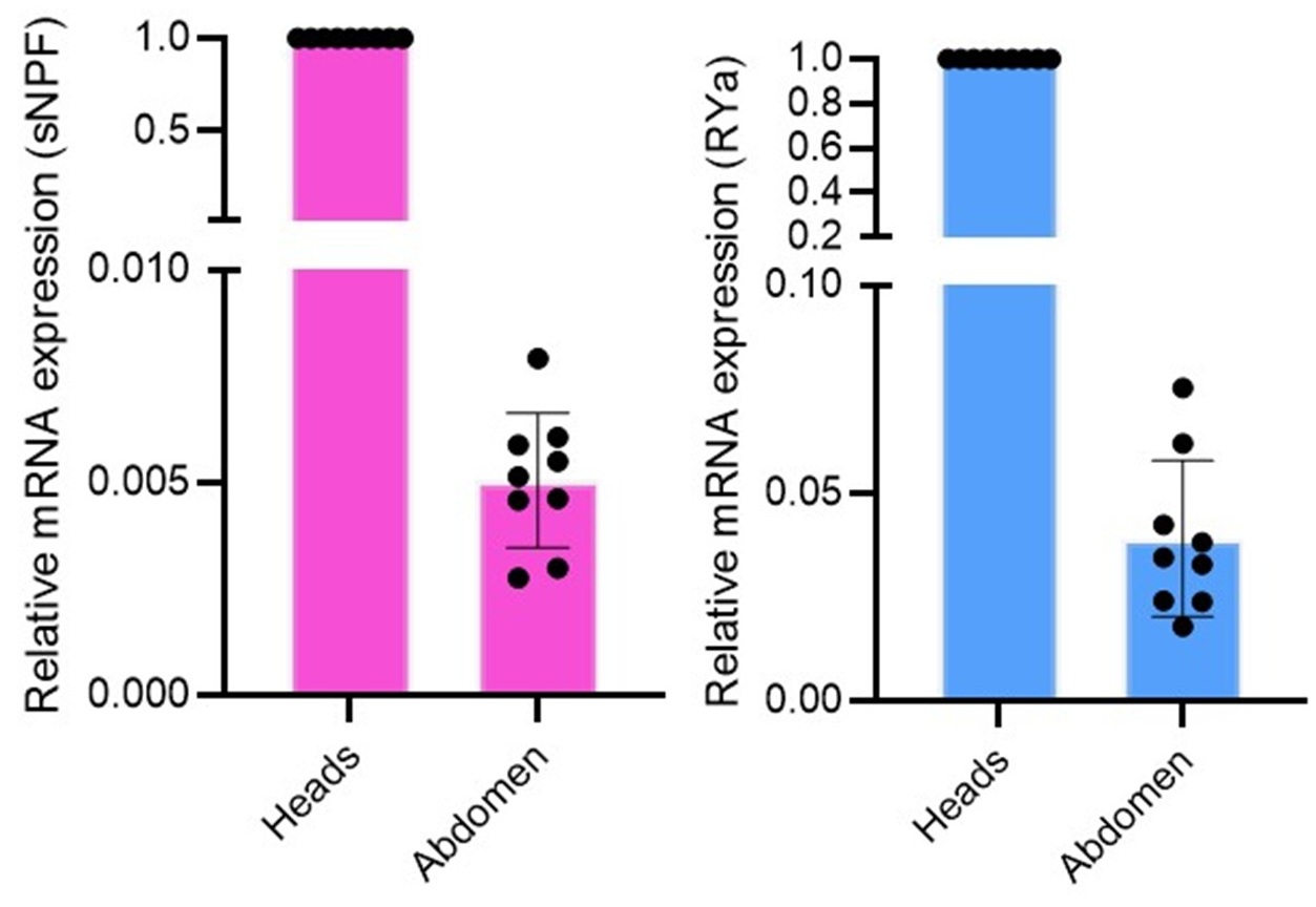
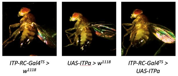
    2. Note: This preprint has been reviewed by subject experts for Review Commons. Content has not been altered except for formatting.

      Learn more at Review Commons


      Referee #3

      Evidence, reproducibility and clarity

      This study reports that importin alpha isoforms enrich strongly in a subset of micronuclei in cancer cells and uses mutagenesis and immunostaining to define how this localization relates to importin alpha's nuclear transport function. This enrichment occurs even though importin-alpha-positive micronuclei also contain Ran and the importin alpha export factor CSE1L, indicating that importin a enrichment is not simply a consequence of the absence of components of the nuclear transport machinery that control its localization. Mutagenesis of importin a indicates that Mn enrichment persists even when the importin beta binding and NLS binding capacities of imp a are impaired. Potential importin alpha interacting proteins are identified by proteomics, although the relationship of these potential binding partners to micronucleus localization is unclear.

      Significance

      1. In Figure S3, the authors show that mutagenesis of importin alpha's CSE1L binding domain decreases the ratiometric enrichment in Mn vs. Pn. However, is this effect occurring because th CSE1L binding mutant decreases Mn enrichment, or increases Pn enrichment? It seems that the latter is possible based on the images shown. If the Pn specifically becomes brighter on average in cells expressing the C-mut, while Mn remain similar in fluorescence intensity, that might suggest that CSE1L has less of an effect on importin alpha export in Mn compared to Pn.
      2. It is unclear from the text or the methods whether RIME identification of importin-alpha binding partners is performed in reversine-treated cells, which would increase the proportion of importin alpha in Mn, or in untreated cells. In either case, it seems likely that the majority of interactors identified would be cargoes that rely on importin alpha for import into the Pn. The rationale for linking these potential interactions to the Mn is unclear. While some of these factors are indeed shown enriched in Mn in Figure 5, the significance of this is also unclear. These points should be clarified.
      3. In Figure 6, the authors perform FRAP of importin alpha in Mn and show that it recovers much more slowly in Mn than in Pn. However, it appears from the images shown that the entire Mn was photobleached in each FRAP experiment. It thus is unclear whether the slow FRAP recovery is limited by slow diffusion of importin alpha within Mn/on Mn chromatin or impaired trafficking of importin alpha into and out of Mn. These distinct outcomes have distinct implications: either importin alpha is immobilized on Mn (eu)chromatin, or alternatively importin alpha is poorly transported into / out of Mn. This ambiguity could be resolved by bleaching a portion of a Mn and testing whether importin alpha diffuses within a single Mn.
    3. Note: This preprint has been reviewed by subject experts for Review Commons. Content has not been altered except for formatting.

      Learn more at Review Commons


      Referee #2

      Evidence, reproducibility and clarity

      Summary:

      The authors have shown that Importin α1, a nuclear transport factor, is enriched in subsets of micronuclei (MN) of cancer cells (MCF7 and HeLa) and, using FRAP, has an altered dynamics in MN. Moreover, the authors have shown that these levels of Importin α1 in the MN are likely not due to its traditional role for signal-dependent protein transport, as suggested by immunofluorescence of other factors important for this function. Additionally, cargo dynamics carrying NLS or NES signals were disrupted in Importin α1-positive micronuclei. Importin α1-positive micronuclei also appear to have a disrupted nuclear envelope, potentially explaining some of these cargo disruptions. The authors also demonstrated that Importin α colocalizes with proteins important for DNA replication, and p53 signaling using RIME, followed by immunofluorescence. Lastly, the authors show that Importin α and RAD51 have mutual exclusivity in the micronuclei.

      Major comments:

      1. A key issue is there are very few statistical tests used in this study. It is crucial to the interpretation of the data. We strongly urge the authors to re-analyze the data using appropriate statistical analyses. Along those lines, in many figures 1 or 2 images are shown without stating how many biological or technical replicates this is representative of or showing quantification of the anlyses. In general, the authors' statements would be strengthened by showing more examples and/or stating "N" in the figure legends or supplement.
      2. Using RIME and immunofluorescence, the authors identify factors that co-localize with Importin α1 in subsets of micronuclei (Figure 5), which is interesting, but there is no functional data associated with this result. Are the authors stating that these differences account for altered DNA damage or replication? It is unclear what the conclusion is beyond "some MN are different than others." Could the authors knockdown/knockout these factors to determine if they recruit Importin α1 into MN or the reciprocal? For many of these factors, they appear to be broadly present throughout the entire primary nucleus as well, indicating there is nothing unique about their MN localization.
      3. In line 274, the authors state that MN highly enriched for Importin α1 inhibits RAD51 accessibility but this is an overstatement of the data. Instead, the authors show that RAD51 and importin α1 do not colocalize in micronuclei, albeit without quantification which weakens their argument. Also, the consequence of this "mutual exclusivity" is unclear. Can the authors inhibit or knockdown Importin α1 and show that RAD51 goes to all micronuclei? And how is this different than the data shown for factors in Figure 5? Some of those show colocalization with Importin α1-positive micronuclei and others do not. Could you perform live imaging of labeled Importin a1 and RAD51 and show that as Importin α1 accumulates in MN that RAD51 or other DNA repair factors are exported? An alternative experiment would be to show that the C-mutant, which is defective in nuclear export, now colocalizes with RAD51 in MN. Please reconcile this or show experiments to prove the statement above.
      4. In the Discussion, line 343-344 states that "importin α1 is uniquely distributed and alters the nuclear/chromatin status when enriched in MN," however this is not currently supported by the present data. The data presented shows correlation (albeit weak) between euchromatic modifications and Importin α1, and it does not definitively show that importin α1 is sufficient to alter the nuclear-chromatin status when enriched in the MN. More substantial experiments would be required to show whether Importin α1 plays an active role in these modifications.

      Minor Comments

      1. Summary statement (page 3 Line 40): The use of "their" is confusing. Whose microenvironment are you referring to?
      2. In Abstract and introduction (page 4, Line 44 and page 5, line 59) it states that MN are membrane enclosed structures, but this is not always the case (see https://doi.org/10.1038/nature23449 as one example).
      3. Given the fact that the RIME result identified proteins involved in DNA replication to be enriched with Importin α1, are these MN enriched in factors described in Fig. 5 simply localizing to MN that are in S phase, as described previously (doi: 10.1038/nature10802)?
      4. The FRAP data is not very compelling. While it is clear there are differences between the PN and MN dynamics, what is driving these differences? Are these differences meaningful to the biology of the MN or PN? It is unclear what this data is contributing to the conclusions of the paper. Also, if the mobility of the MN is plotted on the same graph as the PN, the differences in MN mobility might not look as compelling.
      5. In Results (line 117), you state that "the cytoplasm of those cell lines emitted quite strong signals" for Importin α1, but that phrasing is a little confusing. Yes, Importin α1 is in present the cytoplasm in most cells, but it appears you are referring to the enrichment in MN. I would recommend re-phrasing this statement to make your intent clearer.
      6. In Results (line 135, Figure S2E,F), the ratio of high, low or no Importin α1 intensity is confusing. Is this percentage relative to the total number of MN? It Is unclear what is meant by "whole number" of MN. Is Importin α1 intensity quantified or is it subjective?
      7. Figure 2C is confusing. Are you counting MN with co-localization of Importin α1 and these factors? Please clarify.
      8. Figure S3D quantification is very confusing and unclear. Also, how is this normalized? Are you controlling for total signal in each cell? And can the results of this experiment give you any mechanistic insight as to what is regulating MN localization beyond the interpretation of "MN localization is distinct from PN localization"? The "C-mutant" appears quite a bit different than the others. What might that indicate about the role of CAS/CSE1L in MN enrichment?
      9. For Figures 3A,B and S4, are these images of single z-slices or projections? It would be helpful to clarify for your interpretations as to whether they are truly partial or diffuse or the membrane is in another z-plane. Also, how does the localization of Importin α1 different or similar to other factors that localize to MN with a compromised nuclear envelope, such as cGAS? If it is based on epigenetic marks, it should be different than cGAS, which primarily binds non-chromatinized DNA.
      10. In Results, it is unclear how Fig. 7B was calculated. Are the authors qualitatively assessing if RAD51 is there or looking for MN enrichment relative to PN? Additionally, in Fig. 7C, RAD51 localization is diffuse. It should be enriched in foci. I would recommend the authors repeat this experiment using pre-extraction then quantify RAD51 foci number and/or intensity.
      11. In line 264, "notably" is misspelled.
      12. In line 303, "scenarios" should be changed to the singular form.
      13. In Figure legend, line 571-582, H3K27me3 is shown in Figure 4D, but the written legend does not mention this mark.

      Significance

      Overall, this paper shows compelling evidence for micronuclear localization of regulators of nuclear export, notably Importin α1. Of note, this occurs in subsets of MN that lack an intact nuclear envelope. And while it has been appreciated that compromised micronuclear envelopes lead to genomic instability, this is one of the first that demonstrate alteration in the nuclear envelope may disrupt import or export of nuclear proteins into micronuclei.

      A limitation of the study is that much of the work is based on immunofluorescence and lacks mechanism. While there is much correlative data showing that Importin α1 localizes to micronuclei with compromised envelopes, it is unclear whether Importin α1 drives micronuclear collapse or it is downstream of this process. Additionally, Importin α1 micronuclear localization anti-correlates with RAD51 but does colocalize with other DNA replication factors, yet it is unclear whether their localization is dependent on Importin α1 or its role in nuclear export. Currently, the audience for this manuscript would be focused to those interested in micronuclei. If these concerns about an active role for Importin α1 in micronuclear export are resolved, it would greatly increase the impact of this manuscript to those interested more broadly in genomic instability, DNA repair, and cancer.

      Reviewer's areas of expertise: Genomic instability, cancer epigenetics, and mitosis

    4. Note: This preprint has been reviewed by subject experts for Review Commons. Content has not been altered except for formatting.

      Learn more at Review Commons


      Referee #1

      Evidence, reproducibility and clarity

      Summary:

      Provide a short summary of the findings and key conclusions (including methodology and model system(s) where appropriate). Miyamoto et al. report that importin α1 is highly enriched in a subfraction of micronuclei (about 40%), which exhibit defective nuclear envelopes and compromised accessibility of factors essential for the damage response associated with homologous recombination DNA repair. The authors suggest that the unequal localization and abnormal distribution of importin α1 within these micronuclei contribute to the genomic instability observed in cancer.

      Major comments:

      Are the key conclusions convincing?

      The conclusions drawn by the authors would benefit from additional supportive experiments and a more detailed explanation. 1. It is crucial to quantitatively assess the localization of importin α1 in micronuclei (MN) across non-transformed MCM10A cells compared to transformed cell lines (MC7, HeLa, and MDA-MB-231). This analysis would help determine whether the localization of importin α1 in MN correlates with genomic stability in human cancer cells 2. While the authors provide some evidence indicating partial disruption of nuclear envelopes in MN (Figures 3 and S4), it is noteworthy that this phenomenon also occurs in importin α1-negative MN. Furthermore, according to the figure legends, the data presented in both figures stem from a single experiment. Current literature suggests that compromised nuclear envelope integrity is one of the major contributors to genomic instability, mediated through mechanisms such as chromothripsis and cGAS-STING-mediated inflammation arising from MN. Therefore, a more comprehensive quantification of nuclear envelope integrity-ideally comparing non-transformed MCM10A cells with transformed cell lines (MC7, HeLa, and MDA-MB-231)-is necessary to substantiate the connection between aberrant importin α1 behavior in MN and chromothripsis processes, as well as regulation of the cGAS-STING pathway linked to genomic instability in cancer cells. 3. The schematic illustration presented in Figure 8 does not adequately summarize all findings from this study nor does it clarify how the localization of importin α1 within MN might hypothetically influence genome stability. Although it is reasonable to propose that "importin α can serve as a molecular marker for characterizing the dynamics of MN" (Line 344), the authors assert (Line 325) that their findings, along with others, have "potential implications for the induction of chromothripsis processes and regulation of the cGAS-STING pathway in cancer cells." However, they fail to provide a clear or even hypothetical explanation regarding how their findings contribute to these molecular events. To address this gap, it would be essential for them to contextualize their results within existing literature that explores and links structural integrity deficits or aberrant DNA replication/damage responses in MN with chromothripsis and inflammation (e.g., PMID: 32601372; PMID: 32494070; PMID: 27918550; PMID: 28738408; PMID: 28759889). 4. Fig. 4D does not support the idea that importin α1 is euchromatin enriched: H3K9me3, H3K4me3 and H3K37me3 seem to be all deeply blue.

      Should the authors qualify some of their claims as preliminary or speculative, or remove them altogether?

      Indeed, the data presented by the authors do not adequately support a direct link between the presence of importin α1 in MN and genomic instability in human cancer cells. While the experimental correlations provided may not substantiate this connection definitively, they do lay a foundation for a grounded hypothesis and suggest the need for further research to explore this topic in greater depth. Additionally, it is worth noting that the evidence contributes to the growing list of nuclear proteins exhibiting abnormal behavior in micronuclei (MN). This highlights the significance of studying such proteins to understand their roles in genomic stability and cancer progression.

      Would additional experiments be essential to support the claims of the paper? Request additional experiments only where necessary for the paper as it is, and do not ask authors to open new lines of experimentation.

      Additional experiments are necessary to quantitatively assess the localization of importin α1 in micronuclei (MN) across non-transformed MCM10A cells and transformed cell lines (MC7, HeLa, MDA-MB-231). This analysis would help determine whether the localization of importin α1 in MN correlates with genomic stability in human cancer cells. The authors claim that importin α1 preferentially localizes to euchromatic areas rather than heterochromatic regions within MN. While this assertion is supported by the immunofluorescence (IF) images presented in Figures 4A/B and S5A/B, it remains less clear for Figure S5C/B. To strengthen this claim, providing averages of IF distributions from multiple cells across independent experiments would be beneficial to draw more robust conclusions.

      Furthermore, ChIP-seq data are presented to support the idea that importin α1 preferentially distributes over euchromatin areas in MN. However, as described, the epigenetic chromatin status indicated by these ChIP-seq experiments reflects that of the principal nucleus (PN), not specifically the status within MN in MCF7 cells. Given that MN represent only a small fraction of the cell population under normal culture conditions-likely less than 5% for HeLa cells as shown in Figure S2D-the relevance of this data is limited. Additionally, according to data presented in Figure 1B, importin α1 does not localize or distribute within the PN as it does in MN in MCF7 cells. Therefore, further experiments should be conducted to substantiate that importin α1 preferentially targets euchromatin areas within MN and to compare this distribution with that observed in the principal nucleus. Such studies could reveal potential abnormalities regarding the correlation between epigenetic chromatin status and importin α distribution in MN. To support the hypothesis that importin α1 inhibits RAD51 accessibility within MN, Figures 7D and E should be supplemented with thorough quantification and statistical analysis based on at least three independent experiments. This additional data would enhance confidence in their findings regarding RAD51 accessibility inhibition by importin α1.

      Are the suggested experiments realistic in terms of time and resources? It would help if you could add an estimated cost and time investment for substantial experiments.

      The additional experiments proposed are controls and direct comparisons using the same techniques and experimental designs used by the authors, so it is reasonable that the authors can carry them out within a realistic timeframe.

      Are the data and the methods presented in such a way that they can be reproduced?

      Given the importance of reproducibility and the need to evaluate results based on imaging and quantitation, I strongly recommend that the authors include a detailed description of the optical microscopy procedures utilized in their study. This should encompass imaging conditions, acquisition settings, and the specific equipment used. Providing this information will enhance transparency and facilitate reproducibility. For reference, some valuable guidance on essential parameters for reproducibility can be found in Heddleston et al. (2021) (doi:10.1242/jcs.254144). Incorporating these details will not only strengthen the manuscript but also support other researchers in reproducing the findings accurately.

      Are the experiments adequately replicated and statistical analysis adequate?

      Many of the plots and values in the manuscript lack appropriate statistical analysis, including p-values, which are not detailed in the figures or their legends. Furthermore, the Statistical Analysis section does not provide adequate information regarding the specific statistical tests employed or the criteria used to determine which analyses were applied in each case. To enhance the rigor and clarity of the study, it is essential that these issues be addressed prior to publication. A comprehensive presentation of statistical analysis will improve the reliability of the findings and allow readers to better understand the significance of the results. I recommend that the authors revise this section to include detailed explanations of all statistical methods used, along with corresponding p-values for all relevant comparisons.

      Minor comments:

      Specific experimental issues that are easily addressable.

      The authors claim that importin α1 exhibits remarkably low mobility in the micronuclei (MN) compared to its mobility in the principal nucleus (PN), as illustrated in Figure 1. However, based on the experimental design, this conclusion may not be appropriate. In the current setup, the FRAP experiment conducted in the PN measures the mobility of importin α1 molecules within the cell nucleus, where the influence of nuclear transport is likely negligible. Conversely, in the MN experiments shown, all molecules of importin α1 are bleached within a given MN. Consequently, what is being measured here primarily reflects the effects of nuclear transport rather than intrinsic molecular mobility. To accurately compare kinetics of nuclear transport, it would be essential to completely bleach the entire PN. If measuring molecular mobility between MN and PN is desired, only a small fraction of either MN or PN area/volume should be bleached during FRAP analysis. Additionally, it would be beneficial to include measurements of mobility for other canonical nuclear transport factors (e.g., RAN, CAS, RCC1) for comparative purposes. This broader context would allow for a more comprehensive understanding of importin α1 behavior relative to other factors involved in nuclear transport. Finally, utilizing cells that exhibit importin α1 signals in both PN and MN could further strengthen comparisons and provide more robust conclusions regarding its mobility dynamics.

      Are prior studies referenced appropriately?

      Prior studies are referenced appropriately in general, but the authors missed some references (PMID: 32601372; PMID: 32494070; PMID: 27918550; PMID: 28738408; PMID: 28759889) that I consider key to put the present findings in frame with previous works which link the lack of structural integrity and/or aberrant DNA replication/damage responses in MN with Cchromothripsis and inflammation.

      Are the text and figures clear and accurate?

      The figures presented in the manuscript are clear; however, where plots are included, they require appropriate statistical analysis. It is essential to display p-values on the plots or within their legends to provide readers with information regarding the significance of the results. Including this statistical information will enhance the interpretability of the data and strengthen the overall findings of the study. I recommend that the authors revise these sections accordingly before publication.

      Do you have suggestions that would help the authors improve the presentation of their data and conclusions?

      1. In lines 134-135, it is stated that "up to 40% of the MN showed importin α1 accumulation under both standard culture conditions and the reversine treatment (Fig. S2F)." However, Figure S2F only displays percentages for reversine-treated cells, and there is no mention in the text or figures regarding the percentage of importin α1-positive MN determined by immunofluorescence (IF) under standard culture conditions. This discrepancy should be addressed.
      2. In line 170, the authors state that "Cells in which overexpressed EGFP-importin α1 localized only in PN were excluded from the analysis (see Fig. 1E, top panels)." It is unclear why this exclusion was made. The authors should clarify whether they are referring to all constructs or only to the wild-type (WT) construct when mentioning EGFP-importin α1 localization solely in PN. This clarification is important as it may affect the results highlighted in line 173.
      3. The statement in line 191 ("However, this antibody could not be further used in this context due to cross-reactivity with highly concentrated importin α1 in MN (Fig. S4)") is somewhat misleading. While it hints at a technical issue, it does not provide additional relevant information for understanding its implications for the rationale of the research. Moreover, Figure S4 is referenced but appears to refer specifically to panels S4D and E, which are not mentioned in the text. I recommend clarifying this point or removing it altogether.
      4. Lines 197-199 contain a sentence that could be misleading and would benefit from clearer explanation. Although Figure 3D provides some clarity on this matter, no statistical analysis is included-only a bar plot is presented. A proper statistical analysis should be provided here to enhance understanding.
      5. In lines 218-221, it states that importin α1 associates with euchromatin regions characterized by H3K4me3 and H3K36me3; however, Figure 4D lacks the Spearman's correlation coefficient value for H3K36me3 within the matrix. This omission needs correction.
      6. For consistency in the experimental design aimed at identifying potential importin α1-interacting proteins, it would be more appropriate for Figures 5C/D to show IF data from MCF7 cells rather than HeLa cells.
      7. To substantiate claims that importin α1 inhibits RAD51 accessibility within MN, Figures 7D and E should include thorough quantitation and statistical analysis based on at least three independent experiments.
      8. The meaning of lines 336-338-"Therefore, the enrichment of importin α1 in MN, along with its interaction with chromatin, may regulate the accessibility of RAD51 to DNA/chromatin fibers in MN and protect its activity"-is unclear. I suggest rephrasing this sentence for improved clarity and comprehension.
      9. Fig. 1D: Numbers on the y-axis are missing, x-axis labeling is too small
      10. Fig. 1F: As the PN/MN values of the three experiments are seemingly identical (third column) the distribution of the three individual data of the PN (first column) should mirror the distribution of the three individual data of the MN (second column). The authors might want to check why this is not the case.

      Significance

      • Describe the nature and significance of the advance (e.g. conceptual, technical, clinical) for the field.
      • Place the work in the context of the existing literature (provide references, where appropriate).

      Micronuclei (MN) primarily arise from defects in mitotic progression and chromatin segregation, often associated with chromatin bridges and/or lagging chromosomes. MN frequently exhibit DNA replication defects and possess a rupture-prone nuclear envelope, which has been linked to genomic instability. The nuclear envelope of MN is notably deficient in crucial factors such as lamin B and nuclear pore complexes (NPCs). This deficiency may be attributed to the influence of microtubules and the gradient of Aurora B activity at the mitotic midzone, which inhibits the recruitment of proper nuclear envelope components. Additionally, several other factors may contribute to this process: for instance, PLK1 controls the assembly of NPC components onto lagging chromosomes; chromosome size and gene density positively correlate with the membrane stability of MN; and abnormal accumulation of the ESCRT complex on MN exacerbates DNA damage within these structures, triggering pro-inflammatory pathways. The work presented by Dr. Miyamoto and colleagues reveals the abnormal behavior of importin α1 in MN during interphase. According to their findings, it is reasonable to consider importin α1 as a molecular marker for characterizing MN dynamics. Furthermore, it could serve as a potential clinical marker if the authors provide additional experiments demonstrating significantly different localization patterns of importin α1 in transformed cells (e.g., MC7, HeLa, MDA-MB-231) compared to non-transformed cells (e.g., MCM10A). While the authors present some evidence indicating partial disruption of nuclear envelopes in MN (Figures 3 and S4), it is noteworthy that this phenomenon also occurs in importin α1-negative MN. Moreover, according to the figure legends, data for both figures originate from a single experiment. As such, convincing evidence linking the aberrant behavior of importin α1 in MN with chromothripsis processes or regulation of the cGAS-STING pathway-and its implications for genomic instability in cancer cells-remains lacking. Overall, it is not entirely clear what significance this advance holds for the field; while there are conceptual contributions made by this work, they do not appear sufficiently robust at this time. Further research is needed to clarify these connections and strengthen their conclusions regarding importin α1's role in MN dynamics and genomic instability. - State what audience might be interested in and influenced by the reported findings.

      Scientist and health care professionals that research on mechanism of genomic instability and cancer - Define your field of expertise with a few keywords to help the authors contextualize your point of view. Indicate if there are any parts of the paper that you do not have sufficient expertise to evaluate.

      Mitosis, mitotic chromatin decondensation, nuclear reformation, hematopoietic cancers, light microscopy, image analysis.

    1. Individualisation considers the level of adjustment or customisation available to the agent. At one extreme, this may tailor the device to the individual agent such that it becomes difficult for another to use it, or to adapt it for another task. On the other hand, a device may be easy to pick up, use and understand with little scope or need for improved efficiency or effectiveness, and hence it is not especially individualised. Furthermore, agent and artefact may both be adapted together in what Heersmink calls entrenchment, where the cognitive artefact is individualised according to the user's needs, and in turn the user's behaviour and cognition are adapted by the device in a manner reminiscent of the McLuhanite 'We shape our tools and thereafter our tools shape us' (Culkin 1968, 60). (Heersmink 2012, 52-3; 2015, 590-1).

      Cost-surface weights and clustering hyperparameters reflect my priors (slope, water gaps, caravanserai spacing). I’ll publish a config file and run ablations to avoid over-entrenching my personal settings.

    1. Overview Andreas, age 22, was completing his final year in college and was majoring in computer science. He had worked hard in order to prepare himself for a career in information technology, getting good grades with the hope of landing a job in a top company after graduation. He was the only son of a wealthy family. His father was a well-known lawyer in their average-size hometown and his mother was a cardiologist. Andreas had always received lots of attention from his parents, and they ensured that he got a good education and had everything he wanted. Andreas described his parents as being very strict and critical, requiring that he work hard and receive good grades in order to increase his chances of doing something valuable with his life. What triggered Andreas' s depression was an event that took place at the beginning of the semester. At the end of summer holidays, a renowned multinational information technology company launched a contest inviting all students in their final year of computer science to submit a project on an emerging topic. The prize for this contest was a well-paid 6-month internship with the company, which for Andreas would have been the perfect start to a fabulous career. Twenty internships were awarded among more than 200 students who submitted projects, and Andreas was not among them. This made him feel terrible, especially because he had told his parents about this opportunity because he was confident he would be selected. When he received the news about not having been accepted, he initially did not tell his parents about it or about the fact that he was so depressed, lying to them about not receiving the results each time they asked about it. As a result of being rejected for the award and lying to his parents, Andreas developed strong feelings of shame, guilt, and hopelessness, thinking that he would never be as he had been before. He saw himself as a failure both to himself and to his parents. He had tried to prove his worth by winning the internship, and now that opportunity was gone. Andreas came to therapy after what he described as the worst period of his life in which he felt deeply depressed and experienced suicidal ideation. However, he did not intend to commit suicide and did not make any attempt, stating that he was very afraid of these thoughts. When he came to therapy he had not been to class for more than 3 weeks, and in the previous month he had only gone from time to time in his better moments. In the past 3 weeks, however, the depression had gotten so intense that he barely got out of house. He spent his time sleeping, playing video games, and thinking intensely about his situation and the fact that he would not be able to complete his graduation thesis. In the initial session Andreas was introduced to the CBT model and behavioral activation, and in subsequent sessions he learned how to identify and dispute dysfunctional negative automatic thoughts. After the third session, Andreas started attending classes again and was able to study for winter exams, although he was very stressed about them. He also got up the courage to tell his parents that he had not received the award. He said that they were critical but did not dwell on it. In this fourth session the focus was on his deeper cognitions—the intermediate and core beliefs. I used Andreas' s thought records from the previous week to initiate further exploration of his thoughts using the downward arrow technique to access deeper beliefs. At the end of the session we developed a behavioral experiment to test the functionality of these beliefs. What follows is the transcript of the fourth session.

      Both Andreas and Allison received CBT to challenge negative self beliefs, but Andreas’s therapy focused on perfectionism and conditional self-worth after losing an internship, while Allison’s addressed low self esteem and peer bullying. Andreas’s therapist targeted deep core beliefs, whereas Allison’s therapist used simpler thought challenging and behavior practice. Both learned to replace self criticism with healthier thinking and actions.

    1. Tinsel$65.0024 in stockThe Tinsel letterpress poster was written, designed, carved and printed in November 2017, in Tacoma, Washington.24 in stock Tinsel quantity Add to cart Categories: 2017, November Tags: Christmas, Split Fountain Description DescriptionThe Tinsel letterpress poster is a three-color printer, using a splint fountain. The text was printed with vintage lead type. The image was created with a combination of a hand-carved linocut and an assortment of vintage lead borders. Share On Facebook Tweet This Product Pin This Product Email This Product Related products <img width="500" height="788" src="https://beautifulangle.com/wp-content/uploads/2020/02/LuckyDog_600px-500x788.jpg" class="attachment-woocommerce_thumbnail size-woocommerce_thumbnail wp-post-image lazyload" alt="one lucky dog by beautiful angle" decoding="async" srcset="https://beautifulangle.com/wp-content/uploads/2020/02/LuckyDog_600px-190x300.jpg 190w, https://beautifulangle.com/wp-content/uploads/2020/02/LuckyDog_600px-200x315.jpg 200w, https://beautifulangle.com/wp-content/uploads/2020/02/LuckyDog_600px-400x631.jpg 400w, https://beautifulangle.com/wp-content/uploads/2020/02/LuckyDog_600px-500x788.jpg 500w, https://beautifulangle.com/wp-content/uploads/2020/02/LuckyDog_600px.jpg 600w" sizes="(max-width: 500px) 100vw, 500px" /> Lucky Dog $79.00 Add to cart Details <img width="500" height="840" src="https://beautifulangle.com/wp-content/uploads/2020/04/Trike_600px-500x840.jpg" class="attachment-woocommerce_thumbnail size-woocommerce_thumbnail wp-post-image lazyload" alt="" decoding="async" srcset="https://beautifulangle.com/wp-content/uploads/2020/04/Trike_600px-179x300.jpg 179w, https://beautifulangle.com/wp-content/uploads/2020/04/Trike_600px-200x336.jpg 200w, https://beautifulangle.com/wp-content/uploads/2020/04/Trike_600px-400x672.jpg 400w, https://beautifulangle.com/wp-content/uploads/2020/04/Trike_600px-500x840.jpg 500w, https://beautifulangle.com/wp-content/uploads/2020/04/Trike_600px.jpg 600w" sizes="(max-width: 500px) 100vw, 500px" /> Trike $72.00 Add to cart Details <img width="500" height="323" src="https://beautifulangle.com/wp-content/uploads/2020/02/ClearGlass_h600px-500x323.jpg" class="attachment-woocommerce_thumbnail size-woocommerce_thumbnail wp-post-image lazyload" alt="" decoding="async" srcset="https://beautifulangle.com/wp-content/uploads/2020/02/ClearGlass_h600px-200x129.jpg 200w, https://beautifulangle.com/wp-content/uploads/2020/02/ClearGlass_h600px-300x194.jpg 300w, https://beautifulangle.com/wp-content/uploads/2020/02/ClearGlass_h600px-400x259.jpg 400w, https://beautifulangle.com/wp-content/uploads/2020/02/ClearGlass_h600px-500x323.jpg 500w, https://beautifulangle.com/wp-content/uploads/2020/02/ClearGlass_h600px-600x388.jpg 600w, https://beautifulangle.com/wp-content/uploads/2020/02/ClearGlass_h600px-700x453.jpg 700w, https://beautifulangle.com/wp-content/uploads/2020/02/ClearGlass_h600px-768x497.jpg 768w, https://beautifulangle.com/wp-content/uploads/2020/02/ClearGlass_h600px-800x518.jpg 800w, https://beautifulangle.com/wp-content/uploads/2020/02/ClearGlass_h600px.jpg 929w" sizes="(max-width: 500px) 100vw, 500px" /> Clear Glass $167.00 Add to cart Details Congratulation on making it to The Bottom Of The Page.Check out our privacy policy, if you’re so inclined.  Contact us, if you’re feeling lonely. Contemplate your existence, if you’re feeling self-reflective. Share your story, if you’re feeling chatty. And when in doubt, go back to the beginning. Copyright 2020 Beautiful Angle Page load link var fusionNavIsCollapsed=function(e){var t,n;window.innerWidth<=e.getAttribute("data-breakpoint")?(e.classList.add("collapse-enabled"),e.classList.remove("awb-menu_desktop"),e.classList.contains("expanded")||window.dispatchEvent(new CustomEvent("fusion-mobile-menu-collapsed",{detail:{nav:e}})),(n=e.querySelectorAll(".menu-item-has-children.expanded")).length&&n.forEach((function(e){e.querySelector(".awb-menu__open-nav-submenu_mobile").setAttribute("aria-expanded","false")}))):(null!==e.querySelector(".menu-item-has-children.expanded .awb-menu__open-nav-submenu_click")&&e.querySelector(".menu-item-has-children.expanded .awb-menu__open-nav-submenu_click").click(),e.classList.remove("collapse-enabled"),e.classList.add("awb-menu_desktop"),null!==e.querySelector(".awb-menu__main-ul")&&e.querySelector(".awb-menu__main-ul").removeAttribute("style")),e.classList.add("no-wrapper-transition"),clearTimeout(t),t=setTimeout(()=>{e.classList.remove("no-wrapper-transition")},400),e.classList.remove("loading")},fusionRunNavIsCollapsed=function(){var e,t=document.querySelectorAll(".awb-menu");for(e=0;e<t.length;e++)fusionNavIsCollapsed(t[e])};function avadaGetScrollBarWidth(){var e,t,n,l=document.createElement("p");return l.style.width="100%",l.style.height="200px",(e=document.createElement("div")).style.position="absolute",e.style.top="0px",e.style.left="0px",e.style.visibility="hidden",e.style.width="200px",e.style.height="150px",e.style.overflow="hidden",e.appendChild(l),document.body.appendChild(e),t=l.offsetWidth,e.style.overflow="scroll",t==(n=l.offsetWidth)&&(n=e.clientWidth),document.body.removeChild(e),jQuery("html").hasClass("awb-scroll")&&10<t-n?10:t-n}fusionRunNavIsCollapsed(),window.addEventListener("fusion-resize-horizontal",fusionRunNavIsCollapsed); {"prefetch":[{"source":"document","where":{"and":[{"href_matches":"\/*"},{"not":{"href_matches":["\/wp-*.php","\/wp-admin\/*","\/wp-content\/uploads\/*","\/wp-content\/*","\/wp-content\/plugins\/*","\/wp-content\/themes\/Avada-Child-Theme\/*","\/wp-content\/themes\/Avada\/*","\/*\\?(.+)"]}},{"not":{"selector_matches":"a[rel~=\"nofollow\"]"}},{"not":{"selector_matches":".no-prefetch, .no-prefetch a"}}]},"eagerness":"conservative"}]} jQuery(function(){ var arrLiveStats=[]; var WSM_PREFIX="wsm"; jQuery(".if-js-closed").removeClass("if-js-closed").addClass("closed"); var wsmFnSiteLiveStats=function(){ jQuery.ajax({ type: "POST", url: wsm_ajaxObject.ajax_url, data: { action: 'liveSiteStats', requests: JSON.stringify(arrLiveStats), r: Math.random() } }).done(function( strResponse ) { if(strResponse!="No"){ arrResponse=JSON.parse(strResponse); jQuery.each(arrResponse, function(key,value){ $element= document.getElementById(key); oldValue=parseInt($element.getAttribute("data-value").replace(/,/g, "")); diff=parseInt(value.replace(/,/g, ""))-oldValue; $class=""; if(diff>=0){ diff="+"+diff; }else{ $class="wmcRedBack"; } $element.setAttribute("data-value",value); $element.innerHTML=diff; jQuery("#"+key).addClass($class).show().siblings(".wsmH2Number").text(value); if(key=="SiteUserOnline") { var onlineUserCnt = arrResponse.wsmSiteUserOnline; if(jQuery("#wsmSiteUserOnline").length) { jQuery("#wsmSiteUserOnline").attr("data-value",onlineUserCnt); jQuery("#wsmSiteUserOnline").next(".wsmH2Number").html("<a target=\"_blank\" href=\"?page=wsm_traffic&subPage=UsersOnline&subTab=summary\">"+onlineUserCnt+"</a>"); } } }); setTimeout(function() { jQuery.each(arrResponse, function(key,value){ jQuery("#"+key).removeClass("wmcRedBack").hide(); }); }, 1500); } }); } if(arrLiveStats.length>0){ setInterval(wsmFnSiteLiveStats, 10000); }}); {"@context":"https:\/\/schema.org\/","@graph":[{"@context":"https:\/\/schema.org\/","@type":"BreadcrumbList","itemListElement":[{"@type":"ListItem","position":1,"item":{"name":"Home","@id":"https:\/\/beautifulangle.com"}},{"@type":"ListItem","position":2,"item":{"name":"2017","@id":"https:\/\/beautifulangle.com\/product-category\/beautiful-angle-posters-from-2017\/"}},{"@type":"ListItem","position":3,"item":{"name":"Tinsel","@id":"https:\/\/beautifulangle.com\/product\/tinsel-is-a-beautiful-angle-poster-from-2017\/"}}]},{"@context":"https:\/\/schema.org\/","@type":"Product","@id":"https:\/\/beautifulangle.com\/product\/tinsel-is-a-beautiful-angle-poster-from-2017\/#product","name":"Tinsel","url":"https:\/\/beautifulangle.com\/product\/tinsel-is-a-beautiful-angle-poster-from-2017\/","description":"The Tinsel letterpress poster was written, designed, carved and printed in November 2017, in Tacoma, Washington.","image":"https:\/\/beautifulangle.com\/wp-content\/uploads\/2020\/02\/Tinsel_600px.jpg","sku":532,"offers":[{"@type":"Offer","priceSpecification":[{"@type":"UnitPriceSpecification","price":"65.00","priceCurrency":"USD","valueAddedTaxIncluded":false,"validThrough":"2026-12-31"}],"priceValidUntil":"2026-12-31","availability":"http:\/\/schema.org\/InStock","url":"https:\/\/beautifulangle.com\/product\/tinsel-is-a-beautiful-angle-poster-from-2017\/","seller":{"@type":"Organization","name":"Beautiful Angle","url":"https:\/\/beautifulangle.com"}}]}]} (function () { var c = document.body.className; c = c.replace(/woocommerce-no-js/, 'woocommerce-js'); document.body.className = c; })(); :root{--wp--preset--aspect-ratio--square: 1;--wp--preset--aspect-ratio--4-3: 4/3;--wp--preset--aspect-ratio--3-4: 3/4;--wp--preset--aspect-ratio--3-2: 3/2;--wp--preset--aspect-ratio--2-3: 2/3;--wp--preset--aspect-ratio--16-9: 16/9;--wp--preset--aspect-ratio--9-16: 9/16;--wp--preset--color--black: #000000;--wp--preset--color--cyan-bluish-gray: #abb8c3;--wp--preset--color--white: #ffffff;--wp--preset--color--pale-pink: #f78da7;--wp--preset--color--vivid-red: #cf2e2e;--wp--preset--color--luminous-vivid-orange: #ff6900;--wp--preset--color--luminous-vivid-amber: #fcb900;--wp--preset--color--light-green-cyan: #7bdcb5;--wp--preset--color--vivid-green-cyan: #00d084;--wp--preset--color--pale-cyan-blue: #8ed1fc;--wp--preset--color--vivid-cyan-blue: #0693e3;--wp--preset--color--vivid-purple: #9b51e0;--wp--preset--color--awb-color-1: rgba(255,255,255,1);--wp--preset--color--awb-color-2: rgba(246,246,246,1);--wp--preset--color--awb-color-3: rgba(235,234,234,1);--wp--preset--color--awb-color-4: rgba(224,222,222,1);--wp--preset--color--awb-color-5: rgba(158,158,158,1);--wp--preset--color--awb-color-6: rgba(116,116,116,1);--wp--preset--color--awb-color-7: rgba(175,59,38,1);--wp--preset--color--awb-color-8: rgba(51,51,51,1);--wp--preset--color--awb-color-custom-10: rgba(183,76,40,1);--wp--preset--color--awb-color-custom-11: rgba(235,234,234,0.8);--wp--preset--color--awb-color-custom-12: rgba(232,232,232,1);--wp--preset--color--awb-color-custom-13: rgba(120,120,120,1);--wp--preset--color--awb-color-custom-14: rgba(85,85,85,1);--wp--preset--color--awb-color-custom-15: rgba(190,189,189,1);--wp--preset--color--awb-color-custom-16: rgba(0,0,0,0.1);--wp--preset--color--awb-color-custom-17: rgba(229,229,229,1);--wp--preset--color--awb-color-custom-18: rgba(68,68,68,1);--wp--preset--gradient--vivid-cyan-blue-to-vivid-purple: linear-gradient(135deg,rgba(6,147,227,1) 0%,rgb(155,81,224) 100%);--wp--preset--gradient--light-green-cyan-to-vivid-green-cyan: linear-gradient(135deg,rgb(122,220,180) 0%,rgb(0,208,130) 100%);--wp--preset--gradient--luminous-vivid-amber-to-luminous-vivid-orange: linear-gradient(135deg,rgba(252,185,0,1) 0%,rgba(255,105,0,1) 100%);--wp--preset--gradient--luminous-vivid-orange-to-vivid-red: linear-gradient(135deg,rgba(255,105,0,1) 0%,rgb(207,46,46) 100%);--wp--preset--gradient--very-light-gray-to-cyan-bluish-gray: linear-gradient(135deg,rgb(238,238,238) 0%,rgb(169,184,195) 100%);--wp--preset--gradient--cool-to-warm-spectrum: linear-gradient(135deg,rgb(74,234,220) 0%,rgb(151,120,209) 20%,rgb(207,42,186) 40%,rgb(238,44,130) 60%,rgb(251,105,98) 80%,rgb(254,248,76) 100%);--wp--preset--gradient--blush-light-purple: linear-gradient(135deg,rgb(255,206,236) 0%,rgb(152,150,240) 100%);--wp--preset--gradient--blush-bordeaux: linear-gradient(135deg,rgb(254,205,165) 0%,rgb(254,45,45) 50%,rgb(107,0,62) 100%);--wp--preset--gradient--luminous-dusk: linear-gradient(135deg,rgb(255,203,112) 0%,rgb(199,81,192) 50%,rgb(65,88,208) 100%);--wp--preset--gradient--pale-ocean: linear-gradient(135deg,rgb(255,245,203) 0%,rgb(182,227,212) 50%,rgb(51,167,181) 100%);--wp--preset--gradient--electric-grass: linear-gradient(135deg,rgb(202,248,128) 0%,rgb(113,206,126) 100%);--wp--preset--gradient--midnight: linear-gradient(135deg,rgb(2,3,129) 0%,rgb(40,116,252) 100%);--wp--preset--font-size--small: 15px;--wp--preset--font-size--medium: 20px;--wp--preset--font-size--large: 30px;--wp--preset--font-size--x-large: 42px;--wp--preset--font-size--normal: 20px;--wp--preset--font-size--xlarge: 40px;--wp--preset--font-size--huge: 60px;--wp--preset--spacing--20: 0.44rem;--wp--preset--spacing--30: 0.67rem;--wp--preset--spacing--40: 1rem;--wp--preset--spacing--50: 1.5rem;--wp--preset--spacing--60: 2.25rem;--wp--preset--spacing--70: 3.38rem;--wp--preset--spacing--80: 5.06rem;--wp--preset--shadow--natural: 6px 6px 9px rgba(0, 0, 0, 0.2);--wp--preset--shadow--deep: 12px 12px 50px rgba(0, 0, 0, 0.4);--wp--preset--shadow--sharp: 6px 6px 0px rgba(0, 0, 0, 0.2);--wp--preset--shadow--outlined: 6px 6px 0px -3px rgba(255, 255, 255, 1), 6px 6px rgba(0, 0, 0, 1);--wp--preset--shadow--crisp: 6px 6px 0px rgba(0, 0, 0, 1);}:where(.is-layout-flex){gap: 0.5em;}:where(.is-layout-grid){gap: 0.5em;}body .is-layout-flex{display: flex;}.is-layout-flex{flex-wrap: wrap;align-items: center;}.is-layout-flex > :is(*, div){margin: 0;}body .is-layout-grid{display: grid;}.is-layout-grid > :is(*, div){margin: 0;}:where(.wp-block-columns.is-layout-flex){gap: 2em;}:where(.wp-block-columns.is-layout-grid){gap: 2em;}:where(.wp-block-post-template.is-layout-flex){gap: 1.25em;}:where(.wp-block-post-template.is-layout-grid){gap: 1.25em;}.has-black-color{color: var(--wp--preset--color--black) !important;}.has-cyan-bluish-gray-color{color: var(--wp--preset--color--cyan-bluish-gray) !important;}.has-white-color{color: var(--wp--preset--color--white) !important;}.has-pale-pink-color{color: var(--wp--preset--color--pale-pink) !important;}.has-vivid-red-color{color: var(--wp--preset--color--vivid-red) !important;}.has-luminous-vivid-orange-color{color: var(--wp--preset--color--luminous-vivid-orange) !important;}.has-luminous-vivid-amber-color{color: var(--wp--preset--color--luminous-vivid-amber) !important;}.has-light-green-cyan-color{color: var(--wp--preset--color--light-green-cyan) !important;}.has-vivid-green-cyan-color{color: var(--wp--preset--color--vivid-green-cyan) !important;}.has-pale-cyan-blue-color{color: var(--wp--preset--color--pale-cyan-blue) !important;}.has-vivid-cyan-blue-color{color: var(--wp--preset--color--vivid-cyan-blue) !important;}.has-vivid-purple-color{color: var(--wp--preset--color--vivid-purple) !important;}.has-black-background-color{background-color: var(--wp--preset--color--black) !important;}.has-cyan-bluish-gray-background-color{background-color: var(--wp--preset--color--cyan-bluish-gray) !important;}.has-white-background-color{background-color: var(--wp--preset--color--white) !important;}.has-pale-pink-background-color{background-color: var(--wp--preset--color--pale-pink) !important;}.has-vivid-red-background-color{background-color: var(--wp--preset--color--vivid-red) !important;}.has-luminous-vivid-orange-background-color{background-color: var(--wp--preset--color--luminous-vivid-orange) !important;}.has-luminous-vivid-amber-background-color{background-color: var(--wp--preset--color--luminous-vivid-amber) !important;}.has-light-green-cyan-background-color{background-color: var(--wp--preset--color--light-green-cyan) !important;}.has-vivid-green-cyan-background-color{background-color: var(--wp--preset--color--vivid-green-cyan) !important;}.has-pale-cyan-blue-background-color{background-color: var(--wp--preset--color--pale-cyan-blue) !important;}.has-vivid-cyan-blue-background-color{background-color: var(--wp--preset--color--vivid-cyan-blue) !important;}.has-vivid-purple-background-color{background-color: var(--wp--preset--color--vivid-purple) !important;}.has-black-border-color{border-color: var(--wp--preset--color--black) !important;}.has-cyan-bluish-gray-border-color{border-color: var(--wp--preset--color--cyan-bluish-gray) !important;}.has-white-border-color{border-color: var(--wp--preset--color--white) !important;}.has-pale-pink-border-color{border-color: var(--wp--preset--color--pale-pink) !important;}.has-vivid-red-border-color{border-color: var(--wp--preset--color--vivid-red) !important;}.has-luminous-vivid-orange-border-color{border-color: var(--wp--preset--color--luminous-vivid-orange) !important;}.has-luminous-vivid-amber-border-color{border-color: var(--wp--preset--color--luminous-vivid-amber) !important;}.has-light-green-cyan-border-color{border-color: var(--wp--preset--color--light-green-cyan) !important;}.has-vivid-green-cyan-border-color{border-color: var(--wp--preset--color--vivid-green-cyan) !important;}.has-pale-cyan-blue-border-color{border-color: var(--wp--preset--color--pale-cyan-blue) !important;}.has-vivid-cyan-blue-border-color{border-color: var(--wp--preset--color--vivid-cyan-blue) !important;}.has-vivid-purple-border-color{border-color: var(--wp--preset--color--vivid-purple) !important;}.has-vivid-cyan-blue-to-vivid-purple-gradient-background{background: var(--wp--preset--gradient--vivid-cyan-blue-to-vivid-purple) !important;}.has-light-green-cyan-to-vivid-green-cyan-gradient-background{background: var(--wp--preset--gradient--light-green-cyan-to-vivid-green-cyan) !important;}.has-luminous-vivid-amber-to-luminous-vivid-orange-gradient-background{background: var(--wp--preset--gradient--luminous-vivid-amber-to-luminous-vivid-orange) !important;}.has-luminous-vivid-orange-to-vivid-red-gradient-background{background: var(--wp--preset--gradient--luminous-vivid-orange-to-vivid-red) !important;}.has-very-light-gray-to-cyan-bluish-gray-gradient-background{background: var(--wp--preset--gradient--very-light-gray-to-cyan-bluish-gray) !important;}.has-cool-to-warm-spectrum-gradient-background{background: var(--wp--preset--gradient--cool-to-warm-spectrum) !important;}.has-blush-light-purple-gradient-background{background: var(--wp--preset--gradient--blush-light-purple) !important;}.has-blush-bordeaux-gradient-background{background: var(--wp--preset--gradient--blush-bordeaux) !important;}.has-luminous-dusk-gradient-background{background: var(--wp--preset--gradient--luminous-dusk) !important;}.has-pale-ocean-gradient-background{background: var(--wp--preset--gradient--pale-ocean) !important;}.has-electric-grass-gradient-background{background: var(--wp--preset--gradient--electric-grass) !important;}.has-midnight-gradient-background{background: var(--wp--preset--gradient--midnight) !important;}.has-small-font-size{font-size: var(--wp--preset--font-size--small) !important;}.has-medium-font-size{font-size: var(--wp--preset--font-size--medium) !important;}.has-large-font-size{font-size: var(--wp--preset--font-size--large) !important;}.has-x-large-font-size{font-size: var(--wp--preset--font-size--x-large) !important;} :where(.wp-block-post-template.is-layout-flex){gap: 1.25em;}:where(.wp-block-post-template.is-layout-grid){gap: 1.25em;} :where(.wp-block-columns.is-layout-flex){gap: 2em;}:where(.wp-block-columns.is-layout-grid){gap: 2em;} :root :where(.wp-block-pullquote){font-size: 1.5em;line-height: 1.6;} .wp-block-audio :where(figcaption){color:#555;font-size:13px;text-align:center}.is-dark-theme .wp-block-audio :where(figcaption){color:#ffffffa6}.wp-block-audio{margin:0 0 1em}.wp-block-code{border:1px solid #ccc;border-radius:4px;font-family:Menlo,Consolas,monaco,monospace;padding:.8em 1em}.wp-block-embed :where(figcaption){color:#555;font-size:13px;text-align:center}.is-dark-theme .wp-block-embed :where(figcaption){color:#ffffffa6}.wp-block-embed{margin:0 0 1em}.blocks-gallery-caption{color:#555;font-size:13px;text-align:center}.is-dark-theme .blocks-gallery-caption{color:#ffffffa6}:root :where(.wp-block-image figcaption){color:#555;font-size:13px;text-align:center}.is-dark-theme :root :where(.wp-block-image figcaption){color:#ffffffa6}.wp-block-image{margin:0 0 1em}.wp-block-pullquote{border-bottom:4px solid;border-top:4px solid;color:currentColor;margin-bottom:1.75em}.wp-block-pullquote cite,.wp-block-pullquote footer,.wp-block-pullquote__citation{color:currentColor;font-size:.8125em;font-style:normal;text-transform:uppercase}.wp-block-quote{border-left:.25em solid;margin:0 0 1.75em;padding-left:1em}.wp-block-quote cite,.wp-block-quote footer{color:currentColor;font-size:.8125em;font-style:normal;position:relative}.wp-block-quote:where(.has-text-align-right){border-left:none;border-right:.25em solid;padding-left:0;padding-right:1em}.wp-block-quote:where(.has-text-align-center){border:none;padding-left:0}.wp-block-quote.is-large,.wp-block-quote.is-style-large,.wp-block-quote:where(.is-style-plain){border:none}.wp-block-search .wp-block-search__label{font-weight:700}.wp-block-search__button{border:1px solid #ccc;padding:.375em .625em}:where(.wp-block-group.has-background){padding:1.25em 2.375em}.wp-block-separator.has-css-opacity{opacity:.4}.wp-block-separator{border:none;border-bottom:2px solid;margin-left:auto;margin-right:auto}.wp-block-separator.has-alpha-channel-opacity{opacity:1}.wp-block-separator:not(.is-style-wide):not(.is-style-dots){width:100px}.wp-block-separator.has-background:not(.is-style-dots){border-bottom:none;height:1px}.wp-block-separator.has-background:not(.is-style-wide):not(.is-style-dots){height:2px}.wp-block-table{margin:0 0 1em}.wp-block-table td,.wp-block-table th{word-break:normal}.wp-block-table :where(figcaption){color:#555;font-size:13px;text-align:center}.is-dark-theme .wp-block-table :where(figcaption){color:#ffffffa6}.wp-block-video :where(figcaption){color:#555;font-size:13px;text-align:center}.is-dark-theme .wp-block-video :where(figcaption){color:#ffffffa6}.wp-block-video{margin:0 0 1em}:root :where(.wp-block-template-part.has-background){margin-bottom:0;margin-top:0;padding:1.25em 2.375em} /*! This file is auto-generated */ .wp-block-button__link{color:#fff;background-color:#32373c;border-radius:9999px;box-shadow:none;text-decoration:none;padding:calc(.667em + 2px) calc(1.333em + 2px);font-size:1.125em}.wp-block-file__button{background:#32373c;color:#fff;text-decoration:none} /* <![CDATA[ */ wp.i18n.setLocaleData( { 'text direction\u0004ltr': [ 'ltr' ] } ); /* ]]> */ /* <![CDATA[ */ var wpcf7 = { "api": { "root": "https:\/\/beautifulangle.com\/wp-json\/", "namespace": "contact-form-7\/v1" } }; /* ]]> */ /* <![CDATA[ */ var wc_order_attribution = {"params":{"lifetime":1.0000000000000000818030539140313095458623138256371021270751953125e-5,"session":30,"base64":false,"ajaxurl":"https:\/\/beautifulangle.com\/wp-admin\/admin-ajax.php","prefix":"wc_order_attribution_","allowTracking":true},"fields":{"source_type":"current.typ","referrer":"current_add.rf","utm_campaign":"current.cmp","utm_source":"current.src","utm_medium":"current.mdm","utm_content":"current.cnt","utm_id":"current.id","utm_term":"current.trm","utm_source_platform":"current.plt","utm_creative_format":"current.fmt","utm_marketing_tactic":"current.tct","session_entry":"current_add.ep","session_start_time":"current_add.fd","session_pages":"session.pgs","session_count":"udata.vst","user_agent":"udata.uag"}}; /* ]]> */ /* <![CDATA[ */ var fusionAnimationsVars = {"status_css_animations":"desktop"}; /* ]]> */ /* <![CDATA[ */ var fusionJSVars = {"visibility_small":"640","visibility_medium":"1024"}; /* ]]> */ /* <![CDATA[ */ var fusionLightboxVideoVars = {"lightbox_video_width":"1280","lightbox_video_height":"720"}; /* ]]> */ /* <![CDATA[ */ var fusionEqualHeightVars = {"content_break_point":"800"}; /* ]]> */ /* <![CDATA[ */ var fusionVideoGeneralVars = {"status_vimeo":"1","status_yt":"1"}; /* ]]> */ /* <![CDATA[ */ var fusionVideoBgVars = {"status_vimeo":"1","status_yt":"1"}; /* ]]> */ /* <![CDATA[ */ var fusionLightboxVars = {"status_lightbox":"1","lightbox_gallery":"1","lightbox_skin":"metro-white","lightbox_title":"1","lightbox_arrows":"1","lightbox_slideshow_speed":"5000","lightbox_loop":"0","lightbox_autoplay":"","lightbox_opacity":"0.9","lightbox_desc":"1","lightbox_social":"1","lightbox_social_links":{"facebook":{"source":"https:\/\/www.facebook.com\/sharer.php?u={URL}","text":"Share on Facebook"},"twitter":{"source":"https:\/\/x.com\/intent\/post?url={URL}","text":"Share on X"},"reddit":{"source":"https:\/\/reddit.com\/submit?url={URL}","text":"Share on Reddit"},"linkedin":{"source":"https:\/\/www.linkedin.com\/shareArticle?mini=true&url={URL}","text":"Share on LinkedIn"},"whatsapp":{"source":"https:\/\/api.whatsapp.com\/send?text={URL}","text":"Share on WhatsApp"},"tumblr":{"source":"https:\/\/www.tumblr.com\/share\/link?url={URL}","text":"Share on Tumblr"},"pinterest":{"source":"https:\/\/pinterest.com\/pin\/create\/button\/?url={URL}","text":"Share on Pinterest"},"vk":{"source":"https:\/\/vk.com\/share.php?url={URL}","text":"Share on Vk"},"mail":{"source":"mailto:?body={URL}","text":"Share by Email"}},"lightbox_deeplinking":"1","lightbox_path":"vertical","lightbox_post_images":"1","lightbox_animation_speed":"normal","l10n":{"close":"Press Esc to close","enterFullscreen":"Enter Fullscreen (Shift+Enter)","exitFullscreen":"Exit Fullscreen (Shift+Enter)","slideShow":"Slideshow","next":"Next","previous":"Previous"}}; /* ]]> */ /* <![CDATA[ */ var fusionFlexSliderVars = {"status_vimeo":"1","slideshow_autoplay":"1","slideshow_speed":"7000","pagination_video_slide":"","status_yt":"1","flex_smoothHeight":"false"}; /* ]]> */ /* <![CDATA[ */ var avadaLiveSearchVars = {"live_search":"1","ajaxurl":"https:\/\/beautifulangle.com\/wp-admin\/admin-ajax.php","no_search_results":"No search results match your query. Please try again","min_char_count":"4","per_page":"100","show_feat_img":"1","display_post_type":"1"}; /* ]]> */ /* <![CDATA[ */ var avadaElasticSliderVars = {"tfes_autoplay":"1","tfes_animation":"sides","tfes_interval":"3000","tfes_speed":"800","tfes_width":"150"}; /* ]]> */ /* <![CDATA[ */ var avadaSelectVars = {"avada_drop_down":"1"}; /* ]]> */ /* <![CDATA[ */ var avadaToTopVars = {"status_totop":"desktop","totop_position":"right","totop_scroll_down_only":"0"}; /* ]]> */ /* <![CDATA[ */ var avadaHeaderVars = {"header_position":"top","header_sticky":"","header_sticky_type2_layout":"menu_only","header_sticky_shadow":"1","side_header_break_point":"800","header_sticky_mobile":"","header_sticky_tablet":"","mobile_menu_design":"modern","sticky_header_shrinkage":"","nav_height":"84","nav_highlight_border":"6","nav_highlight_style":"bar","logo_margin_top":"31px","logo_margin_bottom":"31px","layout_mode":"boxed","header_padding_top":"0px","header_padding_bottom":"0px","scroll_offset":"full"}; /* ]]> */ /* <![CDATA[ */ var avadaMenuVars = {"site_layout":"boxed","header_position":"top","logo_alignment":"left","header_sticky":"","header_sticky_mobile":"","header_sticky_tablet":"","side_header_break_point":"800","megamenu_base_width":"site_width","mobile_menu_design":"modern","dropdown_goto":"Go to...","mobile_nav_cart":"Shopping Cart","mobile_submenu_open":"Open submenu of %s","mobile_submenu_close":"Close submenu of %s","submenu_slideout":"1"}; /* ]]> */ /* <![CDATA[ */ var avadaWooCommerceVars = {"order_actions":"Details","title_style_type":"none","woocommerce_shop_page_columns":"3","woocommerce_checkout_error":"Not all fields have been filled in correctly.","related_products_heading_size":"2","ajaxurl":"https:\/\/beautifulangle.com\/wp-admin\/admin-ajax.php","cart_nonce":"f806438cfe","shop_page_bg_color":"rgba(255,255,255,0)","shop_page_bg_color_lightness":"100","post_title_font_size":"50"}; /* ]]> */ /* <![CDATA[ */ var fusionTypographyVars = {"site_width":"1100px","typography_sensitivity":"0.00","typography_factor":"1.50","elements":"h1, h2, h3, h4, h5, h6"}; /* ]]> */ /* <![CDATA[ */ var fusionScrollToAnchorVars = {"content_break_point":"800","container_hundred_percent_height_mobile":"0","hundred_percent_scroll_sensitivity":"200"}; /* ]]> */ /* <![CDATA[ */ var fusionVideoVars = {"status_vimeo":"1"}; /* ]]> */ jQuery( document ).ready( function() { var ajaxurl = 'https://beautifulangle.com/wp-admin/admin-ajax.php'; if ( 0 < jQuery( '.fusion-login-nonce' ).length ) { jQuery.get( ajaxurl, { 'action': 'fusion_login_nonce' }, function( response ) { jQuery( '.fusion-login-nonce' ).html( response ); }); } }); Go to Top

      TEXT- This poster encourages people to focus less on the material aspect like tinsel and lights and instead welcoming others and showing compassion. This poster through the use of "holy" and "prayers" shows Christian values, reminding others that the true spirit of Christmas is love, connection not materials. The font is bond and overall makes someone focus on the text.

      IMAGE- The background is diagonal gradient lines with yellow and sometimes orange, all coming together, symbolistic to people coming together. Lastly, there is a gradient of all the colors combined with the text "less tinsel more love" in cursive. This Overall the color usage gives off peace and more significance to the text.

    1. Note: This response was posted by the corresponding author to Review Commons. The content has not been altered except for formatting.

      Learn more at Review Commons


      Reply to the reviewers

      __Reviewer #1 (Evidence, reproducibility and clarity (Required)): __

      This study explores chromatin organization around trans-splicing acceptor sites (TASs) in the trypanosomatid parasites Trypanosoma cruzi, T. brucei and Leishmania major. By systematically re-analyzing MNase-seq and MNase-ChIP-seq datasets, the authors conclude that TASs are protected by an MNase-sensitive complex that is, at least in part, histone-based, and that single-copy and multi-copy genes display differential chromatin accessibility. Altogether, the data suggest a common chromatin landscape at TASs and imply that chromatin may modulate transcript maturation, adding a new regulatory layer to an unusual gene-expression system.

      I value integrative studies of this kind and appreciate the careful, consistent data analysis the authors implemented to extract novel insights. That said, several aspects require clarification or revision before the conclusions can be robustly supported. My main concerns are listed below, organized by topic/result section.

      TAS prediction * Why were TAS predictions derived only from insect-stage RNA-seq data? Restricting TAS calls to one life stage risks biasing predictions toward transcripts that are highly expressed in that stage and may reduce annotation accuracy for lowly expressed or stage-specific genes. Please justify this choice and, if possible, evaluate TAS robustness using additional transcriptomes or explicitly state the limitation.

      TAS predictions derived only from insect-stage RNA-seq data because in a previous study it was shown that there are no significant differences between stages in the 5’UTR procesing in T. cruzi life stages (https://doi.org/10.3389/fgene.2020.00166) We are not testing an additional transcriptome here, because the robustness of the software was already probed in the original article were UTRme was described (Radio S, 2018 doi:10.3389/fgene.2018.00671).

      Results - "There is a distinctive average nucleosome arrangement at the TASs in TriTryps": * You state that "In the case of L. major the samples are less digested." However, Supplementary Fig. S1 suggests that replicate 1 of L. major is less digested than the T. brucei samples, while replicate 2 of L. major looks similarly digested. Please clarify which replicates you reference and correct the statement if needed.

      The reviewer has a good point. We made our statement based on the value of the maximum peak of the sequenced DNA molecules, which in general is a good indicative of the extension of the digestion achieved by the sample (Cole H, NAR, 2011).

      As the reviewer correctly points, we should have also considered the length of the DNA molecules in each percentile. However, in this case both, T. brucei’s and L major’s samples were gel purified before sequencing and it is hard to know exactly what fragments were left behind in each case. Therefore, it is better not to over conclude on that regard.

      We have now comment on this in the main manuscript, and we have clarified in the figure legends which data set we used in each case.

      * It appears you plot one replicate in Fig. 1b and the other in Suppl. Fig. S2. Please indicate explicitly which replicate is in each plot. For T. brucei, the NDR upstream of the TAS is clearer in Suppl. Fig. S2 while the TAS protection is less prominent; based on your digestion argument, this should correspond to the more-digested replicate. Please confirm.

      The replicates used for the construction of each figure are explicitly indicated in Table S1. Although we have detailed in the table the original publication, the project and accession number for each data set, the reviewer is correct that in this case it was still not completely clear to which length distribution heatmap was each sample associated with. To avoid this confusion, we have now added the accession number for each data set to the figure legends and also clarified in Table S1. Regarding the reviewer’s comment on the correspondence between the observed TAS protection and the extent of samples digestion, he/she is correct that for a more digested sample we would expect a clearer NDR. In this case, the difference in the extent of digestion between these two samples is minor, as observed the length of the main peak in the length distribution histogram for sequenced DNA molecules is the same. These two samples GSM5363006, represented in Fig1 b, and GSM5363007, represented in S2, belong to the same original paper (Maree et al 2017), and both were gel purified before sequencing. Therefore, any difference between them could not only be the result of a minor difference in the digestion level achieved in each experiment but could be also biased by the fragments included or not during gel purification. Therefore, I would not over conclude about TAS protection from this comparison. We have now included a brief comment on this, in the figure discussion

      * The protected region around the TAS appears centered on the TAS in T. brucei but upstream in L. major. This is an interesting difference. If it is technical (different digestion or TAS prediction offset), explain why; if likely biological, discuss possible mechanisms and implications.

      We appreciate the reviewer suggestion. We cannot assure if it is due to technical or biological reasons, but there is evidence that L. major ‘s genome has a different dinucleotide content and it might have an impact on nucleosome assembly. We have now added a comment about this observation in the final discussion of the manuscript.

      Results - "An MNase sensitive complex occupies the TASs in T. brucei": * The definition of "MNase activity" and the ordering of samples into Low/Intermediate/High digestion are unclear. Did you infer digestion levels from fragment distributions rather than from controlled experimental timepoints? In Suppl. Fig. S3a it is not obvious how "Low digestion" was defined; that sample's fragment distribution appears intermediate. Please provide objective metrics (e.g., median fragment length, fraction 120-180 bp) used to classify digestion levels.

      As the reviewer suggests, the ideal experiment would be to perform a time course of MNase reaction with all the samples in parallel, or to work with a fixed time point adding increasing amounts of MNase. However, even when making controlled experimental timepoints, you need to check the length distribution histogram of sequenced DNA molecules to be sure which level of digestion you have achieved.

      In this particular case, we used public available data sets to make this analysis. We made an arbitrary definition of low, intermediate and high level of digestion, not as an absolute level of digestion, but as a comparative output among the tested samples. We based our definition on the comparison of __the main peak in length distribution heatmaps because this parameter is the best metric to estimate the level of digestion of a given sample. It represents the percentage of the total DNA sequenced that contains the predominant length in the sample tested. __Hence, we considered:

      low digestion: when the main peak is longer than the expected protection for a nucleosome (longer than 150 bp). We expect this sample to contain additional longer bands that correspond to less digested material.

      intermediate digestion, when the main peak is the expected for the nucleosome core-protection (˜146-150bp).

      high digestion, when the main peak is shorter than that (shorter than 146 bp). This case, is normally accompanied by a bigger dispersion in fragment sizes.

      To do this analysis, we chose samples that render different MNase protection of the TAS when plotting all the sequenced DNA molecules relative to this point and we used this protection as a predictor of the extent of sample digestion (Figure 2). To corroborate our hypothesis, that the degree of TAS protection was indeed related to the extent of the MNase digestion of a given sample, we looked at the length distribution histogram of the sequenced DNA molecules in each case. It is the best measurement of the extent of the digestion achieved, especially, when sequencing the whole sample without any gel purification and representing all the reads in the analysis as we did. The only caveat is with the sample called “intermediate digestion 1” that belongs to the original work of Mareé 2017, since only this data set was gel purified.

      Whether the sample used in Figure 1 (from Mareé 2017) is also from the same lab and is an MNase-seq. Strictly speaking, there is no methodological difference between MNase-seq and the input of a native MNase-ChIP-seq, since the input does not undergo the IP.

      * Several fragment distributions show a sharp cutoff at ~100-125 bp. Was this due to gel purification or bioinformatic filtering? State this clearly in Methods. If gel purification occurred, that can explain why some datasets preserve the MNase-sensitive region.

      The sharp cutoff is neither due to gel purification or bioinformatic filtering, it is just due to the length of the paired-end read used in each case. In earlier works the most common was to sequence only 50bp, with the improvement of technologies it went up to 75,100 or 125 bp. We have now clarified in Table S1 the length of the paired-reads used in each case when possible.

      * Please reconcile cases where samples labeled as more-digested contain a larger proportion of >200 bp fragments than supposedly less-digested samples; this ordering affects the inference that digestion level determines the loss/preservation of TAS protection. Based on the distributions I see, "Intermediate digestion 1" appears most consistent with an expected MNase curve - please confirm and correct the manuscript accordingly.

      As explained above, it's a common observation in MNase digestion of chromatin that more extensive digestion can still result in a broad range of fragment sizes, including some longer fragments. This seemingly counter-intuitive result is primarily due to the non-uniform accessibility of chromatin and the sequence preference of the MNase enzyme, which has a preference for AT reach sequences.

      The rationale of this is as follows: when you digest chromatin with MNase and the objective is to map nucleosomes genome-wide, the ideal situation would be to get the whole material contained in the mononucleosome band. Given that MNase is less efficient to digest protected DNA but, if the reaction proceeds further, it always ends up destroying part of it, the result is always far from perfect. The better situation we can get, is to obtain samples were ˜80% of the material is contained in the mononucloesome band. __And here comes the main point: __even in the best scenario, you always get some additional longer bands, such as those for di or tri nucleosomes. If you keep digesting, you will get less than 80 % in the nucleosome band and, those remaining DNA fragments that use to contain di and tri nucleosomes start getting digested as well, originating a bigger dispersion in fragments sizes. How do we explain persistence of Long Fragments? The longest fragments (di-, tri-nucleosomes) that persist in a highly digested sample are the ones that were originally most highly protected by proteins or higher-order structure, or by containing a poor AT sequence content, making their linker DNA extremely resistant to initial cleavage. Once the majority of the genome is fragmented, these few resistant longer fragments become a more visible component of the remaining population, contributing to a broader size dispersion. Hence, you end up observing a bigger dispersion in length distributions in the final material. Bottom line, it is not a good practice to work with under or over digested samples. Our main point, is to emphasize that especially when comparing samples, it important to compare those with comparable levels of digestion. Otherwise, a different sampling of the genome will be represented in the remaining sequenced DNA.

      Results - "The MNase sensitive complexes protecting the TASs in T. brucei and T. cruzi are at least partly composed of histones": * The evidence that histones are part of the MNase-sensitive complex relies on H3 MNase-ChIP signal in subnucleosomal fragment bins. This seems to conflict with the observation (Fig. 1) that fragments protecting TASs are often nucleosome-sized. Please reconcile these points: are H3 signals confined to subnucleosomal fragments flanking the TAS while the TAS itself is depleted of H3? Provide plots that compare MNase-seq and H3 ChIP signals stratified by consistent fragment-size bins to clarify this.

      What we learned from other eukaryotic organisms that were deeply studied, such as yeast, is that NDRs are normally generated at regulatory points in the genome. In this sense, yeast tRNA genes have a complex with a bootprint smaller than a nucleosome formed by TFIIIC-TFIIB (Nagarajavel, doi: 10.1093/nar/gkt611). On the other hand, many promotor regions have an MNase-sensitive complex with a nucleosome-size footprint, but it does not contain histones (Chereji, et al 2017, doi:10.1016/j.molcel.2016.12.009). The reviewer is right that from Figure 1 and S2 we could observe that the footprint of whatever occupies the TAS region, especially in T. brucei, is nucleosome-size. However, it only shows the size, but it doesn’t prove the nature of its components. Nevertheless, those are only MNase-seq data sets. Since it does not include a precipitation with specific antibodies, we cannot confirm the protecting complex is made up by histones. In parallel, a complementary study by Wedel 2017, from Siegel’s lab, shows that using a properly digested sample and further immunoprecipitating with a-H3 antibody, the TAS is not protected by nucleosomes at least not when analyzing nucleosome size-DNA molecules. Besides, Briggs et. al 2018 (doi: 10.1093/nar/gky928) showed that at least at intergenic regions H3 occupancy goes down while R-loops accumulation increases. We have now added a supplemental figure associated to Figure 3 (new Suplemental 5) replotting R-loops and MNase-ChIP-seq for H3 relative to our predicted TAS showing this anti-correlation and how it partly correlates with MNase protection as well. As a control we show that Rpb9 trends resembles H3 as Siegel’s lab have shown in Wedel 2018.

      * Please indicate which datasets are used for each panel in Suppl. Fig. S4 (e.g., Wedel et al., Maree et al.), and avoid calling data from different labs "replicates" unless they are true replicates.

      In most of our analysis we used real replicated experiments. Such is the case MNase-seq data used in Figure 1, with the corresponding replicate experiments used in Figure S2; T. cruzi MNase-ChIP-seq data used in Figure 3b and 4a with the respective replicate used in Figures S4 and S5 (now S6 in the revised manuscript). The only case in which we used experiments coming from two different laboratories, is in the case of MNase-ChIP-seq for H3 from T. brucei. Unfortunately, there are only two public data sets coming each of them from different laboratories. The samples used in Fig 3 (from Siegel’s lab) whether the IP from H3 represented in S4 and S5 (S6 n the updated version) comes from another lab (Patterton’s). To be more rigorous, we now call them data 1 and 2 when comparing these particular case.

      The reviewer is right that in this particular case one is native chromatin (Pattertons’) while the other one is crosslinked (Siegel’s). We have now clarified it in the main text that unfortunately we do not count on a replicate but even under both condition the result remains the same, and this is compatible with my own experience, were crosslinking does not affect the global nucleosome patterns (compared nucleosome organization from crosslinked chromatin MNAse-seq inputs Chereji, Mol Cell, 2017 doi: 10.1016/j.molcel.2016.12.009 and native MNase-seq from Ocampo, NAR, 2016 doi: 10.1093/nar/gkw068).

      * Several datasets show a sharp lower bound on fragment size in the subnucleosomal range (e.g., ~80-100 bp). Is this a filtering artifact or a gel-size selection? Clarify in Methods and, if this is an artifact, consider replotting after removing the cutoff.

      We have only filtered adapter dimmer or overrepresented sequences when needed. In Figures 2 and S3 we represented all the sequenced reads. In other figures when we sort fragments sizes in silico, such as nucleosome range, dinucleosome or subnucleosome size, we make a note in the figure legends. What the reviewer points is related to the length of the sequence DNA fragment in each experiment. As we explained above, the older data-sets were performed with 50 bp paired-end reads, the newer ones are 75, 100 or 125bp. This is information is now clarified in Table S1.

      __Results - "The TASs of single and multi-copy genes are differentially protected by nucleosomes": __

      __ __* Please include T. brucei RNA-seq data in Suppl. Fig. S5b as you did for T. cruzi.

      We have shown chromatin organization for T. brucei in S5b to show that there is a similar trend. Unfortunately, we did not get a robust list of multi-copy genes for T. brucei as we did get for T. cruzi, therefore we do not want to over conclude showing the RNA-seq for these subsets of genes. The limitation is related to the fact that UTRme restrict the search and is extremely strict when calling sites at repetitive regions.

      * Discuss how low or absent expression of multigene families affects TAS annotation (which relies on RNA-seq) and whether annotation inaccuracies could bias the observed chromatin differences.

      The mapping of occurrence and annotations that belong to repetitive regions has great complexity. UTRme is specially designed to avoid overcalling those sites. In other words, there is a chance that we could be underestimating the number of predicted TASs at multi-copy genes. Regarding the impact on chromatin analysis, we cannot rule out that it might have an impact, but the observation favors our conclusion, since even when some TASs at multi-copy genes can remain elusive, we observe more nucleosome density at those places.

      * The statement that multi-copy genes show an "oscillation" between AT and GC dinucleotides is not clearly supported: the multi-copy average appears noisier and is based on fewer loci. Please tone down this claim or provide statistical support that the pattern is periodic rather than noisy.

      We have fixed this now in the preliminary revised version

      * How were multi-copy genes defined in T. brucei? Include the classification method in Methods.

      This classification was done the same way it was explained for T. cruzi

      Genomes and annotations: * If transcriptomic data for the Y strain was used for T. cruzi, please explain why a Y strain genome was not used (e.g., Wang et al. 2021 GCA_015033655.1), or justify the choice. For T. brucei, consider the more recent Lister 427 assembly (Tb427_2018) from TriTrypDB. Use strain-matched genomes and transcriptomes when possible, or discuss limitations.

      The most appropriate way to analyze high throughput data, is to aline it to the same genome were the experiments were conducted. This was clearly illustrated in a previous publication from our group were we explained how should be analyzed data from the hybrid CL Brener strain. A common practice in the past was to use only Esmeraldo-like genome for simplicity, but this resulted in output artifacts. Therefore, we aligned it to CL Brener genome, and then focused the main analysis on the Esmeraldo haplotype (Beati Plos ONE, 2023). Ideally, we should have counted on transcriptomic data for the same strain (CL Brener or Esmeraldo). Since this was not the case at that moment, we used data from Y strain that belongs to the same DTU with Esmeraldo.

      In the case of T. brucei, when we started our analysis and the software code for UTRme was written, the previous version of the genome was available. Upon 2018 version came up, we checked chromatin parameters and observed that it did not change the main observations. Therefore, we continue working with our previous setups.

      Reproducibility and broader integration: * Please share the full analysis pipeline (ideally on GitHub/Zenodo) so the results are reproducible from raw reads to plots.

      We are preparing a full pipeline in GitHub. We will make it available before manuscript full revision

      * As an optional but helpful expansion, consider including additional datasets (other life stages, BSF MNase-seq, ATAC-seq, DRIP-seq) where available to strengthen comparative claims.

      We are now including a new suplemental figure including DRIP-seq and Rp9 ChIP-seq (revised S5). Additionally, we added a new panel c to figure 4, representing FAIRE-seq data for T. cruzi fore single and multi-copy genes

      We are working on ATAC-seq analysis and BSF MNase-seq

      Optional analyses that would strengthen the study: * Stratify single-copy genes by expression (high / medium / low) and examine average nucleosome occupancy at TASs for each group; a correlation between expression and NDR depth would strengthen the functional link to maturation.

      We have now included a panel in suplemental figure 5 (now revised S6), showing the concordance for chromatin organization of stratified genes by RNA-seq levels relative to TAS.

      __Minor / editorial comments: __ * In the Introduction, the sentence "transcription is initiated from dispersed promoters and in general they coincide with divergent strand switch regions" should be qualified: such initiation sites also include single transcription start regions.

      We have clarified this in the preliminary revised version

      * Define the dotted line in length distribution plots (if it is not the median, please clarify) and consider placing it at 147 bp across plots to ease comparison.

      The dotted line is just to indicate where the maximum peak is located. It is now clarified in figure legends.

      * In Suppl. Fig. 4b "Replicate2" the x-axis ticks are misaligned with labels - please fix.

      We have now fixed the figure. Thanks for noticing this mistake.

      * Typo in the Introduction: "remodellingremodeling" → "remodeling

      Thanks for noticing this mistake, it is fixed in the current version of the manuscript

      **Referee cross-commenting** Comment 1: I think Reviewer #2 and Reviewer #3 missed that they authors of this manuscript do cite and consider the results from Wedel at al. 2017. They even re-analysed their data (e.g. Figure 3a). I second Reviewer #2 comment indicating that the inclusion of a schematic figure to help readers visualize and better understand the findings would be an important addition.

      Comment 2: I agree with Reviewer #3 that the use of different MNase digestion procedures in the different datasets have to be considered. On the other hand, I don't think there is a problem with figure 1 showing an MNase-protected TAS for T. brucei as it is based on MNase-seq data and reproduces the reported results (Maree et al. 2017). What the Siegel lab did in Wedel et al. 2017 was MNase-ChIPseq of H3 showing nucleosome depletion at TAS, but both results are not necessary contradictory: There could still be something else (which does not contain H3) sitting on the TAS protecting it from MNase digestion.

      Reviewer #1 (Significance (Required)):

      This study provides a systematic comparative analysis of chromatin landscapes at trans-splicing acceptor sites (TASs) in trypanosomatids, an area that has been relatively underexplored. By re-analyzing and harmonizing existing MNase-seq and MNase-ChIP-seq datasets, the authors highlight conserved and divergent features of nucleosome occupancy around TASs and propose that chromatin contributes to the fidelity of transcript maturation. The significance lies in three aspects: 1. Conceptual advance: It broadens our understanding of gene regulation in organisms where transcription initiation is unusual and largely constitutive, suggesting that chromatin can still modulate post-transcriptional processes such as trans-splicing. 2. Integrative perspective: Bringing together data from T. cruzi, T. brucei and L. major provides a comparative framework that may inspire further mechanistic studies across kinetoplastids. 3. Hypothesis generation: The findings open testable avenues about the role of chromatin in coordinating transcript maturation, the contribution of DNA sequence composition, and potential interactions with R-loops or RNA-binding proteins. Researchers in parasitology, chromatin biology, and RNA processing will find it a useful resource and a stimulus for targeted experimental follow-up.

      My expertise is in gene regulation in eukaryotic parasites, with a focus on bioinformatic analysis of high-throughput sequencing data

      __Reviewer #2 (Evidence, reproducibility and clarity (Required)): __

      Siri et al. perform a comparative analysis using publicly available MNase-seq data from three trypanosomatids (T. brucei, T. cruzi, and Leishmania), showing that a similar chromatin profile is observed at TAS (trans-splicing acceptor site) regions. The original studies had already demonstrated that the nucleosome profile at TAS differs from the rest of the genome; however, this work fills an important gap in the literature by providing the most reliable cross-species comparison of nucleosome profiles among the tritryps. To achieve this, the authors applied the same computational analysis pipeline and carefully evaluated MNase digestion levels, which are known to influence nucleosome profiling outcomes.

      In my view, the main conclusion is that the profiles are indeed similar-even when comparing T. brucei and T. cruzi. This was not clear in previous studies (and even appeared contradictory, reporting nucleosome depletion versus enrichment) largely due to differences in chromatin digestion across these organisms. The manuscript could be improved with some clarifications and adjustments:

      1. The authors state from the beginning that available MNase data indicate altered nucleosome occupancy around the TAS. However, they could also emphasize that the conclusions across the different trypanosomatids are inconsistent and even contradictory: NDR in T. cruzi versus protection-in different locations-in T. brucei and Leishmania.

      We start our manuscript by referring to the first MNase-seq data sets publicly available for each TriTryp and we point that one of the main observations, in each of them, is the occurrence of a change in nucleosome density or occupancy at intergenic regions. In T. cruzi, in a previous publication from our group, we stablished that this intergenic drop in nucleosome density occurs near the trans-splicing acceptor site. In this work, we extend our study to the other members of TriTryps: T. brucei and L. major.

      In T. brucei the papers from Patterton’s lab and Siegel’s lab came out almost simultaneously in 2017. Hence, they do not comment on each other’s work. The first one claims the presence of a well-positioned nucleosome at the TAS by using MNase-seq, while the second one, shows an NDR at the TAS by using MNase-ChIP-seq. However, we do not think they are contradictory, or they have inconsistency. We brought them together along the manuscript because we think these works can provide complementary information.

      On one hand, we infer data from Pattertons lab is slightly less digested than the sample from Siegel’s lab. Therefore, we discuss that this moderate digestion must be the reason why they managed to detect an MNase protecting complex sitting at the TAS (Figure 1). On the other hand, Sigel’s lab includes an additional step by performing MNase-ChIP-seq, showing that when analyzing nucleosome size fragments, histones are not detected at the TAS. Here, we go further in this analysis on figure 3, showing that only when looking at subnucleosome-size fragments, we are able to detect histone H3. And this is also true for T. cruzi.

      By integrating every analysis in this work and the previous ones, we propose that TASs are protected by an MNase-sensitive complex (probed in Figure 2). This complex most likely is only partly formed by histones, since only when analyzing sub-nucleosomes size DNA molecules we can detect histone H3 (Figure 3). To be absolutely sure that the complex is not entirely made up by histones, future studies should perform an MNse-ChIP-seq with less digested samples. However, it was previously shown that R-loops are enriched at those intergenic NDRs (Briggs, 2018 doi: 10.1093/nar/gky928) and that R-loops have plenty of interacting proteins (Girasol, 2023 10.1093/nar/gkad836). Therefore, most likely, this MNase-sensitive complexed have a hybrid nature made up by H3 and some other regulatory molecules, possibly involved in trans-splicing. We have now added a new figure S5 showing R-loop co-localization with the NDR.

      Regarding the comparison between different organisms, after explaining the sensitivity to MNase of the TAS protecting complex, we discuss that when comparing equally digested samples T. cruzi and T. brucei display a similar chromatin landscape with a mild NDR at the TAS (See T. cruzi represented in Figure 1 compared to T. brucei represented in Intermediate digestion 2 in Figure 2, intermediate digestion in the revised manuscript). Unfortunately, we cannot make a good comparison with L. major, since we do not count on a similar level of digestion.

      Another point that requires clarification concerns what the authors mean in the introduction and discussion when they write that trypanosomes have "...poorly organized chromatin with nucleosomes that are not strikingly positioned or phased." On the other hand, they also cite evidence of organization: "...well-positioned nucleosome at the spliced-out region.. in Leishmania (ref 34)"; "...a well-positioned nucleosome at the TASs for internal genes (ref37)"; "...a nucleosome depletion was observed upstream of every gene (ref 35)." Aren't these examples of organized chromatin with at least a few phased nucleosomes? In addition, in ref 37, figure 4 shows at least two (possibly three to four) nucleosomes that appear phased. In my opinion, the authors should first define more precisely what they mean by "poorly organized chromatin" and clarify that this interpretation does not contradict the findings highlighted in the cited literature.

      For a better understanding of nucleosome positioning and phasing I recommend the review: Clark 2010 doi:10.1080/073911010010524945, Figure 4. Briefly, in a cell population there are different alternative positions that a given nucleosome can adopt. However, some are more favorable. When talking about favorable positions, we refer to the coordinates in the genome that are most likely covered by a nucleosome and are predominant in the cell population. Additionally, nucleosomes could be phased or not. This refers not only the position in the genome, but to the distance relative to a given point. In yeast, or in highly transcribed genes of more complex eukaryotes, nucleosomes are regularly spaced and phased relative to the transcription start site (TSS) or to the +1 nucleosome (Ocampo, NAR, 2016, doi:10.1093/nar/gkw068). In trypanosomes, nucleosomes have some regular distribution when making a browser inspection but, given that they are not properly phased with respect to any point, it is almost impossible to make a spacing estimation from paired-end data. This is also consistent with a chromatin that is transcribed in an almost constitutive manner.

      As the reviewer mention, we do site evidence of organization. We think the original observations are correct, but we do not fully agree with some of the original statements. In this manuscript our aim is to take the best we learned from their original works and to make a constructive contribution adding to the original discussions. In this regard, in trypanosomes there are some conserved patterns in the chromatin landscape, but their nucleosomes are far from being well-positioned or phased. For a better understanding, compare the variations observed in the y axis when representing av. nucleosome occupancy in yeast with those observed in trypanosomes and you will see that the troughs and peaks are much more prominent in yeast than the ones observed in any TryTryp member.

      Following the reviewer’s suggestion we have now clarified this in the main text

      The paper would also benefit from the inclusion of a schematic figure to help readers visualize and better understand the findings. What is the biological impact of having nucleosomes, di-nucleosomes, or sub-nucleosomes at TAS? This is not obvious to readers outside the chromatin field. For example, the following statement is not intuitive: "We observed that, when analyzing nucleosome-size (120-180 bp) DNA molecules or longer fragments (180-300 bp), the TASs of either T. cruzi or T. brucei are mostly nucleosome-depleted. However, when representing fragments smaller than a nucleosome-size (50-120 bp) some histone protection is unmasked (Fig. 3 and Fig. S4). This observation suggests that the MNase sensitive complex sitting at the TASs is at least partly composed of histones." Please clarify.

      We appreciate the reviewer’s suggestion to make a schematic figure. We are working on this and will be added to the manuscript upon final revision.

      Regarding the biological impact of having mono, di or subnucleosome fragments, it is important to unveil the fragment size of the protected DNA to infer the nature of the protecting complex. In the case of tRNA genes in yeast, at pol III promoters they found footprints smaller than a nucleosome size that ended up being TFIIB-TFIIC (Nagarajavel, doi: 10.1093/nar/gkt611). Therefore, detecting something smaller than a nucleosome might suggest the binding of trans-acting factors different than histones or involving histones in a mixed complex. These mixed complexes are also observed, and that is the case of the centromeric nucleosome which has a very peculiar composition (Ocampo and Clark, Cells Reports, 2015). On the other hand, if instead we detect bigger fragments, it could be indicative of the presence of bigger protecting molecules or that those regions are part of higher order chromatin organization still inaccessible for MNase linker digestions.

      Here we show on 2Dplots, that complex or components protecting the TAS have nucleosome size, but we cannot assure they are entirely made up by histones, since, only when looking at subnucleosome-size fragments, we are able to detect histone H3. We have now added part of this explanation to the discussion.

      By integrating every analysis in this work and the previous ones, we propose that the TAS is protected by an MNase-sensitive complex (Figure 2). This complex most likely is only partly formed by histones, since only when analyzing sub-nucleosomes size DNA molecules we can detect histone H3 (Figure 3). As explained above, to be absolutely sure that the complex is not entirely made up by histones, future studies should perform an MNse-ChIP-seq with less digested samples. However, it was previously shown that R-loops are enriched at those intergenic NDRs (Briggs 2018) and that R-loops have plenty of interacting proteins (Girasol, 2023). Therefore, most likely, this MNase-sensitive complexed have a hybrid nature made up by H3 and some other regulatory molecules. We have now added a new S5 figure showing R-loop co-localization.

      Some references are missing or incorrect:

      we will make a thorough revision

      "In trypanosomes, there are no canonical promoter regions." - please check Cordon-Obras et al. (Navarro's group). Thank you for the appropiate suggestion.

      We have now added this reference

      Please, cite the study by Wedel et al. (Siegel's group), which also performed MNase-seq analysis in T. brucei.

      We understand that reviewer number 2# missed that we cited this reference and that we did used the raw data from the manuscript of Wedel et. al 2017 form Siegel’s group. We used the MNase-ChIP-seq data set of histone H3 in our analysis for Figures 3, S4b and S5b (S6c in the revised version), also detailed in table S1. To be even more explicit we have now included the accession number of each data set in the figure legend.

      Figure-specific comments: Fig. S3: Why does the number of larger fragments increase with greater MNase digestion? Shouldn't the opposite be expected?

      This a good observation. As we also explained to reviewer#1:

      It's a common observation in MNase digestion of chromatin that more extensive digestion can still result in a broad range of fragment sizes, including some longer fragments. This seemingly counter-intuitive result is primarily due to the non-uniform accessibility of chromatin and the sequence preference of the MNase enzyme.

      The rationale of this is as follows: when you digest chromatin with MNase and the objective is to map nucleosomes genome-wide, the ideal situation would to get the whole material contained in the mononucleosome band. Given that MNase is less efficient to digest protected DNA but, if the reaction proceeds further, it always ends up destroying part of it, the result is always far from perfect. The better situation we can get, is to obtain samples were ˜80% of the material is contained in the mononucloesome band. __And here comes the main point: __even in the best scenario, you always have some additional longer bands, such as those for di or tri nucleosomes. If you keep digesting, you will get less than 80 % in the nucleosome band and, those remaining DNA fragments that use to contain di and tri nucleosomes start getting digested as well originating a bigger dispersion in fragments sizes. How do we explain persistence of Long Fragments? The longest fragments (di-, tri-nucleosomes) that persist in a highly digested sample are the ones that were originally most highly protected by proteins or higher-order structure, making their linker DNA extremely resistant to initial cleavage. Once the majority of the genome is fragmented, these few resistant longer fragments become a more visible component of the remaining population, contributing to a broader size dispersion. Hence, there you end up having a bigger dispersion in length distributions in the final material. Bottom line, it is not a good practice to work with under or overdigested samples. Our main point is to emphasize that especially when comparing samples, it important to compare those with comparable levels of digestion. Otherwise, a different sampling of the genome will be represented in the remaining sequenced DNA Fig. S5B: Why not use MNase conditions under which T. cruzi and T. brucei display comparable profiles at TAS? This would facilitate interpretation.

      The reviewer made a reasonable observation. The reason why we used MNase-ChIP_seq instead of just MNase to test occupancy at TAS at the subsets of genes, is because we intended to be more certain if we were talking about the presence of histones or something else. By using IP for histone H3 we can see that at multi-copy genes this protein is present when looking at nucleosome-size fragments. Additionally, as shown in figure S4b, length distribution histograms are also similar for the compared IPs.

      Minor points:

      There are several typos throughout the manuscript.

      Thanks for the observation. We will check carefully.

      Methods: "Dinucelotide frecuency calculation."

      We will add a code in GitHub

      Reviewer #2 (Significance (Required)):

      In my view, the main conclusion is that the profiles are indeed similar-even when comparing T. brucei and T. cruzi. This was not clear in previous studies (and even appeared contradictory, reporting nucleosome depletion versus enrichment) largely due to differences in chromatin digestion across these organisms. Audience: basic science and specialized readers.

      Expertise: epigenetics and gene expression in trypanosomatids.

      __Reviewer #3 (Evidence, reproducibility and clarity (Required)): __

      The authors analysed publicly accessible MNase-seq data in TriTryps parasites, focusing on the chromatin structure around trans-splicing acceptor sites (TASs), which are vital for processing gene transcripts. They describe a mild nucleosome depletion at the TAS of T. cruzi and L. major, whereas a histone-containing complex protects the TASs of T. brucei. In the subsequent analysis of T. brucei, they suggest that a Mnase-sensitive complex is localised at the TASs. For single-copy versus multi-copy genes, the authors show different di-nucleotide patterns and chromatin structures. Accordingly, they propose this difference could be a novel mechanism to ensure the accuracy of trans-splicing in these parasites.

      Before providing an in- depth review of the manuscript, I note that some missing information would have helped in assessing the study more thoroughly; however, in the light of the available information, I provide the following comments for consideration.

      The numbering of the figures, including the figure legends, is missing in the PDF file. This is essential for assessing the provided information.

      We apologized for not including the figure numbers in the main text, although they are located in the right place when called in the text. The omission was unwillingly made when figure legends were moved to the bottom of the main text. This is now fixed in the updated version of the manuscript.

      The publicly available Mnase- seq data are manyfold, with multiple datasets available for T. cruzi, for example. It is unclear from the manuscript which dataset was used for which figure. This must be clarified.

      This was detailed in Table S1. We have now replaced the table by an improved version, and we have also included the accession number of each data set used in the figure legends.

      Why do the authors start in figure 1 with the description of an MNase- protected TAS for T.brucei, given that it has been clearly shown by the Siegel lab that there is a nucleosome depletion similar to other parasites?

      We did not want to ignore the paper from Patterton’s lab because it was the first one to map nucleosomes genome-wide in T. brucei and the main finding of that paper claimed the existence of a well-positioned nucleosome at intergenic regions, what we though constitutes a point worth to be discussed. While Patterton’s work use MNase-seq from gel-purified samples and provides replicated experiments sequenced in really good depth; Siegel’s lab uses MNase-ChIP-seq of histone H3 but performs only one experiment and its input was not sequenced. So, each work has its own caveats and provides different information that together contributes to make a more comprehensive study. We think that bringing up both data sets to the discussion, as we have done in Figures 1 and 3, helps us and the community working in the field to enrich the discussion.

      If the authors re- analyse the data, they should compare their pipeline to those used in the other studies, highlighting differences and potential improvements.

      We are working on this point. We will provide a more detail description in the final revision.

      Since many figures resemble those in already published studies, there seems little reason to repeat and compare without a detailed comparison of the pipelines and their differences.

      Following the reviewer advice, we are now working on highlighting the main differences that justify analyzing the data the way we did and will be added in the finally revised method section.

      At a first glance, some of the figures might look similar when looking at the original manuscripts comparing with ours. However, with a careful and detailed reading of our manuscripts you can notice that we have added several analyses that allow to unveil information that was not disclosed before.

      First, we perform a systematic comparison analyzing every data set the same way from beginning to end, being the main difference with previous studies the thorough and precise prediction of TAS for the three organisms. Second, we represent the average chromatin organization relative to those predicted TASs for TriTryps and discuss their global patterns. Third, by representing the average chromatin into heatmaps, we show for the very first time, that those average nucleosome landscape are not just an average, they keep a similar organization in most of the genome. These was not done in any of the previous manuscripts except for our own (Beati, PLOS One 2023). Additionally, we introduce the discussion of how the extension of MNase reaction can affect the output of these experiments and we show 2D-plots and length distribution heatmaps to discuss this point (a point completely ignored in all the chromatin literature for trypanosomes). Furthermore, we made a far-reaching analysis by considering the contributions of each publish work even when addressed by different techniques. Finally, we discuss our findings in the context of a topic of current interest in the field, such as TriTryp’s genome compartmentalization.

      Several previous Mnase- seq analysis studies addressing chromatin accessibility emphasized the importance of using varying degrees of chromatin digestion, from low to high digestion (30496478, 38959309, 27151365).

      The reviewer is correct, and this point is exactly what we intended to illustrate in figure number 2. We appreciate he/she suggests these references that we are now citing in the final discussion. Just to clarify, using varying degrees of chromatin digestion is useful to make conclusions about a given organism but when comparing samples, strains, histone marks, etc. It is extremely important to do it upon selection of similar digested samples.

      No information on the extent of DNA hydrolysis is provided in the original Mnase- seq studies. This key information can not be inferred from the length distribution of the sequenced reads.

      The reviewer is correct that “No information on the extent of DNA hydrolysis is provided in the original Mnase-seq studies” and this is another reason why our analysis is so important to be published and discussed by the scientific community working in trypanosomes. We disagree with the reviewer in the second statement, since the level of digestion of a sequenced sample is actually tested by representing the length distribution of the total DNA sequenced. It is true that before sequencing you can, and should, check the level of digestion of the purified samples in an agarose gel and/or in a bioanalyzer. It could be also tested after library preparation, but before sequencing, expecting to observe the samples sizes incremented in size by the addition of the library adapters. But, the final test of success when working with MNase digested samples is to analyze length of DNA molecules by representing the histograms with length distribution of the sequenced DNA molecules. Remarkably, on occasions different samples might look very similar when run in a gel, but they render different length distribution histograms and this is because the nucleosome core could be intact but they might have suffered a differential trimming of the linker DNA associated to it or even be chewed inside (see Cole Hope 2011, section 5.2, doi: 10.1016/B978-0-12-391938-0.00006-9, for a detailed explanation).

      As the input material are selected, in part gel- purified mono- nucleosomal DNA bands. Furthermore the datasets are not directly comparable, as some use native MNase, while others employ MNase after crosslinking; some involve short digestion times at 37 {degree sign} C, while others involve longer digestion at lower temperatures. Combining these datasets to support the idea of an MNase- sensitive complex at the TAS of T. brucei therefore may not be appropriate, and additional experiments using consistent methodologies would strengthen the study's conclusions.

      In my opinion, describing an MNase- sensitive complex based solely on these data is not feasible. It requires specifically designed experiments using a consistent method and well- defined MNase digestion kinetics.

      As the reviewer suggests, the ideal experiment would be to perform a time course of MNase reaction with all the samples in parallel, or to work with a fix time point adding increasing amounts of MNase. However, the information obtained from the detail analysis of the length distribution histogram of sequenced DNA molecules the best test of the real outcome. In fact, those samples with different digestion levels were probably not generated on purpose.

      The only data sets that were gel purified are those from Mareé 2017 (Patterton’s lab), used in Figures 1, S1 and S2 and those from L. major shown in Fig 1. It was a common practice during those years, then we learned that is not necessary to gel purify, since we can sort fragment sizes later in silico when needed.

      As we explained to reviewer #1, to avoid this conflict, we decided to remove this data from figures 2 and S3. In summary, the 3 remaining samples comes from the same lab, and belong to the same publication (Mareé 2022). These sample are the inputs of native MNase ChIp-seq, obtain the same way, totally comparable among each other.

      Reviewer #3 (Significance (Required)):

      Due to the lack of controlled MNase digestion, use of heterogeneous datasets, and absence of benchmarking against previous studies, the conclusions regarding MNase-sensitive complexes and their functional significance remain speculative. With standardized MNase digestion and clearly annotated datasets, this study could provide a valuable contribution to understanding chromatin regulation in TriTryps parasites.

      As we have explained in the previous point our conclusions are valid since we do not compare in any figure samples coming from different treatments. The only exception to this comment could be in figure 3 when talking about MNase-ChIP-seq. We have now added a clear and explicit comment in the section and the discussion that despite having subtle differences in experimental procedures we arrive to the same results. This is the case for T. cruzi IP, run from crosslinked chromatin, compared to T. brucei’s IP, run from native chromatin.

      Along the years it was observed in the chromatin field that nucleosomes are so tightly bound to DNA that crosslinking is not necessary. However, it is still a common practice specially when performing IPs. In our own hands, we did not observe any difference at the global level neither in T. cruzi or in my previous work with yeast.

      ...

    2. Note: This preprint has been reviewed by subject experts for Review Commons. Content has not been altered except for formatting.

      Learn more at Review Commons


      Referee #3

      Evidence, reproducibility and clarity

      The authors analysed publicly accessible MNase-seq data in TriTryps parasites, focusing on the chromatin structure around trans-splicing acceptor sites (TASs), which are vital for processing gene transcripts. They describe a mild nucleosome depletion at the TAS of T. cruzi and L. major, whereas a histone-containing complex protects the TASs of T. brucei. In the subsequent analysis of T. brucei, they suggest that a Mnase-sensitive complex is localised at the TASs. For single-copy versus multi-copy genes, the authors show different di-nucleotide patterns and chromatin structures. Accordingly, they propose this difference could be a novel mechanism to ensure the accuracy of trans-splicing in these parasites.

      Before providing an in- depth review of the manuscript, I note that some missing information would have helped in assessing the study more thoroughly; however, in the light of the available information, I provide the following comments for consideration.

      The numbering of the figures, including the figure legends, is missing in the PDF file. This is essential for assessing the provided information. The publicly available Mnase- seq data are manyfold, with multiple datasets available for T. cruzi, for example. It is unclear from the manuscript which dataset was used for which figure. This must be clarified. Why do the authors start in figure 1 with the description of an MNase- protected TAS for T.brucei, given that it has been clearly shown by the Siegel lab that there is a nucleosome depletion similar to other parasites? If the authors re- analyse the data, they should compare their pipeline to those used in the other studies, highlighting differences and potential improvements. Since many figures resemble those in already published studies, there seems little reason to repeat and compare without a detailed comparison of the pipelines and their differences. Several previous Mnase- seq analysis studies addressing chromatin accessibility emphasised the importance of using varying degrees of chromatin digestion, from low to high digestion (30496478, 38959309, 27151365). No information on the extent of DNA hydrolysis is provided in the original Mnase- seq studies. This key information can not be inferred from the length distribution of the sequenced reads. As the input material are selected, in part gel- purified mono- nucleosomal DNA bands. Furthermore the datasets are not directly comparable, as some use native MNase, while others employ MNase after crosslinking; some involve short digestion times at 37 {degree sign} C, while others involve longer digestion at lower temperatures. Combining these datasets to support the idea of an MNase- sensitive complex at the TAS of T. brucei therefore may not be appropriate, and additional experiments using consistent methodologies would strengthen the study's conclusions. In my opinion, describing an MNase- sensitive complex based solely on these data is not feasible. It requires specifically designed experiments using a consistent method and well- defined MNase digestion kinetics.

      Significance

      Due to the lack of controlled MNase digestion, use of heterogeneous datasets, and absence of benchmarking against previous studies, the conclusions regarding MNase-sensitive complexes and their functional significance remain speculative. With standardized MNase digestion and clearly annotated datasets, this study could provide a valuable contribution to understanding chromatin regulation in TriTryps parasites.

    3. Note: This preprint has been reviewed by subject experts for Review Commons. Content has not been altered except for formatting.

      Learn more at Review Commons


      Referee #2

      Evidence, reproducibility and clarity

      Siri et al. perform a comparative analysis using publicly available MNase-seq data from three trypanosomatids (T. brucei, T. cruzi, and Leishmania), showing that a similar chromatin profile is observed at TAS (trans-splicing acceptor site) regions. The original studies had already demonstrated that the nucleosome profile at TAS differs from the rest of the genome; however, this work fills an important gap in the literature by providing the most reliable cross-species comparison of nucleosome profiles among the tritryps. To achieve this, the authors applied the same computational analysis pipeline and carefully evaluated MNase digestion levels, which are known to influence nucleosome profiling outcomes.

      In my view, the main conclusion is that the profiles are indeed similar-even when comparing T. brucei and T. cruzi. This was not clear in previous studies (and even appeared contradictory, reporting nucleosome depletion versus enrichment) largely due to differences in chromatin digestion across these organisms. The manuscript could be improved with some clarifications and adjustments:

      1. The authors state from the beginning that available MNase data indicate altered nucleosome occupancy around the TAS. However, they could also emphasize that the conclusions across the different trypanosomatids are inconsistent and even contradictory: NDR in T. cruzi versus protection-in different locations-in T. brucei and Leishmania.
      2. Another point that requires clarification concerns what the authors mean in the introduction and discussion when they write that trypanosomes have "...poorly organized chromatin with nucleosomes that are not strikingly positioned or phased." On the other hand, they also cite evidence of organization: "...well-positioned nucleosome at the spliced-out region.. in Leishmania (ref 34)"; "...a well-positioned nucleosome at the TASs for internal genes (ref37)"; "...a nucleosome depletion was observed upstream of every gene (ref 35)." Aren't these examples of organized chromatin with at least a few phased nucleosomes? In addition, in ref 37, figure 4 shows at least two (possibly three to four) nucleosomes that appear phased. In my opinion, the authors should first define more precisely what they mean by "poorly organized chromatin" and clarify that this interpretation does not contradict the findings highlighted in the cited literature.
      3. The paper would also benefit from the inclusion of a schematic figure to help readers visualize and better understand the findings. What is the biological impact of having nucleosomes, di-nucleosomes, or sub-nucleosomes at TAS? This is not obvious to readers outside the chromatin field. For example, the following statement is not intuitive: "We observed that, when analyzing nucleosome-size (120-180 bp) DNA molecules or longer fragments (180-300 bp), the TASs of either T. cruzi or T. brucei are mostly nucleosome-depleted. However, when representing fragments smaller than a nucleosome-size (50-120 bp) some histone protection is unmasked (Fig. 3 and Fig. S4). This observation suggests that the MNase sensitive complex sitting at the TASs is at least partly composed of histones." Please clarify. Some references are missing or incorrect:

      "In trypanosomes, there are no canonical promoter regions." - please check Cordon-Obras et al. (Navarro's group).

      Please, cite the study by Wedel et al. (Siegel's group), which also performed MNase-seq analysis in T. brucei.

      Figure-specific comments:

      Fig. S3: Why does the number of larger fragments increase with greater MNase digestion? Shouldn't the opposite be expected?

      Fig. S5B: Why not use MNase conditions under which T. cruzi and T. brucei display comparable profiles at TAS? This would facilitate interpretation.

      Minor points:

      There are several typos throughout the manuscript.

      Methods: "Dinucelotide frecuency calculation."

      Significance

      In my view, the main conclusion is that the profiles are indeed similar-even when comparing T. brucei and T. cruzi. This was not clear in previous studies (and even appeared contradictory, reporting nucleosome depletion versus enrichment) largely due to differences in chromatin digestion across these organisms.

      Audience: basic science and specialized readers.

      Expertise: epigenetics and gene expression in trypanosomatids.

    4. Note: This preprint has been reviewed by subject experts for Review Commons. Content has not been altered except for formatting.

      Learn more at Review Commons


      Referee #1

      Evidence, reproducibility and clarity

      This study explores chromatin organization around trans-splicing acceptor sites (TASs) in the trypanosomatid parasites Trypanosoma cruzi, T. brucei and Leishmania major. By systematically re-analyzing MNase-seq and MNase-ChIP-seq datasets, the authors conclude that TASs are protected by an MNase-sensitive complex that is, at least in part, histone-based, and that single-copy and multi-copy genes display differential chromatin accessibility. Altogether, the data suggest a common chromatin landscape at TASs and imply that chromatin may modulate transcript maturation, adding a new regulatory layer to an unusual gene-expression system.

      I value integrative studies of this kind and appreciate the careful, consistent data analysis the authors implemented to extract novel insights. That said, several aspects require clarification or revision before the conclusions can be robustly supported. My main concerns are listed below, organized by topic/result section.

      TAS prediction:

      • Why were TAS predictions derived only from insect-stage RNA-seq data? Restricting TAS calls to one life stage risks biasing predictions toward transcripts that are highly expressed in that stage and may reduce annotation accuracy for lowly expressed or stage-specific genes. Please justify this choice and, if possible, evaluate TAS robustness using additional transcriptomes or explicitly state the limitation.

      Results

      • "There is a distinctive average nucleosome arrangement at the TASs in TriTryps":
      • You state that "In the case of L. major the samples are less digested." However, Supplementary Fig. S1 suggests that replicate 1 of L. major is less digested than the T. brucei samples, while replicate 2 of L. major looks similarly digested. Please clarify which replicates you reference and correct the statement if needed.
      • It appears you plot one replicate in Fig. 1b and the other in Suppl. Fig. S2. Please indicate explicitly which replicate is in each plot. For T. brucei, the NDR upstream of the TAS is clearer in Suppl. Fig. S2 while the TAS protection is less prominent; based on your digestion argument, this should correspond to the more-digested replicate. Please confirm. The protected region around the TAS appears centered on the TAS in T. brucei but upstream in L. major. This is an interesting difference. If it is technical (different digestion or TAS prediction offset), explain why; if likely biological, discuss possible mechanisms and implications.

      Results

      • "An MNase sensitive complex occupies the TASs in T. brucei":
      • The definition of "MNase activity" and the ordering of samples into Low/Intermediate/High digestion are unclear. Did you infer digestion levels from fragment distributions rather than from controlled experimental timepoints? In Suppl. Fig. S3a it is not obvious how "Low digestion" was defined; that sample's fragment distribution appears intermediate. Please provide objective metrics (e.g., median fragment length, fraction 120-180 bp) used to classify digestion levels.
      • Several fragment distributions show a sharp cutoff at ~100-125 bp. Was this due to gel purification or bioinformatic filtering? State this clearly in Methods. If gel purification occurred, that can explain why some datasets preserve the MNase-sensitive region.
      • Please reconcile cases where samples labeled as more-digested contain a larger proportion of >200 bp fragments than supposedly less-digested samples; this ordering affects the inference that digestion level determines the loss/preservation of TAS protection. Based on the distributions I see, "Intermediate digestion 1" appears most consistent with an expected MNase curve - please confirm and correct the manuscript accordingly. Results - "The MNase sensitive complexes protecting the TASs in T. brucei and T. cruzi are at least partly composed of histones":
      • The evidence that histones are part of the MNase-sensitive complex relies on H3 MNase-ChIP signal in subnucleosomal fragment bins. This seems to conflict with the observation (Fig. 1) that fragments protecting TASs are often nucleosome-sized. Please reconcile these points: are H3 signals confined to subnucleosomal fragments flanking the TAS while the TAS itself is depleted of H3? Provide plots that compare MNase-seq and H3 ChIP signals stratified by consistent fragment-size bins to clarify this.
      • Please indicate which datasets are used for each panel in Suppl. Fig. S4 (e.g., Wedel et al., Maree et al.), and avoid calling data from different labs "replicates" unless they are true replicates.
      • Several datasets show a sharp lower bound on fragment size in the subnucleosomal range (e.g., ~80-100 bp). Is this a filtering artifact or a gel-size selection? Clarify in Methods and, if this is an artifact, consider replotting after removing the cutoff. Results - "The TASs of single and multi-copy genes are differentially protected by nucleosomes":
      • Please include T. brucei RNA-seq data in Suppl. Fig. S5b as you did for T. cruzi.
      • Discuss how low or absent expression of multigene families affects TAS annotation (which relies on RNA-seq) and whether annotation inaccuracies could bias the observed chromatin differences.
      • The statement that multi-copy genes show an "oscillation" between AT and GC dinucleotides is not clearly supported: the multi-copy average appears noisier and is based on fewer loci. Please tone down this claim or provide statistical support that the pattern is periodic rather than noisy.
      • How were multi-copy genes defined in T. brucei? Include the classification method in Methods.

      Genomes and annotations:

      • If transcriptomic data for the Y strain was used for T. cruzi, please explain why a Y strain genome was not used (e.g., Wang et al. 2021 GCA_015033655.1), or justify the choice. For T. brucei, consider the more recent Lister 427 assembly (Tb427_2018) from TriTrypDB. Use strain-matched genomes and transcriptomes when possible, or discuss limitations.

      Reproducibility and broader integration:

      • Please share the full analysis pipeline (ideally on GitHub/Zenodo) so the results are reproducible from raw reads to plots.
      • As an optional but helpful expansion, consider including additional datasets (other life stages, BSF MNase-seq, ATAC-seq, DRIP-seq) where available to strengthen comparative claims. Optional analyses that would strengthen the study:
      • Stratify single-copy genes by expression (high / medium / low) and examine average nucleosome occupancy at TASs for each group; a correlation between expression and NDR depth would strengthen the functional link to maturation.

      Minor / editorial comments:

      • In the Introduction, the sentence "transcription is initiated from dispersed promoters and in general they coincide with divergent strand switch regions" should be qualified: such initiation sites also include single transcription start regions.
      • Define the dotted line in length distribution plots (if it is not the median, please clarify) and consider placing it at 147 bp across plots to ease comparison.
      • In Suppl. Fig. 4b "Replicate2" the x-axis ticks are misaligned with labels - please fix.
      • Typo in the Introduction: "remodellingremodeling" → "remodeling."

      Referee cross-commenting

      Comment 1: I think Reviewer #2 and Reviewer #3 missed that they authors of this manuscript do cite and consider the results from Wedel at al. 2017. They even re-analysed their data (e.g. Figure 3a). I second Reviewer #2 comment indicating that the inclusion of a schematic figure to help readers visualize and better understand the findings would be an important addition.

      Comment 2: I agree with Reviewer #3 that the use of different MNase digestion procedures in the different datasets have to be considered. On the other hand, I don't think there is a problem with figure 1 showing an MNase-protected TAS for T. brucei as it is based on MNase-seq data and reproduces the reported results (Maree et al. 2017). What the Siegel lab did in Wedel et al. 2017 was MNase-ChIPseq of H3 showing nucleosome depletion at TAS, but both results are not necessary contradictory: There could still be something else (which does not contain H3) sitting on the TAS protecting it from MNase digestion.

      Significance

      This study provides a systematic comparative analysis of chromatin landscapes at trans-splicing acceptor sites (TASs) in trypanosomatids, an area that has been relatively underexplored. By re-analyzing and harmonizing existing MNase-seq and MNase-ChIP-seq datasets, the authors highlight conserved and divergent features of nucleosome occupancy around TASs and propose that chromatin contributes to the fidelity of transcript maturation.

      The significance lies in three aspects:

      1. Conceptual advance: It broadens our understanding of gene regulation in organisms where transcription initiation is unusual and largely constitutive, suggesting that chromatin can still modulate post-transcriptional processes such as trans-splicing.
      2. Integrative perspective: Bringing together data from T. cruzi, T. brucei and L. major provides a comparative framework that may inspire further mechanistic studies across kinetoplastids.
      3. Hypothesis generation: The findings open testable avenues about the role of chromatin in coordinating transcript maturation, the contribution of DNA sequence composition, and potential interactions with R-loops or RNA-binding proteins. Researchers in parasitology, chromatin biology, and RNA processing will find it a useful resource and a stimulus for targeted experimental follow-up.

      My expertise is in gene regulation in eukaryotic parasites, with a focus on bioinformatic analysis of high-throughput sequencing data

    1. The studyfocuses on three successive generations—a young person around 18 years old, one of their par-ents, and one of their grandparents—in 14 families (N = 42).

      Method: They interviewed 14 families and analyzed the narratives from 3 generations. (this included narratives from children) (42 people total)

    1. for it was the good will of our creator to place us here,and you know our father, the great president,3 will not allow his white children totake our country away

      This is very interesting. I wonder why they believed in Monroe like this.

    Annotators

    1. Alice says in her interview that even as a child she did not feel animosity toward the black kids that threw things at her bus, as she understood—likely because of the Japanese American experience with white racism—some of the complexities of a racial order where whites controlled school segregation or desegregation.Chou & Feagin 2ed.indb 647/3/14 1:08 PM

      Some children can be aware while others are oblivious of the racism that is occurring because of its normalization in society. Those affected, like in this instance, are forced to accept that it is reality even when they specifically have done nothing to provoke except be born their race. Those inflicting the dance at times aren't aware of what theyre doing, especially children who are likely just copying the behavior of their parents. This is why there needs to be an emphasis on education to ensure all students are aware of their actions and history which took place.

    2. Social science research indicates that children are not born with racist interpre-tations or proclivities but learn racial interpretations and racial framing of the

      I totally agree with this. Many people started to discriminate others based on their environment for friends that they make with. Because of the fact that you are immersed in an environment with lots of hatred to another race, it is barely possible for you not to discriminate that same race. Also, children stepped into their youth, they might get in many different new things such as smoking or vaping, and they think that copying others behavior might make themselves look cool. And I guess copying other people to discriminate another group of people also makes certain people feel like it’s a cool behavior. Hence, the problem lies with how to hinder children from copying inappropriate behaviors at their youth. And my answer to that question is school should educate them in advance by telling them what is wrong and what is right.

    3. In the public mind Asian Americans are often synonymous with academic excellence, in part because their group scores on standardized tests and their college enrollment levels often exceed those of other groups, often including whites.

      Speaking of standardized test, it is definitely most of the Chinese students strength. However, I would like to share phenomenon I see in my high school. I attended the top tier international school back in China, so most of the kids are very smart and hard-working. Therefore, many of the students who are in our school achieved a 1550+ SAT standardized score. For those that usually perform academic excellence in school subject, people would not doubt the authenticity of their score. However, for those who did not perform that well on school subjects, but did perform very well on the standardized testing would be doubted. When I was in the bathroom, I heard people saying a person must have been cheated on SAT because she is not good at school subjects, and that Asians are prone to be cheating. The point I want to make here is that there are rumors saying Asians love cheating, but this is not true, because it depends on individual‘s values. When I hear people of my same race targeted at our own race and play around with the typical stereotype as a joke, I got very angry. This is the same case as for many Black people. I watched a movie regarding slavery, and a line in the movie that stand out the most to me is “ we as the blacks must stop using the N word ourselves before anyone else start to respect us”. This should applies to all different races of people in order to win other peoples respect

    4. This demonstrates a poignant aspect of the reality of those who are not white in this society: they often have a complex relationship with whites, wanting to gain their friendship and approval even at the cost of humiliation.

      The emotional and social burden carried by many racialized individuals to endure or downplay discrimination in order to be accepted in unfortunate. It highlights how racism doesn’t only operate through open hostility but also through subtle dynamics of power and belonging. The desire for social inclusion can force individuals to internalize or minimize harm, showing how oppression is often sustained through everyday interpersonal interactions rather than just overt acts of hatred.

    5. Yet, her later comments did recognize the racial targeting, a slow shift in the interview that happened with numerous respondents.

      At first, what seems like an isolated or neutral event can later be recognized as part of a larger pattern of racial targeting. This delayed recognition shows how systemic racism works not just through direct acts, but through its ability to be hidden and passive.

    6. remember in fifth grade specifically ... I went home every single day in tears because people made fun of me every day. And it probably didn’t help that I didn’t have siblings. I wasn’t particularly tough at all. But I would go home every day in tears because I just felt different, and somebody made fun of me.... I felt that I was inadequate and unable to do anything because I was Asian. It was just the little things that kids would say.... And I would be well aware of the fact that I was different from them

      early racists experiences can deeply affect a childs self esteem and sense of belonging in turn causing kids to internalize their feelings of inadequacy

    7. In the public mind Asian Americans are often synonymous with academic excellence, in part because their group scores on standardized tests and their college enrollment levels often exceed those of other groups, often including whites. One study found that whites, African Americans, Hispanics, and Native Americans perceived Asian Americans to be superior in college preparedness, motivation, and expectations of future career success.3 These perceptions of aca-demic achievement come with a price, however, as Asian American students are also portrayed in the media and in much private discussion among non-Asians as robotic overachievers in the classroom who are nerdy, passive, or inept on a social level

      This passage reveals the double-edged effect of the "model minority" stereotype. Although the academic achievements of Asian students are often regarded as a group advantage, this label strips them of their individual differences and diversity, confining them to the category of "robots" or "lacking social skills".

    8. On December 3, 2009, fifty Asian American students were attacked on and around their South Philadelphia High School campus. Thirty of them sustained injuries serious enough to warrant a hospital visit. These Asian American stu-dents were targeted, and school officials had ignored their complaints of bully-ing and pleas for protection for years. School days were rough for these Asian American students, as their classmates routinely hurled racial epithets; pelted them with food; and beat, punched, and kicked them in school hallways and bathrooms. The students finally had enough after this day of massive attacks, and they staged a boycott for eight days. Media outlets highlighted the racial tensions between the mostly black student attackers and the Asian American victims.2

      This incident highlights the school's failure in fulfilling its role as a safe environment, and also reveals the severity of racial discrimination in the campus setting. What is even more worthy of reflection is that Asian students have repeatedly expressed fear and unease, but their voices have long been ignored.

    1. Reviewer #1 (Public review):

      Summary:

      In this manuscript, authors describe a good quality ancient maize genome from 15th century Boliva and try to link the genome characteristics to Inca influence. Overall, the revised manuscript is still below the standard in the field. While dating of the sample and the authentication of ancient DNA has been evidenced robustly, the downstream genetic analyses do not support the conclusion that genomic changes can be attributed to Inca influence. There is more story telling than story testing in this manuscript, analyses are not robust and possibly of very narrow interest.

      Strengths:

      Technical data related to the maize sample are robust. Radiocarbon dating strongly evidenced sample age, estimated to around 1474 AD. Authentication of ancient DNA has been done robustly. Spontaneous C-to-T substations which are present in all ancient DNA are visible in reported sample with the expected pattern. Despite low fraction of C-to-T at the 1st base, this number could be consistent with cool and dry climate in which the sample was preserved. The distribution of DNA fragment sizes is consistent with expectations for sample of this age.

      Weaknesses:

      (1) The geographic placement of the sample based on genetic data is not robust. To make use of the method correctly, it would be necessary to validate that genetic samples in this region follow the assumption of the 'isolation-by-distance' with dense sampling, which has not been done. Without this important information, we do not know if genetic similarity is influenced by demographic events and/or selection. The analysis is not a robust evidence of sample connectivity.

      (2) The conclusion that Ancient Andean maize is genetically similar to European varieties and hence share similar evolutionary history is not well supported. PCA plot in Fig. 4 merely represents sample similarity based on two components (jointly responsible for about 20% of variation explained). Contrary to authors' conclusion, the direct test of similarity using outgroup f3 statistic does not support that European varieties are particularly closely related to ancient Andean maize. These levels of shared drift could be due ancient Andean maize relationship with other related groups, such as ancient or modern Brazil. A relationship test between multiple populations would be necessary to show significant direct relationship between ancient Andean maize and European maize.

      (3) The conclusion that selection detected in aBM sample is due to Inca influence has no support. Firstly, selection signature can be due to environmental or any other factors. To disentangle those, authors would need to generate the data for a large number of samples from similar cultural context and from a wide-ranging environmental context followed by a formal statistical test. Secondly, allele frequency increase can be attributed to selection or demographic processes, and alone is not a sufficient evidence for selection. Presented XP-EHH method seems unsuitable for single individual. Overall, methods used in this paper raise some concerns: i) how accurate are allele-frequency tests of selection when only single individual is used as a proxy for a whole population, ii) the significance threshold has been arbitrary fixed to an absolute number based on other studies, but the standard is to use, for example, top fifth percentile.

      In sum, this manuscript presents new data that seem to be of high quality, but the analyses are frequently inappropriate and/or over-interpreted.

    2. Reviewer #2 (Public review):

      I am glad to see a revised version of the manuscript. The authors have successfully handled some of my comments, but others require additional attention. In particular, the dataset seems quite robust and valuable to publish, and the descriptive analysis of its position relative to other modern and ancient genomes is generally sound. The selection analyses remain unsupported, and should be removed from the paper. In addition, I agree with the other reviewers and reiterate my comment that the Locator analysis is not robust.

      As I said in my original review, the XP-EHH method is not applicable to pseudohaploid variant calls in a single individual. This method is simply not appropriate to apply to the data at hand, as the method relies on knowledge of diploid genotypes, usually phased, and the results from this test are not robust. It is possible that the XP-EHH method could be extended to this data type or genotype likelihoods with extensive validation and conditioning on a large reference panel, but in general haplotype-based approaches have not been extensible to low-coverage pseudohaplotype datasets. At any rate, any off-the-shelf implementation is inappropriate and unsupported. I am sorry to be this negative about this analysis, but it cannot be used as presented, the results from using it in this way would be spurious by definition.

      In addition, identifying GO terms without statistical assessment of enrichment is not a robust analysis, nor is selecting genes with a high proportion of rare alleles without extensive additional contextualization based on the expectations of neutrality and deviations potentially tied to selection. For this reason, the two genes linked with height traits have no support here as genuinely being targets of selection. It is a frustrating reality for us in the ancient DNA field that small numbers of highly degraded genomes offer extremely limited scope for selection analyses, but that's the unfortunate state of play, and is the situation here.

      My other major critique remains the application of the Locator method. As Reviewer 1 notes, this method must be built on a densely sampled dataset with strong isolation by distance, which is not done here. The authors explained their approach with more detail in their response, but it is fundamentally inappropriate for this dataset. It does not add anything more than the f3 analysis, and creates a falsely precise inference of genetic-geographic origins that is not supported.

      Per authors' response to my previous recommendation 6, it is not advisable to re-map the reads after damage masking, and doing this with a conservative hard-masking approach will lead to a high mismatch rate and significant loss of reads in BWA. This could also exacerbate reference sequence bias which is already a major challenge for ancient DNA (see Gunther et al 2019 PLoS Genet). The correct approach is to map reads, mask or rescale for damage, and then proceed with the modified alignment file. In response to Reviewer 3's comment 3, the authors also refer to a "0 mismatch alignment" strategy. This is not concordant with the damage analysis, and if they truly do not allow mismatches this would be very inadvisable, as it would allow an extreme reference sequence bias.

    3. Author response:

      The following is the authors’ response to the original reviews.

      Reviewer #1 (Public review): 

      Summary: 

      In this manuscript, the authors describe a good-quality ancient maize genome from 15th-century Bolivia and try to link the genome characteristics to Inca influence. Overall, the manuscript is below the standard in the field. In particular, the geographic origin of the sample and its archaeological context is not well evidenced. While dating of the sample and the authentication of ancient DNA have been evidenced robustly, the downstream genetic analyses do not support the conclusion that genomic changes can be attributed to Inca influence. Furthermore, sections of the manuscript are written incoherently and with logical mistakes. In its current form, this paper is not robust and possibly of very narrow interest. 

      Strengths: 

      Technical data related to the maize sample are robust. Radiocarbon dating strongly evidenced the sample age, estimated to be around 1474 AD. Authentication of ancient DNA has been done robustly. Spontaneous C-to-T substitutions, which are present in all ancient DNA, are visible in the reported sample with the expected pattern. Despite a low fraction of C-to-T at the 1st base, this number could be consistent with the cool and dry climate in which the sample was preserved. The distribution of DNA fragment sizes is consistent with expectations for a sample of this age. 

      Weaknesses: 

      Thank you for all your thoughtful comments. See below for comments on each.

      (1) Archaeological context for the maize sample is weakly supported by speculation about the origin and has unreasonable claims weighing on it. Perhaps those findings would be more convincing if the authors were to present evidence that supports their conclusions: i) a map of all known tombs near La Paz, ii) evidence supporting the stone tomb origins of this assemblage, and iii) evidence supporting non-Inca provenance of the tomb. 

      We believe we are clear about what information we have about context.  First, the intake records from the MSU Museum from 1890 are not as detailed as we would like, but we cannot enhance them. The mummified girl and her accoutrements, including the maize, came from a stone tower or chullpa south of La Paz, in what is now Bolivia. We do not know which stone chullpa, so a map would be of limited use.  The mortuary group is identified as Inca, but as we note the accoutrements do not appear of high status, so it is possible that she is not an elite.  Mud tombs are normally attributed to the local population, and stone towers to Inca or elites. We have clarified at multiple places in the text that the maize is from the period of Inca incursion in this part of Bolivia and have modified text to reflect greater uncertainty of Inca or local origin, but that selection for environmentally favorable characteristics had taken place.  Regardless, there are three 15th c CE or AD AMS ages on the maize, a cucurbita rind, and a camelid fiber.  The maize is almost certainly mid to late 15th century CE.

      (2) Dismissal of the admixture in the reported samples is not evidenced correctly. Population f3 statistic with an outgroup is indeed one of the most robust metrics for sample relatedness; however, it should not be used as a test of admixture. For an admixture test, the population f3 statistic should be used in the form: i) target population, ii) one possible parental population, iii) another possible parental population. This is typically done iteratively with all combinations of possible parental populations. Even in such a form, the population f3 statistic is not very sensitive to admixture in cases of strong genetic drift, and instead population f4 statistic (with an outgroup) is a recommended test for admixture. 

      We have removed “Our admixture f3-statistics test results suggest aBM is not admixed” in our revised manuscript. Since our goal here is to identify which group(s) has(have) the highest relatedness with aBM, so population f3 statistic with an outgroup is the most robust metric to do the test and to support our conclusion here.

      (3) The geographic placement of the sample based on genetic data is not robust. To make use of the method correctly, it would be necessary to validate that genetic samples in this region follow the assumption of the 'isolation-by-distance' with dense sampling, which has not been done. Additionally, the authors posit that "This suggests that aBM might not only be genetically related to the archaeological maize from ancient Peru, but also in the possible geographic location." The method used to infer the location is based on pure genetic estimation. The above conclusion is not supported by this method, and it directly contradicts the authors' suggestion that the sample comes from Bolivia.  

      We understood that it is necessary to validate the assumption of the 'isolation-by-distance' with dense sampling. But we did not do it because: 1) the ancient maize age ranges from ~5000BP to ~100BP and they were found in very different countries at different times. 2) isolation-by-distance is a population genetic concept and it's often used to test whether populations that are geographically farther apart are also more genetically different. Considering we only have 17 ancient samples in total our sample size is not sufficient for a big population test.

      For "It directly contradicts the authors' suggestion that the sample comes from Bolivia.”, as we described in our manuscript that “Given the provenience of the aBM and its age, it is possible the samples were local or alternatively were introduced into western highland Bolivia from the Inca core area – modern Peru.” The sample recording file did show the aBM sample was found in Bolivia, but we do not know where aBM originally came from before it was found in Bolivia. To answer this question, we used locator.py to predict the potential geographic location that aBM may have originally come from, and our results showed that the predicted location is inside of modern Peru and is also very close to archaeological Peruvian maize.  

      Therefore, our conclusion that "This suggests that aBM might not only be genetically related to the archaeological maize from ancient Peru, but also in the possible geographic location” does not contradict that the sample was found Bolivia.

      (4) The conclusion that Ancient Andean maize is genetically similar to European varieties and hence shares a similar evolutionary history is not well supported. The PCA plot in Figure 4 merely represents sample similarity based on two components (jointly responsible for about 20% of the variation explained), and European samples could be very distant based on other components. Indeed, the direct test using the outgroup f3 statistic does not support that European varieties are particularly closely related to ancient Andean maize. Perhaps these are more closely related to Brazil? We do not know, as this has not been measured. 

      Our conclusion is “We also found that a few types of maize from Europe have a much closer distance to the archaeological maize cluster compared to other modern maize, which indicates maize from Europe might expectedly share certain traits or evolutionary characteristics with ancient maize. It is also consistent with the historical fact that maize spread to Europe after Christopher Columbus's late 15th century voyages to the Americas. But as shown, maize also has diversity inside the European maize cluster. It is possible that European farmers and merchants may have favored different phenotypic traits, and the subsequent spread of specific varieties followed the new global geopolitical maps of the Colonial era”.

      We understood your concerns that two components only explain about 20% of the variation. But as you can see from the Figure 2b in Grzybowski, M.W. et al., 2023 publication, it described that “the first principal component (PC1) of variation for genetic marker data roughly corresponded to the division between domesticated maize and maize wild relatives is only 1.3%”. It shows this is quite common in maize, especially when the datasets include landraces, hybrids, and wild relatives. For our maize dataset, we have archaeological maize data ranging from ~5,000BP to ~100BP, and we also have modern maize, which makes the genetic structure of our data more complicated. Therefore, we think our two components are currently the best explanation currently possible. We also included PCA plot based on component 1 and 3 in Fig4_PCA13.pdf. It does not show that the European samples are very distant.

      For “Perhaps these are more closely related to Brazil?”, thank you for this very good question, but we apologize that we cannot answer this question from our current study because our study focuses on identifying the location where aBM originally came from, establishing and explaining patterns of genetic variability of maize, with a specific focus on maize strains that are related to our current aBM. Thus, we will not explore the story between maize from Brazil and European maize in our current study.

      (5) The conclusion that long branches in the phylogenetic tree are due to selection under local adaptation has no evidence. Long branches could be the result of missing data, nucleotide misincorporations, genetic drift, or simply due to the inability of phylogenetic trees to model complex population-level relationships such as admixture or incomplete lineage sorting. Additionally, captions to Figure S3, do not explain colour-coding.  

      We have removed “aBM tends to have long branches compare to tropicalis maize, which can be explained by adaption for specific local environment by time.” in our revised manuscript.

      We have added the color-coding information under Fig. S3 in our revised manuscript.

      (6) The conclusion that selection detected in aBM sample is due to Inca influence has no support. Firstly, selection signature can be due to environmental or other factors. To disentangle those, the authors would need to generate the data for a large number of samples from similar cultural contexts and from a wide-ranging environmental context, followed by a formal statistical test. Secondly, allele frequency increase can be attributed to selection or demographic processes, and alone is not sufficient evidence for selection. The presented XP-EHH method seems more suitable. Overall, methods used in this paper raise some concerns: i) how accurate are allele-frequency tests of selection when only single individual is used as a proxy for a whole population, ii) the significance threshold has been arbitrary fixed to an absolute number based on other studies, but the standard is to use, for example, top fifth percentile. Finally, linking selection to particular GO terms is not strong evidence, as correlation does not imply causation, and links are unclear anyway. 

      In sum, this manuscript presents new data that seems to be of high quality, but the analyses are frequently inappropriate and/or over-interpreted. 

      Regarding your suggestion that “from similar cultural contexts and from a wide-ranging environmental context, followed by a formal statistical test”, we apologize that this cannot be done in our current study because we could not find other archaeological maize samples/datasets that are from similar cultural contexts.

      For “Secondly, allele frequency increase can be attributed to selection or demographic processes, and alone is not sufficient evidence for selection.” Yes, we agree, and that’s why we said it “inferred” the conclusion instead of “indicated”. Furthermore, we revised the whole manuscript following all reviewers’ comments and reorganized and reduced the part on selection on aBM.

      For “The presented XP-EHH method seems more suitable”, we do not think XP-EHH is the best method that could be used here because we only have one aBM sample, but XP-EHH is more suitable for a population analysis.

      For “Finally, linking selection to particular GO terms is not strong evidence, as correlation does not imply causation, and links are unclear anyway.”, as we described in our manuscript, our results “inferred” instead of “indicated” the conclusion.

      Reviewer #2 (Public review): 

      Summary: 

      The manuscript presents valuable new datasets from two ancient maize seeds that contribute to our growing understanding of the maize evolution and biodiversity landscape in pre-colonial South America. Some of the analyses are robust, but the selection elements are not supported. 

      Strengths: 

      The data collection is robust, and the data appear to be of sufficiently high quality to carry out some interesting analytical procedures. The central finding that aBM maize is closely related to maize from the core Inca region is well supported, although the directionality of dispersal is not supported. 

      Weaknesses: 

      Thank you for your comments and suggestions. See below for responses and explanations.

      The selection results are not justified, see examples in the detailed comments below. 

      (1) The manuscript mentions cultural and natural selection (line 76), but then only gives a couple of examples of selecting for culinary/use traits. There are many examples of selection to tolerate diverse environments that could be relevant for this discussion, if desired. 

      We have added related examples with references supported in our revised manuscript.  

      (2) I would be extremely cautious about interpreting the observations of a Spanish colonizer (lines 95-99) without very significant caveats. Indigenous agriculture and food ways would have been far more nuanced than what could be captured in this context, and the genocidal activities of the Europeans would have impacted food production activities to a degree, and any contemporaneous accounts need to be understood through that lens.  

      We agree with the first part of this comment and have softened our use of this particular textual material such that it is far less central to interpretation.While of interest, we cannot evaluate the impact of colonial European activities or observational bias for purposes of this analysis.

      (3) The f3 stats presented in Figure 2 are not set up to test any specific admixture scenarios, so it is unsupported to conclude that the aBM maize is not admixed on this basis (lines 201-202). The original f3 publication (Patterson et al, 2012) describes some scenarios where f3 characteristics associate with admixture, but in general, there are many caveats to this approach, and it's not the ideal tool for admixture testing, compared with e.g., f4 and D (abba-baba) statistics.  

      You make an important point that f3 stats is not the ideal tool for admixture testing. Since our study goal here is to identify which group(s) has(have) the highest relatedness with aBM, the population f3 statistic with an outgroup is the most robust metrics with which to do the test and to support our conclusion here. We have removed the “Our admixture f3-statistics test results suggest aBM is not admixed” in our revised manuscript.

      (4) I'm a little bit skeptical that the Locator method adds value here, given the small training sample size and the wide geographic spread and genetic diversity of the ancient samples that include Central America. The paper describing that method (Battey et al 2020 eLife) uses much larger datasets, and while the authors do not specifically advise on sample sizes, they caution about small sample size issues. We have already seen that the ancient Peruvian maize has the most shared drift with aBM maize on the basis of the f3 stats, and the Locator analysis seems to just be reiterating that. I would advise against putting any additional weight on the Locator results as far as geographic origins, and personally I would skip this analysis in this case.  

      As we described in our manuscript, we have 17 archaeological samples in total. Please find more detailed information from the “geographical location prediction” section.

      We cannot add more ancient samples because they are all that we could find from all previous publications. We may still want to keep this analysis because f3 stats indicates the genome similarity, but the purpose of locator.py analysis is indicating the predicted location of origin of a genetic sample by comparing it to a set of samples of known geographic origin. 

      (5) The overlap in PCA should not be used to confirm that aBM is authentically ancient, because with proper data handling, PCA placement should be agnostic to modern/ancient status (see lines 224-226). It is somewhat unexpected that the ancient Tehuacan maize (with a major teosinte genomic component) falls near the ancient South American maize, but this could be an artifact of sampling throughout the PCA and the lack of teosinte samples that might attract that individual.  

      We have removed “which supports the authenticity of aBM as archaeological maize” in our revised manuscript. The PCA was only applied for all maize samples, so we did not include any teosinte samples in the analysis.

      (6) What has been established (lines 250-251) is genetic similarity to the Inca core area, not necessarily the directionality. Might aBM have been part of a cultural region supplying maize to the Inca core region, for example? Without a specific test of dispersal directionality, which I don't think is possible with the data at hand, this is somewhat speculative. 

      We added this and re-wrote this part in our revised manuscript.

      (7) Singleton SNPs are not a typical criterion for identifying selection; this method needs some citations supporting the exact approach and validation against neutral expectations (line 278). Without Datasets S2 and S3, which are not included with this submission, it is difficult to assess this result further. However, it is very unexpected that ~18,000 out of ~49,000 SNPs would be unique to the aBM lineage. This most likely reflects some data artifact (unaccounted damage, paralogs not treated for high coverage, which are extremely prevalent in maize, etc). I'm confused about unique SNPs in this context. How can they be unique to the aBM lineage if the SNPs used overlap the Grzybowski set? The GO results do not include any details of the exact method used or a statistical assessment of the results. It is not clear if the GO terms noted are statistically enriched.  

      We have added references 53 and 54 in our revised manuscript, and we also uploaded the Datasets S2 and S3.

      For “I'm confused about unique SNPs in this context. How can they be unique to the aBM lineage if the SNPs used overlap the Grzybowski set?”, as we described in our materials and method part that “To achieve potential unique selection on aBM, we calculated the allele frequency for each SNPs between aBM and other archaeological maize, resulting in allele frequency data for 49,896 SNPs. Of these,18,668 SNPs were unique to aBM.”  Thus, the unique SNPs for aBM came from the comparison between aBM with other archaeological maize, and we did not use any modern maize data from the Grzybowski set.

      For “The GO results do not include any details of the exact method used or a statistical assessment of the results. It is not clear if the GO terms noted are statistically enriched.” We did not do GO Term enrichment, so there are no statistical assessments for the results. What we have done was we retained the GO Terms information for each gene by checking their biological process from MaizeGDB, after that, we summarized the results in Dataset S4.

      (8) The use of XP-EHH with pseudo haplotype variant calls is not viable (line 293). It is not clear what exact implementation of XP-EHH was used, but this method generally relies on phased or sometimes unphased diploid genotype calls to observe shared haplotypes, and some minimum population size to derive statistical power. No implementation of XP-EHH to my knowledge is appropriate for application to this kind of dataset. 

      We used the same XP-EHH as this publication “Sabeti, P.C. et al. Genome-wide detection and characterization of positive selection in human populations. Nature 449, 913-918 (2007).” Specifically in our analysis, the SNP information of modern maize was compared with ancient maize. The code is available in https://doi.org/10.5061/dryad.w6m905qtd.

      XP-EHH is a statistical method used in population genetics to detect recent positive selection in one population compared to another, and it often applied in modern large maize populations in previous research. In our study, we wanted to detect recent positive selection in modern maize compared to ancient maize, thus, we applied XP-EHH here. Although the population size of ancient maize is not big, it is the best method that we can apply for our dataset here to detect recent selection on modern maize.

      Reviewer #3 (Public review): 

      Summary: 

      The authors seek to place archaeological maize samples (2 kernels) from Bolivia into genetic and geographical context and to assess signatures of selection. The kernels were dated to the end of the Incan empire, just prior to European colonization. Genetic data and analyses were used to characterize the distance from other ancient and modern maize samples and to predict the origin of the sample, which was discovered in a tomb near La Paz, Bolivia. Given the conquest of this region by the Incan empire, it is possible that the sample could be genetically similar to populations of maize in Peru, the center of the Incan empire. Signatures of selection in the sample could help reveal various environmental variables and cultural preferences that shaped maize genetic diversity in this region at that time. 

      Strengths: 

      The authors have generated substantial genetic data from these archaeological samples and have assembled a data set of published archaeological and modern maize samples that should help to place these samples in context. The samples are dated to an interesting time in the history of South America during a period of expansion of the Incan empire and just prior to European colonization. Much could be learned from even this small set of samples. 

      Weaknesses: 

      Many thanks for your comments and suggestions.  We have addressed these below and provided further explanation.

      (1) Sample preparation and sequencing: 

      Details of the quality of the samples, including the percentage of endogenous DNA are missing from the methods. The low percentage of mapped reads suggests endogenous DNA was low, and this would be useful to characterize more fully. Morphological assessment of the samples and comparison to morphological data from other maize varieties is also missing. It appears that the two kernels were ground separately and that DNA was isolated separately, but data were ultimately pooled across these genetically distinct individuals for analysis. Pooling would violate assumptions of downstream analysis, which included genetic comparison to single archaeological and modern individuals. 

      We did not do the morphological assessment of the samples and comparison to morphological data from other maize varieties because we only have 2 aBM kernels, and we do not have other archaeological samples that could be used to do comparison.

      For “It appears that the two kernels were ground separately and that DNA was isolated separately, but data were ultimately pooled across these genetically distinct individuals for analysis”, as you can see from our Materials and Methods section that “Whole kernels were crushed in a mortar and pestle”, these two kernels were ground together before sequenced. 

      While morphological assessment of the sample would be interesting, most morphological data reported for maize are from microremains (starch, phytoliths, pollen) and this is beyond the scope of our study. Most studies of macrobotanical remains do not appear to focus solely on individual kernels, but instead on (or in combination with) cob and ear shape, which were not available in the assemblage.

      (2) Genetic comparison to other samples: 

      The authors did not meaningfully address the varying ages of the other archaeological samples and modern maize when comparing the genetic distance of their samples. The archaeological samples were as old as >5000 BP to as young as 70 BP and therefore have experienced varying extents of genetic drift from ancestral allele frequencies. For this reason, age should explicitly be included in their analysis of genetic relatedness. 

      We have changed related part in our revised manuscript.

      (3) Assessment of selection in their ancient Bolivian sample: 

      This analysis relied on the identification of alleles that were unique to the ancient sample and inferred selection based on a large number of unique SNPs in two genes related to internode length. This could be a technical artifact due to poor alignment of sequence data, evidence supporting pseudogenization, or within an expected range of genetic differentiation based on population structure and the age of the samples. More rigor is needed to indicate that these genetic patterns are consistent with selection. This analysis may also be affected by the pooling of the Bolivian archaeological samples.  

      We do not think it is because of poor alignment of sequence data since we used BWA v0.7.17 with disabled seed (-l 1024) and 0 mismatch alignment. Therefore, there are no SNPs that could come from poor alignment. Please see our detailed methods description here “For the archaeological maize samples, adapters were removed and paired reads were merged using AdapterRemoval60 with parameters --minquality 20 --minlength 30. All 5՛ thymine and 3՛ adenine residues within 5nt of the two ends were hard-masked, where deamination was most concentrated. Reads were then mapped to soft-masked B73 v5 reference genome using BWA v0.7.17 with disabled seed (-l 1024 -o 0 -E 3) and a quality control threshold (-q 20) based on the recommended parameter61 to improve ancient DNA mapping”.

      For “More rigor is needed to indicate that these genetic patterns are consistent with selection”, Could you please be more specific about which method or approach we should use here? For example, methods from specific publications that could be referenced? Or which specific tool could be used?

      “This analysis may also be affected by the pooling of the Bolivian archaeological samples.” As we could not prove these two seeds came from two different individual plants, we do not think this analysis was affected by the pooling of the Bolivian archaeological samples.

      (4) Evidence of selection in modern vs. ancient maize: In this analysis, samples were pooled into modern and ancient samples and compared using the XP-EHH statistic. One gene related to ovule development was identified as being targeted by selection, likely during modern improvement. Once again, ancient samples span many millennia and both South, Central, and North America. These, and the modern samples included, do not represent meaningfully cohesive populations, likely explaining the extremely small number of loci differentiating the groups. This analysis is also complicated by the pooling of the Bolivian archaeological samples. 

      Yes, it is possible that ovule development might be a modern improvement. We re-wrote this part in our revised manuscript.

      Reviewer #1 (Recommendations for the authors): 

      My suggestion is to address the comments that outline why the methods used or results obtained are not sufficient to support your conclusions. Overall, I suggest limiting the narrative of Inca influence and framing it as speculation in the discussion section. Presenting conclusions of Inca influence in the title and abstract is not appropriate, given the very questionable evidence. 

      We agree and have changed the title to “Fifteenth century CE Bolivian maize reveals genetic affinities with ancient Peruvian maize”.

      Reviewer #2 (Recommendations for the authors): 

      (1) Line 74: Mexicana is another subspecies of teosinte; the distinction is between ssp. mexicana and ssp. parviglumis (Balsas teosinte), not mexicana and teosinte. 

      We have corrected this in our revised manuscript.

      (2) Line 100-102: This is a bit confusing, it cannot have been a symbol of empire "since its first introduction", since its introduction long predates the formation of imperial politics in the region. Reference 17 only treats the late precolonial Inca context, while ref 22 (which cites maize cultivation at 2450 BC, not 3000 BC) makes no reference to ritual/feasting contexts; it simply documents early phytolith evidence for maize cultivation. As such, this statement is not supported by the references offered.

      lines 100-102. This point is well taken and was poor prose on our part.  We have modified this discussion to reflect both the confusing statement and we have corrected our mistake in age for reference 22. associated prose has been modified accordingly.

      We have corrected them as “Indeed, in the Andes, previous research showed that under the Inca empire, maize was fulfilled multiple contextual roles. In some cases, it operated as a sacred crop” and “…since its first introduction to the region around 2500 BC”.

      (3) Line 161: IntCal is likely not the appropriate calibration curve for this region; dates should probably be calibrated using SHCal.  

      We greatly appreciate this important (and correct) observation. We have completely recalibrated the maize AMS result based on the southern hemisphere calibration curve, discussed the new calibrations, and have also invoked two other AMS dates also subjected to the southern hemisphere calibration on associated material for comparison.We are confident in a 15th century AD/CE age for the maize, most likely mid- to late 15th century.  

      (4) Lines 167-169: The increase of G and A residues shown in Supplementary Figure S1a is just before the 5' end of the read within the reference genome context, and is related to fragmentation bias - a different process from postmortem deamination. Deamination leads to 5' C->T and 3' G->A, resulting in increased T at 5' ends and increased A at 3' ends, and the diagnostic damage curve. The reduction of C/T just before reads begin is not a result of deamination. 

      We have removed the “Both features are indicative of postmortem deamination patterns” in our revised manuscript.

      (5) Lines 187-196 This section presents a lot of important external information establishing hypotheses, and needs some references.  

      We have added the related references here.

      (6) Line 421: This makes it sound like damage masking was done BEFORE read mapping. However, this conflicts with the previous paragraph about map Damage, and Supplementary Figure 1 still shows a slight but perceptible damage curve, which is impossible if all terminal Ts and As are hard-masked. This should be reconciled.  

      The Supplementary Figure 1 shows the raw ancient maize DNA sample before damage masking. Specifically, Step1: We used map Damage to check/estimate if the damage exists, and we made the Supplementary Figure 1. Step 2: Then we used our own code hard-masked the damage bases and did read mapping.

      The purpose of Supplementary Figure 1 is to show the authenticity of aBM as archaeological maize. Therefore, it should show a slight but perceptible damage curve.

      (7) Line 460: PCA method is not given (just the LD pruning and the plotting).  

      The merged dataset of SNPs for archaeological and modern maize was used for PCA analysis by using “plink –pca”.

      (8) "tropicalis" maize is not common usage, it is not clear to me what this refers to. 

      We have changed all “tropicalis maize” as “tropical maize” in our revised manuscript.

      (9) The Figure 4 color palette is not accessible for colorblind/color-deficient vision.  

      We have changed the color of Figure 4. Please find the new colors in our upload Figure 4.

      (10) Datasets S2 and S3 are not included with this submission. 

      Thank you for letting us know and your suggestion. We have included Datasets S2 and S3 here.

    1. Reviewer #1 (Public review):

      Summary:

      In Causal associations between plasma proteins and prostate cancer: a Proteome-Wide Mendelian Randomization the authors present a manuscript which seeks to identify novel markers for prostate cancer through analysis of large biobank-based datasets, and to extend this analysis to potential therapeutic targets for drugs. This is an area which is already extensively researched, but remains important, due to the high burden and mortality of prostate cancer globally.

      Strengths:

      The main strengths of the manuscript are the identification and use of large biobank data assets, which provide large numbers of cases and controls, essential for achieving statistical power. The databases used (deCODE, FinnGen and the UK Biobank) allow for robust numbers of cases and controls. The analytical method chosen, Mendelian Randomization, however, may not be appropriate to the problem (without extensive validation, MR can be prone to false or misleading discoveries). The manuscript also integrates multi-omic datasets, here using protein data as well as GWAS sources to integrate genomic and proteomic data.

      Weaknesses:

      The main weaknesses of the manuscript relate to the following areas:

      (1) The failure of the study to analyse the data in the context of other closely related conditions such as benign prostatic hyperplasia (BPH) or lower urinary tract symptoms (LUTS), which have some pathways and biomarkers in common, such as inflammatory pathways (including complement) and specific markers such as KLK3. As a consequence, it is not possible for readers to know whether the findings are specific to prostate cancer, or whether they are generic to prostate dysfunction. Given the prevalence of prostate dysfunction (half of men reaching their sixth decade), the potential for false positives and overtreatment from non-specific biomarkers is a major problem, resulting in the evidence presented in this manuscript being weak. Other researchers have addressed this issue using the same data sources as presented here, for example in this paper looking at BPH in the UK Biobank population.<br /> https://www.nature.com/articles/s41467-018-06920-9

      (2) There is no discussion of Gleason scores with regard to either biomarkers or therapies, and a general lack of discussion around indolent disease as compared with more aggressive variants. These are crucial issues with regard to the triage and identification of genomically aggressive localized prostate cancers. See for example the work set out in: https://doi.org/10.1038/nature20788. In the revised version of the manuscript the authors set this out as a limitation, but this does not solve the core problem, which is that without this important biological context, the findings are unlikely to be robust.

      (3) An additional issue is that the field of PCa research is fast-moving. The manuscript cites ~80 references, but too few of these are from recent studies and many important and relevant papers are not included. The manuscript would be much stronger if it compared and contrasted its findings with more recent studies of PCa biomarkers and targets, especially those concerned with multi-omics and those including BPH. In the latest revised version of the manuscript, some changes have been made, but the source data are still too limited for in-depth analysis.

      (4) The Methods section provides no information on how the Controls were selected. There is no Table providing cohort data to allow the reader to know whether there were differences in age, BMI, ethnic grouping, social status or deprivation, or smoking status, between the Cases and Controls. These types of data are generally recorded in Biobank data; in the latest version of the manuscript the authors state that they don't have any ability to derive matched data, which again prevents deep analysis of the data.

      Assessing impact:

      Because of the weaknesses of the approach identified above, without further additions to the manuscript, the likely impact of the work on the field is minimal. There is no significant utility of the methods and data to the community, because the data are pre-existing and are not newly introduced to the community in this work, and mendelian randomization is a well-described approach in common use, and therefore the assets and methods described in the manuscript are not novel. In addition, Mendelian randomization is not always appropriate, especially when analysing publicly available data, see:

      Stender et al. Lipids in Health and Disease (2024) 23:286<br /> https://doi.org/10.1186/s12944-024-02284-w

      With regard to the authors achieving their aims, without assessing specificity and without setting their findings in the context of the latest literature, the authors (and readers) cannot know or assess whether the biomarkers identified or the druggable targets will be useful in the clinic.

      In conclusion, adding additional context and analysis to the manuscript would both help readers interpret and understand the work, and would also greatly enhance its significance. For example, the UK Biobank includes data on men with BPH / LUTS, as analysed in this paper, for example, https://doi.org/10.1038/s41467-018-06920-9. In the latest version of the manuscript and through the responses to earlier review comments, the authors explain why this has not been possible, but this naturally limits the value of the research.

    2. Reviewer #3 (Public review):

      Summary of concerns about the revised submission from the Reviewing Editor:

      With respect to Originality of the work, in the last 18 months, there have been 38 publications on combined topics of: (i) UK Biobank data, (ii) Mendelian randomization, (iii) and prostate cancer. The authors should consider the literature addressing prostate cancer via Mendelian randomization--specifically those using the UK Biobank data--published from 2024 onwards. A proper and comprehensive synthesis of recent findings should be made, to allow readers to compare and contrast how the work supports (or differs) from the findings presented in these other published studies.

      With respect to the significance of the findings, we feel the study data are incomplete for the strength of evidence. Given the deluge of manuscripts and publications on similar topics, the study offers incremental evidence and lacks a synthesis of all currently published findings.

    3. Author response:

      The following is the authors’ response to the original reviews.

      Reviewer #1 (Public review):

      Summary:

      In Causal associations between plasma proteins and prostate cancer: a Proteome-Wide Mendelian Randomization, the authors present a manuscript which seeks to identify novel markers for prostate cancer through analysis of large biobank-based datasets and to extend this analysis to potential therapeutic targets for drugs. This is an area that is already extensively researched, but remains important, due to the high burden and mortality of prostate cancer globally.

      Strengths:

      The main strengths of the manuscript are the identification and use of large biobank data assets, which provide large numbers of cases and controls, essential for achieving statistical power. The databases used (deCODE, FinnGen, and the UK Biobank) allow for robust numbers of cases and controls. The analytical method chosen, Mendelian Randomization, is appropriate to the problem. Another strength is the integration of multi-omic datasets, here using protein data as well as GWAS sources to integrate genomic and proteomic data.

      Thank you for your positive feedback regarding the overall quality of our work and we greatly appreciate you taking time and making effort in reviewing our manuscript.

      Weaknesses:

      The main weaknesses of the manuscript relate to the following areas:

      (1) The failure of the study to analyse the data in the context of other closely related conditions such as benign prostatic hyperplasia (BPH) or lower urinary tract symptoms (LUTS), which have some pathways and biomarkers in common, such as inflammatory pathways (including complement) and specific markers such as KLK3. As a consequence, it is not possible for readers to know whether the findings are specific to prostate cancer or whether they are generic to prostate dysfunction. Given the prevalence of prostate dysfunction (half of men reaching their sixth decade), the potential for false positives and overtreatment from non-specific biomarkers is a major problem, resulting in the evidence presented in this manuscript being weak. Other researchers have addressed this issue using the same data sources as presented here, for example, in this paper, looking at BPH in the UK Biobank population. https://www.nature.com/articles/s41467-018-06920-9

      Thank you for your valuable comment. We fully agree that biomarker development must prioritize specificity to avoid overtreatment. While our study is a foundational step toward identifying potential therapeutic targets or complementary biomarkers for prostate cancer—not as a direct endorsement of these proteins for standalone clinical diagnosis. Mendelian randomization analysis strengthens causal inference by design, and we further ensured robustness through sensitivity analyses (e.g., MR-Egger regression for pleiotropy, Bonferroni correction for multiple testing). These methods distinguish true causal effects from nonspecific associations. Importantly, while PSA’s lack of specificity is widely recognized, its role in reducing PCa mortality underscores the value of biomarker-driven screening. Our findings align with the need to integrate multiple markers (e.g. combining a novel protein with PSA) to improve diagnostic precision. Translating these causal insights into clinical tools remains challenging but represents a necessary next step, and we emphasize that this work provides a rigorous starting point for future validation studies.

      (2) There is no discussion of Gleason scores with regard to either biomarkers or therapies, and a general lack of discussion around indolent disease as compared with more aggressive variants. These are crucial issues with regard to the triage and identification of genomically aggressive localized prostate cancers. See, for example, the work set out in: https://doi.org/10.1038/nature20788

      Thank you for pointing this out. We acknowledge that our original analysis did not directly address this critical issue due to a key data limitation: the publicly available GWAS summary statistics for PCa (from openGWAS and FinnGen) do not provide genetic associations stratified by phenotypic severity or molecular subtypes. This limitation precluded MR analysis of proteins specifically linked to aggressive disease. To partially bridge this gap, we integrate evidence from recent studies in the revised Discussion section to explore the relevance of potential biomarkers to aggressive PCa.

      (3) An additional issue is that the field of PCa research is fast-moving. The manuscript cites ~80 references, but too few of these are from recent studies, and many important and relevant papers are not included. The manuscript would be much stronger if it compared and contrasted its findings with more recent studies of PCa biomarkers and targets, especially those concerned with multi-omics and those including BPH.

      Thank you for your professional comments. We have rigorously updated the manuscript to include more recent publications and we systematically compare and contrast our findings with these recent studies in the revised Discussion section.

      (4) The Methods section provides no information on how the Controls were selected. There is no Table providing cohort data to allow the reader to know whether there were differences in age, BMI, ethnic grouping, social status or deprivation, or smoking status, between the Cases and Controls. These types of data are generally recorded in Biobank data, so this sort of analysis should be possible, or if not, the authors' inability to construct an appropriately matched set of Controls should be discussed as a Limitation.

      We thank the reviewer for raising this important methodological concern. We have expanded the Limitations section to state it.

      “Lastly, our analysis relied exclusively on publicly available GWAS summary statistics from openGWAS and FinnGen, which did not provide individual-level data on covariates, resulting in no direct assessment of demographic or clinical differences between cases and controls.”

      Reviewer #2 (Public review):

      This is potentially interesting work, but the analyses are attempted in a rather scattergun way, with little evident critical thought. The structure of the work (Results before Methods) can work in some manuscripts, but it is not ideal here. The authors discuss results before we know anything about the underlying data that the results come from. It gives the impression that the authors regard data as a resource to be exploited, without really caring where the data comes from. The methods can provide meaningful insights if correctly used, but while I don't have reasons to doubt that the analyses were conducted correctly, findings are presented with little discussion or interpretation. No follow-up analyses are performed.

      In summary, there are likely some gems here, but the whole manuscript is essentially the output from an analytic pipeline.

      We thank the reviewer for the thoughtful evaluation of our work. In response to the concerns regarding manuscript structure and interpretative depth, we have restructured the manuscript to present the Methods section before Results, ensuring transparency in data sources and analytical workflows. Additionally, the Discussion section has been substantially revised to provide mechanistic explanations for key findings (e.g., associated phenotype, causal proteins, druggable targets), contextualize results within recent multi-omics studies and highlight clinical implications.  These revisions aim to transform the work from a pipeline-driven analysis to a biologically grounded investigation, offering actionable insights into prostate cancer pathogenesis and therapeutic development.

      Taking the researchers aims in turn:

      (1) Meta-GWAS - while combining two datasets together can provide additional insights, the contribution of this analysis above existing GWAS is not clear. The PRACTICAL consortium has already reported the GWAS of 70% of these data. What additional value does this analysis provide? (Likely some, but it's not clear from the text.) Also, the presentation of results is unclear - authors state that only 5 gene regions contained variants at p<5x10⁻⁸, but Figure 1 shows dozens of hits above 5x10⁻⁸. Also, the red line in Figure 1 (supposedly at 5x10⁻⁸) is misplaced.

      Thank you very much for your feedback. Although the PRACTICAL consortium constituted the majority of PCa GWAS data, our meta-analysis integrating FinnGen data enhanced statistical power enabling robust detection of low-frequency variants with minor allele frequencies. Moreover, FinnGen's Finnish ancestry (genetic isolate) helps distinguish population-specific effects. The presentation of results showed the top 5 gene regions contained variants at p < 5×10⁻⁸. We apologize for not noticing that the red line was not displayed correctly in the original figures included in the manuscript. We have updated it in the revised manuscript.

      (2) Cross-phenotype analysis. It is not really clear what this analysis is, or why it is done. What is the iCPAGdb? A database? A statistical method? Why would we want to know cross-phenotype associations? What even are these? It seems that the authors have taken data from an online resource and have written a paragraph based on this existing data with little added value.

      We appreciate the opportunity to clarify this analysis. The cross-phenotype analysis was designed to systematically identify phenotypic traits that share genetic or molecular pathways with prostate cancer, thereby uncovering pleiotropic mechanisms or shared risk factors. Here, iCPAGdb (integrated Cross-Phenotype Association Genetics Database) is a curated repository that aggregates GWAS summary statistics and evaluates genetic pleiotropy using LD-proxy associations from the NHGRI-EBI GWAS Catalog. Prostate carcinogenesis involves multisystem interactions, including spanning endocrine dysregulation, immune microenvironment remodeling and metabolic reprogramming, rather than isolated molecular pathway disruptions. Therefore, it is indispensable for discriminating primary pathogenic drivers from secondary compensatory responses, ultimately informing the development of precision therapeutic strategies. 

      In response to your concerns, we have revised the Results section to explicitly define the rationale and methodology of cross-phenotype analysis and restructured the Discussion to interpret phenotype-PCa associations within unified biological frameworks (e.g., metabolic dysregulation, androgen signaling), rather than presenting them as isolated findings.

      (3) PW-MR. I can see the value of this work, but many details are unclear. Was this a two-sample MR using PRACTICAL + FinnGen data for the outcome? How many variants were used in key analyses? Again, the description of results is sparse and gives little added value.

      We thank you for raising this issue. Two-sample MR refers to an analytical design where genetic instruments for the exposure (plasma proteins) and genetic associations with the outcome (PCa) are derived from non-overlapping populations. This ensures complete sample independence between exposure and outcome datasets to avoid confounding biases, regardless of whether the outcome data originate from single or multiple cohorts. The meta-analysis of PRACTICAL and FinnGen GWAS generates 27,210 quality-controlled variants (p < 5×10⁻⁸, MAF ≥ 1%, LD-clumped r² < 0.1) used in key analyses. Regarding the concern about sparse interpretation, we have substantially expanded the Discussion by comparing significant protein findings (e.g., MSMB, SERPINA3) with results from existing functional studies and multi-omics datasets and unravelling new insights.

      (4) Colocalization - seems clear to me.

      (5) Additional post-GWAS analyses (pathway + druggability) - again, the analyses seem to be performed appropriately, although little additional insight other than the reporting of output from the methods.

      The post-MR druggability and pathway analyses serve two primary scientific purposes: (1) therapeutic prioritization - systematically evaluating which MR-identified proteins represent tractable drug targets (either through existing FDA-approved agents or compounds in clinical development) with direct relevance to cancer or PCa management, and (2) mechanistic hypothesis generation - mapping these candidate proteins to coherent biological pathways to guide future functional validation studies investigating their causal roles in prostate carcinogenesis. In response to your feedback, we have restructured the Discussion section under the subheading “Biological Mechanisms and Druggable Targets” to synthesize these findings, explicitly linking biological pathway to therapeutic targets.

      Minor points:

      (6) The stated motivation for this work is "early detection". But causality isn't necessary for early detection. If the authors are interested in early detection, other analysis approaches are more appropriate.

      We appreciate your insightful feedback. Early detection is one motivation for this work, meanwhile, our goal is also to identify causally implicated proteins that may serve as intervention targets for PCa prevention or therapy.  Establishing causality is critical for distinguishing biomarkers that drive disease pathogenesis from those that are secondary to disease progression, as the former holds greater specificity for early detection and prioritization of therapeutic targets. While we acknowledge that validation for early detection may require additional methodologies, MR analysis provides a foundational step by prioritizing candidate proteins with causal links to disease. This approach ensures that downstream efforts focus on biomarkers and targets with the greatest potential to alter disease trajectories, rather than merely correlative markers.

      (7) The authors state "193 proteins were associated with PCa risk", but they are looking at MR results - these analyses test for disease associations of genetically-predicted levels of proteins, not proteins themselves.

      True, in MR, the exposure of interest is the lifelong effect of genetically predicted protein levels. This approach is designed to infer causality while avoiding confounding and reverse causation, as genetic variants are fixed at conception and unaffected by disease processes. When we state “193 proteins were associated with PCa risk,” we specifically refer to proteins whose genetically predicted levels (based on instrument SNPs from protein QTLs) show causal links to PCa. Importantly, MR does not measure the direct association between observed protein concentrations and disease. Instead, it estimates the lifelong causal effect of protein levels predicted by genetics. This distinction is critical for disentangling cause from consequence. For example, a protein elevated due to tumor progression would not be identified as causal in MR if its genetic predictors are unrelated to PCa risk.

      We acknowledge that clinical translation requires further validation of these proteins in observational studies measuring actual protein levels. However, MR provides a robust first step by prioritizing candidates with causal roles, thereby reducing the risk of investing in biomarkers confounded by disease processes.

      Reviewer #1 (Recommendations for the authors):

      As outlined above, the major weakness of the manuscript is its failure to consider BPH / LUTS, and whether the markers and targets are specific to PCa or not. Specific improvements that the authors could consider might include a literature review of the features identified for their 20 high-risk proteins, and ideally also analyze whether these proteins are upregulated or downregulated in the databases they have analysed (for example it will be easy to analyze whether these proteins are dysregulated in BPH patients as these are specifically identified in the UK Biobank).

      The authors may be able to gain context for this approach by looking at papers analyzing BPH and the complement cascade and other proteins from the authors' top 10 or top 20, for example: https://doi.org/10.1002/pros.24639IF: 2.6 Q2

      Other sources can be identified by examining the literature for recent omics papers analysing BPH, especially those that analyse and compare BPH / PCa specifically.

      Thank you for highlighting the critical need to distinguish PCa-specific biomarkers from those shared with BPH. In response, we conducted a literature review of multi-omics datasets and prospective cohort studies, systematically evaluating the specificity of prioritized proteins by comparing their expression trends in PCa and BPH or benign prostate tissues. These findings are now integrated into the revised Discussion section under the subheading " Plasma Proteins Causal Links to Prostate Cancer".

      In the Discussion, the paragraph (line 288) on PSA is extremely weak. The authors state that further research is needed, and yet only reference four articles (from 2008, 2010, 2012, 2014), none of which are from the last decade. Considerable amounts of research from the last ten years have been published on PSA, for example, see this article from 2018, which specifically analyses PSA in the context of the UK Biobank. This section should be made more up-to-date with the latest literature findings. https://doi.org/10.1038/s41467-018-06920-9

      Thank you very much for your feedback. We acknowledge the need to strengthen the discussion on PSA by incorporating recent literature. In the revised manuscript, we have expanded the PSA discussion to integrate contemporary research on the prognostic role of PSA in the progression of PCa and its limitations in cancer screening, ensuring that our discussion reflected the current consensus and controversies. 

      Also in the Discussion, the analysis of phenotypic indicators is insufficiently comprehensive and should reference other recent research. For example, this recent UK Biobank study dealt with a wide range of conditions, including prostate cancer, and identified similar factors to those identified in this paper. The authors should compare and contrast their phenotypic findings with the existing literature. https://doi.org/10.1038/s41588-024-01898-1

      Thank you for addressing the comprehensiveness of phenotypic analysis. We have learned recent large-scale phenome-wide analyses (linked in your feedback) that explore multi-omics biomarkers and their associations with a range of different diseases. We have compared and contrasted our phenotypic findings with the existing literature and revised the Discussion section to interpret phenotype-PCa associations, emphasizing both shared pathways and disease-specific signals.

      Under Methods, there is too little information on how Controls were selected, whether any matching process was conducted, or whether there are fundamental differences between the cases and controls (such as smoking status, BMI, comorbidities). The authors use R, and a library such as MatchIt could be used to ensure that the Controls cohort is appropriately matched to the Cases.

      As outlined above, we acknowledge that our original analysis did not directly address this critical issue due to a key data limitation. The publicly available GWAS summary statistics for PCa (from openGWAS and FinnGen) do not provide individual-level data on covariates, resulting in no direct assessment of demographic or clinical differences between cases and controls.

      An important final point is that, as far as I can tell, no UK Biobank Application Number has been specified in the manuscript. This is vital to establish that there was an original hypothesis being investigated (as opposed to data dredging of open access resources), especially in light of the largely mechanistic flow of the manuscript and lack of PCa and relevant confounder-specific discussion. The authors may be aware of the work of Stender et al (2024) regarding formulaic papers using Mendelian randomization, especially that "[All] combinations of exposure and outcome results based on data available in IEU openGWAS (https://gwas.mrcieu.ac.uk/) can be browsed online on epigraphDB.org. In other words, these results are, in effect, already published. Reporting them again in a scientific paper adds nothing to what can be looked up online in minutes." The authors may wish to address this issue directly.

      Stender, S., Gellert-Kristensen, H. & Smith, G.D. Reclaiming Mendelian randomization from the deluge of papers and misleading findings. Lipids Health Dis 23, 286 (2024). https://doi.org/10.1186/s12944-024-02284-w

      We confirm that all data used in this study were obtained from publicly available GWAS summary statistics (e.g., PRACTICAL consortium, FinnGen) and proteomic datasets (deCODE, UKB-PPP). Our research was guided by a predefined hypothesis to investigate causal plasma protein biomarkers for prostate cancer, rather than exploratory data mining. The analytical pipelines and integrative approaches (e.g., colocalization, druggability assessment) were specifically designed to address this hypothesis, aligning with the ethical use of open-access resources.

      Reviewer #2 (Recommendations for the authors):

      There are several specific recommendations in the public review (e.g., clarify the contribution of the GWAS). Otherwise, there is nothing clearly incorrect, but translational insight is missing - the analyses are not clearly connected to the scientific literature. This is a limitation rather than a flaw - the manuscript will likely still be useful to readers.

      We thank you for highlighting the need to strengthen translational insights and contextualize our findings within existing literature. In the revised manuscript, we have expanded the Discussion section to systematically compare our results with prior mechanistic and clinical studies, including the shared pathways of associated phenotypes, the potential of significant proteins in biomarkers and therapeutic targeting. These revisions ensure our analyses are firmly rooted in the scientific literature.

    1. Reviewer #2 (Public review):

      Summary:

      The geographic range of highly pathogenic avian influenza cases changed substantially around the period 2020, and there is much interest in understanding why. Since 2020 the pathogen irrupted in the Americas and the distribution in Asia changed dramatically. This study aimed to determine which spatial factors (environmental, agronomic and socio-economic) explain the change in numbers and locations of cases reported since 2020 (2020--2023). That's a causal question which they address by applying correlative environmental niche modelling (ENM) approach to the avian influenza case data before (2015--2020) and after 2020 (2020--2023) and separately for confirmed cases in wild and domestic birds. To address their questions they compare the outputs of the respective models, and those of the first global model of the HPAI niche published by Dhingra et al 2016.

      ENM is a correlative approach useful for extrapolating understandings based on sparse geographically referenced observational data over un- or under-sampled areas with similar environmental characteristics in the form of a continuous map. In this case, because the selected covariates about land cover, use, population and environment are broadly available over the entire world, modelled associations between the response and those covariates can be projected (predicted) back to space in the form of a continuous map of the HPAI niche for the entire world.

      Strengths:

      The authors are clear about expected bias in the detection of cases, such geographic variation in surveillance effort (testing of symptomatic or dead wildlife, testing domestic flocks) and in general more detections near areas of higher human population density (because if a tree falls in a forest and there is no-one there, etc), and take steps to ameliorate those. The authors use boosted regression trees to implement the ENM, which typically feature among the best performing models for this application (also known as habitat suitability models). They ran replicate sets of the analysis for each of their model targets (wild/domestic x pathogen variant), which can help produce stable predictions. Their code and data is provided, though I did not verify that the work was reproducible.

      The paper can be read as a partial update to the first global model of H5Nx transmission by Dhingra and others published in 2016 and explicitly follows many methodological elements. Because they use the same covariate sets as used by Dhingra et al 2016 (including the comparisons of the performance of the sets in spatial cross-validation) and for both time periods of interest in the current work, comparison of model outputs is possible. The authors further facilitate those comparisons with clear graphics and supplementary analyses and presentation. The models can also be explored interactively at a weblink provided in text, though it would be good to see the model training data there too.

      The authors' comparison of ENM model outputs generated from the distinct HPAI case datasets is interesting and worthwhile, though for me, only as a response to differently framed research questions.

      Weaknesses:

      This well-presented and technically well-executed paper has one major weakness to my mind. I don't believe that ENM models were an appropriate tool to address their stated goal, which was to identify the factors that "explain" changing HPAI epidemiology.

      Here is how I understand and unpack that weakness:

      (1) Because of their fundamentally correlative nature, ENMs are not a strong candidate for exploring or inferring causal relationships.

      (2) Generating ENMs for a species whose distribution is undergoing broad scale range change is complicated and requires particular caution and nuance in interpretation (e.g., Elith et al, 2010, an important general assumption of environmental niche models is that the target species is at some kind of distributional equilibrium (at time scales relevant to the model application). In practice that means the species has had an opportunity to reach all suitable habitats and therefore its absence from some can be interpreted as either unfavourable environment or interactions with other species). Here data sets for the response (N5H1 or N5Hx case data in domestic or wild birds ) were divided into two periods; 2015--2020, and 2020--2023 based on the rationale that the geographic locations and host-species profile of cases detected in the latter period was suggestive of changed epidemiology. In comparing outputs from multiple ENMs for the same target from distinct time periods the authors are expertly working in, or even dancing around, what is a known grey area, and they need to make the necessary assumptions and caveats obvious to readers.

      (3) To generate global prediction maps via ENM, only variables that exist at appropriate resolution over the desired area can be supplied as covariates. What processes could influence changing epidemiology of a pathogen and are their covariates that represent them? Introduction to a new geographic area (continent) with naive population, immunity in previously exposed populations, control measures to limit spread such as vaccination or destruction of vulnerable populations or flocks? Might those control measures be more or less likely depending on the country as a function of its resources and governance? There aren't globally available datasets that speak to those factors, so the question is not why were they omitted but rather was the authors decision to choose ENMs given their question justified? How valuable are insights based on patterns of correlation change when considering different temporal sets of HPAI cases in relation to a common and somewhat anachronistic set of covariates?

      (4) In general the study is somewhat incoherent with respect to time. Though the case data come from different time periods, each response dataset was modelled separately using exactly the same covariate dataset that predated both sets. That decision should be understood as a strong assumption on the part of the authors that conditions the interpretation: the world (as represented by the covariate set) is immutable, so the model has to return different correlative associations between the case data and the covariates to explain the new data. While the world represented by the selected covariates *may* be relatively stable (could be statistically confirmed), what about the world not represented by the covariates (see point 3)?

      References:

      Dhingra et al, 2016, Global mapping of highly pathogenic avian influenza H5N1 and H5Nx clade 2.3.4.4 viruses with spatial cross-validation, eLife 5, https://doi.org/10.7554/eLife.19571

      Elith, J., Kearney, M., & Phillips, S. (2010). The art of modelling range‐shifting species. Methods in Ecology and Evolution, 1(4), 330-342.

    2. Author response:

      The following is the authors’ response to the current reviews.

      Public Reviews:

      We thank the Reviewers for their thorough attention to our paper and the interesting discussion about the findings. Before responding to more specific comments, here some general points we would like to clarify:

      (1) Ecological niche models are indeed correlative models, and we used them to highlight environmental factors associated with HPAI outbreaks within two host groups. We will further revise the terminology that could still unintentionally suggest causal inference. The few remaining ambiguities were mainly in the Discussion section, where our intent was to interpret the results in light of the broader scientific literature. Particularly, we will change the following expressions:

      -  “Which factors can explain…” to  “Which factors are associated with…” (line 75);

      -  “the environmental and anthropogenic factors influencing” to “the environmental and anthropogenic factors that are correlated with” (line 273);

      -  “underscoring the influence” to “underscoring the strong association” (line 282).

      (2) We respectfully disagree with the suggestion that an ecological niche modelling (ENM) approach is not appropriate for this work and the research question addressed therein. Ecological niche models are specifically designed to estimate the spatial distribution of the environmental suitability of species and pathogens, making them well suited to our research questions. In our study, we have also explicitly detailed the known limitations of ecological niche models in the Discussion section, in line with prior literature, to ensure their appropriate interpretation in the context of HPAI.

      (3) The environmental layers used in our models were restricted to those available at a global scale, as listed in Supplementary Information Resources S1 (https://github.com/sdellicour/h5nx_risk_mapping/blob/master/Scripts_%26_data/SI_Resource_S1.xlsx). Naturally, not all potentially relevant environmental factors could be included, but the selected layers are explicitly documented and only these were assessed for their importance. Despite this limitation, the performance metrics indicate that the models performed well, suggesting that the chosen covariates capture meaningful associations with HPAI occurrence at a global scale.

      Reviewer #1 (Public review):

      The authors aim to predict ecological suitability for transmission of highly pathogenic avian influenza (HPAI) using ecological niche models. This class of models identify correlations between the locations of species or disease detections and the environment. These correlations are then used to predict habitat suitability (in this work, ecological suitability for disease transmission) in locations where surveillance of the species or disease has not been conducted. The authors fit separate models for HPAI detections in wild birds and farmed birds, for two strains of HPAI (H5N1 and H5Nx) and for two time periods, pre- and post-2020. The authors also validate models fitted to disease occurrence data from pre-2020 using post-2020 occurrence data. I thank the authors for taking the time to respond to my initial review and I provide some follow-up below.

      Detailed comments:

      In my review, I asked the authors to clarify the meaning of "spillover" within the HPAI transmission cycle. This term is still not entirely clear: at lines 409-410, the authors use the term with reference to transmission between wild birds and farmed birds, as distinct to transmission between farmed birds. It is implied but not explicitly stated that "spillover" is relevant to the transmission cycle in farmed birds only. The sentence, "we developed separate ecological niche models for wild and domestic bird HPAI occurrences ..." could have been supported by a clear sentence describing the transmission cycle, to prime the reader for why two separate models were necessary.

      We respectfully disagree that the term “spillover” is unclear in the manuscript. In both the Methods and Discussion sections (lines 387-391 and 409-414), we explicitly define “spillover” as the introduction of HPAI viruses from wild birds into domestic poultry, and we distinguish this from secondary farm-to-farm transmission. Our use of separate ecological niche models for wild and domestic outbreaks reflects not only the distinction between primary spillover and secondary transmission, but also the fundamentally different ecological processes, surveillance systems, and management implications that shape outbreaks in these two groups. We will clarify this choice in the revised manuscript when introducing the separate models. Furthermore, on line 83, we will add “as these two groups are influenced by different ecological processes, surveillance biases, and management contexts”.

      I also queried the importance of (dead-end) mammalian infections to a model of the HPAI transmission risk, to which the authors responded: "While spillover events of HPAI into mammals have been documented, these detections are generally considered dead-end infections and do not currently represent sustained transmission chains. As such, they fall outside the scope of our study, which focuses on avian hosts and models ecological suitability for outbreaks in wild and domestic birds." I would argue that any infections, whether they are in dead-end or competent hosts, represent the presence of environmental conditions to support transmission so are certainly relevant to a niche model and therefore within scope. It is certainly understandable if the authors have not been able to access data of mammalian infections, but it is an oversight to dismiss these infections as irrelevant.

      We understand the Reviewer’s point, but our study was designed to model HPAI occurrence in avian hosts only. We therefore restricted our analysis to wild birds and domestic poultry, which represent the primary hosts for HPAI circulation and the focus of surveillance and control measures. While mammalian detections have been reported, they are outside the scope of this work.

      Correlative ecological niche models, including BRTs, learn relationships between occurrence data and covariate data to make predictions, irrespective of correlations between covariates. I am not convinced that the authors can make any "interpretation" (line 298) that the covariates that are most informative to their models have any "influence" (line 282) on their response variable. Indeed, the observation that "land-use and climatic predictors do not play an important role in the niche ecological models" (line 286), while "intensive chicken population density emerges as a significant predictor" (line 282) begs the question: from an operational perspective, is the best (e.g., most interpretable and quickest to generate) model of HPAI risk a map of poultry farming intensity?

      We agree that poultry density may partly reflect reporting bias, but we also assumed it a meaningful predictor of HPAI risk. Its importance in our models is therefore expected. Importantly, our BRT framework does more than reproduce poultry distribution: it captures non-linear relationships and interactions with other covariates, allowing a more nuanced characterisation of risk than a simple poultry density map. Note also that we distinguished in our models intensive and extensive chicken poultry density and duck density. Therefore, it is not a “map of poultry farming intensity”. 

      At line 282, we used the word “influence” while fully recognising that correlative models cannot establish causality. Indeed, in our analyses, “relative influence” refers to the importance metric produced by the BRT algorithm (Ridgeway, 2020), which measures correlative associations between environmental factors and outbreak occurrences. These scores are interpreted in light of the broader scientific literature, therefore our interpretations build on both our results and existing evidence, rather than on our models alone. However, in the next version of the paper, we will revise the sentence as: “underscoring the strong association of poultry farming practices with HPAI spread (Dhingra et al., 2016)”. 

      I have more significant concerns about the authors' treatment of sampling bias: "We agree with the Reviewer's comment that poultry density could have potentially been considered to guide the sampling effort of the pseudo-absences to consider when training domestic bird models. We however prefer to keep using a human population density layer as a proxy for surveillance bias to define the relative probability to sample pseudo-absence points in the different pixels of the background area considered when training our ecological niche models. Indeed, given that poultry density is precisely one of the predictors that we aim to test, considering this environmental layer for defining the relative probability to sample pseudo-absences would introduce a certain level of circularity in our analytical procedure, e.g. by artificially increasing to influence of that particular variable in our models." The authors have elected to ignore a fundamental feature of distribution modelling with occurrence-only data: if we include a source of sampling bias as a covariate and do not include it when we sample background data, then that covariate would appear to be correlated with presence. They acknowledge this later in their response to my review: "...assuming a sampling bias correlated with poultry density would result in reducing its effect as a risk factor." In other words, the apparent predictive capacity of poultry density is a function of how the authors have constructed the sampling bias for their models. A reader of the manuscript can reasonably ask the question: to what degree are is the model a model of HPAI transmission risk, and to what degree is the model a model of the observation process? The sentence at lines 474-477 is a helpful addition, however the preceding sentence, "Another approach to sampling pseudo-absences would have been to distribute them according to the density of domestic poultry," (line 474) is included without acknowledgement of the flow-on consequence to one of the key findings of the manuscript, that "...intensive chicken population density emerges as a significant predictor..." (line 282). The additional context on the EMPRES-i dataset at line 475-476 ("the locations of outbreaks ... are often georeferenced using place name nomenclatures") is in conflict with the description of the dataset at line 407 ("precise location coordinates"). Ultimately, the choices that the authors have made are entirely defensible through a clear, concise description of model features and assumptions, and precise language to guide the reader through interpretation of results. I am not satisfied that this is provided in the revised manuscript.

      We thank the Reviewer for this important point. To address it, we compared model predictive performance and covariate relative influences obtained when pseudo-absences were weighted by poultry density versus human population density (Author response table 1). The results show that differences between the two approaches are marginal, both in predictive performance (ΔAUC ranging from -0.013 to +0.002) and in the ranking of key predictors (see below Author response images 1 and 2). For instance, intensive chicken density consistently emerged as an important predictor regardless of the bias layer used.

      Note: the comparison was conducted using a simplified BRT configuration for computational efficiency (fewer trees, fixed 5-fold random cross-validation, and standardised parameters). Therefore, absolute values of AUC and variable importance may differ slightly from those in the manuscript, but the relative ranking of predictors and the overall conclusions remain consistent.

      Given these small differences, we retained the approach using human population density. We agree that poultry density partly reflects surveillance bias as well as true epidemiological risk, and we will clarify this in the revised manuscript by noting that the predictive role of poultry density reflects both biological processes and surveillance systems. Furthermore, on line 289, we will add “We note, however, that intensive poultry density may reflect both surveillance intensity and epidemiological risk, and its predictive role in our models should be interpreted in light of both processes”.

      Author response table 1.

      Comparison of model predictive performances (AUC) between pseudo-absence sampling were weighted by poultry density and by human population density across host groups, virus types, and time periods. Differences in AUC values are shown as the value for poultry-weighted minus human-weighted pseudo-absences.

      Author response image 1.

      Comparison of variable relative influence (%) between models trained with pseudo-absences weighted by poultry density (red) and human population density (blue) for domestic bird outbreaks. Results are shown for four datasets: H5N1 (<2020), H5N1 (>2020), H5Nx (<2020), and H5Nx (>2020).

      Author response image 2.

      Comparison of variable relative influence (%) between models trained with pseudo-absences weighted by poultry density (red) and human population density (blue) for wild bird outbreaks. Results are shown for three datasets: H5N1 (>2020), H5Nx (<2020), and H5Nx (>2020).

      The authors have slightly misunderstood my comment on "extrapolation": I referred to "environmental extrapolation" in my review without being particularly explicit about my meaning. By "environmental extrapolation", I meant to ask whether the models were predicting to environments that are outside the extent of environments included in the occurrence data used in the manuscript. The authors appear to have understood this to be a comment on geographic extrapolation, or predicting to areas outside the geographic extent included in occurrence data, e.g.: "For H5Nx post-2020, areas of high predicted ecological suitability, such as Brazil, Bolivia, the Caribbean islands, and Jilin province in China, likely result from extrapolations, as these regions reported few or no outbreaks in the training data" (lines 195-197). Is the model extrapolating in environmental space in these regions? This is unclear. I do not suggest that the authors should carry out further analysis, but the multivariate environmental similarly surface (MESS; see Elith et al., 2010) is a useful tool to visualise environmental extrapolation and aid model interpretation.

      On the subject of "extrapolation", I am also concerned by the additions at lines 362-370: "...our models extrapolate environmental suitability for H5Nx in wild birds in areas where few or no outbreaks have been reported. This discrepancy may be explained by limited surveillance or underreporting in those regions." The "discrepancy" cited here is a feature of the input dataset, a function of the observation distribution that should be captured in pseudo-absence data. The authors state that Kazakhstan and Central Asia are areas of interest, and that the environments in this region are outside the extent of environments captured in the occurrence dataset, although it is unclear whether "extrapolation" is informed by a quantitative tool like a MESS or judged by some other qualitative test. The authors then cite Australia as an example of a region with some predicted suitability but no HPAI outbreaks to date, however this discussion point is not linked to the idea that the presence of environmental conditions to support transmission need not imply the occurrence of transmission (as in the addition, "...spatial isolation may imply a lower risk of actual occurrences..." at line 214). Ultimately, the authors have not added any clear comment on model uncertainty (e.g., variation between replicated BRTs) as I suggested might be helpful to support their description of model predictions.

      Many thanks for the clarification. Indeed, we interpreted your previous comments in terms of geographic extrapolations. We thank the Reviewer for these observations. We will adjust the wording to further clarify that predictions of ecological suitability in areas with few or no reported outbreaks (e.g., Central Asia, Australia) are not model errors but expected extrapolations, since ecological suitability does not imply confirmed transmission (for instance, on Line 362: “our models extrapolate environmental suitability” will be changed to “Interestingly, our models extrapolate geographical”). These predictions indicate potential environments favorable to circulation if the virus were introduced.

      In our study, model uncertainty is formally assessed when comparing the predictive performances of our models (Fig. S3, Table S1), the relative influence (Table S3) and response curves (Fig. 2) associated with each environmental factor (Table S2). All the results confirming a good converge between these replicates. Finally, we indeed did not use a quantitative tool such as a MESS to assess extrapolation but did rely on qualitative interpretation of model outputs.

      All of my criticisms are, of course, applied with the understanding that niche modelling is imperfect for a disease like HPAI, and that data may be biased/incomplete, etc.: these caveats are common across the niche modelling literature. However, if language around the transmission cycle, the niche, and the interpretation of any of the models is imprecise, which I find it to be in the revised manuscript, it undermines all of the science that is presented in this work.

      We respectfully disagree with this comment. The scope of our study and the methods employed are clearly defined in the manuscript, and the limitations of ecological niche modelling in this context are explicitly acknowledged in the Discussion section. While we appreciate the Reviewer’s concern, the comment does not provide specific examples of unclear or imprecise language regarding the transmission cycle, niche, or interpretation of the models. Without such examples, it is difficult to identify further revisions that would improve clarity.

      Reviewer #2 (Public review):

      The geographic range of highly pathogenic avian influenza cases changed substantially around the period 2020, and there is much interest in understanding why. Since 2020 the pathogen irrupted in the Americas and the distribution in Asia changed dramatically. This study aimed to determine which spatial factors (environmental, agronomic and socio-economic) explain the change in numbers and locations of cases reported since 2020 (2020--2023). That's a causal question which they address by applying correlative environmental niche modelling (ENM) approach to the avian influenza case data before (2015--2020) and after 2020 (2020--2023) and separately for confirmed cases in wild and domestic birds. To address their questions they compare the outputs of the respective models, and those of the first global model of the HPAI niche published by Dhingra et al 2016.

      We do not agree with this comment. In the manuscript, it is well established that we are quantitatively assessing factors that are associated with occurrences data before and after 2020. We do not claim to determine the causality. One sentence of the Introduction section (lines 75-76) could be confusing, so we intend to modify it in the final revision of our manuscript. 

      ENM is a correlative approach useful for extrapolating understandings based on sparse geographically referenced observational data over un- or under-sampled areas with similar environmental characteristics in the form of a continuous map. In this case, because the selected covariates about land cover, use, population and environment are broadly available over the entire world, modelled associations between the response and those covariates can be projected (predicted) back to space in the form of a continuous map of the HPAI niche for the entire world.

      We fully agree with this assessment of ENM approaches.

      Strengths:

      The authors are clear about expected bias in the detection of cases, such geographic variation in surveillance effort (testing of symptomatic or dead wildlife, testing domestic flocks) and in general more detections near areas of higher human population density (because if a tree falls in a forest and there is no-one there, etc), and take steps to ameliorate those. The authors use boosted regression trees to implement the ENM, which typically feature among the best performing models for this application (also known as habitat suitability models). They ran replicate sets of the analysis for each of their model targets (wild/domestic x pathogen variant), which can help produce stable predictions. Their code and data is provided, though I did not verify that the work was reproducible.

      The paper can be read as a partial update to the first global model of H5Nx transmission by Dhingra and others published in 2016 and explicitly follows many methodological elements. Because they use the same covariate sets as used by Dhingra et al 2016 (including the comparisons of the performance of the sets in spatial cross-validation) and for both time periods of interest in the current work, comparison of model outputs is possible. The authors further facilitate those comparisons with clear graphics and supplementary analyses and presentation. The models can also be explored interactively at a weblink provided in text, though it would be good to see the model training data there too.

      The authors' comparison of ENM model outputs generated from the distinct HPAI case datasets is interesting and worthwhile, though for me, only as a response to differently framed research questions.

      Weaknesses:

      This well-presented and technically well-executed paper has one major weakness to my mind. I don't believe that ENM models were an appropriate tool to address their stated goal, which was to identify the factors that "explain" changing HPAI epidemiology.

      Here is how I understand and unpack that weakness:

      (1) Because of their fundamentally correlative nature, ENMs are not a strong candidate for exploring or inferring causal relationships.

      (2) Generating ENMs for a species whose distribution is undergoing broad scale range change is complicated and requires particular caution and nuance in interpretation (e.g., Elith et al, 2010, an important general assumption of environmental niche models is that the target species is at some kind of distributional equilibrium (at time scales relevant to the model application). In practice that means the species has had an opportunity to reach all suitable habitats and therefore its absence from some can be interpreted as either unfavourable environment or interactions with other species). Here data sets for the response (N5H1 or N5Hx case data in domestic or wild birds ) were divided into two periods; 2015--2020, and 2020--2023 based on the rationale that the geographic locations and host-species profile of cases detected in the latter period was suggestive of changed epidemiology. In comparing outputs from multiple ENMs for the same target from distinct time periods the authors are expertly working in, or even dancing around, what is a known grey area, and they need to make the necessary assumptions and caveats obvious to readers.

      We thank the Reviewer for this observation. First, we constrained pseudo-absence sampling to countries and regions where outbreaks had been reported, reducing the risk of interpreting non-affected areas as environmentally unsuitable. Second, we deliberately split the outbreak data into two periods (2015-2020 and 2020-2023) because we do not assume a single stable equilibrium across the full study timeframe. This division reflects known epidemiological changes around 2020 and allows each period to be modeled independently. Within each period, ENM outputs are interpreted as associations between outbreaks and covariates, not as equilibrium distributions. Finally, by testing prediction across periods, we assessed both niche stability and potential niche shifts. These clarifications will be added to the manuscript to make our assumptions and limitations explicit.

      Line 66, we will add: “Ecological niche model outputs for range-shifting pathogens must therefore be interpreted with caution (Elith et al., 2010). Despite this limitation, correlative ecological niche models  remain useful for identifying broad-scale associations and potential shifts in distribution. To account for this, we analysed two distinct time periods (2015-2020 and 2020-2023).”

      Line 123, we will revise “These findings underscore the ability of pre-2020 models in forecasting the recent geographic distribution of ecological suitability for H5Nx and H5N1 occurrences” to “These results suggest that pre-2020 models captured broad patterns of suitability for H5Nx and H5N1 outbreaks, while post-2020 models provided a closer fit to the more recent epidemiological situation”.

      (3) To generate global prediction maps via ENM, only variables that exist at appropriate resolution over the desired area can be supplied as covariates. What processes could influence changing epidemiology of a pathogen and are their covariates that represent them? Introduction to a new geographic area (continent) with naive population, immunity in previously exposed populations, control measures to limit spread such as vaccination or destruction of vulnerable populations or flocks? Might those control measures be more or less likely depending on the country as a function of its resources and governance? There aren't globally available datasets that speak to those factors, so the question is not why were they omitted but rather was the authors decision to choose ENMs given their question justified? How valuable are insights based on patterns of correlation change when considering different temporal sets of HPAI cases in relation to a common and somewhat anachronistic set of covariates?

      We agree that the ecological niche models trained in our study are limited to environmental and host factors, as described in the Methods section with the selection of predictors. While such models cannot capture causality or represent processes such as immunity, control measures, or governance, they remain a useful tool for identifying broad associations between outbreak occurrence and environmental context. Our study cannot infer the full mechanisms driving changes in HPAI epidemiology, but it does provide a globally consistent framework to examine how associations with available covariates vary across time periods.

      (4) In general the study is somewhat incoherent with respect to time. Though the case data come from different time periods, each response dataset was modelled separately using exactly the same covariate dataset that predated both sets. That decision should be understood as a strong assumption on the part of the authors that conditions the interpretation: the world (as represented by the covariate set) is immutable, so the model has to return different correlative associations between the case data and the covariates to explain the new data. While the world represented by the selected covariates *may* be relatively stable (could be statistically confirmed), what about the world not represented by the covariates (see point 3)?

      We used the same covariate layers for both periods, which indeed assumes that these environmental and host factors are relatively stable at the global scale over the short timeframe considered. We believe this assumption is reasonable, as poultry density, land cover, and climate baselines do not change drastically between 2015 and 2023 at the resolution of our analysis. We agree, however, that unmeasured processes such as control measures, immunity, or governance may have changed during this time and are not captured by our covariates.

      Recommendations for the Authors:

      Reviewer #1 (Recommendations for the authors):

      - Line 400-401: "over the 2003-2016 periods" has an extra "s"; "two host species" (with reference to wild and domestic birds) would be more precise as "two host groups".

      - Remove comma line 404

      Many thanks for these comments, we have modified the text accordingly.

      Reviewer #2 (Recommendations for the authors):

      Most of my work this round is encapsulated in the public part of the review.

      The authors responded positively to the review efforts from the previous round, but I was underwhelmed with the changes to the text that resulted. Particularly in regard to limiting assumptions - the way that they augmented the text to refer to limitations raised in review downplayed the importance of the assumptions they've made. So they acknowledge the significance of the limitation in their rejoinder, but in the amended text merely note the limitation without giving any sense of what it means for their interpretation of the findings of this study.

      The abstract and findings are essentially unchanged from the previous draft.

      I still feel the near causal statements of interpretation about the covariates are concerning. These models really are not a good candidate for supporting the inference that they are making and there seem to be very strong arguments in favour of adding covariates that are not globally available.

      We never claimed causal interpretation, and we have consistently framed our analyses in terms of associations rather than mechanisms. We acknowledge that one phrasing in the research questions (“Which factors can explain…”) could be misinterpreted, and we are correcting this in the revised version to read “Which factors are associated with…”. Our approach follows standard ecological niche modelling practice, which identifies statistical associations between occurrence data and covariates. As noted in the Discussion section, these associations should not be interpreted as direct causal mechanisms. Finally, all interpretive points in the manuscript are supported by published literature, and we consider this framing both appropriate and consistent with best practice in ecological niche modelling (ENM) studies.

      We assessed predictor contributions using the “relative influence” metric, the terminology reported by the R package “gbm” (Ridgeway, 2020). This metric quantifies the contribution of each variable to model fit across all trees, rescaled to sum to 100%, and should be interpreted as an association rather than a causal effect.

      L65-66 The general difficulty of interpreting ENM output with range-shifting species should be cited here to alert readers that they should not blithely attempt what follows at home.

      I believe that their analysis is interesting and technically very well executed, so it has been a disappointment and hard work to write this assessment. My rough-cut last paragraph of a reframed intro would go something like - there are many reasons in the literature not to do what we are about to do, but here's why we think it can be instructive and informative, within certain guardrails.

      To acknowledge this comment and the previous one, we revised lines 65-66 to: “However, recent outbreaks raise questions about whether earlier ecological niche models still accurately predict the current distribution of areas ecologically suitable for the local circulation of HPAI H5 viruses. Ecological niche model outputs for range-shifting pathogens must therefore be interpreted with caution (Elith et al., 2010). Despite this limitation, correlative ecological niche models  remain useful for identifying broad-scale associations and potential shifts in distribution.”

      We respectfully disagree with the Reviewer’s statement that “_there are many reasons in the literature not to do what we are about to do”._ All modeling approaches, including mechanistic ones, have limitations, and the literature is clear on both the strengths and constraints of ecological niche models. Our manuscript openly acknowledges these limits and frames our findings accordingly. We therefore believe that our use of an ENM approach is justified and contributes valuable insights within these well-defined boundaries.

      Reference: Ridgeway, G. (2007). Generalized Boosted Models: A guide to the gbm package. Update, 1(1), 2007.


      The following is the authors’ response to the original reviews.

      Reviewer #1(Public review):

      I am concerned by the authors' conceptualisation of "niche" within the manuscript. Is the "niche" we are modelling the niche of the pathogen itself? The niche of the (wild) bird host species as a group? The niche of HPAI transmission within (wild) bird host species (i.e., an intersection of pathogen and bird niches)? Or the niche of HPAI transmission in poultry? The precise niche being modelled should be clarified in the Introduction or early in the Methods of the manuscript. The first two definitions of niche listed above are relevant, but separate from the niche modelled in the manuscript - this should be acknowledged.

      We acknowledge that these concepts were probably not enough clearly defined in the previous version of our manuscript, and we have now included an explicit definition in the fourth paragraph of the Introduction section: “We developed separate ecological niche models for wild and domestic bird HPAI occurrences, these models thus predicting the ecological suitability for the risk of local viral circulation leading to the detection of HPAI occurrences within each host group (rather than the niche of the virus or the host species alone).”

      The authors should consider the precise transmission cycle involved in each HPAI case: "index cases" in farmed poultry, caused by "spillover" from wild birds, are relevant to the wildlife transmission cycle, while the ecological conditions coinciding with subsequent transmission in farmed poultry are likely to be fundamentally different. (For example, subsequent transmission is not conditional on the presence of wild birds.) Modelling these two separate, but linked, transmission cycles together may omit important nuances from the modelling framework.

      We thank the Reviewer for highlighting the distinction between primary (wild-todomestic) and secondary (farm-to-farm) transmission cycles. Our modelling framework was designed to assess the ecological suitability of HPAI occurrences in wild and domestic birds separately. In the domestic poultry models, the response variables are the confirmed outbreaks data and do not distinguish between index cases resulting from primary or secondary infections.

      One of the aims of the study is to evaluate the spatial distribution of areas ecologically suitable for local H5N1/x circulation either leading to domestic or wild bird cases, i.e. to identify environmental conditions where the virus may have persisted or spread, whether as a result of introduction by wild birds or farm-to-farm transmission. Introducing mechanistic distinctions in the response variable would not necessarily improve or affect the ecological suitability maps, since each type of transmission is likely to be associated with different covariates that are included in the models.

      Also, the EMPRES-i database does not indicate whether each record corresponds to an index case or a secondary transmission event, so in practice it would not be possible to produce two different models. However, we agree that distinguishing between types of transmission is an interesting perspective for future research. This could be explored, for example, by mapping interfaces between wild and domestic bird populations or by inferring outbreak transmission trees using genomic data when available.

      To avoid confusion, we now explicitly clarify this aspect in the Materials and Methods section: “It is important to note that the EMPRES-i database does not distinguish between index cases (e.g., primary spillover from wild birds) and secondary farm-to-farm transmissions. As such, our ecological niche models are trained on confirmed HPAI outbreaks in poultry that may result from different transmission dynamics — including both initial introduction events influenced by environmental factors and subsequent spread within poultry systems.”

      We now also address this limitation in the Discussion section: “Finally, our models for domestic poultry do not distinguish between primary introduction events (e.g., spillover from wild birds) and secondary transmission between farms due to limitations in the available surveillance data. While environmental factors likely influence the risk of initial spillover events, secondary spread is more often driven by anthropogenic factors such as biosecurity practices and poultry trade, which are not included in our current modelling framework.”

      The authors should clarify the meaning of "spillover" within the HPAI transmission cycle: if spillover transmission is from wild birds to farmed poultry, then subsequent transmission in poultry is separate from the wildlife transmission cycle. This is particularly relevant to the Discussion paragraph beginning at line 244: does "farm to farm transmission" have a distinct ecological niche to transmission between wild birds, and transmission between wild birds and farmed birds? And while there has been a spillover of HPAI to mammals, could the authors clarify that these detections are dead-end? And not represented in the dataset? Dhingra et al., 2016 comment on the contrast between models of "directly transmitted" pathogens, such as HPAI, and vector-borne diseases: for vector-borne diseases, "clear eco-climatic boundaries of vectors can be mapped", whereas "HPAI is probably not as strongly environmentally constrained". This is an important piece of nuance in their Discussion and a comment to a similar effect may be of use in this manuscript.

      Following the Reviewer’s previous comment, we have now added clarifications in the Methods and Discussion sections defining spillover as the transmission of HPAI viruses from wild birds to domestic poultry (index cases), and secondary transmission as onward spread between farms. As mentioned in our answer above, we now emphasise that our models do not distinguish these dynamics, which are likely to be influenced by different drivers — ecological in the case of spillover, and often anthropogenic (e.g., poultry trade movement, biosecurity) in the case of farm-to-farm transmission.

      The discussion regarding farm-to-farm transmission and spillovers is indeed an interpretation derived from the covariates analysis (see the second paragraph in the Discussion section). Specifically, we observed a stronger association between HPAI occurrences and domestic bird density after 2020, which may suggest that secondary infections (e.g., farm-to-farm transmission) became more prominent or more frequently reported. We however acknowledge that our data do not allow us to distinguish primary introductions from secondary transmission events, and we have added a sentence to explicitly clarify this: “However, this remains an interpretation, as the available data do not allow us to distinguish between index cases and secondary transmission events.”

      We thank the Reviewer for raising the point of mammalian infections. While spillover events of HPAI into mammals have been documented, these detections are generally considered dead-end infections and do not currently represent sustained transmission chains. As such, they fall outside the scope of our study, which focuses on avian hosts and models ecological suitability for outbreaks in wild and domestic birds. However, we agree that future work could explore the spatial overlap between mammalian outbreak detections and ecological suitability maps for wild birds to assess whether such spillovers may be linked to localised avian transmission dynamics.

      Finally, we have added a comment about the differences between pathogens strongly constrained by the environments and HPAI: “This suggests that HPAI H5Nx is not as strongly environmentally constrained as vector-borne pathogens, for which clear eco-climatic boundaries (e.g., vector borne diseases) can be mapped (Dhingra et al., 2016).” This aligns with the interpretation provided by Dhingra and colleagues (2016) and helps contextualise the predictive limitations of ecological niche models for directly transmitted pathogens like HPAI.

      There are several places where some simple clarification of language could answer my questions related to ecological niches. For example, on line 74, "the ecological niche" should be followed by "of the pathogen", or "of HPAI transmission in wild birds", or some other qualifier that is most appropriate to the Authors' conceptualisation of the niche modelled in the manuscript. Similarly, in the following sentence, "areas at risk" could be followed by "of transmission in wild birds", to make the transmission cycle that is the subject of modelling clear to the reader. On line 83, it is not clear who or what is the owner of "their ecological niches": is this "poultry and wild birds", or the pathogen?

      We agree with that suggestion and have now modified the related part of the text  accordingly (e.g., “areas at risk for local HPAI circulation” and “of HPAI in wild or domestic birds”).

      I am concerned by the authors' treatment of sampling bias in their BRT modelling framework. If we are modelling the niche of HPAI transmission, we would expect places that are more likely to be subject to disease surveillance to be represented in the set of locations where the disease has been detected. I do not agree that pseudo-absence points are sampled "to account for the lack of virus detection in some areas" - this description is misleading and does not match the following sentence ("pseudo-absence points sampled ... to reflect the greater surveillance efforts ..."). The distribution of pseudo-absences should aim to capture the distribution of probable disease surveillance, as these data act as a stand-in for missing negative surveillance records. It is sensible that pseudo-absences for disease detection in wild birds are sampled proportionately to human population density, as the disease is detected in dead wild birds, which are more likely to be identified close to areas of human occupation (as stated on line 163). However, I do not agree that the same applies to poultry - the density of farmed poultry is likely to be a better proxy for surveillance intensity in farmed birds. Human population density and farmed poultry density may be somewhat correlated (i.e., both are low in remote areas), but poultry density is likely to be higher in rural areas, which are assumed to have relatively lower surveillance intensity under the current approach. The authors allude to this in the Discussion: "monitoring areas with high intensive chicken densities ... remains crucial for the early detection and management of HPAI outbreaks".

      We agree with the Reviewer's comment that poultry density could have potentially been considered to guide the sampling effort of the pseudo-absences to consider when training domestic bird models. We however prefer to keep using a human population density layer as a proxy for surveillance bias to define the relative probability to sample pseudoabsence points in the different pixels of the background area considered when training our ecological niche models. Indeed, given that poultry density is precisely one of the predictors that we aim to test, considering this environmental layer for defining the relative probability to sample pseudo-absences would introduce a certain level of circularity in our analytical procedure, e.g. by artificially increasing to influence of that particular variable in our models.

      Furthermore, it is also worth noting that, to better account for variations in surveillance intensity, we also adjusted the sampling effort by allocating pseudo-absences in proportion to the number of confirmed outbreaks per administrative unit (country or sub-national regions for Russia and China). This approach aimed to reduce bias caused by uneven reporting and surveillance efforts between regions. Additionally, we restricted model training to countries or regions with a minimum surveillance threshold (at least five confirmed outbreaks per administrative unit). Therefore, both presence and pseudo-absence points originated from areas with more consistent surveillance data.

      We acknowledge in the Materials and Methods section that the approach proposed by the Reviewer could have been used: “Another approach to sampling pseudo-absences would have been to distribute them according to the density of domestic poultry.” Finally, our approach is also justified in our response to the next comment of the Reviewer.

      Having written my review, including the paragraph above, I briefly scanned Dhingra et al., and found that they provide justification for the use of human population density to sample pseudoabsences in farmed birds: "the Empres-i database compiles outbreak locations data from very heterogeneous sources and in the absence of explicit GPS location data, the geo-referencing of individual cases is often through the use of place name gazetteers that will tend to force the outbreak location populated place, rather in the exact location of the farm where the disease was found, which would introduce a bias correlated with human population density." This context is entirely missing from the manuscript under review, however, I maintain the comment in the paragraph above - have the Authors trialled sampling pseudo-absences from poultry density layers?

      We agree with the Reviewer’s comment and have now added this precision in the Materials and Methods section (in the third paragraph dedicated to ecological niche modelling): “However, as pointed out by Dhingra and colleagues (2016), the locations of outbreaks in the EMPRES-i database are often georeferenced using place name nomenclatures due to a lack of accurate GPS data, which could introduce a spatial bias towards populated areas.”

      The authors indirectly acknowledge the role of sampling bias in model predictions at line 163, however, this point could be clearer: there is sampling bias in the set of locations where HPAI has been observed and failure to adequately replicate this sampling bias in pseudo-absence data could lead covariates that are correlated with the observation distribution to appear to be correlated with the target distribution. This point is alluded to but should be clearly acknowledged to allow the reader to appropriately interpret your results. I understand the point being made on line 163 is that surveillance of HPAI in wild birds has become more structured and less opportunistic over time - if this is the case, a statement to this effect could replace "which could influence earlier data sets", which is a little ambiguous. The Authors acknowledge the role of sampling bias in lines 241-242 - this may be a good place to remind the reader that they have attempted to incorporate sampling bias through the selection of their pseudoabsence dataset, particularly for wild bird models.

      We thank the Reviewer for this comment. We have now clarified in the text that observed data on HPAI occurrence are inherently influenced by heterogeneous surveillance efforts and that failure to replicate this bias in pseudo-absence sampling could effectively lead to misleading correlations with covariates associated with surveillance effort rather than true ecological suitability. We have now rephrased the related sentence as follows: “This decline may indicate a reduced bias in observation data: typically, dead wild birds are more frequently found near human-populated areas due to opportunistic detections, whereas more recent surveillance efforts have become increasingly proactive (Giacinti et al., 2024).”

      Dhingra et al. aimed to account for the effect of mass vaccination of birds in China. This does not appear to be included in the updated models - is this a relevant covariate to consider in updated models? Are the models trained on pre-2020 data predicting to post-2020 given the same presence dataset as previous models? It may be helpful to provide a comment on this if we consider the pre-2020 models in this work to be representative of pre-2020 models as a cohort. Given the framing of the manuscript as an update to Dhingra et al., it may be useful for the authors to briefly summarise any differences between the existing models and updated models. Dhingra et al., also examine spatial extrapolation, which is not addressed here. Environmental extrapolation may be a useful metric to consider: are there areas where models are extrapolating that are predicted to be at high risk of HPAI transmission? Finally, they also provide some inset panels on global maps of model predictions - something similar here may also be useful.

      We thank the Reviewer for these comments. Vaccination coverage is indeed a relevant covariate for HPAI suitability in domestic birds. However, we did not include this variable in our updated models for two reasons. First, comprehensive vaccination data were only available for China, so it is not possible to include this variable in a global model. Second, available data were outdated and vaccination strategies can vary substantially over time.

      We however agree with the Reviewer that the Materials and Methods section did not clarify clearly the differences with Dhingra et al. (2016), and we now detail these differences at the beginning of the Materials and Methods section: “Our approach is similar to the one implemented by Dhingra and colleagues (2016). While Dhingra et al. (2016) developed their models only for domestic birds over the 2003-2016 periods, our models were developed for two host species separately (wild and domestic birds) and for two time periods (2016-2020 and 2020-2023).”

      We also detail the main difference concerning the pseudo-absences sampling:  Dhingra and colleagues (2016) used human population density to sample pseudo-absences to reflect potential surveillance bias and also account for spatial filtering (min/max distances from presence). We adopted a similar strategy but also incorporated outbreak count per country or province (in the case of China and Russia) into the pseudo-absence sampling process to further account for within-country surveillance heterogeneity. We have now added these specifications in the Materials and Methods section: “To account for heterogeneity in AIV surveillance and minimise the risk of sampling pseudo-absences in poorly monitored regions, we restricted our analysis to countries (or administrative level 1 units in China and Russia) with at least five confirmed outbreaks. Unlike Dhingra et al. (2016), who sampled pseudoabsences across a broader global extent, our sampling was limited to regions with demonstrated surveillance activity. In addition, we adjusted the density of pseudo-absence points according to the number of reported outbreaks in each country or admin-1 unit, as a proxy for surveillance effort — an approach not implemented in this previous study.”

      We have now also provided a comparison between the different outputs, particularly in the Results section: “Our findings were overall consistent with those previously reported by Dhingra and colleagues (Dhingra et al., 2016), who used data from January 2004 to March 2015 for domestic poultry. However, some differences were noted: their maps identified higher ecological suitability for H5 occurrences before 2016 in North America, West Africa, eastern Europe, and Bangladesh, while our maps mainly highlight ecologically suitable regions in China, South-East Asia, and Europe (Fig. S5). In India, analyses consistently identified high ecologically suitable areas for the risk of local H5Nx and H5N1 circulation for the three time periods (pre-2016, 2016-2020, and post-2020). Similar to the results reported by Dhingra and colleagues, we observed an increase in the ecological suitability estimated for H5N1 occurrence in South America's domestic bird populations post-2020. Finally, Dhingra and colleagues identified high suitability areas for H5Nx occurrence in North America, which are predicted to be associated with a low ecological suitability in the 2016-2020 models.”

      We acknowledge that some regions predicted as highly suitable correspond to areas where extrapolation likely occurs due to limited or no recorded outbreaks. We have now added these specifications when discussing the resulting suitability maps obtained for domestic birds: “For H5Nx post-2020, areas of high predicted ecological suitability, such as Brazil, Bolivia, the Caribbean islands, and Jilin province in China, likely result from extrapolations, as these regions reported few or no outbreaks in the training data”, and, for wild birds: “Some of the areas with high predicted ecological suitability reflect the result of extrapolations. This is particularly the case in coastal regions of West and North Africa, the Nile Basin, Central Asia (Kyrgyzstan, Tajikistan, Uzbekistan), Brazil (including the Amazon and coastal areas), southern Australia, and the Caribbean, where ecological conditions are similar to those in areas where outbreaks are known to occur but where records of outbreaks are still rare.”

      For wild birds (H5Nx, post-2020), high ecological suitability was predicted along the West and North African coasts, the Nile basin, Central Asia (e.g., Kyrgyzstan, Tajikistan, Uzbekistan), the Brazilian coast and Amazon region, Caribbean islands, southern Australia, and parts of Southeast Asia. Ecological suitability estimated in these regions may directly result from extrapolations and should therefore be interpreted cautiously.

      We also added a discussion of the extrapolation for wild birds (in the Discussion section): “Interestingly, our models extrapolate environmental suitability for H5Nx in wild birds in areas where few or no outbreaks have been reported. This discrepancy may be explained by limited surveillance or underreporting in those regions. For instance, there is significant evidence that Kazakhstan and Central Asia play a role as a centre for the transmission of avian influenza viruses through migratory birds (Amirgazin et al., 2022; FAO, 2005; Sultankulova et al., 2024). However, very few wild bird cases are reported in EMPRES-i. In contrast, Australia appears environmentally suitable in our models, yet no incursion of HPAI H5N1 2.3.4.4b has occurred despite the arrival of millions of migratory shorebirds and seabirds from Asia and North America. Extensive surveillance in 2022 and 2023 found no active infections nor evidence of prior exposure to the 2.3.4.4b lineage (Wille et al., 2024; Wille and Klaassen, 2023).”

      We agree that inset panels can be helpful for visualising global patterns. However, all resulting maps are available on the MOOD platform (https://app.mood-h2020.eu/core), which provides an interactive interface allowing users to zoom in and out, identify specific locations using a background map, and explore the results in greater detail. This resource is referenced in the manuscript to guide readers to the platform.

      Related to my review of the manuscript's conceptualisation above, there are several inconsistencies in terminology in the manuscript - clearing these up may help to make the methods and their justification clearer to the reader. The "signal" that the models are estimating is variously described as "susceptibility" and "risk" (lines 179-180), "HPAI H5 ecological suitability" (line 78), "likelihood of HPAI occurrences" (line 139), "risk of HPAI circulation" (line 187), "distribution of occurrence data" (line 428). Each of these quantities has slightly different meanings and it is confusing to the reader that all of these descriptors are used for model output. "Likelihood of HPAI occurrences" is particularly misleading: ecological niche models predict high suitability for a species in areas that are similar to environments where it has previously been identified, without imposing constraints on species movement. It is intuitively far more likely that there will be HPAI occurrences in areas where the disease is already established than in areas where an introduction event is required, however, the niche models in this work do not include spatial relationships in their predictions.

      We agree with the Reviewer’s comments. We have now modified the text so that in the Results section we refer to ecological suitability when referring to the outputs of the models. In the context of our Discussion section, we then interpret this ecological suitability in terms of risk, as areas with high ecological suitability being more likely to support local HPAI outbreaks.

      I also caution the authors in their interpretation of the results of BRTs, which are correlative models, so therefore do not tell us what causes a response variable, but rather what is correlated with it. On Line 31, "correlated with" may be more appropriate than "influenced by". On Line 82, "correlated with" is more appropriate than "driving". This is particularly true given the authors' treatment of sampling bias.

      We agree with the Reviewer’s comment and have now rephrased these sentences as follows: “The spatial distribution of HPAI H5 occurrences in wild birds appears to be primarily correlated with urban areas and open water regions” and “Our results provide a better understanding of HPAI dynamics by identifying key environmental factors correlated with the increase in H5Nx and H5N1 cases in poultry and wild birds, investigating potential shifts in their ecological niches, and improving the prediction of at-risk areas.”

      The following sentences in line 201 are ambiguous: "For both H5Nx and H5N1, however, isolated areas on the risk map should be interpreted with caution. These isolated areas may result from sparse data, model limitations, or local environmental conditions that may not accurately reflect true ecological suitability." By "isolated", do the authors mean remote? Or ecologically dissimilar from the set of locations where HPAI has been detected? Or ecologically dissimilar from the set of locations in the joint set of HPAI detection locations and pseudo-absences? Or ecologically similar to the set of locations where HPAI has been detected but spatially isolated? These four descriptors are each slightly different and change the meaning of the sentences. "Model limitations" are also ambiguous - could the authors clarify which specific model limitations they are referring to here? Ultimately, the point being made is probably that a model may predict high ecological suitability for HPAI transmission in areas where the disease has not yet been identified, or where a model is extrapolating in environmental space, however, uncertainty in these predictions may be greater than uncertainty in predictions in areas that are represented in surveillance data. A clear comment on model uncertainty and how it is related to the surveillance dataset and the covariate dataset is currently missing from the manuscript and would be appropriate in this paragraph.

      We understand the Reviewer’s concerns regarding these potential ambiguities, and have now rephrased these sentences as follows: “For both H5Nx and H5N1, certain areas of predicted high ecological suitability appear spatially isolated, i.e. surrounded by regions of low predicted ecological suitability. These areas likely meet the environmental conditions associated with past HPAI occurrences, but their spatial isolation may imply a lower risk of actual occurrences, particularly in the absence of nearby outbreaks or relevant wild bird movements.”

      I am concerned by the wording of the following sentence: "The risk maps reveal that high-risk areas have expanded after 2020" (line 203). This statement could be supported by an acknowledgement of the assumptions the models make of the HPAI niche: are we saying that the niche is unchanged in environmental space and that there are now more geographic areas accessible to the pathogen, or that the niche has shifted or expanded, and that there are now more geographic areas accessible to the pathogen? The authors should review the sentence beginning on line 117: if models trained on data from the old timepoint predicting to the new timepoint are almost as good as models trained on data from the new timepoint predicting to the new timepoint, doesn't this indicate that the niche, as the models are able to capture it, has not changed too much?

      We thank the Reviewer for this comment. The statement that "high-risk areas have expanded after 2020" indeed refers to an increase in the geographic extent of areas predicted to have high ecological suitability in models trained on post-2020 data. This expansion likely reflects new outbreak data from regions that had not previously reported cases, which in turn influenced model training.

      However, models trained on pre-2020 data retain reasonable predictive performance when applied to post-2020 data (see the AUC results reported in Table S1), suggesting that the models suggest an expansion in the ecological suitability, but do not provide definitive evidence of a shift in the ecological niche. We have now added a statement at the end of this paragraph to clarify this point: “However, models trained on pre-2020 data maintained reasonable predictive performance when tested on post-2020 data, suggesting that the overall ecological niche of HPAI did not drastically shift over time.”

      The final two paragraphs of the Results might be more helpful to include at the beginning of the Results, as the data discussed there are inputs to the models. Is it possible that the "rise in Shannon index for sea birds" that "suggests a broadening of species diversity within this category from 2020 onwards" is caused by the increasingly structured surveillance of HPAI in wild birds alluded to earlier in the Results? Is the "prevalence" discussed in line 226 the frequency of the families Laridae and Sulidae being represented in HPAI detection data? Or the abundance of the bird species themselves? The language here is a little ambiguous. Discussion of particular values of Shannon/Simpson indices is slightly out of context as the meanings of the indices are in the Methods - perhaps a brief explanation of the uses of Shannon/Simpson indices may be helpful to the reader here. It may also be helpful to readers who are not acquainted with avian taxonomy to provide common names next to formal names (for example, in brackets) in the body of the text, as this manuscript is published in an interdisciplinary journal.

      We thank the Reviewer for these comments. First, we acknowledge that the paragraphs on species diversity and Shannon/Simpson indices describe important data, but we have chosen to present them after the main modelling results in order to maintain a logical narrative flow. Our manuscript first presents the ecological niche models and their predictive performance, followed by interpretations of the observed patterns, including changes in avian host diversity. Diversity indices were used primarily to support and contextualise the patterns observed in the modelling results.

      For clarity, we have revised the relevant paragraphs in the Results (i) to briefly remind readers of the interpretation of the Shannon and Simpson indices (“Note that these indices reflect the diversity of bird species detected in outbreak records, not necessarily their abundance in the wild”) and (ii) to clarify that “prevalence” refers to the frequency of HPAI detection in wild bird species of the Laridae (gulls) and Sulidae (boobies and gannets) families, and not their total abundance. Family of birds includes several species, so the “common name” of a family can sometimes refer to species from other families. We have now added the common names for each family in the manuscript (even if we indeed acknowledge that “penguins” can be ambiguous).

      In the Methods, it is stated: "To address the heterogeneity of AIV surveillance efforts and to avoid misclassifying low-surveillance areas as unsuitable for virus circulation, we trained the ecological niche models only considering countries in which five or more cases have been confirmed." However, it is not clear how this processing step prevents low-surveillance areas from being misclassified. If pseudo-absences are appropriately sampled, low-surveillance areas should be less represented in the pseudo-absence dataset, which should lead the models to be uncertain in their predictions of these areas. Perhaps "To address the heterogeneity of AIV surveillance efforts and to avoid sampling pseudo-absence data in realistically low-surveillance areas" is a more accurate introduction to the paragraph. I am not entirely convinced that it is appropriate to remove detection data where the national number of cases is low. This may introduce further sampling bias into the dataset.

      We take the opportunity of the Reviewer’s comment to further clarify this important step aiming to mitigate bias associated with countries with substantial uncertainty in reporting and/or potentially insufficient HPAI surveillance data. While we indeed acknowledge that this procedure may exclude countries that had effective surveillance but low virus detection, we argue that it constitutes a relevant conservative approach to minimising the risk of sampling a significant number of pseudo-absence points in areas associated with relatively high yet undetected local HPAI circulation due to insufficient surveillance. Furthermore, given that five cases over two decades is a relatively low threshold — particularly for a highly transmissible virus such as AIV — non-detection or non-reporting remains a more plausible explanation than true absence.

      To improve clarity, we have now revised the related sentence as follows: “To account for heterogeneity in AIV surveillance and minimise the risk of sampling pseudo-absences in poorly monitored regions, we restricted our analysis to countries (or administrative level 1 units in China and Russia) with at least five confirmed outbreaks.”

      The reporting of spatial and temporal resolution of data in the manuscript could be significantly clearer. Is there a reason why human population density is downscaled to 5 arcminutes (~10km at the equator) while environmental covariate data has a resolution of 1km? The projection used is not reported. The authors should clarify the time period/resolution of the covariate data assigned to the occurrence dataset, for example, does "day LST annual mean" represent a particular year pre- or post-2020? Or an average over a number of years? Given that disease detections are associated with observation and reporting dates, and that there may be seasonal patterns in HPAI occurrence, it would be helpful to the reader to include this information when the eco-climatic indices are described. It would also be helpful to the reader to summarise the source, spatial and temporal resolution of all covariates in a table, as in Dhingra et al. Could the Authors clarify whether the duck density layer is farmed ducks or wild ducks?

      The projection is WGS 84 (EPSG:4326) and the resolution of the output maps is around 0.0833 x 0.0833 decimal degrees (i.e. 5 arcmin, or approximately 10 km at the equator). We have now added these specifications in the text: “All maps are in a WGS84 projection with a spatial resolution of 0.0833 decimal degrees (i.e. 5 arcmin, or approximately 10 km at the equator).” In addition, we have now specified in the text that duck refers to domestic duck for clarity. 

      Environmental variables retrieved for our analyses were here available as values averaged over distinct periods of time (for further detail see Supplementary Information Resources S1 — description and source of each environmental variable included in the original sets of variables — available at https://github.com/sdellicour/h5nx_risk_mapping). In future works, this would indeed be interesting to associate the occurrences to a specific season with the variables accordingly, specially for viruses such as HPAI which have been found correlated with seasons. However, we did not conduct this type of analysis in the present study, occurrences being here associated with averaged values of environmental data only.

      In line 407, the authors state a number of pseudo-absence points used in modelling, relative to the number of presence points, without clear justification. Note that relative weights can be assigned to occurrence data in most ECN software (e.g., R package gbm), to allow many pseudo-absence points to be sampled to represent the full extent of probable surveillance effort and subsequently down-weighted.

      We thank the Reviewer for this suggestion. We acknowledge that alternative approaches such as down-weighting pseudo-absence points could offer a certain degree of flexibility in representing surveillance effort. However, we opted for a fixed 1:3 ratio of pseudoabsences to presence points within each administrative unit to ensure a consistent and conservative sampling distribution. This approach aimed to limit overrepresentation of pseudoabsences in areas with sparse presence data, while still reflecting areas of likely surveillance.

      There are a number of typographical errors and phrasing issues in the manuscript. A nonexhaustive list is provided below.

      - Line 21: "its" should be "their" - Line 25: "HPAI cases"

      Modifications have been done.

      - Line 63: sentence beginning "However" is somewhat out of context - what is it (briefly) about recent outbreaks that challenge existing models?

      We have now edited that sentence as follows: “However, recent outbreaks raise questions about whether earlier ecological niche models still accurately predict the current distribution of areas ecologically suitable for the local circulation of HPAI H5 viruses.”

      - Lines 71 and 390: "AIV" is not defined in the text - Line 73: "do" ("are" and "what" are not capitalised)

      Modifications have been done.

      - Line 115: "predictability" should be "predictive capacity"

      We have now replaced “predictability” by “predictive performance”.

      - Line 180: omit "pinpointing"

      - Line 192 sentence beginning "In India," should be re-worded: is the point that there are detections of HPAI here and the model predicts high ecological suitability?

      - Line 195 sentence beginning "Finally," phrasing could be clearer: Dhingra et al. find high suitability areas for H5Nx in North America which are predicted to be low suitability in the new model.

      - Line 237: omit "the" in "with the those"

      - Line 374: missing "."

      - Line 375: "and" should be "to" (the same goes for line 421)

      - Line 448: Rephrase "Simpson index goes" to "The Simpson index ranges"

      Modifications have been done.

      Reviewer #2 (Public Review):

      What is the justification for separating the dataset at 2020? Is it just the gap in-between the avian influenza outbreaks?

      We chose 2020 as a cut-off based on a well-documented shift in HPAI epidemiology, notably the emergence and global spread of clade 2.3.4.4b, which may affect host dynamics and geographic patterns. We have now added this precision in the Materials and Methods section: “We selected 2020 as a cut-off point to reflect a well-documented shift in HPAI epidemiology, notably the emergence and global spread of clade 2.3.4.4b. This event marked a turning point in viral dynamics, influencing both the range of susceptible hosts and the geographical distribution of outbreaks.”

      If the analysis aims to look at changing case numbers and distribution over time, surely the covariate datasets should be contemporaneous with the response?

      Thank you for raising this important point. While we acknowledge that, ideally, covariates should match the response temporally, such high-resolution spatiotemporal environmental data were not available for most environmental factors considered in our ecological niche modelling analyses. While we used predictors (e.g., land-use variables, poultry density) that reflect long-term ecological suitability, we acknowledge that rather considering short-term seasonal variation could be an interesting perspective in future works, which is now explicitly stated in the Discussion section: “In addition, aligning outbreak occurrences with seasonally matched environmental variables could further refine predictions of HPAI risk linked to migratory dynamics.”

      I would expect quite different immunity dynamics between domestic and wild birds as a function of lifespan and birth rates - though no obvious sign of that in the raw data. A statement on assumptions in that respect would be good.

      Thank you for the comment. We agree that domestic and wild birds likely exhibit different immunity dynamics due to differences in lifespan, turnover rates, and exposure. However, our analyses did not explicitly model immunity processes, and the data did not show a clear signal of these differences.

      Decisions and analytical tactics from Dhingra et al are adopted here in a way that doesn't quite convey the rationale, or justify its use here.

      We thank the Reviewer for this observation. However, we do not agree with the notion that the rationale for using Dhingra et al.’s analytical framework is insufficiently conveyed. We adapted key components of their ecological niche modelling approach — such as the use of a boosted regression tree methodology and pseudo-absences sampling procedure — to ensure comparability with their previous findings, while also extending the analysis to additional time periods and host categories (wild vs. domestic birds). This framework aligns with the main objective of our study, which is to assess shifts in ecological suitability for HPAI over time and across host species, in light of changing viral dynamics.  

      Please go over the manuscript and harmonise the language about the model target - it is usually referred to as cases, but sometimes the pathogen, and others the wild and domestic birds where the cases were discovered.

      We agree and we have now modified the text to only use the “cases” or “occurrences” terminology when referring to the model inputs.

      Is the reporting of your BRT implementation correct? The text suggests that only 10 trees were run per replicate (of which there were 10 per response (domestic/wild x H5N1 / H5Nx) x distinct covariate set), but this would suggest that the authors were scarcely benefiting from the 'boosting' part of the BRTs that allow them to accurately estimate curvilinear functions. As additional trees are added, they should still be improving the loss function, and dramatically so in the early stages. The authors seem heavily guided by Elith et al's excellent paper[1] explaining BRTs and the companion tutorial piece, but in that work, the recommended approach is to run an initial model with a relatively quick learning rate that achieves the best fit to the held-out data at somewhere over 1000 trees, and then to refine the model to that number of trees with a slower learning rate. If the authors did indeed run only 10 trees I think that should be explained.

      For each model, we used the “gbm.step” function to fit boosted regression trees, initiating the process with 10 trees and allowing up to 10,000 trees in steps of 5. The optimal number of trees was automatically determined by minimising the cross-validated deviance, following the recommended approach of Elith and colleagues (2008, J. Anim. Ecol.). This setup allows the boosting algorithm to iteratively improve model performance while avoiding overfitting. These aspects are now further clarified in the Materials and Methods section: “All BRT analyses were run and averaged over 10 cross-validated replicates, with a tree complexity of 4, a learning rate of 0.01, a tolerance parameter of 0.001, and while considering 5 spatial folds. Each model was initiated with 10 trees, and additional trees were incrementally added (in steps of 5) up to a maximum of 10,000, with the optimal number selected based on cross-validation tests.”

      I'm uncomfortable with the strong interpretation of changes in indices such as those for diversity in the case of bird species with detected cases of avian influenza, and the relative influence of covariates in the environmental niche models. In the former case, if surveillance effort is increasing it might be expected that more species will be found to be infected. In the latter, I'm just not convinced that these fundamentally correlative models can support the interpretation of changing epidemiology as asserted by authors. This strikes me as particularly problematic in light of static and in some cases anachronistic predictor sets.

      We thank the Reviewer for drawing attention to how changes in surveillance intensity might influence our diversity estimates. We have now integrated a new analysis to evaluate the increase in the number of wild birds tested and discussed the potential impact of this increase on the comparison of the bird species diversity metrics presented in our study, which is now interpreted with more caution: “To evaluate whether the post-2020 increase in species diversity estimated for infected wild birds could result from an increase in the number of tests performed on wild birds, we compared European annual surveillance test counts (EFSA et al., 2025, 2019) before and after 2020 using a Wilcoxon rank-sum test. We relied on European data because it was readily accessible and offered standardised and systematically collected metrics across multiple years, making it suitable for a comparative analysis. Although borderline significant (p-value = 0.063), the Wilcoxon rank-sum test indeed highlighted a recent increase in the number of wild bird tests (on average >11,000/year pre-2020 and >22,000 post-2020), which indicates that the comparison of bird species diversity metrics should be interpreted with caution. However, such an increase in the number of tests conducted in the context of a passive surveillance framework would thus also be in line with an increase in the number of wild birds found dead and thus tested. Therefore, while the increase in the number of tests could indeed impact species diversity metrics such as the Shannon index, it can also reflect an absolute higher wild bird mortality in line with a broadened range of infected bird species.”

    1. A 3-by-4 design has 4 factors each at 3 level

      Not correct, it is 2 factors each with different levels, so one has 3 and one has 4 levels. The number of numbers is amount of factors and the value of the numbers is the amount of levels.

    1. BFI, HMRC, or VAT enquirie
      1. As far as I see it, we deal with 2 parties - BFI & HMRC.
      2. And all these VAT, FEU, Tax claims etc are divisions of HMRC.
      3. Why not say "BFI & HMRC (VAT, FEU & even tax) enquiries), to just be as clear as possible.

    Annotators

    1. Reviewer #1 (Public review):

      Summary:

      In this study, the authors identified and described the transcriptional trajectories leading to CMs during early mouse development, and characterized the epigenetic landscapes that underlie early mesodermal lineage specification.

      The authors identified two transcriptomic trajectories from a mesodermal population to cardiomyocytes, the MJH and PSH trajectories. These trajectories are relevant to the current model for the First Heart Field (FHF) and the Second Heart Field (SHF) differentiation. Then, the authors characterized both gene expression and enhancer activity of the MJH and PSH trajectories, using a multiomics analysis. They highlighted the role of Gata4, Hand1, Foxf1, and Tead4 in the specification of the MJH trajectory. Finally, they performed a focused analysis of the role of Hand1 and Foxf1 in the MJH trajectory, showing their mutual regulation and their requirement for cardiac lineage specification.

      Strengths:

      The authors performed an extensive transcriptional and epigenetic analysis of early cardiac lineage specification and differentiation which will be of interest to investigators in the field of cardiac development and congenital heart disease. The authors considered the impact of the loss of Hand1 and Foxf1 in-vitro and Hand1 in-vivo.

      Weaknesses:

      The authors used previously published scRNA-seq data to generate two described transcriptomic trajectories.

      (1) Details of the re-analysis step should be added, including a careful characterization of the different clusters and maker genes, more details on the WOT analysis, and details on the time stamp distribution along the different pseudotimes. These details would be important to allow readers to gain confidence that the two major trajectories identified are realistic interpretations of the input data.

      The authors have also renamed the cardiac trajectories/lineages, departing from the convention applied in hundreds of papers, making the interpretation of their results challenging.

      (2) The concept of "reverse reasoning" applied to the Waddington-OT package for directional mass transfer is not adequately explained. While the authors correctly acknowledged Waddington-OT's ability to model cell transitions from ancestors to descendants (using optimal transport theory), the justification for using a "reverse reasoning" approach is missing. Clarifying the rationale behind this strategy would be beneficial.

      (3) As the authors used the EEM cell cluster as a starting point to build the MJH trajectory, it's unclear whether this trajectory truly represents the cardiac differentiation trajectory of the FHF progenitors:<br /> - This strategy infers that the FHF progenitors are mixed in the same cluster as the extra-embryonic mesoderm, but no specific characterization of potential different cell populations included in this cluster was performed to confirm this.

      - The authors identified the EEM cluster as a Juxta-cardiac field, without showing the expression of the principal marker Mab21l2 per cluster and/or on UMAPs.

      - As the FHF progenitors arise earlier than the Juxta-cardiac field cells, it must be possible to identify an early FHF progenitor population (Nkx2-5+; Mab21l2-) using the time stamp. It would be more accurate to use this FHF cluster as a starting point than the EEM cluster to infer the FHF cardiac differentiation trajectory.

      These concerns call into question the overall veracity of the trajectory analysis, and in fact, the discrepancies with prior published heart field trajectories are noted but the authors fail to validate their new interpretation. Because their trajectories are followed for the remainder of the paper, many of the interpretations and claims in the paper may be misleading. For example, these trajectories are used subsequently for annotation of the multiomic data, but any errors in the initial trajectories could result in errors in multiomic annotation, etc, etc.

      (4) As mentioned in the discussion, the authors identified the MJH and PSH trajectories as non-overlapping. But, the authors did not discuss major previously published data showing that both FHF and SHF arise from a common transcriptomic progenitor state in the primitive streak (DOI: 10.1126/science.aao4174; DOI: 10.1007/s11886-022-01681-w). The authors should consider and discuss the specifics of why they obtained two completely separate trajectories from the beginning, how these observations conflict with prior published work, and what efforts they have made at validation.

      (5) Figures 1D and E are confusing, as it's unclear why the authors selected only cells at E7.0. Also, panels 1D 'Trajectory' and 'Pseudotime' suggest that the CM trajectory moves from the PSH cells to the MJH. This result is confusing, and the authors should explain this observation.

      (6) Regarding the PSH trajectory, it's unclear how the authors can obtain a full cardiac differentiation trajectory from the SHF progenitors as the SHF-derived cardiomyocytes are just starting to invade the heart tube at E8.5 (DOI: 10.7554/eLife.30668).

      The above notes some of the discrepancies between the author's trajectory analysis and the historical cardiac development literature. Overall, the discrepancies between the author's trajectory analysis and the historical cardiac development literature are glossed over and not adequately validated.

      (7) The authors mention analyzing "activated/inhibited genes" from Peng et al. 2019 but didn't specify when Peng's data was collected. Is it temporally relevant to the current study? How can "later stage" pathway enrichment be interpreted in the context of early-stage gene expression?

      (8) Motif enrichment: cluster-specific DAEs were analyzed for motifs, but the authors list specific TFs rather than TF families, which is all that motif enrichment can provide. The authors should either list TF families or state clearly that the specific TFs they list were not validated beyond motifs.

      (9) The core regulatory network is purely predictive. The authors again should refrain from language implying that the TFs in the CRN have any validated role.

      Regarding the in vivo analysis of Hand1 CKO embryos, Figures 6 and 7:

      (10) How can the authors explain the presence of a heart tube in the E9.5 Hand1 CKO embryos (Figure 6B) if, following the authors' model, the FHF/Juxta-cardiac field trajectory is disrupted by Hand1 CKO? A more detailed analysis of the cardiac phenotype of Hand1 CKO embryos would help to assess this question.

      (11) The cell proportion differences observed between Ctrl and Hand1 CKO in Figure 6D need to be replicated and an appropriate statistical analysis must be performed to definitely conclude the impact of Hand1 CKO on cell proportions.

      (12) The in-vitro cell differentiations are unlikely to recapitulate the complexity of the heart fields in-vivo, but they are analyzed and interpreted as if they do.

      (13) The schematic summary of Figure 7F is confusing and should be adjusted based on the following considerations:<br /> (a) the 'Wild-type' side presents 3 main trajectories (SHF, Early HT and JCF), but uses a 2-color code and the authors described only two trajectories everywhere else in the article (aka MJH and PSH). It's unclear how the SHF trajectory (blue line) can contribute to the Early HT, when the Early HT is supposed to be FHF-associated only (DOI: 10.7554/eLife.30668). As mentioned previously in Major comment 3., this model suggests a distinction between FHF and JCF trajectories, which is not investigated in the article.<br /> (b) the color code suggests that the MJH (FHF-related) trajectory will give rise to the right ventricle and outflow tract (green line), which is contrary to current knowledge.

      Minor comments:

      (1) How genes were selected to generate Figure 1F? Is this a list of top differentially expressed genes over each pseudotime and/or between pseudotimes?

      (2) Regarding Figure 1G, it's unclear how inhibited signaling can have an increased expression of underlying genes over pseudotimes. Can the authors give more details about this analysis and results?

      (3) How do the authors explain the visible Hand1 expression in Hand1 CKO in Figure S7C 'EEM markers'? Is this an expected expression in terms of RNA which is not converted into proteins?

      (4) The authors do not address the potential presence of doublets (merged cells) within their newly generated dataset. While they mention using "SCTransform" for normalization and artifact removal, it's unclear if doublet removal was explicitly performed.

      Comments on revised version:

      Summary:

      The authors have not addressed the major philosophical problems with the initial submission. They interpret their data without care to conform to years of prior publications in the field. This causes the authors to draw fanciful conclusions that are highly likely to be inaccurate (at best).

      Q1R1: The authors gave more details about the characterization of cell types and the two identified trajectories.

      a) It remains unclear how the authors generated this list. Are they manually selected genes based on relevant literature or an unbiased marker gene identification analysis? Either references should be added, or the bioinformatics explanation should be included in the method section.<br /> b) Revised text satisfies the comment.<br /> c) Revised text satisfies the comment.

      Other comments:

      Figure 1F: left annotation needs to be corrected (two "JCF specific").

      Q2R1: Revised text satisfies the comment.

      Q3R1 (1): Revised text satisfies the comment.

      Q3R1 (2): a) The explanation of how the authors built the JCF trajectory makes sense and the renaming from "MJH" to "JCF" is correct and better represents the identification that was made using time points from E7.5 to E8.5. However, the explanation given does not answer our original question. Our original comment asked about the FHF differentiation trajectory. The authors built the "MJH" trajectory as the combined "FHF/JCF" trajectory, however, it is not directly established whether the FHF and JCF progenitor differentiation trajectories are the same. The authors did not directly try to identify the FHF and JCF trajectories separately using appropriate real time windows but only assumed that they were the same. Every link between JCF and FHF trajectories assuming that they are shared without prior identification of the FHF progenitor differentiation trajectory should be removed from the manuscript (e.g. page 4: "namely the JCF trajectory (the Hand1-expressing early extraembryonic mesoderm - JCF and FHF - CM)").

      b) Adding the Mab21l2 ICA plot satisfies the comment.

      c) The explanation given by the authors regarding the FHF trajectory analysis is missing important details. The authors started the reverse trajectory analysis from E7.75 cardiomyocytes as being the FHF.

      - The authors should be mindful with the distinction between FHF progenitors and FHF-derived cardiomyocytes.<br /> - It is unclear whether cells called after the starting point (E7.75 CMs) in the reverse FHF trajectory, were collected prior E7.75. Can the authors add more details, and a real time point distribution along the FHF pseudotime to their analysis? Also, what cells belong to the FHF trajectory after the E7.75 CMs in the reverse direction? These cells should be shown as in Figure 1A and 1B for the JCF and SHF trajectories.<br /> - As the FHF arises first and differentiates into the cardiac crescent prior to or at the same time the JCF and SHF emerge, it is impossible for late progenitors (JCF and SHF) to contribute to the early FHF progenitor pool. Therefore, the observation that "both JCF and SHF lineages contribute to the early FHF progenitor population" can not be correct. It is also not what Dominguez et al showed. This misinterpretation goes against the current literature (e.g. DOI: 10.1038/ncb3024) and will leads to confusion.

      Q4R1: Revised text and figure satisfy the comment.

      Q5R1: The answer satisfies the comment.

      Q6R1: a) The authors did not address the question and did not change their language in the manuscript. As SHF-derived cardiomyocytes are missing (because they are generated after E8.5), the part of the SHF trajectory going from SHF progenitors to the E8.5 heart tube must be inaccurate.

      b) The authors correctly mentioned, both JCF and SHF will contribute to the four-chamber heart. However, as the dataset used by the authors spans only to E8.5 (which is days before the completion of the four-chamber heart), and all SHF and the vast majority of JCF contributions don't reach the heart until after E8.5, any claims about trajectories from JCF/SHF progenitor pools to cardiomyocytes should be removed because they do not correspond to prior published and accepted work.

      Q7R1: Especially because gene expression levels change over time, the authors might have considered genes as specific and restricted to a pathway based on their expression at a given time (e.g. later time), but at another time (e.g. earlier time), the same genes could have another expression pattern and not be pathway-specific anymore.

      Q8R1: Revised text satisfies the comment.

      Q9R1: Revised text satisfies the comment.

      Q10R1: Thank you for analyzing deeper the cardiac phenotype of the Hand1 cKO embryos.

      Regarding the presence of a heart tube, while, following the authors' model the FHF/JCF trajectory is disrupted:

      - Renaming the "MSH" to "JCF" is more accurate to the data shown by the authors as mainly the EEM is altered after Hand1 cKO.<br /> - The presence of the heart tube suggests that even if the JCF is altered, the FHF can still produce a cardiac crescent and a heart tube (as observed in Hand1-null embryos DOI: 10.1038/ng0398-266). The schematic Figure 7F suggests that only the SHF contribution will allow the formation of the heart tube. This unorthodox idea would need to be assessed by an alternate approach. More likely is that the model simply ignores the FHF contribution (the most important up to E8.5). The schematic is therefore incomplete and inaccurate and should be removed or edited to correspond to the prior literature.

      Q11R1: It is unclear what "replicates" mean in the authors' answer, as if they have been pooled without replicate-specific barcodes they are no longer replicates and should be considered as a single sample. This should be explicitly written in the method section.<br /> Thank you for your IF staining/quantification. If DAPI was used, it should be written in the figure caption.

      Q12R1: Revised text satisfies the comment.

      Q13R1: The answer given by the authors did not satisfy the comment because of the following:

      - The authors investigated two differentiation trajectories (JCF and SHF) in the article but Figure 7F presents three trajectories (JCF, SHF, and Early HT). The "Early HT" is neither mentioned, nor discussed in the manuscript.<br /> - Figure 7F suggests that the "Early HT" trajectory corresponds to a combination of the SHF and JCF trajectories but does not mention the early FHF trajectory. This is going against the current literature. This relates to the comments of Q10R1.<br /> - As the authors rightly point out, the SHF will be contributing to the heart tube, but through a cell invasion of the already differentiated heart tube (10.1016/j.devcel.2023.01.010). Our prior comments did not question the implication of the SHF to the looping and ballooning process but mentioned that the heart tube arises before the invasion from SHF and is FHF-derived. Figure 7F in the context of Hand1-null suggest that the heart tube will form from the SHF lineage, which is confusing as the SHF is known to contribute by invasion of the (already-formed) FHF-derived heart tube. The FHF lineage is missing from the authors' model.<br /> - In the revised manuscript, the FHF trajectory analysis is still unclear and suggests that the JCF and SHF progenitors contribute to the FHF progenitor which is going against current literature. This relates to the comments of Q3R1 (2).

      Overall, the schematic Figure 7F is very confusing as it does not follow already published data without being fully validated and therefore is inaccurate and misleading.

      Minor comments:

      The answers satisfy the minor comments.

    2. Reviewer #3 (Public review):

      In this manuscript, the Xie et al. delineate two cardiac lineage trajectories using pseudo-time and epigenetic analyses, tracing development from E6.5 to E8.5, culminating in cardiomyocytes (CMs). The authors propose that mutual regulation between the transcription factors Hand1 and Foxf1 plays a role in specifying a first cardiac lineage.

      Following the first round of revision, the authors have renamed their EEM-JCF/FHF (MJH) and PM-SHF (PSH) trajectories JCF and SHF. However, their use of this terminology is confusing. The so-called JCF trajectory appears to represent a mixture of JCF and FHF, as Hand1-expressing early extraembryonic mesoderm contributes to FHF-derived cardiomyocytes (e.g., HCN4+, Tbx5+). The authors then argue that JCF arises from Hand1+ cells and is therefore distinct from FHF, yet elsewhere suggest that both JCF and SHF contribute to FHF. This introduces conceptual inconsistencies.

      Furthermore, the expression of Hand1, Foxf1, and Bmp4 in the lateral plate mesoderm complicates the assertion that JCF is distinct from FHF (Development 2015; 142: 3307-3320; Nat Rev Mol Cell Biol, https://www.nature.com/articles/nrm2618; Circ Res 2021, https://doi.org/10.1161/CIRCRESAHA.121.318943). Mab21l2 expression also overlaps with the cardiac crescent. The designation of Tbx20 as a "key JCF-specific gene" is problematic, why should it not equally be considered an FHF-specific marker (https://pmc.ncbi.nlm.nih.gov/articles/PMC10629681)? Perhaps the JCF trajectory represent a subset of FHF. A designation such as "JCF/FHF" may therefore be more appropriate.

      In Figure 1A, the decision to define a single CM state as the endpoint of both trajectories is also problematic. FHF and SHF are known to give rise to distinct CM subtypes, yet in the authors' reconstruction both lineages converge on one CM population. This was the point raised in Question 1 of my initial review. If both trajectories converge on the same CM state, are they truly independent lineages? This interpretation remains unclear and potentially misleading.

    3. Author response:

      The following is the authors’ response to the original reviews

      Reviewer #1 (Public Review):

      Summary:

      In this study, the authors identified and described the transcriptional trajectories leading to CMs during early mouse development, and characterized the epigenetic landscapes that underlie early mesodermal lineage specification.

      The authors identified two transcriptomic trajectories from a mesodermal population to cardiomyocytes, the MJH and PSH trajectories. These trajectories are relevant to the current model for the First Heart Field (FHF) and the Second Heart Field (SHF) differentiation. Then, the authors characterized both gene expression and enhancer activity of the MJH and PSH trajectories, using a multiomics analysis. They highlighted the role of Gata4, Hand1, Foxf1, and Tead4 in the specification of the MJH trajectory. Finally, they performed a focused analysis of the role of Hand1 and Foxf1 in the MJH trajectory, showing their mutual regulation and their requirement for cardiac lineage specification.

      Strengths:

      The authors performed an extensive transcriptional and epigenetic analysis of early cardiac lineage specification and differentiation which will be of interest to investigators in the field of cardiac development and congenital heart disease. The authors considered the impact of the loss of Hand1 and Foxf1 in-vitro and Hand1 in-vivo.

      Weaknesses:

      The authors used previously published scRNA-seq data to generate two described transcriptomic trajectories.

      We agree that a two-route cardiac development model has been described, which is consistent with our analyses. However, the developmental origins and key events by early lineage specification is unclear. Our study provided new insights from the following aspects:

      a) Computational analyses inferred the earliest cardiac fate segregation by E6.75-7.0.

      b) Provided the new-generated E7.0 multi-omics data which revealed the transcriptomic and chromatin accessibility landscape.

      c) Utilized multi-omics and ChIP-seq data to construct a core regulatory network underlying the JCF lineage specification.

      d) Applied in vitro and in vivo analyses, which elucidated the synergistic and different roles of key transcription factors, HAND1 and FOXF1.

      Q1R1: Details of the re-analysis step should be added, including a careful characterization of the different clusters and maker genes, more details on the WOT analysis, and details on the time stamp distribution along the different pseudotimes. These details would be important to allow readers to gain confidence that the two major trajectories identified are realistic interpretations of the input data.

      R1R1: Thank you for the valuable suggestion. In the last version, we characterized the two major trajectories by identifying their common or specific gene sets, and by profiling the expression dynamics along pseudotime (Figure 1F). But we realized a careful description was not provided. In the revised manuscript, we have made the following improvements:

      a) Provided marker gene analyses based on cell types as well as developmental lineages to support the E7.0 progenitor clusters (Figure S1F).

      b) For Figure 1F: revised the text and introduced characteristic genes for the two trajectories.

      c) For WOT analysis: provided more details in the first paragraph of the ‘Results’ section.

      R2R1: The authors have also renamed the cardiac trajectories/lineages, departing from the convention applied in hundreds of papers, making the interpretation of their results challenging.

      R2R1: Agreed. We have changed the MJH as JCF lineage and PSH as SHF lineage.

      Q3R1: The concept of "reverse reasoning" applied to the Waddington-OT package for directional mass transfer is not adequately explained. While the authors correctly acknowledged Waddington-OT's ability to model cell transitions from ancestors to descendants (using optimal transport theory), the justification for using a "reverse reasoning" approach is missing. Clarifying the rationale behind this strategy would be beneficial.

      R3R1: Thank you for pointing out the unclear explanation. As mentioned in R1R1, we have clarified the rationale in the revised manuscript. 

      We would like to provide some additional details: WOT is designed for time-series scRNA-seq data where the time/stage each single cell is given. At any adjacent time points t<sub>i</sub> and t<sub>i+1</sub>, WOT estimates the transition probability of all cells at t<sub>i</sub> to all cells at t<sub>i+1</sub>. One can select a cell set of interest at any time point t<sub>i</sub> to infer their ancestors at t<sub>i-1</sub> or their descendants at t<sub>i+1</sub> by sums of the transition probabilities. As introduced in the original paper, WOT allows for both ‘forward’ and ‘reverse’ inference (DOI: 10.1016/j.cell.2019.01.006).

      Q3R1: As the authors used the EEM cell cluster as a starting point to build the MJH trajectory, it's unclear whether this trajectory truly represents the cardiac differentiation trajectory of the FHF progenitors:

      - This strategy infers that the FHF progenitors are mixed in the same cluster as the extra-embryonic mesoderm, but no specific characterization of potential different cell populations included in this cluster was performed to confirm this.

      To build the MJH trajectory, we performed a two-step analysis:

      (1) Firstly, we used E8.5 CM cells as a starting point to perform WOT computational reverse lineage tracing and identify CM progenitors at each time point.

      (2) Secondly, we selected EEM cells from the E7.5 CM progenitor pool, as a starting point to perform WOT analysis. Cells along this trajectory consist of the JCF lineage (Figure 1B).

      The reason why we chose to use this subset of E7.5 EEM cells was due to its purity. It is distinct from the SHF lineage as suggested by their separation in the UMAP. It is also different from FHF cells as no FHF/CM markers were detected by E7.5. 

      It is admitted that it is infeasible to achieve 100% purity in this single cell omics analysis, but we believe the current strategy of defining the JCF lineage is reasonable. The distinct gene expression dynamics (Figure 1F) and spatial mapping results (Figure 1C), between JCF and SHF lineages, also supported our conclusion.

      - The authors identified the EEM cluster as a Juxta-cardiac field, without showing the expression of the principal marker Mab21l2 per cluster and/or on UMAPs.

      Thank you for your suggestion. We have added Mab21l2 expression plots in the ICA layout (new Figure S1D), showing its transient expression dynamics, consistent with Tyser et al (DOI: 10.1126/science.abb2986).

      - As the FHF progenitors arise earlier than the Juxta-cardiac field cells, it must be possible to identify an early FHF progenitor population (Nkx2-5+; Mab21l2-) using the time stamp. It would be more accurate to use this FHF cluster as a starting point than the EEM cluster to infer the FHF cardiac differentiation trajectory.

      We appreciate your insights. We used the early FHF progenitor population (E7.75 Nkx2-5+; Mab21l2- CM cells) as the starting point and identified its progenitor cells by E7.0 (Figure S2A). Results suggest both JCF and SHF lineages contribute to the early FHF progenitor population, consistent with live imaging-based single cell tracing by Dominguez et al (DOI: 10.1016/j.cell.2023.01.001).

      These concerns call into question the overall veracity of the trajectory analysis, and in fact, the discrepancies with prior published heart field trajectories are noted but the authors fail to validate their new interpretation. Because their trajectories are followed for the remainder of the paper, many of the interpretations and claims in the paper may be misleading. For example, these trajectories are used subsequently for annotation of the multiomic data, but any errors in the initial trajectories could result in errors in multiomic annotation, etc, etc.

      Thank you for your valuable comments. In the revised manuscript, we have added details about the trajectory analysis including the procedure of WOT lineage inference, marker gene expression and early FHF lineage tracing. We also renamed the two trajectories to avoid confusion with prior published heart field trajectories. Generally, our trajectories are consistent with the published evidence about two major lineages contributing to the linear heart tube:

      a) Clonal analysis: two trajectories exist which demonstrate differential contribution to the E8.5 cardiac tube (Meilhac et al, DOI: 10.1016/s1534-5807(04)00133-9).

      b) Live imaging: JCF cells contribute to the forming heart (Tyser et al, DOI: 10.1126/science.abb2986; Dominguez et al, DOI: 10.1016/j.cell.2023.01.001).

      c) Genetic labelling based lineage tracing: early Hand1+ mesodermal cells differentiate and contribute to the cardiac crescent (Zhang et al, DOI: 10.1161/CIRCRESAHA.121.318943).

      Molecular events by the initial segregation of the two lineages were not characterized before, which are the main focus of our paper. Our analyses suggest that the JCF lineage segregates earlier from the nascent/mixed mesoderm status, also consistent with the clonal analysis (Meilhac et al, DOI: 10.1016/s1534-5807(04)00133-9).

      Q4R1: As mentioned in the discussion, the authors identified the MJH and PSH trajectories as nonoverlapping. But, the authors did not discuss major previously published data showing that both FHF and SHF arise from a common transcriptomic progenitor state in the primitive streak (DOI: 10.1126/science.aao4174; DOI: 10.1007/s11886-022-01681-w). The authors should consider and discuss the specifics of why they obtained two completely separate trajectories from the beginning, how these observations conflict with prior published work, and what efforts they have made at validation.

      R4R1: Thank you for the important question. For trajectory analysis, we assigned cells to the trajectory with higher fate probability, resulting in ‘non-overlapping’ cell sets. However, the statement of ‘two non-overlapping trajectories’ is inaccurate. We performed analysis of fate divergence between two trajectories (which was not shown in the first version), which suggests, before E7.0, mesodermal cells have similar probabilities to choose either trajectory (Figure S1E). We agree with you and previously published data that the JCF and SHF arise from a common progenitor pool. Correction has been made in the revised manuscript.

      Q5R1: Figures 1D and E are confusing, as it's unclear why the authors selected only cells at E7.0. Also, panels 1D 'Trajectory' and 'Pseudotime' suggest that the CM trajectory moves from the PSH cells to the MJH. This result is confusing, and the authors should explain this observation.

      R5R1: Thank you for pointing out the confusion. As mentioned in R4R1, trajectory analysis indicates JCFSHF fate segregation by E7.0 and we used Figures 1D and E to characterize the cellular status. By E7.0, JCF progenitors are at EEM or MM status, while SHF progenitors are still at the earlier differentiation stage (NM). This result is consistent with previous clonal analysis (Meilhac et al, DOI: 10.1016/s1534-5807(04)00133-9) which demonstrates an apparent earlier segregation of the first lineage. Our interpretation of the pseudotime analysis is that it represents different levels of differentiation, instead of developmental direction.

      Q6R1: Regarding the PSH trajectory, it's unclear how the authors can obtain a full cardiac differentiation trajectory from the SHF progenitors as the SHF-derived cardiomyocytes are just starting to invade the heart tube at E8.5 (DOI: 10.7554/eLife.30668).

      R6R1.1: We agree with your opinion. Our trajectory analysis covers E8.5 SHF-derived CM cells and progenitors. Cells that differentiate as CM cells after E8.5 were missed.

      The above notes some of the discrepancies between the author's trajectory analysis and the historical cardiac development literature. Overall, the discrepancies between the author's trajectory analysis and the historical cardiac development literature are glossed over and not adequately validated.

      R6R1.2: Historical cardiac development related literature provided evidence, using multiple techniques, which support the existence of two cardiac lineages with common progenitors at the beginning and overlapping contribution of the four-chamber heart. Our trajectory analysis is in agreement with this model and provides more detailed molecular insights about lineage segregation by E7.0. Thank you for pointing out our mistakes describing the observations. We have corrected the text and provided additional data (Figure S1D-F and S2), aiming to resolved the confusions.

      Q7R1: The authors mention analyzing "activated/inhibited genes" from Peng et al. 2019 but didn't specify when Peng's data was collected. Is it temporally relevant to the current study? How can "later stage" pathway enrichment be interpreted in the context of early-stage gene expression?

      R7R1: The gene sets of "activated/inhibited genes" were collected from several published perturbation datasets (Gene Expression Omnibus accession numbers GSE48092, GSE41260, GSE17879, GSE69669, GSE15268 and GSE31544) using mouse ES cells or embryos. For a specific pathway, the gene set is fixed but the gene expression levels, which change over time, reflect the pathway enrichment. This explains the differential pathway enrichment between early and late stages.

      Q8R1: Motif enrichment: cluster-specific DAEs were analyzed for motifs, but the authors list specific TFs rather than TF families, which is all that motif enrichment can provide. The authors should either list TF families or state clearly that the specific TFs they list were not validated beyond motifs.

      R8R1: Thank you for your comment. For the DAE motif analysis, we firstly inferred the motif and TF families, then tested which specific TFs are expressed in the corresponding cell cluster. We have added this information in the legend of Figure 2D.

      Q9R1: The core regulatory network is purely predictive. The authors again should refrain from language implying that the TFs in the CRN have any validated role.

      R9R1: Thank you for your kind suggestion. We have revised the manuscript to avoid any misleading implications, as follows:

      “Through single-cell multi-omics analysis, a predicted core regulatory network (CRN) in JCF is identified, consisting of transcription factors (TFs) GATA4, TEAD4, HAND1 and FOXF1.”

      Q10R1: Regarding the in vivo analysis of Hand1 CKO embryos, Figures 6 and 7:

      How can the authors explain the presence of a heart tube in the E9.5 Hand1 CKO embryos (Figure 6B) if, following the authors' model, the FHF/Juxta-cardiac field trajectory is disrupted by Hand1 CKO? A more detailed analysis of the cardiac phenotype of Hand1 CKO embryos would help to assess this question.

      R10R1: Thank you for your valuable suggestion. In the revised manuscript, we have added detailed analysis of the cardiac phenotype of Hand1 CKO embryo (Figure S8C). Data suggest that by E8.5 when heart looping initiate in control group (14/17), the hearts of Hand1 CKO embryos (3/3) still demonstrate a linear tube morphology. By E9.5 when atrium and ventricle become distinct in WT embryos, heart looping of Hand1 CKO embryos is abnormal. The cardiac defects of our MESP1CRE driven Hand1 conditional KO are consistent with those of Hand1-null mutant mice (Doi: 10.1038/ng0398-266; D oi: 10.1038/ng0398-271).

      Author response image 1.

      The bright field images of E8.5-E9.5 Ctrl and Hand1 CKO mouse embryos. The arrows indicating the embryonic heart (h) and head folds (hf). Scale bars (E8.5): 200 μm; scale bars (E9.5): 500 μm.

      Q11R1: The cell proportion differences observed between Ctrl and Hand1 CKO in Figure 6D need to be replicated and an appropriate statistical analysis must be performed to definitely conclude the impact of Hand1 CKO on cell proportions.

      R11R1: We appreciate your valuable suggestion. As Figure 6D is based on scRNA-seq experiment, where replicates were merged as one single sequencing library, statistical analysis is infeasible. To address potential concerns about cell proportions, we added IF staining experiments of EEM marker gene, Vim, in serial embryo sections (Figure S8D). Statistical analysis indicates a significant decrease of VIM+ EEM cell proportion of Hand1 CKO embryos.

      Q12R1: The in-vitro cell differentiations are unlikely to recapitulate the complexity of the heart fields invivo, but they are analyzed and interpreted as if they do.

      R12R1: We agree with your opinion. In the revised manuscript, we tuned down the interpretation of the invitro cell differentiation data. 

      Previous version:

      I.  “The analysis indicated that HAND1 and FOXF1 could dually regulate MJH specification through directly activating the MJH specific genes and inhibiting the PSH specific genes.”

      II. “Together, our data indicated that mutual regulation between HAND1 and FOXF1 could play a key role in MJH cardiac progenitor specification.”

      III. “Thus, our data further supported the specific and synergistic roles of HAND1 and FOXF1 in MJH cardiac progenitor specification.”

      Revised version:

      I.  “The analysis indicated that HAND1 and FOXF1 were able to directly activate the JCF specific genes.”

      II. “Together, our in vitro experimental data indicated that mutual regulation between HAND1 and FOXF1 could play a key role in activation of JCF specific genes.”

      III. “These results suggest that HAND1 and FOXF1 may cooperatively regulate early cardiac lineage specification by promoting JCF-associated gene expression and suppressing alternative mesodermal programs.”

      Q13R1: The schematic summary of Figure 7F is confusing and should be adjusted based on the following considerations:

      (a) the 'Wild-type' side presents 3 main trajectories (SHF, Early HT and JCF), but uses a 2-color code and the authors described only two trajectories everywhere else in the article (aka MJH and PSH). It's unclear how the SHF trajectory (blue line) can contribute to the Early HT, when the Early HT is supposed to be FHF-associated only (DOI: 10.7554/eLife.30668). As mentioned previously in Major comment 3., this model suggests a distinction between FHF and JCF trajectories, which is not investigated in the article.

      R13R1(a): Thank you for your great insights. The paper you mentioned used Nkx2.5_cre/+; Rosa26tdtomato+/- and _Nkx2.5_eGFP embryos to reconstruct the cardiac morphologies between E7.5 and E8.2. Their 3D models clearly demonstrate the transition from yolk sac to FHF and then SHF (Figure 2A’ and A’’). The location of yolk sac is defined as JCF in later literature (DOI: 10.1126/science.abb2986). However, as _Nkx2.5 mainly marks cells after the entry of the heart tube, it is unable to reflect the lineage contribution by JCF or SHF. As in R3R1, more and more evidence support the contribution of both lineages to the Early HT, which is discussed in a recent review paper (DOI: 0.1016/j.devcel.2023.01.010).

      (b) the color code suggests that the MJH (FHF-related) trajectory will give rise to the right ventricle and outflow tract (green line), which is contrary to current knowledge.

      R13R1(b): Thank you for pointing out the confusion. The coloring of outflow tract is not an indication of JCF lineage contribution. We have changed the color of JCF/SHF trajectory in the revised model.

      Minor comments:

      Q14R1: How genes were selected to generate Figure 1F? Is this a list of top differentially expressed genes over each pseudotime and/or between pseudotimes?

      R14R1: For each trajectory, we ranked genes by the correlation between expression levels and pseudotime.

      Top 1000 genes for each group were selected.

      Q15R1: Regarding Figure 1G, it's unclear how inhibited signaling can have an increased expression of underlying genes over pseudotimes. Can the authors give more details about this analysis and results?

      R15R1: The increased expression of ‘inhibited genes’ could be explained as an indication of decreasing signaling levels or compensation effect by other signaling pathways. We appreciate your kind suggestion. Details about this analysis have been added in the Method section.

      Q16R1: How do the authors explain the visible Hand1 expression in Hand1 CKO in Figure S7C 'EEM markers'? Is this an expected expression in terms of RNA which is not converted into proteins?

      R16R1: Our opinion is that the visible Hand1 expression caused by the imperfect knock-out efficiency by Mesp1-Cre driven system.

      Q17R1: The authors do not address the potential presence of doublets (merged cells) within their newly generated dataset. While they mention using "SCTransform" for normalization and artifact removal, it's unclear if doublet removal was explicitly performed.

      R17R1: We appreciate your kind reminder. Doublet removal was performed using R package ‘DoubletFinder’ (DOI: 10.1016/j.cels.2019.03.003). We have added this information in the revised manuscript.

      Reviewer #2 (Public review):

      Summary of goals:

      The aims of the study were to identify new lineage trajectories for the cardiac lineages of the heart, and to use computational and cell and animal studies to identify and validate new gene regulatory mechanisms involved in these trajectories.

      Strengths:

      The study addresses the long-standing yet still not fully answered questions of what drives the earliest specification mechanisms of the heart lineages. The introduction demonstrates a good understanding of the relevant lineage trajectories that have been previously established, and the significance of the work is well described. The study takes advantage of several recently published data sets and attempts to use these in combination to uncover any new mechanisms underlying early mesoderm/cardiac specification mechanisms. A strength of the study is the use of an in vitro model system (mESCs) to assess the functional relevance of the key players identified in the computational analysis, including innovative technology such as CRISPR-guided enhancer modulations. Lastly, the study generates mesoderm-specific Hand1 LOF embryos and assesses the differentiation trajectories in these animals, which represents a strong complementary approach to the in vitro and computational analysis earlier in the paper. The manuscript is clearly written and the methods section is detailed and comprehensive.

      Comments and Weaknesses:

      Overall: The computational analysis presented here integrates a large number of published data sets with one new data point (E7.0 single cell ATAC and RNA sequencing). This represents an elegant approach to identifying new information using available data. However, the data presentation at times becomes rather confusing, and relatively strong statements and conclusions are made based on trajectory analysis or other inferred mechanisms while jumping from one data set to another. The cell and in vivo work on Hand1 and Foxf1 is an important part of the study. Some additional experiments in both of these model systems could strongly support the novel aspects that were identified by the computational studies leading into the work.

      We appreciate your positive comments and insightful suggestions. In the revised manuscript, we have incorporated additional analyses and experimental validations to address the concerns raised. Specifically, we added RNA velocity analysis to independently support the identification of the MJH and PSH trajectories, performed immunofluorescence staining of mesodermal and cardiac markers in Hand1 and Foxf1 knockout models, and included Vim staining-based quantification in Hand1 CKO embryos to assess developmental outcomes in vivo. Furthermore, we revised potentially overinterpreted conclusions, clarified methodological details of WOT analysis. These revisions have strengthened both the rigor and clarity of the manuscript.

      Q1R2: Definition of MJH and PSH trajectory:

      The study uses previously published data sets to identify two main new differentiation trajectories: the MJH and the PSH trajectory (Figure 1). A large majority of subsequent conclusions are based on in-depth analysis of these two trajectories. For this reason, the method used to identify these trajectories (WTO, which seems a highly biased analysis with many manually chosen set points) should be supported by other commonly used methods such as for example RNA velocity analysis. This would inspire some additional confidence that the MJH and PSH trajectories were chosen as unbiased and rigorous as possible and that any follow-up analysis is biologically relevant.

      R1R2: We appreciate your valuable comments. It is totally agreed that other commonly used methods help strengthen our conclusion about the two main trajectories. To this end, we performed RNA velocity analysis for the cardiac specification. Results support the contribution to CM along the MJH and PSH routes.

      Author response image 2.

      UMAP layout is colored by cell types. Developmental directions, shown as arrows, are inferred by RNA-velocity analysis.

      Actually, several recent studies indicated a convergence cardiac developing model where progenitors reach a myocardial state along two trajectories (DOI: 10.1016/j.devcel.2023.01.010). However, when and how specification between the two routes were unclear. Our data and analysis revealed a clear fate separation by E7.0 from transcriptomic and epigenetic perspectives, where unbiased RNA velocity analysis was performed (Figure 2C).

      We would like to clarify how we performed WOT (DOI: 10.1016/j.cell.2019.01.006) analysis: the only manually chosen cell set was the starting set, which was all cardiomyocyte cells by E8.5, of computational reverse lineage tracing. The ancestor cells were predicted in an unbiased manner among all mesodermal cells.

      Q2R2.1: Identification of MJH and PSH trajectory progenitors:

      The study defines various mesoderm populations from the published data set (Figure 1A-E), including nascent mesoderm, mixed mesoderm, and extraembryonic mesoderm. It further assigns these mesoderm populations to the newly identified MJH/PSH trajectories. Based on the trajectory definition in Figure 1A it appears that both trajectories include all 3 mesoderm populations, albeit at different proportions and it seems thus challenging to assign these as unique progenitor populations for a distinct trajectory, as is done in the epigenetic study by comparing clusters 8 (MJH) and 2 (PSH)(Figure 2). 

      R2R2.1: According to our model, the most significant difference between the two trajectories is their enrichment of EEM and PM cell types (Figure 1B), which represent the middle stages of cardiac development. Both trajectories begin as Mesp1+ Nascent mesoderm cells (Figure 1F), which is supported by Mesp1 lineage tracing (DOI: 10.1161/CIRCRESAHA.121.318943), and ends as cardiomyocytes. Our epigenetic analysis focused on the E7.0 stage when the two trajectories could be clearly separated and when JCF and SHF lineages were at mixed mesoderm and nascent mesoderm states, respectively. However, SHF lineage was predicted to bypass mixed mesoderm state later on.

      Q2R2.2: Along similar lines, the epigenetic analysis of clusters 2 and 8 did not reveal any distinct differences in H3K4m1, H3K27ac, or H3K4me3 at any of the time points analyzed (Figure 2F). While conceptually very interesting, the data presented do not seem to identify any distinct temporal patterns or differences in clones 2 and 8 (Figure 2H), and thus don't support the conclusion as stated: "the combined transcriptome and chromatin accessibility analysis further supported the early lineage segregation of MJH and the epigenetic priming at gastrulation stage for early cardiac genes".

      R2R2.2: In the epigenetic analysis, we delineated the temporal dynamics of E7.0 cluster-specific DAEs by selecting earlier (E6.5) and later (E7.5) time points. DAEs of C8 and C2 represent regulatory elements for the JCF and SHF lineages, respectively. We also included C1 DAEs as a reference to demonstrate the relative activity of C8 and C2. The overall temporal pattern suggests activation of C8 & C2, as their H3K4me1 and H3K27ac levels surpass C1 over time. Between C8 and C2, the following distinctions could be observed:

      a) H3K4me1 levels of C8 are higher by E6.5 and E7.0, with low H3K27ac levels, indicating early priming of C8 DAEs.

      b) By E7.5, H3K4me1 levels of C8 are caught up by C2 in E7.5 anterior mesoderm (E7.5_AM, Figure 2F column 3), where cardiac mesoderm is located.

      c) H3K4me1 and H3K27ac levels of C8 are similar as C1 in the posterior mesoderm (E7.5_P, Figure 2F column 4) and much higher than C2.

      d) From the perspective of chromatin accessibility, hundreds of characteristic DAEs were identified for C2 and C8 (Figure 2D), exemplified by the primed and active enhancers which were predicted to interact with cluster-specific genes (Figure 2H).

      Together with the transcriptomic analyses (Figure 2C), these data are consistent with our conclusion about early lineage segregation and epigenetic priming.

      Q3R2: Function of Hand1 and Foxf1 during early cardiac differentiation:

      The study incorporated some functional studies by generating Hand1 and Foxf1 KO mESCs and differentiated them into mesoderm cells for RNA sequencing. These lines would present relevant tools to assess the role of Hand1 and Foxf1 in mesoderm formation, and a number of experiments would further support the conclusions, which are made for the most part on transcriptional analysis. For example, the study would benefit from quantification of mesoderm cells and subsequent cardiomyocytes during differentiation (via IF, or more quantitatively, via flow cytometry analysis). These data would help interpret any of the findings in the bulk RNAseq data, and help to assess the function of Hand1 and Foxf1 in generating the cardiac lineages. Conclusions such as "the analysis indicated that HAND1 and FOXF1 could dually regulate MJH specification through directly activating the MJH specific genes and inhibiting PSH specific genes" seem rather strong given the data currently provided.

      R3R2: Thank you for your kind suggestions. We added IF staining of mesodermal (Zic3), JCF (Hand1) and cardiac markers (Tnnt2), followed by cell quantification. Results indicate that Hand1 and Foxf1 knockout leads to reduced commitment to the JCF lineage, evidenced by the loss of Hand1 expression, accumulation of undifferentiated Zic3+ mesoderm, and impaired cardiomyocyte formation (Tnnt2+), consistent with the up-regulation of JCF lineage specific genes and the downregulation of SHF lineage specific genes.

      We also revised the conclusion as “These results suggest that HAND1 and FOXF1 may cooperatively regulate early cardiac lineage specification by promoting JCF-associated gene expression and suppressing alternative mesodermal programs.”.

      (4) Analysis of Hand1 cKO embryos:

      Adding a mouse model to support the computational analysis is a strong way to conclude the study. Given the availability of these early embryos, some of the findings could be strengthened by performing a similar analysis to Figure 7B&C and by including some of the specific EEM markers found to be differentially regulated to complement the structural analysis of the embryos.

      R4R2: hank you for your positive comments and help. In the revised manuscript, we performed IF staining of EEM marker Vim in a similar fashion as Figure 7B&C (Figure S8D). In comparison with control embryos, the Hand1 CKO embryos demonstrated significant less number of Vim+ cells, further strengthening the conclusion that Hand1 CKO blocked the developmental progression toward JCF direction.

      Q5R2: Current findings in the context of previous findings:

      The introduction carefully introduces the concept of lineage specification and different progenitor pools. Given the enormous amount of knowledge already available on Hand1 and Foxf1, and their role in specific lineages of the early heart, some of this information should be added, ideally to the discussion where it can be put into context of what the present findings add to the existing understanding of these transcription factors and their role in early cardiac specification.

      R5R2: We appreciate your positive comments and kind reminder. We have added discussion about how our study could be put into the body of findings on Hand1 and Foxf1. Although these two genes have been validated to be functionally important for heart development, it is unclear when and how they affect this process. Using in-vivo and in-vitro models and single cell multi-omics analyses, we provided evidence to fill the gaps from multiple aspects, including cell state temporal dynamics, regulatory network, and epigenetic regulation underlying the very early cardiac lineage specification.

      Reviewer #3 (Public review):

      Q1R3: In Figure 1A, could the authors justify using E8.5 CMs as the endpoint for the second lineage and better clarify the chamber identities of the E8.5 CMs analysed? Why are the atrial genes in Figure 1C of the PSH trajectory not present in Table S1.1, which lists pseudotime-dependent genes for the MJH/PSH trajectories from Figure 1F?

      R1R3: Thank you for your comments. We used E8.5 CMs as the endpoint of the second (SHF) lineage because this stage represents a critical point where SHF-derived cardiomyocytes have begun distinct differentiation, allowing us to capture terminal lineage states reliably. The chamber identities of E8.5 CMs were determined based on known marker genes (DOI: 10.1186/s13059-025-03633-3). The atrial genes shown in Figure 1C reflect cluster-specific markers that may not meet the strict pseudotime-dependency criteria used to generate Table S1.1, which lists genes dynamically changing along the MJH/PSH trajectories.

      Q2R3: Could the authors increase the resolution of their trajectory and genomic analyses to distinguish between the FHF (Tbx5+ HCN4+) and the JCF (Mab21l2+/ Hand1+) within the MJH lineage? Also, clarify if the early extraembryonic mesoderm contributes to the FHF.

      R2R3: Thank you for your great suggestions. To distinguish between the FHF and JCF trajectories, we used early FHF progenitor population (E7.75 Nkx2-5+; Mab21l2- CM cells) as the starting point and performed WOT lineage inference (Figure S2A). Results suggest that both JCF and SHF progenitors contribute to the FHF, consistent with live imaging-based single cell tracing by Dominguez et al (DOI: 10.1016/j.cell.2023.01.001) and lineage tracing results by Zhang et al (DOI: 10.1161/CIRCRESAHA.121.318943). We also analyzed the expression levels of FHF marker genes (Tbx5, Hcn4) and observed their activation along both trajectories (Figure S2B).

      Q3R3: The authors strongly assume that the juxta-cardiac field (JCF), defined by Mab21l2 expression at E7.5 in the extraembryonic mesoderm, contributes to CMs. Could the authors explain the evidence for this? Could the authors identify Mab21l2 expression in the left ventricle (LV) myocardium and septum transversum at E8.5 (see Saito et al., 2013, Biol Open, 2(8): 779-788)? If such a JCF contribution to CMs exists, the extent to which it influences heart development should be clarified or discussed.

      R3R3: Thank you for the important question. For the JCF contribution to the heart tube, several lines of evidence have been published in recent years using micro-dissection of mouse embryonic heart (DOI: 10.1126/science.abb2986), live imaging (DOI: 10.1016/j.cell.2023.01.001) and lineage tracing approaches (DOI: 10.1161/CIRCRESAHA.121.318943). According to Tyser et al (DOI: 10.1126/science.abb2986), Mab21l2 expression is detected in septum transversum at E8.5 and the Mab21l2+ lineage contribute to LV, basically consistent with the literature you mentioned (Saito et al., 2013, Biol Open, 2(8): 779-788). Our lineage inference analyses further support the model and suggest earlier specification by JCF. However, the focus of our work is the transcriptional and epigenetic regulation of underlying the JCF developmental trajectory.

      Q4R3: Could the authors distinguish the Hand1+ pericardium from JCF progenitors in their single-cell data and explain why they excluded other cell types, such as the endocardium/endothelium and pericardium, or even the endoderm, as endpoints of their trajectory analysis? At the NM and MM mesoderm stages, how did the authors distinguish the earliest cardiac cells from the surrounding developing mesoderm?

      R4R3: We appreciate your insightful question. In our other study (DOI: 10.1186/s13059-025-03633-3), we tried to further divide the CM cells as subclusters and it seems that their difference is mainly driven by the segmentation of the heart tube (e.g. LV, RV, OFT etc.). By the E8.5 stage, we are unable to identify the Hand1+ pericardium cluster. 

      Also, it seems infeasible to distinguish endocardium from other endothelium cells only using singlecell data. High resolution spatial transcriptome data is required. Alternatively, we analyzed the E7.0 mesodermal lineages and determined C5/6 as hematoendothelial progenitors. Marker gene analysis indicate that their lineage segregation has started by this stage (Figure S4C and Author response image 3).

      Author response image 3.

      UMAP layout, using scRNA-seq (Reference data) and snRNA-seq (Multiome data), is colored by cell types (left). Expression of hematoendothelial progenitor marker genes is shown (right).

      We did observe the difference between the earliest cardiac cells from the surrounding developing mesoderm. As in Figure 1D, cells belonging to the JCF lineage (Hand1 high/Lefty2 low) were clustered at the EEM/MM end, in contrast to the NM cells.

      Q5R3: Could the authors contrast their trajectory analysis with those of Lescroart et al. (2018), Zhang et al., Tyser et al., and Krup et al.?

      R5R3: Thank you for the valuable suggestion. We compared our model with the suggested ones and summarized as follows:

      (1) Lescroart et al: The JCF and SHF progenitor cells match their DCT2 (Bmp4+) and DCT3 (Foxc2+) clusters, respectively.

      (2) Zhang et al: The JCF lineage matches their EEM-DC (developing CM)-CM trajectory. The SHF lineage is consistent with their NM-LPM (lateral plate mesoderm)-DC (developing CM)-CM trajectory. Notably, their EEM-DC-CM also expressed FHF marker (Tbx5) at later stages.

      (3) Tyser et al: we performed data integration analysis and found the correspondence between JCF progenitors (EEM cells from the cardiac trajectory) and their Me5, as well as SHF progenitors (PM cells from the cardiac trajectory) with Me7. In their model, both Me5 and Me7 contribute to Me4 (representing the FHF), consistent with our results (see Tyser et al., 2021 and Pijuan-Sala et al., 2019).

      (4) Krup et al also performed URD lineage inference, providing a model with CM (12) and Cardiac mesoderm (29) as cardiac end points. Their model did not seem to suggest distinct trajectories between JCF and SHF lineages, as both JCF (Hand1) and SHF (Isl1) markers co-expressed in CM.

      Q6R3: Previous studies suggest that Mesp2 expression starts at E8 in the presomitic mesoderm (Saga et al., 1997). Could the authors provide in situ hybridization or HCR staining to confirm the early E7 Mesp2 expression suggested by the pseudo-time analysis of the second lineage.

      R6R3: We validated the expression of E7 Mesp2 using Geo-seq spatial transcriptome data (Author response image 4, upper). Results suggest the high spatial enrichment of Mesp2 expression in primitive streak (T+) and/or nascent mesoderm (Mesp1+) cells, which correspond to the progenitors of the second lineage.

      In situ hybridization data (PMID: 17360776) also supports the early expression of Mesp2 by E7 (Author response image 4, lower).

      Author response image 4.

      (Upper) E7 Geo-seq data for selected genes: T, Mesp1, and Mesp2. (Lower) Mesp2 expression during early development; image acquired from Morimoto et al. (PMID: 17360776).

      Q7R3: Could the authors also confirm the complementary Hand1 and Lefty2 expression patterns at E7 using HCR or in situ hybridization? Hand1 expression in the first lineage is plausible, considering lineage tracing results from Zhang et al.

      R7R3: Thank you for your great suggestion. We observed spatially complementary expression patterns of Hand1 and Lefty2 in the Geo-seq spatial transcriptomic data. In the mesoderm layer, Hand1 is highly expressed in the proximal end. While Lefty2+ cells exhibit preference toward the distal direction.

      Author response image 5.

      E7 Geo-seq data for selected genes: Hand1 and Lefty2.

      Q8R3: Could the authors explain why Hand1 and Lefty2+ cells are more likely to be multipotent progenitors, as mentioned in the text?

      R8R3: Thank you for your question. Here, we observed E7.0 Mesp1+ and Lefty2+ nascent mesodermal cells assigned to both the JCF and SHF lineages (Figure 1D), indicating their multipotency. On the other hand, we also found low expressions of JCF markers, Hand1 and Msx2, by the early stage of the SHF trajectory (Figure 1F). Thus, we concluded that both Hand1+ and Lefty2+ E7.0 mesodermal cells are likely to be multipotent.

      Q9R3: Could the authors comment on the low Mesp1 expression in the mesodermal cells (MM) of the MJH trajectory at E7 (Figure 1D)? Is Mesp1 transiently expressed early in MJH progenitors and then turned off by E7? Have all FHF/JCF/SHF cells expressed Mesp1?

      R9R3: Thank you for the insightful questions. Zhang et al. (PMID: 34162224) performed scRNA-seq analysis of Mesp1 lineage-traced cells, which indicate the contribution of Mesp1+ cells to FHF, JCF, and SHF. This is also supported by Dominguez et al. utilizing live imaging approaches (PMID: 36736300). Our temporal dynamics analysis suggests that along the JCF trajectory, Mesp1 is turned off as JCF characteristic genes were up regulated (Figure 1F and S1D).

      Q10R3: Could the authors clarify if their analysis at E7 comprises a mixture of embryonic stages or a precisely defined embryonic stage for both the trajectory and epigenetic analyses? How do the authors know that cells of the second lineage are readily present in the E7 mesoderm they analysed (clusters 0, 1, and 2 for the multiomic analysis)?

      R10R3: Thank you for your questions. Although embryos were collected at E7.0, the developmental stages could be variable. As exemplified by Karl Theiler’s book, “The House Mouse: Atlas of Embryonic Development”, mesoderm was visible for some E7.0 egg cylinders but not in others. To test whether cells of the second lineage are present in the E7.0 mesoderm, we analyzed the WOT lineage tracing results and the cell type composition by E7.0 (Author response image 6, left panel). Most cells belong to the nascent mesoderm (NM) or mixed mesoderm (MM), while almost no cells were assigned to the primitive streak (PS). To avoid the possibility that the E7.0 embryos represented later stages, we also analyzed the E6.75 cells of the second lineage (Author response image 6, middle panel). Results suggest that NM cells were still the dominant contributors to the second lineage, although ~22.6% cells were assigned to the PS. The abovementioned analyses were performed using the scRNA-seq data. The embryos of the E7.0 single-cell multi-omics represent similar developmental stages as the scRNAseq data, as suggested by the well-aligned UMAPs (Figure S1D, right panel). Thus, we conclude that for the multi-omics data, the cells of the second lineage are also readily present in the mesoderm.

      Author response image 6.

      (Left and middle) Lineage inference and cell type composition at E7.0 and E6.75. (Right) UMAPs of E7.0 multi-omics and scRNA-seq data.

      Q11R3: Could the authors further comment on the active Notch signaling observed in the first and second lineages, considering that Notch's role in the early steps of endocardial lineage commitment, but not of CMs, during gastrulation has been previously described by Lescroart et al. (2018)?

      R11R3: We appreciate your kind suggestion. As reported by Lescroart et al. (2018), using Notch1CreERT2/Rosa-tdTomato mice and tamoxifen administration at E6.5, early expression of Notch1 mostly marked endocardial cells (ECs, 76.9-83.9%), with minor contribution to the cardiomyocytes (6.0-16.6%) and to the epicardial cells (EPs, 6.0-6.5%). The lineage specificity of Notch1 is consistent with our E7.0 multi-omics data, where its expression was mainly observed in the NM and hematoendothelial progenitors (Author response image 7). Interestingly, expression of other NOTCH receptor genes (Notch2 and Notch3) and ligand genes (Dll1 and Dll3) in the CM lineages. Notch3 demonstrate higher expression in the first lineage, while Dll1 and Dll3 were highly expressed in the second lineage. The study by Lescroart et al. (2018) emphasized the role of Notch1 as an EC lineage marker, while our analyses aimed at the activity of the NOTCH pathway.

      Author response image 7.

      Expression of representative NOTCH genes at E7.0 (multi-omics data).

      Q12R3: In cluster 8, Figure 2D, it seems that levels of accessibility in cluster 8 are relatively high for genes associated with endothelium/endocardium development in addition to MJH genes. Could the authors comment and/or provide further analysis?

      R12R3: Thanks for you for raising this interesting point. To confirm the association of these genes with endothelium (EC) and/or MJH, we analyzed their expression levels by E7.0 (progenitor stage) and E8.0 (differentiated stage) (Author response image 8). Among target genes of MJH-specific DAEs (cluster 3/7/8 in Figure 2D), Pmp22, Mest, Npr1, Pkp2, and Pdgfb were expressed in the hematoendothelial progenitors. The Nrp1 gene and PDGF pathway play critical roles in endothelial development by modulating cell migration (PMID: 15920019 and 28167492), which is also important for MJH cells. In addition, we observed common ATAC-seq peaks in both hematoendothelial and MJH clusters (Author response image 9), indicating shared regulatory elements. Interestingly, Pdgfb is not expressed by CM in vivo, it is actively expressed in the CM of the in vitro system (Author response image 9). These results indicate regulatory and functional closeness between hematoendothelial and MJH cell groups, at early stages of lineage establishment.

      Author response image 8.

      Regulatory connection between MJH and endothelial cells (ECs).

      Author response image 9.

      Representative genome browser snapshots of scATAC-seq (aggregated gene expression and chromatin accessibility for each cluster) and RNA-seq at the Pdgfb locus.

      Q13R3: Can the authors clarify why they state that cluster 8 DAEs are primed before the full activation of their target genes, considering that Bmp4 and Hand1 peak activities seem to coincide with their gene expression in Figure 2G?

      R13R3: Thanks for your great question. The overall analyses indicate low to medium levels of H3K4me1 and H3K27ac by E6.5-7.0 at cluster 8 DAEs, which were fully activated by E7.5 (Figure 2F). Further inspections suggest different epigenetic status of individual DAEs (Figure 3H), which could be active (K4me1+/K27ac+), primed (K4me1+/K27ac-), or inactive (K4me1-/K27ac-). Thus, we concluded that many DAEs could be primed before full activation. The coincidence of enhancer peak activities and gene expression was observed by aggregating single cell clusters at a single stage E7.0, which does not rule out the possibility that these enhancers are epigenetically primed at earlier stages.

      Q14R3: Did the authors extend the multiomic analysis to Nanog+ epiblast cells at E7 and investigate if cardiac/mesodermal priming exists before mesodermal induction (defined by T/Mesp1 onset of expression)?

      R14R3: We appreciate your kind suggestion. We observed low levels of T/Mesp1 expression in the E7.0 Nanog+ epiblast cells (Author response image 10). Interestingly, the T+/Mesp1+ cells were not clustered toward any specific differentiation directions in the UMAP. We also analyzed DAE activities in each single cell by averaging over the C1/C2/C8 DAE sets. The C2 and C8 DAEs were clearly less active than the C1 DAEs. But C2/C8-DAE active cells were observed among the E7.0 Nanog+ epiblast cells. These data indicate the early priming exists in epiblast cells before the commitment to cardiac/mesodermal differentiation.

      Author response image 10.

      Gene expression and DAE activity levels of E7.0 Nanog+ epiblast cells shown in UMAP layout.

      Q15R3: In the absence of duplicates, it is impossible to statistically compare the proportions of mesodermal cell populations in Hand1 wild-type and knockout (KO) embryos or to assess for abnormal accumulation of PS, NM, and MM cells. Could the authors analyse the proportions of cells by careful imaging of Hand1 wild-type and KO embryos instead?

      R15R3: Thank you for your important question. To assess the proportions of mesodermal cell populations in E7.25 wild-type and Hand1-CKO embryos, we analyzed the serial coronal sections of the extraembryonic portions and performed staining of the Vim gene, which marks the extra-embryonic mesodermal (EEM) cells (Figure S8D). We then counted the numbers of mesodermal/Vim+ EEM cells and calculated the relative proportion of Vim+ EEM cells in each section. The proportion of Vim+ EEM cells was statistically lower in the Hand1-CKO embryo, consistent with our model that Hand1 deletion led to blocked MJH specification.

      Q16R3: Could the authors provide high-resolution images for Figure 7 B-C-D as they are currently hard to interpret?

      R16R3: Thank you for your suggestion. We have replaced Figure 7B-C-D with high-resolution images.

      Recommendations for the authors:  

      Reviewing Editor Comments:

      Discussions among reviewers emphasize the importance of better addressing and validating the trajectory analysis by using more common and alternative bioinformatics and spatial approaches. Further discussion on whether there is a common transcriptional progenitor between the two trajectories is also required to enhance the significance of the study. For functional analysis, further validations are needed as the current data only partially support the claims. Please see public reviews for details.

      Reviewer #2 (Recommendations For The Authors):

      Beyond the suggestions made in the public review, below are some minor aspects for consideration:

      The manuscript is well written overall but may benefit from a thorough read-through and editing of some minor grammatical errors.

      We have carefully read through the manuscript and corrected minor grammatical errors to improve clarity and readability.

      Figure 2C: RNA velocity information gets largely lost due to the color choice of EEM and MM (black) on which the direction of arrows can't be appreciated.

      We have updated the color scheme in Figure 2C.

      Figure 6D: sample information is partially cut off in the graph.

      Sample information is completely shown now.

      The last paragraph of the discussion has some formatting issues with the references.

      We have corrected the formatting issues with the references.

      The methods and results section does not comment on if, or how many embryos were pooled for the sequencing analysis performed for this study.

      We have added the numbers of embryos for sequencing analyses in the methods section.

      Reviewer #3 (Recommendations For The Authors):

      Minor:

      In the discussion, authors could reconsider the sentence: "The process of cardiac lineage segregation is a complex one that may involve TF regulatory networks and signaling pathways," as it is not informative.

      We have re-written the sentence as: “Thus, additional regulation must exist and instructs the process of JCF-SHF lineage segregation.”

    1. Reviewer #1 (Public review):

      I am afraid that the manuscript has not improved much. The authors have barely addressed my specific comments, and the manuscript remains descriptive with little logic in the analyses, and no coherence between the RNA-seq work and the telomere dynamics analysis. The revised title still suggests more causality/mechanism than is demonstrated in the results.

      Of my three main technical concerns, two critical ones were not properly addressed, and for the third concern the answer is not entirely clear. So on balance, in my view the revised manuscript still does not meet the scientific standards of the field.

      (1) Knockdowns should be verified at the protein level:

      Authors state that they are working on this, but the results are not included in the revised manuscript.

      (2) Multiple shRNAs for each protein, or and alternative method such as CRISPR deletion or degron technology, must be tested to rule out such off-target effects:

      Authors state that they are working on this, but have not included the results in the revised manuscript.

      (3) It was not clear whether the replicate experiments are true biological replicates (i.e. done on different days).

      Authors give a somewhat ambiguous answer in the rebuttal: "samples [...] were derived from independently prepared cultures in separate experimental setups". A simple answer would have been "yes they were done on different days", but this is not what is stated, so I still wonder about the experimental design. The Methods text only states "Each experiment was performed with a minimum of three biological replicates" without clarifying how this was implemented.

    2. Author response:

      The following is the authors’ response to the original reviews.

      Reviewer #1 (Public review):

      This manuscript reports a descriptive study of changes in gene expression after knockdown of the nuclear envelope proteins lamin A/C and Nesprin2/SYNE2 in human U2OS cells. The readout is RNA-seq, which is analyzed at the level of gene ontology and focused investigation of isoform variants and non-coding RNAs. In addition, the mobility of telomeres is studied after these knockdowns, although the rationale in relation to the RNA-seq analyses is rather unclear.

      We sincerely thank the reviewer for the thoughtful summary and valuable feedback. Regarding the telomere mobility analyses, our intention was to provide additional evidence supporting the hypothesis that knockdown of lamins and nesprins disrupts nuclear architecture. Although the connection to the RNA-seq data was not explicitly detailed, we believe that the increased telomere mobility may reflect broader changes in chromatin organization, which could contribute to the observed differential gene expression. We have revised the manuscript to clarify this rationale and improve the integration between the two analyses.

      RNA-seq after knockdown of lamin proteins has been reported many times, and the current study does not provide significant new insights that help us to understand how lamins control gene expression. This is particularly because the vast majority of the observed effects on gene expression appear to occur in regions that are not bound by lamin A. It seems likely that these effects are indirect. There is also virtually no overlap between genes affected by laminA/C and by SYNE2, which remains unexplained; for example, it would be good to know whether laminA/C and SYNE2 bind to different genomic regions. The claim in the Title and Abstract that LMNA governs gene expression / acts through chromatin organization appears to be based only on an enrichment of gene ontology terms "DNA conformation change" and "covalent chromatin conformation" in the RNA-seq data. This is a gross over-interpretation, as no experimental data on chromatin conformation are shown in this study. The analyses of transcript isoform switching and ncRNA expression are potentially interesting but lack a mechanistic rationale: why and how would these nuclear envelope proteins regulate these aspects of RNA expression? The effects of lamin A on telomere movements have been reported before; the effects of SYNE2 on telomere mobility are novel (to my knowledge), but should be discussed in the light of previously documented effects of SUN1/2 on the dynamics of dysfunctional telomeres (Lottersberger et al, Cell 2015).

      We sincerely thank the reviewer for this thoughtful and detailed critique. We agree that RNA-seq following knockdown of lamin proteins has been previously reported and appreciate the concern regarding the novelty and mechanistic interpretation of our findings. However, For our study, we revealed novel findings that there is distinct isoform switching and lncRNA affected by lamins and nesprins, which have not been reported yet by previous studies. Furthermore, we also revealed not only lamin A, but also nesprin-2 could also affect chromatin mobility.

      For the analysis of LMNA ChIP-seq data from  human fibroblast (Kohta Ikegami, 2021). Their data revealed that Lamin A/C modulates gene expression through interactions with enhancers. The pathogenesis of disorders associated with LMNA mutations may stem primarily from disruptions in this gene regulatory function, rather than from impaired tethering of chromatin to LADs.

      We acknowledge the reviewer’s concern that gene ontology enrichment related to chromatin conformation alone is insufficient to support claims about chromatin structural changes. We have therefore revised the “Title” and “Abstract” to avoid overstating conclusions and to more accurately reflect the scope of our data.

      Regarding telomere dynamics, while Lamin A's role has indeed been previously documented, our study provides evidence that SYNE2/Nesprin-2 also regulates telomere mobility. We have now expanded the discussion to include prior work, particularly the findings of Lottersberger et al. (Cell, 2015), to better contextualize our results and distinguish the contributions of SYNE2.

      Finally, we appreciate the reviewer’s suggestion about transcript isoform and noncoding RNA expression. While our study primarily provides descriptive data, we agree that further mechanistic investigation is warranted. We have clarified this point in the “Discussion” and framed our findings as a foundation for future studies exploring the broader regulatory roles of nuclear envelope proteins.

      We are grateful for the reviewer’s comments, which have helped us improve the clarity and rigor of our manuscript. Please see the revised highlights in our revised manuscript.

      As indicated below, I have substantial concerns about the experimental design of the knockdown experiments.

      Altogether, the results presented here are primarily descriptive and do not offer a significant advance in our understanding of the roles of LaminA and SYNE2 in gene regulation or chromatin biology, because the results remain unexplained mechanistically and functionally. Furthermore, the RNAseq datasets should be interpreted with caution until off-target effects of the shRNAs can be ruled out.

      We fully acknowledge that the original version of our manuscript lacked sufficient mechanistic insight. In response, we have revised the manuscript to include additional analyses and explanations that clarify the potential functional relevance of our findings. For example, we added following text “These findings further underscore the functional relevance of lamin A in coordinating transcriptional programs through modulation of nuclear architecture. In contrast, LMNA knockdown led to differential expression of genes enriched in pathways related to chromatin organization, suggesting potential disruptions in chromatin regulatory networks. Although direct measurements of chromatin conformation were not performed, these transcriptional changes indicate that LMNA may contribute to maintaining nuclear architecture and genomic stability, which aligns with its established involvement in laminopathies and genome integrity disorders.“ More analyses could be found in the main text.

      Regarding the concern about off-target effects of the shRNA-based knockdowns, we agree that this is an important consideration. While shRNA approaches inherently carry the risk of off-target effects, we have now performed additional analyses that help address this issue. These analyses support the specificity of our observations and suggest that the majority of gene expression changes are likely to be directly related to the targeted knockdown. Nonetheless, we have clearly stated the limitations of the approach in the revised discussion and emphasized the need for future validation using complementary methods.

      We hope that these revisions strengthen the overall impact and interpretability of our study.

      Specific comments:

      (1) Knockdowns were only monitored by qPCR. Efficiency at the protein level (e.g., Western blots) needs to be determined.

      We agree that complementary protein-level validation (e.g., by Western blot) would strengthen the findings, and we are in the process of obtaining suitable reagents to address this point in future experiments. We have now clarified this limitation in the revised manuscript  

      (2) For each knockdown, only a single shRNA was used. shRNAs are infamous for offtarget effects; therefore, multiple shRNAs for each protein, or an alternative method such as CRISPR deletion or degron technology, must be tested to rule out such offtarget effects.

      We fully acknowledge the concern regarding the use of only a single shRNA per knockdown and agree that shRNAs are prone to off-target effects. We recognize the importance of validating our findings using multiple independent shRNAs or alternative knockdown strategies, such as CRISPR deletion or degron-based approaches, to ensure specificity. To address this concern, we have conducted qPCR confirmation the knockdown of target proteins from RNA-seq findings, further supporting the validity of our data. In line with this, we are currently optimizing an auxin-inducible degron system (AtAFB2) for targeted and controlled depletion of lamin C. Our preliminary results indicate approximately a 40% knockdown efficiency after 16 hours of auxin induction, highlighting the necessity for further system optimization (Author response image 1). Future experiments will integrate this improved degron technology alongside multiple independent approaches to rigorously address and mitigate concerns about off-target effects, thereby enhancing the robustness and reproducibility of our data.

      Author response image 1.

      FACS analysis of the lamin C degron system at 0, 1, 3, and 16 hours postinduction with 500 μM indole-3-acetic acid (IAA) (Sigma).

      (3) It is not clear whether the replicate experiments are true biological replicates (i.e., done on different days) or simply parallel dishes of cells done in a single experiment (= technical replicates). The extremely small standard deviations in the RT-qPCR data suggest the latter, which would not be adequate.

      We appreciate the reviewer’s insightful comment regarding the nature of our replicates. The RT-qPCR experiments were indeed performed as true biological replicates, with samples collected on different days and from independently cultured cell batches. We have added this to the manuscript Methods. While we observed some variability in the Scramble control group, the low standard deviations in the shRNAtreated samples likely reflect the consistent and efficient knockdown of target genes.

      For the RNA-seq experiments, samples were collected as two batches during RNA extraction and library preparation. The samples still represent biological replicates, as they were derived from independently prepared cultures in separate experimental setups. This approach was chosen to strike a balance between biological variation and technical consistency, thereby improving the reliability of the RNA-seq results.

      Reviewer #2 (Public review):

      Summary:

      This study focused on the roles of the nuclear envelope proteins lamin A and C, as well as nesprin-2, encoded by the LMNA and SYNE2 genes, respectively, on gene expression and chromatin mobility. It is motivated by the established role of lamins in tethering heterochromatin to the nuclear periphery in lamina-associated domains (LADs) and modulating chromatin organization. The authors show that depletion of lamin A, lamin A and C, or nesprin-2 results in differential effects of mRNA and lncRNA expression, primarily affecting genes outside established LADs. In addition, the authors used fluorescent dCas9 labeling of telomeric genomic regions combined with live-cell imaging to demonstrate that depletion of either lamin A, lamin A/C, or nesprin-2 increased the mobility of chromatin, suggesting an important role of lamins and nesprin2 in chromatin dynamics.

      We sincerely appreciate the reviewer’s thoughtful summary of our study and the key findings. Our work is indeed motivated by the well-established roles of lamin A/C in chromatin tethering at the nuclear periphery and the emerging understanding of their broader influence on chromatin organization and gene regulation. In our study, we aimed to further explore these roles by examining the consequences of depleting lamin A, lamin A/C, and nesprin-2 (SYNE2) on both gene expression and chromatin mobility.

      As the reviewer accurately notes, we observed differential effects on mRNA and lncRNA expression, with many changes occurring outside of previously defined LADs. This finding suggests that lamins and nesprin-2 may also influence transcriptional regulation through mechanisms beyond direct LAD association. Furthermore, using live-cell imaging of fluorescently labeled telomeric regions, we demonstrated that loss of these nuclear envelope components leads to increased chromatin mobility, supporting their role in maintaining chromatin stability and nuclear architecture.

      We thank the reviewer for highlighting these aspects, which we believe contribute to a more nuanced understanding of how nuclear envelope proteins modulate chromatin behavior and gene regulation.

      Strengths:

      The major strength of this study is the detailed characterization of changes in transcript levels and isoforms resulting from depletion of either lamin A, lamin A/C, or nesprin-2 in human osteosarcoma (U2OS) cells. The authors use a variety of advanced tools to demonstrate the effect of protein depletion on specific gene isoforms and to compare the effects on mRNA and lncRNA levels.

      The TIRF imaging of dCas9-labeled telomeres allows for high-resolution tracking of multiple telomeres per cell, thus enabling the authors to obtain detailed measurements of the mobility of telomeres within living cells and the effect of lamin A/C or nesprin-2 depletion.

      We are grateful that the reviewer recognized the comprehensive analysis of transcript and isoform changes upon depletion of lamin A, lamin A/C, or nesprin-2 in U2OS cells. We also thank the reviewer for acknowledging our use of advanced tools to investigate isoform-specific effects and to distinguish between changes in mRNA and lncRNA expression.

      Furthermore, we are pleased that the reviewer highlighted the strength of our TIRF imaging approach using dCas9-labeled telomeres. This technique enabled us to capture high-resolution, multi-locus dynamics within single living cells, and we agree that it is instrumental in revealing the impact of lamin A/C and nesprin-2 depletion on telomere mobility.

      Weaknesses:

      Although the findings presented by the authors overall confirm existing knowledge about the ability of lamins A/C and nesprin to broadly affect gene expression, chromatin organization, and chromatin dynamics, the specific interpretation and the conclusions drawn from the data presented in this manuscript are limited by several technical and conceptual challenges.

      One major limitation is that the authors only assess the knockdown of their target genes on the mRNA level, where they observe reductions of around 70%. Given that lamins A and C have long half-lives, the effect at the protein level might be even lower. This incomplete and poorly characterized depletion on the protein level makes interpretation of the results difficult. The description for the shRNA targeting the LMNA gene encoding lamins A and C given by the authors is at times difficult to follow and might confuse some readers, as the authors do not clearly indicate which regions of the gene are targeted by the shRNA, and they do not make it obvious that lamin A and C result from alternative splicing of the same LMNA gene. Based on the shRNA sequences provided in the manuscript, one can conclude that the shLaminA shRNA targets the 3' UTR region of the LMNA gene specific to prelamin A (which undergoes posttranslational processing in the cell to yield lamin A). In contrast, the shRNA described by the authors as 'shLMNA' targets a region within the coding sequence of the LMNA gene that is common to both lamin A and C, i.e., the region corresponding to amino acids 122-129 (KKEGDLIA) of lamin A and C. The authors confirm the isoform-specific effect of the shLaminA isoform, although they seem somewhat surprised by it, but do not confirm the effect of the shLMNA construct. Assessing the effect of the knockdown on the protein level would provide more detailed information both on the extent of the actual protein depletion and the effect on specific lamin isoforms. Similarly, given that nesprin-2 has numerous isoforms resulting from alternative splicing and transcription initiation. In the current form of the manuscript, it remains unclear which specific nesprin-2 isoforms were depleted, and to what extent (on the protein level).

      We have revised the Methods section to include a clearer and more detailed description of the shRNA design, including the specific regions of the LMNA gene targeted by each construct, as well as the relationship between lamin A and C isoforms resulting from alternative splicing. We agree that this clarification will help prevent confusion for readers.

      Regarding the shLMNA construct, we acknowledge the importance of confirming the knockdown at the protein level, especially given the long half-lives of lamin proteins. In our revised manuscript, we now refer to Supplementary Figure S2, which demonstrates that the shLMNA construct effectively reduces both lamin A and lamin C transcript levels. While we initially focused on mRNA quantification, we recognize that additional proteinlevel validation is valuable and have accordingly emphasized this point in the revised discussion.

      We also appreciate the comment on nesprin-2 isoforms. Given the complexity of nesprin-2 splicing, we are currently working to further characterize the specific isoforms affected and will aim to include protein-level data in a future study. 

      Another substantial limitation of the manuscript is that the current analysis, with the exception of the chromatin mobility measurements, is exclusively based on transcriptomic measurements by RNA-seq and qRT-PCR, without any experimental validation of the predicted protein levels or proposed functional consequences. As such, conclusions about the importance of lamin A/C on RNA synthesis and other functions are derived entirely from gene ontology terms and are not sufficiently supported by experimental data. Thus, the true functional consequences of lamin A/C or nesprin depletion remain unclear. Statements included in the manuscript such as "our findings reveal that lamin A is essential for RNA synthesis, ..." (Lines 79-80) are thus either inaccurate or misleading, as the current data do not show that lamin A is ESSENTIAL for RNA synthesis, and lamin A/C and lamin A deficient cells and mice are viable, suggesting that they are capable of RNA synthesis.

      We agree that our current data do not support the claim that lamin A is essential for RNA synthesis, and we acknowledge the importance of distinguishing between correlation and causal relations in our conclusions. In light of this, we have revised the statement in the manuscript to more accurately reflect our findings:

      “Our findings suggest that lamin A contributes to RNA synthesis, supports chromatin spatial organization through LMNA, and that SYNE2 influences chromatin modifications as reflected in transcript levels.”

      We hope this revision better aligns with the limitations of our dataset and addresses the reviewer’s concerns regarding the interpretation of functional consequences based solely on transcriptomic data.

      Another substantial weakness is that the data and analysis presented in the manuscript raise some concerns about the robustness of the findings. Given that the 'shLMNA' construct is expected to deplete both lamin A and C, i.e., its effect encompasses the depletion of lamin A, which is achieved by the 'shLaminA' construct, one would expect a substantial overlap between the DEGs in the shLMNA and shLaminA conditions, with the shLMNA depletion producing a broader effect as it targets both lamin A and C. However, the Venn Diagram in Figure 4a, the genomic loci distribution in Figure 4b, and the correlation analysis in Supplementary Figure S2 show little overlap between the shLMNA and shLaminA conditions, which is quite surprising. In the mapping of the DEGs shown in Figure 4b, it is also surprising not to see the gene targeted by the shRNA, LMNA, found on chromosome 1,  in the results for the shLMNA and shLamin A depletion.

      We have added the discussion into the revised edition: “Interestingly, although both shLMNA and shLaminA constructs target lamin A, with shLMNA additionally depleting lamin C, the DEGs identified under these two conditions show limited overlap. This unexpected finding suggests that depletion of lamin C in the shLMNA condition may trigger distinct or compensatory transcriptional responses that are not elicited by lamin A knockdown alone. Furthermore, variation in shRNA efficiency or off-target effects may contribute to these differences. Notably, despite directly targeting LMNA, the overlap in DEGs between the two conditions remained limited under our stringent threshold criteria. Together, these observations highlight the complex and non-linear regulatory roles of lamin isoforms in gene expression and underscore the need for further mechanistic studies to dissect their individual and combined contributions [28,29].”

      The correlation analysis in Supplementary Figure S2 raises further questions. The authors use doc-inducible shRNA constructs to target lamin A (shLaminA), lamin A/C (shLMNA), or nesprin-2 (shSYNE2). Thus, the no-dox control (Ctr) for each of these constructs would be expected to be very similar to the non-target scrambled controls (Ctrl.shScramble and Dox.shScramble). However, in the correlation matrix, each of the no-dox controls clusters more closely with the corresponding dox-induced shRNA condition than with the Ctrl.shScramble or Dox.shScramble conditions, suggesting either a very leaky dox-inducible system, strong effects from clonal selection, or substantial batch effects in the processing. Either of these scenarios could substantially affect the interpretation of the findings. For example, differences between different clonal cell lines used for the studies, independent of the targeted gene, could explain the limited overlap between the different shRNA constructs and result in apparent differences when comparing these clones to the scrambled controls, which were derived from different clones.

      We thank the reviewer for this thoughtful observation. We would like to clarify that the samples shown in Supplementary Figure S2 were processed and sequenced in two separate batches, and the data presented in the correlation matrix are unnormalized. As such, batch effects are indeed present and likely contribute to the clustering pattern observed, particularly the closer similarity between the dox-induced and no-dox samples for each individual shRNA construct.

      Importantly, our analyses focus on within-construct comparisons (i.e., doxycyclinetreated vs untreated samples for the same shRNA), rather than direct comparisons across different constructs or scrambled controls. Each experimental pair (dox vs nodox) was processed in parallel within its respective batch to ensure internal consistency. Thus, while the global clustering pattern may reflect batch-related differences or baseline variations between independently derived cell lines, these factors do not affect the main conclusions drawn from the within-construct differential expression analysis.

      The manuscript also contains several factually inaccurate or incorrect statements or depictions. For example, the depiction of the nuclear envelope in Figure 1 shows a single bilipid layer, instead of the actual double bi-lipid layer of the inner and outer nuclear membranes that span the nuclear lumen. The depiction further lacks SUN domain proteins, which, together with nesprins, form the LINC complex essential to transmit forces across the nuclear envelope. The statement in line 214 that "Linker of nucleoskeleton and cytoskeleton (LINC) complex component nesprin-2 locates in the nuclear envelope to link the actin cytoskeleton and the nuclear lamina" is not quite accurate, as nesprin-2 also links to microtubules via dynein and kinesin.

      We sincerely thank the reviewer for pointing out these important inaccuracies. In response, we have revised Figure 1 to accurately depict the nuclear envelope as a double bi-lipid membrane and included SUN domain proteins to better reflect the structural components of the LINC complex. Additionally, we have updated the statement and citations 

      This is the revised part that is incorporated in the manuscript “The linker of nucleoskeleton and cytoskeleton (LINC) complex component nesprin-2 is a nuclear envelope protein that connects the nucleus to the cytoskeleton by interacting not only with actin filaments but also with microtubules through motor proteins such as dynein and kinesin. This structural linkage contributes to cellular architecture and facilitates mechanotransduction between the nuclear interior and the extracellular matrix (ECM) [8,21]

      ”We appreciate the reviewer’s insights, which have helped improve the accuracy and clarity of our manuscript.

      The statement that "Our data show that Lamin A knockdown specifically reduced the usage of its primary isoform, suggesting a potential role in chromatin architecture regulation, while other LMNA isoforms remained unaffected, highlighting a selective effect" (lines 407-409) is confusing, as the 'shLaminA' shRNA specifically targets the 3' UTR of lamin A that is not present in the other isoforms. Thus, the observed effect is entirely consistent with the shRNA-mediated depletion, independent of any effects on chromatin architecture.

      We have rephrased the statement “Our data show that knockdown with shLaminA, which specifically targets the 3' UTR unique to the lamin A isoform, selectively reduced lamin A expression without affecting other LMNA isoforms.”

      The premise of the authors that lamins would only affect peripheral chromatin and genes at LADs neglects the fact that lamins A and C are also found in the nuclear interior, where they form stable structure and influence chromatin organization, and the fact that lamins A and C and nesprins additionally interact with numerous transcriptional regulators such as Rb, c-Fos, and beta-catenins, which could further modulate gene expression when lamins or nesprins are depleted.

      Based on the reviewer’s comment we have added the statement into Discussion part “Beyond their well-established role in tethering heterochromatin at the nuclear periphery through lamina-associated domains (LADs), A-type lamins (lamins A and C) also localize to the nuclear interior, where they contribute to chromatin organization and gene regulation independently of LADs [27,28]. Nuclear lamins can form intranuclear foci that associate with active chromatin and are implicated in supporting transcriptional activity. Additionally, both lamins and nesprins participate in diverse protein-protein interactions that may influence transcriptional regulation. For example, lamin A/C interacts with the retinoblastoma protein (Rb) to modulate E2F-dependent transcription [29], and with c-Fos to regulate its nuclear retention and activity [30]. While βcatenin acts as a co-activator in Wnt signaling relies on nuclear translocation and interaction with transcriptional complexes, and evidence suggests that nuclear architecture and envelope components, including nesprins, can influence this process [31]. Therefore, the observed gene expression changes following depletion of lamins or nesprins are likely not restricted to genes located within lamina-associated domains (LADs), but may also result from broader perturbations in nuclear architecture and transcriptional regulatory networks. This is consistent with our findings that lamins and nesprins influence gene expression in distal, non-LAD regions.”

      The comparison of the identified DEGs to genes contained in LADs might be confounded by the fact that the authors relied on the identification of LADs from a previous study (ref #28), which used a different human cell type (human skin fibroblasts) instead of the U2OS osteosarcoma cells used in the present study. As LADs are often highly cell-type specific, the use of the fibroblast data set could lead to substantial differences in LADs.

      DamID in various mammalian cell types has shown that some LADs are cell-type invariant (constitutive LADs [cLADs]), while others interact with the NL in only certain cell types (facultative LAD [fLADs]) (Bas van Steensel, 2017). We agree that facultative LADs (fLADs), which comprise approximately half of all LADs, are often highly cell-type specific. We acknowledge that this specificity may influence the interpretation of our findings. At present, publicly available LAD datasets for U2OS cells are limited to those associated with LMNB. We concur that generating LMNA-specific LAD maps in U2OS cells would enhance the accuracy and relevance of our analyses, and we view this as an important direction for future research.

      Another limitation of the current manuscript is that, in the current form, some of the figures and results depicted in the figures are difficult to interpret for a reader not deeply familiar with the techniques, based in part on the insufficient labeling and figure legends. This applies, for example, to the isoform use analysis shown in Figure 3d or the GenometriCorr analysis quantifying spatial distance between LADs and DEGs shown in Figure 4c.

      For Figure 3, we added text in the caption to make the figure more readable “Isoform switching analysis reveals differential expression of alternative transcript variants between conditions, highlighting a shift in predominant isoform usage.” For Figure 4c, we added text in the caption “GenometriCorr analysis was used to quantify the spatial relationship between LADs and DEGs, evaluating whether the observed genomic proximity deviates from random expectation through empirical distributionbased statistical testing of pairwise distances between genomic intervals.” And also in the ‘Methods”.

      Overall appraisal and context:

      Despite its limitations, the present study further illustrates the important roles the nuclear envelope proteins lamin A, lamin C, and nesprin-2 have in chromatin organization, dynamics, and gene expression. It thus confirms results from previous studies (not always fully acknowledged in the current manuscript) previously reported for lamin A/C depletion. For example, the effect of lamin A/C depletion on increasing mobility of chromatin had already been demonstrated by several other groups, such as Bronshtein et al. Nature Comm 2015 (PMID: 26299252) and Ranade et al. BMC Mol Cel Biol 2019 (PMID: 31117946). Additionally, the effect of lamin A/C depletion on gene and protein expression has already been extensively studied in a variety of other cell lines and model systems, including detailed proteomic studies (PMIDs 23990565 and 35896617).

      We add more discussions as below “Our findings reinforce the pivotal roles of nuclear envelope proteins lamin A, LMNA and nesprin 2 in regulating chromatin organization, chromatin mobility, and gene expression. These results are consistent with and extend prior studies investigating the consequences of lamin depletion. For instance, increased chromatin mobility following the loss of lamin A/C has been previously demonstrated using live-cell imaging approaches [26,35], supporting our observations of nuclear structural relaxation and chromatin redistribution. Additionally, proteomic profiling following lamin A depletion has been extensively documented across both cellular and mouse models, providing valuable insights into the molecular consequences of nuclear envelope disruption [36,37]. While these earlier studies provide a strong foundation, our work contributes novel insights by integrating isoform-specific perturbations with spatial chromatin measurements. This approach emphasizes contextdependent regulatory mechanisms that involve not only lamina-associated regions but also nesprin-associated domains and distal genomic loci, thereby expanding the current understanding of nuclear envelope protein function in gene regulation.”

      The finding that that lamin A/C or nesprin depletion not only affects genes at the nuclear periphery but also the nuclear interior is not particularly surprising giving the previous studies and the fact that lamins A and C are also founding within the nuclear interior, where they affect chromatin organization and dynamics, and that lamins A/C and nesprins directly interact with numerous transcriptional regulators that could further affect gene expression independent from their role in chromatin organization.

      We have added the following statement into the Discussion part “Beyond their well-established role in tethering heterochromatin at the nuclear periphery through lamina-associated domains (LADs), A-type lamins (lamins A and C) also localize to the nuclear interior, where they contribute to chromatin organization and gene regulation independently of LADs [27,28]. Nuclear lamins can form intranuclear foci that associate with active chromatin and are implicated in supporting transcriptional activity. Additionally, both lamins and nesprins participate in diverse protein-protein interactions that may influence transcriptional regulation. For example, lamin A/C interacts with the retinoblastoma protein (Rb) to modulate E2F-dependent transcription [29], and with c-Fos to regulate its nuclear retention and activity [30]. While β-catenin acts as a co-activator in Wnt signaling relies on nuclear translocation and interaction with transcriptional complexes, and evidence suggests that nuclear architecture and envelope components, including nesprins, can influence this process [31]. Therefore, the observed gene expression changes following depletion of lamins or nesprins are likely not restricted to genes located within lamina-associated domains (LADs), but may also result from broader perturbations in nuclear architecture and transcriptional regulatory networks. This is consistent with our findings that lamins and nesprins influence gene expression in distal, non-LAD regions.”

      The authors provide a detailed analysis of isoform switching in response to lamin A/C or nesprin depletion, but the underlying mechanism remains unclear. Similarly, their analysis of the genomic location of the observed DEGs shows the wide-ranging effects of lamin A/C or nesprin depletion, but lets the reader wonder how these effects are mediated. A more in-depth analysis of predicted regulator factors and their potential interaction with lamins A/C or nesprin would be beneficial in gaining more mechanistic insights.

      We agree that the current findings, while highlighting the broad impact of lamin A/C or nesprin depletion on isoform usage and gene expression, do not fully elucidate the underlying regulatory mechanisms. We acknowledge the importance of identifying upstream regulators and understanding their potential interactions with lamins and nesprins. Future investigations integrating epigenetic approaches, such as ChIP-seq for transcription factors and chromatin-associated proteins, will be essential to clarify how lamins and nesprins contribute to isoform switching and to uncover the mechanistic basis of these regulatory effects.

      Reviewer #3 (Public review):

      Summary:

      This manuscript describes DOX inducible RNAi KD of Lamin A, LMNA coded isoforms as a group, and the LINC component SYNE2. The authors report on differentially expressed genes, on differentially expressed isoforms, on the large numbers of differentially expressed genes that are in iLADs rather than LADs, and on telomere mobility changes induced by 2 of the 3 knockdowns.

      Strengths:

      Overall, the manuscript might be useful as a description for reference data sets that could be of value to the community.

      We acknowledge that the initial version of our manuscript lacked comprehensive comparisons with previous studies. In our revised manuscript, we have included more detailed discussions highlighting how our findings complement and extend existing knowledge. Specifically, our study presents novel insights into the role of lamins and nesprins in regulating non-coding RNAs and isoform switching, areas that have not been extensively explored in prior literatures. We hope these additions will clarify the contribution of our work and demonstrate the potential value to the field.

      Weaknesses:

      The results are presented as a type of data description without formulation of models or explanations of the questions being asked and without follow-up. Thus, conceptually, the manuscript doesn't appear to break new ground.

      In our study, we proposed a conceptual model in which gene expression changes are linked to RNA synthesis, chromatin conformation alterations, and chromatin modifications, potentially mediated by lamin A, LMNA, and nesprin-2 at the transcriptional level. However, we acknowledge that this model remains preliminary and largely unexplored. We agree that additional mechanistic insights and identification of specific regulatory factors are needed to strengthen this framework. Future studies will aim to experimentally validate these hypotheses and clarify the pathways and regulators involved.

      Not discussed is the previous extensive work by others on the nucleoplasmic forms of LMNA isoforms. Also not discussed are similar experiments- for instance, gene expression changes others have seen after lamin A knockdowns or knockouts, or the effect of lamina on chromatin mobility, including telomere mobility - see, for example, a review by Roland Foisner (doi.org/10.1242/jcs.203430) on nucleoplasmic lamina. The authors need to do a thorough search of the literature and compare their results as much as possible with previous work.

      We sincerely thank the reviewer for pointing out the important body of previous work on the nucleoplasmic forms of LMNA isoforms and the impact of lamin A depletion on gene expression and chromatin mobility. In the revised version, we have now included relevant citations. Please see the highlights in the Discussion.

      The authors don't seem to make any attempt to explore the correlation of their findings with any of the previous data or correlate their observed differential gene expression with other epigenetic and chromatin features. There is no attempt to explore the direction of changes in gene expression with changes in nuclear positioning or to ask whether the genes affected are those that interact with nucleoplasmic pools of LMNA isoforms. The authors speculate that the DEG might be related to changing mechanical properties of the cells, but do not develop that further.

      We sincerely appreciate the reviewer’s insightful comments. In our revised manuscript, we have addressed this concern by comparing our telomere mobility results with previously published data (Bronshtein et al., 2015), and we observe consistent findings showing that lamin A depletion leads to increased telomere motility. Furthermore, our study provides novel evidence that nesprin-2 depletion similarly enhances telomere migration, suggesting a broader role for nuclear envelope components in chromatin dynamics.

      We acknowledge the importance of integrating gene expression data with epigenetic and chromatin features. However, to our knowledge, such datasets are currently limited for U2OS cells, particularly in the context of lamin and nesprin perturbation. We agree that understanding the correlation between differentially expressed genes and nuclear positioning or interactions with nucleoplasmic pools of LMNA isoforms is a promising direction. We are actively planning future studies that include chromatin profiling and mechanical perturbation assays to further explore these mechanisms.

      The technical concerns include: 1) Use of only one shRNA per target. Use of additional shRNAs would have reduced concern about possible off-target knockdown of other genes; 2) Use of only one cell clone per inducible shRNA construct. Here, the concern is that some of the observed changes with shRNA KDs might show clonal effects, particularly given that the cell line used is aneuploid. 3) Use of a single, "scrambled" control shRNA rather than a true scrambled shRNA for each target shRNA.

      (1) Regarding the use of a single shRNA per target, we agree that utilizing multiple independent shRNAs would strengthen the conclusions. In our study, we selected validated shRNA sequences with minimal predicted off-targets and confirmed knockdown efficiency at mRNA level (by qPCR).

      (2) As for the use of a single cell clones per inducible construct, we understand the concern that clonal variability, particularly in an aneuploid cell line, could influence the observed phenotypes. To clarify this, we have revised in the manuscript “Multiple independent clones per shRNA were screened for knockdown efficiency using reverse transcription quantitative real-time PCR (RT-qPCR). Three clones demonstrating robust and consistent knockdown were selected and expanded. These clones were subsequently pooled to minimize clonal variability and used for downstream analyses, including RNA-seq”. To mitigate this, we ensured consistent results across biological replicates and used inducible systems to reduce variability introduced by random integration. 

      (3) We also acknowledge that the use of a single scrambled shRNA control, rather than matched scrambled controls for each construct, is a limitation. While we used a standard non-targeting scrambled shRNA commonly applied in similar studies, we understand that distinct scrambled sequences might better control for construct-specific effects. .

      Reviewer #1 (Recommendations for the authors):

      Please make the processed RNA-seq data available for each individual experiment, not only the raw reads and averaged data.

      In response to your suggestion, we have now included the raw count data for each individual experiment in Supplementary Table S5 to enhance transparency and reproducibility.   

      Reviewer #2 (Recommendations for the authors):

      The current text contains numerous typos, and some of the text could benefit from additional editing for clarity and conciseness. In addition, several statements, particularly in the section encompassing lines 321-329, lack supporting references.

      In our revised version, we have carefully edited the text for clarity and conciseness.

      We have included related citations from lines 321-329: “The majority of genes located within LADs tend to be transcriptionally repressed or expressed at low levels. This is because LADs are associated with heterochromatin , a tightly packed form of DNA that is generally inaccessible to the cellular machinery required for gene expression 12,23. Lamin mutations and levels have shown to disrup LAD organization and gene expression that have been implicated in various diseases, including cancer and laminopathies 24,25.”

      The figures would benefit from better labeling, including a clear schematic of which specific regions of the LMNA and SYNE2 genes are targeted by the different shRNA constructs, and by labeling the different isoforms in Figure S1 with the common names. Furthermore, note that lamin A arises from posttranslational processing of prelamin A, not from a different transcript. Likely, the "different LMNA genes" shown in Supplementary Figure S1 are just different annotations, with the exceptions of the splice isoforms lamin C and lamin delta10.

      In the Method, we have clearly denoted the design of corresponding shRNAs as suggested “The shRNA designated as shLMNA targets a region within the coding sequence of LMNA that is shared by both lamin A and lamin C, corresponding to amino acids 122–129 (KKEGDLIA) of lamin A/C (RefSeq: NM_001406985.1). The shRNA against SYNE2 (shSYNE2) targets a sequence encoding amino acids 5133– 5140 (KRYERTEF) of the SYNE2 protein (RefSeq: NM_182914.3).”

      For Figure S1, we have added common isoform names to figure and captions. “lamin A (ENST00000368300.9), LMNA 227 (ENST00000675431.1), pre-lamin A/C (ENST00000676385.2), and lamin C (ENST00000677389.1)."

      Several statements about the novelty of the findings or approach are inaccurate. For example, the authors state in the introduction that "However, whether lamins and nesprins actively govern chromatin remodeling and isoform switching beyond their wellcharacterized functions in mechanotransduction remains an open question", as several previous studies have provided detailed characterization of lamin A/C depletion or mutations on chromatin organization, mobility, and gene expression. The authors should revise these statements and better acknowledge the previous work.

      We have added the citations of previous works and revised the text “While significant progress has been made in understanding the role of lamins in genome organization, the precise mechanisms by which lamins and nesprins regulate gene expression through distal chromatin interactions remain incompletely understood [10,11]. Notably, recent evidence suggests a reciprocal interplay between transcription and chromatin conformation, where gene activity can influence chromatin folding and vice versa [12]. However, whether lamins and nesprins actively govern chromatin remodeling and isoform switching beyond their well-characterized functions in mechanotransduction remains an open question.”

      Reviewer #3 (Recommendations for the authors):

      Overall, the manuscript might be useful as a description for reference data sets that could be of value to the community. Otherwise, I did not derive meaningful biological insights from the manuscript. It was not clear to me also how much might be repeating previous work already reported in the literature (see below). For example, I cited a review on nucleoplasmic lamins by Roland Foisner at the end of the specific comments - scanning it very quickly shows that there are already papers on increased chromatin mobility after lamin perturbations, including telomeres. I know there have also been studies of changes in gene expression after lamin A and B KD. The authors need to do a thorough search of the literature and compare their results as much as possible with previous work.

      We acknowledge that the roles of lamins in regulating chromatin dynamics and gene expression, including the effects of lamin perturbations on chromatin mobility and telomere behavior, have been previously reported. In response, we have revised the manuscript to incorporate relevant citations and to better contextualize our results within the existing literature. Importantly, to our knowledge, the finding that nesprin-2 influences telomere mobility has not been previously reported, and we have highlighted this novel observation in the revised text.

      In response, we have now conducted a more comprehensive literature review and revised the manuscript accordingly to better contextualize our findings. Specifically, we have added comparisons to prior studies reporting chromatin mobility changes following lamin A/C depletion. We also now emphasize the novel aspects of our study, such as the isoform-specific perturbations and the integration of spatial chromatin organization with transcriptomic outcomes.

      We hope these revisions strengthen the manuscript’s contribution as both a useful resource and a mechanistic investigation.

      Not even acknowledged is the previous extensive work on the nucleoplasmic forms of LMNA isoforms - I know Robert Goldman published extensively on this, implicating lamin A, for example, on DNA replication in the nuclear interior as well as transcription. More recently, Roland Foisner worked on this, including with molecular approaches. For example, a 2017 review mentions previous ChIP-seq mapping of lamin A binding to iLAD genes and also describes previous work on chromatin mobility, including telomere mobility. Yet the entire writing in the manuscript seems to only discuss the role of LMNA isoforms in the nuclear lamina per se, explaining the surprise in seeing many iLAD genes differentially expressed after KD.

      We have added related studies as suggested by the reviewer and  added the following statement: “Nucleoplasmic lamins bind to chromatin and have been indicated to regulate chromatin accessibility and spatial chromatin organization [24]. Lamins in the nuclear interior regulate gene expression by dynamically binding to heterochromatic and euchromatic regions, influencing epigenetic pathways and chromatin accessibility. They also contribute to chromatin organization and may mediate mechanosignaling [25]. However, the contribution of nesprins and lamins to isoform switch and chromatin dynamics has not been fully understood [7,10,26]. ”

      Overall, I found a surprising lack of review and citation of previous work (see Specific comments below), including the lack of citations for various declarative statements about previous conclusions in the field about lamin A.

      (1) Introduction:

      "However, the contribution of nesprins and lamins to gene 220 expression has not been fully understood."

      There is a literature about changes in gene expression- at least for lamin KD and KO- both in vitro and in vivo- that the authors could and should review and summarize here.

      To address this, we have now revised the manuscript to include a more comprehensive discussion of the relevant literature and added appropriate citations in the corresponding section. We hope this addition provides better context for our current findings and clarifies the contribution of lamins and nesprins to gene regulation.

      (2) Results:

      "A fragment of shRNA that targeting 3' untranslated region (UTR) in LMNA genes was chosen to knockdown lamin A (shLaminA). A fragment of shRNA that targeting coding sequence (CDS) region in LMNA genes was chosen to knockdown LMNA (shLMNA)". The authors should explain more - does one KD both lamin A and C (shLMNA), versus the other being specific to lamin A but not lamin C? It appears so from later text, but the authors should explicitly explain their targeting strategy right at the beginning to make this clear.

      To make the method clearer, we have clear added the text “The shRNA against lamin A (shLaminA) targets the 3′ untranslated region (UTR) of the LMNA gene, specific to prelamin A, which is post-translationally processed into mature lamin A. The shRNA designated as shLMNA targets a region within the coding sequence of LMNA that is shared by both lamin A and lamin C, corresponding to amino acids 122–129 (KKEGDLIA) of lamin A/C (RefSeq: NM_001406985.1). The shRNA against SYNE2 (shSYNE2) targets a sequence encoding amino acids 5133–5140 (KRYERTEF) of the SYNE2 protein (RefSeq: NM_182914.3).”

      But more importantly, the convention with RNAi is to demonstrate consistent results with at least two different small RNAs. This is to rule out that a physiological result is due to the KD of a non-target gene(s) rather than the target gene. The scrambled shRNA controls are not sufficient for this as they test a general effect of the shRNA culture conditions, including tranfection and dox treatment, etc, rather than a specific KD of a different gene(s) than the target due to off-target RNAi.

      We fully acknowledge the concern regarding the use of only a single shRNA per knockdown and agree that shRNAs are prone to off-target effects. However, we have conducted qPCR confirmation of key RNAseq findings, which strongly supports the specificity and validity of our observed results. Additionally, we recognize the importance of validating our findings using multiple independent shRNAs or alternative knockdown strategies, such as CRISPR deletion or degron-based approaches. To address this rigorously, we are currently optimizing an auxin-inducible degron system (AtAFB2) for targeted depletion of lamin C. Our preliminary data indicate approximately 40% knockdown efficiency after 16 hours of auxin induction, highlighting ongoing optimization efforts (Author response image 1). Future experiments will integrate this improved degron system and multiple independent shRNAs to further substantiate our results and definitively rule out potential off-target effects, thereby enhancing the robustness and reproducibility of our data.

      (3) "Single-cell clones 114 were subsequently isolated and expanded in the presence of 2 μg ml-1 puromycin to 115 establish doxycycline-inducible shRNA-knockdown stable cell lines."

      The authors need to describe explicitly in the Results how exactly they did these experiments. Did they do their analysis using a single clone from each lentivirus shRNA transduction? Did they do analysis - ie RNA-seq- on several clones from the same shRNA transduction and compare? Did they pool clones together?

      In our study, single-cell clones and pooled the three independent clones were mixed following lentiviral transduction with doxycycline-inducible shRNA constructs and selected with 2 μg/ml puromycin. For each shRNA, we screened multiple clones for knockdown efficiency and selected a representative clone exhibiting robust knockdown for downstream experiments, including RNA-seq. We did pool three multiple clones; all functional analyses were performed on pooled clones. We have now revised the Method section to explicitly describe this experimental design: “Multiple independent clones per shRNA were screened for knockdown efficiency using reverse transcription quantitative real-time PCR (RT-qPCR). Three clones demonstrating robust and consistent knockdown were selected and expanded. These clones were subsequently pooled to minimize clonal variability and used for downstream analyses, including RNAseq.”

      One confounding problem is that there are clonal differences among cells cloned from a single cell line. This is particularly true for aneuploid cell lines like U2OS. Ideally, they would use mixed clones, but if not, they should at least explain what they did.

      We added the text to method “Three single-cell clones exhibiting robust knockdown efficiency were individually expanded and subsequently pooled. The pooled clones were maintained in medium containing 2 µg ml ¹ puromycin to establish stable cell lines with doxycycline-inducible shRNA expression. Multiple independent clones per shRNA were screened for knockdown efficiency using reverse transcription quantitative real-time PCR (RT-qPCR). Three clones demonstrating robust and consistent knockdown were selected and expanded. These clones were subsequently pooled to minimize clonal variability and used for downstream analyses, including RNA-seq.”

      (4) I am confused by their shScramble control. This is typically done for each shRNA- ie, a separate scrambled control for each of the different target shRNAs. This is because there are nucleotide composition effects, so the scrambled idea is to keep the nucleotide composition the same.

      However, looking at STable 1 and SFig. 2- shows they used a single scrambled control, thus not controlling for different nucleotide composition among the three shRNAs that they used.

      In our study, we used a single non-targeting shRNA (shScramble) as a control to account for potential effects of the shRNA vector and delivery system. This approach is commonly accepted in the field when the scrambled sequence is validated as non-targeting and does not share significant homology with the genes of interest. While we acknowledge that using separate scrambled controls matched in nucleotide composition for each targeting shRNA can further minimize sequence-dependent effects, we believe that the use of a single validated scramble control is appropriate for the scope of this study.

      (5) In Figure 2 - what is on the x-axis? Number of DEG? Please state this explicitly in the figure legend.

      We have added “Counts” as figure legend, and added the caption “Gene counts are displayed on the x-axis.”

      (6) More importantly, in Figure 2 they only show pathway analysis of DEG. They should show more: a) Fold-change of DEG displayed for all DEG; b) Same for genes in LADs vs iLADs. More explicitly, are the DEG primarily in LADs or iLADs, or a mix? Are the DEGs in LADs biased towards increased expression, as might be expected for LAD derepression? Conversely, what about iLADs - is there a bias towards increased or decreased expression?

      We agree that a more detailed characterization of the differentially expressed genes (DEGs) will strengthen the conclusions. In response we have revised the manuscript as following: “Furthermore, differential expression analysis revealed that the majority of DEGs following depletion of lamins and nesprins were located outside lamina-associated domains (non-LADs). Specifically, for shLaminA knockdown, 8 DEGs within LADs were downregulated and 8 were upregulated, whereas 59 non-LAD DEGs were downregulated and 79 were upregulated. For shLMNA, 7 LAD-associated DEGs were downregulated and 15 were upregulated, with 88 downregulated and 140 upregulated DEGs in non-LAD regions. In the case of shSYNE2 knockdown, 161 LAD DEGs were downregulated and 108 were upregulated, while 2,009 non-LAD DEGs were downregulated and 1,851 were upregulated (Figure 2d). These results indicate that the transcriptional changes resulting from the loss of lamins or nesprins predominantly occur at non-LAD genomic regions.”

      We appreciate the reviewer’s comments, which helped improve the clarity and depth of our analysis.

      (7) Is there a scientific rationale for the authors' focus on DE of isoforms? Is this somehow biologically meaningful and different from the overall DE of all genes? The authors should explain in the Results section what their motivation was in deciding to do this analysis.

      We have add the following statement in response to the reviewer “To uncover transcript-specific regulatory changes, we performed isoform-level differential expression analysis. Many genes produce functionally distinct isoforms, and shifts in their usage can occur without changes in total gene expression, making isoform-level analysis essential for detecting subtle but meaningful transcriptional regulation.  Our analysis demonstrated that depletion of lamins and nesprins induced significant alterations in specific transcript isoforms, indicating regulatory changes in alternative splicing or transcription initiation that are not captured by gene-level differential expression analysis.”

      (8) "Expectedly, the DEGs from 327 depletion of lamin A, LMNA, and SYNE2 seldom intersected with genes in 328 LADs (Figure 4a)."

      Why was this expected? The authors have only cited one review paper. Others have seen significant numbers of genes in LADs that are DE after KD of lamina proteins. What was the fold cutoff used for DE? Was there a cutoff for the level of expression prior to KD? The authors should cite relevant primary literature showing that there are active genes in LADs and that some perturbations of the lamina proteins do result in DE of genes in LADs.

      We acknowledge the reviewer's concerns regarding our statement: "Expectedly, the DEGs from 327 depletion of lamin A, LMNA, and SYNE2 seldom intersected with genes in 328 LADs (Figure 4a)." To clarify, this expectation stems from previous observations that LAD-associated genes are typically transcriptionally silent or expressed at very low levels (Guelen et al., 2008). However, dynamic changes in LADs and gene expression status do occur during cellular differentiation (Peric-Hupkes et al., 2010), and some LAD-resident genes can become active and transcriptionally responsive under specific conditions, such as T cell activation. We applied specific foldchange and baseline expression level thresholds in our analysis, as detailed in the Methods section. We added the following text in the “Method”: “Differential gene expression analysis was performed using thresholds of baseMean > 50, absolute log fold change > 0.5, and p-value < 0.05.”  We agree that additional relevant primary literature demonstrating active gene expression changes within LADs upon perturbation of lamina proteins should be cited and we have added the following statement:

      “LADs exhibit dynamic reorganization and changes in gene expression during cellular differentiation [30]. Although genes within LADs are generally transcriptionally silent or expressed at low levels [31], some LAD-resident genes remain active and can be transcriptionally modulated in response to specific stimuli, such as T cell activation [32].”

      (9) "Expectedly, the DEGs from 327 depletion of lamin A, LMNA, and SYNE2 were seldomly intersected with genes in 328 LADs (Figure 4a)." I disagree with the wording of "seldom" which by definition means rarely. I don't see that this applies to the significant number of genes that are in LADs that are DE as shown in the Venn diagram, Fig. 4a. For example, this includes 57 genes for the shLamin A and ~400 genes for the shSYNE2.

      Is there anything of note about which genes are DE within LADs?

      We have rephrased the text to the following “The Venn diagram analysis revealed limited overlap between DEGs resulting from knockdown of lamin A (shLaminA), LMNA (shLMNA), or SYNE2 (shSYNE2) and genes located within laminaassociated domains (LADs). Specifically, only a small subset of DEGs intersected with LAD-associated genes across all three knockdowns, suggesting that the majority of transcriptional changes occur outside LAD regions”. The DEGs in LADs and non-LADs were shown in supplementary Table S4.

      (10) "The relative distance from DE genes (query features) to LADs (reference feature) is plotted by GenometriCorr package (v 1.1.24). The color depicting deviation from the expected distribution and the line indicating the density of the data at relative distance are shown." The authors should explicitly describe what the reference "expected distribution" was based on. This is all very cryptic right now, so we can't assess the biological possible significance. Third, they should clearly explain what is plotted on the x and y axes of Figure 4C. I really don't have a clue. I assume the x-axis is some measure of "relative distance" but what on earth does that mean? I really don't understand this plot, which is crucial to the whole story. What is on the y-axis? Density of DEGs? What? And they need to explain not only what is plotted on the x and y axes but also provide units.

      We have revised the text to clarify that the GenometriCorr analysis (v1.1.24) was used to assess the spatial association between differentially expressed genes (DEGs, query features) and lamina-associated domains (LADs, reference features). Specifically, this method evaluates whether the observed distances between query and reference genomic intervals significantly deviate from a null distribution generated by random permutation of query features across the genome, while preserving size and chromosomal context.

      In the revised figure legend and main text, we now clarify that the x-axis represents the relative genomic distance between each differentially expressed gene (DEG) and the nearest LAD, scaled between –1 and 1, where values near 0 indicate close proximity, and values approaching –1 or 1 reflect greater distances on either side of the LADs. The y-axis denotes the density (or proportion) of query features (DEGs) at each relative distance bin. The color gradient overlays the plot to indicate deviation from the expected null distribution (based on randomized query positions): red indicates enrichment (closer than expected), while blue indicates depletion (further than expected).

      “GenometriCorr analysis (v1.1.24) was used to assess the spatial relationship between DEGs (query) and LADs (reference) [48]. The x-axis shows the relative genomic distance between each DEG and the nearest LAD, scaled from –1 (far upstream) to 1 (far downstream), with 0 indicating closest proximity. The y-axis represents the density of DEGs at each distance bin. A color gradient indicates deviation from a randomized null distribution: red signifies enrichment (closer than expected), and blue signifies depletion. Statistical significance was determined using the Jaccard test (p < 0.05).”

      Second, to correlate with other features and to give more meaning, the authors should show the chromosome location of the DEGs and scale this by the actual DNA sequence distances. This will be needed to correlate with other features from other studies.

      The genomic positions of DEGs have now been displayed in Figure 4b, with distances shown in base pairs to facilitate cross-reference with other features in future studies.

      Third, they should attempt some kind of analysis themselves to try to understand what might correlate with the DEGs. To begin with, they might try to correlate with lamin A ChiP-seq or other molecular proximity assays. Others in fact have shown that lamin A interacts with 5' regulatory regions of a subset of genes- presumably this is the diffuse nucleoplasmic pool of lamin A that has been studied by others in the past.

      We agree that understanding potential regulatory mechanisms underlying DEG distribution is essential. In response, we have expanded our analysis (Figure 2d) to highlight that a substantial portion of DEGs are located outside of LADs, suggesting potential regulation by the nucleoplasmic pool of lamin A. This is consistent with previous studies showing lamin A interaction with regulatory elements such as 5′ UTRs and enhancers, independent of LAD localization. We have now cited relevant literature to support this hypothesis.

      Fourth, in the table, they should go beyond just giving the fold change in expression. Particularly for genes that are expressed at very low levels, this is not particularly meaningful as it is very sensitive to noise. They should provide a metric related to levels of expression both before and after the KD.

      We acknowledge the reviewer’s concern regarding fold-change interpretation for low-abundance transcripts. To improve clarity and interpretability, we have now included Supplementary Table S4, which provides the raw counts and baseMean values (average normalized expression across all samples) for all DEGs. Additionally, we note that in our differential expression analysis, genes with baseMean < 50 and absolute log<sub>2</sub>fold change > 0.5 were filtered out to reduce potential noise from low-expression genes.

      (11) The figure legend and description in the Results section were completely inadequate. I had little understanding of what was being plotted. It is not sufficient to simply state the name of some software package that they used to measure "XYZ" and to show the results. It has no meaning for the average reader.

      Without some type of explanation of rationale, questions being asked, and conclusions made of biological relevance, this section made zero impact on me.

      Yes- details can be provided in the Methods. But conceptually, the methods and the conceptual underpinnings of the approach and as the question being asked and the rationale for the approach, with the significance of the results, need to be developed in the Results section.

      In response, we have revised the “Results” section to better articulate the rationale behind the analysis, the specific biological questions we aimed to address, and the conceptual relevance of the method used. We have also clarified the meaning of the plotted data and how it supports our conclusions.

      While technical details remain in the “Methods” section, we now provide a more accessible narrative in the Results to guide the reader through the approach and highlight the biological significance of our findings. We hope these revisions make the section more informative and impactful.

      (12) The telomere movement part of the manuscript seems to come out of nowhere. Why telomeres? Where are telomeres normally positioned, particularly relative to the nuclear lamina? Does this change with the KDs - particularly for those that increase motion? The MSD for SYNE2 appears unconstrained- they should explore longer delta time periods to see if it reaches a point of constrained movement.

      If the telomeres are simply tethered at the nuclear lamina, then is that the explanation- that they become untethered? But if they are not typically at the periphery, then where are they relative to other nuclear compartments? And why is there mobility changing? Is it related to the loss of nuclear lamina positioning of adjacent LAD regions to the telomeres? Is it an indirect, secondary effect? What would they see after an acute KD? What about other chromosome regions? Again, there is little explanation for the rationale for these observations. It is one of many possible experiments they could have done. Why did they do this one?

      We added the following explanation “Although telomeres are not uniformly tethered to the nuclear lamina, they can transiently associate with the nuclear periphery, particularly during post-mitotic nuclear reassembly, through interactions involving SUN1 and RAP1 36. Given that lamins and nesprins are key components of the nuclear envelope that regulate chromatin organization and mechanics 37,38, we examined telomere dynamics as a proxy for changes in nuclear architecture. Using EGFP-tagged dCas9 to label telomeric regions in live U2OS cells, we assessed whether knockdown of these proteins leads to increased telomere mobility, reflecting a loss of structural constraint or altered chromatin–nuclear envelope interactions 17.” And “To probe how nuclear envelope components regulate chromatin dynamics, we tracked telomeres as a representative genomic locus whose mobility reflects changes in nuclear mechanics and chromatin organization. Although telomeres are not stably tethered to the nuclear lamina, their motion can be influenced by nuclear architecture and transient peripheral associations [36]. Upon depletion of lamin A, LMNA, or SYNE2, we observed significantly increased telomere mobility and nuclear area explored, quantified by mean square displacement and net displacement (Figure 6b–c, Supplementary Movie S1). These changes likely reflect altered chromatin–lamina interactions or disrupted nuclear mechanical constraints, consistent with prior studies showing that lamins modulate chromatin dynamics and nuclear stiffness [37,38,39]. Thus, our findings support a role for lamins and nesprins in constraining chromatin motion through nuclear structural integrity.”

      (13) "Notably, Lamin A depletion led to enrichment of 392 pathways associated with RNA biosynthesis, supporting its previously suggested role 393 in transcriptional activation and ribonucleotide metabolism."

      There is a literature on this. Say more and cite the references.

      Notably, lamin A depletion led to enrichment of pathways associated with RNA biosynthesis, supporting its previously suggested role in transcriptional activation and ribonucleotide metabolism 45.  

      (14) "This aligns with prior studies indicating that Lamin A contributes to chromatin accessibility and RNA polymerase activity." Again, there is a literature on this. Say more and cite the references.

      This aligns with prior studies indicating that lamin A contributes to chromatin accessibility and RNA polymerase activity 46. These findings further underscore the functional relevance of lamin A in coordinating transcriptional programs through modulation of nuclear architecture.

      (15) "In contrast, LMNA knockdown was linked to alterations in chromatin conformation." No. The authors show gene ontology and implicate perturbed RNA levels for genes implicated in "chromatin conformation". That is not the same thing as measuring chromatin conformation, which is not done, and showing changes in conformation.

      Based on the reviewer’s comment we have revised the text as the following: “In contrast, LMNA knockdown led to differential expression of genes enriched in pathways related to chromatin organization, suggesting potential disruptions in chromatin regulatory networks. Although direct measurements of chromatin conformation were not performed, these transcriptional changes indicate that LMNA may contribute to maintaining nuclear architecture and genomic stability, which aligns with its established involvement in laminopathies and genome integrity disorders.”

      (16) "The findings that DEGs are predominantly located in non-LAD regions highlight a unique regulatory aspect of lamins and nesprins, emphasizing their spatial specificity in gene expression". Is this novel? Can the authors separate direct from indirect effects? Is the percentage of genes in LADs that are altered in expression different from the percentage of genes in iLADs that are altered in expression? There are many more active genes in iLADs, so one expects more DEGs in iLADs even if this is random. Also - how does this correlate with lamin A binding near 5' regulatory regions detected by ChIP-seq? See the following review for references to this question and also previous work on lamin A versus chromatin mobility, including telomeres. J Cell Sci (2017) 130 (13): 2087-2096. https://doi.org/10.1242/jcs.203430

      We appreciate the reviewer’s valuable comments and feedback, we have revised the manuscript as the following to address the feedback. “Furthermore, differential expression analysis revealed that the majority of DEGs following depletion of lamins and nesprins were located outside lamina-associated domains (non-LADs). Specifically, for shLaminA knockdown, 8 DEGs within LADs were downregulated and 8 were upregulated, whereas 59 non-LAD DEGs were downregulated and 79 were upregulated. For shLMNA, 7 LAD-associated DEGs were downregulated and 15 were upregulated, with 88 downregulated and 140 upregulated DEGs in non-LAD regions. In the case of shSYNE2 knockdown, 161 LAD DEGs were downregulated and 108 were upregulated, while 2,009 non-LAD DEGs were downregulated and 1,851 were upregulated (Figure 2d, Supplementary Table S4). These results indicate that the transcriptional changes resulting from the loss of lamins or nesprins predominantly occur at non-LAD genomic regions.

      The percentage of DEGs was consistently higher in non-LADs, which are gene rich and transcriptionally active, whereas LADs, known to be enriched for silent or lowly expressed genes, showed fewer expression changes. These findings are consistent with previous studies demonstrating that active genes are more prevalent in non-LADs and that LAD associated genes are generally repressed or less responsive to perturbation [27,28]. Together, these results support a model in which lamins and nesprins influence gene expression through both structural organization and promoter proximal interactions, particularly within euchromatic nuclear regions [10,26,29].”