DOI: 10.1080/19420862.2025.2570748

Resource: (Jackson ImmunoResearch Labs Cat# 109-005-098, RRID:AB_2337541)

Curator: @scibot

SciCrunch record: RRID:AB_2337541

What is this?

DOI: 10.1016/j.isci.2025.113776

Resource: (MBL International Cat# M180-3, RRID:AB_10951811)

Curator: @scibot

SciCrunch record: RRID:AB_10951811

What is this?

uitbreiden met huidig gemiddelde 3 maanden

Reviewer #3 (Public review):

Rovira, et al., aim to characterize immune cells in the brain parenchyma and identify a novel macrophage population referred to as "dendritic-like cells". They use a combination of single-cell transcriptomics, immunohistochemistry, and genetic mutants to conclude the presence of this "dendritic-like cell" population in the brain. The strength of this manuscript is the identification of dendritic cells in the brain, which are typically found in the meningeal layers and choroid plexus. In addition, Rovira, et al., findings are supported by the findings of the Wen lab and a recent Cell Reports paper. Congratulations on the nice work!

Author response:

The following is the authors’ response to the original reviews.

Reviewer #1 (Public Review):

Weaknesses:

While scRNA-seq data clearly revealed different subsets of microglia, macrophages, and DCs in the brain, it remains somewhat challenging to distinguish DC-like cells from P2ry12- macrophages by immunohistochemistry or flow cytometry.

Indeed, in flow cytometry analyses of adult brain samples, the p2ry12^-; mpeg1⁺ fraction could, in theory, encompass not only DC-like cells but also other macrophage subsets, as well as B cells, since B cells have been reported to express mpeg1 in zebrafish (Ferrero et al., 2020; Moyse et al., 2020). Nevertheless, our data strongly indicate that within the brain parenchyma, DC-like cells represent the predominant component of this population. This conclusion is supported by the pronounced reduction of p2ry12^-; mpeg1⁺ cells in brain sections from ba43 mutants, in which DC development is impaired. Currently, further phenotypic resolution is constrained by the limited availability of zebrafish-specific antibodies and the restricted palette of fluorescent reporter lines capable of distinguishing MNP subsets. We anticipate that future efforts, including the generation of novel transgenic lines informed by our dataset (initiatives already underway in our group), will enable more precise discrimination among these distinct subsets.

Reviewer #2 (Public Review):

A weakness of this study is that it is mainly based on FACS sorting, which might modify the proportion of different subtypes.

We agree that reliance solely on FACS could potentially introduce biases in the proportions of different subtypes. To minimize this concern, we complemented our flow cytometry data with quantification performed directly on brain sections using immunohistochemistry. This approach allowed us to validate cell population distributions in situ, thereby confirming that the trends observed by FACS accurately reflect the cellular composition of microglia and DC-like cells within the brain parenchyma.

Reviewer#3 (Public Review):

A weakness is the lack of specific reporters or labeling of this dendritic cell population using specific genes found in their single-cell dataset. Additionally, it is difficult to remove the meningeal layers from the brain samples and thus can lead to confounding conclusions. Overall, I believe this study should be accepted contingent on sufficient labeling of this population and addressing comments.

While the generation of DC-like specific transgenic lines is indeed a promising direction (and such efforts are currently underway in our group), creating and validating these lines is time-consuming. Importantly, although these additional tools will be valuable for future functional investigations, we believe they would not impact the main conclusions or core message of our current work, where we already provide detailed spatial information on DC-like cells, and we demonstrated their lineage identity through the use of our newly generated batf3 mutant line. 

Recommendations for the authors:

Major Comments: 

The authors should discuss another recent report demonstrating DCs in the zebrafish brain, which also developed independently of Csf1ra, and compare the two datasets (Zhou et al. Cell reports, 2023).

Thank you for highlighting the study by Zhou et al., which offers complimentary insight into the dendritic cell population in the zebrafish brain. We note that in this work, the authors reclassify ccl34b.1^- mpeg1⁺ brain-resident cells as conventional DCs, thus revising their earlier interpretation of these cells as microglia (Wu et al., 2020). This shift in interpretation is based on their transcriptional comparison between the previously characterized ccl34b.1^- mpeg1⁺ population and a new dataset of brain

mpeg1⁺ cells. This updated classification aligns closely with our findings. Given that our data already demonstrate the equivalence between the DC-like cells described in our study and the ccl34b.1^- mpeg1⁺ population, repeating a direct transcriptional comparison would be redundant. We have now included a discussion of this work in the revised manuscript. Specifically, we have added the following sentences in the discussion: “Importantly, since the submission of our manuscript, the Wen lab published an independent study in which they now reclassify the ccl34b.1^- mpeg1⁺ cells in the zebrafish brain as cDCs, revising their earlier interpretation of these cells as microglia (Zhou et al., 2023)”. 

Data reported in Figure 5 should be quantified (cell numbers, how many brains analyzed). 

Thank you for this comment. We would like to clarify that the primary purpose of Figure 5 (and Figure 5 supplement 1) is to provide an initial qualitative overview of the different MNP subsets present in the adult brain, using the currently available transgenic and immunohistochemical tools. These descriptive analyses were instrumental in identifying the most reliable combination, namely the Tg(p2ry12:p2ry12GFP; mpeg1.1:mCherry) double transgenic line in conjunction with L-plastin immunostaining, to distinguish microglia from other parenchymal MNPs. Quantitative analyses using this optimized strategy are presented in Figure 7 (Figure 7 supplement 1), where we systematically enumerate the different MNPs. We therefore believe that performing additional quantification in Figure 5 would be redundant with the more robust data already shown in Figure 7. As requested, we have now included in the Figure 5 legend that images are representative of brain tissue sections from 2-3 fish. 

The title mentions an "atlas", but there is no searchable database or website associated with the paper. Please provide one.

We agree and fully support the importance of data accessibility. To facilitate use of our dataset by the scientific community, we have developed a user-friendly, searchable web interface that allows users to explore gene expression pacerns within our dataset. This website is available at https://scrna-analysis zebrafish.shinyapps.io/scatlas/

This information has now been included in the “Data availability statement” section of the manuscript.  

Reviewer #1 (Recommendations For The Authors): 

Specific comments: 

The authors should discuss another recent report demonstrating DCs in the zebrafish brain, which also developed independently of Csf1ra, and compare the two datasets (Zhou et al. Cell reports, 2023). 

Thank you for this suggestion. Please refer to our response in the major comments section, where we address this point in detail.

Within macrophages, the authors identified 5 clusters including 4 microglia clusters and 1 MF cluster (Figure 4). Does the laUer relate to 'BAMs' and express markers previously described in murine BAMs, including Lyve1, CD206, etc.? Or to monocytes? By flow cytometry, monocytes were detected (Figure 1B), but not by scRNA-seq.  

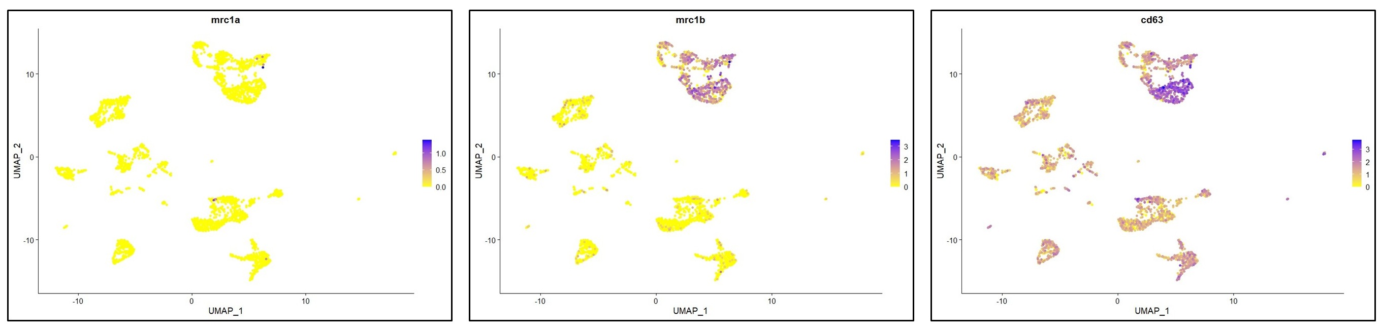
You have raised an important point here. As described in lines 197-202 (“results” section), the cells in the MF cluster exhibit a macrophage identity, based on their expression of classical macrophage markers such as marco, mfap4 or csf1ra. However, we were unable to confidently annotate this cluster more specifically. We also considered whether this population might resemble mammalian BAMs or monocytes, cell types that, to our knowledge, have not yet been clearly identified in zebrafish. However, orthologous markers typically associated with murine BAMs were not detected (lyve1) or not specifically enriched (mrc1a/mrc1b) in the MF cluster (see below). Based on these findings, we can only cautiously propose that this cluster may represent blood-derived macrophages and / or monocytes.

To further address your suggestion, we performed a cell type enrichment analysis using the marker genes of the MF cluster, following the same strategy as for the microglia and DC-like clusters presented in Figure 4 supplement 2 C,D. This analysis revealed significant for “monocytes” and “macrophages”, further supporting a general monocytic/macrophage identity (see below). At present, further characterization of this cluster is limited by the lack of zebrafish-specific antibodies and the restricted palette of fluorescent reporter lines that distinguish among MNP subsets. We anticipate that future studies, including the development of new transgenic lines guided by our dataset, will allow for a more precise analysis of this distinct population. 

Author response image 1.

Do all 4 DC clusters identified by scRNA-seq represent cDC1s? or are there also cDC2s, and cDC3s present?  

In our analyses, the four dendritic cell clusters identified by scRNA-seq (DC1-DC4) exhibit transcriptional profiles consistent with a conventional type 1 dendritic cell (cDC1) identity. These clusters uniformly express hallmark cDC1-associated genes, while lacking expression of markers typically associated with mammalian cDC2 or plasmacytoid dendritic cells (pDCs). For instance, irf4, a key transcription factor required for cDC2 development, is not detected in our dataset. Similarly, we do not observe expression of genes characteristic of pDCs. 

That said, the absence of cDC2 or pDC-like signatures in our dataset does not rule out the presence of these populations in zebrafish.  

While they show that DC-like cells did not express Csf1rb (Figure 4D) or other macrophage/microglia genes, DC-like cells were affected in the Csf1rb mutants and in double mutants, demonstrating that their development depends on Csf1rb signaling, as known for macrophages but not DCs. Can the authors discuss this in more detail with regard to DC differentiation/precursors? 

Thank you for pointing this out. As previously demonstrated, CSF1R signaling in zebrafish is more complex than in mammals, due to the presence of two paralogs, csf1ra and csf1rb, which exhibit partially non-overlapping functions (Ferrero et al., 2021). We and others have shown that csf1rb signaling is implicated in the regulation of definitive hematopoiesis, particularly in the regulation of hematopoietic stem cell (HSC)-derived myelopoiesis. Although the developmental origin of zebrafish brain DC-like cells remains uncharacterized, their reduced numbers in the csf1rb mutant, despite their lack of csf1rb expression, supports the current model in which csf1rb acts at the progenitor level, promoting myeloid lineage commitment. According to this, csf1rb disruption affects the differentiation of multiple myeloid subsets, which likely include DC-like cells. We have developed this point in the discussion section (lines 502506).  

Do the DCs express Csf1ra? 

Csf1ra transcripts are not found in DCs in our dataset. As shown below, csf1ra expression is restricted to the microglia and macrophage clusters. These observations are in line with those made by Zhou et al., 2023.

Author response image 2.

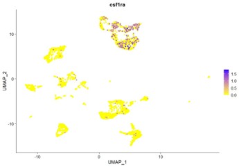
Fig. 5, the number of brains analyzed should be added, and also quantifications of cell numbers included. It is mentioned (line 260) that P2ry12GFP+mpeg1mCherry+ microglia are abundant across brain regions while P2ry12GFP- mpeg1mCherry+ cells particularly localize in the ventral part of the posterior brain parenchyma. It would be nice if images of the different brain regions were provided. 

Regarding the quantification, we refer to our response in the major comments section, where we explain that detailed quantification of microglia and other MNP subsets is provided in Figure 7, using a more refined strategy for distinguishing cell types.

As requested, we have now included representative sections from the forebrain, midbrain and hindbrain of adult Tg(mhc2dab:GFP; cd45:DsRed) fish. These images illustrate the spatial distribution of DC-like cells across brain regions. Notably, DC-like cells are most abundant in the ventral areas of the midbrain and hindbrain, and are also present in the posterior telencephalon, particularly concentrated in the region of the commissura anterior. This regional annotation is based on the zebrafish brain atlas by Wullimann et al., 1996 (Neuroanatomy of the zebrafish brain, https://doi.org/10.1007/978-3-0348-8979-7).

These additional images have been included in Figure 5 Supplement 1 (A-E).

It is sometimes not evident whether the Pr2y12- cells included DC-like cells and macrophages, which should be discussed. 

Thank you for bringing this to our attention. Upon review, we agree this point required clearer explanation throughout the text, particularly beginning with the description of putative DC-like cells in Figure 5. We have now revised the manuscript to improve clarity and becer guide readers through the phenotypic identification of DC-like cells using the Tg(p2ry12:p2ry12-GFP;mpeg1:mCherry) line. Specifically, we have modified the titles in the results section from page 5 to page 9, so that readers can more easily follow the step-by-step approach we used to distinguish DC-like cells from microglia. 

To directly address your comment: the p2ry12^-; mpeg1⁺ fraction may, in theory, include not only DC-like cells but also other macrophage subsets and B cells, as B cells have been shown to express mpeg1 in zebrafish (Ferrero et al., 2020; Moyse et al., 2020). Nevertheless, our data strongly indicate that within the brain parenchyma, DC-like cells represent the predominant component of this population. This conclusion is supported by the pronounced reduction of p2ry12^-; mpeg1⁺ cells in brain sections from ba43 mutants, in which DC development is impaired. 

We have revised the text accordingly to clarify this point in the results section of the manuscript (line 355).

For example, the DC-like cell population in Figure 6C appears to include two populations of cells. Thus, it is unclear whether the sorted mhc2dab:GFP+;CD45:DsRedhi population for bulk-seq also contains the MF population identified in Fig. 2. 

Thank you for this thoughtful observation. During the course of this study, we indeed considered how best to isolate non-microglial macrophages in order to specifically recover the MF population identified in our scRNA-seq analysis. However, with the current repertoire of fluorescent transgenic zebrafish lines, it remains technically challenging to selectively isolate non-microglial macrophages from the adult brain. As a result, the mhc2dab:GFP₊; cd45:DsRedhi sorted population used for bulk RNA-seq may indeed include a mixture of DC-like and other mononuclear phagocytes, potentially the MF population. In contrast, our data demonstrate that the Tg(p2ry12:p2ry12-GFP) line provides a more selective tool for isolating microglia, minimizing contamination from other mononuclear phagocyte subsets.

In Figure 7, a reduction of GFP-mpeg+ cells can be seen in baf3 mutants. Could the remaining cells be the (non-microglia) macrophages? Or in Figure 8, could the remaining P2ry12GFP-Lcp1+ cells in Irf8 mutants be macrophages? 

Indeed, we believe it is likely that the remaining mpeg1⁺ cells observed in ba43 mutants include non-microglial macrophages and/or B cells, as we and others previously showed that zebrafish B cells express mpeg1.1 transcripts and are labeled in the mpeg1.1 reporters (Ferrero et al., 2020). This interpretation is further supported by the observation that the reduction in mepg1+ cells is more pronounced in brain sections than in flow cytometry samples, where non-parenchymal mpeg+ cells, such as peripheral macrophages or B cells, are likely enriched. To explore this possibility, we attempted to assess the expression of MF- and B cell-specific markers in the remaining mpeg1+ population isolated from ba43 mutants. However, due to the very low numbers of cells recovered per animal, we were limited to analyzing only a few markers. Despite multiple attempts, qPCR analyses proved unconclusive, likely due to low transcript abundance. We thank you for your understanding of the technical limitations that currently prevent a more definitive characterization of these remaining cells.  

Regarding the irf8 mutants (Figure 8), irf8 is a well-established master regulator of mononuclear phagocyte development. In mice, deficiency results in developmental defects and functional impairments across multiple myeloid lineages, including microglia, which exhibit reduced density (Kierdorf et al., 2013) and an immature phenotype (Vanhove and al., 2019). Similarly, in zebrafish, irf8 mutants show abnormal macrophage development, with an accumulation of immature and apoptotic cells during embryonic and larval stages (Shiau et al., 2014). Based on these findings, it is plausible that the residual p2ry12:GFP^- Lcp1⁺ cells observed in the irf8 mutant brains represent immature or arrested mononuclear phagocytes, possibly including both microglia and DC-like cells. This is supported by their distinct morphology and specific localization along the ventricle borders. However, as previously noted, our current tools do not permit to conclusively identify these cells.

Reviewer #2 (Recommendations For The Authors): 

A few sentences are not easy to understand for a "non zebrafish specialist". 

(1) Page 3 line 111 The sentence "Interestingly, analyses of brain cell suspensions from double transgenics showed p2ry12:GFP+ microglia accounted for half of cd45:DsRed+ cells (50.9 % {plus minus} 2.9; n=4) (Figure 1D,E). Considering that mpeg1:GFP+ cells comprised ~75% of all leukocytes, these results indicated that approximately 25% of brain mononuclear phagocytes do not express the microglial p2ry12:GFP+ transgene." is not clear. This point is significant and deserves a more detailed explanation. 

We apologize for the lack of clarity in this section. The quantification presented in Figure 1 refers specifically to cd45:Dsred⁺ leukocytes, meaning that the reported percentages of p2ry12:GFP⁺ and mpeg1:GFP⁺ cells are calculated relative to the total cd45+ population (defined as 100%). Specifically, we observed that approximately 51% of all cd45+ cells were p2r12:GFP⁺ microglia, while around ti5% were mpeg1:GFP⁺. From these values, we infer that about 25% of mpeg1:GFP⁺ leukocytes do not express the p2ry12:GFP transgene and therefore likely represent non-microglial mononuclear phagocytes. We agree that this distinction is important and have revised the text accordingly to clarify the interpretation for readers who may be less familiar with zebrafish transgenic lines or gating strategies. See page 3, lines 107 117.

(2) Line 522; Like human and mouse ILC2s, "these cells do not express the T cell receptor cd4-1" is confusing (T cell receptor should be reserved to the ag specific TCR). Also, was TCR isotypes expression analyzed (and how was genome annotation used in this case ?) 

Thank you for this insightful comment.  We agree that the term “T cell receptor” should be used specifically to refer to antigen-specific TCRs, and we have revised the discussion accordingly to avoid any confusion. Regarding your question on the analysis of TCR isotype expression and the use of genome annotation: due to technical limitations, we did not pursue TCR isotype-level analysis in this study. Instead, we relied on established markers such as cd4-1 and cd8a to distinguish T cell populations, acknowledging that cd4-1 is not expressed by ILC2-like cells in our dataset. We have clarified these points in the relevant sections of the manuscript (see lines 168 and 535)

The analysis of single-cell data might be more detailed, with more explanation about possible doublet identification and normalization procedures. 

Thank you for highlighting the need for additional clarity regarding our scRNA-seq analysis.

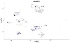
As noted in the Seurat tutorial, “cell doublets or multiplets often exhibit abnormally high gene count” (https://sa7jalab.org/seurat/archive/v3.0/pbmc3k_tutorial). To evaluate this, we performed a dedicated doublet detection analysis using the scDblFinder R package (https://rdrr.io/bioc/scDblFinder/f/vigneces/2_scDblFinder.Rmd). Our results indicated that the proportion of predicted doublets is low (see Figure below), and when present, these doublets are distributed among the different clusters. This contrasts with the typical clustering of doublets into discrete groups and indicates that our single-cell sequencing workflow was sufficiently robust to predominantly capture singlets.

Regarding normalization, we have clarified this in the manuscript. Briefly, single-cell data were normalized using Seurat’s SCTransform method with the following custom parameters: “variable.features.n=4000 and return.only.var.genes=F”. These settings are now clearly described to ensure reproducibility.

Author response image 3.

Reviewer #3 (Recommendations For The Authors):

Major issues

Though baf3 mutants were generated the manuscript will greatly benefit from in situ labeling by RNAscope or the generation of transgenic reporters to conclusively localize this dendritic cell population and address any potential contamination issues. 

We thank you for this constructive suggestion. We agree that in situ labeling approaches such as RNAscope would offer valuable complementary insights. In our current study, however, we already provide detailed spatial information on DC-like cells, and we demonstrated their lineage identity through the use of our newly generated batf3 mutant line. 

To address concerns regarding potential contamination, we have carefully analyzed more than two dozens adult brains to date and consistently observed abundant DC-like cells within the brain parenchyma, exhibiting a reproducible and specific spatial distribution, as described in the manuscript. This consistent localization across multiple samples strongly supports the genuine presence of these cells in the brain rather than artifactual contamination.

While the generation of DC-like specific transgenic lines is indeed a promising direction (and such efforts are currently underway in our group) we note that creating and validating these lines is time-consuming and falls beyond the scope of the present study. Importantly, although these additional tools will be valuable for future functional investigations, we believe they would not impact the main conclusions or core message of our current work. 

The morphological characterization of CD45:DsRed+ macrophages stained with May-Grunwald-Giemsa has been previously reported in the paper, "Characterization of the mononuclear phagocyte system in the zebrafish" Wittamer et al., 2011."Morphologic analyses revealed that the majority of cells exhibited the characteristics of monocytes/macrophages namely low nuclear to cytoplasm ratios and a high number of cytoplasmic vacuoles (Figure 3B). 

We thank you for pointing out the reference to Wittamer et al., 2011. In that study, we indeed provided the first morphological characterization of mononuclear phagocytes (MNPs) in various adult zebrafish organs using the cd45:DsRed line in combination with the mhc2dab:GFP reporter. The focus was primarily on MNPs across peripheral tissues. In the current study, our aim is broader: we investigate the full diversity of brain immune cells, using cd45 as a general marker for leukocytes. As part of this comprehensive characterization, we applied MGG staining, a widely accepted cytological technique, to gain morphological insight into the sorted CD45:DsRed+ population. This method remains a valuable and rapid approach to visually assess cell type heterogeneity, especially when evaluating samples where multiple immune cell lineages may be present. 

While there is some overlap with the methodology used in Wittamer et al., the context, scope, and tissue examined differ substantially. Thus, the inclusion of MGG staining in this study serves to complement our broader transcriptomic analyses by providing supporting morphological evidence specific to brain-resident immune cells.

We have now clarified this distinction in the revised manuscript to better differentiate the current work from our previous findings (see line 85).

Figure 5 data should be quantified.

Please refer to our response in the major comments section, where we address this question in detail.

Figure 7- Figure Supplement 1. J, K has no CD45:DsRed positive cells in baf3 mutants, which is counterintuitive because CD45:DsRed should capture all hematopoietic cells and is not specific to dendritic cells. 

It is correct that cd45 is a general leukocyte marker, labeling all immune cells, including dendritic cells. In this Figure, we used the Tg(cd45:DsRed) transgenic line to visualize the phenotype because it offers an alternative to IHC, with the advantage of strong endogenous fluorescence and easier screening of vibratome sections. However, this technique has limitations: due to fixation, only cells with high fluorescence (e.g. cd45^highdendritic cells) are captured, while those with medium/low expression (e.g. cd45^low microglia) are often not visible. This explains why fewer cells are observed in both wild-type and ba43 mutant brains (Figure 5 KN, Figure 7 – supplement 1 JK). While this approach is quicker and allows for thicker sections, IHC remains the preferred method for the rest of the analyses, including the use of additional markers to identify all relevant cell populations. 

Thank you for bringing this point of confusion to our attention. To improve clarity, we have amended the text in the relevant sections (see lines 704-706, and legend of Figure 7 Supplement 1)

Minor issues: 

The terms in the title, "A single-cell transcriptomic atlas..." are used. What is meant by "atlas"? A searchable database or website is not provided.

Please refer to our response in the major comments section, where we explain that we have made our dataset accessible through a searchable web interface (https://scrna-analysiszebrafish.shinyapps.io/scatlas/) which is now referenced in the Data Availability Statement.

This reviewer considers that it is offensive to use terminology such as "poorly characterized" in reference to others' work. 

Thank you for pointing this out. We understand the concern and have revised the wording to ensure it remains respectful and neutral when referring to previous work. The changes are reflected in lines 20 and 49.

The introduction of this manuscript should consider restructuring and editing. Example: Lines 51-57 introduce the importance of immune cells in zebrafish regeneration studies. However, this study does not investigate such processes. Additionally, the authors focus on the concept of immune heterogeneity in the brain throughout the text however, these studies have been conducted previously by others (Silva et al., 2021) at single-cell level.

The novelty of this manuscript is the identification of "dendritic-like cells" and yet the introduction and text are limited to 68-71 lines. The introduction would benefit by introducing this cell type "dendritic-like cells" and differences between vertebrates. 

Thank you for these valuable comments. In response, we have revised the introduction to better align with the focus of the study (see edited text in page 2). We now emphasize that, while macrophages have been extensively studied in zebrafish, dendritic cells remain much less well characterized in this model.  Also, while we acknowledge that Silva et al. addressed aspects of immune heterogeneity in the zebrafish brain, their study primarily focused on mononuclear phagocytes. In contrast, our work provides a broader and more detailed characterization of the brain immune landscape, integrating transcriptomic data with multiple fluorescent reporter lines and hematopoietic mutants to strengthen cell identity assignments. Importantly, we note that Silva et al. classified DC-like cells within the microglial compartment, whereas our findings support that these cells represent a distinct population. While our data challenge this specific aspect of their conclusions, we believe both studies offer complementary insights that collectively advance our understanding of zebrafish brain immunity. 

Though Figure 6 is a great conformation of scRNA sequencing, it seems redundant and should be supplemental data.

We respectfully disagree with the reviewer’s suggestion. We believe that presenting the data in Figure 6 as the main figure enhances its visibility and impact, particularly highlighting the distinction between microglia and DC-like cells, an aspect we consider highly valuable information for the zebrafish research community. This is especially important given that our conclusions challenge two previous independent reports, further underscoring the relevance of these findings to the field.

/hyperpost/🌐/🎭/gyuri/📓/2025/10/3/index.html

daily notes - third week of October 2025

x

Reviewer #2 (Public review):

Summary:

The authors show that in E. coli the initiator protein DnaA oscillates post-translationally: its activity rises and peaks exactly when DNA replication begins, even if dnaA transcription is held constant. To explain this, they propose an "extrusion" mechanism in which nucleoid-associated proteins such as H-NS, whose amount grows with cell volume, dislodge DnaA from chromosomal binding sites; modelling and H-NS perturbations reproduce the observed drop in initiation mass and extra initiations seen after dnaA shut-down. Together, the data and model link biomass growth to replication timing through chromosome-driven, post-translational control of DnaA, filling gaps left by classic titration and ATP/ADP-switch models.

Strengths:

(1) Introduces an "extrusion" model that adds a new post-translational layer to replication control and explains data unexplained by classic titration or ATP/ADP-switch frameworks.

(2) A major asset of the study is that it bridges the longstanding gap between DnaA oscillations and DNA-replication initiation, providing direct single-cell evidence that pulses of DnaA activity peak exactly at the moment of initiation across multiple growth conditions and genetic perturbations.

(3) A tunable dnaA strain and targeted H-NS manipulations shift initiation mass exactly as the model predicts, giving model-driven validation across growth conditions.

(4) A purpose-built Psyn66 reporter combined with mRNA-FISH captures DnaA-activity pulses with cell-cycle resolution, providing direct, compelling data.

Weaknesses:

(1) What happens to the (C+D) period and initiation time as the dnaA mRNA level changes? This is not discussed in the text or figure and should be addressed.

(2) It is unclear what is meant by "relative dnaA mRNA level." Relative to what? Wild-type expression? Maximum expression? This should be explicitly defined.

(3) It would be helpful to provide some intuition for why an increase in dnaA mRNA level leads to a decrease in initiation mass per ori and an increase in oriC copy number.

(4) The titration and switch models do not explicitly include dnaA mRNA in the dynamics of DnaA protein. Yet, in Figure 2G, initiation mass is shown to decrease linearly with dnaA mRNA level in these models. How was dnaA mRNA level represented or approximated in these simulations?

(5) Is Schaechter's law (i.e., exponential scaling of average cell size with growth rate) still valid under the different dnaA mRNA expression conditions tested?

(6) The manuscript should explain more explicitly how the extrusion model implements post-translational control of DnaA and, in particular, how this yields the nonlinear drop in relative initiation mass versus dnaA mRNA seen in Fig. 6E. Please provide the governing equation that links total DnaA, the volume-dependent "extruder" pool, and the threshold of free DnaA at initiation, and show-briefly but quantitatively-how this equation produces the observed concave curve.

(7) Does this Extrusion model give well well-known adder per origin, i.e., initiation to initiation is an adder.

(8) DnaA protein or activity is never measured; mRNA is treated as a linear proxy. Yet the authors' own narrative stresses post-translational (not transcriptional) control of DnaA. Without parallel immunoblots or activity readouts, it is impossible to know whether a six-fold mRNA increase truly yields a proportional rise in active DnaA.

(9) Figure 2 infers both initiation mass and oriC copy number from bulk measurements (OD₆₀₀ per cell and rifampicin-cephalexin run-out) instead of measuring them directly in single cells. Any DnaA-dependent changes in cell size, shape, or antibiotic permeability could skew these bulk proxies, so the plotted relationships may not accurately reflect true initiation events.

Comments on revisions:

The authors have addressed all of my previous concerns, questions, and suggestions sufficiently.

Author response:

The following is the authors’ response to the original reviews

Public Reviews:

Reviewer #1 (Public review):

Summary:

The study by Li and coworkers addresses the important and fundamental question of replication initiation in Escherichia coli, which remains open, despite many classic and recent works. It leverages single-cell mRNA-FISH experiments in strains with titratable DnaA and novel DnaA activity reporters to monitor DNA activity peaks versus size. The authors find oscillations in DnaA activity and show that their peaks correlate well with the estimated population-average replication initiation volume across conditions and imposed dnaA transcription levels. The study also proposes a novel extrusion model where DNA-binding proteins regulate free DnaA availability in response to biomass-DNA imbalance. Experimental perturbations of H-NS support the model validity, addressing key gaps in current replication control frameworks.

Strengths:

I find the study interesting and well conducted, and I think its main strong points are:

(1) the novel reporters obtained with systematic synthetic biology methods, and combined with a titratable dnaA strain.

(2) the interesting perturbations (titration, production arrest, and H-NS).

(3) the use of single-cell mRNA FISH to monitor transcripts directly.

The proposed extrusion model is also interesting, though not fully validated, and I think it will contribute positively to the future debate.

We thank the reviewer for acknowledging the strengths of our study.

Weaknesses and Limitations:

(1) A relevant limitation in novelty is that DnaA activity and concentration oscillations have been reported by the cited Iuliani and coworkers previously by dynamic microscopy, and to a smaller extent by the other cited study by Pountain and coworkers using mRNA FISH.

(2) An important limitation is that the study is not dynamic. While monitoring mRNA is interesting and relevant, the current study is based on concentrations and not time variations (or nascent mRNA). Conversely, the study by Iuliani and coworkers, while having the drawback of monitoring proteins, can directly assess production rates. It would be interesting for future studies or revisions to monitor the strains and reporters dynamically, as well as using (as a control) the technique of this study on the chromosomal reporters used by Iuliani et al.

We acknowledge the value of dynamic measurements and clarify our methodological rationale.

While luliani et al. provided valuable temporal resolution through protein dynamics, our mRNA FISH approach achieves direct decoupling of transcriptional vs. post-translational regulation (Fig 4F-H), and condition flexibility across 7 growth rates (30-66 min doubling times). This trade-off sacrifices temporal resolution for enhanced population-scale resolution and perturbation flexibility. To directly address temporal coupling, future work will implement dual-color live imaging of DnaA activity concurrent with replication initiation events.

(3) Regarding the mathematical models, a lot of details are missing regarding the definitions and the use of such models, which are only presented briefly in the Methods section. The reader is not given any tools to understand the predictions of different models, and no analytical estimates are used. The falsification procedures are not clear. More transparency and depth in the analysis are needed, unless the models are just used as a heuristic tool for qualitative arguments (but this would weaken the claims). The Berger model, for example, has many parameters and many regimes and behaviors. When models are compared to data (e.g., in Figure 2G), it is not clear which parameters were used, how they were fixed, and whether and how the model prediction depends on parameters.

We agree that model transparency is essential for quantitative validation. To address this, all model parameters (DnaA synthesis rate, activation/deactivation rates etc.) are explicitly tabulated in Supplementary Information Table S6. For the titration (Hansen et al. 1991) and extrusion models, we derive analytical expressions for initiation mass (IM) sensitivity to DnaA expression in Supplementary Note 1. For Figure 2G/S6, we used published parameters (Berger & Wolde 2022 SI Table 2) with experiment growth conditions (μ = 1.54 h^-1).

The extrusion model's validation relies primarily on its ability to resolve paradoxical initiation events under dnaA shutdown (Fig 6C), a test where other models fail categorically. While the Berger titration-switch hybrid can fit steady-state IM trends (Fig S6A), it cannot reproduce post-shutdown dynamics without ad hoc modifications (Fig S6B). We acknowledge that comprehensive analysis of all model regimes exceeds this study's scope but provide full simulation code for independent verification: https://github.com/BaiYangBqdq/dynamics_of_biomass_DNA_coordination

(4) Importantly, the main statement about tight correlations of peak volumes and average estimated initiation volume does not establish coincidence, and some of the claims by the authors are unclear in these respects (e.g., when they say "we resolve a 1:1 coupling between DnaA activity thresholds and replication initiation", the statement could be correct but is ambiguous). Crucially, the data rely on average initiation volumes (on which there seems to be an eternally open debate, also involving the authors), and the estimate procedure relies on assumptions that could lead to biases and uncertainties added to the population variability (in any case, error bars are not provided).

We acknowledge the limitations of population-level inference and have refined our claims: "Replication initiation volume scales proportionally with peak DnaA activity volume with a slope of 1.0 (R₂=0.98, Fig 7G), indicating predictive correspondence rather than absolute coincidence. While population-level  𝑉_𝑖 estimation cannot resolve single-cell stochasticity, the consistent 𝑉*: 𝑉_𝑖 relationship across 20 conditions suggest DnaA activity thresholds predict initiation timing within physiological error margins”. Future work will implement simultaneously DnaA activity and replication forks by using microfluidic single-cell tracking.

(5) The delays observed by the authors (in both directions) between the peaks of DnaAactivity conditional averages with respect to volume and the average estimated initiation volumes are not incompatible with those observed dynamically by Iuliani and coworkers. The direct experiment to prove the authors' point would be to use a direct proxy of replication initiation, such as SeqA or DnaN, and monitor initiations and quantify DnaA activity peaks jointly, with dynamic measurements.

We acknowledge the observed temporal deviations between DnaA activity peaks (𝑉*) and population-derived volumes at initiation ( 𝑉_𝑖) in certain conditions, in line with the findings of Iuliani et al. This might be mechanistically consistent with the time required for orisome assembly or oriC sequestration. They do not contradict our core finding that initiation occurs at a defined DnaA activity threshold (slope=1.0, R₂=0.98 in 𝑉*: 𝑉_𝑖 correlation).

(6) While not being an expert, I had some doubt that the fact that the reporters are on plasmid (despite a normalization control that seems very sensible) might affect the measurements. Also, I did not understand how the authors validated the assumptions that the reporters are sensitive to DnaA-ATP specifically. It seems this assumption is validated by previous studies only.

We employed a plasmid-based reporter system to circumvent the significant confounding effects of chromosomal position on promoter activity, as extensively documented by Pountain et al., where local genomic context (e.g., nucleoid occlusion, supercoiling gradients, and neighboring operons) introduces uncontrolled variability. By housing the P_syn66 test promoter and P_con normalization control in identical low-copy pSC101 vectors (<8 copies/ cell, Peterson & Phillips, Plasmid 2008), we ensured they experience equivalent physical and biochemical environments. This ratiometric design, where DnaA activity is calculated, actively corrects for global fluctuations in RNA polymerase availability, nucleotide pools, and plasmid copy number. Critically, P_syn66’s architecture emulates natural DnaA-responsive elements: its strong DnaAboxes report free DnaA concentration, while its weak box is preferentially bound by DnaA-ATP (Speck et al., EMBO journal 1999), mirroring the nucleotide-state sensitivity of oriC and the native dnaA promoter. This system was indispensable for our central finding, as it uniquely enabled the decoupling of DnaA activity oscillations from transcriptional feedback (Fig. 4F-H), an experiment fundamentally impossible with chromosomally integrated reporters due to autoregulatory interference.

Overall Appraisal:

In summary, this appears as a very interesting study, providing valuable data and a novel hypothesis, the extrusion model, open to future explorations. However, given several limitations, some of the claims appear overstated. Finally, the text contains some selfevaluations, such as "our findings redefine the paradigm for replication control", etc., that appear exaggerated.

We thank the reviewer for highlighting the need for precise language in framing our conclusions. We have implemented the following substantive revisions throughout the manuscript to ensure claims align strictly with empirical evidence:

(1) Changed "redefine the paradigm for replication control" into "advance the paradigm for replication control" (Introduction)

(2) Changed "redefine bacterial cell cycle control" into "refine bacterial cell cycle control as a dynamic interplay..." (Discussion)

(3) Removed the term "spatial" from the Discussion's description of DnaA-chromosome interactions (Discussion, first paragraph).

(4) Changed "provides a blueprint" into "provides a valuable tool for dissecting spatial regulation..." (Discussion, final paragraph)

(5) Scrutinized all superlatives (e.g., "critical feat" into "important capability"; "fundamental principle of cellular organization" into "potential organizational strategy")

(6) Replaced the instances of "robust" with evidence-backed descriptors (e.g., "sensitive," "consistent")

(7) We agree that the extrusion model requires further validation and have emphasized this in Discussion: "While H-NS perturbation supports extrusion mechanism, future work should identify the full extruder interactome and elucidate how metabolic signals modulate their activity" (final paragraph)

This calibrated language more accurately represents our study as a conceptual advance with testable mechanisms, not a complete paradigm shift.

Reviewer #2 (Public review):

Summary:

The authors show that in E. coli, the initiator protein DnaA oscillates post-translationally: its activity rises and peaks exactly when DNA replication begins, even if dnaA transcription is held constant. To explain this, they propose an "extrusion" mechanism in which nucleoidassociated proteins such as H-NS, whose amount grows with cell volume, dislodge DnaA from chromosomal binding sites; modelling and H-NS perturbations reproduce the observed drop in initiation mass and extra initiations seen after dnaA shut-down. Together, the data and model link biomass growth to replication timing through chromosome-driven, posttranslational control of DnaA, filling gaps left by classic titration and ATP/ADP-switch models.

Strengths:

(1) Introduces an "extrusion" model that adds a new post-translational layer to replication control and explains data unexplained by classic titration or ATP/ADP-switch frameworks.

(2) A major asset of the study is that it bridges the longstanding gap between DnaA oscillations and DNA-replication initiation, providing direct single-cell evidence that pulses of DnaA activity peak exactly at the moment of initiation across multiple growth conditions and genetic perturbations.

(3) A tunable dnaA strain and targeted H-NS manipulations shift initiation mass exactly as the model predicts, giving model-driven validation across growth conditions.

(4) A purpose-built Psyn66 reporter combined with mRNA-FISH captures DnaA-activity pulses with cell-cycle resolution, providing direct, compelling data.

We thank the reviewer for acknowledging the strengths of our study.

Weaknesses:

(1) What happens to the (C+D) period and initiation time as the dnaA mRNA level changes? This is not discussed in the text or figure and should be addressed.

We thank the reviewer for this important observation. Our data demonstrate that increased dnaA mRNA levels induce two compensatory changes in cell cycle progression:

(1) Earlier replication initiation, manifested as a reduced initiation mass: the initiation mass decreased from 5.6 to 2.6 (OD₆₀₀·ml per 10¹⁰ cells) as the relative dnaA mRNA level increased from 0.2 to 7.2 (normalized to the wild-type level) (Fig. 2F, red).

(2) Prolonged C+D period: Increased by approximately 60% (from 1.05 to 1.66 hours, Fig. 2F blue).

The complete quantitative relationship is now explicitly described in the Results section: “Concurrently, the initiation mass was reduced by 50%, and the period from initiation to division (C+D) was increased by ~60% (Fig. 2F)”

(2) It is unclear what is meant by "relative dnaA mRNA level." Relative to what? Wild-type expression? Maximum expression? This should be explicitly defined.

The relative dnaA mRNA level was obtained by normalizing to that in wild-type MG1655 cells grown in the same medium. To clarify this point, we have now marked the wild-type level in Fig. 1B, and a clear description of this has also been included in the figure caption.

(3) It would be helpful to provide some intuition for why an increase in dnaA mRNA level leads to a decrease in initiation mass per ori and an increase in oriC copy number.

Thank you for your valuable suggestion. Increased dnaA mRNA accelerates DnaA accumulation, causing cells to reach the initiation threshold at a smaller cell size (reducing initiation mass, Fig. 2F red). This earlier initiation increases oriC copies per cell at populational level (Fig. 2E). This mechanistic interpretation now appears in the Results: “As the DnaA expression level increases, DnaA activity reaches the initiation threshold earlier. Given that cell mass remained nearly unchanged, this earlier initiation led to an increase in population-averaged cellular oriC numbers (Fig. 2E).”

(4) The titration and switch models do not explicitly include dnaA mRNA in the dynamics of DnaA protein. Yet, in Figure 2G, initiation mass is shown to decrease linearly with dnaA mRNA level in these models. How was dnaA mRNA level represented or approximated in these simulations?

All models presented in this article omit explicit modeling of dnaA mRNA dynamics for simplicity. However, at steady state, the relative level of dnaA mRNA can be approximated by the relative expression rate of DnaA protein, as both reflect the expression level of DnaA. This detail is now clarified in the caption of Figure 2G.

(5) Is Schaechter's law (i.e., exponential scaling of average cell size with growth rate) still valid under the different dnaA mRNA expression conditions tested?

Schaechter's law describes the exponential scaling of average cell size with growth rate in bacteria. In our prior work (Zheng et al., Nature Microbiology 2020), where we demonstrated that Schaechter's law fails in slow-growth regimes. However, in current study, growth rate remained constant across different dnaA expression levels (Fig. 2C), and cell mass showed no significant change (Fig. 2D). Since Schaechter's law specifically addresses how cell size scales with growth rate, it does not apply here, as growth rate was invariant in our perturbations, which selectively alter replication initiation dynamics, not growth rate or size scaling.

(6) The manuscript should explain more explicitly how the extrusion model implements posttranslational control of DnaA and, in particular, how this yields the nonlinear drop in relative initiation mass versus dnaA mRNA seen in Figure 6E. Please provide the governing equation that links total DnaA, the volume-dependent "extruder" pool, and the threshold of free DnaA at initiation, and show - briefly but quantitatively - how this equation produces the observed concave curve.

The governing equations linking initiation mass and DnaA expression level is now provided in Supplementary Note S1 for both the titration and the extrusion model. In general, the dependence of initiation mass (𝑉_𝐼) on dnaA expression level (𝛼_𝐴) dependency takes an inverse 1 proportionality form: . In the extrusion model, the incorporated extruder protein is assumed to have similar synthesis dynamics as DnaA and can release DnaA from DnaA-box. After denoting the synthesis rate of the extruder as 𝛼_𝐻, the combined effect of DnaA and the extruder on replication initiation can be briefly described as: . Then the additive contribution of 𝛼_𝐻 dampens the sensitivity of initiation mass to changes in 𝛼_𝐴, resulting in a significantly flattened curve. As a result, the predicted 𝑉_𝐼 − 𝛼_𝐴 relationship has a concave shape in the semi-log plots.

(7) Does this Extrusion model give well well-known adder per origin, i.e., initiation to initiation is an adder.

Yes, the extrusion model can provide the initiation-to-initiation adder phenomenon, this information was provided in fig. S3C.

(8) DnaA protein or activity is never measured; mRNA is treated as a linear proxy. Yet the authors' own narrative stresses post-translational (not transcriptional) control of DnaA. Without parallel immunoblots or activity readouts, it is impossible to know whether a sixfold mRNA increase truly yields a proportional rise in active DnaA.

We acknowledge the reviewer's valid concern regarding the indirect nature of our DnaA activity measurements. While mRNA levels alone cannot resolve active DnaA dynamics, our approach integrates functional replication outcomes with a validated synthetic reporter to infer activity. Crucially, elevated dnaA mRNA causes demonstrable biological effects: earlier replication initiation (Fig. 2F) and increased oriC copies (Fig. 2E), directly confirming enhanced functional DnaA activity at the oriC locus. The P_syn66 reporter, engineered with DnaA-boxes mirroring oriC's architecture, provides orthogonal validation, showing progressive repression to dnaA induction (Fig. 3C). Our operational metric , bases on P_syn66 responds sensitively to DnaA-chromosome interactions within its characterized 8-fold dynamic range (Fig. 3C). Immunoblots would be inadequate here, as they cannot distinguish functionally critical pools: free versus chromosome-bound DnaA, or DnaA-ATP versus DnaAADP, precisely the post-translational states our study implicates in regulation. We therefore prioritize functional readouts (initiation timing) and the P_syn66 reporter, which probes the biologically active fraction relevant to replication control.

(9) Figure 2 infers both initiation mass and oriC copy number from bulk measurements (OD₆₀₀ per cell and rifampicin-cephalexin run-out) instead of measuring them directly in single cells. Any DnaA-dependent changes in cell size, shape, or antibiotic permeability could skew these bulk proxies, so the plotted relationships may not accurately reflect true initiation events.

We acknowledge the reviewer's valid methodological concern and clarify that while bulk measurements carry inherent limitations, our approach is grounded in established techniques with demonstrated reliability. Cell mass was inferred from OD600/cell, which correlates strongly with direct dry weight measurements and microscopic cell volumes across diverse growth conditions, as validated in our prior work (Zheng et al., Nature Microbiology 2020). Crucially, cell mass remained invariant across dnaA expression levels (Fig. 2D).

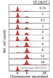
Regarding oriC quantification, the rifampicin-cephalexin run-out assay is a wildly applied for replication initiation studies. Our data shows expected 2ⁿ oriC distributions without abnormal ploidy (as shown below). While single-cell methods offer superior resolution, our bulk approach provides accurate population-level trends.

Author response image 1.

Recommendations for the authors:

Reviewing Editor Comments:

The reviewers felt that the mathematical modeling was not adequately explained in the paper, and that this affected the readability of the manuscript. The authors are encouraged to elaborate on this aspect of the paper (in addition to strengthening other claims, if possible, per the reviewers' comments).

We thank the editor and reviewers for their constructive feedback. We have comprehensively strengthened the mathematical modeling framework to enhance clarity and rigor.

Reviewer #1 (Recommendations for the authors):

The only revision I would do is a recalibration of the claims and a major effort to clarify the modeling part (including a detailed SI appendix), without necessarily performing additional work.

To enhance mathematical modeling transparency, we have completed model description in the method section and a parameter table with literature-sourced values in Supplementary Information Table S6. Moreover, analytical derivations of initiation mass dependencies are performed and presented in the Supplementary Information Note S1.

Of course, there are extra experiments (mentioned in the public review) that would help support some of the big claims, but that can be considered a different project.

Thank you for your suggestion. This will be addressed in our future work.

Minor suggestion: please put signposts or plot jointly to compare the maxima/minima in Figures 4D, E, G, and H.

We added dashed lines in Figures 4D, and E, to synchronize visualization of DnaA activity peaks and transcriptional minima across panels, facilitating direct biological comparisons.

Reviewer #2 (Recommendations for the authors):

(1) Should define what DNA activity is.

We have explicitly defined DnaA activity in the Introduction as “the capacity to initiate replication…” and noted that it is “governed by free DnaA concentration, DnaA-ATP/-ADP ratio, and orisome assembly competence”.

(2) Word repetition - “...grown in in Luria-Bertani (LB) medium...”.

Corrected.

(3) Typographical error - “FISH ... was preformed" should be "performed”.

Corrected.

(4) The manuscript alternates between “ng ml^-1” and “ng·ml^-1”; choose one style and apply it uniformly.

Standardized the units to ng·ml^-1 throughout.

(5) Reference duplicates - Some citations appear twice in the bibliography (e.g., "Bintu et al., 2005a/b" and "Bintu et al., 2005b" listed again later).

The studies by Bintu et al. (2005a, 2005b) represent separate works: 2005a details applications, and 2005b develops models.

Reviewer #2 (Public review):

Summary:

This paper introduces a new function within the Fam3Pro package that addresses the problem of breaking loops in family structures. When a loop is present, standard genotype peeling algorithms fail, as they cannot update genotypes correctly. The solution is to break these loops, but until now, this could not be done automatically and optimally.

The manuscript provides useful background on constructing graphs and trees from family data, detecting loops, and determining how to break them optimally for the case of no loops with multiple matings. For this situation, the algorithm switches between Prim's algorithm and a simple greedy approach and provides a solution. However, here, an optimal solution is not guaranteed.

The theoretical foundations-such as the representation of families as graphs or trees and the identification of loops-are clearly explained and well-illustrated with example pedigrees. The practical utility of the new function is demonstrated by applying it to a dataset containing families with loops.

This work has the potential for considerable impact, especially for medical researchers and individuals from families with loops. These families could previously not be analysed automatically and optimally. The new function changes that, enabling risk assessments and genetic calculations that were previously infeasible.

Strengths:

(1) The theoretical explanation of graphs, trees, and loop detection is clear and well-structured.

(2) The idea of switching between algorithms is original and appears effective.

(3) The function is well implemented, with minimal additional computational cost.

Weaknesses:

(1) In cases with multiple matings, the notion of a "close-to-optimal" solution is not clearly defined. It would be helpful to explain what this means-whether it refers to empirical performance, theoretical bounds, or something else.

(2) In the example pedigree discussed, multiple options exist for breaking loops, but it is unclear which is optimal.

(3) No example is provided where the optimal solution is demonstrably not reached.

(4) It is also unclear whether the software provides a warning when the solution might not be optimal.

Author response:

Response to Reviewer #1:

We plan to extend the discussion section to discuss the clinical implications of this new function. We will note the algorithm's applicability to broader genetic counseling contexts beyond cancer risk assessment.

Response to Reviewer #2:

We will clarify the four points raised:

(1) "Close-to-optimal" definition: We will explain that in multiple-mating cases, finding the global optimum is NP-hard (equivalent to the Weighted Feedback Vertex Set problem). We will clarify that our greedy algorithm provides practically efficient solutions suitable for clinical use, though without theoretical optimality guarantees.

(2) Example clarity: We will improve Figure 1's caption to explain the cost calculations and note that with equal weights, both shown solutions are equivalent.

(3) Non-optimal examples: We will describe scenarios where the greedy algorithm may not achieve the global optimum, particularly in multiple-mating cases with heterogeneous weights.

(4) Warning message: The current version not provide a warning when the solution might be non-optimal. This may be added in the future to the function.

We appreciate your feedback and suggestions to help improve the manuscript.

This tends to come with a lot of pressure that is put on the students because of stereotypes like the model minority. As mentioned in the text, stereotypes amongst Asians include. having high standardized scores, which can lead them to feeling forced to fit into this category. This leads to unhealthy habits which can affect their mental health nd well-being. Many are oblivious to the dangers that come with forcing stereotypes, especially when being forced to such high standards.

This reveals how systemic racism not only inflicts external harm but also demands internalized emotional discipline. The legacy of emotional containment reveals how racism operates through the regulation of affect shaping how marginalized communities are allowed to feel or express themselves. Seeing how both African Americans and Asian American communities have similar constraints shows how institutional racism continues to police emotional expression which tends to have negative effects on mental health and identity formation.

This really comes to show that academic success is no longer being a source of empowerment and joy but a shield against exclusion. Her excellence is only acknowledged narrowly and deeply confined to academics while her broader contributions are overlooked. This shows a systemic bias in regards to how merit is recognized. I think her relationship with school reveals how institutional cultures can distort the meaning of success, turning it to a coping mechanism for navigating environments.

This exposes how school systems tolerate racist bullying and exposes the tendency of institutions to mask harm with performative multiculturalism. Telling Asian American students to toughen up while excusing white peers behavior not only reflects bias but the systems refusal to confront racism. It is really upsetting to see that parents fear speaking out and feel that it is unnecessary due to the fear of being further discriminated against.

Many Chinese students also face similar pressures within the exam-oriented education system: “excellence” becomes a moral label, with no room for failure or emotional expression. This is especially true when studying abroad. Chinese students are often defined as “quiet, strong in science, and lacking creativity”—a narrative that closely mirrors Ann's own experience.

Children are not born racists; they learn racial hierarchies by imitating the behaviors of adults and peers. White children reproduce the social order of “white supremacy” through language and mockery, while Asian children are marginalized from a young age, subjected to ridicule about their appearance and food, thereby learning their subordinate place within the social racial structure. Schools are not neutral learning environments but spaces that reproduce social hierarchies. Through seemingly “playful” interactions, children learn who belongs to the ‘mainstream’ and who is the “other,” while teachers' silence effectively endorses this structure. Similar social stratification exists within China's educational environment—manifesting in stereotypes targeting non-local students, ethnic minorities, those with distinct accents, or students deemed “unsociable.” We frequently hear excuses like “He's just a child, he doesn't understand” to justify discriminatory remarks.

Rejecting of the American norm

研究绝大多数人都绕不开的一个的重要话题——职业。那么我们应该如何才能认知职业的本质，让我们从本质、底层逻辑层面进行深刻理解。进而深刻的理解他、认知他、掌握它、运用它？ 职业是一种生存模式，是一种解决自身问题的生存模式，目标是解决自身的生存问题的模式。但是这种模式必须要进行连接，要将自己的能力、目标与他人进行连接，才能形成并建立一种稳定的联系。 例如：医生是将自己的技能与患者之间的需求进行一种一对多的映射联系，企业家是将自己的综合能力与社会上更加广泛的人们需求建立联系，一个成功的企业家，自然它的服务受众也会约广泛，例如：库克、马斯克、马云。 结论：职业是一种将自己与他人建立联系并解决自身生存问题的生存模式。 职业的价值大小、能力的强弱，评价指标就是自己的职业范畴服务、联系的人员数量人员范畴的人员规模大小，联系强度的强弱。

观念、意愿和能力，他们三者之前到底有什么样的区别和联系？他们在赚钱这个核心的目标实现过程中分别扮演什么样的角色和作用？ 那么在赚钱的这个目标过程中，是否有底层逻辑、原理是通行、通用的，有没有相对稳定的模型、规则是适用统配的？有没有具体的措施、案例可以印证？ 从而让赚钱这件事情，看上去更加通透、触及本质。

Producers of these programs had to adjust their approach when introducing AI to society - instead of a cold robotic, non-existent relationship, they created a false impression of a real "entity" with reason/logic; when in reality it is a program with instructions and training.

In Gemini vs. ChatGPT exercise I asked the programs opinions on my topic and whether they thought the hypothesis was correct according to the findings (in their opinion), like it had thoughts of its own to see what both programs would think.

While controversial, the addition of intelligence to digital cognitive artifacts making them operate independently from humans, remains a completely necessary step in advancement. There are some tasks which would simply require too much time, or are actually impossible for humans to complete if the process relied on their intelligence alone. The ability for an artifcat to work on its own allows for an incredible increase in effeciency, making things that were deemed impossible 20 years ago into a reality.

Note: This response was posted by the corresponding author to Review Commons. The content has not been altered except for formatting.

Learn more at Review Commons

Reply to the reviewers

Note: This preprint has been reviewed by subject experts for Review Commons. Content has not been altered except for formatting.

Reply to the Reviewers

We thank the reviewers for their positive assessments overall and for many helpful suggestions for clarification to make the manuscript more accessible to a broader audience. We made minor text changes and added more labels to the figures to address these comments.

• *

__Referee #1

__

Summary: In this study, the authors show a genetic interaction of the lipid receptors Lpr-1, Lpr-3 and Scav-2 in C. elegans. They show that Lpr-1 loss-of-function specifically affects aECM localization of Lpr-3 and attribute the lethality of Lpr-1 mutants to this phenotype. The authors performed a mutagenesis screen and identified a third lipid receptor, Scav-2, as a modulating factor: loss of scav-2 partially rescues the Lpr-1 phenotype. The authors created a variety of tools for this study, notably Crispr-Cas9-mediated knock-ins for endogenous tagging of the receptors.

Major comments:

1. while the authors provide a nice diagram showing the potential roles and interplay of lpr-1, lpr-3 and scav-2, it remains unclear what their respective cargo is. The nature of interaction between the proteins remains unclear from the data.

Response

• We agree that identifying the relevant cargo(s) will be key to understanding the detailed mechanisms involved and that the lack of such information is a limitation of our study. However, the impact of our study is to show that these lipid transporters functionally interact to affect aECM organization, a role that could be relevant to many systems, including humans.

As an optional (since time-consuming) experiment I would suggest trying more tissue-specific lipidomics.

Response

• This would be an interesting future experiment but is outside our current technical capabilities.

The lipidomics data should be presented in the figures, even if there were no significant changes. Importantly, show the lipid abundance at least of total lipids, better of individual classes, normalized to the material input (e.g. number of embryos, protein).

Response

• The reviewer is right to point out that lipid variations could occur at different levels, and that we should exercise caution. However, the unsupervised lipidomics analysis would have detected not only individual lipid variations, but also variations in the total or subgroup lipid content. Indeed, the eggs were weighed prior to extraction and each sample was extracted with the same precise volume of solvent before analysis. Furthermore, the LC-MS/MS injection sequence included blanks and quality control (QC) samples. The blanks were the extraction solvent, which allowed us to control for features unrelated to the biological samples. The QC sample was a mixture of all the samples included in the injection sequence, reflecting the central values of the model. If a subclass of samples, such as the lpr-1 mutant, had been characterized by a decrease in one lipid, a subgroup of lipids, or all lipids, it would have clustered separately. Instead, our PCA showed that the variation between samples of the same genotype (wild type, lpr-1 mutant, or lpr-1; scav-2) was similar to the variation between samples from two different genotypes. This means that we did not detect modifications to lipid quantity specifically or in total. A figure illustrating the lipid contents would show no difference between groups.

Figure 1g: I do not understand what the lpr3:gfp signal is: the punctae in the overview image? and where are they in the zoom image showing anulli and alae? Also, how where the anulli and alae structures labeled? please provide more information

Response

• All of the fluorescent signal shown in this figure panel corresponds to the indicated LPR fusion - no other labelling method was used. SfGFP::LPR-3 labels the matrix structures (alae and annuli) as well as some puncta – the ratio of matrix to puncta changes over developmental stages. We edited the figure legend to make this more clear.

One point that is not sufficiently adressed is that the authors deduce from the inability of the scav-2 gfp knock in to suppress lpr1 lethality that scav2 function is not impaired. This is quite indirect. Can the authors provide more convincing evidence that scav-2 ki has normal function?

Response

• Suppression of lpr-1 (or other aECM mutant) lethality is the only known phenotype caused by loss of scav-2 Therefore, this is the only phenotype for which we can do a rescue experiment to test functionality of the knock-in. The data presented do indicate that the knock-in fusion retains significant function.

In general, the data is clearly presented and the statistical analyses look sound.

Response

• Thank you

__Minor comments: __

Please provide page and line numbers!

Response:

• done

Avoid contractions like "don't" in both text and figure legends

Response:

• changed one instance of “don’t” to “do not”

Page 12: I do not understand the meaning of the sentence "This transgene also caused more modest lethality in a wild-type background"

Response:

• Wording changed to “This transgene caused very little lethality in a wild-type background (Fig. 6C), indicating it is not generally toxic.”

Figure 7: what is meant with "Dodt"?

Response:

• Dodt gradient contrast imaging is a method for transmitted light imaging similar to DIC and is used on some confocal microscopes. It is now explained in the Methods section. We removed the Dodt label from Figure 7 since it seems to be confusing and it is not really important whether the brightfield image is DIC or Dodt.

  Reviewer #1 (Significance (Required)):

  The study is experimentally sound and uses numerous novel tools, such as endogenously tagged lipid receptors. It is an interesting study for researchers in basic research studying lipid receptors and ECM biology. It provides insights on the genetic interaction of lipid receptors. My expertise is in lipid biochemistry, inter-organ lipid trafficking and imaging. I am not very familiar with C. elegans genetics.

__Referee #2 __ 1. The manuscript is very well written; the documentation is fine, but some more details are needed for better following the subject for readers not familiar with nematode anatomy.

For instance, while alae are somehow explained, annuli are not - structures that look abnormal in lpr1 and lpr1-scav2 mutants (Fig. 5B).

Response

• Apologies for this oversight. We added annuli labels to Figure 1 and Figure 5 panels and added descriptions of annuli to the Figure 1 legend and the Results text.

Moreover, the authors show in Fig. 1 the punctae etc in the epidermis, whereas in Fig. 2 the show Lpr3 accumulation or not in the duct and the pore (lpr1). How do they localize in the cells of these structures at high magnification? It is also important to see the Lpr3 localisation in lpr1 mutants shown in Fig. 2A with the quality of the images shown in Fig. 1F. This applies also to Figs. 4 and 5.

Responses:

• The embryonic duct and pore cells are very small and we have not reliably seen puncta within them. In Figs 2 and 5, we supplemented the duct and pore images with those from the epidermis, which is a much larger tissue, allowing us to resolve puncta and matrix structures with better resolution.
• The laser settings in Figs 2,4,5 (as opposed to Fig. 1) were chosen to avoid saturation of the matrix signal so that we could do accurate quantifications as shown. The images are unmodified with respect to brightness and therefore appear relatively dim – but we think they convey the observations very accurately.

I would like to see punctae in lpr1-scav2 doubles.

Response:

• Puncta in this genotype are shown for the epidermis in Figure 5. It has not been possible to see puncta specifically within the embryonic duct and pore.

Regarding the central mechanism, one possibility is - what the authors describe - that Lpr1 is needed for Lpr3 accumulation in ducts and tubes. Alternatively, Lpr1 is needed for duct and tube expansion, in lack of which Lpr3 is unable to reach its destination that is the lumina. Scav2, in this scenario, might be antagonist of tube and duct expansion, and thereby rescue the Lpr1 mutant phenotype independently. Admittedly, the non-accumulation of Lpr3 in scav2 mutants argues against a lpr1-independent function of scav2.

Responses:

• LPR-1 is indeed needed to maintain duct and pore tube integrity as the tubes grow, but in mutants the tubes appear to collapse at a later stage than we imaged here (Stone et al 2009). The ~normal accumulation of LET-4 and LET-653 further argues that the duct and pore tubes are still intact at the 1.5-to-2-fold stages. Therefore, we conclude that the defect in LPR-3 accumulation precedes duct and pore collapse.
• The changes we document in the epidermis also show that the lpr-1 mutant affects LPR-3 accumulation in another (non-tube) tissue.

In any case, to underline the aspect of Lpr1-Scav2 dosage relationship, the authors may also have a look at Lpr3 distribution in lpr1 heterozygous, and lpr1-scav2 double heterozygous worms. In this spirit, it would be interesting to see the semi-dominant effects of scav2 on Lpr3 localisation in lpr1 mutants by microscopy.

Response:

• Because of the hermaphroditism of C. elegans, it would be technically challenging to confidently identify heterozygous (vs. homozygous) embryos for confocal imaging. We do not think that the results would be informative enough to warrant the effort, given that we’ve already shown that scav-2 heterozygosity can partly suppress lpr-1 The expectation is that LPR-3 levels would be partially restored in the scav-2 het, but it might take a very large sample size to confidently assess that partial effect.

One word to the overexpression studies: it is surprising that the amounts of Scav2 delivered by the expression through the grl-2 promoter in the lpr1, scav2 background are almost matching those by the opposite effect of scav2 mutations on lpr1 dysfunction.

Response:

• The reviewer refers to the transgenic rescue experiment with the grl-2pro::SCAV-2 transgene. Because the scav-2 mutant phenotype being tested is suppression of lpr-1 lethality, the expected result from scav-2 rescue is to restore the lpr-1 lethal phenotype to the strain. This is exactly the result we see. We have revised the text to more clearly explain the logic.

One issue concerns the localization of scav2-gfp "rarely" in vesicles: what are these vesicles?

Response

• Only a handful of vesicles were seen across all the images we collected, and we have not yet identified them. They could be associated with either SCAV-2 delivery or removal from the plasma membrane, as now stated in the text. SCAV-2 trafficking would be an interesting area for further study but is beyond the scope of this paper.

One comment to the Let653 transgenes/knock-ins: the localization of transgenic Let653-gfp may be normal in lpr1 mutants because there are wild-type copies in the background.

Response

• There are wild type copies of LET-653 in the background, but no wild type copies of LPR-1. Even if the untagged LET-653 would be recruiting the tagged LET-653 as the reviewer suggests, we can still conclude that lpr-1 loss does not prevent the untagged LET-653 (and thus also the tagged LET-653) from accumulating in the duct lumen matrix.

One thought to the model: if Scav2 has a function in a lpr1 background, this means that yet another transporter X delivers the substrate for Scav2, isn't it?

Response

• Yes, we completely agree with this interpretation and have revised the discussion and Figure 8 legend to more explicitly make this point.

A word to the term haploinsifficient that is used in this study: scav2 mutants would be haploinsifficient if the heterozygous worms died in an otherwise wild-type background.

Response

• We disagree with this comment. The term “haploinsufficient” simply means that heterozygosity for a deletion or other loss of function allele can cause a mutant phenotype – the term is not restricted to lethal phenotypes.

  Reviewer #2 (Significance (Required)):

  Alexandra C.Belfi and colleagues wrote the manuscript entitled "Opposing roles for lipocalins and a CD36 family scavenger receptor in apical extracellular matrix-dependent protection of narrow tube integrity" in which they report on their findings on the genetic and cell-biological interaction between the lipid transporters Lpr1 and scav2 in the nematode C. elegans. In principle, these two proteins are involved in shaping the apical extracellular matrix (aECM) of ducts by regulating the amounts of Lpr3 in the extracellular space. While seems to act cell autonomously, Lpr1 has a non-cell autonomous effect on Lpr3.

---

__Referee #3 __ Summary: Using a powerful combination of genetic and quantitative imaging approaches, Belfi et al., describe novel findings on the roles of several lipocalins-secreted lipid carrier proteins-in the production and organization of the apical extracellular matrix (aECM) required for small diameter tube formation in C. elegans. The work comprises a substantial extension of previous studies carried out by the Sundaram lab, which has pioneered studies into the roles of aECM and accessory proteins in creating the duct-pore excretion tube and which also plays a role in patterning of the epidermal cuticle. One core finding is that the lipocalin LPR-1 does not stably associate with the aECM but is instead required for the incorporation of another lipocalin, LPR-3. A second major finding is that reduction of function in SCAV-2, a SCARB family membrane lipid transporter, suppresses lpr-1 mutant lethality along with associated duct-pore defects and mislocalization of LPR-3. Likewise loss of scav-2 partially suppresses defects in two other aECM proteins and restores defects in LPR-3 localization in one of them (let-653). Additional genetic and protein localization studies lead to the model that LPR-1 and SCAV-2 may antagonistically regulate one or more lipid or lipoprotein factors necessary for LPR-3 localization and duct-pore formation. A role for LPR-1 and LPR-3 at lysosomes is clearly implicated based on co-localization studies, although a specific role for lysosomes (or related organelles) is not defined. Finally, MS data suggests that neither LPR-1 or SCAV-2 grossly affect lipid composition in embryos, consistent with dietary interventions failing to affect mutant phenotypes. Ultimately, a plausible schematic model is presented to explain for much of the data.

__*Major comments:

*__

1. The studies are very thorough, convincing, and generally well described. Conclusions are logical and well grounded. Additional experiments are not required to support the authors major conclusions, and the data and methods are described in a sufficient detail to allow replication. As such my comments are minor and should be addressable at the author's discretion in writing.

Response

• Thank you for these positive comments

  __Minor comments: __2) In the abstract, "tissue-specific suppression" made me think that there was going to be a tissue-specific knockdown experiment, which was not the case. Rather scav-2 suppression is specific to the duct-pore, which corresponds to where scav-2 is expressed. Consider rewording this.

Response

• Wording was changed to “duct/pore-specific suppression”

  3) Page 5. Suggest wording change to, "Whereas LPR-3 incorporates stably into the precuticle, suggesting a structural role in matrix organization, LPR-1..."

Response

• Done

  4) LIMP-2 versus LIMP2. Both are used. Uniprot lists LIMP2, but some papers use LIMP-2. Choose one and be consistent.

Response

• Everything changed to LIMP2.

  5) Some of the data for S6 Fig wasn't referred to directly in the text. Namely results regarding pcyt-1 and pld-1. I'd suggest incorporating this into the results section possibly using, "As a control for our lipid supplementation experiments..."

Response

• These experiments are now described on page 11.

  6) Page 12 bottom. I understand the use of "oppose", but another way to put it is that SCAV-2 and LPR-1 (antagonistically or collectively) modulate aECM composition. Other terms that might confuse some readers is the use of upstream and downstream, although I OK with its use in the context of this work.

Response

• The genetics indicate that lpr-1 and scav-2 have opposite effects on tube shaping and LPR-3 localization, so they do function antagonistically rather than collectively/cooperatively; we decided to keep this terminology.

  7) Page 16. I understand the logic that SCAV-2 is unlikely to directly modulate LPR-3 given its presumed molecular function. But is it possible that LPR-3 levels are already maxed out in the aECM so that loss of SCAV-2 doesn't lead to any increase? Conversely, one could argue that even if acting indirectly, SCAV-2 could have led to increased LPR-3 levels, unless they were already maxed.

Response

• This is a good point and the possibility is now mentioned in the Results page 9. We also changed our wording in the Abstract and Discussion to acknowledge the possibility that LPR-3 could be the SCAV-2 cargo, though we still don’t favor this model.

  8) Figure legend 1. I did not see an asterisk in figure 1B.

Response

• thanks for catching this error, text removed

  9) Figure 1C. Might want to define the "degree" term in the legend for people outside the field.

Response

• We added an explanation to the figure legend.

  10) Fig 1 G. I was just wondering if cuticle autofluorescence was an issue for taking these images.

Response

• Cuticle auto fluorescence is generally quite dim in L4s with our settings, and it was not an issue at this mid/late L4 stage, which corresponds to when both LPR fusions are at their brightest. Note that both large panels are MAX projections and yet you can’t see any cuticle auto-fluorescence in the LPR-1 panel.

  11) Fig 2 and others. Please define error bars.

Response

• These correspond to the standard deviation; this information is now added to the Methods.

  12) Fig 5. From the images, it looks like lpr-1; scav-2 doubles might have a worse (pre)cuticle defect in LPR-3 localization than lpr-1 singles. If so that would be interesting and would suggest that their relationship with respect to the modulation of LPR-3 is context dependent. Admittedly, the lack of obvious scav-2 expression in the epidermis would not be consistent with an effect (positive or negative).

Response

• The lpr-1 scav-2 strain is certainly not improved over lpr-1 but we have not noted any consistent worsening of the phenotype either.

  13) Consider defining Dodt in the first figure legend where it appears.

Response

• Dodt gradient contrast imaging is a method of transmitted light imaging similar to DIC and is used on some confocal microscopes. It is now explained in the Methods section. We removed the term from Figure 7 since it seems to be confusing.

  14) For Mander's, is there a reason to report just one of the two findings (M1 or M2) versus both?

Response

• We now include the 2nd Manders value in the figure legend and note that value is much lower (0.25) because much of the red signal is lysosomes (where green would be quenched by acidity).

  15) Consider referring to specific panels (A, B...) within references to the supplemental files.

Response

• done

  16) Fig S6E. Neither "increasing nor increasing" to "increasing nor decreasing".

Response

• fixed

  **Referees cross-commenting**

  I thought that Reviewers 1 and 2 brought up some good points. My sense is that Belfi and colleagues can address most of these in writing, but are of course welcome to add new data as they see fit. I get that it's not a "perfect" paper where everything is explained fully or comes together, but I don't see that as a flaw that needs to be fixed. I think that the manuscript represents a good deal of work (as it is) and provides a sufficient advance while also suggesting an interesting link to disease. It will be up to individual journals to decide if the findings meets their criteria.

  Reviewer #3 (Significance (Required)):

  Significance: The work carried out in this paper, and more generally by the Sundaram lab, always has a ground-breaking element because very few labs in the field have studied in detail the developmental roles and regulation of the aECM, in large part because it can be challenging to dissect. The core findings in this study are rather novel and unexpected, namely the opposing roles of the paralogous LPR-1 and LPR-3 lipocalins and their functional interactions with SCAV-2. The study does stop short of finding specific molecules (lipid or lipoprotein) that would mediate the effects they report, and it wasn't yet clear how the lysosomal co-loc plays a role, but this is not a criticism of the work presented or the forward progress. I was particularly intrigued by the idea, presented in the discussion, that disruption of vascular aECM could potentially account for some of the (complex) observations regarding the role of lipocalins and SCARB proteins in human disease. This would represent a new avenue for researchers to consider and underscores the power of using non-biased approaches in model systems.

  As for all my reviews, this is signed by David Fay.

• *

Note: This preprint has been reviewed by subject experts for Review Commons. Content has not been altered except for formatting.

Learn more at Review Commons

Referee #3

Evidence, reproducibility and clarity

Summary:

Using a powerful combination of genetic and quantitative imaging approaches, Belfi et al., describe novel findings on the roles of several lipocalins-secreted lipid carrier proteins-in the production and organization of the apical extracellular matrix (aECM) required for small diameter tube formation in C. elegans. The work comprises a substantial extension of previous studies carried out by the Sundaram lab, which has pioneered studies into the roles of aECM and accessory proteins in creating the duct-pore excretion tube and which also plays a role in patterning of the epidermal cuticle. One core finding is that the lipocalin LPR-1 does not stably associate with the aECM but is instead required for the incorporation of another lipocalin, LPR-3. A second major finding is that reduction of function in SCAV-2, a SCARB family membrane lipid transporter, suppresses lpr-1 mutant lethality along with associated duct-pore defects and mislocalization of LPR-3. Likewise loss of scav-2 partially suppresses defects in two other aECM proteins and restores defects in LPR-3 localization in one of them (let-653). Additional genetic and protein localization studies lead to the model that LPR-1 and SCAV-2 may antagonistically regulate one or more lipid or lipoprotein factors necessary for LPR-3 localization and duct-pore formation. A role for LPR-1 and LPR-3 at lysosomes is clearly implicated based on co-localization studies, although a specific role for lysosomes (or related organelles) is not defined. Finally, MS data suggests that neither LPR-1 or SCAV-2 grossly affect lipid composition in embryos, consistent with dietary interventions failing to affect mutant phenotypes. Ultimately, a plausible schematic model is presented to explain for much of the data.

Major comments:

The studies are very thorough, convincing, and generally well described. Conclusions are logical and well grounded. Additional experiments are not required to support the authors major conclusions, and the data and methods are described in a sufficient detail to allow replication. As such my comments are minor and should be addressable at the author's discretion in writing.

Minor comments:

1) In the abstract, "tissue-specific suppression" made me think that there was going to be a tissue-specific knockdown experiment, which was not the case. Rather scav-2 suppression is specific to the duct-pore, which corresponds to where scav-2 is expressed. Consider rewording this.

2) Page 5. Suggest wording change to, "Whereas LPR-3 incorporates stably into the precuticle, suggesting a structural role in matrix organization, LPR-1..."

3) LIMP-2 versus LIMP2. Both are used. Uniprot lists LIMP2, but some papers use LIMP-2. Choose one and be consistent.

4) Some of the data for S6 Fig wasn't referred to directly in the text. Namely results regarding pcyt-1 and pld-1. I'd suggest incorporating this into the results section possibly using, "As a control for our lipid supplementation experiments..."

5) Page 12 bottom. I understand the use of "oppose", but another way to put it is that SCAV-2 and LPR-1 (antagonistically or collectively) modulate aECM composition. Other terms that might confuse some readers is the use of upstream and downstream, although I OK with its use in the context of this work.

6) Page 16. I understand the logic that SCAV-2 is unlikely to directly modulate LPR-3 given its presumed molecular function. But is it possible that LPR-3 levels are already maxed out in the aECM so that loss of SCAV-2 doesn't lead to any increase? Conversely, one could argue that even if acting indirectly, SCAV-2 could have led to increased LPR-3 levels, unless they were already maxed.

7) Figure legend 1. I did not see an asterisk in figure 1B.

8) Figure 1C. Might want to define the "degree" term in the legend for people outside the field.

9) Fig 1 G. I was just wondering if cuticle autofluorescence was an issue for taking these images.

10) Fig 2 and others. Please define error bars.

11) Fig 5. From the images, it looks like lpr-1; scav-2 doubles might have a worse (pre)cuticle defect in LPR-3 localization than lpr-1 singles. If so that would be interesting and would suggest that their relationship with respect to the modulation of LPR-3 is context dependent. Admittedly, the lack of obvious scav-2 expression in the epidermis would not be consistent with an effect (positive or negative).

12) Consider defining Dodt in the first figure legend where it appears.

13) For Mander's, is there a reason to report just one of the two findings (M1 or M2) versus both?

14) Consider referring to specific panels (A, B...) within references to the supplemental files.

15) Fig S6E. Neither "increasing nor increasing" to "increasing nor decreasing".

As for all my reviews, this is signed by David Fay.

Referees cross-commenting

I thought that Reviewers 1 and 2 brought up some good points. My sense is that Belfi and colleagues can address most of these in writing, but are of course welcome to add new data as they see fit. I get that it's not a "perfect" paper where everything is explained fully or comes together, but I don't see that as a flaw that needs to be fixed. I think that the manuscript represents a good deal of work (as it is) and provides a sufficient advance while also suggesting an interesting link to disease. It will be up to individual journals to decide if the findings meets their criteria.

Significance

Significance:

The work carried out in this paper, and more generally by the Sundaram lab, always has a ground-breaking element because very few labs in the field have studied in detail the developmental roles and regulation of the aECM, in large part because it can be challenging to dissect. The core findings in this study are rather novel and unexpected, namely the opposing roles of the paralogous LPR-1 and LPR-3 lipocalins and their functional interactions with SCAV-2. The study does stop short of finding specific molecules (lipid or lipoprotein) that would mediate the effects they report, and it wasn't yet clear how the lysosomal co-loc plays a role, but this is not a criticism of the work presented or the forward progress. I was particularly intrigued by the idea, presented in the discussion, that disruption of vascular aECM could potentially account for some of the (complex) observations regarding the role of lipocalins and SCARB proteins in human disease. This would represent a new avenue for researchers to consider and underscores the power of using non-biased approaches in model systems.

Note: This preprint has been reviewed by subject experts for Review Commons. Content has not been altered except for formatting.

Learn more at Review Commons

Referee #1

Evidence, reproducibility and clarity

Summary: In this study, the authors show a genetic interaction of the lipid receptors Lpr-1, Lpr-3 and Scav-2 in C. elegans. They show that Lpr-1 loss-of-function specifically affects aECM localization of Lpr-3 and attribute the lethality of Lpr-1 mutants to this phenotype. The authors performed a mutagenesis screen and identified a third lipid receptor, Scav-2, as a modulating factor: loss of scav-2 partially rescues the Lpr-1 phenotype. The authors created a variety of tools for this study, notably Crispr-Cas9-mediated knock-ins for endogenous tagging of the receptors.

Major comments: while the authors provide a nice diagram showing the potential roles and interplay of lpr-1, lpr-3 and scav-2, it remains unclear what their respective cargo is. The nature of interaction between the proteins remains unclear from the data. As an optional (since time-consuming) experiment I would suggest trying more tissue-specific lipidomics. The lipidomics data should be presented in the figures, even if there were no significant changes. Importantly, show the lipid abundance at least of total lipids, better of individual classes, normalized to the material input (e.g. number of embryos, protein). Figure 1g: I do not understand what the lpr3:gfp signal is: the punctae in the overview image? and where are they in the zoom image showing anulli and alae? Also, how where the anulli and alae structures labeled? please provide more information One point that is not sufficiently adressed is that the authors deduce from the inability of the scav-2 gfp knock in to suppress lpr1 lethality that scav2 function is not impaired. This is quite indirect. Can the authors provide more convincing evidence that scav-2 ki has normal function? In general, the data is clearly presented and the statistical analyses look sound.

Minor comments: Please provide page and line numbers! Avoid contractions like "don't" in both text and figure legends Page 12: I do not understand the meaning of the sentence "This transgene also caused more modest lethality in a wild-type background" Figure 7: what is meant with "Dodt"?

Significance

The study is experimentally sound and uses numerous novel tools, such as endogenously tagged lipid receptors. It is an interesting study for researchers in basic research studying lipid receptors and ECM biology. It provides insights on the genetic interaction of lipid receptors.

My expertise is in lipid biochemistry, inter-organ lipid trafficking and imaging. I am not very familiar with C. elegans genetics.

human connection is already depleting due to technology. This highlighted portion supports the claim that A.I. deepens an existing problem

sketch of next thing to do

Open - source - constructs - sauce

info-morphic-conversational Person-first scaling autonomous infrastructures 🤝🧭🧊start-all

URN: 🧊/♖/indy0/app/wiki/assets/pad 🧊🤝🧭 ip.wiki-start-all -

self

Present subjective (my way of understanding it). Something that will probably NOT happen. "If I were to win the lottery..."

AR - tomE IR - subA ER - comprendA

Ocean acidification planetary boundary relates to the saturdation of aragonite in the surface waters. Aragonite saturation state refers to the concentration of dissolved carbonate ions in relation to the solubility or aragonite, refered to by the horeshoe arag symbol

The concentration of ions over the apparent solubility product is how its calculated - the equilibrium constant for the dissolution of the compound aragonite. Other things being equal, the saturation state is depednent on the concentration of calcium and carbonate ions, which vary with chanign CO2 conetreation and Ph. Further more, K increases with temp, so in warmer seas, if calc and carb ion centrations stay the same, the solubility of aragonite will decrease. Overall ion concentrations are expected to be the main influence

The crystal structure of the two minearls differ - calcite forms block cyrstals whilst aragonite forms needle like cystals. Calcite is more stable and most abundant in rocks - its a major component of limestone THe presence of manesium ions in solution in seawater along calcium ions favours the formation of aragonite - many organisms can form from calcite or aragonite in but going against hte energtically favoured form requires greater energy expenditure so isn't common. Marine conditons favour organisms that use aragonite, which is less stable and prone to dissolution than calcite is aragonite can convert to calcite which is why limestone rocks made from teh bodies of marine organisms contain calcite

Reviewer #2 (Public review):

Summary:

Whole-brain network modeling is a common type of dynamical systems-based method to create individualized models of brain activity incorporating subject-specific structural connectome inferred from diffusion imaging data. This type of model has often been used to infer biophysical parameters of the individual brain that cannot be directly measured using neuroimaging but may be relevant to specific cognitive functions or diseases. Here, Ziaeemehr et al introduce a new toolkit, named "Virtual Brain Inference" (VBI), offering a new computational approach for estimating these parameters using Bayesian inference powered by artificial neural networks. The basic idea is to use simulated data, given known parameters, to train artificial neural networks to solve the inverse problem, namely, to infer the posterior distribution over the parameter space given data-derived features. The authors have demonstrated the utility of the toolkit using simulated data from several commonly used whole-brain network models in case studies.

Strength:

Model inversion is an important problem in whole-brain network modeling. The toolkit presents a significant methodological step up from common practices, with the potential to broadly impact how the community infers model parameters.

Notably, the method allows the estimation of the posterior distribution of parameters instead of a point estimation, which provides information about the uncertainty of the estimation, which is generally lacking in existing methods.

The case studies were able to demonstrate the detection of degeneracy in the parameters, which is important. Degeneracy is quite common in this type of models. If not handled mindfully, they may lead to spurious or stable parameter estimation. Thus, the toolkit can potentially be used to improve feature selection or to simply indicate the uncertainty.

In principle, the posterior distribution can be directly computed given new data without doing any additional simulation, which could improve the efficiency of parameter inference on the artificial neural network is well-trained.

Weaknesses:

The z-scores used to measure prediction error are generally between 1-3, which seems quite large to me. It would give readers a better sense of the utility of the method if comparisons to simpler methods, such as k-nearest neighbor methods, are provided in terms of accuracy.

A lot of simulations are required to train the posterior estimator, which is computationally more expensive than existing approaches. Inferring from Figure S1, at the required order of magnitudes of the number of simulations, the simulation time could range from days to years, depending on the hardware. The payoff is that once the estimator is well-trained, the parameter inversion will be very fast given new data. However, it is not clear to me how often such use cases would be encountered. It would be very helpful if the authors could provide a few more concrete examples of using trained models for hypothesis testing, e.g., in various disease conditions.

Author response:

The following is the authors’ response to the previous reviews

Reviewer #1 (Public review):

This work provides a new Python toolkit for combining generative modeling of neural dynamics and inversion methods to infer likely model parameters that explain empirical neuroimaging data. The authors provided tests to show the toolkit's broad applicability, accuracy, and robustness; hence, it will be very useful for people interested in using computational approaches to better understand the brain.

Strengths:

The work's primary strength is the tool's integrative nature, which seamlessly combines forward modelling with backward inference. This is important as available tools in the literature can only do one and not the other, which limits their accessibility to neuroscientists with limited computational expertise. Another strength of the paper is the demonstration of how the tool can be applied to a broad range of computational models popularly used in the field to interrogate diverse neuroimaging data, ensuring that the methodology is not optimal to only one model. Moreover, through extensive in-silico testing, the work provided evidence that the tool can accurately infer ground-truth parameters even in the presence of noise, which is important to ensure results from future hypothesis testing are meaningful.

We appreciate the positive feedback on our open-source tool that delivers rapid forward simulations and flexible Bayesian model inversion for a broad range of whole-brain models, with extensive in-silico validation, including scenarios with dynamical/additive noise.

Weaknesses

The paper still lacks appropriate quantitative benchmarking relative to non-Bayesian-based inference tools, especially with respect to performance accuracy and computational complexity and efficiency. Without this benchmarking, it is difficult to fully comprehend the power of the software or its ability to be extended to contexts beyond large-scale computational brain modelling.

Non-Bayesian inference methods were beyond the scope of this study, as we focused on full posterior estimation to enable uncertainty quantification and detection of degeneracy. Their advantages and disadvantages are briefly discussed in the Introduction and Discussion sections.

Reviewer #2 (Public review):

Whole-brain network modeling is a common type of dynamical systems-based method to create individualized models of brain activity incorporating subject-specific structural connectome inferred from diffusion imaging data. This type of model has often been used to infer biophysical parameters of the individual brain that cannot be directly measured using neuroimaging but may be relevant to specific cognitive functions or diseases. Here, Ziaeemehr et al introduce a new toolkit, named "Virtual Brain Inference" (VBI), offering a new computational approach for estimating these parameters using Bayesian inference powered by artificial neural networks. The basic idea is to use simulated data, given known parameters, to train artificial neural networks to solve the inverse problem, namely, to infer the posterior distribution over the parameter space given data-derived features. The authors have demonstrated the utility of the toolkit using simulated data from several commonly used whole-brain network models in case studies.

Strength:

Model inversion is an important problem in whole-brain network modeling. The toolkit presents a significant methodological step up from common practices, with the potential to broadly impact how the community infers model parameters.

Notably, the method allows the estimation of the posterior distribution of parameters instead of a point estimation, which provides information about the uncertainty of the estimation, which is generally lacking in existing methods.

The case studies were able to demonstrate the detection of degeneracy in the parameters, which is important. Degeneracy is quite common in this type of models. If not handled mindfully, they may lead to spurious or stable parameter estimation. Thus, the toolkit can potentially be used to improve feature selection or to simply indicate the uncertainty.

In principle, the posterior distribution can be directly computed given new data without doing any additional simulation, which could improve the efficiency of parameter inference on the artificial neural network is well-trained.

We thank the reviewer for the careful consideration of important aspects of the VBI tool, such as uncertainty quantification rather than point estimation, degeneracy detection, features selection, parallelization, and amortization strategy.

Weaknesses:

The z-scores used to measure prediction error are generally between 1-3, which seems quite large to me. It would give readers a better sense of the utility of the method if comparisons to simpler methods, such as k-nearest neighbor methods, are provided in terms of accuracy. - A lot of simulations are required to train the posterior estimator, which is computationally more expensive than existing approaches. Inferring from Figure S1, at the required order of magnitudes of the number of simulations, the simulation time could range from days to years, depending on the hardware. The payoff is that once the estimator is well-trained, the parameter inversion will be very fast given new data. However, it is not clear to me how often such use cases would be encountered. It would be very helpful if the authors could provide a few more concrete examples of using trained models for hypothesis testing, e.g., in various disease conditions.

We agree with the reviewer that for some parameters the z-score is large, which could be due to the limited number of simulations, the informativeness of the data features, or non-identifiability, and we do address these possible limitations in the Discussion. In line with our previous study, we stick to Bayesian metrics such as posterior z-scores and shrinkage. The application of an amortized strategy needs to be demonstrated in future work, for example in anonymized personalization of virtual brain twins (Baldy et al., 2025).

Ref: Baldy N, Woodman MM, Jirsa VK. Amortizing personalization in virtual brain twins. arXiv preprint arXiv:2506.21155.

Reviewer #1 (Recommendations for the authors):

(1) The authors want to keep the term "spatio-temporal" data features to make it consistent with the language they use in their code, even though they only refer to statistical and temporal features of the time series. I stand by my previous comment that this is misleading and should be avoided as much as possible because it doesn't take into account the actual spatial characteristics of the data. At the very least, the authors should recognize this in the text.

We have now recognized this point.

(2) There are still some things that need further clarification and/or explanation:

(a) It remains unclear why PCA needs to be applied to the FC/FCD matrices. It was also unclear how many PCs were kept as data features.

We aim to use as many features as possible as a battery of metrics to reduce the number of simulations. The role of each feature can be investigated in future studies.  For instance, PCA is used in the LEiDA approach (Cabral et al., 2017) to enhance robustness to high-frequency noise, thereby overcoming a limitation common to all quasi-instantaneous measures of FC. In this work, the default setting was two PCA components. 

Ref:  Cabral J, Vidaurre D, Marques P, Magalhães R, Silva Moreira P, Miguel Soares J, Deco G, Sousa N, Kringelbach ML. Cognitive performance in healthy older adults relates to spontaneous switching between states of functional connectivity during rest. Scientific reports. 2017 Jul 11;7(1):5135.

(b) It was also unclear which features were used for each model. This is important for reproducibility and to make the users of the software aware of which features are most likely to work best for each model.

We have done our best to indicate the class of features used in each case. This is illustrated more clearly in the notebook examples provided in the repository.

Reviewer #2 (Recommendations for the authors):

Thanks for responding to my suggestions. Here is only one remaining point:

Section 2.1: Please mention the atlas used to parcellate the brain; without this information, readers won't know what area 88 is in Figure 1, for example. 

We have now mentioned this point. In this study we used AAL Atlas.

I have noticed this and it’s strange how far back this goes. I told my dad about this when i was younger and he told me about how it was even worse when he was in hs because there was often fights between the students in regards to race with people often gettting fatally hurt. I think at some point it became a thing of sittting with people who have faced the same hardships that you have

This is true for a lot of minority students who more away from home for the first time to pursue higher education. I think it is a subconscious actions, done to make one feel more welcome and at home. Minority students like myself are likely to gravitate towards others who remind us from home because it make up for the fact we miss our homes. Although this causes a divide, it also forms relationships between who otherwise would feel like imposters.

This passage is not merely describing a dining scene; rather, it uses a mundane detail to bring up a deeper social issue: race.

Reminder to Self: put examples to the definition for better understanding

just a figure that I can go back to to compare how Peridic trends work for Acid Strength

I strongly endorse the main theme of most of the reviews, which is that the progression and underlying justifications for this article’s arguments needs a great deal of work. In my view, this article’s main contribution seems to be the evaluation of the three peer review models against the functions of scientific communication. I say ‘seems to be’ because the article is not very clear on that and I hope you will consider clarifying what your manuscript seeks to add to the existing work in this field.

In any case, if that assessment of the three models is your main contribution, that part is somewhat underdeveloped. Moreover, I never got the sense that there is clear agreement in the literature about what the tenets of scientific communication are. Note that scientific communication is a field in its own right.

I also agree that paper is too strongly worded at times, with limitations and assumptions in the analysis minimised or not stated. For example, all of the typologies and categories drawn could easily be reorganised and there is a high degree of subjectivity in this entire exercise. Subjective choices should be highlighted and made salient for the reader.

Note that greater clarity, rigour, and humility may also help with any alleged or actual bias.

Some more minor points are:

1. I agree with Reviewer 3 that the ‘we’ perspective is distracting.

2. The paragraph starting with ‘Nevertheless’ on page 2 is very long.

3. There are many points where language could be shortened for readability, for example:

   • Page 3: ‘decision on publication’ could be ‘publication decision’.

   • Page 5: ‘efficiency of its utilization’ could be ‘its efficiency’.

   • Page 7: ‘It should be noted…’ could be ‘Note that…’.

4. Page 7: ‘It should be noted that..’ – this needs a reference.

5. I’m not sure that registered reports reflect a hypothetico-deductive approach (page 6). For instance, systematic reviews (even non-quantitative ones) are often published as registered reports and Cochrane has required this even before the move towards registered reports in quantitative psychology.

6. I agree that modular publishing sits uneasily as its own chapter.

7. Page 14: ‘The "Publish-Review-Curate" model is universal that we expect to be the future of scientific publishing. The transition will not happen today or tomorrow, but in the next 5-10 years, the number of projects such as eLife, F1000Research, Peer Community in, or MetaROR will rapidly increase’. This seems overly strong (an example of my larger critique and that of the reviewers).

In "Evolution of Peer Review in Scientific Communication", Kochetkov provides a point-of-view discussion of the current state of play of peer review for scientific literature, focussing on the major models in contemporary use and recent innovations in reform. In particular, they present a typology of three main forms of peer review: traditional pre-publication review; registered reports; and post-publication review, their preferred model. The main contribution it could make would be to help consolidate typologies and terminologies, to consolidate major lines of argument and to present some useful visualisations of these. On the other hand, the overall discussion is not strongly original in character.

The major strength of this article is that the discussion is well-informed by contemporary developments in peer-review reform. The typology presented is modest and, for that, readily comprehensible and intuitive. This is to some extent a weakness as well as a strength; a typology that is too straightforward may not be useful enough. As suggested at the end it might be worth considering how to complexify the typology at least at subordinate levels without sacrificing this strength. The diagrams of workflows are particularly clear.

The primary weakness of this article is that it presents itself as an 'analysis' from which they 'conclude' certain results such as their typology, when this appears clearly to be an opinion piece. In my view, this results in a false claim of objectivity which detracts from what would otherwise be an interesting and informative, albeit subjective, discussion, and thus fails to discuss the limitations of this approach. A secondary weakness is that the discussion is not well structured and there are some imprecisions of expression that have the potential to confuse, at least at first.

This primary weakness is manifested in several ways. The evidence and reasoning for claims made is patchy or absent. One instance of the former is the discussion of bias in peer review. There are a multitude of studies of such bias and indeed quite a few meta-analyses of these studies. A systematic search could have been done here but there is no attempt to discuss the totality of this literature. Instead, only a few specific studies are cited. Why are these ones chosen? We have no idea. To this extent I am not convinced that the references used here are the most appropriate. Instances of the latter are the claim that "The most well-known initiatives at the moment are ResearchEquals and Octopus" for which no evidence is provided, the claim that "we believe that journal-independent peer review is a special case of Model 3" for which no further argument is provided, and the claim that "the function of being the "supreme judge" in deciding what is "good" and "bad" science is taken on by peer review" for which neither is provided.

A particular example of this weakness, which is perhaps of marginal importance to the overall paper but of strong interest to this reviewer is the rather odd engagement with history within the paper. It is titled "Evolution of Peer Review" but is really focussed on the contemporary state-of-play. Section 2 starts with a short history of peer review in scientific publishing, but that seems intended only to establish what is described as the 'traditional' model of peer review. Given that that short history had just shown how peer review had been continually changing in character over centuries - and indeed Kochetkov goes on to describe further changes - it is a little difficult to work out what 'traditional' might mean here; what was 'traditional' in 2010 was not the same as what was 'traditional' in 1970. It is not clear how seriously this history is being taken. Kochetkov has earlier written that "as early as the beginning of the 21st century, it was argued that the system of peer review is 'broken'" but of course criticisms - including fundamental criticisms - of peer review are much older than this. Overall, this use of history seems designed to privilege the experience of a particular moment in time, that coincides with the start of the metascience reform movement.

Section 2 also demonstrates some of the second weakness described, a rather loose structure. Having moved from a discussion of the history of peer review to detail the first model, 'traditional' peer review, it then also goes on to describe the problems of this model. This part of the paper is one of the best - and best -evidenced. Given the importance of it to the main thrust of the discussion it should probably have been given more space as a Section all on its own.

Another example is Section 4 on Modular Publishing, in which Kochetkov notes "Strictly speaking, modular publishing is primarily an innovative approach for the publishing workflow in general rather than specifically for peer review." Kochetkov says "This is why we have placed this innovation in a separate category" but if it is not an innovation in peer review, the bigger question is 'Why was it included in this article at all?'.

One example of the imprecisions of language is as follows. The author also shifts between the terms 'scientific communication' and 'science communication' but, at least in many contexts familiar to this reviewer, these are not the same things, the former denoting science-internal dissemination of results through publication (which the author considers), conferences and the like (which the author specifically excludes) while the latter denotes the science-external public dissemination of scientific findings to non-technical audiences, which is entirely out of scope for this article.

A final note is that Section 3, while an interesting discussion, seems largely derivative from a typology of Waltman, with the addition of a consideration of whether a reform is 'radical' or 'incremental', based on how 'disruptive' the reform is. Given that this is inherently a subjective decision, I wonder if it might not have been more informative to consider 'disruptiveness' on a scale and plot it accordingly. This would allow for some range to be imagined for each reform as well; surely reforms might be more or less disruptive depending on how they are implemented. Given that each reform is considered against each model, it is somewhat surprising that this is not presented in a tabular or graphical form.

Beyond the specific suggestions in the preceding paragraphs, my suggestions to improve this article are as follows:

1. Reconceptualize this as an opinion piece. Where systematic evidence can be drawn upon to make points, use that, but don't be afraid to just present a discussion from what is clearly a well-informed author.

2. Reconsider the focus on history and 'evolution' if the point is about the current state of play and evaluation of reforms (much as I would always want to see more studies on the history and evolution of peer review).

3. Consider ways in which the typology might be expanded, even if at subordinate level.

The work ‘Evolution of Peer Review in Scientific Communication’ provides a concise and readable summary of the historical role of peer review in modern science. The paper categorises the peer review practices into three models: (1) traditional pre-publication peer review; (2) registered reports; (3) post-publication peer review. The author compares the three models and draws the conclusion that the “third model offers the best way to implement the main function of scientific communication”.

I would contest this conclusion. In my eyes the three models serve different aims - with more or less drawbacks. For example, although Model 3 is less chance to insert bias to the readers, it also weakens the filtering function of the review system. Let’s just think about the dangers of machine-generated articles, paper-mills, p-hacked research reports and so on. Although the editors do some pre-screening for the submissions, in a world with only Model 3 peer review the literature could easily get loaded with even more ‘garbage’ than in a model where additional peers help the screening.

Compared to registered reports other aspects can come to focus that Model 3 cannot cover. It’s the efficiency of researchers’ work. In the care of registered reports, Stage 1 review can still help researchers to modify or improve their research design or data collection method. Empirical work can be costly and time-consuming and post-publication review can only say that “you should have done it differently then it would make sense”.

Finally, the author puts openness as a strength of Model 3. In my eyes, openness is a separate question. All models can work very openly and transparently in the right circumstances. This dimension is not an inherent part of the models.

In conclusion, I would not make verdict over the models, instead emphasise the different functions they can play in scientific communication.

A minor comment: I found that a number of statements lack references in the Introduction. I would have found them useful for statements such as “There is a point of view that peer review is included in the implicit contract of the researcher.”

In this manuscript, the author provides a historical review of the place of peer review in the scientific ecosystem, including a discussion of the so-called current crisis and a presentation of three important peer review models. I believe this is a non-comprehensive yet useful overview. My main contention is that the structure of the paper could be improved. More specifically, the author could expand on the different goals of peer review and discuss these goals earlier in the paper. This would allow readers to better interpret the different issues plaguing peer review and helps put the costs and benefits of the three models into context. Other than that, I found some claims made in the paper a little too strong. Presenting some empirical evidence or downplaying these claims would improve the manuscript in my opinion. Below, you can find my comments:

1. In my view, the biggest issue with the current peer review system is the low quality of reviews, but the manuscript only mentions this fleetingly. The current system facilitates publication bias, confirmation bias, and is generally very inconsistent. I think this is partly due to reviewers’ lack of accountability in such a closed peer review system, but I would be curious to hear the author’s ideas about this, more elaborately than they provide them as part of issue 2.

2. I’m missing a section in the introduction on what the goals of peer review are or should be. You mention issues with peer review, and these are mostly fair, but their importance is only made salient if you link them to the goals of peer review. The author does mention some functions of peer review later in the paper, but I think it would be good to expand that discussion and move it to a place earlier in the manuscript.

3. Table 1 is intuitive but some background on how the author arrived at these categorizations would be welcome. When is something incremental and when is something radical? Why are some innovations included but not others (e.g., collaborative peer review, see https://content.prereview.org/how-collaborative-peer-review-can-transform-scientific-research/)?

4. “Training of reviewers through seminars and online courses is part of the strategies of many publishers. At the same time, we have not been able to find statistical data or research to assess the effectiveness of such training.” (p. 5)  There is some literature on this, although not recent. See work by Sara Schroter for example, Schroter et al., 2004; Schroter et al., 2008)

5. “It should be noted that most initiatives aimed at improving the quality of peer review simultaneously increase the costs.” (p. 7)  This claim needs some support. Please explicate why this typically is the case and how it should impact our evaluations of these initiatives.

6. I would rephrase “Idea of the study” in Figure 2 since the other models start with a tangible output (the manuscript). This is the same for registered reports where they submit a tangible report including hypotheses, study design, and analysis plan. In the same vein, I think study design in the rest of the figure might also not be the best phrasing.  Maybe the author could use the terminology used by COS (Stage 1 manuscript, and Stage 2 manuscript, see Details & Workflow tab of https://www.cos.io/initiatives/registered-reports). Relatedly, “Author submits the first version of the manuscript” in the first box after the ‘Manuscript (report)’ node maybe a confusing phrase because I think many researchers see the first version of the manuscript as the stage 1 report sent out for stage 1 review.

7. One pathway that is not included in Figure 2 is that authors can decide to not conduct the study when improvements are required. Relatedly, in the publish-review-curate model, is revising the manuscripts based on the reviews not optional as well? Especially in the case of 3a, authors can hardly be forced to make changes even though the reviews are posted on the platform.

8. I think the author should discuss the importance of ‘open identities’ more. This factor is now not explicitly included in any of the models, while it has been found to be one of the main characteristics of peer review systems (Ross-Hellauer, 2017). More generally, I was wondering why the author chose these three models and not others. What were the inclusion criteria for inclusion in the manuscript? Some information on the underlying process would be welcome, especially when claims like “However, we believe that journal-independent peer review is a special case of Model 3 (“Publish-Review-Curate”).” are made without substantiation.

9. Maybe it helps to outline the goals of the paper a bit more clearly in the introduction. This helps the reader to know what to expect.

10. The Modular Publishing section is not inherently related to peer review models, as you mention in the first sentence of that paragraph. As such, I think it would be best to omit this section entirely to maintain the flow of the paper. Alternatively, you could shortly discuss it in the discussion section but a separate paragraph seems too much from my point of view.

11. Labeling model 3 as post-publication review might be confusing to some readers. I believe many researchers see post-publication review as researchers making comments on preprints, or submitting commentaries to journals. Those activities are substantially different from the publish-review-curate model so I think it is important to distinguish between these types.

12. I do not think the conclusions drawn below Table 3 logically follow from the earlier text. For example, why are “all functions of scientific communication implemented most quickly and transparently in Model 3”? It could be that the entire process takes longer in Model 3 (e.g. because reviewers need more time), so that Model 1 and Model 2 lead to outputs quicker. The same holds for the following claim: “The additional costs arising from the independent assessment of information based on open reviews are more than compensated by the emerging opportunities for scientific pluralism.” What is the empirical evidence for this? While I personally do think that Model 3 improves on Model 1, emphatic statements like this require empirical evidence. Maybe the author could provide some suggestions on how we can attain this evidence. Model 2 does have some empirical evidence underpinning its validity (see Scheel, Schijen, Lakens, 2021; Soderberg et al., 2021; Sarafoglou et al. 2022) but more meta-research inquiries into the effectiveness and cost-benefits ratio of registered reports would still be welcome in general.

13. What is the underlaying source for the claim that openness requires three conditions?

14. “If we do not change our approach, science will either stagnate or transition into other forms of communication.” (p. 2)  I don’t think this claim is supported sufficiently strongly. While I agree there are important problems in peer review, I think would need to be a more in-depth and evidence-based analysis before claims like this can be made.

15. On some occasions, the author uses “we” while the study is single authored.

16. Figure 1: The top-left arrow from revision to (re-)submission is hidden

17. “The low level of peer review also contributes to the crisis of reproducibility in scientific research (Stoddart, 2016).” (p. 4)  I assume the author means the low quality of peer review.

18. “Although this crisis is due to a multitude of factors, the peer review system bears a significant responsibility for it.” (p. 4)  This is also a big claim that is not substantiated

19. “Software for automatic evaluation of scientific papers based on artificial intelligence (AI) has emerged relatively recently” (p. 5)  The author could add RegCheck (https://regcheck.app/) here, even though it is still in development. This tool is especially salient in light of the finding that preregistration-paper checks are rarely done as part of reviews (see Syed, 2023)

20. There is a typo in last box of Figure 1 (“decicion” instead of “decision”). I also found typos in the second box of Figure 2, where “screns” should be “screens”, and the author decision box where “desicion” should be “decision”

21. Maybe it would be good to mention results blinded review in the first paragraph of 3.2. This is a form of peer review where the study is already carried out but reviewers are blinded to the results. See work by Locascio (2017), Grand et al. (2018), and Woznyj et al. (2018).

22. Is “Not considered for peer review” in figure 3b not the same as rejected? I feel that it is rejected in the sense that neither the manuscript not the reviews will be posted on the platform.

23. “In addition to the projects mentioned, there are other platforms, for example, PREreview12, which departs even more radically from the traditional review format due to the decentralized structure of work.” (p. 11)  For completeness, I think it would be helpful to add some more information here, for example why exactly decentralization is a radical departure from the traditional model.

24. “However, anonymity is very conditional - there are still many “keys” left in the manuscript, by which one can determine, if not the identity of the author, then his country, research group, or affiliated organization.” (p.11)  I would opt for the neutral “their” here instead of “his”, especially given that this is a paragraph about equity and inclusion.

25. “Thus, “closeness” is not a good way to address biases.” (p. 11)  This might be a straw man argument because I don’t believe researchers have argued that it is a good method to combat biases. If they did, it would be good to cite them here. Alternatively, the sentence could be omitted entirely.

26. I would start the Modular Publishing section with the definition as that allows readers to interpret the other statements better.

27. It would be helpful if the Models were labeled (instead of using Model 1, Model 2, and Model 3) so that readers don’t have to think back what each model involved.

28. Table 2: “Decision making” for the editor’s role is quite broad, I recommend to specify and include what kind of decisions need to be made.

29. Table 2: “Aim of review” – I believe the aim of peer review differs also within these models (see the “schools of thought” the author mentions earlier), so maybe a statement on what the review entails would be a better way to phrase this.

30. Table 2: One could argue that the object of the review’ in Registered Reports is also the manuscript as a whole, just in different stages. As such, I would phrase this differently.

Good luck with any revision!

Olmo van den Akker (ovdakker@gmail.com)

References

Grand, J. A., Rogelberg, S. G., Banks, G. C., Landis, R. S., & Tonidandel, S. (2018). From outcome to process focus: Fostering a more robust psychological science through registered reports and results-blind reviewing. Perspectives on Psychological Science, 13(4), 448-456.

Ross-Hellauer, T. (2017). What is open peer review? A systematic review. F1000Research, 6.

Sarafoglou, A., Kovacs, M., Bakos, B., Wagenmakers, E. J., & Aczel, B. (2022). A survey on how preregistration affects the research workflow: Better science but more work. Royal Society Open Science, 9(7), 211997.

Scheel, A. M., Schijen, M. R., & Lakens, D. (2021). An excess of positive results: Comparing the standard psychology literature with registered reports. Advances in Methods and Practices in Psychological Science, 4(2), 25152459211007467.

Schroter, S., Black, N., Evans, S., Carpenter, J., Godlee, F., & Smith, R. (2004). Effects of training on quality of peer review: randomised controlled trial. Bmj, 328(7441), 673.

Schroter, S., Black, N., Evans, S., Godlee, F., Osorio, L., & Smith, R. (2008). What errors do peer reviewers detect, and does training improve their ability to detect them?. Journal of the Royal Society of Medicine, 101(10), 507-514.

Soderberg, C. K., Errington, T. M., Schiavone, S. R., Bottesini, J., Thorn, F. S., Vazire, S., ... & Nosek, B. A. (2021). Initial evidence of research quality of registered reports compared with the standard publishing model. Nature Human Behaviour, 5(8), 990-997.

Syed, M. (2023). Some data indicating that editors and reviewers do not check preregistrations during the review process. PsyArXiv Preprints.

Locascio, J. J. (2017). Results blind science publishing. Basic and applied social psychology, 39(5), 239-246.

Woznyj, H. M., Grenier, K., Ross, R., Banks, G. C., & Rogelberg, S. G. (2018). Results-blind review: A masked crusader for science. European Journal of Work and Organizational Psychology, 27(5), 561-576.

Overall thoughts: This is an interesting history piece regarding peer review and the development of review over time. Given the author’s conflict of interest and association with the Centre developing MetaROR, I think that this paper might be a better fit for an information page or introduction to the journal and rationale for the creation of MetaROR, rather than being billed as an independent article. Alternatively, more thorough information about advantages to pre-publication review or more downsides/challenges to post-publication review might make the article seem less affiliated. I appreciate seeing the history and current efforts to change peer review, though I am not comfortable broadly encouraging use of these new approaches based on this article alone.

Page 3: It’s hard to get a feel for the timeline given the dates that are described. We have peer review becoming standard after WWII (after 1945), definitively established by the second half of the century, an example of obligatory peer review starting in 1976, and in crisis by the end of the 20th century. I would consider adding examples that better support this timeline – did it become more common in specific journals before 1976? Was the crisis by the end of the 20th century something that happened over time or something that was already intrinsic to the institution? It doesn’t seem like enough time to get established and then enter crisis, but more details/examples could help make the timeline clear. 

Consider discussing the benefits of the traditional model of peer review.

Table 1 – Most of these are self-explanatory to me as a reader, but not all. I don’t know what a registered report refers to, and it stands to reason that not all of these innovations are familiar to all readers. You do go through each of these sections, but that’s not clear when I initially look at the table. Consider having a more informative caption. Additionally, the left column is “Course of changes” here but “Directions” in text. I’d pick one and go with it for consistency.

3.2: Considering mentioning your conflict of interest here where MetaROR is mentioned.

With some of these methods, there’s the ability to also submit to a regular journal. Going to a regular journal presumably would instigate a whole new round of review, which may or may not contradict the previous round of post-publication review and would increase the length of time to publication by going through both types. If someone has a goal to publish in a journal, what benefit would they get by going through the post-publication review first, given this extra time?

There’s a section talking about institutional change (page 14). It mentions that openness requires three conditions – people taking responsibility for scientific communication, authors and reviewers, and infrastructure. I would consider adding some discussion of readers and evaluators. Readers have to be willing to accept these papers as reliable, trustworthy, and respectable to read and use the information in them. Evaluators such as tenure committees and potential employers would need to consider papers submitted through these approaches as evidence of scientific scholarship for the effort to be worthwhile for scientists.

Based on this overview, which seems somewhat skewed towards the merits of these methods (conflict of interest, limited perspective on downsides to new methods/upsides to old methods), I am not quite ready to accept this effort as equivalent of a regular journal and pre-publication peer review process. I look forward to learning more about the approach and seeing this review method in action and as it develops.

Response to the Editors and the Reviewers

I am sincerely grateful to the editors and peer reviewers at MetaROR for their detailed feedback and valuable comments and suggestions. I have addressed each point below.

Handling editor

1. “However, the article’s progression and arguments, along with what it seeks to contribute to the literature need refinement and clarification. The argument for PRC is under-developed due to a lack of clarity about what the article means by scientific communication. Clarity here might make the endorsement of PRC seem like less of a foregone conclusion.”

The structure of the paper (and discussion) has changed significantly to address the feedback.

2. “I strongly endorse the main theme of most of the reviews, which is that the progression and underlying justifications for this article’s arguments needs a great deal of work. In my view, this article’s main contribution seems to be the evaluation of the three peer review models against the functions of scientific communication. I say ‘seems to be’ because the article is not very clear on that and I hope you will consider clarifying what your manuscript seeks to add to the existing work in this field. In any case, if that assessment of the three models is your main contribution, that part is somewhat underdeveloped. Moreover, I never got the sense that there is clear agreement in the literature about what the tenets of scientific communication are. Note that scientific communication is a field in its own right.”

I have implemented a more rigorous approach to argumentation in response. “Scientific communication” was replaced by “scholarly communication.”

3. “I also agree that paper is too strongly worded at times, with limitations and assumptions in the analysis minimised or not stated. For example, all of the typologies and categories drawn could easily be reorganised and there is a high degree of subjectivity in this entire exercise. Subjective choices should be highlighted and made salient for the reader. Note that greater clarity, rigour, and humility may also help with any alleged or actual bias.”

I have incorporated the conceptual framework and description of the research methodology. However, the Discussion section reflects my personal perspective in some points, which I have explicitly highlighted to ensure clarity.

4. “I agree with Reviewer 3 that the ‘we’ perspective is distracting.”

This has been fixed.

5. “The paragraph starting with ‘Nevertheless’ on page 2 is very long.”

The text was restructured.

6. “There are many points where language could be shortened for readability, for example:

Page 3: ‘decision on publication’ could be ‘publication decision’.

Page 5: ‘efficiency of its utilization’ could be ‘its efficiency’.

Page 7: ‘It should be noted…’ could be ‘Note that…’.”

I have proofread the text.

7. “Page 7: ‘It should be noted that..’ – this needs a reference.”

This statement has been moved to the Discussion section, paraphrased, and reference added

“It should be also noted that peer review innovations pull in opposing directions, with some aiming to increase efficiency and reduce costs, while others aim to promote rigor and increase costs (Kaltenbrunner et al., 2022).”

8. “I’m not sure that registered reports reflect a hypothetico-deductive approach (page 6). For instance, systematic reviews (even non-quantitative ones) are often published as registered reports and Cochrane has required this even before the move towards registered reports in quantitative psychology.”

I have added this clarification.

9. “I agree that modular publishing sits uneasily as its own chapter.”

Modular publishing has been combined with registered reports into the deconstructed publication group of models, now Section 5.1.

10. “Page 14: ‘The "Publish-Review-Curate" model is universal that we expect to be the future of scientific publishing. The transition will not happen today or tomorrow, but in the next 5-10 years, the number of projects such as eLife, F1000Research, Peer Community in, or MetaROR will rapidly increase’. This seems overly strong (an example of my larger critique and that of the reviewers).”

This part of the text has been rewritten.

Reviewer 1

11. “For example, although Model 3 is less chance to insert bias to the readers, it also weakens the filtering function of the review system. Let’s just think about the dangers of machine-generated articles, paper-mills, p-hacked research reports and so on. Although the editors do some pre-screening for the submissions, in a world with only Model 3 peer review the literature could easily get loaded with even more ‘garbage’ than in a model where additional peers help the screening.”

I think that generated text is better detected by software tools. At the same time, I tried and described the pros and cons of different models in a more balanced way in the concluding section.

12. “Compared to registered reports other aspects can come to focus that Model 3 cannot cover. It’s the efficiency of researchers’ work. In the care of registered reports, Stage 1 review can still help researchers to modify or improve their research design or data collection method. Empirical work can be costly and time-consuming and post-publication review can only say that ‘you should have done it differently then it would make sense’.”

Thank you very much for this valuable contribution, I have added this statement at P. 11.

13. “Finally, the author puts openness as a strength of Model 3. In my eyes, openness is a separate question. All models can work very openly and transparently in the right circumstances. This dimension is not an inherent part of the models.”

I think that the model, providing peer reviews to all the submissions, ensures maximum transparency. However, I have made effort to make the wording more balanced and distinguish my personal perspective from the literature.

14. “In conclusion, I would not make verdict over the models, instead emphasize the different functions they can play in scientific communication.”

This idea has been reflected now in the concluding section.

15. “A minor comment: I found that a number of statements lack references in the Introduction. I would have found them useful for statements such as ‘There is a point of view that peer review is included in the implicit contract of the researcher.’”

Thank you for your feedback. I have implemented a more rigorous approach to argumentation in response.

Reviewer 2

16. “The primary weakness of this article is that it presents itself as an 'analysis' from which they 'conclude' certain results such as their typology, when this appears clearly to be an opinion piece. In my view, this results in a false claim of objectivity which detracts from what would

otherwise be an interesting and informative, albeit subjective, discussion, and thus fails to discuss the limitations of this approach.”

I have incorporated the conceptual framework and description of the research methodology. However, the Discussion section reflects my personal perspective in some points, which I have explicitly highlighted to ensure clarity.

17. “A secondary weakness is that the discussion is not well structured and there are some imprecisions of expression that have the potential to confuse, at least at first.”

The structure of the paper (and discussion) has changed significantly.

18. “The evidence and reasoning for claims made is patchy or absent. One instance of the former is the discussion of bias in peer review. There are a multitude of studies of such bias and indeed quite a few meta-analyses of these studies. A systematic search could have been done here but there is no attempt to discuss the totality of this literature. Instead, only a few specific studies are cited. Why are these ones chosen? We have no idea. To this extent I am not convinced that the references used here are the most appropriate.”

I have reviewed the existing references and incorporated additional sources. However, the study does not claim to conduct a systematic literature review; rather, it adopts an interpretative approach to literature analysis.

19. “Instances of the latter are the claim that ‘The most well-known initiatives at the moment are ResearchEquals and Octopus’ for which no evidence is provided, the claim that ‘we believe that journal-independent peer review is a special case of Model 3’ for which no further argument is provided, and the claim that ‘the function of being the "supreme judge" in deciding what is "good" and "bad" science is taken on by peer review’ for which neither is provided.

Thank you for your feedback. I have implemented a more rigorous approach to argumentation in response.

20. “A particular example of this weakness, which is perhaps of marginal importance to the overall paper but of strong interest to this reviewer is the rather odd engagement with history within the paper. It is titled "Evolution of Peer Review" but is really focussed on the contemporary state-of-play. Section 2 starts with a short history of peer review in scientific publishing, but that seems intended only to establish what is described as the 'traditional' model of peer review. Given that that short history had just shown how peer review had been continually changing in character over centuries - and indeed Kochetkov goes on to describe further changes - it is a little difficult to work out what 'traditional' might mean here; what was 'traditional' in 2010 was not the same as what was 'traditional' in 1970. It is not clear how seriously this history is being taken. Kochetkov has earlier written that "as early as the beginning of the 21st century, it was argued that the system of peer review is 'broken'" but of course criticisms - including fundamental criticisms - of peer review are much older than this. Overall, this use of history seems designed to privilege the experience of a particular moment in time, that coincides with the start of the metascience reform movement.”

While the paper addresses some aspects of peer review history, it does not provide a comprehensive examination of this topic. A clarifying statement to this effect has been included in the methodology section.

“… this section incorporates elements of historical analysis, it does not fully qualify as such because primary sources were not directly utilized. Instead, it functions as an interpretative literature review, and one that is intentionally concise, as a comprehensive history of peer review falls outside the scope of this research”.

21. “Section 2 also demonstrates some of the second weakness described, a rather loose structure. Having moved from a discussion of the history of peer review to detail the first model, 'traditional' peer review, it then also goes on to describe the problems of this model. This part of the paper is one of the best - and best - evidenced. Given the importance of it to the main thrust of the discussion it should probably have been given more space as a Section all on its own.”

This section (now Section 4) has been extended, see also previous comment.

22. “Another example is Section 4 on Modular Publishing, in which Kochetkov notes "Strictly speaking, modular publishing is primarily an innovative approach for the publishing workflow in general rather than specifically for peer review." Kochetkov says "This is why we have placed this innovation in a separate category" but if it is not an innovation in peer review, the bigger question is 'Why was it included in this article at all?'.”

Modular publishing has been combined with registered reports into the deconstructed publication group of models, now Section 5.1.

23. “One example of the imprecisions of language is as follows. The author also shifts between the terms 'scientific communication' and 'science communication' but, at least in many contexts familiar to this reviewer, these are not the same things, the former denoting science-internal dissemination of results through publication (which the author considers), conferences and the like (which the author specifically excludes) while the latter denotes the science-external public dissemination of scientific findings to non-technical audiences, which is entirely out of scope for this article.”

Thank you for your remark. As a non- native speaker, I initially did not grasp the distinction between the terms. However, I believe the phrase ‘scholarly communication’ is the most universally applicable term. This adjustment has now been incorporated into the text.

24. “A final note is that Section 3, while an interesting discussion, seems largely derivative from a typology of Waltman, with the addition of a consideration of whether a reform is 'radical' or 'incremental', based on how 'disruptive' the reform is. Given that this is inherently a subjective decision, I wonder if it might not have been more informative to consider 'disruptiveness' on a scale and plot it accordingly. This would allow for some range to be imagined for each reform as well; surely reforms might be more or less disruptive depending on how they are implemented. Given that each reform is considered against each model, it is somewhat surprising that this is not presented in a tabular or graphical form.”

Ultimately, I excluded this metric due to its current reliance on purely subjective judgment. Measuring 'disruptiveness', e.g., through surveys or interviews remains a task for future research.

25. “Reconceptualize this as an opinion piece. Where systematic evidence can be drawn upon to make points, use that, but don't be afraid to just present a discussion from what is clearly a well-informed author.”

I cannot definitively classify this work as an opinion piece. In fact, this manuscript synthesizes elements of a literature review, research article, and opinion essay. My idea was to integrate the strengths of all three genres.

26. “Reconsider the focus on history and 'evolution' if the point is about the current state of play and evaluation of reforms (much as I would always want to see more studies on the history and evolution of peer review).”

I have revised the title to better reflect the study’s scope and explicitly emphasize its focus on contemporary developments in the field.

“Peer Review at the Crossroads”

27. “Consider ways in which the typology might be expanded, even if at subordinate level.”

I have updated the typology and introduced the third tier, where it is applicable (see Fig.2).

Reviewer 3

28. “In my view, the biggest issue with the current peer review system is the low quality of reviews, but the manuscript only mentions this fleetingly. The current system facilitates publication bias, confirmation bias, and is generally very inconsistent. I think this is partly due to reviewers’ lack of accountability in such a closed peer review system, but I would be curious to hear the author’s ideas about this, more elaborately than they provide them as part of issue 2.

I have elaborated on this issue in the footnote.

29. “I’m missing a section in the introduction on what the goals of peer review are or should be. You mention issues with peer review, and these are mostly fair, but their importance is only made salient if you link them to the goals of peer review. The author does mention some functions of peer review later in the paper, but I think it would be good to expand that discussion and move it to a place earlier in the manuscript.”

The functions of peer review are summarized in the first paragraph of Introduction.

30. “Table 1 is intuitive but some background on how the author arrived at these categorizations would be welcome. When is something incremental and when is something radical? Why are some innovations included but not others (e.g., collaborative peer review, see https://content.prereview.org/how-collaborative-peer-review-can-transform-scientific-research/)?”

Collaborative peer review, namely, Prereview was mentioned in the context of Model 3 (Publish-Review-Curate). However, I have extended this part of the paper.

31“‘Training of reviewers through seminars and online courses is part of the strategies of many publishers. At the same time, we have not been able to find statistical data or research to assess the effectiveness of such training.’ (p. 5)  There is some literature on this, although not recent. See work by Sara Schroter for example, Schroter et al., 2004; Schroter et al., 2008)”

Thank you very much, I have added these studies and a few more recent ones.

32. “‘It should be noted that most initiatives aimed at improving the quality of peer review simultaneously increase the costs.’ (p. 7) This claim needs some support. Please explicate why this typically is the case and how it should impact our evaluations of these initiatives.”

I have moved this part to the Discussion section.

33. “I would rephrase “Idea of the study” in Figure 2 since the other models start with a tangible output (the manuscript). This is the same for registered reports where they submit a tangible report including hypotheses, study design, and analysis plan. In the same vein, I think study design in the rest of the figure might also not be the best phrasing. Maybe the author could use the terminology used by COS (Stage 1 manuscript, and Stage 2 manuscript, see Details & Workflow tab of https://www.cos.io/initiatives/registered-reports). Relatedly, “Author submits the first version of the manuscript” in the first box after the ‘Manuscript (report)’ node maybe a confusing phrase because I think many researchers see the first version of the manuscript as the stage 1 report sent out for stage 1 review.”

Thank you very much. Stage 1 and Stage 2 manuscripts look like suitable labelling solution.

34. “One pathway that is not included in Figure 2 is that authors can decide to not conduct the study when improvements are required. Relatedly, in the publish-review-curate model, is revising the manuscripts based on the reviews not optional as well? Especially in the case of

3a, authors can hardly be forced to make changes even though the reviews are posted on the platform.”

All the four models imply a certain level of generalization; thus, I tried to avoid redundant details. However, I have added this choice to the PRC model (now, Model 4).

35. “I think the author should discuss the importance of ‘open identities’ more. This factor is now not explicitly included in any of the models, while it has been found to be one of the main characteristics of peer review systems (Ross-Hellauer, 2017).”

This part has been extended.

36. “More generally, I was wondering why the author chose these three models and not others. What were the inclusion criteria for inclusion in the manuscript? Some information on the underlying process would be welcome, especially when claims like ‘However, we believe that journal-independent peer review is a special case of Model 3 (‘Publish-Review-Curate’).’ are made without substantiation.”

The study included four generalized models of peer review that involved some level of abstraction.

37. “Maybe it helps to outline the goals of the paper a bit more clearly in the introduction. This helps the reader to know what to expect.”

The Introduction has been revised including the goal and objectives.

38. “The Modular Publishing section is not inherently related to peer review models, as you mention in the first sentence of that paragraph. As such, I think it would be best to omit this section entirely to maintain the flow of the paper. Alternatively, you could shortly discuss it in the discussion section but a separate paragraph seems too much from my point of view.”

Modular publishing has been combined with registered reports into the fragmented publishing group of models, now in Section 5.

39. “Labeling model 3 as post-publication review might be confusing to some readers. I believe many researchers see post-publication review as researchers making comments on preprints, or submitting commentaries to journals. Those activities are substantially different from the publish-review-curate model so I think it is important to distinguish between these types.”

The label was changed into Publish- Review-Curate model.

40. “I do not think the conclusions drawn below Table 3 logically follow from the earlier text. For example, why are “all functions of scientific communication implemented most quickly and transparently in Model 3”? It could be that the entire process takes longer in Model 3 (e.g. because reviewers need more time), so that Model 1 and Model 2 lead to outputs quicker. The same holds for the following claim: ‘The additional costs arising from the independent assessment of information based on open reviews are more than compensated by the emerging opportunities for scientific pluralism.’ What is the empirical evidence for this? While I personally do think that Model 3 improves on Model 1, emphatic statements like this require empirical evidence. Maybe the author could provide some suggestions on how we can attain this evidence. Model 2 does have some empirical evidence underpinning its validity (see Scheel, Schijen, Lakens, 2021; Soderberg et al., 2021; Sarafoglou et al. 2022) but more meta-research inquiries into the effectiveness and cost-benefits ratio of registered reports would still be welcome in general.”

The Discussion section has been substantially revised to address this point. While I acknowledge the current scarcity of empirical studies on innovative peer review models, I have incorporated a critical discussion of this methodological gap. I am grateful for the suggested literature on RRs, which I have now integrated into the relevant subsection.

41. “What is the underlaying source for the claim that openness requires three conditions?”

I have made effort to clarify within the text that this reflects my personal stance.

42. “‘If we do not change our approach, science will either stagnate or transition into other forms of communication.’ (p. 2) I don’t think this claim is supported sufficiently strongly. While I agree there are important problems in peer review, I think would need to be a more in-depth and evidence-based analysis before claims like this can be made.”

The sentence has been rephrased.

43. “On some occasions, the author uses ‘we’ while the study is single authored.”

This has been fixed.

44. “Figure 1: The top-left arrow from revision to (re-)submission is hidden”

I have updated Figure 1.

45. “‘The low level of peer review also contributes to the crisis of reproducibility in scientific research (Stoddart, 2016).’ (p. 4) I assume the author means the low quality of peer review.”

This has been fixed.

46. “‘Although this crisis is due to a multitude of factors, the peer review system bears a significant responsibility for it.’ (p. 4) This is also a big claim that is not substantiated”

I have paraphrased this sentence as “While multiple factors drive this crisis, deficiencies in the peer review process remain a significant contributor.” and added a footnote.

47. “‘Software for automatic evaluation of scientific papers based on artificial intelligence (AI) has emerged relatively recently” (p. 5) The author could add RegCheck (https://regcheck.app/) here, even though it is still in development. This tool is especially salient in light of the finding that preregistration-paper checks are rarely done as part of reviews (see Syed, 2023)”

Thank you very much, I have added this information.

48. “There is a typo in last box of Figure 1 (‘decicion’ instead of ‘decision’). I also found typos in the second box of Figure 2, where ‘screns’ should be ‘screens’, and the author decision box where ‘desicion’ should be ‘decision’”

This has been fixed.

49. “Maybe it would be good to mention results blinded review in the first paragraph of 3.2. This is a form of peer review where the study is already carried out but reviewers are blinded to the results. See work by Locascio (2017), Grand et al. (2018), and Woznyj et al. (2018).”

Thanks, I have added this (now section 5.2)

50. “Is ‘Not considered for peer review’ in figure 3b not the same as rejected? I feel that it is rejected in the sense that neither the manuscript not the reviews will be posted on the platform.”

Changed into “Rejected”

51. “‘In addition to the projects mentioned, there are other platforms, for example, PREreview12, which departs even more radically from the traditional review format due to the decentralized structure of work.’ (p. 11) For completeness, I think it would be helpful to add some more information here, for example why exactly decentralization is a radical departure from the traditional model.”

I have extended this passage.

52. “‘However, anonymity is very conditional - there are still many “keys” left in the manuscript, by which one can determine, if not the identity of the author, then his country, research group, or affiliated organization.’ (p.11) I would opt for the neutral ‘their’ here instead of ‘his’, especially given that this is a paragraph about equity and inclusion.”

This has been fixed.

53. “‘Thus, “closeness” is not a good way to address biases.’ (p. 11) This might be a straw man argument because I don’t believe researchers have argued that it is a good method to combat biases. If they did, it would be good to cite them here. Alternatively, the sentence could be

omitted entirely.

I have omitted the sentence.

54. “I would start the Modular Publishing section with the definition as that allows readers to interpret the other statements better.”

Modular publishing has been combined with registered reports into the deconstructed publication group of models, now in Section 5, general definition added.

55. “It would be helpful if the Models were labeled (instead of using Model 1, Model 2, and Model 3) so that readers don’t have to think back what each model involved.”

All the models represent a kind of generalization, which is why non-detailed labels are used. The text labels may vary depending on the context.

56. “Table 2: ‘Decision making’ for the editor’s role is quite broad, I recommend to specify and include what kind of decisions need to be made.”

Changed into “Making accept/reject decisions”

57. “Table 2: ‘Aim of review’ – I believe the aim of peer review differs also within these models (see the ‘schools of thought’ the author mentions earlier), so maybe a statement on what the review entails would be a better way to phrase this.”

Changed into “What does peer review entail?”

58. “Table 2: One could argue that the object of the review’ in Registered Reports is also the manuscript as a whole, just in different stages. As such, I would phrase this differently.

Current wording fits your remark: “Manuscript in terms of study design and execution”

Reviewer 4

59. “Page 3: It’s hard to get a feel for the timeline given the dates that are described. We have peer review becoming standard after WWII (after 1945), definitively established by the second half of the century, an example of obligatory peer review starting in 1976, and in crisis by the end of the 20th century. I would consider adding examples that better support this timeline – did it become more common in specific journals before 1976? Was the crisis by the end of the 20th century something that happened over time or something that was already intrinsic to the institution? It doesn’t seem like enough time to get established and then enter crisis, but more details/examples could help make the timeline clear. Consider discussing the benefits of the traditional model of peer review.”

This section has been extended.

60. “Table 1 – Most of these are self-explanatory to me as a reader, but not all. I don’t know what a registered report refers to, and it stands to reason that not all of these innovations are familiar to all readers. You do go through each of these sections, but that’s not clear when I initially look at the table. Consider having a more informative caption. Additionally, the left column is “Course of changes” here but “Directions” in text. I’d pick one and go with it for consistency.”

Table 1 has been replaced by Figure 2. I have also extended text descriptions, added definitions.

61. “With some of these methods, there’s the ability to also submit to a regular journal. Going to a regular journal presumably would instigate a whole new round of review, which may or may not contradict the previous round of post-publication review and would increase the length of time to publication by going through both types. If someone has a goal to publish in a journal, what benefit would they get by going through the post-publication review first, given this extra time?”

Some of these platforms, e.g., F1000, Lifecycle Journal, replace conventional journal publishing. Modular publishing allows for step-by-step feedback from peers. An important advantage of RRs over other peer review models lies in their capacity to enhance research efficiency. By conducting peer review at Stage 1, researchers gain the opportunity to refine their study design or data collection protocols before empirical work begins. Other models of review can offer critiques such as "the study should have been conducted differently" without actionable opportunity for improvement. The key motivation for having my paper reviewed in MetaROR is the quality of peer review – I have never received so many comments, frankly! Moreover, platforms such as MetaROR usually have partnering journals.

62. “There’s a section talking about institutional change (page 14). It mentions that openness requires three conditions – people taking responsibility for scientific communication, authors and reviewers, and infrastructure. I would consider adding some discussion of readers and evaluators. Readers have to be willing to accept these papers as reliable, trustworthy, and respectable to read and use the information in them. Evaluators such as tenure committees and potential employers would need to consider papers submitted through these approaches as evidence of scientific scholarship for the effort to be worthwhile for scientists.”

I have omitted these conditions and employed the Moore’s Technology Adoption Life Cycle. Thank you very much for your comment!

63. Based on this overview, which seems somewhat skewed towards the merits of these methods (conflict of interest, limited perspective on downsides to new methods/upsides to old methods), I am not quite ready to accept this effort as equivalent of a regular journal and pre-publication peer review process. I look forward to learning more about the approach and seeing this review method in action and as it develops.

The Discussion section has been substantially revised to address this point. While I acknowledge the current scarcity of empirical studies on innovative peer review models, I have incorporated a critical discussion of this methodological gap.

Reviewer #3 (Public review):

In this study, the authors investigate the requirements for the formation of CPSF6 puncta induced by HIV-1 under a high multiplicity of infection conditions. Not surprisingly, they observe that mutation of the Phe-Gly (FG) repeat responsible for CPSF6 binding to the incoming HIV-1 capsid abrogates CPSF6 punctum formation. Perhaps more interestingly, they show that the removal of other domains of CPSF6, including the mixed-charge domain (MCD), does not affect the formation of HIV-1-induced CPSF6 puncta. The authors also present data suggesting that CPSF6 puncta form individual before fusing with nuclear speckles (NSs) and that the fusion of CPSF6 puncta to NSs requires the intrinsically disordered region (IDR) of the NS component SRRM2. While the study presents some interesting findings, there are some technical issues that need to be addressed and the amount of new information is somewhat limited. Also, the authors' finding that deletion of the CPSF6 MCD does not affect the formation of HIV-1-induced CPSF6 puncta contradicts recent findings of Jang et al. (https://doi.org/10.1093/nar/gkae769).

Comments on revisions:

The authors have generally addressed my comments.

Author response:

The following is the authors’ response to the original reviews.

Reviewer #1 (Public review): 

In recent years, our understanding of the nuclear steps of the HIV-1 life cycle has made significant advances. It has emerged that HIV-1 completes reverse transcription in the nucleus and that the host factor CPSF6 forms condensates around the viral capsid. The precise function of these CPSF6 condensates is under investigation, but it is clear that the HIV-1 capsid protein is required for their formation. This study by Tomasini et al. investigates the genesis of the CPSF6 condensates induced by HIV-1 capsid, what other co-factors may be required, and their relationship with nuclear speckels (NS). The authors show that disruption of the condensates by the drug PF74, added post-nuclear entry, blocks HIV-1 infection, which supports their functional role. They generated CPSF6 KO THP-1 cell lines, in which they expressed exogenous CPSF6 constructs to map by microscopy and pull down assays of the regions critical for the formation of condensates. This approach revealed that the LCR region of CPSF6 is required for capsid binding but not for condensates whereas the FG region is essential for both. Using SON and SRRM2 as markers of NS, the authors show that CPSF6 condensates precede their merging with NS but that depletion of SRRM2, or SRRM2 lacking the IDR domain, delays the genesis of condensates, which are also smaller. 

The study is interesting and well conducted and defines some characteristics of the CPSF6-HIV-1 condensates. Their results on the NS are valuable. The data presented are convincing. 

I have two main concerns. Firstly, the functional outcome of the various protein mutants and KOs is not evaluated. Although Figure 1 shows that disruption of the CPSF6 puncta by PF74 impairs HIV-1 infection, it is not clear if HIV-1 infection is at all affected by expression of the mutant CPSF6 forms (and SRRM2 mutants) or KO/KD of the various host factors. The cell lines are available, so it should be possible to measure HIV-1 infection and reverse transcription. Secondly, the authors have not assessed if the effects observed on the NS impact HIV-1 gene expression, which would be interesting to know given that NS are sites of highly active gene transcription. With the reagents at hand, it should be possible to investigate this too. 

We thank the reviewer for her/his valuable feedback on our manuscript. We are pleased to see her/his appreciation of our results, and we did our utmost to address the highlighted points to further improve our work.

To correctly perform the infectivity assay, we generated stable cell clones—a process that required considerable time, particularly during the selection of clones expressing protein levels comparable to wild-type (WT) cells. To accurately measure infectivity, it was essential to use stable clones expressing the most important deletion mutant, ∆FG CPSF6, at levels similar to those of CPSF6 in WT cells (new Fig.5 A-B). Importantly, we assessed the reproducibility of our experiments by freezing and thawing these clones.

Regarding SRRM2, in THP-1 cells we were only able to achieve a knockdown, which still retains residual SRRM2 protein, albeit at much lower levels. Due to the essential role of SRRM2 in cell survival, obtaining a complete knockout in this cell line is not feasible, making it difficult to draw definitive conclusions from these experiments.

In contrast, 293T cells carrying the endogenous SRRM2 deletion mutant (ΔIDR) cannot be infected with replication-competent HIV-1, as they lack expression of CD4 and either CCR4 or CCR5. These cells were instead used to monitor the dynamics of CPSF6 puncta assembly within nuclear speckles. However, they are not a suitable model for studying the impact of the depletion of SRRM2 in viral infection.

Thus, we performed infectivity assays in a more relevant cell line for HIV-1 infection, THP-1 macrophage-like cells, using both a single-round virus and a replication-competent virus. The new results, shown in Figure 5 C-D, indicate that complete depletion of CPSF6 reduces infectivity, as measured by luciferase expression in a single-round infection (KO: ~65%; ΔFG: ~74%; compared to WT: 100% on average). Notably, a more pronounced defect in viral particle production was observed when WT virus was used for infection (KO: ~21%; ΔFG: ~16%; compared to WT: 100% on average). These findings support the referee’s insightful suggestion that the absence of CPSF6 could also impair HIV-1 gene expression. 

Reviewer #2 (Public review): 

Summary: 

HIV-1 infection induces CPSF6 aggregates in the nucleus that contain the viral protein CA. The study of the functions and composition of these nuclear aggregates have raised considerable interest in the field, and they have emerged as sites in which reverse transcription is completed and in the proximity of which viral DNA becomes integrated. In this work, the authors have mutated several regions of the CPSF6 protein to identify the domains important for nuclear aggregation, in addition to the alreadyknown FG region; they have characterized the kinetics of fusion between CPSF6 aggregates and SC35 nuclear speckles and have determined the role of two nuclear speckle components in this process (SRRM2, SUN2). 

Strengths: 

The work examines systematically the domains of CPSF6 of importance for nuclear aggregate formation in an elegant manner in which these mutants complement an otherwise CPSF6-KO cell line. In addition, this work evidences a novel role for the protein SRRM2 in HIV-induced aggregate formation, overall advancing our comprehension of the components required for their formation and regulation. 

Weaknesses: 

Some of the results presented in this manuscript, in particular the kinetics of fusion between CPSF6aggregates and SC35 speckles have been published before (PMID: 32665593; 32997983). 

The observations of the different effects of CPSF6 mutants, as well as SRRM2/SUN2 silencing experiments are not complemented by infection data which would have linked morphological changes in nuclear aggregates to function during viral infection. More importantly, these functional data could have helped stratify otherwise similar morphological appearances in CPSF6 aggregates. 

Overall, the results could be presented in a more concise and ordered manner to help focus the attention of the reader on the most important issues. Most of the figures extend to 3-4 different pages and some information could be clearly either aggregated or moved to supplementary data. 

First, we thank the reviewer for her/his appreciation of our study and to give to us the opportunity to better explain our results and to improve our manuscript. We appreciate the reviewer’s positive feedback on our study, and we will do our best to address her/his concerns. In the meantime, we would like to clarify the focus of our study. Our research does not aim to demonstrate an association between CPSF6 condensates (we use the term "condensates" rather than "aggregates," as aggregates are generally non-dynamic (Alberti & Hyman, 2021; Banani et al., 2017; Scoca et al., JMCB 2022), and our work specifically examines the dynamic behavior of CPSF6 puncta formed during infection and nuclear speckles. The association between CPSF6 puncta and NS has already been established in previous studies, as noted in the manuscript (PMID: 32665593; 32997983). The previous studies (PMID: 32665593; 32997983) showed that CPSF6 puncta colocalize with SC35 upon HIV infection and in the submitted study we study their kinetics.

About the point highlighted by the reviewer: "Kinetics of fusion between CPSF6-aggregates and SC35 speckles have been published before."  

Our study differs from prior work PMID 32665593 because we utilize a full-length HIV genome, and we did not follow the integrase (IN) fluorescence in trans and its association with CPSF6 but we specifically assess if CPSF6 clusters form in the nucleus independently of NS factors and next to fuse with them. In the current study we evaluated the dynamics of formation of CPSF6/NS puncta, which it has not been explored before. Given this focus, we believe that our work offers a novel perspective on the molecular interactions that facilitate HIV / CPSF6-NS fusion.

We calculated that 27% of CPSF6 clusters were independent from NS at 6 h post-infection, compared to only 9% at 30 h. This likely reflects a reduction in individual clusters as more become fused with nuclear speckles over time. At the same time, these data suggest that the fusion process can begin even earlier. Indeed, it has been reported that in macrophages, the peak of viral nuclear import occurs before 6 h post-infection (doi: 10.1038/s41564-020-0735-8).

In addition, we have incorporated new experiments assessing viral infectivity in the absence of CPSF6, or in CPSF6-knockout cells expressing either a CPSF6 mutant lacking the FG peptide or the WT protein. As shown in our new Figure 5, these results demonstrate that the FG peptide is critical for viral replication in THP-1 cells.

For better clarity, we would like to specify that our study focuses on the role of SON, a scaffold factor of nuclear speckles, rather than SUN2 (SUN domain-containing protein 2), which is a component of the LINC (Linker of Nucleoskeleton and Cytoskeleton) complex.

As suggested by the reviewer, we have revised the text and combined figures to improve clarity and facilitate reader comprehension. We appreciate the constructive comment of the reviewer.

Reviewer #3 (Public review): 

In this study, the authors investigate the requirements for the formation of CPSF6 puncta induced by HIV-1 under a high multiplicity of infection conditions. Not surprisingly, they observe that mutation of the Phe-Gly (FG) repeat responsible for CPSF6 binding to the incoming HIV-1 capsid abrogates CPSF6 punctum formation. Perhaps more interestingly, they show that the removal of other domains of CPSF6, including the mixed-charge domain (MCD), does not affect the formation of HIV-1-induced CPSF6 puncta. The authors also present data suggesting that CPSF6 puncta form individual before fusing with nuclear speckles (NSs) and that the fusion of CPSF6 puncta to NSs requires the intrinsically disordered region (IDR) of the NS component SRRM2. While the study presents some interesting findings, there are some technical issues that need to be addressed and the amount of new information is somewhat limited. Also, the authors' finding that deletion of the CPSF6 MCD does not affect the formation of HIV-1-induced CPSF6 puncta contradicts recent findings of Jang et al. (doi.org/10.1093/nar/gkae769). 

We thank the reviewer for her/his thoughtful feedback and the opportunity to elaborate on why our findings provide a distinct perspective compared to those of Jang et al. (doi.org/10.1093/nar/gkae769).

One potential reason for the differences between our findings and those of Jang et al. could be the choice of experimental systems. Jang et al. conducted their study in HEK293T cells with CPSF6 knockouts, as described in Sowd et al., 2016 (doi.org/10.1073/pnas.1524213113). In contrast, our work focused on macrophage-like THP-1 cells, which share closer characteristics with HIV-1’s natural target cells. 

Our approach utilized a complete CPSF6 knockout in THP-1 cells, enabling us to reintroduce untagged versions of CPSF6, such as wild-type and deletion mutants, to avoid potential artifacts from tagging. Jang et al. employed HA-tagged CPSF6 constructs, which may lead to subtle differences in experimental outcomes due to the presence of the tag.

Finally, our investigation into the IDR of SRRM2 relied on CRISPR-PAINT to generate targeted deletions directly in the endogenous gene (Lester et al., 2021, DOI: 10.1016/j.neuron.2021.03.026). This approach provided a native context for studying SRRM2’s role.

We will incorporate these clarifications into the discussion section of the revised manuscript.  

Reviewer #1 (Recommendations for the authors): 

(1) Figure 2E: The statistical analysis should be extended to the comparison between the "+HIV" samples. 

We showed the statistics between only HIV+ cells now new Fig. 2D.  

(2) Figure 4A top panel is out of focus. 

We modified the figure now figure 6A.

Reviewer #2 (Recommendations for the authors): 

(1) Some of the sentences could be rewritten for the sake of simplicity, also taking care to avoid overstatement. 

We modified the sentences as best as we could.

(2) For instance: There is no evidence that "viral genomes in nuclear niches may be contributing to the formation of viral reservoirs" (lines 33-35). 

We changed the sentence as follows: “Despite antiretroviral treatment, viral genomes can persist in these nuclear niches and reactivate upon treatment interruption, raising the possibility that they could play a role in the establishment of viral reservoirs.”

(3) Line 53: unclear sentence. "The initial stages of the viral life cycle have been understood....." The authors certainly mean reverse transcription, but as formulated this is not clear. The authors should also bear in mind that reverse transcription starts already in budding/just released virions. 

We clarified the concept as follows: “the initial stages of the viral life cycle, such as the reverse transcription (the conversion of the viral RNA in DNA) and the uncoating (loss of the capsid), have been understood to mainly occur within the host cytoplasm.”

(4) Line 124: the results in Figure 1 are not at all explained in the text. PF74 does not act on CPSF6, it acts on CA and this in turn leads to CPS6 puncta disappearance. 

PF74 binds the same hydrophobic pocket of the viral core as CPSF6. However, when viral cores are located within CPSF6 puncta, treatment with a high dose of PF74 leads to a rapid disassembly of these puncta, while viral cores remain detectable up to 2 hours post-treatment (Ay et al., EMBO J. 2024). Here, we simply describe what we observed by confocal microscopy. Said that HIV-Induced CPSF6 Puncta include both CPSF6 proteins and viral cores as we have now specified.

(5) Line 130; 'hinges into two key ...' should be 'hinges on'. 

Thanks we modified it.

(6) Supplementary Figures are not cited sequentially in the text. 

We have now modified the numbers of the supplementary figures according to their appearance in the text.

(7) Line 44: define FG. 

We defined it.

Reviewer #3 (Recommendations for the authors): 

Specific comments that the authors should address are outlined below. 

(1) As mentioned in the summary above, the authors' findings seem to be in direct contradiction with recent work published by Alan Engelman's lab in NAR. The authors should address the possible reason(s) for this discrepancy. 

We mention the potential reasons for the differences in the results between our study and Engelman’s lab study in the discussion.

(2) The major finding here that deletion of the CFSF6 FG repeat prevents the formation of CFSP6 puncta is unsurprising, as the FG repeat is responsible for capsid binding. This has been reported previously and such mutants have been used as controls in other studies. 

Our study demonstrates that the FG domain is the sole region responsible for the formation of CPSF6 puncta, rather than the LCR or MCD domains. The unique role of the FG domain in CPSF6 that promotes the formation of CPSF6 puncta without the help of the other IDRs during viral infection is a finding particularly novel, as it has not yet been reported in the literature.

(3) Line 339, the authors state: "incoming viral RNA has been observed to be sequestered in nuclear niches in cells treated with the reversible reverse transcriptase inhibitor, NEV. When macrophage-like cells are infected in the presence of NEV, the incoming viral RNA is held within the nucleus (Rensen et al., 2021; Scoca et al., 2023). This scenario is comparable to what is observed in patients undergoing antiretroviral therapy". In what way is this comparable to what is observed in individuals on ART? I see no basis for this statement. Sequestration of viral RNA in the nucleus is not the basis for maintaining the viral reservoir in individuals on therapy. 

Thanks, we rephrased the sentence.

(4) General comment: analyzing single-cell-derived KO clones is very risky because of random clonal variability between individual cells in the population. If single-cell-derived clones are used, phenotypes could be confirmed with multiple, independent clones. 

We used a clone completely KO for CPSF6 mainly to investigate the role of a specific domain in condensate formation and it will be difficult that clone selection could have introduced artifacts in this context. Other available clones retain residual endogenous protein, which prevents us from accurately assessing CPSF6 cluster formation in the various deletion mutants. A complete CPSF6 knockout is essential for studying puncta formation, as it eliminates potential artifacts arising from protein tags that could alter the phase separation properties of the protein under investigation.

(5) Line 214. "It is predicted to form two short α helices and a ß strand, arranged as: α helix - FG - ß strand - α helix". What is this based on? No citation is provided and no data are shown. 

In fact, the statement "It is predicted to form two short α helices and a ß strand, arranged as: α helix - FG - ß strand - α helix" is based on the data shown in Figure 4E presenting data generated by PSIPRED. 

(6) Figure 1B. "Luciferase values were normalized by total proteins revealed with the Bradford kit". What does this mean? I couldn't find anything explaining how the viral inputs were normalized. 

The amount of the virus used is the same for all samples, we used MOI 10 as described in the legend of Figure 1. It is important to normalize the RLU (luciferase assay) with the total amount of proteins to be sure that we are comparing similar number of cells. Obviously, the cells were plated on the same amount on each well, the normalization in our case it is just an additional important control.

(7) I can't interpret what is being shown in the movies. 

We updated the movie 1B and rephrased the movie legends and we added a new suppl. Fig.4B.

(8) Figure 5B. The differences seen are very small and of questionable significance. The data suggest that by 6 hpi, around 75% of HIV-induced CPSF6 puncta are already fused with NSs. 

We calculated that 27% of CPSF6 clusters were independent from NS at 6 h post-infection, compared to only 9% at 30 h. This likely reflects a reduction in individual clusters as more become fused with nuclear speckles over time. At the same time, these data suggest that the fusion process can begin even earlier. Indeed, it has been reported that in macrophages, the peak of viral nuclear import occurs before 6 h post-infection (doi: 10.1038/s41564-020-0735-8).

(9) Figure 6. Immunofluorescence is not a good method for quantifying KD efficiency. The authors should perform western blotting to measure KD efficiency. This is an important point, because the effect sizes are small, quite likely due to incomplete KD. 

We performed WB and quantified the results, which correlated with the IF data and their imaging analysis. These new findings have been incorporated into Figure 8A. Of note, deletion of the IDR of SRRM2 does not affect the number of SON puncta (Fig.8C), but significantly reduces the number of CPSF6 puncta in infected cells compared to those expressing full-length SRRM2 (Fig.8D).

(10) There are a variety of issues with the text that should be corrected. 

The authors use "RT" to mean both the enzyme (reverse transcriptase) and the process (reverse transcription). This is incorrect and will confuse the reader. RT refers to the enzyme (noun, not verb). 

The commonly used abbreviation for nevirapine is NVP, not NEV. 

In line 60, it is stated that the capsid contains 250 hexamers. This number is variable, depending on the size and shape of the capsid. By contrast, the capsid has exactly 12 pentamers. 

Line 75. Typo: "nuclear niches containing, such as like". 

Line 82. Typo: "the mechanism behinds". 

Line 102. Typo: "we aim to elucidate how these HIV-induced CPSF6 form". 

Line 107. Type: "CPSF6 is responsible for tracking the viral core" ("trafficking the viral core"?). 

Thanks, we corrected all of them.

Reviewer #1 (Public review):

Zhu and colleagues used high-density Neuropixel probes to perform laminar recordings in V1 while presenting either small stimuli that stimulated the classical receptive field (CRF) or large stimuli whose border straddled the RF to provide nonclassical RF (nCRF) stimulation. Their main question was to understand the relative contribution of feedforward (FF), feedback (FB), and horizontal circuits to border ownership (B_own ), which they addressed by measuring cross-correlation across layers. They found differences in cross-correlation between feedback/horizontal (FH) and input layers during CRF and nCRF stimulation.

Comments on revisions:

In the revision, the authors have added a paragraph in the Discussion to address the question of layers 2/3 neurons leading layer 4 neurons, and have provided answers to the questions in the public review without making substantial changes in the paper. However, there were several other recommendations, which I am not sure why were not considered. I am adding those again below.

* For CRF stimulation, the zero lag between 4C and 4A/B with layer 5/6 (Figure 3D last two columns on the right) was surprising to me. I just felt that this could be because layer 6 may also be getting FF inputs. Perhaps better not to club layer 5 with 6, as mentioned earlier also.

* Interpreting the nCRF delays, with often negative delays, was very challenging for me. For example, 4C -> 5/6 (third column in Figure 3) has a significantly negative peak (although that does not show up in statistical analysis because it seems to be a signed test to just test if the median was greater than zero, not if the median was different from zero; line 285). What is the interpretation here? Are spikes in 5/6 causing spikes in 4C (which, as mentioned earlier, would require anatomical projections from 5/6 to 4C)? On the other hand, if FB inputs arrive in 5/6 but there are no inputs going to 4C, then why should there even be a significant cross-correlation?

The only explanation I could think of is somehow an alignment of inputs in these two layers such that FH inputs come in Layer 5/6 just before FF inputs arrive in 4C, each causing a spike in a neuron in each layer which are otherwise not anatomically interconnected. But this would require both a very precise temporal coupling between FF and FH inputs arriving in these areas AND neurons in layer 5/6 which very strongly respond to FH stimulation (I thought that FH inputs are mainly modulatory and not as strong). Anyway, it would be good to see some cross correlation functions which have a negative lag (all examples in Fig 3B has positive or zero lag).

* I think cross-correlation analysis would have been useful if there was data from a feedback area (say V2). In its absence, perhaps latency analysis (by just comparing the PSTH) could have revealed something interesting, given that the hypothesis is about differences in the timings in FH versus FF inputs. Do PSTHs across layers show the type of differences that are being claimed (e.g. in line 295-297)?

* Line 262-63: "Notably, the rates were nearly identical under the two stimulus conditions" - I would have thought CRF stimulation would produce higher rates. Can the authors explain this?

* Line 174-175: Isn't the proportion of border ownership cells in layer 4C higher than one would expect under the assumption that nCRF effects are mediated by horizontal and feedback connections which layer 4C does not receive? Can authors explain?

* Figure 3D: it would also be good to show the heatmaps stacked up in the increasing order of the interelectrode distance of the pairs so that it will be easy to see how the peak lag changes with distance as well.

* It will be good to show the shift in peak lag and CCG asymmetry between CRF and nCRF conditions for the same pairs, using a violin or bar plot with lines connecting each pair in Figure 3.

* Line 594, 603, 628 and 630: What procedure was used to determine the size, location of the CRF, and optimal orientation manually online?

* Line 733-734: Although a reference is cited, please explicitly mention the rationale for keeping the peak lag cutoff at 10 ms.

* It is unclear why a grating was used for the CRF condition, instead of just having the portion of the stimulus within the RF for the nCRF condition, as the comparisons for FHi with FF are with different FF drives in each case.

* Figure 5 - the scatter is enormous, can you please provide the R2 values?

Reviewer #2 (Public review):

Summary:

The authors present a study of how modulatory activity from outside the classical receptive field (cRF) differs from cRF stimulation. They study neural activity across the different layers of V1 in two anesthetized monkeys using Neuropixels probes. The monkeys are presented with drifting gratings and border-ownership tuning stimuli. They find that border-ownership tuning is organized into columns within V1, which is unexpected and exciting, and that the flow of activity from cell-to-cell (as judged by cross-correlograms between single units) is influenced by the type of visual stimulus: border-ownership tuning stimuli vs. drifting-grating stimuli.

Strengths:

The questions addressed by the study are of high interest, and the use of Neuropixels probes yields extremely high numbers of single-units and cross-correlation histograms (CCHs) which makes the results robust. The study is well-described.

Comments on revisions:

The results are interesting and seem robust. However, several of my main points were not addressed. The authors do not analyze or discuss the problem the border ownership stimuli do uniquely isolate feedback from feedforward influences. Here are my remaining points/recommendations:

(1) In my previous review I indicated that the border-ownership signal also provides a strong feedforward drive, a black-white edge, in addition to the border ownership signal. Calling this a "nCRF stimulus" is a misnomer. Please correct this terminology and replace it by something that is appropriate, e.g. changing it into "grating stimulation" (instead of CRF stimulation) and BO-stimulation (instead of nCRF stimulation).

(2) In my previous review I asked if the initial response for the border ownership stimulus show the feedforward signature. It is unclear to me why this suggestions did not lead to an analysis of the feedforward response. I repeat the text from my previous review: "The authors state that they did not look at cross-correlations during the initial response, but if they do, do they see the feedforward-dominated pattern? The jitter CCH analysis might suffice in correcting for the response transient." Can the authors address this point?

(3) In my previous review I asked the authors show the average time course of the response elicited by preferred and nonpreferred border ownership stimuli across all significant neurons. It remains unclear why this plot was not provided.

Reviewer #3 (Public review):

Summary:

The paper by Zhu et al is on an important topic in visual neuroscience, the emergence in the visual cortex of signals about figure and ground. This topic also goes by the name border ownership. The paper utilizes modern recording techniques very skillfully to extend what is known about border ownership. It offers new evidence about the prevalence of border ownership signals across different cortical layers in V1 cortex. Also, it uses pairwise cross correlation to study signal flow under different conditions of visual stimulation that include the border ownership paradigm.

Strengths: The paper's strengths are results of its use of multi-electrode probes to study border ownership in many neurons simultaneously across the cortical layers in V1. Also it provides new useful data about the dynamics of interaction of signals from the non-classical receptive field (NCRF) and the Classical receptive field (CRF).

Weaknesses:

The paper's weakness is that it does not challenge consensus beliefs about mechanisms. Also, the paper combines data about border ownership with data about the NCRF without making it clear how they are similar or different.

Critique:

The border ownership data on V1 offered in the paper replicate experimental results obtained by Zhou and von der Heydt (2000) and confirm the earlier results. The incremental addition is that the authors found border ownership in all cortical layers of V1, extending Zhou and von der Heydt's results that were only about layer 2/3 in V2 cortex. This is an interesting new result using the same stimuli but new measurement techniques.

The cross-correlation results show that the pattern of the cross correlogram (CCG) is influenced by the visual pattern being presented. However, in the initial submitted ms. the results were not analyzed mechanistically, and the interpretation was unclear. For instance, the authors show in Figure 3 (and in Figure S2) that the peak of the CCG can indicate layer 2/3 excites layer 4C when the visual stimulus is the border ownership test pattern, a large square 8 deg on a side. More than one reviewer asked, " how can layer 2/3 excite layer 4C"? . In the revised ms. the authors added a paragraph to the Discussion to respond to the reviewers about this point. The authors could provide an even better response to the reviewers by emphasizing that, consistently, layer 5/6 neurons lead neurons in layer 4, and for the CRF pattern and even more when the NCRF patterns are used.

The problems in understanding the CCG data are indirectly caused by the lack of a critical analysis of what is happening in the responses that reveal the border ownership signals, as in Fig.2. Let's put it bluntly--are border ownership signals excitatory or inhibitory? As the authors pointed out in their rebuttal, Zhang and von der Heydt (2010, JNS) did experiments to answer this question but I do not agree with the authors rebuttal letter about what Zhang and von der Heydt (2010) reported. If you examine Zhang and von der Heydt's Figure 6, you see that the major effect of stimulating border ownership neurons is suppression from the non-preferred side. That result is consistent with many papers on the NCRF (many cited by the authors) that indicate that it is mostly suppressive. That experimental fact about border ownership should be mentioned in the present paper.

What I should have pointed out in the first round, but didn't understand it then, is that there is a disconnect between the the border ownership laminar analysis (Figure 2) and the laminar correlations with CCGs (Figures 3-5) because the CCGs are not limited to border ownership neurons (or at least we are not told they were limited to them). So the CCG results are not mostly about border ownership--they are about the difference between signal flow in responses to small drifting Gabor patterns vs big flashed squares. Since only 21% of all recorded neurons were border ownership neurons, it is likely that most of the CCG statistics is based on neurons that do not show border ownership. Nevertheless, Figures 3 and 4 are very useful for the study of signal flow in the NCRF. It wasn't clear to me and I think the authors could make it clearer what those figures are about.<br /> And I wonder if it might be possible to make a stronger link with border ownership by restricting the CCG analysis to pairs of neurons in which one neuron is a border ownership neuron. Are there enough data?

My critique of the CCG analysis applies to Figure 5 also. That figure shows a weak correlation of CCG asymmetry with Border Ownership Index. Perhaps a stronger correlation might be present if the population were restricted to the much smaller population of neuron pairs that had at least one border ownership neuron.

Author response:

The following is the authors’ response to the original reviews.

Reviewer #1 (Public review): 

Zhu and colleagues used high-density Neuropixel probes to perform laminar recordings in V1 while presenting either small stimuli that stimulated the classical receptive field (CRF) or large stimuli whose border straddled the RF to provide nonclassical RF (nCRF) stimulation. Their main question was to understand the relative contribution of feedforward (FF), feedback (FB), and horizontal circuits to border ownership (Bown), which they addressed by measuring crosscorrelation across layers. They found differences in cross-correlation between feedback/horizontal (FH) and input layers during CRF and nCRF stimulation. 

Although the data looks high quality and analyses look mostly fine, I had a lot of difficulty understanding the logic in many places. Examples of my concerns are written below. 

(1) What is the main question? The authors refer to nCRF stimulation emerging from either feedback from higher areas or horizontal connections from within the same area (e.g. lines 136 to 138 and again lines 223-232). I initially thought that the study would aim to distinguish between the two. However, the way the authors have clubbed the layers in 3D, the main question seems to be whether Bown is FF or FH (i.e., feedback and horizontal are clubbed). Is this correct? If so, I don't see the logic, since I can't imagine Bown to be purely FF. Thus, just showing differences between CRF stimulation (which is mainly expected to be FF) and nCRF stimulation is not surprising to me. 

We thank the reviewer for their thoughtful comments. As explained in the discussion, we grouped cortical layers to reduce uncertainty in precisely assigning laminar boundaries and to increase statistical power. Consequently, this limits our ability to distinguish the relative contributions of feedback inputs, primarily targeting layers 1 and 6, and horizontal connections, mainly within layers 2/3 and 5. Nevertheless, previous findings, especially regarding the rapid emergence of B_own signals, suggest that feedback is more biologically plausible than horizontal-based mechanisms.

Importantly, the emergence of B_own signals in the primate brain should not be taken for granted. Direct physiological evidence that distinguishes feedforward from feedback/horizontal mechanisms has been lacking. While we agree it is unlikely that B_own is mediated solely by feedforward processing, we felt it was necessary to test this empirically, particularly using highresolution laminar recordings.

As discussed, feedforward models of B_own have been proposed (e.g., Super, Romeo, and Keil, 2010; Saki and Nishimura, 2006). These could, in theory, be supported by more general nCRF modulations arising through early feedforward inhibitions, such as those observed in the retinogeniculate pathway (e.g., Webb, Tinsley, Vincent and Derrington, 2005; Blitz and Regehr, 2005; Alitto and Usrey, 2008). However, most B_own models rely heavily on response latency, yet very few studies have recorded across layers or areas simultaneously to address this directly. Notably, recent findings in area V4 show that B_own signals emerge earlier in deep layers than in granular (input) layers, suggesting a non-feedforward origin (Franken and Reynolds, 2021).

Furthermore, although previous studies have shown that the nCRF can modulate firing rates and the timing of neuronal firing across layers, our findings go beyond these effects. We provide clear evidence that nCRF modulation also alters precise spike timing relationships and interlaminar coordination, and that the magnitude of nCRF modulation depends on these interlaminar interactions. This supports the idea that B_own , or more general nCRF modulation, involves more than local rate changes, reflecting layer-specific network dynamics consistent with feedback or lateral integration.

(2) Choice of layers for cross-correlation analysis: In the Introduction, and also in Figure 3C, it is mentioned that FF inputs arrive in 4C and 6, while FB/Horizontal inputs arrive at "superficial" and "deep", which I take as layer 2/3 and 5. So it is not clear to me why (i) layer 4A/B is chosen for analysis for Figure 3D (I would have thought layer 6 should have been chosen instead) and (ii) why Layers 5 and 6 are clubbed. 

We thank the reviewer for raising this important point. The confusion likely stems from our use of the terms “superficial” and “deep” layers when describing the targets of feedback/horizontal inputs. To clarify, by “superficial” and “deep,” we specifically refer to layers 1–3 and layers 5–6, respectively, as illustrated in Figure 3C. Feedback and horizontal inputs relatively avoid entire layer 4, including both 4C and 4A/B.

We also emphasize that the classification of layers as feedforward or feedback/horizontal recipients is relative rather than absolute. For example, although layer 6 receives both feedforward and feedback/horizontal inputs, it contains a higher proportion of feedback/horizontal inputs compared to layers 4C and 4A/B. 

We had addressed this rationale in the Discussion, but recognize it may not have been sufficiently emphasized. We have revised the main text accordingly to clarify this point for readers in the final manuscript version.

(3) Addressing the main question using cross-correlation analysis: I think the nice peaks observed in Figure 3B for some pairs show how spiking in one neuron affects the spiking in another one, with the delay in cross-correlation function arising from the conduction delay. This is shown nicely during CRF stimulation in Figure 3D between 4C -> 2/3, for example. However, the delay (positive or negative) is constrained by anatomical connectivity. For example, unless there are projections from 2/3 back to 4C which causes firing in a 2/3 layer neuron to cause a spike in a layer 4 neuron, we cannot expect to get a negative delay no matter what kind of stimulation (CRF versus nCRF) is used. 

We thank the reviewer for the insightful comment. The observation that neurons within FH_i laminar compartments (layers 2/3, 5/6) can lead those in layer 4 (4C, 4A/B) during nCRF stimulation may indeed seem unexpected. However, several anatomical pathways could mediate the propagation of B_own signals from FH_i compartments to layer 4. We have revised the Discussion section in the final version of the manuscript to address this point explicitly.

In Macaque V1, projections from layers 2/3 to 4A/B have been documented (Blasdel et al., 1985; Callaway and Wiser, 1996), and neurons in 4A/B often extend apical dendrites into layers 2/3 (Lund, 1988; Yoshioka et al., 1994). Although direct projections from layers 2/3 to 4C are generally sparse (Callaway, 1998), a subset of neurons in the lower part of layer 3 can give off collateral axons to 4C (Lund and Yoshioka, 1991). Additionally, some 4C neurons extend dendrites into 4B, enabling potential dendritic integration of inputs from more superficial layers (Somogyi and Cowey, 1981; Mates and Lund, 1983; Yabuta and Callaway, 1998). Sparse connections from 2/3 to layer 4 have also been reported in cat V1 (Binzegger, Douglas and Martin, 2004). Moreover, layers 2/3 may influence 4C neurons disynaptically, without requiring dense monosynaptic connections. 

Importantly, while CCGs can suggest possible circuit arrangements, functional connectivity may arise through mechanisms not fully captured by traditional anatomical tracing. Indeed, the apparent discrepancy between anatomical and functional data is not uncommon. For example, although 4B is known to receive anatomical input primarily from 4Cα, but not 4Cβ, photostimulation experiments have shown that 4B neurons can also be functionally driven by 4Cβ (Sawatari and Callaway, 1996). Our observation of functional inputs from layers 2/3 to layer 4 is also consistent with prior findings in rodent V1, where CCG analysis (e.g., Figure 7 in Senzai, Fernandez-Ruiz and Buzsaki, 2019) or photostimulation (Xu et al., 2016) revealed similar pathways. 

Layers 5/6 provide dense projections to layers 4A/B (Lund, 1988; Callaway, 1998). In particular, layer 6 pyramidal neurons, especially the subset classified as Type 1 cells, project substantially to layer 4C (Wiser and Callaway, 1996; Fitzpatrick et al., 1985). 

Reviewer #2 (Public review): 

Summary: 

The authors present a study of how modulatory activity from outside the classical receptive field (cRF) differs from cRF stimulation. They study neural activity across the different layers of V1 in two anesthetized monkeys using Neuropixels probes. The monkeys are presented with drifting gratings and border-ownership tuning stimuli. They find that border-ownership tuning is organized into columns within V1, which is unexpected and exciting, and that the flow of activity from cellto-cell (as judged by cross-correlograms between single units) is influenced by the type of visual stimulus: border-ownership tuning stimuli vs. drifting-grating stimuli. 

Strengths: 

The questions addressed by the study are of high interest, and the use of Neuropixels probes yields extremely high numbers of single-units and cross-correlation histograms (CCHs) which makes the results robust. The study is well-described. 

Weaknesses: 

The weaknesses of the study are (a) the use of anesthetized animals, which raises questions about the nature of the modulatory signal being measured and the underlying logic of why a change in visual stimulus would produce a reversal in information flow through the cortical microcircuit and (b) the choice of visual stimuli, which do not uniquely isolate feedforward from feedback influences. 

(1) The modulation latency seems quite short in Figure 2C. Have the authors measured the latency of the effect in the manuscript and how it compares to the onset of the visually driven response? It would be surprising if the latency was much shorter than 70ms given previous measurements of BO and figure-ground modulation latency in V2 and V1. On the same note, it might be revealing to make laminar profiles of the modulation (i.e. preferred - non-preferred border orientation) as it develops over time. Does the modulation start in feedback recipient layers? 

(2) Can the authors show the average time course of the response elicited by preferred and nonpreferred border ownership stimuli across all significant neurons? 

We thank the reviewer for the insightful comment—this is indeed an important and often overlooked point. As noted in the Discussion, B_own modulation differs from other forms of figure-ground modulation (e.g., Lamme et al., 1998) in that it can emerge very rapidly in early visual cortex—within ~10–35 ms after response onset (Zhou et al., 2000; Sugihara et al., 2011). This rapid emergence has been interpreted as evidence for the involvement of fast feedback inputs, which can propagate up to ten times faster than horizontal connections (Girard et al., 2001). Moreover, interlaminar interactions via monosynaptic or disynaptic connections can occur on very short timescales (a few milliseconds), further complicating efforts to disentangle feedback influences based solely on latency.

Thus, while the early onset of modulation in our data may appear surprising, it is consistent with prior B_own findings, and likely reflects a combination of fast feedback and rapid interlaminar processing. This makes it challenging to use conventional latency measurements to resolve laminar differences in B_own modulation. Latency comparisons are well known to be susceptible to confounds such as variability in response onset, luminance, contrast, stimulus size, and other sensory parameters. 

Although we did not explicitly quantify the latency of B_own modulation in this manuscript, our cross-correlation analysis provides a more sensitive and temporally resolved measure of interlaminar information flow. We therefore focused on this approach rather than laminar modulation profiles, as it more directly addresses our primary research question.

(3) The logic of assuming that cRF stimulation should produce the opposite signal flow to borderownership tuning stimuli is worth discussing. I suspect the key difference between stimuli is that they used drifting gratings as the cRF stimulus, the movement of the stimulus continually refreshes the retinal image, leading to continuous feedforward dominance of the signals in V1. Had they used a static grating, the spiking during the sustained portion of the response might also show more influence of feedback/horizontal connections. Do the initial spikes fired in response to the borderownership tuning stimuli show the feedforward pattern of responses? The authors state that they did not look at cross-correlations during the initial response, but if they do, do they see the feedforward-dominated pattern? The jitter CCH analysis might suffice in correcting for the response transient. 

We thank the reviewer for the insightful comment. As noted in the final Results section, our CRF and nCRF stimulation paradigms differ in respects beyond the presence or absence of nonclassical modulation, including stimulus properties within the CRF.

We agree with the reviewer’s speculation that drifting gratings may continually refresh the retinal image, promoting sustained feedforward dominance in V1, whereas static gratings might allow greater influence from feedback/horizontal inputs during the sustained response. Likewise, the initial response to the B_own stimulus could be dominated by feedforward activity before feedback/horizontal influences arrive. 

This contrast was a central motivation for our experimental design: we deliberately used two stimulus conditions — drifting gratings to emphasize feedforward processing, and B_own stimuli, which are known to engage feedback modulation — to test whether these two conditions yield different patterns of interlaminar information flow. Our results confirm that they do. While we did not separately analyze the very initial spike period, our focus is on interlaminar information flow during the sustained response, which serves as the primary measure of feedback/horizontal engagement in this study.

Finally, beyond this direct comparison, we show in Figure 5 that under nCRF stimulation alone, the direction and strength of interlaminar information flow correlate with the magnitude of B_own modulation, further supporting the idea that our cross-correlation approach reveals functionally meaningful differences in cortical processing.

(4) The term "nCRF stimulation" is not appropriate because the CRF is stimulated by the light/dark edge. 

We thank the reviewer for the comment. As noted in the Introduction, nCRF effects described in the literature invariably involve stimulation both inside and outside the CRF. Our use of the term “nCRF stimulation” refers to this experimental paradigm, rather than suggesting that the CRF itself is unstimulated. We hope this clarifies our use of the term.

Reviewer #3 (Public review): 

Summary: 

The paper by Zhu et al is on an important topic in visual neuroscience, the emergence in the visual cortex of signals about figures and ground. This topic also goes by the name border ownership. The paper utilizes modern recording techniques very skillfully to extend what is known about border ownership. It offers new evidence about the prevalence of border ownership signals across different cortical layers in V1 cortex. Also, it uses pairwise cross-correlation to study signal flow under different conditions of visual stimulation that include the border ownership paradigm. 

Strengths: 

The paper's strengths are its use of multi-electrode probes to study border ownership in many neurons simultaneously across the cortical layers in V1, and its innovation of using crosscorrelation between cortical neurons -- when they are viewing border-ownership patterns or instead are viewing grating patterns restricted to the classical receptive field (CRF). 

Weaknesses: 

The paper's weaknesses are its largely incremental approach to the study of border ownership and the lack of a critical analysis of the cross-correlation data. The paper as it is now does not advance our understanding of border ownership; it mainly confirms prior work, and it does not challenge or revise consensus beliefs about mechanisms. However, it is possible that, in the rich dataset the authors have obtained, they do possess data that could be added to the paper to make it much stronger. 

Critique: 

The border ownership data on V1 offered in the paper replicates experimental results obtained by Zhou and von der Heydt (2000) and confirms the earlier results using the same analysis methods as Zhou. The incremental addition is that the authors found border ownership in all cortical layers extending Zhou's results that were only about layer 2/3. 

The cross-correlation results show that the pattern of the cross-correlogram (CCG) is influenced by the visual pattern being presented. However, the results are not analyzed mechanistically, and the interpretation is unclear. For instance, the authors show in Figure 3 (and in Figure S2) that the peak of the CCG can indicate layer 2/3 excites layer 4C when the visual stimulus is the border ownership test pattern, a large square 8 deg on a side. But how can layer 2/3 excite layer 4C? The authors do not raise or offer an answer to this question. Similar questions arise when considering the CCG of layer 4A/B with layer 2/3. What is the proposed pathway for layer 2/3 to excite 4A/B? Other similar questions arise for all the interlaminar CCG data that are presented. What known functional connections would account for the measured CCGs? 

We thank the reviewer for raising this important point. As noted in our response to a previous comment, several anatomical pathways could mediate apparent functional inputs from layers 2/3 to 4C and 4A/B. In macaque V1, projections from layers 2/3 to 4A/B have been documented (Blasdel et al., 1985; Callaway and Wiser, 1996), and neurons in 4A/B often extend apical dendrites into layers 2/3 (Lund, 1988; Yoshioka et al., 1994). Although direct projections from layers 2/3 to 4C are generally sparse (Callaway, 1998), a subset of lower layer 3 neurons can give off collateral axons to 4C (Lund and Yoshioka, 1991). Some 4C neurons also extend dendrites into 4B, potentially allowing dendritic integration of inputs from more superficial layers (Somogyi and Cowey, 1981; Mates and Lund, 1983; Yabuta and Callaway, 1998). Sparse connections from 2/3 to layer 4 have also been reported in cat V1 (Binzegger et al., 2004).

Moreover, layers 2/3 may influence 4C neurons disynaptically, without requiring dense monosynaptic connections. While CCGs suggest possible circuit arrangements, functional connectivity may arise through mechanisms not fully captured by anatomical tracing, and apparent discrepancies between anatomical and functional data are not uncommon. For example, although 4B is known to receive anatomical input primarily from 4Cα, 4B neurons can also be functionally driven by 4Cβ using photostimulation (Sawatari and Callaway, 1996). Our observation of functional inputs from layers 2/3 to layer 4 is also consistent with prior findings in rodent V1, where CCG analysis (e.g., Figure 7 in Senzai, Fernandez-Ruiz and Buzsaki, 2019) or photostimulation (Xu et al., 2016) revealed similar pathways. 

Layers 5/6 also provide dense projections to layers 4A/B (Lund, 1988; Callaway, 1998). In particular, layer 6 pyramidal neurons, especially the subset classified as Type 1 cells, project substantially to layer 4C (Wiser and Callaway, 1996; Fitzpatrick et al., 1985). 

We have revised the Discussion section to explicitly address these points and clarify the potential anatomical and functional pathways underlying the measured interlaminar CCGs, highlighting how inputs from layers 2/3 and 5/6 to layer 4 can be mediated via both direct and indirect connections.

The problems in understanding the CCG data are indirectly caused by the lack of a critical analysis of what is happening in the responses that reveal the border ownership signals, as in Figure 2. Let's put it bluntly - are border ownership signals excitatory or inhibitory? The reason I raise this question is that the present authors insightfully place border ownership as examples of the action of the non-classical receptive field (nCRF) of cortical cells. Most previous work on the nCRF (many papers cited by the authors) reveal the nCRF to be inhibitory or suppressive. In order to know whether nCRF signals are excitatory or inhibitory, one needs a baseline response from the CRF, so that when you introduce nCRF signals you can tell whether the change with respect to the CRF is up or down. As far as I know, prior work on border ownership has not addressed this question, and the present paper doesn't either. This is where the rich dataset that the present authors possess might be used to establish a fundamental property of border ownership. 

Then we must go back to consider what the consequences of knowing the sign of the border ownership signal would mean for interpreting the CCG data. If the border ownership signals from extrastriate feedback or, alternatively, from horizontal intrinsic connections, are excitatory, they might provide a shared excitatory input to pairs of cells that would show up in the CCG as a peak at 0 delay. However, if the border ownership manuscript signals are inhibitory, they might work by exciting only inhibitory neurons in V1. This could have complicated consequences for the CCG.The interpretation of the CCG data in the present version of the m is unclear (see above). Perhaps a clearer interpretation could be developed once the authors know better what the border ownership signals are. 

We thank the reviewer for raising this fundamental and thought-provoking question. As noted, B_own signals arise from nCRF, which has often been associated with suppressive effects. However, Zhang and von der Heydt (2010) provided important insight into this issue by systematically varying the placement of figure fragments outside the CRF while keeping an edge centered within the CRF. They found that contextual fragments on the preferred side of B_own produce facilitation, while those on the non-preferred side produce suppression. Thus, the nCRF contribution to B_own reflects both excitatory and inhibitory modulation, depending on the spatial configuration of the figure.

These effects were well explained by their model in which feedback from grouping cells in higher areas selectively enhances or suppresses V1/V2 neuron responses, depending on their B_own preference. In this framework, the B_own signal itself is not inherently excitatory or inhibitory; rather, it results from the net effect of feedback, which can be either facilitative or suppressive. Importantly, it is the input that is modulated — not that the receiving neurons are necessarily inhibitory themselves.

In the current study, our analysis focused on CCGs showing excessive coincident spiking, i.e., positive peaks, which are typically interpreted as evidence for shared excitatory input or excitatory connections. Due to the limited number of connections, we did not analyze inhibitory interactions, such as anti-correlations or delayed suppression in the CCGs, which would be expected if the reference neuron were inhibitory. Therefore, the CCGs we report here likely reflect the excitatory component of the B_own signal, and possibly its upstream drive via feedback. While a full separation of excitatory and inhibitory components remains an important goal for future work, our data suggest that B_own modulation is at least partially mediated through excitatory feedback input.

My critique of the CCG analysis applies to Figure 5 also. I cannot comprehend the point of showing a very weak correlation of CCG asymmetry with Border Ownership Index, especially when what CCG asymmetry means is unclear mechanistically. Figure 5 does not make the paper stronger in my opinion. 

We thank the reviewer for this comment. As described in the Results section for Figure 5, the observation that interlaminar information flow correlates with B_own modulation is important because it demonstrates that these flow patterns are specifically related to the magnitude of B_own signals, independent of the comparisons between CRF and nCRF stimulation. 

In Figure 3, the authors show two CCGs that involve 4C--4C pairs. It would be nice to know more about such pairs. If there are any 6--6 pairs, what they look like also would be interesting. The authors also in Figure 3 show CCG's of two 4C--4A/B pairs and it would be quite interesting to know how such CCGs behave when CRF and nCRF stimuli are compared. In other words, the authors have shown us they have many data but have chosen not to analyze them further or to explain why they chose not to analyze them. It might help the paper if the authors would present all the CCG types they have. This suggestion would be helpful when the authors know more about the sign of border ownership signals, as discussed at length above. 

We thank the reviewer for the insightful comment. The rationale for selecting specific laminar pairs is described in the Results section after Figure 3C and further discussed in the Discussion. In brief, we focused on CCGs computed from pairs in which one neuron resided in laminar compartments receiving feedback/horizontal inputs (layers 2/3 and 5/6) and the other within compartments relatively devoid of these inputs (layers 4C and 4A/B).

To mitigate uncertainty in defining exact laminar boundaries and to maximize statistical power, we combined some anatomical layers into distinct laminar compartments. This approach allowed us to compare the relative spike timing between neuronal pairs during CRF and nCRF stimulation. If feedback/horizontal inputs contribute more during nCRF than CRF stimulation, we expect this to be reflected in the lead-lag relationships of the CCGs. While other pairs (e.g., 5/6–5/6 or 4C– 4A/B) could in principle be analyzed, the hypothesized patterns for these pairs are less clear, and thus they were not the focus of our study. Nonetheless, these additional pairs represent interesting directions for future work.

The set of questions on a survey cannot be considered a scale unless a scaling process was followed to identify the questions and determine how the responses would be combined. So, just because a set of questions on a survey looks like a scale, it collects data using the same response scale, and it is even analyzed like a scale, it isn’t a real scale unless some type of scaling process was used to create it.

Reviewer #3 (Public review):

Summary:

Nucleotide modifications are important regulators of biological function, however, until recently, their study has been limited by the availability of appropriate analytical methods. Oxford Nanopore direct RNA sequencing preserves nucleotide modifications, permitting their study, however many different nucleotide modifications lack an available base-caller to accurately identify them. Furthermore, existing tools are computationally intensive, and their results can be difficult to interpret.

Cheng et al. present SegPore, a method designed to improve the segmentation of direct RNA sequencing data and boost the accuracy of modified base detection.

Strengths:

This method is well described and has been benchmarked against a range of publicly available base callers that have been designed to detect modified nucleotides.

Weaknesses:

However, the manuscript has a significant drawback in its current version. The most recent nanopore RNA base callers can distinguish between different ribonucleotide modifications, however, SegPore has not been benchmarked against these models.

The manuscript would be strengthened by benchmarking against the rna004_130bps_hac@v5.1.0 and rna004_130bps_sup@v5.1.0 dorado models, which are reported to detect m5C, m6A_DRACH, inosine_m6A and PseU.

A clear demonstration that SegPore also outperforms the newer RNA base caller models will confirm the utility of this method.

Author response:

The following is the authors’ response to the original reviews

We thank all the reviewers for their constructive comments. We have carefully considered your feedback and revised the manuscript accordingly. The major concern raised was the applicability of SegPore to the RNA004 dataset. To address this, we compared SegPore with f5c and Uncalled4 on RNA004, and found that SegPore demonstrated improved performance, as shown in Table 2 of the revised manuscript.

Following the reviewers’ recommendations, we updated Figures 3 and 4. Additionally, we added one table and three supplementary figures to the revised manuscript:

· Table 2: Segmentation benchmark on RNA004 data

· Supplementary Figure S4: RNA translocation hypothesis illustrated on RNA004 data

· Supplementary Figure S5: Illustration of Nanopolish raw signal segmentation with eventalign results

· Supplementary Figure S6: Running time of SegPore on datasets of varying sizes

Below, we provide a point-by-point response to your comments.

Reviewer #1 (Public review):

Summary:

In this manuscript, the authors describe a new computational method (SegPore), which segments the raw signal from nanopore-direct RNA-Seq data to improve the identification of RNA modifications. In addition to signal segmentation, SegPore includes a Gaussian Mixture Model approach to differentiate modified and unmodified bases. SegPore uses Nanopolish to define a first segmentation, which is then refined into base and transition blocks. SegPore also includes a modification prediction model that is included in the output. The authors evaluate the segmentation in comparison to Nanopolish and Tombo, and they evaluate the impact on m6A RNA modification detection using data with known m6A sites. In comparison to existing methods, SegPore appears to improve the ability to detect m6A, suggesting that this approach could be used to improve the analysis of direct RNA-Seq data.

Strengths:

SegPore addresses an important problem (signal data segmentation). By refining the signal into transition and base blocks, noise appears to be reduced, leading to improved m6A identification at the site level as well as for single-read predictions. The authors provide a fully documented implementation, including a GPU version that reduces run time. The authors provide a detailed methods description, and the approach to refine segments appears to be new.

Weaknesses:

In addition to Nanopolish and Tombo, f5c and Uncalled4 can also be used for segmentation, however, the comparison to these methods is not shown.

The method was only applied to data from the RNA002 direct RNA-Sequencing version, which is not available anymore, currently, it remains unclear if the methods still work on RNA004.

Thank you for your comments.

To clarify the background, there are two kits for Nanopore direct RNA sequencing: RNA002 (the older version) and RNA004 (the newer version). Oxford Nanopore Technologies (ONT) introduced the RNA004 kit in early 2024 and has since discontinued RNA002. Consequently, most public datasets are based on RNA002, with relatively few available for RNA004 (as of 30 June 2025).

Nanopolish and Tombo were developed for raw signal segmentation and alignment using RNA002 data, whereas f5c and Uncalled4are the only two software supporting RNA004 data.  Since the development of SegPore began in January 2022, we initially focused on RNA002 due to its data availability. Accordingly, our original comparisons were made against Nanopolish and Tombo using RNA002 data.

We have now updated SegPore to support RNA004 and compared its performance against f5c and Uncalled4 on three public RNA004 datasets.

As shown in Table 2 of the revised manuscript, SegPore outperforms both f5c and Uncalled4 in raw signal segmentation. Moreover, the jiggling translocation hypothesis underlying SegPore is further supported, as shown in Supplementary Figure S4.

The overall improvement in accuracy appears to be relatively small.

Thank you for the comment.

We understand that the improvements shown in Tables 1 and 2 may appear modest at first glance due to the small differences in the reported standard deviation (std) values. However, even small absolute changes in std can correspond to substantial relative reductions in noise, especially when the total variance is low.

To better quantify the improvement, we assume that approximately 20% of the std for Nanopolish, Tombo, f5c, and Uncalled4 arises from noise. Using this assumption, we calculate the relative noise reduction rate of SegPore as follows:

Noise reduction rate = (baseline std − SegPore std) / (0.2 × baseline std) ​​

Based on this formula, the average noise reduction rates across all datasets are:

- SegPore vs Nanopolish: 49.52%

- SegPore vs Tombo: 167.80%

- SegPore vs f5c: 9.44%

- SegPore vs Uncalled4: 136.70%

These results demonstrate that SegPore can reduce the noise level by at least 9% given a noise level of 20%, which we consider a meaningful improvement for downstream tasks, such as base modification detection and signal interpretation. The high noise reduction rates observed in Tombo and Uncalled4 (over 100%) suggest that their actual noise proportion may be higher than our 20% assumption.

We acknowledge that this 20% noise level assumption is an approximation. Our intention is to illustrate that SegPore provides measurable improvements in relative terms, even when absolute differences appear small.

The run time and resources that are required to run SegPore are not shown, however, it appears that the GPU version is essential, which could limit the application of this method in practice.

Thank you for your comment.

Detailed instructions for running SegPore are provided in github (https://github.com/guangzhaocs/SegPore). Regarding computational resources, SegPore currently requires one CPU core and one Nvidia GPU to perform the segmentation task efficiently.

We present SegPore’s runtime for typical datasets in Supplementary Figure S6 in the revised manuscript.  For a typical 1 GB fast5 file, the segmentation takes approximately 9.4 hours using a single NVIDIA DGX‑1 V100 GPU and one CPU core.

Currently, GPU acceleration is essential to achieve practical runtimes with SegPore. We acknowledge that this requirement may limit accessibility in some environments. To address this, we are actively working on a full C++ implementation of SegPore that will support CPU-only execution. While development is ongoing, we aim to release this version in a future update.

Reviewer #2 (Public review):

Summary:

The work seeks to improve the detection of RNA m6A modifications using Nanopore sequencing through improvements in raw data analysis. These improvements are said to be in the segmentation of the raw data, although the work appears to position the alignment of raw data to the reference sequence and some further processing as part of the segmentation, and result statistics are mostly shown on the 'data-assigned-to-kmer' level.

As such, the title, abstract, and introduction stating the improvement of just the 'segmentation' does not seem to match the work the manuscript actually presents, as the wording seems a bit too limited for the work involved.

The work itself shows minor improvements in m6Anet when replacing Nanopolish eventalign with this new approach, but clear improvements in the distributions of data assigned per kmer. However, these assignments were improved well enough to enable m6A calling from them directly, both at site-level and at read-level.

Strengths:

A large part of the improvements shown appear to stem from the addition of extra, non-base/kmer specific, states in the segmentation/assignment of the raw data, removing a significant portion of what can be considered technical noise for further analysis. Previous methods enforced the assignment of all raw data, forcing a technically optimal alignment that may lead to suboptimal results in downstream processing as data points could be assigned to neighbouring kmers instead, while random noise that is assigned to the correct kmer may also lead to errors in modification detection.

For an optimal alignment between the raw signal and the reference sequence, this approach may yield improvements for downstream processing using other tools.<br /> Additionally, the GMM used for calling the m6A modifications provides a useful, simple, and understandable logic to explain the reason a modification was called, as opposed to the black models that are nowadays often employed for these types of tasks.

Weaknesses:

The work seems limited in applicability largely due to the focus on the R9's 5mer models. The R9 flow cells are phased out and not available to buy anymore. Instead, the R10 flow cells with larger kmer models are the new standard, and the applicability of this tool on such data is not shown. We may expect similar behaviour from the raw sequencing data where the noise and transition states are still helpful, but the increased kmer size introduces a large amount of extra computing required to process data and without knowledge of how SegPore scales, it is difficult to tell how useful it will really be. The discussion suggests possible accuracy improvements moving to 7mers or 9mers, but no reason why this was not attempted.

Thank you for pointing out this important limitation. Please refer to our response to Point 1 of Reviewer 1 for SegPore’s performance on RNA004 data. Notably, the jiggling behavior is also observed in RNA004 data, and SegPore achieves better performance than both f5c and Uncalled4.

The increased k-mer size in RNA004 affects only the training phase of SegPore (refer to Supplementary Note 1, Figure 5 for details on the training and testing phases). Once the baseline means and standard deviations for each k-mer are established, applying SegPore to RNA004 data proceeds similarly to RNA002. This is because each k-mer in the reference sequence has, at most, two states (modified and unmodified). While the larger k-mer size increases the size of the parameter table, it does not increase the computational complexity during segmentation. Although estimating the initial k-mer parameter table requires significant time and effort on our part, it does not affect the runtime for end users applying SegPore to RNA004 data.

Extending SegPore from 5-mers to 7-mers or 9-mers for RNA002 data would require substantial effort to retrain the model and generate sufficient training data. Additionally, such an extension would make SegPore’s output incompatible with widely used upstream and downstream tools such as Nanopolish and m6Anet, complicating integration and comparison. For these reasons, we leave this extension for future work.

The manuscript suggests the eventalign results are improved compared to Nanopolish. While this is believably shown to be true (Table 1), the effect on the use case presented, downstream differentiation between modified and unmodified status on a base/kmer, is likely limited as during actual modification calling the noisy distributions are usually 'good enough', and not skewed significantly in one direction to really affect the results too terribly.

Thank you for your comment. While current state-of-the-art (SOTA) methods perform well on benchmark datasets, there remains significant room for improvement. Most SOTA evaluations are based on limited datasets, primarily covering DRACH motifs in human and mouse transcriptomes. However, m6A modifications can also occur in non-DRACH motifs, where current models may underperform. Additionally, other RNA modifications—such as pseudouridine, inosine, and m5C—are less studied, and their detection may benefit from improved signal modeling.

We would also like to emphasize that raw signal segmentation and RNA modification detection are distinct tasks. SegPore focuses on the former, providing a cleaner, more interpretable signal that can serve as a foundation for downstream tasks. Improved segmentation may facilitate the development of more accurate RNA modification detection algorithms by the community.

Scientific progress often builds incrementally through targeted improvements to foundational components. We believe that enhancing signal segmentation, as SegPore does, contributes meaningfully to the broader field—the full impact will become clearer as the tool is adopted into more complex workflows.

Furthermore, looking at alternative approaches where this kind of segmentation could be applied, Nanopolish uses the main segmentation+alignment for a first alignment and follows up with a form of targeted local realignment/HMM test for modification calling (and for training too), decreasing the need for the near-perfect segmentation+alignment this work attempts to provide. Any tool applying a similar strategy probably largely negates the problems this manuscript aims to improve upon.

We thank the reviewer for this insightful comment.

To clarify, Nanopolish provides three independent commands: polya, eventalign, and call-methylation.

- The polya command identifies the adapter, poly(A) tail, and transcript region in the raw signal.

- The eventalign command aligns the raw signal to a reference sequence, assigning a signal segment to individual k-mers in the reference.

- The call-methylation command detects methylated bases from DNA sequencing data.

The eventalign command corresponds to “the main segmentation+alignment for a first alignment,” while call-methylation corresponds to “a form of targeted local realignment/HMM test for modification calling,” as mentioned in the reviewer’s comment. SegPore’s segmentation is similar in purpose to Nanopolish’s eventalign, while its RNA modification estimation component is similar in concept to Nanopolish’s call-methylation.

We agree the general idea may appear similar, but the implementations are entirely different. Importantly, Nanopolish’s call-methylation is designed for DNA sequencing data, and its models are not trained to recognize RNA modifications. This means they address distinct research questions and cannot be directly compared on the same RNA modification estimation task. However, it is valid to compare them on the segmentation task, where SegPore exhibits better performance (Table 1).

We infer the reviewer may suggest that because m6Anet is a deep neural network capable of learning from noisy input, the benefit of more accurate segmentation (such as that provided by SegPore) might be limited. This concern may arise from the limited improvement of SegPore+m6Anet over Nanopolish+m6Anet in bulk analysis (Figure 3). Several factors may contribute to this observation:

(i) For reads aligned to the same gene in the in vivo data, alignment may be inaccurate due to pseudogenes or transcript isoforms.

(ii) The in vivo benchmark data are inherently more complex than in vitro datasets and may contain additional modifications (e.g., m5C, m7G), which can confound m6A calling by altering the signal baselines of k-mers.

(iii) m6Anet is trained on events produced by Nanopolish and may not be optimal for SegPore-derived events.

(iv) The benchmark dataset lacks a modification-free (IVT) control sample, making it difficult to establish a true baseline for each k-mer.

In the IVT data (Figure 4), SegPore shows a clear improvement in single-molecule m6A identification, with a 3~4% gain in both ROC-AUC and PR-AUC. This demonstrates SegPore’s practical benefit for applications requiring higher sensitivity at the molecule level.

As noted earlier, SegPore’s contribution lies in denoising and improving the accuracy of raw signal segmentation, which is a foundational step in many downstream analyses. While it may not yet lead to a dramatic improvement in all applications, it already provides valuable insights into the sequencing process (e.g., cleaner signal profiles in Figure 4) and enables measurable gains in modification detection at the single-read level. We believe SegPore lays the groundwork for developing more accurate and generalizable RNA modification detection tools beyond m6A.

We have also added the following sentence in the discussion to highlight SegPore’s limited performance in bulk analysis:

“The limited improvement of SegPore combined with m6Anet over Nanopolish+m6Anet in bulk in vivo analysis (Figure 3) may be explained by several factors: potential alignment inaccuracies due to pseudogenes or transcript isoforms, the complexity of in vivo datasets containing additional RNA modifications (e.g., m5C, m7G) affecting signal baselines, and the fact that m6Anet is specifically trained on events produced by Nanopolish rather than SegPore. Additionally, the lack of a modification-free control (in vitro transcribed) sample in the benchmark dataset makes it difficult to establish true baselines for each k-mer. Despite these limitations, SegPore demonstrates clear improvement in single-molecule m6A identification in IVT data (Figure 4), suggesting it is particularly well suited for in vitro transcription data analysis.”

Finally, in the segmentation/alignment comparison to Nanopolish, the latter was not fitted(/trained) on the same data but appears to use the pre-trained model it comes with. For the sake of comparing segmentation/alignment quality directly, fitting Nanopolish on the same data used for SegPore could remove the influences of using different training datasets and focus on differences stemming from the algorithm itself.

In the segmentation benchmark (Table 1), SegPore uses the fixed 5-mer parameter table provided by ONT. The hyperparameters of the HHMM are also fixed and not estimated from the raw signal data being segmented. Only in the m6A modification task,  SegPore does perform re-estimation of the baselines for the modified and unmodified states of k-mers. Therefore, the comparison with Nanopolish is fair, as both tools rely on pre-defined models during segmentation.

Appraisal:

The authors have shown their method's ability to identify noise in the raw signal and remove their values from the segmentation and alignment, reducing its influences for further analyses. Figures directly comparing the values per kmer do show a visibly improved assignment of raw data per kmer. As a replacement for Nanopolish eventalign it seems to have a rather limited, but improved effect, on m6Anet results. At the single read level modification modification calling this work does appear to improve upon CHEUI.

Impact:

With the current developments for Nanopore-based modification largely focusing on Artificial Intelligence, Neural Networks, and the like, improvements made in interpretable approaches provide an important alternative that enables a deeper understanding of the data rather than providing a tool that plainly answers the question of whether a base is modified or not, without further explanation. The work presented is best viewed in the context of a workflow where one aims to get an optimal alignment between raw signal data and the reference base sequence for further processing. For example, as presented, as a possible replacement for Nanopolish eventalign. Here it might enable data exploration and downstream modification calling without the need for local realignments or other approaches that re-consider the distribution of raw data around the target motif, such as a 'local' Hidden Markov Model or Neural Networks. These possibilities are useful for a deeper understanding of the data and further tool development for modification detection works beyond m6A calling.

Reviewer #3 (Public review):

Summary:

Nucleotide modifications are important regulators of biological function, however, until recently, their study has been limited by the availability of appropriate analytical methods. Oxford Nanopore direct RNA sequencing preserves nucleotide modifications, permitting their study, however, many different nucleotide modifications lack an available base-caller to accurately identify them. Furthermore, existing tools are computationally intensive, and their results can be difficult to interpret.

Cheng et al. present SegPore, a method designed to improve the segmentation of direct RNA sequencing data and boost the accuracy of modified base detection.

Strengths:

This method is well-described and has been benchmarked against a range of publicly available base callers that have been designed to detect modified nucleotides.

Weaknesses:

However, the manuscript has a significant drawback in its current version. The most recent nanopore RNA base callers can distinguish between different ribonucleotide modifications, however, SegPore has not been benchmarked against these models.

I recommend that re-submission of the manuscript that includes benchmarking against the rna004_130bps_hac@v5.1.0 and rna004_130bps_sup@v5.1.0 dorado models, which are reported to detect m5C, m6A_DRACH, inosine_m6A and PseU.<br /> A clear demonstration that SegPore also outperforms the newer RNA base caller models will confirm the utility of this method.

Thank you for highlighting this important limitation. While Dorado, the new ONT basecaller, is publicly available and supports modification-aware basecalling, suitable public datasets for benchmarking m5C, inosine, m6A, and PseU detection on RNA004 are currently lacking. Dorado’s modification-aware models are trained on ONT’s internal data, which is not publicly released. Therefore, it is not currently feasible to evaluate or directly compare SegPore’s performance against Dorado for m5C, inosine, m6A, and PseU detection.

We would also like to emphasize that SegPore’s main contribution lies in raw signal segmentation, which is an upstream task in the RNA modification detection pipeline. To assess its performance in this context, we benchmarked SegPore against f5c and Uncalled4 on public RNA004 datasets for segmentation quality. Please refer to our response to Point 1 of Reviewer 1 for details.

Our results show that the characteristic “jiggling” behavior is also observed in RNA004 data (Supplementary Figure S4), and SegPore achieves better segmentation performance than both f5c and Uncalled4 (Table 2).

Recommendations for the authors:

Reviewing Editor:

Please note that we also received the following comments on the submission, which we encourage you to take into account:

took a look at the work and for what I saw it only mentions/uses RNA002 chemistry, which is deprecated, effectively making this software unusable by anyone any more, as RNA002 is not commercially available. While the results seem promising, the authors need to show that it would work for RNA004. Notably, there is an alternative software for resquiggling for RNA004 (not Tombo or Nanopolish, but the GPU-accelerated version of Nanopolish (f5C), which does support RNA004. Therefore, they need to show that SegPore works for RNA004, because otherwise it is pointless to see that this method works better than others if it does not support current sequencing chemistries and only works for deprecated chemistries, and people will keep using f5C because its the only one that currently works for RNA004. Alternatively, if there would be biological insights won from the method, one could justify not implementing it in RNA004, but in this case, RNA002 is deprecated since March 2024, and the paper is purely methodological.

Thank you for the comment. We agree that support for current sequencing chemistries is essential for practical utility. While SegPore was initially developed and benchmarked on RNA002 due to the availability of public data, we have now extended SegPore to support RNA004 chemistry.

To address this concern, we performed a benchmark comparison using public RNA004 datasets against tools specifically designed for RNA004, including f5c and Uncalled4. Please refer to our response to Point 1 of Reviewer 1 for details. The results show that SegPore consistently outperforms f5c and Uncalled4 in segmentation accuracy on RNA004 data.

Reviewer #2 (Recommendations for the authors):

Various statements are made throughout the text that require further explanation, which might actually be defined in more detail elsewhere sometimes but are simply hard to find in the current form.

(1) Page 2, “In this technique, five nucleotides (5mers) reside in the nanopore at a time, and each 5mer generates a characteristic current signal based on its unique sequence and chemical properties (16).”

5mer? Still on R9 or just ignoring longer range influences, relevant? It is indeed a R9.4 model from ONT.

Thank you for the observation. We apologize for the confusion and have clarified the relevant paragraph to indicate that the method is developed for RNA002 data by default. Specifically, we have added the following sentence:

“Two versions of the direct RNA sequencing (DRS) kits are available: RNA002 and RNA004. Unless otherwise specified, this study focuses on RNA002 data.”

(2) Page 3, “Employ models like Hidden Markov Models (HMM) to segment the signal, but they are prone to noise and inaccuracies.”

That's the alignment/calling part, not the segmentation?

Thank you for the comment. We apologize for the confusion. To clarify the distinction between segmentation and alignment, we added a new paragraph before the one in question to explain the general workflow of Nanopore DRS data analysis and to clearly define the task of segmentation. The added text reads:

“The general workflow of Nanopore direct RNA sequencing (DRS) data analysis is as follows. First, the raw electrical signal from a read is basecalled using tools such as Guppy or Dorado, which produce the nucleotide sequence of the RNA molecule. However, these basecalled sequences do not include the precise start and end positions of each ribonucleotide (or k-mer) in the signal. Because basecalling errors are common, the sequences are typically mapped to a reference genome or transcriptome using minimap2 to recover the correct reference sequence. Next, tools such as Nanopolish and Tombo align the raw signal to the reference sequence to determine which portion of the signal corresponds to each k-mer. We define this process as the segmentation task, referred to as "eventalign" in Nanopolish. Based on this alignment, Nanopolish extracts various features—such as the start and end positions, mean, and standard deviation of the signal segment corresponding to a k-mer. This signal segment or its derived features is referred to as an "event" in Nanopolish.”

We also revised the following paragraph describing SegPore to more clearly contrast its approach:

“In SegPore, we first segment the raw signal into small fragments using a Hierarchical Hidden Markov Model (HHMM), where each fragment corresponds to a sub-state of a k-mer. Unlike Nanopolish and Tombo, which directly align the raw signal to the reference sequence, SegPore aligns the mean values of these small fragments to the reference. After alignment, we concatenate all fragments that map to the same k-mer into a larger segment, analogous to the "eventalign" output in Nanopolish. For RNA modification estimation, we use only the mean signal value of each reconstructed event.”

We hope this revision clarifies the difference between segmentation and alignment in the context of our method and resolves the reviewer’s concern.

(3) Page 4, Figure 1, “These segments are then aligned with the 5mer list of the reference sequence fragment using a full/partial alignment algorithm, based on a 5mer parameter table. For example, 𝐴𝑗 denotes the base "A" at the j-th position on the reference.”

I think I do understand the meaning, but I do not understand the relevance of the Aj bit in the last sentence. What is it used for?

When aligning the segments (output from Step 2) to the reference sequence in Step 3, it is possible for multiple segments to align to the same k-mer. This can occur particularly when the reference contains consecutive identical bases, such as multiple adenines (A). For example, as shown in Fig. 1A, Step 3, the first two segments (μ₁ and μ₂) are aligned to the first 'A' in the reference sequence, while the third segment is aligned to the second 'A'. In this case, the reference sequence AACTGGTTTC...GTC, which contains exactly two consecutive 'A's at the start. This notation helps to disambiguate segment alignment in regions with repeated bases.

Additionally, this figure and its subscript include mapping with Guppy and Minimap2 but do not mention Nanopolish at all, while that seems an equally important step in the preprocessing (pg5). As such it is difficult to understand the role Nanopolish exactly plays. It's also not mentioned explicitly in the SegPore Workflow on pg15, perhaps it's part of step 1 there?

We thank the reviewer for pointing this out. We apologize for the confusion. As mentioned in the public response to point 3 of Reviewer 2, SegPore uses Nanopolish to identify the poly(A) tail and transcript regions from the raw signal. SegPore then performs segmentation and alignment on the transcript portion only. This step is indeed part of Step 1 in the preprocessing workflow, as described in Supplementary Note 1, Section 3.

To clarify this in the main text, we have updated the preprocessing paragraph on page 6 to explicitly describe the role of Nanopolish:

“We begin by performing basecalling on the input fast5 file using Guppy, which converts the raw signal data into ribonucleotide sequences. Next, we align the basecalled sequences to the reference genome using Minimap2, generating a mapping between the reads and the reference sequences. Nanopolish provides two independent commands: "polya" and "eventalign".
The "polya" command identifies the adapter, poly(A) tail, and transcript region in the raw signal, which we refer to as the poly(A) detection results. The raw signal segment corresponding to the poly(A) tail is used to standardize the raw signal for each read. The "eventalign" command aligns the raw signal to a reference sequence, assigning a signal segment to individual k-mers in the reference. It also computes summary statistics (e.g., mean, standard deviation) from the signal segment for each k-mer. Each k-mer together with its corresponding signal features is termed an event. These event features are then passed into downstream tools such as m6Anet and CHEUI for RNA modification detection. For full transcriptome analysis (Figure 3), we extract the aligned raw signal segment and reference sequence segment from Nanopolish's events for each read by using the first and last events as start and end points. For in vitro transcription (IVT) data with a known reference sequence (Figure 4), we extract the raw signal segment corresponding to the transcript region for each input read based on Nanopolish’s poly(A) detection results.”

Additionally, we revised the legend of Figure 1A to explicitly include Nanopolish in step 1 as follows:

“The raw current signal fragments are paired with the corresponding reference RNA sequence fragments using Nanopolish.”

(4) Page 5, “The output of Step 3 is the "eventalign," which is analogous to the output generated by the Nanopolish "eventalign" command.”

Naming the function of Nanopolish, the output file, and later on (pg9) the alignment of the newly introduced methods the exact same "eventalign" is very confusing.

Thank you for the helpful comment. We acknowledge the potential confusion caused by using the term “eventalign” in multiple contexts. To improve clarity, we now consistently use the term “events” to refer to the output of both Nanopolish and SegPore, rather than using "eventalign" as a noun. We also added the following sentence to Step 3 (page 6) to clearly define what an “event” refers to in our manuscript:

“An "event" refers to a segment of the raw signal that is aligned to a specific k-mer on a read, along with its associated features such as start and end positions, mean current, standard deviation, and other relevant statistics.”

We have revised the text throughout the manuscript accordingly to reduce ambiguity and ensure consistent terminology.

(5) Page 5, “Once aligned, we use Nanopolish's eventalign to obtain paired raw current signal segments and the corresponding fragments of the reference sequence, providing a precise association between the raw signals and the nucleotide sequence.”

I thought the new method's HHMM was supposed to output an 'eventalign' formatted file. As this is not clearly mentioned elsewhere, is this a mistake in writing? Is this workflow dependent on Nanopolish 'eventalign' function and output or not?

We apologize for the confusion. To clarify, SegPore is not dependent on Nanopolish’s eventalign function for generating the final segmentation results. As described in our response to your comment point 2 and elaborated in the revised text on page 4, SegPore uses its own HHMM-based segmentation model to divide the raw signal into small fragments, each corresponding to a sub-state of a k-mer. These fragments are then aligned to the reference sequence based on their mean current values.

As explained in the revised manuscript:

“In SegPore, we first segment the raw signal into small fragments using a Hierarchical Hidden Markov Model (HHMM), where each fragment corresponds to a sub-state of a k-mer. Unlike Nanopolish and Tombo, which directly align the raw signal to the reference sequence, SegPore aligns the mean values of these small fragments to the reference. After alignment, we concatenate all fragments that map to the same k-mer into a larger segment, analogous to the "eventalign" output in Nanopolish. For RNA modification estimation, we use only the mean signal value of each reconstructed event.”

To avoid ambiguity, we have also revised the sentence on page 5 to more clearly distinguish the roles of Nanopolish and SegPore in the workflow. The updated sentence now reads:

“Nanopolish provides two independent commands: "polya" and "eventalign".
The "polya" command identifies the adapter, poly(A) tail, and transcript region in the raw signal, which we refer to as the poly(A) detection results. The raw signal segment corresponding to the poly(A) tail is used to standardize the raw signal for each read. The "eventalign" command aligns the raw signal to a reference sequence, assigning a signal segment to individual k-mers in the reference. It also computes summary statistics (e.g., mean, standard deviation) from the signal segment for each k-mer. Each k-mer together with its corresponding signal features is termed an event. These event features are then passed into downstream tools such as m6Anet and CHEUI for RNA modification detection. For full transcriptome analysis (Figure 3), we extract the aligned raw signal segment and reference sequence segment from Nanopolish's events for each read by using the first and last events as start and end points. For in vitro transcription (IVT) data with a known reference sequence (Figure 4), we extract the raw signal segment corresponding to the transcript region for each input read based on Nanopolish’s poly(A) detection results.”

(6) Page 5, “Since the polyA tail provides a stable reference, we normalize the raw current signals across reads, ensuring that the mean and standard deviation of the polyA tail are consistent across all reads.”

Perhaps I misread this statement: I interpret it as using the PolyA tail to do the normalization, rather than using the rest of the signal to do the normalization, and that results in consistent PolyA tails across all reads.

If it's the latter, this should be clarified, and a little detail on how the normalization is done should be added, but if my first interpretation is correct:

I'm not sure if its standard deviation is consistent across reads. The (true) value spread in this section of a read should be fairly limited compared to the rest of the signal in the read, so the noise would influence the scale quite quickly, and such noise might be introduced to pores wearing down and other technical influences. Is this really better than using the non-PolyA tail part of the reads signal, using Median Absolute Deviation to scale for a first alignment round, then re-fitting the signal scaling using Theil Sen on the resulting alignments (assigned read signal vs reference expected signal), as Tombo/Nanopolish (can) do?

Additionally, this kind of normalization should have been part of the Nanopolish eventalign already, can this not be re-used? If it's done differently it may result in different distributions than the ONT kmer table obtained for the next step.

Thank you for this detailed and thoughtful comment. We apologize for the confusion. The poly(A) tail–based normalization is indeed explained in Supplementary Note 1, Section 3, but we agree that the motivation needed to be clarified in the main text.

We have now added the following sentence in the revised manuscript (before the original statement on page 5 to provide clearer context:

“Due to inherent variability between nanopores in the sequencing device, the baseline levels and standard deviations of k-mer signals can differ across reads, even for the same transcript. To standardize the signal for downstream analyses, we extract the raw current signal segments corresponding to the poly(A) tail of each read. Since the poly(A) tail provides a stable reference, we normalize the raw current signals across reads, ensuring that the mean and standard deviation of the poly(A) tail are consistent across all reads. This step is crucial for reducing…..”

We chose to use the poly(A) tail for normalization because it is sequence-invariant—i.e., all poly(A) tails consist of identical k-mers, unlike transcript sequences which vary in composition. In contrast, using the transcript region for normalization can introduce biases: for instance, reads with more diverse k-mers (having inherently broader signal distributions) would be forced to match the variance of reads with more uniform k-mers, potentially distorting the baseline across k-mers.

In our newly added RNA004 benchmark experiment, we used the default normalization provided by f5c, which does not include poly(A) tail normalization. Despite this, SegPore was still able to mask out noise and outperform both f5c and Uncalled4, demonstrating that our segmentation method is robust to different normalization strategies.

(7) Page 7, “The initialization of the 5mer parameter table is a critical step in SegPore's workflow. By leveraging ONT's established kmer models, we ensure that the initial estimates for unmodified 5mers are grounded in empirical data.”

It looks like the method uses Nanopolish for a first alignment, then improves the segmentation matching the reference sequence/expected 5mer values. I thought the Nanopolish model/tables are based on the same data, or similarly obtained. If they are different, then why the switch of kmer model? Now the original alignment may have been based on other values, and thus the alignment may seem off with the expected kmer values of this table.

Thank you for this insightful question. To clarify, SegPore uses Nanopolish only to identify the poly(A) tail and transcript regions from the raw signal. In the bulk in vivo data analysis, we use Nanopolish’s first event as the start and the last event as the end to extract the aligned raw signal chunk and its corresponding reference sequence. Since SegPore relies on Nanopolish solely to delineate the transcript region for each read, it independently aligns the raw signals to the reference sequence without refining or adjusting Nanopolish’s segmentation results.

While SegPore's 5-mer parameter table is initially seeded using ONT’s published unmodified k-mer models, we acknowledge that empirical signal values may deviate from these reference models due to run-specific technical variation and the presence of RNA modifications. For this reason, SegPore includes a parameter re-estimation step to refine the mean and standard deviation values of each k-mer based on the current dataset.

The re-estimation process consists of two layers. In the outer layer, we select a set of 5mers that exhibit both modified and unmodified states based on the GMM results (Section 6 of Supplementary Note 1), while the remaining 5mers are assumed to have only unmodified states. In the inner layer, we align the raw signals to the reference sequences using the 5mer parameter table estimated in the outer layer (Section 5 of Supplementary Note 1). Based on the alignment results, we update the 5mer parameter table in the outer layer. This two-layer process is generally repeated for 3~5 iterations until the 5mer parameter table converges.This re-estimation ensures that:

(1) The adjusted 5mer signal baselines remain close to the ONT reference (for consistency);

(2) The alignment score between the observed signal and the reference sequence is optimized (as detailed in Equation 11, Section 5 of Supplementary Note 1);

(3) Only 5mers that show a clear difference between the modified and unmodified components in the GMM are considered subject to modification.

By doing so, SegPore achieves more accurate signal alignment independent of Nanopolish’s models, and the alignment is directly tuned to the data under analysis.

(8) Page 9, “The output of the alignment algorithm is an eventalign, which pairs the base blocks with the 5mers from the reference sequence for each read (Fig. 1C).”

“Modification prediction

After obtaining the eventalign results, we estimate the modification state of each motif using the 5mer parameter table.”

This wording seems to have been introduced on page 5 but (also there) reads a bit confusingly as the name of the output format, file, and function are now named the exact same "eventalign". I assume the obtained eventalign results now refer to the output of your HHMM, and not the original Nanopolish eventalign results, based on context only, but I'd rather have a clear naming that enables more differentiation.

We apologize for the confusion. We have revised the sentence as follows for clarity:

“A detailed description of both alignment algorithms is provided in Supplementary Note 1. The output of the alignment algorithm is an alignment that pairs the base blocks with the 5mers from the reference sequence for each read (Fig. 1C). Base blocks aligned to the same 5-mer are concatenated into a single raw signal segment (referred to as an “event”), from which various features—such as start and end positions, mean current, and standard deviation—are extracted. Detailed derivation of the mean and standard deviation is provided in Section 5.3 in Supplementary Note 1. In the remainder of this paper, we refer to these resulting events as the output of eventalign analysis or the segmentation task. ”

(9) Page 9, “Since a single 5mer can be aligned with multiple base blocks, we merge all aligned base blocks by calculating a weighted mean. This weighted mean represents the single base block mean aligned with the given 5mer, allowing us to estimate the modification state for each site of a read.”

I assume the weights depend on the length of the segment but I don't think it is explicitly stated while it should be.

Thank you for the helpful observation. To improve clarity, we have moved this explanation to the last paragraph of the previous section (see response to point 8), where we describe the segmentation process in more detail.

Additionally, a complete explanation of how the weighted mean is computed is provided in Section 5.3 of Supplementary Note 1. It is derived from signal points that are assigned to a given 5mer.

(10) Page 10, “Afterward, we manually adjust the 5mer parameter table using heuristics to ensure that the modified 5mer distribution is significantly distinct from the unmodified distribution.”

Using what heuristics? If this is explained in the supplementary notes then please refer to the exact section.

Thank you for pointing this out. The heuristics used to manually adjust the 5mer parameter table are indeed explained in detail in Section 7 of Supplementary Note 1.

To clarify this in the manuscript, we have revised the sentence as follows:

“Afterward, we manually adjust the 5mer parameter table using heuristics to ensure that the modified 5mer distribution is significantly distinct from the unmodified distribution (see details in Section 7 of Supplementary Note 1).”

(11) Page 10, “Once the table is fixed, it is used for RNA modification estimation in the test data without further updates.”

By what tool/algorithm? Perhaps it is your own implementation, but with the next section going into segmentation benchmarking and using Nanopolish before this seems undefined.

Thank you for pointing this out. We use our own implementation. See Algorithm 3 in Section 6 of Supplementary Note 1.

We have revised the sentence for clarity:

“Once a stabilized 5mer parameter table is estimated from the training data, it is used for RNA modification estimation in the test data without further updates. A more detailed description of the GMM re-estimation process is provided in Section 6 of Supplementary Note 1.”

(12) Page 11, “A 5mer was considered significantly modified if its read coverage exceeded 1,500 and the distance between the means of the two Gaussian components in the GMM was greater than 5.”

Considering the scaling done before also not being very detailed in what range to expect, this cutoff doesn't provide any useful information. Is this a pA value?

Thank you for the observation. Yes, the value refers to the current difference measured in picoamperes (pA). To clarify this, we have revised the sentence in the manuscript to include the unit explicitly:

“A 5mer was considered significantly modified if its read coverage exceeded 1,500 and the distance between the means of the two Gaussian components in the GMM was greater than 5 picoamperes (pA).”

(13) Page 13, “The raw current signals, as shown in Figure 1B.”

Wrong figure? Figure 2B seems logical.

Thank you for catching this. You are correct—the reference should be to Figure 2B, not Figure 1B. We have corrected this in the revised manuscript.

(14) Page 14, Figure 2A, these figures supposedly support the jiggle hypothesis but the examples seem to match only half the explanation. Any of these jiggles seem to be followed shortly by another in the opposite direction, and the amplitude seems to match better within each such pair than the next or previous segments. Perhaps there is a better explanation still, and this behaviour can be modelled as such instead.

Thank you for your comment. We acknowledge that the observed signal patterns may appear ambiguous and could potentially suggest alternative explanations. However, as shown in Figure 2A, the red dots tend to align closely with the baseline of the previous state, while the blue dots align more closely with the baseline of the next state. We interpret this as evidence for the "jiggling" hypothesis, where k-mer temporarily oscillates between adjacent states during translocation.

That said, we agree that more sophisticated models could be explored to better capture this behavior, and we welcome suggestions or references to alternative models. We will consider this direction in future work.

(15) Page 15, “This occurs because subtle transitions within a base block may be mistaken for transitions between blocks, leading to inflated transition counts.”

Is it really a "subtle transition" if it happens within a base block? It seems this is not a transition and thus shouldn't be named as such.

Thank you for pointing this out. We agree that the term “subtle transition” may be misleading in this context. We revised the sentence to clarify the potential underlying cause of the inflated transition counts:

“This may be due to a base block actually corresponding to a sub-state of a single 5mer, rather than each base block corresponding to a full 5mer, leading to inflated transition counts. To address this issue, SegPore’s alignment algorithm was refined to merge multiple base blocks (which may represent sub-states of the same 5mer) into a single 5mer, thereby facilitating further analysis.”

(16) Page 15, “The SegPore "eventalign" output is similar to Nanopolish's "eventalign" command.”

To the output of that command, I presume, not to the command itself.

Thank you for pointing out the ambiguity. We have revised the sentence for clarity:

“The final outputs of SegPore are the events and modification state predictions. SegPore’s events are similar to the outputs of Nanopolish’s "eventalign" command, in that they pair raw current signal segments with the corresponding RNA reference 5-mers. Each 5-mer is associated with various features — such as start and end positions, mean current, and standard deviation — derived from the paired signal segment.”

(17) Page 15, “For selected 5mers, SegPore also provides the modification rate for each site and the modification state of that site on individual reads.”

What selection? Just all kmers with a possible modified base or a more specific subset?

We revised the sentence to clarify the selection criteria:

“For selected 5mers that exhibit both a clearly unmodified and a clearly modified signal component, SegPore reports the modification rate at each site, as well as the modification state of that site on individual reads.”

(18) Page 16, “A key component of SegPore is the 5mer parameter table, which specifies the mean and standard deviation for each 5mer in both modified and unmodified states (Figure 2A).”

Wrong figure?

Thank you for pointing this out. You are correct—it should be Figure 1A, not Figure 2A. We intended to visually illustrate the structure of the 5mer parameter table in Figure 1A, and we have corrected this reference in the revised manuscript.

(19) Page 16, Table 1, I can't quite tell but I assume this is based on all kmers in the table, not just a m6A modified subset. A short added statement to make this clearer would help.

Yes, you are right—it is averaged over all 5mers. We have revised the sentence for clarity as follows:

" As shown in Table 1, SegPore consistently achieved the best performance averaged on all 5mers across all datasets..…."

(20) Page 16, “Since the peaks (representing modified and unmodified states) are separable for only a subset of 5mers, SegPore can provide modification parameters for these specific 5mers. For other 5mers, modification state predictions are unavailable.”

Can this be improved using some heuristics rather than the 'distance of 5' cutoff as described before? How small or big is this subset, compared to how many there should be to cover all cases?

We agree that more sophisticated strategies could potentially improve performance. In this study, we adopted a relatively conservative approach to minimize false positives by using a heuristic cutoff of 5 picoamperes. This value was selected empirically and we did not explore alternative cutoffs. Future work could investigate more refined or data-driven thresholding strategies.

(21) Page 16, “Tombo used the "resquiggle" method to segment the raw signals, and we standardized the segments using the polyA tail to ensure a fair comparison.”

I don't know what or how something is "standardized" here.

Standardized’ refers to the poly(A) tail–based signal normalization described in our response to point 6. We applied this normalization to Tombo’s output to ensure a fair comparison across methods. Without this standardization, Tombo’s performance was notably worse. We revised the sentence as follows:

“Tombo used the "resquiggle" method to segment the raw signals, and we standardized the segments using the poly(A) tail to ensure a fair comparison (See preprocessing section in Materials and Methods).”

(22) Page 16, “To benchmark segmentation performance, we used two key metrics: (1) the log-likelihood of the segment mean, which measures how closely the segment matches ONT's 5mer parameter table (used as ground truth), and (2) the standard deviation (std) of the segment, where a lower std indicates reduced noise and better segmentation quality. If the raw signal segment aligns correctly with the corresponding 5mer, its mean should closely match ONT's reference, yielding a high log-likelihood. A lower std of the segment reflects less noise and better performance overall.”

Here the segmentation part becomes a bit odd:

A: Low std can be/is achieved by dropping any noisy bits, making segments really small (partly what happens here with the transition segments). This may be 'true' here, in the sense that the transition is not really part of the segment, but the comparison table is a bit meaningless as the other tools forcibly assign all data to kmers, instead of ignoring parts as transition states. In other words, it is a benchmark that is easy to cheat by assigning more data to noise/transition states.

B: The values shown are influenced by the alignment made between the read and expected reference signal. Especially Tombo tends to forcibly assign data to whatever looks the most similar nearby rather than providing the correct alignment. So the "benchmark of the segmentation performance" is more of an "overall benchmark of the raw signal alignment". Which is still a good, useful thing, but the text seems to suggest something else.

Thank you for raising these important concerns regarding the segmentation benchmarking.

Regarding point A, the base blocks aligned to the same 5mer are concatenated into a single segment, including the short transition blocks between them. These transition blocks are typically very short (4~10 signal points, average 6 points), while a typical 5mer segment contains around 20~60 signal points. To assess whether SegPore’s performance is inflated by excluding transition segments, we conducted an additional comparison: we removed 6 boundary signal points (3 from the start and 3 from the end) from each 5mer segment in Nanopolish and Tombo’s results to reduce potential noise. The new comparison table is shown in the following:

SegPore consistently demonstrates superior performance. Its key contribution lies in its ability to recognize structured noise in the raw signal and to derive more accurate mean and standard deviation values that more faithfully represent the true state of the k-mer in the pore. The improved mean estimates are evidenced by the clearly separated peaks of modified and unmodified 5mers in Figures 3A and 4B, while the improved standard deviation is reflected in the segmentation benchmark experiments.

Regarding point B, we apologize for the confusion. We have added a new paragraph to the introduction to clarify that the segmentation task indeed includes the alignment step.

“The general workflow of Nanopore direct RNA sequencing (DRS) data analysis is as follows. First, the raw electrical signal from a read is basecalled using tools such as Guppy or Dorado, which produce the nucleotide sequence of the RNA molecule. However, these basecalled sequences do not include the precise start and end positions of each ribonucleotide (or k-mer) in the signal. Because basecalling errors are common, the sequences are typically mapped to a reference genome or transcriptome using minimap2 to recover the correct reference sequence. Next, tools such as Nanopolish and Tombo align the raw signal to the reference sequence to determine which portion of the signal corresponds to each k-mer. We define this process as the segmentation task, referred to as "eventalign" in Nanopolish. Based on this alignment, Nanopolish extracts various features—such as the start and end positions, mean, and standard deviation of the signal segment corresponding to a k-mer. This signal segment or its derived features is referred to as an "event" in Nanopolish. The resulting events serve as input for downstream RNA modification detection tools such as m6Anet and CHEUI.”

(23) Page 17 “Given the comparable methods and input data requirements, we benchmarked SegPore against several baseline tools, including Tombo, MINES (26), Nanom6A (27), m6Anet, Epinano (28), and CHEUI (29).”

It seems m6Anet is actually Nanopolish+m6Anet in Figure 3C, this needs a minor clarification here.

m6Anet uses Nanopolish’s estimated events as input by default.

(24) Page 18, Figure 3, A and B are figures without any indication of what is on the axis and from the text I believe the position next to each other on the x-axis rather than overlapping is meaningless, while their spread is relevant, as we're looking at the distribution of raw values for this 5mer. The figure as is is rather confusing.

Thanks for pointing out the confusion. We have added concrete values to the axes in Figures 3A and 3B and revised the figure legend as follows in the manuscript:

“(A) Histogram of the estimated mean from current signals mapped to an example m6A-modified genomic location (chr10:128548315, GGACT) across all reads in the training data, comparing Nanopolish (left) and SegPore (right). The x-axis represents current in picoamperes (pA).

(B) Histogram of the estimated mean from current signals mapped to the GGACT motif at all annotated m6A-modified genomic locations in the training data, again comparing Nanopolish (left) and SegPore (right). The x-axis represents current in picoamperes (pA).”

(25) Page 18 “SegPore's results show a more pronounced bimodal distribution in the raw signal segment mean, indicating clearer separation of modified and unmodified signals.”

Without knowing the correct values around the target kmer (like Figure 4B), just the more defined bimodal distribution could also indicate the (wrongful) assignment of neighbouring kmer values to this kmer instead, hence this statement lacks some needed support, this is just one interpretation of the possible reasons.

Thank you for the comment. We have added concrete values to Figures 3A and 3B to support this point. Both peaks fall within a reasonable range: the unmodified peak (125 pA) is approximately 1.17 pA away from its reference value of 123.83 pA, and the modified peak (118 pA) is around 7 pA away from the unmodified peak. This shift is consistent with expected signal changes due to RNA modifications (usually less than 10 pA), and the magnitude of the difference suggests that the observed bimodality is more likely caused by true modification events rather than misalignment.

(26) Page 18 “Furthermore, when pooling all reads mapped to m6A-modified locations at the GGACT motif, SegPore showed prominent peaks (Fig. 3B), suggesting reduced noise and improved modification detection.”

I don't think the prominent peaks directly suggest improved detection, this statement is a tad overreaching.

We revised the sentense to the following:

“SegPore exhibited more distinct peaks (Fig. 3B), indicating reduced noise and potentially enabling more reliable modification detection”.

(27) Page18 “(2) direct m6A predictions from SegPore's Gaussian Mixture Model (GMM), which is limited to the six selected 5mers.”

The 'six selected' refers to what exactly? Also, 'why' this is limited to them is also unclear as it is, and it probably would become clearer if it is clearly defined what this refers to.

It is explained the page 16 in the SegPore’s workflow in the original manuscript as follows:

“A key component of SegPore is the 5mer parameter table, which specifies the mean and standard deviation for each 5mer in both modified and unmodified states (Fig. 2A1A). Since the peaks (representing modified and unmodified states) are separable for only a subset of 5mers, SegPore can provide modification parameters for these specific 5mers. For other 5mers, modification state predictions are unavailable.”

e select a small set of 5mers that show clear peaks (modified and unmodified 5mers) in GMM in the m6A site-level data analysis. These 5mers are provided in Supplementary Fig. S2C, as explained in the section “m6A site level benchmark” in the Material and Methods (page 12 in the original manuscript).

“…transcript locations into genomic coordinates. It is important to note that the 5mer parameter table was not re-estimated for the test data. Instead, modification states for each read were directly estimated using the fixed 5mer parameter table. Due to the differences between human (Supplementary Fig. S2A) and mouse (Supplementary Fig. S2B), only six 5mers were found to have m6A annotations in the test data’s ground truth (Supplementary Fig. S2C). For a genomic location to be identified as a true m6A modification site, it had to correspond to one of these six common 5mers and have a read coverage of greater than 20. SegPore derived the ROC and PR curves for benchmarking based on the modification rate at each genomic location….”

We have updated the sentence as follows to increase clarity:

“which is limited to the six selected 5mers that exhibit clearly separable modified and unmodified components in the GMM (see Materials and Methods for details).”

(28) Page 19, Figure 4C, the blue 'Unmapped' needs further explanation. If this means the segmentation+alignment resulted in simply not assigning any segment to a kmer, this would indicate issues in the resulting mapping between raw data and kmers as the data that probably belonged to this kmer is likely mapped to a neighbouring kmer, possibly introducing a bimodal distribution there.

This is due to deletion event in the full alignment algorithm. See Page 8 of SupplementaryNote1:

During the traceback step of the dynamic programming matrix, not every 5mer in the reference sequence is assigned a corresponding raw signal fragment—particularly when the signal’s mean deviates substantially from the expected mean of that 5mer. In such cases, the algorithm considers the segment to be generated by an unknown 5mer, and the corresponding reference 5mer is marked as unmapped.

(29) Page 19, “For six selected m6A motifs, SegPore achieved an ROC AUC of 82.7% and a PR AUC of 38.7%, earning the third-best performance compared with deep leaning methods m6Anet and CHEUI (Fig. 3D).”

How was this selection of motifs made, are these related to the six 5mers in the middle of Supplementary Figure S2? Are these the same six as on page 18? This is not clear to me.

It is the same, see the response to point 27.

(30) Page 21 “Biclustering reveals that modifications at the 6th, 7th, and 8th genomic locations are specific to certain clusters of reads (clusters 4, 5, and 6), while the first five genomic locations show similar modification patterns across all reads.”

This reads rather confusingly. Both the '6th, 7th, and 8th genomic locations' and 'clusters 4,5,6' should be referred to in clearer terms. Either mark them in the figure as such or name them in the text by something that directly matches the text in the figure.

We have added labels to the clusters and genomic locations Figure 4C, and revised the sentence as follows:

“Biclustering reveals that modifications at g6 are specific to cluster C4, g7 to cluster C5, and g8 to cluster C6, while the first five genomic locations (g1 to g5) show similar modification patterns across all reads.”

(31) Page 21, “We developed a segmentation algorithm that leverages the jiggling property in the physical process of DRS, resulting in cleaner current signals for m6A identification at both the site and single-molecule levels.”

Leverages, or just 'takes into account'?

We designed our HHMM specifically based on the jiggling hypothesis, so we believe that using the term “leverage” is appropriate.

(32) Page 21, “Our results show that m6Anet achieves superior performance, driven by SegPore's enhanced segmentation.”

Superior in what way? It barely improves over Nanopolish in Figure 3C and is outperformed by other methods in Figure 3D. The segmentation may have improved but this statement says something is 'superior' driven by that 'enhanced segmentation', so that cannot refer to the segmentation itself.

We revise it as follows in the revised manuscript:

”Our results demonstrate that SegPore’s segmentation enables clear differentiation between m6A-modified and unmodified adenosines.”

(33) Page 21, “In SegPore, we assume a drastic change between two consecutive 5mers, which may hold for 5mers with large difference in their current baselines but may not hold for those with small difference.”

The implications of this assumption don't seem highlighted enough in the work itself and may be cause for falsely discovering bi-modal distributions. What happens if such a 5mer isn't properly split, is there no recovery algorithm later on to resolve these cases?

We agree that there is a risk of misalignment, which can result in a falsely observed bimodal distribution. This is a known and largely unavoidable issue across all methods, including deep neural network–based methods. For example, many of these models rely on a CTC (Connectionist Temporal Classification) layer, which implicitly performs alignment and may also suffer from similar issues.

Misalignment is more likely when the current baselines of neighboring k-mers are close. In such cases, the model may struggle to confidently distinguish between adjacent k-mers, increasing the chance that signals from neighboring k-mers are incorrectly assigned. Accurate baseline estimation for each k-mer is therefore critical—when baselines are accurate, the correct alignment typically corresponds to the maximum likelihood.

We have added the following sentence to the discussion to acknowledge this limitation:

“As with other RNA modification estimation methods, SegPore can be affected by misalignment errors, particularly when the baseline signals of adjacent k-mers are similar. These cases may lead to spurious bimodal signal distributions and require careful interpretation.”

(34) Page 21, “Currently, SegPore models only the modification state of the central nucleotide within the 5mer. However, modifications at other positions may also affect the signal, as shown in Figure 4B. Therefore, introducing multiple states to the 5mer could help to improve the performance of the model.”

The meaning of this statement is unclear to me. Is SegPore unable to combine the information of overlapping kmers around a possibly modified base (central nucleotide), or is this referring to having multiple possible modifications in a single kmer (multiple states)?

We mean there can be modifications at multiple positions of a single 5mer, e.g. C m5C m6A m7G T. We have revised the sentence to:

“Therefore, introducing multiple states for a 5mer to accout for modifications at mutliple positions within the same 5mer could help to improve the performance of the model.”

(35) Page 22, “This causes a problem when apply DNN-based methods to new dataset without short read sequencing-based ground truth. Human could not confidently judge if a predicted m6A modification is a real m6A modification.”

Grammatical errors in both these sentences. For the 'Human could not' part, is this referring to a single person's attempt or more extensively tested?

Thanks for the comment. We have revised the sentence as follows:

“This poses a challenge when applying DNN-based methods to new datasets without short-read sequencing-based ground truth. In such cases, it is difficult for researchers to confidently determine whether a predicted m6A modification is genuine (see Supplmentary Figure S5).”

(36) Page 22, “…which is easier for human to interpret if a predicted m6A site is real.”

"a" human, but also this probably meant to say 'whether' instead of 'if', or 'makes it easier'.

Thanks for the advice. We have revise the sentence as follows:

“One can generally observe a clear difference in the intensity levels between 5mers with an m6A and those with a normal adenosine, which makes it easier for a researcher to interpret whether a predicted m6A site is genuine.”

(37) Page 22, “…and noise reduction through its GMM-based approach…”

Is the GMM providing noise reduction or segmentation?

Yes, we agree that it is not relevant. We have removed the sentence in the revised manuscript as follows:

“Although SegPore provides clear interpretability and noise reduction through its GMM-based approach, there is potential to explore DNN-based models that can directly leverage SegPore's segmentation results.”

(38) Page 23, “SegPore effectively reduces noise in the raw signal, leading to improved m6A identification at both site and single-molecule levels…”

Without further explanation in what sense this is meant, 'reduces noise' seems to overreach the abilities, and looks more like 'masking out'.

Following the reviewer’s suggestion, we change it to ‘mask out'’ in the revised manuscript.

“SegPore effectively masks out noise in the raw signal, leading to improved m6A identification at both site and single-molecule levels.”

Reviewer #3 (Recommendations for the authors):

I recommend the publication of this manuscript, provided that the following comments (and the comments above) are addressed.

In general, the authors state that SegPore represents an improvement on existing software. These statements are largely unquantified, which erodes their credibility. I have specified several of these in the Minor comments section.

Page 5, Preprocessing: The authors comment that the poly(A) tail provides a stable reference that is crucial for the normalisation of all reads. How would this step handle reads that have variable poly(A) tail lengths? Or have interrupted poly(A) tails (e.g. in the case of mRNA vaccines that employ a linker sequence)?

We apologize for the confusion. The poly(A) tail–based normalization is explained in Supplementary Note 1, Section 3.

As shown in Author response image 1 below, the poly(A) tail produces a characteristic signal pattern—a relatively flat, squiggly horizontal line. Due to variability between nanopores, raw current signals often exhibit baseline shifts and scaling of standard deviations. This means that the signal may be shifted up or down along the y-axis and stretched or compressed in scale.

Author response image 1.

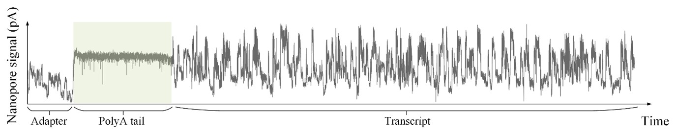
The normalization remains robust with variable poly(A) tail lengths, as long as the poly(A) region is sufficiently long. The linker sequence will be assigned to the adapter part rather than the poly(A) part.

To improve clarity in the revised manuscript, we have added the following explanation:

“Due to inherent variability between nanopores in the sequencing device, the baseline levels and standard deviations of k-mer signals can differ across reads, even for the same transcript. To standardize the signal for downstream analyses, we extract the raw current signal segments corresponding to the poly(A) tail of each read. Since the poly(A) tail provides a stable reference, we normalize the raw current signals across reads, ensuring that the mean and standard deviation of the poly(A) tail are consistent across all reads. This step is crucial for reducing…..”

We chose to use the poly(A) tail for normalization because it is sequence-invariant—i.e., all poly(A) tails consist of identical k-mers, unlike transcript sequences which vary in composition. In contrast, using the transcript region for normalization can introduce biases: for instance, reads with more diverse k-mers (having inherently broader signal distributions) would be forced to match the variance of reads with more uniform k-mers, potentially distorting the baseline across k-mers.

Page 7, 5mer parameter table: r9.4_180mv_70bps_5mer_RNA is an older kmer model (>2 years). How does your method perform with the newer RNA kmer models that do permit the detection of multiple ribonucleotide modifications? Addressing this comment is crucial because it is feasible that SegPore will underperform in comparison to the newer RNA base caller models (requiring the use of RNA004 datasets).

Thank you for highlighting this important point. For RNA004, we have updated SegPore to ensure compatibility with the latest kit. In our revised manuscript, we demonstrate that the translocation-based segmentation hypothesis remains valid for RNA004, as supported by new analyses presented in the supplementary Figure S4.

Additionally, we performed a new benchmark with f5c and Uncalled4 in RNA004 data in the revised manuscript (Table 2), where SegPore exhibit a better performance than f5c and Uncalled4.

We agree that benchmarking against the latest Dorado models—specifically rna004_130bps_hac@v5.1.0 and rna004_130bps_sup@v5.1.0, which include built-in modification detection capabilities—would provide valuable context for evaluating the utility of SegPore. However, generating a comprehensive k-mer parameter table for RNA004 requires a large, well-characterized dataset. At present, such data are limited in the public domain. Additionally, Dorado is developed by ONT and its internal training data have not been released, making direct comparisons difficult.

Our current focus is on improving raw signal segmentation quality, which are upstream tasks critical to many downstream analyses, including RNA modification detection. Future work may include benchmarking SegPore against models like Dorado once appropriate data become available.

The Methods and Results sections contain redundant information - please streamline the information in these sections and reduce the redundancy. For example, the benchmarking section may be better situated in the Results section.

Following your advice, we have removed redundant texts about the Segmentation benchmark from Materials and Methods in the revised manuscript.

Minor comments

(1) Introduction

Page 3: "By incorporating these dynamics into its segmentation algorithm...". Please provide an example of how motor protein dynamics can impact RNA translocation. In particular, please elaborate on why motor protein dynamics would impact the translocation of modified ribonucleotides differently to canonical ribonucleotides. This is provided in the results, but please also include details in the Introduction.

Following your advice, we added one sentence to explain how the motor protein affect the translocation of the DNA/RNA molecule in the revised manuscript.

“This observation is also supported by previous reports, in which the helicase (the motor protein) translocates the DNA strand through the nanopore in a back-and-forth manner. Depending on ATP or ADP binding, the motor protein may translocate the DNA/RNA forward or backward by 0.5-1 nucleotides.”

As far as we understand, this translocation mechanism is not specific to modified or unmodified nucleotides. For further details, we refer the reviewer to the original studies cited.

Page 3: "This lack of interpretability can be problematic when applying these methods to new datasets, as researchers may struggle to trust the predictions without a clear understanding of how the results were generated." Please provide details and citations as to why researchers would struggle to trust the predictions of m6Anet. Is it due to a lack of understanding of how the method works, or an empirically demonstrated lack of reliability?

Thank you for pointing this out. The lack of interpretability in deep learning models such as m6Anet stems primarily from their “black-box” nature—they provide binary predictions (modified or unmodified) without offering clear reasoning or evidence for each call.

When we examined the corresponding raw signals, we found it difficult to visually distinguish whether a signal segment originated from a modified or unmodified ribonucleotide. The difference is often too subtle to be judged reliably by a human observer. This is illustrated in the newly added Supplementary Figure S5, which shows Nanopolish-aligned raw signals for the central 5mer GGACT in Figure 4B, displayed both uncolored and colored by modification state (according to the ground truth).

Although deep neural networks can learn subtle, high-dimensional patterns in the signal that may not be readily interpretable, this opacity makes it difficult for researchers to trust the predictions—especially in new datasets where no ground truth is available. The issue is not necessarily an empirically demonstrated lack of reliability, but rather a lack of transparency and interpretability.

We have updated the manuscript accordingly and included Supplementary Figure S5 to illustrate the difficulty in interpreting signal differences between modified and unmodified states.

Page 3: "Instead of relying on complex, opaque features...". Please provide evidence that the research community finds the figures generated by m6Anet to be difficult to interpret, or delete the sections relating to its perceived lack of usability.

See the figure provided in the response to the previous point. We added a reference to this figure in the revised manuscript.

“Instead of relying on complex, opaque features (see Supplementary Figure S5), SegPore leverages baseline current levels to distinguish between…..”

(2) Materials and Methods

Page 5, Preprocessing: "We begin by performing basecalling on the input fast5 file using Guppy, which converts the raw signal data into base sequences.". Please change "base" to ribonucleotide.

Revised as requested.

Page 5 and throughout, please refer to poly(A) tail, rather than polyA tail throughout.

Revised as requested.

Page 5, Signal segmentation via hierarchical Hidden Markov model: "...providing more precise estimates of the mean and variance for each base block, which are crucial for downstream analyses such as RNA modification prediction." Please specify which method your HHMM method improves upon.

Thank you for the suggestion. Since this section does not include a direct comparison, we revised the sentence to avoid unsupported claims. The updated sentence now reads:

"...providing more precise estimates of the mean and variance for each base block, which are crucial for downstream analyses such as RNA modification prediction."

Page 10, GMM for 5mer parameter table re-estimation: "Typically, the process is repeated three to five times until the 5mer parameter table stabilizes." How is the stabilisation of the 5mer parameter table quantified? What is a reasonable cut-off that would demonstrate adequate stabilisation of the 5mer parameter table?

Thank you for the comment. We assess the stabilization of the 5mer parameter table by monitoring the change in baseline values across iterations. If the absolute change in baseline values for all 5mers is less than 1e-5 between two consecutive iterations, we consider the estimation to have stabilized.

Page 11, M6A site level benchmark: why were these datasets selected? Specifically, why compare human and mouse ribonuclotide modification profiles? Please provide a justification and a brief description of the experiments that these data were derived from, and why they are appropriate for benchmarking SegPore.

Thank you for the comment. These data are taken from a previous benchmark studie about m6A estimation from RNA002 data in the literature (https://doi.org/10.1038/s41467-023-37596-5). We think the data are appropreciate here.

Thank you for the comment. The datasets used were taken from a previous benchmark study on m6A estimation using RNA002 data (https://doi.org/10.1038/s41467-023-37596-5). These datasets include human and mouse transcriptomes and have been widely used to evaluate the performance of RNA modification detection tools. We selected them because (i) they are based on RNA002 chemistry, which matches the primary focus of our study, and (ii) they provide a well-characterized and consistent benchmark for assessing m6A detection performance. Therefore, we believe they are appropriate for validating SegPore.

(3) Results

Page 13, RNA translocation hypothesis: "The raw current signals, as shown in Fig. 1B...". Please check/correct figure reference - Figure 1B does not show raw current signals.

Thank you for pointing this out. The correct reference should be Figure 2B. We have updated the figure citation accordingly in the revised manuscript.

Page 19, m6A identification at the site level: "For six selected m6A motifs, SegPore achieved an ROC AUC of 82.7% and a PR AUC of 38.7%, earning the third best performance compared with deep leaning methods m6Anet and CHEUI (Fig. 3D)." SegPore performs third best of all deep learning methods. Do the authors recommend its use in conjunction with m6Anet for m6A detection? Please clarify in the text.

This sentence aims to convey that SegPore alone can already achieve good performance. If interpretability is the primary goal, we recommend using SegPore on its own. However, if the objective is to identify more potential m6A sites, we suggest using the combined approach of SegPore and m6Anet. That said, we have chosen not to make explicit recommendations in the main text to avoid oversimplifying the decision or potentially misleading readers.

Page 19, m6A identification at the single molecule level: "one transcribed with m6A and the other with normal adenosine". I assume that this should be adenine? Please replace adenosine with adenine throughout.

Thank you for pointing this out. We have revised the sentence to use "adenine" where appropriate. In other instances, we retain "adenosine" when referring specifically to adenine bound to a ribose sugar, which we believe is suitable in those contexts.

Page 19, m6A identification at the single molecule level: "We used 60% of the data for training and 40% for testing". How many reads were used for training and how many for testing? Please comment on why these are appropriate sizes for training and testing datasets.

In total, there are 1.9 million reads, with 1.14 million used for training and 0.76 million  for testing (60% and 40%, respectively). We chose this split to ensure that the training set is sufficiently large to reliably estimate model parameters, while the test set remains substantial enough to robustly evaluate model performance. Although the ratio was selected somewhat arbitrarily, it balances the need for effective training with rigorous validation.

(4) Discussion

Page 21: "We believe that the de-noised current signals will be beneficial for other downstream tasks." Which tasks? Please list an example.

We have revised the text for clarity as follows:

“We believe that the de-noised current signals will be beneficial for other downstream tasks, such as the estimation of m5C, pseudouridine, and other RNA modifications.”

Page 22: "One can generally observe a clear difference in the intensity levels between 5mers with a m6A and normal adenosine, which is easier for human to interpret if a predicted m6A site is real." This statement is vague and requires qualification. Please reference a study that demonstrates the human ability to interpret two similar graphs, and demonstrate how it relates to the differences observed in your data.

We apologize for the confusion. We have revised the sentence as follows:

“One can generally observe a clear difference in the intensity levels between 5mers with an m6A and those with a normal adenosine, which makes it easier for a researcher to interpret whether a predicted m6A site is genuine.”

We believe that Figures 3A, 3B, and 4B effectively illustrate this concept.

Page 23: How long does SegPore take for its analyses compared to other similar tools? How long would it take to analyse a typical dataset?

We have added run-time statistics for datasets of varying sizes in the revised manuscript (see Supplementary Figure S6). This figure illustrates SegPore’s performance across different data volumes to help estimate typical processing times.

(5) Figures

Figure 4C. Please number the hierachical clusters and genomic locations in this figure. They are referenced in the text.

Following your suggestion, we have labeled the hierarchical clusters and genomic locations in Figure 4C in the revised manuscript.

In addition, we revised the corresponding sentence in the main text as follows: “Biclustering reveals that modifications at g6 are specific to cluster C4, g7 to cluster C5, and g8 to cluster C6, while the first five genomic locations (g1 to g5) show similar modification patterns across all reads.”

We are in chapter 3.7.

DOI: 10.1016/j.xpro.2025.104131

Resource: (MBL International Cat# M059-3, RRID:AB_590721)

Curator: @scibot

SciCrunch record: RRID:AB_590721

What is this?

Reviewer #1 (Public review):

Summary:

The authors attempted to clarify the impact of N protein mutations on ribonucleoprotein (RNP) assembly and stability using analytical ultracentrifugation (AUC) and mass photometry (MP). These complementary approaches provide a more comprehensive understanding of the underlying processes. Both SV-AUC and MP results consistently showed enhanced RNP assembly and stability due to N protein mutations.

The overall research design appears well planned, and the experiments were carefully executed.

Strengths:

SV-AUC, performed at higher concentrations (3 µM), captured the hydrodynamic properties of bulk assembled complexes, while MP provided crucial information on dissociation rates and complex lifetimes at nanomolar concentrations. Together, the methods offered detailed insights into association states and dissociation kinetics across a broad concentration range. This represents a thorough application of solution physicochemistry.

Weaknesses:

Unlike AUC, MP observes only a part of the solution. In MP, bound molecules are accumulated on the glass surface (not dissociated), thus the concentration in solution should change as time develops. How does such concentration change impact the result shown here?

Reviewer #3 (Public review):

Summary:

This manuscript investigates how mutations in the SARS-CoV-2 nucleocapsid protein (N) alter ribonucleoprotein (RNP) assembly, stability, and viral fitness. The authors focus on mutations such as P13L, G214C, and G215C, combining biophysical assays (SV-AUC, mass photometry, CD spectroscopy, EM), VLP formation, and reverse genetics. They propose that SARS-CoV-2 exploits "fuzzy complex" principles, where distributed weak interfaces in disordered regions allow both stability and plasticity, with measurable consequences for viral replication.

Strengths:

(1) The paper demonstrates a comprehensive integration of structural biophysics, peptide/protein assays, VLP systems, and reverse genetics.

(2) Identification of both de novo (P13L) and stabilizing (G214C/G215C) interfaces provides a mechanistic insight into RNP formation.

(3) Strong application of the "fuzzy complex" framework to viral assembly, showing how weak/disordered interactions support evolvability, is a significant conceptual advance in viral capsid assembly.

(4) Overall, the study provides a mechanistic context for mutations that have arisen in major SARS-CoV-2 variants (Omicron, Delta, Lambda) and a mechanistic basis for how mutations influence phenotype via altered biomolecular interactions.

Weaknesses:

(1) The arrangement of N dimers around LRS helices is presented in Figure 1C, but the text concedes that "the arrangement sketched in Figure 1C is not unique" (lines 144-146) and that AF3 modeling attempts yielded "only inconsistent results" (line 149).<br /> The authors should therefore present the models more cautiously as hypotheses instead. Additional alternative arrangements should be included in the Supplementary Information, so the readers do not over-interpret a single schematic model.

(2) Negative-stained EM fibrils (Figure 2A) and CD spectra (Figure 2B) are presented to argue that P13L promotes β-sheet self-association. However, the claim could benefit from more orthogonal validation of β-sheet self-association. Additional confirmation via FTIR spectra or ThT fluorescence could be used to further distinguish structured β-sheets from amorphous aggregation.

(3) In the main text, the authors alternate between emphasizing non-covalent effects ("a major effect of the cysteines already arises in reduced conditions without any covalent bonds," line 576) and highlighting "oxidized tetrameric N-proteins of N:G214C and N:G215C can be incorporated into RNPs". Therefore, the biological relevance of disulfide redox chemistry in viral assembly in vivo remains unclear. Discussing cellular redox plausibility and whether the authors' oxidizing conditions are meant as a mechanistic stress test rather than physiological mimicry could improve the interpretation of these results.

The paper could benefit if the authors provide a summary figure or table contrasting reduced vs. oxidized conditions for G214C/G215C mutants (self-association, oligomerization state, RNP stability). Explicitly discuss whether disulfides are likely to form in infected cells.

(4) VLP assays (Figure 7) show little enhancement for P13L or G215C alone, whereas Figure 8 shows that P13L provides clear fitness advantages. This discrepancy is acknowledged but not reconciled with any mechanistic or systematic rationale. The authors should consider emphasizing the limitations of VLP assays and the sources of the discrepancy with respect to Figure 8.

(5) Figures 5 and 6 are dense, and the several overlays make it hard to read. The authors should consider picking the most extreme results to make a point in the main Figure 5 and move the other overlays to the Supplementary. Additionally, annotating MP peaks directly with "2×, 4×, 6× subunits" can help non-experts.

(6) The paper has several names and shorthand notations for the mutants, making it hard to keep up. The authors could include a table that contains mutation keys, with each shorthand (Ancestral, Nο/No, Nλ, etc.) mapped onto exact N mutations (P13L, Δ31-33, R203K/G204R, G214C/G215C, etc.). They could then use the same glyphs (Latin vs Greek) consistently in text and figure labels.

(7) The EM fibrils (Figure 2A) and CD spectra (Figure 2B) were collected at mM peptide concentrations. These are far above physiological levels and may encourage non-specific aggregation. Similarly, the authors mention" ultra-weak binding energies that require mM concentrations to significantly populate oligomers". On the other hand, the experiments with full-length protein were performed at concentrations closer to biologically relevant concentrations in the micromolar range. While I appreciate the need to work at high concentrations to detect weak interactions, this raises questions about physiological relevance. Specifically:

a) Could some of the fibril/β-sheet features attributed to P13L (Figure 2A-C) reflect non-specific aggregation at high concentrations rather than bona fide self-association motifs that could play out in biologically relevant scenarios?

b) How do the authors justify extrapolating from the mM-range peptide behaviors to the crowded but far lower effective concentrations in cells?

The authors should consider adding a dedicated section (either in Methods or Discussion) justifying the use of high concentrations, with estimation of local concentrations in RNPs and how they compare to the in vitro ranges used here. For concentration-dependent phenomena discussed here, it is vital to ensure that the findings are not artefacts of non-physiological peptide aggregation..

Author response:

We thank the Reviewers and Editors for their time and insightful comments. We are encouraged by their positive assessment and we look forward to addressing the points raised. Areas of primary concern include (1) the use of high concentrations in peptide experiments; (2) improvement of the presentation and discussion of the results; and (3) clarification of the impact of surface adsorption on the mass photometry analyses.

Regarding (1), we will better explain why some experiments with isolated disordered N-terminal extension were necessarily carried out at high concentrations, in order to demonstrate the potential for these peptides to weakly self-associate. While much lower nucleocapsid protein concentrations are present in the cytosol on average, and are used in our ribonucleoprotein assembly experiments, there are two important physiologically relevant cases where high local concentrations do occur: First, high effective concentrations of tethered disordered N-terminal extensions exist locally in the volume sampled by individual ribonucleoprotein complexes, and, second, high nucleocapsid concentrations are prevalent in its macromolecular condensates. Thus, weak interactions of N-terminal extensions can play a critical role strengthening fuzzy ribonucleoprotein complexes and also altering condensate properties, both of which were confirmed in our experiments. Nonetheless, we do not expect the observed fibrillar state of the concentrated isolated N-terminal peptide to be physiologically relevant, since physiologically they will always remain tethered to the full-length protein impeding fibrillar superstructures.

(2) We are grateful for the Reviewers’ suggestions to enhance the clarity and accessibility of our findings and to streamline the presentation. We intend to tighten up the text and improve figures throughout, and add discussion points, as proposed.

(3) We plan to add an analysis of the extent that irreversible surface adsorption decreases solute concentration in mass photometry, and discuss why this has negligible impact on the conclusions drawn under our experimental conditions.In summary, we agree these points all provide opportunities to strengthen the manuscript further and we are glad to revise our manuscript accordingly.

Author response:

The following is the authors’ response to the original reviews

Recommendations for the Authors:

Reviewer #1:

We think that this manuscript brings an important contribution that will be of interest in the areas of statistical physicists, (microbiota) ecology, and (biological) data science. The evidence of their results is solid and the work improves the state-of-the-art in terms of methods. We have a few concerns that, in our opinion, the authors should address.

Major concerns:

(1) While the paper could be of interest for the broad audience of e-Life, the way it is written is accessible mainly to physicists. We encourage the authors to take the broad audience into account by i) explaining better the essence of what is being done at each step, ii) highlighting the relevance of the method compared to other methods, iii) discussing the ecological implications of the results.

Examples on how to approach i) include: Modify or expand Figure 1 so that non-familiar readers can understand the summary of the work (e.g. with cartoons representing communities, diseased states and bacterial interactions and their relationship with the inference method); in each section, summarize at the beginning the purpose of what is going to be addressed in this section, and summarize at the end what the section has achieved; in Figure 2, replace symbols by their meaning as much as possible-the same for Figure 1, at the very least in the figure caption.

Example on how to approach ii): Since the authors aim to establish a bridge between disordered systems and microbiome ecology, it could be useful to expand a bit the introduction on disordered systems for biologists/biophysicists. This could be done with an additional text box, which could also highlight the advantages of this approach in comparison to other techniques (e.g. model-free approaches can also classify healthy and diseased states).

Example on how to approach iii): The authors could discuss with more depth the ecological implications of their results. For example, do they have a hypothesis on why demographic and neutral effects could dominate in healthy patients?

We thank the reviewer for the observations. Following the suggestion in the revised version, each section outlines the goal of what will be addressed in that section, and summarizes what we have achieved at the end; We also updated Figure 1 and Figure 2.

(i) For figure 1, we expanded and hopefully made more clear how we conceptualize the problem, use the data, andestablish our method. In Figure 2, we enriched the y labels of each panel with the name associated with the order parameter.

(ii) We thank the reviewer for helping us improve the readability of the introductory part, thus providing moreinsights into disordered systems techniques for a broader audience. We have added a few explanations at the end of page 2 – to explain the advantages of such methodology compared to other strategies and models.

(iii) We thank the reviewer for raising the need for a more in-depth ecological discussion of our results. A simple wayto understand why neutral effects may dominate in healthy patients is the following. Neutrality implies that species differences are mainly shaped by stochastic processes such as demographic noise, with species treated as different realizations of the same underlying stochastic ecological dynamics. In our analysis, we observe that healthy individuals tend to exhibit highly similar microbial communities, suggesting that the compositional variability among their microbiomes is compatible—at least in part—with the fluctuations expected from demographic stochasticity alone. In contrast, patients with the disease display significantly more heterogeneous microbial compositions. The diversity and structure of their gut communities cannot be satisfactorily explained by neutral demographic fluctuations alone.

This discrepancy implies that additional deterministic forces—such as altered ecological interactions—are driving the divergence observed in dysbiotic states. In diseased individuals, the breakdown of such interactions leads to a structurally distinct regime that may correspond to a phase of marginal stability, as indicated by our theoretical modeling. This shift marks a transition from a community governed by neutrality and demographic noise to one dominated by non-neutral ecological forces (as depicted in Figure 4). We added these comments in the discussion section of the revised manuscript.

(2) Taking into account the broader audience, we invite the authors to edit the abstract, as it seems to jump from one ecological concept to another without explicitly communicating what is the link between these concepts. From the first two sentences, the motivation seems to be species diversity, but no mention of diversity comes after the second sentence. There is no proper introduction/definition of what macroecological states are. After that, the authors switch to healthy and unhealthy states, without previously introducing any link between gut microbiota states and the host’s health (which perhaps could be good in the first or second sentence, although other framings can be as valid). After that, interactions appear in the text and are related to instability, but the reader might not know whether this is surprising or if healthy/unhealthy states are generally related to stability.

We pointed out a few examples, but the authors could extend their revision on i), ii) and iii) beyond such specific comments. In our opinion, this would really benefit the paper.

In response to the reviewer’s concern about conceptual clarity and structure, we substantially revised the abstract to improve its accessibility and logical flow. In the revised abstract, we now clearly link species diversity to microbiome structure and function from the outset, addressing initial confusion. We provide a concise definition of ”macroecological states,” framing them as reproducible statistical patterns reflecting community-level properties. Additionally, the revised version explicitly connects gut microbiome states to host health earlier, resolving the previous abrupt shift in focus. Finally, we conclude by highlighting how disordered systems theory advances our understanding of microbiome stability and functioning, reinforcing the novelty and broader significance of our approach. Overall, the revised abstract better serves a broad interdisciplinary audience, including readers unfamiliar with the technicalities of disordered systems or microbial ecology, while preserving the scientific depth and accuracy of our work

(3) The connection with consumer-resource (CR) models is quite unusual. In Equation (12), why do the authors assume that the consumption term does not depend on R? This should be addressed, since this term is usually dependent on R in microbial ecology models.

In case this is helpful, it is known that the symmetric Lotka-Volterra model emerges from time-scale separation in the MacArthur model, where resources reproduce logistically and are consumed by other species (e.g., plants eaten by herbivores). Consumer-resource models form a broad category, while the MacArthur model is a specific case featuring logistic resource growth. For microbes, a more meaningful justification of the generalized Lotka-Volterra (GLV) model from a consumer-resource perspective involves the consumer-resource dynamics in a chemostat, where time-scale separation is assumed and higher-order interactions are neglected. See, for example: a) The classic paper by MacArthur: R. MacArthur. Species packing and competitive equilibrium for many species. Theoretical Population Biology, 1(1):1-11, 1970. b) Recent works on time-scale separation in chemostat consumer-resource models: Anna Posfai et al., PRL, 2017 Sireci et al., PNAS, 2023 Akshit Goyal et al., PRX-Life, 2025

We thank the reviewer for the observation. We apologize for the typo that appeared in the main text and that we promptly corrected. The Consumers-Resources model we had in mind is the classical case proposed by MacArthur, where resources are self-regulated according to a logistic growth mechanism, which leads to the generalized LotkaVolterra model we employ in our work.

Minor concerns:

(1) The title has a nice pun for statistical physicists, but we wonder if it can be a bit confusing for the broader audience of e-Life. Although we leave this to the author’s decision, we’d recommend considering changing the title, making it more explicit in communicating the main contribution/result of the work.

Following the reviewer’s suggestion, we have introduced an explanatory subtitle: “Linking Species Interactions to Dysbiosis through a Disordered Lotka-Volterra Framework”.

(2) Review the references - some preprints might have already been published: Pasqualini J. 2023, Sireci 2022, Wu 2021.

We thank the reviewer for pointing our attention to this inaccuracy. We updated the references to Pasqualini and Sireci papers. To our knowledge, Wu’s paper has appeared as an arXiv preprint only.

(3) Species do not generally exhibit identical carrying capacities (see Grilli, Nat. Commun., 2020; some taxa are generally more abundant than others. The authors could discuss whether the model, with the inferred parameters, can accurately reproduce the distribution of species’ mean abundances.

We thank the reviewer for this insightful comment. As discussed in the revised manuscript (lines 294–299), our current model does not accurately reproduce the empirical species abundance distribution (SAD). This limitation stems from the assumption of constant carrying capacities across species. While empirical observations (e.g., Grilli et al., Nat. Commun., 2020 [1]) show heterogeneous mean abundances often following power-law or log-normal distributions. However, our model assumes constant carrying capacity, resulting in SADs devoid of fat tails, which diverge from empirical data.

This simplification is implemented to maintain the analytical tractability of the disordered generalized Lotka-Volterra (dGLV) framework, a common approach also found in prior works such as Bunin (2017) and Barbier et al. (2018) [2, 3]. Introducing heterogeneity in carrying capacities, such as drawing them from a log-normal distribution, or switching to multiplicative (rather than demographic) noise, could indeed produce SADs that better align with empirical data. Nevertheless, implementing changes would significantly complicate the analytical treatment.

We acknowledge these directions as promising avenues for future research. They could help enhance the empirical realism of the model and its capacity to capture observed macroecological patterns while posing new theoretical challenges for disordered systems analysis

(4) A substantial number of cited works (Grilli, Nat. Commun., 2020; Zaoli & Grilli, Science Advances, 2021; Sireci et al., PNAS, 2023; Po-Yi Ho et al., eLife, 2022) suggest that environmental fluctuations play a crucial role in shaping microbiome composition and dynamics. Is the authors’ analysis consistent with this perspective? Do they expect their conclusions to remain robust if environmental fluctuations are introduced?

We thank the reviewer for stressing this point. The introduction of environmental fluctuations in the model formally violates detailed balance, thereby preventing the definition of an energy function. To date, no study has integrated random interactions together with both demographic and environmental noise within a unified analytical framework. This is certainly a highly promising direction that some of the authors are already exploring. However, given the inherently out-of-equilibrium nature of the system and the absence of a free energy, we would need to adopt a Dynamical Mean-Field Theory formalism and eventually analyze the corresponding stationary equations to be solved self-consistently. We added, however, a brief note in the Discussion section.

(5) The term “order parameters“ may not be intuitive for a biological audience. In any case, the authors should explicitly define each order parameter when first introduced.

We thank the reviewer for the comment. We introduced the names of the order parameters as soon as they are introduced, along with a brief explanation of their meaning that may be accessible to an audience with biological background.

(6) Line 242: Should ψU be ψD?

We thank the reviewer for the observation. We corrected the typo.

(7) Given that the authors are discussing healthy and diseased states and to avoid confusion, the authors could perhaps use another word for ’pathological’ when they refer to dynamical regimes (e.g., in Appendix 2: ’letting the system enter the pathological regime of unbounded growth’).

We thank the reviewer for the helpful comment. As suggested, we used the term “unphysical” instead of “pathological” where needed.

Reviewer #2:

(1) A technical point that I could not understand is how the authors deal with compositional data. One reason for my confusion is that the order parameters h and q0 are fixed n data to 1/S and 1/S2, and thus I do not see how they can be informative. Same for carrying capacity, why is it not 1 if considering relative abundance?

We thank the reviewer for raising this point. We acknowledge that the treatment of compositional data and the interpretation of order parameters h and q0 were not sufficiently clarified in the manuscript. Additionally, there was an imprecision in the text regarding the interpretation of these parameters.

As defined in revised Eq. (4) of the manuscript, h and q0 are to be averaged over the entire dataset, summing across samples α. Specifically, and , where S_α is the number of species present in sample α and is the average over samples. These parameters are therefore informative, as they encapsulate sample-level ecological diversity, and their variation reflects biological differences between healthy and diseased states. For instance, Pasqualini et al., 2024 [4] reported significant differences in these metrics between health conditions, thereby supporting their ecological relevance.

Regarding carrying capacities, we clarify that although we work with relative abundance data (i.e., compositional data), we do not fix the carrying capacity K to 1. Instead, we set K to the maximum value of xi (relative abundance) within each sample, to preserve compatibility with empirical data and allow for coexistence. While this remains a modeling assumption, it ensures better ecological realism within the constraints of the disordered GLV framework.

(2) Obviously I’m missing something, so it would be nice to clarify in simple terms the logic of the argument. I understand that Lagrange multipliers are going to be used in the model analysis, and there are a lot of technical arguments presented in the paper, but I would like a much more intuitive explanation about the way the data can be used to infer order parameters if those are fixed by definition in compositional data.

We thank the reviewer for the observation. The order parameters can be measured directly from the data, even in the presence of compositionality, as explained above. We can connect those parameters with the theory even for compositional data, because the only effect of adding the compositionality constraint is to shift the linear coefficient in the Hamiltonian, which corresponds to shifting the average interaction µ. However, the resulting phase diagram is mostly affected by the variance of the interactions σ2 (as µ is such that we are in the bounded phase).

(3) Another point that I did not understand comes from the fact that the authors claim that interaction variance is smaller in unhealthy microbiomes. Yet they also find that those are closer to instability, and are more driven by niche processes. I would have expected the opposite to be true, more variance in the interactions leading to instability (as in May’s original paper for instance). Is this apparent paradox explained by covariations in demographic stochasticity (T) and immigration rate (lambda)? If so, I think it would be very useful to comment on that.

As Altieri and coworkers showed in their PRL (2021) [5], the phase diagram of our model differs fundamentally from that of Biroli et al. (2018) [6]. In the latter, the intuitive rule – greater interaction variance yields greater instability – indeed holds. For the sake of clarity, we have attached below the resulting phase diagram obtained by Altieri et al.

The apparent paradox arises because the two phase diagrams are tuned by different parameters. Consequently, even at low temperature and with weak interaction variance, our system may sit nearer to the replica-symmetrybreaking (RSB) line.

Fig. 3 in the main text it is not a (σ,T) phase diagram where all other parameters are kept constant. Rather, it is a plot of the inferred σ and T parameters from the data (without showing the corresponding µ).

To capture the full, non-trivial influence of all parameters on stability, we studied the so-called “replicon eigenvalue” in the RS (i.e. single equilibrium) approximation. This leading eigenvalue measures how close a given set of inferred parameters – and hence a microbiome – is to the RSB threshold. For a visual representation of these findings, refer to Figure 4.

Author response image 1.

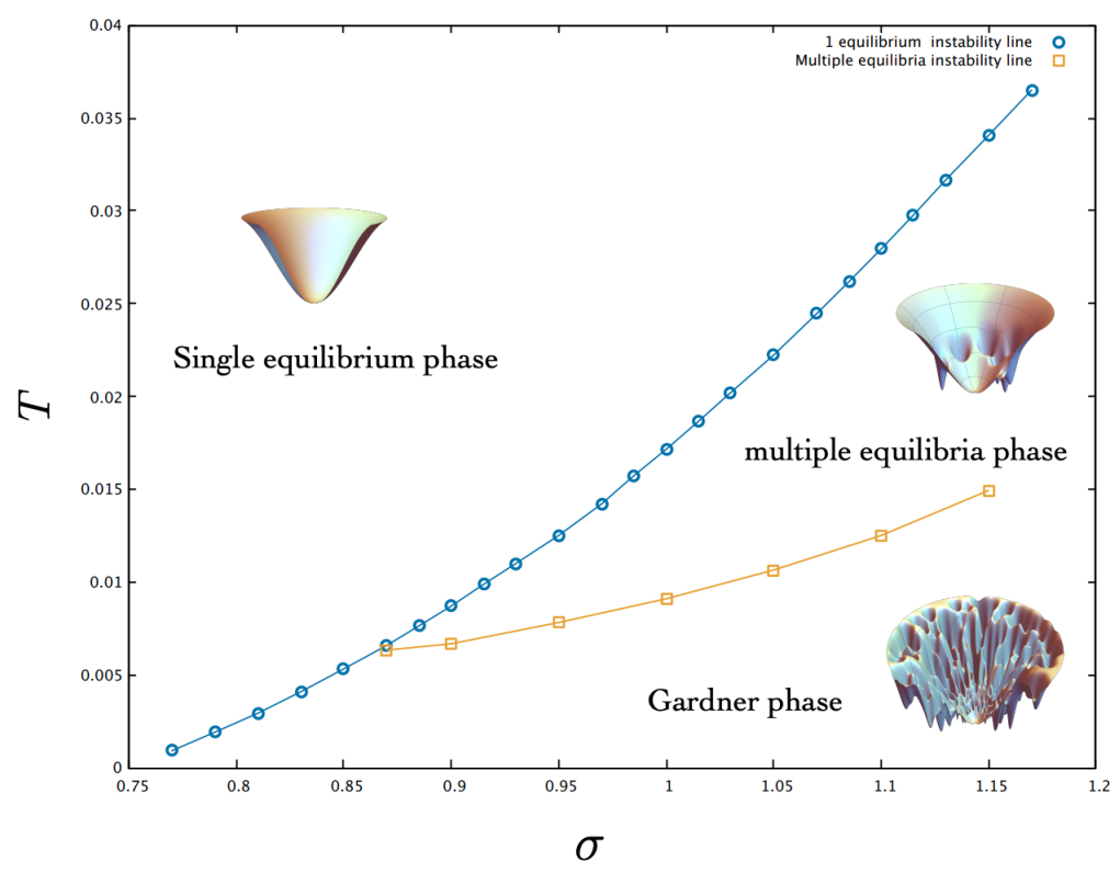
(4) What do the empirical SAD look like? It would be nice to see the actual data and how the theoretical SADs compare.

The empirical species abundance distributions (SADs) analyzed in our study are presented and discussed in detail in Pasqualini et al., 2024 [4]. Given the overlap in content, we chose not to reproduce these figures in the current manuscript to avoid redundancy.

As we also clarify in the revised text, the theoretical SAD is derived from the disordered generalized Lotka-Volterra (dGLV) model in the unique fixed point phase typically exhibit exponential tails. These distributions do not match the heavier-tailed patterns (e.g., log-normal or power-law-like) observed in empirical microbiome data. This discrepancy stems from the simplifying assumptions of the dGLV framework, including the use of constant carrying capacities and demographic noise.

In the revised manuscript, we have added a brief discussion in the revised manuscript to explicitly acknowledge this limitation and emphasize it as a direction for future refinement of the model, such as incorporating heterogeneous carrying capacities or exploring alternative noise structures.

(5) Some typos: often “niche” is written “nice”.

We thank the reviewer for this suggestion. After inspecting the text, we corrected the reported typos.

Reviewer #3:

Major comments:

(1) In the S3 text, the authors say that filtered metagenomic reads were processed using the software Kaiju. The description of the pipeline does not mention how core genes were selected, which is often a crucial step in determining the abundance of a species in a metagenomic sample. In addition, the senior author of this manuscript has published a version of Kaiju that leverages marker genes classification methods (deemed Core-Kaiju), but it was not used for either this manuscript or Pasqualini et al. (2014; Tovo et al., 2020). I am not suggesting that the data necessarily needs to be reprocessed, but it would be useful to know how core genes were chosen in Pasqualini et al. and why Core-Kaiju was not used (2014).

Prior to the current manuscript and the PLOS Computational Biology paper by Pasqualini et al. [4], we applied the core-Kaiju protocol to the same dataset used in both studies. However, this tool was originally developed and validated using general catalogs of culturable organisms, not specifically tuned for gut microbiomes. As a result, we have realized that in many samples Core Kajiu would filter only very few species (in some samples, the number of identified species was as low as 5–10), undermining the reliability of the analysis. Due to these limitations, we opted to use the standard Kaiju version in our work. We are actively developing an improved version of the core-Kaiju protocol that will overcome the discussed limitations and preliminary results (not shown here) indicate the robustness of the obtained patterns also in this case.

(2) My understanding of Pasqualini et al. was that diseased patients experienced larger fluctuations in abundance, while in this study, they had smaller fluctuations (Figure 3a; 2024). Is this a discrepancy between the two models or is there a more nuanced interpretation?

We thank the reviewer for the observation. This is only an apparent discrepancy, as the term fluctuation has different meanings in the two contexts. The fluctuations referred to by the reviewer correspond to a parameter of our theory—namely, noise in the interactions. Conversely, in Pasqualini et al. σ indicates environmental fluctuations. Nevertheless, there is no conceptual discrepancy in our results: in both studies, unhealthy microbiomes were found to be less stable. In fact, also in this study, notably Fig. 4, shows that unhealthy microbiomes lie closer to the RSB line, a phenomenon that is also associated with enhanced fluctuations.

(3) Line 38-41: It would be helpful to explicitly state what “interaction patterns” are being referenced here. The final sentence could also be clarified. Do microbiomes “host“ interactions or are they better described as a property (“have”, “harbor”). The word “host” may confuse some readers since it is often used to refer to the human host. I am also not sure what point is being made by “expected to govern natural ones”. There are interactions between members of a microbiome; experimental studies have characterized some of these interactions, which we expect to relate in some way to interactions in nature. Is this what the authors are saying?

Thanks. We agree that this sentence was not clear. Indeed, we are referring to pairwise species interactions and not to host-microbiome interactions. We have rewritten this part in the following way: In fact, recent work shows that the network-level properties of species-species interactions —for example, the sign balance, average strength, and connectivity of the inferred interaction matrix— shift systematically between healthy and dysbiotic gut communities (see for instance, [7, 8]). Pairwise species interactions have been quantified in simplified in-vitro consortia [9, 10]; we assume that the same classes of interactions also operate—albeit in a more complex form—in the native gut microbiome.

(4) Line 43: I appreciate that the authors separated neutral vs. logistic models here.

(5) Lines 51-75: The framing here is well-written and convincing. Network inference is an ongoing, active subject in ecology, and there is an unfortunate focus on inferring every individual interaction because ecologists with biology backgrounds are not trained to think about the problem in the language of statistical physics.

We thank the reviewer for these positive comments.

(6) Line 87: Perhaps I’m missing something obvious, but I don’t see how ρi sets the intrinsic timescale of the dynamics when its units are 1/(time*individuals), assuming the dimensions of ri are inverse time.

We thank the reviewer for the observation. We corrected this phrase in the main text.

(7) Lines 189-190: “as close as possible to the data” it would aid the reader if you specified the criteria meant by this statement.

We thank the reviewer for the observation. We removed the sentence, as it introduced some redundancy in our argument. In the subsequent text, the proposed method is exposed in details.

(8) Line 198: It would aid the reader if you provided some context for what the T - σ plane represents.

We thank the referee for the helpful indication. Indeed, we have better clarified the mutual role of the demographic noise amplitude and strength of the random interaction matrix, as theoretically predicted in the PRL (2021) by Altieri and coworkers [5]. Please, find an additional paragraph on page 6 of the resubmitted version.

(9) Line 217: Specifying what is meant by “internal modes“ would aid the typical life science reader.

We thank the reviewer for the suggestion. Recognizing that referring to “internal modes” to describe the SAD shape in that context might cause confusion, we replaced “internal modes“ with “peaks”.

(10) Line 219: Some additional justification and clarification are needed here, as some may think of “m“ as being biomass.

We added a sentence to better explain this concept. “In classical and quantum field theory, the particle-particle interaction embedded in the quadratic term is typically referred to as a mass source. In the context of this study, 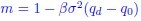captures quadratic fluctuations of species abundances, as also appearing in the expression of the leading eigenvalue of the stability matrix.”

Minor comments:

(1) I commend the authors for removing metagenomic reads that mapped to the human genome in the preprocessing stage of their pipeline. This may seem like an obvious pre-processing step, but it is unfortunately not always implemented.

We thank the referee for pointing this potential issue. The data used in this work, as well as the bioinformatic workflow used to generate them has been described in detail in Pasqualini et al., 2024 [4]. As one of the main steps for preprocessing, we remove reads mapping to the human genome.

(2) Line 13: “Bacterial“ excludes archaea, and while you may not have many high-abundance archaea in your human gut data, this sentence does not specify the human gut. Usually, this exclusion is averted via the term “microbial“, though sometimes researchers raise objections to the term when the data does not include fungal members (e.g., all 16S studies).

We thank the reviewer for this suggestion. As to include archaeal organisms, we adopt the term “microbial“ instead of “bacterial“.

(3) Line 18: This manuscript is being submitted under the “Physics of Living Systems“ tract, but it may be useful to explicitly state in the Abstract that disordered systems are a useful approach for understanding large, complex communities for the benefit of life science researchers coming from a biology background.

Thank. We have modified the abstract following this suggestion.

(4) Line 68: Consider using “adapted“ or something similar instead of “mutated“ if there is no specific reason for that word choice.

We thank the reviewer for this suggestion, which was implemented in the text.

(5) Line 111: It would be useful to define annealed and quenched for a general life science audience.

We thank the reviewer for this suggestion. In the “Results” section, we have opted for “time-dependent disordered interactions” to reach a broader audience and avoid any jargon. Moreover, in the Discussion we added a detailed footnote: “In contrast to the quenched approximation, the annealed version assumes that the random couplings are not fixed but instead fluctuate over time, with their covariance governed by independent Ornstein–Uhlenbeck processes.”

(6) Line 124: Likewise for the replicon sector.

We thank the reviewer for the suggestion. We added a footnote on page 4, after the formula, to highlight the physical intuition behind the introduction of the replicon mode.

“The replicon eigenvalue refers to a particular type of fluctuation around the saddle-point (mean-field) solution within the replica framework. When the Hessian matrix of the replicated free energy is diagonalized, fluctuations are divided into three sectors: longitudinal, anomalous, and replicon. The replicon mode is the most sensitive to criticality signaling – by its vanishing trend – the emergence of many nearly-degenerate states. It essentially describes how ‘soft’ the system is to microscopic rearrangements in configuration space.”

(7) Figure 2: It would be helpful to include y-axis labels for each order parameter alongside the mathematical notation.

We thank the reviewer for this suggestion. Now the y-axis of Figure 2 includes, along the mathmetical symbol, the label of the represented quantities.

(8) Line 242: Subscript “U” is used to denote “Unhealthy” microbiomes, but “D” is used to denote “Diseased” in Figs. 2 and 3 (perhaps elsewhere as well).

We thank the reviewer for this observation. After checking the various subscripts in the text, coherently with figure 2 and 3, we homogenized our notation, adopting the subscript “D“ for symbols related to the diseased/unhealthy condition.

(9) Line 283: “not to“ should be “not due to“

We thank the reviewer for this suggestion. After inspecting the text, we corrected the reported error.

(10) Equations 23, 34: Extra “=“ on the RHS of the first line.

We consistently follow the same formatting across all the line breaks in the equations throughout the text.

We are thus resubmitting our paper, hoping to have satisfactorily addressed all referees’ concerns.

References

(1) Jacopo Grilli. Macroecological laws describe variation and diversity in microbial communities. Nature communications, 11(1):4743, 2020.

(2) Guy Bunin. Ecological communities with lotka-volterra dynamics. Physical Review E, 95(4):042414, 2017.

(3) Matthieu Barbier, Jean-Franc¸ois Arnoldi, Guy Bunin, and Michel Loreau. Generic assembly patterns in complex ecological communities. Proceedings of the National Academy of Sciences, 115(9):2156–2161, 2018.

(4) Jacopo Pasqualini, Sonia Facchin, Andrea Rinaldo, Amos Maritan, Edoardo Savarino, and Samir Suweis. Emergent ecological patterns and modelling of gut microbiomes in health and in disease. PLOS Computational Biology, 20(9):e1012482, 2024.

(5) Ada Altieri, Felix Roy, Chiara Cammarota, and Giulio Biroli. Properties of equilibria and glassy phases of the random lotka-volterra model with demographic noise. Physical Review Letters, 126(25):258301, 2021.

(6) Giulio Biroli, Guy Bunin, and Chiara Cammarota. Marginally stable equilibria in critical ecosystems. New Journal of Physics, 20(8):083051, 2018.

(7) Amir Bashan, Travis E Gibson, Jonathan Friedman, Vincent J Carey, Scott T Weiss, Elizabeth L Hohmann, and Yang-Yu Liu. Universality of human microbial dynamics. Nature, 534(7606):259–262, 2016.

(8) Marcello Seppi, Jacopo Pasqualini, Sonia Facchin, Edoardo Vincenzo Savarino, and Samir Suweis. Emergent functional organization of gut microbiomes in health and diseases. Biomolecules, 14(1):5, 2023.

(9) Jared Kehe, Anthony Ortiz, Anthony Kulesa, Jeff Gore, Paul C Blainey, and Jonathan Friedman. Positive interactions are common among culturable bacteria. Science advances, 7(45):eabi7159, 2021.

(10) Ophelia S Venturelli, Alex V Carr, Garth Fisher, Ryan H Hsu, Rebecca Lau, Benjamin P Bowen, Susan Hromada, Trent Northen, and Adam P Arkin. Deciphering microbial interactions in synthetic human gut microbiome communities. Molecular systems biology, 14(6):e8157, 2018.

Reviewer #3 (Public review):

Summary:

I found the manuscript to be well-written. I have a few questions regarding the model, though the bulk of my comments are requests to provide definitions and additional clarity. There are concepts and approaches used in this manuscript that are clear boons for understanding the ecology of microbiomes but are rarely considered by researchers approaching the manuscript from a traditional biology background. The authors have clearly considered this in their writing of S1 and S2, so addressing these comments should be straightforward. The methods section is particularly informative and well-written, with sufficient explanations of each step of the derivation that should be informative to researchers in the microbial life sciences that are not well-versed with physics-inspired approaches to ecology dynamics.

Strengths:

The modeling efforts of this study primarily rely on a disordered for of the generalized Lotka-Volterra (gLV) model. This model can be appropriate for investigating certain systems and the authors are clear about when and how more mechanistic models (i.e., consumer-resource) can lead to gLV. Phenomenological models such as this have been found to be highly useful for investigating the ecology of microbiomes, so this modeling choice seems justified, and the limitations are laid out.

Weaknesses:

The authors use metagenomic data of diseased and healthy patients that was first processed in Pasqualini et al. (2024). The use of metagenomic data leads me into a question regarding the role of sampling effort (i.e., read counts) in shaping model parameters such as $h$. This parameter is equal to the average of 1/# species across samples because the data are compositional in nature. My understanding is that $h$ was calculated using total abundances (i.e., read counts). The number of observed species is strongly influenced by sampling effort and the authors addressed this point in their revised manuscript.

However, the role of sampling effort can depend on the type of data and my instinct about the role that sampling effort plays in species detection is primarily based on 16S data. The dependency between these two variables may be less severe for the authors' metagenomic pipeline. This potential discrepancy raises a broader issue regarding the investigation of microbial macroecological patterns and the inference of ecological parameters. Often microbial macroecology researchers rely on 16S rRNA amplicon data because that type of data is abundant and comparatively low-cost. Some in microbiology and bioinformatics are increasingly pushing researchers to choose metagenomics over 16S. Sometimes this choice is valid (discovery of new MAGs, investigate allele frequency changes within species, etc.), sometimes it is driven by the false equivalence "more data = better". The outcome though is that we have a body of more-or-less established microbial macroecological patterns which rest on 16S data and are now slowly incorporating results from metagenomics. To my knowledge there has not been a systematic evaluation of the macroecological patterns that do and do not vary by one's choice in 16S vs. metagenomics. Several of the authors in this manuscript have previously compared the MAD shape for 16S and metagenomic datasets in Pasqualini et al., but moving forward a more comprehensive study seems necessary (2024). These points were addressed by the authors in their revised manuscript.

Final review: The authors addressed all comments and I have no additional comments.

References

Pasqualini, Jacopo, et al. "Emergent ecological patterns and modelling of gut microbiomes in health and in disease." PLOS Computational Biology 20.9 (2024): e1012482.

1. No State Party shall expel, return ("refouler") or extradite a person to another State where there are substantial grounds for believing that he would be in danger of being subjected to torture.

2. For the purpose of determining whether there are such grounds, the competent authorities shall take into account all relevant considerations including, where applicable, the existence in the State concerned of a consistent pattern of gross, flagrant or mass violations of human rights.

(3) A claim for refugee protection made by a person inside Canada must be made in person to an officer, must not be made by a person who is subject to a removal order, and is governed by this Part.

95 (1) Refugee protection is conferred on a person when

(a) the person has been determined to be a Convention refugee or a person in similar circumstances under a visa application and becomes a permanent resident under the visa or a temporary resident under a temporary resident permit for protection reasons;

**(b) the Board determines the person to be a Convention refugee or a person in need of protection; or

(c) except in the case of a person described in subsection 112(3), the Minister allows an application for protection.**

Author response:

The following is the authors’ response to the original reviews.

Reviewer #1 (Public Review):

Summary:

The study explored the biomechanics of kangaroo hopping across both speed and animal size to try and explain the unique and remarkable energetics of kangaroo locomotion.

Strengths:

The study brings kangaroo locomotion biomechanics into the 21st century. It is a remarkably difficult project to accomplish. There is excellent attention to detail, supported by clear writing and figures.

Weaknesses:

The authors oversell their findings, but the mystery still persists. 

The manuscript lacks a big-picture summary with pointers to how one might resolve the big question.

General Comments

This is a very impressive tour de force by an all-star collaborative team of researchers. The study represents a tremendous leap forward (pun intended) in terms of our understanding of kangaroo locomotion. Some might wonder why such an unusual species is of much interest. But, in my opinion, the classic study by Dawson and Taylor in 1973 of kangaroos launched the modern era of running biomechanics/energetics and applies to varying degrees to all animals that use bouncing gaits (running, trotting, galloping and of course hopping). The puzzling metabolic energetics findings of Dawson & Taylor (little if any increase in metabolic power despite increasing forward speed) remain a giant unsolved problem in comparative locomotor biomechanics and energetics. It is our "dark matter problem".

Thank you for the kind words.

This study is certainly a hop towards solving the problem. But, the title of the paper overpromises and the authors present little attempt to provide an overview of the remaining big issues. 

We have modified the title to reflect this comment.  “Postural adaptations may contribute to the unique locomotor energetics seen in hopping kangaroos”

The study clearly shows that the ankle and to a lesser extent the mtp joint are where the action is. They clearly show in great detail by how much and by what means the ankle joint tendons experience increased stress at faster forward speeds.

Since these were zoo animals, direct measures were not feasible, but the conclusion that the tendons are storing and returning more elastic energy per hop at faster speeds is solid. The conclusion that net muscle work per hop changes little from slow to fast forward speeds is also solid. 

Doing less muscle work can only be good if one is trying to minimize metabolic energy consumption. However, to achieve greater tendon stresses, there must be greater muscle forces. Unless one is willing to reject the premise of the cost of generating force hypothesis, that is an important issue to confront. Further, the present data support the Kram & Dawson finding of decreased contact times at faster forward speeds. Kram & Taylor and subsequent applications of (and challenges to) their approach supports the idea that shorter contact times (tc) require recruiting more expensive muscle fibers and hence greater metabolic costs. Therefore, I think that it is incumbent on the present authors to clarify that this study has still not tied up the metabolic energetics across speed problems and placed a bow atop the package. 

Fortunately, I am confident that the impressive collective brain power that comprises this author list can craft a paragraph or two that summarizes these ideas and points out how the group is now uniquely and enviably poised to explore the problem more using a dynamic SIMM model that incorporates muscle energetics (perhaps ala' Umberger et al.). Or perhaps they have other ideas about how they can really solve the problem.

You have raised important points, thank you for this feedback. We have added a limitations and considerations section to the discussion which highlights that there are still unanswered questions. Line 311-328

Considerations and limitations

“First, we believe it is more likely that the changes in moment arms and EMA can be attributed to speed rather than body mass, given the marked changes in joint angles and ankle height observed at faster hopping speeds. However, our sample included a relatively narrow range of body masses (13.7 to 26.6 kg) compared to the potential range (up to 80 kg), limiting our ability to entirely isolate the effects of speed from those of mass. Future work should examine a broader range of body sizes. Second, kangaroos studied here only hopped at relatively slow speeds, which bounds our estimates of EMA and tendon stress to a less critical region. As such, we were unable to assess tendon stress at fast speeds, where increased forces would reduce tendon safety factors closer to failure. A different experimental or modelling approach may be needed, as kangaroos in enclosures seem unwilling to hop faster over force plates. Finally, we did not determine whether the EMA of proximal hindlimb joints (which are more difficult to track via surface motion capture markers) remained constant with speed. Although the hip and knee contribute substantially less work than the ankle joint (Fig. 4), the majority of kangaroo skeletal muscle is located around these proximal joints. A change in EMA at the hip or knee could influence a larger muscle mass than at the ankle, potentially counteracting or enhancing energy savings in the ankle extensor muscle-tendon units. Further research is needed to understand how posture and muscles throughout the whole body contribute to kangaroo energetics.”

Additionally, we added a line “Peak GRF also naturally increased with speed together with shorter ground contact durations (Fig. 2b, Suppl. Fig 1b)” (line 238) to highlight that we are not proposing that changes in EMA alone explain the full increase in tendon stress. Both GRF and EMA contribute substantially (almost equally) to stress, and we now give more equal discussion to both. For instance, we now also evaluate how much each contributes: “If peak GRF were constant but EMA changed from the average value of a slow hop to a fast hop, then stress would increase 18%, whereas if EMA remained constant and GRF varied by the same principles, then stress would only increase by 12%. Thus, changing posture and decreasing ground contact duration both appear to influence tendon stress for kangaroos, at least for the range of speeds we examined” (Line 245-249)

We have added a paragraph in the discussion acknowledging that the cost of generating force problem is not resolved by our work, concluding that “This mechanism may help explain why hopping macropods do not follow the energetic trends observed in other species (Dawson and Taylor 1973, Baudinette et al. 1992, Kram and Dawson 1998), but it does not fully resolve the cost of generating force conundrum” Line 274-276.

I have a few issues with the other half of this study (i.e. animal size effects). I would enjoy reading a new paragraph by these authors in the Discussion that considers the evolutionary origins and implications of such small safety factors. Surely, it would need to be speculative, but that's OK.

We appreciate this comment from the reviewer, however could not extend the study to discuss animal size effects because, as we now note in the results: “The range of body masses may not be sufficient to detect an effect of mass on ankle moment in addition to the effect of speed.” Line 193

Reviewer #2 (Public Review):

Summary

This is a fascinating topic that has intrigued scientists for decades. I applaud the authors for trying to tackle this enigma. In this manuscript, the authors primarily measured hopping biomechanics data from kangaroos and performed inverse dynamics. 

While these biomechanical analyses were thorough and impressively incorporated collected anatomical data and an Opensim model, I'm afraid that they did not satisfactorily address how kangaroos can hop faster and not consume more metabolic energy, unique from other animals.  Noticeably, the authors did not collect metabolic data nor did they model metabolic rates using their modelling framework. Instead, they performed a somewhat traditional inverse dynamics analysis from multiple animals hopping at a self-selected speed.

In the current study, we aimed to provide a joint-level explanation for the increases of tendon stress that are likely linked to metabolic energy consumption.

We have now included a limitations section in the manuscript (See response to Rev 1). We plan to expand upon muscle level energetics in the future with a more detailed musculoskeletal model.

Within these analyses, the authors largely focused on ankle EMA, discussing its potential importance (because it affects tendon stress, which affects tendon strain energy, which affects muscle mechanics) on the metabolic cost of hopping. However, EMA was roughly estimated (CoP was fixed to the foot, not measured) and did not detectibly associate with hopping speed (see results Yet, the authors interpret their EMA findings as though it systematically related with speed to explain their theory on how metabolic cost is unique in kangaroos vs. other animals

As noted in our methods, EMA was not calculated from a fixed centre of pressure (CoP). We did fix the medial-lateral position, owing to the fact that both feet contacted the force plate together, but the anteroposterior movement of the CoP was recorded by the force plate and thus allowed to move. We report the movement (or lack of movement) in our results. The anterior-posterior axis is the most relevant to lengthening or shortening the distance of the ‘out-lever’ R, and thereby EMA. It is necessary to assume fixed medial-lateral position because a single force trace and CoP is recorded when two feet land on the force plate. The mediallateral forces on each foot cancel out so there is no overall medial-lateral movement if the forces are symmetrical (e.g. if the kangaroo is hopping in a straight path and one foot is not in front of the other). We only used symmetrical trials so that the anterior-posterior movement of the CoP would be reliable. We have now added additional details into the text to clarify this

Indeed, the relationship between R and speed (and therefore EMA and speed) was not significant. However, the significant change in ankle height with speed, combined with no systematic change in COP at midstance, demonstrates that R would be greater at faster speeds. If we consider the nonsignificant relationship between R and speed to indicate that there is no change in R, then these two results conflict. We could not find a flaw in our methods, so instead concluded that the nonsignificant relationship between R and speed may be due to a small change in R being undetectable in our data. Taking both results into account, we believe it is more likely that there is a non-detectable change in R, rather than no change in R with speed, but we presented both results for transparency. We have added an additional section into the results to make this clearer (Line 177-185) “If we consider the nonsignificant relationship between R (and EMA) and speed to indicate that there is no change in R, then it conflicts with the ankle height and CoP result. Taking both into account, we think it is more likely that there is a small, but important, change in R, rather than no change in R with speed. It may be undetectable because we expect small effect sizes compared to the measurement range and measurement error (Suppl. Fig. 3h), or be obscured by a similar change in R with body mass. R is highly dependent on the length of the metatarsal segment, which is longer in larger kangaroos (1 kg BM corresponded to ~1% longer segment, P<0.001, R²=0.449). If R does indeed increase with speed, both R and r will tend to decrease EMA at faster speeds.”

These speed vs. biomechanics relationships were limited by comparisons across different animals hopping at different speeds and could have been strengthened using repeated measures design

There is significant variation in speed within individuals, not just between individuals. The preferred speed of kangaroos is 2-4.5 m/s, but most individuals showed a wide speed range within this. Eight of our 16 kangaroos had a maximum speed that was 1-2m/s faster than their slowest trial. Repeated measures of these eight individuals comprises 78 out of the 100 trials.   It would be ideal to collect data across the full range of speeds for all individuals, but it is not feasible in this type of experimental setting. Interference with animals such as chasing is dangerous to kangaroos as they are prone to adverse reactions to stress. We have now added additional information about the chosen hopping speeds into the results and methods sections to clarify this “The kangaroos elected to hop between 1.99 and 4.48 m s^-1, with a range of speeds and number of trials for each individual (Suppl. Fig. 9).”  (Line 381-382)

There are also multiple inconsistencies between the authors' theory on how mechanics affect energetics and the cited literature, which leaves me somewhat confused and wanting more clarification and information on how mechanics and energetics relate

We thank the reviewer for this comment. Upon rereading we now understand the reviewers position, and have made substantial revisions to the introduction and discussion (See comments below) 

My apologies for the less-than-favorable review, I think that this is a neat biomechanics study - but am unsure if it adds much to the literature on the topic of kangaroo hopping energetics in its current form.

Again we thank the reviewer for their time and appreciate their efforts to strengthen our manuscript.

Reviewer #3 (Public Review):

Summary:

The goal of this study is to understand how, unlike other mammals, kangaroos are able to increase hopping speed without a concomitant increase in metabolic cost. They use a biomechanical analysis of kangaroo hopping data across a range of speeds to investigate how posture, effective mechanical advantage, and tendon stress vary with speed and mass. The main finding is that a change in posture leads to increasing effective mechanical advantage with speed, which ultimately increases tendon elastic energy storage and returns via greater tendon strain. Thus kangaroos may be able to conserve energy with increasing speed by flexing more, which increases tendon strain.

Strengths:

The approach and effort invested into collecting this valuable dataset of kangaroo locomotion is impressive. The dataset alone is a valuable contribution.

Thank you!

Weaknesses:

Despite these strengths, I have concerns regarding the strength of the results and the overall clarity of the paper and methods used (which likely influences how convincingly the main results come across).

(1) The paper seems to hinge on the finding that EMA decreases with increasing speed and that this contributes significantly to greater tendon strain estimated with increasing speed. It is very difficult to be convinced by this result for a number of reasons:

It appears that kangaroos hopped at their preferred speed. Thus the variability observed is across individuals not within. Is this large enough of a range (either within or across subjects) to make conclusions about the effect of speed, without results being susceptible to differences between subjects? 

Apologies, this was not clear in the manuscript. Kangaroos hopping at their preferred speed means we did not chase or startle them into high speeds to comply with ethics and enclosure limitations. Thus we did not record a wide range of speeds within the bounds of what kangaroos are capable of in the wild (up to 12 m/s), but for the range we did measure (~2-4.5 m/s), there is a large amount of variation in hopping speed within each individual kangaroo. Out of 16 individuals, eight individuals had a difference of 1-2m/s between their slowest and fastest trials, and these kangaroos accounted for 78 out of 100 trials. Of the remainder, six individuals had three for fewer trials each, and two individuals had highly repeatable speeds (3 out of 4, and 6 out of 7 trials were within 0.5 m/s). We have now removed the terminology “preferred speed” e.g line 115. We have added additional information about the chosen hopping speeds into the results and methods, including an appendix figure “The kangaroos elected to hop between 1.99 and 4.48 m s^-1, with a range of speeds and number of trials for each individual (Suppl. Fig. 9).” (Line 381-382)

In the literature cited, what was the range of speeds measured, and was it within or between subjects?

For other literature, to our knowledge the highest speed measured is ~9.5m/s (see supplementary Fig1b) and there were multiple measures for several individuals (see methods Kram & Dawson 1998). 

Assuming that there is a compelling relationship between EMA and velocity, how reasonable is it to extrapolate to the conclusion that this increases tendon strain and ultimately saves metabolic cost?  They correlate EMA with tendon strain, but this would still not suggest a causal relationship (incidentally the p-value for the correlation is not reported). 

The functions that underpin these results (e.g. moment = GRF*R) come from physical mechanics and geometry, rather than statistical correlations. Additionally, a p-value is not appropriate in the relationship between EMA and stress (rather than strain) because the relationship does not appear to be linear. We have made it clearer in the discussion that we are not proposing that entire change in stress is caused by changes in EMA, but that the increase in GRF that naturally occurs with speed will also explain some of the increase in stress, along with other potential mechanisms. The discussion has been extensively revised to reflect this. 

Tendon strain could be increasing with ground reaction force, independent of EMA. Even if there is a correlation between strain and EMA, is it not a mathematical necessity in their model that all else being equal, tendon stress will increase as ema decreases? I may be missing something, but nonetheless, it would be helpful for the authors to clarify the strength of the evidence supporting their conclusions.

Yes, GRF also contributes to the increase in tendon stress in the mechanism we propose (Suppl. Fig. 8), see the formulas in Fig 6, and we have made this clearer in the revised discussion (see above comment).  You are correct that mathematically stress is inversely proportional to EMA, which can be observed in Fig. 7a, and we did find that EMA decreases. 

The statistical approach is not well-described. It is not clear what the form of the statistical model used was and whether the analysis treated each trial individually or grouped trials by the kangaroo. There is also no mention of how many trials per kangaroo, or the range of speeds (or masses) tested. 

The methods include the statistical model with the variables that we used, as well as the kangaroo masses (13.7 to 26.6 kg, mean: 20.9 ± 3.4 kg). We did not have sufficient within individual sample size to use a linear mixed effect model including subject as a random factor, thus all trials were treated individually. We have included this information in the results section. 

We have now moved the range of speeds from the supplementary material to the results and figure captions. We have added information on the number of trials per kangaroo to the methods, and added Suppl. Fig. 9 showing the distribution of speeds per kangaroo.

We did not group the data e.g. by using an average speed per individual for all their trials, or by comparing fast to slow groups for statistical analysis (the latter was only for display purposes in our figures, which we have now made clearer in the methods statistics section). 

Related to this, there is no mention of how different speeds were obtained. It seems that kangaroos hopped at a self-selected pace, thus it appears that not much variation was observed. I appreciate the difficulty of conducting these experiments in a controlled manner, but this doesn’t exempt the authors from providing the details of their approach.

Apologies, this was not clear in the manuscript. Kangaroos hopping at their preferred speed means we did not chase or startle them into high speeds to comply with ethics and enclosure limitations. Thus we did not record a wide range of speeds within the bounds of what kangaroos are capable of in the wild (up to 12 m/s). We have now removed the terminology “preferred speed” e.g. line 115. We have added additional information about the chosen hopping speeds into the results and methods, including an appendix figure (see above comment). (Line 381-382)

Some figures (Figure 2 for example) present means for one of three speeds, yet the speeds are not reported (except in the legend) nor how these bins were determined, nor how many trials or kangaroos fit in each bin. A similar comment applies to the mass categories. It would be more convincing if the authors plotted the main metrics vs. speed to illustrate the significant trends they are reporting.

Thank you for this comment. The bins are used only for display purposes and not within the statistical analysis. We have clarified this in the revised manuscript: “The data was grouped into body mass (small 17.6±2.96 kg, medium 21.5±0.74 kg, large 24.0±1.46 kg) and speed (slow 2.52±0.25 m s^-1, medium 3.11±0.16 m s^-1, fast 3.79±0.27 m s^-1) subsets for display purposes only”. (Line 495-497)

(2) The significance of the effects of mass is not clear. The introduction and abstract suggest that the paper is focused on the effect of speed, yet the effects of mass are reported throughout as well, without a clear understanding of the significance. This weakness is further exaggerated by the fact that the details of the subject masses are not reported.

Indeed, the primary aim of our study was to explore the influence of speed, given the uncoupling of energy from hopping speed in kangaroos. We included mass to ensure that the effects of speed were not driven by body mass (i.e.: that larger kangaroos hopped faster). Subject masses were reported in the first paragraph of the methods, albeit some were estimated as outlined in the same paragraph.

(3) The paper needs to be significantly re-written to better incorporate the methods into the results section. Since the results come before the methods, some of the methods must necessarily be described such that the study can be understood at some level without turning to the dedicated methods section. As written, it is very difficult to understand the basis of the approach, analysis, and metrics without turning to the methods.

The methods after the discussion is a requirement of the journal. We have incorporated some methods in the results where necessary but not too repetitive or disruptive, e.g. Fig. 1 caption, and specifying we are only analysing EMA for the ankle joint

Reviewing Editor (Recommendations For The Authors):

Below is a list of specific recommendations that the authors could address to improve the eLife assessment:

(1) Based on the data presented and the fact that metabolic energy was not measured, the authors should temper their conclusions and statements throughout the manuscript regarding the link between speed and metabolic energy savings. We recommend adding text to the discussion summarizing the strengths and limitations of the evidence provided and suggesting future steps to more conclusively answer this mystery.

There is a significant body of work linking metabolic energy savings to measured increases in tendon stress in macropods. However, the purpose of this paper was to address the unanswered questions about why tendon stress increases. We found that stress did not only increase due to GRF increasing with speed as expected, but also due to novel postural changes which decreased EMA. In the revised manuscript, we have tempered our conclusions to make it clearer that it is not just EMA affecting stress, and added limitations throughout the manuscript (see response to Rev 1). 

(2) To provide stronger evidence of a link between speed, mechanics, and metabolic savings the authors can consider estimating metabolic energy expenditure from their OpenSIM model. This is one suggestion, but the authors likely have other, possibly better ideas. Such a model should also be able to explain why the metabolic rate increases with speed during uphill hopping.

Extending the model to provide direct metabolic cost estimates will be the goal of a future paper, however the models does not have detailed muscle characteristics to do this in the formulation presented here. It would be a very large undertaking which is beyond the scope of the current manuscript. As per the comment above, the results of this paper are not reliant on metabolic performance. 

(3) The authors attempt to relate the newly quantified hopping biomechanics to previously published metabolic data. However, all reviewers agree that the logic in many instances is not clear or contradictory. Could one potential explanation be that at slow speeds, forces and tendon strain are small, and thus muscle fascicle work is high? Then, with faster speeds, even though the cost of generating isometric force increases, this is offset by the reduction in the metabolic cost of muscular work. The paper could provide stronger support for their hypotheses with a much clearer explanation of how the kinematics relate to the mechanics and ultimately energy savings.

In response to the reviewers comments, we have substantially modified the discussion to provide clearer rationale.

(4) The methods and the effort expended to collect these data are impressive, but there are a number of underlying assumptions made that undermine the conclusions. This is due partly to the methods used, but also the paper's incomplete description of their methods. We provide a few examples below:

It would be helpful if the authors could speak to the effect of the limited speeds tested and between-animal comparisons on the ability to draw strong conclusions from the present dataset. ·

Throughout the discussion, the authors highlight the relationship between EMA and speed. However, this is misleading since there was no significant effect of speed on EMA. Speed only affected the muscle moment arm, r. At minimum, this should be clarified and the effect on EMA not be overstated. Additionally, the resulting implications on their ability to confidently say something about the effect of speed on muscle stress should be discussed. 

We have now provided additional details, (see responses above) to these concerns. For instance, we added a supplementary figure showing the speed distribution per individual. The primary reviewer concern (that each kangaroo travelled at a single speed) was due to a miscommunication around the terminology “preferred” which has now been corrected. 

We now elaborate in the results why we are not very concerned that EMA is insignificant. The statistical insignificance of EMA is ultimately due to the insignificance of the direct measurement of R, however, we now better explain in the results why we believe that this statistical insignificance is due to error/noise of the measurement which is relatively large compared to the effect size. Indirect indications of how R may increase with speed (via ankle height from the ground) are statistically significant. Lines 177-185. 

We consider this worth reporting because, for instance, an 18% change in EMA will be undetectable by measurement, but corresponds to an 18% change in tendon stress which is measurable and physiologically significant (safety factor would decrease from 2 to 1.67).  We presented both significant and insignificant results for transparency. 

We have also discussed this within a revised limitations section of the manuscript (Line 311328). 

Reviewer #1 (Recommendations For The Authors):

Title: I would cut the first half of the title. At least hedge it a bit. "Clues" instead of "Unlocking the secrets".

We have revised the title to: “Postural adaptations may contribute to the unique locomotor energetics seen in hopping kangaroos”

In my comments, ... typically indicates a stylistic change suggested to the text.

Overall, the paper covers speed and size. Unfortunately, the authors were not 100% consistent in the order of presenting size then speed, or speed then size. Just choose one and stick with it.

We have attempted to keep the order of presenting size and speed consistent, however there are several cases where this would reduce the readability of the manuscript and so in some cases this may vary. 

One must admit that there is a lot of vertical scatter in almost all of the plots. I understand that these animals were not in a lab on a treadmill at a controlled speed and the animals wear fur coats so marker placements vary/move etc. But the spread is quite striking, e.g. Figure 5a the span at one speed is almost 10x. Can the authors address this somewhere? Limitations section?

The variation seen likely results from attempting to display data in a 2D format, when it is in fact the result of multiple variables, including speed, mass, stride frequency and subject specific lengths. Slight variations in these would be expected to produce some noise around the mean, and I think it’s important to consider this while showing the more dominant effects. 

In many locations in the manuscript, the term "work" is used, but rarely if ever specified that this is the work "per hop". The big question revolves around the rate of metabolic energy consumption (i.e. energy per time or average metabolic power), one must not forget that hop frequency changes somewhat across speed, so work per hop is not the final calculation.

Thank you for this comment. We have now explicitly stated work per hop in figure captions and in the results (line 208). The change in stride frequency at this range of speeds is very small, particularly compared to the variance in stride frequency (Suppl. Fig. 1d), which is consistent with other researchers who found that stride frequency was constant or near constant in macropods at analogous speeds (e.g. Dawson and Taylor 1973, Baudinette et al. 1987). 

Line 61 ....is likely related.

Added “likely” (line 59)

Line 86 I think the Allen reference is incomplete. Wasn't it in J Exp Biology?

Thank you. Changed. 

Line 122 ... at faster speeds and in larger individuals.

Changed: “We hypothesised that (i) the hindlimb would be more crouched at faster speeds, primarily due to the distal hindlimb joints (ankle and metatarsophalangeal), independent of changes with body mass” (Line 121-122).

Line 124 I found this confusing. Try to re-word so that you explain you mean more work done by the tendons and less by the ankle musculature.

Amended: “changes in moment arms resulting from the change in posture would contribute to the increase in tendon stress with speed, and may thereby contribute to energetic savings by increasing the amount of positive and negative work done by the ankle without requiring additional muscle work” (Line 123)

Line 129 hopefully "braking" not "breaking"!

Thank you. Fixed. (Line 130)

Line 129 specify fore-aft horizontal force.

Added "fore-aft" to "negative fore-aft horizontal component" (Line 130-131)

Line 130 add something like "of course" or "naturally" since if there is zero fore-aft force, the GRF vector of course must be vertical. 

Added "naturally" (Line 132)

Line 138 clarify that this section is all stance phase. I don't recall reading any swing phase data.

Changed to: "Kangaroo hindlimb stance phase kinematics varied…" (Line 141)

Line 143 and elsewhere. I found the use of dorsiflexion and plantarflexion confusing. In Figure 3, I see the ankle never flexing more than 90 degrees. So, the ankle joint is always in something of a flexed position, though of course it flexes and extends during contact. I urge the authors to simplify to flextion/extension and drop the plantar/dorsi.

We have edited this section to describe both movements as greater extension (plantarflexion). (Line 147). We have further clarified this in the figure caption for figure 3.  

Line 147 ...changes were…

Fixed, line 150

Line 155 I'm a bit confused here. Are the authors calculating some sort of overall EMA or are they saying all of the individual joint EMAs all decreased?

Thank you, we clarified that it is at the ankle. Line 158

Line 158 since kangaroos hop and are thus positioned high and low throughout the stance phase, try to avoid using "high" and "low" for describing variables, e.g. GRF or other variables. Just use "greater/greatest" etc.

Thanks for this suggestion. We have changed "higher" into "greater" where appropriate throughout the manuscript e.g. line 161

Lines 162 and 168 same comment here about "r" and "R". Do you mean ankle or all joints?

Clarified that it is the gastrocnemius and plantaris r, and the R to the ankle. (Lines 164-165)

Line 173 really, ankle height?

Added: ankle height is "vertical distance from the ground". Line 177

Line 177 is this just the ankle r?

Added "of the ankle" line 158 and “Achilles” line 187 

Line 183 same idea, which tendon/tendons are you talking about here?

Added "Achilles" to be more clear (Line 187)

Line 195 substitute "converted" for "transferred".

Done (Line 210)

Line 223 why so vague? i.e. why use "may"? Believe in your data. ...stress was also modulated by changes....

Changed "may" to "is"

Line 229 smaller ankle EMA (especially since you earlier talked about ankle "height").

Changed “lower” to “smaller” Line 254

Line 2236 ...and return elastic energy…

Added "elastic" line 262

Line 244 IMPORTANT: Need to explain this better! I think you are saying that the net work at the ankle is staying the same across speed, BUT it is the tendons that are storing and returning that work, it's not that the muscles are doing a lot of negative/positive work.

Changed: “The consistent net work observed among all speeds suggests the ankle extensor muscle-tendon units are performing similar amounts of ankle work independent of speed, which would predominantly be done by the tendon.” Line 270-272)

Line 258-261 I think here is where you are over-selling the data/story. Although you do say "a" mechanism (and not "the" mechanism, you still need to deal with the cost of generating more force and generating that force faster.

We removed this sentence and replaced it with a discussion of the cost of generating force hypothesis, and alternative scenarios for the how force and metabolics could be uncoupled. 

Line 278 "the" tendon? Which tendon?

Added "Achilles"

Line 289. I don't think one can project into the past.

Changed “projected” to "estimated"

Line 303 no problem, but I've never seen a paper in biology where the authors admit they don't know what species they were studying!

Can’t be helped unfortunately. It is an old dataset and there aren’t photos of every kangaroo. Fortunately, from the grey and red kangaroos we can distinguish between, we know there are no discernible species effects on the data. 

Lines 304-306 I'm not clear here. Did you use vertical impulse (and aerial time) to calculate body weight? Or did you somehow use the braking/propulsive impulse to calculate mass? I would have just put some apples on the force plate and waited for them to stop for a snack.

Stationary weights were recorded for some kangaroos which did stand on the force plate long enough, but unfortunately not all of them were willing to do so. In those cases, yes, we used impulse from steady-speed trials to estimate mass. We cross-checked by estimated mass from segment lengths (as size and mass are correlated). This is outlined in the first paragraph of the methods.

Lines 367 & 401 When you use the word "scaled" do you mean you assumed geometric similarity?

No, rather than geometric scaling, we allowed scaling to individual dimensions by using the markers at midstance for measurements. We have amended the paragraph to clarify that the shape of the kangaroo changes and that mass distribution was preserved during the shape change (line 441-446) 

Lines 381-82 specify "joint work"

Added "joint work"  (Line 457)

Figure 1 is gorgeous. Why not add the CF equation to the left panel of the caption?

We decided to keep the information in the figure caption. “Total leg length was calculated as the sum of the segment lengths (solid black lines) in the hindlimb and compared to the pelvisto-toe distance (dashed line) to calculate the crouch factor”

Figure 2 specify Horizontal fore-aft.

Done

Figure 3g I'd prefer the same Min. Max Flexion vertical axis labels as you use for hip & knee.

While we appreciate the reviewer trying to increase the clarity of this figure, we have left it as plantar/dorsi flexion since these are recognised biomechanical terms. To avoid confusion, we have further defined these in the figure caption “For (f-g), increased plantarflexion represents a decrease in joint flexion, while increased dorsiflexion represents increased flexion of the joint.”

Figure 4. I like it and I think that you scaled all panels the same, i.e. 400 W is represented by the same vertical distance in all panels. But if that's true, please state so in the Caption. It's remarkable how little work occurs at the hip and knee despite the relatively huge muscles there.

Is it true that the y axes are all at the same scale. We have added this to the caption. 

Figure 5 Caption should specify "work per hop".

Added

Figure 7 is another beauty.

Thank you!

Supplementary Figure 3 is this all ANKLE? Please specify.

Clarified that it is the gastrocnemius and plantaris r, and the R to the ankle.

Reviewer #2 (Recommendations For The Authors):

To 'unlock the secrets of kangaroo locomotor energetics' I expected the authors to measure the secretive outcome variable, metabolic rate using laboratory measures. Rather, the authors relied on reviewing historic metabolic data and collecting biomechanics data across different animals, which limits the conclusions of this manuscript.

We have revised to the title to make it clearer that we are investigating a subset of the energetics problem, specifically posture. “Postural adaptations may contribute to the unique locomotor energetics seen in hopping kangaroos.” We have also substantially modified the discussion to temper the conclusions from the paper. 

After reading the hypothesis, why do the authors hypothesize about joint flexion and not EMA? Because the following hypothesis discusses the implications of moment arms on tendon stress, EMA predictions are more relevant (and much more discussed throughout the manuscript).

Ankle and MTP angles are the primary drivers of changes in r, R & thus, EMA. We used a two part hypothesis to capture this. We have rephased the hypotheses: “We hypothesised that (i) the hindlimb would be more crouched at faster speeds, primarily due to the distal hindlimb joints (ankle and metatarsophalangeal), independent of changes with body mass, and (ii) changes in moment arms resulting from the change in posture would contribute to the increase in tendon stress with speed, and may thereby contribute to energetic savings by increasing the amount of positive and negative work done by the ankle without requiring additional muscle work.”

If there were no detectable effects of speed on EMA, are kangaroos mechanically like other animals (Biewener Science 89 & JAP 04) who don't vary EMA across speeds? Despite no detectible effects, the authors state [lines 228-229] "we found larger and faster kangaroos were more crouched, leading to lower ankle EMA". Can the authors explain this inconsistency? Lines 236 "Kangaroos appear to use changes in posture and EMA". I interpret the paper as EMA does not change across speed.

Apologies, we did not sufficiently explain this originally. We now explain in the results our reasoning behind our belief that EMA and R may change with speed. “If we consider the nonsignificant relationship between R (and EMA) and speed to indicate that there is no change in R, then it conflicts with the ankle height and CoP result. Taking both into account, we think it is more likely that there is a small, but important, change in R, rather than no change in R with speed. It may be undetectable because we expect small effect sizes compared to the measurement range and measurement error (Suppl. Fig. 3h), or be obscured by a similar change in R with body mass. R is highly dependent on the length of the metatarsal segment, which is longer in larger kangaroos (1 kg BM corresponded to ~1% longer segment, P<0.001, R²=0.449). If R does indeed increase with speed, both R and r will tend to decrease EMA at faster speeds.” (Line 177-185)

Lines 335-339: "We assumed the force was applied along phalanx IV and that there was no medial or lateral movement of the centre of pressure (CoP)". I'm confused, did the authors not measure CoP location with respect to the kangaroo limb? If not, this simple estimation undermines primary results (EMA analyses).

We have changed "The anterior or posterior movement of the CoP was recorded by the force plate" to read: "The fore-aft movement of the CoP was recorded by the force plate within the motion capture coordinate system" (Line 406-407) and added more justification for fixing the CoP movement in the other axis: “It was necessary to assume the CoP was fixed in the mediallateral axis because when two feet land on the force plate, the lateral forces on each foot are not recorded, and indeed cancel if the forces are symmetrical (i.e. if the kangaroo is hopping in a straight path and one foot is not in front of the other). We only used symmetrical trials to ensure reliable measures of the anterior-posterior movement of the CoP.” (Line 408-413)

The introduction makes many assertions about the generalities of locomotion and the relationship between mechanics and energetics. I'm afraid that the authors are selectively choosing references without thoroughly evaluating alternative theories. For example, Taylor, Kram, & others have multiple papers suggesting that decreasing EMA and increasing muscle force (and active muscle volume) increase metabolic costs during terrestrial locomotion. Rather, the authors suggest that decreasing EMA and increasingly high muscle force at faster speeds don't affect energetics unless muscle work increases substantially (paragraph 2)? If I am following correctly, does this theory conflict with active muscle volume ideas that are peppered throughout this manuscript?

Yes, as you point out, the same mechanism does lead to different results in kangaroos vs humans, for instance, but this is not a contradiction. In all species, decreasing EMA will result in an increase in muscle force due to less efficient leverage (i.e. lower EMA) of the muscles, and the muscle-tendon unit will be required to produce more force to balance the joint moment. As a consequence, human muscles activate a greater volume in order for the muscle-tendon unit to increase muscle work and produce enough force. We are proposing that in kangaroos, the increase in work is done by the achilles tendon rather than the muscles. Previous research suggests that macropod ankle muscles contract isometrically or that the fibres do not shorten more at faster speeds i.e. muscle work does not increase with speed. Instead, the additional force seems to come from the tendon storing and subsequently returning more strain energy (indicated by higher stress). We found that the increase in tendon stress comes from higher ground force at faster speeds, and from it adopting a more crouched posture which increases the tendons’ stresses compared to an upright posture for a given speed (think of this as increasing the tendon’s stress capacity). We have substantially revised the discussion to highlight this.

Similarly, does increased gross or net tendon mechanical energy storage & return improve hopping energetics? Would more tendon stress and strain energy storage with a given hysteresis value also dissipate more mechanical energy, requiring leg muscles to produce more net work? Does net or gross muscle work drive metabolic energy consumption?

Based on the cost of generating force hypothesis, we think that gross muscle work would be linked to driving metabolic energy consumption. Our idea here is that the total body work is a product of the work done by the tendon and the muscle combined. If the tendon has the potential to do more work, then the total work can increase without muscle work needing to increase.

The results interpret speed effects on biomechanics, but each kangaroo was only collected at 1 speed. Are inter-animal comparisons enough to satisfy this investigation?

We have added a figure (Suppl Fig 9) to demonstrate the distribution of speed and number of trials per kangaroo. We have also removed "preferred" from the manuscript as this seems to cause confusion. Most kangaroos travelled at a range of “casual” speeds.

Abstract: Can the authors more fully connect the concept of tendon stress and low metabolic rates during hopping across speeds? Surely, tendon mechanics don't directly drive the metabolic cost of hopping, but they affect muscle mechanics to affect energetics.

Amended to: " This phenomenon may be related to greater elastic energy savings due to increasing tendon stress; however, the mechanisms which enable the rise in stress, without additional muscle work remain poorly understood." (Lines 25-27).

The topic sentence in lines 61-63 may be misleading. The ensuing paragraph does not substantiate the topic sentence stating that ankle MTUs decouple speeds and energetics.

We added "likely" to soften the statement. (Line 59)

Lines 84-86: In humans, does more limb flexion and worse EMA necessitate greater active muscle volume? What about muscle contractile dynamics - See recent papers by Sawicki & colleagues that include Hill-type muscle mechanics in active muscle volume estimates.

Added: “Smaller EMA requires greater muscle force to produce a given force on the ground, thereby demanding a greater volume of active muscle, and presumably greater metabolic rates than larger EMA for the same physiology”. (Line 80-82)

Lines 106: can you give the context of what normal tendon safety factors are?

Good idea. Added: "far lower than the typical safety factor of four to eight for mammalian tendons (Ker et al. 1988)." Line 106-107

I thought EMA was relatively stable across speeds as per Biewener [Science & JAP '04]. However the authors gave an example of an elephant to suggest that it is typically inversely related to speed. Can the authors please explain the disconnect and the most appropriate explanation in this paragraph?

Knee EMA in particular changed with speed in Biewener 2004. What is “typical” probably depends on the group of animals studied; e.g., cursorial quadrupedal mammals generally seem to maintain constant EMA, but other groups do not.

These cases are presented to show a range of consequences for changing EMA (usually with mass, but sometimes with speed). We have made several adjustments to the paragraph to make this clearer. Lines 85-93.

The results depend on the modeled internal moment arm (r). How confident are the authors in their little r prediction? Considering complications of joint mechanics in vivo including muscle bulging. Holzer et al. '20 Sci Rep demonstrated that different models of the human Achilles tendon moment arm predict vastly different relationships between the moment arm and joint angle.

Our values for r and EMA closely align with previous papers which measured/calculate these values in kangaroos, such as Kram 1998, and thus we are confident in our interpretation.  

This is a misleading results sentence: Small decreases in EMA correspond to a nontrivial increase in tendon stress, for instance, reducing EMA from 0.242 (mean minimum EMA of the slow group) to 0.206 (mean minimum EMA of the fast group) was associated with an ~18% increase in tendon stress. The authors could alternatively say that a ~15% decrease in EMA was associated with an ~18% increase in tendon stress, which seems pretty comparable.

Thank you for pointing this out, it is important that it is made clearer. Although the change in relative magnitude is approximately the same (as it should be), this does not detract from the importance. The "small decrease in EMA" is referring to the absolute values, particularly in respect to the measurement error/noise. The difference is small enough to have been undetectable with other methods used in previous studies. We have amended the sentence to clarify this.

It now reads: “Subtle decreases in EMA which may have been undetected in previous studies correspond to discernible increases in tendon stress. For instance, reducing EMA from 0.242 (mean minimum EMA of the slow group) to 0.206 (mean minimum EMA of the fast group) was associated with an increase in tendon stress from ~50 MPa to ~60 MPa, decreasing safety factor from 2 to 1.67 (where 1 indicates failure), which is both measurable and physiologically significant.” (Line 195-200)

Lines 243-245: "The consistent net work observed among all speeds suggests the ankle extensors are performing similar amounts of ankle work independent of speed." If this is true, and presumably there is greater limb work performed on the center of mass at faster speeds (Donelan, Kram, Kuo), do more proximal leg joints increase work and energy consumption at faster speeds?

The skin over the proximal leg joints (knee and hip) moves too much to get reliable measures of EMA from the ratio of moment arms. This will be pursued in future work when all muscles are incorporated in the model so knee and hip EMA can be determined from muscle force.

We have added limitations and considerations paragraph to the manuscript: “Finally, we did not determine whether the EMA of proximal hindlimb joints (which are more difficult to track via surface motion capture markers) remained constant with speed. Although the hip and knee contribute substantially less work than the ankle joint (Fig. 4), the majority of kangaroo skeletal muscle is located around these proximal joints. A change in EMA at the hip or knee could influence a larger muscle mass than at the ankle, potentially counteracting or enhancing energy savings in the ankle extensor muscle-tendon units. Further research is needed to understand how posture and muscles throughout the whole body contribute to kangaroo energetics.” (Line 321-328)

Lines 245-246: "Previous studies using sonomicrometry have shown that the muscles of tammar wallabies do not shorten considerably during hops, but rather act near-isometrically as a strut" Which muscles? All muscles? Extensors at a single joint?

Added "gastrocnemius and plantaris" Line 164-165

Lines 249-254: "The cost of generating force hypothesis suggests that faster movement speeds require greater rates of muscle force development, and in turn greater cross-bridge cycling rates, driving up metabolic costs (Taylor et al. 1980, Kram and Taylor 1990). The ability for the ankle extensor muscle fibres to remain isometric and produce similar amounts of work at all speeds may help explain why hopping macropods do not follow the energetic trends observed in quadrupedal species." These sentences confuse me. Kram & Taylor's cost of force-generating hypothesis assumes that producing the same average force over shorter contact times increases metabolic rate. How does 'similar muscle work' across all speeds explain the ability of macropods to use unique energetic trends in the cost of force-generating hypothesis context?

Thank you for highlighting this confusion. We have substantially revised the discussion clarify where the mechanisms presented deviate from the cost of generating force hypothesis. Lines 270-309

Reviewer #3 (Recommendations For The Authors):

In addition to the points described in the public review, I have additional, related, specific comments:

(1) Results: Please refer to the hypotheses in the results, and relate the the findings back to the hypotheses.

We now relate the findings back to the hypotheses 

Line 142 “In partial support of hypothesis (i), greater masses and faster speeds were associated with more crouched hindlimb postures (Fig. 3a,c).”.

Lines 205-206: “The increase in tendon stress with speed, facilitated in part by the change in moment arms by the shift in posture, may explain changes in ankle work (c.f. Hypothesis (ii)).” 

(2) Results: please provide the main statistical results either in-line or in a table in the main text.

We (the co-authors) have discussed this at length, and have agreed that the manuscript is far more readable in the format whereby most statistics lie within the supplementary tables, otherwise a reader is met with a wall of statistics. We only include values in the main text when the magnitude is relevant to the arguments presented in the results and discussion.

(3) Line 140: Describe how 'crouched' was defined.

We have now added a brief definition of ‘Crouch factor’ after the figure caption. (Line 143) (Fig. 3a,c; where crouch factor is the ratio of total limb length to pelvis to toe distance).

(4) Line 162: This seems to be a main finding and should be a figure in the main text not supplemental. Additionally, Supplementary Figures 3a and b do not show this finding convincingly There should be a figure plotting r vs speed and r vs mass.

The combination of r and R are represented in the EMA plot in the main text. The r and R plots are relegated to the supplementary because the main text is already very crowded.  Thank you for the suggestion for the figure plotting r and R versus speed, this is now included as Suppl. Fig. 3h

(5) Line 166: Supplementary Figure 3g does not show the range of dorsiflexion angles as a function of speed. It shows r vs dorsiflexion angle. Please correct.

Thanks for noticing this, it was supposed to reference Fig 3g rather than Suppl Fig 3g in the sentence regarding speed. We have fixed this, Line 170. 

We had added a reference to Suppl Fig 3 on Line 169 as this shows where the peak in r with ankle angle occurs (114.4 degrees).

(6) Line 184: Where are the statistical results for this statement?

The relationship between stress and EMA does not appear to be linear, thus we only present R^{^}2 for the power relationship rather than a p-value. 

(7) Line 192: The authors should explain how joint work and power relate/support the overall hypotheses. This section also refers to Figures 4 and 5 even though Figures 6 and 7 have already been described. Please reorganize.

We have added a sentence at the end of the work and power section to mention hypothesis (ii) and lead into the discussion where it is elaborated upon. 

“The increase in positive and negative ankle work may be due to the increase in tendon stress rather than additional muscle work.” Line 219-220 We have rearranged the figure order.

(8) The statistics are not reported in the main text, but in the supplementary tables. If a result is reported in the main text, please report either in-line or with a table in the main text.

We leave most statistics in the supplementary tables to preserve the readability of the manuscript. We only include values in the main text when the magnitude is relevant to the arguments raised in the results and discussion.

Reviewer #3 (Public review):

Summary:

This paper demonstrates that membrane depolarization induces a small increase in cell entry into mitosis. Based on previous work from another lab, the authors propose that ERK activation might be involved. They show convincingly using a combination of assays that ERK is activated by membrane depolarization. They show this is Ca2+ independent and is a result of activation of the whole K-Ras/ERK cascade which results from changed dynamics of phosphatidylserine in the plasma membrane that activates K-Ras. Although the activation of the Ras/ERK pathway by membrane depolarization is not new, linking it to an increase in cell proliferation is novel.

Strengths:

A major strength of the study is the use of different techniques - live imaging with ERK reporters, as well as Western blotting to demonstrate ERK activation as well as different methods for inducing membrane depolarization. They also use a number of different cell lines. Via Western blotting the authors are also able to show that the whole MAPK cascade is activated.

Weaknesses:

In the previous round of revisions, the authors addressed the issues with Figure 1, and the data presented are much clearer. The authors did also attempt to pinpoint when in the cell cycle ERK is having its activity, but unfortunately, this was not conclusive.

Author response:

The following is the authors’ response to the previous reviews

Reviewer #1 (Public review):

Summary:

This is a contribution to the field of developmental bioelectricity. How do changes of resting potential at the cell membrane affect downstream processes? Zhou et al. reported in 2015 that phosphatidylserine and K-Ras cluster upon plasma membrane depolarization and that voltage-dependent ERK activation occurs when constitutively active K-RasG12V mutants are overexpressed. In this paper, the authors advance the knowledge of this phenomenon by showing that membrane depolarization up-regulates mitosis and that this process is dependent on voltage-dependent activation of ERK. ERK activity's voltage-dependence is derived from changes in the dynamics of phosphatidylserine in the plasma membrane and not by extracellular calcium dynamics. This paper reports an interesting and important finding. It is somewhat derivative of Zhou et al., 2015. (https://www.science.org/doi/full/10.1126/science.aaa5619). The main novelty seems to be that they find quantitatively different conclusions upon conducting similar experiments, albeit with a different cell line (U2OS) than those used by Zhou et al. Sasaki et al. do show that increased K+ levels increase proliferation, which Zhou et al. did not look at. The data presented in this paper are a useful contribution to a field often lacking such data.

Strengths:

Bioelectricity is an important field for areas of cell, developmental, and evolutionary biology, as well as for biomedicine. Confirmation of ERK as a transduction mechanism and a characterization of the molecular details involved in the control of cell proliferation are interesting and impactful.

Weaknesses:

The authors lean heavily on the assumption that the Nernst equation is an accurate predictor of membrane potential based on K+ level. This is a large oversimplification that undermines the author's conclusions, most glaringly in Figure 2C. The author's conclusions should be weakened to reflect that the activity of voltage gated ion channels and homeostatic compensation are unaccounted for.

We appreciate the reviewer’s thoughtful comment regarding our reliance on the Nernst equation to estimate membrane potential. We agree that the Nernst equation is a simplification and does not account for the activity of other ions, voltage-gated channels, or homeostatic compensation mechanisms. To address this concern, we conducted electrophysiological experiments in which the membrane potential was directly controlled using the perforated patch-clamp technique (Fig. 3). Under these conditions, we also monitored the membrane potential and confirmed that there was negligible drift within 20 minutes of perfusion with 145 mM K^⁺ (only a 1–5 mV change). These results suggest that the influence of voltage-gated channels and homeostatic compensation is minimal in our experimental setup. We revised the manuscript to clarify these limitations and to present our conclusions more cautiously in light of this point.

“A potential limitation of extracellular K^⁺-based approaches is their reliance on the Nernst equation to estimate membrane potential, which oversimplifies the actual situation by neglecting voltage-gated ion channel activity and compensatory mechanisms. To directly address this concern, we measured membrane potential using the perforated patch-clamp technique and confirmed that the potential was stable during perfusion with 145 mM K^⁺ (only a 1–5 mV drift within 20 min). Moreover, we used a voltage clamp to precisely control the membrane potential and demonstrated that ERK activity was directly regulated by the voltage itself, excluding the influence of other secondary factors. An additional strength of electrophysiology is its ability to examine the effects of repolarization, which is difficult to assess with conventional perfusion-based methods owing to slow solution exchange.”

There are grammatical tense errors are made throughout the paper (ex line 99 "This kinetics should be these kinetics")

We thank the reviewer for pointing out the grammatical errors. We carefully revised the entire manuscript.

Line 71: Zhou et al. use BHK, N2A, PSA-3 cells, this paper uses U2OS (osteosarcoma) cells. Could that explain the differences in bioelectric properties that they describe? In general, there should be more discussion of the choice of cell line. Why were U2OS cells chosen? What are the implications of the fact that these are cancer cells, and bone cancer cells in particular? Does this paper provide specific insights for bone cancers? And crucially, how applicable are findings from these cells to other contexts?

We thank the reviewer for this valuable comment regarding the choice of cell line. We selected U2OS cells primarily because they are well suited for live-cell FRET imaging. We did not use BHK, N2A, or PSA-3 cells, and therefore it is difficult for us to provide a clear comparison with the specific bioelectric properties reported in Zhou et al. Nevertheless, we agree that cancer cell lines, including U2OS, may exhibit bioelectric properties that differ from those of non-cancerous cells. While this could be a potential limitation, we are inclined to consider voltage-dependent ERK activation to be a fundamental and generalizable phenomenon, not restricted to osteosarcoma cells. The key components of this pathway—phosphatidylserine, Ras, MAPK (including ERK)—are expressed in essentially all mammalian cells. In support of our view, we observed voltage-dependent ERK activation not only in U2OS cells but also in HeLa, HEK293, and A431 cells. These results strongly suggest that the mechanism we describe is not cell-type specific but rather a universal feature of mammalian cells. In the revised Discussion, we expanded our rationale to choose U2OS cells, while addressing the potential implications of using a cancer-derived cell line. 

“In this study, we primarily used U2OS cells because their flat morphology makes them suitable for live-cell FRET imaging. Although cancer cell lines, including U2OS, may display bioelectric properties that differ from those of noncancerous cells, our findings raise the possibility that voltage-dependent ERK activation is a fundamental and broadly applicable phenomenon rather than a feature specific to osteosarcoma cells. This conclusion is supported by the fact that essential components of this pathway, namely phosphatidylserine, Ras, and MAPK (including ERK), are ubiquitously expressed in mammalian cells. Consistent with this finding, we observed voltage-dependent ERK activation across multiple cell lines: U2OS, HeLa, HEK293, and A431 cells (Fig.S2). These observations indicate that the mechanism we describe is not cell-type-restricted, but rather a universal property of mammalian cells.”

Line 115: The authors use EGF to calibrate 'maximal' ERK stimulation. Is this level near saturation? Either way is fine, but it would be useful to clarify.

We thank the reviewer for raising this important point. The YFP/CFP ratio obtained after EGF stimulation is generally considered to represent saturation levels detectable by EKAREV imaging. However, we acknowledge that it remains uncertain whether 10 ng/mL EGF induces the absolute maximal ERK activity in all contexts. To clarify this point, we revised the manuscript (result) text as follows:

“To normalize variation among cells, cells were stimulated with EGF (10 ng/mL) at the end of the experiment, which presumably yielded a near-saturated YFP/CFP value (ERK activity). This value was used to determine the maximum ERK activity in each cell”

Line 121: Starting line 121 the authors say "Of note, U2OS cells expressed wild-type K-Ras but not an active mutant of K-Ras, which means voltage dependent ERK activation occurs not only in tumor cells but also in normal cells". Given that U2OS cells are bone sarcoma cells, is it appropriate to refer to these as 'normal' cells in contrast to 'tumor' cells?

We thank the reviewer for pointing this out. We agree that it is not appropriate to contrast U2OS cells with “normal” cells, since they are sarcoma-derived. To address this point, we revised the sentence to weaken the claim and avoid the misleading terminology.

“Importantly, as U2OS cells express wild-type K-Ras rather than an oncogenic mutant (16), our results raise the possibility that voltage-dependent ERK activation may also occur in non-transformed cells.”

Line 101: These normalizations seem reasonable, the conclusions sufficiently supported and the requisite assumptions clearly presented. Because the dish-to-dish and cell-to-cell variation may reflect biologically relevant phenomena it would be ideal if non-normalized data could be added in supplemental data where feasible.

We thank the reviewer for this helpful suggestion. As recommended, we added representative non-normalized data in the Supplemental Figure S1, which illustrates the non-normalized variation across cells and dishes.

Figure 2C is listed as Figure 2D in the text

There is no Figure 2F (Referenced in line 148)

We thank the reviewer for pointing out these errors. The incorrect figure citations were corrected.

Reviewer #2 (Public review):

Sasaki et al. use a combination of live-cell biosensors and patch-clamp electrophysiology to investigate the effect of membrane potential on the ERK MAPK signaling pathway, and probe associated effects on proliferation. This is an effect that has long been proposed, but a convincing demonstration has remained elusive, because it is difficult to perturb membrane potential without disturbing other aspects of cell physiology in complex ways. The time-resolved measurements here are a nice contribution to this question, and the perforated patch clamp experiments with an ERK biosensor are fantastic - they come closer to addressing the above difficulty of perturbing voltage than any prior work. It would have been difficult to obtain these observations with any other combination of tools.

However, there are still some concerns as detailed in specific comments below:

Specific comments:

(1) All the observations of ERK activation, by both high extracellular K+ and voltage clamp, could be explained by cell volume increase (more discussion in subsequent comments). There is a substantial literature on ERK activation by hypotonic cell swelling (e.g. https://doi.org/10.1042/bj3090013, https://doi.org/10.1002/j.1460-2075.1996.tb00938.x, among others). Here are some possible observations that could demonstrate that ERK activation by volume change is distinct from the effects reported here:

(i) Does hypotonic shock activate ERK in U2OS cells?

(ii) Can hypotonic shock activate ERK even after PS depletion, whereas extracellular K+ cannot?

(iii) Does high extracellular K+ change cell volume in U2OS cells, measured via an accurate method such as fluorescence exclusion microscopy?

(iv) It would be helpful to check the osmolality of all the extracellular solutions, even though they were nominally targeted to be iso-osmotic.

(2) Some more details about the experimental design and the results are needed from Figure 1:

(i) For how long are the cells serum-starved? From the Methods section, it seems like the G1 release in different K+ concentration is done without serum, is this correct? Is the prior thymidine treatment also performed in the absence of serum?

(ii) There is a question of whether depolarization constitutes a physiologically relevant mechanism to regulate proliferation, and how depolarization interacts with other extracellular signals that might be present in an in vivo context. Does depolarization only promote proliferation after extended serum starvation (in what is presumably a stressed cell state)? What fraction of total cells are observed to be mitotic (without normalization), and how does this compare to the proliferation of these cells growing in serum-supplemented media? Can K+ concentration tune proliferation rate even in serum-supplemented media?

(3) In Figure 2, there are some possible concerns with the perfusion experiment:

(i) Is the buffer static in the period before perfusion with high K+, or is it perfused? This is not clear from the Methods. If it is static, how does the ERK activity change when perfused with 5 mM K+? In other words, how much of the response is due to flow/media exchange versus change in K+ concentration?

(ii) Why do there appear to be population-average decreases in ERK activity in the period before perfusion with high K+ (especially in contrast to Fig. 3)? The imaging period does not seem frequent enough for photobleaching to be significant.

(4) Figure 3 contains important results on couplings between membrane potential and MAPK signaling. However, there are a few concerns:

(i) Does cell volume change upon voltage clamping? Previous authors have shown that depolarizing voltage clamp can cause cells to swell, at least in the whole-cell configuration: https://www.cell.com/biophysj/fulltext/S0006-3495(18)30441-7 . Could it be possible that the clamping protocol induces changes in ERK signaling due to changes in cell volume, and not by an independent mechanism?

(ii) Does the -80 mV clamp begin at time 0 minutes? If so, one might expect a transient decrease in sensor FRET ratio, depending on the original resting potential of the cells. Typical estimates for resting potential in HEK293 cells range from -40 mV to -15 mV, which would reach the range that induces an ERK response by depolarizing clamp in Fig. 3B. What are the resting potentials of the cells before they are clamped to -80 mV, and why do we not see this downward transient?

(5) The activation of ERK by perforated voltage clamp and by high extracellular K+ are each convincing, but it is unclear whether they need to act purely through the same mechanism - while additional extracellular K+ does depolarize the cell, it could also be affecting function of voltage-independent transporters and cell volume regulatory mechanisms on the timescales studied. To more strongly show this, the following should be done with the HEK cells where there is already voltage clamp data:

(i) Measure resting potential using the perforated patch in zero-current configuration in the high K+ medium. Ideally this should be done in the time window after high K+ addition where ERK activation is observed (10-20 minutes) to minimize the possibility of drift due to changes in transporter and channel activity due to post-translational regulation.

(ii) Measure YFP/CFP ratio of the HEK cells in the high K+ medium (in contrast to the U2OS cells from Fig. 2 where there is no patch data).

(iii) The assertion that high K+ is equivalent to changes in Vmem for ERK signaling would be supported if the YFP/CFP change from K+ addition is comparable to that induced by voltage clamp to the same potential. This would be particularly convincing if the experiment could be done with each of the 15 mM, 30 mM, and 145 mM conditions.

(6) Line 170: "ERK activity was reduced with a fast time course (within 1 minute) after repolarization to -80 mV." I don't see this in the data: in Fig. 3C, it looks like ERK remains elevated for > 10 min after the electrical stimulus has returned to -80 mV

Comments on revisions:

The authors have done a good job addressing the comments on the previous submission.

Reviewer #3 (Public review):

Summary:

This paper demonstrates that membrane depolarization induces a small increase in cell entry into mitosis. Based on previous work from another lab, the authors propose that ERK activation might be involved. They show convincingly using a combination of assays that ERK is activated by membrane depolarization. They show this is Ca2+ independent and is a result of activation of the whole K-Ras/ERK cascade which results from changed dynamics of phosphatidylserine in the plasma membrane that activates K-Ras. Although the activation of the Ras/ERK pathway by membrane depolarization is not new, linking it to an increase in cell proliferation is novel.

Strengths

A major strength of the study is the use of different techniques - live imaging with ERK reporters, as well as Western blotting to demonstrate ERK activation as well as different methods for inducing membrane depolarization. They also use a number of different cell lines. Via Western blotting the authors are also able to show that the whole MAPK cascade is activated.

Weaknesses

A weakness of the study is the data in Figure 1 showing that membrane depolarization results in an increase of cells entering mitosis. There are very few cells entering mitosis in their sample in any condition. This should be done with many more cells to increase the confidence in the results. The study also lacks a mechanistic link between ERK activation by membrane depolarization and increased cell proliferation.

The authors did achieve their aims with the caveat that the cell proliferation results could be strengthened. The results, for the most par,t support the conclusions.

This work suggests that alterations in membrane potential may have more physiological functions than action potential in the neural system as it has an effect on intracellular signalling and potentially cell proliferation.

In the revised manuscript, the authors have now addressed the issues with Figure 1, and the data presented are much clearer. They did also attempt to pinpoint when in the cell cycle ERK is having its activity, but unfortunately, this was not conclusive.

Reviewer #2 (Recommendations for the authors):

Small issues:

Fig. 1A. Please add a mark on the timeline showing when the K+ concentration is changed. Also, please add a time axis that matches the time axis in (C), so readers can know when in C the medium was changed.

1B caption: unclear what "the images were 20 min before and after cytokinesis" means, given that the images go from -30 min to +20 min. Maybe the authors mean, "the indicated times are measured relative to cytokinesis."

Thank you for bringing these points to our attention that can confuse readers. We revised the figure legend.

Line 214: nonoclusters --> nanoclusters

Line 475: 10 mm -> 10 ¥mum

Corrected.

I think this is interesting and I never knew that this was a religious thing.

I would make this a main figure — it seems almost like a graphical abstract of the entire paper and shows readers at a glance how different programs they might be familiar with can all work harmoniously. It might also be good to show this high-level view of the system before showing the more nitty-gritty views in Figure 2

You might want to mention to readers that Airtable also enables no-code automations (and you can use Zapier for some more complicated but still no-code automation) since some labs lack even basic scripting ability. You describe "no-code implementation" early in the manuscript, so it seems important to clarify exactly what can be done without code and what strictly requires it.

Separately, you could also mention that Airtable can communicate with Slack (I see Telegram in Supp Fig 3, but I believe Slack is probably more common among scientists), Google Drive, etc.

This is a shocking statistic. It directly links high nighttime noise levels to a major health problem (insomnia) for a huge majority of residents. This clearly shows the convergence between the measured high noise levels and the perceived negative health impacts. This would be a great quote for Project 2 or 3.

Neste quadro inves de deixar como slider, deixar como 3 colunas (1 com o negativo e outras 2 com o positivo). No celular aparece um abaixo do outro (positivo por cima)

Reviewer #3 (Public review):

Summary:

The finding of rhythmic activity in the brain has for a long time engendered the theory of rhythmic modes of perception, that humans might oscillate between improved and worse perception depending on states of our internal systems. However, experiments looking for such modes have resulted in conflicting findings, particularly in those where the stimulus itself is not rhythmic. This paper seeks to take a comprehensive look at the effect and various experimental parameters which might generate these competing findings: in particular, the presentation of the stimulus to one ear or the other, the relevance of motor involvement, attentional demands, and memory: each of which are revealed to effect the consistency of this rhythmicity.

The need the paper attempts to resolve is a critical one for the field. However, as presented, I remain unconvinced that the data would not be better interpreted as showing no consistent rhythmic mode effect.

Strengths:

The paper is strong in its experimental protocol and its comprehensive analysis which seeks to compare effects across several analysis types and slight experiment changes to investigate which parameters could effect the presence or absence of an effect of rhythmicity. The prescribed nature of its hypotheses and its manner to set out to test them is very clear which allows for a straightforward assessment of its results

Weaknesses:

The papers cited to justify a rhythmic mode are largely based on the processing of rhythmic stimuli. The authors assume the rhythmic mode to be the general default but its not so clear to me why this would be so. The task design seems better suited to a continuous vigilance mode task.

Secondly, the analysis to detect a "rhythmic mode", assumes a total phase rest at noise onset which is highly implausible given standard nonlinear dynamical analysis of oscillator performance. It's not clear that a rhythmic mode (should it be applied in this task) would indeed generate a consistent phase as the analysis searches for.

Thirdly, the number of statistical tests used here make trusting any single effect quite difficult and very few of the effects replicate more than once. I think the better would be interpreted as not confirming evidence for rhythmic mode processing in the ears.

Comments on revised version:

No further comments. The paper has much of the same issues that I expressed in the initial review but I don't think they can be addressed without a replication study which I appreciate is not always plausible.

Author response:

The following is the authors’ response to the original reviews.

Reviewer #1 (Public review):

Summary:

This paper presents results from four independent experiments, each of which tests for rhythmicity in auditory perception. The authors report rhythmic fluctuations in discrimination performance at frequencies between 2 and 6 Hz. The exact frequency depends on the ear and experimental paradigm, although some frequencies seem to be more common than others.

Strengths:

The first sentence in the abstract describes the state of the art perfectly: "Numerous studies advocate for a rhythmic mode of perception; however, the evidence in the context of auditory perception remains inconsistent". This is precisely why the data from the present study is so valuable. This is probably the study with the highest sample size (total of > 100 in 4 experiments) in the field. The analysis is very thorough and transparent, due to the comparison of several statistical approaches and simulations of their sensitivity. Each of the experiments differs from the others in a clearly defined experimental parameter, and the authors test how this impacts auditory rhythmicity, measured in pitch discrimination performance (accuracy, sensitivity, bias) of a target presented at various delays after noise onset.

Weaknesses:

(1) The authors find that the frequency of auditory perception changes between experiments. I think they could exploit differences between experiments better to interpret and understand the obtained results. These differences are very well described in the Introduction, but don't seem to be used for the interpretation of results. For instance, what does it mean if perceptual frequency changes from between- to within-trial pitch discrimination? Why did the authors choose this experimental manipulation? Based on differences between experiments, is there any systematic pattern in the results that allows conclusions about the roles of different frequencies? I think the Discussion would benefit from an extension to cover this aspect.

We believe that interpreting these differences remains difficult and a precise, detailed (and possibly mechanistic) interpretation is beyond the goal of the present study. The main goal of this study was to explore the consistency and variability of effects across variations of the experimental design and samples of participants. Interpreting specific effects, e.g. at particular frequencies, would make sense mostly if differences between experiments have been confirmed in a separate reproduction. Still, we do provide specific arguments for why differences in the outcome between different experiments, e.g. with and without explicit trial initialization by the participants, could be expected. See lines 91ff in the introduction and 786ff in the discussion.

(2) The Results give the impression of clear-cut differences in relevant frequencies between experiments (e.g., 2 Hz in Experiment 1, 6 Hz in Exp 2, etc), but they might not be so different. For instance, a 6 Hz effect is also visible in Experiment 1, but it just does not reach conventional significance. The average across the three experiments is therefore very useful, and also seems to suggest that differences between experiments are not very pronounced (otherwise the average would not produce clear peaks in the spectrum). I suggest making this point clearer in the text.

We have revised the conclusions to note that the present data do not support clear cut differences between experiments. For this reason we also refrain from detailed interpretations of specific effects, as suggested by this reviewer in point 1 above.

(3) I struggle to understand the hypothesis that rhythmic sampling differs between ears. In most everyday scenarios, the same sounds arrive at both ears, and the time difference between the two is too small to play a role for the frequencies tested. If both ears operate at different frequencies, the effects of the rhythm on overall perception would then often cancel out. But if this is the case, why would the two ears have different rhythms to begin with? This could be described in more detail.

This hypothesis was not invented by us, but in essence put forward in previous work. The study by Ho et al. CurrBiol 2017 has reported rhythmic effects at different frequencies in the left and right ears, and we here tried to reproduce these effects. One could speculate about an ear-difference based on studies reporting a right-ear advantage in specific listening tasks, and the idea that different time scales of rhythmic brain activity may be specifically prevail in the left and right cortical hemispheres; hence it does not seem improbable that there could be rhythmic effects in both ears at different frequencies. We note this in the introduction, l. 65ff.

Reviewer #2 (Public review):

Summary:

The current study aims to shed light on why previous work on perceptual rhythmicity has led to inconsistent results. They propose that the differences may stem from conceptual and methodological issues. In a series of experiments, the current study reports perceptual rhythmicity in different frequency bands that differ between different ear stimulations and behavioral measures.

The study suggests challenges regarding the idea of universal perceptual rhythmicity in hearing.

Strengths:

The study aims to address differences observed in previous studies about perceptual rhythmicity. This is important and timely because the existing literature provides quite inconsistent findings. Several experiments were conducted to assess perceptual rhythmicity in hearing from different angles. The authors use sophisticated approaches to address the research questions.

Weaknesses:

(1) Conceptional concerns:

The authors place their research in the context of a rhythmic mode of perception. They also discuss continuous vs rhythmic mode processing. Their study further follows a design that seems to be based on paradigms that assume a recent phase in neural oscillations that subsequently influence perception (e.g., Fiebelkorn et al.; Landau & Fries). In my view, these are different facets in the neural oscillation research space that require a bit more nuanced separation. Continuous mode processing is associated with vigilance tasks (work by Schroeder and Lakatos; reduction of low frequency oscillations and sustained gamma activity), whereas the authors of this study seem to link it to hearing tasks specifically (e.g., line 694). Rhythmic mode processing is associated with rhythmic stimulation by which neural oscillations entrain and influence perception (also, Schroeder and Lakatos; greater low-frequency fluctuations and more rhythmic gamma activity). The current study mirrors the continuous rather than the rhythmic mode (i.e., there was no rhythmic stimulation), but even the former seems not fully fitting, because trials are 1.8 s short and do not really reflect a vigilance task. Finally, previous paradigms on phase-resetting reflect more closely the design of the current study (i.e., different times of a target stimulus relative to the reset of an oscillation). This is the work by Fiebelkorn et al., Landau & Fries, and others, which do not seem to be cited here, which I find surprising. Moreover, the authors would want to discuss the role of the background noise in resetting the phase of an oscillation, and the role of the fixation cross also possibly resetting the phase of an oscillation. Regardless, the conceptional mixture of all these facets makes interpretations really challenging. The phase-reset nature of the paradigm is not (or not well) explained, and the discussion mixes the different concepts and approaches. I recommend that the authors frame their work more clearly in the context of these different concepts (affecting large portions of the manuscript).

Indeed, the paradigms used here and in many similar previous studies incorporate an aspect of phase-resetting, as the presentation of a background noisy may effectively reset ongoing auditory cortical processes. Studies trying to probe for rhythmicity in auditory perception in the absence any background noise have not shown any effect (Zoefel and Heil, 2013), perhaps because the necessary rhythmic processes along auditory pathways are only engaged when some sound is present. We now discuss these points, and also acknowledge the mentioned studies in the visual system; l. 57.

(2) Methodological concerns:

The authors use a relatively unorthodox approach to statistical testing. I understand that they try to capture and characterize the sensitivity of the different analysis approaches to rhythmic behavioral effects. However, it is a bit unclear what meaningful effects are in the study. For example, the bootstrapping approach that identifies the percentage of significant variations of sample selections is rather descriptive (Figures 5-7). The authors seem to suggest that 50% of the samples are meaningful (given the dashed line in the figure), even though this is rarely reached in any of the analyses. Perhaps >80% of samples should show a significant effect to be meaningful (at least to my subjective mind). To me, the low percentage rather suggests that there is not too much meaningful rhythmicity present. 

We note that there is no clear consensus on what fraction of experiments should be expected or how this way of quantifying effects should be precisely valued (l. 441ff). However, we now also clearly acknowledge in the discussion that the effective prevalence is not very high (l. 663).

I suggest that the authors also present more traditional, perhaps multi-level, analyses: Calculation of spectra, binning, or single-trial analysis for each participant and condition, and the respective calculation of the surrogate data analysis, and then comparison of the surrogate data to the original data on the second (participant) level using t-tests. I also thought the statistical approach undertaken here could have been a bit more clearly/didactically described as well.

We here realize that our description of the methods was possibly not fully clear. We do follow the strategy as suggested by this reviewer, but rather than comparing actual and surrogate data based on a parametric t-test, we compare these based on a non-parametric percentile-based approach. This has the advantage of not making specific (and possibly not-warranted) assumptions about the distribution of the data. We have revised the methods to clarify this, l. 332ff. 

The authors used an adaptive procedure during the experimental blocks such that the stimulus intensity was adjusted throughout. In practice, this can be a disadvantage relative to keeping the intensity constant throughout, because, on average, correct trials will be associated with a higher intensity than incorrect trials, potentially making observations of perceptual rhythmicity more challenging. The authors would want to discuss this potential issue. Intensity adjustments could perhaps contribute to the observed rhythmicity effects. Perhaps the rhythmicity of the stimulus intensity could be analyzed as well. In any case, the adaptive procedure may add variance to the data.

We have added an analysis of task difficulty to the results (new section “Effects of adaptive task difficulty“) to address this. Overall we do not find systematic changes in task difficulty across participants for most of the experiments, but for sure one cannot rule out that this aspect of the design also affects the outcomes.  Importantly, we relied on an adaptive task difficulty to actually (or hopefully) reduce variance in the data, by keeping the task-difficulty around a certain level. Give the large number of trials collected, not using such an adaptive produce may result in performance levels around chance or near ceiling, which would make impossible to detect rhythmic variations in behavior. 

Additional methodological concerns relate to Figure 8. Figures 8A and C seem to indicate that a baseline correction for a very short time window was calculated (I could not find anything about this in the methods section). The data seem very variable and artificially constrained in the baseline time window. It was unclear what the reader might take from Figure 8.

This figure was intended mostly for illustration of the eye tracking data, but we agree that there is no specific key insight to be taken from this. We removed this. 

Motivation and discussion of eye-movement/pupillometry and motor activity: The dual task paradigm of Experiment 4 and the reasons for assessing eye metrics in the current study could have been better motivated. The experiment somehow does not fit in very well. There is recent evidence that eye movements decrease during effortful tasks (e.g., Contadini-Wright et al. 2023 J Neurosci; Herrmann & Ryan 2024 J Cog Neurosci), which appears to contradict the results presented in the current study. Moreover, by appealing to active sensing frameworks, the authors suggest that active movements can facilitate listening outcomes (line 677; they should provide a reference for this claim), but it is unclear how this would relate to eye movements. Certainly, a person may move their head closer to a sound source in the presence of competing sound to increase the signal-to-noise ratio, but this is not really the active movements that are measured here. A more detailed discussion may be important. The authors further frame the difference between Experiments 1 and 2 as being related to participants' motor activity. However, there are other factors that could explain differences between experiments. Self-paced trials give participants the opportunity to rest more (inter-trial durations were likely longer in Experiment 2), perhaps affecting attentional engagement. I think a more nuanced discussion may be warranted.

We expanded the motivation of why self-pacing trials may effectively alter how rhythmic processes affect perception, and now also allude to attention and expectation related effects (l. 786ff). Regarding eye movements we now discuss the results in the light of the previously mentioned studies, but again refrain from a very detailed and mechanistic interpretation (l. 782).

Discussion:

The main data in Figure 3 showed little rhythmicity. The authors seem to glance over this fact by simply stating that the same phase is not necessary for their statistical analysis. Previous work, however, showed rhythmicity in the across-participant average (e.g., Fiebelkorn's and similar work). Moreover, one would expect that some of the effects in the low-frequency band (e.g., 2-4 Hz) are somewhat similar across participants. Conduction delays in the auditory system are much smaller than the 0.25-0.5 s associated with 2-4 Hz. The authors would want to discuss why different participants would express so vastly different phases that the across-participant average does not show any rhythmicity, and what this would mean neurophysiologically.

We now discussion the assumptions and implications of similar or distinct phases of rhythmic processes within and between participants (l. 695ff). In particular we note that different origins of the underlying neurophysiological processes eventually may suggest that such assumptions are or a not warranted.  

An additional point that may require more nuanced discussion is related to the rhythmicity of response bias versus sensitivity. The authors could discuss what the rhythmicity of these different measures in different frequency bands means, with respect to underlying neural oscillations.

We expanded discussion to interpret what rhythmic changes in each of the behavioral metric could imply (l. 706ff).

Figures:

Much of the text in the figures seems really small. Perhaps the authors would want to ensure it is readable even for those with low vision abilities. Moreover, Figure 1A is not as intuitive as it could be and may perhaps be made clearer. I also suggest the authors discuss a bit more the potential monoaural vs binaural issues, because the perceptual rhythmicity is much slower than any conduction delays in the auditory system that could lead to interference.

We tried to improve the font sizes where possible, and discuss the potential monaural origins as suggested by other reviewers. 

Reviewer #3 (Public review):

Summary:

The finding of rhythmic activity in the brain has, for a long time, engendered the theory of rhythmic modes of perception, that humans might oscillate between improved and worse perception depending on states of our internal systems. However, experiments looking for such modes have resulted in conflicting findings, particularly in those where the stimulus itself is not rhythmic. This paper seeks to take a comprehensive look at the effect and various experimental parameters which might generate these competing findings: in particular, the presentation of the stimulus to one ear or the other, the relevance of motor involvement, attentional demands, and memory: each of which are revealed to effect the consistency of this rhythmicity.

The need the paper attempts to resolve is a critical one for the field. However, as presented, I remain unconvinced that the data would not be better interpreted as showing no consistent rhythmic mode effect. It lacks a conceptual framework to understand why effects might be consistent in each ear but at different frequencies and only for some tasks with slight variants, some affecting sensitivity and some affecting bias.

Strengths:

The paper is strong in its experimental protocol and its comprehensive analysis, which seeks to compare effects across several analysis types and slight experiment changes to investigate which parameters could affect the presence or absence of an effect of rhythmicity. The prescribed nature of its hypotheses and its manner of setting out to test them is very clear, which allows for a straightforward assessment of its results

Weaknesses:

There is a weakness throughout the paper in terms of establishing a conceptual framework both for the source of "rhythmic modes" and for the interpretation of the results. Before understanding the data on this matter, it would be useful to discuss why one would posit such a theory to begin with. From a perceptual side, rhythmic modes of processing in the absence of rhythmic stimuli would not appear to provide any benefit to processing. From a biological or homeostatic argument, it's unclear why we would expect such fluctuations to occur in such a narrow-band way when neither the stimulus nor the neurobiological circuits require it.

We believe that the framework for why there may be rhythmic activity along auditory pathways that shapes behavioral outcomes has been laid out in many previous studies, prominently here (Schroeder et al., 2008; Schroeder and Lakatos, 2009; Obleser and Kayser, 2019). Many of the relevant studies are cited in the introduction, which is already rather long given the many points covered in this study. 

Secondly, for the analysis to detect a "rhythmic mode", it must assume that the phase of fluctuations across an experiment (i.e., whether fluctuations are in an up-state or down-state at onset) is constant at stimulus onset, whereas most oscillations do not have such a total phase-reset as a result of input. Therefore, some theoretical positing of what kind of mechanism could generate this fluctuation is critical toward understanding whether the analysis is well-suited to the studied mechanism.

In line with this and previous comments (by reviewer 2) we have expanded the discussion to consider the issue of phase alignment (l. 695ff). 

Thirdly, an interpretation of why we should expect left and right ears to have distinct frequency ranges of fluctuations is required. There are a large number of statistical tests in this paper, and it's not clear how multiple comparisons are controlled for, apart from experiment 4 (which specifies B&H false discovery rate). As such, one critical method to identify whether the results are not the result of noise or sample-specific biases is the plausibility of the finding. On its face, maintaining distinct frequencies of perception in each ear does not fit an obvious conceptual framework.

Again this point was also noted by another reviewer and we expanded the introduction and discussion in this regard (l. 65ff).

Reviewer #1 (Recommendations for the authors):

(1) An update of the AR-surrogate method has recently been published (https://doi.org/10.1101/2024.08.22.609278). I appreciate that this is a lot of work, and it is of coursee up to the authors, but given the higher sensitivity of this method, it might be worth applying it to the four datasets described here.

Reading this article we note that our implementation of the AR-surrogate method was essentially as suggested here, and not as implemented by Brookshire. In fact we had not realized that Brookshire had apparently computed the spectrum based on the group-average data. As explained in the Methods section, as now clarified even better, we compute for each participant the actual spectrum of this participant’s data, and a set of surrogate spectra. We then perform a group-average of both to compute the p-value of the actual group-average based on the percentile of the distribution of surrogate averages. This send step differs from Harris & Beale, which used a one-sided t-test. The latter is most likely not appropriate in a strict statistical sense, but possibly more powerful for detecting true results compared to the percentile-based approach that we used (see l. 332ff).

(2) When results for the four experiments are reported, a reminder for the reader of how these experiments differ from each other would be useful.

We have added this in the Results section.

"considerable prevalence of differences around 4Hz, with dual‐task requirements leading to stronger rhythmicity in perceptual sensitivity". There is a striking similarity to recently published data (https://doi.org/10.1101/2024.08.10.607439 ) demonstrating a 4-Hz rhythm in auditory divided attention (rather than between modalities as in the present case). This could be a useful addition to the paragraph.

We have added a reference to this preprint, and additional previous work pointing in the same direction mentioned in there.  

(3) There are two typos in the Introduction: "related by different from the question", and below, there is one "presented" too much.

These have been fixed.

Reviewer #3 (Recommendations for the authors):

My major suggestion is that these results must be replicated in a new sample. I understand this is not simple to do and not always possible, but at this point, no effect is replicated from one experiment to the next, despite very small changes in protocol (especially experiment 1 vs 2). It's therefore very difficult to justify explaining the different effects as real as opposed to random effects of this particular sample. While the bootstrapping effects show the level of consistency of the effect within the sample studied, it can not be a substitute for a true replication of the results in a new sample.

We agree that only an independent replication can demonstrate the robustness of the results. We do consider experiment 1 a replication test of Ho et al. CurrBiol 2017, which results in different results than reported there. But more importantly, we consider the analysis of ‘reproducibility’ by simulating participant samples a key novelty of the present work, and want to emphasize this over the within-study replication of the same experiment.  In fact, in light of the present interpretation of the data, even a within-study replication would most likely not offer a clear-cut answer. 

As I said in the public review, the interpretation of the results, and of why perceptual cycles in arhythmic stimuli could be a plausible theory to begin with, is lacking. A conceptual framework would vastly improve the impact and understanding of the results.

We tried to strengthen the conceptual framework in the introduction. We believe that this is in large provided by previous work, and the aim of the present study was to explore the robustness of effects and not to suggest and discover novel effects. 

Minor comments:

(1) The authors adapt the difficulty as a function of performance, which seems to me a strange choice for an experiment that is analyzing the differences in performance across the experiment. Could you add a sentence to discuss the motivation for this choice?

We now mention the rationale in the Methods section and in a new section of the Results. There we also provide additional analyses on this parameter.

(2) The choice to plot the p-values as opposed to the values of the actual analysis feels ill-advised to me. It invites comparison across analyses that isn't necessarily fair. It would be more informative to plot the respective analysis outputs (spectral power, regression, or delta R2) and highlight the windows of significance and their overlap across analyses. In my opinion, this would be more fair and accurate depiction of the analyses as they are meant to be used.

We do disagree. As explained in the Methods (l. 374ff): “(Showing p-values) … allows presenting the results on a scale that can be directly compared between analysis approaches, metrics, frequencies and analyses focusing on individual ears or the combined data. Each approach has a different statistical sensitivity, and the underlying effect sizes (e.g. spectral power) vary with frequency for both the actual data and null distribution. As a result, the effect size reaching statistical significance varies with frequency, metrics and analyses.” 

The fact that the level of power (or R2 or whatever metric we consider) required to reach significance differs between analyses (one ear, both ears), metrics (d-prime, bias, RT) and between analyses approaches makes showing the results difficult, as we would need a separate panel for each of those. This would multiply the number of panels required e.g. for Figure 4 by 3, making it a figure with 81 axes. Also neither the original quantities of each analysis (e.g. spectral power) nor the p-values that we show constitute a proper measure of effect size in a statistical sense. In that sense, neither of these is truly ideal for comparing between analyses, metrics etc. 

We do agree thought that many readers may want to see the original quantification and thresholds for statistical significance. We now show these in an exemplary manner for the Binned analysis of Experiment 1, which provides a positive result and also is an attempt to replicate the findings by  Ho et al 2017. This is shown in new Figure 5. 

(3) Typo in line 555 (+ should be plus minus).

(4) Typo in line 572: "Comparison of 572 blocks with minus dual task those without"

(5) Typo in line 616: remove "one".

(6) Line 666 refers to effects in alpha band activity, but it's unclear what the relationship is to the authors' findings, which peak around 6 Hz, lower than alpha (~10 Hz).

(7) Line 688 typo, remove "amount of".

These points have been addressed.  

(8) Oculomotor effect that drives greater rhythmicity at 3-4 Hz. Did the authors analyze the eye movements to see if saccades were also occurring at this rate? It would be useful to know if the 3-4 Hz effect is driven by "internal circuitry" in the auditory system or by the typical rate of eye movement.

A preliminary analysis of eye movement data was in previous Figure 8, which was removed on the recommendation of another review.  This showed that the average saccade rate is about 0.01 saccade /per trial per time bin, amounting to on average less than one detected saccade per trial. Hence rhythmicity in saccades is unlikely to explain rhythmicity in behavioral data at the scale of 34Hz. We now note this in the Results.

Obleser J, Kayser C (2019) Neural Entrainment and Attentional Selection in the Listening Brain. Trends Cogn Sci 23:913-926.

Schroeder CE, Lakatos P (2009) Low-frequency neuronal oscillations as instruments of sensory selection. Trends Neurosci 32:9-18.

Schroeder CE, Lakatos P, Kajikawa Y, Partan S, Puce A (2008) Neuronal oscillations and visual amplification of speech. Trends Cogn Sci 12:106-113.

Zoefel B, Heil P (2013) Detection of Near-Threshold Sounds is Independent of EEG Phase in Common Frequency Bands. Front Psychol 4:262.

podział uprawnień: 1. roszczenia - konkretna osoba uprawniona X może żądać od innego podmiotu spełnienia świadczenia na rzecz X 2. uprawnienia kształtujące - uprawniony X ma kompetencję do zmian/zakończenia stosunku prawnego przez jednostronną czynność prawną 3. zarzuty - uprawnienie do odmowy spełnienia roszczenia a) peremptoryjne (trwałe) - skutek: unicestwienie dochodzenia roszczenia w każdej możliwej chwili (np, przedawnienie) b) dylatoryjne (przejściowe) - skutek: ograniczenie możliwości dochodzenia roszczenia, ale tylko w określonym czasie

Reviewer #2 (Public review):

In this manuscript, Meier et al. engineer a new class of light-regulated two-component systems. These systems are built using bathy-bacteriophytochromes that respond to near-infrared (NIR) light. Through a combination of genetic engineering and systematic linker optimization, the authors generate bacterial strains capable of selective and tunable gene expression in response to NIR stimulation. Overall, these results are an interesting expansion of the optogenetic toolkit into the NIR range. The cross-species functionality of the system, modularity, and orthogonality have the potential to make these tools useful for a range of applications.

Strengths:

(1) The authors introduce a novel class of near-infrared light-responsive two-component systems in bacteria, expanding the optogenetic toolbox into this spectral range.

(2) Through engineering and linker optimization, the authors achieve specific and tunable gene expression, with minimal cross-activation from red light in some cases.

(3) The authors show that the engineered systems function robustly in multiple bacterial strains, including laboratory E. coli, the probiotic E. coli Nissle 1917, and Agrobacterium tumefaciens.

(4) The combination of orthogonal two-component systems can allow for simultaneous and independent control of multiple gene expression pathways using different wavelengths of light.

(5) The authors explore the photophysical properties of the photosensors, investigating how environmental factors such as pH influence light sensitivity.

Comments on revisions:

The authors have addressed all my prior concerns.

Reviewer #3 (Public review):

Summary:

This paper by Meier et al introduces a new optogenetic module for regulation of bacterial gene expression based on "bathy-BphP" proteins. Their paper begins with a careful characterization of kinetics and pH dependence of a few family members, followed by extensive engineering to produce infrared-regulated transcriptional systems based on the authors' previous design of the pDusk and pDERusk systems, and closing with characterization of the systems in bacterial species relevant for biotechnology.

Strengths:

The paper is important from the perspective of fundamental protein characterization, since bathy-BphPs are relatively poorly characterized compared to their phytochrome and cyanobacteriochrome cousins. It is also important from a technology development perspective: the optogenetic toolbox currently lacks infrared-stimulated transcriptional systems. Infrared light offers two major advantages: it can be multiplexed with additional tools, and it can penetrate into deep tissues with ease relative to the more widely used blue light activated systems. The experiments are performed carefully and the manuscript is well written.

Weaknesses:

Some of the light-inducible responses described in this compelling paper are complex and difficult to rationalize, such as the dependence of light responses on linker length and differences in responses observed from the bathy-BphPs in isolation versus strains in which they are multiplexed. Nevertheless, the authors should be commended for carrying out rigorous experiments and reporting these results accurately. These are minor weaknesses in an overall very strong paper.

Author response:

The following is the authors’ response to the original reviews.

Reviewer #1 (Public review):

Summary:

This is an interesting study characterizing and engineering so-called bathy phytochromes, i.e., those that respond to near infrared (NIR) light in the ground state, for optogenetic control of bacterial gene expression. Previously, the authors have developed a structure-guided approach to functionally link several light-responsive protein domains to the signaling domain of the histidine kinase FixL, which ultimately controls gene expression. Here, the authors use the same strategy to link bathy phytochrome light-responsive domains to FixL, resulting in sensors of NIR light. Interestingly, they also link these bathy phytochrome light-sensing domains to signaling domains from the tetrathionate-sensing SHK TtrS and the toluene-sensing SHK TodS, demonstrating the generality of their protein engineering approach more broadly across bacterial two-component systems.

This is an exciting result that should inspire future bacterial sensor design. They go on to leverage this result to develop what is, to my knowledge, the first system for orthogonally controlling the expression of two separate genes in the same cell with NIR and Red light, a valuable contribution to the field.

Finally, the authors reveal new details of the pH-dependent photocycle of bathy phytochromes and demonstrate that their sensors work in the gut - and plant-relevant strains E. coli Nissle 1917 and A. tumefaciens.

Strengths:

(1) The experiments are well-founded, well-executed, and rigorous.

(2) The manuscript is clearly written.

(3) The sensors developed exhibit large responses to light, making them valuable tools for ontogenetic applications.

(4) This study is a valuable contribution to photobiology and optogenetics.

We thank the reviewer for the positive verdict on our manuscript.

Weaknesses:

(1) As the authors note, the sensors are relatively insensitive to NIR light due to the rapid dark reversion process in bathy phytochromes. Though NIR light is generally non-phototoxic, one would expect this characteristic to be a limitation in some downstream applications where light intensities are not high (e.g., in vivo).

We principally concur with this reviewer’s assessment that delivery of light (of any color) into living tissue can be severely limited by absorption, reflection, and scattering. That notwithstanding, at least two considerations suggest that in-vivo deployment of the pNIRusk setups we presently advance may be feasible.

First, while the pNIRusk setups are indeed less light-sensitive compared to, e.g., our earlier redlight-responsive pREDusk and pDERusk setups (see Meier et al. Nat Commun 2024), we note that the overall light fluences required for triggering them are in the range of tens of µW per cm₂. By contrast, optogenetic experiments in vivo, in particular in the neurosciences, often employ light area intensities on the order of mW per cm₂ and above. Put another way, compared to the optogenetic tools used in these experiments, the pNIRusk setups are actually quite sensitive to light.

Second, sensitivity to NIR light brings the advantage of superior tissue penetration, see data reported by Weissleder Nat Biotech 2001 and Ash et al. Lasers Med Sci 2017 (both papers are cited in our manuscript). Based on these data, the intensity of blue light (450 nm) therefore falls off 5-10 times more strongly with penetration depth than that of NIR light (800 nm).

We have added a brief treatment of these aspects in the Discussion section.

(2) Though they can be multiplexed with Red light sensors, these bathy phytochrome NIR sensors are more difficult to multiplex with other commonly used light sensors (e.g., blue) due to the broad light responsivity of the Pfr state. This challenge may be overcome by careful dosing of blue light, as the authors discuss, but other bacterial NIR sensing systems with less cross-talk may be preferred in some applications.

The reviewer is correct in noting that, at least to a certain extent, the pNIRusk systems also respond to blue light owing to their Soret absorbance bands (see Fig. 1). That said, we note two points:

First, a given photoreceptor that preferentially responds to certain wavelengths, e.g., 700 nm in the case of conventional bacterial phytochromes (BphP), generally absorbs shorter wavelengths to some degree as well. Absorption of these shorter wavelengths suffices for driving electronic and/or vibronic transitions of the chromophore to higher energy levels which often give rise to productive photochemistry and downstream signal transduction. Put another way, a certain response of sensory photoreceptors to shorter wavelengths is hence fully expected and indeed experimentally borne out, as for instance shown by Ochoa-Fernandez et al. in the so-called PULSE setup (Nat Meth 2020, doi: 10.1038/s41592-020-0868-y).

Second, known BphPs share similar Pr and Pfr absorbance spectra. We therefore expect other BphP-based optogenetic setups to also respond to blue light to some degree. Currently, there are insufficient data to gauge whether individual BphPs systematically differ in their relative sensitivity to blue compared to red or NIR light. Arguably, pertinent experiments may be an interesting subject for future study.

Reviewer #2 (Public review):

Summary:

In this manuscript, Meier et al. engineer a new class of light-regulated two-component systems. These systems are built using bathy-bacteriophytochromes that respond to near-infrared (NIR) light. Through a combination of genetic engineering and systematic linker optimization, the authors generate bacterial strains capable of selective and tunable gene expression in response to NIR stimulation. Overall, these results are an interesting expansion of the optogenetic toolkit into the NIR range. The cross-species functionality of the system, modularity, and orthogonality have the potential to make these tools useful for a range of applications.

Strengths:

(1) The authors introduce a novel class of near-infrared light-responsive two-component systems in bacteria, expanding the optogenetic toolbox into this spectral range.

(2) Through engineering and linker optimization, the authors achieve specific and tunable gene expression, with minimal cross-activation from red light in some cases.

(3) The authors show that the engineered systems function robustly in multiple bacterial strains, including laboratory E. coli, the probiotic E. coli Nissle 1917, and Agrobacterium tumefaciens.

(4) The combination of orthogonal two-component systems can allow for simultaneous and independent control of multiple gene expression pathways using different wavelengths of light.

(5) The authors explore the photophysical properties of the photosensors, investigating how environmental factors such as pH influence light sensitivity.

Weaknesses:

(1) The expression of multi-gene operons and fluorescent reporters could impose a metabolic burden. The authors should present data comparing optical density for growth curves of engineered strains versus the corresponding empty-vector control to provide insight into the burden and overall impact of the system on host viability and growth.

In response to this comment, we have recorded growth kinetics of bacteria harboring the pNIRusk-DsRed plasmids or empty vectors under both inducing (i.e., under NIR light) and noninducing conditions (i.e., darkness). We did not observe systematic differences in the growth kinetics between the different cultures, thus suggesting that under the conditions tested there is no adverse effect on cell viability.

We include the new data in Suppl. Fig. 5c-d and refer to them in the main text.

(2) The manuscript consistently presents normalized fluorescence values, but the method of normalization is not clear (Figure 2 caption describes normalizing to the maximal fluorescence, but the maximum fluorescence of what?). The authors should provide a more detailed explanation of how the raw fluorescence data were processed. In addition, or potentially in exchange for the current presentation, the authors should include the raw fluorescence values in supplementary materials to help readers assess the actual magnitude of the reported responses.

We appreciate this valid comment and have altered the representation of the fluorescence data. All values for a given fluorescent protein (i.e., either DsRed or YPet) across all systems are now normalized to a single reference value, thus enabling direct comparison between experiments.

(3) Related to the prior point, it would be useful to have a positive control for fluorescence that could be used to compare results across different figure panels.

As all data are now normalized to the same reference value, direct comparison across all figures is enabled.

(4) Real-time gene expression data are not presented in the current manuscript, but it would be helpful to include a time-course for some of the key designs to help readers assess the speed of response to NIR light.

In response to this comment, we include in the revised manuscript induction kinetics of bacterial cultures bearing pNIRusk upon transfer to inducing NIR-light conditions. To this end, aliquots were taken at discrete timepoints, transcriptionally and translationally arrested, and analyzed for optical density and DsRed reporter fluorescence after allowing for chromophore maturation.

We include the new data in Suppl. Fig. 5e and refer to them in the manuscript.

Moreover, we note that the experiments in Agrobacterium tumefaciens used a luciferase reporter thus enabling the continuous monitoring of the light-induced expression kinetics. These data (unchanged in revision) are to be found in Suppl. Fig. 9.

Reviewer #3 (Public review):

Summary:

This paper by Meier et al introduces a new optogenetic module for the regulation of bacterial gene expression based on "bathy-BphP" proteins. Their paper begins with a careful characterization of kinetics and pH dependence of a few family members, followed by extensive engineering to produce infrared-regulated transcriptional systems based on the authors' previous design of the pDusk and pDERusk systems, and closing with characterization of the systems in bacterial species relevant for biotechnology.

Strengths:

The paper is important from the perspective of fundamental protein characterization, since bathyBphPs are relatively poorly characterized compared to their phytochrome and cyanobacteriochrome cousins. It is also important from a technology development perspective: the optogenetic toolbox currently lacks infrared-stimulated transcriptional systems. Infrared light offers two major advantages: it can be multiplexed with additional tools, and it can penetrate into deep tissues with ease relative to the more widely used blue light-activated systems. The experiments are performed carefully, and the manuscript is well written.

Weaknesses:

My major criticism is that some information is difficult to obtain, and some data is presented with limited interpretation, making it difficult to obtain intuition for why certain responses are observed. For example, the changes in red/infrared responses across different figures and cellular contexts are reported but not rationalized. Extensive experiments with variable linker sequences were performed, but the rationale for linker choices was not clearly explained. These are minor weaknesses in an overall very strong paper.

We are grateful for the positive take on our manuscript.

Reviewer #1 (Recommendations for the authors):

(1) As eLife is a broad audience journal, please define the Soret and Q-bands (line 125).

We concur and have added labels in fig. 1a that designate the Soret and Q bands.

(2) The initial (0) Ac design in Figure 2b is activated by NIR and Red light, albeit modestly. The authors state that this construct shows "constant reporter fluorescence, largely independent of illumination" (line 167). This language should be changed to reflect the fact that this Ac construct responds to both of these wavelengths.

Agreed. We have amended the text accordingly.

(3) pNIRusk Ac 0 appears to show a greater light response than pNIRusk Av -5. However, the authors claim that the former is not light-responsive and the latter is. This conclusion should be explained or changed.

The assignment of pNIRusk Av-5 as light-responsive is based on the relative difference in reporter fluorescence between darkness and illumination with either red or NIR light. Although the overall fluorescence is much lower in Av-5 than for Av-0, the relative change upon illumination is much more pronounced. We add a statement to this effect to the text.

(4) The authors state that "when combining DmDERusk-Str-YPet with AvTod+21-DsRed expression rose under red and NIR light, respectively, whereas the joint application of both light colors induced both reporter genes" (lines 258-261). In contrast, Figure 3c shows that application of both wavelengths of light results in exclusive activation of YPet expression. It appears the description of the data is wrong and must be corrected. That said, this error does not impact their conclusion that two separate target genes can be independently activated by NIR and red light.

We thank the reviewer for catching this error which we have corrected in the revised manuscript.

(5) Line 278: I don't agree with the authors' blanket statement that the use of upconversion nanoparticles is a "grave" limitation for NIR-light mediated activation of bacterial gene expression in vivo. The authors should either expound on the severity of the limitation or use more moderate language.

We have replaced the word ‘grave’ by ‘potential’ and thereby toned down our wording.

Reviewer #2 (Recommendations for the authors):

(1) Please include a discussion on the expected depth penetration of different light wavelengths. This is most relevant in the context of the discussion about how these NIR systems could be used with living therapeutics.

Given the heterogeneity of biological tissue, it is challenging to state precise penetration depths for different wavelengths of light. That said, blue light for instance is typically attenuated by biological tissue around 5 to 10 times as strongly as near-infrared light is.

We have expanded the Discussion chapter to cover these aspects.

(2) It would be helpful for Figure 2C (or supplementary) to also include the response to blue light stimulation.

We agree and have acquired pertinent data for the blue-light response. The new data are included in an updated Fig. 2c. Data acquired at varying NIR-light intensities, originally included in Fig. 2c, have been moved to Suppl. Fig. 5a-b.

(3) In Figure 4A, data on the response of E. coli Nissle to blue and red light are missing. Including this would help identify whether the reduced sensitivity to non-NIR wavelengths observed in the E. coli lab strain is preserved in the probiotic background.

In response to this comment, we have acquired pertinent data on E. coli Nissle. While the results were overall similar to those in the laboratory strain, the response to blue and NIR light was yet lower in the Nissle bacteria which stands to benefit optogenetic applications.

We have updated Fig. 4a accordingly. For clarity, we only show the data for AvNIRusk in the main paper but have relegated the data on AcNIRusk to Suppl. Fig. 8. (Note that this has necessitated a renumbering of the subsequent Suppl. Figs.)

(4) On many of the figures, there are thin gray lines that appear between the panels that it would be nice to eliminate because, in some cases, they cut through words and numbers.

The grey lines likely arose from embedding the figures into the text document. In the typeset manuscript, which has become available on the eLife webpage in the meantime, there are no such lines. That said, we will carefully check throughout the submission/publishing/proofing process lest these lines reappear.

(5) Page 7, line 155: "As not least seen" typo or awkward phrasing.

We have restructured the sentence and thereby hopefully clarified the unclear phrasing.

(6) Page 7, line 167: It does not appear to be the case that the initial pNIRusk designs show constant fluorescence that is largely independent of illumination. AcNIRusk shows an almost twofold change from dark to NIR. Reword this to avoid confusion.

We concur with this comment, similar to reviewer #1’s remark, and have adjusted the text accordingly.

(7) Page 8, line 174: Related to the previous point, AvNIRusk has one design that is very minimally light switchable (-5), so stating that six light switchable designs have been identified is also confusing.

As stated in our response to reviewer #1 above, the assignment of AvNIRusk-5 as light-switchable is based on the relative fluorescence change upon illumination. We have added an explanation to the text.

(8) Page 10, line 228-229: I was not able to find the data showing that expression levels were higher for the DmTtr systems than the pREDusk and pNIRusk setups. This may be an issue related to the normalization point. It was not clear to me how to compare these values.

We apologize for the initially unclear representation of the data. In response to this reviewer’s general comments above, we have now normalized all fluorescence values to a single reference value, thus allowing their direct comparison.

(9) Page 12, line 264: "finer-grained expression control can be exerted..." Either show data or adjust the language so that it is clear this is a prediction.

True, we have replaced ‘can’ by ‘could’.

(10) Page 25, line 590: CmpX13 cells have a reference that is given later, but it should be added where it first appears.

Agreed, we have added the reference in the indicated place.

(11) Page 25, line 592: define LB/Kan.

We had already defined this abbreviation further up but, for clarity, we have added it again in the indicated position.

(12) Page 40, line 946: "normalized by" rather than "to".

We have implemented the requested change in the indicated and several other positions of the manuscript.

(13) Figures 2C, 3C, and similar plots in the supplementary material would benefit from having a legend for the colors.

We agree and have added pertinent legends to the corresponding main and supplementary figures.

(14) As a reader, I had some trouble following all the acronyms. This is at the author's discretion, but I would eliminate ones that are not strictly essential (e.g. MTP for microtiter plate; I was unable to identify what "MCS" meant; look for other opportunities to remove acronyms).

In the revised manuscript, we have defined the abbreviation ‘MCS’ (for ‘multiple-cloning site’) upon first occurrence. We have decided to retain the abbreviation ‘MTP’ in the text.

(15) Could the authors briefly speculate on why A. tumefaciens activation with red light might occur?

While we can but speculate as to the underlying reasons for the divergent red-light response in A. tumefaciens, we discuss possible scenarios below.

Commonly, two-component systems (TCS) exhibit highly cooperative and steep responses to signal. As a consequence, even small differences in the intracellular amounts of phosphorylated and unphosphorylated response regulator (RR) can give to significantly changed gene-expression output. Put another way, the gene-expression output need not scale linearly with the extent of RR phosphorylation but, rather, is expected to show nonlinear dependence with pronounced thresholding effects.

Differences in the pertinent RR levels can for instance arise from variations in the expression levels of the pNIRusk system components between E. coli and A. tumefaciens. Moreover, the two bacteria greatly differ in their two-component-system (TCS) repertoire. Although TCSs are commonly well insulated from each other, cross-talk with endogenous TCSs, even if limited, may cause changes in the levels of phosphorylated RR and hence gene-expression output. In a similar vein, the RR can also be phosphorylated and dephosphorylated non-enzymatically, e.g., by reaction with high-energy anhydrides (such as acetyl phosphate) and hydrolysis, respectively. Other potential origins for the divergent red-light response include differences in the strength of the promoters driving expression of the pNIRusk system components and the fluorescent/luminescent reporters, respectively.

(16) It would be helpful for the authors to briefly explain why they needed to switch to luminescence from fluorescence for the A. tumeraciens studies.

While there was no strict necessity to switch from the fluorescence-based system used in E. coli to a luminescence-based system in A. tumefaciens, we opted for luminescence based on prior experience with other Alphaproteobacteria (e.g., 10.1128/mSystems.00893-21), where luminescence offered significant advantages. Specifically, it provides essentially background-free signal detection and greater sensitivity for monitoring gene expression. In addition, as demonstrated in Suppl. Fig. 9c and d, the luminescence system enables real-time tracking of gene expression dynamics, which further supported its use in our experimental setup (see our response to reviewer #2’s general comments).

(17) This is a very minor comment that the authors can take or leave, but I got hung up on the word "implement" when it appeared a few times in the manuscript because I tended to read it as "put a plan into place" rather than its other meaning.

In the abstract, we have replaced one instance of the word ‘implement’ by ‘instrument’.

(18) The authors should include the relevant constructs on AddGene or another public strainsharing service.

We whole-heartedly subscribe to the idea of freely sharing research materials with fellow scientists. Therefore, we had already deposited the most relevant AvNIRusk in Addgene, even prior to the initial submission of the manuscript (accession number 235084). In the meantime, we have released the deposition, and the plasmid can be obtained from Addgene since May 15_th of this year.

Reviewer #3 (Recommendations for the authors):

Suggestion for improvement:

This paper relies heavily on variations in linker sequences to shift responses. I am familiar with prior work from the Moglich lab in which helical linkers were employed to shift responses in synthetic two-component systems, with interesting periodicity in responses with every 7 residues (as expected for an alpha helix) and inversion of responses at smaller linker shifts. There is no mention in this paper whether their current engineering follows a similar rationale, what types of linkers are employed (e.g. flexible vs helical), and whether there is an interpretation for how linker lengths alter responses. Can you explain what classes of linker sequences are used throughout Figures 2 and 3, and whether length or periodicity affects the outcome? This would be very helpful for readers who are new to this approach, or if the rationale here differs from the authors' prior work.

The PATCHY approach employed at present followed a closely similar rationale as in our previous studies. That is, linkers were extended/shortened and varied in their sequence by recombining different fragments of the natural linkers of the parental receptors, i.e., the bacteriophytochrome and the FixL sensor histidine kinase, respectively. We have added a statement to this effect in the text and a reference to Suppl. Fig. 3 which illustrates the principal approach.

Compared to our earlier studies, we isolated fewer receptor variants supporting light-regulated responses, despite covering a larger sequence space. Owing to the sparsity of the light-regulated variants, an interpretation of the linker properties and their correlation with light-regulated activity is challenging. Although doubtless unsatisfying from a mechanistic viewpoint, we therefore refrain from a pertinent discussion which would be premature and speculative at this point. As the reviewer raises a valid and important point, we have expanded the text by referring to our earlier studies and the observed dependence of functional properties on linker composition.

It is sometimes difficult to intuit or rationalize the differences in red/IR sensitivity across closely related variants. An important example appears in Figure 3C vs 3B. I think the AvTod+21 in 3B should be the equivalent to the DsRed response in the second column of 3C (AvTod+21 + DmDERusk), except, of course, that the bacteria in 3C carry an additional plasmid for the DERusk system. However, in 3B, the response to red light is substantial - ~50% as strong as that for IR, whereas in 3C, red light elicits no response at all. What is the difference? The reason this is important is that the AvTod+21 and DMDERusk represent the best "orthogonal" red and infrared light responses, but this is not at all obvious from 3B, where AvTod+21 still causes a substantial (and for orthogonality, undesirable) response under red light. Perhaps subtle differences in expression level due to plasmid changes cause these differences in light responses? Could the authors test how the expression level affects these responses? The paper would be greatly improved if observations of the diverse red/IR responses could be rationalized by some design criteria.

As noted above in our response to reviewer #2, we have now normalized all fluorescence readings to joint reference values, thus allowing a better comparison across experiments.

The reviewer is correct in noting that upon multiplexing, the individual plasmid systems support lower fluorescence levels than when used in isolation. We speculate that the combination of two plasmids may affect their copy numbers (despite the use of different resistance markers and origins of replications) and hence their performance. Likewise, the cellular metabolism may be affected when multiple plasmids are combined. These aspects may well account for the absent red-light response in AvTod+21 in the multiplexing experiments which is – indeed – unexpected. As, at present, we cannot provide a clear rationalization for this effect, we recommend verifying the performance of the plasmid setups when multiplexing.

The paper uses "red" and "infrared" to refer to ~624 nm and ~800 nm light, respectively. I wonder whether it might be possible to shift these peak wavelengths to obtain even better separation for the multiplexing experiments. Perhaps shifting the specific red wavelength could result in better separation between DERusk and AvTod systems, for example? Could the authors comment on this (maybe based on action spectra of their previously developed tools) or perhaps test a few additional stimulation wavelengths?

The choice of illumination wavelengths used in these experiments is dictated by the LED setups available for illumination of microtiter plates. On the one hand, we are using an SMD (surface-mount device) three-color LED with a fixed wavelength of the red channel around 624 nm (see Hennemann et al., 2018). On the other hand, we are deploying a custom-built device with LEDs emitting at around 800 nm (see Stüven et al., 2019 and this work). Adjusting these wavelengths is therefore challenging, although without doubt potentially interesting.

To address this reviewer comment, we have added a statement to the text that the excitation wavelengths may be varied to improve multiplexed applications.

Additional minor comments:

(1) Figure 2C: It would be very helpful to place a legend on the figure panel for what the colors indicate, since they are unique to this panel and non-intuitive.

This comment coincides with one by reviewer #2, and we have added pertinent legends to this and related supplementary figures.

(2) Figure 3C: it is not obvious which system uses DsRed and which uses YPet in each combination, since the text indicates that all combinations were cloned, and this is not clearly described in the legend. Is it always the first construct in the figure legend listed for DsRed and the second for YPet?

For clarification, we have revised the x-axis labels in Fig. 3C. (And yes, it is as this reviewer surmises: the first of the two constructs harbored DsRed and the second one YPet.)

Reviewer #1 (Public review):

This is an interesting study on the nature of representations across the visual field. The question of how peripheral vision differs from foveal vision is a fascinating and important one. The majority of our visual field is extra-foveal yet our sensory and perceptual capabilities decline in pronounced and well-documented ways away from the fovea. Part of the decline is thought to be due to spatial averaging ('pooling') of features. Here, the authors contrast two models of such feature pooling with human judgments of image content. They use much larger visual stimuli than in most previous studies, and some sophisticated image synthesis methods to tease apart the prediction of the distinct models.

More importantly, in so doing, the researchers thoroughly explore the general approach of probing visual representations through metamers-stimuli that are physically distinct but perceptually indistinguishable. The work is embedded within a rigorous and general mathematical framework for expressing equivalence classes of images and how visual representations influence these. They describe how image-computable models can be used to make predictions about metamers, which can then be compared to make inferences about the underlying sensory representations. The main merit of the work lies in providing a formal framework for reasoning about metamers and their implications, for comparing models of sensory processing in terms of the metamers that they predict, and for mapping such models onto physiology. Importantly, they also consider the limits of what can be inferred about sensory processing from metamers derived from different models.

Overall, the work is of a very high standard and represents a significant advance over our current understanding of perceptual representations of image structure at different locations across the visual field. The authors do a good job of capturing the limits of their approach I particularly appreciated the detailed and thoughtful Discussion section and the suggestion to extend the metamer-based approach described in the MS with observer models. The work will have an impact on researchers studying many different aspects of visual function including texture perception, crowding, natural image statistics and the physiology of low- and mid-level vision.

The main weaknesses of the original submission relate to the writing. A clearer motivation could have been provided for the specific models that they consider, and the text could have been written in a more didactic and easy to follow manner. The authors could also have been more explicit about the assumptions that they make.

Comments following re-submission:

Overall, I think the authors have done a satisfactory job of addressing most of the points I raised.

There's one final issue which I think still needs better discussion.

I think reviewer 2 articulated better than I have the point I was concerned about: the relationship between JNDs and metamers as depicted in the schematics and indeed in the whole conceptualization.

I think the issue here is that there seems to be a conflating of two concepts- 'subthreshold' and 'metamer'-and I'm not convinced it is entirely unproblematic. It's true that two stimuli that cannot be discriminated from one another due to the physical differences being too small to detect reliably by the visual system are a form of metamer in the strict definition 'physically different, but perceptually the same'.<br /> However, I don't think this is the scientifically substantial notion of metamer that enabled insights into trichromacy. That form of metamerism is due to the principle of univariance in feature encoding, and involves conditions in which physically very different stimuli are mapped to one and the same point in sensory encoding space whether or not there is any noise in the system. When I say 'physically very different' I mean different by a large enough amount that they would be far above threshold, potentially orders of magnitude larger than a JND if the system's noise properties were identical but the system used a different sensory basis set to measure them. This seems to be a very different kind of 'physically different, but perceptually the same'.

I do think the notion of metamerism can obviously be very usefully extended beyond photoreceptors and photon absorptions. In the interesting case of texture metamers, what I think is meant is that stimuli would be discriminable if scrutinised in the fovea, but because they have the same statistics they are treated as equivalent. I think the discussion of this could still be clearly articulated in the manuscript. It would benefit from a more thorough discussion of the difference between metamerism and subthreshold, especially in the context of the Voronoi diagrams at the beginning.

It needs to be made clear to the reader why it is that two stimuli that are physically similar (e.g., just spanning one of the edges in the diagram) can be discriminable, while at the same time, two stimuli that are very different (e.g., at opposite ends of a cell) can't.

Do the cells include BOTH those sets of stimuli that cannot be discriminated just because of internal noise AND those that can't be discriminated because they are projected to literally the same point in the sensory encoding space? What are the strengths and limits of models that involve the strict binarization of sensory representations, and how can they be integrated with models dealing with continuous differences? These seem like important background concepts that ought to be included in either the introduction of discussion sections. In this context it might also be helpful to refer to the notion of 'visual equivalence' as described by:

Ramanarayanan, G., Ferwerda, J., Walter, B., & Bala, K. (2007). Visual equivalence: towards a new standard for image fidelity. ACM Transactions on Graphics (TOG), 26(3), 76-es.

Other than that, I congratulate the authors on a very interesting study, and look forward to reading the final version.

Author response:

The following is the authors’ response to the original reviews.

Reviewer #1 (Public Review):

This is an interesting study of the nature of representations across the visual field. The question of how peripheral vision differs from foveal vision is a fascinating and important one. The majority of our visual field is extra-foveal yet our sensory and perceptual capabilities decline in pronounced and well-documented ways away from the fovea. Part of the decline is thought to be due to spatial averaging (’pooling’) of features. Here, the authors contrast two models of such feature pooling with human judgments of image content. They use much larger visual stimuli than in most previous studies, and some sophisticated image synthesis methods to tease apart the prediction of the distinct models.

More importantly, in so doing, the researchers thoroughly explore the general approach of probing visual representations through metamers-stimuli that are physically distinct but perceptually indistinguishable. The work is embedded within a rigorous and general mathematical framework for expressing equivalence classes of images and how visual representations influence these. They describe how image-computable models can be used to make predictions about metamers, which can then be compared to make inferences about the underlying sensory representations. The main merit of the work lies in providing a formal framework for reasoning about metamers and their implications, for comparing models of sensory processing in terms of the metamers that they predict, and for mapping such models onto physiology. Importantly, they also consider the limits of what can be inferred about sensory processing from metamers derived from different models.

Overall, the work is of a very high standard and represents a significant advance over our current understanding of perceptual representations of image structure at different locations across the visual field. The authors do a good job of capturing the limits of their approach and I particularly appreciated the detailed and thoughtful Discussion section and the suggestion to extend the metamer-based approach described in the MS with observer models. The work will have an impact on researchers studying many different aspects of visual function including texture perception, crowding, natural image statistics, and the physiology of low- and mid-level vision.

The main weaknesses of the original submission relate to the writing. A clearer motivation could have been provided for the specific models that they consider, and the text could have been written in a more didactic and easy-to-follow manner. The authors could also have been more explicit about the assumptions that they make.

Thank you for the summary. We appreciate the positives noted above. We address the weaknesses point by point below.

Reviewer #2 (Public Review):

Summary

This paper expands on the literature on spatial metamers, evaluating different aspects of spatial metamers including the effect of different models and initialization conditions, as well as the relationship between metamers of the human visual system and metamers for a model. The authors conduct psychophysics experiments testing variations of metamer synthesis parameters including type of target image, scaling factor, and initialization parameters, and also compare two different metamer models (luminance vs energy). An additional contribution is doing this for a field of view larger than has been explored previously

General Comments

Overall, this paper addresses some important outstanding questions regarding comparing original to synthesized images in metamer experiments and begins to explore the effect of noise vs image seed on the resulting syntheses. While the paper tests some model classes that could be better motivated, and the results are not particularly groundbreaking, the contributions are convincing and undoubtedly important to the field. The paper includes an interesting Voronoi-like schematic of how to think about perceptual metamers, which I found helpful, but for which I do have some questions and suggestions. I also have some major concerns regarding incomplete psychophysical methodology including lack of eye-tracking, results inferred from a single subject, and a huge number of trials. I have only minor typographical criticisms and suggestions to improve clarity. The authors also use very good data reproducibility practices.

Thank you for the summary. We appreciate the positives noted above. We address the weaknesses point by point below.

Specific Comments

Experimental Setup

Firstly, the experiments do not appear to utilize an eye tracker to monitor fixation. Without eye tracking or another manipulation to ensure fixation, we cannot ensure the subjects were fixating the center of the image, and viewing the metamer as intended. While the short stimulus time (200ms) can help minimize eye movements, this does not guarantee that subjects began the trial with correct fixation, especially in such a long experiment. While Covid-19 did at one point limit in-person eye-tracked experiments, the paper reports no such restrictions that would have made the addition of eye-tracking impossible. While such a large-scale experiment may be difficult to repeat with the addition of eye tracking, the paper would be greatly improved with, at a minimum, an explanation as to why eye tracking was not included.

Addressed on pg. 25, starting on line 658.

Secondly, many of the comparisons later in the paper (Figures 9,10) are made from a single subject. N=1 is not typically accepted as sufficient to draw conclusions in such a psychophysics experiment. Again, if there were restrictions limiting this it should be discussed. Also (P11) Is subject sub-00 is this an author? Other expert? A naive subject? The subject’s expertise in viewing metamers will likely affect their performance.

Addressed on pg. 14, starting on line 308.

Finally, the number of trials per subject is quite large. 13,000 over 9 sessions is much larger than most human experiments in this area. The reason for this should be justified.

In general, we needed a large number of trials to fit full psychometric functions for stimuli derived for both models, with both types of comparison, both initializations, and over many target images. We could have eliminated some of these, but feel that having a consistent dataset across all these conditions is a strength of the paper.

In addition to the sentence on pg. 14, line 318, a full enumeration of trials is now described on pg. 23, starting on line 580.

Model

For the main experiment, the authors compare the results of two models: a ’luminance model’ that spatially pools mean luminance values, and an ’energy model’ that spatially pools energy calculated from a multi-scale pyramid decomposition. They show that these models create metamers that result in different thresholds for human performance, and therefore different critical scaling parameters, with the basic luminance pooling model producing a scaling factor 1/4 that of the energy model. While this is certain to be true, due to the luminance model being so much simpler, the motivation for the simple luminance-based model as a comparison is unclear.

The use of simple models is now addressed on pg. 3, starting on line 98, as well as the sentence starting on pg. 4 line 148: the luminance model is intended as the simplest possible pooling model.

The authors claim that this luminance model captures the response of retinal ganglion cells, often modeled as a center-surround operation (Rodieck, 1964). I am unclear in what aspect(s) the authors claim these center-surround neurons mimic a simple mean luminance, especially in the context of evidence supporting a much more complex role of RGCs in vision (Atick & Redlich, 1992). Why do the authors not compare the energy model to a model that captures center-surround responses instead? Do the authors mean to claim that the luminance model captures only the pooling aspects of an RGC model? This is particularly confusing as Figures 6 and 9 show the luminance and energy models for original vs synth aligning with the scaling of Midget and Parasol RGCs, respectively. These claims should be more clearly stated, and citations included to motivate this. Similarly, with the energy model, the physiological evidence is very loosely connected to the model discussed.

We have removed the bars showing potential scaling values measured by electrophysiology in the primate visual system and attempted to clarify our language around the relationship between these models and physiology. Our metamer models are only loosely connected to the physiology, and we’ve decided in revision not to imply any direct connection between the model parameters and physiological measurements. The models should instead be understood as loosely inspired by physiology, but not as a tool to localize the representation (as was done in the Freeman paper).

The physiological scaling values are still used as the mean of the priors on the critical scaling value for model fitting, as described on pg. 27, starting on line 698.

Prior Work:

While the explorations in this paper clearly have value, it does not present any particularly groundbreaking results, and those reported are consistent with previous literature.The explorations around critical eccentricity measurement have been done for texture models (Figure 11) in multiple papers (Freeman 2011, Wallis, 2019, Balas 2009). In particular, Freeman 20111 demonstrated that simpler models, representing measurements presumed to occur earlier in visual processing need smaller pooling regions to achieve metamerism. This work’s measurements for the simpler models tested here are consistent with those results, though the model details are different. In addition, Brown, 2023 (which is miscited) also used an extended field of view (though not as large as in this work). Both Brown 2023, and Wallis 2019 performed an exploration of the effect of the target image. Also, much of the more recent previous work uses color images, while the author’s exploration is only done for greyscale.

We were pleased to find consistency of our results with previous studies, given the (many) differences in stimuli and experimental conditions (especially viewing angle), while also extending to new results with the luminance model, and the effects of initialization. Note that only one of the previous studies (Freeman and Simoncelli, 2011) used a pooled spectral energy model. Moreover, of the previous studies, only one (Brown et al., 2023) used color images (we have corrected that citation - thanks for catching the error).

Discussion of Prior Work:

The prior work on testing metamerism between original vs. synthesized and synthesized vs. synthesized images is presented in a misleading way. Wallis et al.’s prior work on this should not be a minor remark in the post-experiment discussion. Rather, it was surely a motivation for the experiment. The text should make this clear; a discussion of Wallis et al. should appear at the start of that section. The authors similarly cite much of the most relevant literature in this area as a minor remark at the end of the introduction (P3L72).

The large differences we observed between comparison types (original vs synthesized, compared to synthesized vs synthesized) surprised us. Understanding such difference was not a primary motivation for the work, but it is certainly an important component of our results. In the introduction, we thought it best to lay out the basic logic of the metamer paradigm for foveated vision before mentioning the complications that are introduced in both the Wallis and Brown papers (paragraph beginning p. 3, line 109). Our results confirm and bolster the results of both of those earlier works, which are now discussed more fully in the Introduction (lines 109 and following).

White Noise: The authors make an analogy to the inability of humans to distinguish samples of white noise. It is unclear however that human difficulty distinguishing samples of white noise is a perceptual issue- It could instead perhaps be due to cognitive/memory limitations. If one concentrates on an individual patch one can usually tell apart two samples. Support for these difficulties emerging from perceptual limitations, or a discussion of the possibility of these limitations being more cognitive should be discussed, or a different analogy employed.

We now note the possibility of cognitive limits on pg. 8, starting on line 243, as well as pg. 22, line 571. The ability of observers to distinguish samples of white noise is highly dependent on display conditions. A small patch of noise (i.e., large pixels, not too many) can be distinguished, but a larger patch cannot, especially when presented in the periphery. This is more generally true for textures (as shown in Ziemba and Simoncelli (2021)). Samples of white noise at the resolution used in our study are indistinguishable.

Relatedly, in Figure 14, the authors do not explain why the white noise seeds would be more likely to produce syntheses that end up in different human equivalence classes.

In figure 14, we claim that white noise seeds are more likely to end up in the same human equivalence classes than natural image seeds. The explanation as to why we think this may be the case is now addressed on pg. 19, starting on line 423.

It would be nice to see the effect of pink noise seeds, which mirror the power spectrum of natural images, but do not contain the same structure as natural images - this may address the artifacts noted in Figure 9b.

The lack of pink noise seeds is now addressed on pg. 19, starting on line 429.

Finally, the authors note high-frequency artifacts in Figure 4 & P5L135, that remain after syntheses from the luminance model. They hypothesize that this is due to a lack of constraints on frequencies above that defined by the pooling region size. Could these be addressed with a white noise image seed that is pre-blurred with a low pass filter removing the frequencies above the spatial frequency constrained at the given eccentricity?

The explanation for this is similar to the lack of pink noise seeds in the previous point: the goal of metamer synthesis is model testing, and so for a given model, we want to find model metamers that result in the smallest possible critical scaling value. Taking white noise seed images and blurring them will almost certainly remove the high frequencies visible in luminance metamers in figure 4 and thus result in a larger critical scaling value, as the reviewer points out. However, the logic of the experiments requires finding the smallest critical scaling value, and so these model metamers would be uninformative. In an early stage of the project, we did indeed synthesize model metamers using pink noise seeds, and observed that the high frequency artifacts were less prominent.

Schematic of metamerism: Figures 1,2,12, and 13 show a visual schematic of the state space of images, and their relationship to both model and human metamers. This is depicted as a Voronoi diagram, with individual images near the center of each shape, and other images that fall at different locations within the same cell producing the same human visual system response. I felt this conceptualization was helpful. However, implicitly it seems to make a distinction between metamerism and JND (just noticeable difference). I felt this would be better made explicit. In the case of JND, neighboring points, despite having different visual system responses, might not be distinguishable to a human observer.

Thanks for noting this – in general, metamers are subthreshold, and for the purpose of the diagram, we had to discretize the space showing metameric regions (Voronoi regions) around a set of stimuli. We’ve rewritten the captions to explain this better. We address the binary subthreshold nature of the metamer paradigm in the discussion section (pg. 19, line 438).

In these diagrams and throughout the paper, the phrase ’visual stimulus’ rather than ’image’ would improve clarity, because the location of the stimulus in relation to the fovea matters whereas the image can be interpreted as the pixels displayed on the computer.

We agree and have tried to make this change, describing this choice on pg. 3 line 73.

Other

The authors show good reproducibility practices with links to relevant code, datasets, and figures.

Reviewer #1 (Recommendations For The Authors):

In its current form, I found the introduction to be too cursory. I felt that the article would benefit from a clearer motivation for the two models that are considered as the reader is left unclear why these particular models are of special scientific significance. The luminance model is intended to capture some aspects of retinal ganglion cells response characteristics and the spectral energy model is intended to capture some aspects of the primary visual cortex. However, one can easily imagine models that include the pooling of other kinds of features, and it would be helpful to get an idea of why these are not considered. Which aspects of processing in the retina and V1 are being considered and which are being left out, and why? Why not consider representations that capture even higher-order statistical structure than those covered by the spectral energy model (or even semantics)? I think a bit of rewriting with this in mind could improve the introduction.

Along similar lines, I would have appreciated having the logic of the study explained more explicitly and didactically: which overarching research question is being asked, how it is operationalised in the models and experiments, and what are the predictions of the different models. Figures 2 and 3 are certainly helpful, but I felt further explanations would have made it easier for the reader to follow. Throughout, the writing could be improved by a careful re-reading with a view to making it easier to understand. For example, where results are presented, a sentence or two expanding on the implications would be helpful.

I think the authors could also be more explicit about the assumptions they make. While these are obviously (tacitly) included in the description of the models themselves, it would be helpful to state them more openly. To give one example, when introducing the notion of critical scaling, on p.6 the authors state as if it is a self-evident fact that "metamers can be achieved with windows whose size is matched to that of the underlying visual neurons". This presumably is true only under particular conditions, or when specific assumptions about readout from populations of neurons are invoked. It would be good to identify and state such assumptions more directly (this is partly covered in the Discussion section ’The linking proposition underlying the metamer paradigm’, but this should be anticipated or moved earlier in the text).

We agree that our introduction was too cursory and have reworked it. We have also backed off of the direct comparison to physiology and clarified that we chose these two as the simplest possible pooling models. We have also added sentences at the end of each result section attempting to summarize the implication (before discussing them fully in the discussion). Hopefully the logic and assumptions are now clearer.

There are also some findings that warrant a more extensive discussion. For example, what is the broader implication of the finding that original vs. synthesised and synthesised vs. synthesised comparisons exhibit very different scaling values? Does this tell us something about internal visual representations, or is it simply capturing something about the stimuli?

We believe this difference is a result of the stimuli that are used in the experiment and thus the synthesis procedure itself, which interacts with the model’s pooled image feature. We have attempted to update the relevant figures and discussions to clarify this, in the sections starting on pg 17 line 396 and pg. 19 line 417.

At some points in the paper, a third model (’texture model’) creeps into the discussion, without much explanation. I assume that this refers to models that consider joint (rather than marginal) statistics of wavelet responses, as in the famous Portilla & Simoncelli texture model. However, it would be helpful to the reader if the authors could explain this.

Addressed on pg. 3, starting on line 94.

Minor corrections.

Caption of Figure 3: ’top’ and ’bottom’ should be ’left’ and ’right’

Line 177: ’smallest tested scaling values tested’. Remove one instance of ’tested’

Line 212: ’the images-specific psychometric functions’ -> ’image-specific’

Line 215: ’cloud-like pink noise’. It’s not literally pink noise, so I would drop this.

Line 236: ’Importantly, these results cannot be predicted from the model, which gives no specific insight as to why some pairs are more discriminable than others’. The authors should specify what we do learn from the model if it fails to provide insight into why some image pairs are more discriminable than others.

Figure 9: it might be helpful to include small insets with the ’highway’ and ’tiles’ source images to aid the reader in understanding how the images in 9B were generated.

Table 1 placement should be after it is first referred to on line 258.

In the Discussion section "Why does critical scaling depend on the comparison being performed", it would be helpful to consider the case where the two model metamers *are* distinguishable from each other even though each is indistinguishable from the target image. I would assume that this is possible (e.g., if the target image is at the midpoint between the two model images in image space and each of the stimuli is just below 1 JND away from the target). Or is this not possible for some reason?

Regarding line 236: this specific line has been removed, and the discussion about this issue has all been consolidated in the final section of the discussion, starting on pg. 19 line 438.

Regarding the final comment: this is addressed in the paragraph starting on pg. 16 line 386. To expand upon that: the situation laid out by the reviewer is not possible in our conceptualization, in which metamerism is transitive and image discriminability is binary. In order to investigate situations like the one laid out by the reviewer, one needs models whose representations have metric properties, i.e., which allow you to measure and reason about perceptual distance, which we refer to in the paragraph starting on pg. 20 line 460. We also note that this situation has not been observed in this or any other pooling model metamer study that we are aware of. All other minor changes have been addressed.

Reviewer #2 (Recommendations For The Authors):

Original image T should be marked in the Voronoi diagrams.

Brown et al is miscited as 2021 should be ACM Transactions on Applied Perception 2023.

Figure 3 caption: models are left and right, not top and bottom.

Thanks, all of the above have been addressed.

References

BrownReral Encoding, in the Human Visual System. ACM Transactions on Applied Perception. 2023 Jan; 20(1):1–22.http://dx.doi.org/10.1145/356460, Dutell V, Walter B, Rosenholtz R, Shirley P, McGuire M, Luebke D. Efficient Dataflow Modeling of Periph-5, doi: 10.1145/3564605.

Freeman Jdoi: 10.1038/nn.2889, Simoncelli EP. Metamers of the ventral stream. Nature Neuroscience. 2011 aug; 14(9):1195–1201..

Ziemba CMnications. 2021 jul; 12(1)., Simoncelli EP. Opposing Effects of Selectivity and Invariance in Peripheral Vision. Nature Commu-https://doi.org/10.1038/s41467-021-24880-5, doi: 10.1038/s41467-021-24880-5.

Reviewer #2 (Public review):

Summary:

Neurons in motor-related areas have increasingly shown to carry also other, non-motoric signals. This creates a problem of avoidance of interference between the motor and non-motor-related signals. This is a significant problem that likely affects many brain areas. The specific example studied here is interference between saccade-related activity and slow-changing arousal signals in the superior colliculus. The authors identify neuronal activity related to saccades and arousal. Identifying saccade-related activity is straightforward, but arousal-related activity is harder to identify. The authors first identify a potential neuronal correlate of arousal using PCA to identifying a component in the population activity corresponding to slow drift over the recording session. Next, they link this component to arousal by showing that the component is present across different brain areas (SC and PFC), and that it is correlated with pupil size, an external marker of arousal. Having identified an arousal-related component in SC, the authors show next that SC neurons with strong motor-related activity are less strongly affected by this arousal component (both SC and PFC). Lastly, they show that SC population activity pattern related to saccades and pupil size form orthogonal subspaces in the SC population.

Strengths:

A great strength of this research is the clear description of the problem, its relationship with the performed analysis and the interpretation of the results. the paper is very well written and easy to follow. An additional strength is the use of fairly sophisticated analysis using population activity.

Weaknesses:

(1) The greatest weakness in the present research is the fact that arousal is a functionally less important non-motoric variable. The authors themself introduce the problem with a discussion of attention, which is without any doubt the most important cognitive process that needs to be functionally isolated from oculomotor processes. Given this introduction, one cannot help but wonder, why the authors did not design an experiment, in which spatial attention and oculomotor control are differentiated. Absent such an experiment, the authors should spend more time on explaining the importance of arousal and how it could interfere with oculomotor behavior.

(2) In this context, it is particularly puzzling that one actually would expect effects of arousal on oculomotor behavior. Specifically, saccade reaction time, accuracy, and speed could be influenced by arousal. The authors should include an analysis of such effects. They should also discuss the absence or presence of such effects and how they affect their other results.

(3) The authors use the analysis shown in Figure 6D to argue that across recording sessions the activity components capturing variance in pupil size and saccade tuning are uncorrelated. however, the distribution (green) seems to be non-uniform with a peak at very low and very high correlation specifically. The authors should test if such an interpretation is correct. If yes, where are the low and high correlations respectively? Are there potentially two functional areas in SC?

Comments on revised manuscript:

I remain somewhat concerned that the authors jump immediately into an analysis of the 'arousal-related' effects on SC activity. Before that, I would like to see a more detailed discussion justifying the use pupil size alone (i.e., w/o other indicators such as RT) as indicative of fluctuations in general arousal that are causal to concomitant changes in SC activity. Instead, in its current form, the authors find changes in SC activity and describe them immediately as 'arousal-related'.

Other than this conceptual issue, I do not have major problems with the analysis per se.

Reviewer #3 (Public review):

Summary:

This study looked at slow changes in neuronal activity (on the order of minutes to hours) in the superior colliculus (SC) and prefrontal cortex (PFC) of two monkeys. They found that SC activity shows slow drift in neuronal activity like in the cortex. They then computed a motor index in SC neurons. By definition, this index is low if the neuron has stronger visual responses than motor response, and it is low if the neuron has weaker visual responses and stronger motor responses. The authors found that the slow drift in neuronal activity was more prevalent in the low motor index SC neurons and less prevalent in the high motor index neurons. In addition, the authors measured pupil diameter and found it to correlate with slow drifts in neuronal activity, but only in the neurons with lower motor index of the SC. They concluded that arousal signals affecting slow drifts in neuronal modulations are brain-wide. They also concluded that these signals are not present in the deepest SC layers, and they interpreted this to mean that this minimizes the impact of arousal on unwanted eye movements.

Strengths:

The paper is clear and well-written.

Showing slow drifts in the SC activity is important to demonstrate that cortical slow drifts could be brain-wide.

Weaknesses:

The authors find that the SC cells with the low motor index are modulated by pupil diameter. However, this could be completely independent of an "arousal signal". These cells have substantial visual sensitivity. If the pupil diameter changes, then their activity should be influenced since the monkey is watching a luminous display. So, in this regard, the fact that they do not see "an arousal signal" in the most motor neurons (through the pupil diameter analyses) is not evidence that the arousal signal is filtered out from the motor neurons. It could simply be that these neurons simply do not get affected by the pupil diameter because they do not have visual sensitivity. So, even with the pupil data, it is still a bit tricky for me to interpret that arousal signals are excluded from the "output layers" of the SC.

Of course, the general conclusion is that the motor neurons will not have the arousal signal. It's just the interpretation that is different in the sense that the lack of the arousal signal is due to a lack of visual sensitivity in the motor neurons.

I think that it is important to consider the alternative caveat of different amounts of light entering the system. Changes in light level caused by pupil diameter variations can be quite large. Please also note that I do not mean the luminance transient associated with the target onset. I mean the luminance of the gray display. it is a source of light. if the pupil diameter changes, then the amount of light entering to the visually sensitive neurons also changes.

Comments on revised manuscript:

The authors have addressed my first primary comment. For the light comment, I'm still not sure they addressed it. At the very least, they should explicitly state the possibility that the amount of light entering from the gray background can matter greatly, and it is not resolved by simply changing the analysis interval to the baseline pre-stimulus epoch. I provide more clear details below:

In line 194 of the redlined version of the article (in the Introduction), the citation to Baumann et al., PNAS, 2023 is missing near the citation of Jagadisan and Gandhi, 2022. Besides replicating Jagadisan and Gandhi, 2022, this other study actually showed that the subspaces for the visual and motor epochs are orthogonal to each other

Line 683 (and around) of the redlined version of the article (in the Results): I'm very confused here. When I mentioned visual modulation by changed pupil diameter, I did not mean the transient changes associated with the brief onset of the cue in the memory-guided saccade task. I meant the gray background of the display itself. This is a strong source of light. If the pupil diameter changes across trials, then the amount of light entering the eye also changes from the gray background. Thus, visually-responsive neurons will have different amount of light driving them. This will also happen in the baseline interval containing only a fixation spot. The arguments made by the authors here do not address this point at all. So, please modify the text to explicitly state the possibility that the global luminance of the display (as filtered by the pupil diameter) alters the amount of light driving the visually-responsive neurons and could contribute to the higher effects seen in the more visual neurons.

The figures (everywhere, including the responses to reviewers) are very low resolution and all equations in methods are missing.

I'm very confused by Fig. 2 - supplement 2. Panel B shows a firing rate burst aligned to *microsaccade* onset. Does that mean you were in the foveal SC? i.e. how can neurons have a motor burst to the target of the memory-guided saccade and also for microsaccades? And which microsaccade directions caused such a burst? And what does it mean to compute the motor index and spike count for microsaccades in panel C? if you were in the proper SC location for the saccade target, then shouldn't you *not* get any microsaccade-related burst at all? This is very confusing to me and needs to be clarified

Author response:

The following is the authors’ response to the original reviews.

Reviewer #1 (Public Review):

(1) The authors make fairly strong claims that "arousal-related fluctuations are isolated from neurons in the deep layers of the SC" (emphasis added). This conclusion is based on comparisons between a "slow drift axis", a low-dimensional representation of neuronal drift, and other measures of arousal (Figures 2C, 3) and motor output sensitivity (Figures 2B, 3B). However, the metrics used to compare the slow-drift axis and motor activity were computed during separate task epochs: the delay period (600-1100 ms) and a perisaccade epoch (25 ms before and after saccade initiation), respectively. As the authors reference, deep-layer SC neurons are typically active only around the time of a saccade. Therefore, it is not clear if the lack of arousal-related modulations reported for deep-layer SC neurons is because those neurons are truly insensitive to those modulations, or if the modulations were not apparent because they were assessed in an epoch in which the neurons were not active. A potentially more valuable comparison would be to calculate a slow-drift axis aligned to saccade onset. 

The reviewer makes an important point that the calculation of an axis can depend critically on the time window of neuronal response. We find when considering this that the slow drift axis is less sensitive to this issue because it is calculated on time-averaged activity over multiple trials. In previous work we found that slow drift calculated on the stimulus evoked response in V4 was very well aligned to slow drift calculated on pre-stimulus spontaneous activity (Cowley et al, Neuron, 2020, Supplemental Figure 3A and 3B). To address this issue in the present data, we compared the axis computed for an example session for neural activity during the delay period and neural activity aligned to saccade onset. As shown new Figure 2 – figure supplement 1 in the revised manuscript, we found a similar lack of arousal-related modulations for deep-layer SC neurons when slow drift was computed using the saccade epoch (25ms before to 25ms after the onset of the saccade). Figure 2 – figure supplement 1A shows loadings for the SC slow drift axis when it was computed using spiking responses during the delay period (as in the main manuscript analysis). In contrast, Figure 2 – figure supplement 1B shows loadings from the same session when the SC slow drift axis was computed using spiking responses during the saccade epoch. The plots are highly similar and in both cases the loadings were weaker for neurons recorded from channels at the bottom of the probe which have a higher motor index. Finally, we found that projections onto the SC slow drift axis for this session were strongly correlated when the slow drift axis was computed using spiking responses during the delay period and the saccade epoch (r = 0.66, p < 0.001, Figure 1C). Taken together, these results suggest that arousal-related modulations are less evident in deep-layer SC neurons irrespective of whether slow drift was computed during the delay or saccade epoch (see also Public Reviews, Reviewer 1, Point 2).

(2) More generally, arousal-related signals may persist throughout multiple different epochs of the task. It would be worthwhile to determine whether similar "slow-drift" dynamics are observed for baseline, sensory-evoked, and saccade-related activity. Although it may not be possible to examine pupil responses during a saccade, there may be systematic relationships between baseline and evoked responses. 

Similar to the point above, slow drift dynamics tend to be similar across different response epochs because they are averaged across many trials and seem to tap into responsivity trends that are robust across epochs. As shown in Author response image 1 below, and the Figure 2 – figure supplement 1 in the revised manuscript, similar dynamics were observed when the SC slow drift axis was computed using spiking responses during the baseline, delay, visual and saccade epochs. We did not investigate differences between baseline and evoked pupil responses in the current paper. However, these effects were characterized in one of our previous papers that focused exclusively on the relationship between slow drift and eye-related metrics (Johnston et al., 2022, Cereb. Cortex, Figure 6). In this previous work, we found a negative correlation between baseline and evoked pupil size. Both variables were significantly correlated with slow drift, the only difference being the sign of the correlation.

Author response image 1.

(A-C) Dynamics of slow drift for three example sessions when the SC slow drift axis was computed using spiking responses during the baseline, delay, visual and saccade epochs. Baseline = 100ms before the onset of the target stimulus; Delay = 600 to 1100ms after the offset of the target stimulus; Stim = 25ms to 125ms after the onset of the target stimulus; Sac = 25ms before to 25ms after the onset of the saccade.

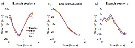
Johnston R, Snyder AC, Khanna SB, Issar D, Smith MA (2022) The eyes reflect an internal cognitive state hidden in the population activity of cortical neurons. Cereb Cortex 32:3331–3346.

(3) The relationships between changes in SC activity and pupil size are quite small (Figures 2C & 5C). Although the distribution across sessions (Figure 2C) is greater than chance, they are nearly 1/4 of the size compared to the PFC-SC axis comparisons. Likewise, the distribution of r2 values relating pupil size and spiking activity directly (Figure 5) is quite low. We remain skeptical that these drifts are truly due to arousal and cannot be accounted for by other factors. For example, does the relationship persist if accounting for a very simple, monotonic (e.g., linear) drift in pupil size and overall firing rate over the course of an individual session? 

Firstly, it is important to note that the strength of the relationship between projections onto the SC slow drift axis and pupil size (r² = 0.06) is within the range reported by Joshi et al. (2016, Neuron, Figure 3). They investigated the median variance explained between the spiking responses of individual SC neurons and pupil size and found it to be approximately 0.02 across sessions. Secondly, our statistical approach of testing the actual distribution of r² values against a shuffled distribution was specifically designed to rule out the possibility that the relationship between SC spiking responses and pupil size occurred due to linear drifts. The shuffled distribution in Figure 2C of the main manuscript represents the variance that can be explained by one session’s slow drift correlated with another session’s pupil, which would contain effects that occurred due to linear drifts alone. That the actual proportion of variance explained was significantly greater than this distribution suggests that the relationship between projections onto the SC slow drift axis and pupil size reflects changes in arousal rather than other factors related to linear drifts.

Joshi S, Li Y, Kalwani RM, Gold JI (2016) Relationships between Pupil Diameter and Neuronal Activity in the Locus Coeruleus, Colliculi, and Cingulate Cortex. Neuron 89:221–234.

(4) It is not clear how the final analysis (Figure 6) contributes to the authors' conclusions. The authors perform PCA on: (i) residual spiking responses during the delay period binned according to pupil size, and (ii) spiking responses in the saccade epoch binned according to target location (i.e., the saccade tuning curve). The corresponding PCs are the spike-pupil axis and the saccade tuning axis, respectively. Unsurprisingly, the spikepupil axis that captures variance associated with arousal (and removes variance associated with saccade direction) was not correlated with a saccade-tuning axis that captures variance associated with saccade direction and omits arousal. Had these measures been related it would imply a unique association between a neuron's preferred saccade direction and pupil control- which seems unlikely. The separation of these axes thus seems trivial and does not provide evidence of a "mechanism...in the SC to prevent arousal-related signals interfering with the motor output." It remains unknown whether, for example, arousal-related signals may impact trial-by-trial changes in neuronal gain near the time of a saccade, or alter saccade dynamics such as acceleration, precision, and reaction time. 

The reviewer makes a good point, and we agree that more evidence is needed to determine if the separation of the pupil size axis and saccade tuning axis is the mechanism through which cognitive and arousal-related signals can be intermixed in the SC. In the revised manuscript (lines 679-682), we have raised this as a possible explanation that necessitates further study rather than stating definitively that it is the exact mechanism through which these signals are kept separate. Our analysis here is similar to the one from Smoulder et al (2024, Neuron, Fig. 2F), in which the interactions between reward signals and target tuning in M1 were examined (and found to be orthogonal). While we agree with the reviewer that it may seem “trivial” for these axes to be orthogonal, it does not have to be so. If, for example, neural tuning curves shifted with changes in pupil size through gain changes that revealed tuning or affected tuning curve shape, there could be projections of the pupil axis onto the target tuning axis. Thus, while we agree with the reviewer that it appears sensible for these two axes to be orthogonal, our result is nonetheless a novel finding. We have edited the text in our revised manuscript, however, to make sure the nuance of this point is conveyed to the reader.

Smoulder AL, Marino PJ, Oby ER, Snyder SE, Miyata H, Pavlovsky NP, Bishop WE, Yu BM, Chase SM, Batista AP. A neural basis of choking under pressure. Neuron. 2024 Oct 23;112(20):3424-33.

Reviewer #2 (Public Review):

(1) The greatest weakness in the present research is the fact that arousal is a functionally less important non-motoric variable. The authors themselves introduce the problem with a discussion of attention, which is without any doubt the most important cognitive process that needs to be functionally isolated from oculomotor processes. Given this introduction, one cannot help but wonder, why the authors did not design an experiment, in which spatial attention and oculomotor control are differentiated. Absent such an experiment, the authors should spend more time explaining the importance of arousal and how it could interfere with oculomotor behavior. 

Although attention does represent an important cognitive process, we did not design an experiment in which attention and oculomotor control are differentiated because attention does not appear to be related to slow drift. In our first paper that reported on this phenomenon, we investigated the effects of spatial attention on slow fluctuations in neural activity by cueing the monkeys to attend to a stimulus in the left or right visual field in a block-wise manner. Each block lasted ~20 minutes and we found that slow drift did not covary with the timing of cued blocks (see Figure 4A, Cowley et al., 2020, Neuron). Furthermore, there is a large body of work showing that arousal also impacts motor behavior leading to changes in a range of eye-related metrics (e.g., pupil size, microsaccade rate and saccadic reaction time - for review, see Di Stasi et al. 2013, Neurosci. Biobehav. Rev.). We also note that the terms attention and arousal are often used in nonspecific and overlapping ways in the literature, adding to some potential confusion here. Nonetheless, pupil-linked arousal is an important variable that impacts motor performance. This has now been stated clearly in the Introduction of the revised manuscript (lines 108-114) to address the reviewer’s concerns and highlight the importance of studying how precise fixation and eye movements are maintained even in the presence of signals related to ongoing changes in brain state. 

Cowley BR, Snyder AC, Acar K, Williamson RC, Yu BM, Smith MA (2020) Slow Drift of Neural Activity as a Signature of Impulsivity in Macaque Visual and Prefrontal Cortex. Neuron 108:551-567.e8.

(2) In this context, it is particularly puzzling that one actually would expect effects of arousal on oculomotor behavior. Specifically, saccade reaction time, accuracy, and speed could be influenced by arousal. The authors should include an analysis of such effects. They should also discuss the absence or presence of such effects and how they affect their other results. 

As described above, several studies across species have demonstrated that arousal impacts motor behavior e.g., saccade reaction time, saccade velocity and microsaccade rate (for review, see Di Stasi et al. 2013, Neurosci. Biobehav. Rev.). This has been clarified in the Introduction of the revised manuscript to address the reviewer's concerns (lines 108-114). Our prior work (Johnston et al, Cerebral Cortex, 2022) shows that slow drift impacts several types of oculomotor behavior. Overall, these studies highlight the impact of arousal on eye movements as a robust effect, and support the present investigation into arousal and oculomotor control signals. While we agree reaction time, accuracy, and speed all can be influenced by arousal depending on task demands, the present study is focused on the connection between slow fluctuations in neural activity, linked to arousal, and different subpopulations of SC neurons. 

Di Stasi LL, Catena A, Cañas JJ, Macknik SL, Martinez-Conde S (2013) Saccadic velocity as an arousal index in naturalistic tasks. Neurosci Biobehav Rev 37:968–975.

Johnston R, Snyder AC, Khanna SB, Issar D, Smith MA (2022) The eyes reflect an internal cognitive state hidden in the population activity of cortical neurons. Cereb Cortex 32:3331–3346.

(3) The authors use the analysis shown in Figure 6D to argue that across recording sessions the activity components capturing variance in pupil size and saccade tuning are uncorrelated. however, the distribution (green) seems to be non-uniform with a peak at very low and very high correlation specifically. The authors should test if such an interpretation is correct. If yes, where are the low and high correlations respectively? Are there potentially two functional areas in SC? 

We agree with the reviewer that our actual data distribution was non-uniform. We examined individual sessions with high and low variance explained and did not find notable differences. One source of this variation has to do with session length. Longer sessions in principle should have a chance distribution of variance explained closer to zero because they contained more time bins. Given that we had no specific hypothesis for a non-uniform distribution, we have simply displayed the full distribution of values in our figure and the statistical result of a comparison to a shuffled distribution.

Reviewer #3 (Public Review):

(1) However, I am concerned about two main points: First, the authors repeatedly say that the "output" layers of the SC are the ones with the highest motor indices. This might not necessarily be accurate. For example, current thresholds for evoking saccades are lowest in the intermediate layers, and Mohler & Wurtz 1972 suggested that the output of the SC might be in the intermediate layers. Also, even if it were true that the high motor index neurons are the output, they are very few in the authors' data (this is also true in a lot of other labs, where it is less likely to see purely motor neurons in the SC). So, this makes one wonder if the electrode channels were simply too deep and already out of the SC? In other words, it seems important to show distributions of encountered neurons (regardless of the motor index) across depth, in order to better know how to interpret the tails of the distributions in the motor index histogram and in the other panels of Figure Supplement 1. I elaborate more on these points in the detailed comments below. 

The reviewer makes a good point about the efferent signals from SC. It is true that electrical thresholds are often lowest in intermediate layers, though deep layers do project to the oculomotor nuclei (Sparks, 1986; Sparks & Hartwich-Young, 1989) and often intermediate and deep layers are considered to function together to control eye movements (Wurtz & Albano, 1980). As suggested by the reviewer, we have edited the text throughout the manuscript to say that slow drift was less evident in SC neurons with a higher motor index, as well as included the above references and points about the intermediate and deep layers (Lines 73-81). Aside from the question of which layers of the SC function as the “motor output”, the reviewer raises a separate and important question – are our deep recordings still in SC. Here, we can say definitively that they are. We removed neurons if they did not exhibit elevated (above baseline) firing rates during the visual or saccade epochs of the MGS task (see Methods section on “Exclusion criteria”). All included neurons possessed a visual, visuomotor or motor response, consistent with the response properties of neurons in the SC. In addition, we found a number of neurons well above the bottom of the probe with strong motor responses and minimal loadings onto the slow drift axis (see Figure 2 – figure supplement 1A), consistent with the reviewer’s comment that intermediate layer neurons are tuned for movement and play a role in saccade production.

Mohler CW, Wurtz RH. Organization of monkey superior colliculus: intermediate layer cells discharging before eye movements. Journal of neurophysiology. 1976 Jul 1;39(4):722-44.

Sparks DL. Translation of sensory signals into commands for control of saccadic eye movements: role of primate superior colliculus. Physiol Rev. 1986 Jan;66(1):118-71. doi: 10.1152/physrev.1986.66.1.118. PMID: 3511480.

Sparks DL, Hartwich-Young R. The deep layers of the superior colliculus. Reviews of oculomotor research. 1989 Jan 1;3:213-55.

Wurtz RH, Albano JE. Visual-motor function of the primate superior colliculus. Annu Rev Neurosci. 1980;3:189-226. doi: 10.1146/annurev.ne.03.030180.001201. PMID: 6774653.

(2) Second, the authors find that the SC cells with a low motor index are modulated by pupil diameter. However, this could be completely independent of an "arousal signal". These cells have substantial visual responses. If the pupil diameter changes, then their activity should be influenced since the monkey is watching a luminous display. So, in this regard, the fact that they do not see "an arousal signal" in most motor neurons (through the pupil diameter analyses) is not evidence that the arousal signal is filtered out from the motor neurons. It could simply be that these neurons simply do not get affected by the pupil diameter because they do not have visual sensitivity. So, even with the pupil data, it is still a bit tricky for me to interpret that arousal signals are excluded from the "output layers" of the SC. 

The reviewer makes an important point about the SC’s visual responses. Neurons with a low motor index are, conversely, likely to have a stronger visual response index. However, we do not believe that changes in luminance can explain why the correlation between SC spiking response and pupil size is weaker for neurons with a lower motor index. Firstly, the changes in pupil size observed in the current paper and our previous work are slow and occur on a timescale of minutes (Cowley et al., 2020, Neuron) and are correlated with eye movement measures such as reaction time and microsaccade rate (Johnston et al., 2022, Cerebral Cortex). This is in stark contrast to luminance-evoked changes in pupil size that occur on a timescale of less than a second. Secondly, as shown the new Figure 5 – figure supplement 1 in the revised manuscript, very similar results were found when SC spiking responses were correlated with pupil size during the baseline period, when only the fixation point was on the screen. Although the luminance of the small peripheral target stimulus can result in small luminance-evoked changes in pupil size, no changes in luminance occurred during the baseline period which was defined as 100ms before the onset of the target stimulus. In Figure 2 – figure supplement 1 and Author response image 1 above, we show that slow drift is the same whether calculated on the baseline response, delay period, or peri-saccadic epoch. Thus, the measurement of slow drift is insensitive to the precise timing of the selection of both the window for the spiking response and the window for the pupil measurement. If luminance were the explanation for the slow changes in firing observed in visually responsive SC neurons, it would require those neurons to exhibit robust, sustained tuned responses to the small changes in retinal illuminance induced by the relatively small fluctuations in pupil size we observed from minute to minute. We are aware of no reports of such behavior in visually-responsive neurons in SC. We have included these analyses and this reasoning in the revised manuscript on lines 478-495.

Reviewer#1 (Recommendations for the author):

(1) It would be useful to provide line numbers in subsequent manuscripts for reviewers.

Line numbers have been added in the revised version of the manuscript.

(2) Page #6; last sentence: "...even impact processing at the early to mid stages of the visuomotor transformation, without leading to unwanted changes in motor output." I do not believe the authors have provided evidence that arousal levels were not associated with changes in motor output.

As suggested by Reviewer 3 (see Public Reviews, Reviewer 3, Point 2), we have edited the text throughout the manuscript to say that slow drift was less evident in SC neurons with a higher motor index. This sentence in the revised manuscript now reads:

“This provides a potential mechanism through which signals related to cognition and arousal can exist in the SC, and even impact processing at the early to mid stages of the visuomotor transformation, without leading to unwanted changes in SC neurons that are linked to saccade execution.”

(3) Page #8; last paragraph: Although deep-layer SC neurons may not have been obtained during every recording session, a summary of the motor index scores observed along the probe across sessions would be useful to confirm their assumptions. 

See Author response image 2 below which shows the motor index of each recoded SC neuron on the x-axis and session number on the y-axis. The points are colored by to the squared factor loading which represents the variance explained between the response a neuron and the slow drift axis (see Figure 3B of the main manuscript). You can see from this plot that neurons with a stronger component loading (shown in teal to yellow) typically have a lower motor index whereas the opposite is true for neurons with a weaker component loading (shown in dark blue).

Author response image 2.

Scatter plot showing the motor index of each recorded neuron along with the session number in which it was recorded. The points are colored by to the squared factor loading for each neuron along the slow drift axis. Note that loadings above 0.5 (33 data points in total) have been thresholded at 0.5 so that we could effectively use the color range to show all of the slow drift axis loadings.

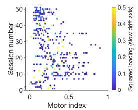
(4) Page #10; first paragraph: The authors should state the time window of the delay period used, since it may be distinct from the pupil analysis (first 200ms of delay). 

This has been stated in the revised version of the manuscript. The sentence now reads:

“We first asked if arousal-related fluctuations are present in the SC. As in previous studies that recorded from neurons in the cortex (Cowley et al., 2020), we found that the mean spiking responses of individual SC neurons during the delay period (chosen at random on each trial from a uniform distribution spanning 600-1100ms, see Methods) fluctuated over the course of a session while the monkeys performed the MGS task (Figure 2A, left).”

(5) Page #10; second paragraph: Extra period at the end of a sentence: " most variance in the data..". 

Fixed in the revised version of the manuscript.

(6) Page #12: "between projections onto the SC slow drift axis and mean pupil size during the first 200ms of the delay period when a task-related pupil response could be observed." What criteria was used to determine whether a task-related pupil response was observed? 

This was chosen based on the results of a previous study in our lab that used the same memory-guided saccade task to investigate the relationship between slow drift and changes in based and evoked pupil size (see Johnston et al., 2022, Cereb. Cortex, Figure 6B). The period was chosen based on plotting the average pupil size aligned on different trial epochs. As we show in Figure 5-figure supplement 3 above, the pupil interactions with slow drift did not depend on the particular time window of the pupil we chose.  

(7) Page #14; Figure 2A: The axes for the individual channels are strangely floating and quite different from all other figures. Please label the channel in the figure legend that was used as an example of the projected values onto the slow drift axis.

The figure has been changed in the revised version of the manuscript so that the tick mark denoting zero residual spikes per second is on the top layer of each plot. A scale bar was chosen instead of individual axes to reduce clutter in the figure as it was used to demonstrate how slow drift was computed. Residual spiking responses from all neurons were projected on the slow drift axis to generate the scatter plot in the bottom right-hand corner of Figure 2A. There is no single neuron to label.

(8) Page #16: "These results demonstrate that even though arousal-related fluctuations are present in the SC, they are isolated from deep-layer neurons that elicit a strong saccadic response and presumably reside closer to the motor output." In line with our major comments, lack of arousal-related activity during the delay period is meaningless for deep-layer SC neurons that are generally inactive during this time. It does not imply that there is no arousal signal! 

Addressed in Public Reviews, Reviewer 1, Point 1 & 2. We found a similar lack of arousal-related modulations reported for deep-layer SC neurons when slow drift was computed using the saccade epoch (Figure 1 above). In addition, similar dynamics were observed when the SC slow drift axis was computed using spiking responses during the baseline, delay, visual and saccade period (Figure 2).

(9) Page #18: "These findings provide additional support for the hypothesis that arousalrelated fluctuations are isolated from neurons in the deep layers of the SC." The same criticism from above applies.

Addressed in Public Reviews, Reviewer 1, Point 1 & 2.

(10) Page #20; paragraph 3: "Taken together, the findings outlined above..." Would be useful to be more specific when referring to "activity" ; e.g., "...these neurons did not exhibit large fluctuations in delay-period activity over time".

This sentence has been changed in the revised manuscript in light of the reviewer’s comments. It now reads:

“In addition to being more weakly correlated with pupil size, the spiking responses of these neurons did not exhibit large fluctuations over time (Figure 2), and when considering the neuronal population as a whole, explained less variance in the slow drift axis when it was computed using population activity in the SC (Figure 3) and PFC (Figure 4).”

Reviewer #3 (Recommendations for the author):

The paper is clear and well-written. However, I am concerned about two main points: 

(1) First, the authors repeatedly say that the "output" layers of the SC are the ones with the highest motor indices. This might not necessarily be accurate. For example, current thresholds for evoking saccades are lowest in the intermediate layers, and Mohler & Wurtz 1972 suggested that the output of the SC might be in the intermediate layers. Also, even if it were true that the high motor index neurons are the output, they are very few in the authors' data (this is also true in a lot of other labs, where it is less likely to see purely motor neurons in the SC). So, this makes one wonder if the electrode channels were simply too deep and already out of the SC. In other words, it seems important to show distributions of encountered neurons (regardless of motor index) across depth, in order to better know how to interpret the tails of the distributions in the motor index histogram and in the other panels of the figure supplement 1. I elaborate more on these points in the detailed comments below. 

Addressed in Public Reviews, Reviewer 3, Point 1.

(2) Second, the authors find that the SC cells with a low motor index are modulated by pupil diameter. However, this could be completely independent of an "arousal signal". These cells have substantial visual responses. If the pupil diameter changes, then their activity should be influenced since the monkey is watching a luminous display. So, in this regard, the fact that they do not see "an arousal signal" in most motor neurons (through the pupil diameter analyses) is not evidence that the arousal signal is filtered out from the motor neurons. It could simply be that these neurons simply do not get affected by the pupil diameter because they do not have visual sensitivity. So, even with the pupil data, it is still a bit tricky for me to interpret that arousal signals are excluded from the "output layers" of the SC. 

Addressed in Public Reviews, Reviewer 3, Point 2.

(3) I think that a remedy to the first point above is to change the text to make it a bit more descriptive and less interpretive. For example, just say that the slow drifts were less evident among the neurons with high motor index. 

We thank the reviewer for this suggestion (see Public Reviews, Reviewer 3, Point 1).

(4) For the second point, I think that it is important to consider the alternative caveat of different amounts of light entering the system. Changes in light level caused by pupil diameter variations can be quite large. 

We thank the reviewer for this suggestion (see Public Reviews, Reviewer 3, Point 2).

(5) Line 31: I'm a bit underwhelmed by this kind of statement. i.e. we already know that cognitive processes and brain states do alter eye movements, so why is it "critical" that high precision fixation and eye movements are maintained? And, isn't the next sentence already nulling this idea of criticality because it does show that the brain state alters the SC neurons? In fact, cognitive processes are already known to be most prevalent in the intermediate and deep layers of the SC. 

It seems clear that while cognitive state does affect eye movements, it is desirable to have some separation between cognitive state and eye movement control. Covert attention, for instance, is precisely a situation where eye movement control is maintained to avoid overt saccades to the attended stimulus, and yet there are clear indications of attention’s impact on microsaccades and fixation. We stand by our statement that an important goal of vision is to have precise fixation and movements of the eye, and yet at the same time the eyes are subject to numerous influences by cognitive state.

(6) Line 65: it is better to clarify that these are "functional layers" because there are actually more anatomical layers. 

We have edited this sentence in the revised version of the manuscript so that it now reads:

“The role of these projections in the visuomotor transformation depends on the functional layer of the SC in which they terminate”.

(7) Line 73: this makes it sound like only the deepest layers are topographically organized, which is not true. Also, as early as Mohler & Wurtz, 1972, it was suggested that the intermediate layers have the biggest impacts downstream of the SC. This is also consistent with electrical microstimulation current thresholds for evoking saccades from the SC. 

We have addressed the reviewers’ comments about the intermediate layers having the biggest impact downstream of the SC in Public Reviews, Reviewer 3, Point 1. Furthermore, line 73 has been changed in the revised manuscript so that it now reads:

“As is the case for neurons in the superficial and intermediate layers, they [SC motor neurons] form a topographically organized map of visual space (White et al. 2017; Robinson 1972; Katnani and Gandhi 2011)”.  

(8) Line 100: there is an analogous literature regarding the question of why unwanted muscle contractions do not happen. Specifically, in the context of why SC visual bursts do not automatically cause saccades (which is a similar problem to the ones you mention about cognitive signals interfering by generating unwanted eye movements), both Jagadisan & Gandhi, Curr Bio, 2022 and Baumann et al, PNAS, 2023 also showed that SC population activity not only has different temporal structure (Jagadisan & Gandhi) but also occupy different subspaces (Baumann et al) under these two different conditions (visual burst versus saccade burst). This is conceptually similar to the idea that you are mentioning here with respect to arousal. So, it is worth it to mention these studies here and again in the discussion. 

We are grateful to the reviewer for these suggestions and have included text in the Introduction (Lines 125-128) and Discussion (Lines 678-682) of the revised manuscript along with the references cited above.

(9) Line 147: as mentioned above, it is now generally accepted that there are quite a few "pure" motor neurons in the SC. This is consistent with what you find. E.g. Baumann et al., 2023. And, again see Mohler and Wurtz in the 1970's. So, I wonder how useful it is to go too much into this idea of the deeper motor neurons (e.g. the correlations in the other panels of the Figure 1 supplement). 

This is related to the reviewer’s comment that the output of the SC might be in the intermediate layers. This concern has been addressed in Public Reviews, Reviewer 3, Point 1.

(10) Figure 1 should say where the RF was for the shown spike rasters. i.e. were these the same saccade target across trials? And where was that location relative to the RF? It would help also in the text to say whether the saccade was always to the RF center or whether you were randomizing the target location. 

We centered the array of saccade targets using the microstimulation-evoked eye movement for SC (see Methods section “Memory-guided saccade task”) to find the evoked eccentricity, and then used saccade targets with equal spacing of 45 degrees starting at zero (rightward saccade target). We did not do extensive RF mapping beyond this microstimulation centering. In Figure 1, the spike rasters are shown for a target that was visually identified to be within the neuron’s RF based on assessing responses to all 8 target angles. We have added information about this to the figure caption.

(11) Line 218: but were there changes in the eye movement statistics? For example, the slow drift eye movements during fixation? Or even the microsaccades? 

Addressed in Public Reviews, Reviewer 2, Point 2.  

(12) Line 248: shuffling what exactly? I think that more explanation would be needed here. 

Addressed in Public Reviews, Reviewer 1, Point 3.  

(13) Line 263: but isn't this reflecting a sensory transient in the pupil diameter, since the target just disappeared? 

Addressed in Public Reviews, Reviewer 3, Point 2.  

(14) Line 271: I suspect that slow drift eye movements (in between microsaccades) would show higher correlations. Not sure how well you can analyze those with a video-based eye tracker. 

We agree that fixational drift would be a worthwhile metric, but it is not one we have focused on here and to our knowledge does require higher precision tracking. 

(15) Line 286: again, see above about similar demonstrations with respect to the visual and motor burst intervals, which clearly cause the same problem (even stronger) as the one studied here. 

See reply, including Figure 2.

(16) Line 330: again, I'm not sure deeper necessarily automatically means closer to the output. For example, current thresholds for evoked saccades grow higher as you go deeper. Maybe the authors can ask their colleague Neeraj Gandhi about this point specifically, just to be safe. Maybe the safest would be to remain descriptive about the data, and just say something like: arousal-related fluctuations were absent in our deepest recorded sites. 

Addressed in Public Reviews, Reviewer 3, Point 1.

(17) Line 332: likewise, statements like this one here would be qualified if the output was the intermediate layers......anyway if I understand what I read so far in the paper, the signal will be anyway orthogonal to the motor burst population subspace. So, maybe there's no need to emphasize that it goes away in the very deepest layers. 

See reply above, Public Reviews, Reviewer 1, Point 4.

(18) Figure 3A: related to the above, I think one issue could be that the deeper contacts might already be out of the SC. Maybe some cell count distribution from each channel should help in this regard. i.e. were you finding way fewer saccade-related neurons in the deepest channels (even though the few that you found were with high motor index)? If so, then wouldn't this just mean that the channel was too deep? I think there needs to be an analysis like this, to convince readers that the channels were still in the SC. Ideally, electrical stimulation current thresholds for evoking saccades at different depths would be tested, but I understand that this can be difficult at this stage. 

Addressed in Public Reviews, Reviewer 3, Point 1.

(19) I keep repeating this because in general, cognitive effects are stronger in the intermediate/deeper layers than in the superficial layers. If these interfere with eye movements like arousal, then why should arousal be different?

Few studies have investigated the effects of attention on “pure” movement SC neurons that only discharge during a saccade. One study, which we cited in Introduction (Ignashchenkova et al., 2004, Nat. Neurosci.), found significant differences in spiking responses between trials with and without attentional cueing for visual and visuomotor neurons. No significant difference was found for motor neurons, consistent with our hypothesis that signals related to cognition and arousal are kept separate from saccade-related signals in the SC.

(20) The problem with Figure 5 and its related text is that the neurons with low motor index are additionally visual. So, of course, they can be modulated if the pupil diameter changes!

Addressed in Public Reviews, Reviewer 3, Point 2.  

(21) I had a hard time understanding Figure 6. 

See reply above, Public Reviews, Reviewer 1, Point 4.

(22) Line 586: these cells have more visual responses and will be affected by the amount of light entering the eye. 

Addressed in Public Reviews, Reviewer 3, Point 2.

DOI: 10.21203/rs.3.rs-7614774/v1

Resource: (MMRRC Cat# 032037-JAX,RRID:MMRRC_032037-JAX)

Curator: @AleksanderDrozdz

SciCrunch record: RRID:MMRRC_032037-JAX

What is this?

DOI: 10.1101/2025.09.30.679484

Resource: (Proteintech Cat# 13019-3-AP, RRID:AB_2199414)

Curator: @scibot

SciCrunch record: RRID:AB_2199414

What is this?

Synthèse sur la situation des enfants sans abri logés dans les écoles en France

Résumé

Le sans-abrisme infantile connaît une augmentation alarmante en France, avec une hausse de 133 % depuis 2020, exacerbée par l'inflation et la crise du logement.

Face à ce que le reportage décrit comme les "carences de l'État", des collectifs citoyens, notamment "Jamais sans toi" à Lyon, organisent l'occupation d'établissements scolaires pour offrir un abri nocturne à des familles à la rue.

Ce document de synthèse se penche sur ce phénomène à travers le témoignage d'une famille d'origine angolaise – une mère et ses enfants – hébergée dans une école lyonnaise.

Leur parcours met en lumière la précarité extrême, le traumatisme d'une tentative d'expulsion avortée, et l'impact psychologique profond sur les enfants.

La situation révèle une tension critique entre la solidarité citoyenne, incarnée par les enseignants et les parents d'élèves, et l'inaction des pouvoirs publics, qui non seulement échouent à proposer des solutions de logement pérennes, mais exercent également une pression administrative sur les acteurs de cette solidarité.

1. Le Phénomène du Sans-abrisme Infantile et la Réponse Citoyenne

Le reportage met en évidence une crise sociale majeure : l'explosion du nombre d'enfants sans domicile fixe en France.

• Expansion et Causes :

◦ Le sans-abrisme infantile a augmenté de 133 % depuis 2020.   

◦ Les facteurs identifiés sont l'inflation, la multiplication des expulsions locatives et la pénurie de logements sociaux.   

◦ Les solutions d'urgence, conçues pour être temporaires, "s'éternisent".

En 2023, les familles logées dans des écoles y sont restées en moyenne plus de six mois.

• L'Occupation des Écoles comme Palliatif :

◦ Face à cette situation, des collectifs citoyens comme "Jamais sans toi" à Lyon organisent l'occupation d'écoles pour héberger des familles.     ◦ Ampleur du phénomène à Lyon :      

▪ Actuellement, 17 écoles de la métropole lyonnaise accueillent 25 familles.       

▪ Depuis 2014, une soixantaine d'établissements ont servi de refuge à plus de 1000 enfants.   

◦ Ce mouvement n'est pas limité à Lyon ; des initiatives similaires existent à Strasbourg, Rennes et Paris.   

◦ Ce soutien repose sur la "générosité citoyenne" (parents d'élèves, professeurs, habitants) qui compense les défaillances de l'État.

2. Étude de Cas : Le Parcours d'une Famille Angolaise

Le reportage se concentre sur le témoignage poignant de Lucy (16 ans), Lina (12 ans) et leur mère, qui illustre la réalité humaine derrière les statistiques.

• De l'Angola à la Précarité en France :

◦ Arrivée en France lorsque Lucy avait 10 ans et Lina 5 ou 6 ans.   

◦ Premières expériences d'hébergement précaire : le 115 à Dijon dans une chambre partagée, puis un foyer à Digoin.   

◦ La journée, la famille devait quitter le 115 et trouver refuge dans des associations (Secours Populaire, églises) pour manger.   

◦ Lina décrit sa déception face à la réalité française, loin de l'image idéalisée des dessins animés :

« Un pays super bien, que tout se passait bien, qu'on avait une vie normale ».  

◦ Elle a également été victime de moqueries et de racisme à l'école en raison de sa langue et de ses cheveux.

• Le Traumatisme de l'Expulsion Manquée (OQTF) :

◦ Il y a deux ans, la famille a fait l'objet d'une Obligation de Quitter le Territoire Français (OQTF).  

◦ La police est intervenue en pleine nuit dans leur appartement. Lucy, alors âgée de 14 ans, décrit une scène de panique et de violence :

ses parents criant, son père menotté, et les enfants enfermés dans une chambre avec des policiers.   

◦ La famille a été conduite à Paris après 5 heures de route et placée dans un centre de détention pendant 4 heures.   

◦ À l'aéroport, leur vol pour l'Angola a été annulé. Les autorités les ont alors "abandonnés à l'aéroport", leur ordonnant simplement "de plus retourner où [ils] étaient".

• La Rupture Familiale et l'Errance :

◦ Après cet épisode, la famille est revenue à Lyon.

Le mariage des parents n'étant pas reconnu en France, leur séparation a suivi. La mère s'est retrouvée seule avec ses enfants.   

◦ Ils ont enchaîné les solutions d'hébergement temporaires :

un camping à Trévoux, un appartement à Bellecour, puis une association qui les a logés avec d'autres femmes, avant de trouver refuge dans l'école.

3. La Vie Quotidienne dans une Salle de Classe

L'école, bien qu'offrant un toit, impose des conditions de vie extrêmement contraignantes et précaires.

Aspect

Description

Logement

La famille dort sur des matelas gonflables dans une salle de classe. Les vêtements sont stockés dans les armoires de la classe et des valises.

Routine

Lever obligatoire entre 6h30 et 6h50.

La famille doit quitter les lieux avant 8h30 et ne peut revenir qu'après 18h00, une fois tous les élèves partis.

Discrétion

La nuit, il est interdit d'allumer les lumières pour ne pas attirer l'attention.

La famille utilise les lampes de poche des téléphones pour s'éclairer.

Insecurité

Des jeunes jouant dans la cour sont déjà montés et ont fouillé dans leurs affaires, profitant d'une porte laissée ouverte.

Perturbations

La vie de la famille est rythmée par la sonnerie de l'école, qui retentit "toutes les heures".

Lutte de la mère

Elle cherche activement du travail (nettoyage, restauration) et des formations gratuites, mais sa situation rend les démarches très difficiles.

4. Impacts Psychologiques et Sociaux sur les Enfants

La précarité et l'instabilité ont des conséquences profondes sur le bien-être et le développement des enfants.

• Le Poids du Secret et de la Honte :

◦ Lucy cache sa situation à la plupart de ses amies par peur du jugement :

« J'angoisse un peu, sachant que beaucoup de jeunes de mon âge [...] se permettent de juger tout simplement. »  

◦ Elle exprime un profond désir de normalité : « Des fois, je me dis que j'aimerais juste avoir une vie normale comme plein d'ados de mon âge. »  

◦ Lina exprime également la peur d'être mise à l'écart par ses camarades parce qu'elle vit dans une école.

• Aspirations et Résilience :

◦ Malgré les épreuves, Lucy est une bonne élève et aspire à devenir avocate.

Son ambition est directement liée à son vécu : « J'ai envie d'être avocate, de défendre les gens parce que je me dis que tout le monde a le droit à une deuxième chance. »   

◦ Face à la détresse, elle a développé une stratégie de contrôle émotionnel : « Quand c'est dur, bah je prends sur moi et puis je me dis ça va aller. »  

◦ Sa plus grande peur reste matérielle et existentielle : « J'ai peur de me retrouver à la rue. Ça me fait peur. »

5. La Solidarité Face à l'Inaction Institutionnelle

Le reportage oppose la solidarité active du terrain à la réponse passive, voire répressive, des institutions.

• Le Soutien du Corps Enseignant :

◦ Une enseignante de l'école s'est fortement impliquée, dormant sur place la première nuit pour rassurer l'équipe périscolaire.  

◦ Elle a accueilli la famille chez elle pendant les vacances de Noël, une période particulièrement symbolique car la famille avait passé le Noël précédent dehors.  

◦ Une cagnotte organisée par ses collègues a permis d'offrir des cadeaux et un repas de fête à la famille.

• La Pression de la Hiérarchie :

◦ Suite à l'occupation, l'enseignante et ses collègues ont été convoquées par l'inspectrice d'académie.   

◦ La rencontre est décrite comme "un bon remontage de bretelle", où elles se sont fait "engueuler".

L'inspectrice les a qualifiées d' "inconscientes", leur faisant porter "toute la responsabilité" sans reconnaître la vulnérabilité de la famille.

• L'Absence de Solutions Pérennes :

◦ Près d'un an après le début de l'occupation, "il n'y a aucune proposition de la mairie, de la métropole, aucune perspective, rien."   

◦ L'occupation de l'école a donc dû se poursuivre au-delà de l'année scolaire, mais avec des règles plus strictes :

la famille n'a plus le droit d'être dans le bâtiment pendant les heures de classe.

Roots are in capitals, and are not words in use at all, but serve as an elucidation of the words grouped together and a connection between them.

J.R.R. Tolkien's note in the Qenya Lexicon[1]

Sauron new

knew that he had been wrong - not everyone would want to use the ring for their own power and Glory

yes Frodo succumbed at the very very end but - he and Sam made it that far and - fate or Providence or the intervention of Uru? himself did the rest

some people are capable of selfless and purely good acts

it wasn't just just Sauron who fell - it was his entire worldview

hope and love and care and friendship - can triumph over evil - however powerful it may seem at the time

1. what is the number one cause of stress in your life? my one cause of stress in my life is college i didn't know that college was going to be that difficult for me

2. what else causes you stress having my house clean for my house

3. what effect does stress have on your studies and academic performance? that i can't focuses so much on college

1 4 4 3 0 0 4 4 2 2 0 3 2 2 3 3

1. list common cause of stress for college students. Everyday Stressors
2. Time pressure: juggling classes, work, and social life
3. Academic anxiety: grades, exams, assignments
4. Financial concerns: tuition, rent, food
5. Relationship conflicts: roommates, partners, family
6. Health issues: frequent illness, poor sleep, allergies
7. Body image and eating habits
8. Loneliness or poor social connection
9. Daily hassles: broken-down car, housing issues

2.Describe the physical, mental, and emotional effects of persistent stress. Physical * Weakened immune system (more frequent illness) Digestive issue (ulcers, constipation, indigestion) * High blood pressure and increased risk of heart disease * Muscle tension headaches, fatigue * Sleep disturbances (insomnia or oversleeping)

Mental * Difficulty concentrating or thinking clearly * Poor memory and reduced academic * Negative thought patterns and pessimism

Emotional * Anxiety, depression, irritability * Feelings of helplessness or frustration * Withdrawal from others or increased conflict

1. List healthy ways college students can manage or cope with stress.
2. Exercise regularly (aerobic activity boosts mood and focus)
3. Get enough sleep (7-9 hour improves resilience)
4. Time management: focus on growth not perfection

4.Develop your personal plan for managing stress in your life long-term vision * Feel more in control of my schedule * Build emotional resilience and confidence * Maintain academic success while enjoying college life

reply to u/EdmundDante718 at https://reddit.com/r/typewriters/comments/1o5x527/missing_carriage_releases_on_scm/

It's incredibly common for these 6 series Smith-Coronas to have broken plastic carriage release levers (a major design flaw). You can call around to shops with parts machines for original replacements. https://site.xavier.edu/polt/typewriters/tw-repair.html

There are numerous YouTube repair videos and ideas including these few I've bookmarked before, though there are surely others: - https://www.youtube.com/watch?v=zNcQvfUk23s - https://www.youtube.com/watch?v=Gb9VlrKcXcM

I've not seen anyone 3-D print a version (yet), but designs for one might be floating around out there.

I've also seen people jury rig all sorts of plastic replacements which is an option as well.

In practice, you generally only need one working one for your dominant hand.

Résumé de la vidéo [00:00:14][^1^][1] - [00:28:20][^2^][2]:

Cette vidéo explore la managérialisation des associations et ses impacts.

Elle aborde les défis et propose des solutions pour renforcer le monde associatif face à cette tendance.

Temps forts:

• [00:00:14][^3^][3] Introduction et contexte
  • Accueil des participants
  • Présentation du webinaire
  • Objectifs de la série
• [00:03:27][^4^][4] Enjeux de la managérialisation
  • Définition et historique
  • Impact sur les associations
  • Comparaison avec d'autres modèles
• [00:07:03][^5^][5] Conséquences et critiques
  • Perte de dimension démocratique
  • Réduction des relations humaines
  • Exemples concrets et témoignages
• [00:15:01][^6^][6] Solutions et alternatives
  • Importance de la participation
  • Réappropriation des termes
  • Exemples de bonnes pratiques
• [00:22:00][^7^][7] Conclusion et perspectives
  • Invitation à l'action collective
  • Importance de la cohérence interne
  • Appel à la réflexion et à l'innovation

Résumé de la vidéo [00:28:22][^1^][1] - [00:54:06][^2^][2]:

Cette vidéo explore la gestion et la gouvernance des associations face à la managérialisation.

Elle met en lumière l'importance de la circulation de l'information, de l'intelligence collective, et de la délibération pour une gouvernance démocratique et efficace.

Points forts : + [00:28:22][^3^][3] Circulation de l'information * Importance de la diffusion de l'information * Mise en commun des connaissances * Héritage des sociétés savantes + [00:29:57][^4^][4] Intelligence collective * Animation et maïeutique * Création d'espaces de travail collaboratif * Qualité de l'animation + [00:31:02][^5^][5] Délibération et décision * Importance de la délibération pour de bonnes décisions * Définition de la démocratie par Paul Ricœur * Travail sur les contradictions + [00:35:02][^6^][6] Tensions et réussites * Identification des tensions dans la gouvernance * Conditions de réussite * Création d'une communauté apprenante + [00:39:02][^7^][7] Exemple pratique * Transformation de la gouvernance au sein du Réseau d'Échange et de Services aux Associations du Pays de Morlaix * Passage à un système de cercles thématiques * Participation et implication des salariés et bénévoles

Ces points forts couvrent les principaux aspects abordés dans la vidéo, offrant une vue d'ensemble des défis et des solutions pour une gouvernance associative efficace.

Résumé de la vidéo [00:54:11][^1^][1] - [01:19:33][^2^][2]:

Cette partie du webinaire traite de la gestion et de l'organisation des associations, en mettant l'accent sur la coprésidence et la participation collective.

Points forts : + [00:54:11][^3^][3] Introduction de la coprésidence * Modification des statuts en 2020 * Importance de la participation collective * Fonctionnement en commissions thématiques + [00:57:02][^4^][4] Formation et participation * Formation annuelle sur la gestion collective * Ouverture des chantiers de travail aux adhérents * Importance de la transparence et de la clarté + [01:00:00][^5^][5] Déplacements et cohésion * Budget pour les déplacements collectifs * Renforcement des liens entre membres * Importance de la convivialité et du plaisir + [01:03:09][^6^][6] Intégration de nouveaux membres * Augmentation du nombre de membres du CA * Processus d'intégration et d'accompagnement * Maintien de la transparence et de la confiance + [01:09:09][^7^][7] Réflexion sur le temps et la gouvernance * Importance de la gestion du temps * Opposition au néolibéralisme * Outils pratiques pour la gouvernance associative

Résumé de la vidéo [01:19:36][^1^][1] - [01:46:07][^2^][2]:

Cette vidéo traite de la managérialisation des associations et des défis liés à la gestion collective et à la formation continue des membres.

Temps forts: + [01:19:36][^3^][3] Partage d'expériences * Importance de partager les échecs * Encouragement à la discussion collective * Utilisation des retours d'expérience + [01:22:01][^4^][4] Formation continue * Formation des équipes salariées * Importance de la coopération * Nécessité de réexpliquer aux nouveaux membres + [01:27:03][^5^][5] Suivi des salariés * Organisation de réunions de médiation * Importance du bien-être au travail * Gestion des conflits internes + [01:33:00][^6^][6] Rôle du syndicalisme * Conditions de travail et temps de travail * Complémentarité entre engagement associatif et syndical * Importance de la démocratie interne + [01:38:00][^7^][7] Taille des associations * Impact de la taille sur la gestion * Importance de la volonté politique * Réflexion sur la géographie et l'échelle d'action

Résumé de la vidéo [01:46:09][^1^][1] - [01:58:34][^2^][2]:

Cette partie du webinaire aborde divers aspects de la gestion et de l'organisation des associations, en mettant l'accent sur les défis et les solutions possibles.

Temps forts: + [01:46:09][^3^][3] Questions sur la loi 3DS * Impact des certifications qualité * Partage de ressources et d'expertises * Importance de la loi pour les associations + [01:49:01][^4^][4] Réorganisation de la GD * Inclusion des salariés et bénéficiaires * Partenariat avec les financeurs * Protection des salariés uniques + [01:50:24][^5^][5] Participation des financeurs * Explication des projets aux financeurs * Importance de leur inclusion dans le CA * Délégation des responsabilités au sein de l'équipe + [01:53:06][^6^][6] Prévention des conflits d'intérêts * Retrait des élus des instances associatives * Importance de maintenir un lien fort avec les financeurs * Anticipation des changements législatifs + [01:55:00][^7^][7] Conclusion et perspectives * Recueil des expériences et des échecs * Construction d'une communauté apprenante * Invitation à partager des ressources et à poursuivre les échanges

La Prévention des Conflits d'Intérêts : Collectivités et Associations

Synthèse

Ce document de synthèse analyse les enjeux juridiques et pratiques liés à la prévention des conflits d'intérêts dans les relations entre les collectivités territoriales et les associations.

Basé sur les interventions d'experts juridiques et de formateurs d'élus, il met en lumière les risques pénaux encourus et propose des préconisations concrètes.

Les points critiques à retenir sont les suivants :

• 1. Le conflit d'intérêts n'est pas une infraction, mais un signal d'alerte. La situation devient délictuelle lorsqu'un élu ou un agent public, conscient de ce conflit, ne se déporte pas et participe à une décision, tombant ainsi sous le coup de la prise illégale d'intérêt, une infraction pénale sévèrement sanctionnée (jusqu'à 5 ans d'emprisonnement et 500 000 € d'amende).

• 1. La notion d'intérêt est extrêmement large. Elle couvre les intérêts matériels, mais aussi moraux ou familiaux. Il n'est pas nécessaire que l'élu se soit enrichi personnellement ou que la collectivité ait subi un préjudice ; la simple apparence d'une impartialité compromise peut suffire à caractériser l'infraction.
• 1. La règle pour les élus impliqués dans une association est le "déport général". Qu'ils soient membres du bureau à titre personnel ou en tant que représentants de la commune, ils doivent s'abstenir de toute participation à une délibération concernant cette association.

Ce déport doit être total :

• ◦ Absence de participation à l'instruction du dossier.
• ◦ Absence de participation aux débats.
• ◦ Absence de participation au vote.

• ◦ Sortie physique de la salle du conseil durant les débats et le vote.

• 1. Les élus locaux sous-estiment massivement ce risque. Les formations de terrain révèlent que la préoccupation principale des élus concerne les aspects techniques des subventions, tandis que le risque de conflit d'intérêts est souvent ignoré, en particulier dans les petites communes où les interférences entre mandats électifs et vie associative sont pourtant maximales.
• 1. Des outils et des bonnes pratiques existent pour sécuriser les processus.

La responsabilité première incombe à chaque élu, qui doit s'auto-évaluer en permanence.

Pour sécuriser les décisions, il est préconisé de voter les subventions au cas par cas, de systématiser la déclaration des conflits en début de séance et de s'appuyer sur des ressources externes comme la Haute Autorité pour la Transparence de la Vie Publique (HATVP) et le référent déontologue, désormais obligatoire pour toutes les communes.

1. Le Cadre Juridique et les Risques Pénaux

L'analyse juridique, menée par Luc Brunet de l'Observatoire SMAC, souligne la nécessité de distinguer deux notions fondamentales qui sont souvent confondues.

Définitions Fondamentales : Conflit d'Intérêts vs. Prise Illégale d'Intérêt

Le conflit d'intérêts est une situation, tandis que la prise illégale d'intérêt est une infraction pénale qui découle de la mauvaise gestion de cette situation. Caractéristique Conflit d'Intérêts Prise Illégale d'Intérêt Nature

Une situation d'interférence entre un intérêt public et des intérêts (publics ou privés) de nature à influencer ou paraître influencer l'exercice d'une fonction.

Une infraction pénale. Le fait de prendre, recevoir ou conserver, directement ou indirectement, un intérêt de nature à compromettre son impartialité.

Source Légale Loi du 11 octobre 2013

Article 432-12 du Code pénal

Sanction

Aucune (ce n'est pas une infraction). La situation doit être prévenue ou résolue.

Jusqu'à 5 ans d'emprisonnement et 500 000 € d'amende.

"Le conflit d'intérêts, c'est la vie. Nous avons tous des conflits d'intérêts. [...] Là où c'est pas normal [...] c'est quand on va se dire 'je vais surtout pas le dire que je suis en situation de conflit d'intérêt'. Et c'est là qu'on franchit la ligne jaune et qu'on passe [...] du côté du code pénal avec le délit de prise illégale d'intérêt." - Luc Brunet

Le Champ d'Application Vaste de la Prise Illégale d'Intérêt

Le délit de prise illégale d'intérêt est l'infraction numéro un pour laquelle les élus locaux sont poursuivis. Son champ d'application est particulièrement étendu :

• Tous les domaines : Contrairement au délit de favoritisme (limité à la commande publique), il s'applique à toutes les décisions d'une collectivité : urbanisme, recrutement, vente de biens, et notamment les subventions aux associations.

• Intérêt moral ou familial : L'intérêt n'est pas nécessairement matériel ou financier.

• Absence de préjudice requis : L'infraction est constituée même si la collectivité n'a subi aucun préjudice, voire si elle a bénéficié de l'opération.

• Intérêts indirects : Le délit couvre les intérêts pris par personne interposée (conjoint, ascendants, descendants, mais aussi amis proches).

La jurisprudence retient une vision très large : "l'infraction s'arrête où le soupçon s'arrête".

• La notion d'apparence : Il ne faut pas seulement ne pas être en conflit d'intérêts, mais aussi ne pas donner l'apparence de l'être.

La Doctrine de la Haute Autorité pour la Transparence de la Vie Publique (HATVP)

La HATVP a établi une doctrine pour clarifier les niveaux de risque. Pour les relations avec les associations, le risque est considéré comme large.

• Zone Rouge (Risque Large) : Concerne la participation d'un élu au sein d'un organisme de droit privé, comme une association, que ce soit à titre personnel ou comme représentant de la commune.

• Règle Appliquée : Le déport général. L'élu concerné doit s'abstenir de participer à toute délibération relative à cet organisme, y compris en l'absence d'enjeu financier direct. Adhérent ou Dirigeant : Une Distinction Cruciale ?

La question se pose de savoir si un simple adhérent est soumis aux mêmes règles qu'un membre du bureau (président, trésorier, etc.).

• Position de la HATVP (Avis du 3 mai 2022) : Le simple fait d'être adhérent ne justifie pas un déport systématique.

Cependant, une analyse au cas par cas doit être menée en fonction de la nature de l'association, de son nombre d'adhérents et de l'objet de la délibération.

• Conseil de Prudence : Face à l'incertitude de l'analyse au cas par cas, il est recommandé aux simples adhérents, par mesure de sécurité, de se déporter systématiquement lors du vote d'une subvention.

2. Règles Pratiques et Préconisations La prévention repose sur une démarche rigoureuse et transparente.

Les Quatre Étapes de la Prévention

• 1. Identifier les situations à risque : L'élu doit se poser les bonnes questions sur ses liens personnels, familiaux ou associatifs en rapport avec les dossiers de la collectivité.

• 2. Déclarer le conflit d'intérêts : Conformément à la Charte de l'élu local, l'élu doit faire connaître ses intérêts personnels avant le débat et le vote.

• 3. Se déporter complètement : Le déport ne se limite pas au non-vote. L'élu ne doit participer ni à l'instruction du dossier, ni aux débats qui précèdent le vote.

• 4. Ne pas influencer : L'élu doit s'abstenir de toute intervention, même informelle ("tirer les ficelles par derrière").

Jurisprudence : Des Exemples Concrets et Marquants Deux cas illustrent la sévérité avec laquelle la justice appréhende ce délit :

• Le maire de Plougastel-Daoulas : Des élus membres du bureau d'une association ad hoc n'ont pas participé au vote de la subvention, mais sont restés dans la salle.

Ce simple fait a été jugé suffisant pour caractériser une influence et a conduit à leur condamnation pour prise illégale d'intérêt.

• Une commune rurale de 250 habitants : Des élus, membres du bureau d'une association organisant la fête du village, ont participé au vote d'une subvention de 250 €.

Ils ont été condamnés pour prise illégale d'intérêt suite à la plainte d'un opposant politique.

Ces exemples démontrent que ni la bonne foi, ni la poursuite de l'intérêt général, ni le faible montant de la subvention ne constituent des protections contre une condamnation.

Préconisations pour Sécuriser les Délibérations

• Pas de vote global : Les subventions aux associations doivent être votées une par une, jamais en bloc.

• Sortir de la salle : L'élu concerné doit physiquement quitter la salle du conseil avant le début des débats et ne revenir qu'une fois le point de l'ordre du jour traité. Cette sortie doit être consignée au procès-verbal.

• Instaurer un "tour de table" déontologique : En début de chaque conseil, le maire peut demander à chaque élu de signaler d'éventuels conflits d'intérêts au regard de l'ordre du jour.

3. Le Témoignage du Terrain : Entre Méconnaissance et Difficultés d'Application

Le témoignage de Sophie Van migom, directrice d'un centre de formation pour élus, révèle un décalage important entre les exigences légales et la perception des élus sur le terrain.

Une Prise de Conscience Limitée chez les Élus

Lors des formations, les préoccupations des élus portent majoritairement sur des questions techniques (conventionnement, prêt de matériel, contrôle financier).

Le risque de conflit d'intérêts est très rarement abordé spontanément, en particulier par les élus des petites communes.

"Sur 90 participants, je n'ai que deux élus qui m'ont parlé de conflit d'intérêt. [...] Les élus des petites communes ne se posent pas la question, alors qu'il y a forcément des interférences entre leur mandat électif, leur vie familiale, leur vie associative." - Sophie Van migom

Les Conséquences Pratiques et les Défis Opérationnels

L'application stricte des règles de déport peut engendrer des difficultés de fonctionnement :

• Problèmes de quorum : Dans une commune de 620 habitants, la mise en place de règles de déport strictes a conduit à ce que la moitié du conseil municipal sorte de la salle, empêchant le quorum d'être atteint. La seule solution est de reconvoquer le conseil, ce qui retarde la décision.

• Paralysie de l'action des élus : Un élu engagé pour son expertise associative (ex: président de l'association des parents d'élèves devenu adjoint aux écoles) peut se retrouver dans l'incapacité d'agir sur les dossiers pour lesquels il a été élu.

Les Doubles Sanctions : Pénale et Administrative Le non-respect des règles de déport expose l'élu et la collectivité à un double risque :

1. Le risque pénal : L'élu est poursuivi pour prise illégale d'intérêt et le maire pour complicité.

2. Le risque administratif : La délibération elle-même est illégale.

Elle peut être annulée par le juge administratif suite à un recours d'un opposant, d'un contribuable ou du préfet. L'association pourrait alors être contrainte de rembourser la subvention perçue.

4. Outils et Bonnes Pratiques

La Responsabilité Personnelle de l'Élu

C'est à chaque élu d'évaluer sa propre situation, d'informer le maire et le conseil, et de prendre la décision de se déporter.

Cette réflexion doit être menée dès le début du mandat pour clarifier les limites de ses fonctions.

Les Aides à la Décision

Les élus ne sont pas seuls face à ces questionnements complexes. Ils peuvent solliciter :

• La Haute Autorité pour la Transparence de la Vie Publique (HATVP) : Il est possible de saisir la HATVP pour obtenir un avis confidentiel et rapide sur une situation personnelle.

• Le référent déontologue : Sa désignation est une obligation pour toutes les collectivités. Il offre un avis qui va au-delà du strict droit, en abordant les questions de probité et d'exemplarité.

Cas Spécifiques Abordés

• Agents de la collectivité : Ils sont également concernés par le délit.

S'ils sont en situation de conflit d'intérêts sur un dossier (ex: instruction d'un marché public pour l'entreprise d'un proche), ils doivent le signaler à leur hiérarchie pour que le dossier leur soit retiré.

• Subventions en nature : La mise à disposition de locaux, de matériel ou d'agents est considérée comme un avantage et suit exactement les mêmes règles de déport que les subventions financières.

• Associations "transparentes" : Une association qui n'est en réalité que le prolongement de la collectivité (ex: toutes les décisions sont prises par la commune) pose des problèmes juridiques majeurs.

Toutes les règles de la collectivité (comptabilité publique, marchés publics) s'appliquent alors à elle, créant un risque juridique élevé.

Reviewer #2 (Public review):

Summary:

In this article, the authors investigate enhancing the therapeutic and regenerative properties of mesenchymal stem cells (MSCs) through genetic modification, specifically by overexpressing genes involved in the glycogen synthesis pathway. By creating a non-phosphorylatable mutant form of glycogen synthase (GYSmut), the authors successfully increased glycogen accumulation in MSCs, leading to significantly improved cell survival under starvation conditions. The study highlights the potential of glycogen engineering to improve MSC function, especially in inflammatory or energy-deficient environments. However, critical gaps in the study's design, including the lack of validation of key findings, limited differentiation assessments, and missing data on MSC-GYSmut resistance to reactive oxygen species (ROS), necessitate further exploration.

Strengths:

(1) Novel Approach: The study introduces an innovative method of enhancing MSC function by manipulating glycogen metabolism.

(2) Increased Glycogen Storage: The genetic modification of GYS1, resulting in GYSmut, significantly increased glycogen accumulation, leading to improved MSC survival under starvation, which has strong implications for enhancing MSC therapeutic properties in energy-deficient environments.

(3) Potential Therapeutic Impact: The findings suggest significant therapeutic potential for MSCs in conditions that require improved survival, persistence, and immunomodulation, especially in inflammatory or energy-limited settings.

(4) In Vivo Validation: The in vivo murine model of pulmonary fibrosis demonstrated the improved survival and persistence of MSC-GYSmut, supporting the translational potential of the approach.

Weaknesses:

(1) Lack of Differentiation Assessments: The study did not evaluate key MSC differentiation pathways, including chondrogenic and osteogenic differentiation. The absence of analysis of classical MSC surface markers and multipotency limits the understanding of the full potential of MSC-GYSmut.

(2) Missing Validation of RNA Sequencing Data: Although RNA sequencing data revealed promising transcriptomic changes in chondrogenesis and metabolic pathways, these findings were not experimentally validated, limiting confidence.

(3) Lack of ROS Resistance Analysis: Resistance to reactive oxygen species (ROS), an important feature for MSCs under regenerative conditions, was not assessed, leaving out a critical aspect of MSC function.

(4) Limited Exploration of Immunosuppressive Properties: The study did not address the immunosuppressive functions of MSC-GYSmut, which are critical for MSC-based therapies in clinical settings.

Conclusion:

The study presents an exciting new direction for enhancing MSC function through glycogen metabolism engineering. While the results show promise, key experiments and validations are missing, and several areas, such as differentiation capacity, ROS resistance, and immunosuppressive properties, require further investigation. Addressing these gaps would solidify the conclusions and strengthen the potential clinical applications of MSC-GYSmut in regenerative medicine.

Author response:

The following is the authors’ response to the original reviews.

Reviewer #1 (Public Review)：

(1) Glycogen biosynthesis typically involves several enzymes. In this context, could the authors comment on the effect of overexpressing a single enzyme - especially a mutant version - on the structure or quality of the glycogen synthesized?

While quantitative molecular weight analysis of synthesized glycogen was not performed, we documented changes in glycogen particle morphology. GYSmut overexpression resulted in significantly enlarged singular glycogen granules, suggesting potential high molecular mass, while GYS-GYG co-overexpression in MSCs (GYG being the essential enzyme for glycogen synthesis initiation) produced a diffuse glycogen distribution pattern rather than particulate structures. We have incorporated this result as new Figure S2C.

These results suggest that overexpression of specific glycogen-metabolizing enzymes significantly influences glycogen structure. Consequently, targeted modulation of glycogen architecture and properties through key enzymes represents a potential avenue for future investigation.

(2) Regarding the in vitro starvation experiments (Figure 2C), what oxygen conditions (pO₂) were used? Are these conditions physiologically relevant and representative of the in vivo lung microenvironment?

Our in vitro starvation experiments (Figure 3C) were conducted under normoxic (21%). The oxygen concentration in human lungs is physiologically lower than atmospheric levels, with healthy individuals exhaling air containing approximately 16% oxygen (Thalakkotur Lazar Mathew, Diagnostics 2015). To our knowledge, direct measurements of alveolar oxygen concentration in pulmonary fibrosis are rare. Therefore, to evaluate the performance of GYSmut under hypoxic conditions, in the revised manuscript, Figure S2 has been augmented to include assessment of cell performance under combined hypoxia （oxygen concentration < 5%）and nutrient deprivation stress, which further corroborate the superiority of the GYSmut group over the control under different oxygen concentrations. 

(3) In the in vitro model, how many hours does it take for the intracellular glycogen reserve to be completely depleted under starvation conditions?

While quantitative cell viability data were recorded up to 72 hours post-implantation (Fig 3C), we observed cell viability at approximately 96 hours. We noticed that the presence of glycogen particles exhibited a correlation with sustained cell viability. However, reliable quantitative assessment of glycogen became increasingly challenging upon significant depletion of viable cells, thereby limiting our measurements during later time points.

(4) For the in vivo model, is there a quantitative analysis of the survival kinetics of the transplanted cells over time for each group? This would help to better assess the role and duration of glycogen stores as an energy buffer after implantation.

We tracked the in vivo distribution and persistence of implanted MSCs using enzymatic activity quantification assays (using Gluc luciferase assay) and live animal imaging (using Akaluc luciferase). The revised manuscript includes quantitative analysis of the in vivo fluorescence imaging data, which has been supplemented as Figure S4. Glycogen-engineered MSCs and control cells were quantitatively assessed at three discrete time points post-implantation. This quantification revealed a transient divergence in cell viability between the experimental and control groups around day 7. However, fluorescence in both cohorts subsequently declined to similar levels over the extended observation period.

(5) Finally, the study was performed in male mice only. Could sex differences exist in the efficacy or metabolism of the engineered MSCs? It would be helpful to discuss whether the approach could be expected to be similarly effective in female subjects.

We appreciate the reviewer’s important question regarding potential sex differences. Our study used male mice based on three key considerations: 1) Clinical Relevance: Idiopathic pulmonary fibrosis (IPF) shows significant male predominance, with diagnosis rates 3.5-fold higher in men (37.8% vs 10.6%, p<0.0001) and greater diagnostic confidence (Assayag et al., Thorax 2020). 2) Model Consistency: The bleomycin model (our chosen method) demonstrates more consistent fibrotic responses in male mice (Gul et al., BMC Pulm Med 2023). 3) Biological Rationale:

Estrogen’s protective effects in females may confound therapeutic assessments (cited in Assayag et al.).

We fully acknowledge this limitation and will include female subjects in subsequent translational studies. The therapeutic principle should theoretically apply to both sexes, but we agree this requires experimental validation.

(6) The number of mice for each group and time point should be specified.

The manuscript text has been revised to enhance clarity, and the number of mice for each group and time point has been specified (line 170 to 182).

Reviewer #2 (Public Review):

(4) Inconsistencies in In Vivo Data: There is a discrepancy between the number of animals shown in the figures and the graph (three individuals vs. five animals), as well as missing details on how luciferase signal intensity was quantified, requiring further clarification.

To assess MSC survival in vivo, we employed two strategies utilizing distinct luciferases optimized for specific detection modalities. MSC viability was quantified ex vivo through Gaussia luciferase (Gluc) activity, leveraging its high sensitivity and established commercial assay kits (n = 3 mice per group per time point). For non-invasive longitudinal tracking within living animals, MSC distribution and viability were monitored via in vivo bioluminescence imaging using Akaluc luciferase, selected for its superior tissue penetration and sensitivity in situ (n = 5 mice per group).The manuscript text has been revised to enhance clarity, and the experiment protocols for luciferase signal detection and quantification has been added into Methods.

（1) (2) (3) (5):

We fully agree that further investigation into the functional consequences of glycogen engineering in MSCs – encompassing core cellular functions, immunomodulatory properties, and associated signaling pathways – is important to fully elucidate the underlying mechanisms. Cellular metabolism is intrinsically intertwined with diverse physiological processes. Consequently, we believe that glycogen engineering exerts multifaceted effects on MSCs, likely extending beyond the modulation of any single specific pathway. Studying the metabolic perturbation induced by such engineering approaches in mammalian cells represents an interesting field. The exploration of these aspects remains an long-term research objective within our group.

Reviewer #2 (Recommendations for the authors):

(6) Clarification of Data in the Murine Model:

In Figure 4B, there is a discrepancy between the number of animals shown in the image (five) and those represented in the graph (three). This discrepancy needs clarification. Additionally, the study lacks information regarding the intensity of the signal in the luciferase assays. It is unclear how luciferase expression in the mice was quantified, and providing this detail would enhance the understanding of the data presented.

We sincerely appreciate these valuable suggestions. We have revised the relevant text for greater clarity. Figure 4B and Figure 4C present results from two distinct experimental approaches, each employing different luciferase reporters and measurement methodologies, and different num of mice were used in these two experiments.

Quantitative data derived from the in vivo bioluminescence imaging has been supplemented as Figure S4. The experiment protocols for luciferase signal detection and quantification has been added into Methods.

To other recommendations of reviewer 2：

We sincerely appreciate your valuable insights, which demonstrate your deep expertise. We fully agree that beyond nutrient availability, factors such as reactive oxygen species (ROS) and the immune microenvironment are also critical limitations affecting the survival and therapeutic efficacy of implanted MSCs.

We propose that glycogen engineering exerts broad effects on MSCs. These effects manifest as changes in multiple cellular characteristics, including proliferation, differentiation, surface marker expression, antioxidant capacity, and immunomodulatory activity – all crucial factors for the therapeutic purpose of MSCs.

We believe these changes likely involve complex networks of interconnected regulatory factors. The underlying mechanisms might be clarified through proteomic and metabolomic profiling.

However, comprehensively investigating these interconnected aspects requires significant time and resources. Some components of this research extend beyond the current scope of our project. Nevertheless, exploring these mechanisms remains an important objective, and we will actively work to investigate them further in our ongoing studies.

L'importance de l'interface dans le numérique

I feel these are great questions to get feedback from your colleagues, to make sure we have covered everything for the kids safety. I believe the last question is crucial because our job is to teach but more than that is to provide an environment for the kids to safe and for their health.

Adler, Mortimer J. 1940. “How to Mark a Book.” Saturday Review of Literature 6: 250–52. https://www.unz.com/print/SaturdayRev-1940jul06-00011/ (January 11, 2023).

Annotations: https://via.hypothes.is/https://docdrop.org/download_annotation_doc/Adler---1940---How-to-Mark-a-Book-fehef.pdf

Annotations alternate: https://jonudell.info/h/facet/?user=chrisaldrich&max=100&exactTagSearch=true&expanded=true&url=https%3A%2F%2Fdocdrop.org%2Fdownload_annotation_doc%2FAdler---1940---How-to-Mark-a-Book-fehef.pdf

Prior [.pdf copy]9https://stevenson.ucsc.edu/academics/stevenson-college-core-courses/how-to-mark-a-book-1.pdf): - Annotations https://hypothes.is/users/chrisaldrich?q=url%3Ahttps%3A%2F%2Fstevenson.ucsc.edu%2Facademics%2Fstevenson-college-core-courses%2Fhow-to-mark-a-book-1.pdf<br /> - Alternate annotation link https://jonudell.info/h/facet/?user=chrisaldrich&max=100&exactTagSearch=true&expanded=true&url=https%3A%2F%2Fstevenson.ucsc.edu%2Facademics%2Fstevenson-college-core-courses%2Fhow-to-mark-a-book-1.pdf

Summary

• Marking a book helps in increasing "the most efficient kind of reading."
• The marked (pun intended) difference between physical vs. intellectual ownership of books
• 3 types of book owners:
  • 1. collector of wood pulp and ink
  • 1. one whose read most and dipped into some
  • 1. one who's annotated and sucked the marrow out of them
• Active reading (annotating and staying awake) and engaging deeply, arguing with, and questioning the author is the point of reading.
• A historical record of your active reading allows you to continue the conversation you've had with the author and yourself. (p12)
• Adler's method of reading and marking:
  1. Underlining major points of importance
  2. Vertical lines for emphasis
  3. Marginal marks (stars, asterisks, etc.) (10-20 per book) to indicate the most important statements in conjunction with dogearing these pages for making it easier to find them subsequently
  4. Numbers in the margin to sequence arguments
  5. Page numbers in the margin for linking ideas across pages, ostensibly for juxtaposing them later
  6. Circling key words or phrases (unsaid here, but this is helpful for indexing as well as helping one to come to terms with the author)
  7. Marginal writing for synopsis of sections as well as questions raised by the text; use of endpapers for a personal index of ideas presented chronologically throughout the book
• Objections to marking books:
  • Using scratch pad (or index cards, which he doesn't mention specifically, but which could be implied) so as not to destroy a precious or rare physical copy (this is a repetition from earlier in the article)
  • Marking slows you down. This is part of the point! Slowing down makes you engage with the author and get more out of the text.
  • You can't loan books because they contain your important thoughts which you don't want to give away (and lose the historical record of your thinking). Solution: Simply require friends to buy their own copy.

References

(1) Doucet-Beaupre H, Gilbert C, Profes MS, Chabrat A, Pacelli C, Giguere N, et al. Lmx1a and Lmx1b regulate mitochondrial functions and survival of adult midbrain dopaminergic neurons. Proc Natl Acad Sci U S A. 2016;113(30):E4387-96. Epub 2016/07/14. doi: 10.1073/pnas.1520387113. PubMed PMID: 27407143; PubMed Central PMCID: PMCPMC4968767.
(2) Jimenez-Moreno N, Kollareddy M, Stathakos P, Moss JJ, Anton Z, Shoemark DK, et al. ATG8-dependent LMX1B-autophagy crosstalk shapes human midbrain dopaminergic neuronal resilience. J Cell Biol. 2023;222(5). Epub 2023/04/05. doi: 10.1083/jcb.201910133. PubMed PMID: 37014324; PubMed Central PMCID: PMCPMC10075225.
(3) Cross SH, Macalinao DG, McKie L, Rose L, Kearney AL, Rainger J, et al. A dominantnegative mutation of mouse Lmx1b causes glaucoma and is semi-lethal via LDB1mediated dimerization [corrected]. PLoS Genet. 2014;10(5):e1004359. Epub 2014/05/09. doi: 10.1371/journal.pgen.1004359. PubMed PMID: 24809698; PubMed Central PMCID: PMCPMC4014447.
(4) Li K, Tolman N, Segre AV, Stuart KV, Zeleznik OA, Vallabh NA, et al. Pyruvate and related energetic metabolites modulate resilience against high genetic risk for glaucoma. Elife. 2025;14. Epub 2025/04/24. doi: 10.7554/eLife.105576. PubMed PMID: 40272416; PubMed Central PMCID: PMCPMC12021409.
(5) Tolman NG, Balasubramanian R, Macalinao DG, Kearney AL, MacNicoll KH, Montgomery CL, et al. Genetic background modifies vulnerability to glaucoma-related phenotypes in Lmx1b mutant mice. Dis Model Mech. 2021;14(2). Epub 2021/01/20. doi: 10.1242/dmm.046953. PubMed PMID: 33462143; PubMed Central PMCID: PMCPMC7903917.