215 Matching Annotations
  1. Mar 2024
  2. Feb 2024
    1. Constructing Prompts for the Command Model Techniques for constructing prompts for the Command model. Developers
    1. Now, let’s modify the prompt by adding a few examples of how we expect the output to be. Pythonuser_input = "Send a message to Alison to ask if she can pick me up tonight to go to the concert together" prompt=f"""Turn the following message to a virtual assistant into the correct action: Message: Ask my aunt if she can go to the JDRF Walk with me October 6th Action: can you go to the jdrf walk with me october 6th Message: Ask Eliza what should I bring to the wedding tomorrow Action: what should I bring to the wedding tomorrow Message: Send message to supervisor that I am sick and will not be in today Action: I am sick and will not be in today Message: {user_input}""" response = generate_text(prompt, temp=0) print(response) This time, the style of the response is exactly how we want it. Can you pick me up tonight to go to the concert together?
    2. But we can also get the model to generate responses in a certain format. Let’s look at a couple of them: markdown tables
    3. And here’s the same request to the model, this time with the product description of the product added as context. Pythoncontext = """Think back to the last time you were working without any distractions in the office. That's right...I bet it's been a while. \ With the newly improved CO-1T noise-cancelling Bluetooth headphones, you can work in peace all day. Designed in partnership with \ software developers who work around the mayhem of tech startups, these headphones are finally the break you've been waiting for. With \ fast charging capacity and wireless Bluetooth connectivity, the CO-1T is the easy breezy way to get through your day without being \ overwhelmed by the chaos of the world.""" user_input = "What are the key features of the CO-1T wireless headphone" prompt = f"""{context} Given the information above, answer this question: {user_input}""" response = generate_text(prompt, temp=0) print(response) Now, the model accurately lists the features of the model. The answer is: The CO-1T wireless headphones are designed to be noise-canceling and Bluetooth-enabled. They are also designed to be fast charging and have wireless Bluetooth connectivity. Format
    4. While LLMs excel in text generation tasks, they struggle in context-aware scenarios. Here’s an example. If you were to ask the model for the top qualities to look for in wireless headphones, it will duly generate a solid list of points. But if you were to ask it for the top qualities of the CO-1T headphone, it will not be able to provide an accurate response because it doesn’t know about it (CO-1T is a hypothetical product we just made up for illustration purposes). In real applications, being able to add context to a prompt is key because this is what enables personalized generative AI for a team or company. It makes many use cases possible, such as intelligent assistants, customer support, and productivity tools, that retrieve the right information from a wide range of sources and add it to the prompt.
    5. We set a default temperature value of 0, which nudges the response to be more predictable and less random. Throughout this chapter, you’ll see different temperature values being used in different situations. Increasing the temperature value tells the model to generate less predictable responses and instead be more “creative.”
  3. Oct 2023
    1. racialized social hierarchies, thus facilitating dominationand exploitation.

      We also talked about that in Traditions and Revolutions

  4. Sep 2023
    1. they do not know enough about the topic at hand or because, they say, theysimply are not “smart enough.”

      I find myself saying this sometimes too

    2. BLEND THE AUTHOR’S WORDS WITH YOUR OWN

      Important to use a quotation for the essay we have to write

    3. VERBS FOR MAKING A CLAIM

      This will be very useful for writing my essays

    4. his ability to enter complex, many-sided conversations has taken on aspecial urgency in today’s polarized red state / blue state America,

      Politics in the United States

    5. Letter from Birmingham Jail,

      Learned in AP Gov, and important document in the Civil Rights Movement

    6. f you have been taught to write atraditional five-paragraph essay, for example, you have learned how todevelop a thesis and support it with evidence.

      What I was taught throughout my high school years

    7. Less experiencedwriters, by contrast, are often unfamiliar with these basic moves and unsurehow to make them in their own writing.

      More reading done means more experience, and better writing.

    8. STATE YOUR OWN IDEAS AS A RESPONSE TOOTHERS

      I think this is a good way for essays to be written, and it seems like I write a lot of essays that require this format.

    9. once you mastered it you no longerhad to give much conscious thought to the various moves that go into doingit.

      This is very true in my life, a lot of things come as second nature such as brushing my teeth and driving.

  5. moodle.lynchburg.edu moodle.lynchburg.edu
    1. “Why don’tyou do something about it?’

      I think this goes to a lot of things in life. A lot of people say this and say that, but none of them ever do anything

  6. moodle.lynchburg.edu moodle.lynchburg.edu
    1. for their knowledge of theirown ignorance.

      Rare ability to be aware of being ignorant, and we all struggle with it.

    2. The father was a quiet, simple soul, calmly ignorant, with no touch of vulgarity. The mother wasdifferent,—strong, bustling, and energetic, with a quick, restless tongue, and an ambition to live“like folks.”

      This is a very similar way to my household, but I know this is not the norm in most.

    1. it is easier to do ill than well in the world

      I think this relates to everyone's life. It's a lot harder to do the right that can help the world than it is to the easy thing that hurts the world thing sometimes.

  7. Jun 2023
    1. We use the same model and architecture as GPT-2

      What do they mean by "model" here? If they have retrained on more data, with a slightly different architecture, then the model weights after training must be different.

  8. May 2023
  9. Apr 2023
    1. Now we are getting somewhere. At this point, we also see that the dimensions of W and b for each layer are specified by the dimensions of the inputs and the number of nodes in each layer. Let’s clean up the above diagram by not labeling every w and b value individually.
    1. The Delta Method, from the field of nonlinear regression. The Bayesian Method, from Bayesian modeling and statistics. The Mean-Variance Estimation Method, using estimated statistics. The Bootstrap Method, using data resampling and developing an ensemble of models.

      Four methods to compute prediction intervals.

    1. A novel method for estimating prediction uncertainty using machine learning techniques is presented. Uncertainty is expressed in the form of the two quantiles (constituting the prediction interval) of the underlying distribution of prediction errors. The idea is to partition the input space into different zones or clusters having similar model errors using fuzzy c-means clustering. The prediction interval is constructed for each cluster on the basis of empirical distributions of the errors associated with all instances belonging to the cluster under consideration and propagated from each cluster to the examples according to their membership grades in each cluster. Then a regression model is built for in-sample data using computed prediction limits as targets, and finally, this model is applied to estimate the prediction intervals (limits) for out-of-sample data. The method was tested on artificial and real hydrologic data sets using various machine learning techniques. Preliminary results show that the method is superior to other methods estimating the prediction interval. A new method for evaluating performance for estimating prediction interval is proposed as well.

      Prediction intervals using quantiles. Use clustering.

  10. Feb 2023
    1. the Elhage et al.(2021) study showing an information-copying role for self-attention.

      It turns out Meng does refer to induction heads, just not by name.

  11. Jan 2023
    1. e twoareas in which the forward-forward algorithm may be superior to backpropagation are as a model oflearning in cortex and as a way of making use of very low-power analog hardware without resortingto reinforcement learning(Jabri and Flower, 1992).
  12. Dec 2022
    1. Our method is based on the hypothesis that the weights of a generator act as Optimal Linear Associative Memory (OLAM). OLAM is a classic single-layer neural data structure for memorizing associations that was described by Teuvo Kohonen and James A Anderson (independently) in the 1970s. In our case, we hypothesize that within a large modern multilayer convolutional network, the each individual layer plays the role of an OLAM that stores a set of rules that associates keys, which denote meaningful context, with values, which determine output.
    1. AI training data is filled with racist stereotypes, pornography, and explicit images of rape, researchers Abeba Birhane, Vinay Uday Prabhu, and Emmanuel Kahembwe found after analyzing a data set similar to the one used to build Stable Diffusion.

      That is horrifying. You'd think that authors would attempt to remove or filter this kind of material. There are, after all models out there that are trained to find it. It makes me wonder what awful stuff is in the GPT-3 dataset too.

    1. We test this hypothesis by training a predicted compute-optimal model, Chinchilla, that uses the same compute budget as Gopher but with 70B parameters and4× more more data. Chinchilla uniformly and significantly outperforms Gopher (280B), GPT-3 (175B),Jurassic-1 (178B), and Megatron-Turing NLG (530B) on a large range of downstream evaluation tasks.This also means that Chinchilla uses substantially less compute for fine-tuning and inference, greatlyfacilitating downstream usage. As a highlight, Chinchilla reaches a state-of-the-art average accuracy of67.5% on the MMLU benchmark, greater than a 7% improvement over Gopher

      By using more data on a smaller language model the authors were able to achieve better performance than with the larger models - this reduces the cost of using the model for inference.

  13. Nov 2022
    1. Kuratierungs-Filter auf Empfängerseite gibt, aber dann wäre auch e-mail-Spam als Problem gelöst und das sehe ich gerade noch nicht passieren.

      gibt es projekte, die Modelle auf gesammelte spam mails trainieren?

    1. “The metaphor is that the machine understands what I’m saying and so I’m going to interpret the machine’s responses in that context.”

      Interesting metaphor for why humans are happy to trust outputs from generative models

  14. Sep 2022
    1. Consider a toy model where we train an embedding of five features of varying importanceWhere “importance” is a scalar multiplier on mean squared error loss. in two dimensions, add a ReLU afterwards for filtering, and vary the sparsity of the features.
    1. The present generation of Southerners are not responsible for the past

      We can't judge or blame people based off of their ancestors' actions. In high school, I always hated that everyone knew my older siblings because it often felt like my future was already written for me even though I had not even experienced it myself yet.

    2. Haytian revolt

      We briefly touched on this in Traditions/Revolutions, and I know we will learn more about it later on in the course.

    3. his educational programme was un-necessarily narrow.

      When I was first annotating "The Education of the Negro," I also found Washington's idea of teaching industrial education singularly focused. However, towards the end of his article he made me come around to the idea because it seemed like a good way to instill a desire in students to work for themselves instead of someone else.

    4. the Free Negroes from 1830 up to war-time hadstriven to build industrial schools, and the American Missionary Associ-ation had from the first taught various trades; and Price and others hadsought a way of honorable alliance with the best of the Southerners. ButMr. Washington first indissolubly linked these things; he put enthusiasm,unlimited energy, and perfect faith into his programme, and changed itfrom a by-path into a veritable Way of Life

      ML: He was nor the first to come up with the idea obviously but he put a face on it. It seems like people myself included have a much easier time following something if there is a person in charge of it for them to follow.

    1. Our schools teach everybody a little of almosteverything, but, in my opinion, they teach very fewchildren just what they ought to know in order tomake their way successfully in life. They do not putinto their hands the tools they are best tted to use,and hence so many failures. Many a mother andsister have worked and slaved, living upon scantyfood, in order to give a son and brother a ’liberaleducation,’ and in doing this have built up a barrierbetween the boy and the work he was tted to do.Let me say to you that all honest work is honorablework. If the labor is manual, and seems common,you will have all the more chance to be thinking ofother things, or of work that is higher and bringsbetter pay, and to work out in your minds betterand higher duties and responsibilities foryourselves, and for thinking of ways by which youcan help others as well as yourselves, and bringthem up to your own higher level.

      I still see this in our school systems today, especially in certain classes where you feel like you are never going to use anything that you have learned in the real world.

    2. Our schools teach everybody a little of almosteverything, but, in my opinion, they teach very fewchildren just what they ought to know in order tomake their way successfully in life. They do not putinto their hands the tools they are best tted to use,and hence so many failures. Many a mother andsister have worked and slaved, living upon scantyfood, in order to give a son and brother a ’liberaleducation,’ and in doing this have built up a barrierbetween the boy and the work he was tted to do.Let me say to you that all honest work is honorablework. If the labor is manual, and seems common,you will have all the more chance to be thinking ofother things, or of work that is higher and bringsbetter pay, and to work out in your minds betterand higher duties and responsibilities foryourselves, and for thinking of ways by which youcan help others as well as yourselves, and bringthem up to your own higher level.

      I still see this in our school systems today, especially in certain classes where you feel like you are never going to use anything that you have learned in the real world.

    3. Our schools teach everybody a little of almosteverything, but, in my opinion, they teach very fewchildren just what they ought to know in order tomake their way successfully in life.

      When I was in high school, my mom would always say that they don't teach us some of the most important life skills in class. She was always ranting about how we should have to take a finance class to prepare for adulthood.

    4. “Our schools teach everybody a little of almosteverything, but, in my opinion, they teach very fewchildren just what they ought to know in order tomake their way successfully in life.

      This is still accurate for schools today. For example, in middle school we had 8 classes a day for 45 minutes each for one semester. Even though we had class everyday it was far too little of time to actually learn a full subject. The teacher had to just give us a little bit of information on each topic we were supposed to cover.

  15. moodle.lynchburg.edu moodle.lynchburg.edu
    1. Uncle Bird had a small, rough farm, all woods and hills, miles from the big road; but he was fullof tales

      My uncles are also full of tales that they like to share with everyone they have the chance to.

    2. willow

      I named my Jeep Willow.

    1. Now, the progression of NLP, as discussed, tells a story. We begin with tokens and then build representations of these tokens. We use these representations to find similarities between tokens and embed them in a high-dimensional space. The same embeddings are also passed into sequential models that can process sequential data. Those models are used to build context and, through an ingenious way, attend to parts of the input sentence that are useful to the output sentence in translation.
    2. Data, matrix multiplications, repeated and scaled with non-linear switches. Maybe that simplifies things a lot, but even today, most architectures boil down to these principles. Even the most complex systems, ideas, and papers can be boiled down to just that:
  16. Aug 2022
  17. Jul 2022
    1. Z-code models to improve common language understanding tasks such as name entity recognition, text summarization, custom text classification and key phrase extraction across its Azure AI services. But this is the first time a company has publicly demonstrated that it can use this new class of Mixture of Experts models to power machine translation products.

      this model is what actually z-code is and what makes it special

    2. have developed called Z-code, which offer the kind of performance and quality benefits that other large-scale language models have but can be run much more efficiently.

      can do the same but much faster

  18. Jun 2022
    1. The dominant idea is one of attention, by which a representation at a position is computed as a weighted combination of representations from other positions. A common self-supervision objective in a transformer model is to mask out occasional words in a text. The model works out what word used to be there. It does this by calculating from each word position (including mask positions) vectors that represent a query, key, and value at that position. The query at a position is compared with the value at every position to calculate how much attention to pay to each position; based on this, a weighted average of the values at all positions is calculated. This operation is repeated many times at each level of the transformer neural net, and the resulting value is further manipulated through a fully connected neural net layer and through use of normalization layers and residual connections to produce a new vector for each word. This whole process is repeated many times, giving extra layers of depth to the transformer neural net. At the end, the representation above a mask position should capture the word that was there in the original text: for instance, committee as illustrated in Figure 1.
    1. This trick of using a one-hot vector to pull out a particular row of a matrix is at the core of how transformers work.

      Matrix multiplication as table lookup

  19. May 2022
    1. Given the complexities of the brain’s structure and the functions it performs, any one of these models is surely oversimplified and ultimately wrong—at best, an approximation of some aspects of what the brain does. However, some models are less wrong than others, and consistent trends in performance across models can reveal not just which model best fits the brain but also which properties of a model underlie its fit to the brain, thus yielding critical insights that transcend what any single model can tell us.
    1. Such a highly non-linear problem would clearly benefitfrom the computational power of many layers. Unfortu-nately, back-propagation learning generally slows downby an order of magnitude every time a layer is added toa network.

      The problem in 1988

    1. The source sequence will be pass to the TransformerEncoder, which will produce a new representation of it. This new representation will then be passed to the TransformerDecoder, together with the target sequence so far (target words 0 to N). The TransformerDecoder will then seek to predict the next words in the target sequence (N+1 and beyond).
  20. Apr 2022
    1. Ourpre-trained network is nearly identical to the “AlexNet”architecture (Krizhevsky et al., 2012), but with local re-ponse normalization layers after pooling layers following(Jia et al., 2014). It was trained with the Caffe frameworkon the ImageNet 2012 dataset (Deng et al., 2009)
    1. Example 1. For example, suppose that the input volume has size [32x32x3], (e.g. an RGB CIFAR-10 image). If the receptive field (or the filter size) is 5x5, then each neuron in the Conv Layer will have weights to a [5x5x3] region in the input volume, for a total of 5*5*3 = 75 weights (and +1 bias parameter). Notice that the extent of the connectivity along the depth axis must be 3, since this is the depth of the input volume. Example 2. Suppose an input volume had size [16x16x20]. Then using an example receptive field size of 3x3, every neuron in the Conv Layer would now have a total of 3*3*20 = 180 connections to the input volume. Notice that, again, the connectivity is local in 2D space (e.g. 3x3), but full along the input depth (20).

      These two examples are the first two layers of Andrej Karpathy's wonderful working ConvNetJS CIFAR-10 demo here

    1. input (32x32x3)max activation: 0.5, min: -0.5max gradient: 1.08696, min: -1.53051Activations:Activation Gradients:Weights:Weight Gradients:conv (32x32x16)filter size 5x5x3, stride 1max activation: 3.75919, min: -4.48241max gradient: 0.36571, min: -0.33032parameters: 16x5x5x3+16 = 1216

      The dimensions of these first two layers are explained here

    1. Here the lower level layers are frozen and are not trained, only the new classification head will update itself to learn from the features provided from the pre-trained chopped up model on the left.
    1. Starting from random noise, we optimize an image to activate a particular neuron (layer mixed4a, unit 11).

      And then we use that image as a kind of variable name to refer to the neuron in a way that more helpful than the the layer number and neuron index within the layer. This explanation is via one of Chris Olah's YouTube videos (https://www.youtube.com/watch?v=gXsKyZ_Y_i8)

  21. Mar 2022
    1. A special quality of humans, not shared by evolution or, as yet, by machines, is our ability to recognize gaps in our understanding and to take joy in the process of filling them in. It is a beautiful thing to experience the mysterious, and powerful, too.
  22. Feb 2022
    1. Verfahren des Relational Machine Learning, welche unter Ausnutzung der Graphstruktur in vielen Fällen Modelle besserer Qualität liefern.

      Rleational Machine Learning-Ansatz

    2. In vielen Anwendungen ist es allerdings notwendig, Daten nicht nur in hoher Qualität und semantisch angereichert zur Verfügung zu stellen, sondern neues Wissen aus vorhandenen Informationen zu generieren. Hierfür nutzen wir Machine Learning.

      Kombination mit ML-Anästze zur Generierung von neuem Wissen

    1. Somewhat confusingly, and for historical reasons, such multiple layer networks are sometimes called multilayer perceptrons or MLPs, despite being made up of sigmoid neurons, not perceptrons. I'm not going to use the MLP terminology in this book, since I think it's confusing, but wanted to warn you of its existence.
  23. Dec 2021
    1. the only thing an artificial neuron can do: classify a data point into one of two kinds by examining input values with weights and bias.

      How does this relate to "weighted sum shows similarity between the weights and the inputs"?

    1. The transformer model introduces the idea of instead of adding another complex mechanism (attention) to an already complex Seq2Seq model; we can simplify the solution by forgetting about everything else and just focusing on attention.
    1. I’m particularly interested in two questions: First, just how weird is machine learning? Second, what sorts of choices do developers make as they shape a project?
  24. Nov 2021
    1. Now that we've made peace with the concepts of projections (matrix multiplications)

      Projections are matrix multiplications.Why didn't you sayso? spatial and channel projections in the gated gmlp

    2. Computers are especially good at matrix multiplications. There is an entire industry around building computer hardware specifically for fast matrix multiplications. Any computation that can be expressed as a matrix multiplication can be made shockingly efficient.
    3. The selective-second-order-with-skips model is a useful way to think about what transformers do, at least in the decoder side. It captures, to a first approximation, what generative language models like OpenAI's GPT-3 are doing.
    1. You'll use a (70%, 20%, 10%) split for the training, validation, and test sets. Note the data is not being randomly shuffled before splitting. This is for two reasons: It ensures that chopping the data into windows of consecutive samples is still possible. It ensures that the validation/test results are more realistic, being evaluated on the data collected after the model was trained.

      Train, Validation, Test: 0.7, 0.2, 0.1

    1. The following figure presents a simple functional diagram of the neural network we will use throughout the article. The neural network is a sequence of linear (both convolutional A convolution calculates weighted sums of regions in the input. In neural networks, the learnable weights in convolutional layers are referred to as the kernel. For example Image credit to https://towardsdatascience.com/gentle-dive-into-math-behind-convolutional-neural-networks-79a07dd44cf9. See also Convolution arithmetic. and fully-connected A fully-connected layer computes output neurons as weighted sum of input neurons. In matrix form, it is a matrix that linearly transforms the input vector into the output vector. ), max-pooling, and ReLU First introduced by Nair and Hinton, ReLU calculates f(x)=max(0,x)f(x)=max(0,x)f(x)=max(0,x) for each entry in a vector input. Graphically, it is a hinge at the origin: Image credit to https://pytorch.org/docs/stable/nn.html#relu layers, culminating in a softmax Softmax function calculates S(yi)=eyiΣj=1NeyjS(y_i)=\frac{e^{y_i}}{\Sigma_{j=1}^{N} e^{y_j}}S(yi​)=Σj=1N​eyj​eyi​​ for each entry (yiy_iyi​) in a vector input (yyy). For example, Image credit to https://ljvmiranda921.github.io/notebook/2017/08/13/softmax-and-the-negative-log-likelihood/ layer.

      This is a great visualization of MNIST hidden layers.

    1. The Query word can be interpreted as the word for which we are calculating Attention. The Key and Value word is the word to which we are paying attention ie. how relevant is that word to the Query word.

      Finally

    1. Other work on interpreting transformer internals has focused mostly on what the attention is looking at. The logit lens focuses on what GPT "believes" after each step of processing, rather than how it updates that belief inside the step.
    1. The cube of activations that a neural network for computer vision develops at each hidden layer. Different slices of the cube allow us to target the activations of individual neurons, spatial positions, or channels.

      This is first explanation of

    1. The attention layer (W in the diagram) computes three vectors based on the input, termed key, query, and value.

      Could you be more specific?

    2. Attention is a means of selectively weighting different elements in input data, so that they will have an adjusted impact on the hidden states of downstream layers.
    1. These findings provide strong evidence for a classic hypothesis about the computations underlying human language understanding, that the brain’s language system is optimized for predictive processing in the service of meaning extraction
    1. To review, the Forget gate decides what is relevant to keep from prior steps. The input gate decides what information is relevant to add from the current step. The output gate determines what the next hidden state should be.Code DemoFor those of you who understand better through seeing the code, here is an example using python pseudo code.
  25. Oct 2021
    1. This approach, visualizing high-dimensional representations using dimensionality reduction, is an extremely broadly applicable technique for inspecting models in deep learning.
    2. These layers warp and reshape the data to make it easier to classify.
    1. Even with this very primitive single neuron, you can achieve 90% accuracy when recognizing a handwritten text image1. To recognize all the digits from 0 to 9, you would need just ten neurons to recognize them with 92% accuracy.

      And here is a Google Colab notebook that demonstrates that

  26. Sep 2021
    1. Humans perform a version of this task when interpretinghard-to-understand speech, such as an accent which is particularlyfast or slurred, or a sentence in a language we do not know verywell—we do not necessarily hear every single word that is said,but we pick up on salient key words and contextualize the rest tounderstand the sentence.

      Boy, don't they

    1. A neural network will predict your digit in the blue square above. Your image is 784 pixels (= 28 rows by 28 columns with black=1 and white=0). Those 784 features get fed into a 3 layer neural network; Input:784 - AvgPool:196 - Dense:100 - Softmax:10.
    1. Personalized ASR models. For each of the 432 participants with disordered speech, we create a personalized ASR model (SI-2) from their own recordings. Our fine-tuning procedure was optimized for our adaptation process, where we only have between ¼ and 2 h of data per speaker. We found that updating only the first five encoder layers (versus the complete model) worked best and successfully prevented overfitting [10]
    1. So whenever you hear of someone “training” a neural network, it just means finding the weights we use to calculate the prediction.
  27. Aug 2021
    1. I'm going to try provide an English text example. The following is based solely on my intuitive understanding of the paper 'Attention is all you need'.

      This is also good

    2. For the word q that your eyes see in the given sentence, what is the most related word k in the sentence to understand what q is about?
    3. So basically: q = the vector representing a word K and V = your memory, thus all the words that have been generated before. Note that K and V can be the same (but don't have to). So what you do with attention is that you take your current query (word in most cases) and look in your memory for similar keys. To come up with a distribution of relevant words, the softmax function is then used.
    1. Here is a list of some open data available online. You can find a more complete list and details of the open data available online in Appendix B.

      DataHub (http://datahub.io/dataset)

      World Health Organization (http://www.who.int/research/en/)

      Data.gov (http://data.gov)

      European Union Open Data Portal (http://open-data.europa.eu/en/data/)

      Amazon Web Service public datasets (http://aws.amazon.com/datasets)

      Facebook Graph (http://developers.facebook.com/docs/graph-api)

      Healthdata.gov (http://www.healthdata.gov)

      Google Trends (http://www.google.com/trends/explore)

      Google Finance (https://www.google.com/finance)

      Google Books Ngrams (http://storage.googleapis.com/books/ngrams/books/datasetsv2.html)

      Machine Learning Repository (http://archive.ics.uci.edu/ml/)

      As an idea of open data sources available online, you can look at the LOD cloud diagram (http://lod-cloud.net ), which displays the connections of the data link among several open data sources currently available on the network (see Figure 1-3).

    1. A neural network with a hidden layer has universality: given enough hidden units, it can approximate any function. This is a frequently quoted – and even more frequently, misunderstood and applied – theorem. It’s true, essentially, because the hidden layer can be used as a lookup table.
    2. Recursive Neural Networks
  28. Jul 2021
    1. In the language of Interpretable Machine Learning (IML) literature like Molnar et al.[20], input saliency is a method that explains individual predictions.
    1. Using multiple copies of a neuron in different places is the neural network equivalent of using functions. Because there is less to learn, the model learns more quickly and learns a better model. This technique – the technical name for it is ‘weight tying’ – is essential to the phenomenal results we’ve recently seen from deep learning.

    1. Vectors with a small Euclidean distance from one another are located in the same region of a vector space. Vectors with a high cosine similarity are located in the same general direction from the origin.
    1. If you're serious about neural networks, I have one recommendation. Try to rebuild this network from memory.
    2. If you're serious about neural networks, I have one recommendation. Try to rebuild this network from memory.
    1. In our research, i.e., the wormnet project, we try to build machine learning models motivated by the C. elegans nervous system. By doing so, we have to pay a cost, as we constrain ourselves to such models in contrast to standard artificial neural networks, whose modeling space is purely constraint by memory and compute limitations. However, there are potentially some advantages and benefits we gain. Our objective is to better understand what’s necessary for effective neural information processing to emerge.
    1. Recommendations DON'T use shifted PPMI with SVD. DON'T use SVD "correctly", i.e. without eigenvector weighting (performance drops 15 points compared to with eigenvalue weighting with (p = 0.5)). DO use PPMI and SVD with short contexts (window size of (2)). DO use many negative samples with SGNS. DO always use context distribution smoothing (raise unigram distribution to the power of (lpha = 0.75)) for all methods. DO use SGNS as a baseline (robust, fast and cheap to train). DO try adding context vectors in SGNS and GloVe.
  29. Jun 2021
    1. One thing that should be learned from the bitter lesson is the great power of general purpose methods, of methods that continue to scale with increased computation even as the available computation becomes very great. The two methods that seem to scale arbitrarily in this way are search and learning

      This is a big lesson. As a field, we still have not thoroughly learned it, as we are continuing to make the same kind of mistakes. To see this, and to effectively resist it, we have to understand the appeal of these mistakes. We have to learn the bitter lesson that building in how we think we think does not work in the long run. The bitter lesson is based on the historical observations that 1) AI researchers have often tried to build knowledge into their agents, 2) this always helps in the short term, and is personally satisfying to the researcher, but 3) in the long run it plateaus and even inhibits further progress, and 4) breakthrough progress eventually arrives by an opposing approach based on scaling computation by search and learning. The eventual success is tinged with bitterness, and often incompletely digested, because it is success over a favored, human-centric approach.

  30. Apr 2021
    1. Machine learning app development has been gaining traction among companies from all over the world. When dealing with this part of machine learning application development, you need to remember that machine learning can recognize only the patterns it has seen before. Therefore, the data is crucial for your objectives. If you’ve ever wondered how to build a machine learning app, this article will answer your question.

    1. Machine learning is an extension of linear regression in a few ways. Firstly is that modern ML

      Machine learning is an extension to linear model which deals with much more complicated situation where we take few different inputs and get outputs.

  31. Nov 2020
    1. 可以认为 π k \pi_k πk​就是每个分量 N ( x ∣ μ k , Σ k ) \mathcal{N}(\boldsymbol{x}|\boldsymbol{\mu}_k, \boldsymbol{\Sigma}_k) N(x∣μk​,Σk​)的权重。

      有的书称为责任

  32. Oct 2020
  33. May 2020
    1. Machine learning has a limited scope
    2. AI is a bigger concept to create intelligent machines that can simulate human thinking capability and behavior, whereas, machine learning is an application or subset of AI that allows machines to learn from data without being programmed explicitly
    1. Machine learning is an application of artificial intelligence (AI) that provides systems the ability to automatically learn and improve from experience without being explicitly programmed
  34. Apr 2020
    1. Keras is a high-level neural networks API, written in Python and capable of running on top of TensorFlow, CNTK, or Theano. It was developed with a focus on enabling fast experimentation. Being able to go from idea to result with the least possible delay is key to doing good research. Use Keras if you need a deep learning library that: Allows for easy and fast prototyping (through user friendliness, modularity, and extensibility). Supports both convolutional networks and recurrent networks, as well as combinations of the two. Runs seamlessly on CPU and GPU. Read the documentation at Keras.io. Keras is compatible with: Python 2.7-3.6.
  35. Jan 2020
    1. Suppose the algorithm chooses a tree that splits on education but not on age. Conditional on this tree, the estimated coefficients are consistent. But that does not imply that treatment effects do not also vary by age, as education may well covary with age; on other draws of the data, in fact, the same procedure could have chosen a tree that split on age instead

      a caveat

    2. hese heterogenous treatment effects can be used to assign treatments; Misra and Dubé (2016) illustrate this on the problem of price targeting, applying Bayesian regularized methods to a large-scale experiment where prices were randomly assigned

      todo -- look into the implication for treatment assignment with heterogeneity

    3. Chernozhukov, Chetverikov, Demirer, Duflo, Hansen, and Newey (2016) take care of high-dimensional controls in treatment effect estimation by solving two simultaneous prediction problems, one in the outcome and one in the treatment equation.

      this seems similar to my idea of regularizing on only a subset of the variables

    4. These same techniques applied here result in split-sample instrumental variables (Angrist and Krueger 1995) and “jackknife” instrumental variables

      some classical solutions to IV bias are akin to ML solutions

    5. Understood this way, the finite-sample biases in instrumental variables are a consequence of overfitting.

      traditional 'finite sample bias of IV' is really overfitting

    6. Even when we are interested in a parameter β ˆ, the tool we use to recover that parameter may contain (often implicitly) a prediction component. Take the case of linear instrumental variables understood as a two-stage procedure: first regress x = γ′z + δ on the instrument z, then regress y = β′x + ε on the fitted values x ˆ. The first stage is typically handled as an estimation step. But this is effectively a prediction task: only the predictions x ˆ enter the second stage; the coefficients in the first stage are merely a means to these fitted values.

      first stage of IV -- handled as an estimation problem, but really it's a prediction problem!

    7. Prediction in the Service of Estimation

      This is especially relevant to economists across the board, even the ML skeptics

    8. New Data

      The first application: constructing variables and meaning from high-dimensional data, especially outcome variables

      • satellite images (of energy use, lights etc) --> economic activity
      • cell phone data, Google street view to measure wealth
      • extract similarity of firms from 10k reports
      • even traditional data .. matching individuals in historical censuses
    9. Zhao and Yu (2006) who establish asymptotic model-selection consistency for the LASSO. Besides assuming that the true model is “sparse”—only a few variables are relevant—they also require the “irrepresentable condition” between observables: loosely put, none of the irrelevant covariates can be even moderately related to the set of relevant ones.

      Basically unrealistic for microeconomic applications imho

    10. First, it encourages the choice of less complex, but wrong models. Even if the best model uses interactions of number of bathrooms with number of rooms, regularization may lead to a choice of a simpler (but worse) model that uses only number of fireplaces. Second, it can bring with it a cousin of omitted variable bias, where we are typically concerned with correlations between observed variables and unobserved ones. Here, when regular-ization excludes some variables, even a correlation between observed variables and other observed (but excluded) ones can create bias in the estimated coefficients.

      Is this equally a problem for procedures that do not assum sparsity, such as the Ridge model?

    11. 97the variables are correlated with each other (say the number of rooms of a house and its square-footage), then such variables are substitutes in predicting house prices. Similar predictions can be produced using very different variables. Which variables are actually chosen depends on the specific finite sample.

      Lasso-chosen variables are unstable because of what we usually call 'multicollinearity.'<br> This presents a problem for making inferences from estimated coefficients.

    12. Through its regularizer, LASSO produces a sparse prediction function, so that many coefficients are zero and are “not used”—in this example, we find that more than half the variables are unused in each run

      This is true but they fail to mention that LASSO also shrinks the coefficients on variables that it keeps towards zero (relative to OLS). I think this is commonly misunderstood (from people I've spoken with).

    13. One obvious problem that arises in making such inferences is the lack of stan-dard errors on the coefficients. Even when machine-learning predictors produce familiar output like linear functions, forming these standard errors can be more complicated than seems at first glance as they would have to account for the model selection itself. In fact, Leeb and Pötscher (2006, 2008) develop conditions under which it is impossible to obtain (uniformly) consistent estimates of the distribution of model parameters after data-driven selection.

      This is a very serious limitation for Economics academic work.

    14. First, econometrics can guide design choices, such as the number of folds or the function class.

      How would Econometrics guide us in this?

    15. These choices about how to represent the features will interact with the regularizer and function class: A linear model can reproduce the log base area per room from log base area and log room number easily, while a regression tree would require many splits to do so.

      The choice of 'how to represent the features' is consequential ... it's not just 'throw it all in' (kitchen sink approach)

    16. Ta b l e 2Some Machine Learning Algorithms

      This is a very helpful table!

    17. Picking the prediction func-tion then involves two steps: The first step is, conditional on a level of complexity, to pick the best in-sample loss-minimizing function.8 The second step is to estimate the optimal level of complexity using empirical tuning (as we saw in cross-validating the depth of the tree).

      ML explained while standing on one leg.

    18. egularization combines with the observability of predic-tion quality to allow us to fit flexible functional forms and still find generalizable structure.

      But we can't really make statistical inferences about the structure, can we?

    19. This procedure works because prediction quality is observable: both predic-tions y ˆ and outcomes y are observed. Contrast this with parameter estimation, where typically we must rely on assumptions about the data-generating process to ensure consistency.

      I'm not clear what the implication they are making here is. Does it in some sense 'not work' with respect to parameter estimation?

    20. In empirical tuning, we create an out-of-sample experiment inside the original sample.

      remember that tuning is done within the training sample

    21. Performance of Different Algorithms in Predicting House Values

      Any reason they didn't try a Ridge or an Elastic net model here? My instinct is that these will beat LASSO for most Economic applications.

    22. We consider 10,000 randomly selected owner-occupied units from the 2011 metropolitan sample of the American Housing Survey. In addition to the values of each unit, we also include 150 variables that contain information about the unit and its location, such as the number of rooms, the base area, and the census region within the United States. To compare different prediction tech-niques, we evaluate how well each approach predicts (log) unit value on a separate hold-out set of 41,808 units from the same sample. All details on the sample and our empirical exercise can be found in an online appendix available with this paper athttp://e-jep.org

      Seems a useful example for trying/testing/benchmarking. But the link didn't work for me. Can anyone find it? Is it interactive? (This is why I think papers should be html and not pdfs...)

    23. Making sense of complex data such as images and text often involves a prediction pre-processing step.

      In using 'new kinds of data' in Economics we often need to do a 'classification step' first

    24. The fundamental insight behind these breakthroughs is as much statis-tical as computational. Machine intelligence became possible once researchers stopped approaching intelligence tasks procedurally and began tackling them empirically.

      I hadn't thought about how this unites the 'statistics to learn stuff' part of ML and the 'build a tool to do a task' part. Well-phrased.

    25. In another category of applications, the key object of interest is actually a parameter β, but the inference procedures (often implicitly) contain a prediction task. For example, the first stage of a linear instrumental variables regres-sion is effectively prediction. The same is true when estimating heterogeneous treatment effects, testing for effects on multiple outcomes in experiments, and flexibly controlling for observed confounders.

      This is most relevant tool for me. Before I learned about ML I often thought about using 'stepwise selection' for such tasks... to find the best set of 'control variables' etc. But without regularisation this seemed problematic.

    26. Machine Learning: An Applied Econometric Approach

      Shall we use Hypothesis to have a discussion ?

  36. Dec 2019
  37. Aug 2019
    1. Machine learning is an approach to making many similar decisions that involves algorithmically finding patterns in your data and using these to react correctly to brand new data
  38. Jul 2019
    1. We translate all patient measurements into statisticsthat are predictive of unsuccesfull discharge

      Egy analitikai pipeline, kb amit nekünk is össze kéne hozni a végére.

  39. Feb 2019
    1. One benefit of SGD is that it's computationally a whole lot faster. Large datasets often can't be held in RAM, which makes vectorization much less efficient. Rather, each sample or batch of samples must be loaded, worked with, the results stored, and so on. Minibatch SGD, on the other hand, is usually intentionally made small enough to be computationally tractable. Usually, this computational advantage is leveraged by performing many more iterations of SGD, making many more steps than conventional batch gradient descent. This usually results in a model that is very close to that which would be found via batch gradient descent, or better.

      Good explanation for why SGD is computationally better. I was confused about the benefits of repeated performing mini-batch GD, and why it might be better than batch GD. But I guess the advantage comes from being able to get better performance by vecotrizing computation.

    1. And so it makes most sense to regard epoch 280 as the point beyond which overfitting is dominating learning in our neural network.

      I do not get this. Epoch 15 indicates that we are already over-fitting to the training data set, on? Assuming both training and test set come from the same population that we are trying to learn from.

    2. If we see that the accuracy on the test data is no longer improving, then we should stop training

      This contradicts the earlier statement about epoch 280 being the point where there is over-training.

    3. It might be that accuracy on the test data and the training data both stop improving at the same time

      Can this happen? Can the accuracy on the training data set ever increase with the training epoch?

    4. What is the limiting value for the output activations aLj

      When c is large, small differences in z_j^L are magnified and the function jumps between 0 and 1, depending on the sign of the differences. On the other hand, when c is very small, all activation values will be close to 1/N; where N is the number of neurons in layer L.

  40. Jan 2019
    1. By utilizing the Deeplearning4j library1 for model representation, learning and prediction, KNIME builds upon a well performing open source solution with a thriving community.
    2. It is especially thanks to the work of Yann LeCun and Yoshua Bengio (LeCun et al., 2015) that the application of deep neural networks has boomed in recent years. The technique, which utilizes neural networks with many layers and enhanced backpropagation algorithms for learning, was made possible through both new research and the ever increasing performance of computer chips.
    3. One of KNIME's strengths is its multitude of nodes for data analysis and machine learning. While its base configuration already offers a variety of algorithms for this task, the plugin system is the factor that enables third-party developers to easily integrate their tools and make them compatible with the output of each other.
  41. Dec 2018
  42. Nov 2018
    1. 三,方法3:MDS

      Multi-dimensional scaling (MDS) and Principla Coordinate Analysis(PCoA) are very similar to PCA, except that instead of converting correlations into a 2-D graph, they convert distance among the samples into a 2-D graph.

      So, in order to do MDS or PCoA, we have to calculate the distance between Cell1 and Cell2, and distance between Cell1 and Cell3...

      • 1 2
      • 1 3
      • 1 4
      • 2 3
      • 2 4
      • 3 4

      One very common way to calculate distance between two things is to calculate the Euclidian distance.

      And once we calculated the distance between every pair of cells, MDS and PCoA would reduce them to a 2-D graph.

      The bad news is that if we used the Euclidean Distance, the graph would be identical to a PCA graph!!

      In other words, clustering based on minimizing the linear distances is the same with maximzing the linear correlations.

      我想这里也就是为什么,李宏毅老师在 t-SNE 课程一开始时说,其他非监督降维算法都只是专注于【如何让·簇内距小·】,而 t-SNE 还考虑了【如何让·簇间距大·】

      也就是说,PCA 的本质(或者叫另一种解释)也只是【找到一种转换函数,他能让原空间中距离近的两点,转换后距离更近】,他压根就没有考虑【簇内or簇外】而是“通杀”所有点。

      The good news is that there are tons of other ways to measure distance!!!

      For example, another way to measure distances between cells is to calcualte between cells is to calculate the average of the absolute value of the log fold changes among genes.

      Finally, we get a plot different from the PCA plot

      A biologist might choose to use log fold change to calculate distance because they are frequently interested in log fold changes among genes...

      But there are lots of distance to choose from...

      1. Manhattan Distance
      2. Hamming Distance
      3. Great Circle Distance

      In summary:

      • PCA creates plots based on correlations among samples;
      • MDS and PCoA create plots based on distances among samples

  43. Oct 2018
    1. T-distribution Stochastic Neighbor Embedding(t-SNE)

      之前介绍的所有方法都存在相同的弊病:

      similar data are close, but different data may collapse,亦即,相似(label)的点靠的确实很近,但不相似(label)的点也有可能靠的很近。

      不同的无监督学习在 MNIST 上的表现

      t-SNE 的原理

      \(x \rightarrow z\)

      t-SNE 一样是降维,从 x 向量降维到 z. 但 t-SNE 有一步很独特的标准化步骤:

      一, t-SNE 第一步:similarity normalization

      这一步假设我们已经知道 similarity 的公式,关于 similarity 的公式在【第四步】单独讨论,因为实在神妙

      这一步是对任意两个点之间的相似度进行标准化,目的是尽量让所有的相似度的度量都处在 [0,1] 之间。你可以把他看做是对相似度进行标准化,也可以看做是为求解KL散度做准备 --- 求条件概率分布

      compute similarity between all pairs of x: \(S(x^i, x^j)\)

      我们这里使用 Similarity(A,B) 来近似 P(A and B), 使用 \(\sum_{A\neq B}S(A,B)\) 来近似 P(B)

      \(P(A|B) = \frac{P(A\cap B)}{P(B)} = \frac{P(A\cap B)}{\sum_{all\ I\ \neq B}P(I\cap B)}\)

      \(P(x^j|x^i)=\frac{S(x^i, x^j)}{\sum_{k\neq i}S(x^i, x^k)}\)

      假设我们已经找到了一个 low dimension z-space。我们也就可以计算转换后样本的相似度,进一步计算 \(z^i\) \(z^j\) 的条件概率。

      compute similarity between all pairs of z: \(S'(z^i, z^j)\)

      \(P(z^j|z^i)=\frac{S(z^i, z^j)}{\sum_{k\neq i}S(z^i, z^k)}\)

      Find a set of z making the two distributions as close as possible:

      \(L = \sum_{i}KL(P(\star | x^i)||Q(\star | z^i))\)

      二, t-SNE 第二部:find z

      我们要找到一组转换后的“样本”, 使得转换前后的两组样本集(通过KL-divergence测量)的分布越接近越好:

      衡量两个分布的相似度:使用 KL 散度(也叫 Infomation Gain)。KL 散度越小,表示两个概率分布越接近。

      \(L = \sum_{i}KL(P(\star | x^i) || Q(\star | z^i))\)

      find zi to minimize the L.

      这个应该是很好做的,因为只要我们能找到 similarity 的计算公式,我们就能把 KL divergence 转换成关于 zi 的相关公式,然后使用梯度下降法---GD最小化这个式子即可。

      三,t-SNE 的弊端

      1. 需要计算所有两两pair的相似度
      2. 新点加入,需要重新计算他与所有点之间的相似度
      3. 由于步骤2导致的后续所有的条件概率\(P\ and\ Q\) 都需要重新计算

      因为 t-SNE 要求我们计算数据集的两两点之间的相似度,所以这是一个非常高计算量的算法。同时新数据点的加入会影响整个算法的过程,他会重新计算一遍整个过程,这个是十分不友好的,所以 t-SNE 一般不用于训练过程,仅仅用在可视化中,即便在可视化中也不会仅仅使用 t-SNE,依旧是因为他的超高计算量。

      在用 t-SNE 进行可视化的时候,一般先使用 PCA 把几千维度的数据点降维到几十维度,然后再利用 t-SNE 对几十维度的数据进行降维,比如降到2维之后,再plot到平面上。

      四,t-SNE 的 similarity 公式

      之前说过如果一种 similarity 公式:计算两点(xi, xj)之间的 2-norm distance(欧氏距离):

      \(S(x^i, x^j)=exp(-||x^i - x^j||_2)\)

      一般用在 graph 模型中计算 similarity。好处是他可以保证非常相近的点才会让这个 similarity 公式有值,因为 exponential 会使得该公式的结果随着两点距离变大呈指数级下降

      在 t-SNE 之前有一个算法叫做 SNE 在 z-space 和 x-space 都使用这个相似度公式。

      similarity of x-space: \(S(x^i, x^j)=exp(-||x^i - x^j||_2)\) similarity of z-space: \(S'(z^i, z^j)=exp(-||z^i - z^j||_2)\)

      t-SNE 神妙的地方就在于他在 z-space 上采用另一个公式作为 similarity 公式, 这个公式是 t-distribution 的一种(t 分布有参数可以调,可以调出很多不同的分布):

      \(S(x^i, x^j)=exp(-||x^i - x^j||_2)\) \(S'(z^i, z^j)=\frac{1}{1+||z^i - z^j||_2}\)

      可以通过函数图像来理解为什么需要进行这种修正,以及这种修正为什么能保证x-space原来近的点, 在 z-space 依旧近,原来 x-space 稍远的点,在 z-space 会拉的非常远

      t-distributin vs. gaussian as similarity measure

      也就是说,原来 x-space 上的点如果存在一些 gap(similarity 较小),这些 gap 就会在映射到 z-space 后被强化,变的更大更大。

    2. Unsupervised Learning: Neighbor Embedding

      著名的 tSNE 算法('NE' --- Neighbor Embedding)

      manifold Learning

      manifold 与 欧氏距离失效

      什么是 manifold,manifold 其实就是一个 2D 平面被卷曲起来成为一个3D物体,其最大的特点是3D空间中的两点之间Euclidean distance并不能衡量两者在(卷曲前)2D空间中的'远近',尤其是两者距离较大的时候,欧式几何不再适用 --- 3D远距离情况下欧式几何失效问题,在3D空间中欧式几何只能用在距离较近的时候。

      manifold and Euclidean distantce invalid

      manifold learning 就是针对3D下欧式几何失效问题要做的事情就是把卷曲的平面摊平,这样可以重新使用欧式几何求解问题(毕竟我们的很多算法都是基于 Euclidean distance)。这种摊平的过程也是一种降维过程。

      manifold learning algo-1: LLE

      又是一种“你的圈子决定你是谁”的算法

      第一步, 计算 w

      针对每个数据集中的点,【选取】他的K(超参数,类似KNN中的K)个邻居,定义名词该\(x^i\)点与其邻居\(x^j\)之间的【关系】为:\(w_{ij}\), \(w_{ij}\) represents the relation between \(x^i\) and \(x^j\)

      \(w_{ij}\) 就是我们要寻找的目标,我们希望借由 \(w_{ij}\) 使得 \(x^i\) 可以被K个邻居通过\(w_{ij}\)的加权和来近似,使用 Euclidean distance 衡量近似程度:

      given \(x_i, x_j\),, find a set of \(w_{ij}\) minimizing

      \(w_{ij} = argmin_{w_{ij},i\in [1,N],j\in [1,K]}\sum_i||x^i - \sum_jw_{ij}x^j||_2\)

      第二步, 计算 z 做降维,keep \(w_{ij}\) unchanged, 找到 \(z_{i}\) and \(z_{j}\)将 \(x^i, x^j\) 降维成\(z^i, z^j\), 原则是保持 \(w_{ij}\) 不变,因为我们要做的是 dimension reduction, 所以新产生的 \(z_i, z_j\) 应该比 \(x_i, x_j\) 的维度要低:

      given \(w_{ij}\), find a set of \(z_i\) minimizing

      \(z_{i} = argmin_{z_{i},i\in [1,N],j\in [1,K]}\sum_i||z^i - \sum_jw_{ij}z^j||_2\)

      LLE 的特点是:它属于 transductive learning 类似 KNN 是没有一个具体的函数(例如: \(f(x)=z\))用来做降维的.

      LLE 的一个好处是:看算法【第二步】,及时我们不知道 \(x_i\) 是什么,但只要知道点和点之间的关系【\(w_{ij}\)】我们依然可以使用 LLE 来找到 \(z_i\) 因为 \(x_i\) 起到的作用仅仅是找到 \(w_{ij}\)

      LLE 的累赘:必须对 K(邻居数量)谨慎选择,必须刚刚好才能得到较好的结果。

      • K 太小,整体 w (模型参数)的个数较少,能力不足,结果不好

      • K 太大,离 \(x_i\) 较远距离的点(x-space 就是卷曲的 2D 平面)也被考虑到,之前分析过 manifold 的特点就是距离太大的点 Euclidean distance 失效问题。而我们的公式计算 w 的时候使用的就是 Euclidean distance,所以效果也不好。

      这也就是为什么 K 在 LLE 中非常关键的原因。

      manifold learning algo-1: Laplacian Eigenmaps

      Graph-based approach, to solve manifold

      算数据集中点的两两之间的相似度,如果超过某个阈值就连接起来,如此构造一个 graph。得到 graph 之后,【两点之间的距离】就可以被【连线的长度】替代,换言之 laplacian eigenmaps 并不是计算两点之间的直线距离(euclidean distance)而是计算两点之间的曲线距离:

      回忆我们之前学习的 semi-supervised learning 中关于 graph-based 方法的描述:如果 x1 和 x2 在一个 high-density region 中相近,那么两者的标签(分类)相同,我们使用的公式是:

      \(L=\sum_{x^r}C(y^r, \hat{y}^r)\) + \lambda S

      \(S=\frac{1}{2}\sum_{i,j}w_{i,j}(y^i - y^j)^2=y^TLy\)

      \(L = D - W\)

      \(w_{i,j} = similarity between i and j if connected, else 0\)

      • \(x^r\): 带标数据
      • \(S\): 图(从整个数据集绘出)的平滑度
      • \(w\):两点之间的相似度,也就是graph的边的值
      • \(y^i\):预测标签
      • \(\hat{y}^r\):真实标签
      • \(L\): graph 的 laplacian

      同样的方法可以用在 unsupervised learning 中, 如果 xi 与 xj 的 similarity(\(w_{i,j}\)) 值很大,降维之后(曲面摊平之后)zi 和 zj 的距离(euclidean distance)就很近:

      \(S=\frac{1}{2}\sum_{i,j}w_{i,j}(z^i - z^j)^2\)

      但是仅仅最小化这个 S 会导致他的最小值就是 0,所以要给 z 一些限制 --- 虽然我们是把高维的扭曲平面进行摊平,但我们不希望摊平(降维)之后他仍然可以继续'摊'(曲面 ->摊平,依然是曲面 -> 继续摊), 也就是说我们这次摊平的结果应该是【最平的】,也就是说:

      if the dim of z is M, \(Span{z^1, z^2, ..., z^N} = R^M\)

      【给出结论】可以证明的是,这个 z 是 Laplacian (\(L\)) 的比较小的 eigenvalues 的 eigenvectors。所以整个算法才叫做 Laplacian eigenmaps, 因为他找到的 z 就是 laplacian matrix 的最小 eigenvalue 的 eigenvector.

      Spectral clustering: clustering on z

      结合刚才的 laplacian eigenmaps, 如果对 laplacian eigenmaps 找出的 z 做 clustering(eg, K-means) 这个算法就是 spectral clustering.

      spectral clustering = laplacian eigenmaps reduction + clustering

      T-distributed Stochastic Neighbor Embedding(t-SNE)

    3. Unsupervised Learning: Word Embedding

      why Word Embedding ?

      Word Embedding 是 Diemension Reduction 一个非常好,非常广为人知的应用。

      1-of-N Encoding 及其弊端

      apple = [1 0 0 0 0]

      bag = [0 1 0 0 0]

      cat = [0 0 1 0 0]

      dog = [0 0 0 1 0]

      elephant = [0 0 0 0 1]

      这个 N 就是这个世界上所有的单词的数量,或者你可以自己创建 vocabulary, 那么这个 N 就是 vocabulary 的 size.但是这样向量化的方式,太众生平等了原本有一定关系的单词,比如 cat 和 dog 都是动物,这根本无法从 [0 0 1 0 0] 和 [0 0 0 1 0] 中看出任何端倪。

      解决这件事情的一个方法是 Word Class

      Word Class 及其弊端

      先把所有的单词 cluster 成簇,然后用簇代替 1-of-N encoding 来表示单词。

      • cluster 1: dog, cat, bird;
      • cluster 2: ran, jumped, walk
      • cluster 3: flower, tree, apple

      虽然 Word Class 保留了单词的词性信息使得同类单词聚在一起,但是不同词性之间的关系依旧无法表达:名词 + 动词 + 名词/代词, 这种主谓宾的关系就没法用 Word Class 表示。

      这个问题可以通过 Word Embedding 来解决

      Word Embedding 把每个单词的 1-of-N encoding 向量都 project 到一个低维度空间中(Dimension Reduction),这个低维度空间就叫做 Embedding. 这样每个单词都是低维度空间中的一个点,我们希望:

      相同语义的单词,在该维度空间中也相互接近

      不但如此,当 Embedding 是二维空间(能够可视化)时,所有的点及其原本单词画在坐标图上之后,很容易就可以看到这个低维度的空间的每个维度(x,y轴)都带有具体的某种含义. 比如,dim-x 可能表示生物,dim-y 可能表示动作。

      How to find vector of Embedding space?

      为什么 autoencoder 无法做出 Word Embedding?

      Word Embedding 本质上是【非监督降维】,我们之前学习的方法最直接的就是使用 autoencoder, 但用在这里很显然是无效的。因为你的输入是 1-of-N encoding 向量,在这种向量表示下每个输入样本都是 independent 的,也就是单个样本之间没有任何关系 --- 毫无内在规律的样本,你怎么可能学出他们之间的关系呢?(ps, 本来无一物,何处惹尘埃。)

      你是什么,是由你的圈子(context)决定的

      我们的目的是让计算机理解单词的意思,这个完全不可能通过常规语言交流达此目的,所以需要曲径通幽,你只能通过其他方法来让计算机间接理解。最常用的间接的方法就是:understand word by its context.

      • 马英九 520 宣誓就职
      • 蔡英文 520 宣誓就职

      及其肯定不知道马英九和蔡英文到底是什么,但是只要他读了【含有‘马英九’和‘蔡英文’的】大量的文章,知道马英九和蔡英文的前后经常出现类似的文字(similar context),机器就可以推断出“马英九”和“蔡英文”是某种相关的东西。

      How to exploit the context?

      • count based
      • predition based

      count based

      这种方法最经典的做法叫做 Glove Vector https://nlp.stanford.edu/projects/glove/

      代价函数与 MF 和 LSA 的一模一样,使用 GD 就可以解,目标是找到越是经常共同出现在一篇文章的两个单词(num. of occur),越是具有相似的word vector(inner-product)

      这种【越是。。。越是。。。】的表达方式,就可以使用前一个“越是”的量作为后一个“越是”的目标去优化。

      越是 A,越是 B ===> \(L = \sum(A-B)^2\)

      if two words \(w_i\) and \(w_j\) frequently co-occur(occur in the same document), \(V(w_i)\) and \(V(w_j)\) would be close to each other.

      • \(V(wi)\) :word vector of word wi

      核心思想类似 MF 和 LSA:

      \(V(w_i) \cdot V(w_j) \Longleftrightarrow N_{i,j}\)

      \(L = \sum_{i,j}(V(w_i)\cdot V(w_j) - N_{i,j})^2\)

      find the word vector \(V(wi)\) and \(V(w)\), which can minimize the distance between inner product of thses two word vector and the number of times \(w_i\) and \(w_j\) occur in the same document.

      prediction based 做法

      prediction based 获取 word vector 是通过训练一个 单层NN 用 \(w_{i-1}\) 预测 \(w_i\) 单词的出现作为样本的数据和标签(\(x=w_{i-1}, y=w_i\)),选取第一层 Hiden layer 的输入作为 word vector.

      【注意】:上面不是刚说过 autoencoder 学不到任何东西么,那是因为 autoencoder 的input 和 output 都是单词 \(w_i\),亦即(\(x=w_i, y=w_i\)),但是这里 prediction-based NN 用的是下一个单词的 1-of-encoding 作为label.

      本质是用 cross-entropy 作为loss-fn训练一个 NN,这个 NN 的输入是某个单词的 1-of-encoding, 输出是 volcabulary-size 维度的(概率)向量--- 表示 volcabulary 中每个单词会被当做下一个单词的概率

      $$ Num.\ of\ volcabulary\ = 10w $$

      $$ \begin{vmatrix} 0 \\ 1 \\ 0 \\ 0 \\ 0 \\.\\.\\. \end{vmatrix}^{R^{10w}} \rightarrow NN \rightarrow \begin{vmatrix} 0.01 \\ 0.73 \\ 0.02 \\ 0.04 \\ 0.11 \\.\\.\\. \end{vmatrix}^{R^{10w}} $$

      • take out theinput of the neurons in 1st layer
      • use it to represent a word \(w\)
      • word vector, word embedding feature: \(V(w)\)

      训练好这个 prediction-based NN 之后,一个新的词汇进来就可以直接用这个词汇的 1-of-N encoding 乘以第一层隐含层的权重,就可以得到这个单词的 word vector.

      $$ x_i = 1-of-N\ encoding\ of\ word\ i $$

      $$ W = weight\ matrix\ of\ NN\ between\ input-layer\ and\ 1st-hidden-layer $$

      $$ WordVector_{x_i} = W^Tx_i $$

      prediction-based 背后原理

      【注意】虽然这里的例子不是单词,但意会一下即可。

      • 马英九 520 宣誓就职
      • 蔡英文 520 宣誓就职

      因为 “马英九” 和 “蔡英文” 后面跟的都是 “520宣誓就职”,所以用在 prediction-based NN 中

      • 马英九 520 宣誓就职 \((x='Mayingjing', y='520 swear the oath of office')\)
      • 蔡英文 520 宣誓就职 \((x='Caiyingwen', y='520 swear the oath of office')\)

      也就是说给 prediction-based NN 输入 马英九 or 蔡英文的时候 NN 会“努力”把两个不同的输入 project 到同一个输出上。那么之后的每一层都会做这件事情,所以我们可以使用第一层的输入来做为 word vector.

      更好的 prediction-based NN

      • 用前 10 个单词预测下一个

      一般情况下我们不会只用前一个单词去预测下一个单词(\(w_{i-1} \Rightarrow w_i\)),并抽取 1st layer's input 作为 word vector, 我们会使用前面至少10个词汇来预测下一个词汇(\([w_{i-10}, w_{i-9}, ..., w_{i-1}] \Rightarrow w_i\))

      • 前10个词汇的相同 1-of-N encoding 位应该使用相同的 w 权重

      如果使用不同的权重,(以前两个预测下一个为例)

      • “马英九宣誓就职时说xxxx”
      • “宣誓就职时马英九说xxxx”

      [w1:马英九] + [w2:宣誓就职时] => [w3:说xxxx]

      [w1:宣誓就职时] + [w2:马英九] => [w3:说xxxx]

      如果使用不同的权重,那么 [w1:马英九] + [w2:宣誓就职时] 和 [w1:宣誓就职时] + [w2:马英九] 就会产生不同的 word vector.

      具体过程描述如下:

      • |V| : volcabulary size, for 1-of-N encoding
      • |z| : word vector size, the dimension of embedding space

      • the length of \(x_{i-1}\) and \(x_{i-2}\) are both |V|.

      • the length of \(z\) is |z|
      • \(z = W_1x_{i-2} + W_2x_{i-1}\)
      • the weight matrix \(W_1\) and \(W_2\) are both |Z|*|V| matrix
      • \(W_1 = W_2 = W \rightarrow z = W(x_{i-2} + x_{i-1})\)
      • we get \(W\) after NN trained
      • a new word's vector is \(wordvector_{w_i} = W(1ofNencdoing_{w_i})\)

      实作时,我们如何保证权重共享呢 --- \(W_1 = W_2\)?

      How to make wi equal to wj?

      Given wi and wj the same initialization, and the same update per step.

      \(w_0 = w_0\)

      \(w_i \leftarrow w_i - \eta \frac{\partial C}{\partial w_i} - \eta \frac{\partial C}{\partial w_i}\)

      \(w_i \leftarrow w_i - \eta \frac{\partial C}{\partial w_i} - \eta \frac{\partial C}{\partial w_i}\)

      扩展 prediction-based 方法

      • Continuous bag of word(CBOW) model

      \([w_{i-1}, w_{i+1}] \Rightarrow w_i\)

      • Skip-gram

      \(w_i \Rightarrow [w_{i-1}, w_{i+1}]\)

      word embedding 用于关系推导和问题回答

      关系推导

      有了 word vector, 很多关系都可以数字化(向量化)

      • 包含关系
      • 因果关系
      • 等等

      两类词汇的 word vector 的差值之间存在某种平行和相似(相似三角形or多边形)性,可以据此产生很多应用。

      \(WordVector_{China} - WordVector_{Beijing} // WordVector_{Spain} - WordVector_{Madrid}\)

      for \(WordVector_{country} - WordVector_{capital}\), if a word A \(\in\) country, and word B \(\in\) capital of this country, then \(A_0 - B_0 // A_1 - B_1 // A_2 - B_2 // . ..\)

      问题回答

      问题回答也是这个思路---利用word vector差值是相互平行的

      \(V(Germany) - V(Berlin) // V(Italy) - V(Rome)\)

      \(vector = V(Berlin) + V(Italy) - V(Rome)\)

      \(find\ a\ word\ from\ corpus\ whose\ word\ vector\ closest\ with\ 'vector'\)

      中英文混合翻译

      学习 word embedding prediction-based NN 的网络原理(单层; 前后单词为一个样本;取第一层输入)可以实现更进一步的应用。

      先获取中文的 word vector, 然后获取英文的 word vector, (这之后开始使用 prediction-based NN 的原理)然后 learn 一个 NN 使得他能把相同意思的中英文 word vector 投影到某个 space 上的同一点,这之后提取这个网络的第一层 hidden layer 的输入权重,就可以用来转换其他的英文和中文单词到该 space 上,通过就近取意的方法获取该单词的意思。

      对图像做 word embedding

      这里也是学习 word embedding prediciton-based NN 的网络原理,他可以实现扩展型图像识别,一般的图像识别是只能识别数据集中已经存在的类别,而通过 word embedding 的这种模式,可以实现对图像数据集中不存在(但是在 word 数据集中存在)的类别也正确识别(而不是指鹿为马,如果image dataset 中原本没有 ‘鹿’ 的话,普通的图像识别会就近的选择最'像'的类别,也就是他只能在指定的类别中选最优的)。

      先通过大量阅读做 word vector, 然后训练一个 NN 输入为图片,输出为(与之前的 word vector)相同维度的 vector, 并且使得 NN 把与 word(eg, 'dog') 相同类型的image(eg, dog img) project 到该word 的 word vector 附近甚至同一点上。

      如此面对新来的图片比如 '鹿.img', 输入给这个 NN 他就会 project 到 word vector space 上的 “鹿” 周围的某一点上。

      对 document 做 embedding

      1. word sequences with different lengths -> the vector with the same length
      2. the vector representing the meaning of the word sequence

      如何把 document 变成一个 vector 呢?

      首先把 document 用 bag of word(a vector) 来表示,然后将其输入给一个 auto encoder , autoencoder 的 bottle-neck layer 就是这篇文章的 embedding vector。

      这里与使用 autoencoder 无法用来做 word embedding 的道理是一样的,只不过对于 word embedding 来说 autoencoder 面对的是完全相互 independent 的 1-of-N encoding, 其本身就无规律可言,所以 autoencoder 不可能学到任何东西,所以没有直接规律,就寻找间接规律 通过学习 context 来判断单词的语义。

      这里 autoencoder 面对的是 document(bag-of-word), bag of word 中包含的信息仅仅是单词的数量 (大概是这样的向量\([22, 1, 879, 53, 109, ....]\))不论 bag-of-word(for document) 还是 1-of-N encoding(for word) 都是语义缺乏的编码方式。所以想通过这种编码方式让NN萃取有价值的信息是不可能的。

      还是那个原则没有直接规律,就寻找间接规律

      • 1-of-N encoding, lack of words relationship, what we lack, what we use NN to predict, we discover(construct) some form of data-pair (x -> y) who can represent the "relationship" to train a NN , and the BY-PRODUCT is the weight of hiden layer --- a function(or call it matrix) who can project the word to word vector(a meaningful encoding)

      • bag-of-word encoding, lack of words ordering(another relationship), using (李宏毅老师没有明说,只列了 reference)

      white blood cells destroying an infection

      an infection destroying white blood cells

      they have same bag-of-words, but vary differentmeaning.

    4. word embedding 感想

      word embedding, 降维,创造关系,非监督

      似乎非监督真的很有用。再思考思考

    5. 关于转导学习 和 归纳学习

      • 迁移学习 transfer learning
      • 转导学习 transductive learning
      • 归纳学习 inductive learning
      • 非监督学习 unsupervised learning
      • 自学习 self-taught learning
      • 多任务学习 multi-task learning

      其中,后五者其实都可以看做迁移学习的子类。

      转导学习与归纳学习的典型算法

      转导学习的典型算法是 KNN:

      1. 初始化 K(超参,自选) 个中心点。
      2. 新来的数据会将其直接用来计算与每个中心点的距离。
      3. 取所有距离中最小的距离所对应的中心点作为该新数据点的“簇”。
      4. 重新计算该簇(加入中心点的簇需重新计算)中心点。

      由上述过程可见:

      我们使用了 unlabeled data 作为测试集数据,并使用之决定新的中心点(新的分类簇)

      这就是课件中所说的:

      Transfuctive learning: unlabeled data is the testing data.

      归纳学习的典型算法是 Bayes:

      \(P(y|x) = \frac{P(x|y)P(y)}{P(x)=\sum^K_{i=1}{P(x|y_i)P(y_i)}}\)

      通过 count-based methodNaive Bayes 或者 Maximum Likelihood(详见 lec5 笔记)(

      \(P([1,3,9,0] | y_1)=P(1|y_1)P(3|y_1)P(9|y_1)P(0|y_1)\) ) 先计算出:

      \(P(x|y_1)P(y_1)\)

      \(P(x|y_2)P(y_2)\)

      \(P(x|y_3)P(y_3)\)

      ...

      然后就可以带入 Bayes 公式,就可以得到一个模型公式。

      \(P(y|x) = \frac{P(x|y)P(y)}{P(x)=\sum^K_{i=1}{P(x|y_i)P(y_i)}}\)

      由此可见,inductive 和 transductive 最大的不同就是,前者会得到一个通用的模型公式,而后者是没有模型公式可用的。新来的数据点对于 inductive learning 可以直接带入模型公式计算即可,而 transductive learning 每次有新点进来都需要重新跑一次整个计算过程。

      对于通用模型公式这件事,李宏毅老师 lec5-LogisticRegression and Generative Model 中提到:

      Bayes model 会脑补出数据集中没有的数据。

      这种脑补的能力会使得他具有一些推理能力,但同时也会犯一些显而易见的错误。

      而 transudctive learning 则是针对特定问题域的算法。

      转导学习与归纳学习的概率学背景

      在 inductive learning 中,学习器试图自行利用未标记示例,即整个学习过程不需人工干预,仅基于学习器自身对未标记示例进行利用。

      transductive learning 与 inductive learning 不同的是

      transfuctive learning 假定未标记示例就是测试例

      学习的目的就是在这些未标记示例上取得最佳泛化能力

      换句话说:我处理且只处理这些点

      inductive learning 考虑的是一个“开放世界”,即在进行学习时并不知道要预测的示例是什么,而直推学习考虑的则是一个“封闭世界”,在学习时已经知道了需要预测哪些示例。

      实际上,直推学习这一思路直接来源于统计学习理论[Vapnik],并被一些学者认为是统计学习理论对机器学习思想的最重要的贡献1。其出发点是不要通过解一个困难的问题来解决一个相对简单的问题。V. Vapnik认为,经典的归纳学习假设期望学得一个在整个示例分布上具有低错误率的决策函数,这实际上把问题复杂化了,因为在很多情况下,人们并不关心决策函数在整个示例分布上性能怎么样,而只是期望在给定的要预测的示例上达到最好的性能。后者比前者简单,因此,在学习过程中可以显式地考虑测试例从而更容易地达到目的。这一思想在机器学习界目前仍有争议

    6. Matrix Factorization

      有时候你会有两种 object, 他们之间由某种共通的 latent factor 去操控。

      比如我们都会喜欢动漫人物,但我们不是随随便便就喜欢的,而是说在我们自己的性格和动漫人物的性格背后隐含着某个相同的“属性列表”

      每个人根据自己的【特点】都可以看成是【属性列表】中的一个向量或是高维空间中的一个点(向量),每个动漫人物也可以根据其【特点】看成是【属性列表】中的一个向量或高维空间中的一个点(向量)。

      如果这两个向量很相似的话,那么两者 match,就会产生【喜欢】

      假设:

      • 已知 \(r_{person}\) 和 \(r_{idiom}\) 是这两个向量
      • 求:人和动漫人物之间的匹配度(喜欢程度)。

      现在:

      • 已知 任何动漫人物之间的匹配度(喜欢程度)
      • 求:向量\(r_{person}\) 和 \(r_{idiom}\)

      【注意】这个 latent vector 的数目是试出来的,一开始我们并不知道。

      比如 latent attribute = ['傲娇', '天然呆']

      person A : \(r^A = [0.7, 0.3]\)

      character 1: \(r^1 = [0.7, 0.3]\)

      \(r^A \cdot r^1 = 0.58\)

      • # of Otaku = M
      • # of characters = N
      • # of latent factor(a vector) = K (means vector r is K dim)

      $$ X \in R^{M*N} \approx \begin{vmatrix} r^A \\ r^B \\r^C\\.\\.\\. \end{vmatrix}^{M*K} * \begin{vmatrix} r^1 & r^2 & r^3 &.&.&. \end{vmatrix}^{K*N} $$

      这个问题可以直接使用 SVD 来解决,虽然SVD分解得到的是三个矩阵,你可以视情况将中间矩阵合并给前面的或后面的

      MF 处理缺值问题 --- Gradient Descent

      上面的是理想情况:table X 中所有的值都完备;

      现实情况是:tabel X 通常是缺值的,有很多 Missing value. 那该如何是好呢?

      使用 GD,来做,目标函数是:

      \(L = \sum_{(i,j)}(r^i \cdot r^j - n_{ij})^2\)

      通过对这个目标函数最小化,就可以求出 r.

      然后就可以用这些 r 来求出 table 中的每一个值。

      more about MF

      MF 的求值函数(table X 的计算函数,我们之前一直假设他是两个 latent vector 的匹配程度)可以考虑更多的因素。他不仅仅可以表示匹配程度

      从: \(r^A \cdot r^1 \approx 5\) 到更精确的: \(r^A \cdot r^1 + b_A + b_1\approx 5\)

      • \(b_A\): 表示他对动漫多感兴趣
      • \(b_1\): 表示这个动漫的推广力度如何

      如此新的 GD 优化目标就变成:

      \(L = \sum_{(i,j)}(r^i \cdot r^j + b_i + b_j - n_{ij})^2\)

      也可以加 L1 - Regularization, 比如 \(r^i, r^j\) 是 sparse 的---喜好很明确,要么天然呆,要么就是傲娇的,不会有模糊的喜好。

      MF for Topic analysis

      MF 技术用在语义分析就叫做 LSA(latent semantic analysis):

      • character -> document
      • otakus -> word
      • table item -> term frequency of word in this document

      注意:通常我们在做 LSA 的时候还会加一步操作,term frequency always weighted by inverse document frequency, 这步操作叫做 TF-IDF.

      也就是说,你用作 \(L = \sum_{(i,j)}(r^i \cdot r^j + b_i + b_j - n_{ij})^2\) 中的 \(n_{ij}\) 不是原始的某篇文章中的某个单词的出现次数而是出现次数乘以包含这个单词的文章数的倒数亦即,

      (n_{ij} = \frac{TF}{IDF})\

      如此当我们通过 GD 找到 latent vector 时,这个向量的每一个位表示的是 topics(财经,政治,娱乐,游戏等)

    7. 从 components-PCA 到 Autoencoder

      根据之前通过 SVD 矩阵分解得到的结论: u = w

      和公式:\(\hat{x} = \sum_{k=1}^Kc_kw^k \approx x-\bar{x}\)

      再结合线性代数的知识,我们可以得到,能让 reconstruction error 最小的 c 就是:

      \(c^k = (x-\bar{x})\cdot w^k\)

      结合这两个公式,我们就可以找到一个 Autoencoder 结构:

      1. \((x-\bar{x})\cdot w^k = c^k\)
      2. \(\sum_{k=1}^Kc^kw^k = \hat{x}\)

      $$ \begin{vmatrix} x_1 - \bar{x} \\ x_2 - \bar{x} \\ .\\.\\. \end{vmatrix} \Rightarrow \begin{vmatrix} c^1 \\ c^2 \end{vmatrix} \Rightarrow \begin{vmatrix} \bar{x_1} \\ \bar{x_2} \\ .\\.\\. \end{vmatrix} $$

      autoencoder 的缺点 --- 无法像 PCA 一样得到完美的数学解

      这样一个线性的 autoencoder 可以通过 Gradient Descent 来求解,但是 autoencoder 得到的解只能无限接近 PCA 通过 SVD 或者 拉格朗日乘数法的解,但不可能完全一致,因为 PCA 得到的 W 矩阵是一个列和列之间都相互垂直的矩阵,autoencoder 确实可以得到一个解,但无法保证参数矩阵 W 的列之间相互垂直

      autoencoder 的优点 --- 可以 deep,形成非线性函数,面对复杂问题更 power

      PCA 只能做压扁不能做拉直

      就像下面显示的这样,PCA 处理这类 manifold(卷曲面)的数据是无能为力的。他只能把数据都往某个方向压在一起。

      PCA - weaknees

      而 deep autoencoder 可以处理这类复杂的降维问题:

      PCA vs. autoencoder

      how many the principle components?

      你要把数据降到几维度,是你可以自己决定的,但是有没有什么比较好的数学依据来hint这件事情呢?

      常用的方法是:

      \(eigen\ ratio\ = \frac{\lambda_i}{\lambda_1 + \lambda_2 + \lambda_3 + \lambda_4 + \lambda_5 + \lambda_6}\)

      • \(\lambda\) : eigen value of Cov(x) matrix

      我们求解 PCA 的函数的时候给出的结论是:

      W 的列是 \(S=Cov(x)\) 的topmost K 个 eignen values 对应的 eigen vectors.

      eigen values 的物理意义是降维后的 z 空间中的数据集在这一维度的 variance。

      在决定 z 空间的维度之前,我们引入一个指标: eigen ratio,这个指标有什么用呢?他能帮助我们估算出前多少个 eigen vector 是比较合适的。

      假设我们预先希望降维到 6 dimension,那么我们就可以通过之前学到的方法得到 6 个 eigen vector 和 6 个 eigen value, 同时也可以得到 6 个 eigen ratio.

      通过这 6 个 eigen ratio 我们就可以看出谁提供的 variance 是非常小的(而我们的目标是找到最大 Variance(z))。eigen ration 太小表示映射之后的那个维度,所有的点都挤在一起了,他没什么区别度,也就是提供不了太多有用的信息。

      之前没有提过,component 的维度应该是与原始 x 样本的维度是一致的,因为你可以把 component 看成是原始维度的一种组合(笔画 <- 像素)。

      以宝可梦为例,说明: 如果把原本 6 个维度的宝可梦,降维到4维度,可以发现的是这个 4 个 componets 大概的物理意义是:

      1. 1st_component: 强度,对应的原始样本 6 维度都是正系数。
      2. 2nd_component: 防御力(牺牲速度),对应的原始样本中 'Def' 最高,'Speed' 最低(负值)
      3. 3rd_component: 特殊防御(牺牲攻击和生命值),对应的原始样本中 'Sp Def' 最高,'HP','Atk'最低(都是负值)
      4. 4th_component: 生命值(牺牲攻击力和防御力),对应的原始样本中的'HP'最高, 'Atk' 'Def' 最低(都是负值)

      从实际应用看 PCA 得到的 'component'

      'component' 不一定是 ‘部分’。

      • 对手写数字图片进行降维

      • 对人脸图片进行降维

      降维之后的数字和脸

      上面的图片所展示的似乎异于我们期望看到的啊!

      我们一直强调 component 似乎是一种部分与整体的感觉,而这里给出的图片似乎是一种图层的感觉 --- 每一张 'component' 给出的不是笔画和五官,而是完整的数字和脸的不同颜色or阴影。

      进一步分析 PCA 得到的 'component' --- 滤镜

      提出一种可能性:先看之前的公式,

      $$ img_9 = c_1w_1 + c_2w_2 + ... $$

      由于我们并没有限制,factor 系数的符号(factor 可正可负),所以他极有可能做的一件事情是,

      为了生成图片 数字9,我的第一个component可以比较复杂,比如图片数字8,给与其正的factor,第二个component可以是一个0,给与其正的factor,第三个component可以是一个 6,给与其负值的factor

      这样 img8 + img0 - img6 看上去就约等于 img9 了。

      如何能使得 component 就是‘部分’

      PCA 我们使用的分解是 SVD 或者 lagrange multiplier. 这种方法无法保证我得到的 component 和 其对应的 factor 都是正的。于是可以使用 NMF(non-negative matrix factorization)

      NMF:

      1. forcing all factors be non-negative
      2. forcing all components be non-negative

      李宏毅老师没有具体讲解这个方法,只列出索引:

      Algorithms for non-negative matrix factorization

      如下图, NMF 使用的 components 更像是 ‘部分’ 而不是 ‘滤镜’

      NMF on mnist

  44. Sep 2018
    1. PCA - Another point of view

      Basic Component can ba analogy to sample after projection

      可以从比较形象的角度来理解 PCA,之前的角度是从x -> z , PCA 其本质就是一个线性函数,把 x 空间中一点,转换到 z 空间中一点。

      $$ img_{28*28} \rightarrow x = \begin{vmatrix} 204 \\ 102 \\ 0 \\ 1 \\ . \\ . \\ . \end{vmatrix}^{784*1} \rightarrow z = \begin{vmatrix} 1 \\ 0.5 \\ 0 \\ 1 \\ 0.3 \end{vmatrix} $$

      如果把 z 的每一位都看成是某种笔画的系数,那么我们就可以用另外一种方式来表示一张图片:

      $$ x - \bar{x} \approx c_1u_1 + c_2u_2 + ... + c_ku_k = \hat{x} $$

      • \(c_i\) is the component of x which is an image
      • \(u_i\) is factor of each component
      • \(x\) is img;
      • \(\bar{x}\) is average color degree of pixels;
      • \(\hat{x}\) is the combination of components of a digit.
      • \(x-\bar{x}\) is a normalization to make average degree of color of an image to be 0
      • \(||(x-\bar{x})-\hat{x}||_2\) is reconstruction error

      这就提供了另一种看待问题的视角:

      • 原始PCA 是通过找到一个方向 w,它能最大化投影之后的Variance
      • Components-PCA 是通过找到各个Components的系数,它能最小化 reconstruction error

      于是优化目标的函数也就改变了:

      • 原始 PCA:

      $$ argmax_{w_i} Var(x) = \sum_x(x-\bar{x})^2, with\ ||w_i||_2 = 1, and\ w_i \cdot \{w_j\}_{j=1}^{i-1} = 0 $$

      • Components-PCA:

      \(argmin_{u_1, ..., u_K}\sum||(x-\bar{x}) - (\sum_{k=1}^Kc_ku_k)||_2\)

      \(\sum_{k=1}^Kc_ku_k = \hat{x}\)

      可以证明的是:这个 \(\{u_k\}_{k=1}^K\) 就是我们要找的 \(\{w_k\}_{k=1}^K\)

      $$ \begin{vmatrix} z_1 \\ z_2 \\ . \\. \\. \\z_K \end{vmatrix} = \begin{vmatrix} w_1 \\ w_2 \\ . \\. \\. \\w_K \end{vmatrix} x = \begin{vmatrix} u_1 \\ u_2 \\ . \\. \\. \\u_K \end{vmatrix} x $$

      证明 u = w

      $$ x^1 - \bar{x} \approx c_1^1u^1 + c_2^1u^2 + ... $$

      $$ x^2 - \bar{x} \approx c_1^2u^1 + c_2^2u^2 + ... $$

      $$ x^3 - \bar{x} \approx c_1^3u^1 + c_2^3u^2 + ... $$

      • \(x^i\) : 第 i 个样本
      • \(c_k^i\) : 第 i 个样本的第 k 个 component 的系数(权重)
      • \(u^k\): 第 k 个 component

      【注意】component 对任意样本都是一样的,样本之间不同的是component的系数(权重)

      我们可以把上面 3 个式子组合成矩阵的形式:

      对于单个样本

      可以写成 向量 = 矩阵 * 向量

      $$ c_1^2u^1 + c_2^2u^2 + ... = \sum_{k=1}^Kc_k^1u^k = [u^1, u^2, ...] \cdot \begin{vmatrix}c_1^1\\c_2^1\\.\\.\\.]\end{vmatrix} $$

      把所有样本都组合起来

      可以写成 矩阵 = 矩阵 * 矩阵

      $$ \underbrace{[x^1 - \bar{x}, x^2-\bar{x}, x^3-\bar{x}, ...]}_{\text{dataset:X}} \approx \underbrace{[u^1, u^2, ...]}_{\text{components matrix}} \cdot \underbrace{ \begin{vmatrix} c_1^1 & c_1^2 & c_1^3\\ c_1^1 & c_1^2 & c_1^3\\ c_1^1 & c_1^2 & c_1^3\\ .&.&.\\ .&.&.\\ .&.&. \end{vmatrix}}_{\text{factor matrix}} \text{how to find the best u to make two side of approx as near as possible?} $$

      我们可以使用 SVD 矩阵分解,对 X 进行分解:

      X 可以分解成3个矩阵的乘积:

      \(X_{m*n} \approx U_{m*k} \Sigma_{k*k}V_{k*n}\)

      • m : the dimension of one sample
      • n : the size of dataset
      • k : number of components

      这里直接给出答案,具体过程见线性代数课程。

      K columns of U: a set of orthonormal eigen vectors corresponding to the k largest eigenvalues of \(XX^T\)

      这个 \(XX^T\) 就是 \(Cov(x)\) , 因为这里的 X 是由 \(x - \bar{x}\) 得到的。所以,u = w。

      再回忆下我们对于 u w 和 z 的定义:

      • u : components of x (eg, 数字的笔画)
      • w : 线性函数矩阵 W 用于做 \(z = W^Tx\) 投影
      • z : 投影之后的“新”的样本

      启示:PCA 找出的那些 w(转换矩阵 W 的 columns) 就是 components

    2. Dimension Reduction 为什么可能是有用的?

      一,例子1 
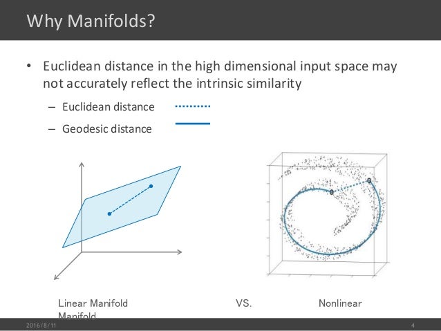
为什么 Dimension Reduction 可能是有用的,如下图示:

      Manifold

      如果我们用 3 dimension 的样本维度去描述他其实是非常浪费的,因为很明显他是卷曲在一起的,如果我们有办法把他展平,不同类型(不同颜色代表不同类型)就很容易区隔开,而展平之后我们只需要 2 dimension 的样本维度。所以根本不需要把这个问题放在 3d 中去考虑,2d 就可以了。

      Manifold and dimension reduction by various methods

      二,例子2

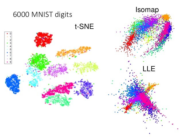
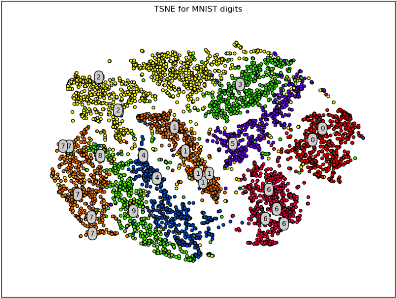
      在手写数字辨识的任务中,你或许根本用不到 28*28 的维度,比如数字 3 他可能有很多形态,但其实大部分都是旋转一下角度而已,所以对于辨识 3 这件事可能需要的维度仅仅是一个旋转角度而已(1维度)

      如何做 dimension reduction 呢?

      对数据降维就是找一个function

      \(f(x) \rightarrow x', dim(x) >> dim(x')\)

      一,方法1: feature selection (略)

      二,方法2:PCA

      基本原理

      PCA 的本质就是通过一个一次线性函数 \(W^Tx\)把高维度的数据样本转换为低维度的数据样本。就像 \(w^Tx\) 如果\(W^T\)矩阵只有一行,这个函数就是两个向量的内积 --- 结果是一个(一维)数值,如果 \(W^T\) 是一个矩阵,那么 \(W^T\) 有多少行最终内积结果就有多少维

      $$ R_W^{1*N} \cdot R_x^{N*1} = R_{x'}^{1*1} R_W^{2*N} \cdot R_x^{N*1} = R_{x'}^{2*1} ... $$

      \(f(x) \rightarrow x', dim(x) >> dim(x')\)

      \(z = Wx, to\ find\ 'W'\)

      找到优化问题 --- projection has max variance

      该如何找到 W 呢,从最简单的开始,我们假设 :

      • reduce x to 1 D vector z, means that 'z' is a digit
      • 'W' matrix only have ONE row
      • this row's L2 norm is equal to 1: \(||w^1||_2=1\).

      如此一来,'z' 就可以看做是 'x' 在 'w' 方向上的投影(内积的几何意义)

      所有的 x: \(x^1, x^2, x^3,...\) 都在 w 方向上做投影就得到了 z: \(z^1, z^2, z^3,...\) , 而我们要做的就是从:

      如何找到 W 变成 找到一个 x 的更好的投影方向

      we want the variance of \(z_1\) as large as possible.

      variance 在图像上的表现就是,投影之后的 z 的取值范围(值域)取值范围越大variance越大

      对于投影到一维空间,找到最佳的 w('w' is a row vector) 使得 x('x' is N dimension) 投影到该方向得到的 z ('z' is a digit)的 variance 是最大的, 用公式表示就是:

      \(find\ a\ w\ to\ maximize:\)

      \(Var(z_1) = \sum_{z_1}(z_1 - \bar{z_1})^2)\)

      \(with\ constaint\ :\ ||w_1||_2=1\)

      对于投影到二维(甚至多维)空间,我们要给每个后面的w一个限制就是: 后面的 w(n+1 th row) 要跟前面的所有 w({1~n} rows) 相互垂直, \(w_{n+1} \cdot \{w_{i}\}_{i=1}^n = 0\).

      整体来看就是:

      the 1st row of W should be:

      \(w_1 = argmax(Var(z_1) = \sum_{z_1}(z_1 - \bar{z_1})^2)\)

      \(constraint:\ ||w_1||_2=1\)

      the 2nd row of W should be:

      \(w_2 = argmax(Var(z_2) = \sum_{z_2}(z_2 - \bar{z_2})^2)\)

      \(constraint:\ ||w_2||_2=1, w_2 \cdot w_1 = 0\)

      the 3rd row of W should be:

      \(w_3 = argmax(Var(z_3) = \sum_{z_3}(z_3 - \bar{z_3})^2)\)

      \(constraint:\ ||w_3||_2=1, w_3 \cdot w_1 = 0, w_3 \cdot w_2 = 0\)

      .......

      then the W should be:

      $$ W = \begin{vmatrix} (w_1)T \\ (w_2)T \\ . \\ . \\ . \end{vmatrix}\quad $$

      这里 W 会是一个 Orthogonal matrix, 因为每一行的 norm 都等于1,并且行行之间相互垂直。

      求解这个带限制条件优化问题 ---- 拉格朗日乘数法

      Lagrange multiplier 可以把带限制条件的优化问题转换>为无限制优化问题: target - a(zero_form of >constraint1) - b(zero_form of constraint2)

      无限制的优化问题,就可以通过偏微分=0来找到最优解

      如果 W 矩阵只有一行

      $$ one\ x\ one\ z_1 \bar{z_1} = \sum{z_1} = \sum{w_1 \cdot x} = w_1 \cdot \sum x = w_1 \cdot \bar{x} Var(z_1) = \sum_{z_1}(z_1 - \bar{z_1})^2 = \sum_x(w_1 \cdot x - w_1 \cdot \bar{x})^2 = \sum_x(w_1 \cdot (x-\bar{x}))^2 $$

      对于 \(w \cdot (x - \bar{x})\), 他是两个向量的内积,对于这种内积的平方,要注意如下的惯用转换公式(值得记住)。

      $$ (a \cdot b)^2 = (a^Tb)^2 $$

      因为 \(a \cdot b\) 是内积,是一个数值,数值的平方无关乎顺序,所以可以写成:

      $$ (a^Tb)^2 = a^Tba^Tb $$

      因为 \(a \cdot b\) 是内积,是一个数值,数值的转置还是自身,所以可以写成:

      $$ (a^Tba^Tb = a^Tb(a^Tb)^T $$

      化简之后:

      $$ a^Tb(a^Tb)^T = a^Tbb^Ta $$

      所以之前 var 的式子可以化简为:

      $$ Var(z_1) = \sum_{z_1}(z_1 - \bar{z_1})^2 = \sum_x(w_1 \cdot x - w_1 \cdot \bar{x})^2 = \sum_x(w_1 \cdot (x-\bar{x}))^2 = \sum_x(w_1)^T(x-\bar{x})(x-\bar{x})^Tw_1 $$

      因为是对 x 来求和,所以 w 可以提出去:

      $$ Var(z_1) = \sum_{z_1}(z_1 - \bar{z_1})^2 = \sum_x(w_1 \cdot x - w_1 \cdot \bar{x})^2 = \sum_x(w_1 \cdot (x-\bar{x}))^2 = \sum_x(w_1)^T(x-\bar{x})(x-\bar{x})^Tw_1 = (w_1)^T(\sum_x(x-\bar{x})(x-\bar{x})^T)w_1 $$

      其中 \(\sum_x(x-\bar{x})(x-\bar{x})^T\) 是什么,这个是 x 向量(样本都是向量)的 covariance matrix. covariance 是对称且半正定对的, 也就是说所有的 eigenvalues 都是非负的

      $$ Var(z_1) = \sum_{z_1}(z_1 - \bar{z_1})^2 = \sum_x(w_1 \cdot x - w_1 \cdot \bar{x})^2 = \sum_x(w_1 \cdot (x-\bar{x}))^2 = \sum_x(w_1)^T(x-\bar{x})(x-\bar{x})^Tw_1 = (w_1)^T(\sum_x(x-\bar{x})(x-\bar{x})^T)w_1 = (w_1)^TCov(x)w_1 $$

      我们设 \(S = Cov(x)\) ,于是我们得到了一个新的优化问题:

      find w1 maximizing:

      \(w_1^T S w_1, with\ constraint\ ||w_1||_2 = 1, means\ w_1^Tw_1 = 1\)

      Lagrange multiplier is target - zero_form of constraints

      之前说明过 \(w_1\) 是 W 矩阵的第一个row,再次提醒下。

      \(g(w_1) =w_1^TSw_1 - \alpha(w_1^Tw_1 - 1)\)

      \(\frac{\partial g(w_1)}{\partial w_{11}} = 0\)

      \(\frac{\partial g(w_1)}{\partial w_{12}} = 0\)

      ....

      通过对 Lagrange 式子 \(g(w_1)\) 的微分为0来求最大最优的w,可以得到如下化简后的式子:

      \(Sw_1 - \alpha w_1 = 0\)

      \(Sw_1 = \alpha w_1\)

      这种形式我们就熟悉了,\(w_1\) 是 S 的 eigen vector

      但是这样的 w1 有很多,因为 S 的 eigen vector 有很多,所以 w1 的潜在选择也很多,哪一个是最好的选择呢?通过我们的优化目标来判断。

      \(w_1^TSw_1 = \alpha w_1^Tw_1 = \alpha\)

      而这里的 \(\alpha\) 是 eigen value,

      所以,因为我们要最大化的目标最后等于 alpha, 而 alpha 是 eigen value, 所以我们选择最大的 eigen value, 一个 eigen value 对应一个 eigen vector, 所以最优的 w1 就是最大的 eigen value 对应的那个 eigen vector.

      之前分析过, Find w2 的情况与 Find w1 略有不同,不同在优化问题的限制条件多出一个与之前所有的w都垂直,那么就是:

      \(Find\ w_2\ maximizing: w_2^TSw_2, w_2Tw_2=1, w_2^Tw_1=0\)

      按照 目标函数 - 系数*zero_form of 限制条件 的拉格朗日使用方法,可以得到如下无限制条件的优化问题:

      如果 W 矩阵有多行

      对于 W 矩阵有多行的情况,优化目标函数需要改变, 要增加限制条件,如果不加改变的话你得到的 wn 永远与 w1 一样,增加的这个限制条件是:后面的每个w都要与前面的所有w相互垂直 --- 内积为0

      \(Find\ w_2\ maximizing:\)

      $$ g(w_2) = w_2^TSw_2 - \alpha(w_2^Tw_2-1)-\beta(w_2^Tw_1-0) $$

      同样的通过微分等于0来求无限制条件的优化问题:

      \(\frac{\partial g(w_1)}{\partial w_{11}} = 0\)

      \(\frac{\partial g(w_1)}{\partial w_{12}} = 0\)

      化简上述结果可以得到:

      \(Sw_2 - \alpha w_2 - \beta w_1 = 0\)

      上述等式两边同时乘以 w1:

      \(w_1^TSw_2 - \alpha w_1^Tw_2 - \beta w_1^Tw_1 = 0\)

      \(w_1^TSw_2 - \alpha * 0 - \beta * 1 = 0\)

      因为 \(w_1^TSw_2\) 本身是一个 向量矩阵向量 的形式,他是一个数值,数值的转置还是自身:

      \(w_1^TSw_2 = (w_1STw_2)^T = w_2^TS^Tw_1\)

      因为 S 是 Covariance Matrix of x, 是对称的,所以 \(S^T=S\)

      \(w_2^TS^Tw_1= w_2^TSw_1\)

      使用 w1 的结论,\(Sw_1 = \lambda_1w_1\), 所以有

      \(w_2^TSw_1=\lambda_1w_2^Tw_1=0\)

      所以,综合起来看:

      \(w_1^TSw_2 - \alpha w_1^Tw_2 - \beta w_1^Tw_1 = 0\)

      \(w_1^TSw_2 - \alpha * 0 - \beta * 1 = 0\)

      \(0 - \alpha * 0 - \beta * 1 = 0\)

      所以:

      \(\beta=0\)

      所以:

      \(Sw_2 - \alpha w_2= 0\)

      \(Sw_2 = \alpha w_2\)

      由于 w2 也是 eigen vector, 同样有很多选择,与 w1 选择的依据一样,我们只能选择剩下最大的那个 eigenvalue of S 对应的 eigenvector

      so,结论是:

      $$ z = Wx $$

      $$ W = \begin{vmatrix} (w_1)T \\ (w_2)T \\ . \\ . \\ . \end{vmatrix}\quad $$

      $$ W = \begin{vmatrix} 1st\ largest\ eigenvalues'\ eigenvector\ of\ Cov(x) \\ 2nd\ largest\ eigenvalues'\ eigenvector\ of\ Cov(x) \\ 3rd\ largest\ eigenvalues'\ eigenvector\ of\ Cov(x) \\ ...\end{vmatrix} $$

      PCA 的副产品 --- 降维后数据点的各个维度互相垂直

      数据点的各个维度互相垂直

      用数学语言来表述就是

      数据点的协方差矩阵是一个 Diagonal matrix

      也就是

      数据点的各个维度之间没有 correlation

      这样有什么作用呢?

      一个很好的作用是,原来的 data 经过 PCA 之后输出的新的 data 可以接其他较为简单的(或是对数据点维度要求无 correlation 的)model ---> eg. Naive Bayes.

      如何证明呢?

      $$ Cov(z) = \sum(z - \bar{z})(z-\bar{z})^T $$

      这一项,可以可以展开合并后成为下面这种形式:

      $$ Cov(z) = \sum(z - \bar{z})(z-\bar{z})^T = WSW^T,\ \ S = Cov(x) $$

      $$ W^T=\begin{vmatrix} w_1 \\ .\\.\\.\\ w_k \end{vmatrix}^T= [w_1, ..., w_k] $$

      注意转置之前 w1 是 W矩阵的行向量,转置后,w1 是 W^T 的 列向量:

      $$ \begin{vmatrix} 1 & 2 & 3 & \rightarrow w_1\\ 4 & 5 & 6 & \rightarrow w_2 \\ 7 & 8 & 9 & \rightarrow w_3 \end{vmatrix}^T \rightarrow \begin{vmatrix} 1 & 4 & 7 \\ 2 & 5 & 8 \\ 3 & 6 & 9 \\ \downarrow & \downarrow & \downarrow \\ w_1 & w_2 & w_3 \end{vmatrix} $$

      $$ WSW^T = WS[w_1, ..., w_k] = W[Sw_1, ..., Sw_k] $$

      利用之前的结论:

      \(Sw_1 = \lambda_1 w_1\)

      $$ W[Sw_1, ..., Sw_k] = W[\lambda_1 w_1, ..., \lambda_k w_k] = [\lambda_1Ww_1, ..., \lmabda_kWw_k] = [\lambda_1e_1, ..., \lambda_ke_k] $$

      其中 \(e_i\) 是指第 \(i\) 位为 1, 其余位都为 0 的列向量。

      所以 \(Cov(z)\) 就是一个 Diagonal matrix.

      总结

      PCA 关键词:

      • linear function, projection
      • maximize Variance of z
      • Covariance Matrix of x
      • eigenvector of Covariance Matrix

      一个重要的结论需要记住: Covariance Matrix is a symmetric, positive-semidefinite matrix, so it has non-negative eigenvalues

      一个重要的技术:

      带限制条件优化

      --- Lagrange multiplier ---> 无限制条件优化

      --- partial dirivitive = 0 --->

      求解。

      一个重要的机器学习常识:

      数据点的各个维度互相垂直

      用数学语言来表述就是

      数据点的协方差矩阵是一个 Diagonal matrix

      也就是

      数据点的各个维度之间没有 correlation

    3. Unsupervised learning - Linear Methods

      Ordinary Clustering

      1. random choose K data point as initial centers
      2. compute the distance of each sample, choose the label of center which has smallest distance between
      3. update the cluster who add-in new element by

      \(b_i^n = 1\ if\ x^n\ is\ most\ close\ to\ c_i,\ else\ 0\)

      \(c_i = \sum_{x^n}b_i^nx^n/\sum_{x^n}b_i^n\)

      Hierarchical Agglomerative Clustering(HAC)

      一, build a tree

      1. 所有 example 两两计算相似度(similarity)
      2. 选相似度最高的两个,并把它们 merge 在一起(具体方式可以使用平均 \(v_{new} = \frac{1}{2}(v_1 + v_2)\)),这样就得到一个同维度的新向量样本
      3. 然后再重复步骤2,choose -> merge -> new vector

      把原来的样本都看作叶子节点,merge 后的样本看成父亲节点,这样一直做下去直到产生root,这样就构成了一棵树。

      二,pick a threshold

      这一刀切在哪里就决定了你有多少个分类。比如下图所示,在第二层节点下切一刀就产生出四个簇。

      HAC - 4 clusters

      Distribution Representation

      如果只做 clustering 就像是我们做的非黑即白假设一样,未免过于武断,所以这里引入了Distribution representation .

      英雄包含7个种类: [强化系,放出系,变化系,操作系,具现化系,特质系]

      • Cluster Representation: clustering 方法要求所有样本都属于并且必须只能属于一个簇,

        \(Noxus\ of\ LOL \in Strength\)

      但有时候这样做未免武断,所以考虑用概率分布的形式来表示一个样本,同时这种表示样本的方法也可以用在 Dimension reduction 中。

      • Distribution Representation: [0.7, 0.25, 0.05, 0.0, 0.0, 0.0, 0.0]

        Distribution Representation 还一个作用,就是用作降维。这个东西与 Dimension reduction 有莫大的关系,对于一个有很高维度的向量样本而言,如果我们用一些特点来描述他,那就可以大幅度的减少样本的维度。

    4. semi-supervised 经典假设-2:Smoothness Assumption

      半监督学习的第一个假设是 非黑即白,进阶版是未必非黑即白,也差不多,基于这个假设我们有了算法 self-training(hard-label) 和 entropy-based regularization。

      半监督学习的第二个知名假设是 近朱者赤,近墨者黑

      不精确的说法: Assumption: "similar" x has the same y.

      精确的说法:

      1. x is not uniform.
      2. if x1 and x2 are close in a high density region, y1 and y2 are the same.

      解释下上面这句话的意思:

      如果 x 的分布是不平均的,有些地方很集中,某些地方很分散。如果两个 x 样本,x1 x2 在一个高密度区域内很近的话,那么他们的标签应该一样。

      一言以蔽之,相近一个必须的前提是:这两个点必须经过一个稠密区间相连。 connected by high density region.

      形象一点该如何理解 稠密区间 呢?也就是一个样本和另一个样本之间存在连续的渐进变换的很多样本,那么就说明两者之间存在稠密区间。

      举例说明:

      1 <====> 11 <-------> 15

      1, 2, 3, 4, 5, 6, 7, 8, 9, 10, 11, ___, 15

      • <====> 表示这里有很多渐变的无标数据点
      • <-------> 表示这里几乎没有无标数据点
      • 只有 1 和 15 是带标数据,其他都是无标数据。

      我们如何判断无标数据 11 的标签?

      ‘1’ 和 ‘11’ 之间存在稠密区间,则两者的label应该是一样的。‘11’ 和 ‘15’ 之间不存在稠密区间。

      这招在文档分类中,作用颇大。Classify astronomy vs. Travel articles.我们做文档分类是基于文档的vocabulary是否存在较大重叠,但是由于人类使用的词汇是如此的多,不同的人对同一个意思会使用不同的词汇去表达,所以文档之间的单词重叠的非常少,这时候就可以借助high density region的假设,只要两个文档之间(一个带标一个无标)存在连续的渐变的很多文档,就可以判断两个数据点具有相同的标签。

      天文:文档1 = [asteroid, bright]

      _ :文档2 = [bright,comet]

      _ :文档3 = [comet,year]

      _ :文档4 = [year,zodiac]

      文档1 与 文档2 标签一致;

      文档2 与 文档3 标签一致;

      文档3 与 文档4 标签一致;

      所以 文档1 与 文档4 标签一致;

      平滑假设下的 smei-supervised 算法框架

      一,构建 pseudo 数据集阶段

      1. 获取 pseudo labels of unlabeled dataset by smoothness assumption and labeled dataset
      2. 将 pseudo label 当做真实 label, 完成数据集构建

      二,supervised learning 算法阶段

      1. function set
      2. loss function
      3. minimize (2) to get the best function from (1)

      一,构建 pseudo 数据集阶段

      平滑度假设下的 pseudo label 获取算法1:cluster and then label

      1. 首先不论带标还是不带标,都当做无标数据点做 clustering。
      2. 做完之后,看每个 cluster 中哪种label的数据点最多,这个 cluster 的所有点就属于这个label。

      注意:clustering then label, 这个方法未必会有用啊,只有在你可以把同一个类 cluster 在一起的时候才有可能有用,如果是图像分类并且用 pixel 做clustering,就非常苦难,基于像素的距离做 clustering 本身就不太可能把同一类 cluster 在一起(同一个 class 可能在像素级别很不像,比如数字识别中像‘1’的‘4’和像‘9’的‘4’;不同 class 可能像素级别很像‘1’和‘4’,‘9’和‘4’),这第一步误差就这么大(各种分类的数据点混在一起),第二步不论怎么搞都不可能有太好的准确率。

      所以,如果要用这个 cluster then label 算法的话,你的 cluster 要非常强,也就是第一步的准确率要足够高。一般使用 deep autoencoder 中间的 code 做 cluster,而不是像素。

      平滑度假设下的 pseudo label 获取算法2:graph-based approach

      cluster, then label 是一种比较直觉的做法,另一种做法是通过引入 graph structure 来做。用 graph structure 来表达 connected by a high density path 这件事

      数据集映射成一个 graph, 每个数据都是图中的一个点。你要做的就是定义并计算两两之间的 similarity,这个similarity就是 graph 中两点之间的边(连线)。

      构建graph之后:

      1. 相连 --- 同类
      2. 不连 --- 不同类

      但是 similarity 也就是 “边” 很多时候不是那么明显的可以定义出来。如果是网页分类,那么网页之间的连接可以看做是一种similarity(医疗的网页应该不会连接到游戏网页),这很直觉。论文分类,论文的索引也可以用在“边”。但更多时候,你需要自己去定义。

      算法2 该如何构图

      graph construction: 该如何构造一张图呢?

      一, define the similarity \(s(x_i, x_j)\) between xi and xj.

      (可以基于像素或者更高阶的方法是用 deep autoencoder 来做相似度),李宏毅教授推荐使用 RBF function 定义相似度:

      \(s(x_i, x_j) = exp(-\gamma||x_i - x_j||^2)\)

      如果想使用欧几里得距离衡量相似度,最好使用 RBF function 作为 similarity function. 为什么呢?因为RBF是一个衰减很快的函数,只要 xi xj 距离稍微远一点相似度就急剧下降。只有具备这种性质,你才能构造出较好的 cluster,他虽然不能保证同簇的相似度高,但至少可以保证不同簇的相似度一定较低(跨簇的距离更大一些的话)。

      二, add edge

      方法1: 可以使用 KNN 建立“边”,每个点都与相似度最近的 K 个点相连: \(|V_{x_i->[x_j]_{j=1}^K}| = argmax_{D'\subset{D}, |D'|=K}s(x_i, x_j)\)

      方法2: 可以使用 e-Neighborhood 方法建立“边”,所有与 xi 相似度大于 e 的数据点都与 xi 建立连接。

      三,edge weightedge

      可以带有权重,他可以与相似度成正比。

      graph-based approach 方法的核心精神标签传染: graph 中的带标节点会依据“边”来传递自己的“标”,而且会一直“传染”下去。

      graph-based approach 方法的核心缺点数据量必须够大: 基于图的传染机制,如果数据不够多,没收集到位,那么本来相连的图由于数据量不够就可能断连,一旦断连就没法传染了。

      二,supervised learning 算法阶段

      1. function set --- defined by DNN
      2. loss function --- defined below
      3. optimize: train DNN

      我们基于以下认知和观察,来定义 loss functin 用以衡量 DNN 训练出的模型的好坏:

      1. 是否可以直接使用 cross-entropy,不加任何“佐料”?

      2. pseudo labels 是在近朱者赤近墨者黑的假设下产生的,不管产生的算法是什么,他都可以看成是一个函数,这个函数是如此特殊他就像是ground truth function(监督学习下,我们不知道的那个f) 一样产生了我们以为真实的标签,所以,我们需要做的是去逼近这样的函数

      3. 我们能做的是,通过 loss function 来“诱导”优化器往这个特殊的函数去优化。

      4. 我们像产生 pseudo labels 的算法那样利用数据集 x 的距离模拟 density 来增加限制,但我们可以通过对标签来近似这种限制,我们可以看到同一个类的标签之间差距很小类和类之间的标签差距很大,但是(构造 pseudo label 时用到的边的weight)同类数据点的边的weight很大,而不同类的数据点的边的weight很小。我们设置两点之间的标签差值乘以两点之间的边的权重作为限制, 希望他不要太大,以此来近似同类标签数据是高密度的这件事,虽然这是一种普杀式的限制 --- 他同样会限制类间标签的差异,但是考虑不同类两点的边权重很小,相乘之后影响较少,这种方法还是可以接受的。

      \(S = \frac{1}{2}\sum_{i,j}w_{i,j}(y_i - y_j)^2\)

      这个值越小,说明越平滑。

      进一步化简这个公式,用矩阵的形式书写(引入 Graph Laplacian):

      把带标和无标的(预测)标签拼在一起,形成一个长向量: \(\vec{y} = [...y_i, ..., y_j...]^T\)

      \(S = \frac{1}{2}\sum_{i,j}w_{i,j}(y_i - y_j)^2 = \vec{y}^TL\vec{y}\)

      L: (R+U) * (R+U) matrix

      L 可以写成两个矩阵相减: \(L = D - W\)

      • W 是两两节点之间的“边”的权重矩阵
      • D 是把 W 矩阵每行值相加放在对角线上,其余设为0.形成的矩阵。

      现在把这个 smoothness 公式与loss-fn 统合起来,形成一个新的代价函数:

      \(L(\Theta) = \sum_{x^r}C(y^r, \hat{y}^r) + \lambdaS\)

      这个 \(\lambdaS\) 有点像是一个正则项,你不仅仅要调整data 让那些 label data 与真正的 label 越接近越好,同时还要做到你预测的标签(包括代标数据和无标数据)要足够平滑。

      在 DNN 中 smoothness 的计算不一定是在 output layer 哪里才计算,而是在任何隐含层都可以(就像 L2 正则项可以加载任何层一样,keras API)可以从某一层输出接触一个 embedding layer 保证这个 embedding layer 是 smooth 的即可, 也可以完全套用 L2 的模式 --- 在每一个隐含层都加入这个正则项,要求每一层的输出都是 smooth 的。

      J.Weston, F.Ratle, "Deep learning via semi-supervised embedding," ICML, 2008

      注意事项1: 两个 similarity

      上面的算法框架中出现过两次 similarity 公式:

      1. 第一次在产生 pseudo 数据集部分的 graph-based 算法中。
      2. 第二次在监督式方法训练部分的 定义 loss function 中。

      其中产生 pseudo 数据集部分,‘similarity’ 是 “similarity of x” --- 计算两个点之间的距离(eg,RBF function)以此作为是否连线两点的依据,而距离作为边的权重。

      而在训练模型的部分,‘similarity’ 是 ‘similarity of y’ 我们用 y 之间的距离不宜过大来近似 'similarity of x'

    5. lec 12 总结

      注意事项2:两个假设

      Semi-supervised 部分我们介绍了两个假设,

      • 其一为 low density separation;
      • 其二为 high density region.

      两个假设都是为了通过有标数据产生无标数据的标签。这一步仅仅是准备数据集,并没有训练任何模型,他就像是监督学习中,产生数据集的那个我们不知道的函数

      而我们在训练模型时,必须要考虑到这个特殊的“函数”,也就是我们训练模型的时候需要让给与训练过程一些限制,让优化器朝着这两个假设的方向去优化函数:

      • 在 low density separation 假设中,我们对模型做的做的改进是仅仅使用非黑即白的标签作为无标数据的“真实”标签,更进一步改进“未必非黑即白,但也差不多”,是给 Loss function 加入 entropy based 正则项来约束模型预测的标签使其更集中

      \(L = \sum_{x^r}C(y^r, \hat{y}^r) + \lambda\sum_{x^u}E(y^u)\)

      • 在 high density region 假设中,我们对模型做的改进是给 Loss function 加入 smoothness 正则项来约束模型预测的标签使其更平滑。

      \(S = \frac{1}{2}\sum_{i,j}w_{i,j}(y_i - y_j)^2 = \vec{y}^TL\vec{y}\)

      \(L(\Theta) = \sum_{x^r}C(y^r, \hat{y}^r) + \lambdaS\)

      三种产生标签(产生数据集)的方式对比

      1. semi-supervised learning for generative model
      2. semi-supervised learning under low density separation assumption
      3. semi-supervised learning under high density region assumption

      EM 系算法产生标签(边产生边更新) -----

                      |--- 生成模型: 初始化prior proba, 预测无标,更新 prior proba
                             |--- 归纳学习,产生model,标签为实数 
      
      
                      |--- low density separation: 用带标产生 f,预测无标,更新 f
                             |--- 归纳学习,产生model,标签为整数
      

      非 EM 系算法产生标签(先构造后产生)----

                      |--- high density region using **cluster and label**: 先构造簇,整簇分为标签最多者
      
                      |--- high density region using **graph-based algo**: 先构造图,相连的分为一类(同标签)
      
    6. looking for better representation

      去芜存菁,化繁为简

      他的核心要旨是:我们所见的世界虽然很复杂,但在复杂背后隐含着比较简单的要素(factor)在操控复杂的世界,如果能窥见一二就可以搞定。

      这个 latent factors 就是 better representions.

    7. semi-supervised 经典假设-1:Low-density Separation Assumption

      low-density separation 这个假设的意思是说非黑即白, 亦即两个class的数据点之间有一条明显的鸿沟,亦即两个class之间的data量是很少的

      Low-density Separation Assumption 最具代表性的算法就是 self-training

      self-training 算法
      1. Labeled data set and unlabeled dataset
      2. repeat from step 3 to step 5:
      3. train model f* from labeled data set, 你用什么方法去 train 这个无所谓,可以用任何方法只要能train一个model出来即可。
      4. 根据 f* 去给不带标签的数据打标签(pseudo-label)
      5. 从不带标签数据集中挑选出一些数据经过步骤 2.2 获得 label 并加入 labeled data 数据集中。比如你可以根据 pseudo-label 的置信度(比如经过 softmax 的概率值)来给 data 加入 weight

      关于这个 self-training 算法的几个注意点

      毫无疑问, regression 问题无法使用self-training

      self-training 是从带标数据集得到一个函数 f, 然后用这个函数去求一个值 y = f(x), x是无标数据, 然后再把这个 (x,y) 加入代标数据集中,这个 y 本身就是通过 f(x) 得到的,他怎么可能改变 f 呢。所以 f 根本就不会变。所以 regression 不能使用这个算法来做。为什么呢,因为 regression 得到的是一个实数,而不是离散的分类。

      self-training( 半监督学习 Low density 假设下的算法) 算法看起来跟 EM (semi-supervised for Generative model)算法很不一样

      两者看起来相似:

      1. 先算出一个模型
      2. 通过模型预测无标数据的标签
      3. 无标数据标签会反噬原模型更新为的模型。

      EM-generative model算法(KNN算法,transductive 学习通用框架):

      1. 模型:任意初始化一个先验概率模型 P(x|C), P(C) 等
      2. 预测:用这些先验概率通过 bayes 预测无标数据点的标签
      3. 反噬:由于步骤2产生了新的带标数据,所以带标数据集改变了,P(x|C), P(C) 的值肯定也就改变了,更新之。

      self-training 算法:

      1. 模型:通过带标数据训练一个模型 f
      2. 预测:利用 f 得到无标数据的标签
      3. 反噬:将新产生的标签当做新的带标数据加入数据集,并重新训练 f。

      两者的不同在于,

      • generative model 算法使用的是 Soft label(更新先验概率(model)的时候我们都是使用unlabeled data能近似多少个labeled data的思想),
      • self-training 算法使用的是 Hard-label.

      举例:

      • f(x)= [0.3, 0.7] 对于 hard-label, 新产生的带标数据(x,y) 是 (x, [0,1])
      • f(x)= [0.3, 0.7] 对于 soft-label, 新产生的带标数据(x,y) 是 (x, [0.3, 0.7])

      毫无疑问,如果是 self-training 使用 DNN 来训练的化, soft-label 完全没用啊,这点和 regression 问题无法使用 self-training 的道理是一样的。你的标签本身就是你的NN得到的一模一样的值,你重新将其加入数据集,他根本不会更新 NN 的参数。

      核心本质:

      我们使用 Hard-label 时我们在使用什么?我们在使用假设 Low density separation* --- 非黑即白中间地带无数据**.

      self-training (hard-label)进阶版: Entropy-based Regularization

      如果觉得非黑即白太武断了,可以使用 Entropy-based Regularization 方法

      Entropy-based regularization 的意思是 未必非黑即白但也差不多啦

      以刚才的例子来说明:

      • f(x)= [0.3, 0.7] 对于 hard-label, 新产生的带标数据(x,y) 是 (x, [0,1])

      这样规定x的标签太武断了,我们希望标签还是可以保留一些小数,亦即NN的输出还是一个正常的概率分布,但不能是下面这样:

      • f(x)= [0.4, 0.6] 对于 hard-label, 新产生的带标数据(x,y) 是 (x, [0.4, 0.6])

      我们希望可以通过加入某种限制,来实现增加区别度使概率分布更集中的目标。这个限制叫做 entropy of distribution. 他可以告诉我们这个分布集中与否。

      entropy 值越小说明越集中(激光小且集中),最小为0

      \(E(y^u) = - \sum_{m=1}^Uy_m^uln(y_m^u)\)

      根据这个假设,我们可以重新设计 loss-function

      labeled data:

      \(L = \sum_{x^r}C(y^r, \hat{y}^r)\)

      unlabeled data(这里是说之前讨论的通用算法框架步骤2中的预测无标数据的标签):

      \(\lambda\sum_{x^u}E(y^u)\)

      我们希望NN对于无标数据的预测结果(一个概率分布)应该越集中越好。

      综合起来看,就是如下公式:

      \(L = \sum_{x^r}C(y^r, \hat{y}^r) + \lambda\sum_{x^u}E(y^u)\)

      self-training (hard-label)进阶版: Semi-supervised SVM

      参考论文:transductive inference for text classification using SVM

      核心精神就是,

      1. 穷举全部无标数据所有可能的标签组合, 2.(联合带标数据)就组成一种数据集 \(D_i\), 对每一种组合对应的数据集 \(D_i\)都做一次 SVM, 得到一个 \(f^{\star}_i\)。
      2. 对于所有的 \(\{D_i, f^{\star}_i\}\) pair,看哪一个pair分的最好(最大margin且最小error)。就选取这个 \(f^{\star}\) 作为最终模型

      遗留问题:

      穷举 怎么做?论文中给出了一个近似的方法,每次该一个无标数据点的标签,看看 SVM 是否会变好,如果可以的话就改。

    8. why semi-supervised learning?

      • 收集数据简单,收集标签困难
      • 作为人类,我们的学习方式也是 semi-supervised learning --- 从课堂到自学,从老师到无师。

      unlabeled data 虽然只有数据没有标签,但是 unlabeled data 的分布可以告诉我们一些东西。比如可以告诉我们什么样的边界是更好的。

      semi-supervised learning 使用 unlabeled data 的情况经常伴随一些假设。semi-supervised learning 有没有效果就取决于你的假设好不好。

      semi-supervised learning 未必有用,这取决于你的假设是否足够好。

      semi-supervised learning for Generative Model

      回忆之前讲过的 Supervised Generative Model, 我们假设每一个 class 的数据点的分布都是一个 gaussian distribution(类的分布共享 \(\Sigma\)):

      \(P(x|y_1) \sim G(\mu_1, \Sigma)\) \(P(x|y_2) \sim G(\mu_2, \Sigma)\)

      得到 prior proba 然后就可以根据公式得到 posterior proba:

      \(P(y_1|x_{new}) = \frac{P(x_{new}|y_1)P(y_1)}{P(x_{new}|y_1)P(y_1) + P(x_{new}|y_2)P(y_2)}\)

      对于 semi-supervised Generative Model, 由于我们多了很多 unlabeled data, 这回改变我们对原来(仅仅通过 supervised Generative Model)获取的分布的认知。就像 KNN 每个新来的数据都会改变原来的中心点的位置。

      算法

      1. Initiliazation: \(\Theta = \{P(C_1), P(C_2), \mu_1, \mu_2, \Sigma\}\)
      2. step1: compute the posterior probability of unlabeled data: \(P_{\Theta}(C_1|x^{\mu})\)
      3. step2: update model:

      3.1 update prior proba:

      \(P(C_1) = \frac{N_1 + \Sigma_{x^{\mu}}P(C_1|x^{\mu})}{N}\)

      \(N\): total number of examples

      \(N_1\): number of examples belonging to C1

      \(x^u\): unlabeled data

      这里注意,supervised learning 中计算 \(P(C_1)\)的公式是:

      \(P(C_1) = \frac{N_1}{N}\)

      现在需要考虑 unlabeled data 对于分类的贡献。

      我们可以把 Posterior praba \(P(C_1|x^u)\) 近似的理解成 (xu贡献的)C1的出现次数,毕竟概率也可以看做是(0.7个,0.5个。。。),我们只要加总所有样本对于 C1 的后验概率,就可以将其近似的理解成 unlabeled data 贡献的分类数据。

      \(\Sigma_{x^{\mu}}P(C_1|x^{\mu})\)

      3.2 update \(\mu_1\)

      这里注意,supervised learning 中计算 \(\mu_1\)的公式是:

      \(\mu_1 = \frac{1}{N_1}\Sigma_{x^r\in{C_1}}x^r\)

      现在需要考虑 unlabeled data 对于分类的贡献。

      对于 unlabeled data 我们同样需要借用 posterior probability 来计算 unlabeled data 的 weighted sum 的平均。

      \(\frac{1}{\sum_{x^u}P(C_1|x^u)}\sum_{x^u}P(C_1|x^u)x^u\)

      1. back to step 2

      理论上这个方法会收敛,但是初始值对结果的影响非常大。同时这个方法也可以理解为 EM 算法。

      maximum likelihood of unlabeled data vs. that of labeled data

      两者最大的区别是前者只能通过 EM 算法进行 iteratively 解;后者有公式解。

      我们是通过【 Maximum likelihood 来找到分类为 Ci 的样本点的最有可能的高斯分布】来求得 Prior proba \(P(x|C_i)\), 我们优化的公式很好解:

      \(logL(\Theta)=\sum_{x^r}logP_{\Theta}(x^r, \hat{y}^r)\)

      但是对于 unlabeled data 我们怎么估测 \(logL(\Theta)\) 呢?

      \(logL(\Theta) = \sigma_{x^r}logP_{\Theta}(x^r) + ?\)

      这里的思想与【把\(P_{\Theta}(C_i|x^u)\)看做 \(x^u\) ‘贡献’的‘次数’】思想类似,只不过利用的是 Prior probability因为我们并不知道 \(x^u\)的分类是多少,所以他可能属于任何分类

      所以这里 \(P_{\Theta(x^u)}\) 应该等于 \(x^u\) 与每个分类的联合概率的和:

      \(P_{\Theta}(x^u)=P_{\Theta}(x^u|C_1)P(C_1) + P_{\Theta}(x^u|C_2)P(C_2)\)

    9. Introduction

      Unlabeled data: \(U\), from \(u=R\) to \(u=U+R\)

      Labeled data: \(R\), from \(r=1\) to \(r=R\)

      Supervised learning:

      \( \{(x^r, \hat{y}^r)\}^R_{r=1}\)

      Semi-supervised learning:

      \( \{(x^r, \hat{y}^r)\}^R_{r=1}\) ,\(\{x^u\}^{R+U}_{u=R}\)

      • U >> R
      • Transductive learing: unlabeled data is the testing data.
      • Inductive learning: unlabeled data is not the testing data.

      直接使用 testing data 不是作弊么,李宏毅老师说,使用 label of testing data 才是作弊。

      transductive learning 的典型算法是 KNN,对于 unlabeled data 我们计算其距离各个中心点的距离。然后重新计算该簇的中心点。可见我们确实使用了 unlabeled data 来学习模型。

      以 kaggle 竞赛为例,有些 kaggle 竞赛是直接可以下载 testing dataset 的,只是 testing data 没有 label 而已。

    10. 如何解决分类问题无法微分

      1. perceptron(introduce in future)
      2. SVM(introduce in future)
      3. generative model: probability based method(introduce here)

      基于概率(Bayes)的分类问题解法 --- 生成模型:

      蓝盒子,绿盒子,其中各置5个球,球也有蓝色和绿色。已知:

      1. 蓝盒:4蓝 + 1绿
      2. 绿盒:2蓝 + 3绿

      问:现抽出一蓝球,问他来自两个盒子概率各是多少:P(blueBox | blueBubble)=?

      这个问题使用 bayes 条件概率公式非常好求,只需要知道四个值

      1. Prior of blueBox: \(P(blueBox)\)
      2. Priof of greenBox: \(P(greenBox)\)
      3. condition probability of blueBubble given blueBox: \(P(blueBubble | blueBox)\)
      4. condition probability of blueBubble given greenBox: \(P(blueBubble | greenBox)\)

      类比:

      蓝盒子 --- class 1;

      绿盒子 --- class 2;

      class 1,class 2,各有很多样本。已知:

      1. class 1:海龟,金枪鱼,
      2. class 2:老鹰,白鸽,

      问:现有一鸭嘴兽,问他来自两个分类的概率各是多少?

      我们同样需要知道 4 个值

      1. Prior
      2. Prior
      3. condition prob
      4. condition prob

      counting based method for Prior

      从训练集中,直接“数”出标签为 C1 的样本数量,和标签为 C2 的样本数量各是多少,记做 N1 , N2.

      \(P(C1) = N1/(N1 + N2)\)

      \(P(C2) = N2/(N1 + N2)\)

      naive bayes method for condition probability

      分类问题中的条件概率不同于“盒子抽球”的最大地方在于:你要计算的 \(P(x|C1)\) 中的 x 是现有样本集中没有的

      把当前 c1 样本 和 c2 样本都想象成概率分布,而当前数据集仅仅是根据概率分布做的抽样(全体中的部分)

      如果我们能得到这个概率分布,我们就可以知道鸭嘴兽属于陆生和海生的概率各是多少。

      假设:c1 和 c2 的概率分布是高斯分布,且他们都是高斯分布集合( gaussian distribution hypothesis )中的一个 gaussian distribution, 我们该如何找到这个高斯分布呢 --- 只需确定 \(\Sigma\) 和 \(\mu \), 就可以唯一确定一个高斯分布。

      那如何通过样本来倒推出 \(\Sigma\) 和 \(\mu \) 呢?

      maximum likelihood

      找到一个 \(\mu, \Sigma\) ,由他确定的高斯分布在所有的高斯分布中,产生数据集的概率是最高的。

      \(f_{\mu,\Sigma}(x) = \frac{1}{(2\pi)^{D/2}}\frac{1}{|\Sigma|^{1/2}}exp(-\frac{1}{2}(x-\mu)^T\Sigma^-1(x-\mu))\)

      \(L(\mu,\Sigma) =f_{\mu,\Sigma}(x^1)f_{\mu,\Sigma}(x^2)f_{\mu,\Sigma}(x^3)......f_{\mu,\Sigma}(x^N)\)

      \(\mu^\star, \Sigma^\star = \arg\max_{\mu,\Sigma}L(\mu,\Sigma)\)

      这个 \(argmax\) 有一个很直观的公式解,可以直接记住:

      \(\mu^\star = \frac{1}{N}\sum_{n=1}^{N}x^n\)

      \(\Sigma^\star = \frac{1}{N}\sum_{n=1}^{N}(x^n-\mu^\star)(x^n-\mu^\star)^T\)

      Naive Bayes

      如果不适用极大似然估计,也可以使用 Naive Bayes 方法来推算 Prior probability.

      \(P(y|x) = \frac{P(x|y)P(y)}{P(x)=\sum^K_{i=1}{P(x|y_i)P(y_i)}}\)

      通过 count-based methodNaive Bayes(

      \(P([1,3,9,0] | y_1)=P(1|y_1)P(3|y_1)P(9|y_1)P(0|y_1)\) ) 先计算出:

      \(P(x|y_1)P(y_1)\)

      \(P(x|y_2)P(y_2)\)

      \(P(x|y_3)P(y_3)\)

      ...

      All done

      一旦得到了这个 \(\mu,\Sigma\) 我们就可以得到分类1 产生 x 的概率(即便他不存在于数据集中)的概率:

      \( P(x | C_1) = P(x | Gaussian_1(\mu_1, \Sigma_1))\)

      分类2 产生 x 的概率, 也很容易得到:

      \( P(x | C_2) = P(x | Gaussian_2(\mu_2, \Sigma_2))\)

      根据 bayes 公式:

      \(P(C_1 | x) = \frac{P(x | C_1) * P(C_1)}{P( x | C_1) * P(C_1) + P(x | C_2) * P(C_2)}\)

    11. 卷积层(strides!=(1,1))输出形状推算

      \(width_{output} = \frac{width_{img} - width_{kernel} + width_{padding}}{width_{strides}} + 1\)

    12. 注意 keras 处理 CNN 的形状

      在 keras 中 fit 给 CNN 的数据集的形状必须是:

      theano: (-1, channel, height, width)

      tensorflow: (-1, height, width, channel)

      如果不是必须reshape到这个形状,第一层卷积层的声明一般为:

      model.add( Conv2D(kernelNum, (kernelHeight, kernelWidth), input_shape=(dataPointChannel, dataPointHeight, dataPointWidth), data_format='channels_first'))

      切记,切记

    13. Normalization

      一列数字,如果每个数字都减去平均值,则新形成的数列均值为0.

      一列数字,如果每个数字都除以标准差,则新形成的数列标准差为1.

      如果我要构造一个均值为0,标准差为 0.1 的数列怎么做?

      1. \(x_i \leftarrow x_i - \mu\)

      2. \(x_i \leftarrow x_i / \sigma\)

      3. \(x_i \leftarrow x_i * 0.1\)

      经过这三步归一化的动作,既能保持原来分布的特点,又能做到归一化为均值为0,标准差为 0.1 的分布。

    14. Why deep is better?

      deep means 模组化(modularize)

      模组化的意思是不直接解原始问题,而是找到一些中间量作为推论'桥'再过渡到原始问题。

      每多一层隐含层,就多了一次 萃取推理

      1 hidden layer: 原始数据 -> 解析特征 -> 通过特征推理结果

      2 hidden layer: 原始数据 -> 解析特征的特征 -> 通过特征的特征推理特征 -> 通过特征推理结果

      ...

      每多一层隐含层,就多了一次抽取特征通过特征进行推理

      实例说明:

      四分类问题,把样本分成四类:

      1. 长发男(样本极少)
      2. 长发女
      3. 短发男
      4. 短发女

      no hidden layer: dataset -> [1|2|3|4]

      很显然,由于分类1的样本太少,分类器处理分类1的错误率就会很高。整体错误率也会较高。

      1 hidden layer: dataset -> [长发|短发] + [男|女] -> [1|2|3|4]

      这样一来,就可以避免某些样本过少会削弱分类器的问题,虽然长发男很少,但是长发vs短发两者几乎相等,男vs.女也几乎相等,也就是 [长|短] 分类器和 [男|女] 分类器都很强。

      把这两个子分类器的结果作为新的样本(new dataset)学出[长发男]的分类器也就很强。

      模组化(modularize) 在这里就是指可以直接利用子分类器的结果作为新的输入,这就有点像是\(f(g(h(x)))\)一样。

      可是实现 end to end learning

      deep learning 可以只给出 input(样本) 和 output(标签) 而我们并不参与中间具体函数的设计,这些具体的函数是自动学出的,这就是 end to end learning。

      可以实现 complex task

      现实问题中经常会遇到:

      • 很相似的输入,输出却大相径庭

      哈士奇和狼的图片作为输入,标签一个是狗,一个是狼

      • 很不同的输入,输出却完全一样

      正面的火车和侧面的火车作为输入,标签却都是火车

      如果你的NN只有一层,你大概只能做简单的转换,没办法形成层次结果和复用。

    15. 什么样的情形可以使用 CNN

      记忆: 小抠样

      记忆:small, regions, subsampling

      • 某些pattern远小于整张图片

      这个是说 filter 一般采取小于整张图片的形状

      • 同样的pattern出现在图片的不同位置

      这个是说 filter 会逐行逐列移动扫描整张图片

      • subsampling 没有什么影响

      这个是说 pooling 是切割图片为多块,每块只取一格(1 pixel)

      关于 subsampling

      这里的意思是说,对于 featuremap 如果池化层 size = 2*2 , maxpooling 会只去最大的一个值(averagePooling 会取平均,但也只是一个值)而忽略其他值。这件事情的物理意义是:featuremap 是由 filter 扫描整张图片得到的,某个pattern(pattern较大,stride较小时)可能被多次扫描到并体现在 featuremap 中类似于 \([0,1,2,5,2,1,0]\),直接丢弃这种长尾效应对判定该某个pattern的位置以及匹配程度是没有任何影响的,他完全可以被最大的那个 5 hold住。

      长尾效应的取舍

      围棋(连续型pattern) vs. 图像识别(离散型pattern)

      图像识别就是这种最大值可以完全hold位置以及匹配程度信息的任务。可是对于其他任务比如围棋,他的核心任务虽然也是识别某个模式,但长尾效应尾部是有作用的。

      在图像识别中被识别的模式是独立的或者叫离散的 --- 一个圆的是形状是眼睛,3/4个圆就不是眼睛了。在围棋中 \([0,1,2,5,2,1,0]\) 那些\(0,1,2\)对判断当前棋子所处的状态是有影响的,甚至他可能更重视长尾效应中的

      结论

      所以,对于是否使用 maxpooling 层要根据你的具体任务来做具体对待:

      • 当任务识别的pattern‘’比较离散”---目标仅仅是寻找和定位pattern,别无其他 适合加上 maxpooling,让模型更专注,也让模型参数更少。

      • 当任务识别的pattern“比较连续”---长尾效应之尾会影响任务目标 最好不加 maxpooling,这样模型可以保存更多现场信息,让结果更精确。

      像围棋这种任务,显然就不能使用纯粹的CNN(包含 maxpooling),所以 alpha-go 中没有使用 maxpooling.

    16. 从可视化某个filter or neuron的激活度到deepdream

      google 的 deepdream 的核心思想就是借用最大化某个filter or neuron.不同的是 deepdream 不是单纯“最大化某filter or neuron的输出”,而是针对某让该层神经元原本输出大的更大,原本输出小的更小。,亦即,

      CNN of deepdream exaggerates what it sees

      assume output of k-th hidden layer is

      \(output_k = [3.9, -1.5, 2.3, ...]\)

      正的扩大,负的缩小

      \([3.9\Uparrow, -1.5\Downarrow, 2.3\Uparrow, ...]\)

      成为

      \(output_k' = [10, -5, 8, ...]\)

      以其为目标,找到 \(x^\star\)

      \(x^\star = argmin_x(output_k - output_k')\)

      从 deepdream 到 deepstyle

      之前都是只考虑了输出这件事,不论是 filter or neuron 还是某一层 hidden layer 我们关注的都是输出。现在如果我们把filter 和 filter 之间的 correlation 纳入考虑范畴。就可以实现风格迁移,这就是 deepstyle 的核心思想。

      1. 一个训练好的 CNN,输入某张图片,获取某一层 hidden layer 的输出(取内容);

      2. 一个训练好的 CNN,输入某张图片,获取某一层 hidden layer 的correlation(取风格);

      目标是:找到一个 \(x\),他经过CNN得到的相同层 hidden layer 的内容像步骤1中的;风格像步骤2中的。

    17. 如何展示某个 filter 学到了什么

      也就是什么样的图片可以让 filter 被激活(度高)

      定义: 核的激活度

      Degree of the activation of k-th filter, 核激活度表示这个 filter 被激活的程度, 他等于该filter输出的 featuremap 矩阵的所有元素的和(一个 filter 只会生成dim=1的featuremap)。

      \(k-th\ filter\ is\ a\ matrix : A^k\)

      assum \(A^k\) is a 11 * 11 matrix

      \(element\ of\ A^k: a_{ij}^k\)

      \(degree\ of\ activation\ of\ k-th\ filter: a^k = \sum_{i=1}^{11}\sum_{j=1}^{11}a_{ij}^k\)

      我们的目标是:找一张img,他可以让这个filter被激活度最大

      \(img^\star = argmax_{img}a^k\) , 亦即

      \(x^\star = argmax_{x}a^k\)

      我们使用 Gradient Ascent 去更新 \(x\) 使得某个filter的被激活度 \(a^k\) 最大。

      如何展示某个 neuron 学到了什么

      也就是什么样的屠屏可以让 neuron 被激活。

      定义:神经元的激活度

      某个神经元的激活度,很简单,就是这个神经元的输出。

      第 j 个神经元的输出记做 \(a^j\)

      我们的目标是: 找一张img, 他可以让这个neuron的输出最大

      \(img^\star = argmax_{img}a^j\) , 亦即

      \(x^\star = argmax_{x}a^j\)

      同上,也使用 Grandient Ascent.

      如何展示某个输出层 neuron 学到了什么

      其他同上

      \(img^\star = argmax_{img}a^j\) , 亦即

      \(x^\star = argmax_{x}y^j\)

      由于是输出层神经元,如果我们在做手写数字识别mnist的话,那么输出层神经元应该有10个(对应数字 0~9),我们是否可以据此产生图片了?类似生成模型。

      但结果并不如人意料,机器学出的东西与人类理解的东西有非常大的不同。我们确实可以通过这种GradientAscent的方法找到10张图片,他们也确实可以被模型正确分类到10个类别中,但这10张图片却无法被人类识别。

      话腐朽为‘数字’

      但我们依然可以对这些数字做一些处理(对 \(x^\start\) 做一些限制 --- 加一些 constraints),让他看起来像是数字:

      \(x^\star = argmax_{x}y^j\)

      change to:

      \(x^\star = argmax_{x}(y^i - \sum_{i,j}|x_{ij}|)\)

      类比 L1-regularization of GD on w:

      \(||\Theta||_1 = |w_1| + |w_2| + ...... + |w_N|\)

      \(L^{'}(\Theta) = L(\Theta) + \lambda ||\Theta||_1\)

      \(w^\star = argmin_wL'(\Theta))\)

      \(w^\star = argmin_{w}(L + \sum_{i=1}^{dim}|w_{i}|)\)

      加上这个限制的意思是,人类可以识别的数字图片(灰度图)应该是大部分为0,小部分为正,并且为正的部分应该相连。

      我们给原始的 \(argmax\) 公式加入 \(L1\) 正则项,让这个 x 可以尽量的稀疏(这是 L1 的特点),也就是大部分 x 的元素是 0,少量为1.

    18. keras 中卷积层的形状问题

      model.add( Convolution2D(25, 3, 3, input_shape=(1,28,28)) )
      model.add( MaxPooling2D((2,2)) )
      

      我们平时表示RGB彩图时,习惯将 通道 维度放在最后: (高,宽,通),opencv/pil/numpy/scikit 处理图片都是采用这种方式,但在 tensorflow/keras 中使用的是 (通,高,宽) 的表达方式。所以:

      Convolution2D(25,3,3, input_shape=(1,28,28))

      1. 表示卷积层有 25size=3*3 的 filter
      2. 输入图片是灰度图像(channel_dim=1), 图片 size=28*28

      对比 Dense Layer:

      Dense(input_shape=(1,28,28), units=800, activation='relu')

      可以看出,

      卷积层只是说明了本层权重的一些信息(filter就是权重) ,而神经元数目则交给系统自动推算; 全连接层则直接指明了本层神经元的数目

      卷积层和池化层形状推算

      Convolution2D(25,3,3, input_shape=(1,28,28))

      会输出一个形状为 (25, (28-3+1), (28-3+1)) 的 feature map。

      卷积层输出形状推算公式为:

      • i --- 本层
      • i-1 --- 前一层

      \(Convol:\) \(feature \ map \ size =(filterNumber_i, imgHeight_{i-1} - filterHeight_i + 1, imgWidth_{i-1} - filterWidth_i + 1)\)

      MaxPooling2D((2,2))

      会输出一个形状为 (25, 13, 13) 的 feature map.

      池化层输出形状推算公式为:

      • i --- 本层
      • i-1 --- 前一层

      \(Pooling:\) \(feature\ map\ size= (filterNumber_{i-1}, imgHeight_{i-1}//poolHeight_i, imgWidth_{i-1} // poolWidth_i)\)

      // 的意思是 celing division, 5//2=2

      卷积层和池化层参数量推算

      卷积层参数量推算公式:

      • i --- 本层
      • i-1 --- 前一层

      \(Convol_{paraNum}=filterNumber_{i-1} * filterNumber_i * filterHeight_i * filterWidth_i\)

      model.add(Convolution2D(25,3,3,input_shape=(1,28,28)))
      model.add(MaxPooling2D((2,2)))
      model.add(Convolution2D(50,3,3))
      

      第一个卷积层的总参数量为: 1 25 3 * 3

      第二个卷积层的总参数量为: 25 50 3 * 3

    19. 简单记忆训练 DNN 的技巧:

      对于坏习惯, 早弃则自活

      前三个针对训练误差小测试误差大的情况;

      后两个针对训练误差就很大的情况;

      tips for good training but bad testing

      1. (早)Early Stopping
      2. (弃)Dropout
      3. (则)Regularization

      tips for bad training

      1. (自)Adaptive learning rate(optimizer)
      2. (活)New activation function

      dropout

      • 训练的时候

      每一次更新参数之前(我们一般一个 mini-batch 更新一次参数,也就是每个 mini-batch 都对神经元做一次随机丢弃),对每一个神经元(包括input layer,这点要注意)做丢弃

      1 mini-batch -> 1 dorpout -> 1 thin-network

      每一个神经元都有 p% 几率被丢弃,所有与被丢弃的神经元相连的权重 w 也都会被丢弃,这样整个网络的结构就变了,深度不变宽度变窄。

      dropout 毫无疑问会让训练结果变差,因为整体模型复杂度降低了。

      • 测试的时候

      需要注意两点:

      1. 测试的时候不对神经元做丢弃
      2. 测试的时候每个权重都乘以 (1-p%): w * (1-p%)

      为什么 dropout 测试机权重需要乘以 (1-p%)

      假设 dropout rate 设为 50%, 在训练的时候我们得到的某个神经元的输出 \(z\) ,是丢弃了输入层一半的神经元及权重得到的:

      \(z=f([x1,x2,x3,x4])\) --> \(z=f([x1,x4])\)

      在测试的时候这个由于不做任何丢弃:

      \(z=f([x1,x2,x3,x4])\))

      该神经元的输出大约会是原来的两倍:

      \(f(\vec{x}) = w * x + b\)

      \(f([x1,x2,x3,x4]) \approx 2 * f([x1,x4])\)

      \(w_{new} = 0.5 * w_{old}\) ,这样:

      \(f([x1,x2,x3,x4]) \approx f([x1,x4])\)

    20. one step further

      为了防止 overfitting,防止参数量太多而引起的数据集和模型的优化方向 mis-match 的情况。我们经常人为设定:

      \(\Sigma_1 = \Sigma_2\)

      需要说明的是:如果做了公用 \(Sigma\) 这种假设的话,最后得到的就是一个直线边界,不做这一假设的话得到的是一个曲线边界。

      likelihood 公式就变成:

      \(N1 = num(samples of C1)\)

      \(N2 = num(samples of C2)\)

      \(L(\mu_1, \mu_2, \Sigma) = f_{\mu_1,\Sigma}(x^1)f_{\mu_1,\Sigma}(x^2)f_{\mu_1,\Sigma}(x^3)......f_{\mu_1,\Sigma}(x^{N1}) * f_{\mu_2,\Sigma}(x^1)f_{\mu_2,\Sigma}(x^2)f_{\mu_2,\Sigma}(x^3)......f_{\mu_2,\Sigma}(x^{N2})\)

      对上面的式子可以通过微分,或者直接记住下面的公式解(其中 \(\mu_1\) \(\mu_2\) 跟原来一样,都是 样本的均值,\(\Sigma\) 是某类别的样本比例作为权重的 \(\Sigma\) 之和):

      \(\mu_1 = avg(sample of C1)\)

      \(\mu_1 = avg(sample of C1)\)

      \(\Sigma = \frac{N_1}{N_1+N_2}\Sigma^1 + \frac{N_2}{N_1+N_2}\Sigma^2\)

    21. 直接用【线性回归】模型解【分类问题】的弊端

      线性回归的标签值 \(y\) 都是实数(亦即可能任意大or任意小),同时线性回归的代价函数是平方误差 \((y-\hat{y})^2\) --- square error. 而代价函数又会通过 GD 直接影响 w 和 b --- 分界线。

      在分类问题中,无论错误程度多高,错点的代价永远算作‘1’;而在线性回归中,做错点的代价与他的错误程度平方正比(远大于1)。两者的代价函数不一样,两者得到的函数(分界线)就肯定不一样。

    22. 从逻辑斯回归到神经网络

      logistic regression 有非常严格的使用限制,线性可分。

      logistic regression 虽然可以理解为对分布的近似,但其本质仍然是一个直线分界线,因为他也是要求出 w 和 b,使用的函数集仍然是 wx+b = y , 也就是要求数据集必须是线性可分的

      如果遇到线性不可分的数据集,可以考虑采用特征转换。但如何做特征转换呢?

      一个很好的方法是cascading logistic regression models --- 把很多个 logistic regression 接起来,就可以做到这件事情。这个东西有点像是在解释 NN,以及为什么他可以做到自动化 feature transform, 然后做分类。

      李老师由此引入 "Neuron" 概念:

      每一个逻辑斯模型的输入可以是其他逻辑斯模型的输出。

      他们可以串在一起形成一个网络,这个网络就叫做神经网络。

    23. 多分类任务

      主要就是利用 softmax:

      第一步:计算 score

      z1 = w1 * x + b1

      z2 = w2 * x + b2

      z3 = w3 * x + b3

      第二步:对 score 做 exponential normalization

      \(y_{1} = \frac{e^{z_{1}}}{\sum^3_{j=1}e^{z_{j}}}\)

      \(y_{2} = \frac{e^{z_{2}}}{\sum^3_{j=1}e^{z_{j}}}\)

      \(y_{3} = \frac{e^{z_{3}}}{\sum^3_{j=1}e^{z_{j}}}\)

      第三步:以 yi 表示 P(Ci | x) --- x 属于第i个分类的预测概率

      \(y_i = P(C_i | x)\)

      为什么叫做 softmax 呢? exponential 函数会让大小值之间的差距变的更大,换言之他会强化最大值。

    1. @mingrutar - Correction: config = tf.ConfigProto() config.gpu_options.allow_growth = True session = tf.Session(config=config)

      当运行 keras 进行模型训练时,如果遇到以下错误:

      failed to create cublas handle: CUBLAS_STATUS_ALLOC_FAILED

      可以添加这样的语句,如此之后可以正常运行了。